Photovoltaic Potential in Building Façades
209
2018 UNIVERSIDADE DE LISBOA FACULDADE DE CIÊNCIAS Photovoltaic Potential in Building Façades Doutoramento em Sistemas Sustentáveis de Energia Sara Regina Teixeira Freitas Tese orientada por: Professor Doutor Miguel Centeno da Costa Ferreira Brito Professora Doutora Paula Maria Ferreira de Sousa Cruz Redweik Documento especialmente elaborado para a obtenção do grau de doutor
-
Upload
khangminh22 -
Category
Documents
-
view
5 -
download
0
Transcript of Photovoltaic Potential in Building Façades

2018
UNIVERSIDADE DE LISBOA
FACULDADE DE CIÊNCIAS
Photovoltaic Potential in Building Façades
Doutoramento em Sistemas Sustentáveis de Energia
Sara Regina Teixeira Freitas
Tese orientada por:
Professor Doutor Miguel Centeno da Costa Ferreira Brito
Professora Doutora Paula Maria Ferreira de Sousa Cruz Redweik
Documento especialmente elaborado para a obtenção do grau de doutor


2018
UNIVERSIDADE DE LISBOA
FACULDADE DE CIÊNCIAS
Photovoltaic Potential in Building Façades
Doutoramento em Sistemas Sustentáveis de Energia
Sara Regina Teixeira Freitas
Tese orientada por:
Professor Doutor Miguel Centeno da Costa Ferreira Brito
Professora Doutora Paula Maria Ferreira de Sousa Cruz Redweik
Júri:
Presidente:
● Doutor João Manuel de Almeida Serra, Professor Catedrático, Faculdade de Ciências da Universidade de Lisboa
Vogais:
● Doutor Wilfried Van Sark, Associate Professor, Faculty of Geosciences da Utrecht University (Holanda)
● Doutor Francesco Frontini, Researcher, Department for Environment Constructions and Design da University of
Applied Scienced and Arts of Southern Switzerland (Suiça)
● Doutora Maria João Rodrigues, Diretora Técnica-Financeira, Associação Lisboa E-nova – Agência de Energia e
Ambiente de Lisboa, na qualidade de individualidade de reconhecida competência na área científica
● Doutor Miguel Centeno da Costa Ferreira Brito, Professor Auxiliar, Faculdade de Ciências da Universidade de Lisboa
(orientador)
Documento especialmente elaborado para a obtenção do grau de doutor
Fundação para a Ciência e Tecnologia, SFRH/BD/52363/2013


Photovoltaic Potential in Building Façades
Sara Regina Teixeira Freitas v
ACKNOWLEDGMENTS
The research presented in this dissertation was possible thanks to the framework and support from
the MIT Portugal Program on Sustainable Energy Systems and the funding received from the
Portuguese Science Foundation (FCT), under the doctoral grant SFRH/BD/52363/2013.
I also acknowledge: Fundação Calouste Gulbenkian, for the Incentive to Research Award I received in
2014; Fundação Luso-Americana para o Desenvolvimento, for the scholarship that allowed me to visit
and present my work at JPL/NASA (California); Project UID/GEO/50019/2013 - Instituto Dom Luiz and
Project PTDC/EMS-ENE/4525/2014 – PVCITY, for the financial support. I am also grateful for being part
of Project Project MITP-TB/CS/0026/2013 – SUSCITY, in the scope of which I developed part of my
research at the MIT (Boston), and Project ED2050-M-05-USS - Urban Sun Skins, which allowed me to
work at HEPIA (Geneva) for 3 weeks.
My supervisor Miguel Brito, for the endless motivation, inspiration and vital support. For inciting me
to face challenges right in the eye, to constantly seek self-improvement and to be creative in the
resolution of the many Columbus’ eggs I have faced during the last 4 years.
My co-supervisor Paula Redweik, for her support and kind words, and for sharing SOL model’s code
and introducing me to its workflow.
Carlos Rodrigues and Antonio Joyce from LNEG for providing the electricity production data from the
Solar XXI PV façade used in the validation of the SOL model.
EDP Distribuição for providing the load demand data associated to the distribution power transformers
in Lisbon.
MIT Portugal SES program coordinator in FCUL João Serra, for his support during the 1st year advanced
course and in financial and travel matters, and MIT Portugal communications director Sílvia Castro, for
sharing my humble achievements with the media.
Christoph Reinhart, for the stimulating lectures and discussions during my visit to the Sustainable
Design Lab (MIT), and his team of inspirational, hardworking and kind individuals.
Gilles Desthieux and Claudio Carneiro, for sharing their experiences as senior researchers and for
engaging in fruitful discussions during my visit to HEPIA.
MSc students with whom I explored dark waters and deepened my knowledge: André Cristóvão, Ana
Barros, João Segadães, Inês Martinho, Sérgio Guimarães, Bernardo Tavares and Sofia Ganilha.
Ex- and current openspace colleagues: Mário Pó, Ivo Costa, Joana Baptista, Rodrigo Silva, Raquel
Figueiredo, Pedro Nunes, Ângelo Casaleiro, Rita Montes, José Silva, Rita Almeida, Filipe Serra, David
Pera. One does not simply forget all the funny moments, engaging discussions, absurd situations,
outreach preparation, sweet pastry and tea time, outdoor lunches, adventures abroad,…

Photovoltaic Potential in Building Façades
vi Sara Regina Teixeira Freitas
Aos que têm alimentado a minha criatividade musical e performativa, a minha imaginação, sem a qual
tudo seria muito menos interessante: os Monolith Moon, o Grupo Coral Stravaganzza, o Gonçalo
Antunes e os PSI.
Ao João e à Paula, pela partilha, a humildade, e por me guiarem no caminho do ashtanga yoga, a cola
que une e me faz compreender tudo o resto.
À Daniela Fonte, pela amizade intemporal, pelo apoio constante aos meus projetos científicos e
artísticos. Pelos bons momentos de gulodice!
À família emprestada, Pires e Gamito, junto dos quais o tempo parece parar. A boa vontade não se
agradece, mas a minha gratidão pela amizade e pelas boas memórias é imensa.
Aos meus pais e irmão, pelo amor incondicional, por estarem sempre presentes nos bons e maus
momentos e pelos valores que me têm transmitido ao longo da vida.
Ao Carlos, por tudo.
E ao universo que, de algum modo, parece conspirar…

Photovoltaic Potential in Building Façades
Sara Regina Teixeira Freitas vii
ABSTRACT Consistent reductions in the costs of photovoltaic (PV) systems have prompted interest in applications
with less-than-optimum inclinations and orientations. That is the case of building façades, with plenty
of free area for the deployment of solar systems. Lower sun heights benefit vertical façades, whereas
rooftops are favoured when the sun is near the zenith, therefore the PV potential in urban
environments can increase twofold when the contribution from building façades is added to that of
the rooftops. This complementarity between façades and rooftops is helpful for a better match
between electricity demand and supply.
This thesis focuses on: i) the modelling of façade PV potential; ii) the optimization of façade PV yields;
and iii) underlining the overall role that building façades will play in future solar cities.
Digital surface and solar radiation modelling methodologies were reviewed. Special focus is given to
the 3D LiDAR-based model SOL and the CAD/plugin models DIVA and LadyBug. Model SOL was
validated against measurements from the BIPV system in the façade of the Solar XXI building (Lisbon),
and used to evaluate façade PV potential in different urban sites in Lisbon and Geneva. The plugins
DIVA and LadyBug helped assessing the potential for PV glare from façade integrated photovoltaics in
distinct urban blocks.
Technologies for PV integration in façades were also reviewed. Alternative façade designs, including
louvers, geometric forms and balconies, were explored and optimized for the maximization of annual
solar irradiation using DIVA. Partial shading impacts on rooftops and façades were addressed through
SOL simulations and the interconnections between PV modules were optimized using a custom Multi-
Objective Genetic Algorithm.
The contribution of PV façades to the solar potential of two dissimilar neighbourhoods in Lisbon was
quantified using SOL, considering local electricity consumption. Cost-efficient rooftop/façade PV mixes
are proposed based on combined payback times. Impacts of larger scale PV deployment on the spare
capacity of power distribution transformers were studied through LadyBug and SolarAnalyst
simulations. A new empirical solar factor was proposed to account for PV potential in future upgrade
interventions. The combined effect of aggregating building demand, photovoltaic generation and
storage on the self-consumption of PV and net load variance was analysed using irradiation results
from DIVA, metered distribution transformer loads and custom optimization algorithms.
SOL is shown to be an accurate LiDAR-based model (nMBE ranging from around 7% to 51%, nMAE
from 20% to 58% and nRMSE from 29% to 81%), being the isotropic diffuse radiation algorithm its
current main limitation. In addition, building surface material properties should be regarded when
handling façades, for both irradiance simulation and PV glare evaluation. The latter appears to be
negligible in comparison to glare from typical glaze/mirror skins used in high-rises.
Irradiation levels in the more sunlit façades reach about 50-60% of the rooftop levels. Latitude biases
the potential towards the vertical surfaces, which can be enhanced when the proportion of diffuse
radiation is high. Façade PV potential can be increased in about 30% if horizontal folded louvers
becomes a more common design and in another 6 to 24% if the interconnection of PV modules are
optimized.
In 2030, a mix of PV systems featuring around 40% façade and 60% rooftop occupation is shown to
comprehend a combined financial payback time of 10 years, if conventional module efficiencies reach
20%. This will trigger large-scale PV deployment that might overwhelm current grid assets and lead to
electricity grid instability. This challenge can be resolved if the placement of PV modules is optimized
to increase self-sufficiency while keeping low net load variance. Aggregated storage within solar

Photovoltaic Potential in Building Façades
viii Sara Regina Teixeira Freitas
communities might help resolving the conflicting interests between prosumers and grid, although the
former can achieve self-sufficiency levels above 50% with storage capacities as small as 0.25kWh/kWpv.
Business models ought to adapt in order to create conditions for both parts to share the added value
of peak power reduction due to optimized solar façades.
KEYWORDS: solar potential; urban environment; building façades; BIPV; electricity grid

Photovoltaic Potential in Building Façades
Sara Regina Teixeira Freitas ix
RESUMO As reduções continuas e consistentes no custo dos sistemas fotovoltaicos registadas nos últimos anos
têm estimulado o interesse em aplicações com orientações e inclinação que não as ótimas. Este é o
caso das fachadas dos edifícios, que possuem uma vasta área livre e disponível para a instalação de
sistemas de energia solares. Do ponto de vista da geração de eletricidade via fotovoltaico, alturas
solares menores são mais benéficas para as superfícies verticais nos edifícios, como as fachadas,
enquanto que os telhados, horizontais ou inclinados, irão produzir mais quando o sol estiver mais
próximo do zénite. Deste modo, o potencial solar fotovoltaico no meio urbano pode aumentar em
duas vezes quando à produção pelos telhados se junta a contribuição das fachadas dos edifícios. Esta
complementaridade entre fachadas e telhados permite uma maior facilidade de ajuste entre o perfil
de consumo e o perfil de fornecimento de eletricidade nos edifícios e nas cidades.
A tese desenvolvida na presente dissertação foca-se, assim, em: i) explorar ferramentas para a
modelação do potencial solar fotovoltaico nas fachadas dos edifícios; ii) testar formas alternativas de
otimizar os ganhos de sistemas fotovoltaicos em fachada; e iii) salientar o papel fundamental que as
fachadas solares irão desempenhar nas cidades do futuro.
Diversas metodologias para a construção de modelos digitais de superfície urbanos e para a simulação
da radiação solar nesses contextos foram revistas. Atenção especial é dada ao modelo tridimensional
SOL, baseado em dados LiDAR, e aos plug-ins DIVA e LadyBug, para o software CAD Rhinoceros 3D. O
primeiro sofreu um processo de validação através da comparação com medidas de produção elétrica
feitas no sistema fotovoltaico integrado na fachada do edifício Solar XXI, localizado no Lumiar, em
Lisboa. Este modelo foi depois utilizado para avaliar o potencial fotovoltaico em várias zonas urbanas
em Lisboa e também em Genebra, na Suíça. As outras duas ferramentas, baseadas do método
raytracing com as propriedades físicas dos materiais implementado em Radiance, serviram, numa
primeira fase, para avaliar potenciais impactos visuais nos espaços exteriores consequentes da
reflexão da luz por módulos fotovoltaicos instalados em fachadas.
Tecnologias existentes no mercado e protótipos de produtos fotovoltaicos para fachadas foram
igualmente revistos. Designs de elementos alternativos para fachadas, incluindo palas fixas horizontais
e verticais e formas geométricas tridimensionais foram exploradas e as suas dimensões otimizadas
para que a coleção anual de radiação solar fosse máxima. Foram também estudadas as dimensões
otimizadas de varandas contendo painéis bifaciais sujeitos à radiação refletida por diferentes materiais
nas envolventes. O plugin DIVA foi usado nestes estudos. No passo seguinte, averiguaram-se as
consequências negativas do sombreamento parcial em sistemas fotovoltaicos em telhados e fachadas
teste, através de simulações realizadas pelo modelo SOL. Um algoritmo genético multi-objectivo foi
proposto como uma possível metodologia para alcançar uma solução com custo-benefício opimo para
a localização dos módulos fotovoltaicos e como devem ser ligadas as strings sujeitos a sombreamento
parcial.
A contribuição de fachadas fotovoltaicas para o potencial solar foi quantificada em duas localidades
distintas em Lisboa usando simulações pelo modelo SOL, considerando o perfil de consumo de
eletricidade no local. Várias percentagens de telhado/fachada com um bom compromisso entre
produção e custos de investimento são propostas com base no tempo de retorno financeiro. Numa
última fase, foram estudados os impactos adversos que uma penetração fotovoltaica a grande escala
pode ter nos equipamentos da rede de distribuição elétrica, nomeadamente na capacidade de os
transformadores locais receberem toda a eletricidade excedente produzida pelos sistemas
fotovoltaicos. A ferramenta SolarAnalyst foi aqui utilizada para simular a irradiação nos telhados,
enquanto que nas fachadas a irradiação foi obtida através do plugin LadyBug. Foi proposto um fator

Photovoltaic Potential in Building Façades
x Sara Regina Teixeira Freitas
solar empírico que seja incorporado nas metodologias de substituição de transformadores antigos ou
no dimensionamento de novos equipamentos para zonas urbanas em construção. O efeito combinado
da agregação dos consumos de eletricidade, da produção agregada de telhados e fachadas e do
armazenamento agregado de vários edifícios no nível de autoconsumo foi analisado em detalhe. A
variância de carga na rede elétrica foi também incluída no estudo dada a existência de dados reais de
consumo a nível dos transformadores de dois bairros em Lisboa. Também aqui foi utilizado o plugin
DIVA para simular a irradiação solar horária em todas as superfícies dos edifícios.
O modelo SOL mostrou-se razoavelmente exato, tendo em conta as limitações impostas pela natureza
dos dados LiDAR. Foram alcançados Erros Viés Médios normalizados na ordem de 7% a 51%, Erros
Absolutos Médios normalizados entre 20% e 58% e Raízes do Erro Quadrático Médio de 29% a 81%. A
principal limitação da versão atual deste modelo deve-se ao algoritmo de radiação difusa ser
isotrópico. Por outro lado, percebeu-se que as propriedades físicas dos materiais constituintes das
superfícies dos edifícios devem ser levadas em conta quando se analisam as fachadas, tanto em termos
da irradiação como no potencial de encadeamento visual. O ultimo, porém, aparenta ser pouco
significativo em comparação com outros materiais típicos de construção como envidraçado e espelho,
muito comuns em arranha-céus.
Os níveis de irradiação nas áreas mais iluminadas das fachadas podem alcançar até 50-60% dos níveis
calculados para os telhados, nas cidades analisadas. Um viés positivo existe à medida que o aumento
da latitude se traduz num maior potencial solar nas superfícies verticais face às horizontais ou pouco
inclinadas. Este efeito é ligeiramente amplificado se as condições atmosféricas no local forem propicias
à ocorrência de céus cobertos e, portanto, a fração de radiação difusa for elevada. Por outro lado, o
potencial fotovoltaico nas fachadas pode aumentar também por meio do design alternativo que,
contemplando módulos fotovoltaicos integrados em palas fixas horizontais, pode chegar aos 30%.
Uma otimização do posicionamento dos módulos e das interligações em strings pode contribuir com
mais 6% a 24% de ganhos (ou perdas evitadas) no sistema.
No ano 2030, se a eficiência dos módulos fotovoltaicos convencionais alcançar os 20%, será possível
obter tempos de retorno financeiro do investimento na ordem dos 10 anos, se um misto de 40% da
área nas fachadas e 60% da área dos telhados numa cidade for ocupado por sistemas solares. Nos anos
seguintes, a manter-se essa tendência de redução de custos e aumento da eficiência, a introdução de
sistemas fotovoltaicos a grande escala será impulsionada. Apesar de as fachadas permitirem alargar o
período de produção e, portanto, um melhor ajuste da geração ao perfil de consumo local, a rede
elétrica atual revela-se incapaz de suportar a injeção de produção excedente dos trilhados orientados
a sul e da vasta área de fachada num cenário 100% penetração fotovoltaica, o que pode levar a
instabilidade na rede. Este desafio pode ser resolvido recorrendo a uma otimização da localização de
cada modulo fotovoltaico nas superfícies dos edifícios de modo a aumentar o autoconsumo e a
minimizar a variância de carga na rede. Sistemas de armazenamento de eletricidade agregados ao
nível de comunidades solares poderão aliviar o conflito de interesses entre prosumidores e a entidade
reguladora da rede, apesar de ser possível aos primeiros obter níveis de autoconsumo acima dos 50%
sem qualquer capacidade de armazenamento, ou alguma na ordem dos 0.25kWh/kWpv. Modelos de
negócio alternativos terão que ser criados ou os atuais terão que se adaptar de maneira a serem
criadas condições que permitam a ambas as partes partilhar do valor acrescentado consequente de
um pico de potencia na rede reduzido graças às fachadas fotovoltaicas.
PALAVRAS-CHAVE: potencial solar; meio urbano; fachadas de edifícios; BIPV; rede elétrica

Photovoltaic Potential in Building Façades
Sara Regina Teixeira Freitas xi
CONTENTS
ACKNOWLEDGMENTS …………………………………….……………………………………………………………………………..… v
ABSTRACT ………………………………….…………………………………………………………………………………………………… vii
RESUMO ………………………………….………………………………………………………………………………..…………….……… ix
LIST OF FIGURES ………………………………….………………………………………………………………………………………… xiii
LIST OF TABLES ………………………………….…………………………………………………………………………………………… xxi
NOMENCLATURE AND ABBREVIATIONS ………………………………….…………………………………………………… xxiii
1. INTRODUCTION ............................................................................................................................. 28
1.1 Background and motivation .................................................................................................. 28
1.2 Thesis outline ........................................................................................................................ 30
2. MODELLING URBAN SOLAR POTENTIAL ....................................................................................... 34
2.1 Introduction .......................................................................................................................... 34
2.1 Digital Urban Models ................................................................................................................ 35
2.2 Empirical Solar Radiation Models ......................................................................................... 37
2.3 Context of Computational Solar............................................................................................ 39
2.4 Urban-scale Solar Potential Models ...................................................................................... 43
2.4.1 GUI-based ...................................................................................................................... 43
2.4.2 GIS-based ...................................................................................................................... 45
2.4.3 Customized models ....................................................................................................... 47
2.4.4 CAD/plugin-based ......................................................................................................... 50
2.4.5 BIM-based ..................................................................................................................... 53
2.4.6 CityGML-based .............................................................................................................. 55
2.5 Online solar maps ................................................................................................................. 57
2.6 Discussion .............................................................................................................................. 60
2.7 Conclusion ............................................................................................................................. 62
3. PV POTENTIAL IN THE VERTICAL PLANE ........................................................................................ 64
3.1 Introduction .......................................................................................................................... 64
3.2 Assessing PV potential of façades ......................................................................................... 65
3.2.1 Validation of SOL model ................................................................................................ 65
3.2.2 Application of SOL ......................................................................................................... 77
3.2.3 Application of DIVA ....................................................................................................... 81
3.3 Outdoor PV glare potential ................................................................................................... 84
3.3.1 Application of DIVA and LadyBug ................................................................................. 85
3.4 Conclusion ............................................................................................................................. 91
4. MAXIMIZING THE PV POTENTIAL OF FAÇADES ............................................................................. 92
4.1 Introduction .......................................................................................................................... 92
4.2 Solar on façades .................................................................................................................... 93
4.3 PV technologies for façades .................................................................................................. 96
4.4 Solar radiation yield optimization ....................................................................................... 110
4.4.1 Wall and shading forms .............................................................................................. 110
4.4.2 Balcony dimensions .................................................................................................... 119
4.5 Conclusion ........................................................................................................................... 124
5. OPTIMIZATION OF PV INTERCONNECTIONS ............................................................................... 126
5.1 Introduction ........................................................................................................................ 126
5.2 Multi-Objective Genetic Algorithm ..................................................................................... 127
5.2.1 Encoding ...................................................................................................................... 128
5.2.2 Fitness and objective functions .................................................................................. 129

Photovoltaic Potential in Building Façades
xii Sara Regina Teixeira Freitas
5.2.3 Selection ...................................................................................................................... 133
5.2.4 Crossover..................................................................................................................... 133
5.2.5 Mutation ..................................................................................................................... 133
5.2.6 Reinsertion .................................................................................................................. 133
5.2.7 Stopping condition ...................................................................................................... 133
5.3 Case-studies ........................................................................................................................ 134
5.4 Results ................................................................................................................................. 136
5.4.1 Comparison with conventional arrangement ............................................................. 136
5.4.2 Comparison with micro-inverter arrangement ........................................................... 140
5.5 Discussion ............................................................................................................................ 142
5.6 Conclusions ......................................................................................................................... 143
6. OFF PEAK VALUE FROM PV FAÇADES ......................................................................................... 146
6.1 Introduction ........................................................................................................................ 146
6.2 Electricity demand .............................................................................................................. 147
6.3 Annual energy production .................................................................................................. 148
6.4 Payback time analysis ......................................................................................................... 149
6.5 Hourly photovoltaic supply ................................................................................................. 151
6.6 Conclusions ......................................................................................................................... 153
7. IMPACT ON THE GRID INFRASTRUCTURE ................................................................................... 154
7.1 Introduction ........................................................................................................................ 154
7.2 Case-study ........................................................................................................................... 156
7.2.1 Solar PV potential ........................................................................................................ 157
7.2.2 Power demand ............................................................................................................ 159
7.3 Results ................................................................................................................................. 159
7.3.1 Transformer spare power ........................................................................................... 160
7.3.2 Effect of storage .......................................................................................................... 164
7.3.3 Solar factor .................................................................................................................. 165
7.4 Conclusion ........................................................................................................................... 166
8. SOLAR COMMUNITY BIPV-LOAD-STORAGE ................................................................................ 168
8.1 Introduction ........................................................................................................................ 168
8.2 Case study ........................................................................................................................... 169
8.3 Aggregated electricity demand ........................................................................................... 170
8.4 Aggregated PV generation .................................................................................................. 171
8.5 Aggregated electricity storage ............................................................................................ 173
8.6 Decision parameters ........................................................................................................... 174
8.6.1 Self-consumption rate ................................................................................................. 174
8.6.2 Self-sufficiency rate ..................................................................................................... 174
8.6.3 Profit from PV systems ................................................................................................ 175
8.6.4 RMSD of the net load variance ................................................................................... 175
8.7 Scenarios: PV optimization and storage strategies ............................................................. 176
8.7.1 PV optimization ........................................................................................................... 177
8.7.2 Storage strategies ....................................................................................................... 178
8.8 Results ................................................................................................................................. 179
8.8.1 PV placement optimization (scenarios A) ................................................................... 179
8.8.2 PV placement optimization and storage strategy (scenarios B and C) ....................... 181
8.9 Discussion ............................................................................................................................ 186
8.10 Conclusion ........................................................................................................................... 188
9. CLOSURE...................................................................................................................................... 190
10. REFERENCES ............................................................................................................................ 194

Photovoltaic Potential in Building Façades
Sara Regina Teixeira Freitas xiii
LIST OF FIGURES Figure 1.1 – Spectral irradiance of: a 5900K blackbody, the sun light outside Earth’s atmosphere and
at sea level (Valley, 1965). .................................................................................................................... 28
Figure 2.1 – Steps and options involved in the assessment of solar potential at a certain location. ... 35
Figure 2.2 - Schematic representation of the radiation reaching a tilted surface by the sky anisotropic
concept, including the anisotropy of the ground reflected component. It is important to note that the
sky and horizon diffuse components may as well not be perfectly isotropic. (Adapted from Magarreiro
et al., 2016). .......................................................................................................................................... 38
Figure 2.3 – Variety of sky division strategies to calculate SVF (Marsh, 2011)..................................... 40
Figure 2.4 – Example of an insolation analysis in the summer and winter as seen in Townscope (Teller
and Azar, 2001). .................................................................................................................................... 44
Figure 2.5 – Distribution of daylight availability in an urban setting computed by SOLENE (Miguet,
2007). .................................................................................................................................................... 45
Figure 2.6 - Global clear-sky solar irradiation for the month of January, as represented by v.sun
(Hofierka and Zlocha, 2012). ................................................................................................................. 46
Figure 2.7 – Comparison between the irradiation on the vertical plane and for an optimal inclination,
modelled in (Esclapés et al., 2014). ...................................................................................................... 46
Figure 2.8 - Irradiation analysis for multiple building façades and rooftops using SURFSUN3D (Liang et
al., 2015). .............................................................................................................................................. 47
Figure 2.9 - Mean solar irradiance collected by the second storey of each façade on the 10th of
December at noon, obtained through the methods presented in (Carneiro et al., 2010). .................. 47
Figure 2.10 - Annual global radiation over façades, roofs and ground as computed by SOL (Catita et al.,
2014). .................................................................................................................................................... 48
Figure 2.11 - Annual irradiation for a surface model with detailed rooftops (Jakubiec and Reinhart,
2013). .................................................................................................................................................... 49
Figure 2.12 - SORAM simulation of global radiation distribution at heights of 0 m and 11.3 m (Erdélyi
et al., 2014). .......................................................................................................................................... 50
Figure 2.13 – Example of the 3D visualisation of the shortwave irradiance computed by SEBE model
(Lindberg et al., 2015). .......................................................................................................................... 50
Figure 2.14 – Global radiation over the façades of a urban 3D model as presented by Ecotect (Ecotect,
2010). .................................................................................................................................................... 51
Figure 2.15 – Implementation of rooftop solar PV using Skelion (Skelion, 2013). ............................... 52
Figure 2.16 – DIVA typical false colour visualization of irradiance results (Jakubiec and Reinhart, 2011).
.............................................................................................................................................................. 52
Figure 2.17 – Example of sunlight hour analysis over a 3D model using LadyBug (Roudsari and Pak,
2013). .................................................................................................................................................... 53
Figure 2.18 – Solar irradiation for the façade surfaces of a 3D building model as represented by Solar
Analysis plug-in for Revit (Egger, 2016). ............................................................................................... 54
Figure 2.19 – Example of irradiance on a custom project and simulation of a rooftop PV system (PVsites,
2017). .................................................................................................................................................... 54
Figure 2.20 - Annual solar irradiation [kWh/m2] estimated using CitySim (Mohajeri et al., 2016). ..... 55
Figure 2.21 - Radiation map simulated using SimStadt (Romero Rodríguez et al., 2017a). ................. 56
Figure 2.22 - Direct irradiation over two city models for the 15th of June (left) and the 15th of January
(right) calculated using the methodology in (Bremer et al., 2016). ..................................................... 56
Figure 2.23 – Global horizontal radiation as presented by PVGIS database and its graphical user
interface (JRC EC, 2014). ....................................................................................................................... 58
Figure 2.24 – PVWATTS user interface for rooftop PV systems costumization (NREL, 2017). ............. 59

Photovoltaic Potential in Building Façades
xiv Sara Regina Teixeira Freitas
Figure 2.25 – User interface in Mapwell Solar Systems for assessing cost and revenue from a
costumized PV rooftop (Mapdwell, 2017). ........................................................................................... 59
Figure 2.26 – Sunlight hour levels on rooftops as presented by Google Sunroof (Google, 2017). ...... 60
Figure 3.1 – Incidence of direct sunlight in vertical façades and tilted rooftops in: a) morning/afternoon;
and b) around noon. ............................................................................................................................. 65
Figure 3.2 - Location of the 13 shooting places in FCUL campus. Points 1, 3 and 4 belong to a façade
(Freitas et al., 2016a). ........................................................................................................................... 66
Figure 3.3 - Fisheye photographs taken in the 13 shooting places in FCUL campus (Freitas et al., 2016a).
.............................................................................................................................................................. 67
Figure 3.4 - Four sky vaults studied: 145, 290, 400 and 1081 divisions (Freitas et al., 2016a). ............ 67
Figure 3.5 - SVF values obtained with 4 different sky vaults in comparison with the fisheye photographs
processed with the annulus and the pixel methods (Freitas et al., 2016a). ......................................... 68
Figure 3.6 - Façade integrated PV system in the Solar XXI building, in LNEG, Lisbon (Freitas and Brito,
2017a). .................................................................................................................................................. 69
Figure 3.7 - Distribution of modules in the façade and interconnections of the strings to the respective
inverter (Rodrigues, 2008), and the location of the radiation sensor (red dot). .................................. 69
Figure 3.8 – Global vertical (red), global horizontal (blue) and diffuse horizontal (black) irradiances for
the months of June (top) and November (bottom) of 2012. ................................................................ 70
Figure 3.9 – Scatter plots of the recorded module temperature against ambient temperature, and
respective linear regression, for the months of June (left) and November (right) of 2012. ................ 70
Figure 3.10 - Cumulative solar irradiation estimated for the month of June 2012 (inset) and the façade
points superimposed over a Google Earth view of the building (Freitas and Brito, 2017a). ................ 71
Figure 3.11 – Global vertical irradiation measured by the sensor against results produced by SOL in an
approximate position, for June (left) and November (right). ............................................................... 71
Figure 3.12 - Comparison between the calculated and measured PV production by inverter, for June
(left) and November (right) of 2012: Setting 1 (top); Setting 2 (middle); and Setting 3 (bottom). (Freitas
and Brito, 2017a) .................................................................................................................................. 74
Figure 3.13 – Boxplot representation of the hourly relative deviation in June (top) and November
(bottom) of 2012, for the 3 Inverters (columns) and through the 3 Methods (rows). (The tops and
bottoms of each "box" are the 25th and 75th percentiles, the red line in the middle of each box is the
median, the black lines extending above and below each box are the extreme values and the red
crosses are the outliers.) (Freitas and Brito, 2017a) ............................................................................. 75
Figure 3.14 – Bird’s eye view and street view of the 4 studied areas: A (38.748630, -9.136996), B
(38.738929, -9.144399) and C (38.756064, -9.156481) in Lisbon, Portugal; and D (46.229499, 6.079182)
in Geneva, Switzerland, retrieved from Google Maps. ......................................................................... 77
Figure 3.15- Yearly solar irradiation in the areas A, B, C and D. The false colour scale highlights the
places with lower (blue) and higher (red) solar potential. The vertical dimensions are different in the 4
maps: tallest buildings reach around 60m in area A, 50m in area B, 40m in area C and 30m in area D
(Freitas et al., 2016b). ........................................................................................................................... 78
Figure 3.16- Annual solar potential histogram. Dashed lines refer to roofs and solid lines to façades
with different colours according to South, East, West and North orientation (i.e. points with azimuth
inside the intervals [45°, 135°[, [135°, 225°[, [225°, 315°[ e [315°, 45°[ where 0° denotes North) (Freitas
et al., 2016b). ........................................................................................................................................ 79
Figure 3.17 – Rooftop meshes over the building geometries in Rhinoceros 3D viewport (left) and a
detail on DIVA-for-Grasshopper Radiation Map components (right). .................................................. 81
Figure 3.18 - Input features for estimating the irradiation using the footprint method (top), the LiDAR
method (middle) and the sketch method (bottom), for Blocks 1 and 2. Note that only the buildings
with red rooftops are part of the studied blocks. ................................................................................. 82

Photovoltaic Potential in Building Façades
Sara Regina Teixeira Freitas xv
Figure 3.19 - Annual solar irradiation for Blocks 1 and 2 using the footprint method (top), the LiDAR
method (middle) and the sketch method (bottom). ............................................................................ 83
Figure 3.20 - Hourly difference relatively to the Sketch method between solar irradiation on rooftops
estimated using the Footprint method and the LiDAR method, for Block 1 and 2. Negative values mean
overestimation. (The tops and bottoms of each "box" are the 25th and 75th percentiles, the red line in
the middle of each box is the median, the black lines extending above and below each box are the
extreme values and the red crosses are the outliers.) ......................................................................... 84
Figure 3.21 – Case-study building, located in Lisbon, with high reflective glass façades: bird’s eye view
(left) and reflection detail (right). Retrieved from Google Earth at 38.7445618, -9.159805. .............. 85
Figure 3.22 – Digital surface model of the target building (circled) and its surroundings (green
represents grass, blue the nearby buildings with blue façades and red are mirror surfaces). ............ 86
Figure 3.23 – Example of the LadyBug component “Sunpath” with solar path diagram and hourly sun
positions for December (top) and component “Bounce from surface” with respective sun rays
(bottom). ............................................................................................................................................... 86
Figure 3.24 – Cumulative density of reflected rays that intersect the ground in the four typical days
(left) and camera positions (right). ....................................................................................................... 87
Figure 3.25 – RGB values for the different shades in the false colour bands of glare images. ............ 88
Figure 3.26 – Example of a false colour luminance image for Camera 3, for the 20th of June at 10h (left)
and respective mask excluding all but the target building façades (right). .......................................... 89
Figure 3.27 – Cumulative frequency of luminance classes per façade material. ................................. 89
Figure 3.28 – PV and mirror luminance images for cameras 1, 2 and 3 in the summer and winter
solstices and autumn equinox, for the morning, midday and afternoon periods. ............................... 90
Figure 4.1 – Examples of distributed in-house electricity generation with a synthesis of PV and
conventional construction materials. (ViaSolis, 2017). ........................................................................ 93
Figure 4.2 –Back ventilated glass PV rainscreen system, Dresden, Germany (Bendheim, 2010). ....... 94
Figure 4.3 – PV curtain wall in Greenstone Government of Canada Building (Manasc Isaac, 2005). .. 94
Figure 4.4 – Double skin PV façade with 0.8m of air gap in the Norwegian University of Science and
Technology, Trondheim (Horisun, 2000). ............................................................................................. 95
Figure 4.5 – Solar PV window tests at FLEXLAB, Solaria BIPV (Solaria, 2016). ..................................... 95
Figure 4.6 – Solar sunshades at a museum in Canada (Taste of Nova Scotia, 2015) (left) and sliding
window shutters with frameless PV modules in a German house (Manz AG, 2017) (right). ............... 96
Figure 4.7 – Triangular c-Si modules installed in one façade of the International Centre for Design, in
Saint-Etienne (Vincent Fillon, 2009). .................................................................................................... 97
Figure 4.8 – Thin film PV products integrated on building façades: a-Si modules (EcoFloLife, 2017) (left)
and CIGS (Global Solar Inc., 2017) (right). ............................................................................................. 97
Figure 4.9 – Air-based PV-thermal system in a building façade in Montreal (Athienitis et al., 2011). . 98
Figure 4.10 – Façade integrated PV-thermal prototype in Hong Kong for water pre-heating (Chow et
al., 2007). .............................................................................................................................................. 98
Figure 4.11 - Bifacial wall at Green Dot Animo School (left) and a façade bifacial prototype with white
reflector sheet (Hezel, 2003) (right). .................................................................................................... 98
Figure 4.12 – Red glass-glass PV modules in the balustrade of Villa Circuitus, in Sweden (Wesslund and
Kreutzer, 2015) (top, left); green PV sunscreens, in London (LOF Solar Corporation, 2014) (top, right);
green screen printing on front glass of façade integrated c-Si modules, in Oslo (Issol, 2015) (bottom,
left); vertical white PV modules (Solaxess, 2017) (bottom, right). ....................................................... 99
Figure 4.13 – Disguised PV modules for façade application (Slooff and et al., 2017) (left) and coloured
PV façades in a school in Copenhagen (John Fitzgerald Weaver, 2017) (right). ................................ 100
Figure 4.14 –Glass with OPV design for vertical applications (OPVIUS, 2017) (left) and tracking DSSC
sunshades in the façade of Swiss-Tech Convention Centre in Lausanne (Solaronix, 2014) (right). ... 100

Photovoltaic Potential in Building Façades
xvi Sara Regina Teixeira Freitas
Figure 4.15 – Example of semi-transparent PV canopy (left) and a solar OPV window made from a
mixture of carbon, hydrogen, oxygen and nitrogen (Solar Window Technologies, 2017) (right). ..... 101
Figure 4.16 – Prototype of a PVCC in: a) opaque state, under 1 sun; and b) bleached state, under 0 sun
(Favoino et al., 2016). ......................................................................................................................... 101
Figure 4.17 – Transparent luminescent solar concentrator with PV cells attached to the edges (Physee,
2017) (left) and external PV louvers for Windows (SolarGaps Inc., 2017) (right). ............................. 101
Figure 4.18 – Vertical (Chemisana and Rosell, 2011) (top) and horizontal (Valckenborg and et al., 2016)
(bottom) reflective solar concentrators. ............................................................................................ 102
Figure 4.19 – Examples of stationary 2D parabolic concentrators for wall integration: (Mallick and
Eames, 2007) (top) and (Brogren et al., 2003) (bottom). ................................................................... 103
Figure 4.20 – Total internal reflection 3D solar concentrators (Baig et al., 2015) (left) and (Abu-Bakar
et al., 2016) (right). ............................................................................................................................. 104
Figure 4.21 - Flat CPV module with Fresnel lenses for façade integration (Bunthof et al., 2016) (top)
and concentrating spherical glass lens with dual axis tracking and triple junction PV cells (Caula, 2012)
(bottom). ............................................................................................................................................. 105
Figure 4.22 - Integrated Concentrating Solar Façade prototypes for building-integrated PV (CASE,
2016). .................................................................................................................................................. 105
Figure 4.23 – Underlying principle behind LSC (left); LSC installed in vertical noise barriers (Slooff and
et al., 2016) (middle); and cylindrical LSC with near-infrared quantum dots (Inman et al., 2011) (right).
............................................................................................................................................................ 106
Figure 4.24 – Transition from fully transparent to translucent state of the reflective concentrating PV
smart window prototype (Connelly et al., 2016). ............................................................................... 107
Figure 4.25 - Trackless holographic concentrating PV modules for buildings and urban furniture
(Rodríguez San Segundo and et al, 2016) and the Holographic Planar Concentrator by Prism Solar
Technologies, Inc. ............................................................................................................................... 107
Figure 4.26 – Solar thermal collectors integrated in façade elements (Sunaitec, 2014). ................... 108
Figure 4.27 – Electricity generating dye-sensitized concrete prototypes with colour and bending
properties (Building Art Invention, 2017). .......................................................................................... 108
Figure 4.28 – Examples of functional and unconventional façade elements in: Belgium (IBA Technics,
2015) (1), Germany (Stylepark, 2016) (2), Korea (American Institute of Architects, 2015) (3), France
(Vergne, 2011) (4), China (Frearson, 2013) (5) and Portugal (CML, 2017) (6). Geometries in pictures 5
and 6 are non-PV. ............................................................................................................................... 111
Figure 4.29 - Studied façade layouts: flat walls (base), horizontal and vertical rotated/folded louvers
(2-4), wall ellipsoids (5) and wall pyramids (6). PV surfaces are coloured in blue. ............................ 111
Figure 4.30 - Overall workflow view of the modelling tools (top) and a detail on the DIVA 3.0 solar
irradiation components used (bottom). ............................................................................................. 112
Figure 4.31 – Overview of the evolutionary optimization through the component Galapagos. In the
leftmost side, the component is connected to the sliders that define the tilt angle of horizontal rotated
louvers. ................................................................................................................................................ 112
Figure 4.32 – Annual irradiation for the east- (top), south- (middle) and west-facing (bottom) vertical
façades in Lisbon (left column) and Oslo (right column). The value in the lower left corner of each
image corresponds to the total annual solar irradiation [kWh/year]. ............................................... 113
Figure 4.33 - Optimal E+S+W rotated louvers, for Lisbon (left column) and Oslo (right column). ..... 114
Figure 4.34 – Optimal E+S+W folded louvers, for Lisbon (left column) and Oslo (right column). ...... 115
Figure 4.35 - Optimal E+S+W wall ellipsoids and hexagonal pyramids, for Lisbon (left column) and Oslo
(right column). .................................................................................................................................... 116
Figure 4.36 – Estimated annual electricity production from the different façades for Lisbon (yellow)
and Oslo (grey): layout total (top) and density per PV occupied area (bottom). (100% means 10.0

Photovoltaic Potential in Building Façades
Sara Regina Teixeira Freitas xvii
MWh/year and 0.11 MWh/year/m2PV, for Lisbon, and 5.8 MWh/year and 0.06 MWh/year/m2
PV, for
Oslo) (Freitas and Brito, 2015). ........................................................................................................... 117
Figure 4.37 – Horizontal (left) and optimal (right) SE+SW rotated louvers, for Lisbon (Freitas and Brito,
2015). .................................................................................................................................................. 117
Figure 4.38 – Yearly irradiation for optimal louver tilt under conservative partial shading, for east-,
southeast-, south-, southwest- and west-facing façades (Freitas and Brito, 2015). .......................... 118
Figure 4.39 – Examples of balcony integration of PV in Finland (Solpros, 2003) (top left), Germany
(Donahue, 2017) (top right), Austria (LOF Solar Corporation, 2010) (bottom left) and France (SADEV,
2015) (bottom right). .......................................................................................................................... 119
Figure 4.40 – Render view of archetype with PV modules on the balcony railings (left) and detail of the
elements considered in the parametric modelling (right) (Freitas and Brito, 2016). ......................... 120
Figure 4.41 - Lisbon: annual solar irradiation in the front and back railing surfaces for the E+S+W+N
(left) and NE+SE+SW+NW (right) configurations (Freitas and Brito, 2016). ....................................... 121
Figure 4.42 - Balcony depths, widths and offsets [m] obtained in the optimization process (Freitas and
Brito, 2016). ........................................................................................................................................ 121
Figure 4.43 - Estimated front and rear PV generation density [kWh/m2/year] for each orientation and
location with optimized balcony dimensions and materials (Freitas and Brito, 2016). ..................... 122
Figure 4.44 - Decrease in PV generation from the optimized dimensions and materials to the scenario
with poor reflective materials. ............................................................................................................ 123
Figure 4.45 - Detail of the simulation with partial-shadow cast by a person standing in a south facing
balcony, in Lisbon (Freitas and Brito, 2016). ....................................................................................... 123
Figure 5.1 – Main scheme of the genetic algorithm (Freitas et al., 2015a). ....................................... 128
Figure 5.2 – Example of a chromosome and its encoding strategy. The different colours highlight
different PV strings (Freitas et al., 2015a). ......................................................................................... 129
Figure 5.3 - Rooftop 1 (yellow circle) and surroundings coloured according to the height. The ground
height of 100m corresponds to the average of the city of Lisbon (Freitas et al., 2015a). .................. 134
Figure 5.4 - Orthogonal view of the hourly irradiation [Wh/m2] in rooftop 1, for a winter (top row) and
a summer (bottom row) day. (Freitas et al., 2015a). .......................................................................... 135
Figure 5.5 – Photograph of an afternoon shadow cast on façade 1 (portion signed in yellow). ........ 135
Figure 5.6 – Orthogonal view of the hourly irradiation [Wh/m2] in façade 1, for a winter (top row) and
a summer (bottom row) day. White denotes excluded positions (Freitas et al., 2015a). .................. 135
Figure 5.7 - Bird’s eye perspective to rooftop 2 (left) and street view of façade 2 (right), retrieved from
Google Earth at approximately 38.7398959, -9.1463554. .................................................................. 136
Figure 5.8 – Yearly total PV production per string of a typical line wise (left) and a column wise (right)
distribution of PV strings, for rooftop 1. Note the different colour scale values in the two graphs (Freitas
et al., 2015a). ...................................................................................................................................... 136
Figure 5.9 – Rooftop 1 layout with lowest cost of electricity achieved in the 70th (left) and 250th (right)
generations (Freitas et al., 2015a). ..................................................................................................... 137
Figure 5.10 – Charts with the overview of the relevant Cost and Energy variables during the
optimization process, for rooftop 1 (Freitas et al., 2015a). ................................................................ 137
Figure 5.11 - Comparison between the Pareto fronts from the initial (left) and 250th (right) generations,
for rooftop 1. The arrow points the individual with minimum cost of energy [€/kWh] (i.e. 0.063€/kWh
and 2240kWh/year) and the yellow circles mark the location of the conventional solutions presented
in Figure 5.8 (i.e. 0.077€/kWh and 2173kWh/year; 0.080€/kWh and 2305kWh/year). Background
shading marks different levels of €/kWh (Freitas et al., 2015a). ........................................................ 138
Figure 5.12 – Yearly total PV production per string of a typical column wise distribution of PV strings,
for façade 1. White areas mean unavailable positions for module deployment (Freitas et al., 2015a).
............................................................................................................................................................ 138

Photovoltaic Potential in Building Façades
xviii Sara Regina Teixeira Freitas
Figure 5.13 - Façade 1 layout with lowest cost of electricity achieved in the initial (left) and 400th (right)
generations. Zeros (darkest blue) denote areas without deployment of modules and white means
unavailable positions (Freitas et al., 2015a). ...................................................................................... 139
Figure 5.14 – Comparison between the Pareto fronts from the initial (left) and 400th (right) generations,
for façade 1. The arrow points the individual with minimum cost of energy [€/kWh] in (i.e. 0.209€/kWh
and 997kWh/year) and the yellow circle marks the location of the conventional solution presented in
Figure 5.12 (i.e. 0.221€/kWh and 1215kWh/year). Background shading marks different levels of €/kWh
(Freitas et al., 2015a). ......................................................................................................................... 139
Figure 5.15 - Charts with the overview of the relevant Cost and Energy variables during the
optimization process, for façade 1 (Freitas et al., 2015a). ................................................................. 140
Figure 5.16 - Yearly total PV production per string of the optimized distribution of strings (left) and the
micro-inverter scenario (right), for the rooftop 2. Zeros (darkest blue) denote areas without
deployment of modules. Note the different colour scale values in the two graphs (Freitas et al., 2015b).
............................................................................................................................................................ 140
Figure 5.17 - Comparison between the Pareto fronts from the initial (left) and 400th (right) generations,
for façade 2. The arrow points the individual with minimum cost of energy [€/kWh] (i.e. 0.22 €/kW h
and 731 kW h/year) and the green triangle marks the location of the micro-inverter scenario (Freitas
et al., 2015b). ...................................................................................................................................... 141
Figure 5.18 - Yearly total PV production per string of the optimized distribution of strings (left) and the
micro-inverter scenario (right), for the façade 2. Zeros (darkest blue) denote areas without deployment
of modules and white means unavailable positions. Note the different colour scale values in the two
graphs (Freitas et al., 2015b). ............................................................................................................. 141
Figure 5.19 - Comparison between the Pareto fronts from the initial (left) and 400th (right) generations.
The arrow points the individual with minimum cost of energy [€/kWh] (i.e. 0.30 €/kW h and 711 kW
h/year) and the green triangle marks the location of the micro-inverter scenario (Freitas et al., 2015b).
............................................................................................................................................................ 142
Figure 6.1 - Annual electricity demand per building, for Area A (left) and Area B (right) (Brito et al.,
2017). .................................................................................................................................................. 148
Figure 6.2 - Monthly PV potential (roofs: dark brown column; façades: lighter brown columns according
to 4 different classes: above 900kWh/m2/year, between 700 and 900, between 500 and 700, and
below 500kWh/m2/year) and electricity demand (blue solid line: non-baseload monthly electricity
demand; blue dashed line: monthly total electricity demand) for Area A (left) and Area B (right) (Brito
et al., 2017). ........................................................................................................................................ 148
Figure 6.3 - Solar radiation for Area A (left) and Area B (right) at 12:00 LST on December 21st (top) and
09:00 LST on June 21st (bottom) (Brito et al., 2017). .......................................................................... 151
Figure 6.4 - Hourly electricity demand (dark blue line) and photovoltaic potential of roofs (black dashed
line), all façades (black solid line), south façades (orange), east façades (yellow), west façades (green),
north façades (light blue) and roofs and façades (red), for Area A (left) and Area B (right) for a winter
day (top) and a summer day (bottom) (Brito et al., 2017). ................................................................ 152
Figure 7.1 - Delimitation of Alvalade within Lisbon (blue area), part of Area A (orange dashed line),
location of the transformers (red dots) and respective DSM of the area (Freitas et al., 2017a). ...... 156
Figure 7.2 - Thiessen polygons depicting the influence zones of all transformers (top) and transformer
power capacities [kVA] (bottom) (Freitas et al., 2017a). .................................................................... 157
Figure 7.3 - 3D model of the buildings inside the transformer influence zones and the number of
residents per building (Freitas et al., 2017a). ..................................................................................... 158
Figure 7.4 - Seasonal reference electricity loads for single dwellings (Freitas et al., 2017a). ............ 159
Figure 7.5 - Aggregated hourly electricity load and PV production (top) and transformers spare power
(bottom), for the 21st of March, June, September and December, in the rooftops only (left) and
rooftops plus façades (right) scenarios (Freitas et al., 2017a). ........................................................... 160

Photovoltaic Potential in Building Façades
Sara Regina Teixeira Freitas xix
Figure 7.6 - 𝑃𝐺𝐴𝑃 at each transformer influence zone considering rooftop PV generation using the
Peak power method (A) and Irradiance method (B). Negative values/coloured zones indicate failure at
the respective transformer (Freitas et al., 2017a). ............................................................................. 161
Figure 7.7 - Absolute difference between the Peak power method and the Irradiance method (A) and
difference relative to the respective transformer capacity (B). The grey shadows in the background
represent the building footprints (Freitas et al., 2017a). ................................................................... 162
Figure 7.8 - 𝑃𝐺𝐴𝑃 at each transformer influence zone considering rooftop and façade PV generation
using the Peak power method (A) and the Irradiance method (B). Negative values indicate failure at
the respective transformer (Freitas et al., 2017a). ............................................................................. 163
Figure 7.9 - Absolute difference between the Irradiance method and the Peak power method (A) and
difference relative to the respective transformer capacity (B) considering building PV façades. The grey
shadows in the background represent the building footprints (Freitas et al., 2017a). ...................... 164
Figure 7.10 - Boxplots representing the distribution of the maximum excess power demand/injected,
as a percentage of the transformers capacity, for different storage capacities in all hours of the typical
days analysed. (The tops and bottoms of each "box" are the 25th and 75th percentiles, the red line in
the middle of each box is the median, the green dots are the average, the black lines extending above
and below each box are the extreme values and the red crosses are the outliers.) (Freitas et al., 2017b).
............................................................................................................................................................ 165
Figure 8.1 - Location of the project site (38°46'05" N, 9°05'38" W), urban context inside the project site
boundary (top) and case-study Blocks 1 and 2 (bottom) (Freitas et al., 2018). ................................. 170
Figure 8.2 - Aggregated electricity consumption for Blocks 1 (left) and 2 (right): frequency of days with
given demand normalized by total floor area (respectively 21242 m2 and 17240 m2) (Freitas et al.,
2018). .................................................................................................................................................. 171
Figure 8.3 - Frequency of average surface irradiation levels in Block 1: tilted rooftop (total of 1875
surfaces), façade (total of 4114 surfaces) and horizontal rooftop (total of 3600 surfaces) (Freitas et al.,
2018). .................................................................................................................................................. 172
Figure 8.4 - Frequency of average surface irradiation levels in Block 2: tilted rooftop (total of 1832
surfaces), façade (total of 1161 surfaces) and horizontal rooftop (total of 10 surfaces) (Freitas et al.,
2018). .................................................................................................................................................. 172
Figure 8.5 - Total hourly estimated electricity production from rooftops (blue), façades (green),
rooftops and façades (black) and measured electricity demand (red), for Blocks 1 and 2, for one year.
............................................................................................................................................................ 173
Figure 8.6 - Histogram of the hourly net load variance over the period of 1 year, for Blocks 1 and 2.
............................................................................................................................................................ 176
Figure 8.7 - Example of the semi-random number generation in the encoding step of the optimization
of the PV placement routine. (H stands for horizontal). .................................................................... 177
Figure 8.8 - Results from Scenario A-opt for Block 1 (left) and 2 (right): first (red) and second (blue)
pareto fronts from the last generation. The cross marks the optimal solution. (Freitas et al., 2018) 179
Figure 8.9 - Optimum distribution of PV area on rooftops and façades for Scenario A-opt (no batteries).
yy-axis shows total area available (bordered bar) and used for PV (coloured bar) as a fraction of total
building area, for each orientation. Results for Block 1 (left) and Block 2 (right), rooftops (up) and
façades (bottom). H stands for horizontal rooftop surfaces. (Freitas et al., 2018) ............................ 180
Figure 8.10 - Scenario A2 for Block 1 (left) and Block 2 (right): percentage of occupancy by PV modules
of the azimuth bins available in rooftop and façade surfaces. ........................................................... 181
Figure 8.11 - Optimum distribution of PV area on rooftops and façades for Scenario B-opt (orange and
light blue) and B-bau (red and dark blue), for Block 1 (left) and Block 2 (right), from lower (top) to
higher storage capacity (bottom). yy-axis shows area used for PV as a fraction of total building area,
for each orientation. The corresponding optimal PV peak power is given. Note that the percentages in
the axis limits are different for the 2 blocks. (Freitas et al., 2018) ..................................................... 182

Photovoltaic Potential in Building Façades
xx Sara Regina Teixeira Freitas
Figure 8.12 - Optimum distribution of PV area on rooftops and façades for Scenario C-opt (light green
and light yellow) and C-bau (dark green and dark yellow), for Block 1 (left) and Block 2 (right), from
lower (top) to higher storage capacity (bottom). yy-axis shows area used for PV as a fraction of total
building area, for each orientation. The corresponding total PV peak power is given. Note that the
percentages in the axis limits are different for the 2 blocks. (Freitas et al., 2018) ............................ 183
Figure 8.13 - Overall results for RMSDNLV, SS, SC and PPVS as a function of storage capacity, for
Scenarios B-opt (blue solid line), B-bau (blue dashed line), C-opt (orange solid line) and C-bau (orange
dashed line). (Freitas et al., 2018)....................................................................................................... 185

Photovoltaic Potential in Building Façades
Sara Regina Teixeira Freitas xxi
LIST OF TABLES
Table 1.1 – Research questions distribution by Chapters..................................................................... 31
Table 3.1 – Normalized Mean Bias Error (nMBE), normalized Mean Absolute Error (nMAE) and
normalized Root Mean Squared Error (nRMSE) by Inverter, for June and November of 2012, for
Settings 1, 2 and 3. (Freitas and Brito, 2017a) ...................................................................................... 76
Table 3.2 – Contribution from rooftops and façades to the solar potential of the studied areas. Shaded
values correspond to points with irradiation > 900kWh/m2/year. ....................................................... 79
Table 3.3 – Relevant visual properties of the different material functions used. ................................ 87
Table 4.1 – Summary of reviewed PV technologies for building façade applications. ....................... 109
Table 4.2 – Optimized parameters for E+S+W horizontal and vertical folded louvers in Lisbon and Oslo.
Positive/negative angle means to the right/left from the normal plane and ascending/descending.
............................................................................................................................................................ 115
Table 4.3 - Optimized parameters for E+S+W wall ellipsoids and hexagonal pyramids in Lisbon and
Oslo. Positive/negative angle means to the right/left from the normal plane and
ascending/descending. ....................................................................................................................... 116
Table 4.4 - Materials assigned to the optimized balcony designs (Freitas and Brito, 2016). ............. 120
Table 5.1 – Typical pc-Si module parameters. .................................................................................... 130
Table 5.2 - List of properties of 12 inverters and 1 micro-inverter. Prices retrieved between December
2014 and August 2015 from (Wholesale Solar, 2015)(CCL Componentes, 2014)(Energy Matters,
2014)(MG Solar, 2014). ....................................................................................................................... 132
Table 5.3 – Parameter specifications for the GA used in the rooftop and façade case-studies. ........ 133
Table 5.4 – Yields and Costs obtained for the 4 case-studies in conventional columnwise, micro-inverter
and optimized arrangements. ............................................................................................................. 142
Table 6.1 - Annual energy demand and solar electricity production for the different system classes
represented in Figure 6.2. ................................................................................................................... 149
Table 6.2 - Financial payback time of investment for an average rooftop system and the threshold of
the different façade classes. ............................................................................................................... 150
Table 6.3 – Mix of roof and façade PV systems for different combined payback time periods. ........ 150
Table 8.1 – Elementary battery characteristics. ................................................................................. 174
Table 8.2 – Type of PV optimization and storage strategy in the considered scenarios (“bau” and “opt”
stand for “business as usual” and “optimal” respectively). ................................................................ 177
Table 8.3 – Annual PV generation and load demand [MWh/year], and decision parameter values for
scenarios A-bau and A-opt for Block 1 and 2. ..................................................................................... 181
Table 8.4 – Maximum absolute peak power in the electricity grid [kW], for Block 1 and 2. Bold highlights
the 3 lowest peak power achieved for each Block. ............................................................................ 187

Photovoltaic Potential in Building Façades
xxii Sara Regina Teixeira Freitas

Photovoltaic Potential in Building Façades
Sara Regina Teixeira Freitas xxiii
NOMENCLATURE AND ABBREVIATIONS
Parameter/index Description
3DCM 3D city model
𝐴𝑏𝑢𝑖𝑙𝑑 [m2] Total available area on all roof and façade surfaces
𝐴𝑓𝑜𝑜𝑡 [m2] Total building footprints area
𝐴𝑓 [m2] Total installed PV area in the façade
𝐴𝑟 [m2] Total installed PV area in the rooftop
𝐴𝑠 [m2] Area of surface 𝑠
AC Alternating current
𝐴𝐿 [-] Losses due to angle of incidence
ALS Aerial laser scanning
AVF Anisotropic view factor
𝑎𝑟 [-] Empirical angular losses coefficient
a-Si Amorphous silicon
𝐵𝑏𝑎𝑡 [kWh/kWpv] Storage capacity
𝐵𝑒𝑥𝑝 [kWh] Electricity stored in the battery that was exported to the grid
𝐵𝑠𝑐 [kWh] Electricity stored in the batteries that supplies for the loads
𝐵𝑠𝑜𝑐,𝑓 [kWh] Ending of cycle battery energy state of charge
𝐵𝑠𝑜𝑐,𝑖 [kWh] Beginning of cycle battery energy state of charge
BIM Building Information Modelling
BAPV Building applied photovoltaics
BIPV Building integrated photovoltaics
𝑏 [-] Block/building index
𝐶0 [€] Initial investment cost
𝐶𝑏𝑎𝑡 [€/kWh] Unitary cost of the battery
𝐶𝑑𝑖𝑣𝑒𝑟𝑠𝑖𝑡𝑦 [-] Simultaneity coefficient for consumption
𝐶𝑖 [€] Inverter cost
𝐶𝑚 [€/m2] Cost of conventional c-Si PV module
𝐶𝑜𝑚 [€] Operation and maintenance costs
𝐶𝑝𝑣,𝑓 [€] Cost of the PV installation for the façade
𝐶𝑝𝑣,𝑟 [€] Cost of the PV installation for the rooftop
𝐶𝑟𝑎𝑡𝑒 [kW/kWh] Charging rate relative to maximum battery capacity
𝐶𝑟𝑒𝑝 [€] Replacement costs of the storage
𝐶𝑠 [€/m] PV string wiring cost
𝐶𝑠𝑦𝑠𝑡 [€] PV system investment cost
𝐶𝑦 [€] Cash flow in year 𝑦
CAD Computer-aided design
CFD Computational fluid dynamics
CIE International Commission on Illumination
CIGS Copper indium gallium (di)selenide
CPV Concentrating photovoltaics
c-Si Crystalline silicon
𝑑𝑔 [%/year] Degradation rate for PV
𝐷𝑖𝑟ℎ𝑜𝑟𝑖𝑧 [kWh/m2] Direct horizontal irradiation
𝐷𝑖𝑟𝑛𝑜𝑟𝑚 [kWh/m2] Direct normal irradiation
𝐷𝑖𝑟𝑣𝑒𝑟𝑡 [kWh/m2] Direct vertical irradiation
𝐷𝑖𝑓ℎ𝑜𝑟𝑖𝑧 [kWh/m2] Diffuse horizontal irradiation

Photovoltaic Potential in Building Façades
xxiv Sara Regina Teixeira Freitas
𝐷𝑖𝑓𝑣𝑒𝑟𝑡 [kWh/m2] Diffuse vertical irradiation
DC Direct current
DIVA Design Iterate Validate Adapt
DSM Digital surface model
DSSC Dye-sensitized solar cells
DTF Diffuse tilt factor
DUM Digital urban model
𝐸𝑑𝑒𝑚 [kWh] Electricity demand
𝐸𝑖𝑚𝑝 [kWh] Electricity purchased from the grid
𝐸𝑠𝑦𝑠𝑡 [kWh/year] PV System anual electricity yield
𝑒𝑝 [€/kWh] Grid single tariff
𝑒𝑠 [€/kWh] Retail electricity market prices
𝐹𝑑𝑖𝑓[-] Transposition factor for diffuse irradiation
𝐹𝑟𝑒𝑓 [-] Transposition factor for ground reflected irradiation
𝐹𝑃𝑉 [-] Solar factor for transformer sizing
𝐹𝑠𝑎𝑓𝑒𝑡𝑦 [-] Safety margin for power transformer capacity
FCUL Faculdade de Ciências, Universidade de Lisboa
𝐺ℎ𝑜𝑟𝑖𝑧 [kWh/m2] Global horizontal irradiation
𝐺𝑟𝑒𝑓 [kWh/m2] Reference global irradiation
𝐺𝑡𝑖𝑙𝑡𝑒𝑑 [kWh/m2] Global irradiation in the tilted plane
𝐺𝑣𝑒𝑟𝑡 [kWh/m2] Global vertical irradiation
GA Genetic algorithm
GIS Geographic information system
GUI Graphical user interface
𝑔ℎ𝑜𝑟𝑖𝑧 [-] Normalized ratio between façade and horizontal rooftop electricity production
𝑔𝑜𝑝𝑡𝑖𝑚 [-] Normalized ratio between façade and optimal rooftop electricity production
ℎ [h] Hourly time step index
H [h] Total number of hours
HPC Holographic planar concentrator
𝑖 [-] Inverter index
𝑖𝑛𝑓 [%] Inflation rate
𝑘𝐷 [-] Diffuse fraction
𝐿 [years] System lifetime
𝐿𝑏𝑎𝑡[years] Battery lifespan
LiDAR Light detection and ranging
LoD Level of detail
LSC Luminescent solar concentrator
𝐿𝑐 [m] Length of PV string wiring
𝑚 [-] PV module index
𝑀𝐴𝐸 Mean absolute error
𝑀𝐵𝐸 Mean bias error
MLS Mobile laser scanning
MOGA Multi objective genetic algorithm
𝑁𝑏 [-] Total number of surfaces in Block 𝑏
NLV Net load variance
𝑁𝑂𝐶𝑇 [°C] Nominal operating cell temperature
𝑛𝑏𝑎𝑡 [-] Number of batteries
nMAE Normalized mean absolute error
nMBE Normalized mean bias error

Photovoltaic Potential in Building Façades
Sara Regina Teixeira Freitas xxv
nRMSD Normalized root mean squared deviation
nZEB Net zero energy building
OGC Open geospatial consortium
OPV Organic photovoltaics
O&M Operation and maintenance
𝑃𝑐𝑜𝑛𝑡𝑟𝑎𝑐𝑡 [kW] Customer contracted power
𝑃𝑑𝑒𝑚𝑎𝑛𝑑 [kW] Local aggregated power demand
𝑃𝐺𝐴𝑃 [kW] Transformer spare power
𝑃𝑜𝑣𝑒𝑟 [kW] Transformer oversized power capacity
𝑃𝑃𝑇 [kVA] Nominal power transformer capacity
𝑃𝑟𝑒𝑓 [W/m2] Nominal PV module power
𝑃𝑠𝑡𝑜𝑟𝑎𝑔𝑒 [kW/kWp] Local aggregated storage capacity
PT Power transformer
PV Photovoltaic
𝑃𝑉 [kWh] PV generated electricity
𝑃𝑉𝑖 [kWh] PV electricity yields by inverter 𝑖
𝑃𝑉𝑚 [kWh] PV generated electricity by module 𝑚
𝑃𝑉𝑏𝑎𝑡 [kWh] PV produced electricity that charges the storage bank
𝑃𝑉𝑒𝑥𝑝 [kWh] PV produced electricity that was exported to the grid
𝑃𝑉𝑠𝑐 [kWh] Self-consumed PV generated electricity
PVCC Photovoltachromic cells
𝑝𝑃𝑉 [kW/m2] PV peak power density
p-Si Polycrystalline silicon
𝑅𝑀𝑆𝐷 Root mean squared deviation
𝑟 [%] Opportunity cost of capital
𝑟𝑎𝑚𝑝 [kW/h] Hourly ramp rate
𝑆 [-] PV string index
SC [%] Self-consumption rate
𝑆𝑂𝐶𝑚𝑎𝑥 [%] Maximum state of charge relatively to the nominal battery capacity
𝑆𝑂𝐶𝑚𝑖𝑛 [%] Minimum state of charge relatively to the nominal battery capacity
SOL Solar out of LiDAR
SRA Simplified radiosity algorithm
𝑆𝑆 [%] Self-sufficiency rate
ST Solar thermal
SVF Sky view factor
𝑠 [-] Surface index
TLS Terrestrial laser scanning
TMY Typical meteorological year
𝑇𝑎 [°C] Ambient temperature
𝑇𝑚 [°C] Temperature of module 𝑚
𝑇𝑟𝑒𝑓 [°C] Reference ambient temperature
VSC Vertical sky component
XML Extensible markup language
𝑦 [year] Yearly time-step
𝑧 [°] Sun zenith angle
𝛼ℎ𝑜𝑟𝑖𝑧 [-] Ratio between façade and horizontal rooftop electricity production
𝛼𝑜𝑝𝑡𝑖𝑚 [-] Ratio between façade and optimal rooftop electricity production
𝛽 [°] Surface tilt
𝛾 [%/°C] Power correction factor for PV module temperature

Photovoltaic Potential in Building Façades
xxvi Sara Regina Teixeira Freitas
𝛥𝜂 [%] Temperature coefficient for efficiency
𝛿 [°] Earth’s declination
𝜂𝑐 [%] Charge efficiency
𝜂𝑑 [%] Discharge efficiency
𝜂𝑖 [%] Inverter efficiency
𝜂𝑟 [%] Average reference efficiency for c-Si solar panels
𝜃 [°] Angle of incidence of the sun rays
𝜌 [-] Foreground albedo
𝜑 [°] Surface azimuth
𝜓 [°] Latitude
𝜔 [°] Hour angle

Photovoltaic Potential in Building Façades
Sara Regina Teixeira Freitas 27
1. INTRODUCTION
In an Era of considerably high electricity demand in urban environments, instigated by the continuous
growth of the world’s population and a consistent migration of people from rural areas to large cities,
the use of Earth energy resources such as coal, oil and gas has produced severe impacts at the
environmental, political and economic levels. The negative outcomes from burning fossil fuels have
gradually become more perceptible by the public in general, who acknowledge the need for non-
polluting and renewable energy technologies to tackle global warming. In this sense, solar
photovoltaics (PV) has emerged not only as a renewable solution, that is free of emissions during
operation, but also as a key player in the future of the electricity supply chain.
1.1 Background and motivation
The light that comes from the sun and reaches our planet may be described as a flux of particles called
photons, which can be decomposed into their spectral distribution as a function of the wavelength.
Solar spectral irradiance is similar to that of a black body at 5900K, but before it reaches the surface
of the Earth it is absorbed in several wavelength bands by the different atmospheric constituents
(Valley, 1965). Figure 1.1 compares the spectral irradiance of a sun-equivalent blackbody with the solar
spectral irradiance outside the atmosphere and after being absorbed by the ozone layer (visible
region), oxygen (near infrared), water vapour and carbon dioxide (near/far infrared). The energy of a
photon decreases with wavelength, thus an energy technology that makes use of solar radiation ought
to preferably operate in the wavelengths associated to higher solar spectral intensities, i.e. around
500nm.
Figure 1.1 – Spectral irradiance of: a 5900K blackbody, the sun light outside Earth’s atmosphere and
at sea level (Valley, 1965).
A solar PV cell produces a current and a voltage when light shines on it. The material responsible for
the absorption of light is usually a semiconductor, within which the photon increases the energy state
of an electric charge which is collected by electric contacts and, then, fed into an external circuit to
supply the load (Green, 1982). Every material has its quantum efficiency (i.e. the ratio of energy
carrying electrons by the number of photons incident on the solar cell), which combined with the

Photovoltaic Potential in Building Façades
28 Sara Regina Teixeira Freitas
incident light spectral distribution determines how much power can be produced. The efficiency of a
PV cell is a measure to characterize how much power can be generated by unit area under a reference
solar spectrum, allowing the comparison among different cell technologies.
In the last four decades, the efficiency of PV cells has increased significantly, with efficiency records
being overcome year after year, although the quantum limits have almost been reached. The most
relevant PV technology is based on crystalline silicon clear market leader due to many factors including
its relative high efficiency, the processing technology spill over from the semiconductor industry, the
abundance of silicon in the Earth’s crust (in the form of silica) and, in an earlier development phase,
to the use of leftovers from the production of high purity materials for the electronics industry. The
manufacturing costs have also been dramatically reduced, especially with economies of scale after
most of the industry has moved to Asia (Meza, 2016). The most efficient cells are multijunction, a
tandem of layers of different semiconductor making use of different wavelength ranges, but
encompass high-priced and complex assemblies. On the other hand, emerging technologies such as
perovskites have achieved recently efficiencies comparable to silicon technologies. Thin-film PV cells
such as CIGS and CdTe are also interesting but avoidable given the use of toxic and rare materials.
Thanks to the interconnection of cells in modules, PV power plants can be installed in a fairly simple
way, especially if mature PV technology such as silicon-based modules is used. The sizing of PV systems
must be thoroughly planned given the interconnection possibilities between modules. Due to the
relatively high current produced by a single silicon PV cell, modules are usually connected in series (i.e.
strings) so that their voltages can be added. The main limitation from this practice is that an individual
shaded or faulty cell can cause current mismatch throughout the whole PV string, compromising its
electricity production, since it will not operate at its maximum power point.
Large PV power plants are often installed in open field areas, making use of ground area that otherwise
would not be used. These plants can be utility-scale and feature nominal generation capacities of the
order of the megawatt. However, even if the estimated total land area required to run the world solely
on solar is relatively small - about the size of Spain according to (Harrington, 2015) - that area would
expand quickly once service roads, operational facilities and transmission lines were incorporated. PV
power plants must also be distributed over a wide area to avoid production breaks caused by weather
events such as storms and cloudy skies and reduce transmission losses in the grid from the point of
production to the point of consumption. Large utility-scale PV plants encompass other limitations such
as a more intricate legal framework associated to permitting, environment clearance and land sitting,
additional costs with grid assets upgrade/expansion, greater impacts on grid stability as PV penetration
increases (Shah, 2011), vast water requirements for wet cooling systems and impacts on wildlife
(Anthony, 2010).
Distributed PV plants have been acquiring special interest. Smaller PV plants can be found in the
periphery of urban areas, as well as integrated in buildings. The latter are generally deployed by
building owners’ initiative, seeking to lower their electricity bill while becoming more independent
from the grid and resilient in case of power outages. As solar becomes more affordable and efficient,
with rooftop PV competing with most of the conventional technologies such as coal, gas and nuclear
(Lazard, 2017), citizens pursue electricity self-sufficiency through their own PV, gradually prompting
the decentralization of electricity production in the urban context.
The integration of solar systems into the urban environment is not always free of obstacles, especially
because the position of the sun changes during the day and the year. The sun has an apparent
movement in the sky associated to the movements of rotation and translation of the Earth. Its position
in the sky is characterized by the azimuth and zenith angles whose change leads to variations in the
incidence angle of the solar rays onto the surfaces. Therefore, depending on the end-use of the energy
system, a fixed PV system must be installed with the appropriate orientation and inclination, which
depend on the geographic location and topography. Usually, in most fixed applications, the modules

Photovoltaic Potential in Building Façades
Sara Regina Teixeira Freitas 29
are facing the equator (facing south if in the northern hemisphere), in an attempt to gather more
radiation around solar noon (i.e. when solar radiation is more intense), and tilted at angles close to
plus 15° of the local latitude (Stein, 2000), to ensure absorption of solar rays at times of the year when
the sun reaches lower zeniths, i.e. in the winter.
In general, the installation of a solar system on buildings is made preferentially on rooftops, which
represent areas with great solar exposure and more free space, allowing the use of mounting
structures to attain the optimum inclinations and orientations, which may be different from those of
the rooftop itself. Building façades, on the other hand, typically vertical, do not at first seem good
candidates for solar applications – for moderate latitudes the sun is high in the sky most of the time,
so a solar panel installed on a façade produces less per unit area than it would if optimally tilted.
Nonetheless, façade area in modern urban agglomerates is far greater than the rooftop area, thus the
combined production from PV façades can represent a relevant fraction of the solar potential of a city.
The solar potential of façades becomes interesting with the decrease in the cost of PV modules. Not
long ago, PV modules were very expensive, preventing their deployment on buildings in less-than-
optimal conditions. However, as prices dropped dramatically - 4 times cheaper in about a decade
(Wirth, 2017) - installation of PV systems in less than optimum conditions is now a viable investment
in many parts of the world, making it more attractive to install panels not only on the best spots of a
building but also on the remainder available area. Furthermore, although solar irradiance is higher
around noon, the electricity demand profile in urban areas does not follow the solar resource
availability –peak demand seldom occurs around noon. In the case of typical residential areas, if most
of the electricity into the grid was from rooftop solar PV, it would be null at night, scarce in the morning
and in the afternoon, and excessive around noon. Thus, another possible benefit of PV on façades is
that the range of orientations throughout the city would allow for different peaks of production at
different times of the day (i.e. a south-facing façade produces more at noon, an east-facing façade
produces more in the morning and those facing west produce more in the afternoon), contributing to
a better match between the production and the demand. There might be other minor gains from PV
façades such as the minimization of the accumulation of dirt, dust and snow in vertically mounted
panels, avoiding optical losses.
Façades in the built context, however, do not always gather the conditions for the suitable installation
of PV panels. The most frequent difficulties are related to dynamic phenomena such as shading caused
by adjacent buildings, trees and other urban structures. Due to the apparent movement of the sun
throughout the day, shadows cast by obstructions also vary, which can dramatically reduce the
attractiveness of a façade area for PV applications. Hence, it is of critical importance to evaluate the
solar potential at a certain area in the early stage of the system and/or building design. Currently,
there are computational numeric models capable of characterizing the urban surfaces and simulate
PV production in a physically-based way, considering the interaction between light and surface
materials in simple and complex façade layouts. These tools produce valuable information on the PV
potential of building façades, which is paramount for urban planning and decision making towards
more sustainable urban environments.
1.2 Thesis outline
The purpose of this thesis is to explore the potential of photovoltaics on façades. The core research
questions, listed below, encompass three challenges: the assessment of the potential of PV façades
(I), followed by the optimization of the realization of that potential (II) and the overall role that PV
façades can play in the city scale (III). Table 1.1 indicates the Chapters addressing each one.

Photovoltaic Potential in Building Façades
30 Sara Regina Teixeira Freitas
I. How to model façade solar potential in an urban context?
II. How to optimize the solar potential of façades?
III. What is the role of building façades for the solar potential of a modern city?
Table 1.1 – Research questions distribution by Chapters.
Chapter
2 3 4 5 6 7 8
Res
earc
h q
ue
stio
ns
I
II
III
This thesis builds on several of the articles published in international scientific journals and conference
proceedings in the course of the research presented in this document. A chronologic list of these
publications follows:
Publications in international peer reviewed journals
• Freitas, S., Catita, C., Redweik, P., Brito, M.C. “Modelling solar potential in the urban
environment: State-of-the-art review”. Renewable and Sustainable Energy Reviews, Volume 41,
Jan 2015, 915–931. DOI: 10.1016/j.rser.2014.08.060
• Freitas, S., Serra, F., Brito, M.C. “PV layout optimization: string tiling using a multi-objective
genetic algorithm”. Solar Energy, Volume 118, Aug 2015, 562–574. DOI:
10.1016/j.solener.2015.06.018
• Brito, M. C., Freitas, S., Guimarães, S., Catita, C., Redweik, P. “The importance of façades for the
solar potential of a city”. Renewable Energy, Volume 111, Oct 2017, 85–94. DOI:
10.1016/j.renene.2017.03.085
• Freitas, S., Reinhart, C., Brito, M. C. “Minimizing storage needs for large scale photovoltaics in
the urban environment”. Solar Energy, Volume 159, Jan 2018, 375-389. DOI:
10.1016/j.solener.2017.11.011
• Freitas, S., Santos, T., Brito, M. C. “Impact of large scale PV deployment in the sizing of urban
distribution transformers”. Renewable Energy, Volume 119, Apr 2018, 767-776. DOI:
10.1016/j.renene.2017.10.096 Publications in conference proceedings
• Freitas, S., Brito, M.C., “Maximizing the Solar Photovoltaic Yield in Different Building Façade
Layouts”. 31st EUPVSEC, Set 2015, Hamburg, Germany. DOI: 10.4229/EUPVSEC20152015-
6AV.5.6
• Freitas, S., Serra, F., Brito, M.C., “Multi-objective genetic algorithm for the optimization of a PV
system arrangement”. ISES Solar World Congress, Nov 2015, Daegu, South Korea. DOI:
10.18086/swc.2015.05.16
• Freitas, S., Brito, M. C., Catita, C., Redweik, P., “Potential solar nas cidades”. Presentation/paper
at the VI Congresso Brasileiro de Energia Solar, Apr 2016, Belo Horizonte, Brazil
• Freitas, S., Cristóvão, A., Silva, R., Brito, M.C., “Obstruction surveying method for PV applications
in urban environments”. 32nd EUPVSEC, Jun 2016, Munich, Germany. DOI:
10.4229/EUPVSEC20162016-6AV.5.18

Photovoltaic Potential in Building Façades
Sara Regina Teixeira Freitas 31
• Freitas, S., Brito, M.C., “Bifacial PV integrated on building balconies”. 32nd EUPVSEC, Jun 2016,
Munich, Germany. DOI: 10.4229/EUPVSEC20162016-6DO.8.1
• Freitas, S., Santos, T., Brito, M.C., “Sizing of urban distribution transformers in a neighbourhood
with PV generation and energy storage”. 33rd EUPVSEC, Sep 2017, Amsterdam, The Netherlands.
DOI: 10.4229/EUPVSEC20172017-6BV.3.95
• Freitas, S., Brito, M.C., “Validation of a façade PV potential model based on LiDAR data”. 33rd
EUPVSEC, Sep 2017, Amsterdam, The Netherlands. DOI: 10.4229/EUPVSEC20172017-6DO.11.6
• Freitas, S., Brito, M.C., “The contribution of façades to the PV potential for sites with high diffuse
fraction”. 33rd EUPVSEC, Sep 2017, Amsterdam, The Netherlands. DOI:
10.4229/EUPVSEC20172017-6BV.3.67
Publications in national magazines
• Magarreiro, C., Freitas, S., Brito, M.C., (2016). “Radiação e energia solar”. Gazeta de física, Vol.
39 – N1/2, pages 57-59
• Rodrigo A. Silva, Vera Reis, Ângelo Casaleiro, Sara Freitas e Miguel C. Brito (2016).
“Dimensionamento de sistemas fotovoltaicos em autoconsumo residencial: a lei dos
pequeninos”. Renováveis magazine, Vol. 28, pages 28-29

Photovoltaic Potential in Building Façades
32 Sara Regina Teixeira Freitas

Photovoltaic Potential in Building Façades
Sara Regina Teixeira Freitas 33
2. MODELLING URBAN SOLAR POTENTIAL
Cityscapes propagating vertically provide a complex environment where solar radiation is unevenly
distributed. Dynamic shading is almost ubiquitous in building surfaces. The ability to portray these
phenomena is essential when it comes to modelling the solar potential in cities. Radiation algorithms
scripted in numerical computing software or coupled with GIS tools and CAD software are useful to
evaluate such complex effects. On the other hand, it is also necessary to develop the tools for reliable
representation of the city terrain, building structures, vegetation and urban equipment, which can be
accomplished through a digital surface model or described in a semantic way. As always, models must
compromise between accuracy and computation time.
In this Chapter, an overview of digital surface and solar radiation modelling is provided, followed by a
thorough revision of solar potential models, from the simplest 2D to the state-of-the-art able to handle
façade solar potential. Web-based solar maps to communicate the benefits of solar energy to the public
are also briefly addressed. 1
2.1 Introduction
The sun represents a clean and plentiful source of energy. Solar energy will be a key player in future
energy systems, thanks to technological improvements, consistent reduction of costs and increasing
public awareness and acceptance. The modularity nature of photovoltaics (PV) and solar thermal (ST)
collectors facilitates their deployment in the urban environment, while prompting the decentralization
of electricity and heat production, which is a cornerstone of the Nearly Zero Energy Buildings (nZEB)
concept, i.e. buildings that become almost independent from the electrical grid due to a systematic
integration of renewable energy sources and building designs that maximize natural ventilation,
daylighting, etc. (Torcellini et al., 2006)(Marszal et al., 2011)(Karlessi et al., 2017).
The built environment, however, is not everywhere suitable for solar energy applications. While in
non-urban locations the constraints to energy yields are mostly related to unfavourable
meteorological conditions, in cityscapes the limited available area and obstructions to the incoming
sunlight also limit the solar energy harvesting. Therefore, the local solar resource must be assessed to
evaluate the system technical and economic feasibility before its deployment. The methods to do so
will depend on the end-goals and the level of detail required: whereas a straightforward estimate by
simple and generalist methods is a usual practice for small scale rooftop installations, a complete
parish- or city-scale study must account for intricate shading events, which asks for more sophisticated
approaches. When vertical surfaces such as building façades are regarded, the physical properties of
the surrounding materials become relevant for the solar irradiance distribution, thus the selection of
the solar potential model ought to be carefully done.
The choice of models also depends on the questions being addressed. In (Izquierdo et al., 2008), a
hierarchical approach with gradual restrictions is defined for the use of a specific renewable resource
such as the solar radiation. The first one concerns the physical potential, i.e. the maximum solar
irradiation level in a certain area. The second level regards the geographic potential that can be
determined by restricting the locations where solar energy systems can be deployed. The next level,
the technical potential, accounts for the technical characteristics of the equipment used in the
1 Chapter includes work published on:
- Freitas, S., Catita, C., Redweik, P., Brito, M.C. “Modelling solar potential in the urban environment: State-of-the-art review”. Renewable and Sustainable Energy Reviews, Volume 41, Jan 2015, 915–931, doi:10.1016/j.rser.2014.08.060
- Magarreiro, C., Freitas, S., Brito, M.C. “Radiação e energia solar”. Gazeta de física 2016, Vol. 39 – N1/2, 57-59

Photovoltaic Potential in Building Façades
34 Sara Regina Teixeira Freitas
conversion of energy from solar radiation. Further levels are defined, such as the economic potential
and the social potential, to deal with the deployment prospects.
Figure 2.1 summarizes the sequential approach for the estimation of the physical and geographic solar
potential. Data concerning the urban features of interest and their surroundings is an input that can
be obtained through different techniques, according to the scale and the required analysis detail.
Weather data-series are also needed; they are usually derived from long-term measurements in
ground-based meteorological stations or from satellite data. The available data might restrict the solar
radiation models that can be employed. These aspects will be explored in Sections 2.1 and 2.2.
Figure 2.1 – Steps and options involved in the assessment of solar potential at a certain location.
Earlier solar potential models were only capable of computing the physical potential in non-urban
scenarios, individual rooftops or 2D elementary digital geometries (addressed in Section 2.3).
Improvement of computer power and advanced modelling techniques allowed for faster estimation
and visualization of the cityscape solar geographical and technical potential using more sophisticated
approaches (detailed in Section 2.4), which facilitates the dissemination of solar energy systems to the
citizens, namely in the form of solar radiation interactive maps available online (Section 2.5). The
policy-making process may also benefit from these tools, which can produce information on the
available energy resources of a country (Ramachandra and Shruthi, 2007) or map a city’s most
interesting areas for the installation of solar systems. Studies such as these can support the
implementation of energy measures or establish a framework for long-term energy supply and
demand strategies, as presented in (Koo et al., 2014).
2.1 Digital Urban Models
Different models have been created to evaluate the solar resource and energy potential in the urban
context. One key element in these models is the digital representation of the buildings, and optionally
the terrain, trees and other urban equipment.
Any digital surface model (DSM) – i.e. a digital urban model (DUM) or a 3D city model (3DCM), when
addressing urban environments - can be represented in different Levels of Detail (LoD), according to
the purpose of the analysis. The concept of LoD as per the CityGML reference (Nouvel et al., 2013)
encompasses 5 levels, from 0 to 4: the lowest LoD contains only the representation of the footprint,
while LoD 1 features buildings represented by basic parallelepipeds, LoD 2 includes the slope of

Photovoltaic Potential in Building Façades
Sara Regina Teixeira Freitas 35
rooftops, LoD 3 has modelled façades elements and the highest LoD features the indoor spaces.
Recently, additional LoDs were proposed to avoid ambiguities (Biljecki et al., 2014), extending the
levels of detail up to 10 categories.
The construction of a DUM or 3DCM can be done through the following techniques:
i) FOOTPRINTS
This type of data consists on the delineation of buildings and related structures, usually in the form of
vector lines or polygons. They can be stored in shapefiles, when associated with Geographical
Information Systems (GIS), or layers, in the case of Computer-aided Design (CAD) software. The largest
source of footprints is OpenStreetMaps (OpenStreetMap contributors, 2017), a free database were
users can copy, distribute, transmit and adapt their data (without guarantee of correctness).
Building footprints are commonly employed in 2D applications, such as the study of flat rooftop solar
potential, but can also be used in 3D models. In this case, the footprints must be extruded to the
heights of the respective buildings to create simple and flat geometries (i.e. a 2.5D model), which can
later be enhanced with further details such as the modelling of façade and rooftop architectonic
elements.
ii) ARCHETYPES
Building archetypes are theoretical buildings created by a composite of several characteristics found
within a category of buildings with similar attributes. A complete city model can be constructed by
populating a terrain model with multiple archetypes of different buildings.
iii) PHOTOGRAMMETRY
The tri-dimensional space can be reconstructed from bi-dimensional images using vertical aerial
photographs from satellites, airplanes or drones. These images are taken with a degree of overlap that,
due to the different perspectives, originate a perception of the three dimensions, allowing the
measurements of elevation in a rigorous way. The data acquisition process has been facilitated by the
use of drones because it is a more affordable option that allows flights at lower altitude, thus avoiding
cloud cover while producing images with higher spatial resolution.
iv) LiDAR
Another option that has become popular in studies of large urban areas is Light Detection And Ranging
(LiDAR). This type of survey consists on spatially contiguous measurements of the urban form. The
LiDAR system in the aircraft emits a laser pulse and records the time taken for that same pulse to
return to a sensor. Accurate distances can be computed using the time of return of the signal. Since
the location of the sensor is known, the LiDAR data can then be used to map the position and height
of objects in its scanning range (Tooke, 2014). The result is a 3D point cloud entailing a large set of
points with assigned x, y and z coordinates that can be used as is or further manipulated: resampled
to a lower resolution, input to produce surfaces by Delaunay triangulation, etc.
LiDAR sensors can be ground-based, Terrestrial Laser Scanning (TLS), or moving sensors that are
mounted either on aircraft, Airborne Laser Scanning (ALS), or ground vehicles, Mobile Laser Scanning
(MLS). Large scale urban environment is usually surveyed using ALS, however, the representation of
vertical elements and the storage of their information is a challenge as the data acquisition is done
from above and parallelly to the ground, the third-dimension attribute of vertical elements may not
be properly grasped, which embodies discontinuities in a 2.5D model. It can, although, be derived by
filling the holes between the ground and the rooftop points, when information on building façades is
required (Redweik et al., 2011), or by a complementary MLS. Still, a proper treatment of MLS data is
essential since only the surfaces that are facing the street can be surveyed and point collection might

Photovoltaic Potential in Building Façades
36 Sara Regina Teixeira Freitas
be incomplete due to trees, window curtains and other objects non-transparent to the laser
wavelength (Jochem et al., 2011).
Although the advancements in remote sensing have provided elevation data to generate 3D city
models of many cities of the world, there are still many unchartered cities. (Biljecki et al., 2017) present
a method to quickly obtain 3D models in LoD1 in places where elevation measurements are scarce,
but there is plenty of footprints from governments and volunteered geoinformation.
2.2 Empirical Solar Radiation Models
The availability of solar energy arriving on a location may be assessed through the measurement of
the solar irradiance (incoming solar power density) and/or insolation (solar irradiance integrated over
time) by fully instrumented ground weather stations or derived from satellite images (Iqbal, 1983). In
the latter, the beam irradiance is usually constructed by knowing the Linke turbidity factor and
performing data fitting techniques, while the diffuse portion is the product of a diffuse transmission
function at zenith and a diffuse angular function (Rigollier et al., 2000). Here emphasis will be given to
ground measurements, the most common approach in modelling urban solar potential.
Meteorological stations generally measure global and/or diffuse irradiance on the horizontal plane
and/or direct normal (or beam) irradiance, related through the following expression:
𝐺ℎ𝑜𝑟𝑖𝑧 = 𝐷𝑖𝑟ℎ𝑜𝑟𝑖𝑧 + 𝐷𝑖𝑓ℎ𝑜𝑟𝑖𝑧 = 𝐷𝑖𝑟𝑛𝑜𝑟𝑚 cos 𝑍 + 𝐷𝑖𝑓ℎ𝑜𝑟𝑖𝑧 , (2.1)
where 𝐺ℎ𝑜𝑟𝑖𝑧 is the global horizontal irradiance, 𝐷𝑖𝑟𝑛𝑜𝑟𝑚 is the direct normal irradiance, 𝐷𝑖𝑓ℎ𝑜𝑟𝑖𝑧 is
the diffuse horizontal irradiance and 𝑍 is the sun’s zenith angle.
Long-term data series from ground stations allow the estimation of the irradiance that reaches other
tilted surfaces employing geometrically-based formulations. These are suited either to clear sky
conditions or to overcast conditions, as long as cloud cover is considered (Angelis-Dimakis et al., 2011).
The classic method to determine global irradiance on a tilted surface, 𝐺𝑡𝑖𝑙𝑡𝑒𝑑, relies on previous
knowledge of its components and can be evaluated through the following expression:
𝐺𝑡𝑖𝑙𝑡𝑒𝑑 = 𝐷𝑖𝑓ℎ𝑜𝑟𝑖𝑧𝐹𝑑𝑖𝑓 + 𝜌𝐺ℎ𝑜𝑟𝑖𝑧𝐹𝑟𝑒𝑓 + 𝐷𝑖𝑟𝑛𝑜𝑟𝑚 𝑐𝑜𝑠 𝜃 , (2.2)
where 𝐹𝑑𝑖𝑓and 𝐹𝑟𝑒𝑓 are, respectively, the transposition factors for diffuse and ground reflection, 𝜌 is
the foreground albedo and 𝜃 is the angle of incidence of the sun rays on the tilted plane. This angle
can be assessed using the trigonometric relation (Duffie and Beckman, 2013):
𝑐𝑜𝑠 𝜃 = 𝑐𝑜𝑠 𝛿 𝑠𝑖𝑛 𝛽 𝑠𝑖𝑛 𝛾 𝑠𝑖𝑛 𝜔 + (𝑐𝑜𝑠 𝜑 𝑐𝑜𝑠 𝛽 + 𝑠𝑖𝑛 𝜑 𝑠𝑖𝑛 𝛽 𝑐𝑜𝑠 𝛾) 𝑐𝑜𝑠 𝛿 𝑐𝑜𝑠 𝜔 +
(𝑠𝑖𝑛 𝜑 𝑐𝑜𝑠 𝛽 − 𝑐𝑜𝑠 𝜑 𝑠𝑖𝑛 𝛽 𝑐𝑜𝑠 𝛾) 𝑠𝑖𝑛 𝛿 , (2.3)
where 𝛿 is the declination angle, 𝛾 is the site’s latitude, 𝛽 is the surface tilt, 𝜔 is the hour angle and
𝜑 is the surface azimuth.
Whereas the transposition of the direct component is rather simple, the same does not hold for diffuse
and ground-reflected radiation. Figure 2.2 illustrates the two critical unknowns in Eq. (2.2), 𝐹𝑑𝑖𝑓 and
𝐹𝑟𝑒𝑓. If the incoming diffuse radiation is assumed isotropic, Eq. (2.4) and (2.5), they take the same
value whether radiation comes from the ground, sky or environments.
𝐹𝑑𝑖𝑓 =1 + 𝑐𝑜𝑠 𝛽
2 , (2.4)
𝐹𝑟𝑒𝑓 =1 − 𝑐𝑜𝑠 𝛽
2 . (2.5)

Photovoltaic Potential in Building Façades
Sara Regina Teixeira Freitas 37
Figure 2.2 - Schematic representation of the radiation reaching a tilted surface by the sky anisotropic
concept, including the anisotropy of the ground reflected component. It is important to note that the
sky diffuse component may as well not be perfectly isotropic. (Adapted from Magarreiro et al.,
2016).
If the diffuse component is considered anisotropic, varying with its origin and the physical properties
of surrounding features, the transposition factors need to be adapted. The specularity of reflections
may also be defined. Another often disregarded component is the diffuse circumsolar radiation, which
refers to light that, to an observer on the ground, appears to originate from the region around the sun.
This component is highly dependent on the percentage of haze, but can also vary when the solar disc
is partially obstructed.
The simplest empirical radiation model is that of Liu and Jordan (Liu and Jordan, 1960). This model
considers diffuse radiation to originate from the entire visible sky. The global solar radiation
aggregates only three components: direct beam, isotropic diffuse and diffusely reflected from the
ground. More realistic models consider anisotropic diffuse radiation, such as the Hay model (Hay,
1979) that defines an anisotropy index, assuming linearity of the isotropic and circumsolar
contributions to the diffuse radiation on a tilted plane. The Perez model (Perez et al., 1987) is perhaps
the most popular radiation model. It incorporates a geometric description of the sky hemisphere
superimposing a circumsolar disc and horizon band on an isotropic background. Multiple coefficients
derived from statistical regression analysis allow a parametric representation of the solar radiation.
This configuration accounts for forward scattering by aerosols and multiple Rayleigh scattering and
retro-scattering near the horizon, two consistent anisotropic effects in the atmosphere. The reflected
radiation component is still treated as incoming from adjacent Lambertian diffusers. More recently, a
new model reported in (Yao et al., 2016) outperformed the Perez and other models by introducing a
third diffuse radiation component, the orthogonal diffuse radiation. It is worth noting that this model
is calibrated to subtropical monsoon climate zones.
Choosing the proper radiation model for a certain application is not trivial, since diversity is great
among literature. A comparison of 12 models for estimating total solar radiation on south and west
facing tilted surfaces was conducted in (Noorian et al., 2008) were both original and simplified Perez
(Perez et al., 1986)(Perez et al., 1990) and Hay (Hay, 1979) models compared well to data from
pyranometers. (Mondol et al., 2008) tested the effect of 12 different combinations of diffuse-global
correlations and tilted surface radiation models, concluding that Perez performs best in comparison
to other anisotropic models, although the prediction of PV generation was more accurate with
isotropic models. (Evseev and Kudish, 2009) compared global solar radiation predictions on a south-
oriented surface tilted at 40 degrees as a function of four different types of sky conditions. Here, Ma–

Photovoltaic Potential in Building Façades
38 Sara Regina Teixeira Freitas
Iqbal model (Ma and Iqbal, 1983) performs best under all sky, clear and partially cloudy conditions,
whilst Muneer model (Muneer et al., 2004) gives the best results for cloudy sky. In (Gueymard, 2009),
Gueymard takes 10 transposition models, with optimal or suboptimal input data, against global
radiation measured on south-facing planes at 40 degrees, vertical planes and on a 2-axis tracker. The
author found that for suboptimal input Hay (Hay, 1979), Reindl (Reindl et al., 1990a) and Skartveit
(Skartveit and Asle Olseth, 1986) models deliver better outputs. However, for ideal input and
conditions the results from anisotropic models fall within the instrumental uncertainty, with
Gueymard (Gueymard, 1987) and Perez (Perez et al., 1990) models performing best. On the other
hand, for ideal input and all-sky conditions Reindl (Reindl et al., 1990a) featured the overall best
performance and gave noteworthy results for vertical surfaces, which are very sensitive to inaccuracies
in the ground reflected radiation.
The ability to portray different sky conditions with detail plays an important role on the success of the
transposition models. (Grigiante et al., 2011) introduced the definition of octas sky covered conditions
as an empirical evaluation of the sky brightness based on experimental data. The global horizontal real
sky irradiance determined using an improved version of Bird’s clear sky model (Bird and Hulstrom,
1981), which encompassed atmospheric parameters such as a cloud cover factor specifically defined
for the studied location. A comparison with global radiometer measurements from a mountainous
area featured an overestimation of 2.16%, a fine result, but an approach on the global radiation
incident on vertical surfaces may change these figures. (Li et al., 2013) estimates the vertical sky
irradiance based on the 15 standard skies adopted by the International Commission on Illumination
(CIE), which cover the whole probable spectrum of skies in the world. Six pyranometers were used to
carry out the measurements of global and diffuse irradiance on a horizontal surface and the global
irradiance on the vertical planes facing north, east, south and west. Solar irradiance was estimated
with RMSE values between 17.9% and 19.8% through the CIE standard skies method.
An exhaustive review of a total of 26 transposition models is presented in (Yang, 2016). Models were
arranged, discussed and validated using 18 case studies from 4 sites. The comparison revealed the
best performing (families of) models: Perez, Muneer, Hay and Gueymard; although no universal
champion model could be identified. The author also highlights that most transposition models
struggle for vertical surfaces, since the foreground albedo is a crucial modelling parameter. This
observation is confirmed by the benchmark of 30 models presented in (de Simón-Martín et al., 2017),
which focuses on the estimation of diffuse solar irradiance on building façades under all sky conditions.
Models ranging from classical semiphysical to the newest non-parametric models were classified
according to their characteristics and evaluated against measurements from high precision
pyranometers placed on vertical positions facing the four cardinal directions. The non-parametric
Multi-Layer Perceptron model obtains the best results, whereas the Perez with local optimized
coefficient is the best among the parametric group.
2.3 Context of Computational Solar
Real topographies and urban landscapes involve more than one single surface, hence physically-based
solar radiation formulations alone cannot compute radiation in particular when there are changing
obstructions. Such analysis can only be conducted employing computational tools that couple
empirical solar radiation formulations with the digital description of the site’s context. It is relatively
simple to determine the reduction of the direct radiation. However, the variation of the diffuse
radiation is a major challenge, not just because of its anisotropic nature but also due to the different
materials that constitute the surroundings – especially for vertical surfaces.

Photovoltaic Potential in Building Façades
Sara Regina Teixeira Freitas 39
The sky view factor (SVF) was introduced to quantify obstructions resulting either from 'self-
shadowing' by the slope itself, known as shading, or from adjacent terrain or elements, called
shadowing (Dubayah and Rich, 1995). It represents the solid angle of the visible celestial hemisphere
normalised by the solid angle of the total celestial hemisphere, i.e. only the geometrical aspect of the
available sky radiation is considered. A procedure to calculate the SVF is suggested in (Tregenza, 1987),
where the division of the sky hemisphere into small segments or sky zones is proposed, each with
similar solid angles. From this work, the CIE recommended the use of a hemisphere evenly-distributed
in 145 virtual light sources. Many other different sky subdivision strategies can be applied, some of
which are illustrated in Figure 2.3.
SVF is time independent unless significant changes occur in the surroundings, which is fairly probable
in the urban environment. (Littlefair, 1998) reviews a range of tools to predict solar access in
obstructed urban situations, including simple angular criteria, sun path diagrams, solar gain indicators
and solar envelopes, among others. (Ratti and Richens, 2004) assume that the whole sky hemisphere
is represented by a large number of disperse light sources, and propose the estimation of the SVF of a
particular point by knowing the number of times that a point has been lit and the total number of
times it could have been lit.
Figure 2.3 – Variety of sky division strategies to calculate SVF (Marsh, 2011).
In a vertical façade point, the SVF is lower than 0.5, since only half of the sky dome is visible. (Rakovec
and Zakšek, 2012) explore different rationale for estimating diffuse radiation on a tilted surface,
proposing a Diffuse Tilt Factor (DTF) which involves the integration of two different radiances over the
two appropriate proportions of the solid angle. The DTF depends on the ratio of ground/sky brightness,
which means that more diffuse radiation will reach the surface if the surface tilt is high and the sky is
brighter than the ground. (Ramírez-Faz et al., 2015) study the SVF on vertical surfaces that have a high
level of obstruction, proposing the calculation of the vertical sky component (VSC) through adequate
projections for vertical planes based on fish-eye photographs. (Ivanova, 2013) modified the anisotropic
model of Muneer (Muneer, 2004) to predict the background sky diffuse radiance falling onto building
wall modelled as rectangular cuboids, under clear and overcast skies, by defining a new anisotropic
view factor (AVF).

Photovoltaic Potential in Building Façades
40 Sara Regina Teixeira Freitas
A modest list of reviewed computational tools is presented in the next pages. This group of tools
comprises the pioneer software developed for solar potential assessment, mostly for small-scale
studies. Some early conceptual tools and auxiliary software packages are also included.
i) GOSOL
One of the first energy simulation software, developed between 1982 and 2013 (Goretzki, 2013), is
based on a model of a whole housing scheme and can analyse energy balance on particular surfaces.
Shading patterns can be visualised and an outline of obstructions on a sun path diagram can be
produced graphically, pointing out the times of day and year when the sun shines on a particular area
of the urban model. GOSOL includes vegetation and climate characteristics. It was designed and hence
it is the most suitable for building data source of german housing types with restricted energy
consumption, such as passive buildings.
ii) SHADOWPACK
Created by Peckham (Peckham, 1990), SHADOWPACK includes a CAD interface developed to facilitate
modest shading studies, for the direct component of solar radiation received by surfaces, which can
be plotted as contour maps. View of the site can also be generated with the shadows at any particular
time of day and year.
iii) ATM
The first topographical solar model was the Atmospheric and Topographic Model (Dubayah, 1992)
which was a collection of UNIX-based tools and raster based programs within an image processing
framework, not explicitly implemented within a GIS.
iv) SOLEI-32
Introduced by Miklánek and Mészároš in 1993, with a last update in 2002 (Mészáros et al., 2002), Solei-
32 calculates potential energy yield from slopes with different orientations, daily solar irradiation,
insolation duration and sunrise time and analyses shadow from surrounding topography and
vegetation. The inputs include elevation data, cloudiness information, albedo and turbidity values.
First developed for DOS environment, the later version of the model was reprogrammed into the
operating system Windows with Fortran programming language.
v) SOLARFLUX
This tool was implemented in the ArcInfo and Grid GIS platform, providing access to a broad range of
GIS capabilities (Hetrick et al., 1993). Through the input of a topographic surface, in the form of a grid
of elevation values, latitude and atmospheric transmission values, SolarFlux delivers total direct and
diffuse radiation, direct sun duration, SVF and fisheye projections of sky obstructions, with flexible
temporal and spatial resolutions. The reflected radiation is not considered. It features a hillshade
function that can be used to simulate topographic shading (Rich et al., 1995) and simulate plant
canopies, when integrated with the program Canopy.
vi) SRAD
This model was developed in (Gallant and Wilson, 2000) to evaluate circumsolar radiation derived
from within 5 degrees of the direct solar beam and the isotropic portion of the diffuse component. It
also generates monthly average cloudiness and sky view factor values, short- and long-wave radiation
components, the net irradiance, surface and air temperatures from inputs such as latitude, surface
slope and aspect, monthly averaged atmospheric transmission or sunshine fraction, ground albedo,
topographic shading and vegetation classification.

Photovoltaic Potential in Building Façades
Sara Regina Teixeira Freitas 41
vii) SOLAR ANALYST
The Solar Analyst (Fu and Rich, 1999) was developed as an ESRI ArcView extension. The radiation
method consists in a geometrical approach that splits the sky into different sectors, defined by pairs
of zenith and azimuth coordinates. Considering either a uniform overcast sky, with the same incoming
diffuse radiation from all sky directions, or a standard overcast sky, where diffuse radiation flux varies
with zenith angle, this model computes a set of radiation maps, fisheye views and a viewshed analysis
similar to SolarFlux (Rich et al., 1995). It is also a very flexible model in terms of temporal and spatial
resolution. Solar Analyst has been featured in many studies of solar potential (Wiginton et al.,
2010)(Faessler, 2010)(Mendes, 2010)(Brito et al., 2012).
viii) R.SUN
Conceptually motivated by the satellite-based ESRA model (Rigollier et al., 2000), r.sun was developed
as a clear-sky GRASS GIS-based model (Hofierka, 1997), later improved (Hofierka et al., 2002), to
overcome the limitations of some of the previously discussed models: Solei-32 (Mészáros et al., 2002),
SolarFlux (Rich et al., 1995), SolarAnalyst (Fu and Rich, 1999) and SRAD (Gallant and Wilson, 2000). The
r.sun model uses raster maps of the terrain, latitude, turbidity and clear-sky index in order to produce
irradiance and irradiation raster maps, reflectance and shadow maps for horizontal or inclined
surfaces, and relies on diffuse transmission and altitude functions. Reflected ground radiation is
considered isotropic and it is calculated from the fraction of visible ground. It is fit to overcast and
clear-sky conditions. It may run in instant time mode or daily mode, that can be used separately or in
combination to provide estimates for any desired time step or interval. r.sun is optimized for European
climate conditions, being the PVGIS online database (Suri et al., 2005) its most notable application,
also employed in an early GIS tri-dimensional study of the rooftop solar potential of a small city
(Hofierka and Kaňuk, 2009).
ix) RADIANCE
This software employs a light backward ray-tracing algorithm based on the physical behaviour of light
in a volumetric 3D model, including complicated curved geometries with different reflectance and
specular properties (Ward, 1994). It is extensively validated and successfully used in applications
related to solar potential in building roofs and façades for electricity generation and daylighting
analysis (Compagnon, 2004). Another early example of application of Radiance is the work of Robinson
(Robinson, 2006), who showed that the relation between SVF and irradiance is not linear, as it depends
on the different materials, geometry of the street canyons, etc. More recently, (Fath et al., 2015) used
Radiance to evaluate the economic potential of PV in urban areas. Given that Radiance is a powerful
tool for evaluating the light distribution in indoor and outdoor spaces, architects and designers were
the first to benefit from its implementation within several CAD interfaces such as Autodesk Ecotect
Analysis (Ecotect, 2010), DIVA4RHINO (Jakubiec and Reinhart, 2011), among others. A database with
material properties for lighting simulations with Radiance is freely available (Jakubiec and
Balakrishnan, 2015).
x) DAYSIM
Daysim is a validated Radiance-based daylighting analysis program (Reinhart and Walkenhorst, 2001)
that employs a daylight coefficient method (Mardaljevic, 2000) based on ray-trace calculations and
the Perez all-weather sky model (Perez et al., 1993). The workflow of Daysim consists on generating
an annual illuminance profile at each point in and around the digital model of the buildings, followed
by a ray-trace operation, which takes a 145 segments sky dome and 3 ground segments, and a second
raytracing run with approximately 65 direct solar positions distributed along the annual solar path. By

Photovoltaic Potential in Building Façades
42 Sara Regina Teixeira Freitas
tracing backwards from the simulation sensor points, each sky segment and solar position is weighed
relative to its contribution to each point in the scene (Reinhart, 2011). Contextual shading and
reflections are, therefore, considered. Typical climate data series are usually input and any incremental
time step is allowed. Currently, Daysim is part of the package for energy simulation in a variety of CAD
plug-ins including Autodesk Ecotect Analysis (Ecotect, 2010), DIVA4RHINO (Jakubiec and Reinhart,
2011) and LadyBug (Roudsari and Pak, 2013).
xi) ALBEDO CALCULATOR/VIEWER
These are two associated graphical user interface-based applications that provide simulation of
albedos within 3D urban structures, considering perfect isotropic return from multiple reflections and
shading in the urban canopy (Chimklai et al., 2004). Albedo viewer consists of a web application that
offers access to a database of instantaneous calculations of albedo. Comparison with literature and
observations reveal that calculated albedo is positively biased when the sun is low in the horizon,
probably due to the isotropic assumption.
xii) CUMULATIVE SKY
The Cumulative Sky approach is a method introduced in (Robinson and Stone, 2004) to produce annual
irradiation results from a single simulation. It was included in Radiance (Ward, 1994) as a module called
GenCumulativeSky and consists on the sky division discussed in (Tregenza, 1987), in which each of the
145 patches subtends a similar solid angle. The all-weather Perez model (Perez et al., 1993) is then
used to predict the global irradiance at the centroid of these patches, achieving an elegant balance
between computational accuracy and efficiency. This module has become common within recent
energy simulation tools such as (Dogan and Reinhart, 2017) and (Roudsari and Pak, 2013).
xiii) SRA
Proposed in (Robinson and Stone, 2005), the Simplified Radiosity Algorithm was developed and
applied to predict shortwave irradiance, interior illuminance and longwave irradiance in an urban
setting. The solar radiation model accounts for the effects of obstructions in reducing direct and
anisotropic diffuse radiation and contributing reflected radiation. On the other hand, the longwave
model considers obstructions to an isotropic sky, emissions from these obstructions and from the
ground, possibly covered with vegetation. The sky vault is split into 145 divisions (Tregenza, 1987) and
the all-weather Perez model (Perez et al., 1993) is used to define the luminance from each one of
them. SRA results compared well to simulations done with Radiance (Ward, 1994).
2.4 Urban-scale Solar Potential Models
The assessment of the building façades solar potential in the urban environment requires more
sophisticated methods to perform full 3D radiation operations in the intricate digital surface model.
Moreover, the management of numerical results and their visual representation might not be trivial.
A high degree of user-friendliness is desirable for large-scale solar potential models, which changes
with the number of software tools that are required to perform different tasks within a complete
analysis. The associated input/output data format and the user interface also contribute to a
successful dissemination of these models among users and research community.
In the following Sub-sections, the state-of-the-art solar potential models able to deal with building
façades are chronologically described, grouped by GUI-based (2.4.1), GIS-based (2.4.2), Customized
(2.4.3), CAD/plugin-based (2.4.4), BIM-based (2.4.5) and CityGML-based (2.4.6) model categories.

Photovoltaic Potential in Building Façades
Sara Regina Teixeira Freitas 43
2.4.1 GUI-based
Graphical User Interface-based models encompass a program where most of the solar potential
modelling steps can be carried on. These are typically very user-friendly options since most of the
functionalities are concentrated in one single software. Examples of such models are TOWNSCOPE and
SOLENE.
i) TOWNSCOPE
TOWNSCOPE II was a follow-up of the earlier model CAM.UR (Computer Aided Management System
for Urban Renewal) developed in the 80s. It was developed to support solar access decision-making in
a sustainable urban design perspective within the POLIS project 1996-1998. It was applied to a number
of case studies, including the LISBOA’98 international exhibit, in Portugal, and a central urban located
open space, the place Saint-Lambert, in Belgium (Teller and Azar, 2001). The software consists on 3D
urban information system coupled with solar evaluation tools, morphological and wind risk analysis
tools. 3D volumes are represented as 3D point, polyline, border, face and volume, applying a
triangulation to define ground and other irregular surfaces, however holes may not be described. The
3D objects can be acquired either via CAD software or direct data acquisition tools.
Figure 2.4 – Example of an insolation analysis in the summer and winter as seen in Townscope (Teller
and Azar, 2001).
Data-processing tools calculate clear-sky hourly direct, diffuse and reflected solar radiation on any
point or face defined by the user from latitude, altitude, humidity and turbidity information, or more
precise meteorological data, if available. Direct component calculations are based on analytical
geometry equations made on the sphere, considering partial solar masks, through transmissivity and
diffusion factor applied to the volumes, and possible density of foliage. Diffuse radiation is assumed
to be isotropic, to which SVF and a sky component factor based on the CIE standard overcast conditions
are calculated. Reflected radiation is computed from surrounding faces considering view factors,
isotropy and one inter-reflection. Specularity is not included. The masks of shade and sunshine
duration can also be evaluated for any specified point through stereographical projections. This tool
can also evaluate human thermal comfort in an urban open space and perform sky opening, view
lengths and visibility analysis. A newer version of the software is commercially available (Azar, 2013).
ii) SOLENE
To overcome some limitations of the existing tools, such as restrictive conditions about the input
geometry, limited sky conditions, and a separate approach for indoor and outdoor spaces, a set of
numerical models for the simulation of natural light in the urban morphologies (Figure 2.5) was created
and named SOLENE (Miguet and Groleau, 2001). It relies on the solar constant value, altitude,
eccentricity, air mass, turbidity, 3D meshed geometry of the scene, the nature of the surface materials
and their physical parameters to compute radiation in small sets of buildings and streets. The sky vault

Photovoltaic Potential in Building Façades
44 Sara Regina Teixeira Freitas
is divided in patches to account for anisotropic distribution of the sky diffuse radiation, employing the
all-weather Perez model (Perez et al., 1993), with further implementation of CIE overcast and clear
skies. Emphasis is given to the processing of transparencies and using a multi-reflection method.
Figure 2.5 – Distribution of daylight availability in an urban setting computed by SOLENE (Miguet,
2007).
A newer version of the software, SOLENE-microclimate (Morille et al., 2015) splits the radiation
spectrum into solar radiation and infrared thermal radiation to perform dynamic simulations of the
evolution of surface temperatures. It is also able to perform Computational Fluid Dynamic (CFD)
analysis and multizone building nodal network modelling to fully evaluate building energy
consumption.
2.4.2 GIS-based
When an algorithm runs solely inside a GIS platform, large sets of information can be manipulated and
heavy solar potential calculations performed on them, although some GIS programs still do not handle
full 3D operations. In this Sub-section, the models employing v.sun, gvSIG and SURFSUN3D are
described.
i) V.SUN
The v.sun module (Hofierka and Zlocha, 2012) is a free open-source program created specifically for
vector-based data. It is implemented within GRASS GIS and it is based on the r.sun model (Hofierka et
al., 2002), with a new calculation technique based on the combined vector-voxel (Alias and Pilouk,
2008) approach to process 3-D vector data representing complex urban environments. Solar radiation
analysis comprises beam, diffused and reflected radiation, for clear- or real-sky conditions, and the
results are saved to an attribute table of polygon elements. The shadowing effects of surrounding
objects are considered using an exclusive algorithm considering the effects of neighbouring buildings:
given partial shading on some façades or roofs, the original 3-D polygons representing those surfaces
are segmented to smaller elements if spatial variation of attributes such as solar radiation are
accounted for. A perpendicular projection of segmentation polygons to the solar ray vector is
calculated either using a voxel bit mask or a projection technique. Radiation reduction due to
vegetation canopy can also be implemented in the v.sun model through voxels representing an
attenuation factor.

Photovoltaic Potential in Building Façades
Sara Regina Teixeira Freitas 45
Figure 2.6 - Global clear-sky solar irradiation for the month of January, as represented by v.sun
(Hofierka and Zlocha, 2012).
The applicability of the model was demonstrated for the urban area of Presov, Slovakia (Figure 2.6).
Smaller voxel size provides more spatial details and higher estimation accuracy but calculation time is
inversely affected, hence, the 3D city model of this sample area was represented in LoD1, as a
compromise between accuracy and execution time.
ii) GVSIG
The method proposed in (Esclapés et al., 2014) relates variables of solar irradiance with urban
geometry to estimate the insolation and solar irradiance in the urban fabric. The code is written in Java
and has been designed to run with several libraries of the open source gvSIG. However, there is still
no graphical interface, hence only preformatted input and output files work with this tool. This is the
first GIS-based method specifically developed for the study of façade integrated PV potential in bulky
areas (Figure 2.7). The model can calculate the usable surface area for the installation of PV systems,
potential energy generation and corresponding avoided CO2 emissions. Several other files are
generated, containing 3D cartography data associated with annual and monthly insolation, solar
irradiance, losses related to shading, orientation and inclination.
Figure 2.7 – Comparison between the irradiation on the vertical plane and for an optimal inclination,
modelled in (Esclapés et al., 2014).
iii) SURFSUN3D
In (Liang et al., 2015) the efficient computation with Compute Unified Device Architecture (CUDA)-
accelerated shadow casting and GPU-based parallel computing are explored to evaluate the irradiation
levels in georeferenced 3D buildings. Thanks to the significant achieved speedup, the calculations run
on-demand and their results can be visualized in real-time through surface mapping techniques, which
transform 3D surfaces into 2D raster maps, thus facilitating conventional GIS operations and real-time
rendering. The algorithm is based in the r.sun model (Hofierka, 1997) and performs radiation
calculations on a cell-by-cell basis. Users can query the space by numerically specifying a region of

Photovoltaic Potential in Building Façades
46 Sara Regina Teixeira Freitas
interest or by interactively identifying an individual building through mouse actions. The orientation
and tilt of hypothetical rooftop PV systems can be adjusted to simulate their irradiation, when a
building is selected, which is promptly shown in line plots.
Figure 2.8 - Irradiation analysis for multiple building façades and rooftops using SURFSUN3D (Liang et
al., 2015).
2.4.3 Customized models
This Sub-section includes models that work mostly based on raytracing principle, with preformatted
input/output and no associated GUI. Some were developed from scratch within a numerical modelling
software, generally MatLab, where the results manipulation and visualization can be achieved or
exported to other platforms such as GIS. The development of such models is usually accomplished in
a case-study approach.
i) CARNEIRO ET AL
The framework presented in (Carneiro et al., 2010) starts with the construction of a 2.5D urban surface
model derived from LiDAR data, 2D vector buildings footprints and altimetric information on building
heights. All surfaces with slopes greater than 60° are considered vertical façades. The solar radiation
in roofs and façades is estimated using Hay’s anisotropic model (Hay, 1979). Data from Meteonorm
consisting on average hourly irradiation for each month of a typical year is input to estimate hourly
direct and diffuse radiation incident in any surface slope and aspect. Reflection from proximities is also
included and an SVF algorithm to account for the radiation reduction due to the surroundings, which
was based on Ratti’s algorithm (Ratti and Richens, 2004).
Figure 2.9 - Mean solar irradiance collected by the second storey of each façade on the 10th of
December at noon, obtained through the methods presented in (Carneiro et al., 2010).

Photovoltaic Potential in Building Façades
Sara Regina Teixeira Freitas 47
To overcome the discontinuity in the third dimension associated with the LiDAR data, the model works
with façades sliced at regular height levels, every 3 meters, which approximately represents the typical
height of a floor. However, those slices are not discretized in the horizontal dimensions, thus only one
irradiation value is assigned to an entire façade slice (Figure 2.9). The estimated energy generation is
obtained by multiplying the global irradiation incident on a given roof section by the installed power
of a given PV panel and a performance ratio. Solar thermal evaluation was also performed.
The first version of this model was used to estimate the solar potential in the city of Geneva,
Switzerland. An updated version of this model, yet to be published, features several improvements on
the spatial resolution, which now has the same detail for façades and rooftops, and the execution
time, which was significantly reduced since the whole code was re-written to Java and cloud
computing allowed.
ii) SOL
Solar Out of LiDAR (SOL) is an algorithm written in Matlab environment for the assessment of solar
potential in the urban environment at any point of an urban landscape regardless of its location on a
roof, ground or façade (Redweik et al., 2011). The methodology starts from a geo-referenced LiDAR
data cloud, re-sampled for a 1x1m2 raster. Pixels with a slope greater than 72° are considered vertical
walls or façades. Local typical meteorological year (TMY) data set, featuring hourly mean horizontal,
direct and diffuse irradiation averaged over 30 years is used. To determine the irradiance on tilted
surfaces, a geometrical approach based on the position of the sun is employed, although, solar
constant radiation models could be used instead.
At every instant, a shadow algorithm takes each point of the DSM, thus including trees, as a shadow
caster along the line opposite to the direction of the sun. If this line is interrupted, i.e. when a DSM
cell along that line features a Z value lower than the shadow line at that position, the pixel is in shadow
and receives the attribute 0, otherwise receives 1, creating a binary map. The SVF method (Ratti and
Richens, 2004) includes a non-uniform disposition of sky light sources, with higher density in the zenith
for portraying the circumsolar diffuse irradiation. Points in façades correspond to hyperpoints, which
aggregates several points with the same XY but different Z coordinates. Since a hyperpoint in a façade
can be totally in shadow, partially in shadow or totally sunlit, the SVF algorithm must treat each single
point individually. The application of the model to the Faculty of Science of the University of Lisbon
(FCUL) campus (Redweik et al., 2013)(Catita et al., 2014), the first study which conveniently addressed
building façade solar potential in the urban scale (Figure 2.10), showed façades show smaller seasonal
variations than rooftops.
Figure 2.10 - Annual global radiation over façades, roofs and ground as computed by SOL (Catita et
al., 2014).

Photovoltaic Potential in Building Façades
48 Sara Regina Teixeira Freitas
iii) JAKUBIEC AND REINHART
The model described in (Jakubiec and Reinhart, 2013) employs the validated Radiance/Daysim
backward-raytracing daylight simulation engines (Reinhart, 2011; Ward, 1994) on a LiDAR-derived 3D
representation of the city of Cambridge, USA. Using GIS datasets from the city, buildings and ground
were separated into two categories of points, for posterior Delaunay triangulation. The result was
converted into a Radiance compatible format. Building walls were considered Lambertian diffusers
with 35% reflectance, whereas the surrounding landscape was attributed a diffuse reflectance of 20%.
The reflectance and absorptivity values for rooftops were calibrated according to their surface
material. For simplicity, slopes that exceeded 60° were considered vertical surfaces or walls.
All-weather Perez sky model and the cumulative sky approach were employed in irradiation
simulations (Figure 2.11) performed at an hourly time-step with over a 1.5m2 light sensor grid. Hourly
averaged global horizontal irradiation and air temperature from a nearby weather station were input.
Direct beam component was sampled for each ray reflection, considering up to two ambient
reflections from direct solar radiation and one reflection from diffuse sky radiation from the
environment.
Figure 2.11 - Annual irradiation for a surface model with detailed rooftops (Jakubiec and Reinhart,
2013).
Hourly energy production from PV systems was also simulated, based on the calculation of the sol–air
temperature (i.e. the air temperature near urban rooftops, accounting for the effects of convection
and absorptivity on the surfaces, plus the ambient temperature). The panel temperatures were
calculated using the NOCT (Nominal Operating Cell Temperature) model and a derating factor based
on temperature correction. This method was validated against real rooftop PV systems, achieving
errors around 4% in the annual estimated production for the years 2008 to 2011, which is smaller than
inter-annual variations in predictions for PV electrical generation from SolarAnalyst and r.sun.
iv) SORAM
SORAM is described in (Erdélyi et al., 2014) and specifically addresses the computation of direct and
diffuse solar radiation incident on a sloping PV cell in an urban environment. The decomposition model
(Reindl et al., 1990b) is used to convert global horizontal radiation to direct and diffuse radiation and
the direct radiation is determined with a ray-tracing algorithm considering the model of (Duffie and
Beckman, 2013) and (Muneer, 2004). The Perez model (Perez et al., 1990) is refined with a ray-tracing
algorithm to convert diffuse radiation from a patch in the sky to a specific ray. SORAM computes
dynamic 3D shading from urban obstacles, such as buildings or trees. However, no reflected radiation
is considered in this model and the third dimension is treated as slices (Figure 2.12).

Photovoltaic Potential in Building Façades
Sara Regina Teixeira Freitas 49
Figure 2.12 - SORAM simulation of global radiation distribution at heights of 0 m and 11.3 m (Erdélyi
et al., 2014).
A validation attempt was conducted using empirical measurements from two pyranometers installed
in a sample area: one facing southeast and the other southwest, but both slightly tilted. The edges of
the sampled buildings were introduced based on Google Maps images and the obstacles, such as
surrounding buildings and trees, were approximated by voxels. Results show that SORAM overall
performance is better than the standard Perez model.
v) SEBE
The model SEBE, described in (Lindberg et al., 2015), is able to estimate solar irradiance on roofs and
building walls of high resolution DSM, including vegetation. Hourly data of global solar radiation is
used as meteorological input information to the decomposition model of (Reindl et al., 1990b). A
cumulative sky approach is followed using sky vault division with 145 patches of similar solid angles,
thus the position of the sun is derived and added to the centroid of the closest patch to distribute the
direct component. The diffuse radiation component is redistributed based on the all-weather model
of Perez (Perez et al., 1993). The model was evaluated for tilted roofs and walls in the city of Göteborg,
Sweden, proving itself a computational efficient tool. Overall, SEBE is very similar to SOL (Redweik et
al., 2013), but presents several improvements including considering anisotropic diffuse radiation and
reflected radiation and faster calculations, with only 145 sky divisions and no SVF computation. It is
intended to incorporate SEBE into an urban climate planning tool, available as a plugin in QGIS.
Figure 2.13 – Example of the 3D visualisation of the shortwave irradiance computed by SEBE model
(Lindberg et al., 2015).
2.4.4 CAD/plugin-based
Some models that work as non-essential components on a hosting Computer-aided Design (CAD)
software are described in this Sub-section. The main advantage of these methods is that they explore

Photovoltaic Potential in Building Façades
50 Sara Regina Teixeira Freitas
the flexible and advanced 3D modelling functionalities of the CAD, occasionally including parametric
design possibilities (Amado and Poggi, 2014; Anton and Tănase, 2016), coupled with dedicated energy
models. Examples of these tools are Ecotect, DIVA, Skelion and LadyBug.
i) ECOTECT
Ecotect was developed by Square One Research and acquired by Autodesk in 2008, and it has been
commercially available since then, although it has been discontinued in 2016 and replaced by Revit
(Autodesk Inc, 2017), a Building Information Modelling (BIM) software. Ecotect was the combination
of numerous detailed analysis functions with a highly visual and interactive display presenting
analytical results directly within the context of the 3D model. Ecotect followed a split-flux model of
daylighting, featuring several applications, such as solar radiation on windows and surfaces showing
differential incident radiation (Figure 2.14) calculated over any period using longitude, latitude and
climate file as inputs. It also displays the position of the sun and its path relative to the input model at
any date, hour and location. The behaviour of sunlight passing through windows and moving around
within a space can be visualized, and daylight factors and illuminance levels at any point can be
calculated (Ecotect, 2010). The final results can be assigned to the objects in the model as attributes.
Although this tool has been widely used for solar access studies, a comparison with measurements
conducted in (Vangimalla et al., 2011) shows that Ecotect cannot be used for accurate simulations of
thermal loads and illuminance levels.
Figure 2.14 – Global radiation over the façades of a urban 3D model as presented by Ecotect
(Ecotect, 2010).
ii) SKELION
Skelion (Skelion, 2013) was created in 2011 as a plug-in for the former Google SketchUp, now Trimble
Sketchup. This plug-in simulates the electrical output power of a group of PV components incorporated
to a 3D model. Solar obstructions can be projected over the roof with a distance/height or a solstice
shadow criterion to determine the area that accomplishes the required feasibility levels. Geo-
referenced buildings and terrain models can be imported from Google Earth. Solar radiation and the
subsequent electrical PV production estimates are acquired from the PVGIS (Suri et al., 2008), or from
PVWatts (Marion et al., 2001), depending on the site’s location. When using PVWatts, Skelion further
calculates the shade derating factor, the percentage of solar energy available for each panel
considering shadows. If modelled, trees are considered as solid shadow casters. The output is
delivered as reports containing the system components and energy yield, arranged either by face, or
by groups with the same component, slope and aspect, or by arrays. The production levels can be
visible in the sketch, although the irradiation levels are not shown. Nevertheless, such visualization

Photovoltaic Potential in Building Façades
Sara Regina Teixeira Freitas 51
and further functionality in terms of PV simulation is available in its competitor plug-in Archelios Pro
(Trimble, 2016).
Figure 2.15 – Implementation of rooftop solar PV using Skelion (Skelion, 2013).
iii) DIVA
This environmental analysis plug-in is incorporated within both Rhinoceros 5.0 (McNeel, 2016) and its
graphical algorithm editor Grasshopper (Davidson, 2017). The first version of the plug-in worked only
in Rhinoceros (Jakubiec and Reinhart, 2011), but its Grasshopper version has recently been released
with improved functionality (SolemmaLLC, 2016). The first version of DIVA was employed in (Kanters
et al., 2014) to estimate the energy production from solar thermal collectors and PV panels, in a
workflow called Fassades. DIVA is based on the validated daylighting and thermal simulation engines
Radiance (Ward, 1994), Daysim (Reinhart, 2011) and Energy Plus (Crawley et al., 2001). This plug-in
allows for a series of environmental performance evaluations of individual buildings and urban
landscapes, including Radiation Map analysis, which consists on the selection of the geometries of
interest and the input of several details such as analysis period, time step, location, typical
meteorological year weather file, grid resolution. etc., and the output of irradiation values for each
grid element from an hourly to an annual basis.
Figure 2.16 – DIVA typical false colour visualization of irradiance results (Jakubiec and Reinhart,
2011).
DIVA will be used extensively in this thesis, in particular in chapters 3, 4 and 8. A more detailed
operational description is provided in sub-sections 3.2.3 and 4.4.1.
iv) LADYBUG
This plug-in (Roudsari and Pak, 2013) also works within the CAD software Rhinoceros3D (McNeel,
2016), through the capabilities of its integrated graphical algorithm editor Grasshopper (Davidson,

Photovoltaic Potential in Building Façades
52 Sara Regina Teixeira Freitas
2017), and AutoDesk Revit (Autodesk Inc, 2017), through Dynamo (Autodesk Inc, 2016). Similarly to
DIVA (SolemmaLLC, 2016), LadyBug is based on Radiance (Ward, 1994) and several EnergyPlus
(Crawley et al., 2001) validated models to perform a very complete set of energy simulations and
environmental analysis, but it is an open-source tool with freely editable Python code. It has far more
functionalities than DIVA, which makes it slightly harder to master, and it is more unstable. The plug-
in package usually includes HoneyBee, a set of components that focus on the thermal modelling and
energy systems simulation. More recently, a third part has been added to the plug-in to perform CFD
analysis, called Butterfly (Roudsari, 2017).
Figure 2.17 – Example of sunlight hour analysis over a 3D model using LadyBug (Roudsari and Pak,
2013).
2.4.5 BIM-based
Building Information Modelling (BIM) software is an upsurging technology that integrates a 3D building
model with building information from the building model's database through the lifecycle of the
building. The generation and management of the virtual representation of a building/facility, allows
architects to explore different design concepts in a short period of time. One of the features of BIM is
that the building geometry can be extracted to enable energy simulation and analysis, such as solar
exposure, rainwater harvesting, recycled content, etc. When the conceptual design has been finalized,
the BIM model can undergo further development into the schematic design and design development
stage (Kuo et al., 2016).
i) REVIT
Revit (Autodesk Inc, 2017) is a 4D BIM software, which means it has tools to plan and track various
stages in the building's, from concept to construction and later maintenance and/or demolition. Revit
does not feature Rhinoceros 3D’s ability to manipulate an object’s individual polygons and surface
fitting techniques. In this sense, its Solar Analysis (Egger, 2016) plug-in has similar energy simulation
features to DIVA and LadyBug, although less developed. Its solar radiation analysis outputs direct and
diffuse solar irradiation, as well as the amount that is absorbed, reflected and/or transmitted through
the building surfaces. It is possible to assess PV potential of all the surfaces in the building model
(either rooftops or façades) and explore the impact and interaction between several design variables
that affect the PV potential. Like Grasshopper works on objects in Rhinoceros 3D, the same kind of
directly programming the behaviour of hosted components through a drag and drop node interface is
possible in Revit through Dynamo (Autodesk Inc, 2016). Deeper solar and PV potential can thus be
estimated using LadyBug’s version for Dynamo.

Photovoltaic Potential in Building Façades
Sara Regina Teixeira Freitas 53
Figure 2.18 – Solar irradiation for the façade surfaces of a 3D building model as represented by Solar
Analysis plug-in for Revit (Egger, 2016).
According to reviewed literature (Ning et al., 2017)(Ning et al., 2018)(Habibi, 2017), Revit is, currently,
the most used BIM software to assess solar potential in buildings and evaluate design alternatives.
ii) PVSITES
In the scope of the PVSites European project, a software suite based on the BIMsolar platform
(BIMsolar, 2018) was created to allow users to model and evaluate building integrated PV projects in
terms of architectural design, energy production, thermal impacts and light transmission. It consists
of an either online or offline user-friendly interface for importing building 3D models, selecting the
project location and respective weather data, raytracing for irradiance calculations and visualization
of results on all surfaces of the model. Simulation of PV performance and financial analysis can be
carried out through the import of existing PV module templates or assisted self-design of products.
Inverters and module/string interconnections can be automated or manual (PVsites, 2017).
Figure 2.19 – Example of irradiance on a custom project and simulation of a rooftop PV system
(PVsites, 2017).
The software official release is scheduled for early 2019, but its current beta version is available for
free. The updated version will contain further functionalities, such as an extensive built-in database of
PV products, the modelling of energy storage systems with energy management strategies and optical
and thermal simulation of glazing products.

Photovoltaic Potential in Building Façades
54 Sara Regina Teixeira Freitas
2.4.6 CityGML-based
CityGML is an eXtensible Markup Language (XML)-based open data model for the storage and
exchange of virtual 3D city models, issued by the Open Geospatial Consortium (OGC). It provides a
basis for 3D geospatial visualization, analysis, simulation and exploration tools (Nouvel et al., 2013).
Some models which work with CityGML standard are presented next.
i) CITYSIM
CitySim is an update of the SUNtool that goes beyond solar radiation analysis (Robinson et al., 2009).
This tool simulates and optimises hourly building-related resource flows, requiring site location and
associated climate data definition, adjustment of default datasets for the types and age categories of
the buildings in the 3D model, and the description of energy supply and storage systems to be
modelled. The scale of the case-study can range from a few buildings to the city large-scale. Several
core algorithms provide different functionality to the tool: thermal model based on a resistor-capacitor
network; shortwave irradiance; occupant behaviour; heating, ventilating and cooling systems and
energy conversion systems. Regarding the radiation model, it is specifically based on the SRA algorithm
(Robinson and Stone, 2005) to compute the short-wave radiation. The all-weather Perez (Perez et al.,
1993) and 145 sky divisions are also used in this software.
Figure 2.20 - Annual solar irradiation [kWh/m2] estimated using CitySim (Mohajeri et al., 2016).
Although, more recent versions of CitySim make it a very complete and powerful urban planning tool,
it requires the use of external programming scripts to access data stored in databases to create an
essential input XML file, which must contain the geometric description of the urban scene together
with attributes that relate to each of the core models. In (Mohajeri et al., 2016) this approach was
taken to evaluate hourly active and passive solar gains associated with rooftops and façades from
11418 buildings in the city of Geneva, Switzerland. A gateway between CitySim and CityGML is
presented in (Coccolo et al., 2016).
ii) SIMSTADT
Firstly introduced in (Nouvel et al., 2015), SimStadt builds upon the flexible spatio-semantic data
structure for 3D geospatial visualization, multi-domain analysing, simulation and exploration CityGML
reference. It consists on a platform to support the creation of energy strategies for cities, with a variety
of multi-scale energy analyses, and the development and test of new simulation algorithms and new
data sources.
For the solar potential analysis, hourly or monthly weather data can be imported from different
online/software databases or weather data files. The computation of solar irradiation on each building
boundary surface is possible under different radiation models, according to the required level of detail
and accuracy: Hay sky model (Hay, 1979), if the building can be treated as an insulated object; a ray-
casting algorithm coupled with the Hay model and an average urban albedo, if surrounding

Photovoltaic Potential in Building Façades
Sara Regina Teixeira Freitas 55
obstructions must be considered; and SRA (Robinson and Stone, 2005) coupled with the Perez sky
model (Perez et al., 1993), if both shadowing and reflection effects are compulsory for the study.
Figure 2.21 - Radiation map simulated using SimStadt (Romero Rodríguez et al., 2017a).
In (Romero Rodríguez et al., 2017a) the large-scale solar technical and economic potentials in the
Ludwigsburg County, Germany, were evaluated using SimStadt (Figure 2.21). Although reducing the
accuracy of the procedure, the Hay model was chosen with shadowing reduction factors to account
for irradiation losses due to the surroundings. The authors have recently developed tiling strategies to
reduce the computational time (Romero Rodríguez et al., 2017b) and allow for the implementation of
the more reliable radiation model option. Such improvements help to making the large scale more
valuable.
iii) BREMER ET AL.
(Bremer et al., 2016) explore several data representation types of multiple scales to model solar
irradiation. The focus lies on a new kind of 3D spatial sampling combined with multi-scale geometrical
object representations. A texture mapping approach is used for object sampling on the 3D city models.
Contrarily to voxel-intersection and Delaunay-subdivision methods, a decrease in cell sizes does not
exponentially increase file sizes. Therefore, querying data set with high resolution becomes feasible.
This novel technique can produce accurate full 3D irradiation results with similar computational effort
as a 2.5D assessment. The output consists on either a COLLADA or CityGML data structure. It is
highlighted that efficient and intuitive dissemination of the results can be achieved when 3D models
are included into Web Mapping Services (WMS) of cities or into commercial systems such as
GoogleEarth.
Figure 2.22 - Direct irradiation over two city models for the 15th of June (left) and the 15th of January
(right) calculated using the methodology in (Bremer et al., 2016).

Photovoltaic Potential in Building Façades
56 Sara Regina Teixeira Freitas
The city of Innsbruck, Austria, was the case-study for testing this methodology, where the contribution
of vertical features is highlighted (Figure 2.22). Still, some improvements are needed, specifically at
the level of vegetation influence on solar radiation, reflected radiation, surface albedos and
atmospheric turbidity information will also complete the modelling setup.
Many other tools exist for assessing all the levels of potential for solar applications in buildings and
cities. A thorough review of around 200 tools for radiation, daylight and thermal energy simulation
can be found in (Jakica, 2017), as well as a comprehensive table summarising their relevant
functionalities.
2.5 Online solar maps
It is unquestionable that solar potential assessment methods are powerful tools to help in the
resolution of field-related issues. However, one thing is the visual representation of the outcomes of
a particular study; another thing is the possibility of disseminating large-scale results to the general
public, who might be unacquainted with the theory behind the tools. This goal can be achieved
through online solar maps, web-based interfaces that visually represent the solar potential at a specific
location whilst providing on-demand information such as annual solar irradiation, estimated solar
system size, solar electricity generation estimates, etc. Solar maps should be user-friendly tools to
instruct the users about the benefits of solar energy technologies and their associated benefits.
Reviews of solar maps existing in the United States can be found in (Dean et al., 2009) and, more
recently, in (Fish and Calvert, 2017). There are no online solar maps that include building façades.
Some of the most relevant rooftop solar potential maps will be described: PVGIS, PVWatts, Mapdwell
Solar Systems and Google Project Sunroof.
i) PVGIS
The well-known PVGIS database (Huld et al., 2005) allows the visualisation of solar radiation data for
Europe, Africa and South-West Asia, with a spatial resolution of 1km. The tool uses the r.sun model
with ground-based measurements for Europe (1981–1990 data) and Africa (1985-2005 data) and
includes shadows due to the terrain. The interface allows the user to input nominal PV peak power,
orientation and inclination, mounting type, technology used, among other features. The visible
horizon can also be outlined; thus, estimations can be made for an urban façade system. The output
includes optimum panel inclination for a given location, monthly and yearly global irradiation maps,
daily irradiance profiles, climatic parameters and potential PV production, considering ambient
temperature.
This solar map also lets the user choose between the older or a more recent solar database, based on
CM-SAF satellite data, i.e. solar irradiance data derived from instruments on board the Meteosat
satellites. Although mountain areas may still incorporate a significant level of uncertainty, the newer
database has a minimum bias deviation (MBD) of +2%, whereas the older has +5% (Huld et al., 2012).

Photovoltaic Potential in Building Façades
Sara Regina Teixeira Freitas 57
Figure 2.23 – Global horizontal radiation as presented by PVGIS database and its graphical user
interface (JRC EC, 2014).
ii) PVWATTS
The solar mapping tool PVWatts (Marion et al., 2001) was firstly available for locations in the United
States. It combines data from the second TMY dataset with a 40km2 spatial resolution topographic
model, and employs the PVFORM calculator (Menicucci and Fernandez, 1989) and the Perez
anisotropic diffuse model (Perez et al., 1993) to estimate annual PV production, and its economic
value. A newer version of the tool (NREL, 2017) extends the model to any location in the world,
allowing users to delimitate the rooftop of interest after searching for any address, postal code or
geographical coordinates. Additional information such as local electricity costs, tilt and surface
azimuth, tracking mode, DC rating and a de-rating factor can also be stipulated to estimate monthly
energy production.
The new version of PVWATTS also incorporates In My Backyard (IMBY, 2013), another tool to access
PV potential with a map-based interface that allows the user to specify an address or manually select
a rooftop. An hourly satellite-derived dataset with a spatial resolution of 10km was used to calculate
the solar resource. Using the DSIRE database of renewable incentives and taxes (N.C. Clean Energy
Technology Center, 2017), it estimated the electricity produced by a PV system over a year, including
hourly AC output, its value, payback and contribution to the load profile. It was discontinued and
incorporated into the new version of PVWatts.

Photovoltaic Potential in Building Façades
58 Sara Regina Teixeira Freitas
Figure 2.24 – PVWATTS user interface for rooftop PV systems costumization (NREL, 2017).
iii) MAPDWELL SOLAR SYSTEMS
Mapdwell Solar Systems developed online solar maps for Cambridge, created under the scope of
(Jakubiec and Reinhart, 2013), and Washington DC. Both maps include building rooftops and structures
and tree foliage derived from high-resolution LiDAR data. The user can search for an address or
manually select the rooftop of interest and/or change its size. For a queried rooftop, results include
financial, technical and environmental information such as installed peak power, costs to owner,
monthly revenue, payback period and carbon offset, measured in trees per year. A colourmap code
also helps visualizing roofs defined as "poor", "average", "good" and "optimal" or not available at all.
A ±3-5% margin of error is stated, attributed to inaccuracies due to partial sample obsolescence, excess
of vegetation or non-modelled obstructions, incomplete or corrupted databases, incomplete or
corrupted GIS layers, or undetectable partial obstructions based on survey resolution.
Figure 2.25 – User interface in Mapwell Solar Systems for assessing cost and revenue from a
costumized PV rooftop (Mapdwell, 2017).

Photovoltaic Potential in Building Façades
Sara Regina Teixeira Freitas 59
iv) GOOGLE SUNROOF
This project was launched in 2015 and informs users of their rooftop solar potential from the address
(Google, 2017). The model accounts for historical weather patterns, the location of the sun throughout
the year, the geometry of the roof, and shading from nearby objects such as trees and buildings. An
estimate of potential household electricity savings over the term of a 20-year lease is created, which
can be refined if further electricity bill information is provided and different financing options are
chosen. Project Sunroof works by using high-resolution aerial imagery from Google, Google Maps, 3D
models and machine learning to estimate solar generation potential accurately and at large scale. After
a launch phase for a few US cities, its coverage is being extended, reaching about 60 million rooftops
in the United states and around 7 million roofs in Germany (E.ON Solar, 2017).
Figure 2.26 – Sunlight hour levels on rooftops as presented by Google Sunroof (Google, 2017).
2.6 Discussion
Although enhanced computer power has triggered considerable advancement in the modelling of
solar potential in cityscapes, there are still many challenges that require further research and
development. Firstly, the reliability of the methods should not be compromised by differences in the
accuracy of the inputs. Taking PVGIS as an example, its major source of uncertainty comes from the
quality and the spatial distribution of parameters such as atmospheric turbidity, ozone, water vapour,
aerosol optical depth, which may not adequately match the DSM resolution (Suri et al., 2008). On the
other hand, using data from different periods, as well as differences in accuracy between interpolation
from ground station and satellite measurements, might also increase uncertainty. Of course, higher
temporal and spatial resolution are always desirable, but its impacts, in terms of computing time and
propagation of errors, must be carefully weighted.
Further challenges arise from the representation of the surfaces in the modelled scene. In the case of
simpler models, a critical limitation is the disregard of surface slope and/or aspect, whilst other models
consider those properties in the form of flat surfaces, which means that features such as chimneys,
air-conditioning units and other structures are left out. In this sense, façade elements such as windows
and balconies also lack proper representation, which can only be achieved through manual modelling,
labour intensive acquisition procedures and/or machine learning techniques.
LiDAR data-based models also present limitations, especially when building façades are concerned.
(Redweik et al., 2011) points out modelling errors in façades that are very close to each other,
attributing this circumstance to multi-path effects in the LiDAR survey. Outdated LiDAR data may also

Photovoltaic Potential in Building Façades
60 Sara Regina Teixeira Freitas
lead to less reliable results. Conversely, due to its complexity, vegetation is often unsuitably modelled
as solid shadow casters, if not disregarded. It may be noted that (Tooke et al., 2012) reports that a 18%
underestimating of direct irradiance arises from the representation of trees as opaque objects and
(Zhang et al., 2015) highlight this overestimation in winter time. Gap fraction method is presented in
(Jakubiec and Balakrishnan, 2015) as a method to model the trees geometrically and their
corresponding Radiance material definition, and the luminance method, to determine the
transmittance coefficients of the trees. Nevertheless, further research is still needed in this area.
As far as GIS tools are concerned, currently en vogue as they bring together complementary
knowledge, CityGML (Nouvel et al., 2013) is indeed the state-of-the-art standard that allows
performing spatial and attribute query and manipulation in such environments, as well as effective
sharing of models and results. Other options under development include the commercially available
Esri City Engine, combined with analysis tools implemented in ArcGIS. In this case, the development of
databases that handle 3D geometries, such as Postgis or Oracle, and 3D spatial query languages, e.g.
spatial Structured Query Language (SQL), would be needed. Through SQL, the open source PostGIS can
be integrated within a GIS tools for visualization through applications such as GLOBE or Horao
(Oslandia, 2014). With GIS fully able to handle 3D analysis, it will be of interest to create solar maps
including building façade solar potential, with online interfaces and sophisticated interactive features
to enhance the visibility of the environmental, economic and visual impacts of their choices.
Some of the reviewed solar potential models still adopt simplistic isotropic characterization of diffuse
radiation, as a compromise between acceptable results with reasonable computation effort. Thus, the
use of programs such as Radiance is advised when the study requirements involve detail and high
quality, since these are the most appropriate light propagation engines to perform simulation with
anisotropic distribution and specular effects, including inter- and multi-reflections in complex
environments. However, the complexity and spatial resolution of the urban digital representation
paired with detailed models of solar radiation increase the computational requirements. The
programming language used in the scripts/software may also have an influence in the overall
execution time. Parallel computing has become common practice, usually performed using multi-core
processors in one single computer or a cluster of standalone machines connected by a network. An
alternative approach consists on the identification of representative portions of an urban layout, in
terms of their form and energy exchanges, as proposed in (Dogan and Reinhart, 2017), where a
“shoeboxer” method facilitates large-scale urban simulations and is applicable in urban design,
planning and other geospatial energy analysis scenarios.
The conversion of solar radiation to electricity and/or hot water production can be estimated within
the model itself or calculated using the results of the model through another software. The user can
skip the solar potential modelling and jump directly into the energy systems simulation, using, for
instance, specialized software or scripts such as the standalone PVsyst, PVlib for MatLab and
BuildsysPro for Modellica, to simulate solar PV in all its features. When converting irradiation to energy
generation, it is essential to provide and account for ambient temperature and/or module
temperature. For solar thermal potential the analysis must entail estimates of local hot water demand,
e.g. from population distribution, as the conversion efficiency depends on demand (Quiquerez, 2012).
Despite the extensive validation of empirical radiation models, a full 3D solar potential model requires
renewed validation procedures. This requires the accumulation of a significant amount of case studies
since outcomes are site, materials and technology dependent due to the complex light phenomena
involved. These efforts are somewhat hindered by the lack of measured data. Measurement systems
(e.g. pyranometers) are seldom installed in urban scenarios and (monitored) building integrated PV
systems are difficult to find. It is expected that, as solar energy becomes more attractive, more
research will be conducted in this area and people will get more incentives to invest in solar systems
and to share their production data.

Photovoltaic Potential in Building Façades
Sara Regina Teixeira Freitas 61
Most modelling tools only address one specific issue; however, attentions are turning to holistic
approaches to model urban energy systems while taking into account the consumption patterns and
behaviour of citizens. Furthermore, beyond solar PV or thermal, there can be other options that may
alter the optimal building design or urban configuration, such as access to natural daylight, natural
ventilation, outdoor thermal comfort, streets walkability, etc. Urban solar potential models are but
one of the many possible bridges to the nascent field of urban building energy modelling (Reinhart and
Cerezo Davila, 2016). Such models are key tools for the dissemination of renewable energy
deployment in urban environments among the general public and to provide decision makers and
urban planners trustworthy knowledge to drive cities closer to the nZEB goal.
2.7 Conclusion
Reviewing the state-of-the-art tools for modelling the solar potential clarified that this is a complex
area of research, which, in its earlier times, was mainly done by experts with strong mathematics and
physics background. Almost 40 years later, multidisciplinary teams worldwide started to join efforts to
couple sophisticated numerical approaches with modern cloud computing and processing power.
A solid trend in urban solar energy potential studies is the use of GIS-based models, and more recently
CAD and BIM-based models. The former are known for their associated databases, data
interoperability and large-scale spatial analysis functionalities, whereas the latter, which can also
manipulate GIS datasets, concentrate advanced 3D modelling and energy systems simulation
components in a single software. Nevertheless, the ideal tool would be a mix of the urban-scale
processing power of GIS when coupled with CityGML (p.e. SimStadt model) and the parametric design
and simulation options of CAD graphical algorithm editors (p.e. Grasshopper, Dynamo).
The major limitations of current models and tools have been discussed. The most relevant
enhancements yet to be made concern improved data quality, more detailed diffuse radiation
algorithms, upgraded energy conversion modelling, full 3D analysis and city-scale online mapping (i.e.
including building façades and vertical elements), comprehensive manipulation, query and
visualization, and overall model validation, which is paramount for model reliability. User-friendliness
is also desirable, however it may mislead users that are less familiar with the fundamental concepts.
The study of solar potential of façades for electricity generation goes back almost two decades
(Vartiainen, 2001), with the, still operational, Mataro public library (Lloret et al., 1995) being one of
the earliest examples of vertical installation of PV panels in a building. However, only recently it could
be numerically quantified employing more modern techniques: in (Hachem et al., 2011), using
SketchUp to model input buildings for EnergyPlus (Crawley et al., 2001),and in (Brito et al., 2017), using
LiDAR data and the model SOL (Redweik et al., 2013).
Façade potential enabled tools stand out for allowing detailed analysis of irradiation over those
surfaces and their subsequent use for more than just visualization purposes. At the level of radiation
calculations on façades, the customized tools presented in Carneiro et al. and SORAM and the GIS
gvGIS, regardless of the implemented radiation model, are somewhat limited given their regular sliced
façades approach that loses definition by aggregating the solar potential of different portions of the
façade in a single value. Townscope and Solene are high surface spatial resolution GUI tools adequate
for up to the neighbourhood scale. Their specific native functions for evaluating solar potential are
usually non-editable, which might prevent further use of results. Large-scale façade solar potential can
be achieved using LiDAR data and GIS models such as v.sun and customized ones such as SOL and SEBE
that recreate vertical surfaces from elevation data. These might require parallel computing and
simplifications to compute results in a timely manner. The tool SURFSUN3D achieved a significant
improvement with GPU acceleration, being able to create detailed façade potential georeferenced

Photovoltaic Potential in Building Façades
62 Sara Regina Teixeira Freitas
representations on-demand. Promising tools encompass parametric modelling and editing of building
geometries coupled with energy simulation features, including DIVA and LadyBug, which allow for
simulating the building performance with several design alternatives as a function of façade solar
potential. In the latter, the user is free to adapt its source code, create new functions and share with
other users, which prompts faster development of the tool. The combination of LadyBug with the BIM
and semantic database functionalities of Revit can be considered the top state-of-the-art for façade
solar potential modelling in the life cycle of the building. Yet, it is unable to easily scale up from a few
buildings to the citywide context. Non-BIM models based on CityGML, such as SimStadt and Bremer
et al., are also on the top state-of-the-art, since they feature complex radiation models, effortless
computation for high spatial coverage and stablish relationships between the different elements
represented.
Some of the revised models can help professionals of diverse fields evaluating the solar energy
potential of their projects, even without having deep knowledge on the physics behind it or advanced
programming skills. When solar potential models evolve into online maps, estimating the revenue
from a building applied solar system becomes assessible to all citizens, decision makers and local
authorities, who might not be acquainted with solar radiation formulations neither have solar energy
systems background.
In this thesis, three of the revised models will be employed: SOL, DIVA and LadyBug. The first will be
validated against measured production data from an urban façade PV system (chapter 3), used in the
assessment of the large-scale PV potential in several neighbourhoods in Lisbon and Geneva (chapter
3 and 6), and some of these results will be input to PV string arrangement optimizations (chapter 5).
The other two will be used to evaluate different methodologies for constructing a DSM for PV potential
estimation (chapter 3), to analyse the potential for glare events from façade PV systems in urban
settings (chapter 3), to determine solar irradiation over unconventional façade layouts (chapter 4), to
calculate the hourly PV production into the electricity grid in a large urban area (chapter 7) and to
investigate the optimal placement of PV in a solar community (chapter 8).

Photovoltaic Potential in Building Façades
Sara Regina Teixeira Freitas 63
3. PV POTENTIAL IN THE VERTICAL PLANE
Buildings offer large areas available for the deployment of solar energy technologies. Photovoltaics is
often considered for installation on the many rooftops available in cities. But façades, which in tall
buildings feature larger areas than rooftops, are usually disregarded due to their non-optimal
inclination. The assessment of the solar potential of façades requires dedicated tools which require
empirical validation. These tools may then be used to estimate the solar potential of urban regions with
different morphologies and climates. The impacts of photovoltaic façades on the outdoor environment
may also be perceived as an obstacle to its dissemination and therefore ought to be evaluated.
In this Chapter, different solar potential models are used, each one adequate to the scale of the
problem that is addressed: first, the 3D model SOL is validated against measurements from a real
façade integrated photovoltaic system and then used to evaluate the role of solar façades in different
urban contexts. Then, the plugin DIVA is used to compare different methodologies for DSM construction
and, together with LadyBug, to assess potential glare from façade integrated photovoltaics in distinct
urban blocks. 2
3.1 Introduction
In 2015, almost 54% of the world’s population was urban (The World Bank, 2017). The growth in the
number of people living in cities led to an increase in the urban electricity demand, mostly covered by
fossil fuel combustion in utility scale power plants. Albeit waste electricity reduction due to increasing
energy efficiency of household appliances, industrial machinery, public lighting, etc, it is crucial to
explore new clean ways of electricity generation, using local resources and not contributing to climate
change. In this sense, the deployment of PV systems in the built environment appears not only as
promising but also as a logical solution, since the solar resource is abundant in most densely populated
cities.
Conventionally, solar PV modules are installed to maximise the yearly electricity generation. In the
urban environment, building rooftops are usually the main candidates to host PV systems. Pitched
rooftops can integrate PV modules with tilt and aspect angles that increase their exposure to the
sunrays while horizontal rooftops feature substantial free space and easy access. The solar potential
of rooftops has been thoroughly explored in the literature (Assouline et al., 2017) and put into practice
in many locations in the last two decades: the installation of PV panels and/or thermal collectors on
rooftops of buildings has become common practice and part of many modern cityscapes.
However, as urban agglomerates develop vertically, the available area for PV deployment on rooftops
becomes scarcer. High population density leads to high electricity density (kWh/footprint m2).
Furthermore, centralized air conditioning units, recreational structures, gardens/urban farms and car
parking lots are examples of rooftop uses that might invalidate the PV systems on the tops of the
buildings. Thus, vertical surfaces of buildings should not be disregarded, despite their non-optimal
2 Chapter includes work published on:
- Freitas, S., Brito, M. C., Catita, C., Redweik, P., “Potencial solar nas cidades”. VI Congresso Brasileiro de Energia Solar, Apr 2016, Belo Horizonte, Brazil
- Freitas, S., Cristóvão, A., Silva, R., Brito, M.C., “Obstruction surveying methods for PV applications in urban environments”. 32nd EUPVSEC, Jun 2016, Munich, Germany. doi:10.4229/EUPVSEC20162016-6AV.5.18
- Freitas, S., Brito, M.C., “Validation of a façade PV potential model based on LiDAR data”. 33rd EUPVSEC, Sep 2017,
Amsterdam, The Netherlands, doi: 10.4229/EUPVSEC20172017-6DO.11.6

Photovoltaic Potential in Building Façades
64 Sara Regina Teixeira Freitas
inclination, because façades feature larger available area than rooftops and usually face at least 2
different orientations.
A vertical solar PV system will intersect direct solar irradiation differently from a horizontal or an
optimally tilted system, during the day and throughout the year. In the earlier and last hours of the
day, the position of the sun in the sky is closer to the horizon, which means that sunlight will reach
vertical surfaces more perpendicularly, increasing the collection of solar radiation and corresponding
electricity production from a PV façade, as illustrated in Figure 3.1 a). Conversely, a tilted rooftop PV
system will generate more electricity around noon, when the sun is located near the zenith, as shown
in Figure 3.1 b). The same illustrations are valid when comparing summer and winter time PV
generation: due to the varying solar declination, the solar path in the sky is closer to the horizon during
winter, with higher solar elevations in the summer. In winter, the contribution from PV systems
installed in façades is expected to match, or surpass, the rooftop’s.
Figure 3.1 – Incidence of direct sunlight in vertical façades and tilted rooftops in: a)
morning/afternoon; and b) around noon.
3.2 Assessing PV potential of façades
SOL consists of a customized algorithm scripted in MatLab (sub-section 2.4.3 - ii) for the reconstruction
of vertical surfaces in a LiDAR-derived DSM and subsequent irradiation analysis using a local typical
meteorological year data set. The core routine in this model regards the shadow/SVF algorithm, which
consists on taking each DSM point as a shadow caster along the line opposite to the direction of the
sun (represented by one of the pixels in the sky dome division). As long as this line is not interrupted,
i.e. whenever a DSM cell along that line features an elevation value lower than the shadow line at that
position, the pixel is shaded. Whereas shadow maps are produced hourly, the SVF routine runs only
once, since it is not time dependent. It consists on calculating the fraction between the number of sky
divisions that are visible from each DSM point perspective over the total number of divisions (originally
1082, but latter updated to 400). The distribution of sky pixels is equiangular, meaning that those are
more concentrated near the zenith.
In the following Sub-sections, the model SOL, developed in the Faculty of Science of the University of
Lisbon (FCUL), will first be subject of a validation procedure (3.2.1) and then used to study in detail the
PV potential of different neighbourhoods in Lisbon, Portugal, and Geneva, Switzerland (3.2.2).
Moreover, the plugin DIVA will be introduced in the last sub-section to compare results from a
footprint-based with a LiDAR-based DSM (3.2.3).

Photovoltaic Potential in Building Façades
Sara Regina Teixeira Freitas 65
3.2.1 Validation of SOL model
The validation process of the SOL model has two parts: first, the sky view factor algorithm in SOL is
validated through fisheye photographs, and second, the whole model is validated against electricity
production records from a real façade PV system.
i) Sky View Factor validation
To estimate the solar PV potential in all points of a building, neighbourhood or a whole city, the
elements that might obstruct the sun and the sky must be considered. As seen in Section 2.3, the SVF
is the parameter used to describe the degree of obstruction of the sky.
The SOL SVF method is validated against SVF estimation using the standard photographic method for
the evaluation of sky obstruction (Holmer et al., 2001) 3. An Olympus SP-350 photographic camera was
used with a Nikon FC-E8 fisheye converter, a fisheye lens commonly used to capture the entire
surroundings of a shooting place (Grimmond et al., 2001; Unger, 2009), and known for its 180 degree
hemispheric view, depicting the full horizon skyline with great quality. The photographs were taken at
1.20m height using a tripod in different places at the FCUL campus Figure 3.2, including some vertical
façade points.
Figure 3.2 - Location of the 13 shooting places in FCUL campus. Points 1, 3 and 4 belong to a façade
(Freitas et al., 2016a).
After the collection of the photos, the corresponding SVF values were estimated using the
SkyViewFactor Calculator software (Lindberg and Holmer, 2010), a tool that allows the upload of single
fisheye photographs to estimate the SVF using two different methods: the annulus method (Johnson
and Watson, 1984) and the pixel-based method introduced in (Holmer et al., 2001). The SkyViewFactor
Calculator allows small adjustments to images, such as corrections to the skyline delineation in case
the software misses part of it or does improper recognition of non-sky pixels. This is an important
feature, since some of the photos (Figure 3.3) were taken under clear-sky conditions, instead of
overcast and homogeneous sky as recommended in (Chapman et al., 2002).
3 An alternative method for the experimetnal estimation of SVF using the quality of GPS signal was also explored in Freitas et al., 2016a and in the MSc thesis (Cristóvão, 2016).

Photovoltaic Potential in Building Façades
66 Sara Regina Teixeira Freitas
Figure 3.3 - Fisheye photographs taken in the 13 shooting places in FCUL campus (Freitas et al.,
2016a).
The SVF values for the area under analysis were computed by the SOL model using a 1m2 spatial
resolution digital surface model derived from LiDAR data produced in 2006. To ensure that the
coordinates for the extraction of the SVF values from the maps produced by SOL match the locations
of the photographs, the SVF value of the chosen cell coordinates were averaged over the eight
neighbouring cells’ SVF.
The number of sky vault divisions considered by the SVF algorithm was optimized. The original source
code considers 1081 divisions but has been shown to be very time consuming. Hence, sky vaults with
400, 290 and 145 divisions were also tested (Figure 3.4).
Figure 3.4 - Four sky vaults studied: 145, 290, 400 and 1081 divisions (Freitas et al., 2016a).

Photovoltaic Potential in Building Façades
Sara Regina Teixeira Freitas 67
Figure 3.5 presents the SVF values obtained using SOL and the fisheye photographs. It can be noted
that the SVF values for the lower and intermediate floors of the building façade (places 1 and 3) and
in the ground-level corner (place 2) are significantly overestimated by SOL. Open field areas (places 11
– 13) and wide streets (places 8 – 10) achieve good accuracy. However, the method seems to fail when
buildings and vegetation start to fill the near horizon (places 2, 6 and 7).
Figure 3.5 - SVF values obtained with 4 different sky vaults in comparison with the fisheye
photographs processed with the annulus and the pixel methods (Freitas et al., 2016a).
Places 4 and 5 feature unexpected accurate SVF values. Since place 4 is on a vertical façade, an
overestimation in the order of that is verified for places 1 and 3 was expected. Place 4 corresponds to
the top floor of the building, which might indicate that the DSM is either producing a wrong building
height or there are elements being incorrectly represented. On the other hand, the SVF calculated for
place 5 should be underestimated by SOL due to the hole that exists in the façade (Figure 3.3) which
is closed in the DSM representation (because vertical façade points are derived from the terrain and
building heights), thus a smaller amount of sky should be visible. The presence of tall trees obstructing
part of the sky (probably were not as tall as when the LiDAR assessment was carried out in 2006) might
balance out the effect.
Another interesting observation relates to the similar accuracy that is observed for the four sky vaults
in most cases, except for places 2, 5 and 6. Sky models with 145 and 290 divisions do not show
noteworthy differences between them, which is not surprising given that one has only twice the
number of divisions of the other. The main difference from the 145 and 290 pair to the 400 and 1081
pair is that the number of divisions per zenith band is kept the same in the latter, which means that
for places such as 6 and 7 the SVF will always be overestimated relatively to the fisheye photographic
reference when 145 and 290 sky models are used. This might be due to the SkyViewFactor Calculator
algorithm, which also employs a distribution of pixels/divisions with constant number of divisions per
zenith band.
Overall, a sky with 400 divisions emerges as an optimal option, with accurate results with acceptable
computation time. Results validate the SOL sky view factor algorithm but highlight the limitations of
LiDAR-derived DSM representation.
ii) PV potential validation
The full validation of the 400 sky divisions version of the SOL model was done using measured data
from a PV system integrated in the south-facing façade of the Solar XXI building (Figure 3.6), located

Photovoltaic Potential in Building Façades
68 Sara Regina Teixeira Freitas
in Lisbon, Portugal (38.7723037 N, 9.177954 W). The PV system has a peak power of 12.16kW provided
by 76 p-Si modules connected to 3 inverters. The modules are installed vertically as a double skin
façade, i.e. with an air gap between modules and the wall, to provide cooling or heating to the indoor
spaces (Rodrigues, 2008).
Figure 3.6 - Façade integrated PV system in the Solar XXI building, in LNEG, Lisbon (Freitas and Brito,
2017a).
The experimental datasets for the months of June and November of 2012 comprise electricity
production (Wh), power (W), direct (DC) and alternating (AC) voltage and current grouped by inverter
(as shown in the schematic layout presented in Figure 3.7), irradiance on the vertical plane of the
façade (W/m2) (Figure 3.8) and module and ambient temperature (°C) (Figure 3.9), all with a time step
of 15min. Hourly global and diffuse horizontal irradiation (Wh/m2) measured on a nearby weather
station (Figure 3.8) were also used as input to the model SOL to estimate the solar irradiation on a
1x1m2 resolution Digital Surface Model (DSM) of the area. For the sake of readability, and since the
data for 2013 is qualitatively similar to 2012, this discussion only addresses the data for 2012.
Figure 3.7 - Distribution of modules in the façade and interconnections of the strings to the
respective inverter (Rodrigues, 2008), and the location of the radiation sensor (red dot).

Photovoltaic Potential in Building Façades
Sara Regina Teixeira Freitas 69
Figure 3.8 – Global vertical (red), global horizontal (blue) and diffuse horizontal (black) irradiances for
the months of June (top) and November (bottom) of 2012.
Figure 3.9 – Scatter plots of the recorded module temperature against ambient temperature, and
respective linear regression, for the months of June (left) and November (right) of 2012.
Due to lower sun paths, the global vertical irradiance surpasses the global horizontal irradiance in the
winter month, reaching 900W/m2 around solar noon (Figure 3.8, top). Most days in the summer month
correspond to clear sky days, with few partially cloudy hours. In the winter the variability is higher
(Figure 3.8, bottom). In 2012, the amplitude of ambient temperatures ranged between 13°C and 41°C
in June, and between 7°C and 23°C in November. This parameter has direct influence on the

Photovoltaic Potential in Building Façades
70 Sara Regina Teixeira Freitas
temperature of the modules, but the effect of irradiance is more pronounced, as observed in Figure
3.9.
Hourly solar irradiance results were produced for all sample surfaces using SOL. Façade points
corresponding to the Solar XXI façade were manually extracted (Figure 3.10). Those points in the
approximate position of modules were assigned the respective string/inverter number. Comparison
between the sensor measured irradiation and SOL calculated irradiation for the sensor location shows
a slight underestimation in summer and considerable dispersion in winter (Figure 3.11).
Figure 3.10 - Cumulative solar irradiation estimated for the month of June 2012 (inset) and the façade points superimposed over a Google Earth view of the building (Freitas and Brito, 2017a).
Figure 3.11 – Global vertical irradiation measured by the sensor against results produced by SOL in
an approximate position, for June (left) and November (right).
Using the SOL output solar radiation for each module, the hourly PV production of each module (𝑃𝑉𝑚)
was estimated through the following expression (Marion, 2002):

Photovoltaic Potential in Building Façades
Sara Regina Teixeira Freitas 71
𝑃𝑉𝑚 = 𝑃𝑟𝑒𝑓𝐷𝑖𝑟𝑣𝑒𝑟𝑡,𝑚𝐴𝐿 + 𝐷𝑖𝑓𝑣𝑒𝑟𝑡,𝑚
𝐺𝑟𝑒𝑓[1 + 𝛾(𝑇𝑚 − 𝑇𝑟𝑒𝑓)] , (3.1)
where 𝑃𝑟𝑒𝑓=160W/m2 is its nominal power, 𝐷𝑖𝑟𝑣𝑒𝑟𝑡,𝑚 and 𝐷𝑖𝑓𝑣𝑒𝑟𝑡,𝑚 are respectively the direct and
diffuse vertical irradiance estimated for the module 𝑚’s position, and 𝐴𝐿 is a fraction to account for
the angular losses (c.f. below) due to the effect of the angle of incidence in the direct component of
solar radiation, 𝐺𝑟𝑒𝑓=1000W/m2, 𝑇𝑚 is the estimated module temperature, 𝑇𝑟𝑒𝑓=25°C and 𝛾 is the
power correction factor due to the PV module temperature. One can set 𝛾=0 if the effect of
temperature is to be neglected and 𝛾=-0.5%/°C (BP_Solar, 2006) when it is considered.
The hourly temperature of the PV modules was calculated according to:
𝑇𝑚 = 𝑇𝑎 +𝑁𝑂𝐶𝑇 − 20𝑜𝐶
800 W/m2𝐺𝑣𝑒𝑟𝑡,𝑚 , (3.2)
where 𝑇𝑎 is the ambient temperature and 𝑁𝑂𝐶𝑇 is the nominal operating cell temperature, which was
reported to be higher (56°C (Rodrigues, 2008)) than the manufacturer data (47°C (BP_Solar, 2006))
due to the integration in the façade.
Following (Martin and Ruiz, 2001), the factor for the angular losses, 𝐴𝐿, is estimated by:
𝐴𝐿 =1 − 𝑒
−cos𝜃𝑎𝑟
1 − 𝑒−1𝑎𝑟
(3.3)
where 𝜃 is the hourly angle of incidence of the sun rays in the plane of the façade (output by the model
SOL) and 𝑎𝑟=0.159 is an empirical angular losses coefficient for p-Si modules (Martin and Ruiz, 2001).
When the angle of incidence effect is neglected, 𝐴𝐿 can be set to 1. This factor becomes relevant for
angles of incidence above 70°. The angle of incidence effect for the diffuse irradiation was disregarded
since it is more significant when PV module tilt angles are small (Marion, 2017).
Following the string arrangement in Figure 3.7, the hourly PV production by inverter (𝑃𝑉𝑖) was
computed considering that the total production of each string (𝑆) is determined by the lowest
producing module, Eq. (3.4). This method portrays the partial-shading effect in the strings in a
conservative way.
𝑃𝑉𝑖 = 𝜂𝑖∑ 𝑚𝑖𝑛(𝑃𝑉𝑚,𝑆𝑖)𝑛𝑆𝑖𝑁𝑖
1 (3.4)
where 𝜂𝑖=94% (Rodrigues, 2008) is the inverter DC/AC efficiency, 𝑁𝑖 is the total number of strings
connected to inverter 𝑖, 𝑃𝑉𝑚,𝑆𝑖 is the production of module 𝑚 belonging to string 𝑆 connected to
inverter 𝑖 and 𝑛𝑆𝑖 is the total number of modules in that string.
To assess the impact of temperature and angular losses in the model results, the PV production was
estimated from the model SOL radiation output and Equations (3.1) - (3.4) using three different
settings: i) without considering temperature and incidence angle losses; ii) considering the effect of
temperature but no angular losses; and iii) with both. Results from these three settings were compared
against the measurements and performance errors calculated: the mean bias error (MBE, Eq. (3.5)),
which measures the systematic deviations; the mean absolute error (MAE, Eq. (3.6)), which quantifies
negative and positive deviations equally; and the root mean square error (RMSE, Eq. (3.7)) that weights
the larger deviations. Errors were normalized by measured PV power.
𝑛𝑀𝐵𝐸 =
1𝐻∑ (𝑃𝑉𝑖(ℎ) − 𝑃𝑉𝑖,𝑚𝑒𝑎𝑠(ℎ))𝐻ℎ=1
1𝐻∑ 𝑃𝑉𝑖,𝑚𝑒𝑎𝑠(ℎ)𝐻ℎ=1
, (3.5)

Photovoltaic Potential in Building Façades
72 Sara Regina Teixeira Freitas
𝑛𝑀𝐴𝐸 =
1𝐻∑ |𝑃𝑉𝑖(ℎ) − 𝑃𝑉𝑖,𝑚𝑒𝑎𝑠(ℎ)|𝐻ℎ=1
1𝐻∑ 𝑃𝑉𝑖,𝑚𝑒𝑎𝑠(ℎ)𝐻ℎ=1
, (3.6)
𝑛𝑅𝑀𝑆𝐸 =√1𝐻∑ (𝑃𝑉𝑖(ℎ) − 𝑃𝑉𝑖,𝑚𝑒𝑎𝑠(ℎ))
2𝐻ℎ=1
1𝐻∑ 𝑃𝑉𝑖,𝑚𝑒𝑎𝑠(ℎ)𝐻ℎ=1
, (3.7)
where 𝐻 is the total number of hours and 𝑃𝑉𝑖(ℎ) and 𝑃𝑉𝑖,𝑚𝑒𝑎𝑠(ℎ) are respectively inverter 𝑖’s estimated
and measured output in hour ℎ.
Figure 3.12 compares the estimated PV production against the experimental records. It is clear that
electricity generation reached higher levels in the winter month, as lower sun elevation leads to closer
to normal incidence on the façade. The level of scattering is lower in summer, due to fewer cloud cover
events. The model overestimates PV generation in both months.
When the effect of temperature is considered (Figure 3.12, middle), there is better agreement with
experimental data, particularly for high production conditions – thus higher irradiance and therefore
higher module temperatures. Similar improvement is observed when angular losses are considered
(Figure 3.12, bottom). For November, this effect is less relevant, due to the closer to normal incidence.
Electricity production from the strings connected to Inverter 3 is lower than the other strings. The
shadow casted by the trees located near the easternmost part of the façade (which can be seen in
Figure 3.6) might be the cause for such differences. Notice that the LiDAR data (and therefore the DSM
used for the assessment of obstructions to light) is from 2006, when the trees were much younger,
and shorter.

Photovoltaic Potential in Building Façades
Sara Regina Teixeira Freitas 73
June 2012 November 2012
Sett
ing
1
Sett
ing
2
Sett
ing
3
Figure 3.12 - Comparison between the calculated and measured PV production by inverter, for June
(left) and November (right) of 2012: Setting 1 (top); Setting 2 (middle); and Setting 3 (bottom). (Freitas and Brito, 2017a)
The impact of considering the temperature and the angular losses on the model performance is shown
in Figure 3.13, which represents boxplots of the hourly relative deviation for the different simulation
settings. In the summer the model overestimates the production in the morning, around noon and
early evening, especially for Inverter 3, whose strings are partially shadowed more often than the
others. Furthermore, the earlier and later hours of the day, with low levels of solar radiation, are still
challenging moments for the modelling of PV production. Considering temperature losses leads to
slight improvements whilst the impact of angular losses almost zeroth most of the boxes and median
lines. It should be noticed that the range of the vertical axis units is 4 times larger in November and
therefore these effects are much less pronounced in the winter months.

Photovoltaic Potential in Building Façades
74 Sara Regina Teixeira Freitas
June 2012
Inverter 1 Inverter 2 Inverter 3
Sett
ing
1
Sett
ing
2
Sett
ing
3
November 2012
Inverter 1 Inverter 2 Inverter 3
Sett
ing
1
Sett
ing
2
Sett
ing
3
Figure 3.13 – Boxplot representation of the hourly relative deviation in June (top) and November (bottom) of 2012, for the 3 Inverters (columns) and through the 3 Methods (rows). (The tops and
bottoms of each "box" are the 25th and 75th percentiles, the red line in the middle of each box is the median, the black lines extending above and below each box are the extreme values and the red
crosses are the outliers.) (Freitas and Brito, 2017a)
Detailed analysis of model errors shows that highest deviations correspond to diffuse fractions
between 30% and 80% (semi-cloudy skies) and lowest deviations correspond to overcast hours. This is
due to the fact that background diffuse radiation is being modelled as isotropic: overcast conditions

Photovoltaic Potential in Building Façades
Sara Regina Teixeira Freitas 75
are typically isotropic, whilst semi-cloudy and clear skies feature anisotropy, which the model did not
properly describe. The high distribution of sky divisions in the zenith seems to portray the circumsolar
contribution in clear sky conditions well in June, as the sun is almost overhead at noon, with smaller
deviations being observed for diffuse fractions around 20% (Freitas and Brito, 2017a).
The nMBE, nMAE and nRMSE are shown in Table 3.1. Considering temperature losses leads to an
average reduction in the nMBE, for the 3 Inverters, of around less 5% in June and 11% in November.
A similar improvement is observed for systematic errors, since nMAE decreases 5% and 10% and
nRMSE decreases 6% and 15%, respectively. Consideration of angular losses leads to almost no
changes in November (the errors differ only in 1%) but significant improvement in June, with further
decrease in all errors: 10%, 12% and 11% absolute improvement.
Table 3.1 – Normalized Mean Bias Error (nMBE), normalized Mean Absolute Error (nMAE) and normalized Root Mean Squared Error (nRMSE) by Inverter, for June and November of 2012, for
Settings 1, 2 and 3. (Freitas and Brito, 2017a)
Combined electricity production measured for the three inverters reached about 515 kWh in June and
1055 kWh in November, whereas the estimated production was respectively 568 kWh and 1489 kWh
- 10% to 30% overestimation.
Full model (i.e. setting 3 including both temperature and angular losses) performance features the
highest errors for Inverter 3, particularly in the winter. Inverter 1 features the lowest errors in June
and Inverter 2 the lowest errors in November. Overestimation of inverter 3 yields is attributed to
poorly modelled partial shading in the morning, due to the model low spatial resolution (1m2, much
coarser than the solar cell size) and overgrown trees. Errors for inverters 1 and 2 may also be attributed
to shading events, associated to a building to the west and by another group of trees located
southwest of the façade, casting shadows all over the façade in the late afternoon (Rodrigues, 2008).
Overall, PV production estimations produced using the SOL model fairly agree with the experimental
data, featuring nMBE ranging from around 7% to 51%, nMAE from 20% to 58% and nRMSE from 29%
to 81% - higher values observed for the winter month. Part of these errors are attributed to limitations
of the solar radiation to PV generation conversion model, which is not included in the SOL model and
was developed for this particular set of tests.
The DSM 1x1m2 resolution, which is much larger than the dimensions of a solar cell, hinders the model
ability to fine scale rendering of shadows, underestimating partially shadowing electric losses. The
impact of anisotropic diffuse radiation is clearly observed in the model assessment, with poorer results
for partially cloudy sky conditions.
As the model underestimated the irradiation in the approximate position of the sensor, it would be
expected that the estimated PV production would have behaved similarly. However, the smaller size
of the sensor compared to the DSM resolution, and the poorly modelled partial shading in the façade,
prevented better accuracy. This suggests that the horizontal irradiation (input to SOL) ought to be
measured on-site, without casted shadows.

Photovoltaic Potential in Building Façades
76 Sara Regina Teixeira Freitas
Another challenge relates to low light conditions, which may also justify the overestimation in the low
power regimes. A more detailed PV cell model, including the bypass diodes, would be needed to
accurately simulate the behaviour of the PV strings under such partial shading conditions (Stamenic et
al., 2004). However, this was disregarded during the validation procedure given the resolution of the
DSM, that is 10 times lower than the solar cell dimensions. Otherwise, the propagation of errors would
have increased, as well as the computation complexity.
3.2.2 Application of SOL
The solar potential of four dissimilar urban areas (Figure 3.14), three in Lisbon, Portugal, and one in
Geneva, Switzerland, was computed using SOL for typical meteorological data series of each city. Area
A, built around 1950-60, is located in the centre of Lisbon and features both low and irregular buildings
and 10 story residential blocks. Area B, also in Lisbon, is a parish originally developed in the early 20th
century, with narrower roads and tall trees. Typical buildings are 3 to 5 stories high with inner
quadrangles. Area C, corresponding to the campus of the Faculty of Science (FCUL), does not represent
a typical urban arrangement, given its spread out academic buildings. Area D, in Geneva, is mostly
composed of residential 6 story buildings geometrically distributed. All DSMs considered have a spatial
resolution of 1m2, but their coverage differed slightly: 500x500 m2 for areas A and B, 400x380 m2 for
area C and e 300x300 m2 for area D.
Figure 3.14 – Bird’s eye view and street view of the 4 studied areas: A (38.748630, -9.136996), B
(38.738929, -9.144399) and C (38.756064, -9.156481) in Lisbon, Portugal; and D (46.229499, 6.079182) in Geneva, Switzerland, retrieved from Google Maps.

Photovoltaic Potential in Building Façades
Sara Regina Teixeira Freitas 77
Figure 3.15 shows the cumulative yearly solar irradiation in the 4 studied areas. In general, the
potential is higher in rooftops and ground than in the vertical surfaces. Vertical façades achieve about
50% and 60% of the rooftops irradiation levels, in Lisbon and Geneva, respectively. These results
highlight the increasing interest of façades for higher latitudes. Also, considering the available area,
one can conclude that the effective use of façades for solar applications may double or treble the total
solar potential of an urban neighbourhood.
Figure 3.15- Yearly solar irradiation in the areas A, B, C and D. The false colour scale highlights the
places with lower (blue) and higher (red) solar potential. The vertical dimensions are different in the 4 maps: tallest buildings reach around 60m in area A, 50m in area B, 40m in area C and 30m in area D
(Freitas et al., 2016b).
Further analysis requires the selection of building surfaces. Using ArcGIS (ESRI), points belonging to
buildings were extracted from the geographic database based on the spatial relationship between
those points in the DSM and the layer containing the vector footprints. Only residential buildings were
selected, since the footprints layer was incomplete.
Figure 3.16 presents irradiation histograms for different classes of surfaces in buildings: rooftops and
façades with different orientations. The more frequent levels of solar irradiation on the rooftops in
Lisbon are significantly higher than in Geneva (1700kWh/m2/year versus 1200kWh/m2/year), as
expected given its lower latitude and milder climate. For the façades, it is curious to note that there is
a peak of irradiation on the 300 and 650kWh/m2/year in areas A, B and C, but an 800kWh/m2/year
peak is also notable in area C, due to larger spacing between buildings and consequent fewer shading
events (Figure 3.15, C).
North-facing façades feature very low potential, with an irradiation level mode of 300kWh/m2/year,
which might indicate similar levels of isotropic diffuse irradiation in Lisbon and Geneva. In Lisbon, a
few façade points facing north reach 650kWh/m2/year. This relatively high irradiation level is observed
in summer when the azimuth at sunrise/sunset is closer to the northeast /northwest at Lisbon’s
latitude (38.7N), and not at Geneva’s latitude (46.2N).
The solar potential in façades is related to the spatial arrangement of buildings (T. A. de L. Martins et
al., 2016). In area A, high-rise buildings have their larger façades oriented to the east and west (Figure
3.15, A) but most of the predominant smaller buildings feature south-facing façades. Their overall
contribution is equivalent (Figure 3.16, A – orange line versus yellow and green lines). The same result
is observed for area D, but in this case the more common façade orientations are southeast and

Photovoltaic Potential in Building Façades
78 Sara Regina Teixeira Freitas
northwest (Figure 3.15, D). South facing façades in area B seem to be prone to shading events due to
the intricated building arrangements, and its relative relevance to the solar potential is significantly
reduced. Its indented topography leads to a higher façade area, thus higher total façade irradiation,
but higher mutual shading, and therefore lower average irradiation density.
Figure 3.16- Annual solar potential histogram. Dashed lines refer to roofs and solid lines to façades
with different colours according to South, East, West and North orientation (i.e. points with azimuth inside the intervals [45°, 135°[, [135°, 225°[, [225°, 315°[ e [315°, 45°[ where 0° denotes North)
(Freitas et al., 2016b).
The annual PV potential in the 4 areas is presented in Table 3.2. The fraction of ground covered by
buildings is similar across all case studies, although only residential buildings are considered in areas
A and B. Area C features, in average, the lowest buildings, while D is characterized by a greater
homogeneity of heights as its average building height is the closest to the maximum height. Area A is
the one that encompasses more diversity.
Table 3.2 – Contribution from rooftops and façades to the solar potential of the studied areas. Shaded values correspond to points with irradiation > 900kWh/m2/year.
DSM area [m2]
Building area [%]
Average building height
[m]
Maximum Building height
[m]
Total PV [%]
Total PV [kWh/year/m2
building footprint]
Rooftop Façade Rooftop Façade
Area A (Lisbon)
500x500 13 18 67 47 53 149 166
91 9 141 14
Area B (Lisbon)
500x500 19 20 51 49 51 145 150
90 10 135 16
Area C (Lisboa)
400x380 18 14 44 68 32 157 75
94 6 150 10
Area D (Geneva)
300x300 20 18 34 60 40 125 84
97 3 113 3

Photovoltaic Potential in Building Façades
Sara Regina Teixeira Freitas 79
The contribution of façades to the overall PV potential in areas A and B is as relevant as that of
rooftops: the larger available area compensates the lower irradiation levels. Due to the less favourable
geometry and lower built area, the PV potential of façades in areas C and D are only about a 1/3 of the
total solar potential.
If a profitable PV system could be deployed in places with irradiation levels above 900kWh/m2/year
(shaded values in Table 3.2), the contribution from rooftops would be overwhelming as only 3% to
10% of the PV production per m2 of footprint would originate from façades.
Some conceptual simplifications and limitations are worth discussing. First, for simplicity, partial
shading is disregarded as this correction is not expected to be very relevant, since the spatial resolution
(1 point per square meter) is of the order of magnitude of the considered PV module area. If higher
resolution DSM were used the effect of partial shading on the solar yields could be more accurately
evaluated. Nevertheless, this impact can be minimized through techniques reviewed in (Bidram et al.,
2012) or through re-arrangement of the module interconnections (further explored in Chapter 5).
The inclination and orientation of the solar PV panels were considered to be those of the building
surfaces: simulated PV modules on façades were vertical with the orientation of the façade, while PV
modules on the roof followed the rooftop pitch. This option might underestimate the solar potential,
in the sense that PV modules could be integrated on shadings structures or simply be mounted on
other building features with an optimum tilt. Although it depends on the local architecture, (Verso et
al., 2015) suggests that the option for optimum tilt on flat roofs could represent a 12% increase in the
solar potential of an urban area.
As for the façades, the validation results for the SOL model (sub-section 3.2.1), reported an
overestimation in the order of 51% for partially shaded group of vertically installed PV string, thus
other mechanisms might balance out the factors prompting underestimation in the highly exposed
cases. These will be addressed with further detail in Chapters 4 (alternative façade architectures for
irradiation maximization) and 5 (optimization of interconnections of partially shaded PV strings).
It ought to be emphasized that the study of neighbourhood PV potential required an approach that is
more suitable for the large-scale analysis of an urban region, which, thus, involves simplifications
regarding local weather conditions (such as wind speed, reflected radiation, detailed partial shading,
etc.) that may differ significantly among specific applications. These variables may strongly impact the
solar electricity yields of particular building façades or rooftops, especially those hosting back
ventilated PV systems.
One last remark concerns the urban layout and streets arrangements, which directly relates to the
solar potential of a city. Urban compactness aspects such as the spacing between buildings, streets
width and orientation should thoroughly be planned to maximize solar exposure in building façades.
The study conducted in (Mohajeri et al., 2016), which exhaustively addresses several neighbourhoods
in Geneva, provides very clear indications on the impacts of urban compactness in the solar potential
of façades. It notes that there is a tendency for an increase in annual solar irradiation from the city
core to the suburbs (Area D belongs to the latter). Moreover, the PV potential for façades is low in all
neighbourhoods with high plot ratio, volume-area ratio, building density and site-coverage, having the
latter the highest effect: façade PV potential decreases from 20% in low compact areas to 3% in high
site-coverage areas. These parameters can be optimized as done in (A.L. Martins et al.,
2014)(Vermeulen et al., 2015) in a trade-off between electricity production and visual and thermal
impacts.

Photovoltaic Potential in Building Façades
80 Sara Regina Teixeira Freitas
3.2.3 Application of DIVA
The digital model of the buildings and surroundings used in SOL is based on LiDAR data, however, as
reviewed in section 2.1, vector data of building footprints, when existing, allow for straightforward
creation of city models. Rooftops and façade details can then be sketched to produce a full 3D and
more realistic model. Since SOL was not originally scripted to work with this type of data, the
CAD/plugin tool DIVA (version 4 for Grasshopper) was employed to assess the accuracy of irradiation
simulations using the distinct methodologies. Georeferenced vector-based building footprints and 1m2
resampled elevation data from an airborne LiDAR assessment were used, from which two distinct
building blocks were extracted. Block 1 and 2 are located in Lisbon (and will be further described and
their solar potential analysed later in this thesis).
The workflow within DIVA consists on assigning the geometries of interest, usually represented in
Rhinoceros 3D viewport, to a specific geometry component in Grasshopper. For instance, in Figure
3.17 a preview of a “Mesh” component containing several groups of rooftop LiDAR meshes is shown
(orange). Through a drag/drop process, the remaining components can be added from DIVA toolbar
to the Grasshopper canvas and connected to one another as per the analysis goal. In this case, the
rooftops are connected to a “Scene Object” component to acquire material attributes, which then
connects to a “Grid” component that creates the sensor points for irradiation simulation. This last step
is carried on by the “Radiation Map” component. Project location, quality of the raytracing simulation
and daily hour range are some of the mandatory input settings, but it is also possible to define how
many of the processes will run in parallel.
Figure 3.17 – Rooftop meshes over the building geometries in Rhinoceros 3D viewport (left) and a
detail on DIVA-for-Grasshopper Radiation Map components (right).
i) Footprint method
The building footprints in vector based format (Figure 3.18, top) and their corresponding height
information, stored in shapefile type, were input to Rhinoceros 3D/Grasshopper environment using
the plug-in Merkat GIS (Lowe, 2015). Then, through list manipulation and selection operators the
footprints of all the buildings were extruded to their respective heights forming flat 3D volumes, i.e.
flat vertical façades and horizontal rooftops. The buildings of interest and the shadow casting

Photovoltaic Potential in Building Façades
Sara Regina Teixeira Freitas 81
elements, such as surrounding buildings and trees, were separated and input into different functions
of the irradiation analysis component in DIVA.
ii) LiDAR method
The DSM derived from the airborne LiDAR data (Figure 3.18, middle), stored in ascii table form, was
imported into Rhinoceros 3D as a point cloud and underwent a Delaunay triangulation process. The
resulting mesh contained the rooftop surfaces alone, due to the way airborne LiDAR acquires data,
and it was carefully inspected to separate the surfaces of interest from obstructions, such as other
buildings and trees.
iii) Sketch method
This method builds upon the footprint method (i), but aims to further detail the rooftop representation
(Figure 3.18, bottom) by manually sketching its features according to Google Earth views of the
buildings. Trees were included as shadow casting spherical volumes.
Figure 3.18 - Input features for estimating the irradiation using the footprint method (top), the LiDAR
method (middle) and the sketch method (bottom), for Blocks 1 and 2. Note that only the buildings with red rooftops are part of the studied blocks.
In Figure 3.19, the irradiation levels in the buildings of interest are represented. Rooftop surfaces have
greater irradiation potential, in particular when tilted facing southeast (coloured in yellow). However,
most of the south/southeast facing building façades feature irradiation levels above 900kWh/m2/year,
which might still represent areas of high interest for PV installation (as will be discussed in Chapter 6).

Photovoltaic Potential in Building Façades
82 Sara Regina Teixeira Freitas
Figure 3.19 - Annual solar irradiation for Blocks 1 and 2 using the footprint method (top), the LiDAR
method (middle) and the sketch method (bottom).
Most rooftops are coloured in red and orange in the Footprint method as they are all flat and
horizontal, while the LiDAR method shows some levels of green (in the current image perspectives)
over the approximated shapes of the rooftop features. The most realistic approach is given by the
Sketch method, where the different potential throughout the gable rooftops of Block 1 and the
complex shapes of Block 2 are visible.
To evaluate the differences between methods, relatively to the reference method (i.e. the Sketch
method), they were aggregated in hourly bins and plotted in the form of boxplots for Block 1 and 2
(Figure 3.20). The Footprint method, in the case of Block 1, overestimates the irradiation potential in
about 25% of the time, particularly from 9h on, when the gable rooftops with different orientations
unevenly receive radiation. The underestimation occurs in the early morning and late afternoon, with
many outliers going up to more than 50%. As for the LiDAR method, there is no overestimation but a
clear underestimation of around 20% throughout the day. For Block 2, due to the flat horizontal
rooftop representation, the Footprint method underestimates the irradiation in the morning (mostly
below 50% but up to 100%) and overestimates in the afternoon (up to 50%), whereas the LiDAR
method seems very close to the sketch method until 14h, when it starts overestimating slightly, up to
50%, but seldom reaching 100%. It should be highlighted that early and late hours of the day, even
when considering façades, feature very low irradiances and therefore this apparently high relative
deviations are not very significant in absolute (kWh) terms.

Photovoltaic Potential in Building Façades
Sara Regina Teixeira Freitas 83
Figure 3.20 - Hourly difference relatively to the Sketch method between solar irradiation on rooftops
estimated using the Footprint method and the LiDAR method, for Block 1 and 2. Negative values mean overestimation. (The tops and bottoms of each "box" are the 25th and 75th percentiles, the red line in the middle of each box is the median, the black lines extending above and below each box are
the extreme values and the red crosses are the outliers.)
All three methods have advantages and disadvantages: the footprint method is the less labour-
intensive but less accurate, whereas the sketch method is more realistic but produced thousands of
surfaces that significantly slowed down the computational processes. As for the LiDAR method, it
featured a good compromise between accuracy of modelled irradiation and computational
requirements. Nevertheless, new LiDAR surveys are costly and demanding, whilst footprints are more
common and easier to modify.
Lastly, it is worth mentioning that the comparison did not concern façades, given the lack of
architectonic detail on the representation of these surfaces. The spatial resolution of the DSM
promptly compromised such detailed analysis at the rooftop level, since it does not capture the
presence of artefacts, roof overhangs, small chimneys, dormers, or antennas, and thus it was unlikely
that further details could be achieved for façades. The large number of buildings, of course, did not
allow for a more accurate modelling of façade elements in a timely manner.
3.3 Outdoor PV glare potential
The assessment of the solar potential of façades described in the previous section showed that, due
to the large available area, vertical façades offer a very significant opportunity for large scale
deployment of photovoltaics in the urban landscape. However, results also hinted to one serious
obstacle to its implementation: at current prices, profitable PV systems are generally limited to
locations with irradiation levels above 900kWh/m2/year, which are easy to find on rooftops but much
less available on vertical surfaces. This issue will be discussed in more detail later in Chapter 6. This
section explores another issue that is often discussed as a relevant obstacle to the deployment of PV
façades: the impact of glazed PV façades on outdoor visual comfort. This effect is popularly known as
PV glare.

Photovoltaic Potential in Building Façades
84 Sara Regina Teixeira Freitas
3.3.1 Application of DIVA and LadyBug
The case-study building4 for the PV glare assessment is a commercial high-rise building located in the
centre of Lisbon, in a predominantly residential area in a mixed-use neighbourhood delimited by a
traffic road to the north and west (Figure 3.21, left). It is not known if the building was designed prior
to the construction of its closest surrounding buildings and road, or if the planning of its façade
materials took into consideration possible reflection impacts on the outdoor environment. The latter
would not be surprising, since there is little regulation regarding such phenomena and no universally
accepted criteria that defines acceptable limits of reflected visible light (Danks et al., 2016).
Figure 3.21 – Case-study building, located in Lisbon, with high reflective glass façades: bird’s eye view
(left) and reflection detail (right). Retrieved from Google Earth at 38.7445618, -9.159805.
Besides aesthetics, the rationale for the use of high reflective glazing in buildings is usually the
limitation of excessive solar gains. However, reflection glare can be hazardous to passers-by on the
streets below, or vehicle drivers. If reflections on windows and frames may be associated to blinking
glare that distracts, the full glazing skin of this building has the potential to provoke continuous glare,
causing visual fatigue and even disability. This effect is more pronounced in north-south oriented
streets with glass covered buildings (Shih and Huang, 2001).
Similarly to glazing materials, conventional PV modules also reflect radiation, in particular when the
angle of incidence of the solar rays exceeds 70°, as discussed in section 3.2.1. According to the
experimental tests reported in (Juutilainen et al., 2016), a raw solar cell has a relatively high angular
response (i.e. low reflectance) that remains around 85% even at 85°. Its reflectance increases when
encapsulant materials are added. Therefore, the main source of reflection in a commercially available
module is the front cover materials, especially the front glass.
To estimate the glare potential in the case-study building if, instead of high reflective glass, it was
covered with conventional PV modules, a computational approach must be employed. Calculations
involving solar radiation, physical properties of building and environment materials and a retinal
function to emulate the human eye are required. For instance, (Ho et al., 2015) developed Solar Glare
Hazard Analysis Tool (SGHAT) to evaluate glare probability at a site and calculate the retinal irradiance
and subtended angle of the glare source to predict potential ocular hazards ranging from temporary
after-image to retinal burn. However, the tool is not publicly available and it is not clear if it extends
to building façades.
Due to its extensively documented capabilities to deal with radiation phenomena, the plugin DIVA
(version 4) for Rhinoceros 3D/Grasshopper was used instead. A footprint-derived digital model of the
building and its surroundings was available (Figure 3.22). Local trees and urban equipment were not
4 This case study is one of three case studies of PV glare assessment currently being developed in collaboration with the MSc student Ines Martinho, under the author’s supervision.

Photovoltaic Potential in Building Façades
Sara Regina Teixeira Freitas 85
included in the simulation. To minimize computing time, only the equinox and solstice days were
analysed: the 20th of March, the 20th of June, the 22nd of September and the 21st of December.
Figure 3.22 – Digital surface model of the target building (circled) and its surroundings (green
represents grass, blue the nearby buildings with blue façades and red are mirror surfaces).
Firstly, a forward raytracing analysis of the urban context was carried out, which will help
understanding how the solar rays bounce off building surfaces and where concentration will likely
happen, allowing the identification of the most impacted locations. The plugin LadyBug “Sunpath” and
“Bounce from surface” components were used for this purpose. The former displays, among other
options, a solar path diagram over the digital urban model including the position of the sun for the
time of the day and year (Figure 3.23, top). The resulting solar vectors can be used as input to the
“Bounce from surface” component to simulate multi-reflections and identify those reaching the
ground and/or other building façades (Figure 3.23, bottom).
Figure 3.23 – Example of the LadyBug component “Sunpath” with solar path diagram and hourly sun
positions for December (top) and component “Bounce from surface” with respective sun rays (bottom).
The combined analysis for the four days reveals the areas that are probably more affected by reflection
glare, identified in Figure 3.24 (left) using blue dots. Glare analysis using DIVA requires the placement
of perspective cameras. Three locations were chosen according to the likelihood of reflection glare

Photovoltaic Potential in Building Façades
86 Sara Regina Teixeira Freitas
mapping (Figure 3.24, right): one in the square (1), another close to the road (2) and a third on the
street to the left of the building (3). The last position represents the perspective shown in Figure 3.21
(right).
Figure 3.24 – Cumulative density of reflected rays that intersect the ground in the four typical days
(left) and camera positions (right).
The “Glare analysis” component in DIVA also requires the definition of the sky for luminance
simulation and the material properties of the surfaces. The first was set to “Perez from weather file”,
which consists on adapting the sky model of Perez to the typical meteorological data of the site. For
the material properties, described in Table 3.3, the lighting materials database (Jakubiec and
Balakrishnan, 2015) and default Radiance material functions were used. To emulate the real context,
the surfaces of the closest buildings (shown in blue) were assigned glass material. Other buildings’
surfaces were assigned white colour (specified as white street paint), a few mirror areas, oak leaves
were used for nearby grass and bushes and ground was assigned asphalt. Simulations explored
different materials including high reflective mirror, PV modules, glass and new/old white street paint.
It must be noted that, although there is a full characterization of two PV modules in the lighting
materials database, the PV material used was in fact a specular plastic to emulate the front cover of
the module, since the more realistic material definition does not yet work in DIVA for Grasshopper.
Table 3.3 – Relevant visual properties of the different material functions used.
Rtotal [%]
Rred [%]
Rgreen [%]
Rblue [%]
Specularity [%]
Transmittance [%]
Mirror 72 72 72 72 - -
PV 3.87 3.6 3.83 5.32 2.99 -
Low-e glass 71 71 71 71 - 65
New white street paint 64.02 66.06 64.18 50.89 0.55 -
Old white street paint 39.09 42.60 38.63 29.32 0 -
Oak leaf 5.61 4.01 6.6 1.88 0 -
Asphalt 4.17 4.29 4.14 4.01 0 -
False colour fish-eye projections of the camera perspectives were produced, one for each investigated
time and material. Figure 3.26 (left) shows an example of a luminance image. The colours correspond
to levels of luminance, truncated at 10000 cd/m2: a reference level for unbearable glare (Yang et al.,
2013). DIVA can calculate several glare metrics for each luminance image, however, those metrics
refer to indoor glare, characterized by reflections from a working surface inside interior spaces, and
do not hold for outdoor glare, which involves the presence of the sun and a wide spread environment.
Thus, a different approach had to be followed to evaluate glare events in an outdoor urban context
and understand which material causes less visual impact. The frequency of the different luminance

Photovoltaic Potential in Building Façades
Sara Regina Teixeira Freitas 87
classes among the hourly images produced for the typical days was estimated through analysis of the
pixel colours in each image using MatLab image processing routines. An image containing the discrete
scale bands was first analysed to extract the RGB values for each colour band (Figure 3.25). Then, a
mask was drawn on each image, excluding all but the building façades under analysis (Figure 3.26,
right). The RGB values for each pixel, and their respective luminance class, were determined according
to the RGB of the scale bands, depicted in Figure 3.25.
Figure 3.25 – RGB values for the different shades in the false colour bands of glare images.

Photovoltaic Potential in Building Façades
88 Sara Regina Teixeira Freitas
Figure 3.26 – Example of a false colour luminance image for Camera 3, for the 20th of June at 10h
(left) and respective mask excluding all but the target building façades (right).
A luminance class exists in an image and is assigned frequency equal to 1 if there are, at least, ten
pixels belonging to that class. Otherwise, the class is not identified as present on the image. The value
ten was assumed after observing small artefacts in some of the images: a yellow dot (small aggregation
of pixels) is sometimes visible in the façade, however it is uncertain if it represents a specular reflection
of the sun. The maximum frequency value for a luminance class is, therefore, the total number of
hours analysed multiplied by the number of cameras. In Figure 3.27, the cumulative frequency of
luminance classes for the four typical days is represented for the different simulated surface materials.
Figure 3.27 – Cumulative frequency of luminance classes per façade material.
The lower classes of luminance are, as expected, the most frequent since they correlate with lower
radiation sources – more common in urban settings. Mirror and glass have similar frequencies in the
acceptable glare range (0-3200 cd/m2); these frequencies are very high compared to the other
materials. In the discomfort glare range (5600-10000 cd/m2), the frequency of glare events remains
high for mirror but a significant decrease is observed for the glass façade. Both new and old white
paints and PV materials’ luminance frequencies stagnate above 4500 cd/m2, except for new white
paint that features a slight increase in 8500 cd/m2 due to its higher reflectance and specularity.
Intolerable glare (>10000 cd/m2) is highest for mirror, followed by new white paint and glass. Old white
paint and PV feature residual intolerable glare suggesting that the integration of PV modules on
façades leads to lower glare issues than when using conventional office building materials such as glass
or mirror.
Further insight can be obtained through careful inspection of some images from different moments of
the day. Figure 3.28 shows examples of luminance images produced for the morning, midday and
afternoon periods, in the summer solstice, autumn equinox and winter solstice, using PV and mirror
materials. Camera 1 highlights the hazardous reflections caused by a full mirror façade coverage,
especially in the morning and afternoon of summer and autumn (and spring). People walking down
the square on a summer morning must bear the luminous intensity from the sun itself and from a

Photovoltaic Potential in Building Façades
Sara Regina Teixeira Freitas 89
second ‘sun’ mirrored in the façade. In autumn, the sun is behind the building but the mirror façade
reflects back radiation that bounces off from another mirror covered building façade on the other side
of the square. From Camera 2, near the main traffic road, intolerable glare occurs mostly in autumn
(spring) and winter during the morning and midday. A more intricate view is that of Camera 3, which
records dramatic reflections onto the street passers-by and vehicles in the afternoon throughout the
year, except in winter. On other occasions, the mirrored building seem to blend with the surroundings
and sky, becoming almost indistinguishable in the false-colour images.
Morning Midday Afternoon
PV Mirror PV Mirror PV Mirror
Cam
1
Summer solstice
Equinox
Winter solstice
Cam
2
Summer solstice
Equinox
Winter solstice
Cam
3
Summer solstice
Equinox
Winter solstice
Figure 3.28 – PV and mirror luminance images for cameras 1, 2 and 3 in the summer and winter
solstices and autumn equinox, for the morning, midday and afternoon periods.

Photovoltaic Potential in Building Façades
90 Sara Regina Teixeira Freitas
Different results were obtained for the PV coverage scenario. The intolerable glare events can only be
detected by Camera 3’s perspective in the afternoon of summer and autumn (spring) days, when the
angle of incidence of the sunrays in façade is high. In all other times and perspectives, the PV material
is effectively reducing glare. This is not surprising since the purpose of a PV module is to convert
incoming irradiation into electricity and therefore the higher the surface’s reflectance the lower the
photovoltaic conversion efficiency.
It must be noted that, apart from visual impacts of PV, large scale deployment of photovoltaics has
been associated to heat island effect (Barron-Gafford et al., 2016). It is unclear if the same will occur
under a massive deployment of PV in the cityscape. In (Tian et al., 2007), simulations for an urban
location in China revealed that, although the building surfaces experienced important temperature
and heat flux variations, the air temperature of urban canyons with integrated PV varied little
compared to a non-PV scenario. In fact, the opposite was obtained: the increase in conversion
efficiency lead to a reduction in the urban canyon air temperature. Another study concerning the
large-scale PV deployment in Los Angeles region (Taha, 2013) corroborated the findings in the previous
reference.
3.4 Conclusion
This chapter introduced the use of two solar radiation assessment tools suitable to evaluate the solar
potential of PV façades: the SOL model, a customized 3D radiation model developed at the Faculty of
Sciences of the University of Lisbon, and the DIVA/Ladybug plugins for Rhinoceros 3D.
The SOL model was validated against experimental data for a case study of a vertical wall in a flagship
nZEB building in Lisbon, the Solar XXI building in Lumiar. Its SVF algorithm was also experimentally
validated using the classical fisheye photographic method. Results suggested opportunities for
improvement, in particular regarding angular losses and anisotropic diffuse radiation modelling.
Nevertheless, the model was shown to be sufficiently accurate to be useful for the assessment of PV
potential. Its application to different case study areas in Lisbon and Geneva has highlighted the
relevance of PV façades, effectively doubling the solar potential in two of the areas analysed, and
increasing the solar potential in about +50% in the two other case studied areas.
The application of the DIVA/Ladybug plugin method was used to confirm that 1m2 LiDAR-derived
digital surface models allow for fairly accurate irradiation estimates in building rooftops and to assess
the possible effect of PV glare, sometimes perceived as a possible obstacle to large scale deployment
of PV in the urban landscape. An extreme case study was explored in detail showing that PV façades
can actually act as efficient glare mitigating surfaces.
The model results also suggested that the deployment of solar façades may be hindered by the lower
irradiation levels, which lead to less favourable economics. Hence, strategies and technologies for
maximizing PV façade yield ought to be explored. This is the topic of the next chapter.

Photovoltaic Potential in Building Façades
Sara Regina Teixeira Freitas 91
4. MAXIMIZING THE PV POTENTIAL OF FAÇADES
The solar potential of a city can be realized through energy technologies that adapt to its forms.
Photovoltaics is the most promising candidate to tackle the challenge of electricity supply in urban
agglomerates, especially due to its modular and multifunctional nature. Building integrated
photovoltaics (BIPV) can be perceived either as construction material that are PV enabled or as PV
modules that serve as construction elements. The BIPV market is expanding as new solar cell
technologies with improved performance, colour and morphological properties emerge in the PV
market, providing architects and designers with a wide spectrum of possibilities to create nZEB. New
buildings may go beyond the conventional forms to optimize solar radiation collection; façades may
act as both conveyers of a greener image and maximisers of solar harvesting.
In this Chapter, PV technologies for integration in façades are reviewed. Then, different façade layouts,
including louvers, geometric forms and balconies, are studied and optimized for annual solar
irradiation. 5
4.1 Introduction
The 2020 horizon goals (European Commission, 2014) and the high electricity consumption in densely
populated cities, along with the continuous decrease of PV system costs, turned the urban
environment into a playfield for building applied/integrated photovoltaics (BAPV/BIPV). The acronym
BIPV technically refers to systems and concepts in which the photovoltaic element can also act as a
building component, meeting all the building envelope requirements such as mechanical resistance
and thermal insulation, whereas BAPV requires additional mounting systems (Scognamiglio and
Røstvik, 2013)(Bonomo et al., 2017). The latter conventionally employs flat PV modules, but flexible
PV has been used for integration to more complex shapes. Moreover, new PV technologies offer more
sizes, degrees of flexibility, shapes and appearance, making PV particularly suitable for replacing or
being used together with materials that are common in architecture, such as glass or metal, in opaque
and in semi-transparent surfaces (Verberne et al., 2014).
Most BIPV refers to conventional roof-mounted PV modules, which account for 80% of the BIPV
market (Shukla et al., 2017), but façade integrated PV is also becoming attractive. In one hand, as
explored in Chapter 3, façade area may double the solar potential of a neighbourhood. Thus, buildings
forms must adapt to maximize solar exposure. On the other hand, façades are the “face” of the
buildings, the part of the building with higher visual impact. The deployment of façade PV must meet
aesthetical requirements. Hence, a façade PV is both an engineering and a design challenge.
Fortunately, the aesthetics and optimized performance of such systems can be thoughtfully tested
through state-of-the-art software, namely CAD/plugin-based tools that model and simulate building
integrated energy systems as discussed in Chapter 2.
Liveability, thermal and visual comfort to the spaces inside of buildings determine that façades cannot
be fully vertical, opaque and flat: structures such as windows, louvers, sunshades and balconies are
examples of elements that constitute a façade and contribute to the outdoors/indoors synergy
(Roberts and Guariento, 2009). Contemporary construction also often features non-flat façades,
sometimes with very complex shapes, and a vast range of materials and colours. In the perspective of
5 Chapter includes work published on:
- Freitas, S., Brito, M.C., “Maximizing the Solar Photovoltaic Yield in Different Building Façade Layouts”. 31st EUPVSEC, Set 2015, Hamburg, Germany. DOI:10.4229/EUPVSEC20152015-6AV.5.6
- Freitas, S., Brito, M.C., “Bifacial PV integrated on building balconies”. 32nd EUPVSEC, Jun 2016, Munich, Germany. DOI:10.4229/EUPVSEC20162016-6DO.8.1

Photovoltaic Potential in Building Façades
92 Sara Regina Teixeira Freitas
fostering BIPV in cities, these non-vertical (but vertical façade integrated) structures would interact
with solar radiation differently throughout the day, prompting peak electricity production at different
hours. If proper BIPV elements are selected to this end, great amount of façade area, which would
otherwise remain untapped, will gain a new complementary functionality.
(Polo Lopez et al., 2014) emphasized the complementary relationship that other building construction
technologies should have with BIPV façade systems to make them appealing to architects and
engineers, who prefer more standardized products. On the other hand, BIPV represents a key driver
for contemporary innovation (Bonomo et al., 2017). The construction industry has also been pro-
standardization, thus the development of market for BIPV solutions for façades with unconventional
layouts relies on the development of a solution that keeps the trade-off between bulk production and
design flexibility (Hagemann, 2011). Nonetheless, and in particular concerning cityscapes, the
opportunity for the growth of BIPV is almost limitless: the BIPV systems surveyed in (Bonomo et al.,
2017) confirm that BIPV façade applications are a cost-effective substitute for conventional façade
solutions, especially if considered in the earlier stages of building design and construction. However,
the demand is relatively low and economies-of-scale are yet to be fully realized.
4.2 Solar on façades
Several building elements can integrate PV, but when the focus is on the façade there is a wider range
of opportunities: there are cold façades, warm façades, glazing and accessories applications. Figure
4.1 shows examples of façade features and how PV modules can be deployed. They may be integrated
into unitised curtain wall systems, in the vision area or in the spandrel area of the façade, and single
or double-glazed units can be replaced by clear or opaque, single- or double-glazed PV modules
(Roberts and Guariento, 2009).
Figure 4.1 – Examples of distributed in-house electricity generation with a synthesis of PV and
conventional construction materials. (ViaSolis, 2017).
i) Cold façade
Cold façades are typically load-bearing sub-frames, with an air gap and a cladding panel. They are
“cold” because, during hot weather, the heat from the sun is dissipated through the naturally
ventilated air cavity, bringing a cooling effect for the wall and for the PV modules (Shahrestani et al.,

Photovoltaic Potential in Building Façades
Sara Regina Teixeira Freitas 93
2017). The integration of PV modules in this case can be that of a conventional cladding element or a
rainscreen cladding.
The latter (Figure 4.2) features an outer skin of rear-ventilated cladding to the building, but has a form
of double-wall construction. The outer layer is used to keep out the rain and has no connection to the
warm areas of the building, while the inner layer provides thermal insulation, prevents air leakage and
carries wind loading. PV rainscreen cladding typically employs opaque units, thus it represents an
economic alternative in opaque façades, since mature existing PV technology can be used. The
ventilated cavity also provides space and camouflage for electric wirings passages.
Figure 4.2 –Back ventilated glass PV rainscreen system, Dresden, Germany (Bendheim, 2010).
ii) Warm façade
When an exterior wall is attached to the building structure and does not support the loads of the
building it is called a curtain wall (Figure 4.3). It ought to resist water and air infiltration and wind
forces acting on the building. They are also referred to as warm façades since the thermal-insulation
layer is applied directly to the surface of the building, generally embodying a layer of glass supported
by aluminium or steel frames that provide daylighting and aesthetics. The integration of PV is done by
replacing conventional glass with an active glazed pane including PV. Cable routes are concealed by
the load-bearing frames.
Figure 4.3 – PV curtain wall in Greenstone Government of Canada Building (Manasc Isaac, 2005).
Solar gains, indoor thermal and visual comfort become more difficult to control when using highly
glazed curtain walls, thus additional infills such as louvres, operable windows or vents may need to be
included to avoid those issues. Compared to a rainscreen, the lack of rear ventilation of the PV modules
might also cause a reduction in electricity production (Koehl et al., 2016). A double-skin façade (Figure
4.4) can be a solution to this, although it is more complex and expensive.

Photovoltaic Potential in Building Façades
94 Sara Regina Teixeira Freitas
Figure 4.4 – Double skin PV façade with 0.8m of air gap in the Norwegian University of Science and
Technology, Trondheim (Horisun, 2000).
In a double-skin façade, two building skins are separated by a ventilated cavity, which improves
building performance by adapting itself to ambient conditions and balancing out seasonal climate
fluctuations. The thermal buffer between the inner façade and the outer skin can be used passively or
actively to regulate heat, cold, light and wind impacts on the indoor spaces. The width of this space
can be as small as the width of a window or sill or as large as the width of a catwalk, walkway or
hallway. Photovoltaics are integrated in the outer glazing façade, functioning also as solar shading
devices that can improve electrical and thermal performance (Gaillard et al., 2014)(Elarga et al., 2016).
iii) Glazing
Windows are installed or integrated within the load-bearing exterior walls of the building, either as
unitary glazing elements or combined to form continuous bands. These are essential to provide natural
light and, when movable, ventilation to the interior spaces, as well as regulate indoor thermal comfort
and psychological wellbeing of building occupants.
Figure 4.5 – Solar PV window tests at FLEXLAB, Solaria BIPV (Solaria, 2016).
PV windows can be achieved though the encapsulation of solar cell material within glazed panes
(Figure 4.5), hold by aluminium, steel or wood frames. Depending on the solar cell technology,
different degrees of transparency and cover for electric wiring passage can be attained.
iv) Accessories
The design of buildings usually contemplates additional functional elements such as balconies,
parapets, outdoor partitions, window shutters and shading systems. The architectural drive to improve
comfort of occupants with respect to daylighting and views to the outside led to large glazed façades
in office and commercial buildings. Shading systems are essential to control the indoor microclimate
and avoid excessive solar gains. Shadings can be external, interposed or internal; fixed, manually or

Photovoltaic Potential in Building Façades
Sara Regina Teixeira Freitas 95
with electrical tracking; vertical, horizontal or oriented; lamellar, micro-lamellar, sail, grid; curtain or
blind; mobile screen or panels; solar film, selective or prismatic glass.
Figure 4.6 – Solar sunshades at a museum in Canada (Taste of Nova Scotia, 2015) (left) and sliding
window shutters with frameless PV modules in a German house (Manz AG, 2017) (right).
The shadow function is easily combined with electricity production through the lamination of solar cell
material into the shading structure. Different types of façade shadings include: i) external louvres that
can be mounted close or at a distance to the envelope, however the resistance to wind loading and
durability might be low and the access for cleaning and maintenance might not be easy; ii) sunshades,
which are suitable surfaces for PV modules, given their tilt and ventilation, but the self-shadowing onto
each other under certain sun angles reduces output-power performance; and iii) sunscreens,
sunshades closer to vertical and moderating transmission. If tilted to the adequate inclination and
properly oriented, they can provide protection from direct sunlight and significant PV output.
4.3 PV technologies for façades
The examples in Figure 4.2 to Figure 4.6 show use of conventional PV technologies in façade elements,
crystalline silicon (c-Si) modules recognizable by their dark blue colour. PV on flat and opaque surfaces
is still the most common, since it relies on mature technology that can easily be applied on existing
building structures. However, the BIPV market offers plenty of other solutions for applications that
require different degrees of flexibility and colour, unconventional shapes or transparency. This may
be achieved with unconventional module assemblies with c-Si solar cells or other materials, such as
amorphous silicon (a-Si) and other thin-films (Lee and Ebong, 2017) or organic polymers (Ameri et al.,
2013). Furthermore, the electricity generation can be combined with other functionalities, such as pre-
heating of air and water.
i) Shapes
The arrangement of conventional c-Si solar cells makes it possible to construct flat modules with
simple geometrical shapes, thus a degree of standardization is possible. This solution is particularly
interesting for irregular surfaces, where filling all the available space might be an uneasy task.

Photovoltaic Potential in Building Façades
96 Sara Regina Teixeira Freitas
Figure 4.7 – Triangular c-Si modules installed in one façade of the International Centre for Design, in
Saint-Etienne (Vincent Fillon, 2009).
ii) Flexibility
Some irregular and curved surfaces are also 3D complex. In this case, PV modules that can bend are
the most appropriate option regarding aesthetics and an efficient use of all the available area. Thin
film materials such as a-Si and Copper Indium Gallium Selenide (CIGS), are usually used to fabricate
these modules, which also have other advantages such as their lightweight, wind and crack resistance
and lower output reduction due to partial shading. Bendable perovskites solar cells are being
developed, promising combining the benefits of high efficiency and ease of processing over large areas
(Di Giacomo et al., 2016).
Figure 4.8 – Thin film PV products integrated on building façades: a-Si modules (EcoFloLife, 2017)
(left) and CIGS (Global Solar Inc., 2017) (right).
iii) PV-air/water-heating
It is possible to direct outdoor air pre-heated by the hot back surface of PV modules, coupled with an
unglazed transpired collector, into a double-skin façade air cavity. This pre-heating of air helps
reducing air conditioning electricity loads in the warming season and cools down the PV modules.
Other schemes to accomplish pre-heating of outdoor air though façade integrated PV systems are
reviewed in (Lai and Hokoi, 2015).

Photovoltaic Potential in Building Façades
Sara Regina Teixeira Freitas 97
Figure 4.9 – Air-based PV-thermal system in a building façade in Montreal (Athienitis et al., 2011).
A hybrid between electricity production and pre-heating of water can also be achieved by circulating
water in back surface of the PV modules. This solution might help reducing PV modules temperature,
while pre-heating water and cooling down the walls. However, the combined efficiency of these
systems is lower that the individual efficiency of a PV or solar thermal system alone.
Figure 4.10 – Façade integrated PV-thermal prototype in Hong Kong for water pre-heating (Chow et
al., 2007).
iv) Bifacial
Solar cells designed to harvest from both the front and the back sides are known as bifacial cells. The
front surface is as the industry-standard in screen printed solar cells while the back surface has a
‘finger’ grid, instead of a reflective aluminium contact, to allow sunlight through the rear. Typically
modules are made on high quality silicon solar cells and have transparent encapsulating, such as glass,
on both sides. This module technology is especially suitable for areas with high availability of diffuse
radiation, which bounces off the ground and surrounding elements. When vertically installed, bifacial
modules have the potential to peak their electricity production twice during the day. This effect is
more pronounced if east-west-facing, halving the number of conventional modules needed for an
equivalent installation.
Figure 4.11 - Bifacial wall at Green Dot Animo School (left) and a façade bifacial prototype with white
reflector sheet (Hezel, 2003) (right).

Photovoltaic Potential in Building Façades
98 Sara Regina Teixeira Freitas
v) Colour
Standard dark blue PV modules are difficult to hide if the aesthetics require them to. Generally, the
use of coloured glass (Figure 4.12, top left) or different anti-reflection coating thickness (Figure 4.12,
top right) allows the camouflage of PV systems. The front glass of BIPV modules can also be printed
(Figure 4.12, bottom left) using digital techniques, increasing the possibilities of design. These modules
performance can drop more than 10% in comparison to non-printed modules, due to cells shadowing
(Frontini et al., 2016) and changes in reflection and transmission (Eder et al., 2017). Another
alternative is the use of a scattering filter to reflect visible light, letting only infrared light into the cell,
the white PV module (Figure 4.12, bottom right). Relatively higher output and lower module
temperatures can be achieved in comparison to c-Si dark panels (Söderström et al., 2017).
Figure 4.12 – Red glass-glass PV modules in the balustrade of Villa Circuitus, in Sweden (Wesslund and Kreutzer, 2015) (top, left); green PV sunscreens, in London (LOF Solar Corporation, 2014) (top, right); green screen printing on front glass of façade integrated c-Si modules, in Oslo (Issol, 2015)
(bottom, left); vertical white PV modules (Solaxess, 2017) (bottom, right).
Another procedure for merging the PV modules with construction materials has been presented in
(Slooff and et al., 2017): coloured graphics are added at the inside of the module through the
interconnection of the cells via a back contact conducting foil. The appearance of the modules is easily
changed. The power loss is proportional to the percentage of coverage (Figure 4.13, left). Opaque and
low glare coloured modules (Figure 4.13, right) have been fabricated using a complex nano-scale
multilayer deposition by plasma process. The coloured appearance results from the reflection of a
narrow spectral band in the visible part of the solar spectrum, whilst the remaining solar radiation is
transmitted to the solar panel to be converted into energy. The drop in efficiency is between 10-14%,
depending on the module colour (John Fitzgerald Weaver, 2017).

Photovoltaic Potential in Building Façades
Sara Regina Teixeira Freitas 99
Figure 4.13 – Disguised PV modules for façade application (Slooff and et al., 2017) (left) and coloured
PV façades in a school in Copenhagen (John Fitzgerald Weaver, 2017) (right).
The use of other PV technologies also enables the change of the PV module colour. Dye-sensitized
solar cells (DSSC), organic photovoltaics (OPV) (Figure 4.14), and perovskite solar cells (Di Giacomo et
al., 2016) have a flexible lightweight structure and are adaptable to almost any surface. The fact that
they absorb light in a bulk, instead of as a discrete interface like standard PV, permits good low and
diffuse light performance, angular independence and an efficiency that rises with temperature,
although the cell degrades faster with higher temperatures.
Figure 4.14 –Glass with OPV design for vertical applications (OPVIUS, 2017) (left) and tracking DSSC
sunshades in the façade of Swiss-Tech Convention Centre in Lausanne (Solaronix, 2014) (right).
OPV, in particular, uses sustainable carbon-based organic materials, thus being a kind of plastic. It is
even possible to manipulate the electrode and the polymer to produce decorative elements (Lee et
al., 2015) (Figure 4.14, left). Power conversion efficiency of DSSC and OPV is, however, still lower than
10% (Berny et al., 2016) and it depends on the thickness and dye colour: red is more efficient, given
its higher absorbance in the wavelengths where spectral solar radiation peaks (Kang et al., 2013).
Furthermore, both feature short operational lifetimes.
vi) Transparency
The level of visible transmittance characterizes transparent or semi-transparent or translucent
products for façades, which can provide lighting and visual penetration. Rather than having reflective,
tinted or fritted windows to reduce solar transmission, semi-transparent photovoltaic windows may
be used to reduce solar heat gains while generating electricity. Two different strategies can be
employed: modules with Si-based cells arranged and spaced in a way that lets light to pass between
the opaque cells; or see-through modules with thin films (Figure 4.15). Some technologies may alter
the visual perception of the occupants of buildings, due to colour and/or shadow pattern effects.

Photovoltaic Potential in Building Façades
100 Sara Regina Teixeira Freitas
Figure 4.15 – Example of semi-transparent PV canopy (left) and a solar OPV window made from a
mixture of carbon, hydrogen, oxygen and nitrogen (Solar Window Technologies, 2017) (right).
Photovoltachromic cells (PVCC) that rely on electrochromic materials, liquid crystals and
electrophoretic/suspended-particle devices are paving the way to curtain-free smart windows (Kwon
et al., 2015). These switch between the transparent and opaque states (Figure 4.16), by changing their
visible and thermal transmittance characteristics, to obtain a desired level of lighting or heating from
solar energy in response to external triggers.
Figure 4.16 – Prototype of a PVCC in: a) opaque state, under 1 sun; and b) bleached state, under <1
sun (Favoino et al., 2016).
Totally transparent PV is also achievable by using devices that let visible light to pass through while
absorbing in the infrared and ultraviolet, which is the case of the OPV developed in (Lunt and Bulovic,
2011), or redirect infrared light toward solar cells integrated in the edges of windows, such as the
luminescent solar concentrator introduced in (Zhao and Lunt, 2013) and the PowerWindows product
from (Physee, 2017) (Figure 4.17, left). The efficiency of these modules is still very low. Nevertheless,
if one wants to maintain traditional non-PV glass windows, louvers with integrated PV cells can also
be used to regulate incoming sunlight while producing electricity (Koo et al., 2017)(SolarGaps Inc.,
2017) (Figure 4.17, right).
Figure 4.17 – Transparent luminescent solar concentrator with PV cells attached to the edges
(Physee, 2017) (left) and external PV louvers for Windows (SolarGaps Inc., 2017) (right).

Photovoltaic Potential in Building Façades
Sara Regina Teixeira Freitas 101
vii) Concentration
Concentrating solar PV, which means that an external element refracts the sunlight onto a solar cell,
can also be applied to building façades. The idea of deploying a total internal reflection prism in
building walls goes back 40 years (Mills and Giutronich, 1978) and, since then, research has explored
intricate arrangements using reflective and curved surfaces and lenses to couple light concentration
with PV in façades.
In (Chemisana and Rosell, 2011) and (Valckenborg and et al., 2016), two different approaches for
reflective concentration using planar elements are presented: the first is installed vertically (Figure
4.18, top) and can control incoming sunlight with its solar tracking, while the second is horizontal,
known as the ZigZag Solar commercial product (Figure 4.18, bottom), suited to the spandrel areas of
the façade and making different use of direct sunlight throughout the day.
Figure 4.18 – Vertical (Chemisana and Rosell, 2011) (top) and horizontal (Valckenborg and et al.,
2016) (bottom) reflective solar concentrators.
Vertical low concentration through reflection can also be achieved using compound parabolic
elements (Figure 4.19). (Mallick and Eames, 2007) reported an electric power increase of almost 2
times when compared to cells without the concentrator, although the electrical conversion efficiency
was only 10.5%. Results of the same order were produced by the prototype reported in (Brogren et
al., 2003).

Photovoltaic Potential in Building Façades
102 Sara Regina Teixeira Freitas
Figure 4.19 – Examples of stationary 2D parabolic concentrators for wall integration: (Mallick and
Eames, 2007) (top) and (Brogren et al., 2003) (bottom).
Rather than using only 2 dimensions for concentrating mostly the direct radiation, a dielectric material
can be employed to explore total internal reflection phenomena (Figure 4.20). Such systems usually
have a wider acceptance angle, enabling sunlight capture throughout the day from both direct and
diffuse radiations, which makes them best suited for inclined building surfaces.

Photovoltaic Potential in Building Façades
Sara Regina Teixeira Freitas 103
Figure 4.20 – Total internal reflection 3D solar concentrators (Baig et al., 2015) (left) and (Abu-Bakar
et al., 2016) (right).
The prototype in Figure 4.20, right, originated the BIPV product for glazed surfaces called Solar
Squared (Nelson, 2017). The system was outperformed by a standard flat PV panel with the same area
as the concentrator face, due to optical losses as the incidence angle varied, and to output reduction
due to the increase in cell temperature. The increase in production goes up to 4 times when sunrays
are within the half-acceptance angle range of the concentrator. Another advantage of these systems
is their semi-transparency that provides daylighting to interior spaces, however the visual perception
of occupants ought to be evaluated.
Higher concentration systems (Figure 4.21 and Figure 4.22), on the other hand, typically feature a low
acceptance angle, therefore requiring sun-tracking to properly capture direct radiation. Great
reduction in cell area is also achieved, with alleged higher cost-efficiency. These systems are
characterized by theoretical geometrical concentration ratios in the order of the hundreds, in practice
reduced to two thirds (Bunthof et al., 2016).
Different approaches in terms of shapes and integration can be taken. Single lens application such as
the one in (Bunthof et al., 2016) demonstrated a 24% conversion efficiency from a dual-axis tracking
planar Fresnel lens module (Figure 4.21, top) using high efficiency triple-junction PV cells, whereas in
(Caula, 2012) a concentrating sphere lens is presented (Figure 4.21, bottom). The latter aims to
improve energy efficiency by 35% by incorporating a fully rotational natural optical tracking device
that is adequate for functioning on inclined surfaces and curtain walls. It can also make use of diffused
daylight, and even moonlight, for site context applications.

Photovoltaic Potential in Building Façades
104 Sara Regina Teixeira Freitas
Figure 4.21 - Flat CPV module with Fresnel lenses for façade integration (Bunthof et al., 2016) (top)
and concentrating spherical glass lens with dual axis tracking and triple junction PV cells (Caula, 2012) (bottom).
A secondary concentrator is generally added to homogenise the light passing through the primary
optics onto the receiver and to include a tolerance to light rays off the focal area of the primary lens,
in case of misalignment. In this case, the planar property is lost but other functionalities may arise,
such as unitary sun tracking and the re-use of thermal energy trapped inside the glass for heating and
cooling of spaces. In Figure 4.22, two examples of prototypes that make use of the heat generated
inside the system are illustrated, although they do not include a secondary optics.
Figure 4.22 - Integrated Concentrating Solar Façade prototypes for building-integrated PV (CASE,
2016).
Concentrating glass solar PV units are mounted on a tracking mechanism that responds to the position
of the sun to maximize light gain through kinetic receptors. In the first system, glass pyramid shapes
(Figure 4.22, left) magnify the light and increase the natural lighting inside a building. The design is
also meant to capture thermal energy trapped inside the glass pyramids for use in the building’s

Photovoltaic Potential in Building Façades
Sara Regina Teixeira Freitas 105
heating and cooling systems. The same principle (Figure 4.22, middle) is applied in the second system
with a Fresnel lens (Figure 4.22, bottom). In (Zhu et al., 2018), a similar system was tested, concluding
that a secondary optics would double the maximum allowable deviation of the concentrator at the
exchange of -2% in the overall optical efficiency.
The most thrilling developments have, nonetheless, happened at the level of the low concentration
accomplished through luminescent solar concentrators (LSC). The search for a PV technology that
matches colour and semi-transparency has rediscovered the seminal work of the mid 70’s (Weber and
Lambe, 1976). An LSC typically consists of a polymer layer containing luminescent particles, such as
organic dyes or inorganic quantum dots that absorb solar radiation. The absorbed light is emitted
afterwards, but a fraction of it will remain trapped inside the material, due to total internal reflection,
and will travel until it reaches one of the side edges. If PV cells are connected to the sides of the device,
the incoming light will be converted into electricity (Figure 4.23, left). Unlike geometrical concentrator,
LSC makes more efficient use of both direct and diffuse sunlight without the need for sun tracking
(Slooff and et al., 2016). This technology is, therefore, especially adequate to building integration
purposes, even when surfaces are curved. In (Inman et al., 2011) it was found that quantum dot hollow
cylindrical LSC have higher absorption of incident radiation and lower self-absorption than filled
cylindrical and planar geometries with similar geometric factors, resulting in optical efficiencies that
can go up to 7%, depending on quantum dot concentration. Nonetheless, significant degradation was
observed in 6-month-old cylindrical prototypes. On the other hand, ray-tracing simulations discussed
in (Vishwanathan et al., 2015) achieve efficiencies for organic dye bent LSC prototypes of about 4%,
which varied with the type of illumination, prototype size and dye concentration. The major challenge
for commercial deployment of dye LSC technology is its photo-stability under UV light, despite stability
tests for over 2 years have shown that good candidates exist for use in commercial type LSC (Sark et
al., 2008).
Figure 4.23 – Underlying principle behind LSC (left); LSC installed in vertical noise barriers (Slooff and
et al., 2016) (middle); and cylindrical LSC with near-infrared quantum dots (Inman et al., 2011) (right).
Concentrating PV technologies for glazed surfaces can also attain full transparency while passively
regulating incoming light and heat. In (Connelly et al., 2016), a reflective concentrating PV smart
window for buildings is described: a thermotropic layer with integrated PV cells automatically
responds to climatic conditions by varying the balance of solar energy reflected to the PV for electricity
generation and transmitted through the system into the building.

Photovoltaic Potential in Building Façades
106 Sara Regina Teixeira Freitas
Figure 4.24 – Transition from fully transparent to translucent state of the reflective concentrating PV
smart window prototype (Connelly et al., 2016).
This prototype switches from transparent to a translucent state (Figure 4.24) at 42°C, whilst its
transmittance decreases from 90% to 20%. It is a technology that holds great potential for application
in next generation of smart windows.
Holographic planar concentrators (HPC) are a concept of low concentration PV suitable for vertical
façades. They consist on the arrangement of PV rows with a layer of holograms, patterns created in
the material that diffract light. This layer directs light into a glass sheet where it continues to reflect
internally until it reaches a PV stripe. The concentration goes up to 3 in the product described in
(Rodríguez San Segundo and et al, 2016). A specific range of frequencies can also be selected and
focused onto solar cells with higher spectral response at these frequencies, thus maximizing electricity
conversion. In the same sense, heat-generating frequencies can be directed away from the PV cells,
avoiding additional cooling requirements. Different holograms can be designed to focus light with
different angle of incidence thus avoiding the need for sun tracking.
Figure 4.25 - Trackless holographic concentrating PV modules for buildings and urban furniture
(Rodríguez San Segundo and et al, 2016) and the Holographic Planar Concentrator by Prism Solar Technologies, Inc.
It is worth noting that concentrating PV technologies, may not be a profitable option for
implementation on vertical building surfaces. In the study presented in (Freitas and Brito, 2017b), it

Photovoltaic Potential in Building Façades
Sara Regina Teixeira Freitas 107
was estimated that solar façades will generate relatively more electricity at higher latitude sites with
high fraction of diffuse radiation. Thus, concentrating technologies that work generally based on the
direct component of solar radiation, such as façade integrated concentrating PV, might have a very
limited potential.
viii) Other
Many non-PV energy products can be harmoniously integrated on façade walls and accessories. In
Figure 4.26, an example of façade and balcony applied solar thermal collectors with single-axis tracking
(Sunaitec, 2014) is shown, and in Figure 4.27, the appearance of an innovative concrete-based product,
called DysCrete, that produces electricity from solar radiation.
Figure 4.26 – Solar thermal collectors integrated in façade elements (Sunaitec, 2014).
Figure 4.27 – Electricity generating dye-sensitized concrete prototypes with colour and bending
properties (Building Art Invention, 2017).
DysCrete is based on the same underlying principles of DSSC and OPV, using organic dyes to absorb
light and produce electricity through electrochemical reactions. A simple structure of functional layers
combine to form a redox reaction coating that generates energy through an electrochemical process
when exposed to light. The layer system can be tuned to specific wavebands of light, by adjusting the
dye and electrolyte components (Building Art Invention, 2017). Two major advantages of dye-sensi-
tized concrete is its relatively low production cost, since the spray-coating method can be performed
in situ, and its response to diffuse light, which make it suited for manufacturing prefabricated concrete
elements for building construction and new types of building façades.
Table 4.1 summarizes the relevant characteristics of the reviewed PV technologies, their suitable
façade application and rough module/prototype average efficiency.

Photovoltaic Potential in Building Façades
108 Sara Regina Teixeira Freitas
Table 4.1 – Summary of reviewed PV technologies for building façade applications.
Module Main features Façade application Average
efficiency [%]
c-Si
Dark blue, coloured/printed front glass,
selective filter for white or tuned anti-
reflection coating for colour; flat;
simple shapes; lifetime around 25 years
Cold façade, warm
façade, spandrel,
accessories
17
a-Si
Dark blue or coloured/printed front
glass; thin film; bendable; complex
shapes
Cold façade, warm
façade, spandrel,
glazing, accessories,
canopy
8
CIGS Dark blue or black; bendable; thin film;
complex shapes
Cold façade, warm
façade, spandrel,
accessories
13
Bifacial c-Si Dark blue; semi-transparent; flat;
simple shapes; both sides active
Warm façade, glazing,
accessories, canopy
19
Dye, organic
Translucent red to green colour
spectra; thin film; complex shapes;
degradation under UV light
Spandrel, glazing,
accessories, canopy
6
Photovoltachromic Translucent blue to yellow Glazing 4*
Reflective
concentrator
Reflective, 2D compound parabolic or
3D total internal reflection elements
with c-Si cells; semi-transparent; simple
shapes
Spandrel, glazing 10
Lens concentrator
Fresnel lens with dual-axis tracking or
rotational spheres with triple-junction
cells; semi-transparent; re-use of
thermal energy
Glazing, accessories <35
Luminescent
concentrator
Translucent large colour spectra or
transparent to opaque; quantum dot,
dye polymer or thermotropic layer with
c-Si cells; translucent; flat, bendable or
cylindrical; simple shapes; dye
degradation under UV light
Glazing, accessories 4
Holographic
concentrator
Diffracting material and internal
reflection with c-Si cells
Spandrel, accessories 18
*cell

Photovoltaic Potential in Building Façades
Sara Regina Teixeira Freitas 109
4.4 Solar radiation yield optimization
The fast development in PV technologies for building integration enables new questions such as which
façade designs maximize the electricity generation in BIPV installations, in different locations in the
world, and contribute to zero energy buildings (Scognamiglio and Røstvik, 2013). Although these
questions call for the assessment of the energy performance of a façade integrated PV system in a
holistic way, considering its thermal, daylighting and aesthetical functionalities - how it contributes to
the passive design of a building. In this Section only the electricity generation functionality is
addressed. Unconventional façade forms are studied and their PV potential estimated: first, the layout
of walls and shadings is varied and its dimensions optimised for solar irradiation and PV yields; and,
then, the same is done to balconies.
4.4.1 Wall and shading forms
To identify the most suitable façade designs for PV generation, six different layouts were modelled,
motivated by existing architectonical deployment of PV in unusual features. In Figure 4.28, the
integration of c-Si modules in horizontal louvers is visible in 1 and 3, whereas a vertical louver
installation appears in 2 and 4. Pictures number 1 and 2 concern rotated louvers, and folded louvers
in 2 and 4. The remainder, although non-PV, represent design possibilities for more complex
integration of PV cells.
The layouts explored (Figure 4.29) consisted on horizontal (1) and vertical (2) rotated louvers,
horizontal (3) and vertical (4) folded louvers and wall geometrical figures such as ellipsoids (5) and
hexagonal pyramids (6). A seventh layout consisting on a flat vertical PV façade was also modelled for
comparison with the more complex ones. The PV elements are integrated on an archetype of a
representative apartment flat with 10x10x3m3.

Photovoltaic Potential in Building Façades
110 Sara Regina Teixeira Freitas
Figure 4.28 – Examples of functional and unconventional façade elements in: Belgium (IBA Technics, 2015) (1), Germany (Stylepark, 2016) (2), Korea (American Institute of Architects, 2015) (3), France
(Vergne, 2011) (4), China (Frearson, 2013) (5) and Portugal (CML, 2017) (6). Geometries in pictures 5 and 6 are non-PV.
Figure 4.29 - Studied façade layouts: flat walls (base), horizontal and vertical rotated/folded louvers
(2-4), wall ellipsoids (5) and wall pyramids (6). PV surfaces are coloured in blue.
No surrounding elements such as other buildings or trees were considered as shadow casters. Two
locations with dissimilar weather conditions were analysed: Lisbon, a mid-latitude sunny city (38N),
and Oslo (59N), an extreme latitude place with low solar resource. Only the east-, south- and west-
facing façades were studied.
The CAD software Rhinoceros 3D and its integrated graphical algorithm editor Grasshopper were,
again, employed for the parametric modelling of the façade layouts, as well as the plugin DIVA (version
3) (Jakubiec and Reinhart, 2011). Annual solar irradiation on the surfaces of interest was calculated
(Figure 4.30) with a 0.1m2 spatial resolution point grid, with a cumulative sky approach to reduce
execution time.

Photovoltaic Potential in Building Façades
Sara Regina Teixeira Freitas 111
Figure 4.30 - Overall workflow view of the modelling tools (top) and a detail on the DIVA 3.0 solar
irradiation components used (bottom).
The length of both horizontal and vertical rotated louvers was fixed at 1m and the rotational angle
could vary from 0° (horizontal) to 90° (vertical). The maximum offset length of 1m was also set for the
folded louvers, but the horizontal shearing angle could change, between -45° and 45°, as well as the
number of elements. As for the other forms, a sub-group of elementary geometries was modelled,
which would then populate the vertical façade according to its dimensions. In this case, both horizontal
and vertical shearing angles could vary from -90° to 90° and the offset length between 0.1m and 1m.
The changing parameters sliders were input to Galapagos (David Rutten, 2017), a Grasshopper
component (Figure 4.31) for single-objective optimization.
Figure 4.31 – Overview of the evolutionary optimization through the component Galapagos. In the
leftmost side, the component is connected to the sliders that define the tilt angle of horizontal rotated louvers.

Photovoltaic Potential in Building Façades
112 Sara Regina Teixeira Freitas
The evolutionary solver in Galapagos was used for the optimization. It starts by launching a number of
random parameter combinations, which interact amongst themselves throughout several iterations
until a parameter set (i.e. one possible optimal solution) is reached that maximizes, or minimizes, an
objective6. The input parameters depend on the façade layout and can be the tilt angle, the number
of elements, the offset length and the shearing angles, whilst the objective is always the maximization
of yearly solar irradiation.
The optimization of rotated louvers in one façade involved only 1 parameter (3 for all façades), while
the layouts with more complex features involved up to 4 parameters (12 for all façades). In the first
case, 10 seconds were needed for the simulation of a single layout solution, which means that the
whole optimization process (i.e. computation of all possible solutions throughout the iterations) took
about 4 hours (using a machine with an Intel Core i7-3630QM CPU @ 2.40GHz). The latter took twice
that time. For simplicity, given the high computation time during the optimization process, the PV
generated electricity yields were estimated through multiplication of an average solar cell efficiency
of 15% by the total annual solar irradiation of each façade layout. A performance ratio of 80% was also
included to account for temperature losses due to building integration.
An overview of annual solar irradiation optimization for the six layouts is presented in Figure 4.32 to
Figure 4.35. Left columns correspond to Lisbon and right columns to Oslo.
i) Flat wall
Figure 4.32 – Annual irradiation for the east- (top), south- (middle) and west-facing (bottom) vertical
façades in Lisbon (left column) and Oslo (right column). The value in the lower left corner of each image corresponds to the total annual solar irradiation [kWh/year].
It can be inferred that there might be a predominance in aerosols and/or semi-cloudy or overcast
conditions in the afternoon in Lisbon, given the similar irradiation in the façades facing east and south
and lower levels in the one facing west.
Although the sun path is closer to the horizon in Oslo, thus favouring vertical surfaces, the annual
number of sunlight hours is reduced. Consequently, the irradiation levels in Oslo are very low: the east-
6 For a full discussion on evolutionary algorithms cf. sections 5.1 and 5.2, in Chapter 5.

Photovoltaic Potential in Building Façades
Sara Regina Teixeira Freitas 113
facing façade reaches up to 42% of Lisbon’s, the south-goes up to 66% and the west-facing up to 72%.
Nevertheless, the optimization of façade structures might help enhancing the collection of solar
radiation.
ii) Rotated louvers
Figure 4.33 - Optimal E+S+W rotated louvers, for Lisbon (left column) and Oslo (right column).
The angles for horizontal rotated louvers are, respectively for Lisbon and Oslo, -33° and -8° on the east,
-37° and -46° on the south and 0° and -14° on the west. In Lisbon, the optimum tilt of south facing
louvers is identical to the latitude, even with mutual shadowing. As for the vertical louvers, with PV on
both sides, the orientations are -43° and 45° on the east, 16° and 45° on the south and -41° and 45° on
the west (positive/negative angle means to the right/left from the normal plane and
ascending/descending). For Lisbon, the east façade louvers are tilted so that the morning high
radiation is gathered, whilst south facing benefit both morning and afternoon and the west façade
ones try to get more irradiation around noon, given the lower irradiation levels to the west. For Oslo,
optimized louvers seem to be oriented towards solar radiation levels at around noon.

Photovoltaic Potential in Building Façades
114 Sara Regina Teixeira Freitas
iii) Folded louvers
Figure 4.34 – Optimal E+S+W folded louvers, for Lisbon (left column) and Oslo (right column).
The optimization of horizontal and vertical folded louvers involved 3 parameters: the offset length,
the number of elements and the shearing angle (in the x- and z-axis). Figure 4.34 shows the optimized
results for horizontal and vertical layout. In this case, the louvers seem to adjust so that the faces that
are closer to the façade edges gather most of the direct solar radiation coming from the south.
Isotropic diffuse radiation might also contribute to the homogeneous levels of solar irradiation over
the vertical folded louvers in Oslo.
Table 4.2 – Optimized parameters for E+S+W horizontal and vertical folded louvers in Lisbon and Oslo. Positive/negative angle means to the right/left from the normal plane and
ascending/descending.
Lisbon Oslo East South West East South West
Ho
rizo
nta
l Length 1m 1m 1m 1m 0.9m 0.6m
ZZ angle -1° 72° -7° 68° 70° -72°
Elements 3 6 6 9 9 9
Ve
rtic
al Length 1m 1m 1m 0.9m 0.8m 1m
XX angle 57° -57° 57° -10° 86° 2°
Elements 24 24 16 16 8 16

Photovoltaic Potential in Building Façades
Sara Regina Teixeira Freitas 115
iv) Wall geometries
Figure 4.35 - Optimal E+S+W wall ellipsoids and hexagonal pyramids, for Lisbon (left column) and
Oslo (right column).
As for the folded louvers, the ellipsoids and pyramids were optimized by varying their offset length, x-
and z-axis shearing angles and number of elements Figure 4.35). The base radius of the geometries
adapted to fit the façade dimensions according to the number of elements.
It is interesting to note that larger geometries were preferred over smaller ones, which might be due
to larger solar irradiation on the top row elements. For Lisbon the total irradiation is similar for both
ellipsoid and pyramid layouts, although the south-facing façade has smaller features. The opposite is
observed for Oslo. The optimized geometries to the east and west, as observed in previous layouts,
appear to stretch out of the façade to expose the maximum of surface area to the solar radiation
around noon and diffuse radiation throughout the day.
Table 4.3 - Optimized parameters for E+S+W wall ellipsoids and hexagonal pyramids in Lisbon and Oslo. Positive/negative angle means to the right/left from the normal plane and
ascending/descending.
Lisbon Oslo East South West East South West
Ellip
soid
s Length 0.8m 1m 0.9m 1m 1m 1m
XX angle -11° 73° 36° -64° -15° -29°
ZZ angle 25° 51° 14° 13° 16° 47°
Elements 64 64 128 128 128 128
Pyr
amid
s
Length 1m 0.8m 1m 1m 1m 1m
XX angle 52° -13° -73° -65° -5° -38°
ZZ angle -17° -27° -26° -18° 0° -6°
Elements 252 252 252 84 42 168
Regarding the electricity generation from the different façade layouts, it can be observed that all
optimized layouts perform better than the base scenario (Figure 4.36, top). Horizontal folded louvers
(3) achieve about 50% (40%) higher yields for Lisbon (Oslo), followed by horizontal rotated louvers (1),
ellipsoids (5), pyramids (6), vertical folded louvers (4) and vertical rotated louvers (2).

Photovoltaic Potential in Building Façades
116 Sara Regina Teixeira Freitas
It can be said that the relative results are independent from location, since the increase/decrease
across the six layouts is similar for both locations, ± 10%.
Figure 4.36 – Estimated annual electricity production from the different façades for Lisbon (yellow)
and Oslo (grey): layout total (top) and density per PV occupied area (bottom). (100% means 10.0 MWh/year and 0.11 MWh/year/m2
PV, for Lisbon, and 5.8 MWh/year and 0.06 MWh/year/m2PV, for
Oslo) (Freitas and Brito, 2015).
However, the amount of solar cell area required to fill all the surfaces points to high investment costs
of vertical louvers and wall geometries (Figure 4.36, bottom). PV integrated on horizontal rotated
louvers, thus, achieves higher electricity yields while making use of the same area as a flat vertical
façade integration.
The positive results from the layout with horizontal rotated louvers lead to further analysis for Lisbon.
Southeast and southwest façade orientations were introduced and louver tilts optimized (Figure 4.37).
The optimized layout, with southeast louvers tilted -42° and southwest -22°, gathers 12% more
radiation than the configuration with horizontal louvers and achieves 70% of the performance of its
optimal E+S+W equivalent while using 33% less PV area.
Figure 4.37 – Horizontal (left) and optimal (right) SE+SW rotated louvers, for Lisbon (Freitas and
Brito, 2015).
Moreover, knowing that partial shading has a significant impact on the performance of BIPV systems
(Catani et al., 2008), due to the non-linear response of PV modules under non-homogeneous solar
irradiation, the changes in louver tilts under partial shading were investigated. At the time there was
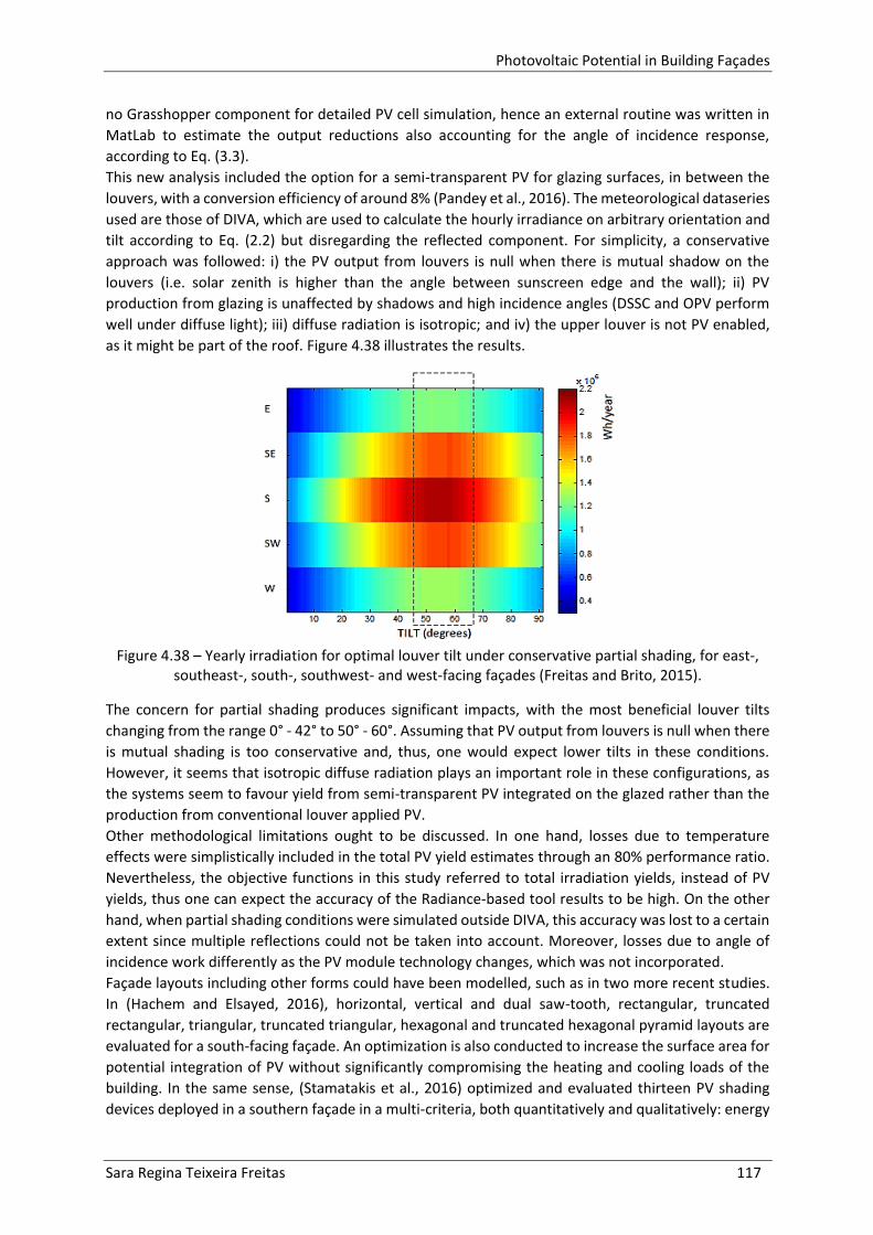
Photovoltaic Potential in Building Façades
Sara Regina Teixeira Freitas 117
no Grasshopper component for detailed PV cell simulation, hence an external routine was written in
MatLab to estimate the output reductions also accounting for the angle of incidence response,
according to Eq. (3.3).
This new analysis included the option for a semi-transparent PV for glazing surfaces, in between the
louvers, with a conversion efficiency of around 8% (Pandey et al., 2016). The meteorological dataseries
used are those of DIVA, which are used to calculate the hourly irradiance on arbitrary orientation and
tilt according to Eq. (2.2) but disregarding the reflected component. For simplicity, a conservative
approach was followed: i) the PV output from louvers is null when there is mutual shadow on the
louvers (i.e. solar zenith is higher than the angle between sunscreen edge and the wall); ii) PV
production from glazing is unaffected by shadows and high incidence angles (DSSC and OPV perform
well under diffuse light); iii) diffuse radiation is isotropic; and iv) the upper louver is not PV enabled,
as it might be part of the roof. Figure 4.38 illustrates the results.
Figure 4.38 – Yearly irradiation for optimal louver tilt under conservative partial shading, for east-,
southeast-, south-, southwest- and west-facing façades (Freitas and Brito, 2015).
The concern for partial shading produces significant impacts, with the most beneficial louver tilts
changing from the range 0° - 42° to 50° - 60°. Assuming that PV output from louvers is null when there
is mutual shading is too conservative and, thus, one would expect lower tilts in these conditions.
However, it seems that isotropic diffuse radiation plays an important role in these configurations, as
the systems seem to favour yield from semi-transparent PV integrated on the glazed rather than the
production from conventional louver applied PV.
Other methodological limitations ought to be discussed. In one hand, losses due to temperature
effects were simplistically included in the total PV yield estimates through an 80% performance ratio.
Nevertheless, the objective functions in this study referred to total irradiation yields, instead of PV
yields, thus one can expect the accuracy of the Radiance-based tool results to be high. On the other
hand, when partial shading conditions were simulated outside DIVA, this accuracy was lost to a certain
extent since multiple reflections could not be taken into account. Moreover, losses due to angle of
incidence work differently as the PV module technology changes, which was not incorporated.
Façade layouts including other forms could have been modelled, such as in two more recent studies.
In (Hachem and Elsayed, 2016), horizontal, vertical and dual saw-tooth, rectangular, truncated
rectangular, triangular, truncated triangular, hexagonal and truncated hexagonal pyramid layouts are
evaluated for a south-facing façade. An optimization is also conducted to increase the surface area for
potential integration of PV without significantly compromising the heating and cooling loads of the
building. In the same sense, (Stamatakis et al., 2016) optimized and evaluated thirteen PV shading
devices deployed in a southern façade in a multi-criteria, both quantitatively and qualitatively: energy

Photovoltaic Potential in Building Façades
118 Sara Regina Teixeira Freitas
optimization (heating–cooling–lighting loads) and user comfort (outdoor view–glare–aesthetic
aspects). Curiously, the horizontal rotated louvers equivalent in this study was among the less suitable
solutions, whilst brise solei (sunshades usually consisting of horizontal or vertical strips of wood,
concrete, etc.) was the most proper. The reference to these studies helps underlining that the
integration of PV into the building must be thoughtfully planned and address all the roles PV might
play in the building functions, which, in short, exist to serve its occupants.
4.4.2 Balcony dimensions
Building façades are a mix of wall and window surfaces: elements that remain inside the building
footprint. In this sense, a balcony represents not just a way of extending the floor area of an apartment
but also of creating additional quality space, improving liveability. The opportunities for integration of
solar PV cells on these accessories are immense, given their exposure to sunlight, variety of
construction materials and design possibilities (Figure 4.39). The front surface of a balcony railing is
not the sole interesting part. The reflectance properties of the surface materials that constitute and
surround a balcony make them potential candidates for concentrating solar radiation on the rear
surface as well and, therefore, increase overall electricity production from balcony integrated PV:
whilst the front surface harvests plain direct radiation, the cells on the back surface make use of diffuse
radiation, originated from the many reflective bounces of the sunrays hitting the nearby surfaces.
Figure 4.39 – Examples of balcony integration of PV in Finland (Solpros, 2003) (top left), Germany
(Donahue, 2017) (top right), Austria (LOF Solar Corporation, 2010) (bottom left) and France (SADEV, 2015) (bottom right).
One particular configuration worth exploring is using bifacial PV. These modules feature front and rear
efficiencies of 16% and 14% (Primsolar, 2016), respectively, and an 80% and 70% performance ratio to

Photovoltaic Potential in Building Façades
Sara Regina Teixeira Freitas 119
approximate the observations reported in (Soria and Gerritsen, 2013)(Lindsay et al., 2015)(Reise and
Schmid, 2015)(Comparotto et al., 2015). For simplicity, the detailed model of PV cells or the impacts
of non-homogeneous irradiation were not included.
A balcony can be recessed, if its dimensions do not exceed the building footprint limits and its open
space goes inwards, or precast, if the railing and the floor comes outwards the façade. Both
configurations might work with PV, therefore the parametric modelling, using Rhinoceros 3D (McNeel,
2016) and Grasshopper (Davidson, 2017), and optimization was conducted considering 3 features:
width, depth and offset. The depth and offset of the balcony could change between 0.1m and 2m, and
the width from 1m to 7m in the course of the optimization process. A fixed balcony door height was
set to 2.5m and the railing to 1m (Figure 4.40). The construction materials were also varied between
white or generic walls and glazing or mirror for the door. These and the PV surface materials are
described in Table 3.3.
Figure 4.40 – Render view of archetype with PV modules on the balcony railings (left) and detail of
the elements considered in the parametric modelling (right) (Freitas and Brito, 2016).
Solar radiation data series for three locations with dissimilar climate conditions were considered: Oslo
(Norway, 59.95°N 10.75°E), Lisbon (Portugal, 38.71°N 9.14°W) and Abu Dhabi (United Arab
Emirates, 24.47°N 54.37°E). As in the previous Sub-section, the plug-in DIVA (version 4.0)
(SolemmaLLC, 2016) was used to compute yearly solar irradiation on both front and back surfaces of
the balcony railings. A 0.1m2 point grid resolution and cumulative sky approach were employed to
reduce computation time, since the optimization procedures of intricate designs is time consuming.
The component Galapagos was used for the optimization of balcony dimensions aiming for the
maximization of PV generation density per module area (kWh/year/m2).
For each location, two optimization routines were executed: first for east, south, west and north and
then for south-east, -west, northeast, -west façade orientations. Only 2 ambient bounces were
allowed for the Radiance simulations, but the optimal configuration was simulated a second time with
5 so that more meaningful estimates could be produced.
Table 4.4 shows the materials assigned to the different surfaces on the optimal balcony configurations.
Table 4.4 - Materials assigned to the optimized balcony designs (Freitas and Brito, 2016).
Walls Door Walls Door Walls Door
East white mirror white mirror white mirror
Southeast white mirror white mirror generic mirror
South white mirror white mirror white mirror
Southwest generic glazing generic glazing generic mirror
West white mirror white glazing generic mirror
Northwest generic mirror generic glazing white glazing
North white mirror white mirror white mirror
Northeast white glazing white glazing generic glazing
ABU DHABI LISBON OSLO

Photovoltaic Potential in Building Façades
120 Sara Regina Teixeira Freitas
An example with a detailed overview of the solar irradiation over the optimal balcony railings is
presented in Figure 4.41 for Lisbon. The depth, width and offset dimensions obtained for optimal
configurations in the three locations are summarized in Figure 4.42.
Figure 4.41 - Lisbon: annual solar irradiation in the front and back railing surfaces for the E+S+W+N
(left) and NE+SE+SW+NW (right) configurations (Freitas and Brito, 2016).
Figure 4.42 - Balcony depths, widths and offsets [m] obtained in the optimization process (Freitas
and Brito, 2016).
There is a preference for deeper balconies on the South-West facing façades in Abu Dhabi and Lisbon,
while for Oslo they should be less deep, except for those facing the Northeast. As for the width, all
locations feature large widths in the North-West-South orientations, with Oslo featuring the widest
ones. The offsets also show a clear leaning to small values for the South, East and North orientations,
but higher values for the remainder.
Regarding the surface materials, as expected, high reflective materials such as white walls and mirrors
are more predominant. However, the Southwest, Northwest and Northeast were attributed slightly
less reflective materials. This would require more careful inspection, since there is no trivial way to

Photovoltaic Potential in Building Façades
Sara Regina Teixeira Freitas 121
find if the interaction of light with surfaces really caused this preference, or if it relates to
methodological limitations, such as the fact that neither a ray-tracing with 2 ambient bounces or an
annual cumulative sky approach are ideal for studies of light interaction with intricate designs.
Comparing the PV generation density results for the optimized configurations in the three locations
(Figure 4.43), it can be inferred that the most interesting façades for the integration of bifacial PV are
all but those facing North in Abu Dhabi and facing West and North in Lisbon. In Oslo only the South-
facing façades are attractive.
Figure 4.43 - Estimated front and rear PV generation density [kWh/m2/year] for each orientation and
location with optimized balcony dimensions and materials (Freitas and Brito, 2016).
Although the increment in total incident radiation is, in general, very high even in orientations that
would, at first, be discarded, it can be noted that some still do not encourage the application of bifacial
PV panels since the contribution of the rear surface to the annual electricity produced is almost
residual. This is the case of most north facing balconies that feature small offsets but large widths,
where non-bifacial PV should be deployed instead.
In Abu Dhabi, a low-mid latitude city, the overall electricity production from balconies might achieve
levels of up to 1MWh/year, given the high solar resource, but a complementary evaluation on the
effects of high ambient temperatures on the PV yields under such conditions should be conducted. On
the other hand, and as expected, Oslo’s balcony configurations feature very low levels of PV
generation, with wide north-facing balconies attempting to harvest most of the diffuse radiation.
However, only the south-facing balcony reaches interesting electricity generation levels – almost the
same as a balcony on a northeast-facing façade in Abu Dhabi. Concerning Lisbon’s optimal solutions,
the conclusions are similar to Abu Dhabi’s, with a tendency for small east- and west-facing balconies
and wide ones in the south and north façades.
To better understand the importance of the door, floor and wall materials as reflecting surfaces, from
where the sun rays might bounce off and into the rear PV surface, poor reflecting materials were
assigned to those elements on each of the optimized designs and recomputed the solar irradiation
(Figure 4.44). As expected, the orientations that feature higher increments due to the use of bifacial
PV modules are more sensitive to the use of materials with lower reflectivity. Three important effects
can be pointed out: i) orientations such as East-South are highly direct sunlit, so a small change in
reflectivity of surrounding materials causes significant changes; ii) orientations that feature low levels
of direct irradiation mainly rely on the reflected diffuse irradiation, so poor reflective surfaces will also
have a strong impact; and iii) light interacts differently when physical properties of surfaces vary, thus
probably there are better geometries for this new set of balcony materials. The value of the
optimization is highlighted, given that it leads to an average increment of around 20% (from 4% and

Photovoltaic Potential in Building Façades
122 Sara Regina Teixeira Freitas
up to almost 30%) in comparison with a low reflective scenario, with the greater impact being observed
in eastern/southern façade orientations.
Figure 4.44 - Decrease in PV generation from the optimized dimensions and materials to the scenario
with poor reflective materials.
Partial shading on the rear surface also causes a decrease in output, although it is slight given its lower
irradiation and lower conversion efficiency. The presence of a person in the balcony is one example of
a source of shading, which causes the radiation to interact differently with the surface materials and,
thus, decrease the PV production of bifacial modules integrated in the railing. This impact was
evaluated by including a human-like figure in the centre of the balcony floor (Figure 4.45), with a “dark
blue jeans” material assigned to it (Vrhel, 2015). The radiation simulations were re-run, but, for
simplicity, only for the optimized south facing balcony in Lisbon.
Figure 4.45 - Detail of the simulation with partial-shadow cast by a person standing in a south facing
balcony, in Lisbon (Freitas and Brito, 2016).
Although Figure 4.45 depicts the cumulative annual irradiation in the rear surface of the bifacial
module (and it would be more realistic to assume permanent furniture and not a person in the
balcony), the significant impact that this new element adds to the inter-reflections between the
balcony surfaces is clear. The estimated PV generation decreases about 5%.
Comparing the estimated bifacial PV yields with hypothetical monofacial yields in a flat PV wall (i.e.
monofacial PV area equal to the balcony door area), the bifacial generation would only differ in
average -15% from the monofacial scenario, ranging from +8% to -32% in Abu Dhabi, +7% to -49% in
Lisbon and +6% to -39% in Oslo, in the whole set of orientations. Still, further analysis would provide

Photovoltaic Potential in Building Façades
Sara Regina Teixeira Freitas 123
more insight into the impacts of partial-shading, that are expected to happen due to the nature of a
space such as a balcony.
The optimization of the façades and balconies are missing: i) an objective function that concerns the
investment costs; and ii) a more detailed PV module (including bypass diode) model that properly
portrays their behaviour under partial shading. The former could be incorporated in a multi-
optimization algorithm, considering different solar cell costs, while the second is more challenging
given its computational requirements. The individual modelling of PV modules and cells is itself time
consuming, thus calculating solar irradiation over each individual cell in an hourly time step might
become infeasible for intricate façade layouts. Nevertheless, given Grasshopper scripting components
(for Python, Visual Basic and C#, at least), it would be possible to do such analysis inside one single
software. Otherwise, solar radiation results would have to be exported to an external numerical
software, such as MatLab, where the electrical simulation would take place. The results would then
influence the input for parametric modelling in the next iterations, and so on until the optimum is
reached (Hofer et al., 2016). Dedicated tool suites can also be developed to thoroughly study BIPV
(Eisenlohr et al., 2017).
4.5 Conclusion
The design opportunities for solar façades that arise from new BIPV technologies are considerably
beyond what conventional modules have offered since the Mataro library PV installation, in 1995.
Alongside this, architects have become more aware of the need for PV integration into their projects
and the subsequent innovation it represents. On the other hand, the often anticipated economy of
scale of BIPV is yet to be realized, due to its incompatibility with most standardized processes at the
core of construction materials industries.
In the long future, it is likely that PV will become an intrinsic part of buildings, so that occupants will
not notice it and the electricity production functionality will be as trivial as water supply pipe systems
or electricity wiring. PV systems might as well take part in kinetic architecture and bring “life” to
animated building skins.
However, in the meantime, there are opportunities for applications such as bifacial PV on balconies,
flexible and colourful customized modules on shadings and spandrel areas on façades in different
locations in the world. The optimal configurations must adapt towards optimized harvesting of both
direct and diffuse solar radiation whilst keeping thermal comfort and the visual perception of
occupants at satisfying levels.
Partial shading is particularly damaging for the performance for BIPV on façades and requires
particular attention. These effects may be limited by the use of micro-inverters at the module level. At
the string level, it leads to further optimization challenges to photovoltaic systems. This is the scope
of the next chapter.

Photovoltaic Potential in Building Façades
124 Sara Regina Teixeira Freitas

Photovoltaic Potential in Building Façades
Sara Regina Teixeira Freitas 125
5. OPTIMIZATION OF PV INTERCONNECTIONS
Cityscapes are particularly diverse in terms of morphology. Buildings are the most predominant
elements, but there are also trees and urban equipment interacting with solar radiation. These features
can become shadow casters on BIPV systems, if they obstruct the path of the sun rays. Façade
integrated PV, thus, has a greater probability of suffering output reductions due to partial shading.
Such impact might be reduced if the placement of modules evades less sunlit areas but as shadow
patterns are constantly morphing, it may not be straightforward to identify those places not
contributing to overall yields during hours of greater solarshine. A holistic approach must be followed
to tackle this particular challenge.
In this Chapter, an artificial intelligence technique is developed and tested for different building
surfaces. The heuristic consists on a multi-objective genetic algorithm aiming at maximizing the PV
production of a system and minimizing its costs through adequate placement and interconnections
between PV modules. The solutions obtained are compared with conventional configurations and with
micro inverter scenarios. 7
5.1 Introduction
The project of a PV system is relatively straightforward for systems deployed in non-obstructed areas,
which is the case for most non-urban PV plants. The process becomes more challenging when surfaces
with intricate shadowing events are involved. In these circumstances, the incident solar radiation is
non-uniformly distributed as continually varying shadow patterns. Since interconnection between PV
modules is done in series (PV strings), a slight shadow cast on one of the cells is enough to significantly
impact the production of the whole module and, consequently, the string. Due to changing sun-paths
throughout the day and the year, achieving the most adequate string arrangement becomes a very
complex problem of systems optimization.
Continuous and complex optimization problems, which cannot be fully represented and solved
through well-defined mathematical formulations, can be solved through evolutionary strategies.
When a problem has neither a unique and trivial solution or the search space is excessively large, or
even if the problem has more than a single objective, Evolutionary Algorithms (Bäck et al., 1993) or
Genetic Algorithms (GA) (Goldberg, 1989) are numerical modelling approaches that can be employed.
The underlying principle of these algorithms is based on Darwin’s principle of “survival of the fittest”:
populations of individuals are created and subjected to selection, recombination and mutation
operators (or only mutation in the case of evolutionary algorithms), and the fittest individuals are
passed on to the next generation.
A few studies regarding the optimization of PV systems using evolutionary strategies can be found in
literature. For instance, (Kornelakis and Koutroulis, 2009) present a sizing optimization scheme for grid
connected PV using a GA to maximize the total net profit of the systems. The study does not include
losses associated to temperature or inverter-to-array sizing ratio, though, and the proposed technique
is only suitable for pitched or flat rooftops where mounting frames can be used to adjust tilt angle.
(Sulaiman et al., 2012) introduces evolutionary programming to optimize the installation area with the
prerequisite of maximising the technical or economic performance. The algorithm is based on pre-
7 Chapter includes work published on:
- Freitas, S., Serra, F., Brito, M.C. “PV layout optimization: string tiling using a multi-objective genetic algorithm”. Solar Energy, Volume 118, Aug 2015, 562–574. DOI:10.1016/j.solener.2015.06.018
- Freitas, S., Serra, F., Brito, M.C., “Multi-objective genetic algorithm for the optimization of a PV system arrangement”. ISES Solar World Congress, Nov 2015, Daegu, South Korea. DOI:10.18086/swc.2015.05.16

Photovoltaic Potential in Building Façades
126 Sara Regina Teixeira Freitas
defined sets of inverters and PV modules that would optimize, technically or economically, the
performance of a fixed system. Despite overcoming the limitations of previous approaches, the
optimal sizing points to a unique very long PV string, not actually feasible in practice. Gómez-Lorente
et al (Gómez-Lorente et al., 2012) study the optimization of sun tracking PV plants in terms of reducing
associated electrical losses. Different evolutionary algorithms were compared, with random mutation
featuring the fastest convergence and identical accuracy. Another GA was explored in (Shirzadi et al.,
2014) to minimize the mismatch losses in PV arrays. In this purely theoretical study, the module
parameters were statistically obtained from the technical specifications of a real PV module and the
radiation set to be uniformly distributed, without shading effects. Nevertheless, the approach can be
applied to a real system for arranging PV modules with known measured parameters.
The alternative approach to partial shading loss minimization would be the use of AC modules with
micro inverters as an alternative to conventional string based systems (Kurokawa et al., 1997). Micro
inverters provide system immunity to output power drop when a module is partially shaded, therefore
avoiding mismatch losses. However, their installed power cost is higher and maintenance can be costly
and hard to perform in urban environments, such as in vertical mounted systems, given that the micro
inverters are usually attached to the back side of the module.
To overcome the limitations in the reviewed literature, and to provide an intelligent approach to
optimized both technical and economic potentials of building deployed conventional PV systems, a
multi-objective genetic algorithm (MOGA) was created. The tool and its tests will be described in the
next Sections. This proposed approach aims to lessen partial shading impacts whilst avoiding movable
parts or dynamic changes to the system. It is worth noting that smart and sophisticated, but far more
complex and expensive, ways of avoiding partial shading impacts in real time have emerged. These
techniques concern the electronical level of the modules and enable the PV strings to reconfigure their
interconnections under whichever irradiance conditions. In (La Manna et al., 2014), dynamic string
reconfiguration using switches is reviewed, concluding that it could be possible to design a
reconfigurable interconnection device supporting different interconnection topologies, but costs
would be increased due to the many switches involved and their limited lifetime.
5.2 Multi-Objective Genetic Algorithm
The technical and economic optimization of a PV system requires a multi-objective approach aiming
simultaneously at the maximization of the energy yield (denoted 𝐸𝑠𝑦𝑠𝑡) and minimization of the system
costs (denoted 𝐶𝑠𝑦𝑠𝑡). This approach produces non-dominated solutions, establishing several Pareto
fronts or isocurves (Fonseca, 1995), i.e. groups of solutions optimizing both objectives and that are
compared among each other based on their objective values (in this case, 𝐸𝑠𝑦𝑠𝑡 and 𝐶𝑠𝑦𝑠𝑡). The
solutions that belong to the outermost Pareto front dominate all the others, and so on. When
comparing solutions in a specific Pareto front, it is impossible to find one solution that improves one
condition without worsening the other. In the present study, an increase in PV production will lead to
an increase in the system costs, and vice-versa. Hence, from a set of optimal Pareto solutions, one will
be able to choose the strings’ layout that better suits the project goals, in terms of the trade-off
between yield and cost.
A non-dominated sorting genetic algorithm was scripted in MatLab environment. The algorithm
mechanism and the operations involved in its execution are shown in Figure 5.1.

Photovoltaic Potential in Building Façades
Sara Regina Teixeira Freitas 127
Figure 5.1 – Main scheme of the genetic algorithm (Freitas et al., 2015a).
All input data sets associated to the solar radiation data required for the energy yields and system
costs calculations were previously stored in MatLab .mat matrices so that they can be loaded only
once, when the code starts running. This eases the handling of large data sets and lowers the
computational time.
The genetic algorithm per se starts afterwards. The first step concerns the creation of an initial
population with an even number of candidate solutions. Each one can be addressed as an “individual”
or “chromosome” and its information, i.e. its genes, is encoded in vector form.
5.2.1 Encoding
The encoding has to simultaneously describe the position of each module in the available positions of
the rooftops or façades and inform on how it is connected to other modules. This was achieved
through integer-valued encoding. The encoding strategy of a hypothetical arrangement is presented
in Figure 5.2.

Photovoltaic Potential in Building Façades
128 Sara Regina Teixeira Freitas
Figure 5.2 – Example of a chromosome and its encoding strategy. The different colours highlight
different PV strings (Freitas et al., 2015a).
The binary matrix on the left-hand side of Figure 5.2 stores the available and unavailable positions for
placing modules with ones and zeroes, respectively, and, given the spatial resolution of 1m2, it provides
height and width information. The coloured matrix on the right informs on the PV string layout, i.e.
each colour/number identifies all modules belonging to different strings. In a row wise procedure, a
module can be saved to a vector as an integer number corresponding to the “colour” of the string it
belongs to. This vector only contains the information regarding the available positions (the 1s in the
binary matrix), but when a zero is saved (e.g. 8th and 14th positions in the hypothetical chromosome)
means that no module is assigned to that position, despite it is available. The decoding of the
information is straightforward by checking back the available positions in the binary matrix.
The initial population of chromosomes is generated randomly on an attempt to cover the search space
as widely as possible: a set of uniformly distributed pseudorandom positive integers, including zeroes,
is generated to occupy all the genes, corresponding to a random distribution of modules per layout.
The first generation of individuals is constrained to a maximum number of PV strings, limiting the
variety of integers that can be generated throughout the generations (which could jeopardise
convergence).
5.2.2 Fitness and objective functions
Having generated a set of chromosomes, a fitness value is calculated for each. Fitness values are
constant and defined linearly or non-linearly according to the population size. In single objective
optimization problems, the fitness is assigned based only on the chromosome ranking, but in multi-
objective problems it is done according to a Pareto ranking. Several fronts are defined and all
individuals in the same front share the same rank (Fonseca, 1995). In this case, the fitness values are
assigned to all individuals according to their rank and, then, the averaged fitness value is given to all
the individuals in the same front.
One of the objective functions consists on the maximization of the annual photovoltaic yield and the
other objective function encompasses the minimization of the total system cost. However, while PV
production and module costs may be directly computed from the positions of the modules and the
strings they form, calculation of the costs include considering wiring and inverters requiring a different
approach.

Photovoltaic Potential in Building Façades
Sara Regina Teixeira Freitas 129
i) Annual PV yield
Knowing the solar irradiation distribution all over a surface for all 𝑛𝑡 sun-hours of a typical
meteorological year, hourly and annual accumulated PV electrical production can be estimated for all
the modules in that surface. Similarly to the workflow in Sub-section 3.2.1, the ambient temperature
data associated to the typical meteorological year in Lisbon is used to estimate hourly module
operating temperature. The indexes in Eq. (3.2) underwent slight adaptations to the problem at hands:
𝑇𝑚,ℎ = 𝑇𝑎,ℎ +𝑇𝑁𝑂𝐶𝑇 − 20℃
800 𝑊𝑚−2𝐺𝑡𝑖𝑙𝑡𝑒𝑑,ℎ , (5.1)
where 𝑇𝑎 is the ambient temperature [°C], 𝑁𝑂𝐶𝑇 is a Nominal Operating Cell Temperature [°C],
𝐺𝑡𝑖𝑙𝑡𝑒𝑑,ℎ is the global irradiation on the tilted plane [Wh/m2], the index 𝑚 identifies a module in the
layout and ℎ is the time index [h]. Table 5.1 summarises the electrical parameters of a typical 1m2 PV
module (to match spatial resolution of the irradiance data) used in the optimization process.
Table 5.1 – Typical pc-Si module parameters. PV module parameter Value
Voc [V] 32.6
Isc [A] 5.51
Vmp [V] 23.5
Imp [A] 4.95
Vs_max [V] 1000
TNOCT [°C] 47
𝜂𝑟𝑒𝑓 [%] 13
𝛾 [%/°C] -0.44
𝛽 [V/°C] -0.0033
a𝑟 0.159
As PV modules are connected in series in a string and subjected to losses due to angle of incidence
(𝐴𝐿𝛼,ℎ), the hourly expected energy yield of each PV string (𝐸 𝑠,ℎ) can be estimated also adapting the
indexes of Eq. (3.1) and (3.3) respectively to:
𝐴𝐿𝛼,ℎ =1 − 𝑒
−cos𝜃ℎ𝑎𝑟
1 − 𝑒−1𝑎𝑟
, (5.2)
𝑃𝑉𝑆,ℎ = 𝑚𝑖𝑛 (𝑃𝑟𝑒𝑓𝐷𝑖𝑟𝑡𝑖𝑙𝑡𝑒𝑑,𝑚,ℎ𝐴𝐿𝛼,𝑡 + 𝐷𝑖𝑓𝑡𝑖𝑙𝑡𝑒𝑑,𝑚,ℎ
𝐺𝑟𝑒𝑓[1 + 𝛾(𝑇𝑚,ℎ − 𝑇𝑟𝑒𝑓)]) 𝑛𝑚,𝑆𝐴𝜂𝑖,𝑠𝑃𝑅 , (5.3)
where the index 𝑆 identifies a PV string, the index 𝑝 identifies the positions of the modules connected
to string 𝑆, 𝑛𝑚,𝑆 is the total number of modules belonging in string 𝑆, 𝐴 = 1 is the individual module
area, 𝜂𝑖,𝑆 = 0.95 denotes an average efficiency of the inverter 𝑖 connected to string 𝑠 and 𝑃𝑅 = 80%.
The 𝑚𝑖𝑛() function, a conservative approach, reflects the fact that the current in a string is determined
by its lowest producing module.
The PV production function of a layout with 𝑛𝑆 strings can be defined by a summation of the hourly
PV yield of all strings throughout the year:
𝐸𝑠𝑦𝑠𝑡 =∑∑𝑃𝑉𝑠,ℎ
𝑛ℎ
ℎ=1
𝑛𝑆
𝑆=1
. (5.4)

Photovoltaic Potential in Building Façades
130 Sara Regina Teixeira Freitas
ii) Total system costs
The system costs of a PV layout comprise three components: the cost of the modules plus the copper
wiring required to connect the modules in series and the inverters needed for the DC to AC output
conversion. Neither maintenance or operating costs nor discount rates were taken into account. The
system costs function defined by:
𝐶𝑠𝑦𝑠𝑡 = 𝐶𝑚∑𝑛𝑚,𝑠
𝑛𝑠
𝑠=1
+∑𝐿𝑠𝐶𝑠
𝑛𝑠
𝑠=1
+∑𝐶𝑖
𝑛𝑖
𝑖=1
, (5.5)
where 𝐶𝑚 = 150€/m2 is the (fixed) cost of the PV module, 𝐿𝑠 and 𝐶𝑠 are the length and wire costs for
string 𝑠, respectively, and 𝐶𝑖 is the cost of each selected inverter. Thus, the first summation refers to
the module cost, the second summation to the wiring cost and the third to the inverter costs.
The typical constraint of 3% for the maximum voltage drop allowed on a PV string was implemented.
Taking the copper resistivity value as 2.112 × 10⁻⁸Ωm, the adequate conductor section can be
selected for each string by knowing the threshold current intensity that different sections can bear.
Copper wire characteristics rated at 90°C (NFPA, 2014) were considered and respective average cable
copper wire costs assumed according to their American Wire Gauge.
Apart from the conductor section, wiring costs are also dependent on the total length required to
connect PV strings. Considering the linking node as the centre of a module, a mixed-integer linear
optimization procedure was included to find the shortest linking path between modules in the same
PV string. This is based on the determination of all possible link combinations between all nodes. Since
the circuit must be closed, the obtained length must be multiplied by 2 in the case of linear strings (for
instance, string 5 in Figure 5.2). Nonetheless, the wiring length that goes from the modules to the
respective inverters is neglected and, thus, a single module string does not have wiring costs.
While cycling through the variety of PV strings in an individual, two equality constraints must be
assured: the number of copper wire segments (links) is equal to the number of modules (nodes) and
each node only has two links attached to it. Solutions with intersections or sub-circuits inside the same
PV string undergo re-optimization until there is only one valid path linking all modules. The method
presented in (MathWorks, 2014) was adapted to meet the objectives set.
In order to distribute the PV strings to a set of inverters, two main constraints must be applied to
prevent unfeasible solutions: 𝑁𝑚,𝑆 the maximum number of modules connected in a string, Eq. (5.6),
and 𝑁𝑠,𝑖 the maximum number of strings connected to a certain inverter 𝑖, Eq. (5.7).
𝑁𝑚,𝑆 ≤𝑚𝑖𝑛(𝑉𝑠𝑚𝑎𝑥 , 𝑉𝐷𝐶 𝑚𝑎𝑥,𝑖 )
𝑉𝑜𝑐[1 + 𝛽(−10 − 25)] , (5.6)
𝑁𝑠,𝑖 ≤𝐼𝐷𝐶 𝑚𝑎𝑥,𝑖1.25𝐼𝑠𝑐
. (5.7)
For each layout another linear optimization procedure is executed to select the inverters according to
three inequality constraints. The first one relates to the maximum input DC voltage that each inverter
can handle 𝑉𝐷𝐶 𝑚𝑎𝑥, i.e. the maximum number of modules in a string linked to the inverter 𝑖 must be
lower than 𝑁𝑚,𝑖, Eq. (5.6), and the second relates to the maximum input DC current allowed to the
inverter 𝐼𝐷𝐶 𝑚𝑎𝑥, which is controlled by the maximum defined by 𝑁𝑠,𝑖, Eq. (5.7). Lastly the total power
of the strings linked to the inverter must, of course, be lower than 𝑃𝐷𝐶 𝑚𝑎𝑥. These properties of 13
inverter models are presented in Table 5.2, including the maximum values allowed for the DC input
current 𝐼𝐷𝐶 𝑚𝑎𝑥, the DC input voltage 𝑉𝐷𝐶 𝑚𝑎𝑥, and the DC input power 𝑃𝐷𝐶 𝑚𝑎𝑥, as well as prices. It

Photovoltaic Potential in Building Façades
Sara Regina Teixeira Freitas 131
must be noted that assuming that the O&M costs are independent of the layout connection of the
strings is an optimistic approach regarding the micro-inverter solution.
Table 5.2 - List of properties of 12 inverters and 1 micro-inverter. Prices retrieved between December 2014 and August 2015 from (Wholesale Solar, 2015)(CCL Componentes, 2014)(Energy
Matters, 2014)(MG Solar, 2014).
Model 𝑃𝑛𝑜𝑚 [kW] 𝐴𝑣𝑔 𝑃𝑟𝑖𝑐𝑒 [€] 𝑉𝐷𝐶 𝑚𝑎𝑥 [V] 𝐼𝐷𝐶 𝑚𝑎𝑥 [A] 𝑃𝐷𝐶 𝑚𝑎𝑥 [kW]
SMA micro 0.24 150 45 8.5 0.24
Fronius 1.5-1 1.5 893 420 13.3 1.5
Fronius 2.0-1 2 916 420 17.8 2
Fronius 2.5-1 2.5 938 420 16.6 2.5
Fronius 3.0-1 3 960 550 19.8 3
IG 20 1.8 832 500 14.3 2.70
IG 30 2.5 1220 500 19.0 3.60
IG 40 3.5 1568 500 29.4 5.5
Plus 60-V1 6 1474 600 27.5 6.32
Plus 70-V2 6.5 1579 600 30.0 6.88
Plus 80-V3 7 1678 600 32.0 7.36
Plus 100-V3 8 1693 600 37.1 8.43
Plus 120-V3 10 1885 600 46.2 10.59
The lower bound to this linear optimization is set to 0 while the upper bound is the number of available
positions in the available surface area, so that the possibility of a layout where all strings are individual
modules with the same inverter model can be covered. In case there is no convergence to a feasible
inverter distribution, the inverter cost is set to infinity and thus the individual will be assigned the
lowest fitness value.
Summarizing, the multi-objective optimization problem can be defined as:
i) maximize the system annual energy yield (𝐸𝑠𝑦𝑠𝑡) and minimize the system costs (𝐶𝑠𝑦𝑠𝑡);
ii) aim at the PV layout with minimum cost for the energy produced in 25 years (𝐶𝑠𝑦𝑠𝑡
𝐸𝑠𝑦𝑠𝑡×25 ),
i.e. find 𝑚𝑖𝑛 𝑓(𝐸𝑠𝑦𝑠𝑡 , 𝐶𝑠𝑦𝑠𝑡) in the 1st pareto front.
Subjected to the following constraints (case-study dependent):
- initial population 0 ≤ 𝑠 ≤ 6 (rooftop) or 4 (façade)
- 0 ≤ 𝐺𝑝,𝑡 ≤ 1000 [Wh/m2]
- 0 ≤ 𝜃𝑡 ≤ 90 [°]
- 0 ≤ 𝑇𝑎,𝑡 ≤ 36 [°C]
- 0 ≤ 𝑛𝑚,𝑠 ≤ 18 (rooftop) or 32 (façade)
- 0 ≤ 𝐸𝑠,𝑡 [Wh]
- 0 ≤ 𝐶𝑚 ≤ 𝑛𝑚,𝑠 × 150 [€]
- 0 ≤ 𝐿𝑠 ≤ 𝑚𝑖𝑛 𝑑𝑖𝑠𝑡𝑎𝑛𝑐𝑒(𝑛𝑚,𝑠) [m]
- 0≤ 𝐶𝑠 ≤ 26.486 [€/m]
- 0 ≤ 𝐶𝑖 ≤ 1885 [€]

Photovoltaic Potential in Building Façades
132 Sara Regina Teixeira Freitas
5.2.3 Selection
After all the population has been ranked according to the fitness values of its individuals, they are
probabilistically selected for recombination, i.e. breeding. The selection of parents is done through a
roulette wheel algorithm. This method is also known as stochastic sampling with replacement, which
means that the selection probability of each individual is attributed according to its fitness value,
therefore, the fittest have higher probability of being chosen for recombination in random trials. A
selective pressure of 2 was used to enhance the probability of selection of the fittest individual
comparing to the average probability of selection of the population.
5.2.4 Crossover
To ease the computation time while keeping high variety of genetic information, the recombination is
done after decoding the selected chromosomes from integer to binary values, as only parts of the
individuals are exchanged between them. The probability of crossover was set to 100%, meaning that
all selected parents will produce offspring. Multi-point crossover is employed, i.e. two crossover
positions in the chromosome are selected uniformly at random and the variables are exchanged
between the individuals between these points, producing two offspring.
5.2.5 Mutation
Resulting offspring has a chance of suffering mutation. The mutation algorithm is also binary-based
and consists on uniformly altering the chromosomes at random by flipping variable values, i.e. a 0
becomes a 1 and vice-versa. The rate of mutation is 3%, since the binary crossover already introduces
high variety to the offspring.
5.2.6 Reinsertion
Before inserting the offspring into the present population, the chromosomes are once again encoded
from binary to integer values. Their fitness values are calculated and the offspring is ranked afterwards.
Two reinsertion algorithms are implemented: whereas one states that only a percentage of the fittest
offspring are inserted into the population by replacing the least fit parents, the other does the same
but reinserts random offspring. The number of individuals is kept constant throughout the generations
by eliminating the same number of parents as the number of inserted offspring.
5.2.7 Stopping condition
One from two conditions can stop the algorithm run. One concerns the maximum number of
generations (Table 5.3) and the other relates to the objective functions: as the population is ranked in
Pareto fronts, a stopping condition can be set by finding, in each generation, the individual that holds
the minimum estimated levelized cost of electricity production [€/kWh] (in 25 years). Comparing this
value from one generation to the other, if a lower €/kWh is found in the previous generation the value
is stored. The generational loop stops whenever the fourth minimum cost of energy €/kWh that
prevails during, at least, 100 generations, is found. Yet, as it might be convenient to monitor the several
variables evolved in the course of the optimization process, in case this ratio remains unchanged for
too many generations the algorithm can be stopped manually.

Photovoltaic Potential in Building Façades
Sara Regina Teixeira Freitas 133
Table 5.3 – Parameter specifications for the GA used in the rooftop and façade case-studies. Parameters Rooftops Façades
Population size 100 50
Max generations 250 400
Crossover type Binary Binary
Crossover points 2 2
Crossover probability 100% 100%
Mutation probability 3% 2%
Selection type Roulette wheel Roulette wheel
Selective pressure 2 2
Reinsertion type Random Elitism
Reinsertion percentage 30% 10%
The parameters in Table 5.3 are more severe for façade studies, since the genes were larger than in
the rooftop case, in an attempt to make the population converge faster.
5.3 Case-studies
The developed MOGA relies on irradiation data to investigate the module sittings and string
interconnections maximizing yearly electricity generation and minimizing investment costs. Two case
studies were addressed to test the algorithm against conventional and micro-inverter arrangements.
i) Comparison with conventional arrangements
A dummy synthetic rooftop and ready results from the SOL model (Redweik et al., 2013) concerning
the study of Lisbon areas B and C from sub-section 3.2.2, were used to estimate hourly electricity
production from the surfaces of interest.
Concerning the synthetic DSM, it was built assuming the average elevation for the city of Lisbon, from
which a 4x8m2 rooftop case-study (here on designated as “rooftop 1”), the circled one in Figure 5.3,
underwent irradiation calculations. The tilted roofs are facing south.
Figure 5.3 - Rooftop 1 (yellow circle) and surroundings coloured according to the height. The ground
height of 100m corresponds to the average of the city of Lisbon (Freitas et al., 2015a).
The adjacent buildings were created to cast very well defined and predictable shadow patterns: in the
morning the building to the right is responsible for casting a shadow on the middle rooftop while the
left one obstructs most of the sunlight in the later hours of the day (Figure 5.4). The original rooftop
model has a defined area of 4x8m2 but the edges of the roof were excluded for realism.

Photovoltaic Potential in Building Façades
134 Sara Regina Teixeira Freitas
Figure 5.4 - Orthogonal view of the hourly irradiation [Wh/m2] in rooftop 1, for a winter (top row)
and a summer (bottom row) day. (Freitas et al., 2015a).
The other case study, denoted “façade 1”, refers to the façade marked with the yellow sector in Figure
5.5. Hourly irradiation was calculated using the SOL model (the building is located in area C described
in sub-section 3.2.2). The wall is facing south-southeast and has an area of around 7x6m2. Due to the
existence of stairs, windows and other structures, not all positions are suitable for the placement of
PV modules. Thus, when extracting the irradiation values of this façade, a first constraint on the area
availability is imposed. In Figure 5.6, hourly irradiation levels in the façade are presented for a summer
and a winter day. The unavailable areas for PV modules are coloured in white.
Figure 5.5 – Photograph of an afternoon shadow cast on façade 1 (portion signed in yellow).
Figure 5.6 – Orthogonal view of the hourly irradiation [Wh/m2] in façade 1, for a winter (top row) and
a summer (bottom row) day. White denotes excluded positions (Freitas et al., 2015a).
Higher levels of irradiation are visible in the upper row, reaching global irradiation values around
900Wh/m2 in the afternoon in winter. Different shadow patterns are also evident, since the incidence
angles of the sunlight change during the day and the year. Irradiation patterns near the right edge of
the building, in particularly at 3pm in the winter day is probably an artefact of the simulation. This
irradiation data was used as is, without any corrections, to further test the robustness of the MOGA.
ii) Comparison with micro-inverter arrangements

Photovoltaic Potential in Building Façades
Sara Regina Teixeira Freitas 135
The other case studies comprise a rooftop and a façade in area B, described in Sub-section 3.2.2. These
will be denoted as “rooftop 2” and “façade 2”. The first is a 3x6m2 south-facing portion of a rooftop,
marked in Figure 5.7, left. The second is also marked in yellow and it is a 7x5m2 portion of a façade
facing west.
Figure 5.7 - Bird’s eye perspective to rooftop 2 (left) and street view of façade 2 (right), retrieved
from Google Earth at approximately 38.7398959, -9.1463554.
5.4 Results
The optimal results for the 4 case-studies will be described in this Section. Rooftop 1 and façade 1 will
be compared with conventional sitting scenarios, whereas rooftop 2 and façade 2 will be compared
against micro-inverter solutions.
5.4.1 Comparison with conventional arrangement
The layouts shown in Figure 5.8 represent conventional interconnections, the first is a line wise and
the other a column wise placement PV strings.
Figure 5.8 – Yearly total PV production per string of a typical line wise (left) and a column wise (right)
distribution of PV strings, for rooftop 1. Note the different colour scale values in the two graphs (Freitas et al., 2015a).
The conventional arrangements in rooftop 1 feature high PV production, with similar annual yields
from all the strings. The system costs are slightly higher in the second layout due to the chosen
inverters, although a column wise placement allows slightly higher production.

Photovoltaic Potential in Building Façades
136 Sara Regina Teixeira Freitas
One possible optimal solution for this case-study, with similar electricity yields but 20% lower cost of
energy, was reached within 70 generations (Figure 5.9, left), with the MOGA set to random reinsertion
at a rate of 30%, a population of 100 individuals and a maximum of 6 PV strings per layout in the initial
population.
Figure 5.9 – Rooftop 1 layout with lowest cost of electricity achieved in the 70th (left) and 250th (right)
generations (Freitas et al., 2015a).
Reviewed literature recommended a higher number of generations (above 200, at least), thus, despite
having found a possible optimal solution in the 70th generation, the optimization process continued
until there were no longer significant changes in the best solution (Figure 5.9, right).
Figure 5.10 presents an overview of the evolution of the layouts across the generations. As expected,
the cost variables tend to become lower as the electricity production variables increase (blue lines).
Initially, the population is largely dispersed and the best solution (red lines) jumps arbitrarily along the
generations. From the 70th to the 250th generation, the best solutions somehow steadied, although a
slight disturbance around the 130th generation is visible (possibly the evasion of a local minimum). The
execution of the algorithm was manually stopped in this case, given the convergence in the Cost of
Energy chart (Figure 5.10 ,top) after the 150th generation. In fact, from the 70th to the last generation
there were no significant improvements, making the achieved solution a possible absolute minimum.
Figure 5.10 – Charts with the overview of the relevant Cost and Energy variables during the
optimization process, for rooftop 1 (Freitas et al., 2015a).

Photovoltaic Potential in Building Façades
Sara Regina Teixeira Freitas 137
The Pareto curve analysis (each one was assigned a number according to the dominance order, in
Figure 5.11) for the initial and last generation shows the widening of the search space and a successful
optimization process. Each of these solutions is itself an optimum according to the multi-objective
function criteria. The final selection of the layout configuration to implement in the system project can
be based on these results plus other conditions such as a minimum cost of electricity (€/kWh), a
minimum PV production level, a maximum cost level, etc.
Figure 5.11 - Comparison between the Pareto fronts from the initial (left) and 250th (right)
generations, for rooftop 1. The arrow points the individual with minimum cost of energy [€/kWh] (i.e. 0.063€/kWh and 2240kWh/year) and the yellow circles mark the location of the conventional
solutions presented in Figure 5.8 (i.e. 0.077€/kWh and 2173kWh/year; 0.080€/kWh and 2305kWh/year). Background shading marks different levels of €/kWh (Freitas et al., 2015a).
As for façade 1, the conventional layout of columnar strings (Figure 5.12) resulted in limited energy
production and high cost of energy.
Figure 5.12 – Yearly total PV production per string of a typical column wise distribution of PV strings, for façade 1. White areas mean unavailable positions for module deployment (Freitas et al., 2015a).
Optimized configuration achieves 6% lower cost of electricity with a 6 PV strings system (Figure 5.13).
From initial to last generation, the energy yield became about 25% higher with similar system costs
reducing significantly the ratio of €/kWh. Among the three solutions presented, the GA provides the
best answer to the trade-off between yields and costs.

Photovoltaic Potential in Building Façades
138 Sara Regina Teixeira Freitas
Figure 5.13 - Façade 1 layout with lowest cost of electricity achieved in the initial (left) and 400th (right) generations. Zeros (darkest blue) denote areas without deployment of modules and white
means unavailable positions (Freitas et al., 2015a).
At the initial stage of the simulation, there were several dispersed Pareto fronts which became more
defined throughout the generations, with only two fronts remaining in the last generation (Figure
5.14).
Figure 5.14 – Comparison between the Pareto fronts from the initial (left) and 400th (right)
generations, for façade 1. The arrow points the individual with minimum cost of energy [€/kWh] in (i.e. 0.209€/kWh and 997kWh/year) and the yellow circle marks the location of the conventional
solution presented in Figure 5.12 (i.e. 0.221€/kWh and 1215kWh/year). Background shading marks different levels of €/kWh (Freitas et al., 2015a).
The upper side of the last generation Pareto curve (Figure 5.14, right) comprehends façade layouts
where strings are more disperse, featuring higher energy yields due to higher number of PV strings
but at higher costs because of an increased number of inverters. On the other hand, the lower and
middle parts of the Pareto are characterized by layouts containing less strings and more zeroes in the
positions that are less sunlit. Of course, the final decision for the project will depend on the weight
specified to the different objective values. In the case of a façade, aesthetical concerns might also
influence the decision.
An overview of the results for the relevant parameters can be grasped from Figure 5.15. It can be
noted that the optimization cycle ended in the 400th generation, since only 3 relative minima were
found. Similarly to rooftop 1, a plateau seemed to be reached by half the simulation.

Photovoltaic Potential in Building Façades
Sara Regina Teixeira Freitas 139
Figure 5.15 - Charts with the overview of the relevant Cost and Energy variables during the
optimization process, for façade 1 (Freitas et al., 2015a).
5.4.2 Comparison with micro-inverter arrangement
In Figure 5.16, the optimal layout for the highly obstructed south-facing rooftop under study (rooftop
2) featured a cost of energy of around 0.22€/kWh, with 5 strings clustered in the most sunlit areas and
two positions without modules, whilst individual modules with micro-inverters achieved 0.29€/kWh.
Figure 5.16 - Yearly total PV production per string of the optimized distribution of strings (left) and
the micro-inverter scenario (right), for the rooftop 2. Zeros (darkest blue) denote areas without deployment of modules. Note the different colour scale values in the two graphs (Freitas et al.,
2015b).

Photovoltaic Potential in Building Façades
140 Sara Regina Teixeira Freitas
Higher electricity yielding solutions, with higher costs, are in the right side of the Pareto front, whilst
more affordable configurations, with lower electricity production, can be found in the left side (Figure
5.17). The layout with micro-inverters is located on the rightmost tip of the Pareto front (green
triangle), achieving the highest yields but requiring a considerable investment, far from the best ratio
€/kWh.
Figure 5.17 - Comparison between the Pareto fronts from the initial (left) and 400th (right)
generations, for façade 2. The arrow points the individual with minimum cost of energy [€/kWh] (i.e. 0.22 €/kW h and 731 kW h/year) and the green triangle marks the location of the micro-inverter
scenario (Freitas et al., 2015b).
Façade 2 optimal layout (Figure 5.18, left) reveals that a west-facing partially obstructed façade can
match PV production of a micro-inverter rooftop PV arrangement in non-optimal conditions (0.30 vs
0.29 €/kWh). The Pareto fronts of the initial population and the last generation (Figure 5.19) also
corroborate the observations done to rooftop 2. Optimal interconnections and module placement for
rooftop 2 and façade 2 feature cost of energy 23% and 24% lower than the equivalent micro-inverter
solution.
Figure 5.18 - Yearly total PV production per string of the optimized distribution of strings (left) and
the micro-inverter scenario (right), for the façade 2. Zeros (darkest blue) denote areas without deployment of modules and white means unavailable positions. Note the different colour scale
values in the two graphs (Freitas et al., 2015b).

Photovoltaic Potential in Building Façades
Sara Regina Teixeira Freitas 141
Figure 5.19 - Comparison between the Pareto fronts from the initial (left) and 400th (right)
generations. The arrow points the individual with minimum cost of energy [€/kWh] (i.e. 0.30 €/kW h and 711 kW h/year) and the green triangle marks the location of the micro-inverter scenario (Freitas
et al., 2015b).
Table 5.4 summarizes costs and yields of a conventional columnwise arrangement and optimized
layouts for the 4 case-studies. The micro-inverter scenario is equivalent to a raw output from the SOL
model, i.e. the PV yield of a system and its costs correspond to the aggregation of the individual yield
and cost of each m2 in the rooftop or façade.
Table 5.4 – Yields and Costs obtained for the 4 case-studies in conventional columnwise, micro-inverter and optimized arrangements.
Conventional Micro-inverter Optimized
Yield [kWh] Cost [€] Yield [kWh] Cost [€] Yield [kWh] Cost [€]
Rooftop 1 2305 4610 2649 6147 2240 3528
Rooftop 2 726 4606 883 6402 731 4022
Façade 1 1215 6713 1493 8550 997 5209
Façade 2 754 5490 775 7500 711 5333
Although the addressed case-studies are worst case scenarios, for their particular challenging shading
conditions, it is clear that considering partial shading in PV systems is essential for the assessment of
the PV potential in a neighbourhood or city, especially when regarding building façades.
5.5 Discussion
The developed multi-objective genetic algorithm (MOGA) helped finding solutions that keep the trade-
off between PV system costs and electricity yield in different façade and rooftop case-studies. For the
synthetic partially obstructed rooftop (rooftop 1) the optimum solution costs 0.063€/kWh, below the
column wise configurations. The same was observed for the southeast-facing façade (façade 1)
reaching 0.209€/kWh, 5% cheaper than the typical arrangement. This façade is characterised by low
afternoon insolation and relatively complex shadow phenomena, which, still, did not prevent the
MOGA from finding optimal solutions.

Photovoltaic Potential in Building Façades
142 Sara Regina Teixeira Freitas
Regarding rooftop 2, a partially obstructed building rooftop facing south extracted from a DSM, a more
profitable string arrangement was found that overcomes a micro-inverter scenario in 23%. A result of
the same order was obtained for façade 2, a west-facing façade also derived from the same DSM.
Nevertheless, the optimum arrangement calculated for rooftop 1 (0.063€/kWh) is more profitable
than rooftop 2’s (0.22€/kWh), despite the same location and orientation. The surroundings of the two
rooftops systems are different and thus the shadows prompt dissimilar irradiation profiles, leading to
a cheaper optimized string arrangement and inverter set for rooftop 1. The same happens between
façade 1 and façade 2, but, in this case, the west-facing façade was expected to produce less electricity
than the southeast-facing one and, thus, be less profitable. Overall, the rooftop optimum layouts are
more clustered and elegant than the façades’, probably due to the less complex shading patterns.
It must be kept in mind that the obtained solutions are solely possible optima, rather than absolute
optima. Hence, given the complexity of the problem at hands and the lengthy chromosomes used to
encode it (18 to 32 genes), it cannot be guaranteed that the search space was entirely covered. For
shorter chromosomes (e.g. bellow 11, which corresponds to the MatLab function perms threshold),
and if the computation of objective functions is not time consuming, it is possible to construct and
evaluate all possible combinations using the number of genes within a reasonable time frame.
Depending on the initial conditions set to the genetic algorithm and the number of available positions,
the execution time can vary. Also, when secondary functionalities, such as the recording of all solutions
and Pareto graphics are disabled, the execution time becomes considerably lower. For instance, in the
study of façade 1 with an initial population with 4 strings per layout, binary crossover and mutation,
population with 50 individuals and a total of 400 generations, about 3 computation hours were
needed, whereas an initial population of 100 individuals with enabled recording of all intermediate
data was 1/3 more time-consuming. The fact that crossover and mutation are binary-based simplifies
the operations, as only bits are manipulated, and achieves a compromise between the reliability of
results and computation time. Parallel computing could also minimize execution time.
Although the diversity of layouts and subsequent convergence is unpredictable when the MOGA first
starts, it could be confirmed that for smaller data grids the best solutions tend to be reached faster
than for larger grids and that the whole population tends to scatter more if the initial forced number
of strings is higher. Due to binary operations and subsequent higher integer variety, it becomes more
difficult to form longer strings, therefore the tendency is to cluster short strings in more sunlit areas
and single module strings, or no modules at all, in positions that are less exposed to sunlight.
The unconventional string interconnections obtained for the façades might trigger questions related
to aesthetics and to the wiring. Concerning cabling routes, it was verified that these do not impact
significantly on the system costs, therefore, the interconnections can somehow extend without
compromising the arrangement performance (as long as the connections follow the order established
by the algorithm). This would be particularly important when cabling crosses window positions, which
is the case of strings number 1 and 4 in façade 1 (Figure 5.13, right) and strings 2 and 5 in façade 2
(Figure 5.18, left).
5.6 Conclusions
Genetic algorithms are non-trivial but reliable methods to find solutions for complex problems.
Arriving at the best solution for a partially obstructed building integrated PV system that maximizes
electricity generation while minimizing installation costs is one example. Although the basics of genetic
algorithms remain the same throughout different problems, the encoding is usually situation specific.
In the mentioned example, the chromosomes should describe both a module’s position and
relationship towards its neighbours so that the impact of partial shading was captured.

Photovoltaic Potential in Building Façades
Sara Regina Teixeira Freitas 143
Different surface tilts and orientations can cause unpredictable shadow casting and the availability of
positions in rooftops and façades can prompt the most intricate optimal string interconnections. This
represents the true value of a heuristic such as a genetic algorithm to the problem of optimizing string
layouts: conventional or intuitive solutions may not reach close to what can be obtained by emulating
the evolution of species in nature. In fact, conventional arrangements were shown to be up to 18%
more costly than a genetic algorithm optimized layout. The use of micro-inverters optimizes energy
yields but at the upper bound of cost, as high as 24% more costly than an optimized PV configuration.
Results discussed in this chapter again showed that PV façades energy yield and cost is clearly less
favourable than PV on roofs. The next chapter explores one of the important benefits of deploying
solar on façades: the value of off peak production.

Photovoltaic Potential in Building Façades
144 Sara Regina Teixeira Freitas

Photovoltaic Potential in Building Façades
Sara Regina Teixeira Freitas 145
6. OFF PEAK VALUE FROM PV FAÇADES
The PV potential in the built environment is not confined to individual buildings. The aggregation of the
total rooftop and façade PV potential in a neighbourhood or a city might be able to satisfy a relevant
fraction of its combined electricity consumption, even at off-peak production hours. The contribution
of the different building surfaces to the electricity supply will vary seasonally and according to the
urban layout, therefore, a cost-effective investment will feature a different share of rooftop and façade.
This Chapter assesses the role of façades and other vertical features for the photovoltaic potential of
two representative neighbourhoods in Lisbon, considering the estimated local electricity consumption.
Annual, monthly and hourly analysis are presented and the best rooftop/façade PV mix is proposed. 8
6.1 Introduction
Solar power has relatively low energy densities, thus large areas are required to produce relevant
amounts of electricity. Urban environments generally encompass high density of tall buildings hence
the available rooftops area becomes scarce for energy supply from solar systems. Building façades
offer an attractive and complementary option. If the whole available area in buildings was used for
deploying PV panels, and neglecting shadings from the surroundings, the total annual electricity
production of a neighbourhood would double that of the roof, as seen in Chapter 3. This ratio grows
as buildings become taller. However, the overall cost of the generated solar electricity [€/kWh] in a
building would also increase, since less than optimum inclination/orientation should be weighted by
economic constraints. Nonetheless, the consistent reduction in the costs of PV, expected to persist in
future years (Wirth, 2017), opens a window of opportunity for this type of applications.
Due to varying sun paths throughout the day and the year, which characterize different angles of
incidence of the sun rays, vertical PV façades are expected to produce relatively more power in winter
and less in summer, and more in the early and late hours of the day, when the sun is lower in the sky.
Since a building has typically four, or at least two, exposed façades with differing orientations, the
solar façades of a building will peak power production at different hours. This can lead to a spreading
of the peak of power production throughout the day and, thus, realizing a closer match to the
electricity load demand, which can then result in significant savings in electricity storage and/or fossil
fuel based backup power (Hummon et al., 2013). The importance of adjusting tilt and azimuth of PV
installations as a means to widen the electricity generation over a larger period of time is also
discussed in (Mohajeri et al., 2016), which highlights that higher tilts are the most favourable option
for south-facing surfaces.
The generally lower solar irradiation levels on building façades have prompted exploration of different
concepts and technological solutions for increasing radiation harvesting and electricity production on
vertical surfaces, as demonstrated in Chapter 4. Since BIPV can replace other construction materials,
its net cost is already lucrative in some applications (Verberne et al., 2014).
There is little literature quantifying the value of off-peak production from PV façades at the
neighbourhood or city scale. One reason might be the lack of interest on such non-optimal surfaces,
since PV used to be unaffordable. Another might be the inexistence of suitable software tools for
simulation or real case studies with monitored data for examination. An example of the first is the
work developed in (Hachem et al., 2011), which concluded that the rotation to the west may increase
8 Chapter includes work published on:
- Brito, M. C., Freitas, S., Guimarães, S., Catita, C., Redweik, P. “The importance of façades for the solar potential of a city”. Renewable Energy, Volume 111, Oct 2017, 85–94. DOI: 10.1016/j.renene.2017.03.085

Photovoltaic Potential in Building Façades
146 Sara Regina Teixeira Freitas
façade irradiation and roof BIPV electricity generation for a summer design day. However, this study
used only five small building archetypes. As for the second, in (Frontini et al., 2014) the retrofit of a
building by façade PV deployment is described. It is observed that although façades are affected by
partial shadows throughout the day, they contributed to the self-consumption of the building by
increasing the number of hours with electricity production without compromising production at mid-
day. (Sánchez and Izard, 2015) also used measurements from BIPV prototypes to highlight the
contribution of façades and to state that a feasible matching demand can be achieved by a smart
combination of different orientations.
In the next sections, the potential for off-peak production from solar façades was analysed in two
neighbourhoods: Areas A and B from Sub-section 3.2.2. Hourly solar irradiation on all points on the
ground, roof and façades of the respective LiDAR-based DSM (including the terrain, buildings and
trees) of both areas were computed using the SOL model.
6.2 Electricity demand
For this study, the electricity demand in both areas was estimated using a top-down approach, where
there is no concern for the stochastic behaviour of electricity demand at the individual level. It
consisted on inferring the population distribution and multiplying it by the average electricity demand.
Since the electricity consumption is distributed in the neighbourhood and not constrained to the
building itself, the importance resides on the aggregated electricity demand per capita, which
encompasses electricity consumption beyond the domestic individual end-users. A bottom-up
approach based on the extrapolation of energy consumption of building archetypes could be used to
refine the understanding of the details associated with the energy consumption (Swan and Ugursal,
2009). This method would, however, require information such as statistical data on household
occupancy, appliances availability and use, among others (Torriti, 2014), that was unavailable for the
present assessment.
To estimate the population distribution, the census population at block group level (INE, 2011) can be
disaggregated by building using the ‘residential volume’ as a proxy variable. The procedure starts by
using the LXI (LXI, 2012), an web-based GIS platform, to characterize each building as ‘residential’ or
‘non-residential’. Furthermore, dwellings may be distinguished according to houses or apartment type
of building. An additional restrictive criterion is implemented: only buildings with at least one floor
above ground, which means an average height above 2.5m, are considered suitable for habitation. The
number of residents per building is calculated through the method proposed in (Ural et al., 2011). Each
building receives a proportional share of the resident population based on the ratio between its
volume and the total resident volume in the block group, which is afterwards weighted by the height
of the building.
The electricity demand of each building was then calculated by multiplying the estimated number of
inhabitants by the per capita electricity consumption. For that purpose, hourly load diagrams for a full
year (REN, 2011), normalized by the number of inhabitants in the country, were considered.
It is important to stress here the concept of non-baseload demand, against which the PV generation
potential will be compared. It is defined as the minimum level of demand on an electrical grid over 24
hours and can be determined by subtracting from the hourly demand load the minimum load of the
previous 24 hours. This minimum is expected to occur during the night period, when electricity
demand tends to be lower.
The number of residents per building and their electricity demand are shown in Figure 6.1. Area A has
the highest population density (a total of 3313 residents) and, thus, higher electricity demand, which
is mainly concentrated in the central high-rise buildings. Conversely, Area B (with 3742 residents) is

Photovoltaic Potential in Building Façades
Sara Regina Teixeira Freitas 147
more compact and uniform. The overall electricity demand was estimated at 63 GWh/year for Area A
and 72 GWh/year for Area B.
Figure 6.1 - Annual electricity demand per building, for Area A (left) and Area B (right) (Brito et al.,
2017).
6.3 Annual energy production
Solar irradiation results from Chapter 3, computed for all ground and rooftop raster points and for all
vertical surface hyperpoints, were used for hourly PV power estimation. It was seen that roofs and
ground were clearly superior to vertical façades (Figure 3.15), which have significantly lower levels of
irradiation, both in Area A, with high rise and generally unobstructed buildings and in Area B, with a
compact arrangement of 4-story buildings. South-facing façades feature higher annual yields than
east- or west-facing ones, which was evident on the central neighbourhoods in Area B. On the other
hand, there is a certain degree of mutual shading in the lower floors, especially observable in the high-
rise façades in Area A and in narrower streets of Area B, which prompts varying solar potential all over
the same façade. Rooftops feature relevant levels of irradiation from 1000 to 1800kWh/m2/year,
depending, of course, on their orientation and inclination (Figure 3.16). Conversely, the incoming solar
radiation is only in the 100 – 1000kWh/m2/year range for façades, which are much more influenced
by orientation, shading from neighbouring buildings and trees.
The PV potential was estimated following the same approach as in Sub-section 3.2.1. The accumulated
monthly PV potential is depicted in Figure 6.2 according to 4 different classes: irradiation above 900,
between 700-900, between 500-700 and below 500kWh/m2/year. For comparison reasons, the
estimated local non-baseload (solid blue line) and full load (dashed) electricity demand is also shown.
Focus will be given to the non-baseload demand, assuming that other renewable energy sources, such
as non-urban biomass, large hydro or wind (if associated to storage) would satisfy baseload demand.
Figure 6.2 - Monthly PV potential (roofs: dark brown column; façades: lighter brown columns
according to 4 different classes: above 900kWh/m2/year, between 700 and 900, between 500 and 700, and below 500kWh/m2/year) and electricity demand (blue solid line: non-baseload monthly
electricity demand; blue dashed line: monthly total electricity demand) for Area A (left) and Area B (right) (Brito et al., 2017).

Photovoltaic Potential in Building Façades
148 Sara Regina Teixeira Freitas
In annual terms, the roof PV potential in both areas exceeds the local non-baseload demand and can
contribute to 26 % (Area A) and 36 % (Area B) of the total electricity demand, but the total PV potential
increases 54 % and 73 % for Area 1 and 2, respectively, if the potential of PV façades is added to that
of the roofs. However, the PV potential in Area B is more favourable than in Area A, for all months of
the year.
It can be observed that, for the summer months, the total rooftop PV potential surpasses the non-
baseload demand in both areas. Furthermore, if both façades and roofs are taken into account, the PV
potential of buildings becomes in the order of magnitude of the total load demand being reached
during the summer in Area B. These results highlight the relevant role that façade integrated PV
systems can play in the electricity system in urban environments.
For the winter months, the load demand increases slightly due to more artificial lighting and heating
demand during shorter and colder days and solar irradiation decreases significantly. It is not, therefore,
surprising that the roof PV potential itself is unable to supply the non-baseload electricity demand
during 5 months in Area A and 4 months in Area B. Yet, this non-baseload demand would be satisfied
if the total PV potential of façades was realised (Table 6.1).
Clearly, the non-baseload electricity demand has potential to be satisfied by solar electricity,
particularly during the summer months. However, complementary non-solar fuels would be required
for the baseload production, which accounts for about ¾ of the total load demand.
Furthermore, given that, in 2015, in the district of Lisbon, 23% of the electricity demand was associated
to residential loads (PORDATA, 2013), it can be inferred that the electricity generation from building
deployed PV systems would be able to satisfy the monthly residential electricity demand of the city.
This highlights the importance of PV on roofs and façades towards the propagation of nZEB in the
urban environment.
Furthermore, the fact that two neighbourhoods with the same area and comparable resident
populations feature relevant differences in the solar potential of roofs and façades, with Area B
presenting a significant higher potential, despite average lower irradiation density due to the larger
façade area, highlights the role of architecture and urban planning for the design of modern cities that
can take the full potential of the solar resource to meet its local electricity needs.
Table 6.1 - Annual energy demand and solar electricity production for the different system classes represented in Figure 6.2.
Area A Area B
Total load demand
[GWh/year]
17.9 15.9 including baseload
4.2 3.7 not including baseload
Energy production
[GWh/year]
4.6 6.4 Roofs ≤ 1800 kWh/m2/year 1.7 2.4
Façade
≤ 500 kWh/m2/year 1.9 2.1 500 – 700 kWh/m2/year 1.1 1.4 700 – 900 kWh/m2/year 0.4 0.7 ≥ 900 kWh/m2/year 9.7 13 Roofs and façades
6.4 Payback time analysis
Different classes of financial payback of investment can be drawn from the classification of façades
according to yearly solar irradiation in Figure 6.2. In this sense, darker brown (above 900kWh/m2/year)
are profitable PV investments even in current market conditions, where one may assume an average

Photovoltaic Potential in Building Façades
Sara Regina Teixeira Freitas 149
building applied PV system cost of 300€/m2 (Verberne et al., 2014) and a grid selling price of
0.156€/kWh (ERSE, 2016a). Lighter browns (below 500kWh/m2/year) might only be interesting as an
investment when PV costs drop significantly. The financial payback time is estimated through:
𝑃𝑎𝑦𝑏𝑎𝑐𝑘 [𝑦𝑒𝑎𝑟𝑠] =300 [€/𝑚2]
𝑆𝑦𝑠𝑡𝑒𝑚 𝑐𝑙𝑎𝑠𝑠 [𝑘𝑊ℎ/𝑚2/𝑦𝑒𝑎𝑟] × 𝜂𝑟𝑒𝑓 × 𝑃𝑅 × 0.1555[€/𝑘𝑊ℎ] (6.1)
where 𝜂𝑟𝑒𝑓=15% is the typical efficiency of a 1m2 module, 𝑃𝑅=80% is the performance ratio and
𝑆𝑦𝑠𝑡𝑒𝑚 𝑐𝑙𝑎𝑠𝑠 can be found in Table 6.1.
Table 6.2 stresses the financial payback time estimated for high generating rooftops and the different
façade classes. It can be highlighted that the combined payback of deploying PV on all rooftops and
high performing façades, those with irradiation above 700kWh/m2/year, would be 19.5 and 18.7 years
for Areas A and B, respectively.
Table 6.2 - Financial payback time of investment for an average rooftop system and the threshold of the different façade classes.
System class Payback time
[years]
Rooftop 1800 kWh/m2/year 8.9
Façade
900 kWh/m2/year 17.9
700 kWh/m2/year 23.0
500 kWh/m2/year 32.2
Moreover, Table 6.3 presents the optimum mix of rooftop and façade PV systems for different levels
of combined payback times. These results were obtained by ordering the points on roofs and façades
according to their payback time (lower paybacks first). The global payback is the weighted average of
the paybacks, where the weights are the fraction of the area with that particular payback.
For both areas, only rooftops PV allows for payback times below 10 years, whilst a 50/50 mix would
lead to payback times of 15 years, with a slightly higher share of façades in Area B. Such long payback
times confirm that, with current costs, and disregarding purposes other than electricity generation,
façade PV might only be attractive in very particular conditions. Still, significant reductions in PV costs
are expected in the medium term (IEA, 2014). With halved costs achieved by 2030, mass deployment
of solar façades in the urban environment will certainly be triggered.
Table 6.3 – Mix of roof and façade PV systems for different combined payback time periods.
Combined payback time [years]
Area A Area B
Roofs Façades Roofs Façades
10 100% --- 100% ---
12 78% 22% 78% 22%
15 50% 50% 48% 52%
With these numbers in mind and referring to Figure 6.2, one concludes that Area B’s non-baseload
electricity demand could be covered for 10 months of the year by cost-effective investments on
rooftop and façade PV systems. As for Area A, where most façades are east- and west-facing and
generating less than 500kWh/m2/year, the contribution of profitable PV deployment on façades would
only be marginal, reducing the deficit from 5 to 4 months.

Photovoltaic Potential in Building Façades
150 Sara Regina Teixeira Freitas
The estimated payback times obviously depend on the average efficiency of the modules. If PV
efficiencies above 20% had been assumed, as it is expected by 2030 (IEA, 2014), payback times for
rooftops would have been reduced to just over 6 years and best locations in façades would have
reached about 13 years. This would translate into around 38% of PV on façades, on both areas, for a
combined payback time below 10 years.
6.5 Hourly photovoltaic supply
The impact non-optimally inclined and oriented solar façades and, therefore, the value of their off-
peak PV production can be grasped from Figure 6.3 and Figure 6.4. The first compares the solar
irradiation distribution over Area A and B at midday in a winter day (top row) and at 9am in a summer
day (bottom row). The latter shows the hourly balance between local electricity demand and the
photovoltaic potential in roofs and façades, for the same days.
The winter day, as expected, features relatively low overall solar irradiation, with south-facing façades
reaching higher irradiation than roofs (or ground) at midday. On the other hand, the solar potential on
façades facing east and west is reduced at that time. However, for the early hours of a summer day, it
can be verified that the winter peak is largely surpassed, even at this early time of the day: high-rise
façades reach about the same irradiation levels as horizontal rooftops. It is also evident that roofs (and
ground) still have much higher solar irradiation density than façades, regardless of their orientations.
Figure 6.3 - Solar radiation for Area A (left) and Area B (right) at 12:00 LST on December 21st (top)
and 09:00 LST on June 21st (bottom) (Brito et al., 2017).
Regarding the hourly PV supply potential (Figure 6.4), results confirm that, for the winter day, the
overall PV generation is insufficient to cover the local daily electricity demand for both areas, due to
lower levels of solar irradiation and relatively short days (note the different hour range from the winter
to the summer day). However, if beyond rooftops façades are also included, the combined peak PV

Photovoltaic Potential in Building Façades
Sara Regina Teixeira Freitas 151
power can achieve electricity demand around noon. The added value of off-peak PV supply is, in this
case, not significant since reduced sunrise and sunset azimuths do not beneficiate solar exposure of
non-south façades during winter days. In fact, façade peak production happens at the same time of
rooftops’, which is not coincident with the morning or the evening increased demand (typically
associated to artificial lighting).
Concerning the summer day, the total rooftop potential peak power itself exceeds demand at midday,
whilst the façade-only potential peak power exceeds morning demand in both areas. The
complementarity between PV production from rooftop and façade systems is, therefore, emphasised
during summer, with a more pronounced effect in Area B.
It must be stressed that, during the summer, the morning and afternoon peak production of east- and
west-facing façades, respectively around 9h and 16h, exceeds that of south-facing façades around
solar noon. The latter do not have a great share in the solar electricity production diagram, since the
solar height (in Lisbon) favours solar roof and not vertical surfaces at midday.
The total electricity demand during daylight hours could be several times satisfied by local photovoltaic
production, doubled for Area A and more than tripled in Area B, if full rooftop and façade PV potential
was exploited. Given that the dynamics between peak production and rooftop and/or façade
orientation leads to a global complementarity between the diversity of building surfaces in a
neighbourhood, even if regulatory or technical restrictions to the use of PV systems would significantly
limit the technical potential of building surfaces, the supply for total local demand during daylight
hours would still be assured in the summer months.
Figure 6.4 - Hourly electricity demand (dark blue line) and photovoltaic potential of roofs (black
dashed line), all façades (black solid line), south façades (orange), east façades (yellow), west façades (green), north façades (light blue) and roofs and façades (red), for Area A (left) and Area B (right) for
a winter day (top) and a summer day (bottom) (Brito et al., 2017).
If commonly available PV modules successfully reach an increased efficiency of 20% by 2025 (IEA,
2014), assuming that the available area on roofs and façades remains unchanged, it would represent
an increase of about 30% on the estimated electricity production (at all times of the day and year,

Photovoltaic Potential in Building Façades
152 Sara Regina Teixeira Freitas
since the efficiency is a multiplicative factor in the present model). The impact would be significant on
the presented results, but one must not disregard the role of other PV technologies, such as less
efficient semi-transparent ones, which could be used in glazed surfaces. Since these might occupy 25%
of the façade area, the overall PV potential growth is slightly reduced. However, aspects such as the
underestimation of façade irradiation by the SOL model and the non-optimized string interconnections
might balance out.
One last remark on the benefits of higher PV efficiency is that it would help solar roofs to address the
electricity demand on their own: PV installed on rooftops and on the best performing façades (those
featuring irradiation > 900kWh/m2/year) would undoubtedly satisfy non-baseload consumption
throughout the year, in Lisbon. The contribution of such PV systems to the adjustment of electricity
generation to the load diagram would be enhanced, therefore, the development of cost-competitive
higher efficiency PV modules is paramount for prompting large-scale PV deployment in cityscapes.
6.6 Conclusions
Rooftops alone cannot tackle current electricity demand, therefore building façades have a role in
sustainable, fully decarbonized urban landscapes. Façades receive lower levels of solar radiation than
roofs, irrespective of their inclinations, but their significantly higher area can enhance the total urban
PV potential, which, in annual terms, can satisfy up to 50-75% of the total electricity demand in a
Mediterranean mid-latitude contemporary neighbourhood. The highest producing solar façades are
the south-facing ones, which can reach irradiation levels of more than 1 MWh/m2/year.
During the winter, with increased heating and artificial lighting demand, and lower irradiation
available, both rooftop and façade PV are essential to cover the non-baseload demand, since façades
can potentially double the solar electricity generation, due to their more favourable inclination. This
effect is mostly evident around midday because relatively shorter days prevent east- and west- facing
façades from being as sunlit as they are in the summer. Façades are paramount to achieve full solar
supply in that time of the day. As for the summer, façades contribute for a relevant spread of the peak
PV production throughout the day, especially in the morning and afternoon when the demand can
only be satisfied with the help of PV façades. Furthermore, the total individual rooftop and façade
potential can exceed the non-baseload demand, but if aggregated it surpasses the total local electricity
demand (in the studied areas).
At current market conditions, non-baseload demand could be satisfied by profitable PV investments
on both façades and rooftops for up to 10 months of the year. A conservative economic analysis shows
that payback times inferior than 10 years can only be achieved if 100% of the PV deployment is on
roofs, whereas a 50/50 share between façades and rooftops would lead to payback times of about 15
years. However, the efficiency of the modules plays an important role: if commercially available
modules became 20% efficient, paybacks of 10 years would be reached with a 38% share of façade
deployment.

Photovoltaic Potential in Building Façades
Sara Regina Teixeira Freitas 153
7. IMPACT ON THE GRID INFRASTRUCTURE
A massive deployment of PV in the built environment might shift the typical peak of production from
midday towards morning or afternoon. This effect becomes noticeable when the variety of rooftop
orientations in a city is regarded, but it can be amplified when façades are added to the PV potential.
A better demand-supply match can be achieved through differently oriented façade PV systems,
however, at a large-scale, it might overwhelm the distribution grid assets due to excessive electricity
generation. Power transformers capacities might not be sufficiently large to accommodate the PV
surplus in future solar cities.
In this Chapter, the hourly power balance at the transformers in a suburb in Lisbon, and their spare
capacity, is evaluated considering full integration of PV into building façades and rooftops. An empirical
solar factor to account for future high PV penetration in the sizing of transformers in urban areas is
proposed. 9
7.1 Introduction
Emerging popularity of urban PV installations often leads to concerns regarding its impacts on the grid
at different times of the day. Therefore, it becomes important to estimate possible outcomes of large-
scale PV deployment: voltage rise and fluctuations, power fluctuations and reverse flow, power factor
changes, frequency regulation and harmonics, unintentional islanding, fault currents and grounding
issues, etc (Karimi et al., 2016). These effects are exhaustively discussed in (Passey et al., 2011), where
mitigation approaches and barriers are proposed. One of the core challenges lies in urban distribution
transformers, the gateways for electricity exchange between the grid and buildings. Their power
capacity must be sufficient not just to supply building load demand but also to accommodate the
surplus PV generated electricity (i.e. which was not self-consumed).
A distribution power transformer (PT) is expected to have an operational lifespan of about 30 years
(Harden, 2011)(Manito et al., 2016). The standard sizing practice contemplates the installation of
oversized equipment to ensure a lower load level on the transformer until an upgrade to its capacity
is required to allow for future demand growth. This translates into Eq. (7.1).
𝑃𝑃𝑇 = 𝐶𝑑𝑖𝑣𝑒𝑟𝑠𝑖𝑡𝑦 ×∑𝑃𝑐𝑜𝑛𝑡𝑟𝑎𝑐𝑡
𝑁
𝑐
× 𝐹𝑠𝑎𝑓𝑒𝑡𝑦 + 𝑃𝑜𝑣𝑒𝑟 , (7.1)
where 𝑃𝑃𝑇 stands for the transformer power capacity, 𝑃𝑐𝑜𝑛𝑡𝑟𝑎𝑐𝑡 is customer 𝑐’s contracted power, 𝑁
is the expected number of customers, 𝐹𝑠𝑎𝑓𝑒𝑡𝑦 is a safety margin of 1.5 to account for the power factor
and for future load growth, 𝑃𝑜𝑣𝑒𝑟 is the oversized power capacity defined by the standard size of the
transformer that is available for commissioning and 𝐶𝑑𝑖𝑣𝑒𝑟𝑠𝑖𝑡𝑦 is a diversity (or simultaneity) coefficient
which is usually defined by:
𝐶𝑑𝑖𝑣𝑒𝑟𝑠𝑖𝑡𝑦 = 0.2 + 0.8
√𝑁 , for residential customers, (7.2)
9 Chapter includes work published on:
- Freitas, S., Santos, T., Brito, M.C., “Sizing of urban distribution transformers in a neighbourhood with PV generation and energy storage”, Poster presentation/paper at the 33rd EUPVSEC, Sep 2017, Amsterdam, The Netherlands, doi: 10.4229/EUPVSEC20172017-6BV.3.95
- Freitas, S., Santos, T., Brito, M. C. “Impact of large scale PV deployment in the sizing of urban distribution transformers”. Renewable Energy, Volume 119, Apr 2018, 767-776. DOI: 10.1016/j.renene.2017.10.096

Photovoltaic Potential in Building Façades
154 Sara Regina Teixeira Freitas
𝐶𝑑𝑖𝑣𝑒𝑟𝑠𝑖𝑡𝑦 = 0.5 + 0.5
√𝑁 , for commercial customers. (7.3)
PTs in a distribution grid usually disregard future PV production potential (Joshi, 2008)(Passey et al.,
2011). However, since building deployed PV systems are becoming more common in urban
environments, present and future local distribution grid ought to consider high PV penetration (Braun
et al., 2012).
The impacts on the grid of large-scale PV deployment and the maximum PV penetration levels to avoid
power quality control issues is a controversial topic in the literature, as reviewed in (Eltawil and Zhao,
2010). (Santos-Martin et al., 2016) provides a literature review of studies addressing the power quality
of distribution networks, along with the simulation of the potential impact of distributed rooftop PV
generation on a low-voltage network in New Zealand, using GIS tools. It was found that the hosting
limit for PV on urban networks is around 45%, although in most cases the overvoltage would not be
much higher than the statutory limit. In (Vera et al., 2014), network details from the city of Corrientes,
Argentina, are used to simulate the optimum conditions for the connection of PV systems to the urban
grid. Time-resolved distribution of voltages in each node of the power network, distribution of currents
in power lines, the energy supplied to the users, etc., shown that both penetration levels of PV in the
power grid and interconnection points must be evaluated to avoid detriment in the quality of energy
supply service. An analogous study carried out in (McPhail et al., 2016) for the low-voltage grid in the
region of Queensland, Australia, concluded that the range of maximum rooftop PV hosting capacity
per customer is between 1.6 - 5 kVA. For an urban distribution grid at Maribor, Slovenia, power quality
assessment showed that low power output due to grid connected PV systems could compromise
voltage quality, violating harmonic distortion requirements (Seme et al., 2017).
Nonetheless, the potential of distributed generation might represent a means of supplementing grid
capacity and consequent postponement of substantial investment on expansions or upgrades of the
distribution systems, such as acquiring new power transformers (Piccolo and Siano, 2009). However,
as high PV penetration affects the operations of distribution networks that PV systems are connected
to, grid reinforcements are still required and ought to be done in a cost-effective manner. In (Chun-
Lien Su and Hsiang-Ming Chuang, 2014), an heuristic optimization method is proposed to maximize
reliability of power supply and quality while minimizing line losses and investment cost. The
combination of control variables, such as line switch and feeder reconfiguration, line upgrading,
construction of a feeder and/or a transformer substation, encompass the optimal long-term
investment strategy and network arrangements in the planning period. Manito et al (Manito et al.,
2016) focused on how grid connected PV would affect utility transformers' lifespan. The authors
confirmed that the maximum PV penetration level depends on the load curve and the irradiation levels
on site, with high irradiation sites showing a smaller hosting capability due to transformer overload,
but feature a potential for 60% reduction in losses at the transformer. Load profiles of commercial
buildings might prevent excessive aging of the transformers, whereas residential load profiles are
innocuous. It was also highlighted that the deferral of equipment replacement may occur, although
proper tuning between generation and demand is crucial, otherwise large-scale PV penetration might
be harmful to the grid’s assets. Although infrastructure costs traditionally include the cost of
transformer, cables, etc., and operation costs refer to the cost incurred due to losses in the network,
thanks to new possibilities such as demand-side management and distributed generation, the
investments are no longer limited to electrical equipment alone, as demonstrated in (Ramaswamy et
al., 2016). In this study, simulations considering a typical medium-voltage network in Wallonia,

Photovoltaic Potential in Building Façades
Sara Regina Teixeira Freitas 155
Belgium, shown that a significant impact on the total cost of the network by using load and generation
flexibility will be realized when the grid infrastructure is mainly sized by the peak.
Among the studies reviewed, none provides a method for the distribution grid operators to account
for high PV penetration in the long-term sizing of transformers for a new built area, neither to evaluate
if the current assets will be able to accommodate future large-scale deployment (expected to happen
between 2025 and 2030). The power gap (𝑃𝐺𝐴𝑃) of the power transformers ought to be estimated
under such scenario to assess if there is enough spare capacity for accommodating all urban solar
potential or if transformers will require upgrade in the medium term. Since part of the energy demand
in building will be supplied by PV (self-consumption), 𝑃𝐺𝐴𝑃 may be defined as:
𝑃𝐺𝐴𝑃(𝑡) = 𝑃𝑃𝑇 − [𝑃𝑉(𝑡) − 𝑃𝑑𝑒𝑚𝑎𝑛𝑑(𝑡)] , (7.4)
where 𝑃𝑉 is the generated PV electricity and 𝑃𝑑𝑒𝑚𝑎𝑛𝑑 is the local power demand. A positive gap means
that PV can be accommodated as is (without any upgrades to the grid), whilst a negative gap indicates
that the local grid would require upgrade prior to the deployment and connection of all that PV to the
grid. Recalling the factors 𝐹𝑠𝑎𝑓𝑒𝑡𝑦 and 𝑃𝑜𝑣𝑒𝑟 from Eq. (7.1), the transformers’ capacity is by default
highly oversized, hence no power losses were considered in the following power balance estimations.
Since suburb level PV deployment is considered, no special focus is given to the network details or
voltage issues in this Section, otherwise the systems’ potential should be classified according to the
best performing system classes (defined in the previous Chapter, sub-section 6.3) to comply with the
safety limits proposed in the reviewed literature.
7.2 Case-study
This study considers the area of Alvalade, also in Lisbon (Figure 7.1). It contains parts of Area A from
the previous Section (orange dashing) and features twice the number of buildings (about 550). The
available data set includes the power capacity of all transformers in the area, as well as georeferenced
vector footprints with information on building heights and respective number of floors.
Figure 7.1 - Delimitation of Alvalade within Lisbon (blue area), part of Area A (orange dashed line),
location of the transformers (red dots) and respective DSM of the area (Freitas et al., 2017a).

Photovoltaic Potential in Building Façades
156 Sara Regina Teixeira Freitas
In the absence of information on the local grid network describing the interconnections between
buildings and transformers, it was assumed that each transformer has its own influence zone,
delimited by Thiessen polygons (i.e. polygons whose boundaries define the area that is closest to each
point relative to all other points) using the location of the transformers (red dots in Figure 7.2, top).
Then, the building polygons whose centroids (i.e. the arithmetic mean position of all the points in each
polygon) fall inside an influence zone are assigned to the respective transformer. Using the centroids
of the building polygons assures a one to one connection and, therefore, each point belongs to a single
influence zone.
Figure 7.2 - Thiessen polygons depicting the influence zones of all transformers (top) and
transformer power capacities [kVA] (bottom) (Freitas et al., 2017a).
The influence zones approach might hold a methodological limitation, since a cost-effective electricity
grid topology should follow the streets arrangement and building delimitations (Buhl et al., 2006). The
distribution of nominal transformer power capacity (Figure 7.2, bottom) also supports this
observation, in the sense that some small influence zones feature very high capacities and vice-versa.
7.2.1 Solar PV potential
Two distinct approaches were used to assess the solar potential: i) the Peak power method, which is
straightforward and considers the available area and the PV module peak power; and ii) the Irradiance
method, which estimates hourly solar radiation considering mutual shading and typical meteorological
conditions, requiring very high computation time. First a rooftop PV only scenario is analysed and,
then, a rooftop plus façades scenario to incorporate the value of off peak façade electricity generation
(Brito et al., 2017).
i) Peak power method
This method assumes that at each hour the maximum PV generation equals the maximum installed
peak power, i.e. it disregards the fluctuation of irradiance during the day, shading effects, the tilt and
orientation of building surfaces, and different contributions from the direct and diffuse components
of solar radiation. The hourly PV generation calculated through this method is constant for every hour

Photovoltaic Potential in Building Façades
Sara Regina Teixeira Freitas 157
of the year, depending solely on the available area on rooftops and façades. It is, of course, expected
to overestimate the PV potential, but represents a maximum threshold.
Assuming typical 1m2 c-Si panels with 𝑃𝑟𝑒𝑓 =160W/m2 peak power, the PV production potential for
each influence zone 𝑧, at time t, can be estimated using:
𝑃𝑉1,𝑧(𝑡) = 𝑃𝑟𝑒𝑓 × 𝑃𝑅 × 𝐴𝑏𝑢𝑖𝑙𝑑 , (7.5)
where 𝑃𝑅 is a performance ratio (80%) and 𝐴𝑏𝑢𝑖𝑙𝑑 is the total available area on all roof and façade
surfaces [m2] within the respective transformer influence zone 𝑧.
There were footprint segments shared by two buildings that required special attention, otherwise the
installed peak power on façades would have been grossly overestimated.
ii) Irradiance method
Time-resolved PV potential generation is paramount for the identification of the moment of peak
production. This particular occasion will define if the overall transformer spare capacity is sufficient
for accommodating all potential PV electricity generation in an urban suburb. Since the peak of
production depends on azimuth and slope of the building surfaces, different transformers will feature
peak electricity injection at different times of the day. The existence of large façade areas ought to
further shift peak production.
The Irradiance method relies on two different software tools to produce hourly time step solar
irradiance results for rooftops and façades for the detection of the instants of highest injection of PV
generated electricity into the grid.
Rooftops
The SolarAnalyst (Fu and Rich, 1999) extension for ArcGIS, reviewed in Section 2.3, and one of the
most commonly used GIS software, was employed for the calculation of hourly solar irradiance on
rooftops. A 1m2 resolution LiDAR-derived DSM of the area and the diffusion portion and transmissivity
assessed for each month were used. The approach reported in (Gomes, 2011) was followed to
compute solar irradiance in tilted rooftops using the building footprints.
Façades
Since the SolarAnalyst extension is not yet capable of handling full-3D solar irradiance simulations,
another tool had to be used to estimate the vertical PV potential. The 3D building model generated in
ArcScene (Figure 7.3) was imported into Rhinoceros3D (McNeel, 2016). Hourly solar irradiance was
computed for the vertical surfaces employing the Grasshopper plugin LadyBug, also reviewed in
Section 2.4. This step was performed inside a main loop that cycled through the total of 550 buildings
and a nested one for the hourly irradiance calculations. Thanks to these loops the software did not
crash due to the huge amount of building geometries.
Figure 7.3 - 3D model of the buildings inside the transformer influence zones and the number of
residents per building (Freitas et al., 2017a).

Photovoltaic Potential in Building Façades
158 Sara Regina Teixeira Freitas
Four reference days were considered in the hourly simulations: the 21st days of March, June,
September and December. The irradiance results were input into Eq. (7.6) to estimate the PV potential,
again assuming standard 1m2 panels with 15% efficiency.
𝑃𝑉2,𝑧(𝑡) = 𝐺𝑡𝑖𝑙𝑡𝑒𝑑,𝑧(𝑡) × 𝜂𝑟 × 𝑃𝑅 , (7.6)
where 𝑃𝑉2,𝑧 means the PV generation potential [kW] obtained through the Irradiance method for a
transformer influence zone 𝑧, at hour 𝑡, 𝐺𝑡𝑖𝑙𝑡𝑒𝑑 is the total hourly solar irradiance in the plane of the
building surfaces [kW] and 𝜂𝑟 is the reference PV module efficiency (15%).
7.2.2 Power demand
Real metered data from Alvalade was not available, therefore time-resolved power demand by
building (𝑃𝑑𝑒𝑚𝑎𝑛𝑑,𝑏) had to be estimated. Reference consumption profiles for low voltage clients in
class C (contracted power below 13.8kVA) for 2017 (ERSE, 2016b) were used. These profiles are
estimated and published by the national transportation grid operator every year for billing purposes,
and are applied to customers who do not own a net metering device. Knowing that average yearly
electricity consumption in the city of Lisbon is around 1.3 MWh/year/person (Brito et al., 2012), the
profiles were adjusted to Alvalade (Figure 7.4).
𝑃𝑑𝑒𝑚𝑎𝑛𝑑,𝑏(𝑡) = 𝑁𝑝,𝑏 × 𝑃𝑑𝑒𝑚𝑎𝑛𝑑,𝑟𝑒𝑓(𝑡) , (7.7)
where 𝑃𝑑𝑒𝑚𝑎𝑛𝑑,𝑏(𝑡) is the electricity consumption [kW] in building 𝑏 at hour 𝑡, 𝑁𝑝,𝑏 is the number of
residents in building 𝑏 and 𝑃𝑑𝑒𝑚𝑎𝑛𝑑,𝑟𝑒𝑓(𝑡) is the value of the reference electricity demand at hour 𝑡
[kW]. The power demand by influence zone 𝑧 is, thus, the summation of all 𝑃𝑑𝑒𝑚𝑎𝑛𝑑,𝑏 where 𝑏 ∈ 𝑧.
Figure 7.4 - Seasonal reference electricity loads for single dwellings (Freitas et al., 2017a).
It can be observed that the reference demand profiles are typical of residential buildings: baseline
consumption mostly during late-night time, with swift increase in the early morning (6/7h), a slight
peak around noon and a more pronounced ramp in the early evening (16/17h). Although some of the
buildings in Alvalade are of mixed use (i.e. comprehend both residential and office or commercial
sections with quite dissimilar demand profiles (Jardini et al., 2000)), the overall aggregation of loads is
expected to produce a profile that is closer to a residential profile. It can be observed that the
consumption is higher in December (purple line), due to increased artificial lighting and heating needs.
The profiles for June and September are similar, possibly due to the tendency for summer weather to
extend into autumn months in recent years.

Photovoltaic Potential in Building Façades
Sara Regina Teixeira Freitas 159
7.3 Results
In the next sub-sections, results produced by the Peak power method and the Irradiance method are
compared. The overwhelming impacts of large-scale PV façade deployment are discussed and a solar
factor is proposed as a means to lessen long-term grid failures.
7.3.1 Transformer spare power
According to the Irradiance method, which produced hourly irradiance results, the whole transformers
grid will suffer the highest PV electricity injection at 12h of June 21st in the rooftop only scenario (Figure
7.5, top left) and at 10h of September 21st in the rooftop plus façades scenario (Figure 7.5, top right).
The period of electricity production is widened and the peak shifted towards the morning period with
the inclusion of façades, except in December when this peak is shifted towards midday. Analogously
to the findings in the previous Section, the PV potential here estimated is more than doubled when
façades are included and greatly surpasses the electricity consumption during daylight hours. Without
façades, the PV production can only satisfy demand for a few hours in summer.
Figure 7.5 - Aggregated hourly electricity load and PV production (top) and transformers spare power
(bottom), for the 21st of March, June, September and December, in the rooftops only (left) and rooftops plus façades (right) scenarios (Freitas et al., 2017a).
Consequently, the aggregated transformers spare power is always positive in the rooftop only
scenario, for the four reference days. Although particular transformers may be faulty, the grid is able

Photovoltaic Potential in Building Façades
160 Sara Regina Teixeira Freitas
to accommodate the rooftop PV power at all times. However, the same does not hold when façades
are considered, most significantly between 8h and 15h in June and September, when, due to the
vertical inclination and larger area, and more favourable weather conditions, they produce more
electricity.
i) Rooftops only
The peak of PV production determined by the Irradiance method for the rooftop only scenario reaches
about 10MW (summer day, at 12h), which corresponds to 62% of the total transformer power capacity
(16.1MW).
The power gap for individual transformers is represented in Figure 7.6 as determined by the Peak
power method (A) and by the Irradiance method (B). Yellow to red colours indicate deficit in
transformer capacity, whereas white corresponds to sufficient spare capacity for satisfying the zones’
demand. The aggregated capacity gap is 68% and 86%, respectively, for plots A and B. This means that,
apart from a few local failures, the grid is resilient and has overall enough reserve capacity to
accommodate peak electricity generation from rooftop PV. In fact, only one transformer presents a
significant issue, given that its capacity (160kVA) might be too low to accommodate a very high PV
potential from all the buildings it is connected to. To solve this, instead of upgrading the failing
transformer, the reserve capacity of neighbouring transformers could dilute the surplus PV production
in the red zone. This suggests that the grid ought to be optimized, representing a more affordable
solution.
Figure 7.6 - 𝑃𝐺𝐴𝑃 at each transformer influence zone considering rooftop PV generation using the
Peak power method (A) and Irradiance method (B). Negative values/coloured zones indicate failure at the respective transformer (Freitas et al., 2017a).
Results of the two methods hold a quite linear relationship, featuring an overestimation of around 1%
by the Irradiance method and a bias of 96kW, which is an important finding in terms of computational
effort versus accuracy: the calculation of hourly solar irradiance on rooftops can, to a certain extent,
be avoided and a straightforward estimate using reference PV peak power used instead. This is valid,

Photovoltaic Potential in Building Façades
Sara Regina Teixeira Freitas 161
at least, for urban arrangements and architectures alike Alvalade’s, where the PV potential on the
variety of rooftop slopes and orientations seems to dilute into the potential of flat and horizontal
surfaces, as proposed in (T. Santos et al., 2014). It can, therefore, be argued that the Peak power
method considering the bias may be sufficiently accurate when only rooftop PV is targeted.
Figure 7.7 (A) highlights the differences between the spare capacity obtained through both
methodologies, in terms of absolute difference and relatively to the nominal transformer capacity.
Higher differences (red) seem to be related to a larger number of pitched rooftops, which are
considered by the Irradiance method but not by the Peak power method. The fact that the Peak power
method does not account for shading events may also justify the lower differences. Furthermore,
larger influence zones tend to feature higher differences than smaller areas, given the uncertainty
caused by a higher number of buildings.
Figure 7.7 - Absolute difference between the Peak power method and the Irradiance method (A) and difference relative to the respective transformer capacity (B). The grey shadows in the background
represent the building footprints (Freitas et al., 2017a).
Conversely, Figure 7.7 (B) shows how an upgrading process could be misled. For instance, considering
the zone coloured with the darkest blue shade (southeast corner), the relative difference of 84% would
translate into an upgrade of the same order of the nominal transformer capacity, whereas the
calculated deficit is only of -65kW. On the other hand, an upgrade to the transformers in zones such
as the light blue ones in the northwest corner, with around 10% relative difference, would not imply
significant differences whatever the PV estimation method used.
ii) Façades and rooftops
When building façade PV potential is added to the rooftops’, the transformer spare capacity estimates
change dramatically. The maximum hourly PV potential determined by the Irradiance method now
approaches 28MW, which is almost twice the whole transformer power capacity. As for the Peak

Photovoltaic Potential in Building Façades
162 Sara Regina Teixeira Freitas
power method, the peak PV production reaches about 73 MW (5 times the grid capacity),
overwhelming the aggregated transformer capacity. The electricity balance distribution on the 21st of
September, at 10h, is represented in Figure 7.8.
Figure 7.8 - 𝑃𝐺𝐴𝑃 at each transformer influence zone considering rooftop and façade PV generation using the Peak power method (A) and the Irradiance method (B). Negative values indicate failure at
the respective transformer (Freitas et al., 2017a).
The electricity balance is very negative almost everywhere when the Peak power method is employed.
For the Irradiance method, which takes into account the lower irradiation on vertical walls and mutual
shading, the transformers with the most significant failures when only the rooftops were considered
are even more impacted after the inclusion of the electricity produced by PV façades. There are,
however, zones featuring relatively fewer buildings with low energy consumption and/or smaller
rooftops that could still accommodate surplus production from their neighbours (Figure 7.8, B).
In this case, the scattering of results between the two approaches is higher when façades are taken
into account: a linear regression with a lower correlation (R2 = 0.40) shows an average overestimation
of 70% by the Peak Power method, with a more pronounced bias of 202 kWh, since the PV production
of façades is highly overestimated by this approach. Therefore, the more computational intensive
approach must be employed, given that proper analysis of irradiance limiting effects is critical to
account for the contribution from solar façades. A similar distribution of absolute differences is
obtained between the two methods after addition of façade potential (same colour pattern, but
proportionally higher values in Figure 7.9, A).

Photovoltaic Potential in Building Façades
Sara Regina Teixeira Freitas 163
Figure 7.9 - Absolute difference between the Irradiance method and the Peak power method (A) and
difference relative to the respective transformer capacity (B) considering building PV façades. The grey shadows in the background represent the building footprints (Freitas et al., 2017a).
In the worst case, if the simpler method was used, an upgrade to the most challenging transformer
zone (dark blue shaded area) would surpass 8 times the transformer capacity. Moreover, after the
individual transformer balance analysis, the Irradiance method points out that with the addition of
façades the overall transformer grid has no spare capacity to accommodate such high electricity feed
in, thus the upgrade of almost all the transformers would be mandatory, regardless of a few changes
to some transformer interconnections.
7.3.2 Effect of storage
Considering the rooftops plus façades scenario as computed by the Irradiance method, and given that
the aggregated PV generation exceeds the transformers capacity, an interesting strategy might be the
inclusion of electricity storage as a means to increase the transformers availability to supply/receive
what prosumers generate/consume. Li-ion technology batteries were assumed, with a roundtrip
efficiency of 95% and a minimum state of charge of 20%, and capacities equal to 0, 0.25, 0.5, 1, 2 and
4 kWh/kWp were analysed.
The storage strategy was applied to the four reference days and followed four basic rules: 1) if the PV
production exceeds the load demand, the surplus is used to charge up storage and the remaining
production, if any, is sold to the grid; 2) the same as 1, but all the surplus is sold if the storage is already
at maximum charge; 3) if the PV production is lower than the electricity demand, the deficit is drawn
from the storage bank; and 4) same as 3, but if the storage hits minimum level, the remaining demand
is purchased from the grid.
The hourly power gap at each PT (𝑃𝐺𝐴𝑃), described in Eq. (7.8), becomes:

Photovoltaic Potential in Building Façades
164 Sara Regina Teixeira Freitas
𝑃𝐺𝐴𝑃(𝑡) = 𝑃𝑃𝑇 + 𝑃𝑑𝑒𝑚𝑎𝑛𝑑(𝑡) + 𝑃𝑠𝑡𝑜𝑟𝑎𝑔𝑒(𝑡) − 𝑃𝑃𝑉(𝑡) , (7.8)
where 𝑃𝑃𝑇 stands for the transformer nominal power capacity, 𝑃𝑑𝑒𝑚𝑎𝑛𝑑 is the local power demand,
𝑃𝑠𝑡𝑜𝑟𝑎𝑔𝑒 is the total storage capacity and 𝑃𝑃𝑉 generated PV electricity.
Figure 7.10 - Boxplots representing the distribution of the maximum excess power demand/injected,
as a percentage of the transformers capacity, for different storage capacities in all hours of the typical days analysed. (The tops and bottoms of each "box" are the 25th and 75th percentiles, the red
line in the middle of each box is the median, the green dots are the average, the black lines extending above and below each box are the extreme values and the red crosses are the outliers.)
(Freitas et al., 2017b).
Figure 7.10 shows that a power capacity upgrade of 4 times would be required without storage
(0kWh/kWp). These impacts are further enhanced, for most influence zones, when the storage
capacity exists but is relatively small (between 0.25 and 1kWh/kWp). This occurs either because there
is an instant when the batteries reach their maximum capacity and a high amount of electricity has to,
suddenly, be fed into the grid, or the reverse, i.e. when batteries discharge completely and the demand
must be satisfied by the grid. As for storage capacities above 2kWh/kWp, a relief impact on the grid, in
particular in the summer, seems to be produced.
7.3.3 Solar factor
The results discussed above highlight the importance of considering the potential deployment of PV
in buildings when sizing local distribution grids. A forthright method for grid operators to do this, and
valid for locations with similar urban arrangements and building architecture as Alvalade, can be
achieved by introducing a new term (a solar factor 𝐹𝑝𝑣 that depends on the available surface area on
rooftops and façades) to Eq. (7.9):
𝑃𝑃𝑇 = 𝑎𝑏𝑠(𝐹𝑝𝑣 − 𝐶𝑑𝑖𝑣𝑒𝑟𝑠𝑖𝑡𝑦 × ∑ 𝑃𝑐𝑜𝑛𝑡𝑟𝑎𝑐𝑡𝑁𝑖 × 𝐹𝑠𝑎𝑓𝑒𝑡𝑦) + 𝑃𝑜𝑣𝑒𝑟 , (7.9)
The solar factor may be determined empirically as (7.10).

Photovoltaic Potential in Building Façades
Sara Regina Teixeira Freitas 165
where 𝑃𝑟𝑒𝑓 is the typical square metre PV panel peak power (0.16 kW/m2), 𝑃𝑅 is the performance
ratio (80%), 𝐴𝑓𝑜𝑜𝑡 is the total building footprints area in the location of interest, 𝐺ℎ𝑜𝑟𝑖𝑧̅̅ ̅̅ ̅̅ ̅̅ is the average
annual global irradiance on the horizontal plane [kWh/m2/year] for the same location and 𝐺ℎ𝑜𝑟𝑖𝑧,𝐿𝑥̅̅ ̅̅ ̅̅ ̅̅ ̅̅ ̅
represents the same variable for Lisbon (1868 kWh/m2/year (SolarGIS, 2017)).
This solar factor deals with variables of straightforward knowledge that characterize the urban solar
access at a specific site, similarly to (Sarralde et al., 2015). The term 0.38 and the constant +140 are,
respectively, the linear regression slope (R2 = 0.75) and bias between the PV potential estimated by
the Irradiance method and the Peak Power method, thus accounting for the site’s latitude (i.e. the
variable solar height during the year) and for the subsequent shading phenomena due to the urban
layout and diversity of building heights and forms. Logically, the PV power per unit area and the
performance ratio are independent of location. Moreover, the total building footprint area shows a
strong correlation (regression coefficient of 4.3 with R2 = 0.93) with the available surface on building
surfaces, which is embedded in the final term 0.21, and the meteorological conditions of the site are
introduced by the ratio between average irradiance and the reference irradiance for the specific
location analysed in this study.
7.4 Conclusion
A scenario of high PV penetration, however, requires grid expansion. The sizing of urban power
transformers for new built areas and the upgrade management of older electrified areas ought to
consider future deployment of solar photovoltaics in buildings. If only rooftops are concerned, a simple
and straightforward estimation method involving building footprints and PV module peak power
represents a valid way of inferring future PV production, while saving time and computational
resources. On the other hand, when façades are included, such approach is not appropriate due to
lower irradiance and shading from other buildings, thus time-resolved irradiance calculations must be
carried out.
Results show that large scale deployment of PV requires grid capacity expansion which ought to be
considered in grid planning. An empirical recipe for transformer sizing including local PV deployable is
proposed.
Results also show that the introduction of low capacity local storage, operating under PV self-
consumption purposes, further enhances the need for grid capacity expansion. Large storage
capacities, on the other hand, may be useful for low grid impact of massive PV production. The
management strategy might be thought carefully along with proper deployment of PV systems, which
should consider the demand profiles and the variety of surface tilts and orientations for achieving a
better demand-supply match. This is the topic of the next chapter.
𝐹𝑝𝑣 = [0.38 × (𝑃𝑟𝑒𝑓 × 𝑃𝑅 × 𝐴𝑏𝑢𝑖𝑙𝑑) + 140] ×𝐺ℎ𝑜𝑟𝑖𝑧̅̅ ̅̅ ̅̅ ̅̅ ̅
𝐺ℎ𝑜𝑟𝑖𝑧,𝐿𝑥̅̅ ̅̅ ̅̅ ̅̅ ̅̅ ̅̅ ̅
= (0.21 × 𝐴𝑓𝑜𝑜𝑡 + 140) ×𝐺ℎ𝑜𝑟𝑖𝑧̅̅ ̅̅ ̅̅ ̅̅ ̅
𝐺ℎ𝑜𝑟𝑖𝑧,𝐿𝑥̅̅ ̅̅ ̅̅ ̅̅ ̅̅ ̅̅ ̅ , (7.10)

Photovoltaic Potential in Building Façades
166 Sara Regina Teixeira Freitas

Photovoltaic Potential in Building Façades
Sara Regina Teixeira Freitas 167
8. SOLAR COMMUNITY BIPV-LOAD-STORAGE
The benefits of combining electricity loads from several buildings and their respective solar PV potential
enhances the match between demand and supply, smoothing peaks and reducing grid instability. With
decreasing costs and rising popularity, urban community photovoltaic projects, within which the
members share investments and revenues, have become more attractive.
This Chapter explores the role of façades on the combined effect of aggregating building demand,
photovoltaic generation and storage on the self-consumption of PV and its impact on the grid. The
main goal is to evaluate to what extent the building integration of PV alone avoids costs of extra
storage while remaining profitable for users and innocuous for the grid. For this purpose, real
aggregated electricity demand data from grid distribution transformers was employed; the amount of
PV installed in each orientation in the façades and rooftops was optimized through a genetic algorithm
aiming for the minimization of ramps and maximization of self-sufficiency; and two storage
management strategies were employed, one for maximizing the prosumer profit and the other to
reduce net load variance. 10
8.1 Introduction
In 2015, almost 54% of the world’s population was urban and its average electricity consumption
exceeded 3.1 MWh/person/year (The World Bank, 2017). Cities have become hot spots for electricity
demand, which has, to date, been mostly covered by fossil fuel combustion in utility scale power
plants. This form of supply, however, directly contributes to global warming and should be replaced
by another that could be commissioned locally, based on local resources and owned by the users. The
commissioning of BIPV can bring buildings one step closer to the nZEB concept.
Since a perfect demand-supply match is difficult to accomplish, as verified in Chapters 6 and 7, the grid
still serves as both a sink for surplus or a backup for insufficient PV generation. Although it depends
on the particular legal framework (Comello and Reichelstein, 2017), from the point of view of the end-
user this generally means a high valorisation of the self-consumed electricity and a penalty for the
exported electricity. Therefore, an interesting PV system configuration is one that maximizes self-
consumption (Luthander et al., 2015). But from the perspective of the grid operator, massive PV
deployment could be a technical challenge associated with voltage and frequency regulation (Obi and
Bass, 2016) and demand/feed-in ramping rates (Grueneich, 2015), i.e. the net load variance
subsequent of changes in the power that is required from the grid to satisfy abrupt increase/decrease
in load demand, or the rapid increase in prosumer exports to the grid. Hence, mutual excluding
interests for prosumers and grid are apparent, which may eventually set a limit for maximum feed-in
power from dwellings (Golden and Paulos, 2015). Nonetheless, this curtailment would entail a loss of
production and, consequently, reduce prosumer revenue.
Although PV systems could – in principle – be commissioned according to a broader plan that ensures
that the resulting solar electricity generation matches the demand profile of the PV host buildings, this
entails a challenge because the behaviour of consumers cannot be trivially inferred. Real dwelling
consumption profiles are intricate, featuring high variability and many spikes, which are hard to model
in a consistent way (Gouveia and Seixas, 2016)(Grandjean et al., 2012). However, if several different
profiles are aggregated, the resulting profile is a much smoother one, with a shape that has a greater
10 Chapter based on author publications:
- Freitas, S., Reinhart, C., Brito, M. C. “Minimizing storage needs for large scale photovoltaics in the urban environment”. Solar Energy, Volume 159, 1 Jan 2018, 375-389, DOI: 10.1016/j.solener.2017.11.011

Photovoltaic Potential in Building Façades
168 Sara Regina Teixeira Freitas
probability of matching the shape of the PV generation profile. When complemented with storage
technologies and suitable management strategies, the combined electricity system might be able to
autonomously control ramps, or the net load variance, and enhance self-consumption and -sufficiency.
Several studies have addressed the effect of the aggregation of demand profiles on self-consumption
and -sufficiency rates of distributed solar PV systems, with and without community electricity storage.
(Parra et al., 2015) used real demand data from a single home to a 100-home community to determine
the optimum community electricity storage system in 2020 and in a zero-carbon year. Cost reductions
about 37% and 66% were obtained for a single home. (Lopes et al., 2016) introduced the concept of a
Cooperative Net Zero Energy Community, extending the discussion to the enhancement of load
matching at the community level. Stochastic load profiles with time resolution of 1 min were employed
to produce simulations that pointed out an increase in the self-sufficiency up to 21% and the self-
consumption up to 15%. (Nyholm et al., 2016) used real data from 2000 households in Sweden in a
model that minimizes the amount of electricity purchased from the grid. Different combinations of PV
system sizes and battery capacities were considered, demonstrating that the latter can increase self-
consumption in between 20% to 50%, but it strongly depends on the load profile of the dwellings.
It is equally interesting to evaluate the effect of the aggregation of photovoltaic generation. If, for
instance, the community PV systems are mostly placed on south-facing rooftops, local high net load
variance is expected at sunrise and sunset times. This effect could, thus, be mitigated by making use
of the variety of orientations and inclinations (Hartner et al., 2015) provided by buildings, such as
building façade area (Martínez-Rubio et al., 2016)(Martín-Chivelet and Montero-Gómez, 2017), which
helps broadening the peak production throughout the day and providing electricity in the morning and
late afternoon, as demonstrated in Chapter 6.
As for the effectiveness of battery storage systems implemented alongside PV, it has been widely
documented in literature. Battery costs have been decreasing, although slower than PV’s, and their
reliability improved. Still, the majority of authors agree that electricity storage is still an unprofitable
option for many users, except in very particular conditions or applications. (Weniger et al.,
2014)(Naumann et al., 2015)(Merei et al., 2016)(Cucchiella et al., 2016)(Camilo et al., 2017)(Vieira et
al., 2017) . On the other hand, the potential of aggregation of electricity storage has not yet been
thoroughly explored. One example is the study presented in (J. M. Santos et al., 2014), which assesses
the importance of distributed storage capacity at the residential level, side by side with the
consumption and generation devices. It demonstrates that storage could be paramount for the grid
management in high residential PV penetration scenarios, since it reduces the annual maximum power
flow values (i.e. the peak power). However, the effect of storage is strongly influenced by its sizing and
operating strategy, as discussed in (Parra et al., 2017). The performance, economic benefits and
optimum battery capacities for community electricity storage systems were quantified as a function
of the size of the community. The optimization algorithm featured demand load shifting strategies
based on PV and load forecasts and showed that optimum storage capacity ought to ensure complete
discharge during the peak period.
8.2 Case study
The project site is in east Lisbon, Portugal (Figure 8.1, top). The building blocks arrangement is
relatively heterogeneous: on the right of the site boundary (by the Tagus river) there is a modern mix
of high/medium rise residential buildings, offices, exhibition and recreational infrastructures,
commercial buildings, green areas and garden paths; the centre and left side features older and
relatively high-density blocks, mainly residential buildings with 2 to 3 stories. The growing
predominance of pitched rooftops is apparent from the right to the left side of the project site.

Photovoltaic Potential in Building Façades
Sara Regina Teixeira Freitas 169
The georeferenced shapefile dataset available for the site included, among other features, the building
footprints, respective heights, the location of urban power distribution transformers and their
interconnections to buildings. However, when crosschecking the location of the PTs and the electricity
measurements provided, some of the PTs were missing from either the shapefiles or from the
electricity registers, which shortened the list of usable Blocks/PTs pairs that could be used. Given the
large dataset, and for simplicity, only two PTs were chosen. The criteria for this choice was based on
the building rooftop features and façade orientations, as well as on the dissimilarity of the electricity
demand profiles (but comparable annual aggregated electricity consumption).
Figure 8.1 - Location of the project site (38°46'05" N, 9°05'38" W), urban context inside the project
site boundary (top) and case-study Blocks 1 and 2 (bottom) (Freitas et al., 2018).
Figure 8.1 (bottom) shows the Google Earth view of the selected Blocks. The core of Block 1 is
composed mostly of 8-10 stories residencies with gable rooftops and façades with diverse
orientations. This Block also comprehends older and smaller dwellings surrounded by tall trees (lower
right corner) and low-rise institutional buildings (upper left corner). Conversely, Block 2 is composed
of 4 mixed use buildings: a residential fraction on the 6 upper floors and a commercial fraction on the
2 lower floors. Its rooftops are mainly tilted towards the east but are very complex in shape. There is
a single façade facing east, with small trees in the front, and a west-facing façade that starts on the
third floor, due to outward extension of the commercial buildings and large balconies.
BLOCK 1 BLOCK 2

Photovoltaic Potential in Building Façades
170 Sara Regina Teixeira Freitas
8.3 Aggregated electricity demand
The available electricity demand data set refers to the year of 2015 and comprises time-resolved loads
measured in the PTs connected to the case-study Blocks every 15 minutes, thus the consumption
profile of each Block is an aggregation of the individual demands from all the different buildings. To
avoid extensive computation time, these data series were resampled to an hourly time step. The
hourly average electricity consumption for Block 1 and 2 is represented in Figure 8.2. These particular
PTs have a nominal power capacity of 1260kVA and 630kVA, respectively for Block 1 and 2.
Figure 8.2 - Aggregated electricity consumption for Blocks 1 (left) and 2 (right): frequency of days
with given demand normalized by total floor area (respectively 21242 m2 and 17240 m2) (Freitas et al., 2018).
Both Blocks 1 and 2 feature an average electricity consumption of about 58kW, with a quite distinct
hourly demand: whereas Block 1 (mostly residential buildings) shows a load profile that resembles the
shape of the national load profile, with clear morning/noon and early evening peaks, Block 2 (a mix of
commercial buildings and dwellings) features a demand profile that bifurcates by 8h, when it either
follows a similar behaviour that of Block 1; or ramps up in the early morning and remains relatively
constant throughout the day, until 22h when the demand decreases. Block 1 demand profile seems
less variable, with a load interval of around 80kW at 7h against Block 2’s 130kW at 12h. Baseload
demands are rather stable from 1h to 6h.
8.4 Aggregated PV generation
To estimate the hourly PV potential generation, hourly-resolved global irradiation in the plane of the
surfaces of interest is mandatory. The irradiation computation, once again, relied on the plugin DIVA
(Jakubiec and Reinhart, 2011), addressed in Sub-section 2.4.4. The LiDAR method addressed in sub-
section 3.2.3 featured a good compromise between accuracy of modelled irradiation and
computational requirements. It was, therefore, the method chosen for PV potential estimation.
Another important step was the determination of the surfaces’ azimuth, so that they were aggregated
from higher to lower level of irradiation by azimuth bins of 45° by 45°. In Figure 8.3 and Figure 8.4, the
variability of irradiation levels by azimuth is displayed for both case-study Blocks.
For both Blocks it is confirmed that the area of façade is greater than rooftop area and that east to
southwest orientations allow irradiation levels above 800kWh/m2/year in the façade, which suggests
their relevance to the PV potential of these buildings. The most predominant surface orientations in
Block 1 are northeast, southeast, southwest and northwest, whereas for Block 2 they are mostly east-

Photovoltaic Potential in Building Façades
Sara Regina Teixeira Freitas 171
and west-facing. The step-like representation of tilted roofs derived from LiDAR data and the existence
of a school building with flat rooftops justifies the higher number of horizontal surfaces in Block 1.
Figure 8.3 - Frequency of average surface irradiation levels in Block 1: tilted rooftop (total of 1875 surfaces), façade (total of 4114 surfaces) and horizontal rooftop (total of 3600 surfaces) (Freitas et
al., 2018).
Figure 8.4 - Frequency of average surface irradiation levels in Block 2: tilted rooftop (total of 1832
surfaces), façade (total of 1161 surfaces) and horizontal rooftop (total of 10 surfaces) (Freitas et al., 2018).

Photovoltaic Potential in Building Façades
172 Sara Regina Teixeira Freitas
After the production of hourly irradiation results, these were automatically operated within
Grasshopper and saved to Excel spreadsheets using the TTtoolbox plug-in (The Core Studio Team,
2017), and imported afterwards as data matrixes to MatLab environment for further analysis. The
manipulation of such large data sets would have been more demanding if done in Grasshopper alone.
The hourly PV generated energy for Block 𝑏, 𝑃𝑉𝑏(ℎ), was determined through the following
expression:
𝑃𝑉𝑏(ℎ) = ∑[𝐺𝑡𝑖𝑙𝑡𝑒𝑑,𝑠(ℎ) × 𝜂𝑟 [1 − Δ𝜂 (𝑇𝑎(ℎ) +𝑁𝑂𝐶𝑇 − 20
800× 𝐺𝑡𝑖𝑙𝑡𝑒𝑑,𝑠(ℎ) − 25)] × 𝐴𝑠 × 𝑃𝑅] ,
𝑁𝑏
𝑠=1
(8.1)
where 𝑠 is the façade or rooftop surface index; 𝑁𝑏 is the total number of surfaces in Block 𝑏;
𝐺𝑡𝑖𝑙𝑡𝑒𝑑,𝑠(ℎ) is the hourly global irradiation on the tilted plane [kWh/m2]; 𝜂𝑟=15% and refers to an
average efficiency for several types of solar panels (Pandey et al., 2016); Δ𝜂=-0.5% and is the
temperature coefficient for efficiency; 𝑇𝑎(ℎ) is the hourly ambient temperature obtained from Lisbon
weather file; 𝑁𝑂𝐶𝑇=48°C is the nominal operating cell temperature; 𝐴𝑠 is the surface area [m2]; and
𝑃𝑅=80% [132][361][362] is the performance ratio to account for further energy losses, which may be
caused by higher temperature due to building integration, angle of incidence losses (here disregarded,
for simplicity), soiling, power electronics efficiency and inaccurately described partial shading from
façade and rooftop elements.
With this procedure, it is possible to aggregate the PV potential either by the total or fractions of
façades or rooftops or the block totals. An annual overview of the latter, for Block 1 and 2, is presented
in Figure 8.5, where the load demand is also plotted for effects of comparison.
Figure 8.5 - Total hourly estimated electricity production from rooftops (blue), façades (green),
rooftops and façades (black) and measured electricity demand (red), for Blocks 1 and 2, for one year.
The electricity demand in both Blocks (red) is greatly surpassed by its aggregated PV potential. Block
1 has relatively the same yields from rooftops (blue) and from façades (green), being higher in the
summer. The combined yields from rooftops and façades (black) double and triple the average load
demand, respectively, in the winter and summer. Block 2 features higher yields from façades in winter
months, which switch roles with rooftops during the summer. The combined yields can be as high as
6 times the average load demand in this block.
It is interesting to note that, unlike the findings in Chapter 7, the two transformers addressed in this
study seem to have enough spare power to accommodate the aggregated PV production even at peak
times (note that some of the electricity produced during the peaks around the 2000th and 6000th hours
of the year will be either self-consumed or stored).

Photovoltaic Potential in Building Façades
Sara Regina Teixeira Freitas 173
8.5 Aggregated electricity storage
The electricity storage system comprehends elementary Li-ion batteries, currently the most promising
battery technology with longer lifespan, higher energy densities and power than conventional lead
acid, NiCd and NiMH batteries. In spite of cost and safety issues, the development of electric vehicles
is expected to prompt their resolution (Diouf and Pode, 2015).
The storage method consists on several batteries aggregated as one big battery for each Block, with
characteristics (Table 8.1) adapted from the commercially available Tesla Powerwall (Tesla Motors,
2017). The total storage capacities explored will be defined by factors of 0, 0.25, 0.5, 1 or 2 kWh of
battery capacity (𝐵𝑏𝑎𝑡) per total kW of mounted PV peak power.
Table 8.1 – Elementary battery characteristics. Parameter Description Value
𝐶𝑟𝑎𝑡𝑒 [kW/kWh] Charging rate relative to maximum battery capacity 0.5 𝐶𝑏𝑎𝑡 [€/kWh] Unitary cost of the battery 470 𝑆𝑂𝐶𝑚𝑖𝑛 [%] Minimum state of charge relatively to the nominal battery capacity 20 𝑆𝑂𝐶𝑚𝑎𝑥 [%] Maximum state of charge relatively to the nominal battery capacity 95
𝜂𝑐 [%] Charge efficiency 95 𝜂𝑑 [%] Discharge efficiency 95 𝜂𝑖𝑛𝑣 [%] Inverter efficiency 92
𝑙𝑖𝑓𝑒𝑡𝑖𝑚𝑒[years] Battery lifespan 10
Losses due to charge/discharge and DC/AC conversion are included through the roundtrip efficiency
of the inverter (Lingel et al., 2016).
8.6 Decision parameters
Since this study aims to understand how the placement of PV addresses the variation of the electricity
demand and the role of storage from the point of view of both users and grid, a set of decision
parameters were chosen to characterize the variety of solutions obtained: self-consumption rate (SC)
to know how much PV generated electricity is effectively consumed by the loads (8.6.1); self-
sufficiency rate (SS) to characterize the relevance of the self-consumed PV electricity (8.6.2); profit
from the PV system (PPVS) to valorise the electricity produced by the PV system (8.6.3); and the net
load variance, characterized by the root mean square deviation (RMSD), to quantify the impact in the
electricity grid (8.6.4).
8.6.1 Self-consumption rate
This parameter translates into the percentage of the electricity generated by the PV system that was
directly or stored and then consumed by the loads, and it is defined in Eq. (8.1).
𝑆𝐶 = ∑𝑃𝑉 − 𝑃𝑉𝑒𝑥𝑝
∑𝑃𝑉 , (8.1)
where 𝑃𝑉𝑒𝑥𝑝refers to the PV produced electricity that was exported to the grid [kWh].

Photovoltaic Potential in Building Façades
174 Sara Regina Teixeira Freitas
8.6.2 Self-sufficiency rate
If one wants to know the percentage of electricity demand that the self-consumed PV represents, the
following expression can be used to determine the self-sufficiency rate:
𝑆𝑆 = ∑𝑃𝑉 − 𝑃𝑉𝑒𝑥𝑝∑𝐸𝑑𝑒𝑚
, (8.2)
where 𝐸𝑑𝑒𝑚means the electricity demand [kWh].
8.6.3 Profit from PV systems
The value of the electricity by the community PV system is estimated under the Portuguese self-
consumption law (ADENE, 2014), including investment, operation and maintenance costs. In one hand,
it involves the self-consumed PV generated electricity that would otherwise be billed at around 0.155
€/kWh, single tariff for 2015 (ERSE, 2016a), and, on the other hand, the PV electricity that is injected
into the grid, which is rewarded at 90% of the retail electricity market prices for 2015, i.e. around 0.055
€/kWh. PPVS is then defined as:
𝑃𝑃𝑉𝑆 = −𝐶0 + ∑
𝐶𝑦 (1 + 𝑖𝑛𝑓)𝑦
(1 + 𝑟)𝑦𝐿𝑦=1
∑𝑃𝑉𝑦 (1 − 𝑑𝑔)
𝑦
(1 + 𝑟)𝑦𝐿𝑦=1
, (8.3)
where 𝐶0 is the initial investment cost [€]; 𝐶𝑦is the return in year 𝑦; 𝑖𝑛𝑓 is the inflation rate (2%); 𝑟 is
the opportunity cost of capital (6.5%); 𝐿 is the lifetime of the system (25 years); 𝑃𝑉𝑦 is the PV system
electricity production in year 𝑦; and 𝑑𝑔 is the degradation rate for PV (0.25%/year).
𝐶0 = 𝐶𝑝𝑣,𝑓 + 𝐶𝑝𝑣,𝑟 + 𝑛𝑏𝑎𝑡𝐶𝑏𝑎𝑡 , (8.4)
where 𝐶𝑝𝑣,𝑓 and 𝐶𝑝𝑣,𝑟, based on (Fath et al., 2015), are the cost [€] of the PV installation for the façade
and rooftop, respectively, considering a decrease of costs due to construction material substitution;
𝐴𝑓 and 𝐴𝑟, respectively, correspond to the areas of PV modules installed in the façade and rooftop
[m2]; 𝑃𝑟𝑒𝑓 is the PV peak power density (0.16 kW/m2); 𝑛𝑏𝑎𝑡 is the number of batteries and 𝐵𝑏𝑎𝑡 is the
storage capacity (0, 0.25, 0.5, 1 or 2 kWh/kWpv) and
𝐶𝑦= [∑ 𝑃𝑉𝑒𝑥𝑝(ℎ)𝑒𝑠(ℎ) +87601 𝑃𝑉𝑠𝑐(ℎ)𝑒𝑝] − 𝐶𝑜𝑚 − 𝐶𝑟𝑒𝑝 , (8.5)
where 𝑃𝑉𝑠𝑐 entails the self-consumed PV generated electricity [kWh]; 𝑒𝑠 is an hourly time series with
the retail electricity market prices for 2015; 𝑒𝑝 is the grid single tariff for 2015; 𝐶𝑜𝑚 is the operation
and maintenance costs (equal to 1% of 𝐶0 a year) and 𝐶𝑟𝑒𝑝 is the replacement costs of the storage
(equal to 𝑛𝑏𝑎𝑡𝐶𝑏𝑎𝑡, but only applicable in years 10 and 20, and if 𝐵𝑏𝑎𝑡 ≠ 0).
8.6.4 RMSD of the net load variance
The rate of electricity exchanges at the PT level (i.e. from the aggregated PV system, to the loads and
from/to the grid) can be analysed in terms of hourly net load variance, colloquially known as ramps.
Figure 8.6 illustrates the net load variance verified when consumption is done solely from the grid. The
variance distribution is relatively symmetrical around 0kW, with most of it located between -10kW
and 10kW, but reaching up to almost -30kW and 40kW.

Photovoltaic Potential in Building Façades
Sara Regina Teixeira Freitas 175
Figure 8.6 - Histogram of the hourly net load variance over the period of 1 year, for Blocks 1 and 2.
A parameter to describe how distant a net load variance series is from the ideal case (i.e. zero variance,
electricity balance at the PT constant during the day) is crucial, thus the root mean squared deviation
(RMSD), defined in Eqs. (8.6) and (8.7), was determined relatively to the ideal net load variance, which
ought to be zero from the point of view of grid stability. Unlike the average of the series, the RMSD
guarantees that the extreme values relatively more weighted.
𝑅𝑀𝑆𝐷𝑁𝐿𝑉 =√∑ (0 − 𝑁𝐿𝑉(ℎ))
287601
8759 , (8.6)
𝑁𝐿𝑉(ℎ) = |𝑃𝑉𝑒𝑥𝑝(ℎ + 1) − 𝑃𝑉𝑒𝑥𝑝(ℎ)| − |𝐸𝑖𝑚𝑝(ℎ + 1) − 𝐸𝑖𝑚𝑝(ℎ)| , (8.7)
where 𝑁𝐿𝑉(ℎ) is the hourly net load variance, 𝐸𝑖𝑚𝑝 is electricity purchased from the grid [kWh] and
𝑃𝑉𝑒𝑥𝑝 is electricity sold to the grid. Since there is no simultaneous purchase and sell, 𝑁𝐿𝑉(ℎ) is defined
to be positive if excess PV electricity is being sold to the grid or negative if demand is being satisfied
by the grid.
8.7 Scenarios: PV optimization and storage strategies
Six scenarios were stablished to evaluate the impact of the location of PV panels, the storage capacity
and its management in the grid stability and profitability for the solar community. The scenarios build
up in complexity: scenario A-opt aims to maximize self-sufficiency and minimize RMSDNLV through an
optimal placement of PV by orientation bins using a multi-objective genetic algorithm (8.7.1); scenario
B-opt has analogous optimization objectives as A-opt but includes a storage strategy to maximize self-
consumption (8.7.2 - i); and scenario C-opt builds up on B-opt but encompasses a storage strategy for
the minimization of RMSDNLV instead (8.7.2 - ii). The three remainder are “business as usual” variations
of these scenarios (denoted as A-, B- and C-bau) as a means for quantification of the improvements
attained by the PV placement optimization. In these scenarios, the surfaces are simply extracted and
aggregated from higher to lower irradiation levels until the PV peak power reaches the same value as
in the corresponding optimized solution. The storage strategies do not change. Table 8.2 provides a
summary of these scenarios.

Photovoltaic Potential in Building Façades
176 Sara Regina Teixeira Freitas
Table 8.2 – Type of PV optimization and storage strategy in the considered scenarios (“bau” and “opt” stand for “business as usual” and “optimal” respectively).
Scenario PV optimization Storage strategy
A-bau Higher irradiation places first No storage
A-opt Percentage of PV by orientation bins to maximize self-sufficiency and minimize RMSDNLV
No storage
B-bau Higher irradiation places first Charge with PV surplus and discharge when PV deficits
B-opt Percentage of PV by orientation bins to maximize self-sufficiency and minimize RMSDNLV
Charge with PV surplus and discharge when PV deficits
C-bau Higher irradiation places first Minimize RMSDNLV
C-opt Percentage of PV by orientation bins to maximize self-sufficiency and minimize RMSDNLV
Minimize RMSDNLV
8.7.1 PV optimization
The placement optimization of PV panels over the building surfaces is the core routine for all scenarios
and entails an adaptation of the multi-objective genetic algorithm described in Section 5.2. Of course,
the encoding step, which needed proper adaptation to the specific problem in the present study, and
the objective functions underwent reworks.
In the present case, the routine starts with the attribution of values to several parameters, loading the
hourly irradiation and load demand data series and generating many random possible solutions
(referred to as chromosomes or individuals) to the objective functions. The population size was set to
200, so that the search space would be enlarged, thus 200 first-generation solutions were created by
distributing a semi-random number between 0 and 100 among the 17 free slots of 200 empty vectors.
(Figure 8.7). Each free slot denominates an azimuth and the percentage refers to the quantity of
surfaces facing that azimuth that will be selected, starting from the surfaces with higher irradiation.
Figure 8.7 - Example of the semi-random number generation in the encoding step of the optimization
of the PV placement routine. (H stands for horizontal).
The fitness of all solutions was evaluated afterwards, in terms of the parameters RMSDNLV and self-
sufficiency: the minimization of the first guarantees the goodness of the solutions from the point of
view of the grid and the maximization of the second assures that the community will make the most
of its PV installation. Similarly to the process in Chapter 5, the population of solutions was then
grouped in pairs and underwent a 2-point crossover. The offspring had a 2% chance of mutation and
only the 10% best replaced the 10% worst parents in the next generation. The resulting population
was evaluated and Pareto fronts were constructed based on the population ranking.
At the end of each cycle, the stopping condition is checked, which in this case is a maximum number
of generations of 200. The last generation is normalized according to the maximum RMSDNLV and self-
sufficiency values. The normalized solution with slope equal to 1 is extracted from the Pareto front,
assuming it is where the best compromise between RMSDNLV and Self-Sufficiency lies.

Photovoltaic Potential in Building Façades
Sara Regina Teixeira Freitas 177
8.7.2 Storage strategies
A loop for the storage strategy was nested inside the PV optimization main routine. This loop runs
individually for each one of the 200 solutions when their performance is being evaluated. Two
different operation strategies were employed: i) strategy SC, for self-consumption maximization, and
ii) strategy RMSD, for RMSDNLV minimization. The batteries were fully discharged at the beginning of
the cycle and all the electricity exchanges with the grid were affected by the inverter efficiency. The
storage capacities studied (𝐵𝑏𝑎𝑡) were 0, 0.25, 0.5, 1 and 2 kWh/kWp.
i) Strategy SC
Given that the generated power is preferably used to satisfy the electricity demand while the surplus
production is stored, this method maximizes self-consumption (Struth et al., 2013). Nevertheless, the
batteries will likely be completely charged before the noon peak PV generation in clear sky days.
This strategy is specific of scenarios B-bau and B-opt and follows four core rules:
1) if the PV production exceeds the load demand, the surplus is used to charge up storage and
the remaining production, if any, is sold to the grid;
2) Storage the same as 1, but all the surplus is sold if the storage is already at maximum charge;
3) if the electricity demand exceeds PV production, the deficit is drawn from the battery bank;
4) same as 3, but if the storage is entirely discharged, the remaining electricity demand is
purchased from the grid.
ii) Strategy RMSDNLV
The goal of this strategy is to minimize ramp RMSDNLV parameter, i.e. minimize the total amount of
electricity exchanges with the grid by finding the best storage schedule. For simplicity, perfect forecast
is assumed given the yearly load demand and PV generation historical data. A linear programming sub-
routine based on (R. Martins et al., 2016) was written for this purpose.
Linear terms can be used to formulate this optimization problem, which is solved once for each day of
the year. It translates into:
𝑚𝑖𝑛∑[𝐸𝑖𝑚𝑝(ℎ) + 𝑃𝑉𝑒𝑥𝑝(ℎ) + 𝐵𝑒𝑥𝑝(ℎ)]
24
ℎ=1
, (8.8)
where 𝐵𝑒𝑥𝑝 is the electricity exported from the batteries to the grid [kWh]. Note that this strategy
allows the battery bank to sell electricity to the grid, since there might be times when it is useful to
discharge the batteries for future charge when there is too much surplus, which might help reducing
the net load variance.
As in any linear programming method, there are constraints that must be met:
{
𝑃𝑉(ℎ) = 𝑃𝑉𝑠𝑐(ℎ) + 𝑃𝑉𝑏𝑎𝑡(ℎ) + 𝑃𝑉𝑒𝑥𝑝(ℎ)
𝐸𝑑𝑒𝑚(ℎ) = 𝑃𝑉𝑠𝑐(ℎ) + 𝐵𝑠𝑐(ℎ) + 𝐸𝑖𝑚𝑝(ℎ)
𝐵𝑠𝑜𝑐,𝑖(ℎ) = 𝐵𝑠𝑜𝑐,𝑓(ℎ) + 𝑃𝑉𝑏𝑎𝑡(ℎ) − 𝐵𝑠𝑐(ℎ) − 𝐵𝑒𝑥𝑝(ℎ)
𝐵𝑠𝑜𝑐,𝑓(ℎ − 1) = 𝐵𝑠𝑜𝑐,𝑖(ℎ) ,
(8.9)
where 𝑃𝑉𝑏𝑎𝑡 entails the PV produced electricity that charges the storage bank [kWh]; 𝐵𝑠𝑐 is the load
demand supplied by the batteries [kWh]; 𝐵𝑠𝑜𝑐,𝑖 and 𝐵𝑠𝑜𝑐,𝑓 are the energy state of charge of the
batteries [kWh] respectively at the beginning and ending of hour ℎ. In the first hour of the first day of
the year, the storage is assumed fully discharged. After the equality constraints are defined as
matrixes, the lower and upper bounds are defined. The lower bounds are 0 for all variables, except for

Photovoltaic Potential in Building Façades
178 Sara Regina Teixeira Freitas
𝐵𝑠𝑜𝑐,𝑖(ℎ) and 𝐵𝑠𝑜𝑐,𝑓(ℎ) that are defined by 𝑆𝑂𝐶𝑚𝑖𝑛 and the PV peak power. The upper bounds for
𝑃𝑉𝑠𝑐(ℎ), 𝑃𝑉𝑏𝑎𝑡(ℎ) and 𝑃𝑉𝑒𝑥𝑝(ℎ) are equal to 𝑃𝑉(ℎ); for 𝐵𝑠𝑐(ℎ) and 𝐸𝑖𝑚𝑝(ℎ) are equal to 𝐸𝑑𝑒𝑚(ℎ);
for 𝐵𝑠𝑜𝑐,𝑖(ℎ) and 𝐵𝑠𝑜𝑐,𝑓(ℎ) that are defined by 𝑆𝑂𝐶𝑚𝑎𝑥 and the PV peak power; and for 𝐵𝑒𝑥𝑝(ℎ) it is
defined by the difference between 𝑆𝑂𝐶𝑚𝑎𝑥 and 𝑆𝑂𝐶𝑚𝑖𝑛 and the PV peak power. The linprog MatLab
function is called to solve the optimization problem.
8.8 Results
This section presents and discusses the effect of optimizing the placement of PV by orientation bins of
the available surfaces (8.8.1) and the impact of battery management and the general compatibility
between the decision parameters is addressed (8.8.2).
8.8.1 PV placement optimization (scenarios A)
The convergence of solutions to a well-defined Pareto front (Figure 8.8) is paramount for the
extraction of the optimal solution (as demonstrated in Chapter 5), which, in this case, is the PV
configuration that maximizes self-sufficiency and minimizes the RMSDNLV.
Figure 8.8 - Results from Scenario A-opt for Block 1 (left) and 2 (right): first (red) and second (blue) pareto fronts from the last generation. The cross marks the optimal solution. (Freitas et al., 2018)
The PV distribution solution that achieves the best compromise between the decision parameters is
marked in the corresponding pareto front in Figure 8.8 and presented in detail in Figure 8.9.
A-opt results for Block 1 show maximum self-sufficiency rates of around 45%, which means that only
45% of the electricity demand is supplied by the community PV system, and minimum RMSDNLV of
10kW/h, meaning that the net load variance is relatively low comparing to the extreme values.
However, the impossibility of achieving high self-sufficiency and simultaneously low RMSDNLV is
apparent. The PV configuration that fulfils both criteria has a self-sufficiency of 39.4% and RMSDNLV of
18.6 kW/h. This solution features a façade installation area that is 6 times as large as the rooftop area,
although façades have a non-optimal inclination and lower annual irradiation levels. Such preference
is due to the lower amount of electricity produced when the demand is lower, but also because some
orientations allow the spread of PV production throughout the day (Brito et al., 2017) (as explored in
Chapter 6).
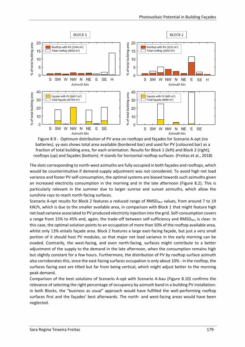
Photovoltaic Potential in Building Façades
Sara Regina Teixeira Freitas 179
Figure 8.9 - Optimum distribution of PV area on rooftops and façades for Scenario A-opt (no
batteries). yy-axis shows total area available (bordered bar) and used for PV (coloured bar) as a fraction of total building area, for each orientation. Results for Block 1 (left) and Block 2 (right),
rooftops (up) and façades (bottom). H stands for horizontal rooftop surfaces. (Freitas et al., 2018)
The slots corresponding to north-west azimuths are fully occupied in both façades and rooftops, which
would be counterintuitive if demand-supply adjustment was not considered. To avoid high net load
variance and foster PV self-consumption, the optimal systems are biased towards such azimuths given
an increased electricity consumption in the morning and in the late afternoon (Figure 8.2). This is
particularly relevant in the summer due to larger sunrise and sunset azimuths, which allow the
sunshine rays to reach north-facing surfaces.
Scenario A-opt results for Block 2 features a reduced range of RMSDNLV values, from around 7 to 19
kW/h, which is due to the smaller available area, in comparison with Block 1 that might feature high
net load variance associated to PV produced electricity injection into the grid. Self-consumption covers
a range from 15% to 45% and, again, the trade-off between self-sufficiency and RMSDNLV is clear. In
this case, the optimal solution points to an occupation of more than 50% of the rooftop available area,
whilst only 13% entails façade area. Block 2 features a large east-facing façade, but just a very small
portion of it should host PV modules, so that major net load variance in the early morning can be
evaded. Contrarily, the west-facing, and even north-facing, surfaces might contribute to a better
adjustment of the supply to the demand in the late afternoon, when the consumption remains high
but slightly constant for a few hours. Furthermore, the distribution of PV by rooftop surface azimuth
also corroborates this, since the east-facing surfaces occupation is only about 10% - in the rooftop, the
surfaces facing east are tilted but far from being vertical, which might adjust better to the morning
peak demand.
Comparison of the best solutions of Scenario A-opt with Scenario A-bau (Figure 8.10) confirms the
relevance of selecting the right percentage of occupancy by azimuth band in a building PV installation:
in both Blocks, the “business as usual” approach would have fulfilled the well-performing rooftop
surfaces first and the façades’ best afterwards. The north- and west-facing areas would have been
neglected.

Photovoltaic Potential in Building Façades
180 Sara Regina Teixeira Freitas
Figure 8.10 - Scenario A-bau for Block 1 (left) and Block 2 (right): percentage of occupancy by PV
modules of the azimuth bins available in rooftop and façade surfaces.
To adequately grasp the importance of the optimization from Scenarios A-opt and A-bau, the
remaining decision parameters must be known. Table 8.3 compares Scenarios A-opt and A-bau for
both case-study blocks. A-bau features surplus production around noon (since PV is mounted in higher
irradiance areas, i.e. mostly south-facing), while A-opt provides better demand-supply balance and,
thus, much higher self-consumption. Self-sufficiency remains high, but it slightly decreased for the
sake of reducing net load variance.
Table 8.3 – Annual PV generation and load demand [MWh/year], and decision parameter values for scenarios A-bau and A-opt for Block 1 and 2. Block 1 Block 2
A-bau A-opt A-bau A-opt
𝐸𝑑𝑒𝑚 522 504
𝑃𝑉 1039 329 272 186
RMSDNLV 53.0 18.6 13.7 9.8
SS 45.0 39.4 41.4 33.6
SC 22.6 62.5 76.7 90.8
PPVS 0.10 0.15 0.16 0.18
Apart from RMSDNLV and self-sufficiency, the positive effects of adjusting the community electricity
generation to its electricity consumption through inclination/orientation management of the PV
modules are also noticeable in terms of self-consumed PV production (up to 90% in the Scenario A-
opt for Block 2). Moreover, the PPVS obtained in Scenarios A-bau was always lower than in A-opt,
stressing the high value of locally produced electricity (which avoided grid purchase). However, the
self-sufficiency rates from A-opt solutions are 20% lower than A-bau’s. This is not surprising since A-
bau solutions would certainly belong to the right hand-side RMSDNLV tip in the Pareto fronts, thus
holding more significant negative impact to the grid side than the user side.

Photovoltaic Potential in Building Façades
Sara Regina Teixeira Freitas 181
8.8.2 PV placement optimization and storage strategy (scenarios B and C)
The numbers presented in the previous Sub-section might be increased using an appropriate storage
strategy. It is expected that the optimal installed PV power changes as the storage capacity increases,
which depends on the employed management approach. Through Figure 8.11 and Figure 8.12, the
optimal percentage of façade and rooftop PV by azimuth bin can be compared, for all the storage
capacities explored in Scenarios B-opt/B-bau and C-opt/C-bau (A-opt and A-bau are also represented
as the null storage capacity case).
Figure 8.11 - Optimum distribution of PV area on rooftops and façades for Scenario B-opt (orange and light blue) and B-bau (red and dark blue), for Block 1 (left) and Block 2 (right), from lower (top) to higher storage capacity (bottom). yy-axis shows area used for PV as a fraction of total building
area, for each orientation. The corresponding optimal PV peak power is given. Note that the percentages in the axis limits are different for the 2 blocks. (Freitas et al., 2018)
The optimal aggregated peak power for Block 1 under Scenarios B-opt/B-bau is twice as high as in
Scenarios A-opt/A-bau, with increased share of façades (blue bars) in the SW, NW, NE and SE
orientations. From B-opt to B-bau, almost all the rooftop surfaces are preferred over façade surfaces,
since the irradiation levels are generally lower in the latter. It can be realised that for a block with a
fair diversity of surface orientations and tilts (Block 1), the inclusion of storage capacity does not cause
significant changes in the optimal installed peak power and PV layout (i.e. large systems increase self-
BLOCK 1 BLOCK 2
Pinst= 1200 kWP 𝐵𝑏𝑎𝑡 =0 kWh/kWpv]
Pinst= 2465 kWP 𝐵𝑏𝑎𝑡 =0.25 kWh/kWpv]
Pinst= 2465 kWP 𝐵𝑏𝑎𝑡 =0.5 kWh/kWpv]
Pinst= 2510 kWP 𝐵𝑏𝑎𝑡 =1 kWh/kWpv]
Pinst= 2212 kWP 𝐵𝑏𝑎𝑡 =2 kWh/kWpv]
Pinst= 288 kWP 𝐵𝑏𝑎𝑡 =0 kWh/kWpv]
Pinst= 861 kWP 𝐵𝑏𝑎𝑡 =0.25 kWh/kWpv]
Pinst= 841 kWP 𝐵𝑏𝑎𝑡 =0.5 kWh/kWpv]
Pinst= 197 kWP 𝐵𝑏𝑎𝑡 =1 kWh/kWpv]
Pinst= 205 kWP 𝐵𝑏𝑎𝑡 =2 kWh/kWpv]

Photovoltaic Potential in Building Façades
182 Sara Regina Teixeira Freitas
sufficiency, but the production from different façades peaks at different times of the day, which helps
reducing net load variance). For large storage capacities, the SC strategy slightly pushes the systems
towards lower installed peak powers, compromising self-sufficiency and RMSDNLV, but increasing self-
consumption. These findings suggest that an aggregated storage bank of 0.25kWh/kWp that follows
the strategy SC would, thus, be appropriate for this community. On the other hand, a larger storage
cluster might be the best option for Block 2, as the recommended PV peak power is higher for small
storage capacities (0.25 and 0.5kWh/kWp). Given that the majority of building surfaces face east or
west, the self-consumption will be high regardless of storage; therefore, one optimal solution consists
on significantly reducing the deployed peak power to further decrease RMSDNLV (to avoid sudden net
load variance due to a fully charged/discharged battery).
Figure 8.12 - Optimum distribution of PV area on rooftops and façades for Scenario C-opt (light green and light yellow) and C-bau (dark green and dark yellow), for Block 1 (left) and Block 2 (right), from lower (top) to higher storage capacity (bottom). yy-axis shows area used for PV as a fraction of total building area, for each orientation. The corresponding total PV peak power is given. Note that the
percentages in the axis limits are different for the 2 blocks. (Freitas et al., 2018)
Although Block 1 features only slight changes in the distribution of PV for storage capacities equal to
0.25 and 0.5 kWh/kWp under Scenarios B-opt, the converse is observed for Scenarios C-opt. Significant
changes occur for storage capacities of 1 and 2 kWh/kWp: the overall share of façades (yellow bars) is
reduced, with no occurrence of façade surfaces facing NE, which might be thanks to the supply during
BLOCK 1 BLOCK 2
Pinst= 1200 kWP 𝐵𝑏𝑎𝑡 =0 kWh/kWpv]
Pinst= 2625 kWP 𝐵𝑏𝑎𝑡 =0.25 kWh/kWpv]
Pinst= 2450 kWP 𝐵𝑏𝑎𝑡 =0.5 kWh/kWpv]
Pinst= 1915 kWP 𝐵𝑏𝑎𝑡 =1 kWh/kWpv]
Pinst= 1684 kWP 𝐵𝑏𝑎𝑡 =2 kWh/kWpv]
𝐵𝑏𝑎𝑡 =0 kWh/kWpv] Pinst= 288 kWP
𝐵𝑏𝑎𝑡 =0.25 kWh/kWpv] Pinst= 499 kWP
𝐵𝑏𝑎𝑡 =0.5 kWh/kWpv] Pinst= 849 kWP
𝐵𝑏𝑎𝑡 =1 kWh/kWpv] Pinst= 873 kWP
𝐵𝑏𝑎𝑡 =2 kWh/kWpv] Pinst= 890 kWP

Photovoltaic Potential in Building Façades
Sara Regina Teixeira Freitas 183
the night time/morning period assured by the large storage capacity. C-bau, however, retains only a
small amount of PV on those places. The community PV capacity more than doubles from A-opt/A-bau
to C-opt/C-bau, but keeps decreasing as storage increases. The contrary is observed for Block 2, where
a significant increase in W and E façade surfaces can be noticed. The share of occupied azimuth bins
remained practically unaltered from storage capacities 0.5 kWh/kWp on: given that the RMSD strategy
sought to minimize RMSDNLV, it was not very effective since that goal had already been accomplished
through a suitable placement of PV.
The overall quality of these aggregation solutions can be analysed considering the four decision
parameters (compiled in Figure 8.13). The difference between scenarios B and C is the storage control
strategy: the first can be understood as a ‘selfish’ strategy, which aims to maximize the benefit for the
prosumers and the latter is a ‘cooperative’ strategy, to minimize impact on the grid. With a small
battery, a selfish strategy can have a relevant impact on the community’s self-consumption and self-
sufficiency at the exchange for negative consequences to the grid: strong net load variance will occur
when the battery is fully charged/discharged (which will happen frequently because the battery is
small). On the other hand, a ‘cooperative’ strategy, thought to lessen net load variance, will prevent
making full use of the (small) battery and, consequently, its effect on self-consumption will be much
less significant. For large storage, both strategies lead to higher levels of self-consumption and
(relatively) low net load variance.
Overall, the PV optimization method together with an adequate battery management (B-opt and C-
opt, solid lines in Figure 8.13) can provide lower RMSDNLV than its equivalent scenario without PV
optimization (B-bau and C-bau, dashed lines in Figure 8.13). This parameter also decreases from
smaller to higher storage capacities. A storage management aiming to reduce RMSDNLV with perfect
forecast (C-opt/C-bau) proves its effectiveness, whereas the maximization of self-consumption per se
(B-opt/B-bau) might induce occasions when the batteries are at maximum/minimum level and cannot
act - sudden high net load variance consequently takes place, as observed in (Luthander et al., 2015).
Self-sufficiency grows with battery capacity, more remarkably from 0 to 0.5 kWh/kWp; this emphasizes
the important role that aggregated storage has on improving what had already been achieved through
the optimized aggregation and placement of PV. This parameter converges asymptotically to 100%,
since the PV installation is fixed and optimized for an aggregated demand profile that varies
throughout the day and year, and not to point-in-time situations. A slight change in a parcel of the
system might produce benefits for an occasion but can be disadvantageous in another, even with
storage it may be impossible to achieve perfect demand-supply match. Thus, the storage operation
strategy and the characteristics of the consumption profile have a strong influence on what can be
considered the absolute optimal configuration of PV and storage.
The trade-off between RMSDNLV and self-sufficiency is undoubtedly apparent: B-bau and C-bau, which
prioritise high irradiation places, entail higher self-sufficiency than B-opt and C-opt, which seek for the
best compromise between self-sufficiency and RMSDNLV. This is more evident for Block 1 than for Block
2, where the PV configuration computed by C-opt or C-bau with storage equal or above 0.5 kWh/kWp
appear to be good solutions, with C-opt achieving a self-consumption rate slightly higher than C-bau.
Regarding Block 1, the estimated self-consumption rates are very high for B-opt and C-opt, but halved
for B-bau and C-bau, which underlines the importance of combining PV from diverse orientations and
inclinations in optimal ways.
The PPVS parameter entails mostly negative values for both Blocks, only positive for small or null
storage capacity. Such outcome is mainly due to the current impracticality of investing in high capacity
storage, even as a community, as pointed out Section 8.1. Large shares of façade PV (in B-opt and C-
opt), which is still less affordable than rooftop PV, might also contribute to higher investment.
Moreover, weighted the advantages of deploying more façade PV and including larger batteries, the
scale inclines towards the first, thus minimizing storage needs for urban solar communities.

Photovoltaic Potential in Building Façades
184 Sara Regina Teixeira Freitas
Figure 8.13 - Overall results for RMSDNLV, SS, SC and PPVS as a function of storage capacity, for Scenarios B-opt (blue solid line), B-bau (blue dashed line), C-opt (orange solid line) and C-bau (orange
dashed line). (Freitas et al., 2018)
BLOCK 1 BLOCK 2 R
MSD
NLV
[kW
/h]
Self
-Su
ffic
ien
cy [
%]
Self
-Co
nsu
mp
tio
n [
%]
PP
VS
[€/k
Wh
]
Storage capacity [kWh/kWp] Storage capacity [kWh/kWp]

Photovoltaic Potential in Building Façades
Sara Regina Teixeira Freitas 185
8.9 Discussion
In this Section, a few methodological limitations of this study and further implications of its findings
will be discussed.
First, it would be beneficial to extend the analysis to other PTs with dissimilar demand profiles and
building blocks with different architectonic features. Ultimately, the study should encompass the
broader cityscape level. In this sense, and given that the computation of time-resolved solar irradiation
is labour-intensive, a possible strategy would be to, first, calculate a reference irradiation profile for
all possible tilt and azimuth combinations and, then, assign those profiles to all the surfaces across the
urban model, instead of computing each one at a time. However, a successful implementation of this
approach would be compromised by the morphing of shadow patterns, a high resolution of tilt and
azimuth angles and sub-hourly time step. Nevertheless, tiling strategies (Romero Rodríguez et al.,
2017b) can be employed for massive urban models.
The demand-supply issues that distributed PV with storage faces were clearly identified, regardless of
specific building morphologies and consumption profiles. Yet, the original time resolution of the
demand profile (15min) was lowered to the hourly level. The higher the time step, the more demand
and generation peaks and breaks are excluded (regardless of aggregation effects), making the net load
variance analysis less accurate.
The use of a reference meteorological year also represents a limitation. Preferably, solar radiation
measurements from a nearby station (of course, covering the same analysis period) would have given
better insight into the relationship between electricity consumption and meteorological conditions.
Assessing the influence of solar radiation variability on these results would also be interesting, since
present and future variability might influence the optimal PV façade layout.
In the method for PV generation estimation, it was considered that the modules were deployed onto
the surfaces as they are, i.e. without tilt or orientation changes (very common in horizontal and non-
south-facing building surfaces), otherwise the complexity of this study would have increased greatly.
However, this addition increases the cost of the system and often causes the systems to become less
aesthetical appealing.
Regarding the economics of the systems, it must be noted that no economy of scale was considered
for neither the aggregated PV nor the aggregated storage portions of the community investment. This
could have significantly lowered the costs of the configurations that entailed large installed peak
power. As for the storage, it is more difficult to infer at current market state. However, it is likely that
the effect of the economy of scale will be pronounced in the medium-term, given decreasing battery
prices (Liebreich, 2017), prompted especially by the urge for electrical mobility.
As for the aggregation per se, although it is suggested that the distribution PT grid defines the
convenient size for a community project, there is no warranty that having the current PT capacities
and interconnections is the optimal solution for massive PV penetration in the city of the future (as
also observed in Chapter 7).
Nonetheless, it was demonstrated that aggregating demand, PV production and storage has
advantages for the user and should therefore be encouraged. This fosters the creation of urban solar
community projects, which consists on the cooperation between multiple members who can benefit
from power and/or revenue from PV systems. In exchange, each individual gives his contribution to
the communal project, for instance, in the form of an up-front purchase of an element for the PV
system or monthly contributions on the electricity bill. The system owner, system host, installation

Photovoltaic Potential in Building Façades
186 Sara Regina Teixeira Freitas
size, number of participants, individual country/state policy, etc., will vary as per the specificities of
each project (Erin Takata, 2017).
It can be argued that, in first approximation, the costs for the electricity grid are mostly dictated by
the maximum peak power. Hence, one concludes that local solar communities have the potential to
assist the grid by lowering their local peak power. Table 8.4 summarizes the peak power obtained in
the scenarios explored.
Table 8.4 – Maximum absolute peak power in the electricity grid [kW], for Block 1 and 2. Bold highlights the 3 lowest peak power achieved for each Block.
Grid peak power 𝑚𝑎𝑥[𝑎𝑏𝑠(𝑠𝑢𝑝𝑝𝑙𝑦 − 𝑑𝑒𝑚𝑎𝑛𝑑)]
Storage capacity
0 kWh/kWp
0.25 kWh/kWp
0.5 kWh/kWp
1 kWh/kWp
2 kWh/kWp
Blo
ck 1
B-bau 476 539 539 540 533
B-opt 142 142 142 160 142
C-bau 476 587 580 543 710
C-opt 142 223 121 121 121
Blo
ck 2
B-bau 126 133 133 126 126
B-opt 126 126 126 126 126
C-bau 126 119 135 106 245
C-opt 126 119 112 113 115
Peak power features a broad range of values for scenarios involving Block 1. For Block 2, due to the
prevalence of east-facing surfaces (Figure 8.4), the maximum peaks are all of similar magnitude. As
expected, scenario C-opt with storage capacities above 0.5 kWh/kWp seems to allow lower costs with
power supply for the grid.
Results reveal that conflicting interests between users and grid exist: higher returns to the solar
community lead to increased burdens to the grid, whereas the smoothening of the demand profile
leads to diminished returns for the PV owners. Nevertheless, traditional utilities have started making
efforts towards understanding how the value from distributed generation and storage can be captured
and fit into their business models (Trabish, 2017). Some key advantages of including those electricity
systems relate to: reduced usage (or entirely removal) of expensive and polluting peaker plants, which
usually sit idle for long periods of time; deferral of upgrades to utility assets or creation of new
transmission and distribution lines; and lessened power outage events.
There are, at the same time, opportunities for the creation of new financial business models if the
value of reduced peak loads is regarded, and benefit sharing between the grid and the local solar
communities. As an example, a storage bank was recently connected to distribution circuits at
Southern California Edison’s Mira Loma substation (Cardwell, 2017) to help smoothing variations in
the power flow from/to rooftop PV clients, hence avoiding curtailment of PV (i.e. loss of profitability
for the community) and the need to supply when conventional power plants cannot meet the
pronounced electricity demand in the early evening. In this example, however, the battery bank is
centralized and owned by the grid, but new business models could explore different ownership aspects
of the storage system, including distributed storage among the community and even third-party
storage. These must bear in mind that the proper energy management of the solar community, and
especially the control strategies for the batteries, has a critical impact on the overall system
performance and the complementarity between solar community and grid (and/or, eventually, all
other electricity consumers): a ‘selfish’ management algorithm could lead to a decrease of up to 35%

Photovoltaic Potential in Building Façades
Sara Regina Teixeira Freitas 187
in self-sufficiency, while annual net load variance would grow up to 50%, with an average 20% higher
peak power (Figure 8.13).
Building deployed PV systems only in locations with high solar exposure (typically those facing south),
instead of making use of the diversity of surface tilts and orientations, will lead to adverse impacts on
the grid. The latter contributes to flatten net load variance profile, since it prompts a wider period of
PV electricity generation that matches the demand profile throughout the day. Therefore, façades that
have been quantitatively considered as “less-than-optimum” places, now become advantageous to a
greater purpose by providing quality electricity. Additionally, possible approaches to entice the
installation of PV systems in façades might include the commonly adopted self-consumption metering
solutions, which favour off-peak generation by valuing avoided consumption over excess generation,
or ‘time-of-use’ feed-in tariffs, which realize higher returns early and/or later in the day.
Lastly, it must be emphasized that a massive growth in local solar communities will trigger a disruption
in the electricity market, since prosumers wish to reduce the purchase of electricity from the grid while
maximizing exchanges of power with other community members (through micro cooperative utilities).
Given the potential for becoming notably present in the grid, the concept of citizen utilities will
certainly convert into reality. As stressed in (Green and Newman, 2017), citizen utilities will need to
be accommodated within the future distributed system paradigm, where the traditional grid will still
have a role to play. This new energy market, managed by consumers, will introduce dramatic changes
to generation, consumption and transaction of electricity.
8.10 Conclusion
The multitude of building surfaces with different tilts and orientations in the urban environment
translates into a greater PV potential that, if well used, results in a better adjustment of local
production to demand, in the context of self-demand PV systems with and without electricity storage.
When the placement of the PV systems is optimized considering different generation profiles triggered
by a diversity of surface tilts and orientations, the consumption from different buildings and the PV
electricity production can be aggregated to improve the demand-supply match within a solar
community, minimizing its storage needs.
The profitability of community PV systems might always be positive when no storage is considered
(reaching almost 0.2 €/kWh in the studied cases), and decrease as storage capacity rises. However,
the inclusion of electricity storage boosts both self-consumption and -sufficiency, which tend
asymptotically to a very high value (even to 100%, in some scenarios). Net load variance has potential
for reduction as storage capacity increases, although slight variations might be observable in the low
storage regime.
From the point of view of a prosumer community, investments on PV may only be viable with null or
very small added storage capacity. Conversely, the electricity grid prevents unmanageable net load
variance while mitigating its consequent costs through higher storage capacities with proper
management strategy. Hence, grid/local authorities ought to support the commissioning of grid,
community or third-party owned storage capacity with adequate management standards to curtail or
control net load variance. At the same time, new business models are required to share the added
values between the interested parts.

Photovoltaic Potential in Building Façades
188 Sara Regina Teixeira Freitas

Photovoltaic Potential in Building Façades
Sara Regina Teixeira Freitas 189
9. CLOSURE
The sustainable development of present generations and their continuity into the future cannot be
detached from renewable energy research and development. Technologies for converting solar
radiation into electricity are especially relevant, since the sun is the most basic source of energy for
planet Earth. A turning point was reached when PV became cheaper enough to be brought closer to
electricity demand hot spots: buildings in the urban environment. Rooftop systems have been the
most adopted solution, whilst façades are often disregarded. This thesis highlights the role of façades
for the solar potential of cities and explores optimization alternatives and tools for its modelling.
The variety of cityscapes in the world prompts different solar potential, apart from the latitude bias,
which must be assessed prior to the deployment of solar energy systems. Empirical solar radiation
models have been developed and improved to estimate the solar radiation falling on surfaces with
arbitrary orientation and tilt, coupled with long-term measurements from ground weather stations
and/or satellite imagery. The intricacy of urban environments requires more sophisticated methods
for the proper modelling of shadows. Diffuse radiation falling in a surface is challenging to compute
given its anisotropy, thus buildings and context materials/coverage and the varying sky conditions
must be accounted for. This is particularly relevant for building façades, since their vertical inclination
gives them higher exposure to ground and surroundings reflected radiation and their sky view factors,
smaller than rooftops’, reduce background sky diffuse radiation according to the sky patches that are
obstructed.
Improved computational power has driven the creation of sophisticated solar potential models relying
on digital surface models that can portray building features with realism. Vector data with building
footprints and LiDAR-derived elevation data are among the cost-efficient methods to create a 3D city
model. Time-resolved irradiation in a full 3D environment including vertical surfaces can be estimated
through state-of-the-art models, with emphasis on GIS, CAD/plugin and CityGML-based tools,
although simplifications might be unavoidable when addressing high density environments. Results
can easily be manipulated to produce significant content related to PV potential to aid in the process
of urban planning and decision making towards sustainable cities.
Experimental validation is fundamental for urban solar potential models that include façades, as it
helps identifying current limitations and where the accuracy of the algorithms fails. Pyranometers are
not commonly installed in building façades to validate model simulations, however, it is possible to
use generation data from PV systems. Irradiation simulations must be carried on over an updated
surface model that includes trees, and then converted into electricity production before it is compared
against reference façade and/or rooftop systems data. The spatial resolution dictates the complexity
of the electricity conversion method, but the effects of temperature on the module efficiency, the
effect of the angle of incidence on the radiation that effectively reaches the solar cells and partial
shading in the PV strings are important loss mechanisms to consider at an hourly time frame and
spatial resolution of 1m2.
Proper modelling of façade PV potential in places with dissimilar climatic conditions gives insight into
where the contribution of vertical surfaces to the PV potential is more relevant and where its
deployment should be encouraged. It is known that higher tilts favour PV production as latitude
increases, as lower sun heights allow for the light to reach these surfaces close to the normal, but the
fraction of diffuse irradiation might also enhance the relevance of façades in respect to the rooftops
in mid-latitude locations. A building has mostly at least two façades facing opposite directions, hence
higher diffuse radiation content traduces into more frequent overcast sky conditions that distribute
the irradiation more evenly across the built environment.

Photovoltaic Potential in Building Façades
190 Sara Regina Teixeira Freitas
Different PV technologies can be employed to make the most of a PV system regardless of climatic
conditions. Whereas the mature technology of c-Si modules is an affordable and efficient solution,
limited aesthetics have been their main drawback when building owners want concealed or disguised
PV systems. Specific projects might result well with conventional flat and opaque modules, but façade
products seek to achieve new colour possibilities for spandrel areas, higher degrees of transparency
for glazing surfaces and flexibility for alternative architecture designs. Glass printing or anti-reflection
coating tuning are techniques that allow for the customization of conventional façade PV systems. On
the other hand, despite their lower quality, thin films are also an option to achieve translucent and
colourful PV façade glazing or canopies. Vertically integrated bifacial modules represent a means to
save space and to give an alternative look to façade elements such as balconies or railings. The raising
popularity of, yet low efficient, luminescent solar concentrators has prompted the creation of
commercial window products that make PV almost unnoticeable. Other types of concentrating
alternatives are, however, inappropriate for façades as they are less responsive to higher diffuse
content.
Building integrated PV can either be perceived as electricity generating devices that are an additional
part of the building skin or the opposite, i.e. an intrinsic building element that has the added value of
producing energy. This dual character of BIPV is what makes it particularly interesting for façade
applications, given the variety of elements and the vast range of possibilities for PV integration. Other
improvements of PV over conventional construction materials relate to the possibility of making use
of the heat generated on the rear side of the modules to passively regulate indoor comfort and, in the
case of semi-transparent and translucent technologies, regulate daylight levels in the interior spaces.
Moreover, these complementary functionalities of BIPV can translate into financial payback.
Systems yields can be further maximized if early-stage façade designs contemplate the integration of
PV. Horizontal tilted louvers can enhance the irradiation that reaches façade PV in about 30% in
comparison to a flat vertical layout, whilst more complex forms increase yields at the cost of using
much more PV material. Another alternative design encompasses the use of bifacial modules as
balcony railings, where the back surface receives reflected radiation from within the balcony area. In
this case, the rear surface of the module contributes with about 1/3 to the total production. These are
examples of strategies to make good use of area that otherwise would remain idle.
Another important issue to take into account in façade PV systems is partial shading, which has a
dramatic effect on the electricity production of PV strings, reducing yearly yields of the whole PV
system in 6% to 24%. Micro-inverters represent a reliable but costly solution to the problem. Module
sitting and string interconnections must be such that more sunlit areas get clustered and relatively
short strings, whilst less lit places either get very short strings or individual modules or no modules at
all. Optimal layouts keep the compromise between annual energy generation potential and
investment costs.
Maximizing the electricity yields either through alternative façade layouts or by seeking the most
adequate module technology have consequences on the outdoor spaces, such as visual discomfort or
disability glare. Fully glazed mirror façades are relatively common architecture in dense modern cities,
but there are no specific guidelines to regulate these issues. Highly reflective materials in building
façades should be discouraged, despite the design goals, unless simulations prove its safety. Other
way around might be to rethink the building layout to adopt PV technologies instead of conventional
reflective materials. Although typical c-Si modules feature reflection losses for high incidence angles,
these are not as dramatic as reported for mirror or glass. Nevertheless, PV glass technologies have
emerged that seek to further reduce reflection losses.
The deployment of PV at a larger scale should primarily match the electricity consumption of
neighbourhoods. Whereas typical south-facing rooftop PV generates surplus around midday, with the
addition of solar façades it is possible to start producing earlier in the day, with east-facing façades,

Photovoltaic Potential in Building Façades
Sara Regina Teixeira Freitas 191
and extended production to later, with west-facing façades. This helps widening the period of the day
when local electricity demand can significantly be covered by solar, especially in the summer. Although
the production of PV façades is higher in the winter, a lower number of sunlight hours reduces the
contribution of solar to the supply chain.
The levels of irradiation over building surfaces translate into different classes of profitability for PV
systems. Combination between façades and rooftops can be deployed as a function of the cost. In a
city like Lisbon, a 50/50 mix would encompass a combined payback time of around 15 years, at current
prices, whereas considering only the most exposed surfaces would lead to paybacks in the order of 19
years. Since the efficiency of the modules is expected to continue increasing with decreasing costs, a
combined payback of around 10 years can be achieved through 40% of the PV deployment in façades.
Further reduction of investment costs and increasing module efficiency will lead to high penetration
of PV in the electricity grid. A scenario of full integration of PV into buildings in a suburb will, however,
overwhelm grid assets such as distribution transformers with lower power capacities. The generation
potential including façades must be taken into account when sizing transformers in new built areas or
when upgrading the existing ones. New interconnections may also be planned, if neighbouring
transformers have spare capacity to accommodate PV surplus, which is a cheaper solution than
increasing transformer capacity in dense urban areas. More than faulty transformers, the whole local
grid might become unmanageable if large amounts of PV are fed into the grid. Sudden net load
variance, either due to abrupt breakdown in PV production in periods of high demand or increased PV
supply when demand is lower, must be avoided since it causes grid management to compensate with
fossil fuel peaking power plants.
The future of solar cities might reside in the creation of local solar communities, sharing the
investment costs and revenues from PV and storage systems optimized to match the aggregated load
profile. Community solar systems will be placed preferably in tilted rooftops and façades with
orientations that will likely produce when consumption is more likely, i.e. they will make use of the
variety of building surfaces and occupy only the places that match the requirements. Aggregated
storage will work as a buffer to further maximize community’s self-sufficiency, but also to avoid excess
PV production being fed into the grid. The grid will continue playing its crucial balancing role, thus
future electricity markets and business models need to consider the arising conflicting interests
between prosumers and grid. Sharing the value of distributed generation and reduced peak due to the
integration of PV in building façades will be one essential component of this integrated system.

Photovoltaic Potential in Building Façades
192 Sara Regina Teixeira Freitas

Photovoltaic Potential in Building Façades
Sara Regina Teixeira Freitas 193
10. REFERENCES
A.L. Martins, T., Adolphe, L., E.G. Bastos, L., 2014. From solar constraints to urban design opportunities: Optimization of built form typologies in a Brazilian tropical city. Energy and Buildings 76, 43–56.
Abu-Bakar, S.H., Muhammad-Sukki, F., Freier, D., Ramirez-Iniguez, R., Mallick, T.K., Munir, A.B., Mohd Yasin, S.H., Abubakar Mas’ud, A., Bani, N.A., 2016. Performance analysis of a solar window incorporating a novel rotationally asymmetrical concentrator. Energy 99, 181–192.
ADENE, 2014. Decreto-Lei n.o 153/2014 D.R. n.o 202/2014, Série I. Retrieved from: http://www.adene.pt/decreto-lei-no-152-2014-de-20-de-marco
Alias, A.-R., Pilouk, M., 2008. Spatial Data Modelling for 3D GIS. Springer, ISBN 3540741674. Amado, M., Poggi, F., 2014. Solar Urban Planning: A Parametric Approach. Energy Procedia 48, 1539–
1548. Ameri, T., Khoram, P., Min, J., Brabec, C.J., 2013. Organic Ternary Solar Cells: A Review. Advanced
Materials 25, 4245–4266. American Institute of Architects, 2015. Design Excellence Awards. Retrieved from:
https://www.aiachicago.org/dea_archive/2015/fki-tower-exterior-wall/ Angelis-Dimakis, A., Biberacher, M., Dominguez, J., Fiorese, G., Gadocha, S., Gnansounou, E., Guariso,
G., Kartalidis, A., Panichelli, L., Pinedo, I., Robba, M., 2011. Methods and tools to evaluate the availability of renewable energy sources. Renewable and Sustainable Energy Reviews 15, 1182–1200.
Anthony, D., 2010. Where Will Solar Power Plants Be Built - Deserts or Rooftops? . Greentech Media. Retrieved from: https://www.greentechmedia.com/articles/read/where-will-solar-power-plants-be-built-deserts-or-rooftops#gs.DdF0njA
Anton, I., Tănase, D., 2016. Informed Geometries. Parametric Modelling and Energy Analysis in Early Stages of Design. Energy Procedia 85, 9–16.
Assouline, D., Mohajeri, N., Scartezzini, J.-L., 2017. Quantifying rooftop photovoltaic solar energy potential: A machine learning approach. Solar Energy 141, 278–296.
Athienitis, A.K., Bambara, J., O’Neill, B., Faille, J., 2011. A prototype photovoltaic/thermal system integrated with transpired collector. Solar Energy 85, 139–153.
Autodesk Inc, 2016. Dynamo BIM. Retrieved from: http://dynamobim.org/learn/ Autodesk Inc, 2017. Revit for Autodesk. Retrieved from: https://www.autodesk.com/education/free-
software/revit Azar, S., 2013. TownScope. Retrieved from: http://townscope.com/ Bäck, T., Rudolph, G., Schwefel, H.-P., 1993. Evolutionary programming and evolution strategies:
Similarities and differences, in: Proceedings of the Second Annual Conference on Evolutionary Programming. pp. 76–78.
Baig, H., Sellami, N., Mallick, T.K., 2015. Performance modeling and testing of a Building Integrated Concentrating Photovoltaic (BICPV) system. Solar Energy Materials and Solar Cells 134, 29–44.
Barron-Gafford, G.A., Minor, R.L., Allen, N.A., Cronin, A.D., Brooks, A.E., Pavao-Zuckerman, M.A., 2016. The Photovoltaic Heat Island Effect: Larger solar power plants increase local temperatures. Scientific Reports 6, 35070.
Bendheim, 2010. Solarwatt GmbH. Retrieved from: https://bendheim.com/project/solarwatt-gmbh/ Berny, S., Blouin, N., Distler, A., Egelhaaf, H.-J., Krompiec, M., Lohr, A., Lozman, O.R., Morse, G.E.,
Nanson, L., Pron, A., Sauermann, T., Seidler, N., Tierney, S., Tiwana, P., Wagner, M., Wilson, H., 2016. Solar Trees: First Large-Scale Demonstration of Fully Solution Coated, Semitransparent, Flexible Organic Photovoltaic Modules. Advanced Science 3.
Bidram, A., Davoudi, A., Balog, R.S., 2012. Control and Circuit Techniques to Mitigate Partial Shading Effects in Photovoltaic Arrays. IEEE Journal of Photovoltaics 2, 532–546.
Biljecki, F., Ledoux, H., Stoter, J., 2017. Generating 3D city models without elevation data. Computers, Environment and Urban Systems 64, 1–18.

Photovoltaic Potential in Building Façades
194 Sara Regina Teixeira Freitas
Biljecki, F., Ledoux, H., Stoter, J., Zhao, J., 2014. Formalisation of the level of detail in 3D city modelling. Computers, Environment and Urban Systems 48, 1–15.
BIMsolar, 2018. BIMsolar. Retrieved from: http://webdc-design.fr/bimsolar/en/bimsolar-4/ Bird, R.E., Hulstrom, R.L., 1981. Simplified clear sky model for direct and diffuse insolation on
horizontal surfaces . National Renewable Energy Laboratory (NREL). Retrieved from: http://www.osti.gov/servlets/purl/6510849/
Bonomo, P., Zanetti, I., Frontini, F., van den Donker, M., Vossen, F., Folkerts, W., 2017. BIPV PRODUCTS OVERVIEW FOR SOLAR BUILDING SKIN, in: 33rd EUPVSEC. Amesterdam.
BP_Solar, 2006. 160-Watt Multicrystalline Photovoltaic Module. Retrieved from: https://www.solarpanelsaustralia.com.au/downloads/bpsolar_bp3160.pdf
Braun, M., Stetz, T., Bründlinger, R., Mayr, C., Ogimoto, K., Hatta, H., Kobayashi, H., Kroposki, B., Mather, B., Coddington, M., Lynn, K., Graditi, G., Woyte, A., MacGill, I., 2012. Is the distribution grid ready to accept large-scale photovoltaic deployment? State of the art, progress, and future prospects. Progress in Photovoltaics: Research and Applications 20, 681–697.
Bremer, M., Mayr, A., Wichmann, V., Schmidtner, K., Rutzinger, M., 2016. A new multi-scale 3D-GIS-approach for the assessment and dissemination of solar income of digital city models. Computers, Environment and Urban Systems 57, 144–154.
Brito, M.C., Freitas, S., Guimarães, S., Catita, C., Redweik, P., 2017. The importance of facades for the solar PV potential of a Mediterranean city using LiDAR data. Renewable Energy 111, 85–94.
Brito, M.C., Gomes, N., Santos, T., Tenedório, J.A., 2012. Photovoltaic potential in a Lisbon suburb using LiDAR data. Solar Energy 86, 283–288.
Brogren, M., Wennerberg, J., Kapper, R., Karlsson, B., 2003. Design of concentrating elements with CIS thin-film solar cells for façade integration. Solar Energy Materials and Solar Cells 75, 567–575.
Buhl, J., Gautrais, J., Reeves, N., Solé, R. V, Valverde, S., Kuntz, P., Theraulaz, G., 2006. Topological patterns in street networks of self-organized urban settlements. The European Physical Journal B 49, 513–522.
Building Art Invention, 2017. DysCrete. Retrieved from: http://www.baukunsterfinden.org/en/research/projects/dyscrete-energy-production-systems/
Bunthof, L.A.A., Kreuwel, F.P.M., Kaldenhoven, A., Kin, S., Corbeek, W.H.M., Bauhuis, G.J., Vlieg, E., Schermer, J.J., 2016. Impact of shading on a flat CPV system for façade integration. Solar Energy 140, 162–170.
Camilo, F.M., Castro, R., Almeida, M.E., Pires, V.F., 2017. Economic assessment of residential PV systems with self-consumption and storage in Portugal. Solar Energy 150, 353–362.
Cardwell, D., 2017. Tesla Gives the California Power Grid a Battery Boost - The New York Times . The New York Times. Retrieved from: https://www.nytimes.com/2017/01/30/business/energy-environment/battery-storage-tesla-california.html?_r=0
Carneiro, C., Morello, E., Desthieux, G., Golay, F., 2010. Urban environment quality indicators: application to solar radiation and morphological analysis on built area. Advances in Visualization, Imaging and Simulation 141–148.
CASE, 2016. High Efficiency Solar Energy Systems. Retrieved from: http://www.case.rpi.edu/page/project.php?pageid=1
Catani, A., Gómez, F., Pesch, R., Schumacher, J., Pietruschka, D., Eicker, U., 2008. Shading Losses of Building Integrated Photovoltaic Systems, in: 23rd European Photovoltaic Solar Energy Conference and Exhibition. Valencia, Spain.
Catita, C., Redweik, P., Pereira, J., Brito, M.C., 2014. Extending solar potential analysis in buildings to vertical facades. Computers & Geosciences 66, 1–12.
Caula, R., 2012. Spherical glass solar energy generator by rawlemon . Designboom. Retrieved from: https://www.designboom.com/technology/spherical-glass-solar-energy-generator-by-rawlemon/
CCL Componentes, 2014. Fronius Inverters. Retrieved from: http://www.cclcomponents.com/range.asp?ID=372

Photovoltaic Potential in Building Façades
Sara Regina Teixeira Freitas 195
Chapman, L., Thornes, J.E., Bradley, A. V., 2002. Sky-view factor approximation using GPS receivers. International Journal of Climatology 22, 615–621.
Chemisana, D., Rosell, J.I., 2011. Design and optical performance of a nonimaging Fresnel transmissive concentrator for building integration applications. Energy Conversion and Management 52, 3241–3248.
Chimklai, P., Hagishima, A., Tanimoto, J., 2004. A computer system to support Albedo Calculation in urban areas. Building and Environment 39, 1213–1221.
Chow, T.T., He, W., Ji, J., 2007. An experimental study of façade-integrated photovoltaic/water-heating system. Applied Thermal Engineering 27, 37–45.
Chun-Lien Su, Hsiang-Ming Chuang, 2014. Distribution network reinforcement planning for high penetration level of distributed generation, in: 2014 IEEE International Energy Conference (ENERGYCON). IEEE, pp. 1170–1175.
CML, 2017. Casa dos Bicos ou de Brás de Albuquerque. Retrieved from: http://www.cm-lisboa.pt/en/equipments/equipment/info/casa-dos-bicos-ou-de-bras-de-albuquerque
Coccolo, C., Mauree, D., Kämpf, J., Scartezzini, J.L., 2016. Integration of outdoor human comfort in a building energy simulation database using CityGML energy ADE, in: Sustainable Built Environment (SBE) Regional Conference. Zurich, pp. 84–89.
Comello, S., Reichelstein, S., 2017. Cost competitiveness of residential solar PV: The impact of net metering restrictions. Renewable and Sustainable Energy Reviews 75, 46–57.
Compagnon, R., 2004. Solar and daylight availability in the urban fabric. Energy and Buildings 36, 321–328.
Comparotto, C., Noebels, M., Wefringhaus, E., Ferretti, N., Mancini, G., Berghold, J., Einhaus, R., Madon, F., 2015. Energy Yield Estimation of Monofacial and Bifacial Solar Modules. 31st European Photovoltaic Solar Energy Conference and Exhibition.
Connelly, K., Wu, Y., Chen, J., Lei, Y., 2016. Design and development of a reflective membrane for a novel Building Integrated Concentrating Photovoltaic (BICPV) “Smart Window” system. Applied Energy 182, 331–339.
Crawley, D.B., Lawrie, L.K., Winkelmann, F.C., Buhl, W.F., Huang, Y.J., Pedersen, C.O., Strand, R.K., Liesen, R.J., Fisher, D.E., Witte, M.J., Glazer, J., 2001. EnergyPlus: creating a new-generation building energy simulation program. Energy and Buildings 33, 319–331.
Cristóvão, A.R., 2016. Análise de obstruções à radiação solar em contexto urbano. MSc thesis, University of Lisbon.
Cucchiella, F., D’Adamo, I., Gastaldi, M., 2016. Photovoltaic energy systems with battery storage for residential areas: an economic analysis. Journal of Cleaner Production 131, 460–474.
Danks, R., Good, J., Sinclair, R., 2016. Assessing reflected sunlight from building facades: A literature review and proposed criteria. Building and Environment 103, 193–202.
David Rutten, 2017. Galapagos. Retrieved from: http://www.grasshopper3d.com/group/galapagos Davidson, S., 2017. Grasshopper. Retrieved from: http://www.grasshopper3d.com/ Dean, J., Kandt, A., Burman, K., Lisell, L., Helm, C., 2009. Analysis of Web-Based Solar Photovoltaic
Mapping Tools, in: ASME 2009 3rd International Conference on Energy Sustainability, Volume 1. ASME, pp. 85–96.
de Simón-Martín, M., Alonso-Tristán, C., Díez-Mediavilla, M., 2017. Diffuse solar irradiance estimation on building’s façades: Review, classification and benchmarking of 30 models under all sky conditions. Renewable and Sustainable Energy Reviews 77, 783–802.
Di Giacomo, F., Fakharuddin, A., Jose, R., Brown, T.M., 2016. Progress, challenges and perspectives in flexible perovskite solar cells. Energy Environ. Sci. 9, 3007–3035.
Diouf, B., Pode, R., 2015. Potential of lithium-ion batteries in renewable energy. Renewable Energy 76, 375–380.
Dogan, T., Reinhart, C., 2017. Shoeboxer: An algorithm for abstracted rapid multi-zone urban building energy model generation and simulation. Energy and Buildings 140, 140–153.
Donahue, T., 2017. Solar Panels On An Apartment Building. Retrieved from: https://www.gettyimages.pt/detail/foto/solar-panels-on-an-apartment-building-fotografia-de-

Photovoltaic Potential in Building Façades
196 Sara Regina Teixeira Freitas
stock/110055267 Dubayah, R., 1992. Estimating net solar radiation using Landsat Thematic Mapper and digital
elevation data. Water Resources Research 28, 2469–2484. Dubayah, R., Rich, P.M., 1995. Topographic solar radiation models for GIS. International journal of
geographical information systems 9, 405–419. Duffie, J.A., Beckman, W.A., 2013. Solar Engineering of Thermal Processes, Solar Engineering of
Thermal Processes: Fourth Edition. John Wiley & Sons, Inc., ISBN 9781118671603, Hoboken, NJ. E.ON Solar, 2017. Google Sunroof zeigt Ihr Solarpotenzial!. Retrieved from: https://www.eon-
solar.de/ EcoFloLife, 2017. Technology. Retrieved from: https://www.ecoflolife.com/technology/ Ecotect, 2010. Autodesk ECOTECT Analysis. Retrieved from:
https://knowledge.autodesk.com/support/ecotect-analysis/learn-explore/caas/video/youtube/watch-v-BKZ35xh4ofw.html
Eder, G.C., Knöbl, K., Maul, L., Aichinger, M., Peharz, G., Berger, K.A., 2017. Designed BIPV-elements with printed front-glass: Simulation and experimental evaluation of the effect of print, in: 12th Conference on Advanced Building Skins. Bern, Switzerland, pp. 1255–1262.
Egger, S., 2016. Solar Access with Insight Revit 2017 plugin . Insight blog. Retrieved from: http://blogs.autodesk.com/insight/solar-access-with-insight-revit-2017-plugin/
Eisenlohr, J., Wilson, H.R., Kuhn, T.E., 2017. Detailed modeling of building-integrated photovoltaics - from component and environmental data to the system output, in: 33rd EUPVSEC. Amesterdam, The Nederlands.
Elarga, H., Zarrella, A., De Carli, M., 2016. Dynamic energy evaluation and glazing layers optimization of façade building with innovative integration of PV modules. Energy and Buildings 111, 468–478.
Eltawil, M.A., Zhao, Z., 2010. Grid-connected photovoltaic power systems: Technical and potential problems—A review. Renewable and Sustainable Energy Reviews 14, 112–129.
Energy Matters, 2014. Fronius IG. Retrieved from: http://store.energymatters.com.au/brand/fronius/products/inverters?show=48
Erdélyi, R., Wang, Y., Guo, W., Hanna, E., Colantuono, G., 2014. Three-dimensional SOlar RAdiation Model (SORAM) and its application to 3-D urban planning. Solar Energy 101, 63–73.
Erin Takata, 2017. Analysis of Solar Community Energy Storage for Supporting Hawaii’s 100% Renewable Energy Goals. University of San Francisco.
ERSE, 2016a. Preços de referência no mercado liberalizado de energia elétrica e gás natural em Portugal continental. Retrieved from: http://www.erse.pt/pt/Simuladores/Documents/PreçosRef_BTN.pdf
ERSE, 2016b. Perfis de perdas, perfis de consumo e de autoconsumo, e perfis de produção. Retrieved from: http://www.erse.pt/pt/electricidade/regulamentos/acessoasredesaasinterligacoes/Paginas/PerfishorariosdeperdasedeconsumoemBTEBTNeIP.aspx?master=ErsePrint.master
Esclapés, J., Ferreiro, I., Piera, J., Teller, J., 2014. A method to evaluate the adaptability of photovoltaic energy on urban façades. Solar Energy 105, 414–427.
European Commission, 2014. HORIZON 2020 in brief. The EU Framework Programme for Research & Innovation. Retrieved from: http://ec.europa.eu/programmes/horizon2020/en/news/horizon-2020-brief-eu-framework-programme-research-innovation
Evseev, E.G., Kudish, A.I., 2009. The assessment of different models to predict the global solar radiation on a surface tilted to the south. Solar Energy 83, 377–388.
Faessler, J., 2010. Evaluation du potentiel solaire en milieu urbain: essais d’application aux toitures du canton de Genève. Retrieved from: https://archive-ouverte.unige.ch/unige:33155
Fath, K., Stengel, J., Sprenger, W., Wilson, H.R., Schultmann, F., Kuhn, T.E., 2015. A method for predicting the economic potential of (building-integrated) photovoltaics in urban areas based on hourly Radiance simulations. Solar Energy 116, 357–370.

Photovoltaic Potential in Building Façades
Sara Regina Teixeira Freitas 197
Favoino, F., Fiorito, F., Cannavale, A., Ranzi, G., Overend, M., 2016. Optimal control and performance of photovoltachromic switchable glazing for building integration in temperate climates. Applied Energy 178, 943–961.
Fish, C.S., Calvert, K., 2017. An Analysis of Interactive Solar Energy Web Maps for Urban Energy Sustainability. Cartographic Perspectives 5–22.
Fonseca, C., 1995. Multiobjective Genetic Algorithms with Application to Control Engineering Problems. Systems Engineering 172.
Frearson, A., 2013. UNStudio’s Chinese shopping centre is covered in silver balls. Retrieved from: https://www.dezeen.com/2013/11/27/shopping-centre-covered-in-silver-balls-by-unstudio/
Freitas, S., Brito, M.C., 2015. Maximizing the solar photovoltaic yield in different building facade layouts, in: 31st European Photovoltaic Solar Energy Conference and Exhibition. Hamburg, pp. 2862–2866.
Freitas, S., Brito, M.C., 2016. Bifacial PV integrated on building balconies, in: 32nd European Photovoltaic Solar Energy Conference and Exhibition. Munich, Germany.
Freitas, S., Brito, M.C., 2017a. Validation of a façade PV potential model based on LiDAR data, in: 33rd EUPVSEC. Amesterdam, The Nederlands.
Freitas, S., Brito, M.C., 2017b. The contribution of façades to the PV potential for sites with high diffuse fraction, in: 33rd EUPVSEC. Amesterdam, The Nederlands.
Freitas, S., Cristóvão, A., Amaro e Silva, R., Brito, M.C., 2016a. Obstruction surveying methods for PV application in urban environments, in: Proceedings of the 32nd European Photovoltaic Solar Energy Conference and Exhibition. Munich, Germany, pp. 2759–2764.
Freitas, S., Redweik, P., Catita, C., Brito, M.C., 2016b. Potencial solar nas cidades, in: VI Congresso Brasileiro de Energia Solar. Belo Horizonte, Brazil.
Freitas, S., Reinhart, C., Brito, M.C., 2018. Minimizing storage needs for large scale photovoltaics in the urban environment. Solar Energy 159, 375–389.
Freitas, S., Santos, T., Brito, M.C., 2017a. Impact of large scale PV deployment in the sizing of urban distribution transformers. Renewable Energy 1–10.
Freitas, S., Santos, T., Brito, M.C., 2017b. Sizing of urban distribution transformers in a neighbourhood with PV generation and energy storage, in: 33rd EUPVSEC. Amesterdam, The Nederlands.
Freitas, S., Serra, F., Brito, M.C., 2015a. Pv layout optimization: String tiling using a multi-objective genetic algorithm. Solar Energy 118, 562–574.
Freitas, S., Serra, F., Brito, M.C., 2015b. Multi-Objective Genetic Algorithm for the Optimization of a PV System Arrangement, in: Proceedings of the ISES Solar World Congress 2015. International Solar Energy Society, Daegu, South Korea.
Frontini, F., Bonomo, P., Saretta, E., Weber, T., Berghold, J., 2016. Indoor and Outdoor Characterization of Innovative Colored BIPV Modules for Façade Application, in: 32nd European Photovoltaic Solar Energy Conference and Exhibition. Munich, Germany.
Frontini, F., Friesen, T., Von Ballmoos, C., Di Gregorio, S., 2014. Palazzo Positivo: Renovation of a Residential Building in Switzerland with BIPV Facades, in: 29th European Photovoltaic Solar Energy Conference and Exhibition. WIP, Amsterdam, The Netherlands, pp. 3733–3737.
Fu, P., Rich, P.M., 1999. Design and implementation of the solar analyst: an arcview extension for modeling solar radiation at landscape scales, in: 19th Annual ESRI User Conference. San Diego, USA, USA, pp. 1–24.
Gaillard, L., Giroux-Julien, S., Ménézo, C., Pabiou, H., 2014. Experimental evaluation of a naturally ventilated PV double-skin building envelope in real operating conditions. Solar Energy 103, 223–241.
Gallant, J.C., Wilson, J.P., 2000. Secondary topographic attributes, in: Terrain Analysis: Principles and Applications. ISBN 0-471-32188-5, pp. 87–131.
Global Solar Inc., 2017. Flexible Solar Panels. Retrieved from: http://www.globalsolar.com/ Goldberg, D.E., 1989. Genetic algorithms in search, optimization, and machine learning. Addison-
Wesley Longman Publishing Co., Inc., ISBN 0201157675.

Photovoltaic Potential in Building Façades
198 Sara Regina Teixeira Freitas
Golden, R., Paulos, B., 2015. Curtailment of Renewable Energy in California and Beyond. The Electricity Journal 28, 36–50.
Gomes, N.M.P., 2011. Integração de dados LIDAR com imagens de muito alta resolução espacial para determinação de áreas urbanas com potencial solar. MSc thesis, Faculdade de Ciências Sociais e Humanas, Universidade Nova de Lisboa.
Gómez-Lorente, D., Triguero, I., Gil, C., Espín Estrella, A., 2012. Evolutionary algorithms for the design of grid-connected PV-systems. Expert Systems with Applications 39, 8086–8094.
Google, 2017. Project Sunroof. Retrieved from: https://www.google.com/get/sunroof#p=0 Goretzki, P., 2013. GOSOL - Solarbüro für energieeffiziente Stadtplanung. Retrieved from:
http://www.gosol.de/gosol.htm Gouveia, J.P., Seixas, J., 2016. Unraveling electricity consumption profiles in households through
clusters: Combining smart meters and door-to-door surveys. Energy and Buildings 116, 666–676.
Grandjean, A., Adnot, J., Binet, G., 2012. A review and an analysis of the residential electric load curve models. Renewable and Sustainable Energy Reviews 16, 6539–6565.
Green, J., Newman, P., 2017. Citizen utilities: The emerging power paradigm. Energy Policy 105, 283–293.
Green, M.A., 1982. Solar cells: operating principles, technology, and system applications. OSTI Identifier 6051511, Prentice-Hall Inc., Englewood Cliffs, NJ, USA.
Grigiante, M., Mottes, F., Zardi, D., de Franceschi, M., 2011. Experimental solar radiation measurements and their effectiveness in setting up a real-sky irradiance model. Renewable Energy 36, 1–8.
Grimmond, C.S.B., Potter, S.K., Zutter, H.N., Souch, C., 2001. Rapid methods to estimate sky-view factors applied to urban areas. International Journal of Climatology 21, 903–913.
Grueneich, D.M., 2015. The Next Level of Energy Efficiency: The Five Challenges Ahead. The Electricity Journal 28, 44–56.
Gueymard, C., 1987. An anisotropic solar irradiance model for tilted surfaces and its comparison with selected engineering algorithms. Solar Energy 38, 367–386.
Gueymard, C.A., 2009. Direct and indirect uncertainties in the prediction of tilted irradiance for solar engineering applications. Solar Energy 83, 432–444.
Habibi, S., 2017. The promise of BIM for improving building performance. Energy and Buildings 153, 525–548.
Hachem, C., Athienitis, A., Fazio, P., 2011. Investigation of solar potential of housing units in different neighborhood designs. Energy and Buildings 43, 2262–2273.
Hachem, C., Elsayed, M., 2016. Patterns of façade system design for enhanced energy performance of multistory buildings. Energy and Buildings 130, 366–377.
Hagemann, I.B., 2011. Perspectives and challenge of BIPV product design, in: 26th European Photovoltaic Solar Energy Conference and Exhibition. Hamburg.
Harden, K.D., 2011. Optimizing energy efficiency standards for low voltage distribution transformers. MSc thesis, Fort Wayne, Indiana: Purdue University.
Harrington, R., 2015. How many solar panels would we need to power the Earth? . Business Insider. Retrieved from: http://www.businessinsider.com/map-shows-solar-panels-to-power-the-earth-2015-9
Hartner, M., Ortner, A., Hiesl, A., Haas, R., 2015. East to west – The optimal tilt angle and orientation of photovoltaic panels from an electricity system perspective. Applied Energy 160, 94–107.
Hay, J.E., 1979. Calculation of monthly mean solar radiation for horizontal and inclined surfaces. Solar Energy 23, 301–307.
Hetrick, W. a., Rich, P.M., Weis, S.B., Weiss, S.B., 1993. Modeling insolation on complex surfaces. Thirteen Annual ESRI User Conference 2, 447–458.
Hezel, R., 2003. Novel applications of bifacial solar cells. Progress in Photovoltaics: Research and Applications 11, 549–556.
Ho, C.K., Sims, C.A., Yellowhair, J., Bush, E., 2015. Solar Glare Hazard Analysis Tool (SGHAT). Retrieved

Photovoltaic Potential in Building Façades
Sara Regina Teixeira Freitas 199
from: www.sandia.gov/glare Hofer, J., Groenewolt, A., Jayathissa, P., Nagy, Z., Schlueter, A., 2016. Parametric analysis and
systems design of dynamic photovoltaic shading modules. Energy Science & Engineering 4, 134–152.
Hofierka, J., 1997. Direct Solar radiation within an open GIS environment, in: Proceedings of JEC-GI’97 Conference. pp. 575–584.
Hofierka, J., Kaňuk, J., 2009. Assessment of photovoltaic potential in urban areas using open-source solar radiation tools. Renewable Energy 34, 2206–2214.
Hofierka, J., Suri, M., Šúri, M., 2002. The solar radiation model for Open source GIS: implementation and applications, in: Proceedings of the Open Source GIS-GRASS Users Conference. pp. 11–13.
Hofierka, J., Zlocha, M., 2012. A New 3-D Solar Radiation Model for 3-D City Models. Transactions in GIS 16, 681–690.
Holmer, B., Postgård, U., Eriksson, M., 2001. Sky view factors in forest canopies calculated with IDRISI. Theoretical and Applied Climatology 68, 33–40.
Horisun, 2000. PVdatabase Project BP Solar Skin. Retrieved from: http://www.pvdatabase.org/projects_view_detailsmore.php?ID=86
Huld, T., Müller, R., Gambardella, A., 2012. A new solar radiation database for estimating PV performance in Europe and Africa. Solar Energy 86, 1803–1815.
Huld, T., Suri, M., Kenny, R.P., Dunlop, E.D., 2005. Estimating PV performance over large geographical regions, in: Conference Record of the 31st IEEE Photovoltaic Specialists Conference. IEEE, pp. 1679–1682.
Hummon, M., Denholm, P., Margolis, R., 2013. Impact of photovoltaic orientation on its relative economic value in wholesale energy markets. Progress in Photovoltaics: Research and Applications 21, 1531–1540.
IBA Technics, 2015. Bio-gerador. Retrieved from: http://www.ibatechnics.be/portfolio-item/bio-generator/
IEA, 2014. Technology Roadmap: Solar Photovoltaic Energy - 2014 edition. Retrieved from: https://www.iea.org/publications/freepublications/publication/technology-roadmap-solar-photovoltaic-energy---2014-edition.html
IMBY, 2013. In My Backyard. Retrieved from: http://www.nrel.gov/eis/imby/ INE, 2011. Censos - Resultados definitivos. Portugal - 2011. Retrieved from:
http://censos.ine.pt/xportal/xmain?xpid=CENSOS&xpgid=ine_censos_publicacao_det&contexto=pu&PUBLICACOESpub_boui=73212469&PUBLICACOESmodo=2&selTab=tab1&pcensos=61969554
Inman, R.H., Shcherbatyuk, G. V., Medvedko, D., Gopinathan, A., Ghosh, S., 2011. Cylindrical luminescent solar concentrators with near-infrared quantum dots. Optics Express 19, 24308.
Iqbal, M., 1983. An Introduction to Solar Radiation. Academic Press Canada, ISBN 9780323151818. Issol, 2015. Union Eiendomsutvikling AS. Retrieved from:
http://www.issol.eu/es/galerias/?album=6412970410205715057 Ivanova, S., 2015. Using cumulative sky approach for variant analysis of the seasonal vertical solar
radiation for different types of urban street canyons, in: WREC XIV. Bucharest, Romania. Ivanova, S.M., 2013. Estimation of background diffuse irradiance on orthogonal surfaces under
partially obstructed anisotropic sky. Part I – Vertical surfaces. Solar Energy 95, 376–391. Izquierdo, S., Rodrigues, M., Fueyo, N., 2008. A method for estimating the geographical distribution
of the available roof surface area for large-scale photovoltaic energy-potential evaluations. Solar Energy 82, 929–939.
Jakica, N., 2017. State-of-the-art review of solar design tools and methods for assessing daylighting and solar potential for building-integrated photovoltaics. Renewable and Sustainable Energy Reviews In Press,.
Jakubiec, J.A., Balakrishnan, P., 2015. Quantifying Materials in Lighting Simulations, in: 14th International Radiance Workshop. Philadelphia.
Jakubiec, J.A., Reinhart, C.F., 2011. DIVA 2.0: Integrating daylight and thermal simulations using

Photovoltaic Potential in Building Façades
200 Sara Regina Teixeira Freitas
rhinoceros 3D, DAYSIM and EnergyPlus. Proceedings of Building Simulation 2011: 12th Conference of International Building Performance Simulation Association 2202–2209.
Jakubiec, J.A., Reinhart, C.F., 2013. A method for predicting city-wide electricity gains from photovoltaic panels based on LiDAR and GIS data combined with hourly Daysim simulations. Solar Energy 93, 127–143.
Jardini, J.A., Tahan, C.M.V., Gouvea, M.R., Ahn, S.U., Figueiredo, F.M., 2000. Daily load profiles for residential, commercial and industrial low voltage consumers. IEEE Transactions on Power Delivery 15, 375–380.
Jochem, A., Höfle, B., Rutzinger, M., 2011. Extraction of Vertical Walls from Mobile Laser Scanning Data for Solar Potential Assessment. Remote Sensing 3, 650–667.
John Fitzgerald Weaver, 2017. Solar panel bling – custom coloring at an affordable price meeting modern efficiency expectations . Electrek. Retrieved from: https://electrek.co/2017/10/30/solar-panel-bling-custom-coloring-at-an-affordable-price-meeting-modern-efficiency-expectations/
Johnson, G.T., Watson, I.D., 1984. The Determination of View-Factors in Urban Canyons. Journal of Climate and Applied Meteorology 23, 329–335.
Joshi, H., 2008. Residential, Commercial and Industrial Electrical Systems: Equipment and Selection, Vol.1. ed. Tata McGraw-Hill Publishing company Limited, ISBN 9780070620964.
JRC EC, 2014. Photovoltaic Geographical Information System (PVGIS) . Joint Research Centre - Institute for Energy and Transport. Retrieved from: http://re.jrc.ec.europa.eu/
Juutilainen, L.T., Thorsteinsson, S., Poulsen, P.B., Thorseth, A., Amdemeskel, M.W., Canulescu, S., Rødderb, P.M., Rødderb, K., 2016. Angle resolved performance meausrements on PV glass and modules, in: 32nd European Photovoltaic Solar Energy Conference and Exhibition. Munich, Germany.
Kang, J.-G., Kim, J.-H., Kim, J.-T., 2013. Performance Evaluation of DSC Windows for Buildings. International Journal of Photoenergy 2013, 1–6.
Kanters, J., Wall, M., Dubois, M.-C., 2014. Development of a Façade Assessment and Design Tool for Solar Energy (FASSADES). Buildings 4, 43–59.
Karimi, M., Mokhlis, H., Naidu, K., Uddin, S., Bakar, A.H.A., 2016. Photovoltaic penetration issues and impacts in distribution network – A review. Renewable and Sustainable Energy Reviews 53, 594–605.
Karlessi, T., Kampelis, N., Kolokotsa, D., Santamouris, M., Standardi, L., Isidori, D., Cristalli, C., 2017. The concept of smart and NZEB buildings and the integrated design approach. Procedia Engineering 180, 1316–1325.
Koehl, M., Hamperl, S., Heck, M., 2016. Effect of thermal insulation of the back side of PV modules on the module temperature. Progress in Photovoltaics: Research and Applications 24, 1194–1199.
Koo, C., Hong, T., Jeong, K., Ban, C., Oh, J., 2017. Development of the smart photovoltaic system blind and its impact on net-zero energy solar buildings using technical-economic-political analyses. Energy 124, 382–396.
Koo, C., Hong, T., Park, H.S., Yun, G., 2014. Framework for the analysis of the potential of the rooftop photovoltaic system to achieve the net-zero energy solar buildings. Progress in Photovoltaics: Research and Applications 22, 462–478.
Kornelakis, A., Koutroulis, E., 2009. Methodology for the design optimisation and the economic analysis of grid-connected photovoltaic systems. IET Renewable Power Generation 3, 476.
Kuo, H.-J., Hsieh, S.-H., Guo, R.-C., Chan, C.-C., 2016. A verification study for energy analysis of BIPV buildings with BIM. Energy and Buildings 130, 676–691.
Kwon, H.-K., Lee, K.-T., Hur, K., Moon, S.H., Quasim, M.M., Wilkinson, T.D., Han, J.-Y., Ko, H., Han, I.-K., Park, B., Min, B.K., Ju, B.-K., Morris, S.M., Friend, R.H., Ko, D.-H., 2015. Optically Switchable Smart Windows with Integrated Photovoltaic Devices. Advanced Energy Materials 5.
La Manna, D., Li Vigni, V., Riva Sanseverino, E., Di Dio, V., Romano, P., 2014. Reconfigurable electrical interconnection strategies for photovoltaic arrays: A review. Renewable and Sustainable Energy

Photovoltaic Potential in Building Façades
Sara Regina Teixeira Freitas 201
Reviews 33, 412–426. Lai, C.-M., Hokoi, S., 2015. Solar façades: A review. Building and Environment 91, 152–165. Lazard, 2017. Lazard’s Levelized Cost of Energy analysis - version 11.0. Retrieved from:
https://www.lazard.com/media/450337/lazard-levelized-cost-of-energy-version-110.pdf Lee, J.Y., Lee, K.-T., Seo, S., Guo, L.J., 2015. Decorative power generating panels creating angle
insensitive transmissive colors. Scientific Reports 4, 4192. Lee, T.D., Ebong, A.U., 2017. A review of thin film solar cell technologies and challenges. Renewable
and Sustainable Energy Reviews 70, 1286–1297. Li, D.H.W., Chau, N.T.C., Wan, K.K.W., 2013. Predicting daylight illuminance and solar irradiance on
vertical surfaces based on classified standard skies. Energy 53, 252–258. Liang, J., Gong, J., Zhou, J., Ibrahim, A.N., Li, M., 2015. An open-source 3D solar radiation model
integrated with a 3D Geographic Information System. Environmental Modelling and Software 64, 94–101.
Liebreich, M., 2017. Bloomberg New Energy Finance Summit. Retrieved from: https://data.bloomberglp.com/bnef/sites/14/2017/04/2017-04-25-Michael-Liebreich-BNEFSummit-Keynote.pdf
Lindberg, F., Holmer, B., 2010. Sky View Factor Calculator User Manual -Version 1.1. Lindberg, F., Jonsson, P., Honjo, T., Wästberg, D., 2015. Solar energy on building envelopes – 3D
modelling in a 2D environment. Solar Energy 115, 369–378. Lindsay, A., Chiodetti, M., Dupeyrat, P., Binesti, D., Lutun, E., Radouane, K., 2015. Key Elements in the
Design of Bifacial PV Power Plants. 31st European Photovoltaic Solar Energy Conference and Exhibition.
Lingel, R., Nordmann, T., Vontobel, T., 2016. Balance of system components performance of recent inverter systems under partial shading conditions results from side-by-side comparison in a field test, in: 32nd European Photovoltaic Solar Energy Conference and Exhibition. Munich, Germany, pp. 1512–1515.
Littlefair, P., 1998. Passive solar urban design : ensuring the penetration of solar energy into the city. Renewable and Sustainable Energy Reviews 2, 303–326.
Liu, B.Y.H., Jordan, R.C., 1960. The interrelationship and characteristic distribution of direct, diffuse and total solar radiation. Solar Energy 4, 1–19.
Lloret, A., Andreu, J., Merten, J., Chantant, M., Servant, J.M., Aceves, O., Sabata, L., Sen, F., Puigdollers, J., Person, C., Eicker, U., 1995. The Mataro public library: a 53 kWp grid connected building with integrated PV-thermal multifunctional modules, in: Proceedings of the 13th European Photovoltaic Solar Energy Conference. Nice, France, pp. 490–493.
LOF Solar Corporation, 2010. Germany Black Forest. Retrieved from: http://www.lofsolar.com/LofsolarPerformance/germanyblackforest-18.html
LOF Solar Corporation, 2014. London Kingsgate House. Retrieved from: http://www.lofsolar.com/LofsolarPerformance/londonkingsgatehouse-sustainablehomeslevel4-69.html
Lopes, R.A., Martins, J., Aelenei, D., Lima, C.P., 2016. A cooperative net zero energy community to improve load matching. Renewable Energy 93, 1–13.
Lowe, N., 2015. Merkat GIS. Retrieved from: http://www.food4rhino.com/app/meerkat-gis Lunt, R.R., Bulovic, V., 2011. Transparent, near-infrared organic photovoltaic solar cells for window
and energy-scavenging applications. Applied Physics Letters 98. Luthander, R., Widén, J., Nilsson, D., Palm, J., 2015. Photovoltaic self-consumption in buildings: A
review. Applied Energy 142, 80–94. LXI, 2012. Online SIG Platform of the Lisbon Council. Retrieved from: http://lxi.cm-lisboa.pt/lxi/ Ma, C.C.Y., Iqbal, M., 1983. Statistical comparison of models for estimating solar radiation on inclined
surgaces. Solar Energy 31, 313–317. Magarreiro, C., Freitas, S., Brito, M.C., 2016. Radiação e energia solar. Gazeta de Física 39, 57–59. Mallick, T., Eames, P., 2007. Design and fabrication of low concentrating second generation PRIDE
concentrator. Solar Energy Materials and Solar Cells 91, 597–608.

Photovoltaic Potential in Building Façades
202 Sara Regina Teixeira Freitas
Manasc Isaac, 2005. Greenstone Government of Canada Building. Retrieved from: https://apps.manascisaac.com/projects/greenstone_building/recognition
Manito, A.R.A., Pinto, A., Zilles, R., 2016. Evaluation of utility transformers’ lifespan with different levels of grid-connected photovoltaic systems penetration. Renewable Energy 96, 700–714.
Manz AG, 2017. Application examples. Retrieved from: https://www.manz.com/markets/solar/system-solutions-for-bipv/application-examples/
Mapdwell, 2017. Cambridge, MA Solar Map. Retrieved from: https://www.mapdwell.com/en/solar/cambridge
Mardaljevic, J., 2000. Simulation of annual daylighting profiles for internal illuminance. Lighting Research and Technology 32, 111–118.
Marion, B., 2002. A method for modeling the current-voltage curve of a PV module for outdoor conditions. Progress in Photovoltaics: Research and Applications 10, 205–214.
Marion, B., 2017. Numerical method for angle-of-incidence correction factors for diffuse radiation incident photovoltaic modules. Solar Energy 147, 344–348.
Marion, B., Anderberg, M., George, R., Gray-Hann, P., Heimiller, D., 2001. PVWATTS version 2 – enhanced spatial resolution for calculating grid-connected PV performance. NCPV Program Review Meeting.
Marsh, A.J., 2011. Sky Subdivision . Natural Frequency. Retrieved from: http://naturalfrequency.com/wiki/sky-subdivision
Marszal, A.J., Heiselberg, P., Bourrelle, J.S., Musall, E., Voss, K., Sartori, I., Napolitano, A., 2011. Zero Energy Building – A review of definitions and calculation methodologies. Energy and Buildings 43, 971–979.
Martín-Chivelet, N., Montero-Gómez, D., 2017. Optimizing photovoltaic self-consumption in office buildings. Energy and Buildings 150, 71–80.
Martin, N., Ruiz, J.M., 2001. Calculation of the PV modules angular losses under field conditions by means of an analytical model. Solar Energy Materials and Solar Cells 70, 25–38.
Martínez-Rubio, A., Sanz-Adan, F., Santamaría-Peña, J., Martínez, A., 2016. Evaluating solar irradiance over facades in high building cities, based on LiDAR technology. Applied Energy 183, 133–147.
Martins, R., Musilek, P., Hesse, H.C., 2016. Optimization of photovoltaic power self-consumption using linear programming, in: 2016 IEEE 16th International Conference on Environment and Electrical Engineering (EEEIC). IEEE, pp. 1–5.
Martins, T.A. de L., Adolphe, L., Bastos, L.E.G., Martins, M.A. de L., 2016. Sensitivity analysis of urban morphology factors regarding solar energy potential of buildings in a Brazilian tropical context. Solar Energy 137, 11–24.
MathWorks, 2014. Traveling Salesman Problem: Solver-Based. Retrieved from: http://www.mathworks.com/help/optim/ug/travelling-salesman-problem.html?requestedDomain=www.mathworks.com
McNeel, 2016. Rhinoceros 5.0. Retrieved from: https://www.rhino3d.com/ McPhail, D., Croker, B., Harvey, B., 2016. A study of solar PV saturation limits for representative low
voltage networks, in: 2016 Australasian Universities Power Engineering Conference (AUPEC). IEEE, pp. 1–6.
Mendes, M., 2010. Localização e caracterização de locais com potencial para produção de energia solar-Caso de estudo no nordeste de Portugal. MSc Thesis, Universidade de Trás-os-Montes e Alto Douro.
Menicucci, D.F., Fernandez, J.P., 1989. User’s manual for PVFORM: A photovoltaic system simulation program for stand-alone and grid-interactive applications. Retrieved from: https://www.osti.gov/scitech/biblio/5964340
Merei, G., Moshövel, J., Magnor, D., Sauer, D.U., 2016. Optimization of self-consumption and techno-economic analysis of PV-battery systems in commercial applications. Applied Energy 168, 171–178.
Mészáros, I., Miklánek, P., Parajka, J., 2002. Solar energy income modelling in mountainous areas, in:
Photovoltaic Potential in Building Façades
Sara Regina Teixeira Freitas 203
Interdisciplinary Approaches in Small Catchment Hydrology: Monitoring and Research - Proceedings of the 9th Conference of the European Network of Experimental and Representative Basins. pp. 127–135.
Meza, E., 2016. IHS examines 22% price gap between modules from China and global rivals . pv magazine. Retrieved from: https://www.pv-magazine.com/2016/04/19/ihs-examines-22-price-gap-between-modules-from-china-and-global-rivals_100024204/
MG Solar, 2014. Fronius IG Plus. Retrieved from: http://mg-solar-shop.com/fronius_ig_plus_150_v_3.html
Miguet, F., 2007. A further step in environment and bioclimatic analysis: the software tool SOLENE. Proceedings: Building Simulation 1630–1637.
Miguet, F., Groleau, D., 2001. Simulation tool including transmitted direct and diffuse light: application to the evaluation of daylighting inside glazed intermediate spaces, in: Proceedings of the 7th IBPSA. pp. 907–914.
Mills, D.R., Giutronich, J.E., 1978. Ideal prism solar concentrators. Solar Energy 21, 423–430. Mohajeri, N., Upadhyay, G., Gudmundsson, A., Assouline, D., Kämpf, J., Scartezzini, J.-L., 2016. Effects
of urban compactness on solar energy potential. Renewable Energy 93, 469–482. Mondol, J.D., Yohanis, Y.G., Norton, B., 2008. Solar radiation modelling for the simulation of
photovoltaic systems. Renewable Energy 33, 1109–1120. Morille, B., Lauzet, N., Musy, M., 2015. SOLENE-microclimate: A Tool to Evaluate Envelopes Efficiency
on Energy Consumption at District Scale. Energy Procedia 78, 1165–1170. Muneer, T., 2004. Solar Radiation and Daylight Models. Muneer, T., Gueymard, C., Kambezidis, H., 2004. Psychrometrics, in: Solar Radiation and Daylight
Models. Elsevier, pp. 317–322. N.C. Clean Energy Technology Center, 2017. DSIRE - Database of State Incentives for Renewables
& Efficiency. Retrieved from: http://www.dsireusa.org/ Naumann, M., Karl, R.C., Truong, C.N., Jossen, A., Hesse, H.C., 2015. Lithium-ion Battery Cost Analysis
in PV-household Application. Energy Procedia 73, 37–47. Nelson, T., 2017. Building the future of energy generation . University of Exeter. Retrieved from:
http://www.exeter.ac.uk/business/expertise/aedm/engineering/solar/ NFPA, 2014. National Electrical Code. Retrieved from:
https://archive.org/download/nfpa.nec.2014/nfpa.nec.2014.pdf Ning, G., Junnan, L., Yansong, D., Zhifeng, Q., Qingshan, J., Weihua, G., Geert, D., 2017. BIM-based PV
system optimization and deployment. Energy and Buildings 150, 13–22. Ning, G., Kan, H., Zhifeng, Q., Weihua, G., Geert, D., 2018. e-BIM: a BIM-centric design and analysis
software for Building Integrated Photovoltaics. Automation in Construction 87, 127–137. Noorian, A.M., Moradi, I., Kamali, G.A., 2008. Evaluation of 12 models to estimate hourly diffuse
irradiation on inclined surfaces. Renewable Energy 33, 1406–1412. Norton, B., Eames, P.C., Mallick, T.K., Huang, M.J., McCormack, S.J., Mondol, J.D., Yohanis, Y.G., 2011.
Enhancing the performance of building integrated photovoltaics. Solar Energy 85, 1629–1664. Nouvel, R., Brassel, K.-H., Bruse, Duminil, E., Coors, V., Eicker, U., Robinson, D., 2015. Simstadt, a new
workflow-driven urban energy simulation platform for citygml city models, in: CISBAT 2015. Lausanne, Switzerland.
Nouvel, R., Schulte, C., Eicker, U., Pietruschka, D., Coors, V., 2013. CityGML-Based 3D City Model for Energy Diagnostics and Urban Energy Policy Support. Proceedings of BS2013: 13th Conference of International Building Performance Simulation Association 218–225.
NREL, 2017. PVWatts Calculator. Retrieved from: http://pvwatts.nrel.gov/ Nyholm, E., Goop, J., Odenberger, M., Johnsson, F., 2016. Solar photovoltaic-battery systems in
Swedish households – Self-consumption and self-sufficiency. Applied Energy 183, 148–159. Obi, M., Bass, R., 2016. Trends and challenges of grid-connected photovoltaic systems – A review.
Renewable and Sustainable Energy Reviews 58, 1082–1094. OpenStreetMap contributors, 2017. OpenStreetMap. Retrieved from:
https://www.openstreetmap.org/

Photovoltaic Potential in Building Façades
204 Sara Regina Teixeira Freitas
OPVIUS, 2017. Applications and projects powered by Organic PV. Retrieved from: http://www.opvius.com/en/applications.html
Oslandia, 2014. OslandiaTechnos. Retrieved from: http://www.oslandia.com/pages/technos.html Pandey, A.K., Tyagi, V.V., Selvaraj, J.A., Rahim, N.A., Tyagi, S.K., 2016. Recent advances in solar
photovoltaic systems for emerging trends and advanced applications. Renewable and Sustainable Energy Reviews 53, 859–884.
Parra, D., Gillott, M., Norman, S.A., Walker, G.S., 2015. Optimum community energy storage system for PV energy time-shift. Applied Energy 137, 576–587.
Parra, D., Norman, S.A., Walker, G.S., Gillott, M., 2017. Optimum community energy storage for renewable energy and demand load management. Applied Energy 200, 358–369.
Passey, R., Spooner, T., MacGill, I., Watt, M., Syngellakis, K., 2011. The potential impacts of grid-connected distributed generation and how to address them: A review of technical and non-technical factors. Energy Policy 39, 6280–6290.
Peckham, R.J., 1990. Shadowpack - P.C. Version 2-0 User’s Guide. Perez, R., Ineichen, P., Seals, R., Michalsky, J., Stewart, R., 1990. Modeling daylight availability and
irradiance components from direct and global irradiance. Solar Energy 44, 271–289. Perez, R., Seals, R., Ineichen, P., Stewart, R., Menicucci, D., 1987. A new simplified version of the
perez diffuse irradiance model for tilted surfaces. Solar Energy 39, 221–231. Perez, R., Seals, R., Michalsky, J., 1993. To all-weather model for sky luminance distribution—
preliminary configuration and validation. Solar Energy 51, 423. Perez, R., Stewart, R., Arbogast, C., Seals, R., Scott, J., 1986. An anisotropic hourly diffuse radiation
model for sloping surfaces: Description, performance validation, site dependency evaluation. Solar Energy 36, 481–497.
Physee, 2017. PowerWindow. Retrieved from: http://www.physee.eu/products/ Piccolo, A., Siano, P., 2009. Evaluating the Impact of Network Investment Deferral on Distributed
Generation Expansion. IEEE Transactions on Power Systems 24, 1559–1567. Polo Lopez, C., Frontini, F., Bonomo, P., Scognamiglio, A., 2014. PV and Façade Systems for the
Building Skin. Analysis of Design Effectiveness and Technological Features, in: 29th European Photovoltaic Solar Energy Conference and Exhibition.
PORDATA, 2013. Consumo de energia eléctrica: total e por tipo de consumo. Retrieved from: http://www.pordata.pt/
Primsolar, 2016. Bifacial module Bi60-343BSTC. Retrieved from: http://www.solcentral.com.br/wp-content/uploads/2016/06/PrismSolar_Bi60-343W-Bifacial_en.pdf
PVsites, 2017. PVSITES software. Retrieved from: http://www.pvsites.eu/software/ Quiquerez, L., 2012. Evaluation du potentiel solaire photovoltaïque et thermique dans un
environnement urbain - Etude de cas de deux territoires genevois : Les Pâquis et Veyrier. Retrieved from: http://www.cuepe.ch/html/enseigne/pdf/trp-rech-2013-01.pdf
Rakovec, J., Zakšek, K., 2012. On the proper analytical expression for the sky-view factor and the diffuse irradiation of a slope for an isotropic sky. Renewable Energy 37, 440–444.
Ramachandra, T., Shruthi, B., 2007. Spatial mapping of renewable energy potential. Renewable and Sustainable Energy Reviews 11, 1460–1480.
Ramaswamy, P.C., Leyder, S., Rapoport, S., Picart, B., De Greve, Z., Vangulick, D., 2016. Impact of load and generation flexibility on the long term planning of YLPIC distribution network, in: CIRED Workshop 2016. Institution of Engineering and Technology.
Ramírez-Faz, J., López-Luque, R., Casares, F.J., 2015. Development of synthetic hemispheric projections suitable for assessing the sky view factor on vertical planes. Renewable Energy 74, 279–286.
Ratti, C., Richens, P., 2004. Raster Analysis of Urban Form. Environment and Planning B: Planning and Design 31, 297–309.
Redweik, P., Catita, C., Brito, M., 2013. Solar energy potential on roofs and facades in an urban landscape. Solar Energy 97, 332–341.
Redweik, P., Catita, C., Brito, M.C., 2011. PV Potential Estimation Using 3D Local Scale Solar Radiation

Photovoltaic Potential in Building Façades
Sara Regina Teixeira Freitas 205
Model Based on Urban Lidar Data. 26th European Photovoltaic Solar Energy Conference and Exhibition 4081–4083.
Reich, N.H., Mueller, B., Armbruster, A., van Sark, W.G.J.H.M., Kiefer, K., Reise, C., 2012. Performance ratio revisited: is PR > 90% realistic? Progress in Photovoltaics: Research and Applications 20, 717–726.
Reindl, D.T., Beckman, W.A., Duffie, J.A., 1990a. Evaluation of hourly tilted surface radiation models. Solar Energy 45, 9–17.
Reindl, D.T., Beckman, W.A., Duffie, J.A., 1990b. Diffuse fraction correlations. Solar Energy 45, 1–7. Reinhart, C., 2011. Simulation-based Daylight Performance Predictions, in: Building Performance
Simulation for Design and Operation. Taylor & Francis, ISBN 9780415474146. Reinhart, C.F., Cerezo Davila, C., 2016. Urban building energy modeling – A review of a nascent field.
Building and Environment 97, 196–202. Reinhart, C.F., Walkenhorst, O., 2001. Validation of dynamic RADIANCE-based daylight simulations
for a test office with external blinds. Energy and Buildings 33, 683–697. Reise, C., Schmid, A., 2015. Realistic Yield Expectations for Bifacial PV Systems – An Assessment of
Announced, Predicted and Observed Benefits. 31st European Photovoltaic Solar Energy Conference and Exhibition.
REN, 2011. Electricity - Real Time Information. Retrieved from: http://www.centrodeinformacao.ren.pt/EN/Pages/CIHomePage.aspx
Rich, P., Hetrick, W., Saving, S., 1995. Modeling topographic influences on solar radiation: A manual for the SOLARFLUX Model. Los Alamos, NM.
Rigollier, C., Bauer, O., Wald, L., 2000. On the clear sky model of the ESRA — European Solar Radiation Atlas — with respect to the heliosat method. Solar Energy 68, 33–48.
Roberts, S., Guariento, N., 2009. Building Integrated Photovoltaics: A Handbook. ISBN 9783764399481.
Robinson, D., 2006. Urban morphology and indicators of radiation availability. Solar Energy 80, 1643–1648.
Robinson, D., Haldi, F., Kämpf, J.H., Leroux, P., Perez, D., Rasheed, A., Wilke, U., 2009. CITYSIM: Comprehensive Micro-Simulation Of Resource Flows For Sustainable Urban Planning. 11th International IBPSA Conference 1083–1090.
Robinson, D., Stone, A., 2004. Irradiation modelling made simple: the cumulative sky approach and its applications, in: 21st PLEA. Eindhoven.
Robinson, D., Stone, A., 2005. A simplified radiosity algorithm for general urban radiation exchange. Building Services Engineering Research and Technology 26, 271–284.
Rodrigues, C., 2008. Centrais solares fotovoltaicas ligadas à rede eléctrica. Provas de acesso à categoria de investigador auxiliar, INETI.
Rodríguez San Segundo, H.J., et al, 2016. Integration of Trackless Holographic CPV Modules in Buildings and Urban Furniture, in: 32nd European Photovoltaic Solar Energy Conference and Exhibition. Munich, Germany.
Romero Rodríguez, L., Duminil, E., Sánchez Ramos, J., Eicker, U., 2017a. Assessment of the photovoltaic potential at urban level based on 3D city models: A case study and new methodological approach. Solar Energy 146, 264–275.
Romero Rodríguez, L., Nouvel, R., Duminil, E., Eicker, U., 2017b. Setting intelligent city tiling strategies for urban shading simulations. Solar Energy 157, 880–894.
Roudsari, M., 2017. Ladybug Tools, food4rhino Apps for Rhino and Grasshopper. Retrieved from: http://www.food4rhino.com/app/ladybug-tools
Roudsari, M.S., Pak, M., 2013. Ladybug: a Parametric Environmental Plugin for Grasshopper To Help Designers Create an Environmentally-Conscious Design. 13th Conference of International building Performance Simulation Association 3129–3135.
SADEV, 2015. Hikari Lyon – France. Retrieved from: http://www.sadev.com/blog/vea-hikari-lyon-france/?lang=en
Sánchez, E., Izard, J., 2015. Performance of photovoltaics in non-optimal orientations: An

Photovoltaic Potential in Building Façades
206 Sara Regina Teixeira Freitas
experimental study. Energy and Buildings 87, 211–219. Santos-Martin, D., Lemon, S., Watson, J.D., Wood, A.R., Miller, A.J.V., Watson, N.R., 2016. Impact of
solar photovoltaics on the low-voltage distribution network in New Zealand. IET Generation, Transmission & Distribution 10, 1–9.
Santos, J.M., Moura, P.S., Almeida, A.T. de, 2014. Technical and economic impact of residential electricity storage at local and grid level for Portugal. Applied Energy 128, 254–264.
Santos, T., Gomes, N., Freire, S., Brito, M.C., Santos, L., Tenedório, J.A., 2014. Applications of solar mapping in the urban environment. Applied Geography 51, 48–57.
Sark, W.G.J.H.M. van, Barnham, K.W.J., Slooff, L.H., Chatten, A.J., Büchtemann, A., Meyer, A., McCormack, S.J., Koole, R., Farrell, D.J., Bose, R., Bende, E.E., Burgers, A.R., Budel, T., Quilitz, J., Kennedy, M., Meyer, T., Donegá, C.D.M., Meijerink, A., Vanmaekelbergh, D., 2008. Luminescent Solar Concentrators - A review of recent results. Optics Express 16, 21773–21792.
Sarralde, J.J., Quinn, D.J., Wiesmann, D., Steemers, K., 2015. Solar energy and urban morphology: Scenarios for increasing the renewable energy potential of neighbourhoods in London. Renewable Energy 73, 10–17.
Scognamiglio, A., Røstvik, H.N., 2013. Photovoltaics and zero energy buildings: a new opportunity and challenge for design. Progress in Photovoltaics: Research and Applications 21, 1319–1336.
Seme, S., Lukač, N., Štumberger, B., Hadžiselimović, M., 2017. Power quality experimental analysis of grid-connected photovoltaic systems in urban distribution networks. Energy 139, 1261–1266.
Shah, A., 2011. Largest Photovoltaic Solar Farms – Are they Advantageous over Distributed Rooftop Solar and Why Utilities Love Them . Green World Investor. Retrieved from: http://www.greenworldinvestor.com/2011/03/05/largest-photovoltaic-solar-farms-are-they-advantageous-over-distributed-rooftop-solar-and-why-utilities-love-them/
Shahrestani, M., Yao, R., Essah, E., Shao, L., Oliveira, A.C., Hepbasli, A., Biyik, E., Caño, T. del, Rico, E., Lechón, J.L., 2017. Experimental and numerical studies to assess the energy performance of naturally ventilated PV façade systems. Solar Energy 147, 37–51.
Shih, N.-J., Huang, Y.-S., 2001. A study of reflection glare in Taipei. Building Research & Information 29, 30–39.
Shirzadi, S., Hizam, H., Wahab, N.I.A., 2014. Mismatch losses minimization in photovoltaic arrays by arranging modules applying a genetic algorithm. Solar Energy 108, 467–478.
Shukla, A.K., Sudhakar, K., Baredar, P., 2017. Recent advancement in BIPV product technologies: A review. Energy and Buildings 140, 188–195.
Skartveit, A., Asle Olseth, J., 1986. Modelling slope irradiance at high latitudes. Solar Energy 36, 333–344.
Skelion, 2013. Skelion 5.0.7 User’s guide. Retrieved from: https://extensions.sketchup.com/en/content/skelion
Slooff, L.H., et al., 2016. Luminescent solar noise barrier - large scale testing and modeling, in: 32nd European Photovoltaic Solar Energy Conference and Exhibition. Munich, Germany.
Slooff, L.H., et al., 2017. An architectual approach for improving aesthetics of PV, in: 33rd EUPVSEC. Amesterdam.
Söderström, K., Musolino, V., Perret-Aebi, L.E., 2017. Temperature and performance monitoring of white panels in facade configuration, in: 33rd EUPVSEC. Amesterdam.
Solar Window Technologies, I., 2017. SolarWindow. Retrieved from: https://solarwindow.com/ SolarGaps Inc., 2017. SolarGaps. Retrieved from: https://solargaps.com/ SolarGIS, 2017. Global horizontal irradiation - Portugal. Retrieved from:
http://solargis.com/assets/graphic/free-map/GHI/Solargis-Portugal-GHI-solar-resource-map-en.png
Solaria, 2016. Solaria PowerView. Retrieved from: http://www.solaria.com/buildings Solaronix, 2014. Solar cells - Technology. Retrieved from:
https://www.solaronix.com/solarcells/technology/ Solaxess, 2017. Image gallery. Retrieved from: http://www.solaxess.ch/default.asp?Language=EN SolemmaLLC, 2016. DIVA. Retrieved from: http://www.solemma.net/

Photovoltaic Potential in Building Façades
Sara Regina Teixeira Freitas 207
Solpros, 2003. Ekoviikki Solar Project. Retrieved from: http://www.kolumbus.fi/solpros/ekoviikki.htm Soria, B., Gerritsen, E., 2013. Vertical Facade Integration of Bifacial PV Modules: Outdoor Testing
& Optical Modelling. 28th EUPVSEC. Stamatakis, A., Mandalaki, M., Tsoutsos, T., 2016. Multi-criteria analysis for PV integrated in shading
devices for Mediterranean region. Energy and Buildings 117, 128–137. Stamenic, L., Smiley, E., Karim, K., 2004. Low light conditions modelling for building integrated
photovoltaic (BIPV) systems. Solar Energy 77, 37–45. Stein, M., 2000. When Technology Fails. Chelsea Green Publishing Company, ISBN 978-1-933392-45-
5, White River Junction, Vermont. Struth, J., Leuthold, M., Aretz, A., Bost, M., 2013. PV-Benefit: a critical review of the effect of grid
integrated PV-storage-systems, in: 8th International Renewable Energy Storage Conference and Exhibition.
Stylepark, 2016. Shadovoltaic Merck-Group Darmstadt. Retrieved from: https://www.stylepark.com/en/colt/shadovoltaic-merck-group-darmstadt
Sulaiman, S.I., Rahman, T.K.A., Musirin, I., Shaari, S., Sopian, K., 2012. An intelligent method for sizing optimization in grid-connected photovoltaic system. Solar Energy 86, 2067–2082.
Sunaitec, 2014. Smart Solar energy | Sunaitec. Retrieved from: http://www.sunaitec.pt/ Suri, M., Huld, T. a., Dunlop, E.D., 2005. PV-GIS: a web-based solar radiation database for the
calculation of PV potential in Europe. International Journal of Sustainable Energy 24, 55–67. Suri, M., Huld, T., Cebecauer, T., Dunlop, E.D., 2008. Geographic Aspects of Photovoltaics in Europe:
Contribution of the PVGIS Website. IEEE Journal of Selected Topics in Applied Earth Observations and Remote Sensing 1, 34–41.
Swan, L.G., Ugursal, V.I., 2009. Modeling of end-use energy consumption in the residential sector: A review of modeling techniques. Renewable and Sustainable Energy Reviews 13, 1819–1835.
Taha, H., 2013. The potential for air-temperature impact from large-scale deployment of solar photovoltaic arrays in urban areas. Solar Energy 91, 358–367.
Taste of Nova Scotia, 2015. Just Us! Coffee Roastery and Museum. Retrieved from: http://tasteofnovascotia.com/members/just-us-coffee-roastery-museum/
Teller, J., Azar, S., 2001. Townscope II—A computer system to support solar access decision-making. Solar Energy 70, 187–200.
Tesla Motors, 2017. Powerwall | The Tesla Home Battery. Retrieved from: https://www.tesla.com/powerwall
The Core Studio Team, 2017. TT Tolboox. Retrieved from: http://www.food4rhino.com/app/tt-toolbox
The World Bank, 2017. Urban population (% of total) | Data. Retrieved from: http://data.worldbank.org/indicator/SP.URB.TOTL.IN.ZS
Tian, W., Wang, Y., Xie, Y., Wu, D., Zhu, L., Ren, J., 2007. Effect of building integrated photovoltaics on microclimate of urban canopy layer. Building and Environment 42, 1891–1901.
Tooke, T.R., 2014. Building energy modelling and mapping using airborne LiDAR. PhD thesis, University of British Columbia.
Tooke, T.R., Coops, N.C., Christen, A., Gurtuna, O., Prévot, A., 2012. Integrated irradiance modelling in the urban environment based on remotely sensed data. Solar Energy 86, 2923–2934.
Torcellini, P., Pless, S., Deru, M., Crawley, D., 2006. Zero Energy Buildings: A Critical Look at the Definition, in: ACEEE Summer Study on Energy Efficiency in Buildings. Pacific Grove, CA, USA.
Torriti, J., 2014. A review of time use models of residential electricity demand. Renewable and Sustainable Energy Reviews 37, 265–272.
Trabish, H.K., 2017. As solar booms, utilities look to build new business models with strategic investments . Utility Dive. Retrieved from: http://www.utilitydive.com/news/as-solar-booms-utilities-look-to-build-new-business-models-with-strategic/437899/
Tregenza, P.R., 1987. Subdivision of the sky hemisphere for luminance measurements. Lighting Research & Technology 19, 13–14.
Trimble, 2016. Archelios PRO | SketchUp Extension Warehouse. Retrieved from:

Photovoltaic Potential in Building Façades
208 Sara Regina Teixeira Freitas
http://extensions.sketchup.com/pt-BR/content/archelios-pro Unger, J., 2009. Connection between urban heat island and sky view factor approximated by a
software tool on a 3D urban database. International Journal of Environment and Pollution 36, 59.
Ural, S., Hussain, E., Shan, J., 2011. Building population mapping with aerial imagery and GIS data. International Journal of Applied Earth Observation and Geoinformation 13, 841–852.
Valckenborg, R.M.E., et al., 2016. ZigZag Structure in Façade Optimizes PV Yield While Aesthetics Are Preserved, in: 32nd European Photovoltaic Solar Energy Conference and Exhibition. Munich, Germany.
Valley, S.L., 1965. Handbook of Geophysics and Space Environments. Retrieved from: http://www.dtic.mil/docs/citations/ADA056800
Vangimalla, P.R., Olbina, S.J., Issa, R.R., Hinze, J., 2011. Validation of Autodesk Ecotect; accuracy for thermal and daylighting simulations, in: Proceedings of the 2011 Winter Simulation Conference (WSC). IEEE, pp. 3383–3394.
Vartiainen, E., 2001. Electricity benefits of daylighting and photovoltaics for various solar facade layouts in office buildings. Energy and Buildings 33, 113–120.
Vera, L.H., Cáceres, M., Busso, A., 2014. Grid Connected Photovoltaic Systems to the Urban Environment of Argentinian Northeast. Energy Procedia 57, 3171–3180.
Verberne, G., Bonomo, P., Frontini, F., van den Donker, M.N., 2014. BIPV products for façades and roofs: a market analysis, in: 29th European Photovoltaic Solar Energy Conference and Exhibition. Amesterdam, pp. 3630–3636.
Vergne, A., 2011. Façade plissée avec cellules photovoltaïques: une double peau innovante . Le Moniteur.fr. Retrieved from: https://www.lemoniteur.fr/article/facade-plissee-avec-cellules-photovoltaiques-une-double-peau-innovante-15832927
Vermeulen, T., Knopf-Lenoir, C., Villon, P., Beckers, B., 2015. Urban layout optimization framework to maximize direct solar irradiation. Computers, Environment and Urban Systems 51, 1–12.
Verso, A., Martin, A., Amador, J., Dominguez, J., 2015. GIS-based method to evaluate the photovoltaic potential in the urban environments: The particular case of Miraflores de la Sierra. Solar Energy 117, 236–245.
ViaSolis, 2017. BIPV. Retrieved from: http://www.viasolis.eu/ru/page/bipv.125/ Vieira, F.M., Moura, P.S., de Almeida, A.T., 2017. Energy storage system for self-consumption of
photovoltaic energy in residential zero energy buildings. Renewable Energy 103, 308–320. Vincent Fillon, 2009. Photographie d’architecture: Cité du Design, Saint Etienne. Retrieved from:
http://vincent-fillon.fr/photographie-architecture/lin-a-cite-design-st-etienne/photo-architecture-finn-geipel.php
Vishwanathan, B., Reinders, A.H.M.E., De Boer, D.K.G., Desmet, L., Ras, A.J.M., Zahn, F.H., Debije, M.G., 2015. A comparison of performance of flat and bent photovoltaic luminescent solar concentrators. Solar Energy 112, 120–127.
Vrhel, M., 2015. Lighting Materials of Simulation: dark blue jeans. Retrieved from: http://www.lighting-materials.com/materials/1690
Ward, G., 1994. The RADIANCE Lighting Simulation and Rendering System, in: 4 SIGGRAPH Conference. pp. 459–72.
Weber, W.H., Lambe, J., 1976. Luminescent greenhouse collector for solar radiation. Applied Optics 15, 2299.
Weniger, J., Tjaden, T., Quaschning, V., 2014. Sizing of Residential PV Battery Systems. Energy Procedia 46, 78–87.
Wesslund, T., Kreutzer, S., 2015. Villa Circuitus. Retrieved from: http://circuitus.se/ Wholesale Solar, 2015. SMA Sunny Boy 240-US-99-10 Inverter. Retrieved from:
https://www.wholesalesolar.com/2960055/sma/inverters/sma-sunny-boy-240-us-99-10-inverter
Wieland, M., Wendel, J., 2015. Computing Solar Radiation on CityGML Building Data. Proceedings of the 18th AGILE conference on Geographic Information Science. 2–5.

Photovoltaic Potential in Building Façades
Sara Regina Teixeira Freitas 209
Wiginton, L.K., Nguyen, H.T., Pearce, J.M., 2010. Quantifying rooftop solar photovoltaic potential for regional renewable energy policy. Computers, Environment and Urban Systems 34, 345–357.
Wirth, H., 2017. Recent Facts about Photovoltaics in Germany . Fraunhofer ISE. Retrieved from: https://www.ise.fraunhofer.de/content/dam/ise/en/documents/publications/studies/recent-facts-about-photovoltaics-in-germany.pdf
Yang, D., 2016. Solar radiation on inclined surfaces: Corrections and benchmarks. Solar Energy 136, 288–302.
Yang, X., Grobe, L., Stephen, W., 2013. Simulation of reflected daylight from building envelopes, in: 13th Conference of International Building Performance Simulation Association. Chambéry, France.
Yao, W., Li, Z., Wang, X., Zhao, Q., Zhang, Z., Lin, L., 2016. A simplified model exploration research of new anisotropic diffuse radiation model. Energy Conversion and Management 126, 724–735.
Zhang, X., Lv, Y., Tian, J., Pan, Y., 2015. An Integrative Approach for Solar Energy Potential Estimation Through 3D Modeling of Buildings and Trees. Canadian Journal of Remote Sensing 41, 126–134.
Zhao, Y., Lunt, R.R., 2013. Transparent Luminescent Solar Concentrators for Large-Area Solar Windows Enabled by Massive Stokes-Shift Nanocluster Phosphors. Advanced Energy Materials 3, 1143–1148.
Zhu, L., Shao, Z., Sun, Y., Soebarto, V., Gao, F., Zillante, G., Zuo, J., 2018. Indoor daylight distribution in a room with integrated dynamic solar concentrating facade. Energy and Buildings 158, 1–13.


![Energy Efficiency through Photovoltaic System Adoption at the Administration Building of a Pre-University Institution [2014]](https://static.fdokumen.com/doc/165x107/631d1962d5372c006e04c2e7/energy-efficiency-through-photovoltaic-system-adoption-at-the-administration-building.jpg)