Experimental Investigation of Impinging Diesel Sprays for ...
Upload
khangminh22Category
view
2download
0
EXPERIMENTAL INVESTIGATION FOR OPTIMISATION OF PROCESS PARAMETERS
DURING MILLING OF D2 TOOL STEEL
A Thesis submitted to Gujarat Technological University
for the Award of
Doctor of Philosophy
in
Mechanical Engineering
By
PATEL RAVIKUMAR DASHARATHLAL (Enrollment No.: 149997119021)
under supervision of
Dr. Sanket N. Bhavsar
GUJARAT TECHNOLOGICAL UNIVERSITY
AHMEDABAD
[May- 2022]

ii
EXPERIMENTAL INVESTIGATION FOR OPTIMISATION OF PROCESS PARAMETERS
DURING MILLING OF D2 TOOL STEEL
A Thesis submitted to Gujarat Technological University
for the Award of
Doctor of Philosophy
in
Mechanical Engineering
By
PATEL RAVIKUMAR DASHARATHLAL (Enrollment No.: 149997119021)
under supervision of
Dr. Sanket N. Bhavsar
GUJARAT TECHNOLOGICAL UNIVERSITY
AHMEDABAD
[May- 2022]

iii
©PATEL RAVIKUMAR DASHARATHLAL

iv
DECLARATION I declare that the thesis entitled Experimental investigation for optimisation of process
parameters during milling of D2 tool steel submitted by me for the degree of Doctor of
Philosophy is the record of research work carried out by me during the period from
November 2014 to 2022 under the supervision of Dr. Sanket N Bhavsar and this has not
formed the basis for the award of any degree, diploma, associateship, fellowship, titles in
this or any other University or other institution of higher learning.
I further declare that the material obtained from other sources has been duly acknowledged
in the thesis. I shall be solely responsible for any plagiarism or other irregularities, if
noticed in the thesis.
Signature of the Research Scholar: Date:30-5-2022
Name of Research Scholar: Patel Ravikumar Dasharathlal Place: Visnagar

v
CERTIFICATE I certify that the work incorporated in the thesis Experimental investigation for
optimisation of process parameters during milling of D2 tool steel submitted by
Shri Patel Ravikumar Dasharathlal was carried out by the candidate under my
supervision/guidance. To the best of my knowledge: (i) the candidate has not submitted
the same research work to any other institution for any degree/diploma, Associateship,
Fellowship or other similar titles (ii) the thesis submitted is a record of original research
work done by the Research Scholar during the period of study under my supervision,
and (iii) the thesis represents independent research work on the part of the Research
Scholar.
Signature of Supervisor: Date: 30-5-2022
Name of Supervisor: Dr. Sanket N Bhavar Place:GCET, Vallabh Vidhyanagar, Anand

vi
Course-work Completion Certificate
This is to certify that Shri Patel Ravikumar Dasharathlal enrollment no.
149997119021is a PhD scholar enrolled for PhD program in the branchMechanical
Engineering of Gujarat Technological University, Ahmedabad.
(Please tick the relevant option(s))
He has been exempted from the course-work (successfully completed during M.Phil Course)
He has been exempted from Research Methodology Course only (successfully completed during M.Phil Course)
He has successfully completed the PhD course work for the partial requirement for the award of PhD Degree. His performance in the course work is as follows
Grade Obtained in Research Methodology
(PH001) Grade Obtained in Self Study Course
(Core Subject) (PH002)
CC
AB
Supervisor’s Sign Dr. Sanket N. Bhavsar

vii
Originality Report Certificate
It is certified that PhD Thesis titled Experimental investigation for optimisation of
process parameters during milling of D2 tool steelby Patel Ravikumar Dasharathlal has
been examined by us. We undertake the following:
a. Thesis has significant new work / knowledge as compared already published or are
under consideration to be published elsewhere. No sentence, equation, diagram,
table, paragraph or section has been copied verbatim from previous work unless it
is placed under quotation marks and duly referenced.
b. The work presented is original and own work of the author (i.e. there is no
plagiarism). No ideas, processes, results or words of others have been presented as
Author own work.
c. There is no fabrication of data or results which have been compiled/ analysed.
d. There is no falsification by manipulating research materials, equipment or
processes, or changing or omitting data or results such that the research is not
accurately represented in the research record.
e. The thesis has been checked using <Urkund> (copy of originality report attached)
and found within limits as per GTU Plagiarism Policy and instructions issued from
time to time (i.e. permitted similarity index <10%).
Signature of the Research Scholar: Date: 30-5-2022
Name of Research Scholar: Patel Ravikumar Dasharathlal
Place: Visnagar Signature of Supervisor: Date: 30-5-2022
Name of Supervisor: Dr. Sanket N. Bhavsar
Place: GCET, Vallabh Vidhyanagar, Anand

viii

ix
PhD THESIS Non-Exclusive License to GUJARAT TECHNOLOGICAL UNIVERSITY
In consideration of being a PhD Research Scholar at GTU and in the interests of the
facilitation of research at GTU and elsewhere, I, Patel Ravikumar Dasharathlal
having (Enrollment No.149997119021)hereby grant a non-exclusive, royalty free and
perpetual license to GTU on the following terms:
a) GTU is permitted to archive, reproduce and distribute my thesis, in whole or in part,
and/or my abstract, in whole or in part ( referred to collectively as the “Work”)
anywhere in the world, for non-commercial purposes, in all forms of media;
b) GTU is permitted to authorize, sub-lease, sub-contract or procure any of the acts
mentioned in paragraph (a);
c) GTU is authorized to submit the Work at any National / International Library, under
the authority of their “Thesis Non-Exclusive License”;
d) The Universal Copyright Notice (©) shall appear on all copies made under the
authority of this license;
e) I undertake to submit my thesis, through my University, to any Library and Archives.
Any abstract submitted with the thesis will be considered to form part of the thesis.
f) I represent that my thesis is my original work, does not infringe any rights of others,
including privacy rights, and that I have the right to make the grant conferred by this
non-exclusive license.
g) If third party copyrighted material was included in my thesis for which, under the
terms of the Copyright Act, written permission from the copyright owners is required,
I have obtained such permission from the copyright owners to do the acts mentioned in
paragraph (a) above for the full term of copyright protection.
h) I retain copyright ownership and moral rights in my thesis, and may deal with the
copyright in my thesis, in any way consistent with rights granted by me to my

x
University in this non-exclusive license.
i) I further promise to inform any person to whom I may hereafter assign or license my
copyright in my thesis of the rights granted by me to my University in this non-
exclusive license.
j) I am aware of and agree to accept the conditions and regulations of PhD including all
policy matters related to authorship and plagiarism.
Signature of the Research Scholar: Name of Research Scholar: Patel Ravikumar Dasharathlal Date: 30-5-2022 Place:Visnagar Signature of Supervisor: Name of Supervisor:Dr. Sanket N Bhavsar Date: 30-5-2022 Place:GCET, Vallabh Vidhyanagar, Anand Seal:

xi
Thesis Approval Form The viva-voce of the PhD Thesis submitted by Shri Patel
Ravikumar Dasharathlal(Enrollment No. 149997119021)entitled “Experimental
investigation for optimisation of process parameters during milling of D2 tool steel”
was conducted on / / 2021 at Gujarat Technological University.
(Please tick any one of the following option)
The performance of the candidate was satisfactory. We recommend that he/she be
awarded the PhD degree.
Any further modifications in research work recommended by the panel after 3
months from the date of first viva-voce upon request of the Supervisor or request of
Independent Research Scholar after which viva-voce can be re-conducted by the
same panel again.
The performance of the candidate was unsatisfactory. We recommend that he/she
should not be awarded the PhD degree.
----------------------------------------------------- ----------------------------------------------------- Name and Signature of Supervisor with Seal 1) (External Examiner 1) Name and Signature
------------------------------------------------------- ------------------------------------------------------- 2) (External Examiner 2) Name and Signature 3) (External Examiner 3) Name and Signature
-----
-----

xii
ABSTRACT
In present scenario, Die and mould making industries have major challenging task to
improve quality with minimum production time. D-grade high carbon and high chromium
AISI D2 tool steel is highly used in the manufacture of rolling die, deep drawing die and
various cold forming dies due to excellent wear characteristics and deep hardening. AISI
D2 tool steel has been used as work material for the current experimentation purpose.
Machining of hardened tool steel is challenging task due to extreme hardness, high
temperature and tool wear. Numerous studies have been done on different coated tools
such as CrN, TiN, AlCrN, AlTiN etc. AlCrN coated tool has higher hot-hardness and
superior oxidation resistance. The present work gives the details of experimental
investigation on AISI D2 tool steel using AlCrN coated end mill tool.
The main objective of the present research work is to investigate the effects of the various
end milling process parameters on the output responses like cutting force and surface
roughness. The working ranges and levels of the milling process parameters have been
found using one variable at a time (OVAT) approach. The response surface methodology
(RSM) has been used to develop the empirical models for response characteristics. In
present research work, quadratic model has been suggested for all responses. ANOVA test
has been carried out for checking adaptability of models. Cutting speed and width of cut
have been identified as significant parameters for the prediction of cutting force. For prediction
of surface roughness value feed rate, axial depth of cut and cutting speed have been identified
as significant parameters. It has been found that feed rate exerts maximum effect in reduction
of surface roughness followed by depth of cut and cutting speed.
The response surface methodology has also been utilized to optimise the various process
parameters during machining of AISI D2 tool steel using AlCrN coated end mill tool. The
influence of different process parameters namely cutting speed, feed, depth of cut and
width of cut have been investigated to evaluate the effect of process parameters on cutting
force (CF) and surface roughness (SR). In order to get minimum cutting force, the process
parameters have been predicted with following values: 101.24 m/min, feed 100.65 mm/min,
0.92 mm depth of cut and 2.5 mm width of cut. The minimum surface roughness can be
achieved by 142.44 m/min cutting speed, 253.66 mm/min feed, 0.28 mm depth of cut and 5.41
mm width of cut. Optimisation of machining parameters is carried out using Genetic
Algorithm (GA) to obtain best surface quality and minimum cutting force. Minimum
cutting force has been achieved by the predicted values of parameters as 102.580 m/min

xiii
cutting speed, 100.46 mm/min feed , 0.95 mm depth of cut and 2.2mm width of cut. The
minimum surface roughness has been achieved by 145 m/min cutting speed, 269 mm/min
feed, 0.1 mm depth of cut and 5.724 mm width of cut. The predicted results from
optimisation methods have been compared with experimental results and it has exhibited
close correlations.

xiv
Acknowledgement
My heartfelt appreciation goes to all those people who have supported my inspiration all
through my journey of doctoral research.
Firstly, I might want to express my sincere thanks to my Ph.D. supervisor, Dr. Sanket N
Bhavsar, Head and professor, Mechatronics Engineering Department, G. H. Patel college
of engineering, Vallabh Vidhyanagar for his continuous support and guidance all through the tenure of my research. I'm particularly obliged to him for his significant approach,
inspiration, and spending important time to sharpen this research work and acquire a
hidden part of research in a light.
I extend the special thanks to my Doctorate Progress Committee (DPC) members, Dr.
Vikram B. Patel, Professor, Mechanical Engineering Department, L. E. College of Engineering, Morbi and Dr. Anand Y. Joshi, Professor, Mechatronics Engineering
Department, G. H. Patel College of Engineering, Vallabh Vidhyanagar, for their
significant remarks, valuable suggestions and encouragement to visualize the problem according to the alternate point of view. Their humble approach and the way of
appreciation for great work have consistently established an amenable environment and lift
up my certainty to stretch the boundary
I am thankful to Honourable Vice-Chancellor, Registrar, Controller of Examination, Dean
Ph.D. section, and all staff members of the Ph.D. Section of Gujarat Technological University (GTU).
I would also like to express my appreciation towards my parent institute, Government Polytechnic Vadnagar, K.D.Polytechnic Patan, and Change University Nadiad for
providing all kinds of technical and non technical support for my research work. I am
thankful to my friends Dr. Sandip P. Patel and Dr. Darshit R. Shah for their valuable support. I am also thankful to my colleagues & faculties and well-wishers for all the
support and motivation.
Finally, I would like to thanks my parents for their blessing. I would also like to thanks to
my beloved wife Mrs Darshana and my son Kavya for encouraging me to do research
and her moral support.
Thanks to Almighty God for giving me patiently to complete research.
Ravikumar Dasharathlal Patel

xv
Table of Content
Title Page
No.
Title Page i Copyright iii Declaration iv Certificate v Course-work Completion Certificate vi Originality Report Certificate vii Originality report viii PhD THESIS Non-Exclusive License to GTU ix Thesis Approval Form xi Abstract xii Acknowledgement and / or Dedication xiv Table of Contents xv List of Abbreviation xix List of Figures xx List of Tables xxiii
CHAPTER 1 INTRODUCTION 1
1.1 Tool steel materials 1
1.1.1 Classification of tool steel
1.1.2 Effects of Common Alloying Elements in Steel
1.1.3 Require mechanical properties of tool steel
1.1.4 Heat treatment of AISI D2 tool steel
1.2 Milling machine 9
1.2.1 Types of Milling Machines
1.2.2 Types of milling process
1.2.3 Milling Machine Operations
1.2.4 Specific terms in milling process:
1.3 Cutting tools 15
1.3.1 Classification of cutting tools
1.3.2 Coated cutting tool
1.3.3 Types of end mill cutting tool
1.4 Measurement of Hardness 22
1.5 Measurement of responses 25

xvi
1.5.1 Cutting force
1.5.2 Surface roughness
1.6 Modeling and Optimisation 27
1.6.1 Response Surface Methodology
1.6.2 Genetic Algorithm
1.7 Statement of the Problem 31
1.8 Organization of thesis 32
CHAPTER 2 LITERATURE REVIEW
2.1 Introduction 33
2.2 Cold work tool steel 34
2.3 Coated cutting tool 37
2.3.1 Experiments on AlCrN coated tool
2.4 End milling process parameters 45
2.4.1 Review on Performance Measure of end milling
process
2.5 Modeling methods 54
2.6 Optimisation methods 56
2.6.1 RSM
2.6.2 GA
2.7 Research gap 59
2.8 Scope and objectives of research work 60
2.9 Methodology of present research work 61
2.10 Summary 61
CHAPTER 3 METHODOLOGY AND EXPERIMENTAL
WORK
3.1 Introduction 63
3.2 Workpiece and cutting tool 64
3.3 Machine and equipments 71
3.4 Output response measuring equipments 74
3.4.1 Cutting force measurement

xvii
3.4.2 Surface roughness measurement
3.5 Experimental setup 79
3.6 One variable at a time 80
3.6.1 Effect of cutting parameters on surface roughness
3.6.2 Effect of cutting parameters on cutting force
3.7 Design of experiment 90
3.7.1 Central composite design
3.7.2 Calculation of α value
3.7.3 Experimental setup
3.8 Summary 103
CHAPTER 4 RESULT AND ANALYSIS
4.1 Selection of adequate model 104
4.2 ANOVA and Statistical Models of Response Quality 109
4.2.1 ANOVA and mathematical model for surface
roughness
4.2.2 ANOVA and mathematical model for cutting force
4.3 Effect of input Parameters on Performance Measure 117
4.3.1 Effect of process variables on surface roughness
4.3.2 Effect of process variables on cutting forces
4.4 Summary 129
CHAPTER 5 OPTIMISATION
5.1 Optimisation using response surface methodology 130
5.1.1 Optimisation of machining parameters for surface roughness using RSM
5.1.2 Optimisation of machining parameters for cutting
force using RSM
5.2 Optimisation using Genetic Algorithm 139
5.2.1 Basic steps of Genetic Algorithm
5.2.2 Implementation of GA
5.2.3 Coding
5.2.4 Fitness function
5.2.5 Genetic operators

xviii
5.2.6 Experimental Validation of Optimisation Results
5.3 Summary 150
CHAPTER 6 CONCLUSION AND FUTURE SCOPE
6.1 Conclusion 151
6.2 Future scope 153
Reference Publication

xix
List of Abbreviation
OVAT One Variable At a Time
C.F. Cutting force
Fx Normal force
Fy Feed force
Fz Axial force
S.R. Surface roughness
ap Width of cut
ae Depth of cut
f Feed
Vc Cutting speed
n Spindle speed
WoC Width of cut
DoC Depth of cut
C.S. Cutting speed
CCD Central composite design
RSM Response surface methodology
GA Genetic algorithm
ANOVA Analysis of variance

xx
List of Figures
Fig.
No. Title
Page
No.
1.1 Classification of tool steel 2
1.2 Vacuum furnaces or heat treatment under protective atmosphere 8
1.3 Principle of milling machine 9
1.4 Up milling 12
1.5 Down milling 13
1.6 End milling operation 13
1.7 Specific terms in end mill 14
1.8 CVD Coating deposition methods 19
1.9 PVD Coating deposition methods 19
1.10 Compare hardness values of workpiece and cutting tools 20
1.11 Types of peripheral cutting edge in end mill 22
1.12 Types of End Cutting Edges in end mill 23
1.13 Types of shank and neck parts in end mill 23
1.14 Principle of Rockwell hardness testing 24
1.15 Principle of Vickers hardness testing 25
1.16 Principle of Brinell hardness testing 26
1.17 Cutting forces in end milling 27
1.18 Arithmetical mean roughness (Ra) 28
1.19 Maximum peak 28
1.20 Ten-point mean roughness 29
1.21 Some basic terms (population, chromosome, gene and allete) 31
2.1 General view of workpiece fixing on dynamometer with thermocouples
37
2.2 Two flute ball end mill 43

xxi
2.3 End mill flank wear Vs length of cut for cutting tool with TiAlN and AlCrN coating
44
2.4 Compare various coated tool during end milling of AISI 1045 carbon steel
45
2.5 Residual stress measurement 49
2.6 SEM image of the damage of two flute and four flute the PVD AlCrN coated end mill tool after 16 cycles of machining
50
2.7 SEM images of the AISI D2 tool steel after EDM 51
2.8 End milling and coordinate systems 53
2.9 Mathematical deviation of Ra 55
2.10 Research Methodology 63
3.1 AISI D2 tool steels before hardening 67
3.2 AISI D2 tool steel after heat-treatment 67
3.3 AlCrN coated end mill tool 70
3.4 Cutting tool parameters 71
3.5 Walter make AlCrN coated tool with dimension 71
3.6 Drawing of AlCrN coated tool with all dimensions 73
3.7 Jyoti CNC machine PX10 74
3.8 Kistler tool Dynamometer Type 9272 77
3.9 Dimensions of Kistler tool dynamometer 78
3.10 Mitutoyo make Surftest SJ-410 80
3.11 Skidless measurement 81
3.12 Skidded measurement 81
3.13 Experimental setup 82
3.14 Calibration curve for axial cutting force Fz 83
3.15 Effect on Surface Roughness of different Cutting speeds by OVAT 88
3.16 Effect on Surface Roughness of different feed by OVAT 89
3.17 Effect on Surface Roughness of different Depth of Cut by OVAT 89

xxii
3.18 Effect on Surface Roughness of different Width of Cut by OVAT 90
3.19 Effect of cutting speed on Cutting force by OVAT 91
3.20 Effect of feed rate on Cutting force by OVAT 91
3.21 Effect of depth of cut on Cutting force by OVAT 92
3.22 Effect of width of cut on Cutting force by OVAT 92
3.23 CCC model 95
3.24 CCI Design 95
3.25 CCF Design 96
3.26 CCD drawing 99
3.27 All machined jobs after end milling 105
4.1 Actual versus predicted value for surface roughness 116
4.2 Actual versus predicted for cutting force 119
4.3 Response graph for effect of cutting speed, feed, depth of cut and width of cut on surface roughness
122
4.4 Combined effect of cutting speed and feed on surface roughness 124
4.5 Combined effect of feed and depth of cut on surface roughness 125
4.6 Response graph for effect of cutting speed, feed, depth of cut and width of cut on cutting force
128
4.7 Combined effect of cutting speed and feed on cutting force 130
4.8 Combined effect of depth of cut and width of cut on cutting force 131
5.1 Ranges of various input process parameters 134
5.2 Contour graphs for surface roughness showing effect of input parameters
136
5.3 Contour graphs for cutting force showing effect of input parameters
141
5.4 An architecture of parameters optimisation using genetic algorithm 143
5.5 Fitness value Vs generation graph for optimisation of surface roughness
150
5.6 Fitness value Vs generation graph for optimisation of cutting force 151

xxiii
List of Tables
Table
No.
Title Page
No.
1.1 Chemical Composition of High-carbon, high-chromium, cold-work
tool steels
3
1.2 Various coated tool with application 21
2.1 List of various experimental works on AISI D2 tool steel 38
2.2 List of various coating properties 41
2.3 List of experimental works on various workpiece materials by
AlCrN coated tool
46
3.1 List of AISI Tool steel grade 66
3.2 Chemical composition of AISI D2 tool steel (%wt) 68
3.3 Hardness testing of Workpiece material before hardening 69
3.4 Hardness testing of Workpiece material after hardening 69
3.5 Specification of Cutting tool parameters 72
3.6 Specifications of Jyoti CNC machine PX10 75
3.7 Technical Data of Kistler 9272 tool dynamometer 79
3.8 Experiment with Variable Cutting Speed 83
3.9 Experiment with Variable feed rate 84
3.10 Experiment with Variable Depth of Cut 86
3.11 Experiment with Variable Width of Cut 87
3.12 Selection of the ranges of input parameters for design of experiment 93
3.13 Number of factor and alpha value 96

xxiv
3.14 Central composite design matrix for 4 factors 97
3.15 Levels for input machining parameters 100
3.16 Convert cutting speed into spindle speed 101
3.17 Design matrix of experiments based on RSM-CCD method 102
4.1 Choice of adequate model of surface roughness 108
4.2 Choice of adequate model of Cutting force 110
4.3 ANOVA for response surface quadratic model of surface roughness 113
4.4 ANOVA for response surface quadratic model of cutting force 117
5.1 Selections of Parameters for RSM 134
5.2 Set of optimal solutions for surface roughness 135
5.3 Optimisation value of surface roughness using response surface
methodology
137
5.4 Point prediction of surface roughness 137
5.5 Set of optimal solutions for cutting force 138
5.6 Optimisation value of surface roughness using response surface
methodology
142
5.7 Specific parameter for genetic algorithm 148
5.8 Output of Genetic Algorithm for minimization of surface roughness 149
5.9 Optimisation value for surface roughness by Genetic algorithm 149
5.10 Output of Genetic Algorithm for minimization of cutting force 150
5.11 Optimisation value for cutting force by Genetic algorithm 152
5.12 Validation of mathematical model of cutting force 152
5.13 Validation of mathematical model of surface roughness 153

Introduction
1
CHAPTER-1
INTRODUCTION
1.1 Tool steel materials
Today, there are a wide variety of tool steels available. Tool steels are a blend of carbon
and alloy steels that exhibit unique properties such as high wear resistance, hardness,
toughness and resistance to softening at elevated temperatures. Tool steel alloys are made
up of carbide-forming elements such as chromium, tungsten, vanadium and molybdenum
in a variety of combinations. Sometimes cobalt or nickel is also added to improve their
high-temperature performance. Tool steel is typically heat-treated to increase its hardness
and is used for stamping, forming, shearing, and cutting dies as well as injection moulding
dies. They are categorized into numerous categories based on their composition and
features.
To satisfy today's service requirements and to achieve higher dimensional control without
cracking during heat treatment, tool steels are alloyed with alloying elements such as
tungsten, molybdenum, manganese and chromium. The performance of tool steel in
service is dependent on a variety of elements including the tool material chosen, the tool
design, the tool's precision and the heat treatment chosen. High-quality tool steel is
contingent upon the proper design and production procedures which are critical elements
in deciding the heat treatment procedure.
1.1.1 Classification of tool steel
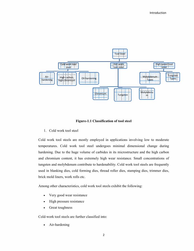
As illustrated in Figure 1.1, tool steels are classified into three broad categories:
1. Cold work tool steels
2. Hot work tool steels
3. High-speed tool steels
Figure
1. Cold work tool steel
Cold work tool steels are mostly employed in applications involving low to moderate
temperatures. Cold work tool steel undergoes minimal dimensional change during
hardening. Due to the huge volume of carbides in its microstructure and the high carbon
and chromium content, it has extremely high wear resistance. Small concentrations of
tungsten and molybdenum contribute to hardenability. Cold work tool steels are frequently
used in blanking dies, cold forming dies, thread roller dies, stamping dies, trimmer dies,
brick mold liners, work rolls etc.
Among other characteristics, cold work tool steels exhibit the following:
• Very good wear resistance
• High pressure resistance
• Great toughness
Cold-work tool steels are further classified into:
• Air-hardening
Cold work tool
steel
Air-
hardeningHigh-carbon,
high-chromium
2
Figure-1.1 Classification of tool steel
Cold work tool steel
Cold work tool steels are mostly employed in applications involving low to moderate
res. Cold work tool steel undergoes minimal dimensional change during
hardening. Due to the huge volume of carbides in its microstructure and the high carbon
and chromium content, it has extremely high wear resistance. Small concentrations of
molybdenum contribute to hardenability. Cold work tool steels are frequently
used in blanking dies, cold forming dies, thread roller dies, stamping dies, trimmer dies,
brick mold liners, work rolls etc.
Among other characteristics, cold work tool steels exhibit the following:
Very good wear resistance
High pressure resistance
work tool steels are further classified into:
Tool Steel
Cold work tool
Oil-hardening
Hot work
tool steel
ChromiumTungsten
Molybdenu
Molybdenum
Introduction
Cold work tool steels are mostly employed in applications involving low to moderate
res. Cold work tool steel undergoes minimal dimensional change during
hardening. Due to the huge volume of carbides in its microstructure and the high carbon
and chromium content, it has extremely high wear resistance. Small concentrations of
molybdenum contribute to hardenability. Cold work tool steels are frequently
used in blanking dies, cold forming dies, thread roller dies, stamping dies, trimmer dies,
Molybdenu
m
High speed tool
steel
Molybdenum
Types
Tungsten
Types

Introduction
3
• High-carbon, high-chromium cold-work steels
• Oil-hardening cold-work steels
The O series of oil-hardening tool steels, the A series of air-hardening tool steels, and the
D series of cold-work tool steels are all examples of cold-work tool steels (high carbon-
chromium).
Due to their high chromium content, the A-series of cold work tool steels exhibit little
deformation after heat treatment. Their machinability is excellent and they exhibit an
excellent blend of hardness and wear resistance. This series consists of the O1 type, the O2
type, the O6 type, and the O7 type. Typically, all steels in this group are hardened at 800
degrees Celsius, oil quenched and then tempered at 200 degrees Celsius. Between 10%
and 13% chromium is contained in the D series of cold-work tool steels, which initially
included types D2, D3, D6, and D7 (which is unusually high). At elevated temperatures,
these steels keep their toughness. These tool steels are frequently used in forging dies, die-
casting die blocks and drawing dies. The composition limitations of various types of high-
carbon, high-chromium D-series cold-work tool steels are listed in Table-1.1.
Table 1.1 Chemical composition of highcarbon, high chromium, cold work tool steels
Designation Composition, %
AISI UNS C Mn Si Cr Ni Mo W V Co
D2
T30402
1.40-
1.60
0.60
max
0.60
max
11.00-
13.00
0.30
max
0.70-
1.20 -
1.10
max -
D3 T30403 2.00-
2.35
0.60
max
0.60
max
11.00-
13.50
0.30
max -
1.00
max
1.00
max -
D4
T30404
2.05-
2.40
0.60
max
0.60
max
11.00-
13.00
0.30
max
0.70-
1.20 -
1.00
max -
D5
T30405
1.40-
1.60
0.60
max
0.60
max
11.00-
13.00
0.30
max
0.70-
1.20 -
1.00
max
2.50-
3.50
D7
T30407
2.15-
2.50
0.60
max
0.60
max
11.50-
13.50
0.30
max
0.70-
1.20 -
3.80-
4.40 -

Introduction
4
2. Hot work tool steel
The term "hot-working tool steels" refers to a class of steel that is used to cut or shape
material at elevated temperatures. Because hot work tool steels are employed in
applications where the tool's operating temperature may reach a high level, heat resistance
and wear resistance are critical. Hot work tool steel has a high resistance to heat and a
moderate resistance to wear. This family of steels is ideal for hot forging dies, hot work
punches, die casting, extrusion dies, plastic injection molding dies, hot mandrels and
among other applications. H-group tool steels are designed for their strength and hardness
when exposed to extreme temperatures for an extended period of time. These low carbon,
moderate to high alloy tool steels exhibit good hot hardness, toughness and wear
resistance due to the presence of a significant quantity of carbide. H1–H19 are chromium-
based; H20–H39 are tungsten-based with a chromium content of 3–4%; and H40–H59 are
molybdenum-based.
Further classifications of hot work tool steels include the following:
• Chromium
• Tungsten
• Molybdenum hot work steels
3. High speed tool steel
The term "high-speed tool steels" refers to their resistance to softening at excessive
temperatures during heavy cutting and high speed. They are the most alloyed tool steels
available. They typically contain a high concentration of tungsten or molybdenum,
chromium, cobalt and vanadium in addition to carbon.
Additionally, high-speed tool steels are classed as follows:
• Molybdenum
• Tungsten

Introduction
5
1.1.2 Effects of Common Alloying Elements in Steel
Steel is a compound of iron and carbon. Steel is alloyed with a variety of elements to
enhance its physical properties and to impart particular characteristics[1]. The following
sections detail the specific implications of the inclusion of such elements:
Carbon (C) is the primary component of steel. It increases tensile strength, hardness and
wear resistance. It has a detrimental effect on ductility and toughness.
Manganese (Mn) is a deoxidizer and degasifier that improve forgeability when combined
with sulfur. It improves tensile strength, hardness, toughness, hardenability and wear
resistance. It reduces the tendency of scaling and distortion. It accelerates carbon
penetration while carburizing.
Phosphorus (P) enhances machinability and boosts strength and hardness. However, it
significantly increases steel's brittleness or cold-shortness.
Sulfur (S) improves the machinability of free-cutting steels. But in the absence of
manganese, it results in brittleness at high temperatures. It reduces the weldability, impact
toughness and ductility of the material.
Silicon (Si) has deoxidizing and degasifying properties. It improves the tensile and yield
strengths, as well as the hardness, forgeability and magnetic permeability of the material.
Chromium (Cr) increases tensile strength, toughness, hardness, wear resistance, corrosion
resistance and scaling at elevated temperatures,
Nickel (Ni) improves ductility and toughness without compromising strength and
hardness. When added in sufficient quantities to high-chromium (stainless) steels, it also
boosts resistance to corrosion and scaling at elevated temperatures.
Molybdenum (Mo) enhances strength, toughness, hardness and creep resistance, as well as
strength at extreme temperatures. It enhances machinability and corrosion resistance and
amplifies the effects of other alloying elements. It improves the red-hardness properties of
hot-work steels and high speed steels.
Tungsten (W) imparts strength, resistance to wear, hardness and toughness. Tungsten
steels are superior in the heat treatment process and have a higher cutting efficiency at
elevated temperatures.

Introduction
6
Vanadium (V) improves tensile strength, hardness, wear resistance and shock resistance. It
inhibits grain growth, allowing for increased quenching temperatures. Additionally, it
increases the red-hardness of high-speed metal cutting tools.
Cobalt (Co) improves the strength and hardness of high speed steel, allowing for greater
quenching temperatures and increasing the red hardness. Additionally, in composite steels,
it amplifies the individual effects of other main constituents.
Aluminum (Al) has deoxidizing and degasifying properties. It inhibits grain growth and is
used to regulate the size of austenitic grains. When employed at concentrations of 1 to
1.25 percent in nitriding steels, it aids in the production of a uniformly hard and strong
nitrided case.
1.1.3 Require mechanical properties of tool steel
To ensure that hardened tool steel performs well in a variety of applications, the following
mechanical properties are required.
Hardness: Hardness refers to a tool steel material's capacity to resist deformation. It is
determined using a standard test that measures the surface resistance to indentation.
Hot hardness is a closely linked and critical component of cutting ability. It refers to the
tool steel's ability to preserve its hardness at elevated temperatures. This feature is critical
because the hardness values at room temperature do not correspond to the values obtained
during machining at high temperature generated by friction between the tool and the
workpiece.
Resistance to wear: The third critical aspect of cutting ability is resistance to wear. The
wear resistance of tool steels is affected by the hardness and composition as well as the
precipitated carbides that provide secondary hardness. In virtually all tool steels, wear
resistance is strongly related to the steel's hardness.
Toughness is the fourth component of cutting ability. It is characterized as a mixture of
two factors: the ability to deform before breaking and the ability to resist permanent
deformation.

Introduction
7
1.1.4 Heat treatment of AISI D2 tool steel
Heat treatment is a controlled process used to modify the microstructure of metals and
alloys to improve the mechanical properties which benefit the working life of a
component. Hardness of AISI D2 tool steel is achieved by heat treatment process[2].
In general, hardening of D2 tool steel entails a quenching operation followed by two
tempering operations. To avoid decarburization or oxidation of surfaces, it is advised to
conduct heat treatments in vacuum furnaces or in protective atmospheres as seen in figure
1.2.
Austenitization
To avoid cracking and deformations, slow heating rates (half-hour hold time per 25 mm
thickness) should be employed in conjunction with homogenization at 750°C. After that,
slow heating rate is maintained during the last stage. Austenitization temperature is
increased up to 1020°C - 1050°C to achieve complete dissolving of secondary carbides in
tool steel. Generally, the time required to maintain an austenitization temperature of 1
minute/mm is maintained. The ultimate holding time varies depending on the size and
shape of the workpiece, the parameters of the furnace and the composition of the furnace
load.
Quenching
The quenching method is used to get the best microstructure (martensite) or hardness to
minimize cracking hazards and to assure the least amount of deformation feasible. Cooling
should occur quickly enough to avoid the production of undesirable components such as
pearlite or bainite. The quenching media are chosen according to the size of the
workpiece.
On the other hand, rapid cooling during quenching can result in significant distortions due
to temperature differences between the workpiece's mid-thickness and surface. When
workpieces have complicated forms, increased stress levels caused by rapid cooling rates
during quenching can also eventually result in cracking. Oil quenching media is mostly
utilized with tool steel.
Tempering
The hardness of D2 tool steel can be increased by adjusting the tempering temperature in
the manner illustrated in the figure1.2. It is highly recommended to temper multiple times

Introduction
8
consecutively, at least two times sequentially. When tempering is carried out at elevated
temperatures (500°C and above), destabilization of remaining austenite is more efficient.
Tempering should not be carried out at low temperatures (200°C), since this may result in
tool deterioration.
Figure 1.2 Vacuum furnaces or heat treatment under protective atmosphere
Stress relieving
In case of heavy or complex shape workpiece, it may be necessary to perform a stress
relieving before hardening to avoid distortion during heat treatment.
Procedure of Stress relieving process of tool Steel is indicated as following:
o Heating around 650°C to 700°C in vacuum furnace to avoid decarburization
o Holding time half hour per 25 mm
o Slow furnace cooling
Annealing
Annealing process is a combination of heating and cooling operations applied to an alloy
or metal for obtaining the desired properties. To soften a tool steel hardened tool steel, it is
possible to perform an annealing process as follows;
o Heating 850°C -900°C
o Holding half hour per 25 mm

Introduction
9
o Still air-cooling
1.2 Milling machine
Milling is a machining operation that involves the removal of metal through the use of a
rotating milling cutter. A milling machine is a machine tool that cuts metal which is fed
against a rotating multipoint cutting tool. The workpiece is commonly held in a vice or
similar device clamped to a table that can move in three perpendicular directions. The
multiple cutting edges of cutting tool revolve with high speed and eliminate metal at a
very fast rate. As a result, one of the most significant machines in the workshop is the
milling machine. All operations can be carried out with excellent precision with milling
machine[3].
In milling machine, the workpiece is rigidly clamped on the table of machine and
revolving multi-tooth cutter is positioned and clamped along the spindle axis. The cutter
revolves at a normal speed and the workpiece is fed through it slowly. The work can be
fed in three directions: longitudinal, vertical and cross direction. The cutter teeth remove
the metal from the work surface, resulting in the required shape.
Figure 1.3 Principle of milling machine

Introduction
10
Following are the different types of milling machines:
The column and knee milling machine is the most common form of milling machine for
general shop operations. The table is supported by the knee-casting, which is in turn
supported by the main column's vertical slides. The column's knee is vertically movable,
allowing the table to be adjusted up and down to accommodate work of varying heights.
The construction of fixed bed type is massive, heavy, and inflexible. The construction of
the table mounting distinguishes these milling machines from column and knee milling
machines. The table is directly attached to the ways of a fixed bed. There are no provisions
for transverse or vertical adjustment; therefore the table can only reciprocate at a right
angle to the spindle axis. It is categorized as simplex, duplex, or triplex depending on
whether the machine has a single, double, or triple spindle head. Planer type milling
machine is also known as a "Plano-Miller." It is a huge machine with vertical and
transversely movable spindle heads that is utilized for heavy-duty tasks. It resembles a
planer and works similarly to a planning machine. The cutters are carried by a cross rail
that may be raised or lowered on this equipment. The saddles and their heads are all
supported by rigid uprights. This configuration of many cutter spindles allows for the
machining of a variety of work surfaces. As a result, it achieves a significant reduction in
production time. Milling machines with non-conventional designs have been created for
specific applications. This machine contains a spindle that rotates the cutter and allows the
tool to be moved in multiple directions. In milling machine, numerical Control technology
was developed in the mid-twentieth century. The functioning of the machine tool is
controlled by the NC control system through the use of specially coded instructions
(combination of alphabet, digit and symbols). NC systems are integrated and permanently
hooked into the control unit and perform a predetermined logical purpose. Around 1972, a
real boom occurred with the introduction of CNC. Modern CNC systems use a specialized
microprocessor with memory registers that store a variety of routings capable of
manipulating logical functions. Due to this adaptability, it enables such widespread
adoption of technology in contemporary industry. CNC stands for computer numerical
control, a computer-assisted procedure for controlling general-purpose machines using
instructions generated by a processor and stored in a memory system. The main
advantages of CNC machines are following that high repeatability, precision, high volume
production and the ability to produce complex contours/surfaces, job change flexibility,
automatic tool settings, less scrap, increased safety, reduced paper work, faster prototype

Introduction
11
production and reduced lead times. As a result, it is utilized in a variety of applications
including aircraft and automobile components, dies and molds, pipe and shaft
manufacturing, turbine and pump manufacture and so on. Additionally there are certain
disadvantages such as high setup costs, professional operators, computers and required
programming skills as well as onerous maintenance. In industry, a variety of CNC
machines are utilized, the most common of which being CNC machining centers, vertical
machining centers (VMCs) and CNC lathes. Milling is a widely used procedure in the die
and mold business. Milling has evolved as a process with new automated machinery and
processes being used to continuously produce the highest quality product. The workpiece
is stationary while the tool rotates during the CNC milling process. The rotating tool with
several cutting blades works over the workpiece to create a plane or straight surface
throughout this machining operation. Milling tools have also evolved significantly from
uncoated high-speed steel tools to the widely used coated tools, owing to the increased
tool life.
1.2.1 Types of milling process
Milling process has basically broad classification. The milling process performed may be
grouped under following separate headings
1. Peripheral milling
2. Face milling
3. End milling
Peripheral Milling
It is a milling cutter operation that produces a machined surface parallel to the cutter's axis
of rotation.
Peripheral milling is classified as;
1. Up milling
2. Down milling
Up milling
When the feed direction of the cutting end mill tool is against the direction of rotation of
the end mill tool at the point of engagement, this is referred to as up milling, as illustrated
in figure 1.4. Up milling causes the chip load on teeth to progressively grow from zero to

Introduction
12
maximum at the point of contact. At the start of tool-workpiece engagement, teeth rub
against the workpiece's surface resulted in improving the surface finish. Tool contact with
the workpiece during engagement may result in unwanted work hardening as a result of
the high temperature generated. Machining by up milling may result in distortion due to
the upward cutting force if the workpiece has a thin cross section. The contact point
generates considerable heat as a result of the progressive accumulation of chip load during
up milling.
Figure 1.4 Up milling
Down milling
When the feed direction of the cutting end mill tool is parallel to the cutter rotation
direction at the point of disengagement, this is referred to as down milling, as seen in
figure 1.5. Down milling gradually reduces the chip load on teeth from maximum to zero
at the point of contact. Because there is little contact between the tool and the workpiece
during engagement, there is less risk of work hardening. There is little danger of distortion
during down milling a workpiece with a thin cross section. Additionally, there is less
probability of heat development at the contact site in down milling than in up milling.
Although the tendency for chip welding is reduced in down milling, chip re-deposition on
the completed surface occurs frequently. In general, down milling is suited for a wide
variety of metal processing operations due to its low deflection and high surface polish.

Introduction
13
Figure 1.5 Down milling
Face Milling
A milling cutter performs this procedure to generate a flat-machined surface perpendicular
to the rotation axis of the cutter. The peripheral cutting edges of cutter do the real cutting,
while the face cutting edges conclude the job by removing a little quantity of metal from
the work area.
End Milling
End milling is the combination of peripheral and face milling. The end milling is the
operation of producing a flat surface which may be vertical, horizontal or at an angle in
reference to the table surface. The end mill operation is shown in figure 1.6. The end
milling cutters are also used for the production of slots, grooves or keyways. A vertical
milling machine is more suitable for end milling operation.
Figure 1.6 End milling operation
1.2.2 Milling Machine Operations

Milling is a machining technique that involves
removing material with rotary cutters. This can be accomplished by adjusting the direction
of one or more axes as well as the cutter head speed and pressure. Milling encompasses a
wide range of procedures and machine
milling operations. The various types of milling machine operations are as follow: Plain
milling operation, face milling operation, side milling operation, straddle milling
operation, angular milling oper
profile milling operation, end milling operation, saw milling operation, milling keyways,
grooves and slot, gear milling, helical milling, cam milling and thread milling.
1.2.3 Specific terms in milling process:
As shown in figure 1.7, various specific terms are discussed in following:
Figure 1.7 Specific terms in end mill
Cutting speed Vc: It indicates the surface speed at which the cutting edge of cutting tool
machines the workpiece.
Where Dc is cutting diameter at cutting depth and n is spindle speed
Feed (Vf): It is the feed of the tool in relation to the workpiece in distance per unit time
related to feed per tooth and number of teeth in the cutter.
14
Milling is a machining technique that involves advancing a cutter into a workpiece and
removing material with rotary cutters. This can be accomplished by adjusting the direction
of one or more axes as well as the cutter head speed and pressure. Milling encompasses a
wide range of procedures and machinery from small individual pieces to large
The various types of milling machine operations are as follow: Plain
milling operation, face milling operation, side milling operation, straddle milling
operation, angular milling operation, gang milling operation, form milling operation,
profile milling operation, end milling operation, saw milling operation, milling keyways,
grooves and slot, gear milling, helical milling, cam milling and thread milling.
Specific terms in milling process:
As shown in figure 1.7, various specific terms are discussed in following:
Figure 1.7 Specific terms in end mill
: It indicates the surface speed at which the cutting edge of cutting tool
�� � ������ m/min
Where Dc is cutting diameter at cutting depth and n is spindle speed
It is the feed of the tool in relation to the workpiece in distance per unit time
related to feed per tooth and number of teeth in the cutter.
Introduction
advancing a cutter into a workpiece and
removing material with rotary cutters. This can be accomplished by adjusting the direction
of one or more axes as well as the cutter head speed and pressure. Milling encompasses a
ry from small individual pieces to large-scale gang
The various types of milling machine operations are as follow: Plain
milling operation, face milling operation, side milling operation, straddle milling
ation, gang milling operation, form milling operation,
profile milling operation, end milling operation, saw milling operation, milling keyways,
grooves and slot, gear milling, helical milling, cam milling and thread milling.
: It indicates the surface speed at which the cutting edge of cutting tool
It is the feed of the tool in relation to the workpiece in distance per unit time

Introduction
15
�� � ��� ��
Where n is spindle speed, Zc is number of effective teeth and fz is feed per tooth
Depth of cut: The depth of cut is the difference between the uncut and the cut surface in
axial direction.
Radial depth of cut: The depth of the tool in the workpiece along its radius as it performs
a cut. If the radial depth of cut is smaller than the radius of the tool, the tool is only
partially engaged, resulting in a peripheral cut. When the radial depth of cut equals the
diameter of the tool, the cutting tool is fully engaged and making a slot.
1.2.4 Importance of milling machining
The milling cutter performs a rotary movement (primary motion) and the workpiece a
linear movement (secondary motion).The milling technique is used to produce, mainly on
prismatic components, flat, curved, parallel, stepped, square and inclined faces as well as
slots, grooves, threads and tooth systems.
CNC Milling (also known as computer numerical control milling) is a method of
manufacturing that utilizes pre-programmed software to control machining tools. Digital
instructions are first of all fed into the computer, which then automatically operates the
machine to create the components that match the specifications.
Continuous Usage
CNC milling machines do not need to take breaks like human workers. Once the
instructions have been details as input into the computer and the machining begins, the
manufacturing can take place throughout the task is completed. This constant usage has
completely transformed the industry and provided manufacturers with a way to drastically
reduce their costs and improve productivity. Large projects that once might have taken
weeks or even months to complete can now be completed in a matter of days or
hours. This means they are able to make a good economics in a shorter space of time
without drastically increasing their costs.

Introduction
16
Consistency
One of the greatest advantages of CNC milling is that the same components over and over
again in huge volumes can be produced. These manufactured parts will be exactly the
same size, shape and dimensions that mean everything will be created to match the right
specifications every single time. Even the most skilled workers will not be able to create
the exact same components time and again. Instead, there will likely be tiny
differentiations with each part.
Reduced Test Runs
A lot of test runs are required in traditional machining methods to ensure that the produced
components will be matched the specifications or not. This is because the operator will
need to familiarize themselves with the process needed to manufacture the component and
may make several mistakes in their first few attempts.
CNC milling machines have ways of avoiding these numerous test runs. They can use
visualization systems that enable the operator to see what will happen after the tool passes
will finish, meaning the engineer will get a good idea of whether the component is going
to match the specifications beforehand.
Design Retention
Once a design has been successfully loaded into the computer system and a perfect
prototype created to ensure that everything is exactly as it should be, the software can
easily retrieve the instructions whenever required again. These instructions ready on file
means that there are no need to start from initial point when the components need
manufacturing again.
This master file also ensures that regardless of outside circumstances, such as a change of
machine operator, the CNC milling process can continue uninterrupted. Additionally, there
is no need to keep up with versions of the design that might exist on paper, a disc, flash
drive, another computer or anywhere else.
Capability
When used in conjunction with advanced computerized design software, CNC milling can
be created output components that simply cannot be replicated by manually operated

Introduction
17
machine, no matter the skill level of the engineers. CNC machines can be produced
components of any size, shape, texture or quantity that is needed, without any hassle or
stress.
1.3 Cutting tools
1.3.1 Classification of cutting tools
Despite the fact, the basic shape of a cutting tool changes widely depending on the type of
activity. Every cutting tool must have a wedge-shaped section with a sharp cutting edge
that can cut material smoothly, as it is supposed to perform. Now, a cutting tool can have
one or more main cutting edges that work together in a single pass to cut material.
Cutting tools are categorized in a variety of ways, the most frequent of which is by the
number of major cutting edges that are involved in the cutting activity at the same time[4].
Cutting tools can be divided into two classes based on this classification, as shown below.
• Single point cutting tool
• Multi point cutting tool
A multi-point cutting tool contains more than two main cutting edges that simultaneously
engage in cutting action in a pass. The number of cutting edges present in a multi-point
cutter may vary from two or more.
Advantages of multi-point cutting tool
� Chip load on each cutting edge is considerably reduced since the overall feed rate
or depth of cut is evenly divided among all cutting edges. As a result, a higher feed
rate or depth of cut can be used to improve material removal rate and hence
productivity.
� The force acting on each cutting edge is greatly reduced due to the dispersion of
chip load. Occasionally, one component of cutting force is automatically
eliminated or lowered.
� During machining, no part of the cutting edge is in constant contact with the work
piece; instead of engagement and disengagement occur frequently. This allows
enough time for heat to dissipate from the tool body, protecting the cutter from

Introduction
18
overheating and plastic deformation. As a result of the intermittent cutting action,
the tool temperature rises at a slower rate.
� Tool wear rate is reduced as a result of shorter engagement times and less heat
generation within the tool body. As a result, the tool life is increased.
1.3.2 Coated cutting tool
The coatings that are now being investigated function exceptionally well while machining
hard materials. These coatings are gaining traction in the industry, with very positive
results in terms of increased performance and tool life. Coatings enhance the quality of the
tool's surface and extend its life. They significantly minimize cutting forces, cutting
temperatures and tool wear, making them an extremely attractive option for the machining
sector.
Direct contact between the tool steel workpiece and the cutting tool can be avoided
successfully by coating on cutting tool acting as a heat and chemical barrier. Coated tools
can nevertheless have a longer cutting life in high-speed and high-temperature cutting
environments due to constant innovation in coating technology. Coatings impart properties
to the tool that are optimal for the machining application, such as thermal dissipation and
wear resistance. These coatings can be designed in a variety of ways; for example, the
outer layer may have an increased wear resistance, while the subsequent layer may focus
on thermal dissipation.
Recent milling machining tools are coated cemented carbide tools. These coatings, which
are either PVD or CVD deposited, are applied on a base material referred to as the
substrate[5]. Chemical Vapor Deposition (CVD) and Physical Vapor Deposition (PVD)
can be used to deposit the coatings (PVD). Chemical vapor deposition films can be created
in a variety of ways, as seen in figure 1.8. CVD films are deposited by pumping a
precursor into a closed reactor and controlling the flux using control valves. The precursor
molecules travel through the substrate and deposit themselves on its surface, forming a
thin hard covering. This technique operates between 300 and 900°C. Additionally, the film
thickness is typically homogeneous throughout the whole surface of the substrate.

FIGURE 1.8 CVD Coating deposition methods
FIGURE 1.9 PVD Coating deposition methods
Arc
19
FIGURE 1.8 CVD Coating deposition methods
FIGURE 1.9 PVD Coating deposition methods
Physical Vapor Deposition
Evaporation
E-beam Inductive
Introduction
Physical Vapor Deposition
Resistive
Sputtering

Introduction
20
PVD coatings can be deposited using a variety of techniques, as seen in figure 1.9, with
DC (direct current) magnetron sputtering being the most frequently utilized. PVD operates
at a lower temperature (less than 500°C) than CVD and is more environmentally friendly
due to the materials used in CVD. Additionally, PVD is a more energy-efficient procedure
than CVD. Consideration must be given to the type of coating used on a cutting tool. CVD
coatings are typically thicker and more suitable for roughing operations; however, they
can be applied only to cemented carbide cutting tools due to their superior behavior at
elevated temperatures, whereas PVD coatings can be applied to coated tool steel due to the
PVD process's overall low temperature.
Figure 1.10 Compare hardness values of workpiece and cutting tools
Coatings are applied in accordance with the machining process and its prerequisites. To
choose which coating to apply and where to apply it, cutting tool behavior has been
evaluated. Numerous elements affect the cutting performance of the cutting tool, including
the cutting speed, feed rate, depth of cut, lubrication regimen, tool shape, and even the
thickness of the tool coating. Cutting tools are used to machine tool steel should have a
hardness value three times greater than the tool steel's Vickers hardness value. Numerous
coated tools are suggested for machining based on the workpiece hardness value, as seen

Introduction
21
in figure 1.10. On hardened workpiece materials, high speed steel (HSS) cannot be used.
Cemented carbide cutting tools can be used on materials with a hardness of up to 30 HRC.
CrN and TiN coated tools are mostly employed on 40 to 50 HRC materials, while AlCrN
coated tools perform exceptionally well on 50-60 HRC workpiece materials.
Table 1.2 Various coated tool with application
COATING APPLICATION
TiN The general-purpose coating for cutting, forming, injection molding as well as
tribological applications
TiCN-MP Universal high-performance coating for cutting such as drilling, milling,
reaming and turning
TiAIN Tough Multi Purpose coating for interrupted cutting, milling, stamping,
forming and hobbing
AlTiN High-performance coating with very high aluminum content and heat
resistance. Used for dry high speed machining
TiCN Conventional carbon nitride coating for interrupted cutting, milling and
tapping, stamping, punching and forming
AlCrN A coating with high wear resistance against abrasive loads, good heat and
oxidation resistance. It performs extremely well in milling applications and is
outstanding for very dry applications.
CrN The standard coating for non-cutting application for moulds, dies and machine
parts. Especially suited for applications where copper is the material being
altered.
ZrN A monolayer coating that effectively reduces the built-up edges when
machining aluminum (<12% Si content) and titanium alloys. ZrN works well
for medical applications and has good heat resistance.

Introduction
22
Coated tool providers offer a wide variety of PVD (Physical Vapor Deposition) and CVD
(Chemical Vapor Deposition) surface treatments. There are numerous coating materials in
the market, including TiN, TiAlN, TiCN, TiC and CrN. To ensure the cutting tool
performs optimally, the appropriate cutting tool materials must be chosen with consider of
its application. The coating materials and their applications are listed in table 1.2.
1.3.3 Types of end mill cutting tool
According to peripheral cutting edge
End mill tools come in a variety of shapes and sizes. The conventional flute type, as
illustrated in figure 1.11 (a), is mostly utilized for side milling and general milling
operations, although it is also employed for slotting. Tapered flutes are utilized in milling
to create mould drafts and angled faces, as illustrated in figure 1.11 (b). Roughing flutes
have a roughing tooth in the shape of a wave as illustrated in figure 1.11 (c), and are ideal
for roughing surfaces. As illustrated in figure 1.11 (d), a formed flute is similar to a corner
radius cutter tool. It is capable of producing an endless variety of shape cutters.
Figure 1.11 Types of peripheral cutting edge in end mill
According to end cutting edge
As illustrated in figure 1.12 (a), square ends (with a center hole) are frequently used for
slotting, side milling, and shoulder milling. This sort of end mill grinds from the center.
Additionally, slotting, side milling, and shoulder milling are performed with a square end
(with center cut). Vertical cutting is possible with this sort of end mill, as illustrated in
figure 1.12 (b). As seen in figure 1.12 (c), a ball end mill is appropriate for profile
machining and pick feed milling. For corner radius milling and contouring, an end mill
cutter with an end radius similar to that shown in figure 1.12 (d) is utilized. Due to the tiny
corner radius and large diameter, it is an efficient tool.

Introduction
23
Figure 1.12 Types of End Cutting Edges in end mill
According to shank and neck parts
Various shanks are utilized for milling purpose as illustrated in figure 1.13. Standard
shank is utilized for general use as seen in figure 1.13 (a). Straight long shank is utilized
for deep slotting, allowing for adjustability of the overhang as illustrated in figure 1.13 (b).
As seen in figure 1.13 (c), the long neck type shank tool is suited for boring operations and
may also be utilized for deep slotting with a small diameter. Due to the taper shank, the
taper neck performs exceptionally well in deep slotting and also on mould draft as
illustrated in figure 1.13 (d).
Figure 1.13 Types of shank and neck parts in end mill

Introduction
24
1.4 Measurement of Hardness
Hardness testing is the most widely used method for determining the hardness of a surface.
It is simple to determine the hardness of a workpiece. The most prevalent method is
hardness testing because the material is not harmed and the device is relatively
inexpensive. The most often used methods for measuring hardness are Rockwell C (HRC),
Vickers (HV) and Brinell (HBW).
ROCKWELL (HRC)
The Rockwell method is only applicable to hardened material and should never be used on
soft annealed material. As seen in Figure 1.14, Rockwell hardness testing involves
pressing a conical diamond indenter with a force F and then with a force (F+F1) on a
specimen of the material whose hardness is to be determined. The increase in the depth of
the impression (d) generated by F1 is determined following unloading to F. The
penetration depth (d) is translated to a hardness value (HRC), which can be read directly
from the tester dial's hardness scale.
Figure 1.14 Principle of Rockwell hardness testing

Introduction
25
VICKERS (HV)
Vickers is the often used in the three procedures. As illustrated in figure 1.15, the Vickers
hardness testing method involves pressing a pyramid-shaped diamond with a square base
and a peak angle of 136° indenter against the material whose hardness is to be evaluated.
After unloading, the impression's diagonals a1 and a2 are measured and the hardness value
(HV) is read from a table. Vickers hardness is denoted by the letters HV followed by a
suffix indicating the mass exerting the load and the loading period, as illustrated in the
following example:
Vickers hardness is defined as HV 50/30 when a force of 50 kgf is applied for 30 seconds.
Figure 1.15 Principle of Vickers hardness testing
BRINELL (HBW)
Brinell hardness testing is appropriate for soft annealed steels and prehardened steels with
a low hardness. As seen in figure 1.16, Brinell hardness testing involves pressing a
tungsten (W) ball against the material whose hardness is to be evaluated. After unloading,
two measurements of the impression's diameter at 90° to one another (d1 and d2) are
obtained, and the HBW value is read from a table based on the average of d1 and d2.

Introduction
26
Figure 1.16 Principle of Brinell hardness testing
When test results are presented, brinell hardness is denoted by the letters HBW followed
by a suffix indicating the diameter of the ball, the mass used to exert the stress and the
loading period as exemplified by the following example:
HBW 5/750/15 = Brinell hardness evaluated using a 5 mm tungsten (W) ball and a 15-
second load of 750 Kgf.
1.5 Measurement of Responses
1.5.1 Cutting force
It is a reaction force caused when a cutting tool is pushed into a workpiece. Cutting force
changes according to cutting conditions. It is considered as three force components as
shown in figure 1.17. Feed force is a horizontal force component in a feed direction. It
determines a magnitude of feed power for cutting. Cutting force is a force component acts
in a direction vertical to feed force. It affects heating value during cutting. Power
requirement during cutting is calculated by a magnitude of cutting force. Thrust force is an
axial force component. It becomes force to deform a workpiece and a tool and decreases
accuracy when it is large.

Introduction
27
Figure 1.17 Cutting forces in end milling
1.5.2 Surface roughness
Surface roughness is specified as follows; arithmetical mean roughness (Ra), maximum
height (Ry) and ten-point mean roughness (Rz). The roughness of the surface is expressed
as the arithmetical mean of a randomly sampled area. Numerous techniques are used for
determining the surface roughness.
1.5.2.1 Techniques used for surface roughness measurement
Arithmetical mean roughness (Ra)
A section of standard length of sample is drawn from mean line on the roughness chart as
shown in figure 1.18. The mean line is laid on a Cartesian coordinate system. The mean
line runs in the direction of the x-axis and magnification is the y-axis. The value obtained
with the below formula is expressed in micrometer when y is equal to f(x).
�� � 1� � |�(�)|��
�

Introduction
28
Figure 1.18 Arithmetical mean roughness (Ra)
Maximum peak (Ry)
A section of standard length is sampled from the mean line on the roughness chart. The
distance between the peaks and valleys of the sampled line is measured as Rp and Rv
respectively in the y direction which are seen in figure 1.19. The value is expressed in
micrometer (µm).
�� � �� + �
Figure 1.19 Maximum peak
Ten-point mean roughness (Rz)
A section of standard length is sampled from the mean line on the roughness chart. The
distance between the peaks and valleys of the sampled line are measured in the y direction
as shown in figure 1.20. Then, the average peak is obtained among 5 tallest peaks
( Y", Y"$, Y"%, Y"&, Y"' ) as is the average valley between 5 lowest valleys

(Y(, Y($, Y(%, Y(&, Y('). The sum of these two values is expressed in micrometer (µm) as
following equation;
�) � |*+ + *+$
Figure 1.20 Ten
AISI D2 tool steel is one of the most useful D grade tool steel. So nu
have been done on it. AISI D2 tool steel has higher hardness so higher cutting tool wear is
the major problem during machining
cutting tools come in market. Various studies have been done by using various cutting
tools such as uncoated CBN cutting insert, PCBN tipped, TiAlN coated tool, ceramic tool
etc. The major objectives of these
improvement in surface roughness, reduce tool wear rate, reduce cutting force,
improvement in MRR, etc. At present various coated cutting tools are available and
selection of coated tool is challenging task during
improvement in machinability.
1.6 Modeling and Optimis
The most critical aspect of manufacturing processes is determining the relationship
between various input factors and output reactions. Experiments are planned
analyzed in such a way that accurate and objective results may be drawn effectively and
rapidly. To derive statistically correct findings from an experiment, it is vital to
incorporate simple yet strong statistical techniques into the experi
methodology. The information gathered from correctly designed, conducted and analyzed
experiments can be utilized to enhance the functional performance of products, decrease
scrap rates, shorten production times, increase product quality and
variability in manufacturing processes.
29
). The sum of these two values is expressed in micrometer (µm) as
+ *+% + *+& + *+'| + , |*- + *-$ + *-% + *-& +.
Figure 1.20 Ten-point mean roughness
AISI D2 tool steel is one of the most useful D grade tool steel. So numbers of experiments
have been done on it. AISI D2 tool steel has higher hardness so higher cutting tool wear is
the major problem during machining of it. From time to time, various new advanced
cutting tools come in market. Various studies have been done by using various cutting
tools such as uncoated CBN cutting insert, PCBN tipped, TiAlN coated tool, ceramic tool
etc. The major objectives of these studies were improvement in machinability,
improvement in surface roughness, reduce tool wear rate, reduce cutting force,
improvement in MRR, etc. At present various coated cutting tools are available and
selection of coated tool is challenging task during machining of AISI D2 tool steel for
improvement in machinability.
Modeling and Optimisation
The most critical aspect of manufacturing processes is determining the relationship
between various input factors and output reactions. Experiments are planned
analyzed in such a way that accurate and objective results may be drawn effectively and
rapidly. To derive statistically correct findings from an experiment, it is vital to
incorporate simple yet strong statistical techniques into the experi
methodology. The information gathered from correctly designed, conducted and analyzed
experiments can be utilized to enhance the functional performance of products, decrease
scrap rates, shorten production times, increase product quality and eliminate excessive
variability in manufacturing processes.
Introduction
). The sum of these two values is expressed in micrometer (µm) as
+ *-'|
mbers of experiments
have been done on it. AISI D2 tool steel has higher hardness so higher cutting tool wear is
of it. From time to time, various new advanced
cutting tools come in market. Various studies have been done by using various cutting
tools such as uncoated CBN cutting insert, PCBN tipped, TiAlN coated tool, ceramic tool
studies were improvement in machinability,
improvement in surface roughness, reduce tool wear rate, reduce cutting force,
improvement in MRR, etc. At present various coated cutting tools are available and
machining of AISI D2 tool steel for
The most critical aspect of manufacturing processes is determining the relationship
between various input factors and output reactions. Experiments are planned, designed and
analyzed in such a way that accurate and objective results may be drawn effectively and
rapidly. To derive statistically correct findings from an experiment, it is vital to
incorporate simple yet strong statistical techniques into the experimental design
methodology. The information gathered from correctly designed, conducted and analyzed
experiments can be utilized to enhance the functional performance of products, decrease
eliminate excessive

Introduction
30
In a designed experiment, the input process parameters will be altered purposely in order
to observe changes in the output process. It is critical to notice that not all parameters have
the same effect on the output response's performance. Some may exert a strong influence
on the output performance, while others exert a moderate influence and still others exert
no influence at all. Thus, the purpose of a well-designed experiment is to establish which
set of variables in a process has the most effect on performance and then to determine the
optimal values for these variables in order to achieve adequate output functional
performance.
1.6.1 RESPONSE SURFACE METHODOLOGY
RSM is a combination of statistical and mathematical tools for designing, enhancing and
optimizing processes[6]. The response surface methodology (RSM), which is classified as
a designed experiments approach, appears to be the most widely used technique for
predicting output responses. RSM is a critical methodology that is used to build new
processes, optimize their performance and enhance the design and formulation of new
goods. It is frequently a critical concurrent engineering technique in which employees
from process development, product design, quality assurance, manufacturing engineering
and operations work together. It is a dynamic and critical design of experiment (DOE) tool
that maps the relationship between a process's responses and its input choice variables in
order to maximize or minimize the response qualities.
1.6.2 Genetic Algorithm
The term "optimisation" refers to the process of improving something. Nature has long
served as a source of inspiration for all of humanity. The genetic algorithm method was
invented by John Holland at the University of Michigan, and it has since been attempted
on a variety of optimisation problems with great success.
The Genetic Algorithm (GA) is a search-based optimisation technique based on genetics
and natural selection principles. GA is usually used to get the best or near-best results
from challenging situations in research and machine learning. Genetic Algorithms (Gas)
are adequately randomized in nature, yet they outperform random local search methods
because they take into account past data.
The population of viable solutions to the given problem is the initial phase in GAs.
Recombination and mutation occur in this population, just as they do in natural genetics.

Introduction
31
Finally, new children are born, and the cycle continues for several generations. Each
individual solution is given a fitness value based on its objective function value, and the
fitter individuals have a better probability of mating and producing more “fit” individuals.
This is consistent with Darwin's "Survival of the Fittest" theory. In this manner, we
continue to "evolve" better individuals or solutions through generations until we reach a
threshold for halting [7].
Knowing certain key terminologies that are utilized throughout the genetic algorithm is
vital. Some basic terms are seen in figure 1.21.
Figure 1.21 Some basic terms (population, chromosome, gene and allete)
Population:
It is a subset of all the possible solutions (as encoded solutions) to the given
problem.
Chromosomes:
It is one such solution to the given population.
Gene:
It is one element position of a chromosome.
Allele:
It is the value a gene takes for a particular chromosome.

Introduction
32
Genotype:
Genotype is the population in the computation space. In the computation space,
the solutions are represented in a way which can be easily understood and
manipulated using a computing system.
Phenotype:
Phenotype is the population in the actual real world solution space in which
solutions are represented in a way they are represented in real world situations.
Decoding and Encoding:
The phenotype and genotype spaces are the same for simple problems. However,
in most of the cases, the phenotype and genotype spaces are different. Decoding is
a process of transforming a solution from the genotype to the phenotype space,
while encoding is a process of transforming from the phenotype to genotype
space. Decoding should be fast as it is carried out repeatedly in a GA during the
fitness value calculation.
Fitness Function:
It is a function which takes the solution as input and produces the suitability of the
solution as the output. The fitness function and the objective function may be the
same or may be different based on the given problem.
Advantages of GAs
Following are the various advantages which have made genetic algorithm immensely
popular;
• It is faster and more efficient as compared to the traditional optimisation methods.
• By using GAs, always gets an answer to the problem which gets better over the
time.
• It does not require any derivative information (which may not be available for
many real-world problems).
• It has very good parallel capabilities.
• By using GAs, obtain optimizes both continuous and discrete functions and also
multi-objective problems.

Introduction
33
• It provides a list of “good” solutions and not just a single solution.
• It is useful when the search space is very large and there are a large number of
parameters involved.
Limitations of GAs
GAs also suffers from a few limitations like any other techniques. These include;
• GAs is not suited for all problems, especially problems which are simple and for
which derivative information is available.
• Fitness value is calculated repeatedly which might be computationally expensive
for some problems.
• Being stochastic, there are no guarantees on the optimality or the quality of the
solution.
• If not implemented properly, the GA may not converge to the optimal solution.
1.7 Statement of the Problem
The current work, titled "Experimental investigation for process parameter optimisation
during milling of D2 tool steel", has been undertaken with the following issues in mind:
� It is necessary to operate automated CNC milling machine as efficiently as
possible. It has been recognized that milling machining conditions such as cutting
speed, feed rate, depth of cut, and other cutting parameters should be chosen in
order to optimize the economics of cutting operations which are assessed by
productivity, tool wear, product quality and other relevant outputs.
� Advanced materials with higher hardness and strength are being developed
continuously. Output responses are not only depended on machining parameters
but also on workpiece materials. AISI D2 tool steel is a suitable materials for
making blanking dies, forging dies, die casting, drawing dies, plastic mould dies,
mandrels, punching tools, hot-worked forging, extrusion dies and also for other
applications. It is essential to investigate the optimal machining parameters for
AISI D2 tool steel.
� Optimal value of machining parameters for specific output responses required to be
derived by various optimization methods. These predicted optimal solutions should
be validated by conducting experiments.

Introduction
34
1.8 Organization of thesis
Chapter-1 is introductory part which introduces tool steel materials, milling machining
operations and parameters, responses, modeling and optimisation, research methodology
and scope of research work.
Chapter-2 entitled as Literature Review presented previous reviews related with this
research work. The details of works related to this research work have been explained
briefly in this chapter. The identified research gap has also been framed in this chapter
also.
Chapter-3, entitled as experimental setup which described the details about pilot
experiment procedure as well as design of experiment methodology. The description of
experimental set up, details of workpiece as well as cutting tool, experimental procedure
and details about experimental data have been discussed in this chapter.
Chapter-4 entitled as result and analysis, presented regression equation which represent
relationship between input variable with output responses. The effects of various input
process parameters on output responses have been discussed in this chapter.
Chapter-5 entitled as Optimisation, discussed on optimized values of input variables with
respect to output responses by various methods. The predicted values have been validated
by experimental values in this chapter.
Chapter-6 entitled as conclusion and future scope, presented output of experiment work
and final contribution of this research work. The future scopes from this research work
have been also discussed in this chapter.

Literature review
35
Chapter-2
Literature Review
2.1 Introduction
Research in optimization of cutting parameters during machining is the subject of
extensive importance due to recent development in engineering materials and demands in
advanced cutting tools in the global production arena. The demand of machining of hard
materials (which hardness ranging from 45 to 68 HRC) is steadily increased in modern
manufacturing technology for providing a more economical way to finish hard material
surface[8].Hard machining is the machining of difficult-to-machine high hardness material
such as hardened steel, with the benefits of increased productivity, increased flexibility,
lower capital costs and less environmental waste[9]. CNC milling system produces the die
faster, more accurate and serve as an alternative to EDM in moulds, dies and automobile
industries. It can give better result in significantly lower manufacturing times and costs
compare that existing production processes[10]. The hard-milling process offered
numerous advantages like attainment of workpiece compressive residual stresses,
reduction in workpiece microstructure alterations, elimination of surface micro-hardness
increases and improvement in fatigue life[11].
During the machining process, numerous input cutting parameters have an impact on the
milling process. Cutting parameters (include cutting speed, feed rate, depth of cut, width
of cut etc.), hardness of workpiece material and cutting tool coatings are influencing
characteristics for machining process because they are directly related to tool life and
surface quality of product. For manufacturers, machining of difficult-to-cut materials has
always been a demanding process. Cutting speed, feed rate, depth of cut, width of cut,
types of coating and many other process factors have a direct impact on output responses
such as surface roughness, dimensional accuracy, tool wear, cutting power and so on. It is
always desirable to have proper correlation between input parameters and output
responses. Optimisation techniques such as Genetic Algorithm (GA), Response Surface
Methodology (RSM) and others have been mostly used to optimise parameters that are
desirable for parameter selection.

Literature review
36
In this chapter, the research work carried out by various researchers in the fields of cold
work tool steel materials, coated cutting tool, process parameter, performance
measurement, modeling method and process parameter optimisation have been covered.
2.2 Cold work tool steel
Hard milling is most accepted traditional machining methods of harder materials which
have hardness greater than 50 HRC. It is the best alternative to EDM (Electrical Discharge
Machining) and grinding process. In hard machining lead time and machining costs are
reduced compared to more traditional route like annealing, heat treatment, grinding, EDM
and polishing. Due to high productivity and environment friendly dry machining process,
it is highly competitiveness over EDM and grinding process in manufacturing
industries[12]. Machining of hardened steel has become more pronounce in manufacturing
industries particularly die and mould making industries[13].Hardened tool steel is used to
produce tools for cutting, moulding or shaping a material into a component appropriate to
perform certain functions. The addition of relatively substantial amounts of tungsten,
molybdenum, manganese and chromium to tool steels can enable to meet satisfy service
requirements as well as provide better dimensional control and crack resistance during
heat treatment. The "Society for Automotive Engineers" (SAE) and "American lron and
Steel Institute" (AISI) are the most often used techniques for tool steel categorization. The
AISI approach is more often used since it simplifies and clarifies tool steel classification.
Cold work tool steels are divided into three classes as per AISI approach: O, A, and D
type. These all three classes have a high carbon content for high hardness and better wear
resistance in cold work applications but the alloy amount varies, affecting hardenability
and carbide distributions in hardened microstructures[14].
AISI D2 cold work tool steel has shown to be a promising choice material in the industries
as a common material in mould and die applications[15]. AISI D2 tool steel is high
carbon, high chromium steel and dimensionally stable with good toughness. AISI D2 is an
air-hardened steel that has many applications such as in the manufacturing of stamping or
forming of dies. End milling is one of the most common machining operations used in
AISI D2 steel fabrication. AISI D2 tool steel (group D) is widely used in manufacturing of
cold-forming dies and blanking dies on account of their excellent deep hardening
characteristics and wear resistance[16][17]. Machinability of AISI type D2 tool steel is
superior to any of the similar types of tool steel. It is used for tools and dies for blanking,

Literature review
37
punching, forming and other operations requiring high compressive strength[18]. Various
numbers of tools have been used for machining of AISI D2 tool steel with respect to
specific responses such as cutting force, tool wear, surface roughness, power consumption
etc as shown in table 2.1. AISI D2 tool steel has been machined by varying feed rate and
cutting speed to analyze their effect on components of resultant force.
Different heat treatment procedures are used to improve the mechanical properties of cold
work tool steels. Heat treatment is used to modify the microstructure in order to achieve
the best mix of hardness and toughness. The toughness of D2 tool steel is improved by the
tempering process [19]. The hardness of AISI D2 tool steel is achieved by hardening at
980°C followed by tempering at 200°C[8]. The AISI D2 tool steel is usually processed by
vacuum hardening followed by multiple tempering cycles[20]. J. B. Saedon et al [21]
developed the first and second order tool life models in terms of cutting speed, feed per
tooth and depth of cut during end-milling of AISI D2 tool steel using 0.5 mm diameter
TiAlN coated tool. Central composite design (CCD) has been employed in developing the
tool life model.
Figure 2.1 General view of workpiece fixing on dynamometer with thermocouples
[22]
Heat flow has been studied during end milling of AISI D2 tool steel and AISI H13 tool
steel by using two types of ball nose end mills: coated with (TiAl)N and tipped with
PCBN. Results indicated a relatively small temperature variation with higher range when
machining of AISI D2 with PCBN-tipped end mill as shown in figure 2.1. The FEM
model has been proposed and it has been found capable of estimating the energy
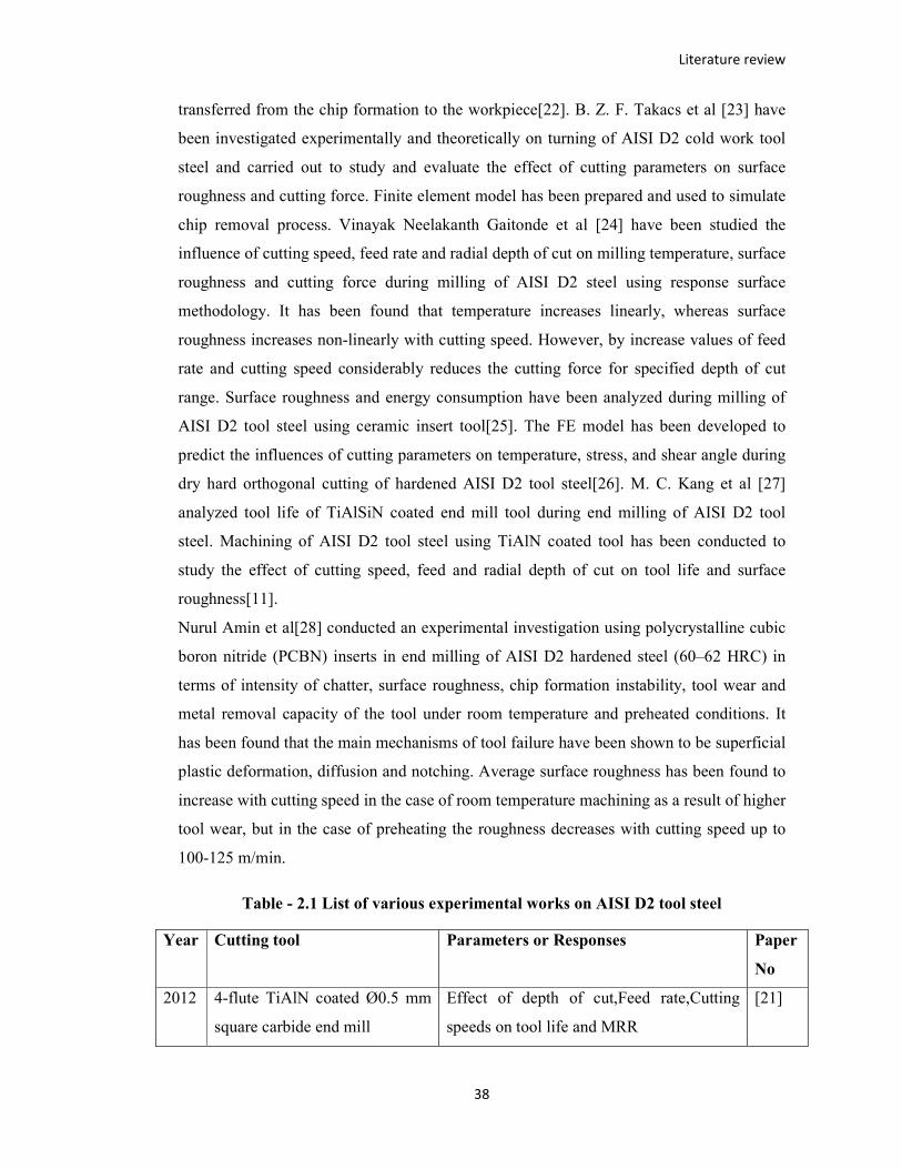
Literature review
38
transferred from the chip formation to the workpiece[22]. B. Z. F. Takacs et al [23] have
been investigated experimentally and theoretically on turning of AISI D2 cold work tool
steel and carried out to study and evaluate the effect of cutting parameters on surface
roughness and cutting force. Finite element model has been prepared and used to simulate
chip removal process. Vinayak Neelakanth Gaitonde et al [24] have been studied the
influence of cutting speed, feed rate and radial depth of cut on milling temperature, surface
roughness and cutting force during milling of AISI D2 steel using response surface
methodology. It has been found that temperature increases linearly, whereas surface
roughness increases non-linearly with cutting speed. However, by increase values of feed
rate and cutting speed considerably reduces the cutting force for specified depth of cut
range. Surface roughness and energy consumption have been analyzed during milling of
AISI D2 tool steel using ceramic insert tool[25]. The FE model has been developed to
predict the influences of cutting parameters on temperature, stress, and shear angle during
dry hard orthogonal cutting of hardened AISI D2 tool steel[26]. M. C. Kang et al [27]
analyzed tool life of TiAlSiN coated end mill tool during end milling of AISI D2 tool
steel. Machining of AISI D2 tool steel using TiAlN coated tool has been conducted to
study the effect of cutting speed, feed and radial depth of cut on tool life and surface
roughness[11].
Nurul Amin et al[28] conducted an experimental investigation using polycrystalline cubic
boron nitride (PCBN) inserts in end milling of AISI D2 hardened steel (60–62 HRC) in
terms of intensity of chatter, surface roughness, chip formation instability, tool wear and
metal removal capacity of the tool under room temperature and preheated conditions. It
has been found that the main mechanisms of tool failure have been shown to be superficial
plastic deformation, diffusion and notching. Average surface roughness has been found to
increase with cutting speed in the case of room temperature machining as a result of higher
tool wear, but in the case of preheating the roughness decreases with cutting speed up to
100-125 m/min.
Table - 2.1 List of various experimental works on AISI D2 tool steel
Year Cutting tool Parameters or Responses Paper
No
2012 4-flute TiAlN coated Ø0.5 mm
square carbide end mill
Effect of depth of cut,Feed rate,Cutting
speeds on tool life and MRR
[21]

Literature review
39
2008 Dia. 16mm coated with (TiAl)N
and tipped with PCBN
Measurement of workpiece temperature [22]
2014 80° nose angle (C-insert type),
rhombic shaped, uncoated CBN
cutting insert with chamfered
edge and nose radius of 0.4 mm
FEM simulation
[23]
2016 TiAlN Coated tungsten carbide
inserts
Effect of cutting speed, feed rate and depth
of cut on temperature, cutting force and
surface roughness
[24]
2002 Carbide and Cermet tools and
solid carbide ball nose end mills
Wear measurement [8]
2008 PVD TiAIN coated carbide
cutting tool
Effect of cutting speed, feed and depth of
cut on tool life
[16]
2011 CBN cutting tool Effect of cutting speed, feed, depth of cuton
temperature fields, residual stress, shear
angle and cutting tool edge temperature
[26]
2008 Coated carbide cutting tool Microstructure, micro-hardness and
oxidation resistance of coatings
[27]
2011 TiAlN coated carbide cutters Effect of cutting speed, feed rate and radial
depth of cut on Tool life and surface
roughness (across & along)
[11]
2008 Polycrystalline cubic boron
nitride (PCBN) inserts
Effect of cutting speed, feed rate, depth of
cut and nose radius on surface roughness
and tool wear
[28]
2014 Ceramic insert Effect of cutting speed, feed rate and depth
of cut on surface roughness and energy
consumption
[25]
2008 The effect of heat treatment
parameters
Dimensional stability [20]
2.3 Coated cutting tool
Milling of hard materials has been gained high interest due to lesser machining time and
machining cost associated with production of moulds and dies [29].To keep pace with the

Literature review
40
times, researchers have been working to improve the coating structure by doping a range
of functional alloy elements, resulting in high-hardness, high-wear-resistant, high-
performance coatings, self-lubricating and high-temperature oxidation-resistant tool
coatings[30].
Tool life is reduced due to machining of hard material. Problems are arisen in machining
of hardened steel due to its high hardness and toughness as well as its inhomogeneous
microstructure, which contributes to accelerated tool wear and chipping. Finding the ways
for enhancement of tool life in the hard milling domain is a major task in manufacturing
industries[31]. Recently, the development of new cutting tools have enabled to machining
of very hard materials like tool steel[32]. Due to higher strength of hardened steel, milling
of hard material is a challenging task for die and mould manufacturing industries. Tool
wear is a major drawback due to higher thermo-mechanical stress on cutting tool[33].
Milling has evolved as a process with new machines and procedures being used to
constantly achieve the greatest results. From the uncoated high speed steel tool to the
presently widely used coated tools, milling tools have undergone
a significant evolution[34]. Coatings of carbide tools increase the tool working life and
reduce tool wear rate in machining processes[35]. When the milling cutter starts cutting of
hard material, it will become more difficult for further machining. Higher cutting force
and higher temperature are generated due to hardening effect. Coated tools are still hard to
bear high load impacts, high temperature and improve wear resistance significantly[36].
Coatings on cutting tools reduce the coefficient of friction between cutting tool and chip.
Due to that it gives better performance under similar cutting condition compare than
uncoated cutting tool[37].
Coating has to possess high hot hardness and improved oxidation resistance at elevated
temperatures for machining of hardened steel, when high load and high temperature
control wear behavior[38]. Coating can effectively improve tool life of cutting tool in hard
milling. Coating enhances lubricity of tool and oxidation resistance, reduces the
temperature variation in the tool, protects the tool against diffusion wear and rendering it
less susceptible to crack[26]. Coated carbide tools are useful especially milling of
hardened material due to their high toughness and hot hardness[39]. Experiments have
been performed on cold work tool steel using various coated tool and found that the
cutting forces are approximately two times higher in the case of uncoated tool[40]. Surface

Literature review
41
topography gains better yield with coated tool as compared to uncoated tool due to high
wear and temperature of hardened steel[41].
There are two well established vapor processing for coating, namely chemical vapor
deposition (CVD), which was the first to appear, and physical vapor deposition (PVD).
TiC, TiN and Al2O3 were the first materials to be used for coating inserts by CVD and
showed excellent results due to their built up edge resistance, wear resistance and heat
resistance respectively. Varying combinations of these coating materials also showed
considerable improvements in tool life. PVD process offered unique advantages over CVD
due to lower deposition temperatures[42]. PVD coatings are generally used to increase
production and tool life of cutting tool. At present, PVD coatings are mostly used in
manufacturing industries due to reducing cycle time of components, reduce wear (which
are caused by chemical interaction, crater wear and build up edge) and reduce the need of
cutting fluid. In last few years, PVD coating is mostly used and replacing the CVD coating
technologies because it is possible to achieve good coating properties like high hardness,
good adhesion and wear resistance. Close tolerance can be achieved by thin PVD coatings.
PVD coating processes are also applied at relatively low coating temperature[43]. PVD
coatings and CVD coating have been compared during milling of AISI 4140 alloyed steel
at normal milling speed as well as high milling speed[44].There are various list of coating
properties and applications shown in Table-2.2. Coated tools of nitride coatings with high
aluminum content (like AlTiN and AlCrN) can be performed better than aluminum-free
nitride coated tools (like TiN and CrN) in wear protection at high temperatures due to their
oxidation resistance, higher hot hardness and lower thermal conductivity[45]. Addition of
Cr creates strong Al–Cr metallic bonds in coating, the hot hardness and oxidation
resistance is improved at high temperatures[38].Because of addition of Cr in metastable
Al-rich metal matrix, the solubility limit of AlN phase is increased in the complex nitride
and the concentration of heavy metal matrix ion vacancies is reduced within crease in
nitrogen ion vacancy content[46].
Table-2.2 List of various coating properties
Coating
type
Coating
colour
Hardness
H [HV]
Friction
Coefficient
Max
Temp
Use
TiN Gold 2447-2855 0.4-0.5 500°C General purpose coating for

Literature review
42
cutting, forming, injection,
moulding applications
AlTiN Black 3875 0.7 900°C For dry high speed
machining for hardened
materials (> 52 HRC)
CrN Metal
Silver
1835 0.3-0.4 700°C For deep drawing,
extrusion, metal die casting
application
ZrN White
Gold
2039 0.4 550°C For machining of aluminum
and titanium alloys
AlCrN Blue-Grey 3059 -
3263
0.3-0.6 1100°C For gear cutting tools, die
casting; punching, hot
forging, moulding and
various hardened materials
Performance of AlCrN coated tool and uncoated tool during machining of austenitic
stainless steel have been compared and found that Al based coatings provide good
chemical inertness, higher hardness and wear résistance due to the formation of Al2O3
layer on the tool surface at high temperatures. Also better surface finish has been produced
by AlCrN coated tool compare than uncoated tool due to less coefficient of friction and
lower thermal conductivity of coating[47]. M. S. Kasim et al [48] have been investigated
tool life and wear mechanism during end milling of Inconel 718 using a physical vapor
deposition coated ball-type end mill. AlCrN coated tool has exhibited higher wear
resistance than TiAlN coated tool in wear mechanism as an abrasion, attrition and
delamination. After machining, the wear on the tool center, the rake and flank faces have
been examined using a scanning electron microscope as shown in figure 2.2 [49].Using a
system Bias and cathodic arc evaporation, a heat-treated monolayer coating of AlCrN is
produced on a tungsten carbide micro-grain commercial substrate by physical vapour
deposition. In a controlled nitrogen atmosphere, Al-Cr alloy is utilised to apply as a
coating. To get a layer with a particular thickness, the deposition time can be modified.

Literature review
43
Figure 2.2 Two flute ball end mill [49]
To ensure that the nitriding of the compound, the coating is applied in a nitrogen
environment and then the sample is heat treated for 4 hours at 500 °C in an inert
atmosphere. Heat treatment is used to change the microstructure of the coating, extending
the diffusion of nitrogen and promote the creation and growth of AlN precipitates. Heat
treatment can also help to reduce amorphous phases created during coating procedures,
allowing the phases to become more crystalline and improving adhesion between the
coating and the substrate. Furthermore, heat treatment aids in the improvement of
structural integrity as well as the reduction of stress and fragility in coatings[50]. A new
AlCrN nano structured coating has been developed based on nitride nano composite by
PVD process. AlCrN coating is a relatively new ternary nitride with high amounts of
aluminum with excellent properties at high temperatures and excellent anti-oxidation
characteristics. It has also anti-spalling and debris removal properties for the contact
interface[50].
2.3.1 Experiments on AlCrN coated tool
Many researchers have performed the investigation on machining of various materials by
AlCrN coated tool as shown in Table 2.3. The wear of AlCrN coated tool has been
evaluated during machining of titanium alloy by different cutting parameters. It has been
found that the flank wear decreases dramatically when cutting speed is 100 m/min and

Literature review
44
feed is 0.04 mm. It has been noted that the higher productivity reached by the operation
with the lower levels of cutting speed and feed per tooth[50]. G. S. Fox-Rabinovich et al
[51] have been compared micro hardness of TiAlN coated tool and AlCrN coated tool
with respect to temperature. It has been found that micro hardness of AlCrN coated tool is
higher compare than TiAlN coated tool at elevated temperature. The elastic modulus of
TiAlN coated tool is reduced with increasing temperature when the elastic modulus of
AlCrN coated tool is increased. Results of cutting test of both coatings are shown in
Figure2.3. The tool life of the end mills with the TiAlN coating is much lower as
compared to the cutting tools with the AlCrN coatings.
Figure 2.3 End mill flank wear Vs length of cut for cutting tool with TiAlN and
AlCrN coating [51]
Mechanical properties of various commercially available hard AlCrN based coated
substrates have been investigated by means of nano and micro indentation and it has been
found that coating of AlCrN and AlCrN/ TiSiN exhibit similar result [52]. W. Kalss et
al[53] have been prepared different wear curves by using various coating tools. It can be
seen that AlCrN coating has performed an excellent during running-in phase by a
stabilized wear rate. This can be observed on the light microscopy photographs at 60, 80
and 100 m tool life. Nearly, no flank wear of AlCrN coated tool could be detected up to a
tool life of around 100 m. After this lifetime a controlled progressive wear could be found

Literature review
45
until the end of the tool life at 130 m as shown in figure 2.4. AlCrN has the best oxidation
resistance coating which could be seen a very thin oxidized layer of around 150 nm in
thickness at 1100°C.
Figure 2.4 Compare various coated tool during end milling of AISI 1045 carbon steel
[53]
The tool life of PVD coated AlCrN coating for cemented carbide inserts has been analyzed
during machining of steel. The abrasive wear mechanisms of AlCrN have been
investigated under dry and wet machining at very high cutting speeds. Approximately 33%
more depth of cut can be achieved by AlCrN coated tool by compare with TiN coated tool
and also attain higher cutting speed due to better thermal resistance of the AlCrN coated
tool. Due to high oxidation resistance, it gives good chemical stability and ability to
withstand temperature up to 1100°C. Also its monolayer structure gives it higher hot
hardness and results in excellent abrasion resistance[54]. Z. Liang et al [55] have been
studied the effects of different coating materials on tool wear and workpiece surface
morphology during the micro milling of Ti-6Al-4V. It has been seen that the AlTiN-based
and AlCrN-based coatings can lead to the reduction of cutting edge chipping and tool wear
length compared to an uncoated micro end mill.

Literature review
46
Table-2.3 List of experimental works carried out on various workpiece materials by
AlCrN coated tool
Year Workpiece Parameters or Responses Paper
No
2010 STAVAX (modified AISI
420 stainless steel) with a
hardness of 40 and 55
HRC
Wear measurement [49]
2013 Inconel 718 Effect of cutting speed, feed, radial depth of
cut and axial depth of cut on cutting force
and wear
[48]
2011 Austenitic stainless steel
SS 316L
Effect of cutting speed, feed and depth of
cut on surface roughness and wear
[47]
2006 Austenitic stainless steel
SS 316
Cutting test and wear measurement [17]
2009 Coating characteristic Mechanical properties of coating [52]
2013 Titanium alloy Machinability [50]
2006 AISI 1040 steel Cutting tool life [51]
2005 AISI 1045 steel Wear resistance, thermal stability such as
oxidation resistance and hardness at elevated
temperatures
[53]
2008 SAE 4140 steel Tool life enhancement, wear progressions [54]
2018 Ti-6Al-4V Tool wear and workpiece surface
morphology
[55]
2019 MDN 250 maraging steel Tool life, surface roughness and cutting
forces
[56]
V. Varghese et al [56] have been performed the performance of AlCrN and AlTiN coated
cemented carbide inserts during end milling of MDN 250 maraging steel under dry, wet
and cryogenic environments. The AlCrN coatings provide better machinability in

Literature review
47
comparison with AlTiN coatings. The aluminium chromium oxide and chromium oxide
films have been formed due to oxidation. Because of it, AlCrN coated tool have a better
wear resistance and lower thermal conductivity.
2.4 End milling process parameters
In comparison to traditional routes such as annealing, heat-treatment, grinding, EDM and
surface finishing, hard machining has the potential benefits to minimise lead time,
improve productivity, expand flexibility, reduce environmental hazards and reduce capital
expenses[24][35]. End milling process is quite possibly the most significant and common
metal cutting process encountered for machining parts in manufacturing industry. By
using this interaction, the material can be effortlessly taken out from the surfaces of molds
and dies[57].
The result showed that wear propagation particularly flank wear is done more rapidly in
up milling operation than down milling operations[36]. In case of up milling, cutter enters
into the workpiece at the beginning of cut with minimum chip thickness. This will result in
excessive work hardened layer in workpiece due to rubbing action between cutter and
workpiece at the beginning of the cut. So higher cutting force, higher tool wear and
shorten tool life have been found in the case of upper milling operation compare than
down milling operation[58]. Traditional machining methods are replaced gradually by dry
hard machining in automotive, die and tool industries because of its substantial advantages
like decline manufacturing costs, reduce finishing time and significantly improve surface
quality[32]. J M Vieira et al[59] investigated performance of various cutting condition
during milling of AISI 8640 and found that higher tool life can be achieved in dry cutting
condition compare than cutting fluid also dry machining produced better surface finish
compare than machining in the presence of cutting fluid. During hard machining, tool life
has been decreased with increase in cutting speed and longer tool life has been observed in
dry machining compared to the machining with cutting fluid. Also best surface finish has
been generated during machining in dry condition[10]. Some problems like physiological,
ecological and economic problems are caused by using the lubricant; these can be
completely avoided with dry machining. The main advantages of dry machining are the
reduction of the problem related to purifying, drying or disposal processes for workpiece
and chips and saving of related expenses also[60]. Dry milling is an absolutely free from
the issues related with storage and removal of cutting fluid. The existing industries need

Literature review
48
ultra hard cutting tools and extremely rigid machine tools [61]. N. Camuscu et al [62]
have been investigated the end milling of cold-work tool steel AISI D3using various
cutting tools. It has been found that coated carbide and coated cermet tools have not
exhibited good performance in high speed cutting operations as compared with the low or
moderate cutting speeds. Minimum surface roughness and maximum compressive
residuals stress have been obtained by optimizing the inclination angle, cutting speed and
feed during end milling of Inconel 718. The high-power proto residual stress analyzer has
been used to measure the two components of surface residual stress, as shown in figure
2.5. The residual stress inside the material can be measured by electrolytic polishing
technology. In this work, the electrolytic polishing instrument has been used to remove the
surface of the material layer-by-layer as shown in figure[63].
(a) X-ray analyzer

Literature review
49
(b) Electrochemical polishing machine
Figure 2.5 Residual stress measurement [63]
M. Okada et al [64] have been used the CBN tools and PVD-coated carbide tools in end-
milling of the K10 and P30 grade carbide hardened steel to identify tool wear, cutting
temperature, cutting force and surface roughness. The tools have been subjected through
several machining cycles and the amount of wear rate has been also affected by the
number of flutes of cutting tool. The top view of end mill with four flutes is shown in
figure. There is chipping and in some cases breakage of the cutting edge. When compared
to the end mill with four flutes, the wear of two flute end mill tool has been occurred
significantly higher after the same number of cycles. Both PVD AlCrN coated end mills
have been compared for 16 machining cycles. Figure 2.6 shows that the end mill with two
flutes caused significantly more damage than the end mill with four flutes[34].

Literature review
50
(a) Two-flute end-mill
(b) Four-flute end-mill
Figure 2.6 SEM image of the damage of two flute and four flute the PVD AlCrN
coated end mill tool after 16 cycles of machining [34]

Literature review
51
Y.H.Guu [65] has been analyzed the surface morphology, surface roughness and micro-
crack of AISI D2 tool steel during machining of the electrical discharge machining
(EDM). The EDM specimens have been also analyzed by means of SEM technique.
Selected image has been shown in Fig. 2.7.
Figure 2.7 SEM images of the AISI D2 tool steel after EDM
2.4.1 Review on performance measure of end milling process
Cutting speed, feed, depth of cut, width of cut, types of coating and other input process
parameters are generally selected as input process parameters in the end milling process,
while cutting force, surface roughness, tool wear, material removal rate and other process
responses are considered as process responses. Since the previous decade, a large number
of efforts have been done by the author community to investigate surface roughness and
cutting force in order to improve surface quality and reduce tool wear using various end
milling procedures.
2.4.1.1 Effects of process parameters on cutting force
Significant cutting force is required on workpiece for metal cutting by cutting tool. By
knowing of cutting force, various significant issues can be calculated like power, spindle
torque, deflection and vibration of cutting tool etc. The value of cutting force can also be
influenced on dimensional accuracy as well as surface quality[66]. Cutting force in milling
process is closely related to machining efficiency and machining quality. It is the most
important technical parameter in computer numerical control machining[67]. Modeling of

Literature review
52
cutting force of end milling is very important for estimate tool life and tool condition
monitoring, chatter prediction and tool deflection which directly affect on final product
quality[68].
Milling operations tasks are perhaps the most widely recognized machining activities in
industry. It tends to be utilized for edge finishing, face finishing, material removal and so
on. There are a few parameters that impact the cutting forces on the cutting tool. On
account of these parameters, the cutting forces may be predictable [69]. Tool wear can be
measured mainly by two methods; direct method and indirect method. In direct method,
measurement of cutting edge of cutting tool is measured by optical microscope. For that,
the cutting tool is detached from machine tool and measure reading. The measuring
accuracy of machine tool may be reduced when the cutting tool is installed again. In
another method (indirect method), the tool wear is measured based on measuring of
cutting force during machining of parts [70]. H. Caliskan et al [40] have been investigated
the effect on cutting forces during hard milling of AISI O2 cold work tool steel with help
of various coated tool and found the effect of input parameters on them. According to the
results of variance analysis, the cutting forces are the most sensitive to feed rate and then
depth of cut. Gopalsamy et al [71] performed end milling of hardened steel by ball end
mill and found that by increasing depth of cut and feed, temperature was raised at cutting
zone causing adhesion phenomenon from workpiece to tool face. Due to that, cutting
forces were increased due to increase of stresses at contact region which resulted into high
tool wear. The effects of input machining variables have been investigated on the milling
force and tool wear during milling of Al7075 and metal matrix composite (MMC) using
an uncoated carbide tool. The test results showed that milling force has been significantly
influenced by the depth of cut (measured by a Kistler 9257B dynamometer) [72]. S.
Wojciechowski et al [73] have been carried out experiment on hardened steel by using
TiAlN coated tool and cubic boron nitride (CBN) ball end mills to measure cutting force
as well as tool wear and observed that tool life of TiAlN coated tool has been found higher
compare than CBN tool. Catastrophic wear of cutting edge has been found for cutting
speed 500 m/min in case of TiAlN coated tool. Analytical method has been proposed
during end milling of AISI 304 stainless steel for modeling the cutting forces. The
workpiece material properties, tool geometry, cutting conditions and types of milling have
been taken as the input data and each cutting edge has been discretized into a series of
infinitesimal elements along the cutter axis and the cutting action of each element has seen

Literature review
53
equivalent to the classical oblique cutting process [74]. Modeling of cutting force has been
done during end milling of aluminum alloy by carbide ball end mill according to the
mechanistic principles of metal cutting and found that the forces acting on end mill tool
were directly proportional to the undeformed chip geometry [68]. Milling of hardened tool
steel H13 has been performed using PCBN tools and concluded that a large chip load has
been yielded a more stable cutting process and increase tool life. The surface quality was
not significantly affected [75]. The correlation has been investigated between the cutting
force and the surface roughness during ballend milling of P20 steel (HRC 30) work-pieces
using solid carbide ball-end mill cutters [76]. A mathematical model has been developed
to predict cutting forces in end milling of AISI D2 tool steel by using RSM. The linear
model and the quadratic model have been compared and it has been found that the
quadratic model has been seen more reliable to predict the cutting force model with
Central Composite Design and the CCD is a very efficient design for fitting the second
order model[77].
An end milling process has been illustrated in figure 2.8. The cutting forces applied on
element Q of cutting edge i, whose elementary length was dz, can be divided into three
components: tangential force dFi,t (z), radial force dFi,r (z) and axial force dFi,z(z). These
can be calculated using
�/0,1(2) � 31ℎ0(2)�2
�/0,5(2) � 35ℎ0(2)�2
�/0,)(2) � 3)ℎ0(2)�2
Figure 2.8 End milling and coordinate systems [78]

Literature review
54
Where hi(z) is the instantaneous uncut chip thickness associated with element Kt, Kr and
Kz which are three cutting force coefficients[78].
A deduced cutting force prediction model for circular end milling process has been
presented. An improved cutting force model for circular end milling process has been
developed based on the typical linear milling force model. The curvature effects of tool
path on chip thickness as well as entry and exit angles have been analyzed and the cutting
force model of linear milling process has been corrected to fit circular end milling
processes[79].
The influence of tool orientation in end milling on the cutting forces has been investigated.
Different cutting force impulse shapes and amplitudes have been obtained for various tool
orientations and machining strategies[80].
A new approach to identify the instantaneous cutting force coefficients and radial cutter
runout in the flat end milling has been studied. Theoretically, it has been demonstrated that
the total cutting forces are separated into two components in angular domain: a nominal
component independent of the cutter run-out and a perturbation component induced by the
run-out. The instantaneous value of the nominal component is used to calibrate the cutting
force coefficients. With the help of the perturbation component and the cutting force
coefficients obtained above, the run-out has been identified[81].
2.4.1.2 Effects of process parameters on Surface roughness
One of the most important parameter is roughness for a mechanical component because
cracks or corrosion is generally formed from irregularities in the surface. Surface
roughness is expensive to control during manufacturing although it is generally
undesirable. Decrease the surface roughness of mechanical part is resulted into increasing
the manufacturing cost[82]. Surface quality of parts as well as production costs are the
major challenge of hard machining industries. Surface roughness is mainly depends on
various machining parameters like cutting speed, feed, depth of cut etc[83]. W. Li et al[84]
have been studied the effect of tool wear on surface integrity during end milling of Inconel
718 alloy using PVD coated carbide inserts. Surface finish can be produced between 0.1
µm and 0.3 µm during end milling. Surface roughness has been found higher in step-over
direction than feed direction. Surface roughness is utilized to decide corrosion, fatigue
strength and wear rate of machined part. The high accuracy machined parts are needed in
basic application and is accomplished by high surface quality. In assembling, poor surface

Literature review
55
finish is undesirable and should be controlled to estimate the performance of the
mechanical parts[85]. Vinh Do et al[86] have been investigated the hard milling of AISI
H13 tool steel by AlTiN coated tool to get better surface finish and found that higher
cutting speed, lower feed rate, lower depth of cut and lower hardness of workpiece lead to
good surface finish. Optimisation methodology using RSM and GA has been applied
during end milling of P20 tool steel to minimize surface roughness. To achieve the
minimum surface roughness, the appropriate process parameters (nose radius, cutting
speed, feed rate, axial depth of cut and radial depth of cut) have been determined. A
predictive model for surface roughness has been developed in terms of the process
parameters using RSM. The RSM model has been interfaced with an effective GA to find
the optimum process parameter values[87].
Figure 2.9 Mathematical deviation of Ra [88]
From figure 2.9, Surface roughness is the most commonly used parameter to describe the
average surface roughness and is defined as an integral of the absolute value of the
roughness profile measured over an evaluation length:
�� � |6| + |6$| + |6%| …… � � +|6�|8
Literature review
56
�� � 91�:� |2(�)|
��
The average roughness is the total area of the peaks and valleys divided by the evaluation
length; it is expressed in µm (thousandths of a millimeter). The arithmetic value of surface
roughness in end milling can be represented by:
�� � 318,(�$)/4?
The required surface finish value should be smaller than or equal to the maximum
achievable surface finish under the existing machining conditions[89]. ANN and GA have
been used to optimize cutting parameters such as cutting speed, feed, axial depth of cut
and radial depth of cut to minimize surface roughness during end milling of Al 7074-
T6[57] and Inconel 718[88].The inherent abnormalities of the workpiece left by various
machining techniques are referred to as surface roughness. Surface roughness can be
described in a variety of ways. Average roughness, abbreviated as Ra, is one of them.
Surface roughness is defined as the arithmetic value of the profile's deviation from the
centerline along the length of the sample [88]. R. Sreenivasulu [90] has been performed
the experimental study in end milling of GFRP composite material using desirability
function analysis integrated with Taguchi technique to optimize multiple performance
considerations namely surface roughness and delamination damage factor.
2.5 Modeling methods
Response surface method is the most effective tool for design of experiment in
manufacturing problems. It is the effective method to study the result obtained from
factorial experiments. It gives more information with fewer numbers of investigations.
RSM is investigated for exploring the limits of the input parameters and emerging
experiential statistical model for the measured response[91]. Response surface method is
an empirical modeling process derived from prior knowledge of the machining processes
to achieve statistical model[92]. RSM is a statistical technique to determine the
relationship between responses and input variables. The main aim of RSM is to obtain
efficient mathematical model by design of experiments in proper sequence with respect to
an optimal response[93]. Response surface method (RSM) is a set of design of
experiments techniques that gives better analysis and optimizes the experimental
responses. A central composite design (CCD) is a widely used response surface in

Literature review
57
designed experiments[72]. The most successful way for analyzing the outcomes of
factorial trials is response surface methodology. It is a useful tool for studying and
modeling engineering challenges. It gives you more information while reducing the
number of experiments you have to do. It's an experimental approach for determining the
input parameters limitations and building an empirical statistical model for the measured
response by approximating the relationship between the response and the input process
parameters[94]. The full form of ANOVA is called the Analysis of Variance. ANOVA is a
statistical tool for obtaining the contribution of variable parameters[95]. Response surface
methodology combined with ANOVA analysis is useful techniques for tool life equation.
This method shows a less number of designed experiments required to generate much
useful information[21].
J.B. Saedon et al [21] developed tool life models during micro-milling of hardened AISI
D2 tool steel in terms of cutting speed, feed and depth of cut using Response Surface
Methodology Central composite design (CCD) method. All of the cutting tests have been
performed within specified ranges of parameters using 0.5 mm diameter TiAlN micro
tools under dry condition. Ashwin et al [96] studied the effect of four input cutting
parameters on surface roughness and developed mathematical model using response
surface methodology. RSM is a statistical strategy for determining a regression model and
obtaining a response (output variable) that is influenced by numerous independent
variables using quantitative data from arelated experiment (input variables). RSM has
been applied to develop mathematical model in terms of various factor and levels of input
parameters. Evaluation of the parametric effects has been done by considering a second
order polynomial response surface mathematical model as given by equation:
@�, � , A +,BA0�0 +BA00�0$ +B B A0C�0�C +∈EF
CG0H
FI
0G
F
0G
F
0G
Where SR is output response, b0 is the mean response over all the test conditions
(intercept), bi is the slope or linear effect of the input factor xi (the first-order model
coefficients), bii the quadratic coefficients for the variable i (linear by linear interaction
effect between the input factor) and bij is the linear model coefficient for the interaction
between factor i and j. Significance testing of the coefficients, adequacy of the model and
analysis of variance have been carried out by using design expert software to find out the
significant factors, square terms and interactions affecting the response (surface
roughness). ∈E is the experimental error[97]. In response surface approach, the limit of the

Literature review
58
process parameters have been determined and the initial testing has been carried out to
identify the machining parameters which effect on temperature rise[94]. A. Tamilarasan et
al [98] have been investigated the effect of process parameters (such as cutting speed,
feed, depth of cut and width of cut) during milling of hardened AISI O1 tool steel using
(TiN/TiAlN) coated carbide tools on the cutting temperature, tool wear and metal removal
rate. The RSM based CCRD design has been used to analyze the influence of four selected
process parameters with five levels. In order to find out optimal parameters, a non-
dominated sorting genetic algorithm has been adopted and found that the cutting
temperature is more influenced by cutting speed and feed rate. A coating peel off over the
tool rake face has been observed at higher cutting speed.
2.6 Optimisation methods
2.6.1 RSM
Hard and dry cutting are required in today's manufacturing units due to continuously
improvement in die quality and effectiveness. It is essentially recognized as well as
aggressive processes which require optimum cutting input parameters with proper cutting
tools. Today’s manufacturing needs is to optimize cutting input parameters and tool
characteristics for obtaining proper outputs[23][45]. The selection of optimum values of
input process parameters of end milling process such as cutting speed, feed rate, depth of
cut and width of cut play a significant role in optimizing the measures of process
performance. In this paper, response surface methodology (RSM) is used to find out the
optimal input process parameters of end milling process. Surface roughness and cutting
force have been considered as responses. It is very difficult to choose the best machining
parameters for achieving optimum performance characteristics during machining of hard
materials[99].Response surface method is the most effective tool for analysis and design
of experiment in manufacturing problems. It gives more information with fewer numbers
of investigations. RSM is investigated for exploring the limits of the input parameters and
emerging experiential statistical model for the measured response. It is useful to optimise
input process parameters for analysis of output responses [100].
The effects of cutting speed, feed rate and depth of cut has been studied on surface
roughness in the hard turning of AISI 4140 steel by uncoated AL2O3/TiC mixed ceramics
tool. Three level factorial experiment designs has been used with a statistical analysis of

Literature review
59
variance (ANOVA) and mathematical model for surface roughness has been developed
using the response surface methodology (RSM) associated with response optimisation
technique to find optimum values of machining parameters with respect to surface
roughness[101]. The machining parameters such as cutting speed, feed rate, depth of cut
and approach angle of the cutting edge have been considered as input parameters whereas,
the surface roughness and tangential forces have been considered the response variables
for investigations. The experimental plan has been developed with four factors and three
levels by central composite design using RSM. RSM has been also used for optimisation
of machining parameters during machining of titanium alloy. The experimental results
indicated that the surface roughness increases with increase in the cutting speed and the
feed rate and decreases with reduction in the value of approach angle and depth of cut,
whereas the tangential force increases with increase in approach angle and depth of cut
and decreases with decrease in cutting speed and feed rate [102]. M. R. S. Yazdi et al
[103] have been investigated the selection of optimal machining parameters such as
spindle speed, depth of cut and feed rate to minimize the surface roughness and to
maximize the material removal rate during the face milling of 6061-T6 Aluminum.
Optimum machining parameters have been obtained using RSM. It has been observed that
the speed and feed rate are the most significant factors for surface roughness model
whereas the depth of cut and feed rate and their interaction are significant factors for the
material removal rate model. V. Sathyamoorthy et al [104] have been studied the effect of
machining parameters such as spindle speed, feed rate and depth of cut on surface
roughness during end milling of magnesium AM60 alloy by TiN coated carbide end mill.
2.6.2 GA
Because of the availability and cost of high-speed computers, optimisation algorithms are
becoming increasingly prevalent in engineering activities. They are widely employed in
engineering challenges involving the maximization or minimization of a certain goal. The
GA technique is used for optimisation purpose provides an efficient and promising tool in
view of high degree or non-linearity in the objective function[105].The genetic algorithm
(GA) is a population-based search optimisation technique. In general, the fittest
individuals of any population tend to reproduce and survive to the next generation, thus
improving successive generations. However, inferior individuals can, by chance, survive
and also reproduce. Genetic algorithms have been shown to solve linear and nonlinear

Literature review
60
problems by exploring all regions of the state space and exponentially exploiting
promising areas through mutation, crossover and selection operations applied to
individuals in the population. The use of a genetic algorithm requires the determination of
six fundamental issues, chromosome representation, selection function, the genetic
operators making up the reproduction function, the creation of the initial population,
termination criteria and the evaluation function[106].
Genetic algorithms are used extensively for the solution of optimisation problems and
were first developed by Holland in the 1970s. These algorithms are based on the biological
evolution process. A similar analogy is used to evolve solutions to complex optimisation
problems. The notable feature of genetic algorithms is that it emulates the biological
system’s characteristics like self-repair and reproduction. It is generally well known that
the human being is a very good example of a decision maker. So researchers began
experimenting with the natural systems and have developed methods like genetic
algorithms and neural networks. The actual differences between the GAs and other
methods of optimisation are briefly summarized below. GA move through the solution
space starting from a population of points and not from a single point. This is similar to
the calculus based methods and the solution can be restarted from a number of points to
ensure global convergence. Genetic algorithm works with the objective function
information directly and not with any other auxiliary information like derivatives.
Constraints are included in the objective function using some penalty function. GAs use
probabilistic rules and not deterministic rules. So, applying to the optimisation problem
and the structure of genetic algorithm is rather easy[107]. In a GA approach to solve
combinatorial optimisation problems, a population of candidate solutions is maintained.
To generate a new population, candidate solutions are randomly paired. For each pair of
solutions, a crossover operator is first applied with a moderate probability (crossover rate)
to generate two new solutions. Each new solution is then modified using a mutation
operator with a small probability (mutation rate). The resulting two new solutions replace
their parents in the old population to form a temporary new population. Each solution in
the temporary population is ranked against other solutions based on a fitness criterion. A
roulette wheel process is then used to determine a new population identical in size to the
previous population, such that higher-ranked candidates are allowed to assume higher
priority in the new population. GA iterates over a large number of generations and, in
general, as the algorithm executes, solutions in the population become fitter, resulting in
better candidate solutions[108]. Genetic algorithms are heuristic search algorithms used

Literature review
61
for optimisation by mimicking the processes of natural evolution. Feed, speed, and depth
of cut are the machining parameters used for optimisation by Genetic Algorithm[25].
The effect of machining parameters such as helix angle of cutter, spindle speed, feed rate,
axial and radial depth of cut has been studied for temperature rise in end milling by using
RSM and the optimisation of machining process parameters has been carried out to obtain
minimum temperature rise using genetic algorithms[94].In contrast to other optimisations
in which machining time and cost have been defined as the objective functions, algorithm
considers tool deflection as the objective function while surface roughness and tool life
have been taken as the constraints[106]. Girish Kant et al [109] performed end milling
process on AISI 1060 steel workpiece by using carbide tool with consider of five level
four factor experimental design. Genetic Algorithm has been used for optimisation of
machining parameters leading to minimum surface roughness and experimental values
have been found very close to the predicted results. Machining of oil hardened non-
shrinking die steel (AISI H13) has been performed for maximizing metal removal rate and
minimizing surface roughness by choosing the optimal parameters. Genetic algorithm has
been used to optimise cutting speed, feed rate and depth of cut[110].
2.7 Research gap
Many researchers have worked on investigation of cutting parameters for various output
responses during end milling of hardened tool steel. AISI D2 tool steel is mostly used to
making moulds, dies, automotive parts and aerospace parts. AISI D2 tool steel has been
machined by using various coated cutting tool like AlTiN, CrN, TiCN etc. At present,
most of the die manufacturing industries are ready to accept machining of hardened AISI
D2 tool steel by AlCrN coated tool. A limited amount of research work has been found on
machining of hardened tool steel using AlCrN coated end mill tool. More attentions is
required to investigate on the effect of various input machining parameters such as cutting
speed, feed rate, depth of cut and width of cut during machining of hard material for
various output responses. Most of the work deals with experimental investigation on
output responses during end milling of hardened tool steel with different coated and
uncoated end mill tool. Effect of input parameters on cutting force are to be investigated
carefully as the minimization of cutting force directly affect tool wear and tool life.
Surface roughness must be minimized in order to avoid dimensional inaccuracy. In this
study the cutting speed, feed rate, depth of cut and width of cut have been considered as

Literature review
62
input parameters. The cutting force and surface roughness have been taken as output
responses. The single objective optimisation is carried out and correlations amongst the
output responses have also been established.
From the literature review, it can be seen that the input machining parameters are directly
affecting the desired responses. Hence for hardened tool steel materials, the selection of
input process parameters is very crucial. AISI D2 tool steel is having high hardness and
wear resistance; it is desirable to carry out research in the direction of finding optimum
parameters. The parameters like cutting speed, feed, depth of cut and width of cut have
been proven influencing parameters for minimization of cutting force and surface
roughness. The cutting force is directly related to tool life and tool wear; and hence it is
selected in this research. Surface roughness is the most important parameter because crack
or corrosion is generally formed from irregularities in the surface; its minimization has
been focused in this research work. The process parameters are optimized by many
researchers by several optimisation techniques for different materials. The comparison of
prediction of parameters using optimisation techniques is also desirable.
2.8 Scope and objectives of research work
Considering the review of research work and problem definition, the key focus of this
research work is optimisation of input process parameters during machining of hard
materials. The selection of process parameters is more important in this research work.
The following are the objectives of this research work to achieve better output results.
� To investigate cutting force during milling of D2 tool steel
� To improve surface finish during milling of D2 tool steel using AlCrN coated tool
� To develop a Mathematical model to predict output responses using response
surface methodology (RSM)
� To optimize the process parameters of milling process and validate the same for
D2 tool steel
Milling process is used to create various shapes on Vertical milling machine using cutting
tool. Machining of hard material (AISI D2 tool steel) is done using hard coated end mill
tool in dry condition. CNC milling system produces the die faster, more accurate and serve
as an alternative to EDM in moulds, dies and automobile industries. It can give better
result in significantly lower manufacturing times and costs compared to existing
production processes.

Manufacturers of various components which are made
D2 tool steel can get complete details of the effect of various cutting conditions on cutting
force and surface roughness. This research work can be directly useful to die and mould
making industries to decide various pro
and cutting force. From this work, output responses like cutting force and surface
roughness can be predicted before machining process. Optimum cutting conditions can be
obtained based on their requirement
The obtained results can be used for their application in manufacturing industry.
2.9 Methodology of present research work
This research work is mainly concerned with mode
milling process parameters for machining of AISI D2 tool steel material. The research
objectives have been achieved by developing the detailed resear
figure-2.10 which highlights the experimental work on milling machine for ma
AISI D2 tool steel. Figure 2.
successful output in results.
Selection of machining process, cutting tool, Workpiece material
Select Input parameters ranges for experimental work using
Develop Mathematical model and
effect on output parameters and Percentage weightage of
63
Manufacturers of various components which are made from tool steel material like AISI
D2 tool steel can get complete details of the effect of various cutting conditions on cutting
force and surface roughness. This research work can be directly useful to die and mould
making industries to decide various process parameters with respect to surface roughness
and cutting force. From this work, output responses like cutting force and surface
roughness can be predicted before machining process. Optimum cutting conditions can be
obtained based on their requirement of response characteristics of AISI D grade tool steel.
The obtained results can be used for their application in manufacturing industry.
2.9 Methodology of present research work
This research work is mainly concerned with modeling and parametric optimis
milling process parameters for machining of AISI D2 tool steel material. The research
objectives have been achieved by developing the detailed research methodology shown in
which highlights the experimental work on milling machine for ma
AISI D2 tool steel. Figure 2.10 depicts the complete flow of work carried out to get
successful output in results.
Figure 2.10 Research Methodology
Selection of machining process, cutting tool, Workpiece material
Select Input parameters ranges for experimental work using
OVAT
Design of Experiment by RSM
Develop Mathematical model and Find out Input parameters
effect on output parameters and Percentage weightage of
input parameters
Optimization & Validation of model
Literature review
from tool steel material like AISI
D2 tool steel can get complete details of the effect of various cutting conditions on cutting
force and surface roughness. This research work can be directly useful to die and mould
cess parameters with respect to surface roughness
and cutting force. From this work, output responses like cutting force and surface
roughness can be predicted before machining process. Optimum cutting conditions can be
of response characteristics of AISI D grade tool steel.
The obtained results can be used for their application in manufacturing industry.
ling and parametric optimisation of
milling process parameters for machining of AISI D2 tool steel material. The research
ch methodology shown in
which highlights the experimental work on milling machine for machining of
depicts the complete flow of work carried out to get

Literature review
64
2.10 Summary
In this chapter the research works carried out by researchers have been discussed in brief.
After a brief introduction about the chapter, research work from literature has been
classified in various sections. Tool steel finds wide applications in manufacturing of cold-
forming dies and blanking dies on account of their excellent deep hardening characteristics
and wear resistance.
AISI D2 tool steel is the first choice in the application where higher compressive strength
and wear resistance is desirable. The research works related to mechanical properties, heat
treatment and applications of AISI D2 tool steel have been discussed in first section. The
second section describes about properties, applications and experiments of coated tool as
well as AlCrN coated tool. The third section describe about end milling process and its
various parameters. Many researchers have contributed in the area of investigation of
process parameters. The significant input process parameters such as cutting speed, feed
rate, depth of cut, hardness of material, types of coating on cutting tools, width of cut etc
are directly affecting output responses like cutting force, tool wear, surface roughness,
material removal rate etc. In the review on performance measurement of end milling
section, investigation of effect of input process parameters on cutting force and surface
roughness have been discussed. In the section of modeling methods, the techniques of
formulating regression models for input process parameters and output responses have
been discussed. RSM has been used by researchers to make effective design of
experiments. Significance and contribution of the process parameters can well be
identified using RSM. Optimisation of process parameters is a major area of research.
Genetic algorithm and RSM are widely used optimisation techniques. Research works
related to optimisation have been briefly discussed in the section of optimisation methods.
From the exhaustive survey of literature the research gap has been identified. The research
gap is the basic motivation for current research. In the last section the gap for research has
been discussed and research objectives along with methodology have been presented.

Methodology and experimental work
65
CHAPTER-3
Methodology and Experimental work
3.1 Introduction
The goal of this study is to see how cutting speed, feed rate, depth of cut and width of cut
affect cutting force and surface roughness during end milling of AISI D2 tool steel. This
chapter explains the technique for conducting experiments. There has been a brief
discussion of the workpiece and the cutting tool. The numbers of input parameter levels as
well as experimental results have been tabulated. In order to investigate machining
properties, Response Surface Methodology (RSM) has been chosen for the design of
experiment. The ranges of input parameter have been chosen based on one variable at a
time (OVAT).
For the efficient performance of experiments, a scientific approach is required to planning
the experiments. The process planning of the experiment is carried out by statistical design
of experiment, which ensures that relevant data is collected and analyzed using statistical
methods, resulting in reliable and objective results. The design of the experiments and the
statistical analysis of the data are thus two parts of an experimental challenge. These two
principles are intertwined since the method of analysis is directly dependent on the
experiment design.
By applying the design of experiments, following advantages are covered such as
improving the performance of existing process, reducing experimental time, improving
reliability, achieving product robustness and reducing the number of trials.
For extracting accurate conclusions from experimental observations, a well-planned and
executed set of experiments is essential. The OVAT (one-variable at a time approach) for
performing screening experiments, as well as the response surface methodology have been
used to design the experiments and investigate the data acquired in this study.
In the present work, all experimental works are executed on Jyoti make CNC machining
centre PX10 at CSPIT, Charusat University, Gujarat, India. The details of workpiece
materials, cutting tool, machine tool, measuring equipment etc .have been discussed
below.

Methodology and experimental work
66
3.2 Workpiece and cutting tool
Tool steels are high-quality carbon and alloy steels used to manufacture of forming,
cutting, shearing, extrusion, stamping and slitting dies. Tool steels are supplied in a soft or
annealed state, allowing them to be machined into tooling components. After being
manufactured into a tool, these steels can be heat-treated to increase their hardness.
Various types of tool steel materials are listed in table 3.1.
Table 3.1 List of AISI Tool steel grade
Sr No Property Characteristics AISI Grade
1 Cold working
Oil Hardening O
Air-hardening A
High carbon High chromium D
2 High speed Tungsten base T
Molybdenum base M
3 Hot working Chromium, Tungsten and
Molybdenum base H
4 Plastic mold Prehardened P
5 Shock resistance low carbon alloys S
6 Special purpose Low alloy L
Carbon tungsten F
7 Water hardening Water hardening W
High carbon and chromium D grade AISI D2 tool steel has been selected and used for
experimental work. It was procured from Vatva GIDC, Ahmedabad, Gujarat. It has wide-
ranging practical applications in tools & dies making firms such as manufacturing of
blanking dies, forming dies, long punch, coining dies, thread rolling dies, extrusion dies
and so on.

Methodology and experimental work
67
Figure 3.1 AISI D2 tool steels before hardening
Figure 3.2 AISI D2 tool steel after heat-treatment
Figure 3.1 shows the workpiece AISI D2 tool steel (80mm in length, 40 mm in width and
16mm in thickness) has been used to conduct experiments. Service properties of D2 tool
steel should be restored by hardening. Generally, heat treatment consists of a quenching

Methodology and experimental work
68
operation and at least two tempering. Figure 3.2 shows a workpiece of AISI D2 tool steel
that has been used for further machining after heat-treatment process.
Chemical composition and mechanical properties have been tested in a Test Well
Laboratory, Odhav, Ahmedabad. Various chemical compositions of AISI D2 tool steel
after laboratory test have been presented in table 3.2. The hardness of workpiece material
before hardening has been shown in table 3.3. The hardness of 59 HRC of the D-grade
AISI D2 tool steel has been achieved by hardening (with oil quenching) at 970°C followed
by 2 hours tempering at 710°C. The hardness of workpiece material after hardening has
been shown in table 3.4.
Table 3.2 Chemical composition of AISI D2 tool steel (%wt)
Elements Content (Wt %)
Carbon (C) 1.56
Silicon (Si) 0.280
Molybdenum (Mo) 0.560
Chromium (Cr) 11.700
Vanadium (V) 0.210
Tungsten (T) 0.460
Sulphur (S) 0.030
Manganese (Mn) 0.340

Methodology and experimental work
69
Table 3.3 Hardness testing of Workpiece material before hardening
Workpiece material AISI D2 tool steel
Test method as per IS 1500 - 2005
Sample Size 80 x 16 mm
Hardness in HRC 22
Table 3.4 Hardness testing of Workpiece material after hardening
Workpiece material AISI D2 tool steel
Test method as per ASTM E18-2016
Sample Size 40x 80 x 16 mm
Hardness in HRC 59
Coatings deposited on cutting tools are ceramic layers with few micrometers in
thickness which exhibit great mechanical strength and hardness, chemical inertness and
low thermal conductivity. As a result, compared to uncoated tools, there is a substantial
improvement in performance.
The AlCrN coating is utilized to produce various tools because it has exceptional
toughness at high temperatures and wear resistance under intense mechanical stress. This
coating is also used to treat materials that are difficult to cut. As shown in figure 3.3,
Walter make AlCrN coated tool has been used for experimental work.
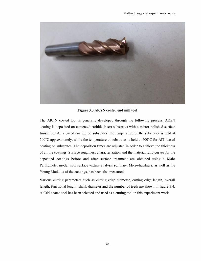
Methodology and experimental work
70
Figure 3.3 AlCrN coated end mill tool
The AlCrN coated tool is generally developed through the following process. AlCrN
coating is deposited on cemented carbide insert substrates with a mirror-polished surface
finish. For AlCr based coating on substrates, the temperature of the substrates is held at
500°C approximately, while the temperature of substrates is held at 600°C for AlTi based
coating on substrates. The deposition times are adjusted in order to achieve the thickness
of all the coatings. Surface roughness characterization and the material ratio curves for the
deposited coatings before and after surface treatment are obtained using a Mahr
Perthometer model with surface texture analysis software. Micro-hardness, as well as the
Young Modulus of the coatings, has been also measured.
Various cutting parameters such as cutting edge diameter, cutting edge length, overall
length, functional length, shank diameter and the number of teeth are shown in figure 3.4.
AlCrN coated tool has been selected and used as a cutting tool in this experiment work.

Methodology and experimental work
71
Figure 3.4 Cutting tool parameters
Specification of coated end mill tool is tabulated in table 3.5 (10 mm diameter, 72 mm
overall shank length, 22 mm cutting edge length, 4 flutes with a flat end, right spiral
direction and 35-degree spiral angle with the center cut, etc). The AlCrN coated tool is
shown in figure 3.5 as a detailed drawing. The drawing of the AlCrN coated end mill tool
has also been shown in figure 3.6 with additional dimensions.
Figure 3.5 Walter make AlCrN coated tool with dimension

Methodology and experimental work
72
Table 3.5 Specification of Cutting tool parameters
Symbol Description Value
Dc Cutting edge diameter 10 mm
Lc Cutting edge length 22 mm
Lo Overall length 72 mm
Lf Functional length 32 mm
Ds Shank diameter 10 mm
Z Number of teeth 4
Cutting direction Right
Spiral direction Right
Spiral angle 35
Type of face Center cut
Type of shank DIN 6535 HB
Coating Thickness 4 µm

Methodology and experimental work
73
Figure 3.6 Drawing of AlCrN coated tool with all dimensions
3.3 Machine and equipments
The most efficient use of the CNC milling process requires the choice of proper sets of
machining process parameters. It can primarily be accomplished by interpreting the
interrelationship between various numbers of input machining process parameters and
identifying the most favourable machining conditions which directly affect the production
time, cost as well as superior quality.
So, in this experimental work, experimental trials have been performed on a particular
machine tool. Various process parameters have been comprehended sequentially for two
major output response measures as surface roughness and cutting force. In the present
work, experiments are executed on Jyoti CNC machining center PX10 as shown in figure
3.7.

Me
tho
do
log
y a
nd
exp
eri
me
nta
l w
ork
74
Fig
ure 3
.7 J
yoti
CN
C m
ach
ine P
X1
0

Methodology and experimental work
75
Table 3.6 Specifications of Jyoti CNC machine PX10
Table Unit Dimensions
Table Size mm 660 x 360
T-Slot Dimension mm 3 x 14 x 125
Capacity Unit Dimensions
X-Axis Travel mm 510
Y-Axis Travel mm 410
Z-Axis Travel mm 510
Feed Unit Dimensions
Rapid Traverse (X,Y & Z Axis) m/min 25
Cutting Feed m/min 10
Main Spindle Unit Dimensions
Spindle Speed Range RPM 0-10000
Spindle Motor Power -Fanuc KW 7.5/ 5.5 [11/7.5]
Spindle Motor Power -Siemens KW 5.6/ 3.8
Automatic Tool Changer Unit Dimensions
Number of Tool 20
Max.Tool Length mm 250
Accuracy Unit Dimensions
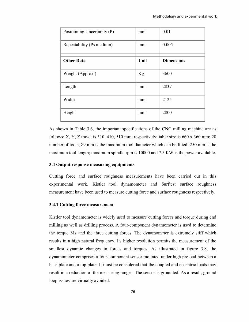
Methodology and experimental work
76
Positioning Uncertainty (P) mm 0.01
Repeatability (Ps medium) mm 0.005
Other Data Unit Dimensions
Weight (Approx.) Kg 3600
Length mm 2837
Width mm 2125
Height mm 2800
As shown in Table 3.6, the important specifications of the CNC milling machine are as
follows; X, Y, Z travel is 510, 410, 510 mm, respectively; table size is 660 x 360 mm; 20
number of tools; 89 mm is the maximum tool diameter which can be fitted; 250 mm is the
maximum tool length; maximum spindle rpm is 10000 and 7.5 KW is the power available.
3.4 Output response measuring equipments
Cutting force and surface roughness measurements have been carried out in this
experimental work. Kistler tool dynamometer and Surftest surface roughness
measurement have been used to measure cutting force and surface roughness respectively.
3.4.1 Cutting force measurement
Kistler tool dynamometer is widely used to measure cutting forces and torque during end
milling as well as drilling process. A four-component dynamometer is used to determine
the torque Mz and the three cutting forces. The dynamometer is extremely stiff which
results in a high natural frequency. Its higher resolution permits the measurement of the
smallest dynamic changes in forces and torques. As illustrated in figure 3.8, the
dynamometer comprises a four-component sensor mounted under high preload between a
base plate and a top plate. It must be considered that the coupled and eccentric loads may
result in a reduction of the measuring ranges. The sensor is grounded. As a result, ground
loop issues are virtually avoided.

Methodology and experimental work
77
Figure 3.8 Kistler tool Dynamometer Type 9272 [67]
Screws may be used to secure the dynamometer to any clean, face-ground supporting
surface such as the table of a machine tool. Eight M8 mm threaded holes on the cover
plate are provided for mounting the workpiece as shown in figure 3.9. To ensure proper
mechanical interaction between the force introducing elements and the cover plate, the
supporting surfaces must be face-ground. The tool holder type 9404 is suitable for
attaching tools with a shank cross-section of up to 20x20 mm.

Methodology and experimental work
78
Figure 3.9 Dimensions of Kistler tool dynamometer
A four-component measuring system requires, in addition to the dynamometer, a multi-
core high-insulation connection cable and four charge amplifier channels. These convert
the dynamometer's charge signals to output voltages. The output voltage is proportional to
the magnitudes of the forces and moments. The multichannel charge amplifier is utilized
for this purpose. Table 3.7 contains technical specifications for the Kistler 9272 tool
dynamometer, which has been utilized in this experimental study. Various softwares (such
as Lab view, Kistler Dyno Ware etc) have been used for data acquisition during
machining.

Methodology and experimental work
79
Table 3.7 Technical Data of Kistler 9272 tool dynamometer
Technical detail Term Value with unit
Measuring Range
Fx -5 to 5 KN
Fy -5 to 5 KN
Fz -5 to 20 KN
Sensitivity
Fx ≈ - 7. 8 pC/N
Fy ≈ - 7.8 pC/N
Fz ≈ - 3.5 pC/N
Operating temperature range °C 0 - 70°C
Temperature coefficient of sensitivity % /°C – 0.02
Threshold
Fx < 0.01 N
Fy < 0.01 N
Fz < 0.02 N
Weight W 4.2 KG
3.4.2 Surface roughness measurement
As shown in figure 3.10, the portable surface roughness tester SJ-410 model has been
used to measure surface roughness in this research work. It has a wide range and is high-
resolution: 800µm/0.01µm.

Methodology and experimental work
80
Figure 3.10 Mitutoyo make Surftest SJ-410
Skidless and skidded measurements can be done by this instrument. Skidless measurement
is where surface features are measured relative to the drive unit reference surface as
shown in figure 3.11. This measures waviness and finely stepped features accurately in
addition to surface roughness, but the range is limited to the stylus travel available. The
SJ-410 series supports a variety of surface feature measurements simply by replacing the
stylus.
In skidded measurements, surface features are measured with reference to a skid
following close behind the stylus as shown in figure 3.12. This cannot measure waviness
and stepped features exactly but the range of movement within which measurement can be
made is greater because the skid tracks the workpiece surface contour.

Methodology and experimental work
81
Figure 3.11 Skidless measurement
Figure 3.12 Skidded measurement
3.5 Experimental Setup
Ranges of various parameters for the design of experiment have beenselected by using
one variable at a time and cutting tool supplier’s data. Cutting speed 50 - 200 m/min, Feed
(f) 50 – 800 mm/min, Depth of cut (ap) 0.1 to 1 mm and Width of cut (ae) 2 to 10 mm
have been used to perform experimental investigation. The wear of the cutting tool is
mainly specified by flank wear and its progressive growth. The abrasion takes place due
to contact between the flank of the cutting tool and workpiece. Flank wear is caused by an
increase in cutting speed resulting in high temperature. When the average flank wear of a
cutting tool reaches a certain limit, the cutting tool has to be replaced and perceived to be
failed. Rejection of cutting tool is based on the criteria as per ISO 8688-2 [50].
Flank wear was observed on cutting tool by using 3D microscope. Cutting tool was
changed when tool failure occurred. In accordance with ISO 8688-2-1989[45], tool life
failure for an end mill has been considered to occur when one of the following criteria is
met:

1. Uniform flank wear reaches 0.3
2. For irregular flank wear, the maximum wear is 0.5 mm
3. Catastrophic failure[22]
Machining has been performed
workpiece. Cutting experiments have been carried out by Jyoti CNC machining Centre
PX10. Walter-made AlCrN coated tool with 10 mm diameter and four flutes flat end mill
has been used for experimental work (shown i
Kistler make) has been mounted on the table of the machine tool to measure the cutting
force signals during machining as shown in the figure. The signals
through a charge amplifier and analog si
(PCI-6-23E, NI) and stored in a computer. Lab VIEW
data acquisition.
In order to determine the elastic deflection of components and conse
voltage under static load, the dynamometer was calibrated. The calibration was made in
Fz direction and the output voltages of m
to 700 N were applied and the strain values were recorded fo
curves were obtained to convert the output readings into cutting force values. Figure
shows the calibration curve for
frequency noise signals have been eliminated and v
in Figure 3.14.
Methodology and experimental work
82
1. Uniform flank wear reaches 0.3 mm
2. For irregular flank wear, the maximum wear is 0.5 mm
performed on a 40x80x16mm size AISI D2 tool steel (59HRC)
workpiece. Cutting experiments have been carried out by Jyoti CNC machining Centre
made AlCrN coated tool with 10 mm diameter and four flutes flat end mill
has been used for experimental work (shown in figure 3.13). A tool dynamometer (9272,
mounted on the table of the machine tool to measure the cutting
force signals during machining as shown in the figure. The signals have been
through a charge amplifier and analog signals are converted using an A/D acquisition card
23E, NI) and stored in a computer. Lab VIEW has been employed for cutting force
Figure 3.13 Experimental setup
In order to determine the elastic deflection of components and consequently the output
voltage under static load, the dynamometer was calibrated. The calibration was made in
nd the output voltages of mV were averaged for each direction. The loads up
N were applied and the strain values were recorded for each load. Thus calibration
curves were obtained to convert the output readings into cutting force values. Figure
shows the calibration curve for axial force. With the help of sensitivity adjustment high
frequency noise signals have been eliminated and very close values were obtained as seen
Methodology and experimental work
40x80x16mm size AISI D2 tool steel (59HRC)
workpiece. Cutting experiments have been carried out by Jyoti CNC machining Centre
made AlCrN coated tool with 10 mm diameter and four flutes flat end mill
l dynamometer (9272,
mounted on the table of the machine tool to measure the cutting
have been amplified
gnals are converted using an A/D acquisition card
employed for cutting force
quently the output
voltage under static load, the dynamometer was calibrated. The calibration was made in
were averaged for each direction. The loads up
r each load. Thus calibration
curves were obtained to convert the output readings into cutting force values. Figure 3.14
With the help of sensitivity adjustment high
ery close values were obtained as seen

Methodology and experimental work
83
Figure 3.14 Calibration curve for axial cutting force Fz
3.6 One Variable at a Time (OVAT)
For experiment work, OVAT initial experiments have been performed for an axial depth
of cut (ap) from 0.1 to 1.5 mm, width of cut (ae) from 1.5 to 10 mm, feed (fz) from 127 to
1500 mm/min and for cutting speeds (Vc) from 25 to 250 m/min for PVD coated AlCrN
coated end mill tool to achieve a relationship amongst above four parameters with surface
roughness and cutting force. In the OVAT method, one among four input parameters is
varied and the other three are kept constant. Various input parameters such as cutting
speed, feed, depth of cut and width of cut have been discussed as follows.
Cutting speed
Table 3.8 Experiment with Variable Cutting Speed
Sr.
No.
Cutting Speed
(m/min)
Cutting Force (N) S.R.
(µm) Fx Fy Fz
1 25 21.784 6.713 739.538 1.300
2 50 52.313 6.713 754.800 1.311
0
20
40
60
80
100
120
140
160
180
0 200 400 600 800
Output Voltage (mV)
Output Voltage (mV)
Linear (Output Voltage
(mV))

Methodology and experimental work
84
3 75 21.784 6.713 693.755 0.783
4 100 21.784 6.713 495.358 0.791
5 125 37.048 21.972 296.962 0.555
6 150 37.048 37.231 342.745 0.344
7 188 21.784 6.713 403.791 0.303
8 200 6.519 21.972 632.710 0.244
9 225 21.784 37.231 586.926 0.243
10 250 21.783 21.972 475.520 0.398
Cutting speeds have been changed at different intervals and feed, depth of cut and width
of cut are fixed at 509 mm/min, 0.5 mm and 10 mm, respectively. Cutting force and
surface roughness have been measured at various cutting speeds as shown in table 3.8.
Feed
Table 3.9 Experiment with Variable feed rate
Sr. No. Feed
(mm/min)
Cutting Force (N) S.R.
Fx Fy Fz
1 127 21.784 37.231 266.439 0.327

Methodology and experimental work
85
2 382 21.784 21.972 388.529 0.907
3 509 52.313 6.713 754.800 1.311
4 637 21.784 6.713 724.277 1.086
5 800 21.784 21.972 1258.422 1.302
6 1000 21.784 6.713 678.494 1.474
7 1200 6.519 21.972 1060.025 1.460
8 1500 6.519 6.713 1655.215 1.601
Feeds are changed at different intervals and cutting speed, depth of cut and width of cut
have been fixed as 50 mm/min, 0.5 mm and 10 mm, respectively. Cutting force and
surface roughness have been measured for various values of feed rate as shown in table
3.9.
Depth of cut
The values of depth of cut have been changed at different intervals and cutting speed, feed
and width of cut are fixed as 50 mm/min, 509 mm/min and 10 mm, respectively. Cutting
force and surface roughness have been measured at various values of depth of cut as
shown in table 3.10
.

Methodology and experimental work
86
Table 3.10 Experiment with Variable Depth of Cut
Sr. No. DOC
(mm)
Cutting Force (N) S.R.
Fx Fy Fz
1 0.1 21.784 6.713 83.304 0.811
2 0.3 21.784 6.713 251.178 1.612
3 0.5 52.313 6.713 754.800 1.311
4 0.8 6.519 21.972 983.719 1.741
5 1 21.784 21.972 1151.593 1.615
6 1.3 21.784 21.972 1426.296 2.219
7 1.5 49.194 49.224 1380.512 1.608
Width of Cut
The values of width of cut have been changed at different intervals and cutting speed, feed
and depth of cut are fixed as 50 mm/min, 509 mm/min and 0.5 mm respectively. Cutting
force and surface roughness have been measured at various values of width of cut as
shown in table 3.11.

Methodology and experimental work
87
Table 3.11 Experiment with Variable Width of Cut
Sr. No. WOC
(mm)
Cutting Force (N) S.R.
Fx Fy Fz
1 1.5 21.784 21.972 22.259 0.673
2 2 21.784 37.231 129.080 0.431
3 3 21.784 21.972 113.826 0.708
4 4 37.048 6.713 174.871 0.839
5 4.5 6.519 21.972 205.394 0.752
6 5 21.784 6.713 266.439 0.790
7 6 6.519 37.231 312.223 0.790
8 10 52.313 6.713 754.800 1.311

Methodology and experimental work
88
3.6.1 Effects of cutting parameters on surface roughness
Effect of various input parameters such as cutting speed, feed, depth of cut and width of
cut on surface roughness have been shown in figure 3.15 - 3.18.
Surface roughness has been reduced when increasing cutting speed from 50 m/min to 200
m/min. Surface roughness has been increased with increased cutting speed above 200
m/min due to formation of built up edge on cutting tool surface. Surface roughness has
been slowly increased with increased feed from 50 to 800 mm/min but after 800 mm/min,
surface roughness has been increased rapidly due to higher thrust force. Surface roughness
has not much been increased with 0.1 mm to 1 mm depth of cut but after 1 mm depth of
cut, surface roughness has been increased tremendously. It has been shown that increase
in width of cut has been resulted in higher surface roughness.
Figure 3.15 Effect on Surface Roughness of different Cutting speeds by OVAT
0
0.2
0.4
0.6
0.8
1
1.2
1.4
1.6
25 50 75 100 125 150 188 200 225 250
Su
rfa
ce r
ou
gh
ne
ss
Cutting Speed

Methodology and experimental work
89
Figure 3.16 Effect on Surface Roughness of different feed by OVAT
Figure 3.17 Effect on Surface Roughness of different Depth of Cut by OVAT
0
0.2
0.4
0.6
0.8
1
1.2
1.4
1.6
1.8
2
127 382 509 637 800 1000 1200 1500
Su
rfa
ce r
ou
gh
ne
ss
Feed
0
0.5
1
1.5
2
2.5
3
0.1 0.3 0.5 0.8 1 1.3 1.5
Su
rfa
ce r
ou
gh
ne
ss
Depth of cut

Methodology and experimental work
90
Figure 3.18 Effect on Surface Roughness of different Width of Cut by OVAT
3.6.2 Effect of cutting parameters on cutting forces
Effect of various input parameters such as cutting speed, feed, depth of cut and width of
cut on cutting force have been shown in figure 3.19 – 3.22. Three types of forces (Normal
force, Feed force and Axial force) have been measured during milling of AISI D2 tool
steel by Kistler dynamometer. Values of the axial forces are much higher than the other
two forces (normal force and feed force). Values of normal force and feed force are very
less and negligible. So the axial force has been used for further analysis.
Cutting force has been reduced with increase cutting speed upto 140 m/min, after that it
has been found higher cutting force. Cutting force has been increased with an increase of
feed rapidly. Cutting force has been increased continuously with an increased depth of
cut. Poor surface finish and high tool wear rate have been found after 1 mm depth of cut.
Cutting force has been increased with increased width of cut upto 6 mm. Cutting force has
been reduced afterward.
0
0.2
0.4
0.6
0.8
1
1.2
1.4
1.6
1.5 2 3 4 4.5 5 6 10
Su
rfa
ce r
ou
gh
ne
ss
Width of cut

Methodology and experimental work
91
Figure 3.19 Effect of cutting speed on Cutting force by OVAT
Figure 3.20 Effect of feed rate on Cutting force by OVAT
0
100
200
300
400
500
600
700
800
900
1000
25 50 75 100 125 150 188 200 225 250
Cu
ttin
g f
orc
e
Cutting speed
Fz
0
500
1000
1500
2000
2500
127 382 509 637 800 1000 1200 1500
Fz
Fz

Methodology and experimental work
92
Figure 3.21 Effect of depth of cut on Cutting force by OVAT
Figure 3.22 Effect of width of cut on Cutting force by OVAT
When cutting speed is increased above 200 m/min, it may be a chance for the failure of
the cutting tool due to tool wear. When cutting speed is reduced to 50 m/min, it may
generate a very poor surface finish as well as develop a higher cutting force. When the
depth of cut has been increased above 1 mm, a poor surface finish has been resulted due to
high tool wear and higher cutting force. When the depth of cut has been reduced than 0.1
mm, a good surface finish has been generated but more machining time has been required.
0
200
400
600
800
1000
1200
1400
1600
1800
0.1 0.3 0.5 0.8 1 1.3 1.5
Fz
Fz
0
100
200
300
400
500
600
700
800
900
1000
1.5 2 3 4 4.5 5 6 10
Fz
Fz

Methodology and experimental work
93
When width of cut has been increased above 10 mm, poor surface finish has been
generated due to higher cutting force. When the width of cut has been decreased to less
than 2 mm, no effect has been seen on increase in cutting force and also reduces surface
roughness. When feed rate has been increased more than 800 mm/min, high tool wear and
vibration have occurred during machining. When feed has been reduced to 50 mm/min,
high machining time has been required due to the low material removal rate. Finally,
experimental investigation on AISI D2 tool steel has been conducted by One Variable at a
Time (OVAT) and chosen ranges of input parameters for the design of experiment work
as shown in table 3.12.
Table 3.12 Selection of the ranges of input parameters for design of experiment
Sr. No. PARAMETERS INITIAL EXP
RANGE
Finally decided
1 C. S. (m/min) 25-250 m/min 50-200 m/min
2 FEED (mm/min) 50-1500 mm/min 50-800 mm/min
3 DOC (mm) 0.1-1.5 mm 0.1-1 mm
4 WOC (mm) 1.5-10 mm 2-10 mm
3.7 Design of Experiment
The response surface method is the most effective method for analyzing factorial
experiment results. It is a powerful tool for modeling and investigating industrial
challenges. It delivers more information with fewer numbers of experiments. It is a
method for determining the limits of the input parameters and developing an experienced
statistical model for the measured response by approximating the relationship between the
response and the input process parameters. For the purpose of developing regression
equations for various milling process quality attributes, the following second-order
response surface has been assumed:

Methodology and experimental work
94
Where Y is predicted responses; bi, bii and bij are the coefficients for linear, quadratic and
interaction term respectively; k is a number of input variable and e is the random error.
3.7.1 Central composite design
A well-designed experiment can significantly reduce the number of experiments required
and hence a CCD approach is the most suitable approach to develop first and second-order
models. This is the most well-known and often used class of designs for fitting second-
order models.
The star point and center point represent the experimental domain in the CCD method,
which aids in determining the response surface plot. By assessing the precision of surface
responses, the worth of α can be resolved; where star configuration has been shown as ±
α. The α value can be resolved by estimating prospects and obtaining the required
precision from surface responses. The location of the α value dictates the nature of the
plan. The configuration rate is determined by the position of the points. The accuracy of
the estimation is impacted by the number of trials conducted at the focal point. The quality
by configuration approach is critical for estimating the variability and reactions of the
coefficients. The critical angle means that the forecast error is indistinguishable from all
points to the center points at a same distance. Finally, the CCD is categorized into three
categories: CCC, CCI and CCF.
CCC (Circumscribed design)
The CCD model is uniformly magnetized with corner points, as indicated by the blue
spots in figure 3.23. The extract points are compelled from the sides by the red-colored
central point. Each factor would have five levels in this CCD model. The star points are
establishing new low and high boundaries for all variables. These layouts have circular,
spherical or hyper spherical symmetry and each variable requires five levels. The CCC
(Circumscribed) is found to be a rotatable design.

Methodology and experimental work
95
Figure 3.23 CCC model
CCI (Inscribed design)
CCI (Inscribe design) has been utilized with the variable setting as star point and factorial
design has been created within those limits of variable settings as shown in figure 3.24. In
short, CCI design is nothing new and complicated design but a modified version of CCC
design. CCI design is generated by dividing the CCC design with α.
Figure 3.24 CCI Design

Methodology and experimental work
96
CCF (Face Centered design)
CCF design is suitable for 3 levels of each variable. In this CCF design, each face of the
factorial space has been shown in figure 3.25 and star points have been shown as the
center point, so α = ±1. CCF (Face centered design) is a non-rotatable design.
Figure 3.25 CCF (Face centered design)
3.7.2 Calculation of α value
The value of α can be defined as the calculated distance of each individual axial star point
from the center in the CCD. If α is less than 1, it indicates the axial point must be inside a
cube. If α value is greater than 1, it indicates the axial point is outside the cube. The value
of α can be determined by the following equation and it is seen in table 3.13;
α = (Number of factors)1/4
Table 3.13 Number of factor and alpha value
Number of factors α value related to ± 1
2 ± 1.414
3 ± 1.682
4 ± 2
5 ± 2.378
6 ± 2.828
In the CCD method, the total numbers of experiments are selected based on the number of
factors. Also, the design of the four factors factorial has been formulated as shown in table
3.14.

Methodology and experimental work
97
Table 3.14 Central composite design matrix for 4 factors
Sr
No.
Factor A Factor B Factor C Factor D
1
Factorial runs 24 =
16
-1 +1 +1 +1
2 +1 -1 +1 +1
3 +1 +1 -1 +1
4 +1 +1 +1 -1
5 +1 +1 +1 +1
6 -1 -1 +1 +1
7 +1 -1 -1 +1
8 +1 +1 -1 -1
9 -1 +1 +1 -1
10 +1 -1 +1 -1
11 -1 +1 -1 +1
12 -1 -1 -1 +1
13 +1 -1 -1 -1
14 -1 +1 -1 -1
15 -1 -1 +1 -1
16 -1 -1 -1 -1
17
Axial point runs 2(4)
= 8
+2 0 0 0
18 0 +2 0 0
19 0 0 +2 0
20 0 0 0 +2
21 -2 0 0 0
22 0 -2 0 0
23 0 0 -2 0
24 0 0 0 -2

Methodology and experimental work
98
25
Centre point = 6
0 0 0 0
26 0 0 0 0
27 0 0 0 0
28 0 0 0 0
29 0 0 0 0
30 0 0 0 0
Followings are the advantages of the CCD method; It turns out to be the extension of 2
level factorial designs. It gives maximum information in a minimum experimental data
and helps to assess the squared terms in the second-order model. It helps to predict
curvature in achieved continuous reactions and to estimate nonlinearity of output
responses in the given informational set.
Followings are limitations of the CCD method; It is seen that the star points are outside
the hypercube, so the quantity of levels that must be adapted to each factor is five rather
than three, and some of the time it is difficult to accomplish the value of factors.
Depending upon the design, the squared terms in the model won't be symmetrical to one
another and inability to estimate individual interaction terms, i.e., linear by quadratic or
quadratic by quadratic
The objective of this research work is to investigate the effect of cutting speed, feed, depth
of cut and width of cut on surface roughness and cutting force during milling of AISI D2
tool steel. The experimental details have been described in this chapter. The details of the
workpiece, cutting tool and machine tool have been described. The details of the
equipment to measure the output responses have also been discussed here. The initial
ranges of input parameters have been chosen based on One Variable at a Time (OVAT).
Response surface methodology (RSM) central composite design (CCD) method is
employed for the design of experiment. A graphic representation of different points has
been shown for the three variables in figure 3.26.

Methodology and experimental work
99
Figure 3.26 CCD drawing
3.7.3 Experimental setup
Response surface methodology is the most effective method to analyze the results
obtained from factorial experiments. It is an effective tool for modeling and analyzing
engineering problems. It provides more information with less number of
experimentation[89]. It is an experimental strategy for exploring the limits of the input
parameters and developing an empirical statistical model for the measured response, by
approximating the relationship existing between the response and input process
parameters. The limit of the process parameters has to be defined in response surface
methodology. The initial experimentation has been carried out to identify the machining
parameters that affect the cutting force and surface roughness and also to explore the
range of the selected machining parameters. In the present work, cutting speed, feed rates,
axial and radial depth of cut have been considered as the machining parameters. The
response surface roughness and cutting force have been expressed as a function of process
parameters such as cutting speed (Vc), feed rate (f), axial depth of cut (ap) and radial depth
of cut (ae).
Surface Roughness (S.R.) = Ø (Vc, f, ap, ae) + eu
Cutting Force (Fz) = Ø (Vc, f, ap, ae) + eu

Methodology and experimental work
100
Where ф is the response surface, eu is the residual, u is the number of observations in the
factorial experiment and iu represents level of the ith factor in the uth observation.
J0 � 2(2J − (JM�N + JM0�))(JM�N − JM0�)
OℎPQP, J0 � QPRSTQP�,UV�P�,WX�SP,V�,X,WXQTXA�P,J
J � X86,WX�SP,V�,YℎP,WXQTXA�P,�QVZ,JM0�YV,JM�N
JM0� � �V[PQ,�TZTY,V�,YℎP,WXQTXA�P
JM�N � S\\PQ,�TZTY,V�,YℎP,WXQTXA�P
]ℎP,T8YPQZP�TXYP,WX�SP^,V�,UV�P�,X^ − 1, 0,X8�,1
Table 3.15 Levels for input machining parameters
Input Variables Lowest Low Centre High Highest
- 2 -1 0 +1 + 2
Cutting Speed (Vc) 50 87.5 125 162.5 200
Feed (mm/min) 50 237.5 425 612.5 800
Depth of cut (mm) 0.1 0.325 0.55 0.775 1
Width of cut (mm) 2 4 6 8 10
In this experimental work, cutting speed Vc is converted into spindle speed N as a
machining parameter. For conversion cutting speed into spindle speed following equation
is used;

Methodology and experimental work
101
�� � `?a1000
Where Vc is cutting speed in m/mm, D is the diameter of the cutting tool in mm and N is
spindle speed in revolutions/ minute.
The diameter of a cutting tool is 10 mm; so the following spindle speeds have been
converted from cutting speeds which have been taken during experiment work as shown
in the table3.16. For 50 m/min cutting speed 1590 rpm, for 87.5 m/min cutting speed 2785
rpm, for 125 m/min cutting speed 3980 rpm, for 162.5 m/min cutting speed 5170 rpm and
for 200 m/min cutting speed 6365 rpm have been set.
Table 3.16 Convert cutting speed into spindle speed
Sr. No. Cutting speed
(m/min) Spindle speed (rpm)
1 50 1590
2 87.5 2785
3 125 3980
4 162.5 5170
5 200 6365
In milling operation, the cutting operation is always intermittent and the risk of thermal
cracking is also caused higher by the coolant. So dry machining is, therefore, the primary
choice to increase tool life, especially when cutting with steels, cast iron and some
stainless materials. In terms of cutting force and chatter stability, the down end-milling
mode is more suited for end milling than the up end-milling mode. All experiments have
been repeated two times and an average value has been considered. Following processor
has been done for experimental work.

Methodology and experimental work
102
1. Cutting tool has been fixed in the spindle of the CNC milling machine.
2. Tool dynamometer has been mounted on the machine bed and connected with the
amplifier and lab view system properly.
3. Workpiece has been mounted on tool dynamometer with help of clamping.
4. Experimental readings have been taken using AlCrN coated end mill tool with cutting
parameters such as cutting speed 50, 87.5, 125, 162.5 and 200 m/min, feed 50, 237.5, 425,
612.5 and 800 mm/min, depth of cut 0.1, 0.325, 0.55, 0.775 and 1 mm and width of cut 2,
4, 6, 8 and 10 mm
5. Total of 30 experiment runs have been done in this way.
6. Cutting forces have been measured during the machining process using a tool
dynamometer
7. Surface roughness has been measured using a surface roughness tester after the machining
process.
8. Results from the experimentation have been tabulated in the table 3.17.
Table 3.17 Design matrix of experiments based on RSM-CCD method
Run
Order
C.S.
m/min
Feed
mm/min
DOC
mm
WOC
mm
Normal
Force
Fx (N)
Feed
Force
Fy (N)
Axial
Force
Fz (N)
S.R.
(Ra) µm
1 0 0 +2 0 21.784 21.972 688.493 0.51
2 -1 +1 +1 -1 21.784 21.972 892.151 0.72
3 +1 +1 -1 +1 21.784 21.972 450 0.32
4 +1 +1 -1 -1 6.519 21.972 400 0.25
5 -1 +1 -1 -1 21.784 21.972 632.709 0.49

Methodology and experimental work
103
6 -1 -1 +1 +1 21.784 21.972 876.89 0.39
7 0 0 0 0 37.152 21.900 557.006 0.26
8 -1 +1 +1 +1 6.519 37.231 1352 0.77
9 0 -2 0 0 21.784 21.972 449.574 0.19
10 0 0 0 0 36.998 22.102 555.993 0.26
11 -2 0 0 0 21.784 37.231 1098 0.68
12 0 0 0 0 37.112 21.889 556.216 0.25
13 +1 -1 +1 -1 21.784 37.231 346.874 0.29
14 0 0 0 0 37.099 21.823 556.901 0.26
15 -1 +1 -1 +1 21.784 21.972 1103 0.57
16 0 0 0 +2 37.048 21.972 934 0.63
17 -1 -1 +1 -1 21.784 37.231 547 0.38
18 +1 -1 -1 -1 21.784 21.972 434.313 0.18
19 +1 -1 -1 +1 21.784 21.972 510.619 0.2

Methodology and experimental work
104
20 0 0 0 0 37.048 21.972 556.403 0.26
21 0 0 0 -2 21.784 21.972 495.358 0.63
22 +1 +1 +1 +1 37.048 37.231 785.322 0.61
23 -1 -1 -1 +1 21.784 21.972 937.935 0.31
24 +1 -1 +1 +1 21.784 21.972 612.709 0.37
25 0 0 -2 0 21.784 21.972 369 0.20
26 +2 0 0 0 21.784 52.490 571.664 0.51
27 0 0 0 0 37.111 22.001 555.982 0.26
28 -1 -1 -1 -1 37.048 21.972 521.142 0.25
29 0 +2 0 0 21.784 21.972 693.755 0.62
30 +1 +1 +1 -1 21.784 21.972 573 0.59

Methodology and experimental work
105
Figure 3.27All machined jobs after end milling
From the table, it can be seen that the minimum value of axial cutting force is 346.874 N
and the minimum surface roughness is 0.18 µm. The maximum value of axial cutting

Methodology and experimental work
106
force is 1352 N and the maximum surface roughness value is 0.77 µm. All machined
workpieces of hardened AISI D2 tool steel have been shown in figure 3.27.
3.8 Summary
In this chapter, the description of the workpiece has been done in detail. The types,
designations and behavior of cutting tool have been discussed. A detailed drawing of the
cutting tool has also been presented. In order to understand the measurement of responses
such as cutting force and surface roughness, the illustrations of measuring equipment have
been discussed. Details of all measuring equipment have been explained with photographs
and principles. Detailed specifications of tool dynamometer, surface roughness measuring
equipment and CNC milling machine have been tabulated. Initial experiments have been
analysed to decide levels of input parameters for the design of experiment by using one
variable at a time. The design of experiment has been tabulated based on the selected level
with the help of response surface methodology. The levels of input parameters and
measured responses have been tabulated. The investigation of input machining parameters
and their significant effect on responses have been reported in the successive chapter.

Result and analysis
107
CHAPTER-4
Result and Analysis
Initial pilot experiments have been discussed to sort out the affecting significant process
parameters on responses and to identify the levels of process parameters for the planning
of experimental design. The number of experiments has been performed as per the design
of experiment recommended by response surface methodology central composite design.
The selection of the appropriate model as well as the development of response surface
models has been carried out with help of statistical software “Design expert”. Results of
experiments have been examined in order to recognize the individual and interaction
effects of input process parameters on two responses. The main effect plot of cutting
speed, feed, depth of cut and width of cut are plotted for cutting force and surface
roughness during end milling of AISI D2 tool steel. The analysis of variance (ANOVA)
has been performed to ensure the competence of the fitted model and carry out graphical
and regression analysis.
4.1 Selection of adequate model
Three different models such as a sequential model sum of squares, lack of fit test and
model summary statistics have been performed to evaluate for an adequate model for
cutting force and surface roughness. The sequential model sum of squares indicates the
contribution of the terms of increasing complexity to the model. This test selects the most
noteworthy request polynomial where the terms are not associated. A model with the
highest F-value and lower p-value is selected. The experimental field is not incorporated
in the regression and variations at which points observed models cannot be accounted for
by random error. This test should indicate an insignificant lack of fit for the fitted model.
A p-value greater than 0.05, nullifies the lack of fit of the model to the response data and
the model can be utilized for the prediction of output response for 95% of a confidence
interval. Model summary statistics give information about standard and predicted
deviation R2 as well as prediction error sum of squares (PRESS) of the model. Generally,

Result and analysis
108
a model with a smaller standard deviation R2
closer to 1 and a smaller value of PRESS is
selected.
Three different tests have been chosen to obtain a satisfactory model to fit surface
roughness quality as shown in table 4.1 (a-c). The result in table has indicated that the
quadratic model among all the models confirms significant. Quadratic model has been
suggested based on F value and p value. Sequential model sum of squares, lack of fit test
and model summary statistics have been shown in below table for surface roughness. R
squared values and adjusted R squared values have been also highly acceptable as per
table 4.1 (c).
Table 4.1 Choice of adequate model of surface roughness
(a) Sequential Model Sum of Squares [Type I]
Source Sum of Squares df Mean Square
F Value
p-value
Prob > F
Mean Vs Total 4.96947 1 4.96947
Linear Vs Mean 0.614383333 4 0.153596 10.565225 < 0.0001
2FI Vs Linear 0.0403375 6 0.006723 0.3953321 0.8728
Quadratic Vs 2FI 0.277600833 4 0.0694 22.875 < 0.0001 Suggested
Cubic Vs Quadratic 0.011816667 8 0.001477 0.3068884 0.9401 Aliased
Residual 0.033691667 7 0.004813
Total 5.9473 30 0.198243

Result and analysis
109
(b) Lack of Fit Tests
Source
Sum of Squares
df Mean Square F Value
p-value
Prob > F
Linear 0.363363333 20 0.018168167 1090.09 < 0.0001
2FI 0.323025833 14 0.023073274 1384.396429 < 0.0001
Quadratic 0.045425 10 0.0045425 272.55 < 0.0001 Suggested
Cubic 0.033608333 2 0.016804167 1008.25 < 0.0001 Aliased
Pure Error 8.33333E-05 5 1.66667E-05
(c) Model Summary Statistics
Source Std.
Dev. R-Squared
Adjusted
R-Squared
Predicted
R-Squared PRESS
Linear 0.120573 0.628313 0.568843 0.486052 0.502554
2FI 0.130406 0.669565 0.495652 0.515726 0.473538
Quadratic 0.055081 0.95346 0.910022 0.732297 0.261768 Suggested
Cubic 0.069376 0.965544 0.857256 -3.94945 4.83972 Aliased
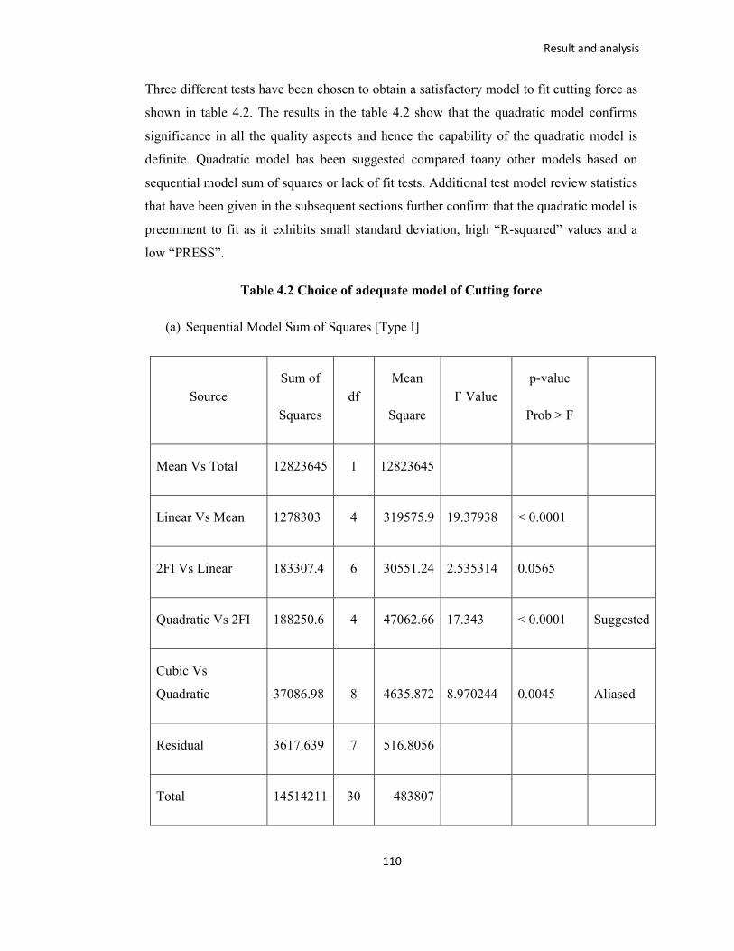
Result and analysis
110
Three different tests have been chosen to obtain a satisfactory model to fit cutting force as
shown in table 4.2. The results in the table 4.2 show that the quadratic model confirms
significance in all the quality aspects and hence the capability of the quadratic model is
definite. Quadratic model has been suggested compared toany other models based on
sequential model sum of squares or lack of fit tests. Additional test model review statistics
that have been given in the subsequent sections further confirm that the quadratic model is
preeminent to fit as it exhibits small standard deviation, high “R-squared” values and a
low “PRESS”.
Table 4.2 Choice of adequate model of Cutting force
(a) Sequential Model Sum of Squares [Type I]
Source Sum of
Squares
df Mean
Square
F Value p-value
Prob > F
Mean Vs Total 12823645 1 12823645
Linear Vs Mean 1278303 4 319575.9 19.37938 < 0.0001
2FI Vs Linear 183307.4 6 30551.24 2.535314 0.0565
Quadratic Vs 2FI 188250.6 4 47062.66 17.343 < 0.0001 Suggested
Cubic Vs
Quadratic 37086.98 8 4635.872 8.970244 0.0045 Aliased
Residual 3617.639 7 516.8056
Total 14514211 30 483807

Result and analysis
111
(b) Lack of Fit Tests
Source Sum of
Squares df
Mean
Square F Value
p-value
Prob > F
Linear 412261.7 20 20613.08 104025.1 < 0.0001
2FI 228954.3 14 16353.88 82530.74 < 0.0001
Quadratic 40703.62 10 4070.362 20541.31 < 0.0001 Suggested
Cubic 3616.648 2 1808.324 9125.808 < 0.0001 Aliased
Pure Error 0.990775 5 0.198155
(c) Model Summary Statistics
Source Std. Dev. R-Squared Adjusted
R-Squared
Predicted
R-Squared PRESS
Linear 128.4154 0.756139 0.717122 0.635539 616144.9
2FI 109.7738 0.864569 0.793289 0.708346 493059.7
Quadratic 52.09262 0.975922 0.95345 0.861316 234454.3 Suggested
Cubic 22.73336 0.99786 0.991135 0.691938 520798.8 Aliased

Result and analysis
112
4.2 Analysis of Variance and Statistical Models of Response Quality
The data are statistically analyzed using analysis of variance (ANOVA). The R2 values
have been checked using ANOVA, which describes the ratio of the variability, explained
by the model to the overall variability in the experiment observation data. It also has
sufficient accuracy, as measured by signal-to-noise ratios. A ratio more than 4 shows that
the model is fit. Significant terms for the specified response parameters are process
variables with a p-value < 0.05. The backward elimination method is used to adjust the
fitted quadratic models by removing insignificant terms, and the unimportant terms are
removed using the backward elimination procedure with α to exit = 0.05 in this study.
Only hierarchical models are invariant under linear transformations, thus the hierarchy of
various models is preserved while building mathematical models. The principle of
hierarchy states that even if the factor's contribution to the response parameter is
determined to be small and its higher-order terms such as interaction or quadratic terms
are significant, the primary effect will be included in the analysis as a term of
significance. The results and analysis for various responses from the application of the
ANOVA test are described in the following sections.
4.2.1 Analysis of variance and mathematical model for surface roughness
The full form of ANOVA is the Analysis of Variance. ANOVA is a statistical tool for
obtaining the contribution of variable parameters like cutting speed, feed, depth of cut and
width of cut towards cutting force and surface roughness[41]. The quadratic model for
surface roughness has been developed by a design expert. It shows ANOVA for the
quadratic model at a 95% confidence level. The Model F-value of 21.95 implies the model
is significant. There is only a 0.01% chance that a "Model F-value" this large could occur
due to noise. Values of "Prob > F" less than 0.0001 indicate model terms are significant.
In this case, A, B, C, AB, BC, A2, B2, D2 are significant model terms. Values greater than
0.1000 indicate the model terms are not significant. If there are many insignificant model
terms, model reduction may improve the model. The "Pred R-Squared" of 0.7323 has
been obtained in reasonable agreement. "Adeq Precision" measures the signal-to-noise
ratio. A ratio greater than 4 is desirable. A ratio of 16.860 indicates an adequate signal.
This model can be used to navigate the design space. ANOVA for response surface
quadratic model of surface roughness has been tabulated in table 4.3.

Result and analysis
113
TABLE 4.3 ANOVA for response surface quadratic model of surface roughness
Analysis of variance table [Partial sum of squares - Type III]
Source Sum of
Squares df
Mean
Square F Value
p-value
Prob > F
Model 0.932322 14 0.066594 21.95018 < 0.0001 Significant
A-A 0.082838 1 0.082838 27.30407 0.0001
B-B 0.329004 1 0.329004 108.4431 < 0.0001
C-C 0.196204 1 0.196204 64.67085 < 0.0001
D-D 0.006338 1 0.006338 2.088903 0.1689
AB 0.015006 1 0.015006 4.946209 0.0419
AC 0.004556 1 0.004556 1.501785 0.2393
AD 6.25E-06 1 6.25E-06 0.00206 0.9644
BC 0.020306 1 0.020306 6.693142 0.0206
BD 0.000156 1 0.000156 0.051502 0.8235
CD 0.000306 1 0.000306 0.100943 0.7551

Result and analysis
114
A^2 0.138836 1 0.138836 45.76173 < 0.0001
B^2 0.015336 1 0.015336 5.054902 0.0400
C^2 0.003407 1 0.003407 1.123126 0.3060
D^2 0.175086 1 0.175086 57.71009 < 0.0001
Residual 0.045508 15 0.003034
Lack of
Fit 0.045425 10 0.004543 272.55 < 0.0001 Significant
Pure
Error 8.33E-05 5 1.67E-05
Cor Total 0.97783 29
Std. Dev. 0.055081 R-Squared 0.95346
Mean 0.407 Adj R-Squared 0.910022
C.V. % 13.53335 Pred R-Squared 0.732297
PRESS 0.261768 Adeq Precision 16.8601

Result and analysis
115
Final equation in terms of coded factors:
Surface Roughness = + 0.26 - 0.12*A + 0.23*B + 0.18 *C + 0.033* D - 0.12*A*B +
0.068*A*C - 2.500E-003*A*D + 0.14*B*C + 0.012*B*D - 0.017*C *D + 0.28*A2 +
0.095*B2 + 0.045*C2+ 0.32*D2 ---------- (4.1)
Final equation in terms of actual factors:
Surface Roughness = 1.70308 - 0.013414*CS + 0.827E-04*FEED - 0.39088*DOC -
0.22872 *WOC – 0.435E-05*CS*FEED + 0.002000*CS*DOC – 0.833E-05*CS*WOC +
0.844E-03 *FEED*DOC + 0.833E-05*FEED*WOC – 0.00972*DOC*WOC + 0.506E-
045926*CS2 + 0.673E-06*FEED2 + 0.22016*DOC2 + 0.019974*WOC2 ---------- (4.2)
It depicts that equation (4.1) and (4.2) are adequate to represent the actual relationship
between process parameters and surface roughness. A normal probability plot is a
graphical tool for assessing set data approximately normally distributed. The data are
plotted against a theoretical normal distribution in such a way that the points should form
an approximate straight line. Departures from this straight line indicate departures from
normality. The coefficient R2 highlights the normal probability plot of residuals for
surface roughness. It evidently shows that errors are normally spread as mainly if the
residuals are clustered just about the straight, which is called determination coefficient,
shows less difference between the predicted and actual values.
Estimates of the location and scale parameters of the distribution are given by the
intercept and slope. As shown in figure 4.1, Probability plots can be generated for several
competing distributions to see which provides the best fit and generate the straightest
probability plot. The predicted value is the value of the variable predicted based on the
regression analysis. The difference between the actual value or observed value and the
predicted value is called the residual in regression analysis.

Result and analysis
116
Figure 4.1 Actual versus predicted value for surface roughness
4.2.2 Analysis of variance and mathematical model for cutting force
The quadratic model for the cutting force has been developed by design expert software as
discussed in section 4.1. Table 4.4 highlights ANOVA for the quadratic model at a 95%
confidence level. It shows that the model F-value is 43.427 and the subsequent p-value is
less than 0.0001 which indicates that the model is considerable. Quadratic model is fitted
because of p-value is only a 0.01%. Moreover, the lack of fit is significant. Therefore, the
quadratic model is considered at a 95% confidence level. The other important
determination coefficient R2 shows less difference between the predicted and actual
values. It has been shown that the value of adjusted R2
is in good value of 0.9534.

Result and analysis
117
TABLE 4.4 ANOVA for response surface quadratic model of cutting force
Analysis of variance table [Partial sum of squares - Type III]
Source
Sum of
Squares df Mean Square F Value
p-value
Prob > F
Model 1649861.517 14 117847.2512 43.42772425 < 0.0001 Significant
A-A 602509.9286 1 602509.9286 222.0300835 < 0.0001
B-B 148689.8017 1 148689.8017 54.79346897 < 0.0001
C-C 111413.5344 1 111413.5344 41.05684434 < 0.0001
D-D 415690.1852 1 415690.1852 153.1854035 < 0.0001
AB 39311.58771 1 39311.58771 14.48665771 0.0017
AC 154.4924702 1 154.4924702 0.056931802 0.8146
AD 71872.2481 1 71872.2481 26.48554072 0.0001
BC 67249.45563 1 67249.45563 24.78200199 0.0002
BD 671.3021903 1 671.3021903 0.247380623 0.6261
CD 4048.331502 1 4048.331502 1.491844929 0.2408
A^2 148257.4912 1 148257.4912 54.63415886 < 0.0001
B^2 1638.230019 1 1638.230019 0.603701832 0.4492
C^2 247.0491802 1 247.0491802 0.091039745 0.7670
D^2 51858.67064 1 51858.67064 19.11036553 0.0005
Residual 40704.61438 15 2713.640958
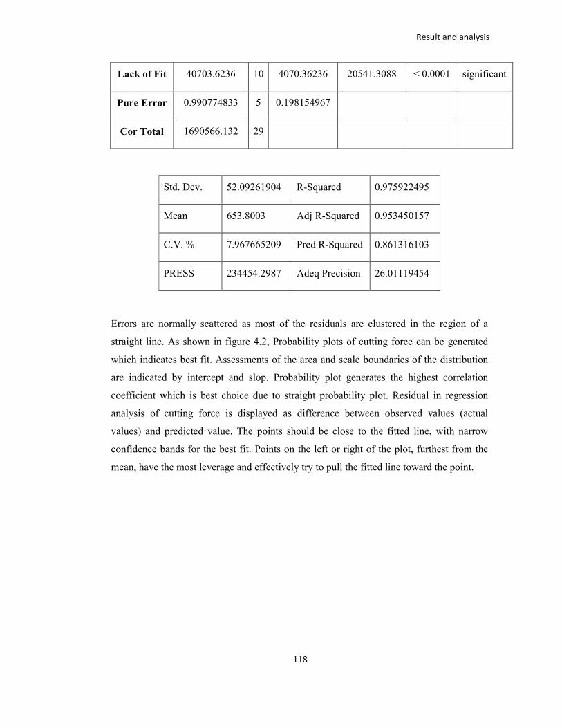
Result and analysis
118
Lack of Fit 40703.6236 10 4070.36236 20541.3088 < 0.0001 significant
Pure Error 0.990774833 5 0.198154967
Cor Total 1690566.132 29
Std. Dev. 52.09261904 R-Squared 0.975922495
Mean 653.8003 Adj R-Squared 0.953450157
C.V. % 7.967665209 Pred R-Squared 0.861316103
PRESS 234454.2987 Adeq Precision 26.01119454
Errors are normally scattered as most of the residuals are clustered in the region of a
straight line. As shown in figure 4.2, Probability plots of cutting force can be generated
which indicates best fit. Assessments of the area and scale boundaries of the distribution
are indicated by intercept and slop. Probability plot generates the highest correlation
coefficient which is best choice due to straight probability plot. Residual in regression
analysis of cutting force is displayed as difference between observed values (actual
values) and predicted value. The points should be close to the fitted line, with narrow
confidence bands for the best fit. Points on the left or right of the plot, furthest from the
mean, have the most leverage and effectively try to pull the fitted line toward the point.

Result and analysis
119
Figure 4.2 Actual versus predicted for cutting force
The effects of the input process variables on the cutting force have been determined by
using design expert software depending on the planned second order polynomial model.
The regression equation in the terms of the actual factor for the cutting force as a function
of four input process variables has been developed using experimental data and is given
underneath. The insignificant coefficients of several terms have been omitted from the
quadratic equation. It depicts that equation (4.3) and (4.4) are adequate to represent the
actual relationship between process parameters and cutting force.
Final Equation in Terms of Coded Factors:
Cutting force = + 556.42 - 316.89 *A + 157.42* B + 136.27 *C + 263.21* D - 198.27 *
A* B + 12.43 * A* C - 268.09*A*D + 259.33*B * C + 25.91*B*D + 63.63*C*D +
294.08*A2 + 30.91 * B2 -12.00*C2 + 173.93*D2 ---------------- (4.3)

Result and analysis
120
Final Equation in Terms of Actual Factors:
Cutting force = 1075.27 - 9.14*CS + 0.16*FEED - 543.21*DOC + 20.28*WOC -0.70E-
02*CS*FEED + 0.37*CS*DOC - 0.89*CS*WOC + 1.54*FEED*DOC +
0.017*FEED*WOC + 35.35*DOC*WOC + 0.052*CS2 + 0.22E-03*FEED2 -
59.28*DOC2 + 10.87*WOC2 -------------- (4.4)
4.3 Effect of input Parameters on Performance Measure
The effect of various input process variables on performance measures such as surface
roughness and cutting force has been presented in this section. Individually as well as the
interaction effects of various input process parameters have been discussed on the
considered responses. The effect of different parameters on different performance
measures is given in subsequent subsections.
4.3.1 Effect of process variables on surface roughness
After the machining process, surface roughness has been measured using Surftest SJ 410
and presented in table-3. Different graphs which indicate correlation between surface
roughness Vs input variables have been generated as shown in figure 4.3 a-d.
From figure 4.3 (a), it can be seen that an increase in cutting speed from 87.5 to 125
m/min leads to reduction in surface roughness. The surface roughness is reduced due to
reduction of the cutting force. From previous research works, surface roughness and
cutting force have a strong positive correlation. Surface roughness has been reduced with
increase in the cutting speed (from 125 to 162.5 m/min) because of thermal softening of
work material and related reduction in cutting force. In general the contact area between
the workpiece and cutting tool has been increased by increasing feed rate. As shown in
figure 4.3 (b), more feed rate has resulted in higher thrust force and vibration which has
produced poor surface finish. More heat is generated at the contact area between
workpiece and cutting tool due to higher thrust force by increasing depth of cut. It has
been presented by figure 4.3 (c) that by increase in depth of cut, surface roughness has
been reduced. It has been observed that by increasing the width of cut from 4 to 6 mm
surface roughness reduces but surface roughness increases with increase in width of cut

Result and analysis
121
from 6 to 8 mm. Lower surface roughness has been observed near 6 mm as shown in
figure 4.3 (d).
(a) Effect of cutting speed on surface roughness
(b) Effect of feed on surface roughness

Result and analysis
122
(c) Effect of depth of cut on surface roughness
(d) Effect of width of cut on surface roughness
Figure 4.3 (a-d) Response graph for effect of cutting speed, feed, depth of cut and
width of cut on surface roughness

Result and analysis
123
Based on table 4.3, two interactions have been found to be significant (cutting speed- feed
and feed - depth of cut) as shown in figures 4.4 and figure 4.5. From Figure 4.4 (a-b),
Cutting speed has been shown in X axis, feed has been shown in Y axis and surface
roughness has been generated in Z axis. Minimum of surface roughness has been obtained
by using this plot. Feed rate more than 612.5 mm/min and cutting speed less than 87.5
mm/min have been produced more surface roughness as per this plot. It has been shown in
red colour in 3D plot. The surface roughness is found to have a decreasing trend with the
cutting speed is set from 87.5 mm/min to 162.5 mm/min. Decreasing of feed rate is also
resulted in lower surface roughness. It has been shown in blue colour in 3D plot. With
lower feed rate, thrust force as well as vibration can be reduced resulting in higher surface
finish.
(a)

Result and analysis
124
(b)
Figure 4.4 (a-b) Combined effect of cutting speed and feed on surface roughness
It is observed from figure 4.5 (a-b) that feed has been shown on X-axis and depth of cut
has been shown in Y-axis. Surface roughness has been generated in Z- axis. Feed more
than 612.5 mm/min and depth of cut more than 0.8 mm have been resulted in higher
surface roughness. It has been indicated as red colour in 3D plot. Surface roughness can
be improved by decreasing feed less than 425 mm/min and depth of cut less than 0.5 mm.
By reducing in depth of cut, contact area is reduced between cutting tool and workpiece
resulting in lower vibration and higher surface finish.

Result and analysis
125
(a)
(b)
Figure 4.5 (a-b) Combined effect of feed and depth of cut on surface roughness

Result and analysis
126
4.3.2 Effect of process variables on cutting forces
Cutting forces is a very important response in the manufacturing process because it leads
to an efficient machining process through the proper selection of operating parameters,
machine tools, fixtures, and tools[42]. Furthermore, cutting force monitoring is frequently
used to detect tool wear and breakage. Three cutting forces (namely Fx, Fy and Fz) exist
during milling by engagement of the cutting teeth with the workpiece. From Table 3, the
axial force (Fz) has been used for further analysis due to significantly high magnitude
compared to other two cutting forces (normal force and feed force).
Figure 4.6(a-d) shows relationships between input parameters with cutting force
respectively. From the graphs, it has been observed that cutting force Fz increases with
increase in all the input machining parameters except cutting speed. From figure 4.8 (a), it
can be seen that an increase in cutting speed from 87.5 m/min to 162.5 m/min leads to
reduction in cutting force due to the thermal effect. Due to increase in temperature,
hardness of material is reduced and facilitates plastic deformation easily. Lower cutting
forces have been observed at higher cutting speed because more heat is generated in the
shear zone which is sufficient for easy plastic deformation and subsequent shearing of
workpiece material. From figure 4.6(b), it has been observed that the cutting force is
increased with increase in feed rate. The reason behind that is more material per tooth per
revolution is removed by increasing the feed rate. As a consequence, more energy is
required, which causes an increase in cutting forces. Also by increasing the value of feed
rate, more resistance is exhibited against cutting tools and resulted in increased friction
between workpiece and tool which leads to increased cutting force. Figure 4.6 (c) shows
that cutting force increases with higher axial depth cut. Contact area is increased between
tool and workpiece by increasing axial depth of cut which has resulted in increased cutting
force. From figure 4.6 (d), it has been seen that the increase in radial depth of cut leads to
increase in contact area between tool and workpiece and cutting forces become larger. The
cutting force increases with increase in width of cut in similar way.

Result and analysis
127
(a) Effect of cutting speed on cutting force
(b) Effect of feed on cutting force

Result and analysis
128
(c) Effect of depth of cut on cutting force
(d) Effect of width of cut on cutting force
Figure 4.6 (a-d) Response graph for effect of cutting speed, feed, depth of cut and
width of cut on cutting force

Result and analysis
129
Based on table 4.4, two interactions have been found to be significant (cutting speed- feed
and depth of cut- width of cut) as shown in figures 4.7 and figure 4.8. From figure 4.7 (a-
b), the cutting force has been found to have a decreasing trend with increase in the cutting
speed as well as reduction in feed rate. With lower feed rate, thrust force can be reduced
resulting in lower cutting force.
(a)

Result and analysis
130
(b)
Figure 4.7(a-b) Combined effect of cutting speed and feed on cutting force
It is observed from figure 4.8 (a-b) that the cutting force can be reduced by decreasing the
depth of cut and width of cut. By reducing in depth of cut and width of cut, contact area is
reduced between cutting tool and workpiece resulting in lower vibration resulting in lower
cutting force.

Result and analysis
131
(a)
(b)
Figure 4.8(a-b) Combined effect of depth of cut and width of cut on cutting force

Result and analysis
132
4.4 Summary
In this chapter, results from experimental analysis have been discussed. The numbers of
experiment have been performed using the design of experiment recommended by
response surface methodology. Sequential model sum of squares, lack of fit test and
model summary statistics have been performed to evaluate for an adequate model for
cutting force and surface roughness. ANOVA is a statistical tool for obtaining the
contribution of variable input machining parameters like cutting speed, feed, depth of cut
and width of cut towards cutting force and surface roughness. The backward elimination
method is used to adjust the fitted quadratic models by removing insignificant terms and
the unimportant terms have been removed using the backward elimination procedure. The
regression equations in terms of the cutting force as well as surface roughness as a
function of four input process variables have been developed using experimental data. The
normal probability plots of residuals for cutting force and surface roughness have been
generated. The effects of various input process parameters (individually as well as the
interaction effects) on output responses such as surface roughness and cutting force have
been discussed in this chapter.

Conclusion and future scope
133
CHAPTER-5
Optimisation using response surface methodology and
Genetic Algorithm
Optimisation, as we all know, is the process of finding the best solution for a given
problem in order to achieve a specific goal by making modifications to the initial solution
and utilizing the information gathered to arrive at the optimal solution. “Doing the most
with the least” is one of the most basic definitions of optimisation. The goal of
optimisation is to come up with the "optimal" design possible based on a set of prioritized
criteria or constraints. These include improve surface quality, higher productivity, low
tool wear, power consumption etc.
5.1 Optimisation using response surface methodology
Response surface methodology (RSM) is a powerful tool for optimising process
parameters in different manufacturing processes such as casting, welding and advanced
material machinability investigations. The process parameters are optimized using the
desirability approach of response surface methodology and validated by confirmation
tests.
Response surface methodology to design optimisation is aimed at reducing the values of
output responses. In this research work, response surface methodology has been used to
optimize output responses such as cutting force and surface roughness during end milling
of AISI D2 tool steel.
5.1.1 Optimisation of machining parameters for surface roughness using RSM
The constraints (ranges of various input process parameters) for the optimisation of
individual output responses such as surface roughness and cutting force have been given
in figure 5.1. Individually, goals and limitations have been identified for each output
parameter in order to determine their influence on individual desire. Each output feature
that has to be optimized has a maximum or minimum level. Lower limits and upper limits

Conclusion and future scope
134
of various input parameters such as cutting speed, feed, depth of cut and width of cut have
been selected as shown in Table 5.1. Output responses have also been selected as surface
roughness.
Table 5.1 Selections of Parameters for RSM
Parameters Lower limit Upper limit
Cutting speed (m/min) 50 200
Feed (mm/min) 50 800
Depth of cut (mm) 0.1 1
Width of cut (mm) 2 10
Output Responses Surface roughness, Cutting force
The purpose of optimisation is to identify the optimum combination of parameters that
will allow achieving all objectives.
Figure 5.1 Ranges of various input process parameters
Using a statistical software design experts, a set of optimal solutions for the specific
design space restrictions for output response characteristics such as surface roughness has
been generated. The best condition for the necessary response is chosen from a selection
of settings with the minimum surface roughness value. Table 5.2 provides the best set of

Conclusion and future scope
135
conditions with the highest desirability function for achieving the desired output response
quality under strict limitations.
Table 5.2 Set of optimal solutions for surface roughness
CS (m/min) Feed (mm/min) DOC (mm) WOC (mm) S.R. (µm)
142.44 253.66 0.28 5.41 0.11
142.95 253.00 0.257 5.594 0.13
141.66 254.24 0.206 5.899 0.12
143.50 253.85 0.243 5.157 0.12
143.00 252.38 0.223 5.748 0.14
The optimum machining conditions for minimum surface roughness value can be found
with specific machining parameters as shown in figure 5.2 (a-b).
(a)

Conclusion and future scope
136
(b)
Figure 5.2 (a-b) Contour graphs for surface roughness showing effect of input
parameters
Cutting speed less than 87.5 m/min and higher feed more than 612.5 mm/min have
produced higher surface roughness. It has been shown in red colour in figure 5.2 (a).
Moderate cutting speed more than 87.5 m/min and less than 162.5 m/min with feed less
than 425 mm/min have produced lower surface roughness. It has been shown in blue
colour in figure 5.2 a. Feed lower than 612.5 mm/min and depth of cut less than 0.78 mm
have produced good surface finish. It has been shown as blue colour in figure 5.2 (b).
Response surface methodology has been implemented for optimisation using design
expert software. Number of ranges of input parameters has been selected for input
parameters as per table 5.1. Minimization of surface roughness has been decided as an
output response. Minimum surface roughness has been obtained by the predicted values of
various input parameters: 142.44 m/min cutting speed, 253.66 mm/min feed, 0.28 mm
depth of cut and 5.41 mm width of cut using response surface methodology as shown in

Conclusion and future scope
137
table 5.3. The optimum response value of surface roughness Ra has been obtained 0.116
µm using RSM.
Table 5.3 Optimisation value of surface roughness using response surface methodology
CS (m/min) FEED (mm/min) DOC (mm) WOC (mm) S.R. (µm)
After RSM 142.44 253.66 0.28 5.41 0.11
Table 5.4 shows the point prediction of surface roughness at the optimum setting of input
process parameters. The 95% confidence interval is the scope in which one can guess the
process average to fall 95% of the time. The prediction interval will be outsized than the
confidence interval as one can be expecting more disperse in individual values than in
averages. Confirmation experiments have been performed at predicted optimal levels and
the results have been found to be within 95% confidence interval.
Table 5.4 Point prediction of surface roughness
Response Prediction 95% CI
low
95% CI
high
Actual value (Mean of
three confirmation
experiments)
Surface
roughness 0.116875 0.094 0.154 0.12
5.1.2 Optimisation of machining parameters for cutting force using RSM
Response surface methodology has been used as an optimisation tool in this research
work. Optimized milling input parameters have been found out to minimize cutting force.
Numbers of optimal solutions for specific design space have been generated using design
expert software for minimum cutting force. From the selection of settings with minimum
cutting force, the best condition for the necessary response has been chosen. The best set
of conditions with the minimum cutting force under necessary constrain is shown in table
5.5.

Conclusion and future scope
138
Table 5.5 Set of optimal solutions for cutting force
CS (m/min) Feed (mm/min) DOC (mm) WOC (mm) C.F. (N)
101.24 100.65 0.92 2.50 259.17
100.88 100.00 0.85 2.91 265.01
101.00 99.54 0.99 2.04 271.66
102.21 101.25 1.03 3.24 261.58
103.08 101.09 0.90 3.85 270.90
It is concluded from contour plots that the minimum value of cutting force can be
achieved by opting for different input cutting parameters like cutting speed, feed, depth of
cut and width of cut as shown in figure 5.3 (a-f).
As shown in figure 5.3 (a), more cutting force has been generated with cutting speed less
than 87.5 m/min and feed more than 612.5 mm/min. It has been seen as red colour in
figure 5.3 (a). Medium range of cutting speed (87.5 m/min to 162.5 m/min) and feed less
than 237.5 mm/min have been resulted in lower cutting force. It has been seen as blue
colour in figure 5.3 (a).
Cutting speed less than 162.5m m/min and depth of cut more than 0.78 mm have
produced lower cutting force as shown in figure 5.3 (b). Lower cutting speed and higher
width of cut have been resulted in higher cutting force. Cutting speed (87.5 m/min to
162.5 m/min) with lower width of cut (less than 6 mm) have generated low cutting force
as shown in figure 5.3 (c).

Conclusion and future scope
139
(a)
(b)

Conclusion and future scope
140
(c)
(d)

Conclusion and future scope
141
(e)
(f)
Figure 5.3 (a-f) Contour graphs for cutting force showing effect of input parameters

Conclusion and future scope
142
From figure 5.3 (d), lower feed rate with various values of depth of cut have generated
lower cutting force. Depth of cut has not been much affected on cutting force. Higher feed
greater than 612.5 mm/min with higher width of cut more than 8 mm have produced
higher cutting force as shown as red colour in figure 5.3 (e). Low feed less than 237.5
mm/min with low width of cut less than 6 mm have produced lower cutting force. Lower
cutting force has been generated with higher depth of cut and lower width of cut as shown
in figure 5.3 (f).
As the contour plot shows, an optimum value of 259.17 N can be achieved by setting
cutting speed to 101.24 m/min, feed rate to 100.65 mm/min, depth of cut to 0.92 mm and
width of cut to 2.49 mm. The optimisation value of surface roughness using response
surface methodology has been tabulated in table 5.6.
Table 5.6 Optimisation value of surface roughness using response surface methodology
CS
(m/min)
FEED
(mm/min)
DOC
(mm)
WOC
(mm)
C.F.
(N)
After RSM 101.24 100.65 0.92 2.5 259.17
5.2 Optimisation using Genetic Algorithm
There are various components of genetic algorithm for optimisation. These include
crossover, mutation, selection, etc.
5.2.1 Basic steps of Genetic Algorithm
The basic steps involved in the genetic algorithm are described below:
1. Choose a coding for given problem
2. Evaluate each string in the population
3. If termination criteria is satisfied, process is terminated
4. Perform reproduction/selection of the population
5. Perform crossover on pair of strings
6. Perform mutation on strings
7. Evaluate strings in the new population then go to no. 3

Conclusion and future scope
143
Genetic algorithms (GAs) were invented by John Holland in the 1960s and were
developed by Holland and his students and colleagues at the University of Michigan in the
1960s and the 1970s.
Genetic Algorithm (GA) is a computerized search and optimisation algorithm based on
the mechanics of natural genetics and natural selection. According to the concept of
survival of the fittest, the fittest individuals of any population have the highest probability
to reproduce and survive to the next generation, thus improving successive generations.
Figure 5.4 An architecture of parameters optimisation using genetic algorithm
The data processed by GA includes a set of strings or chromosomes with an infinite length
in which each bit is called a gene. The architecture of parameter optimisation using the
Genetic Algorithm has been shown in figure 5.4. A selected number of strings are called
population and the population at a given time is known as a generation. Generations of the
initial population of strings are randomly based since the binary alphabet offers the
maximum number of schemata per bit of information of any coding. A binary encoding
scheme is traditionally used to represent the chromosomes using either zeros or ones.
Thereafter, the fitness value of each member is computed. The population is then operated
by the three main operators namely, reproduction, crossover and mutation to create a new

Conclusion and future scope
144
population. The new population is further evaluated and tested for determination. The
current population is checked for acceptability or solution. The iteration is stopped after
the completion of a maximum number of generations or on the attainment of the best
results.
The genetic algorithm (GA) is a population-based search optimisation technique. In
general, the fittest individuals of any population tend to reproduce and survive to the next
generation, thus improving successive generations. However, inferior individuals can, by
chance, survive and also reproduce. Genetic algorithms have been shown to solve linear
and nonlinear problems by exploring all regions of the state space and exponentially
exploiting promising areas through mutation, crossover and selection operations applied
to individuals in the population. The use of a genetic algorithm requires the determination
of six fundamental issues, chromosome representation, selection function, the genetic
operators making up the reproduction function, the creation of the initial population,
termination criteria and the evaluation function.
5.2.2 Implementation of GA
The minimum surface roughness and cutting force within the ranges of input process
parameters have been determined using a global optimisation method: genetic algorithm
(GA).
The optimisation problem of surface roughness and cutting force for end milling of AISI
D2 tool steel can be defined as below in the standard mathematical format;
Find: surface roughness and cutting force
To minimize: surface roughness and cutting force within parameter ranges:
50 m/min ≤ CS ≤ 200 m/min
50 mm/min ≤ feed ≤ 800 mm/min
0.1 mm ≤ DoC ≤ 1 mm
2 mm ≤ WoC ≤ 10 mm
The objective is to minimize surface roughness and cutting force in this study. The
developed mathematical model of surface roughness and cutting force (from chapter 4)
can be utilized to obtain the optimum combination of machining parameters such as
cutting speed (CS), feed (f), depth of cut (DOC) and width of cut (WOC) to obtain desired
responses.

Conclusion and future scope
145
The objective is to minimize the following functions such as:
Minimize, Surface Roughness, SR = + 0.26 - 0.12*A + 0.23*B + 0.18 *C + 0.033* D -
0.12*A*B + 0.068*A*C - 2.500E-003*A*D + 0.14*B*C + 0.012*B*D - 0.017*C *D +
0.28*A2 + 0.095*B2 + 0.045*C2+ 0.32*D2 --------- (4.1)
Minimize, Cutting force, CF = + 556.42 - 316.89 *A + 157.42* B + 136.27 *C + 263.21*
D - 198.27 * A* B + 12.43 * A* C - 268.09*A*D + 259.33*B * C + 25.91*B*D +
63.63*C*D + 294.08*A2 + 30.91 * B2 -12.00*C2 + 173.93*D2 ---------- (4.3)
5.2.3 Coding
In order to use a genetic algorithm to solve the above problem, input machining
parameters have been first coded in some string structures. Binary-coded strings having
1’s and 0’s are primarily used. The length of the string is usually determined according to
the desired solution accuracy. In this study, 8 bits have been chosen for the input
machining parameters. The strings (00000000) and (11111111) would represent the lower
and upper limits of the input process variables and thereby making a total string length of
32.
5.2.4 Fitness function
The genetic algorithm mimics the “survival of the fittest” principle. So naturally, they are
suitable to solve maximization problems. Maximization problems are usually transformed
to minimization problems by some suitable transformation. A fitness function, F(x) is
derived from the given objective function, f(x), and is used in successive genetic
operations. For maximization problems, the fitness function can be considered the same as
the objective function. The minimization problem is an equivalent maximization problem
such that the optimum point remains unchanged. A number of such transformations are
possible.
/(�) � 11 − �(�)
The transformation does not alter the location of the minimum but converts a
minimization problem to an equivalent maximization problem. The fitness function value

Conclusion and future scope
146
of the string is known as the string’s fitness. The operation of genetic algorithms begins
with a population of random strings representing design or decision variables. Thereafter,
each string is then operated by three main operators; reproduction, crossover and mutation
- to create a new population of points. The new population is further evaluated and tested
for termination. If the termination criterion is not met, the population is iteratively
operated by the above three operators and evaluated. This procedure is continued until the
termination criterion is met. One cycle of this generation and the subsequent evaluation
procedure is known as a generation in Genetic Algorithms.
5.2.5 Genetic operators
Reproduction
The first operation on a population is reproduction. Individual strings are copied into a
separate string called the 'mating pool' according to their fitness values, i.e., strings with a
higher value have a greater chance of contributing one or more children in the following
generation. The selection operator is another name for reproduction operator. In
algorithmic form, a reproduction operator can be implemented in a variety of ways. The
simplest method is to build a biased roulette wheel with a roulette wheel slot size
proportional to the fitness of each current string in the population.
As a result, more highly adapted strings have more offspring in the following generation.
An additional duplicate of the string is created once the string has been chosen for
replication. The string is subsequently placed into the mating pool, resulting in the
creation of a preliminary new population for additional genetic operator activity. In
reproduction, excellent strings in a population are given a large number of copies
probabilistically and a mating pool is established, ensuring that no new strings are
generated during the reproduction phase.
Crossover
The population is enriched with excellent strings from the previous generation after
reproduction, but there are no new strings. The population is subjected to a crossover
operator in the hopes of producing superior strings. The crossover probability, which is
the ratio of total strings selected for mating to population size, determines the total
number of participatory threads in the crossover. The crossover operator is primarily

Conclusion and future scope
147
responsible for the search features of the genetic algorithm. In most crossover operators,
two strings are chosen at random from the mating pool and parts of the strings are
swapped between them.
After reproduction, the population is enriched with good strings from the previous
generation but does not have any new strings. A crossover operator is applied to the
population to hopefully create better strings. The total number of participative strings in
the crossover is controlled by the crossover probability, which is the ratio of total strings
selected for mating and the population size. The crossover operator is mainly responsible
for the search aspects of the genetic algorithm. In most crossover operators, two strings
are picked from the mating pool at random and some portions of the strings are exchanged
between the strings.
In the crossover, a number between 1 and 8 is produced at random. If the random number
is 5, the bits in the fifth place are swapped, as seen in the example below.
String 1 - 11001101
String 2 - 01110100
Crossover probability = 0.9
New string (offspring 1) - 11000101
New string (offspring 2) – 01111100
The parent strings are the two strings that participate in the crossover process, and the
children strings are the strings that result.
Mutation
The occasional random modification of the value of a string position, like in the case of a
basic genetic algorithm, is known as mutation. This entails bit-by-bit shifting of 0 to 1 or
vice versa with a small mutation frequency of 0 to 0.1. The necessity for mutation is to
keep the population diverse.
Example:
String 1 - 11000111
String 2 - 01011100
Mutation probability – 0.1
New string (offspring 1) - 01000111
New string (offspring 2) - 01011100

Conclusion and future scope
148
A new population is formed once the genetic algorithm operators are applied. Then
decoded and the values of the objective functions are computed. One generation of the
genetic algorithm is now complete. These repetitions are repeated until the termination
condition is met. Matlab is used to simulate the aforementioned process with a population
size of 20, 500 generations of iteration and crossover and mutation probabilities of 0.8 and
0.1 respectively.
In this work, specific parameters for genetic algorithm have been specified and specific
parameters for GA have been set as shown in Table 5.7.
Table 5.7 Specific parameter for genetic algorithm
Parameter Values
Fitness parameters Cutting Force, Surface Roughness
Population size 20
Generation 500
Selection operator Rank order
Crossover operator Single point
Crossover probability 0.8
Mutation probability 0.1
The objective functions have been evaluated for the minimization of cutting forces and
surface roughness value in end milling of AISI D2 tool steel. After obtaining
mathematical formulation, these models have been transformed into a MATLAB function.
These functions have been given as input into the GA Toolbox of MATLAB as the
objective functions. The fitness graph for surface roughness has been shown in figure 5.5.
Output of genetic algorithm for minimization of surface roughness has been tabulated in
table 5.8. Step of generation has been considered as 25 and values of surface roughness
have been generated with help of genetic algorithm.

Conclusion and future scope
149
Table 5.8 Output of Genetic Algorithm for minimization of surface roughness
Generation Surface roughness Generation Surface roughness
0 0.1050 275 0.1035
25 0.1050 300 0.1034
50 0.1045 325 0.1034
75 0.1045 350 0.1034
100 0.1040 375 0.1032
125 0.1040 400 0.1032
150 0.1040 425 0.1032
175 0.1038 450 0.1032
200 0.1038 475 0.1032
225 0.1035 500 0.1032
250 0.1035
The minimum surface roughness value which has been achieved is 0.103 µm by setting
the cutting parameters with cutting speed 145 m/min, feed 269 mm/min, doc 0.1 mm and
width of cut 5.724 mm using Genetic Algorithm as shown in Table 5.9. The minimum
surface roughness value which has been achieved is 0.103µmby the Genetic Algorithm as
shown in the fitness value graph in figure 5.5.
Table 5.9 Optimisation value for surface roughness by Genetic algorithm
CS (m/min) FEED (mm/min) DOC (mm) WOC (mm) S.R. (µm)
After GA 145 269 0.1 5.724 0.103

Conclusion and future scope
150
Figure 5.5 Fitness value Vs generation graph for optimisation of surface roughness
Step of generation has been taken 25 and values of cutting force have been obtained with
help of genetic algorithm. Output of genetic algorithm for minimization of cutting force
has been tabulated in table 5.10.
Table 5.10 Output of Genetic Algorithm for minimization of cutting force
Generation Cutting Force Generation Cutting Force
0 258.132 275 257.156
25 258.043 300 257.156
50 257.95 325 257.156
75 257.95 350 257.156
100 257.555 375 257.156

Conclusion and future scope
151
125 257.555 400 257.156
150 257.254 425 257.156
175 257.254 450 257.156
200 257.254 475 257.156
225 257.254 500 257.156
250 257.254
Figure 5.6 Fitness value Vs generation graph for optimisation of cutting force
The minimum cutting force value which has been achieved is 257.156 N by the Genetic
Algorithm as shown in the fitness value graph in figure 5.6. Related input parameters

Conclusion and future scope
152
cutting speed 102.580 m/min, feed 100.46 mm/min, doc 0.95 mm and width of cut 2.2
mm have been tabulated in Table 5.11.
Table 5.11 Optimisation value for cutting force by Genetic algorithm
CS (m/min) FEED (mm/min) DOC (mm) WOC (mm) C.F. (N)
After GA 102.580 100.46 0.95 2.2 257.156
5.2.6 Experimental Validation of Optimisation Results
The optimum values of milling parameters obtained from RSM and GA methods have
been tabulated during end milling of AISI D2 tool steel as shown in the Table. Using
these values of process parameters, experiments have been conducted to validate the
mathematical model for cutting force and surface roughness. Reading of confirmation
experiment with input milling process parameters have been tabulated as shown in Table
5.12 and Table 5.13.
Table 5.12 Validation of mathematical model of cutting force
CS
(m/min)
FEED
(mm/min)
DOC
(mm) WOC (mm) C.F. (N)
After RSM 101.24 100.65 0.92 2.5 259.17
After GA 102.580 100.46 0.95 2.2 257.156
Confirmation
experiment 102 100 1 2 268.487

Conclusion and future scope
153
Table 5.13 Validation of mathematical model of surface roughness
CS (m/min) FEED (mm/min) DOC (mm) WOC (mm) S.R. (µm)
After RSM 142.44 253.66 0.28 5.41 0.11
After GA 145 269 0.1 5.724 0.103
Confirmation
experiment 145 268 0.1 6 0.12
5.3 Summary
In this chapter, outputs of optimisation methods have been discussed. Lower limits and
upper limits of various input parameters such as cutting speed, feed, depth of cut and
width of cut have been selected for optimisation. Response surface methodology has been
used for the optimisation of input machining parameters to minimize cutting force and
surface roughness during end milling of AISI D2 tool steel using AlCrN coated tool.
Numbers of optimal solutions have been generated using design expert software for
minimum cutting force as well as surface roughness. From the selection of settings with
minimum cutting force, the best condition for the necessary response has been chosen.
The mathematical models have been transformed into MATLAB functions which have
been chosen as input into the GA Toolbox of MATLAB as the objective functions. Thus
the fitness graphs for surface roughness and cutting force have been generated by using
GA. The optimized parameters and responses have been tabulated. A comparison of
optimisation by RSM and GA has been presented. Predicted optimum values of
machining parameters from RSM and GA methods have been validated with experimental
values.

Conclusion and future scope
154
Chapter-6
Conclusion & Future scope
The objectives of this research work have been focused on cutting force and surface
roughness during end milling of AISI D2 tool steel. The effects of cutting speed, feed,
depth of cut and width of cut have been investigated on output responses. The following
points have been concluded from the experimental study.
6.1 Conclusions
The pilot study has been conducted to decide the range of process parameters such as;
cutting speed from 50 to 200 m/min, feed from 50 to 800 mm/min, depth of cut from 0.1
to 1 mm and width of cut from 2 to 10 mm. These ranges have been carried out for further
investigation on end milling of AISI D2 tool steel.
Quadratic regression models have been developed from experimental data using RSM and
the models have been analyzed by ANOVA. The effects of cutting speed, feed, depth of
cut and width of cut have been observed on cutting force and surface roughness during
end milling of AISI D2 tool steel. Cutting speed and width of cut have been found two
significant machining parameters that affect the cutting force.To achieve a good surface
finish feed rate, axial depth of cut and cutting speed have been identified as dominant
parameters respectively. The width of cut has not been shown much effect on the surface
finish.
The design of experiment has been developed using Response Surface Methodology. The
quadratic model has been fitted for cutting force and surface roughness. Quadratic
regression equations have been generated. By using these quadratic equations, values for
responses have been predicted and tabulated. The predicted value of R2
as 0.8613 is in
good agreement with the value of adjusted R2
as 0.9759 for surface roughness and the
predicted value of R2
as 0.7323 is in good agreement with the value of adjusted R2
as
0.9534 for cutting force.

Conclusion and future scope
155
The main effect plots of input machining parameters on cutting force and surface
roughness have been presented and described. Surface roughness has been reduced with
an increase in the cutting speed, reduction in feed rate, lower depth of cut and medium
range of the width of cut. Whereas Cutting force can be reduced by increasing cutting
speed, lower feed rate, depth of cut and width of cut. The 3D surface plots for various
combinations of machining parameters on responses have also been plotted and discussed.
The developed models have been used as objective functions for the optimisation of input
parameters. Response surface methodology has been used to optimisation of machining
parameters for surface roughness and cutting force. Minimum surface roughness has been
obtained by the predicted values of parameters: 142.44 m/min cutting speed, 253.66
mm/min feed, 0.28 mm depth of cut and 5.41 mm width of cut using response surface
methodology. An optimum value of cutting force 259.17 N can be achieved by setting
cutting speed to 101.24 m/min, feed rate to 100.65 mm/min, depth of cut to 0.92 mm and
width of cut to 2.49 mm using RSM.
Genetic Algorithm (GA) is a computerized search and optimisation algorithm based on
the mechanics of natural genetics and natural selection. According to the concept of
survival of the fittest, the fittest individuals of any population have the highest probability
to reproduce and survive to the next generation, thus improving successive generations.
After applying of Genetic Algorithm, the predicted value of surface roughness has been
found 0.103 µm with cutting speed 145 m/min, feed 269 mm/min, depth of cut 0.1 mm
and width of cut 5.724 mm using Matlab software, whereas the predicted optimized value
of cutting force has been found 257.156 N with cutting speed 102.580 m/min, feed 100.46
mm/min, depth of cut 0.95 mm and width of cut 2.2 mm.
The optimum values of milling parameters from RSM and GA methods have been
obtained during the end milling of AISI D2 tool steel using AlCrN coated tool.
Experiments have been conducted to validate the optimized value of the machining
process. Following confirmation readings from experiments have been obtained.
Predicted values of surface roughness have been validated by experimentally 0.12 µm
with 145 m/min cutting speed, 268 mm/min feed, 0.1 mm depth of cut and 6 mm width of
cut. Cutting force has been noted 268.487 N during the end milling process with 102
m/min cutting speed, 100 mm/min feed, 1 mm depth of cut and 2 mm width of cut.
Conclusion and future scope
156
6.2 Future Scope
The results from this research work can be used directly for the effective and economical
end milling process of tool steel material in industrial applications. The investigation can
be developed in the following directions.
� The issues such as residual stress after machining may be investigated.
� Many advanced and new materials are being invented; various responses can be
analyzed during the machining process to investigate the effect of various
significant machining parameters.
� The other input and output parameters could be considered for further analysis
during machining of AIS D2 tool steel
� At present, many advanced coated tools are being invented; experimental
investigation can be done by using various advanced coated tools
� The weightage to be assigned to input machining parameters should be based upon
requirements of industries
� Various output responses such as tool wear, tool life, MRR, temperature, etc. can
be considered during the machining process
� Prediction of output responses using various optimisation techniques can be
carried out
� Multi-objective optimisation can be done by considering various responses

References
157
REFERENCES
[1] S. Seetharaman, Fundamentals of mettalurgy. Woodhead Publishing Limited, 2005.
[2] A. Attaullah, “Heat Treatment and Toughness Behavior of Tool Steels (D2 and H13) for Cutting blades,” 1999.
[3] H. E. H. Helmi A Youssef, Machining technology. CRC Press, 2008.
[4] Rajender singh, Introduction to basic manufacturing processes and workshop technology. New age inernational publisher, 2006.
[5] R. F. Bunshah, Handbook of hard coatings. NOYES PUBLICATIONS, 2001.
[6] C. M. A. Raymond H Myers, Douglas C Montgomery, Response surface methodology. John Wiley & Sons, 2016.
[7] Mitchell Melanie, An Introduction to Genetic Algorithms. A Bradford Book The MIT Press, 1998.
[8] P. Koshy, R. C. Dewes, and D. K. Aspinwall, “High speed end milling of hardened AISI D2 tool steel (�58 HRC),” J. Mater. Process. Technol., vol. 127, no. 2, pp. 266–273, 2002, doi: 10.1016/S0924-0136(02)00155-3.
[9] B. M. Gopalsamy, B. Mondal, S. Ghosh, K. Arntz, and F. Klocke, “Investigations on hard machining of Impax Hi Hard tool steel,” Int. J. Mater. Form., vol. 2, no. 3, pp. 145–165, 2009, doi: 10.1007/s12289-009-0400-5.
[10] M. Chahal, V. Singh, and R. Garg, “Optimum surface roughness evaluation of dies steel H-11 with CNC milling using RSM with desirability function,” Int. J. Syst. Assur. Eng. Manag., vol. 8, no. 2, pp. 432–444, 2017, doi: 10.1007/s13198-016-0446-y.
[11] A. Iqbal, N. He, and L. Li, “Empirical modeling the effects of cutting parameters in high-speed end milling of hardened AISI D2 under MQL environment,” Proc. World Congr. Eng. 2011, WCE 2011, vol. 1, pp. 734–739, 2011.
[12] T. Ding, S. Zhang, Y. Wang, and X. Zhu, “Empirical models and optimal cutting parameters for cutting forces and surface roughness in hard milling of AISI H13 steel,” Int. J. Adv. Manuf. Technol., vol. 51, no. 1–4, pp. 45–55, 2010, doi: 10.1007/s00170-010-2598-2.
[13] J. A. Ghani, I. A. Choudhury, and H. H. Masjuki, “Wear mechanism of TiN coated carbide and uncoated cermets tools at high cutting speed applications,” J. Mater. Process. Technol., vol. 153–154, no. 1–3, pp. 1067–1073, 2004, doi: 10.1016/j.jmatprotec.2004.04.352.
[14] A. (Ayooq) Arain, “Heat Treatment and Toughness Behavior of Tool Steels (D2 and H13) for Cutting Blades,” 1999.

References
158
[15] M. S. bin Rahim, Mohd Aidil Shah Bin, Abdul , Minhat, Mohamad bin, Hussein, Nur Izan Syahriah Binti, Salleh, “A comprehensive review on cold work of AISI D2 tool steel,” Met. Res. Technol, vol. 104, no. 115, pp. 1–12, 2018.
[16] M. A. Lajis, A. N. M. Karim, A. K. M. N. Amin, A. M. K. Hafiz, and L. G. Turnad, “Prediction of tool life in end milling of hardened steel AISI D2,” Eur. J. Sci. Res., vol. 21, no. 4, pp. 592–602, 2008.
[17] J. L. Endrino, G. S. Fox-Rabinovich, and C. Gey, “Hard AlTiN, AlCrN PVD coatings for machining of austenitic stainless steel,” Surf. Coatings Technol., vol. 200, no. 24, pp. 6840–6845, 2006, doi: 10.1016/j.surfcoat.2005.10.030.
[18] Cincinnati Tool Steel, “AISI D2,” no. 815, 1850.
[19] S. K. Saha, L. Prasad, and V. Kumar, “Experimental Investigations on Heat Treatment of Cold Work Tool Steels: Part 1, Air-Hardening Grade (D2),” Int. J. Eng. Res. Appl. www.ijera.com, vol. 2, no. 2, pp. 510–519, 2012, [Online]. Available: www.ijera.com.
[20] S. Surberg, Cord Henrik and K. Paul, Lingenho, “The effect of some heat treatment parameters on the dimensional stability of AISI D2,” Cryogenics (Guildf)., vol. 48, pp. 42–47, 2008, doi: 10.1016/j.cryogenics.2007.10.002.
[21] J. B. Saedon, S. L. Soo, D. K. Aspinwall, A. Barnacle, and N. H. Saad, “Prediction and optimization of tool life in micromilling AISI D2 (�62 HRC) hardened steel,” Procedia Eng., vol. 41, no. Iris, pp. 1674–1683, 2012, doi: 10.1016/j.proeng.2012.07.367.
[22] A. R. R. Lincoln Cardoso Brandão, Reginaldo Teixeira Coelho, “Experimental and theoretical study of workpiece temperature when end milling hardened steels using (TiAl)N-coated and PcBN-tipped tools,” J. Mater. Process. Technol., vol. 199, no. 1, pp. 234–244, 2008, doi: 10.1016/j.jmatprotec.2007.07.049.
[23] B. Z. F. Takacs, Marton, “Hard Cutting of AISI D2 Steel,” 3rd Int. Conf. Mech. Eng. Mechatronics, no. 176, pp. 1–7, 2014.
[24] S. R. K. Vinayak Neelakanth Gaitonde, C. H. A. Maciel, J. C. C. Rubio, and A. M. Abrão, “Machinability Evaluation in Hard Milling of AISI D2 Steel,” Mater. Res., vol. 19, no. 2, pp. 360–369, 2015, doi: 10.1590/1980-5373-MR-2015-0263.
[25] A. Alrashdan, O. Bataineh, and M. Shbool, “Multi-criteria end milling parameters optimization of AISI D2 steel using genetic algorithm,” Int. J. Adv. Manuf. Technol., vol. 73, no. 5–8, pp. 1201–1212, 2014, doi: 10.1007/s00170-014-5921-5.
[26] L. Tang, J. Huang, and L. Xie, “Finite element modeling and simulation in dry hard orthogonal cutting AISI D2 tool steel with CBN cutting tool,” Int. J. Adv. Manuf. Technol., vol. 53, no. 9–12, pp. 1167–1181, 2011, doi: 10.1007/s00170-010-2901-2.
[27] M. C. Kang, K. H. Kim, S. H. Shin, S. H. Jang, J. H. Park, and C. Kim, “Effect of the minimum quantity lubrication in high-speed end-milling of AISI D2 cold-

References
159
worked die steel (62 HRC) by coated carbide tools,” Surf. Coatings Technol., vol. 202, no. 22–23, pp. 5621–5624, 2008, doi: 10.1016/j.surfcoat.2008.06.129.
[28] M. A. L. A K M Nurul Amin, Shuriani Binti, Marlina Binti, “Effects of workpiece preheating on surface roughness , chatter and tool performance during end milling of hardened steel D2,” J. Mater. Process. Technol., vol. 1, no. 201, pp. 466–470, 2008, doi: 10.1016/j.jmatprotec.2007.11.304.
[29] J. Luiz, S. Ribeiro, and A. M. Abrão, “Milling of Annealed and Hardened Tool Steel With Coated Carbide and Cermet Inserts,” 2007.
[30] Z. Qiang, S. Zhang, L. Zhuang, J. Zhang, and Y. Zhang, “Development of Tool Coating,” Int. J. Eng. Res. Technol., vol. 9, no. 09, pp. 959–962, 2020.
[31] L. Ning and S. C. Veldhuis, “Mechanistic modeling of ball end milling including tool wear,” J. Manuf. Process., vol. 8, no. 1, pp. 21–28, 2006, doi: 10.1016/S1526-6125(06)70098-6.
[32] M. Nordin, R. Sundström, T. I. Selinder, and S. Hogmark, “Wear and failure mechanisms of multilayered PVD TiN/TaN coated tools when milling austenitic stainless steel,” Surf. Coatings Technol., vol. 133–134, pp. 240–246, 2000, doi: 10.1016/S0257-8972(00)00933-6.
[33] B. Denkena, J. Köhler, and B. Bergmann, “Development of cutting edge geometries for hard milling operations,” CIRP J. Manuf. Sci. Technol., vol. 8, pp. 43–52, 2015, doi: 10.1016/j.cirpj.2014.10.002.
[34] Vitor F C and F. J. G. Silva, “Recent Advances on Coated Milling Tool Technology — A Comprehensive Review,” Coatings, vol. 10, no. 235, pp. 1–26, 2020.
[35] M. Arndt and T. Kacsich, “Performance of new AlTiN coatings in dry and high speed cutting,” Surf. Coatings Technol., vol. 163, no. 164, pp. 674–680, 2003, doi: 10.1016/S0257-8972(02)00694-1.
[36] B. M. Gopalsamy, B. Mondal, S. Ghosh, K. Arntz, and F. Klocke, “Experimental investigations while hard machining of DIEVAR tool steel (50 HRC),” Int. J. Adv. Manuf. Technol., vol. 51, no. 9–12, pp. 853–869, 2010, doi: 10.1007/s00170-010-2688-1.
[37] S. M. Bhatia, P. C. Pandey, and H. S. Shan, “The thermal condition of the tool cutting edge in intermittent cutting,” Wear, vol. 61, no. 1, pp. 21–30, 1980, doi: 10.1016/0043-1648(80)90108-8.
[38] G. S. Fox-Rabinovich et al., “Design and performance of AlTiN and TiAlCrN PVD coatings for machining of hard to cut materials,” Surf. Coatings Technol., vol. 204, no. 4, pp. 489–496, 2009, doi: 10.1016/j.surfcoat.2009.08.021.
[39] H. Çalişkan, C. Kurbanoǧlu, P. Panjan, M. Čekada, and D. Kramar, “Wear behavior and cutting performance of nanostructured hard coatings on cemented carbide cutting tools in hard milling,” Tribol. Int., vol. 62, pp. 215–222, 2013, doi:

References
160
10.1016/j.triboint.2013.02.035.
[40] H. Çalişkan, C. Kurbanoǧlu, P. Panjan, and D. Kramar, “Investigation of the performance of carbide cutting tools with hard coatings in hard milling based on the response surface methodology,” Int. J. Adv. Manuf. Technol., vol. 66, no. 5–8, pp. 883–893, 2013, doi: 10.1007/s00170-012-4374-y.
[41] H. Gökkaya and M. Nalbant, “The effects of cutting tool coatings on the surface roughness of AISI 1015 steel depending on cutting parameters,” Turkish J. Eng. Environ. Sci., vol. 30, no. 5, pp. 307–316, 2006, doi: 10.3906/sag-1209-76.
[42] S. Oomen-Hurst, M. D. A. M. Khanna, and S. C. Veldhuis, “Comparative wear behavior studies of coated inserts during milling of NiCrMoV steel,” Tribol. Int., vol. 53, pp. 115–123, 2012, doi: 10.1016/j.triboint.2012.02.020.
[43] G. Strnad and J. Buhagiar, “Latest developments in PVD coatings for tooling,” Sci. Bull. the" Petru Major" Univ. Targu Mures, vol. 7, pp. 32–37, 2010.
[44] R. PORAT and Y. CASSUTO, “a Comparison Between Cvd and Pvd Coated Cemented Carbide Cutting Tools,” Le J. Phys. Colloq., vol. 50, no. C5, pp. C5-803-C5-810, 1989, doi: 10.1051/jphyscol:1989597.
[45] M. N. Durakbasa, A. Akdogan, A. S. Vanli, and A. G. Bulutsuz, “Optimization of end milling parameters and determination of the effects of edge profile for high surface quality of AISI H13 steel by using precise and fast measurements,” Meas. J. Int. Meas. Confed., vol. 68, pp. 92–99, 2015, doi: 10.1016/j.measurement.2015.02.042.
[46] A. I. Kovalev et al., “Impact of Al and Cr alloying in TiN-based PVD coatings on cutting performance during machining of hard to cut materials,” Vacuum, vol. 84, no. 1, pp. 184–187, 2009, doi: 10.1016/j.vacuum.2009.06.019.
[47] S. Gaurav, “Comparative Performance Evaluation of Uncoated and Coated Carbide Inserts in Dry End Milling of Stainless Steel ( SS 316L ),” pp. 1–9, 2011.
[48] M. S. Kasim, C. H. Che Haron, J. A. Ghani, M. A. Sulaiman, and M. Z. A. Yazid, “Wear mechanism and notch wear location prediction model in ball nose end milling of Inconel 718,” Wear, vol. 302, no. 1–2, pp. 1171–1179, 2013, doi: 10.1016/j.wear.2012.12.040.
[49] W. Y. H. Liew, “Low-speed milling of stainless steel with TiAlN single-layer and TiAlN/AlCrN nano-multilayer coated carbide tools under different lubrication conditions,” Wear, vol. 269, no. 7–8, pp. 617–631, 2010, doi: 10.1016/j.wear.2010.06.012.
[50] N. L. Cadena, R. Cue-Sampedro, H. R. Siller, A. M. Arizmendi-Morquecho, C. I. Rivera-Solorio, and S. Di-Nardo, “Study of PVD AlCrN coating for reducing carbide cutting tool deterioration in the machining of titanium alloys,” Materials (Basel)., vol. 6, no. 6, pp. 2143–2154, 2013, doi: 10.3390/ma6062143.
[51] G. S. Fox-Rabinovich et al., “Effect of mechanical properties measured at room

References
161
and elevated temperatures on the wear resistance of cutting tools with TiAlN and AlCrN coatings,” Surf. Coatings Technol., vol. 200, no. 20–21, pp. 5738–5742, 2006, doi: 10.1016/j.surfcoat.2005.08.132.
[52] E. Le Bourhis, P. Goudeau, M. H. Staia, E. Carrasquero, and E. S. Puchi-Cabrera, “Mechanical properties of hard AlCrN-based coated substrates,” Surf. Coatings Technol., vol. 203, no. 19, pp. 2961–2968, 2009, doi: 10.1016/j.surfcoat.2009.03.017.
[53] W. Kalss, A. Reiter, V. Derflinger, C. Gey, and J. L. Endrino, “Modern coatings in high performance cutting applications,” Int. J. Refract. Met. Hard Mater., vol. 24, no. 5, pp. 399–404, 2006, doi: 10.1016/j.ijrmhm.2005.11.005.
[54] Y. J. Lin, A. Agrawal, and Y. Fang, “Wear progressions and tool life enhancement with AlCrN coated inserts in high-speed dry and wet steel lathing,” Wear, vol. 264, no. 3–4, pp. 226–234, 2008, doi: 10.1016/j.wear.2007.03.007.
[55] Z. Liang, P. Gao, X. Wang, S. Li, T. Zhou, and J. Xiang, “Cutting Performance of Different Coated Micro End Mills in Machining of Ti-6Al-4V,” Micromachines, vol. 9, no. 568, pp. 1–12, 2018, doi: 10.3390/mi9110568.
[56] V. Varghese, K. Akhil, M. R. Ramesh, and D. Chakradhar, “Investigation on the performance of AlCrN and AlTiN coated cemented carbide inserts during end milling of maraging steel under dry , wet and cryogenic environments,” J. Manuf. Process., vol. 43, no. April, pp. 136–144, 2019, doi: 10.1016/j.jmapro.2019.05.021.
[57] H. Oktem, T. Erzurumlu, and F. Erzincanli, “Prediction of minimum surface roughness in end milling mold parts using neural network and genetic algorithm,” Mater. Des., vol. 27, no. 9, pp. 735–744, 2006, doi: 10.1016/j.matdes.2005.01.010.
[58] H. Z. Li, H. Zeng, and X. Q. Chen, “An experimental study of tool wear and cutting force variation in the end milling of Inconel 718 with coated carbide inserts,” J. Mater. Process. Technol., vol. 180, no. 1–3, pp. 296–304, 2006, doi: 10.1016/j.jmatprotec.2006.07.009.
[59] J. M. Vieira, A. R. Machado, and E. O. Ezugwu, “Performance of cutting fluids during face milling of steels,” J. Mater. Process. Technol., vol. 116, no. 2–3, pp. 244–251, 2001, doi: 10.1016/S0924-0136(01)01010-X.
[60] G. Kant and K. S. Sangwan, “Predictive modelling for energy consumption in machining using artificial neural network,” Procedia CIRP, vol. 37, pp. 205–210, 2015, doi: 10.1016/j.procir.2015.08.081.
[61] K. L. D. Wins, A. S. Varadarajan, and B. Ramamoorthy, “Optimization of Surface Milling of Hardened AISI4340 Steel with Minimal Fluid Application Using a High Velocity Narrow Pulsing Jet of Cutting Fluid,” Engineering, vol. 02, no. 10, pp. 793–801, 2010, doi: 10.4236/eng.2010.210102.
[62] N. Camuşcu and E. Aslan, “A comparative study on cutting tool performance in end milling of AISI D3 tool steel,” J. Mater. Process. Technol., vol. 170, no. 1–2,

References
162
pp. 121–126, 2005, doi: 10.1016/j.jmatprotec.2005.04.111.
[63] J. Zhou, J. Ren, and C. Yao, “Multi-objective optimization of multi-axis ball-end milling Inconel 718 via grey relational analysis coupled with RBF neural network and PSO algorithm,” Meas. J. Int. Meas. Confed., vol. 102, pp. 271–285, 2017, doi: 10.1016/j.measurement.2017.01.057.
[64] M. Okada, A. Hosokawa, R. Tanaka, and T. Ueda, “Cutting performance of PVD-coated carbide and CBN tools in hardmilling,” Int. J. Mach. Tools Manuf., vol. 51, no. 2, pp. 127–132, 2011, doi: 10.1016/j.ijmachtools.2010.10.007.
[65] Y. H. Guu, “AFM surface imaging of AISI D2 tool steel machined by the EDM process,” vol. 242, pp. 245–250, 2005, doi: 10.1016/j.apsusc.2004.08.028.
[66] S. Bolsunovsky, V. Vermel, and G. Gubanov, “Cutting forces calculation and experimental measurement for 5-axis ball end milling,” Procedia CIRP, vol. 8, pp. 235–239, 2013, doi: 10.1016/j.procir.2013.06.095.
[67] Z. C. Wei, M. L. Guo, M. J. Wang, S. Q. Li, and S. X. Liu, “Prediction of cutting force in five-axis flat-end milling,” pp. 137–152, 2018.
[68] V. M. Sharma and R. Manu, “Empirical Modeling of Cutting Forces in Ball End Milling using Experimental Design,” IIT Guwahati, no. Aimtdr, pp. 1–6, 2014, [Online]. Available: http://www.iitg.ac.in/aimtdr2014/PROCEEDINGS/papers/464.pdf.
[69] W. H. Lai, “Modeling of cutting forces in end milling operations,” Tamkang J. Sci. Eng., vol. 3, no. 1, pp. 15–22, 2000, doi: 10.6180/jase.2000.3.1.02.
[70] J. H. Kim, D. K. Moon, D. W. Lee, J. S. Kim, M. C. Kang, and K. H. Kim, “Tool wear measuring technique on the machine using CCD and exclusive jig,” J. Mater. Process. Technol., vol. 130–131, pp. 668–674, 2002, doi: 10.1016/S0924-0136(02)00733-1.
[71] B. M. Gopalsamy, B. Mondal, and S. Ghosh, “Taguchi method and anova: An approach for process parameters optimization of hard machining while machining hardened steel,” J. Sci. Ind. Res. (India)., vol. 68, no. 8, pp. 686–695, 2009.
[72] Ş. Karabulut, H. Çinici, and H. Karakoç, “Experimental Investigation and Optimization of Cutting Force and Tool Wear in Milling Al7075 and Open-Cell SiC Foam Composite,” Arab. J. Sci. Eng., vol. 41, no. 5, pp. 1797–1812, 2016, doi: 10.1007/s13369-015-1991-4.
[73] S. Wojciechowski and P. Twardowski, “Tool life and process dynamics in high speed ball end milling of hardened steel,” Procedia CIRP, vol. 1, no. 1, pp. 289–294, 2012, doi: 10.1016/j.procir.2012.04.052.
[74] Z. Fu, W. Yang, X. Wang, and J. Leopold, “Analytical modelling of milling forces for helical end milling based on a predictive machining theory,” Procedia CIRP, vol. 31, pp. 258–263, 2015, doi: 10.1016/j.procir.2015.03.013.

References
163
[75] M. A. Elbestawi, L. Chen, C. E. Becze, and T. I. El-Wardany, “High-speed milling of dies and molds in their hardened state,” CIRP Ann. - Manuf. Technol., vol. 46, no. 1, pp. 57–62, 1997, doi: 10.1016/s0007-8506(07)60775-6.
[76] X. Fan and M. Loftus, “The influence of cutting force on surface machining quality,” Int. J. Prod. Res., vol. 45, no. 4, pp. 899–911, 2007, doi: 10.1080/00207540600632208.
[77] S. N. B. Ravi Patel, “Effect on Cutting Force during Hard Machining of AISI D2 Tool Steel Using AlCrN Coated Tool,” Intechopen, vol. 53, no. 9, pp. 1689–1699, 2018, doi: http://dx.doi.org/10.5772/intechopen.81083.
[78] Uddeholms, “HEAT TREATMENT OF TOOL STEEL,” pp. 1–20.
[79] W. U. Baohai, Y. A. N. Xue, L. U. O. Ming, and G. A. O. Ge, “Cutting Force Prediction for Circular End Milling Process,” CHINESE J. Aeronaut., vol. 26, pp. 1–7, 2013, doi: 10.1016/j.cja.2013.04.003.
[80] S. Bolsunovsky, V. Vermel, and G. Gubanov, “Cutting Forces Calculation and Experimental Measurement for 5-axis Ball End Milling,” Procedia CIRP, vol. 8, pp. 235–239, 2013, doi: 10.1016/j.procir.2013.06.095.
[81] W. A. N. Min, Z. Wei-hong, T. A. N. Gang, and Q. I. N. Guo-hua, “New Cutting Force Modeling Approach for Flat End Mill,” Chinese J. Aeronaut., vol. 20, pp. 282–288, 2007.
[82] R. S. Pawade and S. S. Joshi, “Multi-objective optimization of surface roughness and cutting forces in high-speed turning of Inconel 718 using Taguchi grey relational analysis (TGRA),” Int. J. Adv. Manuf. Technol., vol. 56, no. 1–4, pp. 47–62, 2011, doi: 10.1007/s00170-011-3183-z.
[83] M. S. Sukumar, P. Venkata Ramaiah, and A. Nagarjuna, “Optimization and prediction of parameters in face milling of Al-6061 using taguchi and ANN approach,” Procedia Eng., vol. 97, pp. 365–371, 2014, doi: 10.1016/j.proeng.2014.12.260.
[84] W. Li, Y. B. Guo, M. E. Barkey, and J. B. Jordon, “Effect tool wear during end milling on the surface integrity and fatigue life of inconel 718,” Procedia CIRP, vol. 14, pp. 546–551, 2014, doi: 10.1016/j.procir.2014.03.056.
[85] B. Singarvel, T. Selvaraj, and R. Jeyapaul, “Multi objective optimization in turning of EN25 steel using taguchi based utility concept coupled with principal component analysis,” Procedia Eng., vol. 97, pp. 158–165, 2014, doi: 10.1016/j.proeng.2014.12.237.
[86] T. V. Do and Q. C. Hsu, “Optimization of minimum quantity lubricant conditions and cutting parameters in hard milling of AISI H13 steel,” Appl. Sci., vol. 6, no. 3, 2016, doi: 10.3390/app6030083.
[87] B. S. Reddy, J. S. Kumar, and K. V. K. Reddy, “Optimization of surface roughness in CNC end milling using response surface methodology and genetic algorithm,”

References
164
Int. J. Eng. Sci. Technol., vol. 3, no. 8, pp. 102–109, 2011.
[88] B. Ozcelik, H. Oktem, and H. Kurtaran, “Optimum surface roughness in end milling Inconel 718 by coupling neural network model and genetic algorithm,” Int. J. Adv. Manuf. Technol., vol. 27, no. 3–4, pp. 234–241, 2005, doi: 10.1007/s00170-004-2175-7.
[89] P. Palanisamy, I. Rajendran, and S. Shanmugasundaram, “Optimization of machining parameters using genetic algorithm and experimental validation for end-milling operations,” Int. J. Adv. Manuf. Technol., vol. 32, no. 7–8, pp. 644–655, 2007, doi: 10.1007/s00170-005-0384-3.
[90] R. Sreenivasulu, “Optimization of Machining Parameters during End Milling of GFRP Composites by Desirability Function Analysis using Taguchi Technique,” AIMTDR 2014 ,IIT Guwahati, Assam, India, no. Dec 12th-14th, pp. 338 (1–6), 2014.
[91] M. Subramanian, M. Sakthivel, K. Sooryaprakash, and R. Sudhakaran, “Optimization of cutting parameters for cutting force in shoulder milling of Al7075-T6 using response surface methodology and genetic algorithm,” Procedia Eng., vol. 64, pp. 690–700, 2013, doi: 10.1016/j.proeng.2013.09.144.
[92] S. Rao and N. Venkaiah, “Parametric Optimization in Machining of Nimonic-263 Alloy using RSM and Particle Swarm Optimization,” Procedia Mater. Sci., vol. 10, no. Cnt 2014, pp. 70–79, 2015, doi: 10.1016/j.mspro.2015.06.027.
[93] C. J. Tzeng and R. Y. Chen, “Optimization of electric discharge machining process using the response surface methodology and genetic algorithm approach,” Int. J. Precis. Eng. Manuf., vol. 14, no. 5, pp. 709–717, 2013, doi: 10.1007/s12541-013-0095-x.
[94] P. S. Sivasakthivel and R. Sudhakaran, “Optimization of machining parameters on temperature rise in end milling of Al 6063 using response surface methodology and genetic algorithm,” Int. J. Adv. Manuf. Technol., vol. 67, no. 9–12, pp. 2313–2323, 2013, doi: 10.1007/s00170-012-4652-8.
[95] S. Raj and K. Kumar, “Optimization and Prediction of Material Removing Rate in Die Sinking Electro Discharge Machining of EN45 Steel Tool,” Mater. Today Proc., vol. 2, no. 4–5, pp. 2346–2352, 2015, doi: 10.1016/j.matpr.2015.07.296.
[96] A. J. Makadia and J. I. Nanavati, “Optimisation of machining parameters for turning operations based on response surface methodology,” Meas. J. Int. Meas. Confed., vol. 46, no. 4, pp. 1521–1529, 2013, doi: 10.1016/j.measurement.2012.11.026.
[97] S. Sharma, “Optimization of Machining Process Parameters for Surface Roughness of Al-Composites,” J. Inst. Eng. Ser. C, vol. 94, no. 4, pp. 327–333, 2013, doi: 10.1007/s40032-013-0086-9.
[98] A. Tamilarasan, K. Marimuthu, and A. Renugambal, “Investigations and

References
165
optimization for hard milling process parameters using hybrid method of RSM and NSGA-II,” Rev. Tec. la Fac. Ing. Univ. del Zulia, vol. 39, no. 1, pp. 41–54, 2016, doi: 10.21311/001.39.1.06.
[99] B. M. Gopalsamy, B. Mondal, and S. Ghosh, “Optimisation of machining parameters for hard machining: Grey relational theory approach and ANOVA,” Int. J. Adv. Manuf. Technol., vol. 45, no. 11–12, pp. 1068–1086, 2009, doi: 10.1007/s00170-009-2054-3.
[100] M. K. Gupta, P. K. Sood, and V. S. Sharma, “Machining Parameters Optimization of Titanium Alloy using Response Surface Methodology and Particle Swarm Optimization under Minimum-Quantity Lubrication Environment,” Mater. Manuf. Process., vol. 31, no. 13, pp. 1671–1682, 2016, doi: 10.1080/10426914.2015.1117632.
[101] M. A. Kribes, Nabil, Hessainia, Zahia and Yallese, “Optimisation of Machining Parameters in Hard Turning by Desirability Function Analysis Using Response Surface Methodology,” Des. Model. Mech. Syst. - II, vol. 789, pp. 73–81, 2015, doi: 10.1007/978-3-319-17527-0.
[102] K. Dass and S. R. Chauhan, “Optimization of Machining Parameters in Turning of Titanium ( Grade5 ) Alloy Using Response Surface Methodology Materials and Manufacturing Processes Optimization of Machining Parameters in Turning of Titanium ( Grade-5 ) Alloy Using Response Surface Meth,” Mater. Manuf. Process., vol. 27, no. 5, pp. 531–537, 2011, doi: 10.1080/10426914.2011.593236.
[103] M. R. S. Yazdi and A. Khorram, “Modeling and Optimization of Milling Process by using RSM and ANN Methods,” Int. J. Eng. Technol., vol. 2, no. 5, pp. 474–480, 2010.
[104] V. Sathyamoorthy, S. Deepan, S. P. S. Prasanth, and L. Prabhu, “Optimization of Machining Parameters for Surface Roughness in End Milling of Magnesium AM60 Alloy,” Indian J. Sci. Technol., vol. 10, no. August, 2017, doi: 10.17485/ijst/2017/v10i32/104651.
[105] D. Bhandari, “Optimization of Machining Parameters Using Genetic Algorithm,” 2003.
[106] R. J. Saffar, M. R. Razfar, a H. Salimi, and M. M. Khani, “Optimization of machining parameters to minimize tool deflection in the end milling operation using genetic algorithm,” World Appl. Sci. J., vol. 6, no. 1, pp. 64–69, 2009.
[107] V. Savas and C. Ozay, “The optimization of the surface roughness in the process of tangential turn-milling using genetic algorithm,” Int. J. Adv. Manuf. Technol., vol. 37, no. 3–4, pp. 335–340, 2008, doi: 10.1007/s00170-007-0984-1.
[108] Z. G. Wang, Y. S. Wong, and M. Rahman, “Optimisation of multi-pass milling using genetic algorithm and genetic simulated annealing,” Int. J. Adv. Manuf. Technol., vol. 24, no. 9–10, pp. 727–732, 2004, doi: 10.1007/s00170-003-1789-5.

References
166
[109] G. Kant and K. S. Sangwan, “Predictive modelling and optimization of machining parameters to minimize surface roughness using artificial neural network coupled with genetic algorithm,” Procedia CIRP, vol. 31, pp. 453–458, 2015, doi: 10.1016/j.procir.2015.03.043.
[110] N. S. Narayanan, N. Baskar, and M. Ganesan, “Multi Objective Optimization of machining parameters for Hard Turning OHNS/AISI H13 material, Using Genetic Algorithm,” Mater. Today Proc., vol. 5, no. 2, pp. 6897–6905, 2018, doi: 10.1016/j.matpr.2017.11.351.

References
167
List of publications
Sr
No.
Title of paper Name of journal
1 Optimisation of machining parameters on
cutting force during end milling of AISI D2
tool steel using Genetic Algorithm
Industrial Engineering Journal, Ivy Scientific
(UGC listed journal)
2 Experimental investigation during end
milling of AISI D2 tool steel using AlCrN
coated tool
Materials Today: Proceedings -
Elsevier
3 Optimization of Machining Parameters to
Minimize Surface Roughness During End
Milling of AISI D2 Tool Steel Using Genetic
Algorithm
Advances in Materials and
Manufacturing
Engineering, Lecture Notes in
Mechanical
Engineering (LNME)-Springer
4 Effect on cutting force during hard
machining of AISI D2 tool steel using
AlCrN coated tool
In tech open- proceeding of 4th
International Conference
ICIAME 2018
5 Effect on surface roughness and cutting force
during hard machining of AISI D2 tool steel
using AlCrN coated tool using OVAT
International Journal of
Research and Analytical
Reviews IJRAR
Copyright © 2022 FDOKUMEN