DEGREE PROJECT FOR MASTER OF SCIENCE IN ENGINEERING:COMPUTER SCIENCE AND ENGINEERING

Experimental Investigation ofContainer-based VirtualizationPlatforms For a Cassandra

Cluster

Jesper Hallborg | Patryk Sulewski

Blekinge Institute of Technology, Karlskrona, Sweden, 2017

Supervisor: Mikael Svahnberg, Department of Computer Science, BTH

Abstract

Context. Cloud computing is growing fast and has established itself as the next generationsoftware infrastructure. A major role in cloud computing is the virtualization of hardware toisolate systems from each other. This virtualization is often done with Virtual Machines thatemulate both hardware and software, which in turn makes the process isolation expensive. Newtechniques, known as Microservices or containers, has been developed to deal with the overhead.

The infrastructure is conjoint with storing, processing and serving vast and unstructureddata sets. The overall cloud system needs to have high performance while providing scalabilityand easy deployment. Microservices can be introduced for all kinds of applications in a cloudcomputing network, and be a better fit for certain products.Objectives. In this study we investigate how a small system consisting of a Cassandra clusterperform while encapsulated in LXC and Docker containers, compared to a non virtualizedstructure. A specific loader is built to stress the cluster to find the limits of the containers.Methods. We constructed an experiment on a three node Cassandra cluster. Test data is sentfrom the Cassandra-loader from another server in the network. The Cassandra processes are thendeployed in the different architectures and tested. During these tests the metrics CPU, disk I/O,network I/O are monitored on the four servers. The data from the metrics is used in statisticalanalysis to find significant deviations.Results. Three experiments are being conducted and monitored. The Cluster test pointed outthat isolated Docker container indicate major latency during disk reads. A local stress test furtherconfirmed those results. The step-wise test in turn, implied that disk read latencies happened dueto isolated Docker containers needs to read more data to handle these requests. All Microservicesprovide some overheads, but fall behind the most for read requests.Conclusions. The results in this study show that virtualization of Cassandra nodes in a clusterbring latency in comparison to a non virtualized solution for write operations. However, thoselatencies can be neglected if scalability in a system is the main focus. For read operationsall microservices had reduced performance and isolated Docker containers brought out thehighest overhead. This is due to the file system used in those containers, which makes disk I/Oslower compared to the other structures. If a Cassandra cluster is to be launched in a containerenvironment we recommend a Docker container with mounted disks to bypass Dockers filesystem or a LXC solution.

Keywords: Container Virtualization, Cassandra, Docker, LXC, Big data, Microservices, Linuxdistributions

i

Sammanfattning

Bakgrund. Molnprogramvara växer snabbt och har etablerat sig som nästa generations pro-gramvaruinfrastruktur. En viktig roll i molntjänster är virtualisering av hårdvara för att isolerasystem från varandra. Denna virtualisering görs ofta med virtuella maskiner som efterliknarbåde hårdvara och mjukvara, vilket i sin tur gör processisoleringen dyr. Nya tekniker, kända sommikrotjänster eller containers, har utvecklats för att hantera denna overhead.

Infrastrukturen är förenad med lagring, bearbetning och betjäning av stora och ostruktureradedataset. Det övergripandemolnsystemet behöver ha hög prestanda samtidigt som det ger skalbarhetoch en enkel implementering. Mikrotjänster kan introduceras för alla typer av applikationer i ettmolnnätverk och vara bättre anpassad för vissa produkter.Syfte. I den här rapport undersöker vi hur ett system som består av ett Cassandra-kluster beter sigi olika mikrotjänstmiljöer, jämfört med en icke virtualiserad miljö. En Cassandra-lastare byggdesav oss för att interagera med Cassandra-klustret och stressa systemet.Metod. Vi konstruerade ett experiment på ett tre (3) noders Cassandra-kluster. Testdata skickasfrån lastaren från en annan server i nätverket. Cassandra-processerna sätts sedan in i de olikaarkitekturerna och testas. Under dessa test övervakas CPU, disk I / O, nätverk I / O på detre noderna i klustret. Data från mätvärdena används i statistisk analys för att hitta betydandeavvikelser.Resultat. Tre experiment utfördes och övervakades. Testerna indikerar att isolerade en Docker-container ger latens under diskinläsning. Ett lokalt stresstest bekräftade vidare dessa resultat. DetStegvisa testet i sin tur innebar att diskläsningsfördröjningar hände på grund av att den isoleradeDocker-container-arkitekturen behöver läsa mer från disk för att kunna hantera förfrågningar.Alla miljöerna ger någon form av prestandafall, men sjunker som mest vid förfrågningar somkräver diskläsning.Slutsats. Resultaten i denna studie visar att Cassandra noder i containerar ger statistisk signifikanslatens i jämförelse med icke virtualiserade tekniker för skrivoperationer. Dessa latanser kanförsummas om skalbarhet i ett system är i huvudfokus. För läsningsoperationer minskadeprestandan for isolerade Docker-containers avsevärt. Detta beror på det filsystem som användsi containrarna, vilket gör diskens I / O långsammare jämfört med de andra strukturerna. Omett Cassandra-kluster ska användas i en virtualiserad miljö så rekommenderar vi att Dockercontainerar används med monterade diskar för att kringgå begränsningar i filsystemt eller enLXC lösning.

Nyckelord: Container Virtualization, Cassandra, Docker, LXC, Big data, Microservices, Linuxdistributions

iii

Preface

This thesis is submitted to the Department of Computer Science & Engineering at Blekinge Institute ofTechnology in partial fulfillment of the requirements for the degree of Master of Science in Engineering:Computer Science and Engineering. The thesis is equivalent to 20 weeks of full-time studies. We wouldlike to thank Martin from Qvantel Sweden AB for his expertise in Apache Cassandra and guidance for thisthesis work. We would also like to thank Mikael Svahnberg for his experience in software architecturesand guidance. Lastly we would like to thank Torböjrn Fridensköld, for providing us with an office and sixservers for this thesis. Finally we would like thank Emil Alégroth for feedback and guidance with the finalreport.

Contact Information:Authors:Jesper HallborgE-mail: jefh12@student.bth.sePatryk SulewskiE-mail: pasb12@student.bth.se

External advisor:Martin BardQvantel Sweden ABKarlskrona, Sweden

University advisor:Prof. Mikael SvahnbergDept. Computer Science & Engineering

Dept. Computer Science & Engineering Internet : www.bth.se/diddBlekinge Institute of Technology Phone : +46 455 38 50 00SE–371 79 Karlskrona, Sweden Fax : +46 455 38 50 57

v

Nomenclature

Notations

Symbol Description

MB megabyte

MB/s megabyte per second

kB/s kilobyte per second

Mb/s megabits per second

Acronyms

BM Bare Metal

IDC Isolated Docker Container

MDC Mounted Docker Container

LXC LinuX Container

CRUD Create, Read, Update, Delete

BSSaaS Business Support Solution as a Service

VM Virtual Machines

EDR Event Data Records

NAT Network Address Translation

CLI Command-line interface

REST API Representational State Transfer Application Programming Interface

CAP Consistency, Availability, Partition tolerance

CP Consistency, Partition tolerance

CA Consistency, Availability

AP Availability, Partition tolerance

JVM Java Virtual Machines

JDK Java Developer Kit

vii

Table of Contents

Abstract iSammanfattning (Swedish) iiiPreface vNomenclature viiTable of Contents ixList of Figures xiList of Tables xiiList of Code Listings xiii1 Introduction 3

1.1 Introduction . . . . . . . . . . . . . . . . . . . . . . . . . . . . . . . . . . . . 31.2 Background . . . . . . . . . . . . . . . . . . . . . . . . . . . . . . . . . . . . 41.3 Aims & Objectives . . . . . . . . . . . . . . . . . . . . . . . . . . . . . . . . . 51.4 Delimitations . . . . . . . . . . . . . . . . . . . . . . . . . . . . . . . . . . . . 71.5 Thesis question and/or technical problem . . . . . . . . . . . . . . . . . . . . . 8

2 Theoretical Framework 92.1 Software Background . . . . . . . . . . . . . . . . . . . . . . . . . . . . . . . 92.2 Data Storage Solutions . . . . . . . . . . . . . . . . . . . . . . . . . . . . . . 112.3 Related Work . . . . . . . . . . . . . . . . . . . . . . . . . . . . . . . . . . . 14

3 Method 173.1 Choice of Research Design . . . . . . . . . . . . . . . . . . . . . . . . . . . . 173.2 Environment Setup . . . . . . . . . . . . . . . . . . . . . . . . . . . . . . . . 173.3 The Cassandra Cluster . . . . . . . . . . . . . . . . . . . . . . . . . . . . . . 183.4 LXC Container Set-up . . . . . . . . . . . . . . . . . . . . . . . . . . . . . . . 203.5 Docker Container Set-up . . . . . . . . . . . . . . . . . . . . . . . . . . . . . 213.6 Metrics . . . . . . . . . . . . . . . . . . . . . . . . . . . . . . . . . . . . . . . 223.7 Validity . . . . . . . . . . . . . . . . . . . . . . . . . . . . . . . . . . . . . . . 223.8 Experiment . . . . . . . . . . . . . . . . . . . . . . . . . . . . . . . . . . . . 24

4 Developed Components 274.1 System Structure . . . . . . . . . . . . . . . . . . . . . . . . . . . . . . . . . 274.2 Data Generator . . . . . . . . . . . . . . . . . . . . . . . . . . . . . . . . . . 284.3 Cassandra-loader . . . . . . . . . . . . . . . . . . . . . . . . . . . . . . . . . 284.4 Graph and Kruskal-Wallis-files Generator . . . . . . . . . . . . . . . . . . . . . 28

5 Results & Analysis 315.1 Cassandra Cluster Results . . . . . . . . . . . . . . . . . . . . . . . . . . . . 315.2 CRUD-test . . . . . . . . . . . . . . . . . . . . . . . . . . . . . . . . . . . . . 315.3 Local Stress Test . . . . . . . . . . . . . . . . . . . . . . . . . . . . . . . . . 385.4 Step-wise Test . . . . . . . . . . . . . . . . . . . . . . . . . . . . . . . . . . . 40

6 Discussion 436.1 Discussion . . . . . . . . . . . . . . . . . . . . . . . . . . . . . . . . . . . . . 436.2 Microservices Outperforming the Host Machine . . . . . . . . . . . . . . . . . 456.3 Limitation . . . . . . . . . . . . . . . . . . . . . . . . . . . . . . . . . . . . . 466.4 Sustainable Development . . . . . . . . . . . . . . . . . . . . . . . . . . . . . 47

ix

7 Conclusions 498 Recommendations and Future Work 51

8.1 Java version . . . . . . . . . . . . . . . . . . . . . . . . . . . . . . . . . . . . 518.2 Better Network . . . . . . . . . . . . . . . . . . . . . . . . . . . . . . . . . . . 518.3 Different database . . . . . . . . . . . . . . . . . . . . . . . . . . . . . . . . . 51

References 53A Data Specification 57B Data model for Cassandra Cluster 59C Data Generator 63D Cassandra-Loader 69E Graph and Kruskal-Wallis-files Generator 83

x

List of Figures

1.1 BM, Docker and LXC architecture stack . . . . . . . . . . . . . . . . . . . . . . . 51.2 CAP theorem developed by Professor Eric Brewer in the year 2000. . . . . . . . . . 6

2.1 Docker Engine architecture [1] . . . . . . . . . . . . . . . . . . . . . . . . . . . . 92.2 Docker architecture [1] . . . . . . . . . . . . . . . . . . . . . . . . . . . . . . . . 102.3 LXCs architecture . . . . . . . . . . . . . . . . . . . . . . . . . . . . . . . . . . . 112.4 Example of a create and read operation to a Cassandra Cluster [2] . . . . . . . . . 13

3.1 Independent and dependent variable [3] . . . . . . . . . . . . . . . . . . . . . . . 173.2 Draft of the experiment system . . . . . . . . . . . . . . . . . . . . . . . . . . . . 19

4.1 Overview of the system. . . . . . . . . . . . . . . . . . . . . . . . . . . . . . . . . 27

5.1 Received EDR objects during CRUD . . . . . . . . . . . . . . . . . . . . . . . . . 325.2 Mean CPU usage during CRUD . . . . . . . . . . . . . . . . . . . . . . . . . . . 325.3 Mean data receive from network during CRUD . . . . . . . . . . . . . . . . . . . 335.4 Mean data sent over network during CRUD . . . . . . . . . . . . . . . . . . . . . 335.5 Data sent from Cassandra-loader during CRUD . . . . . . . . . . . . . . . . . . . 345.6 Mean data written to disk during CRUD . . . . . . . . . . . . . . . . . . . . . . . 345.7 Mean data read from disk during CRUD . . . . . . . . . . . . . . . . . . . . . . . 355.8 CPU load for writes and updates . . . . . . . . . . . . . . . . . . . . . . . . . . . 405.9 Disk read load for read and deletes . . . . . . . . . . . . . . . . . . . . . . . . . . 415.10 Execution time for each step . . . . . . . . . . . . . . . . . . . . . . . . . . . . . 41

A.1 Data specifications . . . . . . . . . . . . . . . . . . . . . . . . . . . . . . . . . . 57

xi

List of Tables

3.1 Software versions . . . . . . . . . . . . . . . . . . . . . . . . . . . . . . . . . . . 18

5.1 Kruskal-Wallis Test - CRUD . . . . . . . . . . . . . . . . . . . . . . . . . . . . . 365.2 Nemenyi Test - Disk Read . . . . . . . . . . . . . . . . . . . . . . . . . . . . . . . 365.3 Nemenyi Test - Received edr-objects . . . . . . . . . . . . . . . . . . . . . . . . . 365.4 Nemenyi Test - CPU . . . . . . . . . . . . . . . . . . . . . . . . . . . . . . . . . 375.5 Local stress test - Copy to file/Copy from file . . . . . . . . . . . . . . . . . . . . 385.6 Kruskal-Wallis Test - Local Stress . . . . . . . . . . . . . . . . . . . . . . . . . . 395.7 Nemenyi Test - Local Stress . . . . . . . . . . . . . . . . . . . . . . . . . . . . . . 395.8 Kruskal-Wallis Test - Step-wise load . . . . . . . . . . . . . . . . . . . . . . . . . 425.9 Nemenyi Test - Disk Read step-wise . . . . . . . . . . . . . . . . . . . . . . . . . 42

xii

List of Code Listings

3.1 Cassandra configuration file changes. . . . . . . . . . . . . . . . . . . . . . . . . . 193.2 LXC configiration file changes. . . . . . . . . . . . . . . . . . . . . . . . . . . . . 203.3 LXC command line commands. . . . . . . . . . . . . . . . . . . . . . . . . . . . . 203.4 Bash script starting first node. . . . . . . . . . . . . . . . . . . . . . . . . . . . . . 213.5 Bash script starting every node that joins the cluster. . . . . . . . . . . . . . . . . . 22

4.1 Kruskal-Wallis-test written in R . . . . . . . . . . . . . . . . . . . . . . . . . . . . 29

xiii

1 INTRODUCTION

1.1 IntroductionThe Big Data era, introduces a shift in data characteristics as vast, unstructured and complexdata is generated everyday [4]. Together with cloud computing solutions these data volumes areprocessed and stored, which puts pressure on these systems [5]. The symbiosis between BigData and cloud computing requires scalability, fault tolerance, availability and is the foundationfor Not Only Structured Query Language (NoSQL) databases [4]. Apache Cassandra, is one ofthose new databases that provide fault tolerance and scalability over multiple nodes (horizontalscalability) thanks to the peer-to-peer cluster model [6, 2]. It is well used and is popular fornon-relational complex data structures.

In cloud computing, virtualizations of machines is important to offer a product as a service.These virtual machines (VMs) emulate the entire hardware and software of a physical machine andhas been heavily used in industry to isolate products and subsystems [7, 8]. They require a guestoperating system to be present, and produces overhead for all running applications. Due to this,new packaging ways for programs are introduced, known as microservices or containers. Theydiffer from the VM architecture as they run on the Hosting OS, making them more lightweight.VMs have a higher portability and are more flexible. However, containers are said to be easier tomaintain, be more lightweight, faster to set up and provide higher performance than the previousmonolithic chunks[7, 8, 9, 10].

This new way of delivering products can be well adapted into agile development cycles.Each component needs to be continuously integrated into staging and deployment environments.Removing and deploying a new container can be done neatly in these cases. Microservices canthus be of advantage for handling programs for production, testing and deployment as all neededsoftware can be contained within a predefined image. System administrators will benefit fromthis as the pressure on configuring servers drop, and can be maintained easier. The architectureprovide better performance over a VM solution, while being more scalable and portable than aoperative system running on a physical machine (denoted as bare metal (BM)) [9].

The virtualization blossoms since the cloud computing relies on it for effective, large scalesoftware solutions [11]. Cloud computing companies rent their server halls capacity virtually,and customers only pay for what they use. To reduce costs the cloud usage should match the loadof the product, which in turn demands high scalability on the deployed applications. VMs scaleworse than containers since it needs to boot an entire system before scaling the actual application[10, 11]. Apart from the scaling benefits, there is also interests in investigating the capabilities inform of performance for the new architectural design to find both negative and positive aspectsof the product [11, 12].

Container-based solutions are competitive in the virtualization software area, and has naturallyturned researchers to focus on the hypervisors compared to the lightweight container alternative[10, 11, 12, 13, 14]. Hypervisors are used to monitor and coordinate VMs on a physical host andto deploy applications into virtual servers [10, 12, 14]. Since VMs emulate from the hardwarelevel and needs a guest OS to operate, they require more resources in form of RAM and disk spacethan containers. This, however make the VMs more isolated and less likely to cause damage to thehost if compromised. Since containers has less overhead by design, running applications performbetter than on VMs which has also been shown by previous studies [13, 10, 12]. Hypervisors

3

provide higher isolation and security than containers due to assignment of entire environmentto each VM. Which means that executed malicious code on the VM would only negativelyaffect the virtual environment of that OS, not the host, and the VM can be restored easily to itsprevious state. This is not the case for BM and containers [12]. Container-based solutions providesome isolation capability, however they operate along side the host OS with the possibility tocommunicate between each other. That makes the host OS vulnerable to malicious code. In turn,container-based systems such as Docker1 or LinuX Container (LXC)2 handles data throughputbetter [10]. The study of Joy et al. [10], and Chung et al. [12] shows that performance wisecontainer-based architectures outperforms hypervisors by far, which indicates that there is noneed to investigate VM-architecture as the security level is not within the scope of this study.

The scalability and deployment benefits is of interest for database management, as therequirements on storage solutions are interconnected with cloud computing [4, 15]. Since thestorage solution is critical for fast responses from the reminder of the system, reducing built inoverhead is a must. With the introduction of container virtualization, setting up and expandinga Cassandra cluster became easier than previous configuration. However, an overhead is stillpresent, but potentially smaller than for the VMs. This overhead is of concern as the performancemight drop to a point where microservices can not be used in a production environment. Adaptedstorage system for Big Data is crucial for cloud computing. However these databases are partof bigger systems with applications and services that aggregate and process the data [15, 5].Previous VM solution has shown reduced performance compared to BM and container-basedvirtualization. Integrating applications with microservices is a great step for cloud comput-ing but needs to be compared with BM as a baseline to investigate how well it performs. Inturn, this will present whether container platforms could be more widely used in the nearest future.

As confirmed by Qvantel Sweden AB and several studies [7, 12, 16, 17], an overhead isproduced by container-based architectures. Furthermore Qvantel means that the difference issignificant to a point where it is no longer a profitable option for a company to implement it.Not even the scalability and easier portability is worth the overhead introduced by the platformoption. The point of this study is to investigate whether the overhead produced by container-basedplatforms is significant, and if the configuration/implementation of those platforms can reducethis overhead. This will be achieved by stressing, but also incrementally loading the cluster tofind variation in performance between the microservices and the BM solution. These previousstudies benchmark the containers, often in isolation from other containers, to gain results. Wewill instead look at how a Cassandra cluster behaves when the entire underlying platform is usedand needs to interact in a larger system.

1.2 Background

1.2.1 Where did the idea come from?We will collaborate with the company Qvantel Sweden AB that delivers Business SupportSolution as a Service (BSSaaS), and has great performance requirements on their products.Qvantel today uses microservices for their software components, in order to deal with porta-bility, scalability and fast development cycles. They are concerned with how the containerswill handle high amounts of data processing and throughput, specially in their Cassandra

1https://www.Docker.com/ - A tool for building and deploying container-based applications on any hardware2https://linuxcontainers.org

4

clusters. Moreover they are eager to find a threshold for where the container performance-drop is no longer defensible. The goal of this report is to guide Qvantel and other companiesin when to apply container-based virtualization techniques, and when to keep the BM architecture.

1.2.2 What is the problem area?In resent studies a report of drawbacks have been found for microservices compared to BMwhile benchmarking HPC Applications [9, 12, 18]. As the popularity of microservices increases,these potential drawbacks can be of such magnitude to the performance of affected applicationthat there is a need to revert back to the BM solution. For cloud computing the need for themicroservices tools are joint with the storage requirements for the Big Data platform as thesystem needs to serve, store and provide sufficient throughput of data. The transition to a BigData infrastructure has been well discussed on it’s own, and a lot of storage solutions have beeninvestigated [19, 20, 21]. There is however a lack of understanding for these settings togetherwith lightweight virtualizaton techniques.

This study will focus on a Cassandra storage solution in a Docker and LXC setting incomparison to BM. The stack of the platforms can be seen in fig 1.1. LXC is a lower leversolution, which Docker partially is built upon [13]. These two microservices are well used in theindustry and both are able to achieve near native performance during load test [13].

Figure 1.1: BM, Docker and LXC architecture stack

1.3 Aims & ObjectivesCompanies moves towards merging microservices into their software architecture due to easierportability, scalability and faster deployment cycles [22]. It is thus of importance to investigatehow the performance is affected by the load on these containers, in correlation to the BM.

1.3.1 Cassandra clusterThe project will aim to discover a point where container-based virtualization architecture nolonger pays off over BM and if there is a constant overhead as reported by Gantikow et al [9].

5

When high loads of data is applied on an Apache Cassandra cluster, the resources usage increases.Any built in overhead and limitations needs to be restricted to keep the performance of the cluster.How much does the microservices affect the performance and is it of importance? The method athand is to measure the nodes in the cluster for the different architectures.

This study uses a Cassandra database because it is a requirement from the company. Howeverit is a very popular big data database that is widely used in industry. It was developed byFacebook in order to provide high scalability and very flexible schemes [23]. Moreover, due tocolumn-oriented architecture, it is similar to SQL databases which make it easier to transcendregular database models into a big data setting[5]. Qvantel uses this database today becausethey require to save and handle high amounts of data, as well as having high redundancy in theirsystem. As it is stated in Consistency, Availability, and Partition tolerance (CAP) theorem adistributed system can only meet two out of three district needs [23]. Consistency means thateveryone sees the same data, even during updates. Availability says that everyone can find data,even if a failure is present. Whereas Partition tolerance means that the system property stays thesame, even if the system is being partitioned [5]. As seen in Figure 1.2 Cassandra falls under AP,which meets the availability and partition tolerance needs by Qvantel.

Figure 1.2: CAP theorem developed by Professor Eric Brewer in the year 2000.

1.3.2 Cassandra-loaderTo load the data into the Cassandra cluster, a specific component needs to be built. Thiscomponent (referred to as ’Cassandra-loader’) will interpret the data objects built from Qvantel’sspecifications and send requests to the cluster within the network. As it looks right now Qvantelimmensely uses Scala in development and testing, which makes this language a highly possiblepick for the Cassandra-loader. Both Cassandra and Scala runs on Java Virtual Machine (JVM),which provide integration possibilities between the platforms. Moreover, in order to integratethe Cassandra-loader with the company settings and be able to produce results that are as closeto reality as possible, Scala was a clear choice. Nonetheless, there were other technologiesthat could be used for this task. Such as C, Java, or even script languages like Python or Ruby.

6

However, after consideration previously mentioned points indicated that there was no need to useanother language.

Cassandra-loader is a very interesting component because it uses drivers from Datastaxenterprise. Those in turn provide different query options, and Cassandra cluster connection. Thisis the company that is maintaining the version of Cassandra that is used in this study. Because ofthat, there are several more options to alter the cluster and bring out information, which wouldhave been harder using other technologies.

1.3.3 ObjectivesThe following are objectives to be reached within the project time plan:

• Make a theoretical investigation of microservicesSearch for relevant research and synthesis the work.

• Develop the Cassandra-loader together with co-adviser assigned from QvantelConstruct mock data from the data specifications A.1 and construct the component to makerequest to a Cassandra cluster with this data.

• Setup test environmentObtain hardware and set-up a network to isolate the cluster and component. Install allrequired software to be able to run the experiment.

• Conduct the experiment to answers the thesis questionsObserve CPU, Network, Disk I/O and number of requests on the Cassandra cluster.

• Execute and analyze the experimentTake the output from the experiment to construct graphs and use statistical tools to findrelevant differences in the tested levels.

• Evaluate the resultDraw conclusions by combining the experiment and statistical results.

1.4 DelimitationsSix servers were supplied for this study. Three were used as nodes in the Cassandra cluster,two hosted the Cassandra-loader application, and one was used for monitoring the cluster andCassandra-loader. However a traditional Cassandra cluster often contain more than three nodes[24]. This limitation work to our advantage, because of the two sending components. Thesewould not be able to stress-up a cluster with five or ten nodes. In order to make a realistic usecase for this experiment a smaller cluster will be executed. This is due to restrictions regardinghardware that loads the cluster.

This study was equipped with data from a company, which leads to more realistic results thatreflect a real life situation. However because of that, the study captures the behavior of that typeof data model only. In turn, the results potentially may not be generalized.

This research is limited to Cassandra database, which is an effective storage facility. However,the research does not take a stand to other popular databases like MongoDB or MySQL. This isdue to time limitations, whereas executing all tests with yet another database would require at

7

least twice the time. However, it is a great future work recommendation.

A decision to not include microservice architectures such as rkt and OpenVZ was made. Thisis due to time limitations as well as the fact that rkt is very similar to Docker and OpenVZ is verysimilar to LXC [7].

1.5 Thesis question and/or technical problemThe aims of this work can be compressed to the following Thesis Questions (TQ) that sum-marizes the problem approach. These key features will be the theme of the study, and are tobe the foundation of the entire work. In this study performance means the difference betweenarchitectures in CPU load, amount of processed objects, disk read and write, as well as networkpackages sent and received.

• TQ.1:What is the performance difference between container-based virtualization and BMarchitecture for Apache Cassandra?By analyzing the overall performance, the research will be able to show if there is adeviation in which types of application that are being containerized.

• TQ.2: Is there a breaking point for performance between container-based virtualizationand BM as data loads increase?It is essential to determine if the difference between the two testing objects stays at thesame level or if it changes. Moreover, determining the point where that event happens willsuggest actions to take in companies future work.

By answering these questions companies using microservices will get a greater understandingfor when to use the technique. Furthermore, it displays how container-based virtualizationbehaves in a Big Data environment and can motivate for continued research in the area.

Constructing a foundation to build the study is important to gain valuable input for the TQs.This will be done by testing the following hypothesis.

H0: Container-based virtualized applications perform equally to BM applications in regards ofperformance for a Cassandra Cluster.

HA: At least one container-based virtualized application perform different to BM application fora Cassandra cluster.

8

2 THEORETICAL FRAMEWORK

2.1 Software Background

2.1.1 DockerDocker is a software container platform for building, testing and deploying applications in isolatedcontainers . All containers share the underlying Host OS, hence storing only the bins/libs togetherwith the application to make a complete product [12]. This isolation reduces the possible conflictsbetween teams running different software or software versions on the target infrastructure andsimplifies software updates. Docker takes inspiration from LXC to achieve this by isolatingprocesses with Namespaces and CGroups [10]. The software has gained popularity in the industryand is replacing VMs, even in cloud production settings where security and performance are twocritical aspects of the applications [11].

In order to be as minimal as possible Docker is not built for hosting systems, but rather forsingle applications or tasks. Dockers by default uses a file system called Advanced multi-layeredUnification file system (AUFS). AUFS is built out of two layers, image and container, wherethe first layer consist out of several AUFS branches with read-only permission. Each branchonly saves changes made by the user which makes it possible to reuse that image. The changesand modifications of the image are stored in the writable container layer of the file system.Advantages of this layout are the ability to reuse an image as many times as pleased. Howeverthe disadvantage is if the application running on Docker uses the Disk I/O. That type of work canend up causing latency’s in write/read performance, because in order to write to a file Docker hasto find the file, copy it to the top Container layer and then modify the changes [25]. This is thebiggest difference between Docker and other container-based systems like LXC.

Figure 2.1: Docker Engine architecture [1]

Docker engine is a client-server application that consist out of three main parts; Dockerdeamon, REST API, and Command Line Interface (CLI). They co-exist by communicatingwith each other in a chain alike way. User interacts only with CLI, which in order to control andcommunicate with Docker deamon uses the REST API [1]. This co-relation can be examined in

9

Fig 2.1, which pinpoints that Docker deamon creates and manages network, container, image,and data volumes.

The architecture of Docker consist out of several layers as it is presented in Fig 2.2. As seenthe client communicates only with the deamon which in turn perform all the work necessary tocreate, built, run and distribute the containers. If the image can not be found in local repository,the deamon pulls it from Docker registry [1].

Figure 2.2: Docker architecture [1]

2.1.2 LXCLXC is a compound user defined space for a Linux kernel. The API provides the ability to createand manage both system and application containers. The benefit of using LXC as a systemcontainer is that it uses a complete runtime environment, the file system is neural (in contrast toDockers layered solution), and provides an overall lightweight virtual machine. Moreover, thisarchitecture provides features such as Kernel, Namespaces, control of CGroups, usage of chrootsand more [7]. While Docker is often used with AUFS, LXC on the other hand binds its filesystem to the host operative system. The disadvantage of this solution is the cut down flexibility,which means that it is harder to reuse an image with certain configurations, than it is with Docker.

LXC provide system level virtualization, without a hypervisor layer. This allows for multipleisolated clients on a single server host. In contrast to hypervisors, LXC runs only one kernel onthe host for all containers. Moreover, it provides virtual environments similar to chroot, but moreisolated. It leverages cgroups for containers isolation, resource and process limit [26]. LXCsarchitecture is neatly described in the Fig 2.3.

10

Figure 2.3: LXCs architecture

2.1.3 BMA BM architecture is considered to be an full functioning Operating System that lies directlyon the hardware layer. That type of construction eliminates the extra virtual layers created bycontainers and hypervisors, which in turn, theoretically, leads to better performance and greaterresource handling. However in a couple of cases it is observed that this difference could bereduced to near native performance [7, 8, 9].

2.2 Data Storage SolutionsRelational databases management systems (RDBMS) have for long been the norm for storingdata as they provide high data integrity and are designed to normalize data sets to maintain highquality results [27]. These Structured Query Language (SQL) systems where designed withdifferent processing and scaling requirements than in today massive and complex data sets [4].The Big Data era, with the large at high speed and semi-structural data, introduced a requirementfor more flexible type of systems compared to relatively static RDBMS [4, 5]. TraditionalRDBMS are built on Atomicity, Consistency, Isolation and Durability (ACID) to make surethat the read or written information is correct and will persist even during a system failure [24].Once the field of applications grew to on-line environments, such as social media, blogs etc, thecapabilities of relational databases were limited due to slower operations and horizontal scaling

11

difficulties [4, 28]. The NoSQL, systems are not as consistent because of the need for creatinglarge clusters to become partition tolerant. These database nodes should be up and responsivemost of the time. The transitions from one state to another is not strict, i.e no locks are in placeand phantom reads can occur. However, at some point in time the data should be consistent overall nodes [19]. These databases are thus Basically Available, in a soft state and are Eventuallyconsistent (BASE) through the models compared to the RDBMS ACID approach.

There are subcategories to the NoSQL databases depending on data models used. Usuallythe key-value, column, document and graph stores are used as the major classifiers.

2.2.1 Key-ValueThe key-value stores are the simplest in their data model, using a single unique key to index alldata for the entry [4, 24]. These entries are schema-free and can be used to store arbitrary data,which is then distributed over the cluster. With this open solution there is no problem in addingnew attributes or collections into the store, making it flexible as long as relation to other valuesare restricted. The strongest drawback of this type of database is that requests can only be doneon the key and complex retrieval can occur if needed. Redis and Voldemort are well knownkey-value stores which both are in memory databases, suited for online gaming and real-timebidding [28].

2.2.2 DocumentSimilar to the key-value databases, document models store data using keys to locate documentsinside the data store and is not predefined and can hold variations of complex data. The documentscan be indexed on content other than the key, which enables a broader spectra of query alternatives[4]. Documents are often described using JavaScript Object Notation (JSON) or similar formats.CouchDB uses JSON as their storage solution while MongoDB uses Binary JSON (BSON).Even if they are similar, the scaling solutions differ in CouchDB and MongoDB. CouchDB usesasynchronous replication and will at some point have consistency in the cluster. MongoDBinstead utilises a master-slave approach where each request is forced through a master node whichpropagates the requests to the cluster [24]. As with key-value, operations between documents areinefficient and such relations should be avoided.

2.2.2.1 GraphGraph theory is used as the foundation for graph stores and are highly usable for relations betweendata sets. Each set or node, have edges that connects to other nodes which creates a network or agraph of nodes. These types of NoSQL databases, such as Neo4j and Allegro Graph are usefulfor social network applications and pattern recognition [4].

2.2.3 Column OrientedIn comparison to how RDBMS saves data into rows, columnmodels keeps columns of data on diskin order to spread and partition data on both row by keys and in the columns the row is representedin [4]. This splitting of data in both dimensions makes it possible to store information easier over

12

multiple nodes [19]. Databases such as SimpleDB and DynamoDB contain a set of name-valuepairs in each row and are closely related to key-value stores even though they use a table-like datamodel. Other databases such as Apache Cassandra1 engage truly for columns, mapping them intofamilies to create an effective storage solution [4]. Cassandra is a peer-to-peer system where eachnode in a cluster has the same responsibility in contrast to other solutions such as MongoDBsmaster-slaves. These clusters are structured as a one-directional ring where each node is connectedto two other nodes to transfer replication data, receive updates, and handle request to the cluster [2].

2.2.4 Apache CassandraCassandra has automatic replication, but nodes in the cluster need to know how it should bereplicated. This is achieved by assigning a value between 1 − n, where n is the number of nodesin the cluster, to the replication − f actor [2, 6]. Since the data model has eventual consistencythe nodes may be out of synchronization when fetching data from the system. The client canspecify a pre-defined consistency level to ensure the validity of the response data and can contactany node in the cluster. This node will act as a coordinator by forwarding requests in the clus-ter to the affected nodes. A great illustration of this by Pérez-Miguel et al [2] can be seen in fig 2.4.

Consistency levels:• ONE - set one replica node to be sufficient for a response• QUORUM - n

2 + 1 number of nodes in the replica group needs to reply• ALL - query all nodes in the replica group for a response

(a) A create request where the client Auses consistency level ONE. The clusterhas a replication− f actor of 3 with upto date entries represented by the graynodes.

(b) A read request where the client A usesconsistency level QUORUM. The clusterhas a replication − f actor of 3 with upto date entries in the gray nodes.

Figure 2.4: Example of a create and read operation to a Cassandra Cluster [2]

Create, update and delete requests are all viewed as write operations due to the NoSQLssoft state philosophy [29]. To keep track of the requests a Cassandra system is backed up by thelocal file system to hold data [30]. Write requests to the system result in a write to a file knownas a commit log. This log is used for making the write durable and recover-proof. Apart from

1http://Cassandra.apache.org/ - A NoSQL database designed for Big Data Applications

13

this write, an update to an in-memory data structure, known as a memtable, is performed. Thisstructure is then flushed to a sorted string table (SSTable) on disk once the size limit is passed[6], which is a parallel background process. Once the process is complete the related commit logcan be removed. The SSTable is an immutable structure and can only be used to append andfind entries. Many of these files are created and are being merged together to reduce look-uptimes. During this process any entries that are marked to be deleted are removed from the file,and enables the re-usage of disk space.

Incoming Read operations first query the memtable for data. If the requested entry is notpresent in the memtable the files on disk are looked up, from newest to oldest. To make sure thatthe look-up is done in the correct file(s) a bloom filter is used for each file to restrict where to look.This bloom filter is a hash table that is used to summarize all row keys in the mapped file [30]. Ifthe bloom filter report that the requested key is not present, the file is not going to be read.

Cassandra clients uses a query language (CQL) to make various requests to the cluster. Evenif Cassandra is a NoSQL database it uses a form of SQL with support for create, read, update anddelete (CRUD) as well as select queries. These operations can be used to manipulate data in atable or retrieve it. In contrary to SQL, secondary indices are not endorsed and joining of tablesneeds to be constructed on the application level.

Due to Cassandra simplicity in scaling, peer-to-peer architecture and the tolerance againstnode failure makes it popular in industry and a good candidate for evaluation [6, 31, 30].

2.3 Related WorkThis study is targeting container-based software and BM, which is an area with less attentionthan VMs in contrast containers. Chung et al [12] uses the BM performance as a benchmarkin their tests between VMs and Docker, which clearly show the loss of computing power whenusing Docker containers for CPU heavy tasks with an incremental usage of the RAM. This lossseems to be a certain constant overhead which was also noted by other research in native, andcontainer-based (Docker) settings [9, 18, 13]. Gantikow et al [9]. experienced a small latencyfor containers compared to the native setting when measuring execution time between Dockerand a BM solution. When evaluating FLOPs (floating point operations per second), networkand disk throughput the container restrictions can be evaluated more in-depth. Morabito etal [13] and Julian et al [18] found that there is a minimal restriction (0.4%) or increment ofFLOPs when using containers instead of BM. For network throughput the results resembles theFLOPs metric output as no difference could be found except for small upload sizes (8.43 Gbps inmounted Docker and 8.26 Gbps in native). For Docker containers using the host-based NetworkAddress Translation the upload speeds were reduced by 2

3 compared to native performance as thekernel needs to modify the packages [18]. The layer Docker creates, by using the AUFS unionfile system, hurt the disk performance. According to Morabio et al [13] write and read speedsdropped with 14.68% and 42.84% respectively. Julian et al [18] experiment generate similarresults while also testing containers with mounted disks. These mounted containers had nopenalty for disk operations, making them ideal for disk heavy tasks. These findings indicate thatCPU intense applications perform better than heavy read/write applications, such as databasesand storage systems, for Isolated containers. However the mounted containers seems to be up tospeed with the native applications.

Despite containerization being relatively newmicroservice technology, there is a good amountof different software to choose between. Most popular container products on the market are LXC,Docker, OpenVZ, and rkt (Rocket), where the first three have been used in some research papers

14

for performance comparison [7, 8].

Rkt is the newest of mentioned products developed by CoreOS provides a couple of interestingfeatures like pod native container engine, ability to securely isolate hardware with VM architecture,ability to start with systemd instead of deamon, and supports running Docker or other images 2.Rkt seems as a very interesting container engine, with helpful features, that challenge applicationslike Docker. However, it is not used all that much, and a lot of functionality is not there yet asXavier et al. [7] pinpointed. This application cannot be tested to its fullest yet, which is why it isnot included in this study.

OpenVZ is the oldest container system presented in this paper , released in 2005. Whatseparates it from others software is that it is a operating system-level virtualization technology.This means that it uses a single patched Linux kernel, which results in smaller overhead, andin turn makes it faster and more efficient than a true hypervisor. As [32] state both LXC, andDocker are superior solution to OpenVZ, which makes it unnecessary to include this containersolution in this study. Moreover, its structure is very similar to LXC.

As container systems like Docker and LXC differentiate from each other on the fundamentallevel research papers such as [7, 9, 11] indicate that when LXC architecture often performs asgood as BM, Docker drops in performance and efficient resource handling. Research papers[7, 8] pinpoint that when it comes to intensive read/write requests LinuX Container (LXC) isable to outperform Docker in terms of performance. LXC is a system-based container, whereDocker is mainly a application-based container. System containers are very lightweight OS,containing only necessary functionality including the same type of file-system and uses systemdas Linux [7]. Application Containers on the other hand are microservices with minimal OScontaining simpler file-system structure, Advanced multi-layered Unification FileSystem (AUFS)and where the container start from a daemon (such as with Docker) [7]. Docker has the ability tobe used as a system container by making some configuration changes, which can produce betterresults. This has however not been widely explored by other researches. Morabito et al. [13]confirms that LXC containers perform better than Docker for disk I/O, while native perform thebest and KVM (a type of VM) has the lowest score. Moreover in Morabito et al, LXC, Dockerand native had the same computational time for their tests while the total time differed. Thisindicate that the container-based solutions can indeed access and fully exploit the host CPU,while the drawbacks come in form of a layered file system. Performance drop occurs thus tofile-system architecture. Hence including LXC solution in this study could show companies thedifferences between applying system and application containers for virtualization.

Previous studies shows that container-based virtualization often outperforms VMs [9, 10, 11,12, 33, 34] but fewer studies have been made on how containers perform compared to the BM[9, 18]. This may indicate that BM versus containers question is pretty much self explanatory.However as the technology progress the containerized solutions progress along side with it.Gantikow et al [9] found that BM architecture slightly outperforms containers, but the differenceis so small that Docker can be used for HPC tasks. They suggest that it should be used becauseof the provided isolation layer from the rest of the system. As Bowen Ruan et al. [7] demonstratein their study, LXC outperforms Docker in every test. This combined with previous study wouldsuggest that LXC architecture is a preferable solution for HPC tasks. However some of thosestudies didn’t take into consideration that both Docker and LXC can be configured in a variety of

2https://github.com/rkt/rkt

15

different ways. Those configurations can greatly affect the final result. Those differences aregoing to be taken into consideration in this study.

Research papers [9, 10, 12, 11, 33, 34] studies data and computing intensive applications, butmisses I/O heavy software, such as Big Data databases. As those systems constantly use disk I/Ofor read and write purposes the files system architecture and swap efficiency influences databaseperformance. This indicate that a very limited amount of research have been done on the areaand is required to find possible limitations in the growing microservice community for thesetypes of applications.

16

3 METHOD

3.1 Choice of Research DesignThe nature of the questions appears in an explanatory fashion since it is a quantitative measurablecomparison between a container and non-container applications. There are primarily three typesof research available, survey, case study or experiment which could be used to answer the TQs[3]. The following section examines and evaluate the usability of these three types.

The closest survey related to this research problem is an explanatory survey [3]. This isnot possible to do because there are no articles covering Cassandra and microservices to ourknowledge. Moreover, surveys are often performed using some sort of questionnaires whichwould not help in answering thesis questions mentioned in previous section [35]. A casestudy would not be possible as well due to the lack of the control this research needs [3]. Theobjectives and thesis questions imply that there is a need to explore and compare differentenvironment scenarios where the Cassandra-loader and database are located. That indicatesthat a case study is not appropriate to use as it investigates in-depth exploration of one situation [35].

A controlled experiment is needed to measure the performance impact. This method willallow to produce and evaluate the dependent variable for performance using various metrics.Hence a technology-oriented quantitative experiment will be chosen in order to maximize thecontrol and make statistical test possible. The independent variables such as hardware, OS,software, architecture, network throughput will be controlled (see fig 3.1).

Figure 3.1: Independent and dependent variable [3]

3.2 Environment SetupThe Cassandra shards and Cassandra-loader ran on the following hardware listed below. Thenetwork is set-up as a virtual network with 100 Mb/s (12.5MB/s)/full duplex on each port.

• Processor: Intel Core i7-5557U, 4MB cache. 3.1 GHz, 2 Cores, 4 Threads

• Memory: 2x8GB 1600MHz DDR3

• Disk: Samsung SSD 850, 250GB

• Network Interface: 10Gbit/s

17

The majority of the literature use Debian or Red Hat based linux systems as the host OS. Aftertrying both types we settled with using Debian Jessie 3.16.39 Stable1 for the Cassandra clusterand Ubuntu 16.04 LTS 2 for the Cassandra-loader server. Debian based kernel servers have bettersupport than CentOS to our knowledge when it comes to Cassandra applications. Moreoverofficial Cassandra image in Docker supports volume mounting only in Debian based Linuxsystem. LXC and Docker was used to containerize Cassandra. To maintain high comparability,the containers used the same base image as the underlying OS.

Table 3.1: Software versions

Software Version Description

LXC 1.0.6 Managing the Linux containers, using debian jessie as base image.

Docker 17.03.0-ce Managing the Docker containers, using debain jessie as base image.

Cassandra 3.9 Running Datastax distribution of the database.

Jmeter 3.1 During the experiment we need to monitor the metrics. This toolis well used in the literature and fairly easy to set-up together withperfmon.

Scala 2.11.8 The Cassandra-loader is written in Scala1 which is built on Java.To build the application simple build tool2 0.13.13 were used.

Python 2.7 Used for all scripting regarding formatting all output data fromJmeter and generating the mock data for testing.

R 3.3.3 R is a scripting language for statistical tests. It will be used toperform Kruskal-Wallis and Nemenyi tests on the results.

1 https://www.scala-lang.org/, 2 http://www.scala-sbt.org/

3.3 The Cassandra ClusterTo gain a realistic communication within the Cassandra cluster, a set of nodes should be imple-mented. This is due to frequent gossiping of data that would not be achieved with fewer nodes, asthe data between nodes need to be up to date at some point [2]. As the cluster increases in size,more nodes needs to answer to requests which lead to increased transactions within the cluster.Since Cassandra is built to be able to scale horizontally and distribute data over many nodes [20],a group of nodes should be launched to create the cluster. Due to hardware limitations, we will usethree nodes to run the tests, this will however not harm the outcome of the experiment since the fo-cus lays in determining and analyzing the difference in performance between selected architectures.

The cluster needs strict supervision to ensure that the effects indeed comes from the use orlack of microservices. These nodes will hold the Cassandra shards to make a more realisticdatabase architecture. Every Cassandra node will be placed on a separate server running Debian.Beyond that one additional server will be used for the Cassandra-loader. In fig 3.2 a general ideacan be seen on how the system should work without using any mircoservice application. From

1https://www.debian.org/releases/jessie/2https://www.ubuntu.com/

18

Code Listing 3.1: Cassandra configuration file changes.

# Cassandra.yamlCASSANDRA_SEEDS="192.168.46.11,192.168.46.12,192.168.46.13"CASSANDRA_LISTEN_ADDRESS="192.168.46.[11-13]"CASSANDRA_RPC_ADDRESS="192.168.46.[11-13]"CASSANDRA_ENDPOINT_SNITCH=GossipingPropertyFileSnitch

this baseline the experiment then revolves around where different microservices solutions havethe best advantages, if any, in the architecture during increasing data loads on the system. TheCassandra node should not share resources with other processes as it is the backbone for storageand will usually be under pressure from other components in a real life situation. The nodes arethus being reduced to only running processes that are necessary for the server to function normally.

Figure 3.2: Draft of the experiment system

In order to set up Cassandra cluster in previously mentioned configuration aCassandra.yamlfile had to be updated. All IP-addresses of nodes that were included in the cluster had to bementioned in seeds section, the IP-address of current cassndara.yaml file in use were writtenin listen-address and rpc-address sections, and GossipingFileProperty were written in gossipsection. The exact set-up in the Cassandra.yaml file can be seen in code listing 3.1

3.3.1 Keyspace & TablesDepending on the data structure relationships, the model should be built similarly. In our case thetables are built to serve one type of request with only one read to the cluster. To gain a realisticvariety, twelve tables were created where six of those are index tables. In an industrial setting thecluster needs to be partition tolerant. To achieve this we constructed a keyspace with a replicationfactor of three, as it will store the same partition on three nodes in case of failure. This makes thegossip to increase and put more pressure on the nodes. The entire data model set-up can be seenin fig B.1.

Qvantel provided the project with data specifications and a query bed for database modelingpurposes. The model was then developed subsequently using Datastax modelling guide [36] inorder to make the process as standardized as possible. This procedure makes the experiment

19

Code Listing 3.2: LXC configiration file changes.

# config# Distribution configurationlxc.include = /usr/share/lxc/config/debian.common.conflxc.arch = x86_64

# Container specific configurationlxc.rootfs = /var/lib/lxc/node[x]-lxc/rootfslxc.mount.entry = /root/data/Cassandra var/lib/Cassandra none rw,bind 0.0lxc.utsname = node[x]-lxc

# Network configurationlxc.network.type = none

Code Listing 3.3: LXC command line commands.

# Bash command-linesystemctl start lxc.service;lxc-start -n node[x]-lxc -d;lxc-attach -n node[x]-lxc;

generalizable to other companies, giving insight for possible technical decisions.

3.4 LXC Container Set-up

In order to make the experiment more efficient, the set-up of the operating system is executed ona Debian Jessie 3.16.39 container image. That made the comparison between containers andBM as close to the each other as possible. As the company states the LXC-container is a fullyworking, minimal operating system on top of BM with only the absolutely necessary libraries.All software to be able to run Cassandra were installed using Debian’s package manager. AsCassandra is the only running container on the node the host machine’s network interface is useddirectly in the container. This steps removes any translations that would have been required if thevirtual network that LXC provides would have been used. The Cassandra data is directly mountedfrom the host into the container. This will not affect performance, as it is only a mapping fromone folder to another.

In order to appropriately configure LXC container the config file is altered as seen in codelisting 3.2, where [x] is the number of the node in the cluster. Each LXC container is deployed byexecuting the commands in code listing 3.3. Moreover after attaching a terminal window to thecontainer, Java andCassandra was installed in each container. Thereafter theCassandra.yamlfile was altered equivalently to the one in BM case.

20

Code Listing 3.4: Bash script starting first node.

# startNode1.sh#!/bin/shmy_ip=$(ifconfig eth0 | grep ’inet addr’ | cut -d: -f2 | awk ’{print $1}’)volume="-v /root/thesis/doc-Cassandra:/var/lib/Cassandra"if [ "$1" = "i" ]; thenvolume=""

fidocker run --name $(hostname)-docker -d --net=host -p 7000:7000 -p 9042:9042 \-e CASSANDRA_BROADCAST_ADDRESS=$my_ip -e CASSANDRA_LISTEN_ADDRESS=$my_ip \-e CASSANDRA_RPC_ADDRESS=$my_ip \-e CASSANDRA_ENDPOINT_SNITCH=GossipingPropertyFileSnitch $volume \laban/Cassandra:3.9sleep 60cqlsh 192.168.46.11 -e "SOURCE ’../Cassandra-models/edr.cql’"

3.5 Docker Container Set-up

Docker can be used in a variety of different ways and configuration. According to their website,it can be configured to meet most users microservices requirements. In order to make thisexperiment fair and close to industry settings, we are testing performance in two differentDocker configurations. The first structure is fully Isolated, which means that the volume of thecontainer is not mounted to the host OS file system. This architecture takes advantage of Dockersisolation features and makes the container remote from the host OS. This type of structure isoften considered when secure or isolating features are important. The second configurationassembles the volume to the host OS. This leads to faster data processing for write, read and copyoperations on the hard drive since the virtualization layer is skipped. The second configurationsarchitecture is suitable for companies that focus on fast delivery like BSSaS. With that said, thebiggest difference between those two settings is the file system. Docker containers in isolation(IDC) uses Dockers default file system (AUFS), while mounted Docker containers (MDC) usesthe under laying OS file system. For both these settings, the Cassandra containers will use thehost machine’s network interface.

Moreover the official Cassandra image container mounts the volume to operating system bydefault. That issues was dealt with by creating an image that builds upon the official 3.9 release,and instead uses the Dockers AUFS. This image can be found on Docker hub3.

Docker does not require a configuration file, all configurations are rather specified duringstart command. In order to automate the procedure, two Shell Scripts has been written. The firstone (code listing 3.4) is used to start the first node, while the second one (code listing 3.5) startsall other nodes that join the cluster.

As it can be observed, both files give the option to mount a volume point in the container.This is done by either providing argument i or not. This operation create the difference betweenIDC andMDC, whereMDC has a mounted point and is not isolated from the rest of the file system.

3https://hub.Docker.com/r/laban/Cassandra/

21

Code Listing 3.5: Bash script starting every node that joins the cluster.

# startNodes.sh#!/bin/shmy_ip=$(ifconfig eth0 | grep ’inet addr’ | cut -d: -f2 | awk ’{print $1}’)first_ip=$(arp -a | head -n 1 | awk ’{print $2}’ | cut -c 2- | rev | cut -c 2-| rev)

volume="-v /root/thesis/doc-Cassandra:/var/lib/Cassandra"if [ "$1" = "i" ]; thenvolume=""

fi

docker run --name $(hostname)-docker -d --net=host -p 7000:7000 -p 9042:9042 \-e CASSANDRA_BROADCAST_ADDRESS=$my_ip -e CASSANDRA_SEEDS=$first_ip \-e CASSANDRA_LISTEN_ADDRESS=$my_ip -e CASSANDRA_RPC_ADDRESS=$my_ip \-e CASSANDRA_ENDPOINT_SNITCH=GossipingPropertyFileSnitch $volume \laban/Cassandra:3.9

3.6 MetricsFrom TQ.1 and TQ.2 a need to investigate the variables for performance appears. Firstly theCPU usage will be monitored as it can be interpreted of how well the nodes perform to processthe data. This is however not enough since the number of requests and traffic on the LAN mayvary between the levels. Therefore we will also monitor received and sent data on the network.Due to the heavy loads, the RAM memory will increase until it will start swapping data with thedisk. This will be observed and put forward by gather data from disk writes on each node.

As the abstraction levels for systems simplicity increases, performance may be harmed dueto potential overhead. Applying microservices to be able to plug each component neatly into asystem may, therefore, hurt the processing time and throughput for the overall system. By logicreasoning, the load of the system impacts the running applications and the hardware in a negativeway. Controlling the execution time will result in a specific amount of requests for each settingand a time span for each CRUD operation for easier extraction. These requests will be attainedby using datastax nodetool4 command line interface on the nodes in the cluster.

Metrics to be collected:• Received bytes on network• Sent bytes on network• CPU usage (in %)• Disk writes (in bytes)• Number of CRUD requests• Execution time

3.7 ValidityIn order for the experiment result to be valid a validity evaluation has to be conducted. As Wohlin[3] pinpoints there always exists several factors in the experiment that may affect the results. It

4http://docs.datastax.com/en/Cassandra/2.1/Cassandra/tools/toolsNodetool_r.html

22

is of great importance to find out which validity threats exist in a certain study, evaluate thosethreats, and in best case eliminate or at least accept and take into consideration when analyzingthe results. Threats that may affect this experiment are listed below.

• Conclusion Validity– Fishing: It is easy to start fishing for certain results if produced do not meet the

realistic assumptions. This threat will be dealt with by executing the tests as they are.Thereafter presenting and analyzing the results.

– Error rate: The error rate increases as the number of investigation to be testedincreases. The significance level need to be adjusted accordingly, and is done usingthe Bonferroni correction [37]

– Violated assumptions of statistical tests: It is of great importance that the statisticaltests are rightly studied, otherwise the conclusion would not be valid. This is assuredby testing the data with Kruskal-Wallis-test and followingWohlins [3], and Engstrands[37] guidelines.

• Internal Validity– Instrumentation: How data is collected affects the outcome of the experiment. HereJmeter is used for easy monitoring of the servers. With this tool we are able to getdata points for multiple metrics each second. These data points are collected byagents on each server and sent in real-time to the monitoring tool.

– Control group By introducing BM as a baseline the different microservices can beevaluated and compared to how well they perform.

• Construct– Mono-Method bias: Using only one measuring point can be misleading as thedifferences might be found in other places. By monitoring CPU, Disk, and Networkwhile loading the cluster to maximize RAM, we get a clearer picture on what is goingon.

• External Validity– Interaction of setting and treatment: The servers used for this study is not dedicatedserver hardware. The results may not be generalizable to a large server hall withother bottlenecks. However, it does provide an insight on how microservices behave.

23

3.8 ExperimentThe packages that are sent from the Cassandra-loader are constructed from the data specificationA.1, brought to us from Qvantel to make realistic use cases. These Event Data Records (EDR) hasan average size of 1,1 - 2.1 kB in JSON format and twelve million packages will be created for eachtable in the cluster. These packages will be sent in two different ways. Firstly, a CRUD test will beperformed over a period of 180 seconds for each operation, sending as many requests as possiblefrom the Cassandra-loader. Secondly, data blocks will be sent and grow linearly to sequentiallyincrease the load of the cluster (step-wise testing) to find any potential critical points. A mix ofupdate and read requests is used to set pressure on both CPU and disk. Sending write requests arerelatively large and can be limited by the network, using update requests will increase the workloadof Cassandra as more requests can be sent. These steps will be executed for all architectures, andstart with 128 EDRs and increase linearly between cooldowns in 30 steps. The step-wise test willgenerate peaks which needs to be captured. A peak for CPU is defined a mean usage above 3.5%for all nodes in the cluster. Similarly, a peak for Disk is defined as mean usage above 11 MB/s.These values were chosen in order to get a relatively clear peak and not mix in small cool downpeaks in the results. The size of a peak is also measured in seconds and noted as the execution time.

To make the experiment realistic it is important to randomize the data packages. Due to thelimited time frame, all packages will not be sent to the cluster during the CRUD test, makingreading, updates, and deletes fail if the requested data is not present. This will be handled byensuring that all created EDRs are available in the Cluster during these operations.

The CRUD test will be executed to investigate how well each architecture handles thedata load even if the CPU may not be maxed out, using all threads. As a backup to thistest, there will also be a local stress test on the cluster, removing the possible limitation ofthe Cassandra-loader. On each node one table in the keyspace will be saved to csv files withCassandra functionality, and then be used to insert data into another table in the keyspace. Inessence, this is a copy of that table, but will also use file read/writes and distribute the tablesover the cluster. These operations will require a lot of resources and time and will produce howmany processed rows Cassandra could handle each second. The step-wise test is not limited bythe Cassandra-loader and can be sent with ease over the network, and test the cluster while allresources are available. The TQs can be related to each of these tests and are linked in the list below.

• TQ1 - Cluster CRUD and local stress test

• TQ2 - Step-wise test

In order for the experiment to generate reasonable results when it comes to file system testingthe database has to store more data than it is allowed to keep in the memory. In case of thissystem, every node in the Cassandra cluster is supplied with one-fourth of servers memoryfor HEAP-SIZE storage, which is approximately 4 GB by default for this setup[38]. Due toCassandras Big Data utilization CRUD operations in both maximized send and step-wise testsoperate with 30 GB database storage in order to force disk operations. This load is quite smallbut will give an approximated 45% chance of a read request to find the data on disk. By stressingup the disk storage on each node on all platforms, it is possible to examine which architecturehandled more requests under the 180 seconds time frame. The create part of the test does notcare about the quantity of the entries in the database, which in turn forces the experiment toobtain extra measurements from another angle.

24

Observations will be made on the performance difference between BM, LXC, Docker withmounted and unmounted (Isolated) disks to locate any possible critical points for the systems.This will help to assess which architecture is best suited considering containers virtualizationadvantages. The metrics will be gathered for all runs using Jmeter combined with perfmon,and the data will then go through analysis. The nodes in the cluster will be evaluated by theabove-listed metrics. These results will be interpreted using python to produce graphs which willbe presented in the analysis chapter. The source code for all code in this experiment, includingthe parsing of the Jmeter output, can be found on github5.

Both Docker and LXC architectures can be started using different configurations. In thisexperiment, all platforms will use host network, instead of creating their own Network AddressTranslation (NAT). Furthermore, Docker will be tested using two different configurations; withmounted volume in a Docker container, and without it.

In the cluster and local stress test, there are six dependent variables (CPU usage, received andsent bytes on the network, disk I/O and requests handled) that need to be separated for isolatedtesting. Each operation in the CRUD tests creates 180 data points to be cross-referenced. Thereare 30 points for the step-wise test and these are delimited neatly and will be used directly foranalysis. The local stress test results in an average of read or write operations per second whichcan not be reduced further. In order to validate the results, each test is executed five times, whichwill reduce the impact of outliers [3].

To be able to draw conclusions from our quantitative results we need to test our hypothesisusing statistical tests. Since the experiment factor has four levels the Kruskal-Wallis togetherwith Nemenyi test is well suited for the outcome [3, 37]. Which will be used as guidelines for theevaluation of TQ.1 and TQ.2. The Kruskal-Wallis test is used instead of ANOVA since the datasets are nonparametric. If a hypothesis is rejected the Nemenyi test will be used. This test can beused for posthoc rank testing for equally sample sizes. Since the Nemenyi tests multiple pair-wisehypotheses at once the likelihood of finding differences increases. The Bonferroni correctionwill be used to fit the test outcome. As there are six pair-wise tests, the p-value is 0.05

6 = 0.00833.The data to be used is the 180 mean values from the CRUD tests, 30 mean values in the step-wisetests and finally, the five average read and write operations for the local stress test.

Each part of the experiment will have a null and alternative hypothesis to be tested and derivefrom H0. These hypotheses are restricted to distinctions between all container software and BM,but the comparison between all four platforms will be done. H2 - H3 in the list below can be usedfor verifying the result for the Cassandra cluster as they should align with each other.

• H1 : A Cassandra cluster in a container-based virtualization perform equal to BM duringCRUD testing

• HA1 : At least one container software differs in performance for the Cassandra clustercompared to BM during CRUD testing

• H2 : A Cassandra cluster in a container-based virtualization perform equal to BM duringlocal read/write

• HA2 : At least one container software differs in performance for the Cassandra clustercompared to BM during local read/write

5https://github.com/Hallborg/thesis

25

• H3 : A Cassandra cluster in a container-based virtualization perform equal to BM duringstep-wise increase loads

• HA3 : At least one container software differs in performance for the Cassandra clustercompared to BM during step-wise increase loads

26

4 DEVELOPED COMPONENTS

4.1 System Structure

Components developed in this study construct a well-working chain system. Execution starts withdata generator, which produces JSON formatted files for Cassandra-Loader application. Thisapplication in turn, sends EDR entries further to the first node in the Cassandra cluster. The firstnode thereafter gossips out information to the other nodes in the cluster. CPU, Memory, Disk,and Network I/O from the cluster is collected and creates csv files. Those files in turn, representmetrics from each node together with a time stamp. csv records are thereafter forwarded furtherto the python script, where both Kruskal-Wallis-files, and graphs are created. Graphs and resultfrom Kruskal-Wallis-test are then being put forward in the result chapter and analyzed. Thischain of events is being illustrated in Fig 4.1.

Figure 4.1: Overview of the system.

27

4.2 Data GeneratorThe EDR specification was the foundation for generating the mock data. This scheme was putinto a python script and then used to randomly generate the EDRs used in the experiments. EachEDR is printed to a file by row, but are structured as JSON objects for easier management in theCassandra-loader.

As seen in C.1 the code accepts one integer between 0 and 6100000. Thereafter each objectin the EDR table is created randomly from predefined lists. Those Lists contain entries like "Unitof measure", "Charge type", "Event types", "Products", and "Service". Whereas choices dependstrongly on which service has been chosen for a particular EDR object. Service 1 means phonecharges and service 2 means data traffic charges. The entries are then being joined together intoone object using pythons string formatting features. Moreover, the list is being split into four,which provides each thread in the Cassandra-Loader a separate file. At the end, the python listsfill up mock data files with EDR object in form of JSON entries.

4.3 Cassandra-loaderThe Cassandra-loader is constructed to read EDRs from a file, transform them if needed and thensend them to the cluster to be able to stress it. There is however already a stress tool for Cassandraknown as Cassandra-stress tool1. Cassandra-stress tool is developed by Datastax and provides theability to stress-test Cassandra cluster with simple command-line execution. First editions wereonly able to execute the test with predefined key-space and simple tables. This solution is great ifthe main focus of the test is cluster functionality. This is however pointless if a user wants to findout how well his/her keyspace and tables works during stressful condition. As of recent this tool isequipped with features like self-defined keyspaces, where it is possible to introduce user-definedkeyspace and tables in order to test the cluster with more realistic data sets. This tool makes a gooduse when users have simple tables with simple entries. On the other hand, it is still not usablewhen testing complex data structures and big keyspaces, which is the case in this experiment [39].It is possible to bypass the restrictions by tweaking in the configuration file, by replacing TY PESwith other tables etc. However, Datastax does not give any guarantee that this could represent theactual functionality of the key-space in hand. This tool does not support user defined types andis thus not usable for this work sincemany types are generated for the EDRs specification (see B.1).

As seen in D.1 the Cassandra-loader process a file with all EDRs, row by row and cast them toJSON objects. These Objects are then used to create, update, read and delete entities in the cluster.These requests are sent with Datastax Cassandra Driver2 using the executeAsync(...) function inthe session class, which returns a Java Future object, making the request transactions nonblocking.

4.4 Graph and Kruskal-Wallis-files GeneratorThe Jmeter application generates data over the three monitored nodes and was used to constructcsv files for the metrics. These csv files are then processed by a python script to generate theGraphs and required files for the Kruskal-Wallis tests. The graphs are constructed using thematplotlib[40] which is a 2D plotting library. For bar graphs, the mean of the mean value fromthe cvs files were used. These mean values are also used to generate the files to be used in the

1http://docs.datastax.com/en/Cassandra/3.0/Cassandra/tools/toolsCStress.html2http://docs.datastax.com/en/latest-java-driver-api/

28

Code Listing 4.1: Kruskal-Wallis-test written in R

# kruskal_test.R#!/usr/local/bin/Rscript

datas= read.csv(’../csv-and-graphs/csv_files/x_result[file name].csv’)stf <- stack(datas)names(stf) <- c("metric", "architecture")

kruskal.test(metric ~ architecture, data=stf)

NemenyiTest(metric ~ architecture, data=stf)

Kruskal-Wallis test.

As it is presented in E.1 the python script accepts two arguments, where the first one isthe directory to process and the second one is the choice of creating a bar or line graph. Thedirectory represents the monitored metric for each architecture. Furthermore, the csv files arebeing processed by either calculating mean values for each in the case of bar graph creationand extracting peaks in the case of step-wise line-graph. Moreover, data extracted in that phasein saved into Kruskal-Wallis structured files in order to test the significant difference betweenarchitectures. This together with the Nemenyi is in turn done with a small R script shown in 4.1.

29

5 RESULTS & ANALYSIS

All data collected from the executed experiment, are split up into sections for each hypothesis tobe tested. For the CRUD and step-wise tests, data points are taken from perfmon server agentsinstalled on each node, transferring it to Jmeter. The color scheme stays the same for all resultswhere BM is green, LXC is yellow, MDC and IDC is red.

This part of the experiment follows the five-fold cross-validation formulas [41], which meansthat figures presented in this chapter are made out of mean values from five separate executions.The purpose of this is to validate that the retrieved data truly represent real life settings and notrandom occurrences. Mean values from the cross-validation are then plotted using mathplotlibpython library. Each test is executed using the same randomized data set, and the clusters iscleaned between every fold. Those procedures are necessary in order to establish the samesettings during each fold. Moreover, it provided the ability to control the experiment with theonly difference being the levels, i. e. the architectures. As described in section 3.7, the valueswill be verified when needed with the help of Kruskal-Wallis test, together with Nemenyi-testwith Bonferroni correction. The latter test will be executed if the hypothesis gets rejected.

5.1 Cassandra Cluster ResultsCreating and reading are the most stressful on the network, since the requests and responses arelarger than during updates and deletes as more data needs to be transferred. This fact is seenin CRUD network in fig 5.4 and fig 5.3 together with fig 5.1. These bars do not only representthe data sent and received from the Cassandra-loader, but also gossip between the nodes in thecluster. This section is split as follows. First, the Cluster CRUD is presented. Secondly, the localI/O stress test is displayed, where Cassandra has to copy a table into a csv file and then reversethe process. The last subsection in this chapter contains Step-wise testing which main focus is toestablish how many EDR objects it takes to make the architecture drop in performance.

5.2 CRUD-testDuring the CRUD test, the Cassandra-loader sends asynchronous data frames with as manyrequests as it can. Figure 5.1 represents the number of received EDRs for each platform andCRUD operation. Whereas mean CPU usage for this setting can be observed in fig 5.2. Here allplatforms operate at approximately the same quite stable CPU usage, with some minor differencesat the Read stage. Network measurements in fig 5.3 and 5.4, show all requests and responseshandled by each node in the cluster. These transactions came both from the Cassandra-loaderand gossip between nodes for replication. The last measurements that were monitored inthis experiment are disk write in Figure 5.6, and disk read in Figure 5.7. Both figures pro-duce information on howmuch a certain architecture uses disk I/O under different stages of CRUD.

Every CRUD operation packs different loads on the CPU usage, this indicates that differentCQL requests require various amount of CPU operations in order to fully execute. In figure5.2 that difference is clearly visualized. Moreover together with figures 5.3, 5.4, and 5.6, 5.7 itrepresents how well different platforms organize their workload over systems resources.

31

Figure 5.1: Received EDR objects during CRUD

Figure 5.2: Mean CPU usage during CRUD

Figures 5.3, 5.4 represent sent and received amount of data between nodes on the cluster,as well as between cluster and the Cassandra-loader. Since all architectures uses the same host,network information given by bar-graphs shows the actual network I/O usage from all platforms.

In graph 5.1 all platforms seem to handle near equal amount of requests for create and delete,and some variation can be seen for update requests. By examining Table 5.3 it can be concludedthat the architectures can handle the same amount of requests as BM can for these operations.The update bars show some stronger differences and the similarities between MDC and LXCpoints toward them being equally fit to handle the tasks. IDC show a clearer alignment with BMthan the other containers.

32

Figure 5.3: Mean data receive from network during CRUD

Figure 5.4: Mean data sent over network during CRUD

Both Update and Delete operations act similar to each other, they tick off which entry has tobe deleted or updated and proceed with the rest of the query. When pressure on the databasedecreases, the requests are iteratively written to disk in the background.

There is, however, a more distinguish diversity between the architectures during read operation.IDC seems to fall behind every other platform solution. Between MDC the difference is 18.7%,for LXC it is 20.4%, and the BM setup differs with 30%. Both MDC and LXC perform similarduring this operation and are 9% below BM. Performance reduction in both cases is most probablycaused by the virtual layer that the container-architectures come with. Beside the virtual layer,IDC fully utilize the AUFS architecture that causes more management for the read operations.

33

Figure 5.5: Data sent from Cassandra-loader during CRUD

Figure 5.6: Mean data written to disk during CRUD

This assumption can be strengthened by examining the CPU usage in 5.2, where it drops whenIDC is in use. This happens because the system has to read from disk for a longer period of time.During this time the CPU has to wait until it gets a response, which causes the CPU usage to godown more compared to other platforms.

The investigation of 5.6, and 5.7 strengthen the concern about read operation. Especially thelatter graphs show that IDC read 39-45% more than other architectures, which together withCPU and request handling indicate that the file system difference causes serious latency. Diskwrites has the same throughput on all platforms, which in turn is a reasonable result. None of thearchitectures used in this experiment should affect the write performance of the disk.

Moreover Figures 5.3, and 5.4 does not discovers all that much. Both generate differencesthat can be considered significant, however, compared together with previous graphs it wouldsuggest that the gossip between nodes is responsible for those diversities. Important information

34

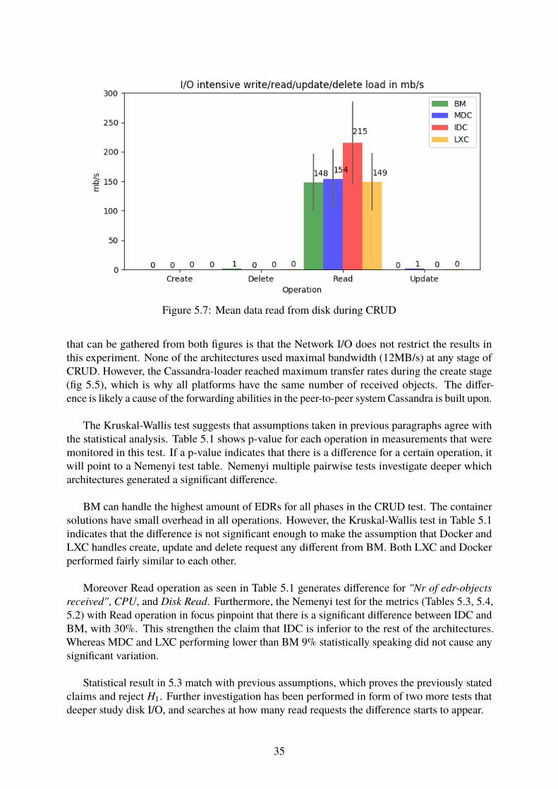
Figure 5.7: Mean data read from disk during CRUD

that can be gathered from both figures is that the Network I/O does not restrict the results inthis experiment. None of the architectures used maximal bandwidth (12MB/s) at any stage ofCRUD. However, the Cassandra-loader reached maximum transfer rates during the create stage(fig 5.5), which is why all platforms have the same number of received objects. The differ-ence is likely a cause of the forwarding abilities in the peer-to-peer system Cassandra is built upon.

The Kruskal-Wallis test suggests that assumptions taken in previous paragraphs agree withthe statistical analysis. Table 5.1 shows p-value for each operation in measurements that weremonitored in this test. If a p-value indicates that there is a difference for a certain operation, itwill point to a Nemenyi test table. Nemenyi multiple pairwise tests investigate deeper whicharchitectures generated a significant difference.

BM can handle the highest amount of EDRs for all phases in the CRUD test. The containersolutions have small overhead in all operations. However, the Kruskal-Wallis test in Table 5.1indicates that the difference is not significant enough to make the assumption that Docker andLXC handles create, update and delete request any different from BM. Both LXC and Dockerperformed fairly similar to each other.

Moreover Read operation as seen in Table 5.1 generates difference for "Nr of edr-objectsreceived", CPU, and Disk Read. Furthermore, the Nemenyi test for the metrics (Tables 5.3, 5.4,5.2) with Read operation in focus pinpoint that there is a significant difference between IDC andBM, with 30%. This strengthen the claim that IDC is inferior to the rest of the architectures.Whereas MDC and LXC performing lower than BM 9% statistically speaking did not cause anysignificant variation.

Statistical result in 5.3 match with previous assumptions, which proves the previously statedclaims and reject H1. Further investigation has been performed in form of two more tests thatdeeper study disk I/O, and searches at how many read requests the difference starts to appear.

35

Table 5.1: Kruskal-Wallis Test - CRUD

Metric Operation p-value Note#edrs received create 0.1033 Same during creates

read 0.0007426 Difference for readsupdate 0.01782 Same during updatesdelete 0.8752 Same during deletes

CPU create 2.2e − 16 Difference for createsread 2.6e − 16 Difference for readsupdate 2.2e − 16 Difference for updatesdelete 2.2e − 16 Difference for deletes

Disk write create 0.7535 Same during createread −− Values are near zero1

update 0.0970 Same during createdelete 0.2737 Same during create

Disk Read create −− Values are near zeroread 2.2e − 16 Difference while readingupdate −− Values are near zerodelete −− Values are near zero

1Values are near zero, which makes the Kruskal-Wallis test irrelevant.

Table 5.2: Nemenyi Test - Disk Read

Operation levels p-value Significant difference foundRead MDC - BM 0.2871 No

IDC - BM 2e − 16 YesLXC - BM 0.9901 NoIDC - MDC 2e − 16 YesLXC - MDC 0.1604 NoLXC - IDC 2e − 16 Yes

Table 5.3: Nemenyi Test - Received edr-objects

Operation levels p-value Significant difference foundRead MDC - BM 0.6599 No

IDC - BM 0.0004 YesLXC - BM 0.7018 NoIDC - MDC 0.0240 NoLXC - MDC 0.9901 NoLXC - IDC 0.0362 No

36

Table 5.4: Nemenyi Test - CPU

Operation levels p-value Significant difference foundCreate MDC - BM 0.0107 No

IDC - BM 0.1192 NoLXC - BM 3.4e − 05 YesIDC - MDC 0.0897 NoLXC - MDC 3.9e − 06 YesLXC - IDC 2e − 16 Yes

Read MDC - BM 0.3690 NoIDC - BM 5.8e − 14 YesLXC - BM 0.2367 NoIDC - MDC 8.8e − 10 YesLXC - MDC 0.1952 NoLXC - IDC 2e − 16 Yes

Update MDC - BM 9.1e − 06 YesIDC - BM 2.2e − 09 YesLXC - BM 0.05467 NoIDC - MDC 0.01330 NoLXC - MDC 0.0691 NoLXC - IDC 2.8e − 07 Yes

Delete MDC - BM 0.0392 NoIDC - BM 0.0267 NoLXC - BM 3.2e − 06 YesIDC - MDC 0.9991 NoLXC - MDC 4.5e − 05 YesLXC - IDC 2.1e − 04 Yes

37

5.3 Local Stress TestThe execution of the local stress test was conducted using Cassandras COPY FROM/ TOcommands, following five-fold test actions query. Both FROM and TO generated five valuesfor average rate, where TO generated amount of created rows as well. Thereafter a mean valuewas calculated for each architecture and operation as seen in Table 5.5. The create operationcopies all rows from a certain table to a csv file, whereas the read uses that csv file and createsthe table objects based on each row. Average Rate columns in Table 5.5 represents the mean ofthe five executed operations. Moreover, it shows the speed in which every architecture is able toprocess the same amount of data, under the same conditions. In regard to the Processed datacolumn it is noticeable that the number of written rows is different for each architecture. This isdue to requested timeout from the cluster, which means that Cassandra was not able to reach therequested entry in the restricted time.

The original data set contained 700’000 rows, which indicates that the different architectureswere unable to copy the whole table within the time limit of every row. Cassandra breaks downthe computation to a set of workers to compute work in parallel which increases the amount ofdisk I/O operations, which may make the process slower for IDC. The BM solution has the bestperformance as it got the least number of timeouts while also copying the most objects to thecsv file. IDC got the second highest Copy To, which can be misleading as it also got the mosttimeout from Cassandra. The Kruskal-Wallis test rejects H2 and the Nemenyi test described inTable 5.7 further show that BM outperform all other architectures for rows/s. However, the #of rows processed does not differ for any of the platforms. This shows that all tested containersolutions introduce similar overhead for these types of operations.

While reading the csv file into the Cassandra Cluster all except IDC perform similar. Afeasible explanation for these results is the AUFS, file system provided by Docker. This drawbackcan be removed by mounting the disk into the Docker containers as the p − value between IDCand MDC is 0. The IDC can only process 59 rows per second which is a reduction with ∼25%compared with the other architectures as it can be seen in Table 5.5.

Table 5.5: Local stress test - Copy to file/Copy from file

Architecture Operation Avg. Rate Processed dataBM Copy to 1798 rows/s Writing 554617 rows of data

Copy From 83 rows/s Reading 30000 rowsMDC Copy to 1675 rows/s Writing 501904 rows of data

Copy From 80 rows/s Reading 30000 rowsIDC Copy to 1676 rows/s Writing 498767 rows of data

Copy From 59 rows/s Reading 30000 rowsLXC Copy to 1664 rows/s Writing 513861 rows of data

Copy From 81 rows/s Reading 30000 rows

The results confirms claim from previous experiment that IDC architecture causes latencieswhen reading information from disk. Whereas MDC and LXC achieve near native results in bothRead and Write operations. In order to decide where the significant difference occurs betweenIDC and the rest of the architectures a Step-wise Test has been conducted.

38

Table 5.6: Kruskal-Wallis Test - Local Stress

Operation Metric p-value NoteCopy to rows/s 0.000233 Differs

# of rows 0.0141 DiffersCopy from rows/s 4.38 × 10−16 Strong significance

Table 5.7: Nemenyi Test - Local Stress

Operation levels p-value Significant differenceCopy to (rows/s) MDC - BM 0.0017198 Yes

IDC - BM 0.0021070 YesLXC - BM 0.0002867 YesIDC - MDC 0.9996207 NoLXC - MDC 0.8028394 NoLXC - IDC 0.7489856 No

Copy to (# of rows) MDC - BM 0.0269180 NoIDC - BM 0.0179260 NoLXC - BM 0.1169333 NoIDC - MDC 0.9968765 NoLXC - MDC 0.8637104 NoLXC - IDC 0.7621468 No

Copy from (rows/s) MDC - BM 0.8078269 NoIDC - BM 0.0000000 YesLXC - BM 0.8078269 NoIDC - MDC 0.0000000 YesLXC - MDC 0.3141183 NoLXC - IDC 0.0000000 Yes

39

5.4 Step-wise TestDuring the step-wise testing the Cassandra-loader is set to send 128 EDRs to six tables in thecluster increasing linearly, that is an increase of 768 requests for each step. Two-thirds of therequests are read, and the rest are update requests. All four architectures ran with the same dataset and started the test at around ∼0-2% CPU usage. How well Cassandra utilize the CPU andDisk Read is visualized in fig 5.8 and fig 5.9. These figures represent the highest value over allnodes during the peak execution time. Moreover, the execution time for each peak is needed tomap the resource usage if it is maximized during the test and can be found in fig 5.10.

Figure 5.8: CPU load for writes and updates

The CPU shows that the processing varies in each platform. MDC, LXC, and BM havesimilar usage as they start of at 12-17% and steadily increase. The IDC stands out from the restas it starts at quite a high CPU usage and reaches 40-45% quicker. The Kruskal-Wallis test inTable 5.8 clearly indicate that there is no difference in CPU usage for the different steps.

IDC quickly reaches disk reads of 300-350 MB/s, compared to the other platforms whichstabilize at 200-250 MB/s. The statistical test in Table 5.8 identifies the distinctions as significantand rejects H3. The MDC configuration has a constant overhead compared to both LXC andBM, but there is no statistical difference according to the Nemenyi test in Table 5.9. There is nostatistical difference between LXC and BM as they almost follow each other. This indicates thatthe neutral file system of LXC can handle disk I/O quite good.

Execution times are mostly between 2 - 3 seconds during the tests up until the 1400 EDRs.After this point the execution times start to increase more for all architectures. The CPU dropsfor IDC, down to 40% which point out that the CPU is not the bottleneck. During these requests,

40

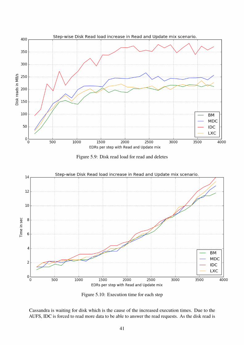
Figure 5.9: Disk read load for read and deletes

Figure 5.10: Execution time for each step

Cassandra is waiting for disk which is the cause of the increased execution times. Due to theAUFS, IDC is forced to read more data to be able to answer the read requests. As the disk read is

41

maxed out the only possible outcome is an increase in execution time. IDC require approximatelyone (1) extra second to complete the task (fig 5.10).

Table 5.8: Kruskal-Wallis Test - Step-wise load

Metric Operation p-value NoteCPU Read & Update Mix 0.9598 No difference

Disk Read Read & Update Mix 2.001e − 11 Difference for mix

Table 5.9: Nemenyi Test - Disk Read step-wise

Operation levels p-value Significant difference foundR&U Mix Docker - BM 0.0124 No

IDC - BM 2.6e − 10 YesLXC - BM 0.8877 No

IDC - Docker 0.0022 NoLXC - Docker 0.0928 NoLXC - IDC 2.6e − 08 Yes

42

6 DISCUSSION

6.1 DiscussionThis thesis main focus was to investigate container-based virtualization architectures in a BigData Cassandra Cluster application. Furthermore, an execution of experimental comparisonbetween those platforms and the more conventional BM solution were performed. This was donein the interest of detecting whether containerized platforms could benefit or introduce hindrancetowards database applications handling big and sparse data sets.

The first question this research should answer is:"TQ1: What is the performance difference between container-based virtualization and BMarchitecture for Apache Cassandra?"

The question refers to included architectures performance with the Cassandra application.Since Cassandra is a database it uses disk I/O very intensively. In turn, this gave us the assumptionthat IDC would have the lowest performance. This is due to previous studies that mentioned adrawback for the AUFS that this platform adopts. The results confirmed that belief as both H1and H2 can be rejected. What we now consider to be true is the following:

"HA1 : At least one container software differs in performance for the Cassandra clustercompared to BM during CRUD testing""HA2 : At least one container software differs in performance for the Cassandra clustercompared to BM during local read/write"

As seen in the results the BM platform showed better results during all CRUD operations,whereas LXC and MDC fall shortly behind. BM processed more object during reading operationsthan any other architecture. At the same time, IDC had around 45% higher MB/s read fromdisk, and CPU declined with a significant difference for other architectures. This suggested thatpreviously mentioned assumption was accurate, and IDC struggles with reading operations andspends more time traversing data than any of the other platforms. This pushed us to execute asecond test that would take only the disk I/O into consideration. This was done by performing alocal stress test of copying a table into a CSV file and then reading the content of that file into theCassandra data model. This experiment strengthens our claim since IDC generated a significantdifference in operation "COPY FROM", which correspond to reading from disk. MDC and LXCperformed surprisingly good during CRUD and local stress tests, and we feel those platformsshould be implemented for a cloud computing setting without strong drawbacks.

Gontikow et al. [9] state that Docker produces a minor overhead in comparison with thenative system under high performance computing task execution. The researchers argue that the2.21% loss in performance is not significant, and mean that Docker performs on the same levelas BM application. Whereas Chung et al. [12] came to the conclusion that Docker producesa latency for computing heavy operations. Furthermore, they argue that Dockers architecturehas fundamental drawbacks in resource management. Both research papers have a fully isolatedset-up on Docker, with no mounting point to the host file system. Their result, however, can notbe directly related in comparison with this thesis. Both papers execute several benchmark tests,which have the purpose of maximizing the use of a specific resource in the test bed. It is a greatway to test how a certain system behaves under extremely stressful conditions. Nonetheless,they are not representing a realistic case, that occurs in the industry. Which is the case for thisstudy. Here, there is an actual component that communicates with a database that contains actualdata model that a company uses. The conclusion from [9] seem to show similarities with those

43

presented in this paper. Container architecture like Docker produce small overhead, but in somecases are able to perform similarly to BM. The same argument can be applied for the work ofMorabito et. al. [13]. Here researchers benchmark four different architectures; LXC, Docker,KVM, and OSv and compare them to the native solution. Their study shows that LXC and Dockerproduce 17-19% latencies in the network I/O and 10-14% latencies in Disk I/O. But producenear native performance when it comes to CPU performance and memory. They even arguethemselves that overhead produced by Docker and LXC can be neglected. We see a statisticallysignificant difference for the Microservices compared to the BM baseline. The difference ishowever quite small for Docker containers except for IDC reading from disk operations.

As stated by Pahl et al. [11] containerized environments like Docker and LXC are beingmore and more adopted in cloud computing settings. According to them, those technologieshave developed to the point where BM solutions are just an inferior choice. The works proposedby Xavier et al. [8] confirms that usage of LXC in cloud computing is a superior choice whencompared to VMs. Their experiment shows that LXC provide much higher performance, whilestill equipping the server with isolation capabilities. However, both research studies do notprovide any valuable comparison with BM solutions, which is the main focus of this study.

Ruan et al. [7] present a paper where they compare Docker in a virtual machine, Docker, andLXC in a cloud environment. According to their results, LXC outperforms other architecturesin every test, while Docker falls shortly behind. By comparing that result to this research wecan conclude that LXC and Docker (in our case MDC) provide near the same performance.Differences occur depending on the application of the architecture. Whereas isolated Dockerseems to land at the last place in both studies. This indicates that no matter the provided isolationabilities, high disk performance applications of Docker architectures often require a mounted pointon the disk. As seen in the work of Xavier et al [32] LXC does not produce large discrepanciesin comparison to a native solution, in MapReduce Clusters1. Which is an equivalent result incorrelation to this study. This strengthens the claim that container-based solutions are able toprovide near native performance where LXC seems to be the better choice. In our case, LXC doesnot outperform MDC, as it proves the same performance. The work of Julian et al. [18] suggestthat Docker operates near to RHEL operative systems native performance. However, this researchexamines only the network bandwidth of different architectures. Whereas the work of Varmaet al. [16] point towards opposite findings. They mean that containers produce major latenciesin comparison to native adaptation. This discrepancy can depend on architectures adaptationin the system, what it is used for, and the settings. Which shows that however good Dockerand LXC performed in this study, there are some applications where those platforms do not exceed.

Nevertheless BM architecture outperformed every other level in this study, however, thesmall difference from MDC shows that Docker has the potential to be adopted in Cassandraapplications if the disk is mounted. The same can be said about LXC but the user will need toaccept a minor performance drop in form of CPU usage and disk output.

Next research question tries to find out:"TQ2: Is there a breaking point for performance between container-based virtualizationand BM as data loads increase?"

To find potential breaking points, for where performance drops for one or more container, astep-wise test was conducted with increasing load on the cluster. The output from Kruskal-Wallis

1https://hadoop.apache.org/docs/r1.2.1/mapred_tutorial.html#Purpose

44

test rejects H3, and H3A will be used."HA3 : At least one container software differs in performance for the Cassandra clustercompared to BM during step-wise increase loads"

MDC has higher disk reads but a CPU graph similar to LXC and BM. This result is similarto what can be found for the read operation in the CRUD test. For disk reads, the MDC is inbetween the other platforms and show no significant distinctions. IDC performed worse than theother architectures as it had to read more data from disk to respond to the requests. This result isconsistent with the other tests on the Cassandra cluster and depends on the same drawback aspresented earlier in this chapter. The 1400 EDRs mark seems to be the point where IDC start todrop off in performance. After this load it uses more time to read the disk for data while alsodropping of in CPU usage which indicates on blocking from disk output. Prior to this point, IDCis using far more CPU to handle the request and also read more data from disk. The critical pointis thus depending on the read speeds on the disk.

We were unable to find any previous studies on how the disk I/O behaves for increasing dataloads on the targeted application. However, some studies incrementally ramp the data loads totest the CPU. Chung et al. [12] load their Linpack [42] set-up to test Docker containers. Theirresults show that Docker containers follow the BM FLOP performance, but with a constantoverhead. Similar Linpack results are presented by Morabito et al. [13] where both Docker andLXC containers follow the BM curve, but without any overhead. These experiments do not fullycorrelate to our result as the disk reads appeared to be the drawback and not the CPU. Togetherwith their findings and our results we can draw the conclusion that there is no particular pointwhere microservices starts to drop in performance. Instead there is always a present overhead fordisk I/O operations. When the disk output speeds are maxed out, the execution time will increase.

The step-wise test and local stress test both show data for disk read operations. MDC performsimilarly to LXC and BM at ∼80 rows/s in the local stress test. For the step-wise test, this equalityis not as visible. The step-wise test includes Update and Read requests which are smaller thanone big COPY request but can still be comparable. IDC drop in performance for COPY f romwith ∼25%. This drawback is quite large and indicates that IDC is not to be used for heavy readoperations. LXC and MDC are aligning with the BM performance which indicates that suchcontainers are well suited for hosting Cassandra nodes.

6.2 Microservices Outperforming the Host MachineThis was the second time this experiment was executed. The first time both Docker architectures,MDC and IDC outperformed BM during Update and Delete phase of CRUD operations. Theresults seemed bizarre, which made us think of possible causes to that problem. Morabito et.al. [13] results concerning CPU operations, present that Docker and LXC scored higher thanBM. They do not address this phenomena, but we thought that our result was similar to theirs. Iftheirs and our results were valid, this would be a groundbreaking study which found a seriousproblem for the Debian Jessie operative system. The best possible cause would be Debiansarchitecture, but in order for it to be valid we had to exclude all the others possible reasons, asSherlock Holmes ones said: "...when you have eliminated the impossible, whatever remains,however improbable, must be the truth?..."2.

2http://www.bestofsherlock.com/top-10-sherlock-quotes.htm#impossible

45

We compared all JVM and Cassandra configuration files for all architectures and found out thatthey were exactly the same, as intended. No other process was interrupting the result gatheringduring the experiments, and we started to think that the problem was not on our side. Thenwe realized that we had not inspected the Java in use. As it turned out BM used Java-8-Oracleversion with Hotspot, whereas the Docker containers used OpenJDK Runtime Environment(1.8.0). By changing the Java version we were able to increase performance of BM with around10%. Furthermore new tests has been executed, and the new results are presented in this study.We used the same operative system for LXC, and as the result we performed the same process ofinstalling Java on that system. Whichmeant that the same issue had to be corrected in LXC as well.

We are not completely certain at the moment why the Java version causes such tremendousperformance drawbacks. However, we can speculate that Java Hotspots JVM handles memoryand other resources differently in comparison to OpenJDK. The Oracles Hotspot FAQ sitementions that this particular VM by default speeds up the time spent running in bytecode. Whichexcludes heavy graphical operations, and I/O operations such as reading and writing throughnetwork and database. They mean that in order to speed up the performance for this JVM, adifferent configuration should be executed3. OpenJDK, on the other hand, does not have thoseproblems by default as it was discovered in the improvement we got in this study. We think thatthe Hotspot JVM cashes the memory worse, at least with default configurations enabled. This, inturn, can be a valid cause for the performance drop.

6.3 LimitationScience this is a school dissertation, we did not have access to much resources. Even though wewere supplied with six servers, the results would be closer to the reality if we were able to designa cluster with at least ten nodes. That way we would be able to imitate a warehouse settings.However, this would not necessary change provided results, but present a closer adaptation towarehouse settings.

Another limitation in this experiment was the hardware. In a real life company situation,the hardware is likely to be of dedicated components. This limitation however does not affectthe results as better hardware components and more servers will increase throughput for allplatforms.

The virtual network that was used for cluster communication restricted the transferring ratesto 100 Mb/s. This had a direct impact on how many create requests the Cassandra-loader couldsend as the port transfer rate was limited.

6.3.1 Low Statistical PowerThe selected sample size seems to be a problem for validating the Kruskal-Wallis and Nemenyitests as uncertainty arose. 30 incremental steps in the step-wise test gave limitations on diskreads as the execution started to increase after ten steps. The CPU did however not reach theutilization the Cassandra CRUD test showed which is an indication of that the Cassandra clusteris able to handle more requests. Increasing the sample size would show if more steps withhigher loads will increase the CPU utilization while also having more samples to analyze in the

3http://www.oracle.com/technetwork/java/hotspotfaq-138619.html#perf_general

46

Kruskal-Wallis and Nemenyi tests. The lack of samples could in a higher degree affecting theCRUD tests and local stress test since each architecture is only tested five times. Due to timerestraints and time-consuming measuring procedures, the number of iterations was accepted butcan be a source of ambiguity.

6.3.2 FishingAs the results showed that MDC and IDC performed better than BM and LXC during Updateand Delete phase in the CRUD test, the willingness to "fish" for another result was present.The experiment was however conducted several times, each time those Docker based platformsperformed better than BM. Moreover, the similarity to [13] indicated that this could be a validphenomena. However, by performing deeper investigation we concluded that the reason for theodd result was the usage of different Java version. By using the same across all levels, the resultchanged.

6.4 Sustainable DevelopmentCloud computing system provides scalability and portability, but also introduce an efficientway of handling resources [43, 44]. The resources in such systems can be shared thanks to thevirtualization techniques. This enables cloud computing providers to maximize the usage ofthe hardware by renting it. The clients only pay for what resources they use and the in-houseinfrastructure can be decreased. From the client’s point of view, the overall functionality of theapplications stays the same, while the economic cost is reduced. These features fit well with’green computing’ where energy efficiency and e-waste minimization are in focus, while alsostriving to provide economical benefits [43]. Integrating a component from a BM architectureinto a cloud service will hence be a good deal for all parties, but also contribute to a moresustainable development.

47

7 CONCLUSIONS

Lightweight container or microservice software enables applications to scale interactively andisolate processes while producing small overhead compared to traditional hypervisor technologies.Due to the simplicity of building, storing and deploying these containers they are sometimes usedinstead of BM solutions. These containers need to be evaluated for different kinds of applicationsto find possible drawbacks in the technology when used in this way. In a Big Data setting thecontainer tools are joint with the storage requirements for the platform as the system needs toserve, store and provide sufficient throughput of data. A popular Big Data database is Apache’sCassandra and was used in this report to analyze microservices. Apart from inspecting theCassandra cluster, a Cassandra-loader was built and used to send Qvantel Sweden AB specificdata objects.

The results of this study show that containerization of Cassandra brings out significantlatency in comparison to BM solution. However, the difference is relatively small when itcomes to operations like update, delete, or create. Furthermore both Docker and LXC havethe potential to be a better choice than BM due to scalability and faster deployment featuresthey provide. Both Docker settings distribute resources with near native precision. BM is stillthe superior solution, where overall performance exceeded. LXC and MDC perform similar toeach other and are both should be considered when adapting microservices. IDC present nearnative results for write, update and delete operations, but brought out major latencies duringread operations. This is due to the AUFS. Cassandras already brings read latencies becauseof its design and is not recommended for systems where a lot of read operations are executed.In turn, this makes IDC harder to recommend, if a complete isolation of the application is required.

Using MDC instead of LXC might be a better option as LXC has slightly higher CPU usagefor create and delete operations. At the same time, both perform equally to IDC for write, updateand delete operations while outperforming it in read operations. This is thanks to the bypassof the AUFS, but it will however not reach the capabilities of the BM solution. If any of thecontainer set-ups are going to be used for a Cassandra cluster a Docker image with mounteddisks as well as LXC is to be preferred as they overall gave the closest representation of the BMconstruct.

49

8 RECOMMENDATIONS AND FUTURE WORK

8.1 Java versionWe are not certain to why the Java version had such impact on the Cassandra performance andwe recommend that an investigation is made to find the issue. It is an interesting phenomena thathas to do with the Java Virtual Machine, that Cassandra operates on. Investigation of it couldlighten up the understanding of the Cassandras structure.

8.2 Better NetworkThe network limited the amount of create requests the cluster could receive. This restrictionreduced the heaviest operation for disk input, as each Cassandra node would have to dump thememtable to disk more often than with update and delete request. By using a better networkset-up for the cluster, other results for write operations could emerge than was found in this study.

8.3 Different databaseMoreover a similar experiment should be conducted using MongoDB database in order toexamine if the results are applicable on other NoSQL databases or if the results are depending onCassandras structure. As MongoDB meets CP needs from CAP thearom, and MySQL meetsCA needs, it would be interesting to examine if results from a database that meets AP needs isequivalent. It would also be interesting to examine how other big data databases behaves whenintegrated with container architectures such as Docker and LXC. Those results could then becompared with this study in order to find combinations that work best together and could be usedin the industry.

51

REFERENCES

[1] Docker overview, May 2017. https://docs.docker.com/engine/docker-overview/#what-can-i-use-docker-for.

[2] Carlos Pérez-Miguel, Alexander Mendiburu, and Jose Miguel-Alonso. Modeling theavailability of Cassandra. Journal of Parallel and Distributed Computing, 86:29–44,December 2015.

[3] Claes Wohlin, Per Runeson, Martin Höst, Magnus C. Ohlsson, Björn Regnell, and AndersWesslén. Experimentation in Software Engineering. Springer Berlin Heidelberg, Berlin,Heidelberg, 2012. DOI: 10.1007/978-3-642-29044-2.

[4] Katarina Grolinger, Wilson A Higashino, Abhinav Tiwari, and Miriam AM Capretz. Datamanagement in cloud environments: NoSQL and NewSQL data stores. Journal of CloudComputing: Advances, Systems and Applications, 2(1):22, 2013.

[5] Min Chen, Shiwen Mao, and Yunhao Liu. Big Data: A Survey. Mobile Networks andApplications, 19(2):171–209, April 2014.

[6] Elif Dede, Bedri Sendir, Pinar Kuzlu, Jessica Hartog, and Madhusudhan Govindaraju. AnEvaluation of Cassandra for Hadoop. pages 494–501. IEEE, June 2013.

[7] Bowen Ruan, Hang Huang, Song Wu, and Hai Jin. A Performance Study of Containers inCloud Environment. In Guojun Wang, Yanbo Han, and Gregorio Martínez Pérez, editors,Advances in Services Computing, volume 10065, pages 343–356. Springer InternationalPublishing, Cham, 2016. DOI: 10.1007/978-3-319-49178-3_27.

[8] Miguel G. Xavier, Israel C. De Oliveira, Fabio D. Rossi, Robson D. Dos Passos, Kassiano J.Matteussi, and Cesar A.F. De Rose. A Performance Isolation Analysis of Disk-IntensiveWorkloads on Container-Based Clouds. pages 253–260. IEEE, March 2015.

[9] H. Gantikow, S. Klingberg, and C. Reich. Container-based virtualization for hpc. pages543 – 50, Setubal, Portugal, 2015//. container-based virtualization;high-performancecomputing clusters;HPCclusters;bare-metal installations;performance loss;VM;privateHPCsites;public clouds;FEA job;risk analysis;Docker installations;multitenant environment;.

[10] Ann Mary Joy. Performance comparison between Linux containers and virtual machines.pages 342–346. IEEE, March 2015.

[11] Claus Pahl and Brian Lee. Containers and Clusters for Edge Cloud Architectures – ATechnology Review. pages 379–386. IEEE, August 2015.

[12] Minh Thanh Chung, Nguyen Quang-Hung, Manh-Thin Nguyen, and Nam Thoai. UsingDocker in high performance computing applications. pages 52–57. IEEE, July 2016.

[13] Roberto Morabito, Jimmy Kjallman, and Miika Komu. Hypervisors vs. LightweightVirtualization: A Performance Comparison. pages 386–393. IEEE, March 2015.

[14] MarceloAmaral, Jorda Polo, DavidCarrera, IqbalMohomed,MerveUnuvar, andMalgorzataSteinder. Performance Evaluation of Microservices Architectures Using Containers. pages27–34. IEEE, September 2015.

[15] Ibrahim Abaker Targio Hashem, Ibrar Yaqoob, Nor Badrul Anuar, Salimah Mokhtar,Abdullah Gani, and Samee Ullah Khan. The rise of big data on cloud computing: Reviewand open research issues. Information Systems, 47:98–115, January 2015.

53

[16] P. China Venkanna Varma, Venkata Kalyan Chakravarthy K., V. Valli Kumari, andS. Viswanadha Raju. Analysis of a Network IO Bottleneck in Big Data Environments Basedon Docker Containers. Big Data Research, 3:24–28, April 2016.

[17] Wes Felter, Alexandre Ferreira, Ram Rajamony, and Juan Rubio. An updated performancecomparison of virtual machines and Linux containers. pages 171–172. IEEE, March 2015.

[18] Spencer Julian, Michael Shuey, and Seth Cook. Containers in Research: Initial Experienceswith Lightweight Infrastructure. In Proceedings of the XSEDE16 Conference on Diversity,Big Data, and Science at Scale, XSEDE16, pages 25:1–25:6, New York, NY, USA, 2016.ACM.

[19] Yu Huang and Tie-jian Luo. NoSQL Database: A Scalable, Availability, High PerformanceStorage for Big Data. In Pervasive Computing and the Networked World, volume 8351,pages 172–183. Springer International Publishing, Cham, 2014.

[20] Anita Brigit Mathew and S. D. Madhu Kumar. Analysis of data management and queryhandling in social networks using NoSQL databases. pages 800–806. IEEE, August 2015.

[21] M. R. Murazza and A. Nurwidyantoro. Cassandra and sql database comparison for nearreal-time twitter data warehouse. In 2016 International Seminar on Intelligent Technologyand Its Applications (ISITIA), pages 195–200, July 2016.

[22] Takanori Ueda, Takuya Nakaike, and Moriyoshi Ohara. Workload characterization formicroservices. pages 1–10. IEEE, September 2016.

[23] Jing Han, Haihong E, Guan Le, and Jian Du. Survey on nosql database. In 2011 6thInternational Conference on Pervasive Computing and Applications, pages 363–366, Oct2011.

[24] Rick Cattell. Scalable SQL and NoSQL Data Stores. SIGMOD Rec., 39(4):12–27, May2011.

[25] Docker and AUFS in practice, May 2017. https://docs.docker.com/engine/userguide/storagedriver/aufs-driver/.

[26] Linux Container Documentation, May 2017. https://linuxcontainers.org/lxc/getting-started/.

[27] Satyadhyan Chickerur, Anoop Goudar, and Ankita Kinnerkar. Comparison of RelationalDatabase with Document-Oriented Database (MongoDB) for Big Data Applications. pages41–47. IEEE, November 2015.

[28] Venkat N. Gudivada, Dhana Rao, and Vijay V. Raghavan. NoSQL Systems for Big DataManagement. pages 190–197. IEEE, June 2014.

[29] Datastax. How Cassandra reads and writes data, April 2017. http://docs.datastax.com/en/cassandra/3.0/cassandra/dml/dmlIntro.html.

[30] Avinash Lakshman and Prashant Malik. Cassandra: A decentralized structured storagesystem. SIGOPS Oper. Syst. Rev., 44(2):35–40, April 2010.

[31] M. Barata, J. Bernardino, and P. Furtado. Cassandra: what it does and what it does not andbenchmarking. International Journal of Business Process Integration and Management,7(4):364 – 71, 2015.

54

[32] M. G. Xavier, M. V. Neves, and C. A. F. D. Rose. A performance comparison of container-based virtualization systems for mapreduce clusters. In 2014 22nd Euromicro InternationalConference on Parallel, Distributed, and Network-Based Processing, pages 299–306, Feb2014.

[33] Theodora Adufu, Jieun Choi, and Yoonhee Kim. Is container-based technology a winnerfor high performance scientific applications? pages 507–510. IEEE, August 2015.

[34] Christian Esposito, Aniello Castiglione, and Kim-Kwang Raymond Choo. Challenges inDelivering Software in the Cloud as Microservices. IEEE Cloud Computing, 3(5):10–14,September 2016.

[35] Christian W. Dawson. Projects in computing and information systems: a student’s guide.Addison-Wesley, Harlow, England ; New York, 2nd ed edition, 2009. OCLC: ocn305421178.

[36] Tyler Hobbs. Basic rules of cassandra data modeling, February 2015. http://www.datastax.com/dev/blog/basic-rules-of-cassandra-data-modeling.

[37] Ulla Engstrand and Ulf Olsson. Variansanalys och försöksplanering. Studentlitteratur,Lund, 2003. OCLC: 473658634.

[38] DataStax Enterprise. Tuning Java resources, May 2017. http://docs.datastax.com/en/cassandra/2.1/cassandra/operations/ops_tune_jvm_c.html.

[39] Improved Cassandra 2.1 Stress Tool: Benchmark AnySchema, May 2017. https://www.datastax.com/dev/blog/improved-cassandra-2-1-stress-tool-benchmark-any-schema.

[40] J. D. Hunter. Matplotlib: A 2d graphics environment. Computing In Science & Engineering,9(3):90–95, 2007.

[41] Peter A. Flach. Machine learning: the art and science of algorithms that make sense ofdata. Cambridge University Press, Cambridge ; New York, 2012. OCLC: ocn795181906.

[42] Zhang Zhang. Intel Math Kernel Library. https://software.intel.com/en-us/articles/intel-mkl-benchmarks-suite.

[43] P. Sasikala. Research challenges and potential green technological applications in cloudcomputing. International Journal of Cloud Computing, 2(1):1, 2013.

[44] Yashwant Singh Patel, Neetesh Mehrotra, and Swapnil Soner. Green cloud computing:A review on Green IT areas for cloud computing environment. pages 327–332. IEEE,February 2015.

55

A DATA SPECIFICATION

Figure A.1: Data specifications

57

B DATA MODEL FOR CASSANDRA CLUSTER

Listing B.1: Data model for Cassandra cluster.CREATE KEYSPACE IF NOT EXISTS cdr WITH replication = {’class’:’SimpleStrategy’, ’replication_factor’: ’3’} AND durable_writes = true;

CREATE TYPE IF NOT EXISTS cdr.products(id TEXT,name TEXT);

CREATE TYPE IF NOT EXISTS cdr.location_information(destination TEXT,location_number TEXT,location_area_identification TEXT,cell_global_idenfitifaction TEXT);

CREATE TYPE IF NOT EXISTS cdr.service_units(amount DECIMAL,currency TEXT,unit_of_measure TEXT);

CREATE TYPE IF NOT EXISTS cdr.charged_amounts(id TEXT,name TEXT,charged_type TEXT,event_type TEXT,resource_type TEXT,amount DECIMAL,end_balance DECIMAL,expiry_date TIMESTAMP);

CREATE TYPE IF NOT EXISTS cdr.call_event_details(traffic_case TEXT,event_type TEXT,is_roaming BOOLEAN,a_party_number TEXT,a_party_location frozen<cdr.location_information>,b_party_number TEXT,b_party_location frozen<cdr.location_information>);

CREATE TYPE IF NOT EXISTS cdr.data_event_details(access_point_name TEXT,is_roaming BOOLEAN,a_party_number TEXT,a_party_location frozen<cdr.location_information>,

59

);

CREATE TYPE IF NOT EXISTS cdr.event_charges(charged_units frozen<cdr.service_units>,products frozen<cdr.products>,charged_amounts list<frozen<cdr.charged_amounts>>);

CREATE TABLE IF NOT EXISTS cdr.edr_by_id (id TEXT PRIMARY KEY,service TEXT,created_at TIMESTAMP,started_at TIMESTAMP,service_units frozen<cdr.service_units>,event_charges frozen<cdr.event_charges>,call_event frozen<call_event_details>,data_event frozen<data_event_details>

);CREATE INDEX IF NOT EXISTS ON cdr.edr_by_id (started_at);

CREATE TABLE IF NOT EXISTS cdr.edr_by_date (id TEXT,service TEXT,created_at TIMESTAMP,started_at TIMESTAMP,service_units frozen<cdr.service_units>,event_charges frozen<cdr.event_charges>,call_event frozen<call_event_details>,data_event frozen<data_event_details>,PRIMARY KEY (started_at, id)

);CREATE INDEX IF NOT EXISTS ON cdr.edr_by_date (created_at);

CREATE TABLE IF NOT EXISTS cdr.edr_by_service (id TEXT,service TEXT,created_at TIMESTAMP,started_at TIMESTAMP,service_units frozen<cdr.service_units>,event_charges frozen<cdr.event_charges>,call_event frozen<call_event_details>,data_event frozen<data_event_details>,PRIMARY KEY (service, started_at)

);CREATE INDEX IF NOT EXISTS ON cdr.edr_by_service (created_at);

CREATE TABLE IF NOT EXISTS cdr.edr_by_destination (id TEXT,destination TEXT,service TEXT,created_at TIMESTAMP,started_at TIMESTAMP,

60

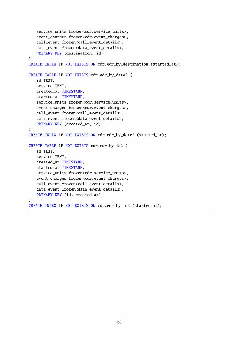
service_units frozen<cdr.service_units>,event_charges frozen<cdr.event_charges>,call_event frozen<call_event_details>,data_event frozen<data_event_details>,PRIMARY KEY (destination, id)

);CREATE INDEX IF NOT EXISTS ON cdr.edr_by_destination (started_at);

CREATE TABLE IF NOT EXISTS cdr.edr_by_date2 (id TEXT,service TEXT,created_at TIMESTAMP,started_at TIMESTAMP,service_units frozen<cdr.service_units>,event_charges frozen<cdr.event_charges>,call_event frozen<call_event_details>,data_event frozen<data_event_details>,PRIMARY KEY (created_at, id)

);CREATE INDEX IF NOT EXISTS ON cdr.edr_by_date2 (started_at);

CREATE TABLE IF NOT EXISTS cdr.edr_by_id2 (id TEXT,service TEXT,created_at TIMESTAMP,started_at TIMESTAMP,service_units frozen<cdr.service_units>,event_charges frozen<cdr.event_charges>,call_event frozen<call_event_details>,data_event frozen<data_event_details>,PRIMARY KEY (id, created_at)

);CREATE INDEX IF NOT EXISTS ON cdr.edr_by_id2 (started_at);

61

C DATA GENERATOR

Listing C.1: Python code that generates EDR objects.# data-generator.py#!/usr/bin/env python2import datetimeimport timeimport randomimport sysimport subprocessimport os

""" Amount of entries we create! """service_to_use = 0

""" Defines enums that exist in the database. """unit_of_measure_enum=["seconds", "monetary", "bytes"]resource_type_enum=["Money", "Kilobytes", "Seconds", "Units"]charged_type_enum=["REAL", "BONUS", "PARTITION"]traffic_case_enum=["originating", "terminating", "forwarding"]event_type_enum=["Voice", "sms", "mms", "video"]edr_service_enum=["1", "2"]products_enum=["Call Plan Normal", "Call Plan Low", "Call Plan High", "CallPlan Allin", \

"Data Plan Normal", "Data Plan Low", "Data Plan High"]access_point_name_enum=["example.com", "hallborg.se", "patryk.se","wikipedia.org", \

"amazon.com", "instagram.com", "twitter.com", "github.com", "reddit.com"]roming_enum=["false", "true"]

""" Make sure that passed argument is an integer """def arg_t(argv):try:argv[0] = int(argv[0])

except ValueError:print "Usage ./data-generator.py <Integer>"exit()

else:if argv[0] < 0:print "Usage ./data-generator.py <Integer>\nNo negatives!"exit()

elif argv[0] > 6100000:print "Usage ./data-generator.py <Integer>\nNumber is too big! \5.000.000 is enough."exit()

amt = argv[0]return amt

""" Service-unit defined """def create_service_unit():

63

serv_unit_ammount = random.randint(46, 50000)if service_to_use == 2:serv_unit_unit = unit_of_measure_enum[2]

else:serv_unit_unit = unit_of_measure_enum[random.randint(0, 1)]

service_unit = """\"service_units" : {"amount": %d, "unit_of_measure": "%s"}\""" % (serv_unit_ammount, serv_unit_unit)return service_unit

""" Product type defined """def create_product():if service_to_use == 2:rand_product = random.randint(4, 6)

else:rand_product = random.randint(0, 3)

prod_id = str(rand_product)prod_name = products_enum[rand_product]products= """\

"products" : { "id": "%s", "name": "%s" } \""" % (prod_id, prod_name)return products

""" Defines charged units """def create_charged_units(service_unit):charged_units = service_unit.replace("service", "charged")return charged_units

""" Charge ammounts list handling """def create_charged_amounts():nr_of_charged_am = random.randint(1, 9)charged_amounts_list = []for i in range(0, nr_of_charged_am):charged_amounts_amount = random.randint(50, 350)charged_amounts_id = str(gen_hex_code(5))charged_amounts_endbalance = random.uniform(0.0, 2100.0)charged_amounts_res_type = resource_type_enum[random.randint(0,3)]charged_amounts_name = charged_type_enum[random.randint(0,2)]charged_amounts_exp_date = "null"charged_amounts_charg_type = charged_type_enum[random.randint(0,2)]if service_to_use == 2:charged_amounts_event_type = "Data"

else:charged_amounts_event_type = event_type_enum[random.randint(0,3)]

charged_amounts_i = """\{ "amount": %d, \"id": "%s", \"end_balance": %.2f, \"resource_type": "%s", \"name": "%s", \"expiry_date": %s, \"charged_type": "%s", \

64

"event_type": "%s" }\""" % (charged_amounts_amount, charged_amounts_id, charged_amounts_endbalance,\

charged_amounts_res_type, charged_amounts_name,charged_amounts_exp_date, \

charged_amounts_charg_type, charged_amounts_event_type)charged_amounts_list.append(charged_amounts_i)

charged_amounts = """\"charged_amounts": %s\""" % (charged_amounts_list)charged_amounts = charged_amounts.replace("\’", "")return charged_amounts

""" Event charges """def create_event_charges(service_unit_t):charged_amounts = create_charged_amounts()products = create_product()charged_units = create_charged_units(service_unit_t)event_charges = """\

"event_charges": { %s, %s, %s }\""" % (charged_amounts, products, charged_units)return event_charges

""" A location generator """def create_a_location():alocation_destination = "732103"+gen_hex_code(8) # 6 first do not changealocation = """ "a_party_location": { "destination": "%s"} """ %(alocation_destination)

return alocation

""" B location generator """def create_b_location():blocation_destination = gen_coordinates()+gen_hex_code(8)blocation = alocation = """ "b_party_location": { "destination": "%s"}""" %(blocation_destination)

return blocation

""" Event Details variables """def create_event_details():alocation = create_a_location()event_d_a_number = str(random.randint(3000000000, 3069999999))event_d_roaming = roming_enum[random.randint(0,1)]if service_to_use == 2:event_d_access_point_name = access_point_name_enum[random.randint(0,8)]event_details = """\

"data_event": { "access_point_name": "%s", \"is_roaming": %s, "a_party_number": "%s", %s }\""" % (event_d_access_point_name, event_d_roaming, event_d_a_number, alocation)

else:event_d_traffic_case = traffic_case_enum[random.randint(0,2)]event_d_b_number = str(random.randint(3000000000, 3069999999))blocation = create_b_location()

65

event_d_event_type = event_type_enum[random.randint(0,3)]event_details = """\

"call_event": {"traffic_case": "%s", %s, "b_party_number": "%s", \"event_type": "%s", "is_roaming": %s, %s, "a_party_number": "%s" }\""" % (event_d_traffic_case, alocation, event_d_b_number, event_d_event_type, \

event_d_roaming, blocation, event_d_a_number)

return event_details

def gen_coordinates():return ’’.join([random.choice(’732103456’) for x in range(6)])

""" Generate random hexa code """def gen_hex_code(amount):return ’’.join([random.choice(’0123456789abcdef’) for x in range(amount)])

""" Generate random timestamp """def started_at_time():mounth=random.randint(1, 12)mounth_str=str(mounth)if mounth < 10: mounth_str="0"+str(mounth)if mounth == 2: day=random.randint(1, 28)else: day=random.randint(1, 30)day_str = str(day)if day < 10: day_str = "0"+str(day)hour=random.randint(0, 23)hour_str = str(hour)if hour < 10: hour_str = "0"+str(hour)timestamp = "%s-%s-%sT%s:%s:%s" % (str(random.randint(2015, 2017)),mounth_str,\

day_str, hour_str, str(random.randint(10,59)), str(random.randint(10,59)))return timestamp

""" EDR table """def create_edr_table(event_details, event_charges, service_unit,edr_service_use):edr_id = gen_hex_code(30) #"006ef78034fff173e2810863037702"edr_service = str(edr_service_use)timestamp = started_at_time()#edr_created_at = str(datetime.datetime.now()) #+str() #"2016-01-13T14:33:37.000Z"

#edr_created_at = edr_created_at[:19]edr_created_at = timestamp # edr_created_at.replace(" ", "T")#edr_started_at = str(datetime.datetime.now())#edr_started_at = edr_started_at[:19] #"2016-01-13T 14:33:37.000Z"edr_started_at = timestamp # edr_started_at.replace(" ", "T")edr = """\

{"id": "%s", "service": "%s", %s, "created_at": "%s", "started_at": "%s", %s,%s }\

""" % (edr_id, edr_service, event_details, edr_created_at, edr_started_at,event_charges, service_unit)

66

""" Table handling """edr_table = """%s""" % (edr)return edr_table

""" Writes the json entries to a file """def write_mocdata_to_a_file(edr_list_json, i):dir_path = os.path.dirname(os.path.realpath(__file__))file = open("%s/../dataModel/mockdata-%d" % (str(dir_path),i), "w")for item in edr_list_json:file.write(item + "\n")

file.close()

""" Create database entries for testing, and handling the EDR list """def create_database_entries(argument):split_amount = int(argument/4)edr_arr = []edr_list = []edr_list_json = []for i in range(0, argument):edr_service = random.randint(1, 2)set_global_var(edr_service)service_unit_t = create_service_unit()edr_table = create_edr_table(create_event_details(), \create_event_charges(service_unit_t), service_unit_t, edr_service)

edr_list.append(edr_table)if int(len(edr_list)) == split_amount:edr_arr.append(edr_list)edr_list = []

return edr_arr

""" Assigns a value to the global variable """def set_global_var(value):global service_to_useservice_to_use = value

def main(argv):""" Starts the timer """t0 = time.clock()amount = arg_t(argv)

""" Creates entries and writes them to a json file """mocdata = create_database_entries(amount)i = 0for entrys in mocdata:write_mocdata_to_a_file(entrys, i)i = i + 1

""" Stops the timer """t1 = (time.clock() - t0)print "Done! Time taken: %s sec" % (t1)

""" Start of the program """if __name__ == "__main__":main(sys.argv[1:2])

67

D CASSANDRA-LOADER

Listing D.1: Application that Loads the Cassandra Cluster.// CassandraClientClass.scalaimport com.datastax.driver.core.{Cluster, ConsistencyLevel}import scala.concurrent.ExecutionContext.Implicits.globalimport scala.concurrent.{Await, Future}import scala.util.{Success, Failure}import com.datastax.driver.core.QueryOptions/*** Created by Patryk Sulewski on 2017-02-23.*/class CassandraClientClass(var ip: String) {var nr_of_successful = 0private val cluster = Cluster.builder()//.addContactPoint("194.47.150.101") //"node 3"//.withQueryOptions(newQueryOptions().setConsistencyLevel(ConsistencyLevel.TWO))

.addContactPoint(ip) //"localhost"

.withPort(9042) // 9042 32776

.build()

val session = cluster.connect()

def execSession(theStr: String) = {

/*Future {session.execute(theStr).one} onComplete {case Success(row) => nr_of_successful += 1case Failure(t) => 1 + 1}*///Future {//session.executeAsync(theStr).get//}session.executeAsync(theStr)}def closeCon(): Unit = {session.close()cluster.close()}def truncate() : Unit = {Seq("TRUNCATE cdr.edr_by_id","TRUNCATE cdr.edr_by_service","TRUNCATE cdr.edr_by_destination","TRUNCATE cdr.edr_by_date") foreach(session.execute(_))}}

69

// idKepper.scalaimport play.api.libs.json.{JsUndefined, JsValue, Json}

import scala.io.Sourceimport scala.util.Random/*** Created by Hallborg on 2017-03-14.*/class IdKeeper(filePath: String) {var temp_json: JsValue = nullvar prev_json: JsValue = null

val source = Source.fromFile(filePath).getLines

def populate_ids(json:JsValue): List[String] = {temp_json = jsonvar dest: JsValue = nullif ((json \ ("data_event")).isInstanceOf[JsUndefined]) {dest = json \ ("call_event") \ ("a_party_location") \ ("destination")}else {dest = json \ ("data_event") \ ("a_party_location") \ ("destination")}

List((json \ "id").toString(),(json \ "started_at").toString(),dest.toString(),(json \ "service").toString(),(json \ "created_at").toString())}

def fetch_random(): List[String] = {populate_ids(Json.parse(source.next()))}

def fetch_prev(): List[String] = {if (prev_json == null) {val r = List("\"2015-12-04T18:34:19\"","\"2015-12-04T18:34:19\"","c3467876c7b41efc2dc9b8af0a5d56")prev_json = temp_jsonr}else {val r = List((prev_json \ "started_at").toString,(prev_json \ "created_at").toString,

70

(prev_json \ "id").toString)prev_json = temp_jsonr}}}

// Importer.scalaimport play.api.libs.json.{JsObject, JsUndefined, JsValue, Json}

/*** Created by Hallborg on 2017-03-09.*/object Importer {

def executeWrite(json: JsValue, con: CassandraClientClass): Unit = {var dest: JsValue = nullif ((json \ "data_event").isInstanceOf[JsUndefined]) {dest = json \ "call_event" \ "a_party_location" \ "destination"}else {dest = json \ "data_event" \ "a_party_location" \ "destination"}val json_dest: JsObject = json.as[JsObject] +("destination" -> dest)

Seq("INSERT INTO cdr.edr_by_id JSON ’%s!’".format(json),"INSERT INTO cdr.edr_by_date JSON ’%s!’".format(json),"INSERT INTO cdr.edr_by_destination JSON ’%s!’".format(json_dest),"INSERT INTO cdr.edr_by_service JSON ’%s!’".format(json),"INSERT INTO cdr.edr_by_date2 JSON ’%s!’".format(json),"INSERT INTO cdr.edr_by_id2 JSON ’%s!’".format(json)) foreach(con.execSession(_))}

def executeRead(keys: List[String], con: CassandraClientClass): Unit = {Seq("SELECT service FROM cdr.edr_by_id WHERE id = %s".format(keys.head),"SELECT service FROM cdr.edr_by_destination WHERE destination = %s and id= %s".format(keys(2),keys.head),

"SELECT id FROM cdr.edr_by_service WHERE service = %s and started_at =%s".format(keys(3), keys(1)),

"SELECT id FROM cdr.edr_by_date WHERE started_at = %s".format(keys(1)),"SELECT started_at FROM cdr.edr_by_date2 WHERE created_at =%s".format(keys(4)),

"SELECT started_at FROM cdr.edr_by_id2 WHERE id = %s and created_at =%s".format(keys.head, keys(4))

) map {s => s.replaceAll("\"", "\’")} foreach (con.execSession(_))}

71

def executeUpdate(keys: List[String], new_vals: List[String],con:CassandraClientClass):Unit = {Seq("UPDATE cdr.edr_by_id SET started_at = %s WHERE id =%s".format(new_vals.head, keys.head),

"UPDATE cdr.edr_by_destination SET started_at = %s WHERE destination = %sand id = %s".format(new_vals.head, keys(2), keys.head),

"UPDATE cdr.edr_by_service SET created_at = %s WHERE service = %s andstarted_at = %s".format(new_vals(1), keys(3), keys(1)),

"UPDATE cdr.edr_by_date SET created_at = %s WHERE started_at = %s and id= %s".format(new_vals(1), keys(3), keys.head),

"UPDATE cdr.edr_by_date2 SET started_at = %s WHERE created_at = %s and id= %s".format(new_vals(1), keys(4), keys.head),

"UPDATE cdr.edr_by_id2 SET started_at = %s WHERE id = %s and created_at =%s".format(new_vals.head, keys.head, keys(4))

) map {s => s.replaceAll("\"", "\’")} foreach (con.execSession(_))}def executeDel(keys: List[String], con: CassandraClientClass): Unit = {Seq("DELETE FROM cdr.edr_by_id WHERE id = %s".format(keys.head),"DELETE FROM cdr.edr_by_destination where destination = %s AND id =%s".format(keys(2),keys.head),

"DELETE FROM cdr.edr_by_service WHERE service = %s AND started_at =%s".format(keys(3), keys(1)),

"DELETE FROM cdr.edr_by_date WHERE started_at = %s AND id =%s".format(keys(1), keys.head),

"DELETE FROM cdr.edr_by_date2 WHERE created_at = %s AND id =%s".format(keys(4), keys.head),

"DELETE FROM cdr.edr_by_id2 WHERE id = %s and created_at =%s".format(keys.head, keys(4))

) map {s => s.replaceAll("\"", "\’")} foreach (con.execSession(_))}

def executeTestRead(con: CassandraClientClass): Unit = {println (con.execSession("SELECT * FROM cdr.edr_by_id WHERE id =’c3467876c7b41efc2dc9b8af0a5d56’"))

}}

// Loader.scalaimport play.api.libs.json.{JsValue, Json}import sys.process._import scala.io.Sourceimport java.io._import scala.util.control.Breaks._import java.util.Calendar/*** Created by Hallborg on 2017-03-09.*/class Loader(setting: Int,thread_name: String, filePath: String, ip: String,crudOp: String) {val INC_AMOUNT = 128

72

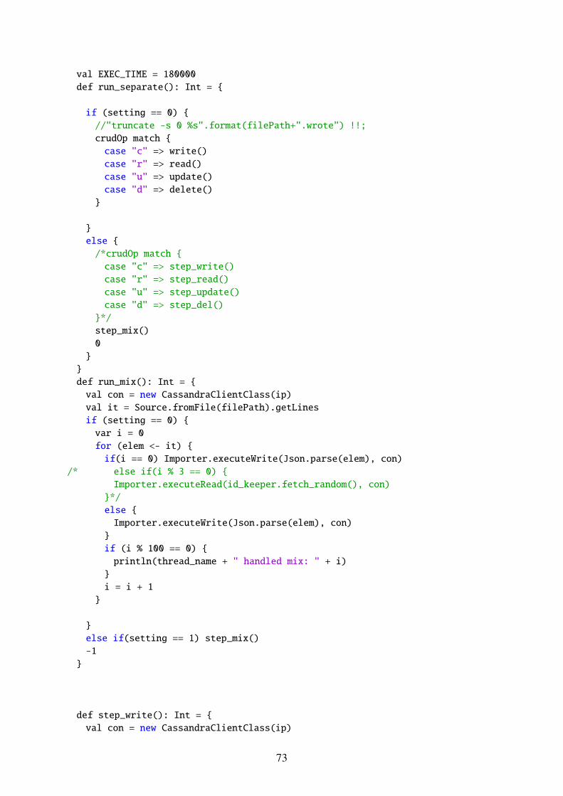
val EXEC_TIME = 180000def run_separate(): Int = {

if (setting == 0) {//"truncate -s 0 %s".format(filePath+".wrote") !!;crudOp match {case "c" => write()case "r" => read()case "u" => update()case "d" => delete()}

}else {/*crudOp match {case "c" => step_write()case "r" => step_read()case "u" => step_update()case "d" => step_del()}*/step_mix()0}}def run_mix(): Int = {val con = new CassandraClientClass(ip)val it = Source.fromFile(filePath).getLinesif (setting == 0) {var i = 0for (elem <- it) {if(i == 0) Importer.executeWrite(Json.parse(elem), con)

/* else if(i % 3 == 0) {Importer.executeRead(id_keeper.fetch_random(), con)}*/else {Importer.executeWrite(Json.parse(elem), con)}if (i % 100 == 0) {println(thread_name + " handled mix: " + i)}i = i + 1}

}else if(setting == 1) step_mix()-1}

def step_write(): Int = {val con = new CassandraClientClass(ip)

73

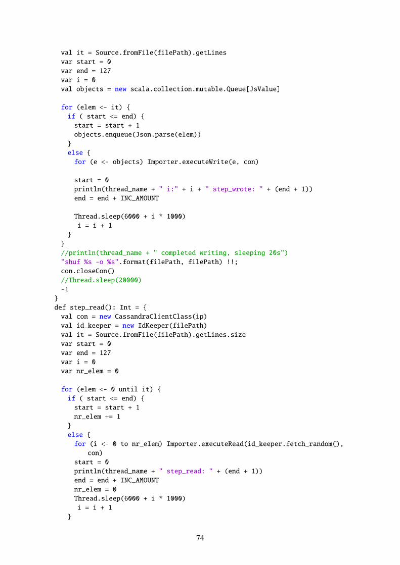
val it = Source.fromFile(filePath).getLinesvar start = 0var end = 127var i = 0val objects = new scala.collection.mutable.Queue[JsValue]

for (elem <- it) {if ( start <= end) {start = start + 1objects.enqueue(Json.parse(elem))}else {for (e <- objects) Importer.executeWrite(e, con)

start = 0println(thread_name + " i:" + i + " step_wrote: " + (end + 1))end = end + INC_AMOUNT

Thread.sleep(6000 + i * 1000)i = i + 1

}}//println(thread_name + " completed writing, sleeping 20s")"shuf %s -o %s".format(filePath, filePath) !!;con.closeCon()//Thread.sleep(20000)-1}def step_read(): Int = {val con = new CassandraClientClass(ip)val id_keeper = new IdKeeper(filePath)val it = Source.fromFile(filePath).getLines.sizevar start = 0var end = 127var i = 0var nr_elem = 0

for (elem <- 0 until it) {if ( start <= end) {start = start + 1nr_elem += 1}else {for (i <- 0 to nr_elem) Importer.executeRead(id_keeper.fetch_random(),con)

start = 0println(thread_name + " step_read: " + (end + 1))end = end + INC_AMOUNTnr_elem = 0Thread.sleep(6000 + i * 1000)i = i + 1

}

74

}

//println(thread_name + " completed reading, sleeping 20s")"shuf %s -o %s".format(filePath, filePath) !!;con.closeCon()//Thread.sleep(20000)-1}

def step_update(): Int = {val con = new CassandraClientClass(ip)val id_keeper = new IdKeeper(filePath)val it = Source.fromFile(filePath).getLines.sizevar start = 0var end = 127var i = 0var nr_elem = 0

for (elem <- 0 until it) {if ( start <= end) {start = start + 1nr_elem += 1}else {for (i <- 0 to nr_elem)Importer.executeUpdate(id_keeper.fetch_random(),id_keeper.fetch_prev(),con)

start = 0println(thread_name + " step_update: " + (end + 1))end = end + INC_AMOUNTnr_elem = 0Thread.sleep(6000 + i * 1000)i = i + 1}

}

//println(thread_name + " completed updating, sleeping 20s")"shuf %s -o %s".format(filePath, filePath) !!;con.closeCon()//Thread.sleep(20000)-1}

def step_del(): Int = {val con = new CassandraClientClass(ip)val id_keeper = new IdKeeper(filePath)val it = Source.fromFile(filePath).getLines.sizevar start = 0var end = 127var i = 0var nr_elem = 0

75

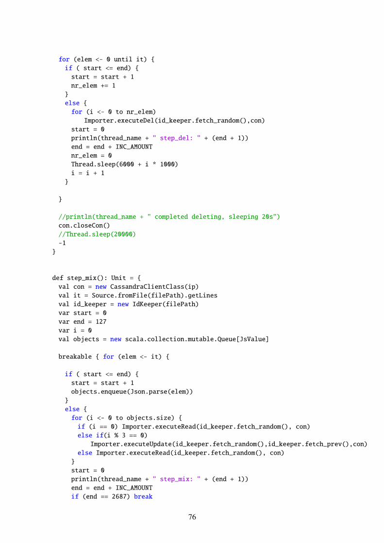
for (elem <- 0 until it) {if ( start <= end) {start = start + 1nr_elem += 1}else {for (i <- 0 to nr_elem)Importer.executeDel(id_keeper.fetch_random(),con)

start = 0println(thread_name + " step_del: " + (end + 1))end = end + INC_AMOUNTnr_elem = 0Thread.sleep(6000 + i * 1000)i = i + 1}

}

//println(thread_name + " completed deleting, sleeping 20s")con.closeCon()//Thread.sleep(20000)-1}

def step_mix(): Unit = {val con = new CassandraClientClass(ip)val it = Source.fromFile(filePath).getLinesval id_keeper = new IdKeeper(filePath)var start = 0var end = 127var i = 0val objects = new scala.collection.mutable.Queue[JsValue]

breakable { for (elem <- it) {

if ( start <= end) {start = start + 1objects.enqueue(Json.parse(elem))}else {for (i <- 0 to objects.size) {if (i == 0) Importer.executeRead(id_keeper.fetch_random(), con)else if(i % 3 == 0)Importer.executeUpdate(id_keeper.fetch_random(),id_keeper.fetch_prev(),con)

else Importer.executeRead(id_keeper.fetch_random(), con)}start = 0println(thread_name + " step_mix: " + (end + 1))end = end + INC_AMOUNTif (end == 2687) break

76

Thread.sleep(10000 + i * 1000)i = i + 1

}/*val sent = con.session.getCluster.getMetrics.getRequestsTimer.getCountval queue =con.session.getCluster.getMetrics.getExecutorQueueDepth.getValue

println(sent, queue)println("nr of responses : " + (queue - sent))*/

} }con.closeCon()"shuf %s -o %s".format(filePath, filePath) !!;//println(thread_name + " completed step_reading, sleeping 20s")

//Thread.sleep(20000)}

def write(): Int = {val con = new CassandraClientClass(ip)val source = Source.fromFile(filePath).getLinesval date_start = Calendar.getInstance.getTimeInMillisvar date_stop = Calendar.getInstance.getTimeInMillisvar nr_of_runs = 0var write_rest = false

breakable {for (elem <- source) {if (date_stop >= date_start + EXEC_TIME) breakImporter.executeWrite(Json.parse(elem), con)//if (nr_of_runs % 100 == 0) println(thread_name + " handled write: " +nr_of_runs)

nr_of_runs = nr_of_runs + 1date_stop = Calendar.getInstance.getTimeInMillis//if(nr_of_runs % 2 == 0) Thread.sleep(1)}}//Seq("bash", "-c", "echo ’%s’ >>%s".format(Json.parse(elem),filePath+".wrote"))!!;

//println(thread_name + " completed writing rest, sleeping 20s")//Seq("bash","-c","echo %s > %s".format(nr_of_runs,thread_name))!!;val sent = con.session.getCluster.getMetrics.getRequestsTimer.getCountval avg =con.session.getCluster.getMetrics.getRequestsTimer.getOneMinuteRate

println(sent)con.closeCon()//Seq("bash","-c","head -n %s %s > %s".format(nr_of_runs,filePath,filePath+".wrote"))!!;

"shuf %s -o %s".format(filePath, filePath) !!;//println(con.nr_of_successful.toDouble / (nr_of_runs*6).toDouble)

77

//Thread.sleep(40000)0}

def read(): Int = {val con = new CassandraClientClass(ip)val id_keeper = new IdKeeper(filePath)val date_start = Calendar.getInstance.getTimeInMillisvar date_stop = Calendar.getInstance.getTimeInMillisvar nr_of_runs = 0val it_s = Source.fromFile(filePath).getLines.size

breakable {for (i <- 0 to it_s -1) {if (date_stop >= date_start + EXEC_TIME) breakImporter.executeRead(id_keeper.fetch_random(), con)//if (i % 100 == 0) println(thread_name + " handled read: " + i)nr_of_runs = nr_of_runs +1date_stop = Calendar.getInstance.getTimeInMillis//if(nr_of_runs % 2 == 0) Thread.sleep(1)}}

//println(thread_name + " completed reading, sleeping 20s")//Seq("bash","-c","echo %s >> %s".format(nr_of_runs,thread_name))!!;

println(con.session.getCluster.getMetrics.getRequestsTimer.getCount +" "+nr_of_runs)

con.closeCon()//Thread.sleep(10000)

"shuf %s -o %s".format(filePath, filePath) !!;con.nr_of_successful}

def update() : Int = {val con = new CassandraClientClass(ip)val id_keeper = new IdKeeper(filePath)val date_start = Calendar.getInstance.getTimeInMillisvar date_stop = Calendar.getInstance.getTimeInMillisvar nr_of_runs = 0val it_s = Source.fromFile(filePath).getLines.size

breakable {for(i <- 0 to it_s -1) {if (date_stop >= date_start + EXEC_TIME) breakImporter.executeUpdate(id_keeper.fetch_random(),id_keeper.fetch_prev(),con)//if (i % 100 == 0) println(thread_name + "handled update: " + i)nr_of_runs += 1date_stop = Calendar.getInstance.getTimeInMillis//if(nr_of_runs % 2 == 0) Thread.sleep(1)}}//println(thread_name + " completed updating, sleeping 20s")//Seq("bash","-c","echo %s >> %s".format(nr_of_runs,thread_name))!!;

78

println(con.session.getCluster.getMetrics.getRequestsTimer.getCount +" "+nr_of_runs)

con.closeCon()"shuf %s -o %s".format(filePath, filePath) !!;

//Thread.sleep(40000)con.nr_of_successful}

def delete(): Int = {val con = new CassandraClientClass(ip)val id_keeper = new IdKeeper(filePath)val date_start = Calendar.getInstance.getTimeInMillisvar date_stop = Calendar.getInstance.getTimeInMillisvar nr_of_runs = 0val it_s = Source.fromFile(filePath).getLines.size

breakable{for(i <- 0 to it_s -1) {if (date_stop >= date_start + EXEC_TIME) breakImporter.executeDel(id_keeper.fetch_random(),con)//if (i % 100 == 0) println(thread_name + "handled delete: " + i)nr_of_runs += 1date_stop = Calendar.getInstance.getTimeInMillis//if(nr_of_runs % 2 == 0) Thread.sleep(1)

}}//println(thread_name + " completed deleting, sleeping 10s")//Seq("bash","-c","echo %s >> %s".format(nr_of_runs,thread_name))!!;//println(thread_name + " completed deleting, sleeping 20s")println(con.session.getCluster.getMetrics.getRequestsTimer.getCount +" "+con.nr_of_successful)

con.closeCon()//Thread.sleep(20000)con.nr_of_successful}

}

// testObj.scalaimport scala.concurrentimport scala.concurrent.ExecutionContext.Implicits.globalimport scala.concurrent.{Await, Future}import sys.process._import scala.concurrent.duration._import java.util.Scanner

import scala.io.Source;/*** Created by Patryk Sulewski on 2017-02-09.*/

object testObj {

79

def main(args: Array[String]): Unit = {

// Running one thread at the moment. Waiting for three seperate files toload.

// args(0), 0 is for full load, 1 is for step-wise load

//val loaders = create_loaders(args)

if (args.size == 4) {val nr_of_successful_requests = new Loader(args(0).toInt,"Thread-1","/root/thesis/dataModel/mockdata", args(1), args(2)).run_separate()

}else {val nr_of_successful_requests = new Loader(args(0).toInt,"Thread-1","../dataModel/mockdata", args(1), args(2)).run_separate()

}Thread.sleep(5000)

println("Test runs completed")

}def calc_sum(ops: String, a: Int, b: Int , c: Int, d: Int) = {Seq("bash","-c","echo %s >> %s".format((a+b+c+d),ops))!!}

def create_loaders(args: Array[String]): List[Loader] = {val scan = new Scanner(System.in);if (args.size == 4) {println("start by typing something")//scan.nextLine()if(args(0).toInt == 0) {List(new Loader(args(0).toInt,"Thread-1","/root/thesis/dataModel/mockdata-0", args(1), args(2)),new Loader(args(0).toInt,"Thread-2","/root/thesis/dataModel/mockdata-1", args(1), args(2)),

new Loader(args(0).toInt,"Thread-3","/root/thesis/dataModel/mockdata-2", args(1), args(2)),

new Loader(args(0).toInt,"Thread-4","/root/thesis/dataModel/mockdata-3", args(1), args(2)))

}else {List(new Loader(args(0).toInt,"Thread-1","~/thesis/dataModel/mockdata-0", args(1), args(2)))

}

}

80

else {

println("start by typing something")//scan.nextLine()if(args(0).toInt == 0) {List(new Loader(args(0).toInt,"Thread-1", "../dataModel/mockdata-0",args(1), args(2)),new Loader(args(0).toInt,"Thread-2", "../dataModel/mockdata-1",args(1), args(2)),

new Loader(args(0).toInt,"Thread-3", "../dataModel/mockdata-2",args(1), args(2)),

new Loader(args(0).toInt,"Thread-4", "../dataModel/mockdata-3",args(1), args(2)))

}else {List(new Loader(args(0).toInt,"Thread-1", "../dataModel/mockdata-0",args(1), args(2)))

}

}}}

81

E GRAPH AND KRUSKAL-WALLIS-FILES GENERATOR

Listing E.1: Python code that generates graphs and files used in Kruskal-Wallis test.# csv_files_into_graphs.py#!/usr/bin/env python2""" Libraries used """import numpy as npimport csvimport matplotlib.pyplot as pltimport sysimport osimport itertoolsfrom os import listdirfrom matplotlib.ticker import NullFormatter

""" Global variables """ITERATION_CELLING=6MAX_POINTS=180PEAK_SIZE=20CSV_AMOUNT=0DEVICE_INDEX=0MIN_VALUE_ACCEPTED=3.5""" Mapping lists """architecture = [’bm’, ’docker’, ’dockeriso’, ’lxc’]clr = [’g’, ’b’, ’r’, ’orange’]device=[’cpu’, ’disk-read’, ’disk-write’, ’receive’, ’sent’, ’amount_c’,’v_step’]

lb_operation=[’create’, ’delete’, ’read’, ’update’]

""" Sets the global variables to the amount of files and min. """def set_global_var(value):global CSV_AMOUNTCSV_AMOUNT = value

def set_global_var3(value):global DEVICE_INDEXDEVICE_INDEX = value

""" Collects path to the files and all file names. """def get_path(extention=""):f = []real_path = str(os.path.dirname(os.path.realpath(__file__)))\+"/../csv-and-graphs/csv_files/%s" %(extention)return real_path

def find_csv_filenames(ext="cpu/bm/",suffix=""):filenames = listdir(get_path(extention=ext))return [ filename for filename in filenames if filename.startswith( suffix) ]

""" Calculates mean value """

83

def mean_calc(a_list=[], amount=MAX_POINTS):return float(sum(a_list)) / amount

""" Extracts 300 data points from each file in architecture directory. """def extract_data_points(reader):means = []nodes = [[], [], []]reader = list(reader)[5:]for row in reader:values = row[1:]i = 0for node_v in values:try:node_v = float(node_v)

except ValueError as e:node_v = 0.0

else:nodes[i].append(float(node_v))

i = i + 1

for node in nodes:if len(node) > 0.1:means.append(mean_calc(a_list=node))

return float(mean_calc(a_list=means, amount=len(means)))

def to_float(a_list):ret = []for s in a_list:ret.append(float(s))

return ret

def filter_am(a_list, b_list):temp = 0for i in range(1, len(a_list)):if a_list[i] < a_list[temp]:temp = i

a_list.pop(temp)b_list.pop(temp)return a_list, b_list

""" """def extract_data_points_step(reader, name, it):if ’disk_’ in it:global MIN_VALUE_ACCEPTEDMIN_VALUE_ACCEPTED=11.0

times = 0peak_means = []time_frame = []reader = list(reader)[4:]iterations = 1temp = []for row in reader:

84

future_row = reader[iterations]future_row = future_row[1:]future_row = to_float(future_row)row = row[1:]row = to_float(row)if float(mean_calc(a_list=row, amount=len(row))) > MIN_VALUE_ACCEPTED:temp.append(mean_calc(a_list=row, amount=len(row)))times = times + 1if float(mean_calc(a_list=future_row, amount=len(future_row))) <MIN_VALUE_ACCEPTED:if ’disk_’ in it:if len(temp) > 2:itere = 0for t in temp:if t < 100:#print "hje"temp.pop(itere)

itere = itere +1peak_means.append(mean_calc(a_list=temp, amount=len(temp)))time_frame.append(times)times = 0temp = []

if iterations < len(reader)-1:iterations = iterations + 1

while len(peak_means) > PEAK_SIZE:peak_means, time_frame = filter_am(peak_means, time_frame)

return peak_means, time_frame

""" Reads files in device and architecture directories. """def csv_to_list(path_to_dir, path_to_files, iteration):means_to_graph = []times_to_graph = []files = find_csv_filenames(ext=path_to_dir+"/"+path_to_files+"/",suffix=iteration)

set_global_var(len(files))for i in range(0,CSV_AMOUNT):withopen(str(get_path(extention=path_to_dir+"/"+path_to_files+"/"))+str(files[i]),’r’) as f:if ’amount_c’ in path_to_dir or ’comp-am’ in path_to_dir:means = list(csv.reader(f))means_to_graph.append(means)

elif device[6] in path_to_dir:#print files[i]means, times = extract_data_points_step(csv.reader(f), files[i],iteration)

means_to_graph = meanstimes_to_graph = times

else:means = extract_data_points(csv.reader(f))means_to_graph.append(means)

85

if device[6] in path_to_dir:return means_to_graph, times_to_graph

else:return means_to_graph

""" """def save_step_to_kruskal(a_list, mon_comp):with open(str(get_path(extention="x_result/"))+mon_comp+".csv", ’wb’) as f:#’wb’ ’ab’writer=csv.writer(f)writer.writerow(architecture)for i in range(0, PEAK_SIZE):writer.writerow([a_list[0][i], a_list[1][i], a_list[2][i],a_list[3][i]])

""" Continuous updating of kruskal """def save_amount_to_kruskal(a_list, mon_comp):bm = a_list[0][0]docker = a_list[1][0]dockeriso = a_list[2][0]lxc = a_list[3][0]for i in range(0, len(lb_operation)):withopen(str(get_path(extention="x_result/"))+mon_comp+"-"+lb_operation[i]+".csv",’wb’) as f: #’wb’ ’ab’writer=csv.writer(f)writer.writerow(architecture)for j in range(0,5):writer.writerow([bm[j][i], docker[j][i], dockeriso[j][i],lxc[j][i]])

""" Continuous updating of kruskal """def save_res_to_kruskal(a_list, mon_comp, index):if index == 1:for i in range(0, len(lb_operation)):withopen(str(get_path(extention="x_result/"))+mon_comp+"-"+lb_operation[i]+".csv",’wb’) as f: #’wb’ ’ab’writer=csv.writer(f)writer.writerow(architecture)writer.writerow([a_list[0][i], a_list[1][i], a_list[2][i],a_list[3][i]])

else:for i in range(0, len(lb_operation)):withopen(str(get_path(extention="x_result/"))+mon_comp+"-"+lb_operation[i]+".csv",’ab’) as f: #’wb’ ’ab’writer=csv.writer(f)writer.writerow([a_list[0][i], a_list[1][i], a_list[2][i],a_list[3][i]])

#def handle_line(name):

86

# pass""" """def cross_validation_data(path_an_min):toRet = []toRet2= []step = [’cpu_’, ’disk_’]if device[5] in path_an_min[0] or ’comp_’ in path_an_min[0]:global ITERATION_CELLINGITERATION_CELLING = 2

elif device[6] in path_an_min[0]:global ITERATION_CELLINGITERATION_CELLING = 3

for i in range(1, ITERATION_CELLING):means = []times = []for op in architecture:print "Doing: %s for %s" % (path_an_min[0], op)if device[6] in path_an_min[0]:m, t = csv_to_list(path_an_min[0], op, str(step[i-1]))means.append(m)times.append(t)

else:means.append(csv_to_list(path_an_min[0], op, str(i)))

if not means[0] or not means[1] or not means[2] or not means[3]:print "Nothing in the list"

else:if device[5] in path_an_min[0]:save_amount_to_kruskal(means, path_an_min[0])

elif device[6] in path_an_min[0]:save_step_to_kruskal(means, str(path_an_min[0])+"-"+str(step[i-1]))save_step_to_kruskal(times,str(path_an_min[0])+"-"+str(step[i-1])+"-times")

toRet.append(means)toRet2.append(times)

else:save_res_to_kruskal(means, path_an_min[0], i)

if ’v_step’ in path_an_min[0]:return toRet, toRet2

else:return [], []

def split_on_arch(a_list):bm = []docker = []dockeriso = []lxc = []i = 0for b_list in a_list:bmt = []dockert = []dockerisot = []lxct = []

87

for c_list in b_list[1:]:bmt.append(float(c_list[0]))dockert.append(float(c_list[1]))dockerisot.append(float(c_list[2]))lxct.append(float(c_list[3]))

bm.append(mean_calc(a_list=bmt, amount=len(bmt) ))docker.append(mean_calc(a_list=dockert, amount=len(dockert) ))dockeriso.append(mean_calc(a_list=dockerisot, amount=len(dockerisot) ))lxc.append(mean_calc(a_list=lxct, amount=len(lxct) ))

return [bm, docker, dockeriso, lxc]

def read_cross_data(path, files):ret = []for name in files:with open(path+name, ’r’) as f:ret.append(list(csv.reader(f)))

return split_on_arch(ret)

""" Calculate y axis lenght. """def calc_mean_std(m):to_ret= []for en in m:temp = ()for val in en:s = int(val)temp = temp +(s/3, )

to_ret.append(temp)return to_ret

""" Appends bars from every file to the graph. """def create_figs(means, lb, clrs, index, width, ax, i, delay, men_std):opacity = 0.65error_config = {’ecolor’: ’0.4’}rects = ax.bar(index-delay, means, width,alpha=opacity, color=clrs, yerr=men_std,error_kw=error_config, label =lb)

for rect in rects:height = rect.get_height()plt.text(float(rect.get_x()) + rect.get_width()/2., 1.05*height+i/2,’%d’ % int(height), ha=’left’, va=’bottom’)

return delay

""" Configures the graph, plots the bars and displays the figure. """def create_graphs(means=[], std_mean=(), graph_type="cpu-bars",xlabel="Operation",ylabel="percent (%)", title="CPU intensive write/read/update/delete load inpercent",

xtick=(’Create’, ’Delete’, ’Read’, ’Update’)):index = np.arange(len(means[0]))width = 0.20i = 0fig, ax = plt.subplots(1,1, figsize=(18, 6), facecolor=’w’, edgecolor=’k’) #

88

fig.subplots_adjust(hspace = .5, wspace=.001)delay = 0for m in means:delay = create_figs(m, architecture[i], clr[i], index, width, ax, i,delay, std_mean[i])

i=i+1delay = delay-width

plt.xlabel(xlabel)plt.ylabel(ylabel)plt.title(title)placement = index + width + width/2plt.xticks(placement, xtick)plt.legend(loc=1, bbox_to_anchor=(1.0, 1.0))plt.savefig(str(get_path(extention="z_graphs/"))+graph_type+".png",dpi=None, facecolor=’w’, edgecolor=’w’,orientation=’portrait’, papertype=None, format=None,transparent=False, bbox_inches=None, pad_inches=0.1,frameon=None)

def handle_graphs(mean_val, name):if device[3] in name or device[4] in name:create_graphs(means=mean_val, std_mean=calc_mean_std(mean_val),graph_type=name+’-bars’,ylabel=’kb/s’, title=’Network I/O intensive write/read/update/deleteload in kb/s’)

elif ’comp_cpu’ in name:create_graphs(means=mean_val, std_mean=calc_mean_std(mean_val),graph_type=name+’-bars’)

elif device[0] in name:create_graphs(means=mean_val, std_mean=calc_mean_std(mean_val))

elif device[1] in name or device[2] in name:create_graphs(means=mean_val, std_mean=calc_mean_std(mean_val),graph_type=name+’bars’,

ylabel=’mb/s’, title=’I/O intensive write/read/update/delete load inmb/s’)

elif ’amount_c’ in name:create_graphs(means=mean_val, std_mean=calc_mean_std(mean_val),graph_type=name+’-bars’, ylabel=’#edrs’,title=’Amount of edrs handled in each operation’)

passelif ’comp-am’ in name:pass

def calc_x_axis(ls):amount = 128x = []c = 1for s in ls:x.append(amount)amount = amount + 128

return x

89

def plot_line_graph(m_y, m_x, subplot, ylabel, xlabel, leg, i, titl, colr):index = np.arange(len(m_y))plt.subplot(subplot)plt.plot(m_x, m_y, label=leg, color=colr)plt.ylabel(ylabel)plt.xlabel(xlabel)plt.grid(True)plt.xticks(m_x)plt.gca().yaxis.set_minor_formatter(NullFormatter())if i == 2:plt.subplots_adjust(top=0.96, bottom=0.05, left=0.05, right=0.9,hspace=0.25,

wspace=0.35)else:plt.subplots_adjust(top=0.96, bottom=0.05, left=0.05, right=0.9,hspace=0.25,

wspace=0.35)#for i in range(0, len(m_y)):# plt.text(m_x[i], m_y[i], round(m_y[i], 2), fontsize=10)plt.title(titl)plt.legend(loc=1, bbox_to_anchor=(1.12, 1.0)) #1.28, 1.0

def save_plot(path_n_file):path = get_path(extention="z_graphs/")#print pathplt.savefig(str(path)+str(path_n_file)+".png", dpi=None, facecolor=’w’,edgecolor=’w’,orientation=’portrait’, papertype=None, format=None,transparent=False, bbox_inches=None, pad_inches=0.1,frameon=None)

def create_time_lines(time_stamps, path, ylabl, title, subplot, txts):i = 0for ls_y in time_stamps:ls_x = calc_x_axis(ls_y)#print ls_y#print ls_xplot_line_graph(ls_y, ls_x, subplot, ylabl, "Objects in second with"+title[0],architecture[i], i, ’Step-wise ’+txts+’ load increase in ’+title[0]+’scenario.’,

clr[i])i = i + 1

def plot_graphs(means=[], time_stamps=[], fig_nr=1, name="", subplot=221):plt.figure(fig_nr)plt.subplots(1,1, figsize=(30, 14), facecolor=’w’, edgecolor=’k’)create_time_lines(means[0], name+"cpu", "CPU ussage in %", ["Read andUpdate mix"], subplot, "CPU")

create_time_lines(means[1], name+"disk", "Disk reads in mb/s", ["Read andUpdate mix"], subplot+1, "Disk Read")

90

create_time_lines(time_stamps[0], name+"-cpu-time", "Time in sec", ["Readand Update mix"], subplot+2, "CPU")

create_time_lines(time_stamps[1], name+"-cpu-time", "Time in sec", ["Readand Update mix"], subplot+3, "Disk Read")

save_plot(name+"cpu-and-disk-read")

def handle_files(path_an_min, t):mean_values, time_stamp_values = cross_validation_data(path_an_min)#print mean_values#print time_stamp_valuesif t == 2:plot_graphs(means=mean_values, time_stamps=time_stamp_values,name=path_an_min[0])

passelif t == 1:means_val = read_cross_data(get_path(extention="x_result/"),find_csv_filenames(ext="x_result/", suffix=path_an_min[0]))

handle_graphs(means_val, str(path_an_min[0]))

""" Handle agruments in """def handle_argvs(argv):try:argv[0] = str(argv[0])

except ValueError as e:print "Usage: ./lineGraphGen.py <extend the directory(cpu, write-read,memory)>\

<Integer (min value where something happens)> <Integer (1 bars, 2 line)>"exit()

else:if ’-h’ in argv[0]:print "Usage: ./lineGraphGen.py <extend the directory(cpu, write-read,memory)>\

<Integer (min value where something happens)> <Integer (1 bars, 2line)>"

exit()try:argv[1] = int(argv[1])

except ValueError as e:print "Usage: ./lineGraphGen.py <extend the directory(cpu, write-read,memory)>\

<Integer (1 bars, 2 line)> <FLoat (values from a certain point)>"exit()

else:if argv[1] == 1 or argv[1] == 2:return [argv[0], argv[1]]

""" Main window. """def main(argv):path_n_min = handle_argvs(argv)for i in range(0, len(device)):if str(path_n_min[0]) in device[i]:set_global_var3(i)

91

if path_n_min[1] == 1:handle_files(path_n_min, 1)

elif path_n_min[1] == 2:handle_files(path_n_min, 2)

else:print ’Wrong option typ -h for help.’

""" Start. """if __name__ == "__main__":main(sys.argv[1:3])

92

Blekinge Institute of Technology, Campus Gräsvik, 371 79 Karlskrona, Sweden