Experimental investigation on the heat transfer between ...
200
Experimental investigation on the heat transfer between condensing steam and supercritical CO 2 in compact heat exchangers Marcel Strätz Mai 2020 IKE 2-164
-
Upload
khangminh22 -
Category
Documents
-
view
0 -
download
0
Transcript of Experimental investigation on the heat transfer between ...
Experimental investigation on the
heat transfer between condensing
steam and supercritical CO2 in
compact heat exchangers
Marcel Strätz
Mai 2020 IKE 2-164


Experimental investigation on the
heat transfer between condensing
steam and supercritical CO2 in
compact heat exchangers
von der Fakultät Energie-, Verfahrens- und
Biotechnik der Universität Stuttgart zur Erlangung
der Würde eines Doktor-Ingenieurs (Dr.-Ing.)
genehmigte Abhandlung
vorgelegt von
M. Sc. Marcel Strätz
Hauptberichter: Prof. Dr.-Ing. Jörg Starflinger
Mitberichter: Prof. Dr.-Ing. Dieter Brillert
Tag der Einreichung: 05.12.2019
Tag der mündlichen Prüfung: 18.05.2020
ISSN: 0173 - 6892
Mai 2020 IKE 2-164


Erklärung über die Eigenständigkeit
Ich versichere, dass ich die vorliegende Arbeit
„Experimental investigation on the heat transfer between
condensing steam and supercritical CO2 in compact heat exchangers“
selbstständig verfasst und keine anderen als die angegebenen Quellen und Hilfsmittel benutzt habe.
Fremde Quellen und Gedanken sind als solche kenntlich gemacht.
Declaration of Authorship
I hereby certify that the dissertation
„Experimental investigation on the heat transfer between
condensing steam and supercritical CO2 in compact heat exchangers“
is my own work. Ideas from other sources are otherwise indicated clearly in the work.
Ort, Datum Marcel Strätz
Augsfeld, den 25.10.2020


Danksagung
Meine Forschungsarbeit auf dem Gebiet der Wärmeübertragung mit überkritischem CO2 und
kondensierendem Dampf in diffusionsgeschweißten Kompaktwärmeübertragern am Institut für
Kernenergetik und Energiesysteme (IKE) der Universität Stuttgart wurde im Rahmen des
EU-Projektes „sCO2-HeRo“ (Projekt-Nr. 662116) innerhalb des Forschungsprogramms
„Horizon-2020“ durchgeführt. Für die finanzielle Förderung möchte ich mich bedanken. Eine
anfängliche sowie abschließende Finanzierung meiner Arbeit erfolgte mit Hilfe eines Stipendiums
des Forschungsinstituts für Kerntechnik und Energiewandlung e.V. Für diese unbürokratische
Unterstützung sage ich herzlichen Dank.
Ein besonderer Dank gilt meinem Betreuer Herrn Prof. Dr.-Ing. Jörg Starflinger für die sehr gute
wissenschaftliche Betreuung meiner Arbeit. Im Rahmen des Projektes fanden viele gemeinsame
Dienstreisen wie z. B. nach Amerika, China, Niederlande, Österreich und Tschechien statt. Für Fragen
stand er mir jederzeit zur Verfügung und während des Projektes unterstützte er mich mit wertvollen
Hinweisen und Tipps. Mein herzlicher Dank geht auch an Herrn Prof. Dr.-Ing. Dieter Brillert für sein
Engagement bei der Übernahme des Mitberichts.
Im Weiteren ist mein Abteilungsleiter Herr Dr.-Ing. Rainer Mertz zu nennen, welcher mir von Beginn
an großes Vertrauen geschenkt und mich bei meiner Arbeit unterstützt hat. Besten Dank für die
hilfreichen Kommentare bei Berichten und Veröffentlichungen. Es war eine sehr angenehme und
freundschaftliche Zusammenarbeit.
Außerdem bedanke ich mich bei den Kolleginnen des Sekretariats und der Verwaltung für die
vielfältige Unterstützung. Zu erwähnen wäre außerdem das Werkstatt-Team für die Fertigung meiner
Versuchsplatten, da ohne diese keine experimentellen Untersuchungen hätten stattfinden können.
Weiterhin bedanke ich mich bei allen Kollegen des IKE für das freundschaftliche Miteinander, den
angenehmen wissenschaftlichen Diskussionen sowie den gemeinsamen Dienstreisen. Ein besonderer
Dank gilt meinem geschätzten Zimmerkollegen Wolfgang Flaig für die nette Aufnahme in seinem
Büro, die gute Zusammenarbeit sowie dem Entstehen einer großartigen Freundschaft.
Nicht zuletzt möchte ich mich bei meinen Eltern, Michael und Margit Strätz, für die fortlaufende
Unterstützung meiner gesamten Ausbildung bedanken - ohne das Verständnis und die Hilfe eurerseits
hätte ich diesen Weg nicht geschafft. Vielen Dank!


Abstract I
I Abstract
In the frame of the sCO2-HeRo project, a self-launching, self-propelling and self-sustaining decay
heat removal system with supercritical CO2 as working fluid is developed. This system can be
attached to existing nuclear power plants and should reliably transfer the decay heat to an ultimate
heat sink, in case of a combined station black-out and loss-of-the-ultimate-heat-sink accident
scenario. Thereby the nuclear core is sufficiently cooled, which leads to safe conditions. To
demonstrate the feasibility of such a system and to gain experimental experience, a small-scale
sCO2-HeRo system is designed, built and installed into the pressurized water reactor glass model at
GfS, Essen. The obtained experimental results are used to validate correlations and models for
pressure drop and heat transfer, which are implemented in the German thermal-hydraulic code
ATHLET. In consideration of the validated models and correlations, new ATHLET simulations of the
sCO2-HeRo system attached to a NPP are performed and the results are analyzed.
After the motivation, the state of the art is summarized, including an outline of the simulation work
with the ATHLET code, a summary of sCO2 test facilities and a description of currently performed
experimental heat transfer investigations in heat exchangers with sCO2 as working fluid. The main
objectives of the work are derived from there. The chapter "sCO2-HeRo" starts with a description of
the pressurized water reactor glass model. Afterwards, the basic sCO2-HeRo system is explained
before a detailed description of the sCO2-HeRo system for the PWR glass model and for the reactor
application is presented. Afterwards, cycle calculations are performed for both systems to determine
the design point parameters in consideration of boundary conditions, restrictions and assumptions
with respect to maximum generator excess electricity. In the following chapter, the test facility for
the investigations on the heat transfer capability between condensing steam and sCO2 is described. It
consists of the sCO2 SCARLETT loop, a high-pressure steam cycle and a low-pressure steam cycle.
The installed measurement devices, measurement uncertainties and calculated error propagations are
explained as well. After a fundamental classification of heat exchangers, the 7 heat exchanger test
configurations are summarized before the diffusion bonding technique, the used plate material, the
mechanical design, the plate design and the manufacturing steps of the heat exchanger test plates are
described. In the chapter "Results", the measurement points are described and an overview of the
performed measurement configurations is given before a summary of all measurement results is
presented. After that, experimental results of the sCO2 pressure drop for unheated flows as well as for
heated flows are depicted and explained, followed by the analysis of the experimental heat transfer
results. The chapter "CHX for the PWR glass model" starts with a summary of the boundary

II Abstract
conditions and measurement results with regard to the design of the heat exchanger for the
sCO2-HeRo system of the glass model. Subsequently, the plate design is presented and manufacturing
steps of the heat exchanger are described by means of pictures. The chapter "ATHLET simulations"
starts with an introduction before the development of performance maps, models and the validation
of correlations based on experimental results as well as CFD simulation results are described. In the
following, these models and performance maps are transferred to a sCO2-HeRo system that can be
attached to a nuclear power plant. Finally, further cycle simulations are carried out and the simulation
results are analyzed.

Kurzfassung III
II Kurzfassung
Im Rahmen des sCO2-HeRo Projektes wird an der Entwicklung eines selbst-erhaltenden
Nachwärmeabfuhrsystems mit überkritischem CO2 als Arbeitsmedium geforscht. Dieses kann in
bestehende Kraftwerksanlagen eingebaut werden und soll im Fall eines Stromausfalls sowie dem
gleichzeitigen Verlust der Wärmesenke die anfallende Nachzerfallswärme zuverlässig an eine
ultimative Wärmesenke transferieren. Hierdurch wird der nukleare Kern hinreichend gekühlt und
befindet sich somit in einem sicheren Betriebszustand. Zur Demonstration der Machbarkeit wird eine
skaliertes sCO2-HeRo System ausgelegt, gebaut und in das Druckwasserreaktor Glasmodell der GfS
in Essen eingebaut. Im Weiteren werden mit Hilfe gewonnener experimenteller Ergebnisse
implementierte Korrelationen und Modelle des Simulationscodes ATHLET validiert und
gegebenenfalls angepasst. Anschließend wird das sCO2-HeRo System für die Reaktoranwendung mit
Hilfe von ATHLET simuliert und die Ergebnisse ausgewertet.
Die vorliegende Arbeit beginnt mit der Motivation sowie dem aktuellen Stand der Technik. Hierbei
wird u. a. ein Augenmerk auf die numerische Arbeit mit Hilfe des Simulationscodes ATHLET gelegt,
bestehende sCO2 Versuchsanlagen zusammengefasst und experimentelle Arbeiten im Bereich der
Wärmeübertragung mit überkritischem CO2 als Arbeitsmedium beschrieben. Anschließend werden
die Ziele der Arbeit definiert. Im Kapitel „sCO2-HeRo“ wird zu Beginn das Druckwasserreaktor
Glasmodell beschrieben. Anschließend wird der grundsätzliche Aufbau des sCO2-HeRo Systems
erläutert bevor detailliert auf das sCO2-HeRo System für das Glasmodell sowie für die
Reaktoranwendung eingegangen werden. Für beide sCO2-HeRo Systeme finden im Weiteren
Kreislaufberechnungen statt und die Auslegungspunkte werden unter Berücksichtigung von
Randbedingungen, Restriktionen und Annahmen in Bezug auf einer maximalen Überschussenergie
am Generator festgelegt. Im nachfolgenden Kapitel wird zu Beginn der Versuchsstand zur
experimentellen Untersuchung der Wärmeübertragungsleistung von kondensierendem Dampf auf
sCO2 beschrieben. Dieser setzt sich aus der sCO2 SCARLETT Versuchsanlage, einem hoch-druck
Dampfkreislauf sowie einem nieder-druck Dampfkreislauf zusammen. Im Weiteren werden
installierte Messinstrumente, Messunsicherheiten sowie Fehlerfortpflanzungen erläutert. Nach einer
grundsätzlichen Klassifizierung der Wärmeübertrager werden die 7 Wärmeübertragerkonfigurationen
beschrieben, mit Hilfe deren die experimentellen Versuche durchgeführt werden. Außerdem wird auf
das Diffusionsschweißen, das verwendete Plattenmaterial, die mechanische Auslegung sowie das
Plattendesign und die Plattenfertigung eingegangen. Im Kapitel „Results“ werden die festgelegten
Messpunkte beschrieben sowie ein Überblick über durchgeführte Messkonfigurationen gegeben,

IV Kurzfassung
bevor eine Zusammenfassung aller Messergebnisse folgt. Anschließend werden u. a. experimentelle
Ergebnisse der sCO2 Druckverluste für unbeheizte sowie beheizte Strömungen dargestellt. Die
Auswertung, graphische Darstellung und Analyse der Wärmeübertragungsversuche schließen sich an.
Das Kapitel „CHX for the PWR glass model“ beginnt mit einer Zusammenfassung aller
Randbedingungen und Messergebnissen, im Hinblick auf die Auslegung des Wärmeübertragers für
das sCO2-HeRo Systems des Glasmodells. Im Folgenden wird das Plattendesign vorgestellt und
entscheidende Herstellungsschritte des Wärmeübertrages anhand von Bildern beschrieben. Im
Kapitel „ATHLET simulations“ wird zu Beginn eine Einleitung gegeben bevor die Entwicklung von
Kennlinien, Modellen und die Validierung von Korrelationen anhand gewonnener experimenteller
Ergebnisse sowie CFD Simulationsergebnisse beschrieben wird. Diese Modelle sowie Kennlinien
werden auf ein sCO2-HeRo System, welches in Kernkraftwerken installiert werden kann, übertragen
bevor weitere Kreislaufsimulationen stattfinden und die Simulationsergebnisse beschrieben werden.
Table of Contents V
III Table of Contents
I Abstract ........................................................................................................................................ I
II Kurzfassung .............................................................................................................................. III
III Table of Contents ........................................................................................................................ V
IV List of figures ......................................................................................................................... VIII
V List of tables ................................................................................................................................ X
VI Nomenclature ........................................................................................................................... XII
1 Introduction ................................................................................................................................. 1
1.1 Motivation ............................................................................................................................. 1
1.2 State of the art........................................................................................................................ 5
1.3 Objectives of the work ........................................................................................................ 11
2 sCO2 heat removal system ........................................................................................................ 13
2.1 The PWR glass model ......................................................................................................... 13
2.2 sCO2-HeRo system ............................................................................................................. 15
2.3 sCO2-HeRo cycle calculations ............................................................................................ 25
3 Test facility and HX test plates ................................................................................................. 39
3.1 Test facility .......................................................................................................................... 39
3.1.1 sCO2 SCARLETT loop .................................................................................................... 39
3.1.2 Steam cycle ...................................................................................................................... 41
3.1.3 Measurement devices and uncertainties .......................................................................... 46
3.2 Heat exchanger .................................................................................................................... 52
3.2.1 Classification ................................................................................................................... 52
3.2.2 CHX test plates ................................................................................................................ 55
4 Results......................................................................................................................................... 65
4.1 Measurement points ............................................................................................................ 65
4.2 Summary of measurement results ....................................................................................... 68
4.3 Pressure drop results ............................................................................................................ 69
4.3.1 Pressure drop results of unheated sCO2 flows ................................................................. 69

VI Table of Contents
4.3.2 Pressure drop results of heated sCO2 flows ..................................................................... 80
4.4 Heat transfer results ............................................................................................................. 85
5 CHX for the PWR glass model ................................................................................................. 99
5.1 Boundary conditions and measurement results ................................................................... 99
5.2 CHX channel and plate design .......................................................................................... 100
5.3 Manufacturing steps of CHX ............................................................................................ 103
6 ATHLET simulations .............................................................................................................. 107
6.1 Introduction ....................................................................................................................... 107
6.2 Development of performance maps and used correlations ............................................... 109
6.2.1 Compressor .................................................................................................................... 109
6.2.2 Turbine ........................................................................................................................... 111
6.2.3 Ultimate heat sink .......................................................................................................... 113
6.2.4 Compact heat exchanger ................................................................................................ 114
6.3 ATHLET simulations and results ...................................................................................... 123
6.3.1 Boundary conditions ...................................................................................................... 123
6.3.2 Results............................................................................................................................ 125
7 Discussion and Perspectives ................................................................................................... 129
8 Summary .................................................................................................................................. 135
9 Bibliographie ............................................................................................................................ 139
Appendix A ..................................................................................................................................... 147
Appendix B ..................................................................................................................................... 151
Appendix C ..................................................................................................................................... 152
Appendix D ..................................................................................................................................... 162

List of figures VIII
IV List of figures
Figure 2-1: PWR glass model at GfS, Essen [65] .................................................................... 13
Figure 2-2: Scheme of sCO2-HeRo system ............................................................................. 17
Figure 2-3: Scheme of the sCO2-HeRo system for PWR glass model .................................... 18
Figure 2-4: Scheme of section 1 and 2 of the sCO2-HeRo cycle ............................................ 20
Figure 2-5: Scheme of section 3 and 4 of the sCO2-HeRo cycle ............................................ 21
Figure 2-6: Scheme of section 5 and 6 of the sCO2-HeRo cycle ............................................ 22
Figure 2-7: Scheme of section 7 and 8 of the sCO2-HeRo cycle ............................................ 22
Figure 2-8: Scheme of the sCO2-HeRo system for NPP ......................................................... 25
Figure 2-9: Scheme of the sCO2-HeRo system for GM and T-S diagram ............................... 27
Figure 2-10: Cycle calculation results - Glass model............................................................... 30
Figure 2-11: Scheme of the sCO2-HeRo system for NPP and T-S diagram ............................ 33
Figure 2-12: Cycle calculation results - NPP ........................................................................... 34
Figure 2-13: Cycle calculation results - NPP II........................................................................ 36
Figure 3-1: P&I diagram of the SCARLETT loop ................................................................... 40
Figure 3-2: P&I diagram of the high-pressure steam cycle with two-plate CHX .................... 42
Figure 3-3: P&I diagram of the low-pressure steam cycle with two-plate CHX ..................... 45
Figure 3-4: Plate-type heat exchangers [44] ............................................................................ 55
Figure 3-5: Schemes of CHX dimensioning ............................................................................ 59
Figure 3-6: Schemes of pipe stresses ....................................................................................... 60
Figure 3-7: Plate design of case BAB ...................................................................................... 64
Figure 3-8: Manufacturing steps of case BAB ......................................................................... 64
Figure 4-1: Results of Δp05 as function of ṁsCO2 of Case BAA-C & AAA-C ........................ 70
Figure 4-2: Cross section area changes .................................................................................... 73
Figure 4-3: Exp. VS. cal. results of Δp05 as function of ṁsCO2 of Case BAA-C & AAA-C ... 75
Figure 4-4: Results of Δp05 as function of ṁsCO2 of Case-BAA-C & BAB-C ........................ 76
Figure 4-5: Results of Δp05 as function of ṁsCO2 of Case BAB-C & BDB-C ........................ 78
Figure 4-6: Results of Δp05 as function of R͞esCO2 of Case BAB-C & BDB-C ....................... 79
Figure 4-7: Results of Δp05 as function of G of Case BAB-A ................................................ 81
Figure 4-8: Results of Δp05 as function of R͞esCO2 of Case BAB-A & BAB-B & BAB-C ...... 83
Figure 4-9: Results of Δp05 as function of N͞usCO2 of Case BAB-A ........................................ 84
Figure 4-10: Results of QsCO2 as function of QH2O of Case BAB-A ........................................ 86
Figure 4-11: Results of QsCO2 as function of QH2O of Case BAB-A & BAB-B ....................... 88

IX List of figures
Figure 4-12: Results of QsCO2 as function of QH2O of Case AAB-A & BAB-A & BAA-A ..... 89
Figure 4-13: Results of QsCO2 as function of QH2O of Case BAB-A & BBB-A ....................... 90
Figure 4-14: Results of QsCO2 as function of ΔTsCO2 of Case BAB-A ..................................... 92
Figure 4-15: Results of QsCO2 as function of ΔTsCO2 of Case BAB/BAA/AAB-A/AAA ......... 93
Figure 4-16: CAD drawing and picture of HX with installed Pt-100 of Case BAB ................ 94
Figure 4-17: Results of TO as function of position X of Case BAB-A ................................... 95
Figure 5-1: Glass model CHX plates ..................................................................................... 102
Figure 5-2: Manufacturing steps of CHX............................................................................... 105
Figure 6-1: Simulation results and developed performance maps for the compressor .......... 109
Figure 6-2: Simulation results and developed performance maps for the turbine ................. 112
Figure 6-3: Schematic drawing of the heat transfer model for the UHS ................................ 113
Figure 6-4: Schematic drawing of the pressure drop model for the CHX ............................. 116
Figure 6-5: CHX pressure drop results of the implemented model ....................................... 118
Figure 6-6: Schematic drawing of the heat transfer model for the CHX ............................... 119
Figure 6-7: CHX temperature profiles of the implemented model for 585 W and 1097 W .. 121
Figure 6-8: CHX heat transfer results of the implemented model ......................................... 122
Figure 6-9: Nodalisation scheme of the sCO2 channel of the CHX ....................................... 125
Figure 6-10: Results of the sCO2 temperature profiles in the CHX for different CV ............ 126
Figure 6-11: Results of sCO2 pressure for different control volumes .................................... 126
Figure 6-12: Calculated power output of compressor and turbine ......................................... 128

List of tables X
V List of tables
Table 1-1: sCO2 test loops ......................................................................................................... 7
Table 2-1: Experimental results at the glass model .................................................................. 14
Table 2-2: Components of the sCO2-HeRo system ................................................................. 23
Table 2-3: Boundary conditions - cycle calculations glass model ........................................... 26
Table 2-4: sCO2-HeRo cycle parameters for the PWR glass model ........................................ 31
Table 2-5: Boundary conditions - cycle calculations NPP ....................................................... 32
Table 2-6: sCO2-HeRo cycle parameters for a NPP ................................................................ 37
Table 3-1: SCARLETT parameters .......................................................................................... 41
Table 3-2: High-pressure steam cycle parameters .................................................................... 43
Table 3-3: High-pressure steam cycle components .................................................................. 43
Table 3-4: Low-pressure steam cycle parameters .................................................................... 45
Table 3-5: Low-pressure steam cycle components................................................................... 45
Table 3-6: Installed measurement devices at LP and HP steam cycle ...................................... 49
Table 3-7: Heat exchanger configurations and nomenclature .................................................. 56
Table 3-8: Mechanical design parameters ................................................................................ 62
Table 4-1: Measurement points ................................................................................................ 66
Table 4-2: Extension of nomenclature ...................................................................................... 67
Table 4-3: Overview of performed measurement configurations ............................................ 68
Table 4-4: Experimental results ................................................................................................ 69
Table 5-1: Boundary conditions of the glass model CHX........................................................ 99
Table 6-1: Design point values of the sCO2-HeRo system .................................................... 123

XI List of tables

Nomenclature XII
VI Nomenclature
Latin Symbols
� m² Area
� mm Channel Height
� mm Channel Width
� mm Plate Width
� mm Diameter
� - Correction Factor
� - Reduction Factor
� (kJ·m²)/kg Heating Load
ℎ kJ/kg Enthalpy
mm Heat Exchanger Height
� mm Roughness
� mm Heat Exchanger Length
mm Channel Length
�� kg/s Mass Flow Rate
� rpm Rotational Speed
� - Number of sCO2-HeRo Units
�� - Nusselt Number
������ - Averaged Nusselt Number
��� W Electrical Power
� bar Pressure
�� bar Pressure Drop
�� - Prandtl Number
� W Heat Power

XIII Nomenclature
� W/m Heat Power Density
� mm Radius
� - Transfer Ratio
���. N/mm² Yield Strength
�� - Reynold Number
������ - Averaged Reynolds Number
! - Safety Factor
" kJ/(kg·K) Entropy
# mm Wall Thickness
#$ mm Wall Thickness Outer Wall
#% mm Wall Thickness Between H2O and sCO2 Channel
#� mm Wall Thickness Pipe
#& mm Wall Thickness Between Neighbored Channels
' °C Temperature
'( °C Temperature Surface sCO2 Plate
') °C Temperature Surface H2O Plate
�' °C Temperature Difference
U mm Circumference
* m³ Volume
+ m/s Velocity
,- mm Length 1
, mm Length 2
. mm Measurement Position

Nomenclature XIV
Greek Symbols
/ W/(m2·K) Heat Transfer Coefficient
0� J/(kg·K) Isobaric Specific Heat Capacity
1 % Efficiency
2 kg/m³ Density
3 Pa·s Dynamic Viscosity
4 W/(m·K) Heat Conductivity
Ϭ N/mm² Stress
σ - Uncertainty
6 - Friction Coefficient
7 ° Deflection Degree
8 - Pressure Ratio
Parameters
�% mm Hydraulic Diameter �% = 4 · �<
�� - Nusselt Number �� = / · �4 �� - Prandtl Number �� = μ · 0�4
�� - Reynold Number �� = 2 · + · �3

XV Nomenclature
Subscripts and Superscripts
1 Inlet Compressor
2 Inlet Compact Heat Exchanger
3’ Inlet Slave Electrical Heater
3 Inlet Turbine
4 Inlet Ultimate Heat Sink
� Axial
�C� Air
�+ Averaged
0 Critical
� Compressor
�. Compact Heat Exchanger
0� 0 Calculated
0ℎ���� Channel
�(2 Carbon Dioxide
�D��C Conditioning Cooling
�D��� Condenser
� Deflection
� Expansion
� Electricity
E+�� Evaporator
�,� Experiment
��" Gas Chiller
�F Glass Model
��# Heating
2( Water
C Inner

Nomenclature XVI
C� Input
C" Isentropic
D"" Losses
� Model
��, Maximum
�C� Minimum
� Narrowing
��� Nuclear Power Plant
� ���� Plenum
�C�� Pipe
� Radial
!E Slave Electrical Heater
"�(2 Supercritical Carbon Dioxide
# Tangential
#� Triple Point
' Turbine
<! Ultimate Heat Sink
D Outer
D��"�# Offset
D�# Output
, Position

XVII Nomenclature
Abbreviations
ASME American Society of Mechanical Engineers
ATHLET Analysis of Thermal-hydraulics of Leaks And Transients
BWR Boiling Water Reactor
C2H2F4 Tetrafluorethan
CAD Computer Aided Design
CD Core Degradation
CFD Computational Fluid Dynamics
CHX Compact Heat Exchanger
CMHE Cast Metal Heat Exchanger
CO2 Carbon Dioxide
CV Control Volume
CVR Centrum Výzkumu Řež
DIN Deutsches Institut für Normung
DP Design Point
EPR European Pressurized Reactor
EU European Union
GCSM General Control Simulation Module
GfS Gesellschaft für Simulatorschulung GmbH
H2O Water
He Helium
HeRo Heat Removal
HECU Heat Transfer and Heat Conduction Module
HP High Pressure
HPLC High Performance Liquid Chromatography
HX Heat Exchanger
IKE Institute of Nuclear Technology and Energy Systems
Nomenclature XVIII
INES International Nuclear and Radiological Event Scale
KAERI Korean Atomic Energy Research Institute
KAIST Korea Advanced Institute of Science and Technology
LOCA Loss of Coolant Accident
LP Low Pressure
LUHS Loss of Ultimate Heat Sink
LWR Light Water Reactor
MIT Massachusetts Institute of Technology
NEUKIN Neutron Kinetics Module
NPP Nuclear Power Plant
ODP Out of Design Point
ODP II Out of Design Point II
P&I Piping and Instrumentation
PCHE Printed Circuit Heat Exchanger
PHE Plate Heat Exchanger
PI Proportional Integral
PM Performance Maps
POSTECH Pohang University of Science and Technology
PWR Pressurized Water Reactor
RBMK Russian Graphite Moderated Water Cooled Boiling Water Reactor
RCIC Reactor Core Isolation Cooling
SCARLETT Supercritical Carbon Dioxide Loop at IKE Stuttgart
SBO Station Black Out
SCIEL Supercritical CO2 Integral Experiment Loop
sCO2 Supercritical Carbon Dioxide
S-CO2 Supercritical Carbon Dioxide Brayton Cycle Test Facility
SEH Slave Electrical Heater

XIX Nomenclature
SNL Sandia National Lab
SUSEN Sustainable Energy
TCS Turbo Compressor System
TFD Thermo Fluid Dynamic Module
TIT Tokyo Institute of Technology
TMI Three Mile Island
TRL Technology Readiness Level
UDE University of Duisburg-Essen
UHS Ultimate Heat Sink
USTUTT University of Stuttgart

Introduction 1
1 Introduction
1.1 Motivation
The demand of primary energy all over the world rise from 260 EJ in the year 1973 to 580 EJ
in 2016, which is an increase of about 125 %. The energy is provided by oil (31 %), coal (29 %),
gas (21 %), renewable energy (14 %) and nuclear energy (5 %) [1]. Compared to the world
average, the composition of primary energy in Germany is quite similar and consists of
oil (35 %), coal (22 %), gas (24 %), renewable energy (13 %) and nuclear energy (6 %) [2]. To
achieve about 6 % of the primary energy with nuclear power, there are about 450 nuclear
reactors in operation and 58 under construction worldwide. Countries with more than
20 operating reactors are currently China (37), France (58), India (22), Japan (43), Korea (25),
Russia (35) and the USA (99) [3]. Neighboring on Germany, there are also countries like
France, the Netherlands, Belgium, Switzerland and the Czech Republic, which are operating
nuclear power plants (NPP). In Germany there are currently 7 nuclear reactors in operation,
which can be classified into the boiling water reactor (BWR) and pressurized water reactor
(PWR). The BWR Gundremmingen and the PWR’s Isar 2, Brokdorf, Philippsuburg 2,
Grohnde, Emsland and Neckarwestheim 2 will be switched off consecutively by 2022 due to
the nuclear phase-out decision in Germany from 2011 [4].
Despite the phase-out in Germany, nuclear energy continues to play an important role globally
because of various advantages compared to other energy sources. For instance, nuclear energy
is irreplaceable when it comes to complying with the COP21 Paris Agreement of decarbonizing
the electrical system and achieving the aim of keeping global warming below 1.5 °C. This
technology has one of the lowest total energy costs and ensures the supply of energy in
combination with highly fluctuating renewable energies because of its high availability and
regardless of weather conditions. The access to uranium sources, the low sensitivity to price
variations and the small quantities of uranium required must be also considered and lead to
reduced dependency on fossil fuels [5]. Due to its high energy density, the land use is lower
than for renewable energies like solar or wind power, which is a benefit for biodiversity and for
the protection of natural habitats. In addition, the high energy density makes it possible to store
fuel assemblies on-site for a number of years of operation, which leads to means greater
independence from supply chains.

2 Introduction
Besides the advantages of nuclear power plants, also negative aspects like accidents and their
impact on human beings and nature must be taken into account. The INES scale (International
Nuclear and Radiological Event Scale) is developed for classifying such events. Events with
low priority and no impact on safety are classified as 0 and incident anomalies as 1. Incidents
are classified as 2 and serious incidents as 3. The step towards an accident with local
consequences is reached at 4 and with wider consequences at 5. A serious accident is classified
as 6 and a major accident as 7. Between 1991 and 2012, only events classified
as 0 (2908 / 97.4 %), 1 (75 / 2.5 %) and 2 (3 / 0.1 %) occurred in Germany [6]. The three
well-known accidents in conventional nuclear power plants, with significant impact on humans
and nature, occur in the reactors of Three Mile Island, Chernobyl and Fukushima-Daiichi. The
accident of Three Mile Island (TMI) happens on 28 March 1979 in Harrisburg (USA) as a
combination of the loss of coolant inventory in the reactor and misinterpretations by the
operators. During the accident small amounts of radioactive gases are released into the
environment, contaminated water is pumped into the river and the core is molten down up
to 50 %. This accident is the most serious one in the USA and it is classified to INES by 5. The
accident in Chernobyl (Ukraine) on 26 April 1986 is the worst NPP accident worldwide and is
classified as 7. During a test procedure of the emergency power supply in the Russian graphite
moderated water cooled boiling water reactor (RBMK) the operators commit serious mistakes,
leading to an explosion and furthermore to a graphite fire, which releases most of the radiation
into the atmosphere. Compared to German reactor types, the RBMK has several disadvantages
like no existing containment and a huge amount of combustible graphite. Safety systems are
not always redundantly available and the loss of coolant can lead to a positive void power
increase. The accident in the Japanese nuclear power plant Fukushima-Daiichi on
11 March 2011 is initiated by an earthquake, causing several flood waves. The first wave
destroys the external power supply as well as the seawater pump of the cooling system and the
second one put the emergency diesel generators out of order. In the following the scrammed
reactor core is not cooled sufficiently, the water inventory is gradually evaporated, the core is
partially uncovered and hydrogen is generated due to the evolving zirconium oxidation. The
hydrogen explosion destroys parts of the reactor building and radioactive inventory is released
uncontrolled into the environment. The accident in Fukushima is classified similar to Chernobyl
as 7 according to INES. However, the amount of released radioactive inventory with 5 % - 10 %
of Chernobyl is much lower and the negative impacts on humans and nature are less significant.

Introduction 3
The accidents of Three Mile Island, Chernobyl and Fukushima-Daiichi show that the increase
of safety in existing NPP and the design of advanced new reactor types has to be one main
objective for scientists and power plant operators. New reactor concepts are designed to
withstand extremely unlikely serious accident scenarios by equipping them with advanced
passive and self-sustaining safety systems. The European Pressurized Reactor (EPR), for
instance, is a new generation III reactor that will be able to withstand accident scenarios with
core degradation due to the installation of a core catcher. To date, one EPR is under construction
in Olkiluoto (Finland), one in Flamanville (France) and two in Taishan (China). Besides new
reactor concepts, scientists and power plant operators are working together to improve the
safety of still operating NPPs by designing and investigating retrofittable safety systems like
core catchers, thermo-siphons and self-sustaining decay heat removal systems. According
to [7], [8] a core catcher is designed as passive or active safety system with various inlet
conditions of the coolant, like top or bottom flooding. This system can be used in the late phase
of a sever accident scenario, in which the core is gradually degraded, the melt penetrates the
pressure vessel and the core catcher is the last possibility of melt retention within the
containment. The thermo-siphon technology is applied according to Grass [9] as a passive heat
removal system for cooling wet storage pools in an NPP in case of a station-blackout scenario.
The heat of the wet storage pool is transferred, driven by natural convection and without any
external power, from the evaporation zone of the thermo-siphon to the condensing zone, which
is located at the ambient air. This system is considered as a retrofittable, self-launching and
self-propelling back-up heat removal system for wet storage pools. In case of a combined
station black-out (SBO) and loss-of-ultimate-heat-sink (LUHS) accident scenario in a NPP, the
reactor is scrammed and the main coolant pumps as well as the turbine are switched off. The
decay must be transferred reliably to an ultimate heat sink to ensure that the core is cooled
sufficiently. If this is not guaranteed, core degradations, failures of the reactor pressure vessel
and the release of radioactive material can occur. To prevent such a Fukushima-like event,
scientists are working on a self-launching, self-propelling and self-sustaining decay heat
removal system with supercritical CO2 (sCO2) as working fluid. This system is a Brayton cycle,
consisting of a compressor, a compact heat exchanger, a turbine, a gas cooler and a generator.
In the design point of this system, it is assumed that the turbine provides more power than used
for the compression, leading to a self-sustaining system, which fulfills the aim of transferring
the decay heat from the reactor core to an ultimate heat sink.

4 Introduction
Venker et al. [10 - 15] carry out a feasibility study of such a sCO2 decay heat removal system,
attached to a generic BWR. The simulation results show that the grace time for interaction can
be increased to more than 72 hrs in consideration of the assumptions and implemented
component models. Based on those results, six partners from three European countries are
working together in the European project “sCO2-HeRo” (supercritical CO2 Heat Removal
System) for the design and assessment of such a cycle. Within the project a two-scale approach
is applied. In the first step on the small-scale a demonstrator unit is designed and installed into
the PWR glass model at Gesellschaft für Simulatorschulung GmbH (GfS), Essen. This is the
step towards Technology Readiness Level 3 (TRL 3), meaning the step from theory to a
demonstrator unit. Therefore, models and correlations for pressure drop, heat transfer, etc. are
validated by using single-effect experiments. These results are used also for the design of the
components of the demonstrator unit. After manufacturing, the performance of each component
is tested before the entire system is installed. After installation, further investigations are
performed to receive more data and to gain experiences of the sCO2-HeRo cycle behaviour,
especially during start-up, steady state and transient conditions. In the second step, the
validation and test results are transferred to component models or performance maps on power
plant size. These are implemented into the thermal-hydraulic system code ATHLET (Analysis
of THermal-hydraulics of LEaks and Transients) [16] and further simulations of the
sCO2-HeRo system, attached to a nuclear power plant, are carried out.
Within the project IKE (Institute of Nuclear Technology and Energy Systems), the University
of Stuttgart, Germany is responsible for the cycle calculations as well as for the design and
manufacturing of the compact heat exchanger of the demonstrator unit, connecting the steam
side of the PWR glass model with the sCO2-HeRo system. The experimental investigations on
the heat transfer between condensing steam and sCO2 in the heat exchanger test plates take
place in the laboratory of IKE by using the sCO2 SCARLETT (Supercritical CARbon dioxide
Loop at IKEStuTTgart) test loop and the low-pressure or high-pressure steam cycle. The
investigations for the demonstrator unit are performed by using the low-pressure steam cycle,
which provides steam similar to the PWR glass model conditions (0.3 bar and 70 °C). For NPP
application, heat transfer investigations are carried out by using the SCARLETT loop and the
high-pressure steam cycle (70 bar and 286 °C). The received experimental data are used firstly
for the design of the compact heat exchanger for the glass model and secondly for validation
purposes, code improvement and advanced sCO2-HeRo cycle simulations for NPP applications
by using the ATHLET code.

Introduction 5
1.2 State of the art
Simulation work with ATHLET
The German thermal-hydraulic code ATHLET is used for the simulation of the thermal behavior
and for power plant transients, e.g. an SBO & LUHS accident scenario, as well as for several
LOCA (loss-of-coolant accident) accidents with different diameters of the break in light water
reactors. In the advanced ATHLET code version (ATHLET-CD), there is also the possibility to
simulate severe accident scenarios with core degradations. The code is capable of simulating
mechanical fuel behavior, core melting, fuel rod cladding and relocation of material combined
with debris bed formation. Moreover, different coolants and working fluids like heavy water
and carbon dioxide are implemented.
Venker [10] conducts a feasibility study, in which she determines the minimum necessary decay
heat which must be removed from the reactor core in case of a SBO & LUHS accident scenario
to ensure a long-term coolability. The results show that, for a boiling water reactor with a
thermal power of 3840 MW, a heat removal of 60 MW is sufficient to prevent the
depressurization of the primary circuit through permanently opened safety and relief valves,
leading to enough coolant inventory in the primary circuit. Furthermore, four decay heat
removal systems in parallel (4 x 15 MW) are used because there is the possibility of switching
off the systems consecutively and following the decay heat curve, which leads to increased
operational time. In the following, the design point parameters of the decay heat removal
systems are determined with respect to maximum generator excess electricity and the main
components are roughly dimensioned. Afterwards, Venker defines four test cases and evaluates
the impact of the decay heat removal on the core cooling. In the first case, the grace time of the
retrofitted BWR is extended by around 30 minutes. The heat removal systems stops after the
depressurization of the reactor pressure vessel, initiated by the reactor protection system due to
low coolant inventory in the core. In the second test case, the partial depressurization is
considered as deactivated, which leads to minor losses of the coolant inventory and thus to
increased operation time of the decay heat removal systems. After 17 hours, the heat removal
exceeds the produced decay heat, which results in a depressurization of the reactor pressure
vessel and thus to decreased steam temperatures. Decreasing steam temperatures cause
declining sCO2 inlet temperatures at the turbine, and this has a negative effect on the cycle
efficiency until the systems are stopped. The third test case is similar to the second one, just
with an additional control system for consecutively switching off the decay heat removal

6 Introduction
systems. At the start of the accident scenario four systems are in operation and transferring the
decay heat from the reactor core to the ultimate heat sink, the ambient air. After about 1.5 hours,
the removed heat exceeds the decay heat, leading to a decrease of the pressure and saturated
steam temperature in the pressure vessel. After reaching a defined threshold pressure, the first
system is switched off and the pressure recovers due to an imbalance of the heat removal, here
too low. In the following, the same procedure occurs again and the second system is switched
off. This control strategy finally leads to a balance of decay heat generation in the core and heat
removal by the decay heat removal system. This balance stabilizes the pressure and temperature
in the reactor pressure vessel, and both decrease slowly with decreasing decay heat. This
procedure leads to a grace time of about 72 hours. In case four the decay heat removal systems
is combined with a reactor core isolation cooling system (RCIC). If a SBO & LUHS accident
scenario occurs, steam from the reactor pressure vessel is released via a turbine into the
condensation chamber, located in the containment of the NPP. The steam-driven turbo-pump of
the RCIC system injects water from the condensation chamber back into the reactor pressure
vessel, independent from external power and coolant. However, this system is just designed for
increasing the time to recover active safety systems because it is only able to transfer heat from
the reactor core into the condensation chamber, but not to remove the heat out of the
containment. Moreover, the RCIC system is one of the remaining safety systems available in
the Fukushima accident 2011 [17]. The ATHLET simulation results of the latter case show that
the combination of the decay heat removal systems with the RCIC system is very beneficial
because the necessary amount of removed heat capacity can be reduced significantly. This is
achieved by the condensation chamber, which acts as a supplementary heat sink right at the
beginning of the accident scenario, where the peak in the decay heat occurs.
Finally, Venker summarizes that the simulation results are derived in consideration of
implemented component models, e.g. for the turbine, compressor and heat exchangers and
recommends that further experimental data should be provided for validation and improvement
of component models in the code. For instance, the pressure drop in the turbine, compressor,
heat exchangers and pipes should be investigated more in depth and compared to simulation
results. Furthermore, the behavior of the turbine and compressor should be analyzed to receive
data under design point and out of design point conditions. The thermal behavior of the compact
heat exchanger has to be understood better, to be able to draw definite conclusions about the
heat transfer capability and the pressure drop inside the component. Therefore, further
experimental investigations should be performed.

Introduction 7
sCO2 test facilities
The focus on sCO2 and their test facilities gains worldwide attention in recent years because
this technology shows the potential of high thermal cycle efficiencies at relatively low
temperatures and the advantage of designing compact components, which results in lower costs,
less thermal inertias and the possibility of retrofitting systems. Moreover, these systems can be
applied to various heat sources like nuclear, coal and gas as well as to renewable energy sources
like solar power, geothermal power and waste heat of high temperature fuel cells [18]. Plenty
of test facilities are in operation and under construction for the experimental investigation of
such sCO2 cycles and their components. A summary of existing sCO2 test facilities is provided
for instance by Vojacek et al. [19]. He classifies the loops according to: 1. sCO2 facilities for
high temperature investigations to heated surfaces near the pseudo-critical point,
2. Experimental sCO2 facilities for high temperature investigations in coolers, 3. Experimental
sCO2 facilities for high temperature investigations in printed circuit heat exchangers
and 4. Design comparison of sCO2 integral test loops. Furthermore, the year of construction as
well as the achievable cycle parameters like temperatures, pressures, mass flow rates and heat
power density are given. In the work of Gampe et al. [20] various sCO2 test facilities are
depicted as a function of the thermal design power and the upper process temperature. Some
operating sCO2 test loops are summarized in Table 1-1.
Table 1-1: sCO2 test loops
Location Name G� HIJK[kg/s] LHIJK[bar] MHIJK[°C]
Institute of Nuclear Technology and
Energy Systems – IKE (Germany) [21] SCARLETT 0.1 140 150
Korean Atomic Energy Research
Institute - KAERI (Korea) [18] SCIEL 4.8 200 500
Knolls Atomic Power Lab - (US) [22] S-CO2 5.0 140 280
Research Centre Rez - (CZE) [23] SUSEN 0.4 300 550
Sandia National Lab - (US) [24] S-CO2 3.5 140 540

8 Introduction
The sCO2 SCARLETT loop is a multipurpose test facility designed and built at the Institute of
Nuclear Technology and Energy Systems (IKE) in Stuttgart, Germany in 2015. Various test
sections such as pipes, heat exchangers, turbines e.g. can be installed and the measurement data
are used for fundamental research, validation purposes and applied science. For instance, the
investigation on the heat transfer between condensing steam and sCO2 in diffusion bonded heat
exchangers and the occurring pressure drop is currently one scientific topic. Besides that,
pressure drop and heat transfer investigations in directly electrically heated or water-cooled
pipe configurations are performed as well. The piston compressor provides a maximum sCO2
mass flow rate of about 0.1 kg/s, the pressure is limited to 140 bar and the temperature to 150 °C
due to material restrictions. Korean scientists from KAERI (Korean Atomic Energy Research
Institute), KAIST (Korea Advanced Institute of Science and Technology) and POSTECH
(Pohang University of Science and Technology) designed and set up at KAERI a Supercritical
CO2 Integral Experiment Loop, called SCIEL [25]. The main objectives of SCIEL are to gain
sCO2 cycle experiences under steady state and transient operation, to establish a convenient
control system and to develop strategies for start-up, normal operation and shutdown scenarios.
Physical phenomena in components like the turbine, compressor and heat exchangers should
be studied as well. The maximum sCO2 mass flow rate of the recompression cycle is determined
at 4.8 kg/s, the pressure at 200 bar and the temperature at the inlet of the high pressure turbine
at 500 °C. The inlet and outlet temperature difference at the printed circuit heat exchangers is
limited to 200 °C in order to manage the thermal stresses. In cooperation with Bechtel Marine
Propulsion Corporation, an integrated supercritical carbon dioxide Brayton cycle test facility,
called S-CO2, is designed and built at the Knolls Atomic Power Lab in Schenectady, USA. The
first start-up of the two-shaft recuperated system with a variable speed turbine driven
compressor and a constant speed turbine driven generator is initiated in 2012 [22]. The main
goals are to demonstrate operational, control and performance characteristics of the two-shaft
sCO2 cycle over a wide range of conditions. Moreover, the experimental data are used for
further improvements of cycle components, material selection, code validation and for
up-scaling approaches. The variable speed turbine driven compressor can provide a maximum
sCO2 mass flow rate of 5.0 kg/s at a pressure of 140 bar. The temperature at the inlet of the
power turbine is limited to 280 °C. The sCO2 test loop at the Research Centre Rez (CVR) is
constructed as a flexible, modifiable and multipurpose test facility, in which performance tests
of key components of sCO2 Brayton cycles such as compressors, turbines and heat exchangers
can be carried out. Moreover, it is intended to perform material investigations of seals,
lubrications and valves. The loop is designed and built within the Sustainable Energy project,

Introduction 9
called SUSEN, and first operational experiences are gained in 2017. The variable speed driven
piston pump provides a maximum sCO2 mass flow rate of 0.4 kg/s at a maximum pressure
of 300 bar. The electrical heaters with a total power of 110 kW can increase the sCO2
temperature at the inlet of the test section to 550 °C [19]. In 2018, Barber Nichols and the
Sandia National Lab (SNL) designed and built a small-scale supercritical CO2 (S-CO2)
compression test loop to investigate the technology issues associated with sCO2 cycles and their
components. One key issue is the experimental research of the compressor performance in
combination with the control strategy of the system near the critical point where significant
changes of fluid properties occur. Besides that, various supporting technology issues like
bearing types, bearing cooling, choice of convenient seals, thrust load behavior and rotor
windage losses of compressors are investigated in depth. During the first investigations, a
turbo-compressor system reaches a speed of 65000 rpm, a pressure ratio of 1.65 and a maximum
mass flow rate of about 4.0 kg/s. According to SNL, the received experimental data agree well
with model predictions and they have a positive implication for the further success of the sCO2
cycle technology [24]. The main compressor in the S-CO2 test loop is a 50 kW motor-driven
radial compressor which provides a sCO2 mass flow rate of 3.5 kg/s in the design point
at 75000 rpm. The pressure is limited to 140 bar and the electrical heating power is sufficient
to provide sCO2 temperatures of about 540 °C. Currently a sCO2 Brayton cycle test facility with
an installed thermal power of more than 10 MW is under construction at the Southwest
Research Institute, San Antonio, Texas. The main focus will be the experimental investigation
of electricity production technologies, their components and limiting conditions.
Experimental work on sCO2 heat exchangers
The following provides a summary of research activities of heat exchangers for sCO2 power
cycle applications, as this is one main topic of this work. According to Carlson et al. [26], heat
exchangers for sCO2 power cycles face significant mechanical and thermal loads. Depending
on the cycle design, sCO2 temperatures between 75 °C and 800 °C and pressures from 75 bar
to 400 bar can occur. Additionally, space limitations in containments etc. must be taken into
account. Only a few heat exchanger types are suitable for these boundary conditions. The first
one is a printed circuit heat exchanger (PCHE), which is widely used in sCO2 test facilities. The
flow passages of PCHE’s are normally chemically etched into the plates before they are stacked
together. Afterwards the heat exchanger block is diffusion bonded and headers as well as pipe
connections are attached. A new type, the cast metal heat exchanger (CMHE), is under
development at Sandia National Laboratories. The idea is derived from the concept on the

10 Introduction
interconnectivity of the flow channels, which are used for advanced PCHE surfaces like the
S-shape and airfoil fins. In the future, the CMHE type may offer similar performances like
PCHE’s at lower manufacturing costs and allowing more flexibility in material selection and
channel geometries [26]. In the work of Nikitin et al. [27] experimental pressure drop and heat
transfer investigations are performed by using a PCHE, designed and manufactured by Heatric.
12 plates with a total of 144 channels, a channel diameter of 1.9 mm and an active channel
length of 1000 mm are used on the low-pressure side of the heat exchanger and 6 plates
with 66 channels, a channel diameter of 1.8 mm and an active channel length of 1100 mm on
the high-pressure side. During the investigations, the sCO2 inlet temperature on the
high-pressure side (65 bar - 105 bar) is adjusted from 90 °C to 108 °C and on the low-pressure
side (22 bar - 32 bar) between 280 °C and 300 °C. The sCO2 mass flow rate is similar for both
sides and it is varied between 11 g/s and 22 g/s. At the Tokyo Institute of Technology (TIT),
Tokyo, Japan, Ngo et al. [28] design a PCHE with advanced S-shaped fins. This heat exchanger
is to replace a hot water supplier in which water is heated from 7 °C to 90 °C by using sCO2
with a temperature of 118 °C and a pressure of 115 bar. The comparison of the two 4.6 kW heat
exchangers shows that on the one hand, the compactness of the new PCHE is 3.3 times higher
and on the other hand, the sCO2 and H2O pressure drops are lower compared to the old one.
The thermal-hydraulic performance is additionally confirmed in a simplified test loop at TIT.
Moreover, the thermal-hydraulic performance of PCHE’s with Z-shaped fines is analyzed by
Ma et al. [29], [30] and for arc-shaped fins by Lee et al. [31], [32]. In the work of
Song et al. [33] experimental investigations are conducted on the heat transfer capability
between sCO2 and water in PCHE’s with zigzag flow channels. Tsuzuki et al. [34] investigates
a PCHE with S-shapes. The numerical results show that the PCHE with S-shaped fins has
similar heat transfer performances and decreased pressure drop results compared to
zigzag-shaped PCHE’s. In the work of Chu et al. [35] a PCHE with straight fins, semi-circular
flow channels, four hot and five cold plates is manufactured and diffusion bonded. The plates
have a height of 2.2 mm, the wall thickness between two neighboring channels is 1.2 mm and
the semi-circular flow channels have a radius of 1.4 mm. The overall plate length is determined
at 150 mm and the width at 100 mm. After successfully passing a pressure test of up to 150 bar,
the PCHE is installed in the test section and experiments are carried out. On the one hand, hot
and cold water heat transfer experiments are performed, in which the mass flow rate on both
sides of the PCHE is varied between 42 g/s to 306 g/s. Furthermore, heat transfer investigations
with hot sCO2 and cold water are conducted. The sCO2 inlet mass flow rate is varied from 42 g/s
to 181 g/s, the pressure from 80 bar to 110 bar and the sCO2 inlet temperature between 37 °C

Introduction 11
and 102 °C in order to receive measurement data under different conditions. The results show,
for instance, that the heat balance between the absorbed heat of water and the released heat of
sCO2 can be re-calculated with a deviation of less than 7 %. Moreover, the Dittus-Boelter
equation can be obtained on the water side of the PCHE after a correction with experimental
data. Hence, the Nusselt number as well as the friction factor of water in the PCHE should be
corrected with experimental results. The data analysis also shows that the achievable heat
transfer from sCO2 to water is 1.2 - 1.5 times higher than from water to water, which means
that the heat transfer ability of sCO2 is better. The CO2 pressure dependency on the heat transfer
performance is furthermore investigated.
1.3 Objectives of the work
The objectives of this work originate from the sCO2-HeRo project, in which an innovative,
self-launching, self-propelling and self-sustaining decay heat removal system with supercritical
CO2 as working fluid is designed. This system should be able to transfer reliably and without
the requirement of external power the decay heat from the nuclear core to an ultimate heat sink,
which leads to an increase of the safety of currently operating light-water rectors in case of a
combined station black-out and loss-of-ultimate-heat-sink accident scenario. A small-scale
demonstrator unit is designed and attached to the PWR glass model at GfS, Essen to show the
feasibility of such a system and receive experimental knowledge.
One main objective is to determine the design point parameters of the sCO2-HeRo demonstrator
unit and for the sCO2-HeRo system of a nuclear power plant. Therefore, cycle calculations are
performed and the design point parameters for both systems are determined with respect to
maximum generator excess electricity, given boundary conditions and restrictions like
minimum necessary mass flow rates and maximum achievable temperatures. To support the
installation of the sCO2-HeRo demonstrator unit, a piping and instrumentation diagram is
developed. It includes the main components of the sCO2-HeRo system like the compressor, the
heat exchangers, the turbine, the slave electrical heater and the generator as well as valves and
components for the start-up procedure like pressure vessels and the leakage pump.
The second main objective is the experimental investigation on the heat transfer capability
between condensing steam and sCO2 in diffusion bonded compact heat exchangers. The
diffusion bonding technology has never been applied before to heat exchangers (HX) of such a

12 Introduction
decay heat removal system and offers excellent opportunities to reduce the system dimensions.
Furthermore, no experimental data of the pressure drop and the heat transfer performance of
such heat exchangers are available for nuclear power plant conditions, especially for design
point and out of design point parameters that can occur for decreasing decay power curves.
Because of that, the influence of the channel dimension, the channel shape, the plenum
geometry and the kind of heat input into the sCO2 on the pressure drop and heat transfer
capability is experimentally investigated within this work. Heat exchangers with rectangular
2x1 mm and 3x1 mm channels, with straight H2O and straight sCO2 channels as well as straight
H2O and Z-shaped sCO2 channels, with 15 channels per plate and 1 plate on each side as well
as heat exchangers with 5 channels per plate and 3/2/1 plates on each side are designed and
manufactured for this purpose. The sCO2 SCARLETT test loop and new constructed steam
cycles are used for the experimental investigations. The low-pressure steam cycle generates
steam similar to the steam conditions of the PWR glass model (0.3 bar, 70 °C) and the
high-pressure steam cycle provides steam with a pressure of 70 bar and a temperature of 286 °C,
similar to the steam conditions in a nuclear power plant. The experiments are carried out
according to the determined measurement points and the obtained data are analyzed. These data
are used on the one hand for the determination of the compact heat exchanger for the
sCO2-HeRo demonstrator unit and on the other hand for validation of correlations and models,
which are implemented into the German thermo-hydraulic code ATHLET.
Based on the results of Venker, the third main objective is to perform new sCO2-HeRo cycle
simulations for the nuclear power plant application by using the ATHLET 3.1 code with
advanced models, developed performance maps and validated correlations. For this purpose,
performance maps of the turbo-compressor system of the small-scale sCO2-HeRo demonstrator
unit are developed in consideration of received CFD data. Next, these are transferred to nuclear
power plant scale using the affinity laws and afterwards they are implemented into the ATHLET
code. The heat transfer capability and the control strategy of the ultimate heat sink is simulated
with a developed heat transfer model. The occurring sCO2 pressure drop and the heat transfer
capability in the compact heat exchanger for the nuclear power plant application are simulated
using developed models. For this purpose, the received experimental results of the single-effect
experiments are used for the validation of correlations and models. In the following, these
models are applied for the determined heat exchanger for the nuclear power plant application.
Finally, further sCO2-HeRo cycle simulations are performed and the results are analyzed.

sCO2 heat removal system 13
2 sCO2 heat removal system
The EU-Project sCO2-HeRo applies a two-scale approach. Showing the feasibility of the
sCO2-HeRo system in a first step on a small-scale, a demonstrator unit is designed, the
components are manufactured and installed at the PWR glass model at GfS. The results of the
single-effect experiments of each component and the results of the sCO2-HeRo demonstrator
unit are used for the validation of models, correlations and performance maps. In the second
step, the validated models and test results are transferred to component models and performance
maps on power plant size. These advanced models and performance maps are implemented into
the thermo-hydraulic code ATHLET and further simulations of the sCO2-HeRo system,
attached to a NPP, are carried out.
2.1 The PWR glass model
At the start a description is given of the PWR glass model in which the sCO2-HeRo
demonstrator unit is installed. It is a demonstration facility of a two loop PWR in the scale 1:10
made of glass. During training and education lectures it is also used as a visualization device
for the thermal-hydraulic behaviour in the core, in steam generators and the piping.
Additionally, complex thermal-hydraulic phenomena in the system are demonstrated during
normal operation and for any kind of accident scenario. The main components like reactor
pressure vessel, steam generators, pipes of the primary and secondary circuit, measurement
devices, flanges and valves are depicted in Figure 2-1.
Figure 2-1: PWR glass model at GfS, Essen [65]
Pressure Vessel
Steam
Generator
Steam
Generator

14 sCO2 heat removal system
During normal operation, the water in the reactor pressure vessel is electrically heated with a
maximum heating power of 60 kW. The hot coolant leaves the pressure vessel at the top and
flows into one of the two steam generators (Figure 2-1). In the steam generator, the heat is
transferred from the primary circuit to the secondary circuit with the consequence of cooling
down the coolant of the primary circuit and evaporating the water of the secondary circuit. The
water of the primary circuit is pumped back into the reactor pressure vessel by main coolant
pumps. The steam in the secondary circuit enters an additional condenser at the ceiling where,
it is condensed before it re-enters the steam generator. The pressure in the glass model is limited
to about 2 bar due to internal pressure and temperature restrictions.
Since also SBO & LUHS accident scenarios can be simulated in the glass model, it is
predestined for retrofitting a sCO2-HeRo demonstrator unit and showing the feasibility of such
a system. The boundary conditions of the steam in the glass model during a simulated accident
scenario are determined by experimental investigations [36]. The received experimental results
in Table 2-1 show that the simulated decay heat power does not exceed 12 kW and that the
steam temperature in the secondary circuit of the glass model is a function of the removed decay
heat. This means that the steam temperature decreases if the removed decay heat is increased.
In addition, the steam temperature corresponds to the steam pressure at saturation conditions in
the secondary circuit, which leads for instance to a steam temperature of about 94 °C at
0.80 bar (0.0 kW), to 80 °C at 0.50 bar (3.2 kW) and 61 °C at 0.20 bar (12 kW). The steam mass
flow rates in the secondary circuit can be calculated for each removed decay heat power by
means of evaporation enthalpy.
Table 2-1: Experimental results at the glass model
Removed Decay Heat [kW] Steam Temperature [°C] Steam Pressure [bar]
0.0 93.5 0.80
0.9 90.0 0.70
1.4 88.0 0.65
2.4 83.4 0.54
3.2 79.7 0.47
4.5 74.9 0.38
5.6 71.4 0.33
6.9 67.4 0.28
9.6 63.2 0.23
12.0 60.7 0.21

sCO2 heat removal system 15
Numerical investigations of the sCO2-HeRo system show furthermore, that an achievable
simulated decay heat power of 12 kW and a saturated steam temperature of 61 °C are not
sufficient for running several small-scale sCO2-HeRo units in parallel. According to
Hacks et al. [37] a turbine inlet temperature of 200 °C and a sCO2 mass flow rate of 0.65 kg/s
are necessary for designing and manufacturing the most compact turbo-compressor-system for
such application. Consequently, one sCO2-HeRo unit is determined for the PWR glass model.
This system is connected to one of the two steam generators, the left one in Figure 2-1. This
one is chosen due to its location near the window, with regard to the installation of the UHS
outside the building. The second steam generator is separated from the cycle in case of a
simulated SBO & LUHS accident scenario.
2.2 sCO2-HeRo system
In case of a combined SBO & LUHS accident scenario in a NPP, plant accident measures
strongly depend on the availability of external power. If this is not guaranteed, the reactor core
can be violated if no other cooling measures will be successful. Such accident scenarios lead to
the development of a self-launching, self-propelling and self-sustaining decay heat removal
system, called sCO2-HeRo. The system is independent from external energy but fulfills the
safety function of transferring the decay heat from the reactor core to an ultimate heat sink, e.g.
the ambient air. A scheme of the sCO2-HeRo system is shown in Figure 2-2. The main
components are a turbo-compressor-system (TCS), a compact heat exchanger (CHX) and an
air-cooled heat exchanger, called ultimate heat sink (UHS). The TCS consists of a turbine, a
compressor and a generator, which are mounted at one shaft. During normal operation, the
working fluid enters the compressor (1), where it is compressed and simultaneously
compression-heated before it flows into the compact heat exchanger (2). In the CHX, the heat
is transferred from the primary to the secondary side, leading to steam condensation and
heating-up of the working fluid (�NO). In the following, the working fluid enters the turbine (3)
and is expanded. Before re-entering the compressor, it flows through the ultimate heat sink (4),
in which it is cooled down (�PQR) to compressor inlet conditions. Since the turbine produces
more power than is used for the compression work, excess electricity (���) can be generated in
the generator for the air-fans of the UHS and for any kind of auxiliary devices in the NPP.

16 sCO2 heat removal system
In fact, the sCO2-HeRo system (Figure 2-2) is a simple Brayton cycle without any
recompression and recuperation because the main objective is to build a robust and
self-sustaining system, which transfers the decay heat reliably from the reactor core to an
ultimate heat sink. On the one hand, sCO2 is chosen as working fluid due to his fluid properties
(Appendix A), which allows designing compact components. This is especially important for
the CHX, connecting the steam generator of the NPP with the sCO2-HeRo cycle, because of
space limitations in containments. On the other hand, achievable cycle efficiencies as well as
moderate temperatures and pressures of CO2 near the critical point are promising for closed
clockwise thermodynamic power cycles [39], [71], [73]. The Massachusetts Institute of
Technology (MIT) conducts in 2004 a study, in which the feasibility of CO2 as working fluid is
investigated [38]. The results show cycle efficiencies of up to 45 % for heat source temperatures
of 600 °C. Taken into account the results of MIT, Sandia National Laboratory [39] build-up a
test facility for the investigation of sCO2 as working fluid for high-temperature nuclear power
plant applications. Due to his advantageous cycle efficiencies, CO2 as an alternative working
fluid for conventional steam power generation cycles is examined for instance by
Angelino [66], [67], [68] and Feher [69]. Both investigate supercritical, subcritical and gaseous
CO2 power cycles. One major advantage of sCO2 cycles for power generation, compared to
partly supercritical or overheated cycles, is the relatively low compression work caused by the
high density of the working fluid near the critical point [74]. A decreased compression work in
combination with a constant expansion work leads to increased generator excess electricity.
Compared to the steam Rankine cycle the sCO2 Brayton cycle is additionally less complex and
more compact, leading to lower investment and maintenance costs [72], [73]. Besides that, also
low-temperature applications with CO2 are of interest. For instance, Venker [15] investigates a
decay heat removal system for a NPP with heat source temperatures of 280 °C.

sCO2 heat removal system 17
Figure 2-2: Scheme of sCO2-HeRo system
The sCO2-HeRo system for the PWR glass model
A schematic drawing of the small-scale sCO2-HeRo demonstrator unit, attached to the steam
generator of the PWR glass model is shown in Figure 2-3. At the start of a simulated
SBO & LUHS accident scenario, solenoid valve I is closed and solenoid valve II is opened
automatically, establishing a natural circulation-driven cooling loop in the primary loop,
marked in red (Figure 2-3). Driven by natural convection, the steam flows upwards into the
compact heat exchanger (IV) located above the steam generator, where the heat is transferred
to the sCO2 and thereby the steam is condensed. The condensate flows downwards, driven by
gravity, and re-enters the steam generator of the glass model through the feedwater line. The
latent heat of the steam heats up the sCO2 on the secondary side of the CHX (2→3’), located in
the building. Afterwards, it flows into a slave electrical heater (SEH), which is only used for
the PWR glass model application because of the given boundary conditions like a pressure of
less than 2 bar, a steam temperature of less than 94 °C and a simulated decay heat power of less
than 12 kW. In the SHE (IV’) the sCO2 temperature at the inlet of the turbine (III) can be
conditioned to a defined temperature. Moreover, it can be also used for out of design point
experiments by adjusting the electrical heating power, which leads to different sCO2
temperatures at the inlet of the turbine. Besides that, experiments even without the glass model
can be carried out using the SHE. This enables the most flexible operation of the sCO2-HeRo
cycle. After heating up the sCO2 in the CHX and the SEH (3’→3), it enters the turbine (III),
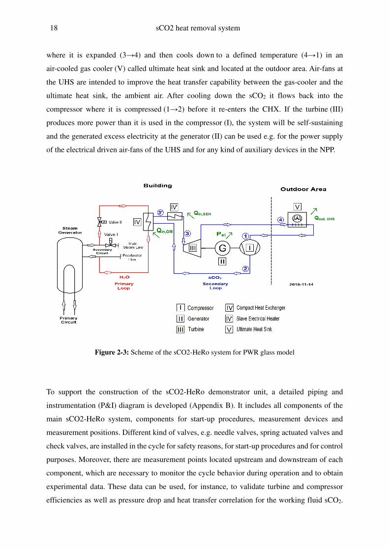
18 sCO2 heat removal system
where it is expanded (3→4) and then cools down to a defined temperature (4→1) in an
air-cooled gas cooler (V) called ultimate heat sink and located at the outdoor area. Air-fans at
the UHS are intended to improve the heat transfer capability between the gas-cooler and the
ultimate heat sink, the ambient air. After cooling down the sCO2 it flows back into the
compressor where it is compressed (1→2) before it re-enters the CHX. If the turbine (III)
produces more power than it is used in the compressor (I), the system will be self-sustaining
and the generated excess electricity at the generator (II) can be used e.g. for the power supply
of the electrical driven air-fans of the UHS and for any kind of auxiliary devices in the NPP.
Figure 2-3: Scheme of the sCO2-HeRo system for PWR glass model
To support the construction of the sCO2-HeRo demonstrator unit, a detailed piping and
instrumentation (P&I) diagram is developed (Appendix B). It includes all components of the
main sCO2-HeRo system, components for start-up procedures, measurement devices and
measurement positions. Different kind of valves, e.g. needle valves, spring actuated valves and
check valves, are installed in the cycle for safety reasons, for start-up procedures and for control
purposes. Moreover, there are measurement points located upstream and downstream of each
component, which are necessary to monitor the cycle behavior during operation and to obtain
experimental data. These data can be used, for instance, to validate turbine and compressor
efficiencies as well as pressure drop and heat transfer correlation for the working fluid sCO2.

sCO2 heat removal system 19
For the control strategy of the cycle, it is also advantageous to have plenty of measurement
positions and measurement devices that provide a whole range of measurement data as input
parameters for the control system. This high density of measurement devices also provides the
possibility to compare the results with each other and to gain information about the quality of
measurement device calibration. Moreover, a unique nomenclature similar to that of the glass
model is introduced. Each component and measurement device is clearly defined by the
nomenclature, which consists of two blocks with letters and numbers, separated by one blank.
The nomenclature as well as a detailed description is given in [36]. For reasons of clarity the
entire sCO2-HeRo set-up is divided into 8 sections according to Appendix B.
Figure 2-4 shows a scheme of section 1 and section 2. Section 1 presents the main sCO2-HeRo
cycle, which is marked with blue and red pipes. The red high-pressure side includes the
compressor, the compact heat exchanger, the slave electrical heater and the turbine. The
low-pressure side is marked with blue pipes and includes the turbine, the ultimate heat sink and
the compressor. Temperature (T), pressure (p), mass flow rate (F) and density (ρ) measurement
devices as well as different kinds of valves are installed to obtain measurement data and for
control purposes. The blue dashed line marked with number 2 (Figure 2-4) depicts the generator
unit of the turbo-compressor-system, which is monitored by a FAG-Smart-Check for measuring
the frequency and a frequency converter. The frequency converter controls the mechanical
load (M), the revolution speed (n), the excess electricity (P) and the temperature (T) at the
generator, according to Hacks et al. [40]. The electricity supply for the frequency converter and
for the FAG-Smart-Check is controlled with voltage (U) and electrical current (I) measurement
devices. To reduce friction losses in the generator and to prevent any kind of damage in the
bearings of the TCS due to high pressure, there is the possibility to have a defined sCO2 leakage
flow in the housing of the TCS [37]; [40], marked with grey pipes. The leakage flow and the
corresponding pressure in the housing can be adjusted by the revolution speed of the leakage
pump and the installed valves. For monitoring the bearing temperatures and the vibration of the
shaft four temperature (T) und two vibration measurement devices (f) are installed.

20 sCO2 heat removal system
Figure 2-4: Scheme of section 1 and 2 of the sCO2-HeRo cycle
The turquoise dashed line on the left in Figure 2-5 shows section 3, the slave electrical heater,
designed and manufactured by ELMESS [41]. The heat input from the SEH into the sCO2 is
controlled and monitored with the measured voltage (U) and current (I) values. Three
temperature measurements (T) at the SEH are used for limiting the electrical heating power
because of internal temperature restrictions. The heat input into the sCO2 can be realized in two
ways. The first one is by adjusting a constant electrical heat power with fixed voltage and
electrical current values and the second one is by means of controlling them via a master-slave
controller. In the master-slave configuration the electrical heating power is adjusted according
to the heat input from the compact heat exchanger, which means that an increased heat input at
the CHX leads to an increased electrical heating power of the SEH. The air side of the ultimate
heat sink is shown on the right in Figure 2-5, marked with a yellow dashed line and numbered
with 4. The air temperature (T) is measured on both sides of the UHS and the pressure (p) as
well as the mass flow rate (F) are measured at the inlet. Since the heat removal to the UHS is
supported by electrical driven fans, voltage (U) and current values (I) can be adjusted and
monitored. An increasing revolution speed of the fans leads to increasing heat transfer
capabilities in the UHS.

sCO2 heat removal system 21
Figure 2-5: Scheme of section 3 and 4 of the sCO2-HeRo cycle
On the left in Figure 2-6, section 5 shows the steam side of the CHX, marked with a purple
dashed line. Measurement devices for measuring the pressure (p) and temperature (T) are
installed at the inlet and outlet of the CHX. The steam mass flow rate (F) is monitored at the
inlet of the CHX. The two needle valves at the inlet and outlet of the CHX on the steam side
are used for connecting or disconnecting the CHX from the PWR glass model. One start-up and
pressure control possibility of the sCO2-HeRo demonstrator unit is shown in section 6, marked
with a green dashed line (on the right in Figure 2-6) [40], [75], [76]. The sCO2 conditions in the
lower chambers of the piston pressure vessels I and II are measured with pressure gauges (p)
and thermocouples (T). It is assumed that in case of an initiated start-up procedure the needle
valve at the bottom of pressure vessel I will be opened and due to the adjusted pressure
difference between the main cycle and the pressure vessel the fluid is forced to flow into the
sCO2-HeRo cycle. It is heated in the CHX and in the slave electrical heater before entering the
turbine, where it forces the turbine to start rotating. After the expansion in the turbine, it flows
through the UHS before it is subdivided into two parts. One part of the sCO2 mass flow rate
enters the lower chamber of pressure vessel II and the other part bypasses the compressor and
re-enters the CHX. After reaching break-even point, the pistons in pressure vessel I and II come
up to defined levels and the TCS is self-sustaining. The amount of sCO2 mass flow rate as well
as the pressure on the high pressure and low pressure side of the cycle can be controlled and
adjusted by varying the nitrogen pressure in the upper chambers of pressure vessel I and II. To
avoid any kind of mechanical overloads in both vessels, spring load safety valves are mounted
at the top of the nitrogen chambers.

22 sCO2 heat removal system
Figure 2-6: Scheme of section 5 and 6 of the sCO2-HeRo cycle
Before starting operation, the sCO2-HeRo cycle has to be evacuated and filled with CO2. The
evacuation is performed by the vacuum-pump unit, marked with a black dashed line, numbered
with 8 and shown on the right in Figure 2-7. For this, the needle valve has to be opened at the
beginning of the evacuation process and closed afterwards. After evacuating the cycle, it is
filled with CO2 by using the blue marked filling-unit of section 7, which is shown on the left
in Figure 2-7. To reduce the chance of freezing, in the first step gaseous CO2 is filled into the
cycle followed by filling with liquid CO2 until the calculated amount of CO2 is reached [40].
Currently the crossed-out needle valve and the CO2-Pump are not installed.
Figure 2-7: Scheme of section 7 and 8 of the sCO2-HeRo cycle

sCO2 heat removal system 23
Table 2-2: Components of the sCO2-HeRo system
Component Manufacturer / Vendor
Compact Heat Exchanger University of Stuttgart
Compressor University of Duisburg-Essen
FAG-Smart-Check Schaeffler Technologies AG & Co. KG
Frequency Converter Vogelsang Elektromotoren GmbH
Generator E+A Elektrotechnik und Aggregatebau mbH
Mass Flow Meters Endress & Hauser Messtechnik GmbH & Co. KG
Pressure Gauges ES Electronic Sensor GmbH
Pressure Vessel I Roth Hydraulics GmbH
Pressure Vessel II Roth Hydraulics GmbH
Pump Speck-Triplex-Pumpen GmbH & Co. KG
Slave Electrical Heater Elmess Thermosystemtechnik
Stainless Steel Pipes Swagelok
Thermal Resistance Thermometers ES Electronic Sensor GmbH
Turbine University of Duisburg-Essen
Ultimate Heat Sink Güntner AG & Co. KG
Vacuum-Pump Available at the glass model
Valves Swagelok
Vibration Sensors Kistler Instrumente GmbH
The components of the sCO2-HeRo demonstrator unit are either manufactured or purchased.
The TCS with integrated generator is designed, manufactured and experimentally investigated
at the University of Duisburg-Essen (UDE), for instance. The compact heat exchanger is
designed, manufactured and testes at the University of Stuttgart (USTUTT). The gas-coolers of
the ultimate heat sink are purchased and investigated at the Research Centre Rez, Prague. The
slave electrical heater, the pressure vessels for the start-up procedure, the stainless steel pipes
as well as the spring-actuated overflow valves, check valves, safety-shut-down valves and
pressure-control valves are purchased. Also the piezo-resistive pressure transmitters, resistance
thermometers, volt- and ampere meters, mass flow meters, frequency converters, FAG
Smart-Checks, electric cables, installation materials, isolating materials, pumps, CO2, nitrogen,
etc. are purchased from different suppliers. After the delivery of all components the system is
built in consideration of the P&I diagram (Appendix B) and commissioning tests are performed.
The most important components are summarized in Table 2-2 in alphabetical order.

24 sCO2 heat removal system
The sCO2-HeRo system for the nuclear power plant
A scheme of the sCO2-HeRo system, attached to the steam generator of a nuclear pressure water
reactor, is shown in Figure 2-8. During normal operation in a PWR, the heat power from the
nuclear core is transferred to the steam generator from the primary circuit to the secondary
circuit. The transferred heat power generates steam in the secondary circuit, which flows
through the main steam line to the turbine, in which it is expanded and condensed before it
re-enters the steam generator via the feedwater line. In case of a combined SBO & LUHS
accident scenario, the reactor is automatically scrammed and the main coolant pumps as well
as the turbine are switched off. To prevent any kind of core damage due to uncontrolled heating
processes, the decay heat must be transferred reliably from the reactor core to the
ultimate-heat-sink. The amount of the decay heat right after shutdown of the reactor is
approximately 6 % of the nominal thermal power and decreases exponentially as a function of
the time [10]. Comparing the schemes of the sCO2-HeRo demonstrator unit (Figure 2-3) and
the sCO2-HeRo system for the NPP (Figure 2-8), it can be seen that both systems are quite
similar. Only the SEH is no longer used in the nuclear power plant application because the
amount of decay heat, the steam pressure and the corresponding steam temperature are
sufficient for designing a self-sustaining decay heat removal system.
Similar to the glass model procedure, at the initiating accident scenario the solenoid valve I is
closed and solenoid valve II is opened automatically, establishing a natural circulation driven
cooling loop in the primary loop, marked in red (Figure 2-8). Driven by natural convection, the
steam flows upwards into a CHX (IV), where the heat is transferred to the sCO2 and the steam
is condensed. The condensate flows downwards and re-enters the steam generator through the
feedwater line. The latent heat of the steam heats up the sCO2 on the secondary side of the
CHX (2→3), located in the containment. After heating up the sCO2 it enters the turbine (III) in
the reactor building, where it is expanded (3→4), followed by cooling down (4→1) in an
air-cooled gas cooler (V) called ultimate heat sink and located at the outdoor area, to a defined
temperature. Air-fans at the UHS are intended to improve the heat transfer capability between
the gas-cooler and the UHS, the ambient air. After cooling down the sCO2 it flows back into the
compressor, where it is compressed (1→2) before it re-enters the CHX. If the turbine (III)
produces more power than is used in the compressor (I), the system will be self-sustaining and
the excess electricity at the generator (II) can be used e.g. for the power supply of the electrical
driven air-fans of the UHS and for any kind of auxiliary devices in the nuclear power plant.

sCO2 heat removal system 25
Figure 2-8: Scheme of the sCO2-HeRo system for NPP
2.3 sCO2-HeRo cycle calculations
After a detailed description of the sCO2-HeRo set-up for the PWR glass model and for the NPP,
the cycle parameters of both sCO2-HeRo systems are determined in this chapter. For this
purpose, cycle calculations are carried out and the design point parameters are determined with
respect to maximum generator excess electricity.
sCO2-HeRo cycle calculations for the PWR glass model
Boundary conditions
The boundary conditions on the steam and sCO2 side are summarized in Table 2-3. The
achievable simulated decay heat power in the PWR glass model is determined by experiments,
according to chapter 2.1. The results show firstly that the higher the heat removal from the
condenser, the lower is the pressure in the steam generator and secondly that the simulated
decay heat power does not exceed 12 kW, which is not suitable for operating more than one
sCO2-HeRo loop at the glass model. In consideration of the experimental data, in which a
higher transferred heat power decreases the driving temperature difference across the CHX and
a lower power remove leads to a very small simulated decay heat power, as a compromise the
design point for the simulated decay heat power is determined at 6 kW. This leads to a saturated

26 sCO2 heat removal system
steam temperature of about 70 °C and a pressure of about 0.3 bar in the steam generator. In
addition, starting from that point, there is also the possibility to perform off-design point
experiments with varying simulated decay heat powers.
The boundary conditions on the sCO2 side must be also considered. For instance, the pressure
and temperature at the inlet of the compressor are the values close to the critical point in the
entire sCO2-HeRo cycle. During operation it must be guaranteed that the inlet conditions are
always above the critical point, which leads to a minimum pressure of about 74 bar and a
minimum temperature of 31 °C. To reduce the complexity and to increase the robustness of the
system, a single stage compressor with a pressure ratio of about 1.5 is chosen [37], [70]. It can
compress the sCO2 from the low-pressure side to a pressure of about 120 bar on the
high-pressure side. To prevent any kind of manufacturing problems of the TCS due to very
small components like the impellers, the minimum necessary sCO2 mass flow rate is set to
0.65 kg/s. The electrical heating power of the SEH is determined, with respect to the accessible
electrical installation power, at 200 kW. This is sufficient for heating up the sCO2 mass flow
rate to a turbine inlet temperature of 200 °C, which is similar to NPP conditions. The turbine
efficiency of 75 % and the compressor efficiency of 65 % are conservative assumptions for
such a small machine from the colleagues from University of Duisburg-Essen (UDE) and they
are assumed to be constant for the entire range of cycle calculations.
Table 2-3: Boundary conditions - cycle calculations glass model
Variable Value Unit Description
�NO,TU 6 kW Decay Heat Power Per Unit - Glass Model �V W 0.3 bar Pressure - Steam 'V W 70 °C Temperature - Steam
�NO,XYV 200 kW Heating Power - SEH �ZW ,[NO 74 bar Pressure - Minimum sCO2 �ZW ,[$\ 120 bar Pressure - Maximum sCO2 'ZW ,[NO 31 °C Temperature - Minimum sCO2 �� ZW ,[NO 0.65 kg/s Mass Flow Rate - Minimum sCO2
1Z,N] 0.65 % Isentropic Efficiency - Compressor 1^,N] 0.75 % Isentropic Efficiency - Turbine
N 1 - Number of sCO2-HeRo Demonstrator Units

sCO2 heat removal system 27
Cycle calculations
A scheme of the sCO2-HeRo demonstrator unit, attached to the PWR glass model, is shown on
the left and the corresponding temperature-entropy (T-S) diagram on the right in Figure 2-9.
The main components are numbered with I, II, III, IV, IV’, V and the thermodynamic state in
front and behind of each component with 1, 2, 3, 3’ and 4.
Figure 2-9: Scheme of the sCO2-HeRo system for GM and T-S diagram
For the cycle calculations it is necessary to specify the compressor inlet pressure �-, the
compressor inlet temperature '-, the isentropic compressor efficiency 1Z,N] and the isentropic
turbine efficiency 1^,N]. Required thermo-physical fluid properties are obtained from the
database NIST Refprop [43].
The calculation starts at point 1 in the T-S diagram (Figure 2-9), where the thermodynamic state
is already defined by the selected pressure �- and temperature '-. The enthalpy - (Eq. (2-1))
and entropy "- (Eq. (2-2)) at the inlet of the compressor (I) are functions of the pressure �- and
temperature '-. Both are calculated with NIST Refprop.
- 9 �_�-, '-` (2-1)
"- 9 �_�-, '-` (2-2)

28 sCO2 heat removal system
The enthalpy ℎ and temperature ' at the outlet of the compressor (I) are calculated by
Eq. (2-3) and Eq. (2-4). The used isentropic enthalpy ℎ N] is calculated with Refprop as a
function of the determined pressure � on the high pressure side and the entropy " N] by
Eq. (2-5). It is assumed that the entropy " N] is equal to "- (Eq. (2-6)).
ℎ = ℎ N] − ℎ-1Z,N] + ℎ- (2-3)
' = �(� , ℎ ) (2-4)
ℎ N] = �(� , " N]) (2-5)
" N] = "- (2-6)
The enthalpy ℎc at the inlet of the turbine (III) is calculated according to Eq. (2-7) as a function
of the turbine inlet pressure �c and the determined turbine inlet temperature 'c. It is assumed
that no pressure drop occurs in the CHX (IV) and in the SHE (IV’), hence �c is equal to �
(Eq. (2-8)). Furthermore, the sCO2 heat input occurs in two steps, firstly from the CHX into the
sCO2 (ℎ → ℎce) and secondly from the SEH into the sCO2 (ℎce → ℎc). The entropy "c at the
inlet of the turbine is a function of the pressure �c and the temperature 'c according to Eq. (2-9).
ℎc = �(�c, 'c) (2-7)
�c = � (2-8)
"c = �(�c, 'c) (2-9)
The enthalpy ℎf and temperature 'f at the outlet of the turbine are calculated by Eq. (2-10) and
Eq. (2-11). The used isentropic enthalpy ℎfN] is calculated by Eq. (2-12) as a function of the
pressure �f and the entropy "fN]. It is assumed that the pressure �f is equal to the compressor
inlet pressure �- (Eq. (2-13)), which means that no pressure drop occurs in the UHS (V) and
that the entropy "fN] is equal to the entropy "c (Eq. (2-14)).

sCO2 heat removal system 29
ℎf = ℎc − (ℎc − ℎfN]) · 1^,N] (2-10)
'f = �(�f, ℎf) (2-11)
ℎfN] = �(�f, "fN]) (2-12)
�f = �- (2-13)
"fN] = "c (2-14)
According to an energy balance, the excess power of the cycle is the difference between turbine
and compressor work multiplied by the mass flow rate �� . Assuming a generator efficiency
of 100 %, the excess electricity ��� can be calculated by Eq. (2-15).
��� = �� · ((ℎc − ℎf) − (ℎ − ℎ-)) (2-15)
Within the cycle calculations, a parameter study is conducted with varying cycle parameters
like the turbine inlet pressure �c, the turbine inlet temperature 'c, the mass flow rate �� , the
temperature at the inlet of the compressor '- and the pressure at the inlet of the compressor �-.
Moreover, the number of TCS for parallel use depends on the required operational time of the
sCO2-HeRo system, the existing amount of decay heat power and the determined sCO2 mass
flow rate. Several turbo-machine sets in parallel give the opportunity to shut down one after
another while the decay heat is decreasing. In consideration of the given boundary conditions
at the glass model, like a decay heat power of 6 kW and a sCO2 mass flow rate of 0.65 kg/s, the
calculations are performed only for one sCO2-HeRo unit.
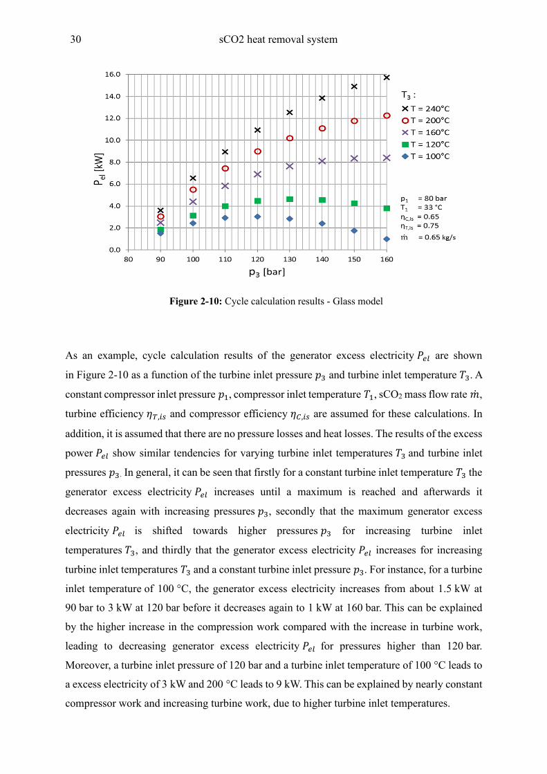
30 sCO2 heat removal system
Figure 2-10: Cycle calculation results - Glass model
As an example, cycle calculation results of the generator excess electricity ��� are shown
in Figure 2-10 as a function of the turbine inlet pressure �c and turbine inlet temperature 'c. A
constant compressor inlet pressure �-, compressor inlet temperature '-, sCO2 mass flow rate �� , turbine efficiency 1^,N] and compressor efficiency 1Z,N] are assumed for these calculations. In
addition, it is assumed that there are no pressure losses and heat losses. The results of the excess
power ��� show similar tendencies for varying turbine inlet temperatures 'c and turbine inlet
pressures �c. In general, it can be seen that firstly for a constant turbine inlet temperature 'c the
generator excess electricity ��� increases until a maximum is reached and afterwards it
decreases again with increasing pressures �c, secondly that the maximum generator excess
electricity ��� is shifted towards higher pressures �c for increasing turbine inlet
temperatures 'c, and thirdly that the generator excess electricity ��� increases for increasing
turbine inlet temperatures 'c and a constant turbine inlet pressure �c. For instance, for a turbine
inlet temperature of 100 °C, the generator excess electricity increases from about 1.5 kW at
90 bar to 3 kW at 120 bar before it decreases again to 1 kW at 160 bar. This can be explained
by the higher increase in the compression work compared with the increase in turbine work,
leading to decreasing generator excess electricity ��� for pressures higher than 120 bar.
Moreover, a turbine inlet pressure of 120 bar and a turbine inlet temperature of 100 °C leads to
a excess electricity of 3 kW and 200 °C leads to 9 kW. This can be explained by nearly constant
compressor work and increasing turbine work, due to higher turbine inlet temperatures.

sCO2 heat removal system 31
In consideration of the boundary conditions (Table 2-3) and the cycle calculation results, the
design point parameters of the sCO2-HeRo demonstrator are determined (Table 2-4). The
compressor inlet pressure �- and inlet temperature '- are set to 78.3 bar and 33 °C, with respect
to their location near the critical point (74 bar / 31 °C). The installed electrical heating power
of the SEH with 200 kW and the comparability with NPP conditions leads to a turbine inlet
temperature 'c of 200 °C. For heating up the sCO2 mass flow rate �� of 0.65 kg/s from about
49 °C at the outlet of the CHX, to 200 °C at the inlet of the turbine, an electrical heating power
of about 196 kW is used. With respect to the achievable compression ratio of the single-stage
compressor, the turbine inlet pressure �c is set to 117.45 bar. The compressor efficiency 1Z,N]
and the turbine efficiency 1^,N] of 0.65 and 0.75 are conservative assumptions for such small
engines. A cooling power of about 187 kW is necessary to cool down the sCO2 mass flow rate
in the UHS. In the design point, the generator provides an excess electricity ��� of about 9 kW.
Table 2-4: sCO2-HeRo cycle parameters for the PWR glass model
Variable Value Unit Description
�- 78.3 bar Pressure - Inlet Compressor '- 33.0 °C Temperature - Inlet Compressor 1Z,N] 65 % Isentropic Efficiency - Compressor �c 117.45 bar Pressure - Inlet Turbine 'c 200.0 °C Temperature - Inlet Turbine 1^,N] 75 % Isentropic Efficiency - Turbine �� 0.65 kg/s Mass Flow Rate - sCO2 �NO,XYV 195.56 kW Heat Input - SEH �PQR,gVX 186.83 kW Heat Output - UHS ��� 8.7 kW Excess Electricity - Generator �NO,TU 6 kW Heat Input - Glass Model

32 sCO2 heat removal system
sCO2-HeRo cycle calculations for a NPP
Boundary conditions
The boundary conditions for the sCO2-HeRo cycle calculations are summarized in Table 2-5.
The simulation results of Venker [10] for a BWR with a thermal power of 3860 MW show for
instance that 60 MW decay heat must be removed by the sCO2-HeRo cycle in order to achieve
a long-term coolability of the nuclear core and to prevent any kind of depressurization. Any
surplus decay heat occurring right after shut-down is stored additionally inside the condensation
chamber. Moreover, saturated steam conditions with a steam pressure of 70 bar and a
corresponding steam temperature of 286 °C are assumed. Furthermore, a minimum temperature
difference of 5 °C is defined for both heat exchangers to ensure an efficient heat transfer. The
temperature of the ambient air is conservatively set to 37 °C.
Table 2-5: Boundary conditions - cycle calculations NPP
Variable Value Unit Description
�NO,hii 15 MW Decay Heat Power Per Unit - NPP �V W 70 bar Pressure - Steam 'V W 286 °C Temperature - Steam
�ZW ,[NO 75 bar Pressure - Minimum sCO2 �ZW ,[$\ 200 bar Pressure - Maximum sCO2 'ZW ,[NO 42 °C Temperature - Minimum sCO2 'ZW ,[$\ 281 °C Temperature - Maximum sCO2
1Z,N] 0.75 % Isentropic Efficiency - Compressor 1^,N] 0.85 % Isentropic Efficiency - Turbine
N 4 - Number of sCO2-HeRo Units
These boundary conditions lead to a minimum sCO2 temperature of 42 °C at the outlet of the
UHS and a maximum sCO2 temperature of 281 °C at the inlet of the turbine. The minimum
sCO2 pressure at the inlet of the compressor is set to 75 bar, with respect to its location near to
the critical point. Furthermore, an isentropic turbine efficiency 1^,N] of 0.85, an isentropic
compressor efficiency 1^,N] of 0.75 and a compression ratio of 3 are assumed. Venker also
recommends that the amount of removed decay heat should be adjusted according to the
existing decay heat in order to ensure a high temperature difference between the ambient air

sCO2 heat removal system 33
and the primary steam, which results in increased operational time of the sCO2-HeRo system.
This is realized by using four equal 15 MW sCO2-HeRo units in parallel, instead of one 60 MW
unit, which can be individually controlled and switched off consecutively. In addition, four
sCO2-HeRo units can be build as physically separated units inside an NPP, which is an
advantage in case of accident scenarios like fire and mechanical impacts.
Cycle calculations
A scheme of a 15 MW sCO2-HeRo unit is shown on the left in Figure 2-11 and the T-S diagram
on the right. The main components are numbered with I, II, III, IV, V and the thermodynamic
state in front of and behind each component with 1, 2, 3 and 4. Comparing the schemes of the
demonstrator (Figure 2-9) and the system for a NPP (Figure 2-11) it can be seen that both are
quite similar. Only the SEH (IV’) is no longer used in the NPP, because the amount of decay
heat and the steam temperature are high enough for the self-sustaining of the sCO2-HeRo.
Figure 2-11: Scheme of the sCO2-HeRo system for NPP and T-S diagram
The cycle calculations are carried out similar to those of the sCO2-HeRo demonstrator unit,
just without the SEH. It must be mentioned that a constant sCO2 mass flow rate �� of 0.65 kg/s
and constant turbine inlet temperatures 'c are assumed for the sCO2-HeRo demonstrator,
leading to different electrical heating powers �NO,XYV of the SEH. In the sCO2-HeRo system for
a NPP, a constant transferred decay heat power �NO,hii of 15 MW and constant turbine inlet
temperatures 'c are assumed, leading to varying sCO2 mass flow rates �� . At the start, the

34 sCO2 heat removal system
compressor inlet pressure �-, the compressor inlet temperature '-, the isentropic compressor
efficiency 1Z,N], the isentropic turbine efficiency 1^,N] the condensing power of the
steam �NO,hii and the turbine inlet temperature 'c are determined. Furthermore, no pressure
losses and heat losses are assumed. Thermo-physical fluid properties are obtained from the
database NIST Refprop [43]. The cycle calculations are performed according to
Eq. (2-1) - (2-14) in consideration of varying compressor inlet pressures �- from 75 bar
to 199 bar, turbine inlet pressures �c from 76 bar to 200 bar and turbine inlet temperatures 'c
of 280 °C, 250 °C, 200 °C and 150 °C. The compressor inlet temperature '-, the isentropic
compressor efficiency 1Z,N], the isentropic turbine efficiency 1^,N] and the transferred
condensing power of the steam �NO,hii are assumed to be constant for the calculations. The
necessary sCO2 mass flow rate �� is calculated with the help of the steam condensing
power �NO,hii and the used turbine inlet temperature 'c. The excess electricity at the
generator ��� is calculated for each configuration according to Eq. (2-15).
A few results of cycle calculation of the generator excess electricity ��� are shown in Figure
2-12 as a function of the sCO2 turbine inlet pressure �c and the turbine inlet temperature 'c.
The compressor inlet pressure �-, the compressor inlet temperature '-, the turbine
efficiency 1^,N], the compressor efficiency 1Z,N] and the transferred condensing power of the
steam �NO,hii are assumed to be constant and given on the bottom right.
Figure 2-12: Cycle calculation results - NPP

sCO2 heat removal system 35
The results in Figure 2-12 show that, for a constant turbine inlet temperature 'c, the generator
excess electricity ��� increases until a maximum is reached and decreases again with increasing
pressures �c. Moreover, the maximum generator excess electricity ��� is shifted towards higher
pressures �c for increasing turbine inlet temperatures 'c and the generator excess electricity ��� increases for increasing turbine inlet temperatures 'c and constant turbine inlet pressures �c.
The results for a turbine inlet temperature of 150 °C show that a turbine inlet pressure of 120 bar
leads to a generator excess electricity of 0.38 MW, 170 bar leads to 0.68 MW and 200 bar leads
to 0.60 MW. Furthermore, a constant turbine inlet pressure of 180 bar and a turbine inlet
temperature of 150 °C leads to a generator excess electricity of 0.64 MW, 200 °C to 1.02 MW,
250 °C to 1.18 MW and 280 °C to a generator excess electricity of 1.22 MW.
For the determination of the optimum pressure ratio of the sCO2-HeRo system, with respect to
maximum excess electricity and the given boundary conditions, the calculated results of the
excess electricity are presented in Figure 2-13 by specific colors. The excess electricity is
calculated by using the generator excess electricity minus the necessary electricity of the air
fans, determined by Venker [10] at 0.165 MW for a 15 MW sCO2-HeRo unit. Areas colored in
blue present pressure ratios where maximum excess electricity is achieved for all investigated
turbine inlet temperatures and areas colored in yellow show pressure ratios where excess
electricity is reached. Areas colored in green show pressure ratios where negative excess
electricity occurs if the turbine inlet temperature does not exceed 150 °C and areas colored in
red present pressure ratios where negative excess electricity occurs at turbine inlet temperatures
which are less than 280 °C. The depicted results show that maximum excess electricity is
achieved for the blue colored pressure ratios of 90/160 bar, 90/170 bar, 90/180 bar, 90/190 bar,
90/200 bar, 100/180 bar, 100/190 bar¸ 100/200 bar and 110/200 bar. Negative excess electricity
occurs for green colored pressure ratios of 80/170 bar, 80/180 bar, 80/190 bar, 80/200 bar,
120/130 bar, 170/190 bar and 180/200 bar if the turbine inlet temperature does not exceed
150 °C. The red colored pressure ratios of 130/140 bar, 140/150 bar, 150/160 bar, 160/170 bar,
170/180 bar, 180/190 bar and 190/2000 bar show pressure ratios, where negative excess
electricity occurs, if the turbine inlet temperature is less than 280 °C. For the design of the
15 MW sCO2-HeRo unit, it is recommended to use pressure ratios colored in blue, because
these are most promising for a robust and self-sustaining system. Pressure ratios colored in red,
green and yellow should be avoided, because they would lead to low or negative excess
electricity. The results also show that maximum excess electricity is achieved for a compressor
inlet pressure of 90 bar, except for a turbine inlet temperature of 150 °C.

36 sCO2 heat removal system
jK [bar]
jk
[bar]
90 100 110 120 130 140 150 160 170 180 190 200
80
90
100
110
120
130
140
150
160
170
180
190
Figure 2-13: Cycle calculation results - NPP II
Because of that, the compressor inlet pressure �- is determined at 90 bar and the compressor
inlet temperature '- is set to 42 °C, with respect to an ambient air temperature of 37 °C and a
minimum temperature difference of 5 °C in the UHS. Furthermore, the results verify that a
compressor inlet pressure of 90 bar and increasing turbine inlet pressures �c results in
increasing excess electricity. Various issues like pressure restrictions, material costs, thermal
inertias, heat transfer behaviors, achievable pressure ratios and the cycle behavior outside the
design point must be taken into account for the determination of the turbine inlet pressure �c.
In consideration of the results, the pressure at the inlet of the turbine is set to 180 bar, which
leads to an excess electricity of 1.21 MW for a turbine inlet temperature 'c of 280 °C. Finally,
the sCO2 mass flow rate �� of 47.7 kg/s, the generator excess electricity ��� of 1.38 MW and
the transferred heat power in the UHS �PQR,gVX of 13.62 MW are calculated for the design point.
The sCO2-HeRo cycle parameters for a nuclear power plant are summarized in Table 2-6.

sCO2 heat removal system 37
Table 2-6: sCO2-HeRo cycle parameters for a NPP
Variable Value Unit Description
�- 90 bar Pressure - Inlet Compressor '- 42 °C Temperature - Inlet Compressor 1Z,N] 75 % Isentropic Efficiency - Compressor �c 180 bar Pressure - Inlet Turbine 'c 280 °C Temperature - Inlet Turbine 1^,N] 85 % Isentropic Efficiency - Turbine �� 47.7 kg/s Mass Flow Rate - sCO2 �PQR,gVX 13.6 MW Heat Output - UHS ��� 1.38 MW Excess Electricity - Generator �NO,hii 15 MW Heat Input - NPP

38 sCO2 heat removal system

Test facility and HX test plates 39
3 Test facility and HX test plates
3.1 Test facility
Three test facilities are used for the experimental investigation on the heat transfer between
condensing steam and supercritical CO2 in compact heat exchangers. The first one is the
SCARLETT loop, which provides sCO2 under defined conditions, the second one is a newly
constructed low-pressure steam cycle, which generates steam similar to the steam conditions at
the glass model, and the third one is a newly constructed high-pressure steam cycle, which
provides steam similar to the steam conditions in a nuclear power plant.
3.1.1 sCO2 SCARLETT loop
The SCARLETT loop is designed and built at the Institute of Nuclear Technology and Energy
Systems, Stuttgart. It is a multi-purpose test facility that provides supercritical CO2 under
defined conditions for different kind of experiments like heat transfer investigations and
research in material science. A simplified piping and instrumentation diagram of the loop is
depicted in Figure 3-1 and described below.
Before starting operation, the SCARLETT loop (Figure 3-1) is evacuated with a vacuum pump
of the filling unit (0). For this purpose, the valves V1 and V2 are opened and the vacuum pump
is switched on until a pressure of less than 0.05 bar is reached. Afterwards, valve V1 is closed
and valves V2 and V3 are opened before gaseous CO2 is filled into the loop until a pressure of
about 7 bar is reached. In the following, the storage vessel (1) is filled with liquid CO2 by a gas
bottle until the necessary amount of CO2 is reached before all valves are closed again. After
finishing the evacuation and filling procedure, the SCARLETT loop is ready for operation.
During normal operation liquid CO2 flows from the storage vessel (1) through the electrical
heated evaporator (2) and is slightly overheated. After leaving the droplet separator (3), where
remaining liquid CO2 is separated from the flow, it enters the compressor (4). In the piston
compressor the CO2 is compressed up to a certain pressure and simultaneously heated-up.
Before entering the test section, marked in green, there is the possibility of conditioning (5) the
sCO2. This means that a defined temperature can be adjusted by means of cooling or heating
the sCO2. In the test section different kind of experiments can be performed, for instance
investigation on the heat transfer capability in CHXs, electrically heated plates and material
science. The installed measurement devices, e.g. pressure gauges, resistance thermometers

40 Test facility and HX test plates
(Pt-100) and mass flow meters, at the inlet (5) and outlet (5’) of the test section measure relevant
parameters of the experiments. After leaving the test section, the sCO2 is cooled down in the
gas chiller (6) at the outdoor area and afterwards it is expanded in the expansion valve (7).
Before entering the storage vessel, it is cooled down again in a condenser (8).
Figure 3-1: P&I diagram of the SCARLETT loop
Table 3-1 summarizes the boundary conditions of the SCARLETT loop. The sCO2 mass flow
rate �� can be adjusted from about 10 g/s to 110 g/s by setting the rotational speed of the piston
compressor. In addition, the achievable mass flow rate depends on the performance map of the
compressor, which leads to a lower mass flow rate at higher pressure ratios and vice versa. The
temperature ' at the inlet of the test section can be varied between 0 °C to 150 °C by means of
cooling or heating, while the pressure � can be adjusted from 75 bar to 120 bar. For evaporating
and overheating the CO2 mass flow rate before it enters the compressor, there is an electrical
heating power �NO,Yl$� of 36 kW installed. After the compressor the sCO2 can be conditioned
before entering the test section by cooling with a power of 48 kW (�PQR,ZPOmN) or heating
with 16 kW (�NO,V�$R). The installed gas chillers can transfer about 32 kW (�PQR,T$]) of waste
heat from the loop to the ambient air. After the expansion in the expansion valve, the CO2 can
be cooled down again in the condenser with a condensing power �PQR,ZPOm� of 13 kW before it
re-enters the storage vessel. The storage vessel has a volume * of 0.07 m³.

Test facility and HX test plates 41
Table 3-1: SCARLETT parameters
Variable Value Unit Description
�� 10 - 110 g/s sCO2 Mass Flow Rate ' 0 - 150 °C Temperature - Inlet Test Section � 75 - 120 bar Pressure - Inlet Test Section �NO,Yl$� 36 kW Power - Evaporator �PQR,ZPOmN 48 kW Power - Conditioning Cooling �NO,V�$R 16 kW Power - Conditioning Heating �PQR,T$] 32 kW Power - Gas Chiller �PQR,ZPOm� 13 kW Power - Condenser * 0.07 m³ Volume - Pressure Vessel
3.1.2 Steam cycle
High-pressure steam cycle
The high-pressure steam cycle is constructed to provide steam with a pressure of 70 bar and a
temperature of 286 °C, similar to the steam conditions in a NPP. It is used in the current work
for the experimental investigation of the heat transfer capability between condensing steam and
sCO2 in heat exchangers. The P&I diagram of the high-pressure steam cycle (red pipes), the
installed two-plate CHX and the sCO2 side (green pipes) is depicted in Figure 3-2. Before
starting operation, a vessel (1) is filled with deionized water. The water is pumped from the
vessel (1) by a high-performance liquid chromatography pump (3) (HPLC) through a filter (2)
into an electrical heated evaporator (4). Inside the water is evaporated and slightly overheated
before the steam enters a test section (5). Different kind of components like two-plate CHX’s
and shell-and-tube heat exchangers can be installed in the test section. The pressure in the cycle
can be adjusted by the mechanical primary pressure control valve (6). After the expansion in
the pressure control valve, the condensate flows into a second vessel (7) and is pumped back
into vessel (1). For monitoring the cycle behavior during operation, measurement devices like
resistance thermometers ('), pressure gauges (�) and a mass flow meter (�� ) are installed. The
measurement position and the nomenclature of each measurement device are also shown. A
detailed description of the used measurement devices, their measurement range and the
measurement uncertainties are given in the following chapter.

42 Test facility and HX test plates
Figure 3-2: P&I diagram of the high-pressure steam cycle with two-plate CHX
The boundary conditions of the high-pressure steam cycle and a summary of the main
components are given in Table 3-2 and Table 3-3. The water volume flow rate �� V W can be
adjusted by the HPLC pump (3) from 0.05 l/h to 2.5 l/h and the electrical heating
power �NO,Yl$� of the evaporator (4) with 1.6 kW is sufficient for evaporating and overheating
the adjusted water volume flow rates. The pressure � at the inlet of the test section can be
adjusted by the mechanical primary pressure control valve (6) from 1 bar to 105 bar and the
corresponding steam temperature ' rises from 100 °C to 315 °C. The water storage vessels (1)
and (7) have a volume * of about 2 liters each and they are manufactured by IKE. A fuel
filter (2) from Festo is installed in front of the HPLC pump to ensure that only pure water flows
through the pump. The HPLC pump (3) and the electrical heated evaporator (4) are purchased
from the company TTI-GmbH-CHEMPION. The primary pressure control valve (6) of the
series 26-1700 is purchased from TESCOM EUROPE GmbH. The ½” and ¼” stainless steel
pipes, valves and pipe connectors from Swagelok are selected with respect to existing pressures
and temperatures. Rock wool and high-temperature Armaflex are used as insulation materials.
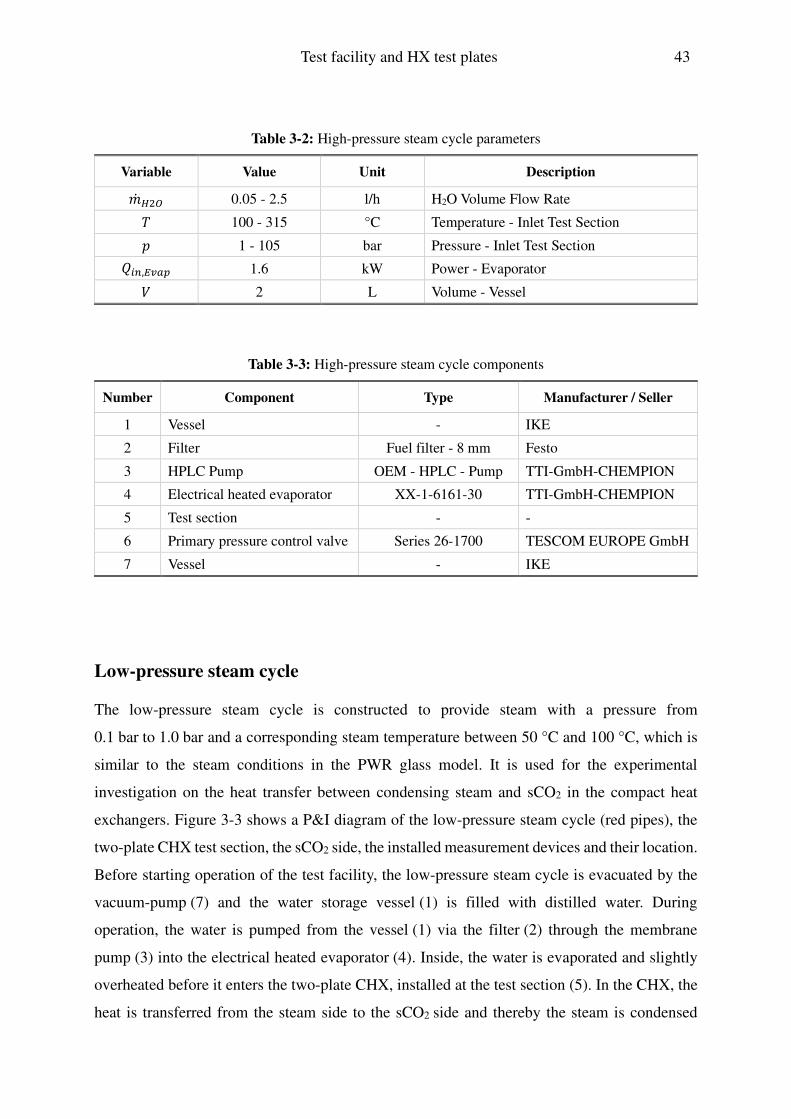
Test facility and HX test plates 43
Table 3-2: High-pressure steam cycle parameters
Variable Value Unit Description
�� V W 0.05 - 2.5 l/h H2O Volume Flow Rate ' 100 - 315 °C Temperature - Inlet Test Section � 1 - 105 bar Pressure - Inlet Test Section �NO,Yl$� 1.6 kW Power - Evaporator * 2 L Volume - Vessel
Table 3-3: High-pressure steam cycle components
Number Component Type Manufacturer / Seller
1 Vessel - IKE
2 Filter Fuel filter - 8 mm Festo
3 HPLC Pump OEM - HPLC - Pump TTI-GmbH-CHEMPION
4 Electrical heated evaporator XX-1-6161-30 TTI-GmbH-CHEMPION
5 Test section - -
6 Primary pressure control valve Series 26-1700 TESCOM EUROPE GmbH
7 Vessel - IKE
Low-pressure steam cycle
The low-pressure steam cycle is constructed to provide steam with a pressure from
0.1 bar to 1.0 bar and a corresponding steam temperature between 50 °C and 100 °C, which is
similar to the steam conditions in the PWR glass model. It is used for the experimental
investigation on the heat transfer between condensing steam and sCO2 in the compact heat
exchangers. Figure 3-3 shows a P&I diagram of the low-pressure steam cycle (red pipes), the
two-plate CHX test section, the sCO2 side, the installed measurement devices and their location.
Before starting operation of the test facility, the low-pressure steam cycle is evacuated by the
vacuum-pump (7) and the water storage vessel (1) is filled with distilled water. During
operation, the water is pumped from the vessel (1) via the filter (2) through the membrane
pump (3) into the electrical heated evaporator (4). Inside, the water is evaporated and slightly
overheated before it enters the two-plate CHX, installed at the test section (5). In the CHX, the
heat is transferred from the steam side to the sCO2 side and thereby the steam is condensed

44 Test facility and HX test plates
before it flows downwards driven by gravity and leaves the two-plate CHX at the bottom. Due
to different test configurations, it can happen that the steam is not completely condensed at the
outlet of the test section. Therefore, an additional condenser is installed to ensure that only
condensate re-enters the water storage vessel (1). The sCO2 enters the test section from the
bottom right, flows upwards in the CHX, is heated and leaves the test section at the top right.
For monitoring the cycle, measurement devices like mass flow rate meter (�� ), temperature
measurement devices ('), pressure gauges (�) as well as Voltage and Ampere meters are
installed. The measurement position and the nomenclature of each measurement device are
depicted in Figure 3-3. Important measurement points are the temperatures, mass flow rates and
pressures at the inlet and outlet of the CHX on both sides and the electrical heating power of
the evaporator, calculated with the Voltage- and Ampere measurement data. A detailed
description of the used measurement devices, their measurement ranges and their measurement
uncertainties are given in the following chapter.
The boundary conditions of the low-pressure steam cycle are shown in Table 3-4 and the
components are summarized in Table 3-5. The water volume flow rate �� V W can be adjusted
by the membrane pump (3) from 0.05 l/h to 2.5 l/h and the electrical heating power �NO,Yl$� of
the evaporator (4) with 1.6 kW is sufficient for evaporating and overheating the adjusted water
volume flow rates. The pressure � at the inlet of the test section can be adjusted from 0.1 bar
to 1.0 bar and the corresponding steam temperature ' rises from about 50 °C to 100 °C. The
water storage vessel (1) has a volume * of about 2 liters and is manufactured by IKE. A fuel
filter (2) from Festo is installed in front of the membrane pump to ensure that only pure water
flows through the pump. The membrane pump (3) and the electrical heated evaporator (4) are
purchased from TTI-GmbH-CHEMPION. The condenser (6) is designed as double-pipe heat
exchanger and manufactured by IKE. The vacuum pump (7) is purchased from Pfeiffer and
the ½” and ¼” stainless steel pipes, valves and pipe connectors are bought from the
manufacturer Swagelok. High-temperature Armaflex is used as insulation material.

Test facility and HX test plates 45
Figure 3-3: P&I diagram of the low-pressure steam cycle with two-plate CHX
Table 3-4: Low-pressure steam cycle parameters
Variable Value Unit Description
�� V W 0.05 - 2.5 l/h H2O Volume Flow Rate ' 50 - 100 °C Temperature - Inlet Test Section � 0.1 - 1.0 bar Pressure - Inlet Test Section �NO,Yl$� 1.6 kW Power - Evaporator * 2 L Volume - Vessel
Table 3-5: Low-pressure steam cycle components
Number Component Type Manufacturer / Seller
1 Vessel - IKE
2 Filter Fuel filter - 8 mm Festo
3 Membrane pump TTI-GmbH-CHEMPION
4 Electrical heated evaporator XX-1-6161-30 TTI-GmbH-CHEMPION
5 Test section - -
6 Condenser - IKE
7 Vacuum pump Uno 6 Pfeiffer

46 Test facility and HX test plates
3.1.3 Measurement devices and uncertainties
This chapter includes a general description of the installed measurement devices and their
measurement techniques. Afterwards, they measurement uncertainties are described followed
by a discussion of the error propagation for calculated parameters.
Type of measurement
Temperature
Thermal resistance platinum thermometers (Pt-100) are used for temperature measurements.
They are classified according to A and B, and the Pt-100 A type is used in both steam cycles.
The Pt-100 has a nominal resistance of 100 Ω at 0 °C and a nearly linear change in the resistance
as a function of the temperature. A mean temperature coefficient of 0.0039 -°Z is assumed
for 0 °C to 100 °C. The measurement uncertainty of the temperature σ is given by the equation
±(0.15 °� + 0.002 · T [°C]), which leads to an uncertainty of ± 0.35 °C at 100 °C, ± 0.55 °C
at 200 °C and ± 0.75 °C at 300 °C. To improve the measurement accuracy and to compensate
resistances in cables, a 4-wire measurement technique is selected. The Pt-100 technology is
chosen because it can be applied for temperatures between - 200 °C and 850 °C, it has a high
measurement accuracy, it is easily replaceable and it guarantees a high long-term stability.
Pressure
The pressure in both steam cycles is measured with piezoresistive pressure transmitters from
Keller, Switzerland. The piezoresistive effect is based on the change in electrical resistance of
the piezoresistive material as a function of the mechanical stress. The mechanical stress, or
more in detail the change in the electrical resistance, is converted into a voltage signal, which
can be used via 3-wire measurement technique in the measurement data acquisition.
Piezoresistive pressure transmitters are constructed as absolute, relative and differential
pressure transmitters. They can be applied for different kind of working fluids with pressures
from 0.2 bar to 1000 bar and temperatures from - 40°C to 300 °C. In consideration of the
existing pressures in the low-pressure steam cycle (0.1 bar - 1.0 bar) and high-pressure steam
cycle (1 bar - 105 bar), the temperatures in the low-pressure steam cycle (20 °C - 100 °C) and
high-pressure steam cycle (100 °C - 315 °C) as well as the occurring pressure drops in the
two-plate CHX test section (0 bar - 3 bar), the pressure transmitters are selected with respect to
each application. A detailed specification of each pressure transmitter and his measurement
error is given in Table 3-6.

Test facility and HX test plates 47
Mass and volume flow rate
The sCO2 mass flow rate is measured with a Coriolis mass flow meter from Schwing
Verfahrenstechnik GmbH, Germany. The chosen RHM-03 measurement transducer is designed
for measuring sCO2 mass flow rates from 0 g/s to 100 g/s with temperatures up to 120 °C and
pressures up to 200 bar. The measurement system is constructed as a two-pipe configuration
with a pipe diameter of 3 mm, arranged in parallel. The transmitter RHE-16 is chosen as
analysis unit with a 4 mA - 20 mA analog output. In general, with Coriolis mass flow meters
pressures up to 1000 bar, temperatures from - 196 °C to 350 °C and mass flow rates
between 1 g/min and 1500 t/h can be measured for various liquid and gaseous working fluids.
In addition, measurement ranges of more than 50:1, measurement uncertainties of less
than ± 0.2 % and reproducibility’s higher than ± 0.1 % can be achieved. The measurement
technique is non-invasive, suitable for pulsating mass flow rates, insensitive to gas inclusions
and based on the Coriolis effect, which is described briefly. Sensors are mounted at the inlet
and outlet of the oscillating system of the Coriolis mass flow meter. If there is no mass flow,
the signals are in phase; otherwise, a phase shift between the two signals occurs. This phase
shift is proportional to the mass flow rate in the measurement device. The water volume flow
rate is measured with the calorimetric volume flow meter DTH08 from the manufacturer
PKP-Prozessmesstechnik. It can be applied for liquid working fluids, has a measurement range
from 0.06 l/h to 120 l/h, withstands temperatures up to 70 °C and pressures up to 10 bar. For
the investigations it is calibrated from 0 l/h to 5 l/h. It is a non-invasive measurement
technology, insensitive to dirt and the measurement device provides 0 V - 10 V analog output
signals for the measurement data acquisition. The measurement technique consists of two
temperature sensors, one is heated. If no working fluid flows through the measurement device,
a constant temperature at the heated sensor and a constant gradient between both sensors exist.
If a media flows, the heated sensor is cooled down and the gradient of the cooling procedure is
proportional to the volume flow rate. A measurement uncertainty of less than ± 5 % of the
measured value can be assumed.

48 Test facility and HX test plates
Measurement devices installed
The measurement devices installed at the low-pressure (LP) and high-pressure (HP) steam cycle
are summarized in Table 3-6. After each variable name, the measurement range, a short
description, the measurement uncertainty and the type of each measurement device are given.
The uncertainties are derived from manufacturers instructions. The uncertainty of the
temperature measurement, for instance, is given as a function of the measured temperature '
according to ±(0.15 °� + 0.002 · T [°C]) and the uncertainty of the pressure measurement
depends on the measurement device as well as on the measurement range. The uncertainty of
the water volume flow rate measurement is given by the manufacturer with ± 5 % of the
measurement value, leading to higher absolute uncertainties for higher volume flow rates and
the uncertainty of the sCO2 mass flow rate is given with ± 0.8 g/s.

Test facility and HX test plates 49
Table 3-6: Installed measurement devices at LP and HP steam cycle
Variable Cycle Value Unit Description Errors Device
�� V W
LP 0 - 5 l/h H2O volume
flow rate ± 5 % of
measurement
DTH08 - calorimetric volume flow meter
HP 0 - 5 l/h H2O volume
flow rate ± 5 % of
measurement
DTH08 - calorimetric volume flow meter
�� ]ZW
LP 0 - 100 g/s sCO2 mass flow rate
± 0.8 g/s RHM-03/RHE-16 - Coriolis mass flow meter
HP 0 - 100 g/s sCO2 mass flow rate
± 0.8 g/s RHM-03/RHE-16 - Coriolis mass flow meter
'01 - '10
LP 0 - 400 °C Temperature ±(0.15 °�+ 0.002 · T)
Pt-100 A - thermal resistance thermometer
HP 0 - 400 °C Temperature ±(0.15 °�+ 0.002 · T)
Pt-100 A - thermal resistance thermometer
�01
LP 0 - 1.0 bar Pressure - inlet H2O evaporator
±(1.0 % · FS) (FS = 1 bar)
PAA-23SY - piezoresistive pressure transmitter
HP 0 - 100 bar Pressure - inlet H2O Evaporator
±(0.5 % · FS) (FS = 100 bar)
PA-23SY - piezoresistive pressure transmitter
�02
LP 0 - 0.6 bar Pressure - inlet
H2O CHX ±(1.5 % · FS) (FS = 1 bar)
PAA-23SY - piezoresistive pressure transmitter
HP 0 - 100 bar Pressure - inlet
H2O CHX ±(0.5 % · FS) (FS = 100 bar)
PA-35XHTC - piezoresistive pressure transmitter
�03 LP 0 - 3.0 bar Differential
pressure - H2O CHX
±(0.15 % · FS) (FS = 3 bar)
PD-33X - diff. piezoresistive pressure transmitter
�04
LP 0 - 0.6 bar Pressure - outlet
H2O CHX ±(1.5 % · FS) (FS = 1 bar)
PAA-23SY - piezoresistive pressure transmitter
HP 0 - 100 bar Pressure - outlet
H2O CHX ±(0.5 % · FS) (FS = 100 bar)
PA-35XHTC - piezoresistive pressure transmitter
�05
LP 0 - 5.0 bar Differential
pressure - sCO2 CHX
±(0.15 % · FS) (FS = 10 bar)
PD-33X - diff. piezoresistive pressure transmitter
HP 0 - 5.0 bar Differential
pressure - sCO2 CHX
±(0.15 % · FS) (FS = 10 bar)
PD-33X - diff. piezoresistive pressure transmitter
�06
LP 0 - 140 bar Pressure - inlet
sCO2 CHX ±(0.5 % · FS) (FS = 200 bar)
PAA-23SY - piezoresistive pressure transmitter
HP 0 - 140 bar Pressure - inlet
sCO2 CHX ±(0.5 % · FS) (FS = 200 bar)
PAA-23SY - piezoresistive pressure transmitter

50 Test facility and HX test plates
Measurement uncertainties and error propagations
The measurement uncertainties of the measurement devices are summarized in Table 3-6. The
error propagation for calculated parameters like enthalpies or heat inputs, with measurement
data from the experiments, are described exemplarily for the sCO2 side. If the deviations are
independent from each other, the equation for the statistical error propagation according to
Eq. (3-1) can be applied.
σ = zσ- + σ + ⋯ (3-1)
σ- presents the measurement uncertainty of the first independent parameter and σ the
measurement uncertainty of the second independent parameter. It is assumed that all
uncertainties to be not correlated.
The sCO2 enthalpies at the inlet and outlet of the CHX are calculated with the NIST database
Refprop [43] as a function of two independent parameters, the measured temperatures and
pressures. Therefore, the sCO2 inlet temperature '07, the outlet temperature '08, the inlet
pressure �06 and the outlet pressure �]ZW ,PQR are used. For values calculated with Refprop, the
commonly used statistical error propagation equation (Eq. (3-1)) is adjusted. If normally
distributed uncertainties in temperature and pressure lead to normally distributed uncertainties
in enthalpy, error propagations can be performed by translating the differential quotient to a
quotient of differences. The propagated sCO2 enthalpy uncertainties for the inlet σ%~���,�� and
outlet σ%~���,���are calculated according to Eq. (3-2) and Eq. (3-3).
σ%~���,�� = 12 ��ℎ]ZW ,NO�^��/������ − ℎ]ZW ,NO�^��/������ � ²+ �ℎ]ZW ,NO����/^����� − ℎ]ZW ,NO����/^����� � ²�-
(3-2)
σ%~���,��� = 12 ��ℎ]ZW ,PQR�^��/�~���,���,��� − ℎ]ZW ,PQR�^��/�~���,���,��� � ²+ �ℎ]ZW ,PQR��~���,���/^����� − ℎ]ZW ,PQR��~���,���/^����� � ²�-
(3-3)
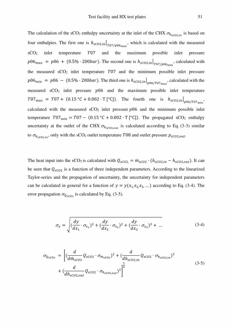
Test facility and HX test plates 51
The calculation of the sCO2 enthalpy uncertainty at the inlet of the CHX σ%~���,�� is based on
four enthalpies. The first one is ℎ]ZW ,NO�^��/������, which is calculated with the measured
sCO2 inlet temperature '07 and the maximum possible inlet pressure
�06[$\ = �06 + (0.5% · 200���). The second one is ℎ]ZW ,NO�^��/������ , calculated with
the measured sCO2 inlet temperature '07 and the minimum possible inlet pressure
�06[NO = �06 − (0.5% · 200���). The third one is ℎ]ZW ,NO����/^�����, calculated with the
measured sCO2 inlet pressure �06 and the maximum possible inlet temperature
'07[$\ = '07 + (0.15 °� + 0.002 · T [°C]). The fourth one is ℎ]ZW ,NO����/^�����,
calculated with the measured sCO2 inlet pressure �06 and the minimum possible inlet
temperature '07[NO = '07 − (0.15 °� + 0.002 · T [°C]). The propagated sCO2 enthalpy
uncertainty at the outlet of the CHX σ%~���,��� is calculated according to Eq. (3-3) similar
to σ%~���,��, only with the sCO2 outlet temperature '08 and outlet pressure �]ZW ,PQR.
The heat input into the sCO2 is calculated with �]ZW , = �� ]ZW · (ℎ]ZW ,NO − ℎ]ZW ,PQR). It can
be seen that �]ZW is a function of three independent parameters. According to the linearized
Taylor-series and the propagation of uncertainty, the uncertainty for independent parameters
can be calculated in general for a function of � = �(,-,, ,,c, … ) according to Eq. (3-4). The
error propagation σ�~��� is calculated by Eq. (3-5).
σ� = �( ���,- · σ\�) + ( ���, · σ\�) + ( ���,c · σ\�) + … (3-4)
σ�~��� = �( ��m� ]ZW �]ZW · σ[� ~���) + ( ��ℎ]ZW ,NO �]ZW · σ%~���,��)
+ ( ��ℎ]ZW ,PQR �]ZW · σ%~���,���) �-
(3-5)

52 Test facility and HX test plates
After deriving �]ZW according to Eq. (3-5) it can be simplified to Eq. (3-6).
σ�~��� = ���ℎ]ZW ,PQR − ℎ]ZW ,NO · σ[� ~����
+ ��� ]ZW · (σ%~���,��� − σ%~���,��)� ¡-
(3-6)
The error propagation σ�~���includes the calculated sCO2 enthalpies at the inlet ℎ]ZW ,NO and
outlet ℎ]ZW ,PQR of the CHX, the measurement uncertainty of the sCO2 mass flow
rate σ[� ~��� , the measurement results of the sCO2 mass flow rate �� ]ZW and the calculated
enthalpy uncertainties σ%~���,��� and σ%~���,��. The error propagation is applied in the same way
for the steam side of the CHX and for all calculated values.
3.2 Heat exchanger
3.2.1 Classification
A classification of heat exchangers according to a) transfer process, b) number of fluids,
c) surface compactness, d) construction type, e) flow arrangement and f) heat transfer
mechanism is given for instance in the book of Shah [44]. The transfer process (a) is
furthermore divided into the indirect contact type, in which the fluids are separated and the heat
transfer occurs through walls, and the direct contact type, in which the hot and cold fluid
interact. The classification according to the number of fluids (b) is further divided into two-fluid
systems, three-fluid systems and more than three-fluid systems. The two-fluid system is the
most common one in technical applications and usually used for heating, cooling or heat
recovery. Three-fluid systems are used for cryogenic and chemical processes and fluid systems
with more than three fluids are special applications e.g. in the chemical industry. The
classification according to the surface compactness (c) is divided into the gas-to-fluid and the
liquid-to-liquid & phase-change heat exchangers. The first one is called compact, if the ratio of
heat transfer area to volume is more than 700 m²/m³ or a hydraulic channel diameter of less
than 6 mm is used. The second one is compact, if the ratio is more than 400 m²/m³ or the
hydraulic diameter is less than 6 mm. Furthermore, heat exchangers can be classified into four
Test facility and HX test plates 53
construction types (d): tubular, plate-type, extended surface and regenerative. The tubular type
includes for instance the double-pipe and the well-known and commonly used shell-and-tube
heat exchanger. The plate-type is subdivided into the plate heat exchanger, the spiral, the plate
coil and printed circuit heat exchanger. The extended surface type is subdivided into the
plate-fin and tube-fin exchangers. Regenerative heat exchangers, also called regenerators, are
constructed as rotary, fixed-matrix or rotating hood systems. The flow arrangement (e) can be
divided into the single-pass and multi-pass flow. The single-pass flow can be designed as
counter-current-flow, co-current-flow, cross-flow, split-flow and divided-flow configuration.
Multi-pass flows configurations are applied for extended-surface, shell-and-tube and plate heat
exchangers. The heat transfer mechanism (f) is further divided into the single-phase convection
on both sides, the single-phase convection on one side and a two-phase convection on the other
side, two-phase convection on both sides and the combined convection.
Plate-type heat exchangers can be broken down into the plate, the spiral, the plate-coil and
printed circuit heat exchangers. These four types are described more in detail, because the heat
transfer between condensing steam and sCO2 in plate-type heat exchangers is experimentally
investigated in this work. A gasketed plate heat exchanger (PHE) is shown on the top left
in Figure 3-4. It consists of rectangular plates that are clamped together with two cover plates,
carrying bars and bolts. The corrugated surface pattern of the plate is usually manufactured by
stamping or embossing. To ensure leak-tightness, different kind of gasketed materials are used,
depending on the operation temperature and pressure. PHE are designed for temperatures
below 150 °C and pressures up to 10 bar, and they are commonly used in the food or chemical
industry. The main advantages of a gasketed PHE are that they can be easily disassembled for
cleaning or inspection and the heat transfer area can be easily adjusted by adding or removing
plates. If higher operation temperatures and pressures are required, the gasketed PHE can be
replaced by welded or brazed plate heat exchangers, which are able to withstand temperatures
up to 350 °C and pressures up to 40 bar. A spiral-plate heat exchanger is shown on the top right.
It consists of two metal strips, which are wrapped helically to form a long pair of spiral channels
for two fluids in a compact manner. The fluids usually flow through the heat exchanger in
counter-current-flow and single-passage configuration. Spiral-plate heat exchangers are used
for more viscous and fouling liquids. Compared to other heat exchangers the flow passages are
easier to clean and no insulation is needed at the outer shell because the cold fluid flows there.
For larger heat transfer units, the temperature is limited to 200 °C and the pressure to 25 bar. A
plate-coil heat exchanger is shown on the bottom left. It consists of a plate with attached

54 Test facility and HX test plates
channels. It can be used as heat sink or heat source, depending on the operational purpose and
the given boundary conditions. The heat exchanger can be manufactured with different plate
materials like carbon steel, stainless steel and titanium by means of die-stamping, spot-welding
or roll-bonding. They withstand pressures up to 18 bar, are relatively cheap and the heat
exchanger design can be changed easily. They are usually used in industrial applications like
the cryogenics, the chemical industry and for solar power applications. A printed circuit heat
exchanger (PCHE) is shown on the bottom right. Stainless steel, titanium or nickel alloys are
used as plate material. The channels are chemically etched or milled into the plates, leading to
rectangular or semi-circular channels with a depth from 0.1 mm to 2 mm. The channels can be
designed as straight or wavy channels with varying angles, depending on process requirements.
It must be considered that increasing channel angles lead to higher flow turbulences, which
results in increased heat transfer capabilities, but also in increased pressure drops. The flow
arrangement between the hot and cold side can be designed as co-current, counter-current and
cross flow. In the co-current flow, both fluids enter the heat exchanger at one side, flow parallel
in the same direction and leave the heat exchanger at the other side. In counter-current flow
heat exchangers, both fluids flow parallel to each other but in opposite directions. According
to [44], [45], [46] the counter-current flow configuration is thermodynamically superior to any
other; it is the most efficient and the highest temperature changes in each fluid can be achieved
for given boundary conditions like the fluid mass flow rates and the fluid inlet temperatures. In
cross flow heat exchangers, the fluids flow in directions normal to each other.
Thermodynamically, the effectiveness is between the co-current flow and counter-current flow.
After designing and manufacturing the plates of the PCHE, they are stacked together before the
diffusion bonding. The diffusion bonding is applied because it provides homogeneous material
properties, which result in higher pressure resistances and higher heat conductivities. Finally,
the fluid inlet and outlet connections are electronic beam welded onto the heat exchanger unit.
PCHE’s can achieve surface area densities of about 650 m²/m³ - 1300 m²/m³, leading to
compact components. This is especially important if space limitations must be taken into
account. Moreover, they are able to withstand pressures up to 500 bar and temperatures up
to 800 °C. They are usually used for clean gases, liquids and phase-change fluids in the
chemical industry, waste heat recovery, power and energy fields and power plant applications.
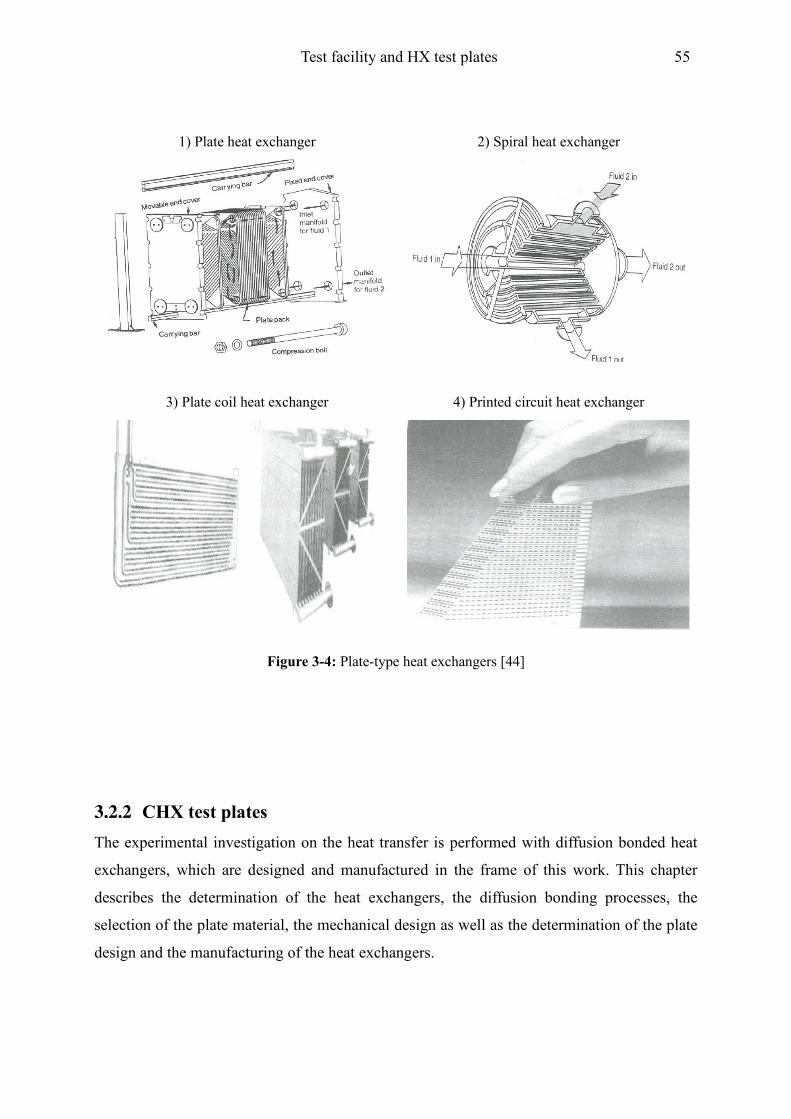
Test facility and HX test plates 55
1) Plate heat exchanger 2) Spiral heat exchanger
3) Plate coil heat exchanger 4) Printed circuit heat exchanger
Figure 3-4: Plate-type heat exchangers [44]
3.2.2 CHX test plates
The experimental investigation on the heat transfer is performed with diffusion bonded heat
exchangers, which are designed and manufactured in the frame of this work. This chapter
describes the determination of the heat exchangers, the diffusion bonding processes, the
selection of the plate material, the mechanical design as well as the determination of the plate
design and the manufacturing of the heat exchangers.

56 Test facility and HX test plates
Heat exchanger test configurations
The channel dimensions, number of channels per plate / number of plates, channel shapes and
heat exchanger test configurations are summarized in Table 3-7. Furthermore, a unique
nomenclature with alphabetic letters (A, B, C, D) is introduced for simplicity.
Table 3-7: Heat exchanger configurations and nomenclature
1. Channel Dimension 2. Number of Channels p. p. / number of plates 3. Channel shape
3x1 mm 2x1 mm 15/1 5/1 5/2 5/3 I/I I/Z
A B A B C D A B
Heat exchanger test configurations
1 AAA 5 BBB
2 AAB 6 BCB
3 BAA 7 BDB
4 BAB
A typical manufacturing process of the channels of a compact heat exchanger, in serial
production, is the chemical etching due to small required channel dimensions and fast
fabrication time. This method leads to semi-circular channel geometries, in which the channel
width is a function of the channel depth. For instance, a channel depth of 0.6 mm leads to a
minimum channel width of about 0.95 mm [47]. The boundary conditions of the chemical
etching combined with the aim to build compact heat exchangers leads to channel diameters
from about 1 mm to 5 mm. Shah [44] also suggests channel diameters between 0.5 mm and
8 mm for CHX’s. To investigate the influence of the channel dimension on different
phenomena, e.g. the heat transfer and the pressure drop, two channel configurations with equal
rectangular channels dimensions on both sides (H2O, sCO2) are determined with respect to
recommended diameters for CHX`s from the literature [44], [48]. According to Table 3-7,
channels with a width of 3 mm and a height of 1 mm (A) as well as with a width of 2 mm and
a height of 1 mm (B) are chosen. The rectangular channel dimension is selected with respect to
an easier and more flexible manufacturing process by milling. The heat exchanger
configurations AAA, AAB, BAA and BAB are designed as so-called “two-plate” heat
exchangers with 15 channels per plate and one plate on each side (15/1). To investigate further
the influence of the plenum geometry on phenomena like the pressure drop, heat exchangers
Test facility and HX test plates 57
with 5 channels per plate (5/1) and a varying number of plates on each side are designed. Heat
exchangers with 1 plate on the steam side and 1 plate on the sCO2 side are called B (5/1),
with 2 plates on each side with C (5/2) and with 3 plates on each side are called D (5/3). These
heat exchangers can also be used for the investigation of the maximum heat transfer because of
the possibility of gradually decreasing the heat transfer area. The influence of the channel shape
on the pressure drop and heat transfer is investigated, too. For this, two-plate heat exchangers
with straight channels on both sides (AAA, BAA) and two-plate heat exchangers with straight
channels on the H2O side and Z-shaped channels on the sCO2 side (AAB, BAB) are designed
and manufactured. The Z-shape of the sCO2 channels is necessary to connect two of the four
plenums with the H2O side and two of the four plenums with the sCO2 side, in consideration of
a stacked CHX with more than one plate on each side. The Z-shape is used on the sCO2 side
because of forced convection, generated by the compressor of the sCO2-HeRo system. To
clarify the introduced nomenclature, one example is given. A heat exchanger with rectangular
2x1 mm channels, 15 channels per plate, one plate on each side and straight channels on both
the H2O and sCO2 side is called BAA.
Diffusion bonding
Diffusion bonding is a solid state welding technique, in which two components can be joined,
based on the atomic diffusion of elements at the joining surface by the application of pressure
and temperature [49], [50]. Similar or dissimilar material combinations of titanium alloys,
zirconium alloys and nickel-based alloys can be joined without macroscopic deformation or
relative motion of the parts. The bonding process can be divided into two parts. In the first step,
a sufficient contact between the components must be achieved by applying pressure, which
deforms the surface roughness and disrupts any kind of contamination. According to
KE-Technology [51] pressures between 350 kg/cm² and 700 kg/cm² are used for the bonding
process, depending on the materials and geometries. The second step includes the diffusion
process itself and the grain growth at the bonding line in consideration of constant pressures
and gradually increasing temperatures up to 1200 °C. This step leads to a metallic bonding
without any visible contact surface line. The contact surfaces must be clean, smooth and free
from oxides to guarantee a successful bonding. If the bonding is successful, the microstructure
at the bonding region has nearly the same physical and mechanical properties as the base
material. This leads to high heat conductivity as well as high pressure and temperature
resistance at the bonding line, which are desirable for compact heat exchangers. At the

58 Test facility and HX test plates
KE-Technology, the vacuum bonding technique is applied, which is usually used for materials
like stainless steel and alloys. The working area of the diffusion bonding device is limited to a
diameter of 325 mm and a height of 350 mm, which must be considered in the design of
components. The pressure is adjusted by hydraulic pistons and the inductive heating process is
carried out in a vacuum chamber.
Plate material
The austenitic stainless steel 1.4301 (X5CrNi18-10 / 304) with 5 % carbon, 18 % chrome
and 10 % nickel is chosen as plate material for the heat exchangers. It has a corrosion resistance
up to 925 °C, but a continuous use between 425 °C and 860 °C is not recommended if corrosion
resistance in combination with water is required. Furthermore, it has average mechanical
properties, a good forgeability, an excellent weldability and an averaged machinability [52].
The excellent weldability and the machinability are important reasons, why 1.4301 is chosen
as plate material. It can be purchased as strips, tubes, pipes, and plates for different kinds of
applications like the chemical industry and the mechanical engineering. At a temperature
of 20 °C it has a density of 8000 kg/m³, a melting point of 1450 °C, a thermal conductivity of
16 W/(m·K), a specific heat capacity of 500 J/(kg·K), a minimum yield strength of 210 N/mm²,
a minimum tensile strength of 520 N/mm² and it is slightly magnetisable [53]. Moreover, the
yield strength ���. is a function of the temperature, leading to 160 N/mm² at 100 °C,
140 N/mm² at 150 °C, 130 N/mm² at 200 °C, 120 N/mm² at 250 °C and 110 N/mm² at 300 °C.
For successfully diffusion bonded components the yield strength is assumed to be more
than 70 % of the yield strength of the base material [54], [55]. This reduction in the yield
strength must be considered by employing a factor � in the mechanical design of diffusion
bonded components to prevent any kind of material failure.
Mechanical design
There are currently no international standard or generally admitted calculation methods for the
mechanical design of compact heat exchangers. Because of that, common methods for ordinary
geometries like pipes, vessels e.g. have to be adjusted. DIN EN 13445-3, for instance, includes
a calculation method in which the wall thickness of a rectangular pressure vessel with
supporting structures can be determined. The heat exchanger manufacturer Heatric uses the

Test facility and HX test plates 59
ASME-BPVC-VIII code for the design of PCHE’s. The models of ASME code are similar to
them of DIN EN but Heatric additionally implemented semi-circular channel geometries [54].
Another approach for the mechanical design of compact heat exchangers is to transform
rectangular channel geometries into circular pipe geometries. This method is used then for the
determination of the minimum wall thickness by ordinary calculation methods like the
Kesselformel or the analytic calculation method for thick-walled pressure vessels.
Figure 3-5: Schemes of CHX dimensioning
A sketch of the dimensioning steps from (1) to (3), for the determination of the minimum wall
thicknesses of the CHX, is shown in Figure 3-5. The dimensioning starts on the left (1), in
which a fictitious HX with a width �, a height and a length � is shown. It consists of two H2O
plates and one sCO2 plate, which are alternately stacked together. Each plate has 5 rectangular
channels with a channel width � and a channel height �. The wall thickness between two
neighboring channels at one plate is #&, the wall thickness between one H2O and one sCO2
channel is #%, and the outer wall thickness is #$. For the compact heat exchangers, equal wall
thicknesses of #& and #% are chosen. At point (2) a representative rectangular sCO2 channel is
marked with a dashed blue line, shown as a separate component on the top right at point (3).
This channel is then transformed by the hydraulic diameter equation into a circular pipe
geometry with an outer radius �P, an inner radius �N and a wall thickness #�. The minimum wall
thickness #� of the pipe is determined by common equations for pressure vessels and pipe
geometries. For the calculation, a sCO2 pressure of 180 bar and a steam pressure of 1 bar are
assumed. The sCO2 pressure is derived from cycle calculation results of the sCO2-HeRo system
for a NPP and the steam pressure is conservatively set to ambient pressure.

60 Test facility and HX test plates
Figure 3-6: Schemes of pipe stresses
The tangential stress ϬR in a pipe (Figure 3-6) can be calculated in general according to Eq. (3-7)
by using the internal pressure �N, the radius at the inner wall �N,R, the radius at the outer wall �P,R
and the radius �\,R at position , [56], [57].
ϬR = �N · �N,R �P,R − �N,R · (�P,R
�\,R + 1) (3-7)
Eq. (3-7) shows that ϬR is a function of the radius �\,R with a maximum stress at the inner wall
radius �N,R and a minimum stress at the outer wall radius �P,R. The maximum tangential
stress ϬR,[$\ can be calculated by Eq. (3-9) after replacing �\,R by �N,R in Eq. (3-7).
ϬR,[$\ = �N · �N,R �P,R − �N,R · (�P,R
�N,R + 1) (3-8)
For a given pressure �N and a maximum tangential stress ϬR,[$\ of the material, the necessary
outer wall radius �P,R, is calculated according to Eq. (3-9) after rewriting Eq. (3-8).
�P,R = �(�N + ϬR,[$\) ϬR,[$\ − �N · �N,R (3-9)

Test facility and HX test plates 61
The radial pipe stress Ϭ¢ (Figure 3-6) is calculated similar to the tangential stress by Eq. (3-10)
as a function of the radius �\,¢. The internal pressure �N, the radius at the inner wall �N,¢ and the
radius at the outer wall �P,¢ are used for this.
Ϭ¢ = − �N · �N,¢ �P,¢ − �N,¢ · (�P,¢
�\,¢ − 1) (3-10)
Eq. (3-10) shows that a minimum radial pipe stress Ϭ¢ occurs if �\,¢ is �P,¢ and a maximum
radial stress occurs if �\,¢ is �N,¢. The maximum radial pipe stress Ϭ¢,[$\ is calculated by
Eq. (3-11) after replacing �\,¢ by �N,¢ (Eq. (3-10)).
Ϭ¢,[$\ = − �N · �N,¢ �P,¢ − �N,¢ · (�P,¢
�N,¢ − 1) (3-11)
The axial stress Ϭ$ (Figure 3-6) in a pipe can be calculated according to Eq. (3-12) by using the
internal pressure �N, the outer pressure �P, the radius at the inner wall �N,$ and outer wall �P,$.
Ϭ$ = �N · �N,$ − �P · �P,$ �P,$ − �N,$ (3-12)
The minimum outer wall radius �P,$ can be calculated according to Eq. (3-13) after rewriting
Eq. (3-12). Therefore, the internal pressure �N, the outer pressure �P, the radius at the inner
wall �N,$ and the allowed axial stress Ϭ$,[$\ of the material are used.
�P,$ = �(�N + Ϭ$,[$\) Ϭ$,[$\ + �P · �N,$ (3-13)
The boundary conditions for the mechanical design, like pressures and temperatures, and the
calculation results are summarized in Table 3-8. The maximum allowed material stress Ϭ[$\
of stainless steel 1.4301 is calculated according to Eq. (3-14) to 29.6 N/mm². For this, a
maximum steam temperature 'V W of 300 °C is defined, leading to a yield strength ���. ,c��°Z

62 Test facility and HX test plates
of 110 N/mm². Moreover, uncertainties of the diffusion bonding process are considered by
using a reduction factor of 0.7 and a safety factor ! of 2.6. The sCO2 pressure �]ZW at the inner
pipe wall is set to 180 bar and the outer pressure �V W to 1 bar. The pipe inner radius �N is
calculated for the rectangular 2x1 mm channel geometry as 0.65 mm and for the 3x1 mm
geometry as 0.75 mm. The minimum outer radius of the pipe �P is determined for both channel
geometries according to Eq. (3-9) and Eq. (3-13) for the tangential stress �P,R and for the axial
stress �P,$. Comparing the results of �P,R and �P,$ they show that for the tangential stress thicker
walls are necessary. The minimum wall thickness #� of the pipe is determined (Eq. (3-15)) with
the inner pipe radius �N and the outer pipe radius �P,R for the 2x1 mm channel geometry to
0.67 mm and for the 3x1 mm channel geometry to 0.77 mm. The radial stress Ϭ¢ is calculated
for both geometries according to Eq. (3-11) and compared to allowable material stresses.
Ϭ[$\ = ���. ,c��°Z · 0.7 · ! (3-14)
#� 9 �P,R − �N (3-15)
Table 3-8: Mechanical design parameters
Variable Value Unit Description
Ϭ[$\ 29.6 N/mm² Material Stress 1.4301 (300 °C / 70 % / 2.6) ! 2.6 - Safety Factor 'V W 300 °C Max. Temperature - H2O �]ZW 180 bar Max. Pressure - sCO2 �V W 1 bar Max. Pressure - H2O
�N, \- 0.65 mm Inner Radius Pipe - 2x1 Channel �N,c\- 0.75 mm Inner Radius Pipe - 3x1 Channel
�P,R, \- 1.32 mm Outer Radius Pipe - Tangential - 2x1 Channel �P,R,c\- 1.52 mm Outer Radius Pipe - Tangential - 3x1 Channel
�P,$, \- 0.82 mm Outer Radius Pipe - Axial - 2x1 Channel �P,$,c\- 0.95 mm Outer Radius Pipe - Axial - 3x1 Channel
#�, \- 0.67 mm Min. Wall Thickness Pipe - 2x1 Channel #�,c\- 0.77 mm Min. wall thickness pipe - 3x1 Channel
Test facility and HX test plates 63
Plate design and manufacturing
The heat exchanger plates are designed with the information of the plate material and the wall
thickness. The minimum wall thickness # between two neighboring channels of one plate is set
to 1.4 mm (2 x 0.67 mm) for the 2x1 mm channels and to 1.6 mm (2 x 0.77 mm) for the
3x1 mm channels. Equal wall thicknesses are planned between one H2O and one sCO2 channel.
The effective channel length is determined at 150 mm with respect to a maximum working area
of the diffusion bonding machine. According to Table 3-7, seven heat exchanger test
configurations are manufactured with different channel dimensions, numbers of channels per
plate / numbers of plates and channel shapes.
As an example, the technical drawings of the heat exchanger of case BAB (2x1 mm - 15/1 - IZ)
are shown in Figure 3-7 without dimensioning, for simplification. The technical drawings of all
seven investigated heat exchangers, including dimensioning, are attached in Appendix C. The
first technical drawing in Figure 3-7 shows the cover plate with a plate thickness of 4 mm, a
length of 247.6 mm and a width of 95.6 mm. The four drillings with a diameter of 12.7 mm are
for the inlet and outlet of the H2O into the plenums of the steam plate. The steam plate
with 15 straight rectangular 2x1 mm channels and a plate thickness of 2.4 mm is shown in the
second drawing. The length of the plenum with 49.6 mm is determined by the number of
15 channels and a wall thickness of 1.4 mm between the channels. The plenum width of 13 mm
results from the diameter of the ½” pipe connections. The two 4 mm drillings are used only for
adjusting the plates against each other during the diffusion bonding process. The third drawing
shows the sCO2 plate with a plate thickness of 5 mm, a length of 247.6 mm and a width
of 95.6 mm. For the sCO2 inlet and outlet into the plenums also four drillings are implemented.
Two plenums of the heat exchanger connect the straight water channels. The other two plenums
connect the sCO2 channels. They are mounted at the side, thus the sCO2 channels are Z-shaped,
in consideration of a stacked CHX with more than one plate on each side. In counter-current
flow configuration, the steam enters the two-plate CHX at the top and leaves it driven by gravity
as condensate at the bottom. The sCO2 enters the CHX at the bottom left and leaves it at the top
right. The effective channel length for sCO2 is determined at 150 mm, which is the straight
length of the middle part of the channels.

64 Test facility and HX test plates
1) Cover Plate 2) Steam Plate 3) sCO2 Plate
Figure 3-7: Plate design of case BAB
Pictures of the manufacturing steps of the heat exchanger BAB are shown in Figure 3-8 as an
example. At the start, the cover, steam and sCO2 plates are manufactured in the workshop by
milling according to the technical drawings (Figure 3-7). The drillings at the outer area of the
plates are only for adjusting the plates during the milling process and for diffusion bonding.
Afterwards, they are cleaned and stacked together, as shown on the left in Figure 3-8. In the
second step, the plates are diffusion bonded before the H2O and sCO2 pipe connections are
electron beam welded onto the plates, which is shown in the center of Figure 3-8. After welding,
a pressure and leakage test is carried out. The pressure test is depicted on the right in Figure
3-8. After successfully passing both tests, the heat exchanger is ready for installation and
experimental investigations can be performed.
1) Stacked Plates 2) Test Plate 3) Pressure Test
Figure 3-8: Manufacturing steps of case BAB

Results 65
4 Results
4.1 Measurement points
The measurement points for the experimental investigations are summarized in Table 4-1. They
are defined in consideration of boundary conditions, derived from investigations at the glass
model as well as from internal restrictions at the SCARLETT loop and both steam cycles. To
be able to compare the results of the low-pressure and high-pressure steam cycle, similar
measurement campaigns are chosen. The low-pressure steam cycle experiments are carried out
according to campaign 1 - 6 with a steam pressure of 0.3 bar, a steam temperature of 70 °C,
varying steam volume flow rates, varying sCO2 mass flow rates and sCO2 inlet pressures
of 95 bar, 100 bar and 110 bar. These results are used for the design of the compact heat
exchanger for the sCO2-HeRo demonstrator unit, attached to the PWR glass model. The
high-pressure steam cycle experiments are carried out according to campaigns 1 - 9. A steam
pressure of 70 bar, a steam temperature of 286 °C, varying steam volume flow rates, varying
sCO2 mass flow rates and sCO2 inlet pressures of 95 bar, 100 bar and 110 bar are used to obtain
results of the heat transfer performance under “Design point” (DP), “Out of design
point” (ODP) and “Out of design point II” (ODP II) conditions. These results are used for
validation purpose and for the improvement of the German thermo-hydraulic code ATHLET.
In the DP experiments the sCO2 mass flow rates �� ]ZW (37 g/s - 68 g/s) and water volume flow
rates �� V W (0.53 l/h - 0.97 l/h) of the measurement campaign 1, 2 and 3 are scaled down in the
same ratio according to the entire amount of sCO2 mass flow rate of 650 g/s and water volume
flow rate of 9.3 l/h, which are used in the design point of the sCO2-HeRo demonstrator unit at
the glass model. The electrical heating power of the evaporator �NO,Yl$� is adjusted according
to the water volume flow rates from 380 W to 680 W to ensure that the water inventory is
completely evaporated. The minimum sCO2 mass flow rate of 37 g/s and the maximum sCO2
mass flow rate of 68 g/s are limited by the SCARLETT test facility. To investigate the heat
transfer also ODP, measurement campaigns 4, 5 and 6 are performed. A constant sCO2 mass
flow rate �� ]ZW of 37 g/s and gradually increasing water volume flow rates �� V W from 0.53 l/h
to 1.74 l/h are applied. The power of the electrically heated evaporator �NO,Yl$� is adjusted
according to the water volume flow rates from 380 W to 1230 W. The water volume flow rate
is limited to 2 l/h and the power of the electrical heated evaporator to 1300 W because of
temperature restrictions. In the ODP II measurement campaigns 7, 8 and 9, investigations with

66 Results
a constant water volume flow rate of 1.74 l/h and an electrical heating power of 1230 W are
performed. The sCO2 mass flow rate is gradually decreased from 37 g/s to about 6 g/s by
adjusting a needle valve and bypassing a part of the sCO2 mass flow rate. To investigate
additionally the influence of the sCO2 inlet pressure �06 on phenomena like the heat transfer
and the pressure drop, sCO2 inlet pressures of 110 bar, 100 bar and 95 bar with an inlet
temperature of 40 °C are chosen. The maximum sCO2 inlet pressure is limited by pressure
restrictions at the SCARLETT loop, the minimum pressure is determined with respect to the
location near to the critical point of sCO2 and the temperature is limited by internal temperature
restrictions at the conditioning unit.
Table 4-1: Measurement points
Campaign L£¤ [bar] M£¥ [°C] Status
1 110 40 Design Point
“DP” 2 100 40
3 95 40
4 110 40 Out of Design Point
“ODP” 5 100 40
6 95 40
7 110 40 Out of Design Point II
“ODP II” 8 100 40
9 95 40
G� HIJK [g/s] G� ¦KJ [l/h] §¨©,ª«¬L [W] Status
37 0.53 380 DP
46 0.65 460 DP
56 0.80 560 DP
68 0.97 680 DP
37 0.53 380 ODP
37 0.65 460 ODP
37 0.80 560 ODP
37 0.97 680 ODP
37 1.17 830 ODP
37 1.43 1010 ODP
37 1.74 1230 ODP
37 - 6 1.74 1230 ODP II

Results 67
The nomenclature introduced in Table 3-7 is extended by two more alphabetic letters according
to Table 4-2. The first letter describes the “Type of heat input” into the sCO2. A heat input with
condensing steam of the high-pressure (HP) steam cycle is named (A), a heat input with
condensing steam of the low-pressure (LP) steam cycle is (B) and no heat input is (C).
Moreover, the “Measurement point campaign” is identified for the “Design point” (DP)
experiments with (A), for the “Out of design point” (ODP) experiments with (B) and for the
“Out of design point II” (ODP II) experiments with (C). To clarify the introduced nomenclature,
one example is given: BAB-AA presents the heat exchanger with rectangular 2x1 mm
channels (B), 15 channels per plate and 1 plate on each side (A), straight H2O channels and
Z-shaped sCO2 channels (B), the high-pressure steam cycle is used for the heat input (A) and
the design point measurement campaign (A) is performed.
Table 4-2: Extension of nomenclature
4. Type of heat input 5. Measurement point campaign
HP LP NO DP ODP ODP II
A B C A B C
An overview of the measurement configurations is shown in Table 4-3. It includes the channel
geometries (3x1 mm / 2x1 mm), the channel/plate configurations (15/1 / 5/1 / 5/2 / 5/3), the
channel shapes (II / IZ), the type of heat inputs (HP / LP / NO) and the measurement campaigns
(DP / ODP / ODP II). The investigated ones are marked with “X”. It can be seen that all seven
heat exchangers are used without a heat input from the steam cycle for the DP, ODP and ODP II
measurement points. These results are used to obtain the pressure drops of unheated flows. The
measurement time for unheated experiments is set to 10 minutes after reaching steady state
configurations. The LP steam cycle experiments are performed to determine the compact heat
exchanger for the sCO2-HeRo demonstrator unit at GfS. For this purpose, the 3x1 mm
and 2x1 mm channel geometry, a channel/plate configuration of (15/1) as well as straight H2O
and Z-shaped sCO2 channels (IZ) are investigated according to the DP and ODP measurement
campaigns. The HP steam cycle experiments are used for all heat exchanger configurations,
except the heat exchangers with a channel geometry of 2x1 mm and channel/plate
configurations of (5/2) and (5/3). A measurement time of 15 minutes, after reaching steady state
configurations is defined for heated experiments.

68 Results
Table 4-3: Overview of performed measurement configurations
3x1 2x1
15/1 15/1 5/1 5/2 5/3
II IZ II IZ IZ IZ IZ
HP
DP X X X X X - -
ODP X X X X X - -
ODP II X X X X X - -
LP
DP - X - X - - -
ODP - - - X - - -
ODP II - - - - - - -
NO
DP X X X X X X X
ODP X X X X X X X
ODP II X X X X X X X
4.2 Summary of measurement results
An example of measurement results is given in Table 4-4 for the LP steam cycle and
the 3x1 mm / 15/1 / IZ heat exchanger configuration. It includes the water volume flow
rate �� V W, the H2O pressure �02 at the inlet of the CHX, the H2O pressure �04 at the outlet of
the CHX, the H2O temperature '03 at the inlet of the CHX, the H2O temperature '04 at the
outlet of the CHX , the calculated electrical heating power of the evaporator �NO,Yl$�, the sCO2
mass flow rate �� ]ZW , the sCO2 pressure drop ��05 in the CHX, the sCO2 inlet pressure �06
into the CHX as well as the sCO2 inlet temperature '07 and outlet temperatures '08 at the
CHX. The number in brackets in the first column in Table 4-4 identifies the measurement
campaign according to Table 4-1. All measurement results are summarized in Appendix D.

Results 69
Table 4-4: Experimental results
Low-pressure steam cycle / sCO2 SCARLETT loop
3x1 mm / 15/1 / IZ
�� V W �02 �04 '03 '04 �NO,Yl$� �� ]ZW ��05 �06 '07 '08
[l/h] [bar] [bar] [°C] [°C] [W] [g/s] [bar] [bar] [°C] [°C]
DP (1)
0.54 0.317 0.300 69.99 37.72 385 36.94 0.675 109.282 39.21 41.23
0.61 0.321 0.299 70.23 37.83 455 45.98 0.975 108.824 39.38 41.11
0.74 0.329 0.300 70.75 37.48 550 55.92 1.425 108.343 39.13 40.78
0.97 0.354 0.311 72.34 38.28 678 67.35 2.053 107.516 39.12 40.63
DP (2)
0.55 0.323 0.305 70.42 36.68 389 36.45 0.672 99.255 39.34 40.59
0.64 0.332 0.309 71.02 37.21 462 45.28 1.023 98.803 39.24 40.34
0.79 0.360 0.330 72.87 37.51 549 56.15 1.548 98.148 39.02 39.93
0.95 0.359 0.317 72.68 36.82 685 67.40 2.226 97.177 38.63 39.35
DP (3)
0.53 0.336 0.320 71.33 37.58 374 36.90 0.728 94.214 38.99 39.80
0.67 0.346 0.325 71.99 37.77 452 45.66 1.106 93.746 39.10 39.69
0.79 0.358 0.329 72.72 37.40 544 52.30 1.493 93.021 39.15 39.66
0.98 0.352 0.307 72.21 37.55 685 67.81 2.459 92.134 38.83 38.74
4.3 Pressure drop results
In the following, representative measurement results of the sCO2 pressure drop of unheated and
heated sCO2 flows are analyzed. These results are used for the design specification of the
compact heat exchanger.
4.3.1 Pressure drop results of unheated sCO2 flows
Experimental results of the sCO2 pressure drop ∆�05 in the heat exchangers of Case BAA
and AAA are shown in Figure 4-1 as a function of the sCO2 mass flow rate �� ]ZW and the sCO2
inlet pressure. The heat exchanger BAA has a rectangular 2x1 mm channel dimension, a
channel length of 150 mm, straight H2O and straight sCO2 channels, 15 channels per plate
and 1 plate on each side. The HX of Case AAA is similar to BAA, except for the channel
dimension of 3x1 mm. The measurements are performed without a sCO2 heat input and a sCO2
inlet temperature of about 39 °C.

70 Results
Figure 4-1: Results of Δp05 as function of ṁsCO2 of Case BAA-C & AAA-C
The upper three graphs in Figure 4-1 show the experimental results of the sCO2 pressure
drop ∆�05 as a function of the mass flow rate �� ]ZW and the sCO2 inlet pressure �06 for the
unheated DP and ODP II investigations of Case BAA-C and the lower three graphs of AAA-C.
The ODP II investigations are carried out with mass flow rates between 7 g/s and 20 g/s and
the DP investigation from about 37 g/s to 68 g/s. The results show that an increasing sCO2 mass
flow rate and a constant sCO2 inlet pressure leads to a parabolic increase of the sCO2 pressure
drop. Furthermore they show that an increasing sCO2 inlet pressure leads to decreasing pressure
drops ∆�05 for constant sCO2 mass flow rates �� ]ZW . This can be explained by the fluid
density, where an increased sCO2 inlet pressure leads to an increased fluid density and thus to
a decreased pressure drop due to lower fluid velocities in the channels of the HX. For the
2x1 mm channel dimension, a sCO2 mass flow rate of about 68 g/s and an sCO2 inlet pressure
of about 110 bar leads to a pressure drop of 0.346 bar, 100 bar to 0.372 bar, and an inlet pressure
of 95 bar leads to a pressure drop of 0.373 bar. A comparison of the results of the sCO2 pressure
drop of Case BAA (2x1 mm) and Case AAA (3x1 mm) shows that a decreasing flow area and
a constant sCO2 mass flow rate leads to increasing pressure drop results at constant sCO2 inlet
pressures. This can be explained by increased flow velocities in the channels. For example, a
sCO2 inlet pressure of 110 bar and a mass flow rate of 68 g/s leads to a pressure drop of
0,00
0,05
0,10
0,15
0,20
0,25
0,30
0,35
0,40
0 10 20 30 40 50 60 70
�p0
5 [b
ar]
ṁsCO2 [g/s]
110 bar100 bar95 bar
AAA-C
BAA-C

Results 71
0.346 bar for the 2x1 mm channels and to 0.192 bar for the 3x1 mm channels. Furthermore, an
increase of the channel dimension from 2x1 mm to 3x1 mm leads to a reduction of the sCO2
pressure drop of more than 45 %, for all shown measurement results and mass flow rates.
In the following, the sCO2 pressure drop is re-calculated for unheated sCO2 flows by means of
correlations for the heat exchangers of Case BAA and AAA and compared to experimental
results. The results are depicted in Figure 4-1. The pressure drop ∆�05 can be calculated for
single-phase flows in general according to Eq. (4-1) [58]. The correction factor �, the friction
coefficient 6, the density of the fluid 2 and the velocity of the fluid + are used for this.
∆�05 = � · 6 · 2 · + 2 (4-1)
The correction factor � determines the type of flow. For a common channel flow, � is a function
of the channel length and channel diameter � (Eq. (4-2)); for cross-section area changes or
flow deflections, � is set to 1 (Eq. (4-3)).
� = � ® �¯ (4-2)
� = 1 (4-3)
The pressure drop in the channel ∆�°%$OO�� can be calculated in general after inserting Eq. (4-2)
into Eq. (4-1) and rewriting it according to Eq. (4-4).
∆�°%$OO�� = 6°%$OO�� · � · 2 · + 2 (4-4)
There are two common approaches for determining the friction coefficient of the channel
6°%$OO�� (Eq. (4-4)). The first one is by using a Moody diagram, where 6°%$OO�� is shown as a
function of the Reynolds number �� and the ratio of pipe roughness � to pipe diameter � [59].
Besides that, the friction coefficient 6°%$OO�� can be calculated with correlations [58] for
laminar and turbulent flow regimes. Laminar flow regimes occur at �� < 2320, turbulent flow

72 Results
regimes occur at �� > 8000 and the transition zone is between 2320 < �� < 8000. For laminar
flow regimes in smooth channels, the friction coefficient 6°%$OO�� can be determined according
to Eq. (4-5). For turbulent flow regimes, various correlations can be applied, depending on the
Reynolds number. The correlation of Blasius (Eq. (4-6)) can be chosen for 3000 < �� < 10±,
the correlation of Konakov (Eq. (4-7)) for 10f < �� < 10� and the correlation of Filonenko
(Eq. (4-8)) for 10± < �� < 5 · 10�. The results of the correlation of Filonenko have a deviation
of less than 0.5 % compared with the results of Eq. (4-9), which is derived from the implicit
correlation of Prandtl and Karman according to Eq. (4-9) and is valid for �� > 10�.
6°%$OO�� = 64�� (4-5)
6°%$OO�� = 0.3164√��³ (4-6)
6°%$OO�� = (1.8 · ´(��) − 1.5)µ (4-7) 1¶ 6°%$OO�� = 1.819 · ´(��) − 1.64 (4-8)
1¶ 6°%$OO�� = −0.8 + 2 · ´ (�� · ¶ 6°%$OO��) (4-9)
The pressure drop due to cross section area changes and flow deflections ∆��P]] can be
calculated according to Eq. (4-10) after inserting Eq. (4-3) into Eq. (4-1) and rewriting it.
∆��P]] = 6�P]] · 2 · + 2 (4-10)
For cross section area changes (like in the plenum of a CHX) there are two possibilities:
contraction and expansion. A channel flow with a sudden contraction of the cross section area
is shown on the top left in Figure 4-2. According to [58] 6�P]],O can be determined as a function
of the ratio of inlet cross section area �- and outlet cross section area � as well as the Reynolds
number �� downstream. The depicted diagram on the bottom left (Figure 4-2) shows that for

Results 73
turbulent flow regimes with �� > 10f, the friction coefficient6�P]],Ohas a linear tendency with
decreasing values for increasing ratios of the cross section area changes and vice versa. 6�P]],O
can be determined with a linear function according to Eq. (4-11). A pipe flow with a sudden
cross section area expansion is shown on the top right in Figure 4-2. The friction loss
coefficient 6�P]],�can be calculated according to Eq. (4-12).
ξ�P]],O 9 0.5 a 0.4 ; � �- (4-11)
ξ�P]],� 9 ®1 a �-� ¯ (4-12)
1) Contraction 2) Expansion
Figure 4-2: Cross section area changes
The friction loss coefficient 6�P]],m of flow deflections in elbows can be determined by means
of diagrams. There 6�P]],mis shown as a function of the deflection degree 7 and the roughness
of the channel �[58]. For a rough channel and a deflection of 90°, the friction loss
coefficient 6�P]],m can be determined according to Eq. (4-13) to 1.25.
6�P]],m 9 1.25 (4-13)

74 Results
The overall sCO2 pressure drop ∆�05 in the HX’s can be re-calculated in general according
to Eq. (4-14). It consists of two parts: the pressure losses due to friction in channels ∆�°%$OO�� and pressure losses due to flow deflections and cross section area changes ∆��P]].
∆�05 = ¹ ∆�°%$OO��,ºN
º»-+ ¹ ∆��P]],¼
O¼»-
(4-14)
Considering friction losses as well as flow deflections and cross section area changes in the HX
of Case BAA and AAA, the pressure drop ∆�05 can be re-calculated according to Eq. (4-15).
∆�05 = ∆��N��,NO + ∆��P]],m,���OQ[,NO + ∆��P]],O,���OQ[,NO + ∆����OQ[,NO+ ∆��P]],O,°%$OO��,NO + ∆�°%$OO�� + ∆��P]],�,°%$OO��,PQR+ ∆����OQ[,PQR + ∆��P]],�,���OQ[,PQR + ∆��P]],m,���OQ[,PQR+ ∆��N��,PQR
(4-15)
The pressure drop due to friction in the inlet pipe of the heat exchanger into the plenum is
considered by ∆��N��,NO , the flow deflection in the plenum by ∆��P]],m,���OQ[,NO , the change of
the cross section area from the inlet pipe into the plenum by ∆p�P]],O,���OQ[,NO , the friction in
the plenum by ∆����OQ[,NO , the cross section area change from the plenum into the channel by
∆��P]],O,°%$OO��,NO , the friction in the channel by ∆�°%$OO�� , the cross section area change from
the channel into the plenum ∆��P]],�,°%$OO��,PQR , the friction in the plenum by ∆����OQ[,PQR ,
the cross section are change from the plenum into the pipe by ∆��P]],�,���OQ[,PQR , the flow
deflection in the plenum by ∆��P]],m,���OQ[,PQR and the pressure drop due to friction in the outlet
pipe of the heat exchanger by ∆��N��,PQR.
The friction loss coefficients are determined for channel flows according to Eq. (4-6) - (4-8)
and for deflections as well as cross section area changes according to Eq. (4-11) - (4-13).
Experimental and calculated sCO2 pressure drop results are shown in Figure 4-3 as a function
of the sCO2 mass flow rate for the heat exchangers of Case BAA (2x1 mm) and AAA (3x1 mm).
Both heat exchangers have straight H2O and sCO2 channels (II), 15 channels per plate
and 1 plate on each side (15/1) and a straight channel length of 150 mm. The experiments are

Results 75
performed without a heat input into the sCO2, a sCO2 inlet pressure of 110 bar, an inlet
temperature of 39 °C and sCO2 mass flow rates between 8 g/s and 68 g/s. The calculated sCO2
pressure drop is determined according to Eq. (4-15) by using the correlation of
Konakov (Eq. (4-7)) for the calculation of the friction coefficient 6°%$OO��. Furthermore, a
homogeneous sCO2 mass flow distribution in the channels and no heat losses are assumed.
Figure 4-3: Exp. VS. cal. results of Δp05 as function of ṁsCO2 of Case BAA-C & AAA-C
The graphs in Figure 4-3 show similar parabolic tendencies with increasing sCO2 pressure
drops ∆�05 for increasing sCO2 mass flow rates �� ]ZW and vice versa. A comparison of the
results shows that the calculated results are always lower than the experimental ones. For
instance, for the 2x1 mm channel dimension a sCO2 mass flow rate of about 36 g/s leads to an
experimental sCO2 pressure drop of 0.112 bar and to an calculated pressure drop of 0.039 bar,
56 g/s leads to 0.232 bar and 0.084 bar, and 68 g/s leads to 0.346 bar and 0.124 bar. For both
channel dimensions (2x1 mm and 3x1 mm) and all investigated mass flow rates, the calculated
sCO2 pressure drop is always 2 to 3 times lower than the experimental one. Similar deviations
between calculated and experimental results can be seen in the work of Flaig [60]. According
to him, the inappropriate plenum geometry and the unsuitable sCO2 inflow conditions into the
plenum are most responsible for that.
0,00
0,05
0,10
0,15
0,20
0,25
0,30
0,35
0,40
0 10 20 30 40 50 60 70
�p0
5 [b
ar]
ṁsCO2 [g/s]
110 bar - 2x1 mm - Exp110 bar - 2x1 mm - Calc110 bar - 3x1 mm - Exp110 bar - 3x1 mm - Calc
BAA-C & AAA-C

76 Results
The influence of the channel shape on the sCO2 pressure drop ∆�05 is shown in Figure 4-4 as
a function of the sCO2 mass flow rate �� ]ZW and the sCO2 inlet pressure �06. The upper three
graphs show pressure drop results of the heat exchanger of Case BAA with a rectangular
channel dimension of 2x1 mm and straight H2O and Z-shaped sCO2 channels (IZ). The lower
three graphs show sCO2 pressure drop results of Case BAB with 2x1 mm channels and straight
H2O and sCO2 channels (II). Both heat exchangers have an effective straight channel length
of 150 mm, 15 channels per plate and 1 plate on each side. All measurements are performed
without a heat input into the sCO2 and a sCO2 inlet temperature of about 39 °C.
Figure 4-4: Results of Δp05 as function of ṁsCO2 of Case-BAA-C & BAB-C
For all measurements, the results depicted in Figure 4-4 show a parabolic tendency of the sCO2
pressure drop ∆�05 as a function of the sCO2 mass flow rate �� ]ZW and the sCO2 inlet
pressure �06. An increasing mass flow rate leads to increased pressure drops. Furthermore, the
experimental results of the pressure drop of Case BAB (2x1 mm - IZ) are shifted towards
higher ∆�05 values for similar inlet conditions, compared to Case BAA (2x1 mm - II).
Especially for increasing sCO2 mass flow rates the deviation between Case BAB and BAA is
increasing. For instance, a sCO2 inlet pressure of 110 bar and a mass flow rate of about 37 g/s
0,0
0,1
0,2
0,3
0,4
0,5
0,6
0,7
0,8
0,9
1,0
1,1
1,2
1,3
1,4
1,5
0 10 20 30 40 50 60 70
�p0
5 [b
ar]
ṁsCO2 [g/s]
110 bar100 bar95 bar
BAB-C
BAA-C

Results 77
leads to a sCO2 pressure drop of 0.112 bar for the 2x1 mm - II configuration, and to 0.426 bar
for the 2x1 mm - IZ configuration. A sCO2 mass flow rate of 68 g/s leads to 0.346 bar (II) and
1.248 bar (IZ), which is about 4 times higher. In addition, the straight 2x1 mm channel shape
reduces the sCO2 pressure drop for the depicted measurement results by more than 70 %
compared with the Z-shaped channels. These deviations can be explained by the channel shape,
the channel length and manufacturing issues. The channel shape of Case BAB with straight
H2O and Z-shaped sCO2 channels is designed for a heat exchanger with more than one plate on
each side. The Z-shape is necessary to connect two of the four plenums with the H2O side and
two of the four plenums with the sCO2 side. In the Z-shaped plate there are two sharp-edged
corners, in which the sCO2 flow is deflected twice and the sCO2 pressure drop is increased.
Furthermore, the flow length in the Z-shaped channels is design-specific more than 150 mm,
which leads to increased pressure drop values. Manufacturing issues like the accuracy, diffusion
bonding and the arrangement of the pipe connections onto the heat exchangers must be taken
also into account, because they influence the sCO2 pressure drop in the HX’s.
The influence of the plenum geometry on the sCO2 pressure drop is further investigated by
using the heat exchangers of Case BAB and BDB. The heat exchanger BAB has rectangular
2x1 mm channels, 15 channels per plate and one plate on each side, straight H2O and Z-shaped
sCO2 channels and an effective straight channel length of 150 mm. As 15 channels are arranged
in parallel at one plate, the inlet plenum has a width of about 50 mm, a height of 1 mm and a
length of 13 mm. This plenum geometry is inappropriate for homogeneous inflow and flow
distributions, especially if the inlet pipe is arranged vertically and the sCO2 flow has to be
deflected 90 degrees within 1 mm height. Because of that, the heat exchanger of Case BDB is
designed and manufactured. Compared to Case BAB, BDB has equal channel dimensions,
channel shapes and channel length, but the 15 channels are arranged on 3 plates, with
5 channels each. Such design leads to a more cubic plenum, in which the sCO2 mass flow rate
can be distributed more homogeneously and the flow is less deflected. The results depicted
in Figure 4-5 show experimental results of the sCO2 pressure drop ∆�05 as a function of the
sCO2 mass flow rate �� ]ZW of Case BAB and BDB. The sCO2 inlet pressure �06 is adjusted
from 110 bar to 95 bar, the unheated sCO2 mass flow rate �� ]ZW is gradually increased from
about 7 g/s to 68 g/s and the sCO2 enters the heat exchangers with a temperature of about 39 °C.

78 Results
Figure 4-5: Results of Δp05 as function of ṁsCO2 of Case BAB-C & BDB-C
The upper three graphs in Figure 4-5 show sCO2 pressure drop results of Case BAB-C with
15 channels per plate and one plate on each side. The lower three graphs show results of
Case BDB with 5 channels per plate and 3 plates on each side of the HX. In general, for both
HX a parabolic tendency of the sCO2 pressure drop as a function of the sCO2 mass flow rate
can be seen, with increasing ∆�05 values for increasing mass flow rates. Furthermore, an
increasing sCO2 inlet pressure �06 and a constant mass flow rate leads to lower pressure drop
values. The shift towards lower pressure drop values for the 5/3 channel configuration verifies
that a more cubic plenum geometry is beneficial for lower pressure drops. The pressure
drop decreases by more than 20 % for all shown measurement results compared with
the 15/1 channel configuration. This can be seen for instance at the 110 bar graphs, in which a
sCO2 mass flow rate of about 68 g/s leads to a pressure drop of 0.948 bar (5/3) and to
1.248 bar (15/1). The decrease of the sCO2 pressure drop in more cubic plenum geometries is
beneficial for the sCO2-HeRo system and can be explained for instance by more homogeneous
inflow conditions and reduced flow deflections in the HX’s.
0,00,10,20,30,40,50,60,70,80,91,01,11,21,31,41,5
0 10 20 30 40 50 60 70
�p0
5 [b
ar]
ṁsCO2 [g/s]
110 bar100 bar95 bar
BDB-C
BAB-C

Results 79
Finally, results of the sCO2 pressure drop ∆�05 of unheated sCO2 flows are shown in Figure
4-6 as a function of the averaged sCO2 Reynolds number ������]ZW of Case BAB-C and BDB-C.
������]ZW is calculated according to Eq. (4-16) as averaged value of the Reynolds number at the
inlet ��]ZW ,NO (Eq. (4-17)) and outlet ��]ZW ,PQR (Eq. (4-18)) of the HX. Both heat exchangers
have rectangular 2x1 mm channels, an effective straight channel length of 150 mm, straight
H2O and Z-shaped sCO2 channels. BAB has 15 channels at 1 plate and one plate on each side
(15/1) and BDB has 5 channels at 1 plate and 3 plates on each side (5/3).
������]ZW = 0.5 · ���]ZW ,NO + ��]ZW ,PQR (4-16)
��]ZW ,NO = �(ṁ¿ÀÁ , �06, '07) (4-17)
��]ZW ,PQR = ��ṁ¿ÀÁ , �]ZW ,PQR, '08 (4-18)
Figure 4-6: Results of Δp05 as function of R͞esCO2 of Case BAB-C & BDB-C
0,0
0,1
0,2
0,3
0,4
0,5
0,6
0,7
0,8
0,9
1,0
1,1
1,2
1,3
1,4
1,5
0 10000 20000 30000 40000 50000 60000 70000 80000
�p0
5 [b
ar]
110 bar - 15/1100 bar - 15/195 bar - 15/1110 bar - 5/3100 bar - 5/395 bar - 5/3
BDB-C
������]ZW [−]
BAB-C
68 g/s
56 g/s

80 Results
The results depicted in Figure 4-6 show parabolic tendencies of the sCO2 pressure drop ∆�05
as a function of ������]ZW with increasing pressure drops for increasing Reynolds numbers. A
constant Reynolds number and a constant sCO2 inlet pressure leads to higher sCO2 pressure
drops for the 15/1 plate configuration (dashed lines), compared to the 5/3 configuration (lines).
This corresponds to the results shown in Figure 4-5 and can be explained by the inappropriate
plenum geometry. Furthermore, an increasing sCO2 inlet pressure and a constant sCO2 mass
flow rate leads to a decreasing Reynolds number on the one hand and on the other hand to a
decreasing pressure drop. This is depicted for instance for sCO2 mass flow rates of 68 g/s
and 56 g/s in Figure 4-6 and can be explained by the pressure dependency of the sCO2 density.
A mass flow rate of 68 g/s leads to a Reynolds number of about 55000 for 110 bar (15/1),
62000 for 100 bar (15/1) and to 65000 for 95 bar (15/1). The sCO2 pressure drop decreases
from about 1.381 bar at 95 bar (15/1) to 1.248 bar at 110 bar (15/1) and from 1.073 bar at
95 bar (5/3) to 0.948 bar at 110 bar (5/3).
4.3.2 Pressure drop results of heated sCO2 flows
As the sCO2 pressure drop ∆�05 depends on the heat input into the sCO2 and on the sCO2 mass
flux, it is shown in Figure 4-7 as a function of the heating load �. It is defined according
to Eq. (4-19) as ratio of the sCO2 heat input �]ZW and the sCO2 mass flux Â]ZW . The sCO2 heat
input is determined according to Eq. (4-20) with the sCO2 mass flow rate �� ]ZW and the sCO2
enthalpies at the inlet ℎ]ZW ,NO and outlet ℎ]ZW ,PQR of the HX. The enthalpies are calculated
according to Eq. (4-21) and Eq. (4-22) by using the NIST database Refprop in consideration of
the measured temperatures and pressures. The sCO2 mass flux Â]ZW is defined according
to Eq. (4-23) as ratio of the measured sCO2 mass flow rate �� ]ZW and the cross section area �.
The heat input into the sCO2 is provided by condensing steam of the HP steam cycle, which
generates saturated steam with a pressure of about 70 bar, a steam temperature of about 286 °C
and adjustable water volume flow rates from about 0.53 l/h to 1.74 l/h. According to the
measurement points, the heating power of the electrical heated evaporator is adjusted from
about 460 W to 1230 W. The heat exchanger of Case BAB has rectangular 2x1 mm channels,
an effective straight channel length of 150 mm, straight H2O and Z-shaped sCO2 channels,
15 channels per plate and 1 plate on each side (15/1). For the experimental investigations sCO2
inlet pressures of 95 bar, 100 bar and 110 bar, gradually increasing sCO2 mass flow rates from
about 5 g/s to 68 g/s and sCO2 heat inputs from about 460 W to 1230 W are used.

Results 81
� = �]ZW Â]ZW (4-19)
�]ZW = �� ]ZW · �ℎ]ZW ,PQR − ℎ]ZW ,NO (4-20)
ℎ]ZW ,NO = �(�06, '07) (4-21)
ℎ]ZW ,PQR = ���]ZW ,PQR, '08 (4-22)
Â]ZW = �� ]ZW � (4-23)
Figure 4-7: Results of Δp05 as function of G of Case BAB-A
The results depicted in Figure 4-7 can be generally classified into three parts: Part 1 is shown
on the left with a heating load of 0.00025 (kJ·m²)/kg. These are the results of the DP campaigns,
in which sCO2 mass flow rates from 68 g/s to 37 g/s, sCO2 inlet pressures of 95 bar, 100 bar
and 110 bar and electrical heating powers between 380 W and 680 W are chosen. Each of them
shows an increasing pressure drop for decreasing sCO2 inlet pressures, in consideration of a
constant sCO2 mass flow rate and heat input. Furthermore, a decreasing sCO2 mass flow rate
0,00,10,20,30,40,50,60,70,80,91,01,11,21,31,41,5
0,E+00 1,E-03 2,E-03 3,E-03 4,E-03 5,E-03 6,E-03 7,E-03
�p0
5 [b
ar]
G [(kJ·m²)/kg]
110 bar100 bar95 bar
Part 1
Part 2
Part 3
BAB-A
68 g/s
56 g/s
46 g/s
37 g/s
37 g/s - 5 g/s

82 Results
leads to decreasing ∆�05 values for constant sCO2 inlet pressures and sCO2 heat inputs. The
results of the ODP measurement campaigns, with heating loads from 0.00031 (kJ·m²)/kg to
0.00095 (kJ·m²)/kg, are shown in the center of Part 2. These experiments are performed with a
sCO2 mass flow rate of 37 g/s, varying sCO2 inlet pressures and gradually increasing sCO2 heat
inputs from 380 W to 1230 W. For all sCO2 inlet pressures, a nearly linear profile with
increasing pressure drop values for increasing sCO2 heat inputs can be obtained. This can be
explained by the decreasing fluid density of sCO2 for increasing temperatures, leading to higher
flow velocities and thus to higher pressure drops in the heat exchanger. The results of the ODP II
measurement campaigns are shown on the right at Part 3. They are performed with heating
loads from 0.0012 (kJ·m²)/kg to 0.0064 (kJ·m²)/kg, which are achieved by adjusting the sCO2
mass flow rate from about 30 g/s to 5 g/s and by setting an electrical heating power of
about 1230 W. These results show a parabolic decrease of the sCO2 pressure drop for decreasing
heating loads from about 0.0012 (kJ·m²)/kg to 0.0030 (kJ·m²)/kg, which corresponds to mass
flow rates from 29.5 g/s to 9.4 g/s, and a linear decrease from about 0.0030 (kJ·m²)/kg to
0.0064 (kJ·m²)/kg. The results verify a strong influence of the sCO2 mass flow rate on the sCO2
pressure drop as well as an influence of the heat input on the pressure drop. Both phenomena
can be explained by changes of the flow velocity and the fluid density.
The kind of heat input into the sCO2 and the influence on the pressure drop is also investigated.
Figure 4-8 shows results of the sCO2 pressure drop ∆�05 as a function of the averaged Reynolds
number ������]ZW for heat inputs with condensing steam of the low-pressure (LP) steam cycle, the
high-pressure (HP) steam cycle and for unheated (No) sCO2 flows. The LP steam cycle provides
saturated steam with a pressure of about 0.3 bar and a temperature of about 70 °C. The HP
steam cycle generates steam with a pressure of about 70 bar and a temperature of about 286 °C.
The heating power of the electrical heated evaporator is limited for both steam cycles to
about 1230 W. The results are obtained from experiments with a sCO2 inlet pressure of 95 bar,
varying sCO2 mass flow rates and sCO2 heat inputs. The heat exchanger of Case BAB is used.
It has rectangular 2x1 mm channels, an effective straight channel length of 150 mm, straight
H2O and Z-shaped sCO2 channels, 15 channels per plate and one plate on each side (15/1).

Results 83
Figure 4-8: Results of Δp05 as function of R͞esCO2 of Case BAB-A & BAB-B & BAB-C
The results in Figure 4-8 show that a heat input via the high-pressure (HP) steam cycle, a sCO2
inlet pressure of 95 bar and consecutively increasing sCO2 mass flow rates lead to a parabolic
tendency of the sCO2 pressure drop ∆�05 as a function of ������]ZW . For instance, an averaged
Reynolds number of about 16000 leads to a pressure drop of 0.050 bar, 26800 to 0.158 bar,
42300 to 0.494 bar 57400 to 0.967 bar and 69200 to 1.389 bar. Comparing the results of the HP
steam cycle (triangle) and low-pressure (LP) steam cycle (circle) it can be seen that both graphs
have similar tendencies with deviations of less than 2 %. This verifies that the pressure drop is
not influenced by the kind of heat input. Only the amount of heat input and the sCO2 inlet
conditions into the heat exchanger, like the inlet pressure, inlet temperature and mass flow rate
influence the sCO2 pressure drop. The results show further that for unheated flows (squares)
and constant sCO2 mass flow rates the Reynolds numbers are shifted towards lower values.
This can be explained by increasing fluid densities, resulting in decreasing flow velocities and
thus to decreasing ������]ZW values.
0,00,10,20,30,40,50,60,70,80,91,01,11,21,31,41,5
0 10000 20000 30000 40000 50000 60000 70000 80000
�p0
5 [b
ar]
95 bar - HP
95 bar - LP
95 bar - No
BAB-A & BAB-B
�� ]ZW [-]
BAB-C
68 g/s
56 g/s
46 g/s
37 g/s

84 Results
The pressure drop and the heat transfer capability are important for the design of heat
exchangers. As an example, results of the sCO2 pressure drop ∆�05 of Case BAB are shown
in Figure 4-9 as a function of the averaged Nusselt number ������]ZW . The averaged Nusselt
number is defined according to Eq. (4-24) as averaged value of the Nusselt numbers at the inlet
��]ZW ,NO (Eq. (4-25)) and outlet ��]ZW ,NO (Eq. (4-26)). Both are calculated by using the
Gnielinski correlation (Eq. (4-27)) for turbulent flow regimes as a function of �� and ��.
������]ZW 9 0.5 ; ���]ZW ,NO b ��]ZW ,PQR (4-24)
��]ZW ,NO 9 ����]ZW ,NO, ��]ZW ,NO (4-25)
��]ZW ,PQR 9 ����]ZW ,PQR, ��]ZW ,PQR (4-26)
�� 9 68 ; �� ; ��1 b 12.7z68 ; _�� /c a 1` (4-27)
6 9 _1.8 ; lg_��` a 1.5`µ (4-28)
Figure 4-9: Results of Δp05 as function of N͞usCO2 of Case BAB-A
0,00,10,20,30,40,50,60,70,80,91,01,11,21,31,41,5
0 50 100 150 200 250 300 350 400
Δp0
5[b
ar]
110 bar100 bar95 bar
BAB-A
Part 1
Part 2
Part 3
68 g/s
56 g/s
46 g/s
37 g/s
������ ]ZW [-]

Results 85
The results in Figure 4-9 show similar tendencies of the sCO2 pressure drop ∆�05 as a function
of ������]ZW for different sCO2 inlet pressures and mass flow rates. For instance, an increasing
sCO2 inlet pressure leads to decreasing pressure drops and Nusselt numbers for constant sCO2
mass flow rates. The results can be classified into three parts. Part 1 shows results of the ODPII
investigations with a heat input of about 1230 W and mass flow rates from about 5 g/s to 37 g/s,
Part 2 depicts results of the ODP investigations with a sCO2 mass flow rate of 37 g/s and heat
inputs from about 380 W to 1230 W and Part 3 shows results of the DP investigations with mass
flow rates from 37 g/s to 68 g/s and heat inputs from 380 W to 680 W. The results confirm that
a sCO2 inlet pressure of 95 bar leads to maximum ������]ZW values, which is beneficial for the
heat transfer. Furthermore, an inlet pressure of 95 bar leads to maximum sCO2 pressure drops
for constant sCO2 mass flow rates, which is inappropriate for heat exchangers which should be
used in the sCO2-HeRo system because these pressure drops must be compensated by the TCS
and thus results into lower excess electricity. In addition, a constant sCO2 mass flow rate and
an increasing sCO2 inlet pressure leads to a lower sCO2 pressure drop and a decreasing Nusselt
number. The increase of the sCO2 inlet pressure from 95 bar to 100 bar leads to a decrease of
the Nusselt number of about 25 % and a decrease of the pressure drop of about 5 %.
4.4 Heat transfer results
Results of the calculated sCO2 heat input �]ZW are shown in Figure 4-10 as a function of the
calculated steam condensing power �V W for the heat transfer investigations at the heat
exchanger of Case BAB. It has rectangular 2x1 mm channels, an effective channel length
of 150 mm, straight H2O and Z-shaped sCO2 channels (IZ), 15 channels per plate and 1 plate
on each side (15/1). The sCO2 heat input is provided by condensing steam of the HP steam cycle
with a pressure of about 70 bar and a temperature of about 286 °C. The water volume flow rates
and the corresponding heating power of the electrical heated evaporator are adjusted according
to the measurement points (Table 4-1). The sCO2 heat input �]ZW is calculated according to
Eq. (4-20) by means of the measured sCO2 mass flow rate �� ]ZW and the sCO2 enthalpy
difference between the inlet ℎ]ZW ,NO (Eq. (4-21)) and outlet ℎ]ZW ,PQR (Eq. (4-22)). The
condensing power of the steam �V W is calculated according to Eq. (4-29) by using the
measured water volume flow rate �� V W and the enthalpy difference between the inlet ℎV W,NO
(Eq. (4-30)) and outlet ℎV W,PQR (Eq. (4-31)). The enthalpies are calculated with NIST
Refprop [43] as a function of the measured fluid temperatures and pressures.

86 Results
�V W = �� V W · �ℎV W,NO − ℎV W,PQR (4-29)
ℎV W,NO = �(�02, '03) (4-30)
ℎV W,NO = �(�04, '04) (4-31)
Figure 4-10: Results of QsCO2 as function of QH2O of Case BAB-A
The depicted results in Figure 4-10 show similar linear tendencies for varying sCO2 inlet
pressures and a schematic offset between the calculated condensing power of the
steam �V W and the calculated sCO2 heat input �]ZW . For instance, a sCO2 inlet pressure
of 110 bar and a calculated condensing power of the steam of 457 W leads to a calculated sCO2
heat input of 372 W, 854 W leads to 759 W, 1006 W leads to 940 W and 1218 W leads to
1109 W. Such offset can be explained by thermal losses due to high operation temperatures of
about 290 °C and an inappropriate ratio of heat emitting to heat transfer area. The offset at each
measurement point �PÅÅ]�R can be determined by the energy balance according to Eq. (4-32).
200
300
400
500
600
700
800
900
1000
1100
1200
1300
1400
200 300 400 500 600 700 800 900 1000 1100 1200 1300 1400
QsC
O2
[W]
QH2O [W]
110 bar - HP100 bar - HP95 bar - HP
BAB-A
Qoffset,av = 133 W

Results 87
�PÅÅ]�R = �V W − �]ZW (4-32)
�PÅÅ]�R,$l = 1� ¹ �PÅÅ]�Rºh
º»N (4-33)
� = �]ZW QV W − �PÅÅ]�R,$l (4-34)
The averaged offset �PÅÅ]�R,$l is calculated according to Eq. (4-33) to 133 W and shown by the
black dashed line in Figure 4-10. Neglecting thermal losses, the calculated heat transfer ratio �
(Eq. (4-34)) is more than 90 % for all 48 measurement points, except 5. The theoretical heat
transfer ratio � of 100 % is visualized by the black line. The results of the steam temperature
measurement '04 at the outlet of the heat exchanger verify additionally that the maximum
achievable amount of steam in the test section is completely condensed and subcooled even for
all ODP measurement points. This means that the heat exchanger installed at the test section is
over-dimensioned and would be able to transfer more heat power from the steam side to the
sCO2 side than could be investigated.
The influence of the steam inlet conditions on the heat transfer is also investigated. Condensing
steam of the low-pressure (LP) steam cycle and high-pressure (HP) steam cycle are used for
this purpose. Figure 4-11 shows experimental results of the calculated sCO2 heat input �]ZW
as a function of the calculated steam condensing power �V W for a sCO2 inlet pressure
of 110 bar and varying steam inlet conditions. These results are obtained from experimental
investigations of the heat exchanger of Case BAB, which has rectangular 2x1 mm channels, an
effective channel length of 150 mm, straight H2O and Z-shaped sCO2 channels (IZ),
15 channels per plate and 1 plate on each side (15/1).

88 Results
Figure 4-11: Results of QsCO2 as function of QH2O of Case BAB-A & BAB-B
The depicted graphs in Figure 4-11 show linear tendencies with increasing sCO2 heat inputs
�]ZW for increasing condensing powers of the steam �V W. For instance, the results of the LP
steam cycle (triangle) experiments show that a sCO2 inlet pressure of 110 bar and a steam
condensing power of 431 W leads to a sCO2 heat input of 425 W, 643 W to 633 W, 813 W to
806 W and 1247 W to 1190 W. The averaged offset of the LP steam cycle experiments is
calculated (Eq. (4-33)) to 9 W and visualized by the upper dashed line. The solid line presents
a theoretical heat transfer ratio � of 100 %, if no heat losses occur. A comparison of the results
of the LP steam cycle (triangle) and HP steam cycle (circle) experiments shows that the heat
transfer ratio � is lower for the HP steam cycle experiments. This can be explained by
increasing thermal losses due to higher steam temperatures of about 290 °C, compared to steam
temperatures of about 70 °C. The averaged offset of the results of the HP steam cycle
measurements is calculated according to Eq. (4-33) to 133 W and visualized by the lower
dashed line.
200
300
400
500
600
700
800
900
1000
1100
1200
1300
1400
200 300 400 500 600 700 800 900 1000 1100 1200 1300 1400
QsC
O2
[W]
QH2O [W]
110 bar - HP
110 bar - LP
BAB-A
Qoffset,av = 120 W
Qoffset,av = 9W
BAB-B

Results 89
To investigate the influence of the channel dimension (2x1 mm & 3x1 mm) and the channel
shape (IZ & II) on the heat transfer, experiments according to Case AAB-A, BAB-A and
BAA-A are performed. The heat exchanger of Case AAB has rectangular 3x1 mm channels,
15 channels per plate and 1 plate on each side (15/1), an effective channel length of 150 mm,
straight H2O and Z-shaped sCO2 channels (IZ). The heat exchanger BAB is similar to AAB,
except the channel dimension of 2x1 mm. BAA is similar to BAB, except the straight sCO2
channels (II). The sCO2 heat input is provided by condensing steam with a pressure of
about 70 bar and a steam temperature of 286 °C, generated in the high-pressure steam cycle.
The results depicted in Figure 4-12 are obtained from experiments with a sCO2 inlet pressure
of 110 bar and mass flow rates according to the determined measurement points (Table 4-1).
Figure 4-12: Results of QsCO2 as function of QH2O of Case AAB-A & BAB-A & BAA-A
The electrical heating power of the steam evaporator with 1600 W is limited to 1300 W due to
internal temperature restrictions of the heating cartridge. In the SCARLETT loop, a minimum
sCO2 mass flow rate of 37 g/s can be provided, and this can be additionally reduced to
about 5 g/s at the inlet of the test section by means of a needle valve and bypassing a part of the
flow. Because of that, there is only one possibility to investigate the transferrable heat in the
HX’s, the decrease of the heat transfer area. For this purpose, the heat exchanger of Case BBB
200
300
400
500
600
700
800
900
1000
1100
1200
1300
1400
200 300 400 500 600 700 800 900 1000 1100 1200 1300 1400
QsC
O2
[W]
QH2O [W]
110 bar - 3x1 mm - 15/1 - SZ - HP110 bar - 2x1 mm - 15/1 - SZ - HP110 bar - 2x1 mm - 15/1 - SS - HP
AAB-A & BAB-A & BAA-A
Qoffset,av
= 135 W
IZ IZ II

90 Results
is designed and manufactured. It has rectangular 2x1 mm channels, 5 channels per plate
and 1 plate on each side (5/1), straight H2O and Z-shaped sCO2 channels (IZ) and an effective
straight channel length of 150 mm. Within the experiments, the sCO2 mass flow rates, the water
volume flow rates and the electrical heating power of the steam evaporator are adjusted
according to the measurement points (Table 4-1). Figure 4-13 shows results of the calculated
sCO2 heat input �]ZW as a function of the calculated condensing power of the steam �V W of
Case BAB-A and BBB-A. The sCO2 heat input is provided by condensing steam with a pressure
of 70 bar and a temperature of 286 °C, generated in the high-pressure steam cycle.
Figure 4-13: Results of QsCO2 as function of QH2O of Case BAB-A & BBB-A
The depicted graphs in Figure 4-13 show results of the ODP measurement campaigns of
Case BAB and BBB with a sCO2 mass flow rate of 37 g/s, gradually increasing steam
condensing power from 460 W to 1250 W and a sCO2 inlet pressure of 110 bar. For both heat
exchangers, an increasing condensing power of the steam �V W leads to a linear increase of the
sCO2 heat input �]ZW . Furthermore, there is an averaged offset of about 105 W, which is shown
by the black dashed line. The results further verify that the heat exchanger of Case BBB
with 5 channels at each side (5/1) and an effective straight channel length of 150 mm is
sufficient to transfer a heat power of about 1250 W from the steam side to the sCO2 side. Further
200
300
400
500
600
700
800
900
1000
1100
1200
1300
1400
200 300 400 500 600 700 800 900 1000 1100 1200 1300 1400
QsC
O2
[W]
QH2O [W]
110 bar - 15/1 - HP
110 bar - 5/1 - HP
BAB-A & BBB-A
Qoffset,av
= 105 W

Results 91
experiments of Case BBB with gradually decreasing sCO2 mass flow rates from about 37 g/s
to 2 g/s show that a sCO2 mass flow rate of about 2 g/s is also sufficient to transfer a heat power
of about 1250 W from the steam side to the sCO2 side. The sCO2 enters the heat exchanger with
a pressure of 110 bar, a mass flow rate of 1.93 g/s and a temperature of 38.48 °C and leaves the
heat exchanger with a temperature of 203.11 °C. The steam enters the HX with a pressure
of 70 bar, a volume flow rate of 1.74 l/h and a temperature of 284.44 °C and leaves the heat
exchanger subcooled with 148.64 °C.
After presenting experimental results of the calculated sCO2 heat input �]ZW as a function of
the calculated condensing power of the steam �V W (Figure 4-10 - Figure 4-13), results of the
calculated sCO2 temperature increase �']ZW are shown as a function of �]ZW . The temperature
increase �']ZW is calculated according to Eq. (4-35) by means of the measured sCO2
temperatures at the inlet '07 and at the outlet '08 of the HX. The sCO2 heat input is calculated
according to Eq. (4-20) in consideration of the sCO2 mass flow rate and the enthalpy difference
between the inlet and outlet.
�']ZW = '08 − '07 (4-35)
Figure 4-14 shows results of �']ZW as a function of �]ZW of Case-BAB-A. These experiments
are carried out with sCO2 heat inputs from 380 W to 1200 W, provided by condensing steam of
the high-pressure steam cycle. A sCO2 mass flow rate of 37 g/s and sCO2 inlet pressures of
110 bar, 100 bar and 95 bar are used.

92 Results
Figure 4-14: Results of QsCO2 as function of ΔTsCO2 of Case BAB-A
The graphs in Figure 4-14 show linear tendencies for varying sCO2 inlet pressures with different
gradients and an increasing sCO2 temperature increase for higher sCO2 heat inputs. The results
of the 95 bar measurement campaign (triangle) show, for instance, that a sCO2 heat input
of 378 W leads to a sCO2 temperature increase of 1.1 °C, 602 W leads to 1.7 °C, 913 W leads
to 2.5 °C and 1128 W leads to 3.1 °C. Moreover, a decreasing sCO2 inlet pressure leads to
decreasing sCO2 temperature increases because of higher specific heat capacities near the
critical point. A sCO2 heat input of about 1150 W, combined with a mass flow rate of 37 g/s and
a sCO2 inlet temperature of about 39.5 °C, leads to a sCO2 temperature increase �']ZW of
6.5 °C for 110 bar, to 4.4 °C for 100 bar, and to 3.1 °C for 95 bar. The specific heat capacity 0�
can be determined for each measurement point according to Eq. (4-36) by using the sCO2 heat
input �]ZW , the mass flow rate �� ]ZW and the temperature increase �']ZW . For an inlet
pressure of 110 bar, the specific heat capacity 0� is between 4.4 kJ/(kg·K) and 4.8 kJ/(kg·K),
for 100 bar between 6.3 kJ/(kg·K) and 7.1 kJ/(kg·K) and for the 95 bar campaign between
9.4 kJ/(kg·K) and 10.0 kJ/(kg·K).
0� = �]ZW �� ]ZW · �']ZW (4-36)
0,0
1,0
2,0
3,0
4,0
5,0
6,0
7,0
8,0
200 300 400 500 600 700 800 900 1000 1100 1200 1300 1400
ΔT
sCO
2[°
C]
QsCO2 [W]
110 bar100 bar95 bar
BAB-A
37 g/s

Results 93
The influence of the channel dimension (2x1 mm / 3x1 mm) and channel shape (II / IZ) on the
sCO2 temperature increase �']ZW is further investigated. Figure 4-15 shows results of �']ZW
as a function of the sCO2 heat input �]ZW of Case BAB-A & BAA-A & AAB-A & AAA-A.
The heat exchanger of Case BAB has rectangular 2x1 mm channels, 15 channels per plate and
1 plate on each side (15/1), straight H2O and Z-shaped sCO2 channels (IZ) and an effective
straight channel length of 150 mm. The heat exchanger BAA is similar to BAB, except for the
straight sCO2 channels (II). AAB is similar to BAB, except for the 3x1 mm channels and AAA
is similar to AAB, except for the straight sCO2 channels. The results are obtained from
experiments with condensing steam of HP steam cycle (A), a sCO2 mass flow rate of 37 g/s, a
sCO2 inlet pressure of 110 bar and varying sCO2 heat inputs from 380 W to 1200 W.
Figure 4-15: Results of QsCO2 as function of ΔTsCO2 of Case BAB/BAA/AAB-A/AAA
The graphs in Figure 4-15 show similar linear tendencies with increasing sCO2 temperature
increases �']ZW for increasing sCO2 heat inputs �]ZW , visualized by the black dashed line.
For instance, a sCO2 heat input of 380 W leads to a sCO2 temperature increase of 2.37 °C,
759 W to 4.52 °C and 1159 W to 6.54 °C for the “110 bar - 15/1 - IZ - 2x1 - HP” configuration.
Moreover, for a constant sCO2 heat input the deviation between the temperature increases
�']ZW is less than 4 %. This means that neither the channel dimension nor the channel shape
0,0
1,0
2,0
3,0
4,0
5,0
6,0
7,0
8,0
200 300 400 500 600 700 800 900 1000 1100 1200 1300 1400
ΔT
sCO
2[°
C]
QsCO2 [W]
110 bar - 2x1 mm - 15/1 - SZ - HP110 bar - 2x1 mm - 15/1 - SS - HP110 bar - 3x1 mm - 15/1 - SZ - HP110 bar - 3x1 mm - 15/1 - SS - HP
BAB-A & BAA-A &
AAB-A & AAA-A
IZ II IZ II

94 Results
has an influence on the sCO2 temperature increase for the current experiment - only the amount
of heat input �]ZW and the sCO2 inlet conditions at the heat exchanger are responsible for the
sCO2 temperature increase �']ZW .
To monitor the surface temperature distribution during the experiments, nine resistance
thermometers (Pt-100) are mounted symmetrically on both sides of the heat exchangers of
Case BAB and BBB. Figure 4-16 shows on the left a CAD (Computer Aided Design) drawing
of the heat exchanger of Case BAB with the measurement positions on the sCO2 plate and on
the right a picture of the HX in the test section with installed Pt-100 measurement devices.
Figure 4-16: CAD drawing and picture of HX with installed Pt-100 of Case BAB
The resistance thermometers are mounted symmetrically in three levels on the surface of the
sCO2 plate of Case BAB, as shown in the CAD drawing (Figure 4-16). The coordinate origin
is located at the bottom left, marked with a red dot. Level 2 is located 132.7 mm above the
coordinate origin in the center line of the plate. Level 1 is located 45 mm below level 2 and
level 3 is located 45 mm above level 2. Pt-100 02, 05 and 08 are mounted in the center line of
the plate, 56.7 mm to the right of the coordinate origin. Pt-100 01, 04 and 07 are located
17.5 mm to the left of the center line and Pt-100 03, 06 and 09 17.5 mm to the right. The
measurement positions of the Pt-100 on the H2O plate are arranged similar but mirror-inverted.

Results 95
Figure 4-17: Results of TO as function of position X of Case BAB-A

96 Results
Experimental results of the sCO2 surface temperatures '( of Case BAB-A are depicted
in Figure 4-17 as a function of the Pt-100 measurement position . and the sCO2 heat input
�]ZW . The heat exchanger of Case BAB has rectangular 2x1 mm channels, an effective straight
channel length of 150 mm, straight H2O and Z-shaped sCO2 channels (IZ), 15 channels per
plate and 1 plate on each side (15/1). The heat input is provided by condensing steam of the
high-pressure steam cycle with a pressure of about 70 bar and a temperature of 286 °C. The
water volume flow rates and the corresponding heating powers of the electrical evaporator are
adjusted accordingly to the ODP measurement campaigns, and the sCO2 mass flow rate is set
to 37 g/s. The sCO2 heat input is calculated according to Eq. (4-20) by means of the measured
mass flow rate and the enthalpy difference between the inlet and outlet. The enthalpies are
calculated with Refprop [43] in consideration of the measured temperatures and pressures.
The first graphs (Figure 4-17) are obtained from measurements with a sCO2 heat input of
600 W, the second ones with 760 W, the third ones with 940 W and the graphs at the bottom
with 1160 W. A sCO2 inlet temperature of about 39.5 °C, a mass flow rate of 37 g/s and an inlet
pressure of 110 bar are chosen. The results show generally a symmetrical temperature profile
with lower surface temperatures in the center line of the HX and higher surface temperatures at
the outer area. Furthermore, a higher sCO2 heat input �]ZW leads to increasing surface
temperatures, especially at the top of the heat exchanger (level 3). This can be explained by the
counter-current flow configuration, in which the steam enters the HX at the top, transfers the
heat to the sCO2 side, is condensed and flows downwards driven by gravity. The sCO2 enters
the heat exchanger at the bottom, flows upwards and leaves the heat exchanger at the top. An
increasing sCO2 heat input corresponds to an increasing steam condensing power and thus to
an increasing steam volume flow rate. Higher steam volume flow rates require an increasing
heat transfer area and this leads to a forced steam flow downwards the HX in the direction of
level 2 and level 1. The results of the surface temperatures '( are described for a sCO2 heat
input of 1160 W, as shown on the bottom (Figure 4-17), as example. The temperature profile at
level 3 shows that the surface temperatures '(_07 with 41.6 °C and '(_09 with 42.0 °C are
higher than '(_08 with 40.8 °C. The increasing temperatures from level 1 to level 3 are taken
from position . = 0 mm. The sCO2 enters the HX at the bottom with a temperature of about
39.5 °C and flows upwards into the channels. Level 1 is located 87.7 mm above the end of the
sCO2 plate and the measured surface temperature '(_02 is 39.0 °C. Flowing upward, the sCO2
is heated due to the heat transfer of condensing steam. This leads to a surface
temperature '(_05 of 39.3 °C on level 2 and '(_08 of 40.8 °C on level 3. In addition, the

Results 97
surface temperatures are in relation to the results of the sCO2 temperature increases �']ZW
(Figure 4-15). There, a sCO2 mass flow rate of 37 g/s, an inlet pressure of 110 bar, an inlet
temperature of about 39.5 °C and a heat input of 1160 W leads to a temperature increase of
about �']ZW of 6.5 °C - which corresponds to the measured surface temperature '(_09 on
level 3 with 42.0 °C. The measured surface temperatures are always lower than the sCO2 fluid
temperatures at the outlet of the HX because of thermal losses and the location of the
measurement position of level 3, which is about 30 mm below the sCO2 outlet.
For comparison of the H2O and sCO2 surface temperatures, results of the surface
temperatures ') (TD_01 – TD_09) on the H2O side of the heat exchanger of Case BAB are
analyzed further. Again, there are symmetrical profiles with lower surface temperatures in the
center line and higher surface temperatures at the outer area. Further, an increasing sCO2 heat
input �]ZW leads to increasing surface temperatures and the increase of the surface
temperatures at level 3 is higher than at level 1. Furthermore, the surface temperatures on the
H2O side are always higher than on the sCO2 side, which is necessary to ensure a heat transfer
from the steam side to the sCO2 side. In consideration of a steam inlet temperature of 286 °C
and H2O surface temperatures on level 3 of about 50 °C, it could be assumed firstly that the
steam is condensed within the first 30 mm and secondly that the heat exchanger of Case BAB
would be able to transfer much more heat power.
Because of limitations in the steam provision of about 1300 W and the aim to investigate the
maximum achievable heat transfer, the heat exchanger of Case BBB is designed. It is similar to
the heat exchanger of Case BAB, except the number of channels. It has 5 channels at one plate
and 1 plate on each side (5/1), which is a third of the heat transfer area of Case BAB. In the
following, results of the surface temperatures on the H2O side ') and sCO2 side '( of
Case BBB are described. These results are obtained from experiments with a sCO2 inlet
pressure of 110 bar, a sCO2 heat input of 1160 W and a mass flow rate of 1.93 g/s.
The results show that the surface temperatures ') on the H2O plate on level 3 and on level 2
are close to the steam inlet temperature of about 286 °C, which confirms that at these
measurement positions, steam still exists in the HX. Going downstream, the surface
temperatures on level 1 with about 210 °C are significantly lower than on level 2 and level 3.

98 Results
This indicates that the steam is condensed completely between level 2 and level 1. The results
of the temperature measurement '04 at the outlet of the HX on the H2O side shows additionally
that the steam is condensed and sub-cooled for all measurement points (Appendix D). The
temperature measurements '( on the surface of the sCO2 plate show similar profiles with lower
surface temperatures, compared to the surface temperatures on the H2O side. The results verify
that a heat exchanger with 5 rectangular 2x1 mm channels and an effective straight channel
length of 150 mm is able to transfer a heat power of about 1160 W from the condensing steam
side to the sCO2 side, for a sCO2 inlet pressure of 110 bar, a sCO2 mass flow rate of 1.93 g/s, a
steam inlet pressure of 70 bar and a corresponding steam inlet temperature of 286 °C.
In consideration of the received experimental data, in the following the compact heat exchanger
for the sCO2-HeRo demonstrator unit, which will be installed at the pressurized water reactor
glass model at GfS, is constructed.

CHX for the PWR glass model 99
5 CHX for the PWR glass model
5.1 Boundary conditions and measurement results
The inlet conditions at the compact heat exchanger for the PWR reactor glass model are
summarized in Table 5-1. The sCO2 inlet pressure, the inlet temperature and the mass flow rate
are defined in consideration of the cycle calculation results according to chapter 2.3. These
parameters are chosen with respect to maximum generator excess electricity and other criteria
like the achievable compression ratio of a single stage compressor and the necessary sCO2 mass
flow rate of the TCS. The inlet conditions on the steam side of the CHX are obtained from
experimental investigations at the glass model according to [36]. The results show that a
transferred simulated decay heat power of 6 kW leads to a steam pressure of 0.32 bar and a
steam temperature of 70.27 °C.
Table 5-1: Boundary conditions of the glass model CHX
Side Variable Value Unit Description
sCO2
�]ZW 117.45 bar Pressure - Inlet CHX ']ZW 46.84 °C Temperature - Inlet CHX �� ]ZW 650 g/s sCO2 Mass Flow Rate
H2O
�V W 0.32 bar Pressure - Inlet CHX 'V W 70.27 °C Temperature - Inlet CHX �� V W 2.60 g/s H2O Mass Flow Rate
- �V W 6.00 kW Transferred Heat Power
A sCO2 mass flow rate of 650 g/s is about six times higher than the achievable sCO2 mass flow
rate in the SCARLETT loop of about 110 g/s. Because of that, scaled down HX’s according to
Table 3-7 are experimentally investigated. In the DP measurement points (Table 4-1) the sCO2
mass flow rates as well as water volume flow rates are scaled down in the same ratio according
to the overall amount of sCO2 (650 g/s) and water (2.60 g/s / 9 l/h), which will be used in the
glass model. Further ODP and ODPII experiments are performed and the influence of the
channel dimensions and channel shape on phenomena like the pressure drop or the transferred
heat power is investigated.

100 CHX for the PWR glass model
To determine the channel dimension and number of channels, the experimental results from
chapter 4 are considered. These show for instance, that the heat is reliably transferred from the
steam side to the sCO2 side for all measurements. In consideration of space limitations and the
aim to build a compact heat exchanger, the entire number of plate pairs could be determined
conservatively at 9 ((650 g/s)/(68 g/s) = 8.8). This would lead to a transferred heat power of
about 640 W per plate, which is achievable. Another important parameter is the sCO2 pressure
drop, because it must be compensated by the TCS. A lower sCO2 pressure drop would be
desirable because it leads to lower compression work and thus to increased excess electricity at
the generator. The experimental results of Case BAB-B show, for instance, that a sCO2 inlet
pressure of 110 bar and a sCO2 heat input of 353 W leads to a sCO2 pressure drop of 0.372 bar
for a sCO2 mass flow rate of 36.8 g/s, 425 W to 0.547 bar for 45.7 g/s, 519 W to 0.794 bar
for 54.8 g/s, and 633 W leads to a pressure drop of 1.190 bar for a mass flow rate of 67.8 g/s.
The choice of the rectangular 2x1 mm channel dimension and an entire number of 14 plate pairs
with 15 channels per plate is a compromise of compactness and acceptable sCO2 pressure drop.
14 pairs of plates lead to a sCO2 mass flow rate of about 46 g/s per plate and to a sCO2 pressure
drop of about 0.547 bar. The results further show that the HX of Case BAB is able to transfer
more condensing power of the steam than is used in the defined design point.
5.2 CHX channel and plate design
The technical drawings of the plates of the CHX for the glass model are shown in Figure 5-1.
The entire plate length and width is chosen with respect to the working area of the diffusion
bonding machine. The wall thickness between neighboring channels, the plate thickness and
the outer wall thickness are determined according to chapter 3.2.2.

CHX for the PWR glass model 101
1) Cover plate
2) sCO2 plate

102 CHX for the PWR glass model
3) H2O plate
4) sCO2 cover plate
Figure 5-1: Glass model CHX plates

CHX for the PWR glass model 103
The upper technical drawing in Figure 5-1 shows the cover plate with a total length of
287.6 mm, a width of 135.6 mm and a plate thickness of 10 mm. The second drawing shows a
sCO2 plate with 15 rectangular Z-shaped channels with a channel dimension of 2x1 mm. The
plate has a length of 287.6 mm, a width of 135.6 mm and a thickness of 2.4 mm. Two plenums
are available for the inlet and outlet of the sCO2 into the channels of the stacked plates.
Compared to other CHX designs, it must be mentioned that in this approach, the plenums are
already integrated into the plates, which is beneficial because no further welding processes are
required for the plenums. The Z-shape of the sCO2 channels is important to connect two of the
four plenums with the sCO2 side and the other two with the steam side. Due to counter-current
flow, the steam enters the HX at the top, transfers the heat to the sCO2 side, is condensed and
leaves it as condensate at the bottom. The sCO2 enters the HX at the bottom and leaves it heated
at the top. The effective straight sCO2 channel length is 150 mm, which is the straight length of
the middle part of the Z-shaped channels. The third technical drawing shows a steam plate
with 15 rectangular straight channels with a channel dimension of 2x1 mm, an entire plate
length of 287.6 mm, a width of 135.6 mm and a thickness of 2.4 mm. There are also two
plenums integrated on the steam side, one for the steam inlet and one for the outlet. The drawing
at the bottom in Figure 5-1 shows the sCO2 cover plate with 15 integrated channels and a plate
thickness of 10 mm. The channel dimension, channel shape, plate length and plate width are
similar to the plates above.
5.3 Manufacturing steps of CHX
To demonstrate the manufacturing process of the CHX, a few pictures of the plates and the
manufacturing steps are shown in Figure 5-2. The first picture shows a H2O plate with
15 straight rectangular 2x1 mm channels and four integrated plenums. Two of them are used
for the inlet and outlet of the H2O into the channels of the CHX. The second picture shows a
sCO2 plate with 15 rectangular 2x1 mm Z-shaped channels and two integrated plenums for the
sCO2 flow. After manufacturing and cleaning the plates in the workshop, they are alternately
stacked together as depicted in picture 3. The two drillings at the outer area are only used for
adjusting and centering the plates during the manufacturing process and for diffusion bonding.
Picture 4 shows one plenum in more detail, so that the plates and the inlets into the channels
can be seen. After stacking the plates, they are pulled together by clamps and additional metal
strips are welded onto the CHX to prevent any kind of slippage during the welding (picture 5).

104 CHX for the PWR glass model
Picture 6 shows the CHX after the diffusion bonding. The homogenous deformation of the
metal strips verifies that the deformation process of the diffusion bonding is evenly distributed.
After welding, the CHX is checked with a leakage and a pressure test. Picture 7 shows the
leakage test, in which the CHX is evacuated and all welds are successfully tested with helium.
In case of a leakage, the device is able to detect the helium inside the CHX and signals it. After
the leakage test, a pressure test is performed. For this, the CHX, placed in a water vessel, is
connected to a gas bottle and the pressure is gradually increased to about 160 bar, seen in
picture 8. After a three-day test procedure with no pressure losses, the test is successfully
finished. Finally, the sCO2 pipe and H2O flange connections are electron beam welded onto the
CHX before it is ready for the installation into the PWR glass model (picture 9). To ensure the
quality of the entire CHX, with pipe and flange connections, a second pressure test is performed
at the MPA University of Stuttgart. Picture 10 shows the CHX attached to the steam generator
of the PWR glass model.

CHX for the PWR glass model 105
1) H2O plate 2) sCO2 plate
3) Stacked plates 4) View into the plenum
5) Preparation for diffusion bonding 6) After diffusion bonding
7) Leakage test 8) Pressure test
9) CHX for the glass model 10) Installed at the glass model
Figure 5-2: Manufacturing steps of CHX

106 CHX for the PWR glass model

ATHLET simulations 107
6 ATHLET simulations
6.1 Introduction
In the sCO2-HeRo project a decay heat removal system with sCO2 as working fluid is designed,
manufactured and installed at the PWR glass model at GfS, Essen, Germany. The received
experimental results, e.g. of the turbine, the compressor and the heat exchangers, are used to
determine the design of the sCO2-HeRo components on the one hand and for the validation and
enhancement of the German thermo-hydraulic code ATHLET on the other. In the first step,
ATHLET is used to simulate the thermodynamic behavior of the sCO2-HeRo system by means
of component models based on developed performance maps and correlations. A code
validation can be achieved by comparing experimental results with simulation results. In the
second step the implemented component models and performance maps are scaled up to nuclear
power plant size and simulations will be carried out for nuclear light water-reactors (LWR) with
a sCO2-HeRo system attached.
The German thermal-hydraulic code ATHLET can be used for the simulation of power plant
transients like SBO & LUHS scenarios and for different kinds of leaks and breaks in light water
reactors. The ATHLET version ATHLET-CD also includes the possibility to simulate accident
scenarios with core degradation (CD). The code simulates mechanical fuel behavior, core
melting, fuel rod cladding and relocation of material in combination with debris bed formation.
Moreover, the applicability of different coolants and working fluids like heavy water, helium,
sodium and carbon dioxide are implemented. The code structure is highly modular with several
basic modules for the calculation of different phenomena. Important modules are the
Thermo-Fluid-Dynamic-Module (TFD), the Heat-Transfer-And-Heat-Conduction-Module
(HECU), the Neutron-Kinetics-Module (NEUKIN) and the General-Control-Simulation-
Module (GCSM). With the basic modules, a thermal-hydraulic system, e.g. the steam cycle of
a Boiling-Water-Reactor or the sCO2-HeRo system, can be simulated by connecting and
defining different elements like pipes, branches and special objects such as turbines, pumps and
heat exchangers. The heat conduction and heat transfer simulation in structures, fuel rods,
electrical heaters and heat exchangers are performed by the HECU module.

108 ATHLET simulations
Venker et al. [10] - [15] perform sCO2-HeRo cycle simulations with ATHLET for a BWR and
the results show that the grace time between an initiating SBO & LUHS accident scenario and
the start of any kind of cooling action can be increased up to 72 hrs (grace period). The results
are obtained from ATHLET in consideration of the implemented component models, e.g. for
the turbine, compressor and heat exchangers. For code improvement and validation, further
ATHLET simulations of the sCO2-HeRo demonstrator unit will be conducted and the
experimental results will be compared with simulation results. This improvement will be
achieved in two steps. In the first step, the ATHLET code from Venker is used to simulate the
sCO2-HeRo glass model setup followed by simulations with an enhanced ATHLET code with
modified performance maps and, if necessary, adjusted correlations for the implemented
models. To develop these performance maps, the turbine, the compressor, the compact heat
exchanger and the sink heat exchanger are manufactured and tested, e.g. in the sCO2
SCARLETT test facility at the University of Stuttgart or the SUSEN sCO2-facility at CVR,
Rez. The performance maps are provided and implemented by means of experimental results
or results from CFD simulations. New simulations are performed and the results are compared
to the experimental one.

ATHLET simulations 109
6.2 Development of performance maps and used correlations
6.2.1 Compressor
The performance maps (PM) of the pressure ratio of the compressor 8Z and the compressor
efficiency 1Z are developed in consideration of the CFD simulation results, validated by
measurements, delivered by University of Duisburg-Essen [61]. The results are depicted on the
left and the developed performance maps on the right in Figure 6-1.
Simulation results - Compressor Developed performance maps - Compressor
Pressure ratio of compressor 8Z [-] as function
of sCO2 outlet mass flow rate �� PQR,Z [kg/s]
Performance map of pressure ratio of compressor 8Z [-] as function of sCO2 outlet mass flow rate �� PQR,Z [kg/s]
and rotational speed �Z [1/min]
Compressor efficiency 1Z [%] as function of sCO2 outlet mass flow rate �� PQR,Z [kg/s]
Performance map of compressor efficiency 1Z [%] as function of sCO2 outlet mass flow rate �� PQR,Z [kg/s]
and rotational speed �Z [1/min]
Figure 6-1: Simulation results and developed performance maps for the compressor

110 ATHLET simulations
The simulation results of the pressure ratio 8Z as a function of the sCO2 outlet mass flow rate
�� PQR,Z and the rotational speed �Z of the compressor are summarized on the top left in Figure
6-1. Constant inlet conditions at the compressor of 78.3 bar and 33 °C are assumed for the
simulations. Additionally, the surge line of the compressor is shown as a red line. The developed
3D performance map of the pressure ratio 8Z as a function of �� PQR,Z and �Z is depicted at the
top right in Figure 6-1. For the development, three additional interpolation points are
determined to be able to extrapolate the mass flow rate and rotational speed for further
simulations. The first additional interpolation point is set at a mass flow rate of 0 kg/s and a
rotational speed of 0 rpm, which leads to a pressure ratio of 1. As only three data points are
available for the rotational speed of 20000 rpm, another performance point is obtained via linear
extrapolation technique to a pressure ratio of 1, which leads to a mass flow rate of 0.7 kg/s. The
third additional interpolation point is defined by using a parabolic function according to
m(n) = an²+bn+c. The parameters a, b and c are chosen with respect to existing interpolation
points to a = 1.75E-9, b = 0 and c = 0, which leads to a function according to m(n) = 1.75E-9n².
This parabolic function is afterwards used for the calculation of the sCO2 mass flow rate
of 0.174 kg/s for a pressure ratio of 1 and a rotational speed of 10000 rpm. Taking into account
the 18 data points and the interpolation points, the polynomial surface fit function for the
compressor ratio 8Z with degrees x : 3 and y : 4 is determined by the software MATLAB. The
result of the surface fit is shown at the top right in Figure 6-1. The coefficients for the
polynomial fit function and the residuals for each point, with a deviation of less than 1 %, are
derived from the MATLAB code and implemented into the ATHLET code. The CFD simulation
results of the compressor efficiency 1Z as a function of the outlet mass flow rate �� PQR,Z are
summarized at the bottom left in Figure 6-1. For the rotational speeds of 50000 rpm, 40000 rpm
and 30000 rpm five data points and for 20000 rpm only two data points are available. Because
of that, the 20000 rpm results are neglected for the development of the PM. The performance
map for the compressor efficiency 1Z is determined in consideration of the 15 data points and
a linear interpolation technique, which is also used for the implementation into ATHLET. The
MATLAB surface plot of 1Z as a function of �� PQR,Z and �Z is shown at the bottom right.

ATHLET simulations 111
6.2.2 Turbine
The performance maps of the turbine pressure ratio 8^ and the turbine efficiency 1^ are
developed similar to the compressor PM’s. Figure 6-2 depicts the results from UDE [61] on the
left and the developed PM’s on the right.
Simulation results of the turbine pressure ratio 8^ are shown at the top left in Figure 6-2 as a
function of the sCO2 inlet mass flow rate �� NO,^ and the rotational speed �^. For the simulations,
a constant inlet pressure of 117.45 bar and an inlet temperature of 200 °C are assumed. For all
rotational speed, the data points show a non-linear tendency of the pressure ratio 8^ with
increasing pressure ratios for increasing mass flow rates. Moreover, a constant sCO2 mass flow
rate and increasing rotational speed leads to increasing pressure ratios. For the development of
the PM one additional interpolation point is determined at 0 kg/s and 0 rpm, which leads to a
pressure ratio of 1. The CFD results and the interpolation point are used for the development of
the 3D performance map of the turbine by using MATLAB and a linear interpolation-technique.
The result of the surface plot is shown at the top right in Figure 6-2 and the linear
interpolation-technique is also applied for the implementation into ATHLET. The data points of
the turbine efficiency 1^ are summarized at the bottom left in Figure 6-2 as a function of the
sCO2 inlet mass flow rate and the rotational speed. A rotational speed of 40000 rpm leads to a
typical tendency of increasing turbine efficiencies with increasing mass flow rates and vice
versa. The two marked data points at a mass flow rate �� NO,^ of 0.235 kg/s (50000 rpm) and
0.335 kg/s (30000 rpm) are neglected for the development of the PM because they do not match
the typical turbine efficiency tendency. Therefore, one new interpolation point is added via
linear extrapolating (0.235/13.69) for the 50000 rpm case, and one (0.335/32.93) via linear
interpolating for a rotational speed of 30000 rpm. The results of the 3D linear-interpolation
surface plot of the turbine efficiency 1^ with MATLAB are depicted at the bottom right as a
function of the sCO2 mass flow rate and the rotational speed. The data points and the additional
interpolation points are marked as red dots. For the implementation of the PM into ATHLET
again the linear interpolation-technique is chosen.

112 ATHLET simulations
Simulation results - Turbine Developed performance maps - Turbine
Pressure ratio of turbine 8^ [-] as function
of sCO2 inlet mass flow rate �� NO,^ [kg/s]
Performance map of pressure ratio of turbine 8^ [-] as function of sCO2 inlet mass flow rate �� NO,^ [kg/s]
and rotational speed �^ [1/min]
Turbine efficiency 1^ [%] as function of sCO2 inlet mass flow rate �� NO,^ [kg/s]
Performance map of turbine efficiency 1^ [%] as function of sCO2 inlet mass flow rate �� NO,^ [kg/s]
and rotational speed �^ [1/min]
Figure 6-2: Simulation results and developed performance maps for the turbine
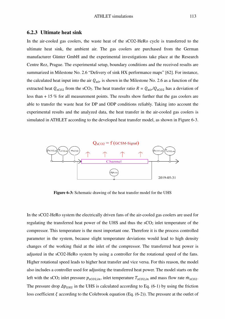
ATHLET simulations 113
6.2.3 Ultimate heat sink
In the air-cooled gas coolers, the waste heat of the sCO2-HeRo cycle is transferred to the
ultimate heat sink, the ambient air. The gas coolers are purchased from the German
manufacturer Günter GmbH and the experimental investigations take place at the Research
Centre Rez, Prague. The experimental setup, boundary conditions and the received results are
summarized in Milestone No. 2.6 “Delivery of sink HX performance maps” [62]. For instance,
the calculated heat input into the air �$N¢ is shown in the Milestone No. 2.6 as a function of the
extracted heat �]ZW from the sCO2. The heat transfer ratio � = �$N¢/�]ZW has a deviation of
less than + 15 % for all measurement points. The results show further that the gas coolers are
able to transfer the waste heat for DP and ODP conditions reliably. Taking into account the
experimental results and the analyzed data, the heat transfer in the air-cooled gas coolers is
simulated in ATHLET according to the developed heat transfer model, as shown in Figure 6-3.
Figure 6-3: Schematic drawing of the heat transfer model for the UHS
In the sCO2-HeRo system the electrically driven fans of the air-cooled gas coolers are used for
regulating the transferred heat power of the UHS and thus the sCO2 inlet temperature of the
compressor. This temperature is the most important one. Therefore it is the process controlled
parameter in the system, because slight temperature deviations would lead to high density
changes of the working fluid at the inlet of the compressor. The transferred heat power is
adjusted in the sCO2-HeRo system by using a controller for the rotational speed of the fans.
Higher rotational speed leads to higher heat transfer and vice versa. For this reason, the model
also includes a controller used for adjusting the transferred heat power. The model starts on the
left with the sCO2 inlet pressure �]ZW ,NO, inlet temperature ']ZW ,NO and mass flow rate �� ]ZW .
The pressure drop ��gVX in the UHS is calculated according to Eq. (6-1) by using the friction
loss coefficient 6 according to the Colebrook equation (Eq. (6-2)). The pressure at the outlet of

114 ATHLET simulations
the UHS �]ZW ,PQR is determined according to Eq. (6-3) and the necessary sCO2 cooling power
according to Eq. (6-4). The enthalpies at the inlet ℎ]ZW ,NO and outlet ℎ]ZW ,PQR of the UHS are
calculated as a function of the inlet and outlet temperatures and pressures. Afterwards, the
calculated sCO2 cooling power �]ZW is used in ATHLET as a GCSM signal and the
implemented PI-controller ensures a constant temperature ']ZW ,PQR at the outlet of the UHS. If
']ZW ,PQR exceeded the target value during the simulation, the PI-controller would automatically
increase the cooling power �]ZW and vice versa.
∆�gVX = 6 · � · 22 · + (6-1)
1¶6 = −2 D´-� Ë 2.51��¶6 + �3.71�Ì (6-2)
�]ZW ,PQR = �]ZW ,NO − ��gVX (6-3)
�]ZW = �� ]ZW · �ℎ]ZW ,NO − ℎ]ZW ,PQR (6-4)
6.2.4 Compact heat exchanger
In the CHX the decay heat is transferred from the steam side of a nuclear power plant to the
sCO2-HeRo system. The investigation on the heat transfer between condensing steam and sCO2
is carried out with heat exchangers according to Table 3-7 at the Institute of Nuclear Technology
and Energy System, Stuttgart. The HX’s, the test facilities, the measurement points, the results
and the data analysis of the low-pressure steam cycle experiments (70 °C / 0.3 bar - glass
model) and high-pressure steam cycle experiments (286 °C / 70 bar - nuclear power plant) are
described in previous chapters. In the following, the data analysis, the chosen correlations, the
comparison between calculated and experimental results and the implementation strategy of the
pressure drop and heat transfer model for the CHX into the ATHLET code are described.

ATHLET simulations 115
The pressure drop ��°$�°,ZVÍ in the CHX can be determined in general according to Eq. (6-5)
with the calculated pressure drop in the channel ��°$�°,°%$OO�� and calculated pressure drops
due to flow deflections as well as contractions and expansions ∆�°$�°,�P]]. The pressure drop in
the channel ��°$�°,°%$OO�� is determined according to Eq. (6-6) by means of the friction loss
coefficient 6, the channel length , the channel diameter �, the density of the fluid 2, and the
velocity of the fluid +. Using a HX with a constant channel length and a constant channel
diameter �, Eq. (6-6) can be simplified according to Eq. (6-7). The sCO2 flow velocity + in
Eq. (6-7) can be rewritten with the sCO2 mass flow rate �� "�(2 and the sCO2 flow cross section
area � according to Eq. (6-8) by using the mass flow rate �� "�(2, the density of the fluid 2, the
volume of the fluid * , the flow velocity of the fluid +, the cross section area �, and the friction
loss coefficient 6. Pressure drops due to flow deflections as well as contractions and expansion
are determined according to Eq. (4-11) - Eq. (4-13).
��°$�°,ZVÍ = ��°$�°,°%$OO�� + ∆�°$�°,�P]] (6-5)
∆�°$�°,°%$OO�� = 6 · � · 22 · + (6-6)
∆�°$�°,°%$OO�� = 6 · 22 · + (6-7)
�� "�(2 = 2 · * � �� "�(2 = 2 · + · � � ��°$�°,°%$OO�� = 622 ® �� "�(2� ¯ (6-8)
A comparison of calculated sCO2 pressure drop results ��°$�°,ZVÍ with experimental result
��05 shows that the experimental ones are 2 to 5 times higher, even though that for the
calculation of ��°$�°,ZVÍ also cross section enhancements, cross section reductions, heat inputs
and bend losses are considered. The deviation between ��05 and ��°$�°,ZVÍ leads to the
development of a pressure drop model (Figure 6-4), which determines the friction loss
coefficients 6NO of the inlet plenum I and 6PQR of the outlet plenum II. These coefficients are
implemented afterwards into the CHX model of the ATHLET code.

116 ATHLET simulations
Figure 6-4: Schematic drawing of the pressure drop model for the CHX
Figure 6-4 shows a schematic drawing of the pressure drop model for the CHX, which can be
divided into three parts: The inlet plenum “Plenum I”, the channel “Channel” and the outlet
plenum “Plenum II”. The calculation starts on the left with a sCO2 inlet pressure �]ZW ,NO, an
inlet temperature ']ZW ,NO and a mass flow rate �� ]ZW . The pressure drop ��NO at the inlet of the
CHX due to flow deflections and cross-section area changes is calculated inside “Plenum I”
according to Eq. (6-9) by means of a determined friction loss coefficient 6NO. Pressure changes
due to cross-section area enhancements and cross-section area reductions are also taken into
account by using the Bernoulli-Equation. The sCO2 pressure at the inlet of the
channel �]ZW ,NO,°%$OO�� is calculated according to Eq. (6-10) and the temperature
']ZW ,NO,°%$OO�� is assumed to be equal to ']ZW ,NO. The pressure drop in the
channel ��°$�°,°%$OO�� is calculated according to Eq. (6-7) with the channel length and
diameter �, the fluid density 2, the flow velocity +, and the friction loss coefficient 6. 6 is
determined by using the Colebrook equation according to Eq. (6-2). The heat input density � is
considered as uniformly distributed over the channel length and the mass, momentum and
energy conservation equation must be fulfilled. The pressure at the outlet of the
channel �]ZW ,PQR,°%$OO�� is determined according to Eq. (6-11) and the temperature
']ZW ,PQR,°%$OO�� is calculated iteratively. The pressure drop ��PQR at the outlet is calculated
similar to ��NO within “Plenum II” by using Eq. (6-9) with �]ZW ,PQR,°%$OO��, ']ZW ,PQR,°%$OO�� and a determined 6PQR. The pressure at the outlet of the CHX �]ZW ,PQR is calculated according
to Eq. (6-12) and the temperature ']ZW ,PQR is assumed to be equal to ']ZW ,PQR,°%$OO��. The
overall pressure drop of the model ��[,ZVÍ is determined according to Eq. (6-13).

ATHLET simulations 117
∆�NO = 6NO · 22 · + (6-9)
�]ZW ,NO,°%$OO�� = �]ZW ,NO − ∆�NO + 0.5 ∗ 2 ∗ �+]ZW ,NO − +]ZW ,NO,°%$OO�� (6-10)
�]ZW ,PQR,°%$OO�� = �]ZW ,NO,°%$OO�� − ∆�°$�°,°%$OO�� (6-11)
�]ZW ,PQR = �]ZW ,PQR,°%$OO�� − ∆�PQR + 0.5 ∗ 2 ∗ �+]ZW ,PQR,°%$OO�� − +]ZW ,PQR (6-12)
��[,ZVÍ = ∆�NO + ��°$�°,°%$OO�� + ∆�PQR (6-13)
After implementing the model into the MATLAB code, an iterative solver is chosen for the
determination of the optimum friction loss coefficients 6NO and 6PQR, which leads to similar
pressure drop results for both the experimental and calculated one. The determined friction loss
coefficients 6NO of 204.332 and 6PQR of 2.371 are included into ATHLET for recalculating the
pressure drops in the investigated CHX. The friction loss coefficient 6NO refers to the inlet
diameter of the pipe into the CHX and 6PQR to the diameter of the pipe at the outlet of the CHX.
Results of the pressure drop model and experimental results are shown in Figure 6-5.
The upper picture in Figure 6-5 shows the experimental sCO2 pressure drop results (red circles)
and the calculated sCO2 pressure drop results (black X) as a function of the sCO2 mass flow
rate. Both graphs show similar parabolic tendencies of the pressure drop with increasing
pressure drop for increasing mass flow rates. The results of the relative prediction errors of the
experimental results compared to the calculated results are depicted in the second picture as a
function of the sCO2 mass flow rate. Except for three measurement points, the relative
prediction error can be limited to less than 10 % for the determined friction loss coefficients 6NO
and 6PQR and for more than half of the measurement points to less than 4 %. The picture at the
bottom shows the calculated sCO2 pressure drop results as a function of the measured sCO2
pressure drop results. The upper black dashed line limits the pressure drop ratio to 110 % and
the lower one to 90 %. The depicted results in Figure 6-5 show that the developed pressure drop
model of the CHX is able to recalculate the experimental results with quite well accordance.

118 ATHLET simulations
Figure 6-5: CHX pressure drop results of the implemented model

ATHLET simulations 119
Besides the pressure drop model described above, also a heat transfer model is developed for
the calculation of the heat transfer in the investigated compact heat exchanger. A schematic
drawing of the model is shown in Figure 6-6.
Figure 6-6: Schematic drawing of the heat transfer model for the CHX
At the left hand side of Figure 6-6, the steam enters the heat transfer model for the CHX at the
top with the steam inlet pressure �V W,NO, inlet temperature 'V W,NO and steam inlet mass flow
rate �� V W. Considering the experimental results, with subcooled conditions at the outlet of the
CHX on the steam side, the MATLAB model can also calculate subcooled water conditions. It
is assumed that saturated steam enters the CHX and flows into the channel in which the heat �
is transferred from the steam side to the sCO2 side. Due to the heat transfer, the steam is
condensed over the channel length and the sCO2 is heated. Depending on the steam and sCO2
inlet conditions, the steam is completely condensed in the model at a channel length ,- and in
the following (channel length , ) the heat transfer occurs between water and sCO2. The water
temperature at the outlet of the CHX 'V W,PQR is iteratively calculated and the pressure �V W,PQR
is assumed to be equal to �V W,NO. Because of counter-current flow conditions the sCO2 enters
at the bottom right (Figure 6-6) with an inlet pressure �]ZW ,NO , inlet temperature ']ZW ,NO and
inlet mass flow rate �� ]ZW . The heat transfer leads to an increase of the sCO2 temperature along
the channel length , and the outlet temperature ']ZW ,PQR at the CHX is iteratively determined.
The sCO2 pressure at the outlet is calculated according to model, as shown in Figure 6-4.

120 ATHLET simulations
The implemented correlations in ATHLET are used to calculate the transferred heat power in
the CHX. According to the ATHLET user guide [63] for the steam side the Nusselt correlation
for laminar film condensation and the Carpenter-and-Colburn correlation for turbulent film
condensation are chosen. One of the two, depending on the flow regime, is used in the channel
length ,- where condensation occurs. The correlation for the calculation of the heat transfer
coefficient in the channel length , is determined in ATHLET according to a heat transfer
correlation-logic-map, which needs temperature and flow regime inputs. On the sCO2 side, the
Gnielinski correlation is used to determine the heat transfer coefficient. If the calculated Nusselt
number is lower than 25, it is automatically set to 25 to avoid numerical instabilities in the code.
In consideration of the heat transfer coefficients on both sides, the transferred heat power is
calculated by means of the plate thickness and heat conductivity. An iterative calculation
process along the channel length determines e.g. the temperature profiles, the pressure drop
profiles, the flow velocity profiles and the transferred heat power on both sides of the CHX.
As an example, results of the temperature profiles in the CHX for the DP investigation with an
sCO2 mass flow rate of 67.7 g/s and an steam condensing power of 585 W as well as for the
ODP II investigation with a mass flow rate of 5.5 g/s and a condensing power of the steam
of 1097 W are shown in Figure 6-7. The upper picture shows temperature profiles of sCO2 and
H2O for the bulk and wall as a function of the channel length for the DP measurement point
with a sCO2 mass flow rate of 67.7 g/s and a steam condensing power of 585 W. Saturated
steam enters the CHX on the left, which leads to a bulk temperature of about 286 °C (black x).
Due to the heat transfer the steam is condensed at a length of about 15 mm and afterwards it is
subcooled to a bulk temperature of about 60 °C. The H2O temperature profile at the wall
(blue +) is lower than the bulk temperature because the heat is transferred from the H2O bulk
via the H2O wall (blue +) and the sCO2 wall (green +) into the sCO2 bulk (red o). The sCO2
enters the HX at the right with a bulk temperature (red o) of about 40 °C and is heated to a
temperature of about 42 °C. The picture at the bottom shows calculated temperature profiles for
the ODP II investigation with a sCO2 mass flow rate of 5.5 g/s and a steam condensing power
of 1097 W. The H2O bulk temperature shows that the steam is condensed at a length of about
45 mm and the sCO2 bulk temperature is heated from about 40 °C to 100 °C at the outlet of the
CHX. A comparison of the two pictures shows that firstly the condensation length of the steam
(blue +) and secondly the outlet temperature of the sCO2 (red o) are increased for the 1097 W
scenario. This can be explained by the steam and sCO2 inlet conditions into the HX.

ATHLET simulations 121
Figure 6-7: CHX temperature profiles of the implemented model for 585 W and 1097 W
Finally, calculated results of the developed heat transfer model and the experimental results are
depicted in Figure 6-8. The first picture shows the calculated steam condensation length ,- as
a function of the sCO2 mass flow rate. On the left it could be seen that for the ODP II
investigations, a steam condensing power of about 1100 W leads to an increasing condensation
length from about 23 mm to 48 mm for decreasing sCO2 mass flow rates from 36.6 g/s to
5.5 g/s. Moreover, the calculated condensation length of 8 mm (�]ZW of 380 W) and 23 mm
(�]ZW of 1100 W) for a sCO2 mass flow rate of about 36 g/s can be explained by different
steam condensing power. The picture at the bottom depicts the calculated sCO2 heat input as a
function of the received experimental results. For all results, there is a linear tendency between
the calculated and experimental results. The upper black dashed line limits the ratio to 110 %

122 ATHLET simulations
and the lower black dashed line to 90 %, which means that the heat transfer model is able to
re-calculate the experimental results with a deviation of less than 10 % for all investigated
measurement points. The results (Figure 6-8) verify that the developed heat transfer model is
able to re-calculate the experimental heat transfer capabilities. Because of that, the implemented
heat transfer correlations in the ATHLET code are used for the determination of the heat transfer
power in the CHX simulations.
Figure 6-8: CHX heat transfer results of the implemented model

ATHLET simulations 123
6.3 ATHLET simulations and results
6.3.1 Boundary conditions
After the implementation of the performance maps and the component models into
ATHLET 3.1, the boundary conditions for the simulations summarized. The design point values
of the sCO2-HeRo system, attached to a LWR, of Venker [10] and the defined design point
values are shown in Table 6-1.
Table 6-1: Design point values of the sCO2-HeRo system
Side Parameter Unit Value (J. Venker) Value
Compressor Inlet (sCO2)
Pressure bar 90 90
Temperature °C 42.0 42.0
Enthalpy kJ/kg 367.00 367.00
Entropy kJ/kg·K 1.54 1.54
CHX Inlet (sCO2)
Pressure bar 180 129
Temperature °C 81.0 62.5
Enthalpy kJ/kg 391.00 379.50
Entropy kJ/kg·K 1.55 1.55
Turbine Inlet (sCO2)
Pressure bar 180 126
Temperature °C 281.0 281.0
Enthalpy kJ/kg 708.00 720.10
Entropy kJ/kg·K 2.28 2.37
UHS Inlet (sCO2)
Pressure bar 90 91
Temperature °C 219.0 255.4
Enthalpy kJ/kg 658.00 699.50
Entropy kJ/kg·K 2.31 2.39
CHX Inlet
(H2O) Temperature °C 286.0 286.0
UHS Inlet (Air)
Temperature °C 37.0 37.0
ΔT Temperature °C 5.0 5.0
Venker determines a compressor inlet pressure of 90 bar and an inlet temperature of 42 °C
(Table 6-1). The sCO2 is compressed to a pressure of 180 bar and simultaneously
compression-heated to a temperature of 81 °C before it enters the CHX. In the CHX it is heated
isobaric to a temperature of 281 °C. After the expansion in the turbine the sCO2 flows with a

124 ATHLET simulations
pressure of 90 bar and a temperature of 219 °C into the UHS where it is cooled isobaric to a
temperature of 42 °C before it re-enters the compressor. The simulations of Venker assume a
constant turbine efficiency of 85 %, a constant compressor efficiency of 80 % and no pressure
losses. For the current simulations equal compressor inlet conditions are chosen. In
consideration of pressure losses and the CFD data from UDE, the pressure at the inlet of the
CHX is determined at 129 bar. The temperature at the inlet is calculated by means of the
compressor efficiency to 62.5 °C. In the CHX the sCO2 is heated to a temperature of 281 °C
and pressure losses in the CHX and in the pipe lead to a pressure of 126 bar at the inlet of the
turbine. According to the implemented performance map, the sCO2 is expanded in the turbine
to a pressure of 91 bar and a temperature of 255.4 °C before it enters the UHS. There the sCO2
is cooled to a temperature of 42 °C and the pressure drop leads to a pressure of 90 bar at the
inlet of the compressor. For all simulations it is assumed that the steam enters the CHX with a
temperature of 286 °C, the air temperature on the secondary side of the UHS is 37 °C and the
minimum temperature difference for heat transfer (pinch point) is 5 °C.
For the ATHLET simulations, a transferred decay heat of 75 MW is defined, leading in the
design point of the sCO2-HeRo system to a sCO2 mass flow rate of 220 kg/s. Furthermore,
five systems in parallel are chosen to be installed. This is beneficial because the systems can be
switch-off consecutively according to the decay-heat-curve, leading to increased operational
time. Furthermore, using five systems means that each system is designed for a decay heat
of 15 MW and a sCO2 mass flow rate of 44 kg/s. The design of the CHX, for 15 MW, is
determined by means of ATHLET and has 14460 rectangular channels with a channel
dimension of 2x1 mm and a channel length of 1.1 m. In the simulation it is defined that the
steam is completely condensed along the channel length and no sub-cooling occurs. The
condensing steam side is simulated by specifying the wall temperature on the H2O side of the
CHX and the implemented Gnielinski correlation is chosen on the sCO2 side. Pressure losses
are calculated according to the developed pressure drop model. The design of the UHS is taken
from Venker with 255 parallel channels, a channel length of 15 m and a channel diameter
of 25 mm. The sCO2 temperature at the outlet of the UHS is controlled in ATHLET by using a
PI-controller, which controls the cooling power on the air side of the UHS. In reality, the sCO2
outlet temperature is controlled by the rotational speed of the air fans. The performance maps
for the turbine and the compressor efficiency as well as pressure ratio are scaled-up from the
glass model conditions to nuclear power plant scale according to the affinity laws for

ATHLET simulations 125
scaling [64]. For the up-scaling, constant pressure ratios, densities, velocities and efficiencies
are assumed. That approach seems to be conservative because the efficiency ratios are assumed
to be constant, but a bigger machine will have a higher efficiency. Comparing the design point
parameters of the glass model and the up-scaled sCO2-HeRo system (Table 6-1) it must be
mentioned that constant density ratios, pressure ratios and velocity profiles could not be applied
for the simulations because the design point of the turbine and the compressor of power plant
size differs from the glass model design point. First results show that in the design point of the
up-scaled sCO2-HeRo system the compressor consumes about 0.53 MW power and the turbine
provides 0.91 MW power which leads to an excess power of about 0.38 MW.
6.3.2 Results
The profile of the steam temperature at the inlet of the CHX is derived from investigations of
Venker [10] for a retrofitted sCO2-HeRo system into a BWR with adapted depressurization
system. It is chosen for specifying the H2O wall temperature of the CHX. For the simulations
in ATHLET 3.1, the channel length of the CHX is divided into 15 control volumes (CV’s)
according to the nodalisation scheme in Figure 6-9. The sCO2 enters the CHX at CV1 and leaves
the CHX heated at CV15. As there is no specific heat exchanger model in ATHLET, the basic
modelling approach is chosen. In this case, only one representative pair of channels
(H2O and sCO2) is modelled and then scaled by the number of channels. The determined
friction loss coefficients at the inlet 6NO and outlet 6PQR of the CHX (chapter 6.2.4) are used for
the recalculation of the experimental sCO2 pressure drop results. The connection between the
sCO2 and H2O side is achieved by using a plate object, which is one heat conduction object.
The heat transfer area of each CV is the product of length and width. The length is determined
by the chosen number of CV’s and the width as well as the thickness can be defined by the user.
Figure 6-9: Nodalisation scheme of the sCO2 channel of the CHX

126 ATHLET simulations
Figure 6-10 depicts simulation results of the sCO2 temperatures in the CHX for three control
volumes of the CHX, namely CV1, CV7 and CV15. CV1 corresponds to the sCO2 inlet, CV7
to the middle of the CHX and CV15 to the sCO2 outlet. Due to the decreasing steam
temperature, the sCO2 temperatures in the CHX are also decreasing over the simulation time.
Figure 6-10: Results of the sCO2 temperature profiles in the CHX for different CV
Figure 6-11: Results of sCO2 pressure for different control volumes

ATHLET simulations 127
Figure 6-11 shows simulation results of the sCO2 pressures from the inlet, outlet, CV1, CV7
and CV15 of the CHX as a function of the simulation time. The major part of the pressure loss
is due to wall friction, which increases along the length of the CHX as the fluid temperature
increases. Consequently, the pressure loss decreases over the simulation time because the outlet
temperature of the CHX also decreases. Inflow and outflow effects, flow distribution and
changes of the cross section flow area cause the second part of the pressure loss at the inlet and
outlet. This pressure loss is modelled as described in the pressure loss model of the CHX
(chapter 6.2.4). Concerning this part of the pressure loss, the major part occurs at the inlet of
the CHX because of the higher form loss coefficient and the additional pressure loss caused by
the reduction of the cross sectional flow area. At the outlet, the expansion of the flow almost
decreases the pressure loss to zero.
Figure 6-12 shows the calculated power output of the turbine and the power consumption of the
compressor as a function of the simulation time. As a result of decreasing steam temperatures,
the power output of the turbine also decreases over time. In contrast, the power consumption of
the compressor is nearly constant, which is achieved by keeping the inlet condition constant.
Additionally, the efficiencies of the turbine and the compressor are nearly constant due to the
only slightly rising mass flow rates and the assumption of a constant rotational speed of the
shaft. At the end of the simulation at about 11.5 h, the net power output of 76 kW is not enough
to power the fans of the ultimate heat sink with a power consumption of 165 kW, according to
Venker [10]. The break-even point is reached after 6.9 h and a steam temperature of 182 °C.
The results of Venker show for the “Retrofitted BWR with Adapted Depressurization System”
scenario that the break-even point is reached after 11.4 h and a steam temperature of 147 °C.
However, the early break-even point here is a consequence of the lower net power output at the
start of the simulation and the lower efficiency compared to the model of Venker.

128 ATHLET simulations
Figure 6-12: Calculated power output of compressor and turbine
Finally, it can be concluded that in further studies extended performance maps should be
developed, implemented and used in the ATHLET code. For example, the performance maps
of the compressor should be extended for a two-stage compressor, which is able to compress
the sCO2 to a pressure of up to 180 bar. Moreover, the scaling and design of the components
for nuclear power plant application needs to be analyzed in more detail to perform more realistic
reactor simulations. Additionally, the control strategies of the sCO2-HeRo system should be
investigated in more detail and the cycle behavior at DP, ODP and closer the critical point
should be experimentally tested at the demonstrator unit at the PWR glass model at GfS, Essen.
In the future also a more realistic model of the UHS should be implemented and the interaction
between nuclear power plant and attached sCO2-HeRo system should be investigated.

Discussion and Perspectives 129
7 Discussion and Perspectives
The design point parameters of the sCO2-HeRo demonstrator unit and for a NPP are determined
by means of cycle calculations in consideration of boundary conditions and assumptions, which
are discussed as follows. The boundary conditions on the steam side of the sCO2-HeRo
demonstrator unit are derived from experiments at the glass model. The water is electrically
heated, and because it is made of glass, the operating pressure is limited to pressures lower
1 bar, leading to steam temperatures below 100 °C. Experiments show that decay heat powers
between 0 - 12 kW can be provided, a higher power extraction decreases the steam temperature
and a decreasing extraction leads to very small transferred heat power to the sCO2 side. As a
compromise, the design point for the decay heat is set to 6 kW, which leads to a saturated steam
temperature of about 70 °C and a steam pressure of about 0.3 bar. Comparing the steam
conditions, the amount of decay heat and the steam temperatures they are significantly lower in
the GM than in a NPP. A nuclear power plant has steam with a pressure of 70 bar and a saturated
steam temperature of 286 °C. Venker [10] suggests that 60 MW of decay heat have to be
removed by the sCO2-HeRo system in order to achieve a long-term coolability of the nuclear
core. Furthermore, the amount of removed decay heat should be adjusted according to the
existing decay heat, to ensure a high temperature difference between the ambient air and the
steam, which results in increasing operational time of the sCO2-HeRo system. This is realized
by using four equal 15 MW sCO2-HeRo units in parallel, instead of one 60 MW unit.
To reduce the complexity and to increase the robustness of the sCO2-HeRo demonstrator unit,
a single stage compressor with a pressure ratio of about 1.5 is chosen. To prevent any kind of
manufacturing problems of the TCS due to very small components, the minimum sCO2 mass
flow rate is set to 0.65 kg/s. Because of the low steam temperature, an additional slave electrical
heater is installed for heating up the sCO2 to a turbine inlet temperature of 200 °C, which is
similar to NPP conditions. The turbine efficiency of 75 % and the compressor efficiency
of 65 % are conservative assumptions for such small machines. Both efficiencies are assumed
to be constant for the entire range of cycle calculations. In comparison, a multi-stage
compressor with a compression ratio of about 3 is selected for a nuclear power plant. The
turbine efficiency of 85 %, the compressor efficiency of 75 % and a compression ratio of 3 are
also conservative assumptions for such big machines. Both efficiencies are assumed to be
constant for the entire range of cycle calculations.

130 Discussion and Perspectives
The cycle calculations are performed for both systems in consideration of boundary conditions
and assumptions like constant turbine and compressor efficiencies, no heat losses and no
pressure losses. With respect to maximum generator excess electricity, the design point
parameters of the sCO2-HeRo demonstrator unit are determined as follows: the compressor
inlet pressure and temperature are set to 78.3 bar and 33 °C, the turbine inlet pressure and
temperature to 117.45 bar and 200 °C and the sCO2 mass flow rate to 0.65 kg/s. A steam
condensing power of 6 kW is determined in the CHX. In the design point, the generator
provides an excess electricity of about 9 kW. These data will have to be confirmed once the
demonstrator unit at GfS starts operation. Four 15 MW sCO2-HeRo systems in parallel are used
for the NPP application. The maximum generator excess electricity of one unit of
about 1.38 MW is reached with a compressor inlet pressure and temperature of 90 bar
and 42 °C, a turbine inlet pressure and temperature of 180 bar and 280 °C, and a sCO2 mass
flow rate of 47.7 kg/s. For heating the sCO2 mass flow rate in the CHX a condensing power of
the steam of 15 MW is defined.
The experimental investigation on the heat transfer between condensing steam and sCO2 in
diffusion bonded compact heat exchangers takes place in the laboratory of the Institute of
Nuclear Technology and Energy Systems (IKE) by using two test facilities.
The SCARLETT test loop provides sCO2 mass flow rates from 30 g/s to 110 g/s, depending on
the compressor performance. The sCO2 temperature at the inlet of the test section can be varied
from 0 °C to 40 °C and the pressure can be adjusted from 75 bar to 110 bar.
The low-pressure steam cycle generates steam similar to the steam conditions at the PWR glass
model. The pressure can be adjusted from 0.1 bar to 1 bar and the steam temperature
corresponds to the pressure and varies between 50 °C and 100 °C. The water volume flow rate
can be varied by the membrane pump from 0.05 l/h to 2.5 l/h and the installed electrical heating
power of the evaporator with 1.6 kW is high enough to evaporate the adjusted water volume
flow rates. For the heat transfer investigations with steam, such as in an NPP, the high-pressure
steam cycle is constructed. The pressure can be adjusted from 1 bar to 105 bar and the
corresponding steam temperature varies between 100 °C and 315 °C. The water volume flow
rate can be varied, similar to the low-pressure steam cycle, by the HPLC pump from 0.05 l/h to

Discussion and Perspectives 131
2.5 l/h and the electrical heating power of the evaporator with 1.6 kW is high enough for
evaporation the water volume flow rates. The electrically heated evaporator is the most
challenging component of both steam cycles. For further investigations, it would be beneficial
to purchase and install an evaporator with increased heating powers, leading to increased steam
volume flow rates in the test section.
Within this work, 7 heat exchangers are constructed and manufactured for the experimental heat
transfer investigations. To investigate the influence of the channel dimension on phenomena
like the heat transfer and the pressure drop, rectangular 2x1 mm and 3x1 mm channels are
chosen with respect to recommended channel dimensions for CHX from the literature. The
influence of the channel shape is investigated by means of heat exchangers with straight H2O
and Z-shaped sCO2 channels (IZ) as well as with heat exchangers with straight H2O and straight
sCO2 channels (II). The IZ channel shape is chosen because it is used for heat exchangers with
more than one plate on each side and stacked plates. The II channel shape is selected because
it is easy to manufacture and experimental results can be used e.g. for validation. The influence
of the plenum geometry is investigated with heat exchangers with 15 channels at 1 plate and
1 plate on each side (15/1) as well as heat exchangers with 5 channels at 1 plate and 3 plates on
each side (5/3) because previous investigations show that a more cubic plenum geometry is
beneficial for decreasing pressure drop. The experimental heat transfer results of the 15/1 and
5/3 plates show that a steam provision of about 1.2 kW is not sufficient to investigate the heat
transfer limits. Therefore, a heat exchanger with 5 channels at 1 plate and 1 plate on each
side (5/1) is manufactured and investigated.
The measurement campaigns are classified according to the “Design Point” (DP), the “Out of
Design Point” (ODP) and the “Out of Design Point II” (ODPII) campaigns. In the DP
experiments, the sCO2 mass flow rates and water volume flow rates are scaled down in the same
ratio as the entire amount of sCO2 mass flow rate and water volume flow rate, used in the design
point of the sCO2-HeRo demonstrator unit at the glass model. The DP investigations are limited
by a maximum achievable sCO2 mass flow rate of 68 g/s and a sCO2 pressure of 110 bar. The
ODP measurement campaigns are performed with a sCO2 mass flow rate of 37 g/s and gradually

132 Discussion and Perspectives
increasing water volume flow rates. The electrical heating power of the evaporator is limited
to 1230 W due to internal temperature restrictions. In the ODP II measurements, investigations
with a water volume flow rate of 1.74 l/h and a maximum electrical heating power of the
evaporator of 1230 W are performed. The sCO2 mass flow rate is gradually decreased from
37 g/s to about 6 g/s by adjusting a needle valve and bypassing a part of the sCO2. The minimum
adjustable sCO2 mass flow rate is limited by the valves opening degree of the needle valve, by
temperature restriction of the Pt-100 and by increasing sCO2 mass flow rate fluctuations for
decreasing sCO2 mass flows.
The data analysis starts with experimental pressure drop results of unheated sCO2 flows. The
results show, for instance, that an increasing sCO2 mass flow rate leads to an increasing sCO2
pressure drop and that a constant sCO2 mass flow rate and an increasing sCO2 inlet pressure
leads to decreasing sCO2 pressure drop, which is in accordance with analytic methods. The
results also confirm that the sCO2 pressure drop is lower for straight sCO2 channels, compared
to Z-shaped channels. In straight channels no sharped-edge deflections exist, which causes this
additional pressure drop. For future channel designs, it is recommended to use smooth bends
instead of sharp-edged deflections. Besides that, also the plenum geometry has an influence on
the pressure drop. In more cubic plenum geometries, a more homogenous mass flow
distribution with less turbulences can be developed, leading to decreasing pressure drops.
For heated sCO2 flows, pressure drop results are shown for instance as a function of the heating
load. The heating load is chosen because it represents the ratio of sCO2 heat input to sCO2 mass
flux and both parameters influence the pressure drop. The results show a strong influence of the
sCO2 mass flux on the sCO2 pressure drop and a slight influence of the heat input on the pressure
drop. The kind of sCO2 heat input (LP steam cycle or HP steam cycle) and the influence on the
pressure drop is further investigated. The results show that the pressure drop is unaffected by
the kind of heat input. Only the amount of heat input and the sCO2 inlet conditions into the heat
exchanger, like inlet pressure, inlet temperature and mass flow rate, have an impact. This can
be advantageous for future investigations, because expensive and complex test facilities like
the high-pressure steam cycle can be replaced by less complex test facilities. Subsequently, the
sCO2 pressure drop is shown as a function of the averaged Nusselt number. It could be seen that
decreasing sCO2 inlet pressures led to increasing Nusselt numbers and increasing pressure
drops. On the one hand, increasing Nusselt numbers are beneficial for the heat transfer, but on

Discussion and Perspectives 133
the other hand, increasing pressure drops are disadvantageous. This must be considered in the
design of the heat exchangers.
The data analysis of heat transfer investigations show, for instance, that the heat is reliably
transferred from the steam side to the sCO2 side for all measurement campaigns and all heat
exchangers. As described, it is recommended for future investigations to install an evaporator
with higher heating power to provide higher steam volume flow rates at the inlet of the test
section. The difference between the calculated steam condensing power and the calculated sCO2
heat input is described by means of an averaged offset, which can be explained by thermal
losses. Thereby it could be seen that the thermal losses are higher for the high-pressure steam
cycle experiments, compared to the low-pressure experiments because of higher steam
temperatures during operation. The obtained heat transfer results of the 5/1 configuration show
that a sCO2 mass flow rate of about 2 g/s is sufficient to transfer a heat power of about 1250 W
from the steam side to the sCO2 side, which is impressive. Besides that, results of the calculated
sCO2 temperature increase are shown and they are corresponding to analytic methods. The
surface temperature results show that there is a symmetrical temperature profile with lower
surface temperatures in the center line of the heat exchanger and higher surface temperatures at
the outer area.
The design of the CHX for the sCO2-HeRo demonstrator is determined in consideration of
measurement results and boundary conditions. The rectangular 2x1 mm channel dimension is
chosen with respect to received experimental results. Summarizing the design of the CHX, the
choice of an entire number of 14 plate pairs is a consideration of the compactness and the
acceptable pressure drop. The number of channels per plate is determined at 15, the effective
channel length at 150 mm and the entire number of channels on each side at 210. The integrated
plenum geometry at the plates is one innovative aspect of the CHX, because no further welding
processes of the plenums is required. The plates are manufactured, diffusion bonded, and after
successfully passing a pressures and leakage test, the CHX is installed at the GM. For future
designs of HX’s, it might be possible to reduce the wall thicknesses, leading to reduced material
effort and less space. A conservative and robust design is chosen for the CHX of the
sCO2-HeRo demonstrator unit, including for instance a safety factor, a reduction factor of the
diffusion bonding process and a conservative allowed material stress of 1.4301.

134 Discussion and Perspectives
The development of performance maps and the validation of correlations for heat transfer and
pressure drop of the ATHLET code are done before new sCO2-HeRo cycle calculations are
carried out for the NPP application. The PM’s for the turbine and compressor are derived
from CFD calculation results. With polynomial and linear surface interpolation techniques in
MATLAB, the PM’s for the determination of the efficiencies and pressure ratios are developed
for all measurement points with a deviation of less than 1 % compared to the received data
points. The results are scaled up in ATHLET to nuclear power plant size according to the affinity
laws. For the UHS, a simple heat transfer model is developed in which the sCO2 outlet
temperature is adjusted via heating or cooling. The transferred heat power is controlled in
ATHLET by using a PI-controller and in the sCO2-HeRo system by adjusting the rotational
speed of the fans. The chosen design of the UHS for the NPP is equal to those of Venker [10].
In consideration of the experimental results of the CHX, a pressure drop model is developed,
in which the experimental results can be recalculated for all measurement campaigns with an
accuracy of more than 90 % (except three values). Besides that, a heat transfer model is
developed as well. The used correlations are already implemented in the ATHLET 3.1 code,
and by using them, the model can recalculate the experimental results with a deviation of less
than 10 %. Afterwards, the CHX for a NPP is designed with the help of ATHLET. In the
simulations it is assumed that the steam is completely condensed at the outlet of the CHX and
there is a minimum temperature difference between H2O and sCO2 of 5 °C. This leads to a CHX
with 14460 rectangular channels with a channel dimension of 2x1 mm and a channel length
of 1.1 m. After specifying the components, thermodynamic cycle calculations of the
sCO2-HeRo system attached to a LWR are performed. The results show that the steam
temperature decreases over the time, which leads to decreasing sCO2 temperatures in the CHX
and thus to lower inlet temperatures at the turbine. Lower turbine inlet temperatures cause lower
turbine power and less net power at the generator. The results of the turbine power and
compressor power as a function of the simulation time show that excess electricity is provided
for more than 12 h. Considering the power consumption of the electrical driven fans with
about 186 kW, the operational time of the sCO2-HeRo system is limited to about 7 h. The
simulations confirm that the sCO2-HeRo approach is feasible; however, more performance
data, especially from the sCO2-HeRo demonstrator unit at the PWR glass model, are needed to
improve the current performance maps and to validate correlations for a wider parameter range.

Summary 135
8 Summary
To improve the safety of nuclear power plants, a self-launching, self-propelling and
self-sustaining decay heat removal system for retrofitting into NPPs is investigated in the
European sCO2-HeRo project. To prevent core damage in case of a station-blackout and
loss-of-ultimate-heat-sink accident scenario, the system should be able to transfer the decay
heat reliably from the reactor core to an ultimate heat sink, e.g. the ambient air. The system
consists of a compressor, a compact heat exchanger, a turbine, a sink heat exchanger and a
generator. Within the project a two-scale approach is applied. To demonstrate the feasibility, a
small-scale demonstrator unit is first designed, manufactured and retrofitted into the PWR glass
model. Single-effect experiments are performed to determine the design of each component of
the demonstrator unit. Then the obtained results of the single-effect experiments are used to
develop heat transfer and pressure drop models, to develop performance maps and to validate
correlations. Afterwards, they are implemented into the German thermal-hydraulic code
ATHLET, transferred to component models on nuclear power plant size and new cycle
calculations are performed.
This work starts with a description of the pressurized water reactor glass model in which the
sCO2-HeRo demonstrator unit is installed. The demonstrator unit is used on the one hand to
receive experimental data for code validation and on the other hand to showing the feasibility
of such a system. Next, the setup of the sCO2-HeRo demonstrator unit is described. To support
the construction of the demonstrator at the glass model, a piping and instrumentation diagram
is developed. It includes the components, the measurement devices and a unique nomenclature.
For reasons of clarity, it is divided into 8 sections. The setup of the sCO2-HeRo system, attached
to the steam generator of a nuclear power plant, is described by means of a schematic drawing.
Further, sCO2-HeRo cycle calculations are carried out for both systems and the design point
parameters are determined with respect to maximum generator excess electricity, boundary
conditions and assumptions. For the demonstrator unit, one sCO2-HeRo system is defined. It
transfers in the design point a simulated decay heat power of 6 kW from the reactor core to the
ultimate heat sink. Four sCO2-HeRo systems in parallel are chosen for the nuclear power plant
application. Each system can transfer a decay heat power of 15 MW from the nuclear core to
the ambient air.

136 Summary
In the second part of this work, the test facility and the heat exchanger test plates are described.
The experimental investigations take place in the sCO2 SCARLETT loop providing sCO2 under
defined conditions, and in a steam cycle. The low-pressure steam cycle is designed and build
to provide steam with a pressure of 0.3 bar and a saturated steam temperature of about 70 °C,
which is similar to the steam conditions of the PWR glass model. The high-pressure steam cycle
is constructed to generate steam similar to the steam conditions of a nuclear power plant
(70 bar / 286 °C). For the experimental investigations, seven heat exchanger configurations are
designed and manufactured. These could be classified according to the channel dimension
(3x1 mm / 2x1 mm), the number of channels per plate and number of plates
(15/1 / 5/1 / 5/2 / 5/3) as well as the channel shape (II / IZ). The mechanical design of the heat
exchangers is determined by transforming rectangular channel geometries into circular pipe
geometries. These pipe geometries are used in the following to determine the minimum wall
thickness by means of ordinary calculation methods. After manufacturing the plates, they are
diffusion bonded. Stainless steel 1.4301 is chosen as plate material.
The third part of this work includes the determination of the measurement parameters and the
experimental investigations. In the “Design point” (DP) experiments the sCO2 mass flow rates
and water volume flow rates are scaled down in the same ratio as the entire amount of sCO2
mass flow rate and water volume flow rate, used in the design point of the sCO2-HeRo
demonstrator unit at the glass model. To investigate the heat transfer e.g. also
“Out of design point” (ODP) a constant sCO2 mass flow rate and gradually increasing water
volume flow rates are applied. In the “Out of design point II” (ODP II) measurements, a
constant water volume flow rate and a gradually decreasing sCO2 mass flow rate are chosen.
The pressure drop results of unheated sCO2 flows show for instance a parabolic increase of the
pressure drop for increasing sCO2 mass flow rates and decreasing pressure drops for increasing
sCO2 inlet pressures. Furthermore, an increasing flow area leads to decreasing sCO2 pressure
drops, for constant sCO2 mass flow rates and sCO2 inlet pressures. A comparison of calculated
pressure drop results and experimental results shows that the experimental ones are always 2 to
3 times higher. This could be attributable primarily to the inappropriate plenum geometry and
the unsuitable sCO2 inflow conditions into the plenum. The results show further that a straight
channel shape reduces the sCO2 pressure drop significantly, compared to the results of the
Z-shaped channels. The plenum geometry also influences the pressure drop with decreasing
sCO2 pressure drops for more cubic plenum geometries and vice versa. For heated sCO2 flows,

Summary 137
the pressure drop results confirm a strong influence of the sCO2 mass flow rate on the pressure
drop and an influence of the heat input on the pressure drop, which can be explained by changes
of the flow velocity and the fluid density. The kind of heat input from the steam (LP / HP) and
the influence of the sCO2 pressure drop is also investigated. The results show, for instance, that
the pressure drop is not influenced by the kind of steam heat input. Only the amount of heat
input and the sCO2 inlet conditions into the heat exchanger influence the sCO2 pressure drop.
The results of the heat transfer investigations also show linear profiles of the calculated sCO2
heat input as a function of the calculated condensing power of the steam, only with varying
offsets for the high-pressure and low-pressure steam cycle. This could be explained by higher
thermal losses at the high-pressure steam cycle due to higher operation temperatures compared
with the low-pressure steam cycle. The heat transfer results show further that a heat exchanger
with 5 channels at each side and an effective straight channel length of 150 mm is sufficient to
transfer a heat power of about 1250 W from the steam side to the sCO2 side. Finally, the
temperatures on the surface of the heat exchanger are measured. The results show symmetrical
temperature profiles with lower surface temperatures in the center line of the HX and higher
surface temperatures at the outer area. Furthermore, a higher sCO2 heat input leads to increasing
surface temperatures, especially at the top of the heat exchanger.
The compact heat exchanger for the sCO2-HeRo demonstrator unit is designed in consideration
of boundary conditions and received experimental data. After constructing and manufacturing
the plates the CHX is diffusion bonded before a pressure and leakage test is carried out. Finally,
it is installed at the PWR glass model at GfS, Essen.
The thermal-hydraulic simulation of the sCO2-HeRo system for a nuclear power plant by using
the ATHLET 3.1 code with advanced models is the last part of that work. For this, correlations
are validated with experimental data and performance maps as well as models for heat transfer
and pressure drop are developed. For instance, performance maps for the compressor and
turbine are developed by means of CFD data and experimental results. Afterwards, these
performance maps are transferred according to the affinity laws to component models on power
plant size and implemented into the ATHLET code. For the simulation of the transferred heat
power in the ultimate heat sink, a heat transfer model is developed in consideration of
experimental data. To simulate the CHX in ATHLET, a pressure drop and heat transfer model

138 Summary
is developed. Both are validated with experimental results and the necessary friction loss
coefficients for calculating the pressure drop are implemented into the ATHLET code. The
design of the CHX for the nuclear power plant application is determined with ATHLET before
advanced sCO2-HeRo cycle simulations are carried out. The simulation results show that the
break-even point of the system is reached after about 6.9 h due to decreasing steam
temperatures, leading to decreased turbine excess power. This value is mainly determined by
the low efficiency of the turbine and compressor, which are obtained after up-scaling the
components of the sCO2-HeRo demonstrator unit. The rotor design of the demonstrator unit
could not be optimized for the small size of a few centimeter. For instance, the height of the
turbine blade is about 1 mm, leaving no space for improvement. It is expected that larger
turbomachines (MW size) will be operated with higher efficiency, thus prolonging the grace
time to the expected 72 hrs.

Bibliographie 139
9 Bibliographie
[1] International Energy Agency (IEA): Statistics Data Browser - Energy Consumption.
2019. (https://www.iea.org/statistics)
[2] Bundesministerium für Wirtschaft und Energie (BMWi): Energiedaten: Gesamtausgabe.
Stand: August 2018.
[3] Deutsches Atomforum e. V. (DAtF): Kernkraftwerke in Europa. Berlin, 2017.
[4] Deutsches Atomforum e. V. (DAtF): Kernenergie Basiswissen. Berlin, 2013.
[5] Foratom: Nuclear Energy Is Essential To EU Low Carbon Future. Brussels, 2019.
[6] Deutsches Atomforum e. V. (DAtF): Sicherheit ist das oberste Gebot. Berlin, 2013.
[7] YILMAZ, Ö.; POHLNER, G.; BUCK, M.; STARFLINGER, J.: Design Consideration
For A Core-Catcher Concept Based On Bottom Flooding Through Porous Concrete.
Proceedings of the 11th International Topical Meeting on Nuclear Reactor Thermal
Hydraulics, Operation and Safety (NUTHOS-11). Gyeongju, Korea, 2016.
[8] FISCHER, M.: The Severe Accident Mitigation Concept And The Design Measures For
Core Melt Retention Of The European Pressurized Reactor (EPR). Nuclear Engineering
and Design 230, p. 169 - 180, 2004.
[9] GRASS, G.; KULENOVIC, R.; STARFLINGER, J.: Experimental Investigtion On
Long Closed Two Phase Thermosyphons To Be Applied In Spent Fuel Pools For Passive
Heat Removal. Proceedings of the 26th International Conference - Nuclear Energy for
New Europe (NENE2017). Bled, Slovenia, 2017.
[10] VENKER, J.: Development And Validation Of Models For Simulation Of Supercritical
Carbon Dioxide Brayton Cycle And Application To Self-Propelling Heat Removal
Systems In Boiling Water Reactors. University of Stuttgart, IKE2-156,
ISSN-0173-6892. Stuttgart, Germany, 2015.
[11] VENKER, J.: A Passive Heat Removal System Retrofit For BWRs. Nuclear Engineering
International 711, p. 14 - 17, 2013.
[12] VENKER, J.; STARFLINGER, J.; SCHAFFRATH, A.: Code Development And
Simulation Of The Supercritical CO2 Heat Removal System. Proceedings of the
European Nuclear Conference. Warsaw, Poland, 2016.
[13] VENKER, J.; VON LAVANTE, D.; BUCK, M.; GITZEL, D.; STARFLINGER, J.:
Interaction Between Retrofittable And Existing Emergency Cooling Systems In BWRs.
Proceedings of the 10th International Topical Meeting on Nuclear Thermal-Hydraulics,
Operation and Safety (NUTHOS-10). Okinawa, Japan, 2014.

140 Bibliographie
[14] VENKER, J.; VON LAVANTE, D.; BUCK, M.; GITZEL, D.; STARFLINGER, J.:
Transient Analysis Of An Autarkic Heat Removal System. Proceedings of the 2014
International Congress on Advances in Nuclear Power Plants (ICAPP 2014).
Charlotte, USA, 2014.
[15] VENKER, J.; VON LAVANTE, D.; BUCK, M.; GITZEL, D.; STARFLINGER, J.:
Concept Of A Passive Cooling System To Retrofit Existing Boiling Water Reactors.
Proceedings of the 2013 International Congress on Advances in Nuclear Power Plants
(ICAPP 2013). Jeju, South Korea, 2013.
[16] STRAETZ, M.; STARFLINGER, J.; MERTZ, R.; SEEWALD, M.; SCHUSTER, S.;
BRILLERT, D.: Cycle Calculations Of A Small Scale Heat Removal System With
Supercritical CO2 As Working Fluid. Proceedings of the 14th International Conference
on Nuclear Engineering (ICONE25). Shanghai, China, 2017.
[17] Tokyo Electric Power Company: Fukushima Nuclear Accident Analysis Report. 2012.
[18] AHN, Y.; BAE, S. J.; KIM, M.; CHO, S. K.; BAIK, S.; LEE, J. I.; CHA, J. E.: Review
Of Supercritical CO2 Power Cycle Technology And Current Status Of Research And
Development. Nuclear Engineering and Technology 47, p. 647 - 661, 2015.
[19] VOJACEK, A.; HACKS, A.; MELICHAR, T.; FRYBORT, O.; HAJEK, P.: Challenges
In Supercritical CO2 Power Cycle Technology And First Operational Experience
At CVR. Proceedings of the 2nd European supercritical CO2 Conference.
Essen, Germany, 2018.
[20] GAMPE, U.; HENOCH, J.; RATH, S.; GERBETH, G.; HAMPEL, U.; HANNEMANN,
F.; GLOS, S.: Concept And Preliminary Design Of A 600 °C+ sCO2 Test Facility.
Proceedings of the 2nd European supercritical CO2 Conference. Essen, Germany, 2018.
[21] FLAIG, W.; MERTZ, R.; STARFLINGER, J.: Setup Of The Supercritical CO2 Test-
Facility „SCARLETT“ For Basic Experimental Investigations Of A Compact Heat
Exchanger For An Innovative Decay Heat Removal System. Proceedings of the 14th
International Conference on Nuclear Engineering (ICONE25). Shanghai, China, 2017.
[22] KIMBALL, K. J.: Supercritical Carbon Dioxide Power Cycle Development Overview.
Proceedings of the 4th International Symposium - Supercritical CO2 Power Cycles
Technologies for Transformational Energy Conversion. Pittsburgh, USA, 2014.
[23] VOJACEK, A.: Workshop „The Supercritical CO2 Heat Removal System” - sCO2
Experimental Loop and CVR R&D Activities. Rez, Prague, 2017.

Bibliographie 141
[24] WRIGHT, S. A.; RADEL, R. F.; VEMON, M. E.; ROCHAU, G. E.; PICKARD, P. S.:
Operation And Analysis Of a Supercritical CO2 Brayton Cycle. Sandia Report -
SAND2010-0171. Albuquerque, New Mexico, 2010.
[25] AHN, Y.; LEE, J.; KIM, S. G.; LEE, J. I.; CHA, J. E.; LEE, S.: Design Consideration
Of Supercritical CO2 Power Cycle Integral Experimental Loop. Energy 86,
p. 115 - 127, 2015.
[26] CARLSON, M. D.; KRUIZENGA, A. K.; SCHALANSKY, C.; FLEMING, D. F.:
Sandia Progress On Advanced Heat Exchangers For sCO2 Brayton Cycles. Proceedings
of the 4th International Symposium - Supercritical CO2 Power Cycles Technologies for
Transformational Energy Conversion. Pittsburgh, USA, 2014.
[27] NIKITIN, K.; KATO, Y.; NGO, L.: Printed Circuit Heat Exchanger Thermal Hydraulic
Performance In Supercritical CO2 Experimental Loop. International Journal
of Refrigeration 29, p. 807 - 814, 2006.
[28] NGO, T. L.; KATO, Y.; NIKITIN, K.; TSUZUKI, N.: New Printed Circuit Heat
Exchanger With S-shaped Fins For Hot Water Supplier. Experimental Thermal and
Fluid Science 30, p. 811 - 819, 2006.
[29] MA, T.; XU, X. Y.; CHEN, Y. T.; WANG, Q. W.: Study On Local Thermal-hydraulic
Performance and Optimization Of Zigzag-Type Printed Circuit Heat Exchanger At High
Temperature. Energy Conversion Management 105, p. 55 - 56, 2015.
[30] MA, T.; XIN, F.; XU, X. Y.; CHEN, Y. T.; WANG, Q. W.: Effect Of Fin-Endwall Fillet
On Thermal Hydraulic Performance Of Airfoil Printed Circuit Heat Exchanger. Applied
Thermal Engineering 89, p. 1087 - 1095, 2015.
[31] LEE, S. M.; KIM, K. Y.: Multi-Objective Optimization Of Arc-Shaped Ribs In The
Channels Of A Printed Circuit Heat Exchanger. International Journal of
Thermal Science 94, p. 1 - 8, 2015.
[32] LEE, S. M.; KIM, K. Y.; KIM, S. W.: Multi-Objective Optimization Of
a Double-Faced Type Printed Circuit Heat Exchanger. Applied Thermal
Engineering 60, p. 44 - 50, 2013.
[33] SONG, H.; METER, J. V.; LOMPERSKI, S.; CHO, D.; KIM, H. Y.; TOKUHIRO, A.:
Experimental Investigations Of A Printed Circuit Heat Exchanger For Supercritical CO2
And Water Heat Exchange. Proceedings of the 5th Korea-Japan Symposium on Nuclear
Thermal Hydraulics and Safety (NTHAS5). Jeju Island, South Korea, 2006.
[34] TSUZUKI, N.; KATO, Y.; ISHIDUKA, T.: High Performance Printed Circuit Heat
Exchanger. Applied Thermal Engineering 27, p. 1702 - 1707, 2007.

142 Bibliographie
[35] CHU, W.; LI, X.; MA, T.; CHEN, Y.; WANG, Q.: Experimental Investigation On SCO2-
Water Heat Transfer Characteristics In A Printed Circuit Heat Exchanger With Straight
Channels. International Journal of Heat and Mass Transfer 113, p. 184 - 194, 2017.
[36] SEEWALD, M.; STRAETZ, M.; FREUTEL, T.: Deliverable D1.1 „Release
thermodynamic cycle parameters“. sCO2 HeRo Project (2015 - 2018). Germany, 2015.
[37] HACKS, A.; SCHUSTER, S.; DOHM, H. J.; BENRA, F.; BRILLERT, D.:
Turbomachine Design for Supercritical Carbon Dioxide Within the sCO2-HeRo.eu
Project. Proceedings of the ASME Turbo Expo. Oslo, Norway, 2018.
[38] DOSTAL, V.; DRISCOLL, M. J.; HEJZLAR, P.: A Supercritical Carbone Dioxice Cycle
for the Next Generation. Nuclear Reactors, Tech. Rep. MIT-ANP-TR-100,
Massachusetts Institute of Technology, USA, 2004.
[39] WRIGHT, A.; CONBOY, T. M.; ROCHAU, G. E.: Overview of Supercritical CO2
Power Cycle Development at Sandia National Laboratories. Proc. University Turbine
Systems Research Workshop Columbus. Ohio, USA, 2011.
[40] HACKS, A.; FREUTEL, T.; STRAETZ, M.; VOJACEK, A.; HECKER, F.;
STARFLINGER, J.; BRILLERT, D.: Operational Experiences and Design of the
sCO2-HeRo loop. Proceedings of the 3rd European supercritical CO2 Conference.
Paris, France, 2019.
[41] ELMESS Thermosystemtechnik GmbH & Co. KG, Nordallee 1, 29525 Uelzen,
Germany. www.elmess.de.
[42] Schick - Gase + Technik + Kälte: Datenblatt: R744 / CO2: Kohlendioxid - ein
unbegrenzt verfügbarer und natürlicher Stoff. Vaihingen/Enz, Germany, 2018.
[43] LEMMON, E. W.; HUBER, M. C.; MCLINDEN M. O.: Refprop - Reference Fluid
Thermodynamic and Transport Properties, Standard Reference Database 23, Version
9.0. National Institute of Standards and Technology (NIST). Boulder, CO, USA, 2010.
[44] SHAH, R. K.; SEKULIC, D. P.: Fundamentals Of Heat Exchanger Design. Wiley: 2003.
[45] BAEHR, H. D.; STEPHAN, K.: Wärme- und Stoffübertragung (8. Auflage).
Springer-Verlag: Berlin, Heidelberg, 2013.
[46] HEIDEMANN, W.: Unterlagen zur Vorlesung - Berechnung von Wärmeübertragern.
Stuttgart, Germany, 2016.
[47] Ätztechnik Herz GmbH & Co. KG: Broschüre: Ätzen - schnell - sauber - gratfrei.
Epfendorf am Neckar, Germany, 2019. (https://www.aetztechnik-herz.de/wp-
content/uploads/2016/07/Layout-Prosp-18-S-herz-Image-D_47_Download.pdf)

Bibliographie 143
[48] HESSELGREAVES, J. E.: Compact heat exchangers. Pergamon: Amsterdam,
New York, 2001.
[49] RUSNALDY: Diffusion Bonding: An Advanced Of Material Process. Journal of
ROTASI - Volume 3, Nomor 1, Januari 2001.
[50] SARANAM, V. R.; PAUL, B. K.: Feasibility Of Using Diffusion Bonding For
Producing Hybrid Printed Circuit Heat Exchangers For Nuclear Energy Applications.
Procedia Manufacturing 26, p. 560 - 569, 2018.
[51] KE-Technologie GmbH: Gespräch 2017. Stuttgart, Germany, 2017.
[52] Deutsche Edelstahlwerke: Datenblatt: 1.4301 - X5CrNi18-10. Witten,
Deutschland, 2007.
[53] Aalco Metals Ltd: Stainless Steel: 1.4301 Sheet and Plate. Wednesbury, UK, 2018.
[54] PIERRES, R. L.; SOUTHALL, D.; OSBORNE, S.: Impact Of Mechanical Design
Issues On Printed Circuit Heat Exchangers. In Proceedings of sCO2 Power Cycle
Symposium 2011. Boulder, USA, 2011.
[55] JENTZ, I.; ANDERSON, M.; SUN, X.: Modelling Of The Mechanical Integrity Of
Arifoil PCHE. In Proceedings of the 16th International Topical Meeting on Nuclear
Reactor Thermal Hydraulics (NURETH-16). Chicago, USA, 2015.
[56] DUBBEL, H.; GROTE, K.: Taschenbuch für den Maschinenbau, 2005.
[57] ALTENBACH, H.; DREYER. H. J.: Holzmann/Meyer/Schumpich - Technische
Mechanik - Festigkeitslehre (12. Auflage). Springer-Verlag: Wiesbaden, 2016.
[58] Verein Deutscher Ingenieure (VDI): VDI-Wärmeatlas. VDI-Verlag: Düsseldorf,
Germany, 2013.
[59] BOHL, W.; ELMENDORF, W.: Technische Strömungslehre (15. Auflage).
Vogel-Buchverlag: Würzburg, 2014.
[60] FLAIG, W.: Thermohydraulische Untersuchung Eines Diffusionsgeschweißten
Kompaktwärmeübertragers Zur Ertüchtigung Eines Wärmeabfuhrsystems Mit
Kohlenstoffdioxid Als Arbeitsmittel. Stuttgart, Germany, 2019.
[61] GOVINDAN, S.; SCHUSTER, S.: Deliverable D 3.2 „Calculated Performance Map
of the Turbo-Machine Set for ATHLET“. sCO2 HeRo Project (2015 - 2018).
Germany, 2017.
[62] VOJACEK, A.: Milestone M2.6 „Delivery of sink HX performance maps“.
sCO2 HeRo Project (2015 - 2018). Germany, 2017.

144 Bibliographie
[63] AUSTREGESILO, H.; BALS, C.; HORA, A.; LERCHL, G.; ROMSTEDT, P.;
SCHÖFFEL, P.; CRON, D. VON DER; WEYERMANN, F.: ATHLET Mod 3.0 Cycle
A - Models and Methods. Gesellschaft für Anlagen- und Reaktorsicherheit (GRS): 2012.
[64] BOHL, W.; ELMENDORF, W.: Strömungsmaschinen 1 - Aufbau und Wirkungsweise
(11. Auflage). Vogel-Buchverlag: Würzburg, 2014.
[65] KSG Kraftwerks-Simulator-Gesellschaft mbH, GfS Gesellschaft für Simulatorschulung
mbH: Schulung am Reaktor-Glasmodell. Essen, Germany, 2019.
(https://simulatorzentrum.de/wp-content/uploads/2018/07/Schulung-am-Reaktor-
Glasmodell-05-2019.pdf)
[66] ANGELINO, G.: Perspectives for the Liquid Phase Compression Gas Turbine, Trans.
ASME, J. Eng. Power, pp. 229–236, 1967.
[67] ANGELINO, G.: Carbon Dioxide Condensation Cycles for Power Production, Trans.
ASME, J. Eng. Power, pp. 287–295, 1968.
[68] ANGELINO, G.: Real Gas Effects in Carbon Dioxide Cycles, ASME
Paper 69-GT-102, 1969.
[69] FEHER, E. G.: The Supercritical Thermodynamic Power Cycle, Energy Conversion,
vol. 8, pp. 85–90, 1968.
[70] HACKS, A.; VOJACEK, A.; DOHMEN, H. J.; BRILLERT, D.: Experimental
investigation of the sCO2-HeRo Compressor. Proceedings of the 2nd European
supercritical CO2 Conference 2018. Essen, Germany, August 2018.
[71] GLOS, S.; WECHSUNG, M.; WAGNER, R.; HEIDENHOF, A.; SCHLEHUBER, D.:
Evaluation of sCO2 Power Cycles for Direct and Waste Heat Applications. Proceedings
of the 2nd European supercritical CO2 Conference. Essen, Germany, 2018.
[72] PERSICHILLI, M.; KACLUDIS, A.; ZDANKIEWICZ, E.; HELD, T.: Supercritical
CO2 Power Cycle Developments and Commercialization: Why sCO2 can Displace
Steam. Proceedings of the Power-Gen India & Central Asia Conference 2012. Pragati
Maidan, New Delhi, India, 19-21 April 2012.
[73] MILLER, J. D.; BUCKMASTER, D. J.; HART, K.; HELD, T. J.; THIMSEN, D.;
MAXSON, A.; PHILLIPS, J. N.; HUME, S.: Comparison of Supercritical CO2 Power
Cycles to Steam Rankine Cycles in Coal-Fired Applications. Proceedings of the ASME
Turbo Expo 2017. Charlotte, North Carolina, USA, 26-30 July 2017.
[74] LEWIS, T. G.; ROCHAU, G. E.: Developments with Sandia’s Supercritical Carbon
Dioxide Brayton Cycle and Advance Energy Technologies. Sandia National
Laboratories Report SAN2012-3293C. USA, 2012.

Bibliographie 145
[75] STRAETZ, M.: Milestone No. 1.2 „Review measurement points“. sCO2 HeRo Project
(2015 - 2018). Germany, 2016.
[76] HACKS, A.: Deliverable D1.5 „Start-up system hardware“. sCO2 HeRo Project
(2015 - 2018). Germany, 2016.

146 Bibliographie

Appendix A 147
Appendix A
Fluid properties of sCO2
CO2 is a colorless, non-flammable, non-toxic and abundantly available natural fluid. It is
chemically inactive, heavier than air and it has a narcotic effect in higher concentrations. It has
no ozone depletion potential and a negligible direct effect on global warming if used as a
working fluid in closed systems [42].
A phase diagram of CO2 is shown below. It can be divided in general into 4 parts: the solid, the
liquid, the gaseous and the supercritical part. The sublimation curve (marked in red) is the
boundary line between the solid and gaseous phase of CO2. It starts at 0 bar and - 273.15 °C and
ends at the triple-point 'R¢ at 5.2 bar and - 56.6 °C. The triple-point is unique because it is the
only point where the solid, liquid and gaseous phase can occur at the same time. The melting
curve (marked in green) is the boundary line between the solid and liquid phase and starts at
the triple-point. The blue marked boundary line between the liquid and gaseous phase is shown
by the vapor pressure curve, which starts at the triple-point and ends at the critical point �° at a
pressure of 73.8 bar and a temperature of 31 °C. The supercritical region is located above the
critical point. In addition, the solid and gaseous phase can occur simultaneously at the
sublimation curve, the solid and liquid phase at the melting curve and the liquid and gaseous
phase at the vapor pressure curve.
Phase diagram of CO2

148 Appendix A
For a more detailed visualization of the CO2 fluid properties, the isobaric specific heat
capacity 0�, the fluid density 2 and the dynamic viscosity 3 are shown below as a function of
the CO2 temperature ' and the CO2 pressure �. Additionally, the calculated heat transfer
coefficient / is shown as a function of the CO2 temperature ' and the CO2 pressure �.
The graphs of the isobaric specific heat capacity 0� are shown in the upper picture. They have
similar tendencies with steep gradients of 0� near the critical and pseudocritical points. The
maximum value of 0� and maximum gradients exist at the critical point (31 °C / 74 bar) and
decrease for parameters that are further away from the critical point. For instance, the value
of 0� increases at a pressure of 70 bar from 2 kJ/(kg·K) at 0 °C to 14 kJ/(kg·K) at 29 °C before
it decreases again to 2 kJ/(kg·K) at 100 °C. Furthermore, the values show a symmetrical profile
with a steep increase of 0� at temperatures just before the pseudocritical point (70 bar / 29 °C)
and a steep decrease right after the pseudocritical point. Similar trends can be seen for other
CO2 pressures, with a shift of the maximum of 0� towards higher temperatures for increased
pressures and vice versa.
The fluid density 2 of CO2 is shown in the second picture. For example, a pressure of 70 bar
leads to a fluid density of about 1000 kg/m³ at 0 °C and decreases to 700 kg/m³ at 28 °C. A
slight temperature increase near the pseudocritical point (70 bar / 29 °C) leads to a strong
decrease of the fluid density from 700 kg/m³ at 28 °C to 300 kg/m³ at 30 °C, which can be
explained as a shift from the liquid to the gaseous phase. A further temperature increase to
100 °C leads to a density of about 120 kg/m³. It can be seen that the gradient of the fluid density
change increases for pressures lower than 74 bar and decreases for pressures higher than the
critical pressure (74 bar). This can be seen for instance at the 120 bar graph, in which the density
starts at about 1000 kg/m³ at 0 °C and decreases nearly linearly to 600 kg/m³ at 50 °C. Near the
pseudocritical point (120 bar / 54 °C) the gradient is significantly lower than for 70 bar, namely
to 450 kg/m³ at 60 °C and 250 kg/m³ at 100 °C. Similar trends, just with different gradients, can
be observed for varying CO2 pressures.

Appendix A 149
The graphs of the dynamic viscosity 3 are shown in the third picture. It can be seen that a
variation of the CO2 pressure between 60 bar and 120 bar leads to similar tendencies of the
dynamic viscosity of about 1.1E-04 Pa·s at 0 °C and 2.0E-05 Pa·s at 100 °C. Just the gradient
of the dynamic viscosity change decreases with higher pressures and the location is shifted
towards higher temperatures. This can be seen for instance at the 60 bar and 120 bar graphs. A
CO2 pressure of 60 bar and a temperature increase of 1 °C near the pseudocritical point
(60 bar / 22 °C) leads to significant dynamic viscosity changes from 6.5E-05 Pa·s at 21.5 °C to
1.9E-05 Pa·s at 22.5 °C. Comparing this with the 120 bar graph, the pseudocritical point is
shifted towards a temperature of 54 °C and the gradient of the dynamic viscosity change near
that pseudocritical point is lower, which leads to dynamic viscosity changes from
3.9E-05 Pa·s at 53.5 °C to 3.8E-05 Pa·s at 54.5 °C.
The graphs of the calculated heat transfer coefficients / are shown in the bottom. A rectangular
flow area of 2x1 mm and a sCO2 mass flow rate of 3.1 g/s are chosen for the calculation. The
Nusselt number �� is calculated according to the correlation of Gnielinski [58] by using the
Reynold number �� and Prandtl number ��. The depicted graphs show firstly similar
tendencies with higher / values near the critical point and secondly that the maximum of / is
shifted towards higher temperatures for higher pressures. For instance, a pressure of 60 bar
leads to a heat transfer coefficient of 8000 W/(m²·K) at 0 °C, which increases rapidly near the
pseudocritical point (60 bar / 22 °C) to 11700 W/(m²·K) at 22 °C before it decreases again to
4300 W/(m²·K) at 100 °C. At a pressure of 80 bar the heat transfer coefficient starts at
8000 W/(m²·K) at 0 °C, increases rapidly near the critical point to about 34000 W/(m²·K) at
35 °C and decreases to 4700 W/(m²·K) at 100 °C.

150 Appendix A
1) Specific heat capacity 0�
2) Density 2
3) Dynamic viscosity 3
4) Heat transfer coefficient /
Fluid properties of CO2 and heat transfer coefficient

Appendix B 151
Appendix B

152 Appendix C
Appendix C
Heat exchanger configuration AAA
1) Cover plate
2) H2O plate

Appendix C 153
3) sCO2 plate

154 Appendix C
Heat exchanger configuration AAB
1) Cover plate
2) H2O plate
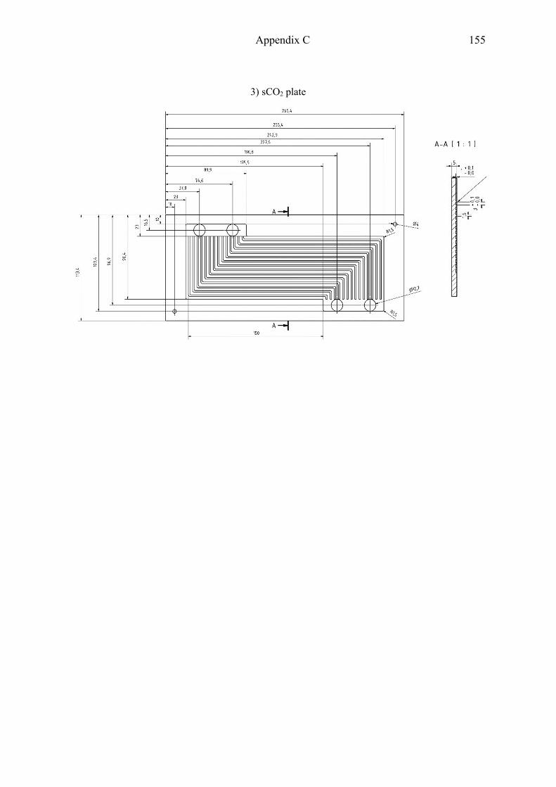
Appendix C 155
3) sCO2 plate

156 Appendix C
Heat exchanger configuration BAA
1) Cover plate
3) H2O plate
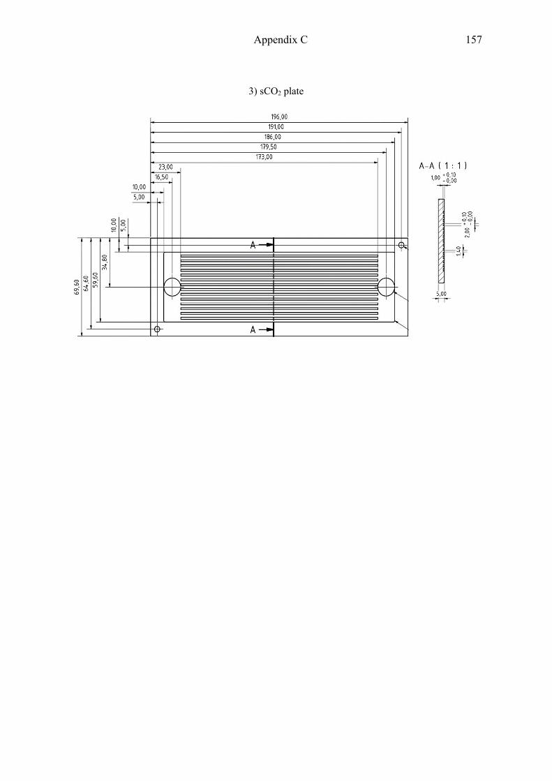
Appendix C 157
3) sCO2 plate

158 Appendix C
Heat exchanger configuration BAB
1) Cover plate
2) H2O plate
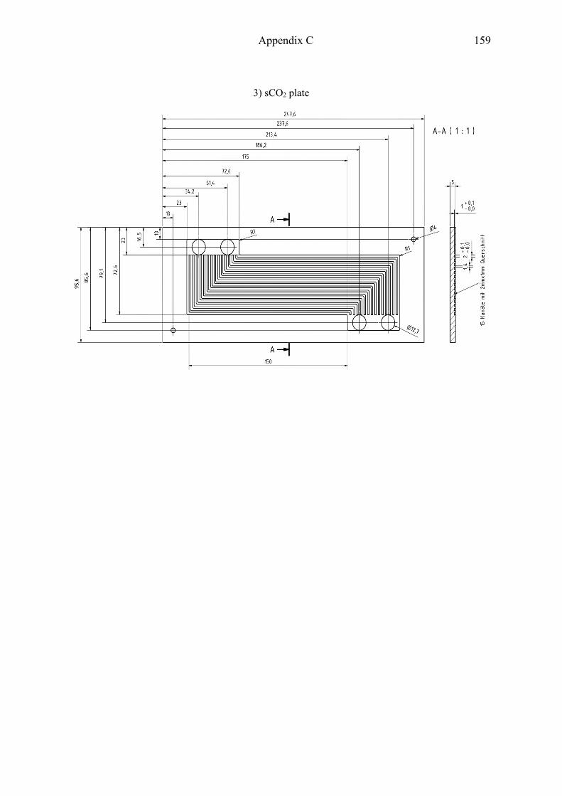
Appendix C 159
3) sCO2 plate

160 Appendix C
Heat exchanger configuration BBB
Heat exchanger configuration BCB
Heat exchanger configuration BDB
1) Cover plate
2) sCO2 plate

Appendix C 161
3) H2O plate
4) sCO2 cover plate

162 Appendix D
Appendix D
Low-pressure steam cycle / sCO2 SCARLETT loop
3x1 mm / 15/1 / IZ
�� V W �02 �04 '03 '04 �NO,Yl$� �� ]ZW ��05 �06 '07 '08
[l/h] [bar] [bar] [°C] [°C] [W] [g/s] [bar] [bar] [°C] [°C]
DP (1)
0.54 0.317 0.300 69.99 37.72 385 36.94 0.675 109.282 39.21 41.23
0.61 0.321 0.299 70.23 37.83 455 45.98 0.975 108.824 39.38 41.11
0.74 0.329 0.300 70.75 37.48 550 55.92 1.425 108.343 39.13 40.78
0.97 0.354 0.311 72.34 38.28 678 67.35 2.053 107.516 39.12 40.63
DP (2)
0.55 0.323 0.305 70.42 36.68 389 36.45 0.672 99.255 39.34 40.59
0.64 0.332 0.309 71.02 37.21 462 45.28 1.023 98.803 39.24 40.34
0.79 0.360 0.330 72.87 37.51 549 56.15 1.548 98.148 39.02 39.93
0.95 0.359 0.317 72.68 36.82 685 67.40 2.226 97.177 38.63 39.35
DP (3)
0.53 0.336 0.320 71.33 37.58 374 36.90 0.728 94.214 38.99 39.80
0.67 0.346 0.325 71.99 37.77 452 45.66 1.106 93.746 39.10 39.69
0.79 0.358 0.329 72.72 37.40 544 52.30 1.493 93.021 39.15 39.66
0.98 0.352 0.307 72.21 37.55 685 67.81 2.459 92.134 38.83 38.74
Low-pressure steam cycle / sCO2 SCARLETT loop
2x1 mm / 15/1 / IZ
�� V W �02 �04 '03 '04 �NO,Yl$� �� ]ZW ��05 �06 '07 '08
[l/h] [bar] [bar] [°C] [°C] [W] [g/s] [bar] [bar] [°C] [°C]
DP (1)
0.51 0.331 0.325 78.24 38.53 383 36.75 0.372 109.312 39.22 41.42
0.63 0.323 0.315 70.99 38.07 462 45.69 0.547 108.876 39.12 41.20
0.77 0.342 0.330 72.65 37.57 556 54.83 0.794 108.385 38.44 40.55
0.94 0.328 0.312 71.52 38.30 684 67.79 1.190 107.546 39.25 41.10
ODP (4)
0.62 0.329 0.321 72.96 38.03 462 36.85 0.377 109.283 39.18 41.89
0.76 0.325 0.313 72.52 38.02 556 36.95 0.367 109.274 39.11 42.28
0.94 0.332 0.314 75.93 38.23 684 36.84 0.371 109.346 39.16 43.12
1.19 0.322 0.296 70.61 38.83 822 36.60 0.385 109.521 39.18 43.99
1.47 0.343 0.304 81.20 39.09 1014 36.61 0.390 109.437 39.16 44.92
1.81 0.371 0.315 94.19 43.21 1221 36.67 0.394 109.593 39.18 45.94
DP (2)
0.53 0.314 0.306 70.43 38.12 389 36.79 0.388 99.251 39.23 40.74
0.67 0.323 0.316 71.10 38.00 462 45.72 0.592 98.842 39.00 40.39
0.78 0.318 0.307 70.78 38.02 556 55.73 0.874 98.143 38.94 40.20
0.95 0.326 0.311 71.37 37.91 684 68.02 1.311 97.172 38.91 39.98
ODP (5)
0.66 0.332 0.324 71.71 38.04 475 37.03 0.395 99.252 39.15 40.96
0.77 0.333 0.322 71.72 38.21 556 36.86 0.394 99.382 39.18 41.36
0.94 0.329 0.312 71.82 38.10 684 36.98 0.401 99.473 39.14 41.80
1.17 0.346 0.321 90.48 38.45 819 36.69 0.400 99.247 39.22 42.43

Appendix D 163
1.48 0.363 0.328 81.87 38.55 1006 36.54 0.404 99.618 39.25 43.11
1.84 0.370 0.317 82.44 40.20 1214 36.73 0.416 99.533 39.23 43.76
DP (3)
0.51 0.321 0.314 83.48 37.66 384 36.53 0.405 94.873 39.20 40.29
0.65 0.334 0.325 72.16 37.77 465 45.64 0.623 94.626 39.06 40.03
0.78 0.330 0.317 71.95 37.65 566 55.69 0.906 94.794 38.91 39.85
0.96 0.354 0.339 73.89 37.90 685 67.67 1.367 94.879 38.97 39.71
ODP (6)
0.68 0.319 0.310 70.88 37.97 462 36.65 0.408 94.743 39.17 40.50
0.79 0.333 0.320 77.01 37.99 563 36.78 0.413 94.854 39.10 40.73
0.98 0.348 0.332 92.00 38.05 685 36.54 0.413 94.633 39.17 41.10
1.19 0.341 0.317 83.02 38.23 828 36.89 0.428 94.901 39.16 41.47
1.51 0.350 0.312 94.04 38.44 1006 36.52 0.431 94.878 39.27 42.02
1.78 0.378 0.320 93.74 39.67 1228 36.76 0.445 94.613 39.19 42.57
High-pressure steam cycle / sCO2 SCARLETT loop
3x1 mm / 15/1 / II
�� V W �02 �04 '03 '04 �NO,Yl$� �� ]ZW ��05 �06 '07 '08
[l/h] [bar] [bar] [°C] [°C] [W] [g/s] [bar] [bar] [°C] [°C]
DP (1)
- - - - - - 37.00 - 110.000 - -
0.64 70.154 70.107 279.18 37.49 477 45.66 0.087 109.043 39.20 41.19
0.79 70.149 70.099 284.67 38.03 580 55.93 0.131 108.460 39.15 41.14
0.98 69.940 69.902 284.56 38.07 693 68.10 0.194 107.681 38.96 40.94
ODP (4)
0.63 69.988 69.951 283.96 38.20 475 37.09 0.063 109.394 39.26 41.85
0.79 70.181 70.139 284.73 38.35 585 36.91 0.063 109.416 39.17 42.41
0.98 69.953 69.910 284.62 38.40 700 36.84 0.062 109.424 39.17 43.06
1.18 70.325 70.275 285.04 38.49 855 36.92 0.062 109.430 39.16 43.93
1.39 70.190 70.149 284.94 38.61 1039 36.91 0.063 109.417 39.19 44.92
1.72 70.356 70.296 285.08 38.69 1252 37.11 0.063 109.418 39.17 45.90
ODP II (7)
1.80 70.372 70.314 285.09 39.06 1252 23.34 0.025 109.926 39.19 49.05
1.80 70.377 70.326 285.09 39.36 1251 18.15 0.016 109.895 39.27 51.96
1.80 70.382 70.338 285.08 39.66 1251 15.07 0.008 110.129 39.34 54.22
1.63 70.380 70.298 285.03 39.86 1252 13.48 0.005 110.138 39.30 55.04
1.80 70.405 70.302 285.06 40.91 1252 11.93 0.005 110.160 39.35 57.32
1.62 70.405 70.306 285.07 42.68 1252 10.24 0.005 110.161 39.33 60.91
1.76 70.402 70.311 285.08 45.11 1252 8.89 0.005 110.173 39.36 65.66
DP (2)
- - - - - - 37.00 - 100.000 - -
0.63 70.182 70.125 282.39 38.33 481 45.62 0.093 98.897 39.21 40.61
0.79 70.239 70.165 284.71 38.40 585 55.76 0.140 98.167 39.25 40.60
0.98 70.086 70.020 284.66 38.31 700 67.74 0.208 97.295 39.19 40.47
ODP (5)
0.63 70.119 70.060 284.54 38.54 481 36.81 0.060 99.279 39.38 41.10
0.79 70.160 70.104 284.69 38.71 578 36.94 0.061 99.320 39.38 41.50
0.98 69.912 69.870 284.54 38.67 693 37.08 0.061 99.262 39.31 41.88
1.18 70.244 70.193 284.94 38.73 847 36.79 0.061 99.267 39.32 42.47
1.39 69.863 69.809 284.58 38.87 1029 36.80 0.062 99.356 39.32 43.13

164 Appendix D
1.80 70.387 70.314 285.07 39.07 1252 37.09 0.064 99.322 39.34 43.86
ODP II (8)
1.80 70.371 70.259 285.00 37.94 1253 35.73 0.062 99.398 39.14 43.86
1.78 70.314 70.221 284.96 38.84 1251 20.74 0.020 99.929 39.37 46.93
1.77 70.305 70.229 284.97 39.12 1252 16.30 0.012 100.024 39.37 49.08
1.80 70.303 70.232 285.00 40.52 1252 11.96 0.005 100.101 39.36 53.98
1.80 70.301 70.229 284.98 43.05 1251 9.98 0.005 100.121 39.36 59.26
1.80 70.276 70.207 284.97 44.90 1251 9.09 0.005 100.133 39.33 62.87
DP (3)
- - - - - - 37.00 - 95.00 - -
0.63 70.214 70.146 284.57 38.46 482 45.61 0.099 93.743 39.08 40.07
0.80 70.206 70.141 284.72 38.51 579 55.59 0.148 93.099 39.06 39.99
0.98 69.925 69.856 284.56 38.48 694 67.58 0.220 92.207 38.82 39.69
ODP (6)
0.63 70.107 70.039 284.58 38.21 481 36.70 0.064 94.244 39.23 40.49
0.80 70.206 70.125 284.77 38.34 578 36.80 0.065 94.236 39.22 40.76
0.98 69.944 69.873 284.68 38.30 692 36.82 0.065 94.246 39.23 41.09
1.18 70.114 70.045 284.90 38.54 847 36.78 0.065 94.244 39.29 41.55
1.39 69.845 69.787 284.65 38.60 1029 36.70 0.066 94.248 39.26 42.02
1.80 70.227 70.161 284.94 38.48 1252 36.92 0.068 94.197 39.10 42.47
ODP II (9)
1.80 70.337 70.242 285.07 39.19 1252 18.34 0.016 94.946 39.52 46.50
1.80 70.346 70.265 285.07 39.53 1252 14.18 0.009 95.033 39.45 49.58
1.80 70.315 70.236 285.07 40.49 1252 11.73 0.005 95.076 39.47 53.35
1.80 70.299 70.228 285.04 42.33 1252 10.59 0.005 95.059 39.41 56.49
1.80 70.310 70.241 285.06 44.28 1252 9.57 0.005 95.123 39.43 60.25
1.80 70.300 70.227 285.05 46.38 1252 8.77 0.005 95.095 39.45 64.30
High-pressure steam cycle / sCO2 SCARLETT loop
3x1 mm / 15/1 / IZ
�� V W �02 �04 '03 '04 �NO,Yl$� �� ]ZW ��05 �06 '07 '08
[l/h] [bar] [bar] [°C] [°C] [W] [g/s] [bar] [bar] [°C] [°C]
DP (1)
- - - - - - 37.00 - 110.000 - -
0.62 70.008 70.002 283.91 39.86 479 45.74 0.911 109.974 39.00 40.87
0.80 70.350 70.337 284.23 38.53 580 55.74 1.328 110.372 39.10 40.93
0.98 70.302 70.291 284.16 38.43 692 67.79 1.945 109.598 39.01 40.70
ODP (4)
0.63 70.535 70.536 284.18 39.67 482 36.51 0.594 110.392 39.31 41.67
0.79 70.512 70.500 284.21 38.58 577 36.51 0.597 110.425 39.22 42.21
0.98 70.346 70.330 284.08 38.41 691 36.67 0.600 110.391 39.26 42.87
1.18 70.543 70.524 284.39 38.47 845 36.47 0.598 110.390 39.18 43.71
1.39 70.511 70.490 284.37 38.44 1026 36.65 0.605 110.441 39.11 44.60
1.80 70.325 70.296 284.22 38.72 1237 36.78 0.616 110.438 39.25 45.74
ODP II (7)
1.80 70.630 70.581 284.55 38.69 1239 36.45 0.612 110.399 39.22 45.68
1.80 70.556 70.536 284.46 38.57 1238 16.48 0.143 111.069 39.38 52.44
1.80 70.514 70.500 284.43 38.47 1237 9.19 0.051 110.128 38.81 63.82
1.80 70.483 70.480 284.40 40.89 1237 5.74 0.024 110.154 38.98 95.39

Appendix D 165
1.79 70.525 70.521 284.45 44.06 1237 4.47 0.017 110.177 38.82 128.07
1.80 70.466 70.450 284.36 47.97 1237 3.92 0.014 110.157 38.73 151.05
DP (2)
- - - - - - 37.00 - 100.000 - -
0.63 70.780 70.703 285.98 36.84 476 45.31 1.003 98.848 38.93 40.06
0.79 70.675 70.631 285.94 37.75 586 55.41 1.463 99.254 39.20 40.25
0.98 70.640 70.598 285.96 38.29 701 68.03 2.172 99.450 39.22 40.09
ODP (5)
0.63 70.672 70.619 286.02 38.30 473 36.70 0.662 99.299 39.25 40.79
0.80 70.650 70.605 285.99 38.27 577 36.72 0.663 99.335 39.18 41.16
0.98 70.557 70.514 285.89 38.29 700 36.76 0.664 99.348 39.19 41.63
1.18 70.465 70.422 285.73 38.52 846 36.73 0.668 99.284 39.27 42.23
1.39 70.458 70.413 285.67 38.60 1018 36.72 0.670 99.323 39.26 42.82
1.64 70.583 70.545 285.78 38.75 1239 36.48 0.674 99.339 39.25 43.59
ODP II (8)
1.74 70.680 70.635 285.91 38.94 1239 18.67 0.197 99.931 39.46 47.80
1.80 70.643 70.588 285.84 38.94 1239 12.99 0.106 100.052 39.42 52.43
1.80 70.637 70.586 285.84 39.35 1239 7.89 0.048 100.081 39.50 70.40
1.80 70.671 70.613 285.84 41.05 1239 5.62 0.029 100.143 39.33 101.36
1.78 70.605 70.545 285.78 45.00 1239 4.20 0.019 100.148 39.33 146.61
DP (3)
- - - - - - 37.00 - 95.000 - -
0.63 70.859 70.774 285.97 37.76 480 45.54 1.056 94.722 38.95 39.67
0.80 70.693 70.635 285.82 37.73 587 55.72 1.536 95.118 38.94 39.61
0.98 70.672 70.619 285.83 37.90 693 67.93 2.310 94.348 38.75 39.11
ODP (6)
0.63 70.396 70.361 285.58 38.35 480 36.44 0.676 95.248 39.32 40.44
0.80 70.329 70.294 285.51 38.39 577 36.54 0.685 95.241 39.28 40.73
0.98 70.516 70.477 285.69 38.13 693 36.87 0.697 95.202 39.08 40.90
1.18 70.343 70.306 285.55 38.54 857 36.72 0.698 95.214 39.29 41.53
1.39 70.687 70.641 285.92 38.72 1030 36.66 0.701 95.199 39.31 42.02
1.74 70.670 70.626 285.86 38.78 1252 36.80 0.715 95.171 39.30 42.58
ODP II (9)
1.79 70.793 70.731 286.01 38.88 1252 18.95 0.214 95.866 39.44 46.57
1.80 70.800 70.740 286.04 39.09 1252 12.45 0.105 95.990 39.52 52.69
1.80 70.639 70.592 285.93 39.33 1252 8.01 0.053 96.047 39.49 71.04
1.80 70.583 70.542 285.86 40.48 1252 5.58 0.031 96.120 39.18 105.03
High-pressure steam cycle / sCO2 SCARLETT loop
2x1 mm / 15/1 / II
�� V W �02 �04 '03 '04 �NO,Yl$� �� ]ZW ��05 �06 '07 '08
[l/h] [bar] [bar] [°C] [°C] [W] [g/s] [bar] [bar] [°C] [°C]
DP (1)
- - - - - - 37.00 - 110.00 - -
0.63 70.188 70.114 284.64 37.24 471 45.62 0.163 108.987 39.04 40.96
0.79 69.980 69.925 284.63 37.94 580 55.47 0.239 108.523 39.45 41.40
0.98 70.232 70.174 284.94 38.43 693 67.36 0.350 107.666 39.39 41.30
ODP (4)
0.63 70.187 70.126 284.74 38.21 475 36.70 0.105 109.458 39.40 41.80
0.79 69.955 69.904 284.68 38.48 577 36.49 0.104 109.443 39.47 42.45
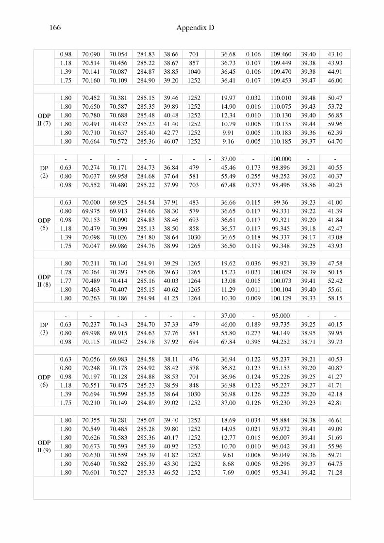
166 Appendix D
0.98 70.090 70.054 284.83 38.66 701 36.68 0.106 109.460 39.40 43.10
1.18 70.514 70.456 285.22 38.67 857 36.73 0.107 109.449 39.38 43.93
1.39 70.141 70.087 284.87 38.85 1040 36.45 0.106 109.470 39.38 44.91
1.75 70.160 70.109 284.90 39.20 1252 36.41 0.107 109.453 39.47 46.00
ODP II (7)
1.80 70.452 70.381 285.15 39.46 1252 19.97 0.032 110.010 39.48 50.47
1.80 70.650 70.587 285.35 39.89 1252 14.90 0.016 110.075 39.43 53.72
1.80 70.780 70.688 285.48 40.48 1252 12.34 0.010 110.130 39.40 56.85
1.80 70.491 70.432 285.23 41.40 1252 10.79 0.006 110.135 39.44 59.96
1.80 70.710 70.637 285.40 42.77 1252 9.91 0.005 110.183 39.36 62.39
1.80 70.664 70.572 285.36 46.07 1252 9.16 0.005 110.185 39.37 64.70
DP (2)
- - - - - - - 37.00 - 100.000 - -
0.63 70.274 70.171 284.73 36.84 479 45.46 0.173 98.896 39.21 40.55
0.80 70.037 69.958 284.68 37.64 581 55.49 0.255 98.252 39.02 40.37
0.98 70.552 70.480 285.22 37.99 703 67.48 0.373 98.496 38.86 40.25
ODP (5)
0.63 70.000 69.925 284.54 37.91 483 36.66 0.115 99.36 39.23 41.00
0.80 69.975 69.913 284.66 38.30 579 36.65 0.117 99.331 39.22 41.39
0.98 70.153 70.090 284.83 38.46 693 36.61 0.117 99.321 39.20 41.84
1.18 70.479 70.399 285.13 38.50 858 36.57 0.117 99.345 39.18 42.47
1.39 70.098 70.026 284.80 38.64 1030 36.65 0.118 99.337 39.17 43.08
1.75 70.047 69.986 284.76 38.99 1265 36.50 0.119 99.348 39.25 43.93
ODP II (8)
1.80 70.211 70.140 284.91 39.29 1265 19.62 0.036 99.921 39.39 47.58
1.78 70.364 70.293 285.06 39.63 1265 15.23 0.021 100.029 39.39 50.15
1.77 70.489 70.414 285.16 40.03 1264 13.08 0.015 100.073 39.41 52.42
1.80 70.463 70.407 285.15 40.62 1265 11.29 0.011 100.104 39.40 55.61
1.80 70.263 70.186 284.94 41.25 1264 10.30 0.009 100.129 39.33 58.15
DP (3)
- - - - - - 37.00 - 95.000 - -
0.63 70.237 70.143 284.70 37.33 479 46.00 0.189 93.735 39.25 40.15
0.80 69.998 69.915 284.63 37.76 581 55.80 0.273 94.149 38.95 39.95
0.98 70.115 70.042 284.78 37.92 694 67.84 0.395 94.252 38.71 39.73
ODP (6)
0.63 70.056 69.983 284.58 38.11 476 36.94 0.122 95.237 39.21 40.53
0.80 70.248 70.178 284.92 38.42 578 36.82 0.123 95.153 39.20 40.87
0.98 70.197 70.128 284.88 38.53 701 36.96 0.124 95.226 39.25 41.27
1.18 70.551 70.475 285.23 38.59 848 36.98 0.122 95.227 39.27 41.71
1.39 70.694 70.599 285.35 38.64 1030 36.98 0.126 95.225 39.20 42.18
1.75 70.210 70.149 284.89 39.02 1252 37.00 0.126 95.230 39.23 42.81
ODP II (9)
1.80 70.355 70.281 285.07 39.40 1252 18.69 0.034 95.884 39.38 46.61
1.80 70.549 70.485 285.28 39.80 1252 14.95 0.021 95.972 39.41 49.09
1.80 70.626 70.583 285.36 40.17 1252 12.77 0.015 96.007 39.41 51.69
1.80 70.673 70.593 285.39 40.92 1252 10.70 0.010 96.042 39.41 55.96
1.80 70.630 70.559 285.39 41.82 1252 9.61 0.008 96.049 39.36 59.71
1.80 70.640 70.582 285.39 43.30 1252 8.68 0.006 95.296 39.37 64.75
1.80 70.601 70.527 285.33 46.52 1252 7.69 0.005 95.341 39.42 71.28

Appendix D 167
High-pressure steam cycle / sCO2 SCARLETT loop
2x1 mm / 15/1 / IZ
�� V W �02 �04 '03 '04 �NO,Yl$� �� ]ZW ��05 �06 '07 '08
[l/h] [bar] [bar] [°C] [°C] [W] [g/s] [bar] [bar] [°C] [°C]
DP (1)
- - - - - - 37.00 - 110.000 - -
0.63 70.202 70.171 284.95 37.82 473 45.57 0.570 110.056 39.20 41.07
0.79 70.126 70.103 284.90 38.08 577 55.70 0.845 110.561 39.24 41.15
0.98 70.210 70.196 285.00 38.24 692 67.74 1.242 109.634 39.28 41.08
ODP (4)
0.63 69.974 69.949 285.12 38.37 474 36.38 0.372 109.497 39.42 41.79
0.80 69.981 69.975 285.18 38.42 578 36.58 0.373 109.462 39.25 42.24
0.98 70.006 69.995 285.23 38.45 693 36.62 0.376 109.470 39.27 42.92
1.18 70.062 70.057 285.26 38.62 847 36.59 0.383 109.452 39.34 43.86
1.39 70.164 70.141 285.32 38.68 1028 36.52 0.386 109.455 39.28 44.77
1.80 70.233 70.204 285.45 38.66 1251 36.71 0.389 109.452 39.32 45.86
ODP II (7)
1.78 70.202 70.140 285.40 38.95 1250 19.51 0.119 110.064 39.43 50.69
1.80 70.190 70.130 285.44 39.22 1250 11.58 0.046 110.229 39.39 58.22
1.80 70.155 70.102 285.43 39.59 1253 9.10 0.030 110.247 39.35 65.49
1.80 70.174 70.114 285.44 40.47 1253 7.42 0.020 110.259 39.35 76.07
1.71 70.151 70.108 285.43 41.84 1253 6.44 0.015 110.271 39.28 86.85
1.70 70.116 70.076 285.41 44.94 1253 5.81 0.012 110.269 39.27 96.62
1.79 70.145 70.094 285.44 48.78 1253 5.46 0.010 110.276 39.26 102.86
DP (2)
- - - - - - 37.00 - 100.000 - -
0.63 70.427 70.384 285.18 35.74 472 45.51 0.620 99.881 38.91 40.17
0.79 70.458 70.415 285.20 37.19 580 56.08 0.918 99.260 38.84 40.07
0.98 70.261 70.234 285.03 37.84 693 67.42 1.320 99.445 39.18 40.27
ODP (5)
0.63 70.265 70.230 285.53 36.77 478 36.59 0.402 99.332 39.20 40.77
0.79 70.180 70.161 285.46 37.68 579 36.34 0.396 99.357 39.36 41.36
0.98 70.161 70.150 285.45 38.17 692 36.49 0.400 99.321 39.36 41.80
1.18 70.134 70.129 285.40 38.25 857 36.57 0.401 99.301 39.27 42.34
1.39 70.275 70.271 285.54 38.59 1029 36.70 0.407 99.311 39.36 42.99
1.80 70.197 70.175 285.47 38.80 1251 36.32 0.404 99.321 39.38 43.78
ODP II (8)
1.76 70.200 70.120 285.44 38.98 1239 29.56 0.271 99.605 39.36 44.74
1.74 70.107 70.080 285.40 39.16 1239 20.76 0.140 99.904 39.39 46.93
1.79 70.078 70.022 285.36 39.42 1238 12.79 0.059 100.077 39.48 52.72
1.77 69.993 69.984 285.30 39.80 1239 9.36 0.034 100.130 39.43 61.54
1.80 69.946 69.907 285.22 40.91 1239 7.39 0.023 100.152 39.33 74.48
1.80 69.917 69.892 285.14 44.29 1239 5.94 0.015 100.169 39.39 94.42
1.79 70.087 70.053 285.32 49.50 1240 5.28 0.011 100.188 39.21 105.58
DP (3)
- - - - - - 37.00 - 95.000 - -
0.63 70.092 70.062 284.83 37.76 475 46.81 0.594 96.672 39.03 40.20
0.79 70.357 70.329 285.15 37.58 569 55.69 0.967 94.159 38.97 39.67
0.98 70.157 70.124 284.89 37.88 700 67.11 1.389 94.320 38.99 39.61
0.63 70.092 70.066 285.29 37.98 474 36.43 0.422 94.266 39.20 40.31

168 Appendix D
ODP (6)
0.80 69.858 69.829 285.12 38.38 577 36.56 0.429 94.223 39.29 40.67
0.98 70.154 70.109 285.35 38.50 700 36.53 0.425 94.269 39.28 41.01
1.18 70.420 70.340 285.49 37.34 856 36.48 0.429 94.247 39.17 41.29
1.39 70.389 70.301 285.47 38.22 1028 36.60 0.434 94.272 39.33 41.87
1.80 70.244 70.198 285.41 38.64 1240 36.36 0.437 94.272 39.38 42.49
ODP II (9)
1.80 70.312 70.282 285.46 38.89 1240 21.10 0.158 94.775 39.53 45.35
1.80 70.272 70.238 285.46 39.15 1240 15.47 0.091 94.956 39.57 48.42
1.80 70.288 70.256 285.48 39.34 1240 11.05 0.050 95.055 39.49 55.31
1.80 70.248 70.218 285.48 39.71 1240 8.53 0.033 95.047 39.50 66.23
1.79 70.319 70.291 285.56 40.52 1240 6.88 0.023 95.083 39.49 81.80
1.78 69.819 69.783 285.05 43.29 1240 5.67 0.016 95.123 39.46 102.34
1.78 70.103 70.078 285.34 49.43 1240 5.06 0.012 95.125 39.46 116.32
High-pressure steam cycle / sCO2 SCARLETT loop
2x1 mm / 5/1 / IZ
�� V W �02 �04 '03 '04 �NO,Yl$� �� ]ZW ��05 �06 '07 '08
[l/h] [bar] [bar] [°C] [°C] [W] [g/s] [bar] [bar] [°C] [°C] DP (1)
- - - - - - - - - - -
ODP (4)
0.63 70.322 70.277 284.51 37.54 474 36.54 4.263 109.413 39.37 40.83
0.80 70.487 70.440 284.38 37.75 574 36.65 4.451 109.269 39.36 41.49
0.98 70.921 70.869 285.08 38.46 692 36.57 4.312 109.408 39.29 41.94
1.18 70.899 70.857 285.07 40.23 847 36.64 4.360 109.414 39.40 42.77
1.39 70.717 70.674 284.89 42.91 1028 36.59 4.364 109.423 39.36 43.59
1.80 70.866 70.823 285.00 49.65 1251 36.68 4.314 109.405 39.33 44.44
ODP II (7)
1.80 70.702 70.651 284.84 52.03 1251 22.43 1.905 109.901 39.32 48.51
1.80 70.579 70.534 284.77 57.42 1251 11.38 0.601 110.145 39.29 57.30
1.80 70.355 70.301 284.52 68.67 1251 5.94 0.238 110.208 38.79 82.85
1.80 69.952 69.915 284.09 98.95 1251 3.13 0.112 110.259 38.70 149.72
1.76 70.345 70.282 284.44 148.64 1251 1.93 0.061 110.281 38.48 203.11
DP (2)
- - - - - - - - - - -
ODP (5)
0.63 69.448 69.403 283.69 36.95 479 36.62 4.183 100.302 39.12 39.66
0.79 69.480 69.431 283.65 37.29 584 36.65 4.381 100.312 39.08 40.00
0.98 69.455 69.407 283.65 38.15 691 36.65 4.417 100.307 39.10 40.39
1.18 69.532 69.461 283.63 39.58 856 36.38 4.409 100.333 39.03 40.92
1.39 69.522 69.444 283.66 42.05 1029 36.54 4.502 100.307 38.92 41.31
1.80 70.596 70.557 284.83 46.78 1251 36.41 4.613 99.272 39.25 41.79
ODP II (8)
1.80 70.573 70.518 284.76 49.45 1251 20.65 1.668 99.855 39.31 46.05
1.80 70.516 70.461 284.65 54.23 1251 10.49 0.538 100.053 39.36 56.72
1.78 70.348 70.299 284.49 67.04 1251 5.64 0.216 100.138 39.17 94.21
1.78 70.119 70.072 284.33 89.38 1251 3.67 0.124 100.172 39.05 149.67
1.76 69.562 69.523 283.70 149.05 1251 2.45 0.071 100.177 38.88 206.73

Appendix D 169
1.79 69.203 69.160 283.39 188.23 1251 1.95 0.050 100.199 38.95 229.32
DP (3)
- - - - - - - - - - -
ODP (6)
0.63 70.323 70.285 284.51 40.41 475 36.50 2.318 95.167 39.12 38.71
0.79 70.389 70.348 284.56 37.80 578 36.93 2.000 95.086 39.20 38.95
0.98 70.349 70.313 284.52 37.96 700 37.02 1.873 95.177 39.16 39.22
1.18 70.521 70.479 284.69 38.70 846 37.09 1.932 95.103 39.19 39.50
1.39 70.678 70.636 284.80 40.68 1027 36.67 2.111 95.188 39.16 39.96
1.80 70.672 70.616 284.79 45.98 1249 36.95 1.959 95.132 39.17 40.30
ODP II (9)
1.80 70.605 70.554 284.79 49.62 1249 17.39 1.312 95.067 39.41 46.05
1.80 70.571 70.529 284.74 52.67 1250 11.66 0.676 94.991 39.49 52.70
1.80 70.541 70.494 284.68 58.33 1251 7.66 0.357 95.042 39.43 70.51
1.80 70.615 70.533 284.78 78.51 1253 4.01 0.152 95.092 38.97 135.23
1.80 70.687 70.615 284.84 147.42 1251 2.43 0.077 95.120 38.91 210.90
No heat input / sCO2 SCARLETT loop
3x1 mm / 15/1 / II
�� V W �02 �04 '03 '04 �NO,Yl$� �� ]ZW ��05 �06 '07 '08
[l/h] [bar] [bar] [°C] [°C] [W] [g/s] [bar] [bar] [°C] [°C]
DP (1)
- - - - - - 36.63 0.059 109.372 39.13 -
- - - - - - 45.55 0.083 110.010 39.29 -
- - - - - - 55.45 0.124 109.432 39.32 -
- - - - - - 68.06 0.192 109.461 38.96 -
ODP II (7)
- - - - - - 19.24 0.015 110.002 39.36 -
- - - - - - 11.14 0.005 110.176 39.09 -
- - - - - - 7.37 0.005 110.225 39.00 -
DP (2)
- - - - - - 36.68 0.058 100.294 39.17 -
- - - - - - 45.49 0.089 99.780 39.00 -
- - - - - - 55.62 0.133 100.290 38.93 -
- - - - - - 67.69 0.195 99.378 38.68 -
ODP II (8)
- - - - - - 18.00 0.012 99.928 39.31 -
- - - - - - 11.51 0.005 100.068 39.17 -
- - - - - - 8.01 0.005 100.101 39.09 -
DP (3)
- - - - - - 36.61 0.062 94.177 39.33 -
- - - - - - 45.84 0.097 94.667 39.19 -
- - - - - - 56.18 0.144 95.077 38.96 -
- - - - - - 67.65 0.205 95.153 38.83 -
ODP II (9)
- - - - - - 19.04 0.014 94.801 39.40 -
- - - - - - 12.72 0.007 94.941 39.19 -
- - - - - - 8.14 0.005 95.010 38.95 -

170 Appendix D
No heat input / sCO2 SCARLETT loop
3x1 mm / 15/1 / IZ
�� V W �02 �04 '03 '04 �NO,Yl$� �� ]ZW ��05 �06 '07 '08
[l/h] [bar] [bar] [°C] [°C] [W] [g/s] [bar] [bar] [°C] [°C]
DP (1)
- - - - - - 36.71 0.607 110.366 39.03 -
- - - - - - 45.07 0.898 109.962 39.04 -
- - - - - - 55.90 1.349 110.347 38.87 -
- - - - - - 67.75 1.963 109.551 38.93 -
ODP II (7)
- - - - - - 20.41 0.195 110.531 39.34 -
- - - - - - 15.18 0.109 110.037 39.29 -
- - - - - - 11.24 0.059 110.096 39.16 -
- - - - - - 8.02 0.028 110.130 39.02 -
DP (2)
- - - - - - 36.13 0.658 99.337 39.05 -
- - - - - - 45.23 1.022 98.893 39.28 -
- - - - - - 55.50 1.506 99.263 39.23 -
- - - - - - 68.12 2.210 99.391 39.07 -
ODP II (8)
- - - - - - 20.56 0.216 99.891 39.35 -
- - - - - - 14.26 0.106 99.981 39.47 -
- - - - - - 11.14 0.065 100.061 39.38 -
- - - - - - 7.93 0.032 100.110 39.18 -
DP (3)
- - - - - - 36.31 0.708 94.278 38.69 -
- - - - - - 45.68 1.074 94.791 39.07 -
- - - - - - 55.26 1.577 94.246 38.95 -
- - - - - - 66.52 2.261 94.295 38.88 -
ODP II (9)
- - - - - - 20.34 0.226 94.816 39.28 -
- - - - - - 15.34 0.131 94.935 39.51 -
- - - - - - 11.01 0.068 95.002 39.53 -
- - - - - - 8.01 0.035 95.020 39.41 -
No heat input / sCO2 SCARLETT loop
2x1 mm / 15/1 / II
�� V W �02 �04 '03 '04 �NO,Yl$� �� ]ZW ��05 �06 '07 '08
[l/h] [bar] [bar] [°C] [°C] [W] [g/s] [bar] [bar] [°C] [°C]
DP (1)
- - - - - - 36.29 0.112 109.350 39.14 -
- - - - - - 45.33 0.157 109.963 39.26 -
- - - - - - 55.55 0.232 110.474 39.09 -
- - - - - - 68.11 0.346 109.510 39.26 -
- - - - - - 19.10 0.029 109.979 39.21 -

Appendix D 171
ODP II (7)
- - - - - - 11.46 0.009 110.122 39.05 -
- - - - - - 7.30 0.005 110.184 38.83 -
DP (2)
- - - - - - 36.62 0.112 99.245 39.19 -
- - - - - - 45.94 0.171 99.786 38.93 -
- - - - - - 55.99 0.252 100.204 39.20 -
- - - - - - 68.15 0.372 99.403 39.10 -
ODP II (8)
- - - - - - 20.21 0.033 99.835 39.33 -
- - - - - - 11.28 0.008 100.024 39.24 -
- - - - - - 7.24 0.005 100.079 39.16 -
DP (3)
- - - - - - 36.73 0.119 94.158 39.23 -
- - - - - - 44.62 0.172 94.695 39.10 -
- - - - - - 55.40 0.261 95.034 38.98 -
- - - - - - 67.03 0.373 95.210 38.81 -
ODP II (9)
- - - - - - 19.51 0.032 94.735 39.10 -
- - - - - - 11.08 0.008 94.965 39.45 -
- - - - - - 7.20 0.005 95.018 39.23 -
No heat input / sCO2 SCARLETT loop
2x1 mm / 15/1 / IZ
�� V W �02 �04 '03 '04 �NO,Yl$� �� ]ZW ��05 �06 '07 '08
[l/h] [bar] [bar] [°C] [°C] [W] [g/s] [bar] [bar] [°C] [°C]
DP (1)
- - - - - - 36.54 0.426 109.667 39.13 -
- - - - - - 45.44 0.581 110.091 39.42 -
- - - - - - 55.70 0.854 109.483 38.93 -
- - - - - - 67.73 1.248 109.622 39.10 -
ODP II (7)
- - - - - - 14.47 0.060 110.080 38.96 -
- - - - - - 10.85 0.033 110.167 39.06 -
- - - - - - 6.62 0.011 110.221 38.82 -
DP (2)
- - - - - - 36.47 0.415 99.799 39.03 -
- - - - - - 45.59 0.623 99.919 38.93 -
- - - - - - 55.81 0.919 100.247 39.21 -
- - - - - - 67.97 1.354 99.415 38.99 -
ODP II (8)
- - - - - - 24.14 0.167 99.760 39.31 -
- - - - - - 16.41 0.078 99.956 39.22 -
- - - - - - 10.05 0.028 100.055 39.15 -
- - - - - - 6.58 0.010 100.098 38.82 -
DP (3)
- - - - - - 36.78 0.433 95.221 39.22 -
- - - - - - 45.81 0.667 94.760 39.09 -
- - - - - - 55.33 0.952 95.139 38.85 -
- - - - - - 67.42 1.381 95.397 38.81 -

172 Appendix D
ODP II (9)
- - - - - - 23.47 0.168 94.789 38.58 -
- - - - - - 11.95 0.043 94.937 39.27 -
- - - - - - 7.18 0.013 95.014 38.93 -
No heat input / sCO2 SCARLETT loop
2x1 mm / 5/1 / IZ
�� V W �02 �04 '03 '04 �NO,Yl$� �� ]ZW ��05 �06 '07 '08
[l/h] [bar] [bar] [°C] [°C] [W] [g/s] [bar] [bar] [°C] [°C] DP (1)
- - - - - - 36.56 4.112 110.322 39.01 -
ODP II (7)
- - - - - - 15.91 0.838 110.021 39.08 -
- - - - - - 10.43 0.375 110.130 39.03 -
- - - - - - 6.18 0.140 110.170 38.72 -
- - - - - - 4.78 0.082 110.194 38.71 -
DP (2)
- - - - - - 37.01 4.297 99.232 39.21 -
ODP II (8)
- - - - - - 24.44 1.918 99.698 39.30 -
- - - - - - 14.23 0.682 99.955 39.24 -
- - - - - - 7.41 0.195 100.050 39.15 -
- - - - - - 4.85 0.084 100.065 38.59 -
DP (3)
- - - - - - 36.74 3.679 95.089 39.15 -
ODP II (9)
- - - - - - 18.98 1.248 94.778 39.39 -
- - - - - - 12.44 0.556 94.946 39.25 -
- - - - - - 8.25 0.250 94.979 39.45 -
- - - - - - 5.32 0.106 95.014 39.32 -
No heat input / sCO2 SCARLETT loop
2x1 mm / 5/2 / IZ
�� V W �02 �04 '03 '04 �NO,Yl$� �� ]ZW ��05 �06 '07 '08
[l/h] [bar] [bar] [°C] [°C] [W] [g/s] [bar] [bar] [°C] [°C]
DP (1)
- - - - - - 36.67 0.989 109.391 38.77 -
- - - - - - 45.70 1.396 110.054 39.21 -
- - - - - - 55.69 2.044 110.415 39.02 -
- - - - - - 67.58 2.995 109.624 38.96 -
ODP II (7)
- - - - - - 15.33 0.181 110.119 39.28 -
- - - - - - 8.67 0.058 110.242 39.10 -
- - - - - - 5.69 0.025 110.265 38.89 -
- - - - - - 36.51 0.974 99.306 39.22 -

Appendix D 173
DP (2)
- - - - - - 45.57 1.490 99.821 38.93 -
- - - - - - 55.14 2.139 100.263 38.83 -
- - - - - - 67.42 3.185 99.431 38.66 -
ODP II (8)
- - - - - - 15.41 0.183 99.993 39.44 -
- - - - - - 9.16 0.064 100.076 39.17 -
- - - - - - 5.60 0.023 100.122 39.11 -
DP (3)
- - - - - - 36.74 1.035 95.165 39.13 -
- - - - - - 45.64 1.592 94.685 38.95 -
- - - - - - 55.79 2.331 94.998 38.99 -
- - - - - - 67.58 3.372 95.079 38.73 -
ODP II (9)
- - - - - - 16.45 0.218 94.911 39.42 -
- - - - - - 9.17 0.069 95.008 39.29 -
- - - - - - 5.70 0.025 95.077 39.11 -
No heat input / sCO2 SCARLETT loop
2x1 mm / 5/3 / IZ
�� V W �02 �04 '03 '04 �NO,Yl$� �� ]ZW ��05 �06 '07 '08
[l/h] [bar] [bar] [°C] [°C] [W] [g/s] [bar] [bar] [°C] [°C]
DP (1)
- - - - - - 36.62 0.307 109.417 39.12 -
- - - - - - 45.46 0.438 109.942 39.18 -
- - - - - - 55.86 0.652 110.397 39.16 -
- - - - - - 67.54 0.948 109.604 38.95 -
ODP II (7)
- - - - - - 14.69 0.049 110.103 39.18 -
- - - - - - 10.25 0.022 110.178 39.08 -
- - - - - - 6.72 0.008 110.214 38.93 -
DP (2)
- - - - - - 36.91 0.315 100.245 39.16 -
- - - - - - 45.61 0.474 99.862 38.94 -
- - - - - - 55.56 0.691 100.277 39.05 -
- - - - - - 67.98 1.025 99.319 38.74 -
ODP II (8)
- - - - - - 16.36 0.062 99.942 39.31 -
- - - - - - 10.16 0.022 100.051 39.28 -
- - - - - - 6.80 0.008 100.096 39.08 -
DP (3)
- - - - - - 36.44 0.324 95.172 39.28 -
- - - - - - 46.05 0.512 94.676 38.95 -
- - - - - - 55.40 0.730 95.031 39.05 -
- - - - - - 67.86 1.073 95.168 38.85 -
ODP II (9)
- - - - - - 15.56 0.060 94.890 39.54 -
- - - - - - 10.82 0.027 95.021 39.46 -
- - - - - - 6.74 0.008 95.031 39.14 -

174 Appendix D