Numerical modelling of the catastrophic flooding of Santa Fe City, Argentina
Upload
khangminh22Category
view
1download
0
Development of Frameworks for Numerical Modelling of Corrosion Fatigue in Offshore Structures
Ontwikkeling van modellen voor numerieke simulatie van corrosie-vermoeiing in offshore constructies
Jie Zhang
Promotor: Prof. dr. ir. W. De Waele, Prof. dr. ir. S. Hertelé Proefschrift ingediend tot het behalen van de graad van Doctor in de Ingenieurswetenschappen: Werktuigkunde-Elektrotechniek Vakgroep: Elektrische Energie, Metalen, Mechanische Constructies en Systemen Voorzitter: Prof. dr. ir. L. Dupré Faculteit Ingenieurswetenschappen en Architectuur Academiejaar 2018-2019

Preface v
Supervisors
Prof. dr. ir. W. De Waele Prof. dr. ir. S. Hertelé
Ghent University Faculty of Engineering and Architecture Department of Electrical Energy, Metals, Mechanical Constructions and Systems
Examination Committee
Prof. P. De Baets (Chair) - Ghent University Prof. W. De Waele - Ghent University Prof. S. Hertelé - Ghent University Prof. H. De Backer - Ghent University Prof. P. Verleysen - Ghent University Prof. H. Den Besten - Delft University of Technology Ir. J. Antonissen - OCAS nv / ArcelorMittal
Research Institute
Ghent University Department of Electrical Energy, Metals, Mechanical Constructions and Systems Soete Laboratory
Technologiepark 46 9052 Zwijnaarde Belgium
Tel. +32 9 331 04 99 Fax +32 9 331 04 90 Mail [email protected]
www.soetelaboratory.ugent.be

vi Preface

Preface vii
“学而不思则罔,思而不学则殆”
“To learn without reasoning leads to confusion,
to think without learning is wasted effort.”
- Confucius (551 B.C.-479 B.C.)

viii Preface

Preface ix
Acknowledgements
First of all, I would like to appreciate my two supervisors, Prof. W. De Waele and Prof. S. Hertelé for giving me the chance to study in Soete Laboratory in Ghent University and to conduct my research in corrosion fatigue topic. Their professional dedication and patient guidance helped me achieving this doctoral degree.
I gratefully acknowledge the financial support from SIM Flanders (Strategic Initiative Materials) and Vlaio (Flemish Agency for innovation and Entrepreneurship) to make this research possible. Moreover, I would like to express my particular thanks to former colleagues Nahuel, Louis and Sven for providing abundant mechanical data of DNV F460 steel with a great amount of experimental results and numerical tools.
I could not easily make it without help from many people. I`d like to give a special acknowledge to our secretary Georgette who is always enthusiastic to provide help on either official or personal affairs. I`d like to also thank Wouter, Jonathan, Johan and Hans for the practical tutorial on test machines, computers software and for preparing my specimens. My four years study in Soete laboratory was rich and colorful. My thanks also go towards to research fellows, Jacob, Jules, Saosometh, Timothy, Koen, Saeedeh, Kannaki, Kaveh, Adam, Klara, Levente, Nadeem, Sameera, Xiaowei, Junyan, Tongan, Xin, Phuc, Truong, Samir, Vitor and Kris for sharing different cultures and stories from all over the globe and scientific discussions in the various topics and unforgettable social activities together.
I would like to thank my friends, Guomei & Reinhard, Yousong, Peixia, Miranda, Jan, Walter & Louise, Kara & Heidi, Bruno & Pauline and Chen Li & Zhuo Lu, for making my staying in Belgium happy and wonderful, and for helping me learning this country and people here, and for practicing my Flemish.
Finally, I would like to thank my wife Fang Bao and my parents Huifang Ma & Zhizhong Zhang for their strong and unconditional supports during all these years. It is worth noting that Andi, my little man, kept me awake to work during nights. They are always my passions to advance.
Thank you all from my heart.
Jie Zhang
Ghent, 2019

x Preface
Preface xi
Summary
In recent years, the increasing demand for green and renewable energy to confront the threat of global warming accelerates the installation of offshore structures for energy generation, such as offshore wind turbines, tidal power stations and wave energy converters. The North Sea is a particularly relevant environment, as it has proven to provide favourable circumstances to the installation of offshore wind farms. The durability of these structures is a critical issue for the rate of investment return, as severe corrosive seawater and atmosphere, besides the complex loading due to wind and currents and wave, dramatically shorten their service duration by the coupled damage from corrosion and fatigue.
Corrosion fatigue is not a simple summation of corrosion and fatigue damage but is rather a process with complex interactions between corrosion and fatigue and bilateral reinforcements between mechanical aging and chemical reactions. Observed in the macro-scale, corrosion fatigue shows a different behavior from fatigue in air. For example, the fatigue limit known to steels disappears in the S-N curve, and the lifetime of crack initiation under a given stress level is remarkably reduced. The fatigue crack growth rate in presence of corrosion is much higher than that in air for the same range of stress intensity factor. Therefore, identification of the damage mechanisms of corrosion fatigue and a establishing better understanding and improved predictive models of combined fatigue-corrosion are required for durability analysis and life prediction of the abovementioned offshore applications.
In this work, a first objective is aimed at the fatigue initiation modelling with account of the corrosion effect. A new model is proposed based on non-linear damage mechanics and damage accumulation theory. Coupled damage from fatigue and corrosion for each cycle is evaluated by degrading the material fatigue properties implemented in the fatigue damage model, as a function of time. The lifetime of crack initiation is obtained when the accumulated corrosion fatigue damage reaches a critical value of the material. The new model is capable to catch the elimination of fatigue limit in the high cycle domain of the S-N curve and simulate load sequence effects in presence of variable amplitude loading. Following, the critical plane method for crack initiation is improved in terms of computational cost, by means of developing
xii Preface
an efficient, simple and robust method to determine of orientation and parameters. A numerical universal framework for fatigue crack initiation analysis is established by object-oriented Python programming to communicate with ABAQUS® for devoted pre-processing and post-processing, thus allowing to compute the lifetime based on the models mentioned above.
Secondly, fatigue crack propagation is simulated by means of the extended finite element method (XFEM) based on linear elastic fracture mechanics (LEFM). The XFEM feature in ABAQUS® is used to obtain stress intensity factors (SIF) without very fine mesh size, which bypasses the difficulties of traditional meshing schemes around the crack geometry and reduces the number of elements, thus decreasing computational cost. Discretized information of SIF along the crack front is used iteratively to calculate crack advance and growth direction. An automated numerical framework for arbitrary non-self-similar three-dimensional crack simulation is established by Python scripting. The framework is validated by carrying out tests on groups of modified compact tension (CT) specimens experimentally and comparing additional predictions on other configurations with data reported in literature.
Predictions of total fatigue lifetime require a criterion to judge when crack initiation is finished, and propagation starts. Such criterion is expressed in terms of a so-called crack transition length. This dissertation adopts the so-called dominated mechanism theory, which assumes that transition from initiation to propagation takes place as soon as crack growth predictions by propagation models dominate those of initiation models. A numerical tool is developed to obtain the crack transition length according to this principle, for the initiation and propagation models earlier developed. The tool produces realistic values of crack transition length, compared to values obtained by other approaches and empirical observations.
Finally, influences of variable amplitude loading and residual stress, which are two of the most important influence factors in fatigue analysis, are investigated. An intermittent cycle-by-cycle algorithm is developed to analyze variable load histories with huge numbers of cycles with a limited computational cost. Crack retardation effects based on Wheeler and Willenborg models (both of which are based on analytical estimations of plastic zone size) are studied numerically and experimentally on eccentrically-loaded single edge cracked tension (ESET) tests. Extended Wheeler and Willenborg models are proposed with a corrected shut-off load ratio and considering out-of-plane constraint effects. These new models have a sounder theoretical basis than their traditional counterparts and rely on a purely experimental calibration of its parameters. A numerical tool to import residual stress and re-equilibrate stress distribution is developed to include its influence. These two extensions are strong supplements for the frameworks, integrating variable amplitude and residual stress, to come close to complex scenarios.
Preface xiii
It is worthy to mention that, throughout this work, DNV F460 steel which is widely used in offshore structures, is the material chosen for the experiments and numerical calculations. Most loading parameters and environmental parameters implemented are cited from literature and were assumed as representative conditions expected for a structure operating in the North Sea environment. Therefore, the results generated in this work can be associated with the behavior of offshore structures in corrosion fatigue conditions. The methodologies developed can also be implemented to guide improving the design and fatigue lifetime estimation of real engineering applications.
The models, frameworks and tools developed in this work manage to balance between accuracy and computation time and extend knowledge over corrosion fatigue and fatigue analysis. In the future, further improvements could be achieved by additional model validations, improvements in the robustness and efficiency of the developed tools, and the development of additional extensions which cover more influencing factors.

xiv Preface

Preface xv
Samenvatting (Dutch summary)
In de afgelopen jaren versnelde de vraag naar groene en hernieuwbare energie om het hoofd te bieden aan de opwarming van de aarde. Dit leidde tot de installatie van steeds meer offshore constructies (o.a. in de Noordzee), zoals offshore windturbines, getijden- en golfenergieconverters. De duurzaamheid van deze constructies is een kritiek aspect voor het rendement van de gemaakte investeringen, omdat het corrosieve zeewater en de mariene atmosfeer, naast de complexe belasting door wind en stromingen en golven, hun levensduur aanzienlijk kunnen verkorten door het gekoppeld effect van corrosie en vermoeiing.
Corrosievermoeiing is geen eenvoudige optelsom van corrosie en vermoeiing, maar is een proces met complexe niet-lineaire interacties tussen corrosie en vermoeiing. Waargenomen op macroschaal, vertoont corrosievermoeiing verschillende gedragingen ten opzichte van vermoeiing in de lucht. De vermoeiingslimiet verdwijnt bijvoorbeeld in de S-N-curve en de duur tot scheurinitiatie bij een gegeven spanningsniveau is opmerkelijk verminderd. De scheurgroeisnelheid is veel hoger dan die in lucht voor dezelfde fluctuatie van spanningsintensiteitsfactor (SIF). Daarom zijn identificatie van het schademechanisme van corrosievermoeiing en het bekomen van een beter begrip en verbeterde voorspellende modellen van gecombineerde vermoeiingscorrosie vereist voor de levensduurvoorspelling van boven vernoemde offshore-toepassingen.
Een eerste doel in dit werk is gericht op het modelleren van vermoeiings-initiatie met inachtneming van het corrosie-effect. Een nieuw model wordt voorgesteld op basis van niet-lineaire schademechanica en schadeaccumu-latietheorie. De gekoppelde schadetoename door vermoeiing en corrosie wordt geëvalueerd door de materiaaleigenschappen m.b.t. vermoeiingsweerstand te degraderen in functie van de tijd, naargelang de mate waarin corrosie het materiaal aantast. Scheurinitiatie wordt voltooid wanneer de geaccumuleerde schade een kritieke waarde bereikt. Het nieuwe model is in staat om een eliminatie van de vermoeiingslimiet in het hoogcyclische spanningsdomein in de S-N-curve te bekomen, en niet-lineaire volgorde-effecten van variabele belastingscycli te simuleren. De zgn. kritische-vlakmethode voor scheurinitiatie wordt nader bestudeerd. Het blijkt dat de
xvi Preface
rekenduur voor deze methode sterk kan verbeterd worden t.o.v. gepubliceerde algoritmes, door middel van een efficiënte, eenvoudige en robuuste methode om de kritische vlakoriëntatie en bijhorende schadeparameters te bepalen. Een numeriek universeel raamwerk voor de analyse van de vermoeiingsscheurinitiatie wordt geïmplementeerd in een Python script, dat communiceert met de eindige elementensoftware ABAQUS® voor modelopbouw en -analyse.
Ten tweede wordt vermoeiingsscheurpropagatie gesimuleerd door middel van de uitgebreide eindige-elementenmethode (E.: extended finite element method of XFEM) op basis van lineaire elastische breukmechanica (LEFM). De XFEM-functie in ABAQUS wordt gebruikt om numeriek nauwkeurige spanningintensiteitsfactoren te bekomen zonder de vereiste van een zeer fijne vermazing rondom het scheurfront. Hierdoor worden de uitdagingen horend bij modelopbouw dramatisch verminderd en neemt de vereiste rekentijd sterk af. Gediscretiseerde informatie over coördinaten en spanningsintensiteits-factoren langs het scheurfront worden iteratief gebruikt om scheurgroei en groeirichting te berekenen. Een geautomatiseerd numeriek raamwerk voor willekeurige driedimensionale scheurgroeisimulatie wordt geïmplementeerd in een Python script dat communiceert met ABAQUS®. Het raamwerk wordt gevalideerd door experimentele proeven op gemodificeerde compacte spanning (E.: compact tension of CT) proefstukken en verdere vergelijkingen met gegevens die in de literatuur worden verstrekt.
Voorspellingen van totale vermoeiingslevensduur vereisen een criterium om te beoordelen wanneer de scheurinitiatie is voltooid en de scheurpropagatie begint. Een dergelijk criterium wordt vertaald in een zogenaamde scheurtransitielengte. Dit proefschrift neemt de zogenaamde “gedomineerde mechanismentheorie” aan, die ervan uitgaat dat de overgang van initiatie naar propagatie plaatsvindt zodra scheurgroeivoorspellingen door propagatiemodellen die van initiatiemodellen domineren. Een numeriek script wordt ontwikkeld om de scheurovergangslengte volgens dit principe te verkrijgen, voor de eerder ontwikkelde initiatie- en propagatiemodellen. Analyses uitgevoerd in dit werk produceren realistische waarden van de lengte van de scheurovergang, vergeleken met waarden verkregen door andere benaderingen en empirische waarnemingen.
Ten slotte worden invloeden van variabele amplitude cyclische belasting en residuele spanning onderzocht. Dit zijn twee van de belangrijkste factoren in vermoeiingsanalyse. Een intermitterend cyclus-per-cyclus algoritme wordt ontwikkeld om de invloed van belastingsgeschiedenis op scheurgroei te berekenen voor enorme aantallen cycli, met een aanvaardbare rekenkost. Het scheurgroeivertragende effect zoals voorspeld door traditionele Wheeler- en Willenborg-modellen wordt numeriek en experimenteel bestudeerd op excentrisch trekbelaste proefstukken met enkele kerf (E.: excentrically single edge notched tension of ESET). Uitgebreidingen op de Wheeler- en

Preface xvii
Willenborg-modellen worden voorgesteld, die gebruik maken van een verbeterde inschatting van de plastische zone rond de scheurtip (rekening houdend met de invloed van een drieassige spanningstoestand). De nieuwe modellen hebben een meer solide theoretische basis dan hun conventionele tegenhangers en kunnen volledig experimenteel gekalibreerd worden. Een numeriek tool om restspanning te importeren en de spanningverdeling op basis hiervan te herverdelen, laat toe haar invloed op vermoeiingsinitiatie en –propagatie in te schatten.
Het is interessant om te vermelden dat DNV F460-staal, dat veel wordt gebruikt in offshore-constructies, het materiaal is dat werd gebruikt in de experimenten en numerieke berekeningen van dit werk. Belastings- en omgevingsparameters worden veelal aangehaald uit literatuur, en worden verondersteld als representatief voor de Noordzee-omgeving.
De modellen, frameworks en tools die in dit werk zijn ontwikkeld, zorgen voor een gezonde balans tussen nauwkeurigheid en rekentijd en vergroten de kennis over corrosiemoeheid en vermoeiingsanalyse. Verbetereringen in de toekomst zouden kunnen worden door bijkomende validatiestudies, verbeteringen naar robuustheid en efficiëntie van de scripts, en de ontwikkeling van uitbreidingen op de bestaande modellen teneinde meer invloedsfactoren in rekening te brengen.

xviii Preface
Preface xix
Publications
A1 Peer reviewed journal publications included in Science Citation Index
1. Zhang, J., Muys, L., De Tender, S., Micone, N., Hertelé, S. and De Waele,
W. (2019). Constraint corrected cycle-by-cycle analysis of crack growth
retardation under variable amplitude fatigue loading. International
Journal of Fatigue. (accepted)
2. Zhang, J., Hertelé, S. and De Waele. An Iterative Framework For 3D
Fatigue Crack Growth Simulation with ABAQUS XFEM (submitted)
A2 Peer reviewed journal publications
1. Muys, L., Zhang, J., Micone, N., De Waele, W., & Hertelé, S.. Cycle-by-
cycle simulation of variable amplitude fatigue crack propagation.
International Journal of Sustainable Construction And Design, 8(1)
(2017). (published)
C/P Conference proceedings
1. Zhang, J., Hertelé, S., Micone, N., & De Waele, W. (2016). Modelling
framework for 3D fatigue crack propagation in welds of offshore steel
structures. IRF2016: 5th International Conference Integrity-Reliability-
Failure (pp. 751–762). Presented at the International Conference on
Integrity : Reliability : Failure, INEGI/FEUP (2016). (published)
2. Zhang, J., Kiekens, C., Hertelé, S., & De Waele, W. (2018). Identification
and Prediction of Mixed-Mode Fatigue Crack Path in High Strength
xx Preface
Low Alloy Steel. Proceedings Of The 18th International Conference On
Experimental Mechanics (Vol. 2). Presented at the The 18th International
Conference on Experimental Mechanics (ICEM 2018), mdpi. (published)
3. Zhang, J., Hertelé, S., & De Waele, W. (2018). A Non-Linear Model for
Corrosion Fatigue Lifetime Based on Continuum Damage
Mechanics. Proceedings Of 12th International Fatigue Congress (Vol.
165). Presented at the 12th International Fatigue Congress (FATIGUE
2018), EDP Sciences.(published)
4. Zhang, J., De Waele, W., & Hertelé, S.. Corrosion Fatigue in Offshore
Structures. Book Of 14th Eawe Phd Seminar on Wind Energy. Presented
at the 14th EAWE PhD Seminar on Wind Energy (2018). (published)
5. Zhang, J., Trogh, S., De Waele, W., & Hertelé, S.. Fatigue Crack
Propagation in HSLA Steel Specimens Subjected to Unordered and
Ordered Load Spectra. the 13th International Conference on Damage
Assessment of Structures (DAMAS 2019). (published)
6. Hojjati Talemi, R., Zhang, J., Hertelé, S., & De Waele, W. (2018). Finite
Element Analysis of Fretting Fatigue Fracture in Lug Joints Made of
High Strength Steel. In G. Hénaff (Ed.), Proceedings of 12th
International Fatigue Congress (Vol. 165). Presented at the 12th
International Fatigue Congress (FATIGUE 2018), EDP Sciences.
(published)
7. Micone, N., De Waele, W., & Zhang, J. (2016). Selection of practical
damage evaluation methods for offshore fatigue
assessment. International Conference on Integrity : Reliability :
Failure (pp. 763–776). Presented at the International Conference on
Integrity : Reliability : Failure, INEGI/FEUP (2016). (published)

Preface xxi

xxii Preface
Contents
Acknowledgements .................................................................... ix
Summary ....................................................................................... xi
Samenvatting (Dutch) ................................................................ xv
Publications ................................................................................ xix
Contents ..................................................................................... xxii
Symbols and acronyms ........................................................ xxviii
Chapter 1: Research Context and Motivation
1 Economic motive for research of fatigue in the offshore
environment ....................................................................................... 1.3
2 SIM MaDurOS program and the SBO-project DeMoPreCI-MDT
............................................................................................................... 1.6
3 Challenges in corrosion fatigue modelling ................................... 1.9
4 Aim and scope of the dissertation ................................................. 1.11
5 Overview of the dissertation .......................................................... 1.11
References ...................................................................................................... 1.13
Chapter 2: An Introduction to Fatigue in an Offshore Environment
1 Overview .............................................................................................. 2.3
2 Metal fatigue ....................................................................................... 2.3
Preface xxiii
2.1 The physical process of fatigue .................................................... 2.3
2.2 Fundamental concepts and categorization ................................. 2.4
3 Corrosion fatigue ................................................................................ 2.7
3.1 Offshore environment ................................................................... 2.7
3.2 Corrosion fatigue process ............................................................. 2.8
3.3 Corrosion effect on material fatigue properties ......................... 2.9
4 Influencing factors in corrosion fatigue ....................................... 2.10
4.1 Multiaxial load and mean stress ................................................ 2.11
4.2 Load sequence and variable amplitude .................................... 2.15
4.3 Residual stress .............................................................................. 2.16
4.4 Temperature, loading frequency and cathodic protection ..... 2.17
5 Summary ............................................................................................ 2.19
References ...................................................................................................... 2.20
Chapter 3: Fatigue Crack Initiation Modelling
1 Overview .............................................................................................. 3.3
1.1 Context and background .............................................................. 3.3
1.2 Damage mechanics approaches ................................................... 3.5
1.2.1 Linear damage accumulation approach ................................ 3.6
1.2.2 Non-linear damage accumulation approaches .................... 3.7
1.3 Critical plane approaches ........................................................... 3.12
1.3.1 Stress-based criteria ............................................................... 3.12
1.3.2 Strain-based criteria ............................................................... 3.14
1.3.3 Energy-based criteria ............................................................. 3.15
1.3.4 Determination of critical plane orientation ......................... 3.17
1.4 Models for corrosion fatigue ...................................................... 3.21
1.4.1 Corrosion pitting and general corrosion ............................. 3.21
1.4.2 Fatigue properties degradation models .............................. 3.25
2 Framework for numerical simulation of corrosion fatigue
initiation ............................................................................................ 3.28
2.1 Proposal for a new corrosion fatigue model ............................ 3.28
xxiv Preface
2.1.1 Extending a 2D S-N curve to a three-dimensional S-N-t surface .................................................................................................. 3.28
2.1.2 Damage accumulation ........................................................... 3.31
2.2 Implementation of the framework for corrosion fatigue initiation ....................................................................................................... 3.32
2.3 A new critical plane identification method .............................. 3.34
2.3.1 Critical plane parameters ...................................................... 3.34
2.3.2 Nelder-Mead simplex method ............................................. 3.36
3 Capability study and discussions .................................................. 3.38
3.1 Corrosion fatigue initiation ........................................................ 3.38
3.1.1 Inputs for corrosion fatigue model ...................................... 3.38
3.1.2 Results and discussions ......................................................... 3.39
3.2 Experimental calibration and validation study ....................... 3.42
3.2.1 Material and experimental details ....................................... 3.42
3.2.2 Results and discussions ......................................................... 3.43
3.3 A case study of critical plane identification ............................. 3.45
3.3.1 FEM analysis ........................................................................... 3.45
3.3.2 Results and discussions ......................................................... 3.46
4 Summary and conclusions .............................................................. 3.51
References ...................................................................................................... 3.55
Chapter 4: Fatigue Crack Propagation Modelling
1 Overview .............................................................................................. 4.3
1.1 Fatigue crack propagation analysis by linear elastic fracture mechanics ....................................................................................... 4.3
1.2 Corrosion fatigue crack propagation .......................................... 4.6
1.2.1 Types of environmental fatigue crack growth behaviour . 4.6
1.2.2 Corrosion fatigue crack propagation modelling ................. 4.7
1.3 Extended finite element method (XFEM) ................................. 4.10
1.3.1 Fundamentals of extended finite element modelling ....... 4.10
1.3.2 Stress intensity factor calculation in ABAQUS by XFEM 4.12
Preface xxv
2 A simulation framework of 3D crack propagation ................... 4.14
2.1 Structure of the framework ........................................................ 4.14
2.2 Implementation details ............................................................... 4.16
2.2.1 Crack insertion ........................................................................ 4.16
2.2.2 Crack front profile updating ................................................. 4.17
3 Validation study and discussions ................................................. 4.24
3.1 Validation against an analytical stress intensity factor solution ....................................................................................................... 4.25
3.1.1 CT specimen modelled in ABAQUS .................................... 4.25
3.1.2 Standard stress intensity factor solution of CT specimen . 4.27
3.1.3 Comparison ............................................................................. 4.27
3.2 Beam with tilted crack subjected to bending moment ............ 4.29
3.2.1 Beam configuration and boundary condition .................... 4.29
3.2.2 Results and discussion ........................................................... 4.30
3.3 Modified compact tension specimen ......................................... 4.32
3.3.1 Material and specimen configuration .................................. 4.32
3.3.2 Results and discussion ........................................................... 4.33
4 Summary and conclusions .............................................................. 4.40
References ...................................................................................................... 4.41
Chapter 5: Transition from Crack Initiation to Propagation
1 Overview .............................................................................................. 5.3
1.1 Empirical estimations .................................................................... 5.4
1.2 Fatigue resistance threshold theory ............................................. 5.4
1.3 Dominated mechanism theory ..................................................... 5.5
2 Numerical tool to determine the transition length ...................... 5.7
2.1 Damage growth rate due to initiation models ........................... 5.7
2.2 Crack growth rate due to propagation model ........................... 5.9
3 Validation study ............................................................................... 5.10
3.1 Transition length based on the Basquin`s model..................... 5.10
3.1.1 Material properties ................................................................. 5.10

xxvi Preface
3.1.2 Results and discussions ......................................................... 5.10
3.2 Transition length based on the SWT model ............................. 5.14
3.2.1 Material properties ................................................................. 5.14
3.2.2 Results and discussions ......................................................... 5.15
3.3 Transition length based on new initiation model proposed .. 5.16
3.3.1 Material and properties ......................................................... 5.16
3.3.2 Results and discussions ......................................................... 5.17
4 Summary and conclusion ................................................................ 5.18
References ...................................................................................................... 5.20
Chapter 6: Extensions to the Frameworks
1 Overview .............................................................................................. 6.3
2 Fatigue crack propagation under variable amplitude loading
conditions ............................................................................................ 6.5
2.1 Plastic zone models ........................................................................ 6.6
2.2 Wheeler model and Willenborg model ..................................... 6.10
2.2.1 Wheeler`s model ..................................................................... 6.11
2.2.2 Willenborg`s model ................................................................ 6.13
2.3 Cycle-by-cycle crack propagation algorithm ........................... 6.14
2.4 Extended Wheeler & extended Willenborg models ................ 6.16
2.5 Crack growth retardation predictions using Wheeler and Willenborg models ...................................................................... 6.18
2.5.1 Material properties and specimen configuration ............... 6.18
2.5.2 Sensitivity analysis of governing parameters ..................... 6.19
2.5.3 Experimental evaluation of crack growth retardation models .................................................................................................. 6.25
3 Residual stress ................................................................................... 6.34
3.1 Establishing stress equilibrium in ABAQUS ............................ 6.34
3.2 Integration with frameworks ..................................................... 6.35
3.2.1 The framework of crack initiation ........................................ 6.35
3.2.2 The framework of crack propagation .................................. 6.36
Preface xxvii
3.3 Numerical study of residual stress effect on stress intensity factor solutions ......................................................................................... 6.37
3.3.1 Material properties and specimen ....................................... 6.37
3.3.2 Generation of residual stress ................................................ 6.38
3.3.3 Results and discussions ......................................................... 6.40
4 Summary and conclusions .............................................................. 6.42
References ...................................................................................................... 6.44
Chapter 7: Conclusions and Perspective of Future Work
1 Global summary and main conclusions ......................................... 7.3
2.1 Methodologies and numerical tools developed......................... 7.3
2.2 Comparison of simulation results compared with literature and experimental data .......................................................................... 7.4
2 Suggestions for future work ............................................................. 7.5
2.1 Experimental validation of the developed frameworks ........... 7.5
2.2 Optimization of the numerical tools ............................................ 7.6
2.3 Additional extensions of the developed frameworks ............... 7.6
2.4 Personal reflections and opinion of the author .......................... 7.7
References ........................................................................................................ 7.8
xxviii Preface
Symbols and acronyms
Symbols
𝑎 crack length 𝑎𝑂𝐿 overload crack length 𝑎𝑡ℎ critical crack length/transition length
𝑑𝑎 𝑑𝑁⁄ crack growth rate ∆𝑎 crack growth length 𝑏 fatigue strength exponent 𝑐 fatigue ductility exponent 𝐶 Paris law constant 𝐷 damage 𝑒 nominal strain 𝐾 stress intensity factor
∆𝐾 stress intensity factor range ∆𝐾𝑒𝑓𝑓 effective stress intensity factor range
∆𝐾𝑡ℎ crack growth threshold 𝐾𝑐 quasi-static fracture toughness 𝐾𝑒𝑞 equivalent stress intensity factor
𝐾𝑓 fatigue notch factor
𝐾𝑚𝑎𝑥 maximum stress intensity factor 𝐾𝑚𝑎𝑥
∗ ‘no retardation’ stress intensity factor 𝐾𝑚𝑖𝑛 minimum stress intensity factor 𝐾𝑜𝑝 crack opening stress intensity factor
𝐾𝑟𝑒𝑑 reduced stress intensity factor 𝐾𝑡 concentration factor 𝐾𝜀 strain concentration factor 𝐾𝜎 stress concentration factor 𝑚 Paris law constant 𝑛 strain hardening exponent 𝑁 number of cycles to failure 𝑁𝐼 crack initiation lifetime 𝑁𝑃 crack propagation lifetime
Preface xxix
𝑁𝑇 total lifetime
𝑝 material characteristic length 𝑝∗ material constant
𝑃 external load 𝑟 notch root radius
𝑟𝑝,0 reference size (plane stress)
𝑟𝑝,0` reference size (plane stress) for strip yield model
𝑟𝑝,𝑂𝐿 overload plastic zone size
𝑟𝑝 plastic zone size
𝑟𝑝∗ ‘no retardation’ plastic zone size
𝑅 stress/load ratio 𝑅𝑂𝐿 overload ratio 𝑅𝑆𝑂 shut-off overload ratio
𝑅𝑆𝑂` corrected shut-off overload ratio
𝑅𝑒𝑓𝑓 effective load ratio
𝑅𝛼 correction factor for Wheeler models 𝑅𝜏 the shear stress ratio 𝑆 nominal stress 𝑆𝑔 material constant in stress gradient
𝑡 thickness of specimen 𝑊 width of specimen
∆𝑊𝐼 strain energy in mode-I crack ∆𝑊𝐼𝐼 strain energy in mode-II crack
𝑌 crack shape factor
𝛼 plastic zone size factor 𝛽 material constant 𝛾 material constant in Walker law
∆𝛾 shear strain amplitude 𝜂 global constraint factor 𝜆 correction factor for Willenborg models
∆𝜀 strain amplitude ∆𝜀1 maximum principal strain range
𝜀𝑓` fatigue ductility coefficient
∆𝜎 stress amplitude 𝜎−1 fatigue limit under fully revered load 𝜎ℎ𝑠 hot spot stress 𝜎𝐻 hydrostatic stress 𝜎𝑎 stress amplitude 𝜎𝑓 fatigue limit/fatigue strength
𝜎𝑚 mean stress 𝜎𝑚𝑎𝑥 maximum stress 𝜎𝑚𝑖𝑛 minimum stress
𝜎𝑛 normal stress

xxx Preface
𝜎𝑟 rupture/fracture stress 𝜎𝑠 structural stress 𝜎𝑢 ultimate tensile strength 𝜎𝑦 yield strength
𝜎𝑓` fatigue strength coefficient
∆𝜏 shear stress range 𝜏 normalized thickness
𝜏` normalized thickness for strip yield model 𝜏−1 shear fatigue limit under fully revered load 𝜙𝑤ℎ Wheeler’s retardation factor
𝜒 stress gradient 𝜔 shape exponent
Preface xxxi
Acronyms
BM Brown and Miller criterion parameter CDM Continuum damage mechanics CT compact tension DCPD direct current potential drop DIC digital image correlation DV Dang Van criterion ESET eccentrically-loaded single edge crack tension FEM finite element method FL Findley criterion parameter FS Fatemi and Socie criterion parameter LEFM linear elastic fracture mechanics LHL low to high to low load sequence MD McDiarmid criterion parameter MT Matake criterion parameter NDT nondestructive testing NLCD non-linear cumulative damage OOP object-oriented programming PZ plastic zone RT Rolovic-Tipton criterion parameter SCF stress corrosion cracking SIF stress intensity factor SN stress (S) against the number of cycles to failure (N) SR semi-random load sequence SSR Shear-Stress-Range criterion parameter SWT Smith-Watson-Topper criterion parameter TCF true corrosion fatigue XFEM extended finite element method

xxxii Preface

Research Context and Motivation

1.2 Research Context and Motivation
<< This page intentionally left blank >>
Chapter 1 1.3
1 Economic motive for research of fatigue in the offshore environment
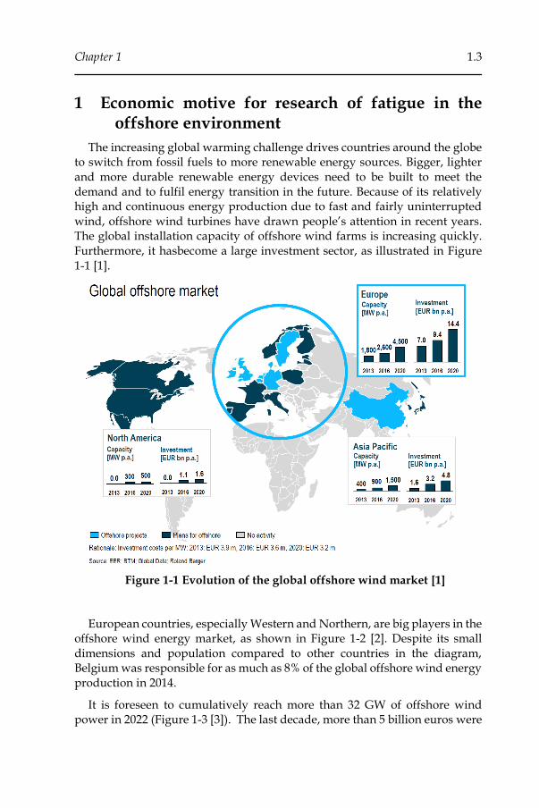
The increasing global warming challenge drives countries around the globe to switch from fossil fuels to more renewable energy sources. Bigger, lighter and more durable renewable energy devices need to be built to meet the demand and to fulfil energy transition in the future. Because of its relatively high and continuous energy production due to fast and fairly uninterrupted wind, offshore wind turbines have drawn people’s attention in recent years. The global installation capacity of offshore wind farms is increasing quickly. Furthermore, it hasbecome a large investment sector, as illustrated in Figure 1-1 [1].
Figure 1-1 Evolution of the global offshore wind market [1]
European countries, especially Western and Northern, are big players in the offshore wind energy market, as shown in Figure 1-2 [2]. Despite its small dimensions and population compared to other countries in the diagram, Belgium was responsible for as much as 8% of the global offshore wind energy production in 2014.
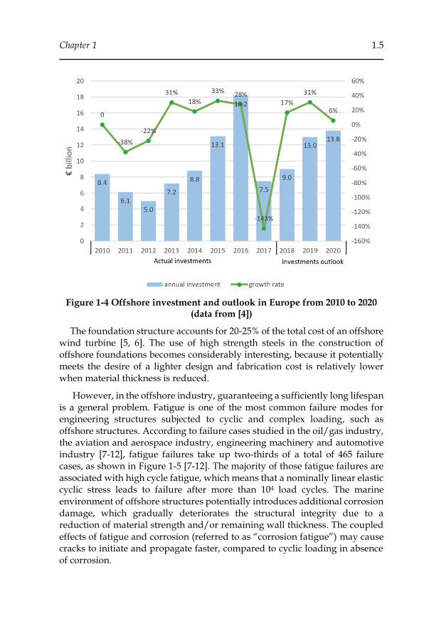
It is foreseen to cumulatively reach more than 32 GW of offshore wind power in 2022 (Figure 1-3 [3]). The last decade, more than 5 billion euros were
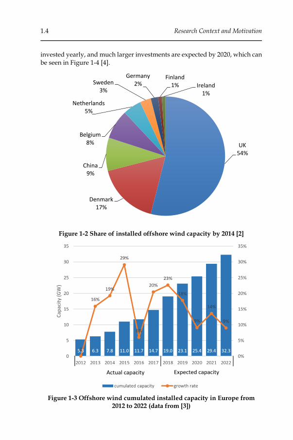
1.4 Research Context and Motivation
invested yearly, and much larger investments are expected by 2020, which can be seen in Figure 1-4 [4].
Figure 1-2 Share of installed offshore wind capacity by 2014 [2]
Figure 1-3 Offshore wind cumulated installed capacity in Europe from 2012 to 2022 (data from [3])
UK54%
Denmark17%
China9%
Belgium8%
Netherlands5%
Sweden3%
Germany2%
Finland1% Ireland
1%
Chapter 1 1.5
Figure 1-4 Offshore investment and outlook in Europe from 2010 to 2020 (data from [4])
The foundation structure accounts for 20-25% of the total cost of an offshore wind turbine [5, 6]. The use of high strength steels in the construction of offshore foundations becomes considerably interesting, because it potentially meets the desire of a lighter design and fabrication cost is relatively lower when material thickness is reduced.
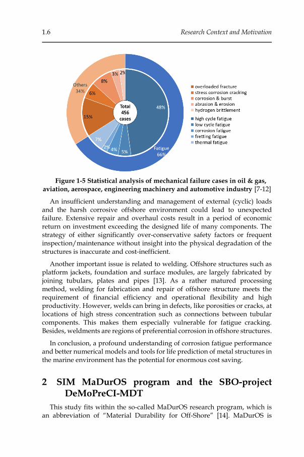
However, in the offshore industry, guaranteeing a sufficiently long lifespan is a general problem. Fatigue is one of the most common failure modes for engineering structures subjected to cyclic and complex loading, such as offshore structures. According to failure cases studied in the oil/gas industry, the aviation and aerospace industry, engineering machinery and automotive industry [7-12], fatigue failures take up two-thirds of a total of 465 failure cases, as shown in Figure 1-5 [7-12]. The majority of those fatigue failures are associated with high cycle fatigue, which means that a nominally linear elastic cyclic stress leads to failure after more than 104 load cycles. The marine environment of offshore structures potentially introduces additional corrosion damage, which gradually deteriorates the structural integrity due to a reduction of material strength and/or remaining wall thickness. The coupled effects of fatigue and corrosion (referred to as “corrosion fatigue”) may cause cracks to initiate and propagate faster, compared to cyclic loading in absence of corrosion.
1.6 Research Context and Motivation
Figure 1-5 Statistical analysis of mechanical failure cases in oil & gas,
aviation, aerospace, engineering machinery and automotive industry [7-12]
An insufficient understanding and management of external (cyclic) loads and the harsh corrosive offshore environment could lead to unexpected failure. Extensive repair and overhaul costs result in a period of economic return on investment exceeding the designed life of many components. The strategy of either significantly over-conservative safety factors or frequent inspection/maintenance without insight into the physical degradation of the structures is inaccurate and cost-inefficient.
Another important issue is related to welding. Offshore structures such as platform jackets, foundation and surface modules, are largely fabricated by joining tubulars, plates and pipes [13]. As a rather matured processing method, welding for fabrication and repair of offshore structure meets the requirement of financial efficiency and operational flexibility and high productivity. However, welds can bring in defects, like porosities or cracks, at locations of high stress concentration such as connections between tubular components. This makes them especially vulnerable for fatigue cracking. Besides, weldments are regions of preferential corrosion in offshore structures.
In conclusion, a profound understanding of corrosion fatigue performance and better numerical models and tools for life prediction of metal structures in the marine environment has the potential for enormous cost saving.
2 SIM MaDurOS program and the SBO-project DeMoPreCI-MDT
This study fits within the so-called MaDurOS research program, which is an abbreviation of “Material Durability for Off-Shore” [14]. MaDurOS is
Chapter 1 1.7
funded by the Strategic Initiative Materials (SIM), which is the materials spearhead cluster of the Belgian “Flanders Innovation & Entrepreneurship” (VLAIO) agency, supporting the growth of research and innovation within the Flemish material sector.
The MaDurOS program was proposed to actively response the target planned by the European Union (“Energy 2020 – A strategy for competitive, sustainable and secure energy”) that, by 2020, 20% of the energy produced by EU members should be supplied by renewable sources. To realize this goal, wind energy will play an important role, and offshore wind has been preferred over onshore wind due to its higher performance efficiency and avoidance of opposing deployment by local inhabitants. To achieve this, devices of wind energy must be scaled up to achieve the required reduction in investment and maintenance cost, such that it is economically competitive with fossil fuel and nuclear power generation. Therefore, breakthroughs in science and engineering technology of the related fields are required to ensure high reliability, accessibility, and low operation and maintenance costs.
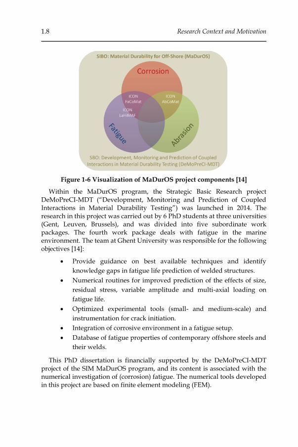
The MaDurOS program aims at inherent characteristics of the offshore environment in which material is frequently and simultaneously exposed to at least two of the following conditions: cyclic fatigue loadings, corrosive atmosphere, and abrasive contact conditions. A visual description of the program is illustrated in Figure 1-6. Conventional knowledge or design methods deal with each scenario individually. They cannot achieve global optimization design in general, which leads to an over-conservative or unsafe solution. The main objectives of this research program are [14]:
• To obtain deeper insight into the material performance under
combined marine service conditions.
• To offer numerical models or tools with coupled damage
mechanisms and testing facilities to allow possibilities of numerical
prediction and experimental testing.
• Eventually, to guide the development of new or improved
materials, material processing techniques, material applications or
inspection and monitoring techniques to strengthen the core
competitiveness of Flanders in the offshore market.
1.8 Research Context and Motivation
Figure 1-6 Visualization of MaDurOS project components [14]
Within the MaDurOS program, the Strategic Basic Research project DeMoPreCI-MDT (“Development, Monitoring and Prediction of Coupled Interactions in Material Durability Testing”) was launched in 2014. The research in this project was carried out by 6 PhD students at three universities (Gent, Leuven, Brussels), and was divided into five subordinate work packages. The fourth work package deals with fatigue in the marine environment. The team at Ghent University was responsible for the following objectives [14]:
• Provide guidance on best available techniques and identify
knowledge gaps in fatigue life prediction of welded structures.
• Numerical routines for improved prediction of the effects of size,
residual stress, variable amplitude and multi-axial loading on
fatigue life.
• Optimized experimental tools (small- and medium-scale) and
instrumentation for crack initiation.
• Integration of corrosive environment in a fatigue setup.
• Database of fatigue properties of contemporary offshore steels and
their welds.
This PhD dissertation is financially supported by the DeMoPreCI-MDT project of the SIM MaDurOS program, and its content is associated with the numerical investigation of (corrosion) fatigue. The numerical tools developed in this project are based on finite element modeling (FEM).
Chapter 1 1.9
3 Challenges in corrosion fatigue modeling
Steel offshore structures are subjected to complex loading conditions due to the combined actions of wind, waves and currents and are exposed to a corrosive seawater environment.
A variable amplitude loading on the structure changes the damage accumulation and fatigue crack propagation rates with respect to a constant amplitude load [15]. Load sequence dependency and interaction effects play an important role in the fatigue life prediction. In general literature suggests that when a first load block has a lower/higher stress amplitude than the next one, it can increase/reduce the crack initiation lifetime [16] or accelerate/retard the crack growth rate. However, generic conclusions cannot be put forward if more complex combinations of load sequences and/or load overloads and underloads are involved [17].
Structural joints produced by welding might not only introduce a weak link due to the presence of defects, but also contain residual stresses due the thermal processes involved in welding [18]. Residual stresses do not affect the cyclic stress range but control the mean stress value, which is a crucial parameter for fatigue damage evaluation. In general, the residual tensile/compressive stresses enhance/prevent crack opening of cracks [15] and therefore increase/decrease fatigue crack propagation rate
Damage from external loads and corrosion deteriorates the durability of materials, potentially leading to the initiation and propagation of fatigue cracks. The simultaneous action of cyclic mechanical stresses and environmental conditions can be more harmful than the summation of the effects of each mechanism acting individually. High strength steels may lose part of their advantages due to the presence of a corrosive environment since the fatigue limit is eliminated and the fatigue resistance is reduced to a level that is independent from the steel grade [19]. This may lead to a plummeting of fatigue life compared to operation in a mild environment. In fatigue design codes, different SN curves and crack growth curves are given depending on the environment. Many experimental investigations on corrosion fatigue of steel specimens and components have been reported [20-26]. Their main goal is to study the contribution of one or more aspects related to fatigue load and corrosion, such as effects of material microstructure, variable ampltidue load, fatigue load ratio, chemical composition of corrosion solution, with/without cathotic protection and temperature. Nevertheless, the state of the art knowledge is insufficient to address total life estimation.
It is hard to obtain a simple and comprehensive view of the synergistic effects of fatigue and corrosion with a sound physical basis and including every affecting factors. Assumpations and simplifications are always required in the development of life prediction methodologies [27]. It is also practically impossible to model corrosion fatigue by simulating each physical stage step
1.10 Research Context and Motivation
by step when the geometry is as big and complex as offshore structures, whilst the scale of damage events is microstructural. Hence, modeling corrosion fatigue behavior and predicting lifetime quantitively is extremely challenging.
Two main branches of challenges in modeling corrosion fatigue of offshore structures are focused on in this work:
1) Efficient computation of fatigue parameters, crack propagation trajectory and lifetime.
a. Fatigue damage or fatigue parameter values based on critical plane criteria need to be determined. For three-dimensional components, commonly used searching loops result in heavy computational burden when a finer mesh is applied to ensure adequate accuracy.
b. Stress intensity factor calculations depend on external load, crack geometry and boundary conditions; numerically they depend on finite element mesh design as well. A fracture mechanics mesh needs to be compatible with crack geometry in order to obtain accurate solutions. Therefore, mesh updating for a propagating crack will be difficult and time-consuming if conventional FEM is used to simulate three-dimensional fatigue crack propagation cycle by cycle.
c. Unlike regular crack shapes controlled by a limited number of parameters, such as elliptical and rectangular cracks, fatigue cracks in structures are potentially irregularly shaped in three dimensions. The evolution of the crack front geometry will depend on the energy equilibrium of the entire structure.
d. No matter the mesh is coarse or fine, computational cost is extremely high if fatigue crack growth increment is calculated for every cycle of a fatigue loading history with a large number of cycles.
e. Formulations of lifetime estimation are high-degree non-linear equations, no analytical solutions being available for practical cases.
2) Numerical discretization of corrosion effects and their combination with classical fatigue models
a. Decomposing interactional damage from fatigue and corrosion to allow numerical integration of damage per load cycle.
b. Including a model parameter(s) into fatigue models to evaluate damage from corrosion.

Chapter 1 1.11
4 Aim and scope of the dissertation
The motivation of this work is the demand for a profound understanding and description of the synergistic effects of fatigue and corrosion damage mechanisms on material deterioration.
The goal of this work is to develop an advanced numerical framework, which is universal and robust to a variety of structural geometries, has a good balance between accuracy and computational time, and is extendable for more features and future models. Purpose of this framework is not the numerical description of the fundamental physical processes, which have been well documented in literature, but targets the transfer of advanced methods to an industrial application level. The framework can benefit the design and analysis of offshore structures in the context of structural integrity. The following particular objectives are put forward:
• Reviewing the state of the art in fatigue crack initiation and
propagation simulation approaches
• Implementing an algorithm to simulate fatigue crack initiation
• Implementing an algorithm to simulate three-dimensional fatigue
crack propagation
• Implementing an algorithm to simulate the effect of variable amplitude
loading on fatigue damage development
• Developing a strategy and algorithm for corrosion fatigue damage
modelling
• Implementing an algorithm to include the effects of (weld) residual
stresses
• Small scale experimental validation of the developed models
This work has been performed within a Strategic Basic Research project. Focus is given to methodology development using simple, small scale laboratory specimens. This being said, the longer-term ambition is to apply the developed techniques on actual, complex welded offshore structures.
5 Overview of the dissertation
This dissertation is organized into seven chapters. It starts with the economic impact of the offshore wind energy industry with recent data and future outlook in Chapter 1. The motivation and outline of the MaDurOS program which is superordinate to this research are introduced. Challenges and objectives are discussed, leading to a motivation of the selected contribution(s) towards the state of the art. Finally, detailed scope and objectives are listed.

1.12 Research Context and Motivation
Chapter 2 starts with an overview of knowledge of fatigue in general and corrosion fatigue in the marine environment. Basic concepts and categorizations are given to help understand the following contents. Influencing factors that may be included in numerical modeling are mentioned. Difficulties and challenges of corrosion fatigue modeling and life prediction are reviewed, and the goal of the current work is highlighted.
Chapter 3 reviews modelling approaches for numerical simulation of corrosion fatigue initiation. A numerical framework for damage and lifetime associated with corrosion fatigue crack initiation is presented. It is an extension of the well-known continuum damage mechanics based model of Chaboche. The results from simulations and experimental tests are compared and discussed. A novel approach for parameter identification of critical plane criteria is implemented. Example cases are given to show the improvement in computational efficiency.
Chapter 4 deals with the simulation of three-dimensional fatigue crack propagation, based on extended finite element method (XFEM) and fracture mechanics. The framework for arbitrary 3D fatigue crack propagation is discussed and experimental validation using modified compact tension specimens is explained.
Having introduced simulation methodologies for two stages of fatigue (crack initiation and propagation) in the previous chapters, chapter 5 focuses on the transition between both stages. Technical methods of defining this transition, both experimentally and numerically, are reviewed. Case studies are given to show the feasibility of the method recommended to use in the frameworks.
In Chapter 6, extensions to achieve advanced features for the numerical frameworks are discussed. Two extensions developed are explained in detail. The first one deals with cycle-by-cycle fatigue crack growth under variable amplitude loading conditions, based on plastic zone models. The second one comprises the implementation of a (weld) residual stress field into the developed frameworks.
At the end of the dissertation, in Chapter 7, conclusions and innovations of this work are reported, and suggestions for future work in this subject are proposed.
Chapter 1 1.13
References
1. Roland Berger, Offshore wind toward 2020: on the pathway to cost competitiveness. 2013.
2. Higgins, P. and A. Foley, The evolution of offshore wind power in the United Kingdom. Renewable and Sustainable Energy Reviews, 2014. 37: p. 599-612.
3. Deloitte, Local impact, global leadership: The impact of wind energy on jobs and the EU economy. 2017.
4. Wind Europe, Financing and investment trends: The European wind industry in 2017. 2017.
5. IRENA, Renewable Power Generation Costs in 2017. 2017.
6. IRENA, Renewable Energy Technologies: Cost Analysis Series. 2012.
7. Lampman, S.R., ASM handbook: volume 19, fatigue and fracture. 1996: ASM International.
8. Makhlouf, A.S.H. and M. Aliofkhazraei, Handbook of Materials Failure Analysis with Case Studies from the Oil and Gas Industry. 2015: Elsevier Science & Technology Books.
9. Makhlouf, A.S.H. and M. Aliofkhazraei, Handbook of Materials Failure Analysis with Case Studies from the Aerospace and Automotive Industries. 2015: Elsevier.
10. Ramachandran, V., Failure Analysis of Engineering Structures: Methodology and Case Histories. 2005: ASM International.
11. Jones, D.R.H., Failure Analysis Case Studies II: A Sourcebook of Case Studies Selected from the Pages of Engineering Failure Analysis 1997-1999. 2001: Elsevier Science.
12. Balan, K.P., Metallurgical Failure Analysis: Techniques and Case Studies. 2018: Elsevier Science & Technology Books.
13. Plessis, J.d., Welding of Offshore Structures. 2012.
14. SIM. MADUROS. 2014; Available from: http://www.sim-flanders.be/research-program/maduros.
15. Schijve, J., Fatigue of Structures and Materials. 2008: Springer Netherlands.
16. Chaboche, J.L. and P.M. Lesne, A Non-Linear Continuous Fatigue Damage Model. Fatigue & Fracture of Engineering Materials & Structures, 1988. 11(1): p. 1-17.

1.14 Research Context and Motivation
17. Zhang, S., et al., Crack Propagation Studies On Al 7475 On The Basis Of Constant Amplitude And Selective Variable Amplitude Loading Histories. Fatigue & Fracture of Engineering Materials & Structures, 1987. 10(4): p. 315-332.
18. Janosch, J.J., et al., Influence of weld residual stresses on the fatigue strength of fillet welded assemblies - Application of the local mechanical approach, in Fatigue Design 1998, Vol I, G. Marquis and J. Solin, Editors. 1998. p. 275-288.
19. Devereux, O.F., et al., Corrosion fatigue: chemistry, mechanics and microstructure : June 14-18, 1971, The University of Connecticut, Storrs, Connecticut. 1972: National Association of Corrosion Engineers.
20. Adedipe, O., F. Brennan, and A. Kolios, Review of corrosion fatigue in offshore structures: Present status and challenges in the offshore wind sector. Renewable and Sustainable Energy Reviews, 2016. 61: p. 141-154.
21. Healy, J. and J. Billingham, A review of the corrosion fatigue behaviour of structural steels in the strength range 350-900MPa and associated high strength weldments. 1997: HSE Books.
22. Webster, S., I. Austen, and W. Rudd, Fatigue, corrosion fatigue and stress corrosion of steels for offshore structures. 1985: Office for Official Publications of the European Communities.
23. Horn, A.M., et al. Proceedings of the 17th International Ship and Offshore Structures Congress-Committee III. 2 Fatigue and Fracture. in The 17th International Ship and Offshore Structures Congress. 2009.
24. Horn, A.M., et al. Proceedings of the 18th International Ship and Offshore Structures Congress-Committee III. 2 Fatigue and Fracture. in The 18th International Ship and Offshore Structures Congress. 2012.
25. Brennan, F.P., et al. Proceedings of the 19th International Ship and Offshore Structures Congress-Committee III. 2 Fatigue and Fracture. in The 19th International Ship and Offshore Structures Congress. 2015.
26. Garbatov, Y., et al. Proceedings of the 20th International Ship and Offshore Structures Congress-Committee III. 2 Fatigue and Fracture. in The 20th International Ship and Offshore Structures Congress. 2018.
27. Larrosa, N., R. Akid, and R. Ainsworth, Corrosion-fatigue: a review of damage tolerance models. International Materials Reviews, 2017: p. 1-26.
Chapter 2
An Introduction to Fatigue in an Offshore Environment

2.2 An Introduction to Fatigue in an Offshore Environment
<< This page intentionally left blank >>

Chapter 2 2.3
1 Overview
The second chapter of this dissertation gives a brief introduction to fatigue in general, and fatigue in an offshore environment in particular. Important concepts and technical terms will be introduced here and used further throughout this dissertation. Major fatigue and corrosion-fatigue influencing factors that will be considered and investigated in this dissertation, are summarized as well.
2 Metal fatigue
Metal fatigue has been investigated for nearly 200 years [1]. Understanding and prediction of the fatigue failure mechanisms have made significant progress. Yet, fatigue is a highly complex physical phenomenon that is governed by a great number of parameters at different scales, including local geometry and stress state, material properties, loading profiles, and environment. As a result, the overall predictability of fatigue damage and its corresponding lifetime remains a major challenge to date.
2.1 The physical process of fatigue
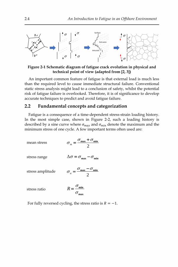
Fatigue comprises two main stages prior to unstable failure, namely crack initiation and crack propagation. As illustrated in Figure 2-1 [2, 3], physically, a large number of dislocations pile up together to form intrusions and extrusions under cyclic fatigue loading. At this stage, the fatigue damage develops in preferred crystallographic slip planes and is governed by shear stress. A crack eventually nucleates at the most damaged slip bands. Technically, a crack is identified as having initiated when its length reaches a size which can be detected by common technical means (non-destructive examination). After forming, the crack will grow in both length and orientation according to the damage development and distribution. When the crack driving force exceeds the material toughness, the propagation of the crack becomes unstable and rapid fracture occurs.
2.4 An Introduction to Fatigue in an Offshore Environment
Intrusion
Extrusion
Surface
Figure 2-1 Schematic diagram of fatigue crack evolution in physical and technical point of view (adapted from [2, 3])
An important common feature of fatigue is that external load is much less than the required level to cause immediate structural failure. Conventional static stress analysis might lead to a conclusion of safety, whilst the potential risk of fatigue failure is overlooked. Therefore, it is of significance to develop accurate techniques to predict and avoid fatigue failure.
2.2 Fundamental concepts and categorization
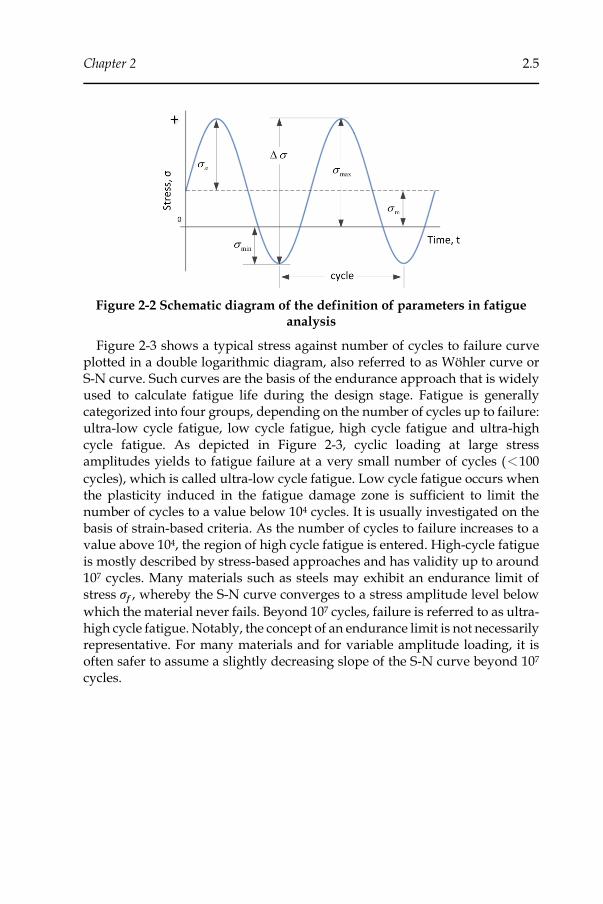
Fatigue is a consequence of a time-dependent stress-strain loading history. In the most simple case, shown in Figure 2-2, such a loading history is described by a sine curve where 𝜎𝑚𝑎𝑥 and 𝜎𝑚𝑖𝑛 denote the maximum and the minimum stress of one cycle. A few important terms often used are:
mean stress 2
max min
m
+=
stress range max min = −
stress amplitude 2
max min
a
−=
stress ratio min
max
R
=
For fully reversed cycling, the stress ratio is 𝑅 = −1.
Chapter 2 2.5
Figure 2-2 Schematic diagram of the definition of parameters in fatigue analysis
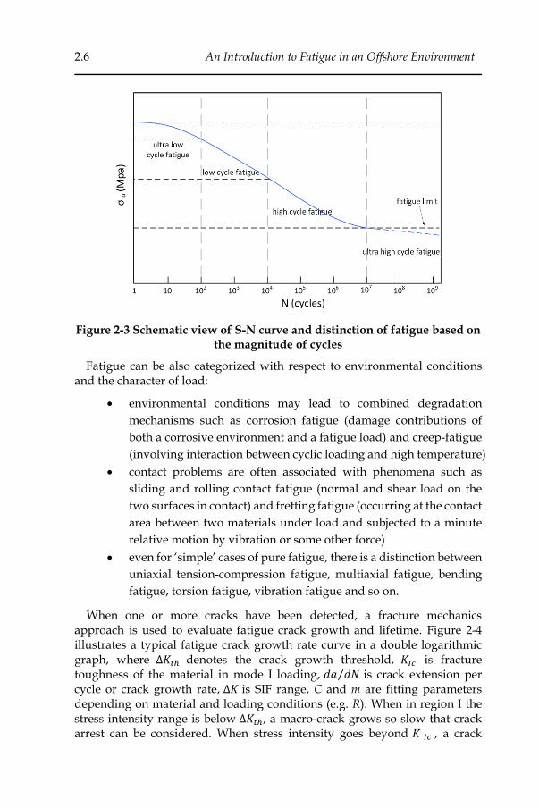
Figure 2-3 shows a typical stress against number of cycles to failure curve plotted in a double logarithmic diagram, also referred to as Wöhler curve or S-N curve. Such curves are the basis of the endurance approach that is widely used to calculate fatigue life during the design stage. Fatigue is generally categorized into four groups, depending on the number of cycles up to failure: ultra-low cycle fatigue, low cycle fatigue, high cycle fatigue and ultra-high cycle fatigue. As depicted in Figure 2-3, cyclic loading at large stress amplitudes yields to fatigue failure at a very small number of cycles (<100
cycles), which is called ultra-low cycle fatigue. Low cycle fatigue occurs when the plasticity induced in the fatigue damage zone is sufficient to limit the number of cycles to a value below 104 cycles. It is usually investigated on the basis of strain-based criteria. As the number of cycles to failure increases to a value above 104, the region of high cycle fatigue is entered. High-cycle fatigue is mostly described by stress-based approaches and has validity up to around 107 cycles. Many materials such as steels may exhibit an endurance limit of stress 𝜎𝑓, whereby the S-N curve converges to a stress amplitude level below
which the material never fails. Beyond 107 cycles, failure is referred to as ultra-high cycle fatigue. Notably, the concept of an endurance limit is not necessarily representative. For many materials and for variable amplitude loading, it is often safer to assume a slightly decreasing slope of the S-N curve beyond 107 cycles.
2.6 An Introduction to Fatigue in an Offshore Environment
Figure 2-3 Schematic view of S-N curve and distinction of fatigue based on the magnitude of cycles
Fatigue can be also categorized with respect to environmental conditions and the character of load:
• environmental conditions may lead to combined degradation
mechanisms such as corrosion fatigue (damage contributions of
both a corrosive environment and a fatigue load) and creep-fatigue
(involving interaction between cyclic loading and high temperature)
• contact problems are often associated with phenomena such as
sliding and rolling contact fatigue (normal and shear load on the
two surfaces in contact) and fretting fatigue (occurring at the contact
area between two materials under load and subjected to a minute
relative motion by vibration or some other force)
• even for ‘simple’ cases of pure fatigue, there is a distinction between
uniaxial tension-compression fatigue, multiaxial fatigue, bending
fatigue, torsion fatigue, vibration fatigue and so on.
When one or more cracks have been detected, a fracture mechanics approach is used to evaluate fatigue crack growth and lifetime. Figure 2-4 illustrates a typical fatigue crack growth rate curve in a double logarithmic graph, where ∆𝐾𝑡ℎ denotes the crack growth threshold, 𝐾𝐼𝑐 is fracture toughness of the material in mode I loading, 𝑑𝑎 𝑑𝑁⁄ is crack extension per cycle or crack growth rate, ∆𝐾 is SIF range, C and m are fitting parameters depending on material and loading conditions (e.g. R). When in region I the stress intensity range is below ∆𝐾𝑡ℎ, a macro-crack grows so slow that crack arrest can be considered. When stress intensity goes beyond 𝐾 𝐼𝑐 , a crack

Chapter 2 2.7
reaches an unstable stage with a high rate of growth till failure (region III). Stable crack growth in the second region will be discussed in the following Chapter 4. This part of the curve is described by the well-known Paris law.
Figure 2-4 Schematic illustration of the fatigue crack growth rate as a function of the SIF range.
3 Corrosion fatigue
3.1 Offshore environment
Regarding offshore structures and their environment, various corrosion mechanisms can be considered. Corrosion can occur as general surface corrosion, localized pitting, crevice and microbial corrosion [4]. Corrosion rates range between 0.1 to 0.7 mm per year for a non-protected structure [5].
As shown in Figure 2-5 [4, 5], distinction can be made between zones of the foundation far above the sea level, the splash zone at the transition from air to water, the submerged part near the mean wave level, the part deeply submerged with microbial action and the part inserted into the seabed. It can be clearly observed that the corrosion rate is quite high at the splash zone as compared to other zones. This is because of sufficient supply of oxygen and humidity reactions in the area [4]. It is worthwhile to mention that around the splash zone, contact with the waves creates widely fluctuating dynamic forces. The interaction between cyclic load and corrosive environment in this region may enhance the speed of fatigue crack initiation and propagation.
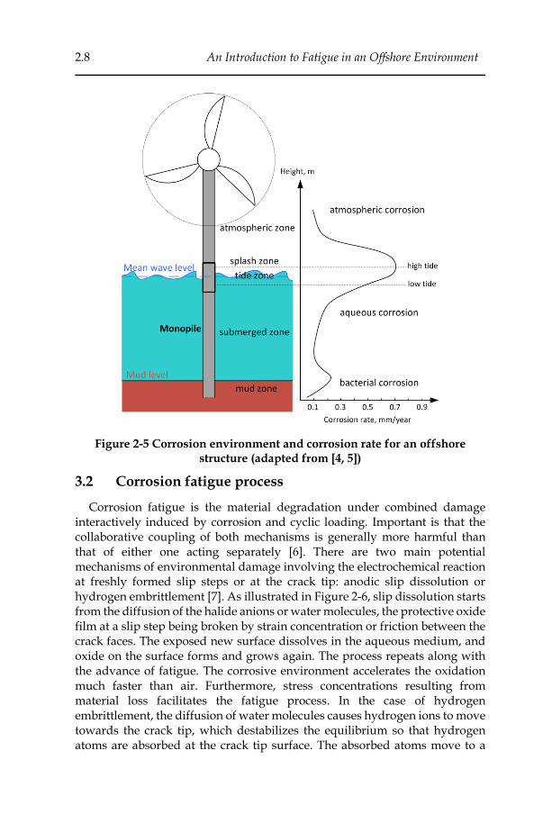
2.8 An Introduction to Fatigue in an Offshore Environment
Figure 2-5 Corrosion environment and corrosion rate for an offshore structure (adapted from [4, 5])
3.2 Corrosion fatigue process
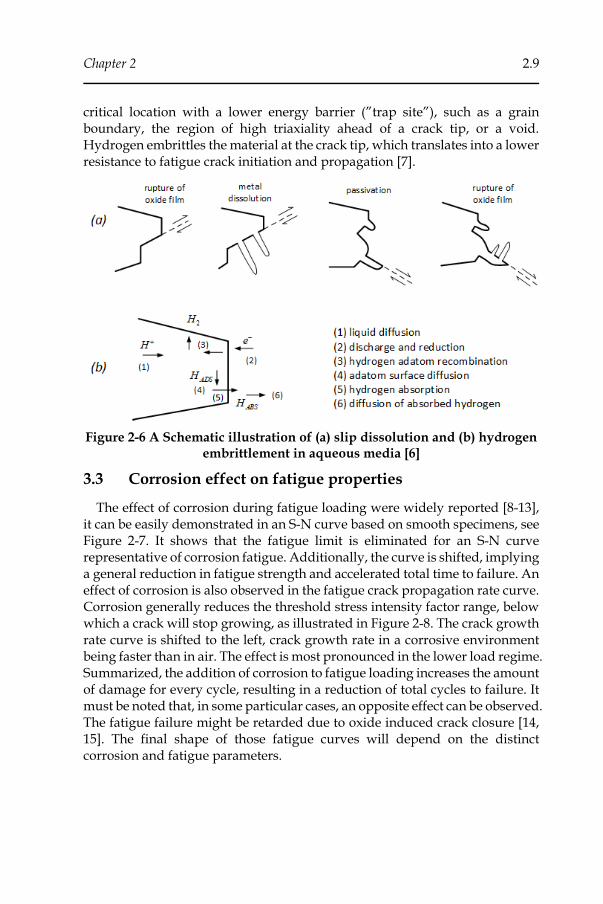
Corrosion fatigue is the material degradation under combined damage interactively induced by corrosion and cyclic loading. Important is that the collaborative coupling of both mechanisms is generally more harmful than that of either one acting separately [6]. There are two main potential mechanisms of environmental damage involving the electrochemical reaction at freshly formed slip steps or at the crack tip: anodic slip dissolution or hydrogen embrittlement [7]. As illustrated in Figure 2-6, slip dissolution starts from the diffusion of the halide anions or water molecules, the protective oxide film at a slip step being broken by strain concentration or friction between the crack faces. The exposed new surface dissolves in the aqueous medium, and oxide on the surface forms and grows again. The process repeats along with the advance of fatigue. The corrosive environment accelerates the oxidation much faster than air. Furthermore, stress concentrations resulting from material loss facilitates the fatigue process. In the case of hydrogen embrittlement, the diffusion of water molecules causes hydrogen ions to move towards the crack tip, which destabilizes the equilibrium so that hydrogen atoms are absorbed at the crack tip surface. The absorbed atoms move to a
Chapter 2 2.9
critical location with a lower energy barrier (”trap site”), such as a grain boundary, the region of high triaxiality ahead of a crack tip, or a void. Hydrogen embrittles the material at the crack tip, which translates into a lower resistance to fatigue crack initiation and propagation [7].
Figure 2-6 A Schematic illustration of (a) slip dissolution and (b) hydrogen embrittlement in aqueous media [6]
3.3 Corrosion effect on fatigue properties
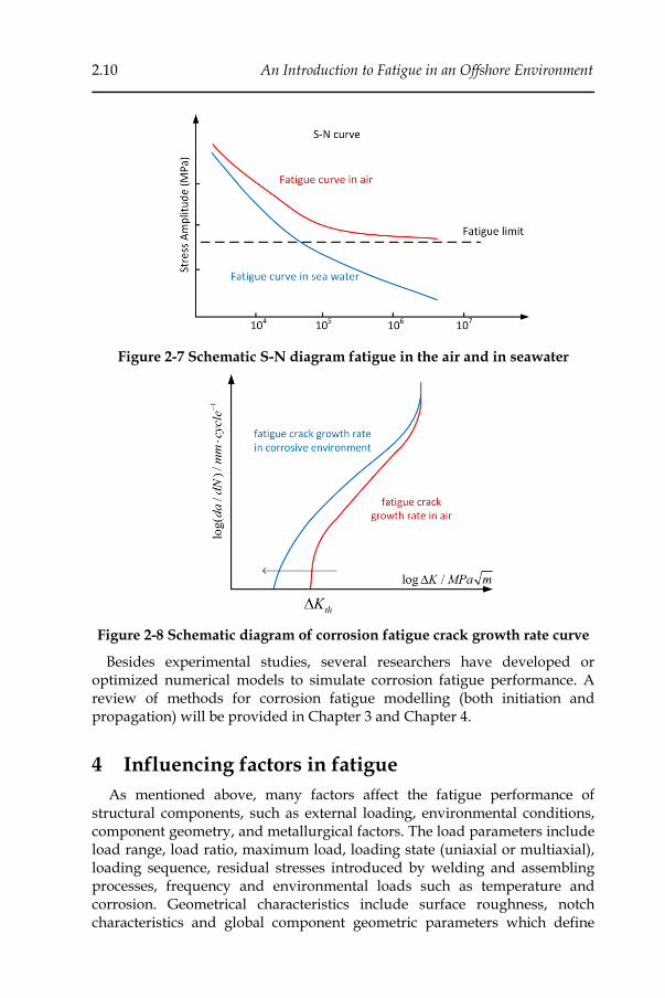
The effect of corrosion during fatigue loading were widely reported [8-13], it can be easily demonstrated in an S-N curve based on smooth specimens, see Figure 2-7. It shows that the fatigue limit is eliminated for an S-N curve representative of corrosion fatigue. Additionally, the curve is shifted, implying a general reduction in fatigue strength and accelerated total time to failure. An effect of corrosion is also observed in the fatigue crack propagation rate curve. Corrosion generally reduces the threshold stress intensity factor range, below which a crack will stop growing, as illustrated in Figure 2-8. The crack growth rate curve is shifted to the left, crack growth rate in a corrosive environment being faster than in air. The effect is most pronounced in the lower load regime. Summarized, the addition of corrosion to fatigue loading increases the amount of damage for every cycle, resulting in a reduction of total cycles to failure. It must be noted that, in some particular cases, an opposite effect can be observed. The fatigue failure might be retarded due to oxide induced crack closure [14, 15]. The final shape of those fatigue curves will depend on the distinct corrosion and fatigue parameters.
2.10 An Introduction to Fatigue in an Offshore Environment
Figure 2-7 Schematic S-N diagram fatigue in the air and in seawater
Figure 2-8 Schematic diagram of corrosion fatigue crack growth rate curve
Besides experimental studies, several researchers have developed or optimized numerical models to simulate corrosion fatigue performance. A review of methods for corrosion fatigue modelling (both initiation and propagation) will be provided in Chapter 3 and Chapter 4.
4 Influencing factors in fatigue
As mentioned above, many factors affect the fatigue performance of structural components, such as external loading, environmental conditions, component geometry, and metallurgical factors. The load parameters include load range, load ratio, maximum load, loading state (uniaxial or multiaxial), loading sequence, residual stresses introduced by welding and assembling processes, frequency and environmental loads such as temperature and corrosion. Geometrical characteristics include surface roughness, notch characteristics and global component geometric parameters which define
Chapter 2 2.11
stress concentrations and stress gradients related to the size effect. Metallurgical and mechanical properties of the materials include their chemical composition, microstructure(s) and strength/ toughness properties.
For offshore structures, the primary factor that affects the fatigue behavior of structural components is the fluctuant stress or strain invoked by the loading conditions. Therefore, those factors will be discussed appropriately in the following. Corrosion is an important factor which increases the rate of fatigue damage by the phenomenon of passivation-depassivation at the interface. According to Arrhenius equation, the chemical reaction rate of corrosion has a direct dependency on the temperature. The water temperature of the North Sea ranges between 0°C and 18°C on average [16, 17]. This is above the ductile-to-brittle transition temperature of contemporary high strength low alloy steels, and definitely below creep. However, it might be challenging to guarantee a sufficiently low transition temperature for welds in offshore steel grades [18]; optimal weld process design and electrode selection is required for low temperature offshore conditions. In this work it is assumed that temperature will affect the corrosion rate, but that it will not change the mechanical failure mechanism. Although mechanical fatigue of steel components is largely unaffected by load frequency, it plays an important role in corrosion fatigue. Corrosion develops on a very slow time scale and its degrading effect on lifetime will depend on the frequencies of the mechanical actions. Typical load frequencies are in the range of 0.1-2Hz for North Sea [4]; wave-current frequencies ranging from 0.2 to 0.35 Hz are employed for the design of fixed offshore wind turbine structures [19, 20].
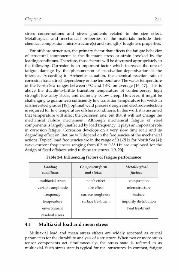
Table 2-1 Influencing factors of fatigue performance
Loading
conditions
Component form
and status
Metallurgical
factors
multiaxial stress notch effect composition
variable amplitude size effect microstructure
frequency surface roughness texture
temperature surface treatment impurity distribution
environment heat treatment
residual stress
4.1 Multiaxial load and mean stress
Multiaxial load and mean stress effects are widely accepted as crucial parameters for the durability analysis of a structure. When two or more stress tensor components act simultaneously, the stress state is referred to as multiaxial. Such stress state is typical for real structures. In contrast, fatigue
2.12 An Introduction to Fatigue in an Offshore Environment
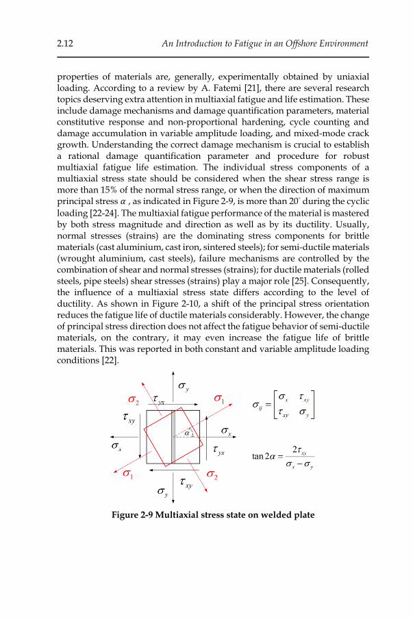
properties of materials are, generally, experimentally obtained by uniaxial loading. According to a review by A. Fatemi [21], there are several research topics deserving extra attention in multiaxial fatigue and life estimation. These include damage mechanisms and damage quantification parameters, material constitutive response and non-proportional hardening, cycle counting and damage accumulation in variable amplitude loading, and mixed-mode crack growth. Understanding the correct damage mechanism is crucial to establish a rational damage quantification parameter and procedure for robust multiaxial fatigue life estimation. The individual stress components of a multiaxial stress state should be considered when the shear stress range is more than 15% of the normal stress range, or when the direction of maximum principal stress 𝛼 , as indicated in Figure 2-9, is more than 20° during the cyclic
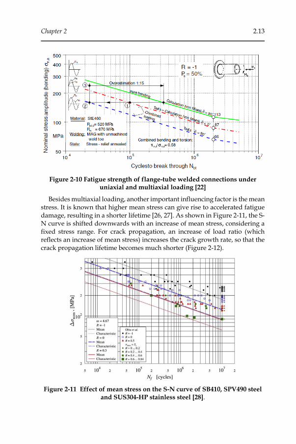
loading [22-24]. The multiaxial fatigue performance of the material is mastered by both stress magnitude and direction as well as by its ductility. Usually, normal stresses (strains) are the dominating stress components for brittle materials (cast aluminium, cast iron, sintered steels); for semi-ductile materials (wrought aluminium, cast steels), failure mechanisms are controlled by the combination of shear and normal stresses (strains); for ductile materials (rolled steels, pipe steels) shear stresses (strains) play a major role [25]. Consequently, the influence of a multiaxial stress state differs according to the level of ductility. As shown in Figure 2-10, a shift of the principal stress orientation reduces the fatigue life of ductile materials considerably. However, the change of principal stress direction does not affect the fatigue behavior of semi-ductile materials, on the contrary, it may even increase the fatigue life of brittle materials. This was reported in both constant and variable amplitude loading conditions [22].
Figure 2-9 Multiaxial stress state on welded plate
Chapter 2 2.13
Figure 2-10 Fatigue strength of flange-tube welded connections under uniaxial and multiaxial loading [22]
Besides multiaxial loading, another important influencing factor is the mean stress. It is known that higher mean stress can give rise to accelerated fatigue damage, resulting in a shorter lifetime [26, 27]. As shown in Figure 2-11, the S-N curve is shifted downwards with an increase of mean stress, considering a fixed stress range. For crack propagation, an increase of load ratio (which reflects an increase of mean stress) increases the crack growth rate, so that the crack propagation lifetime becomes much shorter (Figure 2-12).
Figure 2-11 Effect of mean stress on the S-N curve of SB410, SPV490 steel and SUS304-HP stainless steel [28].

2.14 An Introduction to Fatigue in an Offshore Environment
Figure 2-12 Crack growth rate curves of JIS SM 50B pressure vessel steel under different R-ratios [29].
Various empirical relationships have been proposed to take the mean stress effect on the material fatigue strength into account for uniaxial loading. Those formulations are summarized and plotted in Figure 2-13, where 𝜎𝑦 is yield
strength, 𝜎𝑢 is ultimate tensile strength, 𝜎𝑟 is rupture strength of the material. The plotted criteria can be extended to multiaxial fatigue situations by re-interpreting them in terms of critical plane approaches [27].
Figure 2-13 Comparison of correction methods for mean stress effect [30].
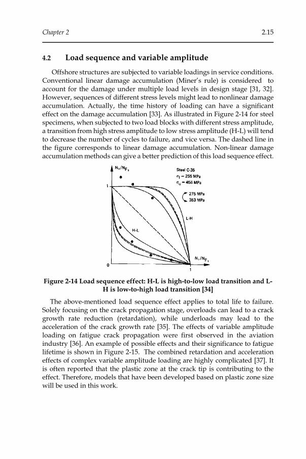
Chapter 2 2.15
4.2 Load sequence and variable amplitude
Offshore structures are subjected to variable loadings in service conditions. Conventional linear damage accumulation (Miner’s rule) is considered to account for the damage under multiple load levels in design stage [31, 32]. However, sequences of different stress levels might lead to nonlinear damage accumulation. Actually, the time history of loading can have a significant effect on the damage accumulation [33]. As illustrated in Figure 2-14 for steel specimens, when subjected to two load blocks with different stress amplitude, a transition from high stress amplitude to low stress amplitude (H-L) will tend to decrease the number of cycles to failure, and vice versa. The dashed line in the figure corresponds to linear damage accumulation. Non-linear damage accumulation methods can give a better prediction of this load sequence effect.
Figure 2-14 Load sequence effect: H-L is high-to-low load transition and L-H is low-to-high load transition [34]
The above-mentioned load sequence effect applies to total life to failure. Solely focusing on the crack propagation stage, overloads can lead to a crack growth rate reduction (retardation), while underloads may lead to the acceleration of the crack growth rate [35]. The effects of variable amplitude loading on fatigue crack propagation were first observed in the aviation industry [36]. An example of possible effects and their significance to fatigue lifetime is shown in Figure 2-15. The combined retardation and acceleration effects of complex variable amplitude loading are highly complicated [37]. It is often reported that the plastic zone at the crack tip is contributing to the effect. Therefore, models that have been developed based on plastic zone size will be used in this work.
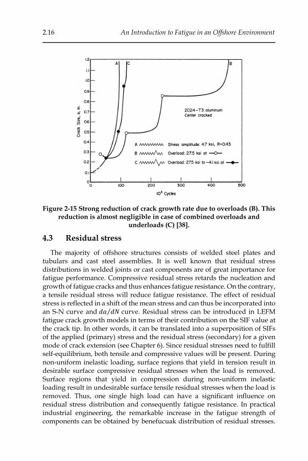
2.16 An Introduction to Fatigue in an Offshore Environment
Figure 2-15 Strong reduction of crack growth rate due to overloads (B). This reduction is almost negligible in case of combined overloads and
underloads (C) [38].
4.3 Residual stress
The majority of offshore structures consists of welded steel plates and tubulars and cast steel assemblies. It is well known that residual stress distributions in welded joints or cast components are of great importance for fatigue performance. Compressive residual stress retards the nucleation and growth of fatigue cracks and thus enhances fatigue resistance. On the contrary, a tensile residual stress will reduce fatigue resistance. The effect of residual stress is reflected in a shift of the mean stress and can thus be incorporated into an S-N curve and 𝑑𝑎 𝑑𝑁⁄ curve. Residual stress can be introduced in LEFM fatigue crack growth models in terms of their contribution on the SIF value at the crack tip. In other words, it can be translated into a superposition of SIFs of the applied (primary) stress and the residual stress (secondary) for a given mode of crack extension (see Chapter 6). Since residual stresses need to fulfill self-equilibrium, both tensile and compressive values will be present. During non-uniform inelastic loading, surface regions that yield in tension result in desirable surface compressive residual stresses when the load is removed. Surface regions that yield in compression during non-uniform inelastic loading result in undesirable surface tensile residual stresses when the load is removed. Thus, one single high load can have a significant influence on residual stress distribution and consequently fatigue resistance. In practical industrial engineering, the remarkable increase in the fatigue strength of components can be obtained by benefucuak distribution of residual stresses.
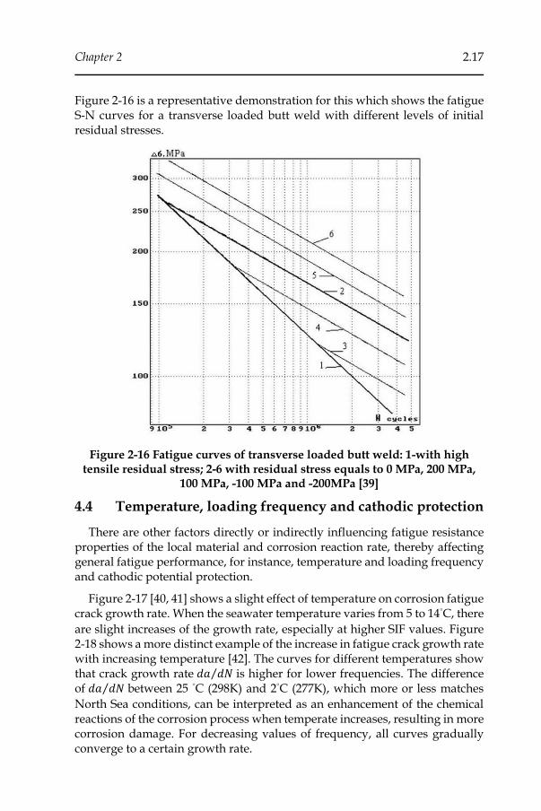
Chapter 2 2.17
Figure 2-16 is a representative demonstration for this which shows the fatigue S-N curves for a transverse loaded butt weld with different levels of initial residual stresses.
Figure 2-16 Fatigue curves of transverse loaded butt weld: 1-with high tensile residual stress; 2-6 with residual stress equals to 0 MPa, 200 MPa,
100 MPa, -100 MPa and -200MPa [39]
4.4 Temperature, loading frequency and cathodic protection
There are other factors directly or indirectly influencing fatigue resistance properties of the local material and corrosion reaction rate, thereby affecting general fatigue performance, for instance, temperature and loading frequency and cathodic potential protection.
Figure 2-17 [40, 41] shows a slight effect of temperature on corrosion fatigue crack growth rate. When the seawater temperature varies from 5 to 14°C, there
are slight increases of the growth rate, especially at higher SIF values. Figure 2-18 shows a more distinct example of the increase in fatigue crack growth rate with increasing temperature [42]. The curves for different temperatures show that crack growth rate 𝑑𝑎 𝑑𝑁⁄ is higher for lower frequencies. The difference of 𝑑𝑎 𝑑𝑁⁄ between 25 °C (298K) and 2°C (277K), which more or less matches
North Sea conditions, can be interpreted as an enhancement of the chemical reactions of the corrosion process when temperate increases, resulting in more corrosion damage. For decreasing values of frequency, all curves gradually converge to a certain growth rate.

2.18 An Introduction to Fatigue in an Offshore Environment
Figure 2-17 Temperature effect on corrosion fatigue crack growth rate of C-Mn steel (R=0.5) with oxygen contents indicated [40, 41]
Figure 2-18 HY-130 steel crack growth rate in 3.5% NaCl solution for multiple temperatures and frequencies [42]
The influence of environment and frequency is also reported in the works of Appleton and Adedipe [41, 43]. As shown in Figure 2-19, crack growth rates are faster in seawater than in air; for a specimen immersed in seawater the crack grows faster at lower frequencies. From Figure 2-20 it can be concluded that compared to crack growth rate in air, the rate in seawater can be several times faster for a wide range of SIFs. The difference is most significant for lower frequencies. For very high SIF ranges all curves converge to each other.
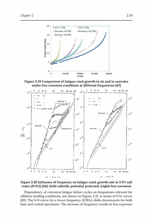
Chapter 2 2.19
Figure 2-19 Comparison of fatigue crack growth in air and in seawater under free corrosion conditions at different frequencies [43]
Figure 2-20 Influence of frequency on fatigue crack growth rate in 3.5% salt water (R=0.2) [44]: (left) cathodic potential protected, (right) free corrosion
Dependency of corrosion fatigue failure cycles on frequencies relevant for offshore loading conditions, are shown in Figure 2-21 in terms of S-N curves [45]. The S-N curve for a lower frequency (0.5Hz) shifts downwards for both bare and coated specimens. The increase of frequency results in less exposure
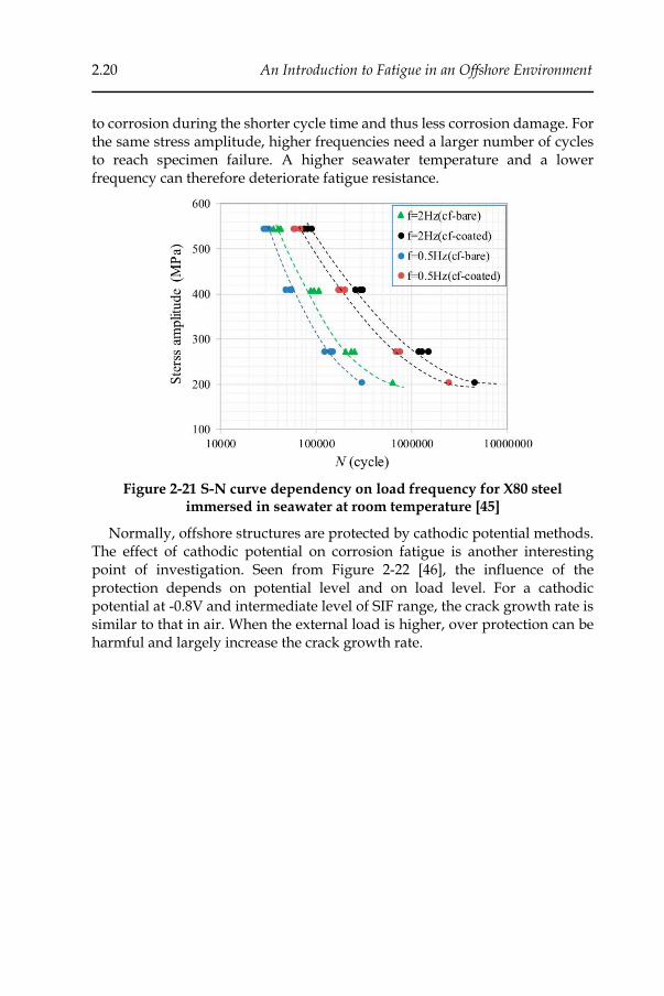
2.20 An Introduction to Fatigue in an Offshore Environment
to corrosion during the shorter cycle time and thus less corrosion damage. For the same stress amplitude, higher frequencies need a larger number of cycles to reach specimen failure. A higher seawater temperature and a lower frequency can therefore deteriorate fatigue resistance.
Figure 2-21 S-N curve dependency on load frequency for X80 steel immersed in seawater at room temperature [45]
Normally, offshore structures are protected by cathodic potential methods. The effect of cathodic potential on corrosion fatigue is another interesting point of investigation. Seen from Figure 2-22 [46], the influence of the protection depends on potential level and on load level. For a cathodic potential at -0.8V and intermediate level of SIF range, the crack growth rate is similar to that in air. When the external load is higher, over protection can be harmful and largely increase the crack growth rate.

Chapter 2 2.21
Figure 2-22 Ratio of corrosion fatigue crack growth rate relative to air as a function of cathodic potential [46]
5 Summary
This introductory chapter is meant to give a basic background of fatigue and corrosion fatigue. Concepts as crack initiation and propagation have been introduced as well as S-N approach and crack growth rate to evaluate fatigue damage and lifetime. A brief overview was given of important factors having an impact on the fatigue process. In the following chapters, a more in-depth review of modelling approaches for fatigue and corrosion-fatigue crack initiation and propagation will be reported. Influencing factors such as variable amplitude and residual stress will be discussed in terms of extensions to the fatigue damage simulation frameworks.
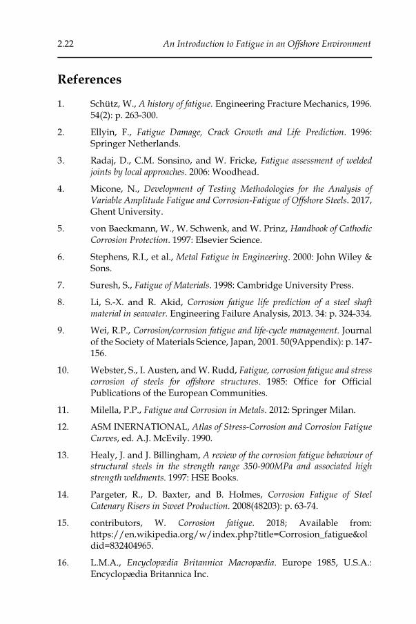
2.22 An Introduction to Fatigue in an Offshore Environment
References
1. Schütz, W., A history of fatigue. Engineering Fracture Mechanics, 1996. 54(2): p. 263-300.
2. Ellyin, F., Fatigue Damage, Crack Growth and Life Prediction. 1996: Springer Netherlands.
3. Radaj, D., C.M. Sonsino, and W. Fricke, Fatigue assessment of welded joints by local approaches. 2006: Woodhead.
4. Micone, N., Development of Testing Methodologies for the Analysis of Variable Amplitude Fatigue and Corrosion-Fatigue of Offshore Steels. 2017, Ghent University.
5. von Baeckmann, W., W. Schwenk, and W. Prinz, Handbook of Cathodic Corrosion Protection. 1997: Elsevier Science.
6. Stephens, R.I., et al., Metal Fatigue in Engineering. 2000: John Wiley & Sons.
7. Suresh, S., Fatigue of Materials. 1998: Cambridge University Press.
8. Li, S.-X. and R. Akid, Corrosion fatigue life prediction of a steel shaft material in seawater. Engineering Failure Analysis, 2013. 34: p. 324-334.
9. Wei, R.P., Corrosion/corrosion fatigue and life-cycle management. Journal of the Society of Materials Science, Japan, 2001. 50(9Appendix): p. 147-156.
10. Webster, S., I. Austen, and W. Rudd, Fatigue, corrosion fatigue and stress corrosion of steels for offshore structures. 1985: Office for Official Publications of the European Communities.
11. Milella, P.P., Fatigue and Corrosion in Metals. 2012: Springer Milan.
12. ASM INERNATIONAL, Atlas of Stress-Corrosion and Corrosion Fatigue Curves, ed. A.J. McEvily. 1990.
13. Healy, J. and J. Billingham, A review of the corrosion fatigue behaviour of structural steels in the strength range 350-900MPa and associated high strength weldments. 1997: HSE Books.
14. Pargeter, R., D. Baxter, and B. Holmes, Corrosion Fatigue of Steel Catenary Risers in Sweet Production. 2008(48203): p. 63-74.
15. contributors, W. Corrosion fatigue. 2018; Available from: https://en.wikipedia.org/w/index.php?title=Corrosion_fatigue&oldid=832404965.
16. L.M.A., Encyclopædia Britannica Macropædia. Europe 1985, U.S.A.: Encyclopædia Britannica Inc.

Chapter 2 2.23
17. Safety at Sea project: Norwegian Coastal Administration. About the North Sea: Key facts. 2008; Available from: https://web.archive.org/web/20081209095426/http://www.safetyatsea.se/index.php?section=northsea.
18. Health, et al., Review of the Performance of High Strength Steels Used Offshore. 2003: HSE Books.
19. Peeringa, J.M. Fatigue loading on a 5MW offshore wind turbine due to the combined action of waves and current. in Journal of Physics: Conference Series. 2014. IOP Publishing.
20. Devriendt, C., et al., Damping estimation of an offshore wind turbine on a monopile foundation. IET Renewable Power Generation, 2013. 7(4): p. 401-412.
21. Fatemi, A. and N. Shamsaei, Multiaxial fatigue: An overview and some approximation models for life estimation. International Journal of Fatigue, 2011. 33(8): p. 948-958.
22. Sonsino, C., Multiaxial fatigue assessment of welded joints – Recommendations for design codes. International Journal of Fatigue, 2009. 31(1): p. 173-187.
23. Sonsino, C.M., Influence of material’s ductility and local deformation mode on multiaxial fatigue response. International Journal of Fatigue, 2011. 33(8): p. 930-947.
24. Hobbacher, A., Recommendations for fatigue design of welded joints and components. 2009: Springer.
25. Sonsino, C. Material Influence on Multiaxial Fatigue Response. in ICMFF9. 2010.
26. Dowling, N.E., Mean stress effects in stress-life and strain-life fatigue. 2004, SAE Technical Paper.
27. Susmel, L., R. Tovo, and P. Lazzarin, The mean stress effect on the high-cycle fatigue strength from a multiaxial fatigue point of view. International Journal of Fatigue, 2005. 27(8): p. 928-943.
28. Nykänen, T. and T. Björk, Assessment of fatigue strength of steel butt-welded joints in as-welded condition – Alternative approaches for curve fitting and mean stress effect analysis. Marine Structures, 2015. 44: p. 288-310.
29. Katoh, A., Kurihara, M. , and Kawahara, M. ,, An Expression of Fatigue Crack Propagation Rates under Wide Ranged Stress Ratios: Analysis Based on the Crack Opening Stress Level Measurements. The Society of Naval Architects of Japan, 1983. 153: p. 8.
2.24 An Introduction to Fatigue in an Offshore Environment
30. Engineering Archives. Mean Stress Equations. Available from: http://www.engineeringarchives.com/les_fatigue_meanstressequations.html.
31. Veritas, D.N., Fatigue design of offshore steel structures. DNV Recommended Practice DNV-RP-C203, 2010.
32. Standard, B., Guide to fatigue design and assessment of steel products, BS 7608: 2014. The British Standards Institution, London, UK, 2014.
33. Zakaria, K.A., S. Abdullah, and M. Ghazali, A Review of the Loading Sequence Effects on the Fatigue Life Behaviour of Metallic Materials. Journal of Engineering Science & Technology Review, 2016. 9(5).
34. Chaboche, J.L. and P.M. Lesne, A Non-Linear Continuous Fatigue Damage Model. Fatigue & Fracture of Engineering Materials & Structures, 1988. 11(1): p. 1-17.
35. Skorupa, M., Load interaction effects during fatigue crack growth under variable amplitude loading—a literature review. Part I: empirical trends. Fatigue & Fracture of Engineering Materials & Structures, 1998. 21(8): p. 987-1006.
36. Hudson, C.M. and H.F. Hardrath, Effects of changing stress amplitude on the rate of fatigue-crack propagation in two aluminum alloys. 1961.
37. Zhang, S., et al., Crack propagation studies on Al 7475 on the basis of constant amplitude and selective variable amplitude loading histories. Fatigue & fracture of engineering materials & structures, 1987. 10(4): p. 315-332.
38. Schijve, J. and D. Broek, Crack propagation: the results of a test programme based on a gust spectrum with variable amplitude loading. Aircraft Engineering and Aerospace Technology, 1962. 34(11): p. 314-316.
39. Kudryavtsev, Y., Residual Stresses Management: Measurements, Fatigue Analysis and Beneficial Redistribution, in Engineering Applications of Residual Stress, Volume 8. 2011, Springer. p. 119-129.
40. Adedipe, O., F. Brennan, and A. Kolios, Review of corrosion fatigue in offshore structures: Present status and challenges in the offshore wind sector. Renewable and Sustainable Energy Reviews, 2016. 61: p. 141-154.
41. Appleton, R.J., Corrosion fatigue of a C-Mn steel. 1985, University of Glasgow.
42. Thomas, J.P. and R.P. Wei, Corrosion fatigue crack growth of steels in aqueous solutions I: Experimental results and modeling the effects of frequency and temperature. Materials Science and Engineering: A, 1992. 159(2): p. 205-221.
Chapter 2 2.25
43. Adedipe, O., F. Brennan, and A. Kolios, Corrosion fatigue load frequency sensitivity analysis. Marine Structures, 2015. 42: p. 115-136.
44. Vosikovsky, O., Fatigue-crack growth in an X-65 line-pipe steel at low cyclic frequencies in aqueous environments. Journal of Engineering Materials and Technology, 1975. 97(4): p. 298-304.
45. Han, Z., X. Huang, and Z. Yang Effect of Al⁻Zn Alloy Coating on Corrosion Fatigue Behavior of X80 Riser Steel. Materials (Basel, Switzerland), 2019. 12, DOI: 10.3390/ma12091520.
46. Murakami, R. and W.G. Ferguson, The Effects Of Cathodic Potential And Calcareous Deposits On Corrosion Fatigue Crack Growth Rate In Sea Water For Two Offshore Structural Steels. Fatigue & Fracture of Engineering Materials & Structures, 1987. 9(6): p. 477-488.
Chapter 3
Fatigue Crack Initiation Modelling

3.2 Fatigue Crack Initiation Modelling
<< This page intentionally left blank >>
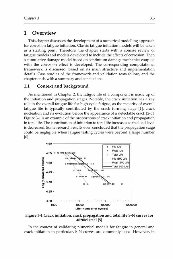
Chapter 3 3.3
1 Overview
This chapter discusses the development of a numerical modelling approach for corrosion fatigue initiation. Classic fatigue initiation models will be taken as a starting point. Therefore, the chapter starts with a concise review of fatigue models and models developed to include the effects of corrosion. Then a cumulative damage model based on continuum damage mechanics coupled with the corrosion effect is developed. The corresponding computational framework is discussed, based on its main structure and implementation details. Case studies of the framework and validation tests follow, and the chapter ends with a summary and conclusions.
1.1 Context and background
As mentioned in Chapter 2, the fatigue life of a component is made up of the initiation and propagation stages. Notably, the crack initiation has a key role in the overall fatigue life for high cycle fatigue, as the majority of overall fatigue life is typically contributed by the crack forming stage [1], crack nucleation and its evolution before the appearance of a detectable crack [2-5]. Figure 3-1 is an example of the proportions of crack initiation and propagation in total life. The contribution of initiation to total life increases as the load level is decreased. Some research results even concluded that the propagation stage could be negligible when fatigue testing cycles were beyond a large number [6].
Figure 3-1 Crack initiation, crack propagation and total life S-N curves for 4620M steel [5]
In the context of validating numerical models for fatigue in general and crack initiation in particular, S-N curves are commonly used. However, in
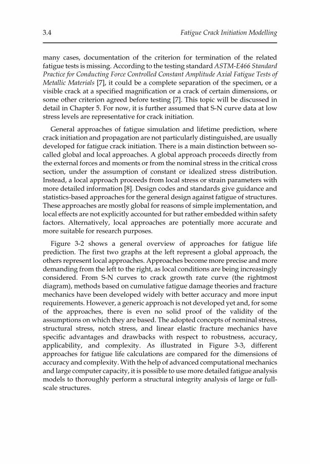
3.4 Fatigue Crack Initiation Modelling
many cases, documentation of the criterion for termination of the related fatigue tests is missing. According to the testing standard ASTM-E466 Standard Practice for Conducting Force Controlled Constant Amplitude Axial Fatigue Tests of Metallic Materials [7], it could be a complete separation of the specimen, or a visible crack at a specified magnification or a crack of certain dimensions, or some other criterion agreed before testing [7]. This topic will be discussed in detail in Chapter 5. For now, it is further assumed that S-N curve data at low stress levels are representative for crack initiation.
General approaches of fatigue simulation and lifetime prediction, where crack initiation and propagation are not particularly distinguished, are usually developed for fatigue crack initiation. There is a main distinction between so-called global and local approaches. A global approach proceeds directly from the external forces and moments or from the nominal stress in the critical cross section, under the assumption of constant or idealized stress distribution. Instead, a local approach proceeds from local stress or strain parameters with more detailed information [8]. Design codes and standards give guidance and statistics-based approaches for the general design against fatigue of structures. These approaches are mostly global for reasons of simple implementation, and local effects are not explicitly accounted for but rather embedded within safety factors. Alternatively, local approaches are potentially more accurate and more suitable for research purposes.
Figure 3-2 shows a general overview of approaches for fatigue life prediction. The first two graphs at the left represent a global approach, the others represent local approaches. Approaches become more precise and more demanding from the left to the right, as local conditions are being increasingly considered. From S-N curves to crack growth rate curve (the rightmost diagram), methods based on cumulative fatigue damage theories and fracture mechanics have been developed widely with better accuracy and more input requirements. However, a generic approach is not developed yet and, for some of the approaches, there is even no solid proof of the validity of the assumptions on which they are based. The adopted concepts of nominal stress, structural stress, notch stress, and linear elastic fracture mechanics have specific advantages and drawbacks with respect to robustness, accuracy, applicability, and complexity. As illustrated in Figure 3-3, different approaches for fatigue life calculations are compared for the dimensions of accuracy and complexity. With the help of advanced computational mechanics and large computer capacity, it is possible to use more detailed fatigue analysis models to thoroughly perform a structural integrity analysis of large or full-scale structures.
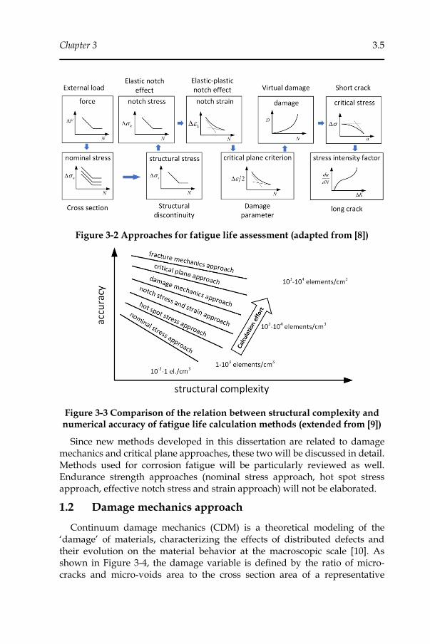
Chapter 3 3.5
Figure 3-2 Approaches for fatigue life assessment (adapted from [8])
Figure 3-3 Comparison of the relation between structural complexity and numerical accuracy of fatigue life calculation methods (extended from [9])
Since new methods developed in this dissertation are related to damage mechanics and critical plane approaches, these two will be discussed in detail. Methods used for corrosion fatigue will be particularly reviewed as well. Endurance strength approaches (nominal stress approach, hot spot stress approach, effective notch stress and strain approach) will not be elaborated.
1.2 Damage mechanics approach
Continuum damage mechanics (CDM) is a theoretical modeling of the ‘damage’ of materials, characterizing the effects of distributed defects and their evolution on the material behavior at the macroscopic scale [10]. As shown in Figure 3-4, the damage variable is defined by the ratio of micro-cracks and micro-voids area to the cross section area of a representative
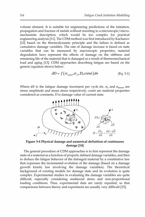
3.6 Fatigue Crack Initiation Modelling
volume element. It is suitable for engineering predictions of the initiation, propagation and fracture of metals without resorting to a microscopic/micro-mechanistic description, which would be too complex for practical engineering analysis [11]. The CDM method was first introduced by Kachanov [12] based on the thermodynamic principle and the failure is defined as cumulative damage variables. The rate of damage increase is based on state variables that can be measured by macroscopic properties; material degradation laws represent the effects of damage on the stiffness and remaining life of the material that is damaged as a result of thermomechanical load and aging [13]. CDM approaches describing fatigue are based on the generic equation shown below:
( ), , ,mean a
dD f D const dn = (Eq. 3-1)
Where 𝑑𝐷 is the fatigue damage increment per cycle 𝑑𝑛 , 𝜎𝑎 and 𝜎𝑚𝑒𝑎𝑛 are stress amplitude and mean stress respectively, const are material properties considered as constants, D is damage value of current state.
Figure 3-4 Physical damage and numerical definition of continuous damage [14]
The general procedure of CDM approaches is to first represent the damage state of a material as a function of properly defined damage variables, and then to deduce the fatigue behavior of the damaged material by a constitutive law that expresses the incremental evolution of the damage (based on a damage growth kinetic law involving the damage variables). The theoretical background of existing models for damage state and its evolution is quite complex. Experimental studies in evaluating the damage variables are quite difficult, especially considering multiaxial stress and non-proportional loading conditions. Thus, experimental data are rarely reported, so that comparisons between theory and experiment are usually very difficult [15].
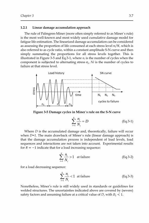
Chapter 3 3.7
1.2.1 Linear damage accumulation approach
The rule of Palmgren-Miner (more often simply referred to as Miner`s rule) is the most well-known and most widely used cumulative damage model for fatigue life estimation. The linearized damage accumulation can be considered as assessing the proportion of life consumed at each stress level 𝑛 𝑁⁄ , which is also referred to as cycle ratio, within a constant amplitude S-N curve and then simply summating the proportions for all stress levels together. This is illustrated in Figure 3-5 and Eq.3-1, where ni is the number of cycles when the component is subjected to alternating stress 𝜎𝑖, Ni is the number of cycles to failure at that stress level.
Figure 3-5 Damage cycles in Miner`s rule on the S-N curve
1
ki
i i
nD
N=
= (Eq.3-1)
Where D is the accumulated damage and, theoretically, failure will occur when D=1. The main drawback of Miner`s rule (linear damage approach) is that the damage accumulation process is independent of load levels, load sequences and interactions are not taken into account. Experimental results for 𝑅 = −1 indicate that for a load increasing sequence:
1
1k
i
i i
n
N=
at failure (Eq.3-2)
for a load decreasing sequence:
1
1k
i
i i
n
N=
at failure (Eq.3-3)
Nonetheless, Miner’s rule is still widely used in standards or guidelines for welded structures. The uncertainties indicated above are covered by (severe) safety factors and assuming failure at a critical value of D, with 𝐷𝑐 < 1.
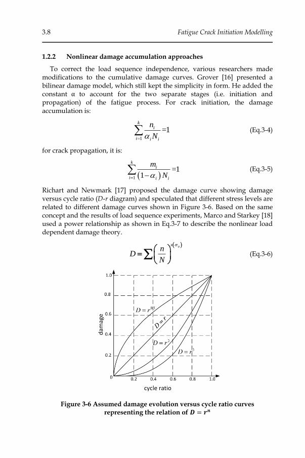
3.8 Fatigue Crack Initiation Modelling
1.2.2 Nonlinear damage accumulation approaches
To correct the load sequence independence, various researchers made modifications to the cumulative damage curves. Grover [16] presented a bilinear damage model, which still kept the simplicity in form. He added the constant α to account for the two separate stages (i.e. initiation and propagation) of the fatigue process. For crack initiation, the damage accumulation is:
1
=1k
i
i i i
n
N=
(Eq.3-4)
for crack propagation, it is:
( )1
=11
ki
i i i
m
N= − (Eq.3-5)
Richart and Newmark [17] proposed the damage curve showing damage versus cycle ratio (D-r diagram) and speculated that different stress levels are related to different damage curves shown in Figure 3-6. Based on the same concept and the results of load sequence experiments, Marco and Starkey [18] used a power relationship as shown in Eq.3-7 to describe the nonlinear load dependent damage theory.
( )axn
DN
=
(Eq.3-6)
Figure 3-6 Assumed damage evolution versus cycle ratio curves representing the relation of 𝑫 = 𝒓𝒏

Chapter 3 3.9
Besides the equations mentioned above, lots of approaches and equations proposed have been based on classical strength theory. Those models agree well with experimental data for some specific materials under certain conditions, but it is either difficult to obtain the corresponding coefficients of the model and/or it is a complicated process to solve the approaches or equations [19]. Continuum damage mechanics using damage variables to describe average material degradation on a macro-mechanics scale was developed. Lemaitre, Chaboche, Plumtree and so on contributed profoundly to developing different forms of fatigue damage equations. Generally, most of these CDM-based approaches are similar to Chaboche’s nonlinear cumulative damage model (NLCD) [20], which is expressed by the following equation:
( ) ( )1 11 1
1 1f
nD
N
+−
= − −
(Eq.3-7)
Where 𝛼 is a function of the stress state and 𝛽 is a material constant, 𝑁𝑓 is the
number of cycles to failure under a certain constant load level. The main differences among published models are characteristics and quantities of the parameters used, additional experiments required for calibration, and their applicability [21].
For uniaxial loading in high cycle fatigue, the Chaboche model can describe damage accumulation by the following differential equation [22]:
( )( )
( )( )1
1 11
,mean aa
mean
dD D dnM D
+ = − − −
(Eq.3-8)
Function M, Eq.3-9, describes the dependency between mean stress 𝜎𝑚𝑒𝑎𝑛 and the fatigue limit. For example, a linear dependency in terms of mean stress is used:
( ) ( )01
mean meanM M b = − (Eq.3-9)
Where 𝑀0, 𝛽 and b are material constants.
11
a f
u aH
−= −
− (Eq.3-10)
Where symbol <> is a step function which defines as <x>=x if x>0 and <x>=0 if x<0; 𝜎𝑢 and 𝜎𝑓 are the ultimate tensile stress and fatigue limit; H is a material
constant. Dattoma et al [23] changed the exponent 𝛼 into a form:
3.10 Fatigue Crack Initiation Modelling
11
a
a f
u aH
−= −
− (Eq.3-11)
Coefficients a, b, 𝛽, H, 𝑀0 can be obtained by fitting with standard S-N curves under fully reversed cyclic loading.
For the case of multiaxial loading, Chaudonneret [24] extended Chaboche’s work and proposed a multiaxial fatigue model for both proportional and non-proportional loadings:
( )( )
( )( )1
0
1 11 3 1
,
,
mean IIAII
H mean
AdD D dn
M b D
+
= − − − −
(Eq.3-12)
( )1 311
,II f H mean
u II
A b
H A
− −= −
− (Eq.3-13)
Where 𝐴𝐼𝐼 is the amplitude of the octahedral shear stress, and 𝜎𝐻,𝑚𝑒𝑎𝑛 is the mean value of hydrostatic pressure during the cycle. 𝐴𝐼𝐼 and 𝜎𝐻,𝑚𝑒𝑎𝑛 can be expressed as follows:
( )21 3
2 2,max ,minII ij ij
A = − (Eq.3-14)
1
6,max ,min
H
mean kk kk = + (Eq.3-15)
Where 𝜎𝑖𝑗,𝑚𝑎𝑥 and 𝜎𝑖𝑗,𝑚𝑖𝑛 are respectively the maximum and minimum stress
values of the ij-component of the deviatoric stress tensor during a cycle.
A damage model proposed by Bhattacharya and Ellingwood [25] calculated cumulative fatigue damage including the mean stress and loading sequence effects to predict the time of crack initiation. The model assumed that fatigue damage occurs homogeneously before the crack localizes. The following equation for homogenous fatigue damage under uniaxial loading was given:
( ) ( )0
1
1 1 ;n
n i
i
D D f =
= − − (Eq.3-16)
Where 휀𝑖 represents the strain limits in the ith cycle, Ω is a set of material constants and 𝐷0 is the initial damage. For a virgin material, 𝐷0 is simplified as zero. The damage function, 𝑓(휀𝑖; Ω), is expressed as:

Chapter 3 3.11
( )
` `
` `
`1 1/ 1/
0 1 0`
max`1 1/ 1/
1`
1 ;;
1
1 ;
i i i
i
i i i
M M
p i
f
M Mipm p pm i
MC
Mf M
CM
otherwise
+
+
− +
+ =
− + +
(Eq.3-17)
`
`
`
1 1/
0 1/
1 0`3 1/
3
1 1/2
i
i i
M
p M
i p pMC
Mh
+
−
= − +
+ (Eq.3-18)
where 𝐷𝑛 is the damage after n cycles of loading, h and 𝑀` are the cyclic hardening coefficient and exponent respectively. 𝜎𝑚𝑎𝑥𝑖
is maximum stress of
the ith cycle, 𝜎𝑓 is the endurance limit, Δ휀0𝑖 is the threshold strain of damage
increment, Δ휀𝑝1𝑖 is the initial plastic strain, Δ휀𝑝𝑚𝑖
is final plastic strain and
Δ휀𝑝0𝑖 is threshold plastic strain for damage increment of the ith cycle. If the
cumulative damage value reaches the material critical damage value, a fatigue crack will initiate. The expression of critical damage is:
` `
` `
2`
1 1/ 1/
0 1 0`
`1 1/ 1/
1`
11
1
i
i i i
i i i
N
M M
p i
c
M M
pm p pm i
MC
MDM
CM
+
+
− +
+= − − + +
(Eq.3-19)
Lemaitre [14, 26] proposed a continuum damage mechanics approach for ductile, creep, fatigue, and brittle failures. His theory is based on the energy dissipation potential functions for elastic and plastic conditions. Fatigue damage during one cycle can be expressed as follows [26-30]:
( ) ( )
( )( )( )0 0
0
2
0
1 1
,max ,min1
0
22 1 3 1 2
3
1 1
H
eq
eq eq
B v v
D
N D
+ +
+
+ + − = −
+ −
(Eq.3-20)
3
3 2
kk
H eq ij ij
= = (Eq.3-21)
Where 𝐵0 and 𝛽0 are material dependent damage parameters which are identified when the one-dimensional case 𝜎𝑒𝑞 = 𝜎, 𝜎𝐻 𝜎𝑒𝑞⁄ . Since then, a few
models claiming to improve Lemaitre and Chaboche`s theories for fatigue
3.12 Fatigue Crack Initiation Modelling
damage problems, have been proposed [31-33]. Their discussion is outside the scope of this dissertation.
1.3 Critical plane approaches
The term ‘critical plane approach’ refers to the identification of the plane along which most damage is experienced under cyclic loading. Failure criteria are developed by considering damage parameters calculated for the critical plane along which failure takes place. It is emphasized that using the correct damage mechanism is essential to develop a robust multiaxial fatigue life estimation method via a proper damage quantification parameter [34]. Because of their capability of incorporating effects of multiaxiality and non-proportionality, critical plane methods gained wide acceptance among various engineering industries. The criteria of multiaxial fatigue failure are categorized into three groups in terms of the fatigue damage parameter used: stress, strain and strain energy density. Many criteria exist, and hereunder only the most common ones are introduced.
1.3.1 Stress-based criteria
Findley proposed a fatigue failure criterion based on a combined contribution of maximum normal stress and the amplitude of shear stress [35]. The critical plane is defined as the plane with the maximum value of its damage parameter, which can be expressed as:
max
2nFL k
= + (Eq.3-22)
Where Δ𝜏/2 is the maximum shear stress amplitude, 𝜎𝑛𝑚𝑎𝑥 is the maximum
normal stress acting on the plane of ∆𝜏, and k is a material constant which expresses the criterion`s sensitivity to normal stress. k is low for ductile materials and high for brittle materials. For ductile materials, k typically ranges from 0.2 to 0.3. Karolczuk [36] mentioned that it is possible to adapt the Findley criterion to variable amplitude loading; it can be determined from multiple fatigue tests covering different stress states. The criterion was established and validated for a proportional combination of fatigue bending and torsion loads on SAE 4340 steel [35]. The study showed that the angle of the critical plane varies from 45° to 21° when k ranges from 0 to 1.1 in case of zero mean stress tests. The Findley parameter is particularly suitable for those cases mostly failing in the shear mode and for which initiation and propagation directions are similar [37]. Alfredsson [38] implemented the method for non-proportional loading during fretting fatigue of SS2506 (Swedish steel grade).
The number of cycles to initiate a crack can be calculated by the following equation [39]:
Chapter 3 3.13
( )2`
` b
f iFL N= (Eq.3-23)
Where 𝜏𝑓` is the fatigue strength coefficient and 𝑏` the fatigue exponent
obtained from pure torsinal fatigue testing.
McDiarmid [40] similarly proposed a stress-based fatigue criterion. The critical plane for this criterion is defined as having a maximum shear stress amplitude. It also includes the normal stress value on the critical plane so that it could precisely describe experimental test results of both non-proportional loading with zero/non-zero mean values of loading, and proportional bending with torsion. According to McDiarmid’s model, the number of cycles to initiate a fatigue crack is expressed as follows:
maxmax 1
2 2n
u
MD
−
= + (Eq.3-24)
Where ∆𝜏𝑚𝑎𝑥 is the maximum range of shear stress, 𝜎𝑛𝑚𝑎𝑥 is the maximum
normal stress in the direction perpendicular to the critical plane, 𝜏−1 is the shear fatigue limit under fully reversed loading and 𝜎𝑢 is the ultimate tensile stress of the material. The number of cycles for crack initiation can be determined from:
( )111 2
2 2
`` b
f i
u
MD N
−
= +
(Eq.3-25)
The criterion is valid for 0.5 < ∆𝜏 𝜏−1⁄ < 1 and 0 < 𝜎𝑛 𝜎𝑢⁄ < 1. The model allowed to precisely describe experimental test results from literature for a wide variety of materials and multiaxial loading conditions, which were both non-proportional loading with zero/non-zero mean values and proportional bending with torsion. For cases with combined bending and torsion, where the ratio between fatigue limits for bending and torsion was 1.55-1.75, good correlations were found within 5% between predicted and experimental values. For cases where the ratio was above 1.75, disagreements with experimental data were greater than 5% on the conservative side. For ratios below 1.55 disagreements were greater than 5% on the non-conservative side [40].
The Shear-Stress-Range model proposed by Lykins et al. is solely based on shear stress range. The maximum shear stress is used to predict the location and the orientation of the crack, and to calculate the number of cycles to crack initiation [41]. It includes the effect of different stress ratios (modified from Walker’s method, which will be explained in the next chapter), as follows:
3.14 Fatigue Crack Initiation Modelling
( ) 2 4
max 1 31m C C
crit i iSSR R C N C N = = − = + (Eq.3-26)
Where 𝜏𝑚𝑎𝑥 is the maximum shear stress, 𝑅𝜏 is the shear stress ratio and the exponent m is a fitting parameter; 𝐶1 to 𝐶4 are constants fitted by experimental data.
1.3.2 Strain-based criteria
Brown and Miller [42] proposed a model based on a physical explanation of the formation and early propagation mechanisms of a fatigue crack. Their study observed the contribution of strain parameters in correlating fatigue test data obtained from a mild steel and QT-35 steel and concluded that fatigue cracks started along the plane of maximum shear strain, which defines the critical plane, after which the crack grew either parallel to the surface or inwards. The maximum shear strain 𝛾13 is expressed as:
13 1 3 1 3
2 2 2f
− + = =
(Eq.3-27)
or ( )2
max
nf
= (Eq.3-28)
The corresponding damage parameter is a function of the maximum shear strain range and the normal strain range. Originally, it was only applied for cases of proportional loading with shear strain and normal strain in phase and their maximum values reached at the same time. The criterion can be written equivalently in a linear combination of shear strain range and maximum normal strain range, as follows:
2
max
nBM S
= + (Eq.3-29)
Where S is a material-dependent coefficient that scales the effect of normal strain range and is obtained by correlating axial and torsion data. The number of cycles can be calculated from the strain life equation:
( ) ( )2 2
`
`b cf
i f iBM N N
E
= + (Eq.3-30)
Wang and Brown extended this model to cover non-proportionality and variable amplitude strains [43] by defining the normal strain range differently. They calculated the normal strain ∆휀𝑛
∗ in the plane of maximum shear strain range ∆𝛾𝑛𝑠 in the cycle with the maximum range of ∆𝛾𝑛𝑠.
Chapter 3 3.15
2
*nsn
WB S
= + (Eq.3-31)
For uniaxial loading cases, considering elastic and plastic strains with a proper Poisson’s ratio, the number of cycles for crack initiation can be obtained from the following equation [44]:
( ) ( ) ( ) ( )1 3 0 7 2 1 5 0 5 2
`
`. . . .
b cf
i f iWB S N S N
E
= + + + (Eq.3-32)
Fatemi and Socie [45] modified Brown-Miller’s critical plane criterion by replacing the normal strain term by normal stress, taking an additional cyclic hardening into consideration during out-of-phase loading conditions. They also accommodated the variable amplitude loading and the effect of mean stress. The critical plane is that for which the shear strain range reaches the maximum when failure is caused in a shear mode. The FS parameter for the fully reversed uniaxial strain condition is defined as follows:
max
max 12
n
y
FS k
= +
(Eq.3-33)
Where ∆𝛾𝑚𝑎𝑥 is the maximum shear strain range, 𝜎𝑛𝑚𝑎𝑥 is the maximum
normal stress perpendicular to the critical plane, 𝜎𝑦 is the yield strength and k
is a constant that is fitted from uniaxial to torsion fatigue test data. The method was extended to non-proportional loading [46] and variable amplitude loading [47, 48] in different materials. The number of cycles to initiation is determined by the following relation:
( ) ( )2 2` `
`
`b cf
i f iFS N N
G
= + (Eq.3-34)
Where the coefficients 𝜏𝑓` and 𝛾𝑓
` , the exponents 𝑏` and 𝑐` are obtained from
torsional experiments.
1.3.3 Energy-based criteria
The Smith-Watson-Topper (SWT) model [49] proposes that the damage parameter for crack initiation is a combination of the maximum normal stress and maximum normal strain, as expressed in Eq.3-35, the parameter can be used to a Mode-I opening crack.
3.16 Fatigue Crack Initiation Modelling
max 1
2nSWT
= (Eq.3-35)
Where 𝜎𝑛𝑚𝑎𝑥 is the maximum normal stress in the plane of maximum principal
strain range ∆휀1 . It is quite popular to determine both location of and number of cycles to crack initiation. It is applicable to low cycle and high cycle fatigue domains, and it also takes mean stress and non-proportional loading effects into consideration. Researchers successfully implemented the criterion for variable amplitude multiaxial fatigue life prediction of AISI 304 stainless steel and SAE 1045 steel [50, 51], by slightly modifying the interpretation of the parameter. The specific equaiton for the number of intiation life cycles is given by the following equation:
( ) ( )2
22 2
`
` `b b cf
i f f iSWT N N
E
+= + (Eq.3-36)
The Rolovic-Tipton criterion was proposed for multiaxial fatigue loading based on a combination of stress and strain, including the mean value of normal stress [52, 53]. The prediction aligned with experimental data for both in-phase and out-of-phase loading. The criterion is written as follows:
max max+0.32 2 2
nn nRT
= +
(Eq.3-37)
Where ∆𝜏/2 and ∆𝛾/2 are the shear stress and shear strain amplitude on the critical plane respectively, 𝜎𝑛
𝑚𝑎𝑥 is the maximum normal stress to the critical plane, and 휀𝑛/2 is the normal strain amplitude. The number of cycles is computed by the strain life equation in the following form:
( ) ( )2
22 2
`
` `b b cf
i f f iRT N N
E
+= + (Eq.3-38)
Liu proposed a strain energy method which considers two different crack modes [54], based on biaxial fatigue experiments on SS304 and 1045 steel. For mode I crack failure, the critical plane is that for which the normal strain energy is maximal. For mode II crack failure, instead, it is that for which the shear strain energy is maximal.
( ) ( )maxI n n
W = + (Eq.3-39)
( ) ( )maxII n n
W = + (Eq.3-40)
The corresponding equations for the calculation of number of cycles are:

Chapter 3 3.17
( ) ( )2
242 4 2
`
` `b b cf
I i f f iW N N
E
+= + (Eq.3-41)
( ) ( )2
242 4 2
` ` ``
` `b b cf
II i f f iW N N
G
+= + (Eq.3-42)
1.3.4 Determination of critical plane orientation
To apply any of the criteria mentioned above to predict the fatigue lifetime, it is required to find the orientation of the most damaged plane. For three dimensional cases, the orientation of a plane is governed by two angles as indicated in Figure 3-7. Covering only half of the sphere is sufficient, as two points that are diametrically opposite to each other represent the same direction vector, so the ranges of both 𝜃 and 𝜑 are from 0° to 180°.
Figure 3-7 Definition of a material plane by its orthogonal direction in a three-dimensional space
Since the location of crack initiation in a structure is a priori unknown, the entire structure (or a selection of potential weakest links) has to be screened. Moreover, for each point of interest there is an infinite number of planes for which to calculate the damage parameter. Considering computational time, the most common strategy is to discretize the surface of the half sphere, in this way a finite number of considered planes is obtained and the plane corresponding to the maximum criterion parameter is selected from these planes. The easiest and therefore most used method [55-57] is discretizing equivalent angle increments of 𝜃 and 𝜑 , named as the strategy of equal increments. A two-layer nested searching loop is then created to identify the critical plane direction. The smaller the increments of 𝜃 and 𝜑 , the more accurate the critical plane direction will be. But, since the searching loop has
3.18 Fatigue Crack Initiation Modelling
two layers, the number of iterations will grow at a quadratic rate with the discretization refinement, as listed in Table 3-1.
As a second drawback to the method above, the discretized regions of the sphere formed by the discretized angles are different in area. Towards the poles, the refinement is much larger than at the equator (left image in Table 3-1). Thus, it does not provide a uniform distribution of inspected areas [58]. Weber et al. proposed a new partitioning scheme so that surface elements have similar areas, which is denominated as the strategy of equal areas. The ∆𝜃 increment is defined as a constant value whereas ∆𝜑 is now a function of 𝜃 as follows. First, the sphere is divided into parallel rings and the ring on the equator is divided into 𝑁𝑒 parts by setting ∆𝜑 at that location equal to ∆𝜃. The area of the element on the equator is defined as a reference area 𝐴𝑟𝑒𝑓, denoted
in Eq.3-43, any other rings defined by angle 𝜃 are divided into 𝑁𝜃, of which each area 𝐴𝛾, expressed as Eq.3-44, is an identical area to 𝐴𝑟𝑒𝑓. The practical
number 𝑁𝜃 is the rounded integer closest to the number of partitions 𝑛𝜃 , calculated by Eq.3-45. The area located on the two poles of the sphere is divided into two identical portions.
2 2
2 2
1 2sin sin
2ref
e e
A dN N
+
−
= = (Eq.3-43)
2
2
1sin 2 sin sin
2e
A dN
+
−
= = (Eq.3-44)
sine
ref
AN n N
A
= = (Eq.3-45)
Building further on the method above, an adaptive algorithm by refining segments with the potential to contain the critical plane was proposed in [59] and is referred to as the strategy of adaptive areas. The potential is expressed by means of a threshold damage 𝐷𝑡ℎ,
maxthD d= (Eq.3-46)
Where 𝑑𝑚𝑎𝑥 is the maximum damage calculated in the previous refinement level and 𝛿 is a fraction between 0 and 1 that can be adjusted by the user. Only those segments with damages exceeding the threshold are refined into four smaller rectangular pieces. The iterations of refining are stopped when the damage difference compared with its parent segment converges within a user defined damage tolerance. The setting of the tolerance should consider the balance between computational cost and accuracy. Refining in this way, the number of searching segments will be reduced further. In Table 3-1, three
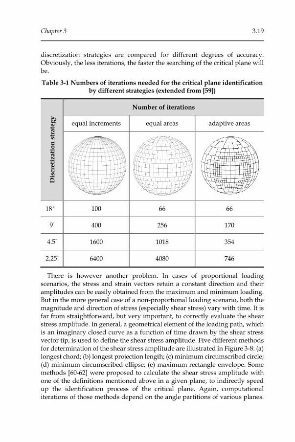
Chapter 3 3.19
discretization strategies are compared for different degrees of accuracy. Obviously, the less iterations, the faster the searching of the critical plane will be.
Table 3-1 Numbers of iterations needed for the critical plane identification by different strategies (extended from [59])
Dis
cre
tiz
ati
on
str
ate
gy
Number of iterations
equal increments equal areas adaptive areas
18° 100 66 66
9° 400 256 170
4.5° 1600 1018 354
2.25° 6400 4080 746
There is however another problem. In cases of proportional loading scenarios, the stress and strain vectors retain a constant direction and their amplitudes can be easily obtained from the maximum and minimum loading. But in the more general case of a non-proportional loading scenario, both the magnitude and direction of stress (especially shear stress) vary with time. It is far from straightforward, but very important, to correctly evaluate the shear stress amplitude. In general, a geometrical element of the loading path, which is an imaginary closed curve as a function of time drawn by the shear stress vector tip, is used to define the shear stress amplitude. Five different methods for determination of the shear stress amplitude are illustrated in Figure 3-8: (a) longest chord; (b) longest projection length; (c) minimum circumscribed circle; (d) minimum circumscribed ellipse; (e) maximum rectangle envelope. Some methods [60-62] were proposed to calculate the shear stress amplitude with one of the definitions mentioned above in a given plane, to indirectly speed up the identification process of the critical plane. Again, computational iterations of those methods depend on the angle partitions of various planes.

3.20 Fatigue Crack Initiation Modelling
Essentially, these methods do not change much the existing high computational cost issue.
A modern numerical algorithm from an optimization point of view was proposed in [63]. The gradient ascent method was used to find the global maxima of the variance matrix of the shear stress in terms of controlling angles and time. However, since the first derivatives of variables are required during the iterative process to reach convergence, the load history needs to be continuously differentiable. Additionally, the derivatives make the algorithm more computational challenging, either numerically or analytically.
Figure 3-8 Methods of defining mean value and amplitude of shear stress
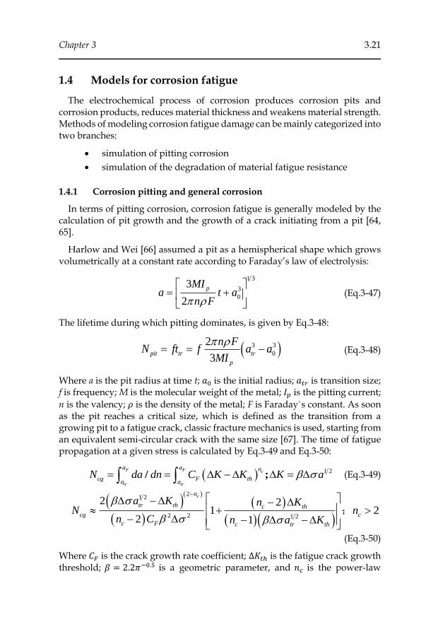
Chapter 3 3.21
1.4 Models for corrosion fatigue
The electrochemical process of corrosion produces corrosion pits and corrosion products, reduces material thickness and weakens material strength. Methods of modeling corrosion fatigue damage can be mainly categorized into two branches:
• simulation of pitting corrosion
• simulation of the degradation of material fatigue resistance
1.4.1 Corrosion pitting and general corrosion
In terms of pitting corrosion, corrosion fatigue is generally modeled by the calculation of pit growth and the growth of a crack initiating from a pit [64, 65].
Harlow and Wei [66] assumed a pit as a hemispherical shape which grows volumetrically at a constant rate according to Faraday’s law of electrolysis:
1 3
3
0
3
2
pMI
a t an F
= +
(Eq.3-47)
The lifetime during which pitting dominates, is given by Eq.3-48:
( )3 3
0
2
3pit tr tr
p
n FN ft f a a
MI
= = − (Eq.3-48)
Where a is the pit radius at time t; 𝑎0 is the initial radius; 𝑎𝑡𝑟 is transition size; f is frequency; M is the molecular weight of the metal; 𝐼𝑝 is the pitting current;
n is the valency; 𝜌 is the density of the metal; F is Faraday`s constant. As soon as the pit reaches a critical size, which is defined as the transition from a growing pit to a fatigue crack, classic fracture mechanics is used, starting from an equivalent semi-circular crack with the same size [67]. The time of fatigue propagation at a given stress is calculated by Eq.3-49 and Eq.3-50:
( ) 1 2/ ;
F F c
tr tr
a a n
cg F tha a
N da dn C K K K a = = − = (Eq.3-49)
( )( )
( )( )
( )( )
21 2
2 2 1 2
2 21 2
2 1
cn
tr th c th
cg c
c F c tr th
a K n KN n
n C n a K
− − − +
− − −
;
(Eq.3-50)
Where 𝐶𝐹 is the crack growth rate coefficient; ∆𝐾𝑡ℎ is the fatigue crack growth threshold; 𝛽 = 2.2𝜋−0.5 is a geometric parameter, and 𝑛𝑐 is the power-law
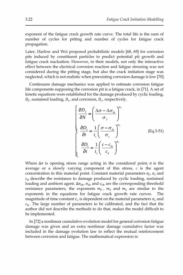
3.22 Fatigue Crack Initiation Modelling
exponent of the fatigue crack growth rate curve. The total life is the sum of number of cycles for pitting and number of cycles for fatigue crack propagation.
Later, Harlow and Wei proposed probabilistic models [68, 69] for corrosion pits induced by constituent particles to predict potential pit growth and fatigue crack nucleation. However, in their models, not only the interactive effect between the electrical corrosion reaction and fatigue stressing was not considered during the pitting stage, but also the crack initiation stage was neglected, which is not realistic when preexisting corrosion damage is low [70].
Continuum damage mechanics was applied to estimate corrosion fatigue life components supposing the corrosion pit is a fatigue crack, in [71]. A set of kinetic equations were established for the damage produced by cyclic loading, 𝐷𝑓, sustained loading, 𝐷𝑠, and corrosion, 𝐷𝑐, respectively.
1
1
f
s
c
m
f th
f
m
s th
c s
m
c th
c d
D
N
D
t t
D c c
t t c
− =
−
=
− =
(Eq.3-51)
Where ∆𝜎 is opening stress range acting in the considered point, σ is the average or a slowly varying component of this stress, c is the agent concentration in this material point. Constant material parameters 𝜎𝑓, 𝜎𝑠 and
𝑐𝑑 describe the resistance to damage produced by cyclic loading, sustained loading and ambient agent. ∆𝜎𝑡ℎ, 𝜎𝑡ℎ and 𝑐𝑡ℎ are the corresponding threshold resistance parameters, the exponents 𝑚𝑓 , 𝑚𝑠 and 𝑚𝑐 are similar to the
exponents in the equations for fatigue crack growth rate curves. The magnitude of time constant 𝑡𝑐 is dependent on the material parameters 𝜎𝑠 and 𝑐𝑑 . The large number of parameters to be calibrated, and the fact that the author did not describe the methods to do that, makes the model difficult to be implemented.
In [72] a nonlinear cumulative evolution model for general corrosion fatigue damage was given and an extra nonlinear damage cumulative factor was included in the damage evolution law to reflect the mutual reinforcement between corrosion and fatigue. The mathematical expression is:
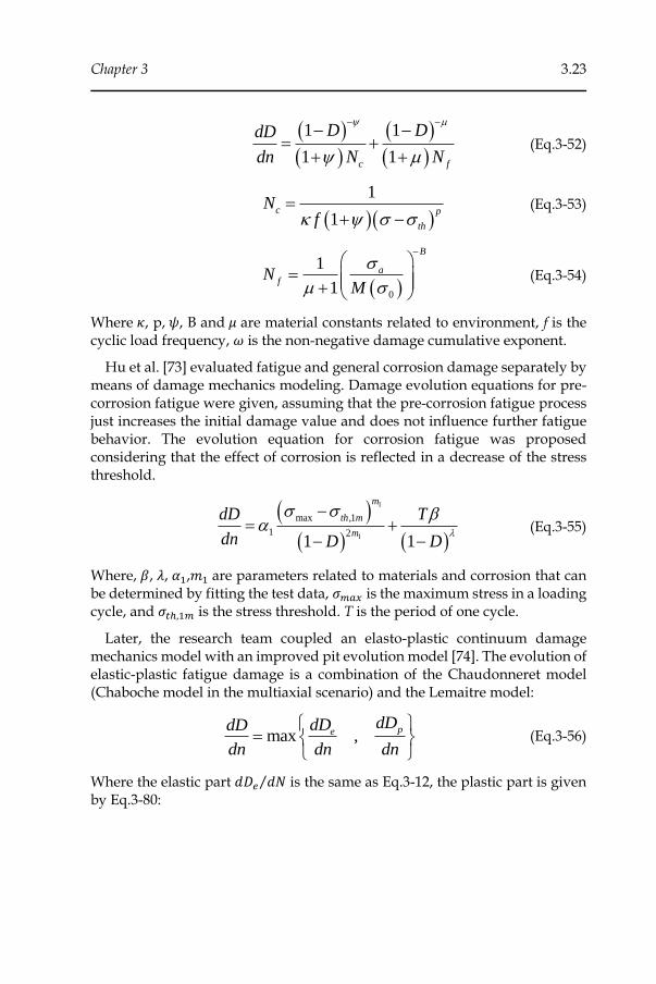
Chapter 3 3.23
( )
( )
( )
( )
1 1
1 1c f
D DdD
dn N N
− −− −
= ++ +
(Eq.3-52)
( )( )
1
1c p
th
Nf
=+ −
(Eq.3-53)
( )0
1
1
B
afN
M
−
= +
(Eq.3-54)
Where 𝜅, p, 𝜓, B and 𝜇 are material constants related to environment, f is the cyclic load frequency, 𝜔 is the non-negative damage cumulative exponent.
Hu et al. [73] evaluated fatigue and general corrosion damage separately by means of damage mechanics modeling. Damage evolution equations for pre-corrosion fatigue were given, assuming that the pre-corrosion fatigue process just increases the initial damage value and does not influence further fatigue behavior. The evolution equation for corrosion fatigue was proposed considering that the effect of corrosion is reflected in a decrease of the stress threshold.
( )( ) ( )
1
1
max ,1
1 21 1
m
th m
m
dD T
dn D D
−= +
− − (Eq.3-55)
Where, 𝛽, 𝜆, 𝛼1,𝑚1 are parameters related to materials and corrosion that can be determined by fitting the test data, 𝜎𝑚𝑎𝑥 is the maximum stress in a loading cycle, and 𝜎𝑡ℎ,1𝑚 is the stress threshold. T is the period of one cycle.
Later, the research team coupled an elasto-plastic continuum damage mechanics model with an improved pit evolution model [74]. The evolution of elastic-plastic fatigue damage is a combination of the Chaudonneret model (Chaboche model in the multiaxial scenario) and the Lemaitre model:
max ,pe
dDdDdD
dn dn dn
=
(Eq.3-56)
Where the elastic part 𝑑𝐷𝑒 𝑑𝑁⁄ is the same as Eq.3-12, the plastic part is given by Eq.3-80:
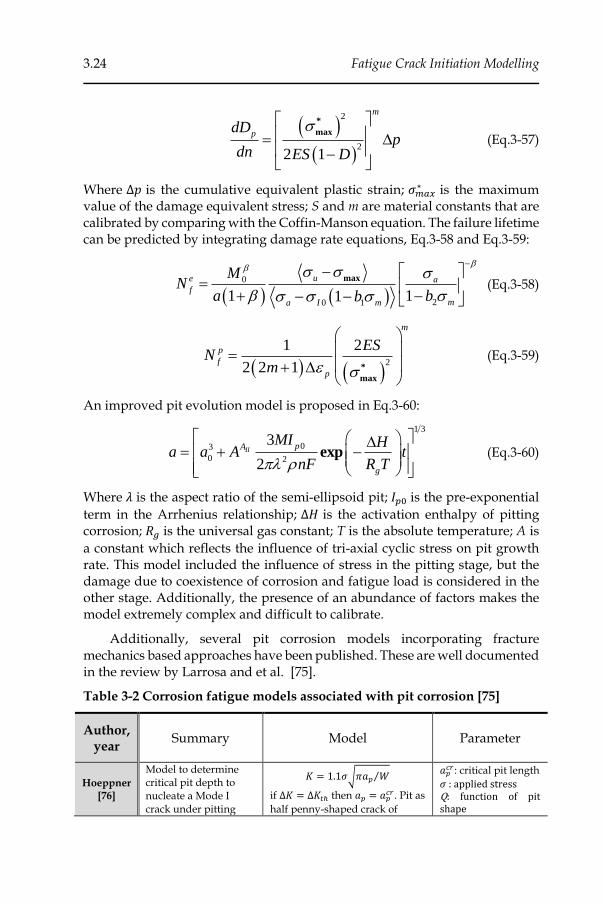
3.24 Fatigue Crack Initiation Modelling
( )( )
2
22 1
*
max
m
pdD
pdn ES D
= −
(Eq.3-57)
Where ∆𝑝 is the cumulative equivalent plastic strain; 𝜎𝑚𝑎𝑥∗ is the maximum
value of the damage equivalent stress; S and m are material constants that are calibrated by comparing with the Coffin-Manson equation. The failure lifetime can be predicted by integrating damage rate equations, Eq.3-58 and Eq.3-59:
( ) ( )0
20 11 11
maxue af
ma I m
MN
a bb
−
− =
+ −− − (Eq.3-58)
( ) ( )
2
1 2
2 2 1 *
max
m
p
f
p
ESN
m
= +
(Eq.3-59)
An improved pit evolution model is proposed in Eq.3-60:
1 3
03
0 2
3
2expII
pA
g
MI Ha a A t
nF R T
= + −
(Eq.3-60)
Where 𝜆 is the aspect ratio of the semi-ellipsoid pit; 𝐼𝑝0 is the pre-exponential
term in the Arrhenius relationship; Δ𝐻 is the activation enthalpy of pitting corrosion; 𝑅𝑔 is the universal gas constant; T is the absolute temperature; A is
a constant which reflects the influence of tri-axial cyclic stress on pit growth rate. This model included the influence of stress in the pitting stage, but the damage due to coexistence of corrosion and fatigue load is considered in the other stage. Additionally, the presence of an abundance of factors makes the model extremely complex and difficult to calibrate.
Additionally, several pit corrosion models incorporating fracture mechanics based approaches have been published. These are well documented in the review by Larrosa and et al. [75].
Table 3-2 Corrosion fatigue models associated with pit corrosion [75]
Author, year
Summary Model Parameter
Hoeppner [76]
Model to determine critical pit depth to nucleate a Mode I crack under pitting
𝐾 = 1.1𝜎√𝜋𝑎𝑝 𝑊⁄
if ∆𝐾 = ∆𝐾𝑡ℎ then 𝑎𝑝 = 𝑎𝑝𝑐𝑟. Pit as
half penny-shaped crack of
𝑎𝑝𝑐𝑟: critical pit length
𝜎 : applied stress Q: function of pit shape
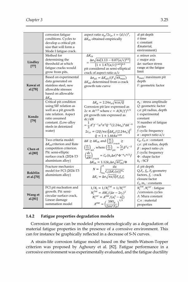
Chapter 3 3.25
corrosion fatigue conditions. Cycles to develop a critical pit size that will form a Mode I fatigue crack.
aspect ratio 𝑎𝑝 2𝑐𝑝⁄ , 𝑡 = (𝑑 𝑐⁄ )3,
∆𝐾𝑡ℎ obtained empirically
d: pit depth t: time c: constant f(material, environment)
Lindley [77]
Method for determining the threshold at which fatigue cracks would grow from pits.
∆𝐾𝑡ℎ
=∆𝜎√𝜋𝑎[1.13 − 0.07(𝑎 𝑐⁄ )0.5]
[1 + 1.47(𝑎 𝑐⁄ )1.65]0.5
pit considered as semi-elliptical crack of aspect ratio 𝑎 𝑐⁄
a: minor axis c: major axis Δ𝜎: surface stress range at the fatigue limit
Kawai et al.[78]
Based on experimental data generated on stainless steel, new allowable stresses based on allowable ∆𝐾𝑡ℎ
∆𝜎𝑎𝑙𝑙 = ∆𝐾𝑎𝑙𝑙/(𝐹√𝜋ℎ𝑚𝑎𝑥)
∆𝐾𝑎𝑙𝑙 determined from a crack growth rate curve
ℎ𝑚𝑎𝑥: maximum pit depth F: geometric factor
Kondo [79]
Critical pit condition using SIF relation as well as a pit growth rate relation. Aspect ratio assumed constant. (Low-alloy steels in deionized water)
∆𝐾𝑝 = 2.24𝜎𝑎√𝜋𝑐𝛼/𝑄
Corrosion pit law expressed as
2𝑐 ∝ 𝐴𝑡1/3 where 𝑐 = 𝐴(𝑁/𝑓)1/3 pit growth rate expressed as 𝑑𝑐 𝑑𝑁⁄
=1
3𝐴3𝑓−1𝛼2𝜋2𝑄−2(2.24𝜎𝑎)4∆𝐾−4
2𝑐𝑐𝑟 = (2𝑄/𝜋𝛼)[∆𝐾𝑝/(2.24𝜎𝑎)]2
𝑄 = 1 + 1.464𝛼1.65
𝜎𝑎 : stress amplitude Q: geometric factor c,a: pit radius, depth i: experimental constant N number of fatigue cycles f: cyclic frequency 𝛼 : aspect ratio a/c
Chen et al.[80]
Two criteria model: ∆𝐾𝑡ℎcriterion and Rate competition criterion. Pit: semi-elliptic surface crack (2024-T3 aluminium alloy)
∆𝐾 ≥ ∆𝐾𝑡ℎ and (𝑑𝑐
𝑑𝑁)
𝑐𝑟𝑎𝑐𝑘≥
(𝑑𝑐
𝑑𝑁)
𝑝𝑖𝑡, where (
𝑑𝑐
𝑑𝑁)
𝑝𝑖𝑡=
𝐶𝑝
2𝜋𝛽2𝑐−2
(𝑑𝑐
𝑑𝑁)
𝑐𝑟𝑎𝑐𝑘= 𝐶𝐹(𝑘𝑡∆𝜎)𝑛Φ−𝑛𝑐𝑛/2𝑓
Δ𝐾𝑡ℎ = 1.12𝑘𝑡Δ𝜎√𝜋𝐶𝑡ℎ/Φ
𝐶𝑝, 𝐶𝐹,n : constant
c,a : pit radius, depth 𝛽 : aspect ratio c/a f: cyclic frequency Φ : shape factor 𝑘𝑡 : SCF
Rokblin et al.[70]
Fracture mechanics model for FCI (2024-T3 aluminium alloy)
𝑁 = ∫𝑑𝑎
𝐶1[Δ𝐾𝐼(𝑎)]𝑚1
𝑑
𝑎𝑡ℎ
Δ𝐾1 = Δ𝜎√𝜋𝑎/𝑄𝐹𝑐𝑓𝑏𝑓𝑐
d: pit depth Q,𝐹𝑐, 𝑓𝑏, 𝐹𝑠:geometry factors, 𝑓𝑐 : crack closure factor 𝐶1, 𝑚1 : constants
Wang et al.[81]
FCI pit nucleation and growth. Pit: semi-circular surface crack, Linear damage summation model
1 𝑁𝑖⁄ = 1 𝑁𝑖𝑓𝑎𝑡⁄ + 1 𝑁𝑖
𝑐𝑜𝑟⁄
𝑁𝑖𝑓𝑎𝑡
= 𝐴𝑊𝑠/(Δ𝜏 − 2𝜏𝑓)2
𝑁𝑖𝑐𝑜𝑟 = 𝐴𝐻𝑊/(𝑎𝑖
3 − 𝑎03)
𝐴𝐻𝑊 = (3𝑀𝐼𝑝
2𝜋𝑛𝑒𝐹𝜌)
1/3
𝑁𝑖𝑓𝑎𝑡
, 𝑁𝑖𝑐𝑜𝑟 : fatigue
/corrosion cycles A: Mura constant C,n : material properties
1.4.2 Fatigue properties degradation models
Corrosion fatigue can be modeled phenomenologically as a degradation of material fatigue properties in the presence of a corrosive environment. This can for instance be graphically reflected in a decrease of S-N curves.
A strain-life corrosion fatigue model based on the Smith-Watson-Topper criterion was proposed by Aghoury et al. [82]. Fatigue performance in a corrosive environment was experimentally evaluated, and the fatigue ductility
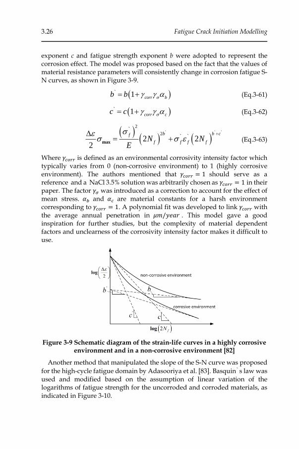
3.26 Fatigue Crack Initiation Modelling
exponent c and fatigue strength exponent b were adopted to represent the corrosion effect. The model was proposed based on the fact that the values of material resistance parameters will consistently change in corrosion fatigue S-N curves, as shown in Figure 3-9.
( )1`
corr bb b = + (Eq.3-61)
( )1`
corr cc c = + (Eq.3-62)
( )( ) ( )
2
2
2 22
` ` ``
` `
max
b b cf
f f f fN N
E
+= + (Eq.3-63)
Where 𝛾𝑐𝑜𝑟𝑟 is defined as an environmental corrosivity intensity factor which typically varies from 0 (non-corrosive environment) to 1 (highly corrosive environment). The authors mentioned that 𝛾𝑐𝑜𝑟𝑟 = 1 should serve as a reference and a NaCl 3.5% solution was arbitrarily chosen as 𝛾𝑐𝑜𝑟𝑟 = 1 in their paper. The factor 𝛾𝜎 was introduced as a correction to account for the effect of mean stress. 𝛼𝑏 and 𝛼𝑐 are material constants for a harsh environment corresponding to 𝛾𝑐𝑜𝑟𝑟 = 1. A polynomial fit was developed to link 𝛾𝑐𝑜𝑟𝑟 with the average annual penetration in 𝜇𝑚/𝑦𝑒𝑎𝑟 . This model gave a good inspiration for further studies, but the complexity of material dependent factors and unclearness of the corrosivity intensity factor makes it difficult to use.
Figure 3-9 Schematic diagram of the strain-life curves in a highly corrosive environment and in a non-corrosive environment [82]
Another method that manipulated the slope of the S-N curve was proposed
for the high-cycle fatigue domain by Adasooriya et al. [83]. Basquin`s law was used and modified based on the assumption of linear variation of the logarithms of fatigue strength for the uncorroded and corroded materials, as indicated in Figure 3-10.
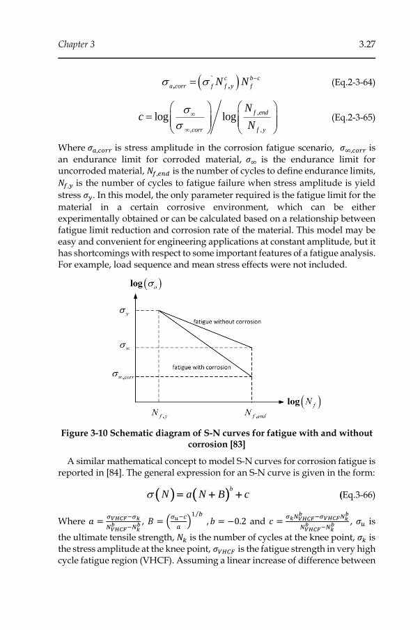
Chapter 3 3.27
( )`
, ,
c b c
a corr f f y fN N −= (Eq.2-3-64)
,
, ,
log logf end
corr f y
Nc
N
=
(Eq.2-3-65)
Where 𝜎𝑎,𝑐𝑜𝑟𝑟 is stress amplitude in the corrosion fatigue scenario, 𝜎∞,𝑐𝑜𝑟𝑟 is an endurance limit for corroded material, 𝜎∞ is the endurance limit for uncorroded material, 𝑁𝑓,𝑒𝑛𝑑 is the number of cycles to define endurance limits,
𝑁𝑓,𝑦 is the number of cycles to fatigue failure when stress amplitude is yield
stress 𝜎𝑦. In this model, the only parameter required is the fatigue limit for the
material in a certain corrosive environment, which can be either experimentally obtained or can be calculated based on a relationship between fatigue limit reduction and corrosion rate of the material. This model may be easy and convenient for engineering applications at constant amplitude, but it has shortcomings with respect to some important features of a fatigue analysis. For example, load sequence and mean stress effects were not included.
Figure 3-10 Schematic diagram of S-N curves for fatigue with and without corrosion [83]
A similar mathematical concept to model S-N curves for corrosion fatigue is reported in [84]. The general expression for an S-N curve is given in the form:
( ) ( )b
N a N B c = + + (Eq.3-66)
Where 𝑎 =𝜎𝑉𝐻𝐶𝐹−𝜎𝑘
𝑁𝑉𝐻𝐶𝐹𝑏 −𝑁𝑘
𝑏 , 𝐵 = (𝜎𝑢−𝑐
𝑎)
1 𝑏⁄
, 𝑏 = −0.2 and 𝑐 =𝜎𝑘𝑁𝑉𝐻𝐶𝐹
𝑏 −𝜎𝑉𝐻𝐶𝐹𝑁𝑘𝑏
𝑁𝑉𝐻𝐶𝐹𝑏 −𝑁𝑘
𝑏 , 𝜎𝑢 is
the ultimate tensile strength, 𝑁𝑘 is the number of cycles at the knee point, 𝜎𝑘 is the stress amplitude at the knee point, 𝜎𝑉𝐻𝐶𝐹 is the fatigue strength in very high cycle fatigue region (VHCF). Assuming a linear increase of difference between
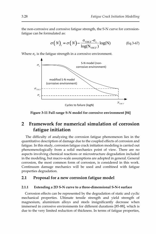
3.28 Fatigue Crack Initiation Modelling
the non-corrosive and corrosive fatigue strength, the S-N curve for corrosion-fatigue can be formulated as:
( ) ( ) VHCF cσ -σ
log(N)log(N )c
VHCF
N N = − (Eq.3-67)
Where 𝜎𝑐 is the fatigue strength in a corrosive environment.
Figure 3-11 Full range S-N model for corrosive environment [84]
2 Framework for numerical simulation of corrosion fatigue initiation
The difficulty of analyzing the corrosion fatigue phenomenon lies in the quantitative description of damage due to the coupled effects of corrosion and fatigue. In this study, corrosion fatigue crack initiation modeling is carried out phenomenologically from a solid mechanics point of view. There are no aspects involving chemical reactions or microstructure degradation included in the modeling, but macro-scale assumptions are adopted in general. General corrosion, the most common form of corrosion, is considered in this work. Continuum damage mechanics will be used and combined with fatigue properties degradation.
2.1 Proposal for a new corrosion fatigue model
2.1.1 Extending a 2D S-N curve to a three-dimensional S-N-t surface
Corrosion effects can be represented by the degradation of static and cyclic mechanical properties. Ultimate tensile strength and yield strength of magnesium, aluminium alloys and steels insignificantly decrease when immersed in corrosive environments for different durations [85-88], which is due to the very limited reduction of thickness. In terms of fatigue properties,
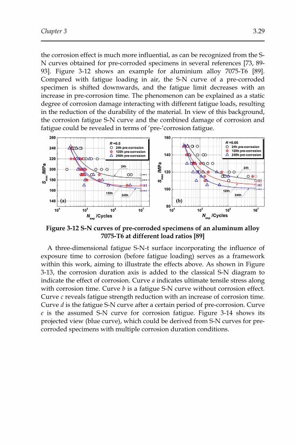
Chapter 3 3.29
the corrosion effect is much more influential, as can be recognized from the S-N curves obtained for pre-corroded specimens in several references [73, 89-93]. Figure 3-12 shows an example for aluminium alloy 7075-T6 [89]. Compared with fatigue loading in air, the S-N curve of a pre-corroded specimen is shifted downwards, and the fatigue limit decreases with an increase in pre-corrosion time. The phenomenon can be explained as a static degree of corrosion damage interacting with different fatigue loads, resulting in the reduction of the durability of the material. In view of this background, the corrosion fatigue S-N curve and the combined damage of corrosion and fatigue could be revealed in terms of ‘pre-‘corrosion fatigue.
Figure 3-12 S-N curves of pre-corroded specimens of an aluminum alloy 7075-T6 at different load ratios [89]
A three-dimensional fatigue S-N-t surface incorporating the influence of exposure time to corrosion (before fatigue loading) serves as a framework within this work, aiming to illustrate the effects above. As shown in Figure 3-13, the corrosion duration axis is added to the classical S-N diagram to indicate the effect of corrosion. Curve a indicates ultimate tensile stress along with corrosion time. Curve b is a fatigue S-N curve without corrosion effect. Curve c reveals fatigue strength reduction with an increase of corrosion time. Curve d is the fatigue S-N curve after a certain period of pre-corrosion. Curve e is the assumed S-N curve for corrosion fatigue. Figure 3-14 shows its projected view (blue curve), which could be derived from S-N curves for pre-corroded specimens with multiple corrosion duration conditions.
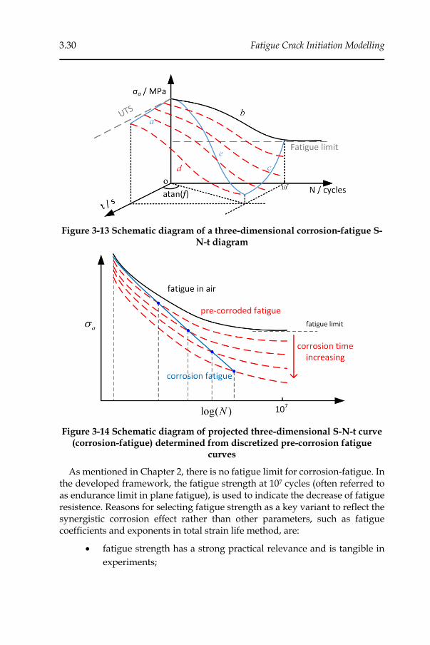
3.30 Fatigue Crack Initiation Modelling
Figure 3-13 Schematic diagram of a three-dimensional corrosion-fatigue S-N-t diagram
Figure 3-14 Schematic diagram of projected three-dimensional S-N-t curve (corrosion-fatigue) determined from discretized pre-corrosion fatigue
curves
As mentioned in Chapter 2, there is no fatigue limit for corrosion-fatigue. In the developed framework, the fatigue strength at 107 cycles (often referred to as endurance limit in plane fatigue), is used to indicate the decrease of fatigue resistence. Reasons for selecting fatigue strength as a key variant to reflect the synergistic corrosion effect rather than other parameters, such as fatigue coefficients and exponents in total strain life method, are:
• fatigue strength has a strong practical relevance and is tangible in
experiments;
Chapter 3 3.31
• fatigue strength can be directly and clearly related to corrosion
duration;
• fatigue strength is one single parameter.
2.1.2 Damage accumulation
The corrosion fatigue model proposed, is based on nonlinear continuum damage mechanics (CDM), which is suitable for modeling the evolution of combined damage from fatigue and corrosion. The basic idea of the corrosion fatigue crack initiation lifetime prediction is to accumulate the discretized coupled damage in every cycle until a failure criterion is reached.
The local failure of material (associated with crack initiation at a certain point) is often assumed to occur when the damage parameter D = 1. However, since CDM models mentioned above are typically calibrated on the basis of S-N curves which express the total lifetime of a specimen (including crack initiation and propagation), researchers have also assumed crack initiation to occur at a critical damage value 𝐷𝑐 smaller than 1. In such a case, 𝐷𝑐 is to be considered as an additional model parameter. For simplification, the 𝐷𝑐 value equals 1 in many studies; the same hypothesis is maintained in this study. Future extensions of the developed model could include a variable level of 𝐷𝑐.
It is assumed that, for a certain stress level, the combined damage generated after a number of corrosion fatigue cycles equals to the damage caused in the pre-corroded specimen at the same number of cycles. The damage accumulation process is visualized in Figure 3-15. The black curve is damage accumulation as a function of numbers of cycles for a non-corroded specimen. The red curves illustrate damage accumulation for fatigue in air after different fixed pre-corrosion times. Each scenario of pre-corrosion time has a different damage evolution trajectory. When corrosion time increases from t1 to t4, more damage from corrosion is introduced. Thus, the durability of the material is reduced, and the material will sustain less fatigue cycles to failure. Therefore, as indicated in Figure 3-15, those curves move to the left side of the graph. The blue curve is the damage accumulation for combined corrosion and fatigue. The damage is built up in each increment by a synergistic effect of corrosion and fatigue load. For example, assume that a specimen has been fatigue-loaded in a corrosive environment for 𝑛3 cycles (corresponding to time t3 and 𝑛3 = 𝑡3/𝑓 ). After a next increment, total number of cycles is equal to n4 and the damage will be characterized by the red dashed curve 𝑡4 (corresponding to 𝑛4 = 𝑡4/𝑓). The damage introduced between cycles 𝑡3 and 𝑡4 should be the difference between the two points on curve 𝑡3 and curve 𝑡4, namely ∆𝐷34
34.
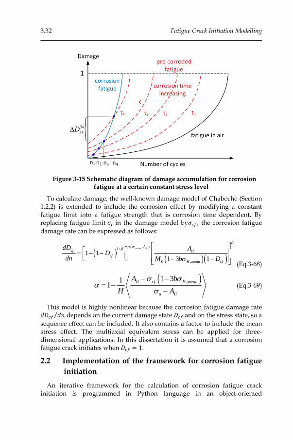
3.32 Fatigue Crack Initiation Modelling
Figure 3-15 Schematic diagram of damage accumulation for corrosion fatigue at a certain constant stress level
To calculate damage, the well-known damage model of Chaboche (Section 1.2.2) is extended to include the corrosion effect by modifying a constant fatigue limit into a fatigue strength that is corrosion time dependent. By replacing fatigue limit 𝜎𝑓 in the damage model by𝜎𝑐𝑓 , the corrosion fatigue
damage rate can be expressed as follows:
( )( )
( )( )1
0
1 11 3 1
,
,
mean IIAcf II
cf
H mean cf
dD AD
dn M b D
+ = − − − − (Eq.3-68)
( )1 311
II cf H mean
u II
A b
H A
− −= −
−
, (Eq.3-69)
This model is highly nonlinear because the corrosion fatigue damage rate 𝑑𝐷𝑐𝑓 𝑑𝑛⁄ depends on the current damage state 𝐷𝑐𝑓 and on the stress state, so a
sequence effect can be included. It also contains a factor to include the mean stress effect. The multiaxial equivalent stress can be applied for three-dimensional applications. In this dissertation it is assumed that a corrosion fatigue crack initiates when 𝐷𝑐𝑓 = 1.
2.2 Implementation of the framework for corrosion fatigue
initiation
An iterative framework for the calculation of corrosion fatigue crack initiation is programmed in Python language in an object-oriented

Chapter 3 3.33
programming (OOP) paradigm. The advantage of Python is that it allows for communication with the interface of ABAQUS® (v6.14-5 used for this work), including the definition of simulation input and extraction of results output. Moreover, the modularity of the OOP framework allows that the framework could be easily extended in the future with additional fatigue damage criteria whilst keeping the main body unchanged.
The framework consists of a pre-processing module, an analysis module, and a post-processing module. These modules are developed to control all commands during the simulation process in respect of different functionalities. The pre-processing module contains several functions to import the geometric model of the structure, to define the material properties and sections, to create boundary conditions and external loads, and to submit and monitor calculation jobs. The post-processing module contains functions to extract stress and strain tensors, and functions to calculate the damage parameter according to the model proposed in the previous section. The framework is iteratively executed for all elements in a selected region of interest (which can be the entire model, or a user-defined region). Figure 3-16 demonstrates the corrosion fatigue simulation framework.
Figure 3-16 Flowchart of the framework of corrosion fatigue initiation life prediction
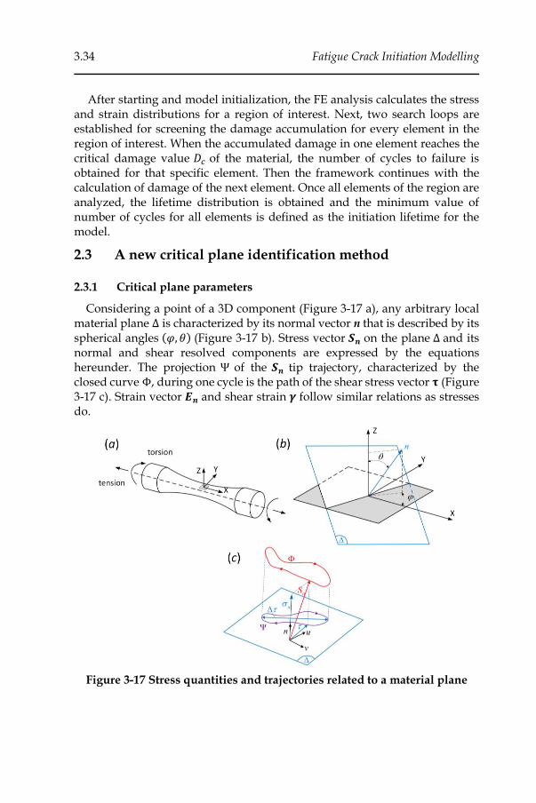
3.34 Fatigue Crack Initiation Modelling
After starting and model initialization, the FE analysis calculates the stress and strain distributions for a region of interest. Next, two search loops are established for screening the damage accumulation for every element in the region of interest. When the accumulated damage in one element reaches the critical damage value 𝐷𝑐 of the material, the number of cycles to failure is obtained for that specific element. Then the framework continues with the calculation of damage of the next element. Once all elements of the region are analyzed, the lifetime distribution is obtained and the minimum value of number of cycles for all elements is defined as the initiation lifetime for the model.
2.3 A new critical plane identification method
2.3.1 Critical plane parameters
Considering a point of a 3D component (Figure 3-17 a), any arbitrary local material plane ∆ is characterized by its normal vector n that is described by its spherical angles (𝜑, 𝜃) (Figure 3-17 b). Stress vector 𝑺𝒏 on the plane ∆ and its normal and shear resolved components are expressed by the equations hereunder. The projection Ψ of the 𝑺𝒏 tip trajectory, characterized by the closed curve Φ, during one cycle is the path of the shear stress vector 𝛕 (Figure 3-17 c). Strain vector 𝑬𝒏 and shear strain 𝜸 follow similar relations as stresses do.
Figure 3-17 Stress quantities and trajectories related to a material plane
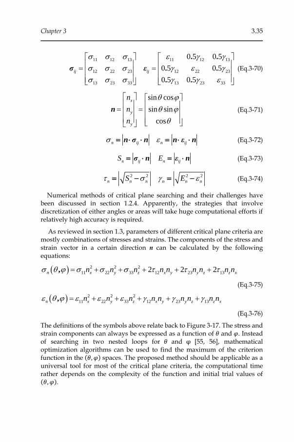
Chapter 3 3.35
11 12 13 11 12 13
12 22 23 12 22 23
13 23 33 13 23 33
0 5 0 5
0 5 0 5
0 5 0 5
σ εij ij
= =
. .
. .
. .
(Eq.3-70)
sin cos
sin sin
cos
x
y
y
n
n
n
= =
n (Eq.3-71)
n σ n n ε nn ij n ij
= = (Eq.3-72)
σ n ε nn ij n ij
S E= = (Eq.3-73)
2 2 2 2
n n n n n nS E = − = − (Eq.3-74)
Numerical methods of critical plane searching and their challenges have been discussed in section 1.2.4. Apparently, the strategies that involve discretization of either angles or areas will take huge computational efforts if relatively high accuracy is required.
As reviewed in section 1.3, parameters of different critical plane criteria are mostly combinations of stresses and strains. The components of the stress and strain vector in a certain direction n can be calculated by the following equations:
( ) 2 2 2
11 22 33 12 23 132 2 2,
n x y z x y y z z xn n n n n n n n n = + + + + +
(Eq.3-75)
( ) 2 2 2
11 22 33 12 23 13n x y z x y y z z xn n n n n n n n n = + + + + +,
(Eq.3-76)
The definitions of the symbols above relate back to Figure 3-17. The stress and strain components can always be expressed as a function of 𝜃 and 𝜑. Instead of searching in two nested loops for 𝜃 and φ [55, 56], mathematical optimization algorithms can be used to find the maximum of the criterion function in the (𝜃, 𝜑) spaces. The proposed method should be applicable as a universal tool for most of the critical plane criteria, the computational time rather depends on the complexity of the function and initial trial values of (𝜃, 𝜑).

3.36 Fatigue Crack Initiation Modelling
2.3.2 Nelder-Mead simplex method
A classic Nelder-Mead simplex algorithm has been implemented for the first time for the identification of critical plane orientations. The method was proposed for unconstrained nonlinear optimization of functions within a multi-dimensional space by performing an iterative search in a heuristic manner [94]. The main advantage of the method is that no derivatives are required, its weakness is that it is not very efficient for problems with more than about 10 variables [95].
The method is an iterative process, as illustrated in Figure 3-18. Parameter combinations, (𝜃, 𝜑) pairs in this work, are grouped into simplices. A simplex is a shape with (n+1) vertices for a n-dimensional space objective function (triangles in a two-dimensional parameter space). Within a simplex, the Nelder-Mead algorithm replaces the parameter combination yielding the worst solution by a new and better one, thus forming a new simplex. This process is repeated until the minimum or a user-defined convergence criterion is reached. By doing so, subsequent simplices ‘move towards’ the solution within the parameter space. The algorithm starts with initializing a first simplex. Then its vertices, which represent results from the objective function, are ordered from the best (lowest function value) to the worst. The remaining part is to adjust the parameter values of the worst point by performing simplex operations so that the simplex moves towards the function minimum. The simplex operations are shown in Figure 3-19 for the n=2 case, they are:
• reflection,
• expansion,
• contraction (outside and inside), and
• shrinkage.
Notably, this algorithm does not guarantee finding the global optimum of the entire parameter space, but rather leads to a local optimum. Finding the global optimum can be promoted by running the algorithm multiple times, starting from different initial simplices.
As mentioned above, the iterative procedure stops when a convergence criterion is met. The criterion used in this work is that the maximum distance between the current best point and other points in the simplex is not more than a pre-defined tolerance 휀:
( )2 1
i besti n
max x x +
− (Eq.3-77)

Chapter 3 3.37
Figure 3-18 Flowchart of the Nelder-Mead simplex algorithm
Figure 3-19 Operations on the simplex in Nelder-Mead algorithm for n=2
Figure 3-20 gives a visual example of the Nelder-Mead searching trajectory for a conical surface function (n=2). Red arrows indicate the searching process.
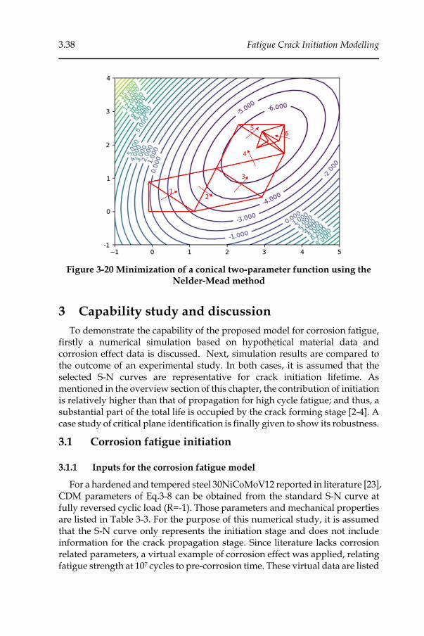
3.38 Fatigue Crack Initiation Modelling
Figure 3-20 Minimization of a conical two-parameter function using the Nelder-Mead method
3 Capability study and discussion
To demonstrate the capability of the proposed model for corrosion fatigue, firstly a numerical simulation based on hypothetical material data and corrosion effect data is discussed. Next, simulation results are compared to the outcome of an experimental study. In both cases, it is assumed that the selected S-N curves are representative for crack initiation lifetime. As mentioned in the overview section of this chapter, the contribution of initiation is relatively higher than that of propagation for high cycle fatigue; and thus, a substantial part of the total life is occupied by the crack forming stage [2-4]. A case study of critical plane identification is finally given to show its robustness.
3.1 Corrosion fatigue initiation
3.1.1 Inputs for the corrosion fatigue model
For a hardened and tempered steel 30NiCoMoV12 reported in literature [23], CDM parameters of Eq.3-8 can be obtained from the standard S-N curve at fully reversed cyclic load (R=-1). Those parameters and mechanical properties are listed in Table 3-3. For the purpose of this numerical study, it is assumed that the S-N curve only represents the initiation stage and does not include information for the crack propagation stage. Since literature lacks corrosion related parameters, a virtual example of corrosion effect was applied, relating fatigue strength at 107 cycles to pre-corrosion time. These virtual data are listed
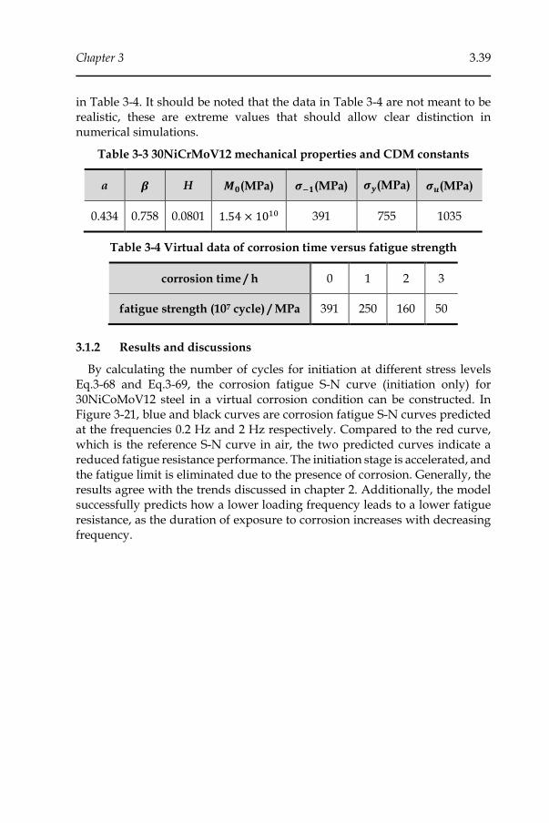
Chapter 3 3.39
in Table 3-4. It should be noted that the data in Table 3-4 are not meant to be realistic, these are extreme values that should allow clear distinction in numerical simulations.
Table 3-3 30NiCrMoV12 mechanical properties and CDM constants
a 𝜷 H 𝑴𝟎(MPa) 𝝈−𝟏(MPa) 𝝈𝒚(MPa) 𝝈𝒖(MPa)
0.434 0.758 0.0801 1.54 × 10¹⁰ 391 755 1035
Table 3-4 Virtual data of corrosion time versus fatigue strength
corrosion time / h 0 1 2 3
fatigue strength (107 cycle) / MPa 391 250 160 50
3.1.2 Results and discussions
By calculating the number of cycles for initiation at different stress levels Eq.3-68 and Eq.3-69, the corrosion fatigue S-N curve (initiation only) for 30NiCoMoV12 steel in a virtual corrosion condition can be constructed. In Figure 3-21, blue and black curves are corrosion fatigue S-N curves predicted at the frequencies 0.2 Hz and 2 Hz respectively. Compared to the red curve, which is the reference S-N curve in air, the two predicted curves indicate a reduced fatigue resistance performance. The initiation stage is accelerated, and the fatigue limit is eliminated due to the presence of corrosion. Generally, the results agree with the trends discussed in chapter 2. Additionally, the model successfully predicts how a lower loading frequency leads to a lower fatigue resistance, as the duration of exposure to corrosion increases with decreasing frequency.
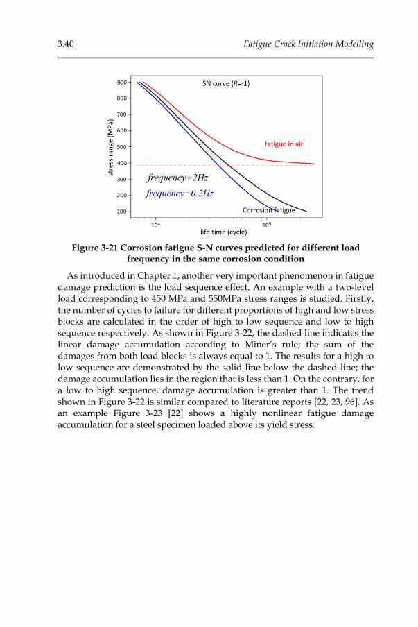
3.40 Fatigue Crack Initiation Modelling
Figure 3-21 Corrosion fatigue S-N curves predicted for different load frequency in the same corrosion condition
As introduced in Chapter 1, another very important phenomenon in fatigue damage prediction is the load sequence effect. An example with a two-level load corresponding to 450 MPa and 550MPa stress ranges is studied. Firstly, the number of cycles to failure for different proportions of high and low stress blocks are calculated in the order of high to low sequence and low to high sequence respectively. As shown in Figure 3-22, the dashed line indicates the linear damage accumulation according to Miner’s rule; the sum of the damages from both load blocks is always equal to 1. The results for a high to low sequence are demonstrated by the solid line below the dashed line; the damage accumulation lies in the region that is less than 1. On the contrary, for a low to high sequence, damage accumulation is greater than 1. The trend shown in Figure 3-22 is similar compared to literature reports [22, 23, 96]. As an example Figure 3-23 [22] shows a highly nonlinear fatigue damage accumulation for a steel specimen loaded above its yield stress.
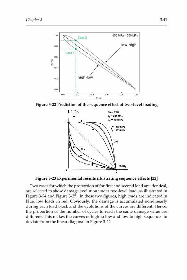
Chapter 3 3.41
Figure 3-22 Prediction of the sequence effect of two-level loading
Figure 3-23 Experimental results illustrating sequence effects [22]
Two cases for which the proportion of for first and second load are identical, are selected to show damage evolution under two-level load, as illustrated in Figure 3-24 and Figure 3-25. In these two figures, high loads are indicated in blue, low loads in red. Obviously, the damage is accumulated non-linearly during each load block and the evolutions of the curves are different. Hence, the proportion of the number of cycles to reach the same damage value are different. This makes the curves of high to low and low to high sequences to deviate from the linear diagonal in Figure 3-22.
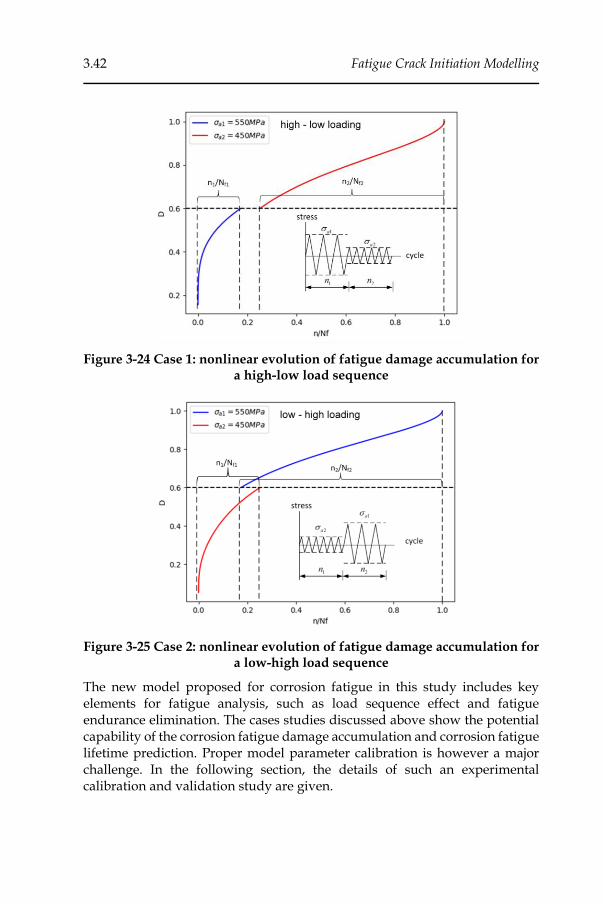
3.42 Fatigue Crack Initiation Modelling
Figure 3-24 Case 1: nonlinear evolution of fatigue damage accumulation for a high-low load sequence
Figure 3-25 Case 2: nonlinear evolution of fatigue damage accumulation for a low-high load sequence
The new model proposed for corrosion fatigue in this study includes key elements for fatigue analysis, such as load sequence effect and fatigue endurance elimination. The cases studies discussed above show the potential capability of the corrosion fatigue damage accumulation and corrosion fatigue lifetime prediction. Proper model parameter calibration is however a major challenge. In the following section, the details of such an experimental calibration and validation study are given.
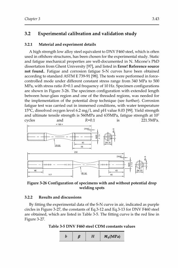
Chapter 3 3.43
3.2 Experimental calibration and validation study
3.2.1 Material and experiment details
A high strength low alloy steel equivalent to DNV F460 steel, which is often used in offshore structures, has been chosen for the experimental study. Static and fatigue mechanical properties are well-documented in N. Micone’s PhD dissertation from Ghent University [97], and listed in Error! Reference source
not found.. Fatigue and corrosion fatigue S-N curves have been obtained according to standard ASTM E 739-91 [98]. The tests were performed in force-controlled mode under different constant stress range from 340 MPa to 500 MPa, with stress ratio R=0.1 and frequency of 10 Hz. Specimen configurations are shown in Figure 3-26. The specimen configuration with extended length between hour-glass region and one of the threaded regions, was needed for the implementation of the potential drop technique (see further). Corrosion fatigue test was carried out in immersed conditions, with water temperature 15°C, dissolved oxygen level 6.2 mg/l, and pH value 8.03 [99]. Yield strength and ultimate tensile strength is 560MPa and 635MPa, fatigue strength at 107 cycles and R=0.1 is 221.5MPa.
Figure 3-26 Configuration of specimens with and without potential drop welding spots
3.2.2 Results and discussions
By fitting the experimental data of the S-N curve in air, indicated as purple circles in Figure 3-27, the constants of Eq.3-12 and Eq.3-13 for DNV F460 steel are obtained, which are listed in Table 3-5. The fitting curve is the red line in Figure 3-27.
Table 3-5 DNV F460 steel CDM constants values
b 𝜷 H 𝑴𝟎(MPa)
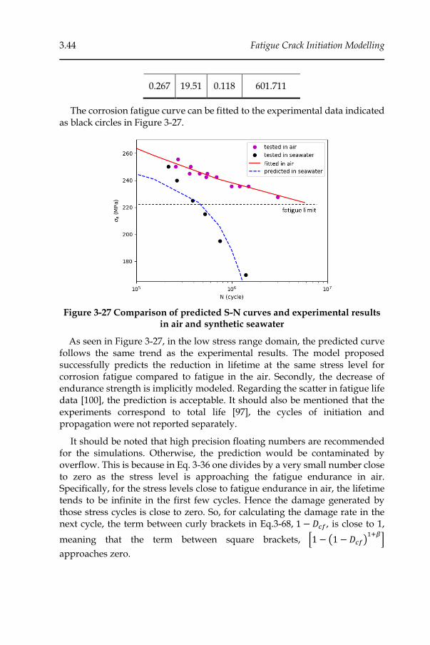
3.44 Fatigue Crack Initiation Modelling
0.267 19.51 0.118 601.711
The corrosion fatigue curve can be fitted to the experimental data indicated as black circles in Figure 3-27.
Figure 3-27 Comparison of predicted S-N curves and experimental results in air and synthetic seawater
As seen in Figure 3-27, in the low stress range domain, the predicted curve follows the same trend as the experimental results. The model proposed successfully predicts the reduction in lifetime at the same stress level for corrosion fatigue compared to fatigue in the air. Secondly, the decrease of endurance strength is implicitly modeled. Regarding the scatter in fatigue life data [100], the prediction is acceptable. It should also be mentioned that the experiments correspond to total life [97], the cycles of initiation and propagation were not reported separately.
It should be noted that high precision floating numbers are recommended for the simulations. Otherwise, the prediction would be contaminated by overflow. This is because in Eq. 3-36 one divides by a very small number close to zero as the stress level is approaching the fatigue endurance in air. Specifically, for the stress levels close to fatigue endurance in air, the lifetime tends to be infinite in the first few cycles. Hence the damage generated by those stress cycles is close to zero. So, for calculating the damage rate in the next cycle, the term between curly brackets in Eq.3-68, 1 − 𝐷𝑐𝑓, is close to 1,
meaning that the term between square brackets, [1 − (1 − 𝐷𝑐𝑓)1+𝛽
]
approaches zero.
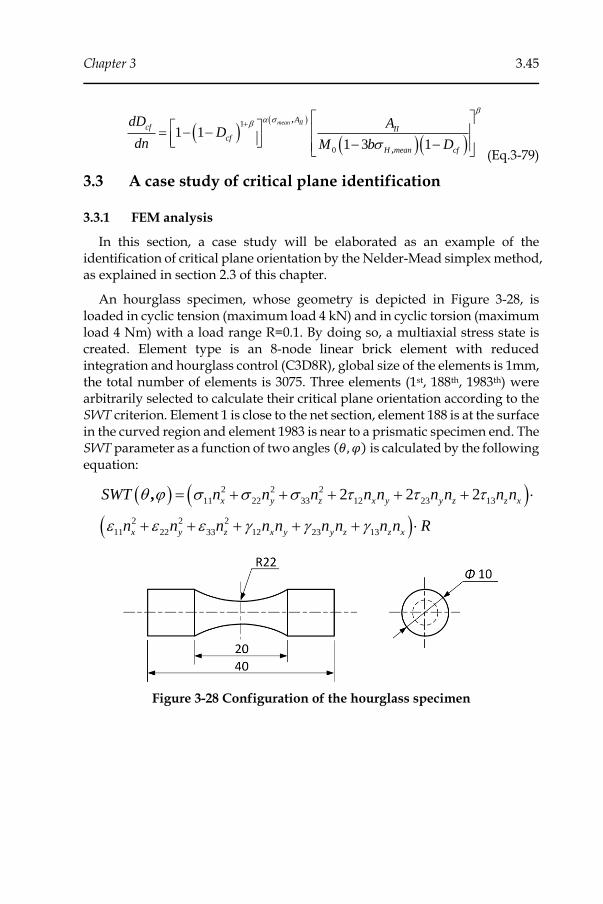
Chapter 3 3.45
( )( )
( )( )1
0
1 11 3 1
,
,
mean IIAcf II
cf
H mean cf
dD AD
dn M b D
+ = − − − − (Eq.3-79)
3.3 A case study of critical plane identification
3.3.1 FEM analysis
In this section, a case study will be elaborated as an example of the identification of critical plane orientation by the Nelder-Mead simplex method, as explained in section 2.3 of this chapter.
An hourglass specimen, whose geometry is depicted in Figure 3-28, is loaded in cyclic tension (maximum load 4 kN) and in cyclic torsion (maximum load 4 Nm) with a load range R=0.1. By doing so, a multiaxial stress state is created. Element type is an 8-node linear brick element with reduced integration and hourglass control (C3D8R), global size of the elements is 1mm, the total number of elements is 3075. Three elements (1st, 188th, 1983th) were arbitrarily selected to calculate their critical plane orientation according to the SWT criterion. Element 1 is close to the net section, element 188 is at the surface in the curved region and element 1983 is near to a prismatic specimen end. The SWT parameter as a function of two angles (𝜃, 𝜑) is calculated by the following equation:
( ) ( )
( )
2 2 2
11 22 33 12 23 13
2 2 2
11 22 33 12 23 13
2 2 2,x y z x y y z z x
x y z x y y z z x
SWT n n n n n n n n n
n n n n n n n n n R
= + + + + +
+ + + + +
Figure 3-28 Configuration of the hourglass specimen
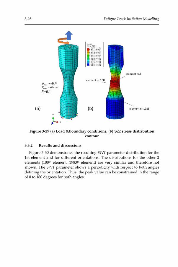
3.46 Fatigue Crack Initiation Modelling
Figure 3-29 (a) Load &boundary conditions, (b) S22 stress distribution contour
3.3.2 Results and discussions
Figure 3-30 demonstrates the resulting SWT parameter distribution for the 1st element and for different orientations. The distributions for the other 2 elements (188th element, 1983th element) are very similar and therefore not shown. The SWT parameter shows a periodicity with respect to both angles defining the orientation. Thus, the peak value can be constrained in the range of 0 to 180 degrees for both angles.
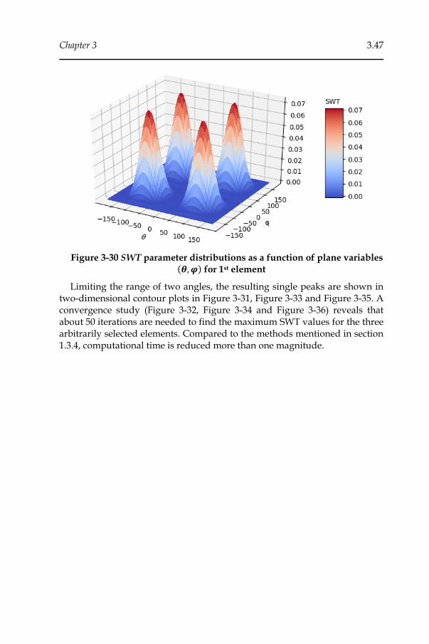
Chapter 3 3.47
Figure 3-30 SWT parameter distributions as a function of plane variables (𝜽, 𝝋) for 1st element
Limiting the range of two angles, the resulting single peaks are shown in two-dimensional contour plots in Figure 3-31, Figure 3-33 and Figure 3-35. A convergence study (Figure 3-32, Figure 3-34 and Figure 3-36) reveals that about 50 iterations are needed to find the maximum SWT values for the three arbitrarily selected elements. Compared to the methods mentioned in section 1.3.4, computational time is reduced more than one magnitude.
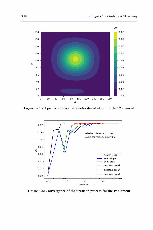
3.48 Fatigue Crack Initiation Modelling
Figure 3-31 2D projected SWT parameter distribution for the 1st element
Figure 3-32 Convergence of the iteration process for the 1st element

Chapter 3 3.49
Figure 3-33 2D projected SWT parameter distribution for the 188th element
Figure 3-34 Convergence of the iteration process for the 188th element
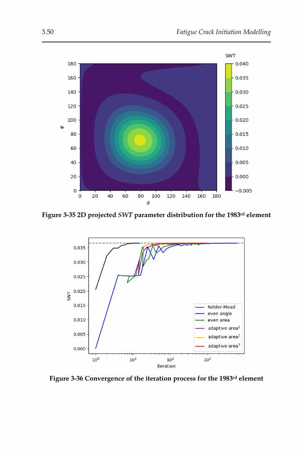
3.50 Fatigue Crack Initiation Modelling
Figure 3-35 2D projected SWT parameter distribution for the 1983rd element
Figure 3-36 Convergence of the iteration process for the 1983rd element

Chapter 3 3.51
Theoretically, the accuracy and efficiency of the Nelder-Mead algorithm depends on the selection of the initial simplex. To check the sensitivity of the convergence rate to this section, both regular triangles and random triangles have been implemented as an initial simplex. As regards the former, right angled triangles with legs of 45 ° have been considered in three different
locations and orientations. As regards the latter, three triangles are randomly generated by a uniform distribution over [0°,90°] for each vertex coordinate
component. A clear view of these initial simplexes is plotted in Figure 3-37. Information on the iteration convergence for different initial simplexes is listed in Table 3-6. The iterations needed to approach the maximum SWT value vary moderately. The searching results, which are the maximum values of the SWT parameter indicated in Table 3-6 are always the same, no matter what the choice of the initial simplex is. The reason for that can be explained by the periodical nature of the objective function. As a consequence, all local maxima are equal to the global maximum and this value is retrieved irrespective of the initial simplex. Since the majority of critical plane criteria can be expressed as a trigonometric function of angle (𝜃, 𝜑), it could be concluded that the Nelder-Mead algorithm is applicable for all of them. Robustness and accuracy are revealed from the results in Table 3-6.
For non-proportional multiaxial loading conditions, the stress state varies during one cycle. Therefore, time must be added as an additional parameter in the function of the critical plane parameter. In this case, the Nelder-Mead algorithm is still valid as it is a universal multi-variable optimization method. It is worth noting that this algorithm is even better for non-proportional loading due to its gradient-free nature, compared to gradient-based optimization algorithms. This is because external load can be discontinuous and indifferentiable at certain time instances. Even in the case of continuous variation of the stress tensors, the Nelder-Mead algorithm allows simple numerical implementation due to the absent need to calculate derivatives.

3.52 Fatigue Crack Initiation Modelling
Figure 3-37 Regular and random selection of initial simplexes
Table 3-6 Influence of initial simplex based on the 188th element data
Initial simplex Max SWT Iterations Function evaluations
regular #1 0.17396 50 97
regular #2 0.17396 49 95
regular #3 0.17396 47 93
random #1 0.17396 49 93
random #2 0.17396 49 92
random #3 0.17396 46 91
4 Summary and conclusions
This chapter firstly reviewed conventional simulation approaches for fatigue crack initiation in the categories of endurance strength approaches, cumulative continuum damage approaches and critical plane approaches. Models reported in literature for corrosion fatigue have been reviewed as well. Endurance strength approaches, either global or local ones, are the standardized and more widely used in the industrial applications. Cumulative
Chapter 3 3.53
continuum damage mechanics and critical plane methods are more common in an academic atmosphere. They provide a more in-depth analysis than endurance strength approaches, but at the cost of a higher complexity.
Based on a classic nonlinear continuum damage mechanics model, this study proposes an innovative corrosion fatigue model which includes the corrosion effect by a time-dependent degradation of the fatigue S-N curve.
An objective-oriented-programming framework for fatigue and corrosion fatigue analysis has been established to estimate lifetime and predict crack initiation location combined with the ABAQUS solver. Pre-processing and post-processing are executed automatically according to user-defined fatigue criteria. The frame is extendable by new damage criteria or new features without modifying the main structure.
The numerical simulation study shows that the model is capable to describe the corrosion effect and corrosion fatigue lifetime. It successfully describes an interaction between corrosion and fatigue and evolution of coupled fatigue-corrosion damage accumulation.
A classic gradient-free optimization algorithm has been implemented for the first time in the identification of orientation and the maximum value of critical plane criteria. The method is simple and robust, can be applied to various critical plane criteria. It significantly reduces the numerical computational cost for either proportional or non-proportional multiaxial fatigue loading conditions. The new critical plane searching methods has been developed as a starting point for a corrosion fatigue model based on critical plane criteria, which is suggested as future work.
For future research, topics of coupling pitting corrosion characteristics to a characterization of surface roughness and to lifetime prediction can be probed. Generally, the fatigue resistance is quite sensitive to surface conditions. Except in special cases where internal defects act as an initiation site, a fatigue crack always starts at the surface. The fatigue limit shows a great dependence on the surface state, which can be described by the surface finish parameter [101]. It can be expressed as a function of roughness condition (commonly represented by 𝑅𝑎) and a certain reference value, as shown in Eq.3-80:
( ),cf a f
f R = (Eq.3-80)
Plenty of studies concluded that high surface roughness significantly reduces fatigue resistance. A rough surface profile introduces small notches that elevate stress concentrations and result in crack initiation after a shorter time. Figure 3-38 is an example of fatigue performance for different values of surface roughness for an aluminium alloy.
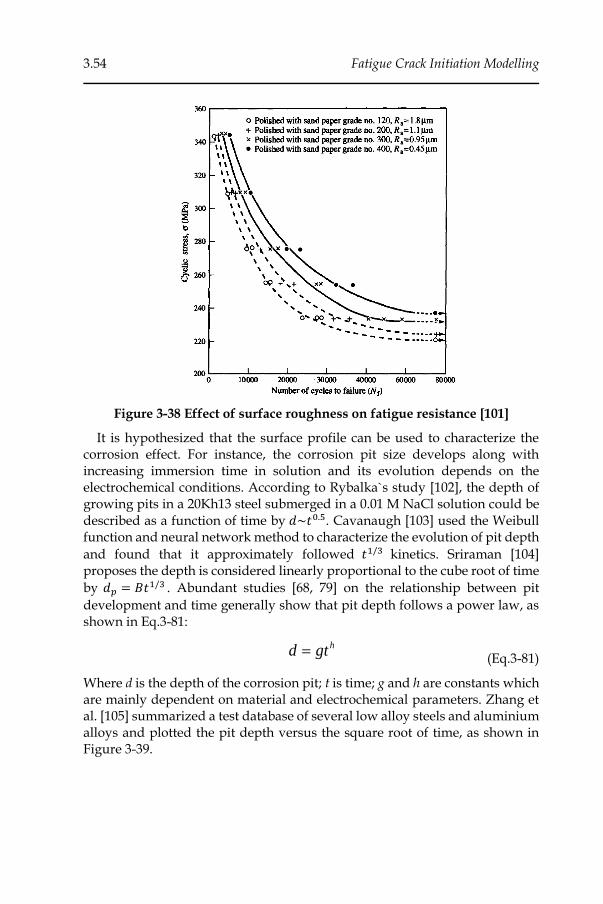
3.54 Fatigue Crack Initiation Modelling
Figure 3-38 Effect of surface roughness on fatigue resistance [101]
It is hypothesized that the surface profile can be used to characterize the corrosion effect. For instance, the corrosion pit size develops along with increasing immersion time in solution and its evolution depends on the electrochemical conditions. According to Rybalka`s study [102], the depth of growing pits in a 20Kh13 steel submerged in a 0.01 M NaCl solution could be described as a function of time by 𝑑~𝑡0.5. Cavanaugh [103] used the Weibull function and neural network method to characterize the evolution of pit depth
and found that it approximately followed 𝑡1/3 kinetics. Sriraman [104] proposes the depth is considered linearly proportional to the cube root of time
by 𝑑𝑝 = 𝐵𝑡1/3 . Abundant studies [68, 79] on the relationship between pit
development and time generally show that pit depth follows a power law, as shown in Eq.3-81:
hd gt= (Eq.3-81)
Where d is the depth of the corrosion pit; t is time; g and h are constants which are mainly dependent on material and electrochemical parameters. Zhang et al. [105] summarized a test database of several low alloy steels and aluminium alloys and plotted the pit depth versus the square root of time, as shown in Figure 3-39.
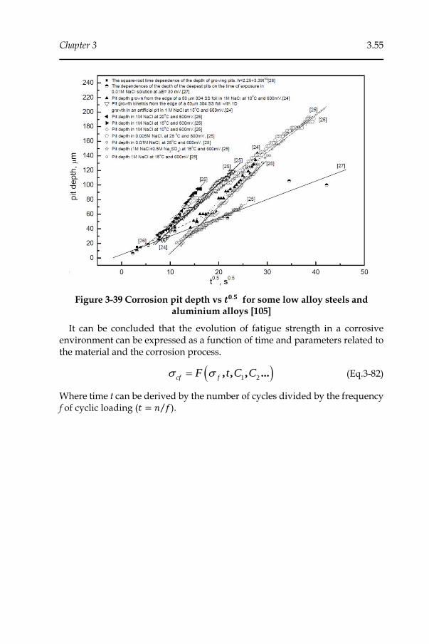
Chapter 3 3.55
Figure 3-39 Corrosion pit depth vs 𝒕𝟎.𝟓 for some low alloy steels and aluminium alloys [105]
It can be concluded that the evolution of fatigue strength in a corrosive environment can be expressed as a function of time and parameters related to the material and the corrosion process.
( )1 2cf fF t C C = , , , ... (Eq.3-82)
Where time t can be derived by the number of cycles divided by the frequency f of cyclic loading (𝑡 = 𝑛 𝑓⁄ ).
3.56 Fatigue Crack Initiation Modelling
References
1. Makkonen, M., Predicting the total fatigue life in metals. International Journal of Fatigue, 2009. 31(7): p. 1163-1175.
2. IBRAHIM, M.F.E. and K.J. MILLER, Determination Of Fatigue Crack Initiation Life. Fatigue & Fracture of Engineering Materials & Structures, 1979. 2(4): p. 351-360.
3. Tu, S.-T. and X.-C. Zhang, Fatigue crack initiation mechanisms. Reference Module in Materials Science and Materials Engineering, 2016: p. 1-23.
4. Provan, J.W. and Z.H. Zhai, Fatigue crack initiation and stage-I propagation in polycrystalline materials. I: Micromechanisms. International Journal of Fatigue, 1991. 13(2): p. 99-109.
5. Singh, A., An Experimental Investigation of Bending Fatigue Initiation and Propagation Lives. Journal of Mechanical Design, 2000. 123(3): p. 431-435.
6. Hachim, A., et al., Prediction and evolution of the fatigue crack initiation in S355 Steel by the probabilistic method. International Journal of Engineering and Science, 2012. Vol. 1(Issue 2): p. 16-21.
7. ASTM E466-15, Standard Practice for Conducting Force Controlled Constant Amplitude Axial Fatigue Tests of Metallic Materials. 2015, ASTM International, West Conshohocken, PA, 2015, www.astm.org.
8. Radaj, D., C.M. Sonsino, and W. Fricke, Fatigue assessment of welded joints by local approaches. 2006: Woodhead publishing.
9. Horn, A.M., et al. Proceedings of the 18th International Ship and Offshore Structures Congress-Committee III. 2 Fatigue and Fracture. in The 18th International Ship and Offshore Structures Congress. 2012.
10. Kondo, D., H. Welemane, and F. Cormery, Basic concepts and models in continuum damage mechanics. Revue européenne de génie civil, 2007. 11(7-8): p. 927-943.
11. Krajcinovic, D., Damage mechanics. Mechanics of Materials, 1989. 8(2–3): p. 117-197.
12. Kachanov, L.M., Rupture time under creep conditions. International journal of fracture, 1999. 97(1-4): p. 11-18.
13. Struik, L.C.E., Physical aging in amorphous polymers and other materials. 1977, TU Delft, Delft University of Technology.
Chapter 3 3.57
14. Lemaitre, J. and R. Desmorat, Engineering Damage Mechanics: Ductile, Creep, Fatigue and Brittle Failures. 2005: Springer.
15. Zhang, W. and Y. Cai, Continuum Damage Mechanics and Numerical Applications. 2010: Springer Berlin Heidelberg.
16. Grover, H.J., An observation concerning the cycle ratio in cumulative damage Symposium on Fatigue of Aircraft Structures ASTM STP 274, 1960: p. 120-124.
17. Rechart, F.E. and N.M. Newmark, A hypothesis for the determination of cumulative damage in fatigue. Proceedings of American Society for Testing and Materials, 1948. 48: p. 767-800.
18. Marco, S.M. and W.L. Starkey, A concept of fatigue damage. Transactions of the ASME, 1954. 76: p. 627-632.
19. Cheng, G. and A. Plumtree, A fatigue damage accumulation model based on continuum damage mechanics and ductility exhaustion. International Journal of Fatigue, 1998. 20(7): p. 495-501.
20. Chaboche, J., Lifetime predictions and cumulative damage under high-temperature conditions. Low-Cycle Fatigue and Life Prediction, ASTM STP, 1982. 770: p. 81-104.
21. Fatemi, A. and L. Yang, Cumulative fatigue damage and life prediction theories: a survey of the state of the art for homogeneous materials. International Journal of Fatigue, 1998. 20(1): p. 9-34.
22. Chaboche, J.L. and P.M. Lesne, A NON-LINEAR CONTINUOUS FATIGUE DAMAGE MODEL. Fatigue & Fracture of Engineering Materials & Structures, 1988. 11(1): p. 1-17.
23. Dattoma, V., et al., Fatigue life prediction under variable loading based on a new non-linear continuum damage mechanics model. International Journal of Fatigue, 2006. 28(2): p. 89-95.
24. Chaudonneret, M., A Simple and Efficient Multiaxial Fatigue Damage Model for Engineering Applications of Macro-Crack Initiation. Journal of Engineering Materials and Technology, 1993. 115(4): p. 373-379.
25. Bhattacharya, B. and B. Ellingwood, Continuum damage mechanics analysis of fatigue crack initiation. International Journal of Fatigue, 1998. 20(9): p. 631-639.
26. Lemaitre, J., How to use damage mechanics. Nuclear Engineering and Design, 1984. 80(2): p. 233-245.
3.58 Fatigue Crack Initiation Modelling
27. Lemaitre, J., Formulation and identification of damage kinetic constitutive equations, in Continuum Damage Mechanics Theory and Application. 1987, Springer. p. 37-89.
28. Chaboche, J.L., Continuum Damage Mechanics: Part I—General Concepts. Journal of Applied Mechanics, 1988. 55(1): p. 59-64.
29. Chaboche, J.L., Continuum Damage Mechanics: Part II—Damage Growth, Crack Initiation, and Crack Growth. Journal of Applied Mechanics, 1988. 55(1): p. 65-72.
30. Krajcinovic, D. and J. Lemaître, Continuum Damage Mechanics: Theory and Applications. 1987: Springer-Verlag Kg.
31. Subhasis, S., et al., Study of Load Sequence Effects in Combined Cyclic Fatigue Using CDM Approach, in 53rd AIAA/ASME/ASCE/AHS/ASC Structures, Structural Dynamics and Materials Conference. 2012, American Institute of Aeronautics and Astronautics.
32. Wang, M., Q. Fei, and P. Zhang, A Modified Fatigue Damage Model for High-Cycle Fatigue Life Prediction. Advances in Materials Science and Engineering, 2016. 2016: p. 7.
33. Xiao, Y.C., S. Li, and Z. Gao, A continuum damage mechanics model for high cycle fatigue. International Journal of Fatigue, 1998. 20(7): p. 503-508.
34. Fatemi, A. and N. Shamsaei, Multiaxial fatigue: An overview and some approximation models for life estimation. International Journal of Fatigue, 2011. 33(8): p. 948-958.
35. Findley, W.N., A theory for the effect of mean stress on fatigue of metals under combined torsion and axial load or bending. 1958: Engineering Materials Research Laboratory, Division of Engineering, Brown University.
36. Karolczuk, A. and E. Macha, Selection of the critical plane orientation in two-parameter multiaxial fatigue failure criterion under combined bending and torsion. Engineering Fracture Mechanics, 2008. 75(3–4): p. 389-403.
37. Bhatti, N.A. and M.A. Wahab, Fretting fatigue crack nucleation: A review. Tribology International, 2018.
38. Alfredsson, B. and M. Olsson, Applying multiaxial fatigue criteria to standing contact fatigue. International Journal of Fatigue, 2001. 23(6): p. 533-548.
Chapter 3 3.59
39. Park, J. and D. Nelson, Evaluation of an energy-based approach and a critical plane approach for predicting constant amplitude multiaxial fatigue life. International Journal of Fatigue, 2000. 22(1): p. 23-39.
40. McDiarmid, D.L., A GENERAL CRITERION FOR HIGH CYCLE MULTIAXIAL FATIGUE FAILURE. Fatigue & Fracture of Engineering Materials & Structures, 1991. 14(4): p. 429-453.
41. Lykins, C.D., S. Mall, and V. Jain, A shear stress-based parameter for fretting fatigue crack initiation. Fatigue & Fracture of Engineering Materials & Structures, 2001. 24(7): p. 461-473.
42. Brown, M.W. and K. Miller, A theory for fatigue failure under multiaxial stress-strain conditions. Proceedings of the Institution of Mechanical Engineers, 1973. 187(1): p. 745-755.
43. Wang, C. and M. Brown, A path‐independent parameter for fatigue under
proportional and non ‐ proportional loading. Fatigue & fracture of engineering materials & structures, 1993. 16(12): p. 1285-1297.
44. Socie, D. and G. Marquis, Multiaxial Fatigue. 2000: Society of Automotive Engineers.
45. Fatemi, A. and D.F. Socie, A Critical Plane Approach To Multiaxial Fatigue Damage Including Out-Of-Phase Loading. Fatigue & Fracture of Engineering Materials & Structures, 1988. 11(3): p. 149-165.
46. Shamsaei, N., A. Fatemi, and D.F. Socie, Multiaxial cyclic deformation and non-proportional hardening employing discriminating load paths. International Journal of Plasticity, 2010. 26(12): p. 1680-1701.
47. Shamsaei, N., A. Fatemi, and D.F. Socie, Multiaxial fatigue evaluation using discriminating strain paths. International Journal of Fatigue, 2011. 33(4): p. 597-609.
48. Shamsaei, N., et al., Multiaxial fatigue of titanium including step loading and load path alteration and sequence effects. International Journal of Fatigue, 2010. 32(11): p. 1862-1874.
49. SMITH, K.N., T.H. Topper, and P. Watson, A Stress-strain Function for the Fatigue of Metals. 1969: Defense Technical Information Center.
50. Bannantine, J.A. and D. Socie. A variable amplitude multiaxial fatigue life prediction methods. in ICBMFF3. 2013.
51. Stephens, R.I., P.M. Dindinger, and J.E. Gunger, Fatigue damage editing for accelerated durability testing using strain range and SWT parameter criteria. International Journal of Fatigue, 1997. 19(8): p. 599-606.

3.60 Fatigue Crack Initiation Modelling
52. Rolović, R. and S.M. Tipton, An energy based critical plane approach to multiaxial fatigue analysis, in Fatigue and Fracture Mechanics: 29th Volume. 1999, ASTM International.
53. Rolovic, R. and S.M. Tipton, Multiaxial Cyclic Ratcheting in Coiled Tubing—Part I: Theoretical Modeling. Journal of Engineering Materials and Technology, 1999. 122(2): p. 157-161.
54. Liu, K., A method based on virtual strain-energy parameters for multiaxial fatigue life prediction, in Advances in multiaxial fatigue. 1993, ASTM International.
55. Li, X., Z. Zuo, and W. Qin, A fretting related damage parameter for fretting fatigue life prediction. International Journal of Fatigue, 2015. 73: p. 110-118.
56. Sum, W.S., E.J. Williams, and S.B. Leen, Finite element, critical-plane, fatigue life prediction of simple and complex contact configurations. International Journal of Fatigue, 2005. 27(4): p. 403-416.
57. Iftikhar, S.H. and J. Albinmousa, A method for assessing critical plane-based multiaxial fatigue damage models. Fatigue & Fracture of Engineering Materials & Structures, 2018. 41(1): p. 235-245.
58. Weber, B., et al., Improvements of multiaxial fatigue criteria computation for a strong reduction of calculation duration. Computational Materials Science, 1999. 15(4): p. 381-399.
59. Wentingmann, M., P. Noever-Castelos, and C. Balzani. An adaptive algorithm to accelerate the critical plane identification for multiaxial fatigue criteria. in Proceedings of 6th European Conference on Computational Mechanics (ECCM 6)/7th European Conference on Computational Fluid Dynamics (ECFD 7). 2018.
60. Papadopoulos, I., Critical Plane Approaches In High-Cycle Fatigue: On The Definition Of The Amplitude And Mean Value Of The Shear Stress Acting On The Critical Plane. Fatigue & Fracture of Engineering Materials & Structures, 1998. 21(3): p. 269-285.
61. Araújo, J.A., et al., On the characterization of the critical plane with a simple and fast alternative measure of the shear stress amplitude in multiaxial fatigue. International Journal of Fatigue, 2011. 33(8): p. 1092-1100.
62. Scalet, G., An efficient algorithm for the solution of min-max problems in multiaxial fatigue. International Journal of Fatigue, 2018. 112: p. 117-129.
Chapter 3 3.61
63. Susmel, L., A simple and efficient numerical algorithm to determine the orientation of the critical plane in multiaxial fatigue problems. International Journal of Fatigue, 2010. 32(11): p. 1875-1883.
64. Hoeppner, D., V. Chandrasekaran, and A. Taylor, Review of pitting corrosion fatigue models. International Committee on Aeronautical Fatigue, 1999.
65. Wei, R.P., Corrosion/corrosion fatigue and life-cycle management. Journal of the Society of Materials Science, Japan, 2001. 50(9Appendix): p. 147-156.
66. Zaman, K.B.M.Q. and R.P. Wei, Probability approach for prediction of corrosion and corrosion fatigue life. AIAA Journal, 1994. 32(10): p. 2073-2079.
67. Dolley, E., B. Lee, and R. Wei, The effect of pitting corrosion on fatigue life. Fatigue & Fracture of Engineering Materials & Structures, 2000. 23(7): p. 555-560.
68. Harlow, D.G. and R.P. Wei, A probability model for the growth of corrosion pits in aluminum alloys induced by constituent particles. Engineering Fracture Mechanics, 1998. 59(3): p. 305-325.
69. Harlow, D.G. and R.P. Wei, Probability modeling and material microstructure applied to corrosion and fatigue of aluminum and steel alloys. Engineering Fracture Mechanics, 2009. 76(5): p. 695-708.
70. Rokhlin, S.I., et al., Effect of pitting corrosion on fatigue crack initiation and fatigue life. Engineering Fracture Mechanics, 1999. 62(4): p. 425-444.
71. Bolotin, V.V. and A.A. Shipkov, Mechanical aspects of corrosion fatigue and stress corrosion cracking. International Journal of Solids and Structures, 2001. 38(40–41): p. 7297-7318.
72. Han, Z.-y., et al., A nonlinear cumulative evolution model for corrosion fatigue damage. Journal of Zhejiang University SCIENCE A, 2014. 15(6): p. 447-453.
73. Hu, W., et al., Corrosion–Fatigue Life Prediction for 2024-T62 Aluminum Alloy Using Damage Mechanics-Based Approach. International Journal of Damage Mechanics, 2012. 21(8): p. 1245-1266.
74. Hu, P., et al., A continuum damage mechanics approach coupled with an improved pit evolution model for the corrosion fatigue of aluminum alloy. Corrosion Science, 2016. 113: p. 78-90.
3.62 Fatigue Crack Initiation Modelling
75. Larrosa, N.O., R. Akid, and R.A. Ainsworth, Corrosion-fatigue: a review of damage tolerance models. International Materials Reviews, 2017. 63(5): p. 283-308.
76. Hoeppner, D., Model for prediction of fatigue lives based upon a pitting corrosion fatigue process, in Fatigue Mechanisms. 1979, ASTM International.
77. Lindley, T., P. McIntyre, and P. Trant, Fatigue-crack initiation at corrosion pits. Metals technology, 1982. 9(1): p. 135-142.
78. Kawai, S. and K. Kasai, Considerations of allowable stress of corrosion fatigue (focused on the influence of pitting). Fatigue & Fracture of Engineering Materials & Structures, 1985. 8(2): p. 115-127.
79. Kondo, Y., Prediction of Fatigue Crack Initiation Life Based on Pit Growth. CORROSION, 1989. 45(1): p. 7-11.
80. Chen, G., et al., Corrosion and Corrosion Fatigue of Airframe Aluminum Alloys. 1994.
81. Wang, Q., R. Pidaparti, and M. Palakal, Comparative study of corrosion-fatigue in aircraft materials. AIAA journal, 2001. 39(2): p. 325-330.
82. Aghoury, I.M.E. and K. Galal, Corrosion-Fatigue Strain-Life Model for Steel Bridge Girders under Various Weathering Conditions. Journal of Structural Engineering, 2014. 140(6): p. 04014026.
83. Adasooriya, N., T. Hemmingsen, and D. Pavlou. Fatigue strength degradation of metals in corrosive environments. in IOP Conference Series: Materials Science and Engineering. 2017. IOP Publishing.
84. Bandara, C., U. Dissanayake, and P. Dissanayake, Novel method for developing SN curves for corrosion fatigue damage assessment of steel structures. 2015.
85. Fu, S., et al., Deterioration of mechanical properties for pre-corroded AZ31 sheet in simulated physiological environment. Materials Science and Engineering: A, 2014. 593: p. 153-162.
86. Obert, B., et al., An investigation of the reduction in tensile strength and fatigue life of pre-corroded 7075-T6 aluminum alloy. Journal of Materials Engineering and Performance, 2000. 9(4): p. 441-448.
87. Hou, Y., et al., Experimental investigation on corrosion effect on mechanical properties of buried metal pipes. International Journal of Corrosion, 2016. 2016.
Chapter 3 3.63
88. Chen, X., et al., Uniaxial low cycle fatigue behavior for pre-corroded 16MND5 bainitic steel in simulated pressurized water reactor environment. Journal of Nuclear Materials, 2018. 504: p. 267-276.
89. Huang, Y., et al., Equivalent crack size model for pre-corrosion fatigue life prediction of aluminum alloy 7075-T6. International Journal of Fatigue, 2016. 88: p. 217-226.
90. Abdulstaar, M., M. Mhaede, and L. Wagner, Pre-Corrosion and Surface Treatments Effects on the Fatigue Life of AA6082 T6. Advanced Engineering Materials, 2013. 15(10): p. 1002-1006.
91. Wang, Z.-b., W.-t. Liu, and X.-f. He, Research on Fatigue Curves for Pre-corroded Aircraft Structures. Chinese Journal of Aeronautics, 2004. 17(4): p. 220-223.
92. Liu, J., et al., Effect of pre-corrosion on fatigue life of high strength steel 38CrMoAl. Journal of Wuhan University of Technology-Mater. Sci. Ed., 2011. 26(4): p. 648-653.
93. Pérez-Mora, R., et al., Very high cycle fatigue of a high strength steel under sea water corrosion: A strong corrosion and mechanical damage coupling. International Journal of Fatigue, 2015. 74: p. 156-165.
94. Nelder, J.A. and R. Mead, A simplex method for function minimization. The computer journal, 1965. 7(4): p. 308-313.
95. Stanford_University. Introduction to Multidisciplinary Design Optimization. 2012; Available from: http://adl.stanford.edu/aa222/Home.html.
96. Peng, Z., et al., A new approach to the investigation of load interaction effects and its application in residual fatigue life prediction. International Journal of Damage Mechanics, 2016. 25(5): p. 672-690.
97. Micone, N., Development of Testing Methodologies for the Analysis of Variable Amplitude Fatigue and Corrosion-Fatigue of Offshore Steels. 2017, Ghent University.
98. ASTM, E739-91. Standard Practice for Statistical Analysis of Linear or Linearized Stress-Life, 2004.
99. Micone, N. and W. De Waele, Evaluation of Methodologies to Accelerate Corrosion Assisted Fatigue Experiments. Experimental Mechanics, 2017. 57(4): p. 547-557.
100. Schijve, J., The significance of fatigue crack initiation for predictions of the fatigue limit of specimens and structures. International Journal of Fatigue, 2014. 61: p. 39-45.

3.64 Fatigue Crack Initiation Modelling
101. Bayoumi, M.R. and A.K. Abdellatif, Effect of surface finish on fatigue strength. Engineering Fracture Mechanics, 1995. 51(5): p. 861-870.
102. Rybalka, K.V., et al., Development of pitting corrosion on 20Kh13 steel. Russian Journal of Electrochemistry, 2009. 45(11): p. 1217-1225.
103. Cavanaugh, M.K., R.G. Buchheit, and N. Birbilis, Modeling the environmental dependence of pit growth using neural network approaches. Corrosion Science, 2010. 52(9): p. 3070-3077.
104. Sriraman, M.R. and R.M. Pidaparti, Life Prediction of Aircraft Aluminum Subjected to Pitting Corrosion Under Fatigue Conditions. Journal of Aircraft, 2009. 46(4): p. 1253-1259.
105. Zhang, X.-Y., S.-X. Li, and R. Liang. Effect of corrosion pits on fatigue life and crack initiation. in ICF13. 2013.
Chapter 4
Fatigue Crack Propagation Modelling

4.2 Fatigue Crack Propagation Modelling
<< This page intentionally left blank >>
Chapter 4 4.3
1 Overview
For simulation of fatigue crack propagation, fracture mechanics based on the concept of stress intensity factor has been widely used with success. Compared to the conventional finite element method (FEM), the extended finite element method (XFEM) is gaining popularity. This chapter starts with a brief review of linear elastic fracture mechanics (LEFM), corrosion fatigue crack propagation simulation and the application of the extended finite element method for fatigue crack propagation analysis. Then, the development of an iterative framework for three-dimensional non-self-similar arbitary fatigue crack growth simulation is discussed in detail. Validations focus on three-dimensional arbitrary crack growth direction. Literature results for a bent center-cracked beam and own results for a modified compact tension specimen are used for the validation of the robustness of the framework developed. The results of a sensitivity study and conclusions are discussed at the end of this chapter.
1.1 Fatigue crack propagation analysis by linear elastic fracture mechanics
Fracture mechanics is the theoretical framework for the study of mechanical behaviour of cracked structures. The governing parameter in linear-elastic conditions is the stress intensity factor (SIF or K), which describes the stress increase to infinity when approaching a sharp crack tip. It is a function of external load, crack size and position as well as component geometry.
Generally, a fatigue crack propagation analysis based on fracture mechanics relates to material properties, loading parameters and crack configuration, as shown in Figure 4-1. Mathematical formulations are typically provided by means of a ”fatigue crack growth rate” equation as follows:
( )da
f K RdN
= , (Eq.4-1)
Where ∆𝐾 represents the SIF range ( 𝐾𝑚𝑎𝑥 − 𝐾𝑚𝑖𝑛 ) due to cyclic loading, 𝑑𝑎 𝑑𝑁⁄ is the crack growth rate, and 𝑅 = 𝐾𝑚𝑖𝑛 𝐾𝑚𝑎𝑥⁄ reflects the load ratio.
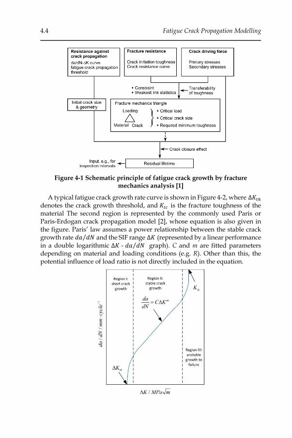
4.4 Fatigue Crack Propagation Modelling
Figure 4-1 Schematic principle of fatigue crack growth by fracture mechanics analysis [1]
A typical fatigue crack growth rate curve is shown in Figure 4-2, where ∆𝐾𝑡ℎ denotes the crack growth threshold, and 𝐾𝐼𝑐 is the fracture toughness of the material The second region is represented by the commonly used Paris or Paris-Erdogan crack propagation model [2], whose equation is also given in the figure. Paris’ law assumes a power relationship between the stable crack growth rate 𝑑𝑎 𝑑𝑁⁄ and the SIF range Δ𝐾 (represented by a linear performance in a double logarithmic ∆𝐾 - 𝑑𝑎 𝑑𝑁⁄ graph). C and m are fitted parameters depending on material and loading conditions (e.g. R). Other than this, the potential influence of load ratio is not directly included in the equation.
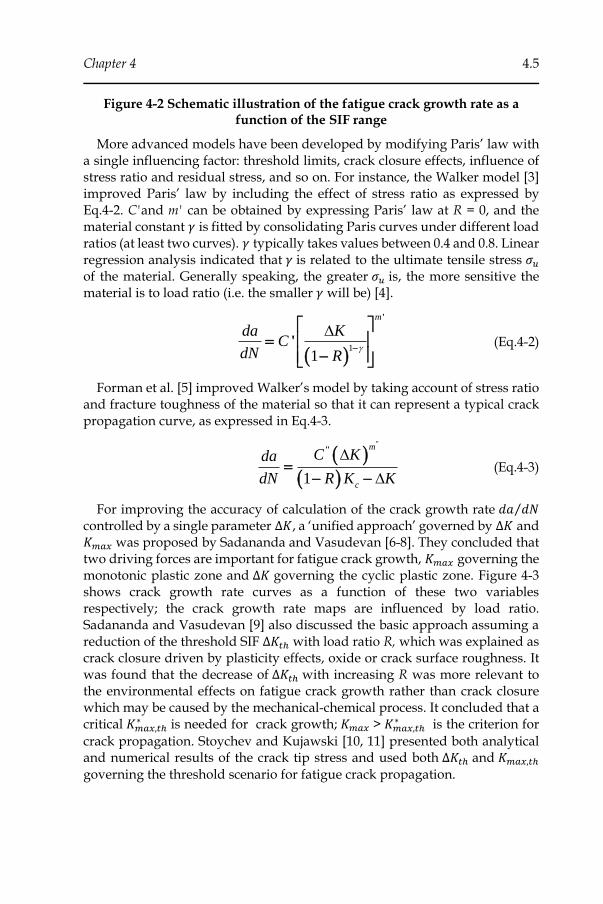
Chapter 4 4.5
Figure 4-2 Schematic illustration of the fatigue crack growth rate as a function of the SIF range
More advanced models have been developed by modifying Paris’ law with a single influencing factor: threshold limits, crack closure effects, influence of stress ratio and residual stress, and so on. For instance, the Walker model [3] improved Paris’ law by including the effect of stress ratio as expressed by Eq.4-2. C'and m' can be obtained by expressing Paris’ law at R = 0, and the material constant 𝛾 is fitted by consolidating Paris curves under different load ratios (at least two curves). 𝛾 typically takes values between 0.4 and 0.8. Linear regression analysis indicated that 𝛾 is related to the ultimate tensile stress 𝜎𝑢 of the material. Generally speaking, the greater 𝜎𝑢 is, the more sensitive the material is to load ratio (i.e. the smaller 𝛾 will be) [4].
( )1
1
m
da KC
dN R
'
'−
=
−
(Eq.4-2)
Forman et al. [5] improved Walker’s model by taking account of stress ratio and fracture toughness of the material so that it can represent a typical crack propagation curve, as expressed in Eq.4-3.
( )( )1
m
c
C Kda
dN R K K
""
=− −
(Eq.4-3)
For improving the accuracy of calculation of the crack growth rate 𝑑𝑎 𝑑𝑁⁄ controlled by a single parameter Δ𝐾, a ‘unified approach’ governed by Δ𝐾 and 𝐾𝑚𝑎𝑥 was proposed by Sadananda and Vasudevan [6-8]. They concluded that two driving forces are important for fatigue crack growth, 𝐾𝑚𝑎𝑥 governing the monotonic plastic zone and Δ𝐾 governing the cyclic plastic zone. Figure 4-3 shows crack growth rate curves as a function of these two variables respectively; the crack growth rate maps are influenced by load ratio. Sadananda and Vasudevan [9] also discussed the basic approach assuming a reduction of the threshold SIF Δ𝐾𝑡ℎ with load ratio R, which was explained as crack closure driven by plasticity effects, oxide or crack surface roughness. It was found that the decrease of Δ𝐾𝑡ℎ with increasing R was more relevant to the environmental effects on fatigue crack growth rather than crack closure which may be caused by the mechanical-chemical process. It concluded that a critical 𝐾𝑚𝑎𝑥,𝑡ℎ
∗ is needed for crack growth; 𝐾𝑚𝑎𝑥 > 𝐾𝑚𝑎𝑥,𝑡ℎ∗ is the criterion for
crack propagation. Stoychev and Kujawski [10, 11] presented both analytical and numerical results of the crack tip stress and used both Δ𝐾𝑡ℎ and 𝐾𝑚𝑎𝑥,𝑡ℎ governing the threshold scenario for fatigue crack propagation.
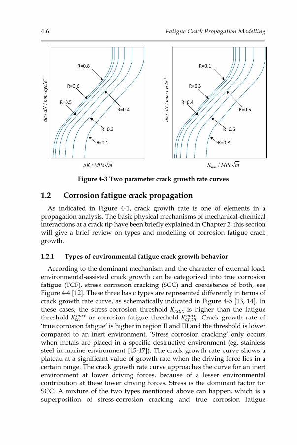
4.6 Fatigue Crack Propagation Modelling
Figure 4-3 Two parameter crack growth rate curves
1.2 Corrosion fatigue crack propagation
As indicated in Figure 4-1, crack growth rate is one of elements in a propagation analysis. The basic physical mechanisms of mechanical-chemical interactions at a crack tip have been briefly explained in Chapter 2, this section will give a brief review on types and modelling of corrosion fatigue crack growth.
1.2.1 Types of environmental fatigue crack growth behavior
According to the dominant mechanism and the character of external load, environmental-assisted crack growth can be categorized into true corrosion fatigue (TCF), stress corrosion cracking (SCC) and coexistence of both, see Figure 4-4 [12]. These three basic types are represented differently in terms of crack growth rate curve, as schematically indicated in Figure 4-5 [13, 14]. In these cases, the stress-corrosion threshold 𝐾𝐼𝑆𝐶𝐶 is higher than the fatigue threshold 𝐾𝑡ℎ
𝑚𝑎𝑥 or corrosion fatigue threshold 𝐾𝑐𝑓,𝑡ℎ𝑚𝑎𝑥 . Crack growth rate of
‘true corrosion fatigue’ is higher in region II and III and the threshold is lower compared to an inert environment. ‘Stress corrosion cracking’ only occurs when metals are placed in a specific destructive environment (eg. stainless steel in marine environment [15-17]). The crack growth rate curve shows a plateau at a significant value of growth rate when the driving force lies in a certain range. The crack growth rate curve approaches the curve for an inert environment at lower driving forces, because of a lesser environmental contribution at these lower driving forces. Stress is the dominant factor for SCC. A mixture of the two types mentioned above can happen, which is a superposition of stress-corrosion cracking and true corrosion fatigue
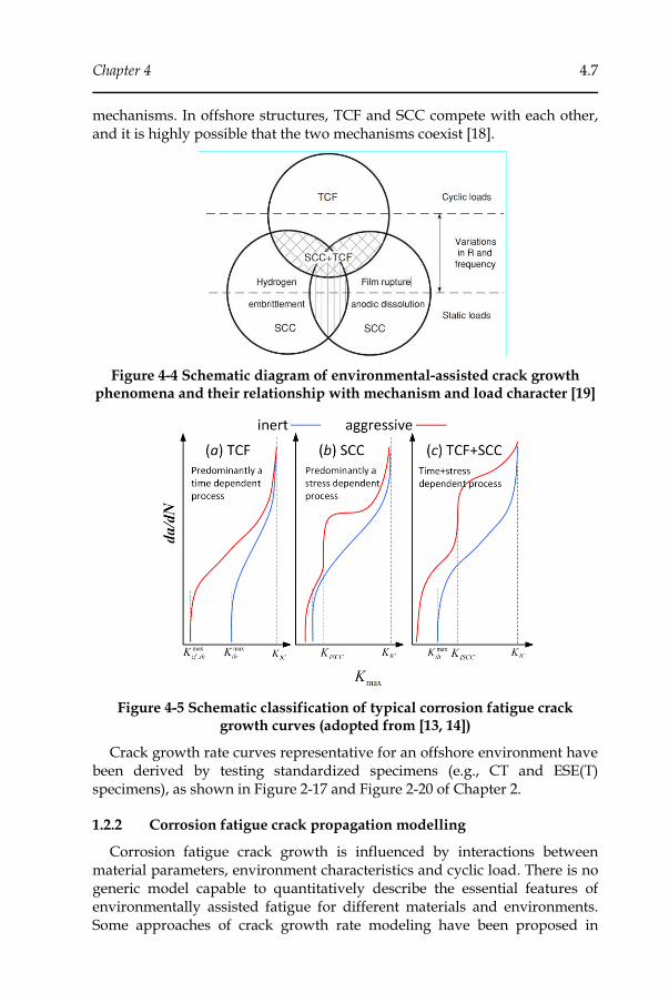
Chapter 4 4.7
mechanisms. In offshore structures, TCF and SCC compete with each other, and it is highly possible that the two mechanisms coexist [18].
Figure 4-4 Schematic diagram of environmental-assisted crack growth phenomena and their relationship with mechanism and load character [19]
Figure 4-5 Schematic classification of typical corrosion fatigue crack growth curves (adopted from [13, 14])
Crack growth rate curves representative for an offshore environment have been derived by testing standardized specimens (e.g., CT and ESE(T) specimens), as shown in Figure 2-17 and Figure 2-20 of Chapter 2.
1.2.2 Corrosion fatigue crack propagation modelling
Corrosion fatigue crack growth is influenced by interactions between material parameters, environment characteristics and cyclic load. There is no generic model capable to quantitatively describe the essential features of environmentally assisted fatigue for different materials and environments. Some approaches of crack growth rate modeling have been proposed in
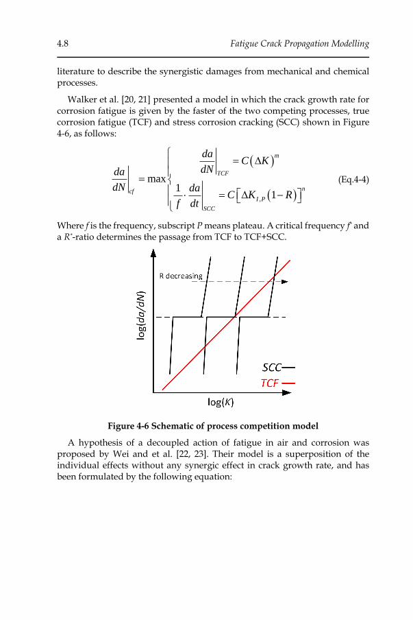
4.8 Fatigue Crack Propagation Modelling
literature to describe the synergistic damages from mechanical and chemical processes.
Walker et al. [20, 21] presented a model in which the crack growth rate for corrosion fatigue is given by the faster of the two competing processes, true corrosion fatigue (TCF) and stress corrosion cracking (SCC) shown in Figure 4-6, as follows:
( )
( ),
max1
1
m
TCF
ncf
I P
SCC
daC K
dNda
dN daC K R
f dt
=
=
= −
(Eq.4-4)
Where f is the frequency, subscript P means plateau. A critical frequency f* and a R*-ratio determines the passage from TCF to TCF+SCC.
Figure 4-6 Schematic of process competition model
A hypothesis of a decoupled action of fatigue in air and corrosion was proposed by Wei and et al. [22, 23]. Their model is a superposition of the individual effects without any synergic effect in crack growth rate, and has been formulated by the following equation:
Chapter 4 4.9
cf f c
da da da
dN dN dN= + (Eq.4-5)
( )m
f c SCCT
da da daC K dt
dN dN dt
= =
(Eq.4-6)
Where T is the duration of the part of a cycle that the stress intensity factor range is larger than 𝐾𝐼𝑆𝐶𝐶 . 𝑑𝑎 𝑑𝑡⁄ is crack growth rate of stress corrosion cracking in terms of time.
Cheng and Chen mentioned that anodic dissolution (AD) and hydrogen embrittlement (HE) are responsible for stress corrosion cracking (SCC) and hydrogen-assisted cracking (HAC). They proposed a model mixing these two mechanisms as follows [24]:
cf AD HE
da da da
dN dN dN= + (Eq.4-7)
( ) ( )1c mb
AD
daAf R K
dN= − (Eq.4-8)
( )
( )
( )
( )
1
2
1
max
2
max
1
1
m
t
IH
mHE
t
IE
B KK K
R K Kda
dN B KK K
R K K
− − =
− −
(Eq.4-9)
Where A, b and c are the material-environmental system coefficients. 𝐾𝐼𝐻 is hydrogen-degraded fracture toughness, 𝐾𝐼𝐻 is equilibrium fracture toughness, 𝐾𝑡 is the transition SIF between environment affected zone and plateau section.
Kang et al. modelled the HE and AD as accelerator of corrosion fatigue crack propagation [25] as well. The crack growth rate was assumed to be a contribution of fatigue in air and of corrosion, as shown in the following equation:
4.10 Fatigue Crack Propagation Modelling
( ) ( )( )
( )1
m f
th
cf crit
C f U K Kda
dN U R K K
− =
− −
(Eq.4-10)
Where U is related to load ratio effect, f is loading frequency. HE and AD effects corresponding to the parameters 𝑚(𝑓) and 𝐶(𝑓), that are obtained by least squares curve fitting to experimental data.
Regarding the influencing factors on corrosion fatigue crack growth rate, beside mechanical and environmental influencing variables (load ratio, frequency, variable amplitude, temperature and et al.) discussed in Chapter 2 and models mentioned above, there are additional factors affecting fatigue crack growth in a corrosive environment. For example, implementation of cathodic protection will affect crack propagation rate. It has been shown for CT specimens of an offshore structural steel (CSM355 TMCP steel) in 10℃
seawater and loaded at 0.35 Hz, that the benefits of cathodic protection strongly depend on R ratio and SIF range [26]. Furthermore, H-induced embrittlement can be enhanced by cathodic hydrogen absorption [19]. Corrosion can give rise to a wedge effect [27]. This is because corrosion products formed inside a crack whilst it is open (at the maximum SIF) will lead to an earlier contact when the crack closes, thereby raising the SIF. Additionally, pH value, dissolved oxygen content, coatings (inhibitors), concentration of damaging species and et al. can also have impact on the behavious of growth rate in corrosive aqueous environment at different levels [28], but their contributions change substantially in importance from system to system. Therefore, it is impossible to constitute a model capable to comprehensively describe the all story.
As mentioned in Chapter 1, this work does not aim to model the fundamental physical processes of corrosion and their effects on fatigue crack growth. Furthermore, there is no established methodology incorporating the effects of all possible mechanisms involved. For these reasons, the crack growth rate for corrosion fatigue is not an outcome of the framework developed, but an important input provided by dedicated experiments of corrosion-fatigue crack propagation. In this way, different mechanisms are implicitly included in the crack growth rate curve representative for a marine environment.
1.3 Extended finite element method (XFEM)
1.3.1 Fundamentals of extended finite element modelling
A robust fatigue crack growth lifetime estimation is based on an accurate calculation of Δ𝐾. Solutions for stress intensity factors of regular and idealized crack geometries under simplified loading conditions can be obtained analytically. However, most crack configurations in structures are of irregular
Chapter 4 4.11
nature and service loads are much more complex. Finite element analysis of SIFs has become a general method with a sound theoretical basis [29]. Thanks to the growing computer capacity, it is possible to investigate an arbitrary crack in large and complex structures by means of FEM.
Stress intensity factor can be obtained with good accuracy by finite element analysis, provided a sufficiently fine mesh is applied around the crack front (where theoretically a stress singularity occurs). However, this remains a challenge for conventional FEM. Many studies have adopted mesh refinement schemes by local remeshing and nodal relaxation at the crack tip [30-34]. Disadvantages of mesh refinement are the complexity of dealing with cracks by finite element analysis and its automation. By using continuous shape functions, finite element method is not tailored towards dealing with discontinuities (such as inclusions and static cracks), and it has a relatively weak capability of analyzing moving boundary problems (such as crack propagation and shear zone evolution). Conventional FEM introduces additional complexity in the sense of remeshing and mesh modification, which consumes a lot of time to achieve reliable results [30-35].
Crack problems can be more appropriately analyzed by introducing discontinuity into the shape functions of the elements. Based on this idea, Belytschko and Black [36] proposed a non-remeshing finite element method with additional discontinuous enrichment functions for the crack tip and crack surface. Following, Moës et al. [37] further developed the method by introducing enrichment functions for cut-through elements and enrichment functions for crack tip elements. In 2000, Daux et al. [38] proposed the method in the sense that a typical approximation algorithm based on displacement was enriched by discontinuous fields for the finite element modeling of branching cracks. The method was named formally as the extended finite element method (XFEM). As illustrated in Figure 4-7, the circular nodes are enriched by discontinuities and the square nodes are enriched by asymptotic modes at the crack ends. In mathematical terms, the introduction of discontinuous enrichment functions into the displacement field u is translated as:
( ) ( )( ) ( ) ( )s cut tip
j
i i i i i i j
ji N i N i N
N x N x H x N x B x
= + + u u a b (Eq.4-11)
with:
• 𝑁𝑠 – usual nodal element
• 𝑁𝑖(𝑥) – normal node function
• 𝑁𝑐𝑢𝑡 – through crack element
• 𝐻(𝑥) – discontinuous jump function
• 𝑁𝑡𝑖𝑝 – partial crack element
• 𝐵𝑗(𝑥) – crack tip function
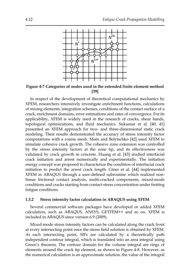
4.12 Fatigue Crack Propagation Modelling
Figure 4-7 Categories of nodes used in the extended finite element method [39]
In respect of the development of theoretical computational mechanics by XFEM, researchers intensively investigate enrichment functions, calculations of mixing elements, integration schemes, conditions of the contact surface of a crack, enrichment domains, error estimations and rates of convergence. For its applicability, XFEM is widely used in the research of cracks, shear bands, topological optimizations, and fluid mechanics. Sukumar et al. [40, 41] presented an XFEM approach for two- and three-dimensional static crack modeling. Their results demonstrated the accuracy of stress intensity factor computations with a coarse mesh. Moës and Belytschko [42] used XFEM to simulate cohesive crack growth. The cohesive zone extension was controlled by the stress intensity factors at the zone tip, and its effectiveness was validated by crack growth in concrete. Huang et al. [43] studied interfacial crack initiation and arrest numerically and experimentally. The initiation energy concept was proposed to characterize the condition of interfacial crack initiation to predict the arrest crack length. Giner et al. [44] implemented XFEM in ABAQUS through a user-defined subroutine which realized non-linear frictional contact analysis, multi-cracked components, mixed-mode conditions and cracks starting from contact stress concentration under fretting fatigue conditions.
1.3.2 Stress intensity factor calculation in ABAQUS using XFEM
Several commercial software packages have developed or added XFEM calculation, such as ABAQUS, ANSYS, GETFEM++ and so on. XFEM is included in ABAQUS since version 6.9 (2009).
Mixed-mode stress intensity factors can be calculated along the crack front at every intersecting point once the stress field solution is obtained by XFEM. At each intersecting point, SIFs are calculated by a theoretically path independent contour integral, which is translated into an area integral using Green’s theorem. The contour domain for the volume integral are rings of elements around the crack tip element, as shown in Figure 4-8. However, as the numerical calculation is an approximate solution, the value of the integral
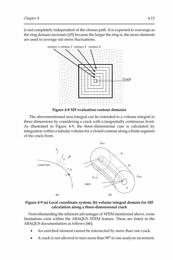
Chapter 4 4.13
is not completely independent of the chosen path. It is expected to converge as the ring domain increases [45] because the larger the ring is, the more elements are used to average out stress fluctuations.
Figure 4-8 SIF evaluation contour domains
The abovementioned area integral can be extended to a volume integral in three dimensions by considering a crack with a tangentially continuous front. As illustrated in Figure 4-9, the three-dimensional case is calculated by integration within a tubular volume for a closed contour along a finite segment of the crack front.
Figure 4-9 (a) Local coordinate system; (b) volume integral domain for SIF calculation along a three-dimensional crack
Notwithstanding the inherent advantages of XFEM mentioned above, some limitations exist within the ABAQUS XFEM feature. These are listed in the ABAQUS documentation as follows [46]:
• An enriched element cannot be intersected by more than one crack.
• A crack is not allowed to turn more than 90° in one analysis increment.
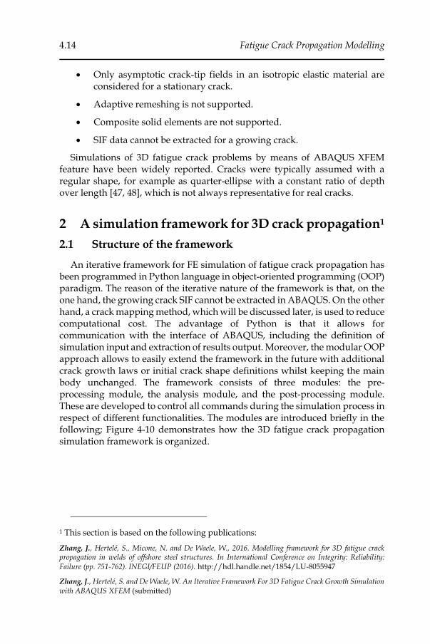
4.14 Fatigue Crack Propagation Modelling
• Only asymptotic crack-tip fields in an isotropic elastic material are considered for a stationary crack.
• Adaptive remeshing is not supported.
• Composite solid elements are not supported.
• SIF data cannot be extracted for a growing crack.
Simulations of 3D fatigue crack problems by means of ABAQUS XFEM feature have been widely reported. Cracks were typically assumed with a regular shape, for example as quarter-ellipse with a constant ratio of depth over length [47, 48], which is not always representative for real cracks.
2 A simulation framework for 3D crack propagation1
2.1 Structure of the framework
An iterative framework for FE simulation of fatigue crack propagation has been programmed in Python language in object-oriented programming (OOP) paradigm. The reason of the iterative nature of the framework is that, on the one hand, the growing crack SIF cannot be extracted in ABAQUS. On the other hand, a crack mapping method, which will be discussed later, is used to reduce computational cost. The advantage of Python is that it allows for communication with the interface of ABAQUS, including the definition of simulation input and extraction of results output. Moreover, the modular OOP approach allows to easily extend the framework in the future with additional crack growth laws or initial crack shape definitions whilst keeping the main body unchanged. The framework consists of three modules: the pre-processing module, the analysis module, and the post-processing module. These are developed to control all commands during the simulation process in respect of different functionalities. The modules are introduced briefly in the following; Figure 4-10 demonstrates how the 3D fatigue crack propagation simulation framework is organized.
1 This section is based on the following publications:
Zhang, J., Hertelé, S., Micone, N. and De Waele, W., 2016. Modelling framework for 3D fatigue crack propagation in welds of offshore steel structures. In International Conference on Integrity: Reliability: Failure (pp. 751-762). INEGI/FEUP (2016). http://hdl.handle.net/1854/LU-8055947
Zhang, J., Hertelé, S. and De Waele, W. An Iterative Framework For 3D Fatigue Crack Growth Simulation with ABAQUS XFEM (submitted)
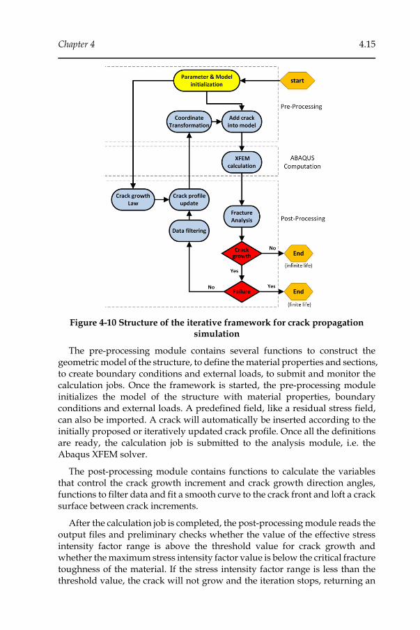
Chapter 4 4.15
Figure 4-10 Structure of the iterative framework for crack propagation simulation
The pre-processing module contains several functions to construct the geometric model of the structure, to define the material properties and sections, to create boundary conditions and external loads, to submit and monitor the calculation jobs. Once the framework is started, the pre-processing module initializes the model of the structure with material properties, boundary conditions and external loads. A predefined field, like a residual stress field, can also be imported. A crack will automatically be inserted according to the initially proposed or iteratively updated crack profile. Once all the definitions are ready, the calculation job is submitted to the analysis module, i.e. the Abaqus XFEM solver.
The post-processing module contains functions to calculate the variables that control the crack growth increment and crack growth direction angles, functions to filter data and fit a smooth curve to the crack front and loft a crack surface between crack increments.
After the calculation job is completed, the post-processing module reads the output files and preliminary checks whether the value of the effective stress intensity factor range is above the threshold value for crack growth and whether the maximum stress intensity factor value is below the critical fracture toughness of the material. If the stress intensity factor range is less than the threshold value, the crack will not grow and the iteration stops, returning an

4.16 Fatigue Crack Propagation Modelling
infinite fatigue life. Else, if the maximum stress intensity factor exceeds the critical fracture toughness value, the crack will grow in an unstable way and the structure will fail. In such case the iterative framework is also stopped, returning a finite fatigue life. In between these two extreme scenarios, the post-processing module performs further calculations based on the crack growth law in order to update the three-dimensional crack profile and then transfers an updated crack front profile to the pre-processing module in order to start a new simulation job.
The framework is iteratively executed via the analysis module which coordinates the first two modules by calling functions until either of the described extreme scenarios in the post-processing module is reached.
2.2 Implementation details
2.2.1 Crack insertion
To simulate the evolution of a fatigue crack, an initial crack must be inserted into the structure geometry. This initial geometry should be selected based on real crack observations or nondestructive testing (NDT) results. In the current version of the framework, similar to the FRANC3D crack library [49], a list of pre-defined simplified planar crack shapes is available for the initial crack. Figure 4-11 illustrates examples of a corner crack, a semi-elliptical crack and a cut-through crack. More complex shapes can be easily added to the library.
Figure 4-11 Examples of initial crack shapes and their geometrical parameters
Because the crack profile is built in a local coordinate system, it needs to be transformed into the global coordinate system before being inserted into the main structure. The location and orientation of the crack are defined by a rotation matrix and a translation vector. Euler angles of crack orientation are defined as shown in Figure 4-12. The transformation matrix 𝑅(𝜓, 𝜃, 𝜑), the translation vector T and the global coordinates vector U’ are given by Eq.4-12 to Eq.4-14:
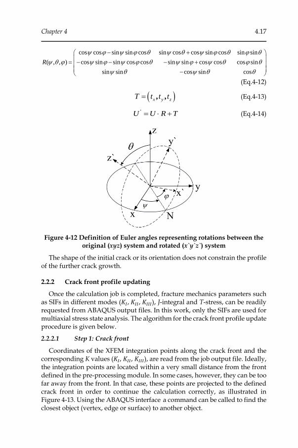
Chapter 4 4.17
cos cos sin sin cos sin cos cos sin cos sin sin
( , , ) cos sin sin cos cos sin sin cos cos cos sin
sin sin cos sin cos
R
− +
= − − − + −
(Eq.4-12)
( ), ,x y z
T t t t= (Eq.4-13)
'U U R T= + (Eq.4-14)
Figure 4-12 Definition of Euler angles representing rotations between the original (xyz) system and rotated (x`y`z`) system
The shape of the initial crack or its orientation does not constrain the profile of the further crack growth.
2.2.2 Crack front profile updating
Once the calculation job is completed, fracture mechanics parameters such as SIFs in different modes (𝐾𝐼, 𝐾𝐼𝐼, 𝐾𝐼𝐼𝐼), J-integral and T-stress, can be readily requested from ABAQUS output files. In this work, only the SIFs are used for multiaxial stress state analysis. The algorithm for the crack front profile update procedure is given below.
2.2.2.1 Step 1: Crack front
Coordinates of the XFEM integration points along the crack front and the corresponding K values (𝐾𝐼, 𝐾𝐼𝐼, 𝐾𝐼𝐼𝐼), are read from the job output file. Ideally, the integration points are located within a very small distance from the front defined in the pre-processing module. In some cases, however, they can be too far away from the front. In that case, these points are projected to the defined crack front in order to continue the calculation correctly, as illustrated in Figure 4-13. Using the ABAQUS interface a command can be called to find the closest object (vertex, edge or surface) to another object.
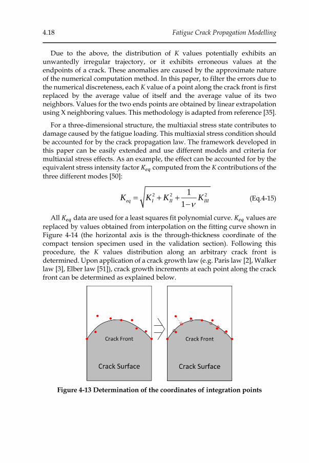
4.18 Fatigue Crack Propagation Modelling
Due to the above, the distribution of K values potentially exhibits an unwantedly irregular trajectory, or it exhibits erroneous values at the endpoints of a crack. These anomalies are caused by the approximate nature of the numerical computation method. In this paper, to filter the errors due to the numerical discreteness, each K value of a point along the crack front is first replaced by the average value of itself and the average value of its two neighbors. Values for the two ends points are obtained by linear extrapolation using X neighboring values. This methodology is adapted from reference [35].
For a three-dimensional structure, the multiaxial stress state contributes to damage caused by the fatigue loading. This multiaxial stress condition should be accounted for by the crack propagation law. The framework developed in this paper can be easily extended and use different models and criteria for multiaxial stress effects. As an example, the effect can be accounted for by the equivalent stress intensity factor 𝐾𝑒𝑞 computed from the K contributions of the
three different modes [50]:
2 2 21
1eq I II IIIK K K K
= + +
− (Eq.4-15)
All 𝐾𝑒𝑞 data are used for a least squares fit polynomial curve. 𝐾𝑒𝑞 values are
replaced by values obtained from interpolation on the fitting curve shown in Figure 4-14 (the horizontal axis is the through-thickness coordinate of the compact tension specimen used in the validation section). Following this procedure, the K values distribution along an arbitrary crack front is determined. Upon application of a crack growth law (e.g. Paris law [2], Walker law [3], Elber law [51]), crack growth increments at each point along the crack front can be determined as explained below.
Figure 4-13 Determination of the coordinates of integration points
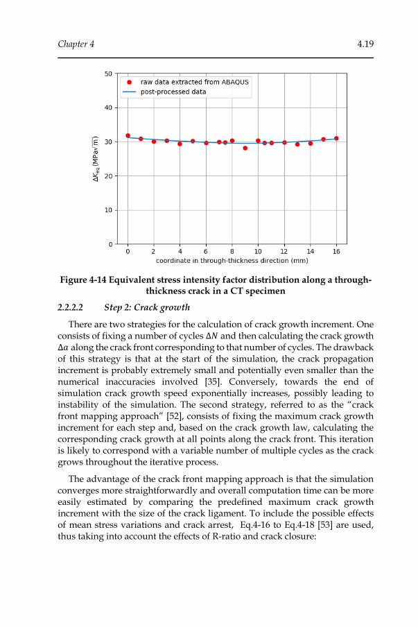
Chapter 4 4.19
Figure 4-14 Equivalent stress intensity factor distribution along a through-thickness crack in a CT specimen
2.2.2.2 Step 2: Crack growth
There are two strategies for the calculation of crack growth increment. One consists of fixing a number of cycles Δ𝑁 and then calculating the crack growth Δ𝑎 along the crack front corresponding to that number of cycles. The drawback of this strategy is that at the start of the simulation, the crack propagation increment is probably extremely small and potentially even smaller than the numerical inaccuracies involved [35]. Conversely, towards the end of simulation crack growth speed exponentially increases, possibly leading to instability of the simulation. The second strategy, referred to as the “crack front mapping approach” [52], consists of fixing the maximum crack growth increment for each step and, based on the crack growth law, calculating the corresponding crack growth at all points along the crack front. This iteration is likely to correspond with a variable number of multiple cycles as the crack grows throughout the iterative process.
The advantage of the crack front mapping approach is that the simulation converges more straightforwardly and overall computation time can be more easily estimated by comparing the predefined maximum crack growth increment with the size of the crack ligament. To include the possible effects of mean stress variations and crack arrest, Eq.4-16 to Eq.4-18 [53] are used, thus taking into account the effects of R-ratio and crack closure:
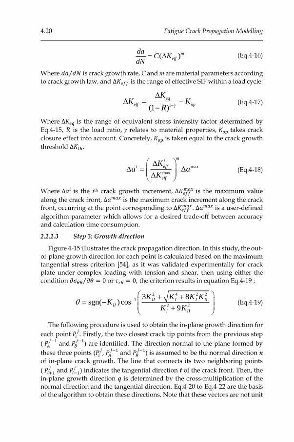
4.20 Fatigue Crack Propagation Modelling
( )m
eff
daC K
dN= (Eq.4-16)
Where 𝑑𝑎 𝑑𝑁⁄ is crack growth rate, C and m are material parameters according to crack growth law, and Δ𝐾𝑒𝑓𝑓 is the range of effective SIF within a load cycle:
1(1 )
eq
eff op
KK K
R −
= −
− (Eq.4-17)
Where Δ𝐾𝑒𝑞 is the range of equivalent stress intensity factor determined by
Eq.4-15, R is the load ratio, 𝛾 relates to material properties, 𝐾𝑜𝑝 takes crack
closure effect into account. Concretely, 𝐾𝑜𝑝 is taken equal to the crack growth
threshold Δ𝐾𝑡ℎ.
max
max
mi
effi
eff
Ka a
K
=
(Eq.4-18)
Where Δ𝑎𝑖 is the ith crack growth increment, Δ𝐾𝑒𝑓𝑓𝑚𝑎𝑥 is the maximum value
along the crack front, Δ𝑎𝑚𝑎𝑥 is the maximum crack increment along the crack front, occurring at the point corresponding to Δ𝐾𝑒𝑓𝑓
𝑚𝑎𝑥. Δ𝑎𝑚𝑎𝑥 is a user-defined
algorithm parameter which allows for a desired trade-off between accuracy and calculation time consumption.
2.2.2.3 Step 3: Growth direction
Figure 4-15 illustrates the crack propagation direction. In this study, the out-of-plane growth direction for each point is calculated based on the maximum tangential stress criterion [54], as it was validated experimentally for crack plate under complex loading with tension and shear, then using either the condition 𝜕𝜎𝜃𝜃 𝜕𝜃⁄ = 0 or 𝜏𝑟𝜃 = 0, the criterion results in equation Eq.4-19 :
2 4 2 2
1
2 2
3 8sgn( )cos
9
II I I II
II
I II
K K K KK
K K −
+ + = − +
(Eq.4-19)
The following procedure is used to obtain the in-plane growth direction for
each point 𝑃𝑖𝑗. Firstly, the two closest crack tip points from the previous step
( 𝑃𝐴𝑗−1
and 𝑃𝐵𝑗−1
) are identified. The direction normal to the plane formed by
these three points (𝑃𝑖𝑗, 𝑃𝐴
𝑗−1 and 𝑃𝐵
𝑗−1) is assumed to be the normal direction n
of in-plane crack growth. The line that connects its two neighboring points
( 𝑃𝑖+1𝑗
and 𝑃𝑖−1𝑗
) indicates the tangential direction t of the crack front. Then, the
in-plane growth direction q is determined by the cross-multiplication of the normal direction and the tangential direction. Eq.4-20 to Eq.4-22 are the basis of the algorithm to obtain these directions. Note that these vectors are not unit
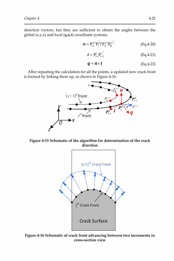
Chapter 4 4.21
direction vectors, but they are sufficient to obtain the angles between the global (x,y,z) and local (q,n,t) coordinate systems.
j-1 j j-1 j-1
A i A BP P ?P Pn = (Eq.4-20)
j j
i-1 i+1P Pt = (Eq.4-21)
q n t= (Eq.4-22)
After repeating the calculation for all the points, a updated new crack front is formed by linking them up, as shown in Figure 4-16.
Figure 4-15 Schematic of the algorithm for determination of the crack direction
Figure 4-16 Schematic of crack front advancing between two increments in cross-section view
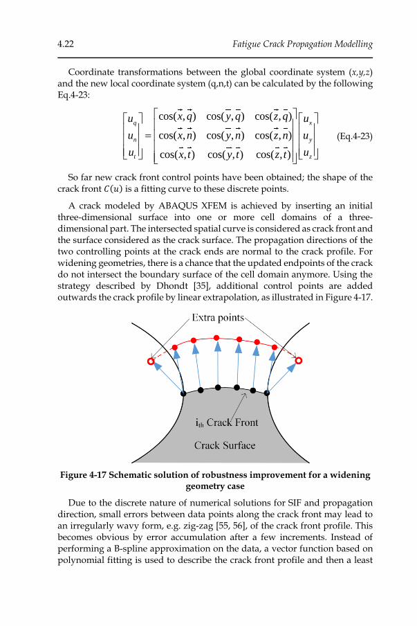
4.22 Fatigue Crack Propagation Modelling
Coordinate transformations between the global coordinate system (x,y,z) and the new local coordinate system (q,n,t) can be calculated by the following Eq.4-23:
cos( , ) cos( , ) cos( , )
cos( , ) cos( , ) cos( , )
cos( , ) cos( , ) cos( , )
q x
n y
t z
x q y q z qu u
u x n y n z n u
u ux t y t z t
=
(Eq.4-23)
So far new crack front control points have been obtained; the shape of the crack front 𝐶(𝑢) is a fitting curve to these discrete points.
A crack modeled by ABAQUS XFEM is achieved by inserting an initial three-dimensional surface into one or more cell domains of a three-dimensional part. The intersected spatial curve is considered as crack front and the surface considered as the crack surface. The propagation directions of the two controlling points at the crack ends are normal to the crack profile. For widening geometries, there is a chance that the updated endpoints of the crack do not intersect the boundary surface of the cell domain anymore. Using the strategy described by Dhondt [35], additional control points are added outwards the crack profile by linear extrapolation, as illustrated in Figure 4-17.
Figure 4-17 Schematic solution of robustness improvement for a widening geometry case
Due to the discrete nature of numerical solutions for SIF and propagation direction, small errors between data points along the crack front may lead to an irregularly wavy form, e.g. zig-zag [55, 56], of the crack front profile. This becomes obvious by error accumulation after a few increments. Instead of performing a B-spline approximation on the data, a vector function based on polynomial fitting is used to describe the crack front profile and then a least

Chapter 4 4.23
squares approximation is applied to these parametric equations, as shown in Eq.4-24:
0 0 0
( ) , ,n n n
k k k
k k k
k k k
r t a t b t c t= = =
= (Eq.4-24)
2.2.2.4 Step 4: Fatigue lifetime
In this study constant amplitude loading is assumed, i.e. there are no crack growth retardation or acceleration effects. These effects will be included and discussed in one of the framework extensions in Chapter 6. It is numerically reasonable to assume that for each crack length increment there is a linear relation between equivalent stress intensity factor and crack length, as shown in Figure 4-18 and in Eq.4-25 and Eq.4-26. The number of loading cycles corresponding to each crack increment can be calculated by integrating the crack growth law, as given by Eq.4-27.
effK a = + (Eq.4-25)
1( ) j j
eff eff effda d K K K += = − (Eq.4-26)
( )
11
1( )
(1 )
mj eff j
jmj
eff
KdaN
C mC K
−+
+
= =−
(Eq.4-27)
Figure 4-18 Stress intensity factor against crack length for life prediction
The total crack propagation life can finally be calculated by the sum of all cycles corresponding to the individual crack increments.
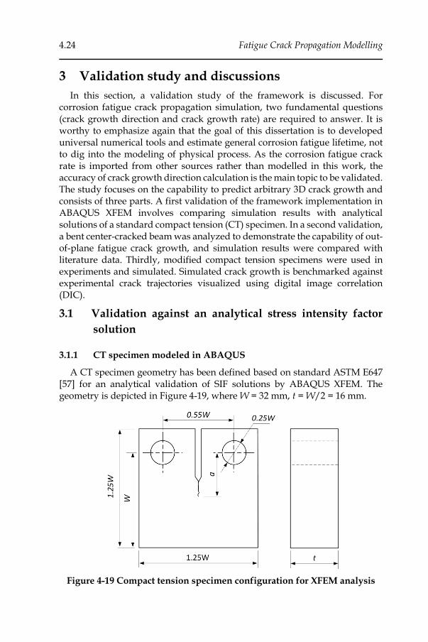
4.24 Fatigue Crack Propagation Modelling
3 Validation study and discussions
In this section, a validation study of the framework is discussed. For corrosion fatigue crack propagation simulation, two fundamental questions (crack growth direction and crack growth rate) are required to answer. It is worthy to emphasize again that the goal of this dissertation is to developed universal numerical tools and estimate general corrosion fatigue lifetime, not to dig into the modeling of physical process. As the corrosion fatigue crack rate is imported from other sources rather than modelled in this work, the accuracy of crack growth direction calculation is the main topic to be validated. The study focuses on the capability to predict arbitrary 3D crack growth and consists of three parts. A first validation of the framework implementation in ABAQUS XFEM involves comparing simulation results with analytical solutions of a standard compact tension (CT) specimen. In a second validation, a bent center-cracked beam was analyzed to demonstrate the capability of out-of-plane fatigue crack growth, and simulation results were compared with literature data. Thirdly, modified compact tension specimens were used in experiments and simulated. Simulated crack growth is benchmarked against experimental crack trajectories visualized using digital image correlation (DIC).
3.1 Validation against an analytical stress intensity factor
solution
3.1.1 CT specimen modeled in ABAQUS
A CT specimen geometry has been defined based on standard ASTM E647 [57] for an analytical validation of SIF solutions by ABAQUS XFEM. The geometry is depicted in Figure 4-19, where W = 32 mm, t = W/2 = 16 mm.
Figure 4-19 Compact tension specimen configuration for XFEM analysis
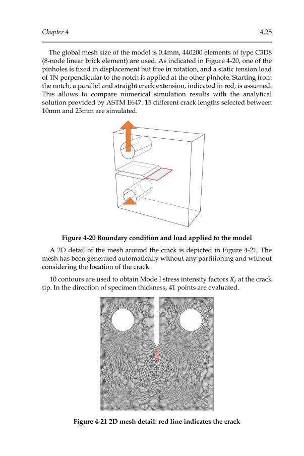
Chapter 4 4.25
The global mesh size of the model is 0.4mm, 440200 elements of type C3D8 (8-node linear brick element) are used. As indicated in Figure 4-20, one of the pinholes is fixed in displacement but free in rotation, and a static tension load of 1N perpendicular to the notch is applied at the other pinhole. Starting from the notch, a parallel and straight crack extension, indicated in red, is assumed. This allows to compare numerical simulation results with the analytical solution provided by ASTM E647. 15 different crack lengths selected between 10mm and 23mm are simulated.
Figure 4-20 Boundary condition and load applied to the model
A 2D detail of the mesh around the crack is depicted in Figure 4-21. The mesh has been generated automatically without any partitioning and without considering the location of the crack.
10 contours are used to obtain Mode I stress intensity factors 𝐾𝐼 at the crack tip. In the direction of specimen thickness, 41 points are evaluated.
Figure 4-21 2D mesh detail: red line indicates the crack

4.26 Fatigue Crack Propagation Modelling
3.1.2 Standard stress intensity factor solution of CT specimen
The stress intensity factor at the crack tip for a CT specimen can be calculated by the following expression suggested by standard ASTM-E647 [57]:
( )
( )( )2 3 4
3 2
20 886 4 64 13 32 14 72 5 6
1. . . . .
I
PK
t W
+= + − + −
−
(Eq.4-28)
Where 𝛼 = 𝑎 𝑊⁄ ; P is applied load; t is thickness, W is width. The expression is valid for 𝛼 ≥ 0.2.
3.1.3 Comparison
Because of the symmetry of the specimen, results of 5 points evenly distributed along half the crack are extracted to reveal the trend of Mode I SIF with increasing contour number, as shown in Figure 4-22. It confirms that the solutions converge when the number of contours increases. To ensure accuracy, it is recommended that the first few contours are discarded and the mean value from the remaining contours is used. In the current case, at least 5 contours are needed to have a converging K value.
Figure 4-22 XFEM solution of 𝑲𝑰 for different crack tip points and increasing number of contours
In Figure 4-23, the results of contours 6 to 10 are plotted against all evaluated points along the crack front. It is observed that KI-values slightly decrease near the surfaces due to the limited constraint.
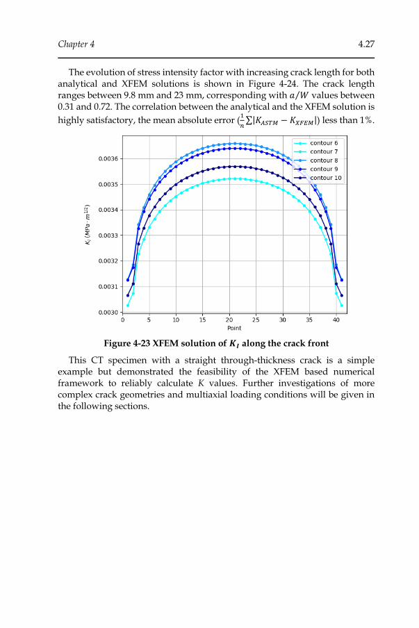
Chapter 4 4.27
The evolution of stress intensity factor with increasing crack length for both analytical and XFEM solutions is shown in Figure 4-24. The crack length ranges between 9.8 mm and 23 mm, corresponding with 𝑎 𝑊⁄ values between 0.31 and 0.72. The correlation between the analytical and the XFEM solution is
highly satisfactory, the mean absolute error (1
𝑛∑|𝐾𝐴𝑆𝑇𝑀 − 𝐾𝑋𝐹𝐸𝑀|) less than 1%.
Figure 4-23 XFEM solution of 𝑲𝑰 along the crack front
This CT specimen with a straight through-thickness crack is a simple example but demonstrated the feasibility of the XFEM based numerical framework to reliably calculate K values. Further investigations of more complex crack geometries and multiaxial loading conditions will be given in the following sections.
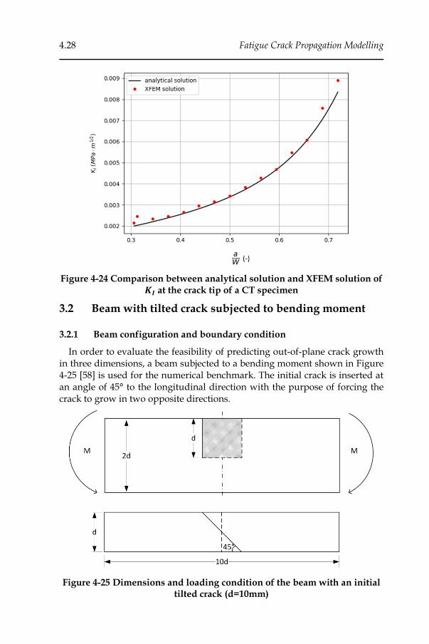
4.28 Fatigue Crack Propagation Modelling
Figure 4-24 Comparison between analytical solution and XFEM solution of 𝑲𝑰 at the crack tip of a CT specimen
3.2 Beam with tilted crack subjected to bending moment
3.2.1 Beam configuration and boundary condition
In order to evaluate the feasibility of predicting out-of-plane crack growth in three dimensions, a beam subjected to a bending moment shown in Figure 4-25 [58] is used for the numerical benchmark. The initial crack is inserted at an angle of 45° to the longitudinal direction with the purpose of forcing the crack to grow in two opposite directions.
Figure 4-25 Dimensions and loading condition of the beam with an initial tilted crack (d=10mm)
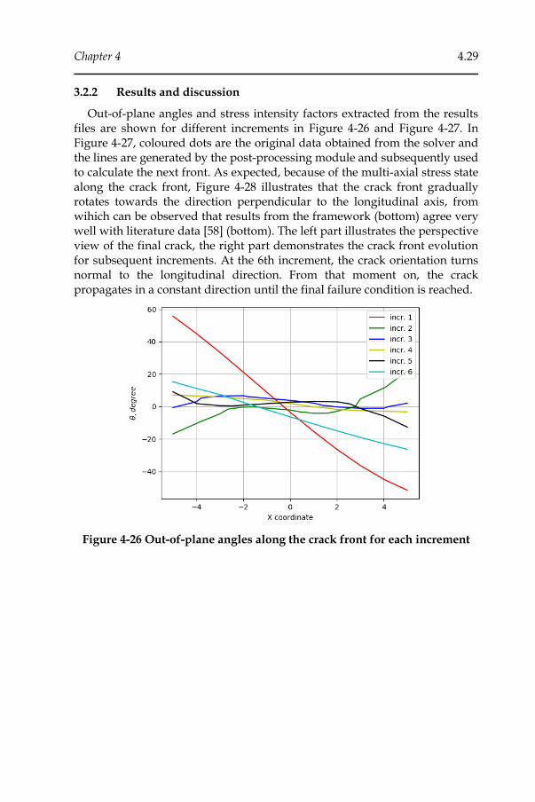
Chapter 4 4.29
3.2.2 Results and discussion
Out-of-plane angles and stress intensity factors extracted from the results files are shown for different increments in Figure 4-26 and Figure 4-27. In Figure 4-27, coloured dots are the original data obtained from the solver and the lines are generated by the post-processing module and subsequently used to calculate the next front. As expected, because of the multi-axial stress state along the crack front, Figure 4-28 illustrates that the crack front gradually rotates towards the direction perpendicular to the longitudinal axis, from wihich can be observed that results from the framework (bottom) agree very well with literature data [58] (bottom). The left part illustrates the perspective view of the final crack, the right part demonstrates the crack front evolution for subsequent increments. At the 6th increment, the crack orientation turns normal to the longitudinal direction. From that moment on, the crack propagates in a constant direction until the final failure condition is reached.
Figure 4-26 Out-of-plane angles along the crack front for each increment
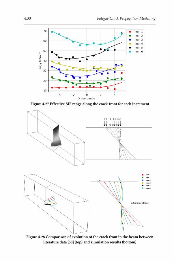
4.30 Fatigue Crack Propagation Modelling
Figure 4-27 Effective SIF range along the crack front for each increment
Figure 4-28 Comparison of evolution of the crack front in the beam between
literature data [58] (top) and simulation results (bottom)
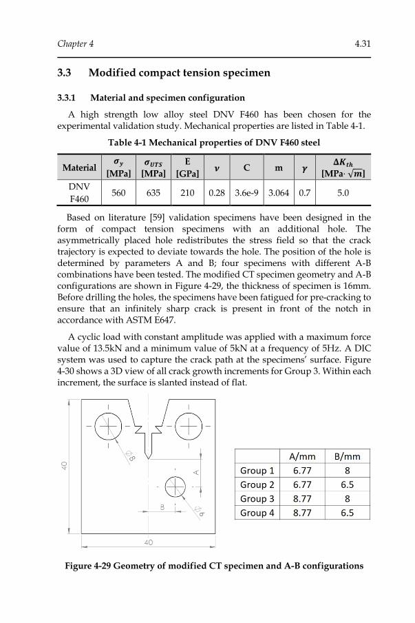
Chapter 4 4.31
3.3 Modified compact tension specimen
3.3.1 Material and specimen configuration
A high strength low alloy steel DNV F460 has been chosen for the experimental validation study. Mechanical properties are listed in Table 4-1.
Table 4-1 Mechanical properties of DNV F460 steel
Material 𝝈𝒚
[MPa] 𝝈𝑼𝑻𝑺
[MPa]
E
[GPa] 𝝂 C m 𝜸
𝚫𝑲𝒕𝒉
[MPa⋅ √𝒎]
DNV
F460 560 635 210 0.28 3.6e-9 3.064 0.7 5.0
Based on literature [59] validation specimens have been designed in the form of compact tension specimens with an additional hole. The asymmetrically placed hole redistributes the stress field so that the crack trajectory is expected to deviate towards the hole. The position of the hole is determined by parameters A and B; four specimens with different A-B combinations have been tested. The modified CT specimen geometry and A-B configurations are shown in Figure 4-29, the thickness of specimen is 16mm. Before drilling the holes, the specimens have been fatigued for pre-cracking to ensure that an infinitely sharp crack is present in front of the notch in accordance with ASTM E647.
A cyclic load with constant amplitude was applied with a maximum force value of 13.5kN and a minimum value of 5kN at a frequency of 5Hz. A DIC system was used to capture the crack path at the specimens’ surface. Figure 4-30 shows a 3D view of all crack growth increments for Group 3. Within each increment, the surface is slanted instead of flat.
Figure 4-29 Geometry of modified CT specimen and A-B configurations

4.32 Fatigue Crack Propagation Modelling
Figure 4-30 Perspective view of the propagating three-dimensional crack profile in a modified CT specimen
3.3.2 Results and discussion
A set of simulations with different mesh sizes have been performed. A specimen of group 3 and automatically meshed (without application of any partitioning strategy) with hex-dominant elements is illustrated in Figure 4-31. The pre-defined maximum crack increment has been defined as 2mm for all simulations.
Figure 4-32 maps the crack paths for different mesh sizes and compares these with experimental results. It clearly shows that refining the mesh does not result in continuous improvement of the accuracy of the crack trajectory prediction but obviously results in much more computational time.
Figure 4-31 Free mesh scheme without partitioning
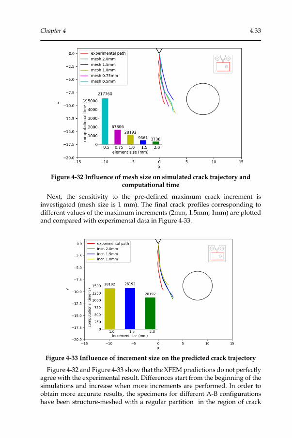
Chapter 4 4.33
Figure 4-32 Influence of mesh size on simulated crack trajectory and computational time
Next, the sensitivity to the pre-defined maximum crack increment is investigated (mesh size is 1 mm). The final crack profiles corresponding to different values of the maximum increments (2mm, 1.5mm, 1mm) are plotted and compared with experimental data in Figure 4-33.
Figure 4-33 Influence of increment size on the predicted crack trajectory
Figure 4-32 and Figure 4-33 show that the XFEM predictions do not perfectly agree with the experimental result. Differences start from the beginning of the simulations and increase when more increments are performed. In order to obtain more accurate results, the specimens for different A-B configurations have been structure-meshed with a regular partition in the region of crack

4.34 Fatigue Crack Propagation Modelling
growth, as shown in Figure 4-34. The element size in the partition is equal to 1mm and the predefined increment value is set as 1mm.
Figure 4-34 Structured mesh scheme with regular partition
Predicted and experimentally determined crack trajectories are compared
for the different specimen configurations; an excellent agreement can be
observed. Results of group 1 to group 4 are shown in Figure 4-35 to Figure 4-38
respectively. The simulated final crack lengths are shorter than the
experimental values. For the fourth group again a very good agreement is
found for the crack trajectory but now the simulated final crack length is
significantly longer than the experimental one.

Chapter 4 4.35
Figure 4-35 Crack path of group 1: (top) visualization by DIC, (middle) predicted by XFEM framework, (bottom) comparison of experimental and
numerical trajectories
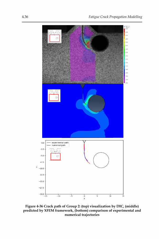
4.36 Fatigue Crack Propagation Modelling
Figure 4-36 Crack path of Group 2: (top) visualization by DIC, (middle) predicted by XFEM framework, (bottom) comparison of experimental and
numerical trajectories

Chapter 4 4.37
Figure 4-37 Crack path of Group 3: (top) visualization by DIC, (middle) predicted by XFEM framework, (bottom) comparison of experimental and
numerical trajectories
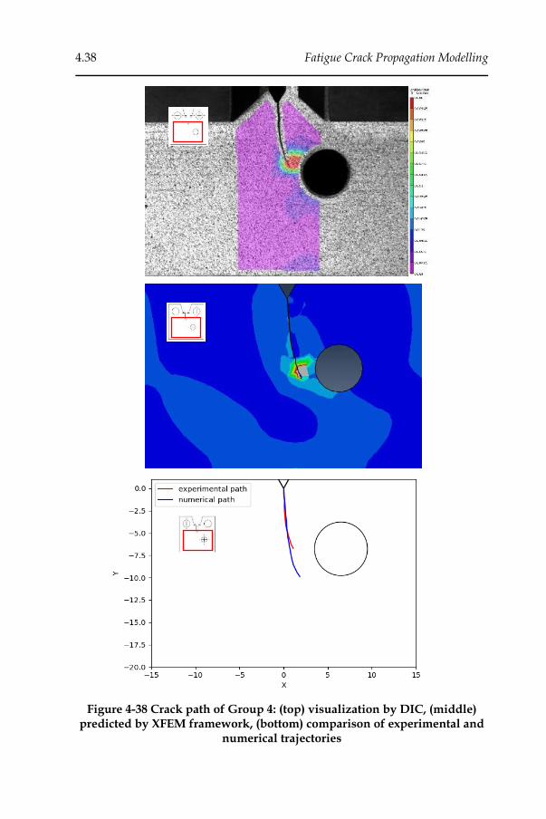
4.38 Fatigue Crack Propagation Modelling
Figure 4-38 Crack path of Group 4: (top) visualization by DIC, (middle) predicted by XFEM framework, (bottom) comparison of experimental and
numerical trajectories
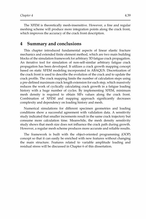
Chapter 4 4.39
The XFEM is theoretically mesh-insensitive. However, a fine and regular meshing scheme will produce more integration points along the crack front, which improves the accuracy of the crack front description.
4 Summary and conclusions
This chapter introduced fundamental aspects of linear elastic fracture mechanics and extended finite element method, which are two main building blocks of the simulation framework for arbitrary 3D fatigue crack propagation. An iterative tool for simulation of non-self-similar arbitrary fatigue crack propagation has been developed. It utilizes a crack growth mapping concept based on static XFEM modeling incorporated in ABAQUS. Discretization of the crack front is used to describe the evolution of the crack and to update the crack profile. The crack mapping limits the number of calculation steps using a pre-defined maximum crack length extension for each step, which massively reduces the work of cyclically calculating crack growth in a fatigue loading history with a huge number of cycles. By implementing XFEM, minimum mesh density is required to obtain SIFs values along the crack front. Combination of XFEM and mapping approach significantly decreases complexity and dependency on loading history and mesh.
Numerical simulations for different specimen geometries and loading conditions show a successful agreement with validation data. A sensitivity study indicated that smaller increments result in the same crack trajectory but consume more calculation time. Meanwhile, the mesh density sensitivity study shows that mesh size does not influence the crack path during growth. However, a regular mesh scheme produces more accurate and reliable results.
The framework is built with the object-oriented programming (OOP) concept so that it can easily be enriched with new features without changing the main structure. Features related to variable amplitude loading and residual stress will be discussed in Chapter 6 of this dissertation.
4.40 Fatigue Crack Propagation Modelling
References
1. Zerbst, U., et al., Review on fracture and crack propagation in weldments – A fracture mechanics perspective. Engineering Fracture Mechanics, 2014. 132: p. 200-276.
2. Paris, P. and F. Erdogan, A critical analysis of crack propagation laws. Journal of Fluids Engineering, 1963. 85(4): p. 528-533.
3. Walker, K., The effect of stress ratio during crack propagation and fatigue for 2024-T3 and 7075-T6 aluminum. Effects of environment and complex load history on fatigue life, 1970. 462: p. 1-14.
4. Dowling, N.E., C.A. Calhoun, and A. Arcari, Mean stress effects in stress-life fatigue and the Walker equation. Fatigue & Fracture of Engineering Materials & Structures, 2009. 32(3): p. 163-179.
5. Forman, R.G., V. Kearney, and R. Engle, Numerical analysis of crack propagation in cyclic-loaded structures. Journal of Fluids Engineering, 1967. 89(3): p. 459-463.
6. A.K. Vasudevan, K.S., G. Glinka, Critical parameters for fatigue damage. International Journal of Fatigue, 2001. 23 (2001).
7. Sadananda, K., Fatigue crack growth mechanisms in steels. International Journal of Fatigue, 2003. 25(9-11): p. 899-914.
8. Sadananda, K., Crack tip driving forces and crack growth representation under fatigue. International Journal of Fatigue, 2004. 26(1): p. 39-47.
9. Vasudevan, A., K. Sadananda, and R. Holtz, Analysis of vacuum fatigue crack growth results and its implications. International Journal of Fatigue, 2005. 27(10-12): p. 1519-1529.
10. Stoychev, S. and D. Kujawski, Analysis of crack propagation using ΔK and Kmax. International Journal of Fatigue, 2005. 27(10-12): p. 1425-1431.
11. Stoychev, S. and D. Kujawski, Crack-tip stresses and their effect on stress intensity factor for crack propagation. Engineering Fracture Mechanics, 2008. 75(8): p. 2469-2479.
12. Fontana, M.G., Corrosion engineering. 2005: Tata McGraw-Hill Education.
13. Devereux, O.F., et al., Corrosion fatigue: chemistry, mechanics and microstructure : June 14-18, 1971, The University of Connecticut, Storrs, Connecticut. 1972: National Association of Corrosion Engineers.
14. Vasudevan, A. and K. Sadananda, Classification of environmentally assisted fatigue crack growth behavior. International Journal of Fatigue, 2009. 31(11): p. 1696-1708.
Chapter 4 4.41
15. Pereira, H.B., et al., Investigation of stress corrosion cracking of austenitic, duplex and super duplex stainless steels under drop evaporation test using synthetic seawater. Materials Research, 2019. 22(2).
16. Machiels, A., B. Gordon, and M. Taylor, Effects of marine environments on stress corrosion cracking of austenitic stainless steels. Electric Power Research Institute, USA, 2005.
17. Deflorian, F., et al., Stress corrosion cracking (SCC) failure in marine areas of fixed guards for climbing. Corrosion Engineering, Science and Technology, 2015. 50(6): p. 462-466.
18. Micone, N., Development of Testing Methodologies for the Analysis of Variable Amplitude Fatigue and Corrosion-Fatigue of Offshore Steels. 2017, Ghent University.
19. Milella, P.P., Fatigue and Corrosion in Metals. 2012: Springer Milan.
20. Austen, I.M., Walker, E.F., Factors affecting the rate of growth of cracks by corrosion-fatigue. British Steel, 1978. 18/802.
21. Walker, E.F., May, M.J., Irvine, K.J., Mechanisms and control of crack growth in steels. 1976.
22. Wei, R.P., Landes, J. D., Correlation between sustained-load and fatigue crack growth in high-strength steels. Materials Research And Standards, 1969. 9: p. 25-27.
23. Wei, R. and G. Simmons, Recent progress in understanding environment assisted fatigue crack growth. International Journal of Fracture, 1981. 17(2): p. 235-247.
24. Cheng, A. and N.-Z. Chen, Corrosion fatigue crack growth modelling for subsea pipeline steels. Ocean Engineering, 2017. 142: p. 10-19.
25. Kang, D.-H., J.-K. Lee, and T.-W. Kim, Corrosion Fatigue Crack Propagation of High-strength Steel HSB800 in a seawater environment. Procedia Engineering, 2011. 10: p. 1170-1175.
26. Yu, J., et al., The effect of cathodic protection potential on corrosion fatigue crack growth rate of an offshore structural steel. Fatigue & Fracture of Engineering Materials & Structures, 1996. 19(8): p. 1019-1029.
27. Komai, K., 4.13 - Corrosion Fatigue, in Comprehensive Structural Integrity, I. Milne, R.O. Ritchie, and B. Karihaloo, Editors. 2003, Pergamon: Oxford. p. 345-358.
28. Lampman, S.R., ASM handbook: volume 19, fatigue and fracture. ASM International, 1996.
29. Dixon, J.R. and L.P. Pook, Stress intensity Factors calculated generally by the Finite Element Technique. Nature, 1969. 224(5215): p. 166-167.

4.42 Fatigue Crack Propagation Modelling
30. Trädegård, A., F. Nilsson, and S. Östlund, FEM-remeshing technique applied to crack growth problems. Computer Methods in Applied Mechanics and Engineering, 1998. 160(1–2): p. 115-131.
31. Bouchard, P.O., et al., Crack propagation modelling using an advanced remeshing technique. Computer Methods in Applied Mechanics and Engineering, 2000. 189(3): p. 723-742.
32. Bouchard, P.O., F. Bay, and Y. Chastel, Numerical modelling of crack propagation: automatic remeshing and comparison of different criteria. Computer Methods in Applied Mechanics and Engineering, 2003. 192(35–36): p. 3887-3908.
33. Shahani, A.R. and M.R. Amini Fasakhodi, Finite element analysis of dynamic crack propagation using remeshing technique. Materials & Design, 2009. 30(4): p. 1032-1041.
34. Khoei, A.R., H. Azadi, and H. Moslemi, Modeling of crack propagation via an automatic adaptive mesh refinement based on modified superconvergent patch recovery technique. Engineering Fracture Mechanics, 2008. 75(10): p. 2921-2945.
35. Dhondt, G., Automatic 3-D mode I crack propagation calculations with finite elements. International Journal for Numerical Methods in Engineering, 1998. 41(4): p. 739-757.
36. Belytschko T, B.T., Elastic crack growth in finite elements with minimal remeshing. International Journal for Numerical Methods in Engineering, 1999. 45(5): p. 601-620.
37. Nicolas Moes, J.D., Ted Belytschko, A Finite Element Method For Crack Method For Crack Growth Without Remeshing. International Journal For Numerical Methods In Engineering, 1999. 46: p. 131-150.
38. Christophe Daux, N.M., John Dolbow, Natarajan Sukumar, Ted Belytschko, Arbitrary branched and intersecting cracks with the extended finite element method. International Journal for Numerical Methods in Engineering, 2000. 48(12): p. 1741-1760.
39. Dolbow, J. and T. Belytschko, A finite element method for crack growth without remeshing. International journal for numerical methods in engineering, 1999. 46(1): p. 131-150.
40. Sukumar, N., et al., Extended finite element method for three-dimensional crack modelling. International Journal for Numerical Methods in Engineering, 2000. 48(11): p. 1549-1570.
41. Moës, N., et al., An Extended Finite Element Method (XFEM) for Two- and Three-Dimensional Crack Modeling. European Congrass on Computational Methods in Applied Sciences and Engineering, Barcelona, 2000.
Chapter 4 4.43
42. NICOLAS MOES, T.B., Extended finite element method for cohesive crack growth. Engineering Fracture Mechanics, 2002. 69: p. 813-833.
43. Huang, Z., et al., Initiation and arrest of an interfacial crack in a four-point bend test. Engineering Fracture Mechanics, 2005. 72(17): p. 2584-2601.
44. Giner, E., et al., An Abaqus implementation of the extended finite element method. Engineering Fracture Mechanics, 2009. 76(3): p. 347-368.
45. Muys, L., XFEM-based cycle-by-cycle simulation of fatigue crack growth. 2017, Ghent University. p. 105.
46. DASSAULT_SYSTEMES, Abaqus 6.14 Documentation. 2014: DASSAULT SYSTEMES.
47. Naderi, M. and N. Iyyer, Fatigue life prediction of cracked attachment lugs using XFEM. International Journal of Fatigue, 2015. 77: p. 186-193.
48. London, T., D. De Bono, and X. Sun. An Evaluation of the Low Cycle Fatigue Analysis Procedure in Abaqus for Crack Propagation: Numerical Benchmarks and Experimental Validation. 2015. SIMULIA UK Regional User Meeting.
49. Carter, B.J., P.A. Wawrzynek, and A.R. Ingraffea, Automated 3-D crack growth simulation. International Journal for Numerical Methods in Engineering, 2000. 47(1-3): p. 229-253.
50. Rhee, H.C. and M.M. Salama, Mixed-mode stress intensity factor solutions of a warped surface flaw by three-dimensional finite element analysis. Engineering Fracture Mechanics, 1987. 28(2): p. 203-209.
51. Wolf, E., Fatigue crack closure under cyclic tension. Engineering Fracture Mechanics, 1970. 2(1): p. 37-45.
52. Shi, J., et al., Abaqus implementation of extended finite element method using a level set representation for three-dimensional fatigue crack growth and life predictions. Engineering Fracture Mechanics, 2010. 77(14): p. 2840-2863.
53. Meggiolaro, M.A. and J.T.P. De Castro, On the dominant role of crack closure on fatigue crack growth modeling. International Journal of Fatigue, 2003. 25(9): p. 843-854.
54. Erdogan, F. and G.C. Sih, On the Crack Extension in Plates Under Plane Loading and Transverse Shear. Journal of Basic Engineering, 1963. 85(4): p. 519-525.
55. Zhang, J.Y., T.R. Hsu, and I.Q. Wang, Numerical modelling of crack propagation using multi-variable and breakable finite elements. Communications in Applied Numerical Methods, 1990. 6(3): p. 215-222.
4.44 Fatigue Crack Propagation Modelling
56. Dhondt, G., General behaviour of collapsed 8-node 2-D and 20-node 3-D isoparametric elements. International Journal for Numerical Methods in Engineering, 1993. 36(7): p. 1223-1243.
57. ASTM, E647 Standard test method for measurement of fatigue crack growth rates, in Annual Book of ASTM Standards, Section Three: Metals Test Methods and Analytical Procedures. 2011. p. 628-670.
58. Gravouil, A., N. Moës, and T. Belytschko, Non-planar 3D crack growth by the extended finite element and level sets—Part II: Level set update. International Journal for Numerical Methods in Engineering, 2002. 53(11): p. 2569-2586.
59. Miranda, A.C.O., et al., Fatigue life and crack path predictions in generic 2D structural components. Engineering Fracture Mechanics, 2003. 70(10): p. 1259-1279.

Transition from Crack Initiation to Propagation

5.2 Transition from Crack Initiation to Propagation
<< This page intentionally left blank >>

Chapter 5 5.3
1 Overview
In the previous two chapters, methods and frameworks have been developed for both fatigue crack initiation and propagation stages. The total fatigue lifetime 𝑁𝑇 of an initially uncracked structure can be estimated by the sum of lifetimes in two stages of fatigue crack evolution.
T I PN N N= + (Eq.5-1)
where 𝑁𝐼 is the crack initiation lifetime and 𝑁𝑃 is the crack propagation lifetime. As mentioned in Chapter 3 of this dissertation, the distinction between initiation and propagation should be clarified so that models for macro-structures can be employed for two stages. There is no universally agreed or accepted definition of the boundary between fatigue crack initiation and propagation [1]. However, it depends on the scale of research interest. The fatigue initiation phase in an intact material is often assumed to comprise negligibly short cracks with respect to the magnitude of structure size, up to a critical size 𝑎𝑡ℎ [2]. From 𝑎𝑡ℎ onwards, fatigue can be modelled by the growth rate of a long size crack in terms of linear elastic fracture mechanics, as illustrated in Figure 5-1. Thus, 𝑎𝑡ℎ is considered as the critical crack length delineating crack initiation and propagation stages in this study. For this study it was decided that the starting point of the crack propagation framework should be a relevant macro-scale size of a crack that can be defined by practical measurement. For instance, the critical crack size can be of similar length as the grain size or the mean diameter of inclusions/defects or minimum sensitivity of non-destructive testing.
Figure 5-1 Stages in the development of a fatigue crack in metals and alloys [3]
In this chapter, the transition of crack initiation to crack propagation is discussed and a numerical tool to calculate the threshold length is developed.
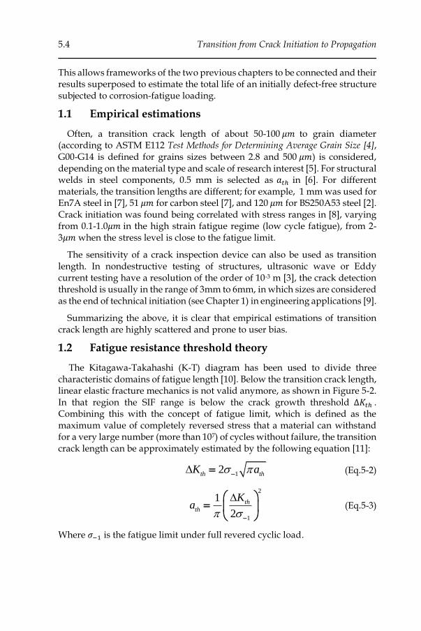
5.4 Transition from Crack Initiation to Propagation
This allows frameworks of the two previous chapters to be connected and their results superposed to estimate the total life of an initially defect-free structure subjected to corrosion-fatigue loading.
1.1 Empirical estimations
Often, a transition crack length of about 50-100 𝜇𝑚 to grain diameter (according to ASTM E112 Test Methods for Determining Average Grain Size [4], G00-G14 is defined for grains sizes between 2.8 and 500 𝜇𝑚) is considered, depending on the material type and scale of research interest [5]. For structural welds in steel components, 0.5 mm is selected as 𝑎𝑡ℎ in [6]. For different materials, the transition lengths are different; for example, 1 mm was used for En7A steel in [7], 51 𝜇𝑚 for carbon steel [7], and 120 𝜇𝑚 for BS250A53 steel [2]. Crack initiation was found being correlated with stress ranges in [8], varying from 0.1-1.0𝜇𝑚 in the high strain fatigue regime (low cycle fatigue), from 2-3𝜇𝑚 when the stress level is close to the fatigue limit.
The sensitivity of a crack inspection device can also be used as transition length. In nondestructive testing of structures, ultrasonic wave or Eddy current testing have a resolution of the order of 10-3 m [3], the crack detection threshold is usually in the range of 3mm to 6mm, in which sizes are considered as the end of technical initiation (see Chapter 1) in engineering applications [9].
Summarizing the above, it is clear that empirical estimations of transition crack length are highly scattered and prone to user bias.
1.2 Fatigue resistance threshold theory
The Kitagawa-Takahashi (K-T) diagram has been used to divide three characteristic domains of fatigue length [10]. Below the transition crack length, linear elastic fracture mechanics is not valid anymore, as shown in Figure 5-2. In that region the SIF range is below the crack growth threshold ∆𝐾𝑡ℎ . Combining this with the concept of fatigue limit, which is defined as the maximum value of completely reversed stress that a material can withstand for a very large number (more than 107) of cycles without failure, the transition crack length can be approximately estimated by the following equation [11]:
12
th thK a
−= (Eq.5-2)
2
1
1
2
th
th
Ka
−
=
(Eq.5-3)
Where 𝜎−1 is the fatigue limit under full revered cyclic load.

Chapter 5 5.5
Figure 5-2 Schematic of the K-T diagram
A similar formula was proposed by Kitagawa [12] in which the dimensionless shape factor Y for K calculation was introduced,
2
1
1 th
th
Ka
Y
−
=
(Eq.5-4)
Solutions for Y can be found for a large number of configurations in standards and handbooks [13]. This method is easy to use for a simple crack profile when the required material properties are known. The disadvange is that the shape factor Y for a complex shaped crack is not documented.
1.3 Dominated mechanism theory
A model that combines cyclic strain fatigue and fracture mechanics was proposed by Socie and et al. [14]. The model is based on the hypotheses that a fatigue crack is initiated when the fatigue damage due to crack propagation mechanisms exceeds that due to crack initiation or cyclic strain fatigue mechanisms. Technically, the two stages of fatigue are treated separately in each stage by cyclic strain fatigue and fracture mechanics methods. The transition crack length was defined as the size when damage induced by crack propagation mechanisms exceeds the damage caused by cyclic strain mechanisms.
As illustrated in Figure 5-3, the crack initiation damage rate dominates for small crack depths measured from the surface, in line with practical observations that cracks initiate at the surface. Contrary, the crack propagation
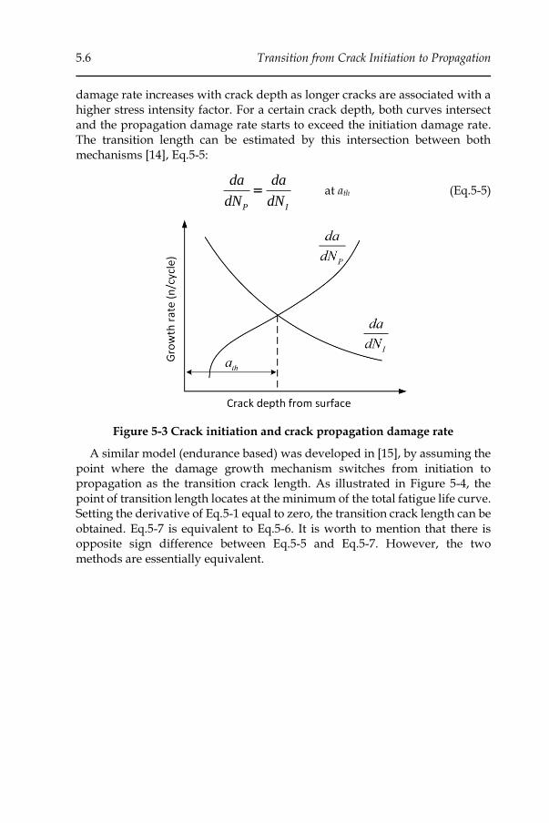
5.6 Transition from Crack Initiation to Propagation
damage rate increases with crack depth as longer cracks are associated with a higher stress intensity factor. For a certain crack depth, both curves intersect and the propagation damage rate starts to exceed the initiation damage rate. The transition length can be estimated by this intersection between both mechanisms [14], Eq.5-5:
P I
da da
dN dN= at ath (Eq.5-5)
Figure 5-3 Crack initiation and crack propagation damage rate
A similar model (endurance based) was developed in [15], by assuming the point where the damage growth mechanism switches from initiation to propagation as the transition crack length. As illustrated in Figure 5-4, the point of transition length locates at the minimum of the total fatigue life curve. Setting the derivative of Eq.5-1 equal to zero, the transition crack length can be obtained. Eq.5-7 is equivalent to Eq.5-6. It is worth to mention that there is opposite sign difference between Eq.5-5 and Eq.5-7. However, the two methods are essentially equivalent.
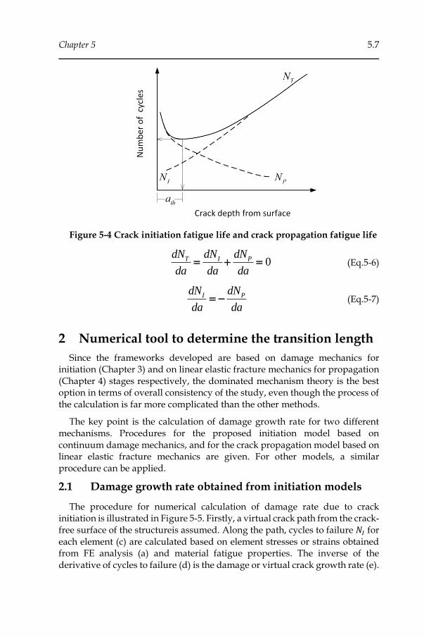
Chapter 5 5.7
Figure 5-4 Crack initiation fatigue life and crack propagation fatigue life
0T I PdN dN dN
da da da= + = (Eq.5-6)
I P
dN dN
da da= − (Eq.5-7)
2 Numerical tool to determine the transition length
Since the frameworks developed are based on damage mechanics for initiation (Chapter 3) and on linear elastic fracture mechanics for propagation (Chapter 4) stages respectively, the dominated mechanism theory is the best option in terms of overall consistency of the study, even though the process of the calculation is far more complicated than the other methods.
The key point is the calculation of damage growth rate for two different mechanisms. Procedures for the proposed initiation model based on continuum damage mechanics, and for the crack propagation model based on linear elastic fracture mechanics are given. For other models, a similar procedure can be applied.
2.1 Damage growth rate obtained from initiation models
The procedure for numerical calculation of damage rate due to crack initiation is illustrated in Figure 5-5. Firstly, a virtual crack path from the crack-free surface of the structureis assumed. Along the path, cycles to failure 𝑁𝐼 for each element (c) are calculated based on element stresses or strains obtained from FE analysis (a) and material fatigue properties. The inverse of the derivative of cycles to failure (d) is the damage or virtual crack growth rate (e).
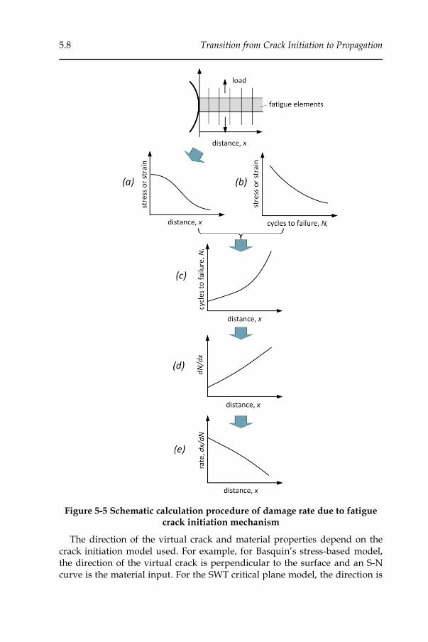
5.8 Transition from Crack Initiation to Propagation
Figure 5-5 Schematic calculation procedure of damage rate due to fatigue crack initiation mechanism
The direction of the virtual crack and material properties depend on the crack initiation model used. For example, for Basquin’s stress-based model, the direction of the virtual crack is perpendicular to the surface and an S-N curve is the material input. For the SWT critical plane model, the direction is

Chapter 5 5.9
along the material plane with the maximum SWT damage parameter, the
cyclic strain properties (fatigue strength coefficient 𝜎𝑓` , fatigue strength
exponent b, fatigue ductility coefficient 𝜀𝑓` and fatigue ductility exponent c) are
required. For the corrosion fatigue model proposed in this study, the S-N curve in the corrosive environment is needed. Since the size of the virtual crack is relatively small, the virtual crack path is a straigth line along the initiation direction.
2.2 Crack growth rate associated with crack propagation
models
The crack propagation rate of a small crack that grows along a certain path can be calculated on the basis of the fracture mechanics concept. As illustrated in Figure 5-6, SIF ranges along the crack path can be extracted from the XFEM based framework (a). Combining these SIF range values with a crack growth rate curve (b), allows to obtain the crack growth rate (or damage rate) along the path (c).
Figure 5-6 Schematic procedure of damage rate calculation based on a crack propagation model
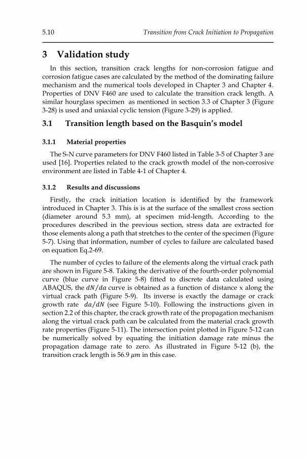
5.10 Transition from Crack Initiation to Propagation
3 Validation study
In this section, transition crack lengths for non-corrosion fatigue and corrosion fatigue cases are calculated by the method of the dominating failure mechanism and the numerical tools developed in Chapter 3 and Chapter 4. Properties of DNV F460 are used to calculate the transition crack length. A similar hourglass specimen as mentioned in section 3.3 of Chapter 3 (Figure 3-28) is used and uniaxial cyclic tension (Figure 3-29) is applied.
3.1 Transition length based on the Basquin’s model
3.1.1 Material properties
The S-N curve parameters for DNV F460 listed in Table 3-5 of Chapter 3 are used [16]. Properties related to the crack growth model of the non-corrosive environment are listed in Table 4-1 of Chapter 4.
3.1.2 Results and discussions
Firstly, the crack initiation location is identified by the framework introduced in Chapter 3. This is is at the surface of the smallest cross section (diameter around 5.3 mm), at specimen mid-length. According to the procedures described in the previous section, stress data are extracted for those elements along a path that stretches to the center of the specimen (Figure 5-7). Using that information, number of cycles to failure are calculated based on equation Eq.2-69.
The number of cycles to failure of the elements along the virtual crack path are shown in Figure 5-8. Taking the derivative of the fourth-order polynomial curve (blue curve in Figure 5-8) fitted to discrete data calculated using ABAQUS, the 𝑑𝑁 𝑑𝑎⁄ curve is obtained as a function of distance x along the virtual crack path (Figure 5-9). Its inverse is exactly the damage or crack growth rate 𝑑𝑎 𝑑𝑁⁄ (see Figure 5-10). Following the instructions given in section 2.2 of this chapter, the crack growth rate of the propagation mechanism along the virtual crack path can be calculated from the material crack growth rate properties (Figure 5-11). The intersection point plotted in Figure 5-12 can be numerically solved by equating the initiation damage rate minus the propagation damage rate to zero. As illustrated in Figure 5-12 (b), the transition crack length is 56.9 𝜇𝑚 in this case.
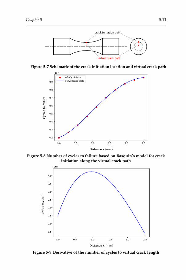
Chapter 5 5.11
Figure 5-7 Schematic of the crack initiation location and virtual crack path
Figure 5-8 Number of cycles to failure based on Basquin’s model for crack initiation along the virtual crack path
Figure 5-9 Derivative of the number of cycles to virtual crack length
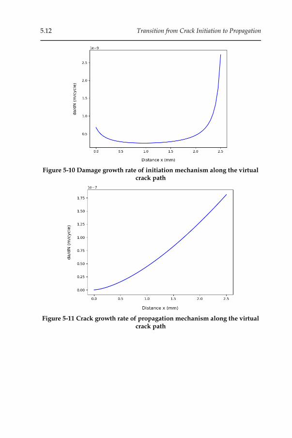
5.12 Transition from Crack Initiation to Propagation
Figure 5-10 Damage growth rate of initiation mechanism along the virtual crack path
Figure 5-11 Crack growth rate of propagation mechanism along the virtual crack path
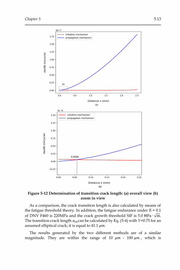
Chapter 5 5.13
Figure 5-12 Determination of transition crack length: (a) overall view (b) zoom in view
As a comparison, the crack transition length is also calculated by means of the fatigue threshold theory. In addition, the fatigue endurance under R = 0.1
of DNV F460 is 220MPa and the crack growth threshold SIF is 5.0 MPa ∙ √m. The transition crack length 𝑎𝑡ℎcan be calculated by Eq. (5-4) with Y=0.75 for an assumed elliptical crack; it is equal to 41.1 𝜇𝑚.
The results generated by the two different methods are of a similar magnitude. They are within the range of 10 𝜇𝑚 - 100 𝜇𝑚 , which is
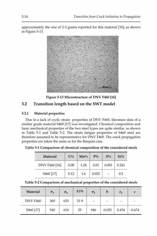
5.14 Transition from Crack Initiation to Propagation
approximately the size of 2-3 grains reported for this material [16], as shown in Figure 5-13.
Figure 5-13 Microstructure of DNV F460 [16]
3.2 Transition length based on the SWT model
3.2.1 Material properties
Due to a lack of cyclic strain properties of DNV F460, literature data of a similar grade material S460 [17] was investigated. Chemical composition and basic mechanical properties of the two steel types are quite similar, as shown in Table 5-1 and Table 5-2. The strain fatigue properties of S460 steel are therefore assumed to be representative for DNV F460. The crack propagation properties are taken the same as for the Basquin case.
Table 5-1 Comparison of chemical composition of the considered steels
Material C% Mn% P% S% Si%
DNV F460 [16] 0.08 1.24 0.01 0.001 0.241
S460 [17] 0.12 1.6 0.025 - 0.5
Table 5-2 Comparison of mechanical properties of the considered steels
Material 𝝈𝒚 𝝈𝒖 A5% 𝝈𝒇` b 𝜺𝒇
` c
DNV F460 560 635 31.9 - - - -
S460 [17] 540 634 35 946 -0.052 0.434 -0.674
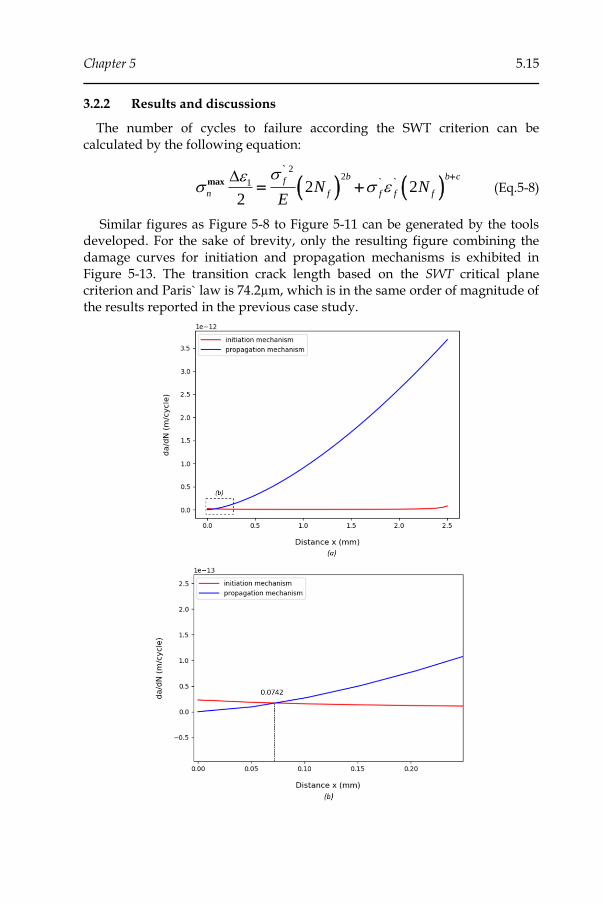
Chapter 5 5.15
3.2.2 Results and discussions
The number of cycles to failure according the SWT criterion can be calculated by the following equation:
( ) ( )2
21 2 2
2
`
max ` `b b cf
n f f f fN N
E
+
= + (Eq.5-8)
Similar figures as Figure 5-8 to Figure 5-11 can be generated by the tools developed. For the sake of brevity, only the resulting figure combining the damage curves for initiation and propagation mechanisms is exhibited in Figure 5-13. The transition crack length based on the SWT critical plane criterion and Paris` law is 74.2µm, which is in the same order of magnitude of the results reported in the previous case study.
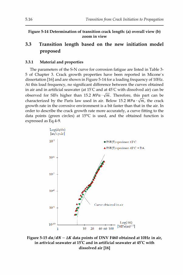
5.16 Transition from Crack Initiation to Propagation
Figure 5-14 Determination of transition crack length: (a) overall view (b) zoom in view
3.3 Transition length based on the new initiation model
proposed
3.3.1 Material and properties
The parameters of the S-N curve for corrosion fatigue are listed in Table 3-5 of Chapter 3. Crack growth properties have been reported in Micone`s dissertation [16] and are shown in Figure 5-14 for a loading frequency of 10Hz. At this load frequency, no significant difference between the curves obtained in air and in artificial seawater (at 15°C and at 45°C with dissolved air) can be
observed for SIFs higher than 15.2 𝑀𝑃𝑎 ∙ √𝑚 . Therefore, this part can be
characterized by the Paris law used in air. Below 15.2 𝑀𝑃𝑎 ∙ √𝑚, the crack growth rate in the corrosive environment is a bit faster than that in the air. In order to describe the crack growth rate more accurately, a curve fitting to the data points (green circles) at 15°C is used, and the obtained function is expressed as Eq.4-9.
Figure 5-15 𝒅𝒂 𝒅𝑵⁄ − ∆𝑲 data points of DNV F460 obtained at 10Hz in air, in artivical seawater at 15°C and in artificial seawater at 45°C with
dissolved air [16]
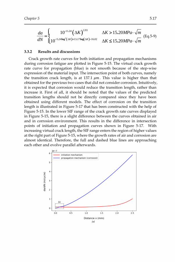
Chapter 5 5.17
( )( ) ( )2
2 9311 24
5 24 13 17 16 02
10 15 20
10 15 20K K
K K MPa mda
dN K MPa m
.- .
. log . log .
.
.− + −
=
(Eq.5-9)
3.3.2 Results and discussions
Crack growth rate curves for both initiation and propagation mechanisms during corrosion fatigue are plotted in Figure 5-15. The virtual crack growth rate curve for propagation (blue) is not smooth because of the step-wise expression of the material input. The intersection point of both curves, namely the transition crack length, is at 137.1 𝜇𝑚 . This value is higher than that obtained for the previous two cases that did not consider corrosion. Intuitively, it is expected that corrosion would reduce the transition length, rather than increase it. First of all, it should be noted that the values of the predicted transition lengths should not be directly compared since they have been obtained using different models. The effect of corrosion on the transition length is illustrated in Figure 5-17 that has been constructed with the help of Figure 5-15. In the lower SIF range of the crack growth rate curves displayed in Figure 5-15, there is a slight difference between the curves obtained in air and in corrosion environment. This results in the difference in intersection points of initiation and propagation curves shown in Figure 5-17. With increasing virtual crack length, the SIF range enters the region of higher values at the right part of Figure 5-15, where the growth rates of air and corrosion are almost identical. Therefore, the full and dashed blue lines are approaching each other and evolve parallel afterwards.

5.18 Transition from Crack Initiation to Propagation
Figure 5-16 Determination of transition crack length : (a) overall view (b) zoom in view
Figure 5-17 Influence of corrosion crack growth rate
4 Summary and conclusion
In this chapter, a definition of transition crack length which distinguishes the technical boundary between fatigue crack initiation and crack propagation was discussed. A numerical tool based on the dominated-mechanism method was developed and the calculation procedures were given in detail.
Chapter 5 5.19
Three examples were carried out to examine the sensitivity and robustness of the tool. Compared to empirical estimation and fatigue resistance threshold method, the dominance mechanism method yields a reasonable transition crack size for two plain fatigue examples; the values obtained from the three methods are close to each other. For the case of corrosion fatigue, the calculated transition crack length was 2 to 3 times higher than observed for non-corrosion cases, which is caused by lower crack growth rate than expected in corrosive environment.
The discussed cases studies demonstrate the capability of the automated numerical tool developed in this work to provide an indicative crack size at the transition from initiation to propagation. Based on the outcome of these three case studies, it is concluded that one should be cautious to use only one method but rather compare predictions from various resources.
5.20 Transition from Crack Initiation to Propagation
References
1. Min, L., S. Qing, and Y. Qing-xiong, Large sample size experimental investigation on the statistical nature of fatigue crack initiation and growth. International journal of fatigue, 1996. 18(2): p. 87-94.
2. Murtaza, G. and R. Akid, Modelling short fatigue crack growth in a heat-treated low-alloy steel. International Journal of Fatigue, 1995. 17(3): p. 207-214.
3. Krupp, U., Fatigue Crack Propagation in Metals and Alloys: Microstructural Aspects and Modelling Concepts. 2007: Wiley.
4. ASTM, E112-96 Standard test methods for determining average grain size. West Conshohocken, PA: ASTM International, 2004.
5. Kujawski, D. and F. Ellyin, Crack initiation and total fatigue life of a carbon steel in vacuum and air. Journal of testing and evaluation, 1992. 20(6): p. 391-395.
6. Scott Martin, W. and P.H. Wirsching, Fatigue crack initiation—Propagation reliability model. Journal of Materials in Civil Engineering, 1991. 3(1): p. 1-18.
7. Kaynak, C., A. Ankara, and T. Baker, Effects of short cracks on fatigue life calculations. International Journal of fatigue, 1996. 18(1): p. 25-31.
8. Ibrahim, M. and K. Miller, Determination of fatigue crack initiation life. Fatigue & Fracture of Engineering Materials & Structures, 1979. 2(4): p. 351-360.
9. Committee on fatigue and fracture reliability of the committee on structural safety and reliability of the structural division, fatigue reliability 1–4, ASCE. Journal of Structural Engineering, 1982. 108: p. 3-88.
10. Hyspecký P. Strnadel B., Conversion Of Short Fatigue Cracks Into A Long Crack. Fatigue & Fracture of Engineering Materials & Structures, 1992. 15(9): p. 845-854.
11. Dowling, N.E., Mechanical behavior of materials: engineering methods for deformation, fracture, and fatigue. 2012: Pearson.
12. Kitagawa, H., Applicability of fracture mechanics to very small cracks or the cracks in the early stage. Proc. of 2nd ICM, Cleveland, 1976, 1976: p. 627-631.
13. Murakami, Y., Stress Intensity Factors Handbook. 2001: Elsevier.

Chapter 5 5.21
14. Socie, D.F., J. Morrow, and W.-C. Chen, A procedure for estimating the total fatigue life of notched and cracked members. Engineering Fracture Mechanics, 1979. 11(4): p. 851-859.
15. Chen, W.-C., A model for joining the fatigue crack initiation and propagation analyses. 1980, University of Illinois at Urbana-Champaign.
16. Micone, N., Development of Testing Methodologies for the Analysis of Variable Amplitude Fatigue and Corrosion-Fatigue of Offshore Steels. 2017, Ghent University.
17. Versaillot, P.D. and L.I. BOTH, Effects of cyclic loading on the mechanical properties of steel. 2017.

Extensions to the Frameworks

6.2 Extensions to the Frameworks
<< This page intentionally left blank >>
Chapter 6 6.3
1 Overview
The fatigue analysis framework introduced in the previous chapters has been designed by means of object oriented programming, which enables potential extension with additional features. Two extensions, taking into account variable amplitude loading and the presence of residual stress, are discussed in this chapter.
Variable amplitude loading has different effects, called sequence and interaction effects, on the fatigue crack initiation and propagation stages. The numerical estimation of fatigue crack initiation lifetime has been discussed in Chapter 3. The damage model introduced inherently covers the sequence effects. In the following section, the influence of variable amplitude loading on fatigue crack propagation and a dedicated FE model will be elaborated.
Fatigue crack growth in a structure depends on the stress amplitude, stress ratio (or mean stress), crack geometry and many other parameters. Scenarios of constant amplitude loading have been successfully described with the help of fracture mechanics by expressing the relationship between SIF range and fatigue crack extension per cycle [1]. However, it is more difficult to model crack growth under more complex fatigue loading conditions, which may comprise singular or sequential overloads, underloads, combinations and/or random loading. The effects of variable loading on fatigue crack propagation were first observed by the aviation industry. Singular overloads contribute to a decrease of the crack growth rate, while underloads to an acceleration of the rate [2]; these are called interaction effects. Experiments revealed that after applying a single overload cycle in between constant amplitude loading cycles, crack propagation was slower than for constant amplitude fatigue [3], a severe overloading can even give rise to crack arrest. The mechanisms contributing to load interaction effects show that plastic straining or residual stress in front of the crack tip induces compressive stress and increases the difficulty of crack opening, thus leading to crack growth retardation [4]. To lower the degree of conservatism of a fatigue design – and thus indirectly the safety factor, material usage and cost – researchers tried to account for the retardation effect. Most studies have focused on the behavior of aluminum alloys, which were frequently used in the aviation industry [3, 5-8].
Other than aluminum and titanium alloys which are applied as a main structural material in the aviation industry, welded steel structures such as bridges, ship hulls, offshore wind turbines, and oil platforms are more widely used. They are continuously subjected to variable loading conditions [9-11] as well, due to various influences from vehicles, sea wave and wind current amongst others. As this problem concerns high cycle fatigue, the first requirement for a suitable fatigue crack propagation model and simulation algorithm is reasonable overall computation time. Additionally, the model
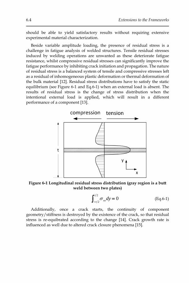
6.4 Extensions to the Frameworks
should be able to yield satisfactory results without requiring extensive experimental material characterization.
Beside variable amplitude loading, the presence of residual stress is a challenge in fatigue analysis of welded structures. Tensile residual stresses induced by welding operations are unwanted as these deteriorate fatigue resistance, whilst compressive residual stresses can significantly improve the fatigue performance by inhibiting crack initiation and propagation. The nature of residual stress is a balanced system of tensile and compressive stresses left as a residual of inhomogeneous plastic deformation or thermal deformation of the bulk material [12]. Residual stress distributions have to satisfy the static equilibrium (see Figure 6-1 and Eq.6-1) when an external load is absent. The results of residual stress is the change of stress distribution when the intentional external load is applied, which will result in a different performance of a component [13].
Figure 6-1 Longitudinal residual stress distribution (gray region is a butt weld between two plates)
2
20
t
xxt
dy−
= (Eq.6-1)
Additionally, once a crack starts, the continuity of component geometry/stiffness is destroyed by the existence of the crack, so that residual stress is re-equibrated according to the change [14]. Crack growth rate is influenced as well due to altered crack closure phenomena [15].
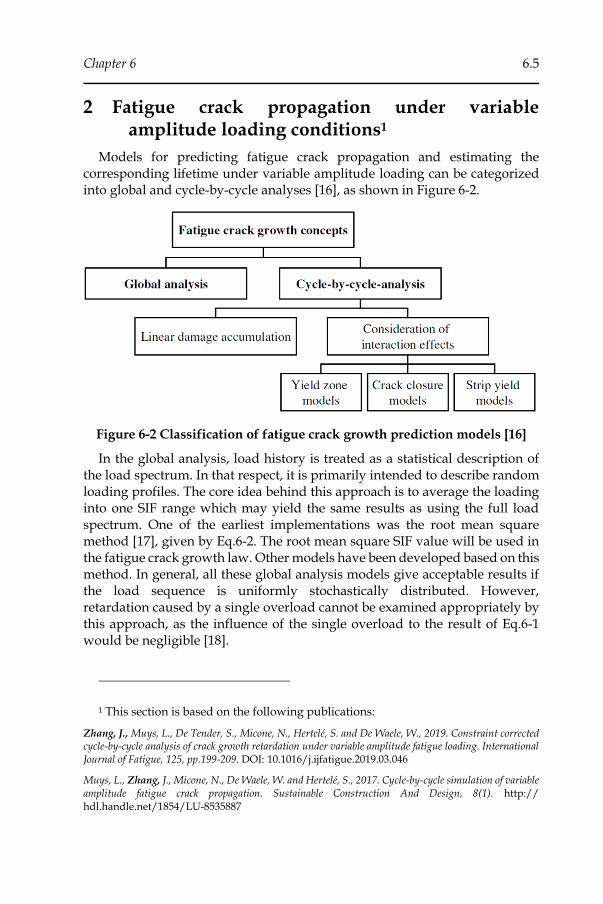
Chapter 6 6.5
2 Fatigue crack propagation under variable amplitude loading conditions1
Models for predicting fatigue crack propagation and estimating the corresponding lifetime under variable amplitude loading can be categorized into global and cycle-by-cycle analyses [16], as shown in Figure 6-2.
Figure 6-2 Classification of fatigue crack growth prediction models [16]
In the global analysis, load history is treated as a statistical description of the load spectrum. In that respect, it is primarily intended to describe random loading profiles. The core idea behind this approach is to average the loading into one SIF range which may yield the same results as using the full load spectrum. One of the earliest implementations was the root mean square method [17], given by Eq.6-2. The root mean square SIF value will be used in the fatigue crack growth law. Other models have been developed based on this method. In general, all these global analysis models give acceptable results if the load sequence is uniformly stochastically distributed. However, retardation caused by a single overload cannot be examined appropriately by this approach, as the influence of the single overload to the result of Eq.6-1 would be negligible [18].
1 This section is based on the following publications:
Zhang, J., Muys, L., De Tender, S., Micone, N., Hertelé, S. and De Waele, W., 2019. Constraint corrected cycle-by-cycle analysis of crack growth retardation under variable amplitude fatigue loading. International Journal of Fatigue, 125, pp.199-209. DOI: 10.1016/j.ijfatigue.2019.03.046
Muys, L., Zhang, J., Micone, N., De Waele, W. and Hertelé, S., 2017. Cycle-by-cycle simulation of variable amplitude fatigue crack propagation. Sustainable Construction And Design, 8(1). http:// hdl.handle.net/1854/LU-8535887
6.6 Extensions to the Frameworks
2
1
1 N
rms i
i
K KN =
= (Eq.6-2)
In a cycle-by-cycle analysis, the load history is examined and updated each cycle to calculate the further crack growth Eq.6-3. The sum of crack growth increments by every individual cycle without accounting for load history delivers satisfactory results only when overload interaction is negligible or when retardation and acceleration phenomena cancel out each other [18].
( )0
1
, ,n
n i i
i
a a f K R history=
= + (Eq.6-3)
To consider load interactions, three main categories of cycle-by-cycle models have been developed in literature: plastic zone models, crack closure models, and residual stress models. Plastic zone models are based on plasticity analysis ahead of the crack tip, while crack closure models focus on compressive forces due to contact between the crack faces as a result of load history effects. Relative to each other, crack closure models require more extensive experimental characterization and/or numerical calculations [16, 19-23], and thus do not meet the requirements stated above. Residual stress models were proposed as an alternative to the crack closure concept and require calculation of the residual stress field in front of the crack tip in detail. They also require a thorough and time-consuming experimental calibration of the models [16, 21].
Due to inherent practical simplicity (relating to a small number of parameters to be experimentally calibrated), plastic zone models will be applied in this dissertation, and extended methods based on the well-known Wheeler model and Willenborg model are proposed. Plastic zone models account for variable amplitude loading effects by considering the state of the material in front of the crack tip, where some regions have undergone yielding while others have not. To this purpose, the plastic zone induced at the crack tip is discussed first. Based on this, the load interaction zone concept, common to all plastic zone models, is introduced and illustrated with the Wheeler model and Willenborg model. These models are implemented in an efficient cycle-by-cycle based numerical framework and simulation results will be evaluated by comparing with experimental results.
2.1 Plastic zone models
Linear elastic stress analysis of perfectly sharp cracks theoretically results in infinitely high stresses at the crack tip, shown in Figure 6-3. In reality, however, the stresses are finite due to the blunting of the crack tip upon loading and plastic deformation in front of the crack tip [24]. The general formula for calculating the plastic zone size for a given SIF level is provided in by Eq.6-4:
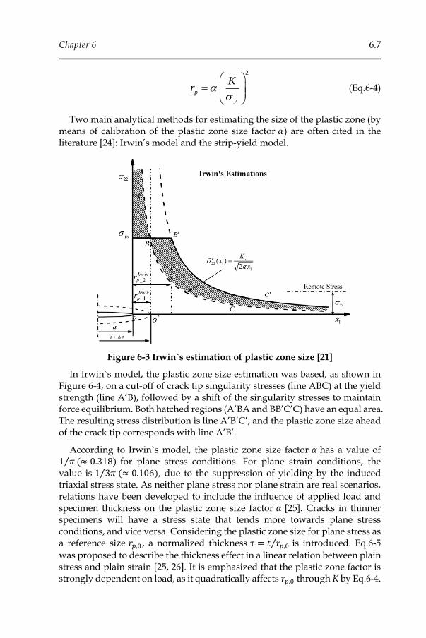
Chapter 6 6.7
2
p
y
Kr
=
(Eq.6-4)
Two main analytical methods for estimating the size of the plastic zone (by means of calibration of the plastic zone size factor 𝛼) are often cited in the literature [24]: Irwin’s model and the strip-yield model.
Figure 6-3 Irwin`s estimation of plastic zone size [21]
In Irwin`s model, the plastic zone size estimation was based, as shown in Figure 6-4, on a cut-off of crack tip singularity stresses (line ABC) at the yield strength (line A’B), followed by a shift of the singularity stresses to maintain force equilibrium. Both hatched regions (A’BA and BB’C’C) have an equal area. The resulting stress distribution is line A’B’C’, and the plastic zone size ahead of the crack tip corresponds with line A’B’.
According to Irwin`s model, the plastic zone size factor 𝛼 has a value of 1 𝜋⁄ (≈ 0.318) for plane stress conditions. For plane strain conditions, the value is 1 3𝜋 (≈ 0.106)⁄ , due to the suppression of yielding by the induced triaxial stress state. As neither plane stress nor plane strain are real scenarios, relations have been developed to include the influence of applied load and specimen thickness on the plastic zone size factor 𝛼 [25]. Cracks in thinner specimens will have a stress state that tends more towards plane stress conditions, and vice versa. Considering the plastic zone size for plane stress as a reference size 𝑟𝑝,0 , a normalized thickness τ = 𝑡 𝑟𝑝,0⁄ is introduced. Eq.6-5
was proposed to describe the thickness effect in a linear relation between plain stress and plain strain [25, 26]. It is emphasized that the plastic zone factor is strongly dependent on load, as it quadratically affects 𝑟𝑝,0 through K by Eq.6-4.

6.8 Extensions to the Frameworks
11
1 2 2 51 2 5
3 3 2 5 1
12 5
3
..
.
.
−
= + −
(Eq.6-5)
The strip yield plastic zone model was developed by Dugdale and Barenblatt, considering small scale yielding conditions as a complement to linear elastic fracture mechanics [27]. The model assumes that all deformation concentrates in a strip in front of the crack. As depicted in Figure 6-4, elastic-plastic behavior is approximated by superimposing two elastic solutions for a through crack of length 2𝑎 + 2𝑟𝑝 in an infinite plate subjected to plane stress
conditions. Remote tension over the entire crack length is supplemented with closure stresses at both crack tips over a length 𝑟𝑝, which is the length of the
long, slender plastic zone. The closure stress is equal to the yield stress of the material. By superposition (expressing that no singularity should occur at the tips of the virtual extended crack having length 2𝑎 + 2𝑟𝑝), 𝛼 = 𝜋 8⁄ (≈ 0.393) is
calculated [24]. Note that this value is slightly different from Irwin`s approach for plane stress conditions (1/ 𝜋 ≈ 0.393).
Figure 6-4 Visual representation of the strip yield model [25]
Guo extended the strip model three-dimensionally to obtain valid solutions for plates of finite thickness [28]. A global plastic constraint factor 𝜂 was introduced to include effects of out-of-plane and in-plane constraint relative to the plane stress equation for rp, as shown in Eq.6-6:
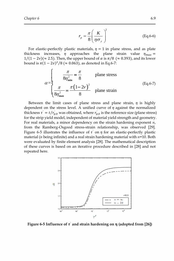
Chapter 6 6.9
2
8p
y
Kr
=
(Eq.6-6)
For elastic-perfectly plastic materials, 𝜂 = 1 in plane stress, and as plate thickness increases, 𝜂 approaches the plane strain value 𝜂𝑚𝑎𝑥 =1 (1 − 2𝜈)(≈ 2.5)⁄ . Then, the upper bound of 𝛼 is 𝜋 8⁄ (≈ 0.393), and its lower bound is 𝜋(1 − 2𝑣)2 8 (≈ 0.063)⁄ , as denoted in Eq.6-7:
( )
2
2
2
plane stress8 8
=1 2
plane strain8 8
min
max
=
−=
(Eq.6-7)
Between the limit cases of plane stress and plane strain, 𝜂 is highly dependent on the stress level. A unified curve of 𝜂 against the normalized
thickness 𝜏 ` = 𝑡 𝑟𝑝,0`⁄ was obtained, where 𝑟𝑝,0
` is the reference size (plane stress)
for the strip yield model, independent of material yield strength and geometry. For real materials, a minor dependency on the strain hardening exponent n, from the Ramberg-Osgood stress-strain relationship, was observed [29].
Figure 6-5 illustrates the influence of 𝜏` on 𝜂 for an elastic-perfectly plastic material (n being infinite) and a real strain hardening material with n=10. Both were evaluated by finite element analysis [28]. The mathematical description of these curves is based on an iterative procedure described in [28] and not repeated here.
Figure 6-5 Influence of 𝝉` and strain hardening on 𝛈 (adopted from [26])
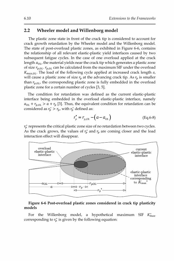
6.10 Extensions to the Frameworks
2.2 Wheeler model and Willenborg model
The plastic zone state in front of the crack tip is considered to account for crack growth retardation by the Wheeler model and the Willenborg model. The state of post-overload plastic zones, as exhibited in Figure 6-6, contains the relationship of all relevant elastic-plastic yield interfaces caused by two subsequent fatigue cycles. In the case of one overload applied at the crack length 𝑎𝑂𝐿, the material yields near the crack tip which generates a plastic zone of size 𝑟𝑝,𝑂𝐿. 𝑟𝑝,𝑂𝐿 can be calculated from the maximum SIF under the overload
𝐾𝑚𝑎𝑥,𝑂𝐿. The load of the following cycle applied at increased crack length a, will cause a plastic zone of size 𝑟𝑝 at the advancing crack tip. As 𝑟𝑝 is smaller
than 𝑟𝑝,𝑂𝐿, the corresponding plastic zone is fully embedded in the overload
plastic zone for a certain number of cycles [3, 5].
The condition for retardation was defined as the current elastic-plastic interface being embedded in the overload elastic-plastic interface, namely 𝑎𝑂𝐿 + 𝑟𝑝,𝑂𝐿 > 𝑎 + 𝑟𝑝 [3]. Thus, the equivalent condition for retardation can be
considered as 𝑟𝑝∗ > 𝑟𝑝, with 𝑟𝑝
∗ defined as:
( ),p p OL OLr r a a = − − (Eq.6-8)
𝑟𝑝∗ represents the critical plastic zone size of no retardation between two cycles.
As the crack grows, the values of 𝑟𝑝∗ and 𝑟𝑝 are coming closer and the load
interaction effect will disappear.
Figure 6-6 Post-overload plastic zones considered in crack tip plasticity models
For the Willenborg model, a hypothetical maximum SIF 𝐾𝑚𝑎𝑥∗
corresponding to 𝑟𝑝∗ is given by the following equation:
Chapter 6 6.11
1max max, max,
, ,
p OL
OL OL
p OL p OL
r a aK K K
r r
−= = − (Eq.6-9)
Then, the condition for retardation can be interpreted as 𝐾𝑚𝑎𝑥∗ > 𝐾𝑚𝑎𝑥 as well.
The following two subsections further elaborate on the Wheeler and Willenborg models respectively.
2.2.1 Wheeler model
Wheeler’s model serves as an independent alternative to Willenborg’s model explained above. Noticing that fatigue lifetime predictions based on linear cumulative crack growth were often found to be ultra-conservative [3], Wheeler modified the non-interaction models for constant amplitude by introducing a retardation factor 𝜙𝑤ℎ to the conventional fatigue crack growth rate (in absence of retardation effects). This factor is in the range between 0 to 1, representing the degree of absence of interaction. The Wheeler model does not change input for the crack growth law (e.g. Δ𝐾 and 𝑅 ), so the straightforward Paris equation can be employed, provided that its parameters C and m were obtained under the correct load ratio R. This is illustrated in Eq.6-10, in which 𝑛 is the number of applied cycles and Δ𝐾𝑖 is the SIF range of cycle 𝑖. Load interaction effects can potentially be simulated as the net crack growth rate is no longer independent of prior load history.
( )0
1
,,
n
n wh i i i
i
a a f K R=
= + (Eq.6-10)
The expression of the retardation factor 𝜙𝑤ℎ is given in Eq.6-11 and Eq.6-12. The equations are based on estimations of plastic zone size. The state of the material in front of the crack tip considered by crack tip plasticity models is illustrated in Figure 6-6.
1
,
,
,
p
OL p OL p
wh OL p OL
OL p OL p
ra r a r
a r a
a r a r
+ + = + −
+ +
(Eq.6-11)
or
1
p
p p
wh p
p p
rr r
r
r r
=
(Eq.6-12)
6.12 Extensions to the Frameworks
The shape exponent 𝜔 is determined experimentally for a given material and type of loading because of its dependency on material strength and overload ratio [3, 30, 31]. Typical reported values range from 1.0 up to 4.0.
As 𝜙𝑤ℎ never equals zero unless 𝐾𝑚𝑎𝑥 is zero, the original Wheeler model will never predict crack arrest due to overloading. However, by introducing Δ𝐾𝑒𝑓𝑓, the retardation effect can also be expressed indirectly as Eq.6-13:
( )0
1
, ,, , i
n
n eff i i eff i i
i
a a f K R K K=
= + = (Eq.6-13)
This simple modification can be used with any form of crack growth law. If the assumed law comprises the threshold limit for zero fatigue crack growth,
Kth, crack arrest after an overload can be predicted when Δ𝐾𝑒𝑓𝑓,𝑖 ≤ ∆𝐾𝑡ℎ. Its
disadvantage is obviously that 𝛽 is an experimental fitting value [32]. However, it can be theoretically obtained by Eq.6-14 as 1/m when the Paris-Erdogan law is applied as a growth rate equation.
1
0
1
, ,( )( ) , i
nm m
n eff i eff i i
i
a a C R K K K=
= + = (Eq.6-14)
Since the model parameters above have not always been experimentally documented and curve-fitting is generally required, a modified Wheeler model based on a fully experimental calibration was proposed [8, 26]. It was based on the observation of crack arrest for overload values exceeding a load ratio value 𝑅𝑆𝑂 with respect to the nominal load. 𝑅𝑆𝑂 typically ranges from 1.5 to 3.0, depending on the material. It was reasoned that at the onset of crack arrest, the effective SIF range does not exceed the threshold SIF range for the material. As 𝑚 is the Paris exponent, the shaping exponent can be determined from readily available material data. It is no longer a constant but a function of the material and the subsequent loading cycles. Assuming a constant 𝛼 for the time being, in the critical case where the effective SIF ∆𝐾𝑒𝑓𝑓 equals the
threshold ∆𝐾𝑡ℎ, the crack arrests to grow and the overload ratio 𝑅𝑂𝐿 = 𝑅𝑆𝑂. Then, 𝜔 can be obtained by solving Eq.6-15 for 𝜔 leading to (Eq.6-16) (noting that 𝑟𝑝 𝑟𝑝,𝑂𝐿⁄ = 𝑅𝑆𝑂
2 when 𝛼 is constant, based on Eq.6-4 which will be
discussed below). For a variable 𝛼, the shut-off ratio 𝑅𝑆𝑂 should be replaced
by the more general expression √𝑟𝑝,𝑂𝐿 𝑟𝑂𝐿⁄ .
( )1
,OL
mm
p
th a a
p OL
rK K K
r
=
= =
(Eq.6-15)
1
2
th
SO
Kmlog log
K R
=
(Eq.6-16)
Chapter 6 6.13
2.2.2 Willenborg model
Different from Wheeler`s model, the Willenborg model assumed that retardation occurs due to the reduction of crack driving force by residual compressive stress generated in the overload plastic zone [5]. Reflected in the formula as shown in Eq.6-17, the Willenborg model modifies the input for crack growth law, ∆𝐾 and R, to calculate the reduced crack growth rate indirectly.
( )0
1
,n
i i
n eff eff
i
a a f K R=
= + (Eq.6-17)
Since different effective load ratios 𝑅𝑒𝑓𝑓 are calculated by the Willenborg
model, Paris law curves corresponding to different load ratios are required. Thus, use of the Forman equation or Walker equation is recommended [5, 6], although the Paris law can be adopted if a quantification of the load ratio effect is lacking or if there is reason to believe the load ratio effect can be neglected [33].
The stress reduced 𝐾𝑟𝑒𝑑 is defined as follows,
max maxredK K K= − (Eq.6-18)
where 𝐾𝑚𝑎𝑥∗ is maximum SIF without retardation, 𝐾𝑚𝑎𝑥 is real maximum SIF.
The effective SIF ranges and load ratio are calculated by reducing both 𝐾𝑚𝑎𝑥 and 𝐾𝑚𝑖𝑛 by 𝐾𝑟𝑒𝑑 and are non-negative values, as shown in Eq.6-19 and Eq.6-20:
0
min
min
max
max min
red
red
redeff
red
K KK K
K KR
K K K
−
−=
(Eq.6-19)
min
max max min
red
eff
red red
K K KK
K K K K K
=
− (Eq.6-20)
According to Eq.6-19 and Eq.6-20, crack arrest can be predicted for high overload ratios leading to high residual stress in the overload plastic zone when 𝐾𝑟𝑒𝑑 exceeds the 𝐾𝑚𝑎𝑥. For lower overload ratios when 𝐾𝑚𝑖𝑛 is beyond 𝐾𝑟𝑒𝑑, only the load ratio (mean stress effect) takes effect, as the SIF range is not changed. The critical value of crack arrest when 𝐾𝑚𝑎𝑥 = 𝐾𝑟𝑒𝑑 results in an invariable overload ratio of 2. However, as already mentioned above, literature reported that crack arrest can happen at different characteristic overload values 𝑅𝑆𝑂 ≠ 2 [7, 26]. This can cause inaccurate and potentially unconservative predictions. Thus, a generalized Willenborg model was

6.14 Extensions to the Frameworks
proposed to introduce a correction factor 𝜆 for 𝐾𝑟𝑒𝑑 to solve the problem [7]. Similar to the crack arrest situation within the Wheeler model, the assumption for the correction is that the effective crack driving force cannot exceed the crack growth threshold SIF range of the material when the crack arrests, as indicated in Eq.6-21. The result of 𝜆 is give in Eq.6-22.
( )max max, maxOLth eff a a OLK K K K K
== = − − (Eq.6-21)
1
1
max
th
SO
K
K
R
−
=−
(Eq.6-22)
2.3 Cycle-by-cycle crack propagation algorithm
As stated above, crack tip plasticity models analyze each applied cycle individually. Therefore, a numerical framework was developed in Python to be able to process a long load history in an automated, cycle-by-cycle way. A schematic overview of this algorithm is given in Figure 6-7.
Figure 6-7 Overview of the cycle-by-cycle crack propagation analysis algorithm
Before the analysis is started, the input load history has to be translated into a block sequence. It is basically a series of blocks in which every block contains the maximum and minimum applied SIF of the block-specific fatigue cycle and the number of experimentally applied cycles. There are different ways to translate load histories into sequential blocks, which are likely to produce (slightly) different retardation effects. Such translations are outside the scope of this dissertation, here a known block loading is assumed as starting point of the analysis.
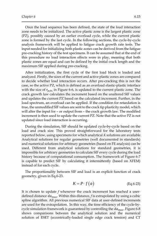
Chapter 6 6.15
Once the load sequence has been defined, the state of the load interaction zone needs to be initialized. The active plastic zone is the largest plastic zone (PZ), possibly caused by an earlier overload cycle, while the current plastic zone is formed by the last cycle. In the following sections, the cycle-by-cycle analysis framework will be applied to fatigue crack growth rate tests. The input needed for initializing both plastic zones can be derived from the fatigue pre-cracking history of the test specimens. It can be assumed that at the end of this procedure no load interaction effects were in play, meaning that both plastic zones are equal and can be defined by the initial crack length and the maximum SIF applied during pre-cracking.
After initialization, the first cycle of the first load block is loaded and analyzed. Firstly, the sizes of the current and active plastic zones are compared to decide whether load interaction occurs. After pre-cracking this is not the case, so the active PZ, which is defined as an overload elastic-plastic interface with the size of 𝑟𝑝,𝑂𝐿 in Figure 6-6, is updated to the current plastic zone. The
crack growth law calculates the increment based on the unaltered SIF values and updates the current PZ based on the calculated increment. Further, in the load spectrum, an overload can be applied. If the condition for retardation is true, the unmodified SIF values are sent to the crack tip plasticity model, which will alter the input for – or output from – the crack growth law. The modified increment is then used to update the current PZ. Note that the active PZ is not updated since load interaction is occurring.
During the simulation, SIF should be updated cycle-by-cycle based on the load and crack size. This proved straightforward for the laboratory tests reported below, using specimens for which analytical K solutions are available. Analytical solutions for regular geometries (well documented in standards) and numerical solutions for arbitrary geometries (based on FE analysis) can be used. Different from analytical solutions for standard geometries, it is impossible for arbitrary geometries to calculate SIF every cycle during the load history because of computational consumption. The framework of Figure 6-7 is capable to predict SIF by calculating it intermittently (based on XFEM) instead of for each cycle.
The proportionality between SIF and load is an explicit function of crack geometry, given in Eq.6-23.
( )K P f a= (Eq.6-23)
It is chosen to update f whenever the crack increment has reached a user-defined distance 𝑑𝑎𝑚𝑎𝑥. Within this distance, f is extrapolated by using a cubic spline algorithm. All previous numerical SIF data at user-defined increments are used for the extrapolation. In this way, the time efficiency of the cycle-by-cycle simulation framework is guaranteed by controlling the 𝑑𝑎𝑚𝑎𝑥. Figure 6-8 shows comparisons between the analytical solution and the numerical solution of ESET (eccentrically-loaded single edge crack tension) and CT
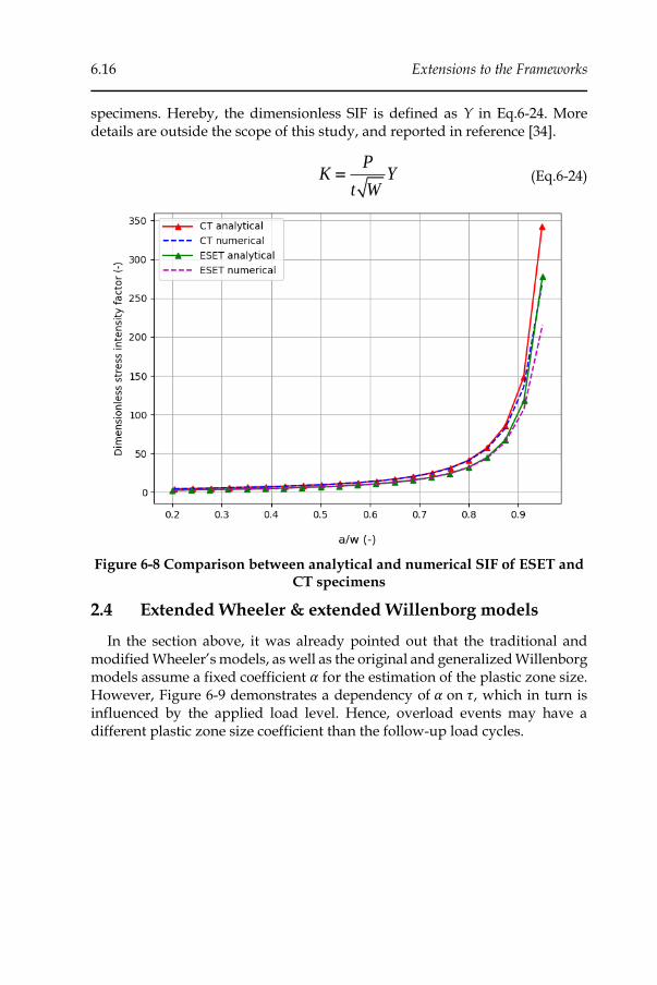
6.16 Extensions to the Frameworks
specimens. Hereby, the dimensionless SIF is defined as Y in Eq.6-24. More details are outside the scope of this study, and reported in reference [34].
PK Y
t W= (Eq.6-24)
Figure 6-8 Comparison between analytical and numerical SIF of ESET and CT specimens
2.4 Extended Wheeler & extended Willenborg models
In the section above, it was already pointed out that the traditional and modified Wheeler’s models, as well as the original and generalized Willenborg models assume a fixed coefficient 𝛼 for the estimation of the plastic zone size. However, Figure 6-9 demonstrates a dependency of 𝛼 on 𝜏, which in turn is influenced by the applied load level. Hence, overload events may have a different plastic zone size coefficient than the follow-up load cycles.
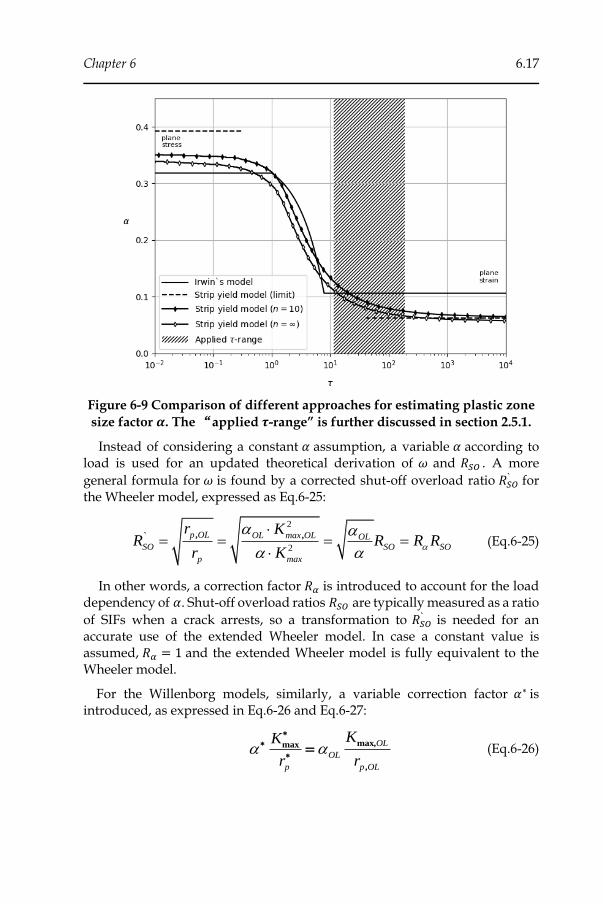
Chapter 6 6.17
Figure 6-9 Comparison of different approaches for estimating plastic zone
size factor 𝜶. The “applied 𝝉-range” is further discussed in section 2.5.1.
Instead of considering a constant 𝛼 assumption, a variable 𝛼 according to load is used for an updated theoretical derivation of 𝜔 and 𝑅𝑆𝑂 . A more
general formula for 𝜔 is found by a corrected shut-off overload ratio 𝑅𝑆𝑂` for
the Wheeler model, expressed as Eq.6-25:
2
2
, ,` p OL OL max OL OLSO SO SO
p max
r KR R R R
r K
= = = =
(Eq.6-25)
In other words, a correction factor 𝑅𝛼 is introduced to account for the load dependency of 𝛼. Shut-off overload ratios 𝑅𝑆𝑂 are typically measured as a ratio
of SIFs when a crack arrests, so a transformation to 𝑅𝑆𝑂` is needed for an
accurate use of the extended Wheeler model. In case a constant value is assumed, 𝑅𝛼 = 1 and the extended Wheeler model is fully equivalent to the Wheeler model.
For the Willenborg models, similarly, a variable correction factor 𝛼∗ is introduced, as expressed in Eq.6-26 and Eq.6-27:
max,max
,
OL
OL
p p OL
KK
r r
= (Eq.6-26)

6.18 Extensions to the Frameworks
max max,
,
p OL
OL
p OL
rK K
r
= (Eq.6-27)
2.5 Crack growth retardation predictions using Wheeler and
Willenborg models
This section compares crack growth predictions using different crack tip plasticity-based retardation models against experimental fatigue crack growth rate data, obtained from high strength low alloy steels.
2.5.1 Material properties and specimen configuration
Different load sequences were applied to 15 mm thick ESET specimens of DNV F460 steel, which is widely used in offshore structures. The configuration of ESET specimens was designed according to standard ASTM E647 [35] as shown in Figure 6-9. Before testing, specimens were fatigue pre-cracked up to a minimum predefined crack length of about 50 % of the specimen width (a0/W ≈ 0.5) as suggested in the standard. Mechanical properties of DNV F460 steel are listed in Table 6-1. Particularly, C and m are experimentally obtained Paris-Erdogan parameters.
Table 6-1 Mechanical properties of DNV F460 steel
𝝈𝒚
(MPa)
𝝈𝒖
(MPa)
𝑲𝒄
(𝐌𝐏𝐚 ∙ √𝐦)
𝜟𝑲𝒕𝒉
(𝑴𝑷𝒂 ∙ √𝒎)
C
(m/cycle) m 𝜸
560 635 84.0 5.0 3.6e-12 3.06 0.7
Figure 6-10 Configuration of the tested ESET specimens (dimensions in mm)
Chapter 6 6.19
In Figure 6-9, the range of 𝜏 values obtained during the ESET tests are shown as a shaded band, along with their corresponding 𝛼 values according to Irwin`s model and the strip yield model. 𝜏 was in the range between 11.5 and 187.0. The figure indicates that the tests had a tendency towards plane strain. The strip yield model indicates variations of 𝛼 between 0.063 and 0.126 for the ESET specimen configuration used. These variations are not captured when using Irwin`s plastic zone model, as shown in the same figure.
2.5.2 Sensitivity analysis of governing parameters
2.5.2.1 Wheeler models
In the crack growth retardation model, many parameters are influential, such as plastic zone size factor 𝛼 , shaping exponent 𝜔 , fatigue crack threshold ∆𝐾𝑡ℎ and shut-off overload ratio. A sensitivity study was performed to analyze the effects of these parameters based on the load profile shown in Figure 6-18. All fatigue blocks of loading were applied with R=0.1, starting with a block
load ∆𝐾 = 22.8𝑀𝑃𝑎√𝑚 in order to obtain a stable linear crack growth. Then,
a single overload of ∆𝐾 = 32.2𝑀𝑃𝑎√𝑚 was applied to create an overload plastic zone. Retardation indeed occurred in the following cycles. The load ranges decreased step-wisely in the following load blocks as indicated in the figure.
Various crack growth predictions are shown in Figure 6-11. The upper dash-dotted line represents a reference case for which crack growth retardation was neglected (i.e., corresponding with the Paris law applied). The other lines represent predictions for different crack growth retardation model parameters, adopting the original Wheeler model. Irwin`s model was used to calculated 𝛼 values for the limit scenarios of plane stress and plane strain.
A first observation is that 𝛼 has a significant effect on the degree of retardation, as the fatigue crack retards more in plane stress conditions than in plane strain conditions. The explanation is that a higher 𝛼 (less constrained at the crack tip) will result in a larger plastic zone. A larger size of the plastic zone size leads to a higher degree of retardation factor and then a lower crack growth rate. It turns out that a correct estimation of plastic zone size is a precondition to achieve accurate crack growth predictions.
Secondly, there is a strong influence of the shaping exponent 𝜔 on crack growth retardation. On the other hand, some effects of 𝛼 and 𝜔 can be separated. 𝛼 rather affects the duration of retardation, whereas 𝜔 rather influences the degree of retardation (initial crack growth slope following an overload). On the other hand, there is a coupled effect: the influence of 𝛼 (plane stress and plane strain) is more pronounced for higher values of 𝜔.
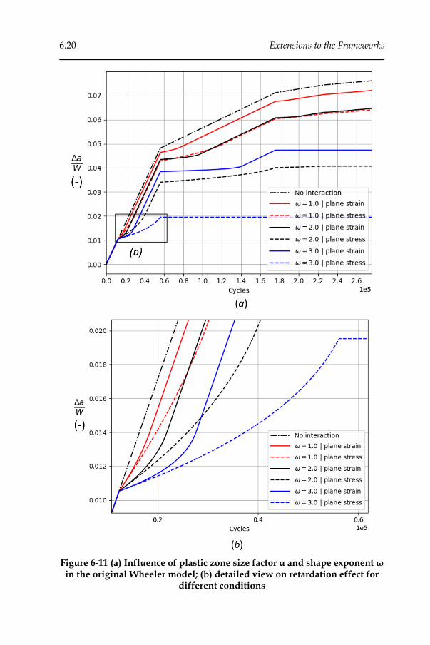
6.20 Extensions to the Frameworks
Figure 6-11 (a) Influence of plastic zone size factor α and shape exponent ω in the original Wheeler model; (b) detailed view on retardation effect for
different conditions

Chapter 6 6.21
In Figure 6-12, it is clear that 𝜔 can vary significantly as a function of load range, so it is not correct to simplify 𝜔 as a constant value in the original and modified Wheeler models. The threshold SIF range is also an influencing parameter, as an increase of ∆𝐾𝑡ℎ results in a decrease of 𝜔. Note that ∆𝐾𝑡ℎ is relatively sensitive to stress ratio R, according to the following empirical equation [36]:
( )01
th thK K R
= − (Eq.6-28)
where ∆𝐾𝑡ℎ0 represents the fatigue crack growth threshold for R=0; 𝛾 is a shaping exponent that varies between 0 and 1, typically 0.5 for mild steels and 0.7-0.9 for pearlitice steels, 𝛾 = 0.7 for DNV F460. In practical terms, ∆𝐾𝑡ℎ generally does not change much, so its influence will be moderate [37]. The influence of shut-off overload ratio 𝑅𝑆𝑂 on crack growth predictions is plotted in Figure 6-13 and Figure 6-14. In Figure 6-13, similar to what Figure 6-11 shows, retardation is quite sensitive to 𝑅𝑆𝑂 and the difference between plane stress and plane strain is even more pronounced. A lower 𝑅𝑆𝑂 increases 𝜔 and the degree of retardation, as the overload ratio 𝑅𝑂𝐿 is quite close to shut-off. As shown in Figure 6-14, when 𝑅𝑆𝑂 approaches the ratio of the single overload (𝑅𝑂𝐿 = 1.5), the retardation becomes very close to crack arrest.
Figure 6-12 Influence of shut-off overload ratio 𝑹𝑺𝑶 and fatigue crack threshold ∆𝑲𝒕𝒉 on the theoretical shaping exponent
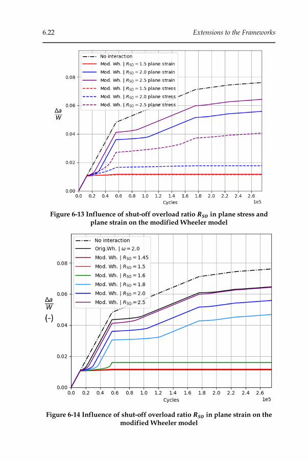
6.22 Extensions to the Frameworks
Figure 6-13 Influence of shut-off overload ratio 𝑹𝑺𝑶 in plane stress and plane strain on the modified Wheeler model
Figure 6-14 Influence of shut-off overload ratio 𝑹𝑺𝑶 in plane strain on the modified Wheeler model
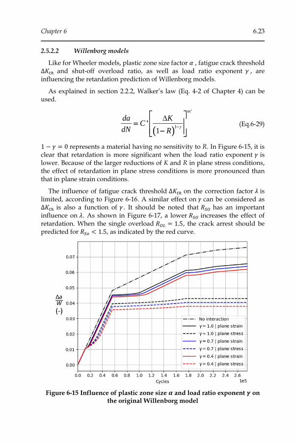
Chapter 6 6.23
2.5.2.2 Willenborg models
Like for Wheeler models, plastic zone size factor 𝛼 , fatigue crack threshold ∆𝐾𝑡ℎ and shut-off overload ratio, as well as load ratio exponent 𝛾 , are influencing the retardation prediction of Willenborg models.
As explained in section 2.2.2, Walker’s law (Eq. 4-2 of Chapter 4) can be used.
( )1
1
m
da KC
dN R
'
'−
=
−
(Eq.6-29)
1 − 𝛾 = 0 represents a material having no sensitivity to R. In Figure 6-15, it is clear that retardation is more significant when the load ratio exponent 𝛾 is lower. Because of the larger reductions of K and R in plane stress conditions, the effect of retardation in plane stress conditions is more pronounced than that in plane strain conditions.
The influence of fatigue crack threshold ∆𝐾𝑡ℎ on the correction factor 𝜆 is limited, according to Figure 6-16. A similar effect on 𝛾 can be considered as ∆𝐾𝑡ℎ is also a function of 𝛾 . It should be noted that 𝑅𝑆𝑂 has an important influence on 𝜆. As shown in Figure 6-17, a lower 𝑅𝑆𝑂 increases the effect of retardation. When the single overload 𝑅𝑂𝐿 = 1.5, the crack arrest should be predicted for 𝑅𝑆𝑜 < 1.5, as indicated by the red curve.
Figure 6-15 Influence of plastic zone size 𝜶 and load ratio exponent 𝜸 on the original Willenborg model
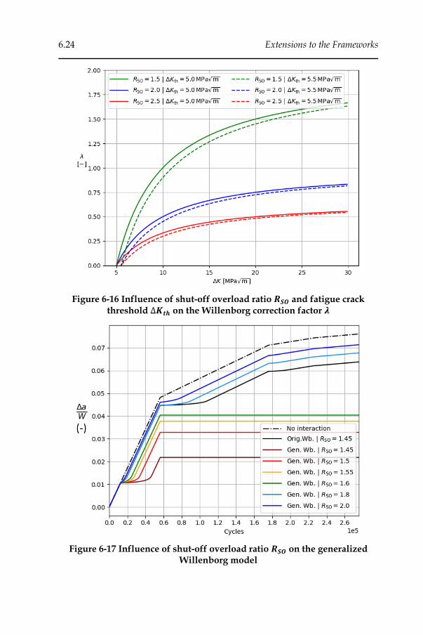
6.24 Extensions to the Frameworks
Figure 6-16 Influence of shut-off overload ratio 𝑹𝑺𝑶 and fatigue crack threshold ∆𝑲𝒕𝒉 on the Willenborg correction factor 𝝀
Figure 6-17 Influence of shut-off overload ratio 𝑹𝑺𝑶 on the generalized Willenborg model
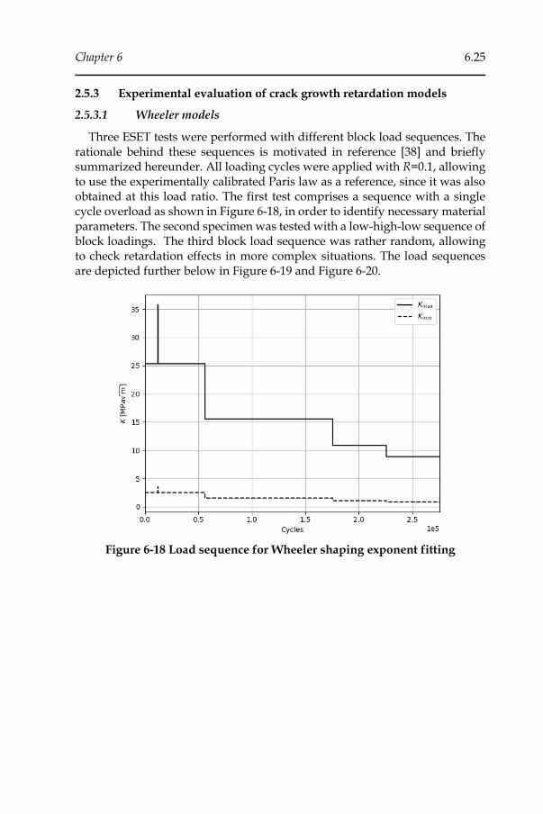
Chapter 6 6.25
2.5.3 Experimental evaluation of crack growth retardation models
2.5.3.1 Wheeler models
Three ESET tests were performed with different block load sequences. The rationale behind these sequences is motivated in reference [38] and briefly summarized hereunder. All loading cycles were applied with R=0.1, allowing to use the experimentally calibrated Paris law as a reference, since it was also obtained at this load ratio. The first test comprises a sequence with a single cycle overload as shown in Figure 6-18, in order to identify necessary material parameters. The second specimen was tested with a low-high-low sequence of block loadings. The third block load sequence was rather random, allowing to check retardation effects in more complex situations. The load sequences are depicted further below in Figure 6-19 and Figure 6-20.
Figure 6-18 Load sequence for Wheeler shaping exponent fitting

6.26 Extensions to the Frameworks
Figure 6-19 Simple load scenario: load sequence in LHL test nr. 2
Figure 6-20 Complex scenario: semi-random load sequence test nr. 3
The Wheeler shaping exponent 𝜔 is a key parameter to calculate the retardation effect with the original Wheeler model. Firstly, 𝜔 is calibrated as Wheeler did originally [6] assuming a plane strain plastic zone as calculated by Irwin`s model. By iteratively adjusting the value of 𝜔, the original Wheeler model fitted the experimental data best with 𝜔 around 3.3, as shown as green curve in Figure 6-21.
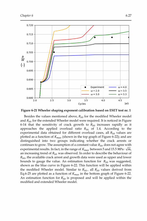
Chapter 6 6.27
Figure 6-21 Wheeler shaping exponent calibration based on ESET test nr. 1
Besides the values mentioned above, 𝑅𝑆𝑂 for the modified Wheeler model
and 𝑅𝑆𝑂` for the extended Wheeler model were required. It is noticed in Figure
6-14 that the sensitivity of crack growth to 𝑅𝑆𝑂 increases rapidly as it approaches the applied overload ratio 𝑅𝑂𝐿 of 1.4. According to the experimental data obtained for different overload cases, all 𝑅𝑆𝑂 values are plotted as a function of 𝐾𝑚𝑎𝑥 (shown in the top graph of Figure 6-22); and are distinguished into two groups indicating whether the crack arrests or continues to grow. The assumption of a constant value 𝑅𝑆𝑂 does not agree with
experimental results. In fact, in the range of 𝐾𝑚𝑎𝑥 between 5 and 15.5 MPa ∙ √m, an increasing trend of 𝑅𝑆𝑂 was observed. In order to describe the behaviour of 𝑅𝑆𝑂, the available crack arrest and growth data were used as upper and lower bounds to gauge the value. An estimation function for 𝑅𝑆𝑂 was suggested, shown as the blue curve in Figure 6-22. This function will be applied within
the modified Wheeler model. Similar to 𝑅𝑆𝑂` , all 𝑅𝑆𝑂
` values derived from Eq.6-25 are plotted as a function of 𝐾𝑚𝑎𝑥 in the bottom graph of Figure 6-22.
An estimation function for 𝑅𝑆𝑂` is proposed and will be applied within the
modified and extended Wheeler model.
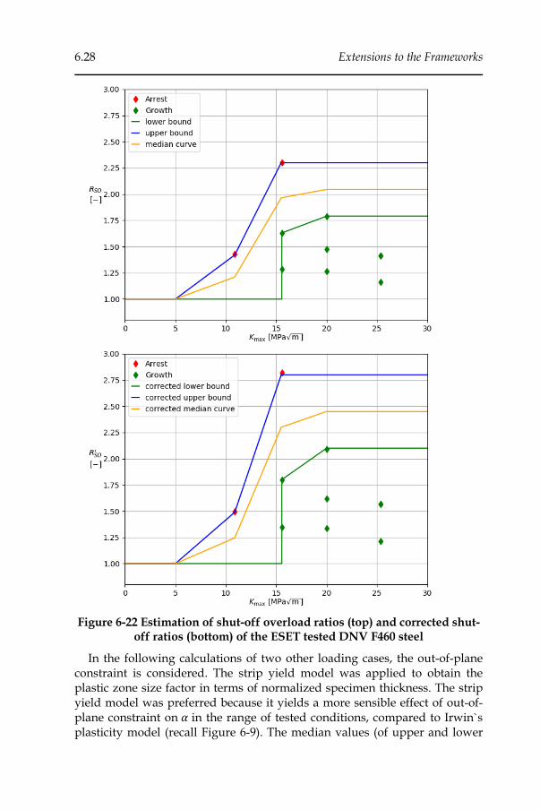
6.28 Extensions to the Frameworks
Figure 6-22 Estimation of shut-off overload ratios (top) and corrected shut-off ratios (bottom) of the ESET tested DNV F460 steel
In the following calculations of two other loading cases, the out-of-plane constraint is considered. The strip yield model was applied to obtain the plastic zone size factor in terms of normalized specimen thickness. The strip yield model was preferred because it yields a more sensible effect of out-of-plane constraint on 𝛼 in the range of tested conditions, compared to Irwin`s plasticity model (recall Figure 6-9). The median values (of upper and lower
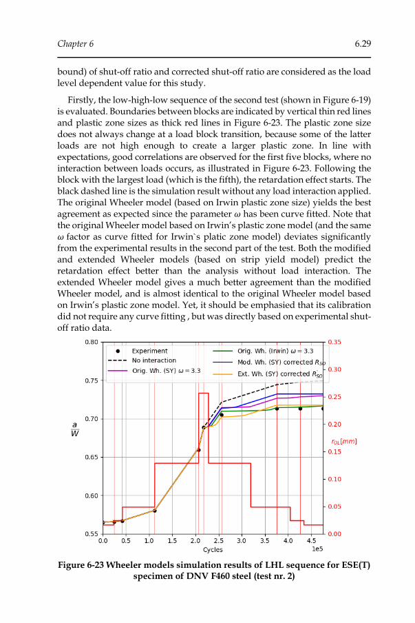
Chapter 6 6.29
bound) of shut-off ratio and corrected shut-off ratio are considered as the load level dependent value for this study.
Firstly, the low-high-low sequence of the second test (shown in Figure 6-19) is evaluated. Boundaries between blocks are indicated by vertical thin red lines and plastic zone sizes as thick red lines in Figure 6-23. The plastic zone size does not always change at a load block transition, because some of the latter loads are not high enough to create a larger plastic zone. In line with expectations, good correlations are observed for the first five blocks, where no interaction between loads occurs, as illustrated in Figure 6-23. Following the block with the largest load (which is the fifth), the retardation effect starts. The black dashed line is the simulation result without any load interaction applied. The original Wheeler model (based on Irwin plastic zone size) yields the best agreement as expected since the parameter 𝜔 has been curve fitted. Note that the original Wheeler model based on Irwin’s plastic zone model (and the same 𝜔 factor as curve fitted for Irwin`s platic zone model) deviates significantly from the experimental results in the second part of the test. Both the modified and extended Wheeler models (based on strip yield model) predict the retardation effect better than the analysis without load interaction. The extended Wheeler model gives a much better agreement than the modified Wheeler model, and is almost identical to the original Wheeler model based on Irwin’s plastic zone model. Yet, it should be emphasied that its calibration did not require any curve fitting , but was directly based on experimental shut-off ratio data.
Figure 6-23 Wheeler models simulation results of LHL sequence for ESE(T) specimen of DNV F460 steel (test nr. 2)

6.30 Extensions to the Frameworks
To further evaluate the agreement of different Wheeler model predictions, the semi-random load sequence from Figure 6-20 has been evaluated. The scenario consisted of a mix of overloads. In Figure 6-24, the original Wheeler model (based on Irwin’s plastic zone size) gives a very good correlation, confirming its validity. The experimental agreement of the original and modified Wheeler models based on strip yield model is moderate. In this case, the extended Wheeler model based on the strip yield plastic zone model shows an excellent agreement – very close to the original Wheeler model based on Irwin’s model.
Figure 6-24 Wheeler models simulation results of the semi-random sequence for ESE(T) specimen of DNV F460 steel (test nr. 3)
So far, all extended Wheeler model simulations were based upon the strip
yield model. Figure 6-25 and Figure 6-26 compare predictive ability to that of an extended Wheeler model assuming Irwin’s plastic zone calculation. Compared with the strip yield model, crack growth predictions deviate more strongly from the experimental data. This is hypothetically because the strip yield model provides a more sensible view on out-of-plane constraint effects, see Figure 6-9.
As a final note prior to summarize, looking back at the first test which was
used to calibrate the original Wheeler model, the prediction of the extended
model reasonably agrees with the experimental data (Figure 6-25).
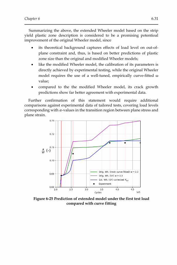
Chapter 6 6.31
Summarizing the above, the extended Wheeler model based on the strip yield plastic zone description is considered to be a promising potentioal improvement of the original Wheeler model, since
• its theoretical background captures effects of load level on out-of-
plane constraint and, thus, is based on better predictions of plastic
zone size than the original and modified Wheeler models;
• like the modified Wheeler model, the calibration of its parameters is
directly achieved by experimental testing, while the original Wheeler
model requires the use of a well-tuned, empirically curve-fitted ω
value;
• compared to the the modified Wheeler model, its crack growth
predictions show far better agreement with experimental data.
Further confirmation of this statement would require additional comparisons against experimental data of tailored tests, covering load levels corresponding with 𝛼-values in the transition region between plane stress and plane strain.
Figure 6-25 Prediction of extended model under the first test load compared with curve fitting
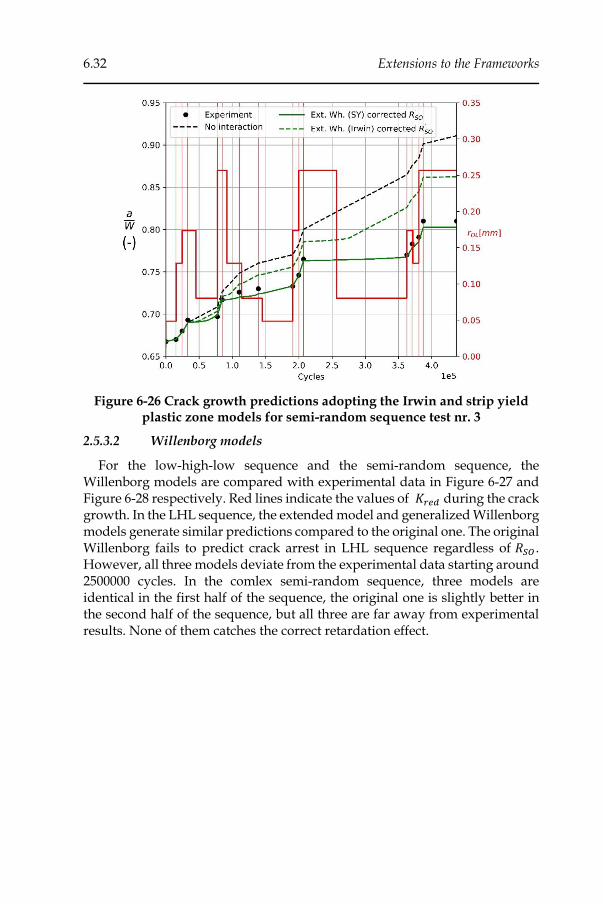
6.32 Extensions to the Frameworks
Figure 6-26 Crack growth predictions adopting the Irwin and strip yield plastic zone models for semi-random sequence test nr. 3
2.5.3.2 Willenborg models
For the low-high-low sequence and the semi-random sequence, the Willenborg models are compared with experimental data in Figure 6-27 and Figure 6-28 respectively. Red lines indicate the values of 𝐾𝑟𝑒𝑑 during the crack growth. In the LHL sequence, the extended model and generalized Willenborg models generate similar predictions compared to the original one. The original Willenborg fails to predict crack arrest in LHL sequence regardless of 𝑅𝑆𝑂 . However, all three models deviate from the experimental data starting around 2500000 cycles. In the comlex semi-random sequence, three models are identical in the first half of the sequence, the original one is slightly better in the second half of the sequence, but all three are far away from experimental results. None of them catches the correct retardation effect.

Chapter 6 6.33
Figure 6-27 Willenborg models simulation results of LHL sequence for ESE(T) specimen in DNV F460 steel test nr. 2
Roughly comparing with the prediction of the Wheeler models, the Willenborg models produce worse results, associated with a general underestimation of retardation effects. This is most probably caused by incorrect Walker`s law parameters, as there is only one crack growth rate curve for R=0.1. In summary, the available data are deemed insufficiently detailed to objectively judge on the predictive abilities of any of the examined Willenborg models, compared to those of the examined Wheeler models.
Figure 6-28 Willenborg models simulation results of the semi-random sequence for ESE(T) specimen in DNV F460 steel test nr. 3
6.34 Extensions to the Frameworks
3 Residual stress
As mentioned in Chapter 1, residual stress has an influence on a wide range of fatigue related aspects, such as crack nucleation and initiation, short crack damage accumulation, and long crack propagation. Scenarios close to real industrial application often involve residual stress, which may be induced by plastic deformation or welding. Therefore, frameworks developed in this study should ideally have the optional capability to include the effects of residual stress.
Including residual stress to a model in ABAQUS can be achieved by defining an initial stress field. ABAQUS offers four options to create an initial stress field [39]: 1) defining initial stresses on individual elements or nodes; 2) providing an external input file which consists of stress information; 3) running a user-defined subroutine SIGINI or UFIELD which is used for pre-defined field variables; 4) by inputting a results file (extension is .fil) or output database file (extension is .odb) generated by a prior ABAQUS analysis. These four options can be implemented by either the CAE graphical user interface (GUI), Python scripts, or modification of the input (.inp) files. Import of the stress field is implemented in the global coordinate system unless a local one is defined and specified.
For example, a residual stress field can be specified by the stress output variables from an ABAQUS/Standard analysis model, giving the specific sequence numbers of the step and increment in the output database (.odb) file of the simulation. This method is preferred for the DeMoPreCI-MDT project (within which this dissertation frames) because another work package of the project deals with ABAQUS based predictions of residual stress resulting from welding. There are specific attention points when coupling two ABAQUS models for residual stress analysis. Particularly, the two models must be defined consistently and mesh definition must be unified. In other words, the element type and numbering have to be exactly the same in both models. Mandatorily, the naming of part instances also has to be the same for both models.
3.1 Establishing stress equilibrium in ABAQUS
Having defined the initial stresses, it is possible that the overall initial stress state is not in a state of equilibrium. This, by definition, is impossible for a residual stress field, which is self-equilibrating. To make sure that the following simulation is successful, a step should be added to adjust the stress state in order to achieve equilibrium. In this study, both frameworks of fatigue crack initiation and fatigue crack propagation have been established in a static analysis. To perform the stress equilibrium, the static procedure should be used as well.
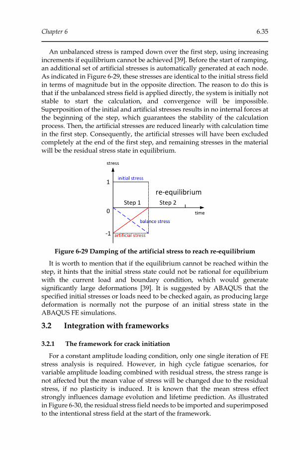
Chapter 6 6.35
An unbalanced stress is ramped down over the first step, using increasing increments if equilibrium cannot be achieved [39]. Before the start of ramping, an additional set of artificial stresses is automatically generated at each node. As indicated in Figure 6-29, these stresses are identical to the initial stress field in terms of magnitude but in the opposite direction. The reason to do this is that if the unbalanced stress field is applied directly, the system is initially not stable to start the calculation, and convergence will be impossible. Superposition of the initial and artificial stresses results in no internal forces at the beginning of the step, which guarantees the stability of the calculation process. Then, the artificial stresses are reduced linearly with calculation time in the first step. Consequently, the artificial stresses will have been excluded completely at the end of the first step, and remaining stresses in the material will be the residual stress state in equilibrium.
Figure 6-29 Damping of the artificial stress to reach re-equilibrium
It is worth to mention that if the equilibrium cannot be reached within the step, it hints that the initial stress state could not be rational for equilibrium with the current load and boundary condition, which would generate significantly large deformations [39]. It is suggested by ABAQUS that the specified initial stresses or loads need to be checked again, as producing large deformation is normally not the purpose of an initial stress state in the ABAQUS FE simulations.
3.2 Integration with frameworks
3.2.1 The framework for crack initiation
For a constant amplitude loading condition, only one single iteration of FE stress analysis is required. However, in high cycle fatigue scenarios, for variable amplitude loading combined with residual stress, the stress range is not affected but the mean value of stress will be changed due to the residual stress, if no plasticity is induced. It is known that the mean stress effect strongly influences damage evolution and lifetime prediction. As illustrated in Figure 6-30, the residual stress field needs to be imported and superimposed to the intentional stress field at the start of the framework.
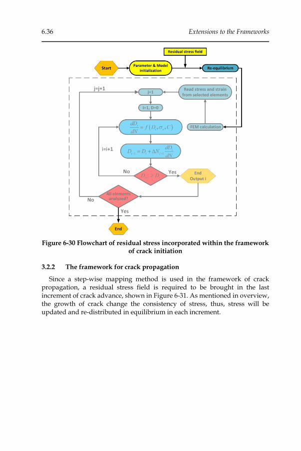
6.36 Extensions to the Frameworks
Figure 6-30 Flowchart of residual stress incorporated within the framework of crack initiation
3.2.2 The framework for crack propagation
Since a step-wise mapping method is used in the framework of crack propagation, a residual stress field is required to be brought in the last increment of crack advance, shown in Figure 6-31. As mentioned in overview, the growth of crack change the consistency of stress, thus, stress will be updated and re-distributed in equilibrium in each increment.
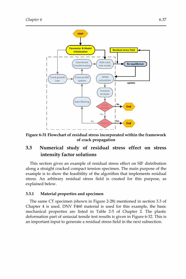
Chapter 6 6.37
Figure 6-31 Flowchart of residual stress incorporated within the framework of crack propagation
3.3 Numerical study of residual stress effect on stress
intensity factor solutions
This section gives an example of residual stress effect on SIF distribution along a straight cracked compact tension specimen. The main purpose of the example is to show the feasibility of the algorithm that implements residual stress. An arbitrary residual stress field is created for this purpose, as explained below.
3.3.1 Material properties and specimen
The same CT specimen (shown in Figure 2-28) mentioned in section 3.3 of Chapter 4 is used. DNV F460 material is used for this example, the basic mechanical properties are listed in Table 2-5 of Chapter 2. The plastic deformation part of uniaxial tensile test results is given in Figure 6-32. This is an important input to generate a residual stress field in the next subsection.
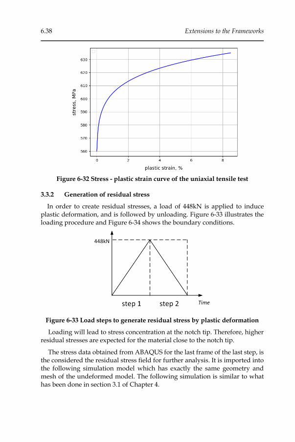
6.38 Extensions to the Frameworks
Figure 6-32 Stress - plastic strain curve of the uniaxial tensile test
3.3.2 Generation of residual stress
In order to create residual stresses, a load of 448kN is applied to induce plastic deformation, and is followed by unloading. Figure 6-33 illustrates the loading procedure and Figure 6-34 shows the boundary conditions.
Figure 6-33 Load steps to generate residual stress by plastic deformation
Loading will lead to stress concentration at the notch tip. Therefore, higher residual stresses are expected for the material close to the notch tip.
The stress data obtained from ABAQUS for the last frame of the last step, is the considered the residual stress field for further analysis. It is imported into the following simulation model which has exactly the same geometry and mesh of the undeformed model. The following simulation is similar to what has been done in section 3.1 of Chapter 4.
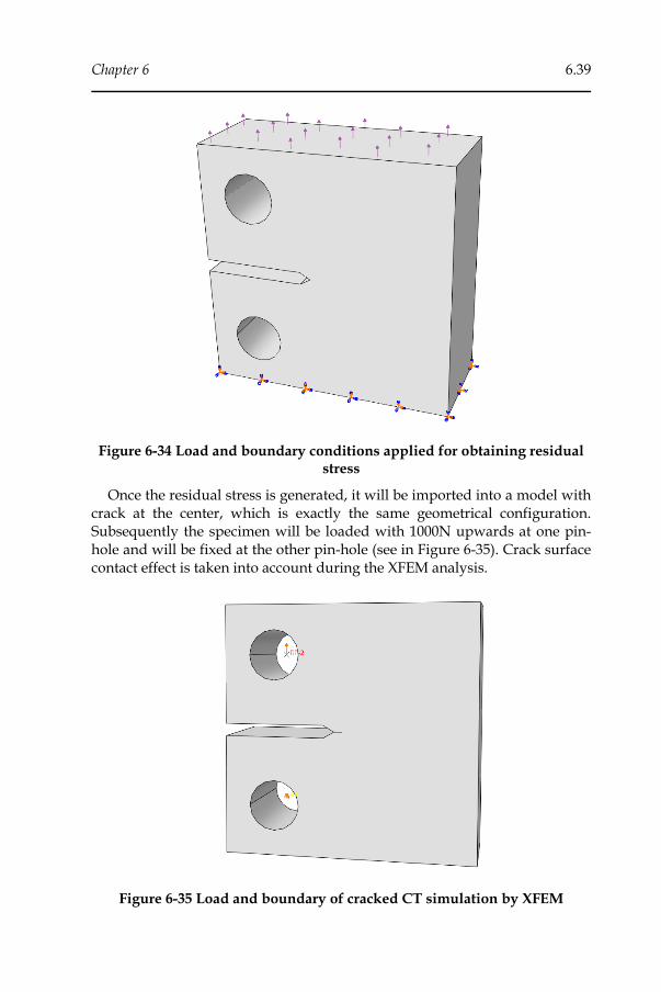
Chapter 6 6.39
Figure 6-34 Load and boundary conditions applied for obtaining residual stress
Once the residual stress is generated, it will be imported into a model with crack at the center, which is exactly the same geometrical configuration. Subsequently the specimen will be loaded with 1000N upwards at one pin-hole and will be fixed at the other pin-hole (see in Figure 6-35). Crack surface contact effect is taken into account during the XFEM analysis.
Figure 6-35 Load and boundary of cracked CT simulation by XFEM
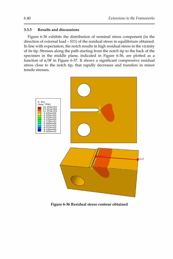
6.40 Extensions to the Frameworks
3.3.3 Results and discussions
Figure 6-36 exhibits the distribution of nominal stress component (in the direction of external load – S11) of the residual stress in equilibrium obtained. In line with expectation, the notch results in high residual stress in the vicinity of its tip. Stresses along the path starting from the notch tip to the back of the specimen in the middle plane, indicated in Figure 6-36, are plotted as a function of 𝑎 𝑊⁄ in Figure 6-37. It shows a significant compressive residual stress close to the notch tip, that rapidly decreases and transfers in minor tensile stresses.
Figure 6-36 Residual stress contour obtained

Chapter 6 6.41
Figure 6-37 S11 from the notch tip to back of the specimen
The influence of residual stress on SIF is shown in Figure 6-38. The solution without residual stress was calculated by Eq. 4-30 in Chapter 4 as follows.
( )
( )( )2 3 4
3 2
20 886 4 64 13 32 14 72 5 6
1. . . . .
I
PK
t W
+= + − + −
−
The effective SIF solutions (Mode I) taking into account residual stress have been obtained from XFEM simulation with 10 integration contours in which the first 3 contours are ignored. The solutions for different crack lengths are the average values along crack tips.
Figure 6-38 Comparison between analytical solution without residual stress and XFEM solution of effective 𝑲𝑰 with residual stress
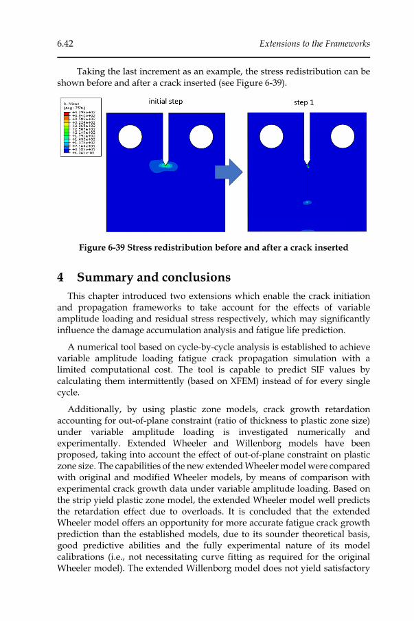
6.42 Extensions to the Frameworks
Taking the last increment as an example, the stress redistribution can be shown before and after a crack inserted (see Figure 6-39).
Figure 6-39 Stress redistribution before and after a crack inserted
4 Summary and conclusions
This chapter introduced two extensions which enable the crack initiation and propagation frameworks to take account for the effects of variable amplitude loading and residual stress respectively, which may significantly influence the damage accumulation analysis and fatigue life prediction.
A numerical tool based on cycle-by-cycle analysis is established to achieve variable amplitude loading fatigue crack propagation simulation with a limited computational cost. The tool is capable to predict SIF values by calculating them intermittently (based on XFEM) instead of for every single cycle.
Additionally, by using plastic zone models, crack growth retardation accounting for out-of-plane constraint (ratio of thickness to plastic zone size) under variable amplitude loading is investigated numerically and experimentally. Extended Wheeler and Willenborg models have been proposed, taking into account the effect of out-of-plane constraint on plastic zone size. The capabilities of the new extended Wheeler model were compared with original and modified Wheeler models, by means of comparison with experimental crack growth data under variable amplitude loading. Based on the strip yield plastic zone model, the extended Wheeler model well predicts the retardation effect due to overloads. It is concluded that the extended Wheeler model offers an opportunity for more accurate fatigue crack growth prediction than the established models, due to its sounder theoretical basis, good predictive abilities and the fully experimental nature of its model calibrations (i.e., not necessitating curve fitting as required for the original Wheeler model). The extended Willenborg model does not yield satisfactory

Chapter 6 6.43
representations of the experimental data, and underestimates the reduction of crack growth rate. It is judged that more detailed experimental material properties (i.e., an R-ratio dependent crack growth rate curve) than those available are required to obtain better agreements with the Willenborg model.
A feature is developed to evaluate the residual stress effect, by importing the residual stress field directly from a specified output database file of an ABAQUS analysis. The re-equilibrium of the stress state with the residual stress is achieved automatically by damping the opposite internal stresses.
6.44 Extensions to the Frameworks
References
1. Paris, P. and F. Erdogan, A critical analysis of crack propagation laws. Journal of Fluids Engineering, 1963. 85(4): p. 528-533.
2. Skorupa, M., Load interaction effects during fatigue crack growth under variable amplitude loading—a literature review. Part I: empirical trends. Fatigue & Fracture of Engineering Materials & Structures, 1998. 21(8): p. 987-1006.
3. Wheeler, O.E., Spectrum Loading and Crack Growth. Journal of Basic Engineering, 1972. 94(1): p. 181-186.
4. Skorupa, M., Load interaction effects during fatigue crack growth under variable amplitude loading—a literature review. Part II: qualitative interpretation. Fatigue & Fracture of Engineering Materials & Structures, 1999. 22(10): p. 905-926.
5. Willenborg, J.E., R. M. ; Wood, H. A., A Crack Growth Retardation Model Using an Effective Stress Concept. 1971.
6. Gallagher, J., A generalized development of yield zone models. 1974, DTIC Document.
7. Gallagher, J. and T. Hughes, Influence of yield strength on overload affected fatigue crack growth behavior in 4340 steel. 1974, AIR FORCE FLIGHT DYNAMICS LAB WRIGHT-PATTERSON AFB OH.
8. Gray, T. and J. Gallagher, Predicting fatigue crack retardation following a single overload using a modified Wheeler model, in Mechanics of crack growth. 1976, ASTM International.
9. Dragt, R., et al. Including load sequence effects in the fatigue damage estimation of an offshore wind turbine substructure. in The 26th International Ocean and Polar Engineering Conference. 2016. International Society of Offshore and Polar Engineers.
10. Maljaars, J., R. Pijpers, and H. Slot, Load sequence effects in fatigue crack growth of thick-walled welded C–Mn steel members. International Journal of Fatigue, 2015. 79: p. 10-24.
11. De Tender, S. and W.p. De Waele, Variable amplitude fatigue in offshore structures. 2016, 2016.
12. Maddox, S.J., Fatigue Strength of Welded Structures. 1991: Elsevier Science.
13. Webster, G.A. and A.N. Ezeilo, Residual stress distributions and their influence on fatigue lifetimes. International Journal of Fatigue, 2001. 23: p. 375-383.

Chapter 6 6.45
14. Sirtori, S. and L. Vergani, Influence of residual stesses on fatigue crack propagation. Metallurgical Science and Tecnology, 1988. 6(2).
15. Beghini, M. and L. Bertini, Fatigue crack propagation through residual stress fields with closure phenomena. Engineering Fracture Mechanics, 1990. 36(3): p. 379-387.
16. Sander, M. and H.A. Richard, Fatigue crack growth under variable amplitude loading Part II: analytical and numerical investigations. Fatigue & Fracture of Engineering Materials & Structures, 2006. 29(4): p. 303-319.
17. Stephens, R.I., Fatigue Crack Growth Under Spectrum Loads. 1976: American Society for Testing and Materials.
18. Sander, M. Comparison of fatigue crack growth concepts with respect to interaction effects. in The 15th European Conference on Fracture. 2004. Stockholm, Sweden.
19. Wolf, E., Fatigue crack closure under cyclic tension. Engineering Fracture Mechanics, 1970. 2(1): p. 37-45.
20. Pippan, R. and A. Hohenwarter, Fatigue crack closure: a review of the physical phenomena. Fatigue & Fracture of Engineering Materials & Structures, 2017. 40(4): p. 471-495.
21. Machniewicz, T., Fatigue crack growth prediction models for metallic materials. Fatigue & Fracture of Engineering Materials & Structures, 2013. 36(4): p. 293-307.
22. Meggiolaro, M.A. and J. Castro. Comparison of load interaction models in fatigue crack propagation. in Proceeding of COBEM. 2001.
23. Abdelkader, M., et al., Crack propagation under variable amplitude loading. Materials Research, 2013. 16(5): p. 1161-1168.
24. Anderson, T.L., Fracture Mechanics: Fundamentals and Applications, Second Edition. 1994: Taylor & Francis.
25. Voorwald, H.J.C., M.A.S. Torres, and C.C.E. Pinto Júnior, Modelling of fatigue crack growth following overloads. International Journal of Fatigue, 1991. 13(5): p. 423-427.
26. Gray, T.D., Fatigue Crack Retardation Following a Single Overload. 1973, AIR FORCE FLIGHT DYNAMICS LAB WRIGHT-PATTERSON AFB OH.
27. Dugdale, D.S., Yielding of steel sheets containing slits. Journal of the Mechanics and Physics of Solids, 1960. 8(2): p. 100-104.
6.46 Extensions to the Frameworks
28. Guo, W., Three-dimensional analyses of plastic constraint for through-thickness cracked bodies. Engineering Fracture Mechanics, 1999. 62(4): p. 383-407.
29. Ramberg, W. and W.R. Osgood, Description of stress-strain curves by three parameters. 1943.
30. Alawi, H., Designing reliably for fatigue crack growth under random loading. Engineering Fracture Mechanics, 1990. 37(1): p. 75-85.
31. Sheu, B.C., P.S. Song, and S. Hwang, Shaping exponent in wheeler model under a single overload. Engineering Fracture Mechanics, 1995. 51(1): p. 135-143.
32. Miranda, A.C., et al., Prediction of Fatigue Life and Crack Path in Complex 2D Structural Components Under Variable Amplitude Loading. Fatigue Testing and Analysis Under Variable Amplitude Loading Conditions, ASTM STP, 2001. 1439.
33. Muys, L., XFEM-based cycle-by-cycle simulation of fatigue crack growth. 2017, Ghent University. p. 105.
34. Zhang, J., et al. Modelling framework for 3D fatigue crack propagation in welds of offshore steel structures. in International Conference on Integrity: Reliability: Failure. 2016. INEGI/FEUP (2016).
35. ASTM International, E647 Standard test method for measurement of fatigue crack growth rates, in Annual Book of ASTM Standards, Section Three: Metals Test Methods and Analytical Procedures. 2011. p. 628-670.
36. Beevers, C.J., Fatigue crack growth characteristics at low stress intensities of metals and alloys. Metal Science, 1977. 11(8-9): p. 362-367.
37. Rushton, P., F. Taheri, and D. Stredulinsky. Threshold and variable amplitude crack growth behavior in 350WT steel. in Proc. 21st Int. Conf. on Pressure Vessels and Piping, ASME-PVP. 2002.
38. Micone, N., Development of Testing Methodologies for the Analysis of Variable Amplitude Fatigue and Corrosion-Fatigue of Offshore Steels. 2017, Ghent University.
39. DASSAULT_SYSTEMES, Abaqus 6.14 Documentation. 2014: DASSAULT SYSTEMES.

Chapter 7
Conclusions and Perspectives for Future
Work

7.2 Conlusions and Perspective of Future Work
<< This page intentionally left blank >>
Chapter 7 7.3
1 Global summary and main conclusions
Since offshore wind energy has drawn great attention worldwide and is expected to exponentially expand in the next years, the durability of offshore structures is an extremely relevant research topic [1]. Fatigue analysis and design of steel structures in an offshore environment are facing strong challenges, as the coupled effects of mechanical load, corrosive seawater and atmosphere come into play. Besides, the stochastic nature of wind, waves and currents imposes complex cyclic loading histories to the structure, which are challenging to translate into conventional fatigue frameworks.
The ambition of this dissertation, as part of a large Flemish research project DeMoPreCi-MDT, was to develop advanced numerical tools to evaluate the combined damage of fatigue and corrosion. Such tools should allow to estimate the (remaining) lifetime of offshore structures. Frameworks based on innovative numerical models and methods have been developed to describe the stages of crack initiation and crack propagation independently. A methodology has also been developed to determine the transition between initiation and propagation stages, which allows to determine the total fatigue life as the sum of initiation time and propagation time. The abilities of the developed tools have been evaluated by comparing with data from devoted experimental tests and data reported in the literature. A summary of the main developments and their evaluation is given in the following subsections.
1.1 Methodologies and numerical tools developed
A new corrosion fatigue crack initiation model based on non-linear damage mechanics has been developed to calculate the coupled damage of fatigue and general corrosion. The starting point of this model is a fatigue initiation model originally developed by Dattoma et al.. It has been optimized by including a method for time-dependent reduction of fatigue strength, which resembles the structural deterioration due to a corrosive environment (Chapter 3).
A numerical framework that allows to predict the lifetime (as number of cycles) for fatigue crack initiation has been implemented in ABAQUS® 6.14 Standard. The framework allows to evaluate the effects of variable load amplitude and the dissapearence of fatigue limit for corrosion fatigue (Chapter 3).
A computationally efficient, simple and robust numerical method based on the Nelder-Mead optimization algorithm has been implemented to identify the orientation of the critical plane and damage parameters of critical plane criteria for multiaxial fatigue. (Chapter 3).
A method that allows to construct an arbitrary 3D fatigue crack front and to simulate non-self-similar crack growth has been developed. Discretization of
7.4 Conlusions and Perspective of Future Work
the crack front is used to describe the evolution of the crack and update the crack profile (Chapter 4). Using this method, an iterative numerical framework was developed to simulate crack propagation by using the stress intensity factor solutions from an XFEM model and a crack mapping approach. Thanks to the XFEM implementation, a much coarser mesh compared to a conventional FEM analysis is sufficient to obtain accurate stress intensity factor values. The crack mapping method predefines a (limited) number of calculation iterations by setting a pre-defined crack extension increment. Compared to integrations over fixed numbers of cycles, mapping significantly relieves the computational burden of calculating fatigue crack propagation (Chapter 4). The effects of corrosion on crack propagation are not modelled explicitly, but by directly using corrosion crack growth rate curves determined from dedicated experiments.
Fatigue crack initiation and propagation are two separate stages of fatigue, and the total fatigue lifetime is determined by the sum of their contributions. Determining this sum requires the definition of a crack length that demarcates the end of initiation and the onset of propagation. A method to calculate this transition crack length based on the hypothesis of a competition between mechanisms representative for the two stages has been implemented (Chapter 5).
Two extensions of the frameworks have been developed; a first one enabling crack propagation calculations to account for variable amplitude loading history, and a second one to account for the presence of residual stresses. Regarding variable amplitude loading, a cycle-by-cycle framework has been developed to take into account crack growth retardation due to overload events. A crack growth mapping approach allows to maintain the calculation time within acceptable limits. Traditional crack growth retardation models (Wheeler and Willenborg), based on estimations of plastic zone size ahead of the crack tip were found limited in their ability to account for out-of-plane constraint effects. Extended Wheeler and Willenborg models were proposed to take these effects into account (Chapter 6). With respect to residual stress, the extension allows to import a residual stress field, and to ensure its self-equilibrium. The residual stress field is superimposed to the service load and its self-equilibrating nature is updated for incrments in crack growth.
1.2 Comparison of simulation results with literature and
experimental data
By comparison with corrosion fatigue S-N curves reported in literature, it was hown that the model successfully predicts the elimination of the conventional fatigue limit and a decrease in number of cycles to failure at a low-stress level (high cycle fatigue region) (Chapter 2). In order to avoid
Chapter 7 7.5
simple curve fitting, a model would be required that allows to describe the physics of corrosion and its interaction with fatigue, whilst retaining a sufficient degree of simplicity for practical application. To date, such models are missing.
The framework of crack propagation has been able to accurately describe experimentally observed crack path deviation in a modified compact tension specimen with an additional hole to create an asymmetrical stress distribution. It could also predict the rotation of a slanted crack within a beam subjected to bending, identical to literature reports (Chapter 4). These comparisons give confidence that the framework allows to simulate three-dimensional crack propagation. To confirm this, further validations on other cases (involving more irregular crack morphologies) are suggested.
By using the new method developed for searching the critical plane for crack initiation, much fewer iterations are required to obtain a highly accurate solution, compared with existing approaches (Chapter 4).
Transition crack lengths calculated by the framework developed in Chapter 6 are in the same order of magnitude of an empirical length based on grain size and length calculated by the KT-diagram method. This supports the credibility of the tool and framework.
The capabilities of the new extended Wheeler model were benchmarked against published original and modified Wheeler models, by means of comparison with experimental crack growth data of laboratory tests with variable amplitude loading. Combining the extended Wheeler model with the strip yield plastic zone model yields highly accurate representations of the experimental data. It is concluded that the extended Wheeler model offers an opportunity for more accurate fatigue crack growth prediction than the established models, due to its sounder theoretical basis, good predictive abilities and the purely experimental nature of its parameter calibration (Chapter 6).
The simple example of the residual stress effect on the solution of effective SIFs of a compact tension specimen shows the functionality of the residual stress re-equilibrium tool implemented (Chapter 6).
2 Suggestions for future work
2.1 Experimental validation of the developed frameworks
One of the major contributions of this dissertation is the establishment of numerical frameworks for crack initiation and propagation analysis. Due to a lack of well-documented and representative experimental data, an elaborate validation study deemed impossible. A dedicated experimental programme

7.6 Conlusions and Perspective of Future Work
allowing a systematic calibration of model parameters and validation of the corrosion fatigue initiaton and propagation frameworks is primordial. The relation between durability properties (e.g., fatigue endurance, crack growth rate and threshold SIF range) and corrosion duration should be explored and verified. Validation of the total fatigue life prediction by integrating both frameworks necessitates an evaluation of the numerical tool for transition crack length and possible tuning with respect to experimental accuracy of determining an initiated crack.
2.2 Optimisation of the numerical tools
Improving and optimizing the robustness and efficiency of the numerical tools is a continuous pursuit. The current version of the framework for crack initiation needs a large number of iterations to calculate damage and lifetime of all individual elements. This is feasible for simple geometries without a high demand for accuracy. But this drastically reduces the efficiency of the framework when refined meshes or complex geometries (e.g. parts of an entire offshore structure) are involved. Automatic pre- and postprocessing combined with submodelling approaches to decrease the number of elements to be screened for damage, could be implemented. By doing so, the highly effective algorithm developed within this work could become highly efficient thanks to significant savings in computational time. The current version of the framework for crack propagation is based on the ABAQUS® XFEM feature. However, it is not as robust as expected for an arbitrary 3D crack. Preferably, a dedicated XFEM code/program should be developed to replace the functionality as implemented in commercial software.
2.3 Additional extensions of the developed frameworks
The modular nature of objective-oriented programming allows additional extension(s) to be developed and easily integrated with the existing frameworks. Chapter 6 has highlighted two particular extensions that have been implemented within the framework of this dissertation. In the future, new extensions could be considered. Potentially interesting topics for extension include:
• Corrosion fatigue properties
The degree of corrosion deteriation on fatigue properties is not fully understood yet and generic models do not exist. Phenomenological or physical relations between corrosion type and duration on the one hand and fatigue resistence on the other hand could be included as an individual module.
• Heterogeneous material

Chapter 7 7.7
Fatigue cracking is often observed in or near welds [2], which comprise different material microstructures due to the imposed heat treatment during welding. The heterogeneity in material properties of the weld region might affect crack initiation and propagation. Including material heterogeneity into the developed frameworks therefore deserves consideration.
• Rainflow counting method
Spectrum load history for real applications is far more complex than loading cycles applied in a laboratory study. Rainflow counting was developed in order to reduce a spectrum of varying stress into blocks of simple stress cycles [3]. A module of modified rainflow counting methods which are better representive in wide applications and yield more accurate damage accumulation results is needed to facilitate the calculation of the damage accumulation to estimate the fatigue life of a structure subjected to complex loading.
• Probabilistic & stochastic analysis
Significant scatter is a noteworthy inherent feature of the fatigue process and fatigue lifetime results. This depends on various uncontrolled factors, such as minor variations of geometry and material properties, loading history etcetera [4]. Numerical simulations based on deterministic methods might therefore not describe the fatigue performance in a sufficiently adequate way. Probability theory, including stochastic processes, is an ideal tool that can be used to represent the unpredictable behavior.
2.4 Personal reflections and opinion of the author
Material fatigue is investigated by means of classic solid mechanics methodologies. Scientists squeeze the abilities of popular mathematical approaches used nowadays to reach advances in fatigue analysis without fundamental innovations. The author believes that there would be a huge leap in this field if mathematical tools would become available that enable to easily link multiscale analysis from atom-scale to macro scale. Fatigue is often described as a mysterious black box, but the author considers it as a semitransparent box in which something can be seen but not in full detail. Nowadays, complex approaches are being developed to unravel the mysteries of a black box. For example, machine learning and artificial intelligence techniques have done a great job in different science fields lacking a sufficiently detailed knowledge of mechanisms. Such an approach could be explored to use in fatigue analysis and modeling.

7.8 Conlusions and Perspective of Future Work
It should be emphasized that the opinions above in this section are only personal dim perceptions after years of experience related to metal fatigue besides four years of doing numerical research on this subject. They could be controversial or unrealistic and should not be considered as absolutely correct.

Chapter 7 7.9
References
1. Karimirad, M., Offshore Energy Structures: For Wind Power, Wave Energy and Hybrid Marine Platforms. 2014: Springer International Publishing.
2. Maddox, S.J., Fatigue Strength of Welded Structures. 1991: Elsevier Science.
3. Matsuishi, M. and T. Endo, Fatigue of metals subjected to varying stress. Japan Society of Mechanical Engineers, Fukuoka, Japan, 1968. 68(2): p. 37-40.
4. Sobczyk, K., Stochastic approach to fatigue: experiments, modelling, and reliability estimation. 1993: Springer-Verlag.
Copyright © 2022 FDOKUMEN