Numerical modelling of thermally induced regional and local ...

Numerical Modelling of Thermally Induced Regional and Local Scale Flows in MacKenzie Basin, New Zealand

A thesis

submitted in fulfillment

of the requirements for the degree

of

Doctor of Philosophy

in the

University of Canterbury

by

Peyman Zawar-Reza

University of Canterbury 2000

Table of Contents

Page Numbers

List of Figures v List of Tables ix List of Symbols xi Acknowledgments xiii Abstract xv

Chapter 1 Introduction 1

1.1 Background 1 1.2 Impetus for Research 2 1.3 Atmospheric Scales of Motion 3 1.4 Physiographically Forced Mesoscale Circulations 4

1.4.1 Terrain-Forced Flows 4 1.4.2 Thermally-Forced Flows 5 1.4.3 Regional Scale Winds in the Context of MacKenzie Basin 11

1.5 Mesoscale Numerical Modelling 12 1.5.1 Prognostic Models 12 1.5.2 Diagnostic Models 13

1.6 Prognostic Mesoscale Modelling in Complex Terrain 13 1.6.1 General Background 13 1.6.2 Numerical Studies of Regional Scale Circulation Systems 14

1.7 Thesis Objectives 15 1.8 Thesis Format 17

Chapter 2 Observations of Thermally Induced Flows in MacKenzie Basin 19

2.1 Introduction 19 2.2 Description of the Experimental Site 20 2.3 Previous Meteorological Research in the Area 23 2.4 Previous Observations of Canterbury Plains Breeze 24 2.5 The Lake Tekapo Experiment (LTEX) 25

2.5.1 Surface Meteorological Monitoring Network 26 2.5.2 Boundary Layer Observation Techniques 27 2.5.3 Wind Regime in the Basin During L TEX 99 28 2.5.4 Case Study Days: 2nd and 12th February 1999 32

2.6 Summary and Conclusion 45

Chapter 3 Model Description 47

3.1 Background 48 3.2 Averaging the Primitive Equations 49 3.3 A Brief Technical Description of RAMS 50

3.3.1 General Equations Solved by RAMS 51 3.3.2 Grid Stagger 53 3.3.3 Terrain-Following coordinate System 55 3.3.4 Vertical Levels 56 3.3.5 Grid Nesting 56 3.3.6 Turbulent Mixing Parameterization 57 3.3.7 Surface Layer Parameterization 58 3.3.8 Spatial Boundary Conditions 60 3.3.9 Soil and Vegetation Parameterization 62

Chapter 4 Three-Dimensional Numerical Modelling of the Regional-Scale Flow 63

4.1 Introduction 63 4.2 Numerical Experiments 65

4.2.1 Three-Dimensional Simulation Development 65 4.3 REG-ECM Simulation 68

4.3.1 Initialization 68 4.3.2 Simulation Results 69

4.4 Idealized Regional-Scale Simulations 75 4.4.1 Initialization 76 4.4.2 Simulation Results 77

4.5 Discussion of Results 86 4.6 Conclusion 88

Chapter 5 Regional-Scale Flows: Simplified Two-Dimensional Numerical Experiments 89


5.2.1 Two-Dimensional Simulation Development 92 5.2.2 Initialization 96

5.3 Simulation Results 97 5.3.1 Plateau Simulations 98 5.3.2 Mountain Simulations 107 5.3.3 Basin Simulations 113


ii

Chapter 6 Numerical Simulations of Local and Regional Scale Flows in the Lake Tekapo 123 Region


6.2.1 Three-Dimensional Simulation Development 124 6.2.2 Initialization 128

6.3 Simulation Results 129 6.3.1 Influence of Regional Scale on Local Scale Flow 129 6.3.2 Influence of Lake Tekapo 132


Chapter 7 Conclusions 141

7.1 Summary of Conclusions 141 7.1.1 Observed Characteristics of the Canterbury Plains Breeze 142 7.1.2 Numerical Simulations of the CPB 142 7.1.3 Interaction of the CPB with Smaller Scale Flows 143 7.1.4 Broader Implications 144

7.2 Suggestions for Future Research 144

References 147 Appendix A 155 Appendix B 159

iii

Figure 1.1 Figure 1.2 Figure 1.3 Figure 1.4 Figure 1.5 Figure 1.6

Figure 2.1 Figure 2.2 Figure 2.3 Figure 2.4

Figure 2.5

Figure 2.6 Figure 2.7 Figure 2.8

Figure 2.9

Figure 2.10

Figure 2.11

Figure 2.12

Figure 2.13

Figure 2.14

Figure 3.1 Figure 3.2 Figure 4.1 Figure 4.2

List of Figures

Time and space magnitudes for micro- and mesoscales Schematic of gap winds

Page Numbers

4

Schematic of the diurnal evolution of sea and land breezes Schematic of diurnal mountain winds Schematic of the Topographic Amplification Factor (T AF) Schematic of pressure gradient forces that produce along-valley wind systems

5 8 9 10 10

Photograph of South Island taken from Sky lab 20 Map of MacKenzie Basin 22 Map of Lake Tekapo area showing the surface monitoring stations 23 Time series of wind speed and direction during L TEX 99 at Base and 29 Twizel Time series of wind speed and direction for Base and Twizel on 12th February 1999 Surface and 500mb analysis for 2nd February 1999 Surface and 500mb analysis for 12th February 1999 Vertical profiles of potential temperature for 2nd and 12th February over the Base site Surface flow field at 1200, 1400, 1600, 1800, and 2000 NZST over Lake Tekapo area on 2nd February 1999 Time series of temperature, specific humidity, and wind speed and direction measured on western slopes of the Two Thumb Range Surface flow field at 1000, 1300, 1600, and 1900 NZST over Lake Tekapo area on 12th February 1999

31

33 34 35

36

38

39

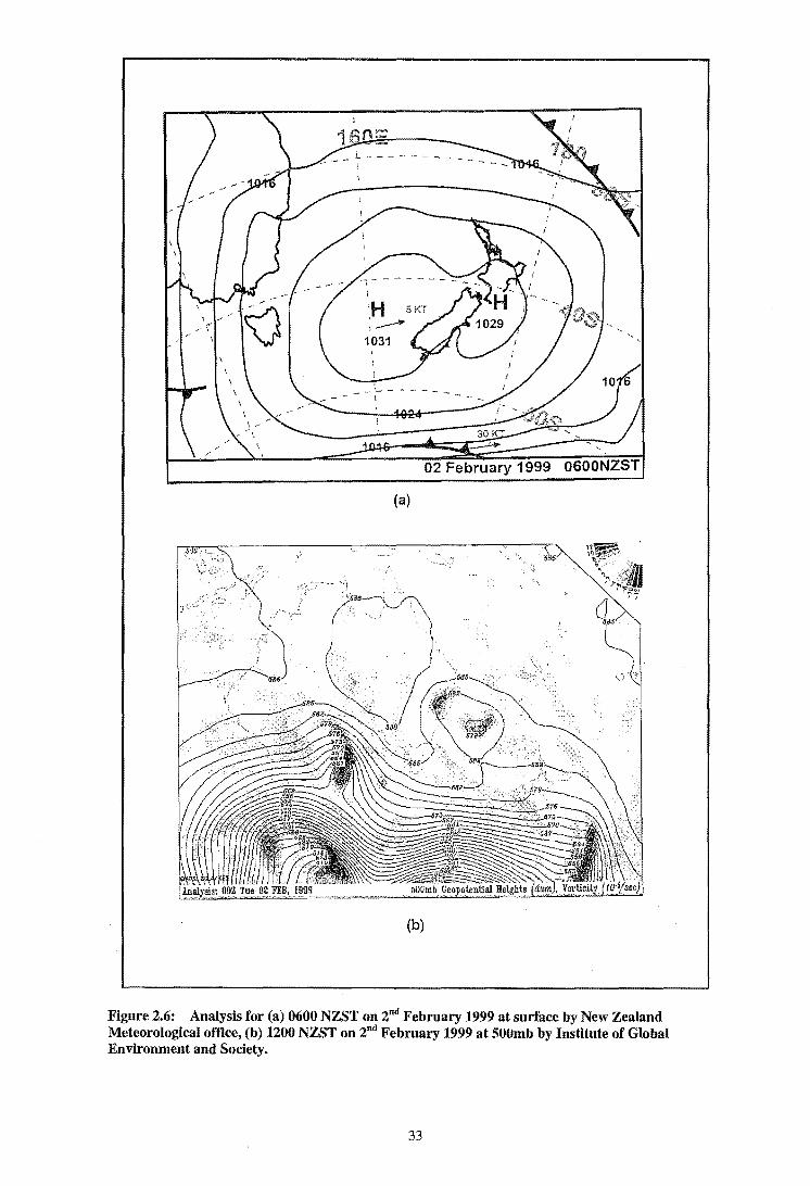
Time series of wind direction, wind speed, and temperature measured 41 at Base site on 2nd and 12th February Contour plots of u- and v- components of measured wind velocity for 43 12th February Measured vertical profiles of potential temperature over Tekapo airport and mid-lake area on 12th February Representation of a grid volume Illustration of Arakawa type C stagger Geographic locations of grids used in three-dimensional runs REG-ECM prediction for surface wind for grid 2 at 0600, and 1400 NZST.

44

50 54 67 70

Figure 4.3 REG-ECM prediction for surface wind for grid 3 at 1100, and 1400 72 NZST.

Figure 4.4 REG-ECM prediction for surface wind for grid 3 at 1600, and 1800 73 NZST.

Figure 4.5 Comparison of time series of wind speed and direction measured at 75 Base site and modelled by REG-ECM for 12th February

v

Figure 4.6 Measured vertical profiles of potential temperature and relative 76 humidity at 1900 NZST on 11th February used to initialize the idealized three-dimensional runs

Figure 4.7 Simulated vertical profiles of potential temperature inside the basin 77 and over the Canterbury Plains at 0600 NZST 12th of February

Figure 4.8 REG-NOW prediction for surface wind and vertical potential 79 temperature field at 1200 NZST on 12th February.



Figure 4.11 REG-NOS prediction for surface wind and vertical potential 83 temperature field at 1200 NZST on 12th February.



Figure 4.14 Comparison of time series of wind speed and direction measured at 87 Base site and modelled by REG-NOW, and REG-NOS simulations for 12th February

Figure 4.15 Comparison of time series of wind speed and direction measured at 88 Timaru and modelled by REG-NOW, and REG-NOS simulations for 12th February

Figure 5.1 Schematic of topographic configurations used for the idealized two- 94 dimensional simulation

Figure 5.2 Simulated vertical profiles of potential temperature at 0600 NZST for 98 inside and outside the plateau for PLT, MTN and BAS experiments

Figure 5.3 Isentrope and isopleth fields for the PLT run at 1200, 1400, 1600 100 NZST

Figure 5.4 Isentrope and isopleth fields for the PLTO run at 1200, 1400, 1600 102 NZST

Figure 5.5 Isentrope and isopleth fields for the PLT-M run at 1200, 1400, 1600 105 NZST

Figure 5.6 Isentrope and isopleth fields for the PLTO-M run at 1200, 1400, 1600 106 NZST

Figure 5.7 Isentrope and isopleth fields for the MTN run at 1200, 1400, 1600 109 NZST

Figure 5.8 Isentrope and isopleth fields for the MTNO run at 1200, 1400, 1600 110 NZST

Figure 5.9 Isentrope and isopleth fields for the MTN-M run at 1200, 1400, 1600 111 NZST

Figure 5.10 Isentrope and isopleth fields for the MTNO-M run at 1200, 1400, 112 1600 NZST

Figure 5.11 Isentrope and isopleth fields for the BAS run at 1200, 1400, 1600 115 NZST

Figure 5.12 Isentrope and isopleth fields for the BASO run at 1200, 1400, 1600 116 NZST

Figure 5.13 Isentrope and isopleth fields for the BAS-M run at 1200, 1400, 1600 117 NZST

Figure 5.14 Isentrope and isopleth fields for the BASO-M run at 1200, 1400, 118 1600 NZST

vi

Figure 5.15 Time series of surface u-component wind at a location over the 120 plateau for all the two-dimensional runs

Figure 6.1 Geographic locations of grids 1 and 2 used in LOC-LAKE, and LOC- 125 LAND simulations

Figure 6.2 Geographic locations of grids 3 and 4 used in LOC-LAKE, and LOC- 126 LAND simulations

Figure 6.3 LOC-LAKE prediction for surface wind for grid 3 at 1000, 1300, and 131 1600 NZST.

Figure 6.4 LOC-LAKE and LOC-LAND predictions for surface wind for grid 4 133 at 1000, and 1300 NZST.

Figure 6.5 LOC-LAKE and LOC-LAND predictions for surface wind for grid 4 134 at 1600 NZST.

Figure 6.6 Vertical cross-sections of simulated potential temperature field and 135 wind vectors by LOC-LAKE and LOC-LAND simulations at 1500 NZST

Figure 6.7 Vertical cross-sections of simulated potential temperature field and 136 wind vectors by LOC-LAKE and LOC-LAND simulations at 1600 NZST

Figure 6.8 Schematic illustration of flushing of cold air in a valley 138 Figure A.l Isentrope and isopleth fields for the BASO-0600 run at 1200,1400, 157

1600 NZST Figure A.2 Time series of u-component of wind velocity for BASO and BASO- 158

0600 simulations

vii

Table 2.1 Table 4.1 Table 4.2 Table 4.3 Table 5.1 Table 5.2 Table 6.1 Table 6.2 Table 6.3

List of Tables

Page

Summary of surface monitoring network Numbers

27 64 66 68 91

Summary of the three-dimensional simulations for regional scale Characteristics of grids configured for the regional scale simulations Summary of model setup for three-dimensional regional scale runs Summary of the two-dimensional simulations Summary of model setup for the two-dimensional runs Summary of the three-dimensional simulations for local scale runs Characteristics of grids configured for the local scale simulations Summary of model setup for three-dimensional local scale runs

ix

96 124 127 128

List of Symbols

drag coefficient specific heat of air at constant pressure specific heat of air at constant volume turbulent kinetic energy viscous dissipation emissivity longwave radiation flux coriolis parameter gravitational acceleration height of the model top Von Karman constant vertical eddy diffusivity for turbulent kinetic energy vertical eddy diffusivity for heat vertical eddy diffusivity for momentum latent heat of vaporization turbulent master length scale Brunt-VaisaIa frequency buoyancy production term for turbulent kinetic energy shear production term for turbulent kinetic energy Exner function synoptic scale reference value for Exner function latent heat flux heat flux from soil sensible heat flux net radiation surface mixing ratio mixing ratio of air close to ground ratio of drag coefficient for momentum and heat (Businger et ai. 1971) gas constant for dry air expansion ratio for vertical grid spacing air density synoptic scale reference value for air density Stefan-Boltzmann constant virtual temperature extrapolated roughness value for temperature potential temperature ice-liquid water potential temperature virtual potential temperature synoptic scale reference value for potential temperature extrapolated roughness length for potential temperature potential temperature scale water species mixing ratio mixing ratio scale bulk Richardson number

xi

nondimensional eddy diffusivity for turbulent kinetic energy nondimensional eddy diffusivity for heat nondimensional eddy diffusivity for momentum dependent variables in formulations of the model air temperature close to ground surface temperature wind speed east-west component of the wind velocity velocity scale north-south component of wind velocity vertical component of wind velocity topography height

>;~f- local topography height :'~~" . 1::~: roughness length

xii

Acknowledgements

First, I would like to offer my sincere thanks to all those who have helped, and

there have been many. I would especially like to thank Associate Professor Andy

Sturman for his support as my supervisor. His guidance and wisdom (plus his ability to

cook a tremendous cheese sauce) have been invaluable throughout the process of my

Ph.D. endeavour. I would also like to thank Dr Dave Whiteman for sponsoring my stay

in Pacific Northwest National Laboratories, and Drs Jerome Fast and Shiyuan Zhong

for assistance with numerical modelling. Paul Gudiksen and Wayne Stephenson

endured hazardous flying conditions during the field campaign, hopefully the

experience did not shave too many years off their life spans, thank you for your

assistance. Dr Meinolf Kossmann and Andrew Oliphant, thank you also for your

friendship and moral support as well as the discussions of a more technical nature.

I would also like to thank Jane Harrison and Julie Cupples for helping me

through difficult times, and Chandra Harrison for technical assistance. Maria Borovnic

was of great help with her knowledge in Shiatsu.

Financial assistance for this research was provided under the project 'Local and

Regional Wind Systems', funded by Marsden fund contract UOC602. I would like to

thank all participants in this project for their assistance in fieldwork.

The Department of Geography has also assisted with technical and

administrative support, both for the fieldwork necessary to gather the data I have used,

and with a friendly supportive environment. Thank you to all the individuals in the

department that have made this process bearable.

xiii

Abstract

Atmospheric flows that result from surface heating and cooling in complex,

mountainous terrain encompass many scales. These flows are induced by horizontal

thermal gradients in the atmosphere associated with topographic relief, and are most

pronounced when synoptic pressure gradients are weak. At the small-scale end of the

spectrum there are slope and along-valley winds, and at the larger scale there are plain-to

basin and plain-to-plateau flows.

The intrusion of a recurring plain-to-basin wind system named the Canterbury

Plains Breeze (CPB) into the MacKenzie Basin and Lake Tekapo region is described using

both observational data and results from a numerical model. Observational data from a

surface monitoring network designed to investigate local flows in the Lake Tekapo area

show that the CPB has an important influence on the wind regime in this region. An

atmospheric mesoscale numerical model was utilized to investigate the origin and forcing

mechanisms for this flow.

The mesoscale model was able to successfully simulate the CPB for a case study

day using realistic synoptic scale winds. To isolate the major forcing mechanisms for this

flow, additional idealized two- and three-dimensional numerical experiments were

conducted. The idealized three-dimensional runs showed that the CPB is a not a sea breeze

intrusion into the MacKenzie Basin as was previously thought, and could be generated by

orography alone.

The two-dimensional runs showed that although the sea breeze outside the basin

does not have a direct impact on the CPB, it can influence the current's intensity by

suppressing the mixed layer growth outside the basin, which increases the horizontal

xv

temperature gradient that forces the CPB. Other surface effects, such as soil moisture

content and land use also seem to affect the characteristic features of the plain-to-basin

flow.

In addition, two high-resolution simulations were performed to investigate the

interaction of the CPB with locally generated thermal flows around Lake Tekapo, where

the surface monitoring network was established. Results show that early in the afternoon

the CPB flows into the region as gap winds through the saddles in the Two Thumb Range,

dominating the local winds. These gap winds are localized in nature, and the model runs

suggest that the monitoring network was not dense enough to adequately describe the

surface flow field around the lake.

n is evident from this research that regional circulation systems, such as the CPB,

could transport air pollutants significant distances from the coastal plains, over complex

terrain into the relatively pristine environment of the South Island's mountain basins. A

knowledge of the physical forcing mechanisms involved in such flows can therefore have

important practical applications for air quality issues.

xvi

Chapter 1

Introduction

1.1 Background

This thesis attempts to determine the dominant physical mechanisms responsible

for the formation of the regional scale Canterbury Plains Breeze (CPB) and its

interaction with other, local scale wind systems during settled weather in spring and

summer with an atmospheric mesoscale numerical model. This wind system was

observed during a field campaign to study local airflows in MacKenzie Basin in the

South Island of New Zealand. The airflow originates from atmospheric thermal

contrasts between the Canterbury Plains and MacKenzie Basin, the wind is usually of

moderate intensity (6 12 ms-I) and blows throughout the basin dominating the locally

.generated circulations. Although its existence to local inhabitants is well known and its

disruptive nature disliked by them, previous meteorological studies in the area paid little

attention to it, since it was believed to be the inflow of a sea breeze circulation which

originates at the coast and then propagates towards the mountain ranges. A visual clue

to the existence of the CPB is the formation of waterfall clouds over mountain saddles,

which is common on days with quiescent synoptic weather conditions.

1

1.2 Impetus for Research

The importance of local air circulations for air pollution transport, weather

forecasting, and land-use management has been realized in the past four decades.

Thermally driven circulations, such as sea breezes and diurnal orographic ally induced

winds, result from an interplay between topographic and thermal forcings. Over simple

terrain, these wind systems can be forecast with a high degree of skill since the

underlying physical mechanisms that drive them are well understood, and adequately

formulated in atmospheric models. An extensive set of earlier literature reviews are

provided by Defant (1951) and Flohn (1969), while books by Oke (1992), Atkinson

(1981), Barry (1992), and Whiteman (2000) provide suitable in-depth description of

these flow systems.

Tourism has long been a part of the economy of MacKenzie Basin, as Mt.

CookJ Aoraki and the nearby glaciers are a major attraction for tourists during summer

months (Morris et al. 1997). Furthermore, the basin provides a focus for hunting,

tramping and climbing. The Department of Conservation (DOC) estimates that around

240,000 visitors pass through the area each year. Therefore a knowledge of wind

systems that could potentially degrade the air quality in the basin is important. Although

no air polluting sources are currently located within the basin, the Canterbury Plains

Breeze is capable of transporting large volumes of air from outside the region. Recently,

degradation of air quality in basins has been a major concern in Japan (Kurita et al.

1990). Even though no local sources of air pollution exist in these basins, high

concentrations of air pollutants are often recorded at night. A wind system (analogous to

the CPB that flows in the MacKenzie Basin) is presumed to be an important component

in transporting polluted air from large industrialized plains outside the Japanese basins

(Kimura and Kuwagata, 1993). Hence, these circulations have the potential to transport

air pollutants across large distances and degrade air quality in pristine mountainous

areas. A knowledge of such a persistent wind system can also aid in flight safety for

local aircraft operators, forecasting early morning clouds (often the CPB transports

moist coastal air into the basin which, combined with nocturnal cooling of the basin

atmosphere, leads to the formation of a basin-wide low stratus cloud in the morning),

and soil erosion.

2

To determine the physical mechanisms responsible for producing a persistent

circulation such as the CPB, a numerical modelling approach was chosen. Numerical

models can generate dense datasets which can be compared with observational data. A

great attraction of modelling approaches is the ability to do sensitivity analysis of

interested phenomena, with key physical forcings being added to, or removed from the

model runs thereby allowing an assessment of their contribution in driving (forcing) the

phenomena. A mesoscale model is utilized in this way in this thesis.

1.3 Atmospheric Scales of Motion

Meteorologists have found it convenient to categorize atmospheric circulations

according to their space and time scales, so that they essentially "quantize" the

atmosphere. This "quantum view" is supported by spectral analysis of wind speed data

which shows strong peaks at frequencies ranging from a few weeks (the planetary scale)

to a few days (the synoptic scale). There are also peaks at 1 year, 1 day (diurnal) and a

few seconds time scales (Vinnichenko 1970). Therefore, weather phenomena can range

from large scale global circulation systems that extend around the Earth to the small

eddies responsible for breaking up cigarette smoke. Figure 1.1 presents scales of

atmospheric motion for micro and mesoscales as suggested by Orlanski (1975).

According to his classification, mesoscale atmospheric phenomena have horizontal

scales between 200 m to 2000 km with typical time scales ranging from minutes to days

respectively. The primary scales of interest for this thesis are meso-y and meso-~. The

term mesoscale was first coined by radar meteorologist Ligda (1951) to describe

phenomena that had spatial scales too small to resolve by conventional observations at

the time (less than the spacing between cities). Mesoscale circulations include diurnal

wind systems such as mountain winds, sea/land (lake/land) breezes, and thunderstorms.

Due to the nature of their scale, mesoscale phenomena cannot be studied with the

established synoptic network of rawinsondes that exist all over the globe, so that

mesoscale meteorologists use dense networks of surface monitoring equipment,

balloon-borne sounding systems, remote sensing systems and instrumented aircraft to

investigate characteristic features of weather at this scale.

3

W ..J « u Ul

..J « i= « n. Ul

..J

~ Z o N

~ J:

1 month

200km

-20km

-2km

-200m

-20m

-2m

-O.2m

-20m

_2mm

TIME SCALE

1 day 1 hour 1 mmute I Hurricanes Fronts

Low-level jet Cloud cluster & MCCJ

l ~,o~raphic disturbanfes U II hnes

(rUnderstorms .t Urban effects Internal gravity waves

Boundary layers Cumulus cloud~ Short gravity waves I Oust devilsl Thermals

Wakes

Surface-layer Plumes

Mechanical turbulence

Isolropic turbulence

1 second

Meso a Scale

Mesol) Scale

Mesol Scale

MlcroCi Scale

Mlc,o p Scate

Micro.., Scale

I---

Micro 6 Scale

Figure 1.1: Time and space orders-of-magnitude for micro- and mesoscales (after Orlanski, 1975).

1.4 Physiographically Forced Mesoscale Circulations

Earth's surface is the only natural boundary for the atmosphere, and there is a constant

exchange of momentum and energy between the two. In mountainous terrain, two types

of mesoscale circulation are generated by the interaction between the atmosphere and

topography. Terrain-forced flows are the result of dynamical modification of large-scale

winds by complex terrain, and thermally-forced flows are produced by horizontal

variations in temperature caused by underlying terrain characteristics (Pielke 1984;

Whiteman 2000).

1.4.1 Terrain-Forced :.Flows

When an air current approaches a mountain barrier, it can either flow over it, go

around it, or flow through any gaps. If the air mass is stably stratified, standing

mountain waves and propagating lee waves can develop in air moving over it (Barry

1992). Because analytic solutions for the two-dimensional case of this type of flow are

available, it has been the most extensively numerically simulated phenomenon.

4

Numerical model results are compared with analytic solutions to test model

performance (Lee et al. 1989). When an air mass is neutrally or unstably stratified, it

can flow over obstacles easily.

When air flows through mountain passes and gaps it is called a gap wind. Gap

winds exist because a trans-mountain pressure gradient directs the flow from one side to

the other through the gap. The pressure gradient can form as a result of the interaction

of synoptic systems with the mountains andlor thermal influences, such as differential

heating rates (Doran and Zhong 2000). When a regional scale circulation such as the

CPB flows across a mountainous area, part of it can go through gaps and be modified

by the local topography leading to strong winds (Figure 1.2).

Pressure Gradient Force

Figure 1.2: Gap winds blow through mountain passes in response to trans-mountain pressure gradient forces (after Whiteman, 2000).

1.4.2 Thermally-Forced Flows

Thermally-forced or thermally-induced circulations result from horizontal

temperature gradients caused by spatial variations in the surface energy budget over

landscape. These variations originate as a combination of:

• variations in surface thermal properties resulting m differential surface

heating (e.g. producing a sea breeze type circulation over flat terrain)

5

• topography of higher elevation acting as an elevated heat source or sink:

(causing slope flows).

• surface relief creating a volume heating effect during day and cold air

drainage at night (e.g. causing along-valley winds)

The development of scientific inquiry into thermally forced flows in

mountainous terrain has evolved along the horizontal scale of the phenomena, from

small to large scale. Early observations focused on the small-scale end of the spectrum,

starting with observations of slope flows (upslope/downslope or anabaticlkatabatic

winds). Theoretical explanation of these winds was developed with reference to

Bjerknes circulation theorem (Jeffreys 1922). In later years, Wagner (1938) and Defant

(1951) expanded the earlier theories with the inclusion of more realistic forcing

mechanisms. More recent observations have shown that thermally induced diurnal

flows can also be developed at meso-~ to meso-a scales (20-2000km), with Tyson and

Preston-Whyte (1972) describing a diurnally reversing circulation system between the

Natal coast and the Drakensburg Plateau. Yet, Tang and Reiter (1984) gave evidence

for a thermally induced circulation that is caused by even larger scale land masses, the

plateau-scale circulation of western United States and Tibet. Also, Bannon (pers.

comms.) has shown that the Asian monsoon is primarily forced by the heating of the

Tibetan Plateau in summer, which acts as an elevated heat source.

The following sections provide a brief descriptive review of thermally forced

flow systems that are often observed in MacKenzie Basin and the surrounding regions.

These include sea/land breezes over the Canterbury Plains (Sturman and Tapper 1996,

McKendry et ai. 1986), and diurnal mountain winds and lake/land breezes in the

MacKenzie Basin (McGowan et al. 1995; McGowan and Sturman 1996). A

mathematical description is intentionally avoided since general equations formulated for

mesoscale atmospheric flows are presented in Chapter 3. These equations together with

various physical parameterizations can be numerically solved to provide a more analytic

description of the flow systems described below.

6

a) Sea/Land (Lake/Land) Breezes

Sea and land breezes over flat terrain have been the most studied mesoscale

phenomena, a sea (lake) breeze is defined to occur when wind is blowing onshore,

whereas a land breeze occurs when wind is blowing in the opposite direction (Atkinson

1981). Defant (1951) offered a qualitative description of sea and land breezes for a

situation when large scale synoptic in±1uences are negligible, and assuming no initial

pressure gradients (Figure 1.3a). Lake/land breezes can also be described in the same

way. The sequence of events is as follows:

• late in the morning, an offshore pressure gradient force is created aloft due to

turbulent heating and mixing of the air over land. The isobars over water

remain flat since the water surface is not heated as quickly (Figure 1.3b)

• the offshore flow aloft creates a low-pressure region at ground level causing

onshore movement of air near the surface (Figure 1.3c)

• the sea breeze advects cooler air onshore, thereby advecting the perturbation

to the horizontal pressure gradient some distance inland depending on total

heat input to the air and the latitude. The pressure gradient remains strongest

at the coastline (Figure 1.3d)

• when the sun sets, longwave radiational cooling becomes the dominant

forcing mechanism, allowing the sea breeze to remove the pressure gradient

(Figure 1.3e)

• continued surface cooling results in the formation of a high-pressure region

aloft over the water which causes the formation of a pressure gradient force

directed onshore aloft (Figure 1.3f)

• since air mass is being lost aloft over the water, a low-pressure region is

formed near the surface over the water causing the land breeze to blow

across the coastline (Figures 1.3g, h).

7

(a) ...:........;--------- P3 ----------------P2 -----------------_P,

..... ....,"'",""'NIh."nw"""." Po 5AM ~ ....

(..,:b)_------PJ --------~~=======P2 ----~~ P, ___ ;",S;;2;C~'ci~,P09AM

Mass mixed upwards

(c) ...:........;---------------P3 -:::::::~r.=======~P2 _ :rf'. P,

=;t'~Jl1I1I,,""nll''') Po Noon

(d) P3---------------

~ ====:,~t .. ;'7~.~+[_====== Po ~;;JJm»""m 3PM

Inland penetration of the sea breeze: penetration distance controlled by latitude ( f )

(e) ~--------------~--------------~ ---------------Po ;lnnn",,,,;II)I,II,,,nJli, 6 PM

Radiational cooling beCOmeS dominant over solar heating; sea breeze winds

(f) remove pressure gradient

~----------------P2---------------------~~. :;;;tHU,UUH" 9PM

SinKing as air COOls by radiative (g) flux divergencej downward mass fluX

P3~~~~~~~~~~~~ P2 ~~ uu... ... • $},"');i/Iiii"ijiiiji/i Midnight

(h) P3---------------------P2------------P 1 :====:;::;;~ .. ~-~+~;;;;;;;:;;;;:; Po .... • o. ~"J;Jiji"nlJ"i>", 3AM

Shallower land breeze· more stable at night

Figure 1.3: Schematic of the diurnal evolution of the sea and land breezes when synoptic pressure gradients are small (after Pielke, 1984).

b) Diurnal Mountain Winds

Literature dealing with atmospheric processes in complex terrain contains

numerous alternative terms referring to the same phenomena. This thesis adopts the

terminology used by Whiteman (2000), who provides an excellent description of

thermally driven diurnal winds in mountainous terrain. He recognized four types of

wind system (Figure 1.4):

• The slope wind system comprising of upslope (anabatic) and downslope

(katabatic) winds. These winds occur due to horizontal temperature

differences between the air close to valley sidewalls and the air over the

centre of the valley

• Cross-valley winds, produced by horizontal temperature differences between

the air over opposing sidewalls (not illustrated in Figure 1.4). These occur

particularly in north-south oriented valleys during morning and evening,

when marked contrasts occur in incoming solar radiation.

8

• Along-valley winds comprised of up-valley (valley) and down-valley (mountain)

winds. These winds are induced by horizontal temperature gradients along the

valley axis or between the valley and adjacent plains

• The mountain-plain wind system, which results from a horizontal temperature

gradient between air over a mountain massif and the air over the surrounding plains.

Appalachian

Figure 1.4: Schematic of three interacting diurnal mountain wind systems. Cross-valley flows are not shown in this figure (after Whiteman, 2000).

The principle mechanism in creating a horizontal temperature gradient within

valleys can be explained by the concept of a Topographic Amplification Factor (T AF),

or volume effect. In an idealized two-dimensional geometry, T AF can be simply

defined as the ratio of the area enclosed by the topography in a valley (or a basin) to an

area enclosed by an equal-width over an adjacent flat plain area (Steinacker 1984;

Whiteman 1990). Assuming equal shortwave/longwave radiation input/output at the

top, the atmosphere in the valley (basin) is heated/cooled to a greater degree because it

contains less air (Figure 1.5). Therefore during the day, a pressure gradient force directs

air into the valley resulting in an up-valley wind (Figure 1.6a), and at night the pressure

gradient force reverses leading to a down-valley wind (Figure 1.6b). This is presumably

enhanced by cold air drainage, as cold, dense air moves towards low points in the

terrain under the influence of gravity.

9

Figure 1.5: Topographic Amplification Factor (TAF). a) The volume of air in the valley (Vv) is smaller than b) the volume of air in a cross section of plains (V p) given the same area at the top (after Whiteman 2000).

Daytime

Nighttime

Figure 1.6: Horizontal pressure gradients produce the along-valley wind systems. During the day (night) the atmosphere inside the valley is warmer (colder) than over the plains leading to a lower (higher) pressure in the valley (after Whiteman, 2000).

The mountain-plain circulation develops because the slopes of the mountain massif can

act as an elevated heat source/sink and create horizontal temperature gradients between

the air over the massif and the nearby plains (Whiteman 1990; Whiteman 2000; Barry

1992). The intensity of this wind system is usually quite weak « 2 ms-I), and the flow

can easily be masked by the prevailing synoptic flow.

10

c) Regional Scale Plain-to-Basin Circulations

Basins can be defined as valleys that have circular or oval shapes. If the basin is

broken by deep openings (i.e. passes or saddles), or if mountain ranges on one side of

the basin are lower than other sides, a plain-to-basin circulation can easily develop

(Kurita et aI. 1990; Whiteman 2000), with thermally generated gap winds occurring

through the passes. This type of circulation has similar origins to the along-valley wind

systems. However, if the basin is surrounded by high passes, upslope flows may

develop over the basin sidewalls during the day in opposition to the plain-to-basin flow,

restricting the penetration of air from outside. Cessation of these upslope winds later in

the day (when sensible heat flux reverses) allows a plain-to-basin wind to flow into the

basin (De Wekker et ai. 1998). The coastal ranges that surround MacKenzie Basin

contain many passes and gaps, so that the Canterbury Plains Breeze is able to flow

through these gaps. It can therefore be categorized as a thermally driven gap wind in

this situation (Doran and Zhong 2000). The CPB can also pour into the basin over the

ridge crests as the observations show. The principle driving mechanism for the plain-to

basin wind is the horizontal temperature gradient that forms between the air over the

basin and the air outside the basin at the same altitude (Doran and Zhong 1994; Doran

and Zhong 2000; Whiteman et al. 2000). Basin atmospheres often show a larger diurnal

temperature range than the atmosphere over a nearby plain at the same elevation

(Kondo et al. 1989).

If the horizontal scale of the basin is small, a plain-to-basin wind can be

classified as a local scale flow, as studied by Whiteman et ai. (1996) and Fast et al.

(1996). However, if a basin occupies an extensive area and is a dominating landscape

feature in an area, it can exert a major regional meteorological influence. In this case,

the flow systems induced by basin topography can be classified as regional.

1.4.3 Regional Scale Winds in the Context of MacKenzie Basin

Throughout the text of this thesis, terms such as local and regional scale flows

will be used to describe certain wind systems. Therefore an explanation of these terms

in the context of circulation systems observed and modelled in MacKenzie Basin is

appropriate at this stage. MacKenzie Basin has a radius of about 30 km, it contains a

number of glacially excavated valleys, and Lake Tekapo (the experimental site) is

11

situated in one such valley. Wind systems that are thermally induced by spatial scales

smaller than the basin are referred to as local scale, these include lakelland breezes,

slope winds, and along-valley winds. Winds generated by thermal contrasts between

MacKenzie Basin and the Canterbury Plains (Le. of a spatial scale larger than the basin)

will be referred to as regional scale, which includes the Canterbury Plains Breeze.

1.5 Mesoscale Numerical Modelling

Mesoscale atmospheric features as defined in section 1.3, have been studied

with numerical models since the early 1970s (pielke 1985). A numerical model can be

defined simply as a computer algorithm that solves time-dependent partial differential

equations that describe fluid or gaseous flow using mathematical numerical methods.

Numerical methods are used since these equations are non-linear and an analytic

solution for them is not known. An explanation of numerical methods used in mesoscale

models is beyond the scope of this thesis, although Pie Ike (1984) provides a

comprehensive background. Two broad categories of mesoscale numerical model exist,

and these are prognostic and diagnostic models. A brief description of each is provided

in the following sub-sections.

1.5.1 Prognostic Models

Prognostic models use the time-dependent partial differential equations to

integrate forward in time, which effectively means that the model makes a forecast of

the future state of the atmosphere (Pielke 1984). Depending on the chosen horizontal

resolution, the forecast can be in minutes or seconds into the future. Currently, a

number of prognostic models are available to study mesoscale features in the

atmosphere, the-most commonly used models include:

.. Mesoscale Model (MM5) (Anthes and Warner 1978)

e Advance Regional Prediction System (ARPS) (Droegemeir et al. 1993)

e The Regional Atmospheric Modeling System (RAMS) (Pielke et al. 1992)

RAMS was the numerical model of choice for this thesis and a detailed

description of some of its formulations and features is provided in Chapter 3.

12

1.5.2 Diagnostic Models

In diagnostic models, time dependency of the equations of fluid motion is either

completely eliminated or the time derivative is used over one finite time step. Therefore

this type of model does not provide a forecast for evolving mesoscale features of the

atmosphere (Pielke 1985). A major drawback in using a diagnostic model is the

requirement for extensive datasets, since at least part of the wind field must be known

before a simulation can begin. Some examples of diagnostic models include those of

Patnack et al. (1983), Dickerson (1978) and Danard (1977). The applicability of

diagnostic models is limited since they cannot represent phenomena unless observations

of them are available.

1.6 Prognostic Mesoscale Modelling in Complex Terrain

1.6.1 General Background

Recent advances in the design of high speed, large memory digital computers

has prompted the formulation and use of more comprehensive numerical models to

simulate atmospheric processes in complex terrain. Although mesoscale models have

been used to investigate a whole range of mesoscale phenomena, a review of all

reported cases is beyond the scope of this work. Pielke (1984) offered an extensive

background to modelling papers published prior to 1984. The first reported mesoscale

simulations were performed to study sea breeze circulations over flat terrain.

McPherson (1970) was the first to perform three-dimensional calculations, followed by

Pielke (1974), Warner et al. (1978), Mahrer and Pielke (1976, 1978), Hsu (1979),

Carpenter (1979), and Kikuchi et ai. (1981).

With the incorporation of a terrain-following coordinate system into the models,

mesoscale modeling over complex terrain also became feasible. Slope and along-valley

wind systems were simulated by Mahrer and Pielke (1977a, b) with an earlier version of

RAMS. The Atmospheric Studies in Complex Terrain (ASCOT) dataset (Dickerson and

Gudiksen 1980, 1981) provided valuable observational data for evaluation of mesoscale

numerical codes. For example, Yamada (1981) performed a three-dimensional

simulation of drainage winds in the ASCOT area in order to evaluate a new turbulence

scheme which was incorporated into RAMS (2.5 order turbulent kinetic energy

13

scheme). Other examples of modelling simulations of along-valley winds include

McNider (1981) and Mannouji (1982).

1.6.2 Numerical Studies of Regional Scale Circulation Systems

One of the earlier numerical studies of wind systems in complex terrain was

conducted by Mannouji (1982). His simplified two-dimensional model runs showed that

mountain winds can be separated into two components according to the scale of the

underlying topography. One component is a circulation that is induced by

heating/cooling of local relief which he termed slope flows, and the other component is

a circulation that is induced by heating/cooling of the whole mountain massif which he

termed plain-to-plateau flow. Later on, Bossert and Cotton (1994b) corroborated his

findings on scale separation of flow systems with numerical experiments. Perhaps the

most comprehensive numerical modelling papers on thermally induced regional scale

circulations are those of Bossert and Cotton (1994a, 1994b). By performing a series of

systematic idealized numerical experiments, they showed the importance of topographic

configuration in generating regional scale circulations along the front range of the

Rocky Mountains in the United States.

Using RAMS as a numerical tool, Bossert (1997) showed that similar

circulations can also occur in Mexico Basin. He identified a regional scale plain-to

plateau wind system that seems to be a climatological feature in the region. Doran and

Zhong (2000) also showed that regional scale horizontal temperature gradients can also

be a forcing mechanism for the thermally driven gap winds observed in the southern

part of Mexico Basin. Yet again, boundary layer evolution and regional scale

circulations in Mexico Basin were the focus of an observational and numerical

investigation by Whiteman et ai. (2000). They were able to confirm Bossert's (1997)

conclusion on the importance of regional scale flows in the Mexico Basin, but due to

lack of suitable observational data could not provide additional information on the exact

nature of this flow system.

Doran and Zhong (1994) recognized the importance of the development of a

regional scale horizontal temperature gradient between the air over Columbia Basin and

the Pacific Northwest Coast in forcing a circulation system which they termed the

"regional drainage flow". Although regional scale thermally induced gap winds were

not the focus of a study by Lu and Turco (1995), they were able to show that this wind

14

system can transport air pollutants originating in the Los Angeles area to the

surrounding mountainous area.

Some investigators have specifically used numerical models to investigate

characteristic features of plain-to-basin winds. Kimura and Kuwagata (1993) showed

that plain-to-basin circulations are thermally induced, and that the flow can intrude into

basins much earlier through mountain passes as no opposing upslope wind is present on

the basin side. In this case, the plain-to-basin flow manifested itself as a thermally

driven gap wind. As mentioned earlier, if no mountain gaps exist, the plain-to-basin

circulation flows into the basin after the cessation of basin side upslope winds. De

Wekker et aI. (1998) presented results from 60 idealized two-dimensional numerical

. simulations with various basin geometries. Their results showed that the key physical

mechanism for the formation of plain-to-basin circulation is the existence of a

horizontal temperature gradient above mountain ridge height.

In New Zealand, the importance of scale interaction in determining local

weather in Canterbury was demonstrated numerically by McKendry et aI. (1986).

Although they recognized the importance of regional scale (100 - 500 krn) influences

on the development of the Canterbury northeasterly, only dynamic causes of lee trough

formation were considered. It will be shown in Chapter 4 that regional scale thermal

influences can also lead to northeasterly winds over the Canterbury Plains.

1.7 Thesis Objectives

A numerical modelling component is usually a highly desirable part of any

meteorological study. Sophisticated models which describe complex non-linear

atmospheric processes have become an invaluable tool in many branches of

meteorology, including the study of thermally forced circulation systems in complex

terrain (Fast 1995). By controlling some parameters (i.e. the initial and boundary

conditions) in model simulations, relationships between atmospheric forcing and

feedback mechanisms can be determined on time and space scales not possible in even

the most comprehensive observational programme. When properly integrated,

numerical modelling and observational studies can be used to complement one another

to yield information not available from either. To achieve this goal, one must give

15

careful consideration to the types of phenomena to be simulated and thereafter select a

numerical model which is capable of performing the desired simulation.

There are two philosophies used in the design of a numerical modelling

programme:

1. to simulate the characteristics of observed phenomena on a case by case

basis with the goal of reproducing specific sets of observations. The

advantage here is the ability to verify the model results with actual

observational data, thereby verifying the physical formulations in the model

and helping to interpret the observations.

2. to design a modelling programme with the goal of reproducing the idealized

structures that are representative of actual observational cases to determine

the dominant forcing and feedback mechanisms leading to the observed flow

phenomena.

The complex topography of the experimental site in MacKenzie Basin and the fact that

detailed data on many forcing factors (i.e. soil moisture, vertical temperature structure

outside the basin) are not available makes application of the fIrst philosophy less

practical for this investigation. For these reasons, the second method is more

appropriate.

Therefore, the objectives of this thesis are to use an atmospheric mesoscale

model to determine:

• What types of thermally driven circulation systems can develop in the

vicinity of MacKenzie Basin?

• If the CPB is an intrusion of the sea breeze that forms along the Canterbury

coast.

!II What are the characteristics of this circulation system and what are the

causal mechanisms?

• How variations in ground wetness affect the characteristics of the CPB

throug~ its effect on boundary layer growth.

The approach used in achieving these objectives involves performing a series of

idealized two- and tbree- dimensional numerical experiments and relating the results to

field observations.

16

1.8 Thesis Format

Chapter 2 presents observational data showing the existence of a recurring

circulation system named the Canterbury Plains Breeze in MacKenzie Basin. It is seen

that this wind system is a common feature of the basin's wind regime during settled

weather. Atmospheric sounding data gathered with the use of a light instrumented

aircraft and surface observations from a network of weather stations were analyzed for

two case study days when thermally induced wind systems were observed.

Chapter 3 offers a more detailed description of the Regional Atmospheric

Modeling System (RAMS), and reviews some of the model formulations.

Chapter 4 presents results from coarse resolution three-dimensional model runs,

where the role of synoptic scale influences and the sea breeze in generating the CPB is

evaluated.

Chapter 5 investigates the physical mechanisms responsible for the development

of the CPB by performing systematic two-dimensional numerical model runs.

Chapter 6 is devoted to analysis of results from two high resolution modelluns.

In this chapter, the interaction between locally generated thermal circulations and the

CPB is investigated.

Chapter 7 revisits the initial objectives of the thesis and provides a summary of

key findings.

17

Chapter 2

Observations of Thermally Induced Flows in MacKenzie Basin

2.1 Introduction

In this chapter, results from observational data gathered in January/February

1999 during a field campaign conducted in MacKenzie Basin are presented. The

primary aim of the research programme -called the Lake Tekapo Experiment (LTEX)

is to gain a better understanding of atmospheric boundary layer processes and local

wind regimes in complex terrain (Sturman et ai. 2000). Participating scientists were

interested in studying a wide variety of meteorological phenomena, ranging from

channelling of the pre-frontal foehn wind (locally referred to as nor'wester) to the

nocturnal development of near surface temperature inversions and local winds close to

sloping terrain. Several different types of meteorological data were collected, although

the principal dataset used in this thesis is from a network of Automatic Weather Stations

(A WS) providing a description of the surface wind field in the basin. In addition, pilot

balloons and an instrumented light aircraft were used to complement surface data and

provide information on the vertical structure of meteorological variables.

During undisturbed weather, this observational evidence will demonstrate the

presence of a recurrent circulation system which influences the wind regime in

MacKenzie Basin from early in the afternoon, advecting relatively cold coastal air into

the basin.

19

2.2 Description of the Experimental Site

MacKenzie Basin is the largest enclosed inland basin in the South Island. A

picture of the island taken from NASA's Skylab highlights the fact that the Canterbury

Plains and MacKenzie Basin are the two most extensive flat regions in the area (Figure

2.1),

Figure 2.1: Photograph of the South Island taken from Skylab showing the Canterbury Plains and the MacKenzie Basin as two extensive flat areas in the region.

20

The basin is situated approximately 180 kilometers southwest of Christchurch, and lies

in the rainshadow of the Southern Alps. It spans an area of approximately 1500 square

kilometers, with an average elevation of 600m.

Three major lakes of glacial origin are situated in the basin, Lake Tekapo (the

experimental site) is at the northeastern corner of the basin immediately west of the

Two~ Thumb Range, while lakes Pukaki and Ohau are situated on the western half of the

basin flanking the Ben Ohau Range (Figure 2.2). The local vegetation in the basin

consists mainly of tussock grassland. The climate of the basin is typical of the inner

montane basins of the South Island, where rain shadow effects and the absence of a

moderating maritime influence on the climate are dominant. Average annual rainfall is

only 600mm per year, with the number of sunshine hours in excess of 2200. Average

daily temperature has a range of 11.6 degrees (Garr and Fitzharris, 1991), Figure 2.3

shows a more detailed map of the Lake Tekapo region where data gathering efforts

were concentrated.

21

Figure 2.2: Map of MacKenzie Basin.

22

N

t _ Tekapo Airport

o Aircraft sounding

@ Pilot balloon station

Weather Station

Lambrecht Anemograph

1600m contour

Contour interval is 400m

Figure 2.3: Map of Lake Tekapo area showing the location of measnring stations.

2.3 Previous Meteorological Research in the Area

The Southern Alps of New Zealand have a strong int1uence on the climatology

of the region. As such, the Alps have recently been the venue for a major collaborative

23

meteorological study. The Southern Alps Experiment (SALPEX) was undertaken in

three phases from 1993 to 1996. The major aims of the project were in gaining

knowledge for improvement of extreme weather forecasts and understanding the role of

mountains on cloud and precipitation development (Wratt and Sinclair 1996; Wratt et

al. 1996). Special data gathering periods occurred when strong northwesterly synoptic

flow was prevalent. Therefore, the SALPEX dataset falls into a dynamic forcing

framework and could not be used as a supplementary source of information for this

thesis. Another study in the area was that of Revell et al. (1996) who were interested in

simulating wind gusts measured at Mt. Cook aerodrome during the passage of a front

(Figure 2.2), RAMS was also their numerical tool of choice, and they showed that the

gusts are generated in a turbulent wake associated with flow separation at ridge crests.

McGowan and Sturman (1996) and McGowan, et ai. (1995) provided relevant

background on thermally induced winds observed around Lake Tekapo. These

investigations were undertaken to understand the thermal and dynamic physical

processes responsible for the initiation of dust storms in the region. In the following

section, their findings are discussed in more detail as background to the L TEX dataset.

2.4 Previous Observations of the Canterbury Plains Breeze

Prior investigations of the wind regime in the vicinity of Lake Tekapo identified

the occurrence of locally generated thermal circulations due to spatial variations in the

landscape. Diurnally reversing, lake/land breezes and valley/mountain circulations were

observed to dominate the surface flow field when synoptic pressure gradients were

weak. Although the importance of scale in generating a hierarchy of thermal

circulations was acknowledged by the investigators, regional scale thermally induced

influences on the wind regime were not considered. Observed airflow intruding through

Burke Pass and Tekapo Saddle was interpreted as a strong sea breeze, but not as a plain

to-plateau or plain-to-basin circulation. Therefore, the existence of the Canterbury Plain

Breeze was not considered, and its meteorological signal was associated with other

phenomena.

McGowan and Sturman (1996) concluded that when synoptic pressure gradients

are weak, thermally induced circulations are generated in Lake Tekapo Basin during

summer and spring. A local scale lake breeze was often observed to interact with the

valley wind system during daytime. They also presented results of analysis from a 30

24

year record of wind data from an anemograph located on Mt. John located near the

southwest comer of Lake Tekapo (Figure 2.3). An interesting feature observed in this

record is small frequency peaks of airflow from between 50° and 90° from 1400 to 2100

NZST in both spring and summer. They associated this airflow with the channelling of

the Canterbury coast northeasterly through Tekapo Saddle. Although onset and

cessation time of this feature suggests an underlying thermal forcing, it was initially

interpreted as a sea breeze rather than topographically generated.

Results from a case study day (6th November 1992) were presented by

McGowan et. al. (1995) to illustrate thermodynamic characteristics and temporal

variations of the lake breeze circulation. Synoptic conditions on this day were

conducive for generating thermally forced wind systems. Vertical profiles of wind

speed and direction were obtained on an hourly basis from a site north of Lake Tekapo.

A peculiar feature of the vertical wind structure is the detection of a 1500 m deep

southerly current of moderate intensity (5 ms· I) at 1800 NZST (their Figure 9).

Although the thermal .origin of this current was recognized, it was believed to be a

combined lake breeze-valley wind airflow. However the time of onset, depth and the

intensity of the flow suggest that other explanations are possible. An alternate

explanation for the phenomena reported by McGowan et. al. (1995) and McGowan and

Sturman (1996) is that during quiescent synoptic conditions, a wind system that is

induced by the horizontal temperature gradient between the atmosphere inside and

outside the basin is observed in the afternoon during spring and summer months. The

investigation of this hypothesis is one of the major objectives of this thesis.

2.5 The Lake Tekapo Experiment (L TEX)

The LTEX research programme lasted for three years, during which two one

month field campaigns, one in NovemberlDecember 1997 and another in

January/February 1999 were conducted (Sturman et at. 2000). An EI Nino event

dominated the first campaign which resulted in a very high incidence of strong westerly

foehn winds. Consequently, days that were suitable for the development of thermally

induced winds were rare. In contrast, the 1999 campaign was carried out during a La

Nina event, resulting in a higher frequency of undisturbed anticyclonic weather. When

settled anticyclonic synoptic weather systems dominated the region, special observation

periods (SOPs) were conducted to collect a more intensive dataset. During the SOPs,

2S

radiosondes, pilot balloons and an instrumented light aircraft collected vertical profiles

of temperature, relative humidity and wind speed and direction at several sites.

As the primary focus of this thesis is numerical modelling, an exhaustive

explanation of data collection techniques is avoided. A brief description of the

monitoring network is provided below.

2.5.1 Surface Meteorological Monitoring Network

The surface monitoring network of L TEX was not designed to capture the

meteorological signal of the regional scale wind system. Complex topography and

remoteness of the region presented logistical challenges, and the monitoring network

design reflected a greater interest in investigating local scale phenomena in the vicinity

of Lake Tekapo. In addition, the importance of the CPB for the wind climatology of the

region was not recognized following the first field campaign in 1997, since persistent

northwesterly foehn winds dominated the period.

Table 2.1 provides a summary of the surface weather stations, and Figure 2.3

provides information on their location. In the naming convention used to label the

stations, the letter A indicates an automatic weather station and L indicates a Lambrecht

anemometer site. Some stations were only mounted temporarily and did not provide a

continuous dataset, and other stations were operated over an extended period.

Supplementary surface data were also obtained from weather stations at Twizel

operated by Landcare Research (Figure 2.2), and at Panorama Ridge in the upper

Godley Valley operated by the Electrical Corporation of New Zealand (station AO,

Figure 2.3).

26

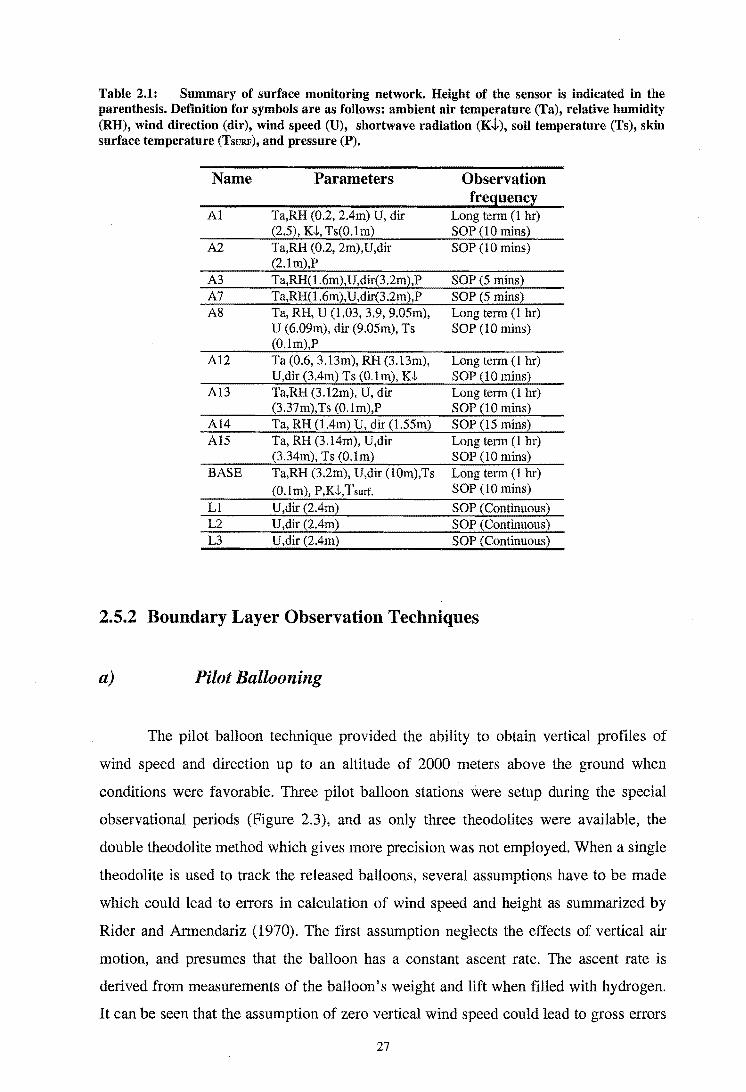
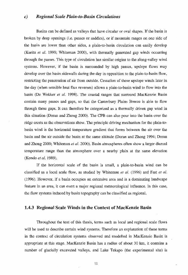
Table 2.1: Summary of surface monitoring network. Height of the sensor is indicated in the parenthesis. Definition for symbols are as follows: ambient air temperature (Ta), relative humidity (RR), wind direction (dir), wind speed (U), shortwave radiation (K-!-), soil temperature (Ts), skin surface temperature (TsURF), and pressure (P).

Name Parameters Observation freguencl:

Al Ta,RH (0.2, 204m) U, dir Long term (1 hr) (2.5), K!, Ts(O.1m) SOP (10 mins)

A2 Ta,RH (0.2, 2m),U,dir SOP (10 mins) (2.Im),P

A3 Ta,RH(1.6m),U,dir(3.2ml,P SOP (5 mins) A7 Ta,RH(1.6m),U,dir(3.2m2,P SOP (5 mins) A8 Ta, RH, U (1.03, 3.9, 9.05m), Long term (1 hr)

U (6.09m), dir (9.05m), Ts SOP (10 mins) (O.1m),P

Al2 Ta (0.6, 3.13m), RH (3. 13m), Long term (1 hr) U,dir (304m) Ts (O.1m), KJ, SOP (10 mins)

A13 Ta,RH (3.12m), U, dir Long term (1 hr) (3.37m),Ts (O.lm),P SOP (10 mins)

A14 Ta, RH (104m) U, dir (l.55m) SOP (15 mins2 A15 Ta, RH (3. 14m), U,dir Long term (1 hr)

(3.34m), Ts (OJm) SOP (10 mins) BASE Ta,RH (3.2m), U,dir (lOm),Ts Long term (1 hr)

(O.lm), P,K!,Tsurf. SOP (10 mins)

L1 U,dir (204m2 SOP (Continuous) L2 U,dir (204m) SOP (Continuous) L3 U,dir (2.4m) SOP (Continuous)

2.5.2 Boundary Layer Observation Techniques

a) Pilot Ballooning

The pilot balloon technique provided the ability to obtain vertical profiles of

wind speed and direction up to an altitude of 2000 meters above the ground when

conditions were favorable. Three pilot balloon stations were setup during the special

observational periods (Figure 2.3), and as only three theodolites were available, the

double theodolite method which gives more precision was not employed. When a single

theodolite is used to track the released balloons, several assumptions have to be made

which could lead to errors in calculation of wind speed and height as summarized by

Rider and Armendariz (1970). The first assumption neglects the effects of vertical air

motion, and presumes that the balloon has a constant ascent rate. The ascent rate is

derived from measurements of the balloon's weight and lift when filled with hydrogen.

It can be seen that the assumption of zero vertical wind speed could lead to gross errors

27

in mountainous terrain during strong winds when considerable vertical velocities might

be generated. Another factor that may lead to errors in calculation of wind speed and

height is variation of air density with altitude. Note that these errors become larger with

increasing height, so that near surface winds are more reliable.

b) Aircraft Data

An instrumented light aircraft (Piper-18I) obtained vertical profiles of pressure,

temperature and relative humidity for the SOP on February 2nd and 1t\ The aircraft

proved to be a very economical way of gathering data in remote areas. On February lth

, the aircraft managed to complete four flights (each being one and half hours in

duration), obtaining a total of 16 vertical profiles at four sites (Figure 2.3).

2.5.3 Wind Regime in the Basin During L TEX 99

The complex topography of the experimental site gives rise to a hierarchy of

topographically induced, multi-scale wind systems, making analysis of surface data a

challenging task. In the following sub-sections, it will be shown that the Canterbury

Plains Breeze is a persistent feature of the wind climatology of MacKenzie Basin.

Although its exact nature cannot be determined due to both paucity of data outside the

basin and the complicated topography inside, numerical experiments in the following

chapters will provide some insight to its origin and its three dimensional characteristics.

The limited amount of data collected in the field allows evaluation of model results in

the basin.

Previous studies paid much attention to investigating the surface wind regime

around Lake Tekapo. In this section, a close examination of daytime surface flow at

Base and Twizel weather stations for the duration of the field campaign in 1999 is made

(Figures 2.2, 2.3).

28

14~.------------~--·············~··············~~----------------------

10t---~~-!~~4-----~----------~----~-J,--';"

g 8+'~+-j4-~-*4H~'---~~--+---------~-r----n-7r-" ., ., ~ 6~~~4-H-~~~--~r+~--~~----~~~~~+-~-"0 c ~ 4

j e OJ .. :!'. c .2 U 1! Ci

" ~

o 25 Jan 30 Jan 04 Feb 09 Feb 13 Feb

(a)

14 ,----------

12+-----------------------------------~--------

10+-T--··*~~----~--------------------_,r_----_+--

8

6

4

2

25 Jan

360

270

180

90

.' J., ·.x .. . ,

0 6

30 Jan 04 Feb

(b)

10 14

Time (NZST)

(c)

18

09 Feb 13 Feb

~","'~, , .:~

,(~t!,;Lt',;ni \·..(t~ ~

22

Figure 2.4: Time series of (a) ten minute averages of wind speed for Base site, and (b) 30 minute averages of wind speed for Twizel, and (c) scatterplot of ten minute averages of wind direction for the Base site on the days when CPB intrusion into the basin took place (arrows indicate the days when the CPB was detected by the surface station),

29

Figures 2.4a, b present time series of wind speed for Base and Twizel stations,

respecti vely. The measurements are considered to be representative of the conditions in

MacKenzie Basin, since both surface stations are situated in relatively uncomplicated

physical settings (Le. not situated in valleys). Of particular interest, is the periodic

appearance of strong winds in MacKenzie Basin, which can also occur with the

grounding of synoptic airflow associated with prefrontal foehn west to northwesterly

winds (McGowan et al.1995). The arrows on Figure 2.4a indicate days that were ideal

for the development of thermally induced flows. On these days:

a) weak synoptic pressure gradients existed over the region

b) the basin was mostly cloud free for a significant portion of the day, as

determined from measurements of short-wave radiation at Base station

c) surface wind speeds before 1200 NZST were less than 6 ms· l (higher

wind speeds would suggest an existing synoptic scale influence).

At the Base weather station, strong southeasterly winds were measured on all

nine days, with an onset time of around 1400 NZST. Figure 2.4c shows a scatterplot of

10- minute-average wind direction data against time of day from the Base site for these

nine days, indicating that the strong winds only occurred from a narrow range of

directions. The strong airflow was usually well established by 1500 NZST, and on most

days it ceased shortly after sunset. A strong easterly wind also occurred at Twize1 on

each day except for 11 th February (Figure 2.4b). On this day, the easterly intrusion only

reached an intensity of 6 ms- l at the Base site. Therefore it seems that generally, the

Canterbury Plains Breeze is strong enough to dominate the surface flow throughout the

basin when it is blowing. The base station is located 8 km from Burke Pass and the

limited range in wind direction might indicate that the CPB is channelled by the pass,

although no weather stations were situated in or close to the pass to confirm this

hypothesis. What is evident is that the strong easterlies are a basin wide phenomenon,

and the physical scale of the forcing does not seem to be local in nature. Figure 2.5

shows that for the 12th February case study day, the easterly current reached the Base

station first and about an hour later arrived at the Twizel site. Assuming that the density

current's propagation speed is roughly equal to wind speed perpendicular to micro

front, with an average wind speed of 8 ms·! air can travel about 28 km suggesting that

the observed strong winds at Twizel are part of the same circulation observed at Base.

30

Therefore, the observations at these two stations reveal the existence of a

recurrent flow phenomenon across the basin. In its most basic form, this flow manifests

itself as a high-speed easterly with early to late afternoon onset period, and on most

days it ceases at these two sites shortly after sunset.

14 1. ....... •• I • • • •• •

12 ~ . ..,... ... ~

_ 10 • • " •• (f)

,§. • "0' 8 <U <U Co

en 6 "0 • !: • ~ 4

I I I I

2:00 10:00 12:00 14:00 16:00 18:00 20:00 22:00

Time (NZST)

(a)

14 f ............. · 12 •

_ 10 T

t,t en 6 T "0 ' !:

~ 4

2

•

• • ••••

••

+

• •

••••••••• •••••••

2:00 4:00 6:00 8:00 10:00 12:00 14:00 16:00 18:00 20:00 22:00

Time (NZST)

(b)

I

•

360

270

180

90

0

360

270

'L !: .9 (:) <U a "0 !:

~

!: .9 (:)

180 <U a ~

90

Figure 2.5: (a) Time series of ten minute averages of wind speed and direction for the Base site on 12th February, (b) time series of 30 minute averages of wind speed and direction for the Twizel station on 12th February (solid line represents wind speed, and diamonds represent wind direction).

31

2.5.4 Case Study Days: 2nd and 12th February 1999

In this section, a closer examination of the evolving wind field and boundary

layer development in the experimental area for the SOPs held on 2nd and 12th February

1999 is provided. On 2nd February, data collection efforts were concentrated at the

northern end of Lake Tekapo to gather information on nocturnal katabatic flows,

consequently pilot ballooning data are not available throughout the day. However, the

aircraft obtained three vertical profiles before noon and one profile in the evening over

the Base site. On 12th February, observational efforts concentrated on the study of

daytime thermally induced circulations along the lake and in Godley Valley, so that the

instrumented aircraft flew four times during the day, in addition, regular pilot balloon

data are available from the ballooning stations.

a) Synoptic Weather Conditions

As indicated previously, thermally induced flows are best observed during clear,

undisturbed weather, and such a condition existed on both 2nd and 12th February. The

slow moving centre of a high-pressure system was situated over the South Island on the

2nd (Figure 2.6a). The anticyclone was not deep, and analysis at 500mb indicates a

moderate southwesterly airflow aloft (Figure 2.6b). The 1200 NZST surface analysis on

Ith February also indicates anticyclonic synoptic scale circulation over New Zealand

(Figure 2.7a), although the high-pressure system was deeper on this day as indicated by

500mb analysis (Figure 2.7b). Therefore, the analysis of synoptic data indicates that

although surface pressure gradients were weak on both case study days, on the 2nd

February pressure gradients aloft were stronger.

Due to the passage of a cold front on 31 st January, the atmosphere inside the

basin was about 5 K colder on the 2nd compared to 12th February (Figure 2.8).

Interestingly enough, similarity in the difference between the first and the last profiles

obtained by the aircraft over the Base site indicates that the basin atmosphere was

heated by similar amounts on both days.

32

02 February 1999 0600NZST

(a)

(b)

Figure 2.6: Analysis for (a) 0600 NZST on 2nd February 1999 at surface by New Zealand Meteorological office, (b) 1200 NZST on 2nd February 1999 at 500mb by Institute of Global Environment and Society.

33

(a)

(b)

Figure 2.7: Analysis for (a) 1200 NZST on 12th February 1999 at surface by New Zealand Meteorological office, (b) 1200th NZST on 12 February 1999 at 500mb by Institute of Global Environment and Society.

34

2900

2700

2500

2300

::J 2100 (J)

~ « 1900 E -1: 1700 tn 'm

1500 J:

1300

1100

900

700 280 290 300 310 320

Potential Temperature (K)

Figure 2.8: Vertical profdes of potential temperature measured by the aircraft over the Base site on 2nd and 12th February.

b) Surface Observations

To gain insight into evolution of surface flow in the MacKenzie Basin and Lake

Tekapo region, a series of surface airflow maps were constructed. Surface airflow maps

using all available wind data at 1200, 1400, 1600, 1800 and 2000 NZST on 2nd February

are presented in Figure 2.9. By 1200 NZST, heating of the land surface around the lake

seems to have generated a lake breeze circulation resulting in a divergent flow (Figure

2.9a).

35

a) 1200 NZST b) 1400 NZST c) 1600 NZST

d) 1800 NZST e) 2000 NZST

10 m/s

1 m/s

Figure 2.9: Surface flow field on the 2nd February over Lake Tekapo region at (a) 1200 NZST, (b) 1400 NZST, (c) 1600 NZST, (d) 1800 NZST ,and (e) 2000 NZST. Wind speed and direction are ten minute averaged values.

36

During this SOP, a dense network of monitoring stations was placed at the northeast

comer of the lake, all the stations indicate a southwesterly flow which is probably a

combined upslope-lake breeze circulation. The two most northern stations in Godley

Valley detected a moderate northerly wind which seemed to converge with a weak

southerly valley wind circulation in Godley Valley. Two hours later at 1400 NZST, the

northerly current seems to have propagated further south (Figure 2.9b), and the

following diagrams show its progression southward, probably reaching the northern end

of Lake Tekapo by 1600 NZST, as detected by station A8 (Figure 2.9c). When the

current left Godley Valley, it seemed to flow to the west of the valley circulation

causing a horizontal wind shear that is maintained for about two hours between 1600 to

1800 NZST (Figures 2.9c, d). The northerly flow is probably generated by pressure

driven channeling (Whiteman and Doran 1993) related to the pressure gradient at higher

levels (Figure 2.6b), andlor foehn winds over the main divide (McGowan and Sturman

1996). By 1600 NZST, therefore, the surface airflow pattern in the study area was made

more complicated by three main features (Figure 2.9c). These were a southeasterly flow

at the Base site caused by the intrusion of the CPB, the locally forced diverging flow

over the lake, and the northerly current established over Godley River delta. The

northerly current weakened, and was retreating northward by 2000 NZST (Figure 2.ge),

probably in response to cessation of surface heating and decoupling of surface flow

from airflow aloft. However, the CPB was still evident at the Base site and moderate

cold air drainage initiated over Lake Tekapo. Time series of specific humidity and

temperature data obtained by a mobile energy balance station located over the eastern

slopes (indicated by MEB on Figure 2.9a) suggest that the downslope wind was

advecting moist air down the slope, indicating a coastal origin for the airmass (Figure

2.10). The easterlies detected by stations A12 and AI3, and the downslope winds on the

Two Thumb Range are likely to be part of the plain-to-basin circulation.

37

8 ......,

7 '701 ..:.: S >-

6 -:a 'E ::I

5 :::c (.) :;: '(3

4 Q) c. en

3

4 8 12 16 20 24

Time (NZST)

4 360

~

3 270 C 'I/) c E- o

:;: "0 (.)

180 III III 2 .... Q) C:i c.

en "0 "0 C c 90 ;: ;:

0

0 4 8 12 16 20 24

Time (NZST) -_ ..... _-

~

Figure 2.10: Time series of (a) temperature and specific humidity, and (b) wind speed and direction, measured by a mobile energy balance station over the western slopes of the Two Thumb Range (values are 15 minute averages).

The surface wind field on 12th February evolved differently. At 1000 NZST

(Figure 2.11a), the stations in Godley Valley detected weak easterlies, these cross

valley winds are probably in response to surface heating of the eastern slopes of the

valley leading to cross-valley temperature gradients. Because of the weak upper level

winds, the strong northerly current that was observed on the 2nd February was not

present. A weak lake breeze circulation had developed around lake Tekapo, which

seemed to intensify by 1300 NZST (Figure 2. llb). Up-valley winds were established in

38

a) 1000 NZST

c) 1600 NZST

1 m/s ..

b) 1300 NZST

Figure 2.11: Surface flow field on the 12th February over Lake Tekapo region at (a) 1000 NZST, (b) 1300 NZST, (c) 1600 NZST, and (d) 1900 NZST. Wind speed and direction are ten minute averaged values.

39

Godley and Macaulay Valleys, and the Canterbury Plains Breeze was now detected at

the Base and L3 stations. At 1600 NZST, the plain-to-basin wind was also flowing

through Tekapo Saddle (Figure 2.1), as detected by station A14, and some parts of the

flow are diverted southward by Mt. John (which has an elevation of 1031 m AMSL) as

measured by the station in Tekapo Village (Figure 2.l1c). A component of this

northerly might be the local lake breeze sheltered by the moraine south of the village.

The moderate intensity of the up-valley wind at the north end of the lake suggests that

the easterly intrusion was channelled towards the two river valleys, in addition, pibal

data indicate that a strong southerly current 200 m in depth was blowing at this time

over the Boundary stream station (Figure 2.l3c). By 1900 NZST, the locally induced

thermal flows had weakened, but the CPB had maintained its intensity, and

interestingly, a strong current evident at Al and A2 stations seemed to be propagating

northwards in Godley Valley (Figure 2.11d).

Figure 2.12 presents time series of temperature, wind speed and direction for the

case study days for the Base weather station. The onset of the CPB at this site occurred

at about 1400 NZST on 12th February and at around 1600 NZST on the 2nd (as indicated

by the arrows). The arrival of the current was associated with decreasing air

temperature, indicating that the CPB was advecting cold air into the basin (Figure

2.l2c).

40

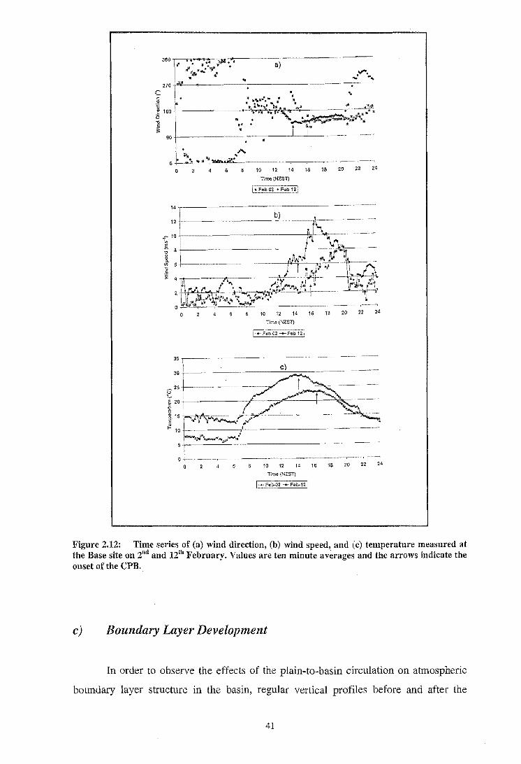
o +--.;.. ..... ~2!c.~'1>=<!''"!'''.''-... ~A. ____ ~_~._~~ ~-... ~ o 4 6 10 12 14

Tlme (NZSl)

16 18 20 22 24

12~----~--~--~---~--·---------

1Q 12 14 16 18 20 22

Tlm. (NZSl)

~25~---------··-~~-4-~~c-··--------

E ~20~ _______ ~_~~~--_~-3~~------

115~~~~---~)~·~~~~---------····~~~ E ~ 10~-------/----------------

o~·····~----- -----------~ ..... -,--~ 10 12 14 16 18 20 22 24

Time iNZST)

Figure 2.12: Time series of (a) wind direction, (b) wind speed, and (c) temperature measured at the Base site on 2nd and 12th February. Values are ten minute averages and the arrows indicate the onset of the CPB.

c) Boundary Layer Development

In order to observe the effects of the plain-to-basin circulation on atmospheric

boundary layer structure in the basin, regular vertical profiles before and after the

41

intrusion are required. Additionally, to quantitatively determine the nature of the forcing

using observational data it would have been desirable to have had vertical profiles

available at a site outside MacKenzie Basin over the Canterbury Plains. As explained

before, as the importance of such a circulation system for the wind regime of the basin

had not been recognized, the opportunity to collect an appropriate dataset was missed.

Since 12th February was chosen as a case study simulation day for the numerical

experiments, and the early morning vertical profile of thermodynamic variables from

the aircraft was used to initialize high resolution model runs in Chapter 6, the observed

boundary layer behaviour is described below.

Figure 2.13 presents contour plots of the u and v components of wind derived

from the data obtained by the three pilot ballooning stations (see figure 2.3). A strong

600 m deep southeasterly flow was detected by the station at Tekapo airport (Figures

2.l3a, b). The head of the current passed this location at about 1400 NZST in agreement

with measurements at Base weather station located 4 km to the south, and continued to

flow until 1800 NZST. Strong southerly currents also developed at Boundary (AB) and

Godley (A2) stations (Figures 2.l3c, e), while surface wind maps suggest that this

current originated from Tekapo Saddle and then was deflected northwards (Figure

2.10c). This southerly current had a depth of 300 m and hence, was not as deep as the

one detected at the airport. The current arrived at Boundary site at 1500 NZST, and

continued to flow until 1800 NZST. A 500 m deep southerly up-valley wind was

measured in Godley Valley from 1100 to 1500 NZST, and then a strong southerly

current with a depth of 600 m passed the pilot balloon station at 1600 NZST (Figure

2.13e). The current maintained its intensity by the time the measurements were stopped

at 2000 NZST.

Figure 2.14 shows the temporal evolution of vertical profiles of potential

temperature measured by the aircraft above Base and mid-lake locations. A parabolic

shaped temperature inversion existed in the morning over the basin, whereas the

temperature structure over the lake was more layered. By 0935 NZST, turbulent

sensible heat flux had caused the formation of a 300 m mixed layer over the basin, and

the profile over the lake still showed the existence of the temperature inversion. The air

below 2100 m seemed to have warmed due to advective heating. The third profile over

each location shows the presence of a 1500m mixed layer, although the mixed layer

over the lake was probably advected from the basin by the southerly valley wind. There

is a four and half hour gap between the third and the fourth profiles, hence no vertical

temperature profiles exist close to the time when the CPB was detected at the Base

42

a) v-component (m/s) 2000

\'h~~.,

1800

1600

1400

en <II 1200 g E 1000 ,£, !J)

J: 800

600

400

200

1000 1200 1400 1600

Time (NZST)

c) v-component (mls) 2000

1800

1600

en en '" <II

g g :c E C) C)

';jj 800 ';jj

J: .~.~ .. ,~~. J:

600

400

200 t,:.1

e) v-component (m/s) 2000r--------r---r--:-r-r------r

1800

1600

1400

g> 1200

E :::- 1000 ..c:: 0>

~ 800

600

600 800 1000 1200 1400 1600 1800 2000

Time (NZST)

u-component (m/s)

u-component (m/s)

800

600

400

f) u-component (m/s) 2000r-------~~-----i~~-,r--,

1800 /"

Figure 2.13: Contour plots of Uw and vwcomponents of wind velocity for the (a, b) airport, (c, d) Boundary Stream, and (e, f) Godley VaDey pilot balloon stations on 12th February.

43

a)

2700 ~ I' -+- 0607 NZST .\ 2500 I ~ 0935 NZST

--1341 NZST 2300

::::- 2100 IJ) i 1900

:c 1700 Cl ~ 1500

1300

1100

900

--1814 NZST

12102199 Airport

700~~~~~~~~~~~~~,-~~-,~~~

285 290

b)

2700 1-+- 0628 NZST 2500 -- 0958 NZST

-- 1403 NZST i

2300 . ~ 1838 NZST

::::- 2100 IJ) i 1900

:c 1700 Cl ~ 1500

1300

295 300 305

Potential Temperature \KJ

12f02f99 Mid-lake

1100 -j'

900 _ 700~~~1~1~1~~~1~'~~-r~~~~·

285 290 295 300 305


310 315

, I

310 315

Figure 2.14: Vertical profiles of potential temperature measured by the aircraft over the (a) airport and (b) mid-lake area on 12th February.

surface station. But the fourth profile in the basin suggests that a 300 m layer

had been affected by cold air advection. There is no significant difference between the

third and the fourth profiles over the lake.

44

2.6 Summary and Conclusion

Although the monitoring network for LTEX was not ideal for a comprehensive

study of a regional scale wind system such as the Canterbury Plain Breeze, available

surface data in the basin reveal interesting characteristics of this circulation. On spring

and summer days when undisturbed weather dominates the region, the CPB will flow

into the basin either through mountain passes and saddles, and/or flow down the slopes

as observed on 2nd February. The breeze has the intensity to dominate surface flow

throughout the basin, and is associated with cold air advection. Therefore, the

Canterbury Plain Breeze is a recurring circulation system during settled weather

conditions. Since the air current seems to originate from outside MacKenzie Basin, its

horizontal forcing falls into the regional scale category.

45

Chapter 3

Model Description

The Regional Atmospheric Modeling System (RAMS) was developed at the

Colorado State University, where it was formed as a result of merging three different

numerical codes (Pielke 1992). The code is almost entirely written in Fortran 77, with

the exception of a few subroutines written in C which deal with dynamic memory

allocation. RAMS, in its current form is a flexible, general purpose numerical code,

capable of simulating a variety of atmospheric flows. It has been used to study flows at

several scales, ranging from flow over buildings to hemispheric circulations. The model

contains a full set of subgrid, microphysical, radiative, convective and surface-layer

parameterizations. Prognostic models for soil and vegetation temperature and moisture

are also included. The model's other capability is a telescoping two-way interactive grid

nesting, so that it is possible for a single simulation to represent forcings from a

multitude of scales.

The model runs are usually configured in a namelist file called RAMSIN.

Various peripheral data preparation codes are also provided for formatting input data

into RAMS. A description of procedures for setting up a model run is not provided here

since it is beyond the scope of this chapter. The version of RAMS used in this thesis is

designated as 3a, and this particular code has been tested by scientists at the Pacific

Northwest National Laboratories in Richland, Washington State since 1995 (Fast et al.

1996; Zhong et al. 1996; De Wekker et al. 1998; Whiteman et al. 2000; Doran and

Zhong 2000). The code has been thoroughly tested, and the known bugs have been

47

fixed. Simulations were carried out on a dual processor (300 MHz each) Ultra

Enterprise Sun Microsystem computer, running the Solaris 2.6 Unix operating system.

At compilation time the executable was optimized to level 5 (05) for maximum

efficiency. The real clock-time for the simulations in Chapter 4 was approximately five

days, the two-dimensional runs in Chapter 5 took seven hours of computation, and the

high resolution runs in Chapter 6 took nearly three weeks to complete.

3.1 Background

The fact that the atmosphere is a hydro-thermodynamic system has been realized

for the past 200 years. This realization meant that atmospheric motions could be

quantified (analyzed by equations) with the familiar Newtonian mechanics and the laws

of thermodynamics (Holton 1979). Subsequently in the 19th century, a basic set of

equations governing the movement of air in the atmosphere known as the "primitive

equations" was developed. The term primitive in no way indicates that the equations are

outmoded, rather it highlights their fundamental nature (Wallace and Hobbs 1977). The

primitive equations are equations of momentum, continuity, thermodynamics and

moisture (Atkinson 1981; Brown 1991). The equations for momentum are sometimes

referred to as the Navier-Stokes equations since Navier and Stokes independently

derived them. However, the title is also used to include the continuity equation and the

thermodynamic equation, therefore nowadays the terms primitive equations and Navier

Stokes equations are used interchangeably. The primitive equations are highly complex

and non-linear which makes them impossible to solve by current available analytic

techniques. Hence, analytic solutions for them are unknown, except when the equation

set is simplified and linearized. Although the simplified forms of the equations give

valuable insight into certain types of atmospheric phenomena, their general applicability

is limited since non-linear influences are ignored. With the development of high-speed

digital computers it has become possible to make extensive use of the primitive

equations in their non-linear form using numerical techniques, since these techniques

require vast amounts of mathematical calculations. Indeed John von Neuman, one of the

pioneers of the development of high-speed digital computers, was the first to recognize

that computers could help in forecasting weather (Wallace and Hobbs, 1977).

48

3.2 Averaging the Primitive Equations

As previously mentioned, because of their non-linearity, analytic solutions for

the primitive equations are not available (this is true for almost all physical problems),

therefore numerical techniques are used to provide approximate solutions to the

equations. Tannehill et al. (1997) provided one of the most highly regarded books on

numerical methods for fluid mechanics and heat transfer, which provides an exhaustive

description of various numerical methods, including the ones used in RAMS.

Holton (1979) provides an in-depth derivation of the primitive equations, while

Pielke (1984) offers derivation and assumptions used to provide a suitable equation set

describing mesoscale flow. In the ensuing section, the set of equations which are solved

by RAMS are presented in their volume averaged form, with an explanation for

averaging provided next.

The primitive equations contain partial differential operators (a/at, alax, a/ay,

a/az) which in the strictest mathematical sense are only valid in the limit when Ot, ox, oy, and oz approach zero (time increment and the three spatial intervals respectively).

Physically, this means that in order to solve the equations exactly with numerical

techniques the solution has to be computed at molecular level, which is for now and the

foreseeable future impossible. To bypass this problem, the conservation equations have

to be integrated over specified spatial and temporal scales determined by the available

computer capacity and its speed of operation. Therefore, an averaging decomposition

(also known as Reynold's decomposition) is performed on the conservation equations:

(3-1)

where ¢ represents anyone of the dependent variables, and if is the average of ¢ over

the finite time increment /).t and space intervals /).x, /).y, and Llz (Figure 3.1). The

variable ¢' is known as the subgrid scale perturbation which is the deviation of¢ from

the average, it is this quantity that has to be parameterized in models. ¢ is formally

defined as:

HM x+& z+fu

if=f J J ¢ dz dy dx dt I (/).t) (/).x) (/).y) (Llz) (3-2) x y

49

In numerical models, !!.t is known as the time step and !!.x, !!.y, and & are the grid

intervals. This averaging operator is applied to the conservation equations, and details

of this mathematical procedure are offered by Pielke (1984), while the final form of the

equations are presented in the next section.

tn

Figure 3.1: Representation of a grid volume. Dependent variables are defined at the corners of the rectangular grid.

3.3 A Brief Technical Description of RAMS

Only a brief technical description of the model is provided in this section. All

model integrations for this work use the non-hydrostatic dynamic framework. This

framework should be included when the scale of resolved features in the model have

aspect ratios near unity, or when the horizontal scale is shorter than the vertical scale.

The additional term in the non-hydrostatic dynamics is vertical acceleration that

contributes to variations in the vertical pressure gradient, so that the hydrostatic balance

is no longer maintained exactly. The general equations for RAMS are described in the

following section (overbars indicating averaged quantities are omitted).

50

3.3.1 General Equations Solved by RAMS

Equations of motion

The horizontal equations of motion are:

au -= at

av at

I

au au au u -v--w-ax ay az -8 an'

ax + tv a(u'u') a(u'v') a (u'w')

+ + +

av av -u-ax Vay

II

ax ay az

wav _ 8 an' az ay

fu a(v'u') a (v'v') a (v'w') + + + ax ay az

III IV V

Term I represents wind acceleration

Term II represents advection

Term III represents the pressure gradient force

Term IV represents coriolis force

Term V represents turbulent diffusion

(3-3)

(3-4)

where u and v are the horizontal velocity components and w is the vertical

component. n' is the perturbation Exner function, which arises in these equations as a

result of replacing pressure with the total Exner function (n) in the equations before

Reynold's averaging is performed on them. In mesoscale models, the pressure gradient

term is expressed with the Exner function rather than pressure. The advantages of using

the Exner function are that the term involving density perturbation (p') is removed

from the equation set, and since the vertical gradient of n is much less than pressure,

fewer numerical errors occur in its calculation during model integration. Total Exner

function is defined as:

n= C Tv p 8 (3-5)

where Cp is specific heat of air at constant pressure, Ty is virtual temperature, and 8 is the

potential temperature. The vertical momentum equation for the non-hydrostatic case is:

51

aw at I

aw aw aw u--v--w-ax ay az II

O a11:' gO~ a(w'u') a(w'v') a (w'w') - -- + + + ---'----'-az 00 ax ay az III IV V

where term IV now represents buoyancy force.

Thermodynamic equation:

The thermodynamic state of the atmosphere is prognosed by:

u---v---w--+ + + + --aOi/ __ aOa aOn aOi/ a(u'o:z) a(v'o:z) a(w'o~) (aOi/) at ax ay az ax ay az at rad

I II III IV

Term I is total heating rate

Term TI represents horizontal advection

Term TIl represents turbulent flux divergence

Term IV represents radiative flux divergence

(3-6)

(3·7)

Oil is the ice-liquid water potential temperature. Ice-liquid water potential temperature

instead of potential temperature is used in RAMS to avoid specification of latent heat

tendencies in Equation (3-7). Oil remains unchanged in the presence of all water phase

changes as demonstrated by Tripoli and Cotton (1981),

Equation of mass continuity:

In the non-hydrostatic framework, the equation for mass continuity is expressed as:

a11:' =_ R11:o (apoOou + apooov + apooowJ at cvPoOo ax ay az (3-8)

Where p is air density, Cv is specific heat for air at constant volume, and R is the gas

constant, and 11:0 , PO' and 00 are synoptic scale reference values of these variables

(Pielke 1984).

52

Equation of continuity for water species mixing ratio:

Tendency for water species mixing ratio (rn) is calculated by:

dr" dr" drn dr" d(u'r:} d(v'r:} d(w'r') --=-u---v---w--+ + + n

dt dX dy dZ dX dY dZ (3-9)

3.3.2 Grid Stagger

RAMS uses the standard C grid configuration after Mesinger and Arakawa

(1976). Thermodynamic and moisture variables are defined at the same points, while

the three velocity components u, v, and w are staggered 112 Ax, 112 Ay, and 112 Az

respectively (Figure 3.2). Figure 3.2a illustrates the horizontal cross section of the grid

lattice structure with one nested grid. The coarse mesh, which is referred to as GRID 1

is represented by upper case letters denoting variable locations: U for west~east

velocity, V for south-north velocity, and T for thermodynamic variables (all variables

other than velocity components). GRID 2 is nested within GRID 1 with a finer mesh.

The variables defined on GRID 2 are denoted by lower case letters completely

analogous to grid 1. Figure 3.2b illustrates a vertical cross section of the grid lattice

structure used in RAMS. Grid nesting is analogous to the horizontal cross section,

except W and ware vertical velocity components for grids I and 2 respectively. Note

that vertical grid nesting capability was not used for simulations presented in this thesis.

The map projection for the horizontal grid is a rotated polar-stereographic

projection. The pole of the projection is rotated to an area near the centre of the model

domain in order to minimize the distortion due to the projection.

53

a)

T

v

"7

b)

If w

Figure 3.2: Illustration of Arakawa type C stagger, (a) horizontal cross-section of the grid lattice structure (b) vertical cross-section of the grid lattice structure. (Note: an explanation for the lattice structure and the symbols is provided in the text.)

54

3.3.3 Terrain~Following Coordinate System

In order to represent topography in mesoscale models, vertical terrain following

coordinate systems are incorporated in their formulations. RAMS uses the (J z terrain

following coordinate system (Gal-Chen and Somerville 1975; Clark 1977; Tripoli and

Cotton 1982). The top of the model domain is exactly flat and the bottom follows the

terrain. The coordinates in such a system are defined as:

* x = x

* y =Y (3-10)

z· H( Z-Zg J H-Zg

where H is the height of the top of the grid and Zg is local topography height which is a

function of x and y. Derivative terms can be written in tensor notation according to

Clark (1977) as:

(3~11)

for i and j = 1,2,3 (three spatial dimensions), and the tensor bij can be written as:

1 0 ~ dZ, [~-lJ a ax H

bi} = 0 1 ~ 3z, [~-1 J (3-12) a ay H

0 0 1

a

A good explanation for tensor notation is provided by Stull (1988).

55

3.3.4 Vertical Levels

It is often desirable to have higher vertical resolution close to the ground so that

the processes in the boundary layer are better resolved. As a result, in RAMS, the user

can specify variable vertical grid spacings. An expansion ratio Rj can be defined as:

(3~13)

where

(3~14)

large expansion ratios are often avoided (note that Z is the thickness of a vertical layer

and should not be confused with z ).

3.3.5 Grid Nesting

RAMS employs the grid nesting technique described in Clark and Farley (1984)

and Clark and Hall (1991). In selected regions, grids with high spatial resolution can be

nested within lower resolution grids. Any number of nested grids can be used, within

the limits of available computer memory. Grids can be configured in a telescoping

sequence where parent grids themselves are nested within coarser grids. A nested grid

need not extend from the ground to the model top, and it can be moved horizontally

during the simulation, this feature is useful in modelling thunderstorms or tropical

cyclones in order to keep the phenomena within the high resolution grid.

The grid nesting technique carries out a two-way exchange of computed values

for all prognostic variables between any nested grid and its parent grid. After each

coarse grid timestep, the computed values are updated at the boundaries of the finer grid

by interpolation. A nested grid usually runs with a shorter timestep than the parent grid,

so that temporal linear interpolation is also performed to update values at the nested grid

boundaries. The nested grid goes through several smaller timesteps and once it is

updated to the same time as the parent grid, reverse communication is accomplished by

averaging the prognostic variables over each set of nested grid cells which occupy a

single parent cell, and replacing the parent grid value.

56

3.3.6 Turbulent Mixing Parameterization

The horizontal and vertical grid spacings of a simulation determine the spatial

scales of the prognostic variables that can be explicitly resolved, while contribution

from spatial scales smaller than the grid spacing have to be parameterized. Simulations

performed for this thesis were set up to use the Mellor and Yamada (1974, 1982)

technique for calculating vertical eddy mixing coefficients. Their so-called level 2.5

scheme predicts turbulent kinetic energy (TKE) , with modification for the case of

growing turbulence (Helfand and Labraga 1988). A local deformation scheme based on

Smagorinsky (1963) is used to calculate horizontal diffusion, which is calculated as the

product of horizontal deformation rate (horizontal gradients of horizontal velocity) and

a length scale squared. A brief description of the vertical diffusion scheme is provided

in this section.

The Mellor and Yamada scheme is based on a prognostic equation for the TKE

(e) which is solved in the numerical model at each timestep. TKE is defined as:

1 (-----;:j + n + --,-:j) e= - u v w 2

(3-15)

while the prognostic equation for TKE is:

de de de de d de d de d de -u--v -w-+ K +-Ke +-Ke +Ps +Pb -£

dt dX dY dZ dX e dX dY dY dZ dZ (3-16)

Psis the shear production term calculated by

(3-17)

whereas Pb is the buoyancy production term determined from

57

P =-.¥...K dev belt dz

and the viscous dissipation term is given by

e~ B=a -

e I

(3-18)

(3-19)

where I is the master length scale, the calculation of which is covered in Mellor and

Yamada (1974). Once TKE is computed, the vertical eddy diffusivities for momentum

(Km), heat (Kh), and TKE itself (Ke) are determined from

K = S 1(2e)h In m

Kit = Sltl(2e)h (3-20)

Ke = Sel(2e)h

where Sm, Sh and Se are nondimensional eddy diffusivities for momentum, heat and

TKE respectively. Details of their calculation is provided in Mellor and Yamada (1982).

3.3.7 Surface Layer Parameterization

The Monin-Obukhov similarity theory provides the most suitable theoretical

framework for the description of fluxes of heat, moisture and momentum in the surface

layer. The basic similarity hypothesis for the surface layer was proposed by Monin and

Obukhov (1954) for a horizontally homogenous flat terrain, under clear sky conditions.

Little is known about the validity of the similarity theory in complex terrain. However,

it seems that the similarity theory may be applied in complicated conditions since

numerical models have relative success under such conditions. RAMS employs a

scheme developed by Louis (1979) to compute the surface layer fluxes of heat,

momentum, and water vapor. His scheme provides precomputed approximations of the

flux profile functions of Businger et al. (1971), which need to be solved iteratively. The

scheme determines fluxes between the land surface and the atmosphere for water

surfaces, bare soil and vegetated surfaces. After the fluxes are computed, the values are

58

used as a lower boundary for the subgrid diffusion scheme. The equations for surface

layer fluxes are:

(3-21)

where R is a constant representing the ratio of drag coefficients for momentum and heat

in the neutral limit, which was estimated to equal 0.74 (Businger et al. 1971), 20 is

roughness length, u* is velocity scale, 8. is temperature scale, r. is mixing ratio scale

(Arya 1988; Louis 1979).

(3·22)

where k is the Von Karman constant. F is evaluated for two conditions, for the unstable

case it can be expressed as:

(3-23)

and for the stable case it can be expressed as:

Ri B is the bulk Richardson number defined as:

(3-25)

59

where g is gravitational acceleration, Tzo and (Jzo are extrapolated roughness length

values for temperature and potential temperature, and U is wind speed. The empirical

constants b and b' are set to 9.4 and 4.7 respectively for both Fm and Fh (Louis 1979).

The constant c is determined by the expression:

(3-26)

where C' is equals to 7.4 for Fm and 5.3 for Fh (Louis 1979).

3.3.8 Spatial Boundary Conditions

Most frequently, mesoscale models are configured to simulate atmospheric

motion in a limited area (they are not designed to be global models), therefore the

model domain has to be artificially enclosed with sides. Hence, it is necessary to assign

values for the dependent variables at the perimeter of the model domain. These values

are referred to as boundary conditions and have to be integrated in time similar to the

interior regions of the domain. In mesoscale models, treatment of each boundary is

different and they are referred to as the bottom, top, or lateral boundary.

a) Lateral Boundary Conditions

It is generally desirable to have the lateral boundary as far away from the region

of interest as possible. Mesoscale models generally employ two types of lateral

boundary conditions:

1) open lateral boundary, where mesoscale perturbations can pass into and

out of the model domain

2) closed lateral boundary, where mesoscale perturbations are not permitted

to enter or exit.

The general form of the lateral boundary condition used on the C-grid stagger of RAMS

is the radiative condition. The radiative condition minimizes reflection of outward

propagating perturbations within the flow, back into the interior of the model domain.

For the east-west boundary, the specification at the lateral boundary is:

60

au at

au -(u+c) ax (3-27)

where u is the wind component normal to the boundary, and c is the phase velocity. In

RAMS, the phase velocity can be specified with several options. The option used for

simulations in this thesis was proposed by Klemp and Wilhelmson (1978a, b) where c

is a constant equal to the model domain height divided by the Brunt-VaisaHi. frequency

multiplied by n. The Brunt-VaisaIa frequency (NBv) is defined by:

N = ~g ae BV e az (3·28)

which is a measure of the static stability of the atmosphere.

For all other variables besides the normal velocity component a scheme called

the zero-gradient condition was chosen. In this scheme, the value of each variable at the

boundary is set to the value immediately adjacent to it in the interior (hence zero

gradient). This option gave the most desirable outcome for the simulations where the

initial conditions were horizontally homogeneous.

RAMS provides the modeller with several different options for the treatment of

the lateral boundary, the most suitable option is usually determined by performing

numerical experiments. For the coarse grid of model simulations used in this thesis, the

Klemp and Wilhelmson condition was activated. With this condition, the normal

velocity component specified at the lateral boundary is effectively advected from the

interior.

The two-dimensional simulations in Chapter 5 used the cyclic lateral boundary

condition for the north-south direction. A cyclic boundary condition makes the model

periodic in the y-direction, effectively eliminating the north-south lateral boundaries

from the solution. This is achieved by forcing the values of dependent variables at one

boundary to be identical to the value at the other end (Pielke 1984).

b) Top Boundary Conditions

For the non-hydrostatic equation set, two options for the treatment of the top boundary

are offered in RAMS. A simple wall option is used for the simulations in this thesis.

61

With this option, the vertical velocity component is set to zero at the model top (w=O),

which is recommended for simulations which are horizontally homogeneously

initialized. For this case, a Rayleigh friction layer has to be applied to the top boundary

to prevent the reflection of gravity waves from the model top. In the friction layer, an

extra term is added to the basic prognostic equations so that the prognostic variables are

relaxed (nudged) towards the horizontally homogenous reference state, by defining:

(3-29)

where <p represents the prognostic variables u, v, w, and e, <Po is the initial value of

these variables, and 't is a timescale. 't is a linear function of height and it's value can be

set by the modeller. Usually a value between 60 and 300 seconds is chosen for the very

top layer which has the strongest effect in damping the waves.

3.3.9 Soil and Vegetation Parameterization

The surface layer parameterization described above requires surface temperature

and moisture values to calculate fluxes. In RAMS, the surface is divided into three

different classes: water, bare soil and vegetated surface. For water surfaces, the code

only allows for spatial variations in temperature, and since most simulations last a few

days or less, no temporal variation is accommodated for in the code. In contrast,

prognostic temperature and moisture models are used to provide predicted values for the

land surfaces. For bare soil, RAMS uses the multi-layer soil model of Tremback and

Kessler (1985), while for vegetated surfaces the model described by A vissar and Pielke

(1989) is used.

62

Chapter 4

Three-Dimensional Numerical Modelling of the Regional-Scale Flow

4.1 Introduction

In Chapter 2, observational data showed the development of a strong easterly wind

in MacKenzie Basin and Lake Tekapo region early in the afternoon during settled

anticyclonic conditions in summer. It was concluded that, when the synoptic scale pressure

gradients over the region are small, the daytime wind field in the basin is dominated by

thermal forcings at two scales. Locally induced upslope and up-valley winds (which are the

focus of numerical simulations in Chapter 6) are a common feature of surface flow until

early in the afternoon, followed by a regionally induced, strong easterly current that

penetrates the basin atmosphere through mountain passes and saddles in the foothills. As

this wind seems to originate from the region east of the foothills (over the Canterbury

Plains) it was named the Canterbury Plains Breeze (CPB). The exact nature of this

circulation cannot be determined due to paucity of observational data inside and outside the

basin.

63

Therefore, it is the aim of this chapter to conduct a preliminary investigation into

the physical mechanisms responsible for this regional-scale circulation by performing

three-dimensional numerical experiments with RAMS. In the following chapter, results

from high resolution two-dimensional sensitivity experiments are presented in order to

provide additional insight into the causes and nature of the CPB circulation. The objectives

of this chapter are the following:

• to determine if RAMS is able to simulate the CPB circulation for the case study day

• to determine if this circulation can evolve in MacKenzie Basin exclusively from terrain

heating

• to determine the extent to which the CPB intrusion into MacKenzie Basin is affected by

sea breeze forcing.

To achieve these objectives, three-dimensional simulations using a realistic

topographic configuration are performed, providing an additional analysis tool for

improved understanding of the CPB circulation. The approach used is to successively

remove forcing parameters from the simulations (from complex to simple) in order to

investigate the nature of the regional scale flow. Therefore, the first simulation (designated

as REG-ECM) includes the effects of evolving synoptic scale winds and land-sea contrasts

on thermally driven circulations in the region. The second simulation (designated as REG

NOW) examines circulations developed solely in response to .heating of the surface by

removing large scale winds. The third simulation removes another forcing parameter by

replacing the ocean around New Zealand with land, therefore eliminating the influence of

sea-breeze circulations. Table 4.1 provides a summary of the three-dimensional

simulations.

Table 4.1: Summary of 3·D simulations conducted.

REG-ECM ECMWF nudged

REG-NOW No synoptic-scale pressure gradient

REG-NOS Same as above, plus no ocean

64

Regional-scale circulation response to synoptic forcings

Response to surface heating alone

To examine the role of the sea breeze

4.2 Numerical Experiments

The case study day chosen for the numerical simulations is February 12, 1999.

Details on synoptic scale conditions and local observations for this day are provided in

Chapter 2. Simulations are initialized on the evening of February 11 to let the model cycle

through a nocturnal phase before the onset of surface heating the next day. This allows the

model to have some "spin-up" time in adjusting the flow fields to the complex topography

of New Zealand, and to allow simulated radiative cooling to produce more realistic low

level stratification over the complex terrain.

The horizontal spatial resolution and grid structure of the simulations are chosen to

simulate forcings at meso-~ scale (20 - 200 kIn), with the main features of MacKenzie

Basin topography (and hence the underlying thermal forcing) well represented. Two

different methods are utilized for initializing the model, as described below. REG-ECM

includes effects of variable winds from the evolving synoptic-scale circulation (Table 4.1).

REG-NOW (no initial wind field) run is initialized with the atmosphere at rest, and only a

single vertical profile for temperature and humidity is specified for the whole domain

(horizontally homogeneous initialization). The flow fields generated by this run should

evolve due to terrain cooling/heating alone. The ocean surrounding New Zealand is

removed from the REG-NOS (no sea) domain to further eliminate circulations produced by

land-sea contrasts. The initialization of this third run is similar to REG-NOW.

4.2.1 Three-Dimensional Simulation Development

a) Grid Structure

Horizontal grid-nesting capability of the model is used for the three-dimensional

simulations. Grid nesting allows focusing of higher spatial resolution on the desired regions

within the domain for greater computational efficiency (for details refer to Chapter 3).

Table 4.2 provides a summary of the settings for each nested grid. Simulations in this

chapter use three grids: the coarse grid covering New Zealand has a 36 kIn horizontal

resolution, the first nested grid (grid 2) has a horizontal resolution of 12 kIn covering the

65

South Island, and the second nested grid (grid 3) has a horizontal resolution of 4 kIn

covering the middle third of the South Island (Figure 4.1). Grid 1 is centered at 171°W and

42°S, while grids 2 and 3 are both centered at 171.4°W and 44°S. The three grids consist of

52, 62, and 50 zonal and meridional grid cells, respectively (Table 4.2).

Vertical grid-nesting capability of RAMS was not employed for these simulations,

therefore each grid has 32 vertical layers, with a 50 m vertical grid spacing in the lowest

layer (Table 4.2). The thickness increases geometrically by the ratio of 1.12 over the first

27 model layers to about 7 kIn AGL and remains at a constant thickness of 1 kIn over the

final 5 layers until the top of the model domain is reached at 12 kIn AGL. The Rayleigh

friction damping scheme is applied to the four vertical layers below the upper boundary to

suppress vertically propagating gravity waves for REG-NOW and REG-NOS experiments.

Since REG-ECM is initialized inhomogeneously with ECMWF data, top boundary nudging

(which also damps gravity waves) was applied to the vertical layers above 7 kIn AGL.

Table 4.2: Characteristics of the grids used for the three-dimensional model runs.

Grid 1 Grid 2 Grid 3

Number of east-west nodes 52 62 50

Number of north-south nodes 52 62 50

Number of vertical nodes 32 32 32

fu, b.y Ckm) 36 12 4

East-west width (km) 1836 732 196

North-south width (km) 1836 732 196

b.z at first level (m) 50 50 50

Vertical stretch ratio 1.12 1.12 1.12

Grid top Ckm) 12 12 12

b.t Cs) 20 6.7 2.2

66

161.2

- 49.6

158.3

NORTH

N

r

Figure 4.1: Geographic locations of grids 1, 2, and 3 for the three-dimensional

simulations.

-179.2 - 33.3

-49.6

-176.3

Topography for all grids is derived from the 30-second (about 1 kIn) terrain

dataset from the U.S. Geological survey (USGS) and smoothed with a silhouette

averaging scheme that preserves realistic topographic heights. The averaging scheme

and the horizontal grid spacing for grid 3 resolves the dominant terrain features of

MacKenzie Basin and the surrounding regions, including coastal regions on both sides

of the main divide (as shown in Figures 4.2, 4.3). Since the horizontal spatial resolution

for this grid is 4 kIn, finer topographic features like the Godley and Macaulay Valleys

are not well resolved. Therefore, the model is not able to produce thermally induced

flows forced by these features (meso-y scale circulations). As the main objective of this

chapter is simulating regional-scale (meso-~) forcings, it is only important to have the

67

basin and the surrounding region well represented. The finer resolution effects are dealt

with in Chapter 6.

b) Model Setup

Table 4.3 provides a summary of the model setup. Since the main focus of this

investigation is on circulations induced by heating of orography alone, the surface

characteristics (for land) are specified homogeneously for the entire domain. This

prevents development of non-classical thermally induced flows. Non-classical flows

result from variation in surface characteristics such as soil moisture and vegetation

cover, which can complicate surface flow field further. Hence, when a numerical

modeller is interested in studying flows due to orography alone, a common practice is

the homogenous specification for surface characteristics. Soil type was specified as

sandy loam, and soil moisture was set at a relatively dry 30% of saturation over the

entire model domain. Desert parameterization (no vegetation effects) was used for all

grids.

Table 4.3: Summary of mode} setup.

Soil type Vegetation type Soil moisture (% of saturation) Sea surface Temperature Roughness length Coriolis force Time differencing Radiation scheme

Sandy loam Desert (no vegetation) 30 16°C 10 cm Activated Hybrid Longwave and shortwave (Chen and Cotton

4.3 REG-ECM Simulation

4.3.1 Initialization

The REG-ECM simulation was started at 1800 NZST 11 February 1999 (0600

UTC 11 Febru~r~ 1999) and run continuously for a period of 30 hours until 2400 NZST

12 February 1999 (1200 UTC 12 February 1999). The run is initialized with the European

68

Centre for Medium Range Weather Forecasts (ECMWF) 10 gridded pressure level data at

1800 NZST 11 February 1999 (0600 UTC 11 February 1999). These data are interpolated

onto an isentropic grid at specified levels, using a scheme developed by Tremback (1990).

The gridded isentropic data are then interpolated onto the coarse model grid, after which

the nested grids are initialized by interpolation from the coarse grid. Similar fields are

prepared for the subsequent four periods when the ECMWF data are available (spaced at 6

hourly intervals) and are used to nudge only the lateral regions of grid 1. No nudging is

done on the interior of grid 1 or any part of grid 2 or 3. Therefore, information on large

scale atmospheric conditions are continuously updated in the lateral regions of the coarse

domain, and the model constantly adjusts to the evolving synoptic-scale fields.

Simultaneously, model solutions at smaller scales are determined by mesoscale circulations

driven by topography and surface heating/cooling within the boundary layer.

4.3.2 Simulation Results

Figure 4.2 illustrates the interaction between synoptic scale winds and the thermally driven

circulations. This figure shows the predicted near surface wind at 25 m AGL after 12 and

20 hours of integration (0600, 1400 NZST respectively). The influence of synoptic scale

winds (anticyclonic circulation) is apparent around the periphery of the domain for the two

time periods shown (Chapter 2 provides a description of the synoptic-scale circulation at

this time). Drainage winds due to overnight radiative cooling of the land are the dominating

feature around the Southern Alps at 0600 NZST (Figure 4.2a). As the solar insolation heats

up the South Island land mass, a converging wind field is produced by the heat low as

shown in the 1400 NZST map (Figure 4.2b). Thermally driven circulations consist of sea

breezes at the coast and upslope (mountain-induced) winds further inland. The formation of

the Canterbury north-easterly circulation is evident north of Banks Peninsula. South of the

peninsula, the sea breeze and mountain-induced winds are responsible for the south

easterly flow.

69

E ==-0) u c:: ra ti 5 .c: 'S o

V? .c: t o z

E ==-0) u c:: ra ti 5 .c: 'S o

V? .c: t o z

a) 0600 NZST Maximum Vector = 10.0 ms·1

rld2---------------100 :::: ~ ~: ~:( :::: ::!.-.?: = =-

o

·100

·200

·300

-400

·500

-400 ·300 ·200

b) 1400 NZST

100

o

·100

·200

·300

-400

·500

·400 ·300 ·200

, I

\ , \

\ , \

' \

·100 o 100 200 300

East·West Distance (km)

Maximum Vector = 12.0 ms·1

13. eI - - -

·100 o

\. 5} \ \

'es. \

100


I I / I I I ~

I I I I \

I I \ \

I \ \ \ \

\ \ \ \.

200 300

Figure 4.2: Topography (200 m contour interval) and wind vectors on grid 2 at 24 m AGL for (a) 0600 NZST, and (b) 1400 NZST for the REG·ECM simulation.

70

Predicted near surface wind fields for the third grid after 17, 20, 22, 24 hours of

integration (1100, 1400, 1600, 1800 NZST respectively) are presented in Figures 4.3 and

4.4. Model solutions for this grid provide more detailed predicted wind fields for the

MacKenzie Basin region. Heating of the surface has resulted in several types of thermally

induced flows by 1100 NZST (Figure 4.3a). On the west coast, a coupled sea breeze and

upslope wind has generated a circulation perpendicular to the coastline and the main divide.

Similar to the west coast, heating of the slopes and the land on the eastern side has set up

flows perpendicular to the topographic gradient and the coast on the Canterbury Plains. In

MacKenzie basin, a divergent flow has been generated by local upslope wind system

(Figure 4.3a). These upslope wind circulations are widespread around the basin periphery.

Later in the afternoon at 1400 NZST, the coupled sea breeze and upslope wind

system is still apparent east of the foothills. An easterly flow has begun to intrude into the

basin over the foothills (Two Thumb Range) and through Burke Pass (Figure 4.3b). Two

hours later at 1600 NZST, the easterly intrusion has totally dominated the flow in

MacKenzie Basin, overwhelming the locally generated thermally driven wind systems

(Figure 4.4a). A major convergence line exists along the main divide. The easterly current

has maintained its intensity at 1800 NZST, even though the circulation systems on the

foothills have started to weaken since surface heating is not as strong at this time of day

(Figure 4.4b).

To demonstrate the ability of the model to simulate observed regional scale

conditions within MacKenzie Basin, a comparison is made of measured and modelled wind

speed and direction (Figure 4.5). Data from the lowest level of the nested grid ( -25 m

AGL) are compared with the Base station located just south of Tekapo village. Data from

the model were simply taken from a grid point closest to the geographical location of the

Base station (Figure 2.3). It has to be pointed out that the model outputs are volume

averages on a horizontal 4 km by 4 km grid, whereas the observations that they are

compared to are point values that may in reality differ significantly from the averages due

to local topographic effects.

71


·140

·160

·180· E 6 II> ·200 0 c:

* i5 ·220 .t: :; a '1 ·240 .t: 1:: a Z ·260

·280

·300

.140 ·120 ·100 ·80 ·60 -40 ·20

East.West Distance (km)

b) 1400 NZST Maximum Vector = 9.3 ms·1

.140

·160

·180· E 6 II> ·200 0 c: .B III

is .220 .t: :; a

.240 '1 .t: 1:: a Z ·260

·280

·300

.140 ·120 ·100 ·80 ·60 -40 ·20 o 20 40


Figure 4.3: Topography (200 m contour interval) and wind vectors on grid 3 at 24 m AGL for (a) 1100 NZST, and (b) 1400 NZST for the REG-EeM simulation.

72

a} 1600 NZST Maximum Vector: 10.0 ms·1

·140

·160

·180 E ~ .. ·200 u c S III 0 ·220

~ 0 '1 ·240 .c: 1:: 0 :z ·260

·280

·300

.140 ·120 ·100 ·80 ·60 40 ·20 o


b} 1800 NZST Maximum Vector: 12.0 ms·1

·140

·160

·180 E ~ .. ·200 u c

* 0 -220 E " 0

'1 .c: 1:: 0 :z

-140 -120 ·100 -80 ·60 40 ·20 20 40

East.West Distance (km)

Figure 4.4: Topography (200 m contour interval) and wind vectors on grid 3 at 24 m AGL for (a) 1600 NZST, and (b) 1800 NZST for the REG·ECMsimulation.

73

Since the finer topographic features of the basin are not resolved in this grid, the

model does a poor job of predicting wind direction from 0600 to 1400 NZST (Figure

4.5a). Over this period, air-flow in MacKenzie Basin is dominated by locally generated

thermal circulations, so that the spatial horizontal resolution is insufficient to resolve

these flows (modelling results for the local scale are presented in Chapter 6). However,

the onset of the regional scale circulation at this location is well predicted by the model,

so that at 1400 NZST both the model and the station show the onset of a south-easterly

current with a wind speed of 8 - 12 ms-! (Figure 4.5b). The modelled and observed

wind directions veer slightly till 2000 NZST, when there is a sudden decrease in wind

speed and shift in wind direction of the observed wind which the model does not

predict (Figure 4.5). The idealized simulations presented in the next section have more

success in predicting the cessation time of the easterly current. The failure of REG

ECM to predict the cessation is due to interpolation of coarse ECMWF data, resulting in

the atmosphere outside the basin being cooler than the idealized runs (figures not

provided here). Hence, the horizontal temperature gradient that forces the easterly exists

for much longer in the simulation. The results could be improved by assimilation of

vertical profiles of temperature outside the baSin if data were available. However, in

summary, REG-ECM manages to simulate the regional mesoscale circulations

adequately and demonstrates the ability of RAMS to model the main features of the

CPB.

74

360 • • ~270 • "-' c •• 0

~ • ~ 180 is "0 C

~ 90

o~~-.-----.----,,-----~---,----,-----~---,-----.

6.00 8.00 10.00 12.00 14.00 16.00 18.00 20.00 22.00 24.00

Time (NZST)

[. Base -,~- REG-ECM I

14~----------------------------------------~-----

12+_--------------------------~-------------------

~10+_------------------------4t~~~--~,~---------"7(J) ,

.§. 87------------------------Cir-------~~~~-------

I w 6+-------------------~~L--------------_+---~~--"0 C

~ 4+------------cr-~7~~~--------------;__f~--~~

o+-~-.-----,--~~--~.----,----~----~---~ ---~

6.00 8.00 10.00 12.00 14.00 16.00 18.00 20.00 22.00 24.00

Time (NZST)

Figure 4.5: Time series of (a) wind direction, and (b) wind speed for 12th February at the Base site compared with prediction by REG·ECM simulation. Note that the measured data are ten minute averages, and the modelled data are instantaneous values.

4.4 Idealized Regional .. Scale Simulations

Results from the REG-ECM simulation were encouraging, with RAMS performing

a reasonably realistic simulation of the regional scale inflow into MacKenzie Basin. In this

section, results from two idealized simulations are presented without additional

75

complications from external forcing parameters such as variable synoptic scale winds. The

experiment designated as REG-NOW (regional scale, no wind) is designed to simulate

regional scale winds in response to terrain heating alone. The ocean surface is removed

from the REG-NOS (regional-scale, no sea) simulation in order to remove sea breeze

effects in this run and to test the hypothesis that the CPB is a sea breeze intrusion into

MacKenzie Basin. This is examined in more detail in Chapter 5.


Both of the runs are initialized horizontally homogeneously using the same vertical

temperature and humidity data constructed by blending the 1900 NZST 11 February 1999

profile measured by the aircraft in the basin (Chapter 2), and the 0000 NZST 12 February

1999 Invercargill rawinsonde profile (Figure 4.6). As no vertical temperature data were

available below the basin elevation (660m), the mixed layer pmfile in the basin was simply

extrapolated to sea level. To isolate thermal forcings, the integration started with the

atmosphere at rest (no initial wind field imposed).

5000

4000

~ 3000 « §, :E .2' ~ 2000

1000

290 300 310


320

5000

4000

~ 3000 « §, :E .2' ~ 2000

1000

O~--~--~~r-~~

o 10 20 30 40

Relative Humidity ('!o)

Figure 4.6: Vertical profiles of potential temperature and relative humidity at 1900 NZST on 11th

February used to initialize the idealized three-dimensional simulations.

76

4.4.2 Simulation Results

As the model cycles through a nocturnal period first, it would be instructive to

examine low level temperature stratification in the morning. Figure 4.7 presents

simulated vertical potential temperature profiles over a grid point in MacKenzie Basin

and the Canterbury Plains at 0600 NZST. Surface radiative cooling overnight has

resulted in temperature inversions at both sites. The atmosphere inside the basin has a

more stable profile due to cold air advection from the side walls leading to the

formation of a cold air pool. Pooling of cold air occurs in basins that are topographically

enclosed and the enhanced stability has been simulated and investigated by Fast et. al

(1996) for Sinbad Basin in the United States. Figure 4.7 shows that the air within the

basin is significantly cooler than at the same altitude over the coastal plain.

2500.0 ~

2000.0

::J ~ 1500.0 « g 1: .¥' 1000.0 . ::t:.

500.0 c

0.0 ..,-----,--..,--.-----r--,-----

285 290 295 300 305 310 315


FBasTr1~ Plain~

Figure 4.7: Simulated vertical profiles of potential temperature at 0600 NZST on 12th February over a grid point inside the basin and over the Canterbury Plains extracted from REG-NOW model run.

77

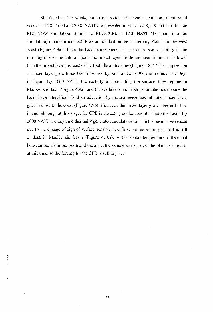
Simulated surface winds, and cross-sections of potential temperature and wind

vector at 1200, 1600 and 2000 NZST are presented in Figures 4.8, 4.9 and 4.10 for $e

REG-NOW simulation. Similar to REG-ECM. at 1200 NZST (18 hours into the

simulation) mountain-induced flows are evident on the Canterbury Plains and the west

coast (Figure 4.8a). Since the basin atmosphere had a stronger static stability in the

morning due to the cold air pool, the mixed layer inside the basin is much shallower

than the mixed layer just east of the foothills at this time (Figure 4.8b). This suppression

of mixed layer growth has been observed by Kondo et al. (1989) in basins and valleys

in Japan. By 1600 NZST, the easterly is dominating the surface flow regime in

MacKenzie Basin (Figure 4.9a), and the sea breeze and upslope circulations outside the

basin have intensified. Cold air advection by the sea breeze has inhibited mixed layer

growth close to the coast (Figure 4.9b). However, the mixed layer grows deeper further

inland, although at this stage, the CPB is advecting cooler coastal air into the basin. By

2000 NZST, the day time thermally generated circulations outside the basin have ceased

due to the change of sign of surface sensible heat flux, but the easterly current is still

evident in MacKenzie Basin (Figure 4.lOa). A horizontal temperature differential

between the air in the basin and the air at the same elevation over the plains still exists

at this time, so the forcing for the CPB is still in place.

78

-140

·160

-180

~ ~ -200 t:

~ is -220 .t: "5 o II( .t: 1: o Z ·260

-280

-300

-320

a) 1200 NZST

<Grid 3 k$I \ \ t I I \

I I \

\

Maximum Vector = 9.0 ms·1

-140 -120 ·100 ·80 ·60 -40 ·20 o 20 40


b} 1200 NZST Maximum Vector = 3.9 ms·1

Grid 4.0

3.5

:::J 3.0 en :?! E 2.5 ::::. ... ..r::. 2.0 C» .; :r:

1.5

1.0

0.5

-140 -120 ·100 -80 ·60 -40 -20 o 20

East-West Distance (km)

Figure 4.8: REG-NOW prediction at 1200 NZST for (a) wind vectors at 24 m AGL, and (b) vertical potential temperature field and wind vectors (through line A-B), Topography contour interval is 200m and potential temperature contour interval is lK.

79


·140 \. \.

-160

·180· E ~ Q) ·200 -(,) t: t1l

ti is ·220 .c '5 0

~ -240 -

1: 0 z -260 -

·280 -

·140 ·120 ·100 ·80 ·60 -40 -20 o 20 40


b) 1600 NZST Maximum Vector = B.B ms-1

Grid 3-4.0

3.5

:::r 3.0 (fJ

:E E 2.5 6 ..... .c 2.0 en '(ij :I:

1.5

1.0

0.5

-140 ·120 ·100 ·80 -60 -40 -20 o 20 40


Figure 4.9: REG-NOW prediction at 1600 NZST for (a) wind vectors at 24 m AGL, and (b) vertical potential temperature field and wind vectors (through line A-B). Topography contour interval is 200m and potential temperature contour interval is 1K.

80

-140

·160

-180 -

~ B -200 -c: J9 U) o ·220 .r: :; o 11 .r: t o z ·260 -

-300

a) 2000 NZST Maximum Vector = 8.9 ms-1

Gri1:t 3 (SJ -

-140 ·120 -100 -80 -60 -40 -20 o 20 40


b) 2000 NZST Maximum Vector = 10.9 ms·1

Grid 3 4.0

3.5-1---_

::r 3.0 (f)

:E 2.5

2.0

1.5

1.0

0.5

·140 ·120 ·100 ·80 ·60 -40 ·20 o 20 40


Figure 4.10: REG-NOW prediction at 2000 NZST for (a) wind vectors at 24 m AGL, and (b) vertical potential temperature field and wind vectors (through line A-B). Topography contour interval is 200m and potential temperature contour interval is 1K.

81

Figures 4.11,4.12 and 4.13 present simulated surface wind field and cross-sections

of potential temperature and wind vectors for the same time period as above, but for the

REG-NOS. The onshore surface wind outside the basin on both sides of the main divide is

weaker due to the absence of the ocean, and hence the lack of a sea-breeze component. The

difference is just noticeable over the Canterbury Plains at 1600 NZST (Figures 4.9a and

4.12a). However, the mixed layer has grown to a depth of 1000 m over the plains,

compared to a few hundred meters in the REG-NOW run (Figures 4.9b, 4.12b). A

mountain-induced converging circulation with weaker return flows aloft had developed by

this time (Figure 4.l2b). The Canterbury Plains Breeze is dominating the surface flow

structure in the basin as before, even though the sea breeze is absent (Figure 4.12a). With

the decline of surface heating, the thermally induced circulations outside the basin have

ceased by 2000 NZST, but similar to REG-NOW, the CBP current is still evident in the

basin (Figure 4.13).

82


-140 . Grrd B

, I \

, \ \

·160

·1S0 E ::..

(!) -200 (.) t: III ... I/)

C ·220 .c ... :::I 0

CJ{ -240 .c 1: 0 z ·260

-2S0

-300

-320

-140 -120 -100 -so -60 -40 ·20 0 20 40


b) 1200 NZST Maximum Vector = 3.7 ms-1

Grid~ 4.0

3.5

3.0 :::r (fJ

:E 2.5 E ::.. ... 2.0 .r:: OJ 'iii :::t:

1.5

1.0

0.5

·140 ·120 ·100 ·80 ·60 -40 ·20 o 20 40


Figure 4.11: REG· NOS prediction at 1200 NZST for (a) wind vectors at 24 m AGL, and (b) vertical potential temperature field and wind vectors (through line A-B). Topography contour interval is 200m and potential temperature contour interval is 1K.

83

3' (/'J

::lE E =-.... .c 0)

'Qj ::x::

E 6

-140

·160

·180 -

~ -200 -c:: 2 (f)

C:i -220 ..c:: <:i o til ..c:: 1:: o z ·260 -

-300

-320 -


-140 -120 ·100 ·80 -60 -40 -20 o 20 40


b 1600 NZST Maximum Vector = 7.6 ms-1

4.0 G~

3.5

3.0

2.5

2.0

1.5

1.0

0.5

-140 ·120 ·100 -80 ·60 -40 ·20 o 20 40


Figure 4.12: REG·NOS prediction at 1600 NZST for (a) wind vectors at 24 m AGL, and (b) vertical potential temperature field and wind vectors (through line A-B). Topography contour interval is 200m and potential temperature contour interval is 1K.

84

·140

·160

E C (U ·200 0 c: <1l ti Ei ·220 .c: -::s 0

·240 IJ)

1= B t: 0 z

.140 ·120 ·100 ·80 ·60 ·40 ·20 o


b 2000 NZST Maximum Vector = 10.4 ms·1

Grid 3 . 4.0 ~ r:-

3.5 _L_~---'-~.-/

:::r 3.0 <1>'"

(f)

::ill E 2.5 :::. ..... .r::: 2.0 C') .(U ::r:

1.5

1.0

0.5

·140 -120 ·100 ·80 ·60 ·40 ·20 o


Figure 4.13: REG-NOS prediction at 2000 NZST for (a) wind vectors at 24 m AGL, and (b) vertical potential temperature field and wind vectors (through line A-B), Topography contour interval is 200m and potential temperature contour interval is 1K.

85

4.5 Discussion of Results

Like the REG-ECM analysis from the previous section, comparison of simulated

data with observational data from the Base station is presented in Figure 4.14. RAMS

performed a satisfactory prediction of onset and cessation time of CPB at this location

when compared to data for lzth February 1999 (Figure 4.14a). At 1700 NZST, when the

current reaches its maximum intensity, there is a difference of 1 ms· l (11 %) between the

two idealized runs (Figure 4.14b). Thereby showing that the CPB is not influenced

significantly by the absence of land-ocean contrasts outside the basin. This slight reduction

in intensity might be due to changes in the horizontal temperature gradients between the air

inside and outside the basin for the two idealized runs. Several sensitivity experiments are

performed in Chapter 5 to investigate this aspect further.

An additional comparison between observational data and model results is made for

the Timaru weather station (Figure 2.1 in Chapter 2) to test the model's performance in

predicting the wind field outside the basin. This station is about 6 km from the coast and is

situated roughly 20 km from the foothills. Therefore, the wind on fair weather days is

expected to be controlled by thermal influences from both orography and the land-sea

contrast. Figure 4.15 presents a comparison of hourly instantaneous wind speed and

direction obtained from the numerical experiments and the Timaru weather station. The

REG-NOW run does a credible job of predicting wind speed, although there is about 45°

difference between predicted and observed wind direction which is probably due to the

coarse horizontal resolution of the run. The absence of ocean in the REG-NOS experiment

has negligible influence on wind direction (between 0800 - 1900 NZST), but it reduces

wind speed by up to 33% ( ~2 ms· l). The negligible difference in wind direction between

the two runs suggests that the local orography has a major influence on the wind at this

station on fair weather days, with the sea breeze enhancing the intensity of wind. This is

likely to be the case for other coastal areas around the South Island.

In the next chapter, a series of idealized two-dimensional experiments are

performed in order to determine the physical mechanisms responsible for the formation of

the CPB.

86

360,---------------------------------------------~~

O~--------~--~--------~----~----.----~~--~~

8.00 10.00 12.00 14.00 16.00

TIme (NZST)

18.00 20.00 22.00 24.00

12+------------------------.~--------------~----

O+-~------~--·--~----~----_r----~----~----.

B.OO 10.00 12.00 14.00 16.00 18.00 20.00 22.00 24.00

Time (NZST)

1--Base .;~. REG·NOW ~'r REG-NOS I

Figure 4.14: Time series of (a) wind direction, and (b) wind speed for 12th February at the Base site compared with prediction by REG-NOW and REG-NOS simulations. Note that the measured data are ten minute averages, and the modelled data are instantaneous values.

87

360

270

C c: 0 n ~ 180 i5 .., c: !i

90

0

6.00 8.00 10.00 12.00 14.00 16.00 18.00 20.00

Time (NZST)

6

~5

"" E :;;4 $ '" " 3 '" c: !i 2

0 6.00 8.00 10.00 12.00 14.00 16.00 18.00 20.00

Time (NZST)

....... Tlmaru . } .. REG-NOW ~;-REG-NOS!

Figure 4.15: Time series of (a) wind direction, and (b) wind speed for 12th February at Timaru compared with prediction by REG-NOW and REG-NOS simulations. Note that the measured data are ten minute averages, and the modelled data are instantaneous values.

4.6 Conclusion

Results from three-dimensional simulations designed to simulate thermal forcings at the

regional scale were presented in this chapter. The influence of the large scale wind field

associated with synoptic weather systems and the sea breeze circulation were successively

removed in each experiment. It can be concluded that the Canterbury Plains Breeze which

usually dominates the surface flow in MacKenzie Basin during settled anticyclonic

conditions, is a thermally induced circulation system. The horizontal scale of the thermal

forcing seems to be larger than the basin, and appears to be of a regional scale. The sea

breeze circulation on the Canterbury Plains does not seem to have a direct influence on the

CPB, although it does change the thermal structure of the atmosphere outside the basin

leading to a slight increase in the intensity of the CPB.

88

Chapter 5

Regional-Scale Flows: Simplified Two-Dimensional Nllmerical Experiments

5.1 Introduction

The objective of this chapter is to investigate the physical forcings that modify the

Canterbury Plains Breeze (CPB) by performing a series of idealized two-dimensional

numerical experiments with the 2-D version of RAMS. Analysis of surface data collected

by several weather stations in the MacKenzie Basin and Lake Tekapo area (Chapter 2)

revealed that the CPB is a recurring flow phenomenon. This circulation dominates the

wind regime in the region during clear-sky, settled anticyclonic conditions in mid

afternoon in summer. Thereafter, three-dimensional numerical simulations with RAMS

were conducted (Chapter 4) to provide details of the horizontal and vertical structure, and

the forcing mechanisms for the CPB. Based on the numerical experiments, the conclusion

was reached that the CPB (from hereinafter also referred to as a density current) is neither

an intrusion of the sea breeze which develops over the Canterbury Plains, nor the

topographically channelled Canterbury north-easterly. When the ocean surface was

removed from the domain of the idealized three-dimensional simulation, a 1 ms-1 (12%)

reduction in the maximum intensity of wind speed occurred inside the basin. The three-

89

dimensional simulations suggest the horizontal scale of the forcing to be of regional scale

(> -lOOkm).

In the following sections, results from twelve two-dimensional numerical

experiments are presented, in which, the model is configured to simulate forcings at

regional scale. The approach used is to build three simplified topography models in 2-D

configuration (roughly representing an east-west cross section of the South Island

through MacKenzie Basin) and analyze the thermally driven flow that is generated. This

way, several forcing mechanisms are investigated for their ability to promote and

influence the regional scale flow at this locality. The physical forcings investigated are

due to spatial variations in:

a) landscape (land-sea contrast), resulting in sea breeze circulations

b) variation in rainfall (and hence soil moisture), resulting in inhomogeneous

boundary layer development between the plains and the basin.

Two-dimensional models have been used extensively by the scientific community

to study thermally and dynamically forced circulations. The models are computationally

inexpensive and allow numerous sensitivity studies to be conducted in a relatively short

period of time. Datasets generated by a particular run are relatively small and require less

effort to analyse. Several investigators have used the two-dimensional framework to

investigate thermally induced flows in complex terrain at a variety of scales. Mannouji

(1982) used a hydrostatic, anelastic equation system to study the characteristic features of

mountain and valley winds. As mentioned in Chapter 1, he concluded that two wind

systems are produced by thermal forcings in complex terrain. A slope wind system

produced by the gradient in the local topography, and a larger scale plain-plateau wind

produced by regional-scale horizontal gradients in temperature, but these are also the

result of gradients in topography, except at a much larger scale. His findings were

corroborated by Bossert and Cotton (1994b), who used the two-dimensional

configuration of RAMS to study regional-scale flows over the Colorado mountain barrier.

They supported the scale separation conclusion reached by Mannouji (1982). Kimura

and Kuwagata (1993) and De Wekker et ai. (1998) performed numerical experiments to

study plain-to-basin winds. An important conclusion reached by De Wekker et ai. (1998)

is the need for a horizontal temperature gradient to exist at the mountain height for

90

development of plain-to-basin wind systems, without the need for the mixed-layer to

grow higher than the ridge. Their findings are also in agreement with Mannouji (1982).


In a two-dimensional model framework, variations in one of the horizontal

directions (most commonly the north-south) is ignored. Therefore in Equations 3 to 9 (in

Chapter 3) all the terms that include (a / ay) are identically equal to zero, thereby

reducing the number of terms that have to be calculated, resulting in considerable

reduction in computation time.

Table 5.1 provides a summary of the twelve experiments conducted for the

MacKenzie Basin cross-section. A description of the topographic configurations is

provided in the next section. There are three topographic configurations and four

different sets of surface characteristics/forcings. For all three sets of topographic

experiments, the effect of land-water contrasts generating a sea-breeze and the effect of

having dryer soil on the elevated plateau (basin) are tested. From hereon, PLT, MTN and

BAS designated simulations are referred to as dry runs, and the rest of the simulations are

referred to as wet runs.

Name

PLT MfN BAS

PLTO MTNO BASO

PLT-M MTN-M BAS-M

PLTO-M MTNO·M BASO-M

Table 5.1: Summary of the 2·D experiments

Description

Symmetric plateau Mountain and plateau Basin topography

Surrounded by ocean

Higher soil moisture on the plains

Higher soil moisture on the plains and o(:ean

Purpose

Examine response to surface heating alone

Examine the influence of the ocean

Examine the effect of variable ground wetness

Examine the combined effect of the above two influences

91

5.2.1 Two-Dimensional Simulation Development

a) Topographic Configurations

The three topographic configurations used are illustrated in Figure 5.1. The

experiments designated as PLT are the simplest representation of topography for an east

west cross section of South Island (Figure 5.1a). The plateau and the sloping terrain (-

1.1 ° gradient) in the east of the domain represent MacKenzie Basin and the Canterbury

Plains respectively. The "plateau" topography is symmetric, the elevated surface is 95

km wide and has a constant elevation of 760 m ASL. The "mountain" runs (MTN) add a

degree of complexity to .the topography by the addition of a 2000 m high mountain

(Figure 5.1b) to the west of the plateau, a rough representation of the main divide

(backbone of the Southern Alps). Consequently, the length of the plateau has decreased

to 44 km, which is approximately the radius of MacKenzie Basin.The mountain has a

half-width of 40 km and an average slope of - 4°. Finally, the basin characteristics are

introduced to the topographic configuration by the addition of a 1200m mountain to the

east of the plateau representing an approximation to the Two Thumb Range (Figure 5.lc).

Four scenarios are tested for each of the topographic configurations:

1) The PLT, MTN and BAS designated experiments (dry runs) have a soil moisture

content of 15% specified for the whole land surface (this value represents

percentage of total water capacity which the soil holds). The objective of these

simulations is to study the effect of topography on the regional-scale circulation

without the added complexity introduced by variations in boundary layer

development.

2) The PLTO, MTNO, and BASO designated experiments are initialized with the

same soil moisture content as in 1), except ocean surface characteristics are added

to the outer domain to represent the ocean around the South Island (Figure 5.1).

The sea surface temperature is specified at 16° C, and the coast is placed at 40 km

92

from the plateau (approximately the distance between MacKenzie Basin and the

east coast of the South Island). The objective here is to investigate how the ocean

around the South Island affects the development of the CPB.

3) The PLT-M, MTN-M, and BAS-M designated experiments have no ocean

characteristics, but the soil moisture content has been increased to 35% outside

the plateau (Figure 5.1). The purpose of these simulations is to isolate the effect of

regional-scale variations in precipitation, and hence soil moisture, on the

thermally induced circulation system. As previously mentioned, the climate of

MacKenzie Basin is typical of inner montane basins of the South Island where the

rain-shadow effects of the surrounding ridges result in annual precipitation rates

of only 600 mm. Therefore the soil moisture content in the basin is usually lower

than the surrounding plains.

4) The runs designated as PLTO-M, MTNO-M, and BASO-M will examine the

combined effects of the presence of the ocean and the variability in soil moisture

on the regional-scale circulation.

93

3.0

2.

2.0

E -"" 1

N

1 .121

0.

121.0

4.(2)

3.

3.0

2.5 E

-"" 2.121

1 .5

1 .121

0

0.0

4.0

3.5

3.0

2.5

.0

1 .5

1 .121

0.5

0.0

(a)

• III

OCEAN

100.

(b)

•

OCEAN

100.

(e)

OCEAN

1121121.

u

OCEAN UIUUllJl!!III!!UIII!I!!lIIl'!!'I!llflUIIIIIII"IIII!l'I!I!I!!I!!!II!!WLUUJII I!I I! !I! !I! tit 1'1 Hllllllilil:ru.-mi::!!!i!!i!!!!!!l

50.

50.

0. x l km 1

0. x 1 km)

121. :x lkrnJ

U

5(2).

• III U

~ OCEAN

50.

• III

OCEAN

5121.

Figure 5.1: Topographic configurations used to represent the MacKenzie Basin cross-section: a) a simple plateau b) mountain plus plateau c) basin between main divide and foothills. The arrowheads indicate where wet soil was placed in tbe wet runs. U-component of wind velocity was extracted from position indicated with u over the elevated plateau.

94

The whole domain uses the desert parameterization as a surface characteristic (which

does not take into account influences from vegetation). Results of tests (not shown in this

chapter), indicate that the main features of the CBP are not affected by using different

land surface characteristics (i.e. grass or irrigated crop) outside the elevated plateau. The

three-dimensional simulations in the previous chapter also used the desert surface option

for the whole domain.

b) Model Setup

A summary cif the model setup is given in Table 5.2. Grid nesting was not used

for the two-dimensional experiments. A grid spacing of 1 km was chosen for the

horizontal direction, the vertical grid spacing starts at 35 m at the surface increasing with

a ratio of 1.12 to 1000 m near the model top which is situated 19 km ASL. Therefore, the

lowest model computational level is at about 25 m AGL, so that with this vertical

resolution, 10 grid points are located within 500 m from the ground. The upper boundary

is a rigid lid, and the eastern and western lateral boundaries employ the radiative

condition following Klemp and Wilhelmson (1978a, b), and the northern and southern

lateral boundaries use the cyclic boundary condition (as explained in Chapter 3). The

cyclic boundary condition combined with the 5 north-south grid nodes effectively makes

the model runs two-dimensional (Table 5.2). A damping scheme is applied to the top ten

vertical layers where the amplitudes of vertically propagating gravity waves and other

disturbances are gradually suppressed to reduce wave reflection from the rigid lid.

Application of the damping scheme is necessary when the domain contains topography

with significant variation in elevation.

95

Table 5.2: Summary of model setup

east-west Number of north-south nodes Number of vertical nodes .:lx, I::.y (m) I::.z(m) Vertical stretch ratio Model top (km) I::.t (s) Soil type Vegetation type Soil moisture percentage of dry soil Soil moisture percentage of wet soil Coriolis force Time differencing Radiation scheme


5 42 1000 35m at bottom, 1000m at top 1.12 19 10 Sandy loam Desert (no vegetation) 15 35 Activated Leapfrog Longwave and shortwave (Chen and Cotton 1983)

For this set of experiments, the model was initialized at 1900 NZST 11 February 1999

(0700 UTC 11 February 1999) and run continuously for a 30 hour period. The integration

starts with the atmosphere at rest (initial wind field is set to zero), so that the resulting

wind field is a response to terrain cooling and heating alone. The initial vertical profiles

of temperature and humidity are the same as the 3-D simulations in Chapter 4. The initial

soil temperature is set to 20°C for all 11 soil levels, with the deepest layer situated at

0.5m.

96

5.3 Simulation Results

Early Morning Profiles

Variation in topography between the three sets of experiments, results in a

different thermal structure for the runs at 0600 NZST, before the surface heating takes

place. The vertical temperature profiles (Figure 5.2) over the elevated terrain and the

plains show that during the night an inversion layer has formed close to the surface.

Surface based inversions are common features of the early morning boundary layer

thermal structure during settled anticyclonic conditions. A significant difference in

profiles exists between the basin experiment and the others over the elevated plateau, as

the temperature profile below l100m is cooler by about 3° over a 300m deep layer.

Advective cooling is the dominant factor, as was shown by Fast et al. (1996). The cold

air generated over the basin slopes fills the basin and is not effectively drained, as

drainage only occurs when the pool height exceeds the lower ridge. With the PLT and

MTN set of simulations, cold air generated by the elevated terrain and the mountain

slopes can effectively drain towards lower elevations. However, over the plains, the

vertical potential temperature structure for the dry runs are not significantly different.

Since less cold air is drained onto the plains, the basin experiment has a slightly higher

temperature for the first two vertical levels over the coastal plains (Figure 5.2). It will be

shown that this difference in the thermal structure of the atmosphere before the surface

heating takes place does not significantly alter the characteristics of the regional-scale

circulation with the three sets of topographic configurations.

In the following sections, the daytime boundary layer development and its effect

on the development of the CPB is discussed. The potential temperature and the u

component wind fields are presented after 17, 19 and 21 hours of integration only for the

eastern half of the domain (1200, 1400, 1600 NZST respectively).

97

:[ ..J en < .. .::: 01 '0; J:

1600,

1200

800

400

Or---~--~--~----~--~--~

280 285 290 295 300 305 310


I ..... PL T ----- BAS -+-- MTN 1

Figure 5.2: Early morning protiles (0600 NZST) after 11 hours of integration for the plateau (PLT), mountain (MTN) and basin (BAS) experiments. The protiles over the higher terrain are taken from a point in the middle of the plateau, and the protiles on the plains are taken from a point 20 km east of the eastern edge of the plateau (basin).

5.3.1 Plateau Simulations

Turbulent transfer of sensible heat from the surface caused the boundary layer to

grow to a depth of approximately 700m throughout the domain by 1200 NZST (Figure

5.3a). Heating of the slope has generated an upslope circulation, and a weak easterly

wind (- 2 ms· l) has developed over the plateau's edge. A baroclinic zone has formed

between the air over the plateau and the air at the same elevation over the plain with a

horizontal potential temperature gradient of -2 K. The reason for this thermal contrast is

that air over the elevated plateau gets heated much more quickly than air at the same

elevation over the plains due to its proximity to the ground. By 1400 NZST, the boundary

layer depth has increased to 1200m (Figure 5.3b), the weak easterly has encroached onto

98

the plateau from the eastern slope, and the gradient of potential temperature is now -2.5

K across the baroclinic zone. The easterly continues to propagate westward at 1600 LST

and has penetrated 19 Ian into the plateau (Figure 5.3c). As the boundary layer depth is

higher than the elevation of the plateau, the differential horizontal temperature gradient

across the baroclinic zone remains close to 2.5 K. This plateau circulation is similar to

that simulated by Bossert and Cotton (1994b) over a plateau 3000 m high and is induced

by the asymmetry of the topography at the plateau's edge. Mannouji (1982) also

describes the numerical development of a similar circulation system over his 2000 m high

plateau, which he termed a plain-plateau breeze.

The forcing mechanism for the development of the density current in the PLT run

is analogous to sea breeze and along-valley circulations. The relatively warmer air mass

over the plateau leads to a hydrostatically lower pressure over the plateau, creating a

pressure gradient force directed towards the plateau, which leads to drawing relatively

colder air from the atmosphere above the plains (cold air advection). The hydrostatic

approximation can be written as:

Z2

M= g f (P2 - Pl)dz (5-1) ZI

where M is the difference between surface pressure over the plateau and pressure at the

same elevation over the plains, Zl is plateau floor height, Z2 is the height where horizontal

temperature gradients diminish, p is the air density, and g is the gravitational

acceleration. The cold air advection by the plain-to-plateau circulation results in

depression of the mixed layer height over the plateau. This depression of mixed layer

height due to cold air advection becomes more pronounced in the subsequent runs.

Therefore, the primary forcing for the density current generated by the PL T run

seems to be the regional-scale differential heating of air due to proximity to the ground ..

99

THE LIBRARY UNIVERSITY OF CANTERBURY

CHRISTCHURCH, N.Z.

a) 3.0

2.5

2.0

~ ::': 1.5

1.0

0.5

0.0

3,0

b) 2.5

2.0

E ::': 1.5

1.0

0.5

0.0

c) 3.0

2.5

2.0

~ ::= 1,5

1.0

0.5

O,0

3.0

~ 2.5 ~ 308.

2.0

-E

::': 1.5 -'34

1,0

0.5

0.0 20. 4O, 60. 8O, 10Q 20, 4O, 00.

x hrnl x I km I

3.0

2,5

2,0

-E

=: 1 .5

1,0

0.5

0.0

20. 40. 60. 80. 10Q x I km J

3.0

2.5

2.0

-E

::': 1.5

N

1.0

O,5

!""!!!",!'!!!'!!"'!!l!"!!!]!!!'''!' O,0

20, 40, 60. 80, 10( 20, 40. 00. x I krn J x Ikml

Figure 5.3: Simulated u-component wind isopleths (ms*l) on the right and the potential temperature field (K) on the left for the plateau experiment (PLT) at a) 1200, b) 1400, c) 1600 NZST. Dashed isopleths indicate negative u-componeut (winds blowing from right to left). Contour interval is 0.5 K for the potential temperature fields, and 0.3 ms·1 for the isopleths.

100

8O, 10Q

10Q

80. 10e

The addition of ocean surface to the domain has a significant impact on the development

of the density current for the PLTO experiment. At 1200 NZST there is a difference in

boundary layer development over the Canterbury Plains (Figure 5.4a) due to a westward

propagating sea breeze circulation that has been generated. Behind the sea-breeze front,

the propagating marine air has caused the formation of the coastal mixed layer. The cold

air advection and the subsidence induced by the return flow result in a decrease of the

mixed-layer depth towards the coast. This depression of the mixed-layer height was also

noted by Anthes (1978) and Lu and Turco (1994) with their two-dimensional

experiments. The boundary layer temperature structure close to the plateau is not affected

by the sea breeze at this time, so that the CPB still has the same characteristics as the PLT

run. It is apparent that the sea breeze and the CPB are two different circulation systems,

generated by different physical forcings. This fact is highlighted at 1400 NZST (Figure

5.4b), when the sea breeze front is about 18 Ian from the plateau's edge (propagating

westward at a speed of 6.4 ms-1 ), while at the same time, a plain-to-plateau circulation

with a wind speed of about 3.2 ms-1 is blowing over the plateau. The front of the current

has penetrated 10 Ian into the plateau. The mixed-layer depth has increased to 1200m

over the plateau (similar to the PLT run), and the development of the boundary layer over

the plains still remains restricted due to the cold air advection associated with the sea

breeze. As a result, the horizontal temperature gradient across the baroclinic zone is -4.5

K. The 1600 NZST (Figure 5.4c) fields show evidence of a well developed CPB current

with an intensity of 6.0 ms-J over the plateau which has propagated about 26 km to the

west, while the horizontal temperature gradient has increased to -5.5 K. This experiment

suggests that sea-breeze formation on the Canterbury coast due to land-sea temperature

contrasts has an indirect impact on the CPB over the plateau. By depressing the boundary

layer height over the plains, the sea-breeze increases the horizontal temperature gradient

at the regional-scale, intensifying the CPB as a result.

101

a) 3.0

2.5

2.0

E ~ 1.5

N

1.0

0.5

0.0

b) 3.0

2.5

2.0

E == 1.5

N

1.0

0.5

0.0

c) 3.0

2.5

2.0

-E

== 1.5

1.0

0.5

0.0

3.0

2.5

2.0

30b. E ~ 1.5

N

1.0

.-----------0.5

0.0 20. 40. 60. 20. x Ikml

3.0

2.5

2.0

-E

::: 1,5

N

1,121

"l.5

0.0 20. 40. 60. 8O. 1011 20. 40. 6O.

x I kill I x Ikml

3.0

2.5

2.0

-E

~ 1.5

N

1.0

0.5

0.0 2O. 40. 60. 8O. 1011 20. 40. 60.

x Ikm I x I km J

Figure 5.4: Simulated u-component wind isopleths Cms-1) on the right and the potential temperature field (K) on the left for the plateau with the ocean experiment (PLTO) at a) 1200, b) 1400, c) 1600 NZST. Dashed isopleths indicate negative u-component (winds blowing from right to left). Contour interval is 0.5 K for the potential temperature fields, and 0.5 ms-1 for the isopleths.

102

,.w':.·'

80. 1011

810. 10.

80. 1011

Variation in soil moisture content also has a dramatic impact on the development of

the CPB (PLT-M experiments). At 1200 NZST (Figure 5.5a), mixed-layer over the plains

has only grown to a depth of 400 m compared with the depth of 800m over the plateau.

Already, a differential horizontal temperature gradient of -3 K exists across the

baroclinic zone. An understanding of soil moisture effects on boundary layer growth can

be gained by examining the surface energy balance equation which controls the turbulent

transfer of heat from the surface. In simple form it can be written as:

(5-2)

where Q * is the net radiation, QH the sensible heat flux, QE the latent heat flux, and QG

the heat flux int%ut of the soil. The sensible (QH) and latent (QE) heat flux terms can be

expanded into:

QH = pCp Cd u (Ts - TJ

QE = P L Cd U (qs -qJ (5-3)

where p is the air density, Cp is the heat capacity of air at constant pressure, Cd is the drag

coefficient, u is the wind speed close to surface, Ts is surface temperature, Ta is air

temperature close to the surface, L is the latent heat of vaporization, qs is the surface

mixing ratio, and qa is the mixing ratio of air close to the surface. When the soil contains

more moisture, q. will be greatly increased leading to partitioning of more of the net

radiation into latent heat. The reduction of sensible heat flux results in a cooler and hence

more shallow boundary layer over the more moist plains.

103

Similar to the PLT run, the mixed-layer depth over the plateau has grown to a

depth of 1200 m by 1400NZST (Figure 5.5b), whereas it has only grown to a depth of

about 500 m over the plains. With the increase of the horizontal temperature gradient to -

6 K, the CPB has intensified to 4 ms- l, and has penetrated 20 Ian into the plateau. At 1600

NZST (Figures 5.5c), the mixed layer has grown to a height of 1 Ian over the plains,

although it is 4 K colder than the mixed layer simulated by the PLT run. Cold air

advection due to CPB has depressed the mixed layer development over the plateau, while

the easterly wind is blowing with an intensity of 6 ms- l . The current has penetrated 30 Ian

into the plateau, which is 5 Ian further than the PLTO run.

The characteristic features of the CPB are the same for the PLTO-M sets of

experiments (Figure 5.6). Since the higher soil moisture over the plains has resulted in a

reduced sensible heat flux near the coast, the sea-breeze circulation is not as vigorous as

the PLTO run (Figure 5.6a, b, c). The combined effect of a reduced sensible heat flux due

to higher soil moisture and the cold air advection by the sea breeze, lead to a very shallow

boundary layer height over the coastal plain slopes for this run.

104

a) 3.0 3.0

2.5 2.5

2.0 2.0

E E ~ ..

:: 1.5 == 1,5 N N

1.0 1.0

0.5 0.5 ....... :::~'''''''~,~:::: ........... \ :

0.0 0.0 20. 40. 60. 80. 10Q 20. 40. 60. 80. 10Q

x Ikml x Ikml

b) 3.0 3.0

2.5 2.5

2.0 2.0

E E

:: 1.5 :: 1.5

N

1.0 1.0

0.5 0.5

0.0 0.0 20. 40. 60. 80. 10e 20. 40. 60. 80. 10Q

x Ikml x Ikml

3.0

c) 2.5 2.5

2.0 2.0

E E

.:: 1.5 = 1 ,5 IV N

1.0 1.0

3.5 0.5

0.0 0. " 20. 40. 60. 80. lee 20. 40. b0. 80. l0Q

x Ikml x Ikml

Figure 5.5: As in Fig. 5.3 but for PLT-M experiment.

105

a) 3.0 3.0

2.5 2.5 30a··~:.J08.~·-~-'--____ ·_·····_308.

2.0 2.0

~ E

~ 1.5 ::: 1.5

N N

1.0 1.0

0.5 0.5

0.0 0.0 20. 40. 00. 8€1. l0e

x !km I

b) 3.0 3.0

2.5 2.5

2.0 2.0

E E

:: 1.5 ::: 1.5

N N

1.0 1.€1

0.5 0.5

0.0 0.0 20. 40. 60. 80. lee 20. 40. 60. 80. lee

x I k m I x Ikml

c) 3.0

3.0

2.5 2.5

2.0 2.0

E E ::: 1.5 :: 1.5

N

1.0 1.0

0.5 0.5

0.0 0.0 20. 40. 60. 80. l0e 20. 40. 60. 80. 10Q

x I km I x Ikml

Figure 5.6: As in Fig. 5.3 but for PLTO·M.

106

5.3.2 Mountain Simulations

In this section, the interaction of the CPB with the plain-to-mountain wind

(Whiteman 2000) is investigated. The interaction of mountain flows and sea breezes were

first studied numerically by Mahrer and Pielke (1977). They represent the closest

situation to that observed in MacKenzie Basin. Mahrer and Pielke (1977) found that the

circulations combined to produce more intense flows during the day. Lu and Turco

(1994), found that the coupling of flows is a function of:

a) the mountain height influencing the sea breeze

b) the distance of the land-sea discontinuity from the mountain

c) the vertical temperature profile of the atmosphere.

It is therefore of interest to find out if the Southern Alps have a similar influence on the

development of the CPB.

At 1200 NZST, the boundary layer thermal structure over the plains generated by

this run is very similar to that of the PLT simulation (Figure 5.7a). Heating of the slopes

has generated a symmetric upslope circulation on both sides of the 2000 m mountain

(Figures 5.7a, only the eastern slopes shown). This upslope circulation is similar to the

simulation made by Mahrer and Pielke (1977) over a 900 m mountain. Due to the

horizontal pressure gradient caused by the mountain, a weak easterly flow has already

been generated over the plateau (Figure 5.7a), while an easterly flow is also evident at the

plateau's edge similar to the PLT run. The density current is well developed by 1400

NZST with an intensity of 3.2 ms· l, and has propagated about 20 krn into the plateau

(Figure 5.7b). In this experiment, the mountain wind and the CPB circulations are not

coupled, suggesting the forcings that induce each flow are quite distinct. By 1600 NZST

(Figure 5.7c), the whole plateau is dominated by an easterly flow with an intensity of

-3.5 ms· l• Therefore for this dry run, the characteristic features of the CPB circulation

were unaffected, except that the flow is intruding into a weak dominant easterly flow

setup by the presence of the mountain.

107

Results for the MTNO, MTN-M, and MTNO-M are illustrated in Figures 5.8, 5.9,

and 5.10 respectively. The characteristics of the boundary layer development over the

plains remains the same as the plateau simulations, and the characteristic features of the

CPB are also unaffected by the presence of the mountain. This suggests that for the

terrain configuration of the two-dimensional experiments, the mountain is so far from the

plateau's edge (the source region for the CPB) that it does not significantly interfere with

its development. The reduction in mixed layer growth and thermal structure over the

plains due to cold air advection by the sea breeze, and the high soil moisture content still

have the most influence on the strength of the CPR

108

a) 3.0

2.5

2.0 E

-" -N 1.5

1.0

0.5

15.0 0.

b)

3.0

2.5

- 2.0 E

-" -N 1.5

1.0

0.5

0.0 0.

c) 3.0

r 2.5

- 2.0 E

-"

N 1.5

1.0

0.5

0.0 0.

20. 40. 01'1. 80. 10Q x I km)

20. 40. 60. 80. l0Q x Ikm i

20. 40. 00. 80. x Ikm)

3.0

2.5

- 2.0 ~

-"

N 1.5

1.0

0.5

0.0

3.0

2.5

2.0 E

-" -N 1.5

1.0

0.5

0.0

3.0

2.5

- 2.0 E

-"

N 1 .5

1 .0

0. 20. 40. 6O, x Ikml

0. 20. "0. 60. x Ikml

0. 20. 40. 60. x I k m J

Figure 5.7: Simulated u-component wind isopleths (ms· I) on the right and

the potential temperatnre field (K) on the left for the mountain experiment (MTN) at a) 1200, b) 1400, c) 1600 NZST. Dashed isopleths indicate negative u-component (winds blowing from right to left), Contour interval is 0.5 K for the potential temperature fields, and 0.5 ms·I for the isopleths.

109

80. 10Q

80. l0e

80. 10Q

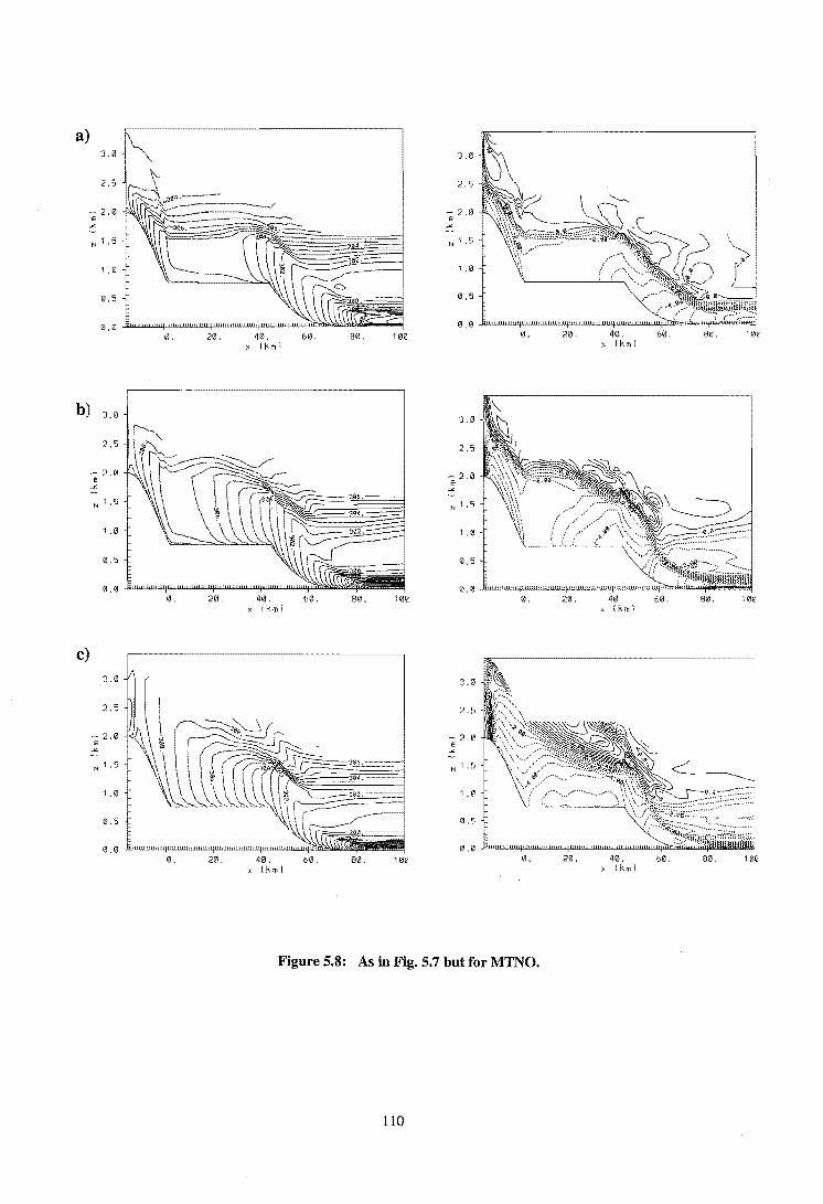
a) 3.0

2.:;

- 2,0 E

N 1,5

1,0

0.5

b) 3.0

2,5

- 2,0 E

N 1.5

1.0

0.5

0.0

c) 3.0

2,5

- 2.0 E

"" N 1.5

1.0

0 5

0.0

0. 20,

0. 2O,

0. 20.

3.0

2,5

N 1.5

1.0

0.5

80. 40, x I km I

60. 0. 20. 40. x I km I

60, 80.

3.0

2.5

- 2.0 E

N 1.5

1.0

0.5

0.0 4O, 60. 80. 10~ 0. 20. 40. &0. 80. 113e

x I km I x Ikml

3.0

2.5

- 2.0 E

"" N 1.5

1.0

0.5

0.0 40. OOl. 8Ol. 10Q 0. 20. 40. 00. 80. 1 ~Q , Ikml x Ikml

Figure 5.8: As in Fig. 5.7 but for MTNO.

110

a) 3.0

2.5 2.5

2.0 - 2.0 E

'" N 1 .5 N 1 .5

1.0 1.0

0.5 0.5

0.0 0. 20. 40. 00. 80. e. 20. 40. 6'1. 80. lee

x I km I x Ikm I

b) 3.0 3.0

2.5 2.5

- 2.0 2.0 E

N 1 .5 N 1.5

1.0 1.0

0.5 0.5

0.0 0.0 lee

x I

C) 3.0 3.0

2.5 2.5

- 2.0 - 2.0 E E

N 1.5 3{HI, N 1.5

1.0 1.0

0.5 ~.5

0 0 0.0 e. 20. 40. 60. 80. 10Q 0. 20. 40. 60. 80. 10Q

x I km I x I km I

Figure 5.9: As in Fig. 5.7 but for MTN-M.

111

a) 3.0

2.5

- 2.0 E

N 1.5

1.0

0.5

0.0 20. 40.

x I km I

b) 3.0

2.5

2.0 E

N 1.5

1.0

0.5

0.0 0. 20. 40.

x I krn I

c) 3.0

2.5

- 2.0

N 1 .5

.0

0.5

0.0 0. 20. 40.

x Ikml

60. 80.

60. 80. 10.

60. 80. Hle

3.0

2.5

- 2.0 E

N 1.5

1.0

0.5

3.0

2.5

- 2.0 E

N 1.5

1.0

0.5

0.0

3.0

2.5

- 2.0 E

N 1.5

1.0

0.5

0.0

0. 20.

0. 20.

0. 20.

Figure 5.10: As in Fig. 5.7 but for MTNO-M

112

40. 60. 80. x I k m I

40. 60. 80. 10e x Ikml

40. 60. 80. lee x Ikrnl

5.3.3 Basin Simulations

Thermally induced flows that transport air into basins have been called plain-to

basin winds. De Wekker et at. (1998) performed a series of two-dimensional experiments

with the same version of RAMS used here, to numerically study the characteristics of this

particular circulation. Several important differences exist between their simulations and

the ones presented in this section. Although they used a variety of topographic

configurations, their basin were always symmetrical (both ridges always had the same

elevation). They also did not investigate the influences of inhomogeneous soil properties,

or the coastal influences on the plain-to-basin circulation. De Wekker et at. (1998)

concluded that the plain-to-basin wind:

a) intrudes into the basin after the cessation of upslope winds on the basin side slope,

when the surface sensible heat flux changes sign

b) the intrusion time does not significantly vary in response to changes in the basin

configuration.

In this study, it was found that in the "basin" experiment (designated as BAS), the

boundary layer thermal structure develops the same way as the previous set of dry runs

(Figure 5.11). Heating of the slopes of the 1200 m mountain on the eastern side of the

basin has generated upslope winds on both sides of the ridge (Figure 5.l1a). However,

because of the horizontal temperature gradients across the ridge, the easterly upslope

flow is beginning to overwhelm the westerly flow generated by the shorter western slope

at this stage. As a comparison, since the horizontal thermal structure remains roughly

symmetric around the 2000 m ridge, the upslope flows on both sides of the ridge

converge at the top (Figures 5.7a, b, c). By 1400 NZST, the density current has

overwhelmed the upslope flow on the basin side and is propagating down the slope with a

wind speed of 3.2 ms- I. The intrusion is occurring three hours before the surface sensible

heat flux changes sign. Hence, it seems the asymmetric basin topography (unequal ridge

heights) has a significant impact on the intrusion time of the CPB (plain-to-basin wind).

Figure 5.12 shows the results from the introduction of ocean to the domain

(BASO). As before, sea breeze front is evident over the plains by 1400 NZST (Figure

113

5.l2b). Similar to the basin run, there is a slight intrusion of the density current onto the

basin side slope, with an intensity of 2 ms-I. By 1600 NZST (Figure 5.12c), the CPB has

propagated westward 5 km further than the dry run, since there is a slight increase of 1

ms-1 in its wind speed (Figure 5.12c).

Figures 5.13 and 5.14 show the results from BAS-M and BASO-M simulations

respectively. There is no significant difference between the thermal structure of the

boundary layer over the plains above the plateau height between these two experiments.

This leads to the development of a similar plain-to-basin circulation system in these two

runs. As before, the existing inversion layer above plateau height in not eroded because

of the prevention of mixed layer growth due to cold air advection by the sea breeze

and/or decrease in sensible heat flux from the surface due to high moisture content of the

soil.

114

a)

b)

C)

3.0

2.5

N 1.5

1.0

~ 0.51 0.0 tHUII'!!!!!!!!1' !I! tjj !WI!! !!!I'I '!!I 'I! 'I! 'W"'I!1'!11WllLllllllllljl1Di!wii=.==ml

40. b0. 0.

3.0

2.5

- 2.0 E

=: N 1,5

1 .0

0.5

0.0 0.

3. '" f

2.5

- 2.0 E

'" N 1.5

1.0

0.5

0.0

'" .

20. 40. x I km I

00. 80. 0. 20. x I k", 1

3.0

2.5

2.0 E

::' N 1,5

1.0

0,5

0.0 20. 40. 00. 80. 102

x I'ml

3.0

2.5

- 2.0 E

::' N 1,5

1.0

~,5

0.0 20. 40. 00. 80. 102 0. 20. 419.

x Ikml x I km I

Figure 5.11: Simulated u-component wind isopleths (ms'l) on the right and the potential temperature field (K) on the left for the basin experiment (BAS) at a) 1200, b) 1400, c) 1600 NZST. Dashed isopleths indicate negative u-component (winds blowing from right to left). Contour interval is 0.5 K for the potential temperature fields, and 0.5 ms'1 for the isopleths.

115

00.

80. 10e

819. 10Q

a) 3.0

2.5

~ 2.0 E

N 1.5

1.0

0.5

0.13

" . 20.

b) 3.13

2.5

- 2.0 E

N 1.5

1.0

0.5

0.~

0. 20.

c) 3.0

2.5

N 1.5

1.0

0. 20.

4O. 6O. 813. 10Q x Ikml

413. 60. 8O. 10Q x Ikwl

40. Ml. 80. x I km I

3.0

2.5

~ 2.0 E

N 1 ,5

1.0

0.5

0.0

3.0

2.5

2.0 E

.x;

N 1,5

1.0

0.5

0.0

3.0

2.5

~ 2.0 E

'" N 1 .5

1.0

0.5

" .

0.

0.

Figure 5.12: As in Fig.S.U but for BASO.

116

213. 4O. b0. 80. 10Q x I km I

20. 40. b0. 8O. 10Q x Ikml

20. 40. b0. 80. x I kw I

a) 3 I')

2 5

- 2.0 E

N 1.5

1.0

0.5

0.0 0. 20.

x

b) "-. 3.0

2.5

- 2.0 E

-'"

1 .5

1.0

0.5

0.0 0. 2O.

x

c) ].0

2.5

- 2.0 E

N 1,5

1.0

0.5

0.0 0. 20.

x

4O. &0. 8O. 10£ Ikml

40. &0. 80. 10Q Ikml

3.0

334.

302

4O, 6O. 80 10Q I Km I

3.0

2.5

- 2.0 E

N 1.5

1.0

0.5

0.0

3 .0

2.5

- 2.0 E

N 1.5

1.0

0.5

0.0

3.0

2.5

- 2.0 " -N 1,5

1.0

0.5

\

0.

0.

0.

Figure 5.13: As iu Fig. 5.11 but for BAS-M.

117

20. 4O. 0o. 8O. 10£ x I km I

20. 40. 00. 8O. 10€ x Ikml

20. 40. 80. x I km I

a) 3.0 3.0

2.5 2.5

- 2.0 2.0 E

N 1.5 N 1.5

1 .0 1.0

0.5

0.0 .lWlL~U1 0.0 0. 20. 40. 60. 80. 10~ 0. 20. 40. 00. 80. 1Ok'

x [km 1 > Ikml

b) 3.0 3.0

2.5 2.5

- 2.0 - 2.0 e E

N 1 .5 N 1,5

1,0 , .0

0.5 0.5

0.0 0.0 0. 20. 40. 00. 60. 10Q

x (kml x I

c) 3.0 3.0

2.5 2

2.0 - 2.0 E E

"" N 1.5

30' N 1.5

1.0 1 .0

0.5 30jL 0.5

0.0 0.0 0. 20 40. 60. 80. 10e 0. 20. 40. 00. 80. 10e

x Ikml x I'ml

Figure 5.14: As in Fig. 5.11 but for BASO-M.

118


In the previous sections, results from the two-dimensional experiments were

presented. It was shown that the CPB is primarily forced by the horizontal temperature

gradient between the air over the elevated plateau (representing MacKenzie Basin) and

the air at the same elevation over the plains (representing the Canterbury Plains).

However, forcings that increase this temperature gradient (such as cold air advection by

the sea breeze or higher soil moisture over the plains) can influence the intensity of the

CPB by about 2 ms· l.

Time series for the u-component of wind from a grid point on the plateau

(indicated by an arrow in Figure 5.1) extracted from the lowest computational level (25 m

AGL) is presented in Figure 5.15 for all twelve experiments. This grid point is chosen to

be representative for the location for the base station AWS mentioned in Chapter 2. For

the plateau experiments, while the maximum intensity of wind increases by 2 ms·l

between the dry and the wet runs (Figure 5.15a), the difference between the wet runs is

negligible. However, there is a significant difference in the onset of the breeze at this

location between the runs. When a higher soil moisture content over the plains is

specified (PLTM experiment), the CPB was detected at this location 3 hours earlier than

the dry run. For this topographic configuration, the difference in soil moisture (and hence

the boundary layer development over the plains) seems to have the strongest influence on

the intensity of the circulation.

Since the mountain range had already set up an easterly current over the plateau,

the intrusion of the CPB into the elevated plateau was not as well defined with the MTN

experiments (Figure 5.15b). There is negligible difference in the maximum intensity of

the wind between this series of runs and the PLT experiments, suggesting that the Alps

do not modify forcing of the CPB at this range.

The CPB is detected at about 1400 NZST at this location for all scenarios for the

basin experiments (Figure 5.15c). The difference being that the horizontal temperature

gradients have to be strong enough across the eastern ridge, so that the density current

can overwhehn the upslope flows opposing it from the basin side before propagating

119

westward. The difference in maximum intensity of the wind between the dry and wet

runs is about 2 ms· l (the same as other two sets of runs), although there is little difference

between the BAS-M and BASO-M. This reinforces the conclusion that the ocean has an

insignificant forcing affect on the CPB.

4~----------------······························~----------······~-- -

2,---------------------------------------

·8·~-~----~--~----~······· -, -~----__ ............• 06:00 08:00 10:00 12:00 14:00 16:00 18:00 20:00 22:00

Time (NZSn

4,-------------------------------------

2+------·---··-------------------------~

'i O~· ---=-=-<>-=~----~ 1,2 T-----~~--=~:;__~~~~__::>F9_-

~ -4 +----- .. -------------"~~.

~+--------------------~-~~~----------

~+----~--~----~--~--~----~---.--~ 06:00 08:00 10:00 12:00 14:00 16:00 18:00 20:00 22:00

Time (NZSn

4,-------------------------------------

·8+----~--~----~--~--~----~--~--~

06:00 08:00 10:00 12:00 14:00 16:00 18:00 20:00 22:00

Time (NZSTJ

Figure 5.15: Time series of surface u-component wind at grid point over the plateau for the a) plateau, b) mountain, and c) basin simulations.

120

5.5 Conclusion

Twelve two-dimensional numerical experiments were performed to confirm the results

from the previous chapter which suggested that the Canterbury Plains Breeze (CPB) is a

regional-scale circulation generated by the horizontal temperature gradient between the

air over the basin and the air at the same level over the Canterbury Plains. The numerical

simulations show that the CPB is greatly modified by the basin topography and the

difference in land surface characteristics between the basin and the plains. Variation of

land surface characteristics influences the intensity of this density current by up to 2 ms- I.

With the three-dimensional runs, this difference was ~ 1 ms- I• It has to be pointed out that

the two-dimensional runs cannot simulate the venturi effect that the mountain passes,

such as Burke Pass, have on the CPB. These were simulated quite clearly by the three

dimensional runs described in Chapter 4.

121

Chapter 6

Numerical Simulations of Local and Regional Scale Flows in the Lake Tekapo Region

6.1 Introduction

In the previous two Chapters, results from a series of two~ and three~ dimensional

numerical experiments were presented in order to investigate the forcing mechanisms for

the Canterbury Plains Breeze. This regionally induced thermal circulation is the dominant

wind system in the MacKenzie Basin and Lake Tekapo region early in the afternoon on fair

weather days. However, before the intrusion of the CPB into the region, locally generated

thermal flows such as the lake breeze and daytime mountain winds (upslope and up-valley

winds) are observed. These features were not simulated in the previous chapters due to the

rather coarse horizontal resolution of the model runs. For the simulations in this chapter,

RAMS was configured to represent forcings at smaller scales in order to investigate the

interaction between regionally and locally induced thermal circulations in the vicinity of

Lake Tekapo.

The objectives of this chapter are:

• to investigate the effect of Lake Tekapo on the simulated surface flow pattern

• to investigate the interaction between the CPB and locally generated flow

systems

123

Table 6.1: Summary of 3-D simulations conducted to examine the influence of Lake Tekapo on local and regional winds.

Name

LOC-LAKE

LOC-LAND


Description

Lake Tekapo present

Lake Tekapo absent

Similar to the regional scale simulations of Chapter 4, the case study day chosen for

numerical experiments was 12 February, 1999. Two numerical experiments were

conducted, the model run designated as LOC-LAKE had a representation of Lake Tekapo

in its domain, while in the LOC-LAND run, the lake was removed (Table 6.1).

6.2.1 Three-Dimensional Simulation Development

a) Grid Structure

Like the model runs in Chapter 4, grid-nesting capability of RAMS is used for the

horizontal direction only. Table 6.2 provides a summary for each nested grid. Numerical

experiments in this chapter use four grids: the coarse grid covering the South Island has a

9.6 km horizontal resolution, the first nested grid (grid 2) has a horizontal resolution of 2.4

km covering the middle third of the South Island (Figure 6.1). The second nested grid (grid

3) has a horizontal resolution of 800 m, covering a rectangular shaped domain including the

Lake Tekapo catchment area to the north and Burke Pass to the south (Figure 6.2). The

third nested grid (grid 4) has a horizontal resolution of 267 m covering Lake Tekapo, and

the Godley and Macaulay valleys. Grids 1 and 2 are centered at 170.4 ° Wand 44°S, while

grids 3 and 4 are centered at 170.6 ° Wand 43.8°S. The four grids consist of 65, 62, 59

and 83 zonal, and 65, 62, 110 and 152 meridional grid cells respectively (Table 6.2).

Vertical grid structure is the same as the three-dimensional model runs of Chapter 4.

124

Grid 1 r---------------------------

I I I I I I I I I I I

N

o 100 Ian

SOUTH

ISLAND

~---------------------------

Figure 6.1: Geographic locations of grids 1 and 2 in the LOC·LAKE and LOC-LAND simulations.

125

Figure 6.2: Geographic locations of grids 3 and 4 in the LOC-LAKE and LOC-LAND simulations.

Due to the high spatial resolution of the numerical experiments and the complexity

of the terrain, a great deal of consideration had to be given to the selection of each

126

parameter. A nesting ratio of 1:4 was selected only between grids 1 and 2, with 1:3 selected

between grids 2 and 3, and grids 3 and 4. Ratios higher than this were not numerically

stable. In addition, nesting ratios higher than 3 are not recommended in areas with complex

terrain, since features of larger-scale flow may not be represented on the finer grid properly

(Doran and Skyllingstad 1992).

Table 6.2: Cbaracteristics of the grids

Grid 1 Grid 2 Grid 3 Grid 4

Number of east-west nodes 65 62 59 83 Number of north-south nodes 65 62 110 152 Number of vertical nodes 32 32 32 32 L\x, Ay (km) 9.6 2,4 0.8 0.267 East-west width (km) 614.4 146.4 46.4 21.9 North-south width (km) 614.4 146.4 87.2 40.3 Az at first level (m) 50 50 50 50 Vertical stretch ratio 1.12 1.12 1.12 1.12 Grid top (km) 12 12 12 12 At (s) 30 10 3.3 0.83

Topography for all grids is derived from the 30-second (about 1 km) United States

Geological Survey (USGS) terrain dataset. Visual examination of interpolated grids 3 and 4

topography indicate that the major features of the landscape are satisfactorily represented

on these high resolution grids. Approximately 17 horizontal nodes span the width of Lake

Tekapo, so that the lake is well resolved and the model should be able to produce thermally

induced circulations resulting from lake-land contrasts.

b) Model Setup

A summary of model setup is provided in Table 6.3. Similar to the regional scale

simulations in Chapter 4, surface characteristics are specified homogeneously for the entire

domain. However, since the main focus of this chapter is in representing forcings in the

MacKenzie Basin and Lake Tekapo region, a lower soil moisture content of 15% (which is

representative of the Base site only) is specified (Oliphant 2000). Because of the high

horizontal resolution of grid 4, Lake Tekapo is resolved adequately, so that its surface

temperature is set to 11°C as indicated by field measurements.

127

Table 6.3: Summary of model setup

Soil type Vegetation type Soil moisture (% of saturation) Sea Surface Temperature (0C) Lake surface temperature (0C) Roughness length (m) Coriolis force Time differencing Radiation scheme


Sandy loam Desert (no vegetation) 15 16 11 0.05 Activated Hybrid Longwave and shortwave (Chen and Cotton 1983)

Temperature and humidity profiles measured by the aircraft early on the morning of

12th February 1999 were used to initialize these runs (Figure 2.8). Above 3000 m AGL

where aircraft data were not available, data from the 0000 NZST Invercargill rawinsonde

were blended in. Simulations were initialized on the morning of 12th February (at 0600

NZST), so that no nocturnal phase is simulated before the onset of surface heating. The

reasons for the choice of initialization time were that:

a) RAMS was not numerically stable during the nocturnal simulation with the

chosen parameters and grid configuration. Experimentation with different

settings is possible but is exceedingly time consuming.

b) The combination of having a high number of nodes for grids 3 and 4, and

the small time-steps required for numerical stability at high resolutions,

meant that these runs were computationally very expensive. It took over 1

day of computation to simulate one hour on the available computer platform.

The simulations presented in this chapter took over 17 days to complete, and

if the nocturnal phase was included the simulations would have taken more

than 25 days.

Therefore, even if a numerically stable configuration for simulating a nocturnal phase was

found, it would have been highly impractical to run the model for more than 12 hours of

simulation time.

128

To avoid initializing at 0600 NZST, experiments were made with other techniques

such as Four Dimensional Data Assimilation (FDDA). For example, the model was

initialized on 11th February with only 3 grids so that the model run would progress faster,

and then the simulation was stopped at 0400 NZST on the 12th. At this stage, grid 4 was

"spawned" on the simulation, and then the model was restarted with FDDA subroutines

activated. RAMS allows addition of new grid(s) to a particular simulation after it has

started, so that a finer mesh grid can be added to a run whenever it is required to save on

computation time. The model was forced (relaxed) towards measured vertical profiles of

thermodynamic variables obtained by the aircraft at 0600 NZST. The radius of influence

for the assimilated data included only the basin, so that the atmosphere outside the basin

used just the model physics. Details on FDDA and relaxation techniques are provided in

Fast (1995). Unfortunately, this technique produced unsatisfactory results after the FDDA

forcing was stopped at 0600 NZST, and was not pursued further.

A drawback with an early morning initialization is that as the atmospheric static

stability is the same inside and outside the basin in the morning (the initialization is

horizontally homogenous), characteristic features of the CPB change slightly. To

investigate the effect of initialization in the morning, a two-dimensional experiment with

the same initial conditions as the three-dimensional runs in this chapter was conducted

(results are presented in Appendix A). The two-dimensional simulation indicates that the

CPB intrusion into the basin occurs almost two hours earlier, but there is negligible

difference in its maximum intensity and cessation time.

6.3 Simulation Results

6.3.1 Influence of Regional Scale on Local Scale Flow

Predicted near surface wind fields for a section of grid 3 after 4, 7 and 10 hours of

integration (1000, 1300,1600 NZST respectively) for LOC-LAKE simulation are presented

in Figures 6.3a, band c. Since the atmosphere was at rest at initialization and no synoptic

scale forcings were imposed, the resulting flow fields at 1000 NZST are due to surface

heating alone (Figure 6.3a). The winds in the middle of the basin are calm at this time

(southwest corner of the domain), as a result of diverging flow set up by the upslope and

129

up-valley winds around the basin's periphery. This fact was previously illustrated by the

regional scale simulations in Chapter 4. Combined upslope and up-valley winds dominate

the surface flow field around Lake Tekapo, and up-valley winds are also established in

Godley and Macaulay valleys. A weak thermally induced gap wind is evident near Burke

Pass, although unfortunately surface wind data are not available to confirm the onset time

of the gap wind at this location. At 1300 NZST, the surface flow became more

complicated, with the CPB now blowing through Burke Pass and Tekapo Saddle (Figure

6.3b). The flow field south of Tekapo Village is dominated by the gap wind through Burke

Pass, while north of the village a gap wind through Tekapo Saddle is pushing away the

upslope, up-valley flows. Three hours later at 1600 NZST, easterlies become well

established over the bottom half of the domain, and an intrusion is now also evident

through the Stoneleigh Saddle (Figure 6.3c). A stagnation zone is created between the

passes due to the convergence of the intruding air currents. It is apparent that the surface

flow field can be very complicated around Lake Tekapo, and the model is able to capture

some of this complexity.

130

30 30

20 20 E E :::. :::. Qj

Qj <> <> c C M 10 .l9 10 iii .!!! i5 Q -:5 ..c ::I :i 0 0 (/) 0 IJl 0 1: ..c 1:: 1:: 0 0 Z Z

·5 o 5 10 15 20 East.West Distance (km)

East·West Distance (km) Z T c) 1600 N S

Maximum Vector = 12 ms-1

30

E 20

:::. OJ <> C

.t; 10

i5 ..c .... ::I 0

IJl 0 ..c 1:: 0 Z

·5 o 5 10 15 20


Figure 6.3: Topography (200 m contour interval) and wind vectors on grid 3 at 24 m AGL for (a) 1000 NZST, (b) 1300 NZST, and.(c) 1600 NZST for the LOC·LAKE simulation.

131

6.3.2 Influence of Lake Tekapo

In this section, a comparison between the two high-resolution simulations is made

in order to assess the influence of Lake Tekapo on the surface wind field in the region.

Therefore, a closer examination of grid 4 model solutions is made in order to observe the

resulting differences. According to observational evidence, Lake Tekapo exerts some

influence on the surface wind field by generating lake breezes (McGowan et al. 1995). The

fourth grid in this series of experiments has a high enough resolution to be able to generate

thermally driven flows due to the lake, hence making possible a qualitative comparison

with observations.

The predicted near surface wind field for the same times as above are presented for

both runs in Figure 6.4. At 1000 NZST, the LOC-LAKE run produces a more divergent

flow field over the lake than the LOC-LAND run (Figure 6.4a,. b). The effect of a lake

breeze component is more evident at the south-east corner of the lake. At 1300 NZST, the

CPB is dominating the surface wind field at the south-east corner of the domain (Figure

6.4c, d). This is the gap wind which is blowing through Tekapo Saddle (Figure 6.3a), and

its front has advanced a little further up the valley in the LOC-LAND run. The most

interesting feature of the lake's influence on the surface wind field is evident at 1600 NZST

(Figures 6.5a, b). When the lake is not present, the easterly intrusion through the saddles

has totally dominated the surface flow field in the valley, with stagnation zones clearly

evident on this grid (Figure 6.Sb). However, the LOC-LAKE simulation does not show

such total dominance of the CPB at this time (Figure 6.5a), since a southerly wind still

exists at the northern end of the lake.

To investigate the mechanism responsible for the difference in characteristics of the

easterly intrusion at the northern end of the lake, an examination of the cross-valley

temperature structure was performed. Simulated potential temperature and wind vector

profiles at 1500 and 1600 NZST for both numerical experiments, through a cross-section of

grid 4 (line A-B in Figures 6.5a, b) are shown in Figure 6.6 and 6.7. At 1500 NZST, both

simulations predict the same intensity and thermal structure (and also the same depth) for

the CPB. The CPB at this time has propagated slightly down the slope into the valley for

132

(I) to) C III 1ii i5 .t: -:::I o II} .t: 1:: o z

E :::, (I) to) c JS III

i5 .t: -:::I o en . .t: t:: o Z

25

20

15

10

5

6 10 14


25

20

15

10

5

6 10 14


E :::, III to) C III -III i5 .t: -:::I o II} .t: t:: o Z

E :;:. (I) to) C III -III i5 .t: -:::I o en . .t: t:: o Z

25

20

15

10

5

6 10 14


25

20

15

10

5

6 10 14


Figure 6.4: Topography (200 m contour interval) and wind vectors on grid 4 at 24 m AGL for (a & b) 1000 NZST, and (c & d) 1300 NZST for LOC·LAKE and LOC-LAND simulations respectively. The solid lines in (a) and (c) indicate the lake's boundary.

133

both cases. A convergence zone between the upslope flow and the CPB is also apparent in

both simulations. However, the presence of the lake has resulted in a colder atmosphere

inside the valley in the LOC-LAKE run, and the lake surface has produced a stable layer

close to the ground (Figure 6.6a). The formation of this cold air pool at the bottom of the

valley in the LOC-LAKE run has some implications for the grounding of the regional scale

flow. Figure 6.7a shows that at 1600 NZST, the CPB is overriding the denser air mass in

the LOC-LAKE simulation, while at the same time, the current simulated by the LAKE

LAND run is dominating the surface flow field (Figure 6.7b). One hour later (figures not

shown), the cold air pool is eroded in the simulation and the easterly in the LOC-LAKE run

is grounded.

25 25

E E :::.. 20 :::.. 20 Q) Q) to) to)

c C 1':1 1':1 .... .... III 15

III 15 i5 i5

..c ..c .... .... ::::I ::::I 0 0

IJJ IJJ . 10 . 10 ..c ..c t:: t:: 0 0 z z

5 5

6 10 14 6 10 14

East-West Distance (km) East-West Distance (km)

Figure 6.5: Topography (200 m contour interval) and wind vectors on grid 4 at 24 m AGL at 1600 NZST for (a) LOC-LAKE, and (b) LOC-LAND simulations respectively. The solid line in (a) indicates the lake's boundary.

134

a) 1500 NZST

4.0 -1=::;:::;:;:::

3.5

3.0

2.5

2.0

1.5

1.0

10

b) 1500 NZST

4.0

3.5

:::r en 3.0 ::2E <t E =- 2.5 ... .r:: C'I 'iii 2.0 :r:

1.5

1.0

10

15

-1 Maximum Vector = 6.7 ms

""" I ,."," "," <,<" "" "," >,.,j, ,'"

20 25


15


20 25


Figure 6.6: Vertical cross-sections of potential temperature aud wind vector in the east-west directiou through line A-B (location indicated in Figure 6.5), of grid 4 at 1500 NZST for (a) LOC-LAKE, and (b) LOC-LAND simulations.

135

:::r (J)

~ E ~ -.E Cl 'iii :I:

a) 1600 NZST

4.0 -\---_

3.5~~0

3.0

2.5

2.0

1.5

1.0 _

10

b) 1600 NZST

4.0

3.5

3.0

2.5

2.0

1.5

1.0

10

15

·1 Maximum Vector = 8.0 ms

20

---2.

25


15


20 25


Figure 6.7: Vertical cross-sections of potential temperature and wind vector in the east-west direction· through line A·B Oocation indicated in Figure 6.5), of grid 4 at 1600 NZST for (a) LOC·LAKE, and (b) LOC-LAND simulations.

136


Since smoothing techniques had to be applied to the topography in order to obtain

numerically stable runs, some of the complexity in local relief was lost. For example, even

though the horizontal grid spacing for grid 4 was 267 m, Mt. John was not resolved at all

on this grid and its influence on the intruding wind system was not simulated. Figure 2.11c

clearly showed the deflection of the gap wind through Tekapo Saddle by Mt. John, and this

feature would obviously be absent in the model runs described here. However, the

complexity of thermally forced wind systems in the Lake Tekapo region was simulated

well by the model. The model was able to show that the CPB has a dominating influence on

surface flow in the afternoon, by flowing through the mountain gaps and setting up a

complex flow system (including stagnation zones) in the vicinity of the lake. Indeed, during

the field campaign it became obvious that more weather stations needed to be added to the

surface monitoring network. For example, station A13 at Boundary Stream (Figure 2.3)

was placed between two saddles and according to model results the gap wind would not be

detected there.

Another interesting result from the high resolution simulations is that the cold air

pool created by the presence of the lake can affect surface flow fields. Simulation results

showed that erosion of the stable layer created by the lake is necessary before the CPB is

detected at the surface. A similar situation was modelled by Segal et al. (1983) in the case

of a cold pool created by a lake confined in a valley. They proposed two mechanisms for

erosion of the cold air pool before the prevailing synoptic winds could reach the valley

bottom. The first mechanism is the development of an internal gravity wave resulting in

flushing of the cold air (Figure 6.8a), and the second mechanism involved erosion from the

top due to shear-induced turbulence (Figure 6.8b).

137

------------------------~

~~81 8, vq-o 'g, 8,<87

~ /"-________ 8;, ~~ Y· g

JA e, ~~ ~~~:::::::IIIIIIellllllllllll, IIIIIIIIIIIIYg ••

MOUNTAINWAYE \~ r-FLUSHING ~

(a)

--------87

~/ -. :~EAR-iNOOCED TURBULENCE AT

Z THE TOP OF THE COLD POCl

(b)

Figure 6.8: Schematic illustration of (a) the flushing of cold air in a valley as a forced internal gravity wave develops over an upwind terrain barrier in response to strengthening synoptic flow, (b) the erosion of cold air in a valley due to shear-induced turbulence at the top of the cold pool (after Segal et al., 1983).

138

6.5 Conclusion

Results from two high-resolution numerical experiments showed a complex

interaction between locally generated thermal circulations and the Canterbury Plains

Breeze. In the vicinity of the lake, the CPB dominates the surface flow field in the

afternoon by flowing-in through mountain passes. The lake can affect this intrusion by

altering the thermal structure of the valley atmosphere through the formation of a stable

surface air layer. Simulation results suggest that the CPB has to erode this stable layer

before reaching the valley floor.

139

Chapter 7

Conclusions

Evidence has been presented from both field observations and numerical model

results of the existence of a recurring plain-to-basin circulation system, named the

Canterbury Plains Breeze (CPB), which dominates the surface flow regime of the

MacKenzie Basin region of the South Island in the afternoon of fair weather days.

Emphasis was placed on investigating the physical mechanisms responsible for generating

the CPB using an atmospheric mesoscale model.

7.1 Summary of Conclusions

It is appropriate at this stage to revisit the original objectives of this thesis from

Chapter 1. The objectives were to determine:

(I What types of thermally driven circulation systems develop in the vicinity of

MacKenzie Basin?

• If the CPB is an intrusion of the sea breeze that forms along the Canterbury

coast.

• What are the characteristics of this circulation system and what are the causal

mechanisms?

• How variations in ground wetness affect the characteristics of the CPB through

its effect on boundary layer growth.

141

The following sections provide a review of the major findings of this thesis, which were

obtained mainly through numerical modelling, but also supported by observations.

7.1.1 Observed Characteristics of the Canterbury Plains Breeze

Observational evidence suggested the presence of a high-speed (> 8ms·!) easterly

wind system, that dominated the surface flow field of the basin in the afternoon, when

synoptic pressure gradients were weak. The surface monitoring stations situated in the

basin showed a predictable onset and cessation time for the CPB, suggesting a thermally

driven origin for this circulation. However, the intrusion characteristics of the CPB in the

Lake Tekapo region were somewhat more complicated. During the 2nd February case study,

a high-speed wind was detected in the basin in the afternoon, but the airflow did not seem

to intrude into the lake area until after sunset, when it blew down the western slopes of the

Two Thumb Range. On the 12th February case study day, the easterly intrusion was again

detected in the basin, and it manifested itself in the Lake Tekapo region as a strong gap

wind flowing through Tekapo Saddle. Measurements from surface stations and vertical

temperature profiles measured by an aircraft suggest that the Canterbury Plains Breeze

advects colder coastal air into the basin, therefore having an important impact on the

climate of the region.

7.1.2 Numerical Simulations of the CPB

Three-dimensional numerical experiments configured to represent mesoscale

forcings on a regional scale showed that the CPB can form exclusively as a result of terrain

heating. The three-dimensional idealized simulations with and without the ocean

surrounding the South Island showed no difference in the onset and cessation time of the

CPB in the basin, although there was a decrease of I ms·! in the intensity of wind in the

simulation with no ocean. This result suggests that the CPB is a separate circulation system

from the sea breeze that forms over the Canterbury Plains due to land-sea contrasts, and is

only affected to a small degree by the ocean surrounding the South Island.

Subsequently, results from twelve two-dimensional numerical experiments showed

that the CPB is a plain-to-basin circulation system forced by horizontal temperature

142

gradients between the air inside the basin and that over the surrounding plains at the same

elevation. The physical forcing mechanism can be explained in the following way, daytime

heating of the atmosphere over the basin results in a hydrostatically created horizontal

pressure gradient force directed from the plains to the basin. This pressure gradient force

causes movement of air towards the basin. The resulting airflow can either go through

mountain saddles or gaps, or flow into the basin over the ridge lines. When the mixed layer

growth outside the basin is suppressed by cold air advection, due to either a sea breeze or

high soil moisture content of the surface of the plains, the intensity of the CPB increases.

The two-dimensional experiments suggest that the reason for this increase is the reduced

heating of air above the plains (at a level above the basin floor height) due to the reduced

mixed layer growth. This results in an increase in the horizontal pressure gradient that

drives the CPB. Therefore, factors that enhance (suppress) mixed layer growth over the

plains decrease (increase) the intensity of the plain-to-basin circulation system. Hence,

even though the sea breeze circulation over the Canterbury Plains does not have a direct

impact on the CPB, it has an indirect influence by reducing the mixed layer height over the

plains (outside the basin).

7.1.3 Interaction of the CPB with Smaller Scale Flows

Results from two high-resolution three-dimensional simulations show how the CPB

affects the surface flow regime in the vicinity of Lake Tekapo, and suggest ways that it can

interact with the cold layer of air created by the presence of the lake. The simulations

clearly showed the intrusion of the CPB as gap winds through several saddles in the Two

Thumb Range which the observational network mostly missed (except for the Base site).

The existence of these flows has implications for the other components of the L TEX

research project, and has to be considered when along-valley budget studies of mass and

heat are performed. The model runs suggest that the plain-to-basin wind will not be

detected at some places by surface weather stations until the stable surface layer created by

the lake is eroded.

143

7.1.4 Broader Implications

High-resolution numerical analysis of thermally generated wind systems has only

been possible in the past decade due to the development of high-speed computers. Research

projects that use mesoscale models in conjunction with observational evidence have had

some success in describing the nature of such flow systems. Due to the large horizontal

extent of the forcing, even the most ambitious field projects like the IMADA-A VER

experiment in Mexico City Basin (Doran et al. 1998) were not able to offer a complete

description of this flow system. Therefore, the findings from the numerical experiments in

this research provides additional information relating to the development of plain-to-basin

type flows, especially for basins that are situated in coastal areas. Broader implications of

this research are that land use patterns can affect the characteristic features of the plain-to

basin wind, so that anthropogenic land use change may affect these wind systems. For

example, planting trees for forestry practices or setting up extensive irrigated areas for

agriculture use can reduce the mixed layer growth in the MacKenzie Basin leading to a

weakened CPB circulation. In addition, the persistence and intensity of the CPB suggests

that it can transport air pollutants from the Canterbury Plains into the mountain basins,

adversely affecting the air quality in this region. As a result, it is clear that degradation of

air quality over the Canterbury Plains could adversely affect the air quality in alpine

regions of the South Island.

7.2 Suggestions for Future Research

Obviously, more research is necessary to understand more fully the exact nature of

regional scale circulations such as the Canterbury Plains Breeze. Currently, more

observational data are needed to confirm the simulated characteristic features of the CPB.

Since the model runs suggest that horizontal pressure gradients are a forcing factor for the·

plain-to-basin type flows, it would be highly desirable to have concurrent vertical profiles

of thermodynamic variables over both the basin (plateau) and the adjacent plains. It would

also be advantageous to have wind measurements over the slopes, mountain gaps and

144

passes. The observational data could be used for further investigation of the phenomenon,

through both model initialization and verification of model results.

The numerical modelling aspects of this research could also be expanded on.

Suggestions for improvement of model formulation are not made here, since the topic was

not investigated in this research. However, there is a need for even higher-resolution model

runs to be performed. With higher resolution runs, local topographic features such as Mt.

John, that have an important influence in diverting airflows could be resolved by the modeL

This improvement would enable a more direct comparison between observations and model

results. The simulations in Chapter 6 were performed with a horizontal grid spacing of 267

m and a vertical grid spacing of 50 m for the first level near the surface. Both grid spacings

could be made smaller using a numerical code like RAMS. However, this was impractical

for this research due to the large amount of computational time required. In spite of this

limitation, the high-resolution runs were able to simulate some observed (although not fully

measured) characteristics of the CPB, and suggested the way that it might interact with the

stable layer created by the cold surface of Lake Tekapo.

It is also suggested that in future meteorological studies in areas of complex terrain,

a preliminary numerical modelling study of the experimental site be conducted in order to

have a better understanding of types of thermally driven winds that can affect the region.

This would hopefully aid in the design of the surface monitoring network.

145

References:

Anthes, R A, 1978: The height of the planetary boundary layer and the production of circulation in a sea breeze model. J. Atmos. Sci., 35, 1231-1239.

Anthes, R A., and T. T. Warner, 1978: Development of hydrodynamic models suitable for air pollution and other mesometeorological studies. Mon. Wea. Rev., 106, 1045-1078.

Arya, S. P., 1988: Introduction to Micrometeorology. Academic Press, 307 pp.

Atkinson, B. W., 1981: Meso-scale Atmospheric Circulations. Academic Press, 495 pp.

Avissar, R, and R A Pielke, 1989: A parameterization of heterogenous land surface for atmospheric numerical models and its impact on regional meteorology. Mon. Wea. Rev., 117,2113-2136.

Barry, R G., 1992: Mountain Weather and Climate. 2d Ed. Routledge, 402 pp.

Bossert, J. E., 1997: An investigation of flow regimes affecting the Mexico City regions. J. Appl. Meteorol., 36, 119-140.

Bossert, J. and W. R Cotton, 1994a: Regional-scale flows in mountainous terrain. Part I: A numerical and observational comparison. Mon. Wea. Rev., 122, 1449-1471.

Bossert, J. E., and W. R. Cotton, 1994b: Regional-scale flows in mountainous terrain. Part II: Simplified numerical experiments. Mon. Wea. Rev., 122, 1472-1489.

Brown, R A, 1991: Fluid Mechanics of the Atmosphere. Academic Press, 489 pp.

Businger, J. A, C. J. Wyngaard, Y. Izumi, and E. F. Bradley, 1971: Flux-profile relationship in the atmospheric surface layer. J. Atmos. Sci., 28, 181-189.

Carpenter, K. M., 1979: An experimental forecast using a nonhydrostatic mesoscale model. Q. J. R. Meteorol. Soc., 105, 629-655.

Chen, C., and W. R Cotton, 1983: A one-dimensional simulation of the stratocumuluscapped mixed layer. Bound.-Layer Meteor., 25,289-321.

Clark, T. L., 1977: A small-scale dynamic model using a terrain-following coordinate transformation. J. Comput. Phys., 24, 186-215.

147

Clark, T. L., and R. D. Farley, 1984: Severe downslope windstorm calculations in two and three spadal dimensions using anelastic interactive grid nesting: a possible mechanism for gustiness. J. Atmos. Sci., 41, 329-350.

Clark, T. L., and W. D. Hall, 1991: Mutli-domain simulations of the time dependent Navier-Stokes equations: benchmark error analysis of some nesting procedures. J. Comput. Phys., 92,456-481.

Danard, M., 1977: A simple model for mesoscale effects of topography on surface winds. Mon. Wea. Rev., 105,572-581.

Defant, F., 1951: Local winds. Compendium of Meteorology, American Meteorological Society, 655-672.

Dickerson, M. H., 1978: MAS CON a mass-consistent atmospheric flux model for regions with complex terrain. J. Appl. Meteorol., 17,241-253.

Dickerson, M. H., and P. H. Gudiksen, 1980: "ASCOT FY-1979 Progress Report", UCRL-52899/ascot/1. Lawrence Livermore National Laboratory, Livermore, California.

Dickerson, M. H., and P. H. Gudiksen, 1981: "ASCOT F-1981 Progress Report", UCID-18878-81, ASCOT-2.

De Wekker, S. F. J., S. Zhong, J. D. Fast, and C. D. Whiteman, 1998: A numerical study of the thermally driven plain-to-basin wind over idealized basin topographies. J. Appl. Meteor., 37, 606-622.

Doran, J. C., and E. D. Skyllingstad, 1992: Multiple-scale terrain forcing of local wind fields. Mon. Wea. Rev., 120,817-825.

Doran, J. C., and S. Zhong, 1994: Regional drainage flows in the Pacific Northwest. Mon. Wea. Rev., 122,1158-1167.

Doran, J. C., and Coauthors, 1998: The IMADA-AVER boundary layer experiment in the Mexico City area. Bull. Amer. Meteor. Soc., 79,2497-2508.

Doran, J. C., and S. Zhong, 2000: Thermally driven gap winds into the Mexico City Basin. J. Appl. Meteor., 39, 1330-1340.

Droegemeier, K. K., M. Xue, K. Johnson, K. Mills, and M. O'Keefe, 1993: Experiences with the scalable-parallel ARPS cloud/mesoscale prediction model on massively parallel and workstation cluster architectures. Parallel Supercompting in Atmospheric Science, G. R. Hoffman and T. Kauranne, Eds., World Scientific, 99-129.

Fast, J. D., 1995: Mesoscale modelling and four-dimensional data assimilation in areas of highly complex terrain. J. Appl. Meteorol., 34,2762-2782.

Fast, J. D., S. Zhong, and C. D. Whiteman, 1996: Boundary layer evolution within a canyonland basin. Part II: numerical simulations of nocturnal flows and heat budgets. J. Appl. Meteor., 35,2162-2178.

148

Flohn, H., 1969: Local wind systems. World Survey of Climatology, Vol 2, Elsevier, New York: 139-171.

Gal-Chen, T., and R C. J. Somerville, 1975: On the use of a coordinate transformation for the solution of the Navier-Stokes equations. l. Comput. Phys., 17,209-228.

Garr, G. E., and B. B. Fitzharris, 1991: A climate classification of New Zealand based on numerical techniques. New Zealand Geographer, 47,60-71.

Helfand, H. M., and J. C. Labraga, 1988: Design of a nonsingular level 2.5 second-order closure model for the prediction of atmospheric turbulence. l. Atmos. Sci., 45, 113-132.

Holton, J. R, 1979: An Introduction to Dynamical Meteorology. 2d ed. Academic Press, 391 pp.

Hsu, H.-M., 1979: Numerical simulations of mesoscale precipitation systems. Ph.D. dissertation, Department of Atmospheric and Oceanic Sciences, University of Michigan, Ann Arbor.

Jeffreys, H., 1922: On the dynamics of the wind. Quart. l. Roy. Meteor. Soc. 48,29-47.

Kikuchi, Y., S. Arakawa, F. Kimura, K. Shirasakin, and Y. Nagano, 1981: Numerical study on the effects of mountains on the land and sea breeze circulation in the Kanto district. 1. Meteorol. Soc. lpn., 59, 723-738.

Kimura, F., and T. Kuwagata, 1993: Thermally induced wind passing from plain to basin over a mountain range. l. Appl. Meteor., 32, 1538-1547.

Klemp, 1. B., and R B. Wilhelmson, 1978a: The simulation of three-dimensional convective storm dynamics. l. Atmos. Sci., 35, 1070-1096.

Klemp, J. B., and R B. Wilhelmson, 1978b: Simulations of right- to left-moving storms produced through storm splitting. l. Atmos. Sci., 35, 1097-1110.

Kondo. 1., T. Kuwagata, and S. Haginoya, 1989: Heat budget analysis of nocturnal cooling and daytime heating in a basin. l. Atmos. Sci., 46,2917-2933.

Kurita, H., H. Ueda, and S. Mitsumoto, 1990: Combination of local wind systems under light gradient wind conditions and its contribution to the long-range transport of air pollutants. l. Appl. Meteor., 29, 331-348.

Lee, T. J., R. A. Pielke, R C. Kessler, and J. Weaver, 1989: Influence of cold pools down-stream of mountain barriers on down-slope winds and flushing. Mon. Wea. Rev., 117,2041-2058.

Ligda, M. G. H., 1951: Radar storm observation. Compendium of Meteorology, American Meteorological Society, 1265-1282.

Louis, J-.F, 1979: A parameteric model of vertical eddy fluxes in the atmosphere. Bound-Layer Meteor., 17, 187-202.

149

Lu, R, and R P. Turco, 1994: Air pollutant transport in a coastal environment. Part I: Two~dimensional simulations of sea-breeze and mountain effects. J. Atmas. Sci., 51, 2285~2308.

Lu, R, and R P. Turco, 1995: Air pollutant transport in a coastal environment. Part II: Three-dimensional simulations over Los Angeles Basin. Atmos. Env., 29, 1499-1518.

Mahrer, Y., and R A, Pielke, 1976: Numerical simulation of air flow over Barbados. Man. Wea. Rev., 104, 1392-1402.

Mahrer, Y, and R A. Pielke, 1977a: A numerical study of the airflow over irregular terrain. Beitr. Phys. Atmos., 50,98-113.

Mahrer, Y., and R A., Pielke, 1977b: The effects of topography on the sea and land breezes in a two-dimensional numerical model Mon. Wea. Rev., 105, 1151-1162.

Mahrer, Y., and R A. Pielke, 1978: The meteorological effect of the changes in surface albedo and moisture. Isr. Meteorol. Res. Pap., 2, 55-70.

Mannouji, N., 1982: A numerical experiment on the mountain and valley winds. J. Meteor. Soc. Japan, 60, 1085-1105.

McGowan, H. A., I. Owens, and A. P. Sturman, 1995: Thermal and dynamic characteristics of alpine lake breezes, Lake Tekapo, New Zealand. Bound. -Layer Meteor., 76,3-24.

McGowan, H. A, and A P. Sturman, 1996: Interacting multi-scale wind systems within an alpine basin, Lake Tekapo, New Zealand. Metearal. Atmas. Phys., 58, 165-177.

McKendry, I. G., A. P. Sturman, and I. F. Owens, 1986: A study of interacting multiscale wind systems, Canterbury Plains, New Zealand. Meteorol. Atmos. Phys., 35, 242~252.

McNider, R T., 1981: Investigation of the impact of topographic circulations on the transport and dispersion of air pollutants. Ph.D. dissertation, University of Virginia, Department of Environmenta Sciences, Charlottesville, Va.

McPherson, RD., 1970: A numerical study of the effect of a coastal irregularity on the sea breeze. J. Appl. Meteoral., 9, 767~777.

Mellor, G. L., and T. Yamada, 1974: A hierarchy of turbulence closure models for planetary boundary layers. J. Atmas. Sci., 31, 1791~1806.

Mellor, G. L., and T. Yamada, 1982: Development of a turbulence closure model for geophysical fluid problems. Rev. Geaphys. Space Phys., 20, 851~875.

150

Mesinger, F., and A Arakawa, 1976: Numerical methods used in atmospheric models. GARP Publication Series, No. 14, WMO/ICSU Joint Organizing Committee, 64 pp.

Morris, C., 1. R Fairweather, and S. R Swaffield, 1997: Investigating Community: Imperatives For but Constraints Against Land Use Change in the MacKenzielWaitaki Basin. Research Report No. 236, Agribusiness & Economics Research Unit, Lincoln University, Canterbury, New Zealand, 96 pp.

Monin, A S., and A M. Obukhov, 1954: Basic regularity in turbulent mixing in the surface layer of the atmosphere. Akad. Nauk. S.S.S.R. Trud. GeoJiz. Inst., 24, 163-187.

Oke, T. R, 1992: Boundary Layer Climates. 2d Ed. Routledge, 435 pp.

Oliphant, A, 2000: Spatial and temporal variability of surface energy fluxes in an alpine catchment. Ph.D. dissertation. University of Canterbury, 200 pp.

Orlanski, 1, 1975: A rational subdivision of scales for atmospheric processes. Bull. Amer. Meteor. Soc., 56, 529-530.

Patnack, P. c., B. E. Freeman, R M. Traci, and G. T. Phillips, 1983: Improved Simulations of Mesoscale Meteorology. Report Atmospheric Science Laboratory, White Sands Missile Range, NM, ASL CR -83-0127 -1.

Pielke, R A., 1974: A three-dimensional numerical model of the sea breezes over south Florida. Mon. Wea. Rev., 102, 115-139.

Pielke, R A, 1984: Mesoscale Meteorological Modeling. Academic Press, 612 pp.

Pielke, R A., 1985: The use of mesoscale numerical models to asses wind distribution and boundary-layer structure in complex terrain. Bound.-Layer Meteor., 31,217-231.

Pielke, R A., W. R Cotton, R L. Walko, C. J. Tremback, W. A Lyons, L. D. Grasso, M. E. Nicholls, M. D. Moran, D. A Wesley, T. J. Lee, and J. H. Copeland, 1992: A comprehensive meteorological modeling system RAMS. Meteorol. Atmos. Phys., 49, 69-91.

Revell, M. J., D. Purnell, and M. K. Lauren, 1996: Requirements for large-eddy simulation of surface wind gusts in a mountain valley. Bound.-Layer Meteor., 80, 333-353.

Rider, D. J., and M. Armendariz, 1970: Vertical wind component estimates up to 1.2 km above ground. J. Appl. Meteor., 5,64-71.

Segal, M., Y. Mahrer, and R A Pielke, 1983: A numerical model study of meteorological patterns assiciated with a lake confined by mountains - the dead sea case. Quart. J. Roy. Me teo ro 1. Soc., 109, 549-564.

151

Smagorinsky, J., 1963: General circulation experiments with the primitive equations. Part I, The basic experiment. Mon. Wea. Rev., 91, 99-164.

Steinacker, R, 1984: Area-height distribution of a valley and its relation to the valley wind. Contrib. Atmos. Phys., 57,64-71.

Stull, R B., 1988: An Introduction to Boundary Layer Meteorology. Kluwer, 666 pp.

Sturman, A P., and N. Tapper, 1996: The Weather and Climate of Australia and New Zealand. Oxford University Press, 476 pp.

Sturman, A. P., S. Bradley, P. Drummond, K. Grant, P. Gudiksen, V. Hipkin, M. Kossman, H. A McGowan, A Oliphant, 1. F. Owens, S. Powell, R SpronkenSmith, T. Webb, and P. Zawar-Reza, 2000: The Lake Tekapo Experiment (LTEX): an investigation of atmospheric boundary layer processes in complex terrain. Bulletin of American Meteorological Society (to be submitted).

Tang, M., and E. R Reiter, 1984: Plateau monsoons of the Northern Hemisphere: a comparison between North America and Tibet. Mon. Wea. Rev., 112,617-637.

Tannehill, J. C., D. A Anderson, and R H. Pletcher, 1997: Computational Fluid Mechanics and Heat Transfer. Taylor & Francis, 792 pp.

Tremback, C. J., and R Kessler, 1985: A surface temperature and moisture parameterization for use in mesoscale numerical models. Preprints, 7th

Conference on Numerical Weather Prediction, 17-20 June 1985, Montreal, Canada, AMS.

Tremback, C. J., 1990: Numerical simulation of a mesoscale convective complex: Model development and numerical results. Ph.D. dissertation. Colorado State University, 247 pp.

Tripoli, G. J.,and W. R Cotton, 1981: The use of ice-liquid water potential temperature as a variable in deep atmospheric models. Mon. Wea. Rev., 109, 1094-1102.

Tripoli, G. J., and W. R Cotton, 1982: The Colorado State University threedimensional cloud/mesoscale model - 1982. Part I: General theoretical framework and sensitivity experiments. J. de Rech. Atmos., 16,185-220.

Tyson, P. D., and R A. Preston-Whyte, 1972: Observations of regional topographicallyinduced wind systems in Natal. J. Appl. Meteor., 11, 643-650.

Vinnichenko, N. K., 1970: The kinetic energy spectrum in the free atmosphere one second to five years. Tellus, 22, 158-166.

Wagner, A, 1938: Theorie und Beobachtung der periodischen gebirgwinde. Gerlands Beitr. Geophys., 52, 408-449. [English translation: Whiteman C. D., and E. Dreiseitl, 1984: Alpine meteorology. Translation of classic contributions by A Wagner, E. Ekhart and F. Defant. PNL-5141/ASCOT-84-3. Pacific Northwest Laboratory, Richland, WA, 121pp.]

152

Wallace, J. M., and P. V. Hobbs, 1977: Atmospheric Science: An Introductory Survey. Academic Press, 467 pp.

Warner, T. J., R. A. Anthes, and A. L. McNab, 1978: Numerical simulations with a three-dimensional mesoscale mode1. Mon. Wea. Rev., 106,1079-1099.

Whiteman, C. D., 1990: Observations of thermally developed wind systems in mountainous terrain. Atmospheric Processes Over Complex Terrain, Meteor. Monogr., No. 45, Amer. Meteor. Soc., 5-42.

Whiteman, C. D., T. B. McKee, and J. C. Doran, 1996: Boundary layer evolution within a canyonland basin. Part I: mass, heat, and moisture budgets from observations. J. Appl. Meteor., 35,2145-2161.

Whiteman, C. D., 2000: Mountain Meteorology. Oxford University Press, 355 pp.

Wratt, D. S., R. N. Ridley, M. R. Sinclair, H. Larsen, S. M. Thompson, R. Henderson, G. L. Austin, S. G. Bradley, A. Auer, A. P. Sturman, 1. Owens, B. Fitzharris, B. F. Ryan, and J.-F. Gayet, 1996: The New Zealand Southern Alps Experiment. Bulletin of American Meteorological Society, 77,683-692.

Wratt, D. S., and M.R. Sinclair, 1996: SALPEX The Southern Alps Experiment. Water and Atmosphere, 4(2),26-28.

Yamada, T., 1981: A numerical simulation of nocturnal drainage flow. J. Meteorol. Soc. Jpn, 59, 108-122.

Zhong, S., J. D. Fast, and X. Bian, 1996: A case study of the Great Plains low-level jet using profiler network data and a high-resolution mesoscale model. Mon. Wea. Rev., 124, 785-806. .

153

Appendix A

Effects of Early Morning Initialization on the

Simulated Development of the CPB

As previously discussed, high resolution simulations in Chapter 6 were

initialized horizontally homogeneously early in the morning at 0600 NZST 12 February.

Therefore, unlike the simulations in the rest of this thesis, the runs did not cycle through

a nocturnal phase. Bypassing the nocturnal phase results in the following differences

between the runs early in the morning:

1) without a simulated nocturnal phase, spatially variable lower level

stratification is not generated and the thermal stratification between the

air inside and outside the basin at the same level is identical (no cold air

pool in the basin early in the morning)

2) nocturnal flows resulting from overnight surface radiative cooling will

be absent in the run that is initialized in the morning (since the

atmosphere starts at rest)

Therefore, the effects of such an initialization on the development of the CPB

needs to be investigated. The approach used is to perform a simplified two-dimensional

numerical experiment with the "basin" topographic configuration (description provided

in Chapter 5) using the initialization procedures for the high resolution simulations in

Chapter 6.

lSS

Two-Dimensional Simulation Development

The two-dimensional test was only performed with the "basin" topographic

configuration, since the characteristic features of the density current did not differ much

between the different configurations. The model setup parameters for this run are the

same as the BASO simulation in Chapter 5, except that the roughness length was set to

5 cm to conform with the value selected for the high resolution simulations. The model

run was initialized at 0600 NZST 12th February 1999 with near zero initial winds, and

with the vertical profile of temperature and humidity presented in Chapter 6. Hence,

except for the time of initialization and the initial thermal stratification, this run is the

same as the BASO run and is designated as BASO-0600.

Simulation Results

Figure A.1 presents simulated potential temperature and u-component wind

fields after 6, 8 and 10 hours of integration (1200, 1400, 1600 NZST respectively). At

1200 NZST the Canterbury Plains Breeze has already propagated down the basin side

slope (Figures A.1a, b). The mixed layer inside the basin has grown to a depth of

approximately 900 m, although, due to the initial thermal stratification, the mixed layer

depth over the slope on the plain side is approximately 300 ill resulting in a shallower

CPB circulation. This is in contrast to the BASO run, where the current was 1 km deep

above the ridge top, highlighting the fact that thermal stratification outside the basin

plays an important role in the characteristics of the CPB. This characteristic feature

cannot be confirmed due to lack of observations. By 1400 NZST the current has

propagated halfway across the basin with an intensity of 4 ms-1 • At this time, the head

of the current is about 10 km ahead of the flow simulated in the BASO run (Figures

A.1c, d). By 1600 NZST the CPB has reached the main divide and is dominating the

flow throughout the basin, whereas in the BASO run the head of the current was 5 km

away from reaching the main divide.

156

(a) 3.0 3.0

2.5 2.5 -::; :::J VI U! :; 2.0

:; 2.0 « « E E ,:;. ,:;. .E 1.5 :E 1.5

.~ 'W :I: 1.0

:I: 1.0

0.5 0.5

20 40 60 80 100 20 40 60 80 100

East-W •• t Oistance (km) east.w.st Distance (km)

(C) 3.0 3.0

2.5 2.5 :::J :::J U! U! :; 2.0

:; 2.0 « « ! E

=-1.5 :E 1.5

-§, 'W .~

:r :r 1.0 1.0

0.5 0.5

20 40 60 80 100 20 40 60 80 100

East·West Distance (km) East-West Distance (km)

3.0 3.0

2.5 2.5 -::; :::J

U! U! :; 2.0 ~ 2.0 « ! E ,:;. .E 1.5 .E 1.5

'" '" ';il ';il :I: :I: 1.0 1.0

0.5 0.5

20 40 60 80 100 20 40 60 80 100

E.st-West Dist.nce (km) Ea.t.W.st Distance (km)

Figure A.1: Simulated u-component wind isopleths (ms· i) on the right and potential temperature

field (K) on the left for the BASO-0600 experiment at (a & b) 1200, (c & d) 1400 and (e & t) 1600 NZST. Dashed isopleths indicate negative u-component (winds blowing from right to left). Contour interval is 0.5 K for the potential temperature fields, and 0.5 ms·i for the isopleths.

Time series of the u-component of wind at the surface (same location as

indicated in Figure 5.1) shows that the CPB reached this site about an hour and a half

earlier than the BASO run (Figure A.2). The onset of the breeze was much more

gradual, but it ceased as quickly as the BASO run. Also, the maximum intensity of the

157

current was about 1 ms-1 less than the BASO run. De Wekker et al. (1998) reported that

if they initialized their two-dimensional simulations in the morning, the plain-to-basin

circulation had a stronger intensity. Their finding seems to be in contradiction with the

results here. However, in their simulations the topographic configuration is symmetrical

(both peaks have the same elevation), and the plain-to-basin intrusion generally occurs

after the upslope flows have ceased. With the asymmetric configuration used here, the

effect on the plain-to-basin circulation is the earlier intrusion time leading to a slightly

less intense inflow.

4

2

·8~~~~~~~~~~~~~~~~~~-.

06:00 08:00 10:00 12:00 14:00 16,00 18:00 20,00 22,00

Time (NZST)

1--BASO ~ BASO·OSOO I

Figure A.2 Time series of u-component winds for BASO and BASO-0600 simulations.

158

AppendixB

The following is an example of the name list file (RAMS IN) used to configure

the BAS model simulation in Chapter 5. Note that only the relevant portions of this file

are included below.

MODEL GRIDS

simulation title (64 chars) EXPNME = '3a-0610' IOTYPE RUNTYPE

0, I INITIAL' ,

TIMEUNIT = ' h' ,

TIMMAX= NGRIDS NNXP NNYP NNZP NNZG NXTNEST

IHTRAN DELTAX DELTAY DELTAZ

use ZZ) DZRAT DZMAX

stretch

30. ,

=

=

1, 465, 5, 42, 11,

1, 1, 2,

1, 1000. , 1000. ,

35.,

1.12, 1000. ,

3,

-l=diagnostic, O=normal run

'h', 'm', 's' - Time units of TIMMAX, TIMSTR, VTIME

Final time of simulation Number of grids to run Number of x gridpoints Number of y gridpoints Number of z gridpoints Number of soil gridpoints Grid number which is the next

coarser grid

Coarse grid specifications

! 0 1-Polar stereo

X and Y grid spacing Z spacing (set to O. to

vertical grid stretch ratio maximum delta Z for vertical

ZZ= 0.0, 50.0, 100.0, 200.0, 300.0, 400.0,

DTLONG = NRATIO IMONTH1 IDATE1 = IYEAR1 = STRTIM

2, 11, 99,

7.0,

10.,

Month Day Year

Vertical levels if DELTAZ 0 Coarse grid long timestep Small timestep ratio

GMT of model TIME O.

159

grid

NSTRATX :=

NSTRATY NNDTRAT := NESTZ 0,

1, 4, 1, 4, 1, 5,

Nest ratios between this

and the next coarser x-direction y-direction time

contort coarser if

NSTRATZ:=4,4,3,3,3,3,2,2,2,2,l,l,l,1, POLELAT := -44.0, Latitude of pole point

! Longitude of pole POLELON = 170.4/ CENTLAT= -44.0, -44.0, CENTLON= 170.4, 170.4,

coarser

southwest

start.

NINEST 0, 0, 0, NJNEST :::: 0, 0, 0, NKNEST :::: 1, 1, 1, NNSTTOP :::: 1, 1,

this NNSTBOT 1, 1,

of the

GRIDU O. , O. ,

GRIDV = O. , O. ,

IOUTPUT= 1, HFILOUT='3a-basin.h' , AFILOUT='3a-basin.a',

0, 0, 1,

1, 1,

1, 1,

o. ,

o. ,

Grid point on the next

nest where the lower

corner of this nest will

IF NINEST or NJNEST := 0, i-point j-point k-point Flag (O-no or 1-yes) if

nest goes the top or bottom

coarsest nest.

o. , u-component for moving

o. , v-component for moving

MODEL FILE INFO

HFUNITS='h', AFUNITS='h',

O-no files, 1-save/dispose history file prefix analysis file prefix history/anal file units

FRQHIS =72000., FRQANL =3600., history/anal file Initial fields -INITIAL 1,

IViII1IND

NUDLAT

TNUDLAT boundary

TNUDCENT domain

TNUDTOP ZNUDTOP

(m)

FRQPRT FRQIPR FRQIST

=

=

0,

5,

900.,

O. ,

7200. , 7000. ,

3600. , 10800. , 10800. ,

initial winds ( only 0 works)

number of points in the lateral bnd

nudging time scale (s) at lateral

nudging time scale (s) in center of

nudging time scale (s) at top of domain nudging at top of domain above this

Printed output controls

Printout frequency Integral print frequency Integral store frequency

160

ISTPFL ::::

INITFLD ::::

l::::print INPRTFL ::::

SFCFILES

ITOPTFLG IPCTLFLG

dataset ISSTFLG ::::

IVEGTFLG SILAVWT ==

averaging TOPTWVL PCTLWVL

filter SSTWVL

filter

NADDSC = NTOPSMTH :::: IZFLAT ::::

ITMDIFF :::: NONHYD SSPCT

model IMPL

l=on ICNTEQ =

anelastic WTKD ::::

ICORFLG =

IBCTOP ::::

prs(hyd)

surface (hyd)

IBND JBND

CPHAS LSFLG

than

outflow

NFPT

::::

::::

the top DISTIM ::::

1, Timestep message freq:uency flag 1, Initial field print flag O::::no print,

1, Namelist print flag O::::no print, l::::print

Input topography variables

'NONE' ,

2,2,2,2, 2 - Fill data in "ruser" 2,2,2,2, 1 Interp data from latlon

2,2,2,2, 0 Interpolate from coarser grid = 2,2,2,2, 1. , 1. , 1. , 1. , Weighting of topo silhouette

4. , 4. , 4. , 4. , Topo wavelength cutoff in filter 2. , 2. , 2. , 2. , Land pet wavelength cutoff in

2. , 2, , 2. , 2. , Land pet wavelength cutoff in

MODEL OPTIONS

0, 0, 0, 0, 0, Number of passes for topography smoother 0, Width of flat margin around domain

2, I, 0, ,

I,

2,

o. ,

I,

0,

1, 4,

20. , 1,

10,

200. ,

NUmerical schemes

l=forward, 2=leapfrog, 3=hybrid nonhydrostatic=l, hydrostatic=O Sound fraction for the nonhydrostatic

Implicit flag for acoustic model O=off,

Hyd - continuity eq:uation - 1 -incomp, 2

Klemp/Durran - current timestep weight

Coriolis flag/2D v-component O=off, l::::on

top boundary condition O-wall on top (nonhyd) 2-prognostic sfc

1-Klemp-Durran(nonhyd/hyd) 3-material

Lateral boundary condition I-Klemp/Wilhelmson, 2-Klemp/Lilly, 3-0rlanski 4-cyclic Phase speed if IBND or JBND 1 Large-scale gradient flag for variables other

normal velocity: o zero gradient inflow and outflow 1 :::: zero gradient inflow, radiative b.c.

2 constant inflow, radiative b.c. outflow 3 :::: constant inflow and outflow Rayleigh friction number of points from

dissipation time scale

161

TIMSCL :=

KSPIN (velocity)

KMSPIN (momentum)

IPRSPLT = IADVL IADVF :=

IPGRAD = transform

interpolate FILT4 =

FXLONG = FYLONG =

ISWRTYP l-Chen

ILWRTYP l-Chen

RADFRQ = seconds

LONRAD = yes)

NNQPARM

CONFRQ = WCLDBS =

convection

ISFCL =

NVGCON

grass

Deciduous

Evergreen

0., Initial wind spin-up time scale 33, - below this level

la, - below this level

0, precipitation scheme - O=off, l=on 2, Order of advection - Leapfrog - 2 or 4 2, Order of advection - Forward - 2 or 6 1, Pressure gradient scheme for topo.: 1-

O. ,

2-

Fourth order filter coefficient (0 - off) ( > a timestep at which 2 delta waves are totally removed)

0.0000, 0.0000,

Long filter coefficient O=off Long filter coefficient O=off

Radiation parameters

1, Shortwave radiation type a-none, 2-Mahrer/Pielke,

1, Longwave radiation type a-none, 2-Mahrer/Pielke,

1200. , Frequency of radiation tendency update in

1, Longitudinal variation of shortwave (a-no, 1-

Cumulus parameterization parameters

0, a, a, a, ! convective parameterization flag a-off, l-on

60., Frequency of conv paramo updates in seconds .001, vertical motion needed at cloud base for

Surface layer and soil parameterization

1,

8,

surface layer/soil/veg model a-specified surface layer gradients 1-soil/vegetation model

1 vegetation type 1 Crop/mixed farming

3 Evergreen needleleaf tree

5 Deciduous broadleaf tree

7 Tall grass

2

4

6

8 9 Tundra 10

Short

Desert

Irrigated crop

water

Evergreen

woodland TSEASN = 298. , TVGOFF '" o. , VWTRCON .000,

111 Semi-desert 113 Bog or marsh

115 Ocean

!17 Deciduous shrub

Average seasonal temp Initial veg temp offset

12 Ice 14 - Inland

16

18 Mixed

Initial veg water storage (not working)

162

UBMIN 0.25, PCTLCON = 1.0, NSLCON 3,

loam

clay loam

ZROUGH ALBEDO SEATMP DTHCON

== =

==

0.05, 0.2,

289. , -0.,

.000,

Minimum U value to use in computing U_* constant land percentage if for all domain constant soil type if for all domain

l=sand 2=loamy sand 3=sandy

4=silt loam 5=loam 6:::sandy

7=silty clay loam 8=clay loam 9==sandy

10==silty clay 11==clay 12==peat

constant roughness if for all domain constant albedo when not running soil model constant water surface temperature

! constant surface layer temp gradient for no

constant surface layer moist gradient for no soil

DRTCON soil

SOILDZ SLZ

= 0., soil model grid spacing -.50,-.40,-.30, .25,-.20,-.16, -.12,-.09,-.06,-.03, O.,! soil grid levels

SLMSTR 0.3, 0.3, 0.3, 0.3, 0.3, ! initial soil moisture 0.3, 0.3, 0.3, 0.3, 0.3, 0.3,

STGOFF= -11. ,-11. , -11., 11., -11. / -11. , -11. , -11. , -11. , -11. , -11. ,

Eddy diffusion coefficient parameters

IDIFFK:::; 1,1,1,1,

Mellor-Yamada

differ)

same)

CSX = .20, coefficient

CSZ = .20, coefficient

XKHKM == 3., deformation

ZKHKM = 1., AKMIN= 1.0,

coefficient

NLEVEL

ICLOUD IRAIN ::: IPRIS ISNOW == IAGGR IGRAUP IHAIL =

1,

0, 0, 0, 0, 0, 0, 0,

K flag: 1 - Horizontal deformation/ Vertical

2 Anisotropic deformation (horiz and vert

3 - Isotropic deformation (horiz and vert

4 - Deardorff TKE (horiz and vert same) Adjustable parameter, deformation horiz. K's

Adjustable parameter, deformation vert. K's

Ratio of horizontal K_h to K_m for TKE or

Ratio of vertical K_h to K_m for TKE or deformation Ratio of minimum horizontal eddy viscosity

to typical value from deformation K

Microphysics

1, 1, 1, ! moisture complexity level

! Microphysics flags 1-------- -------

where X== R rain P pristine crystals S snow A - aggregates

CPARM = 0., 0., RPARM O. , O. , PPARM 0., 0./ SPARM = 0., 0., APARM O. I 0 . I

G graupel H - hail

NIxCNFL 0 - no species 1 - diagnostic concen.

163

GPARM HPARM

0., 0., 0., 0.,

2 specified mean diameter 3 specified y-intercept 4 - specified concentration 5 - prognostic concen.

AMIO CON THOMa

0.0000001, 300.0

233.0,

minimum crystal mass (gro) CCN concentration (number/cc) homogeneous nucleation temperature

MODEL SOUND

Sounding specification Flags for how sounding is specified

IPSFLG=l, specifies what is in PS array o - pressure (mb), 1 - heights (m), PS(l)=sfc

press (mb)

ITSFLG=2, specifies what is in TS array o - temp (C) , 1 - temp(K), 2 pot. temp(K)

IRTSFLG=O, specifies what is in RTS array o - dew pnt. (C), 1 - dew pnt. (K), 2 mix rat(g/kg) 3 - relative humidity on %, 4 - dew pnt depression(K)

IUSFLG=O, specifies what is in US and VS arrays o u,v component (m/s) , 1 umoms-direction, vmoms-

speed

IUSRC 0, source of wind profile:

US

o - umoms, vmoms, valid at sounding levels (PS) 1 - usndg, vsndg, valid at model levels (Z)

PS= 1031, 100, 200, 300, 400, 500, 600, 700, 761, 800, 900, 1000, 1100, 1200, 1250, 1300, 1400, . 1500, 1600, 1700,

2750, 2800, 3000, 3100, 3200, 3300, 3350, 3400, 3500, 3600, 3700, 3800, 3900, 4000, 4100, 4200, 4300, 4400, 4500, 4600, 4700, 4800, 4900, 4950, 5000, 6000, 7000, 8000, 9000,10000,

11000,12000,13000,14000,15000,16000,17000,18000,19000,20000,

TS = 304., 304., 304., 304., 304., 304., 304., 304., 304., 304., 304., 304., 304., 304., 304., 304.5,305.,306.,306.5, 307., 309.7,310., 310., 310., 310., 310.,310.2,310.3,310.3,310.5, 310.7,310.8,311.,311.3,312.,312.5, 313.,313.5, 314.,314.5, 315., 315.5,316., 316.,316.3,320., 323.7,330.6,332.3,336.4, 338.7,341.,342.6,347.6,373.9,393.8,408.5,430.7,465.5,479.9,

RTS 12.,10.4,9.9, 9.7, 9.3,9.,8.7,8.45, -11.5, -14.1, -16.1, 16.7,-12.5,-11.8,-10., 10.7, 12.3,-24.1,-25.3,-25.5, -22.7,-23.1,-18.6, 19.3,-20.,-20.9,-20.9,-20.9,-20.9,-20.9, -20.9,-20.7,-20.7, 20.7,-20.7,-20.7,-20.6,-21.1,-22.4,-23.7, -25.0,-26.3, 27.5,-27.7,-28.0, 33.8,-39.0,-37.7,-46.0, 51.2, 75., -75., -75., -75., -75., -75., -75., -75., -75., -75.,

0.01, 0.01, 0.01, 0.01, 0.01, 0.01, 0.01, 0.01, 0.01, 0.01, 0.01, 0.01, 0.01, 0.01, 0.01, 0.01, 0.01, 0.01, 0.01, 0.01, 0.01, 0.01, 0.01, 0.01, 0.01, 0.01, 0.01, 0.01, 0.01, 0.01, 0.01, 0.01, 0.01, 0.01, 0.01, 0.01, 0.01, 0.01, 0.01, 0.01, 0.01, 0.01, 0.01, 0.01, 0.01, 0.01, 0.01, 0.01, 0.01, 0.01, 0.01, 0.01, 0.01, 0.01, 0.01, 0.01, 0.01, 0.01, 0.01, 0.01, 0.01, 0.01, 0.01, 0.01, 0.01, 0.01, 0.01, 0.01, 0.01, 0.01,

164

VS ° . , ° . , ° . , ° . , ° . , ° . , ° . , ° . , 0. , ° . , ° . , ° . , ° . , ° . , ° . , ° . , ° . , ° . , ° . , 0. , 0. ,0. ,0.,0.,0.,0. ,0. ,0.,0. ,0.,0. ,0. ,0.,0.,0.,0.,0.,0.,0.,0., 0.,0.,0.,0.,0.,0.,0.,0.,0.,0.,0.,0.,0.,0.,0.,0.,0.,0.,0.,0., 0.,0.,0.,0.,0.,0.,0.,0.,0.,0.,0.,0.,0.,0.,0.,0.,0.,0.,0.,0.,

USNDG VSNDG = KMEANl KMEAN2

UMEAN VMEAN

ICONV IVEGE ISFCF IFDDA lTOUT ITGRID lTIB ITIE ITJB ITJE lTKB ITKE FRQlT

= =

0. , 0. ,

° , 0,

0. 0, 0. 0,

0,

° , 1,

::: 0, == 1, = 1, == 182, ::: 465,

1,

= 1, = 20, = 900. I

Wind components if lUSRC= 1

lower model level for calculation of (umean,vmean) upper model level for calculation of (umean,vmean)

u-component for Galilean transformation v-component for Galilean transformation

MODEL USER

1 Kuo cumulus parameterization, = 2 Grell scheme = 1 for batstobats, ° for usgstobats = 1 for ascii surface file, = ° for default values

1 to activate four-dimensional data assimilation = 1 to activate output of tendency terms = nest grid of subdomain (tendency terms)

= beg i-node of subdomain (tendency terms) end i-node of subdomain (tendency terms)

= beg j-node of subdomain (tendency terms) = end j-node of subdomain (tendency terms)

begk-node of subdomain (tendency terms) end k-node of subdomain (tendency terms)

= frequency of tendency output

! Specifies the fields to be printed during the simulation NPLT = 8, Number of fields to be printed at each

time for various cross-sections (limit of

50 ) lPLFLD , THETA' , 'TFZ' , 'QFZ' , 'SLM' , 'RLONG' , 'RSHORT' ,

, TG' , 'TVEG' ,

PLFMT(l) = '3PF7.1', unacceptable

PLFMT(2) = '3PF7.1', unacceptable

PLFMT(3) = '6PF7.1',

'OPF7 .1' , I OPf7 .1' , 'OPf7.1',

! Field names see table below ! Format specification if default is

Format specification if default is

Format specification if default is unacceptable

PLFMT(5) = PLFMT(6) = PLFMT(7) XSCTN 3,3,3,3,3,3,3,3,3,3,3,

! Cross-section type (l=XZ, 2=YZ, 3=XY) ISBVAL 1,1,1,1,1,1,1,1,1,1,1,1,1,

Grid-point slab value for third direction

C C C C C C C C

The following variables can also be set in the $PRNT namelist: lAA, lAB, JOA, JOB, NAAVG, NOAVG, PLTIT, PLCONLO, PLCONHl, and PLCONIN.

'UP' - UP(M!S) 'RC' RC(G!KG) 'PCPT' TOT PRE 'VP' - VP(M!S) 'RR' - RR(G!KG) 'TKE' TKE 'WP' - WP(CM!S) 'RP ' RP(G!KG) 'HSCL' - HL(M) 'PP' - PRS (MB) 'RA' RA(G!KG) 'VSCL' VL(M) 'THP' THP(K) 'THETA' THETA(K) 'RL' - RL(G!KG) 'TG' - TG (K) 'THVP' - THV' (K) 'Rl' - Rl(G!KG) 'SLM' - SLM (PCT) 'TV' - TV(K) 'RCOND'- RD(G!KG) 'CONPR'- CON RATE

165

C 'RT' - RT(G/KG) 'CP' - NPRIS 'CONP' - CON PCP C 'RV' - RV(G/KG) 'RTP' - RT' (G/KG) 'CONH' - CON HEAT C 'CONM' - CON MOIS C 'THIL' Theta-il (K) 'TEMP' - temperature (K) C 'TVP' - Tv' (K) 'THV' - Theta-v (K) C 'RELHUM'-relative humidity (%) 'SPEED' wind speed (m/s) C 'FTHRD' radiative flux convergence (77) C 'MICRO'- GASPRC C 'zO' - ZO (M) 'ZI' - ZI (M) 'ZMAT' ZMAT (M) C 'USTARL'-USTARL(M/S) 'USTARW'-USTARW(M/S) 'TSTARL'-TSTARL (K) C 'TSTARW'-TSTARW(K) 'RSTARL'-RSTARL(G/G) 'RSTARW'-RSTARW(G/G) C 'UW' UW (M*M/S*S) 'vw' - VW (M*M/S*S)

166

Numerical modelling of thermally induced regional and local ...

Documents

Transcript of Numerical modelling of thermally induced regional and local ...