Numerical modelling of chain-link steel wire nets with discrete ...
44
Draft Numerical modelling of chain-link steel wire nets with discrete elements Journal: Canadian Geotechnical Journal Manuscript ID cgj-2017-0540.R3 Manuscript Type: Article Date Submitted by the Author: 22-May-2018 Complete List of Authors: von Boetticher, Albrecht; Eidgenössische Technische Hoschschule Zürich, Department of Environmental Systems Science Volkwein, Axel; WSL Swiss Federal Research Institute Keyword: chain-link mesh, flexible barrier, discrete element simulation, natural hazard protection, rockfall Is the invited manuscript for consideration in a Special Issue? : Not applicable (regular submission) https://mc06.manuscriptcentral.com/cgj-pubs Canadian Geotechnical Journal
-
Upload
khangminh22 -
Category
Documents
-
view
0 -
download
0
Transcript of Numerical modelling of chain-link steel wire nets with discrete ...
Draft
Numerical modelling of chain-link steel wire nets with
discrete elements
Journal: Canadian Geotechnical Journal
Manuscript ID cgj-2017-0540.R3
Manuscript Type: Article
Date Submitted by the Author: 22-May-2018
Complete List of Authors: von Boetticher, Albrecht; Eidgenössische Technische Hoschschule Zürich, Department of Environmental Systems Science Volkwein, Axel; WSL Swiss Federal Research Institute
Keyword: chain-link mesh, flexible barrier, discrete element simulation, natural hazard protection, rockfall
Is the invited manuscript for
consideration in a Special Issue? :
Not applicable (regular submission)
https://mc06.manuscriptcentral.com/cgj-pubs
Canadian Geotechnical Journal

Draft
1
Numerical modelling of chain-link steel
wire nets with discrete elements
Albrecht von Boetticher and Axel Volkwein1
Abstract:2
The chain-link mesh is one of several net types used as protection against rockfall,3
shallow landslides and debris flows. The dynamic impact and the corresponding non-linear4
barrier response require numerical models. Chain-link meshes show a non-linear anisotropic5
behaviour caused by the geometry of the wire. Resolving this geometry and its deformation6
results in a bottleneck of numerical costs. We present a discrete element model which covers7
the non-linear and anisotropic behaviour of the chain-link mesh, using results from either8
small-scale quasi-static tension tests or from a detailed mechanical model as material-law9
input. The mesh stiffness, resistance and failure depend on the inner mesh opening angle10
and thus on the direction of deformation. This information enters the model through the11
transformation of the non-linear three dimensional deformation processes into a non-linear12
material-law, with an interpolated dependency on the inner mesh angle. The model maps13
the resistance of the mesh against impacting masses and covers the energy absorption and14
it is capable of predicting the dynamic behaviour of different protection barriers with high15
accuracy, optimized calculation time and minimized calibration efforts. This is illustrated16
by high impact energy tests which follow the ETAG027 standard, and also with a rockfall17
attenuating system.18
Key words: flexible barrier, wire mesh, simulation, chain-link element, rockfall protection.19
Albrecht von Boetticher1,2 and Axel Volkwein. WSL Swiss Federal Institute for Forest, Snow and LandscapeResearch, 8903 Birmensdorf, Switzerland1 Present Address: ETH Zurich, 8092 Zurich, Switzerland2 Corresponding author (e-mail: [email protected]).
Can. Geotech. J. 99: 1–43 (2018) DOI: 10.1139/Zxx-xxx Published by NRC Research Press
Page 1 of 43
https://mc06.manuscriptcentral.com/cgj-pubs
Canadian Geotechnical Journal

Draft
2 Can. Geotech. J. Vol. 99, 2018
1. Introduction20
Among the natural hazard group of frequently occurring rapid moving mass events, rockfall events21
mobilize volumes and kinetic energies that protection barriers can still stop with reasonable construc-22
tion costs. Flexible barriers use steel nets with support cables, which guide the impact energy towards23
energy absorbing devices where the energy gets dissipated by plastic deformation and frictional pro-24
cesses. Aside from the reduced impact on the environment of a filigree steel net barrier, compared to25
rigid walls with deep foundations or massive dams, the flexible barriers distribute the deceleration of26
impacting material over time due to their dynamic response. As a consequence, peak forces within27
the structure and in the anchorage are controlled and stay below a certain level. The design of such28
barriers requires a numerical model which considers the impact process according to highly non-linear29
dynamic interactions as the impact wave travels through the barrier system, causing large deformations30
of structural components with non-linear elastic-plastic behaviour.31
Numerical modelling of flexible net systems has been performed since first mentioned by Mustoe32
(1993). The level of numerical details and performance changed a lot over the time mostly due to33
increasing computational possibilities. Numerous approaches have been published accordingly that are34
summarized in Albaba et al. (2017) or Effeindzourou et al. (2017).35
Simulation models of protection nets were implemented into different existing simulation codes36
such as YADE (Thoeni et al. , 2013), ABAQUS (Cazzani et al. , 2002), LS-DYNA (Dhakal et al. ,37
2011) or specially developed software to model rockfall protection systems such as FARO (Volkwein ,38
2005). Usually, the simulation is performed based on explicit time step algorithms due to the complex39
dynamic behaviour of the structures which incorporate structural changes, large deformations, fric-40
tional processes and non-linear material behaviour. The main task of such simulations is to map the41
dynamic behaviour of the steel net as for example done by Escallon et al. (2015) or Effeindzourou et42
al. (2017) for chain-link meshes.43
The simulation model described in this article enables the code FARO to handle chain-link meshes.44
The FARO code incorporates discrete elements, where every element corresponds to a single com-45
ponent of the barrier (e.g. posts, ropes or special energy dissipating devices). The steel nets consist46
of several discrete elements, for example single net rings or chain-link-strands as presented in this47
article. All elements are connected through common nodes. The sliding processes between pairs of48
Published by NRC Research Press
Page 2 of 43
https://mc06.manuscriptcentral.com/cgj-pubs
Canadian Geotechnical Journal

Draft
von Boetticher and Volkwein, subm. 3
components are considered within each element, as such special contact algorithms are not necessary.49
In simple words, a chain-link mesh is formed out of zig-zag steel wires (Fig. 1). The contact points50
between the zig-zag spirals form the mesh nodes, as a result of the non-linear processes and geometric51
effects at these nodes this mesh type has superior performance under load. These non-linear processes52
and geometric effects also result in high complexity when modelling this mesh type, making it a subject53
of challenging research. A simplified model for the chain-link elements is introduced. It is fed by54
the results of both a fully detailed mechanical model (Section 3) and small-scale quasi-static tension55
tests to correctly map failure load, mesh elongation and the increase of stiffness upon reloading after56
plastic deformations. The approach is illustrated in Section 4 and has been used in von Boetticher57
(2012). Simulation results could be validated by comparison with results from field tests as described58
in Section 5. The idea of the model is to describe the full behaviour of the chain-link mesh according59
to the actual mesh opening angle α at the individual mesh nodes (Fig. 1c). The considered mesh types60
were Tecco G65-3, Tecco G65-4 and G80-4, Rombo G80-3, Spider 130-4 and Spider 230-4, which are61
all manufactured by the company Geobrugg AG. The last two mesh types use segments which consist62
of multiple strand wire threads rather than single strand wire meshes (Fig. 1b).63
2. Mechanical behaviour and determination of the mesh characteristics64
The chain-link meshes described in this article are formed of segments of straight wires which65
lead to rounded parts at the nodes (see Fig. 1). The wire between two nodes is hereafter referred to as66
segment.67
The deformation of such a mesh under load depends on the steel wire properties and geometric68
details among other ingredients. Bending deformations within the rounded part at the mesh node con-69
tribute to the mesh deformations, not only by changing the mesh opening angle α: By straightening70
the rounded wire parts, bending deformations at the nodes contribute to the increase of node-to-node71
distance of a segment under load. This increase of straight segment length by a decrease of the rounded72
part makes the chain-link meshes a challenge for approaches with classical Finite Element beams,73
because such elements need to resolve the geometry within the rounded part to capture the plastic de-74
formations close to the nodes and the corresponding effect on mesh stiffness. The overall stiffness and75
resistance of the mesh types we address is dominated by the interaction of the three dimensional ge-76
ometry of the rounded parts with the plastic deformations and the interaction of normal force, bending77
Published by NRC Research Press
Page 3 of 43
https://mc06.manuscriptcentral.com/cgj-pubs
Canadian Geotechnical Journal
Draft
4 Can. Geotech. J. Vol. 99, 2018
Oh
i 0
d0
12m
w 12m
h
d0
S0
(c) (d)α
0
(b)(a)
Sr,0
Sx,0
Ltot,0
Transversal direction
Lon
git
ud
ina
l d
ire
ctio
n
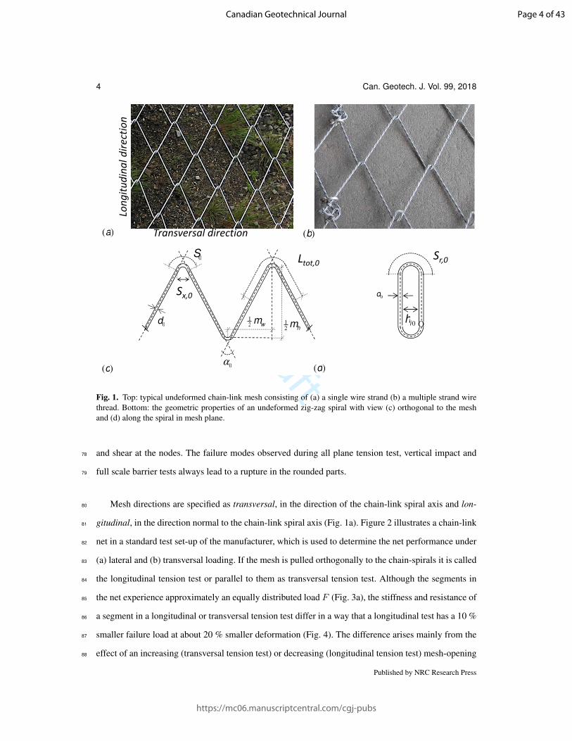
Fig. 1. Top: typical undeformed chain-link mesh consisting of (a) a single wire strand (b) a multiple strand wirethread. Bottom: the geometric properties of an undeformed zig-zag spiral with view (c) orthogonal to the meshand (d) along the spiral in mesh plane.
and shear at the nodes. The failure modes observed during all plane tension test, vertical impact and78
full scale barrier tests always lead to a rupture in the rounded parts.79
Mesh directions are specified as transversal, in the direction of the chain-link spiral axis and lon-80
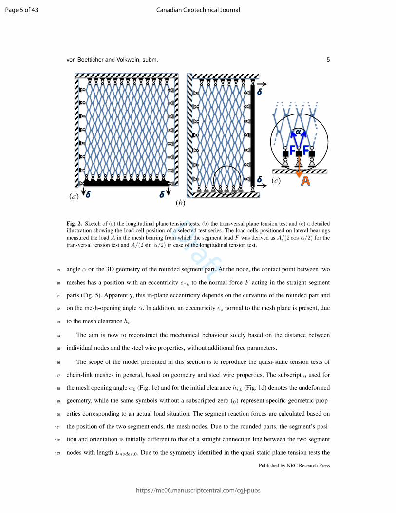
gitudinal, in the direction normal to the chain-link spiral axis (Fig. 1a). Figure 2 illustrates a chain-link81
net in a standard test set-up of the manufacturer, which is used to determine the net performance under82
(a) lateral and (b) transversal loading. If the mesh is pulled orthogonally to the chain-spirals it is called83
the longitudinal tension test or parallel to them as transversal tension test. Although the segments in84
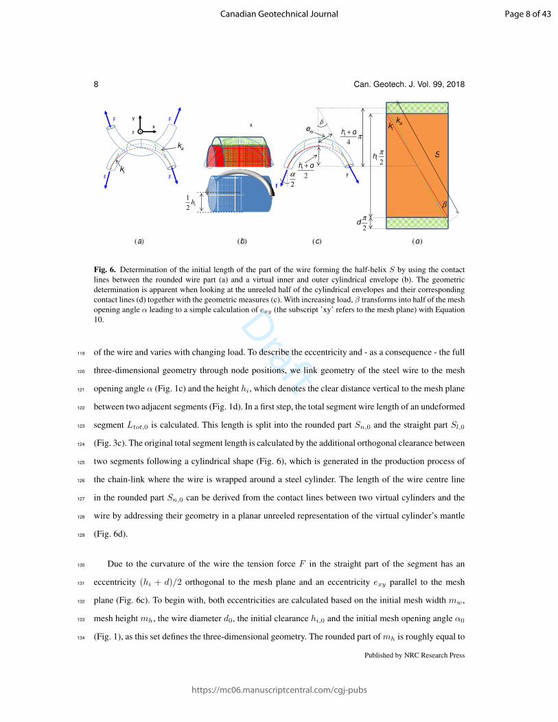
the net experience approximately an equally distributed load F (Fig. 3a), the stiffness and resistance of85
a segment in a longitudinal or transversal tension test differ in a way that a longitudinal test has a 10 %86
smaller failure load at about 20 % smaller deformation (Fig. 4). The difference arises mainly from the87
effect of an increasing (transversal tension test) or decreasing (longitudinal tension test) mesh-opening88
Published by NRC Research Press
Page 4 of 43
https://mc06.manuscriptcentral.com/cgj-pubs
Canadian Geotechnical Journal
Draft
von Boetticher and Volkwein, subm. 5
√©√
√©√
√©√
©√
√
√©√
√©√ √
©√
√©√
√©√
(a)(b)
(c)
Fig. 2. Sketch of (a) the longitudinal plane tension tests, (b) the transversal plane tension test and (c) a detailedillustration showing the load cell position of a selected test series. The load cells positioned on lateral bearingsmeasured the load A in the mesh bearing from which the segment load F was derived as A/(2 cos α/2) for thetransversal tension test and A/(2 sin α/2) in case of the longitudinal tension test.
angle α on the 3D geometry of the rounded segment part. At the node, the contact point between two89
meshes has a position with an eccentricity exy to the normal force F acting in the straight segment90
parts (Fig. 5). Apparently, this in-plane eccentricity depends on the curvature of the rounded part and91
on the mesh-opening angle α. In addition, an eccentricity ez normal to the mesh plane is present, due92
to the mesh clearance hi.93
The aim is now to reconstruct the mechanical behaviour solely based on the distance between94
individual nodes and the steel wire properties, without additional free parameters.95
The scope of the model presented in this section is to reproduce the quasi-static tension tests of96
chain-link meshes in general, based on geometry and steel wire properties. The subscript 0 used for97
the mesh opening angle α0 (Fig. 1c) and for the initial clearance hi,0 (Fig. 1d) denotes the undeformed98
geometry, while the same symbols without a subscripted zero (0) represent specific geometric prop-99
erties corresponding to an actual load situation. The segment reaction forces are calculated based on100
the position of the two segment ends, the mesh nodes. Due to the rounded parts, the segment’s posi-101
tion and orientation is initially different to that of a straight connection line between the two segment102
nodes with length Lnodes,0. Due to the symmetry identified in the quasi-static plane tension tests the103
Published by NRC Research Press
Page 5 of 43
https://mc06.manuscriptcentral.com/cgj-pubs
Canadian Geotechnical Journal
Draft
6 Can. Geotech. J. Vol. 99, 2018
Sl,0
Lnodes,0
Sl = Sl,0 + Sn,0 – Sn
Lnodes
½Sn,0½Sn
Sseg = Lnodes – (Lnodes,0 – Sl,0)
+ 0.7(Sn,0 – Sn )
½Sn
½Sn,0
Sseg,0 = Sl,0
( )a ( )b ( )c ( )d
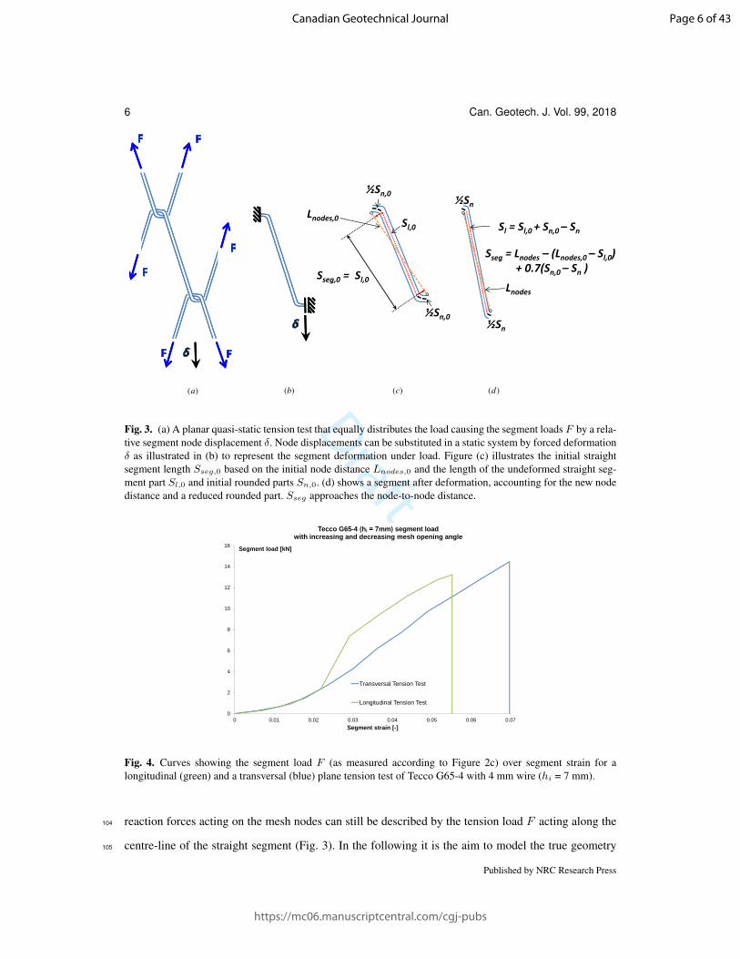
Fig. 3. (a) A planar quasi-static tension test that equally distributes the load causing the segment loads F by a rela-tive segment node displacement δ. Node displacements can be substituted in a static system by forced deformationδ as illustrated in (b) to represent the segment deformation under load. Figure (c) illustrates the initial straightsegment length Sseg,0 based on the initial node distance Lnodes,0 and the length of the undeformed straight seg-ment part Sl,0 and initial rounded parts Sn,0. (d) shows a segment after deformation, accounting for the new nodedistance and a reduced rounded part. Sseg approaches the node-to-node distance.
10
12
14
16 Segment load [kN]
Tecco G65-4 (hi = 7mm) segment load with increasing and decreasing mesh opening angle
0
2
4
6
8
0 0.01 0.02 0.03 0.04 0.05 0.06 0.07
Transversal Tension Test
Longitudinal Tension Test
Segment strain [-]
Fig. 4. Curves showing the segment load F (as measured according to Figure 2c) over segment strain for alongitudinal (green) and a transversal (blue) plane tension test of Tecco G65-4 with 4 mm wire (hi = 7 mm).
reaction forces acting on the mesh nodes can still be described by the tension load F acting along the104
centre-line of the straight segment (Fig. 3). In the following it is the aim to model the true geometry105
Published by NRC Research Press
Page 6 of 43
https://mc06.manuscriptcentral.com/cgj-pubs
Canadian Geotechnical Journal

Draft
von Boetticher and Volkwein, subm. 7
α
2
2���2���
α
2
(a) (b)
x
y
z
Fig. 5. The rounded geometry at the node causes an eccentricity exy of the segment load F within the mesh plane(x-y) which depends on the mesh opening angle α. Figure (a) illustrates the situation in a longitudinal tension testwhile figure (b) represents a transversal tension test. In addition, the eccentricity depends on the mesh clearancein z-direction.
and bending processes, which take place in the rounded parts, depending on the mesh nodes’ positions106
and the segment tension F .107
2.1. Mesh stiffness and bending deformations at the nodes108
If the segment was modelled as a straight steel wire (or multiple wire strand thread) connecting the109
segment nodes, without considering the three-dimensional curvature/geometry of the steel wire in the110
vicinity of the mesh nodes, the segment stiffness would be overestimated by an order of magnitude.111
Furthermore, the true segment stiffness, which would describe the segment tension F depending on112
the distance between segment nodes Lnodes (Fig. 3), has to change with the mesh opening angle α113
(Fig. 1). The key aspects of the varying stiffness result from the three dimensional wire geometry and114
its subsequent deformations under load, which are described in the following subsections.115
2.1.1. Three dimensional wire geometry116
A force F applied to the straight part of the wire has an eccentricity to the contact point at the node117
which lies within the rounded section S0 of the wire. This eccentricity drives the bending deformation118
Published by NRC Research Press
Page 7 of 43
https://mc06.manuscriptcentral.com/cgj-pubs
Canadian Geotechnical Journal
Draft
8 Can. Geotech. J. Vol. 99, 2018
x
z
y
x.
F F
FFβ
F
F
hi
π
2S
ki
ka
dπ
2
α
2
ki
ka
hi + d
2
hi + d
4π
exy
β
(a) (b) (c) (d)
ih
2
1
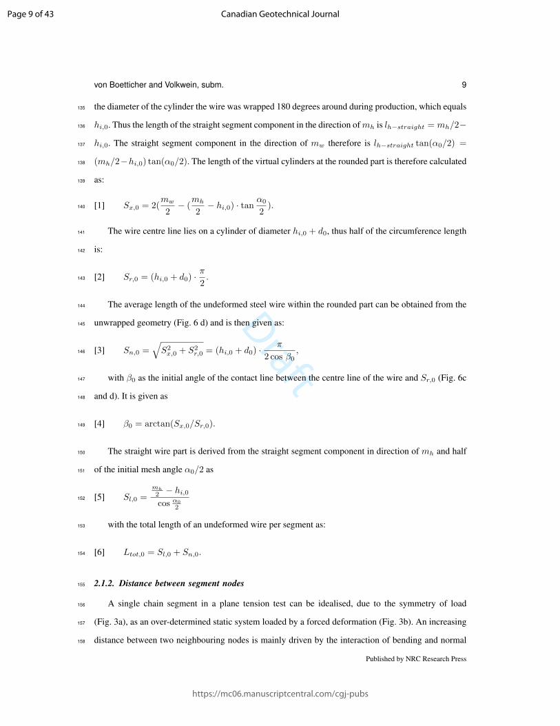
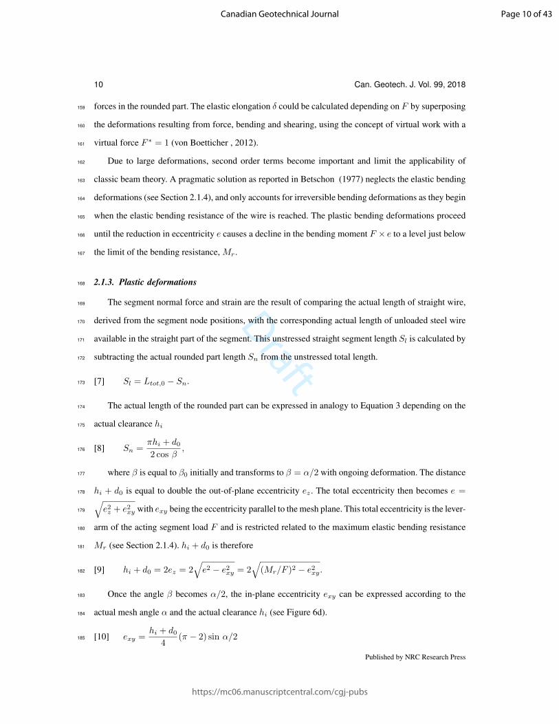
Fig. 6. Determination of the initial length of the part of the wire forming the half-helix S by using the contactlines between the rounded wire part (a) and a virtual inner and outer cylindrical envelope (b). The geometricdetermination is apparent when looking at the unreeled half of the cylindrical envelopes and their correspondingcontact lines (d) together with the geometric measures (c). With increasing load, β transforms into half of the meshopening angle α leading to a simple calculation of exy (the subscript ’xy’ refers to the mesh plane) with Equation10.
of the wire and varies with changing load. To describe the eccentricity and - as a consequence - the full119
three-dimensional geometry through node positions, we link geometry of the steel wire to the mesh120
opening angle α (Fig. 1c) and the height hi, which denotes the clear distance vertical to the mesh plane121
between two adjacent segments (Fig. 1d). In a first step, the total segment wire length of an undeformed122
segment Ltot,0 is calculated. This length is split into the rounded part Sn,0 and the straight part Sl,0123
(Fig. 3c). The original total segment length is calculated by the additional orthogonal clearance between124
two segments following a cylindrical shape (Fig. 6), which is generated in the production process of125
the chain-link where the wire is wrapped around a steel cylinder. The length of the wire centre line126
in the rounded part Sn,0 can be derived from the contact lines between two virtual cylinders and the127
wire by addressing their geometry in a planar unreeled representation of the virtual cylinder’s mantle128
(Fig. 6d).129
Due to the curvature of the wire the tension force F in the straight part of the segment has an130
eccentricity (hi + d)/2 orthogonal to the mesh plane and an eccentricity exy parallel to the mesh131
plane (Fig. 6c). To begin with, both eccentricities are calculated based on the initial mesh width mw,132
mesh height mh, the wire diameter d0, the initial clearance hi,0 and the initial mesh opening angle α0133
(Fig. 1), as this set defines the three-dimensional geometry. The rounded part ofmh is roughly equal to134
Published by NRC Research Press
Page 8 of 43
https://mc06.manuscriptcentral.com/cgj-pubs
Canadian Geotechnical Journal
Draft
von Boetticher and Volkwein, subm. 9
the diameter of the cylinder the wire was wrapped 180 degrees around during production, which equals135
hi,0. Thus the length of the straight segment component in the direction ofmh is lh−straight = mh/2−136
hi,0. The straight segment component in the direction of mw therefore is lh−straight tan(α0/2) =137
(mh/2−hi,0) tan(α0/2). The length of the virtual cylinders at the rounded part is therefore calculated138
as:139
Sx,0 = 2(mw
2− (
mh
2− hi,0) · tan
α0
2).[1]140
The wire centre line lies on a cylinder of diameter hi,0 + d0, thus half of the circumference length141
is:142
Sr,0 = (hi,0 + d0) · π2.[2]143
The average length of the undeformed steel wire within the rounded part can be obtained from the144
unwrapped geometry (Fig. 6 d) and is then given as:145
Sn,0 =√S2x,0 + S2
r,0 = (hi,0 + d0) · π
2 cos β0,[3]146
with β0 as the initial angle of the contact line between the centre line of the wire and Sr,0 (Fig. 6c147
and d). It is given as148
β0 = arctan(Sx,0/Sr,0).[4]149
The straight wire part is derived from the straight segment component in direction of mh and half150
of the initial mesh angle α0/2 as151
Sl,0 =mh
2 − hi,0cos α0
2
[5]152
with the total length of an undeformed wire per segment as:153
Ltot,0 = Sl,0 + Sn,0.[6]154
2.1.2. Distance between segment nodes155
A single chain segment in a plane tension test can be idealised, due to the symmetry of load156
(Fig. 3a), as an over-determined static system loaded by a forced deformation (Fig. 3b). An increasing157
distance between two neighbouring nodes is mainly driven by the interaction of bending and normal158
Published by NRC Research Press
Page 9 of 43
https://mc06.manuscriptcentral.com/cgj-pubs
Canadian Geotechnical Journal
Draft
10 Can. Geotech. J. Vol. 99, 2018
forces in the rounded part. The elastic elongation δ could be calculated depending on F by superposing159
the deformations resulting from force, bending and shearing, using the concept of virtual work with a160
virtual force F ∗ = 1 (von Boetticher , 2012).161
Due to large deformations, second order terms become important and limit the applicability of162
classic beam theory. A pragmatic solution as reported in Betschon (1977) neglects the elastic bending163
deformations (see Section 2.1.4), and only accounts for irreversible bending deformations as they begin164
when the elastic bending resistance of the wire is reached. The plastic bending deformations proceed165
until the reduction in eccentricity e causes a decline in the bending moment F × e to a level just below166
the limit of the bending resistance, Mr.167
2.1.3. Plastic deformations168
The segment normal force and strain are the result of comparing the actual length of straight wire,169
derived from the segment node positions, with the corresponding actual length of unloaded steel wire170
available in the straight part of the segment. This unstressed straight segment length Sl is calculated by171
subtracting the actual rounded part length Sn from the unstressed total length.172
Sl = Ltot,0 − Sn.[7]173
The actual length of the rounded part can be expressed in analogy to Equation 3 depending on the174
actual clearance hi175
Sn =πhi + d02 cos β
,[8]176
where β is equal to β0 initially and transforms to β = α/2 with ongoing deformation. The distance177
hi + d0 is equal to double the out-of-plane eccentricity ez . The total eccentricity then becomes e =178 √e2z + e2xy with exy being the eccentricity parallel to the mesh plane. This total eccentricity is the lever-179
arm of the acting segment load F and is restricted related to the maximum elastic bending resistance180
Mr (see Section 2.1.4). hi + d0 is therefore181
hi + d0 = 2ez = 2√e2 − e2xy = 2
√(Mr/F )2 − e2xy.[9]182
Once the angle β becomes α/2, the in-plane eccentricity exy can be expressed according to the183
actual mesh angle α and the actual clearance hi (see Figure 6d).184
exy =hi + d0
4(π − 2) sin α/2[10]185
Published by NRC Research Press
Page 10 of 43
https://mc06.manuscriptcentral.com/cgj-pubs
Canadian Geotechnical Journal
Draft
von Boetticher and Volkwein, subm. 11
Based on a segment load F causing plastic bending at a current clearance hi and a corresponding186
in-plane eccentricity using Equation 10, the clearance is adjusted according to Equation 9. This in187
turn changes exy and – again – hi. So, this step is repeated until a sufficiently precise hi is found188
which results in the bending moment being just below the bending resistance Mr. Thus, for a given189
segment load F , the corresponding clearance hi and the straight length of the steel wire Sl can be190
calculated based on plastic bending deformations. This elongation from Sl,0 to Sl caused by bending191
in the rounded parts dominates above any elastic elongation of Sl. Any increase of F that causes the192
bending moment in the rounded part to exceed the bending resistance leads to further transfer of steel193
wire from the rounded to the straight part, increasing Sl.194
The force F is derived as the reaction force of the straight steel wire due to its strain,195
F = EA(SsegSl− 1),[11]196
below the elastic tension limit of the wire, where E is the elastic modulus and A the cross-section197
of the segment steel wire.198
An increase in node distance causes an increase in Sseg and thus in F . However, an increase in F199
leads to plastic bending deformations and an increase in Sl, as described above, and based on Equa-200
tion 11 this again relaxes the actual segment tension F , which is why the steps from Equation 9 to201
Equation 11 have to be solved iteratively to find the reaction of a segment to a given node distance.202
This approach is suitable to reproduce the mechanical behaviour of the mesh in detail as shown in the203
following, but the geometry of the rounded part has to be treated accurately.204
Initially, the straight part of the segment does not align with the node-to-node connection due to205
the eccentricity e, but with ongoing reduction in the clearance hi, the segment becomes almost parallel206
to a node-to-node connection Lnodes (Figure 3d). In transversal direction, the length of the rounded207
part at the node can be approximated as hi π/2 tan(β) (see Fig. 6d), and according to von Boetticher208
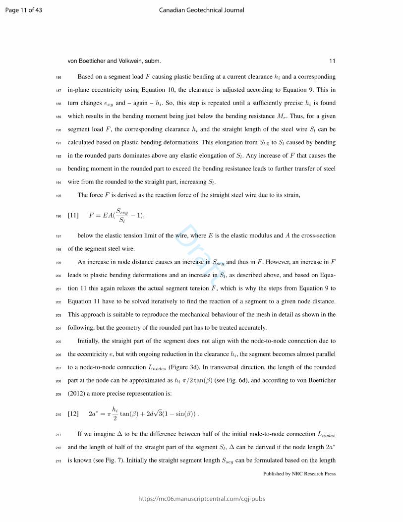
(2012) a more precise representation is:209
2a∗ = πhi2
tan(β) + 2d√
3(1− sin(β)) .[12]210
If we imagine ∆ to be the difference between half of the initial node-to-node connection Lnodes211
and the length of half of the straight part of the segment Sl, ∆ can be derived if the node length 2a∗212
is known (see Fig. 7). Initially the straight segment length Sseg can be formulated based on the length213
Published by NRC Research Press
Page 11 of 43
https://mc06.manuscriptcentral.com/cgj-pubs
Canadian Geotechnical Journal
Draft
12 Can. Geotech. J. Vol. 99, 2018
Fig. 7. Representation of the discrepancy ∆ between the straight segment part and a node-to-node connection. Asz1 = hi/2 and z2 = a
tan β− z1, it is possible to derive that ∆ = a
sin β− z2 cos β with β determined from the
3D representation of the segments (see Fig. 6)
Lnodes derived from node positions by accounting for the difference between the initial node-to-node214
connection Lnodes,0 and the initial length of the straight part of the segment Sl,0,215
Sseg = Lnodes − Lnodes,0 + Sl,0.[13]216
However, as the eccentricity decreases at the node under plastic deformations and the straight seg-217
ment part increases accordingly, the change in ∆ needs to be account for. As ∆ was formulated based218
on β and a∗, ∆ can also be formulated based on the rounded segment part Sn of Equation 8. The219
change in ∆ can be expressed as the change in the rounded part Sn,0 − Sn using Equation 3. Thus we220
modified Equation 13 by reducing the difference between Lnodes,0 and Sl,0 with decreasing length of221
the rounded part Sn:222
Sseg = Lnodes − Lnodes,0 + Sl,0 + 0.7(Sn,0 − Sn) .[14]223
Here the factor 0.7 represents a ratio between (∆0−∆min) and (Sn,0−Sn,min), where ∆min and224
Sn,min are the corresponding remaining lengths at hi = 0. More precisely, the average value for all225
mesh types is 0.737, with a standard deviation of ±0.006.226
Published by NRC Research Press
Page 12 of 43
https://mc06.manuscriptcentral.com/cgj-pubs
Canadian Geotechnical Journal
Draft
von Boetticher and Volkwein, subm. 13
2.1.4. Change of mesh stiffness227
The static system of a segment loaded by an in-plane tension test is comparable to that of a sym-228
metric s-hook with clamped and partially movable nodes (Fig. 3b). As deformations increase in size,229
second order effects appear with the reduction of the eccentricity (Betschon , 1977). The interaction230
between the normal force and the bending moment in the rounded part must then be considered for231
the following reason: the bending deformation in the node reduces the rounded section and therefore232
the lever arm of F , and thereby again the bending load. Consequently the mesh becomes stiffer with233
increasing deformation, because a greater load increase is necessary to achieve the same transfer of234
wire from the rounded part to the straight part of the segment. At the same time, the bending resistance235
of the wire, Mr, which denotes the limit below which no further plastic bending deformations occur,236
is not constant. Two counter-acting processes therefore change Mr: one increases the resistance of the237
wire against further plastic bending deformations while the other process reduces Mr. The increase238
in Mr is due to the spreading of the region within the cross section of the steel wire that reaches the239
yield stress, and furthermore, the increase of the yield stress itself affects Mr due to steel hardening240
with ongoing deformations. The counter-acting reduction of Mr starts at higher loads and is a conse-241
quence of the interaction of bending and normal load. We show our approaches to both processes in242
the following.243
When the elastic bending resistance becomes the plastic bending resistance with ongoing plastic244
bending deformations,Mr evolves to a higher bending resistance than in the beginning, with a plasticity245
shape factor of about 1.7 for a circular cross-section (Knodel , 2010). Furthermore, the high tension246
steel shows a pronounced steel hardening under plastic deformation as the failure stress is much higher247
than the yield stress. We account for this effect with an internal calibration factor By that increases248
the bending resistance, which we calibrated to By = 4 based on the longitudinal tension test of Tecco249
G65-4 (Torres-Vila et al. , 2001) to fit the measured segment stress-strain curve.250
Before the failure limit is reached, the effect of interaction between bending and the normal force251
counteracts the increasing bending resistance, which again modifies Mr. An example for such N-M-252
interaction in chain-link meshes is shown in Escallon et al. (2015). For our approach we consider the253
section close to the node, where the normal force equals F sin α/2. Very generally, we consider the254
cross section of the segment to form a generalized plastic hinge (Jirasek and Bazant , 2002) and we255
receive the remaining wire section area available for a remaining plastic bending resistance Mr by256
Published by NRC Research Press
Page 13 of 43
https://mc06.manuscriptcentral.com/cgj-pubs
Canadian Geotechnical Journal
Draft
14 Can. Geotech. J. Vol. 99, 2018
excluding a central part of the wire section AN . This core area AN is considered to carry the normal257
load, thus AN is defined by the area necessary to carry the normal force load under the yield stress fy258
AN =F sin α/2
fy.[15]259
The left-over ’upper and lower’ cross-section parts not occupied by AN form the plastic bending resis-260
tance, and it is assumed that one part is under tension yield stress and the opposite part under pressure261
yield stress:262
Mr = ysegAsegfyBy,[16]263
where Aseg is the remaining cross-sectional area (the cross-section of the segment minus AN ) and264
yseg the lever arm between the regions of Aseg under tension and the region under pressure at the265
opposite side of the cross-section. The influence of α on the combined interaction of bending, normal266
force and shear and its influence on the in-plane eccentricity exy make the mesh stiffness depending267
on the opening angle. Figure 4 shows the segment load F in the mesh of two in-plane tension tests.268
The load in the single segments is reconstructed from the bearing forces measured at a lateral sliding269
fixation (Fig. 2c). The difference in segment stiffness between transversal and longitudinal tension270
tests occurs due to the increasing opening angle in the transversal tension test and its decrease in the271
longitudinal tension test. The initial stiffness of the segment is the same in both tests because the initial272
opening angle is the same. Between strains of 0.02 and 0.03, the increase in bending resistance and273
the reduction of mesh eccentricity leads to a stiffer segment, and this process is more pronounced for274
smaller mesh angles. Above a strain of 0.03, the momentum- and normal load interaction at the node275
starts to dominate and reduces the segment stiffness. Finally, the mesh fails under bending with normal276
force and shear interaction, and in case of the longitudinal tension test, the shear resistance becomes277
the limiting factor.278
2.2. Mesh resistance279
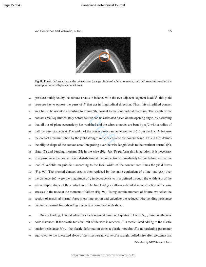
Deduced from scratches and deformations (Fig. 8) of experimentally tested chain-link nets, an280
elliptical contact area can be assumed at the nodes between two chains. With the additional assumption281
of an elastic, perfectly plastic behaviour of the steel wire, the stresses in the contact area cannot exceed282
the yield stress. By integrating the yield stress over the ellipse width, the elliptic area may be substituted283
by an equivalent line load. A minimal contact area under yield pressure can be defined. Because yield284
Published by NRC Research Press
Page 14 of 43
https://mc06.manuscriptcentral.com/cgj-pubs
Canadian Geotechnical Journal
Draft
von Boetticher and Volkwein, subm. 15
Fig. 8. Plastic deformations at the contact area (orange circle) of a failed segment, such deformations justified theassumption of an elliptical contact area.
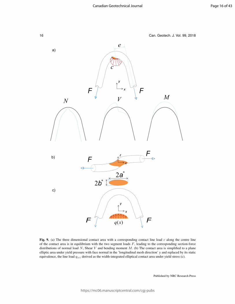
pressure multiplied by the contact area is in balance with the two adjacent segment loads F , this yield285
pressure has to oppose the parts of F that act in longitudinal direction. Thus, this simplified contact286
area has to be oriented according to Figure 9b, normal to the longitudinal direction. The length of the287
contact area 2a∗1 immediately before failure can be estimated based on the opening angle, by assuming288
that all out-of-plane eccentricity has vanished and the wires at nodes are bent by α/2 with a radius of289
half the wire diameter d. The width of the contact area can be derived to 2b∗1 from the load F because290
the contact area multiplied by the yield strength must be equal to the contact force. This in turn defines291
the elliptic shape of the contact area. Integrating over the wire length leads to the resultant normal (N),292
shear (S) and bending moment (M) in the wire (Fig. 9a). To perform this integration, it is necessary293
to approximate the contact force distribution at the connections immediately before failure with a line294
load of variable magnitude c according to the local width of the contact area times the yield stress295
(Fig. 9a). The pressed contact area is then replaced by the static equivalent of a line load q(x) over296
the distance 2a∗1, were the magnitude of q in dependency to x is defined through the width at x of the297
given elliptic shape of the contact area. The line load q(x) allows a detailed reconstruction of the wire298
stresses in the node at the moment of failure (Fig. 9c). To register the moment of failure, we select the299
section of maximal normal force-shear interaction and calculate the reduced wire bending resistance300
due to the normal force-bending interaction combined with shear.301
During loading, F is calculated for each segment based on Equation 11 with Sseg based on the new302
node distances. If the elastic tension limit of the wire is reached, F is recalculated adding to the elastic303
tension resistance NR,el the plastic deformation times a plastic modulus Epl (a hardening parameter304
equivalent to the linearized slope of the stress-strain curve of a straight pulled wire after yielding) that305
Published by NRC Research Press
Page 15 of 43
https://mc06.manuscriptcentral.com/cgj-pubs
Canadian Geotechnical Journal
Draft
16 Can. Geotech. J. Vol. 99, 2018
e
N V MF F
c
a)
FF
2a*
2b*
F F
x
y
)(xq
b)
c)
x
y
x
z
Fig. 9. (a) The three dimensional contact area with a corresponding contact line load c along the centre lineof the contact area is in equilibrium with the two segment loads F , leading to the corresponding section-forcedistributions of normal load N , Shear V and bending moment M . (b) The contact area is simplified to a planeelliptic area under yield pressure with face normal in the ’longitudinal mesh direction’ y and replaced by its staticequivalence, the line load q(x) derived as the width-integrated elliptical contact area under yield stress (c).
Published by NRC Research Press
Page 16 of 43
https://mc06.manuscriptcentral.com/cgj-pubs
Canadian Geotechnical Journal
Draft
von Boetticher and Volkwein, subm. 17
was derived from single wire tension tests:306
F = NR,el + EplA(SsegSl− 1− εy) ,[17]307
where εy is the segment strain at the onset of yielding, when F = NR,el. Subsequently, the normal-308
force shear interaction is calculated along the rounded part at the node, followed by a test whether the309
resistance fulfills the constraint:310
(Q
QR)2 + (
N
NR,pl)2 < 1,[18]311
where Q is the shearing force and QR is the shear resistance of the wire and N and NR,pl denote the312
normal force and the tension resistance of the wire. In case of sufficient wire resistance to normal force313
and shear interaction, the wire resistance in the section with the highest value for the left-hand side of314
Equation 18 is tested for a combined interaction between normal force, shear and bending.315
Based on Schwarzlos (2005) the reduced normal force resistance NR,red due to shear becomes316
NR,red = (1− ρw)NR,pl = fu(1− ρw)πd2
4.[19]317
where fu is the failure stress of the wire, d is the wire diameter and318
ρw = (2Q
QR− 1)2.[20]319
The remaining bending resistance MR,red at this section of normal-force shear interaction is then320
calculated by linear superposition as:321
MR,red = BR ∗MR(1− N
NR,red),[21]322
whereMR is the plastic bending resistance of the wire. The factorBR compensates the neglected bend-323
ing deformation in the straight part of a segment according to Betschon (1977). The model increases324
the bending resistance by the additional factor BR which was calibrated to BR = 2.4 for all mesh325
types to achieve a good agreement of the modelled failure loads with planar tension tests performed by326
Torres-Vila et al. (2001).327
If the bending moment at this section exceeds this bending resistanceMR,red, the combined failure328
of the segment is assumed.329
Published by NRC Research Press
Page 17 of 43
https://mc06.manuscriptcentral.com/cgj-pubs
Canadian Geotechnical Journal
Draft
18 Can. Geotech. J. Vol. 99, 2018
3. Detailed numerical implementation of mesh mechanics330
Above details were implemented into a detailed chain-link discrete element, which reproduces331
the failure load of longitudinal and transversal tension tests for single wire meshes, with wires of 3332
and 4mm diameter. The model uses the wire diameter, the coating against corrosion (which has an333
influence on the steel diameter), the tension yield load of the wire and the failure load as input, as well334
as the ratio of shear strength to tension strength in the wire. Furthermore, the elastic and plastic moduli335
are required along with details of the mesh geometry in terms of mesh width, mesh height, clearance336
and the mesh opening angle. All data except the shear strength and elastic- and plastic moduli are337
available from the standard data sheets of the manufacturer. The shear strength to tension strength338
ratio was approximately determined through plane tension tests using different wire types with a mesh339
opening angle close to zero, ranging from 0.38 to 0.44. In these tests the set-up was identical to the340
usual longitudinal tension test with 1 × 1m specimen mesh, but without lateral fixation, resulting in341
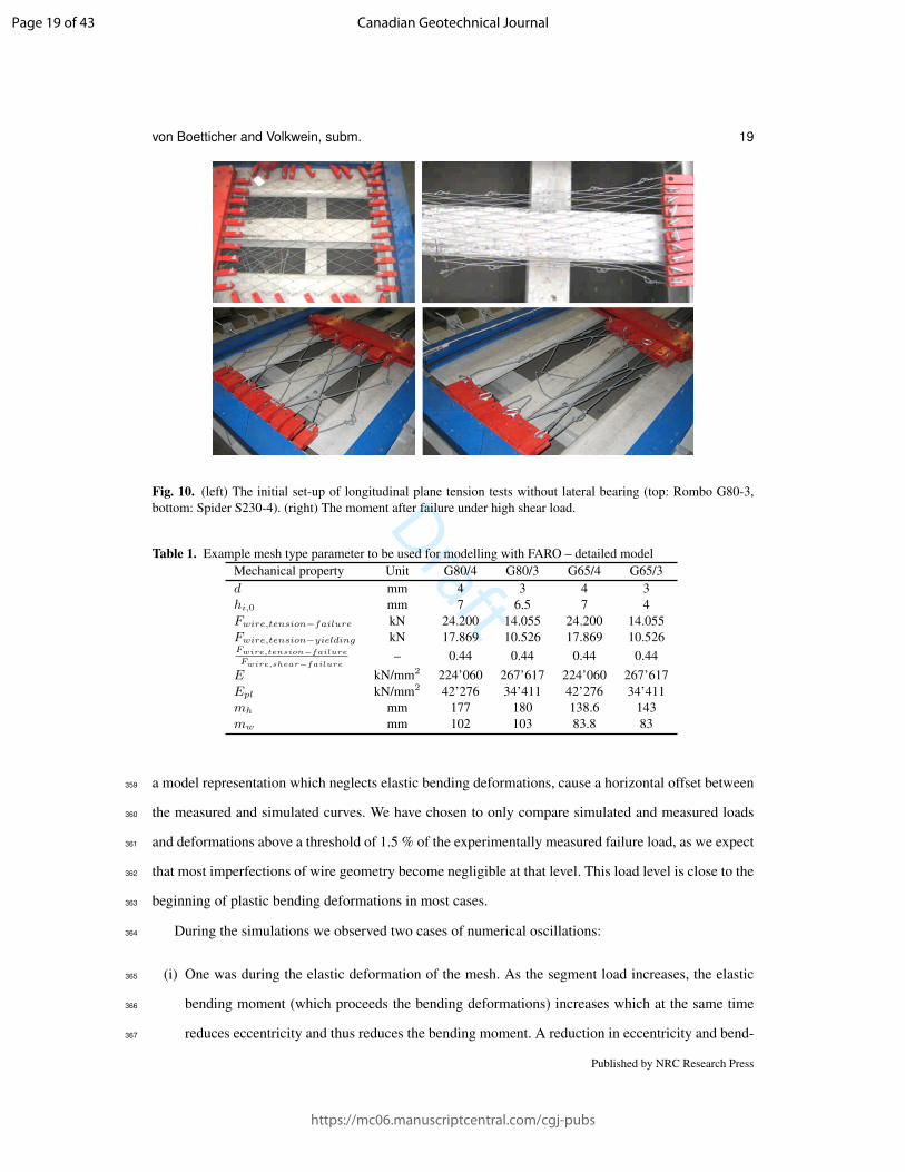
a shear-failure in the segment nodes at mesh opening angles close to zero (Fig. 10). The elastic and342
plastic limits of the wire and the elastic and plastic moduli were taken from single wire tests performed343
by Torres-Vila et al. (2001), Zund (2006), Kastli (2007), Stradtner and Steidl (2009), and Stradtner344
and Steidl (2009a). The plane tension tests (transversal and longitudinal) used for validation were in345
principle set-up according to Figure 2 but in most cases the transversal test had a larger mesh size of 26346
segments in load direction. Additionally, small changes in mesh height have occurred with changes in347
the mesh clearance hi,0, e.g. from 8 mm to a minimal value of 3.5 mm applied for Tecco G65-3-FLAT,348
6 mm for Tecco G65-4, and 5 mm for Tecco G65-3. Other clearances were used for the mesh types349
Tecco G80-4 and Rombo G80-3.350
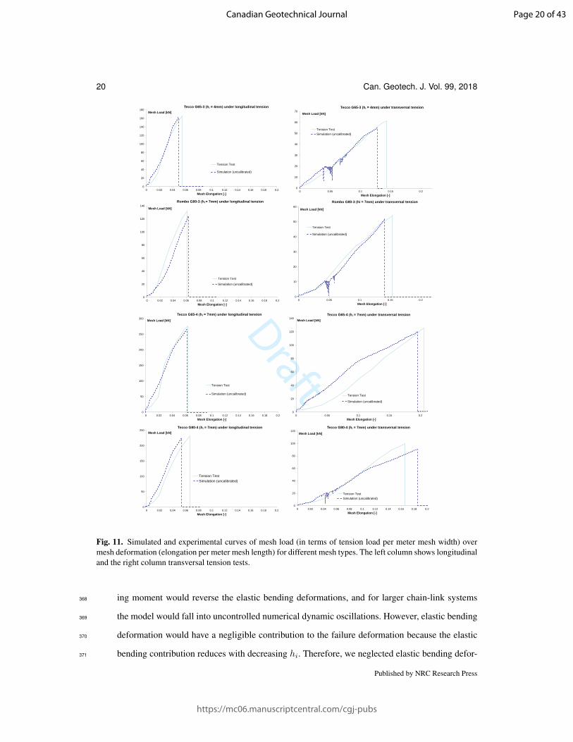
Figure 11 shows example curves of simulated and measured (Zund , 2006; Stradtner and Steidl351
, 2009,a) loads and deformations until failure. The simulation has been done quasi-statically, i.e. the352
same explicit time integration scheme has been applied as for full dynamic simulations, only the speeds353
of the moving nodes are magnitudes lower. All model input was derived from the steel wire properties354
and the mesh geometry without calibration apart from BR and By which are constant for all mesh355
types. Table 1 lists the set of input parameters to model the corresponding plane tension tests shown in356
Figure 11.357
Small offsets and imperfections in the mesh geometry at the beginning of the tests, combined with358
Published by NRC Research Press
Page 18 of 43
https://mc06.manuscriptcentral.com/cgj-pubs
Canadian Geotechnical Journal
Draft
von Boetticher and Volkwein, subm. 19
Fig. 10. (left) The initial set-up of longitudinal plane tension tests without lateral bearing (top: Rombo G80-3,bottom: Spider S230-4). (right) The moment after failure under high shear load.
Table 1. Example mesh type parameter to be used for modelling with FARO – detailed modelMechanical property Unit G80/4 G80/3 G65/4 G65/3d mm 4 3 4 3hi,0 mm 7 6.5 7 4Fwire,tension−failure kN 24.200 14.055 24.200 14.055Fwire,tension−yielding kN 17.869 10.526 17.869 10.526Fwire,tension−failure
Fwire,shear−failure– 0.44 0.44 0.44 0.44
E kN/mm2 224’060 267’617 224’060 267’617Epl kN/mm2 42’276 34’411 42’276 34’411mh mm 177 180 138.6 143mw mm 102 103 83.8 83
a model representation which neglects elastic bending deformations, cause a horizontal offset between359
the measured and simulated curves. We have chosen to only compare simulated and measured loads360
and deformations above a threshold of 1.5 % of the experimentally measured failure load, as we expect361
that most imperfections of wire geometry become negligible at that level. This load level is close to the362
beginning of plastic bending deformations in most cases.363
During the simulations we observed two cases of numerical oscillations:364
(i) One was during the elastic deformation of the mesh. As the segment load increases, the elastic365
bending moment (which proceeds the bending deformations) increases which at the same time366
reduces eccentricity and thus reduces the bending moment. A reduction in eccentricity and bend-367
Published by NRC Research Press
Page 19 of 43
https://mc06.manuscriptcentral.com/cgj-pubs
Canadian Geotechnical Journal
Draft
20 Can. Geotech. J. Vol. 99, 2018
0
10
20
30
40
50
60
0 0.05 0.1 0.15 0.2
Mesh Load [kN]
Mesh Elongation [-]
Rombo G80-3 (hi = 7mm) under transversal tension
Tension Test
Simulation (uncalibrated)
0
50
100
150
200
250
300
0 0.02 0.04 0.06 0.08 0.1 0.12 0.14 0.16 0.18 0.2
Mesh Load [kN]
Mesh Elongation [-]
Tecco G65-4 (hi = 7mm) under longitudinal tension
Tension Test
Simulation (uncalibrated)
0
20
40
60
80
100
120
140
0 0.05 0.1 0.15 0.2
Mesh Load [kN]
Mesh Elongation [-]
Tecco G65-4 (hi = 7mm) under transversal tension
Tension Test
Simulation (uncalibrated)
0
50
100
150
200
250
0 0.02 0.04 0.06 0.08 0.1 0.12 0.14 0.16 0.18 0.2
Mesh Load [kN]
Mesh Elongation [-]
Tecco G80-4 (hi = 7mm) under longitudinal tension
Tension Test Simulation (uncalibrated)
0
20
40
60
80
100
120
0 0.02 0.04 0.06 0.08 0.1 0.12 0.14 0.16 0.18 0.2
Mesh Load [kN]
Mesh Elongation [-]
Tecco G80-4 (hi = 7mm) under transversal tension
Tension Test Simulation (uncalibrated)
0
20
40
60
80
100
120
140
0 0.02 0.04 0.06 0.08 0.1 0.12 0.14 0.16 0.18 0.2
Mesh Load [kN]
Mesh Elongation [-]
Rombo G80-3 (hi = 7mm) under longitudinal tension
Tension Test
Simulation (uncalibrated)
0
20
40
60
80
100
120
140
160
180
0 0.02 0.04 0.06 0.08 0.1 0.12 0.14 0.16 0.18 0.2
Mesh Load [kN]
Mesh Elongation [-]
Tecco G65-3 (hi = 4mm) under longitudinal tension
Tension Test
Simulation (uncalibrated)
0
10
20
30
40
50
60
70
0 0.05 0.1 0.15 0.2 0.25
Mesh Load [kN]
Mesh Elongation [-]
Tecco G65-3 (hi = 4mm) under transversal tension
Tension Test Simulation (uncalibrated)
Fig. 11. Simulated and experimental curves of mesh load (in terms of tension load per meter mesh width) overmesh deformation (elongation per meter mesh length) for different mesh types. The left column shows longitudinaland the right column transversal tension tests.
ing moment would reverse the elastic bending deformations, and for larger chain-link systems368
the model would fall into uncontrolled numerical dynamic oscillations. However, elastic bending369
deformation would have a negligible contribution to the failure deformation because the elastic370
bending contribution reduces with decreasing hi. Therefore, we neglected elastic bending defor-371
Published by NRC Research Press
Page 20 of 43
https://mc06.manuscriptcentral.com/cgj-pubs
Canadian Geotechnical Journal

Draft
von Boetticher and Volkwein, subm. 21
mations.372
(ii) Also, the second order effect of plastic bending deformation may lead to numerical oscillations373
with node deformations in the order of the quasi-statically moving nodes due to the coupling374
between segment load, bending moment, bending deformation and eccentricity as visible in some375
of the diagrams in Figure 11.376
At the beginning of the plane tension tests, geometrical imperfections contribute to the measured377
load. With ongoing mesh deformations, most irregularities of mesh positions are averaged out.378
4. Simplified numerical implementation of mesh mechanics379
The numerical costs of the approach in Section 3 are too high to apply the model to full-scale mesh380
barriers. However, the characteristic mesh behaviour and its mechanical background were captured,381
providing the basis for a simplified chain-link model. We developed a numerical chain-link element that382
uses the output of modelled or measured plane tension tests as described in Section 2 to characterize383
the anisotropic mesh behaviour. The detailed approach served herein as a proof of concept that the384
anisotropic behaviour of chain-link meshes can be formulated in dependency to the mesh angle α.385
We present this efficient and robust model in the following and illustrate its application to full-scale386
rockfall barriers.387
Like in the previous section, the numerical chain-link element of the simplified numerical model is388
designed to represent one zig-zag part of the net and consists of a number of segments that represent389
the wire between neighbouring nodes (Fig. 1). For simplification, possible slip of wire through the390
node is neglected. The length of an undeformed steel wire per node, Ltot,0, can as well be seen as the391
length of an undeformed wire between two contact points / nodes (Fig. 1c).392
Failure loads and the corresponding deformations differ depending on whether the mesh is pulled in393
a longitudinal- or in transversal direction (Fig. 4). As illustrated in Section 2, the mesh-opening angle394
α, and how it evolves during loading, plays a key role as it defines the three-dimensional structure of395
the contact in the nodes. The longitudinal and transversal tension tests deliver the mesh resistance and396
stiffness for two different opening angles. At the scale of a segment, two different maximum segment397
tension forces can be defined accordingly for two different mesh angles as α declines, in the case of the398
longitudinal deformation, or increases in the case of transversal tension test. Without lateral fixation399
Published by NRC Research Press
Page 21 of 43
https://mc06.manuscriptcentral.com/cgj-pubs
Canadian Geotechnical Journal
Draft
22 Can. Geotech. J. Vol. 99, 2018
the mesh angle would decline to 0◦ in a longitudinal test or increase to almost 180◦ in a transversal400
tension test. In the transversal case, the tension strength of the steel wire and its failure deformation401
give a first approximation of the maximum mesh resistance at α = 180◦. The shear resistance of the402
wire approximately corresponds to the failure load for α = 0◦ where failure is expected to happen due403
to the shear caused by the contact force between the single chain wires. The simplified model, which404
we define in the following, takes these four mesh-angle dependant failure loads and deformations from405
plane tension tests as input (longitudinal and transversal tension tests as described in EOTA (2016),406
with and without lateral fixation). With this set of failure loads and failure deformations a coarse407
interpolation of segment stiffness and maximum segment tension for all opening angles is derived.408
The angle dependency identified in the experimental plane tension tests is linearly interpolated,409
providing failure loads Fu and failure strains εu for any given angle α. The failure load is the tension410
force F in the segment at which the wire breaks at the node. The chain-link model calculates the strain411
ε in every segment based on the actual node distance Sseg in relation to a node distance Sl referring to412
the unloaded and undeformed segment:413
ε =SsegSl− 1.[22]414
The actual angles α between the segments are calculated from node positions. The corresponding415
segment load F is then derived from the angle-dependant local failure load Fu(α) and failure strain416
εu(α) as417
F = εFu(α)
εu(α).[23]418
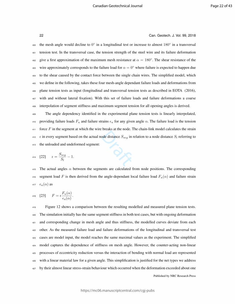
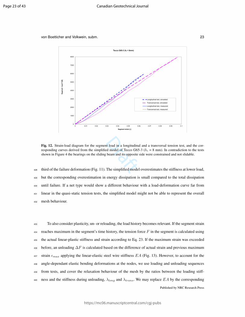
Figure 12 shows a comparison between the resulting modelled and measured plane tension tests.419
The simulation initially has the same segment stiffness in both test cases, but with ongoing deformation420
and corresponding change in mesh angle and thus stiffness, the modelled curves deviate from each421
other. As the measured failure load and failure deformations of the longitudinal and transversal test422
cases are model input, the model reaches the same maximal values as the experiment. The simplified423
model captures the dependence of stiffness on mesh angle. However, the counter-acting non-linear424
processes of eccentricity reduction versus the interaction of bending with normal load are represented425
with a linear material law for a given angle. This simplification is justified for the net types we address426
by their almost linear stress-strain behaviour which occurred when the deformation exceeded about one427
Published by NRC Research Press
Page 22 of 43
https://mc06.manuscriptcentral.com/cgj-pubs
Canadian Geotechnical Journal
Draft
von Boetticher and Volkwein, subm. 23
0
1000
2000
3000
4000
5000
6000
7000
8000
0 0.01 0.02 0.03 0.04 0.05 0.06 0.07 0.08 0.09 0.1
Segm
ent
load
F [N
]
Segment strain [-]
Tecco G65-3 (hi = 8mm)
Longitudinal test, simulated
Transversal test, simulated
Longitudinal test, measured
Transversal test, measured
Fig. 12. Strain-load diagram for the segment load in a longitudinal and a transversal tension test, and the cor-responding curves derived from the simplified model of Tecco G65-3 (hi = 8 mm). In contradiction to the testsshown in Figure 4 the bearings on the sliding beam and its opposite side were constrained and not slidable.
third of the failure deformation (Fig. 11). The simplified model overestimates the stiffness at lower load,428
but the corresponding overestimation in energy dissipation is small compared to the total dissipation429
until failure. If a net type would show a different behaviour with a load-deformation curve far from430
linear in the quasi-static tension tests, the simplified model might not be able to represent the overall431
mesh behaviour.432
To also consider plasticity, un- or reloading, the load history becomes relevant. If the segment strain433
reaches maximum in the segment’s time history, the tension force F in the segment is calculated using434
the actual linear-plastic stiffness and strain according to Eq. 23. If the maximum strain was exceeded435
before, an unloading ∆F is calculated based on the difference of actual strain and previous maximum436
strain εmax applying the linear-elastic steel wire stiffness EA (Fig. 13). However, to account for the437
angle-dependant elastic bending deformations at the nodes, we use loading and unloading sequences438
from tests, and cover the relaxation behaviour of the mesh by the ratios between the loading stiff-439
ness and the stiffness during unloading, λlong and λtrans. We may replace EA by the corresponding440
Published by NRC Research Press
Page 23 of 43
https://mc06.manuscriptcentral.com/cgj-pubs
Canadian Geotechnical Journal
Draft
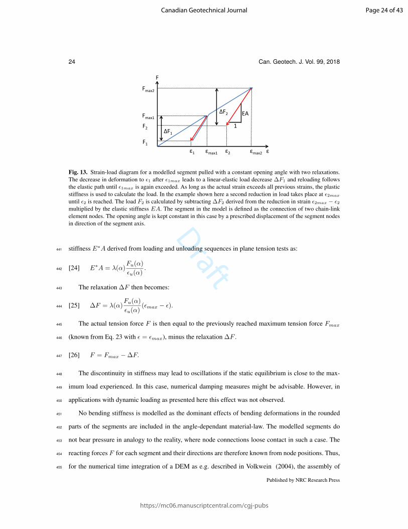
24 Can. Geotech. J. Vol. 99, 2018
ε εmax1 εmax2
1
EA
ε1 ε2
F
Fmax1
Fmax2
F2
F1
ΔF1
ΔF2
Fig. 13. Strain-load diagram for a modelled segment pulled with a constant opening angle with two relaxations.The decrease in deformation to ε1 after ε1max leads to a linear-elastic load decrease ∆F1 and reloading followsthe elastic path until ε1max is again exceeded. As long as the actual strain exceeds all previous strains, the plasticstiffness is used to calculate the load. In the example shown here a second reduction in load takes place at ε2maxuntil ε2 is reached. The load F2 is calculated by subtracting ∆F2 derived from the reduction in strain ε2max − ε2multiplied by the elastic stiffness EA. The segment in the model is defined as the connection of two chain-linkelement nodes. The opening angle is kept constant in this case by a prescribed displacement of the segment nodesin direction of the segment axis.
stiffness E∗A derived from loading and unloading sequences in plane tension tests as:441
E∗A = λ(α)Fu(α)
εu(α).[24]442
The relaxation ∆F then becomes:443
∆F = λ(α)Fu(α)
εu(α)(εmax − ε).[25]444
The actual tension force F is then equal to the previously reached maximum tension force Fmax445
(known from Eq. 23 with ε = εmax), minus the relaxation ∆F .446
F = Fmax −∆F.[26]447
The discontinuity in stiffness may lead to oscillations if the static equilibrium is close to the max-448
imum load experienced. In this case, numerical damping measures might be advisable. However, in449
applications with dynamic loading as presented here this effect was not observed.450
No bending stiffness is modelled as the dominant effects of bending deformations in the rounded451
parts of the segments are included in the angle-dependant material-law. The modelled segments do452
not bear pressure in analogy to the reality, where node connections loose contact in such a case. The453
reacting forces F for each segment and their directions are therefore known from node positions. Thus,454
for the numerical time integration of a DEM as e.g. described in Volkwein (2004), the assembly of455
Published by NRC Research Press
Page 24 of 43
https://mc06.manuscriptcentral.com/cgj-pubs
Canadian Geotechnical Journal

Draft
von Boetticher and Volkwein, subm. 25
Table 2. Example mesh type parameters to be used for modelling with FARO – simplified model (calibrated)Mechanical property Unit S4-230 S4-130 G80/4 G80/3 G65/4 G65/3Rmax,long kN/mm 268’560 465’480 273’120 157’560 334’200 200’400Rmax,trans kN/mm 136’320 205’440 119’520 64’920 148’560 69’230Fwire,tension kN 68.85 68.85 22.95 15.64 22.95 15.64Fwire,shear kN 26.37 26.37 11.00 5.94 11.00 5.94εmax,long – 0.0980 0.12 0.1033 0.0948 0.156 0.121εmax,trans – 0.3556 0.566 0.2433 0.2280 0.410 0.410λlong – 3.3 3.6 3.3 2.7 3.6 2.9λtrans – 3.3 3.6 3.3 2.7 3.6 2.9mh mm 500 315 177 180 138 143mw mm 292 175 102 103 83 83
the nodal forces can take place. The single mesh parameters are listed in Table 2. The parameters can456
be retrieved directly from tension tests on mesh specimen: mh and mw describe the geometrical size457
of one mesh part in width and length. Rmax,long and Rmax,trans contain the maximum loads from458
longitudinal and transversal tension tests. εmax,long and εmax,trans contain the lengthening of the459
tested meshes related to their original dimensions. From maximum loads and corresponding straining460
a kind of elastic stiffness of the mesh can be determined. Fwire,tension and Fwire,shear are the failure461
loads of single mesh wires.462
4.1. Model calibration463
To calibrate above model to the specific meshes three main characteristics have to be addressed:464
failure loads, failure deformation respective net stiffness and relaxation behaviour due to unloading.465
The corresponding calibration procedures are listed in the following resulting in the model parameters466
listed in Table 2.467
4.1.1. Failure loads468
The chain-link mesh parameters for the failure limits are defined both in longitudinal and transver-469
sal directions based on the results derived from small-scale quasi-static in-plane tension tests (Figs. 2470
& 4). From these tests estimates are derived for the failure loads in longitudinal and transversal mesh471
directions, Rmax,long and Rmax,trans , as-well as estimates for the wire failure loads at 0 or 180◦472
opening angles which are named Fwire,shear for 0◦ opening angle, and Fwire,tension for 180◦ opening473
angle. The failure loads at 0 or 180◦ opening angles are either based on quasi-static in-plane tension474
tests without lateral fixation or are calculated from the tension and shear resistance of the single wire.475
Published by NRC Research Press
Page 25 of 43
https://mc06.manuscriptcentral.com/cgj-pubs
Canadian Geotechnical Journal
Draft
26 Can. Geotech. J. Vol. 99, 2018
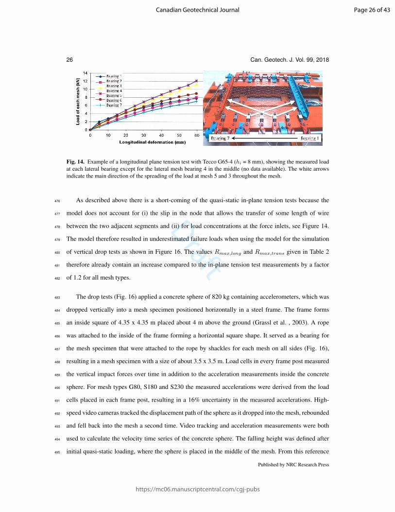
Fig. 14. Example of a longitudinal plane tension test with Tecco G65-4 (hi = 8 mm), showing the measured loadat each lateral bearing except for the lateral mesh bearing 4 in the middle (no data available). The white arrowsindicate the main direction of the spreading of the load at mesh 5 and 3 throughout the mesh.
As described above there is a short-coming of the quasi-static in-plane tension tests because the476
model does not account for (i) the slip in the node that allows the transfer of some length of wire477
between the two adjacent segments and (ii) for load concentrations at the force inlets, see Figure 14.478
The model therefore resulted in underestimated failure loads when using the model for the simulation479
of vertical drop tests as shown in Figure 16. The values Rmax,long and Rmax,trans given in Table 2480
therefore already contain an increase compared to the in-plane tension test measurements by a factor481
of 1.2 for all mesh types.482
The drop tests (Fig. 16) applied a concrete sphere of 820 kg containing accelerometers, which was483
dropped vertically into a mesh specimen positioned horizontally in a steel frame. The frame forms484
an inside square of 4.35 x 4.35 m placed about 4 m above the ground (Grassl et al. , 2003). A rope485
was attached to the inside of the frame forming a horizontal square shape. It served as a bearing for486
the mesh specimen that were attached to the rope by shackles for each mesh on all sides (Fig. 16),487
resulting in a mesh specimen with a size of about 3.5 x 3.5 m. Load cells in every frame post measured488
the vertical impact forces over time in addition to the acceleration measurements inside the concrete489
sphere. For mesh types G80, S180 and S230 the measured accelerations were derived from the load490
cells placed in each frame post, resulting in a 16% uncertainty in the measured accelerations. High-491
speed video cameras tracked the displacement path of the sphere as it dropped into the mesh, rebounded492
and fell back into the mesh a second time. Video tracking and acceleration measurements were both493
used to calculate the velocity time series of the concrete sphere. The falling height was defined after494
initial quasi-static loading, where the sphere is placed in the middle of the mesh. From this reference495
Published by NRC Research Press
Page 26 of 43
https://mc06.manuscriptcentral.com/cgj-pubs
Canadian Geotechnical Journal

Draft
von Boetticher and Volkwein, subm. 27
point, the sphere is lifted until it looses contact with the net and the corresponding height difference is496
considered as elastic deformation helastic. The sphere is then lifted further to the falling height h, with497
an accuracy of ±5 cm.498
4.1.2. Failure deformation499
The initial mesh stiffness is defined through the corresponding longitudinal and transversal failure500
deformation, termed εmax,long for longitudinal in-plane tension tests and εmax,trans for transversal501
in-plane tension tests, as they define the angle-dependency of the failure deformation in Eq. 23. Both502
failure deformations were increased in analogy to the Section 4.1.1 such that the model could capture503
the impact trajectory and mesh deformation at a vertical impact test close to the failure limit (Fig. 17)504
as well as the maximum acceleration (Fig. 16c). The quasi-static failure deformations were increased505
by a factor of 1.4 – 2.0 depending on the mesh type.506
4.1.3. Un- and reloading behaviour507
In case of unloading, the stress-strain-curves of the steel wire and meshes, respectively, follow a508
different path which is covered in the model by converting the original mesh stiffness using the factors509
λlong and λtrans (see Equation 24). These relaxation factors account for the plastic energy dissipation510
during an impact and the corresponding consumption of the plastic reserves which lead to a differed511
mesh performance under follow-up impacts. For each chain-link mesh type in our research it was512
possible to simplify the relaxation factors to λlong = λtrans = λ. To calibrate this mesh-type specific513
relaxation factor also above mentioned drop tests were used. λ was calibrated to match the simulated514
and observed time delay between the first and second maximum impact caused by the rebounding515
concrete sphere falling back into the mesh (Fig. 16c).516
The second impact of the concrete sphere is a perfect indicator of kinetic energy absorbed by the517
mesh during the first impact through (i) the time duration between first impact and rebounce and (ii)518
magnitude of the second impact. When calibrating λ some deviation between simulated and measured519
second impact time is accepted in favour of a correct prediction of the second impact peak decelera-520
tions.521
Published by NRC Research Press
Page 27 of 43
https://mc06.manuscriptcentral.com/cgj-pubs
Canadian Geotechnical Journal
Draft
28 Can. Geotech. J. Vol. 99, 2018
-50
0
50
100
150
200
250
300
350
400
450
-20
-15
-10
-5
0
5
500 700 900 1100 1300 1500 1700
R003S1 1.75 m
Fallen distance, measured
Fallen distance, simulated
Velocity, measured
Velocity, simulated
Acceleration, measured
Acceleration, simulated
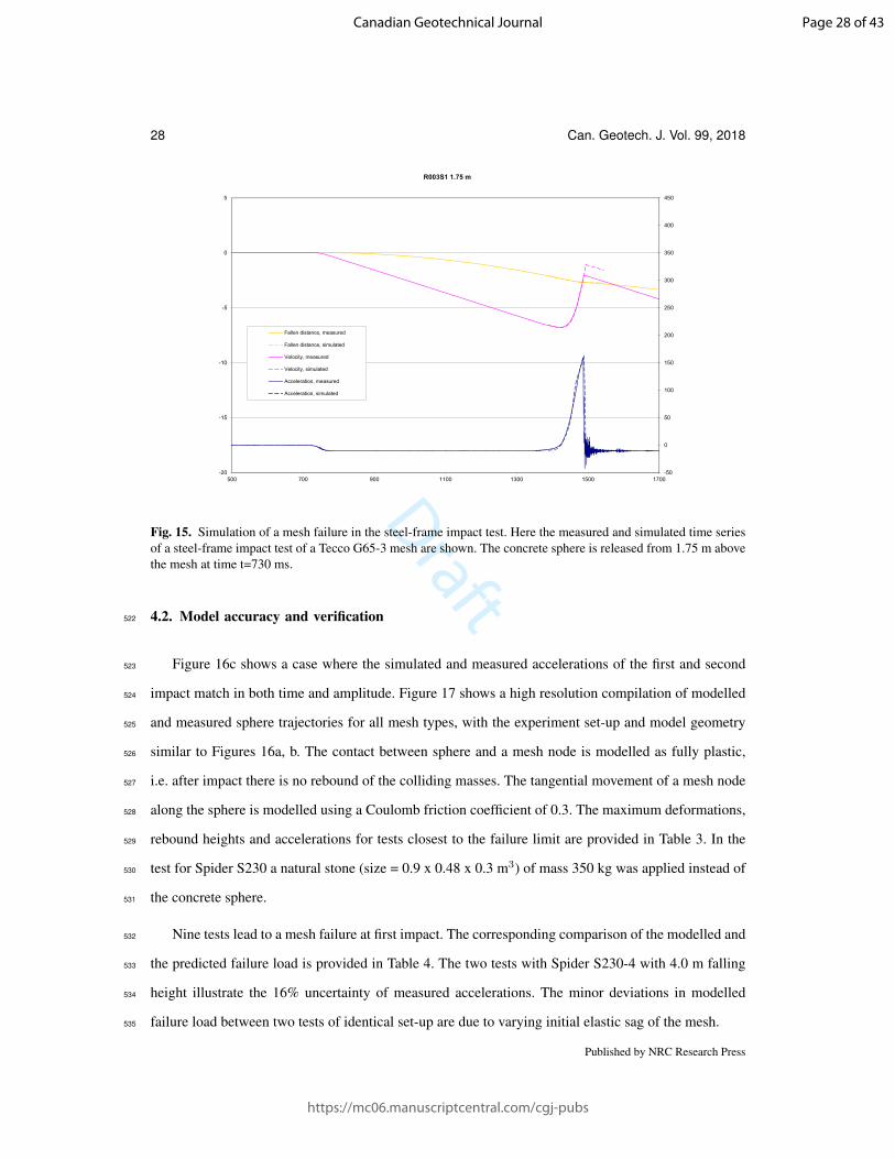
Fig. 15. Simulation of a mesh failure in the steel-frame impact test. Here the measured and simulated time seriesof a steel-frame impact test of a Tecco G65-3 mesh are shown. The concrete sphere is released from 1.75 m abovethe mesh at time t=730 ms.
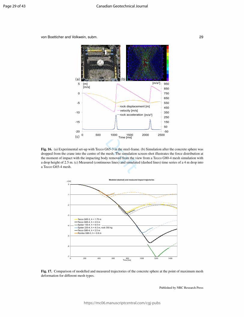
4.2. Model accuracy and verification522
Figure 16c shows a case where the simulated and measured accelerations of the first and second523
impact match in both time and amplitude. Figure 17 shows a high resolution compilation of modelled524
and measured sphere trajectories for all mesh types, with the experiment set-up and model geometry525
similar to Figures 16a, b. The contact between sphere and a mesh node is modelled as fully plastic,526
i.e. after impact there is no rebound of the colliding masses. The tangential movement of a mesh node527
along the sphere is modelled using a Coulomb friction coefficient of 0.3. The maximum deformations,528
rebound heights and accelerations for tests closest to the failure limit are provided in Table 3. In the529
test for Spider S230 a natural stone (size = 0.9 x 0.48 x 0.3 m3) of mass 350 kg was applied instead of530
the concrete sphere.531
Nine tests lead to a mesh failure at first impact. The corresponding comparison of the modelled and532
the predicted failure load is provided in Table 4. The two tests with Spider S230-4 with 4.0 m falling533
height illustrate the 16% uncertainty of measured accelerations. The minor deviations in modelled534
failure load between two tests of identical set-up are due to varying initial elastic sag of the mesh.535
Published by NRC Research Press
Page 28 of 43
https://mc06.manuscriptcentral.com/cgj-pubs
Canadian Geotechnical Journal
Draft
von Boetticher and Volkwein, subm. 29
(a) (b)
(c)-50
50
150
250
350
450
550
650
750
850
950
-20
-15
-10
-5
0
5
0 500 1000 1500 2000 2500
R008S1 4.00 m
rock displacement [m] velocity [m/s] rock acceleration [m/s2]
[m/s2] [m] [m/s] [kJ]
Time [ms]
[m/s2]
Fig. 16. (a) Experimental set-up with Tecco G65-3 in the steel-frame. (b) Simulation after the concrete sphere wasdropped from the crane into the centre of the mesh. The simulation screen-shot illustrates the force distribution atthe moment of impact with the impacting body removed from the view from a Tecco G80-4 mesh simulation witha drop height of 2.5 m. (c) Measured (continuous lines) and simulated (dashed lines) time series of a 4 m drop intoa Tecco G65-4 mesh.
-7
-6
-5
-4
-3
-2
-1
0
0 200 400 600 800 1000 1200 1400
z [m]
Time [ms]
Modeled (dashed) and measured impact trajectories
Tecco G65-3, h = 1.75 mTecco G65-4, h = 4.5 mSpider 130-4, h = 6.5 mSpider 230-4, h = 4.5 m, rock 350 kg Tecco G80-4, h = 2.5 mRombo G80-3, h = 0.8 m
Fig. 17. Comparison of modelled and measured trajectories of the concrete sphere at the point of maximum meshdeformation for different mesh types.
Published by NRC Research Press
Page 29 of 43
https://mc06.manuscriptcentral.com/cgj-pubs
Canadian Geotechnical Journal

Draft
30 Can. Geotech. J. Vol. 99, 2018
Table 3. Comparison of simulated and measured maximum values from tests closest below the failure limit. sdenotes the mesh deformation, ∆ t is the time delay between first and second impact and a stands for acceleration.Spider S230 was tested with a 350 kg block.
Mesh type drop height modelled measured deviationmaximum deflection s
Tecco G65-3 1.75 m 0.88 m 0.93 m -5%Tecco G65-4 4.5 m 1.13 m 1.18 m -4%Rombo G80-3 0.8 m 0.48 m 0.26 m 85%Tecco G80-4 2.5 m 0.49 m 0.32 m 53%Spider S130-4 6.5 m 0.55 m 0.51 m 8%Spider S230-4 4.5 m 0.48 m 0.19 m 253%
re-bounce time ∆t
Tecco G65-3 1.75 m 900 ms 835 ms 8%Tecco G65-4 4.5 m 1130 ms 1114 ms 1%Rombo G80-3 0.8 m 685 ms 769 ms -11%Tecco G80-4 2.5 m 945 ms 942 ms 0%Spider S130-4 6.5 m 1868 ms 1376 ms -2%Spider S230-4 4.5 m 1195 ms 1126 ms 6%
max. acceleration aTecco G65-3 1.75 m 174 m/s2 166 m/s2 5%Tecco G65-4 4.5 m 299 m/s2 315 m/s2 -5%Rombo G80-3 0.8 m 129 m/s2 136 m/s2 -5%Tecco G80-4 2.5 m 232 m/s2 248 m/s2 -6%Spider S130-4 6.5 m 456 m/s2 537 m/s2 -15%Spider S230-4 4.5 m 363 m/s2 420 m/s2 -14%
Table 4. Comparison of simulated and measured failure load from tests above the failure limit. afail stands forthe acceleration of the sphere in the moment of failure.
Mesh type Drop height Modelled Measured Deviationfailure acceleration afail
Tecco G65-3 1.75 m 159 m/s2 163 m/s2 -2%Rombo G80-3 1.0 m 138 m/s2 148 m/s2 -7%Rombo G80-3 1.0 m 134 m/s2 150 m/s2 -11%Tecco G80-4 4.0 m 127 m/s2 82 m/s2 56%Tecco G80-4 3.0 m 128 m/s2 151 m/s2 -15%Tecco G80-4 2.75 m 123 m/s2 139 m/s2 -11%Spider S230-4 4.5 m 194 m/s2 198 m/s2 -2%Spider S230-4 4.0 m 176 m/s2 182 m/s2 -3%Spider S230-4 4.0 m 177 m/s2 167 m/s2 6%
A parameter study was carried out to identify to which uncertainties the model is sensitive to. The536
relaxation factors (λlong and λtrans) are not part of the standard mesh specifications and thus may be537
a source of uncertainty. Besides this, there are several parameters like time step size, viscous damping,538
or properties of the modelled concrete sphere which are properties of the FARO software and have539
no dependency on the implemented chain-link element, although they affect the results. For a detailed540
Published by NRC Research Press
Page 30 of 43
https://mc06.manuscriptcentral.com/cgj-pubs
Canadian Geotechnical Journal
Draft
von Boetticher and Volkwein, subm. 31
R006S1 2.75 m
-10
40
90
140
190
240
290
340
390
440
490
0 200 400 600 800 1000 1200
Time [ms]
-15
-14
-13
-12
-11
-10
-9
-8
-7
-6
-5
-4
-3
-2
-1
0
1
2
3
4
5
MESH WIDTH 0.08051 (-3%); MESH HEIGHT 0.1339 (-3%)
MESH WIDTH 0.0830; MESH HEIGHT 0.138
MESH WIDTH 0.0855 (+3%); MESH HEIGHT 0.1421 (+3%)
thick lines: measured
Velocity [m/s]
Trajectory [m]
Acceleration [m/s2]
Acceleration [m/s2] Velocity [m/s]
Trajectory [m]
Fig. 18. Sensitivity of the modelled impact to the mesh geometry uncertainty of a Tecco G65-4 mesh, for 2.75 mrelease height.
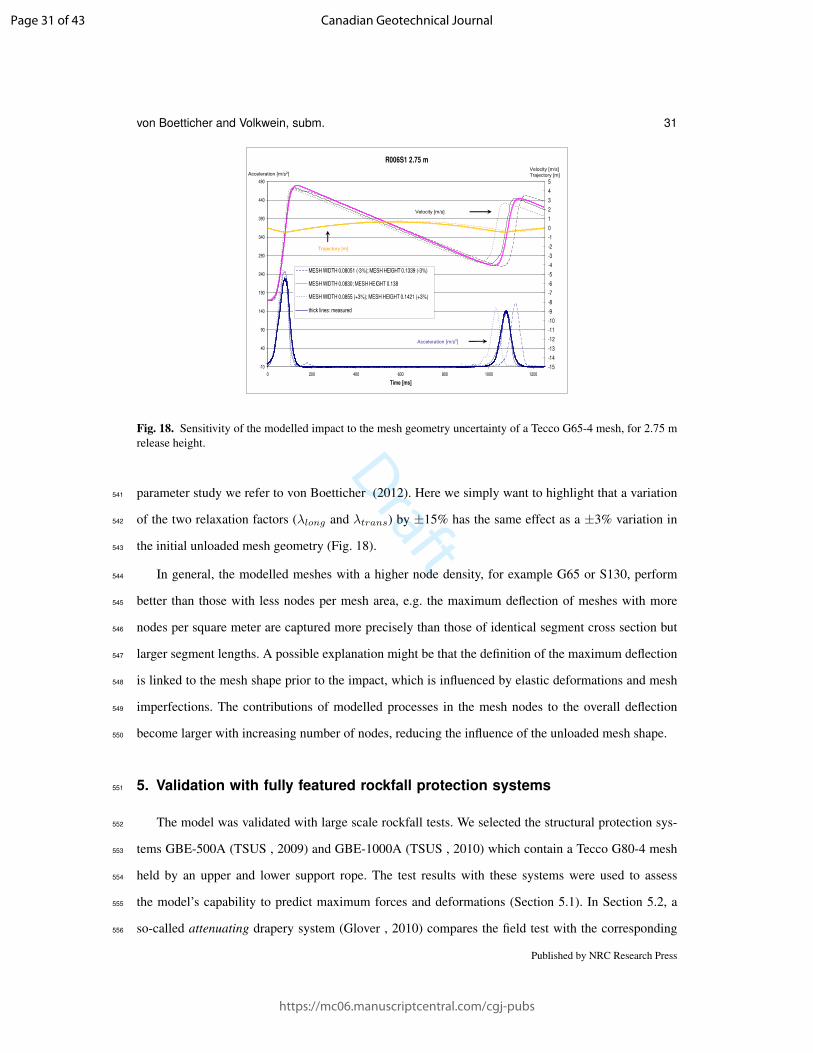
parameter study we refer to von Boetticher (2012). Here we simply want to highlight that a variation541
of the two relaxation factors (λlong and λtrans) by ±15% has the same effect as a ±3% variation in542
the initial unloaded mesh geometry (Fig. 18).543
In general, the modelled meshes with a higher node density, for example G65 or S130, perform544
better than those with less nodes per mesh area, e.g. the maximum deflection of meshes with more545
nodes per square meter are captured more precisely than those of identical segment cross section but546
larger segment lengths. A possible explanation might be that the definition of the maximum deflection547
is linked to the mesh shape prior to the impact, which is influenced by elastic deformations and mesh548
imperfections. The contributions of modelled processes in the mesh nodes to the overall deflection549
become larger with increasing number of nodes, reducing the influence of the unloaded mesh shape.550
5. Validation with fully featured rockfall protection systems551
The model was validated with large scale rockfall tests. We selected the structural protection sys-552
tems GBE-500A (TSUS , 2009) and GBE-1000A (TSUS , 2010) which contain a Tecco G80-4 mesh553
held by an upper and lower support rope. The test results with these systems were used to assess554
the model’s capability to predict maximum forces and deformations (Section 5.1). In Section 5.2, a555
so-called attenuating drapery system (Glover , 2010) compares the field test with the corresponding556
Published by NRC Research Press
Page 31 of 43
https://mc06.manuscriptcentral.com/cgj-pubs
Canadian Geotechnical Journal
Draft
32 Can. Geotech. J. Vol. 99, 2018
simulation.557
A Coulomb friction coefficient of 0.3 was used between the net and a block made of concrete with558
a smooth surface. This friction coefficient was calculated from calibration procedures performed for559
the software FARO by Volkwein (2004). For the simulation of drapery net systems with an impacting560
sphere made of steel we used a friction coefficient of 0.15 instead. For comparison, Thoeni et al. (2014)561
used tan 30◦ = 0.58 for blocks with edges and corners.562
5.1. Model validation with vertical impact tests on GBE rockfall protection barriers563
The upper and lower support ropes of the GBE rockfall protection barriers were held in position564
by four posts that subdivided the barrier into three fields. The support ropes could slide perpendicular565
to the posts which allowed the transfer of the impact energy wave away from the impact location to566
anchors with energy dissipating devices. The bases of the posts were hinge supported to the slope and567
the top of each post was connected to two up-slope ropes. The beginning of the mesh at the first post568
and the end of the mesh at the last post were shackled to a rope that was spanned from the base of the569
post to its top. Two lateral ropes connected the first and last post to anchors positioned aside. All ropes570
were equipped with load cells which recorded the forces exerted on the ropes throughout the test. The571
up-slope and lateral ropes were not in contact with the mesh.572
The barriers were placed on an almost vertical wall at the test site Lochezen in Walenstadt, Switzer-573
land (Gerber , 2001), and retained a concrete block dropped vertically from about 32m above the bar-574
rier into the central area between the inner posts according to the testing standard ETAG 027 (EOTA575
, 2013). For the GBE-500A barrier the dropped block had a mass of 1590 kg resulting in an impact576
energy greater than 500 kJ . The GBE-1000A system retained a block of mass 3200 kg resulting in an577
impact energy of about 1000 kJ .578
For the corresponding simulations, a time step of 5 ∗ 10−6 s was used. The energy dissipating579
devices were modelled as truss elements which undergo plastic elongation. Their modelled material580
behaviour was based on the force-deflection diagrams in which the onset of elongation was taken from581
quasi-static tension tests. The final elongation measured at the MEL-test together with the measured582
peak load at the dissipating devices (taken from test reports for the corresponding MEL-test) formed a583
second point in the force-deflection diagram of the modelled truss element.584
The simulation predicted the measured maximum values well (Table 5, Fig. 19) considering that585
Published by NRC Research Press
Page 32 of 43
https://mc06.manuscriptcentral.com/cgj-pubs
Canadian Geotechnical Journal
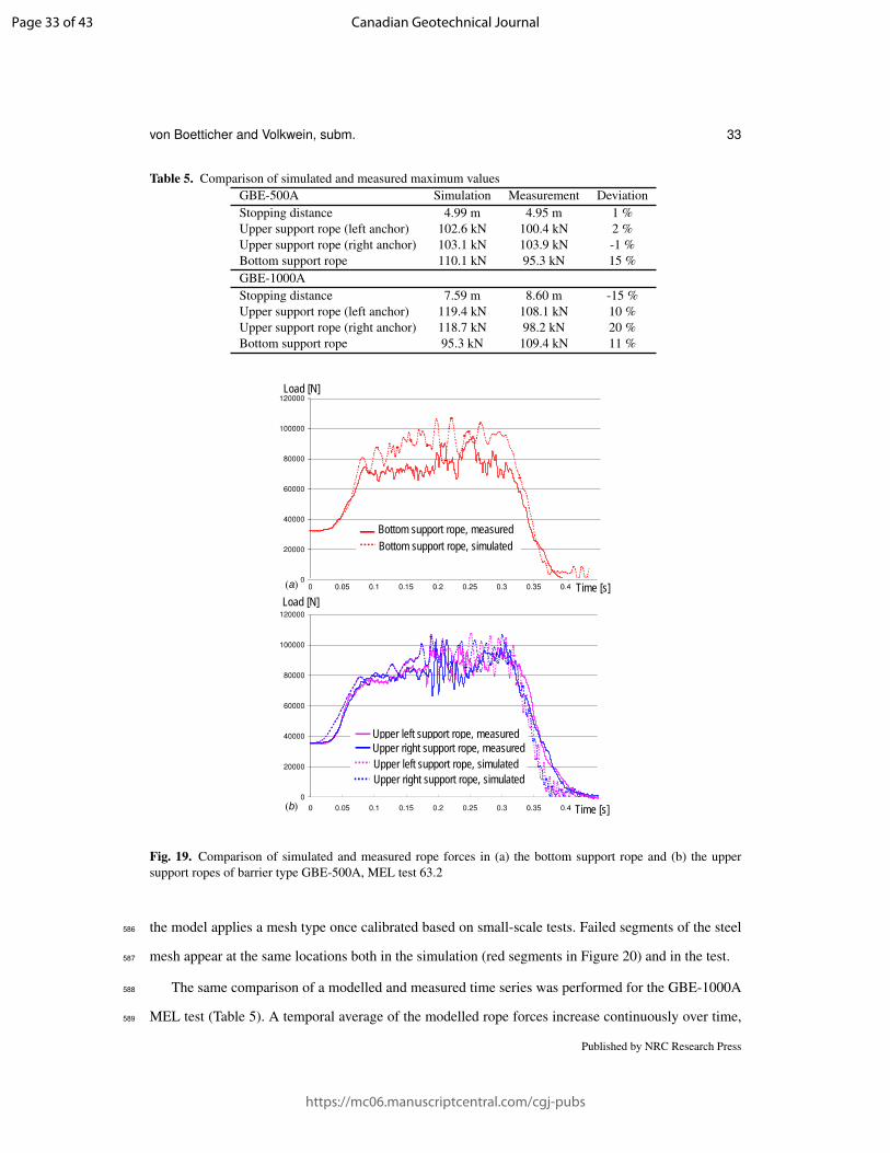
Draft
von Boetticher and Volkwein, subm. 33
Table 5. Comparison of simulated and measured maximum valuesGBE-500A Simulation Measurement DeviationStopping distance 4.99 m 4.95 m 1 %Upper support rope (left anchor) 102.6 kN 100.4 kN 2 %Upper support rope (right anchor) 103.1 kN 103.9 kN -1 %Bottom support rope 110.1 kN 95.3 kN 15 %GBE-1000AStopping distance 7.59 m 8.60 m -15 %Upper support rope (left anchor) 119.4 kN 108.1 kN 10 %Upper support rope (right anchor) 118.7 kN 98.2 kN 20 %Bottom support rope 95.3 kN 109.4 kN 11 %
(a)
Time [s](b)
Upper left support rope, measuredUpper right support rope, measuredUpper left support rope, simulatedUpper right support rope, simulated
Load [N]
Load [N]
Time [s]
Bottom support rope, simulatedBottom support rope, measured
Fig. 19. Comparison of simulated and measured rope forces in (a) the bottom support rope and (b) the uppersupport ropes of barrier type GBE-500A, MEL test 63.2
the model applies a mesh type once calibrated based on small-scale tests. Failed segments of the steel586
mesh appear at the same locations both in the simulation (red segments in Figure 20) and in the test.587
The same comparison of a modelled and measured time series was performed for the GBE-1000A588
MEL test (Table 5). A temporal average of the modelled rope forces increase continuously over time,589
Published by NRC Research Press
Page 33 of 43
https://mc06.manuscriptcentral.com/cgj-pubs
Canadian Geotechnical Journal

Draft
34 Can. Geotech. J. Vol. 99, 2018
Fig. 20. Front view perspective of the modelled barrier GBE-500A at the moment of maximum deformationwith colours corresponding to the degree of utilization of the structure. The rock begins to move upward andsome segments at the upper support rope failed, both in simulation and experiment, when the sliding mesh hit theconnection between the upper support rope and the central posts.
with a clear signal from the onset of elongation at the dissipating devices right before 0.1 s (Fig. 21).590
The evolution of the measured rope forces indicate that the material law of the modelled dissipating591
devices after the onset of elongation was simplified to a point were it cannot reproduce the dynamic592
response in detail. However, the overall energy dissipation was captured well, as the decrease in mea-593
sured rope forces towards the end is represented adequately by the model for both time and amplitude.594
5.2. Wave propagation595
So-called attenuating systems Glover et al. (2012) present a different form of protection, which596
guides the rock downhill between the mesh and the slope. Here, a main visible effect of rock impact is597
the wave propagation along the mesh drape, without any influence from energy dissipating elements,598
resulting in a test case of pure chain-link dynamics. The reference system was tested using a 2700 kg599
steel sphere which impacted horizontally at 10 m/s into an inclined mesh of type Spider 4-130 (Glover600
, 2010) connected to a 40 m long and 17.5 m wide drape mesh of type Spider 4-250. The mesh was601
held on its upper edge by a support rope and laid loosely on the 50◦ inclined hill-slope (Fig. 22). The602
forces were introduced orthogonally and tangentially to the mesh, the latter by friction between the603
steel-sphere and the mesh. The impact wave propagation was dominated by the mesh stiffness under604
low load. Aside from the use of segments formed from multiple wire strand threads for different mesh605
Published by NRC Research Press
Page 34 of 43
https://mc06.manuscriptcentral.com/cgj-pubs
Canadian Geotechnical Journal
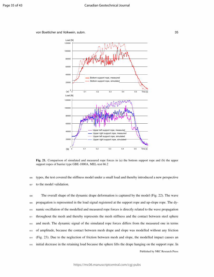
Draft
von Boetticher and Volkwein, subm. 35
0
20000
40000
60000
80000
100000
120000
0 0.1 0.2 0.3 0.4 0.5 0.6
Time [s]
Forc
e [N
]
bottom support rope measuredbottom support rope simulated
MEL Test 66.2 Upper Support Ropes
0
20000
40000
60000
80000
100000
120000
140000
0 0.1 0.2 0.3 0.4 0.5 0.6Time [s]
Forc
e [N
]
upper left support rope measured
upper right support rope measured
upper left rope simulated
upper right rope simulated
(a)
(b)
Upper left support rope, measured Upper right support rope, measured Upper left support rope, simulated Upper right support rope, simulated
Load [N]
MELTest 63.2 Upper Support Ropes
0
20000
40000
60000
80000
100000
120000
0 0.05 0.1 0.15 0.2 0.25 0.3 0.35 0.4 0.45Time [s]
upper left support rope measured
upper right support rope measured
upper left rope simulated
upper right rope simulated
Load [N]
Bottom support rope, measured Bottom support rope, simulated
MELTest 63.2 Upper Support Ropes
0
20000
40000
60000
80000
100000
120000
0 0.05 0.1 0.15 0.2 0.25 0.3 0.35 0.4 0.45
upper left support rope measured
upper right support rope measured
upper left rope simulated
upper right rope simulated
0 0.1 0.2 0.3 0.4 0.5 Time [s]
0 0.1 0.2 0.3 0.4 0.5 Time [s]
Fig. 21. Comparison of simulated and measured rope forces in (a) the bottom support rope and (b) the uppersupport ropes of barrier type GBE-1000A, MEL-test 66.2
types, the test covered the stiffness model under a small load and thereby introduced a new perspective606
to the model validation.607
The overall shape of the dynamic drape deformation is captured by the model (Fig. 22). The wave608
propagation is represented in the load signal registered at the support rope and up-slope rope. The dy-609
namic oscillation of the modelled and measured rope forces is directly related to the wave propagation610
throughout the mesh and thereby represents the mesh stiffness and the contact between steel sphere611
and mesh. The dynamic signal of the simulated rope forces differs from the measured one in terms612
of amplitude, because the contact between mesh drape and slope was modelled without any friction613
(Fig. 23). Due to the neglection of friction between mesh and slope, the modelled impact causes an614
initial decrease in the retaining load because the sphere lifts the drape hanging on the support rope. In615
Published by NRC Research Press
Page 35 of 43
https://mc06.manuscriptcentral.com/cgj-pubs
Canadian Geotechnical Journal
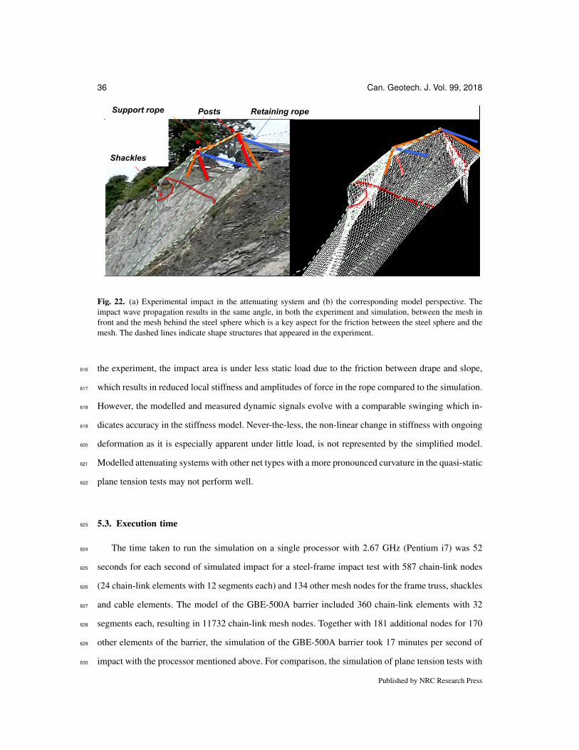
36 Can. Geotech. J. Vol. 99, 2018
Retaining rope Posts Support rope
Shackles
Fig. 22. (a) Experimental impact in the attenuating system and (b) the corresponding model perspective. Theimpact wave propagation results in the same angle, in both the experiment and simulation, between the mesh infront and the mesh behind the steel sphere which is a key aspect for the friction between the steel sphere and themesh. The dashed lines indicate shape structures that appeared in the experiment.
the experiment, the impact area is under less static load due to the friction between drape and slope,616
which results in reduced local stiffness and amplitudes of force in the rope compared to the simulation.617
However, the modelled and measured dynamic signals evolve with a comparable swinging which in-618
dicates accuracy in the stiffness model. Never-the-less, the non-linear change in stiffness with ongoing619
deformation as it is especially apparent under little load, is not represented by the simplified model.620
Modelled attenuating systems with other net types with a more pronounced curvature in the quasi-static621
plane tension tests may not perform well.622
5.3. Execution time623
The time taken to run the simulation on a single processor with 2.67 GHz (Pentium i7) was 52624
seconds for each second of simulated impact for a steel-frame impact test with 587 chain-link nodes625
(24 chain-link elements with 12 segments each) and 134 other mesh nodes for the frame truss, shackles626
and cable elements. The model of the GBE-500A barrier included 360 chain-link elements with 32627
segments each, resulting in 11732 chain-link mesh nodes. Together with 181 additional nodes for 170628
other elements of the barrier, the simulation of the GBE-500A barrier took 17 minutes per second of629
impact with the processor mentioned above. For comparison, the simulation of plane tension tests with630
Published by NRC Research Press
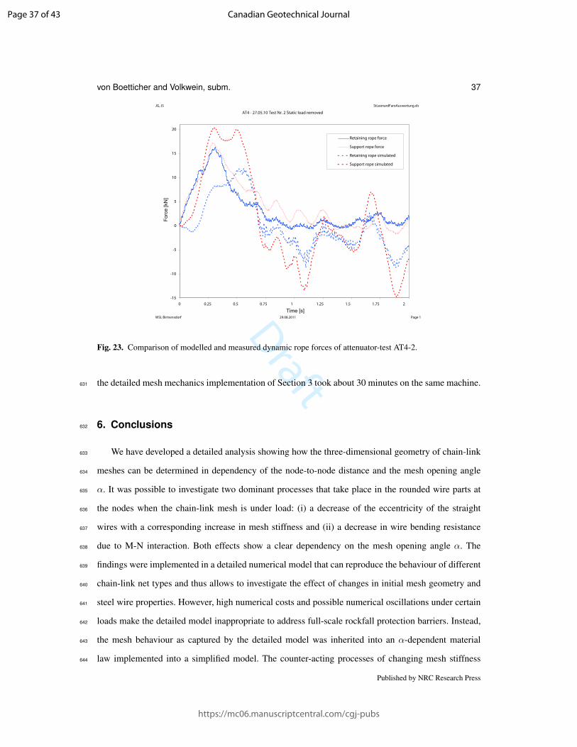
Draft
von Boetticher and Volkwein, subm. 37
JG, JS StLeonardFaroAuswertung.xls
WSL Birmensdorf 29.08.2011 Page 1
AT4 - 27.05.10 Test Nr. 2 Static load removed
-15
-10
-5
0
5
10
15
20
0 0.25 0.5 0.75 1 1.25 1.5 1.75 2
Time [s]
Forc
e [k
N]
Retaining rope force
Support rope force
Retaining rope simulated
Support rope simulated
Fig. 23. Comparison of modelled and measured dynamic rope forces of attenuator-test AT4-2.
the detailed mesh mechanics implementation of Section 3 took about 30 minutes on the same machine.631
6. Conclusions632
We have developed a detailed analysis showing how the three-dimensional geometry of chain-link633
meshes can be determined in dependency of the node-to-node distance and the mesh opening angle634
α. It was possible to investigate two dominant processes that take place in the rounded wire parts at635
the nodes when the chain-link mesh is under load: (i) a decrease of the eccentricity of the straight636
wires with a corresponding increase in mesh stiffness and (ii) a decrease in wire bending resistance637
due to M-N interaction. Both effects show a clear dependency on the mesh opening angle α. The638
findings were implemented in a detailed numerical model that can reproduce the behaviour of different639
chain-link net types and thus allows to investigate the effect of changes in initial mesh geometry and640
steel wire properties. However, high numerical costs and possible numerical oscillations under certain641
loads make the detailed model inappropriate to address full-scale rockfall protection barriers. Instead,642
the mesh behaviour as captured by the detailed model was inherited into an α-dependent material643
law implemented into a simplified model. The counter-acting processes of changing mesh stiffness644
Published by NRC Research Press
Page 37 of 43
https://mc06.manuscriptcentral.com/cgj-pubs
Canadian Geotechnical Journal

Draft
38 Can. Geotech. J. Vol. 99, 2018
mentioned above were simplified to a linear stress-strain relation but with an α-dependent gradient645
and an α-dependent failure limit. The simplified discrete element model can simulate the chain-link646
mesh based on either the results of small-scale quasi-static tension tests or corresponding results of647
simulations using the detailed chain-link model, both serving as material-law input.648
In this study, all necessary information was extracted from the small-scale quasi-static tension tests649
and introduced to the model by transforming the complex non-linear three dimensional deformation650
processes within the mesh nodes into the material-law, with an interpolated dependency on the inner651
mesh opening angle. The α-dependent interpolation of the simplified model allows to account for the652
dynamic dependency of the mesh stiffness, resistance and failure on the inner mesh opening angle. The653
mesh stiffness within an unloading and reloading cycle was captured using a ratio between the elastic654
stiffness of a second loading and the stiffness of the first loading, such that the simplified model can655
capture the energy dissipation of a mesh impact. Under low load, this simplification does not represent656
the true mesh stiffness.657
Some calibration of the overall mesh stiffness is necessary to account for the local impact as loading658
of the mesh is not equally distributed, unlike quasi-static plane tension tests. This mesh stiffness is659
defined by the failure deformation. The failure deformations derived from plane tension tests needed660
to be increased by a factor of 1.4 – 2.0 depending on the mesh type and based on results from medium-661
scaled tests (mesh specimen size about 3.5 x 3.5 m) with a vertical impact. It was further possible to662
calibrate the elastic stiffness of the simplified chain-link mesh, such that the energy loss of a rebounding663
impact body was covered well by the model. The model accurately predicted all first impact mesh664
failures observed at the medium-scale experiments. Furthermore, the change in mesh stiffness by the665
first impact was predicted by the model, such that relatively high loads caused by second impacts were666
accurately captured: Figure 16 shows that a 25% rebound height (1 m) for the second impact can still667
reach 70% of the first impact’s maximum acceleration. Considering rockfall barrier design, this result668
highlights the importance of considering rockfall events with more than one impact.669
Regarding the full-scale tests the simplified model accurately predicts the maximum load as well670
as the maximum deformation of the GBE-500A barrier under an MEL-test (Table 5). Single failed671
segments were predicted by the model at the correct locations. Considering the GBE-1000A rockfall672
barrier, the simulation covered the duration of the impact (Fig. 21), but rope forces were overestimated673
and the maximum deformation was underestimated (Table 5). A possible source for the deviation be-674
Published by NRC Research Press
Page 38 of 43
https://mc06.manuscriptcentral.com/cgj-pubs
Canadian Geotechnical Journal

Draft
von Boetticher and Volkwein, subm. 39
tween modelled and measured rope forces in the GBE-1000A rockfall barrier test may be the modelled675
energy dissipating devices with a simplified material law and by underestimating the energy dissipa-676
tion in the modelled mesh and the friction between the mesh and the ropes. Also, the underestimated677
maximum deformation suggests that the plastic deformation of the segments for large opening angles678
was underestimated. It therefore might be useful to perform additional transversal tension tests without679
lateral fixation to determine the mesh stiffness for large mesh angles more accurately.680
Plane tension tests can serve as a first estimate for the chain-link properties because the limitations681
incurred by not considering an orthogonal impact appear to be systematic. It is possible to account682
for the difference between plane tension tests and orthogonal impacts with standard corrections that683
increase the longitudinal and transversal failure loads and deformations by a predefined factor. In case684
of the mesh types considered here, this resulted in an increase of failure loads by a factor of 1.2 for all685
mesh types. However, as soon as the chain-link design development reaches a state of large scale test686
application, orthogonal impact tests will be necessary to prove if the standard correction also applies687
for the modified mesh.688
Plastic energy dissipation depends on the elastic stiffness, which can be determined by a temporal689
relaxation during a plane tension test. During a vertical impact test orthogonal to the mesh plane the690
dissipation can be measured with high accuracy by considering the time delay between the first and691
second impact when the rebounding sphere falls back into the net, or by the difference in release and692
rebound height. von Boetticher (2012) carried out about 60 experiments with the frame with mesh693
specimen of type Tecco G65-3, Tecco G65-4 and G80-4, Rombo G80-3, Spider 130-4 and Spider 230-694
4 to calibrate the elastic and plastic stiffness for each mesh type. The parameter study indicates that a695
source of uncertainty, considering the rebound height and plastic energy dissipation in the mesh, may696
arise from small variations in the initial mesh geometry. In cases where these variations are distributed697
randomly across the mesh, segment deformations will balance out under high load showing little effect.698
However, if meshes are produced with in general shorter or longer segments or different hi,0 due to an699
update in production, the mesh performance and especially the plastic dissipation is affected.700
The model is capable of predicting the dynamic behaviour and resistance of different protection701
barriers with high accuracy, optimized calculation time and minimized calibration efforts. The detailed702
comparison between simulation and experiment for different scales and types of impact have led to the703
following conclusions:704
Published by NRC Research Press
Page 39 of 43
https://mc06.manuscriptcentral.com/cgj-pubs
Canadian Geotechnical Journal

Draft
40 Can. Geotech. J. Vol. 99, 2018
1. The new chain-link discrete element model was able to simulate the behaviour of all different705
chain-link mesh types tested in von Boetticher (2012).706
2. The model can be applied to different barrier types without recalibration. However, different707
mesh types will require additional testing.708
3. The model can accurately capture the dynamic wave propagation and the corresponding dynamic709
loading throughout the mesh for high energy vertical impact as well as for low energy tangential710
impact.711
4. The model can reproduce the energy dissipation due to plastic deformation and the correspond-712
ing change in mesh stiffness while some uncertainty remains concerning the sensitivity of this713
process to small deviations in the manufactured mesh geometry.714
5. Situations where the sphere broke the net and fell through were captured by the simulation in all715
cases. The reduction of the remaining mesh stiffness due to such holes can be accounted for by716
an unravelling approach (Hendrich , 2010).717
Acknowledgements718
The project that lead to this article has been co-financed by Swiss Commission for Technology and719
Innovation (CTI 9266.1 PFIW-IW) in collaboration with the Company Geobrugg AG. The authors are720
grateful for the possibility to develop the numerical models based on valuable experimental data. The721
conduction of the corresponding tests was enabled by Geobrugg. The authors further thank the two722
reviewers who significantly helped to improve the article.723
References724
Albaba, A., Lambert, S., Kneib, F., Chareyre, B., Nicot, F. DEM modelling of a flexible barrier725
impacted by a dry granular flow. Rock Mechanics and Rock Engineering, 50(11), 3029-3048, 2017.726
Betschon, F. Theoretische und experimentelle Beitrage zur Klarung der statischen und dynamischen727
Beanspruchung von Strickmaschinennadeln. Diss ETH Zurich, 1977.728
Cazzani, A., Mongiov, L., Frenez, T. Dynamic finite element analysis of interceptive devices for falling729
rocks. Int J Rock Mech Mining Sci 2002;39 (3):30321.730
Published by NRC Research Press
Page 40 of 43
https://mc06.manuscriptcentral.com/cgj-pubs
Canadian Geotechnical Journal
Draft
von Boetticher and Volkwein, subm. 41
Dhakal, S., Bhandary, N. P., Yatabe, R., Kinoshita, N. Experimental, numerical and analytical mod-731
elling of a newly developed rockfall protective cable-net structure. Natural Hazards and Earth Sys-732
tem Sciences, 11(12), 3197, 2011.733
Effeindzourou, A., Thoeni, K., Giacomini, A., Wendeler, C.. Efficient discrete modelling of composite734
structures for rockfall protection. Computers and Geotechnics 87, 99114, 2017735
EOTA. Flexible facing systems for slope stabilization and rock protection. European Assessment736
Document. EAD 230025-00-0106, June 2016.737
EOTA. ETAG 027, Guideline for European Technical Approval of falling rock protection kits. Guide-738
line, 2013. EU, Brussels, Belgium.739
Escallon, J. P., von Boetticher, A., Wendeler, C., Chatzi, E., Bartelt, P. Mechanics of chain-link wire740
nets with loose connections. Engineering Structures, 101:68–87, 2015.741
Gerber, W. Richtlinie Uber die Typenprufung von Schutznetzen gegen Steinschlag. Technical report,742
Bundesamt fur Umwelt, Wald und Landschaft (BUWAL), Eidgenossische Forschungsanstalt WSL,743
Bern, 2001.744
Glover, J. CTI - Attenuators, Test report AT4. Technical report, WSL, Birmensdorf, Swizerland, 2010.745
Glover, J., Denk, M., Bourrier, F., Gerber, W., Volkwein, A. Kinetic energy dissipation effects of rock746
fall attenuating systems. Proc. InterPraevent, Grenoble, France, 2012.747
Grassl, H., Bartelt, P., Volkwein, A., Wartmann, S.. Experimental and numerical modeling of highly748
flexible rockfall protection barriers. In Culligan, P.J.; Einstein, H.H.; Whittle, A.J. (eds) Soil and749
Rock America 2003, volume 2, pages 2589–2594. 12th Panamerican Conference on Soil Mechanics750
and Geotechnical Engineering, June 22 – 26, 2003, Camebridge, USA, 2003.751
Hendrich, V. Vergleich zwischen in-situ-Versuchen zur Belastbarkeit von Steinschlagschutzsystemen752
mit den Ergebnissen der Simulationssoftware FARO. Master’s thesis, Institute of applied Geo-753
sciences, Technical University Berlin, Germany, 2010.754
Jirasek, M., Bazant, Z.P. Inelastic analysis of structures. John Wiley & Sons, 2002.755
Published by NRC Research Press
Page 41 of 43
https://mc06.manuscriptcentral.com/cgj-pubs
Canadian Geotechnical Journal
Draft
42 Can. Geotech. J. Vol. 99, 2018
Kastli, A. Testing report Rombo G80-3. Technical report, Geobrugg AG, Romanshorn, Switzerland,756
2007.757
Knodel, P. Plastische Querschnittstragfahigkeit. HS Augsburg, 2010.758
Mustoe, C. G. W., Huttelmaier, H. P. Dynamic simulation of rockfall fence by the discrete element759
method. Microcomputers in Civil engineering, 8:423–437, 1993.760
Schwarzlos, A. Erweiterung der Komponentenmethode nach EC 3-1.8 um die Interaktion der761
Schnittgrossen Biegemoment und Normalkraft. PhD thesis, Technical University Cottbus, Germany,762
2005.763
Stradtner, G., Steidl, F. Testing report no. 69608285. Technical report, TUV Rheinland LGA Bautech-764
nik GmbH, 2009.765
Stradtner, G., Steidl, F. Testing report no. 69613683. Technical report, TUV Rheinland LGA Bautech-766
nik GmbH, 2009a.767
Thoeni, K., Lambert, C., Giacomini, A., Sloan, S. W. Discrete modelling of hexagonal wire meshes768
with a stochastically distorted contact model. Computers and Geotechnics, 49, 158-169, 2013769
Thoeni, K., Giacomini, A., Lambert, C., Sloan, S. W., Carter, J. P. A 3D discrete element modelling770
approach for rockfall analysis with drapery systems. International Journal of Rock Mechanics and771
Mining Sciences, 68, 107-119, 2014.772
Torres-Vila, J. A., Torres-Vila, M. A., Castro-Fresno, D. General report Tecco mesh G-65 mechanical773
mesh properties & simulation models appendix v. Technical report, Geobrugg AG, Romanshorn,774
Switzerland, 2001.775
TSUS. European Technical Approval ETA–09/0263, falling rock protection kit - E1000. Test Report.776
2010, Bratislava, Slovac republic.777
TSUS. Evaluation report for the assessment of European Technical Approval for rockfall protection778
barrier GBE – 500a. Test Report. 2009, Bratislava, Slovac republic.779
Volkwein, A. Numerische Simulation von flexiblen Steinschlagschutzsystemen. PhD thesis, Eid-780
genossische Technische Hochschule Zurich, Schweiz, 2004.781
Published by NRC Research Press
Page 42 of 43
https://mc06.manuscriptcentral.com/cgj-pubs
Canadian Geotechnical Journal
Draft
von Boetticher and Volkwein, subm. 43
Volkwein, A. Numerical simulation of flexible rockfall protection systems. In Proceedings of the782
International Conference on Computing in Civil Engineering, page 11. , July 12-15, 2005, Cancun,783
Mexico, 2005.784
von Boetticher, A. Flexible Hangmurenbarrieren: Eine numerische Modellierung des Tragwerks, der785
Hangmure und der Fluid-Struktur-Interaktion. PhD thesis, Technical University Munich, Germany,786
2012.787
Zund, T. LGA Zugversuche Tecco G65. Technical report, Geobrugg AG, Romanshorn, Switzerland,788
2006.789
Published by NRC Research Press
Page 43 of 43
https://mc06.manuscriptcentral.com/cgj-pubs
Canadian Geotechnical Journal