NETS: Network Estimation for Time Series
74
NETS: Network Estimation for Time Series Matteo Barigozzi Christian Brownlees London School of Economics Universitat Pompeu Fabra & Barcelona GSE Barigozzi & Brownlees (2013) 0/24
-
Upload
khangminh22 -
Category
Documents
-
view
2 -
download
0
Transcript of NETS: Network Estimation for Time Series

NETS: Network Estimation for Time Series
Matteo Barigozzi Christian Brownlees
London School of Economics
Universitat Pompeu Fabra & Barcelona GSE
Barigozzi & Brownlees (2013) 0/24

Introduction
Introduction

Introduction
Motivation
Network analysis has emerged prominently in many fields ofscience over the last years:Computer Science, Social Networks, Economics, Finance, ...
This Work:The literature on network analysis for multivariate time series isunder construction. We propose novel network estimationtechniques for the analysis of high–dim multivariate time series
Barigozzi & Brownlees (2013) 1/24

Introduction
Partial Correlation Network (Dempster, 1972; Meinshausen & Buhlmann, 2006)
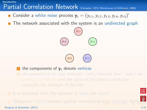
Consider a white noise process yt = (yt 1, yt 2, yt 3, yt 4, yt 5)′
The network associated with the system is an undirected graph
yt 1
yt 2
yt 3yt 4
yt 5
1 the components of yt denote vertices2 the presence of an edge between i and j denotes that i and j are
partially correlated and the value of the partial correlationmeasures the strength of the link.
It is assumed that the network is large yet sparse
Objective: select nonzero partial correlations and estimate them.Barigozzi & Brownlees (2013) 2/24
Introduction
Partial Correlation Network (Dempster, 1972; Meinshausen & Buhlmann, 2006)
Consider a white noise process yt = (yt 1, yt 2, yt 3, yt 4, yt 5)′
The network associated with the system is an undirected graph
yt 1
yt 2
yt 3yt 4
yt 5
1 the components of yt denote vertices2 the presence of an edge between i and j denotes that i and j are
partially correlated and the value of the partial correlationmeasures the strength of the link.
It is assumed that the network is large yet sparse
Objective: select nonzero partial correlations and estimate them.Barigozzi & Brownlees (2013) 2/24

Introduction
Partial Correlation Network (Dempster, 1972; Meinshausen & Buhlmann, 2006)
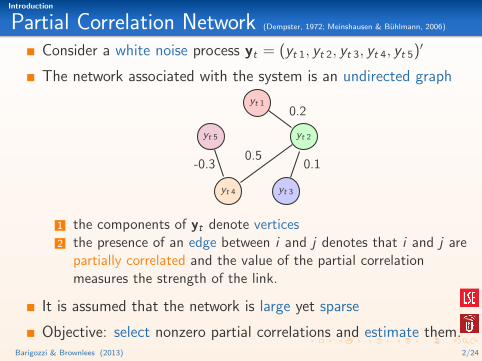
Consider a white noise process yt = (yt 1, yt 2, yt 3, yt 4, yt 5)′
The network associated with the system is an undirected graph
yt 1
yt 2
yt 3yt 4
yt 5
0.2
0.1-0.30.5
1 the components of yt denote vertices2 the presence of an edge between i and j denotes that i and j are
partially correlated and the value of the partial correlationmeasures the strength of the link.
It is assumed that the network is large yet sparse
Objective: select nonzero partial correlations and estimate them.Barigozzi & Brownlees (2013) 2/24

Introduction
Partial Correlation Network (Dempster, 1972; Meinshausen & Buhlmann, 2006)
Consider a white noise process yt = (yt 1, yt 2, yt 3, yt 4, yt 5)′
The network associated with the system is an undirected graph
yt 1
yt 2
yt 3yt 4
yt 5
0.2
0.1-0.30.5
1 the components of yt denote vertices2 the presence of an edge between i and j denotes that i and j are
partially correlated and the value of the partial correlationmeasures the strength of the link.
It is assumed that the network is large yet sparse
Objective: select nonzero partial correlations and estimate them.Barigozzi & Brownlees (2013) 2/24

Introduction
Refresher on Partial Correlation
Partial Correlation measures (cross-sect.) linear conditionaldependence between yt i and yt j given on all other variables:
ρij = Cor(yt i , yt j |{yt k : k 6= i , j}).
Partial Correlation is related to Linear Regression:For instance, consider the model
y1 t = c + β1 2y2 t + β1 3y3 t + β1 4y4 t + β1 5y5 t + u1 t
β13 is different from 0 ⇔ 1 and 3 are partially correlated
Partial Correlation is related to Correlation:If there is exist a partial correlation path between nodes i and j ,then i and j are correlated (and viceversa).
Barigozzi & Brownlees (2013) 3/24

Introduction
Limitations of Partial Correlations for Time Series
Defining the network on the basis of partial correlations ismotivated by the analysis of serially uncorrelated Gaussian data.
However, this is not always satisfactory for economic and financialapplications where data typically exhibit serial dependence.(Partial correlation only captures contemporaneous dependence. However, in economic
datasets it is often the case that the realization of the series A in period t might be
correlated with the realization of series B in period t − 1)
In this work we propose a novel definition of network whichovercomes these limitations.
Barigozzi & Brownlees (2013) 4/24

Introduction
In this Work
1 We propose long run partial correlation network for time series(⇒ partial correlation definition based on the long run covariance)
definition captures contemporaneous as well as lead/lag effectsmodel free – it does not hinge on a specific modeleasy to estimate formulas
2 We propose a network estimation algorithm called NETS
two step LASSO regression procedureallows to estimate large networks in secondswe establish conditions for consistent network estimation
3 We illustrate NETS on a panel of monthly equity returns
The risk of each asset is decomposed in Systematic andIdiosyncratic components where the Idiosyncratic part has aNetwork structure
Barigozzi & Brownlees (2013) 5/24
Introduction
Related Literature
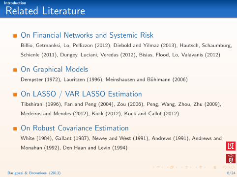
On Financial Networks and Systemic RiskBillio, Getmanksi, Lo, Pellizzon (2012), Diebold and Yilmaz (2013), Hautsch, Schaumburg,
Schienle (2011), Dungey, Luciani, Veredas (2012), Bisias, Flood, Lo, Valavanis (2012)
On Graphical ModelsDempster (1972), Lauritzen (1996), Meinshausen and Buhlmann (2006)
On LASSO / VAR LASSO EstimationTibshirani (1996), Fan and Peng (2004), Zou (2006), Peng, Wang, Zhou, Zhu (2009),
Medeiros and Mendes (2012), Kock (2012), Kock and Callot (2012)
On Robust Covariance EstimationWhite (1984), Gallant (1987), Newey and West (1991), Andrews (1991), Andrews and
Monahan (1992), Den Haan and Levin (1994)
Barigozzi & Brownlees (2013) 6/24

Network for Time Series
Network for Time Series
Network for Time Series
Long Run Partial Correlation Network
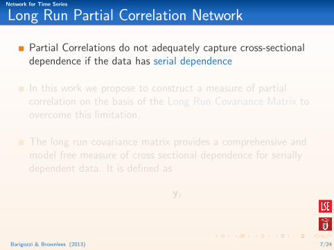
Partial Correlations do not adequately capture cross-sectionaldependence if the data has serial dependence
In this work we propose to construct a measure of partialcorrelation on the basis of the Long Run Covariance Matrix toovercome this limitation.
The long run covariance matrix provides a comprehensive andmodel free measure of cross sectional dependence for seriallydependent data. It is defined as
yt
Barigozzi & Brownlees (2013) 7/24

Network for Time Series
Long Run Partial Correlation Network
Partial Correlations do not adequately capture cross-sectionaldependence if the data has serial dependence
In this work we propose to construct a measure of partialcorrelation on the basis of the Long Run Covariance Matrix toovercome this limitation.
The long run covariance matrix provides a comprehensive andmodel free measure of cross sectional dependence for seriallydependent data. It is defined as
ΣL ≡ limM→∞
1
MVar
(M∑
t=1
yt
)
Barigozzi & Brownlees (2013) 7/24

Network for Time Series
Long Run Covariance
Consider a bivariate system with spillover effects
yt 1 = εt 1 + ψεt−1 2
yt 2 = εt 2with
εt 1 ∼ N (0, σ2)εt 2 ∼ N (0, σ2)
with Cor(εt 1, εt 2) = 0
Then,
Cor (yt 1, yt 2) = 0
Cor(∑12
t=1 yt 1,∑12
t=1 yt 2
)=(
1112
)ψ√1+ψ2
limM→∞ Cor(∑M
t=1 yt 1,∑M
t=1 yt 2
)= ψ√
1+ψ2
Barigozzi & Brownlees (2013) 8/24

Network for Time Series
From LR Covariance to LR Partial Correlation
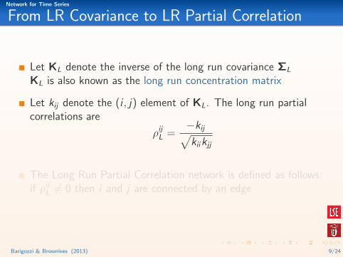
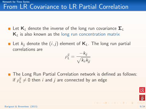
Let KL denote the inverse of the long run covariance ΣL
KL is also known as the long run concentration matrix
Let kij denote the (i , j) element of KL. The long run partialcorrelations are
ρijL =
−kij√kiikjj
The Long Run Partial Correlation network is defined as follows:if ρij
L 6= 0 then i and j are connected by an edge
Barigozzi & Brownlees (2013) 9/24
Network for Time Series
From LR Covariance to LR Partial Correlation
Let KL denote the inverse of the long run covariance ΣL
KL is also known as the long run concentration matrix
Let kij denote the (i , j) element of KL. The long run partialcorrelations are
ρijL =
−kij√kiikjj
The Long Run Partial Correlation network is defined as follows:if ρij
L 6= 0 then i and j are connected by an edge
Barigozzi & Brownlees (2013) 9/24

Network for Time Series
From LR Partial Correlation To LR Concentration
The Long Run Partial Correlation formula:
ρijL =
−kij√kiikjj
where kij denotes the (i , j) element of KL.
This implies that the long run partial correlation network isentirely characterized by KL!If kij is nonzero, then node i and j are connected by an edge.
This fact has important implications for estimation:We can reformulate the estimation of the long run partialcorrelation network as the estimation of a sparse long runconcentration matrix.
Barigozzi & Brownlees (2013) 10/24

Network Estimation NETS Large Sample Properties
Network Estimation
Network Estimation NETS Large Sample Properties
VAR Approximation
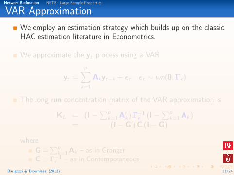
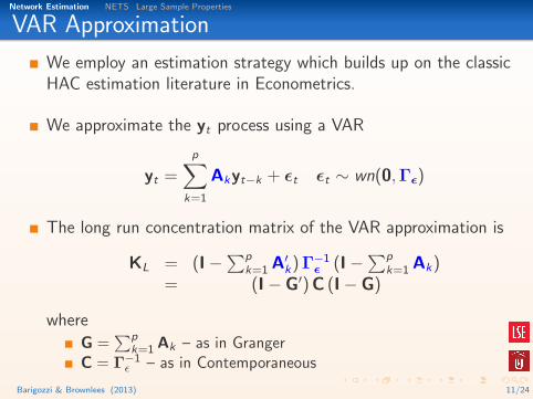
We employ an estimation strategy which builds up on the classicHAC estimation literature in Econometrics.
We approximate the yt process using a VAR
yt =
p∑k=1
Akyt−k + εt εt ∼ wn(0,Γε)
The long run concentration matrix of the VAR approximation is
KL = (I−∑p
k=1 A′k) Γ−1ε (I−
∑pk=1 Ak)
= (I− G′) C (I− G)
where
G =∑p
k=1 Ak – as in GrangerC = Γ−1
ε – as in Contemporaneous
Barigozzi & Brownlees (2013) 11/24

Network Estimation NETS Large Sample Properties
VAR Approximation
We employ an estimation strategy which builds up on the classicHAC estimation literature in Econometrics.
We approximate the yt process using a VAR
yt =
p∑k=1
Akyt−k + εt εt ∼ wn(0,Γε)
The long run concentration matrix of the VAR approximation is
KL = (I−∑p
k=1 A′k) Γ−1ε (I−
∑pk=1 Ak)
= (I− G′) C (I− G)
where
G =∑p
k=1 Ak – as in GrangerC = Γ−1
ε – as in Contemporaneous
Barigozzi & Brownlees (2013) 11/24

Network Estimation NETS Large Sample Properties
VAR Approximation
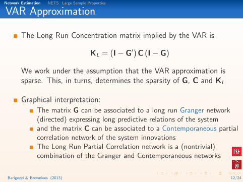
The Long Run Concentration matrix implied by the VAR is
KL = (I− G′) C (I− G)
We work under the assumption that the VAR approximation issparse. This, in turns, determines the sparsity of G, C and KL
Graphical interpretation:
The matrix G can be associated to a long run Granger network(directed) expressing long predictive relations of the systemand the matrix C can be associated to a Contemporaneous partialcorrelation network of the system innovationsThe Long Run Partial Correlation network is a (nontrivial)combination of the Granger and Contemporaneous networks
Barigozzi & Brownlees (2013) 12/24
Network Estimation NETS Large Sample Properties
VAR Approximation
The Long Run Concentration matrix implied by the VAR is
KL = (I− G′) C (I− G)
We work under the assumption that the VAR approximation issparse. This, in turns, determines the sparsity of G, C and KL
Graphical interpretation:
The matrix G can be associated to a long run Granger network(directed) expressing long predictive relations of the systemand the matrix C can be associated to a Contemporaneous partialcorrelation network of the system innovationsThe Long Run Partial Correlation network is a (nontrivial)combination of the Granger and Contemporaneous networks
Barigozzi & Brownlees (2013) 12/24

Network Estimation NETS Large Sample Properties
NETS Algorithm
Our Long Run Partial Correllation Network estimator is based onthe sparse estimation of G and C matrices. Sparse estimation isbased on the LASSO.
We propose an algorithm called“Network Estimator for Time Series” (NETS)to estimate sparse long run partial correlation networks
The NETS procedure consists of estimation KL usinga two step LASSO regression:
1 Estimate A using Adaptive LASSO (based on pre-est. A) on yt
2 Estimate Γ−1ε using LASSO on estimated residuals εt
Barigozzi & Brownlees (2013) 13/24

Network Estimation NETS Large Sample Properties
NETS Steps
Network Estimator for Time Series (NETS) Algorithm: Step 1
Estimate G with
G =
p∑i=1
Ai
where Ai (i = 1, ..., p) are the minimizers of the objective function:
LGT (A1, ...,Ap) =
T∑t=1
(yt −
p∑i=1
Aiyt−i
)2
+ λG
p∑i=1
|Ai ||Ai |
where |Ai | is equal to the sum of the absolute values of thecomponents of Ai .
Barigozzi & Brownlees (2013) 14/24

Network Estimation NETS Large Sample Properties
NETS Steps
The concentration matrix of the systems shocks can be estimatedvia a regression based estimator
Consider the regression model
εt i =N∑
j=1
θijεt j(1− δij) + ut i , i = 1, . . . ,N ,
where δij = 0 if i 6= j and δii = 1
The regression coefficients and residual variance of the regressionis related to the entries of the concentration matrix by thefollowing relations
cii =1
Var(ut i)
andcij = −θijcii
Barigozzi & Brownlees (2013) 14/24
Network Estimation NETS Large Sample Properties
NETS Steps
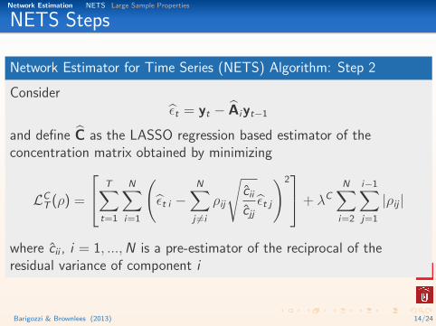
Network Estimator for Time Series (NETS) Algorithm: Step 2
Considerεt = yt − Aiyt−1
and define C as the LASSO regression based estimator of theconcentration matrix obtained by minimizing
LCT (ρ) =
T∑t=1
N∑i=1
(εt i −
N∑j 6=i
ρij
√cii
cjjεt j
)2+ λC
N∑i=2
i−1∑j=1
|ρij |
where cii , i = 1, ...,N is a pre-estimator of the reciprocal of theresidual variance of component i
Barigozzi & Brownlees (2013) 14/24

Network Estimation NETS Large Sample Properties
Large Sample Properties: Assumptions I
(Sketch of) Main Assumptions
1 Data is Weakly Dependent(cf. Doukan and Louhini (1999), Doukhan and Neumann (2007))
2 Data is Covariance Stationary with pd Spectral Density
3 Truncation error of VAR(∞) model decays sufficiently fast
4 Nonzero coefficients are sufficiently large
5 Pre estimators are well behaved
6 Sparsity structure of the VAR parameters
Barigozzi & Brownlees (2013) 15/24

Network Estimation NETS Large Sample Properties
Large Sample Properties: Assumptions II
(Sketch of) Main Assumptions
1 Problem Dimension: nT = O(T ζ1) and pT = O(T ζ2) withζ1, ζ2 > 0.
2 Number of Nonzero Parameters for G and C networks is at most
o(√
Tlog T
)and there is a trade–off between the two.
3 Penalties: λT
T
√qT = o(1) and limT→∞ λT
√T
log T=∞
Barigozzi & Brownlees (2013) 16/24

Network Estimation NETS Large Sample Properties
Large Sample Properties
Proposition I: Granger Network
(a) (Consistent Selection) The probability of correctly selecting thenonzero coefficients of G converges to one.
(b) (Consistent Estimation) For T sufficiently large and each η > 0 thereexists a κ such that with at least probability 1− O(T−η)
||G− G||2 ≤ κλT
T
√qT
Barigozzi & Brownlees (2013) 17/24

Network Estimation NETS Large Sample Properties
Large Sample Properties
Proposition II: Contemporaneous Network
(a) (Consistent Selection) The probability of correctly selecting thenonzero coefficients of C converges to one.
(b) (Consistent Estimation) For T sufficiently large and each η > 0 thereexists a κ such that with at least probability 1− O(T−η)
||C− C||2 ≤ κλT
T
√qT
Barigozzi & Brownlees (2013) 17/24
Network Estimation NETS Large Sample Properties
Large Sample Properties
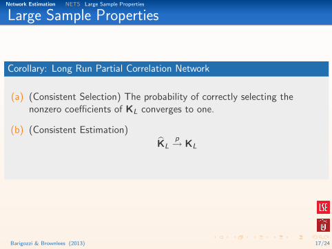
Corollary: Long Run Partial Correlation Network
(a) (Consistent Selection) The probability of correctly selecting thenonzero coefficients of KL converges to one.
(b) (Consistent Estimation)
KLp→ KL
Barigozzi & Brownlees (2013) 17/24

Empirical Application Centrality
Empirical Application

Empirical Application Centrality
Empirical Application
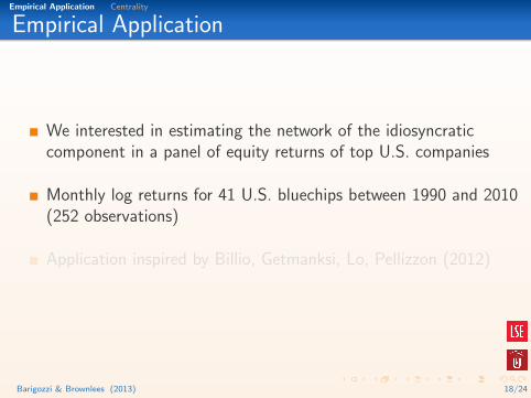
We interested in estimating the network of the idiosyncraticcomponent in a panel of equity returns of top U.S. companies
Monthly log returns for 41 U.S. bluechips between 1990 and 2010(252 observations)
Application inspired by Billio, Getmanksi, Lo, Pellizzon (2012)
Barigozzi & Brownlees (2013) 18/24
Empirical Application Centrality
Empirical Application
We interested in estimating the network of the idiosyncraticcomponent in a panel of equity returns of top U.S. companies
Monthly log returns for 41 U.S. bluechips between 1990 and 2010(252 observations)
Application inspired by Billio, Getmanksi, Lo, Pellizzon (2012)
Barigozzi & Brownlees (2013) 18/24

Empirical Application Centrality
Empirical Application
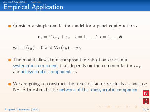
Consider a simple one factor model for a panel equity returns
rit = βi rm t + εit t = 1, ...,T i = 1, ...,N
with E(εit) = 0 and Var(εit) = σit
The model allows to decompose the risk of an asset in asystematic component that depends on the common factor rm t
and idiosyncratic component εit
We are going to construct the series of factor residuals εit and useNETS to estimate the network of the idiosyncratic component.
Barigozzi & Brownlees (2013) 19/24

Empirical Application Centrality
Empirical Application
Consider a simple one factor model for a panel equity returns
rit = βi rm t + εit t = 1, ...,T i = 1, ...,N
with E(εit) = 0 and Var(εit) = σit
The model allows to decompose the risk of an asset in asystematic component that depends on the common factor rm t
and idiosyncratic component εit
We are going to construct the series of factor residuals εit and useNETS to estimate the network of the idiosyncratic component.
Barigozzi & Brownlees (2013) 19/24

Empirical Application Centrality
Empirical Application: Results
We run NETS to estimate the long run partial correlationnetwork. Order p of the VAR is one. The tuning parameters λG
and λC are chosen using a BIC type information criterion.
Out of 820 possible edges, we find 57 edges. The dynamicsaccount for 12% of the edges and the remaining 88% arecontemporaneous.
The idiosyncratic network accounts for a significant portion of therisk of an asset!
The market explains on average 25% of the variability of thestocks in the panel
The linkages identified by the idiosyncratic network account onaverage for an additional 15%
Barigozzi & Brownlees (2013) 20/24

Empirical Application Centrality
Idiosyncratic Risk Network
Barigozzi & Brownlees (2013) 21/24

Empirical Application Centrality
Idiosyncratic Risk Network – Zoom
Barigozzi & Brownlees (2013) 21/24

Empirical Application Centrality
“Reading” the Idiosyncratic Risk Network
Reading a Network can be challenging at times. There is lot ofinformation encoded in the network.
We are going to use some of the tools used in network analysis tosummarise the information in the network. It turns out that theidiosyncratic risk network shares many of the characteristic ofsocial networks.
1 Similarity. Nodes that are similar are linked (industry linkages)
2 Centrality. Financials and Technology are some of the mostcentral sectors.
3 Clustering. Evidence of “Small World Effects”
Barigozzi & Brownlees (2013) 22/24

Empirical Application Centrality
Centrality
Barigozzi & Brownlees (2013) 23/24
Conclusions
Conclusions

Conclusions
Conclusions
We propose a network definition for multivariate time series basedof long run partial correlations
We introduce an algorithm called NETS to estimate sparse longrun partial correlation networks in potentially large systems andprovide large sample analysis of its properties
We apply this methodology to study the network of idiosyncraticshocks in a panel of financial returns.Results show that:
The linkages identified by the idiosyncratic risk network explain aconspicuous part of overall variation in returnsThe idiosyncratic risk network shares many features of socialnetwork
Barigozzi & Brownlees (2013) 24/24
Conclusions
Conclusions
We propose a network definition for multivariate time series basedof long run partial correlations
We introduce an algorithm called NETS to estimate sparse longrun partial correlation networks in potentially large systems andprovide large sample analysis of its properties
We apply this methodology to study the network of idiosyncraticshocks in a panel of financial returns.Results show that:
The linkages identified by the idiosyncratic risk network explain aconspicuous part of overall variation in returnsThe idiosyncratic risk network shares many features of socialnetwork
Barigozzi & Brownlees (2013) 24/24

Conclusions
Conclusions
We propose a network definition for multivariate time series basedof long run partial correlations
We introduce an algorithm called NETS to estimate sparse longrun partial correlation networks in potentially large systems andprovide large sample analysis of its properties
We apply this methodology to study the network of idiosyncraticshocks in a panel of financial returns.Results show that:
The linkages identified by the idiosyncratic risk network explain aconspicuous part of overall variation in returnsThe idiosyncratic risk network shares many features of socialnetwork
Barigozzi & Brownlees (2013) 24/24

Conclusions
Questions?
Thanks!
Barigozzi & Brownlees (2013) 24/24