Petri Nets for Systems and Synthetic Biology

Petri Nets for Systems and Synthetic Biology

Monika Heiner1 David Gilbert2 and Robin Donaldson2

1 Department of Computer Science Brandenburg University of TechnologyPostbox 10 13 44 03013 Cottbus Germany

monikaheinertu-cottbusde2 Bioinformatics Research Centre University of Glasgow

Glasgow G12 8QQ Scotland UKdrgbrcdcsglaacuk radonaldbrcdcsglaacuk

Abstract We give a description of a Petri net-based framework formodelling and analysing biochemical pathways which unifies the qualita-tive stochastic and continuous paradigms Each perspective adds its con-tribution to the understanding of the system thus the three approachesdo not compete but complement each other We illustrate our approachby applying it to an extended model of the three stage cascade whichforms the core of the ERK signal transduction pathway Consequentlyour focus is on transient behaviour analysis We demonstrate how quali-tative descriptions are abstractions over stochastic or continuous descrip-tions and show that the stochastic and continuous models approximateeach other Although our framework is based on Petri nets it can beapplied more widely to other formalisms which are used to model andanalyse biochemical networks

1 Motivation

Biochemical reaction systems have by their very nature three distinctive charac-teristics (1) They are inherently bipartite ie they consist of two types of gameplayers the species and their interactions (2) They are inherently concurrentie several interactions can usually happen independently and in parallel (3)They are inherently stochastic ie the timing behaviour of the interactions isgoverned by stochastic laws So it seems to be a natural choice to model andanalyse them with a formal method which shares exactly these distinctive char-acteristics stochastic Petri nets

However due to the computational efforts required to analyse stochasticmodels two abstractions are more popular qualitative models abstracting awayfrom any time dependencies and continuous models commonly used to approx-imate stochastic behaviour by a deterministic one We describe an overall frame-work to unify these three paradigms providing a family of related models withhigh analytical power

The advantages of using Petri nets as a kind of umbrella formalism are seenin the following

M Bernardo P Degano and G Zavattaro (Eds) SFM 2008 LNCS 5016 pp 215ndash264 2008ccopy Springer-Verlag Berlin Heidelberg 2008 reprint 2010

216 M Heiner D Gilbert and R Donaldson

ndash intuitive and executable modelling stylendash true concurrency (partial order) semantics which may be lessened to inter-

leaving semantics to simplify analysesndash mathematically founded analysis techniques based on formal semanticsndash coverage of structural and behavioural properties as well as their relationsndash integration of qualitative and quantitative analysis techniquesndash reliable tool support

This chapter can be considered as a tutorial in the step-wise modelling andanalysis of larger biochemical networks as well as in the structured design ofsystems of ordinary differential equations (ODEs) The qualitative model is in-troduced as a supplementary intermediate step at least from the viewpoint ofthe biochemist accustomed to quantitative modelling only and serves mainly formodel validation since this cannot be performed on the continuous level and isgenerally much harder to do on the stochastic level Having successfully validatedthe qualitative model the quantitative models are derived from the qualitativeone by assigning stochastic or deterministic rate functions to all reactions in thenetwork Thus the quantitative models preserve the structure of the qualitativeone and the stochastic Petri net describes a system of stochastic reaction rateequations (RREs) and the continuous Petri net is nothing else than a structureddescription of ODEs

systems biology modelling as formal knowledge representation

synthetic biology modelling for system construction

biosystemnatural

biosystemsynthetic

observedbehaviour

predictedbehaviour

model(blueprint)

desiredbehaviour

design construction

verification verification

observedbehaviour

predictedbehaviour

wetlab

model-basedexperiment design

experiments

formalizingunderstanding

wetlab experiments

model(knowledge)

Fig 1 The role of formal models in systems biology and synthetic biology

Petri Nets for Systems and Synthetic Biology 217

This framework is equally helpful in the setting of systems biology as well assynthetic biology see Figure 1 In systems biology models help us in formalisingour understanding of what has been created by natural evolution So first of allmodels serve as an unambiguous representation of the acquired knowledge andhelp to design new wetlab experiments to sharpen our comprehension

In synthetic biology models help us to make the engineering of biology eas-ier and more reliable Models serve as blueprints for novel synthetic biologicalsystems Their employment is highly recommended to guide the design and con-struction in order to ensure that the behaviour of the synthetic biological systemsis reliable and robust under a variety of conditions

Formal models open the door to mathematically founded analyses for modelvalidation and verification This paper demonstrates typical analysis techniqueswith special emphasis on transient behaviour analysis We show how to sys-tematically derive and interpret the partial order run of the signal responsebehaviour and how to employ model checking to investigate related propertiesin the qualitative stochastic and continuous paradigms All analysis techniquesare introduced through a running example To be self-contained we give theformal definitions of the most relevant notions which are Petri net specific

This paper is organised as follows In the following section we outline ourframework discussing the special contributions of the three individual analysisapproaches and examining their interrelations Next we provide an overview ofthe biochemical context and introduce our running example We then presentthe individual approaches and discuss mutually related properties in all threeparadigms in the following order we start off with the qualitative approachwhich is conceptually the easiest and does not rely on knowledge of kineticinformation but describes the network topology and presence of the species Wethen demonstrate how the validated qualitative model can be transformed intothe stochastic representation by addition of stochastic firing rate informationNext the continuous model is derived from the qualitative or stochastic modelby considering only deterministic firing rates Suitable sets of initial conditionsfor all three models are constructed by qualitative analysis Finally we refer torelated work before concluding with a summary and outlook regarding furtherresearch directions

2 Overview of the framework

In the following we describe our overall framework illustrated in Figure 2 thatrelates the three major ways of modelling and analysing biochemical networksdescribed in this paper qualitative stochastic and continuous

The most abstract representation of a biochemical network is qualitative andis minimally described by its topology usually as a bipartite directed graph withnodes representing biochemical entities or reactions or in Petri net terminologyplaces and transitions (see Figures 4 ndash 6) Arcs can be annotated with stoi-chiometric information whereby the default stoichiometric value of 1 is usuallyomitted


Qualitative

Stochastic Continuous

Abs

trac

tion

Approximation type (1)

MoleculesLevels

Qualitative Petri nets

CTLLTL

MoleculesLevels

Stochastic rates

Stochastic Petri nets

RREs

CSLPLTL

Concentrations

Deterministic rates

Continuous Petri nets

ODEs

LTLc

Abstraction


Discrete State Space Continuous State Space

Time-free

Timed

Quantitative

Fig 2 Conceptual framework

The qualitative description can be further enhanced by the abstract repre-sentation of discrete quantities of species achieved in Petri nets by the use oftokens at places These can represent the number of molecules or the level ofconcentration of a species The standard semantics for these qualitative Petrinets (QPN) does not associate a time with transitions or the sojourn of tokensat places and thus these descriptions are time-free The qualitative analysisconsiders however all possible behaviour of the system under any timing Thebehaviour of such a net forms a discrete state space which can be analysed inthe bounded case for example by a branching time temporal logic one instanceof which is Computational Tree Logic (CTL) see [CGP01]

Timed information can be added to the qualitative description in two ways ndashstochastic and continuous The stochastic Petri net (SPN) description preservesthe discrete state description but in addition associates a probabilistically dis-tributed firing rate (waiting time) with each reaction All reactions which occurin the QPN can still occur in the SPN but their likelihood depends on the prob-ability distribution of the associated firing rates Special behavioural propertiescan be expressed using eg Continuous Stochastic Logic (CSL) see [PNK06] aprobabilistic counterpart of CTL or Probabilistic Linear-time Temporal Logic(PLTL) see [MC208] a probabilistic counterpart to LTL [Pnu81] The QPN isan abstraction of the SPN sharing the same state space and transition rela-tion with the stochastic model with the probabilistic information removed Allqualitative properties valid in the QPN are also valid in the SPN and vice versa

The continuous model replaces the discrete values of species with continuousvalues and hence is not able to describe the behaviour of species at the levelof individual molecules but only the overall behaviour via concentrations Wecan regard the discrete description of concentration levels as abstracting over thecontinuous description of concentrations Timed information is introduced by theassociation of a particular deterministic rate information with each transitionpermitting the continuous model to be represented as a set of ordinary differential


equations (ODEs) The concentration of a particular species in such a model willhave the same value at each point of time for repeated experiments The statespace of such models is continuous and linear So it has to be analysed by a lineartime temporal logic (LTL) for example Linear Temporal Logic with constraints(LTLc) in the manner of [CCRFS06] or PLTL [MC208]

The stochastic and continuous models are mutually related by approxima-tion The stochastic description can be used as the basis for deriving a continu-ous Petri net (CPN) model by approximating rate information Specifically theprobabilistically distributed reaction firing in the SPN is replaced by a particularaverage firing rate over the continuous token flow of the CPN This is achievedby approximation over hazard (propensity) functions of type (1) described inmore detail in section 51 In turn the stochastic model can be derived from thecontinuous model by approximation reading the tokens as concentration levelsas introduced in [CVGO06] Formally this is achieved by a hazard function oftype (2) see again section 51

It is well-known that time assumptions generally impose constraints on be-haviour The qualitative and stochastic models consider all possible behavioursunder any timing whereas the continuous model is constrained by its inherentdeterminism to consider a subset This may be too restrictive when modellingbiochemical systems which by their very nature exhibit variability in their be-haviour

3 Biochemical Context

We have chosen a model of the mitogen-activated protein kinase (MAPK) cas-cade published in [LBS00] as a running case study This is the core of the ubiq-uitous ERKMAPK pathway that can for example convey cell division anddifferentiation signals from the cell membrane to the nucleus The model doesnot describe the receptor and the biochemical entities and actions immediatelydownstream from the receptor Instead the description starts at the RasGTPcomplex which acts as a kinase to phosphorylate Raf which phosphorylatesMAPKERK Kinase (MEK) which in turn phosphorylates Extracellular signalRegulated Kinase (ERK) This cascade (RasGTP rarr Raf rarr MEK rarr ERK) ofprotein interactions controls cell differentiation the effect being dependent uponthe activity of ERK We consider RasGTP as the input signal and ERKPP (ac-tivated ERK) as the output signal

The scheme in Figure 3 describes the typical modular structure for sucha signalling cascade compare [CKS07] Each layer corresponds to a distinctprotein species The protein Raf in the first layer is only singly phosphory-lated The proteins in the two other layers MEK and ERK respectively canbe singly as well as doubly phosphorylated In each layer forward reactionsare catalysed by kinases and reverse reactions by phosphatases (Phosphatase1Phosphatase2 Phosphatase3) The kinases in the MEK and ERK layers arethe phosphorylated forms of the proteins in the previous layer Each phospho-rylationdephosphorylation step applies mass action kinetics according to the


following pattern A + E AE rarr B + E taking into account the mechanismby which the enzyme acts namely by forming a complex with the substratemodifying the substrate to form the product and a disassociation occurring torelease the product

Raf RafP

MEKP MEKPPMEK

ERKP ERKPPERK

Phosphatase3

Phosphatase1

Phosphatase2

RasGTP

Fig 3 The general scheme of the considered signalling pathway a three-stage dou-ble phosphorylation cascade Each phosphorylationdephosphorylation step applies themass action kinetics pattern A+E AE rarr B+E We consider RasGTP as the inputsignal and ERKPP as the output signal

4 The Qualitative Approach

41 Qualitative Modelling

To allow formal reasoning of the general scheme of a signal transduction cas-cade which is given in Figure 3 in an informal way we are going to derive acorresponding Petri net Petri nets enjoy formal semantics amenable to math-ematically sound analysis techniques The first two definitions introduce thestandard notion of placetransition Petri nets which represents the basic classin the ample family of Petri net models


Definition 1 (Petri net Syntax) A Petri net is a quadruple N = (P T fm0)where

ndash P and T are finite non empty and disjoint sets P is the set of places (inthe figures represented by circles) T is the set of transitions (in the figuresrepresented by rectangles)

ndash f ((P times T ) cup (T times P )) rarr IN0 defines the set of directed arcs weighted bynonnegative integer values

ndash m0 P rarr IN0 gives the initial marking

Thus Petri nets (or nets for short) are weighted directed bipartite graphsThe idea to use Petri nets for the representation of biochemical networks israther intuitive and has been mentioned by Carl Adam Petri himself in one ofhis internal research reports on interpretation of net theory in the seventies Ithas also been used as the very first introductory example in [Mur89] and wefollow that idea in this tutorial compare Figure 4

Places usually model passive system components like conditions species orany kind of chemical compounds eg proteins or proteins complexes playing therole of precursors or products Transitions stand for active system componentslike atomic actions or any kind of chemical reactions eg association disas-sociation phosphorylation or dephosphorylation transforming precursors intoproducts

The arcs go from precursors to reactions (ingoing arcs) and from reactionsto products (outgoing arcs) In other words the preplaces of a transition corre-spond to the reactionrsquos precursors and its postplaces to the reactionrsquos productsEnzymes establish side conditions and are connected in both directions with thereaction they catalyse we get a read arc

Arc weights may be read as the multiplicity of the arc reflecting knownstoichiometries Thus the (pseudo) arc weight 0 stands for the absence of anarc The arc weight 1 is the default value and is usually not given explicitly

A place carries an arbitrary number of tokens represented as black dots ora natural number The number zero is the default value and usually not givenexplicitly Tokens can be interpreted as the available amount of a given species innumber of molecules or moles or any abstract ie discrete concentration level

In the most abstract way a concentration can be thought of as being lsquohighrsquoor lsquolowrsquo (present or absent) Generalizing this Boolean approach any continuousconcentration range can be divided into a finite number of equally sized sub-ranges (equivalence classes) so that the concentrations within can be consideredto be equivalent The current number of tokens on a place will then specify thecurrent level of the speciesrsquo concentration eg the absence of tokens specifieslevel 0 In the following when speaking in terms of level semantics we alwaysgive the highest level number

A particular arrangement of tokens over the places of the net is called amarking modelling a system state In this paper the notions marking and stateare used interchangeably


We introduce the following notions and notations m(p) yields the numberof tokens on place p in the marking m A place p with m(p) = 0 is called clean(empty unmarked) in m otherwise it is called marked (non-clean) A set ofplaces is called clean if all its places are clean otherwise marked The preset ofa node x isin P cupT is defined as bullx = y isin P cup T |f (y x) 6= 0 and its postset asxbull = y isin P cup T |f (x y) 6= 0 Altogether we get four types of sets

ndash bullt the preplaces of a transition t consisting of the reactionrsquos precursorsndash tbull the postplaces of a transition t consisting of the reactionrsquos productsndash bullp the pretransitions of a place p consisting of all reactions producing this

speciesndash p bull the posttransitions of a place p consisting of all reactions consuming this

species

We extend both notions to a set of nodes X sube P cup T and define the set ofall prenodes bullX =

⋃

xisinXbullx and the set of all postnodes Xbull =

⋃

xisinX xbull SeeFigure 11 for an illustration of these notations

Petri net Semantics Up to now we have introduced the static aspects of aPetri net only The behaviour of a net is defined by the firing rule which consistsof two parts the precondition and the firing itself

Definition 2 (Firing rule) Let N = (P T fm0) be a Petri net

ndash A transition t is enabled in a marking m written as m[t〉 ifforallp isin bullt m(p) ge f(p t) else disabled

ndash A transition t which is enabled in m may firendash When t in m fires a new marking mprime is reached written as m[t〉mprime with

forallp isin P mprime(p) = m(p)minus f(p t) + f(t p)ndash The firing happens atomically and does not consume any time

Please note a transition is never forced to fire Figuratively the firing ofa transition moves tokens from its preplaces to its postplaces while possiblychanging the number of tokens compare Figure 4 Generally the firing of atransition changes the formerly current marking to a new reachable one wheresome transitions are not enabled anymore while others get enabled The repeatedfiring of transitions establishes the behaviour of the net

The whole net behaviour consists of all possible partially ordered firing se-quences (partial order semantics) or all possible totally ordered firing sequences(interleaving semantics) respectively

Every marking is defined by the given token situation in all places m isin IN|P |0

whereby |P | denotes the number of places in the Petri net All markings whichcan be reached from a given marking m by any firing sequence of arbitrarylength constitute the set of reachable markings [m〉 The set of markings [m0〉reachable from the initial marking is said to be the state space of a given system

All notions introduced in the following in this section refer to a placetransi-tion Petri net according to Definitions 1 and 2


Fig 4 The Petri net for the wellknown chemical reaction r 2H2 +O2 rarr 2H2O and three of its mark-ings (states) connected each by afiring of the transition r The tran-sition is not enabled anymore inthe marking reached after these twosingle firing steps

O2

H2 4H2O

H2O

H2

O2

H2O4

H2

O2

r

r

r

22

22

22

Running example In this modelling spirit we are now able to create a Petrinet for our running example We start with building blocks for some typicalchemical reaction equations as shown in Figure 5 We get the Petri net in Figure6 for our running example by composing these building blocks according to thescheme of Figure 3 As we will see later this net structure corresponds exactlyto the set of ordinary differential equations given in [LBS00] Thus the net canequally be derived by SBML import and automatic layout manually improvedfrom this ODE model

Reversible reactions have to be modelled explicitly by two opposite transi-tions However in order to retain the elegant graph structure of Figure 6 we usemacro transitions each of which stands here for a reversible reaction The entire(flattened) placetransition Petri net consists of 22 places and 30 transitionswhere r1 r2 stand for reaction (transition) labels

We associate a discrete concentration with each of the 22 species In thequalitative analysis we apply Boolean semantics where the concentrations canbe thought of as being ldquohighrdquo or ldquolowrdquo (above or below a certain threshold) Thisresults into a two level model and we extend this to a multi-level model in thequantitative analysis where each discrete level stands for an equivalence classof possibly infinitely many concentrations Then places can be read as integervariables

42 Qualitative Analysis

A preliminary step will usually execute the net which allows us to experiencethe model behaviour by following the token flow1 Having established initialconfidence in the model by playing the token game the system needs to beformally analysed Formal analyses are exhaustive opposite to the token gamewhich exemplifies the net behaviour

1 If the reader would like to give it a try just download our Petri net tool [Sno08]


A B A B BA

BA

E

E

BA_EA

A B

E E

BA

A A_E B

E

A

A_E1

B

E1

B_E2

E2 E2

B_E2

E1

B

A_E1

A

r1

r1

r2

r1

r3r2

r1

r1

r2

r3

r1

r2r3

r4

r5r6

r6

r3

(a) (b) (c)

(d) (e) (f)

(g) (h)

(i) (j)

r1r2

r1r2

r1r2

r1r2

r4r5

Fig 5 The Petri net components for some typical basic structures of biochemicalreaction networks (a) simple reaction A rarr B (b) reversible reaction A B (c)hierarchical notation of (b) (d) simple enzymatic reaction Michaelis-Menten kinetics(e) reversible enzymatic reaction Michaelis-Menten kinetics (f) hierarchical notationof (e) (g) enzymatic reaction mass action kinetics A + E A E rarr B + E (h)hierarchical notation of (g) (i) two enzymatic reactions mass action kinetics buildinga cycle (j) hierarchical notation of (i) Two concentric squares are macro transitionsallowing the design of hierarchical net models They are used here as shortcuts forreversible reactions Two opposite arcs denote read arcs see (d) and (e) establishingside conditions for a transitionrsquos firing


Raf

RasGTP

Raf_RasGTP

RafP

RafP_Phase1

MEK_RafP MEKP_RafP

MEKP_Phase2 MEKPP_Phase2

ERK

ERK_MEKPP ERKP_MEKPP

ERKP

MEKPP

ERKPP_Phase3ERKP_Phase3

MEKP

ERKPP

Phase2

Phase3

MEK

Phase1

r3

r6

r21

r18

r9 r12

r15

r24

r27r30

PUR ORD HOM NBM CSV SCF CON SC FT0 TF0 FP0 PF0 NC

Y Y Y Y N N Y Y N N N N nES

DTP CPI CTI SCTI SB k-B 1-B DCF DSt DTr LIV REV

Y Y Y N Y Y Y N 0 N Y Y

r1r2

r4r5

r7r8 r10r11

r16r17

r22r23r19r20

r13r14

r28r29 r25r26

Fig 6 The bipartite graph for the extended ERK pathway model according to thescheme in Figure 3 Places (circles) stand for species (proteins protein complexes)Protein complexes are indicated by an underscore ldquo rdquo between the constituent pro-tein names The suffixes P or PP indicate phosphorylated or doubly phosphorylatedforms respectively The name Phase serves as shortcut for Phosphatase The speciesthat are read as inputoutput signals are given in grey Transitions (squares) standfor irreversible reactions while macro transitions (two concentric squares) specify re-versible reactions compare Figure 5 The initial state is systematically constructedusing standard Petri net analysis techniques At the bottom the two-line result vectoras produced by Charlie [Cha08] is given Properties of interest in this vector for thisbiochemical network are explained in the text


(0) General behavioural properties The first step in analysing a Petri netusually aims at deciding general behavioural properties ie properties whichcan be formulated independently from the special functionality of the networkunder consideration There are basically three of them which are orthogonalboundedness liveness and reversibility [Mur89] We start with an informal char-acterisation of the key issues

ndash boundedness For every place it holds that Whatever happens the maximalnumber of tokens on this place is bounded by a constant This precludesoverflow by unlimited increase of tokens

ndash liveness For every transition it holds that Whatever happens it will alwaysbe possible to reach a state where this transition gets enabled In a live netall transitions are able to contribute to the net behaviour forever whichprecludes dead states ie states where none of the transitions are enabled

ndash reversibility For every state it holds that Whatever happens the net willalways be able to reach this state again So the net has the capability ofself-reinitialization

In most cases these are requirable properties To be precise we give thefollowing formal definitions elaborating these notions in more details

Definition 3 (Boundedness)

ndash A place p is k-bounded (bounded for short) if there exists a positive integernumber k which represents an upper bound for the number of tokens on thisplace in all reachable markings of the Petri netexist k isin IN0 forallm isin [m0〉 m(p) le k

ndash A Petri net is k-bounded (bounded for short) if all its places are k-boundedndash A Petri net is structurally bounded if it is bounded in any initial marking

Definition 4 (Liveness of a transition)

ndash A transition t is dead in the marking m if it is not enabled in any markingmprime reachable from m6 exist mprime isin [m〉 mprime[t〉

ndash A transition t is live if it is not dead in any marking reachable from m0

Definition 5 (Liveness of a Petri net)

ndash A marking m is dead if there is no transition which is enabled in mndash A Petri net is deadlock-free (weakly live) if there are no reachable dead

markingsndash A Petri net is live (strongly live) if each transition is live


Definition 6 (Reversibility) A Petri net is reversible if the initial markingcan be reached again from each reachable marking forallm isin [m0〉 m0 isin [m〉

Finally we introduce the general behavioural property dynamic conflict whichrefers to a marking enabling two transitions but the firing of one transitiondisables the other one The occurrence of dynamic conflicts causes alternative(branching) system behaviour whereby the decision between these alternativesis taken nondeterministically See Figure 7 for an illustration of these behaviouralproperties

BA CD

E F

r1

r2

r3 r5

r6r4

r7

r8

r92 2

Fig 7 A net to illustrate the general behavioural properties The place A is 0-bounded place B is 1-bounded and all other places are 2-bounded so the net is2-bounded The transitions r1 and r2 in the leftmost cycle are dead at the initialmarking The transitions r8 and r9 in the rightmost cycle are live All other transitionsare not live so the net is weakly live The net is not reversible because there is nocounteraction to the token decrease by firing of r4 There are dynamic conflicts egbetween r4 and r5 in a marking with m(C)=2

Running example Our net enjoys the three orthogonal general properties of aqualitative Petri net it is bounded even structurally bounded (SB) live (LIV)and reversible (REV)

Boundedness can always be decided in a static way ie without constructionof the state space while the remaining behavioural properties generally requiredynamic analysis techniques ie the explicit construction of the partial or fullstate space However as we will see later freedom of dead states (DSt) can stillbe decided in a static way for our running example

The essential steps of the systematic analysis procedure for our running ex-ample are given in more detail as follows They represent a typical pattern ofhow to proceed So they may be taken as a recipe of how to analyse your ownsystem

(1) Structural properties The following structural properties are elementarygraph properties and reflect the modelling approach They can be read as pre-liminary consistency checks to preclude production faults in drawing the netRemarkably certain combinations of structural properties allow conclusions onbehavioural properties some examples of such conclusions will be mentionedThe list follows the order as used in the two-line result vector produced by ourqualitative analysis tool Charlie [Cha08] compare Figure 6


PUR A Petri net is pure ifforallx y isin P cup T f(x y) 6= 0 rArr f(y x) = 0ie there are no two nodes connected in both directions This precludes readarcs Then the net structure is fully represented by the incidence matrixwhich is used for the calculation of the P- and T-invariants see step (2)

ORD A Petri net is ordinary ifforallx y isin P cup T f(x y) 6= 0 rArr f(x y) = 1ie all arc weights are equal to 1 This includes homogeneity A non-ordinaryPetri net cannot be live and 1-bounded at the same time

HOM A Petri net is homogeneous ifforallp isin P forallt tprime isin pbull rArr f(p t) = f(p tprime)ie all outgoing arcs of a given place have the same multiplicity

NBM A net has non-blocking multiplicity ifforallp isin P bullp 6= empty andminf(t p)| t isin bullp ge maxf(p t)| t isin pbullie an input place causes blocking multiplicity Otherwise it must hold foreach place the minimum of the multiplicities of the incoming arcs is not lessthan the maximum of the multiplicities of the outgoing arcs

CSV A Petri net is conservative ifforallt isin T

sum

pisinbullt f(p t) =sum

pisintbull f(t p)ie all transitions add exactly as many tokens to their postplaces as they sub-tract from their preplaces or briefly all transitions fire token-preservinglyA conservative Petri net is structurally bounded

SCF A Petri net is static conflict free ifforallt tprime isin T t 6= tprime rArr bullt cap bulltprime = emptyie there are no two transitions sharing a preplace Transitions involved ina static conflict compete for the tokens on shared preplaces Thus staticconflicts indicate situations where dynamic conflicts ie nondeterministicchoices may occur in the system behaviour However it depends on thetoken situation whether a conflict does actually occur dynamically There isno nondeterminism in SCF nets

CON A Petri net is connected if it holds for every two nodes a and b that thereis an undirected path between a and b Disconnected parts of a Petri netcannot influence each other so they can usually be analysed separately Inthe following we consider only connected Petri nets

SC A Petri net is strongly connected if it holds for every two nodes a and bthat there is a directed path from a to b Strong connectedness involvesconnectedness and the absence of boundary nodes It is a necessary conditionfor a Petri net to be live and bounded at the same time

FT0 TF0 FP0 PF0 A node x isin P cup T is called boundary node ifbullx = empty or xbull = empty Boundary nodes exist in four typesndash input transition - a transition without preplaces (bullt = empty shortly FT0)ndash output transition - a transition without postplaces (tbull = empty shortly TF0)ndash input place - a place without pretransitions (bullp = empty shortly FP0)ndash output place - a place without posttransitions (pbull = empty shortly PF0)

A net with boundary nodes cannot be bounded and live at the same timeFor example an input transition is always enabled so its postplaces are


unbounded while input places preclude liveness Boundary nodes modelinterconnections of an open system with its environment A net withoutboundary nodes is self-contained ie a closed system It needs a non-cleaninitial marking to become live

Definition 7 (Net structure classes)

ndash A Petri net is called State Machine (SM) ifforallt isin T |bullt| = |tbull| le 1

ie there are neither forward branching nor backward branching transitionsndash A Petri net is called Synchronisation Graph (SG) if

forallp isin P |bullp| = |pbull| le 1ie there are neither forward branching nor backward branching places

ndash A Petri net is called Extended Free Choice (EFC) ifforallp q isin P pbull cap qbull = empty or pbull = qbull

ie transitions in conflict have identical sets of preplacesndash A Petri net is called Extended Simple (ES) if

forallp q isin P pbull cap qbull = empty or pbull sube qbull or qbull sube pbullie every transition is involved in one conflict at most

Please note these definitions refer to the net structure only neglecting anyarc multiplicities However these net classes are especially helpful in the settingof ordinary nets SM and SG 2 are dual notions a SM net can be converted intoan SG net by exchanging places and transitions and vice versa Both net classesare properly included in the EFC net class which again is properly included inthe ES net class

SM nets are conservative and thus the prototype of bounded models theycorrespond to the well-known notion of finite state automata SG nets are freeof static conflicts and therefore of nondeterminism In EFC nets transitionsin conflict are always together enabled or disabled so there is always a freechoice between them in dynamic conflict situations EFC nets have the pleasantproperty of monotonous liveness ie if they are live in the marking m thenthey remain live for any other marking mprime with mprime ge m In ES nets the conflictrelation is transitive if t1 and t2 are in conflict and t2 and t3 are in conflictthen t1 and t3 are in conflict too ES nets have the distinguished property to belive independently of time ie if they are live then they remain live under anytiming [Sta89]

All these structural properties do not depend on the initial marking Mostof these properties can be locally decided in the graph structure Connectednessand strong connectedness need to consider the global graph structure which canbe done using standard graph algorithms

Running example The net is pure and ordinary therefore homogeneous aswell but not conservative There are static conflicts The net structure does

2 We use synchronisation graph instead of the more popular term marked graph whichmight cause confusion


not comply to any of the introduced net structure classes so it is said to benot Extended Simple (nES) The net is strongly connected which includes con-nectedness and absence of boundary nodes and thus self-contained ie a closedsystem Therefore in order to make the net live we have to construct an initialmarking see step (3) below

(2) Static decision of marking-independent behavioural properties Toopen the door to analysis techniques based on linear algebra we represent the netstructure by a matrix called incidence matrix in the Petri net community andstoichiometric matrix in systems biology We briefly recall the essential technicalterms

Definition 8 (P-invariants T-invariants)

ndash The incidence matrix of N is a matrix C P times T rarr ZZ indexed by P andT such that C(p t) = f(t p)minus f(p t)

ndash A place vector (transition vector) is a vector x P rarr ZZ indexed by P(y T rarr ZZ indexed by T)

ndash A place vector (transition vector) is called a P-invariant (T-invariant) if itis a nontrivial nonnegative integer solution of the linear equation systemx middot C = 0 (C middot y = 0)

ndash The set of nodes corresponding to an invariantrsquos nonzero entries are calledthe support of this invariant x written as supp (x)

ndash An invariant x is called minimal if 6 exist invariant z supp (z) sub supp (x) ieits support does not contain the support of any other invariant z and thegreatest common divisor of all nonzero entries of x is 1

ndash A net is covered by P-invariants shortly CPI (covered by T-invariantsshortly CTI) if every place (transition) belongs to a P-invariant (T-invariant)

CPI causes structural boundedness (SB) ie boundedness for any initialmarking CTI is a necessary condition for bounded nets to be live But maybeeven more importantly invariants are a beneficial technique in model valida-tion and the challenge is to check all invariants for their biological plausibilityTherefore letrsquos elaborate these notions more carefully compare also Figure 8

The incidence matrix of a Petri net is an integer matrix C with a row foreach place and a column for each transition A matrix entry C(p t) gives thetoken change on place p by the firing of transition t Thus a preplace of t whichis not a postplace of t has a negative entry while a postplace of t which is nota preplace of t has a positive entry each corresponding to the arc multiplicitiesThe entry for a place which is preplace as well as postplace of a transitiongives the difference of the multiplicities of the transitionrsquos outgoing arc minusthe transitionrsquos ingoing arc In this case we lose information the non-ordinarynet structure cannot be reconstructed uniquely out of the incidence matrix

The columns of C are place vectors ie vectors with as many entries as thereare places describing the token change on a marking by the firing of the transi-tion defining the column index The rows of C are transition vectors ie vectors


with as many entries as there are transitions describing the influence of alltransitions on the tokens in the place defining the row index For stoichiometricreaction networks eg metabolic networks the incidence matrix coincides withthe stoichiometric matrix

A P-invariant x is a nonzero and nonnegative integer place vector such thatx middotC = 0 in words for each transition it holds that multiplying the P-invariantwith the transitionrsquos column vector yields zero Thus the total effect of eachtransition on the P-invariant is zero which explains its interpretation as a tokenconservation component A P-invariant stands for a set of places over whichthe weighted sum of tokens is constant and independent of any firing ie forany markings m1 m2 which are reachable by the firing of transitions it holdsthat x middotm1 = x middotm2 In the context of metabolic networks P-invariants reflectsubstrate conservations while in signal transduction networks P-invariants oftencorrespond to the several states of a given species (protein or protein complex)A place belonging to a P-invariant is obviously bounded

Analogously a T-invariant y is a nonzero and nonnegative integer transitionvector such that C middot y = 0 in words for each place it holds that multiplyingthe placersquos row with the T-invariant yields zero Thus the total effect of theT-invariant on a marking is zero A T-invariant has two interpretations in thegiven biochemical context

ndash The entries of a T-invariant specify a multiset of transitions which by theirpartially ordered firing reproduce a given marking ie basically occurringone after the other This partial order sequence of the T-invariantrsquos tran-sitions may contribute to a deeper understanding of the net behaviour AT-invariant is called feasible if such a behaviour is actually possible in thegiven marking situation

ndash The entries of a T-invariant may also be read as the relative firing ratesof transitions all of them occurring permanently and concurrently Thisactivity level corresponds to the steady state behaviour

r1 2 AE

minusrarr 2 Br23 A B

r1 r2 r3

A ndash2 ndash1 1B 2 1 ndash1E 0 0 0 A B

E

r1

r2

r3

2 2

x1 = (1 1 0) = (A B)x2 = (0 0 1) = (E)

y1 = (1 0 2) = (r1 2 middot r3)y2 = (0 1 1) = (r2 r3)

y3 = (1 1 3) = y1 + y2

Fig 8 Two reaction equations with the corresponding Petri net its incidence matrixand the minimal P-invariants x1 x2 and the minimal T-invariants y1 y2 and a non-minimal T-invariant y3 The invariants are given in the standard vector notation aswell as in a shorthand notation listing the nonzero entries only The net is not purethe incidence matrix does not reflect the dependency of r1 on E


The two transitions modelling the two directions of a reversible reactionalways make a minimal T-invariant thus they are called trivial T-invariantsA net which is covered by nontrivial T-invariants is said to be strongly coveredby T-invariants (SCTI) Transitions not covered by nontrivial T-invariants arecandidates for model reduction eg if the model analysis is concerned withsteady state analysis only

The set xi of all minimal P-invariants (T-invariants) of a given net is uniqueand represents a generating system for all P-invariants (T-invariants) All invari-ants x can be computed as nonnegative linear combinations n middot x =

sum(ai middot xi)

with n ai isin IN0 ie the allowed operations are addition multiplication by anatural number and division by a common divisor

Technically we need to solve a homogenous linear equation system over natu-ral numbers (nonnegative integers) This restriction of the data space establishesndash from a mathematical point of view ndash a challenge so there is no closed formulato compute the solutions However there are algorithms ndash actually a class ofalgorithms ndash constructing the solution (to be precise the generating system forthe solution space) by systematically considering all possible candidates

This algorithm class has been repetitively re-invented over the years Sothese algorithms come along with different names but if you take a closer lookyou will always encounter the same underlying idea All these versions may beclassified as ldquopositive Gauss eliminationrdquo the incidence matrix is systematicallytransformed to a zero matrix by suitable matrix operations

However there are net structures where we get the invariants almost for freeFor ordinary state machines it holds

ndash each (minimal) cycle is a (minimal) T-invariantndash for strongly connected state machines the reverse direction holds also each

(minimal) T-invariant corresponds to a (minimal) cyclendash all places of a strongly connected state machine form a minimal P-invariant

Likewise for ordinary synchronisation graphs it holds

ndash each (minimal) cycle is a (minimal) P-invariantndash for strongly connected synchronisation graphs the reverse direction holds

also each (minimal) P-invariant corresponds to a (minimal) cyclendash all transitions of a strongly connected synchronisation graph form a minimal

T-invariant

A minimal P-invariant (T-invariant) defines a connected subnet consistingof its support its pre- and posttransitions (pre- and postplaces) and all arcsin between There are no structural limitations for such subnets induced byminimal invariants compare Figure 9 but they are always connected howevernot necessarily strongly connected These minimal self-contained subnets maybe read as a decomposition into token preserving or state repeating moduleswhich should have an enclosed biological meaning However minimal invariantsgenerally overlap and in the worst-case there are exponentially many of them


|||||

Fig 9 The four nets on the left are each covered by one minimal T-invariants Invari-ants can contain any structures (from left to right) cycles forwardbackward branchingtransitions forward branching places backward branching places Generally invariantsoverlap and in the worst-case there are exponentially many of them the net on thefar-right has 24 T-invariants

Running example There are seven minimal P-invariants covering the net(CPI) and consequently the net is bounded for any initial marking (SB) Allthese P-invariants xi contain only entries of 0 and 1 permitting a shorthandspecification by just giving the names of the places involved

x1 = (RasGTP Raf RasGTP)x2 = (Raf Raf RasGTP RafPRafP Phase1 MEK RafP MEKP RafP)x3 = (MEK MEK RafP MEKP RafP MEKP Phase2 MEKPP Phase2

ERK MEKPP ERKP MEKPP MEKPP MEKP)x4 = (ERK ERK MEKPP ERKP MEKPP ERKP ERKPP Phase3

ERKP Phase3 ERK PP)x5 = (Phase1 RafP Phase1)x6 = (Phase2 MEKP Phase2 MEKPP Phase2)x7 = (Phase3 ERKP Phase3 ERKPP Phase3)

Each P-invariant stands for a reasonable conservation rule the species preservedbeing given by the first name in the invariant Due to the chosen naming con-vention this particular name also appears in all the other place names of thesame P-invariant

The net under consideration is also covered by T-invariants (CTI) howevernot strongly covered (SCTI) Besides the expected ten trivial T-invariants forthe ten reversible reactions there are five nontrivial but obvious minimal T-invariants each corresponding to one of the five phosphorylationdephosphoryla-tion cycles in the network structure

y1 = (r1 r3 r4 r6)y2 = (r7 r9 r16 r18)y3 = (r10 r12 r13 r15)y4 = (r19 r21 r28 r30)y5 = (r22 r24 r25 r27)


The interesting net behaviour demonstrating how input signals finally cause out-put signals is contained in a nonnegative linear combination of all five nontrivialT-invariants

y1minus5 = y1 + y2 + y3 + y4 + y5

which is called an IO T-invariant in the following The IO T-invariant is sys-tematically constructed by starting with the two minimal T-invariants involvingthe input and output signal which define disconnected subnetworks Then weadd minimal sets of minimal T-invariants to get a connected subnet which corre-sponds to a T-invariant feasible in the initial marking For our running examplethe solution is unique which is not generally the case

The automatic identification of nontrivial minimal T-invariants is in generaluseful as a method to highlight important parts of a network and hence aids itscomprehension by biochemists especially when the entire network is too complexto easily comprehend

PT-invariants relate only to the structure ie they are valid independentlyof the initial marking In order to proceed we first need to generate an initialmarking

(3) Initial marking construction For a systematic construction of the initialmarking we consider the following criteria

ndash Each P-invariant needs at least one token

ndash All (nontrivial) T-invariants should be feasible meaning the transitionsmaking up the T-invariantrsquos multi-set can actually be fired in an appropriate(partial) order

ndash Additionally it is common sense to look for a minimal marking (as few tokensas possible) which guarantees the required behaviour

ndash Within a P-invariant choose the species with the most inactive or themonomeric state

Running example Taking all these criteria together the initial marking onhand is RasGTP MEK ERK Phase1 Phase2 and Phase3 get each one tokenwhile all remaining places are empty With this initial marking the net is coveredby 1-P-invariants (exactly one token in each P-invariant) therefore the net is1-bounded (indicated as 1-B in the analysis result vector compare Figure 6)That is in perfect accordance with the understanding that in signal transductionnetworks a P-invariant comprises all the different states of one species Obviouslyeach species can be only in one state at any time

Generalising this reasoning to a multi-level concept we could assign n to-kens to each place representing the most inactive state in order to indicate thehighest concentration level for them in the initial state The ldquoabstractrdquo massconservation within each P-invariant would then be n tokens which could bedistributed fairly freely over the P-invariantrsquos places during the behaviour of the


RasGTP Raf MEKPhase2 ERK Phase3

Raf_RasGTP

RasGTP

RafP

MEK_RafP

RafP MEKP

MEKP_RafP

RafP MEKPP

ERK_MEKPP

MEKPP ERKP

MEKPP ERKPP

ERKP_MEKPP

Phase1

RafP_Phase1

Raf Phase1

MEKPP_Phase2

MEKP Phase2

MEKP_Phase2

MEK Phase2 Phase3ERK

ERKP_Phase3

Phase3ERKP

ERKPP_Phase3

r1

r3

r7

r9

r10

r12

r19

r21

r22

r24

r4

r6

r13

r15

r16

r18

r25

r30

r28

r27

Fig 10 The beginning of the infinite partial order run of the IO T-invariant y1minus5 =y1 + y2 + y3 + y4 + y5 of the placetransition Petri net given in Figure 6 We get thisrun by unfolding the behaviour of the subnet induced by the T-invariant whereby anyconcurrency is preserved Here transitions represent events labelled by the name of thereaction taking place while places stand for binary conditions labelled by the name ofthe species set or reset by the event respectively The highlighted set of transitions andplaces is the required minimal sequence of events to produce the output signal ERKPPWe get a totally ordered sequence of events for our running example Generally thissequence will be partially ordered only


model This results in a dramatic increase of the state space as we will later seewhile not improving the qualitative reasoning

We check the IO T-invariant for feasibility in the constructed initial mark-ing which then involves the feasibility of all trivial T-invariants In order topreserve all the concurrency information we have we construct a new net whichdescribes the behaviour of our system net under investigation We obtain an infi-nite partial order run the beginning of which is given as labelled conditioneventnet in Figure 10 Here transitions represent events labelled by the name of thereaction taking place while places stand for binary conditions labelled by thename of the species set or reset by the event respectively We get this run byunfolding the behaviour of the subnet induced by the T-invariant This run canbe characterized in a shorthand notation by the following set of partially orderedwords out of the alphabet of all transition labels T (ldquordquo stands for ldquosequential-ityrdquo ldquordquo for ldquoconcurrencyrdquo)

( r1 r3 r7 r9 r10 r12( ( r4 r6 )

( ( r19 r21 r22 r24 )( ( r13 r15 r16 r18 ) ( r25 r27 r28 r30 ) ) ) ) )

This partial order run gives further insight into the dynamic behaviour ofthe network which may not be apparent from the standard net representationeg we are able to follow the (minimal) producing process of the proteins RafPMEKP MEKPP ERKP and ERKPP (highlighted in Figure 10) and we noticethe clear independence ie concurrency of the dephosphorylation in all three lev-els The entire run describes the whole network behaviour triggered by the inputsignal ie including the dephosphorylation This unfolding is completely definedby the net structure the initial marking and the multiset of firing transitionsThus it can be constructed automatically

Having established and justified our initial marking we proceed to the nextsteps of the analysis

(4) Static decision of marking-dependent behavioural properties Thefollowing advanced structural Petri net properties can be decided by combina-torial algorithms First we need to introduce two new notions

Definition 9 (Structural deadlocks traps)

ndash A nonempty set of places D sube P is called structural deadlock (co-trap) ifbullD sube Dbull (the set of pretransitions is contained in the set of posttransitions)ie every transition which fires tokens onto a place in this structural deadlockset also has a preplace in this set

ndash A set of places Q sube P is called trap if Qbull sube bullQ (the set of posttransitions iscontained in the set of pretransitions) ie every transition which subtractstokens from a place of the trap set also has a postplace in this set


Pretransitions of a structural deadlock 3 cannot fire if the structural deadlockis clean Therefore a structural deadlock cannot get tokens again as soon as itis clean and then all its posttransitions t isin Dbull are dead A Petri net withoutstructural deadlocks is live while a system in a dead state has a clean structuraldeadlock

Posttransitions of a trap always return tokens to the trap Therefore once atrap contains tokens it cannot become clean again There can be a decrease ofthe total token amount within a trap but not down to zero

An input place p establishes a structural deadlock D = p on its own andan output place q a trap Q = q If each transition has a preplace then P bull = T and if each transition has a postplace then bullP = T Therefore in a net withoutboundary transitions the whole set of places is a structural deadlock as wellas a trap If D and Dprime are structural deadlocks (traps) then D cup Dprime is also astructural deadlock (trap)

A structural deadlock (trap) is minimal if it does not properly contain astructural deadlock (nonempty trap) The places of a minimal structural dead-lock (trap) are strongly connected A trap is maximal if it is not a proper subsetof a trap Every structural deadlock includes a unique maximal trap with respectto set inclusion (which may be empty)

The support of a P-invariant is structural deadlock and trap at the sametime But caution not every place set which is a structural deadlock as well as atrap is a P-invariant Even more a P-invariant may properly contain a structuraldeadlock Of special interest are often those minimal deadlocks (traps) whichare not at the same time a P-invariant for which we introduce the notion properdeadlock (trap) See also Figure 11 for an example to illustrate these two notionsof structural deadlock and trap

Structural deadlock and trap are closely related but contrasting notionsWhen they come on their own we get usually deficient behaviour Howeverboth notions have the power to complement each other perfectly

Definition 10 (Deadlock trap property)A Petri net satisfies the deadlock trap property (DTP) if

ndash every structural deadlock includes an initially marked trap

To optimize computational effort this can be translated into

ndash the maximal trap in every minimal deadlock is initially marked

This is only possible if there are no input places An input place establishesa structural deadlock on its own in which the maximal trap is empty andtherefore not marked The DTP can still be decided by structural reasoningonly Its importance becomes clear by the following theorems

3 The notion structural deadlock has nothing in common with the famous deadlockphenomenon of concurrent processes The Petri net community has been quite cre-ative in trying to avoid this name clash (co-trap siphon tube) However none ofthese terms got widely accepted


BA C D

Er1

r2r3

r4

r5

structural deadlock trapbullAB sube ABbull CDEbull sube bullCDEpretransitions bullAB = r1 r2 posttransitions CDEbull = r4 r5posttransitions ABbull = r1 r2 r3 pretransitions bullCDE = r1 r3 r4 r5

Fig 11 The token on place A can rotate in the left cycle by repeated firing of r1 andr2 Each round produces an additional token on place E making this place unboundedThis cycle can be terminated by firing of transition r3 which brings the circulatingtoken from the left to the right side of the Petri net The place set A B cannot gettokens again as soon as it got clean Thus it is a (proper) structural deadlock On thecontrary the place set C D E cannot become clean again as soon as it got a tokenThe repeated firing of r4 and r5 reduces the total token number but cannot removeall of them Thus the place set C D E is a (proper) trap

Theorem 1 (Relations between structural and behavioural proper-ties)

1 An ordinary net without structural deadlocks is live2 ORD andDTP rArr no dead states3 ORD and ES andDTP rArr live4 ORD and EFC andDTP hArr live

The first theorem occasionally helps to decide liveness of unbounded netsThe last theorem is also known as Commonerrsquos theorem published in 1972 The-orems 2-4 have been generalized to non-ordinary nets by requiring homogeneityand non-blocking multiplicity [Sta90] The proof for ordinary Petri nets can befound in [DE95]

Running example The Deadlock Trap Property holds but no special net struc-ture class is given therefore we know now that the net is weakly live ie thereis no dead state (DSt) Please note for our given net we are not able to decideliveness by structural reasoning only

(5) Dynamic decision of behavioural properties In order to decide livenessand reversibility we need to construct the state space This could be done accord-ing to the partial order semantics or the interleaving semantics To keep thingssimple in this introductory tutorial we consider here the interleaving semanticsonly which brings us to the reachability graph


A B

E

r1

r2

r3

2 2

m0 2A E

m1 2B E m2A B E

r1

r3

r2

r2 r3

Fig 12 A Petri net (left) and its reachability graph (right) The states are given in ashorthand notation In state m0 transitions r1 and r2 are in a dynamic conflict thefiring of one transition disables the other one In state m2 transitions r2 and r3 areconcurrently enabled they can fire independently ie in any order In both cases weget a branching node in the reachability graph

Definition 11 (Reachability graph) Let N = (P T fm0) be a Petri netThe reachability graph of N is the graph RG(N ) = (VN EN ) where

ndash VN = [m0〉 is the set of nodesndash EN = (m tmprime) | mmprime isin [m0〉 t isin T m[t〉mprime is the set of arcs

The nodes of a reachability graph represent all possible states (markings)of the net The arcs in between are labelled by single transitions the firingof which causes the related state change compare Figure 12 The reachabilitygraph gives us a finite automaton representation of all possible single step firingsequences Consequently concurrent behaviour is described by enumerating allinterleaving firing sequences so the reachability graph reflects the behaviour ofthe net according to the interleaving semantics

The reachability graph is finite for bounded nets only A branching nodein the reachability graph ie a node with more than one successor reflectseither alternative or concurrent behaviour The difference is not locally decidableanymore in the reachability graph For 1-bounded ordinary state machines netstructure and reachability graph are isomorphic

Reachability graphs tend to be huge In the worst-case the state space growsfaster than any primitive recursive function4 basically for two reasons concur-rency is resolved by all interleaving sequences see Figure 13 and the tokens inover-populated P-invariants can distribute themselves fairly arbitrarily see Fig-ure 14 The state space explosion motivates the static analyses as discussed inthe preceding analysis steps If we succeed in constructing the complete reacha-bility graph we are able to decide behavioural Petri net properties

ndash A Petri net is k-bounded iff there is no node in the reachability graph witha token number larger than k in any place

4 To be precise the size of a reachability graph as a function of the size of the netcannot be bounded by a primitive recursive function [PW03]


ndash A Petri net is reversible iff the reachability graph is strongly connected

ndash A Petri net is deadlock-free iff the reachability graph does not contain ter-minal nodes ie nodes without outgoing arcs

ndash In order to decide liveness we partition the reachability graph into stronglyconnected components (SCC) ie maximal sets of strongly connected nodesA SCC is called terminal if no other SCC is reachable in the partitionedgraph A transition is live iff it is included in all terminal SCCs of the parti-tioned reachability graph A Petri net is live iff this holds for all transitions

The occurrence of dynamic conflicts is checked at best during the construc-tion of the reachability graph because branching nodes do not necessarily meanalternative system behaviour

Fig 13 State explosion problem 1 Thereare n interleaving sequences from m (allplaces plowast1 carry a token) to mprime (all placesplowast2 carry a token) causing 2n minus2 interme-diate states

mprime

m

r1 r2 rn

p12

p21p11

p22

pn1

pn2

Fig 14 State explosion problem 2The k tokens are bound to circulatewithin the given cycle They can arbi-trarily distribute themselves on the nplaces forming a P-invariant There are(n + k minus 1)[(nminus 1) k] possibilities forthis distribution (combinations with rep-etition) Each distribution defines a state

ri+1pi+2

pi+1

pnminus1

kp1

pn

p2r1

rn

ri

rnminus1

pi

Running example We already know that the net is bounded so the reacha-bility graph has to be finite It comprises in the Boolean token interpretation118 states out of 222 theoretically possible ones see Table 1 for some samplesof the size of the state space in the integer token semantics (discrete concen-tration levels) Independently of the size the reachability graph we get formsone strongly connected component Therefore the Petri net is reversible ieeach system state is always reachable again Further each transition (reaction)appears at least once in this strongly connected component therefore the netis live There are dynamic conflicts eg between r2 and r3 in all states whereRaf RasGTP is marked

Moreover from the viewpoint of the qualitative model all of these states ofthe reachability graphrsquos only strongly connected component are equivalent andeach could be taken as an initial state resulting in exactly the same total (dis-crete) system behaviour This prediction will be confirmed by the observationsgained during quantitative analyses see Sections 52 and 62


Table 1 State explosion in the running example

levels IDD data structurea reachability graphnumber of nodes number of states

1 52 1184 115 24 middot104

8 269 61 middot106

40 3697 47 middot1014

80 13472 56 middot1018

120 29347 17 middot1021

a This computational experiment has been performed with idd-ctl a model checkerbased on interval decision diagrams (IDD)

This concludes the analysis of general behavioural net properties ie of prop-erties we can speak about in syntactic terms only without any semantic knowl-edge The next step consists in a closer look at special behavioural net propertiesreflecting the expected special functionality of the network

(6) Model checking of special behavioural properties Temporal logic isparticularly helpful in expressing special behavioural properties of the expectedtransient behaviour whose truth can be determined via model checking It is anunambiguous language providing a flexible formalism which considers the va-lidity of propositions in relation to the execution of the model Model checkinggenerally requires boundedness If the net is 1-bounded there exists a partic-ularly rich choice of model checkers which get their efficiency by exploitingsophisticated data structures and algorithms

One of the widely used temporal logics is the Computational Tree Logic(CTL) It works on the computational tree which we get by unwinding thereachability graph compare Figure 15 Thus CTL represents a branching timelogic with interleaving semantics

The application of this analysis approach requires an understanding of tem-poral logics Here we restrict ourselves to an informal introduction into CTLCTL - as any temporal logic - is an extension of a classical (propositional) logicThe atomic propositions consist of statements on the current token situation ina given place In the case of 1-bounded models places can be read as Booleanvariables with allows propositions such as RafP instead of m(RafP ) = 1Likewise places are read as integer variables for k-bounded models k 6= 1

Propositions can be combined to composed propositions using the standardlogical operators not (negation) and (conjunction) or (disjunction) and rarr (impli-cation) eg RafP and ERKP

The truth value of a proposition may change by the execution of the net egthe proposition RafP does not hold in the initial state but there are reachablestates where Raf is phosphorylated so RafP holds in these states Such tem-poral relations between propositions are expressed by the additionally availabletemporal operators


m0 2A E

m1 2B E m2A B E

r1

r3

r2

r2 r3

m0

m1 m2

m2 m1m0

m1m0 m1 m2 m2

r1 r2

r3 r2

r3 r2 r1 r3

r3

r2

Fig 15 Unwinding the reachability graph (left) into an infinite computation tree(right) The root of the computation tree is the initial state of the reachability graph

φ

φ

φ

φ

φ

φ

φφ

φ

φ

φ

φφ

φ

φφ

φ1

φ1

φ1

φ1

φ2 φ2

φ2

φ2

EX φ AX φ

AF φEF φ

AG φEG φ

E φ1 U φ2 A φ1 U φ2

φ

Fig 16 The eight CTL operators and their semantics in the computation tree whichwe get by unwinding the reachability graph compare Figure 15 The two path quan-tifiers E A relate to the branching structure in the computation tree E - for somecomputation path (left column) A - for all computation paths (right column)


In CTL there are basically four of them (neXt Finally Globally Until)which come in two versions (E for Existence A for All) making together eightoperators Let φ[12] be an arbitrary temporal-logic formulae Then the followingformulae hold in state m

ndash EX φ if there is a state reachable by one step where φ holdsndash EF φ if there is a path where φ holds finally ie at some pointndash EG φ if there is a path where φ holds globally ie foreverndash E (φ1 U φ2) if there is a path where φ1 holds until φ2 holds

The other four operators which we get by replacing the Existence operator bythe All operator are defined likewise by extending the requirement ldquothere is apathrdquo to ldquofor all pathsrdquo A formula holds in a net if it holds in its initial stateSee Figure 16 for a graphical illustration of the eight temporal operators

Running example We confine ourselves here to two CTL properties checkingthe generalizability of the insights gained by the partial order run of the IOT-invariant Recall that places are interpreted as Boolean variables in order tosimplify notation

property Q1 The signal sequence predicted by the partial order run of theIO T-invariant is the only possible one In other words starting at the initialstate it is necessary to pass through states RafP MEKP MEKPP and ERKPin order to reach ERKPP

not [ E ( not RafP U MEKP ) or E ( not MEKP U MEKPP ) orE ( not MEKPP U ERKP ) or E ( not ERKP U ERKPP ) ]

property Q2 Dephosphorylation takes place independently Eg the du-ration of the phosphorylated state of ERK is independent of the duration of thephosphorylated states of MEK and Raf

( EF [ Raf and ( ERKP or ERKPP ) ] and EF [ RafP and ( ERKP or ERKPP ) ] andEF [ MEK and ( ERKP or ERKPP ) ] andEF [ ( MEKP orMEKPP ) and ( ERKP or ERKPP ) ] )

Temporal logic is an extremely powerful and flexible language to describespecial properties however needs some experience to get accustomed to it Ap-plying this analysis technique requires seasoned understanding of the networkunder investigation combined with the skill to correctly express the expectedbehaviour in temporal logics

In subsequent sections we will see how to employ the same technique in a quan-titative setting We will use Q1 as a basis to illustrate how the stochastic andcontinuous approaches provide complementary views of the system behaviour

43 Summary

To summarize the preceding validation steps the model has passed the followingvalidation criteria


ndash validation criterion 0 All expected structural properties hold and allexpected general behavioural properties hold

ndash validation criterion 1 The net is CPI and there are no minimal P-invariantwithout biological interpretation

ndash validation criterion 2 The net is CTI and there are no minimal T-invariant without biological interpretation Most importantly there is noknown biological behaviour without a corresponding not necessarily mini-mal T-invariant

ndash validation criterion 3 All expected special behavioural properties ex-pressed as temporal-logic formulae hold

One of the benefits of using the qualitative approach is that systems canbe modelled and analysed without any quantitative parameters In doing so allpossible behaviour under any timing is considered Moreover the qualitative stephelps in identifying suitable initial markings and potential quantitative analysistechniques Now we are ready for a more sophisticated quantitative analysis ofour model

5 The Stochastic Approach

51 Stochastic Modelling

As with a qualitative Petri net a stochastic Petri net maintains a discrete num-ber of tokens on its places But contrary to the time-free case a firing rate(waiting time) is associated with each transition t which are random variablesXt isin [0infin) defined by probability distributions Therefore all reaction timescan theoretically still occur but the likelihood depends on the probability dis-tribution Consequently the system behaviour is described by the same discretestate space and all the different execution runs of the underlying qualitativePetri net can still take place This allows the use of the same powerful analysistechniques for stochastic Petri nets as already applied for qualitative Petri nets

For better understanding we describe the general procedure of a particularsimulation run for a stochastic Petri net Each transition gets its own localtimer When a particular transition becomes enabled meaning that sufficienttokens arrive on its preplaces then the local timer is set to an initial valuewhich is computed at this time point by means of the corresponding probabilitydistribution In general this value will be different for each simulation run Thelocal timer is then decremented at a constant speed and the transition will firewhen the timer reaches zero If there is more than one enabled transition a racefor the next firing will take place

Technically various probability distributions can be chosen to determine therandom values for the local timers Biochemical systems are the prototype forexponentially distributed reactions Thus for our purposes the firing rates ofall transitions follow an exponential distribution which can be described bya single parameter λ and each transition needs only its particular generallymarking-dependent parameter λ to specify its local time behaviour The follow-ing definition summarises this informal introduction


Definition 12 (Stochastic Petri net Syntax) A biochemically interpretedstochastic Petri net is a quintuple SPNBio = (P T f vm0) where

ndash P and T are finite non empty and disjoint sets P is the set of places andT is the set of transitions


ndash v T rarr H is a function which assigns a stochastic hazard function ht toeach transition t whereby

H =

ht |ht IN|bullt|0 rarr IR+ t isin T

is the set of all stochastic hazard func-

tions and v(t) = ht for all transitions t isin T ndash m0 P rarr IN0 gives the initial marking

The stochastic hazard function ht defines the marking-dependent transitionrate λt(m) for the transition t The domain of ht is restricted to the set ofpreplaces of t to enforce a close relation between network structure and hazardfunctions Therefore λt(m) actually depends only on a sub-marking

Stochastic Petri net Semantics Transitions become enabled as usual ieif all preplaces are sufficiently marked However there is a time which has toelapse before an enabled transition t isin T fires The transitionrsquos waiting timeis an exponentially distributed random variable Xt with the probability densityfunction

fXt(τ) = λt(m) middot e(minusλt(m)middotτ) τ ge 0

The firing itself does not consume time and again follows the standard fir-ing rule of qualitative Petri nets The semantics of a stochastic Petri net (withexponentially distributed reaction times for all transitions) is described by acontinuous time Markov chain (CTMC) The CTMC of a stochastic Petri netwithout parallel transitions is isomorphic to the reachability graph of the under-lying qualitative Petri net while the arcs between the states are now labelled bythe transition rates For more details see [MBC+95] [BK02]

Based on this general SPNBio definition specialised biochemically inter-preted stochastic Petri nets can be defined by specifying the required kind ofstochastic hazard function more precisely We give two examples reading thetokens as molecules or as concentration levels The stochastic mass-action haz-ard function tailors the general SPNBio definition to biochemical mass-actionnetworks where tokens correspond to molecules

ht = ct middotprod

pisinbullt

(m(p)

f(p t)

)

(1)

where ct is the transition-specific stochastic rate constant and m(p) is the cur-rent number of tokens on the preplace p of transition t The binomial coefficient


describes the number of unordered combinations of the f(p t) molecules re-quired for the reaction out of the m(p) available ones

Tokens can also be read as concentration levels as introduced in [CVGO06]The current concentration of each species is given as an abstract level We as-sume the maximum molar concentration is M and the amount of different levelsis N +1 Then the abstract values 0 N represent the concentration intervals0 (0 1 lowastMN ] (1 lowastMN 2 lowast MN ] (N minus 1 lowastMN N lowastMN ] Eachof these (finitely many) discrete levels stands for an equivalence class of (in-finitely many) continuous states The stochastic level hazard function tailors thegeneral SPNBio definition to biochemical mass-action networks where tokenscorrespond to concentration levels for ordinary nets we get

ht = kt middotN middotprod

pisinbullt

(m(p)

N) (2)

where kt is the transition-specific deterministic rate constant and N the numberof the highest level The transformation rules between the stochastic and deter-ministic rate constants are well-understood see eg [Wil06] In practice kineticrates are taken from literature textbooks etc or determined from biochemicalexperiments A hazard function (2) is the means whereby the continuous model(see the framework in Figure 2 and Section 6) can be approximated by thestochastic model this can generally be achieved by a limited number of levels ndashsee Section 52

We only consider here the levelsemantics Since the continuous con-centrations of proteins in our run-ning example are all in the samerange (01 04 mMol in 01 steps)we employ a model with only 4 anda second version with 8 levels com-pare Figure 17The corresponding CTMCs (andreachability graphs) comprise24065 states for the 4 level versionand 6110643 states for the 8 levelversion compare Table 1

Fig 17 The partitioning of theconcentration scale into discretelevels

52 Stochastic Analysis

Due to the isomorphy of the reachability graph and the CTMC all qualitativeanalysis results obtained in Section 4 are still valid The influence of time doesnot restrict the possible system behaviour Specifically it holds that the CTMCof our case study is reversible which ensures ergodicity ie we could start the


system in any of the reachable states always resulting in the same CTMC withthe same steady state probability distribution

Additionally probabilistic analyses of the transient and steady state be-haviour are now available Generally this can be done in an analytical as wellas in a simulative manner The analytical approach works on the CTMC whichtherefore has to be finite Consequently the net to be analysed has to be boundedOn the contrary the simulative approach works also for systems with infinitestate space or state space beyond the current limits of exact analyses and forsystems with complex dynamics as semi-Markov processes or generalized semi-Markov processes

In order to use the probabilistic model checker PRISM [PNK06] for the an-alytical approach we encode the running example in its modelling languageWe follow the technique proposed in [DDS04] which is more natural for Petrinets than the one proposed in [CVGO06] for algebraic models This translationrequires knowledge of the boundedness degree of all species involved which weacquire by the structural analysis technique of P-invariants

In the following the reader is assumed to be familiar with related standardtechniques and terminology

(1) Equivalence check by transient analysis We start with transient anal-ysis to prove the sufficient equivalence between the stochastic model in the levelsemantics and the corresponding continuous model justifying the interpretationof the properties gained by the stochastic model also in terms of the continuousone PRISM permits the analysis of the transient behaviour of the stochasticmodel eg the concentration of RafP at time t is given by

CRafP (t) = 01s

middot4ssum

i=1

(i middot P (LRafP (t) = i)

)

︸︷︷︸

expected value of LRafP (t)

The random variable LRafP (t) stands for the level of RafP at time t We sets to 1 for the 4 level version and to 2 for the 8 level version The factor 01

s

calibrates the expected value for a given level to the concentration scale Inthe 4 level version a single level (token) represents 01 mMol and 005 mMol inthe 8 level version Figure 18 shows the simulation results for the species MEKand RasGTP in the time interval [0100] according to the continuous and thestochastic models respectively These results confirm that 4 levels are sufficientlyadequate to approximate the continuous model and that 8 levels are preferableif the computational expenses are acceptable

(2) Analytical stochastic model checking In Section 42 we employed CTLto express behavioural properties Since we have now a stochastic model we ap-ply Continuous Stochastic Logic (CSL) which replaces the path quantifiers (EA) in CTL by the probability operator P⊲⊳p whereby ⊲⊳ p specifies the prob-ability of the given formula For example introducing in CSL the abbreviation


004

006

008

01

012

014

016

018

02

0 20 40 60 80 100

Concentr

ation

Time

MEK

Continuous

Stochastic 4 level

Stochastic 8 level

0055

006

0065

007

0075

008

0085

009

0095

01

0 20 40 60 80 100

Concentr

ation

Time

RasGTP

Continuous

Stochastic 4 level

Stochastic 8 level

Fig 18 Comparison of the concentration traces

Fφ for trueUφ the CTL formula EFφ becomes the CSL formula Pge0[Fφ ]and AF φ becomes Pge1[Fφ ]

We give two properties related to the partial order run of the IO T-invariantsee Section 42 and qualitative property Q1 therein from which we expect a con-secutive increase of RafP MEKPP and ERKPP Both properties are expressedas so-called experiments which are analysed varying the parameter L over alllevels ie 0 to N For the sake of efficiency we restrict the U operator to 100time steps Note that places are read as integer variables in the following

property S1a What is the probability of the concentration of RafP increas-ing when starting in a state where the level is for the first time at L (the latterside condition is specified by the filter given in braces)

P= [ ( RafP = L ) Ult=100 ( RafP gt L ) RafP = L ]

The results indicate see Figure 19(a) that it is absolutely certain that theconcentration of RafP increases from level 0 and likewise there is no increase fromlevel N this behaviour has already been determined by the qualitative analysisFurthermore an increase in RafP is very likely in the lower levels increase anddecrease are almost equally likely in the intermediate levels while in the higherlevels but obviously not in the highest an increase is rather unlikely (but notimpossible) In summary this means that the total mass circulating within thefirst layer of the signalling cascade is unlikely to be accumulated in the activatedform We need this understanding to interpret the results for the next property

property S2a What is the probability that given the initial concentrationsof RafP MEKPP and ERKPP being zero the concentration of RafP rises abovesome level L while the concentrations of MEKPP and ERKPP remain at zeroie RafP is the first species to react

P= [ ( ( MEKPP = 0 ) and ( ERKPP = 0 ) ) Ult=100 ( RafP gt L ) ( MEKPP = 0 ) and ( ERKPP = 0 ) and ( RafP = 0 ) ]

The results indicate see Figure 19(b) that the likelihood of the concentrationof RafP rising while those of MEKPP and ERKPP are zero is very high in


the bottom half of the levels and quite high in the lower levels of the upperhalf The decrease of the likelihood in the higher levels is explained by propertyS1 Property S2 is related to the qualitative property Q1 (Section 42) and thecontinuous property C1 (Section 62) ndash the concentration of RafP rises beforethose of MEKPP and ERKPP

0

02

04

06

08

1

0 1 2 3 4 5 6 7 8

Pro

babili

ty

Level

4 levels (scaled)8 levels

0

02

04

06

08

1

0 1 2 3 4 5 6 7 8

Pro

babili

ty

Level


Fig 19 Probability of the accumulation of RafP (a) property S1 (b) property S2

Due to the computational efforts of analytical stochastic model checkingwe are only able to treat properties over a stochastic model with 4 or at most8 levels This restricts the kind of properties that we can prove eg in orderto check increases of MEKPP and ERKPP ndash as suggested by the qualitativeproperty Q1 and done above for RafP in the stochastic properties S1 and S2 ndashwe would need 50 or 200 levels respectively

Analytical stochastic model checking becomes more and more impracticalwith increasing size of the state space In order to avoid the enormous compu-tational power required for larger state spaces the time-dependent stochasticbehaviour can be simulated by dedicated algorithms and evaluated by simula-tive stochastic model checking see next step or approximated by a deterministiccontinuous behaviour see Section 6

(3) Simulative stochastic model checking This approach of Monte Carlosampling handles large state spaces through approximating results by analysingonly a subset of the state space ndash a set of finite outputs from a stochastic simu-lation algorithm (SSA) eg Gillespiersquos exact SSA [Gil77]

The type of logic now suitable for describing properties changes from branch-ing time (eg CSL operating over CTMC) to linear time A linear time logicoperates in-turn over sets of linear paths through the state space equivalent tooperating on simulation outputs A given property holds if it holds in all pathsConsequently there are no path quantifiers in LTL

We apply PLTL a probabilistic linear time temporal logic [MC208] Thislogic extends standard LTL to a stochastic setting with a P⊲⊳p operator suchas in CSL and a filter construct φ defining the initial state of the property


However PLTL does not have the ability to embed probability operators orperform steady state analysis

The semantics is defined over sets of linear traces of temporal behaviour inthis case by stochastic simulation runs Each trace is evaluated to a Booleantruth value and the probability of a property holding true is computed by thefraction of true values in the set over the whole set Please note the choice ofsimulator and simulation parameters used to compute the sequence of states canaffect the semantics of the PLTL property and the correctness of the result

This approach to model checking incorporates two approximations The truthvalue of a single trace is approximated by operating over a finite sequence ofstates only and the probability of the property is approximated through sam-pling a finite number of traces (a subset of the modelrsquos behaviours) only

PLTL could be considered as a linear time counterpart to CSL and caneasily be used to formalise the visual evaluation of diagrams as generated by de-terministicstochastic simulation runs or by recording experimental time seriesWe repeat properties S1a and S2a Notice that the properties no longer requiretime bounds on temporal operators

property S1s What is the probability of the concentration of RafP increas-ing when starting in a state where the level is for the first time at L (the latterside condition is specified by the filter given in braces)

P= [ ( RafP = L ) U ( RafP gt L ) RafP = L ]

We check this property using 100 simulation traces from Gillespiersquos algorithmwith a simulation time of 300s as input to the PLTL model checker MC2[MC208]

This property can be assessed with far greater numbers of tokens than pos-sible in the analytical approach We highlight the efficiency of the simulativeapproach in Table 52 providing the time taken at varying numbers of tokens toperform model checking

We extend the analysis of property S1 up to 4000 molecules shown in Fig-ure 20 and observe that when increasing the number of molecules the behaviourof the pathway tends towards the deterministic behaviour The deterministic be-haviour states that the protein RafP will always increase (property probability1) until it reaches its maximum concentration value of around 01182 mMolWith increasing molecules the maximum possible number of molecules in thestochastic behaviour of RafP tends towards the deterministic maximum (verti-cal line) The stochastic behaviour is seen to tend towards a probability of 05in its possible concentration range due to the stochastic nature where there isalways a possibility of the protein decreasing or increasing when at a certainconcentration

property S2s What is the probability that given the initial concentrationsof RafP MEKPP and ERKPP being zero the concentration of RafP rises abovesome level L while the concentrations of MEKPP and ERKPP remain at zeroie RafP is the first species to react


Table 2 Example figures for MC2 model checking of property S1 at varying numberof levelsmolecules

Levels MC Timea Simulation Output Size

4 10 s b 750 KB

8 15 s b 15 MB40 15 minutes b 75 MB400 1 minute c 80 MB4000 30 minutes c 900 MB

a Both Gillespie simulation and MC2 checkingb Computation on a standard workstationc Distributed computation on a computer cluster comprising 45 Sun X2200 serverseach with 2 dual core processors (180 CPU cores)

P= [ ( ( MEKPP = 0 ) and ( ERKPP = 0 ) ) U ( RafP gt L ) ( MEKPP = 0 ) and ( ERKPP = 0 ) and ( RafP = 0 ) ]

To perform the analysis we use the same simulation time (300s) and number ofruns (100) as per S1s Similarly we extend this analysis up to 4000 moleculesshown in Figure 21 and again note that the stochastic behaviour begins to ap-proximate the deterministic behaviour In the deterministic behaviour only atthe initial state of the system are RafP MEKPP and ERKPP all zero hencea probability of 1 at this state and probability of 0 elsewhere With increas-ing molecules the stochastic behaviour becomes less curved and more step-liketending towards the vertical line in the deterministic behaviour

53 Summary

The stochastic Petri net contains discrete tokens and transitions which fire prob-abilistically In summary our results show that

1 Transient analysis helps to decide on the number of tokens to adequatelydescribe the system

2 The stochastic behaviour tends towards the deterministic behaviour Thusthe stochastic model can be approximated by a continuous model represent-ing the averaged behaviour only

3 Stochastic model checking allows a quantification of the probabilities atwhich qualitative properties hold

6 The Continuous Approach

61 Continuous Modelling

In a continuous Petri net the marking of a place is no longer an integer but apositive real number called token value which we are going to interpret as theconcentration of the species modelled by the place The instantaneous firing of


0 1 2 3 400

04

08

4 Molecules

Level

Pro

babili

ty

Deterministic Stochastic

0 10 20 30 40

00

04

08

40 Molecules

Level

Pro

babili

ty


0 100 200 300 400

00

04

08

400 Molecules

Level

Pro

babili

ty


0 1000 2000 3000 4000

00

04

08

4000 Molecules

Level

Pro

babili

ty


Fig 20 Simulative stochastic model checking for property S1 at a varying number ofmolecules 4 40 400 and 4000 This shows a progression towards the deterministicbehaviour as the number of molecules increases

0 1 2 3 4

00

04

08

4 Molecules

Level

Pro

babili

ty


0 10 20 30 40

00

04

08

40 Molecules

Level

Pro

babili

ty


0 100 200 300 400

00

04

08

400 Molecules

Level

Pro

babili

ty


0 1000 2000 3000 4000

00

04

08

4000 Molecules

Level

Pro

babili

ty




Definition 13 (Continuous Petri net Syntax ) A continuous Petri net isa quintuple CONBio = (P T f vm0) where

ndash P and T are finite non empty and disjoint sets P is the set of continuousplaces T is the set of continuous transitions

ndash f ((P times T ) cup (T times P )) rarr IR+0 defines the set of directed arcs weighted by

nonnegative real valuesndash v T rarr H is a function which assigns a firing rate function ht to each

transition t whereby

H =

ht|ht IR|bullt| rarr IR t isin T

is the set of all firing rate functions and

v(t) = ht for all transitions t isin T ndash m0 P rarr IR+

0 gives the initial marking

The firing rate function ht defines the marking-dependent continuous tran-sition rate for the transition t The domain of ht is restricted to the set ofpreplaces of t to enforce a close relation between network structure and firingrate functions Therefore ht(m) actually depends only on a sub-marking

Technically any mathematical function in compliance with this restrictionis allowed for ht However often special kinetic patterns are applied wherebyMichaelis-Menten and mass-action kinetics seem to be the most popular ones

Please note a firing rate may also be negative in which case the reactiontakes place in the reverse direction This feature is commonly used to modelreversible reactions by just one transition where positive firing rates correspondto the forward direction and negative ones to the backward direction

Continuous Petri net Semantics Each continuous marking is a place vector

m isin(IR+

0

)|P | and m(p) yields again the marking on place p which is now a

real number A continuous transition t is enabled in m if forallp isin bullt m(p) gt 0Due to the influence of time a continuous transition is forced to fire as soon aspossible

The semantics of a continuous Petri net is defined by a system of ODEswhereby one equation describes the continuous change over time on the tokenvalue of a given place by the continuous increase of its pretransitionsrsquo flow andthe continuous decrease of its posttransitionsrsquo flow ie each place p subject tochanges gets its own equation

dm (p)

dt=

sum

tisinbullp

f (t p) v (t)minussum

tisinp bull

f (p t) v (t)

Each equation corresponds basically to a line in the incidence matrix wherebynow the matrix elements consist of the rate functions multiplied by the arcweight if any

In other words the continuous Petri net becomes the structured descriptionof the corresponding ODEs Due to the explicit structure we expect to get de-scriptions which are less error prone compared to those ones created manually


from the scratch In fact writing down a system of ODEs by designing continu-ous Petri nets instead of just using a text editor might be compared to high-levelinstead of assembler programming

For our running case study we derive the continuous model from the qual-itative Petri net by associating a mass action rate with each transition in thenetwork

We can likewise derive the continuous Petri net from the stochastic Petri netby approximating over the hazard function of type (1) see for instance [Wil06]In both cases we obtain a continuous Petri net preserving the structure of thequalitative one see our framework in Figure 2

The complete system of nonlinear ODEs generated from the continuous Petrinet of our running example is given in [GHL07a] Appendix C

The initial concentrations as suggested by the qualitative analysis correspondto those given in [LBS00] when mapping nonzero values to 1 For reasons ofbetter comparability we have also considered more precise initial concentrationswhere the presence of a species is encoded by biologically motivated real valuesvarying between 01 and 04 in steps of 01

62 Continuous Analysis

As soon as there are transitions with more than one preplace we get a non-linearsystem which calls for a numerical treatment of the system on hand In orderto simulate the continuous Petri net exactly the same algorithms are employedas for numerical differential equation solvers


(1) Steady state analysis Since there are 22 species there are 222 ie4194304 possible initial states in the qualitative Petri net (Boolean token in-terpretation) Of these 118 were identified by the reachability graph analysis(Section 42) to form one strongly connected component and thus to be ldquogoodrdquoinitial states These are lsquosensiblersquo initial states from the point of view of biochem-istry in that in all these 118 cases and in none of the other 4194186 stateseach protein species is in a high initial concentration in only one of the followingstates uncomplexed complexed unphosphorylated or phosphorylated Theseconditions relate exactly to the 1-P-invariant interpretation given in our initialmarking construction procedure in Section 42

We then compute the steady state of the set of species for each possibleinitial state using the MatLab ODE solver ode45 which is based on an explicitRunge-Kutta formula the Dormand-Prince pair [DP80] with 350 time steps

In Figure 22 (a) we reproduce the computed behaviour of MEK for all 118good initial states showing that despite differences in the concentrations at earlytime points the steady state concentration is the same in all 118 states We alsoreproduce two arbitrary chosen simulations of the model compare Figure 23 The


equivalence of the final states compared with the difference in some intermediatestates is clearly illustrated in these figures

In summary our results show that all of the lsquogoodrsquo 118 states result in thesame set of steady state values for the 22 species in the pathway within thebounds of computational error of the ODE solver In [GHL07b] it is also shownthat none of the remaining possible initial states results in a steady state closeto that generated by the 118 markings in the reachability graph See Table 4 in[GHL07a] Appendix C for the steady state concentrations of the 22 species

This is an interesting result because the net considered here is not coveredby the class of net structures discussed in [ADLS06] with the unique steady stateproperty

0 50 100 150 200 250 300 3500

01

02

03

04

05

06

07

08

09

1

Time (sec)

Con

cent

ratio

n (r

elat

ive

units

)

MEK

MEK

0

002

004

006

008

01

012

0 50 100 150 200 250 300 350

RasGTPRafP

MEKPPERKPP

Fig 22 (a) Steady state analysis of MEK for all 118 lsquogoodrsquo states (b) Continuoustransient analysis of the phosphorylated species RasP MEKPP ERKPP triggered byRasGTP

0 50 100 150 200 250 300 3500

01

02

03

04

05

06

07

08

09

1

Time (sec)

Con

cent

ratio

n (r

elat

ive

units

)

State1

Raf

RKIP

RasGTP

Raf_RasGTP

Rafx

Rafx_Phase1

MEK_Rafx

MEKP_Rafx

MEKP_Phase2

MEKPP_Phase2

ERK

ERK_MEKPP

ERKP_MEKPP

ERKP

MEKPP

ERKPP_Phase3

ERKP_Phase3

MEKP

ERKPP

Phase2

Phase3

MEK

Phase1

0 50 100 150 200 250 300 3500

01

02

03

04

05

06

07

08

09

1

Time (sec)

Con

cent

ratio

n (r

elat

ive

units

)

State10

Raf

RKIP

RasGTP

Raf_RasGTP

Rafx

Rafx_Phase1

MEK_Rafx

MEKP_Rafx

MEKP_Phase2

MEKPP_Phase2

ERK

ERK_MEKPP

ERKP_MEKPP

ERKP

MEKPP

ERKPP_Phase3

ERKP_Phase3

MEKP

ERKPP

Phase2

Phase3

MEK

Phase1

Fig 23 Dynamic behaviour for state 1 (left) and state 10 (right) State 1 correspondsto the initial marking suggested by Section 42


(2) Continuous model checking of the transient behaviour Correspond-ing to the partial order run of the IO T-invariant see Section 42 we expecta consecutive increase of RafP MEKPP ERKPP which we get confirmed bythe transient behaviour analysis compare Figure 22 (b) To formalise the visualevaluation of the diagram we use the continuous linear logic LTLc [CCRFS06]and PLTL [MC208] in a deterministic setting Both are interpreted over thecontinuous simulation trace of ODEs

The following three queries confirm together the claim of the expected prop-agation sequence In the queries we have to refer to absolute values The steadystate values are obtained from the steady state analysis in the previous sectionthese are 012 mMol for RafP 0008 mMol for MEKPP and 0002 mMol forERKPP all of them being zero in the initial state If a speciesrsquo concentrationis above half of its steady state value we call this concentration level signifi-cant Note that in order to simplify the notation places are interpreted as realvariables in the following

property C1 The concentration of RafP rises to a significant level whilethe concentrations of MEKPP and ERKPP remain close to zero ie RafP isreally the first species to react

( (MEKPP lt 0001) and (ERKPP lt 00002) ) U (RafP gt 006)

property C2 if the concentration of RafP is at a significant concentrationlevel and that of ERKPP is close to zero then both species remain in thesestates until the concentration of MEKPP becomes significant ie MEKPP isthe second species to react

( (RafP gt 006) and (ERKPP lt 00002) ) rArr( (RafP gt 006)and (ERKPP lt 00002) ) U (MEKPP gt 0004)

property C3 if the concentrations of RafP andMEKPP are significant theyremain so until the concentration of ERKPP becomes significant ie ERKPPis the third species to react

( (RafP gt 006) and (MEKPP gt 0004) ) rArr( (RafP gt 006)and (MEKPP gt 0004) ) U (ERKPP gt 00005)

Note that properties C1 C2 and C3 correspond to the qualitative propertyQ1 and that S2 is the stochastic counterpart of C1

We recast these three continuous properties to PLTL and perform modelchecking using MC2 which is fed with deterministic simulation traces up tosimulation time 400s produced with the BioNessie simulator A comparison ofthe MC2 results to the Biocham results is summarised in Table 3

The difference in the results is due to the different ODE solvers used inBioNessie and Biocham Due to the adaptive time steps used in Biochamrsquos ODEsolver no state information is outputted for an important time period which isa counter-example to the C2 query shown in Figure 24 The fixed time step andsufficient granularity of time points used in BioNessie do provide state informa-


tion which is a counter-example to this query thus resulting in a false value Thisis an example of where the simulator choice affects the model checking result

Table 3 The results for the replication of C1 C2 and C3 queries in MC2 showing adiscrepancy in C2 with the Biocham results

Query Biocham BioNessie amp MC2

C1 true trueC2 true falseC3 true true

0 20 40 60 80 100

0000

0003

MEKPP Simulation

Time

Concentration

0 20 40 60 80 100

000000

000020

ERKPP Simulation

Time

Concentration

Fig 24 The output of Biocham simulation showing that it does not output a statein the time period where ERKPP (bottom) gt 00002 before MEKPP (top) gt 0004which is a counter example to C2

63 Summary

The continuous Petri net contains tokens with a continuous value and continuousfiring of transitions In summary our results show that

1 All of the 118 good states identified by the reachability graph of the validatedqualitative Petri net result in the same set of steady state values for the 22species in the pathway


2 None of the remaining possible initial states of the qualitative Petri net inthe Boolean semantics results in a final steady state close to that generatedby the good initial markings in the reachability graph

3 Model checking this Petri net which contains only a single deterministicbehaviour is akin to analysing the average behaviour of the system Wehave shown that the properties as derived from the partial order run of thequalitative model also hold in the average behaviour

7 Tools

The running example in its interpretation as the three Petri net models have beendone using Snoopy [Sno08] a tool to design and animate or simulate hierarchicalgraphs among them the qualitative stochastic and continuous Petri nets asused in this chapter Snoopy provides export to various analysis tools as wellas Systems Biology Markup Language (SBML) [HFS+03] import and export[HRS08]

The qualitative analyses have been made with the Petri net analysis toolCharlie [Cha08] Charliersquos result vector is inspired by the Integrated Net AnalyserINA [SR99] the analysis tool we have used for about 20 years The explorationof the state space growth for increasing level numbers has been done with idd-ctl a CTL model checker and reachability analyser utilising interval decisiondiagrams for concise state space representations [Tov08] The Model CheckingKit [SSE03] has been used for qualitative model checking of 1-bounded models

The quantitative analyses have been done using Snoopyrsquos build-in simulationalgorithms for stochastic and continuous Petri nets and by BioNessie [Bio08]an SBML-based simulation and analysis tool for biochemical networks Addi-tionally MATLAB [SR97] was used to produce the steady state analysis of allinitial states in the continuous model

We employed PRISM [PNK06] for probabilistic model checking of branch-ing time logic MC2 [MC208] a model checker by Monte Carlo sampling forprobabilistic and continuous model checking of linear time logic and Biocham[CCRFS06] for LTLc-based continuous model checking

More Petri nets tools and related material can be found on the Petri NetsWorldrsquos web page httpwwwinformatikuni-hamburgdeTGIPetriNets

8 Further Reading and Related Work

Petri nets as we understand them today have been initiated by concepts pro-posed by Carl Adam Petri in his PhD thesis in 1962 [Pet62] The first substan-tial results making up the still growing body of Petri net theory appeared around1970 Initial textbooks devoted to Petri nets were issued in the beginning of theeighties General introductions into Petri net theory can be found for examplein [Mur89] [Rei82] [Sta90] for a comprehensive textbook covering extended freechoice nets see specifically [DE95] An excellent textbook for theoretical issues


is [PW03] which however is in German The text [DJ01] might be useful if youjust want to get the general flavour in reasonable time

Petri nets have been employed for technical and administrative systems innumerous application domains since the mid-seventies The employment in sys-tems biology has been first published in [Hof94] [RML93] Recent surveys onapplying Petri nets for biochemical networks are [Cha07] and [MLM06] offeringa rich choice of further reading pointers among them numerous case studiesapplying Petri nets to biochemical networks Besides the net classes introducedin this chapter coloured Petri nets duration and interval time Petri nets as wellas hybrid Petri nets in various extensions have been employed

Stochastic Petri nets are an established concept for performance and depend-ability analysis of technical systems see [MBC+95] [BK02] recently extendedby probabilistic model checking [DDS04] An excellent textbook for numericalsolution of Markov chains is [Ste94] An overview on stochastic issues for systemsbiology is given in [Wil06] The approximation of continuous behaviour by thediscretisation of speciesrsquo concentrations by a finite number of levels has beenproposed in [CVGO06] The application of stochastic Petri nets to biochemicalnetworks was first proposed in [GP98] where they were applied to a gene regu-latory network Further case studies are discussed in [SPB01] [WMS05] [ST05][SSW05] [Cur06] A precise definition of biochemically interpreted stochasticPetri nets has been introduced in [GHL07b]

A comprehensive survey on timed Petri net concepts among them continu-ous and hybrid Petri nets however not stochastic Petri nets in the context oftechnical systems can be found in [DA05] See [MFD+03] for cases studies em-ploying hybrid Petri nets to model and analyse biochemical pathways A precisedefinition of biochemically interpreted continuous Petri nets has been introducedin [GH06]

P- and T-invariants are well-known concepts of Petri net theory since the verybeginning [Lau73] There are corresponding notions in systems biology calledchemical moieties elementary modes and extreme pathways which are elabo-rated in the setting of biochemical networks in [Pal06] For biochemical systemswithout reversible reactions the notions T-invariants elementary modes and ex-treme pathways coincide The validation of biochemical networks by means ofT-invariants is demonstrated in [HK04]

Model checking has been very popular for the verification of technical sys-tems since the eighties A good starting point for qualitative model checking(CTL LTL) is [CGP01] For biochemical networks qualitative model checking(Boolean semantics) has been introduced in [EKL+02] [CF03] and analyticalstochastic model checking in [CVGO06] [HKN+06] CSL the stochastic coun-terpart to CTL has been originally introduced in [ASSB00] and extended in[BHHK03] PRISM [PNK06] provides an efficient numerical implementation forCSL model checking also exploiting symbolic representations Approximativemodel checking of CSL using discrete event simulation of probabilistic modelshas been proposed in [YS02] and implemented in the tool Ymer [YKNP06] Thesimulative stochastic model checker MC2 has been inspired by the idea of approx-


imative LTL checking of deterministic simulation runs proposed in [APUM03][CCRFS06] [FR07]

The Biocham approach [CCRFS06] as it stands now restricts itself to abranching time Boolean semantics for qualitative models while we consider themore general case of integer semantics which may collapse to the Boolean onePetri net based model checking also supports the partial order semantics Toanalyse continuous models Biocham provides LTLc which we used for continu-ous model checking of the transient behaviour Meanwhile this step is facilitatedsubstantially by the extension introduced in [FR07] which permits the inferenceof the variable values fulfilling a given temporal property from a (set of) contin-uous simulation run(s)

Finally there is a lot of activity relating stochastic and continuous models ndashsee [TSB04] for a review Most work has ignored analysis but instead focussedon simulation at the molecular inherently stochastic level and the population(continuous) level using differential equations possibly stochastic eg [AME04][Kie02] and [SK05] The relation between systems of ordinary differential equa-tions and the net structure of the underlying Petri nets is discussed in [ADLS06]

The systematic qualitative analysis of a metabolic network is demonstrated in[KH08] following basically the same outline as used in section 42 How to com-bine qualitative and quantitative analysis techniques is elaborated in [HDG10]for another signal transduction network and in [GHR+08] for a gene transductionnetwork

9 Summary

In this paper we have described an overall framework that relates the threemajor ways of modelling biochemical networks ndash qualitative stochastic and con-tinuous ndash and illustrated this in the context of Petri nets In doing so we havegiven a precise definition of biochemically interpreted stochastic and continuousPetri nets We have shown that the qualitative time-free description is the mostbasic with discrete values representing numbers of molecules or levels of con-centrations The qualitative description abstracts over two timed quantitativemodels In the stochastic description discrete values for the amounts of speciesare retained but a stochastic rate is associated with each reaction The continu-ous model describes amounts of species using continuous values and associates adeterministic rate with each reaction These two time-dependent models can bemutually approximated by hazard functions belonging to the stochastic world

We have illustrated our framework by considering qualitative stochastic andcontinuous Petri net descriptions of the ERK signalling pathway based on themodel from [LBS00] We have focussed on analysis techniques available in eachof these three paradigms in order to illustrate their complementarity Timingdiagrams as produced by numerical simulation techniques are much harder toassess in term of plausibility That is why we start with qualitative analyses toincrease our confidence in the model structure Our special emphasis has been onmodel checking which is especially useful for transient behaviour analysis and


we have demonstrated this by discussing related properties in the qualitativestochastic and continuous paradigms Although our framework is based on Petrinets it can be applied more widely to other formalisms which are used to modeland analyse biochemical networks

The models developed over the three paradigms share the same structure sothey should share some properties too However the interrelationships betweenthese models are not properly understood yet

Acknowledgements The running case study has been partly carried out bySebastian Lehrack during his study stay at the Bioinformatics Research Centreof the University of Glasgow This stay was supported by the Max GruenebaumFoundation [MGF] and the UK Department of Trade and Industry Beacon Bio-science Programme

We would like to thank Rainer Breitling Richard Orton and Xu Gu for theconstructive discussions as well as Vladislav Vyshermirsky for his support in thecomputational experiments

References

ADLS06 D Angeli P De Leenheer and ED Sontag On the structural mono-tonicity of chemical reaction networks In Proc 45th IEEE Conference onDecision and Control pages 7ndash12 2006

AME04 D Adalsteinsson D McMillen and T C Elston Biochemical networkstochastic simulator (bionetS) software for stochastic modeling of biochem-ical networks BMC Bioinformatics 524 2004

APUM03 M Antoniotti A Policriti N Ugel and B Mishra Model building andmodel checking for biochemical processes Cell Biochemistry and Bio-physics 38 2003

ASSB00 A Aziz K Sanwal V Singhal and R Brayton Model checking continuoustime Markov chains ACM Trans on Computational Logic 1(1) 2000

BHHK03 C Baier B Haverkort H Hermanns and J-P Katoen Model-checkingalgorithms for continuous-time markov chains IEEE Trans on SoftwareEngineering 29(6) 2003

Bio08 BioNessie website A biochemical pathway simulation and analysis toolUniversity of Glasgow httpwwwbionessieorg 2008

BK02 F Bause and PS Kritzinger Stochastic Petri Nets Vieweg 2002CCRFS06 L Calzone N Chabrier-Rivier F Fages and S Soliman Machine learning

biochemical networks from temporal logic properties Trans on ComputatSyst Biol VI LNBI 4220 pages 68ndash94 2006

CF03 N Chabrier and F Fages Symbolic model checking of biochemical net-works In Proc CMSB 2003 pages 149ndash162 LNCS 2602 Springer 2003

CGP01 EM Clarke O Grumberg and DA Peled Model checking MIT Press1999 third printing 2001

Cha07 C Chaouiya Petri Net Modelling of Biological Networks Briefings inBioinformatics 8(4)210 ndash 219 2007

Cha08 Charlie Website A Tool for the Analy-sis of PlaceTransition Nets BTU Cottbus


httpwww-dsszinformatiktu-cottbusdesoftwarecharliecharliehtml2008

CKS07 V Chickarmane B N Kholodenko and H M Sauro Oscillatory dynamicsarising from competitive inhibition and multisite phosphorylation Journalof Theoretical Biology 244(1)68ndash76 January 2007

Cur06 E Curry Stochastic Simulation of the Entrained Circadian Rhythm Mas-ter thesis School of Informatics Univ of Edinburgh 2006

CVGO06 M Calder V Vyshemirsky D Gilbert and R Orton Analysis of signallingpathways using continuous time Markov chains Trans on Computat SystBiol VI LNBI 4220 pages 44ndash67 2006

DA05 R David and H Alla Discrete Continuous and Hybrid Petri NetsSpringer 2005

DDS04 D DrsquoAprile S Donatelli and J Sproston CSL model checking for theGreatSPN tool In Proc ISCIS 2004 LNCS 3280 pages 543ndash552 2004

DE95 J Desel and J Esparza Free Choice Petri Nets Cambridge UniversityPress New York NY USA 1995

DJ01 J Desel and G Juhas What is a Petri Net In Unifying Petri Nets -Advances in Petri Nets pages 1ndash25 Tokyo 2001 LNCS 2128 Spinger

DP80 J R Dormand and P J Prince A family of embedded runge-kutta for-mulae J Comp Appl Math 61ndash22 1980

EKL+02 S Eker M Knapp K Laderoute P Lincoln J Meseguer and K SonmezPathway logic Symbolic analysis of biological signaling In Proc SeventhPacific Symposium on Biocomputing pages 400ndash412 2002

FR07 F Fages and A Rizk On the analysis of numerical data time series intemporal logic In Proc CMSB 2007 pages 48ndash63 LNCSLNBI 4695Springer 2007

GH06 D Gilbert and M Heiner From Petri nets to differential equations - anintegrative approach for biochemical network analysis In Proc ICATPN2006 pages 181ndash200 LNCS 4024 Springer 2006

GHL07a D Gilbert M Heiner and S Lehrack A unifying framework for modellingand analysing biochemical pathways using Petri nets TR I-02 CS DepBTU Cottbus 2007

GHL07b D Gilbert M Heiner and S Lehrack A unifying framework for modellingand analysing biochemical pathways using Petri nets In Proc CMSBpages 200ndash216 LNCSLNBI 4695 Springer 2007

GHR+08 D Gilbert M Heiner S Rosser R Fulton Xu Gu and M Trybi lo A CaseStudy in Model-driven Synthetic Biology In Proc 2nd IFIP Conference onBiologically Inspired Collaborative Computing (BICC) IFIP WCC 2008Milano pages 163ndash175 2008

Gil77 DT Gillespie Exact stochastic simulation of coupled chemical reactionsThe Journal of Physical Chemistry 81(25)2340ndash2361 1977

GP98 P J E Goss and J Peccoud Quantitative modeling of stochastic systemsin molecular biology by using stochastic Petri nets Proc Natl Acad SciUSA 95(June)2340ndash2361 1998

HDG10 M Heiner R Donaldson and D Gilbert Petri Nets for Systems Biologyin Iyengar MS (ed) Symbolic Systems Biology Theory and MethodsChapter 21 Jones and Bartlett Publishers Inc 2010

HFS+03 M Hucka A Finney H M Sauro H Bolouri J C Doyle H Kitanoand et al The Systems Biology Markup Language (SBML) A Medium forRepresentation and Exchange of Biochemical Network Models J Bioin-formatics 19524ndash531 2003


HK04 M Heiner and I Koch Petri Net Based Model Validation in SystemsBiology In Proc ICATPN LNCS 3099 pages 216ndash237 Springer 2004

HKN+06 J Heath M Kwiatkowska G Norman D Parker and O TymchyshynProbabilistic model checking of complex biological pathways In ProcCMSB 2006 pages 32ndash47 LNBI 4210 Springer 2006

Hof94 R Hofestadt A Petri Net Application of Metabolic Processes Journal ofSystem Analysis Modeling and Simulation 16113ndash122 1994

HRS08 M Heiner R Richter and M Schwarick Snoopy - a tool to design and an-imatesimulate graph-based formalisms In Proc PNTAP 2008 associatedto SIMUTools 2008 ACM digital library 2008

KH08 I Koch and M Heiner Petri Nets in BH Junker and F Schreiber (eds)Biological Network Analysis chapter 7 pages 139ndash179 Wiley Book Serieson Bioinformatics 2008

Kie02 A M Kierzek STOCKS STOChastic kinetic simulations of biochemicalsystems with gillespie algorithm Bioinformatics 18(3)470ndash481 2002

Lau73 K Lautenbach Exact Liveness Conditions of a Petri Net Class (in Ger-man) 1973

LBS00 A Levchenko J Bruck and PW Sternberg Scaffold proteins may bipha-sically affect the levels of mitogen-activated protein kinase signaling andreduce its threshold properties Proc Natl Acad Sci USA 97(11)5818ndash58232000

MBC+95 M Ajmone Marsan G Balbo G Conte S Donatelli and G FranceschinisModelling with Generalized Stochastic Petri Nets Wiley Series in ParallelComputing John Wiley and Sons 1995 2nd Edition

MC208 MC2 Website MC2 - PLTL model checker University of Glasgowhttpwwwbrcdcsglaacuksoftwaremc2 2008

MFD+03 H Matsuno S Fujita A Doi M Nagasaki and S Miyano TowardsPathway Modelling and Simulation In Proc 24th ICATPN LNCS 2679pages 3ndash22 2003

MGF Max-Gruenebaum-Foundation wwwmax-gruenebaum-stiftungde

MLM06 H Matsuno C Li and S Miyano Petri Net Based Descriptions for Sys-tematic Understanding of Biological Pathways IEICE Trans FundamElectron Commun Comput Sci E89-A(11)3166 ndash 3174 2006

Mur89 T Murata Petri Nets Properties Analysis and Applications Procof theIEEE 77 4541ndash580 1989

Pal06 BO Palsson Systems Biology Properties of Reconstructed NetworksCambridge University Press 2006

Pet62 CA Petri Communication with Automata (in German) Schriften desInstituts fur Instrumentelle Mathematik Bonn 1962

PNK06 D Parker G Norman and M Kwiatkowska PRISM 30beta1 UsersrsquoGuide 2006

Pnu81 A Pnueli The temporal semantics of concurrent programs Theor Com-put Sci 1345ndash60 1981

PW03 L Priese and H Wimmel Theoretical Informatics - Petri Nets (in Ger-man) Springer 2003

Rei82 W Reisig Petri nets An introduction Springer 1982

RML93 V N Reddy M L Mavrovouniotis and M L Liebman Petri Net Repre-sentations in Metabolic Pathways In rsquoProc of the Int Conf on IntelligentSystems for Molecular Biologyrsquo 1993


SK05 Howard Salis and Yiannis Kaznessis Accurate hybrid stochastic simulationof a system of coupled chemical or biochemical reactions J Chem Phys122 2005

Sno08 Snoopy Website A Tool to Design andAnimateSimulate Graphs BTU Cottbushttpwww-dsszinformatiktu-cottbusdesoftwaresnoopyhtml2008

SPB01 R Srivastava MS Peterson and WE Bentley Stochastic kinetic analysisof the escherichia coli stress circuit using σ32-targeted antisense Biotech-nology and Bioengineering 75(1)120ndash129 2001

SR97 L F Shampine and M W Reichelt The MATLAB ODE Suite SIAMJournal on Scientific Computing 181ndash22 1997

SR99 PH Starke and S Roch INA - The Intergrated Net Analyzer HumboldtUniversity Berlin wwwinformatikhu-berlindesimstarkeinahtml 1999

SSE03 C Schroter S Schwoon and J Esparza The Model Checking Kit InProc ICATPN LNCS 2679 pages 463ndash472 Springer 2003

SSW05 OJ Shaw LJ Steggles and A Wipat Automatic parameterisation ofstochastic Petri net models of biological networks CS-TR-909 School ofCS Univ of Newcastle upon Tyne 2005

ST05 O Schulz-Trieglaff Modelling the randomness in biological systems Mas-ter thesis School of Informatics University of Edinburgh 2005

Sta89 PH Starke Some Properties of Timed Nets under the Earliest FiringRule Advances in Petri Nets LNCS 424418 ndash 432 1989

Sta90 PH Starke Analysis of Petri Net Models (in German) B G TeubnerStuttgart Stuttgart 1990

Ste94 WJ Stewart Introduction to the Numerical Solution of Markov ChainsPrinceton Univ Press 1994

Tov08 A Tovchigrechko Model Checking Using Interval Decision Diagrams PhDthesis BTU Cottbus Dep of CS 2008

TSB04 T E Turner S Schnell and K Burrage Stochastic approaches for mod-elling in vivo reactions Comp Biology and Chemistry 28(3)165ndash178 2004

Wil06 DJ Wilkinson Stochastic Modelling for System Biology CRC Press NewYork 1st Edition 2006

WMS05 A Sujathab W Marwan and C Starostzik Reconstructing the regula-tory network controlling commitment and sporulation in Physarum poly-cephalum based on hierarchical Petri net modeling and simulation J ofTheoretical Biology 236(4)349ndash365 2005

YKNP06 H Younes M Kwiatkowska G Norman and D Parker Numerical vsstatistical probabilistic model checking STTT 8(3)216ndash228 2006

YS02 Hakan L S Younes and Reid G Simmons Probabilistic verification ofdescrete event systems using acceptance sampling In Computer AidedVerification volume 2404 of Lecture Notes in Computer Science pages223ndash235 LNCS 2404 Springer 2002

Remark This paper is a substantially extended version of [GHL07b] The com-plete model specifications are given in the appendix of [GHL07a] The data filesof the running example in its three versions and the analysis results are availableat httpwww-dsszinformatiktu-cottbusdeexampleslevchenko


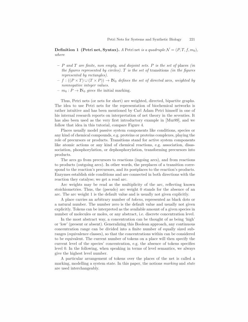
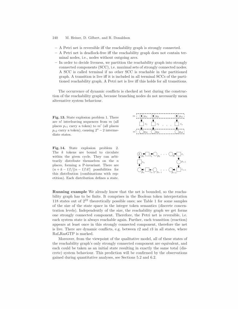
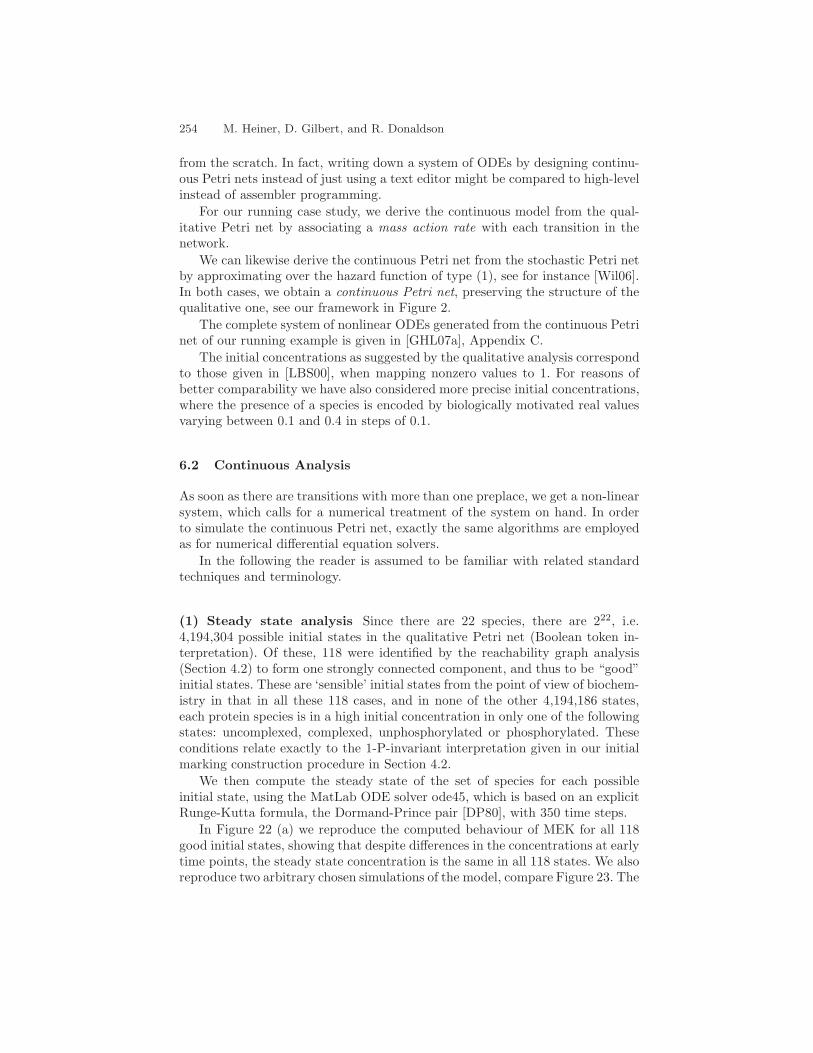ndash intuitive and executable modelling stylendash true concurrency (partial order) semantics which may be lessened to inter-

leaving semantics to simplify analysesndash mathematically founded analysis techniques based on formal semanticsndash coverage of structural and behavioural properties as well as their relationsndash integration of qualitative and quantitative analysis techniquesndash reliable tool support

This chapter can be considered as a tutorial in the step-wise modelling andanalysis of larger biochemical networks as well as in the structured design ofsystems of ordinary differential equations (ODEs) The qualitative model is in-troduced as a supplementary intermediate step at least from the viewpoint ofthe biochemist accustomed to quantitative modelling only and serves mainly formodel validation since this cannot be performed on the continuous level and isgenerally much harder to do on the stochastic level Having successfully validatedthe qualitative model the quantitative models are derived from the qualitativeone by assigning stochastic or deterministic rate functions to all reactions in thenetwork Thus the quantitative models preserve the structure of the qualitativeone and the stochastic Petri net describes a system of stochastic reaction rateequations (RREs) and the continuous Petri net is nothing else than a structureddescription of ODEs

systems biology modelling as formal knowledge representation

synthetic biology modelling for system construction

biosystemnatural

biosystemsynthetic

observedbehaviour

predictedbehaviour

model(blueprint)

desiredbehaviour

design construction

verification verification

observedbehaviour

predictedbehaviour

wetlab

model-basedexperiment design

experiments

formalizingunderstanding

wetlab experiments

model(knowledge)

Fig 1 The role of formal models in systems biology and synthetic biology










Qualitative


Abs

trac

tion


MoleculesLevels


CTLLTL

MoleculesLevels

Stochastic rates


RREs

CSLPLTL

Concentrations

Deterministic rates


ODEs

LTLc

Abstraction



Time-free

Timed

Quantitative














Raf RafP

MEKP MEKPPMEK

ERKP ERKPPERK

Phosphatase3

Phosphatase1

Phosphatase2

RasGTP





















species


⋃


⋃














O2

H2 4H2O

H2O

H2

O2

H2O4

H2

O2

r

r

r

22

22

22








A B A B BA

BA

E

E

BA_EA

A B

E E

BA

A A_E B

E

A

A_E1

B

E1

B_E2

E2 E2

B_E2

E1

B

A_E1

A

r1

r1

r2

r1

r3r2

r1

r1

r2

r3

r1

r2r3

r4

r5r6

r6

r3

(a) (b) (c)

(d) (e) (f)

(g) (h)

(i) (j)

r1r2

r1r2

r1r2

r1r2

r4r5



Raf

RasGTP

Raf_RasGTP

RafP

RafP_Phase1

MEK_RafP MEKP_RafP


ERK


ERKP

MEKPP


MEKP

ERKPP

Phase2

Phase3

MEK

Phase1

r3

r6

r21

r18

r9 r12

r15

r24

r27r30





r1r2

r4r5

r7r8 r10r11

r16r17

r22r23r19r20

r13r14

r28r29 r25r26




















BA CD

E F

r1

r2

r3 r5

r6r4

r7

r8

r92 2












sum









































r1 2 AE


r1 r2 r3


E

r1

r2

r3

2 2

x1 = (1 1 0) = (A B)x2 = (0 0 1) = (E)

y1 = (1 0 2) = (r1 2 middot r3)y2 = (0 1 1) = (r2 r3)

y3 = (1 1 3) = y1 + y2





sum(ai middot xi)










T-invariant



|||||











y1minus5 = y1 + y2 + y3 + y4 + y5













Raf_RasGTP

RasGTP

RafP

MEK_RafP

RafP MEKP

MEKP_RafP

RafP MEKPP

ERK_MEKPP

MEKPP ERKP

MEKPP ERKPP

ERKP_MEKPP

Phase1

RafP_Phase1

Raf Phase1

MEKPP_Phase2

MEKP Phase2

MEKP_Phase2


ERKP_Phase3

Phase3ERKP

ERKPP_Phase3

r1

r3

r7

r9

r10

r12

r19

r21

r22

r24

r4

r6

r13

r15

r16

r18

r25

r30

r28

r27





( r1 r3 r7 r9 r10 r12( ( r4 r6 )

( ( r19 r21 r22 r24 )( ( r13 r15 r16 r18 ) ( r25 r27 r28 r30 ) ) ) ) )





















BA C D

Er1

r2r3

r4

r5









A B

E

r1

r2

r3

2 2

m0 2A E

m1 2B E m2A B E

r1

r3

r2

r2 r3















mprime

m

r1 r2 rn

p12

p21p11

p22

pn1

pn2


ri+1pi+2

pi+1

pnminus1

kp1

pn

p2r1

rn

ri

rnminus1

pi






1 52 1184 115 24 middot104

8 269 61 middot106

40 3697 47 middot1014

80 13472 56 middot1018

120 29347 17 middot1021









m0 2A E

m1 2B E m2A B E

r1

r3

r2

r2 r3

m0

m1 m2

m2 m1m0

m1m0 m1 m2 m2

r1 r2

r3 r2

r3 r2 r1 r3

r3

r2


φ

φ

φ

φ

φ

φ

φφ

φ

φ

φ

φφ

φ

φφ

φ1

φ1

φ1

φ1

φ2 φ2

φ2

φ2

EX φ AX φ

AF φEF φ

AG φEG φ


φ













43 Summary


















H =









ht = ct middotprod

pisinbullt

(m(p)

f(p t)

)

(1)






pisinbullt

(m(p)

N) (2)












CRafP (t) = 01s

middot4ssum

i=1


)

︸︷︷︸



s




004

006

008

01

012

014

016

018

02

0 20 40 60 80 100

Concentr

ation

Time

MEK

Continuous

Stochastic 4 level

Stochastic 8 level

0055

006

0065

007

0075

008

0085

009

0095

01

0 20 40 60 80 100

Concentr

ation

Time

RasGTP

Continuous

Stochastic 4 level

Stochastic 8 level












0

02

04

06

08

1

0 1 2 3 4 5 6 7 8

Pro

babili

ty

Level


0

02

04

06

08

1

0 1 2 3 4 5 6 7 8

Pro

babili

ty

Level






















4 10 s b 750 KB





53 Summary









0 1 2 3 400

04

08

4 Molecules

Level

Pro

babili

ty


0 10 20 30 40

00

04

08

40 Molecules

Level

Pro

babili

ty


0 100 200 300 400

00

04

08

400 Molecules

Level

Pro

babili

ty


0 1000 2000 3000 4000

00

04

08

4000 Molecules

Level

Pro

babili

ty



0 1 2 3 4

00

04

08

4 Molecules

Level

Pro

babili

ty


0 10 20 30 40

00

04

08

40 Molecules

Level

Pro

babili

ty


0 100 200 300 400

00

04

08

400 Molecules

Level

Pro

babili

ty


0 1000 2000 3000 4000

00

04

08

4000 Molecules

Level

Pro

babili

ty









H =









m isin(IR+

0




dm (p)

dt=

sum

tisinbullp


tisinp bull

f (p t) v (t)



















0 50 100 150 200 250 300 3500

01

02

03

04

05

06

07

08

09

1

Time (sec)

Con

cent

ratio

n (r

elat

ive

units

)

MEK

MEK

0

002

004

006

008

01

012

0 50 100 150 200 250 300 350

RasGTPRafP

MEKPPERKPP


0 50 100 150 200 250 300 3500

01

02

03

04

05

06

07

08

09

1

Time (sec)

Con

cent

ratio

n (r

elat

ive

units

)

State1

Raf

RKIP

RasGTP

Raf_RasGTP

Rafx

Rafx_Phase1

MEK_Rafx

MEKP_Rafx

MEKP_Phase2

MEKPP_Phase2

ERK

ERK_MEKPP

ERKP_MEKPP

ERKP

MEKPP

ERKPP_Phase3

ERKP_Phase3

MEKP

ERKPP

Phase2

Phase3

MEK

Phase1

0 50 100 150 200 250 300 3500

01

02

03

04

05

06

07

08

09

1

Time (sec)

Con

cent

ratio

n (r

elat

ive

units

)

State10

Raf

RKIP

RasGTP

Raf_RasGTP

Rafx

Rafx_Phase1

MEK_Rafx

MEKP_Rafx

MEKP_Phase2

MEKPP_Phase2

ERK

ERK_MEKPP

ERKP_MEKPP

ERKP

MEKPP

ERKPP_Phase3

ERKP_Phase3

MEKP

ERKPP

Phase2

Phase3

MEK

Phase1



















0 20 40 60 80 100

0000

0003

MEKPP Simulation

Time

Concentration

0 20 40 60 80 100

000000

000020

ERKPP Simulation

Time

Concentration


63 Summary






7 Tools




















9 Summary








References



















































































Qualitative


Abs

trac

tion


MoleculesLevels


CTLLTL

MoleculesLevels

Stochastic rates


RREs

CSLPLTL

Concentrations

Deterministic rates


ODEs

LTLc

Abstraction



Time-free

Timed

Quantitative














Raf RafP

MEKP MEKPPMEK

ERKP ERKPPERK

Phosphatase3

Phosphatase1

Phosphatase2

RasGTP





















species


⋃


⋃














O2

H2 4H2O

H2O

H2

O2

H2O4

H2

O2

r

r

r

22

22

22








A B A B BA

BA

E

E

BA_EA

A B

E E

BA

A A_E B

E

A

A_E1

B

E1

B_E2

E2 E2

B_E2

E1

B

A_E1

A

r1

r1

r2

r1

r3r2

r1

r1

r2

r3

r1

r2r3

r4

r5r6

r6

r3

(a) (b) (c)

(d) (e) (f)

(g) (h)

(i) (j)

r1r2

r1r2

r1r2

r1r2

r4r5



Raf

RasGTP

Raf_RasGTP

RafP

RafP_Phase1

MEK_RafP MEKP_RafP


ERK


ERKP

MEKPP


MEKP

ERKPP

Phase2

Phase3

MEK

Phase1

r3

r6

r21

r18

r9 r12

r15

r24

r27r30





r1r2

r4r5

r7r8 r10r11

r16r17

r22r23r19r20

r13r14

r28r29 r25r26




















BA CD

E F

r1

r2

r3 r5

r6r4

r7

r8

r92 2












sum









































r1 2 AE


r1 r2 r3


E

r1

r2

r3

2 2

x1 = (1 1 0) = (A B)x2 = (0 0 1) = (E)

y1 = (1 0 2) = (r1 2 middot r3)y2 = (0 1 1) = (r2 r3)

y3 = (1 1 3) = y1 + y2





sum(ai middot xi)










T-invariant



|||||











y1minus5 = y1 + y2 + y3 + y4 + y5













Raf_RasGTP

RasGTP

RafP

MEK_RafP

RafP MEKP

MEKP_RafP

RafP MEKPP

ERK_MEKPP

MEKPP ERKP

MEKPP ERKPP

ERKP_MEKPP

Phase1

RafP_Phase1

Raf Phase1

MEKPP_Phase2

MEKP Phase2

MEKP_Phase2


ERKP_Phase3

Phase3ERKP

ERKPP_Phase3

r1

r3

r7

r9

r10

r12

r19

r21

r22

r24

r4

r6

r13

r15

r16

r18

r25

r30

r28

r27





( r1 r3 r7 r9 r10 r12( ( r4 r6 )

( ( r19 r21 r22 r24 )( ( r13 r15 r16 r18 ) ( r25 r27 r28 r30 ) ) ) ) )





















BA C D

Er1

r2r3

r4

r5









A B

E

r1

r2

r3

2 2

m0 2A E

m1 2B E m2A B E

r1

r3

r2

r2 r3















mprime

m

r1 r2 rn

p12

p21p11

p22

pn1

pn2


ri+1pi+2

pi+1

pnminus1

kp1

pn

p2r1

rn

ri

rnminus1

pi






1 52 1184 115 24 middot104

8 269 61 middot106

40 3697 47 middot1014

80 13472 56 middot1018

120 29347 17 middot1021









m0 2A E

m1 2B E m2A B E

r1

r3

r2

r2 r3

m0

m1 m2

m2 m1m0

m1m0 m1 m2 m2

r1 r2

r3 r2

r3 r2 r1 r3

r3

r2


φ

φ

φ

φ

φ

φ

φφ

φ

φ

φ

φφ

φ

φφ

φ1

φ1

φ1

φ1

φ2 φ2

φ2

φ2

EX φ AX φ

AF φEF φ

AG φEG φ


φ













43 Summary


















H =









ht = ct middotprod

pisinbullt

(m(p)

f(p t)

)

(1)






pisinbullt

(m(p)

N) (2)












CRafP (t) = 01s

middot4ssum

i=1


)

︸︷︷︸



s




004

006

008

01

012

014

016

018

02

0 20 40 60 80 100

Concentr

ation

Time

MEK

Continuous

Stochastic 4 level

Stochastic 8 level

0055

006

0065

007

0075

008

0085

009

0095

01

0 20 40 60 80 100

Concentr

ation

Time

RasGTP

Continuous

Stochastic 4 level

Stochastic 8 level












0

02

04

06

08

1

0 1 2 3 4 5 6 7 8

Pro

babili

ty

Level


0

02

04

06

08

1

0 1 2 3 4 5 6 7 8

Pro

babili

ty

Level






















4 10 s b 750 KB





53 Summary









0 1 2 3 400

04

08

4 Molecules

Level

Pro

babili

ty


0 10 20 30 40

00

04

08

40 Molecules

Level

Pro

babili

ty


0 100 200 300 400

00

04

08

400 Molecules

Level

Pro

babili

ty


0 1000 2000 3000 4000

00

04

08

4000 Molecules

Level

Pro

babili

ty



0 1 2 3 4

00

04

08

4 Molecules

Level

Pro

babili

ty


0 10 20 30 40

00

04

08

40 Molecules

Level

Pro

babili

ty


0 100 200 300 400

00

04

08

400 Molecules

Level

Pro

babili

ty


0 1000 2000 3000 4000

00

04

08

4000 Molecules

Level

Pro

babili

ty









H =









m isin(IR+

0




dm (p)

dt=

sum

tisinbullp


tisinp bull

f (p t) v (t)



















0 50 100 150 200 250 300 3500

01

02

03

04

05

06

07

08

09

1

Time (sec)

Con

cent

ratio

n (r

elat

ive

units

)

MEK

MEK

0

002

004

006

008

01

012

0 50 100 150 200 250 300 350

RasGTPRafP

MEKPPERKPP


0 50 100 150 200 250 300 3500

01

02

03

04

05

06

07

08

09

1

Time (sec)

Con

cent

ratio

n (r

elat

ive

units

)

State1

Raf

RKIP

RasGTP

Raf_RasGTP

Rafx

Rafx_Phase1

MEK_Rafx

MEKP_Rafx

MEKP_Phase2

MEKPP_Phase2

ERK

ERK_MEKPP

ERKP_MEKPP

ERKP

MEKPP

ERKPP_Phase3

ERKP_Phase3

MEKP

ERKPP

Phase2

Phase3

MEK

Phase1

0 50 100 150 200 250 300 3500

01

02

03

04

05

06

07

08

09

1

Time (sec)

Con

cent

ratio

n (r

elat

ive

units

)

State10

Raf

RKIP

RasGTP

Raf_RasGTP

Rafx

Rafx_Phase1

MEK_Rafx

MEKP_Rafx

MEKP_Phase2

MEKPP_Phase2

ERK

ERK_MEKPP

ERKP_MEKPP

ERKP

MEKPP

ERKPP_Phase3

ERKP_Phase3

MEKP

ERKPP

Phase2

Phase3

MEK

Phase1



















0 20 40 60 80 100

0000

0003

MEKPP Simulation

Time

Concentration

0 20 40 60 80 100

000000

000020

ERKPP Simulation

Time

Concentration


63 Summary






7 Tools




















9 Summary








References



















































































Raf RafP

MEKP MEKPPMEK

ERKP ERKPPERK

Phosphatase3

Phosphatase1

Phosphatase2

RasGTP





















species


⋃


⋃














O2

H2 4H2O

H2O

H2

O2

H2O4

H2

O2

r

r

r

22

22

22








A B A B BA

BA

E

E

BA_EA

A B

E E

BA

A A_E B

E

A

A_E1

B

E1

B_E2

E2 E2

B_E2

E1

B

A_E1

A

r1

r1

r2

r1

r3r2

r1

r1

r2

r3

r1

r2r3

r4

r5r6

r6

r3

(a) (b) (c)

(d) (e) (f)

(g) (h)

(i) (j)

r1r2

r1r2

r1r2

r1r2

r4r5



Raf

RasGTP

Raf_RasGTP

RafP

RafP_Phase1

MEK_RafP MEKP_RafP


ERK


ERKP

MEKPP


MEKP

ERKPP

Phase2

Phase3

MEK

Phase1

r3

r6

r21

r18

r9 r12

r15

r24

r27r30





r1r2

r4r5

r7r8 r10r11

r16r17

r22r23r19r20

r13r14

r28r29 r25r26




















BA CD

E F

r1

r2

r3 r5

r6r4

r7

r8

r92 2












sum









































r1 2 AE


r1 r2 r3


E

r1

r2

r3

2 2

x1 = (1 1 0) = (A B)x2 = (0 0 1) = (E)

y1 = (1 0 2) = (r1 2 middot r3)y2 = (0 1 1) = (r2 r3)

y3 = (1 1 3) = y1 + y2





sum(ai middot xi)










T-invariant



|||||











y1minus5 = y1 + y2 + y3 + y4 + y5













Raf_RasGTP

RasGTP

RafP

MEK_RafP

RafP MEKP

MEKP_RafP

RafP MEKPP

ERK_MEKPP

MEKPP ERKP

MEKPP ERKPP

ERKP_MEKPP

Phase1

RafP_Phase1

Raf Phase1

MEKPP_Phase2

MEKP Phase2

MEKP_Phase2


ERKP_Phase3

Phase3ERKP

ERKPP_Phase3

r1

r3

r7

r9

r10

r12

r19

r21

r22

r24

r4

r6

r13

r15

r16

r18

r25

r30

r28

r27





( r1 r3 r7 r9 r10 r12( ( r4 r6 )

( ( r19 r21 r22 r24 )( ( r13 r15 r16 r18 ) ( r25 r27 r28 r30 ) ) ) ) )





















BA C D

Er1

r2r3

r4

r5









A B

E

r1

r2

r3

2 2

m0 2A E

m1 2B E m2A B E

r1

r3

r2

r2 r3















mprime

m

r1 r2 rn

p12

p21p11

p22

pn1

pn2


ri+1pi+2

pi+1

pnminus1

kp1

pn

p2r1

rn

ri

rnminus1

pi






1 52 1184 115 24 middot104

8 269 61 middot106

40 3697 47 middot1014

80 13472 56 middot1018

120 29347 17 middot1021









m0 2A E

m1 2B E m2A B E

r1

r3

r2

r2 r3

m0

m1 m2

m2 m1m0

m1m0 m1 m2 m2

r1 r2

r3 r2

r3 r2 r1 r3

r3

r2


φ

φ

φ

φ

φ

φ

φφ

φ

φ

φ

φφ

φ

φφ

φ1

φ1

φ1

φ1

φ2 φ2

φ2

φ2

EX φ AX φ

AF φEF φ

AG φEG φ


φ













43 Summary


















H =









ht = ct middotprod

pisinbullt

(m(p)

f(p t)

)

(1)






pisinbullt

(m(p)

N) (2)












CRafP (t) = 01s

middot4ssum

i=1


)

︸︷︷︸



s




004

006

008

01

012

014

016

018

02

0 20 40 60 80 100

Concentr

ation

Time

MEK

Continuous

Stochastic 4 level

Stochastic 8 level

0055

006

0065

007

0075

008

0085

009

0095

01

0 20 40 60 80 100

Concentr

ation

Time

RasGTP

Continuous

Stochastic 4 level

Stochastic 8 level












0

02

04

06

08

1

0 1 2 3 4 5 6 7 8

Pro

babili

ty

Level


0

02

04

06

08

1

0 1 2 3 4 5 6 7 8

Pro

babili

ty

Level






















4 10 s b 750 KB





53 Summary









0 1 2 3 400

04

08

4 Molecules

Level

Pro

babili

ty


0 10 20 30 40

00

04

08

40 Molecules

Level

Pro

babili

ty


0 100 200 300 400

00

04

08

400 Molecules

Level

Pro

babili

ty


0 1000 2000 3000 4000

00

04

08

4000 Molecules

Level

Pro

babili

ty



0 1 2 3 4

00

04

08

4 Molecules

Level

Pro

babili

ty


0 10 20 30 40

00

04

08

40 Molecules

Level

Pro

babili

ty


0 100 200 300 400

00

04

08

400 Molecules

Level

Pro

babili

ty


0 1000 2000 3000 4000

00

04

08

4000 Molecules

Level

Pro

babili

ty









H =









m isin(IR+

0




dm (p)

dt=

sum

tisinbullp


tisinp bull

f (p t) v (t)



















0 50 100 150 200 250 300 3500

01

02

03

04

05

06

07

08

09

1

Time (sec)

Con

cent

ratio

n (r

elat

ive

units

)

MEK

MEK

0

002

004

006

008

01

012

0 50 100 150 200 250 300 350

RasGTPRafP

MEKPPERKPP


0 50 100 150 200 250 300 3500

01

02

03

04

05

06

07

08

09

1

Time (sec)

Con

cent

ratio

n (r

elat

ive

units

)

State1

Raf

RKIP

RasGTP

Raf_RasGTP

Rafx

Rafx_Phase1

MEK_Rafx

MEKP_Rafx

MEKP_Phase2

MEKPP_Phase2

ERK

ERK_MEKPP

ERKP_MEKPP

ERKP

MEKPP

ERKPP_Phase3

ERKP_Phase3

MEKP

ERKPP

Phase2

Phase3

MEK

Phase1

0 50 100 150 200 250 300 3500

01

02

03

04

05

06

07

08

09

1

Time (sec)

Con

cent

ratio

n (r

elat

ive

units

)

State10

Raf

RKIP

RasGTP

Raf_RasGTP

Rafx

Rafx_Phase1

MEK_Rafx

MEKP_Rafx

MEKP_Phase2

MEKPP_Phase2

ERK

ERK_MEKPP

ERKP_MEKPP

ERKP

MEKPP

ERKPP_Phase3

ERKP_Phase3

MEKP

ERKPP

Phase2

Phase3

MEK

Phase1



















0 20 40 60 80 100

0000

0003

MEKPP Simulation

Time

Concentration

0 20 40 60 80 100

000000

000020

ERKPP Simulation

Time

Concentration


63 Summary






7 Tools




















9 Summary








References


























































































species


⋃


⋃














O2

H2 4H2O

H2O

H2

O2

H2O4

H2

O2

r

r

r

22

22

22








A B A B BA

BA

E

E

BA_EA

A B

E E

BA

A A_E B

E

A

A_E1

B

E1

B_E2

E2 E2

B_E2

E1

B

A_E1

A

r1

r1

r2

r1

r3r2

r1

r1

r2

r3

r1

r2r3

r4

r5r6

r6

r3

(a) (b) (c)

(d) (e) (f)

(g) (h)

(i) (j)

r1r2

r1r2

r1r2

r1r2

r4r5



Raf

RasGTP

Raf_RasGTP

RafP

RafP_Phase1

MEK_RafP MEKP_RafP


ERK


ERKP

MEKPP


MEKP

ERKPP

Phase2

Phase3

MEK

Phase1

r3

r6

r21

r18

r9 r12

r15

r24

r27r30





r1r2

r4r5

r7r8 r10r11

r16r17

r22r23r19r20

r13r14

r28r29 r25r26




















BA CD

E F

r1

r2

r3 r5

r6r4

r7

r8

r92 2












sum









































r1 2 AE


r1 r2 r3


E

r1

r2

r3

2 2

x1 = (1 1 0) = (A B)x2 = (0 0 1) = (E)

y1 = (1 0 2) = (r1 2 middot r3)y2 = (0 1 1) = (r2 r3)

y3 = (1 1 3) = y1 + y2





sum(ai middot xi)










T-invariant



|||||











y1minus5 = y1 + y2 + y3 + y4 + y5













Raf_RasGTP

RasGTP

RafP

MEK_RafP

RafP MEKP

MEKP_RafP

RafP MEKPP

ERK_MEKPP

MEKPP ERKP

MEKPP ERKPP

ERKP_MEKPP

Phase1

RafP_Phase1

Raf Phase1

MEKPP_Phase2

MEKP Phase2

MEKP_Phase2


ERKP_Phase3

Phase3ERKP

ERKPP_Phase3

r1

r3

r7

r9

r10

r12

r19

r21

r22

r24

r4

r6

r13

r15

r16

r18

r25

r30

r28

r27





( r1 r3 r7 r9 r10 r12( ( r4 r6 )

( ( r19 r21 r22 r24 )( ( r13 r15 r16 r18 ) ( r25 r27 r28 r30 ) ) ) ) )





















BA C D

Er1

r2r3

r4

r5









A B

E

r1

r2

r3

2 2

m0 2A E

m1 2B E m2A B E

r1

r3

r2

r2 r3















mprime

m

r1 r2 rn

p12

p21p11

p22

pn1

pn2


ri+1pi+2

pi+1

pnminus1

kp1

pn

p2r1

rn

ri

rnminus1

pi






1 52 1184 115 24 middot104

8 269 61 middot106

40 3697 47 middot1014

80 13472 56 middot1018

120 29347 17 middot1021









m0 2A E

m1 2B E m2A B E

r1

r3

r2

r2 r3

m0

m1 m2

m2 m1m0

m1m0 m1 m2 m2

r1 r2

r3 r2

r3 r2 r1 r3

r3

r2


φ

φ

φ

φ

φ

φ

φφ

φ

φ

φ

φφ

φ

φφ

φ1

φ1

φ1

φ1

φ2 φ2

φ2

φ2

EX φ AX φ

AF φEF φ

AG φEG φ


φ













43 Summary


















H =









ht = ct middotprod

pisinbullt

(m(p)

f(p t)

)

(1)






pisinbullt

(m(p)

N) (2)












CRafP (t) = 01s

middot4ssum

i=1


)

︸︷︷︸



s




004

006

008

01

012

014

016

018

02

0 20 40 60 80 100

Concentr

ation

Time

MEK

Continuous

Stochastic 4 level

Stochastic 8 level

0055

006

0065

007

0075

008

0085

009

0095

01

0 20 40 60 80 100

Concentr

ation

Time

RasGTP

Continuous

Stochastic 4 level

Stochastic 8 level












0

02

04

06

08

1

0 1 2 3 4 5 6 7 8

Pro

babili

ty

Level


0

02

04

06

08

1

0 1 2 3 4 5 6 7 8

Pro

babili

ty

Level






















4 10 s b 750 KB





53 Summary









0 1 2 3 400

04

08

4 Molecules

Level

Pro

babili

ty


0 10 20 30 40

00

04

08

40 Molecules

Level

Pro

babili

ty


0 100 200 300 400

00

04

08

400 Molecules

Level

Pro

babili

ty


0 1000 2000 3000 4000

00

04

08

4000 Molecules

Level

Pro

babili

ty



0 1 2 3 4

00

04

08

4 Molecules

Level

Pro

babili

ty


0 10 20 30 40

00

04

08

40 Molecules

Level

Pro

babili

ty


0 100 200 300 400

00

04

08

400 Molecules

Level

Pro

babili

ty


0 1000 2000 3000 4000

00

04

08

4000 Molecules

Level

Pro

babili

ty









H =









m isin(IR+

0




dm (p)

dt=

sum

tisinbullp


tisinp bull

f (p t) v (t)



















0 50 100 150 200 250 300 3500

01

02

03

04

05

06

07

08

09

1

Time (sec)

Con

cent

ratio

n (r

elat

ive

units

)

MEK

MEK

0

002

004

006

008

01

012

0 50 100 150 200 250 300 350

RasGTPRafP

MEKPPERKPP


0 50 100 150 200 250 300 3500

01

02

03

04

05

06

07

08

09

1

Time (sec)

Con

cent

ratio

n (r

elat

ive

units

)

State1

Raf

RKIP

RasGTP

Raf_RasGTP

Rafx

Rafx_Phase1

MEK_Rafx

MEKP_Rafx

MEKP_Phase2

MEKPP_Phase2

ERK

ERK_MEKPP

ERKP_MEKPP

ERKP

MEKPP

ERKPP_Phase3

ERKP_Phase3

MEKP

ERKPP

Phase2

Phase3

MEK

Phase1

0 50 100 150 200 250 300 3500

01

02

03

04

05

06

07

08

09

1

Time (sec)

Con

cent

ratio

n (r

elat

ive

units

)

State10

Raf

RKIP

RasGTP

Raf_RasGTP

Rafx

Rafx_Phase1

MEK_Rafx

MEKP_Rafx

MEKP_Phase2

MEKPP_Phase2

ERK

ERK_MEKPP

ERKP_MEKPP

ERKP

MEKPP

ERKPP_Phase3

ERKP_Phase3

MEKP

ERKPP

Phase2

Phase3

MEK

Phase1



















0 20 40 60 80 100

0000

0003

MEKPP Simulation

Time

Concentration

0 20 40 60 80 100

000000

000020

ERKPP Simulation

Time

Concentration


63 Summary






7 Tools




















9 Summary








References












































































O2

H2 4H2O

H2O

H2

O2

H2O4

H2

O2

r

r

r

22

22

22








A B A B BA

BA

E

E

BA_EA

A B

E E

BA

A A_E B

E

A

A_E1

B

E1

B_E2

E2 E2

B_E2

E1

B

A_E1

A

r1

r1

r2

r1

r3r2

r1

r1

r2

r3

r1

r2r3

r4

r5r6

r6

r3

(a) (b) (c)

(d) (e) (f)

(g) (h)

(i) (j)

r1r2

r1r2

r1r2

r1r2

r4r5



Raf

RasGTP

Raf_RasGTP

RafP

RafP_Phase1

MEK_RafP MEKP_RafP


ERK


ERKP

MEKPP


MEKP

ERKPP

Phase2

Phase3

MEK

Phase1

r3

r6

r21

r18

r9 r12

r15

r24

r27r30





r1r2

r4r5

r7r8 r10r11

r16r17

r22r23r19r20

r13r14

r28r29 r25r26




















BA CD

E F

r1

r2

r3 r5

r6r4

r7

r8

r92 2












sum









































r1 2 AE


r1 r2 r3


E

r1

r2

r3

2 2

x1 = (1 1 0) = (A B)x2 = (0 0 1) = (E)

y1 = (1 0 2) = (r1 2 middot r3)y2 = (0 1 1) = (r2 r3)

y3 = (1 1 3) = y1 + y2





sum(ai middot xi)










T-invariant



|||||











y1minus5 = y1 + y2 + y3 + y4 + y5













Raf_RasGTP

RasGTP

RafP

MEK_RafP

RafP MEKP

MEKP_RafP

RafP MEKPP

ERK_MEKPP

MEKPP ERKP

MEKPP ERKPP

ERKP_MEKPP

Phase1

RafP_Phase1

Raf Phase1

MEKPP_Phase2

MEKP Phase2

MEKP_Phase2


ERKP_Phase3

Phase3ERKP

ERKPP_Phase3

r1

r3

r7

r9

r10

r12

r19

r21

r22

r24

r4

r6

r13

r15

r16

r18

r25

r30

r28

r27





( r1 r3 r7 r9 r10 r12( ( r4 r6 )

( ( r19 r21 r22 r24 )( ( r13 r15 r16 r18 ) ( r25 r27 r28 r30 ) ) ) ) )





















BA C D

Er1

r2r3

r4

r5









A B

E

r1

r2

r3

2 2

m0 2A E

m1 2B E m2A B E

r1

r3

r2

r2 r3















mprime

m

r1 r2 rn

p12

p21p11

p22

pn1

pn2


ri+1pi+2

pi+1

pnminus1

kp1

pn

p2r1

rn

ri

rnminus1

pi






1 52 1184 115 24 middot104

8 269 61 middot106

40 3697 47 middot1014

80 13472 56 middot1018

120 29347 17 middot1021









m0 2A E

m1 2B E m2A B E

r1

r3

r2

r2 r3

m0

m1 m2

m2 m1m0

m1m0 m1 m2 m2

r1 r2

r3 r2

r3 r2 r1 r3

r3

r2


φ

φ

φ

φ

φ

φ

φφ

φ

φ

φ

φφ

φ

φφ

φ1

φ1

φ1

φ1

φ2 φ2

φ2

φ2

EX φ AX φ

AF φEF φ

AG φEG φ


φ













43 Summary


















H =









ht = ct middotprod

pisinbullt

(m(p)

f(p t)

)

(1)






pisinbullt

(m(p)

N) (2)












CRafP (t) = 01s

middot4ssum

i=1


)

︸︷︷︸



s




004

006

008

01

012

014

016

018

02

0 20 40 60 80 100

Concentr

ation

Time

MEK

Continuous

Stochastic 4 level

Stochastic 8 level

0055

006

0065

007

0075

008

0085

009

0095

01

0 20 40 60 80 100

Concentr

ation

Time

RasGTP

Continuous

Stochastic 4 level

Stochastic 8 level












0

02

04

06

08

1

0 1 2 3 4 5 6 7 8

Pro

babili

ty

Level


0

02

04

06

08

1

0 1 2 3 4 5 6 7 8

Pro

babili

ty

Level






















4 10 s b 750 KB





53 Summary









0 1 2 3 400

04

08

4 Molecules

Level

Pro

babili

ty


0 10 20 30 40

00

04

08

40 Molecules

Level

Pro

babili

ty


0 100 200 300 400

00

04

08

400 Molecules

Level

Pro

babili

ty


0 1000 2000 3000 4000

00

04

08

4000 Molecules

Level

Pro

babili

ty



0 1 2 3 4

00

04

08

4 Molecules

Level

Pro

babili

ty


0 10 20 30 40

00

04

08

40 Molecules

Level

Pro

babili

ty


0 100 200 300 400

00

04

08

400 Molecules

Level

Pro

babili

ty


0 1000 2000 3000 4000

00

04

08

4000 Molecules

Level

Pro

babili

ty









H =









m isin(IR+

0




dm (p)

dt=

sum

tisinbullp


tisinp bull

f (p t) v (t)



















0 50 100 150 200 250 300 3500

01

02

03

04

05

06

07

08

09

1

Time (sec)

Con

cent

ratio

n (r

elat

ive

units

)

MEK

MEK

0

002

004

006

008

01

012

0 50 100 150 200 250 300 350

RasGTPRafP

MEKPPERKPP


0 50 100 150 200 250 300 3500

01

02

03

04

05

06

07

08

09

1

Time (sec)

Con

cent

ratio

n (r

elat

ive

units

)

State1

Raf

RKIP

RasGTP

Raf_RasGTP

Rafx

Rafx_Phase1

MEK_Rafx

MEKP_Rafx

MEKP_Phase2

MEKPP_Phase2

ERK

ERK_MEKPP

ERKP_MEKPP

ERKP

MEKPP

ERKPP_Phase3

ERKP_Phase3

MEKP

ERKPP

Phase2

Phase3

MEK

Phase1

0 50 100 150 200 250 300 3500

01

02

03

04

05

06

07

08

09

1

Time (sec)

Con

cent

ratio

n (r

elat

ive

units

)

State10

Raf

RKIP

RasGTP

Raf_RasGTP

Rafx

Rafx_Phase1

MEK_Rafx

MEKP_Rafx

MEKP_Phase2

MEKPP_Phase2

ERK

ERK_MEKPP

ERKP_MEKPP

ERKP

MEKPP

ERKPP_Phase3

ERKP_Phase3

MEKP

ERKPP

Phase2

Phase3

MEK

Phase1



















0 20 40 60 80 100

0000

0003

MEKPP Simulation

Time

Concentration

0 20 40 60 80 100

000000

000020

ERKPP Simulation

Time

Concentration


63 Summary






7 Tools




















9 Summary








References











































































A B A B BA

BA

E

E

BA_EA

A B

E E

BA

A A_E B

E

A

A_E1

B

E1

B_E2

E2 E2

B_E2

E1

B

A_E1

A

r1

r1

r2

r1

r3r2

r1

r1

r2

r3

r1

r2r3

r4

r5r6

r6

r3

(a) (b) (c)

(d) (e) (f)

(g) (h)

(i) (j)

r1r2

r1r2

r1r2

r1r2

r4r5



Raf

RasGTP

Raf_RasGTP

RafP

RafP_Phase1

MEK_RafP MEKP_RafP


ERK


ERKP

MEKPP


MEKP

ERKPP

Phase2

Phase3

MEK

Phase1

r3

r6

r21

r18

r9 r12

r15

r24

r27r30





r1r2

r4r5

r7r8 r10r11

r16r17

r22r23r19r20

r13r14

r28r29 r25r26




















BA CD

E F

r1

r2

r3 r5

r6r4

r7

r8

r92 2












sum









































r1 2 AE


r1 r2 r3


E

r1

r2

r3

2 2

x1 = (1 1 0) = (A B)x2 = (0 0 1) = (E)

y1 = (1 0 2) = (r1 2 middot r3)y2 = (0 1 1) = (r2 r3)

y3 = (1 1 3) = y1 + y2





sum(ai middot xi)










T-invariant



|||||











y1minus5 = y1 + y2 + y3 + y4 + y5













Raf_RasGTP

RasGTP

RafP

MEK_RafP

RafP MEKP

MEKP_RafP

RafP MEKPP

ERK_MEKPP

MEKPP ERKP

MEKPP ERKPP

ERKP_MEKPP

Phase1

RafP_Phase1

Raf Phase1

MEKPP_Phase2

MEKP Phase2

MEKP_Phase2


ERKP_Phase3

Phase3ERKP

ERKPP_Phase3

r1

r3

r7

r9

r10

r12

r19

r21

r22

r24

r4

r6

r13

r15

r16

r18

r25

r30

r28

r27





( r1 r3 r7 r9 r10 r12( ( r4 r6 )

( ( r19 r21 r22 r24 )( ( r13 r15 r16 r18 ) ( r25 r27 r28 r30 ) ) ) ) )





















BA C D

Er1

r2r3

r4

r5









A B

E

r1

r2

r3

2 2

m0 2A E

m1 2B E m2A B E

r1

r3

r2

r2 r3















mprime

m

r1 r2 rn

p12

p21p11

p22

pn1

pn2


ri+1pi+2

pi+1

pnminus1

kp1

pn

p2r1

rn

ri

rnminus1

pi






1 52 1184 115 24 middot104

8 269 61 middot106

40 3697 47 middot1014

80 13472 56 middot1018

120 29347 17 middot1021









m0 2A E

m1 2B E m2A B E

r1

r3

r2

r2 r3

m0

m1 m2

m2 m1m0

m1m0 m1 m2 m2

r1 r2

r3 r2

r3 r2 r1 r3

r3

r2


φ

φ

φ

φ

φ

φ

φφ

φ

φ

φ

φφ

φ

φφ

φ1

φ1

φ1

φ1

φ2 φ2

φ2

φ2

EX φ AX φ

AF φEF φ

AG φEG φ


φ













43 Summary


















H =









ht = ct middotprod

pisinbullt

(m(p)

f(p t)

)

(1)






pisinbullt

(m(p)

N) (2)












CRafP (t) = 01s

middot4ssum

i=1


)

︸︷︷︸



s




004

006

008

01

012

014

016

018

02

0 20 40 60 80 100

Concentr

ation

Time

MEK

Continuous

Stochastic 4 level

Stochastic 8 level

0055

006

0065

007

0075

008

0085

009

0095

01

0 20 40 60 80 100

Concentr

ation

Time

RasGTP

Continuous

Stochastic 4 level

Stochastic 8 level












0

02

04

06

08

1

0 1 2 3 4 5 6 7 8

Pro

babili

ty

Level


0

02

04

06

08

1

0 1 2 3 4 5 6 7 8

Pro

babili

ty

Level






















4 10 s b 750 KB





53 Summary









0 1 2 3 400

04

08

4 Molecules

Level

Pro

babili

ty


0 10 20 30 40

00

04

08

40 Molecules

Level

Pro

babili

ty


0 100 200 300 400

00

04

08

400 Molecules

Level

Pro

babili

ty


0 1000 2000 3000 4000

00

04

08

4000 Molecules

Level

Pro

babili

ty



0 1 2 3 4

00

04

08

4 Molecules

Level

Pro

babili

ty


0 10 20 30 40

00

04

08

40 Molecules

Level

Pro

babili

ty


0 100 200 300 400

00

04

08

400 Molecules

Level

Pro

babili

ty


0 1000 2000 3000 4000

00

04

08

4000 Molecules

Level

Pro

babili

ty









H =









m isin(IR+

0




dm (p)

dt=

sum

tisinbullp


tisinp bull

f (p t) v (t)



















0 50 100 150 200 250 300 3500

01

02

03

04

05

06

07

08

09

1

Time (sec)

Con

cent

ratio

n (r

elat

ive

units

)

MEK

MEK

0

002

004

006

008

01

012

0 50 100 150 200 250 300 350

RasGTPRafP

MEKPPERKPP


0 50 100 150 200 250 300 3500

01

02

03

04

05

06

07

08

09

1

Time (sec)

Con

cent

ratio

n (r

elat

ive

units

)

State1

Raf

RKIP

RasGTP

Raf_RasGTP

Rafx

Rafx_Phase1

MEK_Rafx

MEKP_Rafx

MEKP_Phase2

MEKPP_Phase2

ERK

ERK_MEKPP

ERKP_MEKPP

ERKP

MEKPP

ERKPP_Phase3

ERKP_Phase3

MEKP

ERKPP

Phase2

Phase3

MEK

Phase1

0 50 100 150 200 250 300 3500

01

02

03

04

05

06

07

08

09

1

Time (sec)

Con

cent

ratio

n (r

elat

ive

units

)

State10

Raf

RKIP

RasGTP

Raf_RasGTP

Rafx

Rafx_Phase1

MEK_Rafx

MEKP_Rafx

MEKP_Phase2

MEKPP_Phase2

ERK

ERK_MEKPP

ERKP_MEKPP

ERKP

MEKPP

ERKPP_Phase3

ERKP_Phase3

MEKP

ERKPP

Phase2

Phase3

MEK

Phase1



















0 20 40 60 80 100

0000

0003

MEKPP Simulation

Time

Concentration

0 20 40 60 80 100

000000

000020

ERKPP Simulation

Time

Concentration


63 Summary






7 Tools




















9 Summary








References











































































Raf

RasGTP

Raf_RasGTP

RafP

RafP_Phase1

MEK_RafP MEKP_RafP


ERK


ERKP

MEKPP


MEKP

ERKPP

Phase2

Phase3

MEK

Phase1

r3

r6

r21

r18

r9 r12

r15

r24

r27r30





r1r2

r4r5

r7r8 r10r11

r16r17

r22r23r19r20

r13r14

r28r29 r25r26




















BA CD

E F

r1

r2

r3 r5

r6r4

r7

r8

r92 2












sum









































r1 2 AE


r1 r2 r3


E

r1

r2

r3

2 2

x1 = (1 1 0) = (A B)x2 = (0 0 1) = (E)

y1 = (1 0 2) = (r1 2 middot r3)y2 = (0 1 1) = (r2 r3)

y3 = (1 1 3) = y1 + y2





sum(ai middot xi)










T-invariant



|||||











y1minus5 = y1 + y2 + y3 + y4 + y5













Raf_RasGTP

RasGTP

RafP

MEK_RafP

RafP MEKP

MEKP_RafP

RafP MEKPP

ERK_MEKPP

MEKPP ERKP

MEKPP ERKPP

ERKP_MEKPP

Phase1

RafP_Phase1

Raf Phase1

MEKPP_Phase2

MEKP Phase2

MEKP_Phase2


ERKP_Phase3

Phase3ERKP

ERKPP_Phase3

r1

r3

r7

r9

r10

r12

r19

r21

r22

r24

r4

r6

r13

r15

r16

r18

r25

r30

r28

r27





( r1 r3 r7 r9 r10 r12( ( r4 r6 )

( ( r19 r21 r22 r24 )( ( r13 r15 r16 r18 ) ( r25 r27 r28 r30 ) ) ) ) )





















BA C D

Er1

r2r3

r4

r5









A B

E

r1

r2

r3

2 2

m0 2A E

m1 2B E m2A B E

r1

r3

r2

r2 r3















mprime

m

r1 r2 rn

p12

p21p11

p22

pn1

pn2


ri+1pi+2

pi+1

pnminus1

kp1

pn

p2r1

rn

ri

rnminus1

pi






1 52 1184 115 24 middot104

8 269 61 middot106

40 3697 47 middot1014

80 13472 56 middot1018

120 29347 17 middot1021









m0 2A E

m1 2B E m2A B E

r1

r3

r2

r2 r3

m0

m1 m2

m2 m1m0

m1m0 m1 m2 m2

r1 r2

r3 r2

r3 r2 r1 r3

r3

r2


φ

φ

φ

φ

φ

φ

φφ

φ

φ

φ

φφ

φ

φφ

φ1

φ1

φ1

φ1

φ2 φ2

φ2

φ2

EX φ AX φ

AF φEF φ

AG φEG φ


φ













43 Summary


















H =









ht = ct middotprod

pisinbullt

(m(p)

f(p t)

)

(1)






pisinbullt

(m(p)

N) (2)












CRafP (t) = 01s

middot4ssum

i=1


)

︸︷︷︸



s




004

006

008

01

012

014

016

018

02

0 20 40 60 80 100

Concentr

ation

Time

MEK

Continuous

Stochastic 4 level

Stochastic 8 level

0055

006

0065

007

0075

008

0085

009

0095

01

0 20 40 60 80 100

Concentr

ation

Time

RasGTP

Continuous

Stochastic 4 level

Stochastic 8 level












0

02

04

06

08

1

0 1 2 3 4 5 6 7 8

Pro

babili

ty

Level


0

02

04

06

08

1

0 1 2 3 4 5 6 7 8

Pro

babili

ty

Level






















4 10 s b 750 KB





53 Summary









0 1 2 3 400

04

08

4 Molecules

Level

Pro

babili

ty


0 10 20 30 40

00

04

08

40 Molecules

Level

Pro

babili

ty


0 100 200 300 400

00

04

08

400 Molecules

Level

Pro

babili

ty


0 1000 2000 3000 4000

00

04

08

4000 Molecules

Level

Pro

babili

ty



0 1 2 3 4

00

04

08

4 Molecules

Level

Pro

babili

ty


0 10 20 30 40

00

04

08

40 Molecules

Level

Pro

babili

ty


0 100 200 300 400

00

04

08

400 Molecules

Level

Pro

babili

ty


0 1000 2000 3000 4000

00

04

08

4000 Molecules

Level

Pro

babili

ty









H =









m isin(IR+

0




dm (p)

dt=

sum

tisinbullp


tisinp bull

f (p t) v (t)



















0 50 100 150 200 250 300 3500

01

02

03

04

05

06

07

08

09

1

Time (sec)

Con

cent

ratio

n (r

elat

ive

units

)

MEK

MEK

0

002

004

006

008

01

012

0 50 100 150 200 250 300 350

RasGTPRafP

MEKPPERKPP


0 50 100 150 200 250 300 3500

01

02

03

04

05

06

07

08

09

1

Time (sec)

Con

cent

ratio

n (r

elat

ive

units

)

State1

Raf

RKIP

RasGTP

Raf_RasGTP

Rafx

Rafx_Phase1

MEK_Rafx

MEKP_Rafx

MEKP_Phase2

MEKPP_Phase2

ERK

ERK_MEKPP

ERKP_MEKPP

ERKP

MEKPP

ERKPP_Phase3

ERKP_Phase3

MEKP

ERKPP

Phase2

Phase3

MEK

Phase1

0 50 100 150 200 250 300 3500

01

02

03

04

05

06

07

08

09

1

Time (sec)

Con

cent

ratio

n (r

elat

ive

units

)

State10

Raf

RKIP

RasGTP

Raf_RasGTP

Rafx

Rafx_Phase1

MEK_Rafx

MEKP_Rafx

MEKP_Phase2

MEKPP_Phase2

ERK

ERK_MEKPP

ERKP_MEKPP

ERKP

MEKPP

ERKPP_Phase3

ERKP_Phase3

MEKP

ERKPP

Phase2

Phase3

MEK

Phase1



















0 20 40 60 80 100

0000

0003

MEKPP Simulation

Time

Concentration

0 20 40 60 80 100

000000

000020

ERKPP Simulation

Time

Concentration


63 Summary






7 Tools




















9 Summary








References




























































































BA CD

E F

r1

r2

r3 r5

r6r4

r7

r8

r92 2












sum









































r1 2 AE


r1 r2 r3


E

r1

r2

r3

2 2

x1 = (1 1 0) = (A B)x2 = (0 0 1) = (E)

y1 = (1 0 2) = (r1 2 middot r3)y2 = (0 1 1) = (r2 r3)

y3 = (1 1 3) = y1 + y2





sum(ai middot xi)










T-invariant



|||||











y1minus5 = y1 + y2 + y3 + y4 + y5













Raf_RasGTP

RasGTP

RafP

MEK_RafP

RafP MEKP

MEKP_RafP

RafP MEKPP

ERK_MEKPP

MEKPP ERKP

MEKPP ERKPP

ERKP_MEKPP

Phase1

RafP_Phase1

Raf Phase1

MEKPP_Phase2

MEKP Phase2

MEKP_Phase2


ERKP_Phase3

Phase3ERKP

ERKPP_Phase3

r1

r3

r7

r9

r10

r12

r19

r21

r22

r24

r4

r6

r13

r15

r16

r18

r25

r30

r28

r27





( r1 r3 r7 r9 r10 r12( ( r4 r6 )

( ( r19 r21 r22 r24 )( ( r13 r15 r16 r18 ) ( r25 r27 r28 r30 ) ) ) ) )





















BA C D

Er1

r2r3

r4

r5









A B

E

r1

r2

r3

2 2

m0 2A E

m1 2B E m2A B E

r1

r3

r2

r2 r3















mprime

m

r1 r2 rn

p12

p21p11

p22

pn1

pn2


ri+1pi+2

pi+1

pnminus1

kp1

pn

p2r1

rn

ri

rnminus1

pi






1 52 1184 115 24 middot104

8 269 61 middot106

40 3697 47 middot1014

80 13472 56 middot1018

120 29347 17 middot1021









m0 2A E

m1 2B E m2A B E

r1

r3

r2

r2 r3

m0

m1 m2

m2 m1m0

m1m0 m1 m2 m2

r1 r2

r3 r2

r3 r2 r1 r3

r3

r2


φ

φ

φ

φ

φ

φ

φφ

φ

φ

φ

φφ

φ

φφ

φ1

φ1

φ1

φ1

φ2 φ2

φ2

φ2

EX φ AX φ

AF φEF φ

AG φEG φ


φ













43 Summary


















H =









ht = ct middotprod

pisinbullt

(m(p)

f(p t)

)

(1)






pisinbullt

(m(p)

N) (2)












CRafP (t) = 01s

middot4ssum

i=1


)

︸︷︷︸



s




004

006

008

01

012

014

016

018

02

0 20 40 60 80 100

Concentr

ation

Time

MEK

Continuous

Stochastic 4 level

Stochastic 8 level

0055

006

0065

007

0075

008

0085

009

0095

01

0 20 40 60 80 100

Concentr

ation

Time

RasGTP

Continuous

Stochastic 4 level

Stochastic 8 level












0

02

04

06

08

1

0 1 2 3 4 5 6 7 8

Pro

babili

ty

Level


0

02

04

06

08

1

0 1 2 3 4 5 6 7 8

Pro

babili

ty

Level






















4 10 s b 750 KB





53 Summary









0 1 2 3 400

04

08

4 Molecules

Level

Pro

babili

ty


0 10 20 30 40

00

04

08

40 Molecules

Level

Pro

babili

ty


0 100 200 300 400

00

04

08

400 Molecules

Level

Pro

babili

ty


0 1000 2000 3000 4000

00

04

08

4000 Molecules

Level

Pro

babili

ty



0 1 2 3 4

00

04

08

4 Molecules

Level

Pro

babili

ty


0 10 20 30 40

00

04

08

40 Molecules

Level

Pro

babili

ty


0 100 200 300 400

00

04

08

400 Molecules

Level

Pro

babili

ty


0 1000 2000 3000 4000

00

04

08

4000 Molecules

Level

Pro

babili

ty









H =









m isin(IR+

0




dm (p)

dt=

sum

tisinbullp


tisinp bull

f (p t) v (t)



















0 50 100 150 200 250 300 3500

01

02

03

04

05

06

07

08

09

1

Time (sec)

Con

cent

ratio

n (r

elat

ive

units

)

MEK

MEK

0

002

004

006

008

01

012

0 50 100 150 200 250 300 350

RasGTPRafP

MEKPPERKPP


0 50 100 150 200 250 300 3500

01

02

03

04

05

06

07

08

09

1

Time (sec)

Con

cent

ratio

n (r

elat

ive

units

)

State1

Raf

RKIP

RasGTP

Raf_RasGTP

Rafx

Rafx_Phase1

MEK_Rafx

MEKP_Rafx

MEKP_Phase2

MEKPP_Phase2

ERK

ERK_MEKPP

ERKP_MEKPP

ERKP

MEKPP

ERKPP_Phase3

ERKP_Phase3

MEKP

ERKPP

Phase2

Phase3

MEK

Phase1

0 50 100 150 200 250 300 3500

01

02

03

04

05

06

07

08

09

1

Time (sec)

Con

cent

ratio

n (r

elat

ive

units

)

State10

Raf

RKIP

RasGTP

Raf_RasGTP

Rafx

Rafx_Phase1

MEK_Rafx

MEKP_Rafx

MEKP_Phase2

MEKPP_Phase2

ERK

ERK_MEKPP

ERKP_MEKPP

ERKP

MEKPP

ERKPP_Phase3

ERKP_Phase3

MEKP

ERKPP

Phase2

Phase3

MEK

Phase1



















0 20 40 60 80 100

0000

0003

MEKPP Simulation

Time

Concentration

0 20 40 60 80 100

000000

000020

ERKPP Simulation

Time

Concentration


63 Summary






7 Tools




















9 Summary








References
















































































sum









































r1 2 AE


r1 r2 r3


E

r1

r2

r3

2 2

x1 = (1 1 0) = (A B)x2 = (0 0 1) = (E)

y1 = (1 0 2) = (r1 2 middot r3)y2 = (0 1 1) = (r2 r3)

y3 = (1 1 3) = y1 + y2





sum(ai middot xi)










T-invariant



|||||











y1minus5 = y1 + y2 + y3 + y4 + y5













Raf_RasGTP

RasGTP

RafP

MEK_RafP

RafP MEKP

MEKP_RafP

RafP MEKPP

ERK_MEKPP

MEKPP ERKP

MEKPP ERKPP

ERKP_MEKPP

Phase1

RafP_Phase1

Raf Phase1

MEKPP_Phase2

MEKP Phase2

MEKP_Phase2


ERKP_Phase3

Phase3ERKP

ERKPP_Phase3

r1

r3

r7

r9

r10

r12

r19

r21

r22

r24

r4

r6

r13

r15

r16

r18

r25

r30

r28

r27





( r1 r3 r7 r9 r10 r12( ( r4 r6 )

( ( r19 r21 r22 r24 )( ( r13 r15 r16 r18 ) ( r25 r27 r28 r30 ) ) ) ) )





















BA C D

Er1

r2r3

r4

r5









A B

E

r1

r2

r3

2 2

m0 2A E

m1 2B E m2A B E

r1

r3

r2

r2 r3















mprime

m

r1 r2 rn

p12

p21p11

p22

pn1

pn2


ri+1pi+2

pi+1

pnminus1

kp1

pn

p2r1

rn

ri

rnminus1

pi






1 52 1184 115 24 middot104

8 269 61 middot106

40 3697 47 middot1014

80 13472 56 middot1018

120 29347 17 middot1021









m0 2A E

m1 2B E m2A B E

r1

r3

r2

r2 r3

m0

m1 m2

m2 m1m0

m1m0 m1 m2 m2

r1 r2

r3 r2

r3 r2 r1 r3

r3

r2


φ

φ

φ

φ

φ

φ

φφ

φ

φ

φ

φφ

φ

φφ

φ1

φ1

φ1

φ1

φ2 φ2

φ2

φ2

EX φ AX φ

AF φEF φ

AG φEG φ


φ













43 Summary


















H =









ht = ct middotprod

pisinbullt

(m(p)

f(p t)

)

(1)






pisinbullt

(m(p)

N) (2)












CRafP (t) = 01s

middot4ssum

i=1


)

︸︷︷︸



s




004

006

008

01

012

014

016

018

02

0 20 40 60 80 100

Concentr

ation

Time

MEK

Continuous

Stochastic 4 level

Stochastic 8 level

0055

006

0065

007

0075

008

0085

009

0095

01

0 20 40 60 80 100

Concentr

ation

Time

RasGTP

Continuous

Stochastic 4 level

Stochastic 8 level












0

02

04

06

08

1

0 1 2 3 4 5 6 7 8

Pro

babili

ty

Level


0

02

04

06

08

1

0 1 2 3 4 5 6 7 8

Pro

babili

ty

Level






















4 10 s b 750 KB





53 Summary









0 1 2 3 400

04

08

4 Molecules

Level

Pro

babili

ty


0 10 20 30 40

00

04

08

40 Molecules

Level

Pro

babili

ty


0 100 200 300 400

00

04

08

400 Molecules

Level

Pro

babili

ty


0 1000 2000 3000 4000

00

04

08

4000 Molecules

Level

Pro

babili

ty



0 1 2 3 4

00

04

08

4 Molecules

Level

Pro

babili

ty


0 10 20 30 40

00

04

08

40 Molecules

Level

Pro

babili

ty


0 100 200 300 400

00

04

08

400 Molecules

Level

Pro

babili

ty


0 1000 2000 3000 4000

00

04

08

4000 Molecules

Level

Pro

babili

ty









H =









m isin(IR+

0




dm (p)

dt=

sum

tisinbullp


tisinp bull

f (p t) v (t)



















0 50 100 150 200 250 300 3500

01

02

03

04

05

06

07

08

09

1

Time (sec)

Con

cent

ratio

n (r

elat

ive

units

)

MEK

MEK

0

002

004

006

008

01

012

0 50 100 150 200 250 300 350

RasGTPRafP

MEKPPERKPP


0 50 100 150 200 250 300 3500

01

02

03

04

05

06

07

08

09

1

Time (sec)

Con

cent

ratio

n (r

elat

ive

units

)

State1

Raf

RKIP

RasGTP

Raf_RasGTP

Rafx

Rafx_Phase1

MEK_Rafx

MEKP_Rafx

MEKP_Phase2

MEKPP_Phase2

ERK

ERK_MEKPP

ERKP_MEKPP

ERKP

MEKPP

ERKPP_Phase3

ERKP_Phase3

MEKP

ERKPP

Phase2

Phase3

MEK

Phase1

0 50 100 150 200 250 300 3500

01

02

03

04

05

06

07

08

09

1

Time (sec)

Con

cent

ratio

n (r

elat

ive

units

)

State10

Raf

RKIP

RasGTP

Raf_RasGTP

Rafx

Rafx_Phase1

MEK_Rafx

MEKP_Rafx

MEKP_Phase2

MEKPP_Phase2

ERK

ERK_MEKPP

ERKP_MEKPP

ERKP

MEKPP

ERKPP_Phase3

ERKP_Phase3

MEKP

ERKPP

Phase2

Phase3

MEK

Phase1



















0 20 40 60 80 100

0000

0003

MEKPP Simulation

Time

Concentration

0 20 40 60 80 100

000000

000020

ERKPP Simulation

Time

Concentration


63 Summary






7 Tools




















9 Summary








References











































































































r1 2 AE


r1 r2 r3


E

r1

r2

r3

2 2

x1 = (1 1 0) = (A B)x2 = (0 0 1) = (E)

y1 = (1 0 2) = (r1 2 middot r3)y2 = (0 1 1) = (r2 r3)

y3 = (1 1 3) = y1 + y2





sum(ai middot xi)










T-invariant



|||||











y1minus5 = y1 + y2 + y3 + y4 + y5













Raf_RasGTP

RasGTP

RafP

MEK_RafP

RafP MEKP

MEKP_RafP

RafP MEKPP

ERK_MEKPP

MEKPP ERKP

MEKPP ERKPP

ERKP_MEKPP

Phase1

RafP_Phase1

Raf Phase1

MEKPP_Phase2

MEKP Phase2

MEKP_Phase2


ERKP_Phase3

Phase3ERKP

ERKPP_Phase3

r1

r3

r7

r9

r10

r12

r19

r21

r22

r24

r4

r6

r13

r15

r16

r18

r25

r30

r28

r27





( r1 r3 r7 r9 r10 r12( ( r4 r6 )

( ( r19 r21 r22 r24 )( ( r13 r15 r16 r18 ) ( r25 r27 r28 r30 ) ) ) ) )





















BA C D

Er1

r2r3

r4

r5









A B

E

r1

r2

r3

2 2

m0 2A E

m1 2B E m2A B E

r1

r3

r2

r2 r3















mprime

m

r1 r2 rn

p12

p21p11

p22

pn1

pn2


ri+1pi+2

pi+1

pnminus1

kp1

pn

p2r1

rn

ri

rnminus1

pi






1 52 1184 115 24 middot104

8 269 61 middot106

40 3697 47 middot1014

80 13472 56 middot1018

120 29347 17 middot1021









m0 2A E

m1 2B E m2A B E

r1

r3

r2

r2 r3

m0

m1 m2

m2 m1m0

m1m0 m1 m2 m2

r1 r2

r3 r2

r3 r2 r1 r3

r3

r2


φ

φ

φ

φ

φ

φ

φφ

φ

φ

φ

φφ

φ

φφ

φ1

φ1

φ1

φ1

φ2 φ2

φ2

φ2

EX φ AX φ

AF φEF φ

AG φEG φ


φ













43 Summary


















H =









ht = ct middotprod

pisinbullt

(m(p)

f(p t)

)

(1)






pisinbullt

(m(p)

N) (2)












CRafP (t) = 01s

middot4ssum

i=1


)

︸︷︷︸



s




004

006

008

01

012

014

016

018

02

0 20 40 60 80 100

Concentr

ation

Time

MEK

Continuous

Stochastic 4 level

Stochastic 8 level

0055

006

0065

007

0075

008

0085

009

0095

01

0 20 40 60 80 100

Concentr

ation

Time

RasGTP

Continuous

Stochastic 4 level

Stochastic 8 level












0

02

04

06

08

1

0 1 2 3 4 5 6 7 8

Pro

babili

ty

Level


0

02

04

06

08

1

0 1 2 3 4 5 6 7 8

Pro

babili

ty

Level






















4 10 s b 750 KB





53 Summary









0 1 2 3 400

04

08

4 Molecules

Level

Pro

babili

ty


0 10 20 30 40

00

04

08

40 Molecules

Level

Pro

babili

ty


0 100 200 300 400

00

04

08

400 Molecules

Level

Pro

babili

ty


0 1000 2000 3000 4000

00

04

08

4000 Molecules

Level

Pro

babili

ty



0 1 2 3 4

00

04

08

4 Molecules

Level

Pro

babili

ty


0 10 20 30 40

00

04

08

40 Molecules

Level

Pro

babili

ty


0 100 200 300 400

00

04

08

400 Molecules

Level

Pro

babili

ty


0 1000 2000 3000 4000

00

04

08

4000 Molecules

Level

Pro

babili

ty









H =









m isin(IR+

0




dm (p)

dt=

sum

tisinbullp


tisinp bull

f (p t) v (t)



















0 50 100 150 200 250 300 3500

01

02

03

04

05

06

07

08

09

1

Time (sec)

Con

cent

ratio

n (r

elat

ive

units

)

MEK

MEK

0

002

004

006

008

01

012

0 50 100 150 200 250 300 350

RasGTPRafP

MEKPPERKPP


0 50 100 150 200 250 300 3500

01

02

03

04

05

06

07

08

09

1

Time (sec)

Con

cent

ratio

n (r

elat

ive

units

)

State1

Raf

RKIP

RasGTP

Raf_RasGTP

Rafx

Rafx_Phase1

MEK_Rafx

MEKP_Rafx

MEKP_Phase2

MEKPP_Phase2

ERK

ERK_MEKPP

ERKP_MEKPP

ERKP

MEKPP

ERKPP_Phase3

ERKP_Phase3

MEKP

ERKPP

Phase2

Phase3

MEK

Phase1

0 50 100 150 200 250 300 3500

01

02

03

04

05

06

07

08

09

1

Time (sec)

Con

cent

ratio

n (r

elat

ive

units

)

State10

Raf

RKIP

RasGTP

Raf_RasGTP

Rafx

Rafx_Phase1

MEK_Rafx

MEKP_Rafx

MEKP_Phase2

MEKPP_Phase2

ERK

ERK_MEKPP

ERKP_MEKPP

ERKP

MEKPP

ERKPP_Phase3

ERKP_Phase3

MEKP

ERKPP

Phase2

Phase3

MEK

Phase1



















0 20 40 60 80 100

0000

0003

MEKPP Simulation

Time

Concentration

0 20 40 60 80 100

000000

000020

ERKPP Simulation

Time

Concentration


63 Summary






7 Tools




















9 Summary








References













































































sum(ai middot xi)










T-invariant



|||||











y1minus5 = y1 + y2 + y3 + y4 + y5













Raf_RasGTP

RasGTP

RafP

MEK_RafP

RafP MEKP

MEKP_RafP

RafP MEKPP

ERK_MEKPP

MEKPP ERKP

MEKPP ERKPP

ERKP_MEKPP

Phase1

RafP_Phase1

Raf Phase1

MEKPP_Phase2

MEKP Phase2

MEKP_Phase2


ERKP_Phase3

Phase3ERKP

ERKPP_Phase3

r1

r3

r7

r9

r10

r12

r19

r21

r22

r24

r4

r6

r13

r15

r16

r18

r25

r30

r28

r27





( r1 r3 r7 r9 r10 r12( ( r4 r6 )

( ( r19 r21 r22 r24 )( ( r13 r15 r16 r18 ) ( r25 r27 r28 r30 ) ) ) ) )





















BA C D

Er1

r2r3

r4

r5









A B

E

r1

r2

r3

2 2

m0 2A E

m1 2B E m2A B E

r1

r3

r2

r2 r3















mprime

m

r1 r2 rn

p12

p21p11

p22

pn1

pn2


ri+1pi+2

pi+1

pnminus1

kp1

pn

p2r1

rn

ri

rnminus1

pi






1 52 1184 115 24 middot104

8 269 61 middot106

40 3697 47 middot1014

80 13472 56 middot1018

120 29347 17 middot1021









m0 2A E

m1 2B E m2A B E

r1

r3

r2

r2 r3

m0

m1 m2

m2 m1m0

m1m0 m1 m2 m2

r1 r2

r3 r2

r3 r2 r1 r3

r3

r2


φ

φ

φ

φ

φ

φ

φφ

φ

φ

φ

φφ

φ

φφ

φ1

φ1

φ1

φ1

φ2 φ2

φ2

φ2

EX φ AX φ

AF φEF φ

AG φEG φ


φ













43 Summary


















H =









ht = ct middotprod

pisinbullt

(m(p)

f(p t)

)

(1)






pisinbullt

(m(p)

N) (2)












CRafP (t) = 01s

middot4ssum

i=1


)

︸︷︷︸



s




004

006

008

01

012

014

016

018

02

0 20 40 60 80 100

Concentr

ation

Time

MEK

Continuous

Stochastic 4 level

Stochastic 8 level

0055

006

0065

007

0075

008

0085

009

0095

01

0 20 40 60 80 100

Concentr

ation

Time

RasGTP

Continuous

Stochastic 4 level

Stochastic 8 level












0

02

04

06

08

1

0 1 2 3 4 5 6 7 8

Pro

babili

ty

Level


0

02

04

06

08

1

0 1 2 3 4 5 6 7 8

Pro

babili

ty

Level






















4 10 s b 750 KB





53 Summary









0 1 2 3 400

04

08

4 Molecules

Level

Pro

babili

ty


0 10 20 30 40

00

04

08

40 Molecules

Level

Pro

babili

ty


0 100 200 300 400

00

04

08

400 Molecules

Level

Pro

babili

ty


0 1000 2000 3000 4000

00

04

08

4000 Molecules

Level

Pro

babili

ty



0 1 2 3 4

00

04

08

4 Molecules

Level

Pro

babili

ty


0 10 20 30 40

00

04

08

40 Molecules

Level

Pro

babili

ty


0 100 200 300 400

00

04

08

400 Molecules

Level

Pro

babili

ty


0 1000 2000 3000 4000

00

04

08

4000 Molecules

Level

Pro

babili

ty









H =









m isin(IR+

0




dm (p)

dt=

sum

tisinbullp


tisinp bull

f (p t) v (t)



















0 50 100 150 200 250 300 3500

01

02

03

04

05

06

07

08

09

1

Time (sec)

Con

cent

ratio

n (r

elat

ive

units

)

MEK

MEK

0

002

004

006

008

01

012

0 50 100 150 200 250 300 350

RasGTPRafP

MEKPPERKPP


0 50 100 150 200 250 300 3500

01

02

03

04

05

06

07

08

09

1

Time (sec)

Con

cent

ratio

n (r

elat

ive

units

)

State1

Raf

RKIP

RasGTP

Raf_RasGTP

Rafx

Rafx_Phase1

MEK_Rafx

MEKP_Rafx

MEKP_Phase2

MEKPP_Phase2

ERK

ERK_MEKPP

ERKP_MEKPP

ERKP

MEKPP

ERKPP_Phase3

ERKP_Phase3

MEKP

ERKPP

Phase2

Phase3

MEK

Phase1

0 50 100 150 200 250 300 3500

01

02

03

04

05

06

07

08

09

1

Time (sec)

Con

cent

ratio

n (r

elat

ive

units

)

State10

Raf

RKIP

RasGTP

Raf_RasGTP

Rafx

Rafx_Phase1

MEK_Rafx

MEKP_Rafx

MEKP_Phase2

MEKPP_Phase2

ERK

ERK_MEKPP

ERKP_MEKPP

ERKP

MEKPP

ERKPP_Phase3

ERKP_Phase3

MEKP

ERKPP

Phase2

Phase3

MEK

Phase1



















0 20 40 60 80 100

0000

0003

MEKPP Simulation

Time

Concentration

0 20 40 60 80 100

000000

000020

ERKPP Simulation

Time

Concentration


63 Summary






7 Tools




















9 Summary








References











































































|||||











y1minus5 = y1 + y2 + y3 + y4 + y5













Raf_RasGTP

RasGTP

RafP

MEK_RafP

RafP MEKP

MEKP_RafP

RafP MEKPP

ERK_MEKPP

MEKPP ERKP

MEKPP ERKPP

ERKP_MEKPP

Phase1

RafP_Phase1

Raf Phase1

MEKPP_Phase2

MEKP Phase2

MEKP_Phase2


ERKP_Phase3

Phase3ERKP

ERKPP_Phase3

r1

r3

r7

r9

r10

r12

r19

r21

r22

r24

r4

r6

r13

r15

r16

r18

r25

r30

r28

r27





( r1 r3 r7 r9 r10 r12( ( r4 r6 )

( ( r19 r21 r22 r24 )( ( r13 r15 r16 r18 ) ( r25 r27 r28 r30 ) ) ) ) )





















BA C D

Er1

r2r3

r4

r5









A B

E

r1

r2

r3

2 2

m0 2A E

m1 2B E m2A B E

r1

r3

r2

r2 r3















mprime

m

r1 r2 rn

p12

p21p11

p22

pn1

pn2


ri+1pi+2

pi+1

pnminus1

kp1

pn

p2r1

rn

ri

rnminus1

pi






1 52 1184 115 24 middot104

8 269 61 middot106

40 3697 47 middot1014

80 13472 56 middot1018

120 29347 17 middot1021









m0 2A E

m1 2B E m2A B E

r1

r3

r2

r2 r3

m0

m1 m2

m2 m1m0

m1m0 m1 m2 m2

r1 r2

r3 r2

r3 r2 r1 r3

r3

r2


φ

φ

φ

φ

φ

φ

φφ

φ

φ

φ

φφ

φ

φφ

φ1

φ1

φ1

φ1

φ2 φ2

φ2

φ2

EX φ AX φ

AF φEF φ

AG φEG φ


φ













43 Summary


















H =









ht = ct middotprod

pisinbullt

(m(p)

f(p t)

)

(1)






pisinbullt

(m(p)

N) (2)












CRafP (t) = 01s

middot4ssum

i=1


)

︸︷︷︸



s




004

006

008

01

012

014

016

018

02

0 20 40 60 80 100

Concentr

ation

Time

MEK

Continuous

Stochastic 4 level

Stochastic 8 level

0055

006

0065

007

0075

008

0085

009

0095

01

0 20 40 60 80 100

Concentr

ation

Time

RasGTP

Continuous

Stochastic 4 level

Stochastic 8 level












0

02

04

06

08

1

0 1 2 3 4 5 6 7 8

Pro

babili

ty

Level


0

02

04

06

08

1

0 1 2 3 4 5 6 7 8

Pro

babili

ty

Level






















4 10 s b 750 KB





53 Summary









0 1 2 3 400

04

08

4 Molecules

Level

Pro

babili

ty


0 10 20 30 40

00

04

08

40 Molecules

Level

Pro

babili

ty


0 100 200 300 400

00

04

08

400 Molecules

Level

Pro

babili

ty


0 1000 2000 3000 4000

00

04

08

4000 Molecules

Level

Pro

babili

ty



0 1 2 3 4

00

04

08

4 Molecules

Level

Pro

babili

ty


0 10 20 30 40

00

04

08

40 Molecules

Level

Pro

babili

ty


0 100 200 300 400

00

04

08

400 Molecules

Level

Pro

babili

ty


0 1000 2000 3000 4000

00

04

08

4000 Molecules

Level

Pro

babili

ty









H =









m isin(IR+

0




dm (p)

dt=

sum

tisinbullp


tisinp bull

f (p t) v (t)



















0 50 100 150 200 250 300 3500

01

02

03

04

05

06

07

08

09

1

Time (sec)

Con

cent

ratio

n (r

elat

ive

units

)

MEK

MEK

0

002

004

006

008

01

012

0 50 100 150 200 250 300 350

RasGTPRafP

MEKPPERKPP


0 50 100 150 200 250 300 3500

01

02

03

04

05

06

07

08

09

1

Time (sec)

Con

cent

ratio

n (r

elat

ive

units

)

State1

Raf

RKIP

RasGTP

Raf_RasGTP

Rafx

Rafx_Phase1

MEK_Rafx

MEKP_Rafx

MEKP_Phase2

MEKPP_Phase2

ERK

ERK_MEKPP

ERKP_MEKPP

ERKP

MEKPP

ERKPP_Phase3

ERKP_Phase3

MEKP

ERKPP

Phase2

Phase3

MEK

Phase1

0 50 100 150 200 250 300 3500

01

02

03

04

05

06

07

08

09

1

Time (sec)

Con

cent

ratio

n (r

elat

ive

units

)

State10

Raf

RKIP

RasGTP

Raf_RasGTP

Rafx

Rafx_Phase1

MEK_Rafx

MEKP_Rafx

MEKP_Phase2

MEKPP_Phase2

ERK

ERK_MEKPP

ERKP_MEKPP

ERKP

MEKPP

ERKPP_Phase3

ERKP_Phase3

MEKP

ERKPP

Phase2

Phase3

MEK

Phase1



















0 20 40 60 80 100

0000

0003

MEKPP Simulation

Time

Concentration

0 20 40 60 80 100

000000

000020

ERKPP Simulation

Time

Concentration


63 Summary






7 Tools




















9 Summary








References












































































y1minus5 = y1 + y2 + y3 + y4 + y5













Raf_RasGTP

RasGTP

RafP

MEK_RafP

RafP MEKP

MEKP_RafP

RafP MEKPP

ERK_MEKPP

MEKPP ERKP

MEKPP ERKPP

ERKP_MEKPP

Phase1

RafP_Phase1

Raf Phase1

MEKPP_Phase2

MEKP Phase2

MEKP_Phase2


ERKP_Phase3

Phase3ERKP

ERKPP_Phase3

r1

r3

r7

r9

r10

r12

r19

r21

r22

r24

r4

r6

r13

r15

r16

r18

r25

r30

r28

r27





( r1 r3 r7 r9 r10 r12( ( r4 r6 )

( ( r19 r21 r22 r24 )( ( r13 r15 r16 r18 ) ( r25 r27 r28 r30 ) ) ) ) )





















BA C D

Er1

r2r3

r4

r5









A B

E

r1

r2

r3

2 2

m0 2A E

m1 2B E m2A B E

r1

r3

r2

r2 r3















mprime

m

r1 r2 rn

p12

p21p11

p22

pn1

pn2


ri+1pi+2

pi+1

pnminus1

kp1

pn

p2r1

rn

ri

rnminus1

pi






1 52 1184 115 24 middot104

8 269 61 middot106

40 3697 47 middot1014

80 13472 56 middot1018

120 29347 17 middot1021









m0 2A E

m1 2B E m2A B E

r1

r3

r2

r2 r3

m0

m1 m2

m2 m1m0

m1m0 m1 m2 m2

r1 r2

r3 r2

r3 r2 r1 r3

r3

r2


φ

φ

φ

φ

φ

φ

φφ

φ

φ

φ

φφ

φ

φφ

φ1

φ1

φ1

φ1

φ2 φ2

φ2

φ2

EX φ AX φ

AF φEF φ

AG φEG φ


φ













43 Summary


















H =









ht = ct middotprod

pisinbullt

(m(p)

f(p t)

)

(1)






pisinbullt

(m(p)

N) (2)












CRafP (t) = 01s

middot4ssum

i=1


)

︸︷︷︸



s




004

006

008

01

012

014

016

018

02

0 20 40 60 80 100

Concentr

ation

Time

MEK

Continuous

Stochastic 4 level

Stochastic 8 level

0055

006

0065

007

0075

008

0085

009

0095

01

0 20 40 60 80 100

Concentr

ation

Time

RasGTP

Continuous

Stochastic 4 level

Stochastic 8 level












0

02

04

06

08

1

0 1 2 3 4 5 6 7 8

Pro

babili

ty

Level


0

02

04

06

08

1

0 1 2 3 4 5 6 7 8

Pro

babili

ty

Level






















4 10 s b 750 KB





53 Summary









0 1 2 3 400

04

08

4 Molecules

Level

Pro

babili

ty


0 10 20 30 40

00

04

08

40 Molecules

Level

Pro

babili

ty


0 100 200 300 400

00

04

08

400 Molecules

Level

Pro

babili

ty


0 1000 2000 3000 4000

00

04

08

4000 Molecules

Level

Pro

babili

ty



0 1 2 3 4

00

04

08

4 Molecules

Level

Pro

babili

ty


0 10 20 30 40

00

04

08

40 Molecules

Level

Pro

babili

ty


0 100 200 300 400

00

04

08

400 Molecules

Level

Pro

babili

ty


0 1000 2000 3000 4000

00

04

08

4000 Molecules

Level

Pro

babili

ty









H =









m isin(IR+

0




dm (p)

dt=

sum

tisinbullp


tisinp bull

f (p t) v (t)



















0 50 100 150 200 250 300 3500

01

02

03

04

05

06

07

08

09

1

Time (sec)

Con

cent

ratio

n (r

elat

ive

units

)

MEK

MEK

0

002

004

006

008

01

012

0 50 100 150 200 250 300 350

RasGTPRafP

MEKPPERKPP


0 50 100 150 200 250 300 3500

01

02

03

04

05

06

07

08

09

1

Time (sec)

Con

cent

ratio

n (r

elat

ive

units

)

State1

Raf

RKIP

RasGTP

Raf_RasGTP

Rafx

Rafx_Phase1

MEK_Rafx

MEKP_Rafx

MEKP_Phase2

MEKPP_Phase2

ERK

ERK_MEKPP

ERKP_MEKPP

ERKP

MEKPP

ERKPP_Phase3

ERKP_Phase3

MEKP

ERKPP

Phase2

Phase3

MEK

Phase1

0 50 100 150 200 250 300 3500

01

02

03

04

05

06

07

08

09

1

Time (sec)

Con

cent

ratio

n (r

elat

ive

units

)

State10

Raf

RKIP

RasGTP

Raf_RasGTP

Rafx

Rafx_Phase1

MEK_Rafx

MEKP_Rafx

MEKP_Phase2

MEKPP_Phase2

ERK

ERK_MEKPP

ERKP_MEKPP

ERKP

MEKPP

ERKPP_Phase3

ERKP_Phase3

MEKP

ERKPP

Phase2

Phase3

MEK

Phase1



















0 20 40 60 80 100

0000

0003

MEKPP Simulation

Time

Concentration

0 20 40 60 80 100

000000

000020

ERKPP Simulation

Time

Concentration


63 Summary






7 Tools




















9 Summary








References












































































Raf_RasGTP

RasGTP

RafP

MEK_RafP

RafP MEKP

MEKP_RafP

RafP MEKPP

ERK_MEKPP

MEKPP ERKP

MEKPP ERKPP

ERKP_MEKPP

Phase1

RafP_Phase1

Raf Phase1

MEKPP_Phase2

MEKP Phase2

MEKP_Phase2


ERKP_Phase3

Phase3ERKP

ERKPP_Phase3

r1

r3

r7

r9

r10

r12

r19

r21

r22

r24

r4

r6

r13

r15

r16

r18

r25

r30

r28

r27





( r1 r3 r7 r9 r10 r12( ( r4 r6 )

( ( r19 r21 r22 r24 )( ( r13 r15 r16 r18 ) ( r25 r27 r28 r30 ) ) ) ) )





















BA C D

Er1

r2r3

r4

r5









A B

E

r1

r2

r3

2 2

m0 2A E

m1 2B E m2A B E

r1

r3

r2

r2 r3















mprime

m

r1 r2 rn

p12

p21p11

p22

pn1

pn2


ri+1pi+2

pi+1

pnminus1

kp1

pn

p2r1

rn

ri

rnminus1

pi






1 52 1184 115 24 middot104

8 269 61 middot106

40 3697 47 middot1014

80 13472 56 middot1018

120 29347 17 middot1021









m0 2A E

m1 2B E m2A B E

r1

r3

r2

r2 r3

m0

m1 m2

m2 m1m0

m1m0 m1 m2 m2

r1 r2

r3 r2

r3 r2 r1 r3

r3

r2


φ

φ

φ

φ

φ

φ

φφ

φ

φ

φ

φφ

φ

φφ

φ1

φ1

φ1

φ1

φ2 φ2

φ2

φ2

EX φ AX φ

AF φEF φ

AG φEG φ


φ













43 Summary


















H =









ht = ct middotprod

pisinbullt

(m(p)

f(p t)

)

(1)






pisinbullt

(m(p)

N) (2)












CRafP (t) = 01s

middot4ssum

i=1


)

︸︷︷︸



s




004

006

008

01

012

014

016

018

02

0 20 40 60 80 100

Concentr

ation

Time

MEK

Continuous

Stochastic 4 level

Stochastic 8 level

0055

006

0065

007

0075

008

0085

009

0095

01

0 20 40 60 80 100

Concentr

ation

Time

RasGTP

Continuous

Stochastic 4 level

Stochastic 8 level












0

02

04

06

08

1

0 1 2 3 4 5 6 7 8

Pro

babili

ty

Level


0

02

04

06

08

1

0 1 2 3 4 5 6 7 8

Pro

babili

ty

Level






















4 10 s b 750 KB





53 Summary









0 1 2 3 400

04

08

4 Molecules

Level

Pro

babili

ty


0 10 20 30 40

00

04

08

40 Molecules

Level

Pro

babili

ty


0 100 200 300 400

00

04

08

400 Molecules

Level

Pro

babili

ty


0 1000 2000 3000 4000

00

04

08

4000 Molecules

Level

Pro

babili

ty



0 1 2 3 4

00

04

08

4 Molecules

Level

Pro

babili

ty


0 10 20 30 40

00

04

08

40 Molecules

Level

Pro

babili

ty


0 100 200 300 400

00

04

08

400 Molecules

Level

Pro

babili

ty


0 1000 2000 3000 4000

00

04

08

4000 Molecules

Level

Pro

babili

ty









H =









m isin(IR+

0




dm (p)

dt=

sum

tisinbullp


tisinp bull

f (p t) v (t)



















0 50 100 150 200 250 300 3500

01

02

03

04

05

06

07

08

09

1

Time (sec)

Con

cent

ratio

n (r

elat

ive

units

)

MEK

MEK

0

002

004

006

008

01

012

0 50 100 150 200 250 300 350

RasGTPRafP

MEKPPERKPP


0 50 100 150 200 250 300 3500

01

02

03

04

05

06

07

08

09

1

Time (sec)

Con

cent

ratio

n (r

elat

ive

units

)

State1

Raf

RKIP

RasGTP

Raf_RasGTP

Rafx

Rafx_Phase1

MEK_Rafx

MEKP_Rafx

MEKP_Phase2

MEKPP_Phase2

ERK

ERK_MEKPP

ERKP_MEKPP

ERKP

MEKPP

ERKPP_Phase3

ERKP_Phase3

MEKP

ERKPP

Phase2

Phase3

MEK

Phase1

0 50 100 150 200 250 300 3500

01

02

03

04

05

06

07

08

09

1

Time (sec)

Con

cent

ratio

n (r

elat

ive

units

)

State10

Raf

RKIP

RasGTP

Raf_RasGTP

Rafx

Rafx_Phase1

MEK_Rafx

MEKP_Rafx

MEKP_Phase2

MEKPP_Phase2

ERK

ERK_MEKPP

ERKP_MEKPP

ERKP

MEKPP

ERKPP_Phase3

ERKP_Phase3

MEKP

ERKPP

Phase2

Phase3

MEK

Phase1



















0 20 40 60 80 100

0000

0003

MEKPP Simulation

Time

Concentration

0 20 40 60 80 100

000000

000020

ERKPP Simulation

Time

Concentration


63 Summary






7 Tools




















9 Summary








References













































































( r1 r3 r7 r9 r10 r12( ( r4 r6 )

( ( r19 r21 r22 r24 )( ( r13 r15 r16 r18 ) ( r25 r27 r28 r30 ) ) ) ) )





















BA C D

Er1

r2r3

r4

r5









A B

E

r1

r2

r3

2 2

m0 2A E

m1 2B E m2A B E

r1

r3

r2

r2 r3















mprime

m

r1 r2 rn

p12

p21p11

p22

pn1

pn2


ri+1pi+2

pi+1

pnminus1

kp1

pn

p2r1

rn

ri

rnminus1

pi






1 52 1184 115 24 middot104

8 269 61 middot106

40 3697 47 middot1014

80 13472 56 middot1018

120 29347 17 middot1021









m0 2A E

m1 2B E m2A B E

r1

r3

r2

r2 r3

m0

m1 m2

m2 m1m0

m1m0 m1 m2 m2

r1 r2

r3 r2

r3 r2 r1 r3

r3

r2


φ

φ

φ

φ

φ

φ

φφ

φ

φ

φ

φφ

φ

φφ

φ1

φ1

φ1

φ1

φ2 φ2

φ2

φ2

EX φ AX φ

AF φEF φ

AG φEG φ


φ













43 Summary


















H =









ht = ct middotprod

pisinbullt

(m(p)

f(p t)

)

(1)






pisinbullt

(m(p)

N) (2)












CRafP (t) = 01s

middot4ssum

i=1


)

︸︷︷︸



s




004

006

008

01

012

014

016

018

02

0 20 40 60 80 100

Concentr

ation

Time

MEK

Continuous

Stochastic 4 level

Stochastic 8 level

0055

006

0065

007

0075

008

0085

009

0095

01

0 20 40 60 80 100

Concentr

ation

Time

RasGTP

Continuous

Stochastic 4 level

Stochastic 8 level












0

02

04

06

08

1

0 1 2 3 4 5 6 7 8

Pro

babili

ty

Level


0

02

04

06

08

1

0 1 2 3 4 5 6 7 8

Pro

babili

ty

Level






















4 10 s b 750 KB





53 Summary









0 1 2 3 400

04

08

4 Molecules

Level

Pro

babili

ty


0 10 20 30 40

00

04

08

40 Molecules

Level

Pro

babili

ty


0 100 200 300 400

00

04

08

400 Molecules

Level

Pro

babili

ty


0 1000 2000 3000 4000

00

04

08

4000 Molecules

Level

Pro

babili

ty



0 1 2 3 4

00

04

08

4 Molecules

Level

Pro

babili

ty


0 10 20 30 40

00

04

08

40 Molecules

Level

Pro

babili

ty


0 100 200 300 400

00

04

08

400 Molecules

Level

Pro

babili

ty


0 1000 2000 3000 4000

00

04

08

4000 Molecules

Level

Pro

babili

ty









H =









m isin(IR+

0




dm (p)

dt=

sum

tisinbullp


tisinp bull

f (p t) v (t)



















0 50 100 150 200 250 300 3500

01

02

03

04

05

06

07

08

09

1

Time (sec)

Con

cent

ratio

n (r

elat

ive

units

)

MEK

MEK

0

002

004

006

008

01

012

0 50 100 150 200 250 300 350

RasGTPRafP

MEKPPERKPP


0 50 100 150 200 250 300 3500

01

02

03

04

05

06

07

08

09

1

Time (sec)

Con

cent

ratio

n (r

elat

ive

units

)

State1

Raf

RKIP

RasGTP

Raf_RasGTP

Rafx

Rafx_Phase1

MEK_Rafx

MEKP_Rafx

MEKP_Phase2

MEKPP_Phase2

ERK

ERK_MEKPP

ERKP_MEKPP

ERKP

MEKPP

ERKPP_Phase3

ERKP_Phase3

MEKP

ERKPP

Phase2

Phase3

MEK

Phase1

0 50 100 150 200 250 300 3500

01

02

03

04

05

06

07

08

09

1

Time (sec)

Con

cent

ratio

n (r

elat

ive

units

)

State10

Raf

RKIP

RasGTP

Raf_RasGTP

Rafx

Rafx_Phase1

MEK_Rafx

MEKP_Rafx

MEKP_Phase2

MEKPP_Phase2

ERK

ERK_MEKPP

ERKP_MEKPP

ERKP

MEKPP

ERKPP_Phase3

ERKP_Phase3

MEKP

ERKPP

Phase2

Phase3

MEK

Phase1



















0 20 40 60 80 100

0000

0003

MEKPP Simulation

Time

Concentration

0 20 40 60 80 100

000000

000020

ERKPP Simulation

Time

Concentration


63 Summary






7 Tools




















9 Summary








References
























































































BA C D

Er1

r2r3

r4

r5









A B

E

r1

r2

r3

2 2

m0 2A E

m1 2B E m2A B E

r1

r3

r2

r2 r3















mprime

m

r1 r2 rn

p12

p21p11

p22

pn1

pn2


ri+1pi+2

pi+1

pnminus1

kp1

pn

p2r1

rn

ri

rnminus1

pi






1 52 1184 115 24 middot104

8 269 61 middot106

40 3697 47 middot1014

80 13472 56 middot1018

120 29347 17 middot1021









m0 2A E

m1 2B E m2A B E

r1

r3

r2

r2 r3

m0

m1 m2

m2 m1m0

m1m0 m1 m2 m2

r1 r2

r3 r2

r3 r2 r1 r3

r3

r2


φ

φ

φ

φ

φ

φ

φφ

φ

φ

φ

φφ

φ

φφ

φ1

φ1

φ1

φ1

φ2 φ2

φ2

φ2

EX φ AX φ

AF φEF φ

AG φEG φ


φ













43 Summary


















H =









ht = ct middotprod

pisinbullt

(m(p)

f(p t)

)

(1)






pisinbullt

(m(p)

N) (2)












CRafP (t) = 01s

middot4ssum

i=1


)

︸︷︷︸



s




004

006

008

01

012

014

016

018

02

0 20 40 60 80 100

Concentr

ation

Time

MEK

Continuous

Stochastic 4 level

Stochastic 8 level

0055

006

0065

007

0075

008

0085

009

0095

01

0 20 40 60 80 100

Concentr

ation

Time

RasGTP

Continuous

Stochastic 4 level

Stochastic 8 level












0

02

04

06

08

1

0 1 2 3 4 5 6 7 8

Pro

babili

ty

Level


0

02

04

06

08

1

0 1 2 3 4 5 6 7 8

Pro

babili

ty

Level






















4 10 s b 750 KB





53 Summary









0 1 2 3 400

04

08

4 Molecules

Level

Pro

babili

ty


0 10 20 30 40

00

04

08

40 Molecules

Level

Pro

babili

ty


0 100 200 300 400

00

04

08

400 Molecules

Level

Pro

babili

ty


0 1000 2000 3000 4000

00

04

08

4000 Molecules

Level

Pro

babili

ty



0 1 2 3 4

00

04

08

4 Molecules

Level

Pro

babili

ty


0 10 20 30 40

00

04

08

40 Molecules

Level

Pro

babili

ty


0 100 200 300 400

00

04

08

400 Molecules

Level

Pro

babili

ty


0 1000 2000 3000 4000

00

04

08

4000 Molecules

Level

Pro

babili

ty









H =









m isin(IR+

0




dm (p)

dt=

sum

tisinbullp


tisinp bull

f (p t) v (t)



















0 50 100 150 200 250 300 3500

01

02

03

04

05

06

07

08

09

1

Time (sec)

Con

cent

ratio

n (r

elat

ive

units

)

MEK

MEK

0

002

004

006

008

01

012

0 50 100 150 200 250 300 350

RasGTPRafP

MEKPPERKPP


0 50 100 150 200 250 300 3500

01

02

03

04

05

06

07

08

09

1

Time (sec)

Con

cent

ratio

n (r

elat

ive

units

)

State1

Raf

RKIP

RasGTP

Raf_RasGTP

Rafx

Rafx_Phase1

MEK_Rafx

MEKP_Rafx

MEKP_Phase2

MEKPP_Phase2

ERK

ERK_MEKPP

ERKP_MEKPP

ERKP

MEKPP

ERKPP_Phase3

ERKP_Phase3

MEKP

ERKPP

Phase2

Phase3

MEK

Phase1

0 50 100 150 200 250 300 3500

01

02

03

04

05

06

07

08

09

1

Time (sec)

Con

cent

ratio

n (r

elat

ive

units

)

State10

Raf

RKIP

RasGTP

Raf_RasGTP

Rafx

Rafx_Phase1

MEK_Rafx

MEKP_Rafx

MEKP_Phase2

MEKPP_Phase2

ERK

ERK_MEKPP

ERKP_MEKPP

ERKP

MEKPP

ERKPP_Phase3

ERKP_Phase3

MEKP

ERKPP

Phase2

Phase3

MEK

Phase1



















0 20 40 60 80 100

0000

0003

MEKPP Simulation

Time

Concentration

0 20 40 60 80 100

000000

000020

ERKPP Simulation

Time

Concentration


63 Summary






7 Tools




















9 Summary








References











































































A B

E

r1

r2

r3

2 2

m0 2A E

m1 2B E m2A B E

r1

r3

r2

r2 r3















mprime

m

r1 r2 rn

p12

p21p11

p22

pn1

pn2


ri+1pi+2

pi+1

pnminus1

kp1

pn

p2r1

rn

ri

rnminus1

pi






1 52 1184 115 24 middot104

8 269 61 middot106

40 3697 47 middot1014

80 13472 56 middot1018

120 29347 17 middot1021









m0 2A E

m1 2B E m2A B E

r1

r3

r2

r2 r3

m0

m1 m2

m2 m1m0

m1m0 m1 m2 m2

r1 r2

r3 r2

r3 r2 r1 r3

r3

r2


φ

φ

φ

φ

φ

φ

φφ

φ

φ

φ

φφ

φ

φφ

φ1

φ1

φ1

φ1

φ2 φ2

φ2

φ2

EX φ AX φ

AF φEF φ

AG φEG φ


φ













43 Summary


















H =









ht = ct middotprod

pisinbullt

(m(p)

f(p t)

)

(1)






pisinbullt

(m(p)

N) (2)












CRafP (t) = 01s

middot4ssum

i=1


)

︸︷︷︸



s




004

006

008

01

012

014

016

018

02

0 20 40 60 80 100

Concentr

ation

Time

MEK

Continuous

Stochastic 4 level

Stochastic 8 level

0055

006

0065

007

0075

008

0085

009

0095

01

0 20 40 60 80 100

Concentr

ation

Time

RasGTP

Continuous

Stochastic 4 level

Stochastic 8 level












0

02

04

06

08

1

0 1 2 3 4 5 6 7 8

Pro

babili

ty

Level


0

02

04

06

08

1

0 1 2 3 4 5 6 7 8

Pro

babili

ty

Level






















4 10 s b 750 KB





53 Summary









0 1 2 3 400

04

08

4 Molecules

Level

Pro

babili

ty


0 10 20 30 40

00

04

08

40 Molecules

Level

Pro

babili

ty


0 100 200 300 400

00

04

08

400 Molecules

Level

Pro

babili

ty


0 1000 2000 3000 4000

00

04

08

4000 Molecules

Level

Pro

babili

ty



0 1 2 3 4

00

04

08

4 Molecules

Level

Pro

babili

ty


0 10 20 30 40

00

04

08

40 Molecules

Level

Pro

babili

ty


0 100 200 300 400

00

04

08

400 Molecules

Level

Pro

babili

ty


0 1000 2000 3000 4000

00

04

08

4000 Molecules

Level

Pro

babili

ty









H =









m isin(IR+

0




dm (p)

dt=

sum

tisinbullp


tisinp bull

f (p t) v (t)



















0 50 100 150 200 250 300 3500

01

02

03

04

05

06

07

08

09

1

Time (sec)

Con

cent

ratio

n (r

elat

ive

units

)

MEK

MEK

0

002

004

006

008

01

012

0 50 100 150 200 250 300 350

RasGTPRafP

MEKPPERKPP


0 50 100 150 200 250 300 3500

01

02

03

04

05

06

07

08

09

1

Time (sec)

Con

cent

ratio

n (r

elat

ive

units

)

State1

Raf

RKIP

RasGTP

Raf_RasGTP

Rafx

Rafx_Phase1

MEK_Rafx

MEKP_Rafx

MEKP_Phase2

MEKPP_Phase2

ERK

ERK_MEKPP

ERKP_MEKPP

ERKP

MEKPP

ERKPP_Phase3

ERKP_Phase3

MEKP

ERKPP

Phase2

Phase3

MEK

Phase1

0 50 100 150 200 250 300 3500

01

02

03

04

05

06

07

08

09

1

Time (sec)

Con

cent

ratio

n (r

elat

ive

units

)

State10

Raf

RKIP

RasGTP

Raf_RasGTP

Rafx

Rafx_Phase1

MEK_Rafx

MEKP_Rafx

MEKP_Phase2

MEKPP_Phase2

ERK

ERK_MEKPP

ERKP_MEKPP

ERKP

MEKPP

ERKPP_Phase3

ERKP_Phase3

MEKP

ERKPP

Phase2

Phase3

MEK

Phase1



















0 20 40 60 80 100

0000

0003

MEKPP Simulation

Time

Concentration

0 20 40 60 80 100

000000

000020

ERKPP Simulation

Time

Concentration


63 Summary






7 Tools




















9 Summary








References
















































































mprime

m

r1 r2 rn

p12

p21p11

p22

pn1

pn2


ri+1pi+2

pi+1

pnminus1

kp1

pn

p2r1

rn

ri

rnminus1

pi






1 52 1184 115 24 middot104

8 269 61 middot106

40 3697 47 middot1014

80 13472 56 middot1018

120 29347 17 middot1021









m0 2A E

m1 2B E m2A B E

r1

r3

r2

r2 r3

m0

m1 m2

m2 m1m0

m1m0 m1 m2 m2

r1 r2

r3 r2

r3 r2 r1 r3

r3

r2


φ

φ

φ

φ

φ

φ

φφ

φ

φ

φ

φφ

φ

φφ

φ1

φ1

φ1

φ1

φ2 φ2

φ2

φ2

EX φ AX φ

AF φEF φ

AG φEG φ


φ













43 Summary


















H =









ht = ct middotprod

pisinbullt

(m(p)

f(p t)

)

(1)






pisinbullt

(m(p)

N) (2)












CRafP (t) = 01s

middot4ssum

i=1


)

︸︷︷︸



s




004

006

008

01

012

014

016

018

02

0 20 40 60 80 100

Concentr

ation

Time

MEK

Continuous

Stochastic 4 level

Stochastic 8 level

0055

006

0065

007

0075

008

0085

009

0095

01

0 20 40 60 80 100

Concentr

ation

Time

RasGTP

Continuous

Stochastic 4 level

Stochastic 8 level












0

02

04

06

08

1

0 1 2 3 4 5 6 7 8

Pro

babili

ty

Level


0

02

04

06

08

1

0 1 2 3 4 5 6 7 8

Pro

babili

ty

Level






















4 10 s b 750 KB





53 Summary









0 1 2 3 400

04

08

4 Molecules

Level

Pro

babili

ty


0 10 20 30 40

00

04

08

40 Molecules

Level

Pro

babili

ty


0 100 200 300 400

00

04

08

400 Molecules

Level

Pro

babili

ty


0 1000 2000 3000 4000

00

04

08

4000 Molecules

Level

Pro

babili

ty



0 1 2 3 4

00

04

08

4 Molecules

Level

Pro

babili

ty


0 10 20 30 40

00

04

08

40 Molecules

Level

Pro

babili

ty


0 100 200 300 400

00

04

08

400 Molecules

Level

Pro

babili

ty


0 1000 2000 3000 4000

00

04

08

4000 Molecules

Level

Pro

babili

ty









H =









m isin(IR+

0




dm (p)

dt=

sum

tisinbullp


tisinp bull

f (p t) v (t)



















0 50 100 150 200 250 300 3500

01

02

03

04

05

06

07

08

09

1

Time (sec)

Con

cent

ratio

n (r

elat

ive

units

)

MEK

MEK

0

002

004

006

008

01

012

0 50 100 150 200 250 300 350

RasGTPRafP

MEKPPERKPP


0 50 100 150 200 250 300 3500

01

02

03

04

05

06

07

08

09

1

Time (sec)

Con

cent

ratio

n (r

elat

ive

units

)

State1

Raf

RKIP

RasGTP

Raf_RasGTP

Rafx

Rafx_Phase1

MEK_Rafx

MEKP_Rafx

MEKP_Phase2

MEKPP_Phase2

ERK

ERK_MEKPP

ERKP_MEKPP

ERKP

MEKPP

ERKPP_Phase3

ERKP_Phase3

MEKP

ERKPP

Phase2

Phase3

MEK

Phase1

0 50 100 150 200 250 300 3500

01

02

03

04

05

06

07

08

09

1

Time (sec)

Con

cent

ratio

n (r

elat

ive

units

)

State10

Raf

RKIP

RasGTP

Raf_RasGTP

Rafx

Rafx_Phase1

MEK_Rafx

MEKP_Rafx

MEKP_Phase2

MEKPP_Phase2

ERK

ERK_MEKPP

ERKP_MEKPP

ERKP

MEKPP

ERKPP_Phase3

ERKP_Phase3

MEKP

ERKPP

Phase2

Phase3

MEK

Phase1



















0 20 40 60 80 100

0000

0003

MEKPP Simulation

Time

Concentration

0 20 40 60 80 100

000000

000020

ERKPP Simulation

Time

Concentration


63 Summary






7 Tools




















9 Summary








References













































































1 52 1184 115 24 middot104

8 269 61 middot106

40 3697 47 middot1014

80 13472 56 middot1018

120 29347 17 middot1021









m0 2A E

m1 2B E m2A B E

r1

r3

r2

r2 r3

m0

m1 m2

m2 m1m0

m1m0 m1 m2 m2

r1 r2

r3 r2

r3 r2 r1 r3

r3

r2


φ

φ

φ

φ

φ

φ

φφ

φ

φ

φ

φφ

φ

φφ

φ1

φ1

φ1

φ1

φ2 φ2

φ2

φ2

EX φ AX φ

AF φEF φ

AG φEG φ


φ













43 Summary


















H =









ht = ct middotprod

pisinbullt

(m(p)

f(p t)

)

(1)






pisinbullt

(m(p)

N) (2)












CRafP (t) = 01s

middot4ssum

i=1


)

︸︷︷︸



s




004

006

008

01

012

014

016

018

02

0 20 40 60 80 100

Concentr

ation

Time

MEK

Continuous

Stochastic 4 level

Stochastic 8 level

0055

006

0065

007

0075

008

0085

009

0095

01

0 20 40 60 80 100

Concentr

ation

Time

RasGTP

Continuous

Stochastic 4 level

Stochastic 8 level












0

02

04

06

08

1

0 1 2 3 4 5 6 7 8

Pro

babili

ty

Level


0

02

04

06

08

1

0 1 2 3 4 5 6 7 8

Pro

babili

ty

Level






















4 10 s b 750 KB





53 Summary









0 1 2 3 400

04

08

4 Molecules

Level

Pro

babili

ty


0 10 20 30 40

00

04

08

40 Molecules

Level

Pro

babili

ty


0 100 200 300 400

00

04

08

400 Molecules

Level

Pro

babili

ty


0 1000 2000 3000 4000

00

04

08

4000 Molecules

Level

Pro

babili

ty



0 1 2 3 4

00

04

08

4 Molecules

Level

Pro

babili

ty


0 10 20 30 40

00

04

08

40 Molecules

Level

Pro

babili

ty


0 100 200 300 400

00

04

08

400 Molecules

Level

Pro

babili

ty


0 1000 2000 3000 4000

00

04

08

4000 Molecules

Level

Pro

babili

ty









H =









m isin(IR+

0




dm (p)

dt=

sum

tisinbullp


tisinp bull

f (p t) v (t)



















0 50 100 150 200 250 300 3500

01

02

03

04

05

06

07

08

09

1

Time (sec)

Con

cent

ratio

n (r

elat

ive

units

)

MEK

MEK

0

002

004

006

008

01

012

0 50 100 150 200 250 300 350

RasGTPRafP

MEKPPERKPP


0 50 100 150 200 250 300 3500

01

02

03

04

05

06

07

08

09

1

Time (sec)

Con

cent

ratio

n (r

elat

ive

units

)

State1

Raf

RKIP

RasGTP

Raf_RasGTP

Rafx

Rafx_Phase1

MEK_Rafx

MEKP_Rafx

MEKP_Phase2

MEKPP_Phase2

ERK

ERK_MEKPP

ERKP_MEKPP

ERKP

MEKPP

ERKPP_Phase3

ERKP_Phase3

MEKP

ERKPP

Phase2

Phase3

MEK

Phase1

0 50 100 150 200 250 300 3500

01

02

03

04

05

06

07

08

09

1

Time (sec)

Con

cent

ratio

n (r

elat

ive

units

)

State10

Raf

RKIP

RasGTP

Raf_RasGTP

Rafx

Rafx_Phase1

MEK_Rafx

MEKP_Rafx

MEKP_Phase2

MEKPP_Phase2

ERK

ERK_MEKPP

ERKP_MEKPP

ERKP

MEKPP

ERKPP_Phase3

ERKP_Phase3

MEKP

ERKPP

Phase2

Phase3

MEK

Phase1



















0 20 40 60 80 100

0000

0003

MEKPP Simulation

Time

Concentration

0 20 40 60 80 100

000000

000020

ERKPP Simulation

Time

Concentration


63 Summary






7 Tools




















9 Summary








References











































































m0 2A E

m1 2B E m2A B E

r1

r3

r2

r2 r3

m0

m1 m2

m2 m1m0

m1m0 m1 m2 m2

r1 r2

r3 r2

r3 r2 r1 r3

r3

r2


φ

φ

φ

φ

φ

φ

φφ

φ

φ

φ

φφ

φ

φφ

φ1

φ1

φ1

φ1

φ2 φ2

φ2

φ2

EX φ AX φ

AF φEF φ

AG φEG φ


φ













43 Summary


















H =









ht = ct middotprod

pisinbullt

(m(p)

f(p t)

)

(1)






pisinbullt

(m(p)

N) (2)












CRafP (t) = 01s

middot4ssum

i=1


)

︸︷︷︸



s




004

006

008

01

012

014

016

018

02

0 20 40 60 80 100

Concentr

ation

Time

MEK

Continuous

Stochastic 4 level

Stochastic 8 level

0055

006

0065

007

0075

008

0085

009

0095

01

0 20 40 60 80 100

Concentr

ation

Time

RasGTP

Continuous

Stochastic 4 level

Stochastic 8 level












0

02

04

06

08

1

0 1 2 3 4 5 6 7 8

Pro

babili

ty

Level


0

02

04

06

08

1

0 1 2 3 4 5 6 7 8

Pro

babili

ty

Level






















4 10 s b 750 KB





53 Summary









0 1 2 3 400

04

08

4 Molecules

Level

Pro

babili

ty


0 10 20 30 40

00

04

08

40 Molecules

Level

Pro

babili

ty


0 100 200 300 400

00

04

08

400 Molecules

Level

Pro

babili

ty


0 1000 2000 3000 4000

00

04

08

4000 Molecules

Level

Pro

babili

ty



0 1 2 3 4

00

04

08

4 Molecules

Level

Pro

babili

ty


0 10 20 30 40

00

04

08

40 Molecules

Level

Pro

babili

ty


0 100 200 300 400

00

04

08

400 Molecules

Level

Pro

babili

ty


0 1000 2000 3000 4000

00

04

08

4000 Molecules

Level

Pro

babili

ty









H =









m isin(IR+

0




dm (p)

dt=

sum

tisinbullp


tisinp bull

f (p t) v (t)



















0 50 100 150 200 250 300 3500

01

02

03

04

05

06

07

08

09

1

Time (sec)

Con

cent

ratio

n (r

elat

ive

units

)

MEK

MEK

0

002

004

006

008

01

012

0 50 100 150 200 250 300 350

RasGTPRafP

MEKPPERKPP


0 50 100 150 200 250 300 3500

01

02

03

04

05

06

07

08

09

1

Time (sec)

Con

cent

ratio

n (r

elat

ive

units

)

State1

Raf

RKIP

RasGTP

Raf_RasGTP

Rafx

Rafx_Phase1

MEK_Rafx

MEKP_Rafx

MEKP_Phase2

MEKPP_Phase2

ERK

ERK_MEKPP

ERKP_MEKPP

ERKP

MEKPP

ERKPP_Phase3

ERKP_Phase3

MEKP

ERKPP

Phase2

Phase3

MEK

Phase1

0 50 100 150 200 250 300 3500

01

02

03

04

05

06

07

08

09

1

Time (sec)

Con

cent

ratio

n (r

elat

ive

units

)

State10

Raf

RKIP

RasGTP

Raf_RasGTP

Rafx

Rafx_Phase1

MEK_Rafx

MEKP_Rafx

MEKP_Phase2

MEKPP_Phase2

ERK

ERK_MEKPP

ERKP_MEKPP

ERKP

MEKPP

ERKPP_Phase3

ERKP_Phase3

MEKP

ERKPP

Phase2

Phase3

MEK

Phase1



















0 20 40 60 80 100

0000

0003

MEKPP Simulation

Time

Concentration

0 20 40 60 80 100

000000

000020

ERKPP Simulation

Time

Concentration


63 Summary






7 Tools




















9 Summary








References





















































































43 Summary


















H =









ht = ct middotprod

pisinbullt

(m(p)

f(p t)

)

(1)






pisinbullt

(m(p)

N) (2)












CRafP (t) = 01s

middot4ssum

i=1


)

︸︷︷︸



s




004

006

008

01

012

014

016

018

02

0 20 40 60 80 100

Concentr

ation

Time

MEK

Continuous

Stochastic 4 level

Stochastic 8 level

0055

006

0065

007

0075

008

0085

009

0095

01

0 20 40 60 80 100

Concentr

ation

Time

RasGTP

Continuous

Stochastic 4 level

Stochastic 8 level












0

02

04

06

08

1

0 1 2 3 4 5 6 7 8

Pro

babili

ty

Level


0

02

04

06

08

1

0 1 2 3 4 5 6 7 8

Pro

babili

ty

Level






















4 10 s b 750 KB





53 Summary









0 1 2 3 400

04

08

4 Molecules

Level

Pro

babili

ty


0 10 20 30 40

00

04

08

40 Molecules

Level

Pro

babili

ty


0 100 200 300 400

00

04

08

400 Molecules

Level

Pro

babili

ty


0 1000 2000 3000 4000

00

04

08

4000 Molecules

Level

Pro

babili

ty



0 1 2 3 4

00

04

08

4 Molecules

Level

Pro

babili

ty


0 10 20 30 40

00

04

08

40 Molecules

Level

Pro

babili

ty


0 100 200 300 400

00

04

08

400 Molecules

Level

Pro

babili

ty


0 1000 2000 3000 4000

00

04

08

4000 Molecules

Level

Pro

babili

ty









H =









m isin(IR+

0




dm (p)

dt=

sum

tisinbullp


tisinp bull

f (p t) v (t)



















0 50 100 150 200 250 300 3500

01

02

03

04

05

06

07

08

09

1

Time (sec)

Con

cent

ratio

n (r

elat

ive

units

)

MEK

MEK

0

002

004

006

008

01

012

0 50 100 150 200 250 300 350

RasGTPRafP

MEKPPERKPP


0 50 100 150 200 250 300 3500

01

02

03

04

05

06

07

08

09

1

Time (sec)

Con

cent

ratio

n (r

elat

ive

units

)

State1

Raf

RKIP

RasGTP

Raf_RasGTP

Rafx

Rafx_Phase1

MEK_Rafx

MEKP_Rafx

MEKP_Phase2

MEKPP_Phase2

ERK

ERK_MEKPP

ERKP_MEKPP

ERKP

MEKPP

ERKPP_Phase3

ERKP_Phase3

MEKP

ERKPP

Phase2

Phase3

MEK

Phase1

0 50 100 150 200 250 300 3500

01

02

03

04

05

06

07

08

09

1

Time (sec)

Con

cent

ratio

n (r

elat

ive

units

)

State10

Raf

RKIP

RasGTP

Raf_RasGTP

Rafx

Rafx_Phase1

MEK_Rafx

MEKP_Rafx

MEKP_Phase2

MEKPP_Phase2

ERK

ERK_MEKPP

ERKP_MEKPP

ERKP

MEKPP

ERKPP_Phase3

ERKP_Phase3

MEKP

ERKPP

Phase2

Phase3

MEK

Phase1



















0 20 40 60 80 100

0000

0003

MEKPP Simulation

Time

Concentration

0 20 40 60 80 100

000000

000020

ERKPP Simulation

Time

Concentration


63 Summary






7 Tools




















9 Summary








References


























































































H =









ht = ct middotprod

pisinbullt

(m(p)

f(p t)

)

(1)






pisinbullt

(m(p)

N) (2)












CRafP (t) = 01s

middot4ssum

i=1


)

︸︷︷︸



s




004

006

008

01

012

014

016

018

02

0 20 40 60 80 100

Concentr

ation

Time

MEK

Continuous

Stochastic 4 level

Stochastic 8 level

0055

006

0065

007

0075

008

0085

009

0095

01

0 20 40 60 80 100

Concentr

ation

Time

RasGTP

Continuous

Stochastic 4 level

Stochastic 8 level












0

02

04

06

08

1

0 1 2 3 4 5 6 7 8

Pro

babili

ty

Level


0

02

04

06

08

1

0 1 2 3 4 5 6 7 8

Pro

babili

ty

Level






















4 10 s b 750 KB





53 Summary









0 1 2 3 400

04

08

4 Molecules

Level

Pro

babili

ty


0 10 20 30 40

00

04

08

40 Molecules

Level

Pro

babili

ty


0 100 200 300 400

00

04

08

400 Molecules

Level

Pro

babili

ty


0 1000 2000 3000 4000

00

04

08

4000 Molecules

Level

Pro

babili

ty



0 1 2 3 4

00

04

08

4 Molecules

Level

Pro

babili

ty


0 10 20 30 40

00

04

08

40 Molecules

Level

Pro

babili

ty


0 100 200 300 400

00

04

08

400 Molecules

Level

Pro

babili

ty


0 1000 2000 3000 4000

00

04

08

4000 Molecules

Level

Pro

babili

ty









H =









m isin(IR+

0




dm (p)

dt=

sum

tisinbullp


tisinp bull

f (p t) v (t)



















0 50 100 150 200 250 300 3500

01

02

03

04

05

06

07

08

09

1

Time (sec)

Con

cent

ratio

n (r

elat

ive

units

)

MEK

MEK

0

002

004

006

008

01

012

0 50 100 150 200 250 300 350

RasGTPRafP

MEKPPERKPP


0 50 100 150 200 250 300 3500

01

02

03

04

05

06

07

08

09

1

Time (sec)

Con

cent

ratio

n (r

elat

ive

units

)

State1

Raf

RKIP

RasGTP

Raf_RasGTP

Rafx

Rafx_Phase1

MEK_Rafx

MEKP_Rafx

MEKP_Phase2

MEKPP_Phase2

ERK

ERK_MEKPP

ERKP_MEKPP

ERKP

MEKPP

ERKPP_Phase3

ERKP_Phase3

MEKP

ERKPP

Phase2

Phase3

MEK

Phase1

0 50 100 150 200 250 300 3500

01

02

03

04

05

06

07

08

09

1

Time (sec)

Con

cent

ratio

n (r

elat

ive

units

)

State10

Raf

RKIP

RasGTP

Raf_RasGTP

Rafx

Rafx_Phase1

MEK_Rafx

MEKP_Rafx

MEKP_Phase2

MEKPP_Phase2

ERK

ERK_MEKPP

ERKP_MEKPP

ERKP

MEKPP

ERKPP_Phase3

ERKP_Phase3

MEKP

ERKPP

Phase2

Phase3

MEK

Phase1



















0 20 40 60 80 100

0000

0003

MEKPP Simulation

Time

Concentration

0 20 40 60 80 100

000000

000020

ERKPP Simulation

Time

Concentration


63 Summary






7 Tools




















9 Summary








References














































































pisinbullt

(m(p)

N) (2)












CRafP (t) = 01s

middot4ssum

i=1


)

︸︷︷︸



s




004

006

008

01

012

014

016

018

02

0 20 40 60 80 100

Concentr

ation

Time

MEK

Continuous

Stochastic 4 level

Stochastic 8 level

0055

006

0065

007

0075

008

0085

009

0095

01

0 20 40 60 80 100

Concentr

ation

Time

RasGTP

Continuous

Stochastic 4 level

Stochastic 8 level












0

02

04

06

08

1

0 1 2 3 4 5 6 7 8

Pro

babili

ty

Level


0

02

04

06

08

1

0 1 2 3 4 5 6 7 8

Pro

babili

ty

Level






















4 10 s b 750 KB





53 Summary









0 1 2 3 400

04

08

4 Molecules

Level

Pro

babili

ty


0 10 20 30 40

00

04

08

40 Molecules

Level

Pro

babili

ty


0 100 200 300 400

00

04

08

400 Molecules

Level

Pro

babili

ty


0 1000 2000 3000 4000

00

04

08

4000 Molecules

Level

Pro

babili

ty



0 1 2 3 4

00

04

08

4 Molecules

Level

Pro

babili

ty


0 10 20 30 40

00

04

08

40 Molecules

Level

Pro

babili

ty


0 100 200 300 400

00

04

08

400 Molecules

Level

Pro

babili

ty


0 1000 2000 3000 4000

00

04

08

4000 Molecules

Level

Pro

babili

ty









H =









m isin(IR+

0




dm (p)

dt=

sum

tisinbullp


tisinp bull

f (p t) v (t)



















0 50 100 150 200 250 300 3500

01

02

03

04

05

06

07

08

09

1

Time (sec)

Con

cent

ratio

n (r

elat

ive

units

)

MEK

MEK

0

002

004

006

008

01

012

0 50 100 150 200 250 300 350

RasGTPRafP

MEKPPERKPP


0 50 100 150 200 250 300 3500

01

02

03

04

05

06

07

08

09

1

Time (sec)

Con

cent

ratio

n (r

elat

ive

units

)

State1

Raf

RKIP

RasGTP

Raf_RasGTP

Rafx

Rafx_Phase1

MEK_Rafx

MEKP_Rafx

MEKP_Phase2

MEKPP_Phase2

ERK

ERK_MEKPP

ERKP_MEKPP

ERKP

MEKPP

ERKPP_Phase3

ERKP_Phase3

MEKP

ERKPP

Phase2

Phase3

MEK

Phase1

0 50 100 150 200 250 300 3500

01

02

03

04

05

06

07

08

09

1

Time (sec)

Con

cent

ratio

n (r

elat

ive

units

)

State10

Raf

RKIP

RasGTP

Raf_RasGTP

Rafx

Rafx_Phase1

MEK_Rafx

MEKP_Rafx

MEKP_Phase2

MEKPP_Phase2

ERK

ERK_MEKPP

ERKP_MEKPP

ERKP

MEKPP

ERKPP_Phase3

ERKP_Phase3

MEKP

ERKPP

Phase2

Phase3

MEK

Phase1



















0 20 40 60 80 100

0000

0003

MEKPP Simulation

Time

Concentration

0 20 40 60 80 100

000000

000020

ERKPP Simulation

Time

Concentration


63 Summary






7 Tools




















9 Summary








References
















































































CRafP (t) = 01s

middot4ssum

i=1


)

︸︷︷︸



s




004

006

008

01

012

014

016

018

02

0 20 40 60 80 100

Concentr

ation

Time

MEK

Continuous

Stochastic 4 level

Stochastic 8 level

0055

006

0065

007

0075

008

0085

009

0095

01

0 20 40 60 80 100

Concentr

ation

Time

RasGTP

Continuous

Stochastic 4 level

Stochastic 8 level












0

02

04

06

08

1

0 1 2 3 4 5 6 7 8

Pro

babili

ty

Level


0

02

04

06

08

1

0 1 2 3 4 5 6 7 8

Pro

babili

ty

Level






















4 10 s b 750 KB





53 Summary









0 1 2 3 400

04

08

4 Molecules

Level

Pro

babili

ty


0 10 20 30 40

00

04

08

40 Molecules

Level

Pro

babili

ty


0 100 200 300 400

00

04

08

400 Molecules

Level

Pro

babili

ty


0 1000 2000 3000 4000

00

04

08

4000 Molecules

Level

Pro

babili

ty



0 1 2 3 4

00

04

08

4 Molecules

Level

Pro

babili

ty


0 10 20 30 40

00

04

08

40 Molecules

Level

Pro

babili

ty


0 100 200 300 400

00

04

08

400 Molecules

Level

Pro

babili

ty


0 1000 2000 3000 4000

00

04

08

4000 Molecules

Level

Pro

babili

ty









H =









m isin(IR+

0




dm (p)

dt=

sum

tisinbullp


tisinp bull

f (p t) v (t)



















0 50 100 150 200 250 300 3500

01

02

03

04

05

06

07

08

09

1

Time (sec)

Con

cent

ratio

n (r

elat

ive

units

)

MEK

MEK

0

002

004

006

008

01

012

0 50 100 150 200 250 300 350

RasGTPRafP

MEKPPERKPP


0 50 100 150 200 250 300 3500

01

02

03

04

05

06

07

08

09

1

Time (sec)

Con

cent

ratio

n (r

elat

ive

units

)

State1

Raf

RKIP

RasGTP

Raf_RasGTP

Rafx

Rafx_Phase1

MEK_Rafx

MEKP_Rafx

MEKP_Phase2

MEKPP_Phase2

ERK

ERK_MEKPP

ERKP_MEKPP

ERKP

MEKPP

ERKPP_Phase3

ERKP_Phase3

MEKP

ERKPP

Phase2

Phase3

MEK

Phase1

0 50 100 150 200 250 300 3500

01

02

03

04

05

06

07

08

09

1

Time (sec)

Con

cent

ratio

n (r

elat

ive

units

)

State10

Raf

RKIP

RasGTP

Raf_RasGTP

Rafx

Rafx_Phase1

MEK_Rafx

MEKP_Rafx

MEKP_Phase2

MEKPP_Phase2

ERK

ERK_MEKPP

ERKP_MEKPP

ERKP

MEKPP

ERKPP_Phase3

ERKP_Phase3

MEKP

ERKPP

Phase2

Phase3

MEK

Phase1



















0 20 40 60 80 100

0000

0003

MEKPP Simulation

Time

Concentration

0 20 40 60 80 100

000000

000020

ERKPP Simulation

Time

Concentration


63 Summary






7 Tools




















9 Summary








References











































































004

006

008

01

012

014

016

018

02

0 20 40 60 80 100

Concentr

ation

Time

MEK

Continuous

Stochastic 4 level

Stochastic 8 level

0055

006

0065

007

0075

008

0085

009

0095

01

0 20 40 60 80 100

Concentr

ation

Time

RasGTP

Continuous

Stochastic 4 level

Stochastic 8 level












0

02

04

06

08

1

0 1 2 3 4 5 6 7 8

Pro

babili

ty

Level


0

02

04

06

08

1

0 1 2 3 4 5 6 7 8

Pro

babili

ty

Level






















4 10 s b 750 KB





53 Summary









0 1 2 3 400

04

08

4 Molecules

Level

Pro

babili

ty


0 10 20 30 40

00

04

08

40 Molecules

Level

Pro

babili

ty


0 100 200 300 400

00

04

08

400 Molecules

Level

Pro

babili

ty


0 1000 2000 3000 4000

00

04

08

4000 Molecules

Level

Pro

babili

ty



0 1 2 3 4

00

04

08

4 Molecules

Level

Pro

babili

ty


0 10 20 30 40

00

04

08

40 Molecules

Level

Pro

babili

ty


0 100 200 300 400

00

04

08

400 Molecules

Level

Pro

babili

ty


0 1000 2000 3000 4000

00

04

08

4000 Molecules

Level

Pro

babili

ty









H =









m isin(IR+

0




dm (p)

dt=

sum

tisinbullp


tisinp bull

f (p t) v (t)



















0 50 100 150 200 250 300 3500

01

02

03

04

05

06

07

08

09

1

Time (sec)

Con

cent

ratio

n (r

elat

ive

units

)

MEK

MEK

0

002

004

006

008

01

012

0 50 100 150 200 250 300 350

RasGTPRafP

MEKPPERKPP


0 50 100 150 200 250 300 3500

01

02

03

04

05

06

07

08

09

1

Time (sec)

Con

cent

ratio

n (r

elat

ive

units

)

State1

Raf

RKIP

RasGTP

Raf_RasGTP

Rafx

Rafx_Phase1

MEK_Rafx

MEKP_Rafx

MEKP_Phase2

MEKPP_Phase2

ERK

ERK_MEKPP

ERKP_MEKPP

ERKP

MEKPP

ERKPP_Phase3

ERKP_Phase3

MEKP

ERKPP

Phase2

Phase3

MEK

Phase1

0 50 100 150 200 250 300 3500

01

02

03

04

05

06

07

08

09

1

Time (sec)

Con

cent

ratio

n (r

elat

ive

units

)

State10

Raf

RKIP

RasGTP

Raf_RasGTP

Rafx

Rafx_Phase1

MEK_Rafx

MEKP_Rafx

MEKP_Phase2

MEKPP_Phase2

ERK

ERK_MEKPP

ERKP_MEKPP

ERKP

MEKPP

ERKPP_Phase3

ERKP_Phase3

MEKP

ERKPP

Phase2

Phase3

MEK

Phase1



















0 20 40 60 80 100

0000

0003

MEKPP Simulation

Time

Concentration

0 20 40 60 80 100

000000

000020

ERKPP Simulation

Time

Concentration


63 Summary






7 Tools




















9 Summary








References












































































0

02

04

06

08

1

0 1 2 3 4 5 6 7 8

Pro

babili

ty

Level


0

02

04

06

08

1

0 1 2 3 4 5 6 7 8

Pro

babili

ty

Level






















4 10 s b 750 KB





53 Summary









0 1 2 3 400

04

08

4 Molecules

Level

Pro

babili

ty


0 10 20 30 40

00

04

08

40 Molecules

Level

Pro

babili

ty


0 100 200 300 400

00

04

08

400 Molecules

Level

Pro

babili

ty


0 1000 2000 3000 4000

00

04

08

4000 Molecules

Level

Pro

babili

ty



0 1 2 3 4

00

04

08

4 Molecules

Level

Pro

babili

ty


0 10 20 30 40

00

04

08

40 Molecules

Level

Pro

babili

ty


0 100 200 300 400

00

04

08

400 Molecules

Level

Pro

babili

ty


0 1000 2000 3000 4000

00

04

08

4000 Molecules

Level

Pro

babili

ty









H =









m isin(IR+

0




dm (p)

dt=

sum

tisinbullp


tisinp bull

f (p t) v (t)



















0 50 100 150 200 250 300 3500

01

02

03

04

05

06

07

08

09

1

Time (sec)

Con

cent

ratio

n (r

elat

ive

units

)

MEK

MEK

0

002

004

006

008

01

012

0 50 100 150 200 250 300 350

RasGTPRafP

MEKPPERKPP


0 50 100 150 200 250 300 3500

01

02

03

04

05

06

07

08

09

1

Time (sec)

Con

cent

ratio

n (r

elat

ive

units

)

State1

Raf

RKIP

RasGTP

Raf_RasGTP

Rafx

Rafx_Phase1

MEK_Rafx

MEKP_Rafx

MEKP_Phase2

MEKPP_Phase2

ERK

ERK_MEKPP

ERKP_MEKPP

ERKP

MEKPP

ERKPP_Phase3

ERKP_Phase3

MEKP

ERKPP

Phase2

Phase3

MEK

Phase1

0 50 100 150 200 250 300 3500

01

02

03

04

05

06

07

08

09

1

Time (sec)

Con

cent

ratio

n (r

elat

ive

units

)

State10

Raf

RKIP

RasGTP

Raf_RasGTP

Rafx

Rafx_Phase1

MEK_Rafx

MEKP_Rafx

MEKP_Phase2

MEKPP_Phase2

ERK

ERK_MEKPP

ERKP_MEKPP

ERKP

MEKPP

ERKPP_Phase3

ERKP_Phase3

MEKP

ERKPP

Phase2

Phase3

MEK

Phase1



















0 20 40 60 80 100

0000

0003

MEKPP Simulation

Time

Concentration

0 20 40 60 80 100

000000

000020

ERKPP Simulation

Time

Concentration


63 Summary






7 Tools




















9 Summary








References
























































































4 10 s b 750 KB





53 Summary









0 1 2 3 400

04

08

4 Molecules

Level

Pro

babili

ty


0 10 20 30 40

00

04

08

40 Molecules

Level

Pro

babili

ty


0 100 200 300 400

00

04

08

400 Molecules

Level

Pro

babili

ty


0 1000 2000 3000 4000

00

04

08

4000 Molecules

Level

Pro

babili

ty



0 1 2 3 4

00

04

08

4 Molecules

Level

Pro

babili

ty


0 10 20 30 40

00

04

08

40 Molecules

Level

Pro

babili

ty


0 100 200 300 400

00

04

08

400 Molecules

Level

Pro

babili

ty


0 1000 2000 3000 4000

00

04

08

4000 Molecules

Level

Pro

babili

ty









H =









m isin(IR+

0




dm (p)

dt=

sum

tisinbullp


tisinp bull

f (p t) v (t)



















0 50 100 150 200 250 300 3500

01

02

03

04

05

06

07

08

09

1

Time (sec)

Con

cent

ratio

n (r

elat

ive

units

)

MEK

MEK

0

002

004

006

008

01

012

0 50 100 150 200 250 300 350

RasGTPRafP

MEKPPERKPP


0 50 100 150 200 250 300 3500

01

02

03

04

05

06

07

08

09

1

Time (sec)

Con

cent

ratio

n (r

elat

ive

units

)

State1

Raf

RKIP

RasGTP

Raf_RasGTP

Rafx

Rafx_Phase1

MEK_Rafx

MEKP_Rafx

MEKP_Phase2

MEKPP_Phase2

ERK

ERK_MEKPP

ERKP_MEKPP

ERKP

MEKPP

ERKPP_Phase3

ERKP_Phase3

MEKP

ERKPP

Phase2

Phase3

MEK

Phase1

0 50 100 150 200 250 300 3500

01

02

03

04

05

06

07

08

09

1

Time (sec)

Con

cent

ratio

n (r

elat

ive

units

)

State10

Raf

RKIP

RasGTP

Raf_RasGTP

Rafx

Rafx_Phase1

MEK_Rafx

MEKP_Rafx

MEKP_Phase2

MEKPP_Phase2

ERK

ERK_MEKPP

ERKP_MEKPP

ERKP

MEKPP

ERKPP_Phase3

ERKP_Phase3

MEKP

ERKPP

Phase2

Phase3

MEK

Phase1



















0 20 40 60 80 100

0000

0003

MEKPP Simulation

Time

Concentration

0 20 40 60 80 100

000000

000020

ERKPP Simulation

Time

Concentration


63 Summary






7 Tools




















9 Summary








References











































































0 1 2 3 400

04

08

4 Molecules

Level

Pro

babili

ty


0 10 20 30 40

00

04

08

40 Molecules

Level

Pro

babili

ty


0 100 200 300 400

00

04

08

400 Molecules

Level

Pro

babili

ty


0 1000 2000 3000 4000

00

04

08

4000 Molecules

Level

Pro

babili

ty



0 1 2 3 4

00

04

08

4 Molecules

Level

Pro

babili

ty


0 10 20 30 40

00

04

08

40 Molecules

Level

Pro

babili

ty


0 100 200 300 400

00

04

08

400 Molecules

Level

Pro

babili

ty


0 1000 2000 3000 4000

00

04

08

4000 Molecules

Level

Pro

babili

ty









H =









m isin(IR+

0




dm (p)

dt=

sum

tisinbullp


tisinp bull

f (p t) v (t)



















0 50 100 150 200 250 300 3500

01

02

03

04

05

06

07

08

09

1

Time (sec)

Con

cent

ratio

n (r

elat

ive

units

)

MEK

MEK

0

002

004

006

008

01

012

0 50 100 150 200 250 300 350

RasGTPRafP

MEKPPERKPP


0 50 100 150 200 250 300 3500

01

02

03

04

05

06

07

08

09

1

Time (sec)

Con

cent

ratio

n (r

elat

ive

units

)

State1

Raf

RKIP

RasGTP

Raf_RasGTP

Rafx

Rafx_Phase1

MEK_Rafx

MEKP_Rafx

MEKP_Phase2

MEKPP_Phase2

ERK

ERK_MEKPP

ERKP_MEKPP

ERKP

MEKPP

ERKPP_Phase3

ERKP_Phase3

MEKP

ERKPP

Phase2

Phase3

MEK

Phase1

0 50 100 150 200 250 300 3500

01

02

03

04

05

06

07

08

09

1

Time (sec)

Con

cent

ratio

n (r

elat

ive

units

)

State10

Raf

RKIP

RasGTP

Raf_RasGTP

Rafx

Rafx_Phase1

MEK_Rafx

MEKP_Rafx

MEKP_Phase2

MEKPP_Phase2

ERK

ERK_MEKPP

ERKP_MEKPP

ERKP

MEKPP

ERKPP_Phase3

ERKP_Phase3

MEKP

ERKPP

Phase2

Phase3

MEK

Phase1



















0 20 40 60 80 100

0000

0003

MEKPP Simulation

Time

Concentration

0 20 40 60 80 100

000000

000020

ERKPP Simulation

Time

Concentration


63 Summary






7 Tools




















9 Summary








References
















































































H =









m isin(IR+

0




dm (p)

dt=

sum

tisinbullp


tisinp bull

f (p t) v (t)



















0 50 100 150 200 250 300 3500

01

02

03

04

05

06

07

08

09

1

Time (sec)

Con

cent

ratio

n (r

elat

ive

units

)

MEK

MEK

0

002

004

006

008

01

012

0 50 100 150 200 250 300 350

RasGTPRafP

MEKPPERKPP


0 50 100 150 200 250 300 3500

01

02

03

04

05

06

07

08

09

1

Time (sec)

Con

cent

ratio

n (r

elat

ive

units

)

State1

Raf

RKIP

RasGTP

Raf_RasGTP

Rafx

Rafx_Phase1

MEK_Rafx

MEKP_Rafx

MEKP_Phase2

MEKPP_Phase2

ERK

ERK_MEKPP

ERKP_MEKPP

ERKP

MEKPP

ERKPP_Phase3

ERKP_Phase3

MEKP

ERKPP

Phase2

Phase3

MEK

Phase1

0 50 100 150 200 250 300 3500

01

02

03

04

05

06

07

08

09

1

Time (sec)

Con

cent

ratio

n (r

elat

ive

units

)

State10

Raf

RKIP

RasGTP

Raf_RasGTP

Rafx

Rafx_Phase1

MEK_Rafx

MEKP_Rafx

MEKP_Phase2

MEKPP_Phase2

ERK

ERK_MEKPP

ERKP_MEKPP

ERKP

MEKPP

ERKPP_Phase3

ERKP_Phase3

MEKP

ERKPP

Phase2

Phase3

MEK

Phase1



















0 20 40 60 80 100

0000

0003

MEKPP Simulation

Time

Concentration

0 20 40 60 80 100

000000

000020

ERKPP Simulation

Time

Concentration


63 Summary






7 Tools




















9 Summary








References


























































































0 50 100 150 200 250 300 3500

01

02

03

04

05

06

07

08

09

1

Time (sec)

Con

cent

ratio

n (r

elat

ive

units

)

MEK

MEK

0

002

004

006

008

01

012

0 50 100 150 200 250 300 350

RasGTPRafP

MEKPPERKPP


0 50 100 150 200 250 300 3500

01

02

03

04

05

06

07

08

09

1

Time (sec)

Con

cent

ratio

n (r

elat

ive

units

)

State1

Raf

RKIP

RasGTP

Raf_RasGTP

Rafx

Rafx_Phase1

MEK_Rafx

MEKP_Rafx

MEKP_Phase2

MEKPP_Phase2

ERK

ERK_MEKPP

ERKP_MEKPP

ERKP

MEKPP

ERKPP_Phase3

ERKP_Phase3

MEKP

ERKPP

Phase2

Phase3

MEK

Phase1

0 50 100 150 200 250 300 3500

01

02

03

04

05

06

07

08

09

1

Time (sec)

Con

cent

ratio

n (r

elat

ive

units

)

State10

Raf

RKIP

RasGTP

Raf_RasGTP

Rafx

Rafx_Phase1

MEK_Rafx

MEKP_Rafx

MEKP_Phase2

MEKPP_Phase2

ERK

ERK_MEKPP

ERKP_MEKPP

ERKP

MEKPP

ERKPP_Phase3

ERKP_Phase3

MEKP

ERKPP

Phase2

Phase3

MEK

Phase1



















0 20 40 60 80 100

0000

0003

MEKPP Simulation

Time

Concentration

0 20 40 60 80 100

000000

000020

ERKPP Simulation

Time

Concentration


63 Summary






7 Tools




















9 Summary








References



























































































0 20 40 60 80 100

0000

0003

MEKPP Simulation

Time

Concentration

0 20 40 60 80 100

000000

000020

ERKPP Simulation

Time

Concentration


63 Summary






7 Tools




















9 Summary








References













































































7 Tools




















9 Summary








References






















































































9 Summary








References















































































References










































































Petri Nets for Systems and Synthetic Biology

Documents

Transcript of Petri Nets for Systems and Synthetic Biology