1

Least-Cost Planning Sequence Estimation

in Labeled Petri Nets

Lingxi Li and Christoforos N. Hadjicostis

Abstract: This paper develops a recursive algorithm for estimating the least-cost

planning sequence in a manufacturing system that is modeled by a labeled Petri net. We

consider a setting where we are given a sequence of labels that represents a sequence of

tasks that need to be executed during a manufacturing process, and we assume that each

label (task) can potentially be accomplished by a number of different transitions which

represent alternative ways of accomplishing a specific task. The processes via which

individual tasks can be accomplished and the interactions among these processes in the

given manufacturing system are captured by the structure of the labeled Petri net.

Moreover, each transition in this net is associated with a nonnegative cost that captures

its execution cost (e.g., in terms of the amount of workload or power required to execute

the transition). Given the sequence of labels (i.e., the sequence of tasks that has to be

accomplished), we need to identify the transition firing sequence(s) (i.e., the sequence(s)

of activities) that has (have) the least total cost and accomplishes (accomplish) the

desired sequence of tasks while, of course, obeying the constraints imposed by the

manufacturing system (i.e., the dynamics and structure of the Petri net). We develop a

recursive algorithm that finds the least-cost transition firing sequence(s) with complexity

that is polynomial in the length of the given sequence of labels (tasks). An example of

two parallel working machines is also provided to illustrate how the algorithm can be

used to estimate least-cost planning sequences.

Key words: labeled Petri nets; planning sequences estimation; least-cost firing

sequences.

The authors are with the Coordinated Science Laboratory and the Department of

Electrical and Computer Engineering, University of Illinois at Urbana-Champaign, USA.

Address for correspondence: C. N. Hadjicostis, 357 Coordinated Science Laboratory,

University of Illinois at Urbana-Champaign, USA. Email: chadjic@uiuc.edu.

2

1. Introduction

Petri nets (PNs) are widely used to model and analyze dynamical systems. Petri net

models can compactly represent system behavior, and the graphical representation of a

plant as a Petri net model can have advantages when trying to design a monitor, supervise

a system or plan sequences of operations in a given plant. As the size and complexity of

practical systems increase, significant attention is paid to problems of planning,

scheduling, operation, and control of manufacturing systems. In particular, planning has

emerged as one of the most important aspects in manufacturing systems and has led to

the study of several different types of planning problems in the literature, including

assembly and task planning (Rosell, 2004), disassembly planning (Tang et al., 2001), and

process planning (Kiritsis et al., 1999). More generally, assembly and process planning

can be treated as sequence planning problems where different sequences of activities can

accomplish identical tasks (e.g., the assembly of a product); the goal in such settings is to

determine a (feasible and optimal) sequence of activities based on particular criteria of

interest (Kiritsis et al., 1999; Rosell, 2004).

In this paper we consider the sequence planning problem in manufacturing systems in the

context of labeled Petri nets. In our setup, a given sequence of labels represents a

sequence of (possibly different) tasks, each of which may be accomplished via a set of

different transitions (different alternatives for accomplishing a specific task). The

structure of a given labeled Petri net represents the ways in which different tasks can be

accomplished and the interactions among them as imposed by the underlying

manufacturing system; we assume that each transition in the given net is associated with

a nonnegative cost which could represent its viability or process cost (e.g., in terms of the

amount of workload or power required to start a machine or assemble a part). Given a

sequence of labels (i.e., a sequence of tasks) that have to be accomplished, we aim at

finding the transition firing sequence(s) (i.e., the sequence(s) of activities) that

accomplishes (accomplish) the specified sequence of tasks and has (have) the least total

cost, while adhering with the constraints imposed by the given Petri net. We develop a

recursive algorithm that is able to find the least-cost transition firing sequence(s) with

complexity that is polynomial in the length of the given sequence of labels (tasks). This

implies that we are able to efficiently plan a sequence of activities that agrees with the

structure (and dynamics) of the underlying manufacturing system and accomplishes the

desirable sequence of tasks.

Note that in our setting, transitions in the net are associated with costs that represent their

viability or likelihood. The problem of estimating the least-cost planning sequence(s) has

applications in the calculation and prediction of the cost of activities before they are

actually performed; this can be particularly useful during early design phases when

deciding how to make a product (Kiritsis et al., 1999). In the literature, researchers have

also associated transitions with costs for a variety of other applications that could also

benefit from the planning algorithm we develop here. In (Sampath et al., 2008), the

3

authors consider the control reconfiguration problem and associate the firing of each

transition with some cost that captures the dependency level for reconfiguration. In

(Zussman and Zhou, 1999), the authors consider the problem of adaptive planning of a

disassembly process and propose a planning algorithm to find the remanufacturing value;

they show that when transitions are associated with nonnegative real numbers the

solution they propose is optimal. The authors of (Moore et al., 1998) study optimal

disassembly process planning using the reachability tree of a disassembly Petri net, while

allowing markings to be associated with costs that vary as a function of time. The authors

of (Tang et al., 2006) consider labor cost as a fuzzy variable and study disassembly

planning in fuzzy Petri nets.

Related to our work is the work on event estimation in Petri nets which is a problem that

has been studied rather extensively. For instance, a survey on the problem of finding legal

firing sequences (LFS) for a given Petri net is provided in (Watanabe, 2000). The LFS

problem can be described as follows: given a Petri net with an initial marking and

a firing vector … where captures how many times

transition in a net with transitions has occurred, find a sequence of transitions that

can be fired one by one, starting from the initial marking , such that each transition

appears exactly times in the sequence. It was shown in (Watanabe, 2000) that the

LFS problem is NP-hard for general Petri nets but can be solved for some sub-structures

(e.g., unweighted state machines (Morita and Watanabe, 1996) and a class of edge

weighted cactuses (Taoka and Watanabe, 1999)). Note that in the planning problem we

consider here, the given sequence of labels defines the sequence of tasks, thus providing

partial information about the sets of transitions that can fire at each step; an additional

challenge, however, arises from the fact that each label (task) can correspond to a group

of transitions. Also note that in the LFS problem, when the structure of the Petri net

and its initial marking are known, the final marking given a firing vector is unique and

can be obtained easily; however, in our setup, many final markings are possible.

One approach to obtain the least-cost planning sequence(s) under the constraints imposed

by the sequence of labels (tasks) is to exhaustively evaluate the total costs of all

sequences of transitions that are consistent with both the net structure and the sequence of

labels (tasks). An alternative approach that we propose and analyze in this paper is to

start by first obtaining all consistent markings (i.e., operational states of the underlying

manufacturing system) that correspond to each label (task). We then calculate the least-

cost firing transition(s) that could lead to each of these markings. From the observation

that finding the least-cost planning sequence(s) at time epoch (i.e., the completion of

tasks) only depends on the task and the least-cost planning sequences that lead to

each of the consistent markings at time epoch , we are able to develop an efficient

recursive algorithm that returns the transition firing sequence(s) with the least-cost.

Crucial to our algorithmic complexity analysis is the fact that the number of markings

that are consistent with a given sequence of labels is upper bounded by a function that is

polynomial in the length of the given label sequence (Ru and Hadjicostis, 2006). Note

4

that our algorithm resembles the Viterbi algorithm (Viterbi, 1967; Forney, 1973) which is

able to find the sequence of states that best matches a sequence of events; the main

difference is that the set (and number) of consistent markings changes at each time epoch

(each time a new label is considered).

2. Petri net notation

In this section, we provide basic definitions and terminology that will be used throughout

the paper. More details about Petri nets and their modeling capability can be found in

(Murata, 1989; Cassandras and Lafortune, 1999).

A Petri net structure is a weighted bipartite graph where

is a finite set of places (drawn as circles), is a finite

set of transitions (drawn as bars), is a set of arcs (from places to

transitions and from transitions to places), and is the weight function

on the arcs.

Let denote the integer weight of the arc from place to transition , and denote

the integer weight of the arc from transition to place ( , ). Note

that is taken to be zero if there is no arc from place to transition (or vice

versa). We define the input incident matrix (respectively, the output incident

matrix ) to be the matrix with (respectively, ) at its row,

column position. The incident matrix of the Petri net is defined to be .

A marking is a vector that assigns to each place in the Petri net a

nonnegative integer number of tokens (drawn as black dots). We use to denote the

initial marking of the Petri net. A transition is said to be enabled at a marking if

each of its input places has at least tokens, where is the weight of the

arc from place to transition ; this is denoted by . An enabled transition may

fire. When it fires, it removes tokens from each input place of and deposits

tokens to each output place of to yield a new marking ,

where denotes the column of that corresponds to . This is also denoted

by .

5

Let be a transition firing sequence. We say is

enabled with respect to if ; this is denoted by . Let

denote that the firing of from yields and let be the total

number of occurrences of transition in . More specifically, is

the firing vector that corresponds to .

A labeling function assigns to each transition in the net a label (task) from a

given alphabet . Note that two or more transitions may correspond to a same label (i.e.,

there may exist different alternatives for accomplishing a specified task). For a label (task)

, we use to denote the set of transitions with label (i.e., the set of transitions

that accomplish task ). Thus, given a transition firing sequence , the

corresponding label (task) sequence is , i.e., a string in

.

A cost function assigns to each transition a nonnegative integer cost. Given a

transition firing sequence , its total cost is given by .

Definition 1 Given an initial marking and a label (task) sequence , the set of

consistent markings with respect to is and .

Definition 2 Given a label (task) sequence ,

is the prefix of of length . Similarly, given a transition firing

sequence , the prefix of of length is given by .

Example 1 Consider the disassembly and assembly operation in the manufacturing

system (Desrochers and AI-Jaar, 1995) modeled by the labeled Petri net shown in

Figure 1. Transition (associated with label represents a disassembly operation where

one workpiece is removed from the pallet and placed in and the other workpiece

along with the pallet are placed in concurrently. Then, each workpiece receives

subsequent processing (modeled by transitions and the labels associated with

them) before the final assembly operation (modeled by transition with label ) is

accomplished. No assembly operation can occur until both workpieces finish their

processing.

6

The Petri net model of the disassembly and assembly operation has

places ; transitions ; labels

(tasks) ; labeling function defined as , ,

, ; and transition costs given by , , ,

and . Given that our goal is to accomplish the sequence of labels

(tasks) , we see that the only possible firing sequence is and its cost

is . The set of consistent markings with respect to the given label

sequence is given by .

Figure 1. Disassembly and assembly operation modeled by a labeled Petri net.

3. Problem formulation

The problem we deal with in this paper is the following. We are given a labeled Petri net

where different labels in the net represent different tasks, each of which may be

accomplished via a set of different transitions that can be considered as different

alternatives for accomplishing a specific task (these alternatives share the same label in

the Petri net model). Each transition in the net is associated with a nonnegative integer

cost that represents its viability or process cost. Given a sequence of labels

(where ) that specifies the sequence of tasks to be performed, we

aim at finding the underlying (unknown) transition firing sequence(s) that is (are)

consistent with both and the structure of the net, and has (have) the least total cost.

Given the sequence of labels (tasks) , the set of least-cost firing sequence(s) is

the solution to the following problem:

7

& (1)

The problem in (1) could be solved by (i) enumerating each possible length sequence ,

(ii) evaluating whether it satisfies and , and (iii) obtaining the valid

one(s) with the least cost. The problem with this approach is that, in the worst case, the

number of transition sequences that satisfy (1) is exponential in the length of the given

sequence of labels (tasks). However, by looking at this problem in a different way, i.e., in

terms of a trellis diagram (Lin et al., 1998) which describes the evolution of consistent

markings over time epochs as shown in Figure 2, we will argue that one can use a

dynamic programming approach (Bellman, 1957) to obtain the solution more efficiently

in a recursive manner.

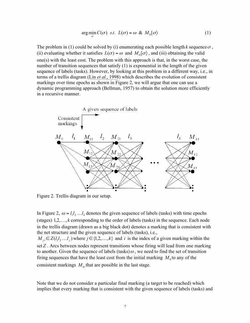
Figure 2. Trellis diagram in our setup.

In Figure 2, denotes the given sequence of labels (tasks) with time epochs

(stages) corresponding to the order of labels (tasks) in the sequence. Each node

in the trellis diagram (drawn as a big black dot) denotes a marking that is consistent with

the net structure and the given sequence of labels (tasks), i.e.,

where and is the index of a given marking within the

set . Arcs between nodes represent transitions whose firing will lead from one marking

to another. Given the sequence of labels (tasks) , we need to find the set of transition

firing sequences that have the least cost from the initial marking to any of the

consistent markings that are possible in the last stage.

Note that we do not consider a particular final marking (a target to be reached) which

implies that every marking that is consistent with the given sequence of labels (tasks) and

8

the net structure can appear as a final node in the trellis diagram. Also, in our setup, the

number of nodes at each time epoch is not fixed: it can increase or decrease with each

time epoch (i.e., the trellis diagram is not regular) but, as we will argue, the number of

nodes (consistent markings) at the stage of the trellis diagram is upper bounded by a

function that is polynomial in .

Definition 3 Let denote the prefix of the given sequence of labels (tasks)

that has length ( ). The set of markings consistent with is given by

where denotes the index of marking within the set

in the trellis diagram.

Definition 4 The set of least-cost firing sequences that lead to the consistent marking

with respect to is given by for such that

and .

By formulating the problem in terms of a trellis diagram, it is clear that each consistent

marking in the set has to be reached via at least one consistent marking in the set

. Moreover, a dynamic programming approach can be used to compute the least-

cost firing sequence(s) recursively. The basic observation is that the transition sequences

which have the least cost at time epoch only depend on the least-cost transition

sequences up to time epoch (specifically, at the sequences for all indices in the

set ) and the label (task). By taking advantage of this observation, one can

search for the sequence that has the least cost, one stage in the trellis diagram at a time. In

our setup, given each consistent marking and their associated least-cost

firing sequence set , the set of least-cost firing sequences associated with

each consistent marking after labels (i.e., after

has been considered) can be computed as follows:

(2)

where and are such that

and and

Remark 1 In the above recursion, the firing sequence that has least total cost after

considering labels (tasks) is not necessarily the prefix of the firing sequence that will

9

give us the least total cost after considering labels (tasks). Therefore, we must keep

track of all markings consistent with labels (tasks) and their corresponding least-cost

firing sequence(s) in order to be able to find those firing sequences that have least total

cost after considering labels (tasks). This is due to the fact that we consider the label

(task) at each time epoch (which may correspond to a set of consistent markings) instead

of only considering a particular consistent marking (the principle of optimality (Bellman,

1957) still holds in our approach if we consider a particular consistent marking instead of

a label (task) at each stage).

By calculating (2) recursively in the number of labels (tasks), we can efficiently find the

firing sequence(s) that has (have) the least cost. Here we want to point out that the total

number of consistent markings (number of nodes in Figure 2) is upper bounded at each

stage by a polynomial function in the length of the given sequence of labels (tasks). As

we will show, this means that the computational complexity for finding the least-cost

firing sequence is polynomial in the length of the given sequence of labels (tasks). In

contrast, if we start with the set of transitions that can fire at each step, the number of

sequences that will be investigated is exponential in the length of given sequence of

labels (tasks).

4. Obtaining the least-cost firing sequence(s)

A. Algorithm

In this section, we propose a recursive algorithm to find the least-cost firing sequence(s)

given a label (task) sequence of length .We use a data structure

to capture the information we need to store for each node

in the trellis diagram. More specifically, at time epoch , denotes the marking

that is associated with the node (and is, of course, consistent with the given label

sequence so far); is the least cost among all valid firing sequences from to

; ( , ) denotes that the least cost firing sequence goes through

at time epoch and leads to via the firing of transition (which is, of

course, enabled at ) .

We describe the algorithm in detail below.

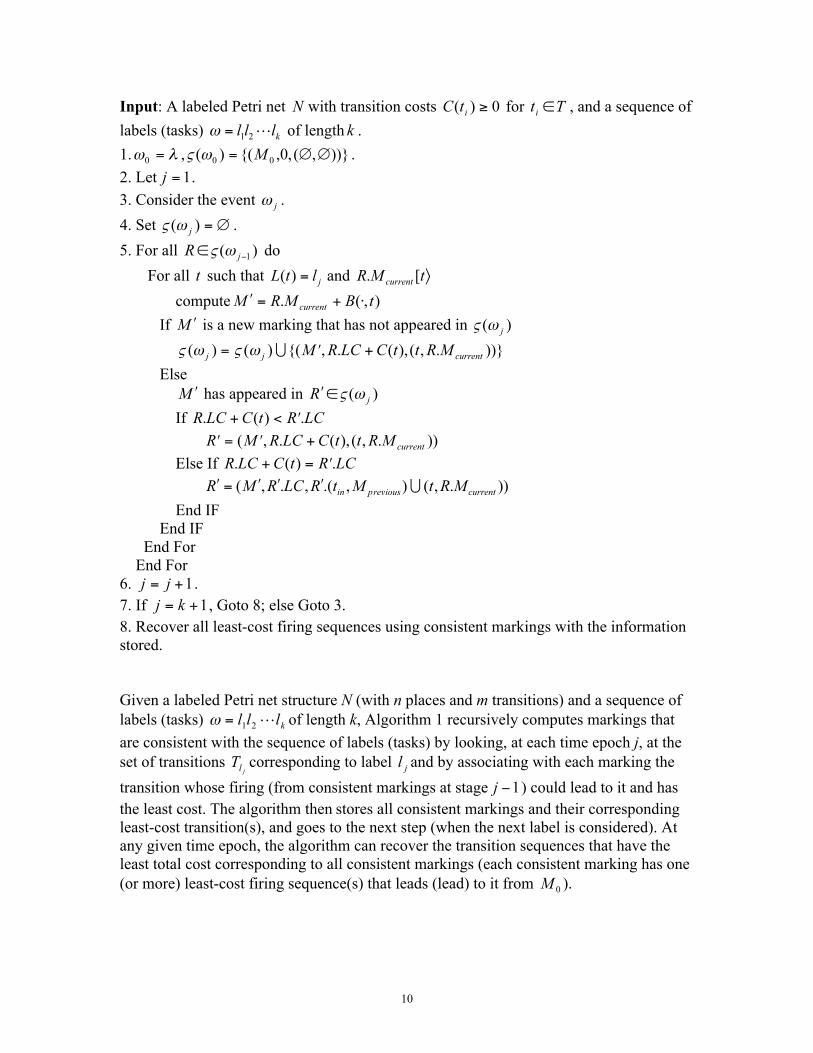
Algorithm 1

10

Input: A labeled Petri net with transition costs for , and a sequence of

labels (tasks) of length .

1. , .

2. Let .

3. Consider the event .

4. Set .

5. For all do

For all such that and

compute

If is a new marking that has not appeared in

Else

has appeared in

If

Else If

End IF

End IF

End For

End For

6. .

7. If , Goto 8; else Goto 3.

8. Recover all least-cost firing sequences using consistent markings with the information

stored.

Given a labeled Petri net structure N (with n places and m transitions) and a sequence of

labels (tasks) of length k, Algorithm 1 recursively computes markings that

are consistent with the sequence of labels (tasks) by looking, at each time epoch j, at the

set of transitions corresponding to label and by associating with each marking the

transition whose firing (from consistent markings at stage ) could lead to it and has

the least cost. The algorithm then stores all consistent markings and their corresponding

least-cost transition(s), and goes to the next step (when the next label is considered). At

any given time epoch, the algorithm can recover the transition sequences that have the

least total cost corresponding to all consistent markings (each consistent marking has one

(or more) least-cost firing sequence(s) that leads (lead) to it from ).

11

Remark 2 For the special case where the incident matrix B has full column rank, i.e.,

rank(B)= m, we know that there is a unique firing vector for each valid final marking in

the given net. Furthermore, all transition sequences that get us to this final marking will

have the same cost. Depending on the underlying objective, the recursive algorithm can

be modified in this case to simply keep track of the number of times each transition

appears in a least-cost firing sequence. In addition, given an observed sequence of labels

that is infeasible (i.e., the set of consistent markings is an empty set), Algorithm

1 will not return any outputs. Note that deadlock is avoided at intermediate stages

( ) because Algorithm 1 by default will eliminate such markings from

further consideration. Deadlocks at the last stage (stage ) can be checked and prevented

using existing deadlock avoidance techniques (Sreenivas, 1997; Park and Reveliotis,

2001; Wu and Zhou, 2005) in literature.

Example 2 Recall the disassembly and assembly operation modeled by the labeled Petri

net with transition costs in Figure 1. If the given sequence of labels (tasks) is ,

the corresponding trellis diagram is shown in Figure 3. We treat each consistent marking

as a node in the diagram and each time epoch corresponds to the time a label is

considered. The set of least-cost firing sequences is given by ,

both with least total cost 10. In terms of our data structure, node would be

.

Figure 3. Trellis diagram for the net in Figure 1with sequence of labels (tasks) .

12

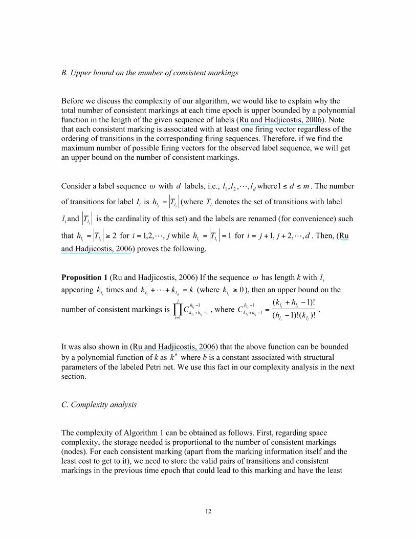
B. Upper bound on the number of consistent markings

Before we discuss the complexity of our algorithm, we would like to explain why the

total number of consistent markings at each time epoch is upper bounded by a polynomial

function in the length of the given sequence of labels (Ru and Hadjicostis, 2006). Note

that each consistent marking is associated with at least one firing vector regardless of the

ordering of transitions in the corresponding firing sequences. Therefore, if we find the

maximum number of possible firing vectors for the observed label sequence, we will get

an upper bound on the number of consistent markings.

Consider a label sequence with labels, i.e., where . The number

of transitions for label is (where denotes the set of transitions with label

and is the cardinality of this set) and the labels are renamed (for convenience) such

that for while for . Then, (Ru

and Hadjicostis, 2006) proves the following.

Proposition 1 (Ru and Hadjicostis, 2006) If the sequence has length k with

appearing times and (where ), then an upper bound on the

number of consistent markings is , where .

It was also shown in (Ru and Hadjicostis, 2006) that the above function can be bounded

by a polynomial function of k as where b is a constant associated with structural

parameters of the labeled Petri net. We use this fact in our complexity analysis in the next

section.

C. Complexity analysis

The complexity of Algorithm 1 can be obtained as follows. First, regarding space

complexity, the storage needed is proportional to the number of consistent markings

(nodes). For each consistent marking (apart from the marking information itself and the

least cost to get to it), we need to store the valid pairs of transitions and consistent

markings in the previous time epoch that could lead to this marking and have the least

13

cost. If denotes the largest possible number of transitions corresponding to a

label in the Petri net, then the number of transitions that could lead from distinct

(consistent) markings in the previous stage to the current (consistent) marking is bounded

by . Thus, for each consistent marking, the information to be stored is a constant

(proportional to ). Clearly, since the number of consistent markings associated with

a given label sequence of length k is upper bounded by (as argued earlier), the total

space needed to store all consistent markings in each stage in the trellis diagram is

which can be simplified as , i.e., the storage required is

polynomial in the length k of the given sequence of labels (tasks).

We now proceed to analyze computational complexity. We use to denote the number

of consistent markings at the stage in the trellis ( ) and to

denote the number of consistent markings at the stage in the trellis ( ).

Given a label , the number of possible transitions enabled from the stage is

upper bounded by where is the largest number of transitions corresponding to

a certain label. For each marking (in the stage) yielding from these transitions, we

need at most comparisons to decide if it has appeared or not (by searching through the

set of existing markings). Thus, the computational complexity for finding the sequence

that has least-cost for all markings at the stage is bounded by , which has

complexity where is a constant. Thus, for consistent markings over all

stages, the total computational complexity is given by , which can be simplified

as . Therefore, the algorithm has complexity that is polynomial in the length k of

the given sequence of labels (tasks).

5. An illustrative example

In this section, we illustrate the algorithm via a more complicated example. In Figure 4,

consider two parallel part producing machines (Proth and Xie, 1996) that are modeled by

a labeled Petri net. The Petri net has 10 places , 12 transitions

, and initial marking . The

labeling function is given by , , ,

, , , and . The cost of each

transition is given by the cost vector

14

. Our goal is to estimate least-

cost planning sequence(s) based on different sequences of labels (tasks).

Figure 4. Petri net model for two parallel machines.

We consider a sequence of labels eeffaabccdeeffabcdabcdgghhabcd of length 30 to

illustrate our algorithm.

Due to space limitations, we do not provide the trellis diagram associated with this

example. Instead, we provide the following table where Label denotes the label (task) in

the given sequence, Num of Markings gives number of consistent markings with the

given label (task), LC captures the least total cost of sequence(s) that is (are) consistent

with the labels given up to the current time epoch and gives the set of planning

sequence(s) that has (have) least total cost up to the current time epoch.

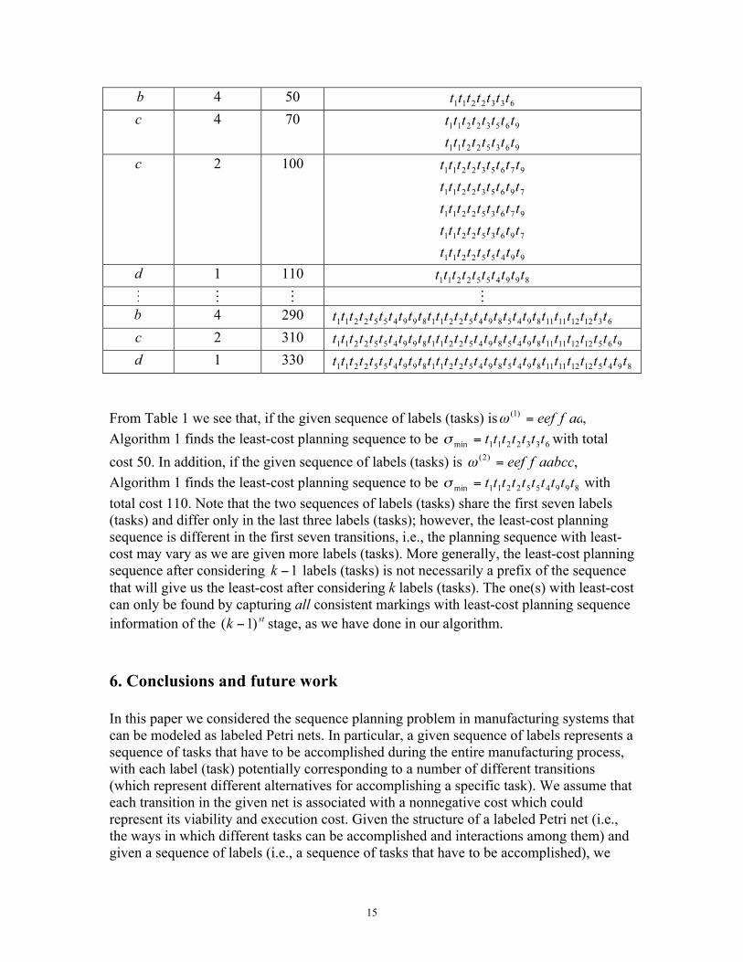
Table 1 Complete results of our example

Label Num of

Markings

LC

e 1 5

e 1 10

f 1 15

f 1 20

a 2 30

a 3 40

15

b 4 50

c 4 70

c 2 100

d 1 110

4 290

c 2 310

d 1 330

From Table 1 we see that, if the given sequence of labels (tasks) is ,

Algorithm 1 finds the least-cost planning sequence to be with total

cost 50. In addition, if the given sequence of labels (tasks) is ,

Algorithm 1 finds the least-cost planning sequence to be with

total cost 110. Note that the two sequences of labels (tasks) share the first seven labels

(tasks) and differ only in the last three labels (tasks); however, the least-cost planning

sequence is different in the first seven transitions, i.e., the planning sequence with least-

cost may vary as we are given more labels (tasks). More generally, the least-cost planning

sequence after considering labels (tasks) is not necessarily a prefix of the sequence

that will give us the least-cost after considering k labels (tasks). The one(s) with least-cost

can only be found by capturing all consistent markings with least-cost planning sequence

information of the stage, as we have done in our algorithm.

6. Conclusions and future work

In this paper we considered the sequence planning problem in manufacturing systems that

can be modeled as labeled Petri nets. In particular, a given sequence of labels represents a

sequence of tasks that have to be accomplished during the entire manufacturing process,

with each label (task) potentially corresponding to a number of different transitions

(which represent different alternatives for accomplishing a specific task). We assume that

each transition in the given net is associated with a nonnegative cost which could

represent its viability and execution cost. Given the structure of a labeled Petri net (i.e.,

the ways in which different tasks can be accomplished and interactions among them) and

given a sequence of labels (i.e., a sequence of tasks that have to be accomplished), we

16

developed a recursive algorithm that finds the planning sequence(s) that has (have) the

least total cost (i.e., the sequence(s) of activities that accomplishes (accomplish) the

specified sequence of tasks and has (have) the least total cost). We also showed that the

algorithm has complexity that is polynomial in the length of the given sequence of labels

(tasks).

One possible direction for future work is to find classes of nets for which the complexity

of the algorithm can be further reduced. Another interesting question is to study the

problem in situations where the initial marking of the net is only partially known.

References

Bellman, R. 1957: Dynamic programming. Princeton University Press.

Cassandras, C. G. and Lafortune, S. 1999: Introduction to discrete event systems. Springer.

Desrochers, A. A. and AI-Jaar, R. Y. 1995: Applications of Petri nets in manufacturing systems:

modeling, control, and performance analysis. IEEE Press.

Forney, G. D. Jr. 1973: The Viterbi algorithm. Proceedings of the IEEE 61, 268–78.

Kiritsis, D., Neuendorf, K.-P. and Xirouchakis, P. 1999: Petri net techniques for process planning cost

estimation. Advances in Engineering Software 30, 375–87.

Lin, S., Kasami, T., Fujiwara, T. and Fossorier, M. 1998: Trellises and trellis-based decoding

algorithms for linear block codes. Kluwer Academic Publishers.

Moore, K. E., Gungor, A. and Gupta, S. M. 1998: Disassembly process planning using Petri nets.

Proceedings of the1998 IEEE International Symposium on Electronics and the Environment, 88–93.

Morita, K. and Watanabe, T. 1996: The legal firing sequence problem of Petri nets with state machine

structure. Proceedings of the 1996 IEEE International Symposium on Circuits and Systems, 64–67.

Murata, T. 1989: Petri nets: properties, analysis and applications. Proceedings of the IEEE 77, 541–80.

Park, J. and Reveliotis, S. A. 2001: Deadlock avoidance in sequential resource allocation systems with

multiple resource acquisitions and flexible routings. IEEE Transactions on Automatic Control 46, 1572–83.

Proth, J.-M. and Xie, X. 1996: Petri nets: a tool for design and management of manufacturing systems.

John Wiley & Sons.

Rosell, J. 2004: Assembly and task planning using Petri nets: a survey. Journal of Engineering

Manufacture 218, 987–94.

Ru, Y. and Hadjicostis, C. N. 2006: State estimation in discrete event systems modeled by labeled Petri

nets. Proceedings of the 45th IEEE International Conference on Decision and Control, 6022–27.

Sampath, R., Darabi, H., Buy, U. and Liu, J. 2008: Control reconfiguration of discrete event systems

with dynamic control specifications. IEEE Transactions on Automation Science and Engineering 5, 84–100.

17

Sreenivas, R. S. 1997: On the existence of supervisory policies that enforce liveness in discrete-event

dynamic systems modeled by controlled Petri nets. IEEE Transactions on Automatic Control 42, 928–45.

Tang, Y., Zhou, M. and Caudill, R. J. 2001: An integrated approach to disassembly planning and

demanufacturing operation. IEEE Transactions on Robotics and Automation 17, 773–84.

Tang, Y., Zhou, M. and Gao, M. 2006: Fuzzy-Petri-net-based disassembly planning considering human

factors. IEEE Transactions on Systems, Man, and Cybernetics–Part A 36, 718–26.

Taoka, S. and Watanabe, T. 1999: A linear time algorithm solving the legal firing sequence problem for a

class of edge-weighted cactuses. Proceedings of the IEEE International Conference on Systems, Man,

and Cybernetics, 893–98.

Viterbi, A. D. 1967: Error bounds for convolutional codes and an asymptotically optimum decoding

algorithm. IEEE Transactions on Information Theory IT-13, 260–69.

Watanabe, T. 2000: The legal firing sequence problem of Petri nets. IEICE Transactions on Information

and Systems 3, 397–406.

Wu, N. and Zhou, M. 2005: Modeling and deadlock avoidance of automated manufacturing systems with

multiple automated guided vehicles. IEEE Transactions on Systems, Man, and Cybernetics–Part B 35,

1193–1202.

Zussman, E. and Zhou, M. 1999: A methodology for modeling and adaptive planning of disassembly

processes. IEEE Transactions on Robotics and Automation 15, 190–94.

18

Figure 1. Disassembly and assembly operation modeled by a labeled Petri net.

19

Figure 2. Trellis diagram in our setup.

20

Figure 3. Trellis diagram for the net in Figure 1with sequence of labels (tasks)

21

Figure 4. Petri net model for two parallel machines.

22

Table 1 Complete results of our example

Label Num of

Markings

LC

e 1 5

e 1 10

f 1 15

f 1 20

a 2 30

a 3 40

b 4 50

c 4 70

c 2 100

d 1 110

4 290

c 2 310

d 1 330