A symbolic algorithm for the synthesis ofbounded Petri nets?

J. Carmona1, J. Cortadella1, M. Kishinevsky2, A. Kondratyev3, L. Lavagno4,and A. Yakovlev5

1 Universitat Politecnica de Catalunya, Spain2 Intel Corporation, USA

3 Cadence Berkeley Laboratories, USA4 Politecnico di Torino, Italy5 Newcastle University, UK

Abstract. This paper presents an algorithm for the synthesis ofbounded Petri nets from transition systems. A bounded Petri net isalways provided in case it exists. Otherwise, the events are split intoseveral transitions to guarantee the synthesis of a Petri net with bisim-ilar behavior. The algorithm uses symbolic representations of multisetsof states to efficiently generate all the minimal regions. The algorithmhas been implemented in a tool. Experimental results show a significantnet reduction when compared with approaches for the synthesis of safePetri nets.

1 Introduction

The problem of Petri net synthesis consists of building a Petri net that has abehavior equivalent to a given transition system. The problem was first addressedby Ehrenfeucht and Rozenberg [ER90] introducing regions to model the sets ofstates that characterize marked places. Mukund [Muk92] extended the conceptof region to synthesize nets with weighted arcs.

Different variations of the synthesis problem have been studied in thepast [Dar07]. Most of the efforts have been devoted to the decidability prob-lem, i.e. questioning about the existence of a Petri net with a specified behavior.An exception is in [BBD95] where polynomial algorithms for the synthesis ofbounded nets were presented. These methods have been implemented in thetool SYNET [Cai02].

Desel and Reisig [DR96] reduced the synthesis problem to the calculation ofthe subset of minimal regions. In [HKT95,HKT96] the classical trace model byMazurkiewicz [Maz87] was extended to describe the behavior of general Petrinets.

? Work of J. Carmona and J. Cortadella has been supported by the project FOR-MALISM (TIN2007-66523), and a grant by Intel Corporation. Work of A. Yakovlevwas supported by EPSRC, Grants EP/D053064/1 and EP/E044662/1.

a b

r1

r2

r1

r2

b a

ba

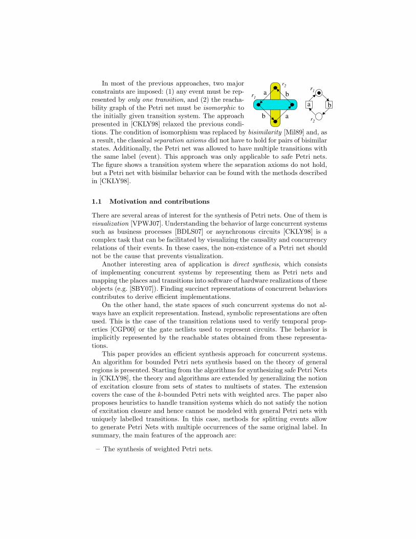
In most of the previous approaches, two majorconstraints are imposed: (1) any event must be rep-resented by only one transition, and (2) the reacha-bility graph of the Petri net must be isomorphic tothe initially given transition system. The approachpresented in [CKLY98] relaxed the previous condi-tions. The condition of isomorphism was replaced by bisimilarity [Mil89] and, asa result, the classical separation axioms did not have to hold for pairs of bisimilarstates. Additionally, the Petri net was allowed to have multiple transitions withthe same label (event). This approach was only applicable to safe Petri nets.The figure shows a transition system where the separation axioms do not hold,but a Petri net with bisimilar behavior can be found with the methods describedin [CKLY98].

1.1 Motivation and contributions

There are several areas of interest for the synthesis of Petri nets. One of them isvisualization [VPWJ07]. Understanding the behavior of large concurrent systemssuch as business processes [BDLS07] or asynchronous circuits [CKLY98] is acomplex task that can be facilitated by visualizing the causality and concurrencyrelations of their events. In these cases, the non-existence of a Petri net shouldnot be the cause that prevents visualization.

Another interesting area of application is direct synthesis, which consistsof implementing concurrent systems by representing them as Petri nets andmapping the places and transitions into software of hardware realizations of theseobjects (e.g. [SBY07]). Finding succinct representations of concurrent behaviorscontributes to derive efficient implementations.

On the other hand, the state spaces of such concurrent systems do not al-ways have an explicit representation. Instead, symbolic representations are oftenused. This is the case of the transition relations used to verify temporal prop-erties [CGP00] or the gate netlists used to represent circuits. The behavior isimplicitly represented by the reachable states obtained from these representa-tions.

This paper provides an efficient synthesis approach for concurrent systems.An algorithm for bounded Petri nets synthesis based on the theory of generalregions is presented. Starting from the algorithms for synthesizing safe Petri Netsin [CKLY98], the theory and algorithms are extended by generalizing the notionof excitation closure from sets of states to multisets of states. The extensioncovers the case of the k-bounded Petri nets with weighted arcs. The paper alsoproposes heuristics to handle transition systems which do not satisfy the notionof excitation closure and hence cannot be modeled with general Petri nets withuniquely labelled transitions. In this case, methods for splitting events allowto generate Petri Nets with multiple occurrences of the same original label. Insummary, the main features of the approach are:

– The synthesis of weighted Petri nets.

– The use of symbolic methods based on BDDs to explore large state spaces.– Efficient heuristics for event splitting.

1.2 Two illustrative examples

b

ca

22

p1

p2 p3

120 111 102

022 013 004031040

b b

b b b b

200a

a a a

c

cc

c

Fig. 1: A transition system and an equivalent bounded Petri net.

Figure 1 depicts a finite transition system with 9 states and 3 events. Aftersynthesis, the Petri net at the right is obtained. Each state has a 3-digit label thatcorresponds to the marking of places p1, p2 and p3 of the Petri net, respectively.The shadowed states represent the general region that characterizes place p2.Each grey tone represents a different multiplicity of the state (4 for the darkestand 1 for the lightest). Each event has a gradient with respect to the region (+2for a, -1 for b and 0 for c). The gradient indicates how the event changes themultiplicity of the state after firing. For the same example, the equivalent safePetri net generated by petrify [CKLY98] has 5 places and 10 transitions.

Another example is shown in Fig. 2. The transition system models a behaviorwith OR-causality, i.e. the event c can be fire as soon as a or b have fired. Thenet model is much simpler and intuitive if bounded nets are used. Instead, themodel with a safe Petri net needs to represent the events a and b with multipletransitions.

a b

c

d

ba

b ac

d

a

a

b

b

ab

ccd

c

(c)(b)(a)

Fig. 2: (a) Transition system, (b) 2-bounded Petri net, (c) safe Petri net.

The algorithm presented in this paper is based on an efficient manipulationof multisets to explore the minimal general regions of a finite transition system.

2 Background

2.1 Petri nets and finite transition systems

Definition 1. A Petri net is a tuple (P, T,W,M0) where P and T represent fi-nite sets of places and transitions, respectively, and W : (P × T ) ∪ (T × P ) → Nis the weighted flow relation. The initial marking M0 ∈ N|P | defines the initialstate of the system.

Definition 2 (Transition system). A transition system (or TS) is a tuple(S, Σ, E, sin), where S is a set of states; Σ is an alphabet of actions, such thatS∩Σ = ∅; E ⊆ S×Σ×S is a set of (labelled) transitions; and sin is the initialstate.

Let TS = (S, Σ, E, sin) be a transition system. We consider connected TSsthat satisfy the following axioms:

– S and E are finite sets.– Every event has an occurrence: ∀e ∈ Σ : ∃(s, e, s′) ∈ E;– Every state is reachable from the initial state: ∀s ∈ S : sin

∗→ s.

A state without outgoing arcs is called deadlock state.

2.2 Multisets

The following definitions establish the necessary background to understand theconcept of region, introduced in Section 2.3. A region is a multiset where addi-tional conditions hold. We start by introducing the multiset terminology.

Definition 3 (Multiset). Given a set S, a multiset r of S is a mappingr : S −→ N.We will also use a set notation for multisets. For example, letS = {s1, s2, s3, s4}, then a multiset r = {s3

1, s22, s3} corresponds to the following

mapping r(s1) = 3, r(s2) = 2, r(s3) = 1, r(s4) = 0.

Henceforth we will assume r, r1 and r2 to be multisets of a set S.

Definition 4 (Support of a multiset). The support of a multiset r is definedas

supp(r) = {s ∈ S | r(s) > 0}

Definition 5 (Power of a multiset). The power of a multiset r, denoted byr�, is defined as

r� = maxs∈S

r(s)

For instance, for the multiset r = {s31, s

22, s3}, r� = 3.

Definition 6 (Trivial multisets). A multiset r is said to be trivial ifr(s) = r(s′) for all s, s′ ∈ S. The trivial multisets will be denoted by 0, 1, . . . ,K when r(s) = 0, r(s) = 1, . . . , r(s) = k, for every s ∈ S, respectively.

Definition 7 (k-bounded multiset). A multiset r is k-bounded if for all s ∈S : r(s) ≤ k.

Definition 8 (Union, intersection and difference of multisets). Theunion, intersection and difference of two multisets r1 and r2 are defined as fol-lows:

(r1 ∪ r2)(s) = max(r1(s), r2(s))(r1 ∩ r2)(s) = min(r1(s), r2(s))(r1 − r2)(s) = max(0, r1(s)− r2(s))

Definition 9 (Subset of a multiset). A multiset r1 is a subset of a multisetr2 (r1 ⊆ r2) if

∀s ∈ S : r1(s) ≤ r2(s)

As usual, we will denote by r1 ⊂ r2 the fact that r1 ⊆ r2 and r1 6= r2.

Definition 10 (k-topset of a multiset). The k-topset of a multiset r, denotedby >k(r), is defined as follows:

>k(r)(s) ={

r(s) if r(s) ≥ k0 otherwise

A multiset r1 is a topset of r2 if there exists some k for which r1 = >k(r2).

Examples. The multiset {s31, s3} is a subset of {s3

1, s22, s3}, but it is not a topset.

The multisets {s31, s

22} and {s3

1} are the 2- and 3-topsets of {s31, s

22, s3}, respec-

tively. As it will be shown in Section 4, k-topsets are the main objects to lookat when constructing the (weighted) flow relation for Petri net synthesis.

Property 1 (Partial order of multisets). The relation ⊆ (subset) on the set ofmultisets of S is a partial order.

Property 2 (The lattice of k-bounded multisets). The set of k-bounded multisetsof a set S with the relation ⊆ is a lattice. The meet and join operations are theintersection and union of multisets respectively. The least and greatest elementsare 0 and K respectively.

2.3 General regions

Let TS = (S, Σ, E, sin) be a transition system. In this section, we will considermultisets of the set S.

Definition 11 (Gradient of a transition). Given a multiset r, the gradientof a transition (s, e, s′) is defined as

∆r(s, e, s′) = r(s′)− r(s)

An event e is said to have a non-constant gradient in r if there are two transitions(s1, e, s

′1) and (s2, e, s

′2) such that

r(s′1)− r(s1) 6= r(s′2)− r(s2)

Definition 12 (Region). A multiset r is a region if all events have a constantgradient in r.

The original notion of region from [ER90] was restricted to subsets of S, i.e.events could only have gradients in {−1, 0,+1}.

Definition 13 (Gradient of an event). Given a region r and an event e with(s, e, s′) ∈ E, the gradient of e in r is defined as

∆r(e) = r(s′)− r(s)

Definition 14 (Minimal region). A region r is minimal if there is no otherregion r′ 6= 0 such that r′ ⊂ r.

Note that the trivial region 0 is not considered to be minimal.

Theorem 1. Let r be a region such that 1 ⊂ r. Then r is not a minimal region.

Proof. Trivial. A smaller region can be obtained by subtracting 1 from each r(s).2

Definition 15 (Excitation and switching regions6). The excitation regionof an event e, ER(e), is the set of states in which e is enabled, i.e.

ER(e) = {s | ∃s′ : (s, e, s′) ∈ E}

The switching region of an event e, SR(e), is the set of states reachable fromER(e) after having fired e, i.e.

SR(e) = {s | ∃s′ : (s′, e, s) ∈ E}

For convenience, ER(e) and SR(e) will be also considered as multisets of stateswhen necessary.

Definition 16 (Pre- and post-regions). A region r is a pre-region of e ifER(e) ⊆ r. A region r is a post-region of e if SR(e) ⊆ r. The sets of pre- andpost-regions of an event e are denoted by ◦e and e◦ respectively.

Note that a region r can be a pre-region and a post-region of the same eventin case ER(e) ∪ SR(e) ⊆ r. The behavior modeled in this situation can be seenas a self-loop in a Petri net.

6 Excitation and switching regions are not regions in the terms of Definition 12. Theycorrespond to the set of states in which an event is enabled or just fired, correspond-ingly. The terms are used due to historical reasons.

Properties of regions

Property 3. Let TS = (S, Σ, E, sin) be a transition system without deadlockstates. Then, for any region r there is an event e for which ∆r(e) ≤ 0.

Proof. By contradiction. Assume that ∆r(e) > 0 for all events. Then for all arcs(s, e, s′) we have that r(s′) > r(s). Since TS has no deadlock states and S isfinite, there is at least one cycle s0 → s1 → . . . → sn → s0. This would result inr(s0) > r(s0), which is a contradiction. 2

Property 4. Let TS = (S, Σ, E, sin) be a transition system in which there is atransition (s, e′, sin) ∈ E. Then, for any region r there is an event e for which∆r(e) ≥ 0.

Proof. By contradiction. Assume that ∆r(e) < 0 for all events. Then for all arcs(s, e, s′) we have that r(s′) < r(s). Since there is (s, e′, sin) ∈ E, there is at leastone cycle sin → s1 → . . . → sn = s → sin. This would result in r(sin) < r(sin),which is a contradiction. 2

Property 5. Let TS = (S, Σ, E, sin) be a transition system without deadlockstates. Then, any region r 6= ∅ is the pre-region of some event e.

Proof. Property 3 guarantees the existence of an event e such that ∆r(e) ≤ 0. If∆r(e) < 0, then every state in ER(e) must be in the support of r and the claimholds. If every event e fulfilling Property 3 satisfies ∆r(e) = 0, then supp(r) = S:if the contrary is assumed, since the transition system is deadlock-free and r 6= ∅,the states in the support of r must be connected to some states out of r. However,if every event has non-negative gradient in r, then in this situation r must containall the states. 2

Property 6. Let TS = (S, Σ, E, sin) be a transition system. Then, any regionr 6= ∅ is the pre-region or the post-region of some event e.

Proof. A similar reasoning of the proof of Property 5 can be applied here, butusing Properties 3 and 4. 2

2.4 Excitation-closed TSs

This section defines a specific class of transition systems, called excitation-closed,for which the synthesis approach presented in this paper guarantees that thePetri net obtained has a reachability graph bisimilar to the initial transitionsystem.

Definition 17 (Enabling topset). The set of smallest enabling topsets of anevent e is denoted by ?e and defined as follows:

?e = {q | ∃r ∈ ◦e, k > 0 : q = >k(r) ∧ ER(e) ⊆ >k(r) ∧ ER(e) 6⊆ >k+1(r)}

Intuitively, q belongs to ?e if it is the topset of a pre-region r of e and thereis no larger topset that includes ER(e).

e

e2

s11 2

1 2

1

0 4 2

0

1 2 3

5

8 4

9

e

ee e

e e

e e

e e

s1 s

2

1 2

4

3 3

1 2 3

5

74 8

10

e

1 2s

e

e

s

s

e

s

e

s

e

2

8

6 66 8 7

10

4 5

2 3121 1 2 1 2 3

54

6 6 6 8 7

105

e e

ee

ee

e e

ee e

e e

ee e

ee

e e

e

e e

e e

e

e e

ee

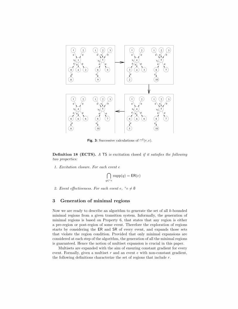
Fig. 3: Successive calculations of u2(r, e).

Definition 18 (ECTS). A TS is excitation closed if it satisfies the followingtwo properties:

1. Excitation closure. For each event e⋂q∈?e

supp(q) = ER(e)

2. Event effectiveness. For each event e, ◦e 6= ∅

3 Generation of minimal regions

Now we are ready to describe an algorithm to generate the set of all k-boundedminimal regions from a given transition system. Informally, the generation ofminimal regions is based on Property 6, that states that any region is eithera pre-region or post-region of some event. Therefore the exploration of regionsstarts by considering the ER and SR of every event, and expands those setsthat violate the region condition. Provided that only minimal expansions areconsidered at each step of the algorithm, the generation of all the minimal regionsis guaranteed. Hence the notion of multiset expansion is crucial in this paper.

Multisets are expanded with the aim of ensuring constant gradient for everyevent. Formally, given a multiset r and an event e with non-constant gradient,the following definitions characterize the set of regions that include r.

1 2

1

0 4 2

0

1 2 3

5

8 4

9

1 2

e

e

s s

e e

e e

e

e

e e e

e

1 2

3

0 2

0

4 4 4

7

44 8

9

1 2s

e

s

e

e

e e

e e

e e

e e

e

2 2

3

0 2

0

6 6 6

7

48

9

e

e

e

s1 s2

e e

e e

e

e e

e e

4

Fig. 4: Successive calculations of u1(r, e).

Definition 19. Let r 6= 0 be a multiset. We define

Rg(r, e) = {r′ ⊇ r|r′ is a region and ∆r′(e) ≤ g}Rg(r, e) = {r′ ⊇ r|r′ is a region and ∆r′(e) ≥ g}

Rg(r, e) is the set of all regions larger than r in which the gradient of e issmaller than or equal to g. Similar for Rg(r, e) and the gradient of e greater thanor equal to g. Notice that in this definition a gradient g is used to partition theset of regions including r into two classes. This binary partition is the basis forthe calculation of minimal k-bounded regions that will be presented at the endof this section.

To expand a multiset in order to convert it into a region, it is necessary toknow the lower bound needed for the increase in each state in order to satisfy agiven gradient constraint. The next functions provide these lower bounds:

Definition 20. Given a multiset r, a state s and an event e, the following δfunctions are defined7:

δg(r, e, s) = max(0, max(s,e,s′)∈E

(r(s′)− r(s)− g))

δg(r, e, s) = max(0, max(s′,e,s)∈E

(r(s′)− r(s) + g))

Informally, δg denotes a lower bound for the increase of r(s), taking intoaccount the arcs leaving from s, to force ∆r′(e) ≤ g in some region r′ largerthan r. Similarly, δg denotes a lower bound taking into account the arcs arrivingat s, to force ∆r′(e) ≥ g. Let us use Figure 3 to illustrate this concept. In thefigure each state is labeled with r(s). For the states s1 and s2 in the top-leftfigure, we have:

δ2(r, e, s1) = 3 δ2(r, e, s2) = 0

δ2(r, e, s1) is determined by the arc 2 e→ 1 and indicates that r′(s1) ≥ 4 incase we seek a region r′ ⊃ r with ∆r′(e) ≥ 2. Analogously, Figure 4 illustratesthe symmetrical concept. For the states s1 and s2 in the leftmost figure we have:7 For convenience, we consider maxx∈D P (x) = 0 when the domain D is empty.

δ1(r, e, s1) = 2 δ1(r, e, s2) = 2

δ1(r, e, s1) is determined by the arc 1 e→ 4 , indicating that r′(s1) ≥ 3 for∆r′(e) ≤ 1. Similarly, δ1(r, e, s2) is determined by the arc 5 e→ 8 .

Definition 21. Given a multiset r and an event e, the multisets ug(r, e) andug(r, e) are defined as follows:

ug(r, e)(s) = r(s) + δg(r, e, s)ug(r, e)(s) = r(s) + δg(r, e, s)

Intuitively, ug(r, e) is a safe move towards growing r and obtaining all regionsr′ with ∆r(e) ≤ g. Similarly, ug(r, e) for those regions with ∆r(e) ≥ g. It iseasy to see that ug(r, e) and ug(r, e) always derive multisets larger than r. Thesuccessive calculations of ug(r, e) and ug(r, e) are illustrated in Figures 3 and 4,respectively.

Theorem 2 (Expansion on events).

(a) Let r 6= 0 be a multiset and e an event such that there exists some (s, e, s′)with r(s′)− r(s) > g. The following hold:1. r ⊂ ug(r, e)2. Rg(r, e) = Rg(ug(r, e), e)

(b) Let r 6= 0 be a multiset and e an event such that there exists some (s, e, s′)with r(s′)− r(s) < g. The following hold:1. r ⊂ ug(r, e)2. Rg(r, e) = Rg(ug(r, e), e)

Proof. (We prove item (a), item (b) is similar.)(a.1) Given the event e, for all states s, s′ with (s, e, s′) either (i) r(s′)−r(s) ≤ gor (ii) r(s′) − r(s) > g. In situation (i), the following equality holds: r(s) =ug(r, e)(s) because δg(r, e, s) = 0 by Definition 20. In situation (ii), δg(r, e, s) > 0,and therefore r(s) < ug(r, e)(s). Given that the rest of states without outgoingarcs labeled e fulfill also r(s) = ug(r, e)(s), and because there exists at least onetransition satisfying (ii), the claim holds.(a.2) To obtain Rg(r, e) it is necessary to guarantee ∆r′(e) ≤ g for each regionr′ ⊇ r. Given (s, e, s′) with r(s′) − r(s) > g, two possibilities can induce agradient lower than g, e.g decreasing r(s′) or increasing r(s), but only the latterleads to a multiset with r as a subset. 2

Figure 5 presents an algorithm for the calculation of all minimal k-boundedregions. It is based on a dynamic programming approach that, starting froma multiset, generates an exploration tree in which an event with non-constantgradient is chosen at each node. All possible gradients for that event are exploredby means of a binary search. Dynamic programming with memoization avoidsthe exploration of multiple instances of the same node. The final step of thealgorithm (lines 16-17) removes all those multisets that are neither regions norminimal regions that have been generated during the exploration.

generate minimal regions (TS,k) {1: R = ∅; /* set of explored multisets */

2: P = {ER(e) | e ∈ E} ∪ {SR(e) | e ∈ E};3: while (P 6= ∅) /* multisets pending for exploration */

4: r = remove one element (P);

5: if (r 6∈ R) /* dynamic programming with memoization */

6: R = R ∪ {r};7: if (r is not a region)

8: e = choose event with non constant gradient (r);9: (gmin, gmax) = ‘‘minimum and maximum gradients of e in r’’;10: g = b(gmin + gmax)/2c; /* gradient for binary search */;

11: r1 = ug(r, e); if ((r�1 ≤ k) ∧ (1 6⊂ r1)) P = P ∪ {r1} endif;12: r2 = ug+1(r, e); if ((r�2 ≤ k) ∧ (1 6⊂ r2)) P = P ∪ {r2} endif;13: endif14: endif15 endwhile;16: R = R \ {r | r is not a region}; /* Keep only regions */

17: R = R \ {r | ∃r′ ∈ R : r′ ⊂ r}; /* Keep only minimal regions */

}

Fig. 5: Algorithm for the generation of all k-bounded minimal regions.

Theorem 3. The algorithm generate minimal regions in Figure 5 calculates allk-bounded minimal regions.

Proof. The proof is based on the following facts:

1. All minimal regions are a pre- or a post-region of some event (property 6).Any pre- (post-) region of an event is larger than its ER (SR). Line 2 of thealgorithm puts all seeds for exploration in P . These seeds are the ERs andSRs of all events.

2. Each r that is not a region is enlarged by ug(r, e) and ug+1(r, e) for someevent e with non-constant gradient. Given that g = b(gmin +gmax)/2c, thereis always some transition s1

e→ s2 such that r(s2) − r(s1) = gmax > g andsome transition s3

e→ s4 such that r(s4)− r(s3) = gmin < g + 1. Therefore,the conditions for theorem 2 hold. By exploring ug(r, e) and ug+1(r, e), nominimal regions are missed.

3. The algorithm halts since the set of k-bounded multisets with ⊆ is a latticeand the multisets derived at each level of the tree are larger than theirpredecessors. Thus, the exploration will halt at those nodes in which thepower of the multiset is larger than k (lines 11-12). The condition (1 6⊂ r′)in lines 11-12 improves the efficiency of the search (see theorem 1). 2

For the case of safe Petri nets, line 9 of the algorithm always givesg = gmin = 0 and gmax = 1. The calculation of u0(r, e) and u1(r, e) with theconstraints r�1 , r�2 ≤ 1 is equivalent to the expansion of sets of states presentedin lemma 4.2 of [CKLY98].

a

a

a

a

b

b b

1

1

1

1

0

0 0

s1

s2

s3

s6s5

s4

s0

s1

s2

s3

s6s5

s4

s0

a

a

a

a

b

b b

6

4

2

3

0

1 0 ba

32

(a) (b) (c)

Fig. 6: Generation of minimal region: (a) ER(a), (b) final region after the explorationshown in table 1, (c) equivalent Petri net.

ri(s) illegal chosenri s0 s1 s2 s3 s4 s5 s6 events event gmin gmax gr1 = ER(a) 1 1 1 0 1 0 0 {a, b} a -1 0 -1r2 = u−1(r1, a) 2 2 1 0 1 0 0 {a, b} b -2 -1 -2r3 = u−2(r2, b) 3 2 1 0 2 0 0 {a, b} a -2 -1 -2r4 = u−2(r3, a) 4 3 2 0 2 0 0 {a, b} b -3 -2 -3r5 = u−3(r4, b) 5 3 2 0 3 0 0 {a, b} b -3 -2 -3r6 = u−3(r5, b) 6 3 2 0 3 0 0 {a} a -3 -1 -2r7 = u−2(r6, a) 6 4 2 0 3 1 0 ∅

Table 1: Path in the exploration tree for the generation of the region in Figure 6(b).

Figure 6 presents an example of calculation of minimal regions. Starting fromER(a), the multiset is iteratively enlarged until a minimal region is obtained.Table 1 describes one of the paths of the exploration tree.

3.1 Symbolic representation of multisets

All the operations required in the algorithm of Figure 5 to manipulate the mul-tisets can be efficiently implemented by using a symbolic representation. A mul-tiset can be modeled as a vector of Boolean functions, where the function atposition i describes the characteristic function of the set of states having car-dinality i. Hence, multiset operations (union, intersection and complement) canbe performed as logic operations (disjunction, conjunction and complement) onBoolean functions. An array of Binary Decision Diagrams (BDDs) [Bry86] isused to represent implicitly a multiset.

4 Synthesis of Petri nets

The synthesis of Petri nets can be based on the generation of minimal regionsdescribed by the algorithm in Figure 5.

For the sake of efficiency, different strategies can be sought for synthesis. Theycan differ in the way the exploration tree is built. One of the possible strategieswould consist in defining upper bounds on the capacity of the regions (kmax)

and on the gradient of the events (wmax). The tree can then be explored withoutsurpassing these bounds. For example, one could start with kmax = gmax = 1to check whether a safe Petri net can be derived. In case the excitation closuredoes not hold, the bounds could be increased, etc. Splitting labels could be donewhen the bounds go too high without finding the excitation closure.

By tuning the search algorithm with different parameters, the search forminimal regions can be pruned at the convenience of the user.

Once all minimal regions have been generated, excitation closure must beverified (see Definition 18). In case excitation closure holds, a minimal saturated8

PN can be generated as follows:

– For each event e, a transition labeled with e is generated.– For each minimal region ri, a place pi is generated.– Place pi contains k tokens in the initial marking if ri(sin) = k.– For each event e and minimal region ri such that ri ∈ ◦e find q ∈? e such

that q = >k(ri). Add an arc from place pi to transition e with weight k.In case ∆ri(e) > −k add an arc from transition e to place pi with weightk + ∆ri(e).

– For each event e and minimal region ri such that SR(e) ⊆ ri add an arc fromtransition e to place pi with weight ∆ri(e)

9.

Given that the approach presented in this paper is a generalization for thecase of safe Petri nets from [CKLY98], the following theorem can be proved:

Theorem 4. Let TS be an excitation closed transitions system. The synthesisapproach of this section derives a PN with reachability graph bisimilar to TS.

Proof. In [CKLY98], a proof for the case of safe Petri nets was given (Theorem3.4). The proof for the bounded case is a simple extension, where only the defi-nition of excitation closure must be adapted to deal with multisets. Due to thelack of space we sketch the steps to attain the generalization.

The proof shows, by induction on the length of the traces leading to a state,that there is a correspondence between the reachability graph of the synthesizednet and TS. The crucial idea is that non-minimal regions can be removed froma state in TS to derive a state in the reachability graph of the synthesized net.Moreover excitation closure ensures that this correspondence preserves the tran-sitions in both transition systems. Based on this correspondence, a bisimulationis defined between the states of TS and the states of the reachability graph ofthe synthesized net. 2

The algorithm described in this section is complete in the sense that if ex-citation closure holds in the initial transition system and a bound large enoughis used, the computation of a set of minimal regions to derive a Petri net withbisimilar behavior is guaranteed.8 The net synthesized by the algorithm is called saturated since all regions are mapped

into the corresponding places [CKLY98].9 If SR(e) ⊆ ri, then the Definition 13 makes ∆ri(e) ≥ 0.

4.1 Irredundant Petri nets

A minimal saturated PN can be redundant. There are two types of redundanciesthat can be considered in a minimal saturated PN:

1. A minimal region is not necessary to guarantee the excitation closure of anyof the events for which the ER is included in it. In this case, the correspondingplace can be simply removed from the PN.

2. Given a minimal region r, its corresponding place p and an event e suchthat ER(e) ⊆ >k(r) and ∆r(e) = g, if the excitation closure can still beensured for e by considering >k−1(r) instead of >k(r), then the arcs p

k→ e

and ek+g→ p in the PN can be substituted by the arcs p

k−1→ e and ek+g−1→ p

respectively as long as k + g − 1 ≥ 0. In the case that k + g − 1 = 0, the arce → p can be removed also.

In fact, the first case of redundancy can be considered as a particular case ofthe second. If we consider that >0(r) = S, we can say that a region r is redundantwhen we can ensure the excitation closure of all events by using always >0(r)instead of >k(r) for some k > 0. Note that in this case, the region would berepresented by an isolated place (all arcs have weight 0) that could be simplyremoved from the Petri net without changing its behavior.

5 Splitting events

Splitting events is necessary when the excitation closure does not hold. Whenan event is split into different copies this corresponds to different transitions inthe Petri net with the same label. This section presents some heuristics to splitevents.

5.1 Splitting disconnected ERs

Assume that we have a situation such as the one depicted in Figure 7 in which

ER3(e1)ER2(e2)ER1(e1)

ER1(e) ER2(e) ER3(e)

Fig. 7: Disconnected ERs.

EC(e) =⋂

q∈?e

supp(q) 6= ER(e)

However, ER(e) has several disconnected compo-nents ERi(e). In the figure, the white part in a ERi(e)represents those states in EC(e)− ERi(e). For someof those components, EC(e) has no states adjacentto ERi(e) (ER2(e) in the Figure). By splitting evente into two events e1 and e2 in such a way that e2 cor-responds to ERs with no adjacent states in EC(e),we will ensure at least the excitation closure of e2.

1

22

a

a a

b

b b

0

1

1

1

1 2

s1 s3

s0

(a)

b

b b

0

1

1

1

1 2

s1 s3

s0

(b)

a

a

a

s5s5s2 s2s4 s4

Fig. 8: Splitting on different gradients.

5.2 Splitting on the most promising expansion of an ER

The algorithm presented in Section 3 for generating minimal regions explores allthe expansions uk and uk of an ER. When excitation closure does not hold, allthese expansions are stored. Finally, given an event without excitation closure,the expansion r containing the maximum number of events with constant gra-dient (i.e. the expansion where less effort is needed to transform it into a regionby splitting) is selected as source of splitting.

Given the selected expansion r where some events have non-constant gradi-ent, let |4r (e)| represent the number of different gradients for event e in r. Theevent a with minimal | 4r (a)| is selected for splitting. Let g1, g2, . . . gn be thedifferent gradients for a in r. Event a is split into n different events, one for eachgradient gi. Let us use the expansion depicted in Figure 8(a) to illustrate thisprocess. In this multiset, events a and b have both non-constant gradient. Thegradients for event a are {0,+1} whereas the gradients for b are {−1, 0,+1}.Therefore event a is selected for splitting. The new events created correspond tothe following ERs (shown in Figure 8(b)):

ER(a1) = {s0}ER(a2) = {s1, s3}

Intuitively, the splitting of the event with minimal | 4r (e)| represents theminimal necessary legalization of some illegal event in r in order to convert itinto a region.

6 Synthesis examples

This section contains some examples of synthesis, illustrating the power of thesynthesis algorithm developed in this paper. We show three examples, all themwith non-safe behavior, and describe intermidiate solutions that combine split-ting with k-bounded synthesis.

1

2

(a)

b

a b

a

s0

a

c s2 s3

s1

s4

a

b

c

(c)

p2

(b)

c

ba

p0 p1

2

2

p0

p1 p2

p3

a

Fig. 9: (a) transition system, (b) 2-bounded Petri net, (c) safe Petri net.

6.1 Example 1

The example is depicted in Figure 9. If 2-bounded synthesis is applied, threeminimal regions are sufficient for the excitation closure of the transition system:

p0 = {s20, s1, s3}, p1 = {s0, s1, s2}, p2 = {s1, s

22, s4}

In this example, the excitation closure of event c is guaranteed by the in-tersection of the multisets >1(p1) and >2(p2), both including ER(c). However,>1(p1) is redundant and the self-loop arc between p1 and c can be omitted. ThePetri net obtained is shown in Figure 9(b). If safe synthesis is applied, event amust be splitted. The four regions guaranteeing the excitation closure are:

p0 = {s0}, p1 = {s1, s2}, p2 = {s1, s3}, p3 = {s2, s4}

The safe Petri net synthesized is shown in Figure 9(c).

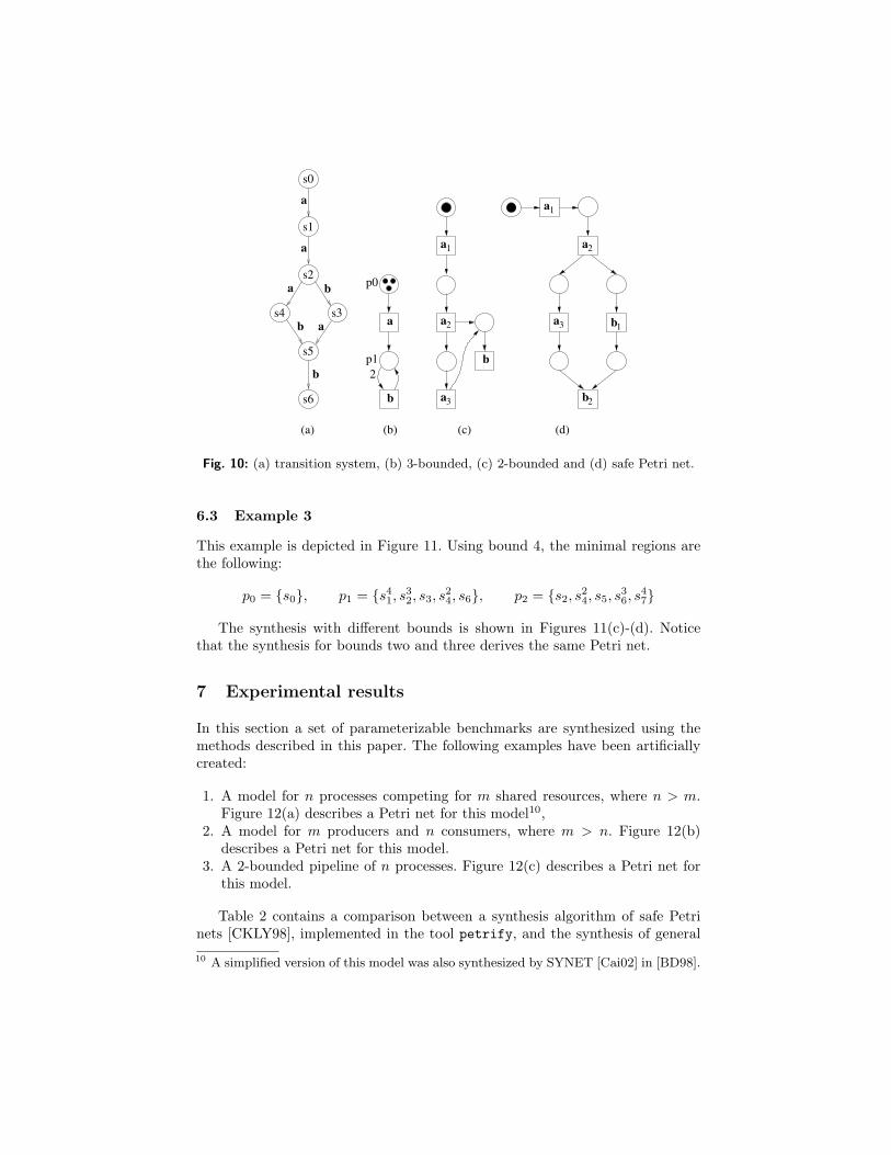
6.2 Example 2

The example is shown in Figure 10. In this case, two minimal regions are sufficientto guarantee the excitation closure when the maximal bound allowed is three(the corresponding Petri net is shown in Figure 10(b)):

p0 = {s30, s

21, s2, s3}, p1 = {s1, s

22, s3, s

34, s

25, s6}

The excitation closure of event b is guaranteed by >2(p1). However we alsohave that ∆b(p1) = −1, thus requiring an arc from p1 to b with weight 2 andanother arc from b to p1 with weight 1. The former is necessary to ensure thatb will not fire unless two tokens are held in p1. The latter is necessary to ensurethe gradient -1 of b with regard to p1. Figures 10(c)-(d) contain the synthesis forbound 2 and 1, respectively.

1

2

3

1

2

3 1

2b

a

p0

(a) (b) (d)(c)

p1

b

a

a

s2

s4

b

a

ab

2

s0

s1

s3

s5

s6

b

a

a

a

a

a

a b

b

Fig. 10: (a) transition system, (b) 3-bounded, (c) 2-bounded and (d) safe Petri net.

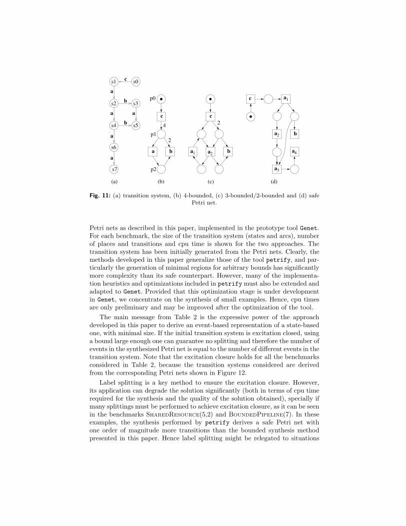
6.3 Example 3

This example is depicted in Figure 11. Using bound 4, the minimal regions arethe following:

p0 = {s0}, p1 = {s41, s

32, s3, s

24, s6}, p2 = {s2, s

24, s5, s

36, s

47}

The synthesis with different bounds is shown in Figures 11(c)-(d). Noticethat the synthesis for bounds two and three derives the same Petri net.

7 Experimental results

In this section a set of parameterizable benchmarks are synthesized using themethods described in this paper. The following examples have been artificiallycreated:

1. A model for n processes competing for m shared resources, where n > m.Figure 12(a) describes a Petri net for this model10,

2. A model for m producers and n consumers, where m > n. Figure 12(b)describes a Petri net for this model.

3. A 2-bounded pipeline of n processes. Figure 12(c) describes a Petri net forthis model.

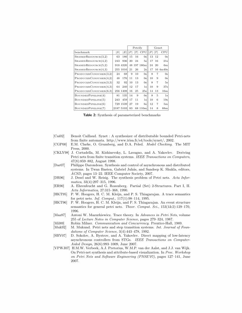
Table 2 contains a comparison between a synthesis algorithm of safe Petrinets [CKLY98], implemented in the tool petrify, and the synthesis of general

10 A simplified version of this model was also synthesized by SYNET [Cai02] in [BD98].

1

1

2

2

3

4

p0

c

a b

2

a

ab

b

s1

s2

s4

s3

s5

s6

s7

a

a

a

a

a

4

p12

p2

b

(a) (b) (c)

c

c

(d)

cs0

a

ba

a

a

Fig. 11: (a) transition system, (b) 4-bounded, (c) 3-bounded/2-bounded and (d) safePetri net.

Petri nets as described in this paper, implemented in the prototype tool Genet.For each benchmark, the size of the transition system (states and arcs), numberof places and transitions and cpu time is shown for the two approaches. Thetransition system has been initially generated from the Petri nets. Clearly, themethods developed in this paper generalize those of the tool petrify, and par-ticularly the generation of minimal regions for arbitrary bounds has significantlymore complexity than its safe counterpart. However, many of the implementa-tion heuristics and optimizations included in petrify must also be extended andadapted to Genet. Provided that this optimization stage is under developmentin Genet, we concentrate on the synthesis of small examples. Hence, cpu timesare only preliminary and may be improved after the optimization of the tool.

The main message from Table 2 is the expressive power of the approachdeveloped in this paper to derive an event-based representation of a state-basedone, with minimal size. If the initial transition system is excitation closed, usinga bound large enough one can guarantee no splitting and therefore the number ofevents in the synthesized Petri net is equal to the number of different events in thetransition system. Note that the excitation closure holds for all the benchmarksconsidered in Table 2, because the transition systems considered are derivedfrom the corresponding Petri nets shown in Figure 12.

Label splitting is a key method to ensure the excitation closure. However,its application can degrade the solution significantly (both in terms of cpu timerequired for the synthesis and the quality of the solution obtained), specially ifmany splittings must be performed to achieve excitation closure, as it can be seenin the benchmarks SHAREDRESOURCE(5,2) and BOUNDEDPIPELINE(7). In theseexamples, the synthesis performed by petrify derives a safe Petri net withone order of magnitude more transitions than the bounded synthesis methodpresented in this paper. Hence label splitting might be relegated to situations

P1

Pn

........

m

(a)

Pm

P1

..........

nn

n

(b)

Pn

P2

P1

..........

2

2 2

2 2

2

(c)

Fig. 12: Parameterized benchmarks: (a) n processes competing for m shared resources,(b) m producers and n consumers, (c) a 2-bounded pipeline of n processes.

where the excitation closure does not hold (see the examples of Section 6), orwhen the maximal bound is not known, or when constraints are imposed on thebound of the resulting Petri net.

8 Conclusions

An algorithm for the synthesis of k-bounded Petri nets has been presented. Byheuristically splitting events into multiple transitions, the algorithm always guar-antees a visualization object. Still, a minimal Petri net with bisimilar behavioris obtained when the original transition systems is excitation closed.

The theory presented in this paper is accompanied with a tool that providesa practical visualization engine for concurrent behaviors.

References

[BBD95] E. Badouel, L. Bernardinello, and P. Darondeau. Polynomial algorithms forthe synthesis of bounded nets. Lecture Notes in Computer Science, 915:364–383, 1995.

[BD98] Eric Badouel and Philippe Darondeau. Theory of regions. In WolfgangReisig and Grzegorz Rozenberg, editors, Petri Nets, volume 1491 of LectureNotes in Computer Science, pages 529–586. Springer, 1998.

[BDLS07] R. Bergenthum, J. Desel, R. Lorenz, and S.Mauser. Process mining basedon regions of languages. In Proc. 5th Int. Conf. on Business Process Man-agement, pages 375–383, September 2007.

[Bry86] Randal Bryant. Graph-based algorithms for Boolean function manipulation.IEEE Transactions on Computer-Aided Design, 35(8):677–691, 1986.

Petrify Genet

benchmark |S| |E| |P | |T | CPU |P | |T | CPU

SHAREDRESOURCE(3,2) 63 186 15 16 0s 13 12 0s

SHAREDRESOURCE(4,2) 243 936 20 24 5s 17 16 21s

SHAREDRESOURCE(5,2) 918 4320 48 197 180m 24 20 6m

SHAREDRESOURCE(4,3) 255 1016 21 26 2s 17 16 4m40s

PRODUCERCONSUMER(3,2) 24 68 9 10 0s 8 7 0s

PRODUCERCONSUMER(4,2) 48 176 11 13 0s 10 9 0s

PRODUCERCONSUMER(3,3) 32 92 10 13 0s 8 7 5s

PRODUCERCONSUMER(4,3) 64 240 12 17 1s 10 9 37s

PRODUCERCONSUMER(6,3) 256 1408 16 25 25s 14 13 16m

BOUNDEDPIPELINE(4) 81 135 14 9 0s 8 5 1s

BOUNDEDPIPELINE(5) 243 459 17 11 1s 10 6 19s

BOUNDEDPIPELINE(6) 729 1539 27 19 6s 12 7 5m

BOUNDEDPIPELINE(7) 2187 5103 83 68 110m 14 8 88m

Table 2: Synthesis of parameterized benchmarks

[Cai02] Benoıt Caillaud. Synet : A synthesizer of distributable bounded Petri-netsfrom finite automata. http://www.irisa.fr/s4/tools/synet/, 2002.

[CGP00] E.M. Clarke, O. Grumberg, and D.A. Peled. Model Checking. The MITPress, 2000.

[CKLY98] J. Cortadella, M. Kishinevsky, L. Lavagno, and A. Yakovlev. DerivingPetri nets from finite transition systems. IEEE Transactions on Computers,47(8):859–882, August 1998.

[Dar07] Philippe Darondeau. Synthesis and control of asynchronous and distributedsystems. In Twan Basten, Gabriel Juhas, and Sandeep K. Shukla, editors,ACSD, pages 13–22. IEEE Computer Society, 2007.

[DR96] J. Desel and W. Reisig. The synthesis problem of Petri nets. Acta Infor-matica, 33(4):297–315, 1996.

[ER90] A. Ehrenfeucht and G. Rozenberg. Partial (Set) 2-Structures. Part I, II.Acta Informatica, 27:315–368, 1990.

[HKT95] P. W. Hoogers, H. C. M. Kleijn, and P. S. Thiagarajan. A trace semanticsfor petri nets. Inf. Comput., 117(1):98–114, 1995.

[HKT96] P. W. Hoogers, H. C. M. Kleijn, and P. S. Thiagarajan. An event structuresemantics for general petri nets. Theor. Comput. Sci., 153(1&2):129–170,1996.

[Maz87] Antoni W. Mazurkiewicz. Trace theory. In Advances in Petri Nets, volume255 of Lecture Notes in Computer Science, pages 279–324, 1987.

[Mil89] Robin Milner. Communication and Concurrency. Prentice-Hall, 1989.[Muk92] M. Mukund. Petri nets and step transition systems. Int. Journal of Foun-

dations of Computer Science, 3(4):443–478, 1992.[SBY07] D. Sokolov, A. Bystrov, and A. Yakovlev. Direct mapping of low-latency

asynchronous controllers from STGs. IEEE Transactions on Computer-Aided Design, 26(6):993–1009, June 2007.

[VPWJ07] H.M.W. Verbeek, A.J. Pretorius, W.M.P. van der Aalst, and J.J. van Wijk.On Petri-net synthesis and attribute-based visualization. In Proc. Workshopon Petri Nets and Software Engineering (PNSE’07), pages 127–141, June2007.