Copyright Warning & Restrictions

The copyright law of the United States (Title 17, United States Code) governs the making of photocopies or other

reproductions of copyrighted material.

Under certain conditions specified in the law, libraries and archives are authorized to furnish a photocopy or other

reproduction. One of these specified conditions is that the photocopy or reproduction is not to be “used for any

purpose other than private study, scholarship, or research.” If a, user makes a request for, or later uses, a photocopy or reproduction for purposes in excess of “fair use” that user

may be liable for copyright infringement,

This institution reserves the right to refuse to accept a copying order if, in its judgment, fulfillment of the order

would involve violation of copyright law.

Please Note: The author retains the copyright while the New Jersey Institute of Technology reserves the right to

distribute this thesis or dissertation

Printing note: If you do not wish to print this page, then select “Pages from: first page # to: last page #” on the print dialog screen

The Van Houten library has removed some of the personal information and all signatures from the approval page and biographical sketches of theses and dissertations in order to protect the identity of NJIT graduates and faculty.

ABSTRACT

Techniques of Petri Net Reduction

by

Sreeranga Kalavapalli

Petri Nets have the capability to analyze large and complex concurrent

systems. However, there is one constraint. The number of reachability states of the

concurrent systems outweighs the capability of Petri Nets. Previous Petri Net

reduction techniques focussed on reducing a subnet to a single transition and hence

not powerful enough to reduce a Petri Net. This paper presents six reduction rules

and discusses their drawbacks. A new reduction technique called Knitting

Technique to delete paths of a Petri Net while retaining all the properties of the

original net is presented. Further Structural matrix which facilitates reduction is

presented.

TECHNIQUES OF PETRI NET REDUCTION

by

Sreeranga Kalavapalli

A ThesisSubmitted to the Faculty of

New Jersey Institute of Technologyin Partial Fulfillment of the Requirements for the Degree of

Master of Science in Computer Science

Department of Computer and Information Science

May 1993

APPROVAL PAGE

Techniques Of Petri Net Reduction

Sreeranga Kalavapalli

Dr. Daniel Yuh Chao, Thesis Adviser (Date)Assistant Professor of Computer and Information Science,

\\..)Dr. David Wang (Date)Assistant Professor of Computer and Information Scien e,NUT

M.C. Zhou (Date)Assistant Professor of Electrical and Computer Engineering,NJIT

BIOGRAPHICAL SKETCH

Author: Sreeranga Kalavapalli

Degree: Master of Science in Computer Science

Date: May 1993

Undergraduate and Graduate Education:

* Master of Science in Computer Science,New Jersey Institute of Technology, Newark, NJ, 1993

* Master of Business Administration in Computer Systems,Osmania University, Hyderabad, India, 1990

* Master of Science in Semi-Conductor Physics,S.V.University, Tirupati, India, 1978

Major: Computer Science

iv

ACKNOWLEDGMENT

I would like to thank my Thesis Advisor, Dr. Daniel Yuh Chao for his help and

guidance in completing this thesis. His constructive criticism coupled with the

time he spent every week on the thesis helped me a great deal in doing this

thesis. The group meetings and the presentations held every week helped to

improve my knowledge in the field of Petri Net Reduction.

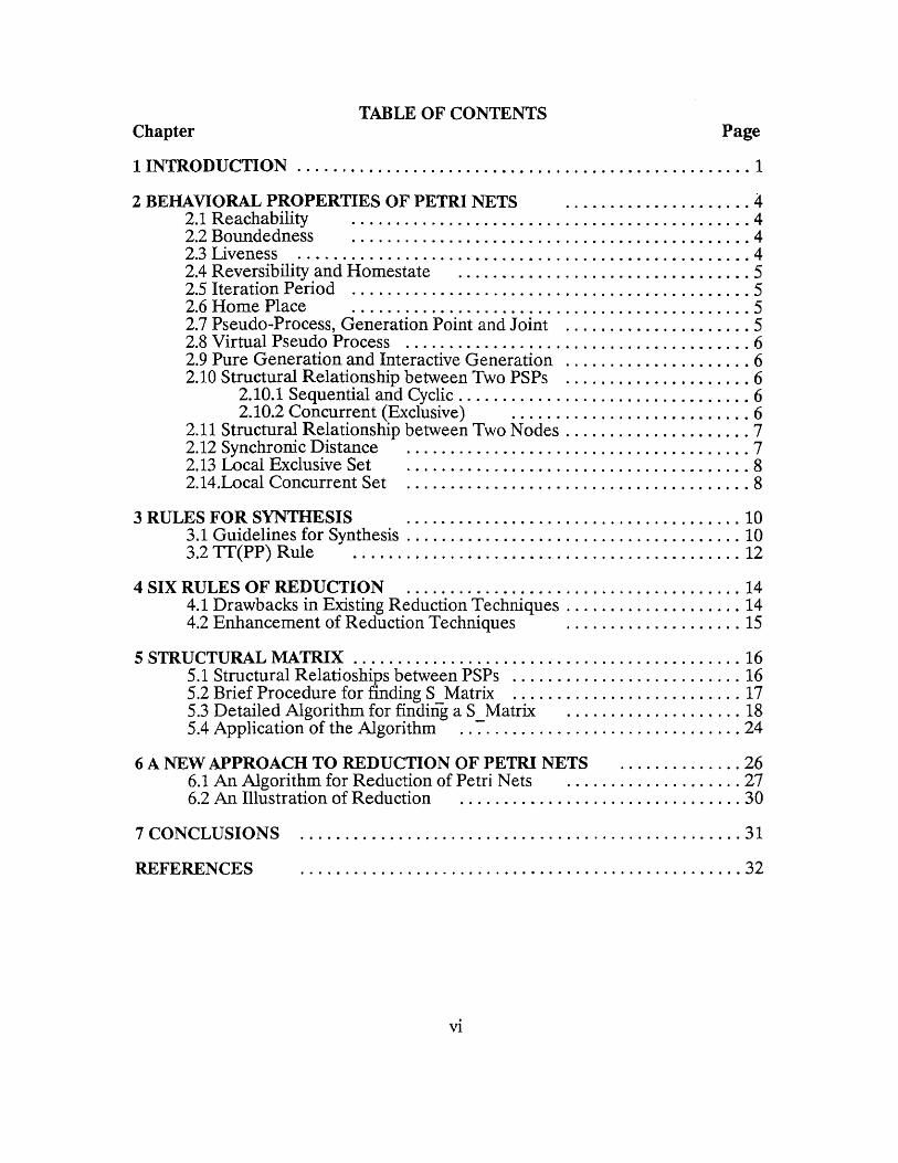
TABLE OF CONTENTSChapter Page

1 INTRODUCTION 1

2 BEHAVIORAL PROPERTIES OF PETRI NETS 42.1 Reachability 42.2 Boundedness 42.3 Liveness 42.4 Reversibility and Homestate 52.5 Iteration Period 52.6 Home Place 52.7 Pseudo-Process, Generation Point and Joint 52.8 Virtual Pseudo . Process 62.9 Pure Generation and Interactive Generation 62.10 Structural Relationship between Two PSPs 6

2.10.1 Sequential and Cyclic 6

2.10.2 Concurrent (Exclusive) 62.11 Structural Relationship between Two Nodes 72.12 Synchronic Distance 72.13 Local Exclusive Set 82.14.Local Concurrent Set 8

3 RULES FOR SYNTHESIS 103.1 Guidelines for Synthesis 103.2 TT(PP) Rule 12

4 SIX RULES OF REDUCTION 144.1 Drawbacks in Existing Reduction Techniques 14

4.2 Enhancement of Reduction Techniques 15

5 STRUCTURAL MATRIX 165.1 Structural Relatioships between PSPs 165.2 Brief Procedure for finding S Matrix 17

5.3 Detailed Algorithm for findirig a S Matrix 185.4 Application of the Algorithm — 24

6 A NEW APPROACH TO REDUCTION OF PETRI NETS 266.1 An Algorithm for Reduction of Petri Nets 276.2 An Illustration of Reduction 30

7 CONCLUSIONS 31

REFERENCES 32

vi

LIST OF FIGURESFigure Page

2.1 A Basic Process with Home place facing 52.2 Pure Generation(dashed line) by using TT

rule and Forward TT Generation facing 52.3 Interactive Generation(dashed line)

connecting PSP1 and PSP4 by using PP rule facing 62.4 Local Exclusive Set facing 82.5 Local Concurrent Set facing 8

3.1 Backward TT Generation facing 113.2 An Example of the Application of the

TT.4 Rule (Completeness Rule 1) facing 133.3 An Example of the Application of the

PP.2 Rule (Completeness Rule 2) facing 134.1 Fusion of Series Places facing 144.2 Fusion of Series Transitions facing 144.3 Fusion of Parallel Places facing 144.4 Fusion of Parallel Transitions facing 144.5 Elimination of Self Loop Places facing 144.6 Elimination of Self Loop Transitions facing 145.1 An Example of a Petri Net facing 245.2 The S Matrix for the PN in Fig. 5.1 facing 246.1 An Ex—ample for Petri Net Reduction facing 306.2 A Reduced Net for Petri Net in Fig. 6.1 facing 306.3 An Example for Petri Net Reduction facing 306.4 A Reduced Net for Petri Net in Fig. 6.3 facing 30

vii

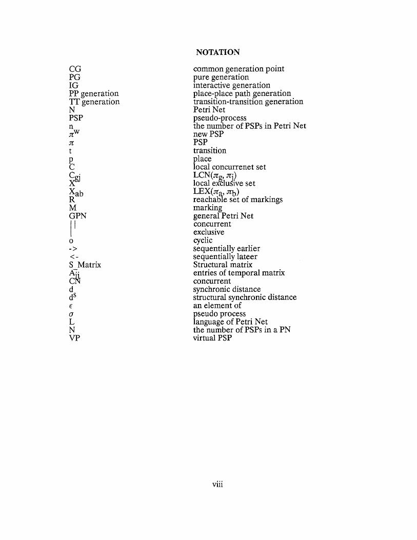
NOTATION

CG common generation pointPG pure generationIG interactive generationPP generation place-place path generationTT generation transition-transition generationN Petri NetPSP pseudo-processn the number of PSPs in Petri Net,71W new PSPa PSPt transitionp placeC local concurrenet setCgi LCN(ng, gr)ilX—local exclugive setXab LEX(za, ab)R reachable set of markingsM markingGPN general Petri Net

concurrentexclusive

o cyclic- > sequentially earlier< - sequentially lateerS Matrix Structural matrixAC:. entries of temporal matrixCP,1 concurrentd synchronic distanceds structural synchronic distanceE an element ofa pseudo processL language of Petri NetN the number of PSPs in a PNVP virtual PSP

viii

CHAPTER 1

INTRODUCTION

Many real world concurrent systems are dynamic as well as complex. Any tool

which aid in analyzing the highly complex and concurrent systems should have

the capability to model concurrency, conflict and asynchrony. Petri Nets(PNs)

besides having the above capability share other properties such as boundedness,

liveness, completeness with the concurrent systems. Hence Petri Nets(PNs) have

been adopted to model and analyze a large class of systems and proposed to

model software [3]-[5]. However, as the system grows in complexity, the number

of reachability states of the concurrent systems outweighs the capability of Petri

Nets(PNs). This is called State Explosion Problem.

In order to solve the above problem researchers have proposed many

reduction techniques, which emphasize on reducing the size of a given PN while

preserving the properties such as liveness, boundedness, dead-lock free and

reversibility and can be used to simplify analysis. The objective is to reduce

several places and transitions into a manageable number of transitions or places

and the conclusion of the analysis is valid to the original net. The reduction

techniques proposed by many researchers so far focussed on reducing a subnet

or a partial PN to a single transition [11]-[13].

In order to do so, the subnet to be reduced should behave equivalently to

a transition. At present, there are only a few types of subnets that may be

reduced to a single transaction such as single output transaction or some other

simple structures [14]. In most of the existing methods the test of a reduced net

has not been automated and is often very complex. Hence there is a necessity to

adopt a new approach which ensures deletion of paths of a PN in a gradual and

automated fashion.

1

A new technique which can reduce nets more efficiently than the

traditional techniques is proposed here. This technique enhances the vigor of the

current reduction techniques. Similar to the generation of paths using synthesis

rules, the deletion of paths must preserve certain properties, both desired and

undesired, of the original net. Such an approach for generalized PNs was

demonstrated by Koh[7]. Yet another technique called Knitting Technique can

synthesize PNs[9] that cannot be synthesized by Koh's fusing technique.

Adopting same rules of the knitting technique in the reverse direction PNs can

be reduced more effectively than the other techniques.

Yaw[8]-[10] developed a rule-based interactive technique called Knitting

Technique. The technique contains some simple rules which can guide the

synthesis of PNs with the desired properties. New paths and cycles to a PN are

added in an incremental way. The system properties such as boundedness,

liveness and reversibility are retained by the PNs at each step. Hence the

tiresome analysis of these properties can be avoided by the designers while

building a Petri Net model for a complicated system. There are two types of

knitting rules- TT and PP rules. These rules guarantee incremental correctness

at each step of synthesis.

A structural matrix is used to record the relationship (sequential, cyclic,

concurrent, exclusive, etc., between any two pseudo-processes in a PN such that

the maximum concurrency at any execution stage is available. Hence a structural

matrix can be used to perform reduction of a Petri Net. Most of the earlier

reduction techniques deal with local transformation. The transformation by

structural matrix can be termed as a global technique

2

The remaining chapters of the paper are organized as follows. Chapter 2

presents some behavioral properties of PNs. Chapter 3 presents general

synthesis rules and some illustrations. Chapter 4 discusses six reduction rules and

the drawbacks of previous reduction rules. Chapter 5 discusses structural matrix

for PNs, the algorithm for constructing a structural matrix and an application as

an illustration. Chapter 6 discusses the reduction algorithm and an application

of the same. The conclusions are given in Chapter 7.

3

CHAPTER 2

BEHAVIORAL PROPERTIES OF PETRI NETS

A major strength of Petri Nets is their support for analysis of many properties

and problems associated with concurrent systems. Most concurrent systems are

designed to achieve cyclic behavior such that the Petri Net model can be made

applicable to them. A brief review of various properties of Petri Nets is

presented below for better understanding of the paper.

2.1 Reachability

The firing of an enabled transition of a Petri Net will change the token marking.

A sequence of firings will result in a sequence of markings. A marking M n is said

to be reachable from a marking Mo if there exists a sequence of firings that

transform Mo to M n.

2.2 Boundedness

A Petri Net is said to be bounded if the number of tokens in each place does not

exceed a finite number. Places in a Petri Net are often used to represent buffers

and registers for storing intermediate data. By verifying that the net is bounded

or safe, it is guaranteed that there will be no overflows in the buffers or registers.

2.3 Liveness

A Petri Net is said to be live if no matter what marking has been reached from

the original place. It is possible to ultimately fire any transition of the net by

progressing through some firing sequence. This means that a PN is said

4

facing 5

Fig. 2.1 A Basic Process with Home place

facing 5

Fig. 2.2 Pure Generation(dashed line) by using Ti rule

and Forward TT Generation

to be live, if it guarantees dead lock free operation, no matter what firing

sequence is chosen.

2.4 Reversibility and Homestate

A PN is said to be reversible if, for each initial marking Mo e R ( N,M) for every

M e R(N,M0) i.e., the initial marking is recovered from any other marking.

2.5 Iteration Period

A reversible PN is the PN whose initial markings can always be recovered; the

corresponding period is termed as the iteration period.

2.6 Home Place

A home place in a PN is the place with token(s) such that it can start the

iteration period. Let transition ta be enabled in the initial marking of a PN and

place ph an input place of ta . This ph is defined as a home place. A basic process

in a PN is a cycle path which contains a home place. (shown in Fig. 2.1)

2.7 Pseudo -Process, Generation Point and Joint

A pseudo-process (PSP) in a PN is a directed elementary path where the

indegree and outdegree of any node (transition or place) inside the path are

both one except its two end nodes; the starting node is defined as the generation

point and the end node as the joint (shown in Fig. 2.2). Any other node in the

PSP has single input node and a single output one. A PSP cannot be subset of

any other PSPs, it is an elementary process of a PN.

5

facing 6

Fig. 2.3 Interactive Generation (dashed line) connectingPSP1 and PSP4 by using PP rule

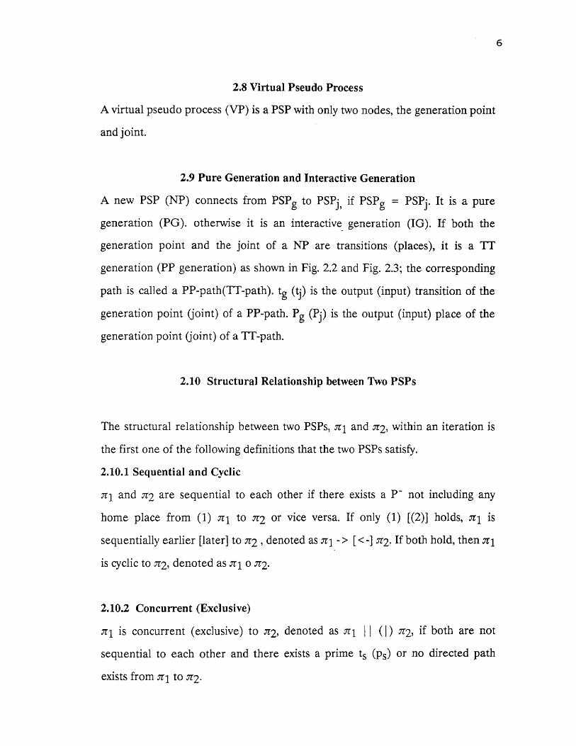
2.8 Virtual Pseudo Process

A virtual pseudo process (VP) is a PSP with only two nodes, the generation point

and joint.

2.9 Pure Generation and Interactive Generation

A new PSP (NP) connects from PSPg to PSPi , if PSPg = PSPj. It is a pure

generation (PG). otherwise it is an interactive generation (IG). If both the

generation point and the joint of a NP are transitions (places), it is a TT

generation (PP generation) as shown in Fig. 2.2 and Fig. 2.3; the corresponding

path is called a PP-path(TT-path). tg (9 is the output (input) transition of the

generation point (joint) of a PP-path. Pg (Pp is the output (input) place of the

generation point (joint) of a TT-path.

2.10 Structural Relationship between Two PSPs

The structural relationship between two PSPs, al and 7r2, within an iteration is

the first one of the following definitions that the two PSPs satisfy.

2.10.1 Sequential and Cyclic

ni and a2 are sequential to each other if there exists a P" not including any

home place from (1) al to n2 or vice versa. If only (1) [(2)] holds, ni is

sequentially earlier [later] to 7r2 , denoted as al > [ < -] 71.2. If both hold, then al

is cyclic to a2, denoted as al 0 a2.

2.10.2 Concurrent (Exclusive)

ri is concurrent (exclusive) to a2, denoted as ni (I) a2, if both are not

sequential to each other and there exists a prime is (ps) or no directed path

exists from al to a2.

6

2.11 Structural Relationship between Two Nodes

If two nodes (transition or place) are in two different PSPs, their structurral

relationship follows that of the two PSPs. If they are in the same PSP, they are

sequential to each other.

It is easy to see that if we execute one iteration of a safe and strongly

connected PN involving sr1 , then ai - > 72 implies that zi is executed earlier

than 72; ;1'1 I 72 implies that there is no need to execute .72 to complete one

iteration; intuitively, two PSPs, 7r1 11 72 are sequential to each other if they are

subject to an intra-iteration precedence relationship; i.e., if both are executed in

one iteration, then one is executed earlier than the other. 71 and 72 are

concurrent to each other if they proceed in parallel. 7r1 and 72 are exclusive to

each other if it is possible to complete one iteration with only one of them being

executed.

2.12 Synchronic Distance

Synchronic distance is a concept closely related to the degree of mutual

dependence between two events in a condition/event system. The definitions of

Petri Net language and Synchronic Distance are given as follows:

The language of a Petri Net N, L( N, M ), is the set of all firing sequences

for the net with the initial marking M : L( N, M)=1a1M[a> M'] 1.

The synchronic distance between two transitions t1 and t2 in a petri net N

is defined as d12 = Max { a ( t1 ) - t2 ), a E L( N, M ) }, where a(t) is the

number of times t appears in a.

This definition can be extended to sets. Thus d (W,V) is the maximum

number of firings of transitions in set W without any transition firing in set V.

Depending on whether dgj = a or 1, different synthesis rules are

constructed for a new TT - generation. If we generate a TT-path between two

7

facing 8

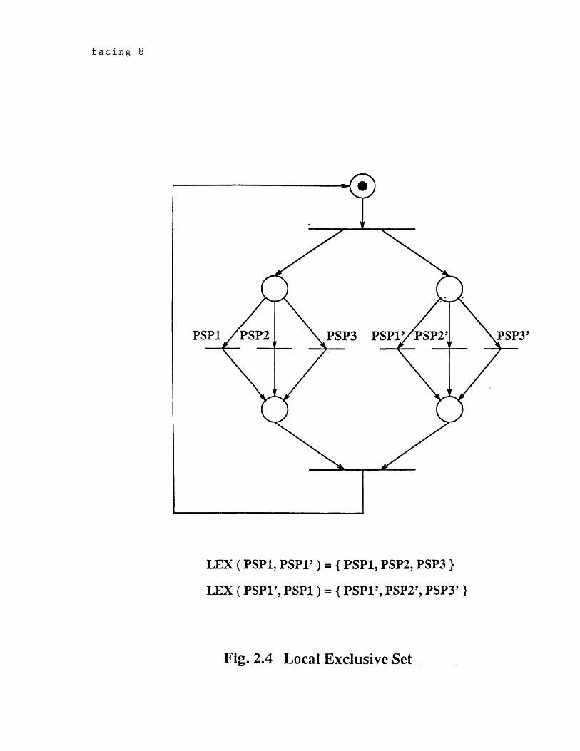
Fig. 2.4 Local Exclusive Set

facing 8

Fig. 2.5 Local Concurrent Set

transitions tg and t. with infinite synchronic distance, unbounded tokens couldJ

accumulate in the TT-path when tg fires infinitely without firing ti once. This

synchronic distance between two concurrent (or sequential) transitions t g and ti

may be a if there exists a transition tx I ti . However, the synchronic distance

between the two sets of transitions containing tg and ti respectively may equal

one. One (called Xgj ) contains tg and all transitions that are exclusive to tg but

concurrent (or sequential) to ti ; the other (Xi g) contains ti and all transitions

that are exclusive to ti but concurrent (or sequential) to tg. The following defines

a similar Xik whose members are PSPs rather than transitions.

2.13 Local Exclusive Set

A local exclusive set (LEX) of Sri with respect to ak, Xik, is the maximal set of

all PSPs which are exclusive to each other and are equal or exclusive to ni, but

not to irk. i.e.,Xik LEX(yri, ark) { I = 79 or az I rz I ( not

exclusive to Yrk}. Fig. 2.4 is an example for a local exclusive set.

2.14 Local Concurrent Set

A local concurrent set (LCN) of al with respect to Yrk, Cik = LCN (ai, irk ), is

the maximal set of all PSPs which are concurrent to each other and are equal or

concurrent to yri but not to 7tk, i.e., Cik = C (ai, = 7rz az = ni or az 1

ni, az I I (not concurrent to) ak }. Fig. 2.5 is an example for a local concurrent

set.

The definition of LEX [LCN] between two PSPs can be extended to the

LEX [ LCN ] between two transitions [ places]. Thus LEX (ti , tk) [LCN(pi, pk) ]

is a set of transitions [places], instead of PSPs. Let G(J) denote the set of all er g

(a.J) involved in a single application

8

of the TT or PP rule. To avoid the unboundedness problem, it is necessary to

have a new directed path from each PSP in X gj to each PSP in Xjg. Both Xgj

and Xjg can be determined from the S Matrix even though d gj = a, which is,

therefore, of no use to the synthesis. For instance, we have observed that when t g

I tj and dgj = 1, the inforamation of dgj = a is of no use and we define that

dsgj = 1. On the contrary, when dgj = a, the TT-generation from tg to tj will

cause unbounded places in the TT-path. This problem cannot be detected by just

checking the T-Matrix and the information of d gj = a is indeed useful here and

the value of dsgj remains to be a. Hence we have the following definition of

structural synchronic distance. The structural synchronic distance between n g

and 79 is dsgj = 1 if dgj is finite and d gj = a if dgj = a.

9

CHAPTER 3

RULES FOR SYNTHESIS

Consider a Petri Net modeling a set of interacting entities. At the outset, each

entity has a home place with tokens indicating that it is ready to fire. Each entity

conducts consecutive tasks ( which can be considered as transitions ), and then

returns to the original ready state. Each state can be considered as a place.

Executing a task means firing a transition. At the completion of executing each

task, the token leaves the original state and enters the next state by firing a

transition. Thus, in the corresponding Petri Net model, the token moves from

the home place through consecutive places by firing a sequence of transitions.

Eventually, the token will return to the home place, forming a cycle as shown in

Fig.2.1. The process yielding this cycle is termed a Basic Process.

3.1 Guidelines For Synthesis

By a set of path generations the Petri Net can be expanded starting from the

basic process. Each path is a PSP. The path generations are of two types: Pure

Generation (PG) and Interactive Generation (IG). PG generates paths within a

single PSP. That means a single PSP can be expanded into a set of PSPs by

adding paths. PG processes are pure growth processes. They do not involve any

interactions between PSPs as shown in Fig. 2.2. Interactive Generation (IG)

generates paths between PSPs to interconnect a set of PSPs. So this method of

generation involves interaction between PSPs as shown in Fig. 2.3.

1 0

facing 11

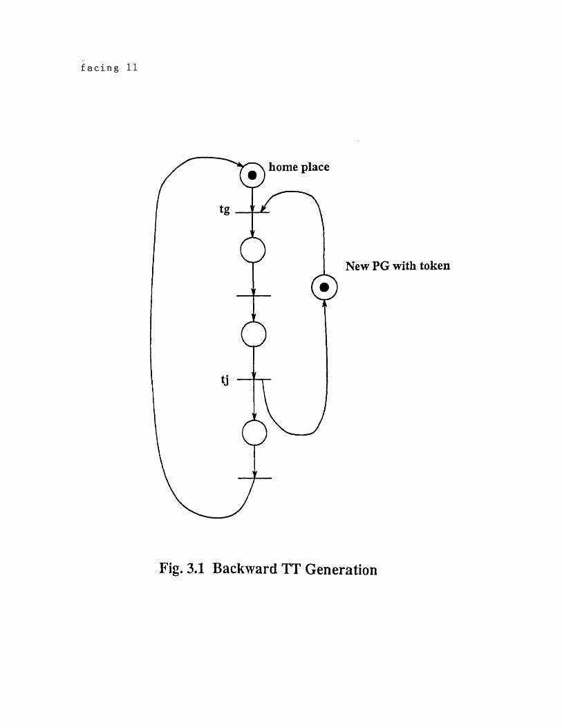
Fig. 3.1 Backward TT Generation

Paths can be generated in two ways for both Pure generation and

Interactive generation. The two types are: IT rule and PP rule. The TT rule

(transition to transition) is applicable to generation of paths from transition to

transition, from the generation point tg to the joint tj; the PP rule (place to

place) is applicable to generation of paths from place to place, from a generation

point Pg to Pi. The Figs. 2.2 and 2.3 explain this concept. There are two types of

generations: Forward and backward. If Pg - > P (tg- > tj), then it is a forward PP

(TT) generation (Fig. 2.2); it is a backward PP(TT) generation if the direction of

- > changes. If it is a backward TT generation, insert token(s) in the new cycle if

it does not have any token (Fig. 3.1).

Given a synthesized net, N1, a set of new paths are generated using some

synthesis rules to form another net, N2. The marking in NP upon the generation

is called its initial marking. This synthesis rules should be such that all transitions

and places in Petri Net N2 are also live and bounded. This can be ensured by.

1) Inhibiting any intrusion into normal transitions firings of N1 prior to the

generations. This guarantees that neither unbounded places nor dead transitions

would occur in N1 since it was live and bounded prior to the generations.

2) Inhibiting any dead transitions and unbounded places in NP.

There are two kinds of intrusion. One is to change the marking of N1; the

other is to eliminate some reachable markings. Inorder for NP to be live, it must

be able to get enough tokens from Pg or by firing tg. When tokens in NP

disappear, the resultant marking of the subnet N1 in N2 must be reachable in N1

prior to the generation of NP. Further, the marking of NP must be reversible in

N2.

The second intrusion may occur when the joint is a transition which may

not be enabled in case of backward TT generation; hence causing some

markings in Ni

11

12

unreachable. Thus, if the joint is a transition, NP must be able to get tokens from

a generation point within each iteration.

Based on the concept of no intrusion, the rules are constructed according

to the following guidelines

1) From Mo, each tg must be potentially (always or has fired for every Q in Ni

enabling the joint which is a transition) firable.

2) These tokens must disappear from NP before it gets unbounded tokens, and

return to Ni to reach a marking M2. The marking of the subnet Ni in N2, M2 (

Ni) of all possible sets of such M2 are identical to those in Ni without the new

paths.

Guidelines (1) and (2) guarantee no intrusion. Guideline (2) guarantees

no dead transitions and no unbounded places in NP (since all tokens can

disappear from NP).

Synthesis rules are presented below. It should be noted that the TT and

PP rules are merged together. The words and notations inside the parentheses

are for the PP rules.

3.2 TT (PP) Rule

Generate a ,7rw from tg ( Pg ) E ng to tj ( Pj) E yri

1) TT.1 (PP.1): If 7rg = then signal " a pure TT (PP) generation".

2) TT.2: If tg < tj , then signal "forming new circles, creating a new home place

". If there does not exist a a to fire tg without firing tj, then insert a token in a

place of nw. If erg = 7tj , then return and the designer may start a new

generation.

If tg I I tj (pg I pi ) or tg (pg)- > tj (pi) or tj (pi) - > tg (pg ), and if 7rg not equal to

7r. then signal "an interactive Tr (PP) generation ".

3) TT.3: If the structure synchronic distance d

a then

facing 13

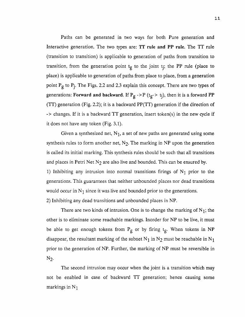
Fig. 3.2 An Example of the Application of theTT.4 Rule (Completeness Rule 1)

facing 13

Fig. 33 An Example of the Application of the PP.2 Rule (Completeness Rule 2 )

3.a) TT.3.1: Apply TT.4 rule,

3.b) TT.3.2: Generate a new TT-path to synchronize tg and tj so that

after step 3.c, dgis changes from a to 1.

3.c) Go to step 2.

4) TT.4: Or Completeness Rule 1 (PP.2 or Completeness Rule 2)

4.a) TT.4.1 (PP.2.1): Generate a TP- path from a transition t g of each Jrg

in X • (a tk of a ,7•Ew ) to a place pk (pi of each 79 in Ci g ) in a ,mow .

4.b) TT.4.2 (PP.2.2): Generate a virtual PT- path from the place pi (a pg

of each .7rg in Cgj ) to a transition tj of each yri in Xjg ( the tg in NP).

5) TT.5 (PP.3): For all other cases, (e.g., tg I tj and pg I I pp, signal "forbidden,

delete the new PSP" and return. Note that during each application of a rule,

more than one .7rw may be generated; we call such a generation a macro

generation. Otherwise, it is a singular generation. An example of the application

of the TT-4 rule (completeness rule) is shown in fig. 3.2. Similarly an example of

the application of the PP.2 rule ( completeness rule 2) is shown in fig. 3.3.

13

facing 14

Fig. 4.1 Fusion of Series Places

facing 14

Fig. 4.2 Fusion of Series Transitions

facing 14

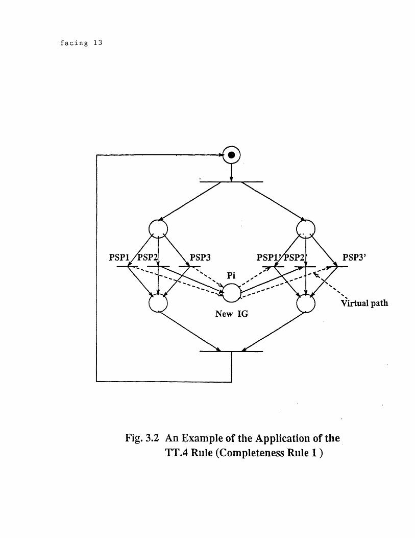
Fig. 4.3 Fusion of Parallel Places

facing,14

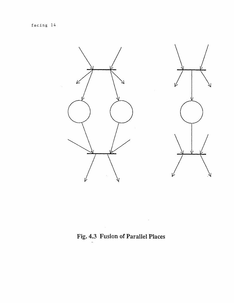
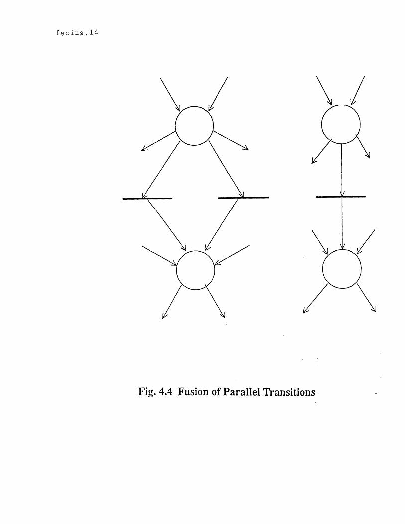
Fig. 4.4 Fusion of Parallel Transitions

facing '14

Fig. 4.5 Elimination of Self Loop Places.

facing 14

Fig. 4.6 Elimination of Self Loop Transitions

CHAPTER 4

SIX RULES OF REDUCTION

The six Reduction rules are as follows

1. Fusion of series places (FSP)

2. Fusion of series transitions (FST)

3. Fusion of parallel places(FPP)

4. Fusion of parallel transitions(FPT)

5. Elimination of self loop places (ESP)

6. Elimination of Self loop Transitions(EST)

The above six operations are shown in the figures 4.1 thru 4.6. From the

figures it can be seen that the reduced places or transitions retain all the

properties of the original sub nets.

4.1 Drawbacks in Existing Reduction Techniques

The present techniques reduce subnets or partial Petri Nets to a single place or

transition. To satisfy the requirement the subnet to be reduced must behave,

viewing from both inside and outside of the subnet, equivalently to a transition.

This has limited the types of subnets that may be reduced to a single transition.

Currently, the reducible subnets need to be of single input-transition, single-

output-transition,or some other simple structures. Further these techniques do

not detect dead locks or unbounded places during the reduction process. Further

the reduction techniques discussed above do not reduce Petri Nets with identical

characteristics. Petri Net reduction is to replace a module with a transition. A

14

module in a Petri Net is subnet whose interfaces with other parts of the net are

through certain well defined

transitions in the module. A set of modules can be reduced to only one module

under the following conditions:

1.They have common output places and input places;

2. They are disjoint;

3. Each module has only one entry transition.

A set of Transitions can be reduced to a single transition,if they have identical

characteristics viz., same input/output places and the number of arcs in between.

4.2 Enhancement of Reduction Techniques

Structural matrix can be used to perform reduction of a Petri Net. All the

techniques mentioned above do not guarantee complete elimination of analysis.

Most of them deal with local transformation. The Transformation by Structural

matrix can be a Global Technique. Transitions and places can be deleted

according to certain rules.

15

CHAPTER 5

STRUCTURAL MATRIX

This chapter discusses the structural relationships between PSP s recorded by

Structural matrix (S Matrix) , a brief procedure for finding S Matrix , a detailed

algorithm for finding S_Matrix and also an example of the application of the

algorithm.

5.1. Structural Relationships Between PSPs

A Petri Net can be expanded by inserting new paths having some physical

meaning such as increasing concurrency, alternatives etc as per the above

discussed Knitting Technique. The resultant net will be an ordinary net with

properties such as liveness, boundedness, safeness, and consistency. With the

help of this technique many entities can be synthesized. This strategy takes

advantage of the fact that the structural relationships between PSPs in a logically

correct PN must satisfy some constraints. Structural matrix records relationships

between PSPs in the PN. If the relationships among a set of PSPs violate some

synthesis rules and which are complete, then the net has some undesired

properties such as unboundedness, deadlocks. Hence S Matrix is very useful for

analysis.

An entry of Structural matrix, S_Matrix[i][j] corresponding to row i and

column j, stands for the structural relationship between PSPi and PSPj. It may be

one of the following.

16

Sequential: PSPi and PSPj are sequential to each other during the iteration

period.

Earlier (PSPi SE PSPj ): If PSPi is sequential earlier to PSPj, then S_Matrix[i][j]

= 'SE'; reversely, S_Matrix[j][i] = 'SL';

Later (PSPi SL PSPi): If PSPi is sequential later to PSPj, then S_Matrix[i][j] =

'SL'; reversely, S_Matrix[j][i] = 'SE'.

Previous (PSPj SP PSPi): If PSPi is sequential previous to PSPi , then

S_Matrix[i][j] = 'SP'; reversely, S matrix[j][i] = 'SN'.

Next (PSPi SN PSPi): If PSPi is equal next to PSPj, then S_Matrix[i][j] = 'SN";

reversely, S_Matrix[j][i] = 'SP'. Exclusive (PSPi SX PSPi) : if PSPi and PSPi are

sequential exclusive to each other during iteration periods, then S_Matrix[i][j] =

S_Matrix[j][i] = 'SX'.

Cyclic(PSPi CL PSPi): If PSPi and PSPj are cyclic to each other during iteration

periods, then they are both earlier and later than each other. Then S_Matrix[i][j]

= S_Matrix[j][i] = 'CL'.

Concurrent (PSPi CN PSPi): If PSPi and PSPj are concurrent to each other

during the iteration period, then S_Matrix[i][j] = S_Matrix[j][i] = 'CN'.

Exclusive (PSPi EX PSPi): If PSPi and PSPj are exclusive to each other during

the iteration period, then S_MAtrix[i][jJ= S_Matrix[j][i] = 'EX'.

5.2 Brief procedure for finding S_Matrix

Two search strategies such as depth-first or breadth-first are used to construct a

S_Matrix for a Petri net. In Petri Net theory sequential means depth, and

concurrent means breadth. In this paper "depth-first' search is adopted to find

the S_Matrix of a Petri Net. There are five major steps in finding the S _Matrix of

a Petri Net.

17

1) Generate a new PSP in depth-first search;

2) Enter the sequential relationships between this new PSP and other generated

PSPs respectively;

3) Update the S_Matrix if there exists a cycle.

4) Find the structural relationships between PSPs from current considered PSPs

and all other existing PSPs;

5) Check whether there exists sequential exclusive between PSPs. If so update

the S Matrix. The detailed algorithm is furnished below.

5.3 Detailed Algorithm for finding a S_Matrix

5.3.1 Unmark and uncheck all nodes in the given PN;

5.3.2 Select an input place of an enable transition in the initial marking as the

home place;

5.3.3 Find the PSP containing this home place ;

Let PSP.number =0;

5.3.4 Let the joint of this PSP be the current node;

5.3.5 Repeat the following steps until every node is checked;

5.3.5.1 If (the current node is a place ) then S = 'P';

else S = 'T';

5.3.5.2 while (1)

{

if (all output nodes of this current

node have been marked)

{

check this node;

backtrack to the generation point of

a PSP whose joint is this current node;

18

let this generation point be the

current node;

}

else

break;

/* while(1)*/

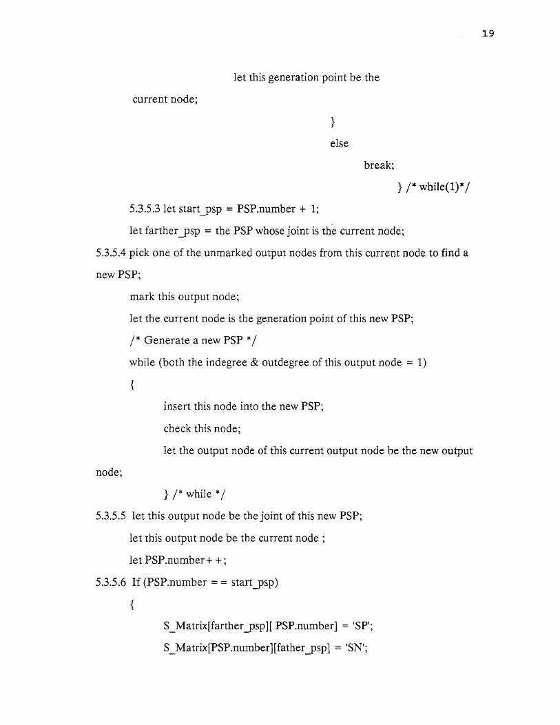
5.3.5.3 let start_psp = PSP.number + 1;

let farther_psp = the PSP whose joint is the current node;

5.3.5.4 pick one of the unmarked output nodes from this current node to find a

new PSP;

mark this output node;

let the current node is the generation point of this new PSP;

/* Generate a new PSP */

while (both the indegree & outdegree of this output node = 1)

{

insert this node into the new PSP;

check this node;

let the output node of this current output node he the new output

node;

} /* while */

5.3.5.5 let this output node be the joint of this new PSP;

let this output node be the current node

let PSP.number+ + ;

5.3.5.6 If (PSP.number = = startpsp)

{

S Matrix[farther_psp][ PSP.number] = 'SF';

S Matrix[PSP.number][fatherpsp] = 'SN';

19

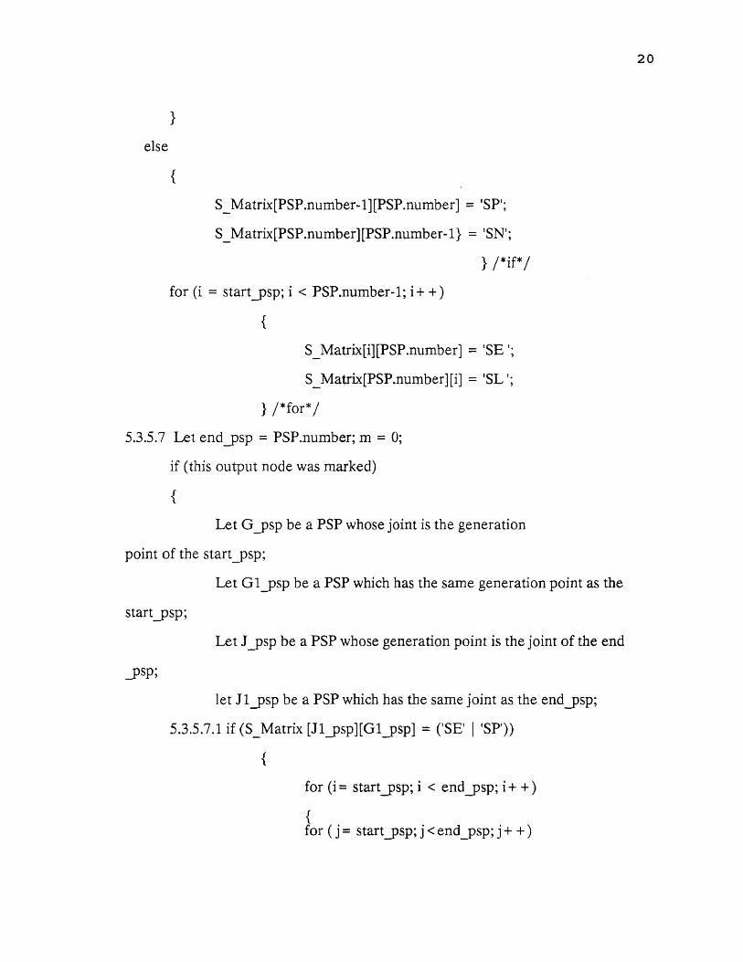
else

{

S Matrix[PSP.number-1][PSP.number] = 'SP';

S Matrix[PSP.number][PSP.number-11 = 'SN';

/ * if* /

for (i = start_psp; i < PSP.number-1; i+ + )

{

S Matrix[i][PSP.number] = 'SE ';

S Matrix[PSP.number][i] = 'SL ';

} /*for*/

5.3.5.7 Let end_psp = PSP.number; m = 0;

if (this output node was marked)

{

Let G_psp be a PSP whose joint is the generation

point of the startpsp;

Let G1_psp be a PSP which has the same generation point as the

start_psp;

_psp;

Let J_psp be a PSP whose generation point is the joint of the end

let J1_psp be a PSP which has the same joint as the end_psp;

5.3.5.7.1 if (S_Matrix [J1_psp][G1_psp] = ('SE' 'SP'))

{

for (i= start_psp; i < end_psp; i+ + )

{for ( j= start_psp; j< end psp; j+ + )

20

21

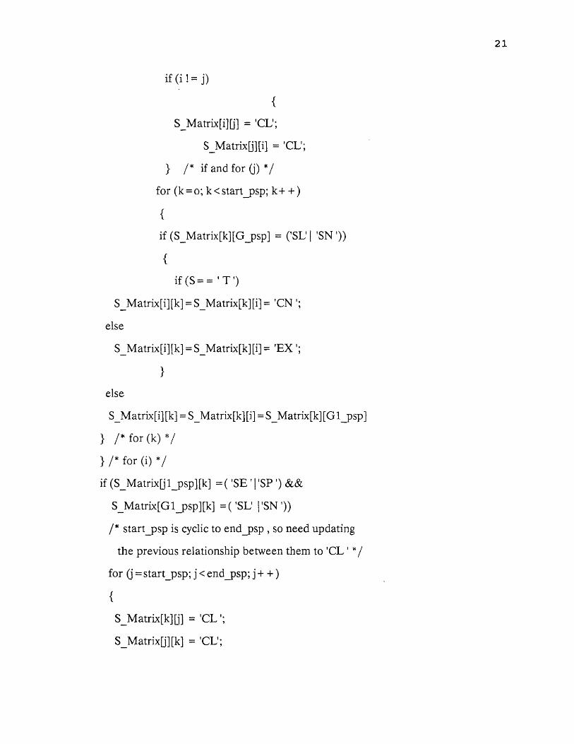
if (i = j)

{

S_Matrix[i][j] = 'CL';

S Matrix[j][i] = 'CL';

} /* if and for (j) */

for (k=o; k <start_psp; k+ +)

{

if (S_Matrix[k][G_psp] = ('SL' 'SN '))

{

if (S= = ' T ')

S Matrix[i][k]=S Matrix[k][i]= 'CN ';

else

S Matrix[i][k]=S Matrix[k][i]= 'EX ';

}

else

S Matrix[i][k] = S Matrix[k][i] = S Matrix[k][Gl_psp]

} /* for (k) */

} /* for (i) */

if (S_Matrix[j 1psp][k] = ( 'SE ' I 'SP ') &&

S Matrix[Glpsp][k] = ( 'SL' I 'SN '))

/* start_psp is cyclic to endpsp , so need updating

the previous relationship between them to 'CL' */

for (j=startpsp; j<endpsp, j+ + )

{

S Matrix[k][j] = 'CL ';

S Matrix[j][k] = 'CL';

22

D[m+ +] = j; /* matrix index, used for updating previous

relationship of 'SE','SP','SL','SN' between start_psp and end_psp to 'CL'*/

for (g=o; g<m-1; g+ +)

{

if (S_Matrix[D[g]][D[m-1]] = ('SE' I 'SP' I 'SL 'SN')

{

S Matrix[D[g]][D[m-1]]= 'CL';

S-Matrix[D[m-1]][D[g]]='CL';

1 /* if */

} /* for (g) */

1 /* for (j) */

}

5.3.5.7.2 /* Find the structure relationships between PSPs from

startpsp to end_psp and all other existing PSPs*7

else /* 5.7.1. if */

{

for (i=o; i<start_psp; i+ +)

{

for =start_psp; j<endpsp; j+ +

{

if (S_Matrix[i][Gpsp] = ('SL' I 'SN '))

{

if (S_Matrix[j1psp][i]! = ('SE' 'SP'))

{

if (S= = 'T ')

S Matrix[j][i]=S Matrix[i][j] = 1 CN,;

else

S Matrix[j][i]=S Matrix[i][j]='EX';

}

else

{

S Matrix[i][j]=S Matrix[i][jl_psp];

S Matrix[j][i] =S Matrix[jlpsp][i];

}

}

else

if(S_Matrix[i][Glpsp] = ='CLI)

{

if (S = ='T')

S Matrix[j][i]=S Matrix[i][j] ='CN ';

else

S Matrix[j][i]=S Matrix[i][j] ='EX ';

}

else

{

S Matrix[i][j]=S Matrix[i][Gl_psp];

S Matrix[j][i]=S Matrix[Glpsp][i];

}

if (i is an input PSP of j)

{

S Matrix[i][j] = 'SP ';

S Matrix[j][i]= 'SN ';

23

facing 24

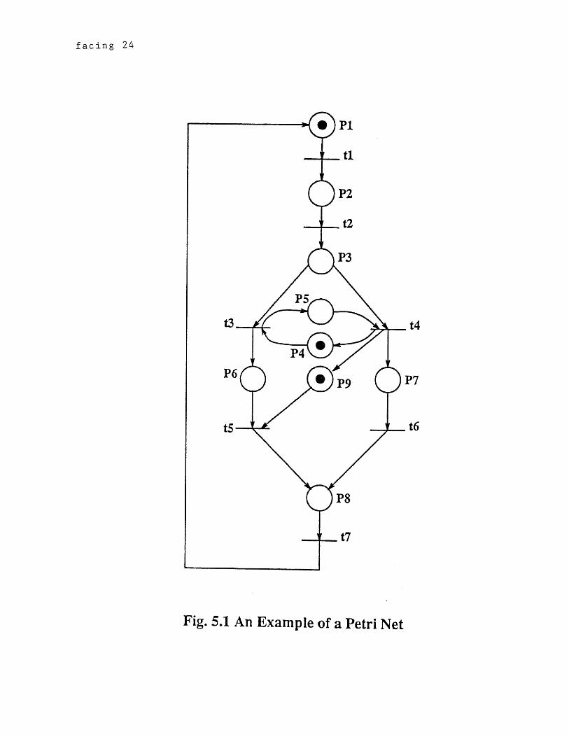
Fig. 5.1 An Example of a Petri Net

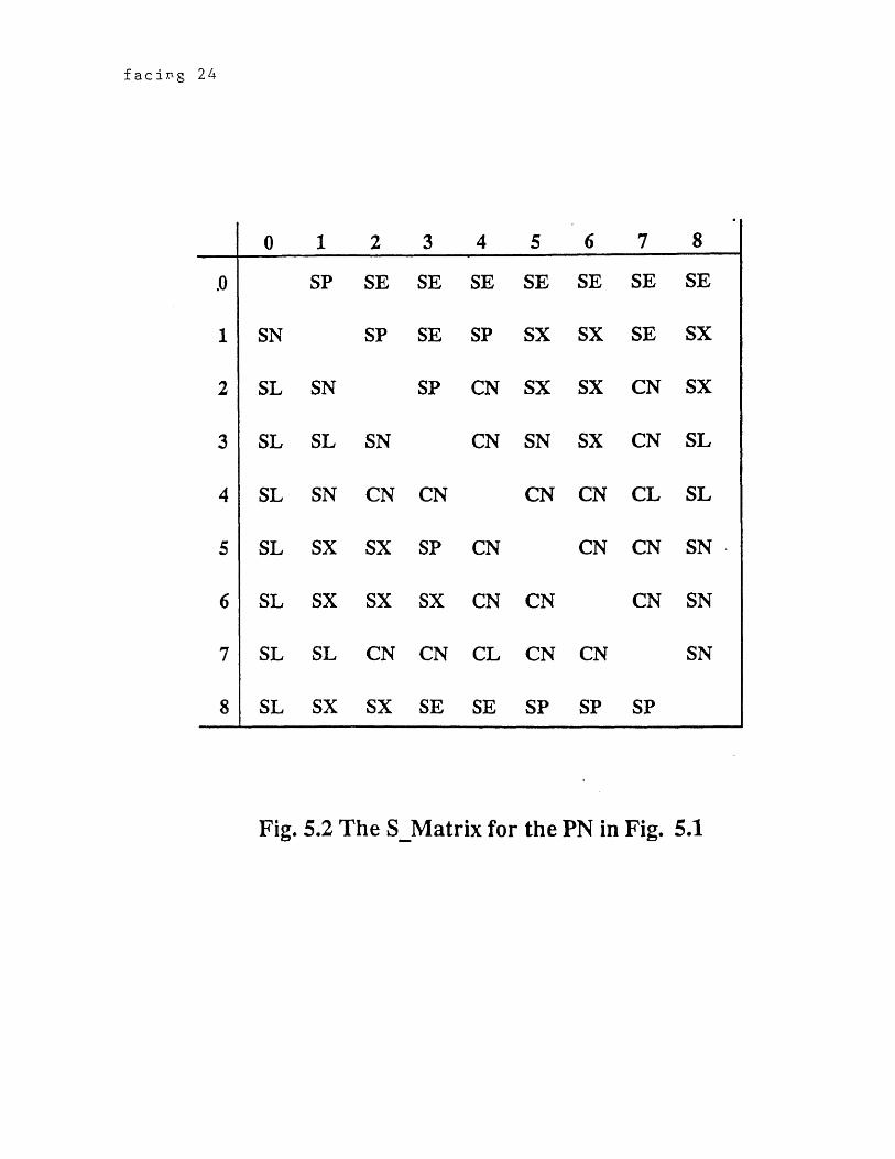
facing 24

Fig. 5.2 The Sffiatrix for the PN in Fig. 5.1

}

else

if (i is an output PSP of j)

{

S Matrix[i][j] = 'SN ';

S Matrix[j][i] = 'SP ';

}

if (i is cyclic to a Gl_psp and a J1_psp)

S Matrix[i]u] =S Matrix[j][i] = 'CL ';

} /* for (j) */

} /* for (i) */

}

5.4 Application of the Algorithm

Consider Fig. 5.1. The steps for finding the S_Matrix are presented below. The

corresponding S_Matrix is shown in Fig. 5.2.

1. In the initial marking, t1 is enabled, hence pick P1 as the home place. The

PSP containing pi is PSP0 = [p8 t7 pi ti P2 t2 p3]. Mark t7 and check p8 since

t7 is the only output node of p8. The current node is p3.

2. t3 and t4 are two output nodes of p3. Pick t3. t3 is not a simple node, hence

the new PSPi. = [p3 t3 ] and S_Matrix[0][1] = 'SP', S_Matrix[1][0] = 'SN'. Mark

t3.

3. p5 and p6 are two output nodes of t3. Pick p6, which is a simple node and it's

output node t5 which is not simple. Hence the new PSP2 = [t3 P6 t5 ], and

S Matrix[0][2] = 'SE', S Matrix[2][0] = 'SL', S Matrix[1][2] =

S Matrix[2][1] = 'SN'. Mark p6.

24

4. The output node pg of t5 is not simple, hence the new PSP3 = [t5 pg]. Mark

pg and check t5. Since pg has been checked, backtrack to t5 which has been

checked. So backtrack to t3 and pick its unmarked output node p5 which is a

simple node. Its output node t4 is not a simple node, hence the new PSP4 = [t3

p5 t4], and S Matrix[2][3] = 'SP', S Matrix[4][1] = 'SN', (PSP0, PSP1) -> PSP3,

(PSP2, PSP3) I I PSP4. Check t3 since all it's output arcs have been traced.

5. pg, p7 and p4 are three output node of t4. Pick pg and find a new PSP5 = [t4

pg t5]. S_Matrix[4][5] = 'SP', and S_Matrix[5][3] = 'SP', (PSP4 , PSP5) I I PSP2,

PSP1 - > (PSP4, PSP5) and PSP0 > (PSP4, PSP5). Mark pg.

6. Since t5 has been checked, backtrack to t4 and pick an unmarked output node

p7, find a new PSP6 = [t4 p7 t6 pg ]. PSP6 I I (PS130,PSP1, PSP4 ) - > PSP6.

Mark p7.

7. Since tg has been checked, backtrack to t4 again and pick the remaining

unmarked output node p4 and find a new PSP7 = [t4 p4 t3] which is cyclic to

PSP4. Hence PSP4 o PSP7, (PSP0, PSP1) -> PSP7 and (PSP2, PSP4) i I PSP7.

Update S_Matrix[4][5] = S_Matrix[4][5] = S_Matrix[5][4] = 'CM. Mark p4 and

check t4.

8. Since t3 has been checked, backtrack to p4. Pick the remained untraced path

P3- > t4 and find a new PSP8 = [p3 t4]. Since t4 has been marked and is on a

cycle, PSP8 SX (PSPi,PSP2), PSP8 I I (PSP5, PSP6, PSP3) and PSP1 SX (PSP5,

PSP6). Both transactions t3 and t4 on this cycle are the joints of the VPs with a

CGP p3. Y1 = PSP2 , PSP3 } and Y2 = {PSP3, PSP5, PSP6 }. PSP2 is 'SX' to

PSP5 and PSP6, and PSP3 is 'SX' to PSP6. Check p3.

9. All PSPs are found and stop.

25

CHAPTER 6

A NEW APPROACH TO REDUCTION OF PETRI NETS

Knitting Technique for Synthesis rules described in Chapter 3 is successfully

applied to Reduction theory of Petri Nets. Path generations previously forbidden

are now allowed without incurring logical incorrectness. For illustration in Fig. 9,

a TT-path generation (PSP4) between two exclusive transitions(t3 and tri, ) was

previously not allowed. But the new rules allow additional path generations

(PSP7) such that the two exclusive transitions become synchronized and hence

sequentially exclusive to each other. Further it is also found that TP and PT

generations, which were not allowed before, may be allowed however by adding

new paths. Each TP(PT) generation must be associated with a new PT(TP)

generation to avoid unboundedness (deadlocks). Each new generation must be

synchronized with existing PT paths with the same generation point as the new

PT path. •I'P rule and PT rule, the names given to the above rules, enable us to

find out that any PNs synthesized using the previous rules in [8] have synchronic

distance 1 or infinity between any two transitions. In accordance with the new

technique it is possible to synthesize PNs with arbitrary synchronic distance

between any two transitions. Further it is possible to allow all generations which

were hitherto forbidden. Thus the new technique called Knitting

Technique(synthesis technique) is more powerful than the traditional

techniques. In addition to the above process another process called reduction,

which is a reverse procedure to synthesis, is more efficient and useful than the

conventional techniques. The S_Matrix is useful in finding any mismatch on

account of existence of some paths which do not conform to synthesis rules.

26

Hence S MAtrix can be used to perform reduction on

any Petri Net. By iterative adoption of the above technique petri nets can be

simplified to the maximum level possible. The algorithm for the above discussed

technique is furnished below.

6.1 An Algorithm for Reduction of Petri Nets

Let GP be a PSP whose joint is the generation point of the start_psp;

JP be a PSP whose generation point is the joint of the end _psp;

PSPc the current PSP under consideration and [X] the cardinality of set X;

At the beginning of the algorithm, set flag = TRUE;

Repeat the following steps (1) to (4) indefinitely until flag = FALSE or errors of

designs detected;

6.1.1 If flag = TRUE and (path,rel,Q1,Q2)

= (TTP,SQ,LEX(GP,JP),LEX(JP,GP))

(PPP,SQ,LCN(GP,JP),LCN(JP,GP)) I (TTP,CN,LEX(GP,JP),LEX(JP,GP

(PPP,EX,LCN(GP,JP),LCN(JP,GP)),

/* where rel is the structural relationship between GP and JP, and

1011 = 1Q21 = 1 (i.e., each set contains only one member) */

6.1.1.1 If path =PPP, then delete the PSPc; else flag =FALSE;

6.1.1.2 If (path,rel) = (TTP,CN) and there does not exist a PSP such that

PSP < - GP and JP - > PSP, then

signal "TT.3 rule violation, unbounded places in the PSP" and exit;

else delete the PSPc and flag = TRUE;

6.1.1.3 If (path,rel) = TTP,SE) and PSPc does not have tokens, then

/* PSPc is in a cycle */

6.1.1.3.a fire all enabled transitions in PSPs which satisfy

JP- > PSP- > GP until all of them are no longer enabled;

27

6.1.1.3.b If the generation point of PSPc has fired more than once,

delete PSPc and flagl =TRUE;

else signal 'TT.2 rule violation, deadlock at the generation

point of PSPc" and exit;

6.1.1.4 If (path,rel) = (TTP,EX), then

signal "exclusive TT interaction, potential deadlock at the joint

and unbounded input place of the joint of the PSPc" and

6.1.2 If (path,rel) = (PPP,CN), then

signal "PP.3 rule violation, potential deadlock at a PSP <- GP and

PSP < - JP" and exit;

6.1.3 For all VPs (VP1, VP2, VPk) whose common generation point is a place

/* There is only one GP and k JPs (JP1,JP2,... JPk) */

6.1 3.1 If LEX(JP1,GP) = {JP1,JP2,...,JPk},

else break;

6.1.3.2 A = {}; /* create an empty set A */

6.1.3.3 If the generation point of GP is a place P, then /* get */

6.1.3.3.a for each input PSP of P

If its generation point is a transition and which has more

than one output PSP, then

insert one of the input PSP of this transition in to A;

else it is a place, make this place be the new P;

go to step 3.3.a.;

6.1.3.3.b let pa be a member PSP in A;

If JP1 - > pa and none of the PSPs,both of whose generation

point and joint have been traced, has tokens, then

perform a similar steps to 1.3.a. & 1.3.b. to ensure

no TT.2 rule violation;

28

6.1.3.3.c else if JP1 I pa, then

perform a similar step to 1.2. to ensure no TT.3 rule violation;

6.1.3.3.d else if JP1 I pa, then

perform a similar step to 1.4. to signal "exclusive TT

interaction, potential deadlock at the joints and unbounded

input places of the joints of JPs" and exit;

6.1.3.3.e else if A = LEX(pa,JP1),then

delete all VP1,... VPk, and all PSPs, both of whose generation

point and joint have been traced, and flag = FALSE;

6.1.4 For all VPs (VP1, VP2,...,VPk) whose common joint is a transition

/* There is only one JP and k GPs (GP1,GP2,...GPk)*/

6.1.4.1 If GP11 I JP, then

signal "PP.3 rule violation, potential deadlock at a PSP <- GP and

PSP < -JP" and exit;

6.1.4.2 If LCN(GP1,JP) = { GP1, GP2,..., GPk},

else break;

6.1.4.3 B = {}; /* create an empty set B */

6.1.4.4 If the joint of JP is a transition T, then /* get B*/

6.1.4.4.a for each output PSP of T,

if its joint is a place and which has more than one input PSP,

insert one of the input PSP of this place in to B;

else it is a transition, make this transition the new T;

go to step 4.4.a.;

6.1.4.4.b let pb be a member PSP in B;

If B = LCN(pb,GP1),then

delete all VP1,... VPk, and all PSPs, both of whose

generation point and joint have been traced, and flag = FALSE;

29

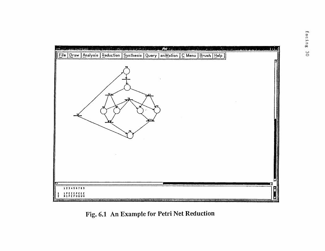
Fig. 6.1 An Example for Petri Net Reduction

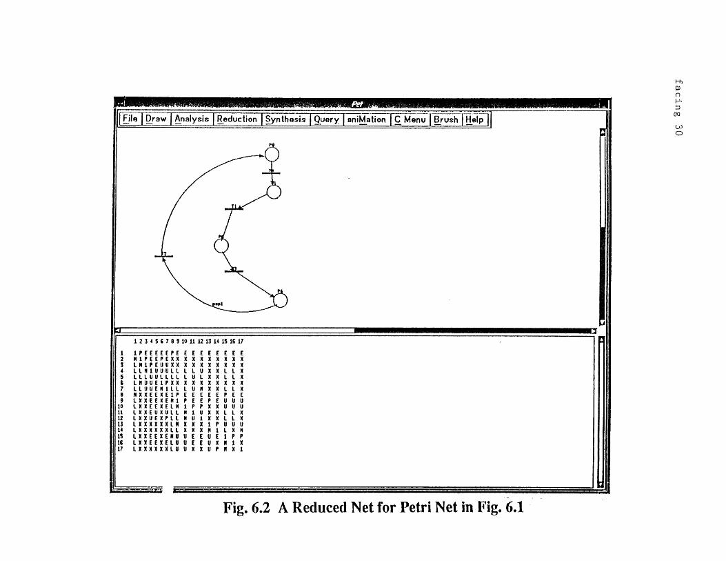
Fig. 6.2 A Reduced Net for Petri Net in Fig. 6.1

Fig. 6.3 An Example for Petri Net Reduction

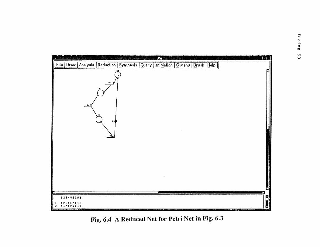
Fig. 6.4 A Reduced Net for Petri Net in Fig. 6.3

6,2 An Illustration of Reduction

The reduction was implemented with the help of a CAD tool which can facilitate

analysis of Petri Nets. The reduction as well as Structural matrix algorithms were

implemented in C language in X-Window/Motif environment. The interactive

CAD tool with which reduction of Petri Net was accomplished is discussed

below.

The tool animates firing of transitions and analyzes the theory and tests

their correctness. The "FILE" button allows files to be imported, copied, deleted

and edited. The reduction button 'reduces the net by using knitting technique.

The "DRAW" button helps us in selecting a function such as clear, print, undo,

draw arcs, arrows, places etc. In addition to reduction the tool can be used for

synthesis also. The figures of the petri nets which were reduced using the above

tool are furnished in Fig.6.1 to Fig.6.4

30

CHAPTER 7

CONCLUSIONS

Conventional reduction techniques such as. six reduction rules discussed in this

paper focuss on reducing a subnet or a partial PN to a single transition as such

they are not powerful enough to reduce a Petri Net to a simplest possible net.

This paper proposes an iterative reduction technique called Knitting Technique

which is more efficient than the previous techniques. An algorithm for

implementing the new reduction technique is also presented. An algorithm to

represent structural relationship of any given Petri Net is also presented. The

proposed iterative reduction technique by S_Matrix is a global technique and

hence is not a transformation technique. It deletes transitions and places

according to certain rules. It has the potential of completely substituting for

analysis. The influence of the proposal is as mentioned below.

1) Advance the Petri Net reduction theory by introducing (a) Automation of

reduction and

(b) provision of more powerful iterative reduction technique than the

conventional ones.

2) The technique may possibly eliminate the reachability analysis.

31

REFERENCES

[1]Murata, T., "Petri Nets: Properties, Analysis and applications," IEEE

Proceedings, Vol. 77,No. 4, April 1989, pp. 541-580.

[2]Peterson, J.L., Petri Net Theory and the Modeling of Systems, Prentice Hall,

Inc., Englewood Cliffs, New Jersey, 1981.

[3]Murata, T., "Modeling and Analysis of Concurrent Systems," in Handbook of

Software Engineering , edited by C.Vick and C.V. Ramamoorthy, Van Nostrand

Reinhold, 1984, pp.39-63.

[4]Ramamoorthy, C. V., and So, H., "Software Requirements and Specifications:

Status and Perspectives," IEEE Tutorial: Software Methodology, 1978.

[5]Yau, S.S., and Caglayan, M.U., "Distributed Software System Design

Representation Using Modified Petri Nets," IEEE Trans. on Software Engineering,

Vol. SE-9, No. 6, Nov.1983, pp. 733-745.

[6]Agerwala, T. and Choed-Amphai, Y., "A Synthesis Rule for Concurrent Systems,"

Proc. of Design Automation Conference, pp. 305-311,1978.

[7]Koh, I., and DiCesare, F., "Transformation Methods for Generalized Petri Nets

and Their Applications to Flexible Manufacturing Systems," The 2nd International

Conference on Computer Integrated Manufacturing, Troy, NY, MAY 1990, pp. 364-

371.

[8]Yaw, Y., "Analysis and Synthesis of Distributed Systems and Protocols," Ph.D.

Dissertation, Dept. of EECS, U.C. Berkely, 1987.

32

[10] Yaw, Y., and Foun, F.L., "The Algorithm of A Synthesis Technique for

Concurrent Systems," 3rd International Petri Net Conf., Dec. 1989, pp. 266-276.

[11] C.V. Ramamoorthy, Y. Yaw, and W.T. Tsai, "A Petri Net Reduction

Algorithm for Protocol Analysis," Computer Communication Review (USA),

Vol. 16, No.3 Aug. 1986, pp. 157-166.

[12] I.Suzuki and T. Murata, "A Method of Stepwise Refinement and

Abstraction of Petri Nets," Journal of Computer and System Sciences 27, 1983,pp

51-76.

[13] R. Valette, "Analysis of Petri Nets by Stepwise Refinement, "Journal of

Computer and System Sciences 18, 1979, pp. 35-46.

[14] G. Berthelot, "Transformations and Decompositions of Nets," LNCS,

Advances in Petri Nets, pp. 359-376, Part I, 1986.

[15] Hyung, Lee-Kwang, "Generelized Petri Net Reduction Method" IEEE

Trans. Syst., Man, Cybern., Vol. SMC-17, No.2, 1987, pp. 297-303.

[16] Ramamoorthy, C. V., Dong, S.T., and Usuda, Y., "The Implementation of an

Automated Protocol Synthesizer (APS) and Its Application to the X.21

Protocol," IEEE Trans. on Software Engineering, pp.886-908, No.9, 1985.

33