A Petri net model for sequence optimization and performance analysis of flexible assembly systems

A Petri net model for sequenceoptimization and performance

analysis of flexibleassembly systems

Hamid UllahNWFP University of Engineering and Technology, Peshawar, Pakistan, and

Erik L.J. BohezSchool of Engineering and Technology, Asian Institute of Technology,

Pathumthani, Thailand

Abstract

Purpose – The purpose of this paper is to present a new generic Petri net (PN) model based onassembly plan for assembly sequence optimization. The model aims to allow modeling the flexibleassembly system (FAS) configuration, determining the optimal work in process, lead time, throughput,and utilization of each station. Moreover, it aims to show assembly features (AFs) as being useful inassembly sequence planning.

Design/methodology/approach – Sophisticated knowledge of AFs is used to get very few feasibleassembly sequences (ASs) rather than all possible ASs for a product. A PN model is developed to findout the near optimal assembly sequence out of the sequences obtained from the AF knowledge. It isalso used for design and performance evaluation of FAS. Multiple optimization criteria are used forassembly sequence optimization, keeping in view the line balancing. The PN is optimized usingweighted-WIP when the throughput is bounded by the utilization of the bottleneck machines.

Findings – The results achieved from the example show a considerable reduction in the number offeasible ASs for a product. The PN optimization gives minimum WIP corresponding to the maximumproduction rate. Moreover, the PN model pushes more inventories to the initial assembly phase.

Research limitations/implications – The proposed PN can be easily extended for inclusion ofdual kanban, where the managers may adjust the number of kanban cards as per the requirement.

Practical implications – Managers may use the concept of multiple AFs in order to design andoperate robot assembly that will result in more efficient sequence planning. Using the PN model, theassembly manager may design, analyze, evaluate, and even optimize the layout of the FAS forminimum WIP, maximum throughput, and reduced lead time. The determination of total WIP, totalnumber of stations in the assembly line, and the number of servers at each station may be helpful inthe factory floor management. Line balancing may result in the highest efficiency and the shortestidling time along with ease of management and supervision.

Originality/value – This paper provides a clear insight into how a large reduction in the number offeasible ASs for a product can be obtained using the knowledge of AFs. It also presents a new PNmodel used for assembly sequence optimization and design and performance analysis of FAS.

Keywords Assembly, Assembly lines, Flexible manufacturing systems

Paper type Research paper

IntroductionAssembly sequence planning (ASP) is the foundation of the assembly process planningwhich plays a key role in the whole product life cycle. ASP is one of the most active

The current issue and full text archive of this journal is available at

www.emeraldinsight.com/1741-038X.htm

Petri net modelfor sequenceoptimization

985

Received April 2007Revised October 2007

Accepted January 2008

Journal of Manufacturing TechnologyManagement

Vol. 19 No. 8, 2008pp. 985-1003

q Emerald Group Publishing Limited1741-038X

DOI 10.1108/17410380810911745

topics in current research. The efficiency and quality of the ASP can influence theassembly process greatly (Su, 2007). The literature shows several methodologies forrepresentation of assembly sequences (ASs).

Homem de Mello and Sanderson (1991a, b) introduced the cut-set based ASP methodusing the three cut-set inferring rules. Huang and Lee (1990) proposed a relationalassembly model, in which a number of aspects including the spatial relationship,contacts, trajectories, types of mating tasks, and stabilities, etc. were encompassed. deFazio and Whitney (1987) proposed a representation scheme based on precedencerelations. Huang and Lee (1990) used a symbolic representation scheme to representprecedence knowledge. Seow and Devanathan (1994) proposed temporal logic as animplicit representation tool and an analytical language for ASP. Homem de Mello andSanderson (1991a, b) introduced an AND/OR graph representation of ASs.

Wilson (1995) proposed a man–computer interactive assembly sequencing methodbased on the evaluation and judgment of the assembly CAD structure. Dini andSantochi (1992) and Gottipolu and Ghosh (1995) designed the mathematical ASPmethods based on the contact and interference arrays between each couple of parts orsubassemblies in the assembly. Swaminathan and Barber (1996) designed anexperience-based assembly sequence planner for mechanical products, in which,assembly was separated into several typical sub-assemblies containing three, four, orfive components. These typical sub-assemblies are modeled using directed liaisongraphs that can be referenced in new ASP problems. However, the approachespresented in Dini and Santochi (1992), Gottipolu and Ghosh (1995), and Swaminathanand Barber (1996) are all subject to the limitation that each part can only be assembledto the assembly along with one of the six orthogonal directions.

Baldwin et al. (1991) developed an ASP system to integrate the geometric feasible ASswith the evaluation and selection of the optimal sequence. However, due to the simplicityof the assembly model, the user has to input various engineering criteria for a number ofstates and operations. In addition to evaluating the large quantity of the geometricpossible ASs, it is an effort intensive and error-prone process. Su (2007) proposed ahierarchical ASP method which can derive the optimal AS based on the precedencerelation classification. He proposed assembly model including assembly structure draft,assembly tree structure, liaisons diagram, liaison parameters, and part parameters.

Most of the above approaches consider all possible ASs for a product and get theoptimal (or near optimal) AS after going through various time consuming and tedioustrail and error methods for elimination of unwanted and unfeasible ASs.

Petri nets (PNs), as graphical and mathematical tools, provide a uniform environmentfor modeling, formal analysis and design of discrete event systems. It has the capabilityfor modeling and planning Flexible Assembly System (FAS). The place, transition, andtoken movement together provide the specification of resource constraints and graphicalrepresentation of serial and concurrent events for the assembly system. There have beenmany applications of PN in the representation, analysis and control of the FAS (Chaoand Sanderson, 1995; Moore and Gupta, 1996; Seeluangsawat and Bohez, 2004; Suzukiet al., 1993; Tang and Zhou, 2004; Thomas et al., 1996). In order to enhance the modelingpower of PN for assembly systems, many attempts have been made to extend andmodify the conventional PNs. These attempts have produced colored PN, control net,timed PN, object PN, and fuzzy PN (Chao and Sanderson, 1995; Moore and Gupta, 1999;Tang and Zhou, 2004; Zhang et al., 2005; Zha et al., 2003).

JMTM19,8

986

Most of these PN applications have certain limitations. For example, some research ofPN applications consider all feasible ASs which are represented by the AND/OR graph(Suzuki et al., 1993; Yee and Ventura, 1999; Zha et al., 1998). Since, for real products, thenumber of all possible ASs is quite large that is not possible to be representedby the AND/OR graph, therefore, their methods are limited to reduced size or heavilyconstrained problems. Some researchers take in consideration all feasible assemblyplans, represented as a PN (Thomas et al., 1996). The ASP are combinatorial problems,impossible to be represented in their totality for industrial size products, and, as aconsequence, impossible to be analyzed and optimized. Others have used open loop PN(Zha et al., 1998) in which the total WIP does not remain constant. Also, open loop PNcannot model a real FAS for repetitive assembly of products in mass production.Moreover, none of the above researches consider line balancing in their approaches forAS optimization and design and performance evaluation of assembly system.

Assembly planning problem is extremely complex. Therefore, simplifications mustbe made, for improving the usefulness of the assembly planning. The most complexaspect of the assembly planning problem can be seen as the generation of all possibleASs for a given product and then finding out the near optimal sequence throughvarious trial and error methods. However, in the present research, assembly features(AFs), are used to demonstrate their usefulness in obtaining very few feasible ASsrather than all possible ASs for a given product. Thus, the knowledge of AFs can beutilized for reduction of the said complexity. Moreover, a new PN model is presentedfor AS optimization and FAS design and performance evaluation.

This paper highlights the following points different from earlier researches:. Knowledge of multiple AFs is used to obtain very few good feasible ASs rather

than all the geometric possible ASs for a product.. A weighted AND/OR graph which is much more compact is used compared to

the conventional AND/OR graph. This method is also capable to represent all thefeasible ASs for a product given by the multiple AFs.

. A closed loop PN is developed for design and performance analysis of a cyclicFAS. It is provided with weighted arcs to account for mating of componentsthrough a number of features connecting together simultaneously. A transition isintroduced for providing feedback for replenishment of new components as soonas final assembly is produced. Also, server circuit at each station is provided forthe purpose of line balancing and capacity planning.

. The PN optimization is influenced by the utilization of the bottleneck machines.

. The PN is optimized based on Weighted-WIP to push more and more tokens inthe input places of the PN as the output place represents the final assembly of theproduct which is more expensive compared to the unconnected parts upstreamthe assembly process.

AFs in sequence planningAF is defined as “a connection between two form features on mating parts, associatedwith assembly intents, where assembly intents include assembly relation, assemblyoperation, and assembly degree of freedom”. AFs are classified into against, fit, single,multiple, soft, hard, functioning, and locking AFs (Ullah et al., 2006). Against and fitAFs are the AFs that depend upon the assembly relation between the connecting form


987

features. Single and multiple AFs depend upon the number of connecting form featuresthat connect together simultaneously. Soft and hard AFs are defined keeping in viewthe assembly operation. Depending upon the degrees of freedom, features are dividedinto functioning AFs and locking AFs. AFs offer a number of useful information tofacilitate the process of ASP as described below.

Precedence relationship represented by AFsPrecedence relationship (or assembly order) is the order of performing some operationsbefore others can be done and leaving some operations to be done after others havebeen performed, because of geometric constraints in the assembly of differentcomponents. This precedence knowledge facilitates ASP, resulting in reduction offeasible ASs that have to be checked in the assembly sequence optimization. Forexample, assembly of parts shown in Figure 1 shows against AF. In this type offeature, P1 is a base feature while P2 is a mating feature. This feature directly shows theassembly order for base feature and mating feature: first the base feature and then themating feature. Similarly, assembly of parts shown in Figure 2 gives two platesconnected together by a bolt-nut arrangement. When the AF knowledge is used, thisassembly of parts gives a hard AF. To make a hard AF, soft AF plays the role of abase. Hard AF is obtained when connector is added to the soft AF. Therefore, as per theprecedence knowledge of AFs, the hard AF represented by the given assembly directlyshows the assembly order for base, bolt and nut: first the base (i.e. soft AF), then thebolt, and finally the nut.

Figure 1.Assembly of parts givingsoft AF

P1 (Base)

P2

Figure 2.Assembly of parts givinghard AF

P1

B

N

P2

JMTM19,8

988

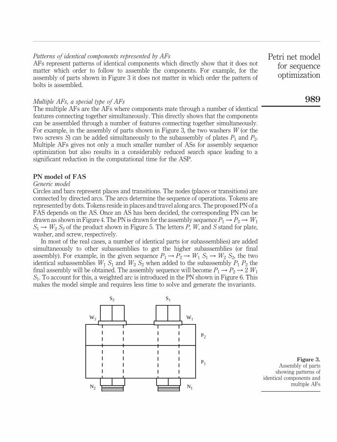
Patterns of identical components represented by AFsAFs represent patterns of identical components which directly show that it does notmatter which order to follow to assemble the components. For example, for theassembly of parts shown in Figure 3 it does not matter in which order the pattern ofbolts is assembled.

Multiple AFs, a special type of AFsThe multiple AFs are the AFs where components mate through a number of identicalfeatures connecting together simultaneously. This directly shows that the componentscan be assembled through a number of features connecting together simultaneously.For example, in the assembly of parts shown in Figure 3, the two washers W (or thetwo screws S) can be added simultaneously to the subassembly of plates P1 and P2.Multiple AFs gives not only a much smaller number of ASs for assembly sequenceoptimization but also results in a considerably reduced search space leading to asignificant reduction in the computational time for the ASP.

PN model of FASGeneric modelCircles and bars represent places and transitions. The nodes (places or transitions) areconnected by directed arcs. The arcs determine the sequence of operations. Tokens arerepresented by dots. Tokens reside in places and travel along arcs. The proposed PN of aFAS depends on the AS. Once an AS has been decided, the corresponding PN can bedrawn as shown in Figure 4. The PN is drawn for the assembly sequenceP1 ! P2 ! W1

S1 ! W2 S2 of the product shown in Figure 5. The letters P, W, and S stand for plate,washer, and screw, respectively.

In most of the real cases, a number of identical parts (or subassemblies) are addedsimultaneously to other subassemblies to get the higher subassemblies (or finalassembly). For example, in the given sequence P1 ! P2 ! W1 S1 ! W2 S2, the twoidentical subassemblies W1 S1 and W2 S2 when added to the subassembly P1 P2 thefinal assembly will be obtained. The assembly sequence will become P1 ! P2 ! 2 W1

S1. To account for this, a weighted arc is introduced in the PN shown in Figure 6. Thismakes the model simple and requires less time to solve and generate the invariants.

Figure 3.Assembly of parts

showing patterns ofidentical components and

multiple AFs

S1

P1

P2

S2

N1N2

W2 W1


989

The PN consists of places Pij and Sij. Places Pij represent an object (where an objectgenerally refers to a part, a subassembly, or final assembly) and places Sij representidentical servers (or machines) to perform assembly operations at each station.To define the initial and final states of the assembly, places Pij contain two sets ofplaces: input places and output places. Input places in the model represent unconnectedparts, while, output places represents the final assembly of the parts. Tokens in placesSij represent the availability of servers (or machines) for each assembly operation. Thetransition Tij represents the assembly operation on a station. Each transition Tij iscontrolled by places Pij and Sij. The circuits representing places Sij will be called servercircuits. The PN in Figure 7 consists of these circuits.

A transition Treplenish (or Trep for simplicity) is introduced as shown in Figure 8 tomodel the transition in readiness for the replenishment of the parts in the input places assoon as the final assembly of parts is produced at the output place of the PN. For thetransition Trep, the input places of the PN become its out places, and the output place ofthe PN becomes its input place. It gives a closed loop PN with circuits connecting placesPij. These circuits will be referred to as parts circuits as shown in Figure 8. The closedloop PN is similar to closed queuing network which contains a fixed number of parts.

Figure 4.Open PN model for theassembly sequenceP1 ! P2 ! W1 S1 ! W2

S2w2s2

w1s1p1p2w1s1w2s2

p1p2w1s1

p1p2

p1

p2

Place P

Transition T

Figure 5.Assembly of six parts

P1

P2

S1S2

W1W2

JMTM19,8

990

A transition can be fired if there is at least one token in each of the input places of thetransition. When a transition fires, the tokens are moved from the input places and stayon the transition for a time equal to the time allocated to this transition. After stayingon the transition, a token is added to each of the output places of the transition. Thismeans that when a transition fires, two unconnected parts are assembled giving anassembly (or subassembly) at that particular transition. The movement of the tokens iscyclic. The longest cycle determines the production rate of the FAS. During this longestcycle, the final assembly of parts is obtained.

Performance evaluationAn elementary circuit is defined as a directed path that starts from one node (place ortransition) and comes back to the same node such that no other nodes are repeated andalways travels in the direction of the arcs.

Figure 7.Open PN model for

assembly sequence withserver circuits

Server place S

p1p2w1s1w2s2

p1p2

p1

p2

w1s1

2

S1 S2 Server circuit

T1

T2

Figure 6.Open PN model for

assembly sequence withweighted arc

p1p2w1s1w2s2

p1p2

p1

p2

w1s1

2

Input place

Output place


991

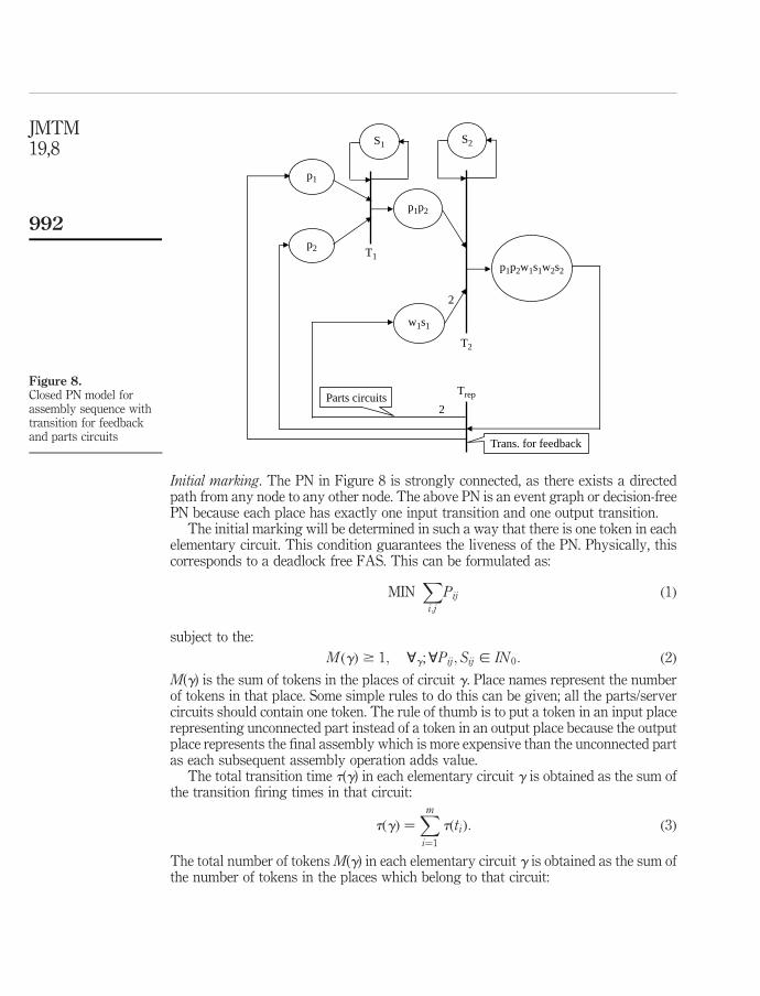
Initial marking. The PN in Figure 8 is strongly connected, as there exists a directedpath from any node to any other node. The above PN is an event graph or decision-freePN because each place has exactly one input transition and one output transition.

The initial marking will be determined in such a way that there is one token in eachelementary circuit. This condition guarantees the liveness of the PN. Physically, thiscorresponds to a deadlock free FAS. This can be formulated as:

MINi;j

XPij ð1Þ

subject to the:

M ðgÞ $ 1; ;g;;Pij; Sij [ IN 0: ð2Þ

M(g) is the sum of tokens in the places of circuit g. Place names represent the numberof tokens in that place. Some simple rules to do this can be given; all the parts/servercircuits should contain one token. The rule of thumb is to put a token in an input placerepresenting unconnected part instead of a token in an output place because the outputplace represents the final assembly which is more expensive than the unconnected partas each subsequent assembly operation adds value.

The total transition time t(g) in each elementary circuit g is obtained as the sum ofthe transition firing times in that circuit:

tðgÞ ¼Xm

i¼1

tðtiÞ: ð3Þ

The total number of tokens M(g) in each elementary circuit g is obtained as the sum ofthe number of tokens in the places which belong to that circuit:

Figure 8.Closed PN model forassembly sequence withtransition for feedbackand parts circuits

T1

T2

Trep

Trans. for feedback

Parts circuits

p1p2w1s1w2s2

p1p2

p1

p2

w1s1

2

2

S1 S2JMTM19,8

992

M ðgÞ ¼Xn

j¼1

M 0ð pjÞ ð4Þ

where M0 is the initial marking.Optimal marking. The cycle timeC(g) of each elementary circuit is the ratio t(g)/M(g).

Let C(gc) be the cycle time of elementary circuit with the largest cycle time. Thiselementary circuit is called critical circuit. The cycle time in steady-state is given by themaximum cycle time taken over all elementary circuits. Increasing the number of tokensin each elementary circuit will reduce the cycle time of the elementary circuits.The server circuit with the largest cycle time will limit the maximum throughput.In other words, this station will be the bottleneck station. It is possible to increase thenumber of tokens in non-server circuits in such a way that the server circuit becomes thecritical circuit. Hence, the objective of Linear Programming (LP) is keeping WIPminimum corresponding to the maximum throughput. Minimum WIP is very importantespecially in assembly, because it gives less lead time, less cost, and less spaced required.The maximum throughput with minimum Weighted-WIP can be formulated as an LPproblem:

MINi;j

XVij

*Pij ð5Þ

where,Vij represents value (or cost) of the WIP (parts, subassemblies, or assemblies) andplace names Pij stand for the number of tokens in that place subject to:

CðgÞ # CðgcÞ ð6Þ

where:

g [ {g : CðgÞ $ CðgcÞ}: ð7Þ

Elementary circuits with cycle times greater than the cycle time of the server circuits areselected for the optimization, since the cycle time of the server circuit merely representsthe capacity of the corresponding station.

Utilization. The utilization U of each station j can be computed as the ratio of thecycle time of the server circuit j and the cycle time of the critical circuit:

Uj ¼CðgsjÞ

CðgcÞð8Þ

with gsj the server circuit for station j.Lead-time. The lead-time LTi can be computed by using Little’s law. The WIP and

critical cycle time are known so the lead time can be computed:

LTi ¼ CðgcÞX

Pij: ð9Þ

ExampleUsefulness of AFs in sequence planningAFs are used to demonstrate their usefulness in providing very few good feasible ASsrather than all possible ASs for a given product. Owing to the reduction in ASs, theAND/OR graph (a graph that shows a set of all feasible ASs for a product) shrinksconsiderably. This gives reduced search space while searching for the near optimum AS.


993

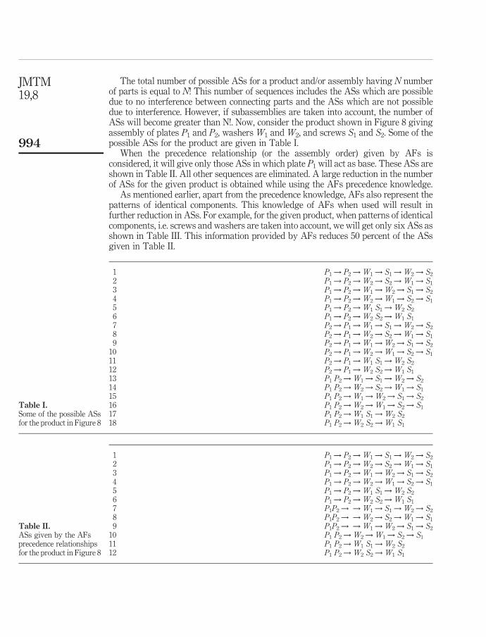
The total number of possible ASs for a product and/or assembly having N numberof parts is equal to N! This number of sequences includes the ASs which are possibledue to no interference between connecting parts and the ASs which are not possibledue to interference. However, if subassemblies are taken into account, the number ofASs will become greater than N!. Now, consider the product shown in Figure 8 givingassembly of plates P1 and P2, washers W1 and W2, and screws S1 and S2. Some of thepossible ASs for the product are given in Table I.

When the precedence relationship (or the assembly order) given by AFs isconsidered, it will give only those ASs in which plate P1 will act as base. These ASs areshown in Table II. All other sequences are eliminated. A large reduction in the numberof ASs for the given product is obtained while using the AFs precedence knowledge.

As mentioned earlier, apart from the precedence knowledge, AFs also represent thepatterns of identical components. This knowledge of AFs when used will result infurther reduction in ASs. For example, for the given product, when patterns of identicalcomponents, i.e. screws and washers are taken into account, we will get only six ASs asshown in Table III. This information provided by AFs reduces 50 percent of the ASsgiven in Table II.

1 P1 ! P2 ! W1 ! S1 ! W2 ! S2

2 P1 ! P2 ! W2 ! S2 ! W1 ! S1

3 P1 ! P2 ! W1 ! W2 ! S1 ! S2

4 P1 ! P2 ! W2 ! W1 ! S2 ! S1

5 P1 ! P2 ! W1 S1 ! W2 S2

6 P1 ! P2 ! W2 S2 ! W1 S1

7 P2 ! P1 ! W1 ! S1 ! W2 ! S2

8 P2 ! P1 ! W2 ! S2 ! W1 ! S1

9 P2 ! P1 ! W1 ! W2 ! S1 ! S2

10 P2 ! P1 ! W2 ! W1 ! S2 ! S1

11 P2 ! P1 ! W1 S1 ! W2 S2

12 P2 ! P1 ! W2 S2 ! W1 S1

13 P1 P2 ! W1 ! S1 ! W2 ! S2

14 P1 P2 ! W2 ! S2 ! W1 ! S1

15 P1 P2 ! W1 ! W2 ! S1 ! S2

16 P1 P2 ! W2 ! W1 ! S2 ! S1

17 P1 P2 ! W1 S1 ! W2 S2

18 P1 P2 ! W2 S2 ! W1 S1

Table I.Some of the possible ASsfor the product in Figure 8

1 P1 ! P2 ! W1 ! S1 ! W2 ! S2

2 P1 ! P2 ! W2 ! S2 ! W1 ! S1

3 P1 ! P2 ! W1 ! W2 ! S1 ! S2

4 P1 ! P2 ! W2 ! W1 ! S2 ! S1

5 P1 ! P2 ! W1 S1 ! W2 S2

6 P1 ! P2 ! W2 S2 ! W1 S1

7 P1P2 ! ! W1 ! S1 ! W2 ! S2

8 P1P2 ! ! W2 ! S2 ! W1 ! S1

9 P1P2 ! ! W1 ! W2 ! S1 ! S2

10 P1 P2 ! W2 ! W1 ! S2 ! S1

11 P1 P2 ! W1 S1 ! W2 S2

12 P1 P2 ! W2 S2 ! W1 S1

Table II.ASs given by the AFsprecedence relationshipsfor the product in Figure 8

JMTM19,8

994

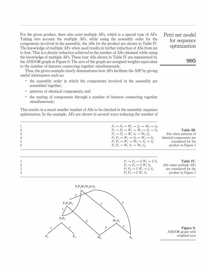
For the given product, there also exist multiple AFs, which is a special type of AFs.Taking into account the multiple AFs, while using the assembly order for thecomponents involved in the assembly, the ASs for the product are shown in Table IV.The knowledge of multiple AFs when used results in further reduction of ASs from sixto four. This is a drastic reduction achieved in the number of ASs obtained while usingthe knowledge of multiple AFs. These four ASs shown in Table IV are represented bythe AND/OR graph in Figure 9. The arcs of the graph are assigned weights equivalentto the number of features connecting together simultaneously.

Thus, the given example clearly demonstrates how AFs facilitate the ASP by givinguseful information such as:

. the assembly order in which the components involved in the assembly areassembled together;

. patterns of identical components; and

. the mating of components through a number of features connecting togethersimultaneously.

This results in a much smaller number of ASs to be checked in the assembly sequenceoptimization. In the example, AFs are shown in several ways reducing the number of

1 P1 ! P2 ! W1 ! S1 ! W2 ! S2

2 P1 ! P2 ! W1 ! W2 ! S1 ! S2

3 P1 ! P2 ! W1 S1 ! W2 S2

4 P1 P2 ! W1 ! S1 ! W2 ! S2

5 P1 P2 ! W1 ! W2 ! S1 ! S2

6 P1 P2 ! W1 S1 ! W2 S2

Table III.ASs when patterns of

identical components areconsidered for the

product in Figure 5

1 P1 ! P2 ! 2 W1 ! 2 S1

2 P1 ! P2 ! 2 W1 S1

3 P1 P2 ! 2 W1 ! 2 S1

4 P1 P2 ! 2 W1 S1

Table IV.ASs when multiple AFs

are considered for theproduct in Figure 5

Figure 9.AND/OR graph with

weighted arcsP1 P2

P1P2W1W2S1S2

P1P2W1

P1P2

W1 S1

W1S12

2 2

22

1

1

1 1


995

ASs. It is seen that much smaller number of ASs exists for the product when theknowledge of multiple AFs is used. Thus, the knowledge of multiple AFs is very usefulfor ASP in robot assembly.

If subassemblies are considered, the assembly sequence P1P2 ! 2WS is better thanall the sequences given in Table IV, since it involves more number of subassemblies.However, if the subassemblies are ignored then the sequence P1 ! P2 ! 2W ! 2Sbecomes the near optimal sequence for the given product.

PN model for assembly sequence optimizationIn this section, the proposed PN will be used to get the near optimal AS out of thesequences given in Table IV. For this purpose, while using the PN representation of ASswe introduce a simple heuristic, which says that a sequence with a less number of placesand transitions is better than the one with more number of places and transitions. Thiswill be verified by the initial marking of the proposed PN. A multiple optimizationcriteria of WIP, lead time, cycle time, throughput, and no. of servers are used.

Let us consider the sequenceP1 ! P2 ! 2W ! 2S for the product shown in Figure 5.According to this sequence, assembly of the product is obtained by first putting plate P2

on the base plate P1 to make a subassembly of plates P1P2. In the second step, twowashersW are added simultaneously to the subassembly of plates. Finally, two screwsSare screwed simultaneously to get the final assembly of the product. The assemblysequence is represented by the graph shown in Figure 10. The graph has four differentlevels: the bottom level shows the unconnected parts, the top level shows the finalassembly of parts, and the intermediate levels show the subassemblies. For example, forthe given sequence, P14 represents Part 1 at Level 4, i.e. plate P1, P13 represents thesubassembly of plates P1 and P2 at Level 3, i.e. P1P2, and P11 represents the finallyassembly of parts at Level 1. After transforming the graph shown in Figure 10 into thePN representation and introducing the server circuits and Trep, the PN model for thesequence P1 ! P2 ! 2W ! 2S becomes as shown in Figure 11.

The first step involves determination of the elementary circuits in the PN model.The PN in Figure 11 consists of two types of elementary circuits:

(1) Parts circuits:

gp1 ¼ ðP14;P13;P12;P11Þ ð10Þ

Figure 10.Graph representing thesequenceP1 ! P2 ! 2W ! 2S

W1

2

2

P1P2W1W2S1S2

P1P2W1W2

1

1

1

P1 P2

P1P2

1

Level 2

Level 3

Level 1

Level 4

S1

JMTM19,8

996

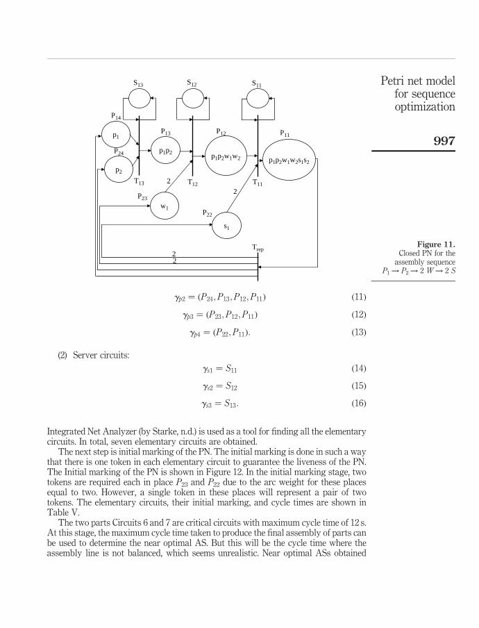
gp2 ¼ ðP24;P13;P12;P11Þ ð11Þ

gp3 ¼ ðP23;P12;P11Þ ð12Þ

gp4 ¼ ðP22;P11Þ: ð13Þ

(2) Server circuits:

gs1 ¼ S11 ð14Þ

gs2 ¼ S12 ð15Þ

gs3 ¼ S13: ð16Þ

Integrated Net Analyzer (by Starke, n.d.) is used as a tool for finding all the elementarycircuits. In total, seven elementary circuits are obtained.

The next step is initial marking of the PN. The initial marking is done in such a waythat there is one token in each elementary circuit to guarantee the liveness of the PN.The Initial marking of the PN is shown in Figure 12. In the initial marking stage, twotokens are required each in place P23 and P22 due to the arc weight for these placesequal to two. However, a single token in these places will represent a pair of twotokens. The elementary circuits, their initial marking, and cycle times are shown inTable V.

The two parts Circuits 6 and 7 are critical circuits with maximum cycle time of 12 s.At this stage, the maximum cycle time taken to produce the final assembly of parts canbe used to determine the near optimal AS. But this will be the cycle time where theassembly line is not balanced, which seems unrealistic. Near optimal ASs obtained

Figure 11.Closed PN for the

assembly sequenceP1 ! P2 ! 2 W ! 2 S

P11

p1p2w1w2s1s2

2

2

P23

P22

Trep 22

T12 T11T13

P13

P24

P12

p1p2 p1p2w1w2

p2

P14

p1

w1

s1

S13 S12 S11 Petri net modelfor sequenceoptimization

997

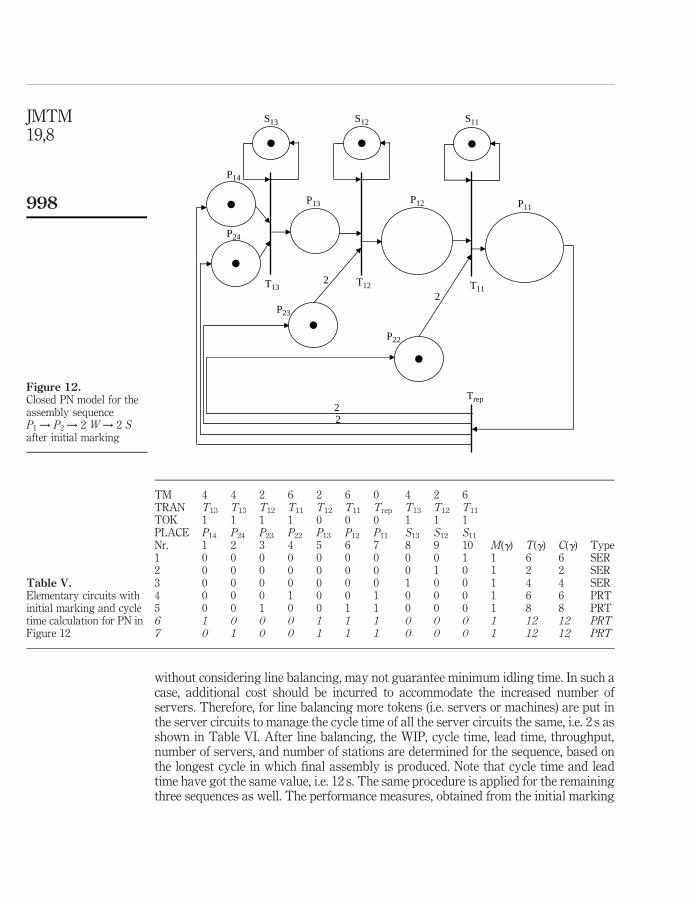
without considering line balancing, may not guarantee minimum idling time. In such acase, additional cost should be incurred to accommodate the increased number ofservers. Therefore, for line balancing more tokens (i.e. servers or machines) are put inthe server circuits to manage the cycle time of all the server circuits the same, i.e. 2 s asshown in Table VI. After line balancing, the WIP, cycle time, lead time, throughput,number of servers, and number of stations are determined for the sequence, based onthe longest cycle in which final assembly is produced. Note that cycle time and leadtime have got the same value, i.e. 12 s. The same procedure is applied for the remainingthree sequences as well. The performance measures, obtained from the initial marking

TM 4 4 2 6 2 6 0 4 2 6TRAN T13 T13 T12 T11 T12 T11 Trep T13 T12 T11

TOK 1 1 1 1 0 0 0 1 1 1PLACE P14 P24 P23 P22 P13 P12 P11 S13 S12 S11

Nr. 1 2 3 4 5 6 7 8 9 10 M(g) T(g) C(g) Type1 0 0 0 0 0 0 0 0 0 1 1 6 6 SER2 0 0 0 0 0 0 0 0 1 0 1 2 2 SER3 0 0 0 0 0 0 0 1 0 0 1 4 4 SER4 0 0 0 1 0 0 1 0 0 0 1 6 6 PRT5 0 0 1 0 0 1 1 0 0 0 1 8 8 PRT6 1 0 0 0 1 1 1 0 0 0 1 12 12 PRT7 0 1 0 0 1 1 1 0 0 0 1 12 12 PRT

Table V.Elementary circuits withinitial marking and cycletime calculation for PN inFigure 12

Figure 12.Closed PN model for theassembly sequenceP1 ! P2 ! 2 W ! 2 Safter initial marking

2

2

P23

P22

Trep 22

T12 T11T13

P13

P24

P12 P11

P14

S13 S12 S11JMTM19,8

998

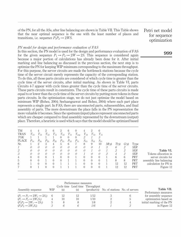
of the PN, for all the ASs, after line balancing are shown in Table VII. This Table showsthat the near optimal sequence is the one with the least number of places andtransitions, i.e. sequence P1P2 ! 2WS.

PN model for design and performance evaluation of FASIn this section, the PN model is used for the design and performance evaluation of FASfor the given sequence P1 ! P2 ! 2W ! 2S. This sequence is considered againbecause a major portion of calculations has already been done for it. After initialmarking and line balancing as discussed in the previous section, the next step is tooptimize the PN for keeping WIP minimum corresponding to the maximum throughput.For this purpose, the server circuits are made the bottleneck stations because the cycletime of the server circuit merely represents the capacity of the corresponding station.To do this, all those parts circuits are considered of which cycle time is greater than thecycle time of the server circuits, after initial marking. As shown in Table VI, partsCircuits 4-7 appear with cycle times greater than the cycle time of the server circuits.These parts circuits result in constraints. The cycle time of these parts circuits is madeequal to or lower than the cycle time of the server circuits by putting more tokens in theseparts circuits. In the optimization stage, we do not just optimize the model based onminimum WIP (Bohez, 2004; Seeluangsawat and Bohez, 2004) where each part placerepresents a single part. In FAS, there are unconnected parts, subassemblies, and finalassembly of parts. The more downstream the place falls in the PN representation themore valuable it becomes. Since the upstream (input) places represent unconnected partswhich are cheaper compared to final assembly represented by the downstream (output)place. Therefore, a heuristic is used which says that the model should be optimized based



Nr. 1 2 3 4 5 6 7 8 9 10 M(g) T(g) C(g) Type1 0 0 0 0 0 0 0 0 0 1 3 6 2 SER2 0 0 0 0 0 0 0 0 1 0 1 2 2 SER3 0 0 0 0 0 0 0 1 0 0 2 4 2 SER4 0 0 0 1 0 0 1 0 0 0 1 6 6 PRT5 0 0 1 0 0 1 1 0 0 0 1 8 8 PRT6 1 0 0 0 1 1 1 0 0 0 1 12 12 PRT7 0 1 0 0 1 1 1 0 0 0 1 12 12 PRT

Table VI.Tokens allocation in

server circuits forassembly line balancing

calculation for PN inFigure 12

Performance measures

Assembly sequence WIPCycle time

(s)Lead time

(s)Throughput(product/s) No. of stations No. of servers

(P1 ! P2 ! 2W1 ! 2S1) 6 12 12 1/12 3 6(P1 ! P2 ! 2W1S1) 4 10 10 1/10 2 5(P1P2 ! 2W1 ! 2S1) 5 8 8 1/8 2 4(P1P2 ! 2W1S1) 3 6 6 1/6 1 3

Table VII.Performance measuresfor assembly sequenceoptimization based on

initial marking of the PNin Figure 12


999

on weighted-WIP. Weighted-WIP means assigning to all parts, subassemblies, and finalassembly their respective value (or cost) in the model. This pushes more and more tokensin the input places of the PN as shown in Table VIII. The optimum condition (i.e.minimum weighted-WIP) can be mathematically represented as an LP problem. Theobjective function for this sequence based on equation (5) is:

MIN ¼ V 14 £ P14 þ V 24 £ P24 þ V 23 £ P23 þ V 22 £ P22 þ V 13 £ P13

þ V 12 £ P12 þ V 11 £ P11:ð17Þ

Each place name represents the number of tokens in that place. The tokens to be added tothe parts circuits can be determined by dividing the cycle time of the parts circuit withthe cycle time of the critical circuit. The number of tokens to be added to the partsCircuits 4-7 should be greater than or equal to 3, 4, 6, and 6, respectively:

Parts circuit 4 : P22 þ P11 .¼ 3 ð18Þ

Parts circuit 5 : P23 þ P12 þ P11 .¼ 4 ð19Þ

Parts circuit 6 : P14 þ P13 þ P12 þ P11 .¼ 6 ð20Þ

Parts circuit 7 : P24 þ P13 þ P12 þ P11 .¼ 6: ð21Þ

After optimization, the distribution of tokens in part places is shown in Table VIII by therow TOK. Each single token in places P23 and P22 shows a pair of two tokens. Theperformance measures are then calculated for the design of FAS as shown in Table IX.



Nr. 1 2 3 4 5 6 7 8 9 10 C(g) C(g)/C(gc)1 0 0 0 0 0 0 0 0 0 1 2 –2 0 0 0 0 0 0 0 0 1 0 2 –3 0 0 0 0 0 0 0 1 0 0 2 –4 0 0 0 1 0 0 1 0 0 0 6 35 0 0 1 0 0 1 1 0 0 0 8 46 1 0 0 0 1 1 1 0 0 0 12 67 0 1 0 0 1 1 1 0 0 0 12 6

Table VIII.Token allocation in partscircuits after optimizationfor PN in Figure 12

Performance measures

Assembly sequence WIPCycle time

(s)Lead time

(s)Through-put

(prod/s)No. of

stationsNo. of

servers

Stationsutilization(per cent)

(P1 ! P2 ! 2W ! 2S) 26 2 2 0.5 3 6 100

Table IX.Performance measuresfor design andperformance analysis ofFAS

JMTM19,8

1000

Summary and conclusionsTo speed up the ASP, AFs are shown useful in reducing the number of sequences inseveral ways. For example, AFs directly indicate the assembly order for thecomponents involved in the assembly. They also represent patterns of identicalcomponents and multiple AFs. However, the knowledge of multiple AFs is seen muchmore useful in reducing the ASs from many to only few. For assembly sequenceoptimization, a generic PN model is developed. A multiple optimization criteria of cycletime, WIP, lead time, throughput, number of servers, number of stations, and stationutilization are used for the AS optimization and FAS design and performance analysis.These performance measures may be helpful in the factory floor management. Linebalancing may result in the highest efficiency and the shortest idling time along withease of management and supervision. A simple heuristic which says that the sequencewith least number of places and transitions is better than the sequence with morenumber of places and transitions is verified using the initial marking of the PN. Since,the final assembly is more costly compared to the unconnected parts, therefore, the PNis optimized based on weighted-WIP. The optimization of the PN is influenced by theutilization of the bottleneck stations. In the example shown, the PN gives minimumWIP for maximum production rate. Minimum WIP gives reduced lead time. The cost ofWIP will be reduced because WIP is kept minimum and it is also pushed in theinput places of the PN. Moreover, full utilization is achieved at all stations in theassembly line.

References

Baldwin, D.F., Abell, T.E., Lui, M.-C., de Fazio, T.L. and Whitney, D.E. (1991),“An integrated computer aid for generating and evaluating assembly sequences formechanical products”, IEEE Transactions on Robotics and Automation, Vol. 7,pp. 78-89.

Bohez, E.L.J. (2004), “A new generic timed Petri net model for design and performance analysis ofa dual kanban FMS”, International Journal of Production Research, Vol. 42 No. 4,pp. 719-40.

Chao, T.H. and Sanderson, A.C. (1995), “Task sequence planning using fuzzy Petri nets”, IEEETransactions on Systems, Man, and Cybernetics, Vol. 25, pp. 755-68.

de Fazio, T.L. and Whitney, D.E. (1987), “Simplified generation of all mechanical assemblysequences”, IEEE Transactions on Robotics and Automation, Vol. RA-3 No. 6,pp. 640-58.

Dini, G. and Santochi, M. (1992), “Automated sequencing and subassembly detection in assemblyplanning”, Annals CIRP, Vol. 41, pp. 1-6.

Gottipolu, R.B. and Ghosh, K. (1995), “Integrated approach to the generation of assemblysequences”, International Journal of Computer Applications in Technology, Vol. 8 Nos 3/4,pp. 125-38.

Homem de Mello, L.S. and Sanderson, A.C. (1991a), “A correct and complete algorithm for thegeneration of mechanical assembly sequences”, IEEE Transactions on Robotics andAutomation, Vol. 7, pp. 228-40.

Homem de Mello, L.S. and Sanderson, A.C. (1991b), “Two criteria for the selection of assemblyplans: maximising the flexibility of sequencing the assembly tasks and minimising theassembly time through parallel execution of assembly tasks”, IEEE Transactions onRobotics and Automation, Vol. 7, pp. 626-33.


1001

Huang, Y.F. and Lee, C.S.G. (1990), “An automatic assembly planning system”, IEEEInternational Conference on Robotics and Automation, Cincinnati, OH, May 13-18,pp. 1594-9.

Moore, K.E. and Gupta, S.M. (1996), “Petri net models of flexible and automated manufacturingsystems: a survey”, International Journal of Production Research, Vol. 34, pp. 3001-35.

Moore, K.E. and Gupta, S.M. (1999), “Stochastic colored Petri net (SCPN) models of traditionaland flexible kanban systems”, International Journal of Production Research, Vol. 37 No. 9,pp. 2135-58.

Seeluangsawat, R. and Bohez, E. (2004), “Integration of JIT flexible manufacturing, assembly anddisassembly system using Petri net approach”, Journal of Manufacturing TechnologyManagement, Vol. 15 No. 7, pp. 700-14.

Seow, S.K. and Devanathan, R. (1994), “A temporal framework for assembly sequencerepresentation and analysis”, IEEE Transactions on Robotics and Automation, Vol. 10No. 2, pp. 220-9.

Starke, H.P. (n.d.), Integrated Network Analyser (INA), available at: www.informatik.huberlin.de/lehrstuehle/automaten/ina/

Su, Q. (2007), “Applying case-based reasoning in assembly sequence planning”, InternationalJournal of Production Research, Vol. 45 No. 1, pp. 29-47.

Suzuki, T., Kanehara, T., Inaba, A. and Okuma, S. (1993), “On algebraic and graph structuralproperties of assembly Petri net”, IEEE International Conference on Robotics andAutomation, Atlanta, GA, pp. 794-800.

Swaminathan, A. and Barber, K.S. (1996), “An experience-based assembly sequences planner formechanical assembly”, IEEE Transactions on Robotics and Automation, Vol. 12,pp. 252-67.

Tang, Y. and Zhou, M. (2004), “Fuzzy-Petri-Net based disassembly planning consideringhuman factors”, IEEE International Conference on Systems, Man and Cybernetics,pp. 4195-200.

Thomas, J.P., Nissanke, N. and Baker, K.D. (1996), “A hierarchical Petri net framewok for therepresentation and analysis of assembly”, IEEE Transaction on Robotics and Automation,Vol. 12 No. 2, pp. 268-79.

Ullah, H., Bohez, E.L.J. and Irfan, M.A. (2006), “Assembly feature: definition, classification, andinstantiation”, Proceedings of the 2nd International Conference on Emerging Technologies,Peshawar, November 13-14, pp. 617-23.

Wilson, R.H. (1995), “Minimising user queries in interactive assembly planning”, IEEETransactions on Robotics and Automation, Vol. 11, pp. 308-11.

Yee, S.T. and Ventura, J.A. (1999), “A Petri net model to determine optimal assembly sequenceswith assembly operation constraints”, Journal of Manufacturing Systems, Vol. 18 No. 3,pp. 203-13.

Zha, X.F., Lim, S.Y.E. and Fok, S.C. (1998), “Integrated knowledge-based assembly sequenceplanning”, International Journal of Advanced Manufacturing Technology, Vol. 14,pp. 50-64.

Zha, X.F., Lim, S.Y.E. and Lu, W.F. (2003), “A knowledge intensive multi-agent system forcooperative/collaborative assembly modeling and process planning”, Society for Designand Process Science, Vol. 7 No. 1, pp. 99-122.

Zhang, W., Freiheit, T. and Yang, H. (2005), “Dynamic scheduling in flexible assembly systembased on timed Petri nets model”, Robotics & Computer-integrated Manufacturing, Vol. 21,pp. 550-8.

JMTM19,8

1002

About the authorsHamid Ullah is an Assistant Professor in the Department of Mechanical Engineering, NWFPUniversity of Engineering and Technology, Peshawar, Pakistan. He did his Master Degree inHigh Speed Machining from his parent department. He is currently working as a doctoralstudent in the Design and Manufacturing Engineering field of study, School of Engineering andTechnology, Bangkok, Thailand. His areas of interest are mathematical modeling, assemblyfeatures, Petri nets (PNs), and assembly sequence planning. Hamid Ullah is the correspondingauthor and can be contacted at: [email protected]; [email protected]

Erik L.J. Bohez is an Associate Professor in the Design and Manufacturing Engineering fieldof study, School of Engineering and Technology, Bangkok, Thailand. His areas of interest areFMS, CAD/CAM, multi-axis machining, error measurement, PNs, and packaging. He has manyrefereed journal papers and conference papers. He is actively involved both in teaching andresearch.


1003

To purchase reprints of this article please e-mail: [email protected] visit our web site for further details: www.emeraldinsight.com/reprints

A Petri net model for sequence optimization and performance analysis of flexible assembly systems

Documents

Transcript of A Petri net model for sequence optimization and performance analysis of flexible assembly systems