arX

iv:2

005.

0510

8v3

[cs

.LO

] 8

Apr

202

2

Whole-grain Petri nets and processes∗

Joachim Kock

Universitat Autonoma de Barcelona∗∗

and Centre de Recerca Matematica

Abstract

We present a formalism for Petri nets based on polynomial-style finite-set config-urations and etale maps. The formalism supports both a geometric semantics in thestyle of Goltz and Reisig (processes are etale maps from graphs) and an algebraicsemantics in the style of Meseguer and Montanari, in terms of free coloured props,and allows the following unification: for P a Petri net, the Segal space of P-processesis shown to be the free coloured prop-in-groupoids on P. There is also an unfoldingsemantics a la Winskel, which bypasses the classical symmetry problems: with thenew formalism, every Petri net admits a universal unfolding, which in turn has as-sociated an event structure and a Scott domain. Since everything is encoded withexplicit sets, Petri nets and their processes have elements. In particular, individual-token semantics is native. (Collective-token semantics emerges from rather drasticquotient constructions a la Best–Devillers, involving taking π0 of the groupoids ofstates.)

Contents

0 Introduction 11 Graphs (according to [46]) 6

2 Whole-grain Petri nets 11

3 Processes 144 The symmetric monoidal Segal space of processes 19

5 Digraphical species from Petri nets 24

6 Free props 27

7 The symmetric monoidal category of processes 30

8 Hypergraphs 33

9 Unfolding 38

10 Rational maps (of Petri nets) 46

11 Notes 50Appendix A: Groupoids and homotopy pullbacks 53

Appendix B: Simplicial groupoids and Segal spaces 55

0 Introduction

Background. Petri nets are an important framework for describing networks in whichresources interact and transform, such as chemical reaction networks and population dy-

∗Previously circulated under the title Elements of Petri nets and processes∗∗Current address: University of Copenhagen

1

namics, including compartmental models in epidemiology. In computer science they serveas a widely used model of concurrency.

A Petri net (cf. Section 2) has places holding tokens, and transitions describing howtokens flow and transform. Arcs connect places and transitions to express the interactions.A Petri net is thus a kind of graph, and may look like the following figure. Places arealways pictured as circles, and transitions as squares. Tokens are drawn as bullets:

••

•

The operational semantics of Petri nets is the mathematical formalisation of their be-haviour, expressed informally in the token game, whereby firing of transitions move aroundtokens between places. Two main classes of operational semantics can be called geometricand algebraic, although this terminology is not standard in the literature. Geometric se-mantics take as starting point the notion of nonsequential processes, formalised as certainmorphisms into a given Petri net from causal nets, certain posets or graphs. This view-point was pioneered by Petri himself [61], and found a very clean formulation in the seminal1983 paper of Goltz and Reisig [32], leading to many developments and insights regardingreachability, density, safeness, as expressed for example in the 1988 monograph of Best andFernandez [14]. Algebraic semantics, on the other hand, focus on the way the transitionsof a Petri net generate a formal algebraic system. After earlier work of Reisig [62] andWinskel [70], a breakthrough was the 1990 work of Meseguer and Montanari [54], who ob-served that Petri nets can be defined as monoids in certain directed graphs, and that theyfreely generate symmetric monoidal categories of certain kinds, equivalently, free props.The morphisms in such a symmetric monoidal category are thus built up from the tran-sitions of a given Petri net by serial and parallel connection (composition and the tensorproduct), and are thus certain equivalence classes of firing sequences.

In view of the well-known graphical calculus for monoidal categories in terms of stringdiagrams [43], one could expect a unification of the geometric and algebraic semantics.This has turned out to be a difficult problem, though: In the ‘geometric’ frameworks,there is no way to compose processes in the sense of category theory, and in the algebraicframeworks there is no synthetic description of processes — they rely solely on formalinductive descriptions. Over the past four decades, a lot of research has been dedicated tothis problem. Already in 1987, Best and Devillers [13] searched for an algebraic descriptionof the Goltz–Reisig processes, finding that it was necessary to impose drastic equivalencerelations on processes. Starting from the Meseguer–Montanari formalism, many people,including in particular Bruni, Meseguer, Montari, and Sassone [16], [17], tried to avoidthese quontientings by introducing further bookkeeping on Petri nets. They arrived at thenotion of pre-net, which are Petri nets with numberings. For the notion of pre-net thesemantics problems can be solved, but pre-nets are not quite a satisfactory substitute forPetri nets. In particular, they do not allow enough morphisms. The final section of thispaper contains some further discussion of these issues.

Closely related to the geometric-algebraic dichotomy is the distinction between individual-token and collective-token philosophies, which roughly asks whether the tokens of a stateof a Petri net execution are individual elements in a set or if they are only the expressionof a quantity, a natural number. (See [30], [31], [18], [29], [17] for more thorough discus-sion.) The geometric semantics favour the individual-token philosophy, since processes are

2

explicit maps from other nets, and in particular involves mappings of sets. In contrast, thealgebraic semantics are more geared towards the collective-token philosophy, as both theirstates and the pre- and post-conditions of a transition are given by multisets, meaningsets with multiplicities. In its full version (see van Glabbeek [29]) the individual-tokenphilosophy requires keeping track of all tokens at all times, which is done by annotatingeach token occurrence with the complete history of the transitions that produced it from agiven initial state. (This involves knowing which tokens enter which input slots of a giventransition, and in particular it is necessary to be able to distinguish such slots, somethingwhich is essentially impossible in the Petri-nets-as-monoids formalism.)

A third main approach to operational semantics is based on the idea of unfolding,pioneered in the work of Winskel [67] and Nielsen, Plotkin, and Winskel [58]. It is importantbecause it establishes connections to domain theory and denotational semantics. The keyingredient, the universal unfolding of a Petri net, was established for safe Petri nets byNielsen, Plotkin, and Winskel, but there are symmetry issues preventing the existenceof a universal unfolding for general Petri nets. Montanari, Meseguer, and Sassone [56],[55] worked around the symmetry problems by considering certain decorated unfoldings,but their construction was not universal in the categorical sense. Baldan, Bruni, andMontanari [7] established instead the existence of a universal unfolding for pre-nets, wherethe symmetries do not come up. Finally Hayman and Winskel [36], [37] came to grips withthe symmetries themselves and established a weaker form of universal property, through anotion of adjunction up to symmetry in a precise technical sense.

Contributions of this paper. The present paper proposes a rather natural solution tothese problems, by using some elementary homotopy theory to overcome the symmetryissues. The novelty essentially boils down to one small modification at the foundationallevel: to abolish the traditional notion of multisets in favour of the representable analogue:Instead of sets of multiplicity functions S → N, we consider groupoids of S-coloured finitesets A → S; instead of assigning to each s ∈ S a multiplicity, there is now assigned anactual set, namely the pre-image As. The isomorphism classes of S-coloured sets are thetraditional multisets on S. The benefit is that S-coloured sets have elements, which canbe accessed individually, giving full control over symmetries.

The multiset modification is incorporated in the very definition of Petri net, followingthe lead of the analogous formalism for directed graphs [46] (in turn motivated by thepolynomial formalism in the theory of operads [45]): we define a Petri net to be a diagramof finite sets

S ←− I −→ T ←− O −→ S.

Here T is the set of transitions, S is the set of places, and I and O are the sets of incomingand outgoing arcs of transitions. In particular, for a transition t ∈ T , the fibres (i.e. pre-image sets) It and Ot are explicit sets, and they are not necessarily subsets of S. In thispaper, the new Petri nets are called whole-grain Petri nets, to distinguish them from thetraditional notion of Petri net. A whole-grain Petri net is thus precisely what we see inthe pictures. It is only a slight modification of the usual definition, but it has importantimplications, and the theory develops quite neatly from it, exploiting some recent insightsfrom algebraic combinatorics [20], [21], [23], [24].

An etale map is a diagram

S ′ I ′ T ′ O′ S ′

S I T O S

αy x

α

3

(the middle squares being pullbacks). A graph is a SITOS diagram where the outer mapsS ← I and O → S are injective [46]. A process is an etale map from an acyclic graph. Theprocesses of a Petri net P assemble naturally into a simplicial groupoid X•, shown to bea symmetric monoidal Segal space. (Segal spaces (recalled below in §4) are a homotopyversion of categories. Appendix 11 provides some background.) The following is the firstmain result of this work.

Theorem. (Cf. 6.9) X• is the free prop-in-groupoids on P.

It expresses the reconciliation of the geometric and algebraic semantics for whole-grainPetri nets. A 1-categorical analogue of this result is also extracted (7.2). Making sense ofthe free prop on a (whole-grain) Petri net depends on an explicit fully faithfully embeddingPetri → PrSh(elGr) of the category of (whole-grain) Petri nets into the presheaf categoryon elementary graphs (5.2, 5.3). Such presheaves, the structure underlying coloured props,are called digraphical species1 (or sometimes bicollections) [46].

The second main result shows the benefit of whole-grain Petri nets for unfolding:

Theorem. (Cf. 9.6) Any (grounded) whole-grain Petri net admits a universal unfolding.

No safety assumptions are required here, in contrast to the classical result of Nielsen–Plotkin–Winskel [58]. It should be stressed that the proof of this theorem follows theideas and arguments employed by Winskel in the safe case — the only novelty is the newwhole-grain setting, where the arguments go through even in the non-safe case.

The key point of the new formalism, as exploited in the proofs of the main theorems,is that whole-grain Petri nets are configurations of sets, and that these sets have elementsthat can be accessed, giving total control over symmetries. With the systematic use ofgroupoids, these symmetries are kept around as they are, giving some advantage over thetraditional formalisms of Petri nets, where the symmetries are difficult to control.

The general importance of groupoids in combinatorics was discovered and advocated byJoyal [39] and Baez–Dolan [3]. The specific insight of representing algebraic structures bygroupoids of configurations of sets has been found useful in algebraic topology (mainly inthe theory of operads) [25], [45], [40], [46], [9], and in algebraic combinatorics (in connectionwith incidence bialgebras and Mobius inversion) [20], [21], [24]. The mathematical tools arethus already available. The whole-grain Petri nets of the present paper can be seen as anintermediate notion between traditional Petri nets and pre-nets [16], [17], in the same wayas polynomial monads are intermediate between symmetric operads and non-symmetricoperads [45].

The basic ideas and results are elementary, relying solely on manipulations with finitesets, mostly pullbacks and pushouts. Some of the theoretical results and justifications(Sections 4–7) require some more category theory, and some elementary homotopy theory.

The core mathematical content could be given more succinctly, but the text has grownlonger for three reasons. Firstly, many examples, figures, and explanations have beenincluded to illustrate the formalism, where different from that of the traditional approachesto Petri nets. Secondly, many arguments of homotopical nature have been accompanied by

1Warning: the word ‘species’ is used here as in combinatorics [10]. It has nothing to do with the useof the word to mean ‘places’, as occurs sometimes in Petri net theory motivated by chemical reactionnetworks (see for example [6] and the references therein).

4

intuitive explanations and background material, hopefully making them accessible also toreaders without background in homotopy theory. Finally, an effort has been made to tryto point out origins of ideas and provide comparison with related developments.

Outline of the paper. We begin in Section 1 with a brief summary of the formalismof directed graphs from [46]. This is where the semantics lives, both in geometric andalgebraic form, and most of the work will take place at this level.

In Section 2 we define the whole-grain Petri nets and their etale maps, and in Section 3we define their processes to be etale maps from (acyclic) graphs. Section 4 sets up thesymmetric monoidal Segal space X• of processes of a fixed Petri net P.

In Section 5 we fully faithfully embed the category of Petri nets into the presheafcategory on elementary graphs — these presheaves are called digraphical species — andcharacterise the image as the flat digraphical species. This embedding is used to define thefree prop on a Petri net in Section 6. We show that the symmetric monoidal Segal spaceX• associated to P is the free prop-in-groupoids on P. This is the first main theorem ofthe paper, Theorem 6.9. In Section 7 we show how to trim down the symmetric monoidalSegal space to a symmetric monoidal category, and discuss the homotopy issues involved.

In Section 8 we set up some definitions and results about certain classes of hypergraphs.This is preparation for Section 9 where we come to the second main theorem of the paper,Theorem 9.6, establishing the existence of universal unfoldings for general Petri nets.

In Section 10 we look into fancier notions of morphisms of Petri nets than the basic etalemaps, and establish functoriality of X• in these more general maps. Modulo the differencein set-up, this covers the notion of morphisms of Meseguer and Montanari [54] (monoidhomomorphisms), as well as the more general notions given in terms of multi-relations,studied by Winskel [70].

The closing Section 11 makes an attempt at situating this work in a bigger picture, andin particular provide comparison with the pre-nets of Bruni, Meseguer, Montanari, andSassone [17]. There are two short appendices: one with a few basic facts about groupoidsand homotopy pullbacks, and one with simplicial groupoids and Segal spaces.

Related work and outlook. After this work was first released in preprint form (May2020), Baez, Genovese, Master, and Shulman [4] have made an important contribution tothe theory, which complements the material in Sections 5–7 in various ways, and constitutesa nice overall picture of monoidal-category theoretic operational semantics. First of all theypropose to work directly with digraphical species (which they call Σ-nets), as a substitutefor Petri nets. This is a fascinating idea, going beyond the strong graphical aspect ofPetri nets. Secondly, they give slick categorical proofs of key adjunctions, including a nicealternative proof of the adjunction described below in 6.4.

Although the field of Petri net theory is very much driven by applications — in com-puter science, natural sciences, and industry — the present work is motivated by theoreticalinterest. Up to the point developed here, I think the theoretical picture is quite satisfac-tory and clean, at the price of some homotopy overhead. It is my opinion that Petri-nettheorists and end users can bargain against this price in various ways (see [26] for someexplicit bargaining), which I think amounts to falling back on previous approaches. It ismy hope nevertheless that the account given here will resonate with modern trends in theo-retical computer science, and with homotopy type theory [65] in particular, where specifiedbijections are part of the whole set-up in the form of terms of identity types.

At the same time, the whole-grain formalism in itself can be appreciated without anyhomotopy overhead. The main contributions, the definitions in Sections 1–3, have no other

5

prerequisites than pullbacks of finite sets. The formalism aligns very well with the wayPetri nets are employed in applications, the main feature being that whole-grain Petrinets are just configurations of finite sets, lending themselves to software implementation.Recently, Baas, Fairbanks, Halter, and Patterson chose the whole-grain formalism as thebasis for an implementation in Julia [44], [15] of a Petri net library [1] (see [59] for theoreticalbackground), and used it in epidemiology, first to give elegant modelling of COVID-19 datafrom the UK [34], and later for a more general compositional approach to epidemiology,cf. Libkind–Baas–Halter–Patterson–Fairbanks [50].

Acknowledgments. I wish to thank Pawe l Sobocinski, Filippo Bonchi, Steve Lack, andMike Shulman for feedback and help. This work was presented as a plenary keynote ad-dress at the 2020 International Conference on Applied Category Theory (ACT 2020). I amgrateful to the programme committee for their confidence and for the opportunity. Finally Iam thankful to various anonymous referees for their feedback, which led to many improve-ments. This work was partially supported by grants MTM2016-80439-P (AEI/FEDER,UE) and PID2020-116481GB-I00 (AEI/FEDER, UE) of Spain and 2017-SGR-1725 of Cat-alonia, and also through the Severo Ochoa and Marıa de Maeztu Program for Centers andUnits of Excellence in R&D grant number CEX2020-001084-M.

1 Graphs (according to [46])

The following formalism for directed graphs (and all the results in this section) are from[46], which in turn was heavily inspired by the polynomial formalism for trees [45] andby the formalism for Feynman graphs of Joyal–Kock [40]. Some further comparison isprovided in Section 11. The graphs will play the role of what are also called causal nets inPetri-net theory (see for example [32]), their purpose being to define processes.

1.1 Graphs (AINOA style). A graph (meaning directed graph admitting open-endededges) is a diagram of finite sets

A I N O A

where the outermost maps are injective. Here A is the set of edges, and N is the set ofnodes. The set I expresses the incidence of edges and nodes from the viewpoint of edgesincoming to nodes, and O the same for outgoing edges. The injectivity condition says thatan edge is incoming (or outgoing) for at most one node. We shall only consider acyclicgraphs, meaning having no directed cycles (see [46] and 1.12 below).

1.2 Example. The graph

{a, b, c, d, e} {b, c, d} {x, y, z} {c, d, e} {a, b, c, d, e}b7→y

c 7→z

d7→z

y← [c

y← [d

y← [e

can be pictured like this:

x

y

z

a

b

cd e

6

The picture is a full rendition of the data of the AINOA diagram, except that the sets Iand O are not explicit. They can be derived from the picture as subsets of A.

1.3 Etale maps. An etale map of graphs is a diagram

A′ I ′ N ′ O′ A′

A I N O A,

αy x

α

where the middle squares are pullbacks. The pullback condition expresses that arities ofnodes must be respected; in other words the map is a ‘homeomorphism’ locally at eachnode. An open map is an etale map that is furthermore injective on nodes and edges.

1.4 Remark. The notion of etale map has a clear intuitive content. It also fits into theaxiomatic notion of classes of etale maps of Joyal–Moerdijk [41]; see also [42], [36]. Thereare other useful notions of morphisms of AINOA graphs, some of which are used in [46](see also [47]), but for the present purposes only etale maps are relevant.

1.5 Sums and connectedness. The category Gr of acyclic graphs and etale maps hascategorical sums given by disjoint union of graphs. These are calculated pointwise (i.e. onA, N , I, and O separately). The empty graph is neutral for sum. A graph is connected ifit is non-empty and cannot be written as a sum of smaller non-empty graphs.2

1.6 Pullbacks. The category Gr has pullbacks, computed pointwise (i.e. for the A, I,N , O components separately).

1.7 Unit graph and edges. The unit graph is the graph 1∅∅∅1. An edge in a graphG = AINOA

1 ∅ ∅ ∅ 1

A I N O A

αy x

α

is incoming to G if the right-most square is a pullback, and outgoing if the left-most squareis a pullback (in addition to the standing requirement that the two middle squares arepullbacks). Accordingly, the in-boundary of G is defined to be the set in(G) of edges inthe complement of O A (that is, the complement of the image of this injective map)and the out-boundary out(G) is similarly defined as the complement of A I. An edge isisolated if it belongs to both the in-boundary and the out-boundary. An edge is inner if itis outgoing to some node and incoming to some node. The set of inner edges is thus theintersection of the (images of the) two maps O A I. We write x ⋖ y if there is aninner edge from x to y.

In Example 1.2, the in-boundary is {a, b}, the out-boundary is {a, e}, and the set ofinner edges is {c, d}.

1.8 Elementary graphs. An elementary graph is a connected graph with no inner edges.An elementary graph is thus either a unit graph or a corolla, which means one of the form

m + n m 1 n m + n.

2Warning: in [46] the symbol Gr denotes the category of connected graphs.

7

Here m is the set of incoming edges and n is the set of outgoing edges.Let elGr ⊂ Gr denote the full subcategory of elementary graphs and etale maps —

in fact it is practical to work rather with a skeleton of this category, as we do henceforth.We denote by [⋆] the unit graph, and by [ n

m ] the corolla with m incoming and n outgoingedges. These are pictured, respectively, as

· · ·

· · ·

m

n

Note that the only non-invertible maps in elGr are the inclusions of [⋆] into a corolla[ nm ] (of which there are m+n). In addition there are the symmetries of the corollas: there

are m!n! invertible maps [ nm ] → [ n

m ]. The etale condition precludes non-invertible mapsbetween corollas. Denote by Cor the full subcategory consisting of the corollas; it is thusa groupoid.

1.9 Colimits and gluing. The category Gr admits enough colimits to account neatlyfor gluing [46]. In particular, if M is a node-less graph (disjoint union of unit graphs),which embeds into the out-boundary of a graph G1 and embeds into the in-boundary of agraph G2, then the pushout

G2

M G

G1

exists in the category Gr, and it is calculated pointwise (i.e. for the A, I, N , O componentsseparately). See [46] for details. The finite-set pushouts are along injections, and can becomputed very explicitly. It gives a clean formalisation of the intuitive idea of gluing partsof the out-boundary of one graph to parts of the in-boundary of another, as exemplified inthis picture:

The reader is encouraged to write down these graphs in AINOA diagrams and actuallycompute the pushout.

Lemma 1.10 ([46]) Every graph is canonically the colimit of its elementary subgraphs:

G ≃ colimE∈el(G)

E.

The colimit is over the category of elements of the graph G, defined as the comma category

el(G) := elGr ↓G,

8

in turn defined by the natural transformation diagram (lax pullback)

elGr↓G 1

elGr Gr.

pGq⇒

The objects of el(G) are thus the elementary subgraphs of G (or more precisely, etale mapsfrom elementary graphs). For details, see [46]. In concrete terms, the diagram consists ofall the edges and all the nodes, with each edge mapping into the corollas it is incident to,as exemplified in this colimit decomposition of a graph G:

G

1.11 Dynamics of graphs. It is fruitful to view a graph as an interpolation betweenthe in-boundary and the out-boundary, an evolution — not with respect to any absolutenotion of time, but reflecting the fact that both N and A carry a preorder structure. Agraph is acyclic if the preorder N is actually a poset (i.e. is an anti-symmetric relation).3

Further notions of time can be imposed in terms of the following concept:

1.12 Level functions. A level function of a graph G = AINOA is a monotone mapf : N → k, where k := {1, 2, . . . , k} for some k ∈ N. Monotone means that for every edgefrom node x to node y we have f(x) ≤ (y). A level function is strict if the inequality isstrict (that is, x⋖ y ⇒ f(x) < f(y)). A graph is acyclic iff it admits a strict level function.

1.13 Layers, cuts, and pushout decompositions. Level functions serve in particularto split graphs into layers. For example, a level function f : N → 2 will partition the nodeset into two sets N = N1 + N2, namely the pre-images N1 := f−1(1) and N2 := f−1(2).This in turn will induce two open subgraphs G1 and G2 called layers, defined as follows. G1

is the open subgraph containing all the nodes in N1 and all their incident edges, and alsothe in-boundary of G. Precisely, to obtain G1, first take pullbacks as indicated with dottedarrows:

in(G) ∪ I1 ∪O1 I1 N1 O1 in(G) ∪ I1 ∪ O1

A I N O A,

y x

then add the dashed arrows, which are just the inclusions. G2 is constructed similarlyfrom N2, but with out(G) instead of in(G). The out-boundary of G1 will coincide with the

3One can also put N and A together in a single poset, whose Hasse diagram is then bipartite. Suchposets form the substrate of the classical poset semantics of Petri nets [61], [27], [32]; see for example themonograph [14].

9

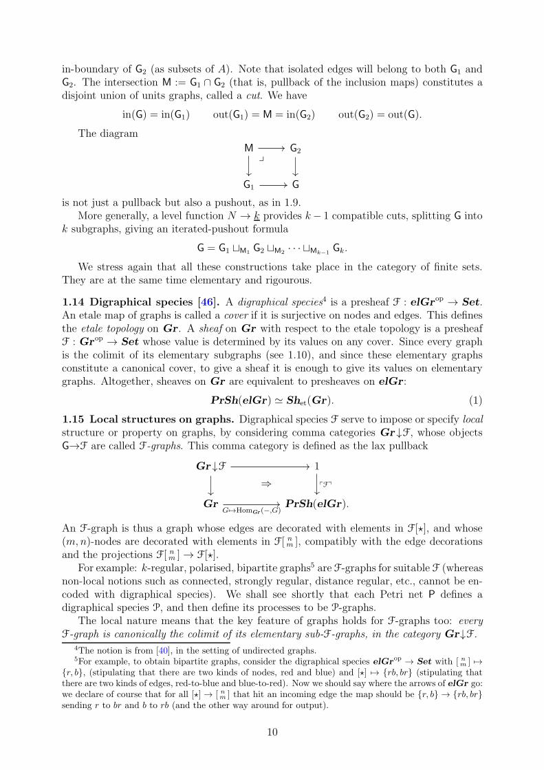
in-boundary of G2 (as subsets of A). Note that isolated edges will belong to both G1 andG2. The intersection M := G1 ∩ G2 (that is, pullback of the inclusion maps) constitutes adisjoint union of units graphs, called a cut. We have

in(G) = in(G1) out(G1) = M = in(G2) out(G2) = out(G).

The diagram

M G2

G1 G

y

is not just a pullback but also a pushout, as in 1.9.More generally, a level function N → k provides k− 1 compatible cuts, splitting G into

k subgraphs, giving an iterated-pushout formula

G = G1 ⊔M1 G2 ⊔M2 · · · ⊔Mk−1Gk.

We stress again that all these constructions take place in the category of finite sets.They are at the same time elementary and rigourous.

1.14 Digraphical species [46]. A digraphical species4 is a presheaf F : elGrop → Set.An etale map of graphs is called a cover if it is surjective on nodes and edges. This definesthe etale topology on Gr. A sheaf on Gr with respect to the etale topology is a presheafF : Grop → Set whose value is determined by its values on any cover. Since every graphis the colimit of its elementary subgraphs (see 1.10), and since these elementary graphsconstitute a canonical cover, to give a sheaf it is enough to give its values on elementarygraphs. Altogether, sheaves on Gr are equivalent to presheaves on elGr:

PrSh(elGr) ≃ Shet(Gr). (1)

1.15 Local structures on graphs. Digraphical species F serve to impose or specify localstructure or property on graphs, by considering comma categories Gr ↓F, whose objectsG→F are called F-graphs. This comma category is defined as the lax pullback

Gr ↓F 1

Gr PrSh(elGr).

pFq⇒

G 7→HomGr(−,G)

An F-graph is thus a graph whose edges are decorated with elements in F[⋆], and whose(m,n)-nodes are decorated with elements in F[ n

m ], compatibly with the edge decorationsand the projections F[ n

m ]→ F[⋆].For example: k-regular, polarised, bipartite graphs5 are F-graphs for suitable F (whereas

non-local notions such as connected, strongly regular, distance regular, etc., cannot be en-coded with digraphical species). We shall see shortly that each Petri net P defines adigraphical species P, and then define its processes to be P-graphs.

The local nature means that the key feature of graphs holds for F-graphs too: everyF-graph is canonically the colimit of its elementary sub-F-graphs, in the category Gr↓F.

4The notion is from [40], in the setting of undirected graphs.5For example, to obtain bipartite graphs, consider the digraphical species elGrop → Set with [ nm ] 7→

{r, b}, (stipulating that there are two kinds of nodes, red and blue) and [⋆] 7→ {rb, br} (stipulating thatthere are two kinds of edges, red-to-blue and blue-to-red). Now we should say where the arrows of elGr go:we declare of course that for all [⋆]→ [ nm ] that hit an incoming edge the map should be {r, b} → {rb, br}sending r to br and b to rb (and the other way around for output).

10

2 Whole-grain Petri nets

The following definition is possibly the main contribution of this work.

2.1 Petri nets (SITOS style). A Petri net P is defined to be a diagram of finite sets

S I T O S

without any conditions. T is now the set of transitions (pictured as small squares) and Sis the set of places (pictured as circles). The sets I and O are the sets of arcs, expressingthe incidences between transitions and places. For t ∈ T , the fibre (i.e. pre-image set) It iscalled the pre-set of t, and the fibre Ot is called the post-set of t. (Note that these are notnecessarily subsets of S, so that there can be parallel arcs.)

This notion of Petri net is the only one used in this work. When contrast with ‘tra-ditional’ definitions is required, we shall refer to the present notion as whole-grain Petrinets.

2.2 Example. The Petri net

{s1, s2, s3} {i1, i2, i3, i4} {t1, t2} {o1, o2, o3, o4} {s1, s2, s3}

s1 i1 t1 o1 s2s2 i2 t1 o2 s3s3 i3 t2 o3 s1s3 i4 t2 o4 s1

is pictured in the usual way as

t1

s1

s2

s3

t2

i1

o1i2

o2

i4

i3o3

o4

There is a one-to-one correspondence between the elements in the SITOS diagram and theelements of the picture. Also the maps of the diagram can be read off the picture.

2.3 Comparison with traditional definitions of Petri nets. Traditionally, instead ofallowing parallel arcs, arcs can have multiplicities. This is usually formalised by equippingtwo incidence relations I ⊂ S × T and O ⊂ T × S with multiplicity functions. An elegantformulation is due to Meseguer and Montanari [54] who define a Petri net to be a pair ofmaps T ⇒ C(S), where C(S) is the free commutative monoid on S.

It is quite curious that the difference between parallel arcs and multiplicities does notseem to have been exploited before. Apparently, parallel arcs and multiplicities have alwaysbeen regarded as the same thing.6

6An early example is Hack (1975) [33], who describes ‘generalised Petri nets’ as having ‘bundles of arcs’,but when he formalises the notion he uses multiplicity functions; see also the influential 1977 survey byPeterson [60].

11

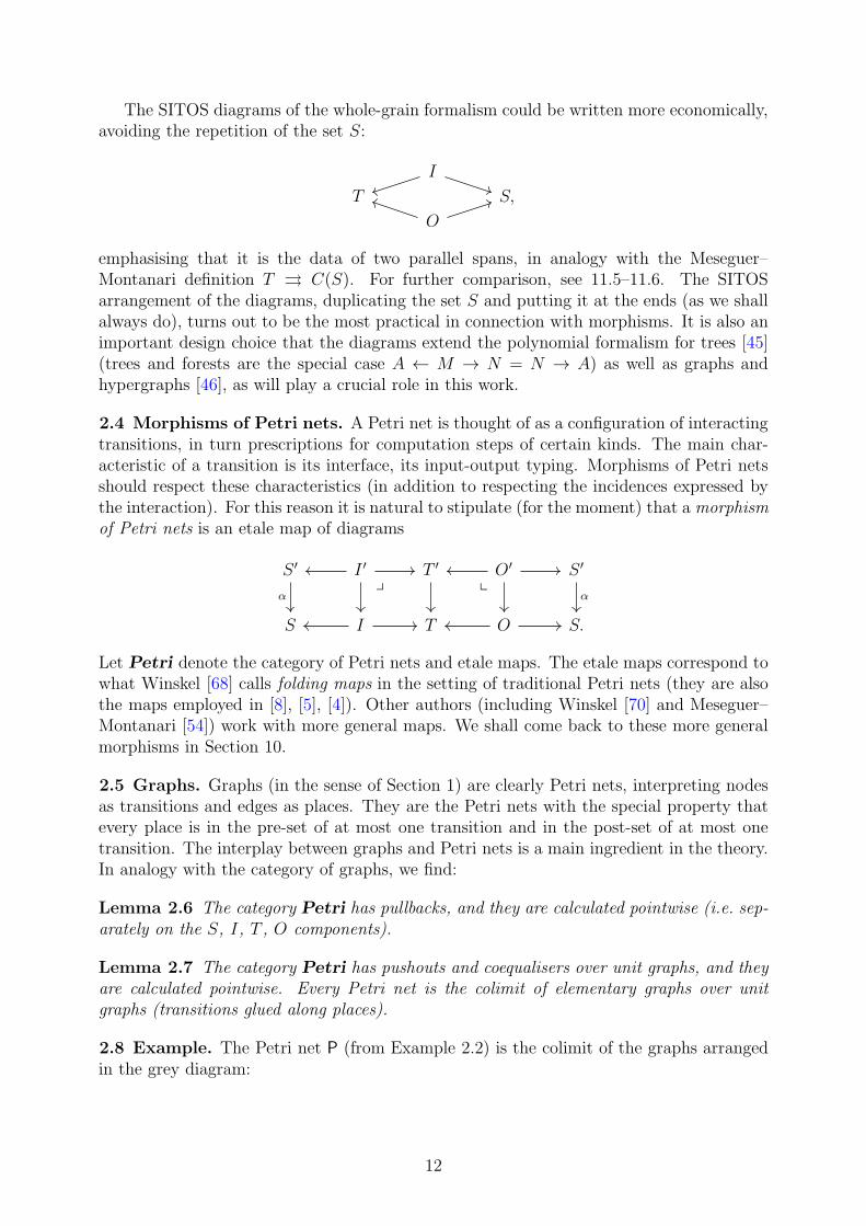
The SITOS diagrams of the whole-grain formalism could be written more economically,avoiding the repetition of the set S:

I

T S,

O

emphasising that it is the data of two parallel spans, in analogy with the Meseguer–Montanari definition T ⇒ C(S). For further comparison, see 11.5–11.6. The SITOSarrangement of the diagrams, duplicating the set S and putting it at the ends (as we shallalways do), turns out to be the most practical in connection with morphisms. It is also animportant design choice that the diagrams extend the polynomial formalism for trees [45](trees and forests are the special case A ← M → N = N → A) as well as graphs andhypergraphs [46], as will play a crucial role in this work.

2.4 Morphisms of Petri nets. A Petri net is thought of as a configuration of interactingtransitions, in turn prescriptions for computation steps of certain kinds. The main char-acteristic of a transition is its interface, its input-output typing. Morphisms of Petri netsshould respect these characteristics (in addition to respecting the incidences expressed bythe interaction). For this reason it is natural to stipulate (for the moment) that a morphismof Petri nets is an etale map of diagrams

S ′ I ′ T ′ O′ S ′

S I T O S.

αy x

α

Let Petri denote the category of Petri nets and etale maps. The etale maps correspond towhat Winskel [68] calls folding maps in the setting of traditional Petri nets (they are alsothe maps employed in [8], [5], [4]). Other authors (including Winskel [70] and Meseguer–Montanari [54]) work with more general maps. We shall come back to these more generalmorphisms in Section 10.

2.5 Graphs. Graphs (in the sense of Section 1) are clearly Petri nets, interpreting nodesas transitions and edges as places. They are the Petri nets with the special property thatevery place is in the pre-set of at most one transition and in the post-set of at most onetransition. The interplay between graphs and Petri nets is a main ingredient in the theory.In analogy with the category of graphs, we find:

Lemma 2.6 The category Petri has pullbacks, and they are calculated pointwise (i.e. sep-arately on the S, I, T , O components).

Lemma 2.7 The category Petri has pushouts and coequalisers over unit graphs, and theyare calculated pointwise. Every Petri net is the colimit of elementary graphs over unitgraphs (transitions glued along places).

2.8 Example. The Petri net P (from Example 2.2) is the colimit of the graphs arrangedin the grey diagram:

12

a corolla for each transition:

a unit graph for each place:

shape of colimit diagram

according to arcs:i2 o1 i1

o3

o4

o2

i3i4

s2s1 s3

t1

i1

i2 o1

o2

t2i3

i4

o3

o4

t1

s1

s2

s3

t2

i1

o1i2

o2

i4

i3o3

o4

P

2.9 Marking (or state). A marking (also called a state7) of a Petri net P = SITOS is amap of finite sets M → S, regarded as an etale map from M∅∅∅M to P. The elements ofM are called tokens. Throughout, we shall use the letter M for a set of tokens, and tacitlywrite M = M∅∅∅M for the corresponding nodeless graph.

The markings of P naturally form a category FinSet↓P ≃ FinSet↓S, but we shall bemore interested in the corresponding groupoid B↓P ≃ B↓S (where B denotes the groupoidof finite sets and bijections), defined by the lax pullback

B↓P 1

B Petri.

pPq⇒

M 7→M∅∅∅M

The objects are thus the markings, and an isomorphism between two markings is a bijec-tion of sets M ∼→M ′ compatible with the maps to P. Two markings are isomorphic in thisgroupoid if and only if they have the same number of tokens for each place. So the iso-morphism classes of markings are precisely the classical multisets on S. More categoricallyspeaking, the groupoid B↓S is the free symmetric monoidal category on S, and its set ofisomorphism classes is π0(B↓S) = C(S), the set of multisets on S. In traditional Petri nettheory, that is the definition of marking.

2.10 Example. To specify a marking (of the Petri net from 2.2) such as

{m1,m2,m3,m′3} ∅ ∅ ∅ {m1,m2,m3,m

′3}

{s1, s2, s3} {i1, i2, i3, i4} {t1, t2} {o1, o2, o3, o4} {s1, s2, s3}

m1 7→s1,m3 7→s3m2 7→s2,m

′3 7→s3

y x

it is necessary to say where each token land, as indicated here on the left-most verticalarrow (recall that the right-most vertical arrow is the same map). Since any finite set Mcan appear in a marking, there is generally no way to avoid specifying the map M → S

7The tendency is to use the word ‘marking’ as long as the Petri net is considered just a combinatorialor pictorial gadget, whereas ‘state’ is used when the operational interpretation is in focus.

13

element by element. However, we may always choose to work with an isomorphic marking,‘renaming’ the tokens for convenience. (In this example the token ‘names’ were chosen sothat the map can be read off the subscripts.) In the drawing

t1

s1

s2

s3

t2

i1

o1i2

o2

i4

i3o3

o4

m1

m2

m3 m′

3

the left-hand picture contains the exact same information as the diagram. The right-handpicture contains only the information of the isomorphism class of the marked Petri net:this contains all the information about the maps in the diagram, except the choices of‘names’ of elements. In practice it may often be the case that the abstract picture (theisomorphism class) exists first, for example as a result of human thought. The act ofchoosing an explicit representative of the iso-class to work with is effectively to choose thenames for the elements in the picture, and use those elements as constituents of the setsS, I, T, O and M . It is thus important that some choice of representing sets is made, sothat there are explicit sets to work with, but it is not important which choice is made.

2.11 Individual vs. collective tokens. (See [30], [31], [18], [29], [17] for more thoroughdiscussion.) Classical Petri-net theory favours the collective-tokens philosophy, accordingto which a state is just a multiplicity function S → N, that is, a multiset on S. In thepresent formalism the tokens of a state form an explicit set, and in particular, each tokenis an individual element in a set (as in the individual-tokens philosophy). However, sincethe states form a groupoid, both the viewpoints are encoded simultaneously: from thegroupoid one can pass to the individual tokens by considering the underlying set of thegroupoid, and one can pass to the indistinguishable-tokens viewpoint by passing to the setof isomorphism classes of the groupoid. At this point the difference is not so big. The realdifference arises when it comes to tracing tokens around in processes, as we shall see.

2.12 Initial state. In many applications, Petri nets have an initial state, and it is commonto include this in the very definition of Petri net. We do not do so here. When required,initial states are given as diagrams M → P, and morphisms are then required to respectthis. The relevant categories are then coslice categories. We shall come back to this inSection 9 in connection with unfolding.

3 Processes

3.1 Simple firing. A firing of a transition t ∈ T in a Petri net P = SITOS in a givenstate M→ P intuitively consumes a token from each of the places ingoing to t and producesa token in each of the outgoing places. More precisely it consumes a token for each elementin the pre-set It (the restriction S ← It tells where the tokens are taken from) and producesa token for each element in the post-set Ot (the restriction Ot → S then tells where thenew tokens are put).

14

The minimal state in which the firing of t ∈ T can occur is

It ∅ ∅ ∅ It

S I T O S,

y x

and the state after the transition has fired will then be

Ot ∅ ∅ ∅ Ot

S I T O S.

y x

The whole firing (in the minimal state enabling it) is encoded geometrically by a singleetale map C→ P from a corolla, namely

It +Ot It {t} Ot It +Ot

S I T O S.

y x

(Note that any other isomorphic sets could take the place of It, Ot to constitute a corolla.)When reading such a C → P as a firing, the initial state is that given by the in-boundaryof C and the final state is that given by the out-boundary of C (cf. 1.7 and 1.11). (In thedisplayed case, these are It and Ot.)

A firing of the transition t ∈ T in a general state is encoded by just adding more tokens.From the viewpoint of the corolla C, this is to add a bunch of isolated edges, so that thegeneral firing of t ∈ T has the form

It +Ot +M It {t} Ot It +Ot +M

S I T O S

y x

for some set M . The domain is then no longer a corolla, but it is still a graph. Theinterpretation of initial and final state in terms of in-boundary and out-boundary of thegraph is still valid, since the isolated edges, corresponding to the tokens not changed bythe firing, belong to both the in- and the out-boundary (cf. 1.7).

3.2 Example. Here is a minimal firing p : C → P of the transition t1 in the Petri net P

from Example 2.2:

{a1, a2, b2, b3} {a1, a2} {x1} {b2, b3} {a1, a2, b2, b3}

{s1, s2, s3} {i1, i2, i3, i4} {t1, t2} {o1, o2, o3, o4} {s1, s2, s3}

p :

a1 7→s1

a2 7→s2

b2 7→s2

b3 7→s3

a1 7→i1

a2 7→i2

y

x1 7→t1b2 7→o1

b3 7→o2

x

The top row is the corolla C; the bottom row is the Petri net P. The vertical maps,constituting the etale map p, are specified (in blue) simply by telling where each individualelement goes. In the picture

15

−→p

x1

a2 a1

b2 b3

t1

s1

s2

s3

t2

i1

o1i2

o2

i4

i3o3

o4

this information is conveyed by the ‘postage stamp’.

3.3 Executions — preliminary discussion. An execution of a Petri net P = SITOSin a state M → P is supposed to be just a bunch of firings taking place in sequence orconcurrently. The fully parallel situation is given by an etale map p : G → P, where G

is a disjoint union of elementary graphs: the corollas in G then express the simultaneousfiring, and the isolated edges are just dead weight contributing to the state. Again theinitial state is the (restriction of p to the) in-boundary of the graph G, and the final stateis the (restriction of p to the) out-boundary of G. Causal relationships between firings areexpressed with more general graphs:

3.4 Processes = P-graphs. A process of a Petri net P = SITOS is an etale mapp : G→ P where G is an acyclic graph. This is also called a P-graph.

We have previously used AINOA notation for graphs. From now on the symbols I andO are reserved for the incidence sets of Petri nets, so for graphs we now use the notationAN and NA for the subsets of A consisting of the edges that are incoming to some nodeand outgoing of some node, respectively. A process for P is thus a diagram

A AN N NA A

S I T O S,

y x

where the top row is an acyclic graph.From the viewpoint of graphs, a process of P is an acyclic graph G where each edge is

decorated by a place of P and each node is decorated with a transition of P of matchinginterface. Furthermore, the elements expressing the incidence relations of the graph G mustbe mapped to arcs of P. We stress that the maps AN → I and NA→ O must be specifiedtoo — they are not implied from the maps N → T and A → S. All these assignmentsshould be compatible, as expressed by the commutativity of the diagram. The initial stateof the process is the (restriction of the etale map to the) in-boundary of G and the finalstate is the (restriction to the) out-boundary of G.

3.5 The category of processes. Define the category of processes of P to be the commacategory

Proc(P) := Gr ↓P.

The morphisms are thus commutative triangles (of etale maps)

G G′

P.

p p′

16

The most important maps in Proc(P) are the invertible maps: on one hand they allowus to use the sets we like as constituents of the graphs, and allow us to replace these setsby isomorphic ones, effectively ‘renaming’ elements to our liking. The invertible maps keeptrack of these ‘renamings’, and ensure the ability to distinguish elements in these sets.There may also be invertible maps from one graph to itself — its symmetries.

The category Proc(P) also has non-invertible maps, such as in particular sub-graphinclusions. From the viewpoint of processes as computations, these represent shorter (orpartial) computations. In particular it is important that the inclusion of the in- or out-boundary of a process is a map in Proc(P) (representing the trivial computation, just astate): our goal will be to define serial composition of processes, which will be achieved(in Section 4) in terms of gluings along graph boundaries, in turn described as pushoutsas in 1.9. For these pushouts (and other colimits) to make sense, it is essential to havenon-invertible maps in Proc(P).

Proposition 3.6 The assignment P 7→ Proc(P) is functorial in etale maps of Petrinets: an etale map of nets f : P′ → P induces canonically a functor f! : Proc(P′) →Proc(P) simply by post-composition of etale maps. Altogether, this defines a functorProc : Petri→ Cat.

3.7 Comparison with traditional notions of processes. Modulo the differences inthe definitions of Petri net and graphs, the above definition of process is precisely thatof Goltz and Reisig [32]. The idea of modelling processes of a Petri net with maps fromgraphs or certain posets goes back to Petri himself [61] (1977).

Despite this close similarity, the passage from traditional Petri nets to whole-grain Petrinets implies some essential differences for processes, as illustrated in the examples, and aswill be important for the main theorems. To indicate the point briefly, consider a transitiont: in a traditional Petri net, pre(t) and post(t) are mere numbers, and the ‘etale’ conditionon a map from a graph says that it can receive only nodes x with that many incomingand outgoing edges, but there is no way to control those incoming and outgoing edges, andin particular there are situations where they can be permuted. In the SITOS formalism,pre(t) and post(t) are actual sets, and being an etale map involves explicit bijections withthese sets, in(x) ∼→ pre(t) and out(x) ∼→ post(t), giving a good handle on symmetries.

3.8 Scheduling. A scheduling of a process p : G → P, also called a run, is just a strictlevel function on G (cf. 1.12). The scheduling is sequential if the level function is bijective,and the scheduling is then called a firing sequence. A strict level function f : G → kprescribes a colimit decomposition of the graph as a sequence of pushouts over nodelessgraphs as in 1.13,

G ≃ G1 ⊔M1 · · · ⊔Mk−1Gk, (2)

where each layer Gi is a disjoint union of elementary graphs, and where the Mi are nodelessgraphs. Therefore, each Mi → P is a state and each Gi is a simultaneous firing Gi → P withinitial state Mi−1 and final state Mi (here we include M0 defined as the in-boundary of G1

(which is also the in-boundary of G) and Mk defined as the out-boundary of Gk (which isalso the out-boundary of G)). If the strict level function is bijective, each firing Gi → P isa simple firing (in the sense of 3.1).

3.9 Example. The main purpose of this example is to show how closely tokens are kepttrack of in a process. The following diagram is a process p : G→ P:

17

{

a1, a2, a3, b1, b2,

b3, c1, c2, c3, d3

} {

a1, a2, a3,

b1, b2, b3

}

{x1, x2, y1}

{

b1, b2, b3c1, c2, c3

} {

a1, a2, a3, b1, b2,

b3, c1, c2, c3, d3

}

{s1, s2, s3} {i1, i2, i3, i4} {t1, t2} {o1, o2, o3, o4} {s1, s2, s3}

p :a1 7→i1,b1 7→i1

a2 7→i2,b2 7→i2

a3 7→i4,b3 7→i3

y x1 7→t1

x2 7→t2

y1 7→t1

b1 7→o3,c1 7→o4

b2 7→o1,c2 7→o1

b3 7→o2,c3 7→o2

x

d3 7→s3

The bottom row is the Petri net P from Example 2.2. In the top row (the graph G), theconstituent arrows have not been indicated, but they can be read off the following picture,where the graph G is on the left. To specify the etale map (the vertical arrows), it isnecessary to tell where each individual element goes, as done with the blue annotations.For the outermost map A → S, the assignments a1 7→s1, a2 7→s2, a3 7→s3, b1 7→s1, b2 7→s2,b3 7→s3, c1 7→s1, c2 7→s2, c3 7→s3 have been suppressed from the diagram to avoid clutter,since they can be inferred from the maps at the I and O levels. (Only the element d3 isnot accounted for like this, since it is an isolated edge.) The reason for bothering with this‘economy’ of annotation is that it is natural from the graphical viewpoint, where it is clearthat the mapping information of p is fully specified by telling where the local interfaces ofeach node are sent (and then annotating the isolated edge separately):

−→p

x1

x2

y1

a1a2 a3

c1c2 c3

d3

d3

b3

b1

b2

i2

o1

i1

o2

i2

o1

i1

o2

i3

o3

i4

o4s3 t1

s1

s2

s3

t2

i1

o1i2

o2

i4

i3o3

o4

A choice of level function has been indicated with the red dashed lines.Note that the maps at the I and O levels contain very precise information about token

flow: we see for example that when t2 fires in the process p, its i3 input slot consumes thetoken that was previously produced by the t1-firing (namely b3) whereas the i4 input slotof t2 consumes the token a3 that was already there from the start. If the etale map weremodified to have a3 7→ i3 instead of a3 7→ i4, and b3 7→ i4 instead of b3 7→ i3 (correspondingto interchanging the two decorations i3 and i4 in the picture), then a different (and non-isomorphic) process would result, with a different flow of tokens.

A more fundamentally different P-process q (with a level function) is pictured here:

q :

i2

o1

i1

o2

t1

i2

o2

i1

o1

t1

i3

o3

i4

o4

t2

18

The decorations specify precisely how the graph maps to P, but the graph itself has onlybeen specified up to isomorphism: it remains to choose representative sets (‘names ofelements’) for the graph. Since we are generally only interested in structural propertiesof Petri nets and processes, it is quite reasonable to indicate only the isomorphism class,leaving the implementation details such as ‘element names’ to the reader. We shall freelydo this throughout the paper.

In process p, there is one token d3 that does not participate other than staying put in s3all the time. In q, all tokens participate actively. This process q also has the property thatit could have been scheduled differently: by choosing a different level function one couldfire t2 before firing t1. This shows that p and q do not have the same causal structure. Infact, it is clear that p and q are not isomorphic: they are not even isomorphic as underlyinggraphs. However, with the level functions indicated in the pictures with dashed red lines,the two processes both correspond the following sequence of isomorphism classes of firings:

t1

t2

t1

t2

t1

t2

t1

t2

t1 t2 t1

This shows that the processes cannot be reconstructed, even up to isomorphism, fromknowledge of the isomorphism classes of the steps in the firing sequence: the isomorphismclasses do not retain enough information about the tokens to be able to compose by gluing.8

4 The symmetric monoidal Segal space of processes

From this point on (and up to and including Section 7), a little bit of elementary homotopytheory of groupoids is involved. This is necessary since we are interested in objects up toisomorphism, but still want to keep track of their symmetries. A few definitions and basicfacts are recollected in Appendix 11. The goal is to assemble processes (for a fixed Petrinet P) into a kind of category. This will require some simplicial structures, explained alongthe way; some background is given in Appendix 11.

4.1 Towards composition of processes. Fix a Petri net P. Let X0 denote the groupoidof states of P. Let X1 = Proc iso(P) denote the groupoid of processes of P. Every stateis also a process, so we have a canonical map s0 : X0 → X1. Every process has an initialstate and a final state, so we also have maps

X0 X1.d0

d1

Here d0 returns the final state and d1 returns the initial state, not the other way around.Although this convention may look a bit counter-intuitive, the indexing is dictated by thestandard simplicial formalism we shall exploit, where an index always indicates the vertexthat was deleted, as explained in B.3. We think of a process p as an arrow in a category,from its initial state d1(p) to its final state d0(p).

8The fact that different graphs/posets can correspond to the same firing sequence was stressed in theBest–Fernandez book [14]. Drastic quotients are required to make the viewpoints match up [13], as weshall briefly comment on in 7.3.

19

Since states form a groupoid, whose morphisms express renaming of tokens, we maybe more interested in composing processes that only match up to a specified isomorphism:given two processes p1 : G1 → P and p2 : G2 → P (that is, p1 ∈ X1 and p2 ∈ X1), weconsider the situation where the final state of p1 is isomorphic to the initial state of p2,with a specified isomorphism σ : d0(p1)

∼→ d1(p2). This means precisely that the triple(p1, p2, σ) is an element in the standard homotopy pullback of groupoids (see A.2)

X1 ×hX0

X1 X1

X1 X0.

y≃proj1

proj2

d1

d0

(3)

We wish to define a weak composition law

X1 ×hX0

X1comp.−→ X1,

allowing to compose processes via connecting isomorphisms of states.9 To formalise thisidea, we first fit X0 and X1 into the structure of a simplicial groupoid X• : ∆op → Grpd;then we show that this simplicial groupoid is a Segal space, which is the standard way toencode weak categories (see Appendix 11 for a bit of background and motivation).

4.2 The simplicial groupoid of processes. Fix a Petri net P. For each k ≥ 0, denote byXk the groupoid of P-graphs p : G→ P equipped with a level function G→ k, i.e. processesG → P equipped with k − 1 compatible cuts, as in 1.13. The morphisms in this groupoidare isomorphisms of graphs compatible with both the etale map to P and the level functionto k. In particular, X1 is just the groupoid of processes (since every P-graph has a unique1-level function), and X0 is the groupoid of states (because a 0-level function can exist onlyfor P-graphs with no nodes). Next, X2 is the groupoid whose objects are processes G→ P

equipped with a cut (as in 1.13).The groupoids Xk assemble into a strict simplicial groupoid (see B.2 and B.5)

X• : ∆op −→ Grpd

[k] 7−→ Xk.

For this we need to describe the face and degeneracy maps (cf. B.1).The degeneracy maps si : Xk → Xk+1 (for 0 ≤ i ≤ k) insert an empty layer. Formally

this can be described as composing level functions G → k with injective monotone mapsk → k+1. We shall not go into details with the degeneracy maps. Although they arerequired to define a simplicial object, they do not play any role for the Segal condition.

The inner face maps Xk−1di←− Xk (0 < i < k) join adjacent layers, or equivalently,

delete cuts. Formally this is to postcompose level functions G→ k with surjective monotonemaps k → k−1.

So far, only the level functions are affected, whereas the underlying P-graph is not

changed. Finally, the outer face maps Xk−1

dk

⇔d0

Xk project away the first or the last layer;

this obviously changes the underlying P-graph.Having defined the face and degeneracy maps, we should now verify the simplicial

identities as listed in B.1. The way the face and degeneracy maps have been defined, this

9See Sassone [63] for a version of this viewpoint.

20

is straightforward. For example, the face-map identities state that if two cuts are deleted,it does not matter in which order, or that throwing away the first two layers is the sameas first joining them and then throwing away the joined layer in one go. The followingexample illustrates that throwing away the first layer and then the last is the same asthrowing away the last and then the first.

4.3 Example. The following is a picture of a 2-layered process p ∈ X2 (of the Petri netin Examples 2.2 and 3.9) and the effect of the three face maps.

p

x2

y1

x1

x1

x2

y1

x1

x2

y1

d1

d0

d2

d1

d0

d0 applied to p erases the first layer; d1 joins the two layers; d2 erases the last layer. Thefurther face maps applied gives the commutative square on the left, which illustrates thesimplicial identity d0d2 = d1d0.

4.4 Remark. Constructions of simplicial groupoids like this are not uncommon in com-binatorics. In fact, this particular simplicial groupoid X• is almost the same as that ofthe directed restriction species of directed graphs explained in Example 7.13 of [23], wheresubstantial details of the construction can be found, although in a much more general set-ting. The difference (apart from the P-decorations) concerns isolated edges, excluded inthe setting of restriction species, but clearly essential to keep for the present purposes.

4.5 Segal spaces. For a simplicial groupoid to work as a (weak) category, it should be aSegal space (see B.6). First of all this means that the canonical map

(d2, d0) : X2 −→ X1 ×hX0

X1

should be an equivalence of groupoids. More generally it is required that for all k ≥ 1 thecanonical map that returns the k layers

Xk −→ X1 ×hX0· · · ×h

X0X1 (4)

is an equivalence of groupoids.To establish this, we first establish the following important fibrancy condition (see A.3),

which allows to use ordinary strict pullbacks instead of homotopy pullbacks.

Lemma 4.6 The face map d0 : X1 → X0 (which given a process returns its final state) isa fibration of groupoids (cf. A.3).10

10By the same argument, also d1 : X1 → X0 (initial state) is a fibration, but we shall not need that.

21

Proof. Given a process p : G → P with final state d0(p) = z : M → P (meaning thatM = out(G)), and given an isomorphism with another state z′ : M ′ → S, amounting to acommutative diagram

M M ′

S,

z

u∼

z′

the statement is that there exists a lift of u to p, namely an isomorphism of processes u :p ∼→ p′ (for some other process p′), whose restriction to the out-boundaries reproduces thebijection u. To construct this, suppose the graph G is given by A← AN → N ← NA→ A,with out-boundary out(G) = M . By the definition of out-boundary (1.7), the set of edgesthus splits into two disjoint subsets

A = M + AN .

Now define the new graph G′ and the morphism u by modifying as little as possible — onlythe out-boundary:

G : M + AN AN N NA M + AN

G′ : M ′ + AN AN N NA M ′ + AN

P : S I N O S.

u u+idy x

u+id

p′ z′+p|AN

y xz′+p|AN

The new graph G′ is naturally a P-graph as indicated, and by construction the new map uis a morphism of P-graphs. �

The benefit of the fibrancy condition is the general fact that homotopy pullbacks alongfibrations can be computed as strict pullbacks (see A.2–A.3).

Proposition 4.7 The simplicial groupoid X• is a Rezk-complete Segal space.

Proof. The Segal condition states that the map Xk −→ X1 ×hX0· · · ×h

X0X1 in (4) is an

equivalence of groupoids. For notational convenience we do the case k = 2 only.11 Sincethis homotopy pullback (which is (3)) is along the fibration d0, we can prove instead that

X2g−→ X1 ×

strictX0

X1

is an equivalence of groupoids. An element in this strict pullback is a pair (p1, p2) ofprocesses such that the final state d0(p1) of the first is literally equal to the initial stated1(p2) of the second.

The map g is bijective at the level of π0, because the pushout construction of 1.9provides an up-to-isomorphism inverse: given processes p1 : G1 → P and p2 : G2 → P without(G1) = M = in(G2), the pushout produces a single P-graph G1 ⊔M G2 with the obvious2-level function; it is clear that this construction is inverse to g up to isomorphism. To

11For higher k, one can use induction, reformulating the Segal condition as Xk ≃ Xk−1 ×h

X0X1.

22

establish that g is an equivalence it remains to check that it is also an isomorphism onautomorphism groups (cf. A.1). The automorphisms of a 2-levelled P-graph

G 2

P

p

f

are the automorphisms of G compatible with both p and f . This amounts to giving anautomorphism of each layer G1 and G2, whose restrictions to the cut M agree. But this isprecisely the description of the automorphism group of the corresponding object (G1,G2)in X1 ×

strictX0

X1.Finally, Rezk completeness (B.6) is the statement that the only invertible processes in

X1 are the degenerate ones, i.e. in the image of s0 : X0 → X1. A 1-simplex p in a Segal spaceis called invertible if composition with it from either side defines an equivalence X1 → X1.In the present case p is a P-graph, and composition is gluing. But composition with agraph having a node will increase the number of nodes, so the only invertible processes arethe node-less graphs. These are precisely those in the image of s0, as required. �

Lemma 4.8 X• is a symmetric monoidal Segal space under disjoint union +. That is,the simplicial maps

1• X• X• ×X•p∅q +

satisfy the standard associative, unital, and symmetry axioms.

Here 1• is the constant simplicial groupoid on the terminal groupoid, and the map indegree k picks out the empty k-levelled P-graph. The required coherence constraints, givenseparately in each simplicial degree, follow from the universal properties of ∅ and + asinitial object and categorical sum.

4.9 Remark. The symmetric monoidal Segal space X• is very easy to set up, sinceit is defined in terms of decomposition instead of composition. This phenomenon, thatdecomposition is easier to achieve than composition, is quite general, and is one startingpoint of the recent theory of decomposition spaces [21], [22], [23], [24]. For the symmetricmonoidal structure it must be appreciated that X• is Rezk complete. This implies thatfunctor categories can be dealt with pointwise, i.e. in each simplicial degree separately. Thesymmetric monoidal structure in each simplicial degree is obvious.

Proposition 4.10 An etale map of Petri nets e : P → P′ induces a symmetric monoidalfunctor of Segal spaces

e! : X• → X•′

by sending a layered process G→ P to the composite G→ P→ P′ with the same layering.

Indeed, the map in simplicial degree 1 is a special case of Proposition 3.6. The remainingsimplicial degrees are a matter of level functions, and refer only to the underlying graphG; they are not affected by P- or P′-structure.

23

5 Digraphical species from Petri nets

Recall that a digraphical species is a presheaf F : elGrop → Set on the category ofelementary graphs, and that we call F[⋆] the set of colours. The set F[ n

m ] is called the setof (m,n)-ary operations.12

5.1 Digraphical species of a Petri net. A Petri net P defines a digraphical species

P : elGrop −→ Set

E 7−→ Hom(E,P),

which is simply the restricted Yoneda embedding along the full inclusions elGr ⊂ Gr ⊂Petri. The set of colours of P is thus the set of places S, and the operations are thetransitions T , symmetrised: indeed to give an etale map from a corolla to P is first of allto say where the unique node of the corolla goes, say 7→ t ∈ T . If the transition t has mincoming arcs and n outgoing arcs, then the domain of the map has to be the [ n

m ]-corolla,by etaleness. There are now are m!n! different etale maps [ n

m ]→ P hitting t. All of thesemaps are valid, as there are no constraints on places. For each map, the corolla will acquirecolours on edges according to the places they are mapped to.

From the decomposition of Petri nets into colimits of elementary graphs (Lemma 2.7),we get:13

Lemma 5.2 (Density lemma.) The functor

Petri −→ PrSh(elGr)

P 7−→ Hom(−,P)

is fully faithful.

The following result provides a characterisation of Petri nets by describing the imageof this embedding.

Proposition 5.3 A digraphical species F : elGrop → Set is a Petri net if and only if it isflat (meaning that the symmetric-group actions (Sm ×Sn) × F[ n

m ] → F[ nm ] are free) and

it takes finite values and has finite support (meaning that there is an upper bound on them and n for which F[ n

m ] is non-empty).

5.4 Remark. This result is a variation of Theorem 2.4.10 of [45], which characterisespolynomial endofunctors among the presheaves on elementary trees. The terminology flatis from the theory of combinatorial species [10]. In the theory of operads, the same conditionis called sigma-cofibrant. Note finally that the flat digraphical species are also essentiallythe same thing as the tensor schemes of Joyal and Street [43].

Proof. Starting with a Petri net P = SITOS, the associated graphical species is Hom(−,P):

elGrop −→ Set

[⋆] 7−→ Hom([⋆],P) = S

[ nm ] 7−→ Hom([ n

m ],P).

12This terminology comes from the theory of operads.13by standard category theory [51, Ch. X, §6]

24

To specify an etale map [ nm ]→ P is to give a transition t ∈ T and bijections βin : m ∼→ pre(t)

and βout : n ∼→ post(t). The natural (Sm ×Sn)-action

(Sm ×Sn)× Hom([ nm ],P) −→ Hom([ n

m ],P)((σin, σout), (t, βin, βout)

)7−→ (t, βin ◦ σin, βout ◦ σout)

is clearly free. Since each transition t has finite pre(t) and post(t), and since there are onlyfinitely many transitions, we find that all the sets Hom([ n

m ],P) are finite, and empty forbig m and n.

Conversely, given a flat digraphical species F : elGrop → Set, we construct a Petri netP = SITOS by putting S := F[⋆] and defining T to be the disjoint union

T :=∑

m,n

F[ nm ]/(Sm ×Sn).

This is a finite set by the finiteness assumptions on F. It remains to define the setsI and O, so as to have correct fibres over T and appropriate ‘colours’. If t ∈ T is inthe (m,n)-summand, then the I-fibre should have m elements and the O-fibre shouldhave n elements. Essentially I and O should be defined as disjoint unions over all suchdata, and the projections to S should return the corresponding colour according to theF-structure. To describe this in a natural way, we first fix m and n and note that F[ n

m ] canbe interpreted as the set {[ n

m ]→ F} via the Yoneda lemma. Consider now the two fancier

sets: {[⋆]in→ [ n

m ]→ F} where the first map is any of the m maps of elementary graphs that

pick out an input edge, and {[⋆]out→ [ n

m ]→ F} where the first map is any of the n maps ofelementary graphs that pick out an output edge. With the natural projections

{[⋆]in→ [ n

m ]→ F} {[⋆]out→ [ n

m ]→ F}

S = {[⋆]→ F} {[ nm ]→ F} {[⋆]→ F} = S

we get the basic building blocks for the final SITOS diagram. It remains to divide out bythe group actions, and sum up all m and n. We already have the free (Sm ×Sn)-actionon the set {[ n

m ]→ F}. For the fancier sets, each group element (σin, σout) ∈ Sm×Sn actsby permuting the [ n

m ] in the middle, sending the upper composite in the diagram

[ nm ]

[⋆] F

[ nm ]

(σin,σout)

to the lower composite. The new map [⋆] [ nm ] is defined as the old map followed by

(σin, σout)−1, which means that the composite [⋆] → F is not changed by the action: it is

still the same colour of F picked out. This means that when we pass to the quotient, themaps to S are still well defined.

Taking now quotients and summing over m,n, the final SITOS-diagram is altogether

25

defined as

∑m,n

{[⋆]in→[ nm ]→F}

Sm×Sn

∑m,n

{[⋆]out→ [ nm ]→F}

Sm×Sn

S = {[⋆]→ F}∑

m,n

{[ nm ]→F}

Sm×Sn{[⋆]→ F} = S

We omit the straightforward verification that the two constructions are inverse to eachother, up to natural isomorphism. �

Lemma 5.5 For P a Petri net, P-graphs have no infinitesimal automorphisms, in the sensethat if an automorphism fixes a node, then it is the identity on that connected component.

Proof. Let f : G ∼→ G be an automorphism of P-graphs that fixes a node x. Since fpreserves the incidences, it must map the set in(x) of incoming edges of x to itself andthe set out(x) of outgoing edges of x to itself. The P-structure is an etale map G → P,mapping x to some transition t, and the etale condition gives bijections in(x) ≃ pre(t)and out(x) ≃ post(t). Since f must commute with these bijections, it is forced to be theidentity on in(x) and out(x). Therefore it must also fix any incident nodes, and so on,forcing altogether the whole connected component to be fixed. �

5.6 Remark. Even when all nodes of a P-graph are fixed, it is still possible to permuteisolated edges that map to the same place in P. This is relevant since isolated edges in aprocess correspond to unaffected tokens (as noted in 3.3), meaning tokens that belong toboth the initial and the final marking.

5.7 Example. There are two possible etale maps

x

−→

t

corresponding to the two possible bijections in(x) ∼→ pre(t). But these two processes areisomorphic by the graph isomorphism that interchanges the two edges. More generally,there are of course infinitely many graphs corresponding to the figure, depending on which2-element set is chosen as set of edges, and so on, and therefore also infinitely many distinctprocesses of this shape. For any two such graphs AINOA and A′I ′N ′O′A′, there are twopossible isomorphisms between them (since there are always two distinct bijections A ≃ A′

between 2-element sets). However, as processes there is precisely one possible bijection,because the process involves a bijection in(x) ∼→ pre(t), and only one bijection A ∼→ A′ canbe compatible with those. In conclusion, any two processes of the shape of the figure areuniquely isomorphic. This illustrates Lemma 5.5.

Here we see a crucial difference with traditional Petri net theory, where instead ofparallel arcs there would be merely a multiplicity:

t

2

26

The domain graph of a process looks the same in traditional Petri net theory, but insteadof the etale condition involving explicit bijections, we now have the condition that thenumber 2 of incoming edges to the node must match the multiplicity 2 in the Petri net.Again it is the case that all possible processes of this shape are isomorphic, but they areno longer uniquely isomorphic: even a fixed process admits a nontrivial automorphism,by interchanging the two edges of the graph. The multiplicity decoration cannot preventthis automorphism. This difference in the behaviour of symmetries is a key feature ofwhole-grain Petri nets compared to traditional Petri nets.

6 Free props

The following description of the free-prop monad is essentially from [46], except that thereonly the free-properad monad is described, considering only connected graphs.

6.1 Residue and [ nm ]-graphs. For an (acyclic) graph G (either an F-graph or naked

(i.e. with no F-structure)), the residue res(G) is the naked corolla formed by the in-boundaryand the out-boundary (and a single node). For example,

res( ) =

This defines a functor res : Gr iso → Cor (and for each F a functor res : Gr iso↓F → Cor).An [ n

m ]-graph is an acyclic graph G equipped with an isomorphism res(G) ≃ [ nm ]. It

amounts to a numbering of the elements in the in-boundary and a separate numberingfor the out-boundary (since we have defined the specific corollas [ n

m ] in terms of naturalnumbers). More formally, the groupoid of [ n

m ]-graphs [ nm ]-Gr iso is the homotopy fibre

(see A.5) of res : Gr iso → Cor over [ nm ]. For F a digraphical species, an [ n

m ]-F-graph isan F-graph G equipped with an isomorphism res(G) ≃ [ n

m ]. These are the objects of thegroupoid [ n

m ]-Gr iso↓F, the homotopy fibre over [ nm ] of the functor res : Gr iso↓F → Cor.

6.2 Remark. Note that we allow non-connected graphs (in contrast to [46]). In particular,a nodeless F-graph U consisting of m isolated edges is a [ mm ]-graph in m!m! ways, dependingof the possible bijections in(U) ≃ m and out(U) ≃ m (which are independent). Thisexample also shows that res : Gr iso↓F → Cor is not a fibration: not all automorphismsof [ mm ] admit a lift to U.

6.3 The idea of props and free props. A category has objects and arrows (forming anunderlying graph), and then a prescription for composing arrows. The free category on agraph will have not only the edges as arrows, but will also promote the paths in the graphto be arrows. Composition in a free category is just concatenation of paths.

A (coloured) prop has colours and many-in/many-out operations (so as to have anunderlying digraphical species), and then a prescription for composing operations. Thefree prop on a digraphical species F will have not only the F-corollas as operations, butwill also promote all F-graphs to be operations. Composition in a free prop is just gluing ofgraphs. The following discussion, although it is a little bit technical, is just a formalisationof this idea.

27

6.4 Free-prop monad.14 We describe the free prop on a digraphical species. Recall(from 1.14) that presheaves on elGr are naturally equivalent to sheaves on Gr, so thata presheaf on elementary graphs can be evaluated also on general (acyclic) graphs by thelimit formula

F[G] ≃ limE∈el(G)

F[E].

The limit is over the elementary subgraphs of G as in 1.10.The free prop monad

PrSh(elGr) −→ PrSh(elGr)

F 7−→ F

is given (at the level of its underlying endofunctor) by F[⋆] := F[⋆] and

F[ nm ] := colim

G∈[ nm ]-Griso

F[G]

≃∑

G∈π0([nm ]-Gr iso)

F[G]

Aut[ nm ](G)

≃ π0([ nm ]-Gr iso↓F

).

Here the first equation follows since [ nm ]-Gr iso is just a groupoid: the sum is over iso-

morphism classes of [ nm ]-graphs, and Aut[ nm ](G) denotes the automorphism group of G in

[ nm ]-Gr iso. The (m,n)-operations of F are thus iso-classes of [ n

m ]-F-graphs.(We omit description of the monad multiplication and unit (essentially gluing of graphs),

although of course this is essential information. See [46] for all details in the connectedcase, the free properad monad.)

6.5 Free prop on a Petri net, and underlying symmetric monoidal category. Thefree prop on a Petri net P has as operations the iso-classes of processes G → P with fixedboundaries.15 An element in π0

([ nm ]-Gr iso↓P

)is a morphism in the underlying symmetric

monoidal category of the free prop. The objects are strings of elements in P[⋆], that ismaps n→ P[⋆]. The domain of an element p : G→ P in π0

([ nm ]-Gr iso↓P

)is the composite

m ≃ in(G)→ Gp→ P, and similarly the codomain is the composite n ≃ out(G)→ G

p→ P.

Composition is given by gluing (pushout in the category Gr). Formally this comesabout from the monad multiplication, whose description we omitted.16

6.6 Remark. It is easy to see that the digraphical species P is flat again, since the groupsSm×Sn act on P only through the boundary isomorphisms. So except for the fact that P

14It should be remarked that the algebras for the prop monad described here are not exactly the sameas the props of Mac Lane [51], and they should properly be called graphical props (see Batanin–Berger [9],Remark 10.5). The difference is with the (0, 0)-operations: in a Mac Lane prop, End(1) is always a commu-tative monoid (by the Eckmann–Hilton argument). In a graphical prop, End(1) can be a noncommutativemonoid. The difference does not affect us here, as we are only concerned with free graphical props, andthese automatically have commutative End(1) and are therefore also props in the sense of Mac Lane.

15The fact that morphisms are P-graphs equipped with specified maps from its domain and codomainonto its boundaries makes it an example of a cospan category with boundaries living in ‘lower dimension’than the apex. Cospans of this nature play also an important role in some recent approaches to open Petrinets; see for example [8], [5], [2].

16For an elegant proof of the adjunction between digraphical species and symmetric monoidal categories,see the very recent Baez–Genovese–Master–Shulman [4].

28

takes infinite values, it could be regarded as a Petri net again, and the free-prop adjunctioncould then be interpreted directly on the category of (infinite) Petri nets. This viewpoint,although it has played an important role in Petri-net theory (from [54] to [17]), is not givenemphasis in the present work, where we insist on Petri nets being finite. While P is ofinterest as a prop or symmetric monoidal category, the corresponding (infinite) Petri netseems to defy the purposes of Petri nets, and is hugely redundant. It has a transition forevery process of P — this includes an ‘identity’ transition for every place s ∈ S and everyn ∈ N, corresponding to the disjoint union of n s-labelled unit graphs.

6.7 Props in groupoids. The free prop formula just described involves taking π0. Avoid-ing this leads to a simpler construction, that of the free prop in groupoids. It works fordigraphical species valued in groupoids, F : elGrop → Grpd. In particular, an ordi-nary graphical species, such as a Petri net, is a groupoid-valued graphical species via theinclusion functor Set→ Grpd.

The free prop-in-groupoid on a digraphical species F : elGrop → Grpd is given byF[⋆] := F[⋆] and

F[ nm ] := [ n

m ]-Gr iso↓F,

without taking π0.Apart from [⋆] (where F 7→ F is the identity anyway), F is simply the groupoid-valued

presheaf corresponding to the projection res : Gr iso↓F → Cor. (It should be notedthough, that since res is not a fibration, it is essential to use homotopy fibres (see A.5)rather than strict fibres, in order to extract the value on a given [ n

m ].)

6.8 Underlying Segal space of F. The underlying (symmetric monoidal) Segal space

Y• of the free prop-in-groupoids F is given as follows: Y1 is the homotopy sum (A.6) of

all the F[ nm ]:

Y1 =

∫ [ nm ]

F[ nm ] ≃

∑

[ nm ]∈π0(Cor)

F[ nm ]//Aut([ n

m ]).

(This is the appropriate homotopical way of describing the groupoid whose homotopy fibre

over [ nm ] is F[ n

m ]. The double bar is homotopy quotient (see A.6). In degree zero we haveY0 = B↓F[⋆], the free symmetric monoidal category on F[⋆]. In higher simplicial degreeswe have Yk = Y1 ×

hY0· · · ×h

Y0Y1. The face and degeneracy maps come from the monad

structure: in particular Y1d1←− Y2 is the monad multiplication, which allows to contract a

2-level graph to a single corolla. (For details, see [46], although that reference only coversthe connected case, the case of properads.)

Theorem 6.9 For P a Petri net, the symmetric monoidal Segal space X• of P-processesis the free prop-in-groupoids on the digraphical species P.

Proof. We compare the mapping groupoids (B.7) of the two Segal spaces. Fix M and Ntwo states of P with m and n tokens, respectively. Both for X• and for the free prop, themapping groupoids consist of processes from M to N , and in a sense the check is routine;we include it to showcase the calculus of homotopy pullbacks (A.2): the two groupoids willbe identified by both satisfying the universal property of the same homotopy pullback.

29

The mapping groupoids appear in the following diagram of homotopy pullbacks:

MapX•

(M,N) P[ nm ] X1

1 (X0 ×X0)[ nm ] X0 ×X0

1 Cor.

y y(d1,d0)

p(M,N)q

p(M,N)q

y

p[ nm ]q

(5)

The curved homotopy-pullback rectangle is the definition of MapX•

(M,N) (cf. B.7): ho-motopy pullback along the curved middle map p(M,N)q. The right-hand composite

homotopy-pullback rectangle is the definition of P[ nm ], realised in two steps. Note that

Cor is the groupoid of naked corollas, without reference to P, whereas X0 × X0 is thegroupoid of pairs of P-states. Since M and N are assumed to have cardinality m and n,the middle curved arrow factors through (X0×X0)[ nm ], inducing first the lower dotted map

by the universal property of the homotopy pullback (X0 ×X0)[ nm ], and inducing next the

upper dotted arrow by the universal property of the homotopy pullback P[ nm ]. The closure

properties of homotopy pullbacks (A.4) force the resulting upper left-hand square to be

a homotopy pullback. This shows that MapX•

(M,N) is both the mapping groupoid in P

and in X•. (It also exhibits P[ nm ] as the homotopy sum (A.6) of its homotopy fibres (A.5)

over varying (M,N):

P[ nm ] ≃

∫ (M,N)∈(X0×X0)[ nm ]

MapX•

(M,N).)

The remaining checks (higher simplicial degrees) follow from the Segal condition. Thesymmetric monoidal structure is clear, as it is just disjoint union. �

7 The symmetric monoidal category of processes

7.1 Segal space vs. category. The symmetric monoidal Segal space X• is nice to workwith for its clean combinatorial description. The fact that there is a groupoid of processes,X1, instead of just a set of them, should be seen as an advantage rather than a drawback.The general point is that since whole-grain Petri nets are configurations of finite sets, it isnatural to admit that these configurations form groupoids, and continue to work with thesegroupoids rather than with their set quotients. Passing to sets of iso-classes too early caneasily lead to unnecessary complications or even serious problems. Concretely, working inthe groupoid of processes, we can glue processes thanks to explicit bijections between theirboundaries (states), but it is plainly not possible to glue isomorphism classes of processesalong isomorphism classes of states.

Notwithstanding the previous paragraph, it is sometimes convenient to extract from X•a honest symmetric monoidal category (C,+, ∅), which is then the free symmetric monoidalcategory on P. (The construction is the same for any digraphical species F.) The answerwas already given: it is the symmetric monoidal category underlying the free prop on P.

30

However, this description is a bit round-about, and in fact we cheated by not describingthe monad multiplication for the free-prop monad (since all the details were given in [46]).Instead we can give a direct description from X•, taking the opportunity to explain a fewhomotopy issues.

Theorem 7.2 The free symmetric monoidal category on P, denoted C, is the homotopycategory of X• (or more precisely, its codescent object17). The objects of C are the statesM→ P, and its hom sets are

HomC(M,N) = π0(

MapX•

(M,N)).

The mapping groupoid (cf. B.7) already appeared in the proof of Theorem 6.9: MapX•

(M,N)is the groupoid whose objects are triples (p, σ1, σ2) consisting of a process p : G → P, andisomorphisms σ1 : M ≃ d1(G) and σ2 : N ≃ d0(G). The arrows of the groupoid Map

X•(M,N)

are isomorphisms of processes p ≃ p′ compatible with the boundary isos. In conclusion,in the free symmetric monoidal category C, the morphisms from M to N are iso-classes ofprocesses (where the isomorphisms are required to fix the boundary).

Before explaining this (without reference to the free prop construction), it is instructiveto consider some other attempts at obtaining an ordinary symmetric monoidal categoryout of X•.

7.3 Brutally applying π0 and trying to cope. . . One could think of simply applyingπ0 on X• degree-wise. This does not immediately work, because π0 does not preservehomotopy pullbacks and will destroy the Segal condition. Again, this is a well-knownphenomenon, explained carefully in [24] in the very similar example of trees.

One may then try to correct the problem by taking quotients. Note first that π0(X0) isthe free commutative monoid on the set of isomorphism classes of states, precisely asemployed in the collective-tokens approach. To correct the problem that π0(X2) −→π0(X1) ×π0(X0) π0(X1) is not a bijection, some stuff must be quotiented out: one hasto identify two processes G and G′ if there exists cuts

G = G1 ⊔M G2 and G′ = G′1 ⊔M′ G′2

such that M = M′, G1 = G′1, and G2 = G′2 — all in π0(X0). In other words, the twoprocesses satisfy the swap property of Best–Devillers [13]: one can cut and reconnect (akind of surgery). For example, the two processes p and q of Example 3.9 are swap equivalent,as they have the same layers, only glued together differently. This is non-trivial to control,and the final result is the Best–Devillers category of equivalence classes of processes [13].In the end the building blocks are the iso-classes of simple firings. Presumably, this isprecisely the free symmetric monoidal category of iso-classes of transitions, of Meseguerand Montanari [54]. Note that it is in fact a commutative monoidal category.

This is not what we want here.

7.4 Weak-double-category viewpoint. A second approach takes the viewpoint of dou-ble categories.18 Observe that a (symmetric monoidal) Segal space can be regarded as aspecial case of a (symmetric monoidal) weak double category, by choosing a pseudo-inverseto the equivalence X2 → X1 ×

hX0

X1. In the present case, the pseudo-inverse is given bygluing graphs. By making a global choice of pushouts one gets a weak double category,

17Codescent object means colimit of X• in Cat weighted by ∆→ Cat; see Lack [48] and Weber [66].18Double-categorical approaches to Petri nets have appeared recently in [6], [5].

31

which is a groupoid in the vertical direction: the objects are the states of P, the verticalarrows are the isomorphisms of states, and the horizontal arrows are the P-processes.

From a weak double category one can always extract its horizontal bicategory, namelyby disregarding the vertical arrows. (Getting a bicategory is an important step towardsgetting an ordinary category, because now one can take π0; this operation does preservepullbacks over discrete objects.) However, in the case of X• this construction will destroythe monoidal structure! The reason is that the coherence constraints of the monoidalstructure live in the vertical dimension, and when they are killed the associativity is lost.

It is worth mentioning this, because the horizontal-bicategory construction is a com-mon way to construct symmetric monoidal bicategories (and then symmetric monoidalcategories, by taking π0), as explained in great detail by Hansen and Shulman [35], andexploited in the context of Petri nets by Baez et al. [5], [2]. However, the Hansen–Shulmanconstruction specifically requires the double category to be fibrant, which means that

X1(d1,d0)−→ X0×X0 should be a fibration. This is not the case for our X•: even though both

d0 and d1 are fibrations individually (cf. Lemma 4.6), the map (d1, d0) is not a fibration.(For example, let p : G → P be the trivial process consisting of n unit graphs mapping tothe same place, then (d1, d0) sends p to the pair of two copies of that state. Now p hasautomorphism group Sn whereas (d1, d0)(p) has automorphism group Sn ×Sn. It is notpossible to lift automorphisms outside the diagonal. (Compare with Remark 6.2.))

With these preliminary analyses, we are ready for the correct solution:

7.5 Change of objects. Instead of getting a bicategory by throwing away the verticalmaps (isomorphisms), the passage from double category to bicategory should incorporatethe vertical maps into the horizontal part. This is achieved as an instance of the standardchange-of-objects construction:

Recall the change-of-objects construction for ordinary categories C: given a map ofsets φ : D → obj(C) one can obtain a new category Cφ with object set D and homsets HomCφ(x, y) := HomC(φx, φy). Then by construction there is a fully faithful functorCφ → C, which is an equivalence if φ is essentially surjective. The same construction worksfor Segal spaces as follows: given a Segal space X• and a map of groupoids φ : D → X0,one gets a new Segal space Xφ

• whose k-simplices are given by the homotopy pullback

(Xφ)k Xk

Dk+1 (X0)k+1.

yreturn thevertices ofa simplex

Now the bicategory associated to a Segal space X• is obtained by applying this generalconstruction to the case D = obj(X0) with the inclusion map φ : obj(X0)→ X0. (Note thatif (d1, d0) is a fibration (as in the Hansen–Shulman situation), then the homotopy pullbackcan be taken to be a strict pullback, and Xφ

• is precisely the horizontal bicategory.)Since Xφ

• is equivalent to X•, the symmetric monoidal structure carries over. It shouldbe noted that Xφ

• is far from being Rezk complete, and the resulting symmetric monoidalstructure is not just pointwise. For example, in simplicial degree 0 it will appear that themonoidal product is not even associative, because there is no room for associators, but theassociators (as well as the unit and symmetry coherence constraints) now live in simplicialdegree 1! Looking into these subtleties makes one appreciate the simplicity of the Rezkcomplete X• itself. But Xφ

• is only an intermediate step towards the:

32

7.6 Codescent object. Coming back to the Segal space of processes X•, we now have an(equivalent) Segal space Xφ

• : ∆op → Grpd with degree-0 discrete, and now the final stepis simply to post-compose with π0 : Grpd → Set. The functor π0 does preserve homotopypullbacks over discrete objects, and since we have arranged for Xφ

0 to be discrete, thecomposite is again a Segal space — that is, a category. Since in any case π0 preservesproducts, the symmetric monoidal structure is preserved.

The final resulting symmetric monoidal category C is as stated in Theorem 7.2. Infact, C is the codescent object of X•, a general construction which in other contexts servesto compute internal-algebra classifiers for monads, as well as the prop envelope of anoperad [66]. As just explained, it is rather easy to compute for Segal spaces (weak doublecategories whose vertical category is just a groupoid); it is considerably more involved tocompute for general double categories [66].

8 Hypergraphs

We now change perspective a little bit, starting to work towards the unfolding theorem,proved in Section 9. While the process semantics of Sections 3–7 is concerned with gluingP-processes in-boundary to out-boundary, the relevant colimits will now be unions of biggerand bigger P-graphs (corresponding to longer and longer computations, accumulating moreand more information), all starting from the same fixed initial state. Such colimits donot usually exist in the category of graphs, but they do exist in the bigger category of(directed) hypergraphs. In this section we set up the necessary machinery. The main taskis to characterise those hypergraphs that arise as colimits of graphs like this.

8.1 Hypergraphs [46]. A hypergraph H is a diagram of sets and maps

A I N O A,

where the two spans are relations. We now allow infinite sets, but insist that the mapsI → N ← O be only finite maps (that is, with finite fibres). The set A is now read as theset of hyper-edges. We picture hypergraphs as Petri nets, with nodes represented as smallsquares, and hyper-edges represented as small circles, like for example

(6)

The notion of etale map is as for graphs and Petri nets, and again an open sub-hypergraph is an etale map that is injective point-wise (i.e. on A, I, N , O componentsseparately). Note that the arity of hyper-edges is not necessarily preserved by etale oropen maps.

Denote by Hgr the category of hypergraphs and their etale maps.

8.2 Forward hypergraphs. We shall only need hypergraphs where the right-hand part isgraph-like, but allow the left-hand part to be general-hypergraph-like. We define a forwardhypergraph to be a hypergraph where the last leg is injective:

A I N O A.

︸ ︷︷ ︸relation

injective

33

This is to say: each hyper-edge is outgoing of at most one node. In pictures, only hyper-edges that locally look like

· · · · · ·

(7)

are allowed. So for example, the hypergraph above in (6) is not forward, whereas those of(10) are forward.

8.3 Various AINOA structures. Except for finiteness conditions, the various AINOA-shape structures introduced can all be considered special cases of Petri nets. We have

acyc.graphs ⊂ occurrence hypergraphs ⊂ forward hypergraphs ⊂ hypergraphs ⊂ Petri nets

(The subtle notion of occurrence hypergraph will be introduced in 8.13 below.) From thisviewpoint, hypergraphs are the Petri nets where there are no parallel arcs (equivalently, inthe traditional setting: all arc multiplicities are 1). The forward condition prohibits whatis called backward conflicts (see [58]) but still allows the forward conflicts pictured in (7).Acyclic graphs are the conflict-free Petri nets, also called causal nets [32], [69].

While it is thus important that all these structures share the same AINOA shape, westress this difference: Petri nets are required to be finite, but express infinite behaviour bynot being required acyclic; hypergraphs are allowed to be infinite, but should instead berequired to be (acyclic and) well-founded,19 which is the next condition we impose:

8.4 Well-founded hypergraphs. We write x ⋖ y for two nodes in a hypergraph H =AINOA if there exists a hyper-edge a which is outgoing for x and incoming for y: moreprecisely, x and a are O-related and a and y are I-related. Note that in a forward hyper-graph the set {x | x ⋖ y} is finite for every node y (as a consequence of the assumptionthat the map I → N is finite). We denote by < the relation on N given as the transitiveclosure of ⋖, and by ≤ the transitive and reflexive closure of ⋖.

A hypergraph H = AINOA is well-founded when the relation < is anti-reflexive (mean-ing that there are no directed cycles) and for each node y the set {x | x ≤ y} is finite.In particular, the relation ≤ is then anti-symmetric, so that (N,≤) is a poset. The fol-lowing equivalent characterisation of well-foundedness is technically convenient: a forwardhypergraph is well-founded when the ‘earliest-start-time’ function20 f : N → N:

{f(y) = 1 when 6 ∃x⋖ y

f(y) = n + 1 when f(x) is defined for all x⋖ y and n = max{f(x) | x⋖ y}

is a total function. In words, f(y) is the length of the longest chain ending in y (plus one).

8.5 B-hypergraphs. Since for a forward hypergraph H = AINOA the map O → Ais injective, it has a well-defined complement called the in-boundary of H. Throughoutwe shall fix a finite set B, with its corresponding node-less graph B = B∅∅∅B, and onlyconsider forward hypergraphs with fixed in-boundary B. These are called B-hypergraphs;they are thus maps B→ H for which the square

∅ B

O A

�(8)

19This contrast was stressed by Scott [64] in the context of flow diagrams.20Winskel [69] calls it depth.

34

is a pushout (and hence also a pullback). Note that by closure properties of pushouts, theB-maps H′ → H have the property that the right-most square is a pushout (and hence apullback):

A′ I ′ N ′ O′ A′

A I N O A

αy

�x

α (9)

A B-subgraph of H will be called a process of H (from B).

8.6 Lowersets. Recall that a lowerset21 of a poset N is a sub-poset L ⊂ N such thatif x ≤ y and y ∈ L then also x ∈ L. A lowerset in a well-founded hypergraph H is anopen sub-hypergraph (i.e., injective etale map) G→ H which is a poset lowerset on nodes.Finally for a well-founded hypergraph H with in-boundary B, we define B-lowerset to bea lowerset whose in-boundary is B again.

Lemma 8.7 For a well-founded B-hypergraph H = AINOA, there is a bijection betweenlowersets L ⊂ N in the sense of posets, and B-lowersets G ⊂ H as B-hypergraphs.

Proof. From a B-lowerset G ⊂ H, just return the poset of nodes in G, which is a lowerset inN by assumption. Conversely, given a lowerset L ⊂ N in the poset of nodes of H, define thehyperedges of G to be those incident to some node in L, together with all the hyperedgesin B. �

8.8 Principal lowersets. For a node y ∈ N in a well-founded hypergraph H = AINOA,we can consider the set of nodes N ↓y := {x ∈ N | x ≤ y}, which is the lowerset in thesense of posets. This set of nodes spans an open sub-hypergraph of H denoted H↓y calledthe principal lowerset of y. Note that H↓y contains also all the outgoing hyper-edges of allits nodes. For example,

a

b

y

⊂ a

b

y

(10)

is the inclusion of the principal lowerset H↓y in the hypergraph H. The hyperedges a andb have to be included even though they are not below the node y, since otherwise therecould not be an etale map.

For B-hypergraphs, we also need the notion of B-lowerset, where we insist on includingthe whole in-boundary B in H↓y, as in Lemma 8.7.

Note that in a well-founded forward hypergraph, all principal lowersets are finite hy-pergraphs, as a consequence of I → N being finite.

Lemma 8.9 Let H = AINOA be a well-founded forward B-hypergraph, and let H′ → H

be an injective etale map of B-hypergraphs (i.e. an open sub-B-hypergraph). Then for eachnode y in H′ there is a natural identification of B-lowersets H′↓y = H↓y.

21also called order ideal, or left-closed subset [69].

35

Proof. In view of well-foundedness, it is enough to show that for x⋖ y in H, we have alsox ⋖ y in H′. The idea is that y has the same incoming hyper-edges in H′ as in H becausethe map is etale, and that each such hyper-edge a has the same preceding nodes in H′ andin H by the property of B-maps (8.5, Equation (9)). The formalisation of this idea is apleasant exercise with pullbacks and AINOA diagrams: The map f : H′ → H is a diagram

A′ I ′ N ′ O′ A′

A I N O A,

y x� (11)

and since it is a B-map, the last square is a pullback (cf. 8.5). The statement x ⋖ y ∈ Ntranslates into the existence of a hyper-edge a ∈ A such that aIy and xOa, which in turnmeans we have elements i ∈ I and o ∈ O like this:

a← [ i 7→ y x← [ o 7→ a.

Furthermore y = f(y′). We need to construct

a′ ← [ i′ 7→ y′ x′ ← [ o′ 7→ a′

in the diagram for H′, mapping to x, i, o, a. Define i′ ∈ I ′ to be the pullback of i and y′,and let a′ be its image in A′; then a′I ′y′ by construction. Now define o′ ∈ O′ to be thepullback of o and a′, and let x′ be its image in N ′; then x′O′a′ by construction. �

Corollary 8.10 Let H be a well-founded forward B-hypergraph, and let H′ → H be an opensub-B-hypergraph. Then H′ is a B-lowerset in H.

Corollary 8.11 A injective etale B-map H′ → H of well-founded forward B-hypergraphsautomatically preserves the earliest-start-time function (of 8.4).

Proof. The value of the earliest-start-time function on a node y of H depends only on theprincipal lowerset H↓y, so the result follows from Lemma 8.9. �

8.12 Remark/example. Without the forward condition, it is not always true that B-sub-hypergraphs are lowersets, and it is not always true that the earliest-start-time functionsagree, as exemplified by

⊂

8.13 Occurrence hypergraphs. A well-founded forward hypergraph H = AINOA iscalled a occurrence hypergraph22 if every principal lowerset is a graph.23 For example, thehypergraphs in (10) are occurrence hypergraphs, whereas the hypergraph of Example 8.16below is not.

We denote by OccHgr the category of occurrence hypergraphs and their etale maps,and by B-OccHgr the category of occurrence B-hypergraphs and etale maps that inducea bijection on in-boundaries.

22Compare Winskel [69, Def.3.3.1].23This is analogous to the following characterisation of forests: a poset P is a forest when for each

element y the principal lowerset P ↓y is a linear order.

36

Proposition 8.14 The category of hypergraphs and etale maps has colimits of connecteddiagrams of injective maps, and they are calculated pointwise (i.e. separately on the A, I,N,Ocomponents).

If the hypergraphs involved are

(1) forward,(2) B-hypergraphs (and the maps are B-maps),(3) well-founded,(4) occurrence hypergraphs,

then the same holds for the colimit hypergraph.

Proof. General hypergraphs — We write down the colimit computed pointwise and checkthat the result is a hypergraph again, and that the maps to it are etale and injective again.Connected colimits can be built from pushouts and filtered colimits, so we can deal withthese two cases separately.

For pushouts, if G ⊂ H′ and G ⊂ H′′ are injective etale maps, then the pointwise pushout

H′′

G H

H′

is a hypergraph again, and the dotted arrows are injective etale again. This is only a slightgeneralisation of Proposition 3.19 of [46], and the proof is essentially the same.

For filtered colimits, if (Hα)α is a filtered diagram of injective etale maps, we need toshow that the pointwise colimit H := colimα Hα is again a hypergraph, and the inducedmaps Hα → H are injective and etale again. To check that the result is a hypergraphagain, note first that the hypergraph condition (that the two spans are relations) can beexpressed with finite limits (namely that the pullback of I → A × N with itself gives Iagain). Now the statement follows from the fact that finite limits commute with filteredcolimits in the category of sets. That the induced maps Hα → H are injective and etaleagain can be checked separated separately on the I ← N and N → O components. Hereit is precisely the fact that filtered colimits of monomorphisms are van Kampen in thecategory of sets [38]. Finally we check the finiteness condition: every node y in the colimitH is a node in some Hα, and since the inclusion is etale, it follows that the pre- and post-set of y can be computed in Hα. In particular they are finite, so that altogether the mapsI → N ← O are finite maps for H, as required.

Forward hypergraphs — The condition of being forward (injectivity of the map O → A)is a finite-limit condition, so the same reasoning as above shows that if all the hypergraphsHα are forward, then so is the colimit H.

B-hypergraphs — Suppose that all the hypergraphs Hα involved are B-hypergraphs andthat all the maps are B-maps. This means that all the right-hand squares in the AINOAdiagrams form pushout squares with ∅ → B, as in (8). But this property is preserved inthe colimit, since colimits commute with pushouts.

Well-founded hypergraphs — Assume that all the hypergraphs Hα are well-founded; letfα : Hα → N be the earliest-start-time functions, as in 8.4. By Corollary 8.11 all the mapsin the diagram are compatible with these functions, so we can define the earliest-start-timefunction on the colimit H := colimα Hα by

f(y) := fα(y) if y ∈ Hα.

37

So H is well-founded again.Occurrence hypergraphs — Assume that all the hypergraphs Hα are occurrence hyper-

graphs. Every node y in the colimit H := colimα Hα belongs to some Hα, and by Lemma 8.9the lowerset H↓y is identified with the lowerset Hα↓y, which is a graph by assumption. SoH too is an occurrence hypergraph. �

Proposition 8.15 Every occurrence B-hypergraph H = AINOA is canonically the colimitof its B-processes:

H = colimB⊂G⊂H

G.

Proof. It is clear that H is the colimit of its principal B-lowersets, H = colimy∈N H↓y,and these lowerset are all graphs by the occurrence assumption. There are many more B-graphs than principal B-lowersets, but each B-graph in H is itself a colimit of its principalB-lowersets, which are also principal B-lowersets in H by Lemma 8.9, so the diagram of allprincipal B-lowersets in H is cofinal in the diagram of all B-graphs in H. �

8.16 Example. The result is not true without the occurrence condition, as exemplifiedby the forward hypergraph H

b

y

where H↓y is not a graph, and y is not contained in any B-subgraph.

9 Unfolding

An important discovery by Winskel is that the totality of all processes of a (marked) Petrican be assembled into denotational structures; first an event structure, then a Scott domain.The key point is the existence of a universal unfolding of a (marked) Petri net. This wasestablished for safe Petri nets by Winskel [67] and Nielsen, Plotkin, and Winskel [58] (seealso [69]), but did not work for non-safe nets, due to problems with symmetries. Variousworkarounds were provided later [56], [55], [7], [36]; see 9.7 below for further discussion.

In this section we show that in the whole-grain setting, the symmetry problems simplydisappear: Winskel’s ideas, notions and proof arguments in the safe case now work in fullgenerality.

After the main Theorem 9.6, we give some examples to illustrate the unfolding of somenon-safe Petri nets to see how the symmetries are taken care of automatically. Finally webriefly comment on the subsequent constructions of event structures and domains.

9.1 Marked Petri nets. Fix a finite set B; denote by B the graph B∅∅∅B. An B-markedPetri net is a Petri net P with a marking B→ P. A morphism of B-marked Petri nets is acommutative triangle of etale maps

B

P′ P.

The B-marked Petri nets thus form the coslice category B-Petri := B↓Petri.

38

9.2 B-P-processes (= B-P-graphs = P-processes from B). For a marked Petri net(P, B) we are concerned with processes that start at the initial marking B, which is to saythat we only consider processes G → P for which the in-boundary of G agrees with B (asfor hypergraphs, this means that square (8) is a pushout). A B-P-process (= P-processfrom B) is thus a commutative triangle of etale maps

B

G P

where the map B→ G is a bijection onto the in-boundary of G. A morphism of B-P-graphs,or B-P-map, is a morphism of P-graphs inducing a bijection of in-boundaries.

9.3 Grounded Petri nets. A Petri net P = SITOS is called grounded24 if the mapI → T is surjective. In other words, the pre-sets of transitions are not allowed to be empty.The condition is natural from the viewpoint of unfolding, because we are interested in thebehaviour springing from the initial marking, and without the grounding assumption atransition could fire spontaneously and produce an arbitrary number of tokens that therewould be no control over.

From a technical viewpoint, an important consequence is the following result.

Lemma 9.4 Let P be a grounded Petri net P with initial marking B.

1. Every morphism of B-P-processes is injective.25

2. A B-P-process has no non-trivial automorphisms.

Proof. By the etale condition, any graph G underlying a P-process is again grounded. Letf : G → H be a morphism of B-P-processes. If two nodes of G have the same image in H,say f(y) = f(y′), then also some of their incoming edges have the same image in H, sayf(a) = f(a′). If f(a) belongs to the in-boundary B of H, then so does a, because f is abijection on B, and this forces a = a′, and thereby also y = y′. If f(a) does not belongto B, then neither do a or a′. They are thus outgoing edges of some x and x′, and sincef(a) = f(a′) we also have f(x) = f(x′). Now repeat the argument. In a finite number ofsteps we arrive at B, where f is a bijection by assumption. This proves (1). Statement (2)follows from a similar argument: we already know from Lemma 5.5 that a P-process has noinfinitesimal automorphisms, other than the identity. If an automorphism had f(y) 6= y,the same would be true for some incoming edge a (which exists by the grounding condition),and so on, until we arrive at B which is fixed by assumption, arguing as before. �

9.5 Unfolding of Petri nets. Let P be a grounded Petri net with initial state B. Weshall continue to require P to be finite, but to accommodate the notion of unfolding, it ispractical temporarily to enlarge the category Petri to allow infinite Petri nets, althoughwe still insist on demanding the two maps I → T ← O to have finite fibres. An unfoldingof P (from B) is a commutative triangle of etale maps

B

H P,

24In the literature (see for example [29]), grounded Petri nets are sometimes called ‘standard Petri nets’.25This is analogous to the fact that a map of trees is injective [45], and that a grounded map of forests

is injective.

39

where B → H is an occurrence B-hypergraph. Note that since P is assumed grounded, sois any unfolding (as an offending node in H would have nowhere in P to land).

Theorem 9.6 Fix a grounded Petri net P, and fix an initial marking B → P (given by afinite set B).

1. There is a universal unfolding of P from B

B→ UBPε→ P,

in the sense that for every unfolding H → P from B there is a unique morphism ofB-hypergraphs over P:

B

H UBP

P.

∃!

ε

2. The universal unfolding is constructed as the colimit in B-Hgr of all P-processesstarting at B:

UBP = colimB→G→P

G.

The diagram takes place in the category Petri where we temporarily allow infinitePetri nets. The first statement can also be formulated like this: for any grounded markedPetri net (P, B) and any occurrence B-hypergraph H, there is a canonical bijection

HomB-Petri(H,P) ≃ HomB-OccHgr(H,UBP).

In other words, UBP represents the functor

B-OccHgrop −→ Set

H 7−→ HomB-Petri(H,P).

Note also that by restricting to graphs, we get

ProcB(P) ≃ ProcB(UBP).

One could also adjust the categories involved so as to formulate the statement asan adjunction: for this define B-Petri to be the category of possibly infinite B-markedPetri nets, but only grounded ones, and let B-OccHgr be the category of occurrence B-hypergraphs also required to be grounded. Then there is a forgetful functor B-OccHgr →B-Petri, and the statement is that this functor has a right adjoint UB.

Proof. The diagram we want to take colimit of consists of injective maps, since morphismsof B-P-processes are always injective by Lemma 9.4 (1). It is therefore of the kind thatadmits a colimit in the category of B-hypergraphs as in Proposition 8.14, and this colimitis an occurrence hypergraph by 8.14 (4). By the universal property of the colimit, it comeswith an etale map to P.

Given an unfolding B → H → P, write H as the colimit of its processes: H =colimB⊂G⊂H G, as in Proposition 8.15. By postcomposition, each G is also a process ofP (still from B), and therefore it maps into the union colimB⊂G⊂P G = UBP, and this mapis unique since P-processes under B have no automorphisms (by Lemma 9.4 (2)). Thiscollection of maps G→ UBP defines a unique map out of the colimit H = colimB⊂G⊂H G. �

40

9.7 Remarks. In the setting of traditional Petri nets, Nielsen, Plotkin, and Winskel [58]proved Theorem 9.6 for safe Petri nets (see [69, Theorems 3.3.9 and 3.3.13]). A markedPetri net is safe if all arcs have multiplicity 1, and the initial marking as well as all reachablemarkings are multiplicity free. For general Petri nets in the traditional sense, the theorembreaks down, as the universal property is violated by symmetries, cf. Example 9.9 below,which is also given by Hayman and Winskel [36]. From the viewpoint of the present paper,one could say that the reason safe Petri nets do satisfy the theorem in the traditional caseis that safe nets are already whole-grain.

Two lines of development led to further insight into unfolding of non-safe Petri nets.One way to tackle the problem was devised by Meseguer, Montanari, and Sassone [56],[55], exploiting certain decorated unfoldings, which prevented the symmetries. Baldan,Bruni and Montanari [7] established the result for pre-nets, where the symmetries do notcome up, due to the rather restrictive notion of morphism (see also van Glabbeek [29]).Finally, Hayman and Winskel [36], rather than trying to avoid the symmetries, managedto embrace them, proving an unfolding theorem where the universal property is replacedby a universal property up to symmetry, a concept they formalised in terms of certainquasi-isomorphisms defined with spans of open maps [37].

It must be stressed that since the theorem is a question of representability, it is a mucheasier question in the ‘representable’ SITOS setting than in the traditional setting. Thewhole-grain formalism bypasses the difficulties, not by any miracle or deep insight, butsimply because the tokens are now elements in specific sets, and this gives complete controlover their symmetries.

We go through a couple of examples, in order to illustrate the workings of unfolding inthe whole-grain setting. The first example is relatively straightforward (but it is not a safenet); the next examples are more subtle, involving multiple markings and parallel arcs.

9.8 Example. Consider the following Petri net P, with its marking B → P by a 3-elementset B:

t1

s1 s2

s3

t2

To compute its universal unfolding, we first list all its processes from B (up to isomor-phism), arranged into a poset with the order given by B-P-maps.26 The small numbers inthe graph pictures indicate the P-structure: for example, the number 1 on an edge indicatesthat it is mapped to place s1, and so on. How the nodes map to transitions is unambiguousfrom the drawings, and since P has no parallel arcs, the effect of the etale maps on the setsof arcs is implied too. There are 9 possible processes from B:

26Note that the diagram of all B-P-graphs is hugely redundant, and includes all isomorphisms of B-P-graphs. By picking one representative from each isomorphism class we get a skeleton to work with instead.Since B-P-graphs have no nontrivial automorphisms and all maps are injective (cf. 9.4), this skeleton is aposet, and this is the poset to work with in practice.

41

1 2 3

1 2

3

1 2

1 23

1 23

1 2

1 2 1 2

3

12

12

3

21

21

3

1 2

1 2

3

1 2

2 1

3

Note that the two zigzag-shaped graphs are isomorphic as abstract graphs, but not iso-morphic as B-graphs.

To compute the colimit of this diagram in the category Hgr, it is enough to computethe colimit of the subdiagram consisting of the three graphs pictured with black frame(technically: that subdiagram is cofinal), so it amounts to computing a single pushout:

1 2

3

1 2

yx

1 2

1 2

3

u v

1 2

2 1

3

1 2

1 2

3

x v y u

UBP

In the figure, the letters on the nodes are only to indicate how the graphs embed intothe colimit hypergraph, the unfolding. As before, the numbers indicate how the fourhypergraphs are P-hypergraphs.

Intuitively, the pushout is obtained by gluing the two 3-node graphs together alongthe overlap: the gluing locus consists of the four edges marked 1 and 2, so these becomehyperedges (the blue circles) in the gluing, rather than plain edges. It should be stressedagain that this computation is really formal and straightforward once the AINOA diagramshave been written down, and that it is nothing but computing a few pushouts in thecategory of sets. For example, all three graphs have 5 edges, so also the colimit hypergraph

42

has 5 hyper-edges; in each of the two 3-node graphs there are 5 incoming arcs (the I-setin an AINOA diagram), and only 1 of them is in common (coming from the small graph),therefore the pushout UBP has 5 + 5 − 1 = 9 incoming arcs, as clearly seen in the figure;and so on. It is an instructive exercise now to write down the processes of UBP from B.One will find the same poset of graphs as for P itself, as an illustration of Theorem 9.6.

9.9 Example. Consider the Petri net P,

{s} {u} {t} ∅ {s},

with its marking B → P by a 2-element set B = {b1, b2}:

t

s

u

Here is the poset of processes, and the colimit, which is the universal unfolding:

=

b1 b2

b1 b2 b1 b2

b1 b2b1 b2

UBP

The decorations with b1 and b2 indicate the B-structure of each graph. Note again thatalthough the two one-node graphs are isomorphic as abstract graphs (and in fact isomorphicas P-graphs), they are not isomorphic as B-graphs. In this case the poset already has aterminal object, which is then of course the colimit.

This very Petri net was indicated by Hayman and Winskel [36, Fig. 1] as an example ofa Petri that does not have a universal unfolding — in the traditional setting. The reasonis that in the traditional setting this unfolding hypergraph (which happens to be a graph)has an automorphism spoiling the universal property. However, this automorphism is anartefact of thinking the marking as a mere multiplicity 2. In the whole-grain setting, themarking is the explicit 2-element set B = {b1, b2}, which fixes the automorphisms.

9.10 Example. Consider the Petri net P

{s} {u, v} {t} ∅ {s},

with its marking B → P by a 2-element set B = {b1, b2}:

t

u v

Here is the poset of processes B → G→ P, and the colimit, the universal unfolding:

43

b1 b2

b1 b2

u v

b1 b2

∼

v u

b1 b2

∼

u uv v

UBP

The decorations with b1 and b2 indicate the B-structure of each graph, whereas the decora-tions with u and v indicate the P-structure. The tilde symbols only serve to remind us thatthe two one-node graphs are not isomorphic (and how they map into the colimit): whilethey are isomorphic as abstract graphs, they are not isomorphic as P-graphs: the decora-tions with the letter u and v indicate the effect of the etale map on incoming arcs (I-sets).From an intuitive operational viewpoint, the difference between the two processes is whichinput arc receives which token, a distinction that would not be visible in traditional Petrinets, where instead of parallel arcs there would be just a multiplicity.

With the previous example understood, we are ready to look at the following interestingvariation of Example 9.8.

9.11 Example. Consider the following Petri net Q, with its marking B → Q by a 3-element set B:

t1

s1

s3

t2

Compared to the Petri net P from Example 9.8, here two places have been joined toone, with otherwise similar distribution of tokens and the same pre- and post-conditions.However, since the tokens are now ‘all in the same pool’ they can flow in many more ways.Here is the universal unfolding:

44

∼ ∼∼ ∼

∼∼

∼ ∼ ∼ ∼

∼ ∼

∼ ∼

∼ ∼

∼ ∼

∼

1 1

1 1

3UBQ

Note that after t1 has fired, there are 4 tokens in s1, and that above that point, the universal

unfolding consists of(42

)= 6 small figures as in Example 9.10, corresponding to which

two of the four tokens in s1 are consumed (and how).

9.12 Event structures and Scott domains. The universal unfolding of a Petri netis the crucial step towards denotational semantics in terms of Scott domains. These dis-coveries and insights are due to Winskel [67] and Nielsen, Plotkin, and Winskel [58]. Webriefly explain how the steps from unfoldings to event structures and domains look in theSITOS formalism. Recall (from Winskel [69]) that a prime event structure is a poset (P,⊑)equipped with a conflict relation #: it is an symmetric, anti-reflexive relation compatiblewith the partial order ⊑ in the sense that if x#y and y ⊑ z then also x#z. The elementsof P are called events, and ⊑ expresses causality. The compatibility axiom says that if twoevents are in conflict, then any event that causally depend on the second event will againbe in conflict with the first (and conversely, by symmetry).

On the the other hand, a finitary prime algebraic domain (the same thing as the dI-domains of Berry [12]) are certain Scott domains which are distributive and where eachfinite element has finite lowerset. We shall not need the precise definition here; we referinstead to Winskel [69], both for the definition and for the equivalence of the category ofthese domains with the category of prime event structures. It is sufficient here to say thatthe domain associated to a prime event structure is the poset of conflict-free lowersets.

45

For any occurrence hypergraph H = AINOA, consider the poset N with ⊑ defined asthe transitive and reflexive closure of the relation ⋖. As in [69], the conflict relation isdefined in two steps, whereby it comes to obey the conflict axiom by construction: we firstdeclare two nodes x and y to be in immediate conflict, written x#my, if x 6= y and thereexists a hyper-edge a such that aIx and aIy. Then we define # to be the closure of #m

under ⊑, meaning that x#z holds if there exists y ≤ z with x#my. By construction, thisis a prime event structure.

The associated domain has as its elements the conflict-free lowersets of this event struc-ture [69]. Now the bijection in Lemma 8.7 yields a one-to-one correspondence betweenthe conflict-free lowersets of the event structure (N,⊑,#) and the conflict-free lowersetsof the occurrence hypergraph that have the whole B as in-boundary. In other words, theelements of the domain are precisely the (possibly infinite) B-processes of the occurrencehypergraph. So far the reasoning concerns any occurrence hypergraph. In the special caseof the universal unfolding UBP of a Petri net P, the main theorem 9.6 tells us that the(possibly infinite) processes of UBP from B are in bijection with the (possibly infinite) pro-cesses of P from B. It is clear that these bijections are also isomorphisms of posets (as inall three cases, the order relation is given by inclusion). All told, the domain associated toa Petri net (P, B) is canonically identified with the set of its (possibly infinite) B-processes,with poset structure given by B-preserving inclusions.

10 Rational maps (of Petri nets)

We are going to introduce more general morphisms of Petri nets, corresponding to notionsstudied in the literature, generally motivated by bisimulation. Winskel’s papers [68], [70]seem to be the most complete studies. His notions of morphism are defined in terms ofmulti-relations. In the whole-grain setting, multi-relations become spans. The generalmorphisms of Petri nets we consider will be spans

P P′ Qspecial etale (12)

consisting of a backwards map of a certain special type, followed by the ‘main part’ whichis an etale map. Where the etale part preserves the interfaces of transitions, the specialbackwards maps will serve to make a kind of ‘place-respecting correction’ prior to theetale map. In the most general situation, ‘special’ will simply mean ‘place-etale’, meaningrespecting the interfaces of places. A place-etale map is thus a diagram of the form

S ′ I ′ T ′ O′ S ′

S I T O S,

βx y

β

and when combined with the etale maps as in (12), the general kind of morphism will thusbe diagrams like the following, to be read from top to bottom:

P : S I T O S

P′ : S ′ I ′ T ′ O′ S ′

Q : R J Z U R

place-etale

etale

β

αy

p

x

qβ

α

(13)

46

This idea does not come out of the blue: composite squares with pullbacks like the onesfrom T to R are precisely the commutative squares in the (bi)category of spans (see [20],[21]): the pullback conditions express that there is a natural isomorphism between thecomposite of T ← O → S with S ← S ′ → R and the composite of T ← T ′ → Z withZ ← U → R (and similarly with the left-hand composite square).

Spans are matrices of sets, and they are the categorical counterpart of linear maps,such as maps given by multi-relations [68], or maps of commutative monoids [54]. In thelatter two notions, there is a matrix of natural-number multiplicities instead of a matrixof sets. This is analogous to the difference in the very definitions of Petri nets: in thetraditional definition of Petri nets, instead of spans S ← I → T and T ← O → S, thereare multi-relations [32], [68], or — equivalently — Kleisli maps for the commutative-monoidmonad:

C(S)← T and T → C(S),

as introduced by Meseguer and Montanari [54].The general maps of (13) correspond to the most general multi-relation maps considered

by Winskel [68], [70]. It may not be entirely clear what the Petri-net meaning of such ageneral map should be, and Winskel himself concentrates on two more restrictive notionsof morphism of Petri nets. A first restriction is to require the transition-level multi-relationto be a partial map; these are simply called morphisms by Winskel [68]. In the presentsetting, this amounts to demanding the map T ′ → T to be injective. A second restrictionconsists in actually demanding it to be a total function, which is to say that T ′ → T isthe identity. These are for Winskel [68] the synchronous maps, and they are (modulo thedifference in definitions) precisely the Petri-net morphisms considered by Meseguer andMontanari [54], which in the free-commutative-monoid formalism take the form

T C(S)

Z C(R)

f g (14)

(with notation as in (13)). A third restriction asks also the multi-relation at the place-levelto be a total function; these are called folding maps by Winskel. In the monoid formalism,as in (14), this amounts to demanding g to be free on a set map. These correspond to theetale maps.

In the following, we could work with any of these three classes of special maps, yieldingthree classes of morphisms of Petri nets beyond the etale maps. For simplicity, we choose tocover only the case of ‘synchronous’ maps, in the sense of Winskel [68], which are also themain class of morphisms studied by Meseguer and Montanari [54] (modulo the differencein the definition of Petri net). The definition will come in 10.5.

10.1 Cabling maps. For (graphs or) Petri nets, a cabling map is a diagram of the form

S ′ I ′ N O′ S ′

S I N O S.

βx y

β

They are thus bijective on transitions, and arity preserving on places.They can do two things:

47

(1) They can add a place to a Petri net, and connect that new place to existing transi-tions in any way.

(2) Or they can take a set of parallel places (i.e. all having the same interface (pre-setsand post-sets) and all connecting to the same transitions) and ‘cable’ them into a singleplace with that same interface with those same transitions.

Note that the interfaces of transitions are not preserved by these changes.It may also be helpful to interpret the morphism in the opposite direction: the moves

one can do are then (1) delete a place and all its arcs (but not the transitions). (2) pick aplace, and refine it into k parallel copies with the same arcs (a cable with k wires), linkingin the same way to the same transitions.

This shows that given a Petri net P = SITOS, the possible cabling maps to P are givenby keeping T fixed, and by pullback along any map β : S ′ → S like this:

S ′ · T · S ′

S I T O S.

βx y

β

Since injections are stable under pullback, we get:

Lemma 10.2 Given a cabling map of Petri nets Q → G where G is a graph, then also Q

is a graph.

Let Petricabl denote the category of Petri nets and cabling maps. There is a pseudo-functor

Petriopcabl −→ Cat

P 7−→ Proc(P).

It takes a cabling map b : P′ → P to the functor

Proc(P) −→ Proc(P′)

p 7−→ b∗(p)

defined by the pointwise pullback

G′ G

P′ P.

yb∗p

cabling

p

cabling

b

It follows easily from closure properties of pullbacks that the map b∗p defined by thispointwise pullback is etale again, and that the map G′ → G is a cabling again. Therefore(by Lemma 10.2), G′ is a graph, and altogether p′ := b∗p is a process. The upshot is thatProc is contravariantly pseudo-functorial in cabling maps.

10.3 Cablings of graphs. The notion of cabling maps is the same for graphs. It shouldalso be noted that cabling interacts well with level functions. Given a level function f : G→k, and given a cabling map G′ → G, there is induced an obvious level function f ′ : G′ → k.Also the induced colimit decompositions restrict along cabling maps (for simplicity we onlytreat the case k = 2): if

G = G1 ⊔M G2

48

is the colimit decomposition induced by a 2-level function G → 2, and if b : G′ → G isa cabling map, then the colimit decomposition G′ = G′1 ⊔M′ G′2 resulting from the levelfunction G′ → G → 2 can also be described as the pullback of the original decomposition.In other words, b restricts to cabling maps between the subgraphs involved. From theseobservations, the next result follows readily:

Lemma 10.4 A cabling map of Petri nets b : P′ → P induces a symmetric monoidalsimplicial map X• → X•

′

10.5 Rational maps of Petri nets. A rational map of Petri nets from P to Q is bydefinition a diagram

P P′ Qcabling etale

— a cabling backwards followed by an etale map. Spelled out, these are thus diagrams

P : S I T O S

P′ : S ′ I ′ T O′ S ′

Q : R J Z U R.

cabling

etale

b

αy

p

x

qb

α

Rational maps are composed by pointwise span composition, i.e. by pullback in thecategory of sets. It is a routine exercise in pullbacks to see that in the result the requiredsquares are pullbacks. Pullback is only defined up to isomorphism, so the composition lawis only weak, and the result is not a category but a bicategory. The 2-cells are isomorphismsof spans

P′

P Q.

P′′

≃

The universal property of pullbacks ensures all the required coherences in the usual way.27

All these constructions restrict to the subcategory of graphs. The only thing to checkis that the injectivity condition is preserved under these pullback manipulations, which isbecause injective maps are stable under pullback.

10.6 Functoriality in rational maps. If P′ → P is a rational map of Petri nets (back-ward cabling followed by forward etale), there is induced a functor

Proc(P′)→ Proc(P)

from the category of processes of P′ to the category of processes of P. (Recall thatProc(P) = Gr ↓P is the category of etale maps from graphs.) This is just a question

27All this is very similar to the situation for polynomial endofunctors [25]: there the cartesian naturaltransformations play the role of etale maps, whereas general natural transformations uniquely decomposeinto something ‘backward’ followed by cartesian.

49

of combining the functorialities already established. This works by refactorisation: a pro-cess is itself an etale map G′ → P′. So now we have altogether an etale map followed by abackward cabling, followed by an etale map

G′etale→ P′

cabling← Q

etale→ P.

Just refactor the first pair into backward cabling followed by etale:

G′ cabling← G

etale→ Q

etale→ P.

The middle object G appearing here is a graph by Lemma 10.2. Then throw away G′.In other words, the process will have a different underlying graph, but with the same

nodes. The way G′ is modified is the minimal way to ensure an etale map to P.

Combining the functorialities already established (4.10 and 10.4), we find

Proposition 10.7 The construction of the symmetric monoidal Segal space X• is functo-rial in rational maps.

11 Notes

11.1 Geometric vs. algebraic process semantics. The geometric process semanticswas pioneered by Goltz and Reisig [32], in the language of posets. As noted in Section 3, thiscannot immediately be linked with firing sequences and the idea of a categorical compositionlaw, but Best and Devillers [13] actually figured out the equivalence relations requiredboth on processes and on ‘occurrence sequences’ (certain free categories) in order to makethem match up. Meanwhile, purely algebraic approaches were introduced by Winskel [70]and Meseguer–Montanari [54], giving symmetric monoidal categories, but without clearconnection to the Goltz–Reisig processes.

It took a longer journey, begun perhaps by Degano, Meseguer, and Montanari [19], tofind a reconciliation of the two viewpoints; this inevitably involved a gradual shift fromcollective- to individual-tokens viewpoints. Roughly, the ideas were to introduce book-keeping devices in ingenious ways, in terms of numbering schemes, in order to compensatefor the slack of multisets, to get enough control over the symmetries of states and processesto be able to compose them in a meaningful way. The short survey of Meseguer–Montanari–Sassone [57] describes this: first concatenable processes [19], introducing numberings ofsubsets of in- and out-boundaries of processes mapping to the same place; then stronglyconcatenable processes [63], with full numbering of in- and out-boundaries, in terms of‘strings as explicit representatives of multisets’. Finally, these developments culminatedwith the clean idea of pre-nets of Bruni, Meseguer, Montanari, and Sassone [16], [17],where ‘everything’ is numbered: here multisets are finally discarded, and replaced by lists:a pre-net is the data of

T ⇒M(S)

where M is the free-monoid monad, instead of the free-commutative-monoid monad C ofthe definition of Meseguer and Montanari [54]. In combination with the idea [7] of workingwith states as words (or lists) of places instead of multisets of places, this gives finallyfull-blown individual-tokens semantics. The individuality of a token in a given state isencoded as its position in a word, and the individuality of token occurrences is encodedthrough its history, as in unfolding semantics.

50

11.2 Symmetry problems in unfolding semantics. The unfolding semantics is notdirectly affected by the dichotomy geometric/algebraic, as it is not concerned with com-position of processes end to end. It may be considered geometric in that the processesare defined as maps from ‘causal nets’, a viewpoint that goes back to Petri himself [61].Nevertheless, the symmetry problems turn out to be of very similar nature, and as we haveseen, the problems can be given the diagnosis that traditional Petri nets are not structuredenough to control symmetries of processes.

Although the developments from concatenable processes to pre-nets were motivatedby monoidal-category semantics, the ideas were also applied to unfolding, where again therigidity imposed by decorations and numberings served to work around the symmetry prob-lems. Important contributions in this direction were Meseguer–Montanari–Sassone [55],[56] and Baldan–Bruni–Montanari [7].

11.3 Pre-nets vs. whole-grain Petri nets. Some of the successive key insights of theBruni–Meseguer–Montanari–Sassone line of work are subsumed in the SITOS formalism.Note first that traditional Petri nets too induce digraphical species, but not generally flatones. The strongly-concatenable-processes insight of numbering boundaries is subsumed inthe general idea of the free-prop monad, and more particularly in the notion of [ n

m ]-graph,an inherent ingredient in the theory of symmetric monoidal categories, present since thenotion of tensor scheme of Joyal and Street [43].

The ultimate consequence of those developments, replacing Petri nets with pre-nets forthe sake of handling symmetries, is a question of imposing structure enough to land inthe subcategory of flat digraphical species. Indeed, Every (finite) flat digraphical speciesis the symmetrisation of a pre-net — simply, because finite sets (as in SITOS diagrams)admit a linear ordering. However, the functor from pre-nets to digraphical species is notfull. Its full image is equivalent to the category of whole-grain Petri nets (by 5.2 and 5.3).If, to correct this deficiency, morphisms of pre-nets were defined to be morphisms of theirassociated flat digraphical species, then in the end it would amount essentially to workingwith whole-grain Petri nets, but with the numberings imposed on top.

Compared to the Bruni–Meseguer–Montanari–Sassone line of development, the presentwork takes a different approach. Instead of numbering schemes and linear orders, theindividuality of elements is encoded simply by taking seriously the graphical rendition ofPetri nets. The elements of the sets

S ← I → T ← O → S

are precisely the elements seen in a picture of a Petri net: places, transitions, and arcs; thenotion is very close to the traditional definition of Petri nets, and does not involve number-ings. But having sets of arcs instead of just numbers of arcs makes a big difference, leadingto the representability feature formalised through the identification (Proposition 5.3) ofSITOS Petri nets with flat digraphical species.

The SITOS Petri nets contain the pre-nets, as the special case where the maps

I → T ← O

are forced to be of the special kind∑

t∈T

mt −→ T ←−∑

t∈T

nt

where all mt and nt are standard linear orders. But while every Petri net is isomorphic toone of this kind, by appropriate choices of representing sets, the general morphisms willnot preserve these choices.

51

11.4 Comparison functors. Baez, Genovese, Master, and Shulman [4] have furtheredthe theory of whole-grain Petri nets and digraphical species (which they call Σ-nets), andprovide in particular the following system of adjunctions which clarifies the relationshipbetween the various notion of net:

PreNet PrSh(elGr) TradPetri

Petri

⊤ ⊤

Note that the right-hand triangle from whole-grain to traditional to digraphical speciesdoes not commute — a key difference between whole-grain Petri nets and traditional Petrinets is the fact that they embed differently into digraphical species. Note that in all thesecategories, the morphisms are only the etale maps. Further work will be required to performsimilar comparison with fancier notions of morphisms, as in Section 10, and in particularit is not clear if embedding into digraphical species would work.

11.5 Which monad? Classical Petri nets are diagrams T ⇒ C(S) for C the free-commutative-monoid monad. Pre-nets are diagrams T ⇒ M(S) for M the free-monoidmonad. Master [52] has begun the study of notions of Petri nets relative to other mon-ads than these two, in fact relative to Lawvere theories. This generality covers also otherinteresting flavours of Petri nets.

The free-commutative-monoid monad C does not provide sufficient grip on the sym-metries. The free-monoid monad M introduces artificial linear orders that are not presentin the intuitive picture we have of Petri nets, and it also does not lead to reasonablenotions of morphism. In between the options C and M there is the symmetric-monoidal-category monad. It has the commutative flavour of the free-commutative-monoid monad(which indeed is its π0), but at the same time has the important property shared with thefree-monoid monad that it is cartesian. The only issue with the free-symmetric-monoidal-category monad — at first sight a serious blow to the idea — is that it does not exist onthe category of sets! It requires at least groupoids: the free symmetric monoidal categoryon a set gives a groupoid. Sassone, in the outlook section of [63], suggests that the symme-try issues related to the strongly-concatenable-processes formalism should be overcome bystepping up to 2-categories. The free-symmetric-monoidal-category monad on Grpd fitsthis idea perfectly. The short expository paper by Bruni–Meseguer–Montanari–Sassone [57]also hints at this, describing the role of the 2-structure being to carry information aboutmultisets, thus making an explicit quotient construction unnecessary. This viewpoint, how-ever, did not find its way into the final paper [17], and apparently it was not pursued. Thesymmetric monoidal Segal space X• can be seen as fleshing out this idea, while insistingthat Petri nets are just configurations of sets.

11.6 SITOS formalism and symmetric-monoidal-category monad. The differencebetween traditional multisets and representable multisets constitutes the passage from thefree-commutative-monoid monad to the free-symmetric-monoidal-category monad, in thefollowing sense, giving an interpretation of the SITOS formalism in terms of the free-symmetric-monoidal-category monad.

In its strictest version, the free-symmetric-monoidal-category monad sends a set S (re-garded as a discrete groupoid) to the groupoids whose underlying set is the set of wordsin S, and whose morphisms are the permutations. A word is just a set map n→ S and a

52

permutation is a commutative diagram

n n

S.

∼

A more invariant presentation uses arbitrary finite sets instead of insisting on the sets n.The groupoid is then B↓S. In this view on multisets, to assign to every transition t itspost-set is to specify a map Ot → S. All these maps can be conveniently bundled into theconfiguration T ← O → S (and similarly of course with pre-sets and S ← I → T ). TheSITOS formalism is therefore almost unavoidable.

11.7 Symmetric operads vs. non-symmetric operads vs. polynomial monads.The use of set-configurations instead of numberings was advocated in the polynomial for-malism in operad theory [45]. Symmetric operads can be seen as the many-in/one-out caseof props. Their symmetry issues are subtle, as expressed by the fact that the correspondingmonads on the category of sets are generally not cartesian but only weakly cartesian. Ev-ery non-symmetric operad defines a symmetric operad by symmetrisation, and the resultis sigma-cofibrant by construction. Every sigma-cofibrant operad admits the structure ofnon-symmetric operad, but does not come with one.28 It turns out that sigma-cofibrantoperads are the same thing as finitary polynomial monads. This hinges on the crucialrepresentability feature of polynomial endofunctors [25]: they are represented by diagrams

I ← E → B → I.

The theory of polynomial functors [25], [45] is the original inspiration for both [46] and thepresent work.

It is interesting to note that the distinction between (finitary) polynomial monads andoperads, which is purely a question of symmetries, goes away in the world of∞-categories,by a theorem of [28] (in fact a groupoid-enriched setting is enough). By the same arguments,the distinction between (whole-grain) Petri nets and digraphical species would vanish ifPetri nets were allowed to have a groupoid of transitions instead of just a set of them.While this might seem wild from the perspectives of current Petri-net theory, it would looknatural from the viewpoint of implementing Petri nets in (intensional) dependent typetheory [65], with places and transitions being types instead of sets. The recent work ofBaez, Genovese, Master, and Shulman [4] can also be seen to point in that direction, theirdefinition of digraphical species (there called Σ-net) having very much the flavour of adependent type.

Appendix A: Groupoids and homotopy pullbacks

We recall here a few basic notions regarding groupoids.

A.1 Groupoids. A groupoid is a category in which all arrows are invertible; a map ofgroupoids is just a functor. For their use in combinatorics, it is rather their topological-space aspects that are important. If X is a groupoid, π0(X) denotes the set of connected

28The distinction is subtle, and it is the origin of some mistakes in the literature on operads and Lawveretheories, as explained in detail in Leinster’s book [49].

53

components, i.e. the set of iso-classes. For each x ∈ X , we denote by π1(X, x) = AutX(x)the group of automorphisms. A map of groupoids is an equivalence iff it is bijective on π0and invertible on each π1 (Whitehead’s theorem).

We are interested in groupoids up to equivalence, and since the ordinary categoricalconstructions with groupoids — such as pullbacks and fibres — are not invariant underequivalence, they should be replaced by their homotopy analogues, which are characterisedby universal properties up to equivalence. If just these homotopy notions are used consis-tently, they behave very much like the ordinary notions do for sets.

A.2 Homotopy pullbacks. A homotopy pullback is an up-to-isomorphism commutativesquare

P Y

X S

q

p

≃

satisfying a universal property among all such squares with common p and q. As such itis determined uniquely up to equivalence. There are different (but equivalent) models forhomotopy pullback. The standard homotopy pullback P = X ×h

S Y has as objects triples(x, y, σ) consisting of x ∈ X , y ∈ Y , and σ : px→ qy in S; its arrows (x, y, σ)→ (x′, y′, σ′)are pairs (φ, ψ) ∈ HomX(x, x′) × HomY (y, y′) such that σ′ ◦ p(φ) = q(ψ) ◦ σ. (From theviewpoint of category theory, the standard homotopy pullback is thus the comma categoryp↓q.) While the standard homotopy pullback is always correct, it can be a bit cumbersometo use. It is sometimes possible to be more economical by exploiting fibrations:

A.3 Fibrations. A map of groupoids p : X → B is a fibration when it satisfies the pathlifting property: for each x ∈ X and β : p(x) ∼→ b in B, there exists an arrow φ : x → x′

such that p(φ) = β. The benefit of this notion is that an ordinary (strict) pullback

X ×strictS Y Y

X S

q

p

is also a homotopy pullback whenever one of the two maps p and q is a fibration.

Lemma A.4 (Prism Lemma) Given a prism diagram of groupoids

X ′′ X ′ X

Y ′′ Y ′ Y

≃ ≃y

in which the right-hand square is a homotopy pullback, then the outer rectangle is a homo-topy pullback if and only of the left-hand square is a homotopy pullback.

A.5 Homotopy fibre. Given a map of groupoids p : X → S and an element s ∈ S, thehomotopy fibre Xs of p over s is the homotopy pullback

Xs X

1 S.

y≃ p

psq

54

A.6 Homotopy quotient and homotopy sum. Given a group action G × X → X(for G a group and X a set or groupoid), instead of the naive quotient (set of orbits), thehomotopy quotient X//G is obtained from X by sewing in a path from x to g.x for eachx ∈ X and g ∈ G. Note that it is a groupoid, not a set. (See Baez–Dolan [3] for a veryenjoyable account of this.)

A homotopy sum is a (homotopy) colimit indexed by a groupoid, just like an ordinarysum is a colimit indexed by a set. It can be computed as an ordinary sum of homotopyquotients: if B is a groupoid and F : B → Grpd is a diagram of groupoids indexed by B,then the homotopy sum is

∫ b∈B

F (b) ≃∑

b∈π0(B)

F (b)//Aut(b).

Appendix B: Simplicial groupoids and Segal spaces

Simplicial methods are fundamental in topology and algebra. Further information can befound in May’s little 1967 book Simplicial Methods in Algebraic Topology [53]. In this paperwe use simplicial groupoids to encode ‘weak categories’, a standard idea in higher categorytheory [49], [11]. For their role in combinatorics, see [24].

B.1 The idea of simplicial sets. Where a directed graph X0 ⇔ X1 (in the ordinarysense, without the open-ended edges of the graphs in Section 1) has vertices and edges,a simplicial set X• has (directed) cells in all dimensions:29 after vertices and edges comea set X2 of triangles, a set X3 of tetrahedra, a set X4 of 4-dimensional simplices, and soon. Just like an edge has two endpoints which are vertices, a triangle has three vertices,numbered 0, 1, 2, but it also has three sides which are edges, so there should be three maps

X1 X2 . Similarly, a tetrahedron has four vertices, numbered 0, 1, 2, 3, and four faces

which are triangles (so as to have four maps from X4 to X3), and so on. Altogether, asimplicial set X• has a sequence of sets X0, X1, X2, X3, X4, . . . with face maps

X0 X1 X2 X3 · · ·d0

d1d1

d2

d0

d3d2d1d0

(15)

subject to the identities given below. The most systematic way of numbering the sides ofa triangle, the faces of a tetrahedron, and so on, is to record the vertex removed to getit. So, for example, face 2 of a tetrahedron is the triangle opposite vertex 2. It is thusimportant to index the face maps such that di removes vertex number i to get a simplex ofone dimension lower. With these conventions (which have proven optimal through manydecades of work in topology and algebra), the face map identities are

didj = dj−1di for all i < j, and in all dimensions,

which essentially say that for two vertices, it does not matter in which order they areremoved. (It turns out to be harmless to use the same name for face maps in all dimensions,although of course they are different maps.)

Furthermore, a simplicial set should have degeneracy maps, whereby a vertex can beregarded as a degenerate edge, and an edge can be regarded as a degenerate triangle (in

29The bullet in X• is there to remind that it is not a single set, but a whole configuration of sets.

55

two ways), and so on. The degeneracy maps are always denoted si. With this furtherstructure we arrive at the full picture of a simplicial set: it is a diagram

X0 X1 X2 X3 · · ·d0

d1s0 d1

d2

d0

s1

s0

d3

d2

d1

d0

s2

s1

s0

(16)

subject to the simplicial identities:

disi = di+1si = 1, (∀i)

didj = dj−1di, dj+1si = sidj, disj = sj−1di, sjsi = sisj−1, (i < j).

While these identities express clear geometric intuition, it takes some practice to getfamiliar with the indices. Luckily there is a categorical way to describe the structure moreconceptually:

B.2 Definition (of simplicial set). Let ∆ denote the category whose objects are thenonempty finite total orders

[k] := {0 ≤ 1 ≤ · · · ≤ k}

and whose arrows are the monotone maps. A simplicial set is a functor X• : ∆op → Set.The value of X• on [k] is denoted Xk, and its elements are called k-simplices.

A simplicial map X• → Y• between simplicial sets is a natural transformation of functors∆op → Set.

The simplicial identities are now accounted for by noting that the category ∆ isgenerated by the injections di : [k−1] → [k] that skip the value i and the surjectionssi : [k+1] → [k] that repeat i. The relations holding between these maps are obvious andinduce the simplicial identities by functoriality.

The reason simplicial sets are fundamental objects in topology is that they providea combinatorial model for spaces up to homotopy [53]. In the present context they areimportant for their role in category theory, which is via the nerve construction:

B.3 The nerve of a small category. The nerve of a small category C is the simplicialset

NC : ∆op → Set

whose set of k-simplices is the set of sequences of k composable arrows in C (allowingidentity arrows).

— The degeneracy maps are given by inserting an identity map in the sequence.— The inner face maps are given by composing adjacent arrows.— The outer face maps discard arrows at the beginning or the end of the sequence.By regarding the total order [k] as a category, we see that a sequence of k composable

arrows in C is the same thing as a functor [k]→ C, and more formally the set of k-simplicescan be described as

(NC)k = Fun([k],C).

Note that d0 : X1 → X0 assigns to an arrow its codomain, and d1 : X1 → X0 assignsto an arrow its domain. Note further that d1 : X2 → X1 is the composition map. Also,d0 : X2 → X1 assigns to a composable pair the second arrow, and d2 : X2 → X1 assigns toa composable pair the first arrow (cf. the standard index convention of B.1).

56

B.4 Nerve theorem. The nerve functor is fully faithful, and it image is characterised bythe Segal condition, which states that the canonical projection map that returns the edgesof a k-simplex

Xk −→ X1 ×X0 X1 ×X0 · · · ×X0 X1 (17)

is a bijection for each k ≥ 1. The fibre products express that the edges match up at thevertices. Extracting the edges of a simplex can be done with iterated use of face maps.The easiest and most important case of the Segal condition is k = 2. Here the conditionsays that the map (d2, d0) : X2 → X1 ×X0 X1 is a bijection, which is equivalent to sayingthat this square is a pullback:

X2 X1

X1 X0.

y

d0

d2 d1

d0

The condition thus says that the 2-simplices are precisely the composable pairs.

B.5 Simplicial groupoids. One can talk about simplicial objects in any category E:they are functors X• : ∆op → E. In particular a simplicial groupoid is a functor

X• : ∆op → Grpd,

and it thus amounts to a sequence of groupoids Xk, (k ≥ 0), and face and degeneracy mapdi : Xk → Xk−1, si : Xk → Xk+1, (0 ≤ i ≤ k), subject to the simplicial identities above.

From the viewpoint of simplicial groupoids, it is now possible (and natural) to weakenthe notion of category, by relaxing the requirement that the maps (17) should be isomor-phisms to just demanding they be equivalences of groupoids, with the caveat that we shouldnow refer to the homotopy pullback instead of the strict pullback. Additionally there isone more technical condition called Rezk completeness:

B.6 Rezk-complete Segal spaces.30 A simplicial groupoid is a Segal space if X2 ≃X1 ×

hX0X1, and in general the canonical projection map

Xk −→ X1 ×hX0X1 ×

hX0· · · ×h

X0X1

is an equivalence of groupoids for each k ≥ 1.Composition in a Segal space is up to equivalence: given a pair of arrows that are

composable up to equivalence, their composite is given by

X1 ×hX0X1

(d2,d0)←−∼

X2d1−→ X1,

where we first have to go backwards along the equivalence to X2: the Segal condition tellsus that a composable pair is equivalent to a whole 2-simplex, and now we can return its‘long edge’, using d1. (Note that d1 deletes the middle vertex of a triangle, so as to leaveus with the ‘long edge’ from vertex 0 to vertex 2.)

An arrow f ∈ X1 is called invertible if composition with it from either side defines anequivalence of groupoids X1 → X1. A Segal space X• is Rezk complete if s0 : X0 → X1 isfully faithful and has as its essential image the invertible arrows.

30The full-blown notion used in homotopy theory and ∞-category theory uses ∞-groupoids instead ofjust ordinary groupoids. Rezk-complete Segal spaces are an important model for weak categories in highercategory theory and homotopy theory; see Bergner [11] for a survey.

57

B.7 Mapping groupoids. Just as an ordinary category has hom sets, a Segal space hasmapping groupoids (often called mapping spaces). Given two objects x, y in a Segal spaceX•, the mapping groupoid MapX•

(x, y) is defined as the homotopy pullback

MapX•(x, y) X1

1 X0 ×X0,

y≃ (d1,d0)

p(x,y)q

which is the appropriate way of picking out those arrows that start in x and end in y —up to homotopy.

From the viewpoint of homotopy theory, it is quite natural to consider that if somecombinatorial structure with symmetries is hard to assemble into a category, then it shouldperhaps be a weak category instead — a (Rezk-complete) Segal space. This is what happensin Section 4.

References

[1] Andrew Baas, James Fairbanks, Micah Halter, and Evan Patter-

son. Algebraic Petri. Julia library for building Petri net models compositionally.https://github.com/AlgebraicJulia/AlgebraicPetri.jl Cited p. 6

[2] John C. Baez and Kenny Courser. Structured cospans. Theory Appl. Categ. 35 (2020),1771–1822, ArXiv:1911.04630. Cited p. 28, 32

[3] John C. Baez and James Dolan. From finite sets to Feynman diagrams. In B. Engquistand W. Schmid, editors, Mathematics unlimited—2001 and beyond, pp. 29–50. Springer-Verlag, Berlin, 2001. ArXiv:math.QA/0004133. Cited p. 4, 55

[4] John C. Baez, Fabrizio Genovese, Jade Master, and Michael Shulman. Categoriesof nets. In Proceedings of the 36th Annual ACM/IEEE Symposium on Logic in ComputerScience, art. no. 16, pp.13. Association for Computing Machinery, New York, NY, USA,2021. ArXiv:2101.04238. Cited p. 5, 12, 28, 52, 53

[5] John C. Baez and Jade Master. Open Petri nets. Math. Structures Comput. Sci. 30(2020), 314–341. ArXiv:1808.05415. Cited p. 12, 28, 31, 32

[6] John C. Baez and Blake S. Pollard. A compositional framework for reaction networks.Rev. Math. Phys. 29 (2017), 1750028, 41pp. ArXiv:1704.02051. Cited p. 4, 31

[7] Paolo Baldan, Roberto Bruni, and Ugo Montanari. Pre-nets, read arcs and unfold-ing: A functorial presentation. In M. Wirsing, D. Pattinson, R. Hennicker, editors, RecentTrends in Algebraic Development Techniques, 16th International Workshop, WADT 2002,Frauenchiemsee, Germany, September 24-27, 2002, Revised Selected Papers, vol. 2755 ofLecture Notes in Computer Science, pp. 145–164. Springer, 2002. Cited p. 3, 38, 41, 50, 51

[8] Paolo Baldan, Andrea Corradini, Hartmut Ehrig, and Reiko Heckel. Compo-sitional semantics for open Petri nets based on deterministic processes. Math. StructuresComput. Sci. 15 (2005), 1–35. Cited p. 12, 28

[9] Michael Batanin and Clemens Berger. Homotopy theory for algebras over polynomialmonads. Theory Appl. Categ. 32 (2017), 148–253. Cited p. 4, 28

58

[10] Francois Bergeron, Gilbert Labelle, and Pierre Leroux. Combinatorial species andtree-like structures, vol. 67 of Encyclopedia of Mathematics and its Applications. CambridgeUniversity Press, Cambridge, 1998. Translated from the 1994 French original by MargaretReaddy, with a foreword by Gian-Carlo Rota. Cited p. 4, 24

[11] Julia E. Bergner. A survey of (∞, 1)-categories. In Towards higher categories, vol. 152of IMA Vol. Math. Appl., pp. 69–83. Springer, New York, 2010. ArXiv:math.AT/0610239.Cited p. 55, 57

[12] Gerard Berry. Modeles compleetement adeequats et stables des lambda-calculs types. PhDthesis, These de Doctorat d’Etat, Universite Paris VII, 1979. Cited p. 45

[13] Eike Best and Raymond Devillers. Sequential and concurrent behaviour in Petri nettheory. Theoret. Comput. Sci. 55 (1987), 87–136. Cited p. 2, 19, 31, 50

[14] Eike Best and Cesar Fernandez. Nonsequential processes — A Petri net view, vol. 13 ofEATCS Monographs on Theoretical Computer Science. Springer-Verlag, Berlin, 1988. Citedp. 2, 9, 19

[15] Jeff Bezanson, Stefan Karpinski, Viral B. Shah, and Alan Edelman. Julia: a fastdynamic language for technical computing. ArXiv:1209.5145. Cited p. 6

[16] Roberto Bruni, Jose Meseguer, Ugo Montanari, and Vladimiro Sassone. Functo-rial semantics for Petri nets under the individual token philosophy. In CTCS ’99: Conferenceon Category Theory and Computer Science (Edinburgh), Electron. Notes Theor. Comput. Sci.29 (1999), 29003, 18pp. Cited p. 2, 4, 50

[17] Roberto Bruni, Jose Meseguer, Ugo Montanari, and Vladimiro Sassone. Func-torial models for Petri nets. Inform. and Comput. 170 (2001), 207–236. Cited p. 2, 4, 5, 14,29, 50, 52

[18] Roberto Bruni and Ugo Montanari. Zero-safe nets: comparing the collective and indi-vidual token approaches. Inform. and Comput. 156 (2000), 46–89. Cited p. 2, 14

[19] Pierpaolo Degano, Jose Meseguer, and Ugo Montanari. Axiomatizing the algebraof net computations and processes. Acta Inform. 33 (1996), 641–667. Cited p. 50

[20] Imma Galvez-Carrillo, Joachim Kock, andAndrew Tonks. Homotopy linear algebra.Proc. Royal Soc. Edinburgh A 148 (2018), 293–325. ArXiv:1602.05082. Cited p. 3, 4, 47

[21] Imma Galvez-Carrillo, Joachim Kock, and Andrew Tonks. Decomposition spaces,incidence algebras and Mobius inversion I: Basic theory. Adv. Math. 331 (2018), 952–1015.ArXiv:1512.07573. Cited p. 3, 4, 23, 47

[22] Imma Galvez-Carrillo, Joachim Kock, and Andrew Tonks. Decomposition spaces,incidence algebras and Mobius inversion II: Completeness, length filtration, and finiteness.Adv. Math. 333 (2018), 1242–1292. ArXiv:1512.07577. Cited p. 23

[23] Imma Galvez-Carrillo, Joachim Kock, and Andrew Tonks. Decomposition spacesand restriction species. Int. Math. Res. Notices 2020 (2020), 7558–7616 ArXiv:1708.02570.Cited p. 3, 21, 23

[24] Imma Galvez-Carrillo, Joachim Kock, and Andrew Tonks. Decomposition spacesin combinatorics. Preprint, arXiv:1612.09225. Cited p. 3, 4, 23, 31, 55

[25] Nicola Gambino and Joachim Kock. Polynomial functors and polynomial monads. Math.Proc. Cambridge Phil. Soc. 154 (2013), 153–192. ArXiv:0906.4931. Cited p. 4, 49, 53

59

[26] Fabrizio Genovese, Alex Gryzlov, Jelle Herold, Marco Perone, Erik Post,

and Andre Videla. Computational Petri nets: adjunctions considered harmful. Preprint,arXiv:1904.12974. Cited p. 5

[27] Hartmann J. Genrich and Ewa Stankiewicz-Wiechno. A dictionary of some basicnotions of net theory. In Net theory and applications (Proc. Adv. Course General Net TheoryProcesses Systems, Hamburg, 1979), vol. 84 of Lecture Notes in Computer Science, pp. 519–535. Springer, Berlin-New York, 1980. Cited p. 9

[28] David Gepner, Rune Haugseng, and Joachim Kock. ∞-operads as analyticmonads. Int. Math. Res. Notices (2021). DOI: http://doi.org/10.1093/imrn/rnaa332.ArXiv:1712.06469. Cited p. 53

[29] Robert Jan van Glabbeek. The individual and collective token interpretations of Petrinets. In CONCUR 2005—concurrency theory, vol. 3653 of Lecture Notes in Computer Sci-ence, pp. 323–337. Springer, Berlin, 2005. Cited p. 2, 3, 14, 39, 41

[30] Rob J. van Glabbeek andGordon D. Plotkin. Configuration structures. In Proceedings,10th Annual IEEE Symposium on Logic in Computer Science, San Diego CA, 1995, pp. 199–209. IEEE Computer Society, 1995. Cited p. 2, 14

[31] Rob J. van Glabbeek and Gordon D. Plotkin. Configuration structures, event struc-tures and Petri nets. Theoret. Comput. Sci. 410 (2009), 4111–4159. Cited p. 2, 14

[32] Ursula Goltz and Wolfgang Reisig. The nonsequential behaviour of Petri nets. Inform.and Control 57 (1983), 125–147. Cited p. 2, 6, 9, 17, 34, 47, 50

[33] Michel Hack. Decidability questions for Petri nets. PhD thesis, Massachusetts Instituteof Technology, Cambridge, MA, USA, 1976. Cited p. 11

[34] Micah Halter and Evan Patterson. Compositional epi-demiological modeling using structured cospans. October 2020.https://www.algebraicjulia.org/blog/post/2020/10/structured-cospans. Cited p.6

[35] Linde Wester Hansen and Michael Shulman. Constructing symmetric monoidal bi-categories functorially. Preprint, arXiv:1910.09240. Cited p. 32

[36] Jonathan Hayman and Glynn Winskel. The unfolding of general Petri nets. In FSTTCS2008: IARCS Annual Conference on Foundations of Software Technology and TheoreticalComputer Science, vol. 2 of LIPIcs. Leibniz Int. Proc. Inform., pp. 223–234. Schloss Dagstuhl.Leibniz-Zent. Inform., Wadern, 2008. Cited p. 3, 7, 38, 41, 43

[37] Jonathan Hayman and Glynn Winskel. Symmetry in Petri nets. In Perspectives inconcurrency theory, pp. 231–263. Univ. Press, Hyderabad, 2009. Cited p. 3, 41

[38] Tobias Heindel and Pawel Sobocinski. Being Van Kampen is a universal property. Log.Meth. Comput. Sci. 7 (2011). ArXiv:1101.4594. Cited p. 37

[39] Andre Joyal. Une theorie combinatoire des series formelles. Adv. Math. 42 (1981), 1–82.Cited p. 4

[40] Andre Joyal and Joachim Kock. Feynman graphs, and nerve theorem for compact sym-metric multicategories (extended abstract). In Proceedings of the 6th International Workshopon Quantum Physics and Logic (Oxford 2009), Electron. Notes Theor. Comput. Sci. 270(2011), 105–113. ArXiv:0908.2675. Cited p. 4, 6, 10

60

[41] Andre Joyal and Ieke Moerdijk. A completeness theorem for open maps. Ann. PureAppl. Logic 70 (1994), 51–86. Cited p. 7

[42] Andre Joyal, Mogens Nielsen, and Glynn Winskel. Bisimulation from open maps.Inform. and Comput. 127 (1996), 164–185. Cited p. 7

[43] Andre Joyal and Ross Street. The geometry of tensor calculus. I. Adv. Math. 88 (1991),55–112. Cited p. 2, 24, 51

[44] The Julia Programming Language. https://julialang.org/. Cited p. 6

[45] Joachim Kock. Polynomial functors and trees. Int. Math. Res. Notices 2011 (2011),609–673. ArXiv:0807.2874. Cited p. 3, 4, 6, 12, 24, 39, 53

[46] Joachim Kock. Graphs, hypergraphs, and properads. Collect. Math. 67 (2016), 155–190.ArXiv:1407.3744. Cited p. 1, 3, 4, 5, 6, 7, 8, 9, 10, 12, 27, 28, 29, 31, 33, 37, 53

[47] Joachim Kock. Cospan construction of the graph category of Borisov and Manin. Publ.Mat. 62 (2018), 331–353. ArXiv:1611.10342. Cited p. 7

[48] Stephen Lack. Codescent objects and coherence. J. Pure Appl. Algebra 175 (2002), 223–241. ArXiv:1510.08925. Cited p. 31

[49] Tom Leinster. Higher Operads, Higher Categories. London Math. Soc. Lecture Note Series.Cambridge University Press, Cambridge, 2004. ArXiv:math.CT/0305049. Cited p. 53, 55

[50] Sophie Libkind, Andrew Baas, Micah Halter, Evan Patterson, and James

Fairbanks. An algebraic framework for structured epidemic modeling. Preprint,arXiv:2203.16345. Cited p. 6

[51] Saunders Mac Lane. Categories for the working mathematician, second edition. No. 5 inGraduate Texts in Mathematics. Springer-Verlag, New York, 1998. Cited p. 24, 28

[52] Jade Master. Petri nets based on Lawvere theories. Math. Structures Comput.Sci. 30 (2020), 833–864. (Previously circulated under the title Generalized Petri nets.)ArXiv:1904.09091. Cited p. 52

[53] J. Peter May. Simplicial objects in algebraic topology. Van Nostrand Mathematical Studies,No. 11. D. Van Nostrand Co., Inc., Princeton, N.J.-Toronto, Ont.-London, 1967. Cited p.55, 56

[54] Jose Meseguer and Ugo Montanari. Petri nets are monoids. Inform. and Comput. 88(1990), 105–155. Cited p. 2, 5, 11, 12, 29, 31, 47, 50

[55] Jose Meseguer, Ugo Montanari, and Vladimiro Sassone. Process versus unfoldingsemantics for place/transition Petri nets. Theor. Comput. Sci. 153 (1996), 171–210. Citedp. 3, 38, 41, 51

[56] Jose Meseguer, Ugo Montanari, and Vladimiro Sassone. On the semantics ofplace/transition Petri nets. Math. Struct. Comput. Sci. 7 (1997), 359–397. Cited p. 3,38, 41, 51

[57] Jose Meseguer, Ugo Montanari, and Vladimiro Sassone. Representation theoremsfor Petri nets. In C. Freksa, M. Jantzen, R. Valk, editors, Foundations of Computer Science:Potential - Theory - Cognition, to Wilfried Brauer on the occasion of his 60th birthday, vol.1337 of Lecture Notes in Computer Science, pp. 239–249. Springer, 1997. Cited p. 50, 52

61

[58] Mogens Nielsen, Gordon Plotkin, and Glynn Winskel. Petri nets, event structuresand domains. I. Theoret. Comput. Sci. 13 (1981), 85–108. Cited p. 3, 4, 34, 38, 41, 45

[59] Evan Patterson, Owen Lynch, and James Fairbanks. Categorical data structures fortechnical computing. Preprint, arXiv:2106.04703. Cited p. 6

[60] James L. Peterson. Petri nets. ACM Comput. Surv. 9 (1977), 223–252. Cited p. 11

[61] Carl A. Petri. Nicht-sequentielle Prozesse. Technical report, Universitat Erlangen-Nurnberg, Arbeitsberichte des IMMD, Vol.9, Nr.8, pp. 57-82 (1976) also: Gesellschaft furMathematik und Datenverarbeitung Bonn, ISF-76-6, 3. revidierte und erganzte Auflage.Translation Non-Sequential Processes by P. Krause, J. Low. Gesellschaft fur Mathematikund Datenverarbeitung Bonn, ISF-77-5, 1977. Cited p. 2, 9, 17, 51

[62] Wolfgang Reisig. Petri Nets: An Introduction, vol. 4 of EATCS Monographs on Theo-retical Computer Science. Springer, 1985. Cited p. 2

[63] Vladimiro Sassone. An axiomatization of the category of Petri net computations. Math.Structures Comput. Sci. 8 (1998), 117–151. Cited p. 20, 50, 52

[64] Dana S. Scott. The lattice of flow diagrams. In E. Engeler, editor, Symposium on Se-mantics of Algorithmic Languages, vol. 188 of Lecture Notes in Mathematics, pp. 311–366.Springer, 1971. Cited p. 34

[65] The Univalent Foundations Program. Homotopy type theory—univalent foundationsof mathematics. The Univalent Foundations Program, Princeton, NJ; Institute for AdvancedStudy (IAS), Princeton, NJ, 2013. Available from http://homotopytypetheory.org/book.Cited p. 5, 53

[66] Mark Weber. Internal algebra classifiers as codescent objects of crossed internal categories.Theory Appl. Categ. 30 (2015), 1713–1792. Cited p. 31, 33

[67] Glynn Winskel. Events in computation. PhD thesis, Department of Computer Science,University of Edinburgh, 1980. Cited p. 3, 38, 45

[68] Glynn Winskel. A new definition of morphism on Petri nets. In STACS 84 (Paris, 1984),vol. 166 of Lecture Notes in Computer Science, pp. 140–150. Springer, Berlin, 1984. Citedp. 12, 46, 47

[69] Glynn Winskel. Event structures. In W. Brauer, W. Reisig, G. Rozenberg, editors, PetriNets: Central Models and Their Properties, Advances in Petri Nets, Part II, Proceedings ofan Advanced Course, Bad Honnef, Germany, 8-19 September 1986, vol. 255 of Lecture Notesin Computer Science, pp. 325–392. Springer, 1986. Cited p. 34, 35, 36, 38, 41, 45, 46

[70] Glynn Winskel. Petri nets, algebras, morphisms, and compositionality. Inform. and Com-put. 72 (1987), 197–238. Cited p. 2, 5, 12, 46, 47, 50

62