Ergodicity and Throughput Bounds of Petri Nets with UniqueConsistent Firing Count VectorJavier Campos� Giovanni Chiolay Manuel Silva�AbstractThis paper addresses ergodicity and throughput bounds characterizations for a subclass of timed and stochas-tic Petri nets, interleaving qualitative and quantitative theories. The considered nets represent an extensionof the well known subclass of marked graphs, de�ned as having a unique consistent �ring count vector, in-dependently of the stochastic interpretation of the net model. In particular, persistent and mono-T-semi ownets subclasses are considered. Upper and lower throughput bounds are computed using linear programmingproblems de�ned on the incidence matrix of the underlying net. The bounds proposed here depend on the initialmarking and the mean values of the delays but not on the probability distributions (thus including both thedeterministic and the stochastic cases). From a di�erent perspective, the considered subclasses of stochastic netscan be viewed as special classes of synchronized queueing networks, thus the proposed bounds can be appliedto these networks.Index terms: Ergodicity, linear programming, Petri nets, structural analysis, synchronized queueing networks,throughput, upper and lower bounds.1 IntroductionIn this paper, which is an improved version of [1],1 we study the possibility of obtaining upper and lower boundson the steady-state performance of two Petri net (PN, for short) subclasses that are characterized by having aunique consistent �ring count vector. Although restricted, the two net subclasses represent two di�erent kind ofgeneralizations of marked graphs (MGs, in what follows), thus some basic results from [2] are brie y recalled. Inparticular in this work we study the throughput of transitions, de�ned as the average number of �rings per timeunit. We derive results that depend only on the mean values and neither on the higher moments nor on the formof the probability distributions of the random variables that describe the timing of the system. Both deterministicand stochastic timings are covered by our bounds. In some sense this independence of the probability distribution isa useful generalization of the results, since higher moments of the delays and forms of the probability distributionsare usually unknown for real cases, and di�cult to estimate and assess. Another extension that becomes possibletaking the bounding approach instead of the exact computation, is that we can derive bounds also in the case ofmarking non-ergodic systems.We assume the reader is familiar with the structure, �ring rules, and basic properties of net models (see [3]for a nice recent survey). Let us recall some notation here: N = hP; T; Pre; Posti is a net with n = jP j placesand m = jT j transitions. If Pre and Post incidence functions take values in f0; 1g, N is said ordinary. PRE,POST , and C = POST � PRE are n �m matrices representing the Pre, Post, and global incidence functions.Vectors Y � 0, Y T �C = 0 (X � 0, C �X = 0) represent P-semi ows, also called conservative components (T-semi- ows, also called consistent components). M (M0) is a marking (initial marking). Finally, � represents a �reablesequence, while ~� is the �ring count vector associated to �. If M is reachable from M0 (i.e. 9� s.t. M0[�iM), thenM =M0 + C � ~� � 0 and ~� � 0.In a PN there is an obvious relation between the concepts of steady-state behaviour and that of repeatable�ring sequences: sequences of transitions that are repeatable only a �nite number of times cannot contributeto the steady-state performance of the model. Here we consider live bounded connected nets (thus stronglyconnected) which are either decision-free or such that the decision policy at e�ective con icts does not change therelative �ring frequencies of transitions in steady-state. A characteristic of these bounded nets is the existence ofa unique consistent �ring count vector ~�R associated with all marking repetitive sequences, i.e. 8M s.t. M [�iM :~� = k~�R; k 2 IN (thus M =M + C � ~� ) C � ~� = 0, i.e. ~� = k~�R is a T-semi ow).�J. Campos and M. Silva are with the Departamento de Ingenier��a El�ectrica e Inform�atica, Universidad de Zaragoza, calle Mar��ade Luna 3, E-50015 Zaragoza, Spain. This work has been supported by project PA86-0028 of the Spanish Comisi�on Interministerial deCiencia y Tecnolog��a (CICYT).yG. Chiola is with the Dipartimento di Informatica, Universit�a di Torino, corso Svizzera 185, I-10149 Torino, Italy. This work wasperformed while G. Chiola was visiting the University of Zaragoza, with the �nancial support of the Caja de Ahorros de la Inmaculadade Zaragoza under Programa Europa of CAI-DGA.1Unless otherwise explicitly stated, all theorem proofs can be found or easily derived from results in [1].1

(b) Structurally persistent net (pre(p2, t2)=2)(a) Extended QN ( : Fork; : Join)F J

F

F

J

θ1, θ1

p2 p3

p4

θ2

θ3

2

p1

t1

p2

t3t2

p3

p4Figure 1: A synchronized queueing network and its PN representation (transitions = stations).The main property of nets with unique consistent �ring count vector is that their relative �ring frequency vectordoes not depend on the stochastic interpretation (even if there exist con icts!). Two overlapping subclasses of netswith unique consistent �ring count vector are identi�ed in this paper: persistent (behaviourally de�ned) and mono-T-semi ow (structurally de�ned) nets. Both persistent and mono-T-semi ow nets allow certain interplay betweenchoice and concurrency. Bounded structurally persistent nets are decision-free and belong to the intersectionbetween bounded persistent and mono-T-semi ow nets. MGs are structurally persistent nets.From a di�erent perspective the obtained results can be applied to the analysis of some monoclass queueingnetworks extended with some synchronization schemes and batch movements (e.g., see the synchronized queueingnetwork in Figure 1.a and its PN representation).The paper is organized as follows. In Section 2 we discuss the stochastic interpretation of nets. The livenessbound concept is also introduced. Ergodicity for the �ring process must be assured, otherwise the throughputcomputation problem makes no sense. Firing and marking ergodicities of nets with unique consistent �ring countvector are considered in Section 3. In particular weak and strong ergodicity are di�erentiated. After that, inSection 4 we identify two net subclasses having a unique consistent �ring count vector: persistent nets (see, e.g.,[4]) and the mono-T-semi ow nets subclass, which is introduced in this work. Some of their qualitative propertiesthat can be exploited to characterize di�erent ergodicities and to derive performance bounds are presented. Upperbounds for the throughput of nets are derived in Section 5. In the particular case of MGs (discussed in detail in [2])the upper bounds, computed by means of proper linear programming problems, are reachable (Section 5.1). Laterin Section 5.2 we propose a method to construct cyclic processes (MGs) starting from non-safe ordinary persistentmodels, that is an extension of a technique originally used by Ramchandani for safe persistent nets [5]. Usingthis extended method we derive reachable upper bounds for the case of bounded persistent nets. Section 5.3 isdevoted to upper bounds for mono-T-semi ow nets. Lower bounds for the throughput of transitions are consideredin Section 6. In the case of MGs, the obtained bounds are reachable. Conclusions are summarized in Section 7.2 Stochastic interpretation of netsIn the original de�nition, PNs did not include the notion of time. Nevertheless the introduction of timing speci�-cation is essential if we want to use this class of models for performance evaluation of distributed systems.2.1 Timing and �ring processHistorically there have been two ways of introducing the concept of time in PN models, namely, associating atime interpretation with either places or transitions; in the latter case transitions have been de�ned to �re eitheratomically or in three phases. A more detailed discussion of the timing and �ring process can be found in [6].Since we are trying to use qualitative results derived from untimed net descriptions, we cannot change the �ringmechanism at the level of the net interpretation. Hence we exclude the three-phase �ring interpretation, whichdoes change the �ring mechanism when the concept of time is introduced. We simply speak of marked nets wherewe mean timed nets with single-phase timed transitions.2.2 Single versus multiple server semantics: enabling and liveness boundsAnother possible source of confusion in the de�nition of the timed interpretation of a net model is the conceptof \degree of enabling" of a transition (or re-entrance). From the queueing theory point of view [7], this can beinterpreted as the number of servers at each station (transition). Of course an in�nite server transition can always2

be constrained to a \k-server" behaviour by reducing its enabling bound to k, just introducing a place self-loopwith k tokens around the transition. Therefore the in�nite server semantics appears to be the most general one,and for this reason it is adopted in this work.The performance of a model with in�nite server semantics depends on the maximal degree of enabling of thetransitions. For this reason we introduce here the concept of enabling bound:De�nition 2.1 Enabling bound: 8t 2 T , E(t) def= maxfk j 9M 2 R(N ;M0) such that M � kPRE[t]g. }In particular, the steady-state performance does depend on the maximal degree of enabling of transitions in steady-state, which can be di�erent from the maximal degree of enabling of a transition during all its evolution from theinitial marking. Therefore, we introduce the concept of liveness bound L(t), which allows us to generalize theclassical concept of liveness of a transition:De�nition 2.2 Liveness bound: 8t 2 T ,L(t) def= maxfk j 8M1 2 R(N ;M0); 9M 2 R(N ;M1) such that M � kPRE[t]g. }Property 2.1 Let hN ;M0i be a marked net, then 8t 2 T : E(t) � L(t). }A net is said to be reversible if the initial marking can always be recovered. In other words, in a reversible net thereachability graph is strongly connected (i.e. there exists no transient marking). Thus the following can be stated:Property 2.2 Let hN ;M0i be a reversible net, then 8t 2 T : E(t) = L(t). }Live MGs are reversible nets, so that enabling and liveness bounds are equal. On the other hand, this is not truefor the more general cases that we consider in this paper; indeed the decision-free non ordinary net in Figure 3.bwith an initial marking of two tokens in p1 and the other two places empty gives an example of a live and boundednet in which E(t1) = 2 > L(t1) = 1.A case of strict inequality in Property 2.1 can be interpreted as a generalization of the concept of non-liveness:there exist transitions that \contain potential servers" that are never used in the steady-state; these additionalservers might only be used in a transient phase (i.e. they eventually die during the evolution of the model). Onthe other hand, the condition L(t) > 0 is equivalent to the usual liveness condition for transition t.The two de�nitions above refer to behavioural properties. Since we are looking for computational techniquesat the structural level, we can also introduce a structural counterpart of one of these concepts.De�nition 2.3 Structural enabling bound: 8t 2 T ,SE(t) def= maxfk j M =M0 + C � ~� � kPRE[t]; ~� � 0g. (LPP1) }Note that, the de�nition of structural enabling bound reduces to the formulation of a linear programming problem(LPP, in what follows) [8] using matrix C (the incidence matrix of the net). From the classical implicationM 2 R(N ;M0) =) M =M0 + C~� ^ ~� � 0 [3], one can easily show that:Property 2.3 Let hN ;M0i be a marked net. Then 8t 2 T : SE(t) � E(t). }3 Ergodicity and measurabilityIn order to compute the steady-state performance of a system we have to assume that some kind of \averagebehaviour" can be estimated on the long run of the system we are studying. The usual assumption in this case isthat the system model must be ergodic, meaning that at the limit when the observation period tends to in�nity,the estimates of average values tend (almost surely) to the theoretical expected values of the (usually unknown)probability distribution functions (PDFs) that characterize the performance indexes of interest.This assumption is very strong and di�cult to verify in general; moreover, it creates problems when we wantto include the deterministic case as a special case of a stochastic model, since the existence of the theoreticallimiting expected value can be hampered by the periodicity of the model [1]. Thus we introduce the concept ofweak ergodicity that allows the estimation of long run performance also in the case of deterministic models.3

De�nition 3.1 Ergodicity:1) A (not necessarily stochastic) process X(t) is said to be weakly ergodic (or measurable in long run) i� thefollowing limit exists: X def= limt!1 1t R t0 X(�) d� <1.2) A stochastic process X(t) is said to be strongly ergodic i� the following condition holds: limt!1 1t R t0 X(�) d� =limt!1E[X(t)] <1 (a.s.). }For stochastic PNs, weak ergodicity of the marking and the �ring processes can be de�ned in the following terms:De�nition 3.2 The marking process of a stochastic marked net is weakly ergodic i� the following limit exists:M def= limt!1 1t R t0 M(�)d� < ~1.The �ring process of a stochastic marked net is weakly ergodic i� the following limit exists: ~�� def= limt!1 ~�(t)t < ~1.The usual (i.e. strong) ergodicity concepts (see, e.g., [9]) are de�ned in the obvious way taking into considerationDe�nition 3.1.2. }Since in this paper we are interested on the computation of bounds for the steady-state throughput of transitions,only weak ergodicity of the �ring process must be assured. This is stated in the next result, for PNs with a uniqueconsistent �ring count vector.Theorem 3.1 If a marked PN has a unique consistent �ring count vector, then its �ring process is weakly ergodic.}Ergodicity of the marking and of the �ring processes are, in general, unrelated properties. Let us consider anM jM j1queue modelled by means of a place with one input and another output single server exponentially distributed timedtransitions. If time-dependent rates �t and �t, with � < � are considered for arrival and service distributions, themarking process is strongly ergodic while the �ring process is non (even weakly) ergodic. In what follows, we donot consider any more time-dependent distributions. On the other hand, if the arrival and the service rates are �and �, respectively, with � > �, then the �ring process is strongly ergodic but the marking process is non (evenweakly) ergodic, because the marking of the place tends to in�nity, almost surely. For bounded nets, ergodicity ofthe �ring process does not imply marking ergodicity. This can be the case if after an initial transient phase, themodel can reach di�erent closed subsets of the state space. Even in those cases in which there does not exist a\true" mean marking (i.e. the limit marking for t!1 is not unique), it makes sense to compute upper and lowerbounds on transition throughputs.Related to marking ergodicity, a su�cient condition for the weak ergodicity of the marking process of boundednets is the existence of a home state. Home states are markings which can be reached from any other reachablemarking. If a bounded PN has a home state, its associated state space has a unique closed subset of markings, andmarking weak ergodicity is assured. This result provides an interesting example of possible interleaving betweenqualitative (home state concept) and quantitative (ergodicity concept) analysis for stochastic PNs.Theorem 3.2 If a bounded marked net has a home state then its marking process is weakly ergodic. }Semi-Markovian nets [9] are stochastic PNs such that their related marking process is a semi-Markov process.An important particular case of semi-Markovian PNs is that using Coxian distributions (i.e. characterized byhaving rational Laplace transform) for transition �ring times. The interest of this family of distributions is thatany distribution function can be approximated with a Coxian, preserving mean and higher moments [7]. Forsemi-Markovian bounded nets with home state, even strong marking ergodicity is assured:Theorem 3.3 If a semi-Markovian bounded marked net has a home state then its marking process is stronglyergodic. }The conditions of this theorem cannot be relaxed. An unbounded net can have home states but non ergodic markingprocess if the mean marking of a place tends to in�nity. On the other hand, nets can have bounded marking meanvalues and be non ergodic because of the presence of more than one closed subset in the state space. However,marking ergodicity does not imply the existence of a home state: for the net in Figure 2, which is live structurallybounded mono-T-semi ow and it has not home state, an exponential distribution timing can be associated withtransitions (for instance, all rates equal to 1) such that the related marking process is ergodic anyway.In the next section, some interesting qualitative and quantitative properties for subclasses of nets with a uniqueconsistent �ring count vector are grouped.4

p 1

p5

p 2

p 4p 3

p15

p6

p 7p 8 p10

p 16

p11 p12

p 9

p13 p 14

t 1 t 2

t 3 t 4

t 5 t 6

t 7 t 8

t 9 t 10

p17p18

Figure 2: A live and bounded mono-T-semi ow net without home states.

t 2

t 1 t 3

t 4

t 5

t 6

p 1

p2

p 3

p4

p 7p 9

p 6

p 8

p 5

(a) Persistent net.

t

2

p 1 1 t 2

t 3

p2

p3

(b) Structurally persistent net.

p1

p 3

p4

p2

t 1

t 2 t 3

(c) Persistent andmono-T-semiflow net

p 1

p3

p4

p2

t 1

t 2 t 3

(d) Non-persistent andmono-T-semiflow net

persistent

structurally persistent

marked graphs

mono-T-semiflowFigure 3: Bounded net subclasses having a unique consistent �ring count vector.5

4 Live and bounded nets with a unique consistent �ring count vectorPersistent and mono-T-semi ow are two non disjoint subclasses of nets with a unique consistent �ring countvector. Persistent nets are behaviourally de�ned, while mono-T-semi ow are structurally characterized. As aparticular case, structurally persistent nets belong to the intersection of these two classes, thus possessing the goodproperties of both. Marked graphs are structurally persistent nets. This section is devoted to the introductionof these nets subclasses and to the presentation of some of their basic properties relevant from the performancepoint of view. Figure 3 provides an overall picture of the relations among the net subclasses considered in thissection. These subclasses do not cover all PNs with unique consistent �ring count vector. A neither persistent normono-T-semi ow net having a unique consistent �ring count vector can be constructed from several persistent andmono-T-semi ow components. Nevertheless, for simplicity we restrict the discussion in this section to persistentand mono-T-semi ow subclasses.4.1 Persistent netsDe�nition 4.1 A marked net hN ;M0i is said to be persistent i� for all reachable marking M and for all di�erenttransitions, t1 and t2, enabled in M , the sequence t1t2 is �reable from M . }Persistent nets are e�ectively con ict-free (structural con icts could exist among transitions, but persistency impliesthat no actual decision is ever made). As an example look at the net in Figure 3.a. This net has structural con icts(e.g. p4 has two output transitions, t2 and t5) but for the initial marking M0 = (1; 0; 0; 0; 1; 0; 0; 0; 1)T no state canbe reached in which a decision must be taken. Persistency is a behavioural property, i.e. the same net structurewith a di�erent initial marking can give non persistent behaviour. For example, the net in Figure 3.c is persistent,but that in Figure 3.d (which has the same structure) is not. In both cases the marked nets are live and bounded,and both their unique consistent �ring count vector are X = (2; 1; 1)T .Let us recall a property and two results that will lead to the conclusion that the �ring process associated with abounded persistent net is weakly ergodic. The property is that of directedness ; this means that any two reachablemarkings have at least one common successor marking.Lemma 4.1 [4] All persistent marked nets have the directedness property. }Lemma 4.2 [10] For bounded marked nets, directedness and the existence of a home state are equivalent properties.}Examples can be found [1] showing that Lemma 4.2 does not hold for unbounded persistent nets.A place is said to be implicit [11] if its marking never is the only one that prevents the �ring of any outputtransition. Using the previous lemmas, the following statement can be derived:Theorem 4.1 Live bounded persistent connected nets without implicit places have a unique consistent �ring countvector (i.e. 9~�R such that 8M 2 R(N ;M0) if M [�iM then ~� = k~�R with k 2 IN). }Now, from Theorems 3.1, 3.2, 3.3, and 4.1, the next result can be stated:Corollary 4.1 Let hN ;M0i be a live bounded connected marked net without implicit places. If hN ;M0i ispersistent then:1) Both the marking and the �ring processes are weakly ergodic.2) If hN ;M0i is semi-Markovian, its marking process is strongly ergodic. }In order to study the steady-state performance of a stochastic net, only recurrent markings are relevant (i.e.transient markings do not a�ect the computation). Even if bounded persistent nets are ergodic this does not meanthat there exist no transient markings. The net in Figure 3.b is structurally persistent, live, and 2{bounded forM0 = (2; 0; 0)T , but M0 is a transient state (i.e. it is not a home state), so that the net is not reversible.4.2 Mono-T-semi ow netsLet us introduce now a structurally characterized class of nets with a unique consistent �ring count vector.De�nition 4.2 A structurally bounded net N is called mono-T-semi ow i� there exists a unique minimal T-semi ow that contains all transitions. }6

hwait

sr

dwait

put take

prod cons

Eprod Econs

Eput Etake

holes data

w1 w2

th td

Bput Btake

Figure 4: A producer-consumer system with mutual exclusion.In a mono-T-semi ow net con icts may be reached, so that di�erent behaviours can occur. However, from thesteady-state performance point of view, these decisions yield a unique consistent �ring count vector, provided thatthe net is live (all di�erent behaviours let the same set of transitions, characterized by the only T-semi ow of thenet, �re, perhaps in a di�erent order). For example, �a = t2t1t3 and �b = t3t1t2 are possible sequences in the netof Figure 3.d, both �reable from M0. Even if the performance can be equal for any con ict resolution policy, fromthe functional point of view the results can be di�erent (imagine t2 and t3 be two non commutative operations).As an example, let us consider the problem of modelling a producer-consumer system composed by two processes,and a bu�er storage with limited capacity. The process P1 produces data that are placed at the bu�er. The processP2 takes data from the bu�er for processing them. Processes P1 and P2 cannot operate simultaneously with thebu�er, which is a shared resource. Thus the system cannot be modelled by means of MGs. The control system forthe production and consumption of data is depicted in Figure 4 by means of a PN. Mutual exclusion is modelledwith place sr.Obviously, the net in Figure 4 is not persistent. Transitions Bput and Btake can be in an e�ective con ict. Thenet is mono-T-semi ow and the unique minimal T-semi ow is the vector with all components equal 1.Structural boundedness (i.e. 9Y > 0 s.t. Y T � C � 0) [3] can be decided in polynomial time. Thus mono-T-semi ow nets can be polynomially characterized.Property 4.1 Let C be the incidence matrix of a mono-T-semi ow net. Then rank(C) =m�1. }The following result is a particularization of theorem 3.1 in [12] that takes into account the existence of a singleT-semi ow.Property 4.2 Let hN ;M0i be a live mono-T-semi ow net. For any �ring sequence � applicable in hN ;M0i wecan write: ~� = rX + b, where X > 0 is the minimal T-semi ow, r 2 IN , and b � 0 is a bounded vector such thatC � b �n 0 is impossible. }Now, from our Theorem 3.1 and the above property, the next result follows:Corollary 4.2 Mono-T-semi ow nets have weakly ergodic �ring process. }Related to marking ergodicity, the following negative result for mono-T-semi ow nets it is shown in [1] by meansof an example:Property 4.3 There exist live mono-T-semi ow nets without home states, so that weak ergodicity of their markingprocesses is not guaranteed. }4.3 Structurally persistent nets and marked graphsAs it was pointed out in Section 4.1, persistency is a behavioural property. Let us introduce a subclass of persistentnets such that the persistency is inherent to the structure.De�nition 4.3 A net N is said to be structurally persistent i� hN ;M0i is persistent for all �nite initial markingM0. }Property 4.4 A net is structurally persistent i� it does not exist any structural con ict in it (i.e. 8p 2 P; jp�j � 1).} 7

Structurally persistent nets are structurally decision-free. Moreover the live and bounded net in Figure 3.b showsthat they may have transient states. Now it is interesting to point out a very well known subclass of these nets forwhich there exists no transient marking, provided the liveness for M0.Property 4.5 Marked graphs (MGs) are structurally persistent nets. The reverse is not true (for example the netin Figure 3.b is not an MG). }Property 4.6 Let N be a structurally persistent net.1) If hN ;M0i is live and bounded for some M0, then N is mono-T-semi ow. The reverse is not true (Figure3.c).2) If N is an MG, then it is consistent, and its unique minimal T-semi ow is ~1. }By Properties 4.6 and 4.1, since MGs are consistent nets, the rank of their incidence matrix is m� 1.Theorem 4.2 [3] Let hN ;M0i be a live (possibly unbounded) MG. The two following statements are equivalent:i) M 2 R(N ;M0), i.e. M is reachable from M0.ii) Bf �M = Bf �M0, with Bf the fundamental circuit matrix of the graph (i.e. its row vectors are a basis of theleft annullers of C), and M � 0. }According to the above theorem M 2 R(N ;M0)()M0 2 R(N ;M). In other words:Property 4.7 Live MGs are reversible. }Property 4.8 Let N be an MG.1) N is structurally bounded (i.e. hN ;M0i is bounded 8M0) i� it is strongly connected.2) Let hN ;M0i be live. Then hN ;M0i is bounded i� N is structurally bounded. }According to the above properties, strong connectivity and boundedness are equivalent properties for live MGs.Taking now into account Theorems 3.2 and 3.3, the following can be stated:Corollary 4.3 If hN ;M0i is a strongly connected live MG then:1) hN ;M0i has weakly ergodic marking process.2) If hN ;M0i is semi-Markovian, its marking process is strongly ergodic. }Finally, an interesting property of live MGs, that allows an e�cient computation of liveness bounds, is the following:Property 4.9 Let hN ;M0i be a live MG, then 8t 2 T : L(t) = E(t) = SE(t) (i.e. L(t) can be computed inpolynomial time by solving (LPP1); see De�nition 2.3). }5 Upper bounds for the steady-state throughputIn this section, upper bounds are presented for the steady-state transition throughputs of nets with a uniqueconsistent �ring count vector. First we derive some general structural results, and then we particularize them tobounded persistent nets and mono-T-semi ow nets.5.1 General approachLet us account only for the �rst moment of the PDFs associated with transitions. In the following, let �i be themean value of the random variable associated with the �ring of transition ti (service time of ti, with queueingnetworks terminology), and D the diagonal matrix with elements �i, i = 1; : : : ;m.The limit �ring count vector per time unit (under weak ergodicity assumption) is ~�� = limt!1 ~�(t)=t, andthe mean time between two consecutive �rings of a selected transition ti (mean cycle time of ti), �i = 1=~��i . Therelative �ring frequency vector (or vector of visiting ratios, from the queueing networks point of view), denotedby Fi = �i~��, is the limit �ring ow vector ~�� normalized for having the ith component equal 1 (note that thismakes sense only if ~��i 6= 0). Then the components of PRE �D � Fi represent the product of the number of tokensneeded for �ring the transitions and the mean length of time that these tokens reside in each place between twoconsecutive �rings of ti. 8

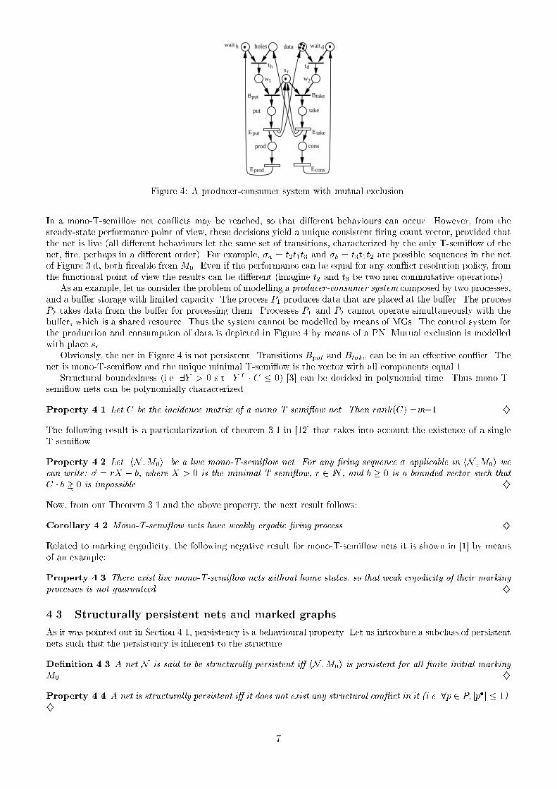
For live mono-T-semi ow nets Fi = Fi(N ) = X is the minimal T-semi ow, thus independent of the initialmarking (provided that liveness is guaranteed) and of the timing interpretation. For persistent nets Fi = Fi(N ;M0)(Figure 3.a) is a T-semi ow (possibly non minimal), and it is independent of the timing interpretation.Let M be the limit vector of the average number of tokens in each place (i.e. M = limt!1 1t R t0 M(s)ds). Then,provided that this limit exists, �iM is the vector of products of the mean number of tokens and the length of onecycle and we have: �iM � PRE �D � Fi (1)From this inequality, a lower bound for the mean cycle time associated with transition ti, �lbi , can be derived.�lbi = maxpj2P PRE[pj ] �D � FiM(pj) (2)Since the vector M is unknown, (2) cannot be solved. However, the following marking invariant can be writtenusing P-semi ow Y : Y T �M0 = Y T �M = Y T �M (3)Now, from (1) and (3): Y T ��iM0 � Y T � PRE �D � Fi, and a lower bound for the mean cycle time in steady-stateis: �lbi = maxY 2fP�semiflowg< Y T � PRE �D � FiY T �M0 (4)Of course, an upper bound for the throughput of ti is 1=�lbi .The previous lower bound for the mean cycle time can be formulated in terms of a particular class of optimizationproblems called fractional programming problems [8], and later transformed into a linear programming problem.Theorem 5.1 For any marked net with unique consistent �ring count vector, a lower bound for the mean cycletime of transition ti can be computed by the following linear programming problem:�lbi = maxfY T � PRE �D � Fi j Y T � C = 0; Y T �M0 = 1; Y � 0g (LPP2) }The previous theorem shows that the problem of �nding an upper bound for the steady-state throughput in apersistent or mono-T-semi ow net can be solved looking at the cycle times associated with P-semi ows, consideredin isolation. These cycle times can be computed making the summation of the average �ring times of all thetransitions involved in the P-semi ow, and dividing by the number of tokens present in it. From a di�erentperspective, from (LPP2) it can be stated that �lbi is �nite i� all P-semi ows are marked (a necessary conditionfor liveness).For the particular case of strongly connected MGs, Fi = ~1 (unique T-semi ow), and the above bound is thesame that has been obtained for the deterministic case by other authors (see, e.g., [5, 13]). For deterministictimed MGs, the reachability of this bound has been shown. Since deterministic timing is just a particular caseof stochastic timing, the reachability of the bound is assured for our proposes. Even more, this bound cannot beimproved only on the base of the knowledge of the coe�cients of variation for the transition �ring times [2].5.2 Upper bounds for bounded persistent netsFor bounded persistent nets, weak ergodicity of the �ring process is assured (Corollary 4.1.1). Thus for these netsa unique limit �ring behaviour exists, and bounds can be computed for the steady-state throughput.As remarked in Section 4.1, persistent nets are behaviourally de�ned. This means that a behavioural analysismust be made before computing performance bounds in order to check for the persistency of the net. Few resultsare known in the literature related to bounds for the performance of bounded persistent nets. A partial result waspresented in [5] for safe and persistent nets with deterministic timing. For these nets a behaviourally equivalentsafe MG (behaviour graph) can be built. The method consists in drawing the initially marked places and enabledtransitions. After that, �ring all transitions and drawing the output places and repeating the procedure untila marking in the process is re-found (see Figure 5). Then, the method explained in Section 5.1 can be appliedfor computing the bounds for this MG and so for the steady-state performances of the initial persistent net.Unfortunately, this analysis is not possible for bounded (non safe) nets when non deterministic timing is considered.Let us now introduce some general results useful for computing bounds for the performance of bounded persistentnets. Later we shall improve some of these results.Let us consider live bounded persistent nets without implicit places. According to Theorem 4.1 consistent �ringcount vectors are proportional to ~�R. Thus the problem (LPP2) can be applied for computing a lower bound of thesteady-state cycle time of a selected transition ti taking into account that Fi = k~�R is a T-semi ow (non minimalif there exist more than one; see Figure 3.a) with Fi(ti) = 1.The optimal value of the previous problem is a non reachable bound in general (i.e. there exist net modelssuch that no stochastic interpretation allows to reach the computed bound, �lbi ). To see it, let us consider for9

p1

p3

p4

p2

t 1

t 2 t 3

p 1

p2 p3

p4

p 1'

p 2'

t 1

t 2

t 3

t 1'

Figure 5: Equivalent MG for safe persistent net.p2 p3

p1

p4

p2't3

t2

t1p1'

t1'

p1

p 3

p4

p2

t 1

t 2 t 3Figure 6: Equivalent MG for deterministic timing.example the net in Figure 3.c. Selecting transition t2, the vector Fi for (LPP2) is Fi = (2; 1; 1)T and the obtainedbound is �lb2 = maxf�2 + �3; (2�1 + �2 + �3)=2g. Now, considering deterministic timing for all transitions with�1 = 2; �2 = 60; �3 = 1, the obtained bound is �lb2 = 61 while the actual cycle time for transition t2 is biggerbecause of the sequence t1t2 which takes 62 units of time. Nevertheless, for safe (and ordinary, in order to be live)persistent nets, the bound given by (LPP2) can be always reached: it would be obtained by deriving the equivalentMG (according to [5]) and computing the bound, using (LPP2).Even though the cycle time bound obtained from (LPP2) can be non reachable for non-safe persistent nets, itcan be pointed out that the bound is �nite if and only if the actual cycle time is �nite, and this trivially characterizesthe liveness of the model.Theorem 5.2 Let hN ;M0i be a bounded persistent net. The following three statements are equivalent:i) The optimal value �lbi of (LPP2) for hN ;M0i is �nite.ii) The actual cycle time of hN ;M0i is �nite.iii) hN ;M0i is live. }The above result is not true for other net classes. In Section 5.3 it is proven that for mono-T-semi ow nets theactual cycle time can be in�nite (so that the net is non live) while the lower bound obtained from (LPP2) is �nite.Improving the upper bound for ordinary nets. Let us now describe a method to compute a reachable upperbound for the steady-state throughput of bounded ordinary persistent nets. Deterministic timing yields the bestperformance for a given persistent (and con ict-free, see Section 4.1) net and average �ring delay associated totransitions. If we consider only deterministic timing, a behaviourally equivalent MG can be derived in an analogousway to that proposed in [5] (see the example in Figure 6): (1) Split the places into instances in such a way thattheir safe markings represent conditions for the enabling of transitions. (2) Develop the behaviour graph of thenet (under deterministic timing assumption) from the initial marking. Since the original net is live, the behaviourgraph can be inde�nitely extended. (3) Identify those instances of places that must be superposed, in such a waythat the relative �ring frequency of transitions is preserved: an MG has been derived.10

p1

t 1 t 2

p2

p3

p6

p7

t 4t 3

p4

p5

Figure 7: Non-live mono-T-semi ow net, even if all P-semi ows are marked and thus �lbi in (LPP2) is �nite.Considering general timing distributions, the original net and the derived MG are not behaviourally equivalent.In fact, the steady-state throughput for the MG is greater than or equal to the one of the original net. Neverthelessfor deterministic timing the equality holds and this provides the following method for computing a reachable boundfor the throughput: (1) consider a bounded ordinary persistent net with general distribution timing; (2) developthe cyclic process for the deterministic case (i.e. the behaviourally equivalent MG for the deterministic timing);and (3) compute the upper bound for the steady-state throughput of the MG using (LPP2).The above computed value is a reachable bound for the steady-state throughput of the original net, becausein the deterministic case the maximal throughput for the net is always obtained and under this condition thethroughputs of the cyclic process and of the original net are equal.5.3 Upper bounds for mono-T-semi ow netsLet us now consider mono-T-semi ow nets (a polynomial time characterizable net subclass, Section 4.2) and giveupper bounds for their steady-state throughput.Unfortunately, the existence of a unique consistent minimal T-semi ow, X , does not guarantee the ergodicityof the marking process (Property 4.3). However, even in the case in which a net is marking non-ergodic, thecomputation of the throughput bounds makes sense. The values that we compute in this section are bounds for allpossible steady-state marking behaviours of the net.The problem (LPP2) de�ning an upper bound for the steady-state throughput of a net with a unique consistent�ring count vector (Section 5.1) can be used taking Fi = kX where kX(ti) = 1. Nevertheless, in general this boundis not reachable. Moreover, a mono-T-semi ow net can be non live and the obtained lower bound for the cycletime be �nite (see Figure 7). In other words:Property 5.1 For mono-T-semi ow nets, liveness is not characterized by the �niteness of the lower bound of thecycle time computed by means of (LPP2). }Comming back to the producer-consumer system of Figure 4, let us suppose that transitions th; td; Bput, and Btakeare immediate (i.e. they �re in zero time) and that the mean values of random variables associated with the restof transitions are: �(Eput) = 2; �(Etake) = 3; �(Eprod) = 4; and �(Econs) = 2.The problem (LPP2) gives a lower bound for the mean cycle time of the net: �lb = maxf�(Eput) + �(Etake),(�(Eput)+�(Etake))=4, �(Eput)+�(Eprod), �(Etake)+�(Econs)g = 6. As it is remarked in Property 5.1, this bound isnon-reachable, in general. However, in this case, the lower bound is equal to the actual cycle time for deterministictiming. In fact, if deterministic timing is considered, the bu�er capacity (initial number of tokens at place data)can be reduced to 1, without modifying the actual cycle time. This is because, in this particular case, there existtwo di�erent P-semi ows Y1 and Y2 (with jjY1jj = fsr; put; takeg and jjY2jj = fholes; data; w1; w2; sr; put; takeg)involving the same set of timed transitions (Eput and Etake). Since Y T1 �M0 = 1, then the number of tokens atplace data can be reduced to 1, and the same optimum value in problem (LPP2) is preserved.6 Lower bounds for the steady-state throughputA trivial lower bound in steady-state performance for a live net with a unique consistent �ring count vector is ofcourse given by the sum of the �ring times of all the transitions weighted by the �ring ow vector itself. Since thenet is live all transition must be �reable, and the sum of all �ring times multiplied by the number of occurrencesof each transition in the (unique) average cycle of the model corresponds to any complete sequentialization of allthe activities represented in the model. This pesimistic behaviour can be reached in some particular cases (e.g.,11

for live and safe MGs) if random variables with arbitrarily large coe�cient of variation are conveniently selectedfor transitions �ring times.Property 6.1 For any live net with unique consistent �ring count vector, an upper bound for the mean cycle timeof transition ti is: �ubi = mXj=1 Fi(tj)�jwhere �j is the mean �ring time of transition tj and Fi is the relative �ring frequency vector of the net for transitionti (i.e. the unique consistent �ring count vector, normalized for having Fi(ti) = 1). }In order to improve the previous bound, an intuitive idea could be to take into account that some work can bedone in parallel at each transition, since in�nite server semantics is assumed. From a queueing theory perspectiveand considering the steady-state behaviour, the number of servers at each station (transition) is equal to thecorresponding enabling bound in steady-state (i.e. liveness bound), and the contribution of each transition to theduration of the complete sequentialization of all activities can be divided by its liveness bound. Thus we couldconjecture the following upper bound for the mean cycle time:�i ?� mXj=1 Fi(tj)�jL(tj) (5)The same value would be obtained taking the algorithm used for the computation of the lower bound (Section 5.1),substituting in it the \max" operator with the sum of the �ring times of all transitions involved, and making somemanipulation to avoid counting more than once the contribution of the same transition.The conjecture (5) has been shown to be true for strongly connected MGs in [2]. In fact, for this subclass ofnets the upper bound for the mean cycle time given by (5) has been shown to be reachable for any net topology,for any speci�cation of the mean �ring delays, and for some assignement of PDFs to the �ring delays of transitions.Moreover, taking into account Property 4.9, the liveness bound can be e�ciently computed for strongly connectedMGs by means of the problem (LPP1, Section 2.2).Concerning structurally persistent nets the conjecture (5) is false (thus it is false for persistent and for mono-T-semi ow nets). This can be shown considering, for example, the structurally persistent net in Figure 1.b with mean�ring times �1; �2; �3 for transitions. For this net, the relative �ring frequency vector is F2 = (2; 1; 1)T , and theliveness bounds of transitions are given by L = (2; 1; 1)T . Thus, the conjecture (5) would give the value �1+�2+�3as upper bound for �2. If exponentially distributed random variables (with means �1; �2; �3; �1 6= �3) are associatedwith transitions, the steady-state cycle time for transition t2 is �2 = �1 + �2 + �3 + �21=2(�1 + �3), which is greaterthan the value obtained applying (5), thus the conjecture is false.Unfortunately, the trivial bound given by Property 6.1 is non-reachable in general, and in some cases its valuecan be too pesimistic. An improving of this bound would probably require more information about the PDFs of�ring times than their mean values, and this approach is not within the scope of this work.7 ConclusionsWe have addressed the problem of computing upper and lower bounds for the throughput of transitions in Petrinet models (or the corresponding synchronized queueing networks) having a unique consistent �ring count vector.The results presented here represent, in some sense, an extension of those described in [2] for the case of boundedmarked graphs. The upper bound in case of persistent nets is a generalization of that obtained for marked graphs,and has been shown to be reachable for ordinary nets. The technique proposed for the derivation of behaviourgraphs for non-safe ordinary persistent nets is an extension of a method originally proposed by Ramchandani forsafe persistent nets, that was not directly applicable.For what concerns the lower bound on throughput, only the trivial bound computed as the inverse of the sumof all transition �ring delays weighted by the �ring count vector can be easily borrowed from the marked graphcase. However this can be too pessimistic in case of persistent or live mono-T-semi ow nets.In any case both the upper and lower bounds are independent of any assumption on the probability distributionof the delays associated with transitions, and their value can be computed based on the knowledge of the averages.This represents a generalization with respect to the usual assumptions needed for the exact performance evaluationof a Petri net model. A second generalization, implicit in the choice of computing throughput bounds instead ofactual values, is that the analysis of marking non-ergodic models still makes sense.Besides the results on the computation of bounds, this paper identi�es two subclasses of bounded nets havinga unique consistent �ring count vector, and contains a discussion of their ergodicity conditions. In particular, theconcept of liveness bound for transitions is a new behavioural property, that comes directly from considerations12

related to the timing semantics of a timed Petri net model. It generalizes the usual concept of liveness for atransition, and provides an example of possible interleaving between qualitative and quantitative analysis for timedand stochastic Petri nets. Another example has been provided by stablishing the strong connection betweenmarking ergodicity and home state concepts.Alternative extensions of the results concerning marked graphs are already being considered. In particular, liveand bounded free choice nets are studied in [14]. In this case, the idea is that several consistent �ring count vectorscan be reproduced in steady-state. However the free choice property leads to the fact that selections are completelygoverned by the structure and the stochastic (routing) interpretation of the net. Thus the \relative �ring frequencyvector" can be computed independently of the marking of the net, provided that liveness is guaranteed.References[1] J. Campos, G. Chiola, and M. Silva. Properties and steady-state performance bounds for Petri nets withunique repetitive �ring count vector. In Proceedings of the 3rd International Workshop on Petri Nets andPerformance Models, IEEE-CS Press, pp. 210{220, Kyoto, Japan, December 1989.[2] J. Campos, G. Chiola, J. M. Colom, and M. Silva. Tight polynomial bounds for steady-state performanceof marked graphs. In Proceedings of the 3rd International Workshop on Petri Nets and Performance Models,IEEE-CS Press, pp. 200{209, Kyoto, Japan, December 1989.[3] T. Murata. Petri nets: properties, analysis, and applications. Proceedings of the IEEE, 77(4):541{580, April1989.[4] G. W. Brams. R�eseaux de Petri: Th�eorie et Pratique. T.1. th�eorie et analyse. Masson, Paris, 1983.[5] C. Ramchandani. Analysis of Asynchronous Concurrent Systems by Petri Nets. PhD thesis, M.I.T. Cambridge,Mass. February 1974.[6] M. Ajmone Marsan, G. Balbo, A. Bobbio, G. Chiola, G. Conte, and A. Cumani. The e�ect of executionpolicies on the semantics and analysis of stochastic Petri nets. IEEE Transactions on Software Engineering,15(7):832{846, July 1989.[7] E. Gelenbe and G. Pujolle. Introduction to Queuing Networks. John Wiley, 1987.[8] K. G. Murty. Linear Programming. John Wiley & Sons, 1983.[9] G. Florin and S. Natkin. Les r�eseaux de Petri stochastiques. Technique et Science Informatiques, 4(1):143{160,1985.[10] E. Best and K. Voss. Free-choice systems have home states. Acta Informatica, (21):89{100, 1984.[11] M. Silva and J. M. Colom. On the computation of structural synchronic invariants in P/T nets. In G.Rozenberg, editor, Advances in Petri Nets 1988, pp. 386{417, LNCS 340, Springer-Verlag, Berlin, 1988.[12] M. Silva. Towards a synchrony theory for P/T nets. In K. Voss, H. Genrich, and G. Rozenberg, editors,Concurrency and Nets, pp. 435{460, Springer-Verlag, Berlin, 1987.[13] C. V. Ramamoorthy and G. S. Ho. Performance evaluation of asynchronous concurrent systems using Petrinets. IEEE Transactions on Software Engineering, 6(5):440{449, September 1980.[14] J. Campos, G. Chiola, and M. Silva. Properties and performance bounds for closed free choice synchro-nized monoclass queueing networks. Research Report GISI-RR-90-2, Dpto. Ingenier��a El�ectrica e Inform�atica,Universidad de Zaragoza, Spain, January 1990.

13