Pattern Recognition Using Spiking Neurons and Firing Rates

Pattern Recognition Using Spiking Neurons and

Firing Rates

Roberto A. Vazquez

Escuela de Ingenierıa - Universidad La SalleBenjamın Franklin 47 Col. Condesa CP 06140 Mexico, D.F.

[email protected]

Abstract. Different varieties of artificial neural networks have provedtheir power in several pattern recognition problems, particularly feed-forward neural networks. Nevertheless, these kinds of neural networksrequire of several neurons and layers in order to success when they areapplied to solve non-linear problems. In this paper is shown how a spikingneuron can be applied to solve different linear and non-linear patternrecognition problems. A spiking neuron is stimulated during T ms withan input signal and fires when its membrane potential reaches a specificvalue generating an action potential (spike) or a train of spikes. Givena set of input patterns belonging to K classes, each input pattern istransformed into an input signal, then the spiking neuron is stimulatedduring T ms and finally the firing rate is computed. After adjusting thesynaptic weights of the neuron model, we expect that input patternsbelonging to the same class generate almost the same firing rate andinput patterns belonging to different classes generate firing rates differentenough to discriminate among the different classes. At last, a comparisonbetween a feed-forward neural network and a spiking neuron is presentedwhen they are applied to solve non-linear and real object recognitionproblems.

1 Introduction

Artificial neural networks have been applied in a wide range of problems: pat-tern recognition, forecasting, intelligent control and so on. Perhaps, among themost popular neural network models we could mention the feed-forward neuralnetwork trained with the back-propagation algorithm [1,2]. Despite of its power,this type of neural network cannot reach an optimum performance in non-linearproblems if it is not well designed. The selection of a learning algorithm andparameters such as number of neurons, number of layers, and the transfer func-tions, determine the accuracy of the network, resulting in complex architecturesto solve the problem [3].

Spiking neuron models have been called the 3rd generation of artificial neuralnetworks [4]. These models increase the level of realism in a neural simulationand incorporate the concept of time. Spiking models have been applied in a widerange of areas from the field of computational neurosciences [5] such as: brain

A. Kuri-Morales and G. Simari (Eds.): IBERAMIA 2010, LNAI 6433, pp. 423–432, 2010.c© Springer-Verlag Berlin Heidelberg 2010

424 R.A. Vazquez

region modeling [6], auditory processing [7,8], visual processing [9,10], robotics[11,12] and so on.

In this paper is shown how a spiking neuron can be applied to solve differentlinear and non-linear pattern recognition problems. The Izhikevich neuron model[13,14,15] is adopted in this research. A spiking neuron is stimulated during Tms with an input signal and fires when its membrane potential reaches a specificvalue generating an action potential (spike) or a train of spikes. Given a set ofinput patterns belonging to K classes, each input pattern is transformed intoan input signal, then the spiking neuron is stimulated during T ms and finallythe firing rate is computed. After adjusting the synaptic weights of the neuronmodel, we expect that input patterns belonging to the same class generate al-most the same firing rate; on the other hand, we also expect that input patternsbelonging to different classes generate firing rates different enough to discrimi-nate among the different classes. At last, a comparison between a feed-forwardneural network trained with the well-known backpropagation and Levenberg-Marquartd algorithms and a spiking neuron is presented when they are appliedto solve non-linear and real object recognition problems.

2 Izhikevich Neuron Model

A typical spiking neuron can be divided into three functionally distinct parts,called dendrites, soma, and axon. The dendrites play the role of the input de-vice that collects signals from other neurons and transmits them to the soma.The soma is the central processing unit that performs an important non-linearprocessing step: if the total input exceeds a certain threshold, then an outputsignal is generated. The output signal is taken over by the output device, theaxon, which delivers the signal to other neurons. The neuronal signals consistof short electrical pulses. The pulses, so-called action potentials or spikes, havean amplitude of about 100 mV and typically a duration of 1-2 ms. The form ofthe pulse does not change as the action potential propagates along the axon. Achain of action potentials emitted by a single neuron is called a spike train (a se-quence of stereotyped events which occur at regular or irregular intervals). Sinceall spikes of a given neuron look alike, the form of the action potential does notcarry any information. Rather, it is the number and the timing of spikes whichmatter. The action potential is the elementary unit of signal transmission. Ac-tion potentials in a spike train are usually well separated. Even with very stronginput, it is impossible to excite a second spike during or immediately after a firstone. The minimal distance between two spikes defines the absolute refractoryperiod of the neuron. The absolute refractory period is followed by a phase ofrelative refractoriness where it is difficult, but not impossible to excite an actionpotential [16].

The Izhikevich model

Cv = k (v − vr) (v − vt)− u + I ifv ≥ vpeakthenu = a {b (v − vr)− u} v ← c, u← u + d

(1)

Pattern Recognition Using Spiking Neurons and Firing Rates 425

has only nine dimensionless parameters. Depending on the values of a and b,it can be an integrator or a resonator. The parameters c and d do not affectsteady-state sub-threshold behavior. Instead, they take into account the actionof high-threshold voltage-gated currents activated during the spike, and affectonly the after-spike transient behavior. v is the membrane potential, u is therecovery current, C is the membrane capacitance, vr is the resting membranepotential, and vt is the instantaneous threshold potential [15].

The parameters k and b can be found when one knows the neuron’s rheobaseand input resistance. The sign of b determines whether u is an amplifying (b < 0)or a resonant (b > 0) variable. The recovery time constant is a. The spike cutoffvalue is vpeak , and the voltage reset value is c. The parameter d describes thetotal amount of outward minus inward currents activated during the spike andaffecting the after-spike behavior.

Various choices of the parameters result in various intrinsic firing patternsincluding [13]: RS (regular spiking) neurons are the most typical neurons inthe cortex, see Fig. 1; IB (intrinsically bursting) neurons fire a stereotypicalburst of spikes followed by repetitive single spikes; CH (chattering) neurons canfire stereotypical bursts of closely spaced spikes; FS (fast spiking) neurons canfire periodic trains of action potentials with extremely high frequency practicallywithout any adaptation(slowing down); and LTS (low-threshold spiking) neuronscan also fire high-frequency trains of action potentials, but with a noticeable spikefrequency adaptation.

3 Proposed Method

Before describing the proposed method applied to solve pattern recognition prob-lems, it is important to notice that when the input current signal changes, theresponse of the Izhikevich neuron also changes, generating different firing rates,see Fig. 1.

The firing rate is computed as the number of spikes generated in an intervalof duration T divided by T . The neuron is stimulated during T ms with an input

0 200 400 600 800 1000−60

−40

−20

0

20

40

Mem

bran

e po

tent

ial,

v(m

V)

Time (ms)

(a)

0 200 400 600 800 1000−60

−40

−20

0

20

40

Time (ms)

Mem

bran

e po

tent

ial,

v(m

V)

(b)

Fig. 1. Simulation of the Izhikevich neuron model 100v = 0.7 (v + 60) (v + 40)−u+ I ,u = 0.03 {−2 (v + 60)− u}, if v ≥ 35 then, v ← −50, u← u + 100 . (a) Injection of thestep of DC current I = 70pA. (b) Injection of the step of DC current I = 100pA.

426 R.A. Vazquez

signal and fires when its membrane potential reaches a specific value generatingan action potential (spike) or a train of spikes.

Let{xi, k

}p

i=1be a set of p input patterns where k = 1, . . . , K is the class to

which xi ∈ IRn belongs. First of all, each input pattern is transformed into aninput signal I, after that the spiking neuron is stimulated using I during T msand then the firing rate of the neuron is computed. With this information, theaverage firing rate AFR ∈ IRK and standard deviation SDFR ∈ IRK of eachclass can be computed.

Finally, we expect that input patterns, which belong to the same class, gen-erate almost the same firing rates (low standard deviation); and input patterns,which belong to different classes, generate firing rates different enough (averagespiking rate of each class widely separated) to discriminate among the differentclasses. In order to achieve that, a training phase is required in the proposedmethod.

During training phase, the synaptic weights of the model, which are directlyconnected to the input pattern, are adjusted by means of a differential evolutionalgorithm.

At last, the class of an input pattern x is determined by means of the firingrates as

cl = argK

mink=1

(|AFRk − fr|) (2)

where fr is the firing rate generated by the neuron model stimulated with theinput pattern x.

3.1 Generating Input Signals from Input Patterns

Izhikevhic neuron model cannot be directly stimulated with the input patternxi ∈ IRn, but with an injection current I. Furthermore, to get a firing rate fromthe neuron model greater than zero, the input signal should be I > 55pA.

Since synaptic weights of the model are directly connected to the input patternxi ∈ IRn, the injection current of this input pattern can be computed as

I = θ + x ·w (3)

where wi ∈ IRn is the set of synaptic weights of the neuron model and θ > 55 isa threshold which guarantees that the neuron will fire.

3.2 Adjusting Synapses of the Neuron Model

Synapses of the neuron model are adjusted by means of a differential evolutionalgorithm. Evolutionary algorithms not only have been used to design artificialneural networks [3], but also to evolve structure-function mapping in cognitiveneuroscience [17] and compartmental neuron models [18].

Differential evolution is a powerful and efficient technique for optimizing non-linear and non-differentiable continuous space functions [19]. Differential evolu-tion is regarded as a perfected version of genetic algorithms for rapid numerical


optimization. Differential evolution has a lower tendency to converge to localmaxima with respect to the conventional genetic algorithm, because it simulatesa simultaneous search in different areas of solution space. Moreover, it evolvespopulations with smaller number of individuals, and have a lower computationcost.

Differential evolution begins by generating a random population of candidatesolutions in the form of numerical vectors. The first of these vectors is selected asthe target vector. Next, differential evolution builds a trial vector by executingthe following sequence of steps:

1. Randomly select two vectors from the current generation.

2. Use these two vectors to compute a difference vector.

3. Multiply the difference vector by weighting factor F.

4. Form the new trial vector by adding the weighted difference vector to

a third vector randomly selected from the current population.

The trial vector replaces the target vector in the next generation if and only if thetrial vector represents a better solution, as indicated by its measured cost valuecomputed with a fitness function. Differential evolution repeats this process foreach of the remaining vectors in the current generation. Differential evolutionthen replaces the current generation with the next generation, and continues theevolutionary process over many generations.

In order to achieve that input patterns, which belong to the same class, gen-erate almost the same firing rates (low standard deviation), and input patterns,which belong to different classes, generate firing rates enough different (averagespiking rate of each class widely separated) to discriminate among the differentclasses, the next fitness function was proposed

f =1

dist (AFR)+

K∑

k=1

SDFRk (4)

where dist (AFR) is the summation of the Euclidian distances among the aver-age firing rate of each class.

4 Experimental Results

To evaluate and compare the accuracy of the proposed method, against feed-forward neural networks, several experiments were performed using 3 datasets.Two of them were taken from UCI machine learning benchmark repository [20]:iris plant and wine datasets. The other one was generated from a real objectrecognition problem.

The iris plant dataset is composed of 3 classes and each input pattern iscomposed of 4 features. The wine dataset is composed of 3 classes and eachinput pattern is composed of 13 features.

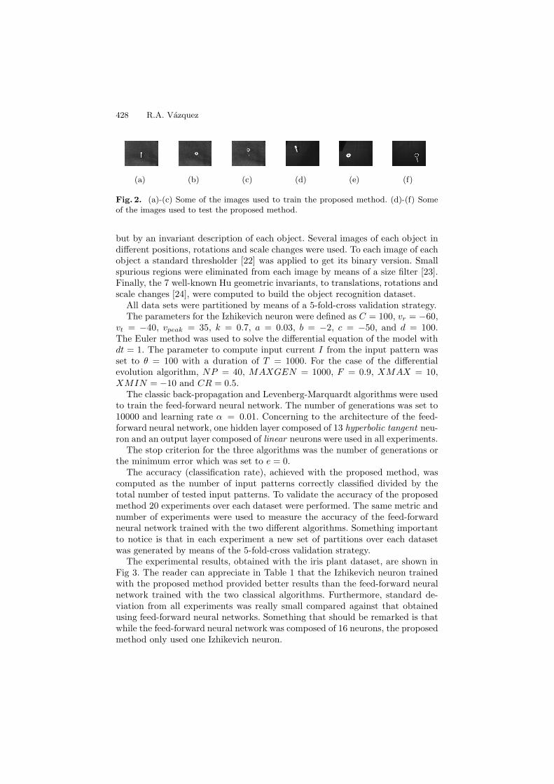
For the case of the real object recognition problem, a dataset was generatedfrom a set of 100 images which contains 5 different objects whose images areshown in Fig. 2 [21]. Objects were not recognized directly from their images,

428 R.A. Vazquez

(a) (b) (c) (d) (e) (f)

Fig. 2. (a)-(c) Some of the images used to train the proposed method. (d)-(f) Someof the images used to test the proposed method.

but by an invariant description of each object. Several images of each object indifferent positions, rotations and scale changes were used. To each image of eachobject a standard thresholder [22] was applied to get its binary version. Smallspurious regions were eliminated from each image by means of a size filter [23].Finally, the 7 well-known Hu geometric invariants, to translations, rotations andscale changes [24], were computed to build the object recognition dataset.

All data sets were partitioned by means of a 5-fold-cross validation strategy.The parameters for the Izhikevich neuron were defined as C = 100, vr = −60,

vt = −40, vpeak = 35, k = 0.7, a = 0.03, b = −2, c = −50, and d = 100.The Euler method was used to solve the differential equation of the model withdt = 1. The parameter to compute input current I from the input pattern wasset to θ = 100 with a duration of T = 1000. For the case of the differentialevolution algorithm, NP = 40, MAXGEN = 1000, F = 0.9, XMAX = 10,XMIN = −10 and CR = 0.5.

The classic back-propagation and Levenberg-Marquardt algorithms were usedto train the feed-forward neural network. The number of generations was set to10000 and learning rate α = 0.01. Concerning to the architecture of the feed-forward neural network, one hidden layer composed of 13 hyperbolic tangent neu-ron and an output layer composed of linear neurons were used in all experiments.

The stop criterion for the three algorithms was the number of generations orthe minimum error which was set to e = 0.

The accuracy (classification rate), achieved with the proposed method, wascomputed as the number of input patterns correctly classified divided by thetotal number of tested input patterns. To validate the accuracy of the proposedmethod 20 experiments over each dataset were performed. The same metric andnumber of experiments were used to measure the accuracy of the feed-forwardneural network trained with the two different algorithms. Something importantto notice is that in each experiment a new set of partitions over each datasetwas generated by means of the 5-fold-cross validation strategy.

The experimental results, obtained with the iris plant dataset, are shown inFig 3. The reader can appreciate in Table 1 that the Izhikevich neuron trainedwith the proposed method provided better results than the feed-forward neuralnetwork trained with the two classical algorithms. Furthermore, standard de-viation from all experiments was really small compared against that obtainedusing feed-forward neural networks. Something that should be remarked is thatwhile the feed-forward neural network was composed of 16 neurons, the proposedmethod only used one Izhikevich neuron.


0 1 2 3 4 5 6 7 8 9 10 11 12 13 14 15 16 17 18 19 20 210

0.1

0.2

0.3

0.4

0.5

0.6

0.7

0.8

0.9

1

# of experiment

Cla

ssifi

catio

n ra

te

Proposed methodLevenberg−MarquardtBackpropagation

(a)

0 1 2 3 4 5 6 7 8 9 10 11 12 13 14 15 16 17 18 19 20 210

0.1

0.2

0.3

0.4

0.5

0.6

0.7

0.8

0.9

1

# of experiment

Cla

ssifi

catio

n ra

te


(b)

Fig. 3. Experimental results obtained with the iris plant dataset. (a) Accuracy of theproposed method during training phase. (b) Accuracy of the proposed method duringtesting phase.

0 1 2 3 4 5 6 7 8 9 10 11 12 13 14 15 16 17 18 19 20 210

0.1

0.2

0.3

0.4

0.5

0.6

0.7

0.8

0.9

1

# of experiment

Cla

ssifi

catio

n ra

te


(a)

0 1 2 3 4 5 6 7 8 9 10 11 12 13 14 15 16 17 18 19 20 210

0.1

0.2

0.3

0.4

0.5

0.6

0.7

0.8

0.9

1

# of experiment

Cla

ssifi

catio

n ra

te


(b)

Fig. 4. Experimental results obtained with the wine dataset. (a) Accuracy of the pro-posed method during training phase. (b) Accuracy of the proposed method duringtesting phase.

The experimental results, obtained with the wine dataset, are shown inFig 4. The reader can appreciate in Table 1 that the Izhikevich neuron trainedwith the proposed method also provided better results than the feed-forwardneural network trained with the backpropagation algorithm; but Levenberg-Marquartd method provided better results with a neural network composed of16 neurons. The average classification rate obtained during testing phase wasnot as good as that obtained during training phase.

The experimental results, obtained with the object recognition dataset, areshown in Fig 5. The reader can appreciate in Table 1 that results provided by theIzhikevich neuron are better compared to those obtained with the feed-forwardneural network. Although the feed-forward neural network was composed with18 neurons and trained during 10000 iterations, the proposed method providedbetter results only with 1000 iterations.

In Table 1 and 2 the average and standard deviation classification rate com-puted from all experimental results are shown. The results obtained with the

430 R.A. Vazquez

0 1 2 3 4 5 6 7 8 9 10 11 12 13 14 15 16 17 18 19 20 210

0.1

0.2

0.3

0.4

0.5

0.6

0.7

0.8

0.9

1

# of experiment

Cla

ssifi

catio

n ra

te


(a)

0 1 2 3 4 5 6 7 8 9 10 11 12 13 14 15 16 17 18 19 20 210

0.1

0.2

0.3

0.4

0.5

0.6

0.7

0.8

0.9

1

# of experiment

Cla

ssifi

catio

n ra

te


(b)

Fig. 5. Experimental results obtained with the object recognition dataset. (a) Accuracyof the proposed method during training phase. (b) Accuracy of the proposed methodduring testing phase.

Table 1. Average accuracy provided by the methods using different databases

Dataset Back-propagation Levenberg-Marquartd Proposed method

Tr. cr. Te. cr. Tr. cr. Te. cr. Tr. cr. Te. cr.Iris plant 0.8921 0.8383 0.8867 0.7663 0.9988 0.9458

Wine 0.4244 0.3637 1 0.8616 0.9783 0.7780Object rec. 0.4938 0.4125 0.6169 0.4675 0.8050 0.7919

Tr. cr = Training classification rate, Te. cr. = Testing classification rate.

Table 2. Standard deviation obtained through the different experiments

Dataset Back-propagation Levenberg-Marquartd Proposed method

Tr. Te. Tr. Te. Tr. Te.Iris plant 0.0684 0.1015 0.0676 0.0918 0.0064 0.0507

Wine 0.0456 0.0674 0 0.0750 0.0359 0.0930Object rec. 0.1586 0.1689 0.0907 0.1439 0.0770 0.0793

spiking neuron model, trained with the proposed method, improve the resultsobtained with feed-forward neural networks, when are applied to non-linear prob-lems. Furthermore, the standard deviations, computed from all experiments,support the stability of the proposed method. While feed-forward neural net-works provided different results through each experiment, the proposed methodprovided similar results.

These preliminary results suggest that spiking neurons can be considered asan alternative way to perform different pattern recognition tasks.

We can also conjecture that if only one neuron is capable to solve patternrecognition problems, perhaps several spiking neurons working together can im-prove the experimental results obtained in this research. However, that is some-thing that should be proved.


5 Conclusions

In this paper a new method to apply a spiking neuron in a pattern recognitiontask was proposed. This method is based on the firing rates produced with anIzhikevich neuron when is stimulated. The firing rate is computed as the numberof spikes generated in an interval of duration T divided by T . A spiking neuronis stimulated during T ms with an input signal and fires when its membranepotential reaches a specific value generating an action potential (spike) or atrain of spikes.

The training phase of the neuron model was done by means of a differen-tial evolution algorithm. After training, we observed that input patterns, whichbelong to the same class, generate almost the same firing rates (low standarddeviation) and input patterns, which belong to different classes, generate firingrates different enough (average spiking rate of each class widely separated) todiscriminate among the different classes.

Through several experiments we observed that the proposed method, signif-icantly improve the results obtained with feed-forward neural networks, whenare applied to non-linear problems. On the other hand, the standard deviationscomputed from all experiments, support the stability of the proposed method.While feed-forward neural networks provided different results through each ex-periment, the proposed method provided similar results. Finally, we can concludethat spiking neurons can be considered as an alternative tool to solve patternrecognition problems.

Nowadays, we are analyzing the different behaviors of the Izhikevich modelin order to determine which configuration is the most suitable for a patternrecognition task. In addition, we are testing different fitness functions to improvethe results obtained in this research. Furthermore, we are researching differentalternatives of combining several Izhikevich neurons in one network to improvethe results obtained in this research and then apply it in more complex patternrecognition problems such as face, voice and 3D object recognition.

Acknowledgements

The authors thank Universidad La Salle for the economical support under grantnumber ULSA I-113/10.

References

1. Anderson, J.A.: Introduction to Neural Networks. MIT Press, Cambridge (1995)2. Werbos, P.J.: Backpropagation through time: What it does and how to do it. Proc.

IEEE 78, 1550–1560 (1990)3. Garro, B.A., Sossa, H., Vazquez, R.A.: Design of Artificial Neural Networks using

a Modified Particle Swarm Optimization Algorithm. IJCNN, 938–945 (2009)4. Maass, W.: Networks of spiking neurons: the third generation of neural network

models. Neural Networks 10(9), 1659–1671 (1997)

432 R.A. Vazquez

5. Rieke, F., et al.: Spikes: Exploring the Neural Code. Bradford Book (1997)6. Hasselmo, M.E., Bodelon, C., et al.: A Proposed Function for Hippo-campal Theta

Rhythm: Separate Phases of Encoding and Retrieval Enhance Re-versal of PriorLearning. Neural Computation 14, 793–817 (2002)

7. Hopfield, J.J., Brody, C.D.: What is a moment? Cortical sensory integration overa brief interval. PNAS 97(25), 13919–13924 (2000)

8. Loiselle, S., Rouat, J., Pressnitzer, D., Thorpe, S.: Exploration of rank order codingwith spiking neural networks for speech recognition. IJCNN 4, 2076–2080 (2005)

9. Azhar, H., Iftekharuddin, K., et al.: A chaos synchronization-based dynamic visionmodel for image segmentation. IJCNN 5, 3075–3080 (2005)

10. Thorpe, S.J., Guyonneau, R., et al.: SpikeNet: Real-time visual processing withone spike per neuron. Neurocomputing 58(60), 857–864 (2004)

11. Di Paolo, E.A.: Spike-timing dependent plasticity for evolved robots. AdaptiveBehavior 10(3), 243–263 (2002)

12. Floreano, D., Zufferey, J., et al.: From wheels to wings with evolutionary spikingneurons. Artificial Life 11(1-2), 121–138 (2005)

13. Izhikevich, E.M.: Simple model of spiking neurons. IEEE Trans. on Neural Net-works 14(6), 1569–1572 (2003)

14. Izhikevich, E.M.: Which model to use for cortical spiking neurons? IEEE Trans.on Neural Networks 15(5), 1063–1070 (2004)

15. Izhikevich, E.M.: Dynamical Systems in Neuroscience: The Geometry of Excitabil-ity and Bursting. The MIT Press, Cambridge (2007)

16. Gerstner, W., et al.: Spiking Neuron Models. Cambridge University Press, Cam-bridge (2002)

17. Frias-Martinez, E., Gobet, F.: Automatic generation of cognitive theories usinggenetic programming. Minds and Machines 17(3), 287–309 (2007)

18. Hendrickson, E., et al.: Converting a globus pallidus neuron model from 585 to 6compartments using an evolutionary algorithm. BMC Neurosci. 8(s2), P122 (2007)

19. Price, K., Storn, R.M., Lampinen, J.A.: Diffentential evolution: a practical ap-proach to global optimization. Springer, Heidelberg (2005)

20. Murphy, P.M., Aha, D.W.: UCI repository of machine learning databases. Dept.Inf. Comput. Sci., Univ. California, Irvine, CA (1994)

21. Vazquez, R.A., Sossa, H.: A new associative model with dynamical synapses. NeuralProcessing Letters 28(3), 189–207 (2008)

22. Otsu, N.: A threshold selection method from gray-level histograms. IEEE Trans.on SMC 9(1), 62–66 (1979)

23. Jain, R., et al.: Machine Vision. McGraw-Hill, New York (1995)24. Hu, M.K.: Visual pattern recognition by moment invariants. IRE Trans. on Infor-

mation Theory 8, 179–187 (1962)

Pattern Recognition Using Spiking Neurons and Firing Rates

Documents

Transcript of Pattern Recognition Using Spiking Neurons and Firing Rates