On Firing Rate Estimation for Dependent

Interspike Intervals

Elisa Benedetto, Federico Polito, Laura Sacerdote∗

Department of Mathematics G. Peano, University of Torino

Via Carlo Alberto 10, 10123, Torino, Italy

Abstract

A time dependent instantaneous firing rate may be related both to a time-

varying behaviour of external inputs and to the lack of independency between

ISIs. In this second case, the instantaneous firing rate does not enlighten

the role of the ISIs dependencies and the conditional firing rate should be

introduced. We propose a non parametric estimator for the conditional instan-

taneous firing rate for Markov, stationary and ergodic ISIs. An algorithm to

check the reliability of the proposed estimator is introduced and its consis-

tency properties are proved. The method is applied to data obtained from a

stochastic two compartment model and to in vitro experimental data.

Keywords: Firing rate; Non parametric estimator; Markov ISIs.

1 Introduction

The firing rate characterizes the behaviour of spiking neurons and it is often used

to evaluate the information encoded in neural responses. Its use dates back to∗Corresponding author. Email: laura.sacerdote@unito.it

1

arX

iv:1

306.

2193

v2 [

mat

h.ST

] 1

4 A

pr 2

014

Adrian (1928) who first assumed that information sent by a neuron is encoded

in the number of spikes per observation time window. The frequency transfer

function is then often studied to illustrate the relationship between input signal

and firing rate, taken as constant for a fixed signal. Typically, the firing rate

increases, generally non-linearly, with an increasing stimulus intensity (Kandel

et al., 2000). The main objection to the use of the transfer function is that it

ignores any information possibly encoded in the temporal structure of the spike

train. Furthermore, different definition of rate give rise to different shapes of the

frequency transfer function. However, different definitions of rate are equivalent

under specific conditions and differ in other instances (see Lansky et al. (2004)).

When the firing rate is not constant, i.e. when the firing is not a Poisson

process, specific techniques are necessary to estimate the instantaneous firing

rate avoiding artifacts (see Cunningham et al. (2009) for a review). An important

tool in this framework is the kernel method. Optimizing the choice of kernels and

of bins becomes necessary in the case of a time dependent input (see Shimazaki &

Shinomoto (2010), Omi & Shinomoto (2011)). A method to estimate the firing rate

in presence of non-stationary inputs was recently proposed in Iolov et al. (2013)

for the case of slowly varying signals while Tamborrino et al. (2013) consider also

the latency to improve the firing rate estimation.

A time dependent instantaneous firing rate is tipically related with a time

dependent input disregarding possible alternative causes that can determine

this time dependencies. However, a time dependent instantaneous firing rate

can also be determined by dependences between ISIs. Farkhooi et al. (2009)

report experimental findings of negative serial correlation in ISIs observed in the

sensory periphery as well as in central neurons in spontaneous activity. Generally

dependences or correlations are studied between ISIs of different neurons of a

group while are neglected those between successive ISIs of a single neuron such

2

as those observed in Farkhooi et al. (2009). These observations may not be related

with input features but may arise, for example, either assuming independent non

exponentially distributed ISIs or jointly dependent ISIs. In the case of dependent

ISIs, the instantaneous firing rate is not the correct tool to analyze data since it

confuses the actual cause of the observed time dependency. To enlighten the role

of the ISIs dependences on the firing rate, a conditional instantaneous firing rate

should be introduced. Indeed by using conditional distibutions it is possible to

remove the classical renewal hypothesis (Cox, 1970) supporting the analysis of

the instantaneous firing. Hence the past history of the spike train is considered in

instantaneous firing estimation. The instantaneous conditional firing is updated

after each ISI, thus accounting for the dependency between ISIs.

Estimators for the conditional spiking intensity exist in the literature in the

framework of maximum likelihood methods (Brown et al., 2001; Gerhard et al.,

2011). Advantages of such estimators include the possibility to perform tests of

hypotheses, to evaluate efficiency features or to compute standard error. However,

these advantages are based on the assumption that a specific model fits the data

and no result holds when the model is not true or is unknown. Unfortunately, the

model is known in a relative small number of cases and often its choice introduces

non controllable approximations.

Aim of this paper is to determine a conditional firing rate estimator for de-

pendent ISIs avoiding to introduce a model to describe their distribution. We

suggest a non parametric estimator for the instantaneous firing rate, conditioned

on the past history of the spike train. Under suitable hypotheses we prove the

consistency of the proposed estimator.

The paper is organized in the following way. In Section 2 we recall different

definitions of the firing rate taking care to enlighten their features if the ISIs are

dependent. In Section 3 we propose an estimator of the conditional instantaneous

3

firing rate of a neuron characterized by an ISI sequence that can be modelled

as a Markov, ergodic and stationary process. The consistency of this estimator

is proved in the Appendix. The direct check of Markov, ergodic and stationary

hypotheses on the available data is not easy but it is necessary to make reliable

the estimates. Hence in Section 4 we develop a statistical algorithm to validate

a posteriori our estimation by checking the underlying hypotheses by means of

the obtained estimate. In Section 5 we apply the proposed method to estimate

the conditional firing rate of simulated dependent ISIs. For this aim we resort to

the stochastic two compartment model proposed in Lansky & Rodriguez (1999).

Indeed Benedetto & Sacerdote (2013) recently showed that suitable choices of

the parameters of this simple model allow to generate sequences of ISIs that are

statistically Markov, ergodic and stationary. Finally, in Section 6 we apply our

results to in vitro experimental data.

2 Definitions of the firing rate

The firing rate can be defined in many different ways. Here we report the most

usual definitions, their relationships and which spike train features best enlighten

each of them. The ability of each definition to catch the nature of neural code

strongly depends on the nature of the observed spike train. Specifically we

distinguish the case of independent identically distributed ISIs from the case with

dependent ISIs.

Let us describe the spike train through the ISIs and let T be a random variable

with the same distribution of the ISIs, shared by the entire spike train. The most

used definitions (see amongst others Burkitt & Clark, 2000; Van Rullen & Thorpe,

2001) are the inverse of the average ISI

1/E(T), (1)

4

which is commonly called firing rate, and the expectation of the inverse of an ISI

E(1/T), (2)

called the instantaneous mean firing rate. Values obtained with the second defini-

tion are always larger than those computed on the considered interval through

1/E(T) (Lansky et al., 2004). Identical distribution of ISIs is required to give sense

to these definitions.

A different description of spike train makes use of the number of spikes

occurred up to time t, i.e. the counting process N(t), t ≥ 0 (see e.g. Cox & Isham,

1980). The quantity N(t)/t, is a measure of instantaneous firing rate accounting for

the total number of spikes N(t) up to time t. The firing rate (1) and the quantity

N(t)/t are connected through the well-known asymptotic formula

1E(T)

= limt→∞

E(N(t))t

(3)

(Cox, 1970; Rudd & Brown, 1997). An alternative definition of the instantaneous

firing rate is (e.g. Johnson, 1996)

λ(t)= lim∆t→0

E[N(t+∆t)−N(t)]∆t

. (4)

This last expression does not consider the cumulative property of N(t)/t that

involves the whole history of the spike train. When the ISIs have a common

distribution, it can be expressed in terms of the ISIs distribution through

λ(t)= f (t)P(T > t)

, (5)

where f (t) is the probability density function of the random ISI T (Cox & Lewis,

1966, Chapter 6).

5

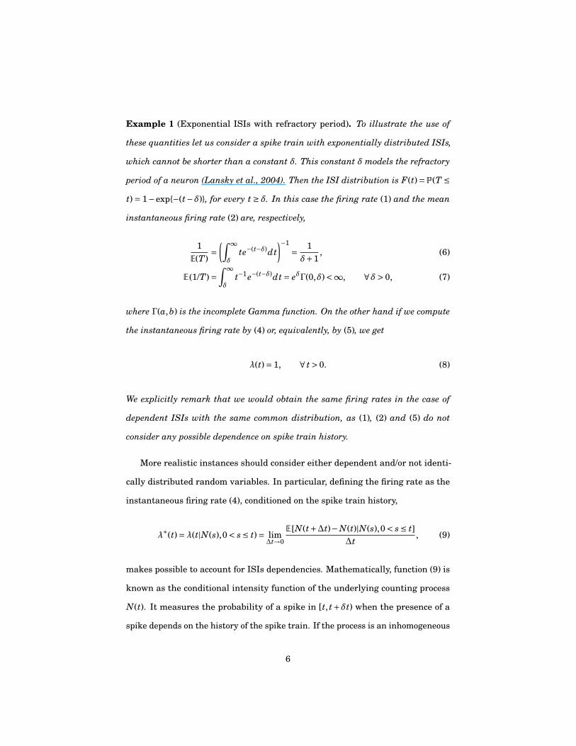
Example 1 (Exponential ISIs with refractory period). To illustrate the use of

these quantities let us consider a spike train with exponentially distributed ISIs,

which cannot be shorter than a constant δ. This constant δ models the refractory

period of a neuron (Lansky et al., 2004). Then the ISI distribution is F(t)=P(T ≤t) = 1−exp{−(t−δ)}, for every t ≥ δ. In this case the firing rate (1) and the mean

instantaneous firing rate (2) are, respectively,

1E(T)

=(∫ ∞

δte−(t−δ)dt

)−1= 1δ+1

, (6)

E (1/T)=∫ ∞

δt−1e−(t−δ)dt = eδΓ(0,δ)<∞, ∀δ> 0, (7)

where Γ(a,b) is the incomplete Gamma function. On the other hand if we compute

the instantaneous firing rate by (4) or, equivalently, by (5), we get

λ(t)= 1, ∀ t > 0. (8)

We explicitly remark that we would obtain the same firing rates in the case of

dependent ISIs with the same common distribution, as (1), (2) and (5) do not

consider any possible dependence on spike train history.

More realistic instances should consider either dependent and/or not identi-

cally distributed random variables. In particular, defining the firing rate as the

instantaneous firing rate (4), conditioned on the spike train history,

λ∗(t)=λ(t|N(s),0< s ≤ t)= lim∆t→0

E [N(t+∆t)−N(t)|N(s),0< s ≤ t]∆t

, (9)

makes possible to account for ISIs dependencies. Mathematically, function (9) is

known as the conditional intensity function of the underlying counting process

N(t). It measures the probability of a spike in [t, t+δt) when the presence of a

spike depends on the history of the spike train. If the process is an inhomogeneous

6

Poisson process, λ∗(t) coincides with the rate of the process. It can also be defined

in terms of the ISIs Ti, i ≥ 1 given the past sequence of the ISIs {T j} j=1,...,(i−1).

Consider a fixed time interval [0,L], 0< L <∞ and denote by l1, l2, . . . , lN(L) the

ordered set of the firing epochs until time L. Then the ISIs sequence can be

expressed as {Ti = l i − l i−1, i ≥ 1, l0 = 0} and the conditional probability density is

f i(t|T j, j = 1, . . . , i−1)= ddtP(Ti ≤ t|T j, j = 1, . . . , i−1). (10)

It is now possible to introduce the alternative definition (Daley & Vere-Jones,

1988, Section 7.2),

λ∗(t)=

h(t), 0< t ≤ l1,

hi(t− l i−1|T j, j = 1, . . . , i−1), l i−1 < t ≤ l i, i ≥ 2.(11)

This definition can be proven equivalent to (9). Here the functions

h(t)=− ddt

ln[S(t)]= f (t)S(t)

, (12a)

hi(t|T j, j = 1, . . . , i−1)=− ddt

ln[Si(t|T j, j = 1, . . . , i−1)

]= f i(t|T j, j = 1, . . . , i−1)

Si(t|T j, j = 1, . . . , i−1), i ≥ 2, (12b)

are the ISI hazard rate function and the conditional ISI hazard rate function,

respectively. Furthermore, S(t) = 1−P(T ≤ t) = 1− ∫ t0 f (s)ds and Si(t|T j, j =

1, . . . , i−1)= 1−P(Ti ≤ t|T j, j = 1, . . . , i−1)= 1−∫ t0 f i(s|T j, j = 1, . . . , i−1)ds are the

corresponding survival functions.

Example 2 (Exponential ISIs with refractory period II). Let us reconsider the

example with exponential ISIs in presence of a refractory period. It is obvious

7

that the conditional instantaneous firing rate coincides with the unconditional

instantaneous firing rate (8) when we have independent ISIs.

Then let us assume the presence of dependence between ISIs. Avoiding any

attempt to give a biological significance to our example let us here hypothesize that

• the ISI sequence is Markov, i.e. in (11), we have hi(t−l i−1|T j, j = 1, . . . , i−1)=hi(t− l i−1|Ti−1).

• the ISIs Ti and Ti+1, i ≥ 1, are dependent with joint distribution function

P(Ti ≤ τ,Ti+1 ≤ϑ)= F(τ)F(ϑ){1+ [1−F(τ)][1−F(ϑ)]},

where τ,ϑ> 0, F(t)=P(T ≤ t).

If we compute the conditional instantaneous firing rate (9), according to equation

(11), we get λ∗(t)= 1 for δ< t ≤ l1, λ∗(t)= 0, for 0< t ≤ δ, and

λ∗(t)=

0, l i−1 < t ≤ l i−1 +δ,

1+(1−2e−(t−l i−1−δ))(1−2e−(Ti−1−δ))2−e−(t−l i−1−δ)−2e−(Ti−1−δ)+2e−(t−l i−1−2δ+Ti−1) , l i−1 +δ< t ≤ l i,

(13)

with i ≥ 2. Despite the exponential distribution of the ISIs, we note that dependent

ISIs determine a time dependent instantaneous firing rate (see Fig. 1 for an example;

in blue, for comparison, the instantaneous firing rate (4)).

With the aid of this example, we realize that time-depending instantaneous

firing rates can be associated either to non stationarity of the increments of N(t)

or to an underlying dependence structure of the ISIs.

The estimation of the firing rate makes use of the observed ISIs or of the

observed counting process. Usually the estimators

1/T = n/n∑

i=1Ti, (14)

8

0 2 4 6 8 10

0.0

1.0

2.0

t

firi

ng

rate

0 2 4 6 8 10

0.0

1.0

2.0

t

firi

ng

rate

0 2 4 6 8 10

0.0

1.0

2.0

t

firi

ng

rate

0 2 4 6 8 10

0.0

1.0

2.0

t

firi

ng

rate

0 2 4 6 8 10

0.0

1.0

2.0

t

firi

ng

rate

0 2 4 6 8 10

0.0

1.0

2.0

t

firi

ng

rate

0 2 4 6 8 10

0.0

1.0

2.0

t

firi

ng

rate

0 2 4 6 8 10

0.0

1.0

2.0

t

firi

ng

rate

0 2 4 6 8 10

0.0

1.0

2.0

t

firi

ng

rate

0 2 4 6 8 10

0.0

1.0

2.0

t

firi

ng

rate

0 2 4 6 8 10

0.0

1.0

2.0

t

firi

ng

rate

0 2 4 6 8 10

0.0

1.0

2.0

t

firi

ng

rate

0 2 4 6 8 10

0.0

1.0

2.0

t

firi

ng

rate

c. fi

ring

rate

Figure 1: A realization of the theoretical conditional instantaneous firing rate (13)(black) together with the corresponding instantaneous firing rate (4) (grey). Herethe parameters are fixed at (λ,δ) = (1,0.5) and the recorded ISIs are indicatedby successive dashed vertical lines. Note that the conditional instantaneousfiring rate is updated after each recorded spike. Except the initial period of timeafter each spike where the conditional instantaneous firing rate is zero (due topresence of refractoriness through the parameter δ), in general it is not constant.In order to clarify the contribution of the dependence between consecutive ISIsto the behaviour of the conditional instantaneous firing rate, note that after avery short ISI (such as the one starting right after time t = 4) the conditionalinstantaneous firing rate becomes very high (after the time lapse δ during whichis zero). Viceversa, the ISI recorded around time t = 6, which is quite long,implies a succeding low conditional instantaneous firing rate. Furthermore noticehow the conditional instantaneous firing rate exhibits a relaxation towards theinstantaneous firing rate (grey) as time passes (see for instance the ISI startingaround t = 1). This is connected to the fact that memory (dependence) is less andless important as time flows.

9

1/T = 1n

n∑i=1

1Ti

, (15)

are used for the inverse of the average ISI and for the instantaneous mean firing

rate, respectively. The ratio between the number of spikes in (0, t) and t can be

used to estimate N(t)/t. While the considered estimators have a very intuitive

meaning if the ISIs are independent and identically distributed they lose their

significance for dependent or not identically distributed ISIs.

Estimation techniques for equations (5) and (11) depend upon the knowledge

of f (t) and f i(t|T j, j = 1, . . . , i−1), i = 2,3, . . . , respectively. When these densities

are given or hypothesized from data, classical parametric methods can be applied

(Kalbfleish & Prentice, 2011). Hazard rate function estimators assuming the

independence of the sample random variables have good convergence properties,

but they are not applicable to dependent neural ISIs. A contribution to the study

of the other cases is the subject of the present paper.

3 Firing rate estimation

The definition (11) of the conditional instantaneous firing rate depends on the

hazard rate functions (12a) and (12b) of the underlying ISI process. Hence our

firing rate estimation problem is strictly connected to the estimation of these

hazard rate functions.

We model the ISIs as a Markov, ergodic and stationary process. Hence the ISIs

are identically distributed random variables with shared unconditional probability

density function f (t). Furthermore, due to the Markov hypothesis, the conditional

probability density functions (10) become

f i(t|Ti−1 = τ,T j = t j, j = 1, . . . , i−2)= f i(t|Ti−1 = τ)= f (t|τ), ∀ i ≥ 1. (16)

10

Therefore the hazard rate function (12b) simplifies to

h(t|τ)= f (t|τ)S(t|τ)

, (17)

where S(t|τ)= 1−∫ t0 f (s|τ)ds is the associated conditional survival function.

In order to estimate the instantaneous conditional firing rate (11) we propose

the following non-parametric estimator for the ISI conditional hazard rate function

(17):

hn(t|τ)= fn(t|τ)Sn(t|τ)

, (18)

where Sn(t|τ)= 1−∫ t0 fn(s|τ)ds and (Arfi, 1998; Ould-Said, 1997)

fn(t|τ)= fn(τ, t)fn(τ)

, (19)

with

fn(τ, t)= 1nc2

n

n∑i=1

K1

(τ−Ti

cn

)K2

(t−Ti+1

cn

), (20)

fn(t)= 1ncn

n∑i=1

K1

(τ−Ti

cn

). (21)

The estimator (19) is a uniform strong consistent estimator for the ISI conditional

probability density function (10) on any compact interval [0, J]⊆R+. Here {cn} is

a sequence of positive real numbers satisfying

limn→∞ cn = 0, lim

n→∞ncn =∞, (22)

11

and K j, j = 1,2, are symmetric and real-valued kernel functions verifying

K j(t)≥ 0,∫ ∞

−∞K j(t)dt = 1, lim

|t|→∞|t|K j(t)= 0. (23)

Moreover, we assume that the kernels have bounded variation and that K1 is

strictly positive.

We do not consider the value of the instantaneous firing rate on the first ISI

because of the lack of knowledge on the preceding ISI. However, it is possible to

estimate the unconditional firing rate through

hn(t)= fn(t)Sn(t)

, (24)

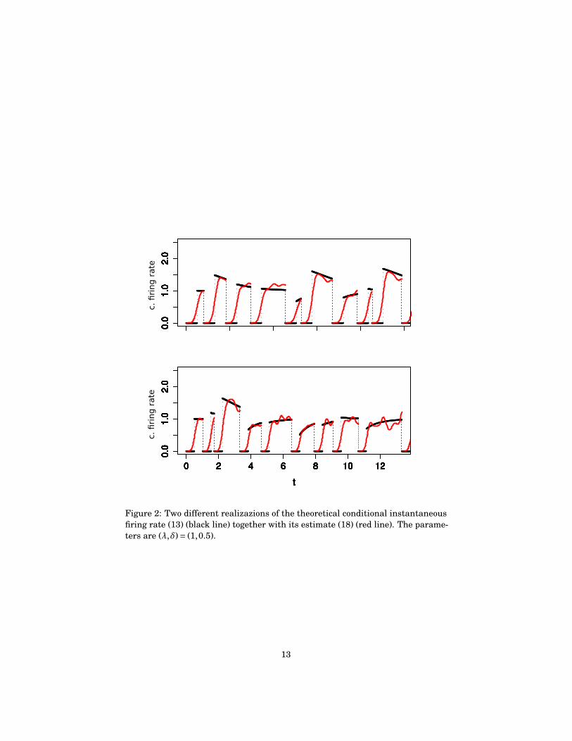
where Sn(t) = 1− ∫ t0 fn(s)ds. In Figure 2 we reconsider Example 2 for which

we compare the theoretical conditional instantaneous firing rate (13) with its

conditional estimator (18). Note furthermore that the use of (24) to estimate (12a)

in (11) is an approximation because the sampling does not start at time zero of

the theoretical model.

We have the following theorem.

Theorem 1. Let us consider a simple point process N(t) (i.e. a point process

admitting at most one single event at any time), with Markov, ergodic and station-

ary inter-event intervals Ti, i ≥ 1. Under some regularity conditions on the ISI

probability density functions and the kernels K1 and K2, for all sequences {bn}

satisfying

limn→+∞

nb4n

lnn=∞, (25)

(see Appendix C for complete details) the estimators (24) and (18) are uniform

strong consistent estimators of the hazard rate functions (12a) and (17) on [0, M],

12

0 2 4 6 8 10

0.0

1.0

2.0

t

firi

ng

rate

0 2 4 6 8 10

0.0

1.0

2.0

t

firi

ng

rate

0 2 4 6 8 10

0.0

1.0

2.0

t

firi

ng

rate

0 2 4 6 8 10

0.0

1.0

2.0

t

firi

ng

rate

0 2 4 6 8 10

0.0

1.0

2.0

t

firi

ng

rate

0 2 4 6 8 10

0.0

1.0

2.0

t

firi

ng

rate

0 2 4 6 8 10

0.0

1.0

2.0

t

firi

ng

rate

0 2 4 6 8 10

0.0

1.0

2.0

t

firi

ng

rate

0 2 4 6 8 10

0.0

1.0

2.0

t

firi

ng

rate

0 2 4 6 8 10

0.0

1.0

2.0

t

firi

ng

rate

0 2 4 6 8 10

0.0

1.0

2.0

t

firi

ng

rate

0 2 4 6 8 10

0.0

1.0

2.0

t

firi

ng

rate

0 2 4 6 8 10

0.0

1.0

2.0

t

firi

ng

rate

0 2 4 6 8 10

0.0

1.0

2.0

t

firi

ng

rate

0 2 4 6 8 10

0.0

1.0

2.0

t

firi

ng

rate

0 2 4 6 8 10

0.0

1.0

2.0

t

firi

ng

rate

0 2 4 6 8 10

0.0

1.0

2.0

t

firi

ng

rate

0 2 4 6 8 10

0.0

1.0

2.0

t

firi

ng

rate

0 2 4 6 8 10

0.0

1.0

2.0

t

firi

ng

rate

0 2 4 6 8 10

0.0

1.0

2.0

t

firi

ng

rate

0 2 4 6 8 10

0.0

1.0

2.0

t

firi

ng

rate

0 2 4 6 8 10

0.0

1.0

2.0

t

firi

ng

rate

0 2 4 6 8 10

0.0

1.0

2.0

t

firi

ng

rate

0 2 4 6 8 10

0.0

1.0

2.0

t

firi

ng

rate

c. fi

ring r

ate

0 2 4 6 8 10 12

0.0

1.0

2.0

t

firi

ng

rate

0 2 4 6 8 10 12

0.0

1.0

2.0

t

firi

ng

rate

0 2 4 6 8 10 12

0.0

1.0

2.0

t

firi

ng

rate

0 2 4 6 8 10 12

0.0

1.0

2.0

t

firi

ng

rate

0 2 4 6 8 10 12

0.0

1.0

2.0

t

firi

ng

rate

0 2 4 6 8 10 12

0.0

1.0

2.0

t

firi

ng

rate

0 2 4 6 8 10 12

0.0

1.0

2.0

t

firi

ng

rate

0 2 4 6 8 10 12

0.0

1.0

2.0

t

firi

ng

rate

0 2 4 6 8 10 12

0.0

1.0

2.0

t

firi

ng

rate

0 2 4 6 8 10 12

0.0

1.0

2.0

t

firi

ng

rate

0 2 4 6 8 10 12

0.0

1.0

2.0

t

firi

ng

rate

0 2 4 6 8 10 12

0.0

1.0

2.0

t

firi

ng

rate

0 2 4 6 8 10 12

0.0

1.0

2.0

t

firi

ng

rate

0 2 4 6 8 10 12

0.0

1.0

2.0

t

firi

ng

rate

0 2 4 6 8 10 12

0.0

1.0

2.0

t

firi

ng

rate

0 2 4 6 8 10 12

0.0

1.0

2.0

t

firi

ng

rate

0 2 4 6 8 10 12

0.0

1.0

2.0

t

firi

ng

rate

0 2 4 6 8 10 12

0.0

1.0

2.0

t

firi

ng

rate

0 2 4 6 8 10 12

0.0

1.0

2.0

t

firi

ng

rate

0 2 4 6 8 10 12

0.0

1.0

2.0

t

firi

ng

rate

0 2 4 6 8 10 12

0.0

1.0

2.0

t

firi

ng

rate

0 2 4 6 8 10 12

0.0

1.0

2.0

t

firi

ng

rate

0 2 4 6 8 10 12

0.0

1.0

2.0

t

firi

ng

rate

0 2 4 6 8 10 12

0.0

1.0

2.0

t

firi

ng

rate

c. fi

ring r

ate

Figure 2: Two different realizazions of the theoretical conditional instantaneousfiring rate (13) (black line) together with its estimate (18) (red line). The parame-ters are (λ,δ)= (1,0.5).

13

0< M ≤ L, i.e.

limn→+∞ sup

t∈[0,M]

∣∣hn(t)−h(t)∣∣= 0 a.s. (26)

limn→+∞ sup

(τ,t)∈[0,M]2

∣∣hn(t|τ)−h(t|τ)∣∣= 0 a.s. (27)

First, note that since on each observed bin it is impossible to record more than

a single spike, it is reasonable to model the spike train through a simple point

process. Second, an estimator for λ∗(t) can be given as

λ∗n(t)= hn(t− l i−1|Ti−1 = ti−1), l i−1 < t ≤ l i. (28)

Formula (28) holds for i = 2, . . . ,n, because for an ergodic and stationary process,

the estimation of λ∗ in the first ISI cannot be performed in the lack of knowledge

on the preceding ISI.

4 An a posteriori validation algorithm

The firing rate estimator (28) has good asymptotic properties when ISIs can be

modelled through stationary ergodic processes. Having a sample of ISIs, specific

tests of stationarity can be performed, checking the behaviour of their mean or of

higher moments or even using ad-hoc techniques as in Sacerdote & Zucca (2007).

These checks cannot garantee strong stationarity of ISIs but can help to detect

time dependences. More difficult is the check of ergodicity. This is a model feature

that cannot be tested from a single time record of ISIs. Wishing to analyzing the

reliability of the proposed estimator, we present here an a posteriori validation

algorithm. The idea of such procedure is the following. We know that, due to the

time-rescaling theorem, any simple point process with an integrable conditional

intensity function λ∗(t) may be transformed into a unit-rate Poisson process, by

the random time transformation t →Λ∗(t)= ∫ t0 λ

∗(u)du (see Appendix A for the

14

complete statement of the theorem). Hence, we perform such transformation and

we check whether the obtained point process is a unit-rate Poisson process. If we

cannot reject the Poisson characterization of the transformed process, we conclude

that our estimator is reliable, having correctly acted as a firing rate.

Formalizing, we first compute the conditional firing rate estimator λ∗n, defined

by equation (28). Then, we perform the following time transformation

t 7→ Λ∗n(t)=

∫ t

0λ∗

n(u)du. (29)

Under this time-change, the ISIs Ti = l i − l i−1, i ≥ 1 and l0 = 0, become

Ti = Λ∗n(l i)− Λ∗

n(l i−1)=∫ l i

l i−1

λ∗n(u)du, i = 1, . . . ,n. (30)

If the firing rate estimator (28) is reliable, i.e. if the hypotheses supporting its

computation are verified, the transformed ISIs (30) should be independent and

identically distributed (i.i.d.) exponential random variables with mean 1, accord-

ing to the time-rescaling theorem. Hence a way to validate our estimator on

sample data is to check the independence and exponential distribution of the

transformed ISIs.

We can perform a goodness-of-fit test to verify if the sequence {Ti, i = 1, . . . ,n}

follows the exponential distribution with mean 1. Then we can compute any

dependence index, like the correlation coefficient ρ (Spearman, 1910) or the

Kendall’s tau (Kendall, 1938), of the couples (Ti, Ti+1), i = 1, . . . ,n−1, to check

whether the successive transformed ISIs are independent.

Here we propose also another alternative test of the hypotheses on the trans-

formed ISIs, based on the concept of independent copula. Intuitively the inde-

pendent copula is the joint probability distribution of two independent uniform

random variables. It is able to fit the relationship of independence between any

15

group of independent random variables (for more details on the independent

copula, see Appendix B). If the transformed ISIs are i.i.d. exponential random

variables with mean 1, the copula of two subsequent transformed ISIs should be

the independent copula, with exponential marginals of mean 1. To verify this, we

consider the further ISI transformation, based on the exponential distribution

assumption,

Zi = 1− e−Ti . (31)

When Ti ∼ exp(1), {Zi, i ≥ 1} is a collection of i.i.d. uniform random variables on

[0,1]. Therefore, the copula of Zi and Zi+1, i = 1,2, . . . ,n, should be the indepen-

dent copula with uniform marginals. Hence, another way to verify the reliability

of (28) on the transformed ISIs is to perform a uniformity test (goodness-of-fit test

for the uniform distribution on [0,1]) and a goodness-of-fit test for the independent

copula on the collection {Zi, i ≥ 1}. In particular, we apply the goodness-of-fit test

for copulas proposed in Genest et al. (2009).

Summarizing, an a posteriori validation test for the proposed firing rate esti-

mator (28) follows this algorithm.

Algorithm 1. (Validation algorithm)

1. Estimate the firing rate through (28).

2. Compute the transformed ISIs

Ti =∫ l i

l i−1

λ∗n(u)du, i = 1,2, . . . ,n.

3. Test the hypothesis that Ti are i.i.d. exponential random variables of mean 1:

a. Apply the transformation Zi = 1− e−Ti , i = 1,2, . . . ,n, and test that these

transformed random variables are uniform on [0,1].

16

b. Perform a goodness-of-fit test for the independent copula on the couples

(Zi, Zi+1), i = 1,2, . . . ,n−1.

Note that testing that Zi, i = 1,2, . . . ,n, are i.i.d. uniform random variables

on [0,1] is equivalent to test that Ti, i = 1,2, . . . ,n, are i.i.d. exponential random

variables with mean 1, i.e. that the transformed process is a unit-rate Poisson

process.

Remark 1. In Algorithm 1 we perform a goodness-of-fit test for copulas to verify

the independence between Zi and Zi+1. However any other test of independence

can be applied, like a classical chi-squared test.

5 The stochastic two-compartment neural model

We consider here the stochastic two-compartment model proposed in Lansky &

Rodriguez (1999). It is a two-dimensional Leaky Integrate and Fire type model

that generalizes the one-dimensional Ornstein–Uhlenbeck model (Ricciardi &

Sacerdote, 1979). The introduction of the second component allows us to relax the

resetting rule of the membrane potential. In a recent paper we showed that spike

trains generated by this model exhibit dependent ISIs for suitable ranges of the

paramenters (Benedetto & Sacerdote, 2013). Here we use ISIs generated by this

model to estimate the conditional firing rate through the estimator proposed in

this paper.

In the stochastic two compartment model the neuron is described by two

interconnected compartments, modelling the membrane potential dynamics of the

dendritic tree and the soma, respectively. The dendritic component is responsible

for receiving external inputs, while the somatic component emits outputs. Hence,

external inputs reach indirectly the soma by the interconnection between the two

compartments.

17

The model is then described by a bivariate diffusion process {X(t), t ≥ 0}, whose

components X1(t) and X2(t) model the membrane potential evolution in the den-

dritic and somatic compartment, respectively. Assuming that external inputs

have intensity µ and variance σ2, the process obeys to the system of stochastic

differential equations

dX1(t)= {−αX1(t)+αr [X2(t)− X1(t)]+µ}dt+σdB(t),

dX2(t)= {−αX2(t)+αr [X1(t)− X2(t)]}dt.

(32)

Here αr accounts for the strength of the interconnection between the two compart-

ments, while α is the leakage constant that models the spontaneous membrane

potential decay in absence of inputs.

Whenever X2(t) reaches a characteristic threshold S the neuron emits an

action potential. Then X2(t) restarts from a resetting potential value that we

assume equal to zero (a shift makes always possible this choice) while X1(t) con-

tinues its evolution. The absence of dendritic resetting makes the ISIs dependent

on the past evolution of the neuron dynamics. Sensitivity analysis was applied in

Benedetto & Sacerdote (2013) to determine the model values of parameters that

make its ISIs stationary but dependent. Here we simulate samples of 1000 ISIs

from this model for different choices of the parameters, we determine the condi-

tional firing rate (11) corresponding to each choice and we check the reliability of

the obtained results by means of the algorithm proposed in the previous section.

According to the hypotheses of Theorem 1 (see Appendix C) for our study we use:

1. Gaussian kernels K1 and K2 with mean zero and standard deviation equal

to 0.2;

2. Kernel weights bn = n−β where n is the sample size and β= 0.2.

We report the results of the algorithm in Table 1. The first three cases in Table 1

18

0 5 10 15 20 25

911

1315

t

X2(t

)

0 5 10 15 20 25

02

46

8

t

X1(t)

0 5 10 15 20 25

0.0

1.0

2.0

t

firi

ng

rate

0 5 10 15 20 25

0.0

1.0

2.0

t

firi

ng

rate

0 5 10 15 20 25

0.0

1.0

2.0

t

firi

ng

rate

0 5 10 15 20 25

0.0

1.0

2.0

t

firi

ng

rate

0 5 10 15 20 25

0.0

1.0

2.0

t

firi

ng

rate

0 5 10 15 20 25

0.0

1.0

2.0

t

firi

ng

rate

0 5 10 15 20 25

0.0

1.0

2.0

t

firi

ng

rate

0 5 10 15 20 25

0.0

1.0

2.0

t

firi

ng

rate

0 5 10 15 20 25

0.0

1.0

2.0

t

firi

ng

rate

0 5 10 15 20 25

0.0

1.0

2.0

t

firi

ng

rate

0 5 10 15 20 25

0.0

1.0

2.0

t

firi

ng

rate

0 5 10 15 20 25

0.0

1.0

2.0

t

firi

ng

rate

c. fi

ring r

ate

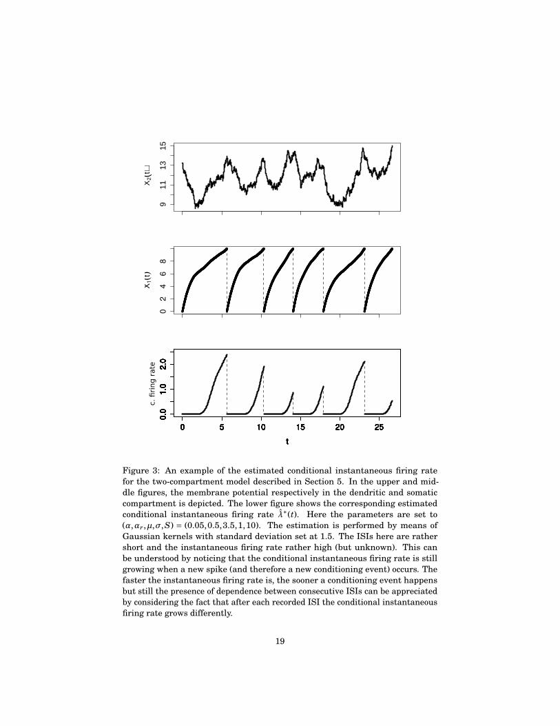
Figure 3: An example of the estimated conditional instantaneous firing ratefor the two-compartment model described in Section 5. In the upper and mid-dle figures, the membrane potential respectively in the dendritic and somaticcompartment is depicted. The lower figure shows the corresponding estimatedconditional instantaneous firing rate λ∗(t). Here the parameters are set to(α,αr,µ,σ,S) = (0.05,0.5,3.5,1,10). The estimation is performed by means ofGaussian kernels with standard deviation set at 1.5. The ISIs here are rathershort and the instantaneous firing rate rather high (but unknown). This canbe understood by noticing that the conditional instantaneous firing rate is stillgrowing when a new spike (and therefore a new conditioning event) occurs. Thefaster the instantaneous firing rate is, the sooner a conditioning event happensbut still the presence of dependence between consecutive ISIs can be appreciatedby considering the fact that after each recorded ISI the conditional instantaneousfiring rate grows differently.

19

correspond to Markov dependent ISIs as shown in Benedetto & Sacerdote (2013).

The proposed estimator cannot be safely applied in the fourth case of Table 1.

Indeed the use of algorithm of Section 4 shows that the hypotheses for its use are

not verified. In this case, successive ISIs exhibit longer memory, as suggested in

Benedetto & Sacerdote (2013). A variant of the proposed estimator can be easily

developed to account for this longer memory. For example one should consider a

rate intensity conditioned on the two previous ISIs.

Table 1: Results of the uniformity test and the copula goodness-of-fit test ofAlgorithm 1, applied on ISIs simulated by the two-compartment model (32). Inthe last case the copula goodness-of-fit test fails, as the ISI process is statisticallya Markov process of order 2. Indeed for values of µ close to the threshold S, theISIs become very short and the evolution of the two-compartment model is moredependent on its past history (see Benedetto & Sacerdote (2013) for details).

ParametersUniformity test Copula goodness-of-fit test

p-value p-valueα= 0.05, αr = 0.5,

0.88 0.97µ= 4, σ= 1, S = 10

α= 0.05, αr = 0.25,0.84 0.62

µ= 4, σ= 1, S = 10

α= 0.05, αr = 0.5,0.69 0.87

µ= 3.5, σ= 1, S = 10

α= 0.05, αr = 0.5,0.21 0.01

µ= 8, σ= 1, S = 10

6 Application to experimental data

We analyze here experimental data taken from the Internet1. This data were

recorded and discussed by Rauch et al. (2003) and correspond to single electrode

in vitro recordings from rat neocortical pyramidal cells under random in vivo-

1http://lcn.epfl.ch/∼ gerstner/QuantNeuronMod2007/

20

0 10 20 30

0.0

0.4

0.8

t

firi

ng

rate

0 10 20 30

0.0

0.4

0.8

t

firi

ng

rate

0 10 20 30

0.0

0.4

0.8

t

firi

ng

rate

0 10 20 30

0.0

0.4

0.8

t

firi

ng

rate

0 10 20 30

0.0

0.4

0.8

t

firi

ng

rate

0 10 20 30

0.0

0.4

0.8

t

firi

ng

rate

0 10 20 30

0.0

0.4

0.8

t

firi

ng

rate

0 10 20 30

0.0

0.4

0.8

t

firi

ng

rate

0 10 20 30

0.0

0.4

0.8

t

firi

ng

rate

0 10 20 30

0.0

0.4

0.8

t

firi

ng

rate

0 10 20 30

0.0

0.4

0.8

t

firi

ng

rate

0 10 20 30

0.0

0.4

0.8

t

firi

ng

rate

c. fi

ring r

ate

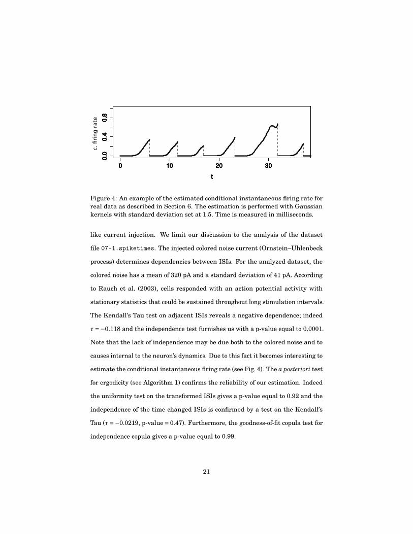
Figure 4: An example of the estimated conditional instantaneous firing rate forreal data as described in Section 6. The estimation is performed with Gaussiankernels with standard deviation set at 1.5. Time is measured in milliseconds.

like current injection. We limit our discussion to the analysis of the dataset

file 07-1.spiketimes. The injected colored noise current (Ornstein–Uhlenbeck

process) determines dependencies between ISIs. For the analyzed dataset, the

colored noise has a mean of 320 pA and a standard deviation of 41 pA. According

to Rauch et al. (2003), cells responded with an action potential activity with

stationary statistics that could be sustained throughout long stimulation intervals.

The Kendall’s Tau test on adjacent ISIs reveals a negative dependence; indeed

τ=−0.118 and the independence test furnishes us with a p-value equal to 0.0001.

Note that the lack of independence may be due both to the colored noise and to

causes internal to the neuron’s dynamics. Due to this fact it becomes interesting to

estimate the conditional instantaneous firing rate (see Fig. 4). The a posteriori test

for ergodicity (see Algorithm 1) confirms the reliability of our estimation. Indeed

the uniformity test on the transformed ISIs gives a p-value equal to 0.92 and the

independence of the time-changed ISIs is confirmed by a test on the Kendall’s

Tau (τ=−0.0219, p-value= 0.47). Furthermore, the goodness-of-fit copula test for

independence copula gives a p-value equal to 0.99.

21

7 Conclusions

The analysis of the features exhibited by recorded ISIs often ground on the study

of their statistics. The most used quantities in this framework are the firing rate

and the instantaneous firing rate. Tipically its estimation is performed assuming

that ISIs are independent despite experimental evidence on dependences between

successive ISIs. This choice may influence analysis results. Here we stressed

consequences of ignoring dependences on the the instantaneous rate estimation

and we propose a non parametric estimator for the case of ergodic stationary ISIs

with successive ISIs characterized by the Markov property. Use of such estimator

could improve data analysis. For example, in the case of in vitro recording,

the comparison of data obtained with white or colored noise could differentiate

dependences determined by the external inputs from those determined by the

internal dynamics of the neuron.

We illustrated the use of the proposed estimator on simulated and on in vitro

recorded data. Furthermore we proved its consistency property and we gave an

algorythm to check the Markov ergodic stationary hypothesis on data.

A natural extension of the proposed approach refers to data exhibiting memory

also between non contiguos ISIs. Furthermore we plan to apply the method to non

stationary data introducig their preliminary cleaning from possible periodicity or

presence of trends.

Acknowledgments

Work supported in part by University of Torino Grant 2012 Stochastic Processes

and their Applications and by project AMALFI (Università di Torino/Compagnia

di San Paolo).

22

A The time-rescaling theorem

For the sake of completeness we recall here the time-rescaling theorem that is a

well-known result in probability theory. In neuroscience it is applied for example

in Brown et al. (2001) and Gerhard et al. (2011) to develop goodness-of-fit tests for

parametric point process models of neuronal spike trains.

Theorem 2 (Time-rescaling theorem). Let N(t) be a point process admitting only

unitary jumps, with integrable conditional intensity function λ∗(t), modelling a

spike train with interspike intervals Ti = l i − l i−1, i ≥ 1, where l0 = 0 and l i, i ≥ 1,

are the spiking epochs. We define

Λ∗(t)=∫ t

0λ∗(u)du. (33)

Then, under the random time transformation t 7→Λ∗(t), the transformed process

N(t)= N(Λ∗−1(t)) is a unit-rate Poisson process.

Moreover the transformed ISIs

Ti =Λ∗(l i)−Λ∗(l i−1)=∫ l i

l i−1

λ∗(u)du,

are i.i.d. exponential random variables with mean 1, as they are waiting times of a

unit-rate Poisson process.

B Bivariate copulas

Let us consider two uniform random variables U and V on [0,1]. Assume that

they are not necessary independent. They are related by their joint distribution

function

C(u,v)=P(U ≤ u,V ≤ v). (34)

23

The function C : [0,1]× [0,1]→ [0,1] is called bivariate copula.

Consider now the marginal cumulative distribution functions FX (x)=P(X ≤ x)

and FY (y)=P(Y ≤ y) of two random variables X and Y . It is easy to check that

C(FX (x),FY (y)) (35)

defines a bivariate distribution with marginals FX (x) and FY (y).

A celebrated theorem by Sklar (1959) establishes that any bivariate distribu-

tion can be written as in (35). Furthermore, if the marginals are continuous then

the copula representation is unique (Nelsen, 1999).

Copulas contain all the information related to the dependence between the

random variables and do not involve marginal distributions. Hence, by means of

copulas we can separate the study of bivariate distributions into two parts: the

marginal behaviour and the dependency structure between the random variables.

The simplest bivariate copula is the independent copula. It is defined as

C(u,v)= uv, (u,v) ∈ [0,1]2, (36)

and it represents the joint distribution of two independent uniform random vari-

ables on [0,1].

C Complete hypotheses and proof of Theorem 1

Here we write

f i(τ, t|T j, j = 1, . . . , i−1)= d2

dτdtP(Ti+1 ≤ τ,Ti ≤ t|T j, j = 1, . . . , i−1)

for the joint conditional density function of the couple (Ti,Ti+1) given the joint past

history of an ISI and its subsequent until the couple (Ti−1,Ti). The convergence

24

properties of the estimator (18) depend on the following hypotheses.

h1. The joint densities f (τ, t) and f i(τ, t|T j, j = 1, . . . , i−1) belong to the space

C0(R2) of real-valued continuous functions on R2 approaching zero at infinity.

h2. The marginal densities f (t) and f i(t|T j, j = 1, . . . , i−1) belong to the space

C0(R) of real-valued continuous functions on R approaching zero at infinity.

h3. The conditional density functions f i(τ, t|T j, j = 1, . . . , i−1) and f i(t|T j, j =1, . . . , i−1) are Lipschitz with ratio 1,

∣∣ f i(τ, t|T j, j = 1, . . . , i−1)− f i(τ′, t′|T j, j = 1, . . . , i−1)∣∣≤ |τ−τ′|+ |t− t′| ,∣∣ f i(t|T j, j = 1, . . . , i−1)− f i(t′|T j, j = 1, . . . , i−1)

∣∣≤ |t− t′|.

h4. Let [0, M] ⊆ R+ be a compact interval. We assume that for all t in an

ε-neighbourhood [0, M]ε of [0, M] there exists γε > 0 such that f (t)> γε.

h5. The kernels K j, j = 1,2, are Hölder with ratio L<∞ and order γ ∈ [0,1],

∣∣K1(τ)−K1(τ′)∣∣≤L|τ−τ′|γ, (τ,τ′) ∈R2,∣∣K2(t)−K2(t′)∣∣≤L|t− t′|γ, (t, t′) ∈R2.

Remark 2. These assumptions are satisfied by any ergodic process with sufficiently

smooth probability density functions (see Delecroix (1987)).

To prove Theorem 1 we first recall that the estimator (21) is a uniform strong

consistent estimator for f (t) on any compact interval [0, J] ⊆ R+ (Parzen, 1962;

Rosenblatt, 1956) (see also Delecroix et al. (1992)), and then we need the following

auxiliary lemma.

25

Lemma 1. Under the hypotheses and notations of Theorem 1,

Sn(t)= 1−∫ t

0fn(s)ds, (37)

Sn(t|τ)= 1−∫ t

0fn(s|τ)ds, (38)

are uniform strong consistent estimator on [0, M] of the survival functions S(t)=1−∫ t

0 f (s)ds and S(t|τ)= 1−∫ t0 f (s|τ)ds, i.e.

limn→∞ sup

t∈[0,M]

∣∣S(t)− Sn(t)∣∣= 0, a.s. (39)

limn→∞ sup

t∈[0,M]

∣∣S(t|τ)− Sn(t|τ)∣∣= 0, a.s. (40)

Proof. We report only the proof for Sn(t), as the proof for Sn(t|τ) is analogous.

supt∈[0,M]

∣∣S(t)− Sn(t)∣∣= sup

t∈[0,M]

∣∣∣∣∫ t

0fn(s)ds−

∫ t

0f (s)ds

∣∣∣∣≤ sup

t∈[0,M]

∫ t

0

∣∣ fn(s)− f (s)∣∣ds

≤ supt∈[0,M]

∫ t

0sup

s′∈[0,M]

∣∣ fn(s′)− f (s′)∣∣ds

= sups′∈[0,M]

∣∣ fn(s′)− f (s′)∣∣ sup

t∈[0,M]

∫ t

0ds

= T sups′∈[0,M]

∣∣ fn(s′)− f (s′)∣∣ .

Finally, by applying the convergence properties of the estimator (21) (or of the

estimator (19) if we are concerned with Sn(t|τ)), we obtain the thesis.

Remark 3. Observe that S(t), S(t|τ), Sn(t) and Sn(t|τ) are bounded and strictly

positive functions on [0, M], as they are survival functions or sums of survival

functions associated to strictly positive kernel functions.

Now we have all the tools to prove Theorem 1.

26

Proof of Theorem 1. We report only the proof for the estimator hn(t), as the proof

for hn(τ|t) is analogous. Under the hypotheses h1–h5, we get

supt∈[0,M]

∣∣hn(t)−h(t)∣∣= sup

t∈[0,M]

∣∣∣∣∣ fn(t)S(t)− f (t)Sn(t)Sn(t)S(t)

∣∣∣∣∣= sup

t∈[0,M]

∣∣∣∣∣ fn(t)S(t)− f (t)S(t)+ f (t)S(t)− f (t)Sn(t)Sn(t)S(t)

∣∣∣∣∣≤ sup

t∈[0,M]

∣∣ fn(t)− f (t)∣∣∣∣Sn(t)S(t)∣∣ |S(t)|+ sup

t∈[0,M]

∣∣S(t)− Sn(t)∣∣∣∣Sn(t)S(t)

∣∣ | f (t)|

≤ supt∈[0,M]∣∣ fn(t)− f (t)

∣∣inft∈[0,M]

∣∣Sn(t)S(t)∣∣ sup

t∈[0,M]|S(t)|

+ supt∈[0,M]∣∣S(t)− Sn(t)

∣∣inft∈[0,M]

∣∣Sn(t)S(t)∣∣ sup

t∈[0,M]| f (t)|

Applying the convergence properties of the estimator (21) and Lemma 1 we get

the thesis, as S(t) and Sn(t) are bounded and strictly positive functions and

f (x) ∈ C0(R).

References

Adrian, E. (1928) The Basis of Sensation. W.W. Norton, New York.

Arfi, M. (1998) Nonparametric prediction from ergodic samples. Journal of

Nonparametric Statistics, 9, 23–37.

Benedetto, E. & Sacerdote, L. (2013) On dependency properties of the ISIs

generated by a two-compartmental neuronal model. Biological cybernetics,

107(1), 95–106.

Brown, E.N., Barbieri, R., Ventura, V., Kass, R.E. & Frank, L.M (2002) The

time rescaling theorem and its application to neural spike train data analysis.

Neural Computation, 14, 325–346.

27

Buracas, G. & Albright, T. (1999) Gauging sensory representations in the brain.

Trends Neurosci., 22, 303–309.

Burkitt, A.N. & Clark, G.M. (2000) Calculation of interspike intervals for integrate-

and-fire neurons with Poisson distribution of synaptic input. Neural Comput.,

12, 1789–1820.

Butts, D.A., Weng, C., Jin, J., et al. (2007) Temporal precision in the neural code

and the time scales of natural vision. Nature, 449 (7158), 92–5.

Cox, D.R. (1970) Renewal theory. Methuen & Co. Ltd., London.

Cox, D.D.R. & Isham, V. (1980) Point processes. Monographs on Applied Probability

and Statistics, Chapman & Hall, London-New York.

Cox, D.R. & Lewis, P.A.W. (1966) Statistical analysis of series of events. London:

Methuen.

Cunningham, J.P., Gilija V., Ryu S.I. & Shenoy K.V. (2009) Methods for estimating

neural firing rates, and their application to brain-machine interfaces. Neural

Networks, 22, 1235–1246.

Daley, D. & Vere-Jones, D. (1988) An introduction to the theory of point processes,

Vol. I Springer–Verlag, New York.

Delecroix, M. (1987) Sur l’estimation et la prévision non parametriques de proces-

sus ergodiques Thèse de Doctorat d’Etat, Université de Lille I.

Delecroix, M., Nogueira, M.E. & Martins, A.C. (1992) Sur l’estimation de la

densité d’observations ergodiques. Stat. et Anal. Données., 16, 25–38.

Engel, T.A., Schimansky-Geier, L., Herz, A.V., Schreiber, S. & Erchova, I. (2008)

Subthreshold membrane-potential resonances shape spike-train patterns in the

entorhinal cortex. Journal of neurophysiology, 100, 1576–1589.

28

Farkhooi F., Strube-Bloss M.F. & Nawrot M.P. (2009) Serial correlation in neural

spike trains: Experimental evidence, stochastic modeling, and single neuron

variability. Phys. Rev. E, 79.

Genest, C., Remillard, B. & Beaudoin, D. (2009) Goodness-of-fit tests for copulas: A

review and a power study. Insurance: Mathematics and Economics, 44, 199–214.

Gerhard, F., Haslinger, R. & Pipa, G. (2011) Applying the multivariate time-

rescaling theorem to neural population models. Neural comput., 23, 1452–1483.

Gerstner, W. & Kistler, W. (2002) Spiking Neuron Models: Single Neurons, Popu-

lations, Plasticity. Cambridge University Press, Cambridge.

Gerstner, W., Kreiter, A.K., Markram, H. & Herz, A.V. (1997) Neural codes: firing

rates and beyond. Proceedings of the National Academy of Sciences, 94(24),

12740-12741.

Iolov, A., Ditlevsen, S. & Longtin, A. (2013) Fokker-Planck and Fortet equation-

based parameter estimation for a leaky integrate-and-fire model with sinusoidal

and stochastic forcing. To appear in Journal of Mathematical Neuroscience.

Johnson, D.H. (1996) Point process models of single-neuron discharges. J. Comput.

Neurosci., 3, 275–300.

Kalbfleisch, J.D. & Prentice, R.L. (2011) The statistical analysis of failure time

data John Wiley & Sons, New York.

Kandel, E., Schwartz, J. & Jessel, T.M. (2000) Principles of Neural Science Elsevier,

New York.

Kendall, M.G. (1938) A new measure of rank correlation. Biometrika, 30, 81–93.

Kostal, L., Lansky, P. & Rospars, J.P. (2007) Neuronal coding and spiking random-

ness. European Journal of Neuroscience, 26(10), 2693–2701.

29

Kriener, B., Tetzlaff, T., Aertsen, A., Diesmann, M. & Rotter, S. (2008) Correlations

and population dynamics in cortical networks. Neural Computation, 20, 2185–

2226.

Lansky, P. & Rodriguez, R. (1999) Two-compartment stochastic model of a neuron.

Physica D, 132, 267–286.

Lansky, P., Rodriguez, R., & Sacerdote, L. (2004) Mean instantaneous firing

frequency is always higher than the firing rate. Neural computation, 16(3),

477-489.

Nelsen, R.B. (1999) An introduction to copulas. Springer, New York.

Omi T. & Shinomoto S. (2011) Optimizing time histograms for Non-Poissonian

Spike Trains. Neural Computation, 23, 12, 3125–3144.

Ould-Said, E. (1997) A Note on Ergodic Processes Prediction via Estimation of the

Conditional Mode Function. Scandinavian Journal of Statistics, 24, 231–239.

Parzen E. (1962) Estimation of a probability density-function and mode. Ann.

Math. Statist., 33, 1065–1076.

Perkel, D. & Bullock, T. (1968) Neural coding. Neurosci. Res. Prog. Sum., 3,

405–527.

Perkel, D.H., Gerstein, G.L. & Moore, G.P. (1967) Neuronal spike trains and

stochastic point processes: I. The single spike train. Biophysical journal, 7(4),

391–418.

Pipa, G., Diesmann, M. & Grün S. (2003) Significance of joint-spike events based

on trial-shuffling by efficient combinatorial methods. Complexity, 8(4), 79–86.

Rauch, A., La Camera, G., Lüscher, H.-R., Senn, W. & Fusi S. (2003) Neocortical

30

Pyramidal Cells Respond as Integrate-and-Fire Neurons to In Vivo-Like Input

Currents. Journal of Neurophysiology, 90, 1598–1612.

Ricciardi, L.M. & Sacerdote, L. (1979) The Ornstein-Uhlenbeck process as a model

for neuronal activity. Biological Cybernetics, 35, 1, 1–9.

Rieke, F., Steveninck, R., Warland, D. & Bialek, W. (1999) Spikes: Exploring the

Neural Code. MIT Press, Cambridge.

Rosenblatt, M. (1956) Remarks on some nonparametric estimates of a density

function. The Annals of Mathematical Statistics, 832-837.

Rudd, M.E. & Brown, L.G. (1997) Noise adaptation in integrate-and-fire neurons.

Neural Comput., 9, 1047–1069.

Sacerdote, L. & Zucca, C. (2007) Statistical study of the inverse first passage time

algorithm. Proc. SPIE 6603, Noise and Fluctuations in Photonics, Quantum

Optics, and Communications, 66030N.

Shimazaki H. & Shinomoto S. (2010) Kernel bandwidth optimization in spike rate

estimation. Journal of Computational Neuroscience, 29, 171–182.

Sklar, M. (1959) Fonctions de répartition à n dimensions et leurs marges Inst.

Statist. Univ. Paris Publ., 8, 229–231.

Softky, W. (1995) Simple codes versus efficient codes. Curr. Opin. Neurobiol., 5,

239–247.

Spearman, C. (1910) Correlation calculated from faulty data. British Journal of

Psychology, 3(3), 271–295.

Stein, R.B., Gossen, E.R. & Jones, K.E. (2005) Neuronal variability: noise or part

of the signal? Nat. Rev. Neurosci., 6 (5), 389–97.

31

Strong, S., Koberle, R., de Ruyter van Steveninck, R. & Bialek, W. (1998) Entropy

and information in neural spike trains. Phys. Rev. Lett., 80, 197–200.

Tamborrino, M., Ditlevsen, S. & Lansky, P. (2013) Parametric inference of neuronal

response latency in presence of a background signal. BioSystems, 112, 249–257.

Van Rullen, R. & Thorpe, S.J. (2001) Rate coding versus temporal order coding:

what the retinal ganglion cells tell the visual cortex. Neural Comput., 13,

1255–1284.

Wu, S., Amari, S. & Nakahara, H. (2002) Population coding and decoding in a

neural field: a computational study. Neural Comput., 14 (5), 999–1026.

32