TWO-SIDED CONFIDENCE INTERVALS FOR THE SINGLE ...

STATISTICS IN MEDICINE

Statist. Med. 17, 857—872 (1998)

TWO-SIDED CONFIDENCE INTERVALS FOR THE SINGLEPROPORTION: COMPARISON OF SEVEN METHODS

ROBERT G. NEWCOMBE*

Senior Lecturer in Medical Statistics, University of Wales College of Medicine, Heath Park, Cardiff CF4 4XN, U.K.

SUMMARY

Simple interval estimate methods for proportions exhibit poor coverage and can produce evidentlyinappropriate intervals. Criteria appropriate to the evaluation of various proposed methods include:closeness of the achieved coverage probability to its nominal value; whether intervals are located too close toor too distant from the middle of the scale; expected interval width; avoidance of aberrations such as limitsoutside [0, 1] or zero width intervals; and ease of use, whether by tables, software or formulae. Sevenmethods for the single proportion are evaluated on 96,000 parameter space points. Intervals based on tailareas and the simpler score methods are recommended for use. In each case, methods are available that aimto align either the minimum or the mean coverage with the nominal 1!a. ( 1998 John Wiley & Sons, Ltd.

1. INTRODUCTION

Applied statisticians have long been aware of the serious limitations of hypothesis tests when usedas the principal method of summarizing data. Following persuasion by medical statisticians, forseveral years the instructions and checklists issued by leading journals, including the BritishMedical Journal and the American Journal of Public Health, for the benefit of prospective authorshave indicated that in general confidence intervals (CIs) are preferred to p-values in the presenta-tion of results. The arguments on which this policy is based are set out by Gardner and Altman.1This shift of emphasis, albeit very welcome, presents considerable practical difficulties — these areperhaps greater than when hypothesis tests are used, because the optimization of the latter hasreceived disproportionate attention. A major advantage of confidence intervals in the presenta-tion of results is that interval estimates, in common with point estimates, are relatively close to thedata, being on the same scale of measurement, whereas the p-value is a probabilistic abstraction.According to Rothman2 (p. 121) ‘confidence intervals convey information about magnitude andprecision of effect simultaneously, keeping these two aspects of measurement closely linked’. Theusual two-sided confidence interval is thus simply interpreted as a margin of error about a pointestimate. Thus any proposed method for setting confidence intervals should be not only a priorireasonable, in terms of justifiable derivation and computed coverage probability, but also

* Correspondence to: Robert G. Newcombe, Senior Lecturer in Medical Statistics, University of Wales College ofMedicine, Heath Park, Cardiff, CF4 4XN, U.K.

CCC 0277—6715/98/080857—16$17.50 Received May 1995( 1998 John Wiley & Sons, Ltd. Revised July 1997

a posteriori reasonable, preferably for every possible set of data. However, this latter considera-tion is not always achieved. There are several ways in which this can occur, which we termaberrations; the extent of the simplest intervals may be inappropriate due to the bounded natureof the parameter space. Moreover, on account of the discrete distributional form, it is not possibleto attain exactly a preset nominal confidence level 1!a.

The present investigation concerns the simplest case, the single proportion. Among theextensive literature on this issue, Vollset3 has evaluated coverage and mean interval width forseveral methods including the seven evaluated in the present study. Complementary to Vollset’sapproach, we develop further criteria for examining performance: exactly calculated coverageprobability based on a sample of parameter space points and then summarized, including calcu-lation of mean coverage; the balance of left and right non-coverage as an indication of location; andthe incidence of various aberrations. Moreover, this approach is designed to be particularlyappropriate to related multiple parameter cases, in particular differences between proportions, forunpaired and paired data. We develop this approach largely to establish a basis for evaluatingmethods for these cases in subsequent papers.4,5 The graphical approach,3 which in the singleparameter case produces coverage curves with many discontinuities, is of very limited applicabil-ity there.

In setting a confidence interval for a single proportion p, the familiar, asymptotic Gaussianapproximation p$zIMp(1!p)/nN is often used, where n denotes the sample size and z denotesthe standard Normal deviate associated with a two-tailed probability a. As well as computationalsimplicity, this approach has the apparent advantage of producing intervals centred on the pointestimate, thus resembling those for the mean of a continuous Normal variate. However, incorpor-ating this kind of symmetry leads to two obvious defects or aberrations, namely overshoot anddegeneracy. For low proportions such as prevalences, when the numerator is small the calculatedlower limit can be below zero. Conversely, for proportions approaching one, such as thesensitivity and specificity of diagnostic or screening tests, the upper limit may exceed one. Theglaring absurdity of overshoot is readily avoided by truncating the interval to lie within [0, 1], ofcourse, but even this is not always done. And a degenerate, zero width interval (ZWI) occurs whenp"0 or 1, for any 1!a(1. Less obviously, coverage is also very poor. Use6 of a continuitycorrection (CC) 1/(2n) improves coverage and avoids degeneracy but leads to more instances ofovershoot.

These deficiencies, though well known to statisticians, are little heeded in leading journals ofmajor areas of application, as evidenced by the examples7 cited in Section 3. They may beavoided by a variety of alternative methods.

The ‘exact’ method of Clopper and Pearson8 has often been regarded as definitive; it eliminatesboth aberrations and guarantees strict conservatism, in that the coverage probability is atleast 1!a for all h with 0(h(1. It comprises all h for which precisely computed,‘exact’ aggregate tail areas are not less than a/2. Numerical values may be obtained iteratively,or by use of published tables (Lentner,9 pp. 89—102) or the F-distribution.10 Statisticalsoftware that inverts the incomplete beta function may be used, for example, SASBETAINV (1!a/2, r#1, n!r) or Minitab invcdf 1!a/2; beta r#1, n!r produce aClopper—Pearson upper limit. The Clopper—Pearson method is known to be unnecessarilyconservative. A closely related method11 uses a ‘mid-p’ enumeration of tail areas12~14 to reduceconservatism.

A likelihood-based approach15 has been suggested as theoretically most appealing,16 bydefinition it already incorporates an important aspect of symmetry about the maximum

858 R. NEWCOMBE

Statist. Med. 17, 857—872 (1998)( 1998 John Wiley & Sons, Ltd.

likelihood estimate (MLE) p. There is no question of either continuity ‘correction’ or mid-pmodification to adjust this method’s coverage properties systematically.

A computationally much simpler approach due to Wilson,17 a refinement of the simpleasymptotic method, is basically satisfactory; h is imputed its true asymptotic variance h (1!h)/nand the resulting quadratic is solved for h. This is more plausible than use of the estimatedvariance p (1!p)/n, and we proceed to show that this results in a good degree and reasonablesymmetry of coverage as well as avoidance of aberrations. It has the theoretical advantageamongst asymptotic methods of being derived from the ‘efficient score’ approach.18 It has a logitscale symmetry property (Appendix), with consequent log scale symmetry for certain derivedintervals.4 Closed-form solutions for lower and upper limits are available, both without17 andwith19 continuity correction.

2. METHODS COMPARED

Seven methods were selected for comparison. All are designed to produce two-sided intervals,whenever this is possible given the data; they are constructed so as to try to align lower and uppertail probabilities symmetrically with a/2. Only methods 1 and 2 can produce limits outside [0, 1]which are then truncated:

1. Simple asymptotic method (‘Wald method’ in Vollset3) without continuity correction:p$zI(pq/n), where z is the 1!a/2 point of the standard Normal distribution, andq"1!p.

2. Asymptotic method with continuity correction:6

p$(zI(pq/n)#1/(2n)).

3. Wilson17 ‘score’ method using asymptotic variance h (1!h)/n and solving for h; no continu-ity correction:

(2np#z2$zI(z2#4npq))/2(n#z2).

4. Score method incorporating continuity correction.6,19 The interval consists of all h suchthat Dp!hD!1/(2n))zIMh(1!h)/nN. Expressions for the lower and upper limits ¸ andº in closed form are available:

¸"

2np#z2!1!zIMz2!2!1/n#4p (nq#1)N2(n#z2)

º"

2np#z2#1#zIMz2#2!1/n#4p (nq!1)N2(n#z2)

.

However, if p"0, ¸ must be taken as 0; if p"1, º is then 1.5. Method using ‘exact’ binomial tail areas;8 the interval is [¸, º], with ¸)p)º, such that

for all h in the interval:

(i) if ¸)h)p

kpr# +

j : r:j)n

pj*a/2,

TWO-SIDED CONFIDENCE INTERVALS FOR THE SINGLE PROPORTION 859

( 1998 John Wiley & Sons, Ltd. Statist. Med. 17, 857—872 (1998)

or equivalently

+j :0)j:r

pj#(1!k)p

r)1!a/2;

(ii) if p)h)º

+j :0)j:r

pj#kp

r*a/2

respectively, where

pj"Pr[R"j]"A

n

jB hj(1!h)n~j,

j"0, 1,2, n, R denoting the random variable of which r is the realization, and k"1. Asusual an empty summation is understood to be zero.

6. Method using ‘mid-p’ binomial tail areas:11 as method 5, but with k"1/2.7. Likelihood-based method.15 The interval comprises all h satisfying

r lnh#(n!r)ln(1!h)*r ln p#(n!r) ln (1!p)!z2/2.

The above are recognized not to constitute a complete summary of the literature, but includethose methods in common use; many others have been proposed. There are several closed-formapproximations to method 5 already mentioned — the Pratt method20,21 being a very closeapproximation indeed.3 Blyth and Still6 reviewed ‘shortened’ intervals, defined to be the shortestintervals that ensure strict conservatism, and hence reduce the excess conservatism of method 5.Use22 of method 6 when r"0 or n slightly reduces the conservatism of method 5, in effect byexpending the whole of a in a one-sided way, and conversely, reverses the anti-conservatism ofmethod 7.

All the above methods are equivariant;6 limits for (n!r)/n are complements of those for r/n.Alternative methods23 based on the Poisson distribution are sometimes used if r;n; suitabletables are available for constructing ‘exact’ (Lentner,9 pp. 152 and 154) and mid-p24 intervals. Inthis situation methods 5 and 6 are often computationally unfeasible, if n is very large, or if theproportion and its denominator are available only in rounded form. However, Poisson intervalsare wider, by a factor of approximately 1/Iq, than those based on the binomial distribution,hence unnecessarily conservative; moreover, they are not equivariant. Methods 3 and 4 do nothave these drawbacks, and are thus preferable, but use of Poisson intervals is unavoidable forrates per person-year of risk.

Bayesian limits consisting of a/2 and 1!a/2 quantiles of the posterior distribution for h, forsuitably uninformative priors (b (!1, !1) or b(0, 0)) are also available.25 They are not evaluatedhere, because the criteria employed, relating to coverage, are not germane to the Bayesianparadigm.

3. ILLUSTRATIVE EXAMPLES

Table I gives 95 per cent confidence intervals for four chosen, illustrative combinations of n andr calculated by the seven methods.

For p"81/26326 one would clearly expect crude methods to perform reasonably. All of themethods yield very similar intervals. The other three examples are taken from Turnbull et al.7 For15/148 the relatively low r and p mean that choice of method starts to be more critical. The last

860 R. NEWCOMBE


Table I. 95 per cent confidence intervals for selected combinations of n and r, calculated using sevenmethods. Asterisked values demonstrate aberrations (directly calculated limits outside [0, 1], or zero-width

interval)

n 263 148 20 29Method r 81 15 0 1

Simple asymptotic1 Without CC 0)2522, 0)3638 0)0527, 0)1500 0)0000, 0)0000* (0)0000*, 0)10092 With CC 0)2503, 0)3657 0)0494, 0)1534 (0)0000*, 0)0250 (0)0000*, 0)1181

Score method3 Without CC 0)2553, 0)3662 0)0624, 0)1605 0)0000, 0)1611 0)0061, 0)17184 With CC 0)2535, 0)3682 0)0598, 0)1644 0)0000, 0)2005 0)0018, 0)1963

Binomial-based5 ‘Exact’ 0)2527, 0)3676 0)0578, 0)1617 0)0000, 0)1684 0)0009, 0)17766 Mid-p 0)2544, 0)3658 0)0601, 0)1581 0)0000, 0)1391 0)0017, 0)1585

Likelihood-based7 0)2542, 0)3655 0)0596, 0)1567 0)0000, 0)0916 0)0020, 0)1432

CC: continuity correction

two cases, 0/20 and 1/29, are clearly ones in which choice of method is very important. Method2 violates the boundary at 0. So does method 1, when r"1, but not when r"0 — but the resultingdegenerate interval is perhaps even less appropriate for interpretation as a margin of error.

It is noteworthy that, irrespective of whether such aberrations occur, the binomial-basedmethods 6 and 5 produce intervals shifted closer to 0)5, relative to their asymptotic counterparts,1 and 2, which are constructed symmetrically about the point estimate p. This applies even whenthere is little obvious difference in interval width. Often in such a situation, though two-sidedlimits are given, it is the upper one that is paid the most attention, as a kind of upper limit onprevalence. It is of concern if this is too low and hence provides false reassurance. Accordingly,and in line with Rothman’s description2 of confidence intervals quoted in Section 1, we regardinterval location as of great importance.

4. CRITERIA FOR EVALUATION

It must first be decided what are appropriate criteria by which to evaluate competing methods.The issue of coverage probability, conservatism and interval width is crucial. A confidenceinterval method is strictly conservative if for all h, the coverage probability CP*1!a.The ‘exact’ method8 seeks to align min CP with 1!a, and does so, for reasons set out byAngus.27 Alternatively, a method may be regarded as conservative on average if

CP":CP(h) df (h)*1!a for some density function f (h) for h: one may seek to align CP with1!a. A criterion of strict conservatism certainly removes the need to make an essentiallyarbitrary choice for the psuedo-prior f. It also has connotations of ‘playing safe’, but this isarguably fallacious. Any probability is merely an average of ones and zeros in any case; given thetrue proportion h, sometimes the interval computed from the data, [¸, º], includes h, sometimes



it does not, and the coverage probability is the average of ones and zeros imputed in these cases,weighted by their probabilities given h. While it is of some interest to examine min

0:h:1CP,27,28

either for chosen n or for all n, in that a value;1!a should be regarded as contraindicating themethod, nevertheless to average a CP further, over a pseudo-prior f, or a series of representativepoints in the (n, h) space sampled accordingly, does no harm, and is arguably more appropriate. Ifit is intended that the nominal 1!a should represent a minimum, methods that are strictlyconservative, but with CPs as little above 1!a as possible, should be chosen. If 1!a is

construed as an average, CP should approximate to 1!a — ideally a little over 1!a, withmin CP a little under 1!a. For any n, and any interval (h

1, h

2) representing a plausible degree of

prior uncertainty for h, CP should be a little over 1!a. These two stances lead to differentchoices of interval, given that CP depends on h in a discontinuous manner and accordingly showswide variation. Vollset3 regarded the very occasional dips in coverage below 1!a, which occurwhen the score method with continuity correction is used, as tolerable within the min CP*1!acriterion.

The Clopper—Pearson method is frequently labelled ‘exact’. This epithet conveys connota-tions of ideal, ‘gold standard’ status, so that other methods have been designed to approximateto it20,21,29~31 or have been evaluated relative to it.3,27 Any term used in antithesis to ‘exact’risks being construed as pejorative. (In the same way, a continuity ‘correction’ may be morereasonably termed a continuity adjustment; the former term begs the issue of whether theadjustment will be beneficial.) Nevertheless ‘exact’ can be used to convey several differentmeanings:

(i) Strictly conservative.(ii) Use of a multiplier 1 for the probability of the outcome observed, as well as those beyond

it, by contrast to the ‘mid-p’ approach, in which the probability of the observed outcomeappears with a coefficient 1/2 in the tail probability.

(iii) Being based on precise enumeration of an assumed underlying probability distribution,such as the binomial or Poisson, not on any asymptotic approximation involving use ofa standard error.

(iv) Attaining a CP equal to the nominal 1!a for all h (and n) constituting the parameterspace.

Both the Clopper—Pearson method and its ‘mid-p’ counterpart are exact in sense (iii), but only theformer is exact in senses (ii) and (iii). No method can achieve exactness in sense (iv), on account ofthe discontinuous behaviour of the coverage probability as h moves past the lower or upper limitcorresponding to any possible r"0, 1,2 , n. Yet this is the sense that consumers of informationpresented in CI form are likely to expect it will imply. Analogously, the Fisher test for the 2]2contingency table is ‘exact’ in senses (i) to (iii), yet one direct consequence of its strict conservatismis an attained a that is too low, for almost all parameter values. Angus,27 pointing out that ‘thetwo-sided Clopper—Pearson interval is not ‘exact’’, is using the term in sense (iv), though thisusage is rare in the literature. Angus and Schafer28 ‘make no claims for the optimality of theClopper—Pearson two-sided CI’. Vollset3 argues that the continuity-corrected score method maybe preferable to the Clopper—Pearson method.

In some,6 but not all evaluations, it is made explicit whether the nominal coverage probabilityis intended to be a minimum or an average over the parameter space. The incidences of suchaberrations as degeneracy and overshoot have not attracted much attention — in the latter case,perhaps because truncation is an obvious (though unsatisfactory) remedy.

862 R. NEWCOMBE


Evaluations are sometimes restricted to ‘round’ n and values of h which may be rational withsmall ‘round’ denominators which are far from coprime to n. For example, Ghosh32 consideredn"15, 20, 30, 50, 100 and 200; h"0)01, 0)05, 0)1, 0)2,2 , 0)9, 0)95 and 0)99. The discrete natureof R causes the coverage probabilities to vary discontinuously as h alters, therefore such choicesfor n and h may be atypical and hence inappropriate.

Furthermore, in constructing a 100(1!a) per cent confidence interval (¸, º) for any parameterh, the intention that coverage should be 1!a imposes only one constraint on the choice of ¸and º. A family of intervals (¸j, ºj) may be constructed, indexed by a parameter j, 0) j)1,where j

1(j

2implies ¸j1

(¸j2and ºj1

(ºj2, and j"0 and j"1 correspond to one-tailed 100(1!a) per cent intervals. One criterion33,34 for choice among such intervals isminimization of width, which has an appealing interpretation as an integral of the probabilityof including false values.35 An alternative criterion14,11 is equalization of tail probabilities.The two criteria lead to the same choice for interval estimation of the mean of a Normaldistribution, but not necessarily in other contexts. The quotation from Rothman2 (Section 1)suggests that as a prerequisite to meaningful interpretation interval location is as importantas width, and arguably should not be left to follow as an indirect consequence of minimizationof width. Nevertheless hitherto evidence on left and right non-coverage separately has beenlacking.

Evaluation of equivariant methods may be restricted to h between 0 and 0)5, without loss ofgenerality, permitting a more pertinent assessment of symmetry of coverage. If h has a symmetri-cal distribution on [0, 1], the true left and right non-coverage probabilities are necessarily equal;comparing them cannot help to assess performance. When the distribution of h is restricted to[0, 0)5], and the attained left and right non-coverage probabilities are enumerated separately,they are interpretable as distal and mesial non-coverage probabilities (DNCP and MNCP),respectively. It is desirable that these should be equal, otherwise the method is regarded asproducing intervals that are either too close to 0)5 or (arguably more seriously) too far from 0)5.Likewise, violations of the nearby and remote boundaries at 0 and 1 are to be enumeratedseparately.

Vollset3 presented graphs showing the relationship of CP to h for n"10, 100 and 1000 forseveral methods including those evaluated here, but did not attempt to assess mean coverageproperties. Closed-form expressions for mean CP, DNCP and MNCP for a given conjugate priordistribution for h may be obtained as weighted sums of incomplete beta integrals. An alternativeapproach is adopted here: parameter space points are sampled from a suitable pseudo-prior,permitting assessment of both average and extreme coverage properties.

Complementary to average coverage is average width. This may be computed for a given h,averaging the widths of intervals for r"0, 1,2, n according to their probabilities given h, oraveraged further with respect to a pseudo-prior f (h). It is desirable to achieve the requiredcoverage with the least width.

Meaningful evaluation of average width presupposes truncation of any overshoot. Intervalwidth is not invariant under monotone transformation, and furthermore its direct application toinherently asymmetrical, right-unbounded measures such as the rate ratio, the odds ratio or thePoisson parameter would be problematic, but these points do not invalidate its use for the singleproportion, nor for differences between proportions. According to the mid-p criterion, the degreeto which an interval method’s CP exceeds 1!a may be regarded as an expression of unnecessarywidth, but that does not make CP a measure of width. For example, with n"5 and h&U(0, 1),methods 2 and 3 have similar mean widths for 95 per cent intervals, 0)562 and 0)558, but very



different mean coverages, 0)815 and 0)955, respectively; the score method produces more appro-priately located intervals and thus expends its width more effectively.

Overshoot, the violation of the boundaries inherent to the problem (0 and 1), incurs a seriousrisk of its transmission, unchecked, along the publication chain.7 This can always be coped withby truncation, or equivalently by careful specification of algorithms in inequality form so as toavoid it, but that obscures the nature of the problem. Thus for r"1, the method 1 lower limit isgenerally negative and would be truncated to 0, but h"0 is ruled out by the data,Pr[R*1Dh"0]"0. Closely adjoining parameter values are also highly implausible: for h"e/n,Pr[R*1 D h]:e, which can be made arbitrarily small by choice of e. To be plausible the lowerlimit needs to be positive, not zero.

5. EVALUATION OF THE SEVEN METHODS

In the main evaluation the performance of 95 per cent intervals calculated by the chosen methodswas evaluated for 96,000 representative parameter space points (PSPs), with 5)n)100and 0(h(0)5. For each n independently, 1000 unround h values were chosen randomlyfrom uniform distributions on [( j!1)/2000, j/2000], using algorithm AS183.36 This simplesampling scheme was chosen after some experimentation to give a reasonable degree of weightingtowards situations in which asymptotic behaviour would be a poor approximation. Though inmany respects it resembles a joint prior for n and h, this is not the intended interpretation— n would generally be predetermined, and what range of h would be plausible varies according tocontext — use of this pseudo-prior is merely an expedient to smooth out discontinuities andapproximate the performance that might be obtained in practice. The investigation was notoriented towards any prior partitioning of the parameter space, but a major objective was todetermine in which parts of the parameter space computationally simple methods might beacceptable. Accordingly, the relationship of coverage properties of each method to n, h and nhwas examined.

Programs were developed to generate ‘tables’ listing the seven types of CI for eachn"5, 6,2, 100. For each n and each h chosen to accompany it, the binomial probabilityPr[R"r D n, h] was generated, for each r for which it was non-negligible (using a tolerance of10~10). Probabilities of each direction of non-coverage, boundary violation and degeneracy asdescribed above were summated across all r with non-negligible probability, to give exactlycomputed measures for each chosen PSP. These were then summarized across the randomlychosen set of PSPs.

It is conceded that the minimum CP found by examining a large number of PSPs will notgenerally identify the absolute minimum over all possible parameter values. With a large numberof PSPs, the empirical minimum approaches the true minimum, for example, for method 3, thetrue minimum is 0)831. The justification for the approach is (i) mean CP is estimated essentially byMonte Carlo integration using systematic sampling, and (ii) it facilitates estimation in casesinvolving several parameters4,5 in which exact determination of min CP is possible but moredifficult.

Additionally, mean and minimum coverage probabilities for nominal 90 per cent and 99 percent intervals for the same set of 96,000 parameter space points were also calculated.

To examine coverage for proportions with large denominators but small to moderate numer-ators, as often encountered in epidemiology, 1000 parameter space points were chosen. log

10n

was sampled from U(2, 5), and the resulting n rounded to the nearest integer. Independently,

864 R. NEWCOMBE


log10

(4nh) was sampled from U(0, 2). Coverage of the resulting 95 per cent intervals wasdetermined.

The above approach was chosen as appropriate for evaluation of coverage, for which theintended value is a constant but dependence on h and consequently n also is locally highlydiscontinuous. A different approach is appropriate for evaluation of expected interval width,which is grossly dependent on n and h, but in a smooth manner. Expected interval width iscalculated exactly for 95 per cent intervals by each method, for selected combinations of n and h:here, each of n"5, 20 and 100 with h"0)5, 0)2 and 0)05. Furthermore, for each of the abovevalues of n, the expected width for h sampled from U[0, 1] is obtained directly, as thenPr[R"r]"1/(n#1) for r"0, 1,2, n.

6. RESULTS

Table II shows the mean and minimum coverage probabilities, and mean and maximum distaland mesial non-coverage probabilities, based on all 96,000 chosen parameter space points, for 95per cent intervals.

The overall average CP ranged from 0)881 (method 1) to 0)971 (methods 4 and 5). On averagemethod 2 is anti-conservative despite the continuity correction. The likelihood-based method 7 isalso slightly anti-conservative on average. Conversely methods 3 and 6 are slightly conservativeon average, with average CP close above 0)95, despite being non-CC and mid-p, respectively. Theaverage DNCP was 0)032 for method 3, and less than the nominal 0)025 for all other methods.The average MNCP was 0)101 for method 1, 0)063 for method 2, 0)029 for method 7, else (0)025.

Methods 1 and 2 produced many totally unacceptable CPs. Methods 3 and 7 are capable ofyielding CP below 0)9. Method 5 is strictly conservative, by a minute margin: for n"45,h"0)4432, we obtain DNCP"0)02494, MNCP"0)02493. Method 4 is capable of being slightlyanti-conservative, for example, n"12, h"0)0043, DNCP"0)0509, MNCP"0 (see Vollset3).

Methods 3 and 4, and to a lesser degree 5 and 6, produced intervals too close to 0)5. Conversely,method 7 produced intervals slightly too far away from 0)5.

As expected, the mean coverage of methods 1 and 2 was heavily dependent upon n, h and nh(Table III). For method 3, CP was remarkably close to being constant, with respect to each of n,

h and nh separately, and indeed jointly. Methods 4 and 5 had a conservative CP, especially for low

values of n, h and nh; cross-tabulations indicated nh was the dominant determinant of CP (though

this is not obvious from Table III). The pattern was similar for method 6, but the CP was close to0)95 when n, h or nh was large. Method 7 was slightly anti-conservative, except for low h; here h isthe dominant determinant of coverage.

Methods 3 to 7 are incapable of violating the inherent [0, 1] bounds for h. The probability ofobtaining an interval entirely within [0, 1] averaged 0)730 and 0)838 for methods 2 and1 (Table IV). The boundary violated was almost always the nearby one at 0. Some combinationsof n and h yield very high probabilities of boundary violation with these methods, in particularthe nearer boundary, though the probability of violating the distant boundary 1 can alsoapproach 0)5.

Zero width intervals can occur only with method 1, and then with probability hn#(1!h)n if0(h(1. This can take values arbitrarily close to 1, as hP0 (or 1); correspondingly, MNCP isarbitrarily close to 1. For given n, and h uniform on [0, 1], the ZWI probability is 2/(n#1);averaged over n"5 to 100, this is 0)0607.



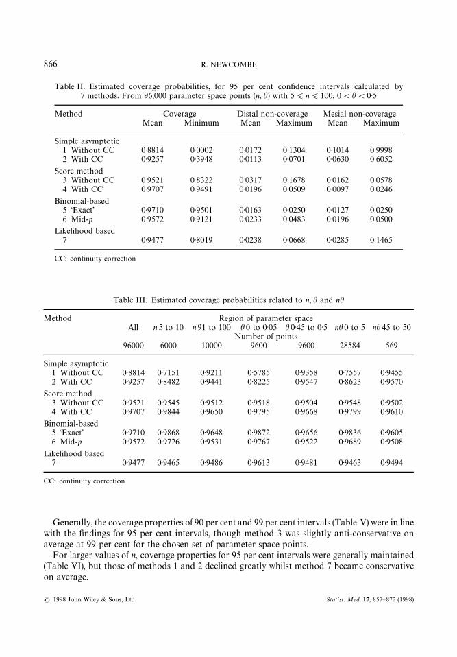
Table II. Estimated coverage probabilities, for 95 per cent confidence intervals calculated by7 methods. From 96,000 parameter space points (n, h) with 5)n)100, 0(h(0)5

Method Coverage Distal non-coverage Mesial non-coverageMean Minimum Mean Maximum Mean Maximum

Simple asymptotic1 Without CC 0)8814 0)0002 0)0172 0)1304 0)1014 0)99982 With CC 0)9257 0)3948 0)0113 0)0701 0)0630 0)6052

Score method3 Without CC 0)9521 0)8322 0)0317 0)1678 0)0162 0)05784 With CC 0)9707 0)9491 0)0196 0)0509 0)0097 0)0246

Binomial-based5 ‘Exact’ 0)9710 0)9501 0)0163 0)0250 0)0127 0)02506 Mid-p 0)9572 0)9121 0)0233 0)0483 0)0196 0)0500

Likelihood based7 0)9477 0)8019 0)0238 0)0668 0)0285 0)1465


Table III. Estimated coverage probabilities related to n, h and nh

Method Region of parameter spaceAll n 5 to 10 n 91 to 100 h 0 to 0)05 h 0)45 to 0)5 nh 0 to 5 nh 45 to 50

Number of points96000 6000 10000 9600 9600 28584 569

Simple asymptotic1 Without CC 0)8814 0)7151 0)9211 0)5785 0)9358 0)7557 0)94552 With CC 0)9257 0)8482 0)9441 0)8225 0)9547 0)8623 0)9570

Score method3 Without CC 0)9521 0)9545 0)9512 0)9518 0)9504 0)9548 0)95024 With CC 0)9707 0)9844 0)9650 0)9795 0)9668 0)9799 0)9610

Binomial-based5 ‘Exact’ 0)9710 0)9868 0)9648 0)9872 0)9656 0)9836 0)96056 Mid-p 0)9572 0)9726 0)9531 0)9767 0)9522 0)9689 0)9508

Likelihood based7 0)9477 0)9465 0)9486 0)9613 0)9481 0)9463 0)9494


Generally, the coverage properties of 90 per cent and 99 per cent intervals (Table V) were in linewith the findings for 95 per cent intervals, though method 3 was slightly anti-conservative onaverage at 99 per cent for the chosen set of parameter space points.

For larger values of n, coverage properties for 95 per cent intervals were generally maintained(Table VI), but those of methods 1 and 2 declined greatly whilst method 7 became conservativeon average.

866 R. NEWCOMBE


Table IV. Estimated probabilities of achieving an interval within [0, 1], and of directly calculated limits¸ and º violating bounds, for 95 per cent confidence intervals calculated by simple asymptotic methods.

From 96,000 parameter space points (n, h) with 5)n)100, 0(h(0)5

Method Within bounds probability Pr [¸(0] Pr [º'1]Pr [0)¸&º)1]

Mean Minimum Mean Maximum Mean Maximum

Simple asymptotic1 Without CC 0)8380 0)0625 0)1584 0)7598 0)0035 0)46832 With CC 0)7303 0)0 0)2637 1)0 0)0060 0)4995


Table V. Estimated coverage probabilities, for 90 per cent and 99 percent confidence intervals calculated by 7 methods. From 96,000 para-

meter space points (n, h) with 5)n)100, 0(h(0)5

Method 90% intervals 99% intervalsMean Minimum Mean Minimum

Simple asymptotic1 Without CC 0)8379 0)0002 0)9197 0)00022 With CC 0)8947 0)3947 0)9521 0)3948

Score method3 Without CC 0)9047 0)7909 0)9890 0)88744 With CC 0)9390 0)9009 0)9940 0)9676

Binomial-based5 ‘Exact’ 0)9384 0)9001 0)9948 0)990016 Mid-p 0)9112 0)8254 0)9921 0)9824

Likelihood based7 0)8955 0)6514 0)9896 0)9369


Variation in expected interval width for 95 per cent intervals (Table VII) between differentmethods is most marked when nh (or n(1!h)) is low. The width is then least for method 1, largelyon account of the high ZWI probability.

7. DISCUSSION

Method 1, the simplest and most widely used, is very anti-conservative on average, witharbitrarily low CP for low h. Indeed, the maximum coverage probability is only 0)959; min DNCPis 0 and min MNCP is 0)0205. In this evaluation with h(0)5, the deficient coverage probabilitystems from right non-coverage; the interval does not extend sufficiently far to the right, asevidenced by the high frequency of ZWIs and the fact that a large part of the calculated intervalmay lie beyond the nearer boundary, 0. For general h, this means the interval is positioned too farfrom 0)5 to attain symmetry in the more pertinent sense of equalizing mesial and distalnon-coverage.



Table VI. Estimated coverage probabilities, for 95per cent confidence intervals calculated by7 methods. From 1000 parameter space points

(n, h) with 100)n)100000, 0)25(nh(25

Method CoverageMean Minimum

Simple asymptotic1 Without CC 0)7279 0)22292 With CC 0)8530 0)3938

Score method3 Without CC 0)9535 0)89494 With CC 0)9731 0)9520

Binomial-based5 ‘Exact’ 0)9788 0)95076 Mid-p 0)9656 0)9165

Likelihood based7 0)9575 0)8411

Method 2, incorporating the continuity correction, is an improvement in some respects, but isstill very inadequate, also being highly anti-conservative and asymmetrical in coverage, andincurs an even higher risk of violating the nearer boundary, largely but not entirely instead of theZWIs.

Even though, for large n and mesial p (for example, for 81/263 in Table I), methods 1 and 2approximate acceptably to the better methods, it is strongly recommended that intervals cal-culated by these methods should no longer be acceptable for the scientific literature; highlytractable alternatives are available which perform much better. Use of the simple asymptoticstandard error of a proportion should be restricted to sample size planning (for which it isappropriate in any case) and introductory teaching purposes.

The average coverage probability of the score method 3 is very close to the nominal value. Forsome n and h the CP can be considerably lower — for a 95 per cent interval, as low as 0)831,occurring at h:0)18/n, and 0)89 for a nominal 99 per cent interval. Average left and rightnon-coverage probabilities are 0)032 and 0)016, thus the interval tends to be located too close to0)5 — an overcorrection of the asymmetry of method 1. However, these are its only drawbacks; it isnearly as easy to calculate as method 1, but greatly superior, and involves neither aberrations norspecial cases when r"0 or n.

The score method’s continuity-corrected counterpart, method 4, is nearly strictly conservative,with minimum coverage 0)949. Consequently the average coverage, 0)971, is quite conservative,which may be interpreted to mean the interval is simply unnecessarily wide. With distal andmesial non-coverage probabilities 0)020 and 0)010, these intervals likewise are located too closeto 0)5.

The classical Clopper—Pearson method 5, the ‘gold standard’ of the strictly conservativecriterion, has average coverage characteristics similar to method 4; again the location is slightlytoo mesial, though less so than method 4. The empirical minimum coverage and maximum mesialand distal non-coverage are practically identical to the theoretical values of 0)95 and 0)025.

868 R. NEWCOMBE


Table VII. Average width of 95 per cent confidence intervals calculated using seven methods. Selected values of n; selected values of h, andh uniform on [0, 1]

n h Simple asymptotic Score method Binomial-based Likelihood-basedNo CC CC No CC CC ‘Exact’ mid-p

1 2 3 4 5 6 7

5 0)5 0)6904 0)7904 0)6183 0)7225 0)7553 0)6981 0)66240)2 0)4414 0)5414 0)5540 0)6573 0)6720 0)6111 0)54510)05 0)1308 0)2308 0)4707 0)5733 0)5667 0)4991 0)3884

Uniform 0)4600 0)5600 0)5581 0)6616 0)6779 0)6168 0)5516

20 0)5 0)4268 0)4768 0)3927 0)4342 0)4460 0)4129 0)40760)2 0)3263 0)3659 0)3256 0)3667 0)3671 0)3362 0)32540)05 0)1225 0)1479 0)2188 0)2586 0)2380 0)2095 0)1808

Uniform 0)3160 0)3564 0)3254 0)3663 0)3661 0)3348 0)3218

100 0)5 0)1950 0)2050 0)1914 0)2010 0)2024 0)1936 0)19320)2 0)1556 0)1656 0)1543 0)1639 0)1640 0)1555 0)15450)05 0)0815 0)0896 0)0884 0)0979 0)0942 0)0867 0)0839

Uniform 0)1518 0)1614 0)1523 0)1619 0)1614 0)1531 0)1517


TW

O-S

IDE

DC

ON

FID

EN

CE

INT

ER

VA

LS

FO

RT

HE

SIN

GL

EP

RO

PO

RT

ION

869

(1998

John

Wiley

&Sons,

Ltd

.Statist.

Med.17,

857—872

(1998)

The ‘mid-p’ binomial-based method 6, with average coverage 0)957 and minimum 0)912, is

highly acceptable according to the criterion that seeks to align CP with 1!a. With average distaland mesial non-coverage probabilities 0)023 and 0)020, it is also located slightly too mesially.

The likelihood-based method 7, a ‘worthy alternative’ to method 6,15 is in fact slightlyanti-conservative, with average coverage probability 0)948. This is similar to the CP of 0)949obtained for the profile-likelihood-based unconditional CI for the paired difference of propor-tions.5 On average, distal and mesial aspects of non-coverage are reasonably closely balanced,however, for some PSPs there is considerable mesial non-coverage, up to 0)1465 which isexp (!z2/2). The minimum coverage is barely above 0)8.37

Methods 5 and 6, which were set up in terms of tail areas, thus have better total coverageproperties than method 7, which is based on the likelihood function. The same occurs for thecorresponding unconditional methods for unpaired4 and paired5 differences in proportions. Thissuggests that, generally, likelihood-based interval methods may not perform very well whenevaluated in terms of coverage. An alternative interpretation is that they should rather beregarded as leading to a different kind of interval estimate, which should be called ‘likelihoodinterval’ to distinguish it from a confidence interval (or indeed a Bayes interval).

8. CONCLUSION

Choice of method must depend on an explicit decision whether to align minimum or meancoverage with 1!a. For the conservative criterion, the Clopper—Pearson method is readilyavailable, from extensive tabulations, and also software. The Pratt closed form approximation isa very close one, but requires a programmable calculator or software. Vollset3 argues forpreferring method 4. The more complicated shortened intervals6 are less conservative than

Clopper—Pearson, and deserve to be made available in software. According to the CP"1!acriterion, method 6 performs very well; method 3 also performs well, and has the advantage ofa simple closed form, equally applicable whether n is 5 or 50 million.

The most widely-used general statistical software packages are largely oriented towardshypothesis testing and do not serve to encourage the user to present appropriate CIs forproportions or related quantities. Neither SAS nor Minitab draws attention to the availability ofClopper—Pearson intervals indirectly by using the inverse of the beta integral; SPSS providesnothing for what their authoring teams must have regarded as a trivial task. The package CIA,38designed specifically for calculating CIs, provides method 1 or 5 depending on n and r; the criteriadetermining the choice are not made clear. StatXact22 uses a hybrid of methods 5 and 6, asdescribed above. Of the methods that perform well, only the score method is calculator-friendly.Statistical package producers are strongly urged to direct users to appropriate procedures for thevery basic, but computationally non-trivial, task of setting confidence intervals for proportions.

APPENDIX: LOGIT SCALE SYMMETRY OF THE WILSON SCORE INTERVAL

The anomalous behaviour of the simple asymptotic interval is a consequence of its symmetry onthe additive scale. By imputing a variance based on h instead of p, the Wilson17 score intervalreplaces this property with a more appropriate logit scale symmetry.

The Wilson limits ¸ and º are the roots of the quadratic

Fp"h2(1#a)!h(2p#a)#p2"0

870 R. NEWCOMBE


where a"z2/n. Their product is thus ¸º"p2/(1#a). Similarly, 1!¸ and 1!º satisfyFq"0 where q"1!p, so (1!¸)(1!º)"q2/(1#a). Consequently, assuming

qO0, (¸/(1!¸))(º/(1!º ))"p2/q2, thus logit(p)!logit(¸)"logit(º)!logit(p), and the in-terval for p/q is symmetrical on a multiplicative scale. The same property applies in a nugatoryway if q or p is zero.

ACKNOWLEDGEMENTS

I thank Professor G. A. Barnard for helpful discussion of the likelihood-based method, ProfessorO. S. Miettinen for correspondence relating to Bayesian methods, and two anonymous refereesfor many helpful suggestions.

REFERENCES

1. Gardner, M. J. and Altman, D. G. (eds). Statistics with Confidence. Confidence Intervals and StatisticalGuidelines, British Medical Journal, London, 1989.

2. Rothman, K. Modern Epidemiology. Little Brown, Boston, 1986.3. Vollset, S. E. ‘Confidence intervals for a binomial proportion’, Statistics in Medicine, 12, 809—824 (1993).4. Newcombe, R. G. ‘Interval estimation for the difference between independent proportions: comparison

of eleven methods’, Statistics in Medicine, 17, 873—890 (1998).5. Newcombe, R. G. ‘Improved confidence interval methods for the difference between binomial propor-

tions based on paired data’. Submitted for publication.6. Blyth, C. R. and Still, H. A. ‘Binomial confidence intervals’, Journal of the American Statistical

Association, 78, 108—116 (1983).7. Turnbull, P. J., Stimson, G. V. and Dolan, K. A. ‘Prevalence of HIV infection among ex-prisoners in

England’, British Medical Journal, 304, 90—91 (1992).8. Clopper, C. J. and Pearson, E. S. ‘The use of confidence or fiducial limits illustrated in the case of the

binomial’, Biometrika, 26, 404—413 (1934).9. Lentner, C. (ed). Geigy Scientific ¹ables, 8th edition, volume 2, Ciba-Geigy, Basle, 1982.

10. Miettinen, O. S. ‘Estimation of relative risk from individually matched series’, Biometrics, 26, 75—86(1970).

11. Miettinen, O. S. ¹heoretical Epidemiology, Wiley, New York, 1985, pp. 120—121.12. Lancaster, H. O. ‘The combination of probabilities arising from data in discrete distributions’, Biomet-

rika, 36, 370—382 (1949).13. Stone, M. ‘The role of significance testing. Some data with a message’, Biometrika, 56, 485—493 (1969).14. Berry, G. and Armitage, P. ‘Mid-P confidence intervals: a brief review’, Statistician, 44, 417—423

(1995).15. Miettinen, O. S. and Nurminen, M. ‘Comparative analysis of two rates’, Statistics in Medicine, 4,

213—226 (1985).16. Barnard, G. A. Personal communication, 1992.17. Wilson, E. B. ‘Probable inference, the law of succession, and statistical inference’, Journal of the American

Statistical Association, 22, 209—212 (1927).18. Cox, D. R. and Hinkley, D. V. ¹heoretical Statistics, Chapman and Hall, London, 1974.19. Fleiss, J. L. Statistical Methods for Rates and Proportions, 2nd edn, Wiley, New York, 1981.20. Pratt, J. W. ‘A normal approximation for binomial, F, beta, and other common, related tail probabilities.

II’, Journal of the American Statistical Association, 63, 1457—1483 (1968).21. Blyth, C. R. ‘Approximate binomial confidence limits’, Journal of the American Statistical Association,

81, 843—855 (1986).22. Mehta, C. and Patel, N. StatXact. Statistical Software for Exact Nonparametric Inference, Version 2.

Cytel, Cambridge, MA, 1991.23. Garwood, F. ‘Fiducial limits for the Poisson distribution’, Biometrika, 28, 437—442 (1936).24. Cohen, G. R. and Yang, S. Y. ‘Mid-p confidence intervals for the Poisson expectation’, Statistics in

Medicine, 13, 2189—2203 (1994).



25. Lindley, D. V. Introduction to Probability and Statistics from a Bayesian »iewpoint. Part 2. Inference,Cambridge University Press, Cambridge, 1965, pp. 141—148.

26. Altman, D. G. Practical Statistics for Medical Research, Chapman and Hall, London, 1991, pp.161—165.27. Angus, J. E. ‘Confidence coefficient of approximate two-sided confidence intervals for the binomial

probability’, Naval Research ¸ogistics, 34, 845—851 (1987).28. Angus, J. E. and Schafer, R. E. ‘Improved confidence statements for the binomial parameter’, American

Statistician, 38, 189—191 (1984).29. Anderson, T. W. and Burstein, H. ‘Approximating the upper binomial confidence limit’, Journal of the

American Statistical Association, 62, 857—861 (1967).30. Anderson, T. W. and Burstein, H. ‘Approximating the lower binomial confidence limit’, Journal of the

American Statistical Association, 63, 1413—1415 (1968).31. Fujino, Y. ‘Approximate binomial confidence limits’, Biometrika, 67, 677—681 (1980).32. Ghosh, B. K. ‘A comparison of some approximate confidence intervals for the binomial parameter’,

Journal of the American Statistical Association, 74, 894—900 (1979).33. Kendall, M. G. and Stuart, A. ¹he Advanced ¹heory of Statistics. »olume 2. Inference and Relationship,

2nd edn, Griffin, London, 1967, pp. 101—102.34. Bickel, P. J. and Doksum, K. A. Mathematical Statistics: Basic Ideas and Selected ¹opics, Holden-Day,

San Francisco, 1977, p. 155.35. Pratt, J. W. and Gibbons, J. D. Concepts of Nonparametric ¹heory, Springer Verlag, New York, 1981.36. Wichmann, B. A. and Hill, I. D. ‘An efficient and portable pseudorandom number generator’, in

Griffiths, P. and Hill, I. D. (eds), Applied Statistics Algorithms, Ellis Horwood, Chichester, 1985.37. Newcombe, R. G. ‘Confidence intervals for a binomial proportion’, Statistics in Medicine, 13, 1283—1285

(1994).38. Gardner, M. J. Confidence Interval Analysis, British Medical Journal, London, 1989.

872 R. NEWCOMBE


* Correspondence to: Robert G. Newcombe, Senior Lecturer in Medical Statistics, University of Wales College ofMedicine, Heath Park, Cardiff CF4 4XN, U.K.

CCC 0277—6715/98/080873—18$17.50 Received May 1995( 1998 John Wiley & Sons, Ltd. Revised July 1997

STATISTICS IN MEDICINE

Statist. Med. 17, 873—890 (1998)

INTERVAL ESTIMATION FOR THE DIFFERENCEBETWEEN INDEPENDENT PROPORTIONS: COMPARISON

OF ELEVEN METHODS

ROBERT G. NEWCOMBE *

Senior Lecturer in Medical Statistics, University of Wales College of Medicine, Heath Park, Cardiff CF4 4XN, U.K.

SUMMARY

Several existing unconditional methods for setting confidence intervals for the difference between binomialproportions are evaluated. Computationally simpler methods are prone to a variety of aberrations and poorcoverage properties. The closely interrelated methods of Mee and Miettinen and Nurminen perform well butrequire a computer program. Two new approaches which also avoid aberrations are developed andevaluated. A tail area profile likelihood based method produces the best coverage properties, but is difficultto calculate for large denominators. A method combining Wilson score intervals for the two proportions tobe compared also performs well, and is readily implemented irrespective of sample size. ( 1998 John Wiley& Sons, Ltd.

1. INTRODUCTION

Interval estimation for proportions and their differences encounters two problems that cannotarise in the continuous case: intervals that do not make sense, termed aberrations; and a coverageprobability (achieved confidence level) that can be quite different to the intended nominal 1!a.Vollset1 and Newcombe2 are recent comparative evaluations of different available methods forthe single proportion.

Similar issues apply to the difference between two proportions, a particularly importantsituation, arising naturally in prospective comparative studies such as the randomized controlledclinical trial. Unfortunately, standard statistical software including Minitab, SPSS and SAS, andeven StatXact, has nothing to offer the user. Hence, by default, the computationally simplestasymptotic methods continue to be used, despite their known poor coverage characteristics andpropensity to aberrations.

Table I shows the notation adopted for the comparison of two independent binomial propor-tions. It is assumed that the denominators m and n are fixed, leading to unconditional methods.Appendix I gives methods for the ratio of two proportions, which assume a different conditioning,namely m#n fixed.

Table I. Notation for comparison of two independent proportions

Observed frequencies:Sample

1 2# a b! c d

Total m n

Theoretical proportions: Observed proportions:EA/m"n

1p1"a/m

EB/n"n2. p

2"b/n.

Here A and B denote random variables of which a and b are realizations.

Reparameterization:Parameter of interest h"n

1!n

2Nuisance parameter t"(n

1#n

2)/2.

Beal3 reviewed and evaluated several asymptotic unconditional methods — see Section 2 forexplicit formulae. All of these involve identifying the interval within which (h!hK )2)z2» (tI , hI )where hK "a/m!b/n, and »(t, h)"uM4t(1!t)!h2N#2l (1!2t)h"n

1(1!n

1)/

m#n2(1!n

2)/n is the variance of hK , u"1

4(1/m#1/n), l"1

4(1/m!1/n), and z is the standard

Normal deviate associated with a two-tailed probability a. Here tI and hI denote hypotheticalvalues of t and h. The simple asymptotic method involves substitution of MLEs, tI "tK andhI "hK . This may be improved upon in several ways using hI "h and solving for h which isanalogous to the method of Wilson4 for the single proportion. A simple alternative class ofestimators of this form involves setting hI "h and tI as a Bayes posterior estimate of t. Bealexamined two resulting methods, termed the Haldane and Jeffreys—Perks methods; both per-formed generally better than the simple asymptotic method, and of the two, that of Jeffreys—Perkswas preferable. These methods are, however, prone to certain novel anomalies, especially latentovershoot, as described later.

Beal also evaluated the closely interrelated methods of Mee5 and Miettinen and Nurminen6

which are based on, but superior to, Anbar.7 Here hI "h and tI "th, the profile estimate oft given h, that is, the MLE of t conditional on the hypothesized value of h. The form of th isdescribed in Appendix II, distinguishing the four cases NZ (no zero cells), OZ (one zero), RZ (twozeros in the same row) and DZ (two zeros on the same diagonal). The Miettinen—Nurminenmethod involves imputing to hK a variance which is (m#n)/(m#n!1) times as large as theexpression for » above. Recently Wallenstein8 published a closely related non-iterative methodwith similar coverage.

Miettinen and Nurminen also6 considered a true profile likelihood method, involvingMh: ln "(h, th)!ln "(hK , tK )*!z2/2N, where " denotes the likelihood function. They concluded itwas theoretically inferior, for reasons set out by Cox and Reid;9 it is not amenable to continuitycorrection to mitigate its anti-conservatism.

An alternative approach involving precisely computed tail probabilities based on h and th wasfound greatly superior to existing methods for the paired difference case,10 and is included in thepresent evaluation also. This approach leads naturally to consideration of a pair of methods.

SIM 779

874 R. NEWCOMBE


A so-called ‘exact’ definition of tail probabilities aims to align the minimum coverage probability(CP) with 1!a. Alternatively, ‘mid-p’ tail areas11~13 represent the attempt to achieve a meancoverage of 1!a.

The simple asymptotic method, without and with the continuity correction, and the methodsdescribed in the above four paragraphs constitute methods 1 to 9 of the 11 methods considered inthe present evaluation; in general, there is a progressive improvement in performance from thesimple asymptotic method 1 to method 9, at the cost of greatly increased computationalcomplexity. Nevertheless, the tail area profile likelihood methods 8 and 9, which are the mostcomplex of any evaluated here, but which as we will show have the best coverage and locationproperties, display a novel anomaly. Suppose a, m and the ratio p

2"b/n are held constant, while

nPR through values which keep b integer valued. We would expect that a good method fora/m!b/n would produce a sequence of intervals, each nested within its predecessor, tendingasymptotically towards some corresponding interval for the single proportion, shifted by theconstant p

2. Yet these methods give a sequence of lower limits which increase up to a certain n,

but subsequently decrease, violating the above consideration. Evaluation of just what the lowerlimit is converging towards is computationally prohibitive, but there is clearly an anomaly here.

Now, it is clear that the simple method’s asymptotic behaviour is appropriate in this respect.The anomaly can only arise because the reparameterization (h, t) leads to disregard of the factthat a/m and b/n are independently sufficient statistics for n

1and n

2, respectively. A simple

combination of single-sample intervals for a/m and b/n, which avoids the deficiencies of methods1 and 2, is thus worth considering, indeed would seem to correspond most closely to the chosenconditioning on m and n only. We may combine Wilson4 score intervals (without or withcontinuity correction) for each single proportion in much the same way as the simple method isconstructed. The resulting methods avoid all aberrations.

2. METHODS COMPARED

Eleven unconditional methods were selected for comparison. Only methods 1 to 4 are capable ofviolating the [!1, #1] boundaries, in which case the resulting interval is truncated. Methods1 to 4 and 10 to 11 involve direct computation, methods 5 to 9 are iterative, of which methods8 and 9 are the most complex. For notation see Table I, and Appendix II for the form of th:

1. Simple asymptotic method, no continuity correction:

hK $zJ(ac/m3#bd/n3).

2. Simple asymptotic method, with continuity correction (reference 14, p. 29):

hK $(zJMac/m3#bd/n3N#(1/m#1/n)/2).

3. Beal’s Haldane method:3 limits are h*$w where

h*"hK #z2l(1!2tI )

1#z2u

w"

z

1#z2uJ[uM4tI (1!tI )!hK 2N#2l (1!2tI )hK #4z2u2(1!tI )tI #z2l2(1!2tI )2]

tI "(a/m#b/n)/2, u"(1/m#1/n)/4 and l"(1/m!1/n)/4.

SIM 779

INTERVAL ESTIMATION FOR DIFFERENCE BETWEEN INDEPENDENT PROPORTIONS 875


4. Beal’s Jeffreys—Perks method:3 as above, but with

tI "1

2 Aa#0)5

m#1#

b#0)5

n#1 B.5. Method of Mee:5 the interval is

Gh: DhK !hD)zSCjG(th#h/2)(1!th!h/2)

m#

(th!h/2)(1!th#h/2)

n HDHwhere j"1.

6. Method of Miettinen and Nurminen (reference 6, equations 8 and 9 with Wilson-formvariance): as method 5, but j"(m#n)/(m#n!1).

7. True profile likelihood method (reference 6, appendix III): the interval consists of allh satisfying

a lnth#h/2

a/m#b ln

th!h/2

b/n#c ln

1!th!h/2

c/m#d ln

1!th#h/2

d/n*!

z2

2

omitting any terms corresponding to empty cells.8. Profile likelihood method based on ‘exact’ tail areas: interval is ¸)h)º such that

(i) if ¸)h)hK , kPx# +

1*m;x

Pm*a2

(ii) if hK )h)º, kPx# +

~1)m:x

Pm*a2

where Pm"Pr[A/m!B/n"mDh, th], x"a/m!b/n and k"1.9. Profile likelihood method based on ‘mid-p’ tail areas: as method 8, but with k"0)5.

10. Method based on the Wilson4 score method for the single proportion, without continuitycorrection:

¸"hK !d, º"hK #e where

d"JM(a/m!l1)2#(u

2!b/n)2N"zJMl

1(1!l

1)/m#u

2(1!u

2)/nN

e"JM(u1!a/m)2#(b/n!l

2)2N"zJMu

1(1!u

1)/m#l

2(1!l

2)/nN

l1

and u1

are the roots of Dn1!a/m D"zJMn

1(1!n

1)/mN, and l

2and u

2are the roots of

Dn2!b/n D"zJMn

2(1!n

2)/nN.

11. Method using continuity-corrected score intervals (reference 14, pp. 13—14): as method 10,but l

1and u

1delimit the interval

Mn1: Dn

1!a/m D!1/(2m))zJ[n

1(1!n

1)/m]N.

Note that if a"0, l1"0; if c"0, u

1"1. Similarly l

2and u

2delimit the interval

Mn2: Dn

2!b/n D!1/(2n))zJ[n

2(1!n

2)/n]N.

Table II shows the eleven methods applied to eight selected combinations of a, m, b and n,representing all of cases NZ, OZ, RZ and DZ. Clearly when all four cell frequencies are large, as inexample (a) (reference 14, p. 101), all methods produce rather similar intervals. Choice between

SIM 779

876 R. NEWCOMBE


Table II. 95 per cent confidence intervals for selected contrasts, calculated using eleven methods. Asterisked values denote aberrations (limits beyond $1 orinappropriately equal to hK )

ContrastMethod (a) (b) (c) (d) (e) (f ) (g) (h)

56/70—48/80 9/10—3/10 6/7—2/7 5/56—0/29 0/10—0/20 0/10—0/10 10/10—0/20 10/10—0/10

1. Asympt, no CC #0)0575, #0)3425 #0)2605, #0)9395 #0)1481, #0)9947 #0)0146, #0)1640 0)0000*, 0)0000* 0)0000*, 0)0000* #1)0000*, #1)0000 #1)0000*, #1)00002. Asympt, CC #0)0441, #0)3559 #0)1605, '#1)0000* #0)0053, '#1)0000* !0)0116, #0)1901 !0)0750, #0)0750 !0)1000, #0)1000 #0)9250, '#1)0000* #0)9000, '#1)0000*3. Haldane #0)0535, #0)3351 #0)1777, #0)8289 #0)0537, #0)8430 !0)0039, #0)1463 0)0000*, #0)0839 0)0000*, 0)0000* #0)7482, #1)0000 #0)6777, #1)00004. Jeffreys—Perks #0)0531, #0)3355 #0)1760, #0)8306 #0)0524, #0)8443 !0)0165, #0)1595 !0)0965, #0)1746 !0)1672, #0)1672 #0)7431, '#1)0000* #0)6777, #1)00005. Mee #0)0533, #0)3377 #0)1821, #0)8370 #0)0544, #0)8478 !0)0313, #0)1926 !0)1611, #0)2775 !0)2775, #0)2775 #0)7225, #1)0000 #0)6777, #1)00006. Miettinen—

Nurminen #0)0528, #0)3382 #0)1700, #0)8406 #0)0342, #0)8534 !0)0326, #0)1933 !0)1658, #0)2844 !0)2879, #0)2879 #0)7156, #1)0000 #0)6636, #1)00007. True profile #0)0547, #0)3394 #0)2055, #0)8634 #0)0760, #0)8824 #0)0080, #0)1822 !0)0916, #0)1748 !0)1748, #0)1748 #0)8252, #1)0000 #0)8169, #1)00008. ‘Exact’ #0)0529, #0)3403 #0)1393, #0)8836 !0)0104, #0)9062 !0)0302, #0)1962 !0)1684, #0)3085 !0)3085, #0)3085 #0)6915, #1)0000 #0)6631, #1)00009. ‘Mid-p’ #0)0539, #0)3393 #0)1834, #0)8640 #0)0470, #0)8840 !0)0233, #0)1868 !0)1391, #0)2589 !0)2589, #0)2589 #0)7411, #1)0000 #0)7218, #1)0000

10. Score, no CC #0)0524, #0)3339 #0)1705, #0)8090 #0)0582, #0)8062 !0)0381, #0)1926 !0)1611, #0)2775 !0)2775, #0)2775 #0)6791, #1)0000 #0)6075, #1)000011. Score, CC #0)0428, #0)3422 #0)1013, #0)8387 !0)0290, #0)8423 !0)0667, #0)2037 !0)2005, #0)3445 !0)3445, #0)3445 #0)6014, #1)0000 #0)5128, #1)0000


SIM

779

methods is more critical when the numbers are smaller, as in cases (b) to (h). The degree ofconcordance with hypothesis testing is limited, not surprisingly, as the conditioning is different:constrast (d) (Goodfield et al.,15 cited by Altman and Stepniewska16) exemplifies the anti-conservatism of methods 1 and 7, whilst (c) suggests methods 8 and 11 are conservative. Overtoverflow (see below) can occur with methods 2 and 4 and indeed also method 1. Limitsinappropriately equal to hK can occur with methods 1 and 3.

3. CRITERIA FOR EVALUATION

The present evaluation presupposes the principles set out in detail by Newcombe.2 In brief,a good method will avoid all aberrations and produce an appropriate distribution of coverageprobabilities. The coverage probability2 CP is defined as Pr[¸)h)º] where ¸ and º are thecalculated limits. The ‘exact’ criterion requires CP*1!a for all points in the parameter space,but by the smallest attainable margin. We interpret2 the ‘mid-p’ criterion to imply that for anym and n the mean coverage probability CP is to be close to but not below 1!a, and min

0:h:1CP should not be too far below 1!a, for chosen m and n or for any m and n. All methodsevaluated aim to have a/2 non-coverage at each end, except in boundary cases (hK "$1). Inrecognition of the importance of interval location we examine symmetry as well as degree ofcoverage. When, as here, all methods are equivariant,17 that is, show appropriate properties ofsymmetry about 0 when p

1and p

2are interchanged or replaced by 1!p

1or 1!p

2, equality

of left and right non-coverage as h ranges from !1 to #1 is gratuitous. It is more pertinent todistinguish probabilities of non-coverage at the mesial (closer to 0) and distal (closer to $1) endsof the interval. Here, as with the single proportion, the relationship of coverage to the parametervalue shows many discontinuities (see, for example, graphs in Vollset1). To minimize the potentialfor distortion as a result of this, h and t are randomly sampled real numbers, not rationals, andsimilarly we avoid use of selected, round values of m and n.

The ‘exactness’ claimed for any method can only relate to its mode of derivation, and does notcarry across to the achieved coverage probabilities for specific combinations of m, n, h and t. It isnecessary to evaluate these for a representative set of points in the parameter space. It is alsoimportant to examine the location of ¸ and º in relation to each other, to boundaries that shouldnot be violated (!1 and #1), and to boundaries that should be violable (that is, avoidance ofinappropriate tethering to hK , as defined below).

For any method of setting a confidence interval [¸, º] for h"n1!n

2, with ¸)hK )º, two

properties are considered desirable:

(i) Appropriate coverage and location: ¸)h)º should occur with probability 1!a and¸'h and º(h each with probability a/2.

(ii) Avoidance of aberrations, defined as follows.

Several kinds of aberrations can arise, principally point estimate tethering and overshoot. Tether-ing occurs when one or both of the calculated limits ¸ and º coincides with the point estimate hK .In the extreme case, where hK "#1, it is appropriate that º"hK , likewise that ¸"hK whenhK "!1. Otherwise this is an infringement of the principle that the CI should represent some‘margin of error’ on both sides of hK , and is counted as adverse. Bilateral point estimate tethering,¸"hK "º, constitutes a degenerate or zero-width interval (ZWI) and is always inappropriate.

Point estimate tethering can only occur in case RZ (two zeros in the same row) for methods1 and 3, and in case DZ (two zeros on the same diagonal), exemplified in Table II, contrasts (e) to

SIM 779

878 R. NEWCOMBE


(h). The Haldane method produces appropriate, unilateral tethering in case DZ. In case RZ, itproduces unilateral tethering if mOn, and a ZWI at hK "0 if m"n, both of which are inappropri-ate. Method 1 produces a totally inappropriate ZWI at 0 in case RZ, and a ZWI at#1 (or !1) incase DZ, for which unilateral tethering would be appropriate. In case DZ, the Jeffreys—Perksmethod reduces to the Haldane method if m"n, otherwise produces overt overshoot.

Overt overshoot (OO) occurs when either calculated limit is outside [!1, #1]; º"#1 is notcounted as aberrant when hK "#1, and correspondingly at !1. Methods 1 to 4 are liable toproduce OO, in which case we truncate the resulting interval to be a subset of [!1, #1];instances in which OO would otherwise occur are counted in the evaluation.

Furthermore, methods 3 and 4 substitute an estimate tI for t which is formed without referenceto h, and very often one or two of the implied parameters

nJ1L"tI #¸/2, nJ

2L"tI !¸/2, nJ

1U"tI #º/2, nJ

2U"tI !º/2

lie outside [0, 1]. This anomaly is termed latent overshoot (LO); overt overshoot always implieslatent overshoot, but latent overshoot can occur in the absence of overt overshoot, when inherentbounds for h are not violated but the bounding rhombus 1

2DhD)t)1!1

2DhD is. The formulae

still work, and do not indicate anything peculiar has occurred. In this evaluation the frequency ofoccurrence of any LO (irrespective of whether involving one or two implied parameters, and ofwhether OO also occurs) is obtained for methods 3 and 4, using the chosen a"0)05. Unlike overtovershoot, latent overshoot cannot effectively be eliminated by truncation; as well as affectingcoverage, such truncation can produce inappropriate point estimate tethering, or even an intervalthat excludes hK . Latent overshoot and its sequelae, like the inappropriate asymptotic behaviour ofmethods 8 and 9, appears a consequence of losing the simplicity of using information concerningn1

and n2

separately.

4. EVALUATION OF THE ELEVEN METHODS

The main evaluation of coverage is based on a sample of 9200 parameter space points (PSPs)(m, n, t, h), with m and n between 5 and 50 inclusive. This approach is adopted for reasons set outin a preceding article.2 The computer-intensive part of the process is the setting up of ‘tables’ ofintervals for each (m, n) pair for the iterative methods, especially 8 and 9. Therefore a subset of 230out of the 2116 possible pairs was selected (Figure 1), comprising all 46 diagonal entries withm"n, together with 92 pairs (m, n) with mOn and the corresponding reversed pairs (n, m) whichrequire the same tables. For each of m"5, 6,2, 50, two values of n were chosen, avoidingdiagonal elements, duplicates and mirror-image pairs. These were selected so that m and n shouldbe uncorrelated and that distributions of Dm!n D and the highest common factor (HCF) of m andn should be very close to those for all 2070 off-diagonal points. The rationale for examining theHCF is that when tail areas are defined in terms of a/m!b/n, the difference between ‘mid-p’ and‘exact’ limits could be great when m"n but relatively small when m and n are coprime. Theconfiguration shown, the result of an iterative search, has m and n uncorrelated (Pearson’sr"!0)00006), and Kolmogorov—Smirnov statistics for Dm!n D and HCF 0)011 and 0)012,respectively. Thus the chosen set of off-diagonal (m, n) combinations may be regarded asrepresentative, in all important respects, of all 2070 possible ones; these are used together witha deliberate over-representation of diagonal pairs, in view of their commonness of occurrence, togive a set of (m, n) pairs which may be regarded as typical.

SIM 779



Figure 1. 230 (m, n) pairs chosen for the main evaluation

For each of the 230 (m, n) pairs, 40 (t, h) pairs were chosen, with h"jM1!D2t!1 DN andt and j&º(0, 1), all sampling being random and independent using algorithm AS183.18 Thisresulted in a set of h values with median 0)193, quartiles 0)070 and 0)393. For each chosen point(m, n, t, h) of the parameter space, frequencies of all possible outcomes were determined asproducts of binomial probabilities. The achieved probability of coverage of h by nominally 95 percent confidence intervals calculated by each of the 11 methods was computed by summating allappropriate non-negligible terms. Mean coverage was also examined for subsets of the parameterspace defined according to HCF, min(m, n), minimum expected frequency, t and h in turn.Minimum coverage probabilities were also examined. Mesial and distal non-coverage rates werecomputed similarly, as were incidences of overt overshoot for methods 1 to 4, and latentovershoot at 1!a"0)95 for methods 3 and 4. Probabilities of inappropriate tethering formethods 1 and 3 were computed by examining frequencies of occurrence of cases RZ and DZ, inconjunction with whether m and n were equal. Additionally, mean and minimum coverageprobabilities for nominal 90 per cent and 99 per cent intervals for the same set of 9200 parameterspace points were calculated.

To check further the effect of restricting to the chosen (m, n) pairs, coverage of 95 per centintervals by methods 10 and 11 only was evaluated on a further set of 7544 parameter spacepoints, 4 for each of the 1886 unused (m, n) pairs, with t and h sampled as above.

A third evaluation examined the coverage of 95 per cent intervals by methods 10 and 11only, when applied to the comparison of proportions with very large denominators but smallto moderate numerators. 1000 parameter space points were chosen, with log

10m and

SIM 779

880 R. NEWCOMBE


log10

n&º (2, 5), and log10

(4mn1) and log

10(4nn

2)&º (0, 2), all sampling being independent

and random.In the first two evaluations, h is positive, and left and right non-coverage are interpreted as

mesial and distal non-coverage, respectively, with probabilities denoted here by MNCP andDNCP. Thus MNCP"+Ma,b: l'hN p

ab, and DNCP"+Ma,b: u(hN p

ab, where l and u are the cal-

culated limits corresponding to observed numerators a and b, and pab"Pr[A"a, B"b D h, t].

In the third evaluation, as in the intended application, h may be of either sign, and mesial anddistal non-coverage were imputed accordingly.

Expected interval width was calculated exactly for 95 per cent intervals by each method,truncated to lie within [!1, #1] where necessary, for n

1"n

2"0)5 or 0)01 with m and n 10 or 100.

5. RESULTS

Table III shows that in the main evaluation the coverage probability of nominal 95 per centintervals, averaged over the 9200 parameter space points, ranged from 0)881 (method 1) to 0)979(method 11). In addition to method 1, method 3 was also anti-conservative on average, andmethod 7 slightly so; method 8 was slightly conservative, whereas other methods had appropriatemean coverage rates.

The maximum CP of method 1 in this evaluation was only 0)9656; for all other methods someparameter space points have CP"1. The coverage probability of method 1 is arbitrarily close to0 in extreme cases, either MNCP can approach 1 (when t&0 or 1 and h&0) or DNCP can(when t+0)5 and h&1), due to ZWIs at 0 and 1, respectively. The continuity correction ofmethod 2, though adequate to correct the mean CP, yields an unacceptably low min CP of 0)5137in this evaluation. DNCP approaches exp(!0)5)"0)6065 with n;m but nPR, h"1

2(1/m#1/n)#e, n

1"1!e; a similar supremum applies to MNCP. The coverage of method

2 exhibited appropriate symmetry; for method 1, overall, distal non-coverage predominated inthis evaluation.

Method 3, like method 1, can have CP arbitrarily close to 0, but only DNCP can approach 1, astP1 (if m)n) or tP0 (if m*n), due to inappropriate tethering at 0. Method 4 eliminates thisdeficiency as well as the low mean CP, and reduces the preponderance of distal non-coverage.

Methods 5 and 6 have generally very similar coverage properties to each other, with overallcoverage similar to method 4. The coverage probability was only 0)8516 when m"42, n"7,t"0)9752, h"0)0253, with MNCP"0)1484, DCNP"0; substantial distal non-coverage canalso occur. These methods exhibited very good symmetry of coverage.

Coverage of method 7 was symmetrical but slightly anti-conservative on average, with minCP"0)8299 (m"48, n"23, t"0)9751, h"0)0806, MNCP"0)0344, DNCP"0)1356).Values of either DNCP or MNCP around 0)14 can occur.

Even method 8 fails to be strictly conservative, the min CP in this evaluation being 0)9424,when m"32, n"25, t"0)2640 and h"0)4016. Here both MNCP (0)0279) and DNCP (0)0297)exceed the nominal a/2; there are other parameter space points for which either exceeds 0)03. (Thiscontrasts with the performance of the analogous method for the paired case19 for which min CPwas 0)9546, and DNCP (but not MNCP) was always less than 0)025.) The lowest coverageobtained for its ‘mid-p’ analogue, method 9, was 0)9131, at m"n"8, t"0)4890, h"0)4705.Both these methods yielded symmetrical coverage.

For method 10, the lowest coverage obtained in the main evaluation was 0)8673, with m"35,n"15, t"0)5087, h"0)9645; this and other extremes arose entirely as distal non-coverage.

SIM 779



Table III. Estimated coverage probabilities for 95, 90 and 99 per cent confidence intervals calculated by 11 methods. Based on 9200 points inparameter space with 5)m)50, 5)n)50, 0(t(1 and 0(h(1!D2t!1 D

Method 95% intervals 90% intervals 99% intervalsCoverage Mesial non-coverage Distal non-coverage Coverage Coverage

Mean Minimum Mean Maximum Mean Maximum Mean Minimum Mean Minimum

1. Asympt, no CC 0)8807 0)0004 0)0417 0)7845 0)0775 0)9996 0)8322 0)0004 0)9253 0)00042. Asympt, CC 0)9623 0)5137 0)0183 0)4216 0)0194 0)4844 0)9401 0)5137 0)9811 0)5156

3. Haldane 0)9183 0)0035 0)0153 0)0656 0)0664 0)9965 0)8696 0)0035 0)9574 0)00354. Jeffreys—Perks 0)9561 0)8505 0)0140 0)0606 0)0299 0)1418 0)9123 0)7655 0)9896 0)9083

5. Mee 0)9562 0)8516 0)0207 0)1484 0)0231 0)1064 0)9076 0)8057 0)9919 0)94706. Miettinen—Nurminen 0)9584 0)8516 0)0196 0)1484 0)0220 0)1064 0)9114 0)8057 0)9925 0)9478

7. True profile 0)9454 0)8299 0)0268 0)1440 0)0278 0)1384 0)8912 0)6895 0)9893 0)9613

8. ‘Exact’ 0)9680 0)9424 0)0149 0)0308 0)0170 0)0317 0)9305 0)8862 0)9948 0)98819. ‘Mid-p’ 0)9591 0)9131 0)0197 0)04996 0)0212 0)0470 0)9116 0)8374 0)9933 0)9847

10. Score, no CC 0)9602 0)8673 0)0134 0)0660 0)0264 0)1327 0)9162 0)8226 0)9916 0)917311. Score, CC 0)9793 0)9339 0)0061 0)0271 0)0147 0)0661 0)9553 0)9012 0)9957 0)9399


SIM

779

882R

.N

EW

CO

MB

E

Statist.

Med.17,

873—890

(1998)(

1998Jo

hn

Wiley

&Sons,

Ltd

.

Table IV. Estimated coverage probabilities for 95 per cent confidence intervals calculated by 11 methods,for 9200 points in parameter space (PSPs). Determinants of coverage

Method min (m, n) min expected frequency t in range h in range5—9 30—50 0—1 5—25 (0)1 0)4—0)6 0—0)05 0)5—1

or '0)9Number of PSPs

1720 2360 3031 1875 1835 1907 1784 1422

1. Asympt, no CC 0)8063 0)9176 0)7981 0)9385 0)7416 0)9045 0)7604 0)89592. Asympt, CC 0)9470 0)9685 0)9616 0)9666 0)9665 0)9530 0)9791 0)9516

3. Haldane 0)9039 0)9276 0)8648 0)9480 0)8296 0)9474 0)8536 0)94374. Jeffreys—Perks 0)9617 0)9530 0)9649 0)9492 0)9793 0)9499 0)9782 0)9490

5. Mee 0)9602 0)9527 0)9679 0)9486 0)9732 0)9507 0)9675 0)95326. Miettinen—

Nurminen 0)9632 0)9542 0)9697 0)9505 0)9744 0)9530 0)9692 0)9553

7. True profile 0)9476 0)9460 0)9561 0)9463 0)9566 0)9440 0)9553 0)9457

8. ‘Exact’ 0)9766 0)9628 0)9833 0)9551 0)9880 0)9612 0)9798 0)96709. ‘Mid-p’ 0)9674 0)9542 0)9745 0)9489 0)9803 0)9525 0)9734 0)9566

10. Score, no CC 0)9604 0)9584 0)9737 0)9486 0)9849 0)9468 0)9751 0)949711. Score, CC 0)9837 0)9750 0)9877 0)9682 0)9950 0)9698 0)9889 0)9715


(The highest MNCP was 0)0660, but more extreme mesial non-coverage, up to 0)0998, occurredin the third evaluation with larger denominators (Table V)). MNCP can approach 0)1685,corresponding to the limiting non-coverage for the score method for the single proportion2

when h"¸1!e, n

2"e, m small, nPR, where ¸

1is the lower score limit for 1/m. Method

11 produced its lowest CP, 0)9339, when m"n"8, t"0)5160, h"0)9233, entirely fromdistal non-coverage; this compares unfavourably with 0)949 for the corresponding methodfor the single proportion.2 Both methods 10 and 11 yielded intervals erring towards mesiallocation.

Mean coverage was very similar whether m and n were equal, coprime or intermediate, exceptthat for method 3, the mean CP was 0)9225 for mOn but 0)9015 for m"n. Table IV illustratesthe relation of mean coverage probability to other parameters: the lower of the two denominatorsm and n; the lowest of the four expected frequencies mn

1, m(1!n

1), nn

2and n (1!n

2). Method 8,

11 and 6 (but not 5) were conservative on average in all zones of the parameter space examined.As expected, for most methods the mean coverage became closer to the nominal 0)95 as min(m, n)increased. Method 2 was anti-conservative for min(m, n) from 5 to 9, had mean CP 0)9628 for 10to 19, which subsequently increased slightly. Method 7’s mean coverage remained close to theoverall mean of 0)9454. Method 11 remained very conservative for the larger values of m and n inthe main evaluation.

The pattern according to minimum expected cell frequency (that is, min[mn1, m(1!n

1), nn

2,

n(1!n2)] was generally similar, but more pronounced. Methods 2 and 7 were conservative on

average even when the lowest expected frequency was under 1. For several methods whose overallmean coverage was over 0)95, the mean coverage dipped to slightly below 0)95 when all expectedfrequencies were over 5; this applies to methods 9, 10, 4 and 5, but not 6, apparently.

SIM 779



Table V. Estimated coverage probabilities for 95 per cent confidence intervals calculated by methods 10and 11. Based on 1000 points in parameter space with 100)m)100,000, 100)n)100,000, 0(t(1

and 0(h(1!D2t!1 D

Coverage Mesial non-coverage Distal non-coverageMean Minimum Mean Maximum Mean Maximum

10. Score, no CC 0)9618 0)9002 0)0265 0)0998 0)0116 0)065711. Score, CC 0)9785 0)9520 0)0153 0)0435 0)0062 0)0274


Most methods had coverage closer to 0)95 for mesial t (0)4 to 0)6) than for distal t ((0)1 or'0)9). Method 10 was slightly anti-conservative for 0)4(t(0)6, and also for h'0)5; method4 was slightly anti-conservative for 0)2(t(0)8, and for h'0)25. Conversely method 7 wasconservative on average for t outwith (0)1, 0)9) and for h(0)05.

For method 1, the preponderance of distal non-coverage was gross for t outwith (0)1, 0)9)(MNCP"0)0112, DNCP"0)2472) or h(0)05. Conversely, for large h, non-coverage waspredominantly mesial (0)5(h(1: MNCP"0)0877, DNCP"0)0164) — see examples (b) and (c)in Table II — with corresponding behaviour for mesial t. Thus when h is large, method 1 does noterr on the safe side, the interval fails to exclude values of h which are considerably too large. Forother methods, the mesial-distal location was less dependent upon h and t.

Overt overshoot was common using methods 1 (mean probability 0)0270) and 2 (0)0594), less sofor methods 3 (0)0012) and 4 (0)0052). It occurs with probability approaching 1 for method 2 ashP1, and also for method 4 provided mOn. For method 1, the maximum overshoot probabilityis lower, 0)7996, since as hP1, Pr[ZWI at 1]P1. Latent overshoot occurred with probabilityaround 0)5 for methods 3 and 4; some parameter space points produced latent overshoot withprobability 1.

The Haldane method produced unilateral point estimate tethering with probability 0)0413when mOn, and a ZWI at 0 with probability 0)0471 when m"n. Method 1 produced a ZWI at0 in both these cases, and also a ZWI at 1 with probability 0)0035. For both methods theprobability of inappropriate tethering approaches 1 as tP0 or 1.

Table III also shows coverage properties of 90 per cent and 99 per cent intervals, which wheregenerally in line with the findings for 95 per cent intervals. Method 11 was strictly conservative forthe chosen parameter space points at 90 per cent, but can be very anti-conservative at 99 per cent.The average coverage of method 4 became anti-conservative at 99 per cent.

In the second evaluation, using (m, n) pairs not included in the first, the coverage properties ofmethods 10 and 11 were virtually identical to those in the main evaluation.

In the third evaluation (Table V), with denominators ranging from 100 to 100,000, the meancoverage was very similar to the main evaluation, but the minimum CPs were more favourable,and contrastingly, the location of the interval was too distal. The lowest CP for method 10, 0)9002,resulted entirely from mesial non-coverage, with m"140, n"67622, mn

1"0)5349,

nn2"8)9480; the highest DNCP was only 0)0657. In the main evaluation, the location of these

intervals was too mesial, but this asymmetry disappeared in the zone h(0)05.Variation in expected interval width (Table VI) between different methods is most marked

when any of the expected frequencies mn1, m(1!n

1), nn

2or n (1!n

2) is low. The width is then

least for method 1 or 3, largely on account of the high frequency of degeneracy.

SIM 779

884 R. NEWCOMBE


Table VI. Average interval width for 95 per cent confidence intervals calculated by 11 methods, for selectedparameter space points

mMethod 10 10 10 100 100 100 100 100 100

n10 10 10 10 10 10 100 100 100

n1

0)01 0)5 0)95 0)01 0)5 0)95 0)01 0)5 0)95n2

0)01 0)5 0)05 0)01 0)5 0)05 0)01 0)5 0)05

1. Asympt, no CC 0)0702 0)8302 0)2407 0)0635 0)6177 0)1996 0)0493 0)2758 0)11882. Asympt, CC 0)2702 1)0296 0)3420 0)1735 0)7277 0)2618 0)0693 0)2958 0)13853. Haldane 0)0646 0)7640 0)4316 0)1819 0)5904 0)2906 0)0487 0)2732 0)12274. Jeffreys—Perks 0)3580 0)7679 0)4327 0)2624 0)5930 0)3246 0)0644 0)2732 0)12275. Mee 0)5634 0)7737 0)4224 0)3286 0)5529 0)3507 0)0888 0)2732 0)12256. Miettinen—

Nurminen 0)5840 0)7910 0)4371 0)3307 0)5549 0)3526 0)0891 0)2739 0)12287. True profile 0)3748 0)7990 0)3440 0)2233 0)5794 0)2871 0)0664 0)2745 0)11948. ‘Exact’ 0)6298 0)8801 0)4661 0)3372 0)5885 0)3541 0)0919 0)2840 0)12969. ‘Mid-p’ 0)5324 0)8128 0)4075 0)2978 0)5803 0)3384 0)0800 0)2749 0)1214

10. Score, no CC 0)5627 0)7231 0)4773 0)3289 0)5430 0)3522 0)0895 0)2707 0)126411. Score, CC 0)6945 0)8232 0)5744 0)4036 0)6121 0)4213 0)1061 0)2843 0)1398


6. DISCUSSION

As for the single proportion, the only virtue of the simple asymptotic method is simplicity; thealignment of its coverage with 1!a is merely nominal, an attribute of its method of construction,quite divorced from its attained coverage properties. Overt overshoot and inappropriate tether-ing are common, and coverage not symmetric.

Method 2 is a great improvement in terms of degree and symmetry of coverage, but theminimum coverage remains poor, and the improved mean coverage is attained at the cost of a stillhigher overshoot rate.

The Haldane and Jeffreys—Perks methods (3 and 4) attempt to overcome these deficiencieswhile maintaining closed-form tractability. The Haldane method suffers from poor mean andminimum coverage rates, severe asymmetry and proneness to aberrations. The Jeffreys—Perksmethod is a clear improvement, but still inadequate.

Methods 5 to 11 cannot produce any of the aberrations listed in Table V. The Mee andMiettinen—Nurminen methods (5 and 6) show slightly conservative mean coverage probability.Method 7, described6 as theoretically and empirically somewhat inferior to method 6, is slightlyanti-conservative; all three have a rather poor minimum coverage probability, however.

Methods 8 and 9 achieve much the performance they were designed to achieve, though method8 as well as method 9 has a minimum coverage probability less than the nominal value. Theyrequire lengthy source code in any case, and also large amounts of computation time except whenm and n are small.

Methods 10 and 11 are remarkable. They are computationally simpler than any of methods5 to 9, and tractable for very large m and n. At least for 95 per cent and 90 per cent intervals, they

SIM 779



attain a coverage distribution inferior only to their highly complex tail-area profile basedcounterparts, methods 9 and 8, respectively; the coverage distribution for method 10 is broadlysimilar to that of the fairly complex methods 5 and 6. (Method 10 is strictly less effective thanmethod 9, in that its mean CP is higher but min CP lower; similarly for method 11 in comparisonto method 8.) They avoid all aberrations, including the anomalous asymptotic behaviour ofmethods 8 and 9 as described in Section 1.

In Newcombe,2 the Wilson method for the single proportion produced an interval that waslocated too mesially, with a distal non-coverage rate approximately 0)015 greater than the mesial.This is propagated into a similar difference, in both direction and size, between left and rightnon-coverage rates for method 10 in the main evaluation here. The same applies to thecorresponding continuity-corrected methods, with a distal-mesial non-coverage preponderanceapproximately 0)01. The simple asymptotic method for the single proportion yielded an intervalthat was too distal, corresponding to the propensity to overshoot. Nevertheless, in the presentevaluation method 1 intervals were located too mesially; the set of parameter space points wasweighted away from high h, for which location is too distal, ZWIs were common at hK "0 but rareat hK "1. Gart and Nam20 found that a skewness correction, after Bartlett,21 led to littleimprovement upon the Mee method.5

7. CONCLUSION

For the difference between independent proportions, a novel pair of methods (10 and 11) arepresented, which are computationally very tractable irrespective of m and n, free from aberrations,and achieve better coverage properties than any except the most complex methods. In the absenceof off-the-shelf software, these methods are strongly recommended over methods 1 and 2, the onlyones commonly in use. Nevertheless, software producers are strongly urged to provide readilyavailable routines for appropriate methods for the unpaired difference case, as also for the paireddifference case and indeed the single proportion case.

APPENDIX I: MULTIPLICATIVE SCALE SYMMETRY OF CONDITIONALINTERVALS DERIVED FROM THE WILSON SCORE INTERVAL

In a preceding paper2 we showed that the Wilson score interval4 is symmetrical on a logit scale.Interval estimates for certain types of ratio may be derived from intervals for proportions. Thesemethods are conditional in nature in that the appropriate denominator n relates to only a subsetof the N individuals studied, and has itself arisen as a result of sampling. From an appropriateinterval estimate about p"r/n we may derive a corresponding interval for any monotonicfunction of it, in particular the odds r/(n!r). In the following examples, when the Wilson intervalis used for r/n, the resulting derived interval is symmetrical on the multiplicative scale.

The simplest case22~24 is the ratio of two Poisson counts, r1/r

2. Armitage and Berry23

considered the ratio of two bacterial colony counts of 13 and 31. A Wilson 95 per cent interval forthe proportion 13/44 would be 0)1816 to 0)4422. This corresponds to an interval0)1816/(1!0)1816)"0)2218 to 0)4422/(1!0)4422)"0)7928 for r

1/r

2, which is symmetrical

about the point estimate 0)4194 on a multiplicative scale.Furthermore, interest sometimes centres on the ratio of two proportions derived from indepen-

dent samples, p1/p

2where p

i"r

i/n

i, i"1, 2. Analogously, two rates expressed per person-year at

SIM 779

886 R. NEWCOMBE


risk may be contrasted by their ratio; here the odds ratio is inapplicable as no meaning attaches to1!p

i, i"1, 2. Some existing methods are summarized by Miettinen and Nurminen6 and

Rothman.25A simple method, appropriate for use when both proportions or rates are very small, may

likewise be derived from an interval estimate for a single proportion. For example, 41 cases ofbreast carcinoma developed in a series25,26 exposed to radiation, with 28,010 woman-years atrisk, 1)856 times the rate in controls which was 15/19,017. We may base the calculation on anysuitable interval for the proportion (41/56) of cases that arose in the exposed group. A Wilsoninterval for this proportion would be 0)604 to 0)830. The corresponding limits for the odds (41 : 15)are 1)526 and 4)897, which are then divided by the ratio of the denominators to yield limits 1)036and 3)325 for the rate ratio. The method may be refined to standardize for age or otherconfounders, by adjusting the ratio of the denominators.27

Similarly, in an individually matched comparative retrospective study, the odds ratio u isestimated by f /g, the ratio of the counts of discordant pairs. If (¸, º) is a confidence interval forf /( f#g), then ¸/(1!¸) and º/(1!º) serve28 as corresponding limits for u. For example, Millset al.29 studied smoking habits in 106 psoriatics and individually matched controls, and obtainedf"38, g"14, u"2)71. A score-based 95 per cent confidence interval for this odds ratio wouldbe 1)48 to 4)96.

Coverage properties of such derived intervals follow from those of the interval method used forr/n. The Clopper—Pearson method30 is often used,28 and its conservatism carries across toconditional intervals derived from it. While choice of coverage intention is more important thansymmetry, the latter is nonetheless a noteworthy property.

APPENDIX II: PROFILING OF t, THE NUISANCE PARAMETER, AS thWhen applied directly via the likelihood function " (h, t)"Pr[A"a & B"b D h, t], byobtaining

Mh : ln "(h, th)!ln "(hK , tK )*!z2/2N

the profile likelihood approach has attracted censure as being in general anti-conservative.9Nevertheless the Mee and Miettinen—Nurminen methods for the unpaired difference, selected asoptimal by Beal,3 and the optimal methods for the paired difference10,19 all involve substitutionof the appropriate profile estimate for the nuisance parameter.

For the unpaired difference, with reparameterization as in Table I, the log-likelihood reduces(within an additive constant) to

ln ""a ln(t#h/2)#b ln(t!h/2)#c ln(1!t!h/2)#d ln(1!t#h/2)

with the understanding that terms corresponding to empty cells are omitted. The constraints0)n

i)1, i"1, 2 translate into restricting evaluation of ln " only within the bounding rhombus

12DhD)t)1!1

2Dh D.

The four diagonal boundaries of this are: t"!h/2; h/2; 1!h/2; and 1#h/2. The likelihood iszero on each of these boundaries, unless the corresponding cell entry (a, b, c or d, respectively) iszero.

We distinguish four situations, according to the pattern of zero cells:

NZ: no zero cells; all four edges precipitous.

SIM 779



OZ: one cell zero, for example, c"0, abd'0; upper right edge t"1!h/2 is nowavailable.

RZ: two cells in same row zero, for example a"b"0, cd'0; lower edges t"$h/2 arenow available.

DZ: two cells on same diagonal zero, for example, b"c"0, ad'0; right-hand edgest"h/2 and 1!h/2 are now available.

These represent all situations allowed, as m and n must be greater than zero.

Case NZ: abcd'0.

The log-likelihood function, regarded as a function of either h or t, is a sum of terms of the formln(jm#k), where m can represent either h or t, and jO0, whence

L2

Lm2ln(jm#k)"

!j2

(jm#k)2(0.

So both L2/Lt2 ln" and L2/Lh2 ln" are negative throughout the bounding rhombus; thelog-likelihood surface is smoothly convex, with chasms to !R at all four edges in all cases. Thusthere is a unique maximizing th for each h with !1(h(1, and 100(1!a) per cent profilelikelihood limits for h always exist, away from the boundary, for any a'0. L/Lt ln" takes theform

C(t)

<(t$h/2) (1!t$h/2)

where C(t) is a cubic in t, but maximization is more readily performed iteratively. The MLEpoint is hK "a/m!b/n, tK "(a/m#b/n)/2; at h"0, th reduces to t

0"(a#b)/(m#n), the

weighted proportion; as hP#1 or !1, thP12.

Case OZ: c"0, abd'0 say. nL1"1'n

2

The attainable region here is the interior of the rhombus plus the edge t"1!h/2, 0(h(1. Onthis edge,

LLt

ln""a#b

1!h!

d

h

which tends to !R as hP0 and to #R as hP1. It has a unique zero at

h"h*"a#n!JM(a#n)2!4adN

2a

where 0(h*(1.For h*)h(1, th is simply 1!h/2. For !1(h(h*, th is within the rhombus and is

(B#JMB2!4ACN)/(2A) where A"a#n, B"a (1#h)#b, C"M(a!b)(1#h/2)!dh/2Nh/2.The MLE point is hK "d/n where h*(hK (1, tK "1!hK /2, on the permitted edge.

SIM 779

888 R. NEWCOMBE


Case RZ: a"b"0, cd'0 say. nL1"nL

2"hª"tK "0

This is the most tractable case for methods involving th, though conversely the one that wouldinvalidate the conditional approach for interval estimation of h.

LLt

ln")0 for all h with 12DtD(h(1!1

2DtD

so the likelihood is maximized by th"12DhD, that is, on the two lower boundaries of the rhombus.

Thus for h'0, t"th implies n1"h, n

2"0; for h(0, n

1"0, n

2"!h.

Standard 95 per cent intervals for methods 7, 8 and 9 are then (!1#c1@n, 1!c1@m) wherec"0)1465, 0)025 and 0)05, respectively. These limits correspond to non-zero ones for the singleproportions 0/n and 0/m (Miettinen and Nurminen,6 equation 5, Clopper and Pearson30 andMiettinen31). Methods 5 and 10 produce the limits (!z2/(n#z2), z2/(m#z2)), which correspondto Wilson4 limits for 0/n and 0/m; similarly for the analogous continuity-corrected methods.

Case DZ: a"m, b"0, say. hª"nL1!nL

2"1!0"1

In this situation, a good method is expected to produce unilateral tethering. The right-handboundaries of the rhombus, t"h/2 and t"1!h/2, are now attainable. The form of th heredepends on the relative sizes of m and n:

If m"n, th"12

for all h with !1(h(1.

Otherwise, a pair of intersecting straight lines:

If m'n, th"1!h/2 when n/m)h)1,

th"m#(m!n)h/2

m#nwhen !1)h)n/m.

If m(n, th"h/2 when m/n)h)1,

th"m#(m!n)h/2

m#nwhen !1)h)m/n.

ACKNOWLEDGEMENTS

I am grateful to Dr. E. C. Coles for helpful discussion, to Mr. C. M. Berners-Lee for assistancewith programming, and to two anonymous referees for many helpful suggestions.

REFERENCES

1. Vollset, S. E. ‘Confidence intervals for a binomial proportion’, Statistics in Medicine, 12, 809—824 (1993).2. Newcombe, R. G. ‘Two-sided confidence intervals for the single proportion: comparison of seven

methods’, Statistics in Medicine, 17, 857—872 (1998).3. Beal, S. L. ‘Asymptotic confidence intervals for the difference between two binomial parameters for use

with small samples’, Biometrics, 43, 941—950 (1987).4. Wilson, E. B. ‘Probable inference, the law of succession, and statistical inference’, Journal of the American

Statistical Association, 22, 209—212 (1927).5. Mee, R. W. ‘Confidence bounds for the difference between two probabilities’, Biometrics, 40, 1175—1176

(1984).

SIM 779



6. Miettinen, O. S. and Nurminen, M. ‘Comparative analysis of two rates’, Statistics in Medicine, 4,213—226 (1985).

7. Anbar, D. ‘On estimating the difference between two probabilities with special reference to clinicaltrials’, Biometrics, 39, 257—262 (1983).

8. Wallenstein, S. ‘A non-iterative accurate asymptotic confidence interval for the difference between twoproportions’, Statistics in Medicine, 16, 1329—1336 (1997).

9. Cox, D. R. and Reid, N. ‘Parameter orthogonality and approximate conditional inference’, Journal of theRoyal Statistical Society, Series B, 49, 1—39 (1992).

10. Newcombe, R. G. ‘Unconditional confidence interval methods for the difference between two binomialproportions based on paired data’, 16th International Biometric Conference, Hamilton, New Zealand,1992.

11. Lancaster, H. O. ‘The combination of probabilities arising from data in discrete distributions’, Biomet-rika, 36, 370—382 (1949).

12. Stone, M. ‘The role of significance testing. Some data with a message’, Biometrika, 56, 485—493 (1969).13. Berry, G. and Armitage, P. ‘Mid-P confidence intervals: a brief review’, Statistician, 44, 417—423 (1995).14. Fleiss, J. L. Statistical Methods for Rates and Proportions, 2nd edn, Wiley, New York, 1981.15. Goodfield, M. J. D., Andrew, L. and Evans, E. G. V. ‘Short-term treatment of dermatophyte

onychomycosis with terbinafine’, British Medical Journal, 304, 1151—1154 (1992).16. Altman, D. G. and Stepniewska, K. A. ‘Confidence intervals for small proportions, including zero’,

British Medical Journal, in submission.17. Blyth, C. R. and Still, H. A. ‘Binomial confidence intervals’, Journal of the American Statistical

Association, 78, 108—116 (1983).18. Wichmann, B. A. and Hill, I. D. ‘An efficient and portable pseudo-random number generator’, in

Griffiths, P. and Hill, I. D. (eds), Applied Statistics Algorithms, Ellis Horwood, Chichester, 1985.19. Newcombe, R. G. ‘Improved confidence interval methods for the difference between binomial propor-

tions based on paired data’, Submitted for publication.20. Gart, J. J. and Nam, J-M. ‘Approximate interval estimation of the difference in binomial parameters:

correction for skewness and extension to multiple tables’, Biometrics, 46, 637—643 (1990).21. Bartlett, M. S. ‘Approximate confidence intervals. III. A bias correction’, Biometrika, 42, 201—204 (1955).22. Kahn, H. A. ‘The relationship of reported coronary heart disease mortality to physical activity of work’,

American Journal of Public Health, 53, 1058—1067 (1963).23. Armitage, P. and Berry, G. Statistical Methods in Medical Research, 2nd edn, Wiley, New York, 1987.24. Ederer, F. and Mantel, N. ‘Confidence limits on the ratio of two Poisson variables’, American Journal of

Epidemiology, 100, 165—167 (1974).25. Rothman, K. Modern Epidemiology, Little Brown, Boston, 1986.26. Boice, J. A. and Monson, R. R. ‘Breast cancer in women after repeated fluoroscopic examination of the

chest’, Journal of the National Cancer Institute, 59, 823—832 (1977).27. Gardner, M. J. and Altman, D. G. (eds). Statistics with Confidence. Confidence Intervals and Statistical

Guidelines, British Medical Journal, London, 1989.28. Breslow, N. E. and Day, N. E. Statistical Methods in Cancer Research. 1. ¹he Analysis of Case-Control

Studies, IARC, Lyon, 1980.29. Mills, C. M., Srivastava, E. D., Harvey, I. M., Swift, G. L., Newcombe, R. G., Holt, P. J. A. and Rhodes, J.

‘Smoking habits in psoriasis: a case-control study’, British Journal of Dermatology, 127, 18—21 (1992).30. Clopper, C. J. and Pearson, E. S. ‘The use of confidence or fiducial limits illustrated in the case of the

binomial’, Biometrika, 26, 404—413 (1934).31. Miettinen, O. S. ¹heoretical Epidemiology, Wiley, New York, 1985, pp. 120—121.

SIM 779

890 R. NEWCOMBE


TWO-SIDED CONFIDENCE INTERVALS FOR THE SINGLE ...

Documents

Transcript of TWO-SIDED CONFIDENCE INTERVALS FOR THE SINGLE ...