Two new confidence intervals for the coefficient of variation in a normal distribution

PLEASE SCROLL DOWN FOR ARTICLE

This article was downloaded by: [Shahid Beheshti University]On: 31 May 2009Access details: Access Details: [subscription number 907379448]Publisher Taylor & FrancisInforma Ltd Registered in England and Wales Registered Number: 1072954 Registered office: Mortimer House,37-41 Mortimer Street, London W1T 3JH, UK

Journal of Applied StatisticsPublication details, including instructions for authors and subscription information:http://www.informaworld.com/smpp/title~content=t713428038

Two new confidence intervals for the coefficient of variation in a normaldistributionRahim Mahmoudvand a; Hossein Hassani bc

a Group of Statistics, Payame Noor University of Toyserkan, Toyserkan, Iran b Group of Statistics, CardiffSchool of Mathematics, Cardiff University, Cardiff, UK c Central Bank of the Islamic Republic of Iran, Tehran,Islamic Republic of Iran

First Published:April2009

To cite this Article Mahmoudvand, Rahim and Hassani, Hossein(2009)'Two new confidence intervals for the coefficient of variation in anormal distribution',Journal of Applied Statistics,36:4,429 — 442

To link to this Article: DOI: 10.1080/02664760802474249

URL: http://dx.doi.org/10.1080/02664760802474249

Full terms and conditions of use: http://www.informaworld.com/terms-and-conditions-of-access.pdf

This article may be used for research, teaching and private study purposes. Any substantial orsystematic reproduction, re-distribution, re-selling, loan or sub-licensing, systematic supply ordistribution in any form to anyone is expressly forbidden.

The publisher does not give any warranty express or implied or make any representation that the contentswill be complete or accurate or up to date. The accuracy of any instructions, formulae and drug dosesshould be independently verified with primary sources. The publisher shall not be liable for any loss,actions, claims, proceedings, demand or costs or damages whatsoever or howsoever caused arising directlyor indirectly in connection with or arising out of the use of this material.

http://www.informaworld.com/smpp/title~content=t713428038

http://dx.doi.org/10.1080/02664760802474249

http://www.informaworld.com/terms-and-conditions-of-access.pdf

Journal of Applied StatisticsVol. 36, No. 4, April 2009, 429–442

Two new confidence intervalsfor the coefficient of variation

in a normal distribution

Rahim Mahmoudvanda and Hossein Hassanib,c∗

aGroup of Statistics, Payame Noor University of Toyserkan, Toyserkan, Iran; bGroup of Statistics, CardiffSchool of Mathematics, Cardiff University, Cardiff, UK; cCentral Bank of the Islamic Republic of Iran,

Tehran, Islamic Republic of Iran

(Received 24 January 2008; final version received 12 September 2008)

In this article we introduce an approximately unbiased estimator for the population coefficient of variation,τ , in a normal distribution. The accuracy of this estimator is examined by several criteria. Using thisestimator and its variance, two approximate confidence intervals for τ are introduced. The performance ofthe new confidence intervals is compared to those obtained by current methods.

Keywords: coefficient of variation; confidence interval; normal distribution

1. Introduction

It is well known that the coefficient of variation of a distribution, defined as its standard deviationσ divided by the mean μ, τ = σ/μ, is one of the most useful statistical measures, especiallyin situations where the distribution is normal. The coefficient of variation gives the standarddeviation as a proportion of the mean. Thus, for describing the variation within the data, τ is moremeaningful than σ . When the random variable X is normally distributed, the natural estimate ofτ , based on a sample of size n is the statistic cv = S/X̄, where X̄ and S are the sample mean andsample standard deviation, respectively. The sample coefficient of variation, cv, is considered asa point estimate of τ , and is widely calculated and interpreted, often for very small n [23]. Thismeasure has many good features, but in some cases, using the coefficient of variation may lead toincorrect conclusions about empirical phenomena. Mahmoudvand et al. [14], for example, haveshown that in many cases cv provides a poor estimate of τ . Therefore the coefficient of variationshould be used with care, if at all.

In the case of normality, McKay [15], Pearson [18] and Fieller [3] have studied a numericalapproximation to the distribution of the sample coefficient of variation. Hendricks and Robey [5]studied the distribution of cv when the sample is drawn from a normal distribution. Koopmans

∗Corresponding author. Email: [email protected]

ISSN 0266-4763 print/ISSN 1360-0532 online© 2009 Taylor & FrancisDOI: 10.1080/02664760802474249http://www.informaworld.com

Downloaded By: [Shahid Beheshti University] At: 07:00 31 May 2009

430 R. Mahmoudvand and H. Hassani

et al. [11] showed that without some prior information about the range of the parameter μ, it isimpossible to obtain confidence intervals for τ that have finite length with probability one for allvalues of μ and σ , except by a purely sequential sampling scheme. Rao and Bhatta [19] usedthe Edgeworth expansions for the distribution function of cv to derive a more accurate large-sample test for τ when the observations come from a normal distribution. Generalized confidenceintervals and tests for a single within-subject coefficient of variation have been developed usingthe concept of generalized pivots under the assumption of a one-way random effect model [21].Ahmed [1] presented the improved simultaneous estimation of several coefficients of variations.

Even though the estimated coefficient of variation can be a useful measure, perhaps its best use,as a point estimate, is to construct a confidence interval for τ . McKay [15] derived a confidenceinterval for τ , which was later modified by Vangel [23] and shown to be nearly exact undernormality. The confidence interval obtained by McKay’s method works well when τ < 0.33[3,6,7,18,22] and it has been shown that this interval is also acceptable when 0.33 < τ < 0.67(see [16]). Sharma and Krishna [20] developed the asymptotic distribution of the reciprocal of cv,which is called Icv, without making any assumptions about the distribution. Ng [17] comparedthe performance of several confidence intervals for τ obtained by McKay’s, Miller’s and Sharma–Krishna’s methods.

Verril [24] discussed the confidence intervals for τ in normal and log-normal distributions. Anexact method for confidence interval for τ based on the non-central t distribution is obtainedby Lehmann [12], but it is computationally cumbersome. Chaturvedi and Rani [2] developed asequential procedure in order to construct a confidence interval of ‘fixed-width and preassignedcoverage probability’ for the inverse of the coefficient of variation of a normal population. Vangel[23] presented a method based on an analysis of the distribution of a class of approximate pivotalquantities for the normal coefficient of variation. Wong and Wu [25] proposed a simple andaccurate method to approximate confidence intervals, as well as p-values, for the coefficient ofvariation for both normal and non-normal models. However, their calculation shows that theirmethod gives results similar to those obtained by Vangel’s method for the normal distribution andaccurate results for the non-normal distribution. Here we introduce two new confidence intervalsfor τ for circumstance where the data is distributed normally and compare the performance ofthe proposed confidence interval with the current methods. Despite the fact that some methodsused to calculate the confidence interval are complicated (see, for example [13]), the simplicity ofthe new method can be considered as one advantage. Note that various asymptotic methods havebeen considered in literature, which need the sample size to be large. The method we proposehere works well even for a small sample size.

The rest of the paper is organized as follows. The theoretical background of the methods isdiscussed in Section 2. The numerical results that are obtained by simulation are presented inSection 3, and some conclusions are given in Section 4.

2. Theoretical results

In this section, we shall consider the mean and the variance of cv for a normal distribution. Weshall introduce an asymptotically unbiased estimator for τ , obtain its variance and finally constructa confidence interval. The accuracy of the suggested estimate is considered using several criteria.

Applying the Taylor series expansion of (X̄)−1 at X̄ = μ:

cv = S

X̄= S

∞∑k=1

(−1)k−1(X̄ − μ)k−1

μk. (1)


Journal of Applied Statistics 431

It is known that X̄ and S are independent in a normal distribution. Taking the expectation ofEquation (1):

E(cv) = E(S)

∞∑k=1

(−1)k−1E(X̄ − μ)k−1

μk, (2)

one can see that (see, for example [13])

E(S) = cn σ, E(X̄ − μ)2k = 2k �(k + (1/2))√π

(σ 2

n

)k

, E(X̄ − μ)2k+1 = 0, (3)

where k is a natural number and cn = √(2/(n − 1))(�(n/2)/�((n − 1)/2)).

Using Equation (3) in Equation (2) it follows that

E(cv) = cnσ

∞∑k=0

2k�(k + (1/2))√πμ2k+1

(σ 2

n

)k

= cnτ

{1 +

∞∑k=1

2k�(k + (1/2))√π

(τ 2

n

)k}

= cnτ + cnτ

∞∑k=1

2k�(k + (1/2))√π

(τ 2

n

)k

= cnτ + cnτ

∞∑k=1

2k∏k

j=1(k − j + (1/2))�(1/2)√π

(τ 2

n

)k

= cnτ + cnτ

∞∑k=1

k∏j=1

(2k − 2j + 1)

(τ 2

n

)k

= cnτ + cnτ

∞∑k=1

(2k)!2kk!

(τ 2

n

)k

. (4)

Note that cn → 1 as n → ∞. Therefore, it follows that

limn→∞ E(cv) = τ. (5)

It means that cv is an asymptotically unbiased estimator of τ for a normal distribution. Therefore,we have from Equations (4) and (5) that

cnτ

∞∑k=1

(2k)!2kk!

(τ 2

n

)k

≈ (1 − cn)τ. (6)

Thus, an approximation of E(cv) can be obtained as

E(cv) ≈ τ + (1 − cn)τ =⇒ E(cv) ≈ (2 − cn)τ. (7)

Note also that (2 − cn)τ → τ as n → ∞, thus another asymptomatically unbiased estimator ofτ is τ̂ = cv/(2 − cn). In the rest of the paper, we shall use this estimator as a point estimate of τ .Let us consider τ̃ = cv/(β − cn) as an estimate of τ , in place of τ̂ = cv/(2 − cn), where β



minimizes the mean square error of τ̃ , MSEβ(τ̃ ). We will show that the value of β is close to 2.The MSEβ(τ̃ ) is

MSEβ(τ̃ ) = var(cv)

(β − cn)2+

(E(cv)

(β − cn)− τ

)2

. (8)

It can be seen that the value of β that minimizes Equation (8) is E(cv2)/τE(cv) + cn. Figures 1and 2 show MSEβ(τ̃ ) for some values of n and τ . As it can be seen from Figures 1 and 2, the valueof β that minimizes MSEβ(τ̃ ) is close to 2. Moreover, it is easy to show, from Equations (7) and(11), that E(cv2) = (τ 2/cn)(dE(cv)/dτ), and therefore an estimate for β is obtained as 1/cn + cn

which is very close to 2 for every value of n.We now examine the accuracy of τ̂ from another point of view. Let us first consider the following

theorem.

Theorem 1 Let δ be any unbiased estimator for g(θ) with Eθ(δ2) < ∞ and the derivative with

respect to θi of Eθ(δ) (or g(θ)) exist for each i and can be obtained by differentiating under theintegral sign. Then

varθ (δ) ≥ S ′I−1(θ)S,

where S ′ is the row matrix with ith element si = (∂/∂θi)g(θ) and I (θ) is the information matrixof the vector θ .

Proof See [12, p. 128].

Figure 1. MSEβ(τ̃ ) for τ = 0.05 (left side) and τ = 0.15 (right side).

Figure 2. MSEβ(τ̃ ) for τ = 0.25 (left side) and τ = 0.35 (right side).



By setting θ = (μ, σ 2) and g(θ) = σ/μ = τ in Theorem 1, it is easy to show that

varτ ( ˆ̂τ) ≥ τ 2(0.5 + τ 2)

n, (9)

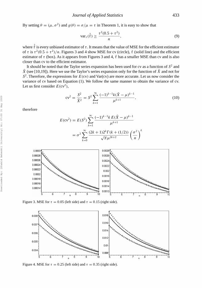
where ˆ̂τ is every unbiased estimator of τ . It means that the value of MSE for the efficient estimatorof τ is τ 2(0.5 + τ 2)/n. Figures 3 and 4 show MSE for cv (circle), τ̂ (solid line) and the efficientestimator of τ (box). As it appears from Figures 3 and 4, τ̂ has a smaller MSE than cv and is alsocloser than cv to the efficient estimator.

It should be noted that the Taylor series expansion has been used for cv as a function of S2 andX̄ (see [10,19]). Here we use the Taylor’s series expansion only for the function of X̄ and not forS2. Therefore, the expressions for E(cv) and Var(cv) are more accurate. Let us now consider thevariance of cv based on Equation (1). We follow the same manner to obtain the variance of cv.Let us first consider E(cv2),

cv2 = S2

X̄2= S2

∞∑k=1

(−1)k−1k(X̄ − μ)k−1

μk+1, (10)

therefore

E(cv2) = E(S2)

∞∑k=1

(−1)k−1k E(X̄ − μ)k−1

μk+1

= σ 2∞∑

k=0

(2k + 1)2k�(k + (1/2))√πμ2k+2

(σ 2

n

)k

Figure 3. MSE for τ = 0.05 (left side) and τ = 0.15 (right side).

Figure 4. MSE for τ = 0.25 (left side) and τ = 0.35 (right side).



= τ 2∞∑

k=0

(2k + 1)!2kk!

(τ 2

n

)k

. (11)

Using Equations (4) and (5) we obtain

var(cv) = τ 2∞∑

k=0

(2k + 1)!2kk!

(τ 2

n

)k

−(

cnτ

∞∑k=0

(2k)!2kk!

(τ 2

n

)k)2

. (12)

Thus

limn→∞ var(cv) = 0.

It means that cv is asymptotically consistent for τ . Moreover, note that

cv = S

X̄≈ S

μ− S(X̄ − μ)

μ2

=⇒ var(cv) ≈ var(S)

μ2+ var(S(X̄ − μ))

μ4− 2

cov(S, S(X̄ − μ))

μ3

= (1 − c2n)τ

2 + τ 4

n

= τ 2(n(1 − c2

n) + τ 2)

n. (13)

Next, we will show that n(1 − c2n) → 0.5. The asymptotic expansion of the gamma function ratio

is (see [4])

�(j + (1/2))

�(j)= √

j

(1 − 1

8j+ 1

128j 2+ · · ·

). (14)

Now, if j = (n − 1)/2 in Equation (14), we have

cn =√

2

n − 1

�(n/2)

�((n − 1)/2)

=√

2

n − 1

[√n − 1

2

(1 − 1

4(n − 1)+ 1

32(n − 1)2+ · · ·

)]

= 1 − 1

4(n − 1)+ O

(1

(n − 1)3/2

).

Thus we obtain

n(1 − c2n) = n

(1

2(n − 1)+ O

(1

(n − 1)2

))−→ 1

2.

Therefore, var(cv) → τ 2(0.5 + τ 2

)/n. This means that this estimator is asymptotically efficient

(see Equation (9)).



Now, we consider two approximations for the variance of cv. If we neglect τ 4/n inEquation (13), we have

var(cv) ≈ (1 − c2n)τ

2 =⇒ var(τ̂ ) ≈ (1 − c2n)

(2 − cn)2τ 2. (15)

Therefore, τ̂ is also asymptotically consistent for τ . Now, using the normal approximation, wehave

z = τ̂ − τ√var(τ̂ )

= cv/(2 − cn) − τ√τ 2(1 − c2

n)/(2 − cn)2= cv − (2 − cn)τ

τ√

1 − c2n

−→ N(0, 1). (16)

Therefore, the 100(1 − α)% confidence interval for τ based on Equation (16) is

cv

2 − cn + z1−α/2

√1 − c2

n

≤ τ ≤ cv

2 − cn − z1−α/2

√1 − c2

n

, (17)

where z1−α/2 is the 100(1 − α/2) percentile of the standard normal distribution.However, if we use Equation (13) without neglecting τ 4/n we have

z = τ̂ − τ√v̂ar(τ̂ )

= τ̂ − τ√(τ̂ 2(1 − c2

n) + τ̂ 4/n)/(2 − cn)2−→ N(0, 1). (18)

Therefore, the 100(1 − α)% confidence interval for τ based on Equation (18) is

τ̂ − τ̂

2 − cn

z1−α/2

√(1 − c2

n) + τ̂ 2

n≤ τ ≤ τ̂ − τ̂

2 − cn

z1−α/2

√(1 − c2

n) + τ̂ 2

n. (19)

�

3. Numerical results

Let us examine the performance of the proposed confidence intervals (17) and (19). Kang andSchmeiser [8] introduced a graphical assessment technique to evaluate the performance of confi-dence intervals. They considered three criteria; coverage percentage (the percentage of times τ isincluded in the confidence interval), width of the confidence interval and variance of the intervalwidth. Here, we consider only the first two. We shall consider several methods namely, Miller’s,Mckay’s, Vangel’s and Sharma–Krishna’s methods:

Miller : τ ∈{

cv − z1−α//2

[cv2

n − 1

(1

2+ cv2

)]1/2

, cv + z1−α//2

[cv2

n − 1

(1

2+ cv2

)]1/2}

,

Mckay : τ ∈{

cv

[(u1

n − 1− 1

)cv2 + u1

n − 1

]−1/2

, cv

[(u2

n − 1− 1

)cv2 + u2

n − 1

]−1/2}

,

Vangel : τ ∈{

cv

[(u1 + 2

n − 1− 1

)cv2 + u1

n − 1

]−1/2

, cv

[(u2 + 2

n − 1− 1

)cv2 + u2

n − 1

]−1/2}

,

Sharma–Krishna : τ−1 ∈{

cv−1 − zα/2√n

, cv−1 + zα/2√n

},

where u1 = χ2(n−1),1−α/2, u2 = χ2

(n−1),α/2 are the 100(1 − α/2) and 100(α/2) percentile of thechi-squared distribution with (n − 1) degrees of freedom, respectively. The upper Mckay’s bound



will have to be set to ∞ if [24]

S/X̄ ≥ √n

√u2

(n − 1)(n − u2),

and the upper Vangel’s bound will have to be set to ∞ if

S/X̄ ≥ √n

√u2

(n − 1)(n − u2 − 2).

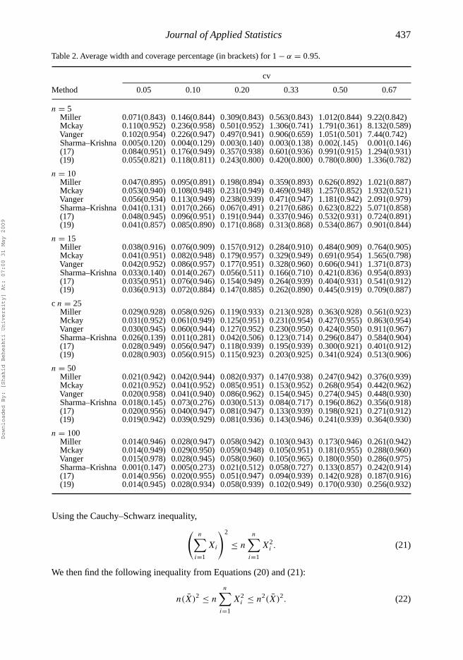
The results are presented at 95% and 99% confidence levels. To compare the results with thoseobtained by Miller [16], the same sample size n and cv is used. We have used 10,000 simulations toobtain the pairs (n, cv). Without loss of generality, we consider observations drawn from N(μ, 1).So one only needs to adjust μ to get the required cv. The results are presented in Tables 1–3. Tocompare the performance of the six methods we use one way analysis of variance (ANOVA). Theresults are presented in Table 1. Table 1 indicates that there is a significant discrepancy betweenthe six methods. To find the best method we examine the results presented in Tables 2 and 3. Asit appears from Tables 2 and 3, Sharma–Krishna’s method is constantly poorer than the other fivemethods in terms of coverage percentage. It can be seen that Mckay’s and Vangel’s methods haveslightly longer widths than Miller’s and the new confidence intervals.

Note also that McKay suggests that his method should only be used when one can assume thatτ < 0.33 (see [15, p. 637]). Moreover, as we mentioned above, Mckay’s and Vangel’s methodshave infinite length in some conditions. Hence, in the following, we only compare the resultsobtained by Equation (17), (19), and Miller’s confidence interval. For n ≥ 15, confidence inter-val (17) is closer to the nominal level than Miller’s and Equation (19). However, the coveragepercentage is slightly smaller than Miller’s method in some cases. For n < 15 and cv > 0.33,Equation (17) is better than Miller’s methods and for n > 15 and cv > 0.33, Equation (17) outperforms Miller’s methods in terms of coverage percentage. It should be noted that Equation (17)gives the better results even for small sample sizes n. As it appears from Tables 2 and 3, theaverage width of the confidence interval (19) is smaller than Miller’s method in all cases andsmaller than (17) in some cases. However, the coverage percentage is slightly smaller than theconfidence interval (17) and Miller’s method in some cases.

In the following we obtain some bounds for cv for a non-negative data set. Let X1, . . . , Xn bea non-negative data set. The following inequality comes from the non-negativity of data:(

n∑i=1

Xi

)2

>

n∑i=1

X2i . (20)

Table 1. The results of the ANOVA test 1% confidence level.

cv

n 0.05 0.10 0.20 0.33 0.50 0.67

5 44803.43 43163.10 1167.90 674.92 1829.47 8.9910 64193.62 67927.19 3712.78 1777.08 3095.69 6.07215 162342.95 140172.41 5614.84 2316.64 713.91 272.7425 280709.82 234459.73 11950.11 4998.25 1776.51 662.8850 454318.83 384346.73 23265.45 8448.15 4007.47 2049.83100 1454575.68 802002.64 54098.80 17982.27 5359.35 3127.45



Table 2. Average width and coverage percentage (in brackets) for 1 − α = 0.95.

cv

Method 0.05 0.10 0.20 0.33 0.50 0.67

n = 5Miller 0.071(0.843) 0.146(0.844) 0.309(0.843) 0.563(0.843) 1.012(0.844) 9.22(0.842)Mckay 0.110(0.952) 0.236(0.958) 0.501(0.952) 1.306(0.741) 1.791(0.361) 8.132(0.589)Vanger 0.102(0.954) 0.226(0.947) 0.497(0.941) 0.906(0.659) 1.051(0.501) 7.44(0.742)Sharma–Krishna 0.005(0.120) 0.004(0.129) 0.003(0.140) 0.003(0.138) 0.002(.145) 0.001(0.146)(17) 0.084(0.951) 0.176(0.949) 0.357(0.938) 0.601(0.936) 0.991(0.915) 1.294(0.931)(19) 0.055(0.821) 0.118(0.811) 0.243(0.800) 0.420(0.800) 0.780(0.800) 1.336(0.782)

n = 10Miller 0.047(0.895) 0.095(0.891) 0.198(0.894) 0.359(0.893) 0.626(0.892) 1.021(0.887)Mckay 0.053(0.940) 0.108(0.948) 0.231(0.949) 0.469(0.948) 1.257(0.852) 1.932(0.521)Vanger 0.056(0.954) 0.113(0.949) 0.238(0.939) 0.471(0.947) 1.181(0.942) 2.091(0.979)Sharma–Krishna 0.041(0.131) 0.017(0.266) 0.067(0.491) 0.217(0.686) 0.623(0.822) 5.071(0.858)(17) 0.048(0.945) 0.096(0.951) 0.191(0.944) 0.337(0.946) 0.532(0.931) 0.724(0.891)(19) 0.041(0.857) 0.085(0.890) 0.171(0.868) 0.313(0.868) 0.534(0.867) 0.901(0.844)


c n = 25Miller 0.029(0.928) 0.058(0.926) 0.119(0.933) 0.213(0.928) 0.363(0.928) 0.561(0.923)Mckay 0.031(0.952) 0.061(0.949) 0.125(0.951) 0.231(0.954) 0.427(0.955) 0.863(0.954)Vanger 0.030(0.945) 0.060(0.944) 0.127(0.952) 0.230(0.950) 0.424(0.950) 0.911(0.967)Sharma–Krishna 0.026(0.139) 0.011(0.281) 0.042(0.506) 0.123(0.714) 0.296(0.847) 0.584(0.904)(17) 0.028(0.949) 0.056(0.947) 0.118(0.939) 0.195(0.939) 0.300(0.921) 0.401(0.912)(19) 0.028(0.903) 0.056(0.915) 0.115(0.923) 0.203(0.925) 0.341(0.924) 0.513(0.906)



Using the Cauchy–Schwarz inequality,(n∑

i=1

Xi

)2

≤ n

n∑i=1

X2i . (21)

We then find the following inequality from Equations (20) and (21):

n(X̄)2 ≤ n

n∑i=1

X2i ≤ n2(X̄)2. (22)



Table 3. Average width and coverage percentage (in brackets) for 1 − α = 0.99.

cv

Method 0.05 0.10 0.20 0.33 0.50 0.67







Applying the definition of sample variance and Equation (22), we have

0 ≤ cv ≤ √n, (23)

thus for a non-negative data set, the upper bound for cv is√

n. Consequently, if L(17), L(19) andLMiller are the length of the respective confidence intervals for τ , the following equation can be



obtained from Equation (23):

Max L(17) = 2√

n√

1 − c2n

(2 − cn)2 − z21−α/2(1 − c2

n)z1−α/2

Max L(19) = 2

√n

(2 − cn)

√(1 − c2

n) + 1

(2 − cn)2z1−α/2 (24)

Max LMiller = 2√

n

√0.5 + n

n − 1z1−α/2

Figure 5 shows Max L(17), Max L(19) and MaxLMiller for different values ofn.As the figure showsMaxL(17) < Max L(19) < MaxLMiller for all cases. It also shows that the accuracy of Miller’s andconfidence interval (19) decreases as n increases while the accuracy increases for interval (17).

It has been shown that the values of τ larger than 0.33 imply that the standard deviation ismore than three times larger than the mean, which would further imply that the lower end of thedistribution would be expected to contain some proportion less than zero (see [9]). Let us considerP(cv < 0) for τ > 0.33 in a normal distribution:

P(cv < 0) = P(X̄ < 0) = �

(−

√n

τ

),

Figure 5. Maximum width of the confidence interval for α = 0.05 (left side) and α = 0.01 (right side) basedon Miller’s method (circle), confidence interval (17) (solid line) and confidence interval (19) (cross).

Figure 6. Probability of having a negative cv.



where �(z) is the cumulative distribution function of N (0, 1). Figure 6 shows the probability forthe pairs (n, cv) (5 ≤ n ≤ 100, 0.5 ≤ τ ≤ 2). As it appears from Figure 6 that the probability ofhaving a negative cv is very small (less than 0.0062) for n > 25. Therefore, considering the upperbound for cv is acceptable.

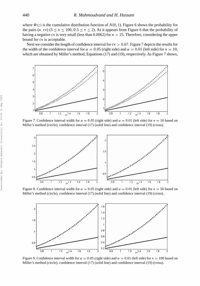
Next we consider the length of confidence interval for cv > 0.67. Figure 7 depicts the results forthe width of the confidence interval for α = 0.05 (right side) and α = 0.01 (left side) for n = 10,which are obtained by Miller’s method, Equations (17) and (19), respectively. As Figure 7 shows,

Figure 7. Confidence interval width for α = 0.05 (right side) and α = 0.01 (left side) for n = 10 based onMiller’s method (circle), confidence interval (17) (solid line) and confidence interval (19) (cross).





the width obtained by Miller’s method and confidence interval (19) increases exponentially whilethe width increases linearly for the interval (17). In fact the Miller’s method and Equation (19) arefunctions of cv2 whilst Equation (17) is a function of cv. Similar results are obtained for largervalue of n (see Figures 8–9).

4. Conclusion

We introduced a new approximate point estimator, τ̂ , for the coefficient of variation, τ , for situationwhere data was distributed normally. Several criteria were considered, in order to evaluate theaccuracy of τ̂ . The results showed that τ̂ is asymptotically unbiased and also has less variancethan the typical estimate of τ , which is the sample coefficient of variation, cv. We also comparedthe accuracy of τ̂ and the efficient estimate of τ . The comparison results indicate that τ̂ has lessMSE than cv and also is closer to the efficient estimator.

We proposed two new approximate confidence intervals for τ based on the τ̂ and its variance.The results show that the performance of the proposed confidence intervals are as good as or betterthan current methods of calculating confidence intervals for τ (Tables 2 and 3). Despite the factthat some methods used to calculate the confidence interval are complicated (see, for example[13]), the simplicity of the new confidence intervals can be considered as one advantage. Anotheradvantage is that the method works well even for a small sample size. Note that various asymptoticmethods have been considered in the literature, which need the sample size to be large. Moreover,our research indicates several directions for the future. The asymptotic results obtained here canbe generalized for non-normal distributions.

Acknowledgements

The authors would like to thank the editor and the referees for their constructive comments, which have led to substantialimprovements in this paper. The authors are grateful to their colleague Dr Rebecca Haycroft (Cardiff University) foruseful suggestions.

References

[1] S.E. Ahmed, Simultaneous estimation of coefficient of variations, J. Stat. Plan. Inference 104 (2002), pp. 31–51.[2] A. Chaturvedi and U. Rani, Fixed-width confidence interval estimation of the inverse coefficient of variation in a

normal population, Microelectron. Reliab. 36(9) (1996), pp. 1305–1308.[3] E.C. Fieller, A numerical test of the adequacy of A. T. McKay’s approximation. J. R. Stat. Soc. 95 (1932), pp. 699–702.[4] R.L. Graham, D.E. Knuth, and O. Patashnik, Answer to problem 9.60 in Concrete Mathematics: A Foundation for

Computer Science, 2nd ed., Addison-Wesley, Reading, MA, 1994.[5] W.A. Hendricks and W.K. Robey, The sampling distribution of the coefficient of variation, Ann. Math. Stat. 7 (1936),

pp. 129–132.[6] B. Iglewicz, Some properties of the coefficient of variation, Ph.D. thesis, Virginia Polytechnic Institute, 1967.[7] B. Iglewicz and R.H. Myers, Comparisons of approximations to the percentage points of the sample coefficient of

variation, Technometrics 12 (1970), pp. 166–169.[8] K. Kang and B.W. Schmeiser, Methods for evaluating and comparing confidence interval procedures, Tech. Rep.,

Department of Industrial Engineering, University of Miami, FL, 1986.[9] K. Kelley, Sample Size Planning for the Coefficient ofVariation from theAccuracy in Parameter EstimationApproach,

Behav. Res. Methods 39(4) (2007), pp. 755–766.[10] M.G. Kendall and A. Stuart, The Advanced Theory of Statistics, Vol. 1, Charles Griffin, London, 1969.[11] L.H. Koopmans, D.B. Owen, and J.I. Rosenblatt, Confidence intervals for the coefficient of variation for the normal

and lognormal distributions, Biometrika 51(1–2) (1964), pp. 25–32.[12] E.L. Lehmann, Theory of Point Estimation, 2nd edn, Wiley, New York, 1983.[13] E.L. Lehmann, Testing Statistical Hypotheses, 2nd edn, Wiley, New York, 1996.[14] R. Mahmoudvand, H. Hassani, R. Wilson, Is the sample coefficient of variation a good estimatore for the population

coefficient of variation, World Appl. Sci. J. 2(5) (2007), pp. 519–522.



[15] A.T. Mckay, Distribution of the coefficient of variation and the extended ′t ′ distribution, J. B. Stat. Soc. 95 (1932),pp. 696–698.

[16] E.G. Miller, Asymptotic test statistics for coefficient of variation, Comm. Statist. Theory Methods, 20 (1991),pp. 3351–3363.

[17] K.C. Ng, Performance of three methods of interval estimation of the coefficient of variation, InterStat (2006).Available at http://interstat.statjournals.net/YEAR/2006/articles/0609002.pdf

[18] E.S. Pearson, Comparison of A. T. McKay’s approximation with experimental sampling results, J. B. Stat. Soc. 95(1932), pp. 703–704.

[19] K.A. Rao and A.R.S. Bhatta, A note on test for coefficient of variation, Calcutta Stat. Assoc. Bull. 38 (1989),pp. 225–229.

[20] K.K. Sharma and H. Krishna,Asymptotic sampling distribution of imverse coefficient of variation and its applications,IEEE Trans. Reliab. 43(4) (1994), pp. 630–633.

[21] L. Tian, Inferences on the within-subject coefficient of variation, Stat. Med. 25 (2006), pp. 2008-–2017.[22] G.J. Umphrey, A comment on McKay’s approximation for the coefficient of variation, Comm. Stat. Sim. Comp.

12(5) (1983), pp. 629–635.[23] M.G. Vangel, Confidence intervals for a normal coefficient of variation, Amer. Statist. 50 (1996), pp. 21–26.[24] S. Verrill, Confidence bounds for normal and log-normal distribution coefficient of variation, Research Paper,

EPL-RP-609, Madison, Wisconsin, US, 2003.[25] A.C.M. Wong and J. Wu, Small sample asymptotic inference for the coefficient of variation: normal and nonnormal

models, J. Stat. Plan. Inference 104 (2002), pp. 73–82.


Two new confidence intervals for the coefficient of variation in a normal distribution

Documents

Transcript of Two new confidence intervals for the coefficient of variation in a normal distribution