Uncertainty in Population Growth Rates: DeterminingConfidence Intervals from Point Estimates of ParametersEleanor S. Devenish Nelson1*, Stephen Harris2, Carl D. Soulsbury2, Shane A. Richards1, Philip A.

Stephens1

1 School of Biological and Biomedical Sciences, Durham University, Durham, United Kingdom, 2 School of Biological Sciences, University of Bristol, Bristol, United Kingdom

Abstract

Background: Demographic models are widely used in conservation and management, and their parameterisation oftenrelies on data collected for other purposes. When underlying data lack clear indications of associated uncertainty, modellersoften fail to account for that uncertainty in model outputs, such as estimates of population growth.

Methodology/Principal Findings: We applied a likelihood approach to infer uncertainty retrospectively from pointestimates of vital rates. Combining this with resampling techniques and projection modelling, we show that confidenceintervals for population growth estimates are easy to derive. We used similar techniques to examine the effects of samplesize on uncertainty. Our approach is illustrated using data on the red fox, Vulpes vulpes, a predator of ecological and culturalimportance, and the most widespread extant terrestrial mammal. We show that uncertainty surrounding estimatedpopulation growth rates can be high, even for relatively well-studied populations. Halving that uncertainty typically requiresa quadrupling of sampling effort.

Conclusions/Significance: Our results compel caution when comparing demographic trends between populations withoutaccounting for uncertainty. Our methods will be widely applicable to demographic studies of many species.

Citation: Devenish Nelson ES, Harris S, Soulsbury CD, Richards SA, Stephens PA (2010) Uncertainty in Population Growth Rates: Determining Confidence Intervalsfrom Point Estimates of Parameters. PLoS ONE 5(10): e13628. doi:10.1371/journal.pone.0013628

Editor: Louis-Felix Bersier, University of Fribourg, Switzerland

Received July 6, 2010; Accepted September 24, 2010; Published October 25, 2010

Copyright: � 2010 Devenish Nelson et al. This is an open-access article distributed under the terms of the Creative Commons Attribution License, which permitsunrestricted use, distribution, and reproduction in any medium, provided the original author and source are credited.

Funding: This work was funded by a Durham University Doctoral Fellowship (EDN). S. Harris was funded by the Dulverton Trust. The funders had no role in studydesign, data collection and analysis, decision to publish, or preparation of the manuscript.

Competing Interests: The authors have declared that no competing interests exist.

* E-mail: e.s.nelson@durham.ac.uk

Introduction

Demographic modelling is widely used in conservation and

management [1,2]. As modelling techniques have become

increasingly sophisticated, a growing literature has dealt with the

importance of acknowledging process error (or environmentally-

driven variation in demographic parameters) in model analyses

[3,4,5]. By contrast, assessments of the implications of observation

error (arising from sampling limitations) for model precision are

often lacking, but see [6,7], perhaps due to a widespread

acknowledgement of the ubiquity of sampling constraints [8].

Here, we discuss methods to infer accuracy of vital rate estimates,

even where parameter uncertainty has not been reported

explicitly. We show that acknowledging limits to precision can

be an important element of demographic inference, with

implications for data collection protocols.

Age- or stage-structured (Leslie or Lefkovitch) matrix population

models are conceptually clear and relatively easily parameterised,

with well-characterised properties; as such, the use of matrix

models is particularly widespread in ecology [4,9]. Studies utilising

matrix population modelling rely on data from a variety of

sources. Frequently, the studies’ authors have also collected the

demographic data used to parameterise the transition matrix. In

these cases, sample variance is used to establish vital rate

distributions and resampling techniques are available to determine

the consequences of that uncertainty for estimates of population

growth e.g., [10,11]. In spite of this, many authors routinely

publish point estimates of asymptotic population growth (l),

without accompanying metrics of precision such as standard errors

or confidence intervals. Furthermore, this practice is not limited to

relatively low-ranking journals; see supplementary material, Table

S1.

When modellers use data that were not collected specifically for

the purposes of demographic insight, further problems arise.

Hunting records are a common source of such data, even though

they are associated with a number of important assumptions that

limit their use and compel caution in their interpretation [12].

Even accepting these limitations, hunting data are often reported

inconsistently and, in particular, are frequently presented without

estimates of accompanying uncertainty. In these situations,

likelihood approaches provide a convenient method to infer the

distribution and extent of uncertainty around the best estimate for

the parameter of interest. Hitherto, likelihood methods have

largely been neglected for exposing the uncertainty associated with

the output of projection matrices.

In this paper, we present techniques for inferring, retrospec-

tively, the uncertainty of demographic parameters due to

observation error in demographic data. Following others e.g.,

[13] we distinguish between Bernoulli processes, such as survival

or probability of breeding, and Poisson processes, such as litter

PLoS ONE | www.plosone.org 1 October 2010 | Volume 5 | Issue 10 | e13628

size. We illustrate this approach with reference to the red fox

(Vulpes vulpes), the most widely distributed extant wild terrestrial

mammalian species [14], extensively studied throughout its

geographic range due to its ecological, economic, and cultural

importance e.g., [15,16]. The red fox is widely hunted, making the

species a rich source of demographic data. Comparisons of red fox

population growth rates in different parts of the world have been

used to classify the species along the ‘‘fast-slow’’ life history

continuum [17], and have also been used to make inferences about

the species’ response to different environmental and management

pressures [18]. Determining the confidence that we can place in

these assessments is, therefore, crucial for a number of applica-

tions.

Here, we begin by illustrating how likelihood profiles can be

determined for red fox demographic parameters and use

resampling techniques to assess confidence in resultant estimates

of population growth. Our results highlight the need for caution in

generalising about differences in the dynamics of populations. We

illustrate the utility of this resampling approach to provide

information about required sampling effort.

Methods

Likelihood profiles for demographic parametersAge-specific survival and proportion of breeding females are

Bernoulli processes, in the sense that each female can be

considered a ‘trial’ with a binomial outcome (live or die, breed

or fail to breed). Taking the example of survival, hunting data

often yield numbers of individuals in different age classes. If the

data are assumed to have been collected at a time when the

population approximated its stable age distribution, survival of

individuals of age x can be inferred from the relative number of

individuals in age classes x and x+1 (fx and fx+1, respectively). The

point estimate of survival, Px, is given by Px = fx+1/fx. Occasionally,

fx+1.fx, or the population is known to have been growing at some

rate (r) during the period of data collection; Caughley [12] presents

methods to deal with both of these situations. Very often, sample

sizes for older age classes are sufficiently restricted that it is useful

to truncate the age distribution and create composite classes for all

age classes beyond a given age. In these cases, the point estimate of

survival is given by Px* = fx.x*/ (fx+fx.x*), where x* is the final age

class.

In the previous formulae, the number of trials is represented by

the denominator of the point estimate equation, whilst the number

of events (or successes) is given by the numerator. However, the

point estimate for survival is only an estimate. It is often more

interesting to consider the relative probability with which any

other true parameter value could have yielded the same outcome,

i.e. the same number of events from the same number of trials.

Assuming a uniform prior probability for any putative survival

rate, the likelihood of any given survival rate, Px, is given by:

L Pxjfx,fxz1ð Þ~fx

fxz1

� �Px

fxz1 1{Pxð Þfx{fxz1 ð1Þ

This likelihood distribution is easily evaluated using the

‘‘dbinom(events,trials,Px)’’ function in R. Given data, for example,

on the proportion of shot females that show signs of breeding, the

same approach can be used to determine the likelihood profile for

the probability of breeding, Bx. If we have prior information about

the focal parameter, then it can easily be incorporated using a

Bayesian approach [13].

When estimating age-dependent, per capita, fecundity rates we

assume that we only have information on the number of females of

age x that bred, denoted Nx, and the total number of offspring that

they produced, denoted Yx. Here, we assume that the number of

offspring a female produces, given that she has produced at least

one offspring, is distributed according to a shifted Poisson

distribution. The point estimate for average litter size for breeding

females in age class x is simply mx = Yx/Nx. The likelihood that the

true mean litter size is mx, is:

L mxjNx,Yxð Þ~ mNxð Þye{mNx

y!ð2Þ

where m = mx21 and y = Yx2Nx. These adjustments are necessary

to shift the Poisson distribution of litter sizes one interval to the

right [19], removing the possibility of zero litter sizes for females

that breed. This likelihood distribution is also easily determined in

R using the ‘‘dpois(y, mNx)’’ function.

Confidence intervals for population growth estimates: the

red fox as an example. We extracted published demographic

data for three red fox populations of management interest: a culled

Australian population [20,21,22], a non-culled Australian

population [23], and a culled USA population [24,25,26,27,28].

We constructed female-only, post-breeding ‘birth-pulse’ models of

the form Nt+1 = A.Nt, where Nt is a vector of numbers of females in

each age class at time t and A is the transition matrix. The

transition matrix was based on four age classes (juveniles, ,1 year;

yearlings, 1–2 years; young adults, 2–3 years; and older adults, $3

years) and took the form:

A~

F1 F2 F3 F4�

P1 0 0 0

0 P2 0 0

0 0 P3 P4�

26664

37775 ð3Þ

To avoid small sample size issues among older age classes, only

four age classes were used; it is unusual for individuals to survive

past 4 years [25,29].

Deterministic growth, li, of population i, was determined from

the dominant eigenvalue of Ai using point estimates of each matrix

element for survival, calculated as detailed above. Fecundity

matrix elements (Fx) were determined from the proportion of

breeding females (Bx), the average age-specific litter size (mx) and a

generalised birth sex ratio of 1:1 [30], so that Fx = 0.5PxBxmx.

Confidence intervals were determined using a resampling (or

parametric bootstrap) approach [10]. Specifically, we determined

li from 10,000 replicate projection matrices, with each element

drawn from its corresponding likelihood distribution; confidence

intervals for li were taken as the range encompassing the central

95% of li estimates.

Implications for sample sizeTo illustrate an additional benefit of the resampling approach

for quantifying uncertainty, we created a ‘generic’ red fox

population, sensu [31], from the focal studies. Generic demo-

graphic parameters were calculated by summing ‘events’ and

‘trials’ across the three studies; thus, parameters were weighted by

the size of studies. The stable stage distribution (SSD) was

calculated from the right eigenvector of the generic projection

matrix, Ag. We investigated the effect of different sample sizes on

the level of confidence that could be placed in estimates of

population growth, lg. Specifically, for a given sample size, S, we

Population Growth Uncertainty

PLoS ONE | www.plosone.org 2 October 2010 | Volume 5 | Issue 10 | e13628

assumed that the number of females available for demographic

analysis was proportioned among age classes according to the

SSD. We selected those S individuals randomly, resampling with

replacement, and calculated all matrix elements according to the

fates of the selected individuals (whether they lived or died, bred or

failed to breed and, if they bred, the number of offspring they

produced, drawn from the relevant likelihood distribution). From

this resampled matrix, we determined lg,S,j, where S was the

sample size and j = 1, 2 … 104 resampled matrices. We repeated

the process for a range of sample sizes from 50 to 2,000 females,

reflecting the range of sample sizes available for published studies

of red foxes (minimum 42 [28], maximum 1701 [32]). Resultant

95% confidence intervals for estimates of lg,S were plotted against

sample size.

Results

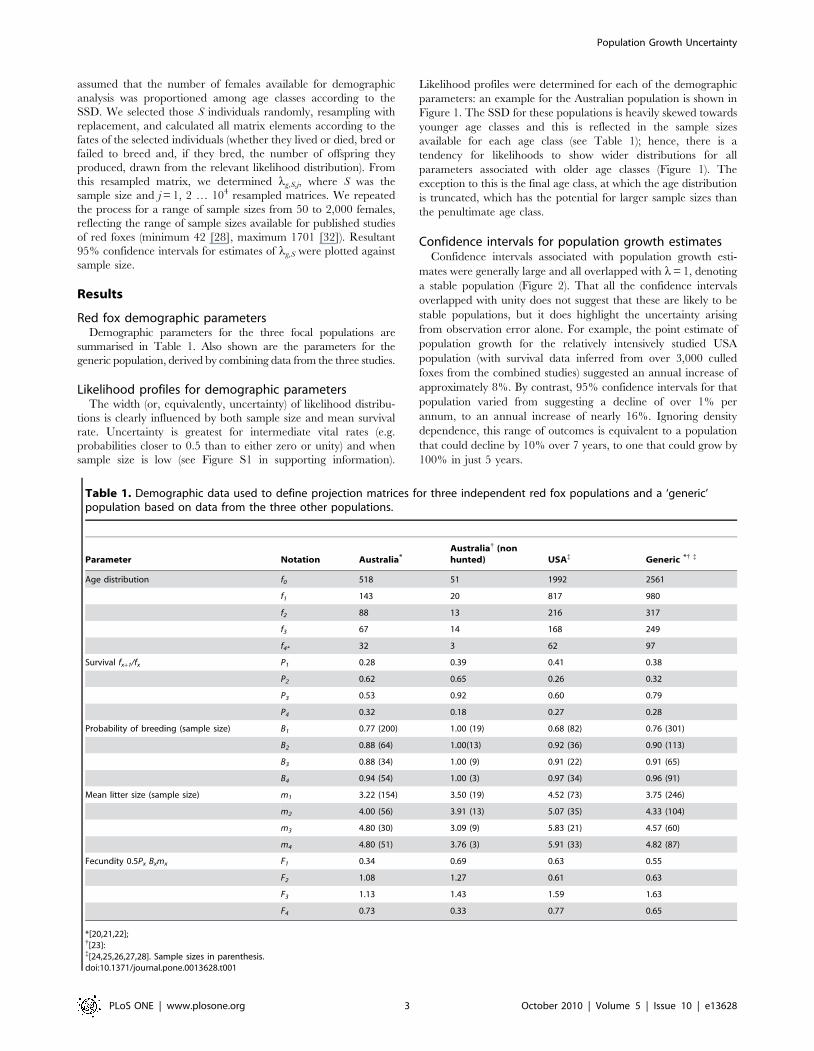
Red fox demographic parametersDemographic parameters for the three focal populations are

summarised in Table 1. Also shown are the parameters for the

generic population, derived by combining data from the three studies.

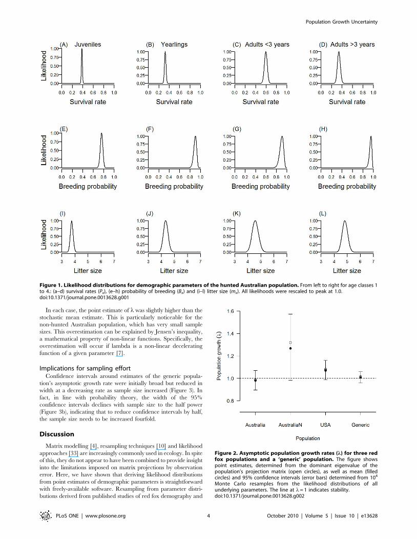
Likelihood profiles for demographic parametersThe width (or, equivalently, uncertainty) of likelihood distribu-

tions is clearly influenced by both sample size and mean survival

rate. Uncertainty is greatest for intermediate vital rates (e.g.

probabilities closer to 0.5 than to either zero or unity) and when

sample size is low (see Figure S1 in supporting information).

Likelihood profiles were determined for each of the demographic

parameters: an example for the Australian population is shown in

Figure 1. The SSD for these populations is heavily skewed towards

younger age classes and this is reflected in the sample sizes

available for each age class (see Table 1); hence, there is a

tendency for likelihoods to show wider distributions for all

parameters associated with older age classes (Figure 1). The

exception to this is the final age class, at which the age distribution

is truncated, which has the potential for larger sample sizes than

the penultimate age class.

Confidence intervals for population growth estimatesConfidence intervals associated with population growth esti-

mates were generally large and all overlapped with l= 1, denoting

a stable population (Figure 2). That all the confidence intervals

overlapped with unity does not suggest that these are likely to be

stable populations, but it does highlight the uncertainty arising

from observation error alone. For example, the point estimate of

population growth for the relatively intensively studied USA

population (with survival data inferred from over 3,000 culled

foxes from the combined studies) suggested an annual increase of

approximately 8%. By contrast, 95% confidence intervals for that

population varied from suggesting a decline of over 1% per

annum, to an annual increase of nearly 16%. Ignoring density

dependence, this range of outcomes is equivalent to a population

that could decline by 10% over 7 years, to one that could grow by

100% in just 5 years.

Table 1. Demographic data used to define projection matrices for three independent red fox populations and a ‘generic’population based on data from the three other populations.

Parameter Notation Australia*Australia{ (nonhunted) USA{ Generic *{ {

Age distribution f0 518 51 1992 2561

f1 143 20 817 980

f2 88 13 216 317

f3 67 14 168 249

f4* 32 3 62 97

Survival fx+1/fx P1 0.28 0.39 0.41 0.38

P2 0.62 0.65 0.26 0.32

P3 0.53 0.92 0.60 0.79

P4 0.32 0.18 0.27 0.28

Probability of breeding (sample size) B1 0.77 (200) 1.00 (19) 0.68 (82) 0.76 (301)

B2 0.88 (64) 1.00(13) 0.92 (36) 0.90 (113)

B3 0.88 (34) 1.00 (9) 0.91 (22) 0.91 (65)

B4 0.94 (54) 1.00 (3) 0.97 (34) 0.96 (91)

Mean litter size (sample size) m1 3.22 (154) 3.50 (19) 4.52 (73) 3.75 (246)

m2 4.00 (56) 3.91 (13) 5.07 (35) 4.33 (104)

m3 4.80 (30) 3.09 (9) 5.83 (21) 4.57 (60)

m4 4.80 (51) 3.76 (3) 5.91 (33) 4.82 (87)

Fecundity 0.5Px Bxmx F1 0.34 0.69 0.63 0.55

F2 1.08 1.27 0.61 0.63

F3 1.13 1.43 1.59 1.63

F4 0.73 0.33 0.77 0.65

*[20,21,22];{[23]:{[24,25,26,27,28]. Sample sizes in parenthesis.doi:10.1371/journal.pone.0013628.t001

Population Growth Uncertainty

PLoS ONE | www.plosone.org 3 October 2010 | Volume 5 | Issue 10 | e13628

In each case, the point estimate of l was slightly higher than the

stochastic mean estimate. This is particularly noticeable for the

non-hunted Australian population, which has very small sample

sizes. This overestimation can be explained by Jensen’s inequality,

a mathematical property of non-linear functions. Specifically, the

overestimation will occur if lambda is a non-linear decelerating

function of a given parameter [7].

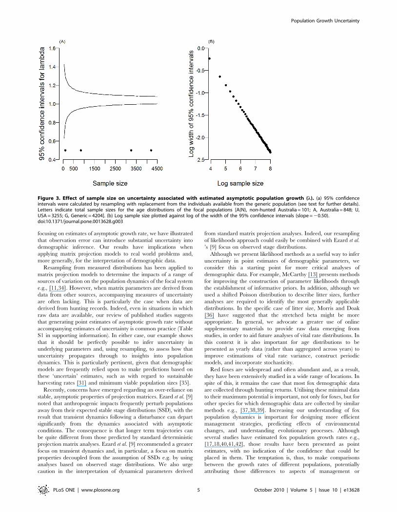
Implications for sampling effortConfidence intervals around estimates of the generic popula-

tion’s asymptotic growth rate were initially broad but reduced in

width at a decreasing rate as sample size increased (Figure 3). In

fact, in line with probability theory, the width of the 95%

confidence intervals declines with sample size to the half power

(Figure 3b), indicating that to reduce confidence intervals by half,

the sample size needs to be increased fourfold.

Discussion

Matrix modelling [4], resampling techniques [10] and likelihood

approaches [33] are increasingly commonly used in ecology. In spite

of this, they do not appear to have been combined to provide insight

into the limitations imposed on matrix projections by observation

error. Here, we have shown that deriving likelihood distributions

from point estimates of demographic parameters is straightforward

with freely-available software. Resampling from parameter distri-

butions derived from published studies of red fox demography and

Figure 1. Likelihood distributions for demographic parameters of the hunted Australian population. From left to right for age classes 1to 4.: (a–d) survival rates (Px), (e–h) probability of breeding (Bx) and (i–l) litter size (mx). All likelihoods were rescaled to peak at 1.0.doi:10.1371/journal.pone.0013628.g001

Figure 2. Asymptotic population growth rates (l) for three redfox populations and a ‘generic’ population. The figure showspoint estimates, determined from the dominant eigenvalue of thepopulation’s projection matrix (open circles), as well as mean (filledcircles) and 95% confidence intervals (error bars) determined from 104

Monte Carlo resamples from the likelihood distributions of allunderlying parameters. The line at l= 1 indicates stability.doi:10.1371/journal.pone.0013628.g002

Population Growth Uncertainty

PLoS ONE | www.plosone.org 4 October 2010 | Volume 5 | Issue 10 | e13628

focusing on estimates of asymptotic growth rate, we have illustrated

that observation error can introduce substantial uncertainty into

demographic inference. Our results have implications when

applying matrix projection models to real world problems and,

more generally, for the interpretation of demographic data.

Resampling from measured distributions has been applied to

matrix projection models to determine the impacts of a range of

sources of variation on the population dynamics of the focal system

e.g., [11,34]. However, when matrix parameters are derived from

data from other sources, accompanying measures of uncertainty

are often lacking. This is particularly the case when data are

derived from hunting records. Indeed, even in situations in which

raw data are available, our review of published studies suggests

that generating point estimates of asymptotic growth rate without

accompanying estimates of uncertainty is common practice (Table

S1 in supporting information). In either case, our example shows

that it should be perfectly possible to infer uncertainty in

underlying parameters and, using resampling, to assess how that

uncertainty propagates through to insights into population

dynamics. This is particularly pertinent, given that demographic

models are frequently relied upon to make predictions based on

these ‘uncertain’ estimates, such as with regard to sustainable

harvesting rates [31] and minimum viable population sizes [35].

Recently, concerns have emerged regarding an over-reliance on

stable, asymptotic properties of projection matrices. Ezard et al. [9]

noted that anthropogenic impacts frequently perturb populations

away from their expected stable stage distributions (SSD), with the

result that transient dynamics following a disturbance can depart

significantly from the dynamics associated with asymptotic

conditions. The consequence is that longer term trajectories can

be quite different from those predicted by standard deterministic

projection matrix analyses. Ezard et al. [9] recommended a greater

focus on transient dynamics and, in particular, a focus on matrix

properties decoupled from the assumption of SSDs e.g. by using

analyses based on observed stage distributions. We also urge

caution in the interpretation of dynamical parameters derived

from standard matrix projection analyses. Indeed, our resampling

of likelihoods approach could easily be combined with Ezard et al.

’s [9] focus on observed stage distributions.

Although we present likelihood methods as a useful way to infer

uncertainty in point estimates of demographic parameters, we

consider this a starting point for more critical analyses of

demographic data. For example, McCarthy [13] presents methods

for improving the construction of parameter likelihoods through

the establishment of informative priors. In addition, although we

used a shifted Poisson distribution to describe litter sizes, further

analyses are required to identify the most generally applicable

distributions. In the specific case of litter size, Morris and Doak

[36] have suggested that the stretched beta might be more

appropriate. In general, we advocate a greater use of online

supplementary materials to provide raw data emerging from

studies, in order to aid future analyses of vital rate distributions. In

this context it is also important for age distributions to be

presented as yearly data (rather than aggregated across years) to

improve estimations of vital rate variance, construct periodic

models, and incorporate stochasticity.

Red foxes are widespread and often abundant and, as a result,

they have been extensively studied in a wide range of locations. In

spite of this, it remains the case that most fox demographic data

are collected through hunting returns. Utilising these minimal data

to their maximum potential is important, not only for foxes, but for

other species for which demographic data are collected by similar

methods e.g., [37,38,39]. Increasing our understanding of fox

population dynamics is important for designing more efficient

management strategies, predicting effects of environmental

changes, and understanding evolutionary processes. Although

several studies have estimated fox population growth rates e.g.,

[17,18,40,41,42], those results have been presented as point

estimates, with no indication of the confidence that could be

placed in them. The temptation is, thus, to make comparisons

between the growth rates of different populations, potentially

attributing those differences to aspects of management or

Figure 3. Effect of sample size on uncertainty associated with estimated asymptotic population growth (l). (a) 95% confidenceintervals were calculated by resampling with replacement from the individuals available from the generic population (see text for further details).Letters indicate total sample sizes for the age distributions of the focal populations [A(N), non-hunted Australia = 101; A, Australia = 848; U,USA = 3255; G, Generic = 4204]. (b) Log sample size plotted against log of the width of the 95% confidence intervals (slope = 20.50).doi:10.1371/journal.pone.0013628.g003

Population Growth Uncertainty

PLoS ONE | www.plosone.org 5 October 2010 | Volume 5 | Issue 10 | e13628

ecological circumstance. In this context, determining confidence

intervals about estimates of l is obviously essential, and our results

highlight the need for caution in making comparisons between

populations without accounting for uncertainty.

Knowledge of optimal sample sizes has implications for

allocating resources, e.g. sampling effort for capture-mark-

recapture studies. Our results indicate that, for red foxes, small

initial increases in sample size will yield substantial reductions in

uncertainty; however, as sample sizes increase, further effort to

collect additional samples yields diminishing returns explained by

a simple power law. Doak et al. (2005) suggest that it might often be

beneficial to increase study duration, rather than sampling

intensity. However, smaller sample sizes often lead to bias in

demographic inference [7]. Our results suggest that small studies

should be avoided but that, as sample size increases, it will be

beneficial to devote resources towards determining the mechanis-

tic basis for intrinsic variation, rather than simply to collect more

samples; in many systems, this argues in favour of extending study

duration to capture the drivers of inter-annual variation,

commonly a significant source of variance.

To derive the relationship between sample size and uncertainty in

l, we assumed that individuals would be sampled approximately in

proportion to the SSD. For studies based on mortalities such as

shooting or road deaths, this seems to be an appropriate approach,

assuming that the population approximates the SSD, but see [9]. In

addition, studies that have considered the best allocation of

sampling effort by age or stage e.g., [7,43] have shown that

sampling in proportion to the SSD is the approach likely to yield the

least uncertainty in demographic parameters. Certainly, sampling in

proportion to the SSD will yield a higher number of juveniles, which

typically make the most significant contribution to fox population

growth i.e. have the highest elasticities [18,32]. Owing to the fact

that the most important observation errors will arise from

inadequate sampling of life stages with the highest elasticities [44],

the value (in this case) of sampling in proportion to the SSD is clear.

Although it is not possible to define a one-size-fits-all sampling

intensity, the simple approach that we present should be applicable

to a wide range of species. Moreover, the finding that quadrupling

the sample size will typically halve the confidence interval is likely to

be very general.

We have presented a brief example of how more information can

be extracted from the type of published data that form a common

source for demographic modelling. Our results highlight the fact

that, even for well-studied species such as the red fox, sampling

limitations and inherent variability can limit the precision with

which we can identify characteristics of population dynamics. We

recommend a more widespread use of these straightforward

approaches (and related techniques), in order to promote a greater

awareness of the limitations of many population analyses.

Supporting Information

Figure S1 Likelihood distributions for vital rates simulated with

varying sample sizes. Average survival rates of 0.1, 0.5, and 1.0 are

simulated with varying age class sample sizes: (a–c) N = 10, (d–f)

N = 100. All likelihoods were rescaled to peak at 1.0.

Found at: doi:10.1371/journal.pone.0013628.s001 (0.22 MB

DOC)

Table S1 Results of a literature review showing the number of

studies that failed to include an accompanying measure of

uncertainty of the estimated population growth rate. We

conducted a Web of Science (http://apps.isiknowledge.com)

search from January 2008 to May 2010 using the search terms

‘population growth’, ‘matrix model’, and ‘demography’. We

separated the results by taxa, and further distinguished those that

used previously published data to estimate matrix transition

elements. We also recorded the impact factor of the journal for

each result. The results are presented as a percentage of the total

studies, the number of studies using published demographic data,

and those published in a journal with a 5-year impact factor of

four or higher (based on Web of Science, Journal Citation

Reports).

Found at: doi:10.1371/journal.pone.0013628.s002 (0.04 MB

DOC)

Author Contributions

Conceived and designed the experiments: ESDN SAR PAS. Performed the

experiments: ESDN PAS. Analyzed the data: ESDN SAR PAS. Wrote the

paper: ESDN SH CDS SAR PAS. Collated the data: ESDN.

References

1. Mills LS (2007) Conservation of wildlife populations: demography, genetics, andmanagement. Oxford: Blackwell. 424 p.

2. Milner-Gulland EJ, Rowcliffe JM (2007) Conservation and sustainable use.Oxford: Oxford University Press. 320 p.

3. de Valpine P (2009) Stochastic development in biologically structuredpopulation models. Ecology 90: 2889–2901.

4. Salguero-Gomez R, de Kroon H (2010) Matrix projection models meet variationin the real world. Journal of Ecology 98: 250–254.

5. Tenhumberg B, Louda SM, Eckberg JO, Takahashi M (2008) Monte Carloanalysis of parameter uncertainty in matrix models for the weed Cirsium vulgare.

Journal of Applied Ecology 45: 438–447.

6. Doak DF, Gross K, Morris WF (2005) Understanding and predicting the effects

of sparse data on demographic analyses. Ecology 86: 1154–1163.

7. Fiske IJ, Bruna EM, Bolker BM (2008) Effects of sample size on estimates of

population growth rates calculated with matrix models. PLoS ONE 3: e3080.

8. Beissinger SR, Westphal MI (1998) On the use of demographic models of

population viability in endangered species management. Journal of WildlifeManagement 62: 821–841.

9. Ezard THG, Bullock JM, Dalgleish HJ, Millon A, Pelletier F, et al. (2010) Matrixmodels for a changeable world: the importance of transient dynamics in

population management. Journal of Applied Ecology 47: 515–523.

10. Wisdom MJ, Mills LS, Doak DF (2000) Life stage simulation analysis: estimating

vital-rate effects on population growth for conservation. Ecology 81: 628–641.

11. Kalisz S, McPeek MA (1992) Demography of an age-structured annual:

resampled projection matrices, elasticity analyses, and seed bank effects. Ecology

73: 1082–1093.

12. Caughley G (1977) Analysis of vertebrate populations. London: Wiley

Interscience. 234 p.

13. McCarthy MA (2007) Bayesian methods for ecology. Cambridge: CambridgeUniversity Press. 310 p.

14. Schipper J, Chanson JS, Chiozza F, Cox NA, Hoffmann M, et al. (2008) The

status of the world’s land and marine mammals: diversity, threat, andknowledge. Science 322: 225–230.

15. Saunders GR, Gentle MN, Dickman CR (2010) The impacts and management

of foxes Vulpes vulpes in Australia. Mammal Review 40: 181–211.

16. Heydon MJ, Reynolds JC (2000) Demography of rural foxes (Vulpes vulpes) inrelation to cull intensity in three contrasting regions of Britain. Journal of

Zoology 251: 265–276.

17. Oli MK, Dobson FS (2003) The relative importance of life-history variables to

population growth rate in mammals: Cole’s prediction revisited. American

Naturalist 161: 422–440.

18. McLeod SR, Saunders GR (2001) Improving management strategies for the red

fox by using projection matrix analysis. Wildlife Research 28: 333–340.

19. Kendall BE, Wittmann ME (2010) A stochastic model for annual reproductivesuccess. American Naturalist 175: 461–468.

20. Saunders GR, McIlroy J, Kay B, Gifford E, Berghout M, et al. (2002)

Demography of foxes in central-western New South Wales, Australia.Mammalia 66: 247–257.

21. Coman BJ (1988) The age structure of a sample of red foxes (Vulpes vulpes L.)

taken by hunters in Victoria. Wildlife Research 15: 223–229.

22. McIlroy J, Saunders G, Hinds LA (2001) The reproductive performance of

female red foxes, Vulpes vulpes, in central-western New South Wales during and

after a drought. Canadian Journal of Zoology 79: 545–553.

23. Marlow NJ, Thomson PC, Algar D, Rose K, Kok NE, et al. (2000)

Demographic characteristics and social organisation of a population of red

foxes in a rangeland area in Western Australia. Wildlife Research 27: 457–464.

Population Growth Uncertainty

PLoS ONE | www.plosone.org 6 October 2010 | Volume 5 | Issue 10 | e13628

24. Nelson BB, Chapman JA (1982) Age determination and population character-

istics of red foxes from Maryland. Zeitschrift fur Saugetierkunde 47: 296–311.25. Tullar BF, Berchielli LT (1981) Population characteristics and mortality factors

of the red fox in central New York. New York Fish and Game Journal 28:

138–149.26. Tullar BF, Berchielli LT (1982) Comparison of red foxes and gray foxes in

central New York with respect to certain features of behavior, movement andmortality. New York Fish and Game Journal 29: 127–133.

27. Storm GL, Andrews RD, Phillps RL, Bishop RA, Siniff DB, et al. (1976)

Morphology, reproduction, dispersal and mortality of midwestern red foxpopulations. Wildlife Monographs 49: 3–82.

28. Allen SH (1984) Some aspects of reproductive performance in female red fox inNorth Dakota. Journal of Mammalogy 65: 246–255.

29. Soulsbury CD, Baker PJ, Iossa G, Harris S (2008) Fitness costs of dispersal in redfoxes (Vulpes vulpes). Behavioral Ecology and Sociobiology 62: 1289–1298.

30. Vos A, Wenzel U (2001) The sex ratio of the red fox (Vulpes vulpes); an adaptive

selection? Lutra 44: 15–22.31. Marboutin E, Bray Y, Peroux R, Mauvy B, Lartiges A (2003) Population

dynamics in European hare: breeding parameters and sustainable harvest rates.Journal of Applied Ecology 40: 580–591.

32. Harris S, Smith GC (1987) Demography of two urban fox (Vulpes vulpes)

populations. Journal of Applied Ecology 24: 75–86.33. Hobbs NT, Hilborn R (2006) Alternatives to statistical hypothesis testing in

ecology: a guide to self teaching. Ecological Applications 16: 5–19.34. Schleuning M, Matthies D (2008) Habitat change and plant demography:

assessing the extinction risk of a formerly common grassland perennial.Conservation Biology 23: 174–183.

35. Reed DH, O’Grady JJ, Brook BW, Ballou JD, Frankham R (2003) Estimates of

minimum viable population sizes for vertebrates and factors influencing those

estimates. Biological Conservation 113: 23–34.

36. Morris WF, Doak DF (2002) Quantitative conservation biology: theory and

practice of population viability analysis. Sunderland: Sinauer Associates. 480 p.

37. Solberg EJ, Saether BE, Strand O, Loison A (1999) Dynamics of a harvested

moose population in a variable environment. Journal of Animal Ecology 68:

186–204.

38. Bischof R, Fujita R, Zedrosser A, Soderberg A, Swenson JE (2008) Hunting

patterns, ban on baiting, and harvest demographics of brown bears in Sweden.

Journal of Wildlife Management 72: 79–88.

39. Hagen CA, Loughin TM (2008) Productivity estimates from upland bird

harvests: Estimating variance and necessary sample sizes. Journal of Wildlife

Management 72: 1369–1375.

40. Heppell SS, Caswell H, Crowder LB (2000) Life histories and elasticity patterns:

perturbation analysis for species with minimal demographic data. Ecology 81:

654–665.

41. Hone J (1999) On rate of increase (r): patterns of variation in Australian

mammals and the implications for wildlife management. Journal of Applied

Ecology 36: 709–718.

42. Pech R, Hood GM, McIlroy J, Saunders G (1997) Can foxes be controlled by

reducing their fertility? Reproduction, Fertility and Development 9: 41–50.

43. Gross K (2002) Efficient data collection for estimating growth rates of structured

populations. Ecology 83: 1762–1767.

44. Caswell H (2001) Matrix population models: construction, analysis, and

interpretation. Sunderland: Sinauer Associates. 722 p.

Population Growth Uncertainty

PLoS ONE | www.plosone.org 7 October 2010 | Volume 5 | Issue 10 | e13628