M. Bujorianu and M. Fisher (Eds.):Workshop on Formal Methods for Aerospace (FMA)

EPTCS 20, 2010, pp. 1–15, doi:10.4204/EPTCS.20.1

c© M.H.C. Everdij & H.A.P. BlomThis work is licensed under theCreative Commons Attribution License.

Bisimulation Relations Between Automata,Stochastic Differential Equations and Petri Nets

Mariken H.C. Everdij Henk A.P. BlomNational Aerospace Laboratory NLR

Amsterdam, Netherlandseverdij@nlr.nl blom@nlr.nl

Two formal stochastic models are said to be bisimilar if their solutions as a stochastic process areprobabilistically equivalent. Bisimilarity between two stochastic model formalisms means that thestrengths of one stochastic model formalism can be used by the other stochastic model formalism.The aim of this paper is to explain bisimilarity relations between stochastic hybrid automata, stochas-tic differential equations on hybrid space and stochastic hybrid Petri nets. These bisimilarity relationsmake it possible to combine the formal verification power of automata with the analysis power ofstochastic differential equations and the compositional specification power of Petri nets. The rela-tions and their combined strengths are illustrated for an air traffic example.

1 Introduction

Two formal stochastic models are said to be bisimilar if their solutions as a stochastic process (i.e.their executions) are probabilistically equivalent [8, 23]. Bisimilarity relations between formal stochasticmodels are very useful to study since they allow one stochastic model to take advantage of the strengths ofthe other stochastic model. The aim of this paper is to show bisimulation relations between three differentstochastic modelling formalisms: stochastic hybrid automata, stochastic differential equations on hybridspace, and stochastic hybrid Petri nets. These bisimulation relations make it possible to combine theformal verification power of automata with the analysis power of stochastic differential equations andthe compositional specification power of Petri nets.

For the stochastic automata formalism, we take the general stochastic hybrid system (GSHS) theoret-ical setting developed by [7]. A GSHS is a hybrid automaton defined on a hybrid state space. This hybridstate space consists of a countable set of discrete modes, and per discrete mode a Euclidean subset. Perdiscrete mode, a stochastic differential equation (SDE) is defined. Two additional GSHS elements are ajump rate function and a GSHS transition measure. The execution of these elements provides a stochasticprocess that follows the solution of the SDE connected to the initial discrete mode. After a time period,defined by the jump rate function, the process state may spontaneously jump to another mode, definedby the GSHS transition measure. A jump may also be forced if the process state hits the boundary of theEuclidean subset. The GSHS execution is referred to as general stochastic hybrid process (GSHP). Oneof the main strengths of the automata formalism is the availability of formal verification tools.

For the hybrid stochastic differential equations formalism we take the hybrid stochastic differentialequations (HSDE) theoretical setting developed in a series of complementary studies [1, 2, 20, 21]. AHSDE consists of a sequence of SDEs on a hybrid state space, driven by a Poisson random measure.When the Poisson random measure generates a multivariate point, a spontaneous jump occurs. A jumpmay also be forced if the process state hits the boundary of a Euclidean subset. The HSDE solutionprocess is referred to as general stochastic hybrid process (GSHP). In [16] it is shown that whereas theGSHS formalism is at some points more general than HSDE (for GSHS the dimension of the Euclidean

2 Bisimulation Relations Between Automata, Stochastic Differential Equations and Petri Nets

subset may depend on the discrete mode; for HSDE this dimension is fixed), HSDE has the advantage ofan established semi-martingale property and includes the coverage of jump-linear systems.

For the stochastic hybrid Petri nets formalism, we take stochastically and dynamically coloured Petrinets (SDCPN) developed in a series of studies by [13, 14, 15]. A Petri net has places (circles), whichmodel possible discrete states or conditions, and which may contain one or more tokens (dots), mod-elling which of these states are current. The places are connected by transitions (squares), which modelstate switches by removing input tokens and producing output tokens along arcs (arrows). In SDCPN,the tokens have Euclidean-valued colours that follow SDEs. Some of the transitions remove and pro-duce tokens spontaneously, other transitions are forced and occur when the colours of their input tokensreach the boundary of a Euclidean subset. The collection of token colours in all places forms a generalstochastic hybrid process (GSHP). The specific strength of SDCPN is their compositional specificationpower, which makes available a hierarchical modelling approach that separates local modelling issuesfrom global modelling issues. This is illustrated for a large distributed example in air traffic manage-ment [17], which covers many distributed agents each of which interacts in a dynamic way with theothers. Other typical Petri net features are concurrency and synchronisation mechanism, hierarchicaland modular construction, and natural expression of causal dependencies, in combination with graphicaland equational representation.

The aim of this paper is to illustrate the relations between SDCPN, GSHP, HSDE and GSHS whichshow that SDCPN, GSHS and HSDE are bisimilar. This means that if we take the elements of any one ofthese formalisms, we can construct the elements of another formalism in such a way that their associatedGSHPs are probabilistically equivalent. Fig. 1 shows the relations between the formalisms, and the keytools available for each of them.

Compositional

specification

Automatatheory

Probabilisticanalysis

Stochasticanalysis

SDCPN

HSDE

GSHS

GSHP

[E2]

[E1]

[B][E2]

[BL]

[E1]

denotes bisimilarity

denotes execution

Figure 1: Relationship between SDCPN, GSHS, GSHP and HSDE, and their key properties and advan-tages. The [B] arrow is established in [1]. The [BL] arrow is established in [7]. The [E1] arrows areestablished in [15]. The [E2] arrows are established in [16].

With these relations, the properties and advantages of the various approaches come within reachof each other. The compositional specification power of SDCPN makes it relatively easy to developa model for a complex system with multiple interactions. Subsequently, in the analysis stage threealternative approaches can be taken. The first is direct execution of SDCPN and evaluation through e.g.

M.H.C. Everdij & H.A.P. Blom 3

Monte Carlo simulation. The second is mapping the SDCPN into a GSHS and evaluating its execution,with the advantages of connection to formal methods in automata theory and to optimal control theory[6]. The third is mapping the SDCPN into HSDE and evaluating its solution, with the advantages ofstochastic analysis for semi-martingales [10, 11]. With the GSHP resulting from any of these threemeans, properties become available such as convergence of discretisation, existence of limits, existenceof event probabilities, strong Markov properties, and reachability analysis [7, 9, 12].

The organisation of this paper is as follows. Section 2 defines SDCPN and the related SDCPNprocess. Section 3 presents an example SDCPN model for a simple but illustrative air traffic situation.Section 4 defines GSHS and illustrates how the example SDCPN can be mapped to a bisimilar GSHS.Section 5 defines HSDE and illustrates how the example SDCPN can be mapped to a bisimilar HSDE.Section 6 gives conclusions.

2 SDCPN

This section outlines stochastically and dynamically coloured Petri net (SDCPN). For a more formaldefinition, we refer to [16].

Definition 2.1 (Stochastically and dynamically coloured Petri net.) An SDCPN is a collection of ele-ments (P , T , A , N , S , C , I , V , W , G , D , F ), together with an SDCPN execution prescriptionwhich makes use of a sequence Ui; i = 0,1, . . . of independent uniform U [0,1] random variables, ofindependent sequences of mutually independent standard Brownian motions Bi,P

t ; i = 1,2, . . . of appro-priate dimensions, one sequence for each place P, and of five rules R0–R4 that solve enabling conflicts.

2.1 SDCPN elements

The SDCPN elements (P , T , A , N , S , C , I , V , W , G , D , F ) are defined as follows:

• P is a finite set of places.

• T is a finite set of transitions which consists of 1) a set TG of guard transitions, 2) a set TD ofdelay transitions and 3) a set TI of immediate transitions.

• A is a finite set of arcs which consists of 1) a set AO of ordinary arcs, 2) a set AE of enabling arcsand 3) a set AI of inhibitor arcs.

• N : A →P×T ∪T ×P is a node function which maps each arc A ∈A to a pair of orderednodes N (A), where a node is a place or a transition.

• S ⊂ R0,R1,R2, . . . is a finite set of colour types, with R0 , /0.

• C : P → S is a colour type function which maps each place P ∈P to a specific colour type.Each token in P is to have a colour in C (P). If C (P) = R0 then a token in P has no colour.

• I is a probability measure, which defines the initial marking of the net: for each place it definesa number ≥ 0 of tokens initially in it and it defines their initial colours.

• V = VP;P ∈P,C (P) 6= R0 is a set of token colour functions. For each place P ∈P forwhich C (P) 6= R0, it contains a function VP : C (P)→ C (P) that defines the drift coefficient of adifferential equation for the colour of a token in place P.

4 Bisimulation Relations Between Automata, Stochastic Differential Equations and Petri Nets

• W = WP;P ∈P,C (P) 6= R0 is a set of token colour matrix functions. For each place P ∈Pfor which C (P) 6= R0, it contains a measurable mapping WP : C (P)→ Rn(P)×h(P) that definesthe diffusion coefficient of a stochastic differential equation for the colour of a token in place P,where h : P→ N and n : P→ N is such that C (P) = Rn(P). It is assumed that WP and VP satisfyconditions that ensure a probabilistically unique solution of each stochastic differential equation.

• G = GT ;T ∈ TG is a set of transition guards. For each T ∈ TG, it contains a transition guardGT , which is an open Euclidean subset with boundary ∂GT .

• D = DT ;T ∈ TD is a set of transition delay rates. For each T ∈ TD, it contains a locallyintegrable transition delay rate DT .

• F = FT ;T ∈ T is a set of firing measures. For each T ∈ T , it contains a firing measure FT ,which generates the number and colours of the tokens produced when transition T fires, given thevalue of the vector that collects all input tokens: For each output arc, zero or one token is produced.For each fixed H, FT (H; ·) is measurable. For any c, FT (·;c) is a probability measure.

For the places, transitions and arcs, the graphical notation is as in Figure 2.

Place Guard transitionG

Delay transitionD

Immediate transitionI

Ordinary arc

Enabling arc

Inhibitor arc

Figure 2: Graphical notation for places, transitions and arcs in an SDCPN

2.2 SDCPN execution

The execution of an SDCPN provides a series of increasing stopping times, τi; i = 0,1, . . ., τ0 = 0, withfor t ∈ (τk,τk+1) a fixed number of tokens per place and per token a colour which is the solution of astochastic differential equation.

Initiation. The probability measure I characterises an initial marking at τ0, i.e. it gives each placeP ∈P zero or more tokens and gives each token in P a colour in C (P), i.e. a Euclidean-valued vector.

Token colour evolution. For each token in each place P for which C (P) 6= R0: if the colour of thistoken is equal to CP

0 at time t = τ0, and if this token is still in this place at time t > τ0, then the colourCP

t of this token equals the probabilistically unique solution of the stochastic differential equation dCPt =

VP(CPt )dt +WP(CP

t )dBi,Pt with initial condition CP

τ0=CP

0 , and with Bi,Pt an h(P)-dimensional standard

Brownian motion. Each token in a place for which C (P) = R0 remains without colour.

Transition enabling. A transition T is pre-enabled if it has at least one token per incoming ordinaryand enabling arc in each of its input places and has no token in places to which it is connected by aninhibitor arc. For each transition T that is pre-enabled at τ0, consider one token per ordinary and enabling

M.H.C. Everdij & H.A.P. Blom 5

arc in its input places and write CTt , t ≥ τ0, as the column vector containing the colours of these tokens;

CTt evolves through time according to its corresponding token colour functions. If this vector is not

unique (i.e., if one input place contains several tokens per arc), all possible such vectors are executed inparallel. A transition T is enabled if it is pre-enabled and a second requirement holds true. For T ∈ TI ,the second requirement automatically holds true at the time of pre-enabling. For T ∈ TG, the secondrequirement holds true when CT

t ∈ ∂GT . For T ∈ TD, the second requirement holds true at t = τ0 +σT1 ,

where σT1 is generated from a probability distribution function DT (t− τ0) = 1− exp(−∫ t

τ0DT (CT

s )ds).A Uniform random variable Ui is used to determine this σT

1 . In the case of competing enablings, thefollowing rules apply:

R0 The firing of an immediate transition has priority over the firing of a guard or a delay transition.

R1 If one transition becomes enabled by two or more sets of input tokens at exactly the same time,and the firing of any one set will not disable one or more other sets, then it will fire these sets oftokens independently, at the same time.

R2 If one transition becomes enabled by two or more sets of input tokens at exactly the same time,and the firing of any one set disables one or more other sets, then the set that is fired is selectedrandomly, with the same probability for each set.

R3 If two or more transitions become enabled at exactly the same time and the firing of any onetransition will not disable the other transitions, then they will fire at the same time.

R4 If two or more transitions become enabled at exactly the same time and the firing of any onetransition disables some other transitions, then each combination of transitions that can fire inde-pendently without leaving enabled transitions gets the same probability of firing.

Transition firing. If T is enabled, suppose this occurs at time τ1 and in a particular vector of tokencolours CT

τ1, it removes one token per ordinary input arc corresponding with CT

τ1from each of its input

places (i.e. tokens are not removed along enabling arcs). Next, T produces zero or one token along eachoutput arc: If (eT

τ1,aT

τ1) is a random hybrid vector generated from probability measure FT (·;CT

τ1) (by

making use of a Uniform random variable Ui), then vector eTτ1

is a vector of zeros and ones, where theith vector element corresponds with the ith outgoing arc of transition T . An output place gets a token iffit is connected to an arc that corresponds with a vector element 1. Moreover, aT

τ1specifies the colours of

the produced tokens.

Execution from first transition firing onwards. At t = τ1, zero or more transitions are pre-enabled (ifthis number is zero, no transitions will fire anymore). If these include immediate transitions, then theseare fired without delay, but with use of rules R0–R4. If after this, still immediate transitions are enabled,then these are also fired, and so forth, until no more immediate transitions are enabled. Next, the SDCPNis executed in the same way as described above for the situation from τ0 onwards.

2.3 SDCPN stochastic process

The marking of the SDCPN is given by the numbers of tokens in the places and the associated colour val-ues of these tokens and can be mapped to a probabilistically unique SDCPN stochastic process Mt ,Ctas follows: For any t ≥ τ0, let a token distribution be characterised by the vector M′t = (M′1,t , . . . ,M

′|P|,t),

where M′i,t ∈N denotes the number of tokens in place Pi at time t and 1, . . . , |P| refers to a unique order-ing of places adopted for SDCPN. At times t ∈ (τk−1,τk) when no transition fires, the token distribution

6 Bisimulation Relations Between Automata, Stochastic Differential Equations and Petri Nets

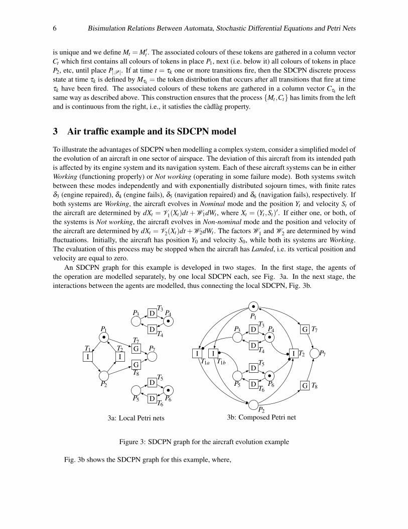
is unique and we define Mt = M′t . The associated colours of these tokens are gathered in a column vectorCt which first contains all colours of tokens in place P1, next (i.e. below it) all colours of tokens in placeP2, etc, until place P|P|. If at time t = τk one or more transitions fire, then the SDCPN discrete processstate at time τk is defined by Mτk = the token distribution that occurs after all transitions that fire at timeτk have been fired. The associated colours of these tokens are gathered in a column vector Cτk in thesame way as described above. This construction ensures that the process Mt ,Ct has limits from the leftand is continuous from the right, i.e., it satisfies the cadlag property.

3 Air traffic example and its SDCPN model

To illustrate the advantages of SDCPN when modelling a complex system, consider a simplified model ofthe evolution of an aircraft in one sector of airspace. The deviation of this aircraft from its intended pathis affected by its engine system and its navigation system. Each of these aircraft systems can be in eitherWorking (functioning properly) or Not working (operating in some failure mode). Both systems switchbetween these modes independently and with exponentially distributed sojourn times, with finite ratesδ3 (engine repaired), δ4 (engine fails), δ5 (navigation repaired) and δ6 (navigation fails), respectively. Ifboth systems are Working, the aircraft evolves in Nominal mode and the position Yt and velocity St ofthe aircraft are determined by dXt = V1(Xt)dt +W1dWt , where Xt = (Yt ,St)

′. If either one, or both, ofthe systems is Not working, the aircraft evolves in Non-nominal mode and the position and velocity ofthe aircraft are determined by dXt = V2(Xt)dt +W2dWt . The factors W1 and W2 are determined by windfluctuations. Initially, the aircraft has position Y0 and velocity S0, while both its systems are Working.The evaluation of this process may be stopped when the aircraft has Landed, i.e. its vertical position andvelocity are equal to zero.

An SDCPN graph for this example is developed in two stages. In the first stage, the agents ofthe operation are modelled separately, by one local SDCPN each, see Fig. 3a. In the next stage, theinteractions between the agents are modelled, thus connecting the local SDCPN, Fig. 3b.

P2

I

T1

I

T2

•P1

G

T7

GT8

P7

P3

DT4

DT3

•P4

P5 DT6

DT5

•P6

3a: Local Petri nets 3b: Composed Petri netP2

IT1a

IT1b

I T2

•P1

G T7

G T8

P7

P3

DT4

DT3

•P4

P5 DT6

DT5

•P6

Figure 3: SDCPN graph for the aircraft evolution example

Fig. 3b shows the SDCPN graph for this example, where,

M.H.C. Everdij & H.A.P. Blom 7

• P1 denotes aircraft evolution Nominal, i.e. evolution is according to V1 and W1.

• P2 denotes aircraft evolution Non-nominal, i.e. evolution is according to V2 and W2.

• P3 and P4 denote engine system Not working and Working, respectively.

• P5 and P6 denote navigation system Not working and Working, respectively.

• P7 denotes the aircraft has landed.

• T1a and T1b denote a transition of aircraft evolution from Nominal to Non-nominal, due to enginesystem or navigation system Not working, respectively.

• T2 denotes a transition of aircraft evolution from Non-nominal to Nominal, due to engine systemand navigation system both Working again.

• T3 through T6 denote transitions between Working and Not working of the engine and navigationsystems.

• T7 and T8 denote transitions of the aircraft landing.

The graph in Fig. 3b completely defines SDCPN elements P , T , A and N , where TG = T7,T8,TD = T3,T4,T5,T6 and TI = T1a,T1b,T2. The other SDCPN elements are specified below:

S : Two colour types are defined; S = R0,R6.

C : C (P1) = C (P2) = C (P7) = R6, i.e. tokens in P1, P2 and P7 have colours in R6; the colour com-ponents model the 3-dimensional position and 3-dimensional velocity of the aircraft. C (P3) =C (P4) = C (P5) = C (P6) = R0 , /0.

I : Place P1 initially has a token with colour X0 = (Y0,S0)′, with Y0 ∈ R2 × (0,∞) and S0 ∈ R3 \

Col0,0,0. Places P4 and P6 initially each have a token without colour.

V , W : The token colour functions for places P1, P2 and P7 are determined by (V1,W1), (V2,W2),and (V7,W7), respectively, where (V7,W7) = (0,0). For places P3 – P6 there is no token colourfunction.

G : Transitions T7 and T8 have a guard defined by GT7 = GT8 = R2× (0,∞)×R2× (0,∞).

D : The jump rates for transitions T3, T4, T5 and T6 are DT3(·) = δ3, DT4(·) = δ4, DT5(·) = δ5 andDT6(·) = δ6.

F : Each transition has a unique output place, to which it fires a token with a colour (if applicable)equal to the colour of the token removed.

4 From SDCPN to GSHS

Following [7], this section first presents a definition of general stochastic hybrid system (GSHS) and itsexecution. In [15] it has been proven that under a few conditions, SDCPN and GSHS are bisimilar. InSubsection 4.2 this is illustrated by showing how the SDCPN example of the previous section can bemapped to a bisimilar GSHS.

8 Bisimulation Relations Between Automata, Stochastic Differential Equations and Petri Nets

4.1 GSHS definition

Definition 4.1 (General stochastic hybrid system) A GSHS is an automaton (K, d, X , f , g, Init, λ , Q),where

• K is a countable set.

• d : K→ N maps each θ ∈K to a natural number.

• X : K→Eθ ;θ ∈K maps each θ ∈K to an open subset Eθ of Rd(θ). With this, the hybrid statespace is given by E , θ×Eθ ;θ ∈K.• f : E→Rd(θ);θ ∈K is a vector field.

• g : E→Rd(θ)×h;θ ∈K is a matrix field, with h ∈ N.

• Init: B(E)→ [0,1] is an initial probability measure, with B(E) the Borel σ -algebra on E.

• λ : E→ R+ is a jump rate function.

• Q : B(E)× (E ∪∂E)→ [0,1] is a GSHS transition measure, where ∂E , θ×∂Eθ ;θ ∈K isthe boundary of E, in which ∂Eθ is the boundary of Eθ .

Definition 4.2 (GSHS execution) A stochastic process θt ,Xt is called a GSHS execution if thereexists a sequence of stopping times 0 = τ0 < τ1 < τ2 · · · such that for each k ∈ N:

• (θ0,X0) is an E-valued random variable extracted according to probability measure Init.

• For t ∈ [τk,τk+1), θt = θτk and Xt = Xkt , where for t ≥ τk, Xk

t is a solution of the stochastic differ-

ential equation dXkt = f (θτk ,X

kt )dt + g(θτk ,X

kt )dB

θτkt with initial condition Xk

τk= Xτk , and where

Bθt is h-dimensional standard Brownian motion for each θ ∈K.

• τk+1 = τk +σk, where σk is chosen according to a survivor function given by F(t) =1(t<τ∗) exp(−∫ t

0 λ (θ ,Xks )ds). Here, τ∗ = inft > τk | Xk

t ∈ ∂Eθτk and 1 is indicator function.

• The probability distribution of (θτk+1 ,Xτk+1), i.e. the hybrid state right after the jump, is governedby the law Q(·;(θτk ,Xτk+1−)).

[7] show that under assumptions G1-G4 below, a GSHS execution is a strong Markov Process andhas the cadlag property (right continuous with left hand limits).

G1 f (θ , ·) and g(θ , ·) are Lipschitz continuous and bounded. This yields that for each initial state(θ ,x) at initial time τ there exists a pathwise unique solution Xt to dXt = f (θ ,Xt)dt +g(θ ,Xt)dBt ,where Bt is h-dimensional standard Brownian motion.

G2 λ : E → R+ is a measurable function such that for all ξ ∈ E, there is ε(ξ ) > 0 such that t →λ (θt ,Xt) is integrable on [0,ε(ξ )).

G3 For each fixed A ∈ B(E), the map ξ → Q(A;ξ ) is measurable and for any (θ ,x) ∈ E ∪ ∂E,Q(·;θ ,x) is a probability measure.

G4 If Nt = ∑k 1(t≥τk), then it is assumed that for every starting point (θ ,x) and for all t ∈R+, ENt < ∞.This means, there will be a finite number of jumps in finite time.

M.H.C. Everdij & H.A.P. Blom 9

4.2 A bisimilar GSHS for the example SDCPN

Next we transform the SDCPN example model of Section 3 into a bisimilar GSHS. The first step is toconstruct the state space K for the GSHS discrete process θt. This is done by identifying the SDCPNreachability graph. Nodes in the reachability graph provide the number of tokens in each of the SDCPNplaces. Arrows connect these nodes as they represent transitions firing. The SDCPN of Fig. 3b has sevenplaces hence the reachability graph for this example has elements that are vectors of length 7. Thesenodes, excluding the nodes that enable immediate transitions, form the GSHS discrete state space.

V4 =(0,1,1,0,1,0,0) (0,0,1,0,1,0,1)=V8

V2 =(0,1,1,0,0,1,0) (0,1,0,1,1,0,0)=V3

V6 =(0,0,0,1,1,0,1) (0,0,1,0,0,1,1)=V7

(1,0,1,0,0,1,0)(0,1,0,1,0,1,0)(1,0,0,1,1,0,0)

V1 =(1,0,0,1,0,1,0) (0,0,0,1,0,1,1)=V5

T5T6 T3 T4

T8

T3T4 T6 T5

T1a T3 T5 T1b

T8

T5 T6 T4T3

T4 T2 T6

T7

T8

Figure 4: Reachability graph for the SDCPN of Fig. 3b. The nodes in bold type face correspond with theelements of the GSHS discrete state space K.

The reachability graph is shown in Fig. 4, with nodes that form the GSHS discrete state space in Boldtypeface, i.e. K= V1, . . . ,V8, with V1 = (1,0,0,1,0,1,0), V2 = (0,1,1,0,0,1,0), V3 = (0,1,1,0,1,0,0),V4 = (0,1,0,1,1,0,0), V5 = (0,0,0,1,0,1,1), V6 = (0,0,1,0,0,1,1), V7 = (0,0,1,0,1,0,1), V8 = (0,0,0,1,1,0,1). Since initially there is a token in places P1, P4 and P6, the GSHS initial mode equals θ0 =V1 = (1,0,0,1,0,1,0). The GSHS initial continuous state value equals the vector containing the initialcolours of all initial tokens. Since the initial colour of the token in Place P1 equals X0, and the tokensin places P4 and P6 have no colour, the GSHS initial continuous state value equals ColX0, /0, /0 = X0.The GSHS drift coefficient f is given by f (θ , ·) = V1(·) for θ =V1, f (θ , ·) = V2(·) for θ ∈ V2,V3,V4,and f (θ , ·) = 0 otherwise. For the diffusion coefficient, g(θ , ·) = W1 for θ = V1, g(θ , ·) = W2 for θ ∈V2,V3,V4, and g(θ , ·) = 0 otherwise. The hybrid state space is given by E = θ×Eθ ;θ ∈M, wherefor θ ∈ V1,V2,V3,V4: Eθ = R2× (0,∞)×R2× (0,∞) and for θ ∈ V5,V6,V7,V8: Eθ = R6. Alwaystwo delay transitions are pre-enabled: either T3 or T4 and either T5 or T6. This yields λ (V1, ·) = λ (V5, ·) =δ4 +δ6, λ (V2, ·) = λ (V6, ·) = δ3 +δ6, λ (V3, ·) = λ (V7, ·) = δ3 +δ5, λ (V4, ·) = λ (V8, ·) = δ4 +δ5. For thedetermination of GSHS transition measure Q, we make use of the reachability graph, the sets D , G andF and the rules R0–R4. In Table 1, Q(θ ′,x′;θ ,x) = p denotes that if (θ ,x) is the value of the GSHSstate before the hybrid jump, then, with probability p, (θ ′,x′) is the value of the GSHS state immediatelyafter the jump.

With this, the SDCPN of the aircraft evolution example is uniquely mapped to an GSHS. It can beshown that the SDCPN execution and the execution of the resulting GSHS are probabilistically equiva-

10 Bisimulation Relations Between Automata, Stochastic Differential Equations and Petri Nets

Table 1: Example GSHS transition measure for size of jumpFor x /∈ ∂EV1 : Q(V2,x;V1,x) = δ4

δ4+δ6, Q(V4,x;V1,x) = δ6

δ4+δ6

For x ∈ ∂EV1 : Q(V5,x;V1,x) = 1For x /∈ ∂EV2 : Q(V3,x;V2,x) = δ6

δ3+δ6, Q(V1,x;V2,x) = δ3

δ3+δ6

For x ∈ ∂EV2 : Q(V6,x;V2,x) = 1For x /∈ ∂EV3 : Q(V4,x;V3,x) = δ3

δ3+δ5, Q(V2,x;V3,x) = δ5

δ3+δ5

For x ∈ ∂EV3 : Q(V7,x;V3,x) = 1For x /∈ ∂EV4 : Q(V3,x;V4,x) = δ4

δ4+δ5, Q(V1,x;V4,x) = δ5

δ4+δ5

For x ∈ ∂EV4 : Q(V8,x;V4,x) = 1For all x: Q(V6,x;V5,x) = δ4

δ4+δ6, Q(V8,x;V5,x) = δ6

δ4+δ6

For all x: Q(V7,x;V6,x) = δ6δ3+δ6

, Q(V5,x;V6,x) = δ3δ3+δ6

For all x: Q(V8,x;V7,x) = δ3δ3+δ5

, Q(V6,x;V7,x) = δ5δ3+δ5

For all x: Q(V7,x;V8,x) = δ4δ4+δ5

, Q(V5,x;V8,x) = δ5δ4+δ5

lent, i.e. the SDCPN and the GSHS are bisimilar. Thanks to this bisimilarity we can now use the automataframework to analyse the GSHP that is defined by the SDCPN model for the example.

5 From SDCPN to HSDE

Following [1] and [2], this section first presents a definition of hybrid stochastic differential equation(HSDE) and gives conditions under which the HSDE has a pathwise unique solution. This pathwiseunique solution is referred to as HSDE solution process or GSHP. The basic advantage of using HSDEin defining a GSHP over using GSHS is that with the HSDE approach the spontaneous jump mechanismis explicitly built on an underlying stochastic basis, whereas in GSHS the execution itself imposes anunderlying stochastic basis. In [16] it has been proven that under a few conditions, SDCPN and HSDEare bisimilar. In Subsection 5.2 this is illustrated by showing how the SDCPN example of the previoussection can be mapped to a bisimilar HSDE.

5.1 HSDE definition

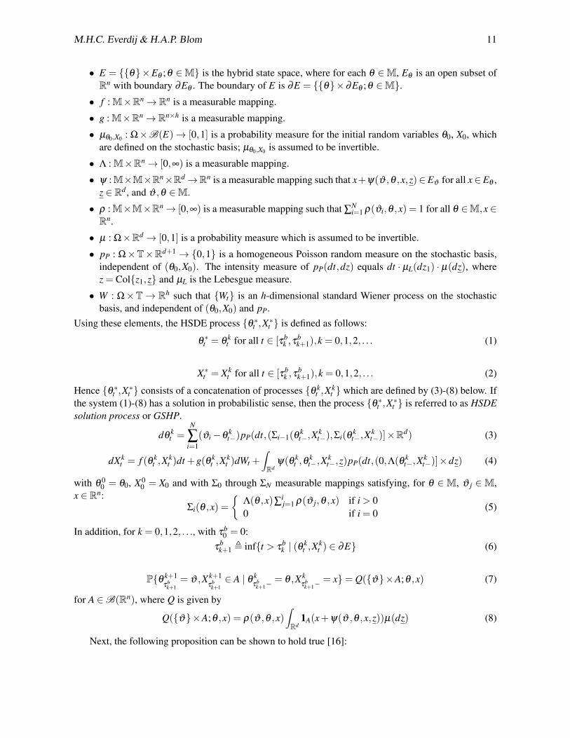
For the HSDE setting we start with a complete stochastic basis (Ω,ℑ,F,P,T), in which a completeprobability space (Ω,ℑ,P) is equipped with a right-continuous filtration F = ℑt on the positive timeline T = R+. This stochastic basis is endowed with a probability measure µθ0,X0 for the initial state,an independent h-dimensional standard Wiener process Wt and an independent homogeneous Poissonrandom measure pP(dt,dz) on T×Rd+1.

Definition 5.1 (Hybrid stochastic differential equation) An HSDE on stochastic basis (Ω,ℑ,F,P,T), isdefined as a set of equations (1)-(8) in which a collection of elements (M, E, f , g, µθ0,X0 , Λ, ψ , ρ , µ , pP,Wt) appear.

The elements (M, E, f , g, µθ0,X0 , Λ, ψ , ρ , µ , pP, Wt) are defined as follows:

• M= ϑ1, . . . ,ϑN is a finite set, N ∈ N, 1≤ N < ∞.

M.H.C. Everdij & H.A.P. Blom 11

• E = θ×Eθ ;θ ∈M is the hybrid state space, where for each θ ∈M, Eθ is an open subset ofRn with boundary ∂Eθ . The boundary of E is ∂E = θ×∂Eθ ;θ ∈M.• f : M×Rn→ Rn is a measurable mapping.

• g : M×Rn→ Rn×h is a measurable mapping.

• µθ0,X0 : Ω×B(E)→ [0,1] is a probability measure for the initial random variables θ0, X0, whichare defined on the stochastic basis; µθ0,X0 is assumed to be invertible.

• Λ : M×Rn→ [0,∞) is a measurable mapping.

• ψ :M×M×Rn×Rd→Rn is a measurable mapping such that x+ψ(ϑ ,θ ,x,z)∈Eϑ for all x∈Eθ ,z ∈ Rd , and ϑ ,θ ∈M.

• ρ : M×M×Rn→ [0,∞) is a measurable mapping such that ∑Ni=1 ρ(ϑi,θ ,x) = 1 for all θ ∈M,x ∈

Rn.

• µ : Ω×Rd → [0,1] is a probability measure which is assumed to be invertible.

• pP : Ω×T×Rd+1 → 0,1 is a homogeneous Poisson random measure on the stochastic basis,independent of (θ0,X0). The intensity measure of pP(dt,dz) equals dt · µL(dz1) · µ(dz), wherez = Colz1,z and µL is the Lebesgue measure.

• W : Ω×T→ Rh such that Wt is an h-dimensional standard Wiener process on the stochasticbasis, and independent of (θ0,X0) and pP.

Using these elements, the HSDE process θ ∗t ,X∗t is defined as follows:

θ∗t = θ

kt for all t ∈ [τb

k ,τbk+1),k = 0,1,2, . . . (1)

X∗t = Xkt for all t ∈ [τb

k ,τbk+1),k = 0,1,2, . . . (2)

Hence θ ∗t ,X∗t consists of a concatenation of processes θ kt ,X

kt which are defined by (3)-(8) below. If

the system (1)-(8) has a solution in probabilistic sense, then the process θ ∗t ,X∗t is referred to as HSDEsolution process or GSHP.

dθkt =

N

∑i=1

(ϑi−θkt−)pP(dt,(Σi−1(θ

kt−,X

kt−),Σi(θ

kt−,X

kt−)]×Rd) (3)

dXkt = f (θ k

t ,Xkt )dt +g(θ k

t ,Xkt )dWt +

∫Rd

ψ(θ kt ,θ

kt−,X

kt−,z)pP(dt,(0,Λ(θ k

t−,Xkt−)]×dz) (4)

with θ 00 = θ0, X0

0 = X0 and with Σ0 through ΣN measurable mappings satisfying, for θ ∈M, ϑ j ∈M,x ∈ Rn:

Σi(θ ,x) =

Λ(θ ,x)∑ij=1 ρ(ϑ j,θ ,x) if i > 0

0 if i = 0(5)

In addition, for k = 0,1,2, . . ., with τb0 = 0:

τbk+1 , inft > τ

bk | (θ k

t ,Xkt ) ∈ ∂E (6)

Pθ k+1τb

k+1= ϑ ,Xk+1

τbk+1∈ A | θ k

τbk+1−

= θ ,Xkτb

k+1−= x= Q(ϑ×A;θ ,x) (7)

for A ∈B(Rn), where Q is given by

Q(ϑ×A;θ ,x) = ρ(ϑ ,θ ,x)∫Rd

1A(x+ψ(ϑ ,θ ,x,z))µ(dz) (8)

Next, the following proposition can be shown to hold true [16]:

12 Bisimulation Relations Between Automata, Stochastic Differential Equations and Petri Nets

Proposition 5.1 Let conditions H1-H8 below hold true. Let (θ ∗0 (ω),X∗0 (ω)) = (θ0,X0) ∈ E for all ω .Then for every initial condition (θ0,X0), (1)-(8) has a pathwise unique solution θ ∗t ,X∗t which is cadlagand adapted and is a semi-martingale assuming values in the hybrid state space E.

H1 For all θ ∈ M there exists a constant K(θ) such that for all x ∈ Rn, | f (θ ,x)|2 + ‖g(θ ,x))‖2 ≤K(θ)(1+ |x|2), where |a|2 = ∑i(ai)

2 and ||b||2 = ∑i, j(bi j)2.

H2 For all r ∈ N and for all θ ∈M there exists a constant Lr(θ) such that for all x and y in the ballBr = z ∈ Rn | |z| ≤ r+1, | f (θ ,x)− f (θ ,y)|2 +‖g(θ ,x)−g(θ ,y)‖2 ≤ Lr(θ)|x− y|2.

H3 For each θ ∈M, the mapping Λ(θ , ·) : Rn→ [0,∞) is continuous and bounded, with upper bound aconstant CΛ.

H4 For all (θ ,ϑ) ∈M2, the mapping ρ(ϑ ,θ , ·) : Rn→ [0,∞) is continuous.

H5 For all r ∈ N there exists a constant Mr(θ) such that

sup|x|≤r

∫Rd|ψ(ϑ ,θ ,x,z)|µ(dz)≤Mr(θ), for all ϑ ,θ ∈M

H6 |ψ(θ ,θ ,x,z)|= 0 or > 1 for all θ ∈M, x ∈ Rn, z ∈ Rd

H7 (θ ∗t ,X∗t ) hits the boundary ∂E a finite number of times on any finite time interval

H8 |ϑi−ϑ j|> 1 for i 6= j, with | · | a suitable metric well defined on M.

5.2 A bisimilar HSDE for the example SDCPN

Next we transform the SDCPN example model of Section 3 into a bisimilar HSDE. This mapping followsmuch the same procedure as for SDCPN to GSHS, except that the discrete state space is now referredto as M (rather than K) and the Markov jump rate is now referred to as Λ (rather than λ ). The mainadditional difference is that the HSDE elements do not include a transition measure Q to define the size ofjump, but include functions ψ , ρ and µ instead. The mapping of SDCPN to HSDE uses the constructionof transition measure Q as an intermediate step, however. For the particular example SDCPN in thispaper, these functions can be determined from Q as follows: Since the continuous valued process jumpsto the same value with probability 1, we find that ψ(V i,V j,x,z) = 0 for all V i, V j, x, z. Moreover,ρ(V i,V j,x) = PQ(V i,x,V j,x) and µ may be any given invertible probability measure.

With this, the SDCPN of the aircraft evolution example is uniquely mapped to an HSDE. If in addi-tion, we want to make use of the HSDE properties of Proposition 5.1, i.e. the resulting HSDE solutionprocess being adapted and a semi-martingale, we need to make sure that HSDE conditions H1-H8 aresatisfied. It is shown below that they are, under the following sufficient condition D1 for the exampleSDCPN.

D1 For P ∈ P1,P2, there exist KvP, Lv

P, KwP and Lw

P such that for all c,a ∈ C (P),|VP(c)|2 ≤ Kv

P(1+ |c|2) and |VP(c)−VP(a)|2 ≤ LvP|c−a|2 and

‖WP(c)‖2 ≤ KwP (1+ |c|2) and ‖WP(c)−WP(a)‖2 ≤ Lw

P |c−a|2.

We verify that under condition D1, HSDE conditions H1-H8 hold true in this example.

H1: From the construction of f and g above we have for θ = V1: | f (θ ,x)|2 + ‖g(θ ,x)‖2 = |V1(x)|2 +‖W1(x)‖2 ≤ Kv

P1(1+ |x|2)+Kw

P1(1+ |x|2) = K(θ)(1+ |x|2), with K(θ) = (Kv

P1+Kw

P1). For θ =

V2,V3,V4 the verification is with replacing V1, W1 by V2, W2.

M.H.C. Everdij & H.A.P. Blom 13

H2: From the construction of f and g above we have for θ = V1: | f (θ ,x)− f (θ ,y)|2 + ‖g(θ ,x)−g(θ ,y)‖2 = |V1(x)−V1(y)|2 +‖W1(x)−W1(y)‖2 ≤ Lv

P1|x− y|2 +Lw

P1|x− y|2 = Lr(θ)|x− y|2 with

Lr(θ) = LvP1+Lw

P1. For θ =V2,V3,V4 replace V1, W1 by V2, W2.

H3: Since δ3–δ6 are constant, for all θ , Λ(θ , ·) is bounded and continuous, with upper bound CΛ =maxδ4 +δ6,δ3 +δ6,δ3 +δ5,δ4 +δ5.

H4: Since for all θ ,ϑ , PQ(ϑ , ·;θ ,x) is constant, we find ρ(ϑ ,θ ,x) = PQ(ϑ ,x,θ ,x) is continuous.

H5 and H6: These are satisfied due to ψ(V i,V j,x,z) = 0 for all V i, V j, x, z.

H7: This condition holds due to δ3–δ6 being finite and the fact that in this SDCPN example, there is nofiring sequence of more than one guard transition.

H8: This condition holds for all V1, . . . ,V8, with metric |a|2 = ∑i(ai)2.

Thanks to this bisimilarity mapping we can now use HSDE tools to analyse the GSHP that is defined bythe execution of the SDCPN model for the example.

6 Conclusions

The aim of this paper was to explain bisimilarity relations between SDCPN (stochastically and dynami-cally coloured Petri net), GSHS (general stochastic hybrid system) and HSDE (hybrid stochastic differ-ential equation), which means that the strengths of one stochastic model formalism can be used by bothof the other stochastic model formalisms. More specifically, these bisimilarity relations make it possibleto combine the formal verification power of automata with the analysis power of stochastic differentialequations and the compositional specification power of Petri nets.

We started in Section 2 by defining SDCPN and the resulting SDCPN stochastic process, whichis referred to as a GSHP (general stochastic hybrid process). In Section 3 we presented a simple butillustrative SDCPN example model. In Section 4 we studied GSHP as an execution of a GSHS andillustrated by using the example of Section 3 that SDCPN and GSHS are bisimilar. Next, in Section 5we studied GSHP as a stochastic process solution of HSDE and showed with an illustrative example thatSDCPN and HSDE are bisimilar.

The bisimilarities between SDCPN, GSHS and HSDE models for the example considered mean thatthe resulting example model inherits the strengths of all three formal stochastic modelling formalisms.This has been depicted in Fig. 1 in the introduction. Examples of GSHP properties are convergence indiscretisation, existence of limits, existence of event probabilities, strong Markov properties, reachabil-ity analysis. Examples of GSHS features are their connection to formal methods in automata theory andoptimal control theory. Examples of HSDE features are stochastic analysis tools for semi-martingales.Examples of SDCPN features are natural expression of causal dependencies, concurrency and synchro-nisation mechanism, hierarchical and modular construction, and graphical representation. These com-plementary advantages of SDCPN, GSHS, HSDE and GSHP perspectives tend to increase with the com-plexity of the system considered.

An illustrative large scale application of bisimularity relations between SDCPN, HSDE and stochas-tic hybrid automata has been developed in air traffic management. Currently pilots depend of air trafficcontrollers in solving potential conflicts between their flight trajectories. This places a huge requirementon the tasks of an air traffic controller. Imagine a similar kind of approach for road traffic; then each cardriver would be blind and depends of instructions that some road traffic controller is communicating withthe car drivers. How many cars do you think can be managed by one road traffic controller? The number

14 Bisimulation Relations Between Automata, Stochastic Differential Equations and Petri Nets

of aircraft that one air traffic controller can handle ranges between 10 and 20, depending of the complex-ity of the traffic pattern. Over a decade ago, it had been suggested by [22] that this limitation of the airtraffic controller can be solved by moving the responsibility of conflict resolution from the air traffic con-troller to the pilots. Since then this airborne self separation idea has received a lot of research attention.Nevertheless, it still is unknown how much more air traffic can safely be accommodated under a well de-signed airborne self separation way of working. In order to add to the solution of this debate, a series oflarge European studies towards solving this question have been started under the name HYBRIDGE [18]and iFly [19] respectively. The way of working is to first develop a well defined SDCPN model of theairborne self separation concept of operation to be analysed, e.g. [17]. Subsequently this SDCPN modelis further analysed using a bisimilar HSDE and hybrid automation formal model representation [5, 3], inwhich powerful stochastic analysis theory is exploited for the speeding up of Monte Carlo simulations.Using this approach, [4] have shown that the first generation of airborne self separation concept designsfalls short in safely accommodating higher air traffic demand than conventional ATM can. The feedbackof this finding to advanced air traffic concept designers triggered the development of more advancedairborne self separation concept of operation, e.g. see [19].

References

[1] H.A.P. Blom (2003): Stochastic hybrid processes with hybrid jumps. In: Proceedings IFAC conference onanalysis and design of hybrid system (ADHS), Saint-Malo, Brittany, France. pp. 361–365.

[2] H.A.P. Blom, G.J. Bakker, M.H.C. Everdij & M.N.J. Van der Park (2003): Stochastic analysisbackground of accident risk assessment for air traffic management. HYBRIDGE Report, D2.2.http://hosted.nlr.nl/public/hosted-sites/hybridge/.

[3] H.A.P. Blom, G.J. Bakker & J. Krystul (2009): Rare event estimation for a large scale stochastic hybridsystem with air traffic application. In: G. Rubino & B. Tuffin, editors: Rare event simulation using MonteCarlo methods, forthcoming. J.Wiley.

[4] H.A.P. Blom, B. Klein Obbink & G.J. Bakker (2009): Simulated collision risk of an uncoordinated airborneself separation concept of operation. ATC Quarterly 17, pp. 63–93.

[5] H.A.P. Blom, J. Krystul, G.J. Bakker, M.B. Klompstra & B. Klein Obbink (2007): Free flight collision riskestimation by sequential Monte Carlo simulation. In: C.G. Cassandras & J. Lygeros, editors: Stochastichybrid systems: recent developments and research trends, Control engineering 24, chapter 10. Taylor &Francis Group / CRC Press, pp. 247–281.

[6] M.L. Bujorianu & J. Lygeros (2004): General stochastic hybrid systems: modelling and optimal control. In:Proceedings 43rd conference on decision and control (CDC), Nassau, Bahamas.

[7] M.L. Bujorianu & J. Lygeros (2006): Toward a general theory of stochastic hybrid systems. In: H.A.P. Blom& J. Lygeros, editors: Stochastic hybrid systems: theory and safety critical applications, Lectures notes incontrol and information sciences (LNCIS) 337. Springer, pp. 3–30.

[8] M.L. Bujorianu, J. Lygeros & M.C. Bujorianu (2005): Different approaches on bisimulation for stochastichybrid systems. In: M. Morari & L. Thiele, editors: Proceedings 8th international workshop on hybridsystems: computation and control (HSCC), Zurich, Switzerland, Lecture notes in computer science (LNCS)3414. pp. 198–214.

[9] M.H.A. Davis (1993): Markov models and optimization, Monographs on statistics and applied probability 49.Chapman and Hall, London.

[10] R.J. Elliott (1982): Stochastic calculus and applications, Applications of mathematics: Stochastic modellingand applied probability 18. Springer-Verlag.

M.H.C. Everdij & H.A.P. Blom 15

[11] R.J. Elliott, L. Aggoun & J.B. Moore (1995): Hidden Markov models: estimation and control, Applicationsof mathematics: stochastic modelling and applied probability 29. Springer-Verlag.

[12] S.N. Ethier & T.G. Kurtz (1986): Markov processes, characterization and convergence. Wiley series inprobability and mathematical statistics. John Wiley & Sons, New York.

[13] M.H.C. Everdij & H.A.P. Blom (2003): Petri nets and hybrid state Markov processes in a power-hierarchyof dependability models. In: Proceedings IFAC conference on analysis and design of hybrid system (ADHS),Saint-Malo, Brittany, France. pp. 355–360.

[14] M.H.C. Everdij & H.A.P. Blom (2005): Piecewise deterministic Markov processes represented by dynam-ically coloured Petri nets. In: S. Jacka, editor: Stochastics: an international journal of probability andstochastic processes, 77, number 1. Taylor & Francis, pp. 1–29.

[15] M.H.C. Everdij & H.A.P. Blom (2006): Hybrid Petri nets with diffusion that have into-mappings with gener-alised stochastic hybrid processes. In: H.A.P. Blom & J. Lygeros, editors: Stochastic hybrid systems: theoryand safety critical applications, Lectures notes in control and information sciences (LNCIS) 337. Springer,pp. 31–63.

[16] M.H.C. Everdij & H.A.P. Blom (2010): Hybrid state Petri nets which have the analysis power of stochastichybrid systems and the formal verification power of automata. In: P. Pawlewski, editor: Petri nets: Applica-tions, chapter 12. InTech, pp. 227–252.

[17] M.H.C. Everdij, M.B. Klompstra, H.A.P. Blom & B. Klein Obbink (2006): Compositional specification ofa multi-agent system by stochastically and dynamically coloured Petri nets. In: H.A.P. Blom & J. Lygeros,editors: Stochastic hybrid systems: theory and safety critical applications, Lectures notes in control andinformation sciences (LNCIS) 337. Springer, pp. 325–350.

[18] HYBRIDGE (2002). EC project description. http://hosted.nlr.nl/public/hosted-sites/hybridge.[19] iFly (2007). EC project description. http://iFly.nlr.nl.[20] J. Krystul (2006): Modelling of stochastic hybrid systems with applications to accident risk assessment.

Ph.D. thesis, University of Twente, The Netherlands.[21] J. Krystul, H.A.P. Blom & A. Bagchi (2007): Stochastic hybrid systems, chapter 2: Stochastic differential

equations on hybrid state spaces, pp. 15–45. Number 24 in Control engineering series. Taylor and Francis /CRC Press.

[22] RTCA (1995): Final report of RTCA Task Force 3; Free Flight implementation. Final, RTCA Inc., Washing-ton DC.

[23] A.J. Van der Schaft (2004): Equivalence of dynamical systems by bisimulation. IEEE transactions on auto-matic control 49(12), pp. 2160–2172.