A Formal Definition of Hierarchical Predicate Transition Nets

Xudong He

Department of Computer Science North Dakota State University

Fargo, ND 58105, U.S.A.

Abstract. Hierarchical predicate transition nets have recently been introduced as a visual formalism for specifying complex reactive systems. They extend predicate transition nets with hierarchical structures so that large systems can be specified and understood stepwisely, and thus are more suitable for real-world applications. In this paper, we provide a formal syntax and an algebraic semantics for hierarchical predicate transition nets, which establish the theory of hierarchical predicate transition nets for precise specification and formal reasoning.

1 Introduction

Petri nets are an excellent model for studying concurrent and distributed systems due to their modeling power and simple graphical notation. Petri nets, unlike many other graphical modeling techniques, have a well-defined algebraic semantics supporting formal analysis of system properties as well as an operational semantics for exhibiting dynamic system behaviors. However traditional Petri nets have the distinct drawback of producing very large and unstructured system specifications for even small systems, which are normally very difficult to understand due to their low-levelness and primitive structures. In the past decade, various types of high-level Petri nets ([1], [5], [13], [19]) have been developed to partially overcome the above drawback; which represents a major progress similar to that from low-level programming languages to high-level programming languages. As the next natural step, modular and hierarchical mechanisms have recently been incorporated into high-level Petri nets ([1% [12], [14], [15], [20]) to make them more suitable for real-world applications.

Heuristic principles and rules for composing and refining large predicate transition net specifications (one type of high-level Petri nets) were first proposed in [20] and then further investigated and formulated in [10]. Although the above research effort has provided a systematic way to incorporate modularity and hierarchies into predicate transition nets, there is a lack of formal definition of both syntax and semantics of the underlying net model.

This paper presents both a formal syntax and an algebraic semantics of hierarchical predicate transition nets, which establish the foundation of hierarchical predicate transition nets for precise specification and formal reasoning. With the formal syntax and semantics, the validity of a net specification can be automatically checked during its construction process and many properties of the net specification can be statically derived without its execution. The formal syntax and semantics also provide a basis for rigorous comparison among different types of hierarchical high-level Petri nets and between hierarchical high- level Petri nets and other formal specification methods. This paper also presents a result for deriving a behavioral equivalent non-hierarchical predicate transition net from a given hierarchical predicate transition net, which provides an alternative semantic definition of

213

hierarchical predicate transition nets and opens the possibility of adapting existing analysis techniques of flat predicate transition nets to hierarchical predicate transition nets.

2 Brief History of Hierarchical Predicate Transition Nets

The development of hierarchical predicate transition nets (HPrT nets in the sequel) was motivated by the need to construct specifications for large systems using Petri nets and inspired by the development of modern high-level programming languages and other hierarchical and graphical specification methods such as data flow diagrams [22] and statecharts [6]. With the introduction of hierarchical structures into predicate transition nets (PrT nets in the sequel), not only the resulting net specifications are more understandable but also the specification construction process becomes more manageable.

During the development of HPrT nets, the following rationals and criteria were followed: (1) Simplicity: the introduction of new concepts and notations should be kept minimal; (2) Understandability: the new concepts and notations should resemble and be closely related to those in PrT nets; (3) Hierarchy and information hiding: different levels of abstraction should be supported; (4) Executability: HPrT nets should be direct executable without the need being translated into behavioral equivalent PrT nets. The semantics concepts of HPrT nets should be closely related to those of PrT nets; (5) Compositionality: the new concepts and notations should facilitate the compositional development of large HPrT nets from small existing HPrT nets; (6) Stepwise abstraction and refinement: the new concepts and notations should support top-down as well as bottom-up development approaches including stepwise abstraction and refinement of predicates, transitions, constraints, labels, and tokens; and (7) Maintainability: the new concepts and notations should facilitate simple specification modification and extension.

The basic ideas of HPrT nets were first proposed in [20], which were refined in [7] with the introduction of super nodes (dotted predicates and transitions) and non- terminating arcs adapted from statecharts [6]. The above notations along with the four transformational development rules (abstraction, refinement, decomposition, and synthesis) were formalized in [10]. In [10], two label construction operators, + (non- detenninancy) and X (concurrency), and the associated rules were also developed based on the semantics of PrT nets and inspired by the data flow balancing concept in data flow diagrams [22]. HPrT nets have been applied to specifying several small systems including an elevator system [10] and a library system [11]. Heuristics and strategies adapted from modern structured analysis [22] were proposed for constructing HPrT net specifications in [11]. An hybrid analysis technique for HPrT nets was presented in [8], which adapts two temporal induction rules ([17], [18]) and combines structural, behavioral, and logic reasoning.

3 Syntax and Static Semantics of Hierarchical Predicate Transition Nets

The syntax and static semantics (typing information) of traditional Petri nets can be represented graphically as well as defined algebraically. In this section, we generalize the traditional graphical representation and algebraic definition to HPrT nets.

214

3.1 Graphical Notat ion

The traditional graphical notation of Petri nets include circles denoting predicates, boxes denoting transitions, and directed arcs denoting flow relation, which are naturally retained in HPrT nets. To represent the hierarchical structure and behavior of HPrT nets, we further introduce the following symbols and conventions: (I) dotted circles / boxes (super nodes) are used to stand for either abstractions or refinements of existing HPrT nets. Predicate P l and transition t2 in Fig. I are such examples. Hierarchies are introduced through a sequence of dotted nodes where a lower level one reveals more details than its ancestors. The idea is similar to those of data flow diagrams [22]. (2) non-terminating arcs (one end being connected to the boundary of a dotted node) are introduced to keep track of data flow relationships between a child net with its external environment. I f the tail of a non-terminating arc connects to a boundary, it is called an incoming non-terminating arc and is referenced as (.n, n) (where n is the node, and on is the traditional notation for the pre-set of n and denotes the external environment related to n); otherwise it is called a outgoing non-terminating arc (n, n,) (n~ is the post-set of n). Arcs (P3, P3 ~ and (P4, P4 ~ in Fig. 1(2) are such examples. The use of non-terminating arcs has been motivated by statecharts [6].

tl pl t2 p2 t3 I ~"-'l~(I-'l<ll'x>x<12'y> ,-" -,N <13,x>+<14,y>~~.._.____..lm~ ! < 1 5 , u > + < / ~

U \ . - ' L i

(1) pl

p3 " N /

! I [ I I ~ < 1 2 ' y > ~ / /

NN. p4 / "

(2)

t2

I t4

!

I

</4,3~> r--zT-y-zT-~/6,v> It , y ~ v

I I i t5 I !

(3)

Fig. 1 - An HPrT net

3.2 Arc Labels

In an HPrT net, an arc may corresponds to many different arcs in a PrT net, which have been merged during the construction of the HPrT net. Thus the role of a label defines not only the type and number of tokens to be moved along an arc, but also its component arcs. In order to distinguish component arcs, we need to associate an identification with an arc, i.e. make an identification part of its label. In HPrT nets, a compound arc has a label expression having label constructor + or • (+ and X express non-determinancy and

215

concurrency respectively, and specify proper control flow relations between different abstraction levels [10]. For example, label <ll, x> X <12, y> of arc (tl, P l ) in Fig.l(1) defines that two tokens instantiated with x and y flow to p 1 concurrently; and label <ll, x> + <12, y> of arc (Pl, t2 ) in Fig.l(1) expresses that either a token instantiated with x or a token instantiated with y can enable transition t2); therefore, it is only necessary to assign identifications to simple labels (labels without + or X). To avoid ambiguity, the identifications of all simple labels in a compound label must be distinct, and the identifications of all simple labels in arcs connected to a node must be distinct. Arcs are related through the same identification of their simple labels. For example, arc (Pl, t2 ) in Fig.l(1), arc (p3, P3 o) in Fig.l(2), and arc ('t4, t4 ) in Fig.l(3 ) are related through label identification I1.

3.3 Algebraic Definition

There are a few possible ways to define HPrT nets algebraically. One obvious way is to define an entire HPrT net as a collection of related individual PrT nets, which, we found, does not provide a satisfactory unified algebraic framework to represent and analyze the distinct features of HPrT nets. Thus we choose to give a single algebraic definition for an entire HPrT net. An HPrT net N consists of (1) a finite hierarchical net structure (P, T, F, p), (2) an algebraic specification SPEC, and (3) a net inscription (~0, L, R, M0) The definitions of the above components are given and discussed in the following sections.

3.3.1 Hierarchical Net Structure

An HPrT net N has a finite hierarchical net structure (P, T, F, p). (P, T, F) is the essential net structure, where P u Tis the set of nodes satisfying the condition P n T = ~ . P is called the set of predicates andT is called the set of transitions. In

particular, we identify two subsets IN c_ P u T a n d O U T c P u T such that I N contains the heads of all incoming non-terminating arcs and OUT contains the tails of all outgoing non-terminating arcs. We use . IN to denote the set of the pre-sets of all

elements in IN, i . e . . IN = {.n In ~ IN}; and OUT, to denote the set of post-sets of all elements in O UT. F is the set of arcs and is called the flow relation satisfying the condition: F c _ ( . I N x I N ~ P x T u T x P u O U T x O U T . ) . N o t i c e t h a t w e u s e the pre-set and post-set notations for two differnt purposes: (1) traditional use to denote a set, and (2) as an implicit node of a non-terminating arc, i.e. treating the pre-set or post- set as a single entity. The above uses not only do not cause any ambiguity, but also reflect the true meaning of the pre-set and post-set of any node in an HPrT net.

p: P u T---> go(P u T) is a hierarchical function that defines the hierarchical relationships among the nodes in P and T. For any node n, p(n) defines the immediate

descendant nodes of n. Let p -1, p+, and p* denote the inverse, irreflexive transitive closure, and reflexive transitive closure of p respectively, the ancester and descendants of any node can be easily expressed using the above notations. To avoid complexity and ensure the correctness of refinement, the following constraints are imposed: (1) a node cannot be its own descendant (no recursive definition), (2) the refinement hierarchies have a tree structure (no structure sharing), (3) consistent interfaces among different hierarchies

216

(the interface nodes e IN u OUT be all predicates if their parent node is a predicate or all transitions if their parent node is a transition) [20], and (4) completeness (a refined net must have a parent node). The above constraints are formulated as following rules:

�9 Rule 1: V n e P u T . ( n q ~ p + ( n ) ) ,

�9 Rule 2: Vnl ,n 2 e P u T . ( P ( n l ) n P ( n 2 ) ~ O ~ n 1 = n 2 ) ,

�9 Rule 3: V p e P . ( p ( p ) n ( I N u O U T ) c P ) ^

Vt e T.(p(t) n ( IN u OUT) c_ T)

�9 Rule 4: V n e P u T . ( n e l N u O U T ~ p - l ( n ) ~ O ) .

The hierarchical net structure of Fig. 1 is algebraically defined as follows:

P = {Pl,P2,P3,P4},

T = {tl,t2,t3,t4,t5},

F = {(t 1 , Pl ), (Pl, t2), (t2, P2 ), (P2, t3), ( 'P3, P3 ), (P3, P3 "),

( 'P4, P4), (P4, P4~ (P5, t4), (t4, t4"),( ' t5, t5),(t5, t5 ~

p = {tl b-~O, t2b-->{t4,t5}, t3~--~f~, t4~-)Q~, t5b-->O,

Pl b-4 {P3,P4}, P2 ~'~ O, P3 ~-~ f~, P4 ~ ~}"

3 .3 .2 U n d e r l y i n g S p e c i f i c a t i o n

An HPrT net N contains a underlying specification SPEC = (S, OP, Eq) consisting of a signature Z = (S, OP) and a set Eq of Z-equations. Signature Y. = (S, OP) includes a set

of sorts and a family OP = ( OP R,...,s., s ) of sorted operations for Sl , . . . , s n, s e S. For

each s e S, we use CONs to denote OP ,s (the 0-ry operation of sort s), i.e. the set of constant symbols of sort s. The E-equations in Eq define the maenings and properties of operations in OP, for example, the associativity and commutativity of addition operation on real numbers. Algebraic specifications for many familiar sorts can be found in [2] and [3]. Several integrations of Petri nets with algebraic specifications are given in [21] and [16]. We often simply use familiar operations and their properties without explicitly listing the relevant equations. Based on SPEC, tokens, labels, and constraints of an HPrT net are defined.

Tokens of an HPrT net are essentially constant symbols of the family OP. The tokens of sort s are elements inCONs.

To express the number and type of (identical and / or different) tokens to be moved along an arc, the following multi-set expression {klv 1 ..... knvn} is adequate, in which each k i is a natural number, and each v i is either a member of X s (the set of variables of sort s disjoint to OP). Often we drop the set notation { } when there is only one distinctive element in the multi-set. We define the set of all such expressions of sort s as:

Exps (Xs ) = { {klvl ..... knvn} I 1 < i < n ^ k i e CON s ^ v i e Xs }.

The set of simple labels is defined as follows: SlabeIs (X) = { <l, e> I l e CONid A e e UExPs (Xs)}

s e S

where id is a distinctive sort of label identifications and CONid denotes the set of

constants of sort id. X = (Xs)se S is a family of variables disjoint to OP.

217

The set of compound labels (or labels) are recursively defined as follows:

Labels(X) = Slabel S u { l 1 + l 2 ! l 1 , t 2 ~ Label S (X) }

{l 1 x/2 I ll , l 2 ~ Labels(X)}

Let I be any label, we use slab(l) to denote the multi-set of simple labels in l. The set of labels defines syntactically valid labels, and the net inscription (to be defined in the next section) assures semantically valid labels for an HPrT net.

Constraints of an HPrT net are logic formulas, which are Z_terms of sort bool over

X, denoted as TermoP,bool(X ) . The set TermoP,boo l (X) is formally defined as follows:

(1) if v ~ CONbool t.3 Xbool , then v ~ TermoP,bool(X),

(2) i fv 1 ~ TermOP,s l (X) ..... v k ~ TermOP,sk(X), op ~ OPsl . . .sk ,bool , then

op(v l ..... Vk ) ~ TermoP,bool(X).

By treating logical connectives and quantifiers as algebraic operations, the resulting definition is simpler than traditional definitions of logic formulas.

The underlying SPEC for the net shown in Fig. 1 is as follows: S = { a l p h a , boo I } , O P , alpha = { a , b } , O P , bool = {true , f a l s e } ,

OPalpha,alpha,bool = { = },

and the family of sorted variables is: Xalph a = {x, y,u ,v, w}. Eq includes conventional equations about equality [2].

3 . 3 . 3 N e t I n s c r i p t i o n

An HPrT net N contains a net inscription (qg, L, R, M0), which associates each graphical symbol of the net structure (P, T, F, p ) with an entity in the underlying SPEC, and thus defines the static semantics of an HPrT net.

Each predicate in an HPrT net is a data structure and a component of the overall system state. The sort of each predicate defines its valid values, i.e. proper tokens. The sorts of elementary predicates are members of S. The sort of a super predicate is defined as the union of sorts of its descendant predicates. Therefore, we associate each predicate p in P with a subset of sorts in S, and give the following sort assignment: ~0 : P ---) go(S) (go is the power set operation).

L: F ---r Labels (X) is a sort-respecting labeling of N. As discussed in Arc Label section, the identifications of simple labels must be distinct when they are related through (1) a compound label (denoting a merged arc), and (2) a node (possiblly involving non- terminating arcs). The constraints for the above two situations are formulated as the following four identification uniqueness rules: �9 R u l e 5: Va ~ F.(l ~ slab(L(a)) ~ 2l ~ slab(L(a))) Rule 5 specifies that all simple labels of any compound label are distinct, i.e. slab returns a set instead of a multi-set.

�9 R u l e 6: V a ~ F . ( l l , l 2 ~ s l a b ( L ( a ) ) ^ l 1 ~ l 2 ~ 11[1] ~ 1211]) l[1] represents the projection on the 1st component of l. Rule 6 defines the uniqueness of the identifications of all simple labels in any compound label.

�9 R u l e 7: Vn ~ P w T. (Vnl ,n 2 ~ .n.(n 1 r n 2 ~ s lab(L(n l ,n ) )n slab(L(n2,n)) = 0 )

^ Vnl ,n 2 ~ n' .(n I ~ n 2 ~ slab(L(n,nl))V~slab(L(n, n2)) = 0 )

/x Vn t ~ .n,n 2 ~ n . . ( s lab(L(n l ,n ) )n slab(L(n,n2) ) = ~ ) )

218

Rule 7 specifies that all simple labels of arcs connected to a node are distinct.

�9 R u l e 8: V n ~ P u T . ( ( I I , 1 2 E Us lab(L(n ' ,n ) )u n' E*t~

Uslab(L(n,n' )))A 11 ~ 12 ~ 11[1] r 1211]) n' E n *

Rule 8 defines the uniqueness of the identifications of al l simple labels of all arcs connected to a node.

Since compound labels defines data flows as well as control flows. The following basic control flow patterns [10] must be correctly labeled: (1) data flows into and out of an elementary transition must take place concurrently, and (2) data flows into and out of an elementary predicate can occur at different times. Thus the following control flow preserving rules are needed:

�9 R u l e 9: V t e T . ( p ( t ) = O A ( ( t ' , t ) ~ F ~ l l , l z E L a b e I s ( X )

A (L(t ' , t ) r l 1 +12)) A((t,t' ) ~ F ~ Ii,12 ~ Labels (X )

n ( L ( t , f ) ~ I 1 +/2)))

�9 R u l e 10: V p e P . ( p ( p ) = O A ( ( p ' , p ) e F ~ I i , 1 2 e L a b e I s ( X )

A (L(p' ,p) r l 1 X/2)) A((p,p' ) E F ~ / i , 1 2 E Labels (X )

/x (L (p ,p ' ) r l 1 • Further the data flows between different levels of hierarchies must be balanced, i.e. a

simple label occurs in a non-terminating arc if and only if it also appears in an arc with the same direction connected to the enclosing super node. This constraint is defined as the following rule: �9 R u l e 11: V n e P u T . ( p ( n ) ~ O ~ ( l e Uslab(L(n',n))r

n' e . n

I e Ostab(L(.E,E))) "ff ep ( n ) n l N

A (l ~ Uslab(L(n,n')) r I e Uslab(L(~ff,-ff.)))) n' en . ~ep(n)c~OUT

With Rules 5 to I1, we can precisely determine the external environment of an interface node using the following rules:

�9 Ru le 12: Vn e IN.( .n = {n' [ n' E . p - l ( n ) A (slab(L(.n,n))

n slab(L(n' ,p- l (n)) ) v O)})

~ Rule 13: Vn ~ OUT.(n�9 = {n' I n' E p - l (n ) ~ A(slab(L(n,n�9

n s lab(L(p- l (n) ,n ' )) r ~)})

For example, in Fig . l (2) , P- I (p3) = Pl, t 2 E Pl ", slab(L(P3,P3")) =

{< 13,x >}, and slab(L(Pl,t2)) = {< 13,x >,< 14,Y >}; thus p3 ~ = { t 2 }.

R : T ---) TermoP,bool(X) is a well-defined constraining mapping of N, which

associates each transition t in T with a logic formula. Since a super transition is an abstraction of lower level transitions, it should not have any constraint, i.e. its constraint is always true as defined by the following rule: �9 R u l e 14: k/t ~ T.(p(t) r f~ ~ R(t) = true).

219

By convention, the logical constant symbol true is not explicitly represented in a transition.

M0: P --~ M C O N s is a sort-respecting initial marking of N, which assigns a multi- set of tokens to each predicate p in P with the same sort (where M C O N S =

{ kc I k ~ CONna t ^ c ~ CON S }). The above requirement is defined by the following

rule: �9 Rule 15: Vp �9 P.(kc ~ Mo(P) ~ c ~ CONcp(p))

Since a super predicate's state is defined by its lower level predicates, we define the tokens in a super predicate as the union of tokens of its next level predicates as follows:

�9 Rule 16: Vp e P. (p(p) ~ 0 ~ Mo(p) = UM0(p ' )). p' cO(p)

The net inscription of Fig. I is as follows:

~o = { Pl ~-4 alpha, P2 ~-4 alpha, P3 ~ alpha, P4 ~ alpha };

L = {(t l ,Pl) ~ < ll,X > x < 12,Y >, (Pl , t2) ~ < 13,x > + < 14,Y >,

( t2 ,P2) r--~< 15,u > + < 16,v >, (P2,t3) ~-~< 17,w >,(�9 ~"~< ll,X >,

(p3,P3 �9 I--+< 13,x >, (~ ~--~< 12,y >, (P4,P4 ~ ~-~< 14,y >,

( �9 ~---)< 13,x >, (t4,t4-) ~-r< 15,u >, (ot5,t5) r--~< 14,Y >, (t5,t5 �9 ~--~< 16,v >};

R = { t 1 ~ t r u e , t 2 ~ t r u e , t 3 ~-~true, t 4 ~ - ~ x = u , t 5 ~ y = v } ;

MO = ( Pl ~ {a,b}, P2 ~ { }, P3 ~-~ {a}, P4 ~ {b} }.

Theorem 1. Each simple label creates a unique data flow link between one elementary predicate and one elementary transition. Proof. the existence of a data flow link between an elementary predicate and an elementary transition identified by a simple label is ensured by data flow balance Rule 11, and the uniqueness of such a data flow link is ensured by Rules 5 to 8. [1

4 D y n a m i c S e m a n t i c s o f H i e r a r c h i c a l P r e d i c a t e T r a n s i t i o n N e t s

In this section, we define the dynamic semantics of HPrT nets including markings, transition enabling conditions, and transition firing rules.

4.1 Markings

A marking M of an HPrT net is a mapping P --9 M C O N S from the set of predicates to multi-sets o f tokens. Since a super predicate denotes an abstraction of a lower level net; thus its state is defined its next level predicates. We define the tokens of a super predicate as the union of the tokens in its next level predicates. Therefore the following rules similar to the initial marking are required: �9 Rule 17: Vp ~ P.(kc E M(p) ~ c �9 CONq~(p)) and

�9 Rule 18: V p e P . ( p ( p ) ~ O ~ M ( p ) = U M(p ' ) ) . p' ~p(p)

220

Further new markings resulted from transition firings also satisfy the above rules, which is ensured by the transition firing rule to be given in a following section.

4.2 Transition Enabling Conditions

An elementary transition in an HPrT net defines some concrete token processing as in a PrT net, thus it is natural to adapt the transition enabling conditions in PrT nets to HPrT nets. Let t be an elementary transition, tx be an occurrence mode instantiating all the variables related to t , and M be a marking, t enabled with ct under M, written as enabled(M[t /a>) , would be defined as follows if the definition of transition enabling condition for PrT nets were adapted:

Vp ~ .t.( Ut~(/[2]) c M(p)) ^ a(R(t ) ) leslab(L(p,t))

But the above formula is incorrect since the tokens in a super predicate defined by Rule 18 are not necessarily in relevant predicates (related through label identification). Fig. 2 shows a simple example, in which t 1 is not enabled, but would be enabled according to

the above formula ( P l e ot 1 and M(Pl) = {a,b}).

w /

/ ! !

pl

t l

1" " p2 " ~ , <ll,x> U

O "~" i

</1,x> ~, . . \ �9 -- \

I ~ <12,y> I t ~

~ ' / <12,y> ir ,

Fig. 2 - Another HPrT net

In order to define the correct enabling condition of a transition, we must use the tokens in relevant predicates. According to Theorem 1, we only need to consider the tokens in relevant elementary predicates or simply the exterior interface elementary predicates of any predicate in the pre-set of a transition. To determine the exterior interface elementary predicates, the following two functions are defined for any p ~ P:

in(p) = p(p) n IN and out(p) = p(p) n OUT.

Fur the r we def ine inO (p) = out~ (p) = {p}, ini+l (p) = in(ini (p)), and

out i+l (p) = out(outi(p)) . Let m and n be the smallest numbers such that into(p) = ~ ,

and out n (p) = O respectively, we define the finite irreflexive transitive closures for in

and out as follows respectively:

221

in+ (p) = Uini (p) and out+ (p) = Uouti (p) l<i<_m l<i<n

enabled(M[t/o:>) is thus defined by the following rule:

�9 R u l e 19: Vp' ~ "t .((p(p') = 0 ~ os(L(p ~ ,t)[2]) __. M(p' )) ^

(Vp ~ out+ (p ' ) .(p(p)) = ~ ot((slab(L(p', t)) n slab(L(p, p.)))[21) ___ M(p)))) ^ a(R(t ) )

A super transition is an abstraction of some low-level action. As long as some lower level transition is enabled, we consider the super transition is enabled since local changes and extenal visible changes can take place. Therefore we define the enabling condition for a super transition t with occurrence mode o~ under marking M as follows:

�9 R u l e 20: 3t 'e p( t) . (enabled(M[t ' /a >)).

As an example, the transition t2 in Fig.1 (1) is enabled with occurrence mode a = {x F-~a, u ~--~a} under the initial marking M 0 since elementary transition t4 in Fig. 1 (3) is enabled with the same occurrence mode under the initial marking.

4 . 3 T r a n s i t i o n F i r i n g R u l e

The firing of an enabled transition results in a new marking. Since the enabling condition of a super transition is defined in terms of some of its lower level transition(s), the firing of a super transition is thus the firing of its lower level transition(s). Therefore it is adequate to only define the transition firing rule for elementary transitions. Since the tokens in a super predicate are defined in terms of the union of tokens in its next level predicates specified by Rule 17 and eventually defined by the tokens in all its descendant elementary predicates; but a transition firing involving a super predicate can only affect the tokens in its interface predicates. Therefore we only need to define token changes in its exterior interface elementary predicates caused by the transition firing.

To simplify the definition of the transition firing rule, we define the extended version of labeling function:

f f " ( f ) = { ~ f ) if f ~ F i f f ~ F

Let t be an elementary transition enabled with occurrence mode a under marking M; the firing of t results in a following marking M', written as M[t/a'>lW, defined by:

�9 R u l e 21: Vp' ~ .t u t ' .((p(p' ) = ~

M" (p' ) = M(p' ) w o~(slab(-L(t,p' )[2]) - ot(slab(-s ,t)[2])) ^

Vp E (in+ (p ' ) u out+ (p ' )) .(p(p) = s ~ M" (p) = M ( p ) u G a i n ( t , p ) - Loss(p,t)) ^

Vp ~ (p+ (p' ) n P - (in+ (p ' ) u out+ (p ' ))) . (p(p) = O ~ M' (p) = M(p)) ) ^

Vp' ~ ot u to.(Vp ~ p ' ( p ' ) n (P t_) T).(M" (p) = m(p) ) )

222

where Gain(t, p) = o~((slab(-L(t, p' )) ch slab(-s p)))[2]), and

Loss(p, t) = ~((slab( 's , t)) ~ s lab(L(p , p,)))[2]).

In Rule 21, (1) the first line defines token changes in p' when predicate p' connected to t is an elementary predicate, (2) the second line defines token changes in any exterior interface elementary predicate p ofp ' , (3) the third line specifes that no changes to any interior elementary predicate ofp' , and (4) the fourth line specifies that no changes to any elementary predicate unrelated to t.

4.4 Behav io r (Dynamic Semantics) of An H P r T Net

Two enabled transitions are said to be in conflict when the firing of one of them disables the other. Conflicts are resolved nondeterministically. Non-conflicting enabled transitions can fire at the same time, which also includes the situation where the same transition is enabled with two different occurrence modes. The firing of a super transition is always considered to be concurrent with some of its lower level transition(s). Therefore three types of concurrency can occur: (1) two completely unrelated enabled transitions fire simultaneously, (2) two versions of the same transition enabled with two occurrence modes fire at the same time, and (3) the firing of a super transition concurrently with some of its lower level transition(s).

The behavior of an HPrT net is defined as the set of maximal execution sequences, in which each execution step consists of a set of firing transitions. We call an execution sequence an essential execution sequence if we drop all super transitions in all steps.

The following is an example of an execution step of the HPrT net in Fig. 1: The marking M1 resulted in from firing transition t 1 and t4 (thus t2) at the same time with occurrence modes t~ 1 = {x ~-4a, y ~-~b } and ct 2 = {x ~-~a , y ~-~b} respectively under marking M 0 (notice the x and y associated with arc (tl, P l ) are different from x and yassoc ia t edwi tharc (P l , t 2 ) ) :M1 - {Pl ~ {a, 2b },P2 ~ {a},p3 ~ {a} ,p4 ~ {2b }}.

5 Equivalent PrT Net for An HPrT Net

In this section, we show that there is a unique behavioral equivalent PrT net for any HPrT net. A PrT net is a special HPrT where (1) graphically, there is only a single connected net without super (dotted) nodes and non-terminating arcs; and (2) algebraically, the hierarchy function becomes a map from each node to an empty set and thus can be dropped, and all labels are simple labels. Based on the above analysis, we can derive a PrT net for any given HPrT net.

For a given HPrT net N = (P, T, F, p) + S P E C + ( ~ p , L , R , Mo) , in w h i c h + denotes the disjoint union as in [2] and is overloaded with our label constructor (but does not create any ambiguity); we define a PrT net N ' = (P ', T ', F ') + S P E C ' + (~p', L', R', MO') as follows:

(1) F = {p ] p e P ^ p ( p ) = O},

(2) 7" = {t [ t e T ^ p( t ) = r

(3) F = (F n ( F xlr u~F x F )) u F 1 u F 2, with

F I = {(p,t) [ p s P ' ^ t ~ T ' ^ p ' c ' t A p ~ o u t + ( p ' ) ^

223

(slab( L( p, p~ ) ) c7 slab( L( p' , t ) ) ) r 0 } ,

F 2 = {(t,p) [ p e F ^ t e 7" ^p ' e t~ Ap e in+ (p ' ) A

(slab( L( , p, p ) ) c~ slab( L( t, p' ))) r (~} .

(4) SPEC ' = SPEC ,

(5) ~o' = {p ~ ~o(p) [ p ~ e' },

(6) L ' = { f ~ - > L ( f ) ] f e F c T ( F x Y w r x F ) } w

{(p,t) ~ (slab( L(p,p~ ) ~ slab( L(p' ,t)))[2] I (p , t ) e F 1 ^ f i e .t A p e OUt+ (p ' )}

{(t,p) ~ (stab(L(.p,p))C7 slab(L(t,p' )))[2] I ( t ,p) e F 2 ^p ' e t . ^ p e in+ (p ' )},

(7) R' = {t ~-~ R(t) ] t e 7"},

(8) M 0 ' = { p ~ M 0(p) [ p e F } .

In the above definition of the PrT net N ' , components (1), (2), (4), (5), (7), and (8) are basically restrictions of the corresponding components of the given HPrT net, and thus are always feasible. The feasibility of the definitions of components (3) and (6) is ensured by Theorem 1. Notice that L' is a mapping: F' ---> ExPs (Xs ) , i.e. we have

dropped the identifications in labels since they are no longer needed in PrT nets. From the definition N ~, we obtain the following corollary:

C o r o l l a r y 1. An arc (p, t ) is in F ' of N' if and only if p is a part of the enabling

condition of t in N, and the label of (p, t) is the same as that common to p and t in the

enabling condition and the transition firing of t in N. An arc (t, p) is in F ' of N ' if and

only if p is affected by the firing of t in N , and the label of (t, p) is the same as that

common to p and t in the transition firing of t in N.

Proof. a simple comparision of relevant items in the definition of N ' , and definitions of Rule 19 and 21 is adequate. []

Let t be a transition in T ', ~ be an occurrence mode instantiating all the variables related to t , and M be a marking, t enabled with ot under M, written as enabled(M[t /o~>), is defined by: �9 R u l e 22: Vp ~ .t.(o~(L' (p,t)) c M(p) )^ (x(t~ (t))

Similar to the extension of L, and extend the definition of L' as follows:

L ' ( f ) = { ~ ( f ) i f f ~ F i f f e F

Let t be a transition in T ' enabled with occurrence mode o~ under marking M; the firing of t results in a following marking M', written as M[t lot>M", defined by:

�9 R u l e 23: Vp ~ "t u t ~ ( M' (p) = M(p ) u OI(-L' (t, p)) - tr(-L' (p, t))) ^

Vp ~ "t w t~ (p) = M(p))

Based on the Rule 22 and 23, we obtain the following theorem:

224

Theorem 2. The PrT net N' is behaviorally equivalent to the given HPrT net N.

Proof. We only need to show the following fact: (*) the set of execution sequences of N' is identical to the set of essential execution sequences of N. Since the set of execution sequences are generated by firings of enabled transitions, we only need to prove that the enabling condition and firing effect of any elementary transition in N are the same as those of the corresponding transition in N ' with any occurrence mode under any reachable marking, which however is ensured by Corollary 1, transition enabling and firing Rules 19 and 21 in N, and transition enabling and firing Rules 22 and 23 in Iq' (the detailed comparison is omitted here). []

The equivalent PrT net for the HPrT net in Fig. 1 is defined as follows:

F = { P 2 , P 3 , P 4 } ,

7" = { t l , t 3 , t 4 , t 5 } ,

F = {(t 1 , P3 ), (P3, t4 ), (tl, P4 ), (P4, t5 ), (t4, P2), (P2, t3 ), (t5, P2 )},

qg ' = { P2 ~ a lpha , P3 ~ a lpha , P4 ~-') a lpha };

L' = {(tl,P3) ~-~ x, (P3,t4) ~ x, ( t l ,P4) ~ y, (P4,t5) ~ y, ( t2,P2) ~ u,

( t5,P2) ~ v, (P2,t3) ~ w}

R ' = {t 1 ~ t r u e , t 3 ~-) true, t 4 ~ x = u, t 5 ~ y = v };

M0'= { P2 ~ { }, P3 ~-) {a}, P4 ~ {b} }.

Graphical transformation is straightforward, in which all super nodes and non- terminating arcs are deleted. New arcs and labels are created according to (3) and (6) in the definition of a derived PrT net. The equivalent PrT net for the HPrT net in Fig. 1 is shown in Fig. 3.

x ,4

~-r x=u

L.__I N ~ ~ t5 y = V

~ N ~ u p2 t3

Fig. 3 - The equivalent PrT net of the HPrT net in Fig.1

225

6 Related Work

6.1 Hierarchical Colored Petri Nets (HCPN)

Hierarchical colored Petri nets were proposed in [12], which contain five hierarchical constructs: substituion of places, substitution of transitions, invocation of transitions, fusion of places, and fusion of transitions. A formal definition of hierarchical colored Petri nets with two of the above hierarchy constraints: substitution of transitions and fusion of places was given in [14], and further refined in [15]. In the following sections, we briefly compare major characteristics in the formal definition of hierarchical colored Petri nets with those in our formal definition of hierarchical predicate transition nets.

6.1.1 Graphical Notations

(1) HPrT nets: Dotted transitions and predicates are used to represent super nodes, and a dotted boundary (circle or box) is used to enclose a subnet. Non-terminating arcs are used in subnets to indicate the proper data flows and labels associated with non-terminating arcs maintain the correct flow relationships between subnets with their external environments. Therefore, it is straightforward to identify and substitute a super node and its corresponding subnet.

(2) HCPN nets: Different types of boxes and arcs are used to distinguish super nodes and ordinary nodes, and an enclosing box is used for a subnet called a page. Additional hierarchy inscriptions are used to define the types of hierarchy structures and types of flow directions. The environment nodes surrounding a substitution transition are called socket nodes, which are repeated and marked in the subnet (called port nodes). Declarations are introduced to define a family of structurally identical subnets, which is more descriptive than our approach but is more difficult to understand.

6.1.2 Algebraic Definition

(1) Hierarchy: �9 HPrT nets:

A hierarchical function p defines the hierarchical relationships among all nodes, which ensures (1) non-recursiveness, (2) tree structure, (3) consistent interfaces, and (4) structuredness. It is easy to find the descedants and predecessors of a node by using the transitive closure and the inversed closure of p.

�9 HCPN nets: A set SN of substitution transitions, a set S of corresponding pair-wise disjoint non- hierarchical colored Petri nets (pages), and a non-recursive page assignment function SA from SN to S are defined. It is clear SA is less general than p and does not have the properties of the inverse and transitive closures since SA maps a node to a net instead of a set of nodes in the subnet. A set PN of port nodes in S and an associated port type function indicating the flow directions of arcs are defined. The relationships between the set of port nodes and their correspondences (called socket nodes) are defined through a port assignment function, which also ensures that a pair of matching socket node and port node have the same type, color sets, and an equivalent initial marking.

226

(2) Place Sharing and Distinctive Instances: �9 HPrT nets:

No place sharing is allowed in HPrT nets since the hierarchy is a tree structure instead of a network structure. This restriction simplifies the net definition, maintains the distributed nature of Petri nets, and avoids the potential specification problems due to non-explicit sharing states.

�9 HCPN nets: A finite set FS of fusion sets are defined such that members of a fusion set have identical color sets and an equivalent initial marking. A fusion type function FT specifies three types of sharing including global, page, and instance fusions. A multi- set PP of prime pages defines the distinctive instances of pages.

(3) Arc Labels: �9 HPrT nets:

Arc labels play an essential role in HPrT nets, denote the unique channels relating external environments with subnets through unique identifications, and indicate data flow patterns through label constructors • and + (concurrency or non-determinancy). The transformation rules on labels in [10] facilitate proper stepwise refinement and abstraction of data flows.

�9 HCPN nets: Arc labels are expressions, which are not formally defined. It also seems that there are missing constraints in HCPN net definition to ensure that socket nodes and the corresponding port nodes have the same labels.

(4) Transition Constraints: �9 HPrT nets:

Constraints are logical expressions defined using the underlying algebra in HPrT nets.

�9 HCPN nets: Constraints are logical expressions, which are not formally defined.

(5) Markings �9 HPrT nets:

Tokens are defined by constant symbols of the underlying algebraic specification. The initial marking ensures the correct types and number of tokens among related interface predicates at different abstraction levels (the tokens in a super predicate are the sum of tokens in the predicates at the next level). The transition firing rule ensures the above property. Therefore successive refinement and abstraction of tokens are possible, and different abstraction levels of system states can be represented and viewed.

�9 HCPN nets: Tokens are defined by color sets. The initial marking ensures the correct types and number of tokens (1) in related port and socket nodes, and (2) shared places. However it is not clear how the marking concept can be extended to substitution places.

6.1.3 Dynamic Semantics

�9 HPrT nets: The enabling condition for an elementary transition is defined, which is quite different from the traditional definition for non-hierarchical nets as discussed in a previous section. The enabling condition for a super transition is defined in terms of enabling

227

condition of its lower level elementary transition(s). The firing of an enabled transition results in a new marking defined by a new fwing rule. The new firing rule defines token changes in all related elementary predicates, and thus all relevant predicates at all abstraction levels. Concurrent firings of two non-conflicting enabled transitions are possible.

�9 HCPN nets: The enabling condition for a step (essentially a multi-set of non-conflicting transitions) is defined using place instance groups characterizing the set of all equivalent place instances, which is basically a general description of the enabling condition for transition instances. Similarly, a general firing rule using place instance groups is given.

6.2 Hierarchical Petri Nets with Building Blocks (HPNBB)

In [4], a definition of hierarchical Petri nets was presented, which dealt with the net structure only without considering any semantic related concepts and issues. A hierarchical Petri net consisted of (1) a set of (elementary and super) places, (2) a set of (elemntary and super) transitions, (3) a set of arcs connecting only elementary nodes (the finest net), (4) a predecessor mapping relating descendent nodes to their ancesters, and (5) a top element (the root of the hierarchy tree). The connections among nodes at higher levels can be generated by cuts. The relationship between a hierarchical Petri net with sequences of refinements (net morphisms) was established. Based on the definition of hierarchical Petri nets, a new definition for hierarchical Petri nets with building blocks was given, which supported the reuse of existing subnets.

Some of the basic ideas in the above paper are similar to those of ours. For example, the predecessor mapping is actually the inverse of our hierarchy function p. However the above work only addressed the relationships of net structures during refinements without defining any semantic related concepts, thus it does not offer a technique for modeling and analyzing system behavior.

7 C o n c l u s i o n

HPrT nets have been introduced to model large and complex concurrent and distributed systems ([10], [11]), but lacked a formal definition of syntax and semantics and thus may have the problems such as impreciseness and ambiguity of informal methods. This paper provides a formal syntax and semantics definition for HPrT nets. Our major contributions include (1) establishing the theoretical foundation of a very promising formal method - HPrT nets, and (2) providing the basis for the rigorous comparison of various hierarchical formal methods. The direct formal semantics definition of HPrT nets facilitates compositional net specification and verification [8].

In our formal definition of HPrT nets, we limited the hierarchical structure to be a tree, which has simplifed the formal semantics definition considerably but does not support additional structural sharing. It is easy to accommodate structural sharing by introducing a substitution relation in the syntax definition, but it is not simple to define a formal semantics for structural sharing since the meaning of the shared structure can be interpreted in two different ways: it is a single shared component (similar to the module concept in a typical high-level programming language) or it represents non-shared identical copies (similar to the macro mechanism in a typical assembly language). Both of them are useful under different circumstances, but cannot be defined concisely in a

228

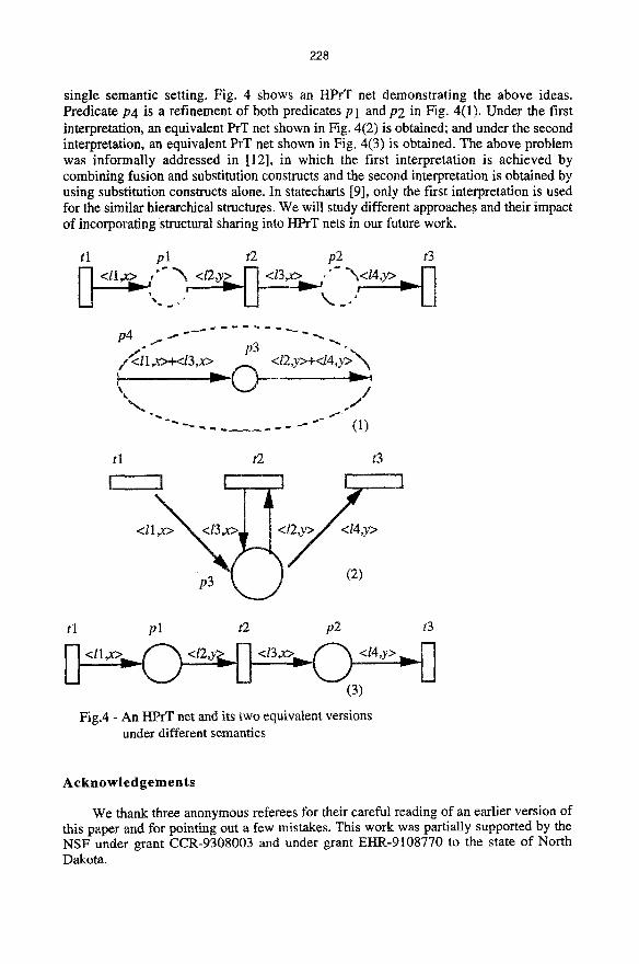
single semantic setting. Fig. 4 shows an HPrT net demonstrating the above ideas. Predicate P4 is a refinement of both predicates Pl and P2 in Fig. 4(1). Under the first interpretation, an equivalent PrT net shown in Fig. 4(2) is obtained; and under the second interpretation, an equivalent PrT net shown in Fig. 4(3) is obtained. The above problem was informally addressed in [12], in which the first interpretation is achieved by combining fusion and substitution constructs and the second interpretation is obtained by using substitution constructs alone. In statecharts [9], only the first interpretation is used for the similar hierarchical structures. We will study different approaches and their impact of incorporating structural sharing into HPrT nets in our future work.

t l p l t2 p2 t3

. . - U ' , . . - U

//<il,x>+</3,x> p3 <12,y>+<14,y>,NN

"" . . . . . . . . . "- (1)

tl t2 t3

<ll,x> < >

t I p 1 t2 p2 t3

(3)

Fig.4 - An HPrT net and its two equivalent versions under different semantics

Acknowledgements

We thank three anonymous referees for their careful reading of an earlier version of this paper and for pointing out a few mistakes. This work was partially supported by the NSF under grant CCR-9308003 and under grant EHR-9108770 to the state of North Dakota.

229

R e f e r e n c e s

1. J. Billington, G.R. Wheeler, and M.C. Wilbur-ham, PROTEAN: a high-level Petri net tool for the specification and verification of communication protocols. IEEE Transactions on Software Engineering, vol.14, no.3, 1988, 301-316.

2. H. Ehrig and B. Mahr, Fundamentals of Algebraic Specification 1, Springer-Verlag, 1985.

3. H. Ehrig and B. Mahr, Fundamentals of Algebraic Specification 2, Springer-Verlag, 1990.

4. R. Fehling, A concept of hierarchical Petri nets with building blocks, Lecture Notes in Computer Science, vol. 674, 1993, 148-168.

5. H.J. Genrich, and K. Lautenbach, System modeling with high-level Petri nets. Theoretical Computer Science, vo].13, 1981, 109-136.

6. D. Harel, On visual formalisms. Communications of the ACM, vol. 31, 1988, 514- 530.

7. X. He, Integrating formal specification and verfication methods in software development, Ph.D. dissertation, Virginia Polytechnic Institute & State University, June, 1989.

8. X. He, A method for analysing properties of hierarchical predicate transition nets, Proceedings of the 19th Annual International Computer Software & Applications Conference (COMPSAC'95), Dallas, TX, August, 1995, 50-55.

9. D. Haret, and C.-A. Kahana, On statecharts with overlapping. ACM Transactions on Software Engineering and Methodology, vol. 1, no.4, 1992, 399-42 I.

10. X. He, and J.A.N. Lee, A methodology for constructing predicate transition net specifications. Software - Practice and Experience, vol.21, no.8, 1991, 845-875.

11. X. He, and C.H. Yang, Structured analysis using hierarchical predicate transition nets. Proc. of the 16th Int'l Computer Software and Applications Conference (COMPSAC'92), Chicago, 1992, 212-217.

12. P. Huber, K. Jensen, and R.M. Shapiro, Hierarchies in colored Petri nets. Lecture Notes in Computer Science, vo1.483, Spriner-Verlag, 1990, 313-341.

13. K. Jensen, Colored Petri nets and the invariant method. Theoretical Computer Science, vo1.14, 1981, 317-33&

14. K. Jensen, Colored Petri nets: a high level language for system design and analysis, Lecture Notes in Computer Science, vol. 483, 1990, 342-416.

15. K. Jensen, Colored Petri Nets, vol.1, Springer-Verlag, 1992. 16. C. Kan and X. He, High-level algebraic Petri nets, Information and Software

Technology, vol.37, no.l, 1995, 23-30. 17. Z. Manna and A. Pnueli, Completing the temporal picture, Theoretical Computer

Science, vol. 83, pp.97-130, 1991. 18. Z. Manna and A. Pnueli, Models for reactivity, Acta Informatica, vol.30, pp.609-

678, 1993. 19. W. Reisig, Petri Nets - An Introduction. EATCS Monographs on Theoretical

Computer Science, vol.4, Springer-Verlag, 1985. 20. W. Reisig, Petri nets in software engineering. Lecture Notes in Computer Science,

vol.255, Springer-Verlag, 1987, 63-96. 21. W. Reisig, Petri nets and algebraic specifications. Theoretical Computer Science,

vol.80, 1991, 1-34. 22. E. Yourdon, Modern Structured Analysis, Yourdon Press, 1989.