design improvement in water distribution systems: a life cycle

DESIGN IMPROVEMENT IN WATER DISTRIBUTION SYSTEMS: A LIFE CYCLE

THINKING APPROACH

by

Shahnawaz Khan

B.Sc., Balochistan University of Engineering and Technology Khuzdar, 2010

A THESIS SUBMITTED IN PARTIAL FULFILLMENT OF

THE REQUIREMENTS FOR THE DEGREE OF

MASTER OF APPLIED SCIENCE

in

THE COLLEGE OF GRADUATE STUDIES

(Civil Engineering)

THE UNIVERSITY OF BRITISH COLUMBIA

(Okanagan)

April 2019

© Shahnawaz Khan, 2019

ii

The following individuals certify that they have read, and recommend to the College of Graduate

Studies for acceptance, a thesis/dissertation entitled:

DESIGN IMPROVEMENT IN WATER DISTRIBUTION SYSTEMS: A LIFE CYCLE THINKING APPROACH

Submitted by Shahnawaz Khan in partial fulfillment of the requirements of

the degree of Master of Applied Science

Dr. Rehan Sadiq, School of Engineering

Supervisor

Dr. Kasun Hewage, School of Engineering

Supervisory Committee Member

Dr. Shahria Alam, School of Engineering

Supervisory Committee Member

Dr. Lukas Bichler, School of Engineering

University Examiner

iii

Abstract

Potable water is mainly delivered to communities through a complex network of underground

pipes referred to as a water distribution system (WDS). WDSs are conventionally designed to

deliver water with the required quantity, quality, and continuity under suitable pressure. Over the

past few decades, sustainability has become widely acknowledged as a significant consideration

for all engineering projects. For a sustainable water infrastructure, it is important to incorporate

cost, energy efficiency, environmental performance, and social factors in the designing and

management of a WDS. This research has proposed a new approach where the sustainability of a

WDS is ensured by incorporating a life cycle thinking (LCT) in the conventional design process.

The approach follows four-steps: 1) traditional hydraulic design of the system, 2) the design

improvement considering hydraulic efficiency, 3) incorporation of environmental and energy

aspects in the designs, 4) design selection through systematic decision making.

To demonstrate the utility of the proposed approach, an existing WDS was analysed. Twelve new

design scenarios were generated based on the proposed approach and compared to the existing

design. An alternate design was suggested at the end, which proved to be more economical and

contributed to fewer emissions compared to the existing design. Considering the current global

environmental challenges, the approach can readily be adopted by the water supply industry and

will allow consideration of environmental criteria in the design process find suitable grounds.

iv

Lay Summary

Access to safe drinking water is vital for human life. Each year, an enormous amount of energy is

used in the water sector for the extraction and distribution of water, resulting in environmental

impacts. Potable water is mainly delivered to urban communities through a complex network of

underground pipes referred to as a water distribution system (WDS). WDSs are designed to deliver

water with the required quantity, quality, continuity, and at sufficient pressure. However, it is also

very important to consider cost, energy efficiency, and environmental performance in the design

process. This research has proposed a new approach where sustainable WDS design is achieved

by incorporating a life cycle thinking (LCT) in the design process. To demonstrate the usefulness

of the proposed approach, an existing small WDS in Okanogan Valley was selected. Twelve design

scenarios were generated and compared to the existing design. The proposed design proved to be

more economical and less emission intensive than the existing design.

v

Preface

This thesis is an original, unpublished work presented to the College of Graduate Studies at the

University of British Columbia (Okanagan Campus) as a partial requirement for the Master of

Applied Science degree. The research presented in this thesis is conducted by Shahnawaz Khan

under the supervision of Dr. Rehan Sadiq.

vi

Table of Contents

Abstract………………………………………………………………………………………... iii

Lay Summary………………………………………………………………………………….. iv

Preface………………………………………………………………………………………….. v

Table of Contents.….…………………………………………………...………………………vi

List of Tables………………………………………………………………………………… viii

List of Figures………………………………………………………………………………….. x

List of Symbols……………………………………………………………………………….. xii

List of Abbreviations………………………………………………………………………… xiv

Acknowledgements.….……………………………………………………………………….. xv

Dedication………...………………………………………………………………………….. xvi

Chapter 1: Introduction ................................................................................................................... 1

1.1 Overview ......................................................................................................................... 1

1.2 Background ..................................................................................................................... 3

1.3 Research Objectives ........................................................................................................ 5

1.4 Thesis Outline ................................................................................................................. 6

Chapter 2: Literature Review .......................................................................................................... 7

2.1 Water Distribution System (WDS) ................................................................................. 7

2.2 Design of a Water Distribution System (WDS) ............................................................ 17

2.3 Hydraulic Analysis........................................................................................................ 19

2.4 Improvement Strategies for WDS Design .................................................................... 27

2.5 LCEA in WDS Analysis and Design ............................................................................ 36

2.6 Life Cycle Cost Analysis (LCCA) ................................................................................ 47

vii

Chapter 3. Proposed Approach and Methodology ........................................................................ 49

3.1 Hydraulic Design .......................................................................................................... 49

3.2 Scenario Analysis.......................................................................................................... 51

3.3 Life Cycle Thinking (LCT) ........................................................................................... 52

3.4 Decision Making ........................................................................................................... 61

Chapter 4: Results and Discussions .............................................................................................. 63

4.1 Step I: Hydraulic Design ............................................................................................... 63

4.2 Step II- Scenario Analysis ............................................................................................ 68

4.3 Step IIIa- Life Cycle Energy Analysis (LCEA) ............................................................ 71

4.4 Step IIIb: Life Cycle Cost Analysis (LCCA) ................................................................ 78

Chapter 5: Conclusions and Recommendations ........................................................................... 88

References ..................................................................................................................................... 90

Appendices .................................................................................................................................. 100

viii

List of Tables

Table 2.1. Common pipe materials and their key characteristics ................................................... 9

Table 2.2. Characteristic of water main joints .............................................................................. 10

Table 2.3. Commonly used valves in WDS and their function .................................................... 16

Table 2.4. Basic WDS design requirements ................................................................................. 19

Table 2.5. WDS optimization objective function, constraint, and decision variables .................. 29

Table 2.6. Optimization studies related to the WDS design improvement ................................... 30

Table 2.7. Summary of the studies related to LCT use in WDS analysis ..................................... 35

Table 2.8. Embodied energy and density of some common types of pipes .................................. 38

Table 2.9. Effect of the roadway grade on the fuel economy of class-8 trucks ............................ 40

Table 2.10. Recommended trench dimensions ............................................................................. 41

Table 2.11. Productivity rate of the construction job/equipment.................................................. 42

Table 2.12. The fuel consumption rate of the construction equipment ........................................ 42

Table 2.13. HDD Production rate, excluding access and splice pits ............................................ 44

Table 2.14. LCCA equations for each phase of a project ............................................................. 48

Table 3.1. Effect of decision variables on the design scenario ..................................................... 51

Table 4.1. Pipe dimensions of the Swick Road ............................................................................ 65

Table 4.2. Pipes length and size of the baseline design and 12 alternative candidate designs ..... 68

Table 4.3. Design performance comparison of the suggested and the existing design ................ 84

Table A1. Average peaking factor values ................................................................................... 102

Table A2. Trench dimensions for the open-cut installation ........................................................ 101

Table A3. Pipe cost and class considered for the study .............................................................. 102

Table A4. Cost of the various construction jobs related to the life cycle of a WDS .................. 103

ix

Table A5. Cost of an HDD job ................................................................................................... 104

Table A6. Cost of a CIPP job including the flexible felt resin ................................................... 105

Table A7. Pipe bursting cost replacing with HDPE pipe ............................................................ 106

Table A8. Exponential function coefficients for VI index ......................................................... 107

x

List of Figures

Figure 1.1. Typical North American surface water supply system energy consumption ............... 2

Figure 2.1. A typical water supply system ...................................................................................... 7

Figure 2.2. Percent distribution of total length of pipes based on material types in Canada ........ 10

Figure 2.3. The branched layout of WDS ..................................................................................... 11

Figure 2.4. The looped layout of WDS ......................................................................................... 12

Figure 2.5. Water pumping with the storage reservoir ................................................................. 13

Figure 2.6. Storage reservoir storage distribution ......................................................................... 14

Figure 2.7. Total static head of the system ................................................................................... 15

Figure 2.8. Pipes in a series system .............................................................................................. 21

Figure 2.9. Pipes in parallel .......................................................................................................... 22

Figure 2.10. Branching pipe system; three-reservoir junction scenario ....................................... 23

Figure 2.11. Schematic of a looped pipe network ........................................................................ 24

Figure 2.12. Open-cut pipe installation......................................................................................... 41

Figure 2.13. Horizontal directional drilling .................................................................................. 43

Figure 3.1. Flow diagram of the proposed approach .................................................................... 50

Figure 3.2. Life cycle phases of a WDS ....................................................................................... 53

Figure 3.3. LCCA of a WDS for the proposed approach.............................................................. 59

Figure 4.1. The layout of Swick Road system selected for this study .......................................... 63

Figure 4.2. Elevation diagram of the Swick Road WDS .............................................................. 64

Figure 4.3. A sample from the design drawings ........................................................................... 64

Figure 4.4. EPANET extended period analysis at time zero of 24 hours. .................................... 66

Figure 4.5. EPANET extended period analysis at time 19-hours of 24-hour ............................... 67

xi

Figure 4.6. Diurnal demand pattern for EPANET ........................................................................ 67

Figure 4.7. Pump operation duration pattern ................................................................................ 68

Figure 4.8. EPANET analysis at pipe roughness of 145............................................................... 70

Figure 4.9. EPANET analysis at pipe roughness of 80................................................................. 70

Figure 4.10. LCEA result of all the designs for a 100-year planning period ................................ 71

Figure 4.11. Embodied Energy of all the design scenarios........................................................... 72

Figure 4.12. Emissions related to the transportation..................................................................... 73

Figure 4.13. Total emissions for the open-cut installation in alternate designs .......................... 733

Figure 4.14. Total emissions for the trenchless installation in alternate designs .......................... 74

Figure 4.15. Deterioration curve of 350 mm PVC, DI, and HDPE pipes ..................................... 75

Figure 4.16. Total life cycle emission of the use phase for all the designs .................................. 76

Figure 4.17. Pump operation graph after an increase in water demand ........................................ 77

Figure 4.18. Total emissions of the disposal phase in tons of CO2 .............................................. 77

Figure 4.19. LCCA of all the designs scenarios ........................................................................... 78

Figure 4.20. The acquisition cost of all the designs scenarios ...................................................... 79

Figure 4.21. Total cost for the open-cut installation method ........................................................ 80

Figure 4.22. Total cost for the trenchless installation method.. .................................................... 80

Figure 4.23. Operating cost of all the designs for the 100-year planning period ......................... 81

Figure 4.24. Deterioration curve of a 350 mm pipe without lining and relining .......................... 82

Figure 4.25. Disposal cost comparison for all scenarios .............................................................. 82

Figure 4.26. The combined weighted sum scale of all the design alternatives ............................. 83

Figure 4.27. LCEA of the suggested design D2-PVC .................................................................. 85

Figure 4.28. Life cycle cost analysis of the suggested design D2-PVC ....................................... 86

xii

List of Symbols

Qin Pipe flow into node

Qout Pipe flow out of the node

qext External demand or supply

ℎ𝐿,𝑖 The headless across the component i along the path

hp,j The head added by pump j

ΔE The difference in energy between the end points of the path

h The residual pressure

hmin Total dynamic head of the system

P Pump power

Q Flow capacity

ρ Density of fluid

ɡ Gravity

η The efficiency of the pump

A Present annual cost

i Discount rate

g Inflation rate

n Number of subsequent years

α Exponential function coefficients

β Exponential function coefficients

Qmelt Total energy needed to melt the material

M Mass of the material

C Specific heat of the material

ΔT Change in temperature from room to melting point

Hfus Latent heat of fusion

R Outer diameter

r Internal diameter

xiii

EET Total embodied energy

EEkg Unit EE of a pipe material

Ukg Total weight of the pipe in kg

Vu Unit volume of a pipe

HPg Horsepower generated

SFP Specific fuel consumption

S The surface area of the hollow tube in unit2

Ht The height of a tube

Pann The present value of a growing annuity

Pcost Total present cost

Ai Alternative in terms of criteria

wj The relative weight of importance of criteria

aij Performance value of alternative

c The minimum value of the scale

x The value which needs to be normalized

Amin Minimum alternative performance value

Bmin Maximum alternative performance value

b Maximum scale value

K Friction loss coefficient

Zj Elevation head

Pj/γ Pressure head

Cc Capital cost

Cmrr Maintenance, repair, replace cost

Ce End of life cost

xiv

List of Abbreviations

WDS Water Distribution System

DI Ductile Iron

PVC Polyvinyl Chloride

HDPE High-Density Polyethylene

LCC Life cycle costing

LCT Life cycle thinking

LCEA Life cycle energy analysis

LCA Life cycle assessment

MDD Maximum Daily Demand

PHD Peak Hourly Demand

GHG Green House Gas

OD-LCT Optimal Design based on Life cycle thinking

D Design

EE Embodied Energy

BCY Bank Cubic Yard

LCY Loose Cubic Yard

ECY Embankment Cubic Yard

S.Y. Square Yard

HDD Horizontal Directional Drilling

CIPP Cured-in-Place Piping

SFP Specific fuel consumption

VI Vulnerability Index

xv

Acknowledgements

Throughout this research, I received guidance and help from my supervisors and lab peers,

especially Haroon Mian and Dr. Guangji Hu. I am also thankful to the City of Kelowna for

providing the designs and technical information of the water distribution system at Swick Road,

which was selected as a case study to demonstrate the implementation of the proposed approach,

especially Brad Stuart: Water Supply & Pump Stations Supervisor. I am also thankful to the Higher

Education Commission of Pakistan and BUITEMS for providing funding for this research.

Finally, I am thankful to the UBC Okanagan office staff who helped and made things easy for me.

xvi

Dedication I dedicate this work to all mighty Allah; the sustainer of the universe, my creator and my master.

My teacher and the messenger Muhammadملسو هيلع هللا ىلص; who taught us the purpose of life. My parents, wife,

family, and friends who stand by me when things look bleak. My professors for their support and

guidance whenever I needed it.

1

Chapter 1: Introduction

1.1 Overview

United Nations (UN) declares that access to safe water is a basic human right (UN 2001). Abundant

fresh water is a fundamental requirement for the socio-economic development of any society

(Booth and Charlesworth 2014; Feldman 2017). Many great civilizations of the past flourished

along major freshwater sources such as Indus Valley Civilization along Indus River Basin,

Mesopotamian Civilization along Tigris and Euphrates, and Egyptian Civilization along River

Nile. Also, the Romans in the early half of the first century introduced conduits and aqueducts to

deliver water into the cities (Mays 2000). The Persians used ‘Qanat’ systems to deliver clean water

into the cities 30 miles away from the water sources (Najafi 2010).

In modern times, potable water is generally delivered to cities through water supply systems. A

water supply system is a complex infrastructure for the extraction, treatment, storage, and

distribution of water. A water supply system is constructed, operated, and maintained by water

utilities which can be a public or privately-owned entity. The water is generally taken from

different sources (i.e., surface water and ground water); it is treated to an acceptable level, and

then delivered to consumers within an appropriate time, with continuity and at the required

pressure. Depending on the water source and topography of the system, water can be transported

through gravity, or pumping, or combination of both.

Water is an excellent solvent and relatively heavy compound, which makes water treatment and

delivery process highly energy intensive. Annual global energy consumption in the water sector is

1400 terawatt hours (TWh), which accounts for 8% of total annual global energy consumption

(IEA 2016). More specifically, the water supply systems consume 4.8% (845 TWh) of annual

global energy (IEA 2016). Around 60% (820 TWh) of this energy is consumed in the form of

2

electricity, whereas as the rest (40%) comprises of thermal energy. There are several downsides to

this energy consumption; e.g., air pollution, greenhouse gas emissions (especially in the case of

fossil-fuel based energy), higher economic cost, and decreasing infrastructure life (USEPA 2013b;

USEPA 2013a). The decrease in infrastructure life is associated with less efficient operations

which can result in increased energy consumption and strain on equipment. This can eventually

lead to a high operation and maintenance requirements (USEPA 2013b; USEPA 2013a).

There are several factors which can impact the energy consumption, such as; water source,

topography, climatic conditions, degree of treatment, water losses, and size of the system.

Considering the North-American context, the water is mainly taken/withdrawn from surface water

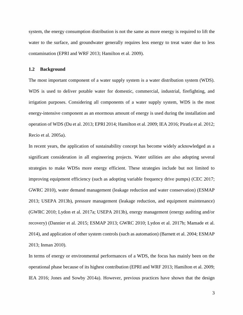
sources (IEA 2016). The annual energy consumption distribution for North-American surface

water supply is shown in Figure 1.1 (EPRI and WRF 2013; Hamilton et al. 2009; Ontario 2016;

Piratla et al. 2012)

Figure 1.1. Typical North American surface water supply system energy

consumption profile

As shown in Figure 1.1, the finished (or treated) water pumping is the most energy-intensive

process followed by water treatment, source water pumping, and pumping within the plant.

Overall, pumping accounts for almost 85% of the total energy consumption. In groundwater supply

Source water

pumping, 11%

Water treatment,

14%

Pumping within

plant, 8%Finished water

pumping, 67%

0% 10% 20% 30% 40% 50% 60% 70% 80% 90% 100%

ENERGY CONSUMPTION DISTRIBUTION

3

system, the energy consumption distribution is not the same as more energy is required to lift the

water to the surface, and groundwater generally requires less energy to treat water due to less

contamination (EPRI and WRF 2013; Hamilton et al. 2009).

1.2 Background

The most important component of a water supply system is a water distribution system (WDS).

WDS is used to deliver potable water for domestic, commercial, industrial, firefighting, and

irrigation purposes. Considering all components of a water supply system, WDS is the most

energy-intensive component as an enormous amount of energy is used during the installation and

operation of WDS (Du et al. 2013; EPRI 2014; Hamilton et al. 2009; IEA 2016; Piratla et al. 2012;

Recio et al. 2005a).

In recent years, the application of sustainability concept has become widely acknowledged as a

significant consideration in all engineering projects. Water utilities are also adopting several

strategies to make WDSs more energy efficient. These strategies include but not limited to

improving equipment efficiency (such as adopting variable frequency drive pumps) (CEC 2017;

GWRC 2010), water demand management (leakage reduction and water conservation) (ESMAP

2013; USEPA 2013b), pressure management (leakage reduction, and equipment maintenance)

(GWRC 2010; Lydon et al. 2017a; USEPA 2013b), energy management (energy auditing and/or

recovery) (Dannier et al. 2015; ESMAP 2013; GWRC 2010; Lydon et al. 2017b; Mamade et al.

2014), and application of other system controls (such as automation) (Barnett et al. 2004; ESMAP

2013; Inman 2010).

In terms of energy or environmental performances of a WDS, the focus has mainly been on the

operational phase because of its highest contribution (EPRI and WRF 2013; Hamilton et al. 2009;

IEA 2016; Jones and Sowby 2014a). However, previous practices have shown that the design

4

process for WDS is mainly “hydraulic driven,” which could result in the exclusion of important

strategic actions that can further improve the system. It is very important to ensure that the

improvement measures consider holistic view instead of focusing on isolated segments or

equipment efficiency only (Jones and Sowby 2014b). This will require enhancement of the system

architecture (such as adjusting layout, tank location, or pipe diameter) and operations,

simultaneously (ESMAP 2013). To add the element of sustainability to improve WDS

performance, it is important to incorporate economics, energy, and environmental factors in the

design of a WDS.

Generally, WDS is designed keeping in view its primary function, which is to deliver water with

the required quantity, quality, and continuity with the desired pressure. Improvements in the design

process were initially done by developing efficient algorithms for flow analysis (Walters 1992).

Later studies introduced various mathematical optimization techniques in the design process to

minimize the overall WDS cost while improving system hydraulics (Saldarriaga et al. 2010; Savic

and Walters 1997; Shamir 1974). With a recent increase in environmental awareness, few studies

expanded the scope of WDS performance improvement by ensuring that environmental and energy

aspects need to be considered in addition to economic aspects (Dandy et al. 2006; Herstein et al.

2011; Stokes et al. 2012; Wu et al. 2010). Incorporating these various aspects can bring long-term

effectiveness and efficiency in terms of WDS management.

The traditional designing practices of WDS have proven very successful; the systems designed

over a hundred years ago are still operational. However, with the adoption of sustainable

development goals, the global challenges in terms of environmental impacts and energy use have

gained much importance (NASA 2010). There is a need for an approach, which can readily address

these current global challenges, particularly in the water industry by incorporating sustainability

5

objective when designing WDSs. In this research, a new approach is proposed where the

sustainability of a WDS is ensured by incorporating the life cycle thinking (LCT) approach in the

conventional design process. LCT is a management approach that holistically considers various

alternatives and enhances an understanding of impacts. Applying LCT can facilitate in selecting

the most efficient WDS design that ensures minimal environmental and economic impacts while

ensuring human health. LCT can also help in avoiding burden shifting from one phase of the

system’s life cycle to another phase. It is noteworthy that WDS is a complex integrated

infrastructure, implications of even a small design change can propagate throughout all phases of

the life cycle (i.e., from the extraction of raw materials through manufacturing, transportation,

installation, operation, and the final disposal phase). Broadly, the approach consists of four steps:

1) traditional hydraulic design, 2) design improvement considering hydraulic efficiency, 3)

incorporation of the environmental and energy aspects in the designs, 4) design selection through

systematic decision making.

1.3 Research Objectives

The main objective of this research is to develop a approach to improve WDS performance through

LCT-based design. To achieve this, the following sub-objectives must be achieved:

• Conduct a state-of-the-art review of life cycle thinking use in WDS analysis and

management.

• Develop an integrated approach to incorporate LCT in the conventional WDS design, by

performing a cradle-to-cradle life cycle energy analysis (LCEA), and life cycle cost

analysis (LCCA).

• Apply the proposed approach to a real life WDS as a case study.

6

1.4 Thesis Outline

Chapter 2 provides a comprehensive literature review, which includes information related to WDS

design and components, use of LCT approach in WDS analysis and management, epecially in the

context of environmental and energy performance. In Chapter 3, an integrated approach is

proposed for the WDS design. This chapter also contains methodology and techniques applied in

the development, validation, and application of the approach. Chapter 4 provides the results and

discussions on the application of the proposed approach on a real WDS. Finally, Chapter 5 provides

conclusions and future research direction of this research.

7

2 Chapter 2: Literature Review

This chapter provides a general introduction to a water distribution system (WDS) and life cycle

thinking (LCT) approach in the context of water distribution system analysis. Section 2.1 explains

the functional components of a WDS, and section 2.2 provides the background information for

WDS design and hydraulic analysis. Section 2.3 highlights the strategies adopted in studies to

improve WDS design and management. The literature related to LCT use in WDS analysis has

been discussed in sections 2.4 and 2.5.

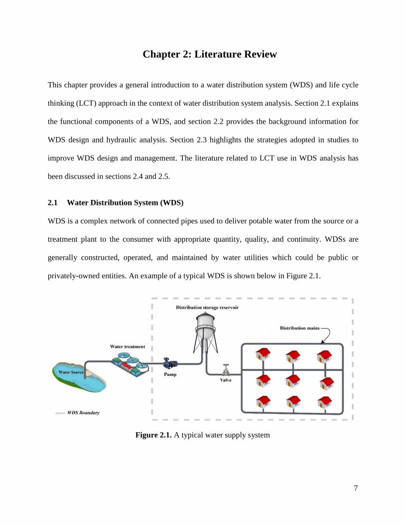
2.1 Water Distribution System (WDS)

WDS is a complex network of connected pipes used to deliver potable water from the source or a

treatment plant to the consumer with appropriate quantity, quality, and continuity. WDSs are

generally constructed, operated, and maintained by water utilities which could be public or

privately-owned entities. An example of a typical WDS is shown below in Figure 2.1.

Figure 2.1. A typical water supply system

8

In terms of size, WDSs are categorized into small, medium, and large systems. There are several

factors which determine the size of the system, e.g., the extent of population served, technical and

financial resources available, production of GHG emissions, etc. (Haider et al. 2014). Considering

the population factor, small WDSs are ones with population ≤ 3300 people, medium WDSs serve

population ϵ 3300-50000, and a large WDSs serve population ≥ 50000 people (USEPA 2002).

WDS consists of various components including pumps, storage reservoir, valves, and water mains

(pipes), etc. Main components of a WDS are briefly explained in the following sections.

2.1.1 Water Mains

WDS pipelines are generally referred to as water mains, which can be further divided into

transmission mains and distribution mains. Transmission mains carry a large quantity of water

from the source or treatment plant to distribution mains, from where distribution mains distribute

the water throughout the system and delivers it to consumers. Water mains, in general, have the

highest share in the capital cost and serve for the longest period (Filion et al. 2004; Mays 2000).

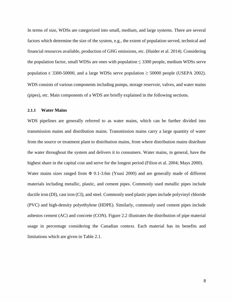
Water mains sizes ranged from Φ 0.1-3.6m (Ysusi 2000) and are generally made of different

materials including metallic, plastic, and cement pipes. Commonly used metallic pipes include

ductile iron (DI), cast iron (CI), and steel. Commonly used plastic pipes include polyvinyl chloride

(PVC) and high-density polyethylene (HDPE). Similarly, commonly used cement pipes include

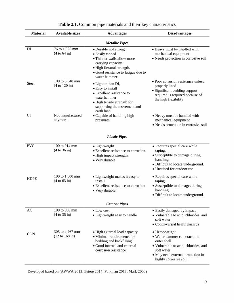
asbestos cement (AC) and concrete (CON). Figure 2.2 illustrates the distribution of pipe material

usage in percentage considering the Canadian context. Each material has its benefits and

limitations which are given in Table 2.1.

9

Table 2.1. Common pipe materials and their key characteristics

Material Available sizes Advantages Disadvantages

Metallic Pipes

DI 76 to 1,625 mm

(4 to 64 in)

• Durable and strong

• Easily tapped

• Thinner walls allow more

carrying capacity.

• High flexural strength.

• Good resistance to fatigue due to

water hammer.

• Heavy must be handled with

mechanical equipment

• Needs protection in corrosive soil

Steel 100 to 3,048 mm

(4 to 120 in) • Lighter than DI,

• Easy to install

• Excellent resistance to

waterhammer

• High tensile strength for

supporting the movement and

earth load

• Poor corrosion resistance unless

properly lined

• Significant bedding support

required is required because of

the high flexibility

CI Not manufactured

anymore • Capable of handling high

pressures

• Heavy must be handled with

mechanical equipment

• Needs protection in corrosive soil

Plastic Pipes

PVC 100 to 914 mm

(4 to 36 in) • Lightweight.

• Excellent resistance to corrosion.

• High impact strength.

• Very durable

• Requires special care while

taping.

• Susceptible to damage during

handling.

• Difficult to locate underground.

• Unsuited for outdoor use

HDPE 100 to 1,600 mm

(4 to 63 in) • Lightweight makes it easy to

install

• Excellent resistance to corrosion

• Very durable.

• Requires special care while

taping.

• Susceptible to damage\ during

handling.

• Difficult to locate underground.

Cement Pipes

AC 100 to 890 mm

(4 to 35 in) • Low cost

• Lightweight easy to handle

• Easily damaged by impact

• Vulnerable to acid, chlorides, and

soft water

• Controversial health hazards

CON 305 to 4,267 mm

(12 to 168 in) • High external load capacity

• Minimal requirements for

bedding and backfilling

• Good internal and external

corrosion resistance

• Heavyweight

• Water hammer can crack the

outer shell

• Vulnerable to acid, chlorides, and

soft water

• May need external protection in

highly corrosive soil.

Developed based on (AWWA 2013; Briere 2014; Folkman 2018; Mark 2000)

10

Figure 2.2. Percent distribution of total length of pipes based on material

types in Canada (Folkman 2018)

2.1.2 Joints

Many small segments of water mains are connected through joints during the installation process

to build a network. The joints are of different types including push-on, mechanical, and butt-

fusion (AWWA 2013). The characteristics of these joints are presented in Table 2.2.

Table 2.2. Characteristic of water main joints

Joint type Characteristics

Push-on • Flexible and simple to assemble.

• Enables pipeline deflection for street or road curvature

Mechanical • Less flexible than the push-on joint

• More labor intensive.

Butt-fusion • Includes a thermofusion process

• Pipe ends are brought together under controlled pressure and

temperature. Widely used in HDPE pipes

Adopted from (AWWA 2013; DIPRA 2017)

11

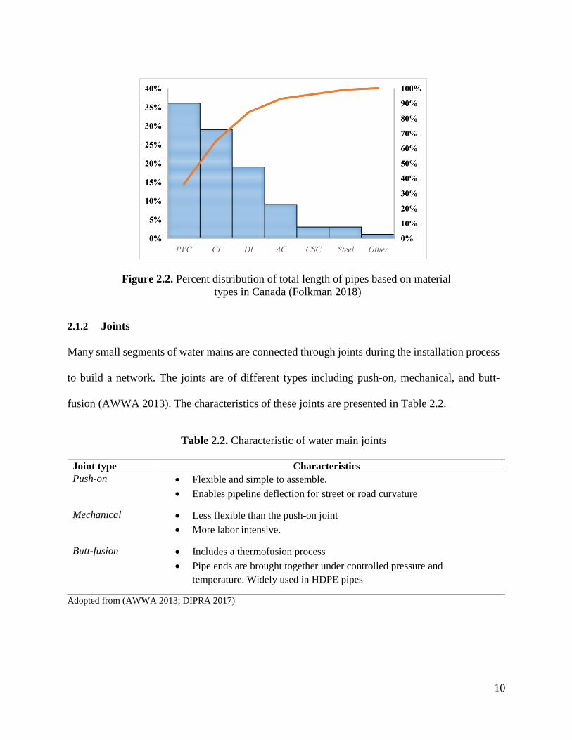
2.1.3 Layout

A WDS network can be arranged using different pipe layouts, which typically is dependent on

the water source, area topography, and diurnal water demand. The layout of the network can be

either branched (Figure 2.3), looped (Figure 2.4), or a combination of branched and looped.

Figure 2.3. The branched layout of WDS (Source: Swick Road in the City of Kelowna)

In a branched network, water has only one possible pathway from the source to final distribution

points. A branched network is simple and economical with fewer isolation valves. However, the

branched network is less reliable and generally suffer from water quality concerns due to

stagnation. In the hydraulic analysis, the demand on water supply pipes is represented at nodes.

The nodes are not physical objects; they are placed at the end of the pipe to present the demand on

the pipe during hydraulic analysis. Moreover, the nodes are categorized into the junction and fixed-

grade nodes: junction nodes are also called demand nodes which have an input and output flow,

whereas a fixed-grade node represents a reservoir.

12

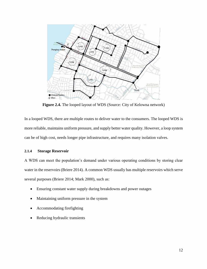
Figure 2.4. The looped layout of WDS (Source: City of Kelowna network)

In a looped WDS, there are multiple routes to deliver water to the consumers. The looped WDS is

more reliable, maintains uniform pressure, and supply better water quality. However, a loop system

can be of high cost, needs longer pipe infrastructure, and requires many isolation valves.

2.1.4 Storage Reservoir

A WDS can meet the population’s demand under various operating conditions by storing clear

water in the reservoirs (Briere 2014). A common WDS usually has multiple reservoirs which serve

several purposes (Briere 2014; Mark 2000), such as:

• Ensuring constant water supply during breakdowns and power outages

• Maintaining uniform pressure in the system

• Accommodating firefighting

• Reducing hydraulic transients

13

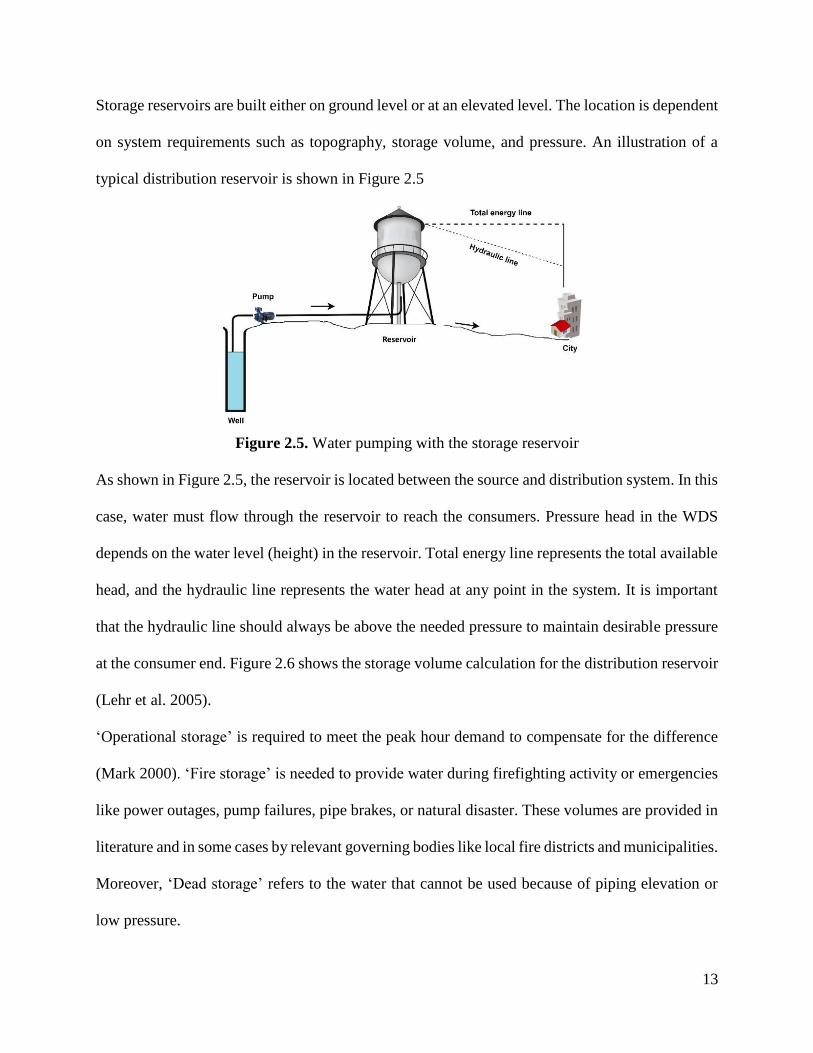
Storage reservoirs are built either on ground level or at an elevated level. The location is dependent

on system requirements such as topography, storage volume, and pressure. An illustration of a

typical distribution reservoir is shown in Figure 2.5

Figure 2.5. Water pumping with the storage reservoir

As shown in Figure 2.5, the reservoir is located between the source and distribution system. In this

case, water must flow through the reservoir to reach the consumers. Pressure head in the WDS

depends on the water level (height) in the reservoir. Total energy line represents the total available

head, and the hydraulic line represents the water head at any point in the system. It is important

that the hydraulic line should always be above the needed pressure to maintain desirable pressure

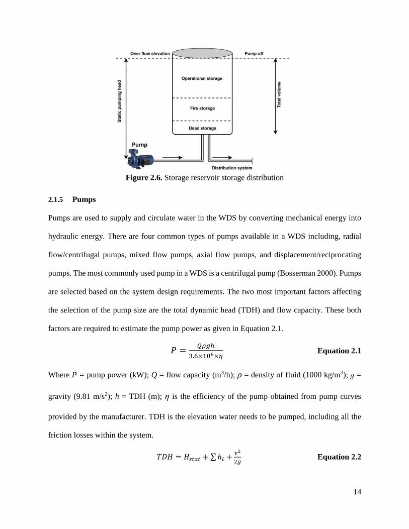
at the consumer end. Figure 2.6 shows the storage volume calculation for the distribution reservoir

(Lehr et al. 2005).

‘Operational storage’ is required to meet the peak hour demand to compensate for the difference

(Mark 2000). ‘Fire storage’ is needed to provide water during firefighting activity or emergencies

like power outages, pump failures, pipe brakes, or natural disaster. These volumes are provided in

literature and in some cases by relevant governing bodies like local fire districts and municipalities.

Moreover, ‘Dead storage’ refers to the water that cannot be used because of piping elevation or

low pressure.

14

Figure 2.6. Storage reservoir storage distribution

2.1.5 Pumps

Pumps are used to supply and circulate water in the WDS by converting mechanical energy into

hydraulic energy. There are four common types of pumps available in a WDS including, radial

flow/centrifugal pumps, mixed flow pumps, axial flow pumps, and displacement/reciprocating

pumps. The most commonly used pump in a WDS is a centrifugal pump (Bosserman 2000). Pumps

are selected based on the system design requirements. The two most important factors affecting

the selection of the pump size are the total dynamic head (TDH) and flow capacity. These both

factors are required to estimate the pump power as given in Equation 2.1.

𝑃 =𝑄𝜌𝑔ℎ

3.6×106×𝜂 Equation 2.1

Where P = pump power (kW); Q = flow capacity (m3/h); ρ = density of fluid (1000 kg/m3); ɡ =

gravity (9.81 m/s2); h = TDH (m); η is the efficiency of the pump obtained from pump curves

provided by the manufacturer. TDH is the elevation water needs to be pumped, including all the

friction losses within the system.

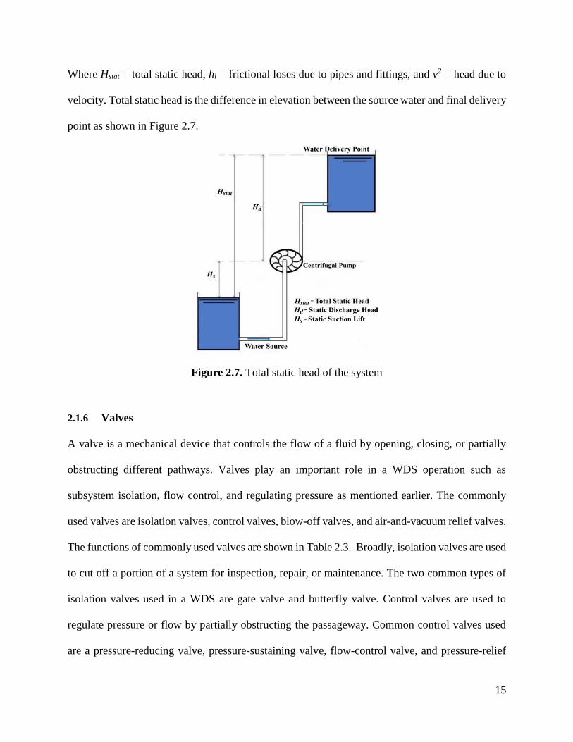
𝑇𝐷𝐻 = 𝐻𝑠𝑡𝑎𝑡 + ∑ℎ𝑙 +𝑣2

2𝑔 Equation 2.2

15

Where Hstat = total static head, hl = frictional loses due to pipes and fittings, and v2 = head due to

velocity. Total static head is the difference in elevation between the source water and final delivery

point as shown in Figure 2.7.

Figure 2.7. Total static head of the system

2.1.6 Valves

A valve is a mechanical device that controls the flow of a fluid by opening, closing, or partially

obstructing different pathways. Valves play an important role in a WDS operation such as

subsystem isolation, flow control, and regulating pressure as mentioned earlier. The commonly

used valves are isolation valves, control valves, blow-off valves, and air-and-vacuum relief valves.

The functions of commonly used valves are shown in Table 2.3. Broadly, isolation valves are used

to cut off a portion of a system for inspection, repair, or maintenance. The two common types of

isolation valves used in a WDS are gate valve and butterfly valve. Control valves are used to

regulate pressure or flow by partially obstructing the passageway. Common control valves used

are a pressure-reducing valve, pressure-sustaining valve, flow-control valve, and pressure-relief

16

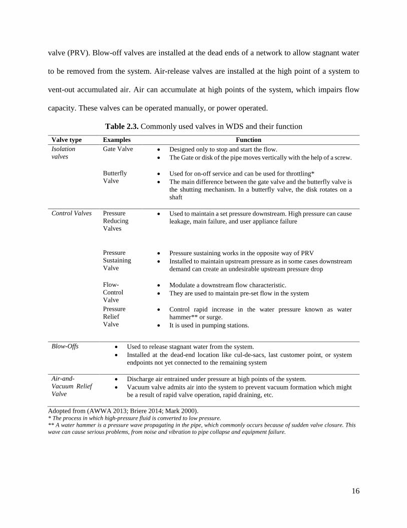
valve (PRV). Blow-off valves are installed at the dead ends of a network to allow stagnant water

to be removed from the system. Air-release valves are installed at the high point of a system to

vent-out accumulated air. Air can accumulate at high points of the system, which impairs flow

capacity. These valves can be operated manually, or power operated.

Table 2.3. Commonly used valves in WDS and their function

Valve type Examples Function

Isolation

valves

Gate Valve • Designed only to stop and start the flow.

• The Gate or disk of the pipe moves vertically with the help of a screw.

Butterfly

Valve • Used for on-off service and can be used for throttling*

• The main difference between the gate valve and the butterfly valve is

the shutting mechanism. In a butterfly valve, the disk rotates on a

shaft

Control Valves Pressure

Reducing

Valves

• Used to maintain a set pressure downstream. High pressure can cause

leakage, main failure, and user appliance failure

Pressure

Sustaining

Valve

• Pressure sustaining works in the opposite way of PRV

• Installed to maintain upstream pressure as in some cases downstream

demand can create an undesirable upstream pressure drop

Flow-

Control

Valve

• Modulate a downstream flow characteristic.

• They are used to maintain pre-set flow in the system

Pressure

Relief

Valve

• Control rapid increase in the water pressure known as water

hammer** or surge.

• It is used in pumping stations.

Blow-Offs • Used to release stagnant water from the system.

• Installed at the dead-end location like cul-de-sacs, last customer point, or system

endpoints not yet connected to the remaining system

Air-and-

Vacuum Relief

Valve

• Discharge air entrained under pressure at high points of the system.

• Vacuum valve admits air into the system to prevent vacuum formation which might

be a result of rapid valve operation, rapid draining, etc.

Adopted from (AWWA 2013; Briere 2014; Mark 2000). * The process in which high-pressure fluid is converted to low pressure.

** A water hammer is a pressure wave propagating in the pipe, which commonly occurs because of sudden valve closure. This

wave can cause serious problems, from noise and vibration to pipe collapse and equipment failure.

17

2.2 Design of a Water Distribution System (WDS)

2.2.1 Design Criteria

WDSs are designed to provide adequate water for domestic, commercial, agricultural and fire-

fighting purposes. A good WDS design should supply water at consumer’s tap at a reasonable

pressure, meet fire demand, and maintain water quality requirements. The WDS design criteria are

based on guidelines established over the years from a recognition of what usually constitutes a

successful design. The traditional design criteria used for the comparison are water quantity,

storage, service pressure, and flow (Briere 2014; Mark 2000). Each of the design criteria is

explained below.

2.2.2 Water Quantity

In WDS design, the first step is estimating the quantity of water required, with a provision for

anticipated future needs. The water supply should be large enough to meet different water demand

conditions. Engineers must design a WDS so that it can meet the maximum daily demand (MDD)

plus fire flow demand (Briere 2014). MDD is the largest water demand for any 24 hours over a

year. Also, there exists a scenario of peak hour demand (PHD). The PHD is the highest demand

of water for an hour. In general, PHD and MDD are calculated by applying the peaking factor (PF)

to the average daily demand (ADD).

𝐴𝐷𝐷 = 𝐴𝑛𝑛𝑢𝑎𝑙 𝑤𝑎𝑡𝑒𝑟 𝑐𝑜𝑛𝑠𝑢𝑚𝑝𝑡𝑖𝑜𝑛

365 𝑑𝑎𝑦𝑠 Equation 2.3

𝑃𝐹𝐷 =𝑀𝐷𝐷

𝐴𝐷𝐷 Equation 2.4

𝑃𝐹𝐻 =𝑃𝐻𝐷

𝐴𝐷𝐷 Equation 2.5

18

Where 𝑃𝐹𝐷 and 𝑃𝐹𝐻 are the peaking factors. Peak factors are higher for small communities and

lower for large communities (OME 2016). Average PF values for the design of a WDS is given in

appendix (Table A1).

The fire demand typically depends on land use and type of community. For example, a typical fire

flow requirement for an area with single-family residential is 500-2000 gal/min, multi-family

residential is 1500-3000 gal/min, and central business district is 2500-15000 gal/min (Mays 2000).

US National Board of Fire Underwriters suggests the following equations for needed fire flow

(NFF) demand

𝑁𝐹𝐹 = 65√𝑃(1 − 0.01√𝑃) Equation 2.6

Where P is the population in the 1000’s, and NFF is in liters per second (lps). The board also

recommends considering a fire duration of 4-10 hours while designing a WDS.

2.2.3 Service Pressure

The working service pressures in a WDS is customarily maintained between 30-65 psi (Mays

2000). The uniform plumbing code recommends that water pressure should not exceed 80 psi and

should not drop below 20 psi under all flow conditions (AWWA 2013; Mark 2000). Higher

pressure may increase leakage in the system and service faucets, wear off valve seats, and hasten

the failure of water using appliances, whereas low pressure can cause hindrance in a fire-fighting

activity or reduction in flow if more than one water-using device is in use at consumer’s resident.

2.2.4 Flow Velocity

Generally, it is recommended that the flow velocity in a WDS should be around 1.5 m/sec on

average (AWWA 2013), and should not be greater than 3 m/sec and less than 0.3 m/sec in any

case (Briere 2014). Higher velocities could result in excessive friction losses, system component

failure like water main breaks, and excessive head loss, whereas low flow velocity is responsible

19

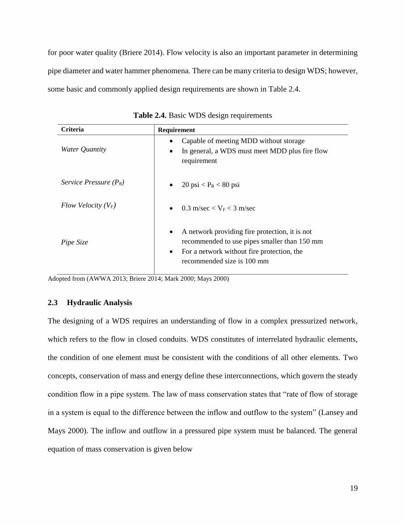
for poor water quality (Briere 2014). Flow velocity is also an important parameter in determining

pipe diameter and water hammer phenomena. There can be many criteria to design WDS; however,

some basic and commonly applied design requirements are shown in Table 2.4.

Table 2.4. Basic WDS design requirements

Criteria Requirement

Water Quantity

• Capable of meeting MDD without storage

• In general, a WDS must meet MDD plus fire flow

requirement

Service Pressure (PR) • 20 psi < PR < 80 psi

Flow Velocity (VF) • 0.3 m/sec < VF < 3 m/sec

Pipe Size

• A network providing fire protection, it is not

recommended to use pipes smaller than 150 mm

• For a network without fire protection, the

recommended size is 100 mm

Adopted from (AWWA 2013; Briere 2014; Mark 2000; Mays 2000)

2.3 Hydraulic Analysis

The designing of a WDS requires an understanding of flow in a complex pressurized network,

which refers to the flow in closed conduits. WDS constitutes of interrelated hydraulic elements,

the condition of one element must be consistent with the conditions of all other elements. Two

concepts, conservation of mass and energy define these interconnections, which govern the steady

condition flow in a pipe system. The law of mass conservation states that “rate of flow of storage

in a system is equal to the difference between the inflow and outflow to the system” (Lansey and

Mays 2000). The inflow and outflow in a pressured pipe system must be balanced. The general

equation of mass conservation is given below

20

∑𝑄𝑖𝑛 − ∑𝑄𝑜𝑢𝑡 = 𝑞𝑒𝑥𝑡 Equation 2.7

Where Qin is the pipe flow towards the nodes, Qout is the pipe flow exiting the nodes, and qex is the

external demand or supply. Conservation of energy states that “difference in energy between two

points is equal to the fictional and minor losses and the energy added to the flow in components

between these points” (Lansey and Mays 2000). The law of energy conservation is presented below

∑ ℎ𝐿,𝑖𝑖∈𝑙𝑝 + ∑ ℎ𝑝,𝑗𝑗∈,𝐽𝑝 = 𝛥𝐸 Equation 2.8

Where ℎ𝐿,𝑖 is the head loss across the component i along the path, ℎ𝑝,𝑗 is the head added by pump

j, and 𝛥𝐸 is the difference in energy between the ends of the path. Head loss is the loss of pressure

due to friction in the system components.

As explained earlier, generally a WDS has three types of layouts, i.e., branching, looped, or

combination of both. The steps to analyze the hydraulic conditions of the different layout are

explained in the following sections.

2.3.1 Branching System

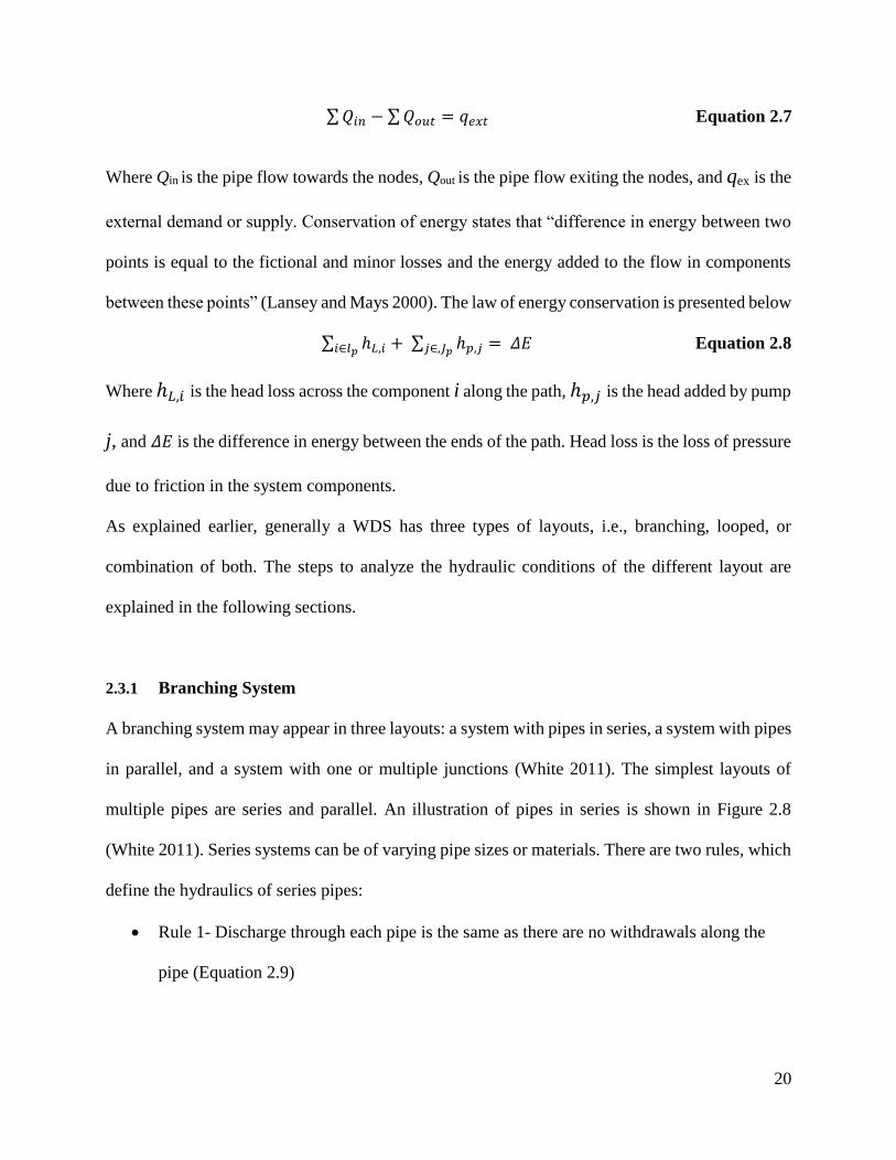
A branching system may appear in three layouts: a system with pipes in series, a system with pipes

in parallel, and a system with one or multiple junctions (White 2011). The simplest layouts of

multiple pipes are series and parallel. An illustration of pipes in series is shown in Figure 2.8

(White 2011). Series systems can be of varying pipe sizes or materials. There are two rules, which

define the hydraulics of series pipes:

• Rule 1- Discharge through each pipe is the same as there are no withdrawals along the

pipe (Equation 2.9)

21

• Rule 2- Total head loss is equal to the sum of head loss in each pipe (Equation 2.10)

(Briere 2014)

Figure 2.8. Pipes in a series system

𝑄1 = 𝑄2 = 𝑄3 = ⋯𝑄𝑝 = 𝑄 Equation 2.9

ℎ𝐴−𝐵 = ℎ𝑡 = ℎ𝑡1 + ℎ𝑡2 + ℎ𝑡3 +⋯+ ℎ𝑡𝑝 ⇒ ℎ𝑡 = ∑ ℎ𝑡𝑝𝑝𝑖=1 Equation 2.10

Where Q is the discharge, h is the head loss, and p is the number of pipes in series. Equation 2.10

can be rewritten in terms of the friction and minor losses given that discharge in all the pipes in

series are identical as Equation 2.11 (White 2011)

ℎ𝑡 = 𝑄𝑝 ∑ ℎ𝑝𝑝𝑖=1

𝑓𝑖 + 𝑄2∑ 𝐾𝑙𝑖

𝑝𝑙𝑖=1 Equation 2.11

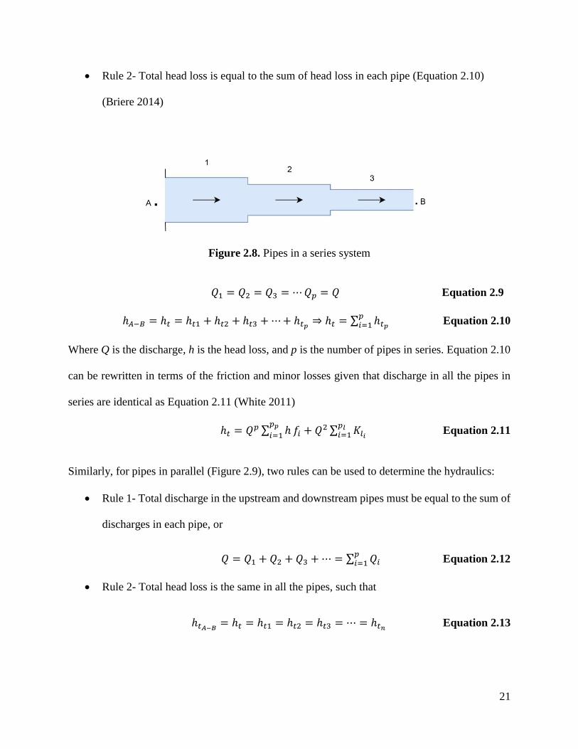
Similarly, for pipes in parallel (Figure 2.9), two rules can be used to determine the hydraulics:

• Rule 1- Total discharge in the upstream and downstream pipes must be equal to the sum of

discharges in each pipe, or

𝑄 = 𝑄1 + 𝑄2 + 𝑄3 +⋯ = ∑ 𝑄𝑖𝑝𝑖=1 Equation 2.12

• Rule 2- Total head loss is the same in all the pipes, such that

ℎ𝑡𝐴−𝐵 = ℎ𝑡 = ℎ𝑡1 = ℎ𝑡2 = ℎ𝑡3 = ⋯ = ℎ𝑡𝑛 Equation 2.13

22

Where p is the number of pipes in parallel, and ht is the total head loss. Equation 2.13 can be

rewritten as

ℎ𝑡𝑖 = ℎ𝑓𝑖 + ∑ℎ𝑙𝑖 = 𝐾𝑝𝑖𝑄𝑖𝑝 + ∑𝐾𝑙𝑖 𝑄𝑖

2 Equation 2.14

Where Kl is friction and local loss coefficients, hf is the loss due to pipe friction, pp and pl are the

number in-series pipes and local devices respectively.

Figure 2.9. Pipes in parallel

In general, one of the following scenarios may occur:

• Discharge is given which could be used to calculate the head loss using Equation 2.11 and

Equation 2.14, depending on the system requirement

• Head loss is given, and an iteration-based method is performed using an initial guess for

the friction factors of each pipe. Qi is calculated for each pipe using Equation 2.11. The

process is iterated until friction factors, and Kp remains unchanged. Problem converges at

this point, and the condition is satisfied at this point.

• If Q is known, finding total loss will be an iterative process where Equation 2.12, 2.13,

and 2.14 must be solved simultaneously.

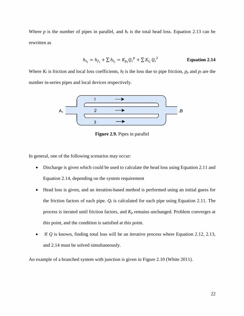
An example of a branched system with junction is given in Figure 2.10 (White 2011).

23

Figure 2.10. Branching pipe system; three-reservoir junction scenario

The governing relation for the branched system is the conservation of mass at the junction. The

flow at the junction must balance, since water is not stored in the pipes, such that

𝑄1 +𝑄2 + 𝑄3 = 0 Equation 2.15

Where signs on variable represent the direction of flow to or from the node. The static head at the

junction will be

ℎ𝑗 = 𝑍𝑗 +𝑝𝑗

𝛾 Equation 2.16

Where hj is the static head, zj is the elevation head, 𝑝𝑗

𝛾 is the pressure head. Assuming each reservoir

has an atmospheric pressure at the surface (i.e., 𝑝1 = 𝑝2 = 𝑝3 = 0), then the total loss can be found

with Equation 2.17 (White 2011)

∆ℎ =𝑉2𝑓𝐿

2𝑔𝑑= 𝑧 − ℎ𝑗 Equation 2.17

The discharge through the system can then be found by first taking an initial guess for the position

hj, solve Equation 2.16 for V through each pipe and hence Q1, Q2, and Q3. Then Iterating until

discharge balances at the junction according to Equation 2.15.

24

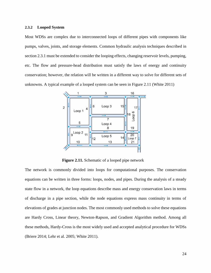
2.3.2 Looped System

Most WDSs are complex due to interconnected loops of different pipes with components like

pumps, valves, joints, and storage elements. Common hydraulic analysis techniques described in

section 2.3.1 must be extended to consider the looping effects, changing reservoir levels, pumping,

etc. The flow and pressure-head distribution must satisfy the laws of energy and continuity

conservation; however, the relation will be written in a different way to solve for different sets of

unknowns. A typical example of a looped system can be seen in Figure 2.11 (White 2011)

Figure 2.11. Schematic of a looped pipe network

The network is commonly divided into loops for computational purposes. The conservation

equations can be written in three forms: loops, nodes, and pipes. During the analysis of a steady

state flow in a network, the loop equations describe mass and energy conservation laws in terms

of discharge in a pipe section, while the node equations express mass continuity in terms of

elevations of grades at junction nodes. The most commonly used methods to solve these equations

are Hardy Cross, Linear theory, Newton-Rapson, and Gradient Algorithm method. Among all

these methods, Hardy-Cross is the most widely used and accepted analytical procedure for WDSs

(Briere 2014; Lehr et al. 2005; White 2011).

25

Hardy-Cross method was proposed and developed in the year 1936. It can be used if the entire

length and diameter of pipes are fixed, and either the head losses or flows between inlets and

outlets are known. The method is a relaxation technique in which the procedure starts with an

initially assumed flow value through each pipe making sure that continuity at the junctions is

maintained. If the flow is correctly chosen, then the sum of the head losses in all the pipes around

the loop being analyzed should be zero. Generally, in the first trial, the head loss around the loop

is not zero. Hence, flow rates are then adjusted by calculating the correction factor using Hardy-

Cross method. This process stops when the correction factors are zero or nearly zero. A step-by-

step procedure is given below (White 2011):

• Define a set of independent pipe loops and ensure that every pipe in the network is part of

at least one loop.

• Choose a value of flow (Q) arbitrarily in each pipe, such that the algebraic sum of the flow

rates must be zero at the nodes and continuity is satisfied

• Choose a sign convention for each loop and define Q to be positive if the assumed direction

of flow is clockwise concerning loop under consideration and vice versa.

• Compute the head loss in each pipe using Equation 2.18. The algebraic sum of the head

losses across the loop must be equal to zero. Presumably, this will not be the case based on

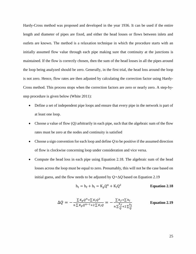
initial guess, and the flow needs to be adjusted by Q+ΔQ based on Equation 2.19

ht = hf + hl = KpQn + KlQ

2 Equation 2.18

∆𝑄 = −∑𝐾𝑝𝑄

𝑛+∑𝐾𝑙𝑄2

𝑛∑𝐾𝑝𝑄𝑛−1+2∑𝐾𝑙𝑄

= −∑ℎ𝑓+∑ℎ𝑙

𝑛∑ℎ𝑓

𝑄+2∑

ℎ𝑙𝑄

Equation 2.19

26

Where hf and hl are the frictional and local losses. The Hardy-Cross method is simple considering

single-loop systems; however, considering a full-scale WDS the application of this method is

impractical without the aid of computers. The computer models can perform the tedious

calculations including multiple loops much more quickly and accurately than manual calculations

(AWWA 2012).

In summary, The hydraulic analysis can be generalized into two main steps: the formulation of the

problem, and solution of the problem (Murty 2007). The problems are a set of nonlinear

mathematical equations which are formulated based on the principles of continuity, conservation,

and momentum to describe the flow characteristics of the system. The problem formulation could

be for a node balance, or a loop balance method. In a node balance method, the flow is balanced

around the node, i.e., the inflow minus outflow minus demand should be equal to zero. The

formulation of the problem to find a relation between head loss and flow results in a series of non-

linear equations. Several calculation methods can be adopted to solve these non-linear equations

simultaneously such as Hardy Cross, Linear theory, Newton-Rapson, and gradient algorithm

method as discussed earlier.

In modern times, computer modeling is an integral part of the planning, design, and operation of

WDSs. Computer models are used to predict the performance of a WDS to solve a wide variety of

design, operational, and water quality problems. These models, when properly implemented, are

an essential part of the decision-making process for engineers, planners, and managers. There are

two main components of a computer model: (1) a database, which describes the infrastructure,

operational characteristics, and demands, and (2) an algorithm, which solves a set of conservation

equations or optimization equation to identify suitable pressure, velocity, tank levels, and water

quality. (AWWA 2012). There are two types of analysis known as steady-state and extended-

27

period simulations. Steady-state analysis is like a snapshot of pipe system conditions at any given

time (AWWA 2012). Extended-period simulation is a sequence of steady-state simulations

extended over a specified time. It can be used to model demand variation, water quality, storage

tank operation, and flow through pipes. An extended period hydraulic modeling is also the primary

tool for system architecture optimization which can capture the behavior of the system under

different water demand scenarios and allow changes in design configuration during a period (Jones

and Sowby 2014a).

2.4 Improvement Strategies for WDS Design

Historically, the focus of WDS design improvement was to develop efficient algorithms for flow

analysis and making sure that a specified set of demands at the nodes and minimum pressure

constraints are satisfied (Walters 1992). Later on, different optimization techniques were adopted

in the design process to minimize the overall system cost while meeting a set of design criteria like

hydraulic constraints, water demand, and pressure requirements (Saldarriaga et al. 2010; Savic and

Walters 1997; Shamir 1974). More recently with an increase in environmental and energy

awareness and issues related to GHG emissions, few studies also included a sustainability factor

in the design improvement process.

The primary focus of this research is to improve the WDS design in terms of sustainability. The

sustainability in this research is referred to as the improvement in environmental and cost

performances. Only those improvement strategies are discussed in this literature review which is

related to these aspects. The two primary strategies are mathematical optimization and the life

cycle thinking approach (LCT) (Dandy et al. 2006; Du et al. 2013; Filion et al. 2004; Herstein et

al. 2011; Wu et al. 2010). Both approaches are discussed below; however, the LCT approach is

explained in more detail as it is primarily adopted for this research.

28

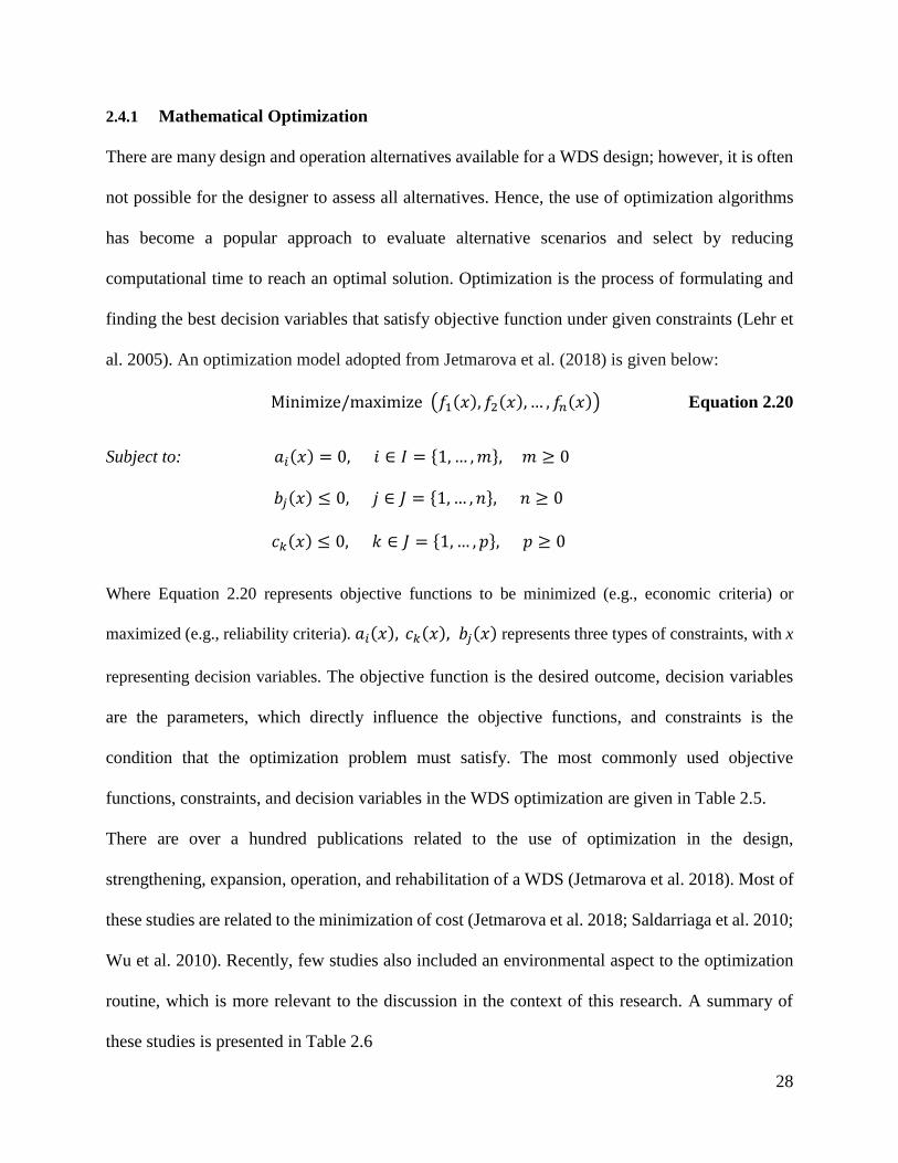
2.4.1 Mathematical Optimization

There are many design and operation alternatives available for a WDS design; however, it is often

not possible for the designer to assess all alternatives. Hence, the use of optimization algorithms

has become a popular approach to evaluate alternative scenarios and select by reducing

computational time to reach an optimal solution. Optimization is the process of formulating and

finding the best decision variables that satisfy objective function under given constraints (Lehr et

al. 2005). An optimization model adopted from Jetmarova et al. (2018) is given below:

Minimize/maximize (𝑓1(𝑥), 𝑓2(𝑥),… , 𝑓𝑛(𝑥)) Equation 2.20

Subject to: 𝑎𝑖(𝑥) = 0, 𝑖 ∈ 𝐼 = {1,… ,𝑚}, 𝑚 ≥ 0

𝑏𝑗(𝑥) ≤ 0, 𝑗 ∈ 𝐽 = {1,… , 𝑛}, 𝑛 ≥ 0

𝑐𝑘(𝑥) ≤ 0, 𝑘 ∈ 𝐽 = {1,… , 𝑝}, 𝑝 ≥ 0

Where Equation 2.20 represents objective functions to be minimized (e.g., economic criteria) or

maximized (e.g., reliability criteria). 𝑎𝑖(𝑥), 𝑐𝑘(𝑥), 𝑏𝑗(𝑥) represents three types of constraints, with x

representing decision variables. The objective function is the desired outcome, decision variables

are the parameters, which directly influence the objective functions, and constraints is the

condition that the optimization problem must satisfy. The most commonly used objective

functions, constraints, and decision variables in the WDS optimization are given in Table 2.5.

There are over a hundred publications related to the use of optimization in the design,

strengthening, expansion, operation, and rehabilitation of a WDS (Jetmarova et al. 2018). Most of

these studies are related to the minimization of cost (Jetmarova et al. 2018; Saldarriaga et al. 2010;

Wu et al. 2010). Recently, few studies also included an environmental aspect to the optimization

routine, which is more relevant to the discussion in the context of this research. A summary of

these studies is presented in Table 2.6

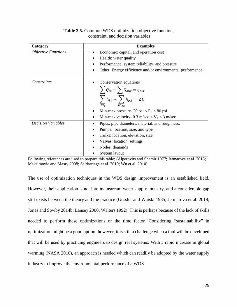
29

Table 2.5. Common WDS optimization objective function,

constraint, and decision variables

Category Examples

Objective Functions • Economic: capital, and operation cost

• Health: water quality

• Performance: system reliability, and pressure

• Other: Energy efficiency and/or environmental performance

Constraints • Conservation equations

∑𝑄𝑖𝑛 −∑𝑄𝑜𝑢𝑡 = 𝑞𝑒𝑥𝑡

∑ℎ𝐿,𝑖𝑖∈𝑙𝑝

+ ∑ ℎ𝑝,𝑗𝑗∈,𝐽𝑝

= 𝛥𝐸

• Min-max pressure- 20 psi < PR < 80 psi

• Min-max velocity- 0.3 m/sec < VF < 3 m/sec

Decision Variables • Pipes: pipe diameters, material, and roughness,

• Pumps: location, size, and type

• Tanks: location, elevation, size

• Valves: location, settings

• Nodes: demands

• System layout

Following references are used to prepare this table; (Alperovits and Shamir 1977; Jetmarova et al. 2018;

Maksimovic and Masry 2008; Saldarriaga et al. 2010; Wu et al. 2010).

The use of optimization techniques in the WDS design improvement is an established field.

However, their application is not into mainstream water supply industry, and a considerable gap

still exists between the theory and the practice (Gessler and Waiski 1985; Jetmarova et al. 2018;

Jones and Sowby 2014b; Lansey 2000; Walters 1992). This is perhaps because of the lack of skills

needed to perform these optimizations or the time factor. Considering “sustainability” in

optimization might be a good option; however, it is still a challenge when a tool will be developed

that will be used by practicing engineers to design real systems. With a rapid increase in global

warming (NASA 2010), an approach is needed which can readily be adopted by the water supply

industry to improve the environmental performance of a WDS.

30

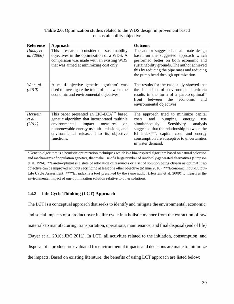
Table 2.6. Optimization studies related to the WDS design improvement based

on sustainability objective

Reference Approach Outcome

Dandy et

al. (2006)

This research considered sustainability

objectives in the optimization of a WDS. A

comparison was made with an existing WDS

that was aimed at minimizing cost only.

The author suggested an alternate design

based on the suggested approach which

performed better on both economic and

sustainability grounds. The author achieved

this by reducing the pipe mass and reducing

the pump head through optimization

Wu et al.

(2010)

A multi-objective genetic algorithm* was

used to investigate the trade-offs between the

economic and environmental objectives.

The results for the case study showed that

the inclusion of environmental criteria

results in the form of a pareto-optimal**

front between the economic and

environmental objectives.

Herstein

et al.

(2011)

This paper presented an EIO-LCA*** based

genetic algorithm that incorporated multiple

environmental impact measures on

nonrenewable energy use, air emissions, and

environmental releases into its objective

functions.

The approach tried to minimize capital

costs and pumping energy use

simultaneously. Sensitivity analysis

suggested that the relationship between the

EI index****, capital cost, and energy

consumption are susceptive to uncertainties

in water demand.

*Genetic-algorithm is a heuristic optimization techniques which is a bio-inspired algorithm based on natural selection

and mechanisms of population genetics, that make use of a large number of randomly-generated alternatives (Simpson

et al. 1994). **Pareto-optimal is a state of allocation of resources or a set of solution being chosen as optimal if no

objective can be improved without sacrificing at least one other objective (Manne 2016). ***Economic Input-Output-

Life Cycle Assessment. ****EI index is a tool presented by the same author (Herstein et al. 2009) to measures the

environmental impact of one optimization solution relative to other solutions.

2.4.2 Life Cycle Thinking (LCT) Approach

The LCT is a conceptual approach that seeks to identify and mitigate the environmental, economic,

and social impacts of a product over its life cycle in a holistic manner from the extraction of raw

materials to manufacturing, transportation, operations, maintenance, and final disposal (end of life)

(Bayer et al. 2010; JRC 2011). In LCT, all activities related to the initiation, consumption, and

disposal of a product are evaluated for environmental impacts and decisions are made to minimize

the impacts. Based on existing literature, the benefits of using LCT approach are listed below:

31

• LCT is considered as a comprehensive environmental management technique, and can

easily be adjusted to accommodate specific project needs (ISO 2006a; JRC 2011; Klopffer

and Grahl 2014)

• It can help avoid shifting burdens from one stage of a product to other stages in the life

cycle, e.g., making changes to a product might improve environmental performance in one

phase while worsening another phase (Belcham 2015). For example in a pipe Φ > 30”, DI

pipe manufacturing has lower emissions than the polyvinyl chloride (PVC) pipe (Du et al.

2013). However, DI pipe can deteriorate faster than a PVC pipe (Francisque et al. 2016)

resulting in high operational cost and energy use. Similarly, reducing pipe diameter can

lower the emissions and cost of manufacturing but might do the opposite in operational

stage due to a drop in the system pressure (Du et al. 2013; Filion et al. 2004; Piratla et al.

2012)

• The effect of adjusting decision variables such as pipe size, demand patterns, and other

component location can be holistically observed throughout all the phases.

• Performance evaluation of WDS generated from LCT studies can be an effective pre-

screening and benchmarking tool for future sustainability measures.

There are several techniques (or methods) that comes under the umbrella of LCT approach

including life cycle assessment (LCA), life cycle energy analysis (LCEA), life cycle management

(LCM), life cycle cost analysis (LCCA), and life cycle screening (LCS) (FET 2014). Two most

commonly used LCT techniques for environmental evaluation are life cycle assessment (LCA)

and life cycle energy analysis (LCEA) (Dennison et al. 1999; Du et al. 2013; Filion et al. 2004;

Piratla et al. 2012), whereas life cycle cost analysis (LCCA) is commonly used for the cost

assessment.

32

2.4.2.1 Life Cycle Assessment (LCA)

LCA is the most comprehensive environmental management technique to evaluate environmental

impacts associated with all stages of a product's life from the extraction of raw materials through

manufacturing, transportation, use, maintenance, and final disposal (end of life) (FET 2014). This

technique is being standardized by the International Organisation of Standardisation (ISO 2006b,

2006a). The main steps of this technique are:

1) Goal and Scope: this includes defining of a system boundary, functional unit, necessary

assumptions, types of impact categories, types of analysis, and data requirements for the system

under study. Essentially the required level of detail for a product(s) or service(s) is defined in this

step. The depth and breadth of LCA can differ significantly based on the goal of the study.

2) Life cycle inventory analysis: It is the most challenging phase of an LCA process. It tells how

much resources are consumed, and the amount of pollutants released in the environment during

each step under study. It provides an inventory of all input and output flows for a product.

Inventory flows include inputs of energy, resources consumed, and raw materials, and output in

the form of releases to air, land, and water. Use of various software tools such as SimaPro and

GaBi is a common practice because it is very difficult to examine individual material and process

from scratch each time when LCA is conducted. The software tools are integrated with the

available product and process databases; these databases contain information related to material

and energy use. There are several databases available to perform LCA, to name few: CIRAIG

(Canadian database), ecoinvent, ProBas, New Energy Externalities Developments for

Sustainability (NEEDS) and the United States Life Cycle Inventory (U.S. LCI) databases.

3) Life cycle impact assessment (LCIA): In this phase, the significance of potential environmental

impacts from the flow results of inventory analysis are evaluated. LCIA relatively assesses and

33

compares the impact of product or service on the environment, humans, and eco-system. The

impact categories and indicators are also defined at this step.

4) Interpretation: Results from the previous step are summarized during this phase. The cause and

effect of each process under the study are interpreted, limitations are explained, and

recommendations are provided transparently. The results of interpretation are generally presented

in graphical or tabular form.

2.4.2.2 Life Cycle Energy Analysis (LCEA)

LCEA is a simplification of LCA (Crawford 2012). LCEA is a pre-screening technique, which is

carried out for an initial overview of the environmental impacts and identify key issues for further

investigations. LCEA follows the same steps as full LCA, however, it can never claim to replace

it, because LCA provides an overall environmental impact of a product in the form of emissions

to soils, water, and air, whereas LCEA is a simple input-output model which uses only energy as

an input to measures the environmental impacts (Crawford 2012). In the present study, the concept

of LCEA has been applied to evaluate and compare various WDS design in terms of their

environmental and economic performance.

2.4.2.3 Life Cycle Cost Analysis (LCCA)

LCCA is a technique used to examine the total cost of owning an asset over its entire lifetime and

provide a basis for comparing initial investments with future costs over a specified period (Dhillon

2010). LCCA analyzes economic aspect all the phases of a system; it is generally used with LCA

and LCEA to achieve an optimal design in terms of least environmental and economic impacts

(Bayer et al. 2010). Broadly, the LCCA of any infrastructure can be classified into direct and

indirect costs. Direct cost includes the capital cost involved in planning, system design, and

installation phase, whereas the indirect cost involves the operation cost such as energy,

34

maintenance, inspections, repairs, leakage, and replacement. Direct costs are relatively easy to

quantify in monetary terms as compared to indirect costs (Rajani and Kleiner 2014). The total LCC

of a WDS can be determined as follows:

𝑇𝐿𝐶𝐶 = 𝐶𝑐 + ∑𝐶𝑚𝑟𝑟 + 𝐶𝑒 Equation 2.21

Where Cc= capital cost, Cmrr= maintenance, repair, and replacement, and Ce= the end of life cost.

2.4.2.4 LCT in the Water Sector

LCT use in the water sector was first introduced by Emmerson et al. (1995). They used LCA to

compare two small-scale sewage treatment processes. Similarly, the LCT use in WDS analysis

was first adopted by Dennison et al. (1999) to compare the environmental impacts of two different

potable water pipe materials. Several studies were carried out later using the aspects of LCT to

evaluate and improve the performance of WDS. However, there is still a research gap to improve

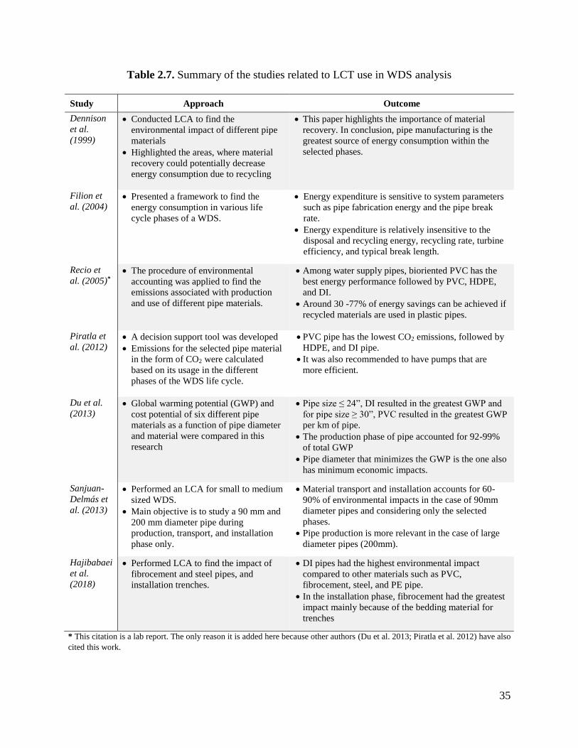
WDS analysis and design in the LCT context. A summary of a few important studies can be seen

in Table 2.7. Following are a few important observations:

• The LCT approach is most effective at the initial design stage in terms of overall

environmental and cost benefits. Because the changes can be made more easily at the early

stages compared to when a design is about to complete. A designer may be reluctant to

redesign part of the project, even though the long-term environmental benefits and cost

savings can be realized.

• The LCT approach in WDS analysis and design should be standardized to make the

performance evaluation system more reliable, which can be adopted and integrated into

design practices by the water industry.

• There is a research gap in LCCA of a WDS. An LCCA framework needs to be formulated

which can be used to identify a more realistic and optimal solution.

35

Table 2.7. Summary of the studies related to LCT use in WDS analysis

Study Approach Outcome

Dennison

et al.

(1999)

• Conducted LCA to find the

environmental impact of different pipe

materials

• Highlighted the areas, where material

recovery could potentially decrease

energy consumption due to recycling

• This paper highlights the importance of material

recovery. In conclusion, pipe manufacturing is the

greatest source of energy consumption within the

selected phases.

Filion et

al. (2004) • Presented a framework to find the

energy consumption in various life

cycle phases of a WDS.

• Energy expenditure is sensitive to system parameters

such as pipe fabrication energy and the pipe break

rate.

• Energy expenditure is relatively insensitive to the

disposal and recycling energy, recycling rate, turbine

efficiency, and typical break length.

Recio et

al. (2005)*

• The procedure of environmental

accounting was applied to find the

emissions associated with production

and use of different pipe materials.

• Among water supply pipes, bioriented PVC has the

best energy performance followed by PVC, HDPE,

and DI.

• Around 30 -77% of energy savings can be achieved if

recycled materials are used in plastic pipes.

Piratla et

al. (2012) • A decision support tool was developed

• Emissions for the selected pipe material

in the form of CO2 were calculated

based on its usage in the different

phases of the WDS life cycle.

• PVC pipe has the lowest CO2 emissions, followed by

HDPE, and DI pipe.

• It was also recommended to have pumps that are

more efficient.

Du et al.

(2013) • Global warming potential (GWP) and

cost potential of six different pipe

materials as a function of pipe diameter

and material were compared in this

research

• Pipe size ≤ 24”, DI resulted in the greatest GWP and

for pipe size ≥ 30”, PVC resulted in the greatest GWP

per km of pipe.

• The production phase of pipe accounted for 92-99%

of total GWP

• Pipe diameter that minimizes the GWP is the one also

has minimum economic impacts.

Sanjuan-

Delmás et

al. (2013)

• Performed an LCA for small to medium

sized WDS.

• Main objective is to study a 90 mm and

200 mm diameter pipe during

production, transport, and installation

phase only.

• Material transport and installation accounts for 60-

90% of environmental impacts in the case of 90mm

diameter pipes and considering only the selected

phases.

• Pipe production is more relevant in the case of large

diameter pipes (200mm).

Hajibabaei

et al.

(2018)

• Performed LCA to find the impact of

fibrocement and steel pipes, and

installation trenches.

• DI pipes had the highest environmental impact

compared to other materials such as PVC,

fibrocement, steel, and PE pipe.

• In the installation phase, fibrocement had the greatest

impact mainly because of the bedding material for

trenches

* This citation is a lab report. The only reason it is added here because other authors (Du et al. 2013; Piratla et al. 2012) have also

cited this work.

36

Based on the literature review most commonly used LCT technique for the analysis of WDS is

LCEA. Probably this is because LCEA is an efficient pre-screening method for an initial overview

of the environmental impacts to identify key issues, which can further be investigated using a much

detailed LCA. Additionally, LCEA does not necessarily require any special software tools or

connectivity to an extensive life cycle database. LCEA has successfully been adopted several times

in other similar studies, and for the same reason, it is also adopted for this research. The specific

literature related to the use of LCEA in a WDS analysis is given below.

2.5 LCEA in WDS Analysis and Design

LCEA follows similar steps as described to conduct LCA. However, the description of these steps

in the context of LCEA has been given in the following section along with typical literature values.

2.5.1 Scope and Goal definition

It is important in LCEA to create a realistic model, which requires to carefully defined goal and

scope (PRe 2016). An important step at this stage is to determine the functional unit and define the

scope and goal.

For an accurate comparison of two different products/processes, a reference unit of comparison is

required, which guarantees that the products/processes being compared deliver an equal level of

function or service (ISO 2006a; Olsen et al. 2001). This unit is known as its functional unit. LCEA

is an approach for relative assessment, which means the outcome of each assessment/analysis is

relative to the object under study only. For example, to determine the environmental impacts of a

WDS in terms of different pipe materials, a suitable functional unit used in the literature is the

length, diameter, and design life of the pipe. A PVC pipe with a one-meter length, six-inch

diameter, and fifty years of design life will be compared with a DI pipe of similar specifications.

37

The basic assumption in selecting this type of unit is to ensure that the function or level of service

should be the same for both the PVC and DI pipe (i.e., meeting the design requirements such as

pressure, velocity, or demand continuously).

Similarly, another functional unit in WDS can be the volume of water delivered. This functional

unit is useful in optimizing pumping energy or overall system performance. In this case, pipe

diameters and lengths can vary, but the design requirements should be met at all times. Venkatesh

and Brattebø (2011) used one-year operations of a network as a functional unit. Sanjuan-Delmás

et al. (2013) have used a declared unit as a functional unit. The declared unit is used when the

precise function of the product or scenario is not defined, or when the LCT based study is not a

full cradle-to-grave or cradle-to-cradle analysis.

After defining the functional unit, creating a system boundary is necessary to decide about unit

processes to be included in the LCEA. The main objective of defining a system boundary must

include the activities relevant to the goal of the study. According to Tillman et al. (1994), System

boundaries must be specified in several dimensions; geographical area, boundaries between nature

and technological system, time horizon, and production of capital goods. The initial system

boundary can be changed or adjusted later if there is a possibility that desired goals are not

achievable in current settings.

Previously in LCT based analysis researchers have included activities, which were directly

involved in the production, use, and disposal of the system components. For example, in the pipe

production, the system boundary might exclude the manufacturing of machines that were used to

extrude pipes; however, the energy consumed to operate these machines will most likely be

included in the study. Details of each phase and processes to be included in the present LCEA are

explained in the following sections.

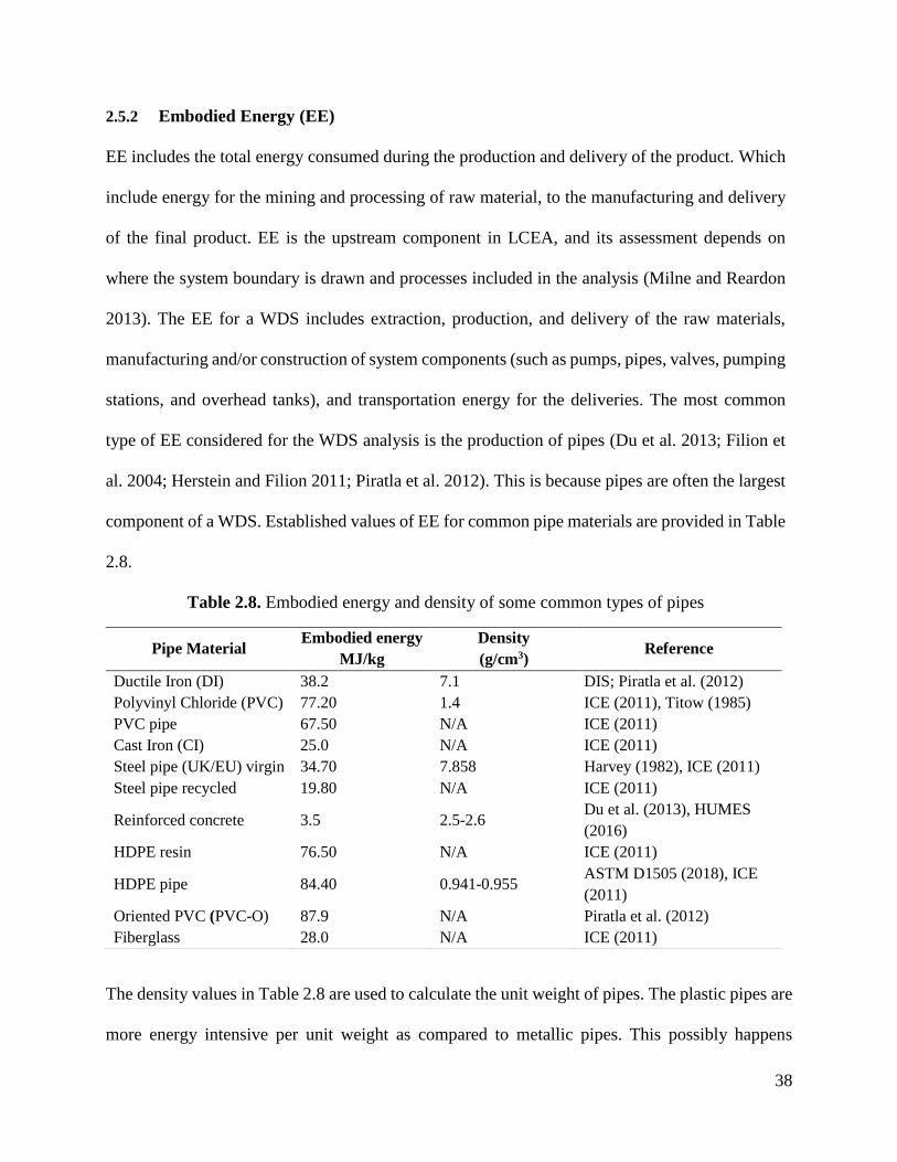
38

2.5.2 Embodied Energy (EE)

EE includes the total energy consumed during the production and delivery of the product. Which

include energy for the mining and processing of raw material, to the manufacturing and delivery

of the final product. EE is the upstream component in LCEA, and its assessment depends on

where the system boundary is drawn and processes included in the analysis (Milne and Reardon

2013). The EE for a WDS includes extraction, production, and delivery of the raw materials,

manufacturing and/or construction of system components (such as pumps, pipes, valves, pumping

stations, and overhead tanks), and transportation energy for the deliveries. The most common

type of EE considered for the WDS analysis is the production of pipes (Du et al. 2013; Filion et

al. 2004; Herstein and Filion 2011; Piratla et al. 2012). This is because pipes are often the largest

component of a WDS. Established values of EE for common pipe materials are provided in Table

2.8.

Table 2.8. Embodied energy and density of some common types of pipes

The density values in Table 2.8 are used to calculate the unit weight of pipes. The plastic pipes are

more energy intensive per unit weight as compared to metallic pipes. This possibly happens

Pipe Material Embodied energy

MJ/kg

Density

(g/cm3) Reference

Ductile Iron (DI) 38.2 7.1 DIS; Piratla et al. (2012)

Polyvinyl Chloride (PVC) 77.20 1.4 ICE (2011), Titow (1985)

PVC pipe 67.50 N/A ICE (2011)

Cast Iron (CI) 25.0 N/A ICE (2011)

Steel pipe (UK/EU) virgin 34.70 7.858 Harvey (1982), ICE (2011)

Steel pipe recycled 19.80 N/A ICE (2011)

Reinforced concrete 3.5 2.5-2.6 Du et al. (2013), HUMES

(2016)

HDPE resin 76.50 N/A ICE (2011)

HDPE pipe 84.40 0.941-0.955 ASTM D1505 (2018), ICE

(2011)

Oriented PVC (PVC-O) 87.9 N/A Piratla et al. (2012)

Fiberglass 28.0 N/A ICE (2011)

39

because plastic pipes are manufactured with new raw materials, whereas metallic pipes are mostly

manufactured from recycled materials (DIPRA 2016; Mantia 2004). According to Uni-Bell (2017),

the energy used in the extraction of raw materials and manufacturing of PVC pipe is 99% of the

total EE. Similarly, according to Dennison et al. (1999), the main energy consumption in the

manufacturing of DI and HDPE pipes is due to processing of material in plants. During

manufacturing of DI pipes, a large amount of energy is used to melt the scrap metals like shredded

cars and demolished building materials (DIPRA 2016). In Canada, the source of energy in

manufacturing is electricity (NRC 2008), which is mainly generated from hydropower (NRC

2014). The carbon emissions from 1 kWh hydropower electricity are approximately 24 g CO2eq

(Schlömer et al. 2014).

2.5.3 Transportation Energy

Emissions associated with transportation is due to direct energy consumption in the form of fuel

burnt from vehicles. Different types of transportation means can be adopted based on the freight

load, distance, and location. The common transport medium used over a long distance is using

heavy-duty trucks, trains, and ships. Under special circumstances, airfreight is also used, which is

considered as the fastest and most expensive. Based on some previous studies, it has been noted

that a class-8 (13 ton) truck has been used as a freight vehicle (Du et al. 2013). The average fuel

economy of the class-8 truck is 7.3 miles per gallons (mpg) (Oak Ridge 2016). However,

considering the fact that the average fuel economy negates the effects of material weight on total

emissions. Hence many factors affect the fuel economy such as driving at higher speeds, travel

distance, weather conditions, cargo weight, running electrical accessories, road conditions, 4-

wheel vs. 2-wheel drive, and roadway grade (Energy 2017). Fuel economy of class-8 trucks as a

function of roadway grade is given in Table 2.9

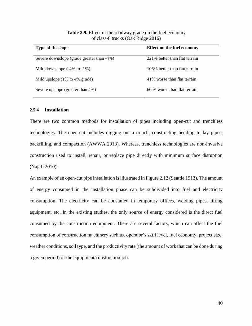
40

Table 2.9. Effect of the roadway grade on the fuel economy

of class-8 trucks (Oak Ridge 2016)

Type of the slope Effect on the fuel economy

Severe downslope (grade greater than -4%) 221% better than flat terrain

Mild downslope (-4% to -1%) 106% better than flat terrain

Mild upslope (1% to 4% grade) 41% worse than flat terrain

Severe upslope (greater than 4%) 60 % worse than flat terrain

2.5.4 Installation

There are two common methods for installation of pipes including open-cut and trenchless

technologies. The open-cut includes digging out a trench, constructing bedding to lay pipes,

backfilling, and compaction (AWWA 2013). Whereas, trenchless technologies are non-invasive

construction used to install, repair, or replace pipe directly with minimum surface disruption

(Najafi 2010).

An example of an open-cut pipe installation is illustrated in Figure 2.12 (Seattle 1913). The amount

of energy consumed in the installation phase can be subdivided into fuel and electricity

consumption. The electricity can be consumed in temporary offices, welding pipes, lifting

equipment, etc. In the existing studies, the only source of energy considered is the direct fuel

consumed by the construction equipment. There are several factors, which can affect the fuel

consumption of construction machinery such as, operator’s skill level, fuel economy, project size,

weather conditions, soil type, and the productivity rate (the amount of work that can be done during

a given period) of the equipment/construction job.

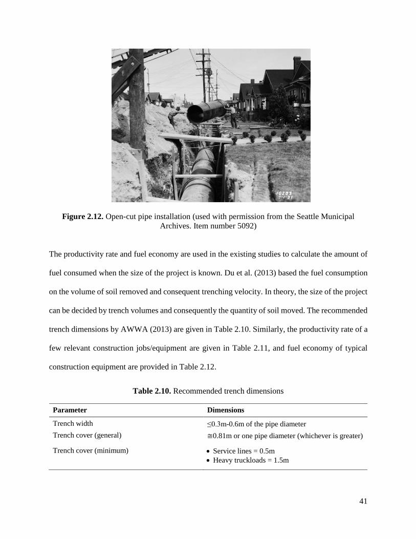
41

Figure 2.12. Open-cut pipe installation (used with permission from the Seattle Municipal

Archives. Item number 5092)

The productivity rate and fuel economy are used in the existing studies to calculate the amount of

fuel consumed when the size of the project is known. Du et al. (2013) based the fuel consumption

on the volume of soil removed and consequent trenching velocity. In theory, the size of the project

can be decided by trench volumes and consequently the quantity of soil moved. The recommended

trench dimensions by AWWA (2013) are given in Table 2.10. Similarly, the productivity rate of a

few relevant construction jobs/equipment are given in Table 2.11, and fuel economy of typical

construction equipment are provided in Table 2.12.

Table 2.10. Recommended trench dimensions

Parameter Dimensions

Trench width ≤0.3m-0.6m of the pipe diameter

Trench cover (general) ≅0.81m or one pipe diameter (whichever is greater)

Trench cover (minimum) • Service lines = 0.5m

• Heavy truckloads = 1.5m

42

Table 2.11. Productivity rate of the construction job/equipment (RSMeans 2018)

Construction job/equipment Productivity rate

Trench excavation (4 – 10 ft. deep, 1 Cubic yard excavator, common earth) 400 Bank Cubic Yard/ Day

Trench excavation (10 – 14 ft deep, 1 Cubic yard excavator, common earth) 360 Bank Cubic Yard/ Day

Trench excavation (1.5 ft wide, 9’ deep, flywheel trencher, common earth) 4981 Bank Cubic Yard/ Day

Backfill (55 hp dozer or front-end loader, 50’ haul, common earth) 200 Loose Cubic Yard/day

Backfill (105 hp dozer or front-end loader, 50’ haul, common earth) 1225 Loose Cubic Yard/day

Compaction (1 ft layer, vibrating plate) 90 Embankment cubic

yard/day

Compaction (1 ft layer, roller compaction operator walking) 150 Embankment cubic

yard/day

Compaction (vibrating roller, 1 ft lift, 2 passes) 5200 Embankment cubic

yard/day

Paving (asphalt pavement replacement over trench 0.33 ft thick) 70 Square yard/day

Paving (asphalt pavement replacement over trench 0.5 ft thick) 55 Square yard/day

Table 2.12. The fuel consumption rate of the construction equipment

Machines Fuel consumption Reference

Backhoe 8 L/h ICTF (2016)

Excavator 15 L/h ICTF (2016)

Asphalt paver 10 L/h Cmplindia 2016, Scribd (2016)

Vibrating roller 9 L/h ICTF (2016), Scribd (2016)

Vibrating plate 1.9 L/h A&B (2017)

Loader 13 L/h ICTF (2016)

Ditch witch J10 13.9 L/h Theoretical

Ditch witch FM13V Fluid Management

System, 66hp 5.3 L/h Theoretical

Medium duty truck 0.25 L/km Fuelly (2017)

Fuel consumption compressor (100% load) 10 L/h Airman (2017)

Fuel consumption compressor (70% load) 7.5 L/h Airman (2017)

Theoretically, the fuel consumption in Table 2.12 can be calculated using Equation 2.22

𝐹 =𝐻𝑃𝑔×𝑆𝐹𝑃

1.87 Equation 2.22

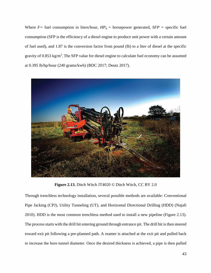
43

Where F= fuel consumption in liters/hour, HPg = horsepower generated, SFP = specific fuel

consumption (SFP is the efficiency of a diesel engine to produce unit power with a certain amount

of fuel used), and 1.87 is the conversion factor from pound (lb) to a liter of diesel at the specific

gravity of 0.853 kg/m3. The SFP value for diesel engine to calculate fuel economy can be assumed

at 0.395 lb/hp/hour (240 grams/kwh) (BDC 2017; Deutz 2017).

Figure 2.13. Ditch Witch JT4020 © Ditch Witch, CC BY 2.0

Through trenchless technology installation, several possible methods are available: Conventional

Pipe Jacking (CPJ), Utility Tunneling (UT), and Horizontal Directional Drilling (HDD) (Najafi

2010). HDD is the most common trenchless method used to install a new pipeline (Figure 2.13).

The process starts with the drill bit entering ground through entrance pit. The drill bit is then steered

toward exit pit following a pre-planned path. A reamer is attached at the exit pit and pulled back

to increase the bore tunnel diameter. Once the desired thickness is achieved, a pipe is then pulled

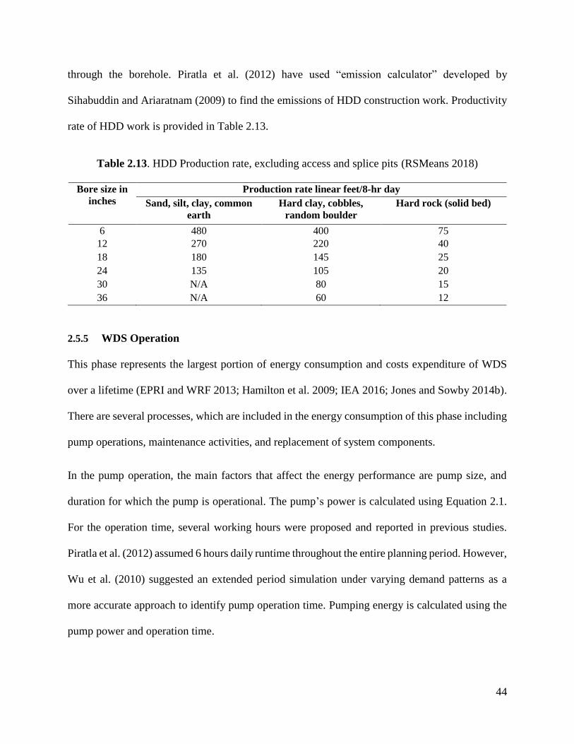
44

through the borehole. Piratla et al. (2012) have used “emission calculator” developed by

Sihabuddin and Ariaratnam (2009) to find the emissions of HDD construction work. Productivity

rate of HDD work is provided in Table 2.13.

Table 2.13. HDD Production rate, excluding access and splice pits (RSMeans 2018)

Bore size in

inches

Production rate linear feet/8-hr day

Sand, silt, clay, common

earth

Hard clay, cobbles,

random boulder

Hard rock (solid bed)

6 480 400 75

12 270 220 40

18 180 145 25

24 135 105 20

30 N/A 80 15

36 N/A 60 12

2.5.5 WDS Operation

This phase represents the largest portion of energy consumption and costs expenditure of WDS

over a lifetime (EPRI and WRF 2013; Hamilton et al. 2009; IEA 2016; Jones and Sowby 2014b).

There are several processes, which are included in the energy consumption of this phase including

pump operations, maintenance activities, and replacement of system components.

In the pump operation, the main factors that affect the energy performance are pump size, and

duration for which the pump is operational. The pump’s power is calculated using Equation 2.1.

For the operation time, several working hours were proposed and reported in previous studies.

Piratla et al. (2012) assumed 6 hours daily runtime throughout the entire planning period. However,

Wu et al. (2010) suggested an extended period simulation under varying demand patterns as a

more accurate approach to identify pump operation time. Pumping energy is calculated using the

pump power and operation time.

45

The maintenance activities are performed to keep physical, hydraulic, and water quality integrity.

Physical integrity includes repair/replace components, corrosion control, and protecting the system

environment. An example of hydraulic integrity is the leak detection and cleaning of pipes to

remove accumulated sediment. Water quality integrity includes cleaning and flushing of pipes,

cleaning of strainers, and routine testing. According to Piratla et al. (2012), energy consumed to

inspect and clean the pipes is negligible.

One basic activity of the maintenance process is pipe’s repair which can be done either by open-

cut or trenchless methods. For the open-cut repair, a common method used is to isolate a broken

pipe section by shutting off the valves and then repair a break using repair sleeve (AWWA 2013).

According to Piratla et al. (2012), the total energy needed to repair a single break is the sum of all

energies needed to manufacture sleeve, equipment operation, and transportation for the equipment

mobilization. Repair sleeves are commonly made up of stainless steel material (Canada 2017;

Romac 2017; Wolseley 2017). In the trenchless repair, several methods can be applied: namely,

cement-mortar lining, epoxy lining, slip lining and cured in place pipe lining (CIPP). CIPP is the

most commonly used trenchless technology method (DAS 2016; Supplement 2013). In CIPP, a

polyester felt tube saturated with resin is pulled into the deteriorated pipe section and inverted with

the help of water or compressed air. The felt tube is then cured inside the pipe through hot steam,

ultraviolet light, or hot water (AWWA 2013).

Water utilities may choose to replace the pipes if the breakage rate is high as pipe repair is not

feasible (Walski and Male 2000). Moreover, apart from the break rate, other leading causes of

pipe replacement reported by the utilities were pipe age, low flows, and condition of materials

(WRF 2016). The annual pipe break rate for DI, PVC, and HDPE is 3.82/100 kilometers (km),

0.85/100 km, and 0.39/100 km (Folkman 2012; Venkatesh 2012). The pipes can either be replaced

46

using open-cut or trenchless technology methods. The processes involved in the open-cut pipe

replacement are similar to open-cut installation. In the trenchless technology method, the primary

technique used is known as pipe bursting (Najafi 2010) where pipes are destroyed inside the

ground by pulling a larger diameter conical shaped bursting head through the existing pipelines.

The pipe is attached to the bursting head. As the head moves through the host pipe, the broken

pipe fragments are pushed into the ground, forming a cavity for the product pipe.

One important consideration during the LCEA of WDS is to predict the maintenance and

replacement time. WDS components fail at a different rate over the planned analysis period; pipe

deterioration models can be used to predict the time of a major repair or a failure. Filion et al.

(2004) used the roughness-growth model proposed by Sharp and Walski (1988) to predict the

repair time. Similarly, Piratla et al. (2012) used a regression-based model by Shamir and Howard

(1979) to obtain pipe breakage rate. That model only considers a single variable parameter such

as historical pipe breakage rate. All these models predicted pipe failure based on a single parameter

(Shamir and Howard 1979; Sharp and Walski 1988), but recently several new models were

developed that considered multiple parameters such as soil corrosiveness, material age, water

quality, and diameter to make result more reliable (Francisque et al. 2016; Kabir et al. 2015). Pipe

deterioration models, in general, are subjective to the nature of the study, numerous pipe failure

prediction models can be found in the literature. A detailed comparison of these models is given

in Kimutai et al. (2015), Kleiner and Rajani (2001), and Wilson et al. (2015).

2.5.6 End of life

At the end of useful life, the WDS components could be abandoned, disposed, or recycled.

Generally, the underground pipes are abandoned rather than restoring them, because of the

resources required to unearth the pipes (Piratla et al. 2012; Recio et al. 2005). In terms of material

47

recycling, plastic pipes such as PVC are generally made of new materials, because pipes made

with recycled materials believed to have poor properties (Mantia 2004). Metallic pipes such as DI

are mainly made up of recycled materials which come from shredded cars and building scraps

(DIPRA 2016). Cambridge and MIT (2005) have suggested the recycling energy of PVC and

HDPE to be 35-40 MJ/kg and 35-45 MJ/kg, respectfully. Filion et al. (2004) suggested the

following equations to calculate the disposal and recycling energy

𝐸𝑑 = (1 − 𝛼′) ∑ ∑ 𝐿𝑖𝑒𝑑

𝑃𝑖=1

𝑀𝑗=1 Equation 2.23

𝐸𝑟 = 𝛼′∑ ∑ 𝐿𝑖𝑒𝑟

𝑃𝑖=1

𝑀𝑗=1 Equation 2.24

Where Ed = total disposal energy (TJ), ed = unit energy required to dispose of pipes (GJ/m), Er=

total energy to recycle old pipes (GJ/m), M = number of pipe replacement, P = number of pipes in

the system, α’= closed-loop recycling rate. The closed-loop recycling rate is difficult to predict as

it can change with pipe aging. The total life cycle energy requirement associated with a specific

planning scenario is finally calculated by adding the energy requirements of all the life cycle

phases of a system.

𝐸𝑇𝑜𝑡𝑎𝑙 = 𝐸𝐸𝑚𝑏𝑜𝑑𝑖𝑒𝑑 + 𝐸𝑇𝑟𝑎𝑛𝑠𝑝𝑜𝑟𝑡 + 𝐸𝐼𝑛𝑠𝑡𝑎𝑙𝑙 + 𝐸𝑂𝑝𝑒𝑟𝑎𝑡𝑖𝑜𝑛 + 𝐸𝐷𝑖𝑠𝑝𝑜𝑠𝑎𝑙 Equation 2.25

2.6 Life Cycle Cost Analysis (LCCA)

Evaluating construction projects on their initial cost alone has long been recognized as

unsatisfactory (Ashworth 2014). It became obvious with the time that some method of financial

analysis must be used, which takes into account the running (i.e., maintenance, and management)

cost of a project (Ashworth 2014). LCCA is used to facilitate the decision-making process to

eliminate competing, mutually exclusive schemes, based on all the costs incurred during its life

(Dale 2014).

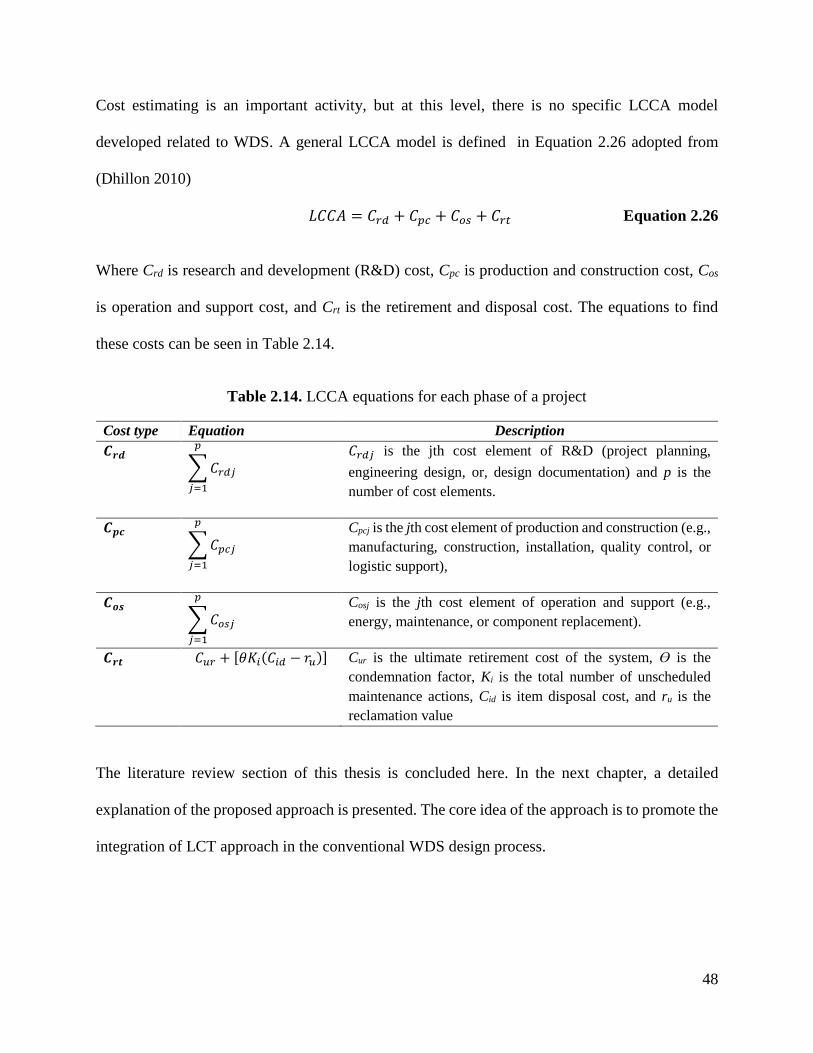
48

Cost estimating is an important activity, but at this level, there is no specific LCCA model

developed related to WDS. A general LCCA model is defined in Equation 2.26 adopted from

(Dhillon 2010)

𝐿𝐶𝐶𝐴 = 𝐶𝑟𝑑 + 𝐶𝑝𝑐 + 𝐶𝑜𝑠 + 𝐶𝑟𝑡 Equation 2.26

Where Crd is research and development (R&D) cost, Cpc is production and construction cost, Cos

is operation and support cost, and Crt is the retirement and disposal cost. The equations to find

these costs can be seen in Table 2.14.

Table 2.14. LCCA equations for each phase of a project

Cost type Equation Description

𝑪𝒓𝒅

∑𝐶𝑟𝑑𝑗

𝑝

𝑗=1

𝐶𝑟𝑑𝑗 is the jth cost element of R&D (project planning,

engineering design, or, design documentation) and p is the

number of cost elements.

𝑪𝒑𝒄 ∑𝐶𝑝𝑐𝑗

𝑝

𝑗=1

Cpcj is the jth cost element of production and construction (e.g.,

manufacturing, construction, installation, quality control, or

logistic support),

𝑪𝒐𝒔 ∑𝐶𝑜𝑠𝑗

𝑝

𝑗=1

Cosj is the jth cost element of operation and support (e.g.,

energy, maintenance, or component replacement).

𝑪𝒓𝒕 𝐶𝑢𝑟 + [𝜃𝐾𝑖(𝐶𝑖𝑑 − 𝑟𝑢)] Cur is the ultimate retirement cost of the system, ϴ is the

condemnation factor, Ki is the total number of unscheduled

maintenance actions, Cid is item disposal cost, and ru is the

reclamation value

The literature review section of this thesis is concluded here. In the next chapter, a detailed

explanation of the proposed approach is presented. The core idea of the approach is to promote the

integration of LCT approach in the conventional WDS design process.

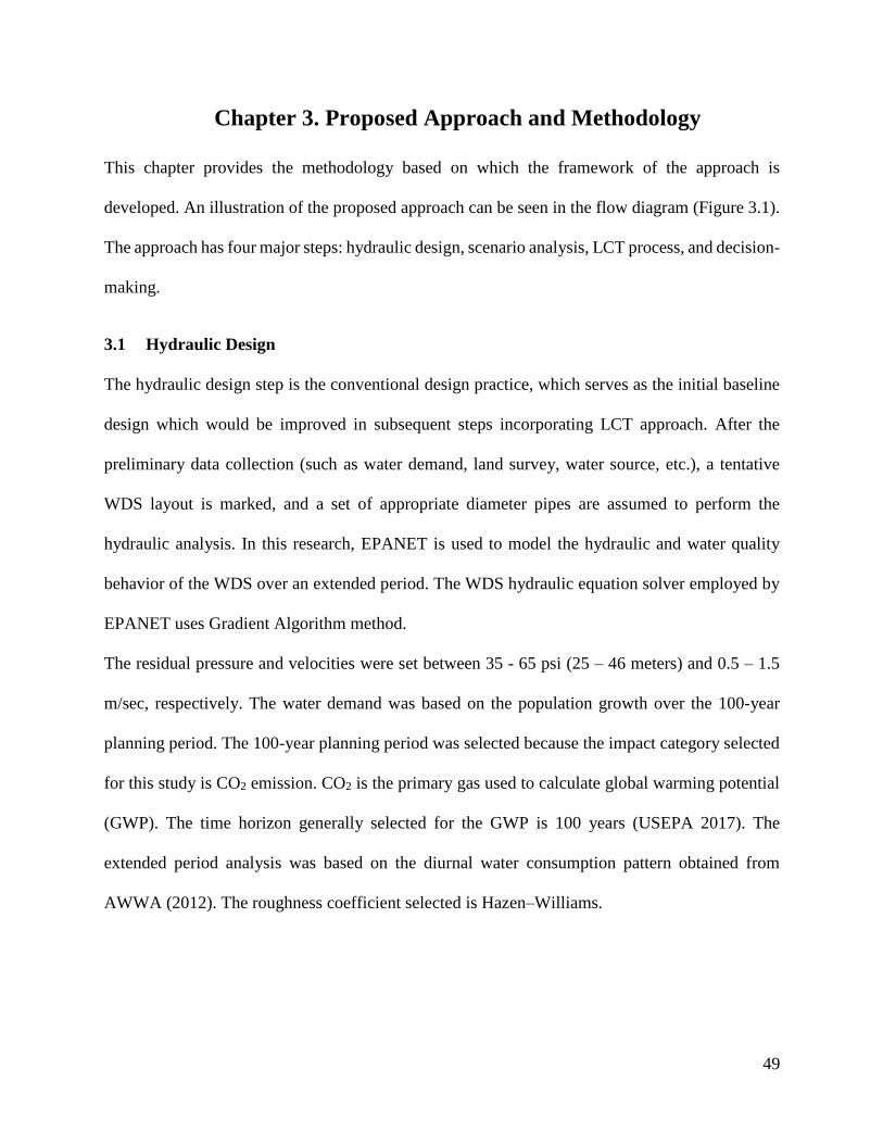
49

3 Chapter 3. Proposed Approach and Methodology

This chapter provides the methodology based on which the framework of the approach is

developed. An illustration of the proposed approach can be seen in the flow diagram (Figure 3.1).

The approach has four major steps: hydraulic design, scenario analysis, LCT process, and decision-

making.

3.1 Hydraulic Design

The hydraulic design step is the conventional design practice, which serves as the initial baseline

design which would be improved in subsequent steps incorporating LCT approach. After the

preliminary data collection (such as water demand, land survey, water source, etc.), a tentative

WDS layout is marked, and a set of appropriate diameter pipes are assumed to perform the

hydraulic analysis. In this research, EPANET is used to model the hydraulic and water quality

behavior of the WDS over an extended period. The WDS hydraulic equation solver employed by

EPANET uses Gradient Algorithm method.

The residual pressure and velocities were set between 35 - 65 psi (25 – 46 meters) and 0.5 – 1.5

m/sec, respectively. The water demand was based on the population growth over the 100-year

planning period. The 100-year planning period was selected because the impact category selected

for this study is CO2 emission. CO2 is the primary gas used to calculate global warming potential

(GWP). The time horizon generally selected for the GWP is 100 years (USEPA 2017). The

extended period analysis was based on the diurnal water consumption pattern obtained from

AWWA (2012). The roughness coefficient selected is Hazen–Williams.

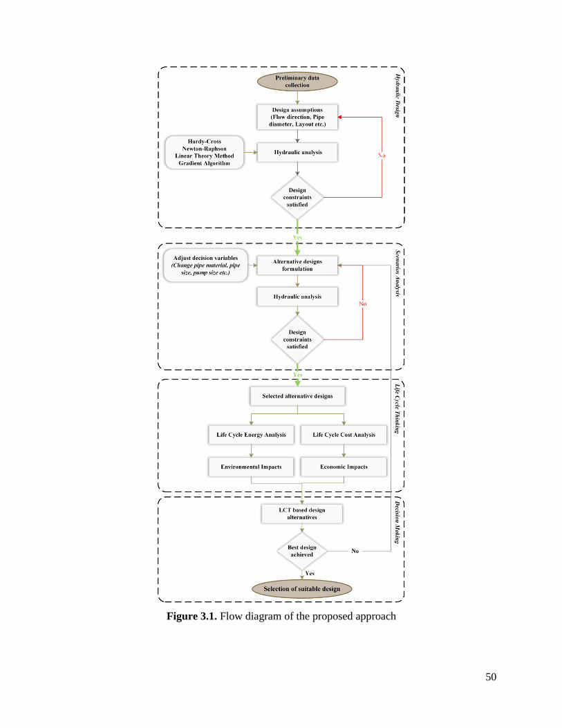
50

Figure 3.1. Flow diagram of the proposed approach

51

3.2 Scenario Analysis

The initial successful run of hydraulic analysis does not guarantee that the design produced will in

any sense be the most sustainable. To improve sustainability, the decision variables are adjusted

again, and a new set of diameters are assumed, and the analysis is run again. The decision variables

can influence the alternate design scenarios in several ways; this relation can be seen in Table 3.1.

Table 3.1. Effect of decision variables on the design scenario

Decision

variables

Activity Possible outcomes

Pipes Reduction or increment in diameter Total mass and system pressure can fluctuate

Tanks Altering elevation or location The system pressure and pump head can vary

Pipe

material

Variation in pipe material selection The maintenance requirement over the planning

period and mass is increased or decreased

System

layout

Altering the layout The network length and overall system pressure

is influenced

Pumps Altering location, and type (i.e.,

variable or fixed speed drive)

The pumping efficiency and the pump head can

improve or degrade

Adopted from (Dandy et al. 2006; Francisque et al. 2016; Lejano 2006; Maksimovic and Masry 2008)

Each time the decision variables are adjusted, and results are validated through extended period

simulation, an alternate design is recorded. An extended period simulation can capture the behavior

of the system under different loading conditions and changes in design configuration during an

extended period. The adjustment of decision variables is subjective and depends on the preference

and skill level of the analyst. The primary focus of this step is to improve the hydraulic efficiency

such as pumps operating at the lower head, or smallest possible pipe sizes. Once the desired pipe

sizes are attained, tank location and/or elevation can then be adjusted and so on while satisfying

all design constraints.

52

Generally, it is uncommon that a very large and complex WDS is constructed at one given point

in time (Gessler and Waiski 1985). Systems usually grow over many years in relatively small

increments. For example, a new development of square mile might need the sizing of only a few

main lines once the main supply grid of an existing WDS is in place (Gessler and Waiski 1985).

3.3 Life Cycle Thinking (LCT)

After the generation of alternate design scenarios, each design is analyzed using LCT by

performing LCEA and LCCA. There are several reasons that an LCEA technique is adopted here

instead of a detailed LCA, for example,

• Several alternative designs are generated due to the iterative nature of the approach, and

each design is analyzed for environmental and energy sustainability. LCEA method is an

efficient pre-screening method for an initial overview. It is simple and relatively easy to

apply.

• LCEA follows the same steps and includes the same phases as LCA, and it does not require

any special tools.

• LCEA has been successfully applied previously to assess the sustainability of a WDS.

However, the main disadvantage of relying only on LCEA is that it is not regulated, and the results

might not be as accurate as LCA. A detailed methodology to perform LCEA and LCCA on WDS

is explained in the following sections 3.3.1 and 3.3.2.

3.3.1 Life Cycle Energy Analysis (LCEA)

The LCEA resumes with the definition of functional unit, scope, and goal. The functional unit

selected for this study is the one-year operation of the system maintaining minimum residual

pressure of h ≥ hminimum where h is the residual pressure, and hminimum is the TDH of the system.

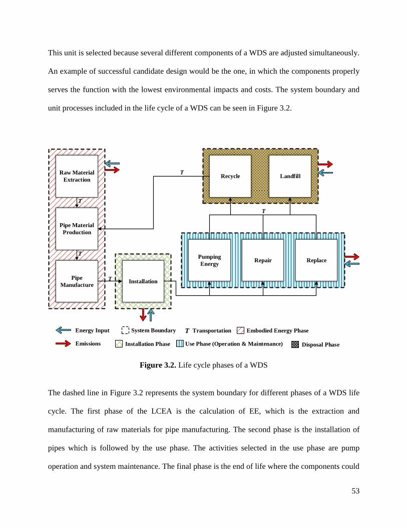
53

This unit is selected because several different components of a WDS are adjusted simultaneously.

An example of successful candidate design would be the one, in which the components properly

serves the function with the lowest environmental impacts and costs. The system boundary and

unit processes included in the life cycle of a WDS can be seen in Figure 3.2.

Figure 3.2. Life cycle phases of a WDS

The dashed line in Figure 3.2 represents the system boundary for different phases of a WDS life

cycle. The first phase of the LCEA is the calculation of EE, which is the extraction and

manufacturing of raw materials for pipe manufacturing. The second phase is the installation of

pipes which is followed by the use phase. The activities selected in the use phase are pump

operation and system maintenance. The final phase is the end of life where the components could

Energy Input

Raw Material

Extraction

Pipe Material

Production

Pipe

ManufactureInstallation

Pumping

EnergyRepair Replace

Recycle Landfill

T

T

T

T

T

Emissions

System Boundary T Transportation Embodied Energy Phase

Installation Phase Use Phase (Operation & Maintenance) Disposal Phase

54

either be the disposal in landfills or recycled. Transportation is not presented as a separate phase

because transportation has been considered in the form of equipment mobilization during all

phases. However, transportation is included in the calculation of final emissions.

The results of LCEA are reported in the form of CO2 emissions. CO2 is the primary gas used to

calculate GWP, the principal greenhouse gas (GHG) emitted through human actions, and is

considered as one of the targets of cap and trade environmental regulation scheme (EDF 2017).

The activities producing low carbon emissions are preferred over the ones producing high

emissions. There are no guidelines for the selection of impact categories, and is a matter between

the commissioner and the practitioner (EPA 2005)

The methods used to calculate emissions are different for each phase based on the type of direct

energy input. For example, the embodied energy of the pipes is calculated in MJ/kg, and the source

of energy is electricity. Where as, 1 kWh = 3.6 megajoules, and 1 kWh (hydropower) = 24 g CO2eq

(Schlömer et al. 2014). The assumptions related to the LCEA are included with in the discussion

of each phase below.

3.3.1.1 Embodied Energy (EE)

The EE represents the manufacturing and delivery of pipes. Because pipes often constitute the

largest components of a WDS. The total EE of the network pipes is calculated by taking a product

of EE values shown in Table 2.8, and the total weight of the pipes. This relation can be seen in

Equation 3.1. In this study, electricity is assumed as the main source of energy consumption in the

embodied phase as explained in section 2.5.2.

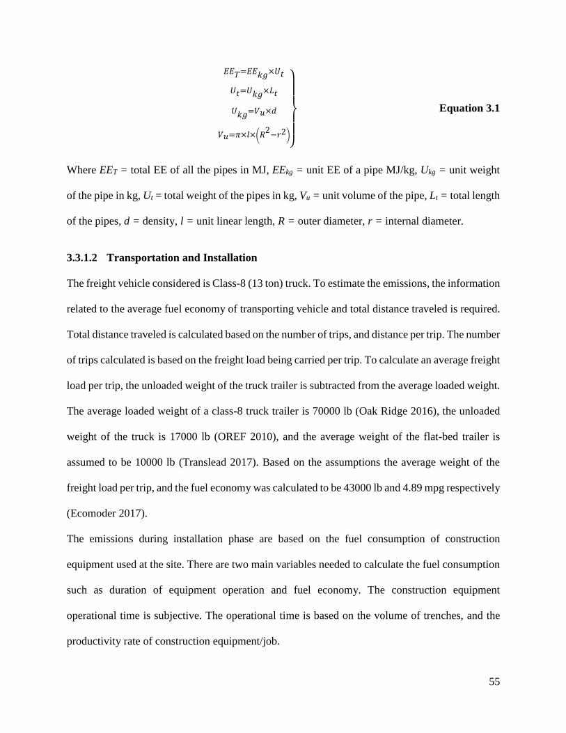
55

𝐸𝐸𝑇=𝐸𝐸𝑘𝑔×𝑈𝑡

𝑈𝑡=𝑈𝑘𝑔×𝐿𝑡

𝑈𝑘𝑔=𝑉𝑢×𝑑

𝑉𝑢=𝜋×𝑙×(𝑅2−𝑟2)

}

Equation 3.1

Where EET = total EE of all the pipes in MJ, EEkg = unit EE of a pipe MJ/kg, Ukg = unit weight

of the pipe in kg, Ut = total weight of the pipes in kg, Vu = unit volume of the pipe, Lt = total length

of the pipes, d = density, l = unit linear length, R = outer diameter, r = internal diameter.

3.3.1.2 Transportation and Installation

The freight vehicle considered is Class-8 (13 ton) truck. To estimate the emissions, the information

related to the average fuel economy of transporting vehicle and total distance traveled is required.

Total distance traveled is calculated based on the number of trips, and distance per trip. The number

of trips calculated is based on the freight load being carried per trip. To calculate an average freight

load per trip, the unloaded weight of the truck trailer is subtracted from the average loaded weight.

The average loaded weight of a class-8 truck trailer is 70000 lb (Oak Ridge 2016), the unloaded

weight of the truck is 17000 lb (OREF 2010), and the average weight of the flat-bed trailer is

assumed to be 10000 lb (Translead 2017). Based on the assumptions the average weight of the

freight load per trip, and the fuel economy was calculated to be 43000 lb and 4.89 mpg respectively

(Ecomoder 2017).

The emissions during installation phase are based on the fuel consumption of construction

equipment used at the site. There are two main variables needed to calculate the fuel consumption

such as duration of equipment operation and fuel economy. The construction equipment

operational time is subjective. The operational time is based on the volume of trenches, and the

productivity rate of construction equipment/job.

56

In the open-cut installation, main activities included are the excavation, backfilling, and

compaction of trenches. Similarly, the equipment used for the trenchless installation is the drill

rig, fluid mud mixing system, and a light to medium duty vehicles to mobilize equipment. The fuel

economy and productivity rate of construction equipment/job have already been shown in Tables

2.11 and 2.12. The distance assumed for equipment mobilization is a round trip between the site

and the rental warehouse.

3.3.1.3 Use Phase

The selected activities responsible for the use phase emissions are the pump operation,

maintenance, and pipe replacement. Emissions related to the pump operation is direct energy

consumptions in the form of electricity. The total electricity consumption can be calculated if the

pump power and the pump running time is known. The pump running time is obtained from a

computer model extended period analysis. Pumps operations can be controlled with simple rule-

based commands in a computer hydraulic analysis model. Total pumping energy is then calculated

in kWh by multiplying the duration with the pump power.

The maintenance activities include the repair and replacement of the components. The repairs can

use either open-cut or trenchless. The energy needed to repair a single break is the sum of all

energies needed to manufacture the sleeve, the equipment operation for digging and refilling of

splice pits, and the transportation fuel for the equipment mobilization. Emissions for the equipment

operation in an open-cut repair follows the same process as an open-cut installation in section 2.5.4.

To find the number of breaks in each year, the annual pipe break rate is used.

The emissions for the trenchless repair method are based on the fuel consumed by the air

compressor, and energy to manufacture the polyester liner. The trenchless repair method

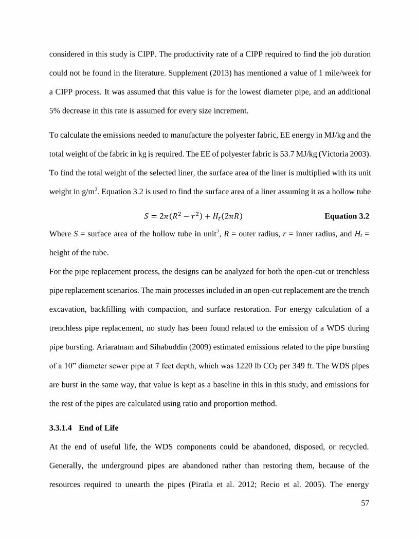
57

considered in this study is CIPP. The productivity rate of a CIPP required to find the job duration

could not be found in the literature. Supplement (2013) has mentioned a value of 1 mile/week for

a CIPP process. It was assumed that this value is for the lowest diameter pipe, and an additional

5% decrease in this rate is assumed for every size increment.

To calculate the emissions needed to manufacture the polyester fabric, EE energy in MJ/kg and the

total weight of the fabric in kg is required. The EE of polyester fabric is 53.7 MJ/kg (Victoria 2003).

To find the total weight of the selected liner, the surface area of the liner is multiplied with its unit

weight in g/m2. Equation 3.2 is used to find the surface area of a liner assuming it as a hollow tube

𝑆 = 2𝜋(𝑅2 − 𝑟2) + 𝐻𝑡(2𝜋𝑅) Equation 3.2

Where S = surface area of the hollow tube in unit2, R = outer radius, r = inner radius, and Ht =

height of the tube.

For the pipe replacement process, the designs can be analyzed for both the open-cut or trenchless

pipe replacement scenarios. The main processes included in an open-cut replacement are the trench

excavation, backfilling with compaction, and surface restoration. For energy calculation of a

trenchless pipe replacement, no study has been found related to the emission of a WDS during

pipe bursting. Ariaratnam and Sihabuddin (2009) estimated emissions related to the pipe bursting

of a 10” diameter sewer pipe at 7 feet depth, which was 1220 lb CO2 per 349 ft. The WDS pipes

are burst in the same way, that value is kept as a baseline in this in this study, and emissions for

the rest of the pipes are calculated using ratio and proportion method.

3.3.1.4 End of Life

At the end of useful life, the WDS components could be abandoned, disposed, or recycled.

Generally, the underground pipes are abandoned rather than restoring them, because of the

resources required to unearth the pipes (Piratla et al. 2012; Recio et al. 2005). The energy

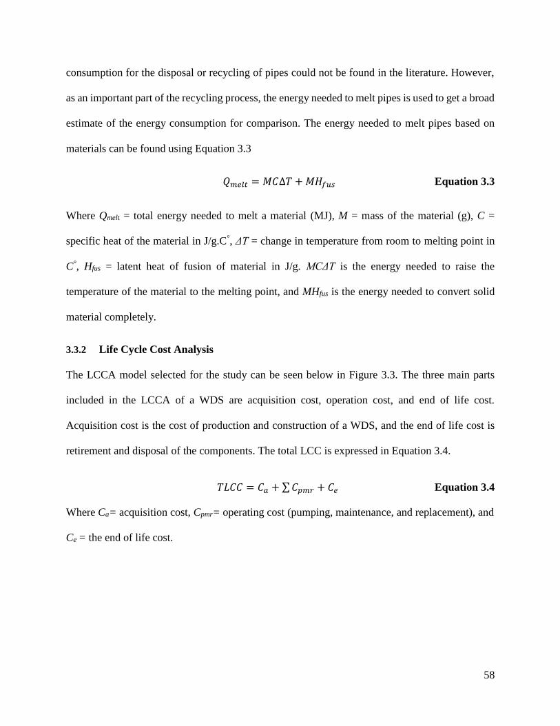
58

consumption for the disposal or recycling of pipes could not be found in the literature. However,

as an important part of the recycling process, the energy needed to melt pipes is used to get a broad

estimate of the energy consumption for comparison. The energy needed to melt pipes based on

materials can be found using Equation 3.3

𝑄𝑚𝑒𝑙𝑡 = 𝑀𝐶∆𝑇 +𝑀𝐻𝑓𝑢𝑠 Equation 3.3

Where Qmelt = total energy needed to melt a material (MJ), M = mass of the material (g), C =

specific heat of the material in J/g.C°, ΔT = change in temperature from room to melting point in

C°, Hfus = latent heat of fusion of material in J/g. MCΔT is the energy needed to raise the

temperature of the material to the melting point, and MHfus is the energy needed to convert solid

material completely.

3.3.2 Life Cycle Cost Analysis

The LCCA model selected for the study can be seen below in Figure 3.3. The three main parts

included in the LCCA of a WDS are acquisition cost, operation cost, and end of life cost.

Acquisition cost is the cost of production and construction of a WDS, and the end of life cost is

retirement and disposal of the components. The total LCC is expressed in Equation 3.4.

𝑇𝐿𝐶𝐶 = 𝐶𝑎 + ∑𝐶𝑝𝑚𝑟 + 𝐶𝑒 Equation 3.4

Where Ca= acquisition cost, Cpmr= operating cost (pumping, maintenance, and replacement), and

Ce = the end of life cost.

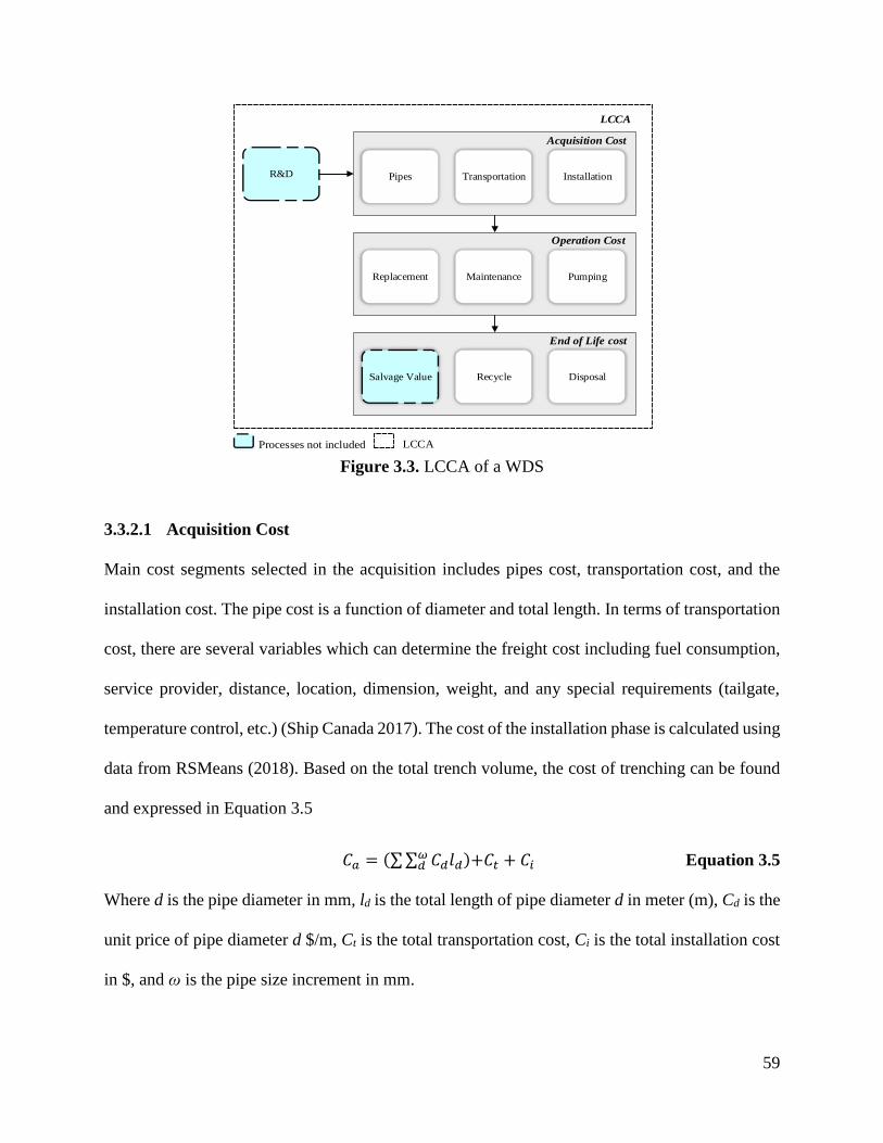
59

Figure 3.3. LCCA of a WDS

3.3.2.1 Acquisition Cost

Main cost segments selected in the acquisition includes pipes cost, transportation cost, and the

installation cost. The pipe cost is a function of diameter and total length. In terms of transportation

cost, there are several variables which can determine the freight cost including fuel consumption,

service provider, distance, location, dimension, weight, and any special requirements (tailgate,

temperature control, etc.) (Ship Canada 2017). The cost of the installation phase is calculated using

data from RSMeans (2018). Based on the total trench volume, the cost of trenching can be found

and expressed in Equation 3.5

𝐶𝑎 = (∑∑ 𝐶𝑑𝑙𝑑𝜔𝑑 )+𝐶𝑡 + 𝐶𝑖 Equation 3.5

Where d is the pipe diameter in mm, ld is the total length of pipe diameter d in meter (m), Cd is the

unit price of pipe diameter d $/m, Ct is the total transportation cost, Ci is the total installation cost

in $, and ω is the pipe size increment in mm.

R&D Pipes Transportation Installation

Acquisition Cost

Replacement Maintenance Pumping

Operation Cost

Salvage Value Recycle Disposal

End of Life cost

LCCA

Processes not included LCCA

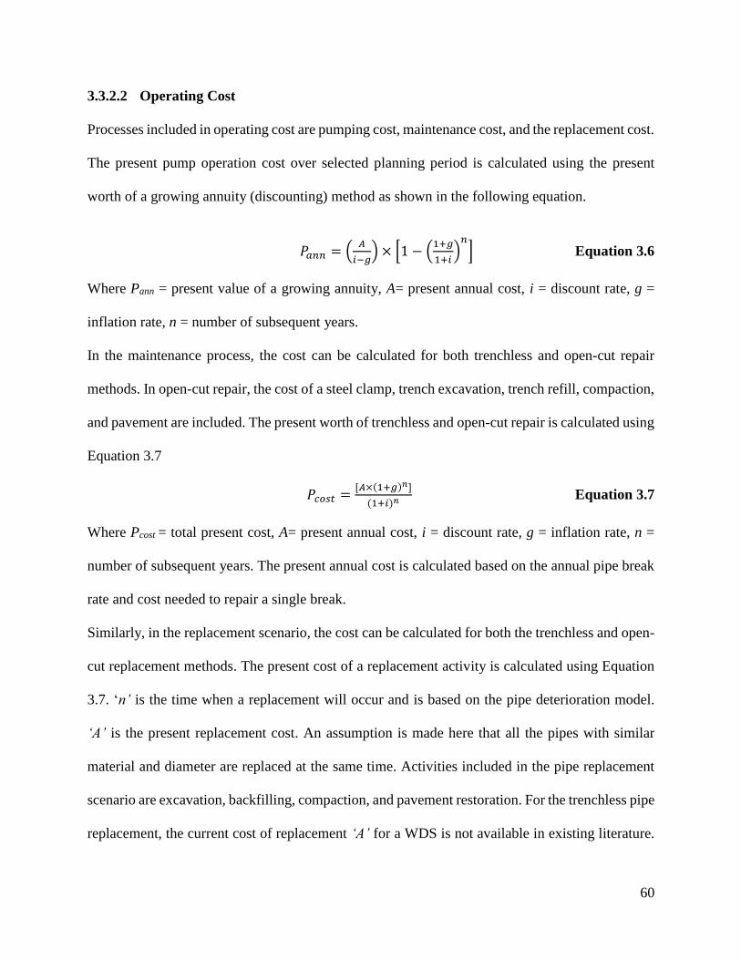
60

3.3.2.2 Operating Cost

Processes included in operating cost are pumping cost, maintenance cost, and the replacement cost.

The present pump operation cost over selected planning period is calculated using the present

worth of a growing annuity (discounting) method as shown in the following equation.

𝑃𝑎𝑛𝑛 = (𝐴

𝑖−𝑔) × [1 − (

1+𝑔

1+𝑖)𝑛

] Equation 3.6

Where Pann = present value of a growing annuity, A= present annual cost, i = discount rate, g =

inflation rate, n = number of subsequent years.

In the maintenance process, the cost can be calculated for both trenchless and open-cut repair

methods. In open-cut repair, the cost of a steel clamp, trench excavation, trench refill, compaction,

and pavement are included. The present worth of trenchless and open-cut repair is calculated using

Equation 3.7

𝑃𝑐𝑜𝑠𝑡 =[𝐴×(1+𝑔)𝑛]

(1+𝑖)𝑛 Equation 3.7

Where Pcost = total present cost, A= present annual cost, i = discount rate, g = inflation rate, n =

number of subsequent years. The present annual cost is calculated based on the annual pipe break

rate and cost needed to repair a single break.

Similarly, in the replacement scenario, the cost can be calculated for both the trenchless and open-

cut replacement methods. The present cost of a replacement activity is calculated using Equation

3.7. ‘n’ is the time when a replacement will occur and is based on the pipe deterioration model.

‘A’ is the present replacement cost. An assumption is made here that all the pipes with similar

material and diameter are replaced at the same time. Activities included in the pipe replacement

scenario are excavation, backfilling, compaction, and pavement restoration. For the trenchless pipe

replacement, the current cost of replacement ‘A’ for a WDS is not available in existing literature.

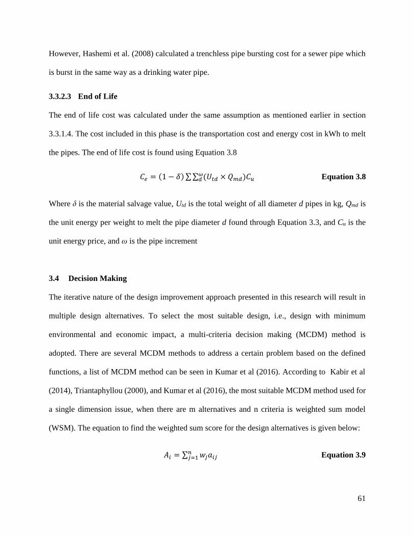
61

However, Hashemi et al. (2008) calculated a trenchless pipe bursting cost for a sewer pipe which

is burst in the same way as a drinking water pipe.

3.3.2.3 End of Life

The end of life cost was calculated under the same assumption as mentioned earlier in section

3.3.1.4. The cost included in this phase is the transportation cost and energy cost in kWh to melt

the pipes. The end of life cost is found using Equation 3.8

𝐶𝑒 = (1 − 𝛿)∑∑ (𝑈𝑡𝑑 × 𝑄𝑚𝑑)𝐶𝑢𝜔𝑑 Equation 3.8

Where δ is the material salvage value, Utd is the total weight of all diameter d pipes in kg, Qmd is

the unit energy per weight to melt the pipe diameter d found through Equation 3.3, and Cu is the

unit energy price, and ω is the pipe increment

3.4 Decision Making

The iterative nature of the design improvement approach presented in this research will result in

multiple design alternatives. To select the most suitable design, i.e., design with minimum

environmental and economic impact, a multi-criteria decision making (MCDM) method is

adopted. There are several MCDM methods to address a certain problem based on the defined

functions, a list of MCDM method can be seen in Kumar et al (2016). According to Kabir et al

(2014), Triantaphyllou (2000), and Kumar et al (2016), the most suitable MCDM method used for

a single dimension issue, when there are m alternatives and n criteria is weighted sum model

(WSM). The equation to find the weighted sum score for the design alternatives is given below:

𝐴𝑖 = ∑ 𝑤𝑗𝑎𝑖𝑗𝑛𝑗=1 Equation 3.9

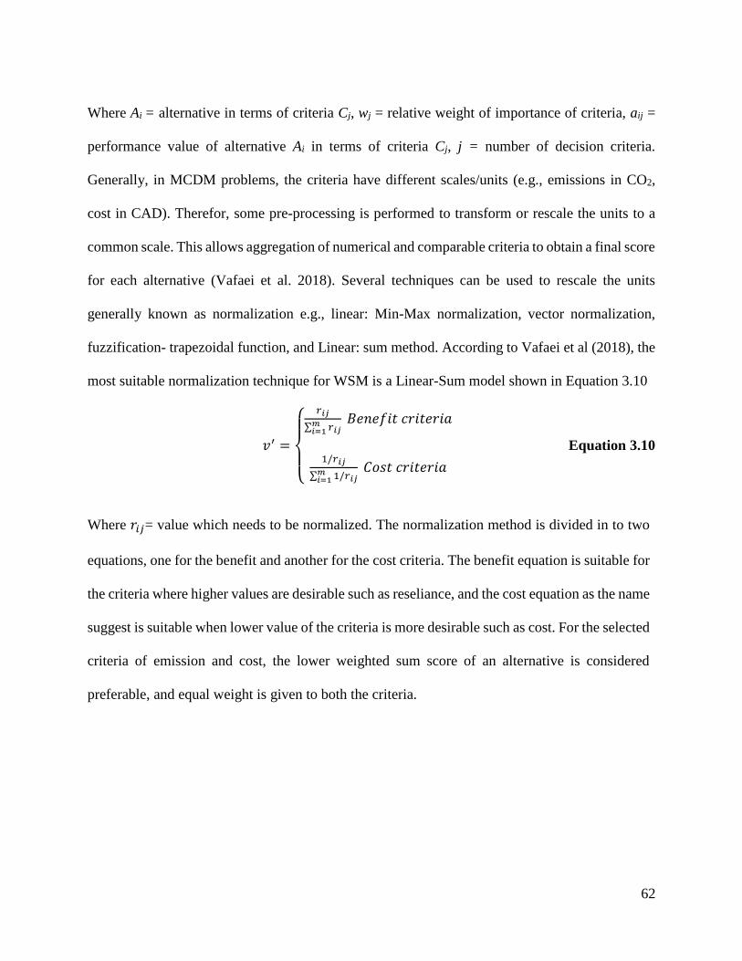
62

Where Ai = alternative in terms of criteria Cj, wj = relative weight of importance of criteria, aij =

performance value of alternative Ai in terms of criteria Cj, j = number of decision criteria.

Generally, in MCDM problems, the criteria have different scales/units (e.g., emissions in CO2,

cost in CAD). Therefor, some pre-processing is performed to transform or rescale the units to a

common scale. This allows aggregation of numerical and comparable criteria to obtain a final score

for each alternative (Vafaei et al. 2018). Several techniques can be used to rescale the units

generally known as normalization e.g., linear: Min-Max normalization, vector normalization,

fuzzification- trapezoidal function, and Linear: sum method. According to Vafaei et al (2018), the

most suitable normalization technique for WSM is a Linear-Sum model shown in Equation 3.10

𝑣′ =

{

𝑟𝑖𝑗

∑ 𝑟𝑖𝑗𝑚𝑖=1

𝐵𝑒𝑛𝑒𝑓𝑖𝑡 𝑐𝑟𝑖𝑡𝑒𝑟𝑖𝑎

1/𝑟𝑖𝑗

∑ 1/𝑟𝑖𝑗𝑚𝑖=1

𝐶𝑜𝑠𝑡 𝑐𝑟𝑖𝑡𝑒𝑟𝑖𝑎

Equation 3.10

Where 𝑟𝑖𝑗= value which needs to be normalized. The normalization method is divided in to two

equations, one for the benefit and another for the cost criteria. The benefit equation is suitable for

the criteria where higher values are desirable such as reseliance, and the cost equation as the name

suggest is suitable when lower value of the criteria is more desirable such as cost. For the selected

criteria of emission and cost, the lower weighted sum score of an alternative is considered

preferable, and equal weight is given to both the criteria.

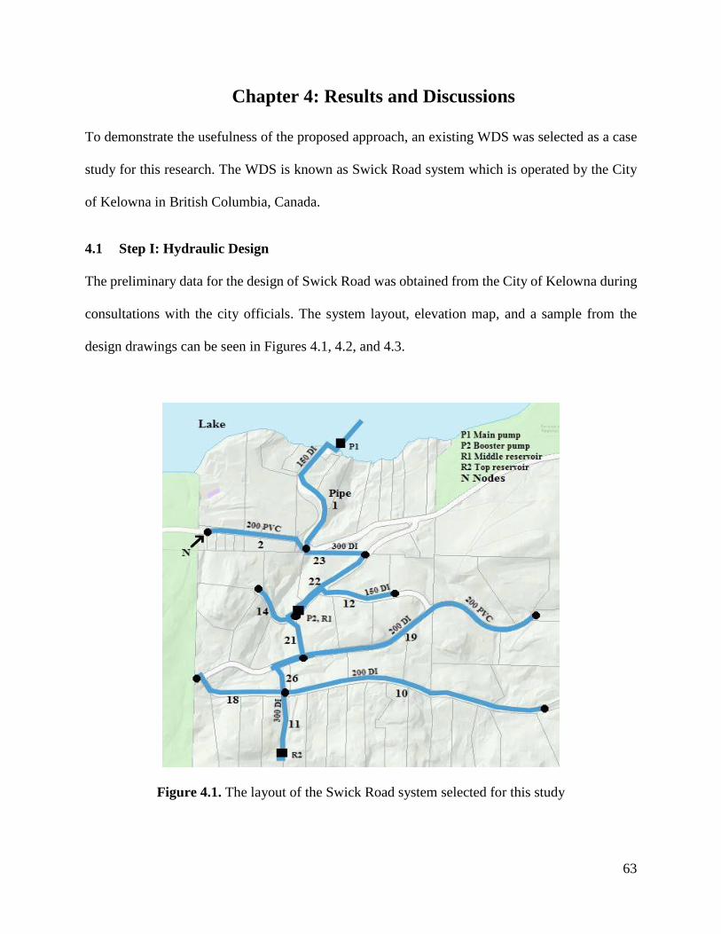
63

4 Chapter 4: Results and Discussions

To demonstrate the usefulness of the proposed approach, an existing WDS was selected as a case

study for this research. The WDS is known as Swick Road system which is operated by the City

of Kelowna in British Columbia, Canada.

4.1 Step I: Hydraulic Design

The preliminary data for the design of Swick Road was obtained from the City of Kelowna during

consultations with the city officials. The system layout, elevation map, and a sample from the

design drawings can be seen in Figures 4.1, 4.2, and 4.3.

Figure 4.1. The layout of the Swick Road system selected for this study

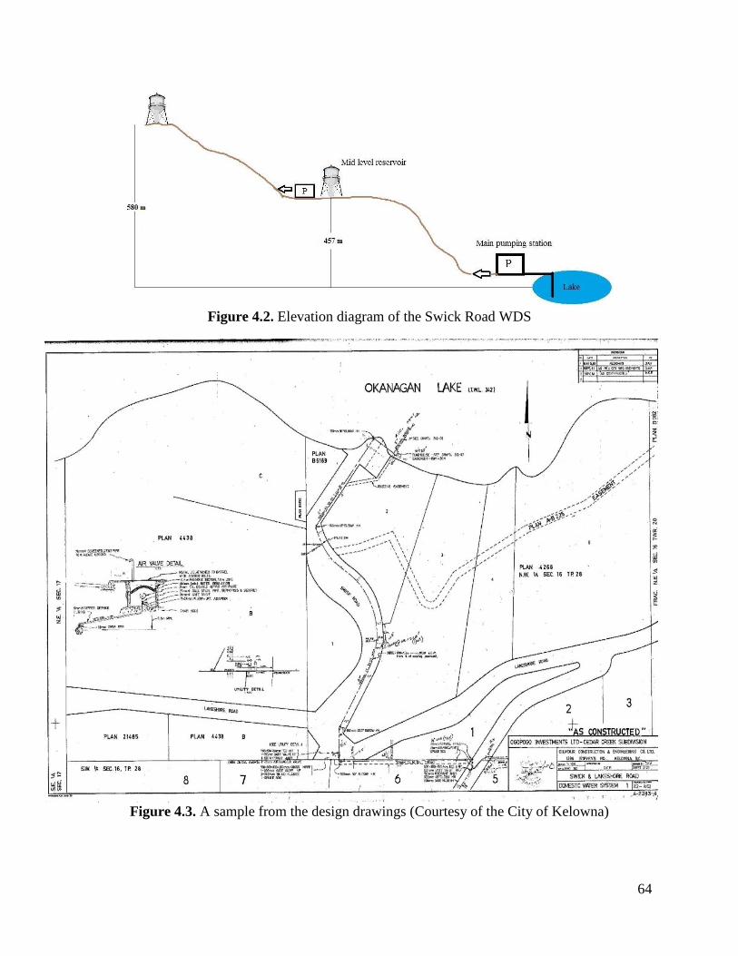
64

Figure 4.2. Elevation diagram of the Swick Road WDS

Figure 4.3. A sample from the design drawings (Courtesy of the City of Kelowna)

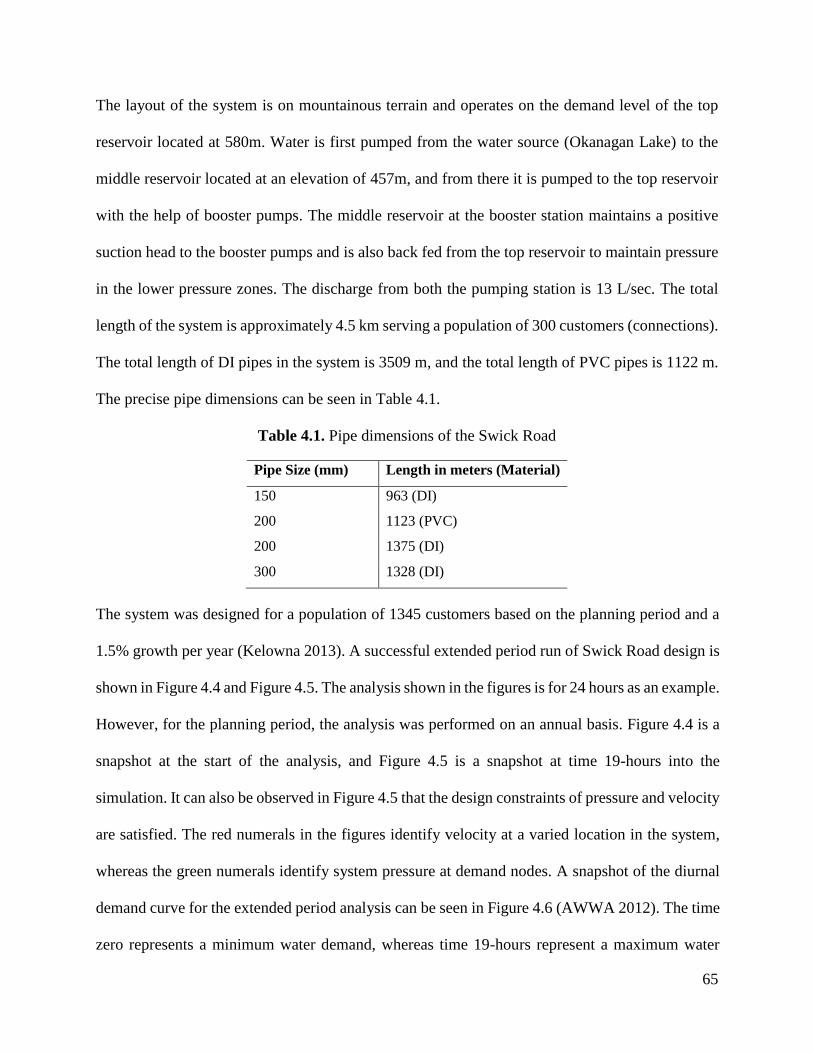
65

The layout of the system is on mountainous terrain and operates on the demand level of the top

reservoir located at 580m. Water is first pumped from the water source (Okanagan Lake) to the

middle reservoir located at an elevation of 457m, and from there it is pumped to the top reservoir

with the help of booster pumps. The middle reservoir at the booster station maintains a positive

suction head to the booster pumps and is also back fed from the top reservoir to maintain pressure

in the lower pressure zones. The discharge from both the pumping station is 13 L/sec. The total

length of the system is approximately 4.5 km serving a population of 300 customers (connections).

The total length of DI pipes in the system is 3509 m, and the total length of PVC pipes is 1122 m.

The precise pipe dimensions can be seen in Table 4.1.

Table 4.1. Pipe dimensions of the Swick Road

Pipe Size (mm) Length in meters (Material)

150 963 (DI)

200 1123 (PVC)

200 1375 (DI)

300 1328 (DI)

The system was designed for a population of 1345 customers based on the planning period and a

1.5% growth per year (Kelowna 2013). A successful extended period run of Swick Road design is

shown in Figure 4.4 and Figure 4.5. The analysis shown in the figures is for 24 hours as an example.

However, for the planning period, the analysis was performed on an annual basis. Figure 4.4 is a

snapshot at the start of the analysis, and Figure 4.5 is a snapshot at time 19-hours into the

simulation. It can also be observed in Figure 4.5 that the design constraints of pressure and velocity

are satisfied. The red numerals in the figures identify velocity at a varied location in the system,

whereas the green numerals identify system pressure at demand nodes. A snapshot of the diurnal

demand curve for the extended period analysis can be seen in Figure 4.6 (AWWA 2012). The time

zero represents a minimum water demand, whereas time 19-hours represent a maximum water

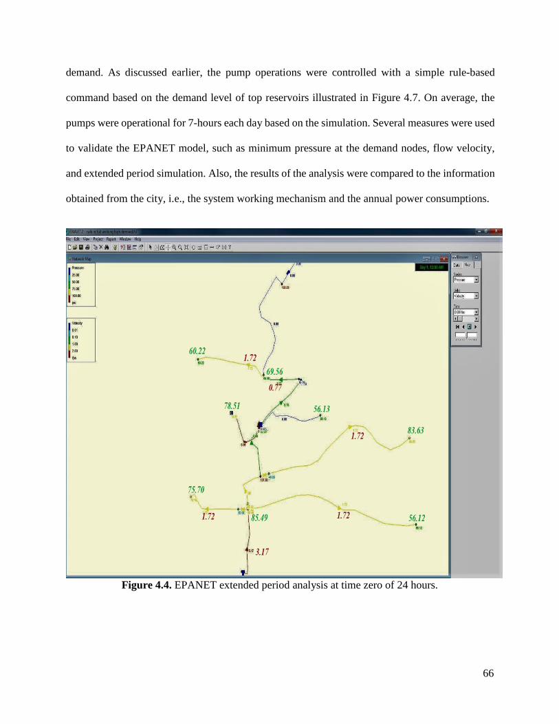
66

demand. As discussed earlier, the pump operations were controlled with a simple rule-based

command based on the demand level of top reservoirs illustrated in Figure 4.7. On average, the

pumps were operational for 7-hours each day based on the simulation. Several measures were used

to validate the EPANET model, such as minimum pressure at the demand nodes, flow velocity,

and extended period simulation. Also, the results of the analysis were compared to the information

obtained from the city, i.e., the system working mechanism and the annual power consumptions.

Figure 4.4. EPANET extended period analysis at time zero of 24 hours.

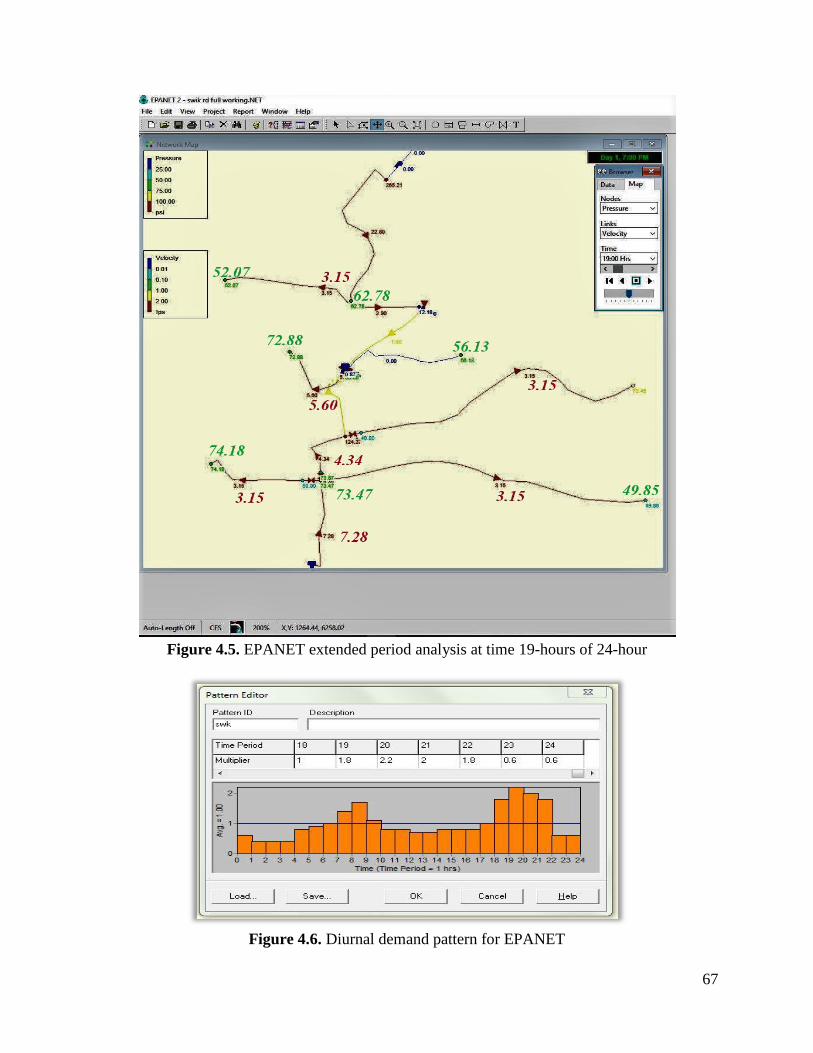
67

Figure 4.5. EPANET extended period analysis at time 19-hours of 24-hour

Figure 4.6. Diurnal demand pattern for EPANET

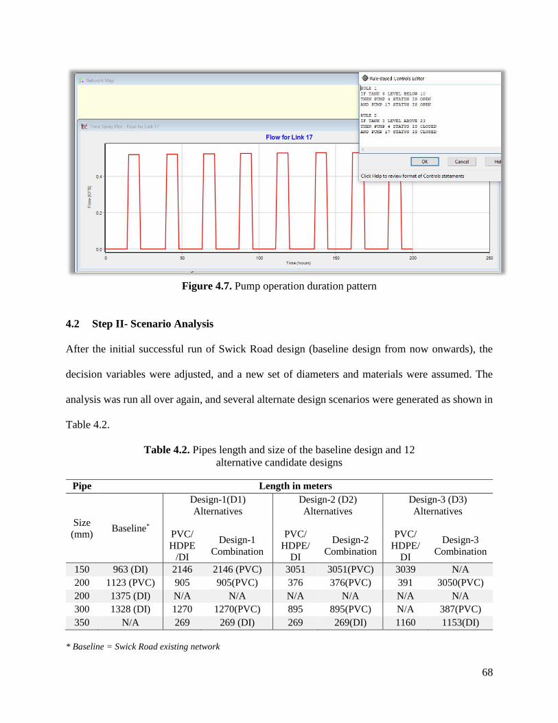
68

Figure 4.7. Pump operation duration pattern

4.2 Step II- Scenario Analysis

After the initial successful run of Swick Road design (baseline design from now onwards), the

decision variables were adjusted, and a new set of diameters and materials were assumed. The

analysis was run all over again, and several alternate design scenarios were generated as shown in

Table 4.2.

Table 4.2. Pipes length and size of the baseline design and 12

alternative candidate designs

Pipe Length in meters

Size

(mm) Baseline*

Design-1(D1)

Alternatives

Design-2 (D2)

Alternatives

Design-3 (D3)

Alternatives

PVC/

HDPE

/DI

Design-1

Combination

PVC/

HDPE/

DI

Design-2

Combination

PVC/

HDPE/

DI

Design-3

Combination

150 963 (DI) 2146 2146 (PVC) 3051 3051(PVC) 3039 N/A

200 1123 (PVC) 905 905(PVC) 376 376(PVC) 391 3050(PVC)

200 1375 (DI) N/A N/A N/A N/A N/A N/A

300 1328 (DI) 1270 1270(PVC) 895 895(PVC) N/A 387(PVC)

350 N/A 269 269 (DI) 269 269(DI) 1160 1153(DI)

* Baseline = Swick Road existing network

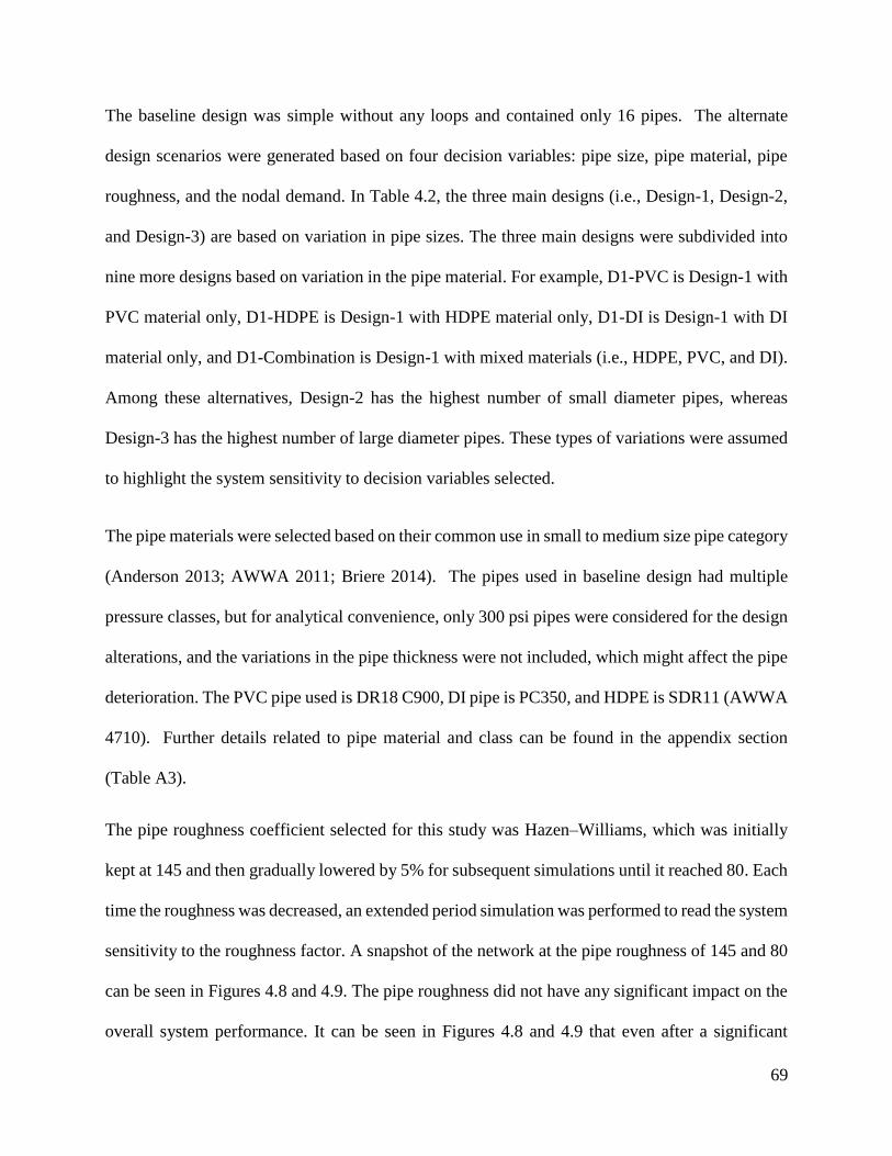
69

The baseline design was simple without any loops and contained only 16 pipes. The alternate

design scenarios were generated based on four decision variables: pipe size, pipe material, pipe

roughness, and the nodal demand. In Table 4.2, the three main designs (i.e., Design-1, Design-2,

and Design-3) are based on variation in pipe sizes. The three main designs were subdivided into

nine more designs based on variation in the pipe material. For example, D1-PVC is Design-1 with

PVC material only, D1-HDPE is Design-1 with HDPE material only, D1-DI is Design-1 with DI

material only, and D1-Combination is Design-1 with mixed materials (i.e., HDPE, PVC, and DI).

Among these alternatives, Design-2 has the highest number of small diameter pipes, whereas

Design-3 has the highest number of large diameter pipes. These types of variations were assumed

to highlight the system sensitivity to decision variables selected.

The pipe materials were selected based on their common use in small to medium size pipe category

(Anderson 2013; AWWA 2011; Briere 2014). The pipes used in baseline design had multiple

pressure classes, but for analytical convenience, only 300 psi pipes were considered for the design

alterations, and the variations in the pipe thickness were not included, which might affect the pipe

deterioration. The PVC pipe used is DR18 C900, DI pipe is PC350, and HDPE is SDR11 (AWWA

4710). Further details related to pipe material and class can be found in the appendix section

(Table A3).

The pipe roughness coefficient selected for this study was Hazen–Williams, which was initially

kept at 145 and then gradually lowered by 5% for subsequent simulations until it reached 80. Each

time the roughness was decreased, an extended period simulation was performed to read the system

sensitivity to the roughness factor. A snapshot of the network at the pipe roughness of 145 and 80

can be seen in Figures 4.8 and 4.9. The pipe roughness did not have any significant impact on the

overall system performance. It can be seen in Figures 4.8 and 4.9 that even after a significant

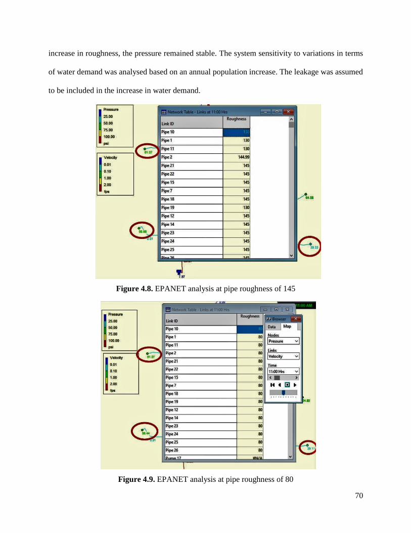
70

increase in roughness, the pressure remained stable. The system sensitivity to variations in terms

of water demand was analysed based on an annual population increase. The leakage was assumed

to be included in the increase in water demand.

Figure 4.8. EPANET analysis at pipe roughness of 145

Figure 4.9. EPANET analysis at pipe roughness of 80

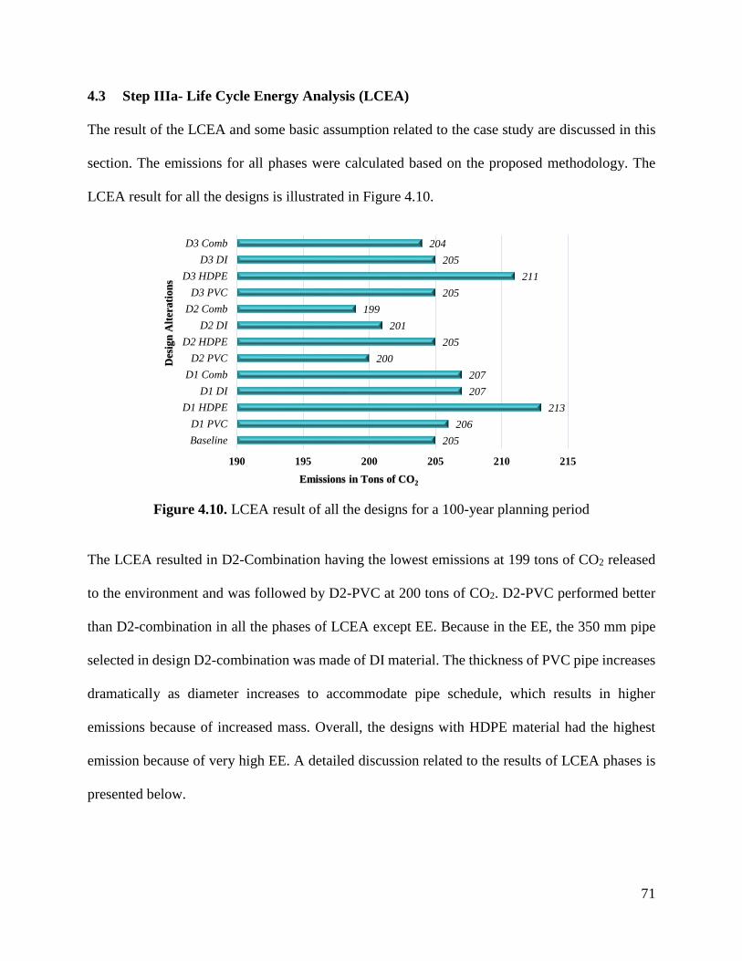
71

4.3 Step IIIa- Life Cycle Energy Analysis (LCEA)

The result of the LCEA and some basic assumption related to the case study are discussed in this

section. The emissions for all phases were calculated based on the proposed methodology. The

LCEA result for all the designs is illustrated in Figure 4.10.

Figure 4.10. LCEA result of all the designs for a 100-year planning period

The LCEA resulted in D2-Combination having the lowest emissions at 199 tons of CO2 released

to the environment and was followed by D2-PVC at 200 tons of CO2. D2-PVC performed better

than D2-combination in all the phases of LCEA except EE. Because in the EE, the 350 mm pipe

selected in design D2-combination was made of DI material. The thickness of PVC pipe increases

dramatically as diameter increases to accommodate pipe schedule, which results in higher

emissions because of increased mass. Overall, the designs with HDPE material had the highest

emission because of very high EE. A detailed discussion related to the results of LCEA phases is

presented below.

205

206

213

207

207

200

205

201

199

205

211

205

204

190 195 200 205 210 215

Baseline

D1 PVC

D1 HDPE

D1 DI

D1 Comb

D2 PVC

D2 HDPE

D2 DI

D2 Comb

D3 PVC

D3 HDPE

D3 DI

D3 Comb

Emissions in Tons of CO2

Des

ign

Alt

erati

on

s

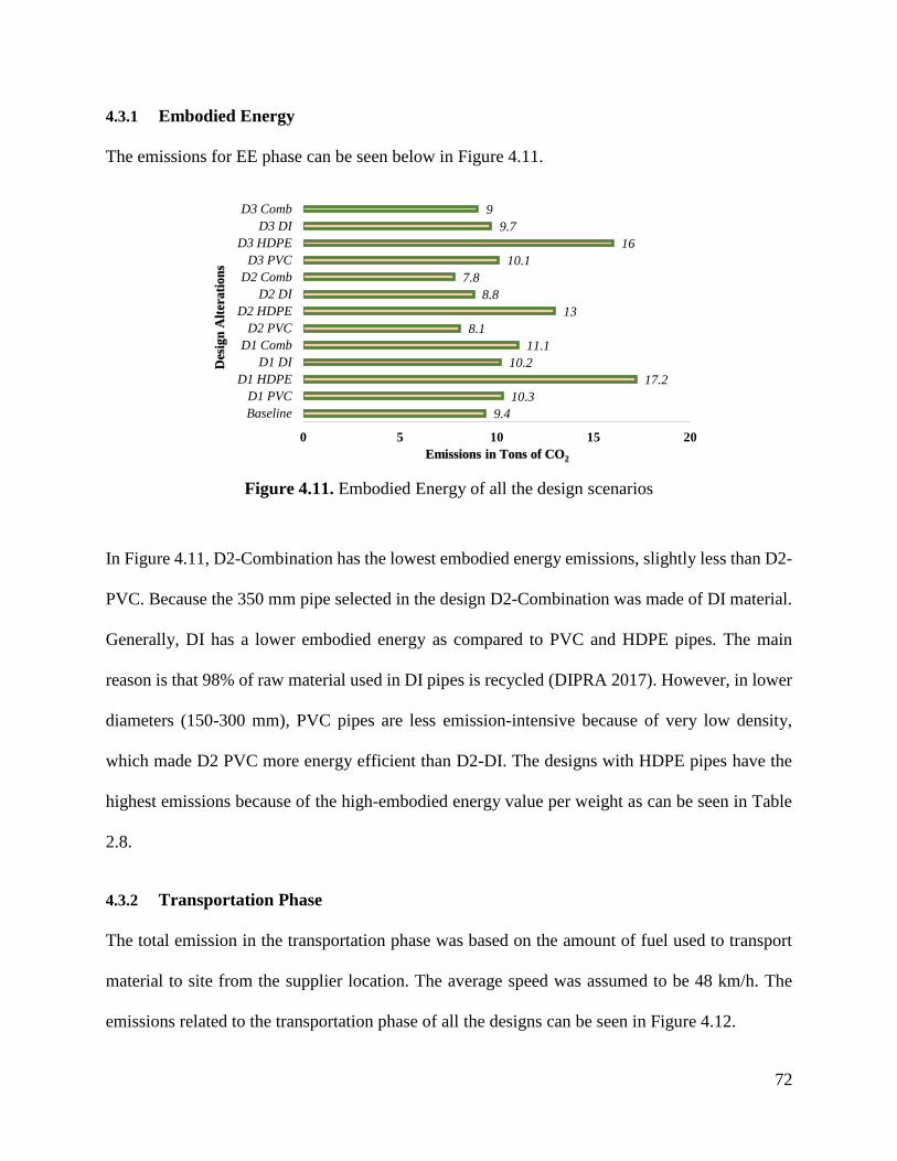
72

4.3.1 Embodied Energy

The emissions for EE phase can be seen below in Figure 4.11.

Figure 4.11. Embodied Energy of all the design scenarios

In Figure 4.11, D2-Combination has the lowest embodied energy emissions, slightly less than D2-

PVC. Because the 350 mm pipe selected in the design D2-Combination was made of DI material.

Generally, DI has a lower embodied energy as compared to PVC and HDPE pipes. The main

reason is that 98% of raw material used in DI pipes is recycled (DIPRA 2017). However, in lower

diameters (150-300 mm), PVC pipes are less emission-intensive because of very low density,

which made D2 PVC more energy efficient than D2-DI. The designs with HDPE pipes have the

highest emissions because of the high-embodied energy value per weight as can be seen in Table

2.8.

4.3.2 Transportation Phase

The total emission in the transportation phase was based on the amount of fuel used to transport

material to site from the supplier location. The average speed was assumed to be 48 km/h. The

emissions related to the transportation phase of all the designs can be seen in Figure 4.12.

9.4

10.3

17.2

10.2

11.1

8.1

13

8.8

7.8

10.1

16

9.7

9

0 5 10 15 20

Baseline

D1 PVC

D1 HDPE

D1 DI

D1 Comb

D2 PVC

D2 HDPE

D2 DI

D2 Comb

D3 PVC

D3 HDPE

D3 DI

D3 Comb


Des

ign

Alt

erati

on

s

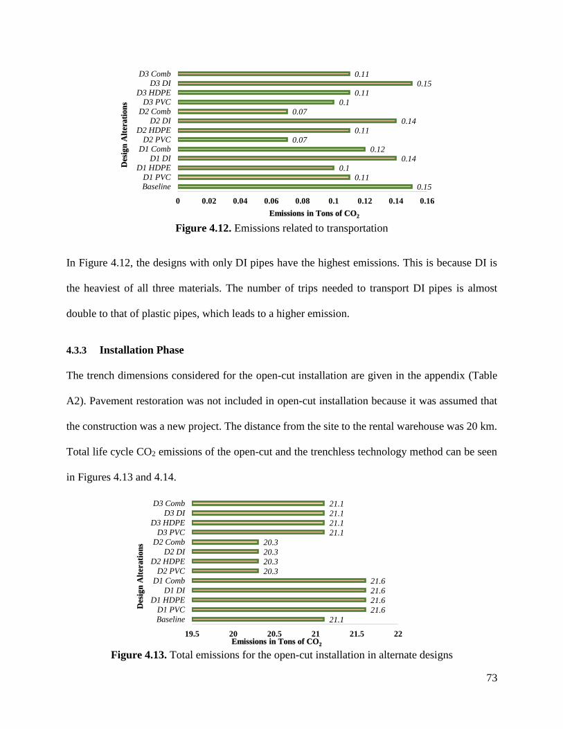
73

Figure 4.12. Emissions related to transportation

In Figure 4.12, the designs with only DI pipes have the highest emissions. This is because DI is

the heaviest of all three materials. The number of trips needed to transport DI pipes is almost

double to that of plastic pipes, which leads to a higher emission.

4.3.3 Installation Phase

The trench dimensions considered for the open-cut installation are given in the appendix (Table

A2). Pavement restoration was not included in open-cut installation because it was assumed that

the construction was a new project. The distance from the site to the rental warehouse was 20 km.

Total life cycle CO2 emissions of the open-cut and the trenchless technology method can be seen

in Figures 4.13 and 4.14.

Figure 4.13. Total emissions for the open-cut installation in alternate designs

0.150.11

0.10.14

0.120.07

0.110.14

0.070.1

0.110.15

0.11

0 0.02 0.04 0.06 0.08 0.1 0.12 0.14 0.16

BaselineD1 PVC

D1 HDPED1 DI

D1 CombD2 PVC

D2 HDPED2 DI

D2 CombD3 PVC

D3 HDPED3 DI

D3 Comb


Des

ign

Alt

erati

on

s

21.1

21.6

21.6

21.6

21.6

20.3

20.3

20.3

20.3

21.1

21.1

21.1

21.1

19.5 20 20.5 21 21.5 22

Baseline

D1 PVC

D1 HDPE

D1 DI

D1 Comb

D2 PVC

D2 HDPE

D2 DI

D2 Comb

D3 PVC

D3 HDPE

D3 DI

D3 Comb


Des

ign

Alt

erati

on

s

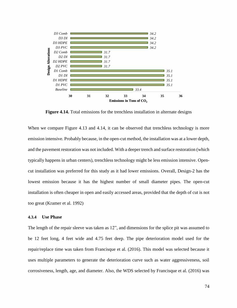
74

Figure 4.14. Total emissions for the trenchless installation in alternate designs

When we compare Figure 4.13 and 4.14, it can be observed that trenchless technology is more

emission intensive. Probably because, in the open-cut method, the installation was at a lower depth,

and the pavement restoration was not included. With a deeper trench and surface restoration (which

typically happens in urban centers), trenchless technology might be less emission intensive. Open-

cut installation was preferred for this study as it had lower emissions. Overall, Design-2 has the

lowest emission because it has the highest number of small diameter pipes. The open-cut

installation is often cheaper in open and easily accessed areas, provided that the depth of cut is not

too great (Kramer et al. 1992)

4.3.4 Use Phase

The length of the repair sleeve was taken as 12”, and dimensions for the splice pit was assumed to

be 12 feet long, 4 feet wide and 4.75 feet deep. The pipe deterioration model used for the

repair/replace time was taken from Francisque et al. (2016). This model was selected because it

uses multiple parameters to generate the deterioration curve such as water aggressiveness, soil

corrosiveness, length, age, and diameter. Also, the WDS selected by Francisque et al. (2016) was

33.4

35.1

35.1

35.1

35.1

31.7

31.7

31.7

31.7

34.2

34.2

34.2

34.2

30 31 32 33 34 35 36

Baseline

D1 PVC

D1 HDPE

D1 DI

D1 Comb

D2 PVC

D2 HDPE

D2 DI

D2 Comb

D3 PVC

D3 HDPE

D3 DI

D3 Comb


Des

ign

Alt

erati

on

s

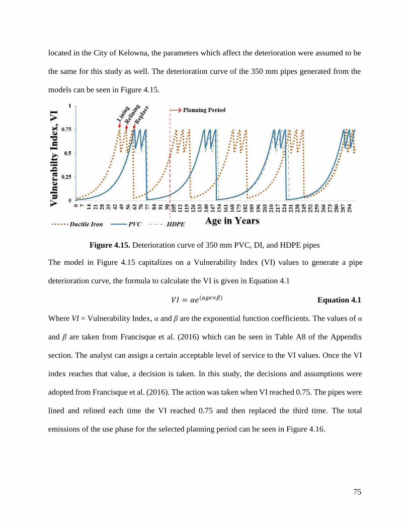
75

located in the City of Kelowna, the parameters which affect the deterioration were assumed to be

the same for this study as well. The deterioration curve of the 350 mm pipes generated from the

models can be seen in Figure 4.15.

Figure 4.15. Deterioration curve of 350 mm PVC, DI, and HDPE pipes

The model in Figure 4.15 capitalizes on a Vulnerability Index (VI) values to generate a pipe

deterioration curve, the formula to calculate the VI is given in Equation 4.1

𝑉𝐼 = 𝛼𝑒(𝑎𝑔𝑒×𝛽) Equation 4.1

Where VI = Vulnerability Index, α and β are the exponential function coefficients. The values of α

and β are taken from Francisque et al. (2016) which can be seen in Table A8 of the Appendix

section. The analyst can assign a certain acceptable level of service to the VI values. Once the VI

index reaches that value, a decision is taken. In this study, the decisions and assumptions were

adopted from Francisque et al. (2016). The action was taken when VI reached 0.75. The pipes were

lined and relined each time the VI reached 0.75 and then replaced the third time. The total

emissions of the use phase for the selected planning period can be seen in Figure 4.16.

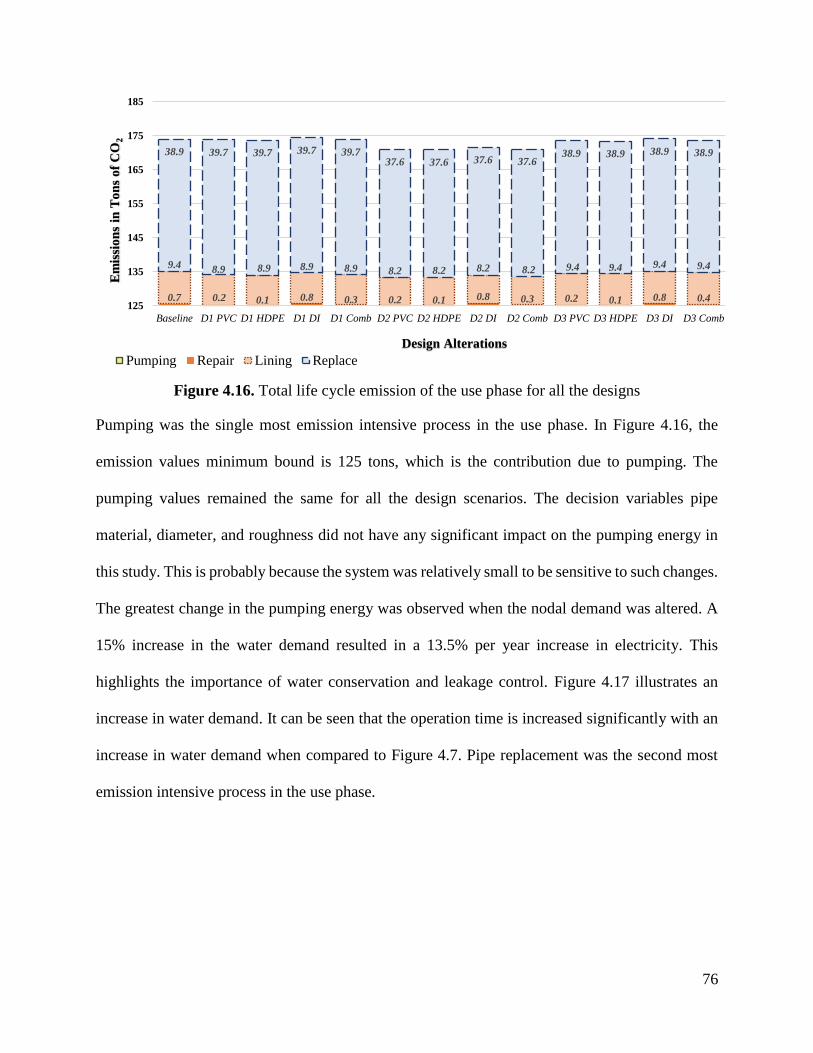
76

Figure 4.16. Total life cycle emission of the use phase for all the designs

Pumping was the single most emission intensive process in the use phase. In Figure 4.16, the

emission values minimum bound is 125 tons, which is the contribution due to pumping. The

pumping values remained the same for all the design scenarios. The decision variables pipe

material, diameter, and roughness did not have any significant impact on the pumping energy in

this study. This is probably because the system was relatively small to be sensitive to such changes.

The greatest change in the pumping energy was observed when the nodal demand was altered. A

15% increase in the water demand resulted in a 13.5% per year increase in electricity. This

highlights the importance of water conservation and leakage control. Figure 4.17 illustrates an

increase in water demand. It can be seen that the operation time is increased significantly with an

increase in water demand when compared to Figure 4.7. Pipe replacement was the second most

emission intensive process in the use phase.

0.7 0.2 0.1 0.8 0.3 0.2 0.1 0.8 0.3 0.2 0.1 0.8 0.4

9.4 8.9 8.9 8.9 8.9 8.2 8.2 8.2 8.2 9.4 9.4 9.4 9.4

38.9 39.7 39.7 39.7 39.737.6 37.6 37.6 37.6

38.9 38.9 38.9 38.9

125

135

145

155

165

175

185

Baseline D1 PVC D1 HDPE D1 DI D1 Comb D2 PVC D2 HDPE D2 DI D2 Comb D3 PVC D3 HDPE D3 DI D3 Comb

Em

issi

on

s in

To

ns

of

CO

2

Design Alterations

Pumping Repair Lining Replace

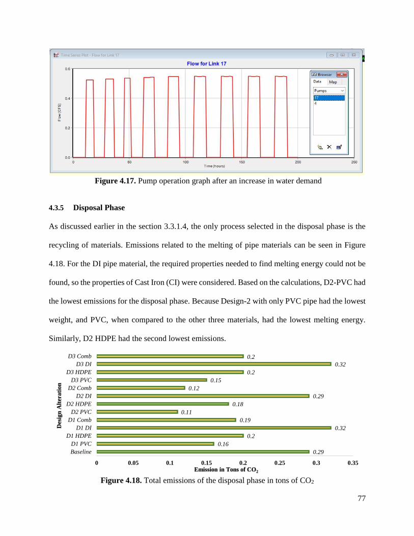
77

Figure 4.17. Pump operation graph after an increase in water demand

4.3.5 Disposal Phase

As discussed earlier in the section 3.3.1.4, the only process selected in the disposal phase is the

recycling of materials. Emissions related to the melting of pipe materials can be seen in Figure

4.18. For the DI pipe material, the required properties needed to find melting energy could not be

found, so the properties of Cast Iron (CI) were considered. Based on the calculations, D2-PVC had

the lowest emissions for the disposal phase. Because Design-2 with only PVC pipe had the lowest

weight, and PVC, when compared to the other three materials, had the lowest melting energy.

Similarly, D2 HDPE had the second lowest emissions.

Figure 4.18. Total emissions of the disposal phase in tons of CO2

0.29

0.16

0.2

0.32

0.19

0.11

0.18

0.29

0.12

0.15

0.2

0.32

0.2

0 0.05 0.1 0.15 0.2 0.25 0.3 0.35

Baseline

D1 PVC

D1 HDPE

D1 DI

D1 Comb

D2 PVC

D2 HDPE

D2 DI

D2 Comb

D3 PVC

D3 HDPE

D3 DI

D3 Comb

Emission in Tons of CO2

Des

ign

Alt

erati

on

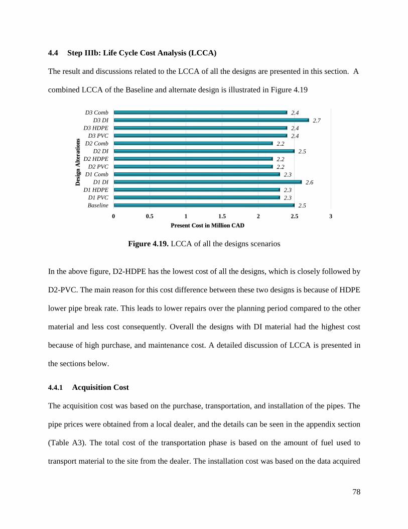
78

4.4 Step IIIb: Life Cycle Cost Analysis (LCCA)

The result and discussions related to the LCCA of all the designs are presented in this section. A

combined LCCA of the Baseline and alternate design is illustrated in Figure 4.19

Figure 4.19. LCCA of all the designs scenarios

In the above figure, D2-HDPE has the lowest cost of all the designs, which is closely followed by

D2-PVC. The main reason for this cost difference between these two designs is because of HDPE

lower pipe break rate. This leads to lower repairs over the planning period compared to the other

material and less cost consequently. Overall the designs with DI material had the highest cost

because of high purchase, and maintenance cost. A detailed discussion of LCCA is presented in

the sections below.

4.4.1 Acquisition Cost

The acquisition cost was based on the purchase, transportation, and installation of the pipes. The

pipe prices were obtained from a local dealer, and the details can be seen in the appendix section

(Table A3). The total cost of the transportation phase is based on the amount of fuel used to

transport material to the site from the dealer. The installation cost was based on the data acquired

2.5

2.3

2.3

2.6

2.3

2.2

2.2

2.5

2.2

2.4

2.4

2.7

2.4

0 0.5 1 1.5 2 2.5 3

Baseline

D1 PVC

D1 HDPE

D1 DI

D1 Comb

D2 PVC

D2 HDPE

D2 DI

D2 Comb

D3 PVC

D3 HDPE

D3 DI

D3 Comb

Present Cost in Million CAD

Des

ign

Alt

erati

on

s

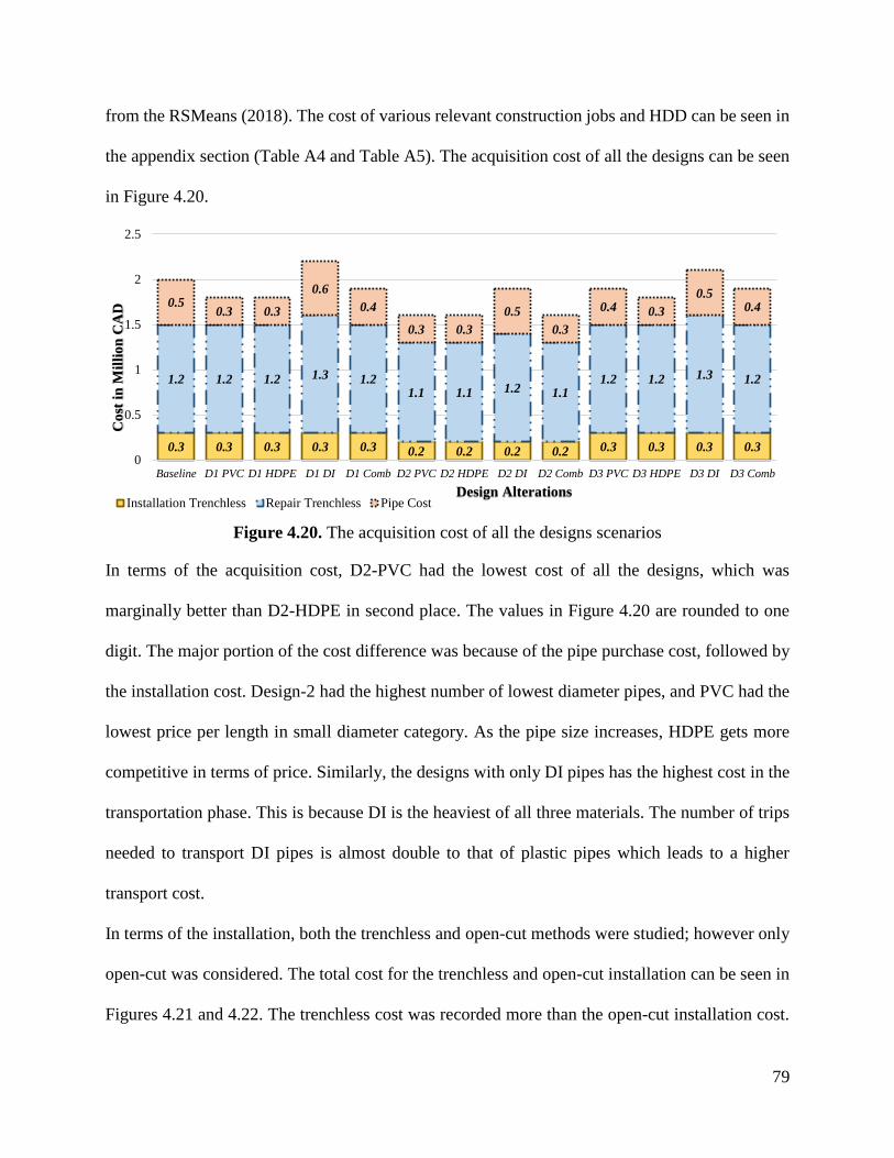
79

from the RSMeans (2018). The cost of various relevant construction jobs and HDD can be seen in

the appendix section (Table A4 and Table A5). The acquisition cost of all the designs can be seen

in Figure 4.20.

Figure 4.20. The acquisition cost of all the designs scenarios

In terms of the acquisition cost, D2-PVC had the lowest cost of all the designs, which was

marginally better than D2-HDPE in second place. The values in Figure 4.20 are rounded to one

digit. The major portion of the cost difference was because of the pipe purchase cost, followed by

the installation cost. Design-2 had the highest number of lowest diameter pipes, and PVC had the

lowest price per length in small diameter category. As the pipe size increases, HDPE gets more

competitive in terms of price. Similarly, the designs with only DI pipes has the highest cost in the

transportation phase. This is because DI is the heaviest of all three materials. The number of trips

needed to transport DI pipes is almost double to that of plastic pipes which leads to a higher

transport cost.

In terms of the installation, both the trenchless and open-cut methods were studied; however only

open-cut was considered. The total cost for the trenchless and open-cut installation can be seen in

Figures 4.21 and 4.22. The trenchless cost was recorded more than the open-cut installation cost.

0.3 0.3 0.3 0.3 0.3 0.2 0.2 0.2 0.2 0.3 0.3 0.3 0.3

1.2 1.2 1.2 1.3 1.21.1 1.1 1.2 1.1

1.2 1.2 1.3 1.2

0.50.3 0.3

0.6

0.4

0.3 0.3

0.5

0.3

0.4 0.3

0.50.4

0

0.5

1

1.5

2

2.5


Co

st i

n M

illi

on

CA

D

Design AlterationsInstallation Trenchless Repair Trenchless Pipe Cost

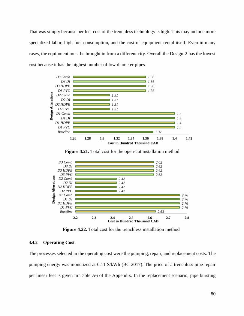
80

That was simply because per feet cost of the trenchless technology is high. This may include more

specialized labor, high fuel consumption, and the cost of equipment rental itself. Even in many

cases, the equipment must be brought in from a different city. Overall the Design-2 has the lowest

cost because it has the highest number of low diameter pipes.

Figure 4.21. Total cost for the open-cut installation method

Figure 4.22. Total cost for the trenchless installation method

4.4.2 Operating Cost

The processes selected in the operating cost were the pumping, repair, and replacement costs. The

pumping energy was monetized at 0.11 $/kWh (BC 2017). The price of a trenchless pipe repair

per linear feet is given in Table A6 of the Appendix. In the replacement scenario, pipe bursting

1.37

1.4

1.4

1.4

1.4

1.31

1.31

1.31

1.31

1.36

1.36

1.36

1.36

1.26 1.28 1.3 1.32 1.34 1.36 1.38 1.4 1.42

Baseline

D1 PVC

D1 HDPE

D1 DI

D1 Comb

D2 PVC

D2 HDPE

D2 DI

D2 Comb

D3 PVC

D3 HDPE

D3 DI

D3 Comb

Cost in Hundred Thousand CAD

Des

ign

Alt

erati

on

s

2.63

2.76

2.76

2.76

2.76

2.42

2.42

2.42

2.42

2.62

2.62

2.62

2.62

2.2 2.3 2.4 2.5 2.6 2.7 2.8

Baseline

D1 PVC

D1 HDPE

D1 DI

D1 Comb

D2 PVC

D2 HDPE

D2 DI

D2 Comb

D3 PVC

D3 HDPE

D3 DI

D3 Comb

Cost in Hundred Thousand CAD

Des

ign

Alt

erati

on

s

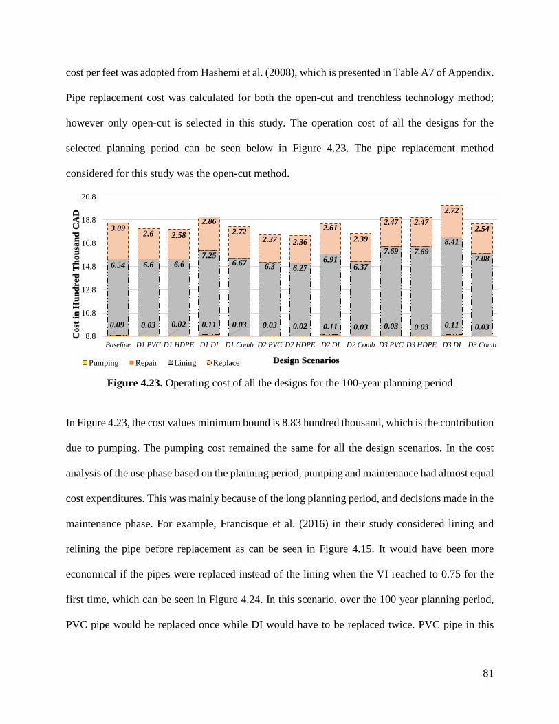
81

cost per feet was adopted from Hashemi et al. (2008), which is presented in Table A7 of Appendix.

Pipe replacement cost was calculated for both the open-cut and trenchless technology method;

however only open-cut is selected in this study. The operation cost of all the designs for the

selected planning period can be seen below in Figure 4.23. The pipe replacement method

considered for this study was the open-cut method.

Figure 4.23. Operating cost of all the designs for the 100-year planning period

In Figure 4.23, the cost values minimum bound is 8.83 hundred thousand, which is the contribution

due to pumping. The pumping cost remained the same for all the design scenarios. In the cost

analysis of the use phase based on the planning period, pumping and maintenance had almost equal

cost expenditures. This was mainly because of the long planning period, and decisions made in the

maintenance phase. For example, Francisque et al. (2016) in their study considered lining and

relining the pipe before replacement as can be seen in Figure 4.15. It would have been more

economical if the pipes were replaced instead of the lining when the VI reached to 0.75 for the

first time, which can be seen in Figure 4.24. In this scenario, over the 100 year planning period,

PVC pipe would be replaced once while DI would have to be replaced twice. PVC pipe in this

0.09 0.03 0.02 0.11 0.03 0.03 0.02 0.11 0.03 0.03 0.03 0.11 0.03

6.54 6.6 6.67.25

6.67 6.3 6.276.91

6.37

7.69 7.69

8.41

7.08

3.092.6 2.58

2.86

2.722.37 2.36

2.61

2.39

2.47 2.47

2.72

2.54

8.8

10.8

12.8

14.8

16.8

18.8

20.8


Co

st i

n H

un

dred

Th

ou

san

d C

AD

Design ScenariosPumping Repair Lining Replace

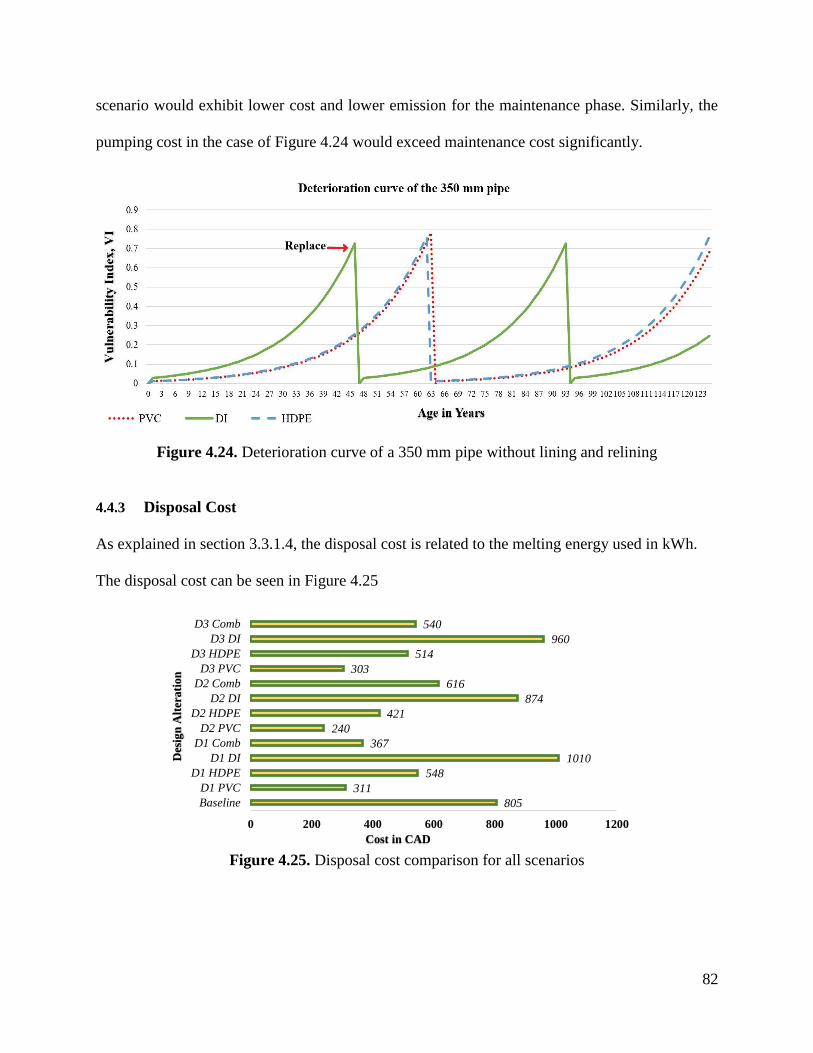
82

scenario would exhibit lower cost and lower emission for the maintenance phase. Similarly, the

pumping cost in the case of Figure 4.24 would exceed maintenance cost significantly.

Figure 4.24. Deterioration curve of a 350 mm pipe without lining and relining

4.4.3 Disposal Cost

As explained in section 3.3.1.4, the disposal cost is related to the melting energy used in kWh.

The disposal cost can be seen in Figure 4.25

Figure 4.25. Disposal cost comparison for all scenarios

805

311

548

1010

367

240

421

874

616

303

514

960

540

0 200 400 600 800 1000 1200

Baseline

D1 PVC

D1 HDPE

D1 DI

D1 Comb

D2 PVC

D2 HDPE

D2 DI

D2 Comb

D3 PVC

D3 HDPE

D3 DI

D3 Comb

Cost in CAD

Des

ign

Alt

erati

on

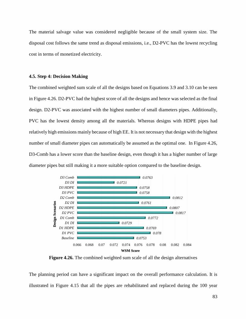
83

The material salvage value was considered negligible because of the small system size. The

disposal cost follows the same trend as disposal emissions, i.e., D2-PVC has the lowest recycling

cost in terms of monetized electricity.

4.5. Step 4: Decision Making

The combined weighted sum scale of all the designs based on Equations 3.9 and 3.10 can be seen

in Figure 4.26. D2-PVC had the highest score of all the designs and hence was selected as the final

design. D2-PVC was associated with the highest number of small diameters pipes. Additionally,

PVC has the lowest density among all the materials. Whereas designs with HDPE pipes had

relatively high emissions mainly because of high EE. It is not necessary that design with the highest

number of small diameter pipes can automatically be assumed as the optimal one. In Figure 4.26,

D3-Comb has a lower score than the baseline design, even though it has a higher number of large

diameter pipes but still making it a more suitable option compared to the baseline design.

Figure 4.26. The combined weighted sum scale of all the design alternatives

The planning period can have a significant impact on the overall performance calculation. It is

illustrated in Figure 4.15 that all the pipes are rehabilitated and replaced during the 100 year

0.0753

0.078

0.0769

0.0729

0.0772

0.0817

0.0807

0.0761

0.0812

0.0758

0.0758

0.0721

0.0763

0.066 0.068 0.07 0.072 0.074 0.076 0.078 0.08 0.082 0.084

Baseline

D1 PVC

D1 HDPE

D1 DI

D1 Comb

D2 PVC

D2 HDPE

D2 DI

D2 Comb

D3 PVC

D3 HDPE

D3 DI

D3 Comb

WSM Score

Des

ign

Sce

nari

os

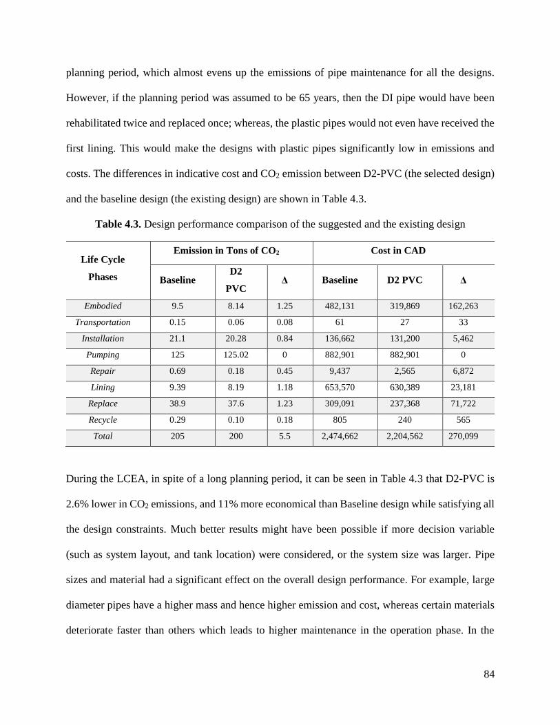
84

planning period, which almost evens up the emissions of pipe maintenance for all the designs.

However, if the planning period was assumed to be 65 years, then the DI pipe would have been

rehabilitated twice and replaced once; whereas, the plastic pipes would not even have received the

first lining. This would make the designs with plastic pipes significantly low in emissions and

costs. The differences in indicative cost and CO2 emission between D2-PVC (the selected design)

and the baseline design (the existing design) are shown in Table 4.3.

Table 4.3. Design performance comparison of the suggested and the existing design

Life Cycle

Phases

Emission in Tons of CO2 Cost in CAD

Baseline D2

PVC Δ Baseline D2 PVC Δ

Embodied 9.5 8.14 1.25 482,131 319,869 162,263

Transportation 0.15 0.06 0.08 61 27 33

Installation 21.1 20.28 0.84 136,662 131,200 5,462

Pumping 125 125.02 0 882,901 882,901 0

Repair 0.69 0.18 0.45 9,437 2,565 6,872

Lining 9.39 8.19 1.18 653,570 630,389 23,181

Replace 38.9 37.6 1.23 309,091 237,368 71,722

Recycle 0.29 0.10 0.18 805 240 565

Total 205 200 5.5 2,474,662 2,204,562 270,099

During the LCEA, in spite of a long planning period, it can be seen in Table 4.3 that D2-PVC is

2.6% lower in CO2 emissions, and 11% more economical than Baseline design while satisfying all

the design constraints. Much better results might have been possible if more decision variable

(such as system layout, and tank location) were considered, or the system size was larger. Pipe

sizes and material had a significant effect on the overall design performance. For example, large

diameter pipes have a higher mass and hence higher emission and cost, whereas certain materials

deteriorate faster than others which leads to higher maintenance in the operation phase. In the

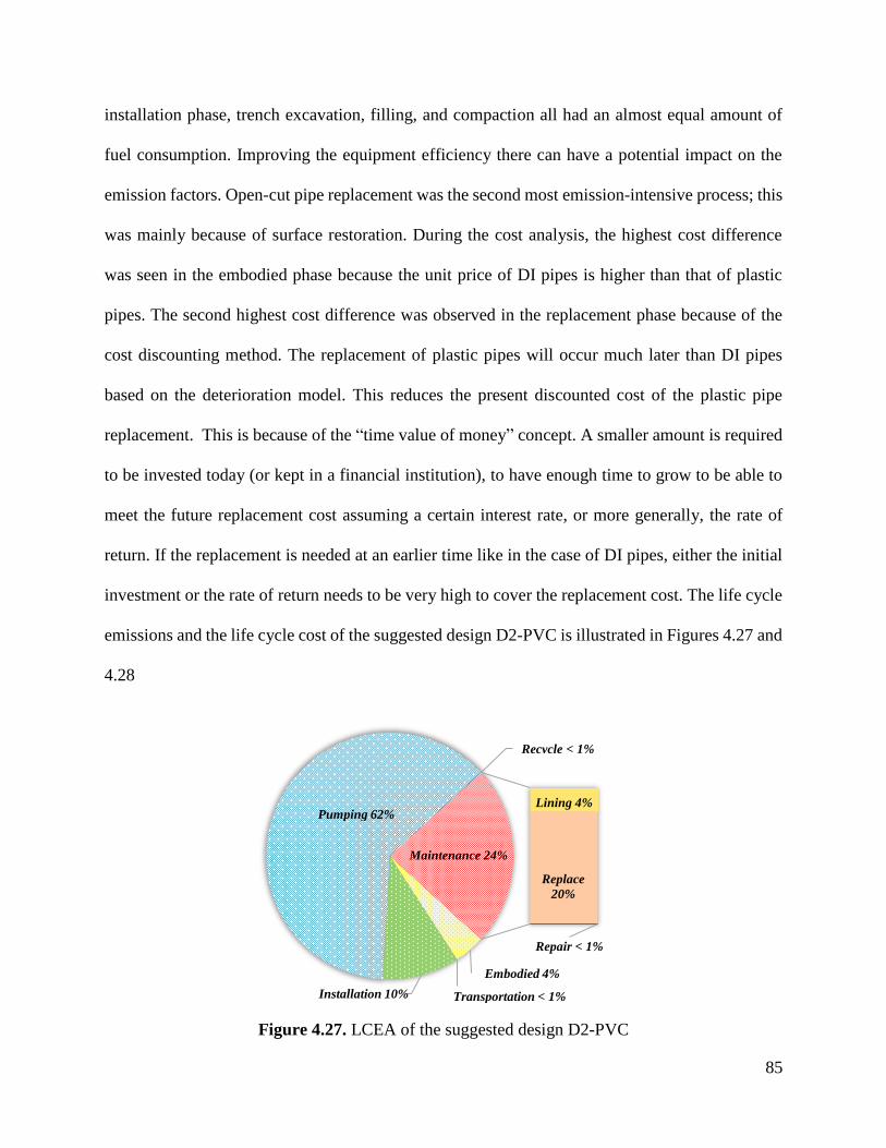
85

installation phase, trench excavation, filling, and compaction all had an almost equal amount of

fuel consumption. Improving the equipment efficiency there can have a potential impact on the

emission factors. Open-cut pipe replacement was the second most emission-intensive process; this

was mainly because of surface restoration. During the cost analysis, the highest cost difference

was seen in the embodied phase because the unit price of DI pipes is higher than that of plastic

pipes. The second highest cost difference was observed in the replacement phase because of the

cost discounting method. The replacement of plastic pipes will occur much later than DI pipes

based on the deterioration model. This reduces the present discounted cost of the plastic pipe

replacement. This is because of the “time value of money” concept. A smaller amount is required

to be invested today (or kept in a financial institution), to have enough time to grow to be able to

meet the future replacement cost assuming a certain interest rate, or more generally, the rate of

return. If the replacement is needed at an earlier time like in the case of DI pipes, either the initial

investment or the rate of return needs to be very high to cover the replacement cost. The life cycle

emissions and the life cycle cost of the suggested design D2-PVC is illustrated in Figures 4.27 and

4.28

Figure 4.27. LCEA of the suggested design D2-PVC

Embodied 4%

Transportation < 1%Installation 10%

Pumping 62%

Recycle < 1%

Lining 4%

Replace

20%

Repair < 1%

Maintenance 24%

https://en.wikipedia.org/wiki/Interest_rate

https://en.wikipedia.org/wiki/Rate_of_return

https://en.wikipedia.org/wiki/Rate_of_return

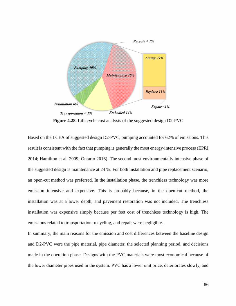
86

Figure 4.28. Life cycle cost analysis of the suggested design D2-PVC

Based on the LCEA of suggested design D2-PVC, pumping accounted for 62% of emissions. This

result is consistent with the fact that pumping is generally the most energy-intensive process (EPRI

2014; Hamilton et al. 2009; Ontario 2016). The second most environmentally intensive phase of

the suggested design is maintenance at 24 %. For both installation and pipe replacement scenario,

an open-cut method was preferred. In the installation phase, the trenchless technology was more

emission intensive and expensive. This is probably because, in the open-cut method, the

installation was at a lower depth, and pavement restoration was not included. The trenchless

installation was expensive simply because per feet cost of trenchless technology is high. The

emissions related to transportation, recycling, and repair were negligible.

In summary, the main reasons for the emission and cost differences between the baseline design

and D2-PVC were the pipe material, pipe diameter, the selected planning period, and decisions

made in the operation phase. Designs with the PVC materials were most economical because of

the lower diameter pipes used in the system. PVC has a lower unit price, deteriorates slowly, and

Embodied 14%Transportation < 1%

Installation 6%

Pumping 40%

Recycle < 1%

Lining 29%

Replace 11%

Repair <1%

Maintenance 40%

87

has a lower pipe break rate, which can affect greatly on the overall system cost. Small diameter

pipes can significantly reduce the embodied emissions and costs because of the lower mass;

however, a pressure drop might be experienced during the operation phase due to increased

friction. The existing system is relatively small with low water demands, so using lower diameter

pipes should not have any significant effect on the residual pressure. The cost and emissions related

to transportation, recycling, and repair were negligible. The labor cost is not included in the LCCA

of WDS, which can be up to 45% of the total operation cost (Hamilton et al. 2009).

It is important to note that these results are based on specific pipes investigated by Francisque et

al. (2016), the assumptions, and the case study. Several other factors can change the outcome of

this case study such as the system type and size, scoping of the LCEA, and methodology used;

which can be further investigated.

88

5 Chapter 5: Conclusions and Recommendations

5.1. Summary and Conclusions

It is very important for 21st-century infrastructure designs to achieve minimum cost, energy

efficiency, and environmental performance. Considering environmental objectives in the design

process of a WDS can provide plenty of opportunity for sustainability improvement. An approach

was proposed in this thesis to improve the environmental performance of a WDS by incorporating

life cycle thinking (LCT) approach in the initial design process. The decisions are made based on

a holistic approach where the performance is analyzed considering all the phases of a WDS, from

the initial design phase through the manufacturing, installation, operation, maintenance, and to the

end of service life. To verify the usefulness of the suggested approach, the methodology was

applied to an existing WDS. Several alternate design scenarios were generated and compared to

the existing one. The final design suggested was more economical and less emission intensive than

the existing one.

The Canadian population is steadily increasing. New water infrastructure is needed as well as

existing capacity needs to be enhanced to accommodate the increasing potable water demands.

With environmental awareness and use of modern tools, sustainability can easily become part and

parcel of every WDS design process along with the technical objectives. Environmental

performance is generally considered as an indirect cost during the design process, which must be

paid eventually by the public. Including environmental performance in the design process can bring

benefits to all the parties involved. The approach presented in this thesis is intended to be used by

engineers working in the area. Eventually, the purpose of this research is to offer practical advice

that can readily be adopted by engineering designers. This will allow consideration of

environmental criteria in design process find suitable grounds in the water supply industry.

89

5.2. Contribution

This research highlights the importance of including environmental performance in the initial

design of a WDS. A different approach was proposed to incorporate sustainaility by including life

cycle thinking (LCT) process in the conventional WDS design. With the inclusion of LCT in the

tradition design process, long-term effectiveness and efficiency in terms of management can be

improved.

5.2. Limitations and Recommendations

The main limitations and related recommendations are provided below:

• A formal optimization model was not used for the scenario analysis in the case study. The

alternate designs were generated by arbitrarily assuming pipe sizes and materials, which

might not be the optimal solution. In future experiments, an optimization sub routine will

be included in the second step of this approach.

• A sensitivity analysis could not be performed for the decision variables selected in the case

study. In future research, more decision variables will be included, and a formal sensitivity

analysis technique will be adopted for an increased understanding of the relationships

between input and output variables.

• The sensitivity of the project to the changing discount rate was not analyzed. Since social

projects last for many years and the discount rates will most likely change over that time.

• During the cradle-to-cradle LCEA and LCCA, several important processes including

transportation from the manufacturer to the dealer, pipe recovery, and sociological aspects

were not included due to lack of data availability.

90

6 References

A&B. (2017). “Plate Tamper, Rev. 1000 Lbs.”

https://www.abtoolrentals.com/equipment.asp?action=category&category=35&key=035-

0060

Airman. (2017). “Airman PDS100S Portable Air Compressor brochure.”

https://catalog.compressedairsystems.com/item/all-categories/airman-portable-air-

compressors/airman-pds100s-portable-air-compressor

Alperovits, E., and Shamir, U. (1977). “Design of Optimal Water Distribution Systems.” Water

Resources Research, 13(6).

Anderson, R. F. (2013). "The United States Conference of Mayors: Municipal Procurement,

Procurement Process Improvements Yield Cost-Effective Public Benefits."

Ariaratnam, S. T., and Sihabuddin, S. S. (2009). “Comprison of Emitted Emissions Between

Trenchless Pipe Replacement and Open-cut Utility Construction.” Journal of Green

Building, (775), 126–140.

Ashworth, A. (2014). “How life cycle costing could have improved existing costing.” Lice Cycle

Costing for Construction.

ASTM. (2018). "Standard Test Method for Density of Plastics by the Density-Gradient

Technique - D1505." American Society for Testing and Material.

AWWA. (2011). "Buried No Longer: Confronting America’s water infrastructure challenge."

American Water Works Association.

AWWA. (2012). "Computer Modeling of Water Distribution Systems - Manual of Water Supply

Practices, M32 (3rd Edition)." American Water Works Association.

AWWA. (2013). "Water Distribution Operator Training Handbook." American Water Works

Association.

Barnett, M., Lee, T., Jentgen, L., Conrad, S., Kidder, H., Woolschlager, J., Lozano, E. C., Kelly,

S., Eaton, M., Hollifield, D., and Groff, C. (2004). “Real-time Automation of Water Supply

and Distribution for the City of Jacksonville, Florida, USA.” Water Supply, 15–29.

Bayer, C., Gamble, M., Gentry, R., and Joshi, S. (2010). “Guide to Building Life Cycle

Assessment in Practice.” American Institute of Architects, 1–193.

BC. (2017). “Electricity Rates.” Fortis BC,

https://www.fortisbc.com/NaturalGas/Homes/Rates/Pages/default.aspx

BDC. (2017). “Diesel engine power to Fuel Consumption table - Naturally aspirated Engines.”

Barrington Diesel Club, https://www.barringtondieselclub.co.za/technical/fuel/diesel-fuel-

91

consumption-nat-aspirated.pdf

Belcham, A. (2015). "Manual of Enviromental Management." Routledge.

Booth, C. A., and Charlesworth, S. M. (2014). "Water Resources in the Built Environment:

Management Issues and Solutions." John Wiley & Sons.

Bosserman, B. E. (2000). “Pump System Hydraulic Design.” Water Distribution Systems

Handbook, Larry W. Mays.

Briere, F. G. (2014). "Drinking-Water Distribution, Sewage, and Rainfall Collection." Presses

Internationales Polytechnique.

Cambridge, and MIT. (2005). "Recycling of plastic."

Canada, M. (2017). “Pipe Repair.” Muellercompany, https://www.muellercompany.com/en-

ca/water-works/pipe-repair/stainless-steel-clamps/

CEC. (2017). “Variable-Frequency Drive.” California Energy Comission,

http://www.energy.ca.gov/process/water/watersupply.html

Cmplindia. (2016). “Fuel Consumption of Construction Equipment.”

http://www.cmplindia.com/Articles/fuel consumption of construction equipment.htm

Commons. (2008). “Directional drilling.” Wikimedia Commons,

https://commons.wikimedia.org/wiki/File:Bohranlage25N.jpg

Crawford, R. (2012). “Life Cycle Energy Analysis.” Environmental Design Guide, (September

2003), 1–8.

Dandy, G., Roberts, A., Hewitson, C., and Chrystie, P. (2006). “Sustainability Objectives For

The Optimization Of Water Distribution Networks.” Water Distribution Systems Analysis

Symposium 2006, ASCE, 1–11.

Dannier, A., Del Pizzo, A., Giugni, M., Fontana, N., Marini, G., and Proto, D. (2015).

“Efficiency evaluation of a micro-generation system for energy recovery in water

distribution networks.” Elsevier.

DAS, S. (2016). “Evaluation of Cured-in-Place Pipe Lining Installations.” The University of

Alberta.

Dennison, F. J., Azapagic, A., Clift, R., and Colbourne, J. S. (1999). “Life cycle assessment:

Comparing strategic options for the mains infrastructure - Part I.” Water Science and

Technology, 39(10–11), 315–319.

Deutz. (2017). “Deutz TD 2.9 Engines.” Deutz, https://www.deutz.com/en/products/engines/

Developers, G. (2018). “Google developers- Machine learning-Normalization.” Google

Developers, https://developers.google.com/machine-learning/data-

92

prep/transform/normalization

Dhillon, B. S. (2010). "Life cycle costing for engineers."

DIPRA. (2016). "Celebrate Sustainable Infrastructure." Ductile Iron Pipe Research Association,

DIPRA. (2017). “The Benefits of Ductile Iron Pipe.” Ductile Iron Pipe Research Association,

https://www.dipra.org/ductile-iron-pipe/benefits

DIS. (n.d). "Ductile iron data for design engineers." Ductile Iron Society.

Du, F., Woods, G., and Kang, D. (2013). “Life Cycle Analysis for Water and Wastewater Pipe

Materials.” Journal of Environmental Engineering, 703–711.

Ecomoder. (2017). “Aerodynamic & rolling resistance, power & MPG calculator.”

http://ecomodder.com/forum/tool-aero-rolling-resistance.php

EDF. (2017). “How cap and trade works.” Environmental Defence Fund

Emmerson, R. H. C., Morse, G. K., Lester, J. N., and Edge, D. R. (1995). “The Life Cycle

Analysis of Small Scale SewageTreatment Processes.” Water and Environment Journal,

9(3), 317–325.

Energy. (2017). “Many Factors Affect Fuel Economy.” U.S. Department of Energy,

https://www.fueleconomy.gov/feg/factors.shtml

EPA. (2005). " Impact Categories, Normalisation and Weighting in LCA." Danish Ministry of

the Environment, https://www2.mst.dk/udgiv/publications/2005/87-7614-574-3/pdf/87-

7614-575-1.pdf

EPRI. (2014). “National Assessment of Energy Use by Water Sector and Water Consumption by

all Sectors.” Electric Power and Research Institute.

EPRI. (2013). Electricity Use and Management in the Municipal Water Supply and Wastewater

Industries.

ESMAP. (2013). "A Primer on Energy Efficiency for Municipal Water and Wastewater

Utilities." Energy Sector Management Assistance Program.

Feldman, D. L. (2017). "The Water-Sustainable City."

FET, A. M. (2014). “Environmental Management Tools and Their Application – a Review With

References To Case Studies.”

Filion, Y. R., Maclean, H. L., Karney, B. W., (2004). “Life-Cycle Energy Analysis of a Water

Distribution System.” Journal of Infrastructure Systems, ASCE, 120–130.

Folkman, S. (2012). "Water Main Break rates in USA and Canada."

93

Folkman, S. (2018). "Water Main Break Rates In the USA and Canada: A Comprehensive

Study."

Francisque, A., Tesfamariam, S., Kabir, G., Haider, H., Reeder, A., and Sadiq, R. (2016). “Water

mains renewal planning framework for small to medium sized water utilities: a life cycle

cost analysis approach.” Urban Water Journal, 1–9.

Fuelly. (2017). “Ford F-450 Super Duty MPG.”

Gessler, J., and Waiski, T. M. (1985). "Water Distribution System Optimization."

GWRC, (2010). "Energy Efficiency in the Water Industry: A Compendium of Best Practices and

Case Studies - Global Report." Global Water Research Coalition.

Haider, H., Sadiq, R., and Tesfamariam, S. et al. (2014). “Performance indicators for small- and

medium-sized water supply systems: a review.” Environmental Reviews, 1–40.

Hajibabaei, M., Nazif, S., and Tavanaei Sereshgi, F. (2018). “Life cycle assessment of pipes and

piping process in drinking water distribution networks to reduce environmental impact.”

Sustainable Cities and Society, Elsevier, 538–549.

Hamilton, G., Arzbaecher, C., Partners, G. E., Ehrhard, R., and Murphy, J. (2009). “Driving

Energy Efficiency in the U . S. Water & Wastewater Industry by Focusing on Operating and

Maintenance Cost Reductions.” American Council for an Energy-Efficient Economy-

ACEEE, 30–42.

Harvey, P. D. (1982). "Engineering Properties of Steel." American Society for Metals.

Hashemi, B., Najafi, M., and Mohamed, R. (2008). “Cost of Underground Infrastructure

Renewal : A Comparison of Open-Cut and Trenchless Methods.” Pipelines Congress 2008,

ASCE, 1–11.

Herstein, L. M., and Filion, Y. R. (2011). “Life-cycle assessment of common water main

materials in water distribution networks.” Journal of Hydroinformatics, 346.

Herstein, L. M., Filion, Y. R., and Hall, K. R. (2009). “Evaluating Environmental Impact in

Water Distribution System Design.” Journal of Infrastructure Systems, 241–250.

Herstein, L. M., Filion, Y. R., and Hall, K. R. (2011). “Evaluating the Environmental Impacts of

Water Distribution Systems by Using EIO-LCA-Based Multiobjective Optimization.”

Journal of Water Resources Planning and Management, 162–172.

HUMES. (2016). "concrete pipe reference manual."

ICE. (2011). "Inventory of Carbon and Energy." Circular Ecology.

ICTF. (2016). “Union Pacific ICTF Modernization Project Conceptual Construction Equipment

Utilization.” Intermodal Container Transfer Facility, http://www.ictf-

94

jpa.org/document_library/application_development_project_approval/App B.pdf

IEA. (2016). “Water Energy Nexus.” International Energy Agency.

Inman, J. (2010). “Automation for energy and operations optimization in water distribution

systems.” Water Security Congress and Distribution Systems Symposium and Exposition

2010, 284–306.

ISO. (2006a). "ISO 14040: Environmental management- Life Cycle Assessment - Principles and

framework." International Organization for Standardization, Geneva.

ISO. (2006b). “ISO 14044- Environmental management - Life Cycle Assessment - Requirements

and guidelines.” International Organization for Standardization.

Jetmarova, M. H., Sultanova, N., and Savic, D. (2018). “Lost in Optimisation of Water

Distribution Systems? A Literature Review of System Design.” Water 2018, MDPI, 307.

Jones, S. C., and Sowby, R. B. (2014a). “Water system optimization: Aligning energy efficiency,

system performance, and water quality.” American Water Works Association, 106(6).

Jones, S. C., and Sowby, R. B. (2014b). “Quantifying Energy Use in The U.S. Public Water

Industry - A Summary.” 16(4).

JRC. (2011). "Supporting Environmentally Sound Decisions for Bio-Waste Management - A

practical guide to Life Cycle Thinking (LCT) and Life Cycle Assessment (LCA)." Joint

Research Centre European Commission.

Kabir, G., Demissie, G., Sadiq R., and Tesfamariam S. (2015). “Integrating Failure Prediction

Models for Water Mains: Bayesian Belief Network Based Data Fusion.” Knowledge-Based

Systems, 159–169.

Kabir, G., Sadiq, R., and Tesfamariam, S. (2014). “A review of multi-criteria decision-making

methods for infrastructure management.” Structure and Infrastructure Engineering, Taylor

& Francis.

Kelowna. (2013). “Official Community Plan.” The city of Kelowna.

Kimutai, E., Betrie, G., Brander, R., Sadiq, R., and Tesfamariam, S. (2015). “Comparison of

Statistical Models for Predicting Pipe Failures: Illustrative Example With the City of

Calgary Water Main Failure.” Journal of Pipeline Systems Engineering and Practice, 6(4).

Kleiner, Y., and Rajani, B. (2001). “Comprehensive Review of Structural Deterioration of Water

Mains: Statistical Models.” Urban Water, 131–150.

Klopffer, W., and Grahl, B. (2014). "Life Cycle Assessment (LCA): A Guide to Best Practice."

Kramer, S. R., McDonald, W. J., and Thomson, J. C. (1992). "An Introduction to Trenchless

Technology."

95

Lansey, K. E. (2000). “Optimal Design of Water Distribution System” Water distribution system

handbook, Mays, L. W.

Lansey, K., and Mays, L. W. (2000). “Hydraulics of Distribution system” Water Distribution

Systems Handbook, Mays, L. W.

Lehr, J., Keeley, J., and Lehr, J. (2005). "Water Encyclopedia."

Lejano, R. P. (2006). “Optimizing the Layout and Design of Branched Pipeline Water

Distribution Systems.” Irrigation and Drainage Systems, 125–137.

Lydon, T., Coughlan, P., and McNabola, A. (2017a). “Pressure Management and Energy

Recovery in Water Distribution Networks: Development of Design and Selection

Methodologies Using Three Pump-As-Turbine Case Studies.” Renewable Energy, 114,

1038–1050.

Lydon, T., Coughlan, P., and McNabola, A. (2017b). “Pump-as-Turbine: Characterization as an

Energy Recovery Device for The Water distribution Network.” Journal of Hydraulic

Engineering, 143.

Maksimovic, C., and Masry, E. N. (2008). “Potentials for Improvement of Energy Efficiency for

New Design of Water Distribution Systems.” Water Distribution Systems Analysis 2008, 1–

8.

Mamade, A., Loureiro, D., Covas, D., and Alegre, H. 1. (2014). “Energy Auditing as a Tool for

Improving Service Efficiency of Water Supply Systems.” Procedia Engineering, v 89.

Manne, J. R. (2016). "Multiobjective Optimization in Water and Environmental Systems

Management- MODE Approach."

Mantia, F. P. La. (2004). “Polymer mechanical recycling: Downcycling or upcycling?” Progress

in Rubber, Plastics and Recycling Technology, 20(1), 11–24.

Mark, A. Y. (2000). “System Design: an overview.” Water Distribution Systems Handbook,

Mays L. W.

Mays, L. W. (2000). "Water Distribution Systems Handbook." Mc Graw Hill.

Milne, G., and Reardon, C. (2013). “Australian Government: Embodied energy.”

http://www.yourhome.gov.au/materials/embodied-energy

Murty, B. S. (2007). “Water Distribution Networks-Lecture 37.” NPTEL, National Programme

on Technology Enhanced Learning, http://textofvideo.nptel.ac.in/105106119/lec37.pdf

Najafi, M. (2010). "Trenchless Technology Piping: Installation And Inspection."

NRC. (2008). "Energy Use in the Canadian Manufacturing Sector." National Research Council

of Canada.

96

NRC. (2014). “About Electricity.” National Research Council of Canada,

http://www.nrcan.gc.ca/energy/electricity-infrastructure/about-electricity/7359

Oak Ridge. (2016). "Vehicle Technologies Market Report."

Olsen, S. I., Christensen, F. M., Hauschild, M., Pedersen, F., Larsen, H. F., and Torslov, J.

(2001). “Life Cycle Impact Assessment and Risk Assessment of Chemicals - a

Methodological Comparison.” Environmental Impact Assessment Review, 21(4), 385–404.

OME. (2016). “Design Guidelines for Drinking-Water Systems.” Ontario Ministry of

Environment.

Ontario. (2016). “Every Drop Counts.” Environmental Commissioner of Ontario.

OREF. (2010). “Fact #620: April 26, 2010 Class 8 Truck Tractor Weight by Component.”

https://energy.gov/eere/vehicles/fact-620-april-26-2010-class-8-truck-tractor-weight-

component

Piratla, K. R., Ariaratnam, S. T., and Cohen, A. (2012). “Estimation of CO2 Emissions from the

Life Cycle of a Potable Water Pipeline Project.” Journal of Management, 22–30.

PRe. (2016). “Introduction to LCA with SimaPro.”

Rajani, B., and Kleiner, Y. (2014). “Alternative Strategies for Pipeline Maintenance / Renewal

NRC Publications Archive ( NPArC ).” National Research Council Canada.

Recio, J. M. B., Guerrero, P. J., María Gonçalves Ageitos, and Narváez, R. P. (2005a). “Estimate

of Energy Consumption and CO2 Emission Associated With the Production , Use and Final

Disposal of PVC , HDPE , PP , Ductile Iron and Concrete Pipes.”

Recio, J. M. B., Narváez, R. P., and Guerrero, P. J. (2005b). "Estimate of Energy Consumption

and CO2 Emission Associated With the Production, Use and Final Disposal of PVC,

Aluminium and Wooden Windows." Département de Projectes d’Engineyeria, Universitat

Politecnica de Catalunya, Environmental Modelling Lab., Barcelona, Spain.

Romac. (2017). “All Stainless Steel Repair Clamps.” Romac, http://romac.com/clamps/

RSMeans. (2018). "2018 Heavy Construction Costs Books."

S.J.Dale. (2014). “Introduction to life cycle costing.” Life Cycle Costing for Construction.

Saldarriaga, J., Takahashi, S., Hernéndez, F., Díaz, D. M., and Ochoa, S. (2010). “An Energy

Methodology for the Design of Water Distribution Systems.” Proceedings of the World

Environmental and Water Resources Congress 2010: Challenges of Change, (1984), 4303–

4313.

Sanjuan-Delmás, D., Petit-Boix, A., Gasol, C. M., Villalba, G., Suárez-Ojeda, M. E., Gabarrell,

X., Josa, A., and Rieradevall, J. (2013). “Environmental Assessment of Different Pipelines

97

for Drinking Water Transport and Distribution Network in Small to Medium Cities: A Case

from Betanzos, Spain.” Journal of Cleaner Production, Elsevier Ltd, 66, 588–598.

Savic, D. A., and Walters, G. A. (1997). “Genetic Algorithms for Least-Cost Design of Water.”

67–77.

Schlömer S., Fulton, L., Hertwich, E., McKinnon, A., Perczyk, D. J. Roy, Sims, R., Smith, P.,

and Wiser, R. (2014). "ANEX III - Technology-Specific Cost and Performance

Parameters."

Scribd. (2016). “Standard Fuel Consumption (Model)(2).” Scribd

https://www.scribd.com/doc/44059673/Standard-Fuel-Consumption-Model-2

Seattle. (1913). “Item 5092- Installing E. 80th Street pipeline, 1931.” Seattle Municipal Archives

http://archives.seattle.gov/digital-collections/index.php/Detail/objects/28788

Shamir, U. (1974). “Optimal Design and Operation of Water Distribution Systems.” Water

Resources Research, 10(1), 27–36.

Shamir, U., and Howard, C. D. (1979). “An Analytical Approach to Scheduling Pipe

Replacement.” American Water Works Association, 71(5).

Sharp, W. W., and Walski, T. M. (1988). “Predicting Internal Roughness in Water Mains.”

80(11), 34–40.

Ship Canada. (2017). “shipping rates.” https://www.shipcanada.ca/shipping-rates.php

Sihabuddin, S. S., and Ariaratnam, S. T. (2009). “Methodology for estimating emissions in

underground utility construction operations.” Journal of Engineering, Design and

Technology.

Simpson, A. R., Dandy, G. C., and Murphy, L. J. (1994). “Genetic Algorithms Compared to

Other Techniques for Pipe Optimization.” Journal of Water Resources Planning and

Management, 120(4), 423–443.

Stokes, C., Simpson, A., and Maier, H. (2012). “An Improved Framework for the Modelling and

Optimisation of Greenhouse Gas Emissions Associated with Water Distribution Systems.”

Proceedings of the International Congress on Environmental Modelling and Software:

Managing Resources of a Limited Planet, 6th Biennial Meeting, 818–825.

Supplement. (2013). “2013 Pipe Relining Guide.” Trenchless Technology Special.

Tillman, A. M., Ekvall, T., Baumann, H., and Rydbergl, T. (1994). “Choice of System

Boundaries in Life Cycle Assessment.” J. Cleaner Prod., 2(1).

Titow, W. V. (1985). “PVC Technology.” Polymer International, 17(3).

Translead, H. (2017). “Duralite Flatbed Trailer.” http://www.translead.com/trailers/flatbed-

98

trailers

Triantaphyllou, E. (2000). "Multi-Criteria Decision Making Methods: A Comparative Study."

Springer-Verlag Berlin Heidelberg.

UN. (2001). “Access to Safe Water FundamentaL Human Need, Basic Human Right, Says

Secretary-General in Message on World Water Day.” United Nations

https://www.un.org/press/en/2001/sgsm7738.doc.htm

Uni-Bell. (2017). "Life Cycle Assessment of Pvc Water and Sewer Pipe and comparative

sustainability analysis of Pipe Materials."

USEPA. (2013). “Strategies for Saving Energy at Public Water Systems.” 1–16.

USEPA. (2002). “Community Water System Survey.”

https://www.epa.gov/dwstandardsregulations/community-water-system-survey

USEPA. (2013a). “Energy Efficiency in Water and Wastewater Facilities.”

USEPA. (2013b). "Water Efficiency for Public Water System."

USEPA. (2017). "Understanding Global Warming Potentials" United States Environmental

Protection Agency, https://www.epa.gov/ghgemissions/understanding-global-warming-

potentials

Venkatesh, C. (2012). “Performance Comparison of High Density Polyethylene Pipe (HDPE) in

Municipal Water Applications.”

Venkatesh, G., and Brattebø, H. (2011). “Energy Consumption, Costs and Environmental

Impacts for Urban Water Cycle Services : Case Study of Oslo ( Norway ).” Energy, Elsevier

Ltd, 36(2), 792–800.

Victoria. (2003). "Table of Embodied Energy Coefficients." Victoria University Wellington

School of Architecture.

Walski, T. M., and Male, J. W. (2000). “Maintenance and Rehabilitation/Replacement.” Water

Distribution Systems Handbook, Mays L. W.

Walters, G. A. (1992). “A Review of Pipe Network Optimization Techniques.” Fluid Mechanics

and its Applications: Pipeline Systems.

White, F. (2011). “Fluid Mechanics.” McGraw-Hill, New York, 862.

Wilson, D., Filion, Y., and Moore, I. (2015). “State-of-the-Art Review of Water Pipe Failure

Prediction Models and Applicability to Large-Diameter Mains.” Urban Water Journal,

Taylor & Francis, 1–12.

Wolseley. (2017). “Clamps & Saddles.” http://www.wolseleywaterworks.com/clamps.html

99

WRF. (2016). "Asset Management breaks and leaks." Water Research Foundation.

Wu, W., Simpson, A. R., and Maier, H. R. (2010). “Accounting for Greenhouse Gas Emissions

in Multiobjective Genetic Algorithm Optimization of Water Distribution Systems.” 146–

155.

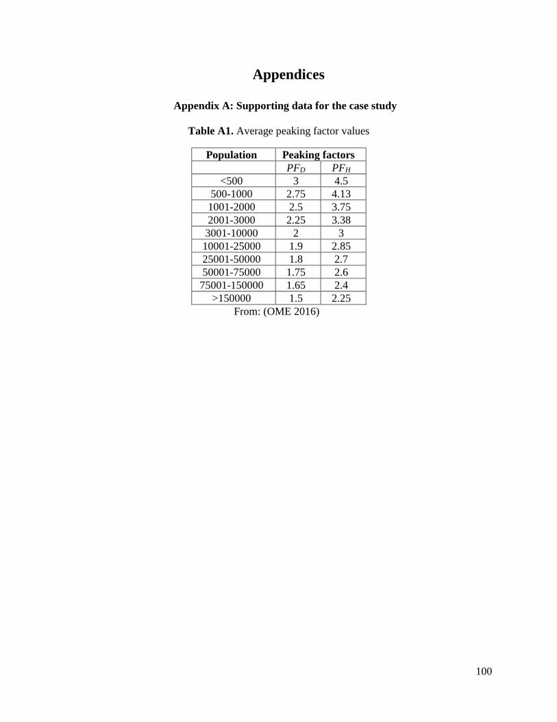
100

7 Appendices

Appendix A: Supporting data for the case study

Table A1. Average peaking factor values

Population Peaking factors

PFD PFH

<500 3 4.5

500-1000 2.75 4.13

1001-2000 2.5 3.75

2001-3000 2.25 3.38

3001-10000 2 3

10001-25000 1.9 2.85

25001-50000 1.8 2.7

50001-75000 1.75 2.6

75001-150000 1.65 2.4

>150000 1.5 2.25

From: (OME 2016)

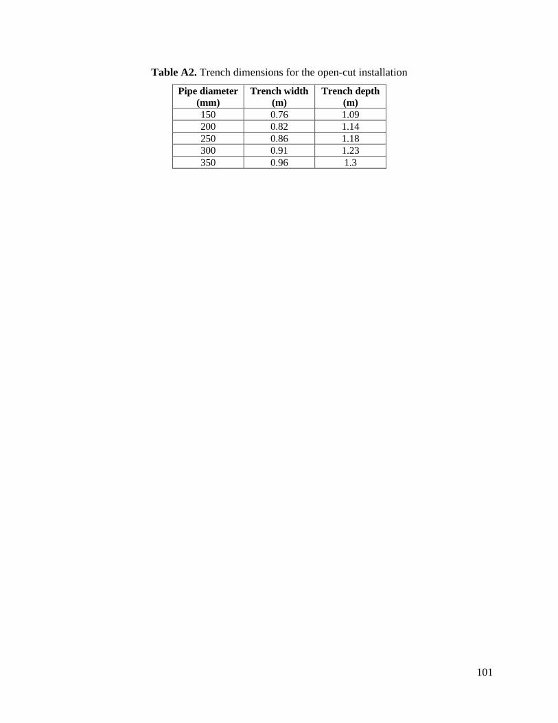
101

Table A2. Trench dimensions for the open-cut installation

Pipe diameter

(mm)

Trench width

(m)

Trench depth

(m)

150 0.76 1.09

200 0.82 1.14

250 0.86 1.18

300 0.91 1.23

350 0.96 1.3

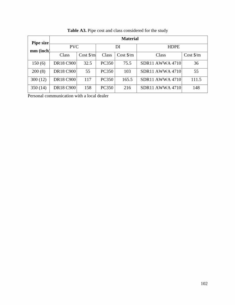
102

Table A3. Pipe cost and class considered for the study

Pipe size

mm (inch)

Material

PVC DI HDPE

Class Cost $/m Class Cost $/m Class Cost $/m

150 (6) DR18 C900 32.5 PC350 75.5 SDR11 AWWA 4710 36

200 (8) DR18 C900 55 PC350 103 SDR11 AWWA 4710 55

300 (12) DR18 C900 117 PC350 165.5 SDR11 AWWA 4710 111.5

350 (14) DR18 C900 158 PC350 216 SDR11 AWWA 4710 148

Personal communication with a local dealer

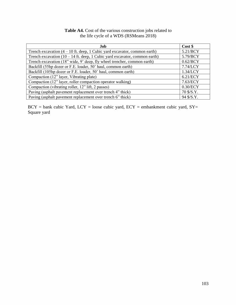
103

Table A4. Cost of the various construction jobs related to

the life cycle of a WDS (RSMeans 2018)

Job Cost $

Trench excavation (4 – 10 ft. deep, 1 Cubic yard excavator, common earth) 5.21/BCY

Trench excavation (10 – 14 ft. deep, 1 Cubic yard excavator, common earth) 5.79/BCY

Trench excavation (18” wide, 9’ deep, fly wheel trencher, common earth) 0.62/BCY

Backfill (55hp dozer or F.E. loader, 50’ haul, common earth) 7.74/LCY

Backfill (105hp dozer or F.E. loader, 50’ haul, common earth) 1.34/LCY

Compaction (12” layer, Vibrating plate) 6.21/ECY

Compaction (12” layer, roller compaction operator walking) 7.63/ECY

Compaction (vibrating roller, 12” lift, 2 passes) 0.30/ECY

Paving (asphalt pavement replacement over trench 4” thick) 70 $/S.Y.

Paving (asphalt pavement replacement over trench 6” thick) 94 $/S.Y.

BCY = bank cubic Yard, LCY = loose cubic yard, ECY = embankment cubic yard, SY=

Square yard

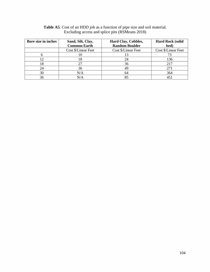
104

Table A5. Cost of an HDD job as a function of pipe size and soil material.

Excluding access and splice pits (RSMeans 2018)

Bore size in inches Sand, Silt, Clay,

Common Earth

Hard Clay, Cobbles,

Random Boulder

Hard Rock (solid

bed)

Cost $/Linear Feet Cost $/Linear Feet Cost $/Linear Feet

6 10 13 73

12 18 24 136

18 27 36 217

24 36 49 271

30 N/A 64 364

36 N/A 85 451

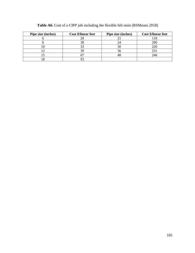
105

Table A6. Cost of a CIPP job including the flexible felt resin (RSMeans 2018)

Pipe size (inches) Cost $/linear feet Pipe size (inches) Cost $/linear feet

6 29 21 118

8 30 24 200

10 33 30 220

12 39 36 231

15 67 48 246

18 93

106

Table A7. Pipe bursting cost replacing with HDPE pipe

Pipe diameter in mm Cost CAD/ft

150 117

200 140

250 169

300 196

350 241

Note: The cost rates in Table A7 were estimated for the year 2018 using 0.16% inflation rate and

then converted to Vancouver, Canada using RSMeans city cost indexing method.

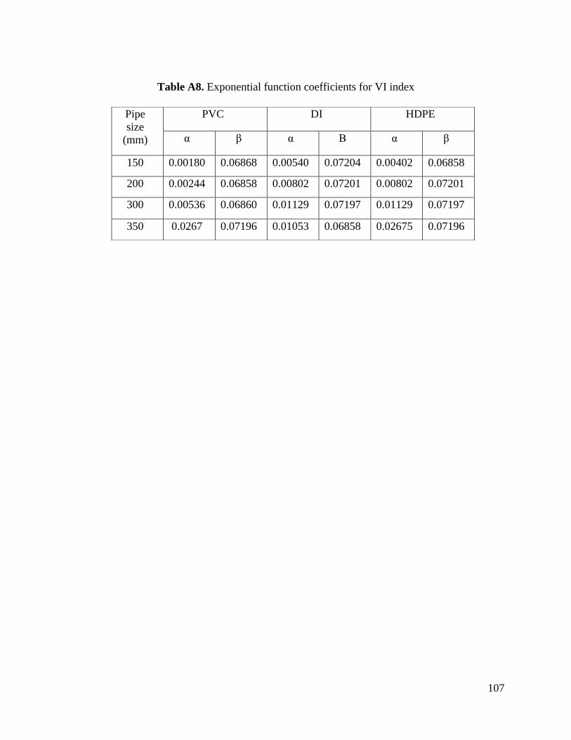
107

Table A8. Exponential function coefficients for VI index

Pipe

size

(mm)

PVC DI HDPE

α β α Β α β

150 0.00180 0.06868 0.00540 0.07204 0.00402 0.06858

200 0.00244 0.06858 0.00802 0.07201 0.00802 0.07201

300 0.00536 0.06860 0.01129 0.07197 0.01129 0.07197

350 0.0267 0.07196 0.01053 0.06858 0.02675 0.07196

design improvement in water distribution systems: a life cycle

Documents

Transcript of design improvement in water distribution systems: a life cycle