a comparison of single-cycle versus multiple-cycle proof ...

A COMPARISON OF SINGLE-CYCLE VERSUS

MULTIPLE-CYCLE PROOF TESTINGSTRATEGIES: FINAL REPORT

R. C. McClung, G. G. Chell, and H. R. Millwater

Southwest Research Institute

San Antonio, Texas

D. A. Russell and G. E. Orient

Rocketdyne Division

Rockwell International Corporation

Canoga Park, California

December 1996

NASA Contractor Report

Contract NAS8-37451

Prepared for

NASA-GEORGE C. MARSHALL SPACE FLIGHT CENTER

Marshall Space Flight Center, Alabama 35812

Approved:

Stephe_J. Hudak, Jr., Director

Materials Engineering Department

ACKNOWLEDGEMENTS

The continuing encouragement and support of the NASA-Marshall technical staff is

gratefully acknowledged. In particular, Gwyn C. Faile, Henry M. Lee, and Rod Stallworth

maintained a cordial and cooperative relationship with the program team that was essential to the

success of the research.

A number of our colleagues at Southwest Research Institute made important contributions

to the program. Vic Aaron, Tom Masden, and Jack FitzGerald are thanked for their invaluable

assistance in conducting the crack growth experiments. Dr. V. P. Swaminathan led the

fractographic investigations, and Jim Spencer performed the crack length measurements from the

fracture surfaces. John Hanley was task leader for the acoustic emission studies. Tim Grant

helped with the development of improved J solutions. Janet Buckingham performed some of the

statistical analysis. Luz H. Escobedo provided extensive assistance with preparation of this

report. Dr. Stephen J. Hudak, Jr., is especially thanked for his advice and support throughout theentire research effort.

TABLE OF CONTENTS

Page

LIST OF TABLES .................................................. viii

LIST OF FIGURES .................................................. ix

DEFINITION OF SYMBOLS .......................................... xiv

NONSTANDARD ABBREVIATIONS .................................... xvi

EXECUTIVE SUMMARY ............................................ xvii

1. INTRODUCTION ................................................. 1

1.1 General Background to the MCPT Problem ......................... 1

1.2 Review of Key Background Information from Phase I .................. 3

1.2.1 Rocketdyne Experience with MCPT ........................ 4

1.2.2 Distributions of Initial Flaw Sizes and Shapes ................. 4

1.2.3 J-Integral Solutions for Semi-Elliptical Surface Flaws ........... 4

1.2.4 Fracture Mechanics Properties of Inconel 718 ................. 5

1.2.5 First-Generation Analytical Model for MCPT ................. 6

1.2.6 Phase I Conclusions ................................... 6

1.3 Work Scope for Phase II Investigations ............................ 7

2. ANALYTICAL DEVELOPMENT ..................................... 8

2.1 Improved J-Integral Solutions for Surface Flaws ...................... 8

2.2 J-Integral Solutions for Cracks at Notches ......................... 15

2.2.1 Finite Element Results ................................ 15

2.2.2 Simple J-Estimation Technique .......................... 21

2.3 Elastic-Plastic Fatigue Crack Growth Analysis ...................... 27

2.4 Tear-Fatigue Theory ........................................ 29

, EXPERIMENTAL CHARACTERIZATION AND VALIDATION .............. 34

3.1 Updated J-Resistance Curves .................................. 34

3.2 Relationship Between J-Resistance Curves and Fatigue Crack Growth ...... 37

3.3 Characterizing the Onset of Stable Tearing ........................ 41

3.4 Elastic-Plastic Fatigue Crack Growth Experiments ................... 42

3.5 Experimental Simulation of Multiple Cycle Proof Testing .............. 47

3.6 Effect of Proof Testing on Subsequent Fatigue Crack Growth Rates ....... 55

3.7 Fractographic Observations................................... 56

3.7.1. Crack Growth Mechanisms ............................. 56

3.7.2. Crack Shapes ...................................... 64

3.8 Acoustic Emission Investigations ............................... 69

vi

TABLE OF CONTENTS (CONT.)

Page

° PROBABILISTIC ANALYSIS ....................................... 78

4.1 The MCPT Question ........................................ 78

4.2 Probabilistic Formulation ..................................... 80

4.3 An Example Problem ....................................... 81

4.4 Parameter Studies .......................................... 91

4.5 Cracks at Notches .......................................... 104

4.6 Memory vs. Loss-of-Memory in Tear-Fatigue Theory ................. 105

. DISCUSSION .................................................. 111

5.1 Other Proof Testing Issues .................................... 111

5.1.1. Hold Times and Time-Dependent Fracture Behavior ........... 111

5.1.2. Cyclic Hardening and Softening ......................... 113

5.1.3. Weldments ........................................ 114

5.2 The Generality of the Results .................................. 115

6. SUMMARY AND CONCLUSIONS ................................... 117

. ENGINEERING GUIDELINES ...................................... 121

7.1 General Background ........................................ 121

7.2 Introduction to Flow Chart Format and Decision Process ............... 122

7.3 Engineering Guidelines: Detailed Description ....................... 126

8. REFERENCES .................................................. 140

APPENDIX A. Further Documentation of Improved J Solutions for Surface Flaws .... A. 1

Finite Element Solutions ........................................ A. 1

Reference Stress Estimates ....................................... A.4

Comparisons of Reference Stress and Finite Element Results .............. A. 14

Discussion: Accuracy of J Solutions ............................... A.24

Acknowledgements ........................................... A.25References ................................................. A.25

vii

LIST OF TABLES

Page

Table 2.1. Numerical values of the shape factors for K, = 4.29 ................... 22



Table 3.1. Summary of test conditions for specimens examined fractographically ...... 57

Table A1. Summary of geometries and constitutive laws for finite element J solutions . . A.2

Table A2. Summary of reference stress parameters calculated from finite element solutions..A.9

Table A3. Ratio of predicted to published h i for different _/c values ............. A.15

viii

LIST OF FIGURES

Figure 1.1.

Figure 2.1.

Figure 2.2.

Figure 2.3.

Figure 2.4.

Figure 2.5.

Figure 2.6.

Figure 2.7.

Figure 2.8.

Figure 2.9.

Figure 2.10.

Figure 3.1.

Figure 3.2.

Figure 3.3.

Page

Single-cycle proof test logic represented in terms of residual strength and

residual fatigue life ...................................... 2

Geometric construction for limit load solution of surface-cracked plate,

illustrating effective plate width ............................. 12

Comparison of reference stress J predictions (solid line) with Wang (top)and Dodds (bottom) finite element results ...................... 14

Schematic showing geometrical relationship between notch depth (D), notch

root radius (ro), crack depth (d), notch plus crack depth (a), and half plate

width (b) ............................................. 17

Linear elastic solutions for cracks at double edge notches in plates with K,= 4.29 ............................................... 18

Linear elastic solutions for cracks at double edge notches in plates with K,= 6.43 ............................................... 19

Linear elastic solutions for cracks at double edge notches in plates with K,

= 8.57 ............................................... 20

Asymptotic behavior of hl(alb, n) for K t = 4.29 as dlr o increases (d=rot2corresponds to a/b = 0.3622) ............................... 23

Asymptotic behavior of h_(a/b, n) for K t = 6.43 as d/r o increases (d=ro/2

corresponds to a/b = 0.32425) .............................. 24

Asymptotic behavior of h_(a/b, n) for K, = 8.57 as dlr o increases (d=rJ2

corresponds to a/b - 0.3129) ............................... 25

Schematic representation of tear-fatigue theory ................... 31

Crack growth resistance curves for Inconel 718 .................. 36

Fatigue crack growth data for Inconel 718 with superimposed resistancecurve data

• * " " " " " " " " " * " • " " " ° ° * ° " * " " ' " " " " " • * • ° • • • • • • • • • 38

Resistance curves for Inconel 718 with superimposed FCG curve ...... 39

ix

LIST OF FIGURES (CONT.)

Page

Figure 3.4. Typical load-displacement records from zero-max loading (top) and zero-max displacement (bottom) tests ............................. 44

Figure 3.5. Elastic-plastic fatigue crack growth data superimposed on scatterbands from

SSY FCG data ......................................... 45

Figure 3.6. Load vs. crack mouth opening displacement history for test $26 showingfailure on the second cycle at the terminal maximum load ........... 48

Figure 3.7. Load vs. crack mouth opening displacement history for test $27 ....... 49

Figure 3.8. Load vs. crack mouth opening displacement history for test $20 showing

failure on the fifth cycle at the terminal maximum load ............. 52

Figure 3.9. Load vs. load line displacement history for simulated proof test followed bysimulated service cycling .................................. 54

Figure 3.10. Fracture surface of specimen SD-3 at 300x (top) and 3000x (bottom)

showing quasi-cleavage fracture features and fatigue striations ......... 58

Figure 3.11. Fracture surface of specimen S-25 at 300x (top) and 3000x (bottom) showing

transgranular fatigue striations .............................. 59


tear ridges and ductile dimples at precipitate particles .............. 61

Figure 3.13. Fracture surface of specimen SCR-8 at 300x (top) and 3000x (bottom)

showing tear ridges and ductile dimples at precipitate particles ........ 62


tear ridges and few ductile dimples ........................... 63

Figure 3.15. Fracture surface of multiple cycle crack growth specimen (zero-max

displacement, five cycles) .................................. 65

Figure 3.16. Crack growth as a function of angular position for selected multiple cycle

crack growth specimens ................................... 66

Figure 3.17. Crack growth as a function of angular position for selected single-cycle

crack growth specimens ................................... 67

Figure3.18.

Figure 3.19.

Figure 3.20.

Figure3.21.

Figure 3.22.

Figure4.1.

Figure4.2.

Figure4.3

Figure4.4.

Figure4.5.

Figure4.6.

Figure4.7.

Figure4.8.

Figure 4.9.

Figure4.10.

Figure4.11.


Page

CMOD and load history of specimen S19 ...................... 70

CMOD vs. load for specimen S 19 ............................ 72

CMOD vs. AE count rate for specimen S19 ..................... 73

CMOD vs. AE event rate for specimen S19 ..................... 74

AE activity and CMOD history for specimen $27 ................. 76

Schematic representation of calculation of P[(Ns < Ns')] ............ 82

Schematic representation of calculation of P[(Ns < Ns') n ('Np > Np')] . . 83

Distribution of initial crack depths and corresponding exponential

distribution ............................................ 85

PDF of crack depth before and after proof testing for a sample problem 87

CDF of crack depth before and after proof testing for a sample problem 87

Service cycles to failure as a function of initial crack depth for a sampleproblem .............................................. 89

Probability of failure as a function of service cycles for a sample problem 89

Probability of failure in service as a function of number of proof cycles for

a sample problem ....................................... 90

CDF of in-service failure probability after different numbers of proof cycles

(N), conditional on proof test success, for proof factor of 1.1 (top) and 1.3

(bottom) .............................................. 92


(N), conditional on proof test success, for low tearing resistance (top) and

high tearing resistance (bottom) ............................. 93


(N), conditional on proof test success (a) CT R-curve and 1.3 proof factor

(b) upper bound R-curve and 1.1 proof factor .................... 94

xi


Figure 4.12.

Figure 4.13.

Figure 4.14.

Figure 4.15.

Figure 4.16.

Figure 4.17.

Figure 4.18.

Figure 4.19.

Figure 4.20.

Figure 4.21.

Figure 7.1.

Page

CDF of in-service failure probability after different numbers of proof cycles,

conditional on proof test success (a) a/c = 0.1 (b) a/c = 0.2 (c) a/c = 0.5 96

Probability of failure in service as a function of number of proof cycles for

a/c -- 0.5 example ....................................... 98

Cumulative distribution functions (top) and probability density functions

(bottom) for three exponential distributions of initial crack depth ...... 100


conditional on proof test success (a) exponential distribution with mean

value a = 0.01 in. (b) exponential distribution with mean value a = 0.08

in. , • ° • • • , ° • , . • . , • , • . • • • , • • , • • • , • • • , • • • , • • . • . , , . • ° ° . .

101

Cumulative distribution functions (top) and probability density functions

(bottom) for three Weibull distributions of initial crack depth ......... 102


conditional on proof test success (a) WeibuU distribution with shape

parameter 13- 0.5 (b) Weibull distribution with shape parameter 13 = 2.0 103

CDF of in-service failure probability after different numbers of proof cycles;

notched geometry, 100 ksi proof stress, a i = exp[.05] .............. 106

Total, elastic, and plastic J values for cracks emanating from double edge

notches with 100 ksi nominal stress ........................... 107


notched geometry, 50 ksi proof stress, a i = exp[.05] ............... 107

Computed in-service failure probability for different numbers of proof cycles

and different assumptions about material memory following the proofoverload .............................................. 110

Flow chart for Engineering Guidelines ......................... 123

xii

FigureA1.

Figure A2.

FigureA3.

FigureA4.

Figure A5.

FigureA6.

FigureA7.

FigureA8.

FigureA9.

FigureA 10.

Figure AI 1.

Figure A 12.

Figure A 13.


Geometric nomenclature for semi-elliptical surface crack in finite plate . .

Variation in extracted h_ with applied stress from Wang (1988) analyses

Variation in extracted hi with applied stress from Dodds (1992) analyses

Page

A.3

A.5

A.6

Comparison of h I values from various authors ................... A.7

Normalized representative plate width _/(b-c) as function of a/t ...... A.11

Normalized representative plate width _lt as function of a/t ......... A. 12

Normalized representative plate width _lc as function of a/t ......... A.13

Comparison of reference stress J predictions with Wang (1988) finite

element results ......................................... A. 16

Comparison of reference stress J predictions with Dodds (1992) finite

element results ......................................... A.17

Comparison of reference stress J predictions with Wang (1991) finite

element results ......................................... A. 18

Comparison of reference stress J predictions with Kirk (1992) finite element

results in terms of normalized applied stress ..................... A. 19

Comparison of reference stress J predictions with Kirk (1992) finite element

results in terms of normalized applied strain ..................... A.20

Comparison of reference stress hi predictions with Yagawa (1993) finiteelement results ......................................... A.21

°°°

XlII

DEFINITION OF SYMBOLS

a

a'

,2:Qi

b

C

C

d

D

da/dN

(daldN):

d,E

E"

fF

h

H

hl

J

J*

:a.,

J.=,J,,=

Jtotal

K or K I

X,cK,._

K,m

rl

N

UjN,NpNs

P

xiv

crack depth

area-equivalent crack depth for semi-elliptical crack (= _a/4)final crack size

initial crack size

half-width of a (cracked) plate

half surface crack length, or half of the remaining ligament for double edge cracked platecrack growth law constant

constant in crack-tip plastic zone size equation

length of crack growing from notch root

notch depth

crack growth rate per cycle

fatigue crack growth rate

effective length of crack at notch root (including plastic zone correction)

Young's modulus

E/(1. v2), effective modulus in plane strain

collapse function or yield function (= OL/Oy,)geometric term in expression for K 1

half-height of a (cracked) plate

crack growth function giving number of service cycles for an initial flaw size

non-dimensional factor in fully plastic Jp termJ-integral

an advanced path-area integral used in nonlinear fracture mechanicsapplied value of J

elastic component of J

some suitable measure of J for the initiation of tearing

J at crack initiation, measure of toughness

crack-growth resistance value of J for ductile tearing under monotonic loadingJ at maximum load in fatigue cycleminimum value of J

plastic component of J

total J, generally the sum of elastic and plastic componentsstress intensity factor

fracture toughness

K 1 at maximum load in fatigue cycle

KI at minimum load in fatigue cycle

stress concentration factor (based on gross section stress)

exponent in fatigue crack growth law

strain-hardening exponent in Ramberg-Osgood constitutive equation

number of load cycles (sometimes number of proof cycles)residual fatigue life

residual fatigue life corresponding to a i

number of proof cycles (Np' is a specific value)

number of service cycles (Ns' is a specific value)applied load

Po o

Po

aR

ro

ry

Sr

t

T*

U

V

O_

Ae

Ao

Aa

Aat

AJ

AK

AK_

6_V

o oro.

Oo

O flow

0 L

Oma.r

0 rain

0 open

Op

Or

O ref

0 s

0 ult

Oys

CO

e ref

gP,_f

characteristic yield load

optimized yield load

hydrostatic crack tip stress parameter

ratio of minimum to maximum load in fatigue cyclenotch root radius

radius of crack-tip plastic zone

nominal applied (gross section) stress in notched body

thickness of a specimen or component

an advanced path-area integral used in nonlinear fracture mechanics

effective stress range ratio

structural parameter in optimized reference stress method

constant in Ramberg-Osgood constitutive equation

shape parameter of a Weibull distribution

cyclic change in strain, or strain range

cyclic change in stress, or stress range

change in crack length due to crack growth

total crack extension due to ductile tearing

cyclic change in J

effective value of AJ (corrected for crack closure)

cyclic change in stress intensity factor

range of the strain intensity factor

effective value of AK (corrected for crack closure)

crack tip opening displacementPoisson's ratio

geometric term in effective plate width expressionusual meaning

applied nominal stress

stress constant in Ramberg-Osgood constitutive equationflow stress

plastic limit stress

stress at maximum load in cycle

stress at minimum load in cycle

crack opening stress

proof stress

residual strengthreference stress

service stress

ultimate strength

yield stress

factor in effective crack depth (plastice zone correction) expressionoptimized value of

strain constant in Ramberg-Osgood constitutive equationreference strain

reference plastic strain

XV

NONSTANDARD ABBREVIATIONS

AE

ASTM

CDF

CEGB

CMOD

CT

DECP

EDM

EDS

EPFCG

EPRI

FAD

FCG

FE

HRR

MCPT

NDE

PDF

PTP

RSECP

RSM

SCPT

SEM

SSME

SSY

STA

SwRI

Acoustic Emission

American Society for Testing and MaterialsCumulative Distribution Function

Central Electricity Generating Board

Crack Mouth Opening Displacement

Compact Tension (specimen)

Double Edge Cracked Plate

Electro-Discharge Machining

Energy Dispersive Spectography

Elastic-Plastic Fatigue Crack GrowthElectric Power Research Institute

Failure Assessment Diagram

Fatigue Crack GrowthFinite Element

Hutchinson-Rice-Rosengren

Multiple Cycle Proof TestingNondestructive Evaluation

Probability Distribution Function

Proof Test Philosophy

Restrained Single Edge Cracked Plate (specimen)Reference Stress Method

Single Cycle Proof Testing

Scanning Electron Microscope

Space Shuttle Main Engine

Small-Scale Yielding

Solution Treated and AgedSouthwest Research Institute

xvi

EXECUTIVE SUMMARY

Single-cycle and multiple-cycle proof testing (SCPT and MCPT) strategies for reusable

aerospace propulsion system components are critically evaluated and compared from a rigorous

elastic-plastic fracture mechanics perspective within a probabilistic framework.

Previous research on MCPT included documentation of Rocketdyne experience with

MCPT, distributions of initial flaw sizes and shapes in selected SSME hardware and test coupons,development of J-integral solutions for surface flaws, characterization of the fracture mechanics

properties of Inconel 718, and development of a fu'st-generation analytical model for MCPT. The

results of these previous studies are briefly reviewed.

New J-integral estimation methods based on the reference stress approach are derived andvalidated for semi-elliptical surface cracks and for cracks at notches. A limited number of new

elastic-plastic finite element J-integral solutions were developed to support the derivation and

validation of the simple estimation methods, which have broader generality.

An engineering methodology based on the J-integral is developed to characterize crack

growth rates during elastic-plastic fatigue crack growth (FCG) and the tear-fatigue interaction

near instability. The FCG methodology employs the correlating parameter A Jen, which

incorporates the effects of fatigue crack closure. These methodologies are integrated to develop

an improved deterministic analytical model for crack growth and failure during MCPT.

Surface crack growth experiments were conducted with Inconel 718 to characterize tearing

resistance, FCG under small-scale yielding and elastic-plastic conditions, and crack growth during

simulated MCPT. Fractography and acoustic emission studies provide additional insight into

fracture behavior. The test results provide validation of the engineering methodologies for

elastic-plastic FCG and tear-fatigue, and the analytical model for crack growth during MCPT.

The relative merits of SCPT and MCPT for ductile materials are directly compared using

a probabilistic analysis linked with an elastic-plastic crack growth computer code. The

conditional probability of failure in service is computed for a population of components that have

survived a previous proof test, based on an assumed distribution of initial crack depths in the

proof-tested hardware. Parameter studies investigate the influence of proof factor, tearingresistance, crack shape, initial crack depth distribution, and notches on the MCPT versus SCPTcomparison.

Both analytical and experimental studies clearly show that MCPT can be effective in

removing some of the largest flaws from the population that would not have been removed byconventional SCPT at the same proof loads. Hence, MCPT can be an effective means of

identifying and removing defective hardware that could go undetected by conventional SCPT.

MCPT can also cause additional subcritical crack growth to occur in components that do not fail

during the proof test. Therefore, in general, a cracked component that survives MCPT has a

slightly shorter remaining service life than if the component had been subjected to a SCPT at the

same load. However, this service life difference is negligibly small in most cases.

xvii

In general,the probabilistic studiesshow that for ductile materials,when MCPT isconsistentlyappliedto a fleet of componentscontaininga disu'ibutionof initial flaws,the overallfleet reliability will behigherfor a populationof componentsthathavebeensubjectedto MCPTthan for a populationof componentsthat havebeensubjectedto SCPTat the sameproof load.This benefit generally increaseswith increasing numbers of proof cycles, although theincrementalbenefitof additionalproof cyclesdecreaseswith increasingnumbersof cycles.

MCPT can be inferior to SCPT under certain conditions: when the probability of failure

due to any proof loading is itself negligibly small; when the crack driving force decreases with

increasing crack size; and when cracks arc located at severely stressed notch roots and the crack

lengths of concern are comparable to the plastic notch field or smaller.

MCPT can be preferable to SCPT only when viewed from the perspective of component

reliability; i.e., a probabilistic assessment of structural integrity. From a purely deterministic

standpoint, the potential advantages of MCPT cannot be recognized or documented. In particular,

if proof testing is being used for the specific purpose of establishing a guaranteed maximum size

for any flaw remaining in the component following the proof test, then MCPT offers no

additional benefit. MCPT does not increase or decrease this guaranteed maximum flaw size

relative to SCPT. The potential advantage of MCPT over SCPT is that the inferred frequency

of flaws that are slightly smaller than this critical maximum flaw size may be decreased, thereby

improving component reliability from a probabilistic perspective.

The parameter studies conducted under the current contract indicate that for wide ranges

of variation in many of the important factors, the overall performance of MCPT in comparison

to SCPT is relatively consistent. MCPT appears to be either beneficial or benign in comparison

to SCPT, and any benefit generally continues to increase with increasing numbers of proof

cycles. In situations where component failure risk is relatively high, MCPT can be a useful

means of obtaining additional reliability. In situations where component failure risk is relatively

low, MCPT itself offers no additional benefit. However, if multiple proof cycles are desirable

or required for other (non-fracture mechanics) reasons, then these multiple cycles will not

generally cause any significant deterioration of fleet reliability.

The specific benefit or detriment associated with MCPT depends on a large number of

different factors, including proof loads, material fracture properties, and crack and component

geometries. Therefore, it is not possible to provide a simple set of universal formulas or graphs

that can be used to select the mathematically optimum proof test protocol and quantify the

incremental benefit of that protocol. Individual fracture mechanics analyses of critical component

locations are recommended to perform this evaluation for specific proof testing problems. These

analyses would be facilitated by the availability of a general-purpose computer code for elastic-

plastic crack growth analysis with simple probabilistic capabilities.

Within this limitation, a series of practical engineering guidelines are proposed to help

select the optimum proof test protocol in a given application. The guidelines are given in the

form of an annotated flow chart that provides detailed, step-by-step guidance to evaluate the

relative suitability of SCPT vs. MCPT for a given proof testing application.

°.°

XVlll

1. INTRODUCTION

1.1 General Background to the MCPT Problem

Although proof testing is generally not the preferred method of crack detection, it has

proven useful as a supplement to conventional nondestructive evaluation (NDE) methods,

particularly when NDE is compromised by geometric complexities of the component or structure.

The objective of proof testing is to screen out gross manufacturing or material deficiencies and

therefore provide additional quality assurance of delivered hardware. It is in this spirit that

Rocketdyne has utilized proof testing on components of the Space Shuttle Main Engine (SSME).

Since 1952, Rocketdyne has selectively implemented a modified version of conventional

single-cycle proof testing (SCPT) involving multiple proof cycles. This multiple-cycle proof

testing (MCPT) was originally motivated by component failures on the Nalar program at

pressures significantly less than the initial hydrostatic proof. Failures were experienced as low

as 46% of proof pressure. The current procedure for MCPT on the SSME consists of the

application of five proof cycles at a minimum pressure of 1.2 times the maximum operating

pressure, each with a minimum hold time of 30 seconds. Since the inception of MCPT,

Rocketdyne proof testing has shown that component failures can occur on the second, third,

fourth, or fifth cycles at significantly lower pressures than applied on the fh-st cycle [ 1]. These

failures generally initiated from undetected flaws in the component, typically in thin sections

where the defects were large compared to the thickness. In several cases these hardware

deficiencies, revealed only after having passed the f'u'st proof pressure cycle, were judged to have

presented a significant risk of component failure or malfunction in service. Literature searches

located several additional manuscripts also describing component failure during multiple proof

cycles, including experience in both aerospace pressure vessel [2,3] and gas transmission line

pipe [4] applications. This direct hardware experience illustrates a potential deficiency in the

conventional single cycle test, demonstrates the potential benefit arising from MCPT, and poses

a challenge to determine optimum strategies for proof testing.

The primary justification for five-cycle proof testing has been the successful record of

performance of Rocketdyne engines and the lack of service failures of pressurized components

whenever this procedure has been implemented. There has not been, however, a well-established

theoretical basis either to demonstrate clearly the superiority of MCPT (in comparison to

conventional SCPT) or to specify the optimum proof pressures, temperature, and numbers of

cycles to achieve maximum component reliability. The current practice is based heavily on

engineering experience rather than analytical models. The purpose of the research described in

this report has been to develop such an analytical model for MCPT which enables proof testingstrategies to be evaluated on a rational basis.

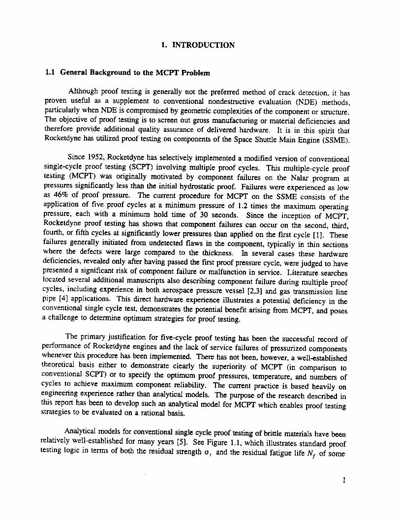
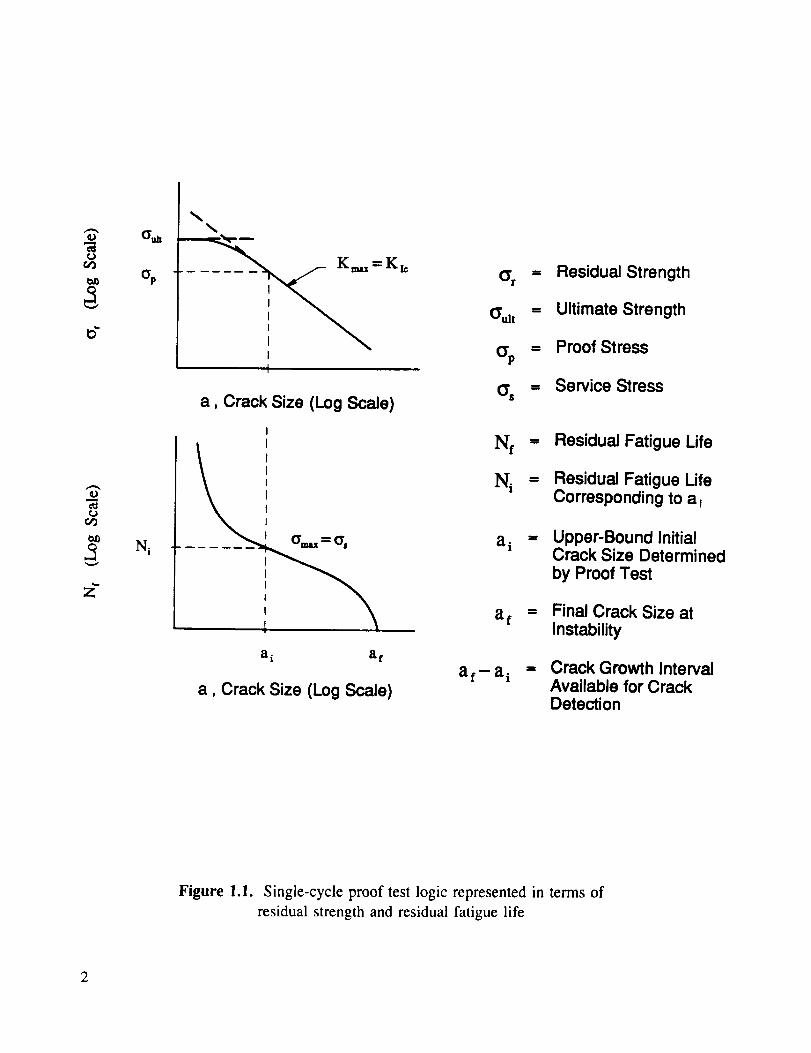
Analytical models for conventional single cycle proof testing of brittle materials have been

relatively well-established for many years [5]. See Figure 1.1, which illustrates standard proof

testing logic in terms of both the residual strength o r and the residual fatigue life N s of some

O

O

o3

2

z"

N i

_ K== = K,_ (Yt ffi

O'alt

, %

a, Crack Size (Log Scale)

I

i \ai a t

a, Crack Size (Log Scale)af-a i

Residual Strength

Ultimate Strength

Proof Stress

Service Stress

Nf = Residual Fatigue Life

Ni = Residual Fatigue LifeCorresponding to a_

a i = Upper-Bound InitialCrack Size Determinedby Proof Test

a t = Final Crack Size atInstability

ffi Crack Growth IntervalAvailable for CrackDetection

Figure 1.1. Single-cycle proof test logic represented in terms of

residual strength and residual fatigue life

2

structuralcomponent. Sincebrittle materialsexhibit a well-definedinstability point given byK,,_ = K_c, the successful application of ap guarantees that any flaw still present is less than some

size ai. Taking a i as the initial crack size in a fracture mechanics based fatigue crack growth

analysis defines a corresponding minimum residual fatigue life Nr Rigorous characterization of

this fracture process typically requires only determination of the applied stress intensity factor

K,,_ and the inherent fracture toughness of the material, K_c.

The application of additional proof cycles to a brittle material system is of no benefit,

since stable crack growth does not occur during loading. Stable crack growth can occur during

proof testing of a ductile material system, however, and this phenomenon suggests possible

advantagesmand disadvantages----of a multiple cycle proof testing strategy. The potential

advantage of MCPT is that a flaw which is not large enough to cause failure during the first

proof cycle may nevertheless be revealed by growing sufficiently to cause failure during a

subsequent proof cycle. The potential disadvantage is that stable crack growth may occur without

failure during all proof cycles, so that the remaining service life of the component is actuallydecreased by the proof testing process.

The current research starts with the assumption that damage growth and failure during

MCPT can be described as fracture mechanics events. This assumption implies that defects are

crack-like during the first proof cycle and enables us to draw upon a broad base of elastic-plastic

fracture mechanics technology. The goals of the research are to characterize the extent of

subcritical flaw growth during SCPT and MCPT of reusable propulsion system components, to

characterize flaws which are removed from the population during SCPT and MCPT, and to move

towards the identification of an optimum MCPT strategy.

1.2 Review of Key Background Information from Phase I

Results from the first two years of work under this contract were summarized in a major

technical report subsequently published by NASA as Contractor Report 4318 [6]. Full

documentation of these early results will not be repeated in the current Final Report. For

convenience, however, the key investigations and key results from those first two years will be

briefly summarized in the paragraphs that follow. The new investigations and new results

presented in detail in the current Final Report naturally build on the earlier work, leading to a

final set of program conclusions. In some cases, the new results and conclusions are based on

the early investigations in their original form; in other cases the new material is an extension or

updating of the older material; and in still other cases the new approaches or results have

superseded their counterparts from the first two years.

For convenience, the first two years of work summarized in Contractor Report 4318 will

be denoted as "Phase I" throughout this Final Report. The work conducted after the Contractor

Report was submitted to NASA, leading up to the preparation of this Final Report, will bedenoted as "Phase II."

1.2.1 Rocketdyne Experience with MCPT

The specific details of Rocketdyne experience with multiple-cycle proof testing were

collected and summarized. This study focused on observed proof failures on a subsequent proof

cycle, after the component had successfully endured one or more proof cycles at the same proof

load. Where details were found identifying the defect size, the defect depths were generally an

appreciable fraction of the component thickness, and the defect lengths were many times the

thickness. Many of the failures occurred in relatively thin sections. MCPT failures were not

isolated to a particular material or material system, but were observed to occur in a broad rangeof materials. Inconel 718 was the most common material.

1.2.2 Distributions of Initial Flaw Sizes and Shapes

Data relative to initial defect sizes and shapes for SSME hardware or fabrication processes

were collected at Rocketdyne. The data sources included material test coupons, selected SSME

hardware, and available multi-cycle proof failure information. Although some of the defect

shapes were irregular, it was found useful to idealize all of the defects as semi-elliptical surface

cracks and to determine the equivalent depth and surface length for each flaw. Statistical

distributions were then defined to model the depth and aspect ratio of the defects. The

predominant defect shape was found to be roughly semi-circular. The lognormal distribution was

chosen to describe crack depth, based on conventional statistical tests of the available data.

1.2.3 J-Integral Solutions for Semi-Elliptical Surface Flaws

A fracture mechanics description of the SSME MCPT process must be elastic-plastic,

rather than linear elastic, in nature. The material of greatest interest, IN-718, has a relatively

high initiation toughness, so brittle fracture does not readily occur. Furthermore, the flaws of

interest in SSME components are physically small, so the crack driving force is not significant

unless the applied stresses are large. When the applied stresses are large, as is frequently the

case, linear elasticity is typically not satisfied. In particular, since the crack depths of probable

interest are large compared to the section thickness, stresses in the net section may approach or

surpass the yield strength of the material.

The J-integral was chosen as the characteristic fracture mechanics parameter for the

current study in view of its widespread use in elastic-plastic fracture analysis. Use of J also

makes available the well-developed stability and failure assessment schemes presented in the

EPRI elastic-plastic fracture handbook [7]. This approach to crack growth analysis requires two

key inputs: an expression for the applied J and a description of the material J-resistance curve,

both corresponding to the particular specimen and crack geometry of interest.

No closed form solutions were available in the literature to estimate the applied value of

J, J, pp for a semi-circular surface crack in a finite thickness plate. A limited number of finite

element results for specific crack and specimen geometries and materials had been published, but

these had not yet led to generalized analytical expressions. A new J estimation method was

4

derivedbasedon the referencestressapproachdevelopedby Ainsworth and colleaguesat theCentralElectricityGeneratingBoard(CEGB)of the UnitedKingdom [8]. The reference stress

technique requires only three basic pieces of information, all of which are readily available in

this case: (1) a solution for the linear elastic stress intensity factor K; (2) a description of the

elastic-plastic constitutive response; and (3) an estimate of the limit load for the cracked member,

assuming an elastic-perfectly plastic material. An additional modification to the reference stress

solution was then implemented based on the J estimates developed by Dowling [9] for

semi-circular flaws in infinite bodies. Comparisons of this modified J estimation scheme with

the available finite element results for semi-ellipitical surface flaws showed good agreement.

1.2.4 Fracture Mechanics Properties of Inconel 718

All experimental investigations were performed on IN-718 heat-treated to the STA-1

condition (designed for optimum resistance to hydrogen embrittlement). Tensile tests determined

that the average 0.2% yield strength was 161.2 ksi, ultimate tensile strength 205.5 ksi, elongation

22.2%, and reduction in area 33.3%. The elastic modulus was 29.69(10) 3 ksi.

A J-resistance curve for surface-flawed IN-718 was generated experimentally. Thespecimens had a rectangular cross-section 1.25 inches in width and were either 0.2 or 0.5 inches

thick. Semi-circular surface cracks were initiated by electro-discharge machining and fatigue

pre-cracking. Initial crack depths after pre-cracking ranged from a/t = 0.36 to 0.73. Loads were

applied in uniaxial tension. Tests were conducted in both load control and crack mouth opening

displacement control. No significant changes in crack shape were observed during stable crackgrowth.

The resistance curve was constructed from the experimental data by directly measuring

initial crack depth a and crack extension Aa and by estimating J in one of two ways. The first

method used the modified reference stress estimation scheme described earlier. An independent

second method was based on an "equivalent energy" approach. These two estimation techniques

gave results which usually agreed within 10 percent. The apparent toughness of the surface-

cracked configuration was significantly higher than the toughness observed for thick compacttension (CT) specimens.

Fatigue crack growth (FCG) tests were conducted on through-thickness cracked panels

to determine both baseline FCG rate data and information regarding fatigue range marking. Two

tests were run on 0.2-in. thick specimens and one on a 0.5-in. thick specimen to provide data

over a wide range of growth rates. Visual examination of the fracture surfaces revealed

significant differences in the fracture surface morphology at high and low growth rates, verifying

that range marking could be used successfully to delineate the crack front fractographically. A

series of crack shape study experiments were then conducted on surface-flawed 0.2-in. thick

specimens under small-scale yielding conditions. The crack shape was found to remain nearlyconstant around a/2c - 0.5 as the crack grew from a/t ---0.3 to 0.9.

1.2.5 First-Generation Analytical Model for MCPT

A comprehensive survey of the available literature suggested that it was not yet possible

to predict with certainty how crack growth would be influenced by multiple proof cycles. A

variety of different behaviors had been reported experimentally, and several different analytical

approaches had been proposed. However, it was found useful to assemble a simple first-

generation model for crack extension during simulated MCPT. This analytical model was

designed to demonstrate the potential effects of many different variables on ductile crack growth

during SCPT and MCPT and to make a preliminary evaluation of the possible differences

between SCPT and MCPT. The model was a simple numerical tool to explore "what-iF'

scenarios and to plan further critical experiments.

The simple model was based on the Electric Power Research Institute (EPRI)oelastic-

plastic fracture analysis scheme and considered only crack advance due to ductile tearing. Stable

(or unstable) crack growth was evaluated by comparison of J, pv and J-resistance curves. The

capability to model different values of system compliance, ranging from pure load control to pure

displacement control, was included. Analysis of crack growth on subsequent proof cycles after

the first was addressed by regarding each reload cycle as the first loading cycle in a new test.

The initial crack length for this new test was taken as the predicted final crack length from the

end of the previous proof cycle. This caused a translation of the J-resistance curve along the A a

axis, although the shape of the resistance curve was assumed to be unchanged by the unload-

reload cycle. This approach was thought to give an upper bound estimate of crack advance innearly all cases.

The model was exercised to investigate the effects of crack geometry, applied load,

number of proof cycles, resistance curve shape, system compliance, and other variables on crack

growth during MCPT. However, the key issue in evaluating SCPT vs. MCPT is not how a singleflaw behaves, but rather how a proof test protocol influences a distribution of defect sizes which

may be present in a population of components. Therefore, Monte Carlo simulation was used to

evaluate the effects of SCPT and MCPT on crack size distributions before vs. after various prooftest procedures.

1.2.6 Phase I Conclusions

The changes in the crack size distribution during MCPT were shown to depend on the

interactions between the number of proof cycles applied, the nature of the resistance curve, the

initial crack size distribution, the component boundary conditions, and the magnitude of the

applied load or displacement. Therefore, the relative advantages and disadvantages of single-

cycle versus multiple-cycle proof testing appeared to be specific to individual componentgeometry, material, and loading.

However, a number of important issues were not resolved by the Phase I investigations.

In particular, no direct experimental evaluations of the Phase I analytical model were carried out

in Phase I. Other major remaining issues included the potential contributions of fatigue crack

6

growthmechanisms,therelationshipbetweenductile tearing and fatigue, possible changes in the

behavior of very deep cracks, and the full significance of local control mode (load vs.

displacement). Finally, it was not yet clear how best to quantify the differences between MCPT

and SCPT with respect to the practical implications for hardware reliability. In other words, what

is the best numerical way to ask and answer the MCPT vs. SCPT question?

1.3 Work Scope for Phase H Investigations

The Phase II investigations were designed to resolve these outstanding issues in search

of a more definitive answer to the MCPT question. The effort involved close coordination

between experimental and analytical investigations. Critical experiments were used to developclearer understandings of fundamental fracture mechanics issues and to evaluate or validate the

original and subsequent improved analytical models. Analytical development activities included

the development of new or improved J solutions and the development of practical fracture

mechanics approaches to characterize crack growth, including improved models for crack growth

during MCPT. Finally, a series of probabilistic analyses employed these improved MCPT models

to evaluate the implications of SCPT and MCPT for predicted fleet reliability, leading to a series

of conclusions about the selection of the optimum proof test strategies.

The remainder of this Final Report is a careful documentation of the Phase U

investigations, results, and conclusions. The Analytical Development chapter summarizes

improved J solutions for surface cracks, new finite element solutions and simple estimates of J

for cracks growing from notches, an engineering methodology to characterize elastic-plastic

fatigue crack growth, and a new second-generation model for MCPT based on tear-fatigue theory.

The Experimental Characterization and Validation chapter first presents updated J-resistance

curves and shows the relationship between the J-R curves and FCG curves. Then critical

experiments are documented which characterize elastic-plastic FCG and tear-fatigue behavior,

along with the effect of proof testing on subsequent FCG rates. Fractographic observations and

the results of acoustic emission studies are also summarized. In the Probabilistic Analysis

chapter, the SCPT vs. MCPT question is posed and answered from a more rigorous quantitative

standpoint with respect to fleet reliability. The results of extensive parameter studies are

presented to show the effects of important proof testing variables on the probability of hardware

failure in service. A Discussion chapter provides some broader perspective and briefly addresses

a variety of other secondary MCPT issues outside the scope of this contract. Finally, the

Summary and Conclusions and Engineering Guidelines chapters summarize the important

results of the study and their practical implications for the specification of optimum proof test

protocols. The guidelines are organized as an annotated flow chart that provides detailed, step-

by-step guidance to evaluate the relative suitability of SCPT vs. MCPT for a given proof testingapplication.

7

2. ANALYTICAL DEVELOPMENT

In Phase I, analytical development work included the development of J solutions for semi-

elliptical surface cracks, the implementation of the EPRI J scheme for the analysis of ductile

tearing, and the development of a simple analytical model for MCPT based on ductile tearingconsiderations.

Significant new analytical development activities were conducted in Phase H. An

improved reference stress J estimate was developed for the semi-elliptical surface crack, drawing

from newly available finite element J solutions. Phase I observations about the significance of

local control mode led to increased interest in cracks growing from notches, so new J solutions

were generated for this important geometry. A limited set of elastic-plastic finite element

solutions were produced first, providing a basis for the derivation and verification of a simple

J estimation method. An engineering methodology was developed to treat fatigue crack growth

under elastic-plastic cycling. Finally, an improved analytical model for crack growth during

MCPT was developed based on tear-fatigue theory. All of these analytical activities and

associated results are documented in some detail in the remainder of the chapter.

2.1 Improved J-Integral Solutions for Surface Flaws

The approach developed in Phase I to estimate J for the important semi-elliptical surface

crack geometry was based on a reference stress formulation [8] and the only set of finite element

solutions [10] for that geometry available at that time. The reference stress formulation was

modified by adapting an earlier solution by Dowling [9] for a surface crack in a semi-infinite

body in order to improve agreement with the FE results.

In the years immediately following the completion of Phase I, several additional sets of

finite element J-integral solutions for the surface crack became available [11-14], including a

wider variety of geometries and constitutive relationships. The Phase I solution did not always

show good agreement with the new FE results. Therefore, in the Phase II effort, these new

numerical results were used to develop an improved reference stress estimate of J with greater

generality. A more complete description of this analytical effort is given in Appendix A. For

convenience, a shorter synopsis of the method and results is provided here.

Following the EPRI handbook [7] approach, a general form for J in a Ramberg-Osgoodmaterial can be written according to

/fJto,°, - K F 2 n-1 (°._!°_0)2 + o eoth (2.1)E 1+ - • o

The first term in Eqn. 2.1 represents the elastic component of J, J,, and the bracketed

factor is an effective crack length correction similar to the EPRI handbook suggestion for

evaluating first order plastic effects with F defined as a geometry-dependent term in the elastic

K expression:

K = Fo V_ a (2.2)

The coefficient C2 is set equal to 2 for plane stress and 6 for plane strain based on arguments

about the size of the crack-tip plastic zone. The effective elastic modulus E' is set equal to E for

plane stress and El(1 - v 2) for plane strain.

The second term in Eqn. 2.1 represents the plastic component of J, Jp, and is defined in

terms of the Ramberg-Osgood (constitutive) constants e o and o o, which satisfy the stress-strainlaw of the general form

(=o)'°• _ o + a (2.3)

E o O o

Here e is the uniaxial strain corresponding to the stress, a, and Eo = aJE. The applied (uniform

uniaxial) stress a., and the non-dimensional factor hi depends on geometry and strain hardening

exponent but not on the magnitude of the applied stress. It is this h I which is tabulated in the

elastic-plastic fracture handbooks, and it is this h_ (or its equivalent) which any simple estimation

technique must compute accurately.

The basic form of the Ainsworth reference stress expression for the plastic component is

gP

J = K 2 ref (2.4)P

o,¢f

where the reference stress or,/is computed as

0

at/ = a._ (2.5)o r

Here or. is the plastic limit stress for a cracked body for a rigid plastic material of yield stress

oys. Note that oys is also the plastic limit stress for an elastic-perfectly plastic uncracked body.

For convenience, a collapse function f is defined as the ratio of the two plastic limit loads:

0 L

f - (2.6)O

ys

9

Note thatf is always bounded by 0 and 1, and so the reference stress will always be equal to or

(in general) greater than the applied stress. Note also that f is a function of geometry and the

type of applied load (tensile, pressure, bending) but not a function of the magnitude of the load

or constitutive law. The reference strain plastic p ", ,,: Is calculated from the constitutive relationship

as the uniaxial plastic strain corresponding to a uniaxial stress o_p

In order to compare the reference stress estimates more directly with the FE J solutions,

Eqn. 2.6 was expanded and an effective crack length term added to give the general form,

ff tatal

g 2

E-- -- dI-

.+, 1(2.7)

where ere is the total (elastic plus plastic) reference strain. For simplicity and slight

conservatism, plane stress was assumed in this particular formulation. Expanding the second

(plastic J) term for a Ramberg-Osgood material, it is possible to derive the general form,

JP

n+l

(2.8)

Note that the term in the curly brackets in Eqn. 2.8 is equivalent to h_ in Eqn. 2.1. In order to

estimate h_ using the reference stress approach, then, (and hence to estimate total J) only F and

f must be determined. Since F can be extracted directly from the K solution, the challenge is

focused on f, and ultimately on the proper form for the plastic limit stress or, as the onlysignificant remaining unknown.

Unfortunately, "exact" theoretical solutions do not exist for f as they do for K. Various

bounding theorems can be used to estimate f, but different approaches can yield different

expressions for the limit stress. Furthermore, it is not intuitively obvious for the surface cracked

geometry whether the relevant limit stress should characterize the overall plastic deformation of

the cracked structure (a global limit stress) or the plastic deformation local to a point on the

defect (a local limit stress). Miller [15] and Chell [16] concluded from their studies that global

limit stresses gave better agreement with FE results than local limit stresses. In general, as Chell

has noted [16], the optimum choice of the collapse function f does not necessarily represent the

true plastic yield load of the structure. Instead, it can represent an empirical yield load which

will produce good agreement between the reference stress procedure and elastic-plastic FEcomputations of the J-integral.

10

Thesimplestchoiceof yield functionf for the surface flaw is that based on the reduction

in load bearing area due to the presence of the defect. This gives the global yield function,

Macf = I- _ (2.9)

4bt

Here a is the maximum depth and 2c the surface length of a semi-elliptical surface crack in a

plate of thickness t, width 2b, and height 2h. This was the form used in the Phase I estimate.

A potential disadvantage of this form, as will be shown later, is that f appears to be over

estimated for wide plates (large b/c ratios). As b/c goes to inf'mity, this simple net section area

criterion implies that the effect of the defectDno matter how deep---is vanishingly small. The

limit stress is then merely that of a defect-free plate, and f = 1.

An alternative approach is to define some effective plate dimension (in the width

direction) that characterizes collapse. One such construction is shown in Fig. 2.1, where the

effective width is given as (2_ + 2c). The limit stress is defined when stresses in this enclosed

region are at yield. The remaining problem now is to select the proper value of _.

Remembering that the optimum choice of a limit load can be driven by optimum agreement with

FE solutions, it is possible to work backwards from available numerical solutions to evaluate

different means of defining _.

The limit or yield function for the geometrical construction of Fig. 2.1 can be written as

f R

(2.10)

Here the actual semi-elliptical cracked area has been represented by the equivalent rectangulararea a' x 2c, where a' = ha/4.

There are several possible ways that _ might be related to the plate geometry. If the form

of h I in Eqn. 2.8 and the nominal net section area criterion (Eqn. 2.9) are correct, then _ = (b-c)

and the non-dimensional quantity _l(b-c) will be equal to 1. Alternatively, it is possible that

is related to the plate thickness t, so that the ratio _/t will be approximately constant. Another

characteristic dimension of the cracked geometry is the crack width 2c, so the nondimensionalratio _/c may be significant.

Yield functions f were computed for the five sets of recently published FE solutions, and

then _ values were calculated by inversion of Eqn. 2.10. In general, _ was found to be

considerably smaller than the remaining plate width (b-c), especially for large b/c ratios.

Therefore, the nominal net section area criterion (Eqn. 2.9) often gave limit load estimates much

too high and reference stress J estimates too low. This was precisely the finding in Phase I. The

Phase I approach attempted to solve this problem by calibrating the reference stress formulation

11

I I I II I I II I I I

II _-a=4a i

2bI--

Figure 2.1. Geometric construction for limit load solution of surface-cracked plate,

illustrating effective plate width

12

to a solution for a surface crack in a semi-infinite plate. While this approach gave good

agreement with the earlier Wang FE results, it did not agree well with all of the more recent FE

results. Furthermore, it is not clear that the specific calibration factor used in Phase I for a

semi-circular crack in an infinite plate is necessarily applicable to all crack shapes and component

geometries, and alternative calibration factors were not generally available. These limitations

prompted the Phase II investigations into alternative reference stress formulations.

The parameter _ was also found to be poorly correlated with the plate thickness t.

However, a better correlation was exhibited between _ and the crack half-width c. The ratio _/c

was approximately bounded by 1 and 3 for most of the geometries considered.

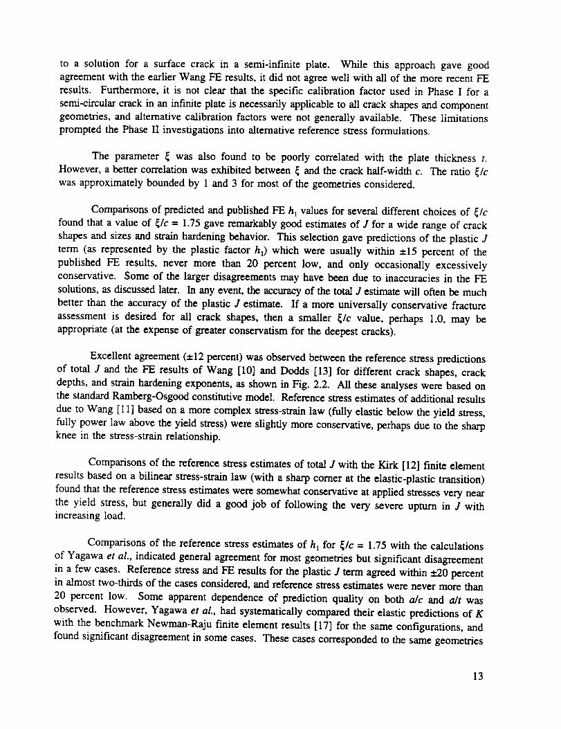
Comparisons of predicted and published FE h_ values for several different choices of _/c

found that a value of _lc -- 1.75 gave remarkably good estimates of J for a wide range of crack

shapes and sizes and strain hardening behavior. This selection gave predictions of the plastic J

term (as represented by the plastic factor hi) which were usually within +15 percent of the

published FE results, never more than 20 percent low, and only occasionally excessively

conservative. Some of the larger disagreements may have been due to inaccuracies in the FE

solutions, as discussed later. In any event, the accuracy of the total J estimate will often be much

better than the accuracy of the plastic J estimate. If a more universally conservative fracture

assessment is desired for all crack shapes, then a smaller _/c value, perhaps 1.0, may be

appropriate (at the expense of greater conservatism for the deepest cracks).

Excellent agreement (±12 percent) was observed between the reference stress predictions

of total J and the FE results of Wang [10] and Dodds [13] for different crack shapes, crack

depths, and strain hardening exponents, as shown in Fig. 2.2. All these analyses were based on

the standard Ramberg-Osgood constitutive model. Reference stress estimates of additional results

due to Wang [ 11] based on a more complex stress-strain law (fully elastic below the yield stress,

fully power law above the yield stress) were slightly more conservative, perhaps due to the sharpknee in the stress-strain relationship.

Comparisons of the reference stress estimates of total J with the Kirk [12] finite element

results based on a bilinear stress-strain law (with a sharp corner at the elastic-plastic transition)

found that the reference stress estimates were somewhat conservative at applied stresses very near

the yield stress, but generally did a good job of following the very severe upturn in J withincreasing load.

Comparisons of the reference stress estimates of h t for _lc = 1.75 with the calculations

of Yagawa et al., indicated general agreement for most geometries but significant disagreement

in a few cases. Reference stress and FE results for the plastic J term agreed within ±20 percent

in almost two-thirds of the cases considered, and reference stress estimates were never more than

20 percent low. Some apparent dependence of prediction quality on both a/c and a/t was

observed. However, Yagawa et al., had systematically compared their elastic predictions of K

with the benchmark Newman-Raju finite element results [17] for the same configurations, and

found significant disagreement in some cases. These cases corresponded to the same geometries

13

to °

b _

5

4

3

2

0

Wang (1988)

[] n=lO

• n=5

a/t = 05

a/c = 1

0.2 0.4 0.6 0.8 1 1.2

°_

6

5

4

3

2

0

Dodds (1992)

0 n=lO

n=4

a/t = 0.25

a/c = 0.33

0 0.5 1 1.5 2 2.5

Figure 2.2. Comparison of reference stress J predictions (solid line)

with Wang (top) and Dodds (bottom) finite element results

14

wherethereferencestressJ estimates most disagreed with Yagawa, indicating that some of the

Yagawa results may be in error.

More detailed comparisons of the simple estimation technique with the various FE results

are given in Appendix A.

The search for improved J solution techniques is continuing under other contract efforts

[18] at SwRI as new finite element J solutions become available and new insights into the

reference stress approach axe gained. However, the technique described above, which was used

throughout the Phase II effort on the current contract, appears to be a reasonably accurate and

robust approach for members loaded in uniform uniaxial tension.

2.2 J-Integral Solutions for Cracks at Notches

The behavior of cracks at notches during MCPT was a topic of particular interest due to

the observations in the Phase I studies about the effects of local control mode on crack growth.

Notched geometries are one form of intermediate control mode; although the remote boundary

conditions may be driven in load control, the local elastic-plastic deformation at the notch root

generates a local response which exhibits some characteristics of displacement or strain control.

However, J solutions are not readily available for cracks at notches. Only a very limited

number of solutions for a very limited range of geometries and loading conditions are available

in the literature. Therefore, it was necessary to generate a new series of J solutions that could

be used in later parameter studies of MCPT behavior. First, a series of finite element analyses

were performed on a selected notch geometry in order to obtain elastic and fully plastic J

solutions. Next, a simple estimation technique with greater generality was derived and validated

against these FIE calculations. The estimation technique was required for the parameter studies

because it was not practical to perform the full FE analysis for each crack size and notch

geometry in the parameter studies.

2.2.1 Finite Element Results

J solutions were computed for cracks emanating from notches using the elastic-plastic

finite element method. Preliminary linear elastic runs were made to verify the finite element

model used in the computations would provide good accuracy. The stress intensity factors for

cracks were calculated, and these solutions were compared with the expected values for very

short cracks (which experience an approximately uniform local stress of K$_ where K, is the

stress concentration factor, and S r the nominally applied stress) and relatively long cracks (which

should behave as cracks of depth a = D + d subjected to a gross section stress, S_ where D is

the depth of the notch and d the actual crack depth measured from the root of the notch).

Three double edge notch geometries under plane stress tensile loading were considered

in the investigation, corresponding to K, values of 4.29, 6.43, and 8.57 where

15

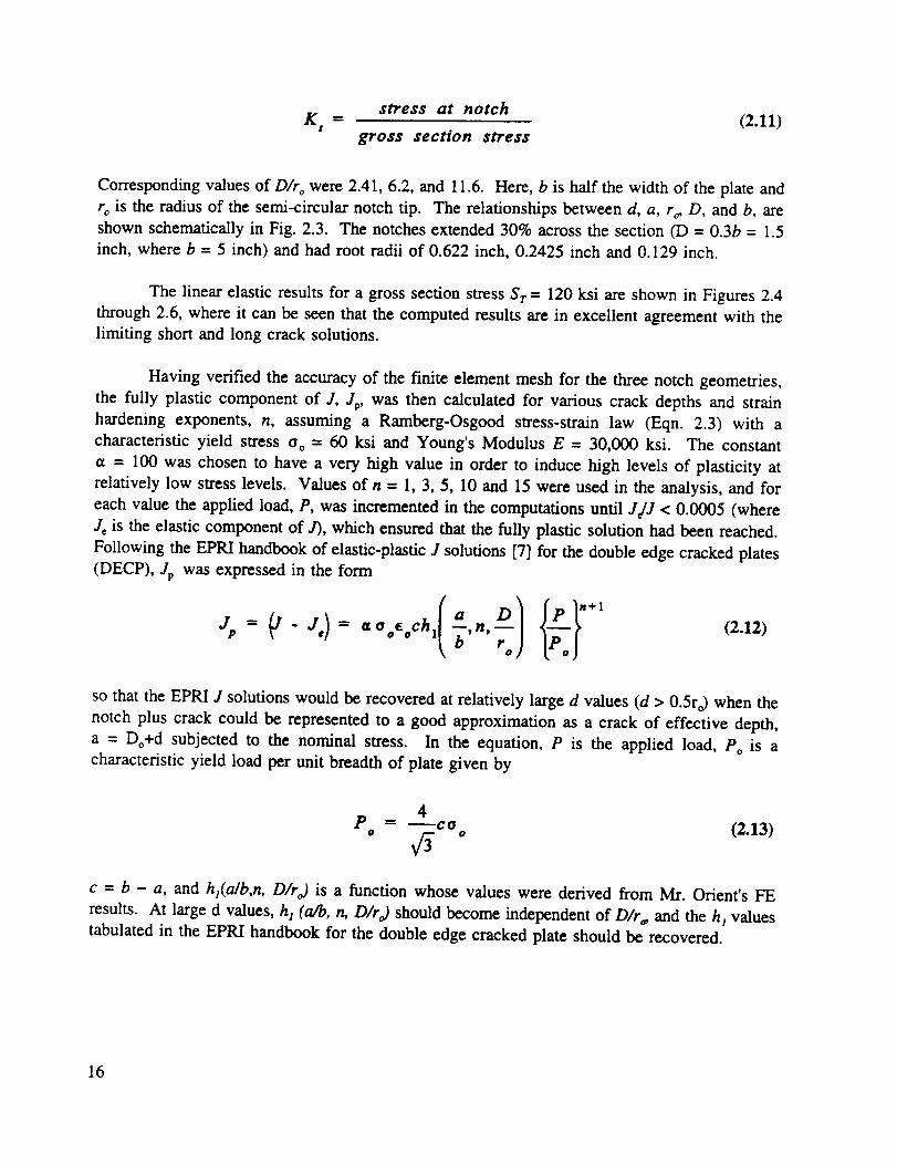
stress at notchK t = (2.11)

gross section stress

Corresponding values of D/ro were 2.41, 6.2, and 11.6. Here, b is half the width of the plate and

ro is the radius of the semi-circular notch tip. The relationships between d, a, r o, D, and b, are

shown schematically in Fig. 2.3. The notches extended 30% across the section (D = 0.3b = 1.5

inch, where b = 5 inch) and had root radii of 0.622 inch, 0.2425 inch and 0.129 inch.

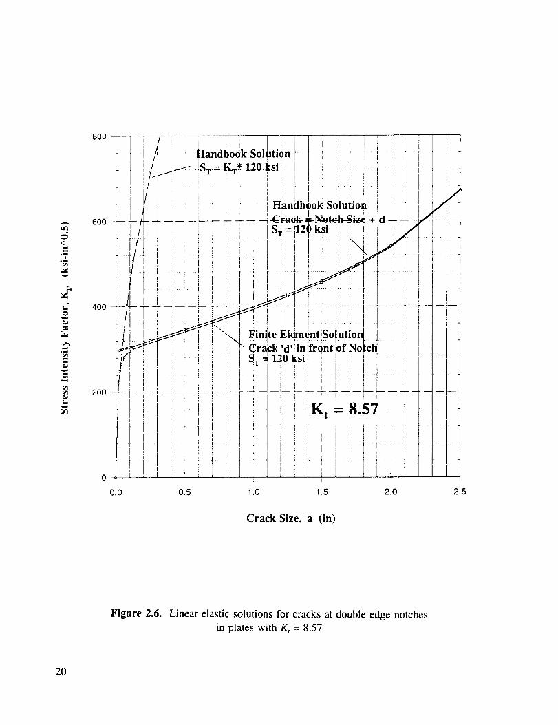
The linear elastic results for a gross section stress S r = 120 ksi are shown in Figures 2.4

through 2.6, where it can be seen that the computed results are in excellent agreement with the

limiting short and long crack solutions.

Having verified the accuracy of the finite element mesh for the three notch geometries,

the fully plastic component of J, Jp, was then calculated for various crack depths and strain

hardening exponents, n, assuming a Ramberg-Osgood stress-strain law (Eqn. 2.3) with a

characteristic yield stress Oo = 60 ksi and Young's Modulus E = 30,000 ksi. The constant

tt = 100 was chosen to have a very high value in order to induce high levels of plasticity at

relatively low stress levels. Values of n = 1, 3, 5, 10 and 15 were used in the analysis, and for

each value the applied load, P, was incremented in the computations until JJJ < 0.0005 (where

Je is the elastic component of J), which ensured that the fully plastic solution had been reached.

Following the EPRI handbook of elastic-plastic J solutions [7] for the double edge cracked plates

(DECP), Jp was expressed in the form

_, - = '_ (2.12)

L oJ

so that the EPRI J solutions would be recovered at relatively large d values (d > 0.Sro) when the

notch plus crack could be represented to a good approximation as a crack of effective depth,

a = Do+d subjected to the nominal stress. In the equation, P is the applied load, P° is a

characteristic yield load per unit breadth of plate given by

4P = _co (2.13)

° °

c = b - a, and hl(a/b,n, D/ro) is a function whose values were derived from Mr. Orient's FE

results. At large d values, h I (o/b, n, D/r,) should become independent of D/r,,, and the hl values

tabulated in the EPRI handbook for the double edge cracked plate should be recovered.

16

1) tlcrack

11 -"1

Figure 2.3. Schematic showing geometrical relationship between notch depth (D), notch root

radius (r,,), crack depth (d), notch plus crack depth (a), and half plate width (b)

17

<=

°_!

¢,

m

r_

://

t-

8OO

200 - -

i

O-

i

[ :I

i

Hafld$o0k SolUtion

'd'

]

I

K t = 4.29

/ I I1 "

Crack Size, a (in)

Figure 2.4. Linear elastic solutions for cracks at double edge notches in plates with K,= 4.29

18

800 "

600

!

Crack Size, a (in)

Figure 2.5. Linear elastic solutions for cracks at double edge notches

in plates with K, = 6.43

19

<@u

.mi

C

."4

¢.iN

m

t_

8OO

/

Crack Size, a (in)

Figure 2.6. Linear elastic solutions for cracks at double edge notches

in plates with K, = 8.57

20

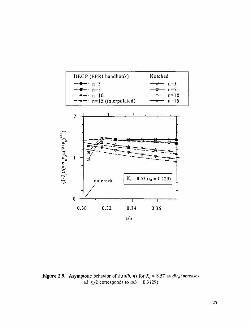
The computedvaluesfor the functionhl(a/b,n,D/r o) for various a/b values are shown in

Tables 2.1 through 2.3 for the cases where Kt=4.29, 6.43, and 8.57, respectively. The same

results are shown in graphical form in Figures 2.7 through 2.9, where the asymptotic behavior

of the solutions at relatively large d/ro can be observed (d = ro/2 corresponds to a/b = 0.3622

in Fig. 2.7, 0.32425 in Fig. 2.8, and 0.3129 in Fig. 2.9). Also shown in the figures are the

h_(a/b,n,D/ro) values given in the EPRI handbook. It can be seen that the results for the deepest

crack obtained in the present study agree reasonably well with the EPRI solutions, showing that,

as in the linear elastic case, the effect of the notch is limited to crack depths, d, which are less

than about half the root radius, ro, of the notch.

2.2.2 Simple J-Estimation Technique

A simple J-estimation technique with greater generality was developed and validated

against these FE calculations. These development and validation exercises were performed under

another NASA-Marshall contract on elastic-plastic fatigue crack growth (EPFCG) [ 18] in order

to fulfill the statement of work of that contract, and so details of the analysis are provided

elsewhere [ 19]. For convenience, since the resulting J-estimation method was employed in the

current program, a brief summary of the method is provided here.

The proposed J estimation scheme for cracks at notches combines the scheme adopted by

EPRI and used in the elastic-plastic handbooks, with the reference stress method (RSM). In the

proposed scheme, hereafter referred to as the modified RSM, first order plasticity effects are

included in J via a first order plastically corrected value for the linear elastic solution, J_, givenby

J (d) = J (d + ,ry) (2.14)

where

J _ K2 (2.15)

c E

and K t is the stress intensity factor. The effective depth, d e = d + _ry, includes a plastic zone

correction determined by the terms _b and ry which are defined as

(2.16)

(2.17)

21

Table 2.1. Numerical values of the shape factors for K, = 4.29

a/b n=3 n=5 n=10 n=15

0.315 0.929 1.072 1.203 1.210

0.326 1.203 1.327 1.350 1.223

0.337 1.345 1.425 1.304 1.157

0.347 1.416 1.440 1.257 1.100

0.358 1.449 1.419 1.215 1.050

0.369 1.459 1.398 1.175 1.006

0.380 1.457 1.378 1.139 0.966

Table 2.2. Numerical values of the shape factors

a/b n-3 n=5 n=10 n=15

0.315 1.290 1.416 1.376 1.261

0.326 1.426 1.453 1.319 1.190

0.337 1.444 1.428 1.270 1.130

0.347 1.442 1.407 1.229 1.079

0.358 1.440 1.389 1.191 1.034

0.369 1.438 1.372 1.155 0.994

0.380 1.436 1.356 1.124 0.958

for K, = 6.43

Table 2.3. Numerical values of the shape factors for K, = 8.57

a/b n-3 n=5 n=10 n-15

0.304 0.952 1.115 1.265 1.283

0.315 1.417 1.457 1.351 1.241

0.326 1.434 1.432 1.302 1.178

0.337 1.432 1.413 1.260 1.124

0.347 1.431 1.397 1.221 1.076

0.358 1.430 1.381 1.185 1.029

0.369 1.429 1.366 1.150 0.986

0.380 1.428 1.350 1.117 0.947

22

DECP (EPRI handbook) Notched

---e--- n=3 _ n=3

---!--- n=5 _ n=5

---A--. n=lO _ n=lO

--_---n=15 (interpolated) _ n=15

2

0

no crack

/' I

0.30 0.32

= 4.29 (r o = 0.622)

' I ' I

0.34 0.36

a/b

Figure 2.7. Asymptotic behavior of tb(a/b, n) for K, = 4.29 as d/r o increases

(d=ro/2 corresponds to a/b = 0.3622)

23

DECP (EPRI handbook) Notched

---o--. n=3 + n=3

--4--- n=5 + n=5---A--- n=10 + n=10

---v---n=15 (interpolated) + n=15

÷a

UO

tdQ

_..,.t u

!

2 I l I i I l

0

no crack

/K, = 6.43 (ro = 0.2425) [

0.30 0.32 0.34 0.36

a/b

Figure 2.8. Asymptotic behavior of h,(alb, n) for K, = 6.43 as d/r o increases

(d=ro/2 corresponds to a/b = 0.32425)

24

DECP (EPRI handbook) Notched---o--- n=3 + n=3

---_--- n=5 _ n=5

---_--- n=10 + n=10

---v--- n=15 (interpolated) + n=15

2

_o 1

!

0

no crack

/' t

I_ = 8.57 (ro = 0.129) I

' I _ I '

0.30 0.32 0.34 0.36

a/b

Figure 2.9. Asymptotic behavior of hl(a/b, n) for K, = 8.57 as d/r o increases

(d=rJ2 corresponds to a/b = 0.3129)

25

Here again C2 equals 2 for plane stress, and 6 for plane strain. This ensures that the correct

linear elastic limit is recovered by the scheme.

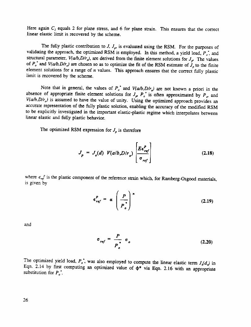
The fully plastic contribution to Z Jp, is evaluated using the RSM. For the purposes of

validating the approach, the optimized RSM is employed. In this method, a yield load, Po', and

structural parameter, V(a/b,D/ro), are derived from the finite element solutions for J¢ The values

of Po" and V(a/b,D/ro) are chosen so as to optimize the fit of the RSM estimate of Jp to the finite

element solutions for a range of n values. This approach ensures that the correct fully plasticlimit is recovered by the scheme.

Note that in general, the values of Po" and V(a/b,D/r,) are not known a priori in the

absence of appropriate finite element solutions for Jw Po" is often approximated by Po, and

V(a/b,D/r o) is assumed to have the value of unity. Using the optimized approach provides an

accurate representation of the fully plastic solution, enabling the accuracy of the modified RSM

to be explicitly investigated in the important elastic-plastic regime which interpolates betweenlinear elastic and fully plastic behavior.

The optimized RSM expression for Jp is therefore

J- J(d) V(a/b,D/ro)E e ,P,f

a ref

(2.18)

where e,,f is the plastic component of the reference strain which, for Ramberg-Osgood materials,is given by

(2.19)

and

P

a,,f • a, (2.20)P

O

The optimized yield load, Po', was also employed to compute the linear elastic term J,(do) in

Eqn. 2.14 by first computing an optimized value of _* via Eqn. 2.16 with an appropriatesubstitution for Po'.

26

Thisestimationtechniquewasextensivelyvalidatedby comparisonwith availablefiniteelementresults,includinga total of 10EPRIJ solutions [20] and 88 J solutions generated in this

program (as described earlier). Agreement was excellent in nearly all cases. Further details areavailable in Reference [19].

2.3 Elastic-Plastic Fatigue Crack Growth Analysis

The customary approach to analysis of crack growth under monotonic loading employs

the maximum value of the stress intensity factor, K, or the J-integral. However, crack growth

during multiple cycle proof testing can occur due not only to monotonic modes such as ductile

tearing, but also due to cyclic modes such as fatigue crack growth (FCG).

When small-scale yielding is satisfied, the range of the stress intensity factor (AK) is

well-established as the parameter of choice to solve practical FCG problems. In the

elastic-plastic regime, however, AK is clearly invalid, and an alternative parameter must be

employed [21 ]. Proposed choices in this case include relatively simple parameters such as the

range of the strain intensity factor (AKe), the crack-tip opening displacement (fit), and the

J-integral (A J); and more sophisticated path-area integrals [22] such as J* and 7"*.

The selection of the optimum parameter must be guided equally by at least three

considerations. The first is that the parameter must represent with sufficient accuracy the actual

driving force for crack extension or the actual crack growth mechanism: the parameter must be

physically meaningful and theoretically valid. The second is that the parameter must be easily

and accurately calculated or estimated for a variety of actual materials, loads, and crack

configurations: it must be practical. The third is that the parameter must have demonstrated

success in the actual correlation of FCG rate data under different conditions: it must be useful.

At the present time and based on these criteria, AJ appears to be the parameter of choice

for characterization of EPFCG. J is now widely recognized as an appropriate and physically

meaningful parameter to characterize elastic-plastic crack growth under monotonic loading, and

early objections about the use of J for cyclic loading have been answered satisfactorily [23-25].

The large number of J solutions and J-estimation schemes developed for elastic-plastic fracture

problems are readily available to characterize the crack driving force in FCG quickly and

accurately for many different geometries and materials. And finally, AJ has been used

successfully by dozens of researchers and engineers during the past twenty years to correlateactual FCG data and predict actual fatigue lives.

Lamba and others [23-25] have pointed out that the correct estimate of AJ comprises the

monotonic J expression with single values of o and e replaced by their ranges, A o and A e (not

independent calculations of J,,_ and Jm,,)" The cyclic analog of Eqn. 2.1, then, is

27

A J- _/(2I F2 ( n-IE- l+_ C 2 n+ 1 a. /a o + 4aa oeoah 1 2°oj (2.21),+(o'-,oorJJ

Here the plastic term includes the "doubling" of the monotonic stress-strain curve to approximate

correctly the effects of reversed deformation. Further changes in the constitutive relationship due

to cyclic hardening or softening are addressed through changes in the Ramberg-Osgood constants,

as discussed later. Alternative formulations based on the reference stress approach can easily be

written for non-Ramberg-Osgood materials.

However, many authors have concluded that the proper form of AJ for correlation of

EPFCG data must include corrections for plasticity-induced crack closure [21]. This closure

correction is particularly important because crack opening stresses under EPFCG conditions can

be significantly different from typical small-scale yielding (SSY) behavior. Based on energy

arguments [21], the correct form of the closure-corrected Ajar expression appears to be given

approximately by

{ /A Joy (UaK) 2 1+E' C 2

o._/0....._2_o + 4a aotoa h IU _ (2.22)

,+(o.-.-,oo)'jjwhere U is the effective stress range ratio,

O -O

U = "_ "P"" (2.23)O -O

mix ram

Here Oo_ n is the nominal stress at which the crack first becomes fully open during the

load-increasing half of the cycle. Note that in the derivation of Eqn. 2.22, U was applied to the

stress range and the elastic strain range, but not to the plastic strain range. Kubo et al. [26] have

shown from their finite element analyses of growing cracks under cyclic loading that AJef fapproximately satisfies path-independence.

The effective stress range ratio U was estimated as a function of o=,,/o o and the stress

ratio R = o_/o_,_ from finite element analyses of crack closure in a low hardening material

under intermediate and large scale yielding conditions [27]. Alternatively, U can be estimated

from a set of simple equations developed by Newman [28] based on his modified-Dugdale

closure model. Although the Newman equations were originally developed for SSY conditions,

their extension into the EPFCG regime with a suitable choice of o o has been demonstrated [21].

28

Adequatepredictionsof crack growth ratesdue to FCG mechanismsfollow from anaccuratecharacterizationof Ajar and a simple Paris equation crack growth relationship

da

dN- c ,,) (2.24)

Exceptions to this philosophy are those applications in which alternative crack growth

mechanisms come into play, such as ductile tearing or creep-fatigue.

A more comprehensive engineering methodology for elastic-plastic fatigue crack growth

is under development in another contract effort [18, 29-30].

2.4 Tear-Fatigue Theory

The fundamental problem in developing an analytical model of multiple-cycle proof

testing is understanding and quantitatively describing crack growth during large

load-unload-reload cycles, when deformation is elastic-plastic and both fatigue and ductile tearing

crack extension mechanisms may be active. As noted in the Interim Report from Phase I [6],

a variety of analytical theories and experimental data have been published to support different

fracture mechanics approaches to related load-unload-reload problems. These different

approaches are not always consistent, and some experimental data appear to conflict with sometheories.

A simple analytical model was proposed in the Phase I Report as an aid to further

analytical and experimental investigations in the context of the MCPT contract. This model was

based on the J-resistance curve and so directly addressed only ductile tearing contributions to

crack extension. The effects of multiple cycles were included by updating the origin (initial

crack length) of the resistance curve to the final crack length from the previous cycle. This was

recognized as a bounding criterion; the other bound was to do no updating and hence to predictno growth on any subsequent cycle to the same maximum load.

Around the same time that the SwRI/Rocketdyne team was beginning the Phase I effort,

technical staff at the former Central Electricity Generating Board (CEGB) in the UK were

engaged in detailed studies of related load-unload-reload crack growth phenomena which were

motivated by their power plant applications. They developed an analytical theory and a

corresponding computational framework to describe these phenomena, which they described as

"tear-fatigue" [31, 32], and conducted detailed experimental validations. One of the principal

investigators in these studies, Dr. Graham Chell, subsequently joined the SwRI technical staff.

Upon critical review, the tear-fatigue concepts were found tO be generally consistent with the

Phase I and early Phase II experimental results and with the evolving analytical approach in

Phase II. Furthermore, the tear-fatigue approach appears to provide a suitable quantitative

framework within which to describe MCPT effects in aerospace propulsion systems.

29

The tear-fatiguemodeldescribescrackgrowth asthe linearsummationof growth due tofatigueandductile fracture,

da/dN = (da/dN)f + (da/dN')t (2.25)

where (da/dN)t is the crack growth rate given by a relationship describing the fatigue contribution

to crack extension, such as the Paris Law, and (da/dN)t is the crack growth in each load cycle

due to ductile tearing, as expressed by a J-resistance curve construction. In this model, it is

assumed that fatigue and ductile fracture mechanisms do not interact. For ductile tearing to occur

during cyclic loading, it is necessary for the value of the J integral calculated at maximum load,

"/max, to increase with each cycle.

Equation 2.25 can be further expanded to give the crack growth rate equation

Here Jm,, is the crack growth resistance value of J characterizing ductile tearing as measured

under monotonic loading, and A a t is the total crack extension due to ductile tearing. The term

(dJmJdN) describes the increase in J=_ in each cycle due to an increase in crack length caused

by the fatigue and tearing mechanisms. These equations were originally assumed to apply only

for Jm_ > Ji, where Ji is some suitable measure of J for the initiation of tearing. As will be

shown later, the customary value of J_c may be a poor choice for Ji under some conditions.

This model is interpreted geometrically in Fig. 2.10. Here the ductile crack growth

relationship is expressed in terms of the interaction between the J-applied and J-resistance curves

in J vs. total a space. The J-resistance curve originates from the true initial crack length for a

"virgin" precracked specimen. As noted above, on subsequent cycles the effective origin of the

tearing resistance curve is advanced by an increment equal to the fatigue crack growth

contribution, (da/dN)t. The two individual components of crack growth are shown more clearly

in the idealized inset diagram. Note in this construction that dJ=ddN includes the slight increase

in Jm_x due to the additional tearing dA a t.

Several minor extensions of this model appear to be required to address the full range of

possible MCPT problems. First of all, although the original tear-fatigue model was expressed

in terms of A J, subsequent work concentrated on assumed FCG calculations based on the linear

elastic stress intensity factor, AK. For generality, the model was modified to express the crack

driving force in terms of the appropriate elastic-plastic parameter, Ajar [21], including crack

closure effects. For many load-unload-reload proof test applications with a minimum applied

stress of zero, the fully plastic component of Ajar will be essentially zero (since the effective

cyclic yield strength for reversed loading is twice the normal monotonic value), even if the

maximum load or stress exceeds the yield condition. However, the intermediate-scale plasticity

term in AJ_ (the effective crack length term, which is a fast-order plasticity correction) may not

30

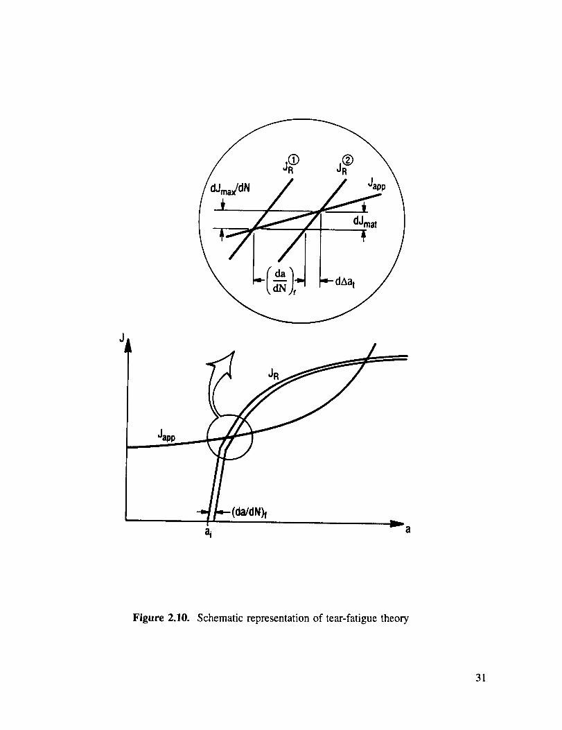
J

JR

(da/dN)f

ai _ a

Figure 2.10. Schematic representation of tear-fatigue theory

31

be negligible. And if constraint conditions impose locally compressive loading (i.e., a negative

stress ratio), the fully plastic Ajar term may make some meaningful contributions. Furthermore,

the general J (rather than K) framework for the fatigue calculation facilitates other modifications

which involve the relationship between the fatigue and tearing resistance curves.

Two minor modifications to the model appear useful to preserve consistency between the

treatment of tearing and fatigue under conditions when fatigue precedes tearing, the two

contributions are of comparable magnitude, and the crack advance per cycle is comparatively

large in comparison to the section thickness or remaining ligament. The first modification

addresses the first occurrence of ductile tearing following previous fatigue cycling. Traditional

applications of tear-fatigue theory assumes that no tearing occurs until Jm_ exceeds some value

J,, which is commonly taken as J_c or some similar standard measure of initiation toughness.

However, since these typical values of Ji are associated with some finite value of Aa, on the J-

resistance curve, the fast exceedance of Ji will cause a sudden jump in the crack length by Aa_

When A aj is a small number in comparison to the local geometry (crack size, section depth,

remaining ligament, etc.) this artificial jump is of no consequence, but when the local geometric

scale is small (and hence Aa_ is relatively large), the jump can be problematic.

This artificial jump can be avoided in one of two ways. The computationally simplest

way is to employ the entire J-resistance curve as a description of ductile crack advance (ignoring,

for the moment, the differentiation between crack tip blunting and ductile tearing) and to set J_

(and therefore Aa_) as an artificially very small number. The problem can also be addressed

from the standpoint of fatigue crack growth analysis by updating on each cycle the contribution

to fatigue crack advance due to the largest elastic-plastic cycle (from the original J = 0 to the

current J = Jm_) as J_ increases cycle-by-cycle. This approach effectively performs updated

rainflow cycle counting on the entire cyclic J history. This approach also requires translating the

J-resistance curve in accordance with the crack advance due to fatigue crack growth. These two

approaches (employing the entire J resistance curve with an artificially low Ji value, or employing

a more complex FCG analysis with a more realistic J, value) give essentially the same result

when the FCG curve and blunting line portion of the J-R curve are approximately coincidental(see Section 3.2).

One potentially significant difference between the analysis of fatigue crack growth

resistance and tearing resistance in this regime still remains. The classical engineering approach

to tearing resistance curve analysis compares the applied and resistance J curves at the updated

or final crack length (a + Aa), as shown in Fig. 2.10. In other words, J_ - J,_,(a + Aa), and

the final calculated Aa value is also a function of the change in the resistance curve between

Jmax(a) and Jm_(a + Aa). In contrast, the traditional approach to FCG analysis calculates the

cyclic crack growth increment on the basis of the current crack length and does not consider the

influence of this growth increment on the subsequent change in resistance to fatigue crack

growth: J_ = Jm_,(a). Again, this difference is insignificant when the incremental Aa is very

small in comparison to the total a, or when the change in J_ with Aa is negligible, and so no

adjustment is needed for the great majority of FCG analyses. However, when Aa is relatively

large and the applied Jm,_ begins to increase significantly with further Aa (as may often occur

32

nearinstability,especiallyin thin-walledsmall components),anothersmall modificationmay beappropriate.A simplef'u'st-ordercorrectionto thecracklengthappearsadequate.This fu'st-order

correction involves first simply predicting an initial guess for Aa c1_on the basis of the crack

length at the beginning of the cycle: j, c_ = j_a_(at,',). Then an updated value of J,,_ based on

the new crack length (a tn_+ Aa tlr) is computed, and this new value of j, c2_is used to make an

updated prediction for Aa c21. The final predicted value of the crack length is then a cn÷_ = a _D_+

Aa c2_. The additional accuracy introduced by further iteration is insufficient to warrant the effort.

33

3. EXPERIMENTAL CHARACTERIZATION AND VALIDATION

In Phase I, experimental characterization work included the generation of a J-resistance

curve for surface-flawed IN-718 (employing the Phase I reference stress estimates for _,

generation of baseline fatigue crack growth properties under small-scale yielding conditions, and

SSY FCG crack shape studies based on range marking and post-test fractography.

Significant new experimental characterization and validation activities were conducted in

Phase II. An updated form of the J-resistance curve was developed, based on the Phase I test

results, a few additional surface crack J-R experiments, and the improved reference stress J

estimation methods. The relationship between the J-resistance curve and the fatigue crack growth

curve was explored. A number of additional crack growth tests were conducted to guide and

verify methodology development, with a primary focus on the effects of various cyclic histories

(different control conditions and load ratios) and crack depths. Specialized tests examined

simulated MCPT load histories as well as fatigue cycling following a proof overload.

Fractographic studies were conducted to evaluate crack growth micromechanisms and crack shape

development during elastic-plastic loading. The suitability of acoustic emission to detect crack

growth during MCPT was briefly evaluated. All of these experimental activities and associated

results are documented in some detail in the remainder of the chapter. Further information about

specimen geometry and material properties was provided in the Phase I report [6].

3.1 Updated J-Resistance Curves

Updated Analysis Methods. As noted in the Introduction, a J-resistance curve had been

generated earlier in the program for semi-circular surface cracks in finite-sized plates of Inconel

718. This Phase I J-R curve was based on the Phase I reference stress J estimation techniques

and the surface-crack experiments also conducted during Phase I of the program. As noted in

the Analytical Development section, improved reference stress estimates of J for the semi-

elliptical surface crack in a finite-sized flat plate were developed in Phase II of the program.

Using these new reference stress J estimates, all of the original crack growth experiments that

had been used to construct the Phase I surface crack resistance curve were re-analyzed to

generate a Phase II resistance curve. The Ramberg-Osgood constants (Eqn. 2.3) used in these

J calculations were e 0 = 0.006, o 0 = 179.8 ksi, n - 15.8, and ¢t = 1.

New Surface Crack Experiments. The surface crack experiments conducted in Phase I

were limited to initial crack depths in the general range of a/t = 0.36 to 0.73, with most crack

depths about a/t = 0.6. A critical question posed early in the Phase II investigations was whether

significantly deeper cracks might exhibit different tearing behavior, and if so, whether this might

be an important factor in MCPT failures. In order to investigate these questions, two additional

surface crack tearing resistance experiments were conducted in Phase II. These tests involved

the application of single displacement-controlled cycles to specimens with surface flaw depths

in the range from a/t = 0.8 to 0.9. The tearing resistance data obtained from these deep crack

tests were found to be similar to the previous data from less deep cracks.

34

The updatedtearingresistancedatafor surface-crackedIN-718,includingboth of the newexperiments,andthenewanalysisof bothold andnewexperiments,areshownin Fig. 3.1. Alsoshownon this figure arethe original resistancecurvedatafrom compacttensionspecimens.

Effect of Specimen Thickness on Tearing Resistance. The Phase I analysis of the surface

crack resistance curve had suggested that crack growth resistance in the thicker (t = 0.5) surface

crack specimen was similar to crack growth resistance in the thinner (t - 0.2 in.) surface crack

specimen. The Phase II analysis of the surface crack resistance curves indicated that the new J

formulas gave generally similar results to the old J formulas for the thinner specimens, so that

the J-R curve did not change significantly. However, the new calculated J values for the thicker

specimens were slightly lower than the values calculated in Phase II, so that the 0.2 in. and 0.5

in. data no longer appear to belong to the same population. Although firm conclusions should

not be derived from only four data points, it appears that the crack growth resistance for the thick

surface crack specimens is lower than for the thin surface crack specimens, but still higher thanfor the CT configuration.

The decrease in apparent crack growth resistance for the thicker specimens is qualitatively

consistent with an expected increase in constraint due to the thicker geometry. The thick surface

crack geometry can be thought of as an intermediate case between the thick CT specimens and

the thin surface crack specimens. Note that constraint is affected by a variety of factors,

including specimen thickness, specimen configuration, and applied stress as a fraction of the yield

stress. Constraint generally increases with increasing thickness, tendencies towards bending

rather than tensile configurations, and decreasing applied stress. The thick surface crack

specimens compared to the thinner specimens also experienced slightly lower maximum applied

stresses (Om_x = 120-150 ksi for thick specimens, 150-180 ksi for thin specimens, compare Oys= 165 ksi).

Current thinking in the international fracture mechanics community is that these apparentchanges in crack growth resistance may in fact be only apparent effects and not real effects. The

argument is that a single parameter (J) description is insufficient to describe the changes in the

driving force for crack extension that are caused by changes in constraint. In other words,

constraint actually influences the applied driving force, not the resistance. The approach

currently receiving the most attention as a means of correcting this claimed deficiency is a two-

parameter characterization of the driving force based on J and a factor Q, which is derived from

the higher order terms in the crack-tip stress field expression and which essentially describes the

hydrostatic stress components via comparison with the benchmark Hutchinson-Rice-Rosengren

(HRR) stress fields. Unfortunately, practical applications of J-Q theory are still largely in their

infancy at this writing. Most investigations to date have focused on two-dimensional geometries

rather than surface cracks, and elastic-plastic crack extension involving cleavage rather than stable

ductile tearing. Therefore, at the present time, these constraint effects must be characterized in

terms of apparent changes in the resistance curve.

35

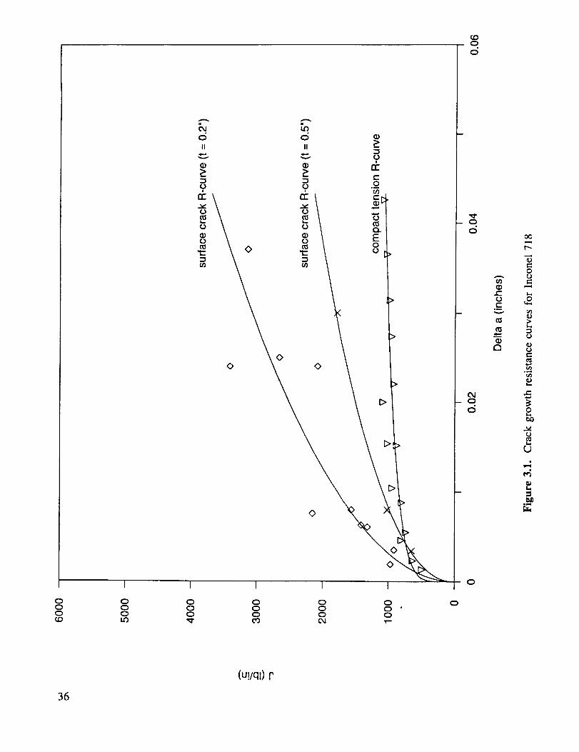
t.O0

0 0 0 0 0 00 0 0 0 0 00 0 0 0 0 0

0

0

°--

t_

00

t-O

r-

t-

O

om

36

(u!/ql) r

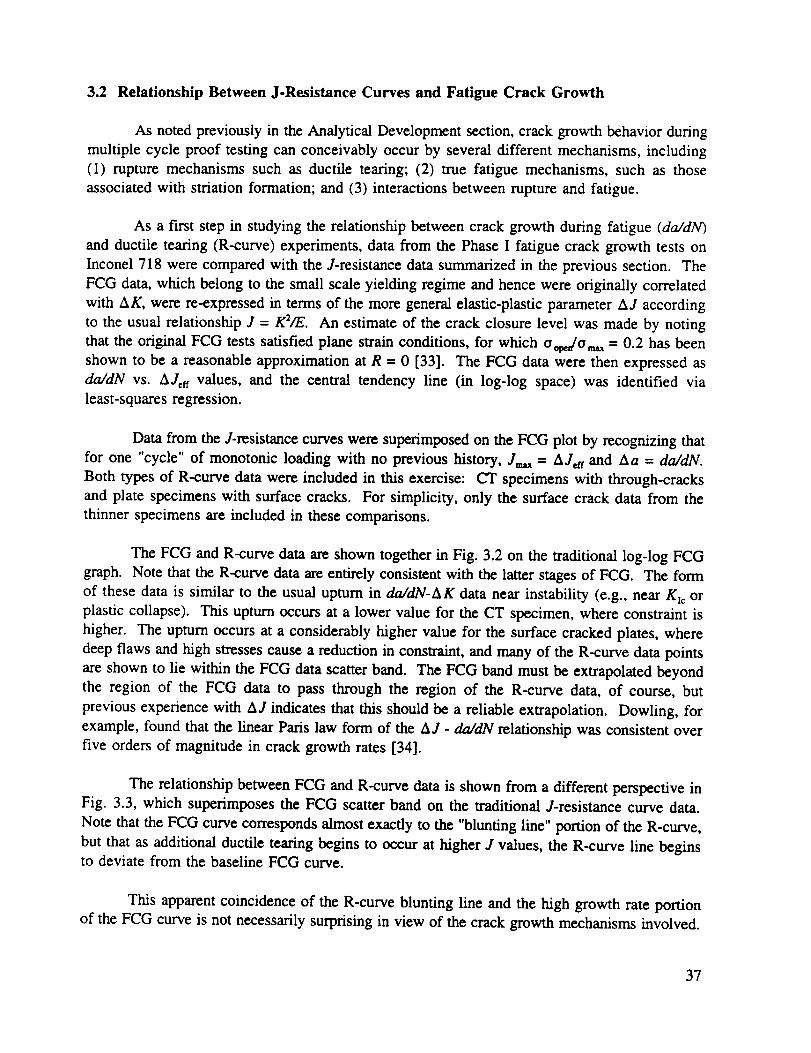
3.2 Relationship Between J-Resistance Curves and Fatigue Crack Growth

As noted previously in the Analytical Development section, crack growth behavior during

multiple cycle proof testing can conceivably occur by several different mechanisms, including

(1) rupture mechanisms such as ductile tearing; (2) true fatigue mechanisms, such as those

associated with striation formation; and (3) interactions between rupture and fatigue.

As a first step in studying the relationship between crack growth during fatigue (da/dN)

and ductile tearing (R-curve) experiments, data from the Phase I fatigue crack growth tests on

Inconel 718 were compared with the J-resistance data summarized in the previous section. The

FCG data, which belong to the small scale yielding regime and hence were originally correlated

with AK, were re-expressed in terms of the more general elastic-plastic parameter AJ according

to the usual relationship J = K2/E. An estimate of the crack closure level was made by noting

that the original FCG tests satisfied plane strain conditions, for which Oo_JOm_ = 0.2 has been

shown to be a reasonable approximation at R = 0 [33]. The FCG data were then expressed as

da/dN vs. A Jen values, and the central tendency line (in log-log space) was identified via

least-squares regression.

Data from the J-resistance curves were superimposed on the FCG plot by recognizing that

for one "cycle" of monotonic loading with no previous history, J_, = Ajar and Aa = da/dN.

Both types of R-curve data were included in this exercise: CT specimens with through-cracks

and plate specimens with surface cracks. For simplicity, only the surface crack data from the

thinner specimens are included in these comparisons.

The FCG and R-curve data are shown together in Fig. 3.2 on the traditional log-log FCG

graph. Note that the R-curve data are entirely consistent with the latter stages of FCG. The form

of these data is similar to the usual upturn in da/dN-AK data near instability (e.g., near Kit or

plastic collapse). This upturn occurs at a lower value for the CT specimen, where constraint is

higher. The upturn occurs at a considerably higher value for the surface cracked plates, where

deep flaws and high stresses cause a reduction in constraint, and many of the R-curve data points

are shown to lie within the FCG data scatter band. The FCG band must be extrapolated beyond

the region of the FCG data to pass through the region of the R-curve data, of course, but

previous experience with AJ indicates that this should be a reliable extrapolation. Dowling, for

example, found that the linear Paris law form of the AJ - da/dN relationship was consistent over

five orders of magnitude in crack growth rates [34].

The relationship between FCG and R-curve data is shown from a different perspective in

Fig. 3.3, which superimposes the FCG scatter band on the traditional J-resistance curve data.

Note that the FCG curve corresponds almost exactly to the "blunting line" portion of the R-curve,

but that as additional ductile tearing begins to occur at higher J values, the R-curve line beginsto deviate from the baseline FCG curve.

This apparent coincidence of the R-curve blunting line and the high growth rate portion

of the FCG curve is not necessarily surprising in view of the crack growth mechanisms involved.

37

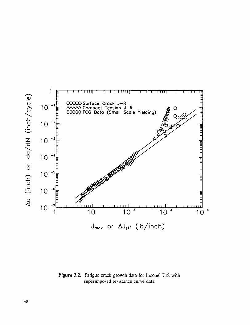
(J>,,(O

..E(Oc-

=m

Z"O

0-O

L.

0

..EL)E

0<3

10 -' , i | lilllJ I I I JlJlJl I I ! IIIIIJ I l I IIII

I 10 10 2 10 3 10'

Jmox or AJ,,, (Ib/inch)

Figure 3.2. Fatigue crack growth data for Inconel 718 with

superimposed resistance curve data

38

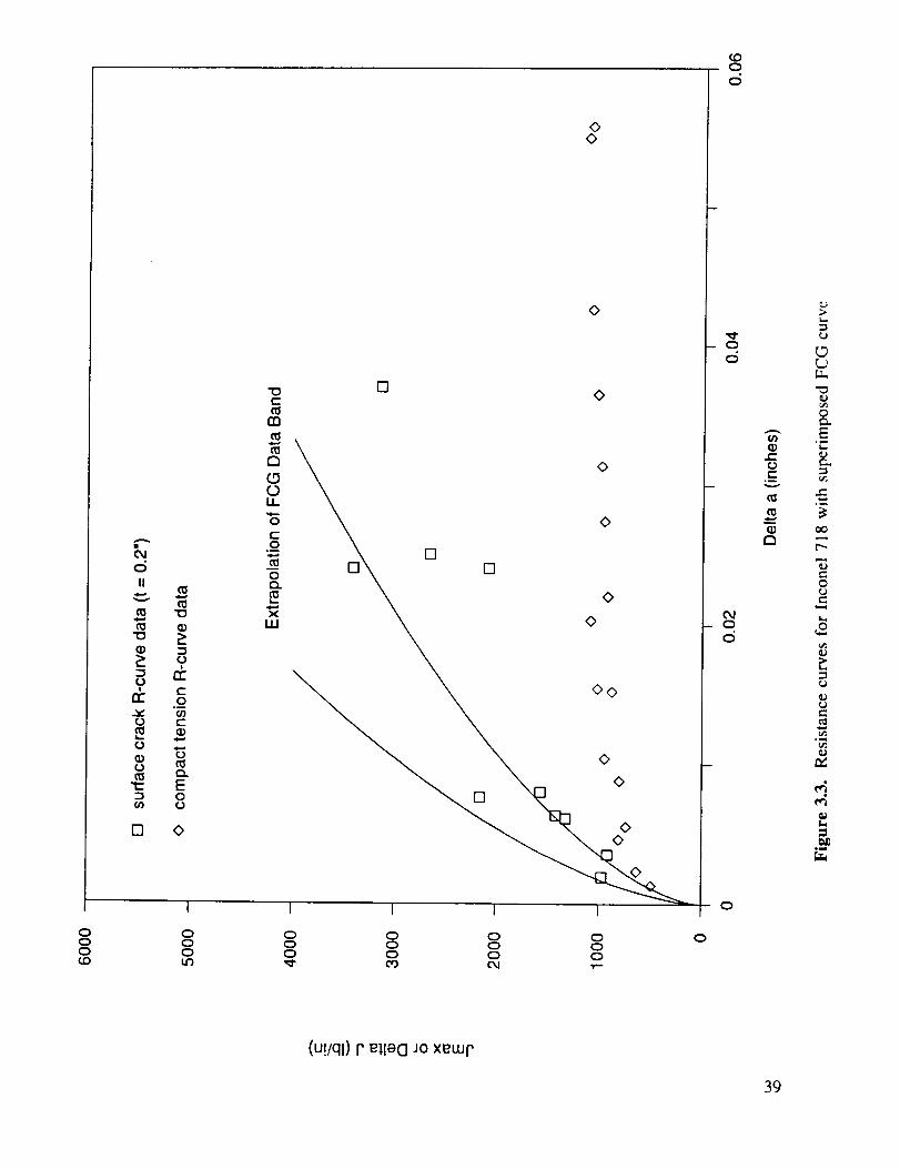
O

O

II

v

n_

?rr

[]

?rrc-O°_

E

O.

EO

o

"OE

m

a

_)U_

O

EO°D

OO.

xW

oo

o

E]O

[]

o

[]

o

I I I I I

O O O O O OO O O O O OO O O O O O

O

d

-- O

d

C_- O

d

O

a)

E

r_

L..

O

E

0o

O

L_

(u!/ql) I" E]IaO JO xEwr'

39

The so-called "blunting" line of the R-curve, as its name implies, is thought to describe the crack

extension during initial loading that occurs due to crack tip blunting alone, before the initiation

of ductile tearing (or brittle cleavage) [35]. On the other hand, the mechanism of Stage II crack

growth during low cycle fatigue is widely believed to be a progressive plastic blunting process

[36]. The broadening of slip zones at the crack tip and the associated blunting of the crack tip

during the tensile loading excursion in low cycle fatigue define the extent of crack advance

during that particular cycle, before the application of reversed loading (locally compressive)

causes a reversal of slip directions and a crushing/folding of the new crack surfaces. The point

to be made is that the basic mechanism of crack extension is apparently the same in both the

"low cycle fatigue crack growth" process and the blunting portion of the "ductile fracture"

process. The material at the crack tip is largely unaware of whether initial blunting will be

followed by further loading to tearing or by unloading. The primary difference in the two

processes is the more complex residual stress/deformation field that develops in the vicinity of

the fatigue crack tip due to previous load/unload and crack growth histories. Consideration of

crack closure effects, as we have done above, represents a first-order compensation for thisdifference.

Wilhem and Ratwani [37] previously suggested a similar relationship between fatigue and

fracture data as described by the linear elastic stress intensity factor (AK and Ka), based on their

empirical observations of crack growth in 2024-T3 aluminum. They proposed a "full range

resistance curve" that was a continuous, monotonically increasing function of crack extension and

that was composed of both fatigue (da vs. K,_) and fracture (Aa vs. Kr0 data. Their primary

goal was apparently to reconcile thickness effects in fatigue crack growth rate data by relating

them to thickness effects on the R-curve. Wilhem and Ratwani went on to suggest that there

may not be a smooth transition between fatigue resistance and fracture resistance portions of the

curve, based on their supposition that the crack tip plastic zone in fatigue was different in size

from that developed during static (monotonic) loading. Actually, however, the size of the

"forward" plastic zone has been shown to be essentially the same under monotonic and cyclic

loading [38]. Any apparent discontinuities between fatigue and fracture data may instead be dueto uncompensated differences in crack closure behavior.

This line of thinking is consistent with the ideas of Kobayashi et al. [39], who suggested

that the Paris Law (striation mechanism) portion of the fatigue crack growth curve was parallel

to the blunting line. The difference between the two lines was attributed to plasticity-induced

crack closure. The specific data generated by Kobayashi et al. to evaluate these ideas are

somewhat difficult to interpret, however, due in part to the wide range of stress ratios (R = -1.5

to +0.5) and applied loads (elastic to elastic-plastic) considered. Crack closure levels (which

were not measured) are certain to change considerably with both stress ratio and applied load,

and the CT geometry employed was not an ideal choice for load histories with large compressive

excursions. The present investigations were simplified by considering only a single stress ratiofor all tests (R = 0).

The available data are too limited to draw definitive conclusions about the relationship

between the FCG curve and the tearing resistance curve. In the current research program, we

40

have studied only a single material, and only about twenty surfacecrack tests have beenperformed,all with thesamecrackshapeandspecimenwidth. The fatigue crackgrowth curveis extrapolatedfrom lower valuesof thecyclic driving force andthereforesomewhatuncertain,andwe havenot explicitly addressedthe normal+2x scatter in fatigue crack growth rates (the

curve shown represents the mean value). It does appear possible that the fatigue curve serves

as an approximate upper bound to the tearing resistance curve, and the two may be effectively

equivalent for lower constraint and smaller crack growth increments. For higher constraint and

larger crack growth increments, it seems clear that the onset of stable tearing will cause a

divergence of the two curves.

3.3 Characterizing the Onset of Stable Tearing

Also shown in Fig. 3.1 is a power law representation of the surface crack tearing

resistance curve for 0.2-in. thick specimens with the general form (units are inches and lb/in)

da = 3.16(10)'9 (/ )2 (3.1)

As noted in the Phase I Report, there is no single theoretically correct mathematical form of the

resistance curve. Several different empirical forms have been proposed [40]. The power law

form was chosen here because it seemed to correspond well to the individual data points, and

because it was consistent with the general power law form of the fatigue crack growth curve.

The general form of the FCG curve, for comparison, was

da

dN- 3.5 0(1 0)-8 (A jeff)l.62 (3.2)

An appropriate value for Ji, the critical value at which ductile tearing initiates, can be

chosen as the intersection of the fatigue crack growth curve and the tearing resistance curve,

which is essentially the point at which the two curves diverge for increasing crack extension.

For the t = 0.2-in. surface crack data shown, this value was Ji = 557 in.-lbs/in. 2.

Note that conventional definitions for Ji, such as the Jic value based on the ASTM

Standard Test Method E 1737, are not appropriate for this application. The current E 1737

methodology defines J_c as the intersection of a constructed offset line parallel to a hypothetical

blunting line of slope 2ono_, where the offset is 0.2 mm (0.008 in.). This definition would lead

to a J_¢ value greater than 2000. in.-Ibs/in. 2 for the given surface crack data, which would cause

serious errors in calculation of crack growth for some intermediate J,_ values by the customary

tear-fatigue approach. Note that the Aa value corresponding to this ark value is on the order of

0.01, which is a significant fraction of the crack depth for some MCPT applications. Of course,

the strict ASTM validity restrictions on JI¢ would also rule out its use for this surface crack

configuration, since the plane strain constraint limitations are not satisfied for the low constraint,high stress surface crack tests.

41

It is also interestingthat the point at which the power law representationof the CTresistancecurveintersectsthefatiguecrackgrowthcurveis about586. in.-lbs/in.:,which is closeto the intersectionpoint of the fatigue curvewith the surfacecrackresistancecurve. Despiteextensiveresearchin the areaby many fracturemechanicsexpertsaroundthe world during thepast few years, the effects of constrainton apparentductile tearing resistanceare still notunderstoodwell. It is not clear if we shouldexpecta higher Ji value for lower constraint, a

higher tearing modulus value (the slope of the tearing resistance curve above J), or both.

3.4 Elastic-Plastic Fatigue Crack Growth Experiments

Further experiments were conducted to investigate fatigue crack growth under elastic-

plastic loading conditions. The cyclic histories were varied to explore the effects of differentloading regimes and different control conditions.

Specimens were 0.2-in thick with semi-circular surface cracks. Initial flaws were

introduced by electro-discharge machining (EDM) followed by fatigue pre-cracking at relatively

low applied stresses. The specimens were heat tinted following the precrack and then again

(under less severe conditions, resulting in a lighter tint) following the completion of the test in

order to aid identification of the fracture surfaces. Most tests were conducted at fixed rates of

crack mouth displacement in order to provide greater experimental control, but some tests were

conducted in load control, and some tests employed a manual form of displacement control in

which decisions about displacement reversals were actually based on observations of applied load.

Careful monitoring of the load and crack mouth opening displacement (CMOD)

information (including on-line computer data acquisition) made it possible to accurately estimate

the changing crack depth by noting the change in elastic specimen compliance and comparing

these values with analytical estimates. Inspection of final crack surfaces showed that the crack

shape remained relatively constant during this large growth, although crack growth immediately

at the specimen surface is typically retarded and some slight "canoeing" is observed. A

photograph of a typical fracture surface is shown in Section 3.7.2 on fractography of crackshapes.

In the first series of elastic-plastic fatigue crack growth tests, initial crack depths were

approximately a/t = 0.6 (a = 0.12-in.). Final crack depths were typically around a/t = 0.75 -

0.85, or about 0.04-in. of crack growth in the depth direction.

The extent of unloading was observed to have a large effect on crack growth during

subsequent loading cycles. Tests in which extensive crack growth on the fast cycle was followed

by unload-reload cycles between zero load and the previous maximum load or displacement (so-

called zero-max loading) resulted in essentially no crack growth during a small number of

subsequent cycles. Other tests in which crack growth on the first cycle was followed by

unloading to zero crack mouth displacement (which corresponds to a large compressive stress)

and repeated reloadings between zero displacement and the previous maximum displacement (so-

called zero-max displacement) resulted in substantial crack growth on essentially all subsequent

cycles. Load vs. crack mouth opening displacement histories for these two types of tests are

42

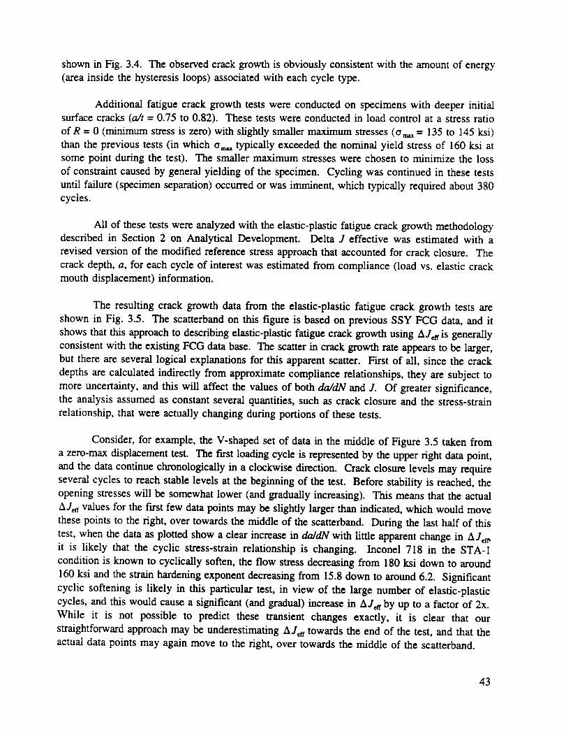
shown in Fig. 3.4. The observed crack growth is obviously consistent with the amount of energy

(area inside the hysteresis loops) associated with each cycle type.

Additional fatigue crack growth tests were conducted on specimens with deeper initial

surface cracks (a/t = 0.75 to 0.82). These tests were conducted in load control at a stress ratio

ofR = 0 (minimum stress is zero) with slightly smaller maximum stresses (o,_ = 135 to 145 ksi)

than the previous tests (in which o_ typically exceeded the nominal yield stress of 160 ksi at

some point during the test). The smaller maximum stresses were chosen to minimize the loss

of constraint caused by general yielding of the specimen. Cycling was continued in these tests

until failure (specimen separation) occurred or was imminent, which typically required about 380

cycles.

All of these tests were analyzed with the elastic-plastic fatigue crack growth methodology

described in Section 2 on Analytical Development. Delta J effective was estimated with a

revised version of the modified reference stress approach that accounted for crack closure. The

crack depth, a, for each cycle of interest was estimated from compliance (load vs. elastic crack

mouth displacement) information.

The resulting crack growth data from the elastic-plastic fatigue crack growth tests are

shown in Fig. 3.5. The scatterband on this figure is based on previous SSY FCG data, and it

shows that this approach to describing elastic-plastic fatigue crack growth using Ajar is generally

consistent with the existing FCG data base. The scatter in crack growth rate appears to be larger,

but there are several logical explanations for this apparent scatter. First of all, since the crack

depths are calculated indirectly from approximate compliance relationships, they are subject to

more uncertainty, and this will affect the values of both da/dN and J. Of greater significance,

the analysis assumed as constant several quantities, such as crack closure and the stress-strain

relationship, that were actually changing during portions of these tests.

Consider, for example, the V-shaped set of data in the middle of Figure 3.5 taken from

a zero-max displacement test. The first loading cycle is represented by the upper right data point,

and the data continue chronologically in a clockwise direction. Crack closure levels may require

several cycles to reach stable levels at the beginning of the test. Before stability is reached, the

opening stresses will be somewhat lower (and gradually increasing). This means that the actual

AJef t values for the f'trst few data points may be slightly larger than indicated, which would move

these points to the fight, over towards the middle of the scatterband. During the last half of this

test, when the data as plotted show a clear increase in daMN with little apparent change in AJef _

it is likely that the cyclic stress-strain relationship is changing. Inconel 718 in the STA-1

condition is known to cyclically soften, the flow stress decreasing from 180 ksi down to around

160 ksi and the strain hardening exponent decreasing from 15.8 down to around 6.2. Significant

cyclic softening is likely in this particular test, in view of the large number of elastic-plastic

cycles, and this would cause a significant (and gradual) increase in Ajar by up to a factor of 2x.

While it is not possible to predict these transient changes exactly, it is clear that our

straightforward approach may be underestimating Ajar towards the end of the test, and that the

actual data points may again move to the right, over towards the middle of the scatterband.

43

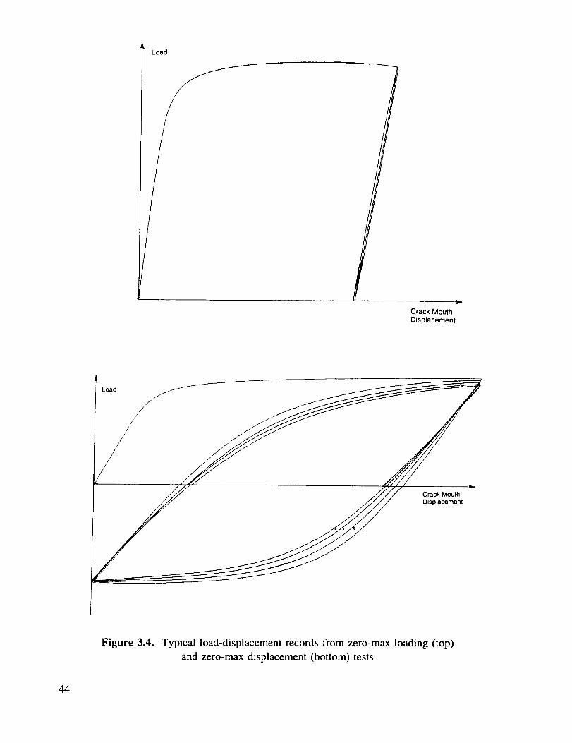
Load

Crack Mouth

Displacement

Load

//

/

Crack Mouth

Displacemenl

Figure 3.4. Typical load-displacement records from zero-max loading (top)

and zero-max displacement (bottom) tests

44

m

m

IIII I I I I Jllll I I I I illlll I I I

Cna,)¢,.)

¢,),.e,,-.0

°m

|

.=_.

c:v,..

ID

m

IIII I I I

i I ! i

nO<>_

0

IIIII I I I

?0

<>

O0 o

III I I I I I

Illl I I I t I lilt I I I t

? 1'(:3 0

'wP,-,-

(ato/[o/u!) Np/0p

O

-O

O

Ee_

.D

Ip

<:}

k_

O

xoE

O(JU.

>-

O

'-or.

,.D

r_

=@

O

E._

L.

,m

J::

@

tj

o_

._.9.

.u

N

I=,

l,u

45

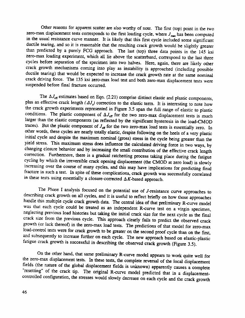
Other reasons for apparent scatter are also worthy of note. The fu'st (top) point in the two

zero-max displacement tests corresponds to the first loading cycle, where J,_ has been computed

in the usual resistance curve manner. It is likely that this first cycle included some significant

ductile tearing, and so it is reasonable that the resulting crack growth would be slightly greater

than predicted by a purely FCG approach. The last (top) three data points in the 145 ksi

zero-max loading experiment, which all lie above the scatterband, correspond to the last three

cycles before separation of the specimen into two halves. Here, again, there are likely other

crack growth mechanisms coming into play as instability is approached (including possible

ductile tearing) that would be expected to increase the crack growth rate at the same nominal

crack driving force. The 135 ksi zero-max load test and both zero-max displacement tests weresuspended before final fracture occurred.

The AJarr estimates based on Eqn. (2.21) comprise distinct elastic and plastic components,

plus an effective crack length (AJz) correction to the elastic term. It is interesting to note how

the crack growth experiments represented in Figure 3.5 span the full range of elastic to plastic

conditions. The plastic component of AJen for the two zero-max displacement tests is much

larger than the elastic components (as reflected by the significant hysteresis in the load-CMOD

traces). But the plastic component of J,n for the two zero-max load tests is essentially zero. In

other words, these cycles are nearly totally elastic, despite following on the heels of a very plastic

initial cycle and despite the maximum nominal (gross) stress in the cycle being greater than the

yield stress. This maximum stress does influence the calculated driving force in two ways, by

changing closure behavior and by increasing the small contribution of the effective crack length

correction. Furthermore, there is a gradual ratchetting process taking place during the fatigue

cycling by which the irreversible crack opening displacement (the CMOD at zero load) is slowly

increasing over the course of many cycles, and this may have implications for predicting final

fracture in such a test. In spite of these complications, crack growth was successfully correlated

in these tests using essentially a closure-corrected A K-based approach.

The Phase I analysis focused on the potential use of J-resistance curve approaches to

describing crack growth on all cycles, and it is useful to reflect briefly on how those approaches

handle this multiple cycle crack growth data. The central idea of that preliminary R-curve model

was that each cycle could be treated as an independent R-curve test on a virgin specimen,

neglecting previous load histories but taking the initial crack size for the next cycle as the final

crack size from the previous cycle. This approach clearly fails to predict the observed crack

growth (or lack thereof) in the zero-max load tests. The predictions of that model for zero-max

load-control tests were for crack growth to be greater on the second proof cycle than on the fn'st,

and subsequently to increase further on each cycle. The new approach based on elastic-plastic

fatigue crack growth is successful in describing the observed crack growth (Figure 3.5).

On the other hand, that same preliminary R-curve model appears to work quite well for

the zero-max displacement tests. In these tests, the complete reversal of the local displacement

fields (the nature of the global displacement fields is unknown) apparently causes a complete

"resetting" of the crack tip. The original R-curve model predicted that in a displacement-

controlled configuration, the stresses would slowly decrease on each cycle and the crack growth

46

rateswould alsodecreaseoneachcycle. Both phenomenawere observedto occur (exceptforthe increasein da/dN during the last half of one test, which has been discussed previously).

Estimates of J,_ for these tests based on conventional R-curve approaches give values that are

similar to the calculated A Jetr values, and so would give similar predictions for crack growth on

each cycle.

3.5 Experimental Simulation of Multiple Cycle Proof Testing

Three surface crack experiments were performed to investigate crack growth under

simulated MCPT histories. These experiments also provided data to evaluate the tear-fatigue

relationships presented earlier in the Analytical Development section.

The initial crack depth on the lust two specimens was slightly larger than previously

tested, between a/t = 0.8 and 0.9, with an aspect ratio around a/c = 0.9. The tests were

conducted in pure load control, at maximum stresses that were expected to cause measurable

crack growth but not to cause gross yielding of the entire uncracked section area. Because the

remaining ligament to the back face was so small, severe plastic deformation was certain to occur

in that region. Multiple load cycles were applied with a hold time at maximum load of 30

seconds. The loading half of the cycle was completed in 10 seconds, while the unloading halfwas completed in 5 seconds.

The fundamental goal in these two tests was to find a maximum stress level at which

appreciable crack growth would occur on more than one cycle. In other words, the intent was

to generate crack growth during several consecutive cycles of a pure zero-max load control test.

In previous experiments, we had typically either seen fracture on the In'st cycle of a load control

test, or some crack growth on the first cycle followed by negligible crack growth per cycle on

subsequent loading cycles.

In short, we were successful in causing crack growth during more than one cycle of these

zero-max load tests. The specific load (P) vs. crack mouth opening displacement histories for

the two tests are shown in Figures 3.6 and 3.7. In both tests, the initial maximum stress was

about 140 ksi, or a load of about 35 kips (note that the yield stress for this IN-718 is about 160

ksi). At least two identical cycles were conducted at that stress level. If no additional increase

in the CMOD was observed on the second cycle (which suggests no additional crack growth),

then the maximum stress was slightly increased, and at least two cycles were conducted at that

new maximum stress. If some CMOD increase was observed on the second cycle at a given

maximum stress, then cycling continued at the same maximum stress (and with the same hold

times) until the CMOD increase per cycle became negligible or until the specimen fractured.

On the first test (specimen $26, Fig. 3.6), the initial maximum stress was 140 ksi. On

the first cycle, some additional CMOD accumulated during the hold time, but the second cycle

P-CMOD trace was essentially elastic with no further CMOD increase during the hold time. The

maximum stress was increased to 143 ksi for the third cycle, and more extensive CMOD increase

occurred during the hold time. On the second cycle at 143 ksi (the fourth cycle overall), how-

47

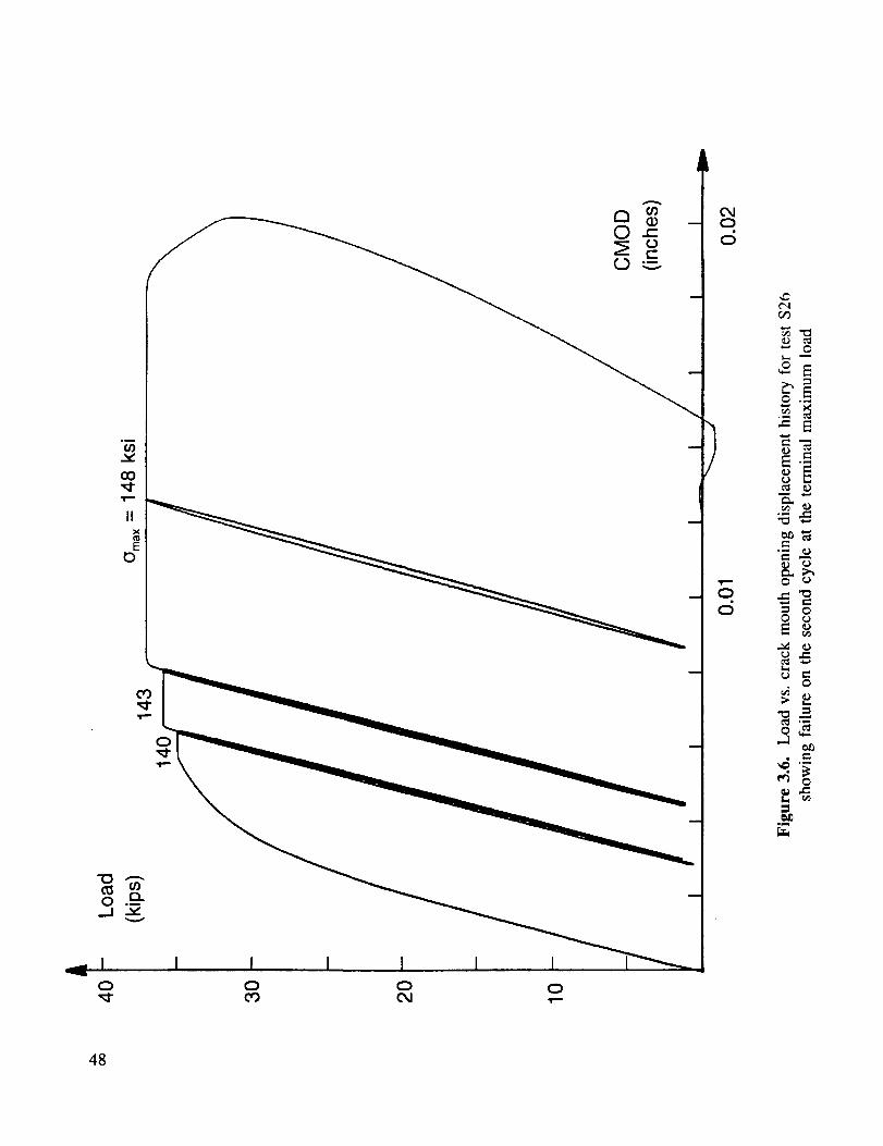
"0

0_.J

--I

0

II×

0

o=o

i

0 0 0CO C_I ,--

c_

c5

Oq

"_ 0

_ E

_ °_

•= E"NE'-'

°_ _

0 _

E_

• O

o_-1

e_° _

. ....q

_ o

48

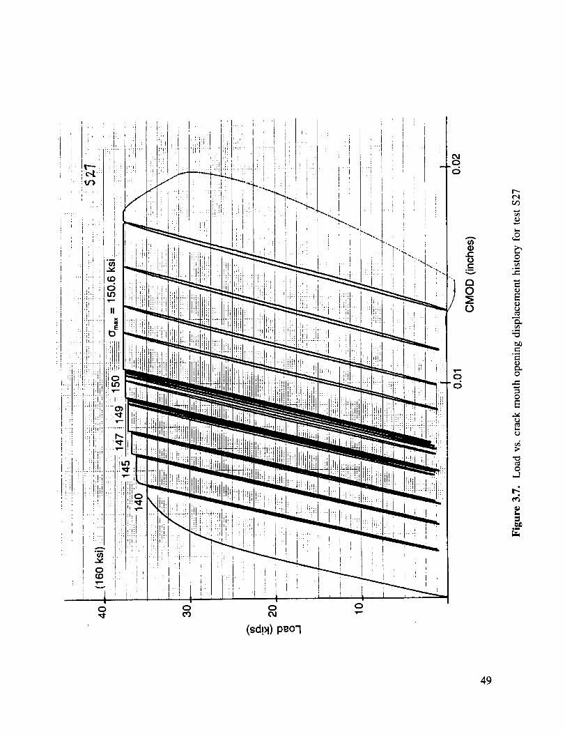
I

0

(sd!_l) p_o'l

0

(/)(1)¢,..0

0

o

0

0

0

°_

o,.._

o_

0

0E

t_

0

=.m

49

ever, the CMOD did not increase further. For the fifth cycle, the maximum stress was again

increased to about 148 ksi. Much more extensive CMOD increase occurred during the 30-sec.

hold time. The rate of CMOD increase increased slightly during the first 5 or 10 seconds and

then gradually decreased, so that by the end of the 30 seconds the rate of CMOD increase had

almost decreased to zero. On the second cycle at 148 ksi (the sixth cycle overall), the CMOD

increased very slowly during the In'st few seconds of the hold time, and then gradually increased

faster and faster. After about 25 seconds of the hold time, the specimen fractured completely and

the load dropped (the CMOD trace is meaningless beyond this point because the clip gauge

breaks away from the specimen surface). Also note the appreciable hysteresis in the load/unload

trace prior to the last cycle.

The second test ($27, Fig. 3.7) was slightly more complicated, because smaller load steps

were employed in an attempt to get more than two cycles at the final stress before fracture. A

second goal was to unload immediately before final fracture seemed imminent in order to see if

anything different happened on the next (failure) cycle. At the ftrst three maximum stress levels

(140, 145, and 147 ksi), some CMOD increase was observed (as before) during the hold time on

the first cycle and no CMOD increase during the hold time on the second cycle. At the fourth

and fifth maximum stress levels (about 149 and 150 ksi), a little growth was observed during the

second cycles (mostly towards the end of the hold time), so additional cycles were conducted at

the same stress level. The CMOD increase per cycle decreased to nearly zero on successive

cycles, however, so after 1-3 additional cycles the maximum stress was increased again. The

final maximum stress was 150.6 ksi. CMOD growth was fairly slow and steady during the hold

times of the first two cycles, with slightly less growth on the second cycle than on the first.

After a few seconds of hold time on the third cycle, the CMOD began to increase more and more

rapidly, so the specimen was unloaded after only 15 seconds in order to prevent fracture. On the

fourth cycle at 150.6 ksi, the CMOD again began to increase rapidly during the hold time, and

the specimen was unloaded after about 7 seconds. On the fifth cycle (the 20th cycle overall),

the specimen fractured in less than 1 second after reaching maximum load.

During each of the cycles at the final maximum stress in both tests, the elastic compliance

(measured on the forward loading portion of the P-CMOD trace) increases (the stiffness

decreases) slightly but measurably, indicating that crack growth was occurring on each individual

cycle.

The gradually stepping up of the load is not thought to be particularly significant to the

overall fracture process. This stepping up was done primarily because it was not possible to

predict in advance what an appropriate failure stress would be (before the specimen is broken

open, the true initial crack depth is not known). If we had known a priori to load to 148 ksi on

the very first cycle on specimen $26, we probably would have seen subcritical crack growth on

the first two cycles and then failed sometime during the third cycle.

The load stepping process does provide some interesting information, however. Note that

it is possible to be very close to the "failure stress" (within a few percent) and still see no

significant crack growth on subsequent loading cycles. Another way of looking at this is that if

50

theappliedstressis not very closeto the "failure stress,"subsequentloadingcycleswill not doadditionaldamageto the specimen.

An additional MCPT experimentwas conductedto evaluate the generality of thetear-fatiguecrack growth theory. This test, like the previous two such critical tests, wasconductedwith largeamplitudezero-maxloadcontrolcycling until failure occurred. In the firsttwo tests,the initial crack depthwasquite large (a/t = 0.8 to 0.9) and the maximum nominal

applied stress was less than yield (Om_ around 150 ksi, compare oy s = 165 ksi) so that some

elastic constraint was maintained on the remaining ligament. In this latest test, the initial crack

depth was chosen somewhat shallower (a/t = 0.6) and the maximum nominal applied stress was

above yield (final o=_ = 169 ksi), so relatively little elastic constraint was maintained. The goal

was to determine if the same sort of fracture behavior was observed under these conditions (as

would be predicted by the tear-fatigue theory), or if the behavior observed previously was

somehow unique to the very deepest flaws with lower applied stresses.

In short, the new test ($20) exhibited very similar behavior to the previous two such tests.

This is apparently a further confirmation of the tear-fatigue model. The load vs. crack mouth

opening displacement history from the test is shown in Fig. 3.8. Note that in this test, as in the

two previous, the initial load excursions employed smaller maximum stresses. This was done

primarily because the depth of the initial crack was not known until after the test; the depth could

only be estimated from the surface length. If the crack depth was significantly underestimated,

then the specimen could easily be broken on the very first cycle by going to a maximum stresstoo great.

This practice of going up to the terminal maximum stress in small steps was also useful

to show, however, that multiple cycling at smaller maximum loads (i.e., J_,_ values significantly

less than some critical value for tearing) does not produce significant additional crack growth.

The test protocol was to select a maximum stress and conduct at least two cycles at that o=_,

each with a 30-second hold time. Some increase in CMOD, probably corresponding to increases

in crack depth, always occurred on the trust cycle to some new maximum stress, because J_., was

increasing to a new maximum. In general, however, the second or any subsequent cycle to the

same maximum load did not produce significant additional CMOD increase (or crack growth).

If some additional CMOD increase occurred on the second cycle, then a third cycle to the same

Om_ was conducted, and so on. When an additional cycle produced no significant crack growth

(which was usually the case), then the maximum stress was increased slightly for the next cycle

and the same process was repeated." In test $20, significant CMOD increases occurred on

The excursions at lower maximum stresses are thought to be relatively inconsequential

for crack growth in comparison to later cycles at the highest maximum stress, since J=_

increases so sharply with increasing maximum stress (in this case, a 5 percent increase in

maximum stress from 160 to 169 ksi produces nearly a 40 percent increase in J,.Q.

Fatigue contributions to crack growth under these conditions are always small, and are

relatively insignificant until we are very close to instability.

51

0¢._

o E°_ _

e- c_

_ ME c_e-

_ Ec_ L.

,.., ,-

C_

,.,, .._

_ C_

C_

e..

_Gom

52

subsequent cycles only at the terminal o_,_,, 169 ksi. Failure occurred after 29 seconds (of a

30-second hold time!) on the fifth cycle at 169 ksi.

Quantitative Verification of Tear-Fatigue Theory. This experimentally observed behavior

provides a clear qualitative verification of the tear-fatigue theory described in Section 2 on

Analytical Development. It is also useful to evaluate the tear-fatigue formulation on a more

rigorous quantitative basis. The actual initial flaw size and shape, and the actual maximum stress

value during the failure cycles, are known after the test has been completed. Based on these

values, it is possible to predict the number of simulated proof cycles to failure. As discussed

earlier, this simple calculation assumes that negligible crack growth occurs during previous

simulated proof cycles at lower stresses.

A computer code was developed to model crack growth during simulated MCPT cycling.

This computer code, which was originally derived from a similar code developed in Phase I,

implemented the elastic-plastic fatigue crack growth and tear-fatigue models described in

Section 2, and was ultimately used to perform the probabilistic studies described in Section 4.

The predicted number of proof cycles to failure was approximately 13 cycles for $26, 2

cycles for $27, and 6 cycles for $20. This compares to actual experimental numbers of 2 cycles

for $26, 5 cycles for $27, and 5 cycles for $20. This agreement is excellent, especially

considering the extreme sensitivity of the predicted numbers to minor variations in crack

size/shape or maximum stress. For example, specimen $20 was predicted to fail on the 6th cycle

at 167 ksi. Changing the maximum stress to 168 ksi predicted failure on the first cycle, while

changing to 166 ksi predicted 20 cycles. Keeping a 167 ksi maximum stress but changing the

initial crack depth from 0.123 to 0.120 predicted 20 cycles. Even a small change in the crack

aspect ratio from 0.984 to 1.0 changes the prediction from 6 cycles to 10 cycles. Given the

inherent uncertainties associated with the J-resistance curve, estimation of J_,_, and measurement

of the exact crack size and shape, the predictions are shown to be very good.

A few additional experimental investigations into the tear-fatigue phenomenon have been

conducted under the broader "Proof Test Philosophy" (PTP) contract [41] in conjunction with the

validation of the general failure assessment diagram (FAD) approach to proof test analysis. The

FAD approach is a convenient diagrammatic representation of the J-based approach employed

in the current contract. These tear-fatigue investigations are being documented in more detail

in reports under the PTP contract. However, since the results are highly relevant to the MCPT

contract effort, the highlights are briefly reviewed here. All of these tests were conducted with

the same Inconel 718 material studied in the current contract.

In these tests, conducted with restrained single edge cracked plate (RSECP) specimens,

two specimens were tested under simulated service cyclic loads, and two received a proof

overload before cyclic loading. The load vs. load line displacement history from one of the proof

overload tests is shown in Fig. 3.9. Note that the simulated proof overload was conducted in

displacement control to insure stability, while the ensuing simulated service cycling was

conducted in load control to permit tear-fatigue behavior as instability was approached. The

53

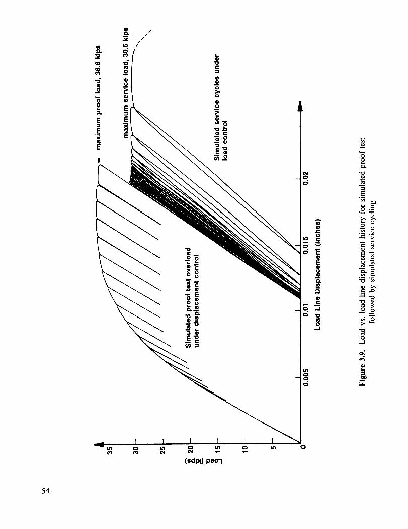
I I I I

A

J=¢)C

v

8¢)

D.

¢)

OC

,J

"O¢IO

.J

OO

c_

"_

_J

_=-_

¢)

"¢I "_

O Om

;>

r_

o_

54

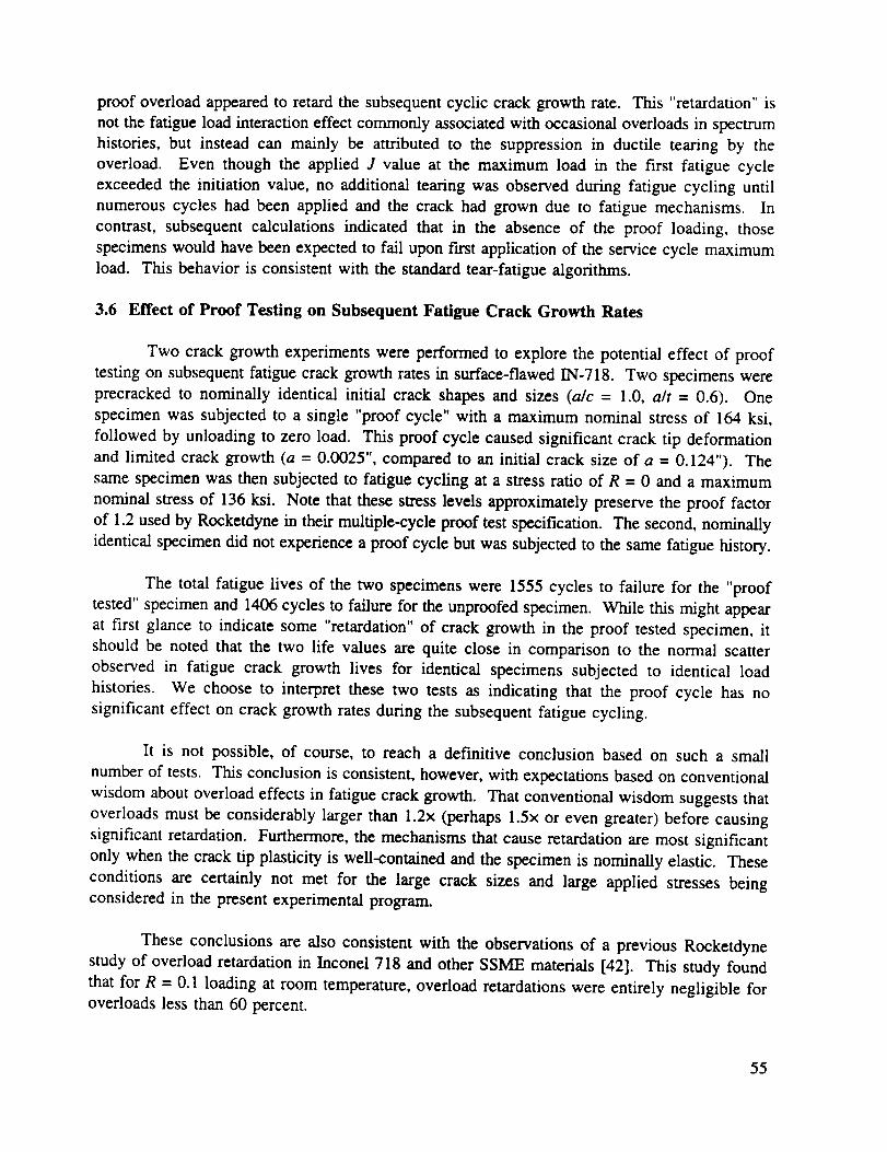
proof overload appeared to retard the subsequent cyclic crack growth rate. This "retardation" is

not the fatigue load interaction effect commonly associated with occasional overloads in spectrum

histories, but instead can mainly be attributed to the suppression in ductile tearing by the

overload. Even though the applied J value at the maximum load in the first fatigue cycle

exceeded the initiation value, no additional tearing was observed during fatigue cycling until

numerous cycles had been applied and the crack had grown due to fatigue mechanisms. In

contrast, subsequent calculations indicated that in the absence of the proof loading, those

specimens would have been expected to fail upon fast application of the service cycle maximum

load. This behavior is consistent with the standard tear-fatigue algorithms.

3.6 Effect of Proof Testing on Subsequent Fatigue Crack Growth Rates

Two crack growth experiments were performed to explore the potential effect of proof

testing on subsequent fatigue crack growth rates in surface-flawed IN-718. Two specimens were

precracked to nominally identical initial crack shapes and sizes (a/c = 1.0, a/t = 0.6). One

specimen was subjected to a single "proof cycle" with a maximum nominal stress of 164 ksi,

followed by unloading to zero load. This proof cycle caused significant crack tip deformation

and limited crack growth (a = 0.0025", compared to an initial crack size of a = 0.124"). The

same specimen was then subjected to fatigue cycling at a stress ratio of R = 0 and a maximum

nominal stress of 136 ksi. Note that these stress levels approximately preserve the proof factor

of 1.2 used by Rocketdyne in their multiple-cycle proof test specification. The second, nominally

identical specimen did not experience a proof cycle but was subjected to the same fatigue history.

The total fatigue lives of the two specimens were 1555 cycles to failure for the "proof

tested" specimen and 1406 cycles to failure for the unproofed specimen. While this might appear

at first glance to indicate some "retardation" of crack growth in the proof tested specimen, it

should be noted that the two life values are quite close in comparison to the normal scatter

observed in fatigue crack growth lives for identical specimens subjected to identical load

histories. We choose to interpret these two tests as indicating that the proof cycle has no

significant effect on crack growth rates during the subsequent fatigue cycling.

It is not possible, of course, to reach a definitive conclusion based on such a small

number of tests. This conclusion is consistent, however, with expectations based on conventional

wisdom about overload effects in fatigue crack growth. That conventional wisdom suggests that

overloads must be considerably larger than 1.2x (perhaps 1.5x or even greater) before causing

significant retardation. Furthermore, the mechanisms that cause retardation are most significant

only when the crack tip plasticity is well-contained and the specimen is nominally elastic. These

conditions are certainly not met for the large crack sizes and large applied stresses beingconsidered in the present experimental program.

These conclusions are also consistent with the observations of a previous Rocketdyne

study of overload retardation in Inconel 718 and other SSME materials [42]. This study found

that for R = 0.1 loading at room temperature, overload retardations were entirely negligible foroverloads less than 60 percent.

55

We draw the conclusion,then, basedon acceptedtheory and a limited number ofconfLrmingexperiments,thatproof testingof largesurfaceflaws in 13'4-718at proof stressesthatare capableof producing measurablecrack growth during the proof cycle hasa negligibleinfluenceon the subsequentfatiguecrackgrowth rates. It appearsthat other factorsaremoresignificant for variationsin crackgrowth andhencefor remainingstructurallife.

3.7 Fractographic Observations

3.7.1. Crack Growth Mechanisms

The analytical approach proposed to address MCPT problems is based on a single elastic-

plastic fatigue crack growth relationship employing AJ_ that can be applied from the small scale

yielding regime up into the elastic-plastic and fully plastic regime. At this high end, the elastic-

plastic FCG relationship is postulated to interface smoothly with a ductile crack extension

relationship employing the J-resistance curve. Empirical observations of crack growth data also

indicated a possible relationship between the blunting portion of monotonic crack advance and

the elastic-plastic regime of the FCG curve.

A brief series of fractographic studies were performed on five different crack growth

specimens in order to investigate the micromechanisms of crack advance under different

conditions and to determine if the proposed analytical approach appeared to be consistent with

the range of observed material responses. The five specimens had experienced five different

types of load histories: SSY fatigue crack growth, zero-max load control fatigue cycling with

maximum stress near yield, zero-max displacement control fatigue cycling with both severe and

moderate plasticity, and a single monotonic load excursion. Table 3.1 provides a convenient

overview of the test conditions for each specimen. These fractographic investigations were led

by SwRI Staff Engineer V. P. Swaminathan, who assisted in the preparation of this portion of

the report.

Specimen SD-3 was used to generate baseline fatigue crack growth information in the

traditional SSY range under constant amplitude load cycling with a simple through-crack

(center-crack) configuration. Fractography showed that crack propagation was by the usual

transgranular cyclic growth mechanism. Scanning electron microscope (SEM) investigations

under low magnifications (<300X) showed quasi-cleavage fracture features, as seen in Fig. 3.10

(top). Under higher magnifications (3000X), clear fatigue striations were predominant, as shown

in Fig. 3.11 (bottom). Striation spacing increased with crack length. Even at the higher AK

values, the fracture surface revealed predominantly striations with very limited ductile tearing.

Specimen S-25 was used to study crack growth under zero-max load control cycling with

a high maximum stress. The crack configuration was a semi-circular surface crack with an

original precrack depth of about a/t = 0.75. The specimen separated into two pieces after 385

56

Table 3.1. Summary of test conditions for specimens examined fractographically

Specimen

SD-3

S-25

S-11

SCR-8

S-13

Test Type

SSY FCG

SSY FCG with high o_

severe EPFCG

monotonic

moderate EPFCG

Maximum Stress

(cf. oy, = 160 ksi)

~ 56 ksi

~ 145 ksi

168-157 ksi

176 ksi

158-138 ksi

AJ,n or J,,_

35-140 lb./in.

110-150 lb./in.

~2000 lb./in.

~2900 lb./in.

350-600 lb./in.

57

58074

58076

Figure 3.10. Fracturesurfaceof specimenSD-3at 300x (top) and3000x(bottom)showingquasi-cleavagefracturefeaturesand fatiguestriations

58

59282

59283

Figure 3.11. Fracturesurfaceof specimenS-25at 300x (top) and 3000x(bottom)showingtransgranularfatiguestriations

59

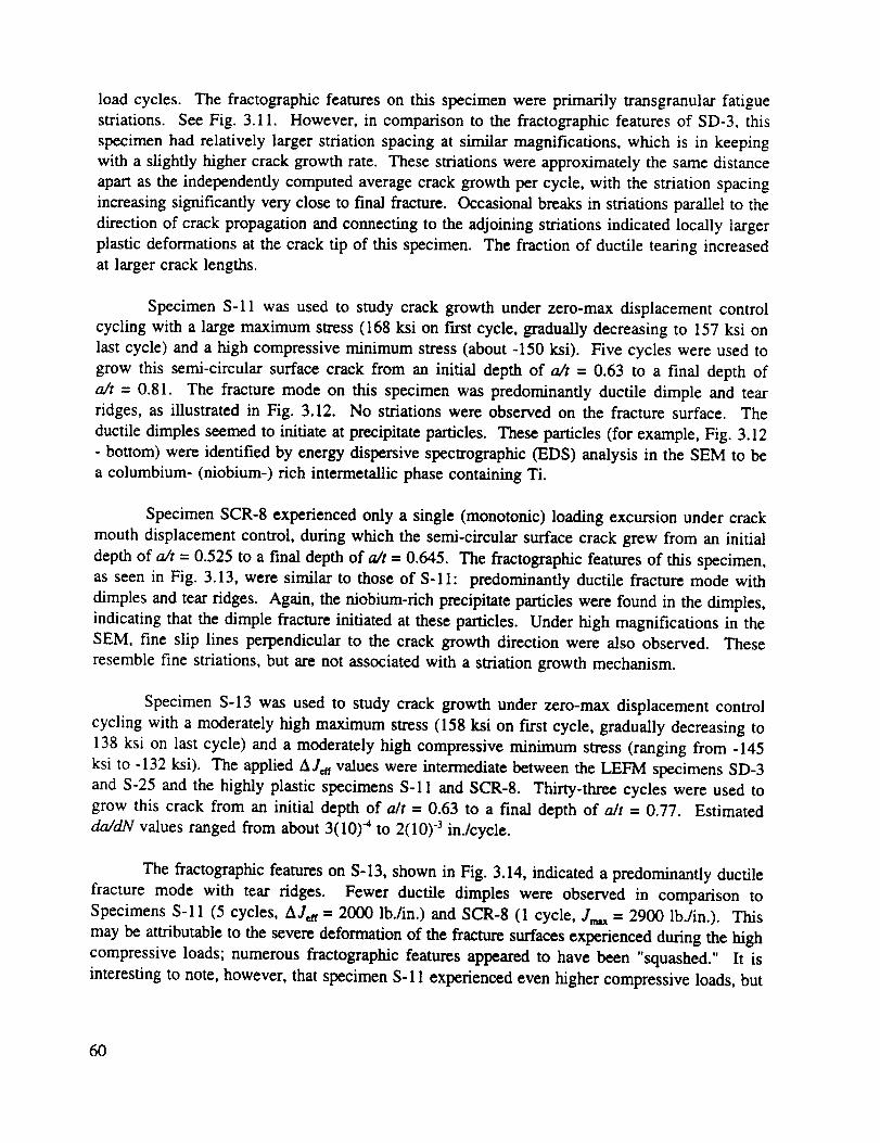
load cycles. The fractographicfeatureson this specimenwereprimarily transgranularfatiguestriations. SeeFig. 3.11. However,in comparisonto the fractographicfeaturesof SD-3, thisspecimenhad relatively largerstriationspacingat similar magnifications,which is in keepingwith a slightlyhighercrackgrowthrate. Thesestriationswereapproximatelythesamedistanceapartasthe independentlycomputedaveragecrackgrowthper cycle,with the striation spacingincreasingsignificantlyverycloseto final fracture. Occasionalbreaksin striationsparallelto thedirectionof crackpropagationandconnectingto the adjoiningstriationsindicatedlocally largerplastic deformationsat thecracktip of this specimen.The fractionof ductile tearing increasedat largercrack lengths.

SpecimenS-11was usedto study crack growth underzero-maxdisplacementcontrolcycling with a largemaximumstress(168 ksi on first cycle,graduallydecreasingto 157ksi onlast cycle)anda high compressiveminimumstress(about-150 ksi). Five cycleswereusedtogrow this semi-circularsurfacecrack from an initial depth of a/t - 0.63 to a final depth of

a/t = 0.81. The fracture mode on this specimen was predominantly ductile dimple and tear

ridges, as illustrated in Fig. 3.12. No striations were observed on the fracture surface. The

ductile dimples seemed to initiate at precipitate particles. These particles (for example, Fig. 3.12

- bottom) were identified by energy dispersive spectrographic (EDS) analysis in the SEM to be

a columbium- (niobium-) rich intermetallic phase containing Ti.

Specimen SCR-8 experienced only a single (monotonic) loading excursion under crack

mouth displacement control, during which the semi-circular surface crack grew from an initial

depth of a/t = 0.525 to a final depth of a/t - 0.645. The fractographic features of this specimen,

as seen in Fig. 3.13, were similar to those of S-11: predominantly ductile fracture mode with

dimples and tear ridges. Again, the niobium-rich precipitate particles were found in the dimples,

indicating that the dimple fracture initiated at these particles. Under high magnifications in the

SEM, fine slip lines perpendicular to the crack growth direction were also observed. These

resemble fine striations, but are not associated with a striation growth mechanism.

Specimen S-13 was used to study crack growth under zero-max displacement control

cycling with a moderately high maximum stress (158 ksi on first cycle, gradually decreasing to

138 ksi on last cycle) and a moderately high compressive minimum stress (ranging from -145

ksi to -132 ksi). The applied Ajar values were intermediate between the LEb'M specimens SD-3

and S-25 and the highly plastic specimens S-11 and SCR-8. Thirty-three cycles were used to

grow this crack from an initial depth of alt = 0.63 to a final depth of a/t -- 0.77. Estimated

da/dN values ranged from about 3(10) "4 to 2(10) .3 in./cycle.

The fractographic features on S-13, shown in Fig. 3.14, indicated a predominantly ductile

fracture mode with tear ridges. Fewer ductile dimples were observed in comparison to

Specimens S-11 (5 cycles, Ajar = 2000 lb./in.) and SCR-8 (1 cycle, J_, = 2900 lb./in.). This

may be attributable to the severe deformation of the fracture surfaces experienced during the high

compressive loads; numerous fractographic features appeared to have been "squashed." It is

interesting to note, however, that specimen S- 11 experienced even higher compressive loads, but

60

58117

58032

Figure 3.12. Fracture surface of specimen S-11 at 300x (top) and 2000x (bottom)

showing tear ridges and ductile dimples at precipitate particles

61

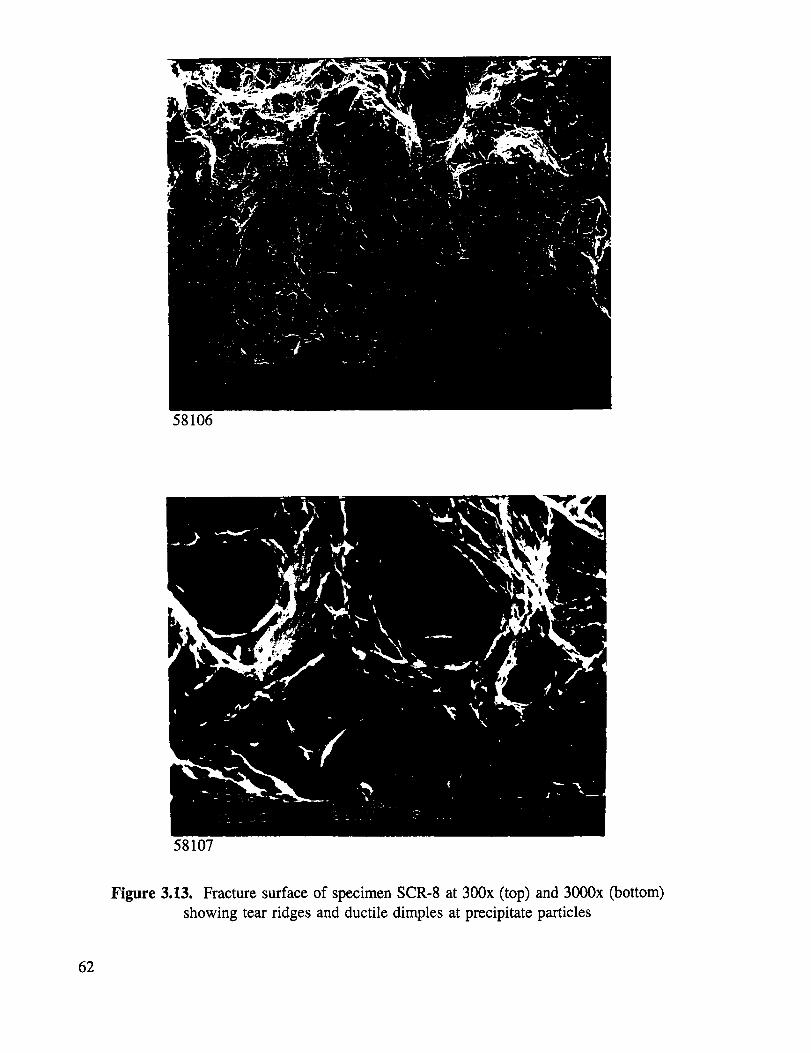
58106

58107

Figure 3.13. Fracturesurfaceof specimenSCR-8at 300x (top) and3000x (bottom)showingtearridgesandductiledimplesat precipitateparticles

62

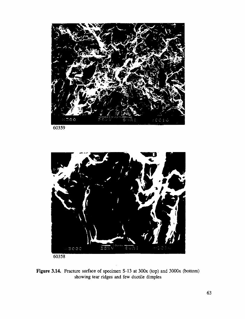
60359

,ei

60358

Figure 3.14. Fracture surface of specimen S-13 at 300x (top) and 3000x (bottom)

showing tear ridges and few ductile dimples

63

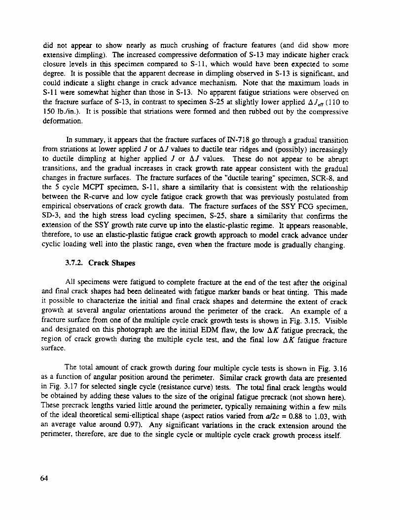
did not appearto show nearly as much crushingof fracture features(and did show moreextensivedimpling). Theincreasedcompressivedeformationof S-13may indicatehighercrackclosurelevels in this specimencomparedto S-11,which would havebeenexpectedto somedegree. It is possiblethat theapparentdecreasein dimplingobservedin S-13is significant,andcould indicatea slight changein crackadvancemechanism.Note that the maximumloadsinS-11weresomewhathigherthanthosein S-13. No apparentfatiguestriationswereobservedonthe fracturesurfaceof S-13,in contrastto specimenS-25at slightly lower appliedhJeu (110 to

150 lb./in.). It is possible that striations were formed and then rubbed out by the compressivedeformation.

In summary, it appears that the fracture surfaces of IN-718 go through a gradual transition

from striations at lower applied J or AJ values to ductile tear ridges and (possibly) increasingly

to ductile dimpling at higher applied J or AJ values. These do not appear to be abrupt

transitions, and the gradual increases in crack growth rate appear consistent with the gradual

changes in fracture surfaces. The fracture surfaces of the "ductile tearing" specimen, SCR-8, and

the 5 cycle MCPT specimen, S-11, share a similarity that is consistent with the relationship

between the R-curve and low cycle fatigue crack growth that was previously postulated from

empirical observations of crack growth data. The fracture surfaces of the SSY FCG specimen,

SD-3, and the high stress load cycling specimen, S-25, share a similarity that conf'u'ms the

extension of the SSY growth rate curve up into the elastic-plastic regime. It appears reasonable,

therefore, to use an elastic-plastic fatigue crack growth approach to model crack advance under

cyclic loading well into the plastic range, even when the fracture mode is gradually changing.

3.7.2. Crack Shapes

All specimens were fatigued to complete fracture at the end of the test after the original

and final crack shapes had been delineated with fatigue marker bands or heat tinting. This made

it possible to characterize the initial and final crack shapes and determine the extent of crack

growth at several angular orientations around the perimeter of the crack. An example of a

fracture surface from one of the multiple cycle crack growth tests is shown in Fig. 3.15. Visible

and designated on this photograph are the initial EDM flaw, the low AK fatigue precrack, the

region of crack growth during the multiple cycle test, and the final low AK fatigue fracturesurface.

The total amount of crack growth during four multiple cycle tests is shown in Fig. 3.16

as a function of angular position around the perimeter. Similar crack growth data are presented

in Fig. 3.17 for selected single cycle (resistance curve) tests. The total final crack lengths would

be obtained by adding these values to the size of the original fatigue precrack (not shown here).

These precrack lengths varied little around the perimeter, typically remaining within a few mils

of the ideal theoretical semi-elliptical shape (aspect ratios varied from aJ2c = 0.88 to 1.03, with

an average value around 0.97). Any significant variations in the crack extension around the

perimeter, therefore, are due to the single cycle or multiple cycle crack growth process itself.

64

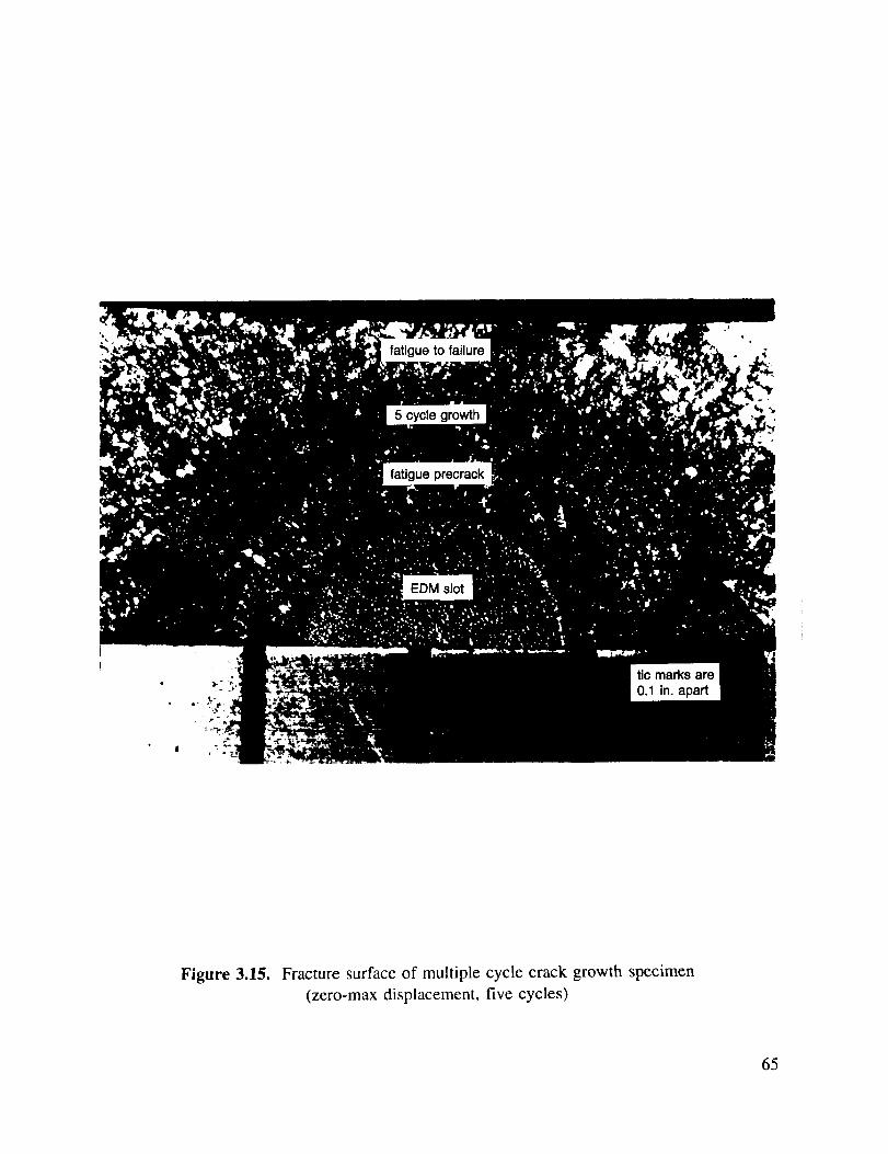
Figure 3.15. Fracture surface of multiple cycle crack growth specimen

(zero-max displacement, five cycles)

65

;0

;lie

O000

|l|l

oooo 0

EEEE

6666

0

(=0

.m

f_

0

CL

0

D

c:

.o

o"2

_ U

e_

_E

L.

.._

(Sl!CU) ql_oj O >looj 9

66

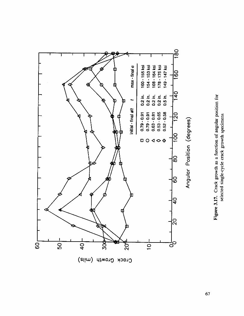
I !

o

0

0

(D"10

V

E0

o_

om

0n

0

E,,<

o

o

0 o°,.. L,

ao 0D

0 0 o0

0

67

There is a distinct maximum in the crack extension at an angular position around 30

degrees from the front surface of the crack in those specimens experiencing substantial crack

growth. Some of these specimens also exhibited a clear retardation of growth at the specimen

surface itself; the specimen shown in Fig. 3.15 was the most extreme case observed. Specimens

that experienced only small increments of crack growth, including other tests not shown here,

generally experienced crack extension that was more uniform around the perimeter.

These results are consistent with the three-dimensional elastic-plastic finite element

calculations of applied J at higher maximum stresses for semi-circular (a/c = 1) surface cracks

as a function of angular position published by Wang and Parks [10]. They found a similar

maximum in J at about 30 degrees for applied stresses near yield and a sharp decrease in J

approaching the front surface. Similar numerical results for deep semi-circular surface cracks

have recently been published by Yagawa et al. [14], who show that the specific angular variation

of J changes with both crack depth and crack aspect ratio. Bauschke, et al. [43] reported a

comparable angular dependence for surface crack growth in their experiments with A1

7075-T7351 for a/c = 0.4 - 1.1 and a/t = 0.3 - 0.75 at loads near the yield load, although they

typically measured more retardation at the surface and much larger differences between the

maximum growth and the growth at the position 90 degrees from the surface for smaller a/cvalues.

It is particularly interesting that the zero-max loading multiple cycle tests produced a

similar crack shape to the zero-max displacement and the single cycle tests, even though the

zero-max cycles were nominally elastic. In contrast, small scale yielding fatigue crack growth

tests with lower (elastic) maximum stresses produced crack shapes that were much more regular,

even for very deep cracks that had experienced substantial growth. This may indicate that the

development of the crack shape is influenced by J_ in ways that are not fully reflected by oursimple, one-dimensional cycle-by-cycle computation of AJ.

The crack growth data and analyses summarized in Figs. 3.1 and 3.5 were based on crack

growth measurements at the deepest point of the crack (90 degree position), although it is clear

from Figs. 3.15 - 3.17 that this is not always the position of greatest extension. Nevertheless,

this original choice of the 90 degree position is thought to be an appropriate one for engineering

applications. The reference stress J estimates used are based on the K solution at this 90 degree

position. The global limit load solution employed in the reference stress estimate is not tied to

any particular crack front location, but failure of this geometry in this material occurs primarily

by extension of the crack at the 90 degree position to the back surface, followed quickly by final

fracture of the resulting through crack. And this seems to be the key issue from an engineering

standpoint. The slightly greater crack extension at the 30 degree position, while certainly

interesting from a fracture mechanics research standpoint, does not appear in these particular tests

to exert any direct influence on tendencies for final fracture, which occurs as the 90 degree

position of the crack approaches the back face. The complex crack shape does exert some

influence on the resulting applied J at the 90 degree position, but this is a more indirect effect

that might be neglected in an engineering approach to predicting crack growth or fracture. Of

68

course,otherapplicationsin which the crackshapechangeswere moreseveremight requireamorerigoroustreatmentof theseeffects.

It shouldbe possibleto usea three-dimensionalfinite element calculation of variations

in applied J around the perimeter to predict the experimentally observed variability in crack

extension around the perimeter. This could be accomplished using the resistance curve

construction of Fig. 3.3 or the fatigue crack growth curve of Fig. 3.2, although there may also

be some variations in material resistance to crack extension around the perimeter (e.g., due to

changes in stress state) that would complicate such a prediction. Since the K-solution does not

exhibit a similar maximum at some intermediate position around the crack perimeter, it is not

immediately evident how the reference stress approach might be used to estimate these angularvariations in applied J.

3.8 Acoustic Emission Investigations

The acoustic emission (AE) technique can provide valuable supplemental information

during the course of proof testing, particularly for tough, ductile materials where stable crack

growth can occur on loading. Acoustic emission may be defined as transient elastic waves

generated by the rapid release of energy from localized sources within a material. These

localized sources may be associated with severe deformation, with localized fracture events, or

even with the rubbing of mating crack surfaces. The resulting sound waves typically occur in

short bursts or groups of bursts at very high frequencies (above 100 kHz) and of very lowintensity.

Acoustic emission could potentially provide the capability to detect otherwise undetectable

subcritical crack growth during proof testing, and hence could perhaps eliminate one of the major

potential disadvantages of MCPT. Therefore, a limited series of AE investigations were

conducted in conjunction with the experimental studies of crack growth during MCPT. The

actual AE monitoring and subsequent analysis was performed by John Hanley of the SwRI

Nondestructive Evaluation Science and Technology Division, who assisted in the preparation ofthis portion of the report.

Acoustic emission was monitored during mechanical testing on specimen S19, which had

a nominal cross-section of 0.2 x 1.25 in. and a semi-circular fatigue precrack about 0.12 in. deep.

The specimen was subjected to a complex series of load and displacement excursions for the

particular purpose of recording the AE from various phenomena. Figure 3.18 shows crack mouth

opening displacement and load versus time in seconds. The CMOD was f'trst extended to 15,

17.5 and 20 mils from 0 to 900 seconds, interrupted only by brief elastic unloadings to zero load.

The specimen was then taken into compression to a large compressive load and then returned to

the original CMOD for two cycles from 900 to 1500 seconds. The CMOD was then extended

monotonically to 23 mils and fatigue cycled at zero-max load for 2100 seconds at approximately

0.25 Hz. The CMOD was finally extended to 27.5 mils and the specimen was fatigue cycled at

zero-max load at approximately 0.1 Hz until failure. The clip gauge was disconnected at about

2600 seconds so that it would not be damaged when the specimen failed.

69

00cO

000CO

0'_

09 o<

J

J

y -4

00

Eu

8,

0

0

o_

0

=

0

=

0

ill ,,,i

_ 0

%

,i ,J, _,11

u') 0

(Sl!W)clov_o

t_ 0

00

0

00000000000

(sdpt) peoq

7O

A Physical Acoustics (PAC) U-30 AE sensor was coupled to the specimen with vacuum

grease and fastened with a C-clamp. A PAC 1220A preamp with 60 dB gain was used to

amplify the AE signals collected by a PAC 3000/3004 AE system. The system records clock

time and AE parameters such as amplitude, energy, duration, counts, and rise time for every

event. Frequency content can also be derived from counts and duration. An event is recorded

whenever the voltage level of AlE exceeds a preset threshold. Voltages proportional to CMOD

and load were also recorded for every event so that CMOD-load variations could be correlatedwith AE.

For AE characterization, the load excursions were classified into three categories:

1) CMOD increase (along the "backbone" of the load-displacement curve)

2) Crack rubbing during decreasing load (below the backbone)

3) Crack rubbing during increasing load (below the backbone)

The CMOD versus load plot in Fig. 3.19 shows where these AE events occurred during

the testing (excluding those events recorded during prolonged zero-max fatigue cycling).

Figure 3.19 also gives a clearer indication of the test history. Note that load is directly

proportional to applied stress; the nominal applied stress (in ksi) is 4.0x the applied load (in

kips). CMOD increase produced slightly more events than either of the crack rubbing categories.

The AE parameters did not, by themselves, indicate from which of the three categories a loneevent may have come.

Potential correlations were explored between different mechanical test parameters related

to fracture mechanics "events" and a wide range of AE parameters in both the time and frequency

domains. The strongest correlations found were between event rate and count rate versus CMOD

during CMOD increase, as shown in Figs. 3.20 and 3.21. Both of these plots show

monotonically increasing curves. Similar relationships have been reported in the literature.

However, the same correlations were not apparent from any rubbing phenomena during the test,including fatigue cycling.

The crack almost certainly experienced stable tearing during the "CMOD increasing"

portions of the history, and so it is likely that the AE events recorded then were generated by the

crack advancing through the material. There should have also been some measurable crack

advance during the two large unload-reload cycles (with severe compressive peaks), and it is

possible that the AE events recorded in the upper one-third of those loading cycles were also

generated by crack growth. The crack closure level for these large cycles (i.e., the load at which

the crack first becomes fully open during loading or first becomes partially closed during

unloading) was probably in the vicinity of zero load. Possible evidence for this statement is

provided by the large number of events that began around zero load during the unloading half

of these large cycles, events that may have been caused by rubbing of crack surfaces now in

contact. If the crack opened during reloading at around the same load level or even slightly

higher, then it would have been fully open by the time the AE events were recorded between +15

and +40 kips. In other words, the "rubbing up" or "rubbing down" events detected at large

71

u) c.-

oC}_Dc-

O_.C}.Q .o

O_crOl>,q

0

(3")

Z

0

I

0 C) 0 0 0 0LO CO ,,-- ,,-- CO L_

! ! I

(sd!_l)peoq

?2

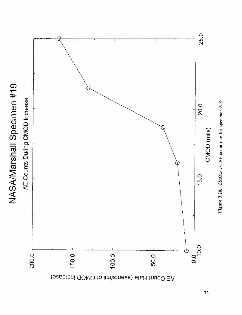
o

(1) •f" 0

mm m

cO a• 0

"__.

o0 a

C

o

UJ

Z

0 0 0 00 0 0 00 LO 0 LOC_ "T-- "T--

(eseeJ0u! OOIhlO jo I!W/s;ueAe) elel:t lunoo :iV

oL504

OO04

Ou3

oo

0 _-o

O0

Ev

0

o

e-,

o0

0

e_

t_

°_

73

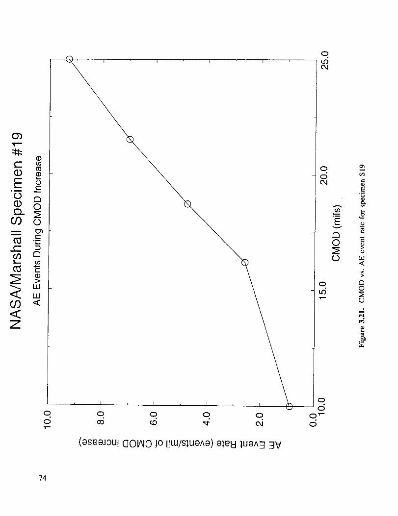
:LI:(D

c- co

0C

im m

ro D(1) 0

£D o

_ Ct'_ "_-t--" __ D

f--

W

£.0 <

Z

oo

I ' I I

(ase0JgU! C]OIA]O JO I!W/S:IUOAO)ele}::l :IUOA=I=IV

o

0d

oo

ou_

oo

0""o

m,i

Ev

0

0

M

E

2L,

L_<

0

e__4

74

positive loads probably did not originate from actual crack surface rubbing, but perhaps from

some crack tip event.

It is also possible that these AE events (and those recorded during CMOD increase) were

generated by near-tip deformation rather than actual crack extension. On the other hand, the

absence of AE events during the fast 8 mils of CMOD increase, when crack tip deformation was

becoming severe but crack extension via tearing had not yet initiated, may indicate that these AE

events are actually indicative of crack advance processes. There were a few AE events, not

shown on Fig. 3.19, recorded during the initial loading process, but most of these occurred when

the applied load was less than 10 kips and therefore probably reflect initial crack opening or

other "start-up" events. No AE events were recorded between CMOD = 1.5 and 8 mils, when

pre-tearing crack tip deformation would have been particularly intense.

It is not clear if the AE information could be linked to quantitative estimates of crack size

or crack growth. Other cracked configurations (specimens or structures) may respond with

different monotonic relationships (Figs. 3.20 and 3.21), since geometry and material

characteristics have much influence on the AE signal. Further testing would be required to better

assess the feasibility of measuring damage with AE.

Acoustic emission monitoring was also conducted during the test of specimen $27. Due

to scheduling conflicts, the hydraulic isolation system could not be installed to reduce the level

of background acoustic activity. Nevertheless, we decided that it would be useful to "listen"

during the test in order to determine if important events could still be detected. This may be

significant to application of AE in a "production" environment, where complete acoustic isolation

of major background noise may not be feasible.

As expected, the increased level of background noise made it more difficult to detect AE

activity generated by crack extension. Nevertheless, by adjusting the threshold settings and

conducting further post-processing of the signals, some useful information could be detected.

One view of the AE history is given in Figure 3.22, which shows the AE amplitude of those

events with more than 10 counts, along with the corresponding CMOD vs. time history (a

numerical scale is not shown for the CMOD values). Note the extensive AE activity during the

first loading cycle, when the crack ftrst experiences severe plastic deformation and begins to

extend. AE activity during the following cycles, even when the load is increased slightly, is

limited and scattered, and does not seem to follow any definite pattern. If the working

environment was quieter, of course, more meaningful patterns of activity might have been

detected, but we cannot say for sure. It is likely that very little crack extension occurred during

these intermediate cycles, so the absence of detected AE activity may be appropriate.

The important observation, however, is the definite increase in AE activity on the last few

cycles before final fracture (especially during the next-to-last cycle, conducted at around the

42-minute mark). In retrospect, this was probably a signal that crack growth or crack tip damage

was beginning to increase significantly and that failure was imminent. If CMOD information was

unavailable (as would be the case in an actual proof test), this AE signal could serve as a

75

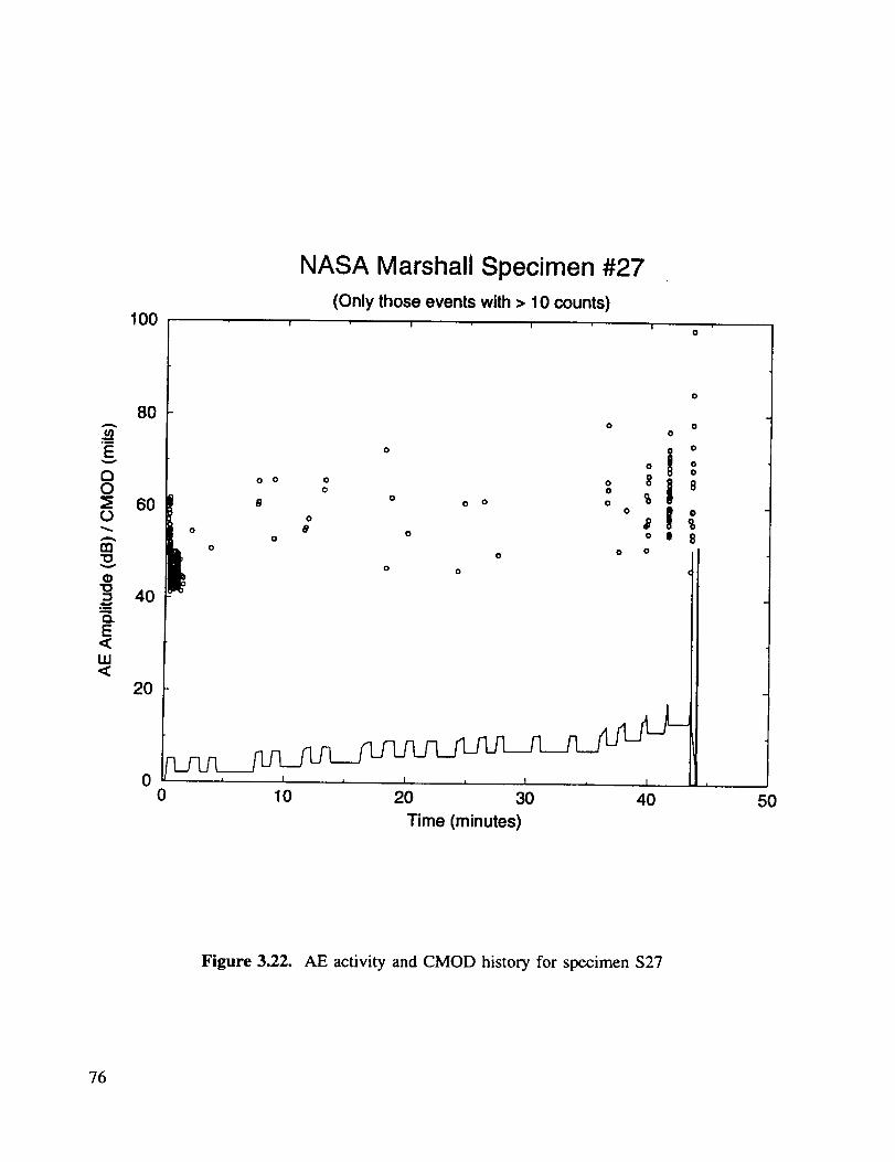
ca

E

C)0

0

c_E

W

100

80

6O

40

20

00

NASA Marshall Specimen #27

(Only those events with > 10 counts)

I I

o 00

o _ o00 0

oo o 81

o g 8e o o o o

o _o • o o IIo 8

I o o o o /I

10 20 30 40

Time (minutes)

50

Figure 3.22. AE activity and CMOD history for specimen $27

?6

warning that substantialflaw growth had occurredand that the part may havebeenseriouslydamaged,eventhoughactual"failure" maynot haveoccurred.

The limited informationavailablefrom this particularAlEmonitoring suggeststhat AEactivity dueto the presenceof a significant flaw may bemost likely to occuron thevery firstloadingcycle,whenthecrackfirst deformsplasticallyandbeginsto extend,or on loadingcyclesvery nearto failure. While othercyclesmayalsogenerateAE activity thatmay helpto identifythepresenceof a crack,in practicethesesignalsmay be harderto identify asclear indicationsof a flawed component. Of course,theseare all preliminary conclusions,and much morerigoroustestingandevaluationwouldbe requiredto validatethe procedurefor specifichardwaresystems.

Isolation and filtering of backgroundnoise could still be a problemfor the practicalapplicationof AE in a production environment. Sourcelocation algorithms,which employmultiple AE transducersand signalprocessinginvolving triangulationbasedon time-of-flightconceptsto identify the probablelocationof the AE source,could be useful as one meansofseparatingmeaningfulAE signalsfrom backgroundnoise.

77

4. PROBABILISTIC ANALYSIS

In Phase I, defect size data from actual SSME hardware or fabrication processes were

collected and analyzed to determine a representative distribution for initial crack size. This

distribution and the first-generation analytical model for MCPT were employed to perform simple

Monte Carlo analyses of the changes in crack size distributions predicted for various proof testprotocols.

Extensive probabilistic analyses were conducted in Phase II. These new analyses, which

were based on the improved second-generation analytical model for MCPT, and which employed

more rigorous probabilistic methods, completely supersede the Phase I probabilistic analyses.

The defect size information collected in Phase I was re-analyzed to obtain a more probable

distribution of initial crack depths. A simple probabilistic method was derived to compute the

conditional probability of failure in service for a population of components that have survived

a previous proof test, based on an assumed distribution of initial crack depths. The method was

used to perform a series of parameter studies that investigated the effects of proof factor, tearing

resistance, constitutive relationship, crack shape, initial crack depth distribution, and notches on

the MCPT vs. SCPT comparison. The potential impact of the memory assumption in the tear-

fatigue model on this comparison was also evaluated. The probabilistic parameter studies

provided a rational basis to draw conclusions about the relative merits of MCPT and SCPT.

4.1 The MCPT Question

It is useful to review briefly the fundamental problem which has motivated this entire

research investigation. Engineering hardware may contain crack-like defects of various sizes.

Larger defects obviously pose a greater and more immediate risk to hardware integrity in service.

One means of screening hardware to identify components containing dangerously large flaws is

to subject the hardware to a "proof test": a controlled overload of the component to a maximum

load which is generally greater than the maximum load expected in service. Flaws which are

larger than some critical size (which can be defined from fracture mechanics analysis) will cause

the component to fail during the proof test, thereby preventing a seriously defective componentfrom entering service.

However, the component may also contain flaws which are smaller than the critical size.

If the component material behaves in a brittle manner, then these smaller flaws will not be

significantly affected by the proof test; i.e., they will not grow to a larger size. However, if the

component material behaves in a ductile manner, then these smaller flaws could grow during the

proof test without causing failure of the component. These small flaws could therefore remain

undetected by the proof test, and their size could even be increased. If the flaws were extremely

small, then their existence and their limited growth during the proof test are probably of little

consequence to the in-service reliability of the component. However, it is possible that a

relatively large flaw which is still too small to cause failure during the proof test will grow

significantly during the proof test, thereby damaging the component and seriously increasing theprobability of early in-service failure.

78

These arguments are true for any proof testing approach to components made from ductile

materials, regardless of the number of proof cycles. However, the introduction of multiple proof

cycles further complicates the issue. Additional proof cycles could, on the one hand, cause the

failure of additional components containing relatively large flaws which were not large enough

to fail during the first cycle, but which grew to criticality during subsequent proof cycles. On

the other hand, additional proof cycles could cause additional subcritical crack growth (i.e., crack

growth that does not cause failure during the proof test) which could leave the component more

damaged than after the first proof cycle. This additional damage might be negligible, orconsiderable.

The challenge is to select the appropriate proof testing protocol which maximizes the

relative benefit of removing defective components from the population, while minimizing the

relative detriment of causing additional damage to components which pass the proof test. But

this challenge can not be satisfactorily addressed by considering only individual components with

individual cracks. If the individual crack was big enough to cause failure during a particular proof

test, then that particular proof test was the right thing to do. But if the individual crack was not

big enough to cause failure during the proof test, then that particular proof test was the wrong

thing to do, because the proof test may have caused some additional (arguably unnecessary!)

damage to the component.

The desirability of a particular proof test protocol must be assessed, instead, on the basis

of how it impacts a population of components containing a population of defects of different

sizes. Taking into account the probability that a defect of a given initial size exists in the

component, and employing a fracture mechanics analysis to determine how much a crack of a

given size will grow during the proof test (or if it will fail during the proof test), it is possible

to consLruct the probable distribution of crack sizes at the end of the proof test. This exercise

was carried out in Phase I, based on the initial crack size distribution and analytical MCPT crackgrowth model available at that time.

However, determining the final crack size distribution, and comparing it with the initial

crack size distribution, will not (in general) be sufficient to determine if a particular proof testing

protocol was good or bad. In general, the proof test will remove some large flaws from the

population, while increasing the size of the smaller flaws, and hence possibly increasing the

probability of f'mding flaws of some intermediate size. What is needed is some way of weighing

and comparing the relative good and bad of these two changes in the flaw size distribution.

The natural approach, consistent with the logical construction behind Figure 1.1 in the

Introduction, is to consider how the changes in the distribution of crack size will impact the

distribution of component life once the component is put into service. Components with larger

flaws will have a relatively shorter service life, while components with smaller flaws will have

a relatively longer service life. Again, a simple probabilistic analysis can be carried out in which

the crack size distribution at the beginning of the service life can be linked to a fracture

mechanics calculation of the remaining life for each initial crack size, in order to determine the

probability of failure in service after a given number of service cycles. A proof test protocol that

79

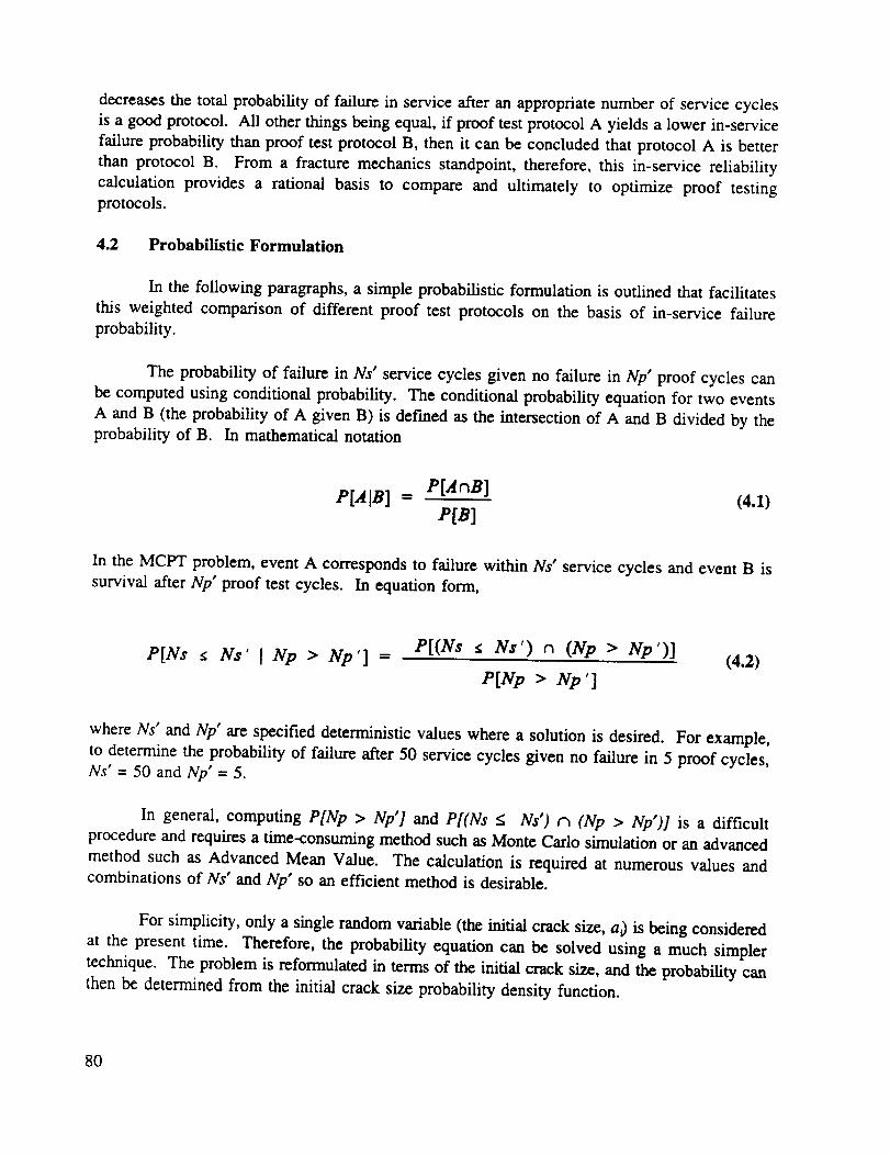
decreasesthetotal probabilityof failure in serviceafteranappropriatenumberof servicecyclesis agoodprotocol. All otherthingsbeingequal,if proof testprotocolA yieldsa lower in-servicefailure probability thanproof testprotocolB, then it canbeconcludedthat protocolA is betterthan protocol B. From a fracturemechanicsstandpoint,therefore,this in-servicereliabilitycalculation provides a rational basis to compareand ultimately to optimize proof testingprotocols.

4.2 Probabilistic Formulation

In the following paragraphs, a simple probabilistic formulation is outlined that facilitates

this weighted comparison of different proof test protocols on the basis of in-service failure

probability.

The probability of failure in Ns" service cycles given no failure in Np" proof cycles can

be computed using conditional probability. The conditional probability equation for two events

A and B (the probability of A given B) is defined as the intersection of A and B divided by theprobability of B. In mathematical notation

P[AIB] P[AnB]- (4.1)P[B]

In the MCPT problem, event A corresponds to failure within Ns" service cycles and event B is

survival after Np" proof test cycles. In equation form,

P[Ns < Ns' I Np > Np'] = P[(Ns < Na') n (Np > Np')] (4.2)

P[Np > Np']

where Ns" and Np" are specified deterministic values where a solution is desired. For example,

to determine the probability of failure after 50 service cycles given no failure in 5 proof cycles,Ns" = 50 and Np' = 5.

In general, computing P[Np > Np'] and P[(Ns < Ns') n (Np > Np')] is a difficult

procedure and requires a time-consuming method such as Monte Carlo simulation or an advanced

method such as Advanced Mean Value. The calculation is required at numerous values and

combinations of Ns" and Np" so an efficient method is desirable.

For simplicity, only a single random variable (the initial crack size, a.) is being considered

at the present time. Therefore, the probability equation can be solved using a much simpler

technique. The problem is reformulated in terms of the initial crack size, and the probability can

then be determined from the initial crack size probability density function.

80

Mathematically, this can be represented as,

P[Ns<Ns'] = P[H(a_)<Ns'] = P[a,,:HI(Ns')] = p[ai<a; ] (4.3)

where a_ is the initial crack size random variable, Ns = H(a) denotes the crack growth, H t is the

inverse crack growth function, and a i' = HI(Ns ") is the initial crack size that causes failure on

the Ns" service cycle.

P[a, < a_'] can be determined analytically since the probability density function and

cumulative distribution function of ai are both known. Therefore, the task is to find the initial

crack size, a,', that corresponds to failure on the Ns" service cycle. Note that this particular

procedure cannot be used for more than one random variable because combinations of random

variable values can cause failure on the Ns" cycle; thus, it is not possible to determine a single

a,, or any other random variable value, that can represent the failure condition. Monte Carlo or

advanced methods would be required in this case.

Rather than developing a new crack growth code to solve the inverse problem, even if

possible, the a_' that corresponds to Ns" can be computed using any existing crack growth code

and a search procedure. A simple bisection root finding method is sufficient. A similar

procedure is performed for P[Np > Np']. The probability calculation procedure is shown inFigure 4.1.

Computing the intersection of two events is a system reliability problem which can be

difficult to solve. But again, because only one random variable is being considered, the solution

is much simpler than in the general case. Because P[(Ns < Ns')] and P[(Np > Np')] can both

be represented in terms of the initial crack size distribution a_ the intersection can be computedalgebraically. An example is shown in Figure 4.2.

The above methodology can be repeated for different values of Ns" and Np'. The solutionis quick, requiring only several minutes of cpu time on an HP workstation for the MCPT crack

growth code employed in these studies.

4.3 An Example Problem

The MCPT crack growth computer code originally developed in Phase I was extensively

modified to perform probabilistic analyses of fleet reliability. The fast major step was to modify

the deterministic crack growth algorithms to follow the analytical approaches described earlier

in Section 2 on Analytical Development. These new algorithms included the improved reference

stress J solutions for semi-elliptical surface cracks, the general elastic-plastic fatigue crack growth

methodology, and tear-fatigue theory, including the minor modifications required to address

typical reusable aerospace propulsion system applications. The code was also modified to permit

analysis of proof testing at one stress level, followed by service cycling at another stress level.

81

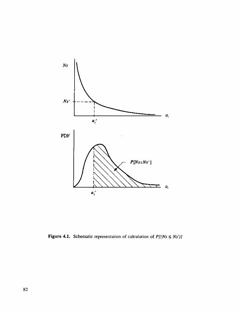
Ns

I

air

ai

PDF

P[Ns_:Ns' ]

a i

Figure 4.1. Schematic representation of calculation of P[(Ns < Ns')]

82

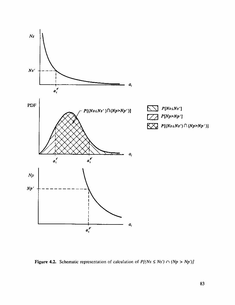
Ns

iV$ i

I

It"

aj

ai

PDF

Np

.,Vp')]

_ ai

t p'

a I al

I

II aite

C11

P[Ns_:Ns']

e[(Ns_Ns') D (Np>Np')]

Figure 4.2. Schematic representation of calculation of P[(Ns < Ns') n (Np > Np')]

83

Analysis of crack growth during proof testing or service cycling followed the same approach.

Failure during proof or service cycling was defined as either catastrophic rupture (burst) or full

penetration of a crack (leak). The updated deterministic MCPT code was then linked to

appropriate probabilistic analysis routines, which were taken from the general purpose NESSUS

computer code originally developed at SwRI under long-term NASA funding [44].

In order to illustrate this type of analysis and the types of results which it generates, one

particular sample MCPT problem was solved and illustrated with a series of graphs.

Initial Crack Depth Distribution. In this problem, each component was assumed to

contain a single defect from a given distribution of initial defect depths. In Phase I, a distribution

of initial crack sizes was developed from a study of SSME hardware and fabrication processes.

The data sources included material test coupons, selected SSME hardware, and available multi-

cycle proof failure information. A particular lognormal distribution was selected as the most

accurate statistical description of the collected crack depth data.

While this lognormal form did exhibit the closest agreement with the available data based

on rigorous statistical tests, further study led to the conclusion that the lognormal was not the

most realistic representation of actual initial flaw size distributions in engine hardware. The

lognormal probability distribution function (PDF) goes to zero for very small crack sizes. This

is consistent with the collected data, because very few very small cracks were detected, measured,

and recorded. However, in reality, many very small flaws were likely present but either not

detected (due to the lower probability of detection for small flaws) or not recorded based on

judgements about their relative significance. Therefore, a more realistic initial crack depth

distribution would likely follow a monotonically increasing frequency with decreasing size. This

conclusion is, in fact, very consistent with other studies of initial flaw distributions in the

literature. For example, Becher and Pedersen [45], Bruckner and Munz [46], and Lidiard and

Williams [47] all selected exponential distributions. Therefore, the collected crack depth data

from Phase ! were used to generate an exponential distribution. The collected data and the

resulting exponential distribution are shown together in Figure 4.3. The mean value of thisexponential distribution was 0.0212 inches.

Note that although the probabilistic analysis conservatively assumes that every component

has an initial flaw, the form of the exponential distribution implies that the majority of these

cracks will be negligibly small. The analysis conducted here did not evaluate the more

complicated problem in which each component may itself contain a distribution of initial flaws.

Crack Shape. Each defect was assumed to have an aspect ratio of a/c = 0.1. The actual

population of defect shapes was found to have a mean value around a/c = 1.0, but many actual

MCPT failures are associated with much smaller a/c ratios, so this was thought to be a goodchoice for demonstration purposes.

In this example problem, and in later parameter studies where different initial values of

a/c were considered, the crack aspect ratio was assumed to be fixed as the crack grew under

84

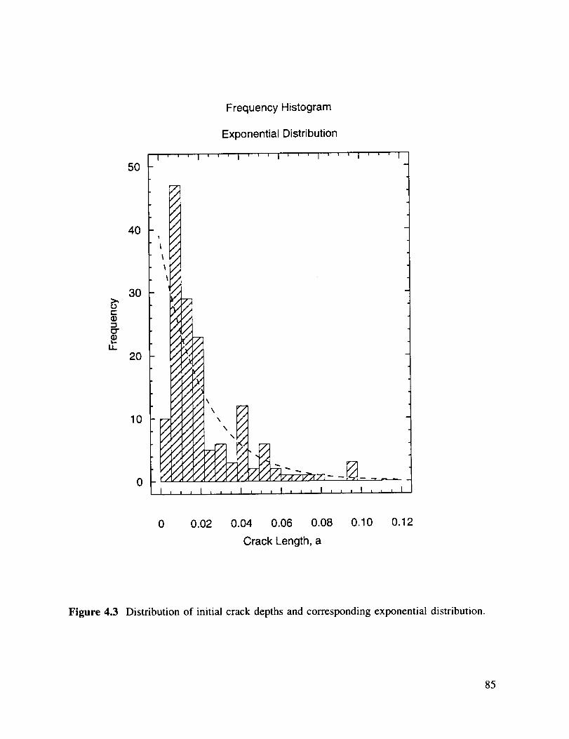
50

40

30

I.L.

20

10

0

Frequency Histogram

Exponential Distribution

I ' ' ' I ' ' ' I ' ' ' I ' ' ' 1 ' ' ' I ' ' ' I

I A

f.,q

f

i//II , , , I , , , I , , , I , _ , I , I , , ,-I

0 0.02 0.04 0.06 0.08 0.10 0.12

Crack Length, a

Figure 4.3 Distribution of initial crack depths and corresponding exponential distribution.

85

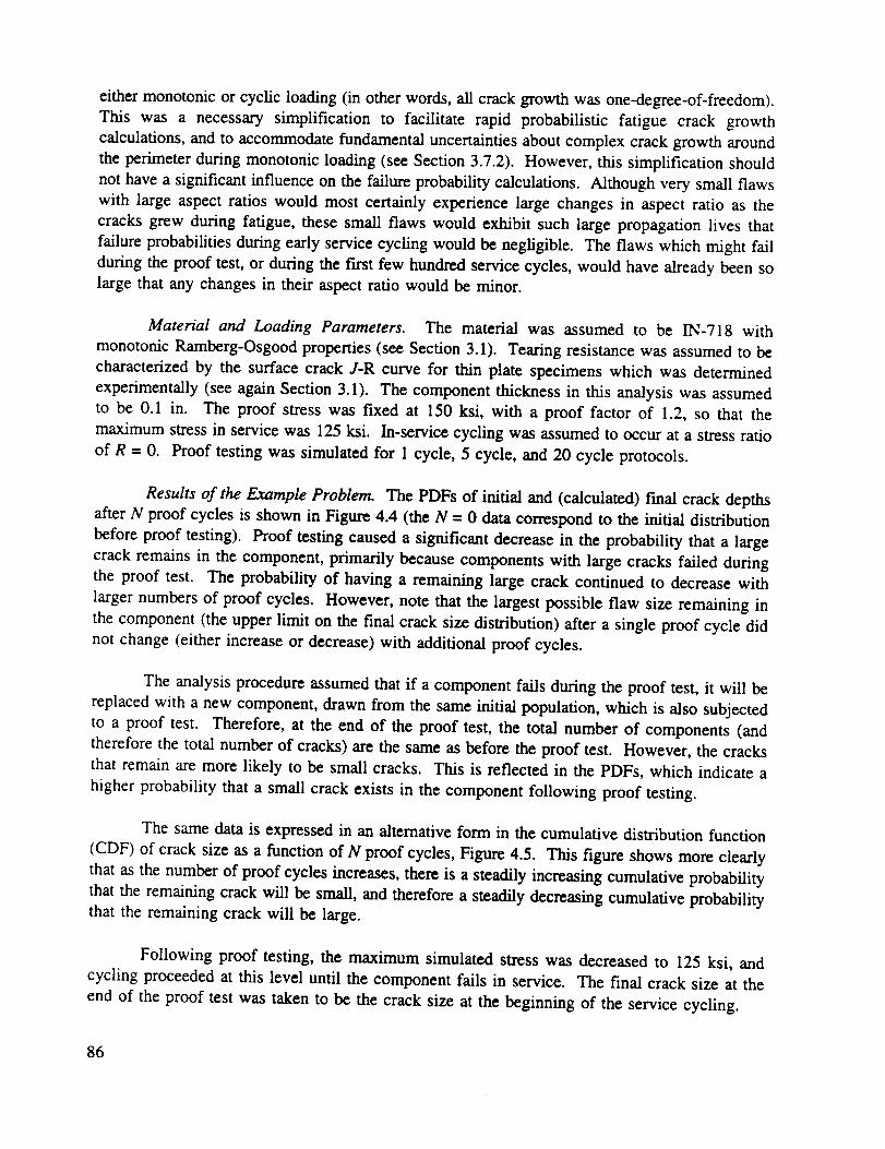
eithermonotonicor cyclic loading(in otherwords,all crackgrowthwasone-degree-of-freedom).This was a necessarysimplification to facilitate rapid probabilistic fatigue crack growthcalculations,andto accommodatefundamentaluncertaintiesaboutcomplexcrackgrowtharoundtheperimeterduringmonotonicloading(seeSection3.7.2). However,this simplificationshouldnothaveasignificantinfluenceon thefailureprobabilitycalculations.Althoughvery smallflawswith large aspectratios would most certainly experiencelarge changesin aspectratio as thecracksgrew during fatigue, thesesmall flaws would exhibit such large propagationlives thatfailureprobabilitiesduringearlyservicecycling wouldbenegligible. Theflawswhich might failduringthe proof test,or during thefirst few hundredservicecycles,would havealreadybeensolarge that anychangesin their aspectratio would beminor.

Material and Loading Parameters. The material was assumed to be IN-718 with

monotonic Ramberg-Osgood properties (see Section 3.1). Tearing resistance was assumed to be

characterized by the surface crack J-R curve for thin plate specimens which was determined

experimentally (see again Section 3.1). The component thickness in this analysis was assumed

to be 0.1 in. The proof stress was fixed at 150 ksi, with a proof factor of 1.2, so that the

maximum stress in service was 125 ksi. In-service cycling was assumed to occur at a stress ratio

of R = 0. Proof testing was simulated for 1 cycle, 5 cycle, and 20 cycle protocols.

Results of the Example Problem. The PDFs of initial and (calculated) final crack depths

after N proof cycles is shown in Figure 4.4 (the N = 0 data correspond to the initial distribution

before proof testing). Proof testing caused a significant decrease in the probability that a large

crack remains in the component, primarily because components with large cracks failed during

the proof test. The probability of having a remaining large crack continued to decrease with

larger numbers of proof cycles. However, note that the largest possible flaw size remaining in

the component (the upper limit on the final crack size distribution) after a single proof cycle did

not change (either increase or decrease) with additional proof cycles.

The analysis procedure assumed that if a component fails during the proof test, it will be

replaced with a new component, drawn from the same initial population, which is also subjected

to a proof test. Therefore, at the end of the proof test, the total number of components (and

therefore the total number of cracks) are the same as before the proof test. However, the cracks

that remain are more likely to be small cracks. This is reflected in the PDFs, which indicate a

higher probability that a small crack exists in the component following proof testing.

The same data is expressed in an alternative form in the cumulative distribution function

(CDF) of crack size as a function of N proof cycles, Figure 4.5. This figure shows more clearly

that as the number of proof cycles increases, there is a steadily increasing cumulative probability

that the remaining crack will be small, and therefore a steadily decreasing cumulative probabilitythat the remaining crack will be large.

Following proof testing, the maximum simulated stress was decreased to 125 ksi, and

cycling proceeded at this level until the component fails in service. The final crack size at the

end of the proof test was taken to be the crack size at the beginning of the service cycling.

86

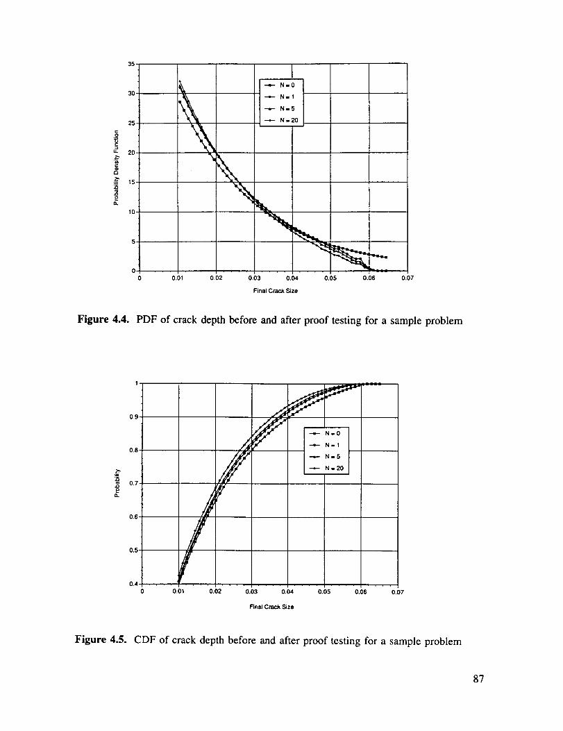
IJ-

ra

.0o

tl.

35

3O

25

2O

15

10

0.01 0.02 0.03 0.04 0.05 0.06 0.07

Final Crack Size

Figure 4.4. PDF of crack depth before and after proof testing for a sample problem

25

2CL

1,

0.9.

0.6-

0.7.

0.6-

0.5 o /

f .-e- N=0.-e- N-1

•-,_ N=5

N-20

0.4- .... I , , , _ .........

0 0.01 0.02 0.03 0.04 0.05 0.06 0.07

Final Crack Size

Figure 4.5. CDF of crack depth before and after proof testing for a sample problem

87

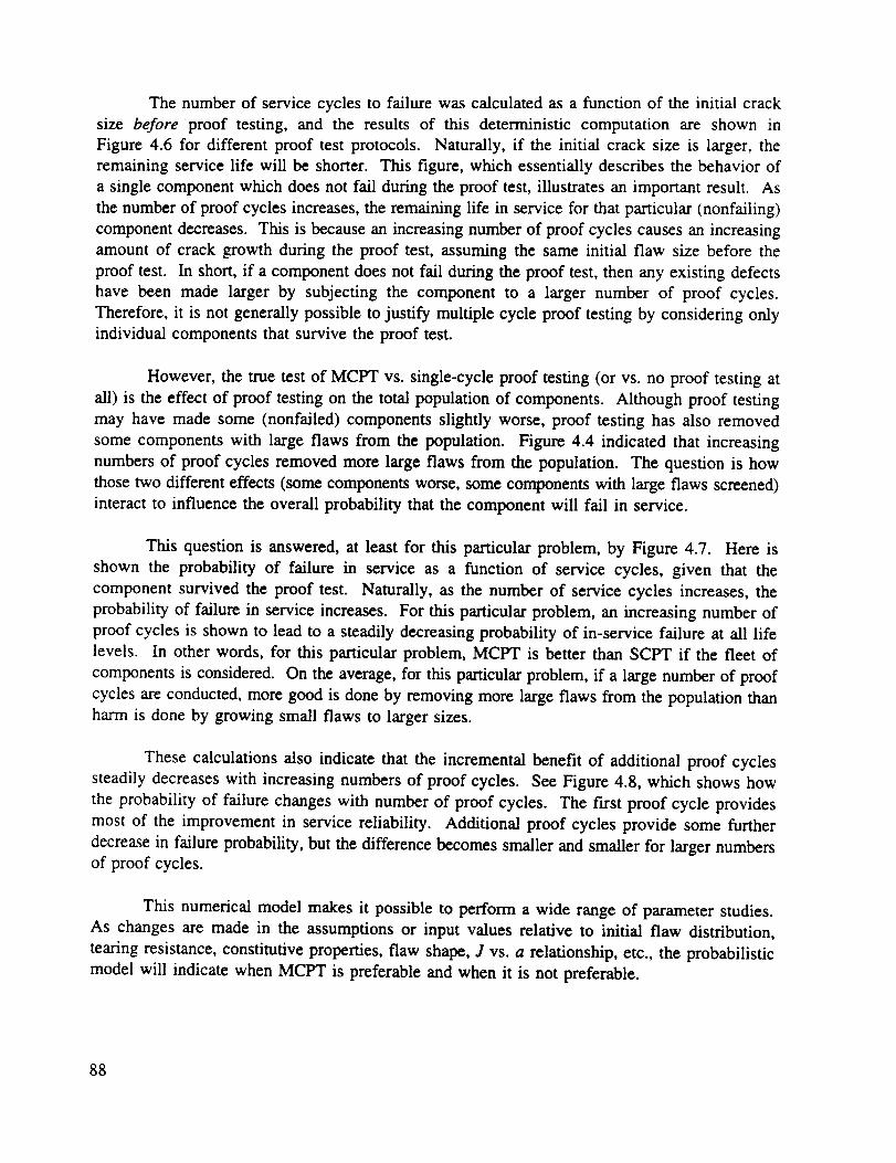
The number of service cycles to failure was calculated as a function of the initial crack

size before proof testing, and the results of this deterministic computation are shown in

Figure 4.6 for different proof test protocols. Naturally, if the initial crack size is larger, the

remaining service life will be shorter. This figure, which essentially describes the behavior of

a single component which does not fail during the proof test, illustrates an important result. As

the number of proof cycles increases, the remaining life in service for that particular (nonfailing)

component decreases. This is because an increasing number of proof cycles causes an increasing

amount of crack growth during the proof test, assuming the same initial flaw size before the

proof test. In short, if a component does not fail during the proof test, then any existing defects

have been made larger by subjecting the component to a larger number of proof cycles.

Therefore, it is not generally possible to justify multiple cycle proof testing by considering only

individual components that survive the proof test.

However, the true test of MCPT vs. single-cycle proof testing (or vs. no proof testing at

all) is the effect of proof testing on the total population of components. Although proof testing

may have made some (nonfailed) components slightly worse, proof testing has also removed

some components with large flaws from the population. Figure 4.4 indicated that increasing

numbers of proof cycles removed more large flaws from the population. The question is how

those two different effects (some components worse, some components with large flaws screened)

interact to influence the overall probability that the component will fail in service.

This question is answered, at least for this particular problem, by Figure 4.7. Here is

shown the probability of failure in service as a function of service cycles, given that the

component survived the proof test. Naturally, as the number of service cycles increases, the

probability of failure in service increases. For this particular problem, an increasing number of

proof cycles is shown to lead to a steadily decreasing probability of in-service failure at all life

levels. In other words, for this particular problem, MCPT is better than SCPT if the fleet of

components is considered. On the average, for this particular problem, if a large number of proof

cycles are conducted, more good is done by removing more large flaws from the population than

harm is done by growing small flaws to larger sizes.

These calculations also indicate that the incremental benefit of additional proof cycles

steadily decreases with increasing numbers of proof cycles. See Figure 4.8, which shows how

the probability of failure changes with number of proof cycles. The first proof cycle provides

most of the improvement in service reliability. Additional proof cycles provide some further

decrease in failure probability, but the difference becomes smaller and smaller for larger numbersof proof cycles.

This numerical model makes it possible to perform a wide range of parameter studies.

As changes are made in the assumptions or input values relative to initial flaw distribution,

tearing resistance, constitutive properties, flaw shape, J vs. a relationship, etc., the probabilistic

model will indicate when MCPT is preferable and when it is not preferable.

88

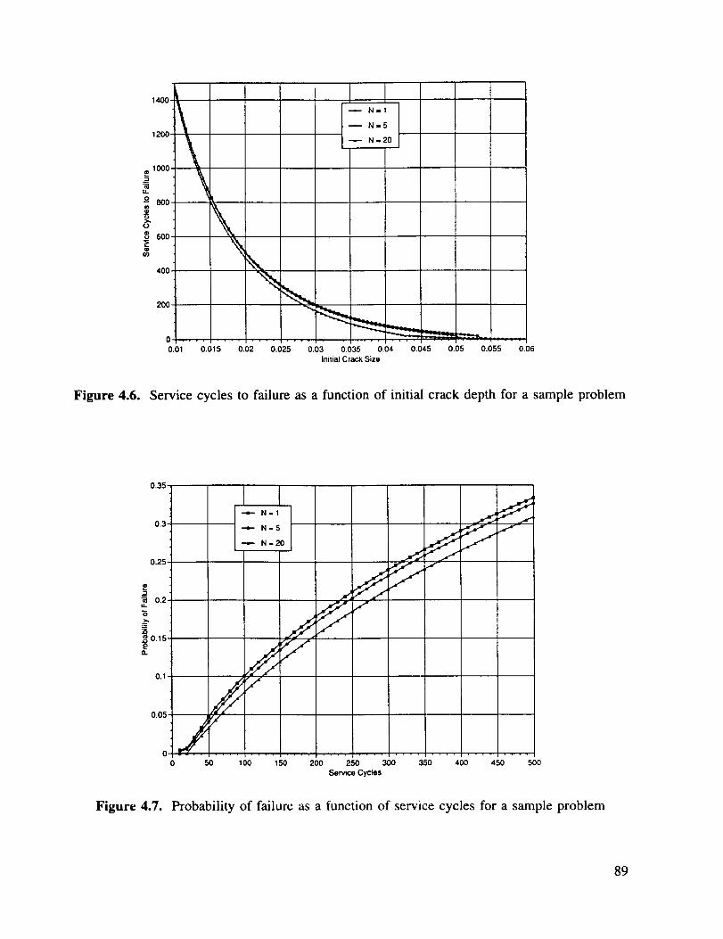
1400

1200

1000

t,

o 8OO

0

8600

400

\

200

tN-5

N=20

\0

0.01 0.015 0.02 0.025 0,03 0.035 0.04 0.045 0.05 0,055 0.06

Initial Crack Size

Figure 4.6. Service cycles to failure as a function of initial crack depth for a sample problem

0.35.

0.3-

0.25-

I I--o-- N = 1

•-'=- N =5

--- N=20

'_ 0.2.

o

25_ 0.15,

0.1. S"

0.05

0

0 50 100 150 200 250 300 350 400 450 500

Service Cycles

Figure 4.7. Probability of failure as a function of service cycles for a sample problem

89

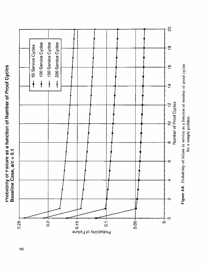
m

0

00

0L_

I=

ZI,I,,,-

0

I=0

im

C

_=.£o

s=•om

i _ (/3 00 O00 0 C)

0 C_ _ 0LO .,- .,-- OJ

u')0_1

04

0

9O

0

o

011

0

0

._ "&

r.,.°_

L.

_o°_

0

r'.;

,.o0L.

#,,,

I._

t,,,_

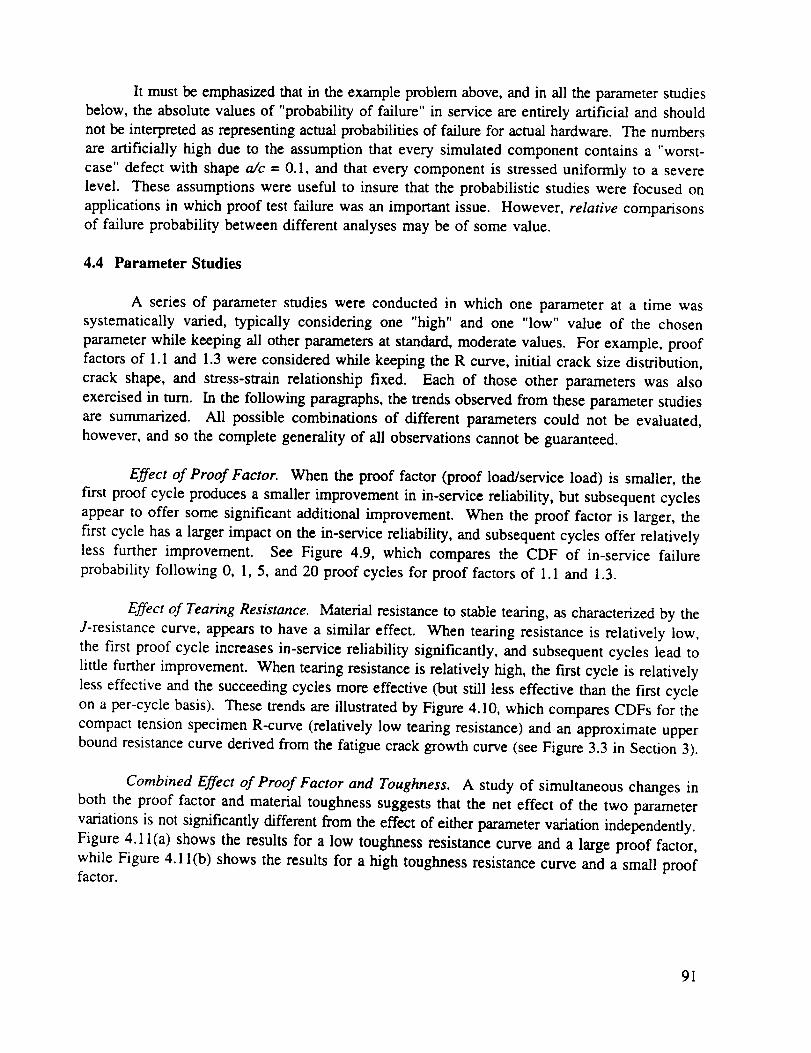
It must be emphasized that in the example problem above, and in all the parameter studies

below, the absolute values of "probability of failure" in service are entirely artificial and should

not be interpreted as representing actual probabilities of failure for actual hardware. The numbers

are artificially high due to the assumption that every simulated component contains a "worst-

case" defect with shape a/c = O. 1, and that every component is stressed uniformly to a severe

level. These assumptions were useful to insure that the probabilistic studies were focused on

applications in which proof test failure was an important issue. However, relative comparisons

of failure probability between different analyses may be of some value.

4.4 Parameter Studies

A series of parameter studies were conducted in which one parameter at a time was

systematically varied, typically considering one "high" and one "low" value of the chosen

parameter while keeping all other parameters at standard, moderate values. For example, proof

factors of 1.1 and 1.3 were considered while keeping the R curve, initial crack size distribution,

crack shape, and stress-strain relationship fixed. Each of those other parameters was also

exercised in turn. In the following paragraphs, the trends observed from these parameter studies

are summarized. All possible combinations of different parameters could not be evaluated,

however, and so the complete generality of all observations cannot be guaranteed.

Effect of Proof Factor. When the proof factor (proof load/service load) is smaller, the

first proof cycle produces a smaller improvement in in-service reliability, but subsequent cycles

appear to offer some significant additional improvement. When the proof factor is larger, the

first cycle has a larger impact on the in-service reliability, and subsequent cycles offer relatively

less further improvement. See Figure 4.9, which compares the CDF of in-service failure

probability following O, 1, 5, and 20 proof cycles for proof factors of 1.1 and 1.3.

Effect of Tearing Resistance. Material resistance to stable tearing, as characterized by the

J-resistance curve, appears to have a similar effect. When tearing resistance is relatively low,

the first proof cycle increases in-service reliability significantly, and subsequent cycles lead to

little further improvement. When tearing resistance is relatively high, the first cycle is relatively

less effective and the succeeding cycles more effective (but still less effective than the first cycle

on a per-cycle basis). These trends are illustrated by Figure 4.10, which compares CDFs for the

compact tension specimen R-curve (relatively low tearing resistance) and an approximate upper

bound resistance curve derived from the fatigue crack growth curve (see Figure 3.3 in Section 3).

Combined Effect of Proof Factor and Toughness. A study of simultaneous changes in

both the proof factor and material toughness suggests that the net effect of the two parameter

variations is not significantly different from the effect of either parameter variation independently.

Figure 4.11 (a) shows the results for a low toughness resistance curve and a large proof factor,

while Figure 4.1 l(b) shows the results for a high toughness resistance curve and a small prooffactor.

91

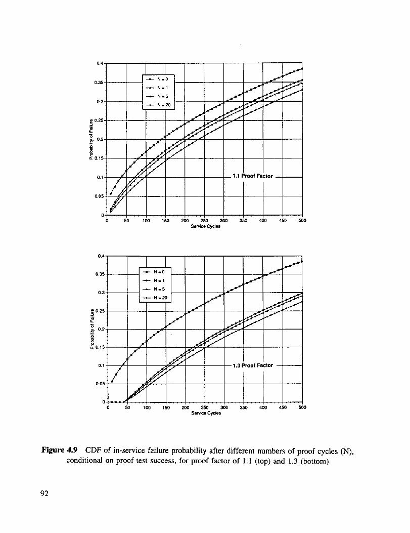
0.4.

0.35"

0.3,

-4- N=O

-.,,-. N=5 J

_._..20 j0.25,

:3

>. 0.2.

_ /o. 0.15

Ol f 1.1 Proof Factor

0.05 _ _

00 50 1oo 150 200 250 300 350 400 450 500

Service Cycles

Figure 4.9 CDF of in-service failure probability after different numbers of proof cycles (N),

conditional on proof test success, for proof factor of 1.1 (top) and 1.3 (bottom)

92

04

0.35

0,3

0.25

o:_ 0.2

o_ 0.15

0.1

0.05

0

j.

=

f:J

5O 100

CT R curve

i

150 200 250 300 350 400 450 500

Service Cycles

0.35

Upperbound R

i .... i ...........

200 250 300 350 400

Service Cycles

J

curve_ --

J

f

450 500

Figure 4.10. CDF of in-service failure probability after different numbers

of proof cycles (N), conditional on proof test success,

for low tearing resistance (top) and high tearing resistance (bottom)

93

O.3-m

.-=- N= 1

-,,.-- N - 5

N=20

0.25

"6._. 0.2

_oA'- 0.15

0.05 J /

0

0

JJ

fJ

J

_" CT R-curve1.3 proof factor___

50 1O0 150 200 250 300 350 400 450

Service Cycles

(a)

5O0

0.4

--..o j

0,3 --__.___ .-2o I""

0.2

0.1

Upperbound R-curve

0.05 1.1 proof factor

(b)0

0 50 100 150 200 250 300 350 400 450 500

Sennce Cycles

Figure 4.11. CDF of in-service failure probability after different numbers

of proof cycles (N), conditional on proof test success

(a) CT R-curve and 1.3 proof factor

(b) upper bound R-curve and 1.1 proof factor

94

Effect of Material Stress-Strain Curve. A significant change in the material stress-strain

curve alone does not appear to have much of an effect on proof test efficacy, for the parameter

combinations considered in this study.

Effect of Crack Shape. Most analyses of MCPT behavior conducted in the recent history

of the program have focused on long, shallow flaws (aspect ratio typically a/c = 0.1). These are

the flaw geometries which have been shown by analysis and experience to be most likely to fail

during proof testing, especially multiple cycle proof testing. Rocketdyne experience, as

documented in Table 1 of the Phase I report, is that pre-existing defects which could be identified

after a multiple cycle proof testing failure typically exhibited high aspect ratios. Experimental

and analytical studies conducted in the current program have shown that for high toughness

materials such as Inconel 718, small aspect ratio flaws are not likely to fail unless applied

stresses are extremely high (greater than yield) or the cracks are extremely large. High aspect

ratio flaws, for which the crack driving force is considerably higher at the same crack depth, are

more likely to fall at more reasonable applied stresses.

However, the majority of defects in actual hardware will have relatively smaller aspect

ratios. A study of actual material defects from Rocketdyne experience (selected SSME hardware,

available MCPT proof failure information, and material test coupons) found that the predominant

crack shape was roughly semicircular (a/c - 1). This study was also reported in the Phase I

report. Therefore, the behavior of these more typical defects during MCPT is also important.

To address this issue, MCPT parameter studies were conducted in which a/c was varied

while all other variables were held constant. Results are shown in Figure 4.12 for a/c values of

0.1, 0.2, and 0.5. For larger values of a/c, the probabilities of failure are much lower for all

scenarios (no proof test, or different numbers of proof cycles). Proof testing of any type (single

cycle or multiple cycle) is also of relatively less benefit, and multiple cycle testing offers

relatively little advantage over single cycle testing. In fact, for a/c = 0.5, some probabilities of

failure in service were actually found to be marginally higher for larger numbers of proof cycles.

However, it must be emphasized that the differences were extremely small, and that the total

probabilities of failure are significantly lower (an order of magnitude) than the baseline case

considered in Section 4.3. See Figure 4.13, which shows the probability of failure in service as

a function of number of proof cycles for the a/c = 0.5 case.

Effect of Crack Size Distribution. Nearly all MCPT parameter studies to date have been

based on a particular crack size distribution which was derived from analysis of the Rocketdyne

flaw data cited earlier. As noted earlier, a particular exponential distribution has been employed

in the Phase II analysis. Of course, the actual distribution of defects in a given population of

components will certainly differ from this single prototypical distribution, and in general the

actual distribution will not be known. The key question for MCPT analysis is how different

initial defect distributions may impact the suitability of different MCPT protocols. In order to

investigate this question further, a number of MCPT analyses were conducted in which different

initial crack depth distributions were assumed. For the purposes of this study, all other variables

(including crack aspect ratio, a/c = 0.1) were held constant at baseline values.

95

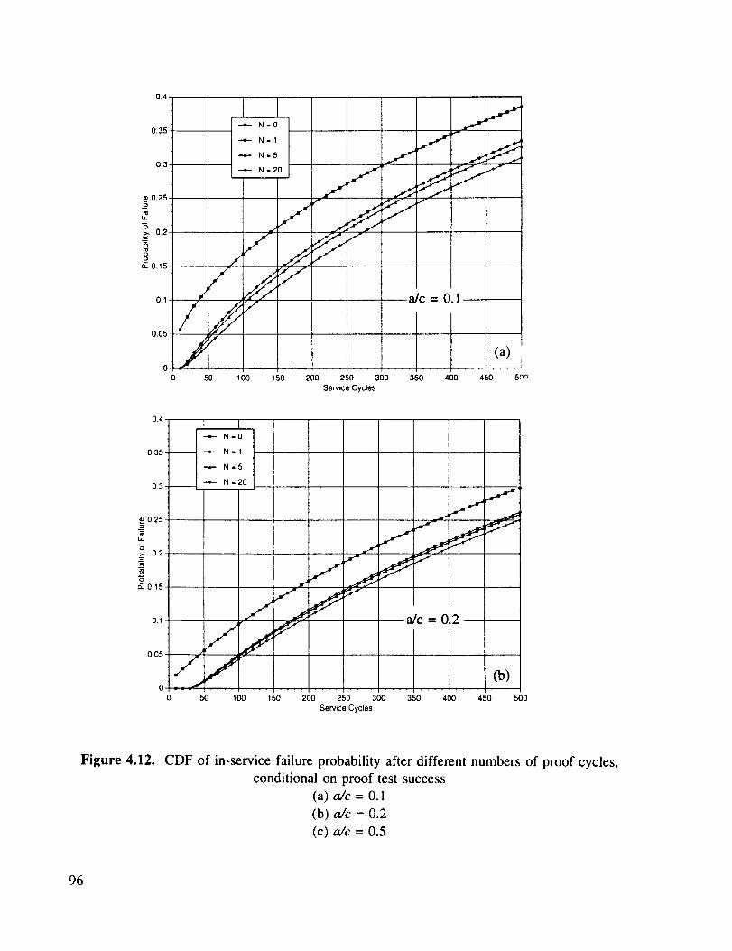
0.4

0.35

0.3

•-,_ N =0

_ N.I

_ N=5

N.20 J

fi

J

y/-

a/c = 0.1

250 300 350 400

Sennce Cycles

(a)

450 5nq

0.4. Am J__

--_- N=0 10.35-- _ N= 1

_ N=5

N=200.3.--

¢' 0.25-5

2

>, 0.2-

=oE. ot5-

i

JJ

J

o.1. _ a/c = 0.2

0.05. // /p_ Co)o --J --

0 50 100 150 200 250 300 350 400 450 500

Service Cycles

Figure 4.12. CDF of in-service failure probability after different numbers of proof cycles,

conditional on proof test success

(a) a/c = 0.1

(b) a,/c = 0.2

(c) a/c = 05

96

50 1O0 150 200 250 300 350 400 450 500

Service Cycles


conditional on proof test success (Cont.)

(a) a/c = 0.1

(b) a/c = 0.2

(c) a/c = 0.5

97

I.D¢%1O

O

98

C3 (3 (D

O9 GO 03

o o oo Iz3 o

o,IO

o

•,-- OO OC)

aJnl!e-I j0 fq!l!qeq0Jcl

It')OO

O

o_

cO

r.D

(..)

Oo

Q I:%

O

..O

o0 z

f,D

-CX]

-O

O

O

E

O

O".,._

..._p. O

II

° ,...q

°,_

0

°_

t_

.m

One set of analyses considered three different exponential distributions for initial crack

depth (before any proof testing). The baseline distribution has a mean value very nearly equal

to a = 0.02 in. Alternative exponential distributions with mean values of a = 0.01 and a = 0.08

were also employed as inputs to the MCPT analysis. The cumulative distribution functions

(CDFs) and probability density functions (PDFs) for these three exponential forms are shown inFigure 4.14.

Resulting calculations of in-service reliability are shown in Figure 4.15 for the two new

distributions (compare Figure 4.12(a) for the baseline distribution). When nearly all cracks are

extremely small, Figure 4.15(a), proof testing is of very little value in improving the reliability

in service. Closer inspection of the data reveals that 5 cycle proof testing yields slightly lower

probabilities of failure than single cycle testing, and 20 cycle proof testing slightly higher

probabilities of failure than single cycle testing, but these differences are so small as to be

negligible. When flaws are extremely small, proof testing has essentially no impact --good or

bad--on reliability in service. When many cracks are large, Figure 4.15(5) (note change in scale),

proof testing is shown to have a large impact on in-service reliability, as would be expected. Of

greater interest, multiple cycle testing appears to offer some significant additional benefit beyond

single cycle testing, and this relative benefit appears to increase with larger numbers of proofcycles.

A second set of analyses of crack size distribution effects employed three different

Weibull distributions. The Weibull clistdbution is a more general mathematical function than the

exponential distribution and is characterized by both a "scale parameter" and a "shape parameter."

The shape parameter, 13, describes the fundamental form of the distribution. When 13 = 1, the

Weibull distribution is the same as an exponential distribution. In this brief study, distributions

with 13 = 0.5, 1, and 2 were considered. The 13 = 1 distribution was chosen identical to the

original baseline exponential distribution, so only two new initial crack size distributions were

analyzed. The CDFs and PDFs for these three Weibull distributions are shown in Figure 4.16.

Note that the three Weibulls were constructed in such a way that the cumulative probability of

occurrence was identically equal to 0.95 at a = 0.06 in. for all three distributions. In other words,

95% of all cracks were smaller than 0.06 in. deep for all three distributions.

The computed values of in-service failure probability from the usual MCPT probabilistic

analysis for the two new runs are shown in Figure 4.17 (again compare Figure 4.12(a) for the

results from the baseline 13 = 1 case). Although total failure probabilities differ dramatically for

the three input distributions, proof testing has a strikingly similar effect on failure probability in

all three cases. A single proof cycle decreases failure probabilities about 0.05, and additional

proof cycles decrease the failure probability by incrementally smaller values. This is an

encouraging result, if it is in fact general, because it suggests that the relative merits of SCPT

and MCPT are not strongly influenced by specific assumptions made about the form of the initialcrack size distribution.

In general, these parameter studies showed that when MCPT is consistently applied to a

fleet of components containing a distribution of initial flaws, the overall fleet reliability will be

99

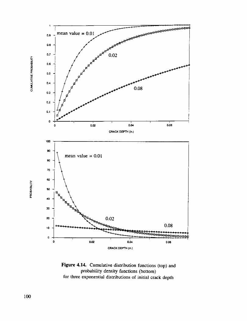
tO0

mean value = 0.01

0.02

0.08

0.02 0.04 0.00

CRACK DEPTH (In.)

O

o.

9O

80 w

70

6O

5O

4O

30

2O

10

0

mean value = 0.01

0.02

0.08

0.02 0.04 0.06

CRACK DEPTH (in.)

Figure 4.14. Cumulative distribution functions (top) and

probability density functions (bottom)

for three exponential distributions of initial crack depth

100

0.4

0.35

0.3

0.25

_. 0,2

_- 0.15

0.1

.4- N=0

--,.._- N=I

_ N=5

N=20

Exponentialn-ean value = 0.01 ___

0.05

0 ...,,===F

0 50 100

If

150 200 250 300

Service Cycles

(a)

350 400 450 500

0

0 50 100 150 200 250 300 350 400 450 500

Service Cycles



(a) exponential distribution with mean value a = 0.01 in.

(b) exponential distribution with mean value a = 0.08 in.

101

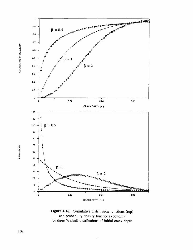
..I

t_©eerl

laJ

7--5

--a¢D

1

0.9 t

0.8

0.7

0.6

0.5

0,4

0.3

0.2

0.1

0

120

/ 13=1

13=2

0.02 0.04 0.06

CRACK DEPTH (in.)

¢1

,.no

el.

110

100

9O

8O

70

6O

5O

40

30

2O

10

0

[3=1

0.02 0.04 0.06

CRACK DEPTH (in.)

Figure 4.16. Cumulative distribution functions (top)

and probability density functions (bottom)

for three Weibull distributions of initial crack depth

102

0.4

0.35

0.3-

-_- N-0

N=I

_ N=5

N=20

Weibull

13 =0.5

0.25.

"6:_ 0.2

_- o._5

0. t

0.05

0

0

f

f

J

f

50 100 150 200 250 300

Service Cycles

350

l(a)

400 450 500

0.4-

0.35-

0.3-

*_ 0.25 •

LI-

0.2

_. 0.15

0.1

0.05

0-0 50 100 150 200 250 300 350 400 450 500

Service Cycles



(a) Weibull distribution with shape parameter 13 = 0.5

(b) Weibull distribution with shape parameter 13 = 2.0

103

higherfor a populationof componentsthathavebeensubjectedto MCPT than for a populationof componentsthat havebeensubjectedto SCPTat thesameproof load. From the standpointof in-servicereliability, moregoodis doneby removinga few additional largeflaws from thepopulationthanharmis doneby incrementalgrowthof manysmallflaws in thepopulation.Thisbenefitgenerally increaseswith increasingnumbersof proof cycles,althoughthe incrementalbenefitof additionalproof cyclesdecreaseswith increasingnumbersof cycles. In somecases,the improvementproducedby thesubsequentcyclesis negligible for all practicalpurposes.

On the otherhand,theparameterstudiesindicatedthat from the standpoint of in-service

fleet reliability, MCPT can be inferior to SCPT, albeit negligibly so, when the probability of

failure due to any proof loading is itself negligibly small. This situation may arise, for example,

when the proof loads are relatively small, the possible crack sizes are relatively small, and the

material is relatively tough, so that the driving force for crack extension is substantially lower

than the material toughness. In this situation, the potential benefit to be gained by removing

additional large flaws from the population is negligibly small. Therefore, the additional

subcritical crack growth caused by the additional proof cycles will reduce net in-service

reliability. However, in most cases, this decrease in reliability will also be negligibly small.

Therefore, while MCPT is of no additional benefit in this situation compared to SCPT, it can be

regarded as being of no additional detriment, either.

4.5 Cracks at Notches

An elastic-plastic J estimation computer software module for a crack at a hole was

incorporated into the probabilistic MCPT/NESSUS computer code. This module was based on

a new J estimation technique developed under the EPFCG contract, and documented in Section

2.2. The computer code was then used to study the relative influence of different numbers of

proof cycles on in-service reliability following a successful proof test. In this report, some sampleresults are shown in order to illustrate the observed trends.

The J solutions were based on a double edge notched plate, with small through-cracks

growing out of the notch roots. This was a convenient geometry for the generation of FE J

solutions, against which the simple estimates could be validated, and the general results are

expected to be typical of a variety of similar notched configurations. A schematic of the notch

geometry was shown previously in Figure 2.3. These studies focused on a notch with D/R = 2.41

and stress concentration factor, K, - 4.29. The exponential distribution of initial crack depths

used in previous studies (see Section 4.3) was implemented here as the initial distribution of

crack size, d, measured from the root of the notch. The half-width of the notched plate, b, waschosen as 1 in., and the notch depth, D, was fixed at 0.3 in.

Several different loads and resistance curves were explored, along with some variations

in the mean value of the initial crack size distribution. The proof factor was 1.2 in all analyses

discussed here. The stress-strain relationship was the same set of Inconel 718 monotonic

Ramberg-Osgood properties used in the previous parameter studies.

104

As anticipated,the notchesbrought about somedifferencesin someof the SCPTvs.MCPT comparisons. Thesedifferencesare clearestin one of the extremecasesexamined.Figure4.18showsthe usualcomparisonof failure probability in servicevs. numberof servicecyclesfollowing differentnumbersof proof cycles. In this case,thenominal proof stresswas100ksi, soextremeyieldingoccurredat theroot of thenotch(rememberK, = 4.29). A resistance

curve with a low tearing modulus (the CT R-curve) was employed. The mean value of the

exponential distribution of initial crack depth was increased from d = 0.02 in. to d = 0.05 in.

Figure 4.18 indicates that, in this case, a larger number of proof cycles (1 to 5 to 20) leads to

a higher probability of failure in service. In the extreme case of 20 proof cycles, in-service

reliability after about 200 service cycles is actually worse than without any proof test.

The calculated elastic, plastic, and total values of the J-integral under these same

conditions (100 ksi) are presented in Figure 4.19. Ductile fracture is driven by the total J value,

while fatigue crack growth under zero-max cycling is driven by A J, which is approximately equal

to the elastic J under these conditions. As a reference point, the critical crack size for ductile

fracture with the CT R-curve is about d = 0.17 in. at 100 ksi. Note that the total J value is

relatively large and increases only slightly with crack length for cracks which are relatively close

to the notch root (esp. for d < 0.15 in.). This trend is, to some degree, a reflection of the

intermediate control condition in the notch vicinity, where local deformation introduces a form

of secondary loading somewhat akin to displacement control. This shape of the J-a curve means

that, for cracks in this size range, it is possible for the crack to grow substantially without

significantly increasing the chance that it will fail. Therefore, additional proof cycling is more

likely to cause additional damage to the structure without failing additional defective structures.

When the cracks are larger compared to the notch field, these notch effects on the crack

tip driving force become less important. The studies of J solutions for cracks at notches (Section

2.2) found that the notch field had effectively no influence on J for cracks that were larger than

30 to 50 percent of the notch root radius. The J solution for these longer cracks growing from

a notch root was the same as the J solution for a crack of the same total length (the sum of the

notch depth and crack length) in an unnotched body. Therefore, the notch effect on MCPT

behavior would be negligible.

At a lower applied stress (50 ksi proof stress), keeping all other variables constant,

increasing numbers of proof cycles still lead to an increase in in-service failure probability, but

on a much-diminished scale. See Figure 4.20. Note that here all of the failure probabilities are

extremely small numbers, and the differences between different numbers of proof cycles are

minimal. One might conclude in this situation that, although additional proof cycles are moredamaging, the effect is entirely negligible.

4.6 Memory vs. Loss-of-Memory in Tear-Fatigue Theory

The tear-fatigue model employed in the current MCPT/NESSUS computer code effectively

describes crack growth during concurrent fatigue cycling and ductile tearing. The model has

105

09

0.8

07

0.6- --

|u. 05

•_ 0.4

0n

0.3

0.2

0.1

I----.- N _ 0

_ N=I

N-5

N=20

o0 50 100 150 200 250 300 350 400 450 500

Service Cycles

Figure 4.18. CDF of in-service failure probability after different numbers of proof cycles;

notched geometry, 100 ksi proof stress, a i = exp[.05]

106

10

9

8- --

7

6

5

4

3-

2

1-

0

0

-4- Je

-e- Jp

--=.- J Total

...... - n m _- ._ _-

/

0.05 0.1 0.15 0.2 0.25 0.3

Crack Size

Figure 4.19. Total, elastic, and plastic J values for cracks emanating from

double edge notches with 100 ksi nominal stress

0.001 -

0.0009 -

0.0008 -

0.0007

0.0003-

0.0002

0.0001 •

Figure 4.20.

0 50 1O0 150 200 250 300 350 400 450 500

Service Cycles


notched geometry, 50 ksi proof stress, a i "- exp[.05]

107

been validated for severalmaterials,including IN-718, under conditions in which dJmddNincreaseson eachcycleor remainsapproximatelyconstantwith cycling. In short, tear-fatiguetheory requiresthat once tearing has initiated, additional ductile tearing does not occur onsubsequentfatiguecyclesuntil J,,_ increases beyond its previous maximum value.

Tear-fatigue behavior following step changes in applied load, such as the step decrease

which occurs between proof loading and subsequent service cycling, has not been studied to the

same extent. One key question is whether fatigue (service) cycling at the lower load level must

continue until the previous J,_ value (from the proof testing at the higher load level) is exceeded

before tearing continues. This would be consistent with the general tear-fatigue rules, which

effectively assume that the ductile fracture process zone at the crack tip advances with the crack

as it extends by fatigue. This implies that the crack retains full "memory" of its previous history.

On the other hand, it is possible that ductile tearing (and subsequent tear-fatigue) during service

cycling will re-initiate somewhat independently of the previous proof test response (in other

words, when J,,_ from the fatigue cycling exceeds the initiation toughness, even if the previous

Jr_ from the proof testing was higher). This approach implies a "loss of memory" of previouscrack growth events.

It is simple to envision contrasting scenarios in which each behavior might be observed.

Consider one situation where proof testing initiates significant tearing; the subsequent decrease

in applied load is relatively small; and the subsequent increase in Jm_ with crack growth is

relatively rapid, so that J,,_ exceeds its previous maximum value before the crack tip has moved

far beyond its position at the end of the proof cycle. In this case it is reasonable to assume that

the ductile fracture process zone does in fact advance with the crack tip as it grows in fatigue.

On the other hand, consider a situation where the subsequent decrease in applied (service) loading

is sufficiently appreciable that J_,_ decreases considerably, and extensive crack growth is required

before Jma_ again increases to proof test levels. In this case, it is more likely that the fatigue

crack will simply grow through the previous ductile fracture process zone. Once this has

occurred, material memory of the previous ductile tearing event is largely forgotten, and tearing

will re-initiate during service cycling when the usual conditions for tearing are satisfied (J_ firstexceeds the initiation toughness).

In practice, actual material response is likely to lie somewhere between these two

extremes: rigorous tear-fatigue rules on the one hand, and a complete loss of material memory

tresetting of the resistance curve) on the other hand. Experimental and analytical characterization

of the exact response is beyond the scope of the present effort. However, it is important to

assess if this ambiguity has a significant effect on the assessment of the relative merits of single

and multiple cycle proof testing. If it does not, then it is not so important to understand thebehavior completely at this time.

The MCPT/NESSUS computer code was modified to make crack growth predictions based

on either the full "memory" or full "loss of memory" theories at the end of proof cycling, and

the code was then exercised with various parameter choices to determine what difference it would

make. The results show that, in terms of total probability of failure for a fleet of components

108

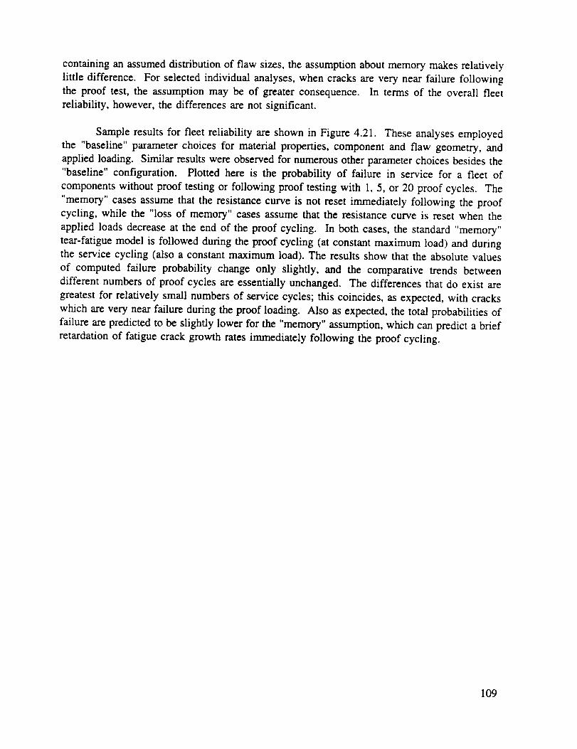
containing an assumed distribution of flaw sizes, the assumption about memory makes relatively

little difference. For selected individual analyses, when cracks are very near failure following

the proof test, the assumption may be of greater consequence. In terms of the overall fleet

reliability, however, the differences are not significant.

Sample results for fleet reliability are shown in Figure 4.21. These analyses employed

the "baseline" parameter choices for material properties, component and flaw geometry, and

applied loading. Similar results were observed for numerous other parameter choices besides the

"baseline" configuration. Plotted here is the probability of failure in service for a fleet of

components without proof testing or following proof testing with 1, 5, or 20 proof cycles. The

"memory" cases assume that the resistance curve is not reset immediately following the proofcycling, while the "loss of memory" cases assume that the resistance curve is reset when the

applied loads decrease at the end of the proof cycling. In both cases, the standard "memory"

tear-fatigue model is followed during the proof cycling (at constant maximum load) and during

the service cycling (also a constant maximum load). The results show that the absolute values

of computed failure probability change only slightly, and the comparative trends between

different numbers of proof cycles are essentially unchanged. The differences that do exist are

greatest for relatively small numbers of service cycles; this coincides, as expected, with cracks

which are very near failure during the proof loading. Also as expected, the total probabilities of

failure are predicted to be slightly lower for the "memory" assumption, which can predict a brief

retardation of fatigue crack growth rates immediately following the proof cycling.

109

0.12

0.1

0.08

It.

0.06 -

]5

on

0.04-

0.02-

0 5 10 15 20 25 30 35 40 45 50

Service Cycles

Figure 4.21. Computed in-service failure probability for different numbers of proof cycles

and different assumptions about material memory following the proof overload

110

5. DISCUSSION

5.1 Other Proof Testing Issues

Proof testing is a complex subject. A large number of structural, material, and loading

variables can influence the response of a (potentially) flawed component during a proof test and

subsequent service cycling. Therefore, in principle, many variables can influence the relative

merits of single cycle and multiple cycle proof testing. The current research study, on the other

hand, has been necessarily limited in scope. Not all proof test variables have been evaluated

quantitatively, and not all potential modes of proof test or in-service failure have been considered.

The investigators have attempted to focus on the most significant proof test variables, and they

have emphasized the most significant mode of structural failure: the growth of a pre-existing

crack as characterized by the established principles of fracture mechanics. Before closing, it is

useful to discuss briefly some other proof test variables and some other potential modes of proof

test failure. Some of these issues are being treated in more depth under another research contract[41].

5.1.1. Hold Times and Time-Dependent Fracture Behavior

Most proof test loading includes some hold time at a steady maximum load. This hold

time may be as short as a few seconds merely to insure that the steady state maximum load has

been achieved, or as long as many hours to permit inspection of the component or structure under

maximum load. The current Rocketdyne MCPT protocol stipulates hold times of 30 seconds at

maximum load on each cycle.

Hold times at maximum load can influence fracture behavior. In general, a component

that can withstand a certain maximum critical load for a few seconds may not be able to

withstand the same load without failure if held at that level for a longer period of time. This

phenomenon occurs because of time-dependent fracture behavior: cracks can grow slowly at a

fixed load (or exhibit accelerated growth under cyclic loading when the loading frequency is

slower). This crack growth phenomenon can ultimately be linked to time-dependent mechanical

deformation or, in some situations, to time-dependent environmental damage in the material.

Although a detailed review of the hold time effect in proof testing is beyond the scope of thiscontract, some brief observations are useful.

Tiffany [48] and Schliessmann [3] were among the f'trst to address hold time effects in

proof testing. They both observed that in relatively inert environments, sustained stress crack

growth was only significant when the applied stress intensity factor was a large fraction of the

critical (time-independent) K value for failure, usually 80 to 90 percent. If the applied K was less

than some "threshold" value, as Tiffany termed it, then sustained stress effects were negligible.

However, Tiffany noted that this threshold stress could decrease dramatically when environmental

factors were introduced, such as high pressure hydrogen gas with Inconel 718. Johnson and Paris

[49] subsequently reviewed several more detailed investigations (included their own) of sustained

111

stresscrack growth and noted severalcharacteristictrends in the subcritical crack growthbehavior.Typically,thecrackgrowthrateundersustainedloadinitially decreased,andthecrackcould halt if the stressintensity factor waslow enough. At higherstressintensities,the crackgrowth rate wasobservedto passthrougha minimum and then increasesteadilyas unstablefractureapproached.

Thesephenomenawere all observedin the simulatedMCPT surfacecrack growthexperiments (all with 30-secondhold times) conductedunder the current contract, andsummarizedin Section3.5. In particular,substantialtime-dependentcrackgrowthwasobservedonly at applied loadsvery closeto the ultimatefailure load. The crackgrowth rategenerallydecreased to zero after a brief period of growth, except when failure was imminent. In this case,

the crack growth rate decreased to a minimum and then increased steadily to instability.

The proper analytical treatment of time-dependent crack growth is not yet entirely clear.

Landes and Wei [50] published one of the first significant studies linking subcritical crack growth

in an inert environment to creep deformation at the crack tip. More recently Brust and Leis [51-

52] have forwarded an analytical method that characterizes time dependent crack growth due to

an increase in the elastic-plastic crack driving force that results, not from an increase in load, but

from a reduction in the yield properties of the material around the crack tip due to time-

dependent creep deformation. Their formulation, however, is currently limited to certain classes

of materials in which the local stresses at the crack tip increase with time. It remains possible

that some forms of sustained stress crack growth are due to time-dependent changes in the crack

advance mechanism, not in the near-tip material properties.

Ingham and Modand [53] took a somewhat simpler approach, considering time-dependent

crack growth in the context of a simple J-resistance curve framework, and generating different

resistance curves at different displacement rates. They also concluded that time-dependent crack

growth was only significant when the sustained loads were within a few percent of the collapse

load and the remaining ligament was fully plastic. Therefore, time-dependent failure would not

be significant in structures with contained yielding.

What are the implications of time-dependent crack growth and therefore hold timesmfor

the comparison between SCPT and MCPT? Time-dependent crack growth can be thought of as

another form of subcritical crack growth, analogous to the subcritical cyclic crack growth that

occurs during multiple proof cycles. This subcritical cyclic crack growth was shown in the

current contract to become significant only when failure was relatively imminent, and this is

entirely similar to the earlier observation that sustained stress crack growth becomes significant

only near instability. Therefore, by analogy, it would appear that hold times would be most

beneficial under the same conditions in which multiple cycles are most beneficial, and that the

time-dependent and cycle-dependent phenomena would work together to remove additional near-

critical flaws from the population. It is even possible that hold times may improve the relative

advantages of MCPT under these conditions. In the limited experimental studies of simulated

MCPT conducted in the present contract, it appears that if the hold times had been significantly

shorter, failure would not have occurred at the proof loads and numbers of cycles applied. Also

112

by analogy,it is possiblethat longerholdtimes,like increasingnumbersof cycles,would furtherimprovefleet reliability, albeitwith diminishingincrementalbenefit.

On the otherhand,whenmultiple proof cyclesarelessbeneficial,hold timesmay alsobelessbeneficial,although(asfor multiplecycles)anyadditionalsubcriticaldamagedueto time-dependentcrackgrowthwould typically benegligiblewhenfailure is not imminent. However,it mustbeemphasizedthat no rigorousanalysesor experimentalevaluationsof holdtime effectson MCPT havebeenconductedunderthecurrentcontract,andthereforeall of thesecommentsandconclusionsmustbe regardedasspeculativeratherthandefinitive.

5.1.2. Cyclic Hardening and Softening

It is well-known that the constitutive properties of some materials can change significantly

following relatively severe cyclic elastic-plastic deformation. Hard materials can soften, and soft

materials can harden. As noted in Section 3.4, for example, Inconel 718 in the monotonic

condition has a relatively high yield strength and relatively low strain hardening, while its

cyclically stable properties include a lower yield strength and higher strain hardening.

Is this significant for the evaluation of MCPT? While no detailed studies of this question

were conducted in the current contract, the answer appears to be a qualified "no". First of all,

limited parameter studies found that changes in the constitutive relationship alone did not lead

to significant changes in fleet reliability following SCPT or MCPT. Second, as long as the

number of proof cycles is kept relatively low (five, for example), extensive cyclic changes in the

constitutive properties of the material are not likely. Cyclic hardening or softening is a gradual,

not an instant process, and often requires many cycles to achieve. The common rule of thumb

is to determine cyclic properties at the half-life of a fatigue specimen subjected to constant

amplitude straining, thereby implying that the stabilization process will occur much more quicklyunder more severe cyclic straining.

Of course, cyclic hardening or softening (in a suitable material) is always taking place in

the crack tip region due to the locally severe deformation occurring there (even if the remote

stresses and strains are mild). Therefore, this effect is automatically included in any normal

characterization of crack growth rate properties, and should require no explicit treatment.

On the other hand, cyclic hardening or softening may need to be considered explicitly in

the evaluation of SCPT or MCPT when both the proof test deformation and the in-service cyclic

deformation are relatively severe. In this case, the assessment of in-service crack growth may

need to employ cyclic stress-strain properties (for example, in the computation of AJcn ) when

those provide a more conservative answer than monotonic properties. However, it may be

prudent to retain monotonic properties in the analysis of the proof test itself.

Another possible exception involves proof testing of materials with a pronounced yield

point, such as certain steels. These materials can exhibit a more pronounced and rapid change

113

in the stress-strainrelationshipfollowing only a few load excursions near or above the yield

point, and so a more detailed assessment may be required.

5.1.3. Weidments

Weldments can introduce a new set of complex issues into any fracture analysis.

Although nominally the weld metal often retains the same properties as the base metal, and the

weldment as a whole can often be treated as a homogenous component, other complications are

also possible. Weldments can introduce significant residual stresses, for example. The weld

metal and/or the heat affected zone can exhibit different material properties, and sometimes the

weld metal properties are intentionally chosen higher or lower than the base metal in order to

achieve a certain structural performance. Weldments are also a prime location for initial or

service-induced crack-like defects, of course, due to potential inhomogeneities in the weldment

itself or to irregularities in the surface or weldment interface.

Although none of these issues have been addressed directly in the current contract, a few

speculative observations are useful. Residual stresses can relax somewhat under severe cyclic

loading, and so multiple cycle proof testing could cause some additional relaxation. If the

residual stresses were previously beneficial for service loading, then MCPT could slightly degrade

the in-service performance; the reverse might then be true if the residual stresses were originally

detrimental to in-service performance.

Significant variations of local material properties in a weldment, whether intentional or

unintentional, could introduce new complications to a tear-fatigue analysis. Due to this

complexity, no speculation about SCPT or MCPT outcomes is offered here. Additional analysiswould be required to assess these issues.

Another set of potential issues introduced by weldments relates to unusual defect shapes.

Actual weldment defects, of course, do not typically take a uniform elliptical or semi-elliptical

shape. The study of many such actual weldment defects during Phase I did find that the semi-

circular surface crack was a reasonable representative on average, but that same study

documented the wide variety of actual shapes, including many irregular shapes that are quite

unlike any normal idealized geometry. Furthermore, these irregular weldment defects can occur

in local clusters, with small ligaments between them.

Growth of these flaws during proof testing may not follow the customary form of

idealized fracture mechanics equations. Early growth may be dedicated to the transformation of

irregular shapes (where the crack driving force varies widely around the perimeter of the flaw)

into more regular shapes (where the crack driving force is more uniform around the perimeter).

Local ligaments between neighboring flaws may fail due to plastic collapse to form new,

coalesced cracks. Failure of local ligaments due to severe low cycle fatigue or localized ductile

tearing could lead to the sharpening and, effectively, the formation of cracks where blunter voids

once existed. Again, these complex crack growth phenomena were not addressed in the current

contract, and no damage growth phenomena were considered that were not explicitly fracture

114

mechanicsevents. In general,however,additionalproof cycleswould likely be helpful in theformation and failure (and thereforethe detection)of theseweldmentdefects. Of course,itremainspossiblethat additionalproof cyclescould makea local defectworsewithout causingit to fail, therebyreducingthein-servicereliability, but asnotedearlier,theMCPT problemmustalwaysbe treatedfrom thestandpointof thetotal fleetpopulation.Moredefinitiveanswersaboutthe problemof irregularor unusualweld defectswould requirefurther analysis.

5.2 The Generality of the Results

The investigations conducted in the current contract have necessarily been limited in

scope. Only a small number of crack geometries, crack sizes, resistance curves, etc. have been

studied, and only a limited number of combinations of different variables could be considered.

Although the parameter studies were intended to exercise several key variables over a wide range

or values, and although those parameter studies were interpreted and extended in terms of

fundamental understandings about the fundamental crack growth phenomena involved, it must

be emphasized most strongly that many practical combinations of parameters remain unexamined.

And, of course, the experimental studies under this contract were necessarily limited to a single

material and a narrow range of geometries.

In contrast, the real world of reusable aerospace propulsion system components is filled

with many different materials, many different geometries, and many different potential hardware

defects. Even a single component or proof tested assembly may contain several different critical

locations, each with a unique geometrical configuration, local level of constraint, etc. And

therein lies a paradox of sorts. On the one hand, as noted in the conclusions to the Phase I

report, and confirmed quantitatively in the Phase II work, the selection of an optimum proof test

protocol depends on many different variables and may be component-specific. On the other

hand, what is needed is a set of general guidelines about the relative merits of SCPT and MCPT

that will provide useful engineering guidance for a wide range of real hardware.

This contract has always pursued these general goals, and in fact is concluding now by

proposing a general set of practical engineering guidelines for the selection of an optimum proof

test protocol (see Sections 6 and 7). However, the complete generality of these guidelines cannot

be absolutely guaranteed, in view of the many complex variables involved. And it is exactly this

complexity that prevents the formulation of specific, quantitative rules-of-thumb to guide the

design of an optimum proof test for every single component. Instead, the guidelines must bemore qualitative in nature.

The solution to this dilemma, for the practicing engineer who must confidently design a

specific proof test protocol for a specific component, is to perform a specific quantitative analysis

of that specific problem. One set of tools that would facilitate this job would be (1) a general-

purpose crack growth computer code that provides acceptably accurate predictions of elastic-

plastic crack growth due to fatigue, tearing, and their interaction for a variety of practical crack

geometries; and (2) a simple probabilistic driver to evaluate the impact on in-service reliability

for a given proof test protocol, given some assumed distribution of initial defects. This is a

115

similar approach to the analysis performed in the current contract, although the research software

used in the performance of this contract had limited generality and a cumbersome user interface.

But if software of this type was available, the engineer could identify critical locations on his

hardware (locations with high stress and/or increased likelihood of initial defects), choose a

representative flaw geometry, and choose a representative initial defect distribution, and let the

software evaluate changes in reliability for different combinations of proof factor and number of

cycles. Software of this type would also be useful in conducting additional research studies of

MCPT, including some of the unaddressed issues cited above.

116

6. SUMMARY AND CONCLUSIONS

. Multiple cycle proof testing can be effective in removing some of the largest flaws from

the population that would not have been removed by conventional single cycle proof

testing at the same proof loads. This conclusion is clearly supported both by fracture

mechanics theory and by validating experimental observations. Hence, MCPT can be an

effective means of identifying and removing defective hardware that could go undetected

by conventional SCPT.

. Multiple cycle proof testing can also cause additional subcritical crack growth to occur

in components that do not fall during the proof test. Unfailed cracks can grow more

during a multiple cycle proof test than during a single cycle proof test. Therefore, in

general, a cracked component that survives a multiple cycle proof test has a slightly

shorter remaining service life than if the component had been subjected to a single cycle

proof test at the same load. However, this service life difference is negligibly small in

most cases. The difference will be significant only in those cases where cracks are

relatively large and failure is relatively imminent following the proof test.

Probabilistic studies have shown that, in general, when MCPT is consistently applied to

a fleet of components containing a distribution of initial flaws, the overall fleet reliability

will be higher for a population of components that have been subjected to MCPT than for

a population of components that have been subjected to SCPT at the same proof load.

From the standpoint of in-service reliability, more good is done by removing a few

additional large flaws from the population than harm is done by incremental growth of

many small flaws in the population. This benefit generally increases with increasing

numbers of proof cycles, although the incremental benefit of additional proof cycles

decreases with increasing numbers of cycles. Three possible exceptions to this general

principle are addressed in the following three conclusions.

. From the standpoint of in-service fleet reliability, MCPT can be inferior to SCPT (albeit

negligibly so) when the probability of failure due to any proof loading is itself negligibly

small. This situation may arise, for example, when the proof loads are relatively small,

the possible crack sizes are relatively small, and the material is relatively tough, so that

the driving force for crack extension is substantially lower than the material toughness.

In this situation, the potential benefit to be gained by adding proof cycles to remove

additional large flaws from the population is negligibly small. Therefore, the additional

subcritical crack growth caused by the additional proof cycles will reduce net in-service

reliability. However, in most cases, this decrease in reliability will also be negligibly

small. Therefore, while MCPT is of no additional benefit in this situation compared to

SCPT, it can be regarded as being of no substantial detriment, either.

. When the crack driving force decreases with increasing crack size, failure during proof

testing is highly unlikely, although subcritical crack growth can occur for even the largest

flaws. Proof testing to any number of cycles (one cycle or many cycles) will be

117

.

.

.

detrimental under these conditions and should be avoided unless supported by a detailed

fracture mechanics analysis. This situation can occur for displacement-controlled

configurations, or for configurations in which crack growth in one member merely causes

load shedding to an ahemative structural member due to the increased compliance of the

cracked member, or if the crack resides in a steeply falling stress field due, for example,

to residual welding strains. If proof testing cannot be avoided under these conditions, the

number of proof cycles should be kept to a minimum, and a comprehensive proof test

analysis should be performed based on fracture mechanics.

When cracks are located at notch roots and the crack lengths of concern are comparable

to the plastic notch field or smaller, and when the stresses and strains in the notch root

are severe, then MCPT may not provide additional benefit compared to SCPT. In these

situations, additional proof cycles can degrade in-service fleet reliability, although

typically by small amounts. This behavior occurs due to the local control condition in

the notch root, which causes J values to be relatively high but to increase only slightly

with increasing crack length. Therefore, although additional subcritical crack growth

occurs relatively easily, failure is unlikely. When the crack lengths are large compared

to the notch field, or when local stresses and strains are less severe, the notch is less of

a problem for MCPT.

The specific benefit or detriment associated with MCPT will depend on a number of

different factors, including the proof load factor, the number of proof cycles, the

toughness and tearing resistance of the material, the geometric configuration of the crack,

the level of structural constraint in the vicinity of the crack, and the distribution of

potential crack sizes and crack shapes. Because of these many complex factors, it is not

possible to provide a simple set of universal formulas or graphs to select the

mathematically optimum proof test protocol and quantify the incremental benefit of that

protocol.

Individual fracture mechanics analyses of critical component locations are recommended

to determine the most appropriate proof test protocol for specific proof testing problems.

These analyses would be facilitated by the availability of a general-purpose computer

code for crack growth analysis that includes a variety of elastic-plastic fracture mechanics

solutions for common crack geometries (especially surface cracks) based on the J-integral

parameter, along with practical crack growth algorithms based on J to address monotonic

and cyclic crack growth processes and the tear-fatigue interaction between these two

mechanisms. Also of benefit would be a simple probabilistic analysis routine to evaluate

the changes in fleet reliability for a population of components containing a distributionof initial crack sizes.

. The parameter studies conducted under the current contract indicate that for wide ranges

of variation in many of the important factors, the overall performance of MCPT in

comparison to SCPT is relatively consistent. MCPT appears to be either beneficial or

benign in comparison to SCPT, and any benefit generally continues to increase with

118

increasingnumbersof proof cycles. In situations where component failure risk is

relatively high, MCPT can be a useful means of obtaining additional reliability. In

situations where component failure risk is relatively low, MCPT itself offers no additional

benefit. However, if multiple proof cycles are desirable or required for other (non-

fracture mechanics) reasons, then these multiple cycles will not generally cause any

significant deterioration of fleet reliability. Some additional recommendations for

selecting an appropriate proof test protocol are contained in the Engineering Guidelines,which follow these conclusions.

10.

11.

12.

MCPT can be preferable to SCPT only when viewed from the perspective of component

reliability; i.e., a probabilistic assessment of structural integrity. From a purely

deterministic standpoint, the potential advantages of MCPT cannot be recognized or

documented. In particular, if proof testing is being used for the specific purpose of

establishing a guaranteed maximum size for any flaw remaining in the component

following the proof test (e.g., a quantitative flaw screening in conjunction with a

deterministic fatigue crack growth analysis to guarantee a minimum safe remaining lifein service), then MCPT offers no apparent additional benefit. The maximum flaw size

(based on a deterministic analysis) that could theoretically remain in the component

following a proof test to a certain fixed proof load does not change if single or multiple

proof cycles are performed; MCPT does not increase or decrease this maximum flaw size

relative to SCPT. The potential advantage of MCPT over SCPT is that the frequency of

flaws that are slightly smaller than this critical (deterministic) maximum flaw size may

be decreased, thereby improving component reliability from a probabilistic perspective.

Proof testing to typical proof factors for advanced reusable propulsion systems (factors

of 1.2 and less) does not appear to cause significant retardation of fatigue crack growth

at service load levels. The overload retardation phenomenon becomes significant only athigher overload ratios.

Acoustic emission (AE) shows some promise as a means of detecting significant

subcritical crack growth during proof testing. While proof testing and associated flaw

behaviors can generate a variety of detectable AE activity, the most substantial AE signals

appear to be associated with crack extension as instability is approached. If it were

possible to use AE monitoring to detect this damaging subcritical growth, then it could

be possible to eliminate the single greatest risk associated with MCPT--substantial

subcritical growth of large flaws that are not quite large enough to cause failureBwhile

further improving the ability of the MCPT process to screen potentially dangerous flaws

(down to even slightly smaller flaw sizes). AE monitoring would potentially be aided by

multiple proof cycles (rather than a single cycle) because the multiple cycles would

provide more opportunities for monitoring. However, these conclusions are based on

controlled laboratory experiments in which isolation and filtering of extraneous

background noise was relatively simple to accomplish, and in which the number of

potential AE sources was relatively small. Further studies would be required to evaluate

119

thefeasibilityof employingsuchanAE approachduring proof testing of actual hardware

in a production environment.

13. Estimates of the J-integral based on modified reference stress formulations are acceptably

accurate for many engineering applications. This approach was specifically validated in

this study for two important classes of cracked geometries, the semi-elliptical surface

crack in a finite thickness plate, and the edge crack growing at a notch root. The

modified reference stress estimates are most accurate when they can be guided by limited

finite element results. These numerical results provide important assistance in identifying

an optimum yield load and/or structural parameter for the reference stress formula, which

can then be used to generate J solutions for a much wider range of geometries than can

be addressed by the available finite element solutions.

14. Crack growth and instability in tough, ductile materials during single cycle and multiple

cycle proof testing is satisfactorily described by elastic-plastic fracture mechanics based

on a J-integral characterization. The behavior of cracks during cyclic loading is

satisfactorily described by a AJcn approach that accounts for crack closure, while crack

behavior during monotonic loading approaching instability is satisfactorily addressed by

a J-resistance curve approach. The interactions between monotonic and fatigue crack

growth as cycling occurs near instability are satisfactorily described by tear-fatigue theory.

These conclusions have been validated by critical experiments with Inconel 718. The

broad outlines of these elastic-plastic fracture mechanics approaches are described in the

main body of this report. Detailed engineering methodologies for carrying out the

computations are being developed and fully documented in two companion contractefforts.

120

7. ENGINEERING GUIDELINES

7.1 General Background

A series of general conclusions about the comparison between MCPT and SCPT was

provided in the Summary and Conclusions section that immediately precedes these Engineering

Guidelines. It was concluded that, in general, when MCPT is consistently applied to a fleet of

components containing a distribution of initial flaws, the overall fleet reliability will be higher

for a population of components that have been subjected to MCPT than for a population of

components that have been subjected to SCPT at the same proof load. This conclusion was

found to be generally true for relatively wide variations in a number of different material, crack,

and proof test parameters, although some exceptions were identified.

The Summary and Conclusions section also noted that, due to the large number of

different factors influencing proof test performance, it was not possible to provide a simple set

of formulas or graphs to select the mathematically optimum proof test protocol and quantify the

incremental benefit of that protocol. Instead, individual fracture mechanics analyses of critical

component locations, based on the engineering methodology developed under the current contract

and two other contracts, were recommended to determine the most appropriate proof test protocol

for specific proof testing problems. As noted, these analyses must be probabilistic to determine

properly the relative advantages or disadvantages of MCPT.

Nevertheless, it is useful to summarize some of the lessons learned from the analytical

and experimental investigations in this contract in a manner that provides some additional

engineering guidance for the selection of a proof test protocol. It will undoubtedly remain a

source of some frustration that, due to the complexity of the problem, these guidelines cannot

provide simple quantitative rules that unambiguously specify all of the relevant proof test

parameters for a given piece of hardware. However, some additional guidance about specific

proof testing issues and parameters should be useful to NASA staff and contractors as theyapproach new proof testing problems.

It must also be emphasized that these engineering guidelines are necessarily based

primarily on the analytical and experimental investigations conducted under the current contract,

aided by the broader engineering experience and judgement of the investigators. The

investigations under the current contract were particularly focused on Inconel 718, an alloy of

particular relevance to the SSME and representative of a broader class of tough, ductile

superalloys. Therefore, it must be recognized that the generality of the guidelines is necessarily

somewhat limited. Further experience with the analysis of proof testing following the general

approach described in this report may lead to some revisions in these guidelines. However, the

investigators have made every reasonable effort possible within the scope of the contract to

develop a fracture mechanics methodology with sufficient generality, and to exercise that

methodology over a sufficient range of parameters, to ensure the overall robustness of theseguidelines.

121

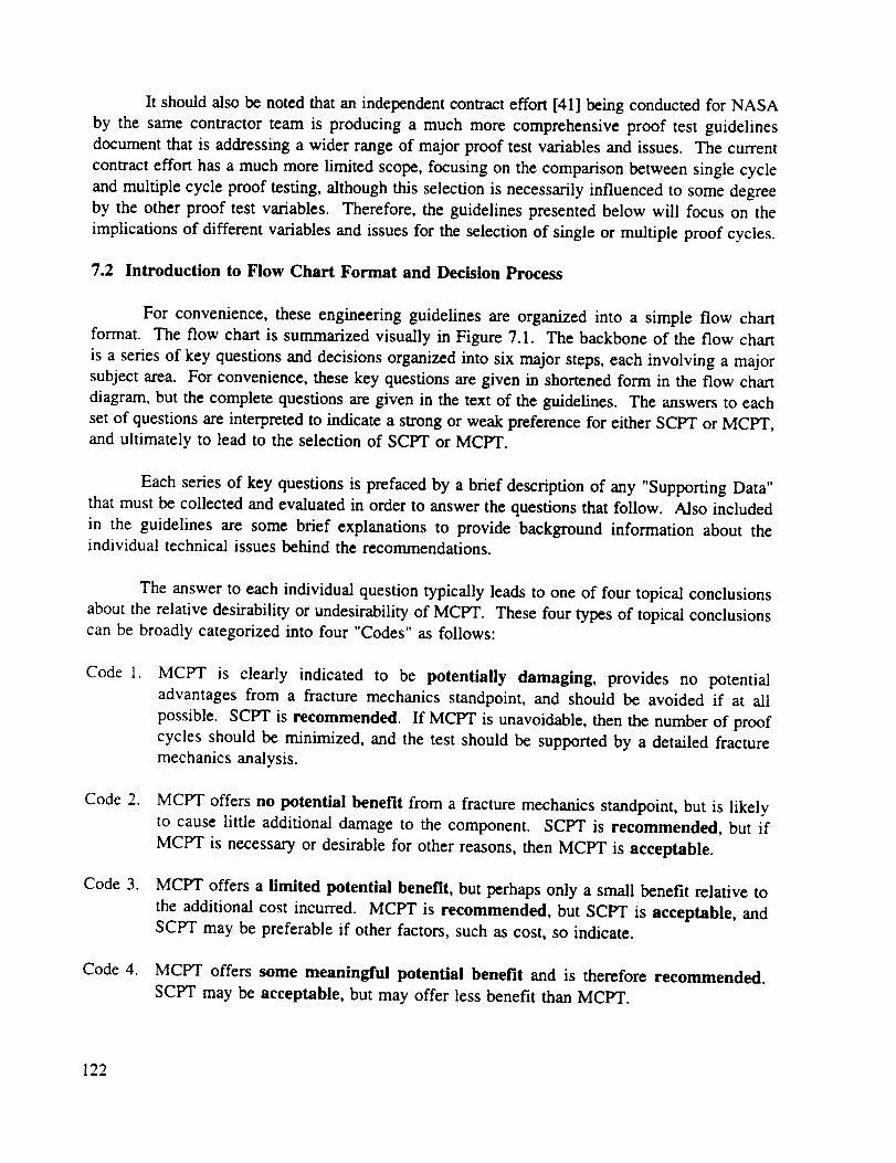
It shouldalsobenotedthatanindependentcontracteffort [41] beingconductedfor NASAby the samecontractorteam is producinga much morecomprehensiveproof test guidelinesdocumentthat is addressinga wider rangeof majorproof testvariablesandissues.The currentcontracteffort hasa muchmorelimited scope,focusingon thecomparisonbetweensinglecycleandmultiplecycleproof testing,althoughthis selectionis necessarilyinfluencedto somedegreeby the otherproof test variables. Therefore,theguidelinespresentedbelow will focus on theimplicationsof differentvariablesandissuesfor the selectionof singleor multiple proof cycles.

7.2 Introduction to Flow Chart Format and Decision Process

For convenience, these engineering guidelines are organized into a simple flow chart

format. The flow chart is summarized visually in Figure 7.1. The backbone of the flow chart

is a series of key questions and decisions organized into six major steps, each involving a major

subject area. For convenience, these key questions are given in shortened form in the flow chart

diagram, but the complete questions are given in the text of the guidelines. The answers to each

set of questions are interpreted to indicate a strong or weak preference for either SCPT or MCPT,

and ultimately to lead to the selection of SCPT or MCPT.

Each series of key questions is prefaced by a brief description of any "Supporting Data"

that must be collected and evaluated in order to answer the questions that follow. Also included

in the guidelines are some brief explanations to provide background information about theindividual technical issues behind the recommendations.

The answer to each individual question typically leads to one of four topical conclusions

about the relative desirability or undesirability of MCPT. These four types of topical conclusionscan be broadly categorized into four "Codes" as follows:

Code 1.MCPT is clearly indicated to be potentially damaging, provides no potential

advantages from a fracture mechanics standpoint, and should be avoided if at all

possible. SCPT is recommended. If MCPT is unavoidable, then the number of proof

cycles should be minimized, and the test should be supported by a detailed fracture

mechanics analysis.

Code 2.MCPT offers no potential benefit from a fracture mechanics standpoint, but is likely

to cause little additional damage to the component. SCPT is recommended, but if

MCPT is necessary or desirable for other reasons, then MCPT is acceptable.

Code 3. MCPT offers a limited potential benefit, but perhaps only a small benefit relative to

the additional cost incurred. MCPT is recommended, but SCPT is acceptable, and

SCPT may be preferable if other factors, such as cost, so indicate.

Code 4. MCPT offers some meaningful potential benefit and is therefore recommended.

SCPT may be acceptable, but may offer less benefit than MCPT.

122

ASSESS MATERIAL FRACTURE BEHAVIORSTEP1.

1.A. Brittle behavior?

no

1.B. Low effective tearing modulus?

STEP 2. ASSESS CRITICAL CRACK SIZES

yes

2.A. Can worst-case rogue flaw fail during proof test?

yes

2.B. Critical flaws likely to be found by NDE?

2.C. Mature, trouble-free manufacturing process?

no

Figure 7.1 Flow chart for Engineering Guidelines

123

STEP 3. ASSESS COMPONENT GEOMETRY EFFECTS

3.m.

9

Displacimeni:°ntr°l •

3.B. Significant cracks in notch fields?

STEP 4.

no

ASSESS PREDETERMINED PROOF TEST

PARAMETERS

yes

I yes __

4.m. Aggressive environment?

4.B.

no

Moderate/high value of proof factor?

Figure 7.1 Flow chart for Engineering Guidelines (Cont.)

124

+STEP 5. SELECT MCPT VS. SCPT

+5.A. All answers Code 3?

no

5.B. All answers Code 4?

yes

. _ choose

5.C. Other compelling reasons for MCPT?

STEP 6. SELECT MCPT PROOF TEST PARAMETERS

6.A. Number of Proof Cycles ]

___V6.B. Proof Factor

6.C. Hold Time

V

no

J

Figure 7.1 Flow chart for Engineering Guidelines (Cont.)

125

The overall evaluation process to select MCPT or SCPT is integrated in Step 5. If this

evaluation process leads to a decision to implement MCPT, the remaining decisions are the

selection of the specific number of proof cycles, the proof factor, and the hold time. Some brief

guidance on these decisions is available under Step 6 in the flow chart.

Note that any answer yielding a Code 1 or Code 2 automatically short-circuits the

decision process to Step 5. Under these circumstances, MCPT is recommended only if there are

compelling reasons for multiple proof cycles other than fracture control. If there are no othercompelling reasons, then SCPT is selected.

Because of this short-circuit, it may be efficient to begin the flow chart process byconsidering only those questions that can potentially yield a Code 1 or Code 2. These are

questions 1.A, 2.A, 3.A, 3.B, and 4.A. If none of the answers to these questions yields a Code 1

or Code 2, then MCPT may provide some increased benefit relative to SCPT. The user can then

work through the entire flow chart to make a final decision about MCPT vs. SCPT.

7.3 Engineering Guidelines: Detailed Description

STEP 1. ASSESS MATERIAL FRACTURE BEHAVIOR

The toughness and tearing resistance of a material is perhaps the issue with the most

significance for the efficacy of a proof test. The ability of the material to resist fracture

determines the flaw sizes that will be screened at a given proof load. The tendency of the

material to exhibit significant subcritical crack extension from ductile tearing and/or fatigue prior

to fracture is perhaps the issue with the most significance for the efficacy of multiple cycle proof

testing. This crack growth prior to failure is essential to any incremental benefit of additional

proof cycles, because it permits some additional flaws to grow to critical size. Ironically,

subcritical crack growth also provides the potential for incremental damage during additionalproof cycles.

Supporting Data Required:

An experimental measure of the material resistance to fracture, including a description of

subcritical crack growth prior to catastrophic separation, must be available. The preferred

characterization of toughness for ductile materials is a crack growth resistance curve based on

the J-integral, the most commonly used parameter for elastic-plastic fracture mechanics. The J-

resistance curve provides an indication of the toughness level at which ductile tearing is initiated,

usually denoted by J_c- The resistance curve also provides an indication of the increasing

resistance to additional crack growth, described by the slope of the J vs. Aa curve beyond J_,and often denoted as the tearing modulus.

This resistance curve may have been generated according to standard test methods, such

as ASTM standards. However, these standard test results may be inadequate for an accurate

assessment of the fracture behavior of the component. Most standard fracture tests are designed

126

to maintaina high level of structuralconstraint,whichyields a lower boundvalueof toughnessand tearing resistance. Many componentstructuralconfigurationsexhibit a lower level ofstructuralconstraint.

Theinfluenceof local structural constraint on fracture behavior has been widely studied

in the international fracture community for the past ten years. Configurations in which high

hydrostatic constraint is maintained (e.g., contained plasticity, plane strain, etc.) generally exhibit

lower apparent toughness and/or tearing resistance than configurations in which hydrostatic

constraint is low (uncontained plasticity, plane stress, etc.). Different crack geometries are also

associated with different levels of constraint. Constraint is typically lower for tension loading

in comparison to bend geometries, or for cracks that are particularly shallow (or in some cases,

very deep). Highly loaded surface cracked structures exhibit substantially less structural

constraint than laboratory test specimens subjected predominantly to bending, such as compacttension specimens.

It is now believed that the effect of structural constraint on fracture behavior is more

properly described by a change in the crack driving force, as J-dominance is lost at the crack tip

and higher-order terms become more significant for the description of the crack tip field.

Practical applications of this fracture mechanics theory, however, are still in their infancy.

Therefore, from a pragmatic standpoint, it is often useful to associate low constraint with high

apparent toughness and high constraint with low apparent toughness, especially in the tearingregime.

A material that exhibits relatively low toughness in a thick compact tension or bend

specimen, which is designed for high constraint, may exhibit relatively high effective toughness

in a structural geometry involving (for example) tension-loaded surface cracks in thin sections.

Therefore, any assessment of material fracture behavior must also take into account any

significant differences between the constraint levels for the laboratory data and the structuralapplication.

In order to assess the level of local structural constraint, the nature of the stress fields

(tension vs. bending) and the characteristic component dimensions at any fracture-critical

locations should be determined. One simple measure of crack-tip constraint is to compute the

approximate size of the crack-tip plastic zone and to compare this dimension with the

characteristic specimen thickness or remaining ligament. If the plastic zone is small compared

to the characteristic specimen dimension, then high constraint (approaching plane strain) is likely.

If the plastic zone is on the same order as the characteristic specimen dimension, then lowerconstraint is likely.

If the structural configuration at any fracture-critical location is characterized by moderate

to low constraint, then the standard fracture test results may be inappropriate. A better

experimental characterization of ductile fracture in this case would be a crack growth resistance

curve based on tests employing a specimen and crack geometry and applied stress level that are

representative of the actual structural configuration. If a structurally-relevant measure of material

127

fracture behavior is not available, then available data must be interpreted in the light ofengineering experience.

Key Questions:

1.A. Does the material behavior in a brittle manner in this structural configuration ? Does the

material fracture catastrophically with little or no prior subcritical crack extension ?

"YES" _ Code 2

1.B.

Materials that are relatively brittle and that exhibit little or no stable crack extension

before failure are poor candidates for MCPT, since the potential advantages of MCPT are

based on the potential for stable growth of cracks leading to failure on a subsequent proof

cycle. If, however, MCPT is required or desirable for other reasons, relatively little

subcritical damage should be done to the component by a limited number of proof cycles.

Note that materials which behave in a brittle manner in a highly constrained laboratory

test do not always behave in a brittle manner in a low constraint structural geometry.

Does the material behave in a ductile manner in this structural configuration, such that

some subcritical crack extension can occur prior to failure, but does the fracture

resistance curve exhibit relatively little increase in toughness as the crack tears ? In other

words, does the material exhibit a relatively flat tearing resistance curve with a relativelylow tearing modulus?

"YES" _ Code 3

"NO" _ Code 4

Materials with a low tearing modulus are also relatively poor candidates for realizingsignificant benefits from MCPT, because the sharp knee in the J-resistance curve means

that little tear-fatigue extension is likely. However, some incremental benefit is possible,

and relatively little subcritical damage is likely, if MCPT is required or desirable for otherreasons.

Materials that exhibit moderate to high toughness, some subcritical crack growth before

failure, and some significant increase in toughness as the crack tears, are ideally suited

to realize the benefits of MCPT. In this case, MCPT will generally provide someimprovement in reliability over SCPT.

However, if the material exhibits extremely high toughness and/or tearing resistance,

another practical issue can become dominant. If the toughness and tearing resistance are

sufficiently high, and the applied loads are sufficiently low, it may be impossible to cause

128

failure during the proof testdue to any flaws exceptthosethat areexceptionallylarge(andhencedetectableby othermeans). This possibility is addressedin Step2.

Again, note that materialsthat exhibit low tearingresistancein a highly constrainedlaboratorytestdo not alwaysexhibit low tearingresistancein a low constraintstructuralgeometry. Structuralgeometrieswith low constraintare more likely to exhibit highapparenttearingresistanceandhenceto be moresuitablecandidatesfor MCPT. Highconstraintgeometriesaremostlikely to exhibit low apparenttearingresistanceandhenceto be moresuitedfor SCPT.

STEP 2: ASSESS CRITICAL CRACK SIZES

Specific information about the sizes and shapes of flaws in a component of interest is, in

general, not known prior to performing a proof test, unless detailed NDE has been performed.

The proof test itself provides only limited information about the presence or absence of relatively

large flaws. Nevertheless, the probable range of sizes and shapes of flaws that may be present

is an important variable to consider when designing a proof test and choosing the number of

proof cycles.


Simple scoping calculations based on elastic-plastic fracture mechanics principles must

be conducted to estimate the critical crack size during the proof test and/or to determine if rogue

flaws of practical significance would fail during a proof test. This calculation requires:

(a) A structurally relevant measure of the material fracture behavior, as discussed in Step 1.

A complete J-resistance curve is ideal. For the purposes of some scoping calculations

below, a simple J,c value can be adequate.

(b) An estimate of the proof load or proof stress. Although the proof factor itself may not

have been formally defined yet, it should be possible to identify a typical or bounding

value (e.g., a minimum proof factor from the fracture control requirements) for the

purposes of this scoping calculation.

(c) An estimate of the size and shape of a worst-case rogue flaw that might potentially be

present at a critical location in the component. This estimate may be based on historical

information about defect distributions and engineering judgment about the component

itself. If a defect distribution is available, then the rogue flaw size might be chosen to

correspond to an extreme value in the right tail of the distribution (for example, the mean

value plus three to five times the standard deviation, depending on the level of reliabilitydesired).

129

(d) An elastic-plasticfracturemechanicsmethodologyfor calculatingtheelastic-plasticcrackdriving force for the rogueflaw (c) in the componentunder a single cycle of proofloading (b) and the comparisonof this driving force with the material resistancetofracture(a). This methodologyshouldalsopermit the computationof the critical cracksizefor the estimatedproof loading.

Informationshouldbe obtained about the NDE inspections, if any, to be conducted on the

component prior to proof test or following the proof test. This NDE information should include

some measure of the detectability limits for the given inspection techniques on the given

component; i.e., how small of a flaw can be reliability detected?

Finally, information should obtained about the maturity of the specific manufacturing

process used to produce the specific component, including historical information about defective

components that have been produced previously.

Key Questions:

2oAo Will the largest rogue flaw size reasonably possible in the component in its current

condition cause the failure of the component under anticipated proof loads ?

"NO" _ Code 2

This evaluation is actually fundamental to the decision to perform any sort of proof test

at all. If there is no chance that the largest rogue flaw that could be expected to be

present in the component would cause failure under the expected proof loads, then there

is no reason to perform the proof test from a fracture mechanics standpoint. On the other

hand, if proof testing of such a component is required for other (non-fracture mechanics)

reasons, then the application of a small number of proof cycles should cause no

significant damage to the component.

This calculation should ideally be performed with the complete structurally-relevant

resistance curve, accounting for the effects of ductile tearing. For the purposes of

evaluating MCPT vs. SCPT in this particular context, it is conservatively adequate to

compare the elastic-plastic crack driving force with the initiation toughness value (e.g.,

J_¢), and neglect the more complicated assessment of crack growth and failure during

tearing. [In contrast, note that the use of J_c alone to estimate critical crack sizes in a

conventional proof test flaw screening calculation is non-conservative].

If the postulated worst-case rogue flaw only marginally initiates tearing in a ductile

material, but the material exhibits such appreciable toughening with crack advance (a

large value of the tearing modulus) that failure of this worst-case flaw is not predicted

under the expected proof load, then a worst-case scenario is possible. MCPT has the

potential to cause serious subcritical damage to the component without screening defective

flaws from the component. In this case, MCPT should be avoided if at all possible.

130

2°Bo Has the component received prior nondestructive evaluation, or will the component

receive post-test NDE, that would be highly likely to detect flaws of critical size in the

component ?

"YES" _ Code 3

2oC.

Here "flaws of critical size" are identified based on a scoping calculation performed with

the data collected at the beginning of Step 2. This question and answer are related to

2.A, because N'DE can be used as a flaw screening tool to remove critically cracked

components from the population. If NDE were 100% reliable, then question 2.B would

become the same as 2.A. However, since NDE is not 100% reliable, some potential

benefit may remain for proof testing, and hence for MCPT, as a flaw screening method.

Is the specific manufacturing process used to produce this particular component a mature

and trouble-free process, such that a relatively large number of non-rejectable parts (and

a negligible number of defective or rejectable parts) have been produced?

The relative maturity of the manufacturing process can impact component integrity. Early

in the development cycle of a component, the probability of finding a large rogue defect

is usually higher, when all of the potential "bugs" have not yet been identified and

eliminated from the production process. In this situation, MCPT can provide greater

potential value. On the other hand, when the component design and manufacturing

process has improved and stabilized, the chances of finding a large rogue defect may be

generally much smaller, and in this situation, SCPT may be preferable to MCPT. In fact,

this example is consistent with Rocketdyne MCPT experience. Most Rocketdyne MCPT

failures have occurred in the early stages of the hardware development process. Once that

development process has matured, no additional MCPT failures have occurred.

Additional Background:

The primary issue relative to crack geometry (depth, length, and shape) is the resulting

magnitude of the crack driving force (J or K), in comparison to the material resistance. Larger

cracks generate a larger driving force and hence an enhanced probability of failure during the

proof test, while smaller cracks generate a smaller driving force and hence a decreased

probability of failure during the proof test. MCPT provides a greater benefit relative to SCPT

when the probability of failure during the proof test is higher. Therefore, if it is more probable

that some large flaws are present in the hardware prior to the proof test, then MCPT is of greater

benefit. On the other hand, if it can be established prior to the proof test that relatively large

flaws are highly unlikely, then MCPT may result only in subcritical growth in the remaining

population of small flaws. In this case, SCPT would be preferred, although MCPT would not

131

likely causesignificantdegradationof componentremaininglife if multiple proof cycleswererequiredfor otherreasons.

It must be recognizedthat the shapeof a flaw may bea more importantfactor than itsdepth. In particular,theaspectratio of a surfaceflaw canhavea dramatic'impacton the crackdriving force. A 10:1aspectratio flaw hasa dramaticallyhigher J value than does a semi-

circular flaw of the same depth. It is possible that in a high toughness material, a semi-circular

surface flaw of substantial depth could experience no crack extension during a proof test, while

a 10:1 flaw could fail. Parameter studies conducted in the current program showed that these

high aspect ratio cracks could easily motivate a preference for MCPT, while low aspect ratio

cracks of comparable depth (which are generally more common in hardware) generally exhibited

a slight preference for SCPT. Again, these observations axe consistent with Rocketdyne

experience. The majority of MCPT failures in which a specific initiating defect could be

identified were associated with high aspect ratio surface flaws. Therefore, if the nature of the

component geometry or manufacturing process provides some advance indication of the probable

range of crack shapes, then this should be considered when performing the scoping calculations.

STEP 3: ASSESS COMPONENT GEOMETRY EFFECTS

Independent of crack geometry, the geometrical configuration of the component itself can

play an importantrolein planning a proof test.Significantissuesincludethe controlmode, any

prominent stressconcentrations,and the generallevelof localstructuralconstraint.


The engineer needs to understand how any fracture-critical location is loaded or strained,

and how the crack driving force changes (increase or decrease?) with crack advance. If fracture-

critical locations include significant stress concentrations from which cracks might form and

grow, then the root radius of the stress concentration should be determined.

Key Questions:

3°A°Are fracture-critical locations in the component in displacement control, such that the

crack driving force decreases with increasing crack length? Or does crack growth at

fracture-critical locations cause load shedding to alternate structural members, so that

the crack driving force decreases with increasing crack length?

"YES" ::_ Code 1

As noted earlier in the Summary and Conclusions, proof testing to any number of cycles

should be avoided for displacement-controlled configurations, in which the crack driving

force decreases with increasing crack length. If proof testing is unavoidable, the number

132

of proof cyclesshouldbe minimized, and the test shouldbe supportedby a detailedfracturemechanicsanalysisbasedon accuratestructuralmodelingof the hardware.

Fortunately,most proof testsare conductedunder simple pressureloading or simplecentrifugalloading(e.g.,spinpit testing). Both of theseareusuallyclassicload controlconfigurations,in which the crackdriving force increaseswith increasingcrack length.

The primary exceptionof potential concernhere is a load-drivenconfiguration withenoughredundancyto permit load-sheddingto analternativestructuralmemberduetocompliancechangesin a cracked member. Proof testing should again be avoidedaltogetherin this situation.

Displacementcontrolconfigurations,whentheyoccur,arealsolesslikely to be fracture-critical locations,so this problemshouldariseonly rarely.

3.B. Are significant cracks located at the roots of moderate�severe notches or other stressconcentrations ?

"YES" :=_ Code 1 or 2 (see below)

Multiple cycle proof testing is not recommended for certain classes of components

potentially containing significant cracks at heavily stressed notches or other stress

concentrations. In particular, if initial crack sizes of significance for in-service reliability

are small compared to the notch field dimensions (typically, less than 30 to 50 percent

of the notch root radius), and if the notch is also severely stressed so that the crack

dimensions are comparable to the plastic enclave at the uncracked notch root (but elastic

constraint is maintained farther away from the notch), then MCPT should generally be

avoided if possible.

If the critical crack size for failure during proof loading is also on the order of the notch

field or only slightly larger, then the probability of damaging subcritical crack growth

(crack advance without failure) during multiple proof cycles is enhanced. In this case,

MCPT is strongly discouraged and must be supported by detailed fracture mechanics

analysis if required by other considerations. (Code 1).

If the critical crack sizes for failure due to proof loading are large compared to the initial

crack sizes, then proof testing of any type may be of limited value. Subcritical crack

growth near the notch root, however, is unlikely to cause significant damage, and so a

limited number of proof cycles is acceptable if necessary (Code 2).

In general, in some cases, the initial crack sizes will be sufficiently small that any

subcritical crack growth during MCPT will be inconsequential for remaining service life.

Here, again, MCPT is acceptable, although of limited value (Code 2).

133

If the initial cracksizeis largecomparedto thenotchroot radius,or if the plasticenclaveat the (uncracked)notchroot is smallcomparedto thecracksize,thenthe notchwill nothave a deleteriouseffect on the MCPT vs. SCPTcomparison,and the proof testingprotocolshouldbeevaluatedwithout any explicit considerationof the notcheffect (i.e.,neglectthe notchfor thepurposesof theproof testanalysis).

STEP 4. ASSESS PREDETERMINED PROOF TEST PARAMETERS

In some cases, some proof test parameters may have already been fixed prior to, and

independent of, the selection of the number of proof cycles. For example, design considerations

related to component static yielding or failure may limit the proof factor to some relatively small

ratio. Alternatively, critical crack size considerations may have imposed a relatively large proof

factor. The test environment may introduce the potential for environmental influences on crack

growth or fracture. Under Step 4, the question is how these predetermined proof test parameters

influence the decision between SCPT and MCPT. If these proof test parameters have not been

predetermined, then go directly to Step 5.

Key Questions:

4.A° Will the proof test be conducted in an environment which is known or suspected to act

aggressively to promote crack growth or fracture ?

"YES" _ Code 1

4°l.

Certain environments can act aggressively on certain materials to enhance crack tip

damage, leading to accelerated subcritical crack growth and/or a decrease in the effective

fracture toughness of the material. In general, these time-assisted processes are not well-

characterized, and therefore it is difficult, if not impossible, to incorporate their effects

in a proof test analysis. On the other hand, these aggressive environments clearly provide

the opportunity for enhanced subcritical damage: damage which decreases the integrity

and reliability of the component without being detected. Therefore, the total time of

exposure to these environments during the proof test should be minimized. One way of

minimizing exposure time is to limit the number of proof cycles to a single cycle. If

possible, proof testing should be avoided altogether in aggressive environments.

Is the predetermined proof factor a moderate to high value?

"YES" :=_ Code 3

"NO" ::_ Code 4

Parameter studies conducted under the current contract indicate that the incremental

benefit of multiple cycles is relatively smaller when the proof factor is greater (and,

134

hence,whenthe benefit of the first cycle itself is greater). Therefore, multiple proof

cycles may be of more value when the proof factor is limited by other considerations to

a relatively smaller number.

It may be possible in some situations to "trade" numbers of proof cycles for a different

proof factor. Due to the many complex issues involved, however, it is not possible to

provide any simple rules-of-thumb for this trade-off. Here, a detailed probabilistic

fracture mechanics analysis should be performed to estimate the effect on fleet reliability

of various combinations of proof factor and numbers of cycles.

STEP 5. SELECT SCPT OR MCPT

Step 5 addresses directly the fundamental question about the relative desirability of single-

cycle versus multiple-cycle proof testing.


The input to Step 5 is all the answers to the key questions in Steps 1 through 4. Those

answers should be collected and integrated as described in the key questions that follow. Note

that if any previous questions in Steps 1 through 4 resulted in a Code 1 or Code 2, the flow chart

goes directly to question 5.C.

Key Questions:

5.A. Are all answers "Code 3" ?

"YES" ==_ SCPT is recommended, but MCPT is acceptable and could be beneficial

In general, as noted in the Introduction to the flow chart, Code 3 indicates a slight

potential preference for MCPT over SCPT. However, in the unlikely event that MCPT has at

most a marginal potential benefit from all perspectives simultaneously (a low effective tearing

modulus, a low probability of critical flaws in the hardware, and a moderate to high value of the

proof factor), the expected overall benefit from MCPT may be negligible at best. In this

situation, the slight increase in subcritical damage for all potential smaller flaws may outweigh

the slight increase in flaw screening capability. Therefore, SCPT is recommended, but MCPT

is still acceptable if other considerations so warrant.

5.B. Are all answers "Code 4" ?

"YES" ==_MCPT is recommended, but SCPT may be acceptable

"NO" _ MCPT is recommended, but SCPT is acceptable

135

5.C.

If all answers are Code 4, then the component is likely an ideal candidate for MCPT.

SCPT may still give an acceptable assurance of structural reliability, but may provide

measurably less benefit than MCPT.

If a mixture of Code 3 and Code 4 answers have been obtained, then MCPT will likely

provide some marginal benefit and is therefore recommended. However, SCPT is

acceptable, and may be the preferred choice based on other considerations such as cost.

The final selection here should be based on engineering judgement about the relative

significance of the various answers in Steps 1 through 4, along with other considerations

such as cost and historical precedent.

Are there other compelling reasons to perform multiple proof cycles?

"YES" =_MCPT will be performed

This question is asked only if the prior evaluation process has indicated a preference for

SCPT over MCPT. However, in some situations, multiple proof cycles will be desired

or required for reasons other than a fracture-mechanics based assessment of component

integrity. For example, an assembly sequence may require proof testing at different times

during the assembly, such that some components added early in the assembly are tested

more than once. Or repeated proof testing may be needed to confirm general

workmanship quality not necessarily related to structural integrity (e.g., leak checks).

If Code 2 has been indicated, then it is prudent to go back and review all questions in the

flow chart that can potentially yield a Code 1. The short-circuiting nature of the flow

chart whenever a Code 1 or Code 2 is indicated means that some of the Code 1 questions

may not have been considered previously. It is important to identify if any feature of the

problem would indicate a Code 1 condition, because under Code 1 MCPT is potentiallydamaging.

If Code 1 has been indicated anywhere on the flow chart, then it is most desirable to

avoid multiple proof cycles altogether. The other "compelling reasons" should be

reviewed to determine if they can be overruled in favor of SCPT.

If MCPT has been judged "acceptable," (Code 2 or Code 3) then it may be implemented

with confidence. However, it may be prudent (and cost-efficient) to limit the number of

multiple cycles, especially if Code 2 has been indicated.

STEP 6: SELECT OTHER PROOF TEST PARAMETERS FOR MCPT

All questions under Step 6 are based on the assumption that MCPT has been selected

from the decision process in Step 5. If SCPT has been selected, then no guidance is available

in this document to choose other proof test parameters.

136

6.A. How many proof cycles should be selected?

The guidelines proposed above and below all address the relative merits of MCPT vs.

SCPT, without specifying the optimum number of proof cycles. What is the optimum

number of proof cycles?

The parameter studies conducted in the current research program generally indicate that

if two proof cycles are shown to be better than one proof cycle for a given proof testing

problem, then three will be better than two, four will be better than three, and so on

without limit. In other words, from a strict reliability standpoint, if MCPT is better than

SCPT, then more cycles is always better. There is no single optimum number of cycles

that can be calculated mathematically in most cases.

However, this observation must be immediately tempered by two additional observations.

First of all, the incremental benefit of each additional cycle continuously decreases. The

additional benefit accrued by cycle four is generally less than the additional benefit

accrued by cycle three. The principle of diminishing returns holds true, and frequently

the returns diminish dramatically. The incremental benefit obtained by hypothetical

cycles 15 through 20 might be less than the incremental benefit of cycle 2. And in most

cases, even when MCPT leads to a perceptible increase in service reliability, the benefit

of the first proof cycle is substantially greater than the benefit of any subsequent

cycle--perhaps even greater than the summed incremental benefit of all subsequent proof

cycles put together.

The second tempering observation is that proof testing is not free. Each additional cycle

costs some additional time and manpower. In the extreme case, a large number of proof

cycles could cause enough subcritical damage to produce an unnecessarily high proof test

mortality rate, or to cause the premature retirement of the remaining unfailed components

from service, and hence to incur unnecessary replacement costs.

Therefore, a balanced approach to the selection of the optimum number of proof cycles

should be taken. In situations where MCPT is preferable to SCPT (Code 3 and Code 4),

a significant but still relatively small number of cycles appears reasonable. The five-cycle

protocol currently used by Rocketdyne appears to be a reasonable choice, but from a fleet

reliability standpoint there will not be a substantial difference if four cycles, or six cycles,

or even ten cycles are adopted. Other considerations, such as experience, convenience,

cost, and other reasons for proof testing may legitimately come into play.

In view of these considerations, for convenience, and for the purposes of establishing and

maintaining historical precedent, five proof cycles are recommended (but not mandated)

whenever MCPT is indicated as being desirable (Code 3 or Code 4).

137

6oB.

6°C°

If Code 1 or Code 2 were previously indicated, then MCPT is of no benefit from a

fracture mechanics standpoint. In this case, the number of proof cycles should be limited

to the minimum number possible.

If Code I was previously indicated, then every effort should be made to limit the number

of proof cycles, and to avoid multiple cycles if at all possible. Furthermore, the test

should be supported by a detailed fracture mechanics analysis.

What should be the proof factor?

The proof factor is a particularly important parameter for proof test efficacy, and the

specification of the proof factor itself is a complex and crucial issue for the optimum

design of the proof test. That detailed specification is outside the scope of this particular

contract and these guidelines. Detailed guidance on the selection of the proof factor will

be provided in the comprehensive guidelines being developed under the Proof TestPhilosophy contract.

However, as noted above under Step 4, it may be possible in some situations to "trade"

numbers of proof cycles for a different proof factor. Due to the many complex issues

involved, however, it is not possible to provide any simple rules-of-thumb for this trade-

off. Here, a detailed probabilistic fracture mechanics analysis should be performed to

estimate the effect on fleet reliability of various combinations of proof factor and numbersof cycles.

It is not recommended to decrease the proof factor only because additional proof cycles

could be imposed. The proof factor should be chosen as high as is reasonably prudent

for the component at hand, in order to maximum the flaw-screening capability without

unnecessarily deforming otherwise safe components.

What should be the proof test hold time ?

Hold time issues were discussed in more detail in Section 5. Longer hold times provide

additional opportunities for subcritical crack growth, and this subcritical crack growth will

be most substantial for cracks that are near criticality. Small cracks that are far below

criticality will generally exhibit no additional subcritical growth during hold times. Due

to the limited nature of the investigations of hold time under the current contract, it is not

possible to make definitive recommendations for the influence of the hold time on theselection of the number of cycles.

In general, it appears that proof tests with longer hold times increase the benefits of

MCPT compared to SCPT. Therefore, if multiple proof cycles have been selected, then

consideration should be given to implementing or maintaining nonnegligible hold times

during the proof test. However, on the other hand, the nature and extent of time-

dependent crack growth is not well-understood or well-characterized. Hold times

138

introduce an additional element of uncertainty into the interpretation of the proof test.

Therefore, long hold times are not recommended.

If multiple cycle testing is unavoidable in aggressive environments, hold times should be

minimized or, if possible, eliminated altogether.

139

8. REFERENCES

.

2.

A. L. Hallden, Rockwell International Internal Letter 9114-8062, 28 September 1979.

C. E. Hartblower and P. P. Crimmins, "Fracture of Structural Metals as Related to

Pressure-Vessel Integrity and In-Service Monitoring," ASME Paper 71-PVP-60, February1971.

.

.

J. A. Schliessmann, "Pressure Vessel Proof Test Variables and Flaw Growth," Journal of

Materials, Vol. 7, No. 4, December 1972, pp. 465-469.

J. F. Kiefner, W. A. Maxey, and R. J. Eiber, "A Study of the Causes of Failures of

Defects That Have Survived a Prior Hydrostatic Test," NG-18, Report No. 111 to Pipeline

Research Committee, American Gas Association, AGA Catalog No. L51398, November1980.

.

.

.

.

.

10.

11.

E. F. Tiffany and E. J. Masters, "Applied Fracture Mechanics," Fracture Toughness

Testing, ASTM STP 381, 1965, pp. 249-277.

S. J. Hudak, Jr., R. C. McClung, M. L. Bartlett, J. H. FitzGerald, and D. A. Russell, "A

Comparison of Single-Cycle Versus Multiple-Cycle Proof Testing Strategies," NASA

Contractor Report 4318, Aug. 1990.

V. Kumar, M. D. German, and C. F. Shih, "An Engineering Approach for Elastic-Plastic

Fracture Analysis," Report NP-1931, Electric Power Research Institute, July 1981.

R. A. Ainsworth, "The Assessment of Defects in Structures of Strain Hardening Material,"

Engineering Fracture Mechanics, Vol. 19, 1984, pp. 633-642.

N. E. Dowling, "J-Integral Estimates for Cracks in Inf'mite Bodies," Engineering Fracture

Mechanics, Vol. 18, 1983, pp. 925-938.

Y.-Y. Wang, "Analysis of Fracture Initiation in Surface-Cracked Plates," M.S. Thesis,

Massachusetts Institute of Technology, 1988. See also D. M. Parks and Y.-Y. Wang,

"Elastic-Plastic Analysis of Part-Through Surface Cracks," Analytical, Numerical, and

Experimental Aspects of Three Dimensional Fracture Processes, AMD-Vol. 91, ASME,1988, pp. 19-32.

Y.-Y. Wang, "A Two-Parameter Characterization of Elastic-Plastic Crack Tip Fields and

Applications to Cleavage Fracture," Ph.D. Thesis, Massachusetts Institute of Technology,1991.

140

12.

13.

14.

15.

16.

17.

18.

19.

20.

21.

22.

23.

M. T. Kirk andR. H. Dodds,Jr., "ApproximateTechniquesof J Estimation Applicable

to Part-Through Surface Cracks," Engineering Fracture Mechanics, Vol. 43, 1992,

pp. 123-136.

R. H. Dodds, Jr., C. F. Shih, and T. L. Anderson, "Continuum and Micromechanics

Treatment of Constraint in Fracture," Structural Research Series Report No. 573,

Department of Civil Engineering, University of Illinois at Urbana-Champaign, November

1992.

G. Yagawa, Y. Kitajima, and H. Ueda, "Three-Dimensional Fully Plastic Solutions for

Semi-elliptical Surface Cracks," International Journal of Pressure Vessels and Piping,

Vol. 53, 1993, pp. 457-510.

A. G. Miller, "J Estimation for Surface Defects," Report TPRD/B/0811/R86, Central

Electricity Generating Board, 1986.

G. G. Chell, "Application of the CEGB Failure Assessment Procedure, R6, to Surface

Flaws," Fracture Mechanics: Twenty-First Symposium, ASTM STP 1074, 1990, pp. 525-544.

J. C. Newman, Jr., and I. S. Raju, "Analyses of Surface Cracks in Finite Plates under

Tension or Bending Loads," NASA TP-1578, 1979.

"Elastic-Plastic and Fully Plastic Fatigue Crack Growth," Contract NAS8-37828, NASA

George C. Marshall Space Hight Center, Southwest Research Institute Project 06-5013,

1992-present.

G. G. Chell, "A J Estimation Scheme for Cracks at Notches," Appendix to Monthly

Technical Progress Report No. 48, NASA-MSFC Contract No. NAS8-37828, January 25,1996.

A. Zahoor, Ductile Fracture Handbook, NP-6301-D, Vols. 1-3, EPRI, 1989-1991.

R. C. McClung and H. Sehitoglu, "Characterization of Fatigue Crack Growth in

Intermediate and Large Scale Yielding," ASME Journal of Engineering Materials and

Technology, Vol. 113, 1991, pp. 15-22.

K. S. Kim and T. W. Orange, "A Review of Path-Independent Integrals in Elastic-Plastic

Fracture Mechanics," Fracture Mechanics: Eighteenth Symposium, ASTM STP 945, 1988,

pp. 713-729.

H. S. Lamba, "The J-Integral Applied to Cyclic Loading," Engineering Fracture

Mechanics, Vol. 7, 1975, pp. 693-703.

141

24. C. Wuthrich, "TheExtensionof the J-Integral Concept to Fatigue Cracks," International

Journal of Fracture, Vol. 20, 1982, pp. R35-R37.

25. K. Tanaka, "The Cychc J-Integral as a Criterion for Fatigue Crack Growth," International

Journal of Fracture, Vol. 22, 1983, pp. 91-104.

26. S. Kubo, T. Yafuso, M. Nohara, T. Ishimam, and K. Ohji, "Investigation on Path-Integral

Expression of the J-Integral Range Using Numerical Simulations of Fatigue Crack

Growth," JSME International Journal, Series I, Vol. 32, 1989, pp. 237-244.

27. R. C. McClung, "Finite Element Modeling of Fatigue Crack Growth," Theoretical

Concepts and Numerical Analysis of Fatigue, Engineering Materials Advisory Services,1992, pp. 153-172.

28. J. C. Newman, Jr., "A Crack Opening Stress Equation for Fatigue Crack Growth,"

International Journal of Fracture, Vol. 24, 1984, pp. R131-R135.

29. R. C. McClung, G. G. Chell, D. A. Russell, and G. E. Orient, "Development of a Practical

Methodology for Elastic-Plastic Fatigue Crack Growth," Advanced Earth-to-Orbit

Propulsion Technology - 1994, NASA CP 3282, NASA George C. Marshall Space Flight

Center, 1994, Vol. 1I, pp. 248-257.

30. R. C. McClung, G. G. Chell, D. A. Russell, and G. E. Orient, "A Practical Methodology

for Elastic-Plastic Fatigue Crack Growth," Fatigue and Fracture Mechanics: 27th Volume,

ASTM STP 1296, R. S. Piascik, J. C. Newman, Jr., and N. E. Dowling, Eds., American

Society for Testing and Materials, in press.

31. K. J. Nix, N. Knee, T. C. Lindley, and G. G. Chell, "An Investigation of Fatigue Crack

Growth in a Ductile Material at High Growth Rates," Fatigue and Fracture of

Engineering Materials and Structures, Vol. 11, 1988, pp. 205-220.

32. K. J. Nix, G. G. Chell, N. Knee, and T. C. Lindley, "An Investigation of the Interaction

Between Ductile Tearing and Fatigue in a Low Alloy Steel," Advances in Fracture and

Fatigue for the 1990% Vol. I: Load History Effects of Fracture Resistance, PVP - Vol.

166, ASME, 1989, pp. 33-39.

33. R. C. McClung, B. H. Thacker, and S. Roy, "Finite Element Visualization of Fatigue

Crack Closure in Plane Stress and Plane Strain," International Journal of Fracture,Vol. 50, 1991, pp. 27-49.

34.N. E. Dowling, "Geometry Effects and the J-Integral Approach to Elastic-Plastic Fatigue

Crack Growth," Cracks and Fracture, ASTM STP 601, 1976, pp. 19-32.

142

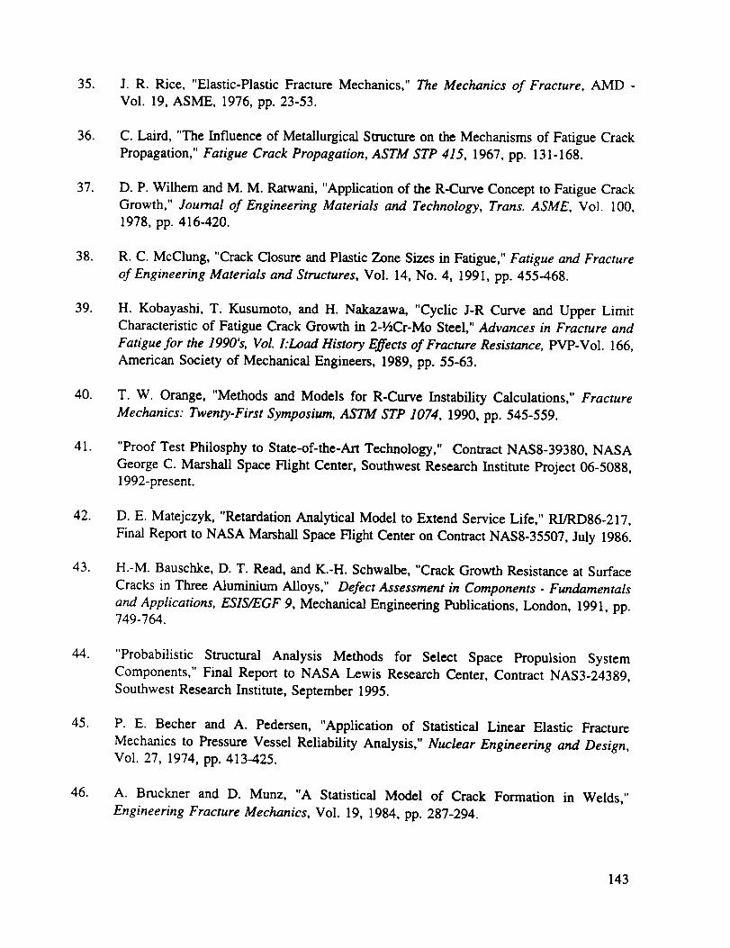
35.

36.

37.

38.

39.

40.

41.

42.

43.

4.

45.

46.

J. R. Rice, "Elastic-Plastic Fracture Mechanics," The Mechanics of Fracture, AMD -

Vol. 19, ASME, 1976, pp. 23-53.

C. Laird, "The Influence of Metallurgical Structure on the Mechanisms of Fatigue Crack

Propagation," Fatigue Crack Propagation, ASTM STP 415, 1967, pp. 131-168.

D. P. Wilhem and M. M. Ratwani, "Application of the R-Curve Concept to Fatigue Crack

Growth," Journal of Engineering Materials and Technology, Trans. ASME, Vol. 100,

1978, pp. 416-420.

R. C. McClung, "Crack Closure and Plastic Zone Sizes in Fatigue," Fatigue and Fracture

of Engineering Materials and Structures, Vol. 14, No. 4, 1991, pp. 455-468.

H. Kobayashi, T. Kusumoto, and H. Nakazawa, "Cyclic J-R Curve and Upper Limit

Characteristic of Fatigue Crack Growth in 2-Y2Cr-Mo Steel," Advances in Fracture and

Fatigue for the 1990% Vol. l:Load History Effects of Fracture Resistance, PVP-Vol. 166,

American Society of Mechanical Engineers, 1989, pp. 55-63.

T. W. Orange, "Methods and Models for R-Curve Instability Calculations," Fracture

Mechanics: Twenty-First Symposium, ASTM STP 1074, 1990, pp. 545-559.

"Proof Test Philosphy to State-of-the-Art Technology," Contract NAS8-39380, NASA

George C. Marshall Space Flight Center, Southwest Research Institute Project 06-5088,1992-present.

D. E. Matejczyk, "Retardation Analytical Model to Extend Service Life," RI/RD86-217,

Final Report to NASA Marshall Space Flight Center on Contract NAS8-35507, July 1986.

H.-M. Bauschke, D. T. Read, and K.-H. Schwalbe, "Crack Growth Resistance at Surface

Cracks in Three Aluminium Alloys," Defect Assessment in Components - Fundamentals

and Applications, ESIS/EGF 9, Mechanical Engineering Publications, London, 1991, pp.749-764.

"Probabilistic Structural Analysis Methods for Select Space Propulsion System

Components," Final Report to NASA Lewis Research Center, Contract NAS3-24389,

Southwest Research Institute, September 1995.

P. E. Becher and A. Pedersen, "Application of Statistical Linear Elastic Fracture

Mechanics to Pressure Vessel Reliability Analysis," Nuclear Engineering and Design,Vol. 27, 1974, pp. 413-425.

A. Bruckner and D. Munz, "A Statistical Model of Crack Formation in Welds,"

Engineering Fracture Mechanics, Vol. 19, 1984, pp. 287-294.

143

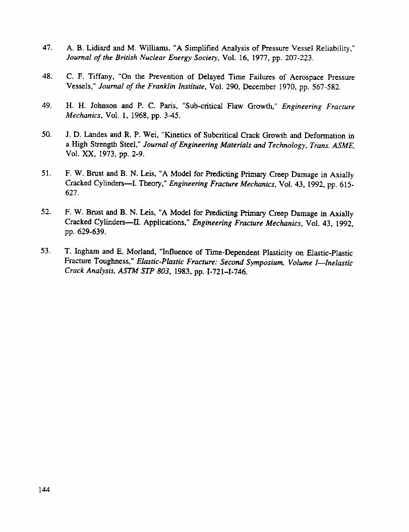
47.

48.

49.

50.

51.

52.

53.

A. B. Lidiard and M. Williams, "A Simplified Analysisof PressureVesselReliability,"Journal of the British Nuclear Energy Society, Vol. 16, 1977, pp. 207-223.

C. F. Tiffany, "On the Prevention of Delayed Time Failures of Aerospace Pressure

Vessels," Journal of the Franklin Institute, Vol. 290, December 1970, pp. 567-582.

H. H. Johnson and P. C. Paris, "Sub-critical Flaw Growth," Engineering Fracture

Mechanics, Vol. 1, 1968, pp. 3-45.

J. D. Landes and R. P. Wei, "Kinetics of Subcritical Crack Growth and Deformation in

a High Strength Steel," Journal of Engineering Materials and Technology, Trans. ASME,

Vol. XX, 1973, pp. 2-9.

F. W. Brust and B. N. Leis, "A Model for Predicting Primary Creep Damage in Axially

Cracked Cylinders--I. Theory," Engineering Fracture Mechanics, Vol. 43, 1992, pp. 615-627.

F. W. Brust and B. N. Leis, "A Model for Predicting Primary Creep Damage in Axially

Cracked CylindersmII. Applications," Engineering Fracture Mechanics, Vol. 43, 1992,

pp. 629-639.

T. Ingham and E. Morland, "Influence of Time-Dependent Plasticity on Elastic-Plastic

Fracture Toughness," Elastic-Plastic Fracture: Second Symposium, Volume 1--Inelastic

Crack Analysis, ASTM STP 803, 1983, pp. 1-721-1-746.

144

APPENDIX A. Further Documentation of Improved J Solutions for Surface Flaws

In Section 2.1 of the main body of this report, a short synopsis was provided of an

improved reference stress technique for estimating J for surface cracks in finite thickness

geometries. The development of the improved technique was guided by several recently

published sets of t-mite element (FE) J solutions, and these same FE solutions were used to

demonstrate the performance of the general solution technique in its final form. In this appendix,

further documentation is provided for the FE solutions, the derivation of the modified reference

stress technique, and the final comparisons of the FE and reference stress solutions.

Finite Element Solutions

Several finite element solutions for surface cracks in finite bodies were available at the

time of this study [A1, A2, A3, A4, A5]. These efforts included a variety of plate and flaw

geometries and constitutive relationships, as summarized in Table A1. The geometric

nomenclature is illustrated in Figure A1.

Comparison of various numerical results with each other and with simple analytical

formulas requires a suitable mathematical framework. Following the EPRI handbook approach,

a general form for J in a Ramberg-Osgood material can be postulated according to

E'L+R "+' ' +("-'"oYJJ+ a Ooeoth I

n+l

(A.1)

The last (plastic) term contains a non-dimensional factor h 1that changes with both geometry and

strain hardening exponent but not with applied stress. It is this h_ which is tabulated in the

elastic-plastic fracture handbooks, and it is this h_ (or its equivalent) which any simple estimation

technique must compute accurately.

The analysis of Yagawa et al. [A5] was based on a fully plastic FE solution, and so the

results are already expressed in terms of h_ (Yagawa et al. call it 3_a)). On the other hand, the

early analysis of Wang [A1] and the work of Dodds et al. [A4] both employed a

Ramberg-Osgood total strain constitutive relationship, and the results were expressed in terms

of total J at different applied stresses. In order to compare these results more directly with

Yagawa et al. and with simple estimation schemes, it would be preferable to extract an estimate

of h_. This extraction can be carried out based on Eqn. AI: the published FE value of total J is

set equal to the left hand side of the equation; the elastic term (including the effective crack

length correction) is estimated from the Newman-Raju K solution and then subtracted off to leave

only the plastic term; and the plastic term is then normalized to solve for h v If this process is

successful, then the computed h_ should be approximately the same at all applied stresses. This

A.1

TABLE A 1Summaryof geometriesandconstitutivelawsfor finite elementJ solutions

Author

Wang

(1988)

Wang

(1991)

Kirk

(1992)

Dodds

(1992)

Yagawa

(1993)

Ref.

[A1]

[A2]

[A3]

[A4]

[A5]

a/t

0.5

0.6

0.15

0.60

0.13

0.25

0.25

0.25

0.2

0.2

0.2

0.5

0.5

0.5

0.8

0.8

0.8

a/c

1.0

O.24

0.24

0.24

0.763

0.769

0.333

0.333

0.2

0.6

1.0

0.2

0.6

1.0

0.2

0.6

1.0

b/c

16

3.2

16

3.2

11.77

6.15

2.67

2.67

4

4

4

4

4

4

4

4

4

h/t

16

16

16

16

2.85

2.85

2.85

2.85

4

1.33

0.8

10

3.339

16

5.33

3.2

Constitutive Law

Ramberg-Osgood

(n = 5, 10)

fully elastic/

fully power-law (n = 10)

bilinear

(plastic slope = E/84)

Ramberg-Osgood

(n - 4, 10)

power-law fully plastic

(n = 1, 2, 3, 5, 7, 10)

A.2

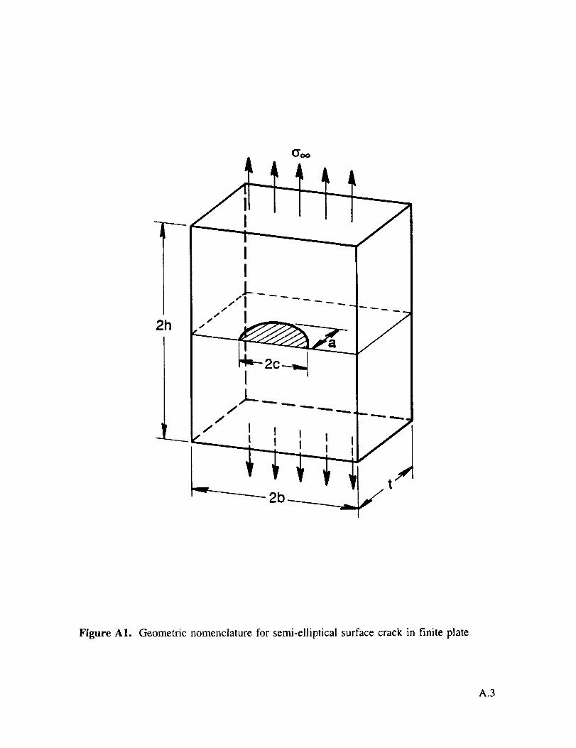
21"1

d, I// t , , /---L--_L 1 I ', 1 II

_ , vv t '+1._2b ___,, -/

II

. I

IJ-__..

Figure AI. Geometric nomenclature for semi-elliptical surface crack in finite plate

A.3

successfulresultwouldalso serveasan indirect confirmation of the process by which J,o_ can

be accurately estimated by summing independent elastic and plastic components.

Graphs of hi as a function of applied stress are given for the four earlier Wang analyses

in Fig. A2 and the two Dodds et al. analyses in Fig. A3. In all cases, hi is remarkably constant.

Apparent variations in h 1 at lower applied stresses occur because the plastic term itself is very

small and small inaccuracies in any variable cause large errors in h _.

These derived values of hi are compared with the published h 1 values of Yagawa in

Fig. A4 for n = 10. The Wang calculation for a/t = 0.5, a/c = 1.0 agrees closely with the

corresponding Yagawa value (h_ = 2.4 vs. 2.57). The Dodds result for a/t = 0.25, a/c = 0.333,

and the Wang result for aJt = 0.6, a/c = 0.24, appear to be too high in comparison to neighboring

Yagawa results. This disagreement may be partially attributable to small values of b/c for Dodds

and Wang, but it may also indicate some inaccuracies in the FE results. These issues will be

investigated in more depth below. Similar results were obtained at n = 5, where the Wang and

Yagawa calculations of hi for a/t = 0.5, aJc = 1.0, were identical, but the Yagawa computations

seem low in comparison to the Wang a/t = 0.6, a/c = 0.24 values.

It is not possible to compare the later results of Wang [A2] or the solutions of Kirk [A3]

with the other three sets of results on this same h 1 basis, because different constitutive

relationships were employed. The later Wang analysis used a stress-strain law which was

perfectly elastic below the yield stress and simple power-law fully plastic above the yield stress.

The Kirk analysis was based on a bilinear stress-strain curve. An alternative means of comparingthese two solution sets will be developed below.

Reference Stress Estimates

A brief outline of the reference stress method and the key equations for J estimation were

provided in Section 2.1. Identification of a suitable form for the yield function f was identifiedas a key step in the method.

The simplest choice of yield function f for the surface flaw is that based on the reduction

in load bearing area due to the presence of the defect. This gives the global yield function,

7t acf = 1 (A.2)

4bt

This was the form used in the Phase I estimation technique. As noted in the main body of the

report, this form can give f estimates too large for wide plates (large b/c ratios).

An alternative approach is to define some effective plate dimension (in the width

direction) that characterizes collapse. One such construction was shown in Fig. 2.1, where the

effective width is given as (2_ + 2c). When stresses in this enclosed region are in yield, collapse

A.4

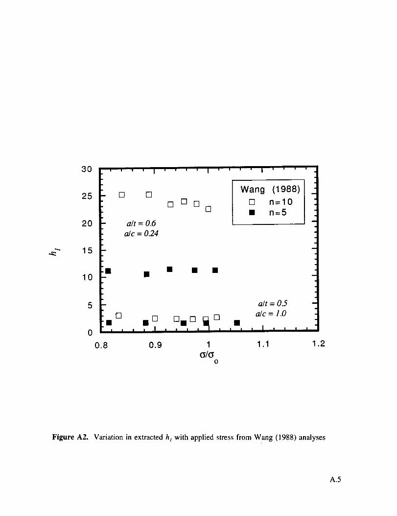
3O

25

2O

15

10

5

0

[] []

a/t = 0.6

a/c = 0.24

[]

• • •• •

I Wang (1988)

[] n=lO

• n=5

a/t = 0.5

[] • [] ,_,rim[] [] • a/ c = 1.0

0.8 0.9 1 1.1 1.2

0

Figure A2. Variation in extracted h I with applied stress from Wang (1988) analyses

A.5

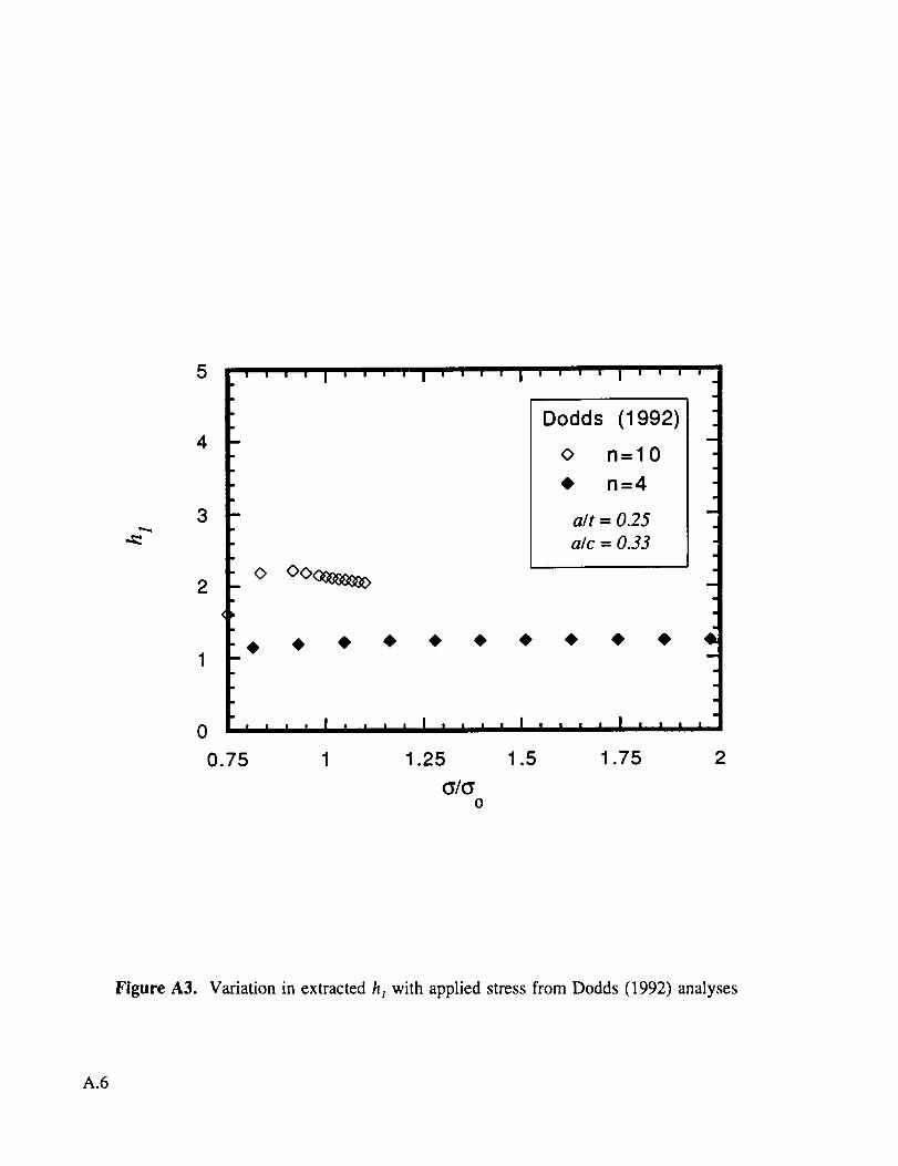
5

4

3

2

0

0.75

' ' ' ' I ' ' ' ' I ' ' ' ' I ' ' ' ' I ' ' ' '

Dodds (1992)

o n=lO

• n=4

a/t = 0.25

a/c = 0.33

0 O0<_e_a

• • • • • • • • • • 4n

i i i i I i l ' ' I .... I , , , , I ....

1 1.25 1.5 1.75

C/C0

2

Figure A3. Variation in extracted h I with applied stress from Dodds (1992) analyses

A.6

100

10

0.1

' ' I

n=10

0.33 O

0.20

0.6 ©

1.00

I ' ' ' I ' ' ' I ' '

_c= 0.24 []

0.20

O.6O

1.00

0.2 ©

0.6 0

1.0 0

© Yagawa (1993)[] Wang (1988)o Dodds (1992)

, , , I , , , I i i l I = ' ' I

0 0.2 0.4 0.6 0.8

oJt

! | |

1

Figure A4. Comparison of h_ values from various authors

A.?

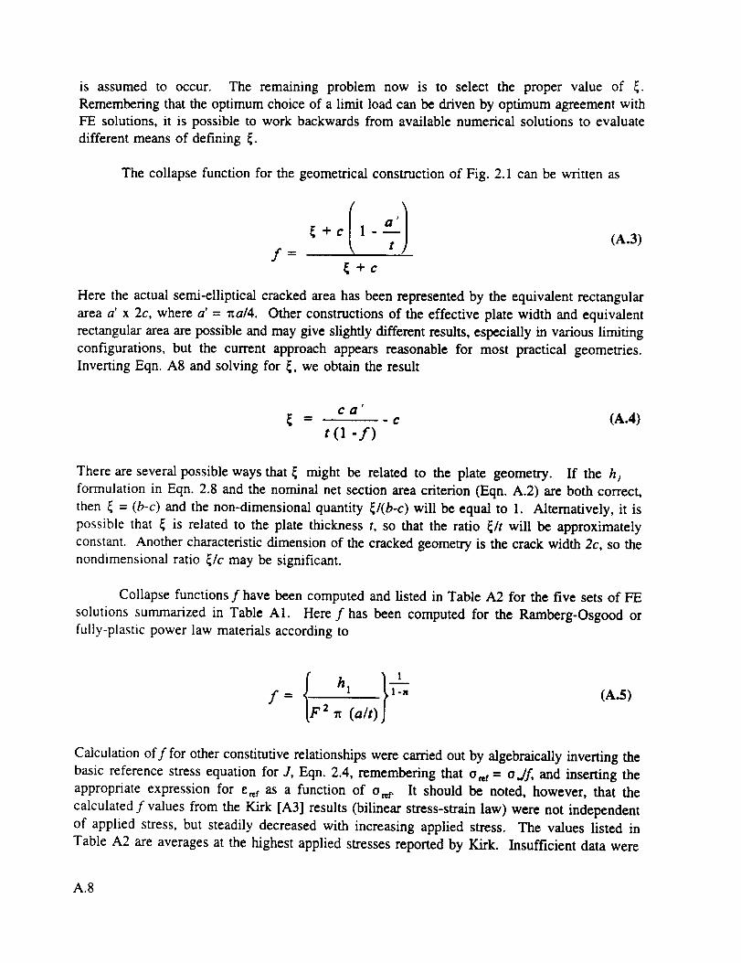
is assumed to occur. The remaining problem now is to select the proper value of _.

Remembering that the optimum choice of a limit load can be driven by optimum agreement with

FE solutions, it is possible to work backwards from available numerical solutions to evaluate

different means of defining _.

The collapse function for the geometrical construction of Fig. 2.1 can be written as

f

(A.3)

Here the actual semi-elliptical cracked area has been represented by the equivalent rectangular

area a' x 2c, where a' = rta/4. Other constructions of the effective plate width and equivalent

rectangular area are possible and may give slightly different results, especially in various limiting

configurations, but the current approach appears reasonable for most practical geometries.

Inverting Eqn. A8 and solving for _, we obtain the result

ca'- ¢ (A.4)

t(1 -f)

There are several possible ways that _ might be related to the plate geometry. If the hj

formulation in Eqn. 2.8 and the nominal net section area criterion (Eqn. A.2) are both correct,

then _ = (b-c) and the non-dimensional quantity _l(b-c) will be equal to 1. Alternatively, it is

possible that _ is related to the plate thickness t, so that the ratio _lt will be approximately

constant. Another characteristic dimension of the cracked geometry is the crack width 2c, so the

nondimensional ratio _/c may be significant.

Collapse functions f have been computed and listed in Table A2 for the five sets of FE

solutions summarized in Table A1. Here f has been computed for the Ramberg-Osgood or

fully-plastic power law materials according to

f = 2 _ (a/t)

(A.5)

Calculation off for other constitutive relationships were carried out by algebraically inverting the

basic reference stress equation for J, Eqn. 2.4, remembering that o,_f = o.ff, and inserting the

appropriate expression for e,_t as a function of o_. It should be noted, however, that the

calculated f values from the Kirk [A3] results (bilinear stress-strain law) were not independent

of applied stress, but steadily decreased with increasing applied stress. The values listed in

Table A2 are averages at the highest applied stresses reported by Kirk. Insufficient data were

A.8

TABLE A2

Summary of reference stress parameters calculated from finite element solutions

Author a/t a/c h_

Wang (1988) 0.5 1.00 2.40n=lO 0.6 0.24 23.25

n=5 0.5 1.00

0.6 0.24

Wang (1991) 0.15 0.24

0.6 0.24

Kirk (1992) 0.13 0.76

bilinear 0.25 0.77

0.25 0.33

Dodds (1992)

n=4

n=10

Yagawa (1993)

n=10

n=5

1.59

11.09

0.25 0.33 1.24

0.25 0.33 2.09

0.2 O.2 1.33

0.2 0.6 0.83

0.2 1.0 0.58

0.5 0.2 8.24

0.5 0.6 4.26

0.5 1.0 2.57

0.8 0.2 24.56

0.8 0.6 12.06

0.8 1.0 7.20

0.2 0.2 1.07

0.2 0.6 0.66

0.2 1.0 0.45

0.5 0.2 5.58

0.5 0.6 2.66

0.5 1.0 1.56

0.8 0.2 12.67

0.8 0.6 5.45

0.8 1.0 3.20

f

0.879

0.830

0.833

0.792

0.971

0.883

0.970

0.937

0.937

0.900

0.911

0.945

0.939

0.923

0.904

0.887

0.876

0.895

0.852

0.832

0.930

0.921

0.893

0.877

0.858

0.841

0.922

0.851

0.810

I (b-c)

0.15

0.81

0.09

0.58

0.26

1.38

0.22

0.41

1.27

0.58

0.72

0.62

0.53

0.35

1.03

0.83

0.72

1.66

1.08

0.91

0.42

0.33

0.15

0.73

0.59

0.49

2.34

1.07

0.77

_lt

1.12

4.43

0.68

3.16

1.91

7.57

0.41

0.69

1.59

0.72

0.91

1.86

0.53

0.21

7.73

2.06

1.08

19.94

4.33

2.19

1.24

0.33

0.09

5.48

1.47

0.73

28.04

4.29

1.85

_/c

2.25

1.77

1.35

1.27

3.06

3.03

2.40

2.12

2.12

0.96

1.21

1.86

1.58

1.04

3.09

2.48

2.16

4.98

3.25

2.74

1.24

0.99

0.46

2.19

1.77

1.46

7.01

3.22

2.31

A.9

available from the 1991 Wang [A2] results with a nontraditional constitutive relationship to

evaluate the consistency off.

Calculated values of the three normalized _ functions are shown in Table A2 and in

Figures A5, A6, and A7 as functions of the normalized crack depth a/t. Note that different

authors and strain hardening exponents (or constitutive relationships) are distinguished by symbol.

Open symbols denote n = 10, filled symbols represent n = 5 or 4 (Dodds), and the crossed

squares identify the Kirk bilinear results. Variations in a/c are not specified in these figures.

Figure A5 shows that _ was, in general, considerably smaller than the remaining plate

width (b-c), especially for large b/c ratios. Note in Table A2, for example, the Wang [A 1] results

for a semi-circular crack with b/c =16, when the cracked area is only 2.5 percent of the total

gross section area. Therefore, the nominal net section area criterion 0Eqn. A.2) often gave limit

load estimates much too high and reference stress J estimates too low. This was precisely the

finding in Phase I, where the nominal net section area approach to defining a limit stress was

employed. The agreement appeared to worsen gradually for shallower cracks.

Figure A6 shows that _ was not well correlated with the plate thickness t. A constant _lt

criterion would tend to give reference stress estimates of J much too high (collapse functions f

much too low) for deeper cracks, especially for small a,/c values (see also Table A2). At the

same time, a constant _/t could give very nonconservatively low J estimates (f too high) for

shallower cracks and larger alc values.

A better correlation was exhibited in Fig. A7 between _ and the crack half-width c. The

ratio _/c was approximately bounded by 1 and 3 for most of the geometries considered, although

some apparent dependence on a/t, a/c, and perhaps n remained. The only prominent outliers in

the data were the results of Yagawa et al. [A5] for one shallow semicircular flaw and one deep,

elongated flaw. These exceptions will be discussed further below.

Several approaches can be taken to the selection of an optimum _/c value. One approach,

which might be more appropriate in the development of global analysis rules for practical safety

assessments, would be to choose a constant value for _/c which would apply uniformly to all

crack shapes and constitutive relationships. If a best estimate of J is desired, then an

intermediate value of perhaps _/c = 1.5 - 2.0 may be a good choice. This selection gave

predictions of the plastic J term (as represented by the plastic factor h_) which were usually

within ±15 percent of the published FE results, never more than 20 percent low, and only

occasionally excessively conservative. Some of the larger disagreements may have been due to

inaccuracies in the FE solutions, as discussed later. And, as also discussed further below, note

that the accuracy of the total J estimate will often be much better than the accuracy of the plastic

J estimate. If a more universally conservative fracture assessment is desired for all crack shapes,

then a smaller _/c value, perhaps 1.0, may be appropriate (at the expense of greater conservatism

for the deepest cracks).

A.10

4 ' -- I ' ' ' I ' ' I ' ' I ' '

8 -_g .....a awa (1993)[] Wang (1988)

3 A Wang (1991)[] Kirk (1992)o Dodds (1992) •

_,_2

z_

1

.0 ,_ I , , I ,i I , , I , ,

0 0.2 0.4 0.6 0.8 1

Figure A5. Normalized representative plate width _/(b-c) as function of a/t

A.1I

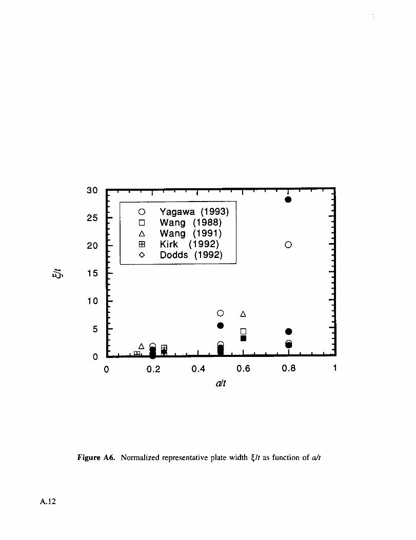
30

25

20

15

10

I ' ' ' I ' ' ' I

0

[]A

[]

0

Yagawa (1993)Wang (1988)

Wang (1991)

Kirk (1992)Dodds (1992)

! l n i I I I

0

0 A

5 ,. • [] • I

0 0.2 0.4 0.6 0.8 1

_t

Figure A6. Normalized representative plate width _lt as function of a/t

A. I2

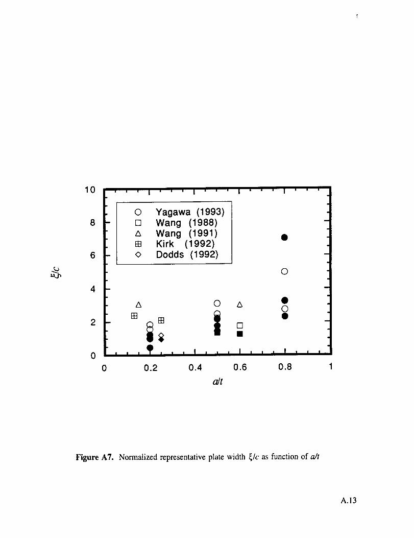
10

8

6

4

2

0

' I ' ' ' I ' ' ' I

© Yagawa (1993)

[] Wang (1988)A Wang (1991)

EB Kirk (1992)o Dodds (1992)

, , , I ' , ,

0

0 0.2 0.4 0.6 0.8 1

_/t

Figure A7. Normalized representative plate width _/c as function of a/t

A.13

Comparisons of Reference Stress and Finite Element Results

Comparisons of predicted and published FE h_ values for several different choices of _/c

are summarized in Table A3. These comparisons suggest that the engineering analyst may wish

to fine tune his selection of _/c depending on the general nature of his applications problem:

perhaps choosing _/c slightly smaller for shallower flaws or higher strain hardening (smaller n),

or _/c slightly larger for deeper flaws or lower strain hardening. Note that the h_ predictions

were slightly less sensitive to _/c for shallower flaws and smaller strain hardening exponents.

It may also be useful to develop a more complex expression which gives a more accurate _/c as

a function of other geometry parameters, such as a/t and a/c, and perhaps also as a function of

constitutive variables, such as n. It should be emphasized, however, that a single intermediate

value of _/c will give remarkably good estimates of J for a wide range of crack shapes and sizes

and strain hardening behavior. This simplicity and universality is one of the strengths of the

general reference stress approach.

Predictions of total J based on the reference stress approach (Eqn. 2.7) with a constant

_/c = 1.75 are compared with the original FE results of Wang, Dodds, and Kirk in Figures A8

- A12. Note that if _ was calculated to be greater than the remaining plate width (b-c), then

was set equal to (b-c), because the theoretical area defined by the larger _ was not actually

available to carry load. Reference stress predictions of h 1 for a fully plastic material are

compared with the Yagawa results in Fig. A13 for n - 5 and 10.

Wang (1988), Wang (1991), and Dodds (1992)

Figures A8 and A9 show excellent agreement (±12 percent) between the reference stress

predictions of total J and the FE results of Wang [A1] and Dodds [A4] for different crack shapes,

crack depths, and strain hardening exponents. All these analyses were based on the standard

Ramberg-Osgood constitutive model. The reference stress estimates for the later Wang [A3]

results based on a more complex stress-strain law (fully elastic below the yield stress, fully power

law above the yield stress) were more conservative, especially for the deeper crack, although very

limited FE results were available. The excellent agreement between the reference stress and

earlier Wang results for the exact same geometry (but a Ramberg-Osgood constitutive

relationship) suggests that this later disagreement was related to the nature of the stress-strain

relationship, which contained a sharp discontinuity in the rate of increase of plastic strain at the

yield stress. A similar conservatism in reference stress estimates was also observed for another

set of FE results based on a stress-strain curve with a sharp comer, the Kirk analyses discussedbelow.

Kirk (1992)

The reference stress estimates of total J are compared with the Kirk [A3] finite element

results based on a bilinear stress-strain law in Figures A11 and A12. The comparisons expressed

in terms of normalized applied stress, Fig. A 11, showed that the reference stress estimates were

somewhat conservative at applied stresses very near the yield stress, but generally did a good job

of following the very severe upturn in J with increasing load. These changes in J are depicted

more clearly in Fig. A12, which emulates the original figures of Kirk by representing J as a

A.14

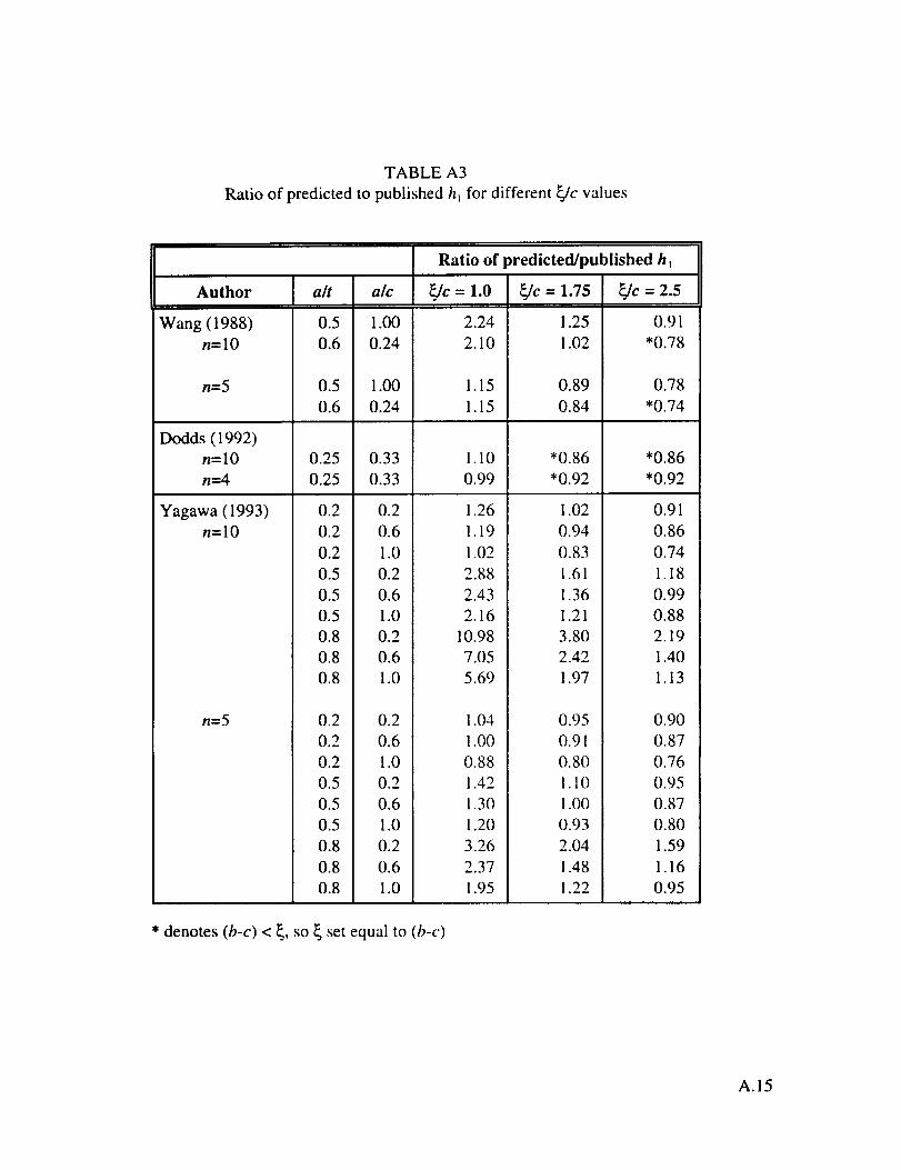
TABLE A3

Ratio of predicted to published h_ for different _c values

Ratio of predicted/published h_

Author alt aic _c = 1.0

Wang (1988) 0.5 1.00 2.24 1.25n=lO 0.6 0.24 2.10 1.02

n=5

Dodds (1992)

n=lO

n=4

Yagawa (1993)

n=lO

_/c = 1.75 _c = 2.5

0.5 1.00 1.15 0.89

0.6 0.24 1.15 0.84

0.25 0.33 1.10 *0.86

0.25 0.33 0.99 *0.92

0.2 0.2 1.26 1.02

0.2 0.6 1.19 0.94

0.2 1.0 1.02 0.83

0.5 0.2 2.88 1.61

0.5 0.6 2.43 1.36

0.5 1.0 2.16 1.21

0.8 0.2 10.98 3.80

0.8 0.6 7.05 2.42

0.8 1.0 5.69 1.97

n=5 0.2 0.2 1.04 0.95

0.2 0.6 !.00 0.91

0.2 1.0 0.88 0.80

0.5 0.2 1.42 !. 10

0.5 0.6 1.30 1.00

0.5 1.0 1.20 0.93

0.8 0.2 3.26 2.04

0.8 0.6 2.37 1.48

0.8 1.0 1.95 1.22

0.91

0.86

0.74

1.18

0.99

0.88

2.19

1.40

1.13

0.90

0.87

0.76

0.95

0.87

0.80

1.59

1.16

0.95

* denotes (b-c) < _, so _ set equal to (b-c)

A.15

b _

5

4

3

2

Wang (1988)[] n=lO• n=5

a/t = 0.5oJc = 1

0

0.2 0.4 0.6 0.8 1 1.2

0"/(_0

30 ' ' i ' ' " i ' ' ' J ' ' ' , '

Wang (1988)

25 [] n=lO• n=5 I

a/t = 0.6

20 a/c = 0.24

_- 1 •

15 •

10

5

0

0.2 0.4 0.6 0.8 1 1.2

_C0

Figure A8. Comparison of reference stress J predictions

with Wang (1988) finite element results

A.16

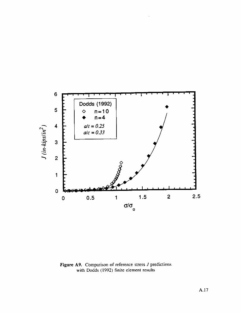
o_,_

6

5

4

3

2

0

Dodds (1992)0 n=10• n=4

alt = 0.25

a/c = 0.33

0

0 0.5 1 1.5 2 2.5

0


with Dodds (1992) finite element results

A.17

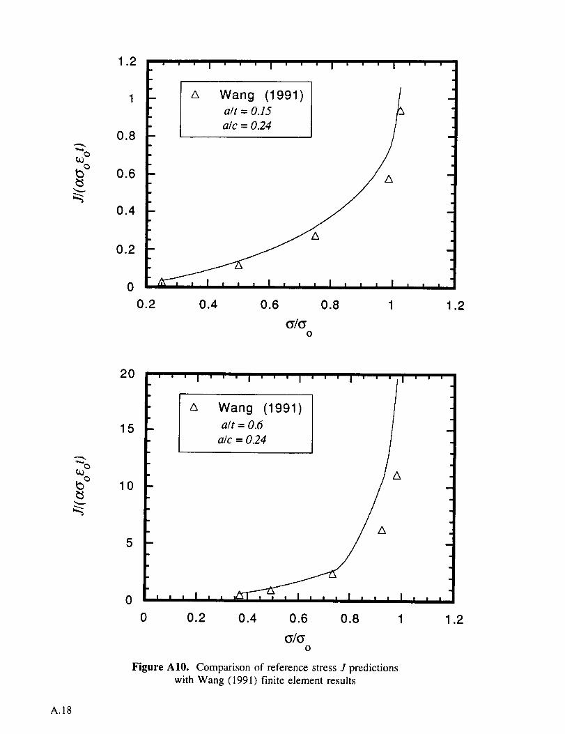
1.2

0.8

0.6

0.4

0.2

0

0.2

A Wang (1991)a/t = 0.15

a/c = 0.24

A

0.4 0.6 0.8 1 1.2

0

20

15

10

5

0

' ' ' I ' ' ' I ' ' ' I ' ' ' I ' ' ' I ' ' '

Z_ Wang (1991)

a/ t = 0.6

a/c = 0.24

u

0 0.2 0.4 0.6 0.8 1 1.2

0


with Wang (1991) finite element results

A.18

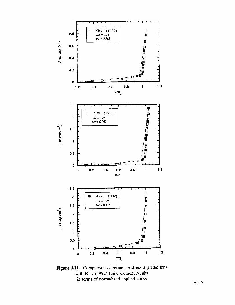
',,.n

0.8

0.6

0.4

0.2

o

0.2

i I I

EB Kirk (1992)wt = 0.13ale = O.765

0.4 0.6 0.8 1

(_/C_o

I'''

, i

1.2

2.5

1.5

0.5

' ' ' I ' ' ' I ' ' ' I ' ' ' I ' ' ' I ' ' '

m Kirk (1992)

wt = 0.25ale = 0.769

, ,_, I m r , I , , ,

0.2 0.4 0.6 0.8 1

0

1.2

._

3.5

3

2.5

2

1.5

1

0.5

0

, ' ' ' I ' " ' I ' ' ' I ' ' ' I ' ' ' I ' ' '

FR Kirk (1992)alt = 0.25

ale = 0.333

I Ir_l I _ _...J;_F---'r_, I_, , , I i , , I , , , "

0 0.2 0.4 0.6 0.8 1 1.2

0

Figure All. Comparison of reference stress J predictions

with Kirk (1992) finite element results

in terms of normalized applied stressA.19

.E

0.8

0.2

.... I .... I .... t .... I ' _ ' '

[] Kirk (1992)a/t = 0.13

I aIc = 0765 _ m

I . . , , I , , , i I .... I , , , .

1 2 3 4

Gage Strain / Yield Strain

2.5

2

1.5

1

0.5

0

.... I .... I ' ' ' ' I .... I .... .

m

FR

, I t i

0 1 2 3 4 5


A.20

.E

3.5

3

2.5

2

1.5

1

0.5

0

• ' ' ' ' I .... I .... I .... I ....

mFn

[] Kirk (1992)

a/t = 0.25

a/c = 0.333

,-,_. _ .... I .... ,, 7T7i-,_-

0 1 2 3 4 5


Figure AI2. Comparison of reference stress J predictions

with Kirk (1992) finite element results

in terms of normalized applied strain

100

10

0.1

0

' ' I ' ' ' I ' ' ' I ' ' ' I ' ' '

Yagawa (1993) wc= 0.2

• n=5 • 0.5

• 1.0

, , I , , , I , J , I , , , I , , ,

0.2 0.4 0.6 0.8

a/t

1 000

100

10

0.1

0

' ' I ' ' ' I ' ' ' I ' ' ' I ' '

Yagawa (1993) oJc=© n=lO

, i , I , , , I i , , i , , , I , ,

0.2 0.4 0.6 0.8

oJr

Figure A13. Comparison of reference stress h/predictions

with Yagawa (1993) finite element results

0.2

0.5 !

1.0

A.2I

function of normalized applied strain. These graphs show that the reference stress estimates

could be quite conservative - as much as a factor of 2x or 3x - at applied stresses within a few

percent of the yield stress, but that the reference stress estimates were increasingly accurate at

higher and lower applied stresses.

This large change in accuracy with changes in applied stress, which was not observed in

any of the estimates for power law hardening materials, was consistent with the earlier

observation that the derived value of the collapse function, f, changed significantly with applied

stress. The derived values off at applied stresses very near yield were generally significantly

higher (closer to f = 1), which implies a larger value of _/c and (ultimately) a smaller J value.

Improvements in J estimates would require some means of predicting this change in collapse

function or characteristic plate length. Remember that a similar conservatism in J was observed

for the Wang (1991) FE analysis with a similar two-stage constitutive relationship. It appears,

therefore, that this particular reference stress formulation may have difficulty in handling the

sharp discontinuity in the rate of plastic strain increase - from zero to a large positive number

- at the yield stress. Further studies of the reference stress method for these types of stress-strain

curves are required. It is encouraging, however, that the errors in the current reference stress

estimates are systematically conservative rather than nonconservative.

Of course, it should be noted that in actual engineering practice, reliable predictions of

J for any material with such a sharp knee in the stress-strain curve will be precarious at applied

stresses very near the yield stress. Even an "exact" analysis scheme can significantly

overestimate or underestimate J if the assumed yield strength is in error by only 1 or 2 percent.

Actual safety assessments must pay close attention to appropriate conservative bounds on botho and J.

ys

Comments on two observations by Kirk [A3] about the reference stress method in general

are also in order here. He concluded from comparison of his own reference stress J estimates

with his FE results that the reference stress estimates always significantly underestimated J. He

also remarked that the reference stress method was unable to model correctly the general trends

in the J vs. strain relationship in tension because it failed to distinguish the different regimes of

post-yield behavior, including the distinction between net-section and gross-section yielding.

These two statements may have been true at least in part, however, because Kirk chose to neglect

the influence of the crack on the limit load calculation; i.e., he chose f= 1 for all geometries, so

that o_f = o® everywhere. The reference stress estimates in Figure A12 appear to demonstrate

two distinct regimes of post-yield behavior: a change from small-scale yielding to net ligament

or net section yielding when o,_f > oys, transitioning to gross section yielding (with a

corresponding decrease in the J vs. strain slope) when o.. > aye. However, additional study is

needed to evaluate further the accuracy of reference stress estimates based on a global collapse

function for characterization of the elastic-plastic fracture mechanics response of a part-through

crack exhibiting net section yield in the remaining ligament.

A.22

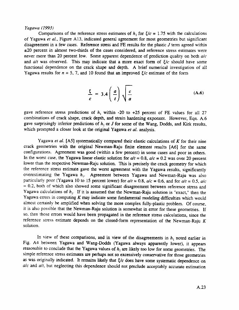
Yagawa (1993)

Comparisons of the reference stress estimates of h a for _/c = 1.75 with the calculations

of Yagawa et al., Figure A13, indicated general agreement for most geometries but significant

disagreement in a few cases. Reference stress and FE results for the plastic J term agreed within

±20 percent in almost two-thirds of the cases considered, and reference stress estimates were

never more than 20 percent low. Some apparent dependence of prediction quality on both a/c

and a/t was observed. This may indicate that a more exact form of _/c should have some

functional dependence on the crack shape and depth. A brief numerical investigation of all

Yagawa results for n = 5, 7, and 10 found that an improved _lc estimate of the form

gave reference stress predictions of h t within -20 to +25 percent of FE values for all 27

combinations of crack shape, crack depth, and strain hardening exponent. However, Eqn. A.6

gave surprisingly inferior predictions of hi or J for some of the Wang, Dodds, and Kirk results,

which prompted a closer look at the original Yagawa et al. analysis.

Yagawa et al. [A5] systematically compared their elastic calculations of K for their nine

crack geometries with the original Newman-Raju finite element results [A6] for the same

configurations. Agreement was good (within a few percent) in some cases and poor in others.

In the worst case, the Yagawa linear elastic solution for a/t = 0.8, a/c = 0.2 was over 20 percent

lower than the respective Newman-Raju solution. This is precisely the crack geometry for which

the reference stress estimate gave the worst agreement with the Yagawa results, significantly

overestimating the Yagawa h_. Agreement between Yagawa and Newman-Raju was also

particularly poor (Yagawa 10 to 15 percent lower) for a/t -- 0.8, a/c = 0.6, and for a/t = 0.5, a/c

= 0.2, both of which also showed some significant disagreement between reference stress and

Yagawa calculations of h_. If it is assumed that the Newman-Raju solution is "exact," then the

Yagawa errors in computing K may indicate some fundamental modeling difficulties which would

almost certainly be amplified when solving the more complex fully-plastic problem. Of course,

it is also possible that the Newman-Raju solution is somewhat in error for these geometries. If

so, then those errors would have been propagated in the reference stress calculations, since the

reference stress estimate depends on the closed-form representation of the Newman-Raju Ksolution.

In view of these comparisons, and in view of the disagreements in h_ noted earlier in

Fig. A4 between Yagawa and Wang-Dodds (Yagawa always apparently lower), it appears

reasonable to conclude that the Yagawa values of h_ are likely too low for some geometries. The

simple reference stress estimates are perhaps not so excessively conservative for those geometries

as was originally indicated. It remains likely that _/c does have some systematic dependence on

a/c and a/t, but neglecting this dependence should not preclude acceptably accurate estimation

A.23

of J for many crack shapes and sizes. As additional FE results become available, it should be

possible to refine these observations about _/c and draw firmer conclusions.

Discussion: Accuracy of J Solutions

Any discussion of solution accuracy must begin with consideration of the accuracy of the

original FIE J solutions. Numerical analysis of such complex elastic-plastic problems is not a

trivial exercise, and the results cannot be automatically assumed to be infallible. Round-robin

analysis exercises have found a disturbingly large scatter in results for J on even simple

two-dimensional geometries [A7]. Improved understandings of numerical modeling issues should

prompt improved solution accuracy, but error will not be eradicated. It is instructive to note that

several of the numerical solutions investigated in this report disagreed with the "benchmark"

Newman-Raju solution in the elastic regime by as much as 10 percent in K -- and sometimes

much more, as noted above in discussion of the Yagawa et al. results. Of course, the

Newman-Raju solution is not infallible, either. Remember that a large number of different elastic

K solutions were proposed for the semi-elliptical surface crack geometry before Newman-Raju

emerged and was accepted as an informal standard. Therefore, it is probably not possible to

claim better than about 10 to 20 percent accuracy in J for any of the FE results considered in this

report, and much worse accuracy appears likely for a few FE results.

Furthermore, this accuracy is conditional on a reasonably exact representation of the

material constitutive relationship and the actual crack shape. Differences between the actual

stress-strain response of the material and the idealized Ramberg-Osgood (or other constitutive)

relationship which has been assumed, including the effects of cyclic softening or hardening, can

introduce significant errors in the calculated J, especially at large n. The implications of even

small errors in estimating the yield strength were highlighted above in discussions of the Kirkpredictions for materials with a bilinear stress-strain curve.

A reference stress J estimate which is good to within 20 or even 30 percent, then, may

be about as accurate as can be expected or required in practice. Even larger errors in the

estimation of the plastic J term (which is the real focus of the reference stress approach, since

the elastic term follows directly from the K solution alone) may not be particularly troublesome.

For a Ramberg-Osgood material, the relative magnitude of the elastic and plastic J terms in a

reference stress formulation is given approximately by

n-1

(A.7)

The plastic term will only become dominant when odo0 is greater than f, and this dominance

will be particularly intense only for larger n. For many problems, however, the elastic and plastic

terms in J will be of similar magnitude. In this case, even a 50 percent error in estimating Jp

A.24

wouldcauseonly about a 25 percent error in calculating total J (and less than a 15 percent error

in calculating the equivalent K value), assuming that the elastic solution is known accurately.

In view of these observations about solution accuracy, we conclude that the proposed

reference stress estimate of J will be entirely acceptable for many engineering applications.

Furthermore, the reference stress approach is particularly attractive in view of its successful

application to not only a wide range of crack shapes and sizes but also a variety of constitutive

relationships. This simplicity and robustness suggest that the reference stress method might be

preferred over a more "rigorous" finite element approach for some applications.

Acknowledgements

Prof. G. Yagawa, Prof. R. H. Dodds, Jr., Dr. M. T. Kirk, and Dr. Y.-Y. Wang are thanked for

promptly providing their numerical results in various forms.

References

A1.

A2.

A3.

A4.

A5.

A6.

A7.

Y.-Y. Wang, "Analysis of Fracture Initiation in Surface-Cracked Plates," M.S. Thesis,

Massachusetts Institute of Technology, 1988. See also D. M. Parks and Y.-Y. Wang,

"Elastic-Plastic Analysis of Part-Through Surface Cracks," Analytical, Numerical, and

Experimental Aspects of Three Dimensional Fracture Processes, AMD-Vol. 91, ASME,

1988, pp. 19-32.

Y.-Y. Wang, "A Two-Parameter Characterization of Elastic-Plastic Crack Tip Fields and

Applications to Cleavage Fracture," Ph.D. Thesis, Massachusetts Institute of Technology,1991.

M. T. Kirk and R. H. Dodds, Jr., "Approximate Techniques of J Estimation Applicable

to Part-Through Surface Cracks," Engineering Fracture Mechanics, Vol. 43, 1992,

pp. 123-136.

R. H. Dodds, Jr., C. F. Shih, and T. L. Anderson, "Continuum and Micromechanics

Treatment of Constraint in Fracture," Structural Research Series Report No. 573,

Department of Civil Engineering, University of Illinois at Urbana-Champaign, November1992.

G. Yagawa, Y. Kitajima, and H. Ueda, "Three-Dimensional Fully Plastic Solutions for

Semi-elliptical Surface Cracks," International Journal of Pressure Vessels and Piping,Vol. 53, 1993, pp. 457-510.

J. C. Newman, Jr., and I. S. Raju, "Analyses of Surface Cracks in Finite Plates under

Tension or Bending Loads," NASA TP-1578, 1979.

L. H. Larsson, "The EGF Round Robin on Numerical EPFM," Proc. 5th European

Conference on Fracture (ECF5), September 1984, pp. 425-445.

A.25

REPORT DOCUMENTATION PAGE FormApprovedONIB No. 0704-0188

Public reporung burden for this collecuon of informanon is esumaled to average 1 hour per response, including the ume for reviewing m.m'ucuo_, searcbng exlsung data sources.gathwmg and mamuumng the data needed, and completing and revmwmg the collecuon of informanon. Send commeats regarding tins burden esumate or any other aspect ofthis collection of mformwon, including suggesUons for reducing this burden to Washington Headquarters Servaces, Directorate for lnformauon Opea-auons and Reports, 1215JeffersonDavas Highway. State1204,Arlmgum, VA 22202-4302,and theOfficeof Management and Budget.Paperwork ReductaonProject(0704-0188),Washington.DC 20503_

I. AGENCY USE ONLY (Leave Blank) 2. REPORT DATE 3. REPORT TYPE AND DATES COVERED

December 1996 ContractorReport (Final),Nov. 1987 - Dec. 1996

4. TITLE AND SUBTITLE

A Comparison of Single-Cycle Versus Multiple-Cycle Proof Testing Strategies: Final Report

AUTHORfS)

R. C. McClung, G. G. Chell, H. R. Millwater, D. A. Russell*, and G. E. Orient*

PERFORMING ORGANIZATION NAME(S) AND ADDRESS(S)Southwest Research Institute

P. O. Drawer 28510

San Antonio, TX 78228-0510

9. SPONSORING/MONITORING AGENCY NAME(S) AND ADDRESS(ES)

National Aeronautics and Space Administration

George C. Marshall Space Flight Center

Marshall Space Flight Center, AL 35812

5. FUNDING NUMBERS

NAS 8-37451

8. PERFORMING ORGANIZATION

REPORT NUMBERS

06-2009

10. SPONSORING/MONITORING

AGENCY REPORT NUMBER

11. SUPPLEMENTARY NOTES

*Subcontract support from Rocketdyne Division, Rockwell International Corporation

6633 Canoga Avenue; Canoga Park, CA 91303

Prepared for Structures & Dynamics Laboratory, Science & Engineering Directorate Technical Monitor; Henry M. Lee

12a. DISTRIBUTION/AVAR.ABILITY5TATW_._[ENT

Unclassified-Unlimited; Subject Category: 3912b. DISTRIBUTION CODE

13. ABSTRACT (Maximum 200 words)

Single-cycle and multiple-cycle proof testing (SCPT and MCPT) strategies for reusable aerospace propulsion system components are

critically evaluated and compared from a rigorous elastic-plastic fracture mechanics perspective. Earlier MCPT studies are brieflyreviewed. New J-integral estimation methods for semi-elliptical surface cracks and cracks at notches are derived and validated.

Engineering methods are developed to characterize crack growth rates during elastic-plastic fatigue crack growth (FCG) and the tear-

fatigue interaction near instability. Surface crack growth experiments are conducted with Inconel 718 to characterize tearing resistance,

FCG under small-scale yielding and elastic-plastic conditions, and crack growth during simulated MCPT. Fractography and acoustic

emission studies provide additional insight. The relative merits of SCPT and MCPT are directly compared using a probabilistic analysis

linked with an elastic-plastic crack growth computer code. The conditional probability of failure in service is computed for a population

of components that have survived a previous proof test, based on an assumed distribution of initial crack depths. Parameter studies

investigate the influence of proof factor, tearing resistance, crack shape, initial crack depth distribution, and notches on the MCPT vs.

SCPT comparison. The parameter studies provide a rational basis to formulate conclusions about the relative advantages and

disadvantages of SCPT and MCPT. Practical engineering guidelines are proposed to help select the optimum proof test protocol in agiven application.

14. SUBJECT IIzRMS

multiple cycle proof testing, elastic-plastic fracture mechanics, resistance curves, elastic-plastic

fatigue crack growth, tear-fatigue, surface cracks, notches, J-integral, reference stress method,

_robabilistic analysis, Inconel 718, acoustic emission, fraetography

17. SECURITY CLASSIFICATION 18. SECURITY CLASSIFICATION 19. SECURITY CLASSIFICATION

OF THIS PAGE OF ABSTRACT

Unclassified Unclassified Unclassified

15. NUMBER OF PAGES

187

16. PRICE CODE

20. LIMITATION OF ABSTRACT

Unlimited

NSN 7540-01-280-5500 Standard Form 298 (Rev. 2-89)F:XMA'rMECHR.HE20Og-FRN.FNL Pre,_ribe..d by ANSI Std. 239-18

a comparison of single-cycle versus multiple-cycle proof ...

Documents

Transcript of a comparison of single-cycle versus multiple-cycle proof ...