Automatic Computation of the Complete

Root Classification for a Parametric

Polynomial

Songxin Liang ∗, David J. Jeffrey

Department of Applied Mathematics, University of Western Ontario, London, Ontario, Canada

Abstract

An improved algorithm, together with its implementation, is presented for the automatic com-putation of the complete root classification of a real parametric polynomial. The algorithm offersimproved efficiency and a new test for non-realizable conditions. The improvement lies in thedirect use of ‘sign lists’, obtained from the discriminant sequence, rather than ‘revised sign lists’.It is shown that the discriminant sequences, upon which the sign lists are based, are closely re-lated both to Sturm-Habicht sequences and to subresultant sequences. Thus calculations basedon any of these quantities are essentially equivalent.

One particular application of complete root classifications is the determination of the con-ditions for the positive definiteness of a polynomial, and here the new algorithm is applied toa class of sparse polynomials. It is seen that the number of conditions for positive definitenessremains surprisingly small in these cases.

Key words: complete root classification, parametric polynomial, real quantifier elimination,real root, subresultant polynomials.

1. Introduction

Counting and classifying the roots of a polynomial is a well-established problem area;see Basu, Pollack & Roy (2003) for references. Our present goal is to compute automat-ically the Complete Root Classification (CRC) of a parametric polynomial. The CRChas been applied in studies of ordinary differential equations, of integral equations, ofmechanics problems, and to real quantifier elimination; for references see Liang & Jef-frey (2006). This paper describes two improvements that enable more efficient automaticcomputation. As well, an implementation in Maple is used to solve a series of problemsin quantifier elimination, specifically in positive definiteness testing.

∗ Corresponding author.

Email addresses: sliang22@uwo.ca (Songxin Liang), djeffrey@uwo.ca (David J. Jeffrey).

Preprint submitted to Elsevier Science 25 May 2009

Definition 1 (RC and CRC). Let p(x) ∈ R[x]. The root classification (RC) of p(x) isdenoted by [ [n1, n2, . . .], [m1,−m1,m2,−m2, . . .] ] where nk are the multiplicities of thedistinct real roots of p(x), and mk are the multiplicities of the distinct complex conjugatepairs of p(x).

For a polynomial p(x) with real parametric coefficients, the complete root classification(CRC) of p(x) is a collection of its all possible root classifications (RCs), together withthe conditions on the parametric coefficients such that each RC is realized.

The CRC of a real parametric quartic polynomial was found by Arnon (1988), butthe first method for establishing the CRC of a real parametric polynomial of any de-gree was given by Yang, Hou & Zeng (1996), using their discriminant sequence. Theyillustrated their method by computing the CRC of a reduced sextic polynomial. Liang& Zhang (1999) proposed and implemented an algorithm for the automatic generationof a CRC, and also extended the approach to complex parametric polynomials. Furtherimprovements to the algorithm were proposed by Liang & Jeffrey (2006). In parallel,Gonzalez-Vega (1998) proposed the use of Sturm-Habicht sequences (Gonzalez-Vega,Lombardi, Recio & Roy, 1998) to solve similar problems. We show here that discrim-inant sequences, principal Sturm-Habicht coefficient sequences, principal subresultantcoefficient sequences and signed subresultant coefficient sequences (Basu, Pollack & Roy,2003) are equivalent for CRC computations.

This paper presents several advances on the above works. The main efficiency im-provement is to work directly with ‘sign lists’, defined below, rather than ‘revised signlists’. A second improvement concerns the conditions generated. The basic approach,using any of the above sequences, produces a large set of conditions on the (symbolic)coefficients of the polynomial. A separate, but important, task is to reduce this set toa more manageable size, both by eliminating conditions that can never be realized, andby combining conditions into more compact forms. The automation of this step is alsodesirable. Here a new method is used to filter extraneous cases during the generation ofthe results.

The new algorithm has been implemented in Maple. As an application, some well-known benchmark problems are considered: the positive definiteness of polynomials. How-ever, it should be emphasized that the CRC of a polynomial contains more informationthan is needed for these problems, and consequently it has more potential applicationsthan the examples given here. As the problem of real quantifier elimination is well-knownto be unsolvable in polynomial time for the general case (Davenport & Heintz, 1988),we have concentrated on a class of sparse polynomials, for which surprisingly compactresults are possible.

The rest of the paper is organized as follows. In Section 2, the relationships betweenthe discriminant sequence of a polynomial and other related concepts are discussed.In Section 3, existing algorithms related to CRC and their weaknesses are reviewed.In Section 4, the definitions and theorems on which the improved algorithm is basedare presented. In Section 5, the improved algorithm is proposed, and its features arediscussed. In Section 6, some CRCs and their applications to real quantifier eliminationare shown. Finally, in Section 7, some issues for future consideration are mentioned.

2. Relationships among Different Concepts

As mentioned above, different approaches use equivalent constructions for CRC cal-culations. We show the equivalences here before reviewing the existing algorithms.

2

2.1. Discriminant Sequence and Related Sequences

Yang, Hou & Zeng (1996) defined the following quantities as the basis of their algo-rithm. Let p ∈ R[x] and write p(x) = anxn + an−1x

n−1 + · · ·+ a0, where an 6= 0.

Definition 2. The discrimination matrix of p is the 2n× 2n matrix

M =

an an−1 an−2 . . . a0

0 nan (n− 1)an−1 . . . a1

an an−1 . . . a1 a0

0 nan . . . 2a2 a1

......

an an−1 an−2 . . . a0

0 nan (n− 1)an−1 . . . a1

. (1)

Definition 3 (Discriminant Sequence). For 1 ≤ k ≤ 2n, let Mk be the kth principal mi-nor of M , and let Dk = M2k. The n-tuple D = [D1, D2, . . . , Dn] is called the discriminantsequence of p.

Definition 4 (Sign List). If [D1, D2, . . . , Dn] is the discriminant sequence of p and sgn x

is the signum function with sgn 0 = 0, then the sign list of p is [sgn D1, sgnD2, . . . , sgnDn].

Definition 5 (Revised Sign List). The revised sign list [e1, e2, . . . , en] of p is constructedfrom the sign list s = [s1, s2, . . . , sn] of p as follows.

If [si, si+1, . . . , si+j ] is a section of s, where si 6= 0, si+1 = si+2 = . . . = si+j−1 = 0 andsi+j 6= 0, then we replace the subsection [si+1, . . . , si+j−1] by [−si,−si, si, si,−si,−si, . . .]such that ei+r = (−1)b(r+1)/2csi (r = 1, 2, . . . , j−1), and keep other elements unchanged,i.e., let ek = sk.

The revised sign list of p is denoted by rsl(p). Similarly, the revised sign list of s isdenoted by rsl(s).

Definition 6 (∆-Sequence). Let ∆(p) denote gcd(p(x), p′(x)), and let ∆0(p) = p(x),∆j(p) = ∆(∆j−1(p)), j = 1, 2, . . . . Then ∆0(p),∆1(p), ∆2(p), . . . is called the ∆-sequenceof p.

Definition 7. The multiple factor sequence of p, denoted Θ0(p), Θ1(p), . . . , Θn−1(p) isdefined using submatrices of (1). Let Mk,i denote the submatrix formed by the first 2k

rows of M , the first 2k−1 columns of M and the (2k+ i)th column of M . In the notationof the Maple LinearAlgebra package (Jeffrey & Corless, 2006), Mk,i is the matrix

< M[ 1..2*k , 1..2*k-1 ] | M[ 1..2*k , 2*k+i ] > .Then

Θk(p) =k∑

i=0

det(Mn−k,i)xk−i , for k = 0, . . . , n− 1.

3

2.2. Sturm-Habicht Sequence and Related Sequences

Let p(x) = anxn + an−1xn−1 + · · · + a0 and q(x) = bmxm + bm−1x

m−1 + · · · + b0 betwo real polynomials with n = deg(p) > m = deg(q).

In this section, we introduce the concept of subresultant sequence which comes fromSylvester (1853) and Collins (1967), the concept of Sturm-Habicht sequence which wasfirst introduced by Habicht (1948) and extensively studied by Gonzalez-Vega, Lombardi,Recio & Roy (1998), and the concept of signed subresultant sequence which was exten-sively studied by Lombardi, Roy & Safely el Din (2000) and Lickteig & Roy (2001). Wealso discuss the relationship between each of them and the multiple factor sequence.

Definition 8. For 0 ≤ j ≤ m, the jth subresultant associated to p and q is

Sresj(p, n, q, m) =j∑

k=0

M jk(p, q)xk

where each M jk(p, q) is the determinant of the submatrix built by selecting columns

1, 2, . . . , n + m− 2j − 1 and column n + m− k − j from the matrix

mj(p, n, q, m) =

an · · · · · · · · · a0

. . .. . .

an · · · · · · · · · a0

bm · · · · · · · · · b0

. . .. . .

bm · · · · · · · · · b0

.

This matrix has dimensions (n + m− 2j)× (n + m− j) and its rows are the polynomi-als xm−j−1p, . . . , xp, p, xn−j−1q, . . . , xq, q expressed in the basis xn+m−j−1, . . . , x, 1. Thedeterminant M j

j (p, q) is called the jth principal subresultant coefficient and is denotedby sresj(p, n, q, m).

Remark 9. The relationship between the discriminant sequence (Definition 3) and theprincipal subresultant coefficients of p(x) and p′(x) is as follows. For 1 ≤ j ≤ n,

Dj = (−1)j(j−1)/2an sresn−j(p, n, p′, n− 1).

Consequently, the relationship between the multiple factor sequence (Definition 7) ofp(x) and the subresultant sequence of p(x) and p′(x) is as follows. For 0 ≤ j ≤ n− 1,

Θj(p) = (−1)(n−j)(n−j−1)/2an Sresj(p, n, p′, n− 1).

Definition 10. The Sturm-Habicht sequence associated to p and q is defined as thesequence of polynomials {StHaj(p, q)}j=0,1,...,v+1 where v = n+m−1, StHav+1(p, q) = p,StHav(p, q) = p′q and for 0 ≤ j ≤ v − 1,

StHaj(p, q) = (−1)(v−j)(v−j+1)/2 Sresj(p, v + 1, p′q, v).

For 0 ≤ j ≤ v + 1, the jth principal Sturm-Habicht coefficient sthaj(p, q) is defined asthe coefficient of xj in StHaj(p, q).

4

Remark 11. The relationship between the discriminant sequence [D1, . . . , Dn] of p andthe principal Sturm-Habicht coefficients of p and 1 is: Dj = an sthan−j(p, 1) (1 ≤ j ≤ n).

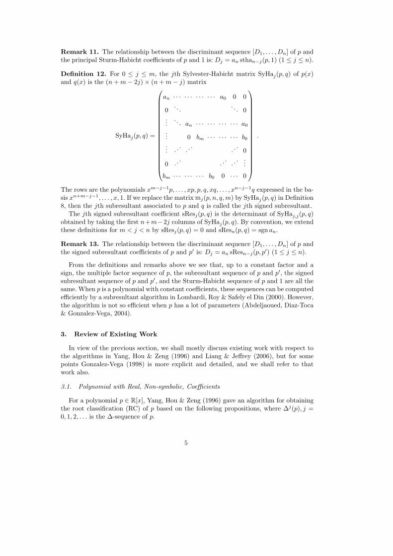
Definition 12. For 0 ≤ j ≤ m, the jth Sylvester-Habicht matrix SyHaj(p, q) of p(x)and q(x) is the (n + m− 2j)× (n + m− j) matrix

SyHaj(p, q) =

an · · · · · · · · · · · · a0 0 0

0. . .

. . . 0...

. . . an · · · · · · · · · · · · a0

... 0 bm · · · · · · · · · b0

... . ..

. ..

. ..

0

0 . ..

. ..

. .. ...

bm · · · · · · · · · b0 0 · · · 0

.

The rows are the polynomials xm−j−1p, . . . , xp, p, q, xq, . . . , xn−j−1q expressed in the ba-sis xn+m−j−1, . . . , x, 1. If we replace the matrix mj(p, n, q, m) by SyHaj(p, q) in Definition8, then the jth subresultant associated to p and q is called the jth signed subresultant.

The jth signed subresultant coefficient sResj(p, q) is the determinant of SyHaj,j(p, q)obtained by taking the first n+m−2j columns of SyHaj(p, q). By convention, we extendthese definitions for m < j < n by sResj(p, q) = 0 and sResn(p, q) = sgn an.

Remark 13. The relationship between the discriminant sequence [D1, . . . , Dn] of p andthe signed subresultant coefficients of p and p′ is: Dj = an sResn−j(p, p′) (1 ≤ j ≤ n).

From the definitions and remarks above we see that, up to a constant factor and asign, the multiple factor sequence of p, the subresultant sequence of p and p′, the signedsubresultant sequence of p and p′, and the Sturm-Habicht sequence of p and 1 are all thesame. When p is a polynomial with constant coefficients, these sequences can be computedefficiently by a subresultant algorithm in Lombardi, Roy & Safely el Din (2000). However,the algorithm is not so efficient when p has a lot of parameters (Abdeljaoued, Diaz-Toca& Gonzalez-Vega, 2004).

3. Review of Existing Work

In view of the previous section, we shall mostly discuss existing work with respect tothe algorithms in Yang, Hou & Zeng (1996) and Liang & Jeffrey (2006), but for somepoints Gonzalez-Vega (1998) is more explicit and detailed, and we shall refer to thatwork also.

3.1. Polynomial with Real, Non-symbolic, Coefficients

For a polynomial p ∈ R[x], Yang, Hou & Zeng (1996) gave an algorithm for obtainingthe root classification (RC) of p based on the following propositions, where ∆j(p), j =0, 1, 2, . . . is the ∆-sequence of p.

5

Proposition 14. Let p ∈ R[x] have revised sign list rsl(p). If the number of non-vanishingelements in rsl(p) is s, and the number of sign changes in rsl(p) is v, then p(x) has vpairs of distinct complex conjugate roots and s− 2v distinct real roots.

Proposition 15. If ∆j(p) has k distinct roots with respective multiplicities n1, n2, . . . , nk,then ∆j+1(p) has at most k distinct roots with respective multiplicities n1 − 1, n2 −1, . . . , nk − 1.

Proposition 16. If ∆j(p) has k distinct roots with respective multiplicities n1, n2, . . . , nk,and ∆j−1(p) has m distinct roots, then m ≥ k, and the multiplicities of these m distinctroots are n1 + 1, n2 + 1 . . . , nk + 1, 1, . . . , 1 respectively.

The algorithm uses these propositions to count the number of roots of p, and thenif necessary to count the roots of each relevant ∆j(p) (until there are no multiplici-ties). When a polynomial has symbolic coefficients, however, the algorithm needs to bemodified.

3.2. Polynomial with Symbolic Coefficients

For a parametric polynomial p ∈ R[a0, a1, . . . , an][x], we first note that the ∆-sequenceof p is difficult to compute directly, because if a standard GCD function is applied to aparametric polynomial the function will in general give gcd(p, p′) = 1. However, when thecoefficients are specialized, the gcd(p, p′) might not be equal to 1. Therefore the multiplefactor sequence or its equivalents must be used.

At this point, the description in Gonzalez-Vega (1998) is clearer. Suppose the polyno-mial p has discriminant sequence

[D1, D2, . . . , Dn] .

For each Di in the sequence that contains symbolic terms, we assign combinatorially thepossible values +1, 0, and −1. In principle, this could give 3n−1 cases (the first entry ofa sign list is always 1). For each case, a revised sign list is constructed and the numberof roots for this case is determined. To determine the multiplicities of the roots, thecombinatorial procedure is repeated for each entry in the ∆-sequence.

3.3. An Example

The following example will be used at several places in the exposition below.

Example 17. We consider the real parametric polynomial

p(x) = x6 + ax2 + bx + c . (2)

Its sign list is[1, 0, 0, sgnD4, sgnD5, sgn D6] (3)

where

D4 = a3 , D5 = 256a5 + 1728a2c2 − 5400ab2c + 1875b4 ,

D6 =−1024a6c + 256a5b2 − 13824a3c3 + 43200a2b2c2 − 22500ab4c

+3125b6 − 46656c5 .

6

Since each of D4, D5, D6 can be positive, zero or negative, there are 27 possible realiza-tions of this sign list to examine. Let us consider the following example sign list: the caseD4 < 0, D5 = 0, D6 = 0. For this case, the sign list becomes [1, 0, 0,−1, 0, 0], implying arevised sign list [1,−1,−1,−1, 0, 0]. Then by Proposition 14, p(x) has one pair of distinctcomplex conjugate roots and two distinct real roots. For finding the multiplicities, theGCD is obtained from the multiple factor sequence as ∆1(p) = Θ2(p) = 4ax2 +5bx+6c.The discriminant sequence for this polynomial is [1, E2], where E2 = 25b2 − 96ac. IfE2 > 0, then again using Proposition 14, ∆1(p) has two distinct real roots. Therefore,we conclude that the case D4 < 0, D5 = D6 = 0, E2 > 0 implies that p(x) has onepair of complex conjugate roots of multiplicity 1 and two real roots of multiplicities 2. IfE2 < 0, then ∆1(p) has a pair of complex conjugate roots. So we conclude that for thiscase p(x) has one pair of complex conjugate roots of multiplicity 2 and two real roots ofmultiplicities 1. Similarly, if E2 = 0, then p(x) has one pair of complex conjugate roots ofmultiplicity 1 and two real roots of respective multiplicities 1 and 3. This analysis couldbe repeated for each case.

There are 27 possible cases of the sign list in this example, but we show below thatthere are only 10 cases of RC in the CRC (further details of this problem are given belowas Example 27). Therefore, there remains the work of condensing the 27 cases of sign listsinto just 10 cases. This is done by ad hoc analysis, as noted by Gonzalez-Vega (1998).

3.4. Automatic Computation of CRC

An algorithm for the automatic computation of CRCs was described in Liang & Zhang(1999) and Liang & Jeffrey (2006). Although based on the propositions above, it followeda different direction. We first notice the following facts. For a general parametric poly-nomial of degree n (i.e. one in which all coefficients are present and symbolic), the initialnumber of cases in its sign list that must be examined is 3n−1 (see Section 3.2). Someof these cases will have subcases. In contrast, the number of entries in the CRC of apolynomial of degree n is

bn/2c∑

k=0

P(n− 2k)P(k) < exp(π√

2n/3)

/4√

3 ,

where P(k) denotes the number of partitions of the integer k. The upper bound uses thewell-known asymptotic result for P.

Not only is the number of members in a CRC less than the number of cases of asign list, but in many applications, not all members of a CRC are needed. For example,in the applications to positive definiteness given below, only those RCs in a CRC withno real roots are needed. Therefore it is more efficient computationally to approach thecalculations differently. The approach of Liang & Zhang (1999) and Liang & Jeffrey(2006) starts by generating all required RC members of the CRC. Then for each RC, theconditions that the coefficients of the polynomial should satisfy are found.

3.5. Need for Improvement

We identify the points in the existing algorithms where improvements are made here.The first point is the use of revised sign lists. This is a major source of inefficiency,because conditions expressed in terms of revised sign lists have until now been transferredto conditions in terms of sign lists manually. Definition 5 is equivalent to defining a

7

mapping Φ from a sign list to a revised sign list. Therefore the existing algorithmsrequire the inverse mapping Φ−1. However, Φ is not injective, so Φ−1 is multivalued, andmore importantly is difficult to compute.

As an example, consider the polynomial p6 := x6 + ax2 + bx + c, whose discriminantsequence was given in (3). One condition (among many) for p6 having no real roots isthat its revised sign list be [1,−1,−1, 1,−1,−1]. According to the special structure ofthe discriminant sequence of p6, we have

Φ−1[1,−1,−1, 1,−1,−1] = {[1, 0, 0, 1,−1,−1], [1, 0, 0, 1, 0,−1], [1, 0, 0, 0,−1,−1]} .

Therefore, the given condition is transferred to the following:

[D4 > 0∧D5 < 0∧D6 < 0]∨ [D4 > 0∧D5 = 0∧D6 < 0]∨ [D4 = 0∧D5 < 0∧D6 < 0].

This case, already cumbersome, is none the less relatively simple because of the natureof the polynomial. However, if the polynomial were a general parametric polynomial, itwould be very difficult to find Φ−1[1,−1,−1, 1,−1,−1], and of course more so for higherdegrees. Consequently, it would be a great improvement to avoid revised sign lists.

The second point concerns the realizability of the conditions obtained by the inversemapping Φ−1. We continue with the example of x6 + ax2 + bx + c.

Example 18. For the case of no real roots, one condition given above is

D4 = 0 ∧D5 < 0 ∧D6 < 0 , (4)

with the Dk given in (3).We assert that this condition is not realizable. Since D4 = 0, then a = 0, and then

D5 = 1875b4 ≥ 0. This is a contradiction. So non-realizable conditions are included inthe output of the existing algorithm, and no mechanism was offered to detect them.

In summary, although the old CRC algorithms give correct results, the computationsare difficult because we have to transfer conditions on revised sign lists to conditionson sign lists, and the results may contain non-realizable conditions. These weaknessesprovide the motivation of the current paper.

4. Basis of Algorithm

We now continue to the basis of the new algorithm. The following definitions can befound in Basu, Pollack & Roy (2003).

Definition 19 (TaQ). Let p(x), q(x) be two polynomials in R[x]. The Tarski Query ofq for p in R is the number

TaQ(q, p) = #{α ∈ R|p(α) = 0 ∧ q(α) > 0} −#{α ∈ R|p(α) = 0 ∧ q(α) < 0} .

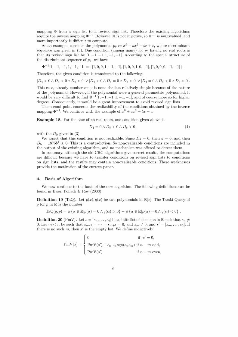
Definition 20 (PmV). Let s = [sn, . . . , s0] be a finite list of elements in R such that sn 6=0. Let m < n be such that sn−1 = · · · = sm+1 = 0, and sm 6= 0, and s′ = [sm, . . . , s0]. Ifthere is no such m, then s′ is the empty list. We define inductively

PmV(s) =

0 if s′ = ∅,PmV(s′) + εn−m sgn(snsm) if n−m odd,

PmV(s′) if n−m even,

8

where εn−m = (−1)(n−m)(n−m−1)/2.The main theorem for the improved CRC algorithm requires the following lemmas

which can be found in Basu, Pollack & Roy (2003). Let Ind(q/p) be the Cauchy index ofq/p on R.

Lemma 21. Given two polynomials p(x), q(x) in R[x], we have TaQ(q, p) = Ind(p′q/p).

Lemma 22. Let p(x), q(x) be the two polynomials in Section 2.2. We have

PmV([sResn(p, q), sResn−1(p, q), . . . , sRes0(p, q)]) = Ind(q/p) .

The main theorem is the following

Theorem 23. Let D = [D1, . . . , Dn] be the discriminant sequence of a real polynomialp(x) of degree n, and let ` be the maximal subscript such that D` 6= 0. If PmV(D) = r,then p(x) has r +1 distinct real roots and 1

2 (`− r−1) pairs of distinct complex conjugateroots.

Proof. We first prove that

#{α ∈ R|p(α) = 0} = PmV([D1, . . . , Dn]) + 1 .

Observe that #{α ∈ R|p(α) = 0} = TaQ(1, p). Then from Lemma 21, we have TaQ(1, p) =Ind(p′/p). By Lemma 22,

Ind(p′/p) = PmV([sResn(p, p′), sResn−1(p, p′), . . . , sRes0(p, p′)]) .

By Remark 13,

PmV([sResn(p, p′), sResn−1(p, p′), . . . , sRes0(p, p′)])

= PmV([sgn(an), D1/an, . . . , Dn/an]) = 1 + PmV([D1/an, . . . , Dn/an]) ,

since sgn(an) and D1/an = nan have the same sign. Finally,

1 + PmV([D1/an, . . . , Dn/an]) = 1 + PmV([D1, . . . , Dn]) .

Now noticing that p(x) has ` distinct roots, the last part of the theorem follows. 2

From Theorem 23, we obtain the following important corollary, which is necessary fordetecting non-realizable sign lists in the output conditions.

Corollary 24. Let S = [s1, . . . , sn] and R = [r1, . . . , rn] be the sign list and the revisedsign list of p(x) respectively. Then PmV(S) = PmV(R).

Proof. Let ` be the maximal subscript of S such that s` 6= 0. Let m and ν be thenumber of sign permanences and the number of sign changes of R. By Theorem 23, wehave PmV(S) = #{α ∈ R|p(α) = 0}−1. By Proposition 14, #{α ∈ R|p(α) = 0} = `−2ν.So

PmV(S) = `− 2ν − 1 . (5)On the other hand, it is easy to see that PmV(R) = m− ν and `− 1 = m + ν. So

2ν = `− 1− PmV(R) . (6)

Therefore, from (5) and (6), we get PmV(S) = `− (`−1−PmV(R))−1 = PmV(R). 2

9

Example 25. We give an example of the use of the above corollary, by proving the non-realizability of condition (4) from a different point of view. The condition is equivalentto the sign list [1, 0, 0, 0,−1,−1], which has revised sign list [1,−1,−1, 1,−1,−1]. Since

PmV([1, 0, 0, 0,−1,−1]) = 1 6= −1 = PmV([1,−1,−1, 1,−1,−1]),

then Corollary 24 states that the sign list [1, 0, 0, 0,−1,−1] is not realizable for p6. Sim-ilarly we can prove that the sign list [1, 0, 0,−1, 0,−1] is not realizable for p6, because

PmV([1, 0, 0,−1, 0,−1]) = 1 6= −1 = PmV([1,−1,−1,−1, 1,−1]) .

Observe that, by Proposition 14, rsl(p6) = [1,−1,−1,−1, 1,−1] is one condition forp6 having no real roots, and [1, 0, 0,−1, 0,−1] ∈ Φ−1[1,−1,−1,−1, 1,−1], where Φ is themapping from sign lists to revised sign lists (Section 3.5). This example shows again thatthe process for transferring the output conditions on revised sign lists to conditions onsign lists may include non-realizable conditions.

Example 26. Let P4 = x4 + a3x3 + a2x

2 + a1x + a0 and sj denote the jth principalSturm-Habicht coefficient sthaj(P4, 1) (Definition 10). Gonzalez-Vega (1998) used hiscombinatorial algorithm to derive the conditions for (∀x P4 > 0). In order to reduce theoutput conditions, he removed the case when s2 = 0 and s1 > 0 by an ad hoc argument.

In the following, we use Corollary 24 to detect this non-realizable condition. By Re-mark 11, noticing a4 = 1, we have [s3, s2, s1, s0] = [D1, D2, D3, D4]. So the case isequivalent to the sign list [1, 0, 1, sgnD4]. By Corollary 24, it is not realizable since itsrevised sign list is [1,−1, 1, sgnD4] and

PmV([1, 0, 1, sgnD4]) = PmV([1,−1, 1, sgnD4]) + 2.

5. Algorithm

In the first part of this section, we propose an improved algorithm for computing theCRC of a real parametric polynomial. In the second part, we summarize some features ofthe algorithm. Examples for explaining the algorithm will be given in Example 27 below.

5.1. Algorithm Description

We need the following functions to present the algorithm.

• AllListsReal: Input n ∈ N; output the list of all possible RCs for a real parametricpolynomial of degree n. See Liang & Jeffrey (2006) for details.

• RCInfo: Input an RC L of a polynomial with real coefficients; output the list [n, `, r],where n is the degree of the polynomial, ` the number of distinct (real and complex)roots, and r the number of distinct real roots specified by L.

• MaxSubs: Input a sign list S; output the maximal subscript of non-vanishing elementsin S.

• MinusOne: Input an RC L; output the RC generated from L by decreasing the absolutevalues of all elements in L by 1, and then erasing all elements of value 0.

• Op: Input a set {a1, . . . , an}; output the sequence a1, . . . , an.

10

Let p(x) = anxn + . . . + a1x + a0 be a real parametric polynomial with an 6= 0. Thealgorithm starts from generating all possible RCs for p(x) using AllListsReal. Then foreach RC L, we find the conditions on the parametric coefficients of p(x) such that L isrealized.

We first compute all possible sign lists of p(x) for p(x) having L as its RC.

Algorithm 1. GenAllSLInput: A real parametric polynomial p(x) and an RC L.Output: The set of all the sign lists of p(x) that lead to the RC given by L.Procedure:• [n, `, r] ← RCInfo(L).• Compute the discriminant sequence D = [D1, . . . , Dn] of p.• Compute the set S0 of all possible sign lists from D: for 1 < k ≤ n, if Dk ∈ R,

then Dk → sgn(Dk); otherwise, Dk → {−1, 0, 1}. For example, if D = [1,−2, a], thenS0 = {[1,−1,−1], [1,−1, 0], [1,−1, 1]}.

• Compute S = {s ∈ S0| MaxSubs(s) = `, PmV(s) = PmV(rsl(s)) = r − 1},• Return S.

Then S = GenAllSL(p, L) is the set of all possible sign lists of p(x) for p(x) having Las its RC. In order to make the multiplicities of the roots of p(x) be those specified by L,we also have to determine the possible sign lists of the polynomials in the ∆−sequenceof p(x) (Definition 6), except for the following five cases (termination conditions): if theRC of p(x) is L and is such that [n, `, r] = RCInfo(L), then these cases are

(1) n = `,(2) ` = 1.(3) ` = 2 and r = 0.(4) n− ` = 1.(5) r = 0 and n− ` = 2.

For other cases, ∆1(p) = Θn−`(p), the (n − `)th multiple factor of p(x) (Definition7). By Proposition 15, the RC of ∆1(p) would be L1 = MinusOne(L). Then we cancall GenAllSL recursively. This is the basis of the following algorithm which generatesthe conditions for p(x) having L as its root classification. The output conditions are asequence of mixed lists. Each mixed list consists of a polynomial in the ∆-sequence ofp(x), followed by all of its possible sign lists. We denote the empty sequence by NULL.Notice that if NULL is returned, then L is not realizable.

Algorithm 2. CondInput: a real parametric polynomial p(x); an RC L.Output: A sequence of mixed lists (the conditions for p(x) having L as its RC).Procedure:[n, `, r] ← RCInfo(L)S ← GenAllSL(p, L)if S = ∅

return NULLelse if [n, `, r] meets one of the five cases

return [p, Op(S)]else

11

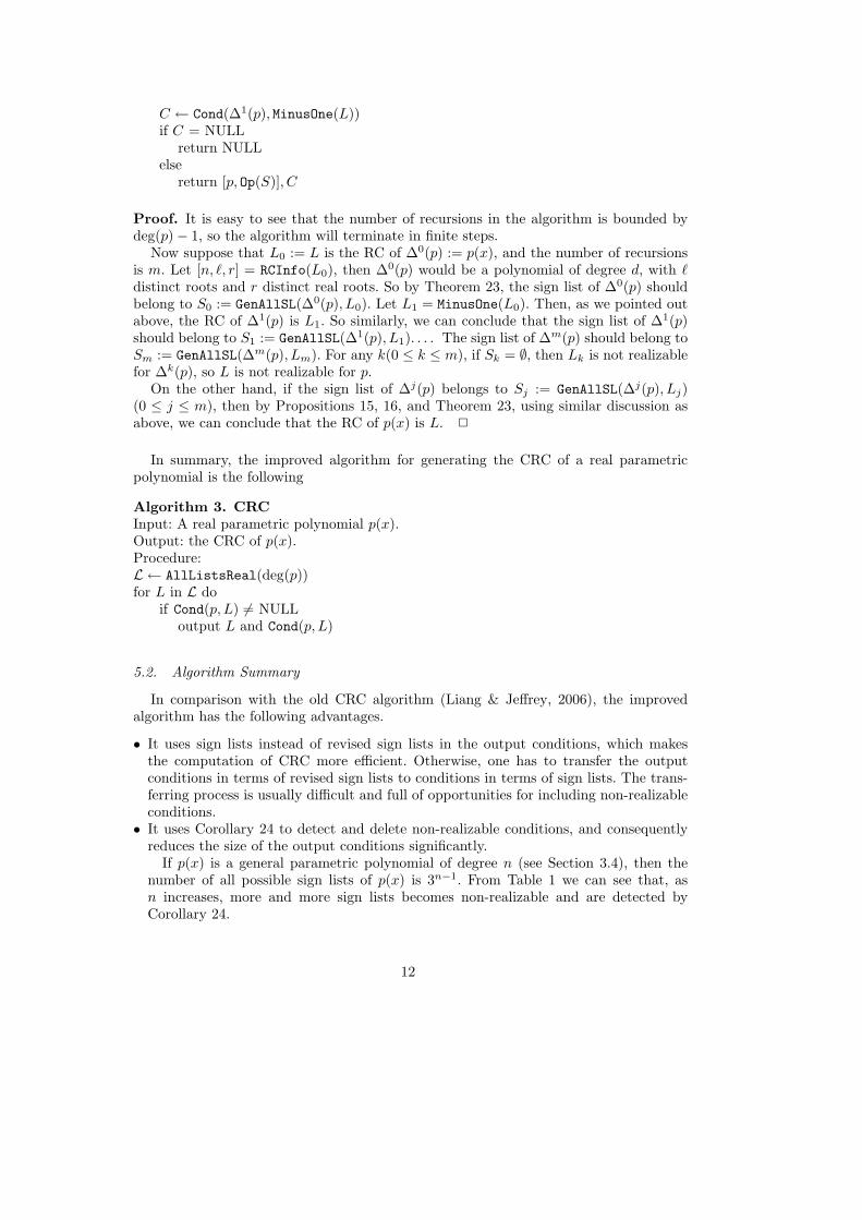
C ← Cond(∆1(p), MinusOne(L))if C = NULL

return NULLelse

return [p, Op(S)], C

Proof. It is easy to see that the number of recursions in the algorithm is bounded bydeg(p)− 1, so the algorithm will terminate in finite steps.

Now suppose that L0 := L is the RC of ∆0(p) := p(x), and the number of recursionsis m. Let [n, `, r] = RCInfo(L0), then ∆0(p) would be a polynomial of degree d, with `distinct roots and r distinct real roots. So by Theorem 23, the sign list of ∆0(p) shouldbelong to S0 := GenAllSL(∆0(p), L0). Let L1 = MinusOne(L0). Then, as we pointed outabove, the RC of ∆1(p) is L1. So similarly, we can conclude that the sign list of ∆1(p)should belong to S1 := GenAllSL(∆1(p), L1). . . . The sign list of ∆m(p) should belong toSm := GenAllSL(∆m(p), Lm). For any k(0 ≤ k ≤ m), if Sk = ∅, then Lk is not realizablefor ∆k(p), so L is not realizable for p.

On the other hand, if the sign list of ∆j(p) belongs to Sj := GenAllSL(∆j(p), Lj)(0 ≤ j ≤ m), then by Propositions 15, 16, and Theorem 23, using similar discussion asabove, we can conclude that the RC of p(x) is L. 2

In summary, the improved algorithm for generating the CRC of a real parametricpolynomial is the following

Algorithm 3. CRCInput: A real parametric polynomial p(x).Output: the CRC of p(x).Procedure:L ← AllListsReal(deg(p))for L in L do

if Cond(p, L) 6= NULLoutput L and Cond(p, L)

5.2. Algorithm Summary

In comparison with the old CRC algorithm (Liang & Jeffrey, 2006), the improvedalgorithm has the following advantages.

• It uses sign lists instead of revised sign lists in the output conditions, which makesthe computation of CRC more efficient. Otherwise, one has to transfer the outputconditions in terms of revised sign lists to conditions in terms of sign lists. The trans-ferring process is usually difficult and full of opportunities for including non-realizableconditions.

• It uses Corollary 24 to detect and delete non-realizable conditions, and consequentlyreduces the size of the output conditions significantly.

If p(x) is a general parametric polynomial of degree n (see Section 3.4), then thenumber of all possible sign lists of p(x) is 3n−1. From Table 1 we can see that, asn increases, more and more sign lists becomes non-realizable and are detected byCorollary 24.

12

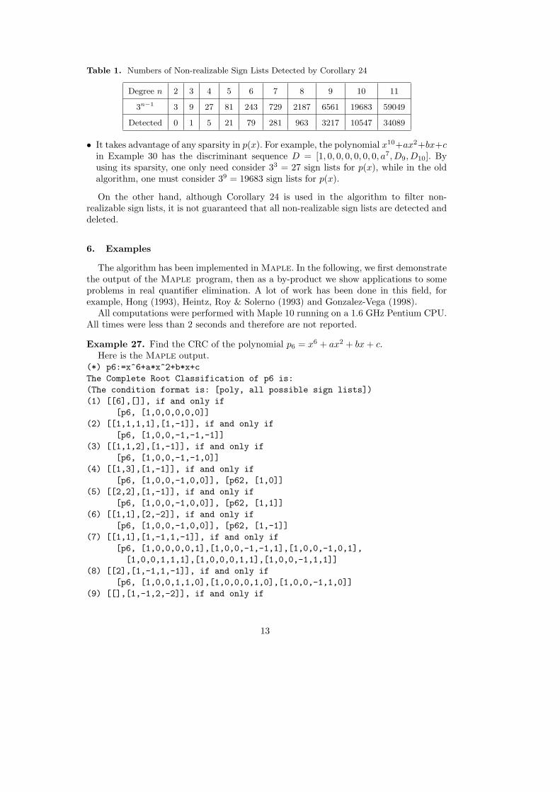
Table 1. Numbers of Non-realizable Sign Lists Detected by Corollary 24

Degree n 2 3 4 5 6 7 8 9 10 11

3n−1 3 9 27 81 243 729 2187 6561 19683 59049

Detected 0 1 5 21 79 281 963 3217 10547 34089

• It takes advantage of any sparsity in p(x). For example, the polynomial x10+ax2+bx+cin Example 30 has the discriminant sequence D = [1, 0, 0, 0, 0, 0, 0, a7, D9, D10]. Byusing its sparsity, one only need consider 33 = 27 sign lists for p(x), while in the oldalgorithm, one must consider 39 = 19683 sign lists for p(x).

On the other hand, although Corollary 24 is used in the algorithm to filter non-realizable sign lists, it is not guaranteed that all non-realizable sign lists are detected anddeleted.

6. Examples

The algorithm has been implemented in Maple. In the following, we first demonstratethe output of the Maple program, then as a by-product we show applications to someproblems in real quantifier elimination. A lot of work has been done in this field, forexample, Hong (1993), Heintz, Roy & Solerno (1993) and Gonzalez-Vega (1998).

All computations were performed with Maple 10 running on a 1.6 GHz Pentium CPU.All times were less than 2 seconds and therefore are not reported.

Example 27. Find the CRC of the polynomial p6 = x6 + ax2 + bx + c.Here is the Maple output.

(*) p6:=x^6+a*x^2+b*x+cThe Complete Root Classification of p6 is:(The condition format is: [poly, all possible sign lists])(1) [[6],[]], if and only if

[p6, [1,0,0,0,0,0]](2) [[1,1,1,1],[1,-1]], if and only if

[p6, [1,0,0,-1,-1,-1]](3) [[1,1,2],[1,-1]], if and only if

[p6, [1,0,0,-1,-1,0]](4) [[1,3],[1,-1]], if and only if

[p6, [1,0,0,-1,0,0]], [p62, [1,0]](5) [[2,2],[1,-1]], if and only if

[p6, [1,0,0,-1,0,0]], [p62, [1,1]](6) [[1,1],[2,-2]], if and only if

[p6, [1,0,0,-1,0,0]], [p62, [1,-1]](7) [[1,1],[1,-1,1,-1]], if and only if

[p6, [1,0,0,0,0,1],[1,0,0,-1,-1,1],[1,0,0,-1,0,1],[1,0,0,1,1,1],[1,0,0,0,1,1],[1,0,0,-1,1,1]]

(8) [[2],[1,-1,1,-1]], if and only if[p6, [1,0,0,1,1,0],[1,0,0,0,1,0],[1,0,0,-1,1,0]]

(9) [[],[1,-1,2,-2]], if and only if

13

[p6, [1,0,0,1,0,0]](10) [[],[1,-1,1,-1,1,-1]], if and only if

[p6, [1,0,0,0,1,-1],[1,0,0,-1,1,-1],[1,0,0,1,0,-1],[1,0,0,0,0,-1],[1,0,0,1,-1,-1],[1,0,0,1,1,-1]]

where(#1) p6:=x^6+a*x^2+b*x+c,and its discriminant sequence is:[1, 0, 0, a^3, 256*a^5+1728*c^2*a^2-5400*a*c*b^2+1875*b^4,-1024*a^6*c+256*a^5*b^2-13824*c^3*a^3+43200*c^2*a^2*b^2-22500*b^4*c*a+3125*b^6-46656*c^5](#2) p62:=4*a*x^2+5*b*x+6*c,and its discriminant sequence is:[1, 25*b^2-96*a*c]

Let us explain the CRC of p6 with respect to the improved algorithm. First, thealgorithm CRC calls the function AllListsReal to generate all possible root classifications(RCs) for a polynomial of degree 6. There are 23 RCs as follows. For the sake of simplicity,the order of them has been changed.[ [[3,3],[]], [[2,4],[]], [[2,2,2],[]], [[1,5],[]], [[1, 2,3],[]],[[1,1,4],[]], [[1,1,2,2],[]], [[1,1,1,3],[]], [[1,1,1,1,2],[]],[[1,1,1,1,1,1],[]], [[4],[1,-1]], [[2],[2,-2]], [[],[3,-3]],[[6],[]], [[1,1,1,1],[1,-1]], [[1,1,2],[1,-1]], [[1,3],[1,-1]],[[2,2],[1,-1]], [[1,1],[2,-2]], [[1,1],[1,-1,1,-1]], [[2],[1,-1,1,-1]], [[],[1,-1,2,-2]], [[],[1,-1,1,-1,1,-1]] ]

Second, in a “for-loop”, for each RC L above and p6, the algorithm Cond is called togenerate the conditions for p6 having L as its RC. It turns out that, for the first 13 RCs(those RCs in the first 3 lines), the outputs of Cond are all NULL (empty sequence).So the first 13 RCs are not realizable for p6. On the other hand, the rest 10 RCs arerealizable for p6. There are 10 numbered lines in the output of the CRC algorithm, andeach line represents an RC and the conditions such that the RC is realized for p6.

For example, the first line describes that p6 has a single real root of multiplicity 6,if and only if p6 has the sign list [1, 0, 0, 0, 0, 0]. Since the discriminant sequence of p6 is[1, 0, 0, a3, D5, D6] (see the Maple output above), where

D5 = 256a5 + 1728a2c2 − 5400ab2c + 1875b4 ,

D6 =−1024a6c + 256a5b2 − 13824a3c3 + 43200a2b2c2 − 22500ab4c

+3125b6 − 46656c5 ,

p6 has a single real root of multiplicity 6, if and only if a3 = 0 ∧D5 = 0 ∧D6 = 0. Thelatter is equivalent to a = b = c = 0. In summary, p6 has a single real root of multiplicity6, if and only if a = b = c = 0, which is what we expect.

Now we consider line (5). It describes that p6 has 2 real roots, each of multiplicity2, and one complex conjugate pair of multiplicity 1, if and only if p6 has the sign list[1, 0, 0,−1, 0, 0] and p62 has the sign list [1, 1]. The algorithm Cond works as follows. LetL = [[2, 2], [1,−1]]. First, it calls the function RCInfo(L) and gets the information aboutL: [n, `, r] = [6, 4, 2]; then it calls GenAllSL(p6, L) to generate the set S of all possible sign

14

lists of p6 for p6 having L as its RC, and it turns out that S = {[1, 0, 0,−1, 0, 0]}. BecauseS 6= ∅ and [n, `, r] does not meet the termination conditions, Cond also has to computeall possible sign lists of ∆1(p6) which is p62 above, for ∆1(p6) having MinusOne(L) =[[1, 1], [ ]] as its RC. So Cond calls itself again: Cond(p62, [[1, 1], [ ]]). It turns out thatp62 has [[1, 1], [ ]] as its RC, if and only if p62 has the sign list [1, 1]. At this point, thetermination condition (1) is reached, and the algorithm Cond terminates.

Therefore, p6 has 2 real roots, each of multiplicity 2, and one complex conjugate pairof multiplicity 1, if and only if p6 has the sign list [1, 0, 0,−1, 0, 0] and p62 has the signlist [1, 1]. The condition can be expressed as a3 < 0∧D5 = 0∧D6 = 0∧E2 > 0, where E2

is the second element of the discriminant sequence of p62 (see the Maple output above)

E = [1, E2], E2 = 25b2 − 96ac.

In summary, p6 has 2 real roots, each of multiplicity 2, and one complex conjugatepair of multiplicity 1, if and only if a < 0 ∧D5 = 0 ∧D6 = 0 ∧ E2 > 0.

Next we consider line (8). It states that p6 has one real root of multiplicity 2, and twopairs of complex conjugate roots, each of multiplicity 1, if and only if the sign list of p6

be one of [1, 0, 0, 1, 1, 0], [1, 0, 0, 0, 1, 0] or [1, 0, 0,−1, 1, 0]. The latter can be expressed as[a > 0 ∧ D5 > 0 ∧ D6 = 0] ∨[a = 0 ∧ D5 > 0 ∧ D6 = 0] ∨ [a < 0 ∧ D5 > 0 ∧ D6 = 0].It can be further simplified as D5 > 0 ∧ D6 = 0. Therefore p6 has one real root ofmultiplicity 2, and two pairs of complex conjugate roots, each of multiplicity 1, if andonly if D5 > 0 ∧D6 = 0.

Other lines can be explained similarly. Finally, note that in line (10), the two non-realizable sign lists [1, 0, 0, 0,−1,−1] and [1, 0, 0,−1, 0,−1] have been detected and deletedby the improved algorithm automatically.

Problem 28. Find the CRC of the polynomial p6 = x6 + ax3 + bx2 + cx + d.The following is the Maple output (where the discriminant sequences of p6, p62 and

p63 are omitted in order to give a more pleasing layout).(*) p6:=x^6+a*x^3+b*x^2+c*x+dThe Complete Root Classification of p6 is:(The condition format is: [poly,its all possible sign lists])(1) [[6],[]], if and only if

[p6, [1,0,0,0,0,0]](2) [[1,1,1,1],[1,-1]], if and only if

[p6, [1,0,-1,-1,-1,-1],[1,0,0,-1,-1,-1]](3) [[1,1,2],[1,-1]], if and only if

[p6, [1,0,-1,-1,-1,0],[1,0,0,-1,-1,0]](4) [[1,3],[1,-1]], if and only if

[p6, [1,0,-1,-1,0,0],[1,0,0,-1,0,0]], [p62, [1,0]](5) [[2,2],[1,-1]], if and only if

[p6, [1,0,-1,-1,0,0],[1,0,0,-1,0,0]], [p62, [1,1]](6) [[4],[1,-1]], if and only if

[p6, [1,0,-1,0,0,0]], [p63, [1,0,0]](7) [[1,1],[2,-2]], if and only if

[p6, [1,0,-1,-1,0,0],[1,0,0,-1,0,0]], [p62, [1,-1]](8) [[1,1],[1,-1,1,-1]], if and only if

15

[p6, [1,0,-1,0,0,1],[1,0,0,0,0,1],[1,0,-1,-1,0,1],[1,0,0,-1,0,1],[1,0,-1,-1,-1,1],[1,0,0,-1,-1,1],[1,0,-1,1,1,1],[1,0,0,1,1,1],[1,0,-1,0,1,1],[1,0,0,0,1,1],[1,0,-1,-1,1,1],[1,0,0,-1,1,1]]

(9) [[2],[2,-2]], if and only if[p6, [1,0,-1,0,0,0]], [p63, [1,1,-1],[1,0,-1],[1,-1,-1]]

(10) [[2],[1,-1,1,-1]], if and only if[p6, [1,0,-1,1,1,0],[1,0,0,1,1,0],[1,0,-1,0,1,0],

[1,0,0,0,1,0],[1,0,-1,-1,1,0],[1,0,0,-1,1,0]](11) [[],[1,-1,2,-2]], if and only if

[p6, [1,0,0,1,0,0],[1,0,-1,1,0,0]](12) [[],[1,-1,1,-1,1,-1]], if and only if

[p6, [1,0,0,1,0,-1],[1,0,-1,0,0,-1],[1,0,0,0,0,-1],[1,0,-1,1,-1,-1],[1,0,0,1,-1,-1],[1,0,-1,1,1,-1],[1,0,0,1,1,-1],[1,0,-1,0,1,-1],[1,0,0,0,1,-1],[1,0,-1,-1,1,-1],[1,0,0,-1,1,-1],[1,0,-1,1,0,-1]]

where(#1) p62:=-9*c*a^3-180*d*c*a+192*d*b^2+Q1*x+Q2*x^2,(#2) p6:=x^6+a*x^3+b*x^2+c*x+d,(#3) p63:=-3*a*x^3-4*b*x^2-5*c*x-6*d,and

Q1:=160*c*b^2-18*b*a^3-150*a*c^2-144*a*d*b,Q2:=-27*a^4+108*d*a^2-240*a*b*c+128*b^3,

The discriminant sequence of p6 is D := [1, 0,−a2, D4, D5, D6], where

D4 = −27a4 + 108da2 − 240abc + 128b3

D5 = 81a5c− 27a4b2 − 1134dca3 + 648a2db2 + 1620c2a2b

−1344acb3 + 3240acd2 + 256b5 + 1728d2b2 − 5400bdc2 + 1875c4

D6 = 108c3a5 + 729d2a6 − 8748d3a4 + 34992a2d4 − 46656d5 − 486ca5db

+21384ca3d2b− 9720c2b2da2 − 77760d3cab− 22500dc4b + 43200c2b2d2

+6912ab4cd + 3125c6 − 27b2a4c2 + 108b3a4d− 8640b3a2d2 − 1350dc3a3

+2250c4ba2 − 13824d3b3 + 27000d2ac3 − 1600ab3c3 + 256b5c2 − 1024b6d.

From the CRC of p6, we can obtain the conditions on a, b, c, d such that (∀x)[p6 > 0].(∀x)[p6 > 0] ⇔ case (11) or case (12) holds. We can write the sign conditions directly.No mapping of conditions is necessary.

Case (11) holds ⇔ the sign list of p6 be [1, 0, 0, 1, 0, 0] or [1, 0,−1, 1, 0, 0] ⇔ [−a2 =0∧D4 > 0∧D5 = 0∧D6 = 0]∨ [−a2 < 0∧D4 > 0∧D5 = 0∧D6 = 0] ⇔ D4 > 0∧D5 =0 ∧D6 = 0.

Case (12) holds ⇔ the sign list of p6 be one of the following 12 lists:[1, 0, 0, 1, 0,−1] ⇔ [−a2 = 0 ∧D4 > 0 ∧D5 = 0 ∧D6 < 0][1, 0,−1, 0, 0,−1] ⇔ [−a2 < 0 ∧D4 = 0 ∧D5 = 0 ∧D6 < 0][1, 0, 0, 0, 0,−1] ⇔ [−a2 = 0 ∧D4 = 0 ∧D5 = 0 ∧D6 < 0][1, 0,−1, 1,−1,−1] ⇔ [−a2 < 0 ∧D4 > 0 ∧D5 < 0 ∧D6 < 0]

16

[1, 0, 0, 1,−1,−1] ⇔ [−a2 = 0 ∧D4 > 0 ∧D5 < 0 ∧D6 < 0][1, 0,−1, 1, 1,−1] ⇔ [−a2 < 0 ∧D4 > 0 ∧D5 > 0 ∧D6 < 0][1, 0, 0, 1, 1,−1] ⇔ [−a2 = 0 ∧D4 > 0 ∧D5 > 0 ∧D6 < 0][1, 0,−1, 0, 1,−1] ⇔ [−a2 < 0 ∧D4 = 0 ∧D5 > 0 ∧D6 < 0][1, 0, 0, 0, 1,−1] ⇔ [−a2 = 0 ∧D4 = 0 ∧D5 > 0 ∧D6 < 0][1, 0,−1,−1, 1,−1] ⇔ [−a2 < 0 ∧D4 < 0 ∧D5 > 0 ∧D6 < 0][1, 0, 0,−1, 1,−1] ⇔ [−a2 = 0 ∧D4 < 0 ∧D5 > 0 ∧D6 < 0][1, 0,−1, 1, 0,−1] ⇔ [−a2 < 0 ∧D4 > 0 ∧D5 = 0 ∧D6 < 0]

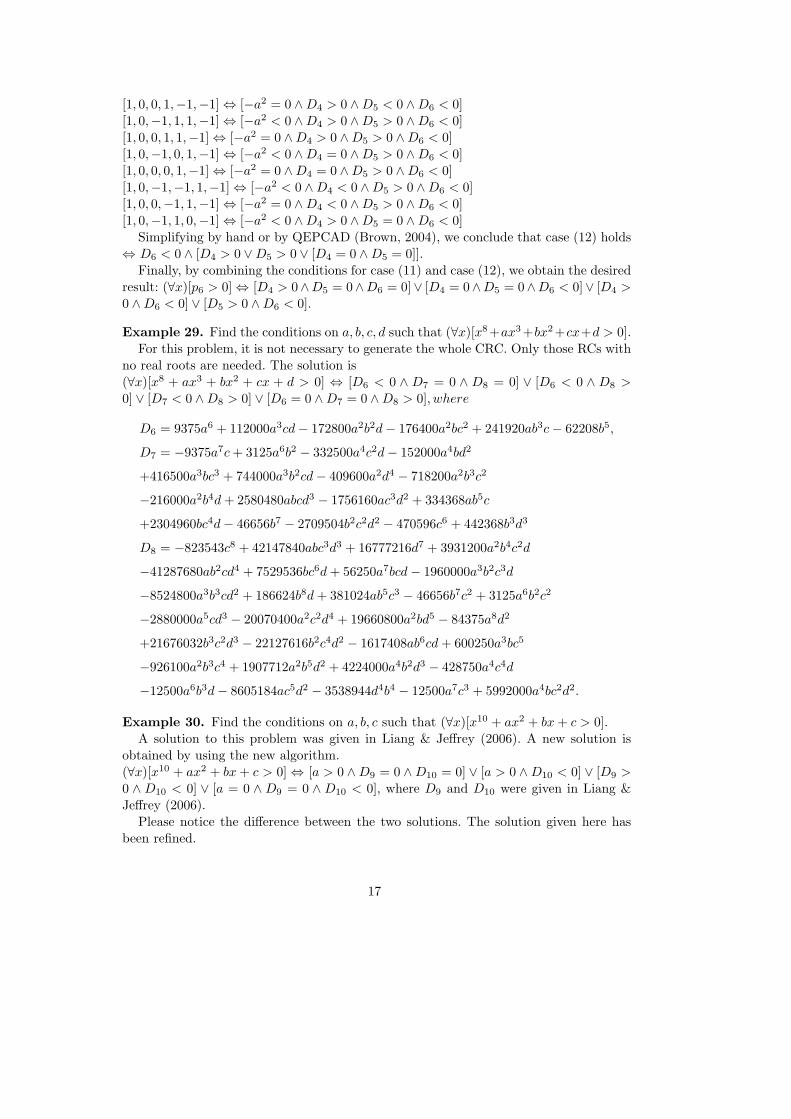
Simplifying by hand or by QEPCAD (Brown, 2004), we conclude that case (12) holds⇔ D6 < 0 ∧ [D4 > 0 ∨D5 > 0 ∨ [D4 = 0 ∧D5 = 0]].

Finally, by combining the conditions for case (11) and case (12), we obtain the desiredresult: (∀x)[p6 > 0] ⇔ [D4 > 0∧D5 = 0∧D6 = 0]∨ [D4 = 0∧D5 = 0∧D6 < 0]∨ [D4 >

0 ∧D6 < 0] ∨ [D5 > 0 ∧D6 < 0].

Example 29. Find the conditions on a, b, c, d such that (∀x)[x8+ax3+bx2+cx+d > 0].For this problem, it is not necessary to generate the whole CRC. Only those RCs with

no real roots are needed. The solution is(∀x)[x8 + ax3 + bx2 + cx + d > 0] ⇔ [D6 < 0 ∧ D7 = 0 ∧ D8 = 0] ∨ [D6 < 0 ∧ D8 >

0] ∨ [D7 < 0 ∧D8 > 0] ∨ [D6 = 0 ∧D7 = 0 ∧D8 > 0], where

D6 = 9375a6 + 112000a3cd− 172800a2b2d− 176400a2bc2 + 241920ab3c− 62208b5,

D7 = −9375a7c + 3125a6b2 − 332500a4c2d− 152000a4bd2

+416500a3bc3 + 744000a3b2cd− 409600a2d4 − 718200a2b3c2

−216000a2b4d + 2580480abcd3 − 1756160ac3d2 + 334368ab5c

+2304960bc4d− 46656b7 − 2709504b2c2d2 − 470596c6 + 442368b3d3

D8 = −823543c8 + 42147840abc3d3 + 16777216d7 + 3931200a2b4c2d

−41287680ab2cd4 + 7529536bc6d + 56250a7bcd− 1960000a3b2c3d

−8524800a3b3cd2 + 186624b8d + 381024ab5c3 − 46656b7c2 + 3125a6b2c2

−2880000a5cd3 − 20070400a2c2d4 + 19660800a2bd5 − 84375a8d2

+21676032b3c2d3 − 22127616b2c4d2 − 1617408ab6cd + 600250a3bc5

−926100a2b3c4 + 1907712a2b5d2 + 4224000a4b2d3 − 428750a4c4d

−12500a6b3d− 8605184ac5d2 − 3538944d4b4 − 12500a7c3 + 5992000a4bc2d2.

Example 30. Find the conditions on a, b, c such that (∀x)[x10 + ax2 + bx + c > 0].A solution to this problem was given in Liang & Jeffrey (2006). A new solution is

obtained by using the new algorithm.(∀x)[x10 + ax2 + bx + c > 0] ⇔ [a > 0 ∧D9 = 0 ∧D10 = 0] ∨ [a > 0 ∧D10 < 0] ∨ [D9 >

0 ∧ D10 < 0] ∨ [a = 0 ∧ D9 = 0 ∧ D10 < 0], where D9 and D10 were given in Liang &Jeffrey (2006).

Please notice the difference between the two solutions. The solution given here hasbeen refined.

17

7. Conclusion

In this paper, we have proposed an improved algorithm for the automatic computationof the complete root classification of a real parametric polynomial, and a new test for non-realizable conditions. However, some issues deserve further consideration. For example,the output conditions are basically equalities and inequalities in terms of the parametriccoefficients. A further step would be to determine what are the possible values of theparametric coefficients such that the conditions described are satisfied. This is essentiallythe problem of solving semi-algebraic systems, a problem well-known to be difficult. Thisproblem may be addressed using interval analysis (Colagrossi & Miola, 1983) or methodbased on Grobner basis (Rouillier, 2005). We will leave these issues in further work.

Acknowledgements

We are indebted to Professor Hoon Hong for his helpful discussion at MACIS 2006,Beijing. The discussion initiated this paper. We would like to thank the anonymousreferees for valuable suggestions which help us greatly improve the first version of thepaper.

References

Abdeljaoued, J., Diaz-Toca, G.M., Gonzalez-Vega, L., 2004. Minor of Bezout matrices,Subresultants and parameterization of the degree of the polynomial greatest commondivisor. International Journal of Computer Mathematics 81, 1223-1238.

Arnon, D.S., 1988. Geometric Reasoning with Logic and Algebra. Artificial Intelligence37, 37-60.

Basu, S., Pollack, R., Roy, M.-F., 2003. Algorithms in Real Algebraic Geometry. Springer-Verlag.

Brown, C.W., 2004. QEPCAD B: a program for computing with semi-algebraic sets usingCADs. ACM SIGSAM Bulletin 37, 97-108.

Colagrossi, A., Miola, A.M., 1983. Computing real zeros of polynomials with parametriccoefficients. ACM SIGSAM Bulletin 17, 12-15.

Collins, G.E., 1967. Subresultants and reduced polynomial remainder sequences. Journalof Association for Computing Machinery 14, 128-142.

Davenport, J.H., Heintz, J., 1988. Real quantifier elimination is doubly exponential.Journal of Symbolic Computation 5, 29-36.

Gonzalez-Vega, L., 1998. A combinatorial algorithm solving some quantifier eliminationproblems. Quantifier Elimination and Cylindrical Algebraic Decomposition (B.F. Cavi-ness and J.R. Johnson, eds.), Springer-Verlag, 365-375.

Gonzalez-Vega, L., Lombardi, H., Recio, T., Roy, M.-F., 1998. Sturm-Habicht sequences,determinants and real roots of univariate polynomials. Quantifier Elimination andCylindrical Algebraic Decomposition (B.F. Caviness and J.R. Johnson, eds.), Springer-Verlag, 300-316.

Habicht, V.W., 1948. Eine Verallgemeinerung des Sturmschen Wurzelzahlverfahrens.Comm. Math. Helvetici 21, 99-116.

Heintz, J., Roy, M.-F., Solerno, P., 1993. On the theoretical and practical complexity ofthe existential theory of the reals. The Computer Journal 36(5), 427-431.

18

Hong, H., 1993. Quantifier elimination for formulas constrained by quadratic equations.ISSAC’93 Proceedings, ACM Press, 264-274.

Jeffrey, D.J., Corless, R.M., 2006. Linear Algebra in Maple. In CRC Handbook of LinearAlgebra, Editor L. Hogben. Chapter 72.

Liang, S., Jeffrey, D.J., 2006. An algorithm for computing the complete root classificationof a parametric polynomial. Lecture Notes in Computer Science 4120, 116-130.

Liang, S., Zhang, J., 1999. A complete discrimination system for polynomials with com-plex coefficients and its automatic generation. Science in China (Series E) 42, 113-128.

Lickteig, T., Roy, M.F., 2001. Sylvester-Habicht sequences and fast Cauchy index com-putation. Journal of Symbolic Computation 31, 315-341.

Lombardi, H., Roy, M.F., Safely el Din, M., 2000. New structure theorem for subresul-tants. Journal of Symbolic Computation 29, 663-689.

Rouillier, F., 2005. On solving parametric systems. In Workshop on Challenges in Lin-ear and Polynomial Algebra in Symbolic Computation Software. Banff InternationalResearch Center.

Sylvester, J.J., 1853. On a theory of syzygetic relations of two rational integral functions,comprising an application to the theory of Sturm’s function and that of the greatestalgebraical common measure. Trans. Roy. Soc. London 143, 407-548.

Yang, L., 1999. Recent advances on determining the number of real roots of parametricpolynomials. Journal of Symbolic Computation 28, 225-242.

Yang, L., Hou, X., Zeng, Z., 1996. Complete discrimination system for polynomials.Science in China (Series E) 39, 628-646.

19