Image computation for polynomial dynamical systems usingthe Bernstein expansion

Thao Dang and David Salinas

VERIMAG,Centre Equation,

2 avenue de Vignate, 38610 Gieres, France

Abstract. This paper is concerned with the problem of computing the image of a set by apolynomial function. Such image computations constitute a crucial component in typical toolsfor set-based analysis of hybrid systems and embedded software with polynomial dynamics,which found applications in various engineering domains. One typical example is the computa-tion of all states reachable from a given set in one step by a continuous dynamics described bya differential or difference equation. We propose a new algorithm for over-approximating suchimages based on the Bernstein representation of polynomial functions. The images are storedusing template polyhedra. Using a prototype implementation, the performance of the algo-rithm was demonstrated on two practical systems as well as a number of randomly generatedexamples.

1 Introduction

Hybrid systems, that is, systems exhibiting both continuous and discrete dynamics, have been anactive research domain, thanks to their numerous applications in chemical process control, avionics,robotics, and most recently in molecular biology. Due to the safety critical features of many suchapplications, formal analysis is a topic of particular interest. A major component in any verificationalgorithm for hybrid systems is an efficient method to compute the reachable set of their continuousdynamics described by differential or difference equations. Well-known properties of affine systemsand other simpler systems can be exploited to design relatively efficient methods1 (such as a recently-developed method can handle continuous systems of 100 and more variables [14]). Nevertheless,nonlinear systems are much more difficult to analyze.

In this work, we address the following image computation problem: given a set in Rn, compute itsimage by a polynomial. This problem typically arises when we need to deal with a dynamical systemof the form xk+1 = π(xk) where π is a multivariate polynomial. Such dynamical systems couldresult from a numerical approximation of a continuous or hybrid system. Many existing reachabilitycomputation methods for continuous systems can be seen as an extension of numerical integration.For reachability analysis which requires considering all possible solutions (for example, due to non-determinism in initial conditions), one has to solve the above equation with sets, that is xk andxk+1 in the equation are subsets of Rn (while they are points if we only need a single solution, as innumerical integration). In addition, similar equations can arise in embedded control systems, such

1 The hybrid systems reachability computation literature is vast. The reader is referred to the recent pro-ceedings of the conference HSCC.

as some physical system controlled by a computer program, which is the implementation of somecontinuous (or possibly hybrid) controller using appropriate discretization.

One reason for which we are interested in the image computation problem for polynomials is thatsuch systems can be used to model a variety of physical phenomena in engineering, economy andbio-chemical networks. This problem was previously considered in [7], where a method using Beziertechniques from Computer Aided Geometric Design (CADG) was proposed. The drawback of thismethod is that it requires expensive convex hull and triangulation computation, which restrictsits application to systems of dimensions not higher than 3, 4. The essence of the new method wepropose in this paper can be summarized as follows. By using a special class of polyhedra togetherwith optimization, we are able to reduce the complexity of the required polyhedral manipulation.Furthermore, by exploiting a technique from CADG, namely the Bernstein expansion, we only needto solve linear programming problems instead of polynomial optimization problems.

Our method is similar to a number of existing methods for continuous and hybrid systems in the useof linear approximation. Its novelty resides in the efficient way of computing linear approximations.Indeed, a common method to approximate a non-linear function by a piecewise linear one, as in thehybridization approach [2] for hybrid systems, requires non-linear optimization. Our method exploitsthe Bernstein expansion of polynomials to replace expensive polynomial programming by linearprogramming. Besides constrained global optimization, other important applications of the Bernsteinexpansion include various control problems [10] (in particular, robust control). The approximation ofthe range of a multivariate polynomial over a box is also used in program analysis and optimization(for example [26, 5]). In the hybrid systems verification, polynomial optimization is used to computebarrier certificates [22], and the algebraic properties of polynomials are used to compute polynomialinvariants [27].

The paper is organized as follows. In Section 2 we introduce the notion of template polyhedraand the Bernstein expansion of polynomials. We then formally state our problem and describe anoptimization based solution. In order to transform the polynomial optimization problem to a linearprogramming problem, a method for computing bound functions for polynomials is then presented.Section 4 describes an algorithm summarizing the main steps of our method. Some experimentalresults, in particular the analysis of a control and a biological systems, are reported in Section 6.

2 Preliminaries

Notation. Let R denote the set of reals. Throughout the paper, vectors is often written usingbold letters. Exceptionally, scalar elements of multi-indices, introduced later, are written using boldletters. Given a vector x, xi denotes its ith component. Capital letters, such as A, B, X, Y denotematrices or sets. If A is a matrix, Ai denotes the ith row of A. An affine function is thus representedas cTx + d.

We use Bu to denote the unit box anchored at the origin, that is Bu = [0, 1]n. We use π to denotea vector of n functions such that for all i ∈ {1, . . . , n}, πi is an n-variate polynomial of the formπi : Rn → R. In the remainder of the paper, we sometimes refer to π simply as “a polynomial”.

To discuss the Bernstein expansion of polynomials, we use multi-indices of the form i = (i1, i2, . . . , in)where each ij is a non-negative integer. Given two multi-indices i and d, we write i ≤ d if for allj ∈ {1, . . . , n}, ij ≤ dj . Also, we write i

d for (i1/d1, i2/d2, . . . , in/dn) and(id

)for(i1d1

)(i2d2

). . .(indn

).

2.1 Template polyhedra

A convex polyhedron is a conjunction of a finite number of linear inequalities described as Ax ≤ b,where A is a m× n matrix, b is a column vector of size m. Template polyhedra are commonly usedin static analysis of programs for computing invariants. Ranges [6] and the octagon domains [20] arespecial template polyhedra. General template polyhedra are used as an abstract domain to representsets of states in [23, 4].

We now briefly recall template polyhedra and algorithms for their manipulation. The reader isreferred to [23] for a thorough description of template polyhedra. A template is a set of linearfunctions over x = (x1, . . . , xn). We denote a template by an m×n matrix H, such that each row Hi

corresponds to the linear function Hix. Given such a template H and a real-valued vector d ∈ Rm,a template polyhedron is defined by considering the conjunction of the linear inequalities of the form∧i=1,...,mH

ix ≤ di. We denote this polyhedron by 〈H,d〉.By changing the values of the elements of d, one can define a family of template polyhedra

corresponding to the template H. We call d a polyhedral coefficient vector. Given d,d′ ∈ Rm, if∀i ∈ {1, . . . ,m} : di ≤ d′i, we write d � d′. Given an m × n template H and two polyhedralcoefficient vectors d,d′ ∈ Rm, if d � d′ then the inclusion relation 〈H,d〉 ⊆ 〈H,d′〉 holds, and wesay that 〈H,d〉 is not larger than 〈H,d′〉.

The advantage of template polyhedra over general convex polyhedra is that the Boolean operations(union, intersection) and common geometric operations can be performed more efficiently [23].

2.2 Bernstein expansion

We consider an n-variate polynomial π : Rn → Rn defined as: π(x) =∑

i∈Id aixi where ai is a vectorin Rn; i and d are two multi-indices of size n such that i ≤ d; Id is the set of all multi-indices i ≤ d,that is Id = {i | i ≤ d}. The multi-index d is called the degree of π.

Given a set X ⊂ Rn, the image of X by π, denoted by π(X), is defined as follows:

π(X) = {(π1(x), . . . , πn(x)) | x ∈ Rn}.

In order to explain the Bernstein expansion of the polynomial π, we first introduce Bernsteinpolynomials. For x = (x1, . . . , xn) ∈ Rn, the ith Bernstein polynomial of degree d is: Bd,i(x) =βd1,i1(x1) . . . βdn,in(xn) where for a real number y, βdj ,ij (y) =

(dj

ij

)yij (1 − ydj−ij ). Then, for all

x ∈ Bu = [0, 1]n, the polynomial π can be written using the Bernstein expansion as follows: π(x) =∑i∈Id biBd,i(x) where for each i ∈ Id the Bernstein coefficient bi is defined as:

bi =∑j≤i

(ij

)(dj

)aj. (1)

The following properties of the Bernstein coefficients are of particular interest.

1. Convex-hull property: Conv{(x, π(x)) : x ∈ Bu} ⊆ Conv{(i/d,bi) | i ∈ Id}. The points bi arecalled the control points of π.

2. The above enclosure yields: ∀x ∈ Bu : π(x)) ∈ 2({bi | i ∈ Id}) where 2 denotes the boundingbox of a point set.

3. Sharpness of some special coefficients: ∀i ∈ I0d : bi = π(i/d) where I0

d is the set of all the verticesof [0,d1]× [0,d2] . . . [0,dn].

Let us return to the main problem of the paper, which is computing the image of a set by apolynomial. Using the above convex-hull property, we can use the coefficients of the Bernstein ex-pansion to over-approximate the image of the unit box Bu by the polynomial π. To compute theimage of a general convex polyhedron, one can over-approximate the polyhedron by a box and thentransform it to the unit box via some affine transformation. A similar idea, which involves using thecoefficients of the Bezier simplex representation, was used in [7] to compute the image of a convexpolyhedron. However, the convex hull computation is expensive especially in high dimensions, whichposes a major problem in continuous and hybrid systems verification approaches using polyhedralrepresentations.

In this work, we propose a new method which can avoid complex convex hull operations over generalconvex polyhedra as follows. First, we use template polyhedra to over-approximate the images.Second, the problem of computing such template polyhedra can be formulated as a polynomialoptimization problem. This optimization problem is computationally difficult, despite recent progressin the development of methods and tools for polynomial programming (see for example [28, 17, 9]and references therein). We therefore seek their affine bound functions for polynomials, in order totransform the polynomial optimization problem to a linear programming one, which can be solvedmore efficiently (in polynomial time) using well-developed techniques, such as Simplex [8] and interiorpoint techniques [3]. Indeed, the above-described Bernstein expansion is used to compute these affinebound functions. This is discussed in the next section.

2.3 Bound functions

To compute bound functions, we use the method using the Bernstein expansion, published in [12].Computing convex lower bound functions for polynomials is a problem of great interest, especially inglobal optimization. The reader is referred to [11–13] for more detailed descriptions of this methodand its variants.

Before continuing, it is important to note that the method described in this section only works forthe case where the variable domain is the unit box Bu. We however want to compute the imagesof more general sets, in particular polyhedra. An extension of this method to such cases will bedeveloped in Section 3.2.

A simple affine lower bound function is a constant function, which can be deduced from the secondproperty of the Bernstein expansion: xi ≤ min{bi | i ∈ Id} = bi0 = b0. The main idea of the methodis as follows. We first compute the affine lower bound function whose corresponding hyperplane passesthrough this control point b0. Then, we aditionally determine (n− 1) hyperplanes passing throughn other control points. This allows us to construct a sequence of n affine lower bound functionsl0, l1, . . . ln. We end up with ln, a function whose corresponding hyperplane passes through a lowerfacet of the convex hull spanned by these control points. A summary of the algorithm can be foundin Appendix. Note that we can easily compute upper bound functions of π by computing the lowerbound functions for −π using this method and then multiply each resulting function by −1.

3 Image approximation using template polyhedra

This section is concerned with the main problem of the paper, which can be formulated as follows.We want to use a template polyhedron 〈H,d〉 to over-approximate the image of a polyhedron Pby the polynomial π. The template matrix H, which is of size m × n is assumed to be given; thepolyhedral coefficient vector d ∈ Rm is however unknown. The question is thus to find d such that

π(P ) ⊆ 〈H,d〉. (2)

It is not hard to see that the following condition is sufficient for (2) to hold: ∀x ∈ P : Hπ(x) ≤ d.Therefore, to determine d, one can formulate the following optimization problem:

∀i ∈ {1, . . . ,m}, di = max(Σnk=1H

ikπk(x)) subj. to x ∈ P. (3)

where Hi is the ith row of the matrix H and Hik is its kth element. Note that the above functions to

optimize are polynomials. As mentioned earlier, polynomial optimization is expensive. Our solution isto bound these functions with affine functions, in order to transform the above optimization problemto a linear programming one. This is formalized as follows.

3.1 Optimization-based solution

In Section 2.3 we discussed lower bound functions for polynomials. Note that these bound functionsare valid only then the variables x are inside the unit box Bu. To consider more general domains,we introduce the following definition.

Definition 1 (Upper and lower bound functions). Given a function f : Rn → R, the functionυ : Rn → R is called an upper bound function of f w.r.t. a set X ⊂ Rn if ∀x ∈ X : f(x) ≤ υ(x). Alower bound function can be defined similarly.

The following property of upper and lower bound functions is easy to prove.

Lemma 1. Given two set X,Y ⊆ Rn such that Y ⊆ X, if υ is an upper (lower) bound function off w.r.t. X, then υ is also an upper (lower) bound function of f w.r.t. Y .

For each k ∈ {1, . . . ,m}, let uk(x) and lk(x) respectively be an upper bound function and a lowerbound function of πk(x) w.r.t. a bounded polyhedron P ⊂ Rn. We consider the following optimizationproblem:

∀i ∈ {1, . . . ,m}, di = Σnk=1H

ikωk. (4)

where the term Hikωk is defined as follows:

– If the element Hik > 0, Hi

kωk = Hik maxuk(x) subj. to x ∈ P ;

– If the element Hik ≤ 0, Hi

kωk = Hik min lk(x) subj. to x ∈ P .

The following lemma is a direct result of (4).

Lemma 2. If a polyhedral coefficient vector d ∈ Rm satisfies (4). Then π(P ) ⊆ 〈H,d〉.

Proof. It is indeed not hard to see that the solution di of the optimization problems (4) is greaterthan or equal to the solution of (3). Hence, if d satisfies (4), then

∀i ∈ {1, . . . ,m} ∀x ∈ P : Σnk=1H

ikπk(x) ≤ di.

This implies that ∀x ∈ P : Hπ(x) ≤ d, that is the image π(P ) is included in the template polyhedron〈H,d〉.

We remark that if all the bound functions in (4) are affine and P is a bounded convex polyhedron,d can be computed by solving 2n linear programming problems. It remains now to find the affinebound functions uk and lk for π w.r.t. a polyhedron P , which is the problem we tackle in the nextsection.

3.2 Computing affine bound functions over polyhedral domains

As mentioned earlier, the method to compute affine bound functions for polynomials in Section 2.3can be applied only when the function domain is a unit box, anchored at the origin. The reasonis that the expression of the control points of the Bernstein expansion in (1) is only valid for thisunit box. If we over-approximate P with a box B, it is then possible to derive a formula expressingthe Bernstein coefficients of π over B. However, this formula is complex and its representation andevaluation can become expensive.

We alternatively consider the composition of the polynomial π with an affine transformation τthat maps the unit box Bu to B. The functions resulting from this composition are still polynomials,for which we can compute their bound functions over the unit box, using the formula (1) of theBernstein expansion. This is explained more formally in the following.

Let B be the bounding box of the polyhedron P , that is, the smallest box that includes P .The composition γ = (π o τ) is defined as γ(x) = π(τ(x)). The functions τ and γ can be computed

symbolically, which will be discussed later.

Lemma 3. Let γ = π o τ . Then, π(P ) ⊆ γ(Bu).

Proof. By the definition of the composition γ, γ(Bu) = {π(τ(x)) | x ∈ Bu}. Additionally, τ(Bu) = B.Therefore, γ(Bu) = π(B). Since the polyhedron P is included in its bounding box B, we thus obtainπ(P ) ⊆ π(B) = γ(Bu).

We remark that the above proof is still valid for any affine function τ . This means that insteadof an axis-aligned bounding box, we can over-approximate P more precisely with an oriented (i.e.non-axis-aligned) bounding box. This can be done using the following method.

Computing an oriented bounding box

The directions of an oriented bounding box can be computed using Principal Component Anal-ysis [15]. For a thorough description of the Principal Component Analysis (PCA), the reader isreferred to [18].

We first choose a set S = {s1, s2, . . . , sm} of m points2 in the polyhedron P , such that m ≥ n. Wedefer a discussion on how this point set is selected to the end of this section. PCA is used to find an2 By abuse of notation we use m to denote both the number of template constraints and the number of

points here.

orthogonal basis that best represents the point set S. More concretely, we use s to be the mean ofS, that is s =

∑mi=1 si and we denote si,j = sji − si. For two points si and sj in S, the covariance of

their translated points is: cov(si, sj) = 1m−1

∑mk=1 sk,isk,j . Then, we define the co-variance matrix as

follows:

C =

cov(s1, s1) cov(s1, s2) . . . cov(s1, sm)cov(s2, s1) cov(s2, s2) . . . cov(s2, sm)

. . .cov(sm, s1) cov(sk, s2) . . . cov(sm, sm)

.

The n largest singular values of C provide the orientation of the bounding box. More concretely,since C is symetric, by singular value decomposition, we have C = UΛUT where Λ is the matrix ofsingular values. The axes of the bounding box are hence determined by the first n columns of thematrix U , and its centroid is s.

We now discuss how to select the set S. When the vertices of P are available, we can include themin the set. However, if P is given as a template polyhedron, this requires computing the verticeswhich is expensive. Moreover, using only the vertices, when their distribution do not represent thegeometric form of the polyhedron, may cause a large approximation error, since the resulting principaldirections are not the ones along which the points inside P are mostly distributed. To remedy this,we sample points inside P as follows. First, we compute an axis-aligned bounding box of P (this canbe done by solving 2n linear programming problems). We then uniformly sample points inside thisbounding box and keep only the points that satisfy the constraints of P . Uniform sampling on theboundary of P in general enables a better precision. More detail on this can be found in [8].

4 Image computation algorithm

The following algorithm summarizes the main steps of our method for over-approximating the imageof a bounded polyhedron P ⊂ Rn by the polynomial π. The templates are an input of the algorithm.In the current implementation of the algorithm, the templates can be fixed by the user, or thetemplates forming regular sets are used.

Algorithm 1 Over-approximating π(P )/* Inputs: convex polyhedron P , polynomial π, templates H */

B = PCA(P ) /* Compute an oriented bounding box */τ = UnitBoxMap(B) /* Compute the function mapping the unit box Bu to B */γ = π o τ(u, l) = BoundFunctions(γ) /* Compute the affine bound functions */d = PolyApp(u, l,H) /* Compute the coefficient vector d */Q = 〈H, d〉 /* Form the template polyhedron and return it */Return(Q)

The role of the procedure PCA is to compute an oriented bounding box B that encloses P . Theprocedure UnitBoxMap is then used to determine the affine function τ that maps the unit box Bu

at the origin to B. This affine function is composed with the polynomial π, the result of which is thepolynomials γ. The affine lower and upper bound functions l and u of γ are then computed, using theBernstein expansion. The function PolyApp determines the polyhedral coefficient vector d by solvingthe linear programs in (4) with u, l and the optimization domain is Bu. The polyhedral coefficientvector d are then used to define a template polyhedron Q, which is the result to be returned.

Based on the analysis so far, we can state the correctness of Algorithm 1.

Theorem 1. Let 〈H, d〉 be the template polyhedron returned by Algorithm 1. Then π(P ) ⊆ 〈H, d〉.

We remark that u and l are upper and lower bound functions of γ with respect to Bu. It is nothard to see that τ−1(P ) ⊆ Bu where τ−1 is the inverse of τ . Using the property of bound functions,u and l are also bound functions of γ with respect to τ−1(P ). Hence, if we solve the optimizationproblem over the domain τ−1(P ) (which is often smaller than Bu), using Lemma 1, the resultingpolyhedron is still an over-approximation of π(P ). This remark can be used to obtain more accurateresults.

5 Approximation error and computation cost

We finish this section by briefly discussing the precision and complexity of the method. A moredetailed analysis can be found in [8]. The approximation error are caused by the bound functions,the oriented bounding box approximation, and the use of template polyhedra.

The following lemma states an important property of the Bernstein expansion.

Lemma 4. Let Cπ,B be the piecewise linear function defined by the Bernstein control points of πwith respect to the box B. Then, for all x ∈ B, |π(x)− Cπ,B(x)| ≤ Kδ2(B) where | · | is the infinitynorm on Rn, δ(B) is the box size (i.e. its largest side length), Kk = maxx∈B;i,j∈{1,...,n}|∂i∂jπk(x)|,K = maxk∈{1,...,n}Kk.

From this result it can be proven that in one dimensional case, the error between the bound functionscomputed using the Bernstein expansion and the original polynomial is quadratic in the length ofbox domains. This quadratic convergence seems to hold for higher dimensional cases in practice, asshown in [12]. We conjecture that there exists a subdivision method of the box B which allows aquadratic convergence of the error. This subdivision method is similar to the one used for findingroots of a polynomial with quadratic convergence [21].

On the other hand, a polyhedron can be approximated by a set of non-overlapping oriented boxeswith arbitrarily small error. Then, for each box, we compute a bounding function, with which we thencompute a coefficient for each template. Finally, for each template, we take the largest coefficientto define the template polyhedron. Since the boxes are smaller, the bounding functions are moreprecise, we can thus improve the coefficients as much as desired.

Concerning the error inherent to the approximation by template polyhedra, it can be controlledby fine-tuning the number of template constraints. If using this method with a sufficient number oftemplates to assure the same precision as the convex hull in our previous Bezier method [7], then theconvergence of both methods are quadratic. However the Bezier method requires expensive convex-hull and triangulation operations, and geometric complexity of resulting sets may grow step after step.Combining template polyhedra and bounding functions allows a good accuracy-cost compromise.

Concerning complexity issues, the computation of bound functions and PCA only requires ma-nipulating matrices and linear equations. Linear programming can be solved in polynomial time.

Hence, one can expect that our method depends polynomially on the dimensions. When iteratingthis method to compute the reachable set of a polynomial dynamical system, if the number of tem-plate constraints is constant, the complexity depends linearly on the number of iterations.

6 Experimental results

We have implemented our method in a prototype tool. The implementaion uses the template polyhe-dral library developed by S. Sankaranarayanan [24] and the library lpsolve for linear programming.The tool can be used to analyze hybrid systems with polynomial continuous dynamics. In the follow-ing, we demonstrate the method with two examples: a control system (modelled as a hybrid system)and a biological system (modelled as a continuous system). The time efficiency of the tool is alsoevaluated by considering using a number of randomly generated polynomials.

6.1 A control system

The control system we consider is the Duffing oscillator taken from [19, 9]. This is a nonlinearoscillator of second order, the continuous-time dynamics is described by y(t)+2ζy(t)+y(t)+y(t)3 =u(t), where y ∈ R is the state variable and u ∈ R is the control input. The damping coefficientζ = 0.3. In [9], using a forward difference approximation with a sampling period h = 0.05 time units,this system is approximated by the following discrete-time model:

x1(k + 1) = x1(k) + hx2(k)x2(k + 1) = −hx1(k) + (1− 2ζh)x2(k) + hu)k)− hx1(k)3

In [9], an optimal predictive control law u(k) was computed by solving a parametric polynomialoptimization problem. In Figure 6.1 one can see the phase portrait of the system under this controllaw and without it (i.e. ∀kge0 u(k) = 0) is shown . We model this control law by the followingswitching law with 3 modes:

u(k) = 0.5 ∗ k if 0 ≤ k ≤ 10u(k) = 5− 0.5 ∗ (k − 10)/3 if 10 < k ≤ 40u(k) = 0 if k > 40

The controlled system is thus modelled as a hybrid automaton [1] with 3 discrete states. The resultobtained using our tool on this system is shown in Figure 6.1, which is coherent with the phaseportrait in [9]. The initial set is a ball with radius 1e − 04. The number of template constraintsis 100. In addition to the reachable set after 120 steps (computed after 3s), in Figure 6.1, we alsoillustrate the approximation error by visualizing the template polyhedron after the first step anda cloud of exact points (obtained by sampling the initial set and applying the polynomial to thesampled points).

6.2 A biological system

The second example is the well-known Michaelis-Menten enzyme kinetics, taken from [16]. The kineticreaction of this signal transduction pathway is represented in Figure 3, where E is the concentration

Fig. 1. The Duffing oscillator: phase portrait, the reachable set, and the reachable set after the first step.

Fig. 2. Michaelis-Menten enzyme kinetics

of an enzyme that combines with a substrate S to form an enzyme substrate complex ES. In thenext step, the complex can be dissociated into E and S or it can further proceed to form a productP . This pathway kinetics can be described by the following ODEs where x1, x2, x3 and x4 are theconcentrations of S, E, ES and P :

x1 = −θ1x1x2 + θ2x3

x2 = −θ1x1x2 + (θ2 + θ3)x3

x3 = θ1x1x2 + (θ2 + θ3)x3

x4 = θ3x3

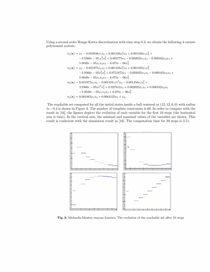
Using a second order Runge Kutta discretization with time step 0.3, we obtain the following 4-variatepolynomial system:

π1(x) = x1 − 0.053838x1x2 + 0.001458x21x2 + 0.001458x1x

22 +

−3.9366e− 05.x21x

22 + 0.005775x3 − 0.002025x1x3 − 0.000162x2x3 +

5.9049e− 05x1x2x3 − 6.075e− 06x23

π2(x) = x2 − 0.051975x1x2 + 0.001458x21x2 + 0.001458x1x

22

−3.9366e− 05x21x

22 + 0.0721875x3 − 0.002025x1x3 − 0.000162x2x3 +

5.9049e− 05x1x2x3 − 6.075e− 06x23

π3(x) = 0.051975x1x2 − 0.001458.x12x2 − 0.001458x1x22 +

3.9366e− 05x12x22 + 0.927812x3 + 0.002025x1x3 + 0.000162x2x3

−5.9049e− 05x1x2x3 + 6.075e− 06x23

π4(x) = 0.001863x1x2 + 0.0664125x3 + x4.

The reachable set computed for all the initial states inside a ball centered at (12, 12, 0, 0) with radius1e−0.4 is shown in Figure 3. The number of template constraints is 60. In order to compare with theresult in [16], the figures depicts the evolution of each variable for the first 10 steps (the horizontalaxis is time). In the vertical axis, the minimal and maximal values of the variables are shown. Thisresult is conherent with the simulation result in [16]. The computation time for 20 steps is 3.7s.

Fig. 3. Michaelis-Menten enzyme kinetics. The evolution of the reachable set after 10 steps

6.3 Randomly generated systems

In order to evaluate the performance of our method, we tested it on a number of randomly generatedpolynomials in various dimensions and maximal degrees (the maximal degree is the largest degreefor all variables). For a fixed dimension and degree, we generated different examples to estimate anaverage computation time. In the current implementation, polynomial composition is done symbol-ically, and we do not yet exploit the possibility of sparsity of polynomials (in terms of the numberof monomials). The computation time shown in the table in Figure 4 does not include the time forpolynomial composition. Note that the computation time for 7-variate polynomials of degree 3 issignificant, because the generated polynomials have a large number of monomials; however, practicalsystems often have a much smaller number of monomials.

As expected, the computation time grows linearly w.r.t. the number of steps. This can be explainedby the use of template polyhedra where the number of constraints can be chosen according to requiredprecisions and thus control better the complexity of the polyhedral operations, compared to generalconvex polyhedra. Indeed, when using general polyhedra, the operations such as convex hull mayincrease their geometric complexity (roughly described by the number of vertices and constraints).

7 Conclusion

In this paper we propose a new method to compute images of polynomials. This method combinesthe ideas from optimization and the Bernstein expansion. This result can be readily applicable tosolve the reachability analysis problem for hybrid systems with polynomial continuous dynamics.

The performance of the method was demonstrated using a number of randomly generated examples,which shows an improvement in efficiency compared to our previously developed method using Beziertechniques [7]. These encouraging results also show an important advantage of the method: thanksto the use of template polyhedra, the complexity and precision of the method are more controllablethan those using polyhedra as symbolic set representations.

There are a number interesting directions to explore. Indeed, different tools from geometric model-ing could be exploited to improve the efficiency of the method. For example, polynomial compositioncan be done for sparse polynomials more efficiently using the blossoming technique [25]. In additionto more experimentation on other hybris systems case studies, we intend to explore a new applicationdomain, which is verification of embedded control software. In fact, multivariate polynomials arise inmany situations when analyzing programs that are automatically generated from practical embeddedcontrollers.

References

1. R. Alur, C. Courcoubetis, N. Halbwachs, T.A. Henzinger, P.-H. Ho, X. Nicollin, A. Olivero, J. Sifakis,and S. Yovine. The algorithmic analysis of hybrid systems. Theoretical Computer Science, 138:3–34,1995.

2. E. Asarin, T. Dang, and A. Girard. Hybridization methods for the analysis of nonlinear systems. ActaInformatica., 43(7):451–476, 2007.

3. S. Boyd and S. Vandenberghe. Convex optimization. Cambridge University Press, 2004.4. L. Chen, A. Mine, and P. Cousot. A sound floating-point polyhedra abstract domain. In Proc. of the

Sixth Asian Symposium on Programming Languages and Systems (APLAS’08), volume 5356 of LNCS,pages 3–18, Bangalore, India, December 2008. Springer.

Fig. 4. Computation time for randomly generated polynomial systems in various dimensions and degrees

5. F. Clauss and I.Yu. Chupaeva. Application of symbolic approach to the bernstein expansion for programanalysis and optimization. Program. Comput. Softw., 30(3):164–172, 2004.

6. P. Cousot and R. Cousot. Static determination of dynamic properties of programs. In Proceedings of theSecond International Symposium on Programming, Dunod, Paris, pages 106–130, 1976.

7. T. Dang. Approximate reachability computation for polynomial systems. In HSCC, pages 138–152, 2006.8. T. Dang and D. Salinas. Computing set images of polynomias. Technical report, VERIMAG, June 2008.9. I.A. Fotiou, P. Rostalski, P.A. Parrilo, and M. Morari. Parametric optimization and optimal control

using algebraic geometriy methods. International Journal of Control, 79(11):1340–1358, 2006.10. J. Garloff. Application of bernstein expansion to the solution of control problems. In University of

Girona, pages 421–430, 1999.11. J. Garloff, C. Jansson, and A.P. Smith. Lower bound functions for polynomials. Journal of Computational

and Applied Mathematics, 157:207–225, 2003.12. J. Garloff and A.P. Smith. An improved method for the computation of affine lower bound functions for

polynomials. In C. A. Floudas and P. M. Pardalos, editors, Frontiers in Global Optimization, Series Non-convex Optimization and Its Applications, pages 135–144. Kluwer Academic Publ.,Boston, Dordrecht,New York, London, 2004.

13. J. Garloff and A.P. Smith. A comparison of methods for the computation of affine lower bound functionsfor polynomials. In C. Jermann, A. Neumaier, and D. Sam, editors, Global Optimization and ConstraintSatisfaction, LNCS, pages 71–85. Springer, 2005.

14. A. Girard. Reachability of uncertain linear systems using zonotopes. In HSCC, pages 291–305, 2005.15. S. Gottschalk, M. C. Lin, and D. Manocha. Obb-tree: A hierarchical structure for rapid interference

detection. In Computer Graphics SIGGRAPH ’96, pages 171–180, 1996.16. F. He, L. F. Yeung, and M. Brown. Discrete-time model representation for biochemicql pathway systems.

IAENG International Journal of Computer Science, 34(1), 2007.17. D. Henrion and J.B. Lasserre. Gloptipoly: Global optimization over polynomials with matlab and sedumi.

In Proceedings of the IEEE Conference on Decision and Control, 2002.18. I. T. Jolliffe. Principal Component Analysis. Springer, 2002.19. D.W. Jordan and P. Smith. Nonlinear Ordinary Differential Equations. Oxford Applied Mathematics

and Computer Science. Oxford University Press, 1987.20. A. Mine. A new numerical abstract domain based on difference-bound matrices. In PADO II, LNCS

2053, pages 155–172. Springer, 2001.21. B. Mourrain and J. P. Pavone. Subdivision methods for solving polynomial equations. Technical report,

INRIA Research report, 5658, August 2005.22. Stephen Prajna and Ali Jadbabaie. Safety verification of hybrid systems using barrier certificates. In

Rajeev Alur and George J. Pappas, editors, Hybrid Systems: Computation and Control, volume 2993 ofLecture Notes in Computer Science, pages 477–492. Springer, 2004.

23. S. Sankaranarayanan, H. Sipma, and Z. Manna. Scalable analysis of linear systems using mathematicalprogramming. In Verification, Model-Checking and Abstract-Interpretation (VMCAI 2005), LNCS 3385.Springer, 2005.

24. Sriram Sankaranarayanan. Mathematical analysis of programs. Technical report, Standford, 2005. PhDthesis.

25. H.-P. Seidel. Polar forms and triangular B-spline surfaces. In Blossoming: The New Polar-Form Approachto Spline Curves and Surfaces, SIGGRAPH ’91 Course Notes 26, ACM SIGGRAPH, pages 8.1–8.52,1991.

26. I. Tchoupaeva. A symbolic approach to bernstein expansion for program analysis and optimization. InIn 13th International Conference on Compiler Construction, CC 2004, pages 120–133. Springer, 2004.

27. Ashish Tiwari and Gaurav Khanna. Nonlinear systems: Approximating reach sets. In Hybrid Systems:Computation and Control, volume 2993 of Lecture Notes in Computer Science, pages 600–614. Springer,2004.

28. S. Vandenberghe and S. Boyd. Semidefinite programming. SIAM Review, 38(1):49–95, 1996.

A Computing affine bound functions using the Bernstein expansion

We describe the algorithm for computing these functions published in [12]. Let us consider a poly-nomial πk(x), which is the kth component of π(x) and for simplicity we denote it simply by p(x).The Bernstein coefficient of p is denoted by the scalars bi. We shall compute an affine lower boundfunction denoted by l(x).

– Iteration 1.• Define the direction u1 = (1, 0, . . . , 0).• Compute the slopes from each bi to b0 in the direction u1:

∀i ∈ Id : i[1] 6= i0[1], g1i =

bi − b0

i[1]/d[1]− i0[1]/d[1]

• Let i1 be the multi-index with the smallest absolute value of g1i . Define the lower bound

function:l1(x) = b0 + g1

i1u1(x− i0/d).

– Iteration j = 2, . . . , n.• Compute the direction uj = (β1, . . . , βj−1, 0, . . . , 0) such that uj ik−i0

d = 0 for all k =1, . . . , j − 1. This requires solving a system of j − 1 linear equations with j − 1 unknownvariables. Then normalize uj = uj/||uj ||.

• Compute the slopes from each bi to b0 in the direction uj :

∀i ∈ Id :i[1]− i0[1]

duj 6= 0, gji =

bi − lj−1(i/d)(i/d− i0/d)uj

• Let ij be the multiindex with the smallest absolute value of gji . Define the lower boundfunction:

lj(x) = lj−1(x) + gjij uj(x− i0/d).