Approximation of function and its derivatives using radial basis function networks
24
Approximation of function and its derivatives using radial basis function networks Nam Mai-Duy, Thanh Tran-Cong * Faculty of Engineering and Surveying, University of Southern Queensland, Toowoomba, QLD 4350, Australia Received 8 January 2001; accepted 5 September 2002 Abstract This paper presents a numerical approach, based on radial basis function networks (RBFNs), for the approximation of a function and its derivatives (scattered data interpolation). The approach proposed here is called the indirect radial basis function network (IRBFN) approximation which is compared with the usual direct approach. In the direct method (DRBFN) the closed form RBFN approximating function is first obtained from a set of training points and the derivative functions are then calculated directly by differentiating such closed form RBFN. In the indirect method (IRBFN) the formulation of the problem starts with the decomposition of the derivative of the function into RBFs. The derivative expression is then integrated to yield an expression for the original function, which is then solved via the general linear least squares principle, given an appropriate set of discrete data points. The IRBFN method allows the filtering of noise arisen from the interpolation of the original function from a discrete set of data points and pro- duces a greatly improved approximation of its derivatives. In both cases the input data consists of a set of unstructured discrete data points (function values), which eliminates the need for a discretisation of the domain into a number of finite elements. The results obtained are compared with those obtained by the feed forward neural network approach where appropriate and the ‘‘finite element’’ methods. In all examples considered, the IRBFN approach yields a superior accuracy. For example, all partial derivatives up to second order of the function of three variables y ¼ x 2 1 þ x 1 x 2 2x 2 2 x 2 x 3 þ x 2 3 are approximated with at least an order of magnitude better in the L 2 -norm in comparison with the usual DRBFN approach. Ó 2002 Elsevier Science Inc. All rights reserved. Keywords: Radial basis function networks; Function approximation; Derivative approximation; Scattered data interpolation; Global approximation * Corresponding author. Tel.: +61-7-4631-2539; fax: +61-7-4631-2526. E-mail address: [email protected] (T. Tran-Cong). 0307-904X/02/$ - see front matter Ó 2002 Elsevier Science Inc. All rights reserved. PII:S0307-904X(02)00101-4 Applied Mathematical Modelling 27 (2003) 197–220 www.elsevier.com/locate/apm
-
Upload
independent -
Category
Documents
-
view
1 -
download
0
Transcript of Approximation of function and its derivatives using radial basis function networks

Approximation of function and its derivatives usingradial basis function networks
Nam Mai-Duy, Thanh Tran-Cong *
Faculty of Engineering and Surveying, University of Southern Queensland, Toowoomba, QLD 4350, Australia
Received 8 January 2001; accepted 5 September 2002
Abstract
This paper presents a numerical approach, based on radial basis function networks (RBFNs), for the
approximation of a function and its derivatives (scattered data interpolation). The approach proposed here
is called the indirect radial basis function network (IRBFN) approximation which is compared with the
usual direct approach. In the direct method (DRBFN) the closed form RBFN approximating function is
first obtained from a set of training points and the derivative functions are then calculated directly bydifferentiating such closed form RBFN. In the indirect method (IRBFN) the formulation of the problem
starts with the decomposition of the derivative of the function into RBFs. The derivative expression is then
integrated to yield an expression for the original function, which is then solved via the general linear least
squares principle, given an appropriate set of discrete data points. The IRBFN method allows the filtering
of noise arisen from the interpolation of the original function from a discrete set of data points and pro-
duces a greatly improved approximation of its derivatives. In both cases the input data consists of a set of
unstructured discrete data points (function values), which eliminates the need for a discretisation of the
domain into a number of finite elements. The results obtained are compared with those obtained by the feedforward neural network approach where appropriate and the ‘‘finite element’’ methods. In all examples
considered, the IRBFN approach yields a superior accuracy. For example, all partial derivatives up to
second order of the function of three variables y ¼ x21 þ x1x2 � 2x22 � x2x3 þ x23 are approximated with at
least an order of magnitude better in the L2-norm in comparison with the usual DRBFN approach.
� 2002 Elsevier Science Inc. All rights reserved.
Keywords: Radial basis function networks; Function approximation; Derivative approximation; Scattered data
interpolation; Global approximation
*Corresponding author. Tel.: +61-7-4631-2539; fax: +61-7-4631-2526.
E-mail address: [email protected] (T. Tran-Cong).
0307-904X/02/$ - see front matter � 2002 Elsevier Science Inc. All rights reserved.
PII: S0307-904X(02)00101-4
Applied Mathematical Modelling 27 (2003) 197–220
www.elsevier.com/locate/apm

1. Introduction
Numerical methods for differentiation are of significant interest and importance in the study ofnumerical solutions of many problems in engineering and science. For example, the approximationof derivatives is needed either to convert the relevant governing equations into a discrete form or tonumerically estimate various terms from a set of discrete or scattered data. This is commonlyachieved by discretising the domain of analysis into a number of elements which are defined by asmall number of nodes. The interpolation of a function and its derivatives over such an elementfrom the nodal values can then be achieved analytically via the chosen shape functions. Examplesof elements include finite elements (FE) and boundary elements (BE) associated with the finiteelement method (FEM) (e.g. [1]) and the boundary element method (BEM) (e.g. [2]). Element-based methods are referred to as conventional methods in this paper. Common shape functions forone, two and three-dimensional elements can be found in most texts on FEM and BEM (e.g. [1,2]).However, the element technique requires mesh generation which is time consuming and thereforeaccounts for a high proportion of the analysis cost, especially for problems with moving or un-known boundaries. For practical analysis, automatic discretisation or meshing is a highly desirablefeature but rarely available in general. Thus there are great interests in element-free numericalmethods in both engineering and scientific communities. In particular, neural networks have beendeveloped and become one of the main fields of research in numerical analysis. Radial basisfunction networks (RBFNs) [3–11] can be used for a wide range of applications primarily because itcan approximate any regular function [6,7,10] and its training is faster than that of a multilayerperceptron when the RBFN combines self-organised and supervised learning [11]. The design of anRBFN is considered as a curve-fitting (approximation) problem in a high-dimensional space.Correspondingly, the generalization of the approach is equivalent to the use of a multidimensionalsurface to interpolate the test data [9]. The networks just need an unstructured distribution ofcollocation points throughout a volume for the approximation and hence the need for discreti-sation of the volume of the analysis domain is eliminated. In this paper new approximationmethods based on RBFNs are reported. The primary aim of the presented methods is theachievement of a more accurate approximation of a target function�s derivatives. From the resultsobtained here it is suggested that the present indirect radial basis function network (IRBFN)approach could be, in addition to its ability to approximate scattered data, a potential candi-date for future development of element-free methods for engineering modelling and analyses. Thepaper is organized as follows. In Section 2, the problem is defined. A brief review of RBFNs is givenin Section 3 and then, in Sections 4 and 5, a direct RBFN (DRBFN) and an IRBFNmethod for theapproximation of a function and its derivatives are discussed. The DRBFN method is includedto provide the basis for the assessment of the presently proposed IRBFN approach. Both meth-ods are illustrated with the aid of three numerical examples of function of one, two and threevariables in Section 6. Section 7 concludes the paper.
2. Description of problem
The problem considered in this paper is described as follows (superscripts are used to indexelements of a set of neurons and subscripts denote scalar components of a p-dimensional vector):
198 N. Mai-Duy, T. Tran-Cong / Appl. Math. Modelling 27 (2003) 197–220

• Given a set of data points whose elements consist of paired values of the independent variables(a vector x) and the dependent variable (a scalar y), denoted by fxðiÞ; yðiÞgni¼1 where n is the num-ber of input points and x ¼ ½x1; x2; . . . ; xpT where p is the number of dimensions and the super-script T denotes the transpose operation,
• find a closed form approximate function f of the dependent variable y and its closed form ap-proximate derivative functions.
3. Function approximation by RBFNs
An RBFN represents a map from the p-dimensional input space to the one-dimensional outputspace f : Rp ! R1 that consists of a set of weights fwðiÞgmi¼1, and a set of radial basis functionsfgðiÞgmi¼1 where m6 n. There is a large class of radial basis functions which can be written in ageneral form gðiÞðxÞ ¼ /ðiÞðkx� cðiÞkÞ, where k � k denotes the Euclidean norm and fcðiÞgmi¼1 is a setof the centers that can be chosen from among the data points. The following are some commontypes of radial basis functions that are of particular interest in the study of RBFNs [9]:
1. multiquadrics
/ðiÞðrÞ ¼ /ðiÞðkx� cðiÞkÞ ¼ffiffiffiffiffiffiffiffiffiffiffiffiffiffiffiffiffiffir2 þ aðiÞ2
pfor some aðiÞ > 0; ð1Þ
2. inverse multiquadrics
/ðiÞðrÞ ¼ /ðiÞðkx� cðiÞkÞ ¼ 1ffiffiffiffiffiffiffiffiffiffiffiffiffiffiffiffiffiffir2 þ aðiÞ2
p for some aðiÞ > 0; ð2Þ
3. Gaussians
/ðiÞðrÞ ¼ /ðiÞðkx� cðiÞkÞ ¼ exp
�� r2
aðiÞ2
�for some aðiÞ > 0; ð3Þ
where aðiÞ is usually referred to as the width of the ith basis function and r ¼ kx� cðiÞk ¼ffiffiffiffiffiffiffiffiffiffiffiffiffiffiffiffiffiffiffiffiffiffiffiffiffiffiffiffiffiffiffiffiffiffiffiffiffiffiffiffiðx� cðiÞÞ � ðx� cðiÞÞ
p.
The inverse multiquadrics (2) and Gaussians function (3) have a local response, i.e. they de-crease monotonically with increasing distance from the center (localized function). In contrast, themultiquadrics (1) increases with increasing distance from the center and therefore exhibits a globalresponse (non-localized function). An important property of the RBFN is that it is a linearlyweighted network in the sense that the output is a linear combination of m radial basis functionswritten as
f ðxÞ ¼Xmi¼1
wðiÞgðiÞðxÞ: ð4Þ
With the model f constructed as a linear combination of m fixed functions in a given family, theproblem is to find the unknown weights fwðiÞgmi¼1. For this purpose, the general least squaresprinciple is used to minimise the sum squared error
SSE ¼Xn
i¼1
½yðiÞ � f ðxðiÞÞ2; ð5Þ
N. Mai-Duy, T. Tran-Cong / Appl. Math. Modelling 27 (2003) 197–220 199
with respect to the weights of f , resulting in a set of m simultaneous linear algebraic equations(normal equations) in the m unknown weights
ðGTGÞw ¼ GTy; ð6Þwhere
G ¼
gð1Þðxð1ÞÞ gð2Þðxð1ÞÞ � � � gðmÞðxð1ÞÞgð1Þðxð2ÞÞ gð2Þðxð2ÞÞ � � � gðmÞðxð2ÞÞ
..
. ... . .
. ...
gð1ÞðxðnÞÞ gð2ÞðxðnÞÞ � � � gðmÞðxðnÞÞ
2666437775;
w ¼ ½wð1Þ;wð2Þ; . . . ;wðmÞT;
y ¼ ½yð1Þ; yð2Þ; . . . ; yðnÞT:However, in the special case where n ¼ m, the resultant system is just
Gw ¼ y: ð7Þ
4. Function derivatives by direct RBFN method
In an arbitrary RBFN where the basis functions are fixed and the weights are adaptable, thederivative of the function computed by the network is also a linear combination of fixed functions(the derivatives of the radial basis functions). The partial derivatives of the approximate functionf ðxÞ (4) can be calculated as follows
okfoxj � � � oxl
¼ f;j...lðxÞ ¼Xmi¼1
wðiÞ okgðiÞ
oxj � � � oxl; ð8Þ
where ðokgðiÞÞ=ðoxj � � � oxlÞ is the corresponding basis function for the derivative function f;j...lðxÞ,which is obtained by differentiating the original basis function gðiÞðxÞ which is continuously dif-ferentiable. For example, considering the first order derivative of function f ðxÞ with respect to xj,denoted by f;j, the corresponding basis functions are found analytically as follows:
1. for multiquadrics
hðiÞðxÞ ¼ ogðiÞ
oxj¼
xj � cðiÞjðr2 þ aðiÞ2Þ0:5
; ð9Þ
2. for inverse multiquadrics
hðiÞðxÞ ¼ ogðiÞ
oxj¼ �
xj � cðiÞjðr2 þ aðiÞ2Þ1:5
; ð10Þ
3. for Gaussians
hðiÞðxÞ ¼ ogðiÞ
oxj¼
�2ðxj � cðiÞj ÞaðiÞ2
exp
�� r2
aðiÞ2
�: ð11Þ
200 N. Mai-Duy, T. Tran-Cong / Appl. Math. Modelling 27 (2003) 197–220

Considering the second order derivative of function f ðxÞ with respect to xj, denoted by f;jj, thecorresponding basis functions will be
1. for multiquadrics
�hhðiÞðxÞ ¼ ohðiÞ
oxj¼
r2 þ aðiÞ2 � ðxj � cðiÞj Þ2
ðr2 þ aðiÞ2Þ1:5; ð12Þ
2. for inverse multiquadrics
�hhðiÞðxÞ ¼ ohðiÞ
oxj¼
3ðxj � cðiÞj Þ2
ðr2 þ aðiÞ2Þ2:5� 1
ðr2 þ aðiÞ2Þ1:5; ð13Þ
3. for Gaussians
�hhðiÞðxÞ ¼ ohðiÞ
oxj¼ 2
aðiÞ22
aðiÞ2ðxj
�� cðiÞj Þ2 � 1
exp
�� r2
aðiÞ2
�: ð14Þ
Similarly, the basis functions for f;kj are as follows:
1. for multiquadrics
�hhðiÞðxÞ ¼ ohðiÞ
oxk¼ �
ðxj � cðiÞj Þðxk � cðiÞk Þðr2 þ aðiÞ2Þ1:5
; ð15Þ
2. for inverse multiquadrics
�hhðiÞðxÞ ¼ ohðiÞ
oxk¼
3ðxj � cðiÞj Þðxk � cðiÞk Þðr2 þ aðiÞ2Þ2:5
; ð16Þ
3. for Gaussians
�hhðiÞðxÞ ¼ ohðiÞ
oxk¼
4ðxj � cðiÞj Þðxk � cðiÞk ÞaðiÞ4
exp
�� r2
aðiÞ2
�: ð17Þ
Once f ðxÞ is determined by solving (6) or (7) for the unknown weights, which is referred to asnetwork training, it is straightforward and economical to compute its derivatives according to (8).However, this direct method has some drawbacks that are illustrated in the following example.
4.1. Example to illustrate the drawbacks of the DRBFN method
The function
yðxÞ ¼ x3 þ xþ 0:5; �36 x6 2;
is sampled at 50 uniformly spaced training points as depicted in Fig. 1. Parameters to be decidedbefore the start of network training are the number of centers m, their locations fcðiÞgmi¼1 and aset of the corresponding widths faðiÞgmi¼1. The ideal data points used here are not corruptedby noise. According to Cover�s Theorem [9], the more basis functions are used, the better the
N. Mai-Duy, T. Tran-Cong / Appl. Math. Modelling 27 (2003) 197–220 201
approximation will be and so all data points will be taken to be the centers of the network ðm ¼ nÞin this study. Thus fcðiÞ ¼ xðiÞgni¼1. The width of the ith basis function is determined according tothe following relation [11]
aðiÞ ¼ bdðiÞ; ð18Þwhere b is a factor, b > 0, and dðiÞ is the distance from the ith center to the nearest neighbouringcenter. As a measure of the accuracy of different approximate schemes, a norm of the error of thesolution, Ne, is defined as
Ne ¼ffiffiffiffiffiffiffiffiffiffiffiffiffiffiffiffiffiffiffiffiffiffiffiffiffiffiffiffiffiffiffiXnti¼1
ðyðiÞ � f ðiÞÞ2s
; ð19Þ
where f ðiÞ and yðiÞ are the calculated and exact function values at the point i, and nt is the totalnumber of test nodes. Smaller Nes indicate more accurate approximations.
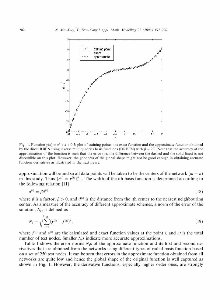
Table 1 shows the error norms Nes of the approximate function and its first and second de-rivatives that are obtained from the networks using different types of radial basis function basedon a set of 250 test nodes. It can be seen that errors in the approximate function obtained from allnetworks are quite low and hence the global shape of the original function is well captured asshown in Fig. 1. However, the derivative functions, especially higher order ones, are strongly
Fig. 1. Function yðxÞ ¼ x3 þ xþ 0:5: plot of training points, the exact function and the approximate function obtained
by the direct RBFN using inverse multiquadrics basis functions (DRBFN) with b ¼ 2:0. Note that the accuracy of the
approximation of the function is such that the error (i.e. the difference between the dashed and the solid lines) is not
discernible on this plot. However, the goodness of the global shape might not be good enough in obtaining accurate
function derivatives as illustrated in the next figure.
202 N. Mai-Duy, T. Tran-Cong / Appl. Math. Modelling 27 (2003) 197–220
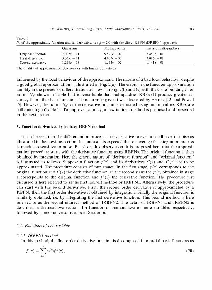
influenced by the local behaviour of the approximant. The nature of a bad local behaviour despitea good global approximation is illustrated in Fig. 2(a). The errors in the function approximationamplify in the process of differentiation as shown in Fig. 2(b) and (c) with the corresponding errornorms Nes shown in Table 1. It is remarkable that multiquadrics RBFs (1) produce greater ac-curacy than other basis functions. This surprising result was discussed by Franke [12] and Powell[5]. However, the norms Nes of the derivative functions estimated using multiquadrics RBFs arestill quite high (Table 1). To improve accuracy, a new indirect method is proposed and presentedin the next section.
5. Function derivatives by indirect RBFN method
It can be seen that the differentiation process is very sensitive to even a small level of noise asillustrated in the previous section. In contrast it is expected that on average the integration processis much less sensitive to noise. Based on this observation, it is proposed here that the approxi-mation procedure starts with the derivative function using RBFNs. The original function is thenobtained by integration. Here the generic nature of ‘‘derivative function’’ and ‘‘original function’’is illustrated as follows. Suppose a function f ðxÞ and its derivatives f 0ðxÞ and f 00ðxÞ are to beapproximated. The procedure consists of two stages. In the first stage, f ðxÞ corresponds to theoriginal function and f 0ðxÞ the derivative function. In the second stage the f 0ðxÞ obtained in stage1 corresponds to the original function and f 00ðxÞ the derivative function. The procedure justdiscussed is here referred to as the first indirect method or IRBFN1. Alternatively, the procedurecan start with the second derivative. First, the second order derivative is approximated by aRBFN, then the first order derivative is obtained by integration. Finally the original function issimilarly obtained, i.e. by integrating the first derivative function. This second method is herereferred to as the second indirect method or IRBFN2. The detail of IRBFN1 and IRBFN2 isdescribed in the next two sections for function of one and two or more variables respectively,followed by some numerical results in Section 6.
5.1. Functions of one variable
5.1.1. IRBFN1 method
In this method, the first order derivative function is decomposed into radial basis functions as
f 0ðxÞ ¼Xmi¼1
wðiÞgðiÞðxÞ; ð20Þ
Table 1
Ne of the approximate function and its derivatives for b ¼ 2:0 with the direct RBFN (DRBFN) approach
Gaussians Multiquadrics Inverse multiquadrics
Original function 7:002e� 01 9:570e� 02 7:459e� 01
First derivative 3:035eþ 01 4:053eþ 00 3:086eþ 01
Second derivative 1:214eþ 03 1:564eþ 02 1:141eþ 03
The quality of approximation deteriorates with higher derivatives.
N. Mai-Duy, T. Tran-Cong / Appl. Math. Modelling 27 (2003) 197–220 203

Fig. 2. Function yðxÞ ¼ x3 þ xþ 0:5: zoom in on the original, first derivative and second derivative functions ðb ¼ 2:0Þ.Solid line: exact function and dashed line: DRBFN approximation using inverse multiquadrics. The plots illustrate the
shortcomings of the DRBFN approach where the associated error norms are 7:459e� 1, 3:086eþ 1 and 1:141eþ 3 for
the approximation of the function, its first derivative and second derivative respectively.
204 N. Mai-Duy, T. Tran-Cong / Appl. Math. Modelling 27 (2003) 197–220

where fgðiÞðxÞgmi¼1 is a set of radial basis functions and fwðiÞgmi¼1 is the set of corresponding weights.With this approximation, the original function can be calculated as
f ðxÞ ¼Z
f 0ðxÞdx ¼Z Xm
i¼1
wðiÞgðiÞðxÞdx ¼Xmi¼1
wðiÞZ
gðiÞðxÞdx ¼Xmi¼1
wðiÞH ðiÞðxÞ þ C1; ð21Þ
where C1 is the constant of integration and fH ðiÞðxÞgmi¼1 is the set of corresponding basis functionsfor the original function with H ðiÞðxÞ ¼
RgðiÞðxÞdx. The radial basis functions fgðiÞgmi¼1 are con-
tinuously integrable, but only two basis functions fH ðiÞðxÞgmi¼1 corresponding to the multiquadric(1) and the inverse multiquadric (2) are able to be obtained analytically here. This paper focuseson the use of these two RBFs in the indirect method. The corresponding basis functions are:
1. for multiquadrics
H ðiÞðxÞ ¼ðx� cðiÞÞ
ffiffiffiffiffiffiffiffiffiffiffiffiffiffiffiffiffiffiffiffiffiffiffiffiffiffiffiffiffiffiffiffiffiðx� cðiÞÞ2 þ aðiÞ2
q2
þ aðiÞ2
2ln ðx�
� cðiÞÞ þffiffiffiffiffiffiffiffiffiffiffiffiffiffiffiffiffiffiffiffiffiffiffiffiffiffiffiffiffiffiffiffiffiðx� cðiÞÞ2 þ aðiÞ2
q �; ð22Þ
2. for inverse multiquadrics
H ðiÞðxÞ ¼ ln ðx�
� cðiÞÞ þffiffiffiffiffiffiffiffiffiffiffiffiffiffiffiffiffiffiffiffiffiffiffiffiffiffiffiffiffiffiffiffiffiðx� cðiÞÞ2 þ aðiÞ2
q �: ð23Þ
The training to determine the weights in (20) and (21) is equivalent to a minimisation of thefollowing sum squared error
SSE ¼Xn
i¼1
½yðiÞ � f ðxðiÞÞ2: ð24Þ
Eq. (21) is used in Eq. (24) in the minimisation procedure, which results in a system of equationsin terms of the unknown weights wðiÞ. The data used in training the network for the derivative andoriginal functions just consists of a set of discrete values fyðiÞgni¼1 of the dependent variable y andthe closed form of the derivative function (20). The minimisation of (24) can be achieved bysolving the corresponding normal equations [13]. However in practice the normal equationsmethod of solution can produce less than optimum solution, i.e. the norm of the solution (in theleast square sense) is not the smallest. Fortunately, singular value decomposition (SVD) method[13] can overcome this difficulty and will be used to solve (24) for the unknown weights and theconstant of integration in the remainder of this paper. The SVD method provides a solutionwhose norm is the smallest in the least-squares sense, i.e. any combination of basis functionsirrelevant to the fit is driven down to a small value. After solving (24), a set of the weights isobtained and used for approximating the derivative function via (20) and together with theconstant C1 for estimating the original function via (21). The example in Section 4.1 is recon-sidered here using the IRBFN1 method. The Nes over a set of 250 test nodes are decreasedconsiderably as shown in Tables 2–4. There is a significant improvement in the results obtained bythe IRBFN1 over those obtained by the DRBFN not only for the derivative functions but also forthe original function. The improvement factor is defined as follows
N. Mai-Duy, T. Tran-Cong / Appl. Math. Modelling 27 (2003) 197–220 205
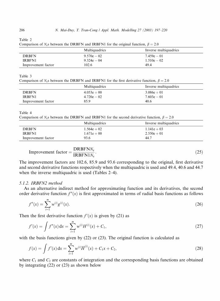
Improvement factor ¼ DRBFNNe
IRBFN1Ne
: ð25Þ
The improvement factors are 102.6, 85.9 and 93.6 corresponding to the original, first derivativeand second derivative functions respectively when the multiquadric is used and 49.4, 40.6 and 44.7when the inverse multiquadric is used (Tables 2–4).
5.1.2. IRBFN2 method
As an alternative indirect method for approximating function and its derivatives, the secondorder derivative function f 00ðxÞ is first approximated in terms of radial basis functions as follows
f 00ðxÞ ¼Xmi¼1
wðiÞgðiÞðxÞ: ð26Þ
Then the first derivative function f 0ðxÞ is given by (21) as
f 0ðxÞ ¼Z
f 00ðxÞdx ¼Xmi¼1
wðiÞH ðiÞðxÞ þ C1; ð27Þ
with the basis functions given by (22) or (23). The original function is calculated as
f ðxÞ ¼Z
f 0ðxÞdx ¼Xmi¼1
wðiÞHðiÞðxÞ þ C1xþ C2; ð28Þ
where C1 and C2 are constants of integration and the corresponding basis functions are obtainedby integrating (22) or (23) as shown below
Table 2
Comparison of Nes between the DRBFN and IRBFN1 for the original function, b ¼ 2:0
Multiquadrics Inverse multiquadrics
DRBFN 9:570e� 02 7:459e� 01
IRBFN1 9:324e� 04 1:510e� 02
Improvement factor 102.6 49.4
Table 3
Comparison of Nes between the DRBFN and IRBFN1 for the first derivative function, b ¼ 2:0
Multiquadrics Inverse multiquadrics
DRBFN 4:053eþ 00 3:086eþ 01
IRBFN1 4:720e� 02 7:603e� 01
Improvement factor 85.9 40.6
Table 4
Comparison of Nes between the DRBFN and IRBFN1 for the second derivative function, b ¼ 2:0
Multiquadrics Inverse multiquadrics
DRBFN 1:564eþ 02 1:141eþ 03
IRBFN1 1:671eþ 00 2:550eþ 01
Improvement factor 93.6 44.7
206 N. Mai-Duy, T. Tran-Cong / Appl. Math. Modelling 27 (2003) 197–220

1. for multiquadrics
HðiÞðxÞ ¼
ZH ðiÞðxÞdx
¼ ððx� cðiÞÞ2 þ aðiÞ2Þ1:5
6þ aðiÞ2
2ðx� cðiÞÞ ln ðx
�� cðiÞÞ þ
ffiffiffiffiffiffiffiffiffiffiffiffiffiffiffiffiffiffiffiffiffiffiffiffiffiffiffiffiffiffiffiffiffiðx� cðiÞÞ2 þ aðiÞ2
q �� aðiÞ2
2
ffiffiffiffiffiffiffiffiffiffiffiffiffiffiffiffiffiffiffiffiffiffiffiffiffiffiffiffiffiffiffiffiffiðx� cðiÞÞ2 þ aðiÞ2
q; ð29Þ
2. for inverse multiquadrics
HðiÞðxÞ ¼
ZH ðiÞðxÞdx
¼ ðx� cðiÞÞ ln�ðx� cðiÞÞ þ
ffiffiffiffiffiffiffiffiffiffiffiffiffiffiffiffiffiffiffiffiffiffiffiffiffiffiffiffiffiffiffiffiffiðx� cðiÞÞ2 þ aðiÞ2
q ��
ffiffiffiffiffiffiffiffiffiffiffiffiffiffiffiffiffiffiffiffiffiffiffiffiffiffiffiffiffiffiffiffiffiðx� cðiÞÞ2 þ aðiÞ2
q: ð30Þ
In the present IRBFN2 method, the improvement factors have increased (Tables 5 and 6) forboth the original function and its derivatives in comparison with the first indirect method IR-BFN1. It is remarkable here that the improvement in the case of multiquadrics is very significantfor all approximate functions (more than 16 times). Thus, the multiquadric function maintains itssuperior performance in terms of accuracy among the radial basis functions used in IRBFN2.
5.1.3. The role of ‘‘constants’’ of integration‘‘Constants’’ of integration in Eqs. (21) and (28) appear naturally in the present indirect for-
mulation. The structure of the approximant therefore looks like
f ðxÞ ¼Xmi¼1
wðiÞHðiÞðxÞ þ polynomial: ð31Þ
Table 6
Comparison of Nes between the two indirect methods using inverse multiquadrics for b ¼ 2:0
Original First derivative Second derivative
IRBFN1 1:510e� 02 7:603e� 01 2:550eþ 01
IRBFN2 2:200e� 03 9:760e� 02 4:073eþ 00
Improvement factor 6.9 7.8 6.3
Here the improvement factor is defined as the improvement of IRBFN2 relative to IRBFN1.
Table 5
Comparison of Nes between the two indirect methods using multiquadrics for b ¼ 2:0
Original First derivative Second derivative
IRBFN1 9:324e� 04 4:720e� 02 1:671eþ 00
IRBFN2 3:968e� 05 2:100e� 03 1:022e� 01
Improvement factor 23.5 22.5 16.3
Here the improvement factor is defined as the improvement of IRBFN2 relative to IRBFN1.
N. Mai-Duy, T. Tran-Cong / Appl. Math. Modelling 27 (2003) 197–220 207
As a result, if yðxÞ is flat or closer to a polynomial fit, the above structure (31) has the ability forbetter accuracy. This is in addition to the inherent smoothing of error in the process of inte-gration.
5.2. Functions of two or more variables
In this section the indirect methods discussed in Section 5.1 are extended to the case of func-tions of many variables. The case of functions of two variables is discussed in detail and theprocedure for functions of three or more variables can be similarly developed.
5.2.1. IRBFN1 method
Consider the approximation of a function of two variables f ðx1; x2Þ. In the IRBFN1 method,the first order partial derivative of f ðx1; x2Þ with respect to x1, denoted by f;1, is first approximatedin terms of radial basis functions
f;1ðx1; x2Þ ¼Xmi¼1
wðiÞgðiÞðx1; x2Þ; ð32Þ
where fgðiÞðx1; x2Þgmi¼1 is a set of radial basis functions and fwðiÞgmi¼1 is the set of correspondingweights.
The original function can be calculated as
f ðx1; x2Þ ¼Z
f;1ðx1; x2Þdx1 ¼Z Xm
i¼1
wðiÞgðiÞðx1; x2Þdx1 ¼Xmi¼1
wðiÞZ
gðiÞðx1; x2Þdx1
¼Xmi¼1
wðiÞH ðiÞðx1; x2Þ þ C1ðx2Þ; ð33Þ
where C1ðx2Þ is a function of the variable x2 and fH ðiÞðx1; x2Þgmi¼1 is the set of corresponding basisfunctions for the original function and given below
1. for multiquadrics
H ðiÞðx1; x2Þ ¼ðx1 � cðiÞ1 Þ
ffiffiffiffiffiffiffiffiffiffiffiffiffiffiffiffiffiffir2 þ aðiÞ2
p
2þ r2 � ðx1 � cðiÞ1 Þ2 þ aðiÞ2
2ln ðx1�
� cðiÞ1 Þ þffiffiffiffiffiffiffiffiffiffiffiffiffiffiffiffiffiffir2 þ aðiÞ2
p �;
ð34Þ
2. for inverse multiquadrics
H ðiÞðx1; x2Þ ¼ ln ðx1 � cðiÞ1 Þ þffiffiffiffiffiffiffiffiffiffiffiffiffiffiffiffiffiffir2 þ aðiÞ2
p� �: ð35Þ
The added term on the right hand side of (33) is a function of the variable x2 only. ThusC1ðx2Þ canbe interpolated using the IRBFN2 method for univariate functions as follows (in the previoussection, IRBFN2 is shown to be the better alternative among themethods investigated in this work).
208 N. Mai-Duy, T. Tran-Cong / Appl. Math. Modelling 27 (2003) 197–220

C001ðx2Þ ¼
XMi¼1
�wwðiÞgðiÞðx2Þ; ð36Þ
C01ðx2Þ ¼
XMi¼1
�wwðiÞH ðiÞðx2Þ þ bCC1; ð37Þ
C1ðx2Þ ¼XMi¼1
�wwðiÞHðiÞðx2Þ þ bCC1x2 þ bCC2; ð38Þ
where bCC1 and bCC2 are constants of integration; �wwðiÞ are the corresponding weights; and M is thenumber of centres whose x2 coordinates are distinct. Upon applying the general linear least squaresprinciple, a system of linear algebraic equations is obtained. The unknown of the system which isfound by the SVDmethod as mentioned earlier, consists of the set of weights in (32), the second setof weights in (36) and the constants of integration bCC1, bCC2. The strategy of approximation is thesame for the derivative function of f ðx1; x2Þ with respect to the variable x2 ðf;2ðx1; x2ÞÞ.
5.2.2. IRBFN2 method
In this method, the second order derivative functions are first approximated in terms of radialbasis functions. For example, in the case of f;11 the basis functions for the first derivative function,f;1, are given by (34) or (35) while for the original function f , the basis functions are obtained byintegrating (34) or (35) and shown below
1. for multiquadrics
HðiÞðx1; x2Þ ¼
ZH ðiÞðx1; x2Þdx1
¼ ðr2 þ aðiÞ2Þ1:5
6þ r2 � ðx1 � cðiÞ1 Þ2 þ aðiÞ2
2ðx1 � c1Þ ln
�ðx1 � cðiÞ1 Þ þ
ffiffiffiffiffiffiffiffiffiffiffiffiffiffiffiffiffiffir2 þ aðiÞ2
p �
�r2 � ðxj � cðiÞj Þ2 þ aðiÞ2
2
ffiffiffiffiffiffiffiffiffiffiffiffiffiffiffiffiffiffir2 þ aðiÞ2
p; ð39Þ
2. for inverse multiquadrics
HðiÞðx1; x2Þ ¼
ZH ðiÞðx1; x2Þdx1 ¼ ðx1 � c1Þ ln
�ðx1 � cðiÞ1 Þ þ
ffiffiffiffiffiffiffiffiffiffiffiffiffiffiffiffiffiffir2 þ aðiÞ2
p ��
ffiffiffiffiffiffiffiffiffiffiffiffiffiffiffiffiffiffir2 þ aðiÞ2
p: ð40Þ
The original function is calculated as
f ðx1; x2Þ ¼Xmi¼1
wðiÞHðiÞðx1; x2Þ þ C1ðx2Þx1 þ C2ðx2Þ; ð41Þ
where C1ðx2Þ and C2ðx2Þ are constants of integration which are interpolated in the same manner asshown by (36)–(38).
For the purpose of illustration, some numerical results are presented in the next section.
N. Mai-Duy, T. Tran-Cong / Appl. Math. Modelling 27 (2003) 197–220 209
6. Numerical results
In this section, examples of approximation of functions of one, two and three variables aregiven. As mentioned, the multiquadric function appears to be the better one in terms of accuracyamong the basis functions considered and will be used to solve the example problems. The factorb that influences the accuracy of the solution is just chosen to be 2.0 until now. In the followingexamples, for the purpose of investigation of its effect, b will take values over a wide range with anincrement of 0.2. From the numerical experiments discussed shortly, it appears that there is anupper limit for b above which the system of Eqs. (6) or (7) is ill-conditioned, which is also ob-served by Tarwater [14]. In the present work, the value of b is considered to reach an upper limitwhen the condition of the system matrix is Oð1017Þ, i.e. the estimate for the reciprocal of thecondition of the matrix in 1-norm using LINPACK condition estimator [15] is of Oð10�17Þ.
6.1. Example 1
Consider the following function of one variable
y ¼ 0:02ð12þ 3x� 3:5x2 þ 7:2x3Þð1þ cos 4pxÞð1þ 0:8 sin 3pxÞ;with 06 x6 1, a problem studied by Hashem and Schmeiser [16]. They reported a method, namelymean squared error-optimal linear combinations of trained feedforward neural networks (MSE-OLC), for an approximation of the function and its derivatives. The authors suggest that the usualapproach is to try a multiple of networks with possibly different structures and values for trainingparameters and the ‘‘best’’ network (based on some optimality criterion) is selected. Instead of theusual approach just described the authors investigated a new approach where a combination ofthe trained networks is constructed by forming the weighted sum of the corresponding outputs ofthe trained networks. The authors claim that their MSE-OLC method yields more accurate ap-proximations in comparison with the best trained feed forward neural network (FFNN). For thisproblem, with a set of 200 training nodes and 10,000 test nodes, the resultant MSEs for theoriginal, the first and second order derivative functions produced by MSE-OLC are 0.000017, 0.1and 133.3, respectively, which are 87.3%, 69.7% and 64.5%, respectively, less than the MSEsproduced by the best FFNN [16]. Here, both the direct and indirect RBFN methods are applied tosolve this problem using 200 training points and 10,000 test nodes, uniformly spaced along the x-axis. The training points are displayed in Fig. 4(a). In contrast, Hashem and Schmeiser [16] usedthe same number of data points but randomly distributed. In order to compare the present resultswith those obtained by Hashem and Schmeiser [16] the latter�s MSEs are converted into norms Nesas defined in this paper. Thus the norms Nes corresponding to the original, first derivative andsecond derivative are 0.41, 31.62 and 1154.56, respectively. Fig. 3 compares the quality of ap-proximation obtained by the DRBFN, IRBFN1, IRBFN2, MSE-OLC and the conventionalelement method (with linear element) in the range 0:26 b6 9:0 and indicates that the quality ofapproximation improves significantly with RBFN, and particularly that the IRBFN1 yields su-perior results over the whole range of values of b (e.g. with b ¼ 9 the Nes for the second derivativeare 0.0877 (IRBFN1), 5.6869 (DRBFN), 209.89 (conventional) and 1154.56 (MSE-OLC) [16]).Even more accurate results can be obtained by using the second indirect method IRBFN2ðNe ¼ 0:0517Þ, as shown in the same Fig. 3. Fig. 4 shows the plots of the function and its
210 N. Mai-Duy, T. Tran-Cong / Appl. Math. Modelling 27 (2003) 197–220

Fig. 3. Approximant f of the function y ¼ 0:02ð12þ 3x� 3:5x2 þ 7:2x3Þð1þ cos 4pxÞð1þ 0:8 sin 3pxÞ and its deriva-
tives: plots of the norm Ne as a function of b. Legends (þ) MSE-OLC, (�) conventional element method, (––) DRBFN,
(-�-�-�) IRBFN1 and (- - -) IRBFN2.
N. Mai-Duy, T. Tran-Cong / Appl. Math. Modelling 27 (2003) 197–220 211
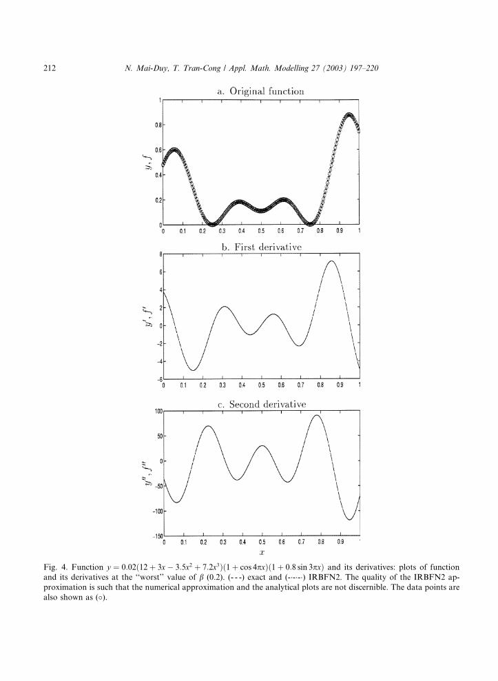
Fig. 4. Function y ¼ 0:02ð12þ 3x� 3:5x2 þ 7:2x3Þð1þ cos 4pxÞð1þ 0:8 sin 3pxÞ and its derivatives: plots of function
and its derivatives at the ‘‘worst’’ value of b (0:2). (- - -) exact and (-�-�-�) IRBFN2. The quality of the IRBFN2 ap-
proximation is such that the numerical approximation and the analytical plots are not discernible. The data points are
also shown as (�).
212 N. Mai-Duy, T. Tran-Cong / Appl. Math. Modelling 27 (2003) 197–220

Fig. 5. Approximant f of the function yðx1; x2Þ ¼ x21x2 þ x32=3þ x22=2 and its derivatives: plots of the norm Ne as a
function of b. Legends (�) conventional element method, (––) DRBFN, (-�-�-�) IRBFN1 and (- - -) IRBFN2. It can be
seen that the quality of the approximation for the derivatives is much better with the IRBFN approach.
N. Mai-Duy, T. Tran-Cong / Appl. Math. Modelling 27 (2003) 197–220 213
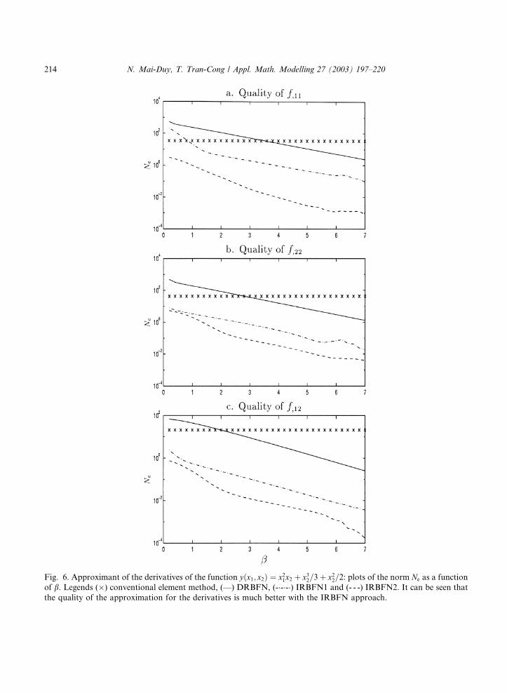
Fig. 6. Approximant of the derivatives of the function yðx1; x2Þ ¼ x21x2 þ x32=3þ x22=2: plots of the norm Ne as a function
of b. Legends (�) conventional element method, (––) DRBFN, (-�-�-�) IRBFN1 and (- - -) IRBFN2. It can be seen that
the quality of the approximation for the derivatives is much better with the IRBFN approach.
214 N. Mai-Duy, T. Tran-Cong / Appl. Math. Modelling 27 (2003) 197–220

derivative at b ¼ 0:2 obtained with the IRBFN2 where the ‘‘worst’’ value of b is used to dem-onstrate the superior performance of the IRBFN2.
6.2. Example 2
Consider the following bivariate function
y ¼ x21x2 þ x32=3þ x22=2;
where �36 x1 6 3 and �36 x2 6 3. This is a non-trivial example which has a complicated rootstructure [17]. The data consist of 441 points, uniformly spaced along both axes x1 and x2 fortraining and 1764 points for testing. The results obtained from both DRBFN and IRBFNmethods are compared with the accuracies achieved by the conventional method using linearshape function over triangular elements. Fig. 5 shows the quality of the approximation of thefunction f ðx1; x2Þ and its first derivatives while Fig. 6 shows the quality of the approximation ofsecond order derivatives using the DRBFN, IRBFN1 and IRBFN2 with b in the range0:26 b6 7:0. Again, the results are more accurate with IRBFN2 as shown in Figs. 5 and 6. Thus itcan be seen that the IRBFN2 yields better performance than the IRBFN1 which in turn performsbetter than the DRBFN.
Fig. 7. Approximant of the function y ¼ x21 þ x1x2 � 2x22 � x2x3 þ x23: plots of the norm Ne as a function of b. (––)DRBFN, (-�-�-�) IRBFN1 and (- - -) IRBFN2. It can be seen that the quality of the approximation is much better with
the IRBFN approach.
N. Mai-Duy, T. Tran-Cong / Appl. Math. Modelling 27 (2003) 197–220 215

Fig. 8. Approximant of the derivatives of the function y ¼ x21 þ x1x2 � 2x22 � x2x3 þ x23: plots of the norm Ne as a
function of b. Legends (�) conventional element method, (––) DRBFN, (-�-�-�) IRBFN1 and (- - -) IRBFN2. It can be
seen that the quality of the approximation is much better with the IRBFN approach.
216 N. Mai-Duy, T. Tran-Cong / Appl. Math. Modelling 27 (2003) 197–220

Fig. 9. Approximant of the derivatives of the function y ¼ x21 þ x1x2 � 2x22 � x2x3 þ x23: plots of the norm Ne as a
function of b. Legends (�) conventional element method, (––) DRBFN, (-�-�-�) IRBFN1 and (- - -) IRBFN2. It can be
seen that the quality of the approximation is much better with the IRBFN approach.
N. Mai-Duy, T. Tran-Cong / Appl. Math. Modelling 27 (2003) 197–220 217
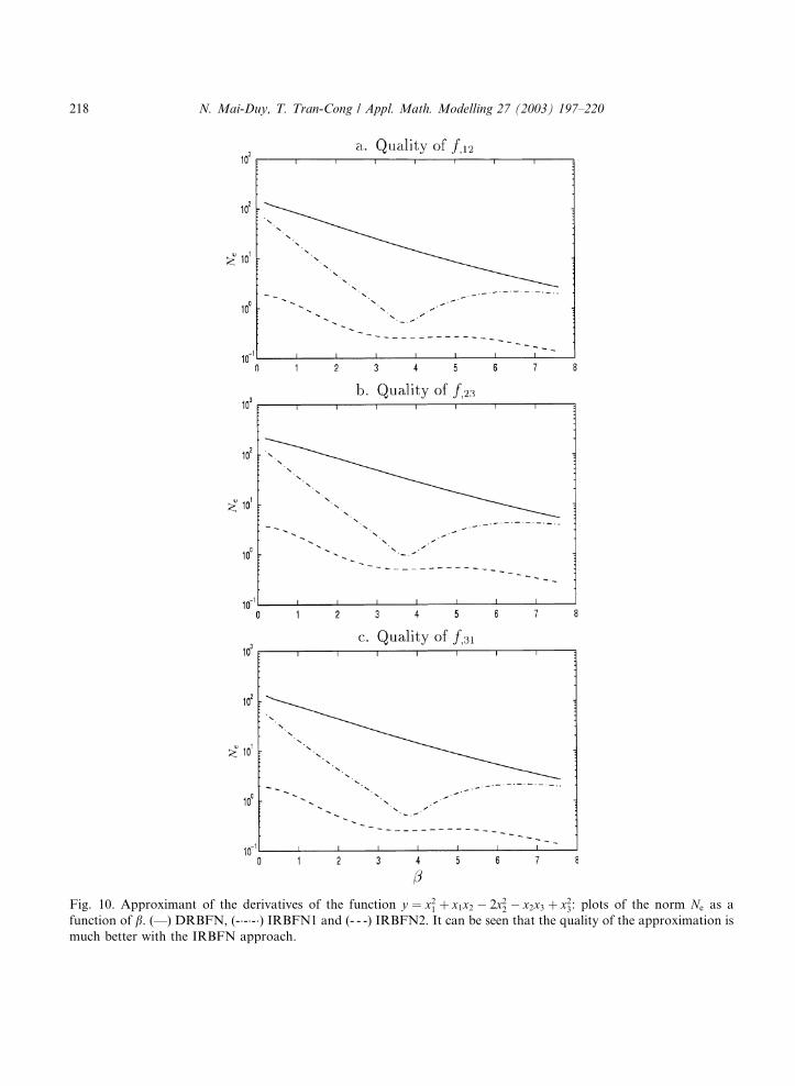
Fig. 10. Approximant of the derivatives of the function y ¼ x21 þ x1x2 � 2x22 � x2x3 þ x23: plots of the norm Ne as a
function of b. (––) DRBFN, (-�-�-�) IRBFN1 and (- - -) IRBFN2. It can be seen that the quality of the approximation is
much better with the IRBFN approach.
218 N. Mai-Duy, T. Tran-Cong / Appl. Math. Modelling 27 (2003) 197–220
6.3. Example 3
Consider the following function of three variables
y ¼ x21 þ x1x2 � 2x22 � x2x3 þ x23;
where 06 x1 6 0:5, 06 x2 6 0:5 and 06 x3 6 0:5. In this example, 216 points, uniformly spacedalong the axes x1, x2 and x3, are used for training and 1728 points for testing. Fig. 7 shows thequality of the approximation of the original function. Fig. 8 shows the plots of norm Ne asfunction of b (0:26 b6 7:6) for first order derivative functions f;1, f;2 and f;3, while Figs. 9 and 10are for second order derivative functions f;11, f;22, f;33, f;12, f;23 and f;31. Figs. 7–10 again show thatthe IRBFN2 method exhibits superior performance over other methods.
7. Concluding remarks
This paper reports the successful development and implementation of function approximationmethods based on RBFNs for functions of one, two and three variables and their derivatives(scattered data interpolation). Both the direct RBFN method and the indirect RBFN methodare able to offer better results in comparison with the conventional method using linear shapefunctions. The present RBFN methods also eliminate the need for FE-type discretisation of thedomain of analysis. Among the RBFs considered, multiquadrics RBF offers the best perfor-mance in accuracy in both DRBFN and IRBFN method. Numerical results show that IRBFNs,especially IRBFN2, achieve greater accuracy than DRBFN in the approximation of bothfunction and especially its derivatives. Furthermore, this superior accuracy is maintained over awide range of RBF�s width ð0:2 < b < 9Þ. A formal theoretical proof of the superior accuracyof the present IRBFN method cannot be offered at this stage, at least by the present authors.However, a heuristic argument can be presented as follows. In the direct methods, the star-ting point is the decomposition of the unknown functions into some finite basis and all deri-vatives are obtained as a consequence. Any inaccuracy in the assumed decomposition is usuallymagnified in the process of differentiation. In contrast, in the indirect approach the startingpoint is the decomposition of the highest derivatives into some finite basis. Lower derivativesand finally the function itself are obtained by integration which has the property of damping outor at least containing any inherent inaccuracy in the assumed shape of the derivatives. At thisstage, it is recommended that the IRBFN2 method is the better one among the methods con-sidered for an accurate approximation of a function and its derivative. In a subsequent study,the application of the DRBFN and IRBFN methods in solving differential equations will bereported.
Acknowledgements
This work is supported by a Special USQ Research Grant to Thanh Tran-Cong (grant no. 179-310). NamMai-Duy is supported by a USQ scholarship. This support is gratefully acknowledged.The authors would like to thank the referees for their helpful comments.
N. Mai-Duy, T. Tran-Cong / Appl. Math. Modelling 27 (2003) 197–220 219
References
[1] R.D. Cook, D.S. Malkus, M.E. Plesha, Concepts and Applications of Finite Element Analysis, John Wiley & Sons,
Toronto, 1989.
[2] C.A. Brebbia, J.C.F. Telles, L.C. Wrobel, Boundary Element Techniques: Theory and Applications in Engineering,
Springer-Verlag, Berlin, 1984.
[3] M.J.D. Powell, Radial basis functions for multivariable interpolation: a review, in: J.C. Watson, M.G. Cox (Eds.),
IMA Conference on Algorithms for the Approximation of Function and Data, Royal Military College of Science,
Shrivenham, England, 1985, pp. 143–167.
[4] D.S. Broomhead, D. Lowe, Multivariable functional interpolation and adative networks, Complex Systems 2
(1988) 321–355.
[5] M.J.D. Powell, Radial basis function approximations to polynomial, in: D.F. Griffiths, G.A. Watson (Eds.),
Numerical Analysis 1987 Proceedings, University of Dundee, Dundee, UK, 1988, pp. 223–241.
[6] T. Poggio, F. Girosi, Networks for approximation and learning, in: Proceedings of the IEEE 78, 1990, pp. 1481–
1497.
[7] F. Girosi, T. Poggio, Networks and the best approximation property, Biological Cybernetics 63 (1990) 169–176.
[8] S. Chen, F.N. Cowan, P.M. Grant, Orthogonal least squares learning algorithm for radial basis function networks,
IEEE Transaction on Neural Networks 2 (1991) 302–309.
[9] S. Haykin, Neural Networks: A Comprehensive Foundation, Prentice-Hall, New Jersey, 1999.
[10] J. Park, I.W. Sandberg, Approximation and radial basis function networks, Neural Computation 5 (1993) 305–316.
[11] J. Moody, C.J. Darken, Fast learning in networks of locally-tuned processing units, Neural Computation 1 (1989)
281–294.
[12] R. Franke, Scattered data interpolation: tests of some methods, Mathematics of Computation 38 (157) (1982) 181–
200.
[13] W.H. Press, B.P. Flannery, S.A. Teukolsky, W.T. Vetterling, Numerical Recipes in C: The Art of Scientific
Computing, Cambridge University Press, Cambridge, 1988.
[14] A.E. Tarwater, A parameter study of Hardy�s multiquadrics method for scattered data interpolation, Technical
Report UCRL-563670, Lawrence Livemore National Laboratory, 1985.
[15] J.J. Dongarra, J.R. Bunch, C.B. Moler, G.W. Stewart, LINPACK User�s Guide, SIAM, Philadelphia, 1979.
[16] S. Hashem, B. Schmeiser, Approximating a function and its derivatives using MSE-optimal linear combinations of
trained feedforward neural networks, in: Proceedings of the 1993 World Congress on Neural Networks, vol. 1,
Lawrence Erlbaum Associates, Hillsdale, New Jersey, 1993, pp. 617–620.
[17] S.V. Chakravarthy, J. Ghosh, Function emulation using radial basis function networks, Neural Networks 10 (1997)
459–478.
220 N. Mai-Duy, T. Tran-Cong / Appl. Math. Modelling 27 (2003) 197–220