Use of the q-Gaussian Function in Radial Basis

Function Networks

Renato Tinos and Luiz Otavio Murta Junior

Departamento de Fısica e MatematicaFaculdade de Filosofia, Ciencias e Letras de Ribeirao Preto (FFCLRP)Universidade de Sao Paulo (USP)Av. Bandeirantes, 390014040-901, Ribeirao Preto, SP, Brazilrtinos@ffclrp.usp.br , murta@ffclrp.usp.br

Summary. Radial Basis Function Networks (RBFNs) have been successfully em-ployed in several function approximation and pattern recognition problems. InRBFNs, radial basis functions are used to compute the activation of artificial neu-rons. The use of different radial basis functions in RBFN has been reported in theliterature. Here, the use of the q-Gaussian function as a radial basis function inRBFNs is investigated. An interesting property of the q-Gaussian function is thatit can continuously and smoothly reproduce different radial basis functions, like theGaussian, the Inverse Multiquadratic, and the Cauchy functions, by changing a realparameter q. In addition, the mixed use of different shapes of radial basis functionsin only one RBFN is allowed. For this purpose, a Genetic Algorithm is employedto select the number of hidden neurons, and center, width and q parameter of theq-Gaussian radial basis function associated with each radial unit. The RBF Networkwith the q-Gaussian RBF is compared to RBF Networks with Gaussian, Cauchy,and Inverse Multiquadratic RBFs in problems in the Medical Informatics domain.

1 Introduction

Radial Basis Function (RBF) Networks are a class of Artificial Neural Net-works where RBFs are used to compute the activation of artificial neurons.RBF Networks have been successfully employed in real function approxima-tion and pattern recognition problems. In general, RBF Networks are associ-ated with architectures with two layers, where the hidden layer employs RBFsto compute the activation of the neurons. Different RBFs have been used, likethe Gaussian, the Inverse Multiquadratic, and the Cauchy functions [22]. Inthe output layer, the activations of the hidden units are combined in order toproduce the outputs of the network. While there are weights in the outputlayer, they are not present in the hidden layer.

2 Renato Tinos and Luiz Otavio Murta Junior

When only one hidden layer and output neurons with linear activationfunction are employed, RBF Networks can be trained in two steps. First, theparameters of the radial basis units are determined. Then, as the outputs ofthe hidden units and the desired outputs for each pattern are known, theweights are computed by solving a set of linear equations via least squares orsingular value decomposition methods [14]. Thus, gradient descendent tech-niques are avoided and determining the radial basis units’ parameters becomesthe main problem during the training phase.

The selection of the parameters of the radial basis units means to de-termine the number of hidden neurons, the type, widths, and centers of theRBFs. In several cases, the first three parameters are previously defined, andonly the radial basis centers are optimized [20]. Besides the centers, the num-ber of hidden neurons [6], [25] and the widths [5] can be still optimized. Ingeneral, all the radial units have the same type of RBF, e.g., the Gaussianfunction, which is chosen before the training.

In [13], the effect of the choice of radial basis functions on RBF Networkswas analyzed in three time series prediction problems. Using the k-means algo-rithm to determine the radial basis centers, the authors compared the resultsproduced by RBF Network with different types of RBFs for different numbersof hidden neurons and widths of the RBFs. In the experiments conducted in[13], all radial units have the same fixed RBF type and width for each RBFNetwork. The authors concluded that the choice of the RBF type is problemdependent, e.g., while the RBF Network with hidden neurons with Gaussiantransfer function presented best performance in one problem, the choice ofthe Inverse Multiquadratic function was beneficial for another problem.

Here, the mixed use of different shapes of radial basis functions in RBFNetworks, i.e., the hidden neurons can have different radial basis functions in asame RBF Network, is investigated. For this purpose, the q-Gaussian function,which reproduces different RBFs by changing a real parameter q, is used.Thus, the choice of the number of hidden neurons, center, type (parameterq), and width of each RBF can be viewed as a search problem.

In this work, a Genetic Algorithm (GA) is employed to select the numberof hidden neurons, center, type, and width of each RBF associated with eachhidden unit. The methodology used here is presented in Section 5. Before, Sec-tion 2 presents the RBF Network model, Section 3 introduces the q-Gaussianfunction, and Section 4 discusses the use of the q-Gaussian RBF. Section 6presents and discusses an experimental study with two pattern recognitionproblems of the Medical Informatics domain, in order to test the performanceof the investigated methodology. In the experiments, the RBF Network withthe q-Gaussian RBF is compared to RBF Networks with Gaussian, Cauchy,and Inverse Multiquadratic RBFs. Finally, Section 7 presents the final con-clusions.

Use of the q-Gaussian Function in Radial Basis Function Networks 3

2 Radial Basis Function Networks

RBF are a class of real-valued functions where its output depends on thedistance between the input pattern and a point c, defined as the center ofthe RBF. Moody and Darken proposed the use of RBFs in Artificial NeuralNetworks (ANNs) inspired by the selective response of some neurons [20].ANNs where RBFs are used as activation functions are named RBF Networks.The architecture and the learning of RBF Networks are described in the nextsections.

2.1 Architecture

RBF Networks can have any number of hidden layers and outputs with linearor nonlinear activation. However, RBF Networks are generally associated witharchitectures with only one hidden layer without weights and with an outputlayer with linear activation (Figure 1). Such architecture is employed becauseit allows the separation of the training in two phases: when the radial units’parameters are determined, the weights of the output layer generally can beeasily computed.

Fig. 1. RBF Network with one hidden layer.

The output of the k-th neuron in the output layer of an RBF Network,where k = 1, . . . , q, is given by

4 Renato Tinos and Luiz Otavio Murta Junior

yk(x) =m

∑

j=1

wkjhj(x) (1)

where hj(x) is the activation of the radial unit j = 1, . . . , m for the inputpattern x and wkj is the synaptic weight between the radial unit j and theoutput neuron k. The activation of the j-th radial unit is dependent on thedistance between the input pattern and the hidden unit center cj . Using anEuclidean metric [22], the activation of the j-th radial unit can be defined as

hj(x) = φj

(

dj(x))

(2)

where

dj(x) =‖x − cj‖2

r2j

, (3)

φj(.) and rj are, respectively, the RBF and the scalar parameter that definesits width for the j-th radial unit, and ‖.‖ is the Euclidean norm.

The most common RBF is the Gaussian function, which is given by

φj

(

dj(x))

= e−dj(x) (4)

Neurons with Gaussian RBF present a very selective response, with highactivation for patterns close to the radial unit center and very small activationfor distant patterns.

In this way, other RBFs with longer tails are often employed. Two exam-ples of such RBFs are the Cauchy function, given by

φj

(

dj(x))

=1

1 + dj(x)(5)

and the Inverse Multiquadratic, defined by

φj

(

dj(x))

=1

(

1 + dj(x))1/2

(6)

2.2 Learning

The first step in the training of the RBF Network presented in Figure 1 isthe choice of the number of radial units and the parameters of each one ofthem. The original method proposed in [20] employs the k-means algorithm todetermine the RBF center locations. In this case, the number of radial unitsis equal to k and is determined before the training. The width and the typeof the RBFs are fixed too.

Instead of using the k-means to determine the RBF centers, the inputpatterns of the training set can be used as center locations. The simplestmethod is to select all the input patterns of the training set as centers ofthe radial units. However, this method is not generally used because of the

Use of the q-Gaussian Function in Radial Basis Function Networks 5

large number of radial units employed and the occurrence of overfitting. Subsetselection can be an interesting approach to avoid such problems. Thus, besidesthe center locations, the number of hidden neurons can still be optimized.The problem of finding the best subset of input patterns to be used as radialunits’ centers is generally intractable when the training set is large. In thisway, heuristics can be used to find a good subset.

In [8], Forward Selection and Orthogonal Least Squares were employed toselect the centers of the radial units based on the instances of the trainingset. Besides the centers, the widths of the RBFs can be optimized, like in theGeneralized Multiscale RBF Network [5].

In recent years, there is a growing interest in optimizing the radial units’parameters of RBF Networks using Evolutionary Algorithms [14], which area class of meta-heuristic algorithms successfully employed in several similarsearch problems.

In [6], a GA is used to select a subset of radial units centers based onthe instances of the training set. The chromosome of each individual i of apopulation is composed of a subset of indexes of the input patterns of thetraining set. For each index in the chromosome i, a radial unit with centerlocated at the respective input pattern is added to the RBF Network i. Forexample, if the chromosome of the individual i is zT

i = [ 2 98 185], then aRBF Network is created with three radial units with centers located at theinput patterns x2, x98, and x185. For the fitness evaluation of the individual i,the respective RBF Network is created and the Akaike’s Information Criterion(AIC) is computed. Then, the computed AIC, which has a term that evaluatesthe RBF Network performance and a term that evaluates the RBF Networkcomplexity, is used as the fitness of the individual i. All radial units have thesame type of RBF, which is defined a priori. In [16], the radial unit widthsare incorporated in the chromosomes too.

The next step is to compute the weights of the RBF Network. When thenumber of hidden units and the parameters of the RBFs are fixed, then theradial unit activation can be determined for each instance of the training setand the system defined by Eq. 1 can be viewed as a linear model. Minimizingthe sum of squared errors, the optimal weight vector of the k-th output neuron[22] can be computed by

wk =(

HTH)

−1HTyk (7)

where yk is the vector of the desired outputs of the k-th neuron for theinstances of the training set, H is the design matrix formed by the activationsof the radial units hj(.) for each instance of the training set, and HT denotesthe transpose of the matrix H.

6 Renato Tinos and Luiz Otavio Murta Junior

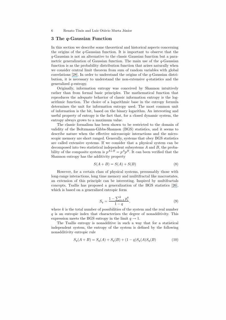
3 The q-Gaussian Function

In this section we describe some theoretical and historical aspects concerningthe origins of the q-Gaussian function. It is important to observe that theq-Gaussian is not an alternative to the classic Gaussian function but a para-metric generalization of Gaussian function. The main use of the q-Gaussianfunction is as the probability distribution function that arises naturally whenwe consider central limit theorem from sum of random variables with globalcorrelations [28]. In order to understand the origins of the q-Gaussian distri-bution, it is necessary to understand the non-extensive q-statistics and thegeneralized q-entropy.

Originally, information entropy was conceived by Shannon intuitivelyrather than from formal basic principles. The mathematical function thatreproduces the adequate behavior of classic information entropy is the log-arithmic function. The choice of a logarithmic base in the entropy formuladetermines the unit for information entropy used. The most common unitof information is the bit, based on the binary logarithm. An interesting anduseful property of entropy is the fact that, for a closed dynamic system, theentropy always grows to a maximum value.

The classic formalism has been shown to be restricted to the domain ofvalidity of the Boltzmann-Gibbs-Shannon (BGS) statistics, and it seems todescribe nature when the effective microscopic interactions and the micro-scopic memory are short ranged. Generally, systems that obey BGS statisticsare called extensive systems. If we consider that a physical system can bedecomposed into two statistical independent subsystems A and B, the proba-bility of the composite system is pA+B = pApB. It can been verified that theShannon entropy has the additivity property

S(A + B) = S(A) + S(B) (8)

However, for a certain class of physical systems, presumably those withlong-range interactions, long time memory and mulitifractal like macrostates,an extension of this principle can be interesting. Inspired by multifractalsconcepts, Tsallis has proposed a generalization of the BGS statistics [26],which is based on a generalized entropic form

Sq =1 −

∑ki=1 pq

i

1 − q, (9)

where k is the total number of possibilities of the system and the real numberq is an entropic index that characterizes the degree of nonadditivity. Thisexpression meets the BGS entropy in the limit q → 1.

The Tsallis entropy is nonadditive in such a way that for a statisticalindependent system, the entropy of the system is defined by the followingnonadditivity entropic rule

Sq(A + B) = Sq(A) + Sq(B) + (1 − q)Sq(A)Sq(B) (10)

Use of the q-Gaussian Function in Radial Basis Function Networks 7

From this paradigm, a kind of q-mathematics [27], [12], [21], [7] that is ap-propriate to q-statistics has emerged. By definition, the q-sum of two numbersis defined as

x +q y = x + y + (1 − q)xy (11)

The q-sum is commutative, associative, recovers the conventional summingoperation if q = 1 (i.e. x+1y = x+ y), and preserves 0 as the neutral element(i.e. x +q 0 = x). By inversion, one can define the q-subtraction as

x −q y =x − y

1 + (1 − q)y(12)

The q-product for x, y is defined by the binary relation

x.qy = [x1−q + y1−q − 1]1/(1−q) (13)

This operation, also commutative and associative, recovers the usual prod-uct when q = 1, and preserves 1 as the unity. It is defined only whenx1−q + y1−q ≥ 1. Also by inversion, it can be defined the q-division

x/qy = (x1−q − y1−q + 1)1/(1−q) (14)

As well known in classical statistical mechanics, the Gaussian maximizes,under appropriate constraints, the classic entropy. The q-generalization of theclassic entropy introduced in [26] as the basis for generalizing the classic theoryreaches its maximum at the distributions usually referred to as q-Gaussian.This fact, and a number of conjectures [9] and numerical indications [10],suggest that there should be a q-analog of the central limit theorem (CLT)as well. Limit theorems, in particular, the CLTs, surely are among the mostimportant theorems in probability theory and statistics. They play an essentialrole in various applied sciences as well. Various aspects of this theorem and itslinks to statistical mechanics and diffusion have been discussed during recentdecades as well.

The q-analysis began at the end of the 19th century, as stated by McAnally[18], recalling the work of Rogers [23] on the expansion of infinite products.Recently, however, its development brought together the need for the general-ization of special functions to handle nonlinear phenomena [10]. The problemof the q-oscillator algebra [4], for example, has led to q-analogues of many spe-cial functions, in particular the q-exponential and the q-gamma functions [18],[1], the q-trigonometric functions [2], q-Hermite and q-Laguerre polynomials[9], [3], which are particular cases of q-hypergeometric series.

4 The q-Gaussian Radial Basis Function

The use of the q-Gaussian function as a radial basis function in RBF Networksis interesting because it allows changing the shape of the RBF according to

8 Renato Tinos and Luiz Otavio Murta Junior

the real parameter q [29]. The q-Gaussian RBF for the radial unit j can bedefined as

φj

(

dj(x))

= e−dj(x)qj

(15)

where qj is a real valued parameter and the q-exponential function of −dj(x)[27] is given by

e−dj(x)qj

≡

{ 1(

1+(qj−1)dj(x)) 1

qj−1

if(

1 + (qj − 1)dj(x))

≥ 0

0 otherwise(16)

An interesting property of the q-Gaussian function is that it can reproducedifferent RBFs for different values of the real parameter q. For large negativenumbers, the function is concentrated around the center of the RBF. Whenthe value of q increases, the tail of the function becomes larger.

In the next, Eq. 16 will be analyzed for q → 1, q = 2, and q = 3. Forsimplicity, the index j and the dependence on x will be omitted in the followingequations. For q → 1, the limit of the q-Gaussian RBF can be computed

limq→1

e−dq = lim

q→1

1(

1 + (q − 1)d)

1

q−1

(17)

If we write z = (q − 1)d, then

limq→1

e−dq = lim

z→0

(

1 + z)

−dz

limq→1

e−dq = lim

z→0

(

(

1 + z)

1

z

)

−d

(18)

The limit of the function (1+z)1

z is well know and converges to e when z → 0.Thus,

limq→1

e−dq = e−d (19)

In this way, we can observe that the q-Gaussian RBF (Eq. 16) reduces to thestandard Gaussian RBF (Eq. 4) when q → 1.

Replacing q = 2 in Eq. 16, we have

e−dq =

1

1 + d(20)

i.e., the q-Gaussian RBF (Eq. 16) is equal to the Cauchy RBF (Eq. 5) forq = 2.

When q = 3, we have

e−dq =

1(

1 + 2d)1/2

(21)

Use of the q-Gaussian Function in Radial Basis Function Networks 9

i.e., the activation of a radial unit with an Inverse Multiquadratic RBF (Eq.6) for d is equal to the activation of a radial unit with a q-Gaussian RBF (Eq.16) for d/2.

Figure 2 presents the radial unit activation for the Gaussian, Cauchy,and Inverse Multiquadratic RBFs. The activation for the q-Gaussian RBF fordifferent values of q is still presented. One can observe that the q-Gaussianreproduces the Gaussian, Cauchy, and Inverse Multiquadratic RBFs for q → 1,q = 2, and q = 3. Another interesting property of the q-Gaussian RBF is stillpresented in Figure 2: a small change in the value of q represents a smoothmodification on the shape of the RBF.

In the next section, a methodology to optimize the RBF parameters of thehidden units in RBF Networks via Genetic Algorithms is presented.

−4 −3 −2 −1 0 1 2 3 40

0.1

0.2

0.3

0.4

0.5

0.6

0.7

0.8

0.9

1

x

h(x)

q=−1q=−0.5q=0q=0.5q=1

q=1.5q=2q=2.5q=3q=3.5

Fig. 2. Radial unit activation in an one-dimensional space with c = 0 and r = 1for different RBFs: Gaussian (‘x’), Cauchy (‘o’), Inverse Multiquadratic for

p(2)x

(‘+’), and q-Gaussian RBF with different values of q (solid lines).

10 Renato Tinos and Luiz Otavio Murta Junior

5 Selection of Parameters of the q-Gaussian RBFs via

Genetic Algorithms

In the investigated methodology, a Genetic Algorithm (GA) is used to definethe number of radial units m, and the parameters of each RBF related toeach hidden unit j = 1, . . . , m, i.e., the center, width, and parameter q foreach radial unit with q-Gaussian RBF. Algorithm 1 describes the procedureto select the parameters of the radial units. The GA is described in the next.

Algorithm 1

1: Initialize the population composed of random individuals zT

i = [ b1 r1 q1 b2 r2 q2

. . . bN rN qN ], where N is the size of the training set, the bit bj (j = 1, . . . , N)defines if the j-th training pattern is used as the center of a radial unit withwidth rj and q-parameter qj .

2: while (stop criteria are not satisfied) do

3: Apply elitism and tournament selection to generate the new individuals4: Apply crossover and mutation5: Compute the fitness (Eq. 25) of each individual i in the new population by

evaluating the RBF Network defined by the individual i. The number of radialunits mi of the RBF Network related to individual i is equal to the numberof ones in the elements bj (j = 1, . . . , N) of the vector zi. When bj = 1, anew radial unit is added with center defined by the j-th training pattern, andwidth and q-parameter given by rj and qj . The outputs of the RBF Networkare computed using eqs. 1, 2, and 7.

6: end while

5.1 Codification

A hybrid codification (binary and real) is employed in the GA used in thiswork. Each individual i (i = 1, . . . , µ) is described by a vector (chromosome)with 3N elements, where N is the size of the training set. The individual i isdefined by the vector

zTi = [ b1 r1 q1 b2 r2 q2 . . . bN rN qN ] (22)

where bj is a bit that defines the use of the j-th training pattern as a centerof a radial unit. If bj = 1, a radial unit is created with center equal to thetraining pattern xj , and with width and q-parameter respectively given bythe real numbers rj and qj . The number of radial units mi for each individuali is equal to the number of ones in the bits bj of the vector zi. In the firstgeneration, the number of elements bj equal to 1, i.e. the number of radialunits mi, is generated with mean nb. Then, the number of radial units mi isallowed to change by crossover and when a bit bj is mutated.

For example, if the chomosome of the individual i is given by

Use of the q-Gaussian Function in Radial Basis Function Networks 11

zTi = [0 0.11 1.26 1 0.21 0.82 1 0.15 1.67 0 0.32 0.96 1 0.02 2.3 ] (23)

where, for simplicity, N = 5, then the RBF i is composed of three radial unitswith: centers located in the input patterns x2, x3, and x5; widths 0.21, 0.15,and 0.02; q-parameters 0.82, 1.67, and 2.3.

5.2 Operators

Here, the GA uses three standard operators:

Selection

Tournament selection and elitism are employed here. Elitism is employed inorder to preserve the best individuals of the population. Tournament selec-tion is an interesting alternative to the use of fitness-proportionate selectionmainly to reduce the problem of premature convergence and the computa-tional cost [19]. In tournament selection, two (or more) individuals from thepopulation are randomly chosen with uniform distribution in order to form atournament pool. When the tournament size is equal to two, a random numberwith uniform distribution in the range [0,1] is generated and, if this number issmaller than the parameter ps, the individual with the best fitness from thetournament pool is selected. Otherwise, the remaining individual is selected.This procedure is repeated until the new population is complete.

Crossover

When the standard crossover is applied, parts of the chromosomes of twoindividuals are exchanged. Two point crossover is applied in each pair ofnew individuals with crossover rate pc. Here, the crossover points are allowedonly immediately before the elements bj (see Eq. 22). In this way, individualsexchange all the parameters of a radial unit each time.

Mutation

Two types of mutation are employed. The standard flip mutation is employedwith mutation rate pm in the elements bj. Thus, if an element bj is equal tozero, it is flipped to one when it is mutated, what implies in the insertion tothe RBF Network of a new radial unit with center at the training pattern xj ,and with width and q-parameter respectively given by the real numbers rj

and qj . If an element bj is equal to one, it is flipped to zero, what implies inthe deletion of the radial unit with center in the training pattern xj .

When an element rj or qj is mutated, its value gj is changed according to

gj = gj exp(

τmN (0, 1))

(24)

12 Renato Tinos and Luiz Otavio Murta Junior

where τm denotes the standard deviation of the Gaussian distribution withzero mean employed to generate the random deviation N (0, 1). It is importantto observe that silent mutations can occur in the elements rj and qj when theelement bj is equal to zero.

5.3 Fitness Computation

In the fitness computation, the individual is decoded and the correspondingRBF Network is evaluated. First, the number of hidden units in the RBFNetwork i (related to individual i), mi, is defined as the number of ones inthe elements bj of the vector zi. Then, the centers of the RBFs are defined. Ifbj is equal to one, a center is defined at the training pattern xj . The next stepis to set the widths and q-Gaussian parameters of each radial unit accordingto elements rj and qj of the chromosome of the individual i. The activations ofthe hidden units for each instance of the training set and the optimal outputweights are then computed (eqs. 2 and 7). Then the RBF Network i can beevaluated.

In this work, the AIC, which evaluates the RBF Network performance andthe RBF Network complexity, is employed. In RBF Networks with supervisedlearning, the AIC [6] is defined as

f(i) = N log1

N

N∑

n=1

[

(

y(n) − y(

x(n), zi

)

)T

×(

y(n) − y(

x(n), zi

)

)]

+ cmi (25)

where x(n) is the n-th instance of the training set, y(n) is the respectivevector of desired outputs, and c is a real number that controls the balancebetween RBF Networks with small training set errors and with small numberof radial units. Here c = 4 if minf ≤ mi ≤ msup, and c = 12 otherwise. In thisway, individual with a small (mi < minf ) or large (mi > msup) are punished.

6 Experimental Study

In this section, in order to test the performance of RBF Networks withq-Gaussian RBFs (Section 4), experiments with three pattern recognitiondatabases in the Medical Informatics domain are presented. In order to com-pare the performance of the RBF Network with different RBFs, the samemethodology described in last section is applied in RBF Networks with fourdifferent RBFs: Gaussian, Cauchy, Inverse Multiquadratic, and q-Gaussian.However, in the experiments with Gaussian, Cauchy, and Inverse Multi-quadratic RBFs, the values of the parameter q of each RBF are not presentin the chromosome of the individuals of the GA. The shape of the RBFscan change for the RBF Network with the q-Gaussian RBFs (by changing

Use of the q-Gaussian Function in Radial Basis Function Networks 13

the parameter q), while it is fixed for the experiments with the other threefunctions.

The databases employed in the experiments were obtained from the Ma-

chine Learning Repository of the University of California - Irvine. The firstdatabase, Wisconsin Breast Cancer Database [17], contains 699 instances.Nine attributes obtained from histopathological examination of breast biopsiesare considered. Here the RBF Network is employed to classify the instances intwo classes, benign and malignant and 16 instances with missing attribute val-ues are discarded [11]. The second database, Pima Indians Diabetes Database,contains 768 instances with 8 attributes obtained from clinical information ofwomen of Pima Indian heritage [24]. The objective is to classify the occur-rence of diabetes mellitus. In the third database, Heart Disease Database,the objective is to classify the presence of heart disease in the patient basedon the information of 14 attributes obtained from medical examination. Thedatabase originally contains 303 instances, but only 270 are used here [15].

The experiments with the methodology presented in Section 5 applied inthe three pattern classification problems presented in the last paragraph aredescribed in the next section. Then, the experimental results and its analysisare presented in Section 6.2.

6.1 Experimental Design

In order to compare the performance of RBF Networks with different RBFsfor each database, each GA was executed 20 times (with 20 different randomseeds) in the training of each RBF Network. The number of instances in thetraining set is 50% of the total number of instances, and the same numberis used in the test set. For each run of the GA, the individuals of the ini-tial population are randomly chosen with uniform distribution in the allowedrange of values, which are 0.01 ≤ rj ≤ 1.0 for the radial widths and, for theexperiments with the q-Gaussian RBF, 0.5 ≤ qj ≤ 3.0.

For all experiments, the population size is set to 50 individuals, the twobest individuals of the population are automatically inserted in the next pop-ulation (elitism), the tournament size is set to 2, ps = 0.8, pc = 0.3, nb = 20(mean number of radial units in the first generation), minf = 15, msup = 60,pm = 0.0025 (mutation rate for the elements bj), and τm = 0.02 (standarddeviation of the Gaussian distribution used to mutate the real elements rj

and qj). Each GA is executed for 300 generations for the experiments withdatabases Breast Cancer and Heart Disease and 500 for the experiments withdatabase Pima.

6.2 Experimental Results

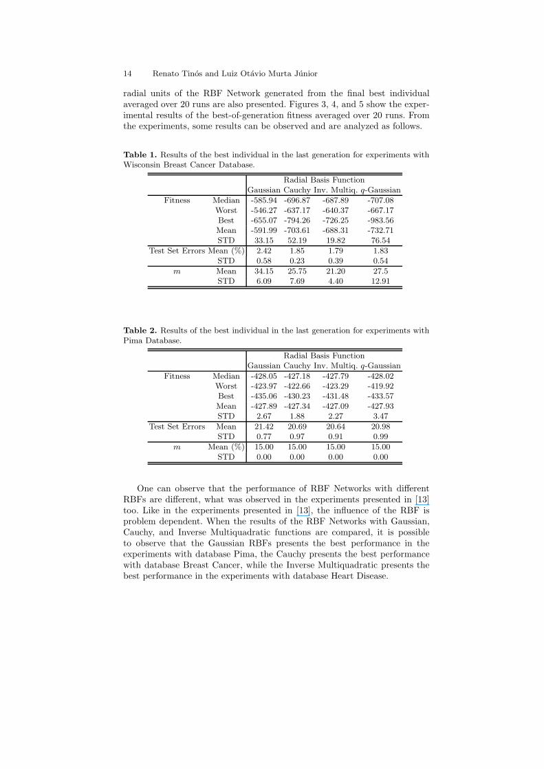
The experimental results of the fitness of the best individual in the last gen-eration averaged over 20 runs are presented in tables 1, 2, and 3. The resultsof the percentage of classification errors for the test sets and the number of

14 Renato Tinos and Luiz Otavio Murta Junior

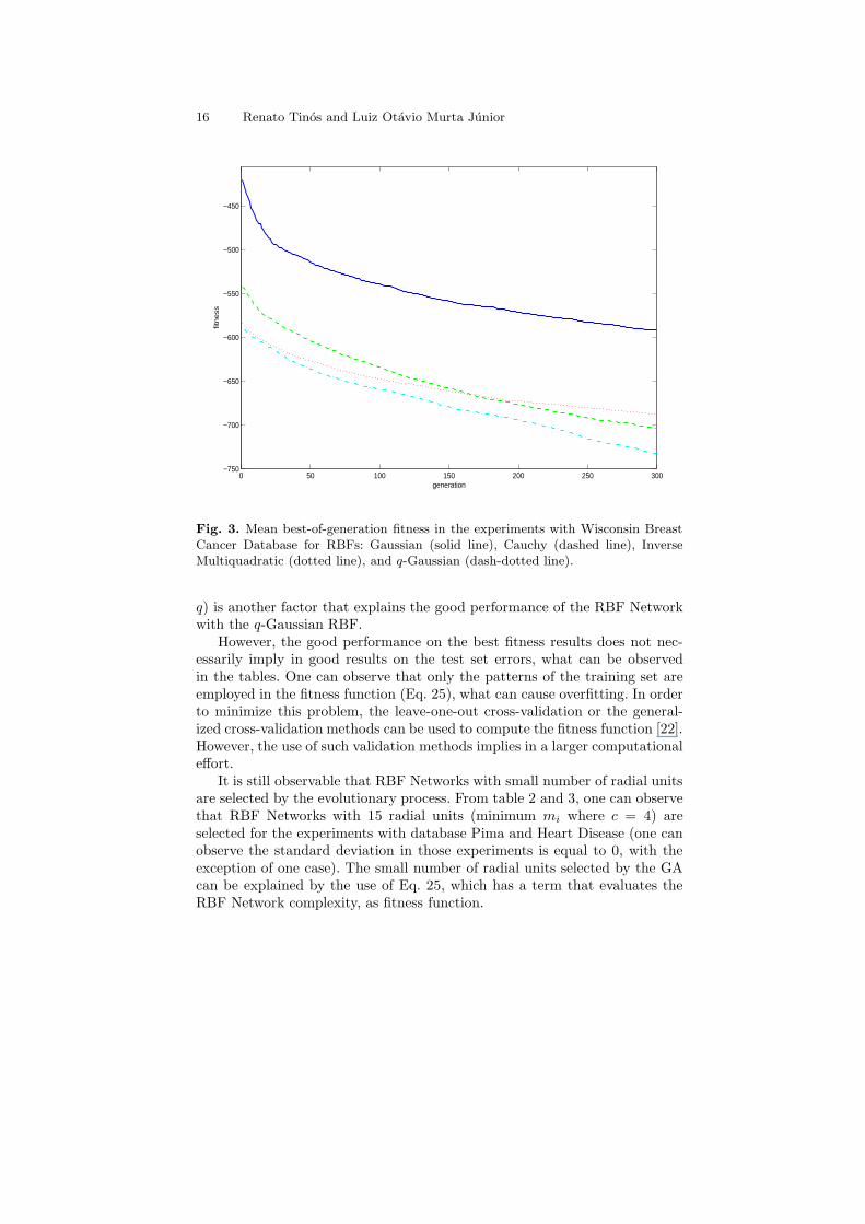
radial units of the RBF Network generated from the final best individualaveraged over 20 runs are also presented. Figures 3, 4, and 5 show the exper-imental results of the best-of-generation fitness averaged over 20 runs. Fromthe experiments, some results can be observed and are analyzed as follows.

Table 1. Results of the best individual in the last generation for experiments withWisconsin Breast Cancer Database.

Radial Basis FunctionGaussian Cauchy Inv. Multiq. q-Gaussian

Fitness Median -585.94 -696.87 -687.89 -707.08Worst -546.27 -637.17 -640.37 -667.17Best -655.07 -794.26 -726.25 -983.56Mean -591.99 -703.61 -688.31 -732.71STD 33.15 52.19 19.82 76.54

Test Set Errors Mean (%) 2.42 1.85 1.79 1.83STD 0.58 0.23 0.39 0.54

m Mean 34.15 25.75 21.20 27.5STD 6.09 7.69 4.40 12.91

Table 2. Results of the best individual in the last generation for experiments withPima Database.

Radial Basis FunctionGaussian Cauchy Inv. Multiq. q-Gaussian

Fitness Median -428.05 -427.18 -427.79 -428.02Worst -423.97 -422.66 -423.29 -419.92Best -435.06 -430.23 -431.48 -433.57Mean -427.89 -427.34 -427.09 -427.93STD 2.67 1.88 2.27 3.47

Test Set Errors Mean 21.42 20.69 20.64 20.98STD 0.77 0.97 0.91 0.99

m Mean (%) 15.00 15.00 15.00 15.00STD 0.00 0.00 0.00 0.00

One can observe that the performance of RBF Networks with differentRBFs are different, what was observed in the experiments presented in [13]too. Like in the experiments presented in [13], the influence of the RBF isproblem dependent. When the results of the RBF Networks with Gaussian,Cauchy, and Inverse Multiquadratic functions are compared, it is possibleto observe that the Gaussian RBFs presents the best performance in theexperiments with database Pima, the Cauchy presents the best performancewith database Breast Cancer, while the Inverse Multiquadratic presents thebest performance in the experiments with database Heart Disease.

Use of the q-Gaussian Function in Radial Basis Function Networks 15

Table 3. Results of the best individual in the last generation for experiments withHeart Disease Database.

Radial Basis FunctionGaussian Cauchy Inv. Multiq. q-Gaussian

Fitness Median -120.73 -133.34 -138.76 -136.94Worst -103.92 -128.22 -134.42 -128.53Best -126.72 -143.56 -149.34 -143.71Mean -120.27 -133.93 -139.53 -137.28STD 5.35 3.56 3.69 3.89

Test Set Errors Mean 24.00 16.04 17.59 18.93STD 2.73 1.16 1.63 2.98

m Mean (%) 15.05 15.00 15.00 15.00STD 0.22 0.00 0.00 0.00

When the shape of the RBFs are compared (Figure 2), one can observe thatthe Gaussian function presents a higher local activation, which is interestingin the experiments with database Pima, but presents a clear disadvantage inother experiments. It is still possible to observe that the optimization of thewidths of the RBFs is beneficial, as the fitness decays during the evolutionaryprocess, but the choice of the RBF generally has a big influence in the fitnessperformance.

The RBF Network with q-Gaussian RBF presents fitness results better orsimilar to those obtained by the RBF Network with the Gaussian RBF in theexperiment with database Pima and with the Cauchy RBF in the experimentwith database Breast Cancer. In the experiment with database Heart Disease,the results obtained by the RBF Network with q-Gaussian RBF are worsethan those obtained by the RBF Network with Inverse Multiquadratic RBF.However, the results of the q-Gaussian RBF are better that the results of theGaussian and Cauchy RBFs.

The good results of the RBF Network with the q-Gaussian RBF can beexplained because the GA generally can find good values of the parameterq for the radial units, which generates a better choice for the shape of theRBFs. While the final values of q in the experiments with database Pima areclose to 1, i.e., the shape of the q-Gaussian functions is similar to the shapeof the Gaussian function, which showed to be a good choice for this database,the values of q are higher in the experiments for the other databases. Thebetter performance of the Inverse Multiquadratic RBF in the Heart DiseaseDatabase can be explained by the use of a maximum allowed value of q equalto 3, which is the value of q where the q-Gaussian RBF reproduces the shapeof Inverse Multiquadratic RBF (see Figure 2 and Eq. 21). In the experimentswith the Heart Disease Database, values of q equal or larger than 3 should befound, which implies in RBFs with longer tails, like the Inverse MultiquadraticRBF. The use of radial units with different RBF shapes (different values of

16 Renato Tinos and Luiz Otavio Murta Junior

0 50 100 150 200 250 300−750

−700

−650

−600

−550

−500

−450

generation

fitn

ess

Fig. 3. Mean best-of-generation fitness in the experiments with Wisconsin BreastCancer Database for RBFs: Gaussian (solid line), Cauchy (dashed line), InverseMultiquadratic (dotted line), and q-Gaussian (dash-dotted line).

q) is another factor that explains the good performance of the RBF Networkwith the q-Gaussian RBF.

However, the good performance on the best fitness results does not nec-essarily imply in good results on the test set errors, what can be observedin the tables. One can observe that only the patterns of the training set areemployed in the fitness function (Eq. 25), what can cause overfitting. In orderto minimize this problem, the leave-one-out cross-validation or the general-ized cross-validation methods can be used to compute the fitness function [22].However, the use of such validation methods implies in a larger computationaleffort.

It is still observable that RBF Networks with small number of radial unitsare selected by the evolutionary process. From table 2 and 3, one can observethat RBF Networks with 15 radial units (minimum mi where c = 4) areselected for the experiments with database Pima and Heart Disease (one canobserve the standard deviation in those experiments is equal to 0, with theexception of one case). The small number of radial units selected by the GAcan be explained by the use of Eq. 25, which has a term that evaluates theRBF Network complexity, as fitness function.

Use of the q-Gaussian Function in Radial Basis Function Networks 17

0 50 100 150 200 250 300 350 400 450 500

−428

−426

−424

−422

−420

−418

−416

−414

−412

−410

−408

−406

generation

fitn

ess

Fig. 4. Mean best-of-generation fitness in the experiments with Pima Database forRBFs: Gaussian (solid line), Cauchy (dashed line), Inverse Multiquadratic (dottedline), and q-Gaussian (dash-dotted line).

7 Conclusions

The use of the q-Gaussian function as a radial basis function in RBF Networksemployed in pattern recognition problems is investigated here. The use of q-Gaussian RBFs allows to modify the shape of the RBF by changing the realparameter q, and to employ radial units with different RBF shapes in a sameRBF Network. An interesting property of the q-Gaussian function is that it cancontinuously and smoothly reproduce different radial basis functions, like theGaussian, the Inverse Multiquadratic, and the Cauchy functions, by changinga real parameter q. Searching for the values of the parameter q related to eachradial unit via GAs implies in searching for the best configuration of RBFs tocover the pattern space according to the training set.

The choice of different RBFs is generally problem dependent, e.g., whenRBF Networks with Gaussian, Cauchy and Inverse Multiquadratic RBFs arecompared in Section 6, each one of these three RBFs presented the best per-formance in one different experiment. By adjusting the parameter q using theGA, the RBF Network with q-Gaussian RBF can present, in the experimentspresented in Section 6, performance similar to those reached by the RBF Net-work with the RBF that reached the best result. One can observe that the GA

18 Renato Tinos and Luiz Otavio Murta Junior

0 50 100 150 200 250 300

−140

−130

−120

−110

−100

−90

−80

−70

generation

fitn

ess

Fig. 5. Mean best-of-generation fitness in the experiments with Heart DiseaseDatabase for RBFs: Gaussian (solid line), Cauchy (dashed line), Inverse Multi-quadratic (dotted line), and q-Gaussian (dash-dotted line).

can search for the best configuration of the values of q, changing the shape ofthe RBFs, and allowing good results.

Acknowledgments:

This work is supported by Fundacao de Amparo a Pesquisa do Estado de Sao

Paulo (FAPESP) under Proc. 2004/04289-6 and 2006/00723-9.

References

1. N. M. Atakishiyev. On a one-parameter family of q-exponential functions. Jour-

nal of Physics A: Mathematical and General, 29(10):L223 –L227, 1996.2. N. M. Atakishiyev. On the fourier-gauss transforms of some q-exponential and

q-trigonometric functions. Journal of Physics A: Mathematical and General,29(22):7177 – 7181, 1996.

3. N. M. Atakishiyev and P. Feinsilver. On the coherent states for the q-Hermitepolynomials and related Fourier transformation. Journal of Physics A: Mathe-

matical and General, 29(8):1659–1664, 1996.

Use of the q-Gaussian Function in Radial Basis Function Networks 19

4. L. C. Biedenharn. the quantum group suq(2) and a q-analogue of the bosonoperators. Journal of Physics A: Mathematical and General, 22(18):l873–l878,1989.

5. S. Billings, H.-L. Wei, and M. A. Balikhin. Generalized multiscale radial basisfunction networks. Neural Networks, 20:1081–1094, 2007.

6. S. Billings and G. Zheng. Radial basis function network configuration usinggenetic algorithms. Neural Networks, 8(6):877–890, 1995.

7. E. P. Borges. A possible deformed algebra and calculus inspired in nonextensivethermostatistics. Physica A: Statistical Mechanics and its Applications, 340(1-3):95 – 101, 2004.

8. S. Chen, C. F. N. Cowan, and P. M. Grant. Orthogonal least squares learningalgorithm for radial basis function networks. IEEE Transactions on Neural

Networks, 2(2):302 – 309, 1991.9. R. Floreanini and L. Vinet. Q-orthogonal polynomials and the oscillator quan-

tum group. Letters in Mathematical Physics, 22(1):45–54, 1991.10. R. Floreanini and L. Vinet. Quantum algebras and q-special functions. Annals

of Physics, 221(1):53–70, 1993.11. D. B. Fogel, E. D. Wasson, and E. M. Boughton. Evolving neural networks for

detecting breast cancer. Cancer Letters, 96:49–53, 1995.12. M. Gell-Mann and C. Tsallis. Nonextensive Entropy - Interdisciplinary Appli-

cations. Oxford University Presss, 2004.13. C. Harpham and C. W. Dawson. The effect of different basis functions on a

radial basis function network for time series prediction: A comparative study.Neurocomputing, 69:2161–2170, 2006.

14. C. Harpham, C. W. Dawson, and M. R. Brown. A review of genetic algorithmsapplied to training radial basis function networks. Neural Computing and Ap-

plications, 13(3):193–201, 2004.15. Y. Liu and X. Yao. Evolutionary design of artificial neural networks with dif-

ferent nodes. In Proc. of the IEEE Conference on Evolutionary Computation,

ICEC, pages 670 – 675, 1996.16. E. P. Maillard and D. Gueriot. Rbf neural network, basis functions and genetic

algorithms. In Proc. of the IEEE International Conference on Neural Networks,volume 4, pages 2187 – 2190, 1997.

17. O. L. Mangasarian and W. H. Wolberg. Cancer diagnosis via linear program-ming. SIAM News, 23(5):1–18, 1990.

18. D. S. McAnally. Q-exponential and q-gamma functions. i. q-exponential func-tions. Journal of Mathematical Physics, 36(1):546 – 573, 1995.

19. M. Mitchell. An Introduction to Genetic Algorithms. MIT Press, 1996.20. J. Moody and C. Darken. Fast learning in networks of locally-tuned processing

units. Neural Computation, 1:281 – 294, 1989.21. L. Nivanen, A. Le Mehaute, and Q. A. Wang. Generalized algebra within a

nonextensive statistics. Reports on Mathematical Physics, 52(3):437–444, 2003.22. M. Orr. Introduction to radial basis function networks. Center for Cognitive

Science, Edinburgh University, Scotland, U. K., 1996.23. L. J. Rogers. Second memoir on the expansion of certain infinite products.

Proceedings of London Mathematical Society, 25:318–343, 1894.24. J. W. Smith, J. E. Everhart, W. C. Dickson, W. C. Knowler, and R. S. Johannes.

Using the adap learning algorithm to forecast the onset of diabetes mellitus. InProc. of the Symposium on Computer Applications and Medical Care, pages261– 265, 1988.

20 Renato Tinos and Luiz Otavio Murta Junior

25. R. Tinos and M. H. Terra. Fault detection and isolation in robotic manipu-lators using a multilayer perceptron and a rbf network trained by kohonen’sself-organizing map. Rev. Controle e Automacao, 12(1):11–18, 2001.

26. C. Tsallis. Possible generalization of boltzmann-gibbs statistics. Journal of

Statistical Physics, 52:479–487, 1988.27. C. Tsallis. What are the number that experiments provide? Quımica Nova,

17:468, 1994.28. S. Umarov, C. Tsallis, and S. Steinberg. On a q-central limit theorem consistent

with nonextensive statistical mechanics. Milan Journal of Mathematic, DOI -10.1007/s00032-008-0087-y, 2008.

29. T. Yamano. Some properties of q-logarithm and q-exponential functions intsallis statistics. Physica A, 305:486–496, 2002.