Sequential Gaussian simulation using multi-variable cokriging

SGS-MultiCorkrig

Sequential Gaussian simulation using multi-variable cokriging

Kiki (Hong) Xu∗†, Jian Sun†, Brian Russell∗, Kris Innanen†

ABSTRACT

Uncertainty analysis is a key element in reservoir properties prediction, and many tech-niques have been developed, such as simulation, which is usually performed by least squaremethod. Least square estimation is a classic and well known approach as a best fit solver,which is equivalent to simple kriging or cokriging system in case of geostatistics filed. In-spired by the distinction of simple and ordinary system in geostatistics and benefited fromthe extended cokriging system, for reservoir properties prediction, we propose an approachto implement sequential simulation with multiple priori information using the extendedcokriging system. As it implies, the conditional mean and variance in the posterior distri-bution are obtained by performing the extended cokriging system. Comparison betweenthis approach and traditional sequential simulation using least square method are discussedin sense of semivariogram. The advantage are further analyzed through the estimated errormap, which indicates that simulation using the extended geostatistics method can producean more an accurate map, especially dealing with the data has the dramatical changes.

INTRODUCTION

Geostatistical inversion methods can reduce uncertainty in the reservoir properties pre-diction away from the control points, by integrating well log data (sampled sparsely butaccurate) as primary data and seismic data (sampled well but band limited) as secondarydata. Number of discussions have been presented. One of the classic methods is determinis-tic inversion, such as kriging, cokriging. To use variate secondary data, Russell et al. (2002)combined cokriging and multiattribute transforms. As Russell et al. (2002) illustrated, theimproved secondary input of cokriging can be generated by multi-attribute analysis. Babakand Deutsch (2009) improved the cokriging model by merging all secondary data into asingle super secondary data and then implementing the cokriging system with this singlemerged secondary data. Two or more than two secondary variables were employed in theestimation system without knowing stationary mean was presented by (Xu et al., 2015,2016). However, a limitation is that deterministic methods provide the result that has trou-ble capturing the natural variability and heterogeneity of reservoirs due to the smoothingeffect.

The sequential simulation technique provides a series of equal valid and possible real-izations that indirectly reflect the distribution of reservoir properties. Deutsch and Journel(1992) calculated the kriging mean and variance at unmeasured locations and simulated thevalue at those points by using Sequential Gaussian Simulation (SGS). A posterior Gaus-sian distribution can be also described by a simple kriging system, therefore it is possibleto draw samples of a posteriori probability density function by using sequential simula-tion(Hansen et al., 2006). Ligas and Kulczycki (2010) observed least squares prediction

∗Hampson Russell Software, CGG†CREWES Project,University of Calgary

CREWES Research Report — Volume 28 (2016) 1

Xu et al.,

and geostatistical method of simple kriging are equivalent.

In this paper, we re-investigate the relation between least square method and geostatis-tics methods which shows that both least square and simple geostatistics methods are equiv-alent to conditional expectation in the posterior distribution. It indicates that the advantageof ordinary approach, compared to the simple system, are also superior to least squaremethod. Furthermore, to take the benefit from the extended corkiging system, we imple-ment the sequential simulation with the posterior mean and covariance calculated from theextended cokriging system. Finally, this approach is applied to Black foot data for porositysimulation.

METHOD

Any estimation, interpolation, projection or transformation problem, based on a givendata d, can be treated as the inversion of model parameters that generates the data underaction of the operator G (Claerbout, 1992):

d = Gm (1)

Therefore, the problem becomes to find the best fit model m with the projection opera-tor G using the observed data d. Here, the projection operator is relatively unconventionalwhich leads to G does not needs to be dependent on any physical law. The classical princi-ple to solve Eq. 1 is the estimated model has to satisfy the unbiased minimum error variancecriteria, which turns the above problem into the well-known least-square prediction.

To further understand least-square prediction, the simplest case with one single esti-mate, instead of a set, is discussed in the following context. It’s known that the least-squaremethod gives an unique, best fit estimate if three criteria are met: linearity, unbiasedness,and minimum error variance. Based on these assumptions, an estimate φ can be describedas the weighted (λ) combination of a realization Ψ, which can be considered as a secondorder stationary random function with zero mean (Heiskanen and Moritz, 1967; Dermanis,1984). In matrix notation, the predictor can be written as

φ = λTΨ (2)

If the mean of the second order stationary random realization Ψ is not zero, whichmeans the second criteria, unbiasedness, does not hold, one has to transfer the observeddata into a new zero-mean random function by subtracting its true (or estimated) mean(Dermanis, 1984; Ligas and Kulczycki, 2010). The optimal set for coefficient vector λcan be calculated by minimizing the mean square error (prediction error variance), and thesolution can be expressed as

λ = C−1c (3)

where, C is the covariance matrix of an observed dataset (i.e., Ψ), c is the vector of covari-ances between the estimate point (φ) and the observed data (Ψ).

The least square estimation can be obtained by substituting the coefficient vector λ intothe predictor Eq. (2), written as

φ = cTC−1Ψ (4)

2 CREWES Research Report — Volume 28 (2016)

SGS-MultiCorkrig

and, in case of non-zero mean realization, it can be expressed as

φ = µφ + cTC−1(Ψ− µΨ) (5)

with the prediction error variance calculated by

Var(R) = Cφ0 − cTC−1c (6)

where, Cφ0 is the variance of φ, or the sill of the φ semivariogram.

The above derivation indicates that the least square prediction is equivalent to a simplekriging (SK) system when the prediction becomes to the interpolation problem (Ψ → Φ).The unbiased condition is satisfied in an automatic manner regardless of choice of weights.Beyond that, (Tarantola, 2005) demonstrated that least square problem (Eq.1) can also bedescribed as the posterior Gaussian probability density in the model space

P(m|d) = const.exp[−1

2(m− µm|d)

TΣ−1m|d(m− µm|d)

](7)

with the conditional mean as

µm|d = µm + (GCm)T (GCmGT + Cd)

−1(d− µd) (8)

and the conditional covariance matrix

Σm|d = Cm − CmGT (GCmGT + Cd)−1(d− µd) (9)

where, µm and µd are the mean vector for model and given data respectively, Cm and Cd

are the model and data covariance matrices. Here, as mentioned before, the conditionalmean and covariance are identical to the simple kriging (SK) mean and covariance.

Following the demonstration prensented by Tarantola (2005), Hansen et al. (2006) ex-pand the Gaussian linear inverse problem involving two types of dataset. The projectionbetween model parameter and two given datasets is given by

d0 = Gm (10)

where,

d0 =

[a0

b0

],Cd =

[Caa Cab

CTab Cbb

],µ0 =

[µa0

µb0

](11)

Again, it can be described as the posterior Gaussian probability density in the modelspace based on two datasets

P(m|a0,b0) = const.exp[−1

2(m− µm|a0,b0)

TΣ−1m|a0,b0(m− µm|a0,b0)

](12)

Here, the conditional mean µm|a0,b0 and covariance Σm|a0,b0 have the same matrix no-tation as the previous illustrated in Eq. (8) and Eq. (9), except the data covariance matrix


Xu et al.,

is replaced by Eq. (11). Therefore, the conditional mean µm|a0,b0 and covariance Σm|a0,b0coincide with the mean and covariance solved by a traditional simple cokriging (SCK)system.

Analogously, the inverse problem can be expanded and be described as the posteriorGaussian probability distribution based on given N-datasets (d =

[dT1 ,d

T2 , . . . ,d

Tn

]T),

P(m|d1, . . . ,dn) = const.exp[−1

2(m− µm|(d1,...,dn))

TΣ−1m|(d1,...,dn)(m− µm|(d1,...,dn))

](13)

where the conditional mean µm|(d1,...,dn) and covariance Σm|(d1,...,dn) are equivalent to themean and prediction error covariance calculated from an extended simple cokriging (SCK)system involving N-datasets demonstrated by Xu et al. (2015, 2016).

By implementing one of the above three methods in a random sequence, a sequentialconditional (co)simulation can be achieved (Goovaerts, 1997; Gloaguen et al., 2005b,a;Gomez-Hernandez et al., 2005; Hansen and Mosegaard, 2008; Journel and Huijbregts,1978). As we know, sequential simulation is a technique to generate a series of inde-pendent realizations based on the known model parameters and given data. The posteriorprobability density function based on known model parameters and given data, at any lo-cation xi, needs to be calculated and then be moved to the next location depending onthe random sequence. Assume we have known model parameters Φ0(xi) at m locations(xi ∈ {x1, x2, . . . , xm}) and two given data A and I, one estimated realization at other lo-cations (xj ∈ {x1, x2, . . . , xn}) using sequential conditional simulation based on knownmodel parameters Φ(xi) and given data A and I can be performed as following steps,

(1) Sorting the estimated locations into a random sequence {x1, x2, . . . , xn}.

(2) Visit the grid point xj according to the path generated in step (1).

(3) Calculating the conditional mean and covariance at visited location xj based onknown Φ0 and pre-simulated model parameters Φ(x1, ..., xj−1) and two given datasets (Aand I), by performing one of three methods mentioned above, i.e., least-square prediction,simple geostatistical methods, or conditional expectation approach.

(4) Build the posterior probability distribution P {Φ(xj)|Φ0,A, I,Φ(x1, ..., xj−1)}, anddraw a random value.

(5) Add the simulated value at location xj into the known dataset.

(6) Move to the next location xj+1 in the sequence, and repeat step 2-5 until the lastgrid point in the sequence is encountered.

Note that the conditional mean and covariance are calculated by least square (LS) orsimple geostatistical methods (SK, SCK, or extended SCK), and both of them are equiva-lent to conditional expectation in the sense of Gaussian random field (Ligas and Kulczycki,2010). In other words, one shares the strengths as others do, as well as the drawbacks. Oneof the defects is that, either least-square and conditional expectation or the simple geosta-


SGS-MultiCorkrig

tistical methods, requires a zero-mean second order stationary random realization as theobserved data. Again, the known mean needs to be utilized to transfer the data into a zero-mean random function if the unbiasedness does not hold. However, in practice, the meanis usually unknown and is replaced by an estimated mean which can be calculated, for ex-ample, by the trend removal technique (Dermanis, 1984). Beyond that, the automatic-meetunbiased condition implies that no constraint is applied to the coefficient (weight) vectorduring the process. This may generate singular value occurring in the estimation when thesignificant changes of magnitude between the objective and observed data occur.

The procedure we propose for sequential conditional Gaussian simulation (SCGS) isinspired by the ongoing development into the extend corkging system (Xu et al., 2015).Detailed comparisons between simple, ordinary, and rescaled ordinary methods for krigingand cokriging were discussed by Goovaerts (1998). It concluded that, instead of a sta-tionary mean in simple (co)kriging system, the (rescaled) ordinary cokriging (OCK andROCK) utilizing the estimated local mean. Further more, compared to two constraints ofthe ordinary cokriging (OK), only one unbiasedness constraint applied for the weight vec-tor in the rescaled cokriging (ROCK) system lessens the risk of producing unacceptableestimates, such as negative values (Goovaerts, 1998; Xu et al., 2016).

Also the extended (rescaled) ordinary cokriging equation allows for more than two sec-ondary variables participating in the estimation system without requiring stationary meanof model parameters to be known (Xu et al., 2015, 2016). Therefore, in this paper, weperform the sequential conditional Gaussian simulation (SCGS) by replacing the 3rd stepillustrated above with the extend (rescaled) ordinary cokriging (OCK and ROCK) systemto obtain the conditional mean and covariance. Investigation of differences between sim-ulation using least square method, simulation with extend ordinary cokriging (OCK), andsimulation with extended rescaled ordinary cokriging (ROCK) system are analyzed.

IMPLEMENTATION

Neighborhood search and pre-calcuated covariance

Before performing the simulation process, the computation efficiency will be discussedby considering extend ordinary cokriging system. Based on the previous research (Xu et al.,2015), the extend ordinary cokriging (OCK) system involving two secondary variables canbe written in matrix notation, as

CΦΦ CΦA CΦI 1 0 0CAΦ CAA CAI 0 1 0CIΦ CIA CII 0 0 11T 0 0 0 0 00 1T 0 0 0 00 0 1T 0 0 0

λ1

λ2

λ3

α1

α2

α3

=

Cφ0Φ

Cφ0A

Cφ0I

100

(14)

In the implementation of sequential conditional Gaussian simulation (SCGS), the co-variance matrix becomes larger and larger as the iteration number of simulation increases,which makes the approach considerably time consuming, or possibly even being incalcu-lable. However, in the view of geostatistics (Deutsch et al., 1998), data far beyond the


Xu et al.,

range of semivariogram has little contribution in the conditioning mean and covariance ofposterior probability distribution. Therefore, the covariance matrix in extended ordinarycokriging (OCK) system can be limited into an acceptable subset with the range in gridpoint.

Even though the covariance matrix is restricted in a small set, the calculation of covari-ance in each iteration is still a computational burden. To make the utmost of calculatedcovariance in previous iterations, and to avoid the repetitive computation of covariance atthe same location, the pre-calculated covariance table is utilized. This ensures the covari-ance between two identical locations is only calculated once. In addition, for an isotropicmodel, the covariance function does not depend on absolute locations, but rather on thedistance between two locations. Therefore, the pre-calculated covariance table is very com-putational efficient. Another advantage is, the covariance between two specified locationsis identified with an unique label, which can be easily referenced during the iteration.

Initial input of LS, extend OCK and ROCK method

The survey data was recorded from the Blackfoot field located in southern Alberta in1995 for Canadian Petroleum. There were twelve wells involved in this study case, allof which contained the calculated porosity logs. An average porosity value between thepicked top and base of the zone of interest in each well, is considered as the sampledknown “model parameters” (Ψ0). Figure 1 shows that the well distribution on the surveyarea and the porosity value at each well location.

FIG. 1: Well distribution and average porosity value in the zone of interest.

Representative secondary inputs are attribute key elements for geostatistical methods.Instead of directly using acquired seismic data, two slices extracted from different 3-Dvolumes, the acoustic impedance inversion and the stacked P-wave seismic data, are used.The inversion volume was obtained using Hampson-Russell Software (Russell et al., 2002).First, build an initial model from the well logs and pick horizon on the seismic section.Second, stop perturbing this model when the synthetic seismogram has a best match with


SGS-MultiCorkrig

(a) The final CDP stack and interested zone

(b) P-wave impedance section and interested zone

FIG. 2: Crossline 18 from the 3-D seismic volume.

the original data. Crossline 18 extracted from the seismic volume is illustrated in Figure 2showing a seismic input line (Figure 2a) and an inverted impedance line (Figure 2b).

An inversion slice was trimmed by picking 10ms average window below the channeltop from 3D inverted volume. Similarly, we extracted three data slices, seismic amplitude,amplitude envelope, and instantaneous phase, by applying a 10ms window of RMS averageon the zone of interest. To choose appropriate inputs for simulation, correlation coefficientswere calculated between the porosity and all four created data slices. The best two corre-lation coefficients were observed from inversion slice and seismic amplitude slice, whichwere -0.65 and 0.41, respectively. Thus, in this case, seismic amplitude slice (indicated asA) shown in Figure 3 and inversion slice (indicated as I) shown in Figure 4 are consideredas the two conditioning datasets for the sequential simulation study.

As discussed previously, to make the approach computationally efficient, the distanceand covariance table are calculated before the iteration, delineated in Figure 5 and Fig-ure 6, respectively. Figure 6 shows the covariance tables among porosity, RMS amplitude,and acoustic P-impedance, are diagonal symmetric due to the isotropic nature of relations.The limited covariance matrices in Eq. 14 can be readily indexed from the pre-calculated


Xu et al.,

FIG. 3: The average RMS amplitude slice at the interested zone.

FIG. 4: The average acoustic P-impedance slice at the interested zone.

covariance tables, respectively.

Simulated realizations using SCGS with extend LS, OCK, and ROCK

The sequential conditional Gaussian simulation is performed by implementing the pro-cedure 1-6 already demonstrated, except that the least-square (or simple geostatistics) con-


SGS-MultiCorkrig

FIG. 5: Precalculated distance table on the entire area.

FIG. 6: Precalculated covariance table on the entire area among the porosity, P-impedance,and RMS amplitude. (a) CΦΦ, (b) CAA, (c) CII , (d) CΦA, (e) CΦI , (f) CAI

ditional mean and variance calculation is replaced by an extend ordinary cokriging, or byan extended rescaled ordinary cokriging system, respectively. 1000 independent realiza-tions are generated by performing the sequential simulation process with 1000 randompaths, conditioned to known porosity (Figure 1), inverted P-impedance data (Figure 4), andRMS amplitude slice (Figure 3). Figure 7 and Figure 9 shows 9 of all 1000 realizationsby performing sequential conditional simulation using extend OCK and ROCK systems,respectively.

Note that all realizations shown in Figure 7 and in Figure 9 delineate the correct trendsof porosity variation, i.e., high porosity values around well 08-08, 09-08, 29-08, 16-08 andaround the right bottom corner with well 13-16, which can be identified using the priorinformation of known “model parameters” shown in Figure 1. However, the SCGS withextend OCK method generated negative values in all realizations (see in Figure 7) which


Xu et al.,

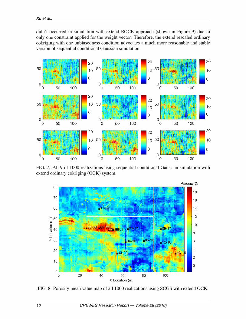
didn’t occurred in simulation with extend ROCK approach (shown in Figure 9) due toonly one constraint applied for the weight vector. Therefore, the extend rescaled ordinarycokriging with one unbiasedness condition advocates a much more reasonable and stableversion of sequential conditional Gaussian simulation.

FIG. 7: All 9 of 1000 realizations using sequential conditional Gaussian simulation withextend ordinary cokriging (OCK) system.

FIG. 8: Porosity mean value map of all 1000 realizations using SCGS with extend OCK.


SGS-MultiCorkrig

FIG. 9: All 9 of 1000 realizations using sequential conditional Gaussian simulation withextend rescaled ordinary cokriging (ROCK) system.

FIG. 10: Porosity mean value map of all 1000 realizations using SCGS with ROCK.

The mean porosity maps obtained by SCGS with extend OCK and ROCK based on1000 realizations are shown in Figure 8 and Figure 10. A similar trend of porosity vari-ation on mean maps are achieved by SCGS, either with extended OCK system or usingextended ROCK approach. Both are analogous to the estimated map we illustrated pre-viously (Xu et al., 2015), which reinforces the validity and feasibility of the sequential


Xu et al.,

conditional simulation using an extend cokriging system presented in this paper. Also notethe difference between SCGS with extend OCK and with ROCK, porosity values estimatedby ROCK are higher than those estimated using OCK, and negative values are avoided.

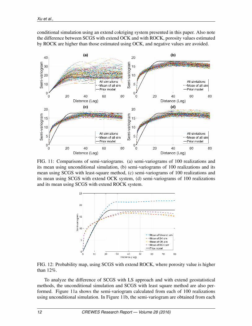
FIG. 11: Comparisons of semi-variograms. (a) semi-variograms of 100 realizations andits mean using unconditional simulation, (b) semi-variograms of 100 realizations and itsmean using SCGS with least-square method, (c) semi-variograms of 100 realizations andits mean using SCGS with extend OCK system, (d) semi-variograms of 100 realizationsand its mean using SCGS with extend ROCK system.

FIG. 12: Probability map, using SCGS with extend ROCK, where porosity value is higherthan 12%.

To analyze the difference of SCGS with LS approach and with extend geostatisticalmethods, the unconditional simulation and SCGS with least square method are also per-formed. Figure 11a shows the semi-variogram calculated from each of 100 realizationsusing unconditional simulation. In Figure 11b, the semi-variogram are obtained from each


SGS-MultiCorkrig

of 100 realizations using SCGS with least square method. Figure 11c illustrates the semi-variogram obtained from each of 100 realizations using SCGS with extend OCK system.And comparisons of semi-variograms of each of 100 realizations using SCGS with ex-tend ROCK approach are delineated in Figure 11d. The ergodic fluctuations of condi-tional simulation (Figure 11b,c,d) are noticeable smaller as compared to those observedfor unconditional simulation (Figure 11a). Further analysis are discussed by comparingthe semi-variogram of their mean map, shown in Figure 12. The sill of semi-variogramobtained from unconditional simulation is much higher than conditional simulations withother three approaches.

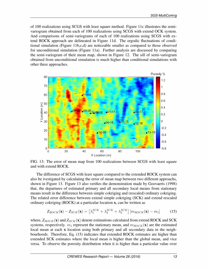
FIG. 13: The error of mean map from 100 realizations between SCGS with least squareand with extend ROCK.

The difference of SCGS with least square compared to the extended ROCK system canalso be ivestigated by calculating the error of mean map between two different approachs,shown in Figure 13. Figure 13 also verifies the demonstration made by Goovaerts (1998)that, the departures of estimated primary and all secondary local means from stationarymeans result in the difference between simple cokriging and (rescaled) ordinary cokriging.The related error difference between extend simple cokriging (SCK) and extend rescaledordinary cokriging (ROCK) at a particular location x, can be written as

ZROCK(x)− ZSCK(x) =[λSCK1 + λSCK2 + λSCK3

][mROCK(x)−m1] (15)

where, ZROCK(x) and ZSCK(x) denote estimations calculated from extend ROCK and SCKsystems, respectively. m1 represent the stationary mean, and mROCK(x) are the estimatedlocal mean at each x location using both primary and all secondary data in the neigh-bourhoods. Therefore, Eq. (15) indicates that extended ROCK estimates are higher thanextended SCK estimates where the local mean is higher than the global mean, and viceversa. To observe the porosity distribution when it is higher than a particular value over


Xu et al.,

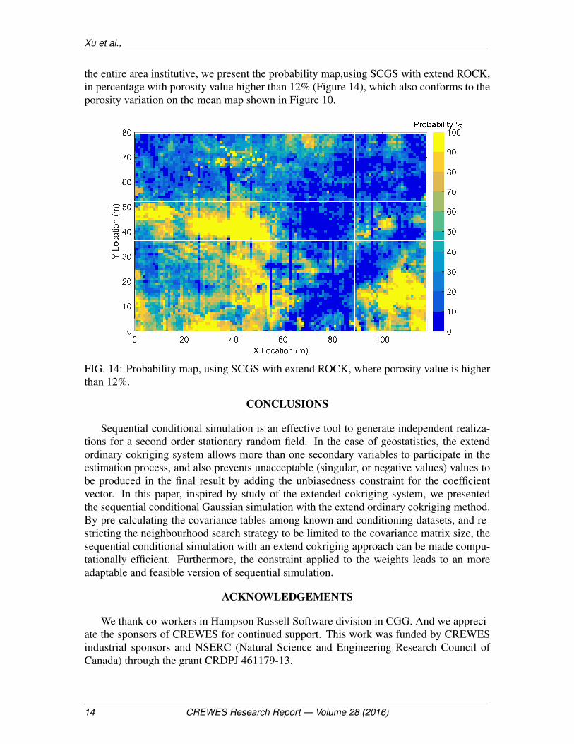
the entire area institutive, we present the probability map,using SCGS with extend ROCK,in percentage with porosity value higher than 12% (Figure 14), which also conforms to theporosity variation on the mean map shown in Figure 10.

FIG. 14: Probability map, using SCGS with extend ROCK, where porosity value is higherthan 12%.

CONCLUSIONS

Sequential conditional simulation is an effective tool to generate independent realiza-tions for a second order stationary random field. In the case of geostatistics, the extendordinary cokriging system allows more than one secondary variables to participate in theestimation process, and also prevents unacceptable (singular, or negative values) values tobe produced in the final result by adding the unbiasedness constraint for the coefficientvector. In this paper, inspired by study of the extended cokriging system, we presentedthe sequential conditional Gaussian simulation with the extend ordinary cokriging method.By pre-calculating the covariance tables among known and conditioning datasets, and re-stricting the neighbourhood search strategy to be limited to the covariance matrix size, thesequential conditional simulation with an extend cokriging approach can be made compu-tationally efficient. Furthermore, the constraint applied to the weights leads to an moreadaptable and feasible version of sequential simulation.

ACKNOWLEDGEMENTS

We thank co-workers in Hampson Russell Software division in CGG. And we appreci-ate the sponsors of CREWES for continued support. This work was funded by CREWESindustrial sponsors and NSERC (Natural Science and Engineering Research Council ofCanada) through the grant CRDPJ 461179-13.


SGS-MultiCorkrig

REFERENCES

Babak, O., and Deutsch, C. V., 2009, Improved spatial modeling by merging multiple secondary data forintrinsic collocated cokriging: Journal of Petroleum Science and Engineering, 69, No. 1, 93–99.

Claerbout, J., 1992, Earth sounding analysis: processing versus inversion: Blackwell science publications.

Dermanis, A., 1984, Kriging and collocation: A comparison: Manuscripta geodaetica, 9, No. 3, 159–167.

Deutsch, C. V., Journel, A. et al., 1998, Geostatistical software library and userâAZs guide: Oxford UniversityPress, New York.

Deutsch, C. V., and Journel, A. G., 1992, Gslb: Geostatistical Software Library and User’s Guide: OxfordUniversity Press.

Gloaguen, E., Marcotte, D., and Chouteau, M., 2005a, A non-linear gpr tomographic inversion algorithmbased on iterated cokriging and conditional simulations, in Geostatistics Banff 2004, Springer, 409–418.

Gloaguen, E., Marcotte, D., Chouteau, M., and Perroud, H., 2005b, Borehole radar velocity inversion usingcokriging and cosimulation: Journal of Applied Geophysics, 57, No. 4, 242–259.

Gomez-Hernandez, J. J., Froidevaux, R., and Biver, P., 2005, Exact conditioning to linear constraints inkriging and simulation, in Geostatistics Banff 2004, Springer, 999–1005.

Goovaerts, P., 1997, Geostatistics for natural resources evaluation: Oxford University Press on Demand.

Goovaerts, P., 1998, Ordinary cokriging revisited: Mathematical Geology, 30, No. 1, 21–42.

Hansen, T. M., Journel, A. G., Tarantola, A., and Mosegaard, K., 2006, Linear inverse gaussian theory andgeostatistics: Geophysics, 71, No. 6, R101–R111.

Hansen, T. M., and Mosegaard, K., 2008, Visim: Sequential simulation for linear inverse problems: Comput-ers & Geosciences, 34, No. 1, 53–76.

Heiskanen, W. A., and Moritz, H., 1967, Physical geodesy: Bulletin Géodésique (1946-1975), 86, No. 1,491–492.

Journel, A. G., and Huijbregts, C. J., 1978, Mining geostatistics: Academic press.

Ligas, M., and Kulczycki, M., 2010, Simple spatial prediction-least squares prediction, simple kriging, andconditional expectation of normal vector: Geodesy and Cartography, 59, No. 2, 69–81.

Russell, B., Hampson, D., Todorov, T., and Lines, L., 2002, Combining geostatistics and multi-attributetransforms: A channel sand case study, blackfoot oilfield (alberta): Journal of Petroleum Geology, 25,No. 1, 97–117.

Tarantola, A., 2005, Inverse problem theory and methods for model parameter estimation: siam.

Xu, H., Russell, B., and Innanen, K. A., 2016, Determination of reservoir thickness and distribution usingimproved rescaled cokriging, in SEG Technical Program Expanded Abstracts 2016, Society of ExplorationGeophysicists, 2967–2971.

Xu, H., Sun, J., Russell, B., and Innanen, K., 2015, Porosity prediction using cokriging with multiple sec-ondary datasets: CSEG Geoconvention.


Sequential Gaussian simulation using multi-variable cokriging

Documents

Transcript of Sequential Gaussian simulation using multi-variable cokriging