ITB J. ICT, Vol. 5, No. 2, 2011, 141-156 141

Copyright © 2011 Published by LPPM ITB, ISSN: 1978-3086, DOI: 10.5614/itbj.ict.2011.5.2.5

Modeling Marine Electromagnetic Survey

with Radial Basis Function Networks

Agus Arif, Vijanth S. Asirvadam & M.N. Karsiti

Dept. of Electrical & Electronic Eng., Universiti Teknologi PETRONAS

Bandar Seri Iskandar, 31750 Tronoh, Perak, Malaysia

Email: agusarif@gmail.com

Abstract. A marine electromagnetic survey is an engineering endeavour to

discover the location and dimension of a hydrocarbon layer under an ocean floor.

In this kind of survey, an array of electric and magnetic receivers are located on

the sea floor and record the scattered, refracted and reflected electromagnetic

wave, which has been transmitted by an electric dipole antenna towed by a

vessel. The data recorded in receivers must be processed and further analysed to

estimate the hydrocarbon location and dimension. To conduct those analyses

successfuly, a radial basis function (RBF) network could be employed to become

a forward model of the input-output relationship of the data from a marine

electromagnetic survey. This type of neural networks is working based on

distances between its inputs and predetermined centres of some basis functions.

A previous research had been conducted to model the same marine

electromagnetic survey using another type of neural networks, which is a multi

layer perceptron (MLP) network. By comparing their validation and training

performances (mean-squared errors and correlation coefficients), it is concluded

that, in this case, the MLP network is comparatively better than the RBF

network1.

Keywords: controlled source electromagnetic method; forward modeling; multilayer

perceptron; radial basis function.

1 Introduction

Marine electromagnetic survey is an engineering endeavour to remotely

determine the location and dimension of a hydrocarbon (i.e. oil, gas, basalt, or

hydrate) layer inside a seabed. There are many techniques to do this kind of

survey, such as by seismic sounding, well-borehole logging, and controlled

source electromagnetic (CSEM) method. In the last method, an electric dipole

antenna, while submerged and deep-towed by a ship, is emitting electro-

magnetic signals throughout the sea and its surrounding in various directions.

1 This manuscript is an extended version of our previous paper, entitled Radial Basis

Function Networks for Modeling Marine Electromagnetic Survey, which had been

presented on 2011 International Conference on Electrical Engineering and Informatics,

17-19 July 2011, Bandung, Indonesia.

142 Agus Arif, Vijanth S. Asirvadam, & M.N. Karsiti

At the same time, an array of electromagnetic receivers is located at the bottom

of the sea (Figure 1). These receivers record the electric and magnetic fields

which are directed, refracted or reflected from all parts of air, seawater,

sediments, and hydrocarbon layer.

Figure 1 Conceptual diagram of the marine CSEM method. A deep-towed

transmitter close to the seafloor injects a current of several hundred amps into the

seawater from an electric dipole, creating magnetic and electric fields that

propagate diffusively into the seafloor. Dipole receivers record the seafloor

electric fields at various ranges from the transmitter (adapted from [1]).

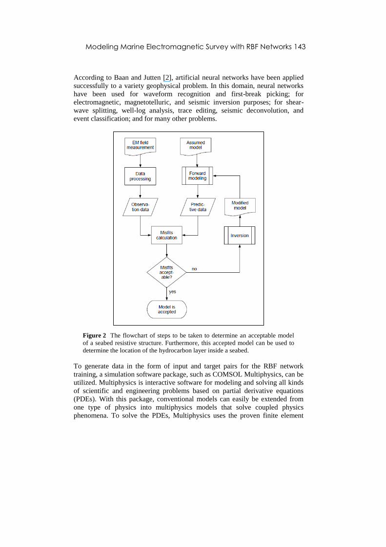
To process the recorded data, several steps should be taken, similar to the

flowchart of Figure 2. First, the electromagnetic field measurement is modified

to be suitable for the next steps and resulted in some observation data.

Meanwhile, a model of seabed structure is assumed to be supplied to forward

modeling step. This step will produce some predictive data that will be

compared to the observation data. Misfits, between these two sets of data,

become an indicator to decide whether the model can be accepted. If the misfits

are considered un-acceptable, the inversion step should be taken to modify the

original model and then supplied again to the step of forward modeling.

Therefore, forward modeling is an essential procedure in finding the acceptable

model, which then can be used to achieve the goal of seabed logging.

Forward modeling is performed to acquire a representation of the real physical

phenomena. The result of this effort is a mathematical model which is

sufficiently suitable to describe the original phenomena. Also, with forward

modeling, a set of predictive or synthetic data can be generated that can be

compared to the real measurement data.

Modeling Marine Electromagnetic Survey with RBF Networks 143

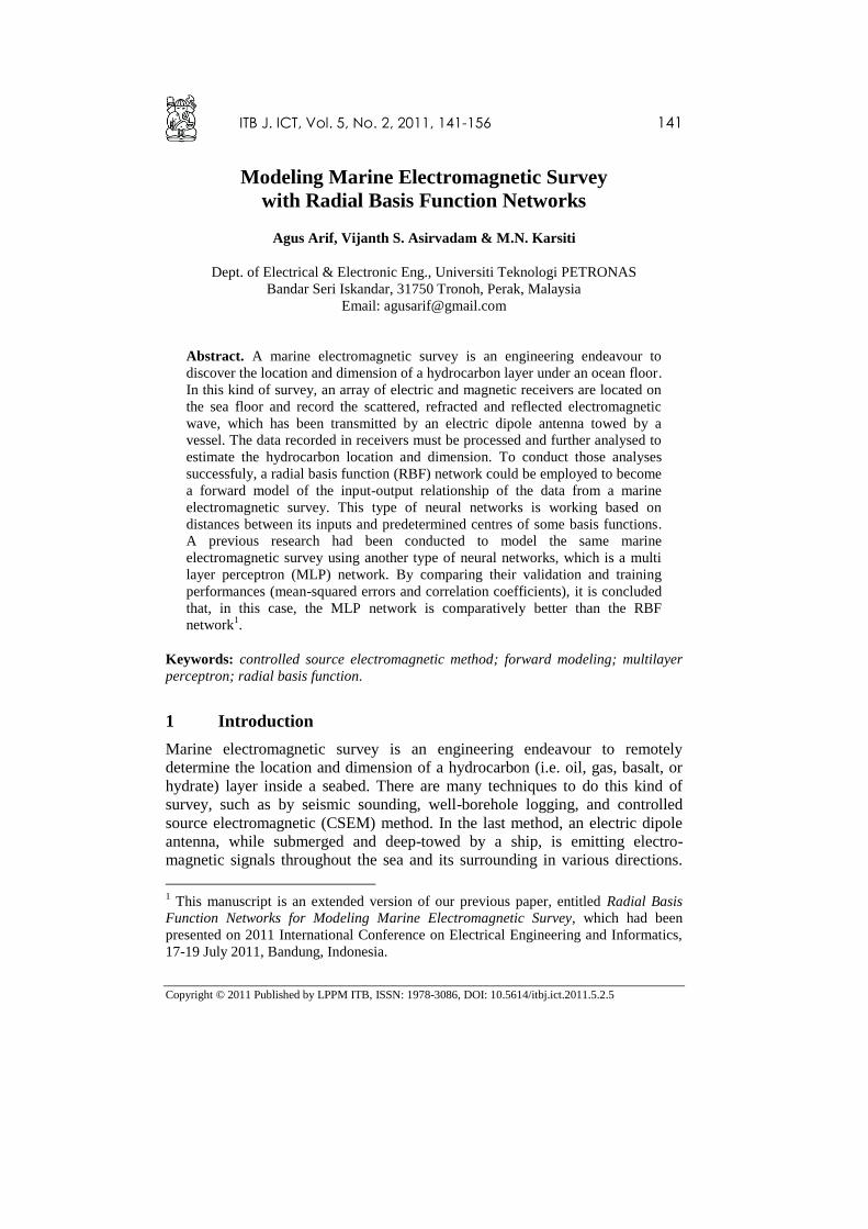
According to Baan and Jutten [2], artificial neural networks have been applied

successfully to a variety geophysical problem. In this domain, neural networks

have been used for waveform recognition and first-break picking; for

electromagnetic, magnetotelluric, and seismic inversion purposes; for shear-

wave splitting, well-log analysis, trace editing, seismic deconvolution, and

event classification; and for many other problems.

Figure 2 The flowchart of steps to be taken to determine an acceptable model

of a seabed resistive structure. Furthermore, this accepted model can be used to

determine the location of the hydrocarbon layer inside a seabed.

To generate data in the form of input and target pairs for the RBF network

training, a simulation software package, such as COMSOL Multiphysics, can be

utilized. Multiphysics is interactive software for modeling and solving all kinds

of scientific and engineering problems based on partial derivative equations

(PDEs). With this package, conventional models can easily be extended from

one type of physics into multiphysics models that solve coupled physics

phenomena. To solve the PDEs, Multiphysics uses the proven finite element

144 Agus Arif, Vijanth S. Asirvadam, & M.N. Karsiti

method (FEM). The software runs the finite element analysis together with

adaptive meshing and error control using a variety of numerical solvers. There

are optional modules provided for several key application areas, such as

electromagnetism and radio frequency (RF). The RF Module contains a set of

application modes adapted to a broad category of electromagnetic simulations

[3],[4].

The objective of this research is to confirm that a radial basis function (RBF)

network could be used to model a CSEM survey. Then, this modeling result will

be compared to the result of a previous research that had been conducted to

model the same marine electromagnetic survey using another type of neural

networks, which is a multi layer perceptron (MLP) network.

2 Methodology

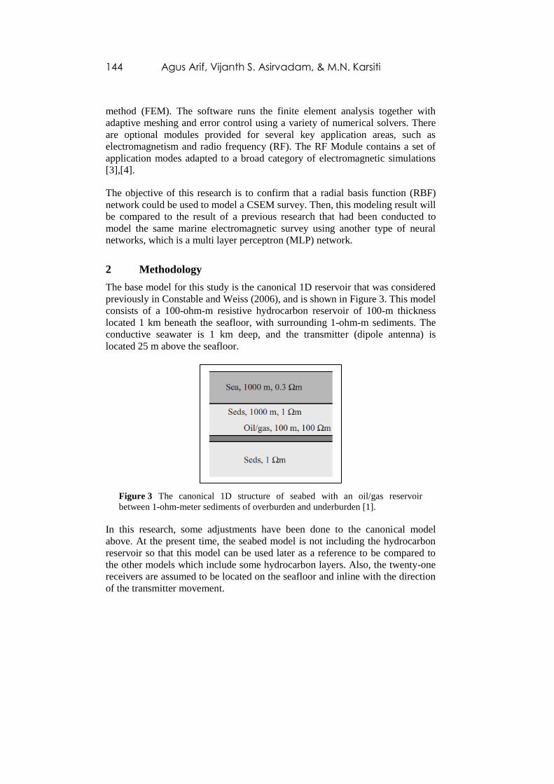
The base model for this study is the canonical 1D reservoir that was considered

previously in Constable and Weiss (2006), and is shown in Figure 3. This model

consists of a 100-ohm-m resistive hydrocarbon reservoir of 100-m thickness

located 1 km beneath the seafloor, with surrounding 1-ohm-m sediments. The

conductive seawater is 1 km deep, and the transmitter (dipole antenna) is

located 25 m above the seafloor.

Figure 3 The canonical 1D structure of seabed with an oil/gas reservoir

between 1-ohm-meter sediments of overburden and underburden [1].

In this research, some adjustments have been done to the canonical model

above. At the present time, the seabed model is not including the hydrocarbon

reservoir so that this model can be used later as a reference to be compared to

the other models which include some hydrocarbon layers. Also, the twenty-one

receivers are assumed to be located on the seafloor and inline with the direction

of the transmitter movement.

Modeling Marine Electromagnetic Survey with RBF Networks 145

2.1 Generating Data

Generally, there are five main steps to generate data using Multiphysics and its

modules [3]; which are preliminary, drawing, physics, calculation, and post-

processing steps. Each step will be further explained, while at the same time a

structure of seabed is being built concurrently, according to the previously

mentioned canonical model.

2.1.1 Preliminary Step

At the beginning of running the Multiphysics software, a template can be

chosen that is appropriate to the model which is being built. In this research, the

work-space dimension is 3D and the suitable application mode is Harmonic

Propagation which is found under Electromagnetic Waves option, inside the RF

Module.

In the main window, all constants that will be used in this modeling can be

defined as in Table 1. The constant values were taken from references [1],[3],

and [5].

Table 1 Constants for the seabed model.

Name Expression Value Description

eps1 80 80 Relative permittivity of seawater

rho1 0.3 [ohm*meter] 0.3 [Ω·m] Resistivity of seawater

sig1 1/rho1 3.333333[S/m] Conductivity of seawater

eps2 30 30 Relative permittivity of sediment

rho2 1 [ohm*meter] 1[Ω·m] Resistivity of sediment

sig2 1/rho2 1[S/m] Conductivity of sediment

eps3 4 4 Relative permittivity of hydrocarbon

rho3 100[ohm*meter] 100[Ω·m] Resistivity of hydrocarbon

sig3 1/rho3 0.01[S/m] Conductivity of hydrocarbon

freq 1[Hz] 1[1/s] Transmitter frequency

txi 10e3[A] 10000[A] Transmitter current

2.1.2 Drawing Step

In this research, the horizontal length of the seabed model is 22 km, and the

vertical length of all layers are in accord with the 1D canonical structure in

Figure 3 (except without the hydrocarbon layer). All layers can be drawn using

Rectangle/Square object which is provided in the tools bar of Multiphysics. The

result of this step is displayed in Figure 4.

146 Agus Arif, Vijanth S. Asirvadam, & M.N. Karsiti

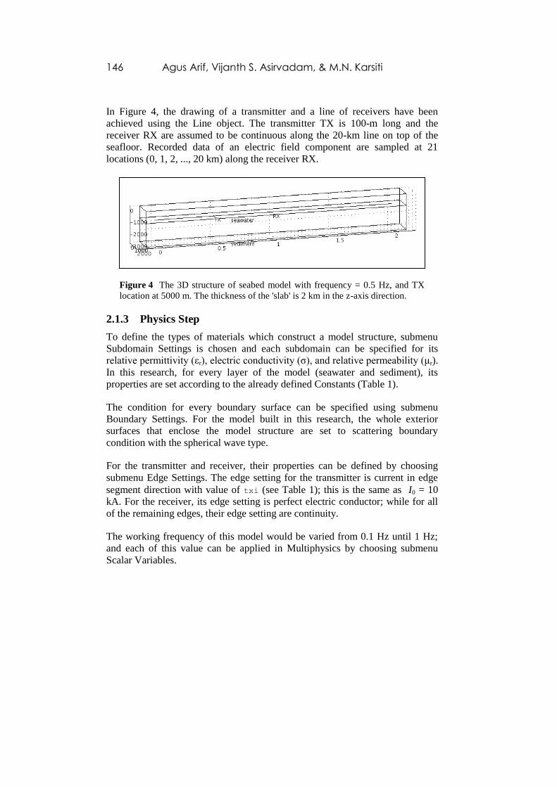
In Figure 4, the drawing of a transmitter and a line of receivers have been

achieved using the Line object. The transmitter TX is 100-m long and the

receiver RX are assumed to be continuous along the 20-km line on top of the

seafloor. Recorded data of an electric field component are sampled at 21

locations (0, 1, 2, ..., 20 km) along the receiver RX.

Figure 4 The 3D structure of seabed model with frequency = 0.5 Hz, and TX

location at 5000 m. The thickness of the 'slab' is 2 km in the z-axis direction.

2.1.3 Physics Step

To define the types of materials which construct a model structure, submenu

Subdomain Settings is chosen and each subdomain can be specified for its

relative permittivity (εr), electric conductivity (σ), and relative permeability (μr).

In this research, for every layer of the model (seawater and sediment), its

properties are set according to the already defined Constants (Table 1).

The condition for every boundary surface can be specified using submenu

Boundary Settings. For the model built in this research, the whole exterior

surfaces that enclose the model structure are set to scattering boundary

condition with the spherical wave type.

For the transmitter and receiver, their properties can be defined by choosing

submenu Edge Settings. The edge setting for the transmitter is current in edge

segment direction with value of txi (see Table 1); this is the same as I0 = 10

kA. For the receiver, its edge setting is perfect electric conductor; while for all

of the remaining edges, their edge setting are continuity.

The working frequency of this model would be varied from 0.1 Hz until 1 Hz;

and each of this value can be applied in Multiphysics by choosing submenu

Scalar Variables.

Modeling Marine Electromagnetic Survey with RBF Networks 147

2.1.4 Calculation Step

After all those initial definitions, drawings, and element specifications, the mesh

for finite element computation can be determined. In this research, the mesh is

customized with the maximum element size is equal to 1000. The result of this

mesh making is displayed in Figure 5.

Figure 5 The mesh of the seabed model with working frequency = 0.5 Hz, and

TX location at 5000 m.

The actual finite element calculation is started by choosing submenu Solve

Problem. While running its computation, the software is displaying the progress

of its calculation. After a certain duration (an average of 1 minute in this

research), the result of problem solving is displayed as a 3D figure of a

subdomain plot. (This type of figure, actually, can be chosen differently by

using submenu Plot Parameters).

2.1.5 Post-processing Step

From various choices in the Postprocessing menu, the Line/ Extrusion option is

chosen to obtain a graph of electric field amplitudes versus the receivers’

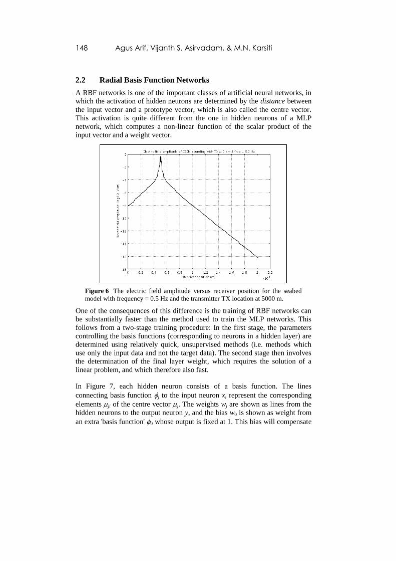
positions, as displayed in Figure 6. In addition, this step is also used to export

data of the electric fields, in a complex number format, which are sampled from

21 locations of the receivers.

All those data generation steps (detailed description about them can be found in

Arif, et al. [6]) had been repeated to simulate the movement of the dipole

antenna in 21 positions (0, 1, 2, …, 20 km) and the 7 variations of working

frequency (0.01, 0.05, 0.1, 0.25, 0.5, 0.75, and 1 Hz). In the end, the result was

3087 values of electric field amplitudes, in a format of real and imaginary parts,

which later will be used to train and test the RBF network as a model of marine

CSEM survey.

148 Agus Arif, Vijanth S. Asirvadam, & M.N. Karsiti

2.2 Radial Basis Function Networks

A RBF networks is one of the important classes of artificial neural networks, in

which the activation of hidden neurons are determined by the distance between

the input vector and a prototype vector, which is also called the centre vector.

This activation is quite different from the one in hidden neurons of a MLP

network, which computes a non-linear function of the scalar product of the

input vector and a weight vector.

Figure 6 The electric field amplitude versus receiver position for the seabed

model with frequency = 0.5 Hz and the transmitter TX location at 5000 m.

One of the consequences of this difference is the training of RBF networks can

be substantially faster than the method used to train the MLP networks. This

follows from a two-stage training procedure: In the first stage, the parameters

controlling the basis functions (corresponding to neurons in a hidden layer) are

determined using relatively quick, unsupervised methods (i.e. methods which

use only the input data and not the target data). The second stage then involves

the determination of the final layer weight, which requires the solution of a

linear problem, and which therefore also fast.

In Figure 7, each hidden neuron consists of a basis function. The lines

connecting basis function j to the input neuron xi represent the corresponding

elements ji of the centre vector j. The weights wj are shown as lines from the

hidden neurons to the output neuron y, and the bias w0 is shown as weight from

an extra 'basis function' 0 whose output is fixed at 1. This bias will compensate

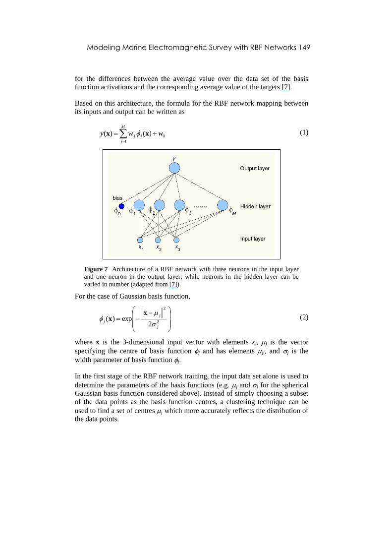
Modeling Marine Electromagnetic Survey with RBF Networks 149

for the differences between the average value over the data set of the basis

function activations and the corresponding average value of the targets [7].

Based on this architecture, the formula for the RBF network mapping between

its inputs and output can be written as

M

j

jj wwy1

0)()( xx (1)

Figure 7 Architecture of a RBF network with three neurons in the input layer

and one neuron in the output layer, while neurons in the hidden layer can be

varied in number (adapted from [7]).

For the case of Gaussian basis function,

2

2

2exp)(

j

j

j

xx (2)

where x is the 3-dimensional input vector with elements xi, j is the vector

specifying the centre of basis function j and has elements ji, and j is the

width parameter of basis function j.

In the first stage of the RBF network training, the input data set alone is used to

determine the parameters of the basis functions (e.g. j and j for the spherical

Gaussian basis function considered above). Instead of simply choosing a subset

of the data points as the basis function centres, a clustering technique can be

used to find a set of centres j which more accurately reflects the distribution of

the data points.

150 Agus Arif, Vijanth S. Asirvadam, & M.N. Karsiti

In this research, K-means clustering algorithm is selected to determine the basis

function centres. If there are N data points xn in total, then the algorithm will

find a set of K representative vectors j where j = 1, …, K. The algorithm seeks

to partition the data points {xn} into K disjoint subsets Sj containing Nj data

points, in such a way to minimize the sum-of-squares clustering function given

by

K

j Sn

j

n

j

J1

2

x (3)

where j is the mean of the data points in set Sj and is given by

jSn

n

j

jN

x1

(4)

In this research, the width parameter j is kept constant for all j = 1, …, M.

After determining the basis functions, they are then kept fixed while the second-

layer weights are found in the second stage of training. To begin this stage, the

bias parameter in Eq. (1) is absorbed into the weights to give

M

j

jjwy0

)()( xx (5)

and can be written in matrix notation as

Wxy )( (6)

where W = (wj) and = (j).

The weights W can be determined by minimization of a suitable error function.

In this case, it is convenient to consider a sum-of-squares error function given

by

n

nn tyE 2

21 })({ x (7)

where tn is the target value for the output neuron when the RBF network is

presented with input vector xn. Since the error function is a quadratic function of

the weights, its minimum can be found in terms of the solution of a set of linear

equations:

TWTTT (8)

where (T)n = tn and ()nj = j(x

n). The formal solution for the weight is given by

[7]

TWT (9)

Modeling Marine Electromagnetic Survey with RBF Networks 151

where the notation denotes the pseudo-inverse of and is given by

TT 1)( (10)

Based on all above equations, the RBF network has been constructed using

MATLAB programming with 3 neurons in the input layer. These neurons act as

source nodes to supply the various values of frequency, transmitter and receiver

positions of the SBL model. The one neuron in the output layer represents the

electric field amplitude value. While neurons in the hidden layer would be

varied between 1 and 20 neurons.

The data set that has been generated with Multiphysics was further processed to

convert the complex number format of the electric field amplitude values into

their corresponding magnitude and phase values. Then, only the normalized

logarithmic magnitude values were used in the training and testing of the RBF

network. From 3087 values, 3000 values were used in the training session,

while the remaining 87 values were used to test the network.

3 Results and Discussion

The implementation of the RBF network was realized using a MATLAB script.

The commands used to define, train, and test the network were formulated from

the appropriate equations in Methodology section. When the training was over,

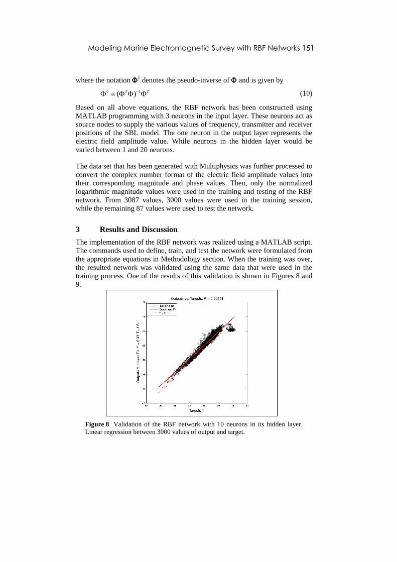
the resulted network was validated using the same data that were used in the

training process. One of the results of this validation is shown in Figures 8 and

9.

Figure 8 Validation of the RBF network with 10 neurons in its hidden layer.

Linear regression between 3000 values of output and target.

152 Agus Arif, Vijanth S. Asirvadam, & M.N. Karsiti

Figure 9 Validation of the RBF network with 10 neurons in its hidden layer.

Comparison of the first 300 values of electric field amplitude between output

(circle) and target (line).

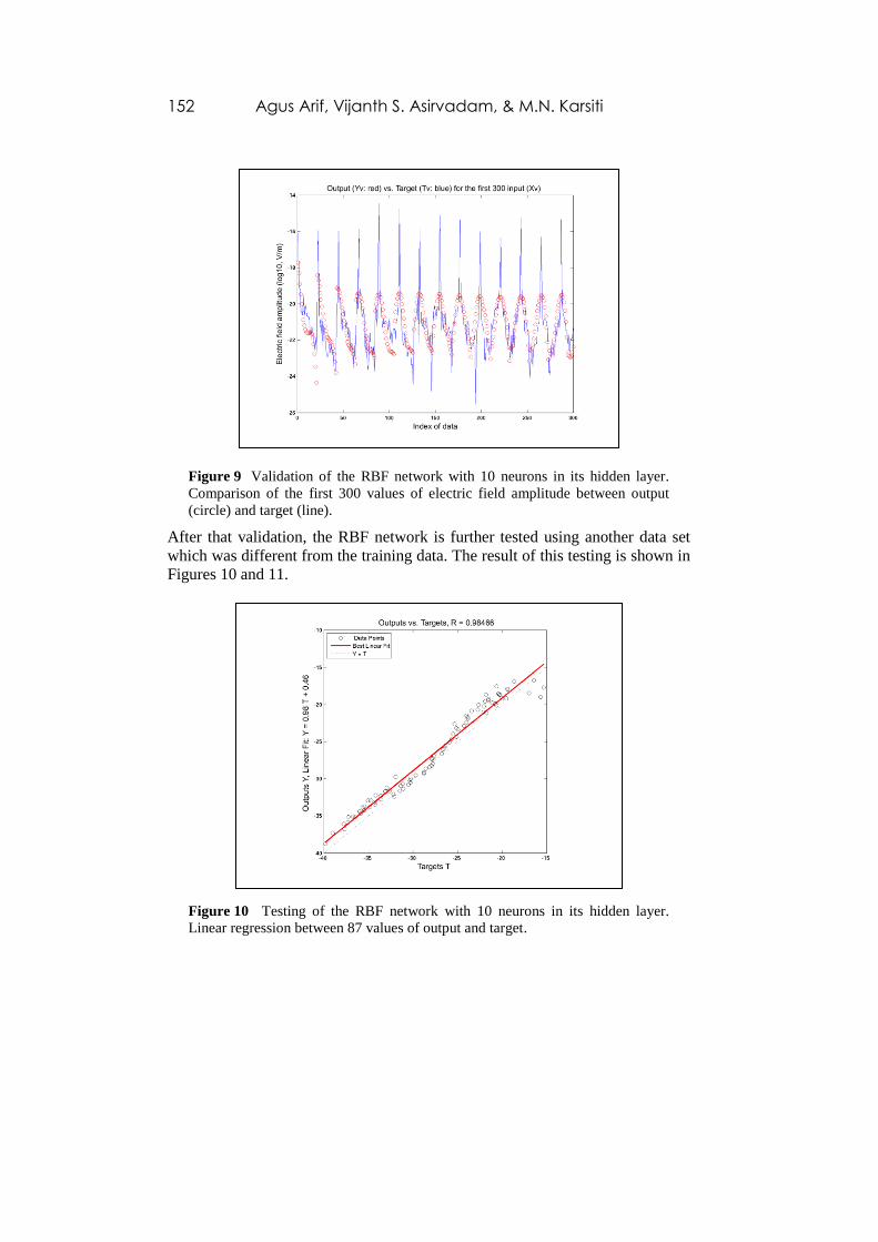
After that validation, the RBF network is further tested using another data set

which was different from the training data. The result of this testing is shown in

Figures 10 and 11.

Figure 10 Testing of the RBF network with 10 neurons in its hidden layer.

Linear regression between 87 values of output and target.

Modeling Marine Electromagnetic Survey with RBF Networks 153

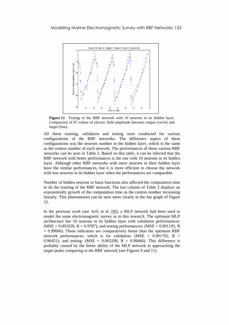
Figure 11 Testing of the RBF network with 10 neurons in its hidden layer.

Comparison of 87 values of electric field amplitude between output (circle) and

target (line).

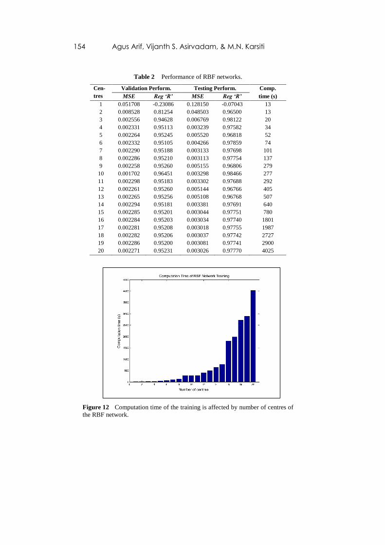
All these training, validation and testing were conducted for various

configurations of the RBF networks. The difference aspect of these

configurations was the neurons number in the hidden layer, which is the same

as the centres number of each network. The performances of these various RBF

networks can be seen in Table 2. Based on this table, it can be inferred that the

RBF network with better performances is the one with 10 neurons in its hidden

layer. Although other RBF networks with more neurons in their hidden layer

have the similar performances, but it is more efficient to choose the network

with less neurons in its hidden layer when the performances are comparable.

Number of hidden neurons or basis functions also affected the computation time

to do the training of the RBF network. The last column of Table 2 displays an

exponentially growth of the computation time as the centres number increasing

linearly. This phenomenon can be seen more clearly in the bar graph of Figure

12.

In the previous work (see Arif, et al. [8]), a MLP network had been used to

model the same electromagnetic survey as in this research. The optimum MLP

architecture has 10 neurons in its hidden layer with validation performances:

(MSE = 0.001028, R = 0.9787); and testing performances: (MSE = 0.001195, R

= 0.99066). These indicators are comparatively better than the optimum RBF

network performances, which is for validation: (MSE = 0.001702, R =

0.96451); and testing: (MSE = 0.003298, R = 0.98466). This difference is

probably caused by the better ability of the MLP network in approaching the

target peaks comparing to the RBF network (see Figures 9 and 11).

154 Agus Arif, Vijanth S. Asirvadam, & M.N. Karsiti

Table 2 Performance of RBF networks.

Cen-

tres

Validation Perform. Testing Perform. Comp.

MSE Reg ‘R’ MSE Reg ‘R’ time (s)

1 0.051708 -0.23086 0.128150 -0.07043 13

2 0.008528 0.81254 0.048503 0.96500 13

3 0.002556 0.94628 0.006769 0.98122 20

4 0.002331 0.95113 0.003239 0.97582 34

5 0.002264 0.95245 0.005520 0.96818 52

6 0.002332 0.95105 0.004266 0.97859 74

7 0.002290 0.95188 0.003133 0.97698 101

8 0.002286 0.95210 0.003113 0.97754 137

9 0.002258 0.95260 0.005155 0.96806 279

10 0.001702 0.96451 0.003298 0.98466 277

11 0.002298 0.95183 0.003302 0.97688 292

12 0.002261 0.95260 0.005144 0.96766 405

13 0.002265 0.95256 0.005108 0.96768 507

14 0.002294 0.95181 0.003381 0.97691 640

15 0.002285 0.95201 0.003044 0.97751 780

16 0.002284 0.95203 0.003034 0.97740 1801

17 0.002281 0.95208 0.003018 0.97755 1987

18 0.002282 0.95206 0.003037 0.97742 2727

19 0.002286 0.95200 0.003081 0.97741 2900

20 0.002271 0.95231 0.003026 0.97770 4025

Figure 12 Computation time of the training is affected by number of centres of

the RBF network.

Modeling Marine Electromagnetic Survey with RBF Networks 155

4 Conclusions

Based on the results of this research, it was shown that a RBF network, after

several appropriate training and testing, has a possibility to become a model for

marine electromagnetic survey with CSEM method.

By comparing the performances of several RBF networks with different number

of hidden neurons (or basis functions with their own centres), the best RBF

network to model the CSEM survey is the one with 10 neurons in its hidden

layer. But the performances of this optimum RBF network are still slightly

lower when it is compared with the previous built MLP network to model the

same survey.

In future work, the RBF network can be improved using a localized version of

this network. Then, it could be used to generate the electric field amplitude

magnitude at a certain working frequency and at a particular location of the

trans-mitter and receiver of a marine electromagnetic survey.

Nomenclature

E = error function

J = clustering function

j = index of basis function

K = number of clusters or disjoiunt subsets

M = number of basis functions

N = number of data points

n = index of data point

Nj = number of data points in disjoint subset

Sj = disjoint subset

T = vector of target values

tn = target value

W = matrix of weights

wj = weight from hidden layer to output layer

w0 = bias in hidden layer

x = 3-dimensional input vector

xi = neuron in input layer

xn = data point

y = neuron in output layer

= matrix of basis functions

= matrix of centres

j = basis function

156 Agus Arif, Vijanth S. Asirvadam, & M.N. Karsiti

0 = extra basis function

j = vector of centres

ji = element of centre vector

j = width parameter

References

[1] Constable, S. & Weiss, C.J., Mapping Thin Resistors and Hydrocarbons

with Marine EM Methods: Insights From 1D Modeling, Geophysics,

71(2), March-April 2006.

[2] Baan, M. van der & Jutten, C., Neural Networks in Geophysical Appli-

Cations, Geophysics, 65(4), pp. 1032–1047, July-Aug. 2000.

[3] COMSOL AB, COMSOL Multiphysics Quick Start and Quick Refe-

rence, version 3.5a, Nov. 2008.

[4] COMSOL AB, RF Module User’s Guide, version 3.5a, Nov. 2008.

[5] Key, K., 1D Inversion of Multicomponent, Multifrequency Marine CSEM

Data: Methodology and Synthetic Studies for Resolving Thin Resistive

Layers, Geophysics, 74(2), March–April 2009.

[6] Arif, A., Asirvadam, V.A. & Karsiti, M.N., Forward Modeling of Seabed

Logging using COMSOL Multiphysics, 10th Biannual Postgraduate

Research Symposium, UTP, July 2010.

[7] Bishop, C.M., Neural Networks for Pattern Recognition, Oxford

University Press, chap. 5, 1994.

[8] Arif, A., Asirvadam, V.A. & Karsiti, M.N., Forward Modeling of Seabed

Logging with Controlled Source Electromagnetic Method using

Multilayer Perceptron, IEEE Asia Pacific Conference on Applied

Electromagnetic (APACE), Nov. 2010.