ORIGINAL PAPER

Backpropagation to train an evolving radial basis functionneural network

Jose de Jesus Rubio • Diana M. Vazquez •

Jaime Pacheco

Received: 23 October 2009 / Accepted: 21 August 2010 / Published online: 25 September 2010

� Springer-Verlag 2010

Abstract In this paper, a stable backpropagation algo-

rithm is used to train an online evolving radial basis

function neural network. Structure and parameters learning

are updated at the same time in our algorithm, we do not

make difference in structure learning and parameters

learning. It generates groups with an online clustering. The

center is updated to achieve the center is near to the

incoming data in each iteration, so the algorithm does not

need to generate a new neuron in each iteration, i.e., the

algorithm does not generate many neurons and it does not

need to prune the neurons. We give a time varying learning

rate for backpropagation training in the parameters. We

prove the stability of the proposed algorithm.

Keywords Evolving systems � Fuzzy neural networks �Clustering � Backpropagation � Stability

1 Introduction

In the last few years, the application of fuzzy neural networks

to nonlinear system identification has been a very active area

(Lin 1994; Mitra and Hayashi 2000). Fuzzy and neural net-

works modeling involves structure and parameters identifi-

cation. The parameters identification is usually addressed by

some gradient descent variant, i.e., the least square algorithm

and backpropagation. In this paper online identification is

addressed (Angelov and Zhou 2006; Lughofer and Angelov

2009). The nonlinear system identification can be used for

classification or for control (Iglesias et al. 2010).

In online identification, model structure and parameters

identification are updated immediately after each input–

output pair has been presented, i.e., after each iteration.

Online identification also includes: (i) model structure and

(ii) parameters identification. There are some interesting

methods which work online in the literature. In Juang and

Lin (1998), the input space is partitioned according to an

aligned clustering-based algorithm. After the number of

rules is decided, the parameters are tuned by recursive least

square algorithm, it is called SONFIN. In Wang (1997), it

is the recurrent case of the above case, it is called

RSONFIN. In Tzafestas and Zikidis (2001), the input space

is automatically partitioned into fuzzy subsets by adaptive

resonance theory mechanism. Fuzzy rules that tend to give

high output error are split in two, by a specific fuzzy rule

splitting procedure. In Kasabov (2001), he proposes that

the radius to make clustering updates. In Angelov and Filev

(2004a), it is considered that if a new data, which is

accepted as a focal point of a new rule is too close to a

previously existing rule then the old rule is replaced by the

new one, but the self-constructing neural fuzzy networks

above do not have a pruning method, though they can be

used for on-line learning. In order to extract fuzzy rules in a

growing fashion from a large numerical data-base, some

self-constructing fuzzy networks have been presented. The

self-organizing fuzzy neural network (SOFNN) (Leng et al.

2005) approach proposes a pruning method devised from

the optimal brain surgeon (OBS) approach (Hassibi and

Stork 1993). The basic idea of the SOFN N is to use the

second derivative information to find the unimportant

neuron. In the simplified method for learning evolving

Takagi-Sugeno fuzzy models (simpl_eTS) given in

Angelov and Filev (2005), they introduce the population,

J. de Jesus Rubio (&) � D. M. Vazquez � J. Pacheco

Seccion de Estudios de Posgrado e Investigacion,

ESIME Azcapotzalco, Instituto Politecnico Nacional,

Av. De las Granjas, No. 682, Col. Sta. Catarina. Azcapotzalco,

02250 Mexico, D.F., Mexico

e-mail: jrubioa@ipn.mx

123

Evolving Systems (2010) 1:173–180

DOI 10.1007/s12530-010-9015-9 Author's personal copy

they monitor the population of each cluster and if it amounts

to less than 1% of the total data samples, that cluster is

ignored. In the Sequential Adaptive Fuzzy Inference Sys-

tem (SAFIS) given in Rong et al. (2006), it is used one

threshold parameter for adding a rule or neuron and another

threshold parameter for pruning a rule or neuron.

In this paper, we propose the backpropagation algorithm

to train online an evolving radial basis function neural

network. Structure and parameters learning are updated at

the same time in our algorithm, we do not make difference

in structure learning and parameters learning. It generates

groups with an online clustering. The center is updated to

achieve the center is near to the incoming data in each

iteration, so the algorithm does not need to generate a

new neuron in each iteration, i.e., the algorithm does not

generate many neurons and it does not need to prune

the neurons. We give a time varying learning rate for

backpropagation training in the parameters. We prove the

stability of the proposed algorithm.

2 Evolving radial basis function neural network

Consider following unknown discrete-time nonlinear system:

yðk � 1Þ ¼ f Xðk � 1Þ½ � ð1Þ

where Xðk� 1Þ ¼ ½x1ðk� 1Þ. . .xNðk� 1Þ� ¼ ½yðk� 2Þ; . . .;yðk� n� 1Þ;u k� 2ð Þ; . . .;u k�m� 1ð Þ� 2 <N (N = n ? m)

is the input vector, uðk� 1Þj j2�u;yðk� 1Þ is the output of

the plant, f is a general nonlinear smooth function f [ C?.

In the case of Jang and Sun (1997), we consider the

evolving radial basis function neural network as follows:

byðk� 1Þ ¼ aðk� 1Þ=bðk� 1Þ

aðk� 1Þ ¼X

M

j¼1

vjðk� 1Þzjðk� 1Þ; bðk� 1Þ ¼X

M

j¼1

zjðk� 1Þ

zjðk� 1Þ ¼ exp �X

N

i¼1

xiðk� 1Þ� cijðk� 1Þrijðk� 1Þ

� �

" #28

<

:

9

=

;

ð2Þ

where xi(k - 1) are inputs of system (1), (i = 1…N),

cij(k - 1) and rij(k - 1) are the centers and the widths of

the Gaussian functions, respectively, (j = 1…M), vj(k - 1)

is the output of the Gaussian functions.

3 Structure identification

We use the online clustering to train the structure of the

algorithm (Chiu 1994). Choosing an appropriate number of

hidden neurons is important in designing the online clus-

tering for neuro fuzzy systems, because too many hidden

neurons result in a complex evolving system that may be

unnecessary for the problem and it can cause overfitting

(Jang and Sun 1997), whereas too few hidden neurons

produce a less powerful neural system that may be insuf-

ficient to achieve the objective (Soleimani et al. 2010). We

view the number of hidden neurons as a design parameter

and determine it based on the input–output pairs and on the

number of elements of each hidden neuron.

The basic idea is to group the input–output pairs into

clusters and use one hidden neuron for one cluster as in

Kasabov (2001), Soleimani et al. (2010), and Wang

(1997); i.e., the number of hidden neurons equals the

number of clusters.

One of the simplest clustering algorithms is the nearest

neighborhood clustering algorithm. In this algorithm, first

we put the first data as the center of the first cluster. Then, if

the distances of a data to the cluster centers are less than a

pre-specified value (the radius r), put this data into the cluster

whose center is the closest to this data; otherwise, set this

data as a new cluster center. The details are given as follows.

Let xi(k - 1) are newly incoming pattern, then we get:

pðk � 1Þ ¼ max1� j�M

zjðk � 1Þ ð3Þ

If p(k - 1) C r, then a rule or neuron is not generated

and in the case that zj(k - 1) = p(k - 1) we have the

winner rule or neuron cij� ðkÞ; the centers of this rule or

neuron are updated as:

cij� ðkÞ ¼ cij� ðk � 1Þ þ 1

1þ x2i ðk � 1Þ þ c2

ij� ðk � 1Þ� xiðk � 1Þ � cij� ðk � 1Þ� �

ð4Þ

While if zj(k - 1) is not equal to p(k - 1), nothing

happens.

If p(k - 1) \ r, then a new rule or neuron is generated

(each neuron correspond to each center) and M = M ? 1

where r is a selected radius, r 2 0; 1ð Þ: Once a new rule or

neuron is generated, the next step is to assign initial centers

and widths of the corresponding membership functions.

ci;Mþ1ðkÞ ¼ xiðkÞ ri;Mþ1ðkÞ ¼1

xiðkÞ � cij� ðkÞvMþ1ðkÞ ¼ yðkÞ

ð5Þ

where cij� ðkÞ is the winner rule or neuron defined in (4).

Remark 1 The structure identification is a little similar to

the given in Juang and Lin (1998), Juang and Lin (1999),

but they do not take the max of zj(k - 1) as (3), this idea is

taken from the competitive learning of ART recurrent

neural network (Hilera and Martines 1995; Jang and Sun

1997) to get the winner rule or neuron (in the case of ART

is the winner neuron). If the algorithm of Juang and Lin

(1998, 1999) do not generate a new rule or neuron, it does

nothing, in this paper the center is updated as in (4) to

174 Evolving Systems (2010) 1:173–180

123

Author's personal copy

achieve the center is near to the incoming data in each

iteration, in this way, it does not need to generate a new

rule or neuron in each iteration, i.e., it does not generate

many rules or neurons and it does not need to prune the

rules or neurons. This idea is similar to the updating of

weights in the Kohonen recurrent neural network (Hilera

and Martines 1995) (in this case they speak of weights of

their network and we speak about the weights of the

Gaussian function for our network).

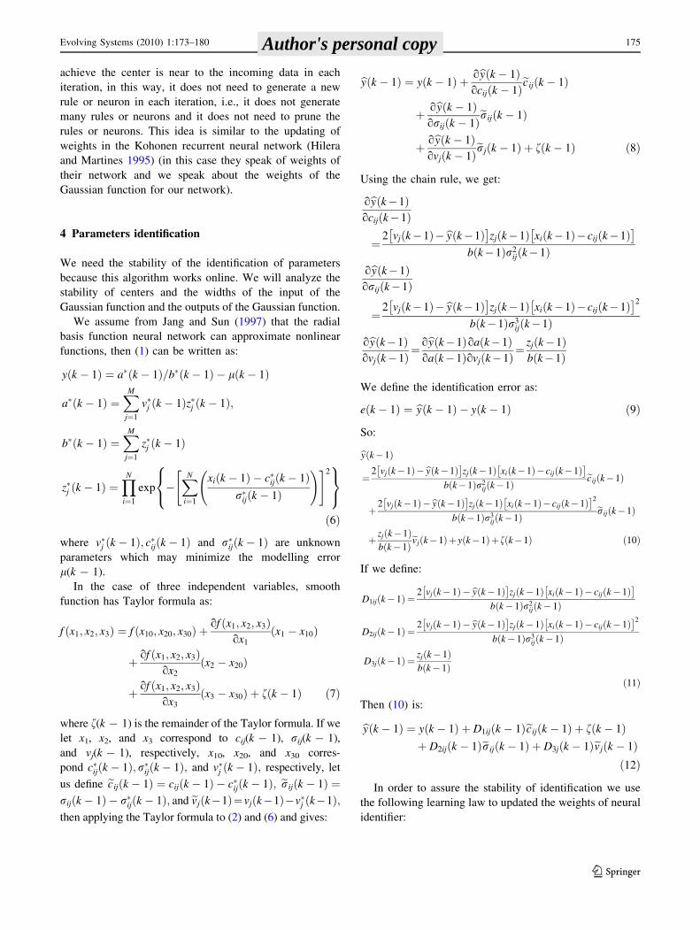
4 Parameters identification

We need the stability of the identification of parameters

because this algorithm works online. We will analyze the

stability of centers and the widths of the input of the

Gaussian function and the outputs of the Gaussian function.

We assume from Jang and Sun (1997) that the radial

basis function neural network can approximate nonlinear

functions, then (1) can be written as:

yðk � 1Þ ¼ a�ðk � 1Þ=b�ðk � 1Þ � lðk � 1Þ

a�ðk � 1Þ ¼X

M

j¼1

v�j ðk � 1Þz�j ðk � 1Þ;

b�ðk � 1Þ ¼X

M

j¼1

z�j ðk � 1Þ

z�j ðk � 1Þ ¼Y

N

i¼1

exp �X

N

i¼1

xiðk � 1Þ � c�ijðk � 1Þr�ijðk � 1Þ

!" #28

<

:

9

=

;

ð6Þ

where v�j ðk � 1Þ; c�ijðk � 1Þ and r�ijðk � 1Þ are unknown

parameters which may minimize the modelling error

l(k - 1).

In the case of three independent variables, smooth

function has Taylor formula as:

f ðx1; x2; x3Þ ¼ f ðx10; x20; x30Þ þof ðx1; x2; x3Þ

ox1

x1 � x10ð Þ

þ of ðx1; x2; x3Þox2

x2 � x20ð Þ

þ of ðx1; x2; x3Þox3

x3 � x30ð Þ þ fðk � 1Þ ð7Þ

where f(k - 1) is the remainder of the Taylor formula. If we

let x1, x2, and x3 correspond to cij(k - 1), rij(k - 1),

and vj(k - 1), respectively, x10, x20, and x30 corres-

pond c�ijðk � 1Þ; r�ijðk � 1Þ; and v�j ðk � 1Þ; respectively, let

us define ecijðk � 1Þ ¼ cijðk � 1Þ � c�ijðk � 1Þ; erijðk � 1Þ ¼rijðk � 1Þ � r�ijðk � 1Þ; and evjðk�1Þ¼vjðk�1Þ�v�j ðk�1Þ;then applying the Taylor formula to (2) and (6) and gives:

byðk � 1Þ ¼ yðk � 1Þ þ obyðk � 1Þocijðk � 1Þecijðk � 1Þ

þ obyðk � 1Þorijðk � 1Þerijðk � 1Þ

þ obyðk � 1Þovjðk � 1Þerjðk � 1Þ þ fðk � 1Þ ð8Þ

Using the chain rule, we get:

obyðk�1Þocijðk�1Þ

¼2 vjðk�1Þ� byðk�1Þ� �

zjðk�1Þ xiðk�1Þ� cijðk�1Þ� �

bðk�1Þr2ijðk�1Þ

obyðk�1Þorijðk�1Þ

¼2 vjðk�1Þ� byðk�1Þ� �

zjðk�1Þ xiðk�1Þ� cijðk�1Þ� �2

bðk�1Þr3ijðk�1Þ

obyðk�1Þovjðk�1Þ¼

obyðk�1Þoaðk�1Þ

oaðk�1Þovjðk�1Þ¼

zjðk�1Þbðk�1Þ

We define the identification error as:

eðk � 1Þ ¼ byðk � 1Þ � yðk � 1Þ ð9Þ

So:

byðk�1Þ

¼2 vjðk�1Þ� byðk�1Þ� �

zjðk�1Þ xiðk�1Þ�cijðk�1Þ� �

bðk�1Þr2ijðk�1Þ ecijðk�1Þ

þ2 vjðk�1Þ� byðk�1Þ� �

zjðk�1Þ xiðk�1Þ�cijðk�1Þ� �2

bðk�1Þr3ijðk�1Þ erijðk�1Þ

þ zjðk�1Þbðk�1Þevjðk�1Þþyðk�1Þþ fðk�1Þ ð10Þ

If we define:

D1ijðk� 1Þ ¼2 vjðk� 1Þ� byðk� 1Þ� �

zjðk� 1Þ xiðk� 1Þ� cijðk� 1Þ� �

bðk� 1Þr2ijðk� 1Þ

D2ijðk� 1Þ ¼2 vjðk� 1Þ� byðk� 1Þ� �

zjðk� 1Þ xiðk� 1Þ� cijðk� 1Þ� �2

bðk� 1Þr3ijðk� 1Þ

D3jðk� 1Þ ¼ zjðk� 1Þbðk� 1Þ

ð11Þ

Then (10) is:

byðk � 1Þ ¼ yðk � 1Þ þ D1ijðk � 1Þecijðk � 1Þ þ fðk � 1Þþ D2ijðk � 1Þerijðk � 1Þ þ D3jðk � 1Þevjðk � 1Þ

ð12Þ

In order to assure the stability of identification we use

the following learning law to updated the weights of neural

identifier:

Evolving Systems (2010) 1:173–180 175

123

Author's personal copy

cijðkÞ ¼ cijðk � 1Þ � gðk � 1ÞD1ijðk � 1Þe k � 1ð ÞrijðkÞ ¼ rijðk � 1Þ � gðk � 1ÞD2ijðk � 1Þe k � 1ð ÞvjðkÞ ¼ vjðk � 1Þ � gðk � 1ÞD3jðk � 1Þe k � 1ð Þ

ð13Þ

where j = 1…M, i = 1…N and D1ij(k - 1), D2ij(k - 1),

and D3j(k - 1) are given in (11). The dead-zone is applied

to g(k - 1) as:

gðk � 1Þ ¼g0

1þqðk�1Þ if e2 k � 1ð Þ� f2

1�g

0 if e2 k � 1ð Þ\ f2

1�g

8

<

:

ð14Þ

where q(k - 1) = D1ij2 (k - 1) ? D2ij

2 (k - 1) ? D3j2 (k - 1),

0 \ g0 B 1.

The following theorem gives the stability of neural

identification in the case of centers and widths input of the

Gaussian functions and the outputs of the Gaussian

functions.

Theorem 1 If we use radial basis function neural network

(2) to identify the nonlinear system (1), the learning law

(11), (13) with dead-zone (14) make the identification sta-

ble, i.e., (1) the identification error e(k - 1) is bounded (2)

The identification error e(k - 1) satisfies:

limk!1

e2 k � 1ð Þ ¼ f2

1� g0

ð15Þ

where f is upper bound of f (k - 1).

Proof Please see Appendix for proof of this theorem. h

Remark 2 The normal learning (11), (13) has similar form

as backpropagation (Wang 1997), the only difference is

that we use normalizing learning rate g(k - 1), Wang

(1997) use fixed learning rate. The time-varying learning

rate can assure the stability of the identification error. This

learning rate is easy to get, no any prior information is

required, for example we may select g0 = 0.9.

5 The proposed algorithm

The proposed algorithm is as given in Fig. 1.

Remark 3 The parameters r and g0 are selected to achieve

the best behavior of the algorithm, the other parameters are

are updated by the algorithm. If r is big, the algorithm

generates a high number of neurons, if r is small, the

algorithm generates a low number of neurons, but a too

high or a too low number of neurons could cause a bad

behavior of any algorithm, that is way r is bounded. If g0 is

small, the steps of the algorithm are short, so the algorithm

is slow, if g0 is big, the steps of the algorithm are long, so

the algorithm is fast, but if g0 is too big, it could cause that

the algorithm never reach the minimum, i.e. the algorithm

could become unstable, that is way the parameter g0 is

bounded.

Remark 4 The proposed algorithm is different to the

algorithms proposed by Juang and Lin (1998) and Juang

and Lin (1999) because of three reasons: (1) from Theorem

1 the proposed algorithm is assured to be stable while the

algorithms of Juang and Lin (1998) and Juang and Lin

(1999) are not assured to be stable. It is important to assure

the stability of the algorithms because an algorithm that

becomes unstable could cause damage of the instruments

or could cause accidents in people, (2) in Juang and Lin

(1998) and Juang and Lin (1999) after the number of rules

is decided, the parameters are tuned by recursive least

square algorithm while in the proposed algorithm the

number of rules or neurons and the parameters are updated

in each iteration, and (3) if the algorithms of Juang and Lin

(1998, 1999) do not generate a new rule or neuron, it does

nothing, while if the proposed algorithm does not generate

a new rule or neuron, the winner center is updated as in (4)

to get that the center is near to the incoming data in each

iteration.

Fig. 1 The proposed algorithm

176 Evolving Systems (2010) 1:173–180

123

Author's personal copy

Remark 5 Evolving systems are inspired by the idea of

system model evolution in a dynamically changing and

evolving environment. They use inheritance and gradual

change with the aim of life-long learning and adaptation,

self-organization including system structure evolution in

order to adapt to the (unknown and unpredictable) envi-

ronment as structures for information representation with

the ability to fully adapt their structure and adjust their

parameters (Angelov and Filev 2004b; Angelov et al.

2010). The aim of the life-long learning adaptation is

addressed with Eq. 4 because in this equation the center is

updated to achieve the center is near to the incoming data in

each iteration. The structure is updated with Eqs. 3 and 4.

The parameters learning is updated with Eqs. 2, 9, 11, 13,

and 14. As the three characteristics of the evolving systems

are satisfied, the proposed algorithm is an evolving system.

6 Simulations

In this section, the suggested online self-organized algo-

rithm is applied for nonlinear system identification (Rivals

and Personnaz 2003). Note that in this study, the structure

and parameters learning work at each time-step and they

work online. Two examples are considered in this section.

In the first example, the proposed network will be com-

pared with networks that add and remove neurons online,

such as the Simpl_eTS (Angelov and Filev 2005), the

SOFNN (Leng et al. 2005), and the SAFIS (Rong et al.

2006), because these networks have good performance. In

the second example, the proposed network will be com-

pared with the network that add neurons online called

RSONFIN (Juang and Lin 1999).

The evolving radial basis function neural network as all

the neural networks has a training phase and a testing phase

because they have the capacity to learn a nonlinear behav-

ior. The training phase is where the weights of the evolving

radial basis function neural network are updated to learn a

nonlinear behavior. The testing phase is where the weights

of the evolving radial basis function neural network are not

updated because the evolving radial basis function neural

network ended to learn the nonlinear behavior.

Example 1 Let us consider the nonlinear system given

and used in earlier studies (Rong et al. 2006; Wang 1997):

yðkÞ ¼ yðk � 1Þyðk � 2Þ yðk � 1Þ � 0:5½ �1þ y2ðk � 1Þ þ y2ðk � 2Þ þ uðk � 1Þ ð16Þ

As in the earlier studies (Rong et al. 2006; Wang 1997),

the input u(k) is given by uðkÞ ¼ sinð2pk=25Þ: The three

values y(k - 1), y(k - 2), and u(k - 1) are the inputs of

the networks or systems and y(k) is the output of the

networks or systems.

The parameters of the proposed algorithm are g0 = 0.12,

r = 0.99. For the purpose of training and testing, 5,000 and

200 data are produced, respectively. The average perfor-

mance comparison of the proposed algorithm with the

eTS (Angelov and Filev 2004a) with parameters r = 1.8,

X = 106, the Simpl_eTS (Angelov and Filev 2005) with

parameters r = 2.0, X = 106, and the SAFIS (Rong et al.

2006) with parameters c = 0.997, emax = 1, k = 1, emin =

0.1, eg = 0.05, ep = 0.005 is shown in Table 1, where the

root mean square error (RMSE) (Kasabov 2001) is:

RMSE ¼ 1

N

XN

k¼1

e2ðk � 1Þ !1

2

ð17Þ

From Table 1, it can be seen that the proposed algorithm

achieves similar accuracy when compared with the other

networks. In addition, the proposed algorithm achieves this

accuracy with the smallest number of neurons. The evo-

lution of the neurons for the proposed algorithm for a

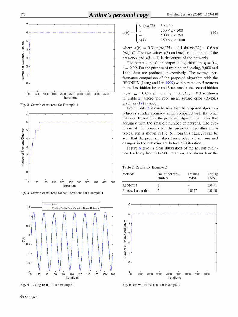
typical run is shown in Fig. 2. From this figure, it can be

seen that the proposed algorithm produces 6 neurons and

changes in the behavior are before 500 iterations.

Figure 3 gives a clear illustration of the neuron evolu-

tion tendency from 0 to 500 iterations, and shows how the

proposed algorithm can automatically add a neuron during

learning. In addition, the number of neurons of the pro-

posed algorithm grows very slowly because the centers of

the neurons are updated each iteration.

Figure 4 shows the testing result for the proposed

algorithm, i.e. this figure presents the comparison between

the output of the plant y(k - 1) given by Eq. 1 and the

output of the evolving radial basis function neural network

byðk � 1Þ given by Eq. 2, it is the testing result because it is

the case where the weights of the evolving radial basis

function neural network are not updated (the testing phase).

Example 2 Let us consider the system used in the earlier

study (Juang and Lin 1999):

yðk þ 1Þ

¼ yðkÞyðk � 1Þyðk � 2Þuðk � 1Þ yðk � 2Þ � 1½ � þ uðkÞ1þ y2ðk � 2Þ þ y2ðk � 1Þ

ð18Þ

As in the earlier study (Juang and Lin 1999), the input

u(k) for the testing is given by:

Table 1 Results for Example 1

Methods No. of neurons/

clusters

Training

RMSE

Testing

RMSE

eTS 49 0.0292 0.0212

Simpl_eTS 22 0.0528 0.0225

SAFIS 17 0.0539 0.0221

Proposed algorithm 6 0.0737 0.0225

Evolving Systems (2010) 1:173–180 177

123

Author's personal copy

uðkÞ ¼

sinðpk=25Þ k\250

1 250� k\500

�1 500� k\750

aðkÞ 750� k\1000

8

>

>

<

>

>

:

ð19Þ

where aðkÞ ¼ 0:3 sinðpk=25Þ þ 0:1 sinðpk=32Þ þ 0:6 sin

ðpk=10Þ: The two values y(k) and u(k) are the inputs of the

networks and y(k ? 1) is the output of the networks.

The parameters of the proposed algorithm are g = 0.4,

r = 0.99. For the purpose of training and testing, 9,000 and

1,000 data are produced, respectively. The average per-

formance comparison of the proposed algorithm with the

RSONFIN (Juang and Lin 1999) with parameters 5 neurons

in the first hidden layer and 3 neurons in the second hidden

layer, g0 ¼ 0:055; q ¼ 0:8;Fin ¼ 0:2;Fout ¼ 0:3 is shown

in Table 2, where the root mean square error (RMSE)

given in (17) is used.

From Table 2, it can be seen that the proposed algorithm

achieves similar accuracy when compared with the other

network. In addition, the proposed algorithm achieves this

accuracy with the smallest number of neurons. The evo-

lution of the neurons for the proposed algorithm for a

typical run is shown in Fig. 5. From this figure, it can be

seen that the proposed algorithm produces 5 neurons and

changes in the behavior are before 500 iterations.

Figure 6 gives a clear illustration of the neuron evolu-

tion tendency from 0 to 500 iterations, and shows how the

Fig. 2 Growth of neurons for Example 1

Fig. 3 Growth of neurons for 500 iterations for Example 1

Fig. 4 Testing result of for Example 1

Table 2 Results for Example 2

Methods No. of neurons/

clusters

Training

RMSE

Testing

RMSE

RSONFIN 8 – 0.0441

Proposed algorithm 5 0.0377 0.0400

Fig. 5 Growth of neurons for Example 2

178 Evolving Systems (2010) 1:173–180

123

Author's personal copy

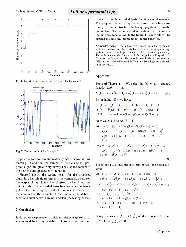
proposed algorithm can automatically add a neuron during

learning. In addition, the number of neurons of the pro-

posed algorithm grows very slowly because the centers of

the neurons are updated each iteration.

Figure 7 shows the testing result for the proposed

algorithm, i.e. this figure presents the comparison between

the output of the plant y(k - 1) given by Eq. 1 and the

output of the evolving radial basis function neural network

byðk � 1Þ given by Eq. 2, it is the testing result because it is

the case where the weights of the evolving radial basis

function neural network are not updated (the testing phase).

7 Conclusion

In this paper we presented a quick and efficient approach for

system modeling using an stable backpropagation algorithm

to train an evolving radial basis function neural network.

The proposed neural fuzzy network uses the online clus-

tering to train the structure, the backpropagation to train the

parameters. The structure identification and parameter

learning are done online. In the future, this network will be

applied to some real problems to see the behavior.

Acknowledgments The authors are grateful with the editor and

with the reviewers for their valuable comments and insightful sug-

gestions, which can help to improve this research significantly.

The authors thank the Secretaria de Investigacion y Posgrado, the

Comision de Operacion y Fomento de Actividades Academicas del

IPN, and the Consejo Nacional de Ciencia y Tecnologia for their help

in this research.

Appendix

Proof of Theorem 1 We select the following Lyapunov

function L1(k - 1) as:

L1ðk � 1Þ ¼ ec2ijðk � 1Þ þ er2

ijðk � 1Þ þ ev2j ðk � 1Þ ð20Þ

By updating (13), we have:

ecijðkÞ ¼ ecijðk � 1Þ � gðk � 1ÞD1ijðk � 1Þe k � 1ð ÞerijðkÞ ¼ erijðk � 1Þ � gðk � 1ÞD2ijðk � 1Þe k � 1ð ÞevjðkÞ ¼ evjðk � 1Þ � gðk � 1ÞD3jðk � 1Þe k � 1ð Þ

Now we calculate DL1(k - 1):

DL1ðk � 1Þ ¼ ecijðk � 1Þ � gðk � 1ÞD1ijðk � 1Þe k � 1ð Þ� �2

� ec2ijðk � 1Þ þ erijðk � 1Þ � gðk � 1ÞD2ijðk � 1Þe k � 1ð Þ

� �2

� er2ijðk � 1Þ þ evjðk � 1Þ � gðk � 1ÞD3jðk � 1Þe k � 1ð Þ

� �2

� ev2j ðk � 1Þ

¼ g2ðk � 1Þ D21ijðk � 1Þ þ D2

2ijðk � 1Þ þ D23jðk � 1Þ

n o

e2 k � 1ð Þ

� 2gðk � 1Þ D1ijðk � 1Þecijðk � 1Þ þ D2ijðk � 1Þerijðk � 1Þ�

þD3jðk � 1Þevjðk � 1Þ�e k � 1ð Þð21Þ

Substituting (12) into the last term of (21) and using (14)

gives:

DL1ðk � 1Þ ¼ �2gðk � 1Þ e k � 1ð Þ � fðk � 1Þ½ �e k � 1ð Þ

þ g2ðk � 1Þ D21ijðk � 1Þ þ D2

2ijðk � 1Þ þ D23jðk � 1Þ

n o

e2 k � 1ð Þ

� g2ðk � 1Þ 1þ D21ijðk � 1Þ þ D2

2ijðk � 1Þ þ D23jðk � 1Þ

n o

e2 k � 1ð Þ

� gðk � 1Þe2 k � 1ð Þ þ gðk � 1Þf2ðk � 1Þ� g2ðk � 1Þ 1þ qðk � 1Þf ge2 k � 1ð Þ� gðk � 1Þe2 k � 1ð Þ þ gðk � 1Þf2ðk � 1Þ

� � gðk � 1Þ 1� gðk � 1Þ 1þ qðk � 1Þ½ �f ge2 k � 1ð Þþ gðk � 1Þf2ðk � 1Þ

Using the case e2 k � 1ð Þ� f2

1�g of dead zone (14), then

gðk � 1Þ ¼ g0

1þqðk�1Þ[ 0 :

Fig. 6 Growth of neurons for 500 iterations for Example 2

Fig. 7 Testing result of for Example 2

Evolving Systems (2010) 1:173–180 179

123

Author's personal copy

DL1ðk� 1Þ� � gðk� 1Þ 1� g0

1þ qðk� 1Þ 1þ qðk� 1Þ½ ��

e2 k� 1ð Þþ gðk� 1Þf2ðk� 1ÞDL1ðk� 1Þ� � gðk� 1Þ 1� g0ð Þe2 k� 1ð Þ

þ gðk� 1Þf2ðk� 1Þ

With f2 k� 1ð Þ�f2

:

DL1ðk � 1Þ� � gðk � 1Þ 1� g0ð Þe2 k � 1ð Þ � f2

h i

ð22Þ

From the dead-zone, e2 k � 1ð Þ� f2

1�g0and g(k - 1) [ 0,

DL1(k - 1) B 0. L1(k) is bounded. If e2 k � 1ð Þ\ f2

1�g0;

from (14) we know g(k - 1) = 0, all of weights are not

changed, they are bounded, so L1(k) is bounded.

When e2 k � 1ð Þ� f2

1�g0; summarize (22) from 2 to T:

XT

k¼2

gðk � 1Þ 1� g0ð Þe2 k � 1ð Þ � f2

h i

� L1ð1Þ � L1ðTÞ

ð23Þ

Since L1(T) is bounded and using gðk � 1Þ ¼ g0

1þqðk�1Þ [ 0 :

limT!1

XT

k¼2

g0

1þ qðk � 1Þ

� �

1� g0ð Þe2 k � 1ð Þ � f2

h i

\1

ð24Þ

Because

e2 k � 1ð Þ� f2

1�g ;g0

1þqðk�1Þ

�

1� g0ð Þe2 k � 1ð Þ � f2

h i

� 0;

so:

limk!1

g0

1þ qðk � 1Þ

� �

1� g0ð Þe2 k � 1ð Þ � f2

h i

¼ 0 ð25Þ

Because L1(k - 1) is bounded, so q(k - 1) \?, and asg0

1þqðk�1Þ [ 0 :

limk!1

1� g0ð Þe2 k � 1ð Þ ¼ f2 ð26Þ

That is (15). When e2 k � 1ð Þ\ f2

1�g0½ � ; it is already in this

zone.

References

Angelov PP, Filev DP (2004a) A approach to online identification of

Takagi-Sugeno fuzzy models. IEEE Trans Syst Man Cybern

32(1):484–498

Angelov PP, Filev DP (2004b) Flexible models with evolving

structure. Int J Intell Syst 19(4):327–340

Angelov PP, Filev DP (2005) Simpl_eTS: a simplified method for

learning evolving Takagi-Sugeno fuzzy models. In: The inter-

national conference on fuzzy systems, pp 1068–1072

Angelov P, Zhou X (2006) Evolving fuzzy systems from data streams

in real-time. In: International symposium on evolving fuzzy

systems, pp 29–35

Angelov P, Ramezany R, Zhou X (2008) Autonomous novelty

detection and object tracking in video streams using evolving

clustering and Takagi-Sugeno type neuro-fuzzy system. In: IEEE

World Congress on computational intelligence, pp 1457–1464

Angelov P, Filev D, Kasabov N (2010) Editorial. Evol Syst 1:1–2

Chiu SL (1994) Fuzzy Model Identification based on cluster

estimation. J Intell Fuzzy Syst 2(3):267–278

Hassibi D, Stork DG (1993) Second order derivatives for network

pruning. In: Advances in neural information processing, vol 5.

Morgan Kaufmann, Los Altos, pp 164–171

Hilera JR, Martines VJ (1995) Redes Neuronales Artificiales,

Fundamentos, Modelos y Aplicaciones. Adison Wesley Ibero-

americana, USA

Iglesias JA, Angelov P, Ledezma A, Sanchis A (2010) Evolving

classification of agents’ behaviors: a general approach. Evol

Syst 3

Jang JSR, Sun CT (1997) Neuro-fuzzy and soft computing. Prentice

Hall, Englewood Cliffs

Juang CF, Lin CT (1998) An on-line self constructing nural fuzzy

inference network and its applications. IEEE Trans Fuzzy Syst

6(1):12–32

Juang CF, Lin CT (1999) A recurrent self-organizing fuzzy inference

network. IEEE Trans Neural Netw 10(4):828–845

Kasabov N (2001) Evolving fuzzy nural networks for supervised/

unsupervised online knowledge-based learning. IEEE Trans Syst

Man Cybern 31(6):902–918

Leng G, McGinnity TM, Prasad G (2005) An approach for online

extraction of fuzzy rules using a self-organising fuzzy neural

network. Fuzzy Sets Syst 150:211–243

Lin CT (1994) Neural fuzzy control systems with structure and

parameter learning. World Scientific, New York

Lughofer E, Angelov P (2009) Detecting and reacting on drifts and

shifts in on-line data streams with evolving fuzzy systems. In:

International Fuzzy Systems Association World Congress,

pp 931–937

Mitra S, Hayashi Y (2000) Neuro-fuzzy rule generation: survey in

soft computing framework. IEEE Trans Neural Netw 11(3):

748–769

Rivals I, Personnaz L (2003) Neural network construction and

selection in non linear modelling. IEEE Trans Neural Netw

14(4):804–820

Rong HJ, Sundararajan N, Huang GB, Saratchandran P (2006)

Sequential adaptive fuzzy inference system (SAFIS) for nonlin-

ear system identification and prediction. Fuzzy Sets Syst 157(9):

1260–1275

Soleimani H, Lucas C, Araabi BN (2010) Recursive Gath–Geva

clustering as a basis for evolving neuro-fuzzy modeling. Evol

Syst 1:59–71

Tzafestas SG, Zikidis KC (2001) On-line neuro-fuzzy ART-based

structure and parameter learning TSK model. IEEE Trans Syst

Man Cybern 31(5):797–803

Wang LX (1997) A course in fuzzy systems and control. Prentice

Hall, Englewood Cliffs

180 Evolving Systems (2010) 1:173–180

123

Author's personal copy