ARTICLE IN PRESS

Computers & Geosciences 35 (2009) 1592–1602

Contents lists available at ScienceDirect

Computers & Geosciences

0098-30

doi:10.1

� Corr

E-m

ffs0b@u1 Te

journal homepage: www.elsevier.com/locate/cageo

Construction of a radial basis function network using an evolutionaryalgorithm for grade estimation in a placer gold deposit

B. Samanta a,�, S. Bandopadhyay b,1

a Department of Mining Engineering, Indian Institute of Technology, Kharagpur, Kharagpur 721302, Indiab School of Mineral Engineering, University of Alaska Fairbanks, Box 755800, Fairbanks, AK 99775, USA

a r t i c l e i n f o

Article history:

Received 21 December 2007

Received in revised form

19 January 2009

Accepted 21 January 2009

Keywords:

RBF network

Grade estimation

Data division

Genetic algorithms

Evolutionary algorithms

04/$ - see front matter & 2009 Elsevier Ltd. A

016/j.cageo.2009.01.006

esponding author. Tel.: +913222 283718; fax

ail addresses: samantab@mining.iitkgp.ernet.i

af.edu (S. Bandopadhyay).

l.: +1907474 7730; fax: +1907474 6994.

a b s t r a c t

This paper presents a study highlighting the predictive performance of a radial basis function (RBF)

network in estimating the grade of an offshore placer gold deposit. In applying the radial basis function

network to grade estimation of the deposit, several pertinent issues regarding RBF model construction

are addressed in this study. One of the issues is the selection of the RBF network along with its center

and width parameters. Selection was done by an evolutionary algorithm that utilizes the concept of

cooperative coevolutions of the RBFs and the associated network. Furthermore, the problem of data

division, which arose during the creation of the training, calibration and validation of data sets for the

RBF model development, was resolved with the help of an integrated approach of data segmentation

and genetic algorithms (GA). A simulation study conducted showed that nearly 27% of the time, a bad

data division would result if random data divisions were adopted in this study. In addition, the efficacy

of the RBF network was tested against a feed-forward network and geostatistical techniques.

The outcome of this comparative study indicated that the RBF model performed decisively better

than the feed-forward network and the ordinary kriging (OK).

& 2009 Elsevier Ltd. All rights reserved.

1. Introduction

Ore-grade modeling is usually commenced at the explorationstage of a mining project and is continued throughout the life of amine. The major focus of this task lies in reserve and gradeestimations, which are useful for mine investment decisions, pitdesign and grade control planning. Such a modeling exercise ismainly carried out using the exploratory borehole data. Thisexploratory data is often scanty, and drill-hole sampling is done atwide intervals. Any estimate of grade or reserve, based on limiteddata, becomes unreliable and, hence, is associated with a low levelof confidence.

Gold deposits frequently occur in narrow, discontinuous veins.The severity of discontinuity can be so prominent that two pointslocated even one or two meters apart can have markedly differentore properties. A gold deposit characterized by narrow, discontin-uous veins naturally poses a great challenge when estimation iscarried out using limited drill-hole data. To compound theproblem, forceful collection of samples using a vertically inserteddrill pipe, with or without casing, distorts the ground constituents

ll rights reserved.

: +913222 255303.

n (B. Samanta),

during the drilling process, sometimes resulting in a deceptivelybiased sample. A marine placer gold deposit further complicatesthe problem due to its wide grade variation in ore mineralization.

The conventional linear geostatistical techniques such asordinary and simple kriging (SK) techniques, although proven toprovide consistently better estimates, are known to producesmooth estimates (Yamamoto, 2005). Therefore, use of conven-tional geostatistical techniques might produce inaccurate esti-mate in such a situation. Several advanced non-lineargeostatistical techniques have emerged, including indicator kri-ging (Journel and Posa, 1990), lognormal kriging (Armstrong andBoufassa, 1988) and disjunctive kriging (Rendu, 1980). Recently,the use of neural networks (NN) has appeared as one of the mostversatile techniques in grade estimation. Several researchersdocumented the application of NN in the spatial mapping ofgeoscience data. For example, Wu and Zhou (1993) used neuralnetworks for copper reserve estimation. Rizzo and Dougherty(1994) applied NNs for aquifer characterization. Koike et al. (2002)applied neural networks for determining the principal metalcontents of the Hokuroku district in the Northern Japan. Koike andMatsuda (2003) used the NN technique for estimating the contentimpurities of a limestone mine (namely, SiO2, Fe2O3, MnO andP2O5). Yama and Lineberry (1999) explored neural networks indetermining sulfur content of a coal deposit, and Samanta et al.(2004, 2005) applied neural networks in grade estimations ofgold and bauxite deposits. A neural network is a non-linear

ARTICLE IN PRESS

B. Samanta, S. Bandopadhyay / Computers & Geosciences 35 (2009) 1592–1602 1593

mathematical structure that is capable of performing any curve-fitting operation in multidimensional space and hence, able torepresent an arbitrarily complex data generating process thatrelates the inputs and the outputs of that process. The theoreticaljustification for utilizing the NN approach is that, provided thenetwork structure is sufficiently large, any continuous functioncan be approximated with an arbitrarily high accuracy. A feed-forward network is the commonly used NN in the field of spatial

10200

10000

9800

9600

9400

9200

9000

8800

8600

8400

82007600 7800 8000 8200 8400

Eastin

Nor

thin

g (m

)

160.0

120.0

80.0

400.0g

8

40.0

0.00.0

Freq

uenc

y

X 105

4

3

2

1

00 100 200

Dist

Var

iogr

am (m

g2/m

6)

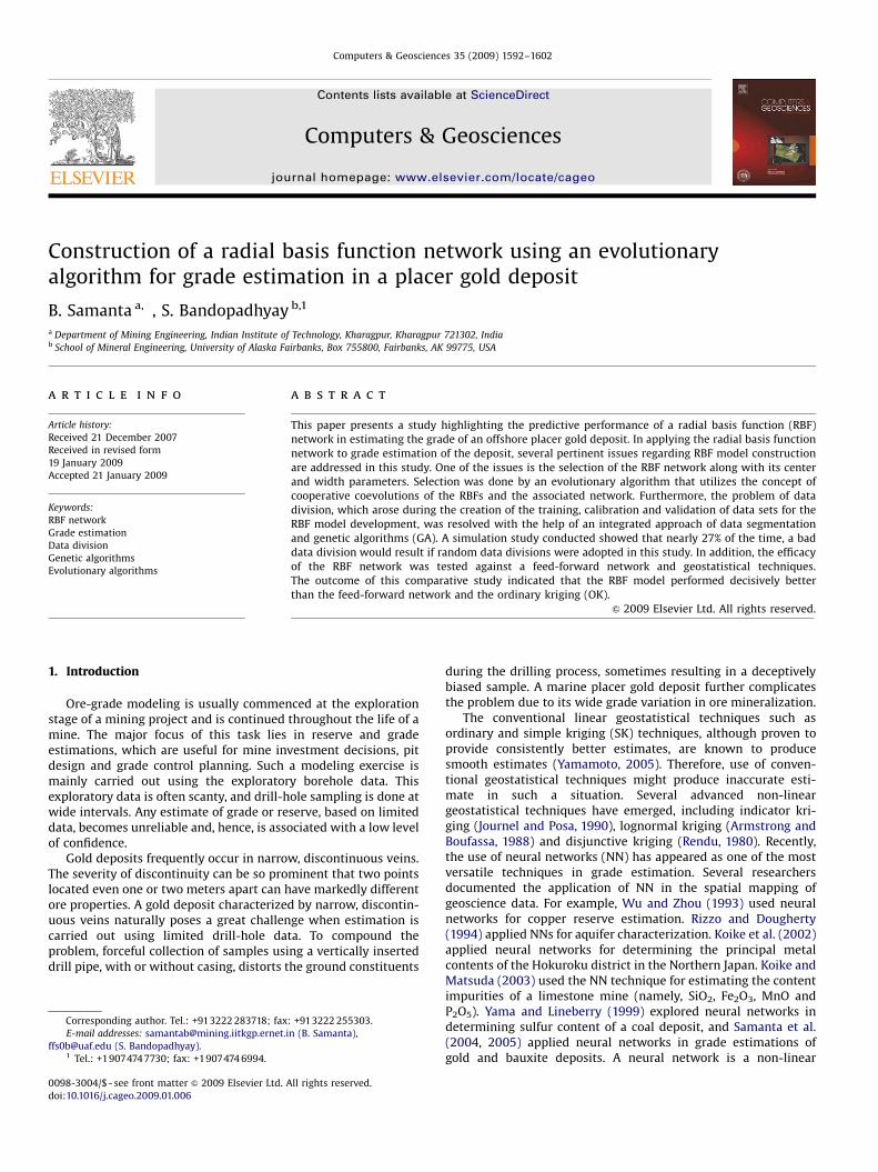
Fig. 1. (a) Spatial plot of composite borehole data. (b) Histogram plot of co

mapping (Singer and Kouda, 1996; Kapageridis and Denby, 1998;Koike and Matsuda, 2003). An obvious disadvantage of such anetwork is that it is highly non-linear in the parameter space. Themodel is built up using a learning algorithm that employs acomplex non-linear optimization technique including gradientdescent back-propagation learning. Even with the application ofsuch optimization algorithm, the model is not free from the scareof being trapped into the local minima of the chosen error

8600 8800 9000 9200 9400g (m)

old1200.0 1600.000.0

300 400ance (m)

0<=gold<100

300<=gold<6212100<=gold<300

mposite borehole data. (c) Variogram plot of composite borehole data.

ARTICLE IN PRESS

B. Samanta, S. Bandopadhyay / Computers & Geosciences 35 (2009) 1592–16021594

minimization criterion, resulting in a sub-optimal network. Otheroptimization algorithms such as genetic algorithms (GA)(Montana and Davis, 1989) and the simulated annealing (Portoet al., 1995) generate global minimum but require extensivecomputational efforts. A suitable alternative to the computation-ally expensive feed-forward NN is the radial basis function (RBF)network. The RBF network has proved to be effective in manymultidimensional interpolation tasks including signal and imageprocessing (Acosta, 1995; Mulgrew, 1996) and time-series model-ing (Ryad et al., 2003; Whitehead and Choate, 1996). This paperpresents an application of the RBF network in grade estimation ofan offshore placer gold deposit.

2. Placer deposit under study

The placer deposit under study is situated in the Nome districtof Alaska on the south shore of the Seward Peninsula. It is located840 km west of the city of Fairbanks and 860 km northwest of thecity of Anchorage. The offshore placer gold deposit at Nome wasdiscovered in the year 1898. Gold and antimony have beenreported as the predominant metals in the deposit. Other valuablemetals include tungsten, iron, copper, bismuth, molybdenum, leadand zinc.

The Nome deposit has been explored by various agencies overtime. All together, 3500 exploratory boreholes have been drilled inan area of 22,000 acres. For operational convenience, the leaseboundary was arbitrarily divided into the nine blocks: Coho,Halibut, Herring, Humpy, King, Pink, Red, Silver and Tomcod.Rusanowski (1994) presented an excellent summary of the Nomeoffshore placer project. The present study focused on a part ofthe deposit in the Herring block. The exploration program in theHerring block resulted in 415 drill holes, which is the only sourceof data used in this study. Exploration samples are in the form ofcores collected from the bottom sediment of the sea floor.The average depth of the holes is roughly 30 m. A comprehensivedatabase of the core samples was made available to studythe deposit. An earlier study led by Ke (2002) suggested that thepotential gold resource of the deposit is confined within 5 m of thesea floor bottom sediment. Hence, raw drill-core samplescomposited within 5 m of the sea floor bottom sediment wereused for grade estimation of the deposit.

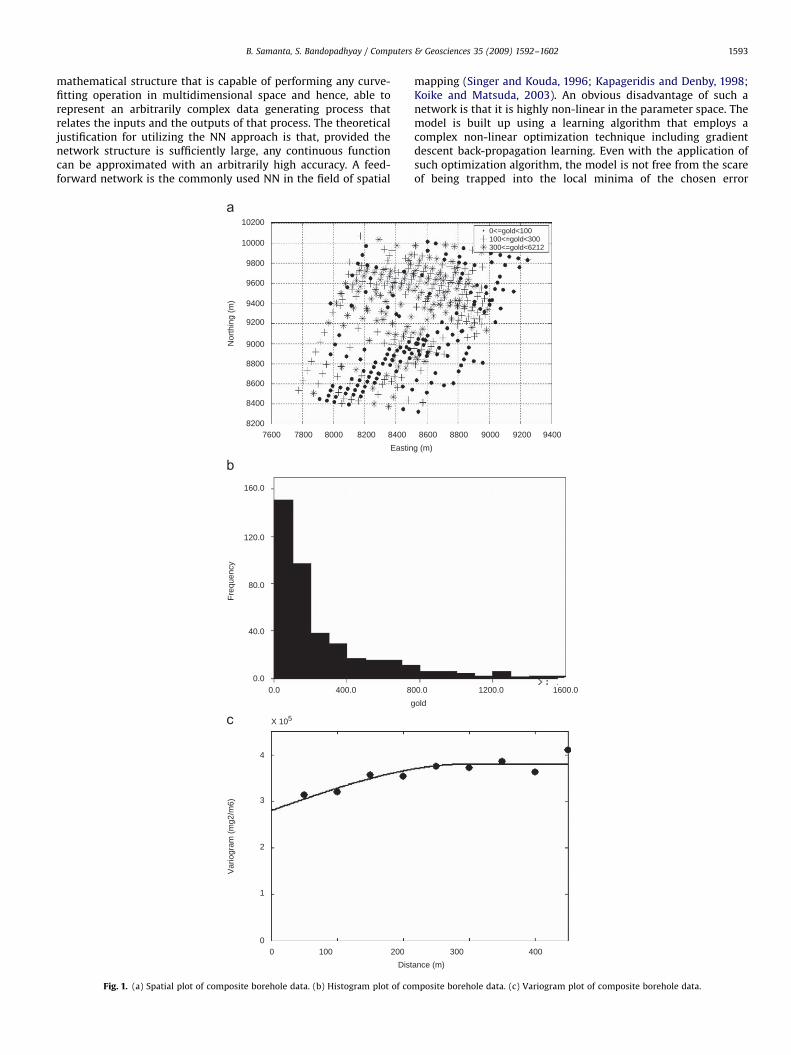
Fig. 2. A Simplified diagram of radial basis function network alo

Before commencing for the grade estimation, the compositeborehole data were thoroughly analyzed using various statisticaltools, since a comprehensive understanding of the statisticalproperties of the grade attribute is prerequisite to drawing ameaningful interpretation of a model output. Analysis involved astatistical summarization of the gold values along with thevarious graphical representations of the data including spatial,histogram and variogram plots. Statistical summary of the datarevealed that the mean value of the gold concentration is in theorder of 440.17 mg/m3 with a standard deviation of 650.58 mg/m3.The coefficient of variation is 148% indicating a highly hetero-geneous deposit. A spatial plot of the borehole data is shown inFig. 1(a). It can be seen that the boreholes are located in anirregular grid. A histogram plot of the data is presented in Fig. 1(b).The histogram shape is akin to the lognormal probabilitydistribution. This feature of gold grade distribution is quiteexpected as most of the gold deposits in nature typically occursporadically in a few small patches with high gold concentrationin the region of the low-grade zone. The spatial continuity of thedeposit was captured through a variography study. Fig. 1(c)presents an omni-directional variogram model prepared forcapturing the spatial continuity of the deposit. The variogramexhibits a picture of poor spatial correlation in the study region.The nugget plays a dominant role in the variogram model, inexplaining the total spatial variability of the data indicating asignificant influence of noise in the data variation. Therefore, theregional component constitutes a minor part of data variability.The omni-directional variogram modeling was also followedby directional variogram modeling to check for the presenceof anisotropy. No discernable anisotropy was observed in anyparticular direction.

3. RBF network for spatial interpolation

The RBF network has three layers: input, hidden and output.A simplified architecture of the RBF network for spatial interpola-tion of a grade attribute is presented in Fig. 2. In a spatial mappingexercise, spatial coordinates such as northing (y-coordinate) andthe easting (x-coordinate) might be used as inputs (X) into theinput layer. These inputs are then non-linearly transformed by aset of RBFs, creating a new space, j, in the hidden layer. Through

ng with different mathematical operators in various layers.

ARTICLE IN PRESS

B. Samanta, S. Bandopadhyay / Computers & Geosciences 35 (2009) 1592–1602 1595

this non-linear transformation only, the network acquires thecapability of non-linear functional mapping. The most commonlyused non-linear RBF is the Gaussian function. Other types of non-linear functions such as multiquadratic and the thin-plate splineare alternately used (Haykins, 1999). The general consensus is thatthe type of the basis function does not have much impact on thegeneral performance of the RBF network. The Gaussian RBFs of thenetwork are characterized by two sets of parameters: radial basiscenters, m, and widths, s. Hence, the different basis functions inthe hidden layer are recognized by these parameters. The ith basisfunction of the network can be expressed by the followingmathematical formula:

fiðXÞ ¼ exp�kX � mik

si(1)

where fi(X) is the output from the ith basis function, mi the centerof the ith basis function, si the width of the ith basis function andJ � J the Euclidian distance of the input from the center.

The outputs from the hidden layer are then linearly combinedto produce the final output (Y) of the network, which in the studyis the gold concentration. This can be expressed as

Y ¼Xn

i¼1

WinfiðXÞ (2)

where Y is the output of the network, Wi the weight associatedwith the ith basis function and n the number of the basis functions.

While the weight parameters of a feed-forward network aredetermined using a complex non-linear optimization algorithm,demanding expensive computational time, the weight parametersof a RBF network can be fixed by using a least square algorithm.This is the point where a RBF network gains substantialcomputational advantage over a feed-forward network.

It is evident that the operational principle of the RBF networkresembles the kriging technique; of course, certain disparities arepresent. Like the kriging technique, a RBF network is a local fittingalgorithm in the sense that only a few RBFs influence the output ofa spatial attribute at a particular location. Similarly, in kriging,only a few samples that fall inside a search radius influence theestimation. The range of influence of a RBF for determining outputis dictated by the width parameter of the basis function, while therange parameter of a variogram model decides the influence of asample set in determining the kriging estimate. With the krigingtechnique, neighboring sample values are linearly combined toproduce output, whereas with RBF modeling, the RBFs are linearlycombined to generate output. Although in kriging, the originaldata values of the attribute (in this case, gold) are used for linearcombiner, in RBF the non-linear outputs generated from the basisfunctions are used in the linear combiner. The degree of influenceof a basis function for determining the output at a point dependsupon the proximity of the basis center to that point, which is alsotrue for a kriging estimate. The weights of a kriging estimate aredetermined by solving the kriging system of equation which usesinformation from a variogram model, whereas, the weights of theRBF model, by comparison, are determined by a linear least squarealgorithm. One major advantage of the RBF model is that it doesnot require a variogram model. For insufficient and noisy data,construction of a variogram model is a grueling task. Hence, theRBF model would offer a great advantage over kriging wherevariogram modeling is a difficult task.

4. Evolutionary algorithm and parameter selection of the RBF

Once the number of RBFs and their center and widthparameters are judicially decided, the creation of the RBF networkis only a matter of determining the weight parameters which can

easily be ascertained using a least square algorithm. Therefore, thecentral problem remaining for construction of a RBF network isselection of the number of basis functions, and their center andwidth parameters. For the selection of a suitable RBF network,some researchers have attempted the use of RBF network as astrict interpolator (Micchelli, 1986; Powell, 1987). As a strictinterpolator, the RBF network uses the locations of all trainingdata points as the centers of the basis functions, thus choosing asmany basis centers as the training data points. This strategy,however, led to a problem of numerical instability and the curse ofover-fitting the model to the noise. To combat with theseinadequacies of the methodology, Yee and Haykins (1999)suggested to add a regularized parameter in the RBF model. Thisapproach also did not lead to a fruitful proposition due to itsrelatively high computational effort, particularly for the largerdata sets. Consequently, researchers began to realize the need fora RBF network with fewer RBFs. A major problem then arose inselecting basis centers and the associated width parameters, sothat the best generalization and the prediction performance couldbe achieved. This problem was approached by some investigatorswho used data-point clustering, and selected cluster centers aslocation of basis centers (Moody and Darken, 1989). However,Dutta et al. (2005) pointed out that in a spatial interpolationexercise of grade estimation, where data are most often collectedin a regular grid, the clustering algorithm would not be beneficial.Chen et al. (1991) also developed a technique based on theorthogonal least square algorithm for choosing the best combina-tion of the RBFs in a network. In this study, however, anevolutionary algorithm was applied for the selection of anappropriate RBF network. It employed the concept of cooperativecoevolution, which is a recent idea used in creating the ensembleneural network (Garcia-Pedraias et al., 2005). Hence, this studypresents a novel approach for RBF network construction byintroducing the same paradigm of cooperative coevolution indesigning a RBF network.

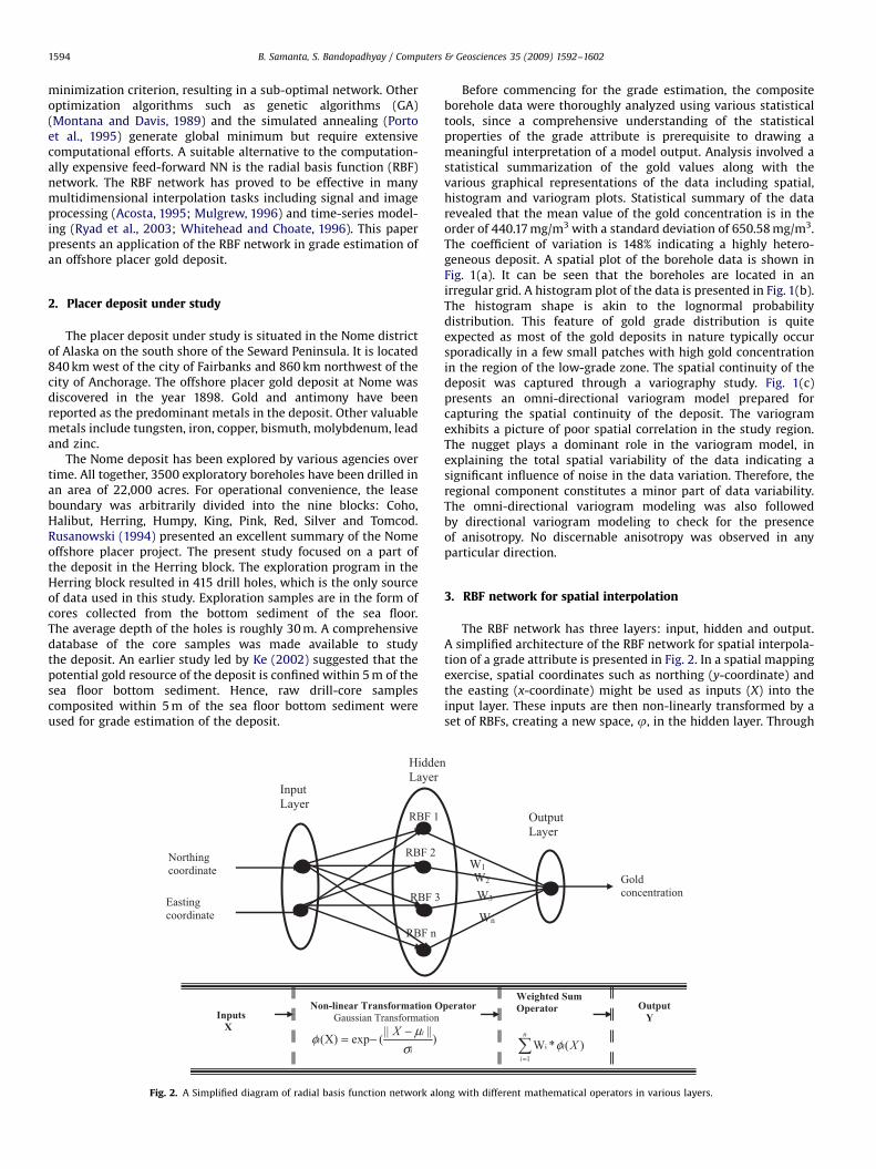
In the framework of cooperative coevolution, two separatepopulations evolved simultaneously: (i) a population of the radialbasis functions and (ii) a population of the RBF networks. Fig. 3presents a simplified diagram of this algorithm for the selectionof a RBF network. The population of RBFs consists of a numberof subpopulations (n), where each subpopulation containsseveral basis functions (m). Simultaneous evolution of thesesubpopulations favors the speciation of similar RBFs, and hencemaintains the genetic diversity of RBFs among subpopulations.The RBFs of these subpopulations are then used in the formation ofRBF networks. The population of RBF networks is formed by a setof networks, each network being constructed by the amalgamationof RBFs from all the subpopulations. Each generation of the wholeprocess involves generation of the radial basis functions populationfollowed by the generation of the RBF network population. Theevolution of these subpopulations is described below.

4.1. Evolution of the RBF population

Each RBF is recognized by the three parameters: the centers(x and y coordinates) and the width (s). The centers of the RBFs forthe initial population are selected randomly from the locations oftraining data points. The width parameter of these basis functionsis set as the average distance of the training data points. However,note that the width parameter of the basis functions subsequentlychanges as the population evolves through each generation. Eachsubpopulation, consisting of m number of RBFs is, thus, builtup gradually and a population containing n number of suchsubpopulations is formed. The fitness of each RBF is then assessedthrough an appropriate fitness measuring function. The decision

ARTICLE IN PRESS

# NN 1

# NN 2

# NN 3

# NN 4

# NN 5

# NN m

Fitness of each RBF network

Elite Selection (best p2% of the population)

Eliminated from the population if not selected

Crossover (q2% of the population)

Crossover operation Mutation(r2% of the population)

Exchanging a RBF from the Population of RBF

NEXT GENERATION

Evolution of RBF Network Population Evolution of RBF Population

Each RBF is represented by 3-parameters

If not selected then removed from the

Elite Selection (Best p1% of the

Fitness of each RBF in the subpopulation

#1

#2

#3

#n

Parametric Mutation Change the values of Centers (Xc, Yc) and

Introduction of new RBF from the training set

NEXT GENERATION

Random selection of RBF from the training data initially

subpopulation)

(q1 %of the subpopulation)

(r1 %of the subpopulation)

subpopulation

width (σ)

Fig. 3. Cooperative coevolution of evolutionary algorithm for RBF model selection.

B. Samanta, S. Bandopadhyay / Computers & Geosciences 35 (2009) 1592–16021596

for selecting a fitness measuring function is crucial as the fitnessfunction forces appropriate RBFs to stay in the population, hencecontrolling the overall performance of the algorithm. The maincriteria on which the RBF suitability is judged relate to: (a) thediversity of RBFs among the subpopulations and (b) the proximityof RBFs in the same subpopulation. These two criteria are favoredwith a hope that the different species of RBFs could be retained inthe population, and that selection of RBFs from each species(subpopulation) would make it possible to construct networkswith dissimilar RBFs. This approach is believed to improve thepredictive performance of the network, since the dissimilar RBFsin the network will carry uncorrelated information. In thisconnection, it is noteworthy to point out that both the diversityand proximity criteria could be evaluated based on measures ofstatistical correlation among RBFs. Recall that when an inputvector is presented to a network, each basis function in the hiddenlayer being activated emits a signal. If the activated signals of twosuch basis functions are similar, then they are correlated and actsimilarly. To measure this correlation, the input data (Xj) of thetraining sets consisting of N data points are presented to eachof the basis functions, and the activated signals due to N inputvectors are normalized. The normalized activated signalfrom the ith basis function due to jth input vector would be

fnormi ðxjÞ ¼ fiðxjÞ=

PNj¼1

f2i ðxjÞ. Then the inner product between fi

and f0i activation functions actually defines the statisticalcorrelation between the ith and i0th RBFs. Hence, if thediversity criterion is allowed to persist among RBFs of differentsubpopulations, then the measures of statistical correlationamong different RBFs of subpopulations should be as low aspossible. On the other hand, for the proximity criterion to sustain

among the RBFs of the same subpopulation, the measures ofstatistical correlation of these RBFs should be as high as possible.To impose the above criteria, a sharing function approach thatemploys a ranking selection and a niching method is used inassigning a fitness value to the individual RBF in the population(Goldberg and Richardson, 1987). In niching method, eachmember of RBFs in a subpopulation (also called as niche) has itsvalue degraded depending upon its niche count. The niche countof a RBF is calculated based upon the diversity of the RBF amongthe RBFs of the different subpopulation and the proximity of theRBF among the RBFs of the same subpopulation. For this purpose,a niche radius is defined. If the diversity value according todiversity criterion (same procedure follows for the proximitycriterion) between the two RBFs exceeds the niche radius, theniche count becomes 1, otherwise the niche count value will varylinearly in between 0 and 1. To this end, each RBF is assigned anequal dummy fitness value, Fdummy, at the beginning. The fitnessof a RBF is then devalued as per its niche count. Therefore, given apopulation of RBFs, the fitness value of the individual RBF iscalculated using the following procedure:

(a)

Compute the diversity value of every individual p of the ithsubpopulation (i ¼ 1, 2,y, n) with the every individual q of jthpopulation (jai) by divpq ¼ fnorm

pfnormq. Compare this value

with a niche radius sr and calculate a penalty value P1(divpq)by applying the following function:

P1ðdivpqÞ ¼1�

divpq

sr

� �2

; if divpqosr

0 . . . Otherwise

8><>:

ARTICLE IN PRESS

B. Samanta, S. Bandopadhyay / Computers & Geosciences 35 (2009) 1592–1602 1597

Compute the proximity value of the pth individual of the ith

(b) (i ¼ 1, 2,y, n) subpopulation with the qth individual of thesame population (paq) by clpq ¼ fnorm

pfnormq. Compare this

value with a niche radius sr and calculate a penalty valueP2(clpq) by applying the following function:

P2ðclpqÞ ¼1�

clpq

sr

� �2

; if clpqosr

0 . . . Otherwise

8><>:

(c)

Calculate the niche count for the pth individual of the ithsubpopulation by

mp ¼Xn

iai

Xmq¼1

P1ðdivpqÞ þXmqap

P2ðclpqÞ

( )jp 2 i

" #

(d)

Modify the fitness of the individual according to its nichecount

f 0p ¼f dummy

mp

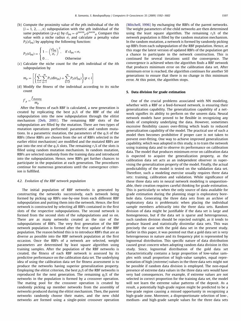
After the fitness of each RBF is calculated, a new generation iscreated by replicating the best p1% of the RBF of the oldsubpopulation into the new subpopulation through the elitistmechanism (Deb, 2001). The remaining RBF slots of thesubpopulation are filled by the mutation. There are two types ofmutation operations performed: parametric and random muta-tions. In a parametric mutation, the parameters of the q1% of theRBFs (these RBFs are chosen from the set of RBFs selected in theearlier elitist mechanism) are modified and the mutated RBFs areput into the rest of the q1% slots. The remaining r1% of the slots isfilled using random mutation mechanism. In random mutation,RBFs are selected randomly from the training data and introducedinto the subpopulation. Hence, new RBFs get further chances toparticipate in the population at each generation. The procedurescontinue for numerous generations until the convergence criter-ion is fulfilled.

4.2. Evolution of the RBF network population

The initial population of RBF networks is generated byconstructing the networks successively, each network beingformed by picking up RBFs one-by-one from each different RBFsubpopulation and putting them into the network. Hence, the firstnetwork is constructed by selecting all RBFs contained in the firstslots of the respective subpopulations. The second network isformed from the second slots of the subpopulations and so on.There are as many networks created as the size of thesubpopulations of RBFs. The very first generation of the RBFnetwork population is formed after the first update of the RBFpopulation. The reason behind this is to introduce RBFs that are asdiverse as possible into the RBF network population at the firstoccasion. Once the RBFs of a network are selected, weightparameters are determined by least square algorithm usingtraining samples. After the population of the RBF networks iscreated, the fitness of each RBF network is assessed by itspredictive performance on the calibration data set. The underlyingidea of using the calibration data set for fitness assessment is toproduce the networks having superior generalization property.Employing the elitist criterion, the best p2% of the RBF networks isreproduced for the next generation. The remaining q2% of thenetworks in the population is formed by a crossover operation.The mating pool for the crossover operation is created byrandomly picking up member networks from the assembly ofnetworks produced during the elitist mechanism. Then, the parentnetworks randomly choose their mates, and the new childnetworks are formed using a single-point crossover operation

(Mitchell, 1996) by exchanging the RBFs of the parent networks.The weight parameters of the child networks are then determinedusing the least square algorithm. The remaining r2% of thenetwork population is filled by the random mutation mechanism.In the random mutation, a network is formed by randomly pickingup RBFs from each subpopulation of the RBF population. Hence, atthis stage the latest version of updated RBFs of the population geta chance to participate in the network construction. This iscontinued for several iterations until the convergence. Theconvergence is achieved when the algorithm finds a RBF networkthat produces minimum error on the calibration data set. Afterminimum error is reached, the algorithm continues for another 50generations to ensure that there is no change in this minimumerror. At this point, the algorithm stops.

5. Data division for grade estimation

One of the crucial problems associated with NN modeling,whether with a RBF or a feed-forward network, is ensuring theirgeneralization capability. The generalization capability of a net-work signifies its ability to perform on the unseen data. Neuralnetwork models have proved to be flexible in recognizing anykinds of complexity underlying the data. However, sometimesexcessive flexibility causes over-fitting which leads to reducedgeneralization capability of the model. The practical use of such amodel then becomes prohibitive if proper care is not taken toprevent over-fitting. One way to achieve improved generalizationcapability, which was adopted in this study, is to train the networkusing training data and to observe its performance on calibrationdata. The model that produces minimum error on calibration datais expected to acquire the generalization property, as thecalibration data set acts as an independent observer in super-vising the generalization property of the model. Finally, the actualpredictability of the model is tested on the validation data set.Therefore, such a modeling exercise usually requires three datasets: training, calibration and validation. While significance ofthese three data sets in neural network modeling is unquestion-able, their creation requires careful thinking for grade estimation.This is particularly so when the only source of data available forgrade estimation during the planning stage is exploratory bore-hole data. Generating the three data sets from an archive ofexploratory data is problematic when placing the individualsample members arbitrarily into the three data sets. Randomdivision of data might be justifiable if the data set is large andhomogeneous, but if the data set is sparse and heterogeneous,such random division should be rejected outright, as it tends toproduce biased and statistically dissimilar data sets. This wasprecisely the case with the gold data set in the present study.Earlier in this paper, it was pointed out that a gold data set is veryheterogeneous in nature and its frequency plot is represented bylognormal distribution. This specific nature of data distributioncaused great concern when adopting random data division in thisstudy. Since, lognormal distribution of the gold data setcharacteristically contains a large proportion of low-value sam-ples with small proportion of high-value samples, equal repre-sentation of high (extreme) values in the three data sets might notbe possible if random data division is employed. The non-equalpresence of extreme data values in the three data sets would havevery bad consequences. For example, if extreme values are notselected in correct proportion for the training data set, the modelwill not learn the extreme value patterns of the deposit. As aresult, a potentially high-grade region might be predicted to be alow-grade region causing a missed opportunity in recognizing ahigh-grade zone. Moreover, a disproportionate selection of low-,medium- and high-grade sample values for the three data sets

ARTICLE IN PRESS

B. Samanta, S. Bandopadhyay / Computers & Geosciences 35 (2009) 1592–16021598

will result in dissimilar characteristics of the data sets. This wouldcause a problem in measuring the generalization capability of themodel, since the general behavior of the data sets differs.

The quality of the data division produced by a randomselection algorithm in this data set was examined through asimulation study. A particular data division is deemed to be bad,if the mean difference of the three data sets is statisticallysignificant. The statistical means of each data subgroup arereckoned with respect to all input and output variables includingnorthing, easting and gold. In this part of the study, 100 datadivisions were generated in each simulation by randomly pickingthe sample members in the three data sets: training, calibrationand validation. The mean difference of the data sets was examinedusing the ANOVA F test for variables northing and easting, and theWald test (Tu and Zhou, 1999) for variable gold. The Wald test isuseful for a variable that follows lognormal distribution andcontains some zero observations. Note that the gold data setcontains some zero observation, as no trace of the gold value wasobserved for a few of the exploratory boreholes. The simulationstudy indicated that nearly 27% of the random data divisionswere bad. This figure was arrived at by averaging 100 simulation

Table 1Statistical summary for one of random divisions.

Attribute Mean Standard deviation

Training Calibration Validation Training Calibration Validation

X-coordinate (m) 8503.5 8436.3 8586.2 290.52 319.28 314.54

Y-coordinate (m) 9228.7 9173.8 9401.0 474.5 447.17 312.25

Gold (mg/m3) 228.47 246.02 633.1 269.91 285.99 944.00

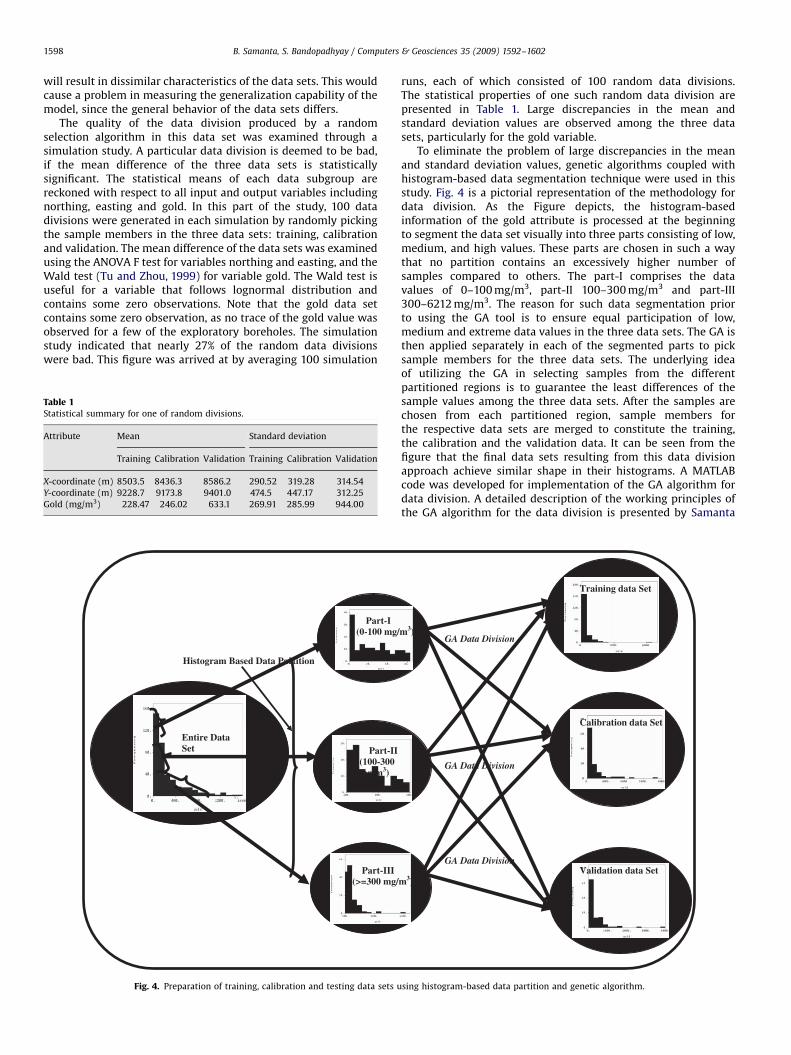
Histogram Based Data Partition

Part-I(0-100 mg/

Part-II(100-300mg/m3)

Part-III (>=300 mg/

Entire Data Set

Fig. 4. Preparation of training, calibration and testing data sets u

runs, each of which consisted of 100 random data divisions.The statistical properties of one such random data division arepresented in Table 1. Large discrepancies in the mean andstandard deviation values are observed among the three datasets, particularly for the gold variable.

To eliminate the problem of large discrepancies in the meanand standard deviation values, genetic algorithms coupled withhistogram-based data segmentation technique were used in thisstudy. Fig. 4 is a pictorial representation of the methodology fordata division. As the Figure depicts, the histogram-basedinformation of the gold attribute is processed at the beginningto segment the data set visually into three parts consisting of low,medium, and high values. These parts are chosen in such a waythat no partition contains an excessively higher number ofsamples compared to others. The part-I comprises the datavalues of 0–100 mg/m3, part-II 100–300 mg/m3 and part-III300–6212 mg/m3. The reason for such data segmentation priorto using the GA tool is to ensure equal participation of low,medium and extreme data values in the three data sets. The GA isthen applied separately in each of the segmented parts to picksample members for the three data sets. The underlying ideaof utilizing the GA in selecting samples from the differentpartitioned regions is to guarantee the least differences of thesample values among the three data sets. After the samples arechosen from each partitioned region, sample members forthe respective data sets are merged to constitute the training,the calibration and the validation data. It can be seen from thefigure that the final data sets resulting from this data divisionapproach achieve similar shape in their histograms. A MATLABcode was developed for implementation of the GA algorithm fordata division. A detailed description of the working principles ofthe GA algorithm for the data division is presented by Samanta

m3)

m3)

Training data Set

Calibration data Set

Validation data Set

GA Data Division

GA Data Division

GA Data Division

sing histogram-based data partition and genetic algorithm.

ARTICLE IN PRESS

B. Samanta, S. Bandopadhyay / Computers & Geosciences 35 (2009) 1592–1602 1599

et al., (2005). For the convenience of the readers, however,a concise description of the GA algorithm is provided here.

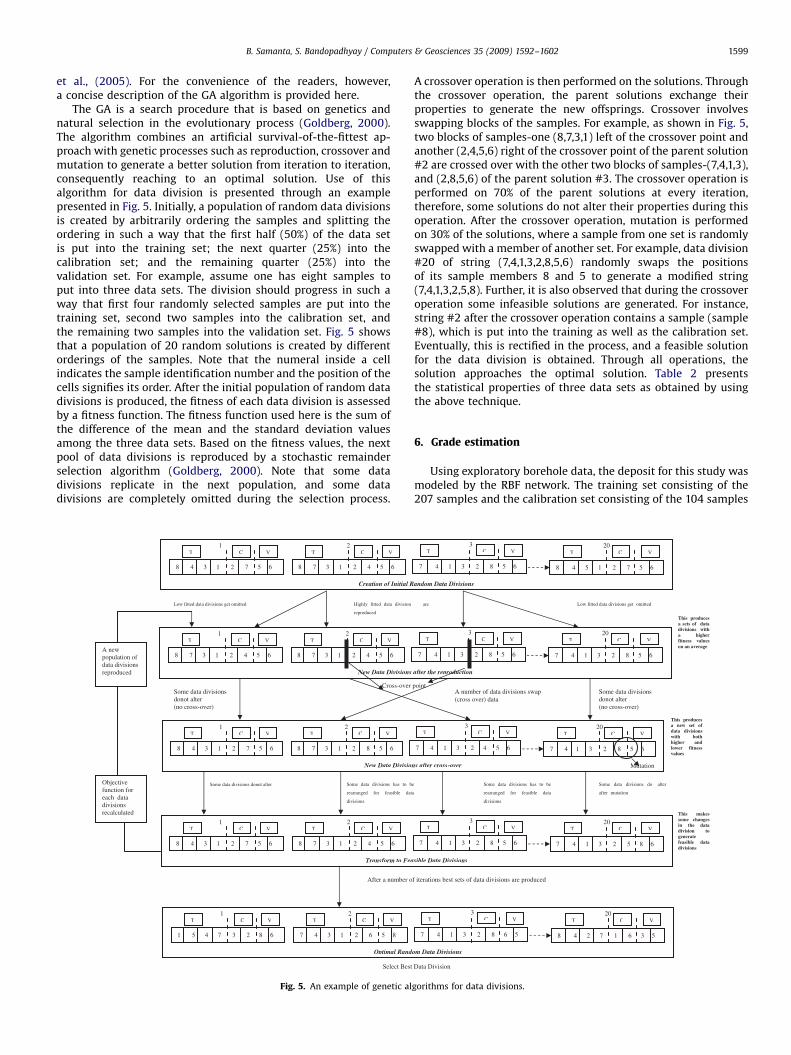
The GA is a search procedure that is based on genetics andnatural selection in the evolutionary process (Goldberg, 2000).The algorithm combines an artificial survival-of-the-fittest ap-proach with genetic processes such as reproduction, crossover andmutation to generate a better solution from iteration to iteration,consequently reaching to an optimal solution. Use of thisalgorithm for data division is presented through an examplepresented in Fig. 5. Initially, a population of random data divisionsis created by arbitrarily ordering the samples and splitting theordering in such a way that the first half (50%) of the data setis put into the training set; the next quarter (25%) into thecalibration set; and the remaining quarter (25%) into thevalidation set. For example, assume one has eight samples toput into three data sets. The division should progress in such away that first four randomly selected samples are put into thetraining set, second two samples into the calibration set, andthe remaining two samples into the validation set. Fig. 5 showsthat a population of 20 random solutions is created by differentorderings of the samples. Note that the numeral inside a cellindicates the sample identification number and the position of thecells signifies its order. After the initial population of random datadivisions is produced, the fitness of each data division is assessedby a fitness function. The fitness function used here is the sum ofthe difference of the mean and the standard deviation valuesamong the three data sets. Based on the fitness values, the nextpool of data divisions is reproduced by a stochastic remainderselection algorithm (Goldberg, 2000). Note that some datadivisions replicate in the next population, and some datadivisions are completely omitted during the selection process.

Objectivefunction for each data divisionsrecalculated

A new population of data divisions reproduced

Select Best

After a number o

Some data divisions donot alter (no cross-over)

Cross-over

Optimal Rand

7 4 3 1 2 6 5 8

2T C V

1 5 4 7 3 2 8 6

1VCT

8 7 3 1 2 4 5 6

2T C V

8 7 3 1 2 4 5 6

1VCT

New Data Divisions

New Data Divisio

8 7 3 1 2 8 5 6

2T C V

8 4 3 1 2 7 5 6

1VCT

Creation of Initial R

8 7 3 1 2 4 5 6

2T C V

8 4 3 1 2 7 5 6

1VCT

Transform to Fea

8 7 3 1 2 4 5 6

2T C V

8 4 3 1 2 7 5 6

1VCT

Fig. 5. An example of genetic al

A crossover operation is then performed on the solutions. Throughthe crossover operation, the parent solutions exchange theirproperties to generate the new offsprings. Crossover involvesswapping blocks of the samples. For example, as shown in Fig. 5,two blocks of samples-one (8,7,3,1) left of the crossover point andanother (2,4,5,6) right of the crossover point of the parent solution#2 are crossed over with the other two blocks of samples-(7,4,1,3),and (2,8,5,6) of the parent solution #3. The crossover operation isperformed on 70% of the parent solutions at every iteration,therefore, some solutions do not alter their properties during thisoperation. After the crossover operation, mutation is performedon 30% of the solutions, where a sample from one set is randomlyswapped with a member of another set. For example, data division#20 of string (7,4,1,3,2,8,5,6) randomly swaps the positionsof its sample members 8 and 5 to generate a modified string(7,4,1,3,2,5,8). Further, it is also observed that during the crossoveroperation some infeasible solutions are generated. For instance,string #2 after the crossover operation contains a sample (sample#8), which is put into the training as well as the calibration set.Eventually, this is rectified in the process, and a feasible solutionfor the data division is obtained. Through all operations, thesolution approaches the optimal solution. Table 2 presentsthe statistical properties of three data sets as obtained by usingthe above technique.

6. Grade estimation

Using exploratory borehole data, the deposit for this study wasmodeled by the RBF network. The training set consisting of the207 samples and the calibration set consisting of the 104 samples

Data Division

f iterations best sets of data divisions are produced

Some data divisions donot alter (no cross-over)

A number of data divisions swap (cross over) data

point

om Data Divisions

8 4 2 7 1 6 3 5

T20

C V

7 4 1 3 2 8 6 5

3VCT

7 4 1 3 2 8 5 6

T20

C V

7 4 1 3 2 8 5 6

3VCT

after the reproduction

ns after cross-over

7 4 1 3 2 8 5 6

T20

C V

7 4 1 3 2 4 5 6

3VCT

andom Data Divisions

8 4 5 1 2 7 5 6

T20

C V

7 4 1 3 2 8 5 6

3VCT

sible Data Divisions

7 4 1 3 2 5 8 6

T20

C V

7 4 1 3 2 8 5 6

3VCT

Mutation

gorithms for data divisions.

ARTICLE IN PRESS

B. Samanta, S. Bandopadhyay / Computers & Geosciences 35 (2009) 1592–16021600

were used to build the RBF model. The selection of basis functionswas accomplished using the evolutionary algorithm discussedearlier. After some trial exercises, the parameters of the evolu-tionary algorithm (shown in Table 3) were fixed. Once theevolutionary algorithm converged into the optimal solution, thebest network resulting from the algorithm was chosen as the finalRBF model for grade estimation. Network’s performance was thenexamined on the validation data set consisting of 103 sampleobservations to find its predictive accuracy. A MATLAB code wasdeveloped for the implementation of the algorithm. Forjustification of using the RBF network for this deposit, acomparative evaluation of the same was carried out with theother types of prediction algorithms including feed-forward NNsand geostatistics.

For construction of the feed-forward network, northing andeasting coordinates were used as input variables and goldattribute was used as output variable. The network consisted ofan input layer having two nodes, a single hidden layer with30 nodes, and an output layer of one node. The hidden layer wasformed with a variety of non-linear activation functions such asthe Gaussian, the Hyperbolic tangent and the Gaussian comple-mentary, whereas the output layer used the logistic activationfunction. The number of nodes in the hidden layer was fixed after

Table 2Statistical summary of data using histogram-based data partition and genetic

algorithm.

Attribute Mean Standard deviation

Training Calibration Validation Training Calibration Validation

X-coordinate (m) 8505.4 8509.6 8507.5 308.4 309.3 308.4

Y-coordinate (m) 9256.9 9256.4 9260.3 443.15 441.49 436.46

Gold (mg/m3) 324.04 350.24 334.43 561.09 558.38 536.83

Table 3Parameters of evolutionary algorithms for RBF model selection.

Category Parameters Parameter values

Population of RBFs No. of subpopulations 15

No. of RBF in each subpopulation 10

P1 (%of elite) 40%

q2 (%parametric mutation) 30%

r2 (%random mutation) 30%

Population of network No. of networks 10

No. of RBF in each network 15

P2 (%of elite) 60%

q2 (% of crossover) 20%

r2 (% of mutation) 20%

Diversity function Niche radius 0.2

Proximity function Niche radius 0.2

Individual RBF Fdummy 100

Table 4Comparative performance of different algorithms for validation data set.

Model statistics RBF network Feed-forward network

Mean error (mg/m3)�28.51 �37.25

Error variance (mg2/m6) 223397 258462

Mean square error (mg2/m6) 224210 259850

R2 (%) 21 10

observing the model’s output on the calibration data set with thevarying number of hidden nodes. The Leavenberg–Marquardtback-propagation (MLBP) algorithm was used to train thisnetwork (Hagan et al., 2002). Over-fitting of the model wasrestricted using the early stop training (Haykins, 1999) strategy. Inthis training exercise, the model was trained using training data;however, its performance was observed on calibration data.Initially, both training and calibration errors began to reduce,but after certain iterations, the calibration error started to rise dueto learning noisy patterns. The training was stopped at the lowesterror on the calibration data. After the model was developed, itsperformance was tested on the same validation data set that wasused for the RBF model.

Various geostatistical techniques were investigated for com-parison purpose. These models include: (i) simple kriging,(ii) ordinary kriging (OK), (iii) kriging with linear drift function(KLD), and (iv) kriging with quadratic drift function (KQRD).Although, these models work on the same fundamental principle,they have some distinguishable features. For example, simplekriging and ordinary kriging work on the principle of meanstationary assumption. Further, while simple kriging performs onthe global mean of the data, ordinary kriging operates on the localmean of the data. In contrast, the KLD and the KQRD modelsassume that the mean varies over the spatial region and can bemodeled by a drift (trend) component, which is a function of thespatial location. The KLD uses a linear trend model, while theKQRD employs a quadratic trend model. Detail description ofthese geostatistical models can be found in Goovaerts (1997).All the geostatistical techniques require a variogram model tooperate. The variogram model was created using a data setprepared by merging the training and calibration data sets, sinceno separate calibration data set was required for development ofthe geostatistical models. After these models were created, theywere tested on the same validation set as used by the feed-forward and the RBF networks.

For comparison of the models, the following error statisticswere used: (i) mean error or bias, (ii) error variance, (iii) meansquare error, and (iv) coefficient of determination, R2. The meanerror or bias indicates a lack of fit of the model to the data. It alsosignifies an over estimation or under estimation of the prediction.The error variance attributes to the confidence attached to theprediction. The mean square error might be expressed as the sumof error variance and the square of the bias, hence, it takes intoaccount both the bias and the error variance making it a bettermeasure of prediction accuracy than the error variance. The R2

represents the percentage of data variance explained by the modeland, therefore, signifies the predictive capacity of the model.

Table 4 presents the error statistics of the three types ofmodels. It can be seen from the models’ outputs that all thegeostatistical models performed more or less equally for thisdeposit considered in this study. The bias of the geostatisticalmodels is relatively low in comparison with the other two types ofNN models. The mean square error of the RBF network is thelowest, followed by geostatistics and feed-forward network.

Geostatistical techniques

SK OK KLD KQRD

8.97 7.97 6.93 5.93

246569 246726 246751 247154

246650 246790 246800 247190

13 13 13 13

ARTICLE IN PRESS

B. Samanta, S. Bandopadhyay / Computers & Geosciences 35 (2009) 1592–1602 1601

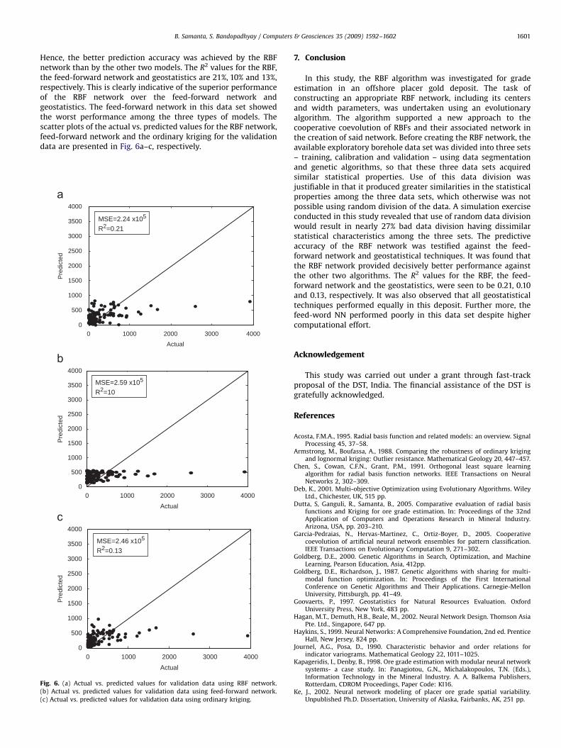
Hence, the better prediction accuracy was achieved by the RBFnetwork than by the other two models. The R2 values for the RBF,the feed-forward network and geostatistics are 21%, 10% and 13%,respectively. This is clearly indicative of the superior performanceof the RBF network over the feed-forward network andgeostatistics. The feed-forward network in this data set showedthe worst performance among the three types of models. Thescatter plots of the actual vs. predicted values for the RBF network,feed-forward network and the ordinary kriging for the validationdata are presented in Fig. 6a–c, respectively.

0 1000 2000 3000 40000

500

1000

1500

2000

2500

3000

3500

4000

Actual

Pre

dict

ed

0 1000 2000 3000 40000

500

1000

1500

2000

2500

3000

3500

4000

Actual

Pre

dict

ed

0 1000 2000 3000 40000

500

1000

1500

2000

2500

3000

3500

4000

Actual

Pre

dict

ed

MSE=2.24 x105

R2=0.21

MSE=2.59 x105

R2=10

MSE=2.46 x105

R2=0.13

Fig. 6. (a) Actual vs. predicted values for validation data using RBF network.

(b) Actual vs. predicted values for validation data using feed-forward network.

(c) Actual vs. predicted values for validation data using ordinary kriging.

7. Conclusion

In this study, the RBF algorithm was investigated for gradeestimation in an offshore placer gold deposit. The task ofconstructing an appropriate RBF network, including its centersand width parameters, was undertaken using an evolutionaryalgorithm. The algorithm supported a new approach to thecooperative coevolution of RBFs and their associated network inthe creation of said network. Before creating the RBF network, theavailable exploratory borehole data set was divided into three sets– training, calibration and validation – using data segmentationand genetic algorithms, so that these three data sets acquiredsimilar statistical properties. Use of this data division wasjustifiable in that it produced greater similarities in the statisticalproperties among the three data sets, which otherwise was notpossible using random division of the data. A simulation exerciseconducted in this study revealed that use of random data divisionwould result in nearly 27% bad data division having dissimilarstatistical characteristics among the three sets. The predictiveaccuracy of the RBF network was testified against the feed-forward network and geostatistical techniques. It was found thatthe RBF network provided decisively better performance againstthe other two algorithms. The R2 values for the RBF, the feed-forward network and the geostatistics, were seen to be 0.21, 0.10and 0.13, respectively. It was also observed that all geostatisticaltechniques performed equally in this deposit. Further more, thefeed-word NN performed poorly in this data set despite highercomputational effort.

Acknowledgement

This study was carried out under a grant through fast-trackproposal of the DST, India. The financial assistance of the DST isgratefully acknowledged.

References

Acosta, F.M.A., 1995. Radial basis function and related models: an overview. SignalProcessing 45, 37–58.

Armstrong, M., Boufassa, A., 1988. Comparing the robustness of ordinary krigingand lognormal kriging: Outlier resistance. Mathematical Geology 20, 447–457.

Chen, S., Cowan, C.F.N., Grant, P.M., 1991. Orthogonal least square learningalgorithm for radial basis function networks. IEEE Transactions on NeuralNetworks 2, 302–309.

Deb, K., 2001. Multi-objective Optimization using Evolutionary Algorithms. WileyLtd., Chichester, UK, 515 pp.

Dutta, S, Ganguli, R., Samanta, B., 2005. Comparative evaluation of radial basisfunctions and Kriging for ore grade estimation. In: Proceedings of the 32ndApplication of Computers and Operations Research in Mineral Industry.Arizona, USA, pp. 203–210.

Garcia-Pedraias, N., Hervas-Martinez, C., Ortiz-Boyer, D., 2005. Cooperativecoevolution of artificial neural network ensembles for pattern classification.IEEE Transactions on Evolutionary Computation 9, 271–302.

Goldberg, D.E., 2000. Genetic Algorithms in Search, Optimization, and MachineLearning, Pearson Education, Asia, 412pp.

Goldberg, D.E., Richardson, J., 1987. Genetic algorithms with sharing for multi-modal function optimization. In: Proceedings of the First InternationalConference on Genetic Algorithms and Their Applications. Carnegie-MellonUniversity, Pittsburgh, pp. 41–49.

Goovaerts, P., 1997. Geostatistics for Natural Resources Evaluation. OxfordUniversity Press, New York, 483 pp.

Hagan, M.T., Demuth, H.B., Beale, M., 2002. Neural Network Design. Thomson AsiaPte. Ltd., Singapore, 647 pp.

Haykins, S., 1999. Neural Networks: A Comprehensive Foundation, 2nd ed. PrenticeHall, New Jersey, 824 pp.

Journel, A.G., Posa, D., 1990. Characteristic behavior and order relations forindicator variograms. Mathematical Geology 22, 1011–1025.

Kapageridis, I., Denby, B., 1998. Ore grade estimation with modular neural networksystems- a case study. In: Panagiotou, G.N., Michalakopoulos, T.N. (Eds.),Information Technology in the Mineral Industry. A. A. Balkema Publishers,Rotterdam, CDROM Proceedings, Paper Code: KI16.

Ke, J., 2002. Neural network modeling of placer ore grade spatial variability.Unpublished Ph.D. Dissertation, University of Alaska, Fairbanks, AK, 251 pp.

ARTICLE IN PRESS

B. Samanta, S. Bandopadhyay / Computers & Geosciences 35 (2009) 1592–16021602

Koike, K., Matsuda, S., 2003. Characterizing content distributions of impurities in alimestone mine using a feedforward neural network. Natural ResourcesResearch 12, 209–223.

Koike, K., Matsuda, S., Suzuki, T., Ohmi, M., 2002. Neural network based estimationof principal metal contents in the Hokuroku district Northern Japan forexploring Kuroko-type deposits. Natural Resources Research 11, 135–156.

Micchelli, C.A., 1986. Interpolation of scattered data, distance matrices andconditionally positive definite functions. Constructive Approximation 2, 11–22.

Mitchell, M., 1996. Introduction to Genetic Algorithms. MIT Press, Cambridge, MA,USA, 209 pp.

Montana, D., Davis, L., 1989. Training feedforward neural networks using geneticalgorithms. In: Proceedings of the Eleventh International Joint Conference onArtificial Intelligence. Morgan Kaufmann, San Mateo, CA, pp. 762–767.

Moody, J., Darken, C.J., 1989. Fast learning in networks of locally-tuned processingunits. Neural Computation 1, 281–294.

Mulgrew, B., 1996. Applying radial basis functions. IEEE Signal ProcessingMagazine 13, 50–65.

Porto, V.W., Fogel, D.B., Fogel, L.J., 1995. Alternative neural network trainingmethods. IEEE Expert: Intelligent Systems and their Applications 10, 16–22.

Powell, M., 1987. Radial basis functions for multivariable interpolation-A review.In: Mason, J.C., Cox, M.G. (Eds.), Algorithms for Approximation. Oxford,Clarendon, pp. 143–168.

Rendu, J.M., 1980. Disjunctive Kriging, comparison of theory with actual results.Mathematical Geology 12, 305–319.

Rizzo, D.M., Dougherty, D.E., 1994. Characterization of aquifer properties usingartificial neural networks: Neural Kriging. Water Resources Research 30,483–497.

Rusanowski, P.C., 1994. Nome offshore gold placer project. Nova Natural ResourcesCorporation, Alaska, 292 pp.

Ryad, Z., Daniel, R., Noureddine, Z., 2003. Recurrent radial basis function networkfor time-series prediction. Engineering Applications of Artificial Intelligence16, 453–463.

Samanta, B., Bandopadhyay, S., Ganguli, R., 2004. Data segmentation and geneticalgorithms for sparse data division in Nome placer gold grade estimationusing neural network and geostatistics. Mining and Exploration Geology 11,69–76.

Samanta, B., Ganguli, R., Bandopadhyay, S., 2005. Comparing the predictiveperformance of neural network technique with ordinary kriging technique ina bauxite deposit. Transactions Institute of Mining and Metallurgy 114,A1–A12.

Singer, D.A., Kouda, R., 1996. Application of a feedforward neural network in thesearch for Kuroko deposits in the Hokuroku district, Japan. MathematicalGeology 28, 1017–1023.

Tu, W., Zhou, X., 1999. A Wald test comparing medical costs based onlog-normal distributions with zero valued costs. Statistics in Medicine 18,2749–2761.

Whitehead, B.A., Choate, T.D., 1996. Cooperative-competitive genetic evolution ofradial basis function centers and widths for time series prediction. IEEETransactions on Neural Networks 7, 869–880.

Wu, X., Zhou, Y., 1993. Reserve estimation using neural network techniques.Computers & Geosciences 19, 567–575.

Yama, B.R., Lineberry, G.T., 1999. Artificial neural network application for apredictive task in mining. Mining Engineering 51, 59–64.

Yamamoto, J.K., 2005. Correcting the smoothing effect of ordinary krigingestimates. Mathematical Geology 37, 69–94.

Yee, P., Haykin, S., 1999. A dynamic regularized radial basis function network fornonlinear, nonstationary time series prediction. IEEE Transactions on SignalProcessing 47, 2503–2521.