A multilevel nonlinear mixed-effects approach to model growth in pigs

For Peer Review

A multilevel nonlinear mixed-effects approach to model growth in pigs

Journal: Journal of Animal Science

Manuscript ID: E-2009-1822.R1

Manuscript Type: Animal Nutrition - NonRuminant

Date Submitted by the Author:

15-May-2009

Complete List of Authors: Strathe, Anders; University of Copenhagen, Department of Basic Animal and Veterinary Sciences Danfaer, Allan; University of Copenhagen, Department of Basic Animal and Veterinary Sciences Sørensen, Helle; University of Copenhagen, Department of

Mathematical Sciences Kebreab, Ermias; University of Manitoba, Animal Science

Key Words: Pigs, growth, sigmoid functions, multilevel mixed effect model

ScholarOne, 375 Greenbrier Drive, Charlottesville, VA, 22901

Journal of Animal Science

For Peer Review

A multilevel nonlinear mixed-effects approach to model growth in 1

pigs1 2

3

A. B. Strathe,*2 A. Danfær,*

H. Sørensen,† and E. Kebreab§ 4

5

*Section of Nutrition, Department of Basic Animal and Veterinary Sciences, Faculty of 6

Life Sciences, University of Copenhagen, DK-1870, Frederiksberg, Denmark; 7

†Department of Mathematical Sciences, University of Copenhagen, Universitetsparken 8

5, 2100 Copenhagen Ø, Denmark;§Department of Animal Science, University of 9

Manitoba, Winnipeg, Manitoba R3T 2N2, Canada 10

11

12

Running head: Multilevel mixed-effect growth models 13

14

15

1Funding from the Danish Research School in Animal Nutrition and Physiology is 16

acknowledged. This research was undertaken, in part, thanks to funding from the 17

Canada Research Chairs Program. 18

Corresponding author: A. B. Strathe2. 19

Email: [email protected] 20

Phone: +45 40621060 21

Fax: +45 89991525 22

23

Page 1 of 32



http://www.math.ku.dk/english/

For Peer Review

24

Abstract: Growth functions have been used to predict market weight of pigs and 25

maximize return over feed costs. This study was undertaken to compare 4 growth 26

functions and methods of analyzing data, particularly one that considers nonlinear 27

repeated measures. Data were collected from an experiment with 40 pigs kept from birth 28

to maturity and their weight measured weekly or biweekly up to 1007 days. Gompertz, 29

Logistic, Bridges and Lopez functions were fitted to the data and compared using 30

information criteria. For each function, a multilevel nonlinear mixed effects model was 31

employed because it allowed for estimation of all growth profiles simultaneously and 32

different sources of variation (i.e. gender, pig and litter effects) were incorporated 33

directly into the parameters. Furthermore, variance in-homogeneity and within-pig 34

correlation were introduced to the functions. Inclusion of a variance of power function 35

and a continuous autoregressive process of first order rendered a substantially improved 36

fit to data for all 4 growth functions. The Lopez function provided the best fit to the data 37

set and was used for characterizing mean growth curves for the 3 genders (barrows, 38

boars and gilts). It was estimated that the maximum growth rate occurs at 117, 134 and 39

96 kg body weight for barrows, boars and gilts, respectively. Hence, the gilts reached 40

their maximum growth rate at earlier stage in life compared to boars. Mature size of 41

pigs varied systematically with gender and it was estimated to be 466, 537 and 382 kg 42

body weight for the barrows, boars and gilts, respectively. These estimates are 43

significantly influenced by the duration of the experimental period and it is 44

recommended that future studies looking at estimating the mature size in animals are 45

conducted long enough so that the body weight visually stabilizes. Furthermore, studies 46

Page 2 of 32



For Peer Review

should consider adding continuous autoregressive process when analyzing nonlinear 47

mixed models with repeated measures. 48

49

Keywords: growth, multilevel mixed effect model, sigmoidal functions 50

51

INTRODUCTION 52

Growth functions have been extensively used to describe the size vs. age 53

relationship in pigs and thus many functions are presented in the literature including 54

polynomials (Wellock et al., 2004). It is expected that the growth curve of an individual 55

pig deviates from that of the population which must be modeled. Furthermore, some of 56

the pigs might share similar genetic background because they are littermates thus 57

specification of pig within litter relationship (i.e. nested random effects) is necessary in 58

order to model the hierarchical data structure. Body weight recordings, which are taken 59

on the same individual, are not independent. Statistical issues such as heteroscedastic 60

and serial correlated errors in relation to modeling animal growth curves have 61

previously been described but solutions to circumvent this problem have not been 62

proposed (Wang and Zuidhof, 2004). Recent development in statistical theory and 63

computational power allows for specification of multilevel nonlinear mixed effect 64

models (NLME) (Pinheiro and Bates, 2000). These models have been previously 65

described to express age vs. size relations in pigs and broilers (e.g., Craig and 66

Schinckel, 2001; Wang and Zuidhof, 2004). Comparison between growth curves of 67

different genders ranging from 20 to 120 kg BW has received some attention and an 68

elegant modeling approach was presented by Andersen and Pedersen (1996). However, 69

Page 3 of 32



For Peer Review

analysis of growth patterns beyond 120 kg BW is limited and could potentially yield 70

valuable biological insights into swine growth of different genders (Knap, 2000). 71

Therefore the objectives of the present investigation were to (1) specify 72

multilevel NLME-models including variance functions and correlation structures for 73

dealing with repeated measures growth data which enables comparison between 74

different growth functions in their ability to describe pig growth; and (2) characterize 75

growth patterns of different genders based on the best performing growth model. 76

77

MATERIALS AND METHODS 78

All experimental procedures complied with the Danish Ministry of Justice, Law no. 382 79

(June 10, 1987) and Act no. 726 (September 9, 1993), regarding animal experimentation 80

and care. 81

82

Animals and Diets 83

The data used in this analysis was part of a serial slaughter experiment set up to 84

determine growth capacity, energy and nutrient utilization in growing pigs. The 85

experimental pigs used in this study were crosses of Yorkshire x Landrace sows and 86

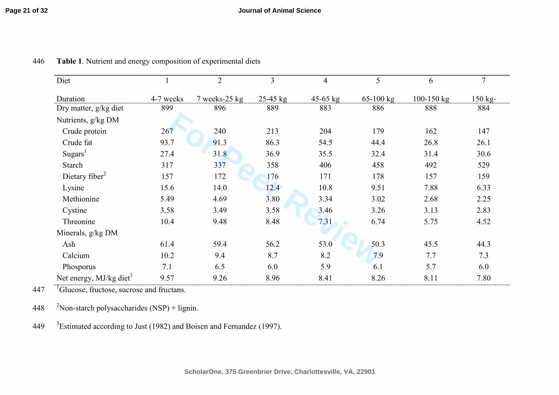
Duroc boars. The pigs were fed 7 diets in the corresponding intervals: 4 to 7 weeks, 7 87

weeks to 25 kg, 25 to 45 kg, 45 to 65 kg, 65to 100 kg, 100 to 150 kg and 150 kg to 88

maturity. The chemical composition of the diets is presented in Table 1. The pigs were 89

housed individually under thermoneutral conditions and given ad libitum access to feed 90

and water during the entire growth period in order to maximize growth. All pigs were 91

weighed at birth, weaning, weekly until approximately 150 kg BW and then every 92

second week until the time of slaughter. The dataset consisted of 40 animals from 17 93

Page 4 of 32



For Peer Review

litters, which were of 3 genders (barrow, boar and gilt). The 3 genders were represented 94

by 11, 16 and 13 pigs, respectively. There were a minimum of 25 and maximum 65 with 95

an average of 36 data points per pig available for the analysis. Thus, a total of 1431 BW 96

recordings were used. The average BW and standard deviations are calculated by 97

grouping measurements into weekly and after 150 kg BW into biweekly groups for each 98

gender. These average growth curves with error bars are plotted as a function of age for 99

each of the 3 sexes in Figure 1. 100

101

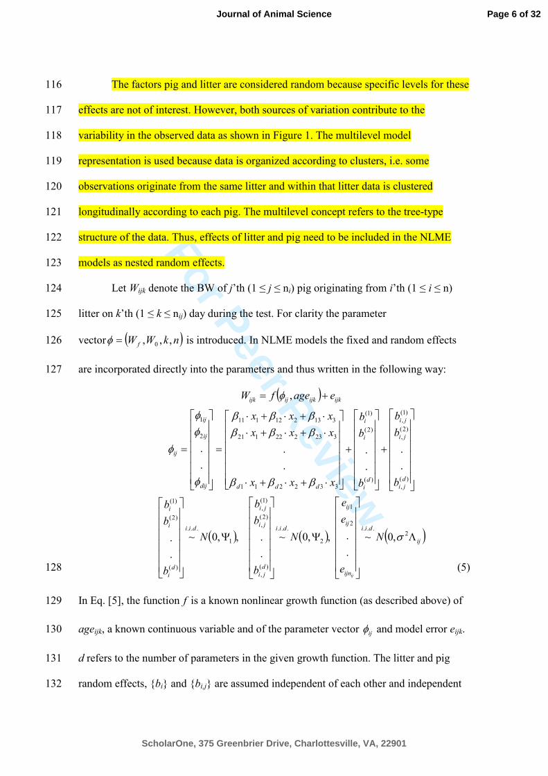
Growth Functions 102

Four sigmoid growth functions are considered in the data analysis and will be 103

referred to as the Gompertz, Logistic, Bridges, and Lopez (Gompertz, 1825; Robertson, 104

1908; Bridges et al., 1986; Lopez et al., 2000; Eq. [1] to [4]). The growth functions are 105

parameterized as follows: 106

××−−×=

0

0 log))(exp(1expW

WAgekWW

f (1) 107

)exp()( 00

0

AgekWWW

WWW

f

f

×−×−−

×= (2) 108

))exp(1(0

n

f AgekWWW ×−−×+= (3) 109

nn

n

f

n

AgeK

AgeWKWW

+

×+×= 0

(4) 110

Where W denotes the expected BW at a given age, Wf is the asymptotic BW (kg) of the 111

pigs, W0 is the initial BW (kg), k is a rate constant (day -1

), K is the age to approximately 112

half maximum BW (days) and n is a dimensionless exponent. 113

114

Multilevel Nonlinear Mixed Models 115

Page 5 of 32



For Peer Review

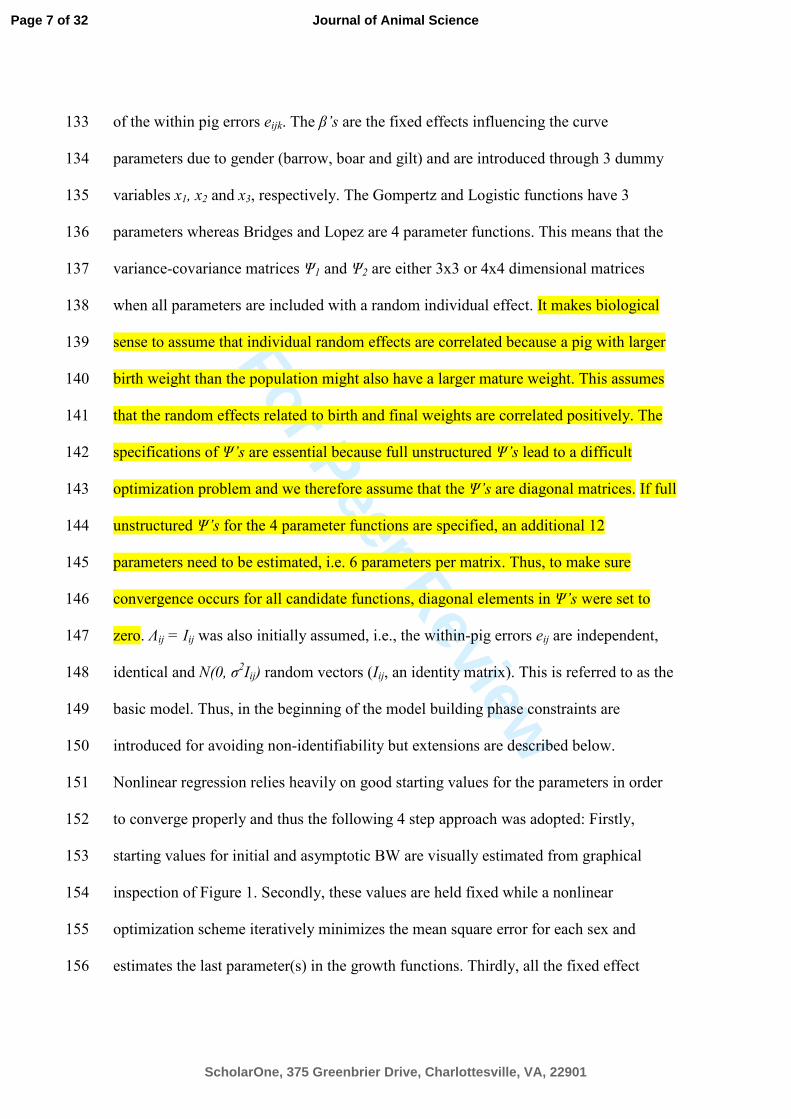
The factors pig and litter are considered random because specific levels for these 116

effects are not of interest. However, both sources of variation contribute to the 117

variability in the observed data as shown in Figure 1. The multilevel model 118

representation is used because data is organized according to clusters, i.e. some 119

observations originate from the same litter and within that litter data is clustered 120

longitudinally according to each pig. The multilevel concept refers to the tree-type 121

structure of the data. Thus, effects of litter and pig need to be included in the NLME 122

models as nested random effects. 123

Let Wijk denote the BW of j’th (1 ≤ j ≤ ni) pig originating from i’th (1 ≤ i ≤ n) 124

litter on k’th (1 ≤ k ≤ nij) day during the test. For clarity the parameter 125

vector ( )nkWW f ,,, 0=φ is introduced. In NLME models the fixed and random effects 126

are incorporated directly into the parameters and thus written in the following way: 127

( )

( ) ( ) ( )ij

dii

ijn

ij

ij

dii

d

ji

ji

ji

dii

d

i

i

i

d

ji

ji

ji

d

i

i

i

ddddij

ij

ij

ij

ijkijkijijk

N

e

e

e

N

b

b

b

N

b

b

b

b

b

b

b

b

b

xxx

xxx

xxx

eagefW

ij

Λ

Ψ

Ψ

+

+

⋅+⋅+⋅

⋅+⋅+⋅

⋅+⋅+⋅

=

=

+=

2...

2

1

2

...

)(

,

)2(

,

)1(

,

1

...

)(

)2(

)1(

)(

,

)2(

,

)1(

,

)(

)2(

)1(

332211

323222121

313212111

2

1

,0~

.

. ,,0~

.

. ,,0~

.

.

.

.

.

.

.

.

.

.

,

σ

βββ

ββββββ

φ

φφ

φ

φ

(5) 128

In Eq. [5], the function f is a known nonlinear growth function (as described above) of 129

ageijk, a known continuous variable and of the parameter vector ijφ and model error eijk. 130

d refers to the number of parameters in the given growth function. The litter and pig 131

random effects, {bi} and {bi,j} are assumed independent of each other and independent 132

Page 6 of 32



For Peer Review

of the within pig errors eijk. The β’s are the fixed effects influencing the curve 133

parameters due to gender (barrow, boar and gilt) and are introduced through 3 dummy 134

variables x1, x2 and x3, respectively. The Gompertz and Logistic functions have 3 135

parameters whereas Bridges and Lopez are 4 parameter functions. This means that the 136

variance-covariance matrices Ψ1 and Ψ2 are either 3x3 or 4x4 dimensional matrices 137

when all parameters are included with a random individual effect. It makes biological 138

sense to assume that individual random effects are correlated because a pig with larger 139

birth weight than the population might also have a larger mature weight. This assumes 140

that the random effects related to birth and final weights are correlated positively. The 141

specifications of Ψ’s are essential because full unstructured Ψ’s lead to a difficult 142

optimization problem and we therefore assume that the Ψ’s are diagonal matrices. If full 143

unstructured Ψ’s for the 4 parameter functions are specified, an additional 12 144

parameters need to be estimated, i.e. 6 parameters per matrix. Thus, to make sure 145

convergence occurs for all candidate functions, diagonal elements in Ψ’s were set to 146

zero. Λij = Iij was also initially assumed, i.e., the within-pig errors eij are independent, 147

identical and N(0, σ2Iij) random vectors (Iij, an identity matrix). This is referred to as the 148

basic model. Thus, in the beginning of the model building phase constraints are 149

introduced for avoiding non-identifiability but extensions are described below. 150

Nonlinear regression relies heavily on good starting values for the parameters in order 151

to converge properly and thus the following 4 step approach was adopted: Firstly, 152

starting values for initial and asymptotic BW are visually estimated from graphical 153

inspection of Figure 1. Secondly, these values are held fixed while a nonlinear 154

optimization scheme iteratively minimizes the mean square error for each sex and 155

estimates the last parameter(s) in the growth functions. Thirdly, all the fixed effect 156

Page 7 of 32



For Peer Review

parameters in the growth function are allowed to vary during final parameter estimation 157

without random effects. Finally, the parameter values from the last nonlinear 158

optimization step are transferred as starting values to the NLME estimations procedure. 159

These methods work on an approximation to the likelihood function for the NLME 160

model (Pinheiro and Bates, 2000; Littell et al., 2006). The estimation routine fits a set of 161

linear estimation equations using a linear mixed model estimation (LME) routine as 162

computing engine at each stage (Pinheiro and Bates, 2000). In the first stage of LME 163

iterations the random effects are initialized by setting them to zero and thus initial 164

estimates of variance parameters (Ψ’s, σ2) are not necessary. All statistical computations 165

were implemented in R (R-project, 2007) and parameter estimation was carried out by 166

means of the nlme-library (Pinheiro et al., 2007). The R-language was chosen because it 167

is an open source language, however, SAS (SAS Inst. Inc., Cary, NC) is commonly 168

used in animal science, therefore, codes based on R and SAS are presented in appendix 169

1. The SAS implementation uses the %nlinmix version 8. 170

Extension of the Basic Model. Model diagnostics is a central part of modeling 171

because plotting the residuals against predicted values reveals whether the variance is 172

constant and systematic deviations (serial correlation) are present visually. Moreover, 173

residual and empirical auto-correlation plots can be used to diagnose violations of 174

model assumptions. The basic model fit suggests that the within-pig variability 175

increased with increasing BW and auto-correlation is also present. This section presents 176

extensions of the basic model due to shortcomings of the current model formulation. 177

Extensions imposed on the basic model formulation apply to all growth models because 178

all functions should be compared on the same basis. The assumption that Λij = Iij has to 179

be relaxed in order to correct misspecifications of the basic models. The matrix Λij can 180

Page 8 of 32



For Peer Review

be decomposed into a variance structure component and a correlation structure 181

component which allows specification of model variance heterogeneity and serial 182

correlation (Pinheiro and Bates, 2000). As mentioned earlier, the variance of the within-183

pig residuals increased with increasing expected values, suggesting variance 184

heterogeneity in the data. Therefore, variance of the within-pig errors was modeled 185

using a variance function, i.e., a function that describes the variance of errors through 186

covariates. An obvious candidate covariate is the predicted values because the variance 187

of the within-pig errors are dependent on both the fixed effects β and random effects bi 188

and bi,j. The data suggests a variance function, which expresses the variance as a power 189

(VP) of the expected values (vijk), i.e. ( ) δσ

22

ijkijk veVar = . A fixed δ value of 0.5 was 190

used, which specifies a model where the variance of a measurement increases linearly 191

with the predicted BW value. Thus, the variance weights are defined as the inverse of 192

the variance function values i.e. δ2/1 ijkv which are used to weight the errors eijk. The nlme-193

library provides several other variance functions for modeling heteroschedasticity of the 194

within-group errors using covariates (Pinheiro et al., 2007). 195

In order to define the appropriate correlation structure for the within-pig 196

residuals it is important to realize that the BW measurements are unequally spaced in 197

time and differ across pigs. Adapting a continuous time autoregressive process of first 198

order (CAR(1)) to the within-pig errors has the properties for dealing with unequally 199

spaced observations. The CAR(1) process is a generalization of an autoregressive 200

process of first order and has the following correlation function (Littell et al., 2006): 201

( ) || ', kk AgeAgeh

−== ϕϕϕτ τ (6) 202

where φ ≥ 0 is the single correlation parameter and τ expresses the absolute distance 203

between two observations on the same individual e.g. τ =|Agek – Agek’|. The CAR(1) 204

Page 9 of 32



For Peer Review

process is driven by random variables or innovations that are assumed to be independent 205

and normally distributed. The innovations can be considered as the residuals in the 206

CAR(1) process. 207

The best performing model was used for subsequent analysis based on the 208

following goodness-of-fit indicators: Akaike information criterion (AIC), Bayesian 209

information criterion (BIC) and residual standard deviation (RSD). Likelihood ratio 210

tests (LRT) are used for nested model (Pinheiro and Bates, 2000). Model reductions are 211

done in two steps. Firstly, the random part of the model was reduced followed by the 212

systematic part. At each step the least significant factor was identified and removed 213

from the model. This was done successively until the final model was obtained. 214

Parameter estimates are presented with corresponding 95% confidence intervals. When 215

additional traits (i.e. points of inflexion) are calculated as function of the fixed effect 216

estimates g(β), the corresponding standard error is obtained by means of the delta 217

method. The method approximates the standard error of a transformation g(β) of a 218

random variable β = (β1, β12, ...), given estimates of the mean and covariance matrix of 219

β. The delta method expands the differentiable function g(β) of a random variable about 220

its mean, with a first-order Taylor approximation, and then takes the variance (Oehlert, 221

1992). The codes for fitting the VP + CAR(1) version of the Lopez-model are presented 222

in Appendix 1. 223

224

RESULTS AND DISCUSSION 225

Comparison of Growth Functions 226

Four growth functions with either 3 or 4 parameters were fitted to growth data and 227

compared for their accuracy of prediction. Literature search and the review by Wellock 228

Page 10 of 32



For Peer Review

et al. (2004) shows that there are several other functions which can be of interest. 229

However, all 4 functions chosen have been used previously to describe growth in pigs 230

although the Gompertz function has been the most popular. The results of fitting the 4 231

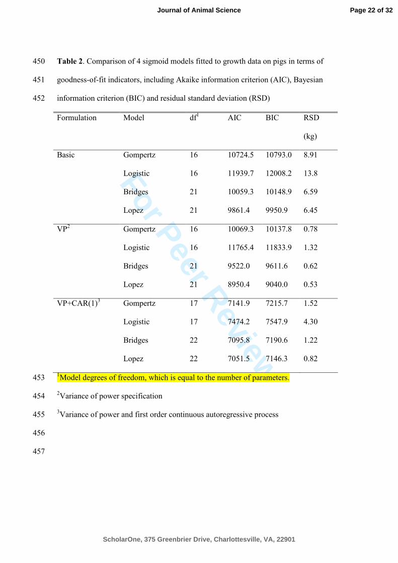
models to data are presented in Table 2 for the basic model formulation and extensions 232

i.e. VP and VP + CAR(1). The results indicate the following ranking of the growth 233

functions: Lopez, Bridges, Gompertz, and Logistic, independent of modifications of the 234

error structure. A recent study by Schulin-Zeuthen et al. (2008) introduced the 235

Schumacher growth function for interpreting growth data, and compared it to the 236

Gompertz and Weibull growth functions. For each of the five datasets, the AIC was 237

lowest for Weibull which supports usage of 4 parameter functions for modeling BW vs. 238

age relations in pigs. Schinckel et al. (2006) showed that Lopez produced a marginally 239

better fit for pig growth data than the Weibull and Bridges growth functions. The 240

current analysis provides evidence that the 4 parameter functions perform better than the 241

3 parameter functions, independent of modifications to the error structure of the models. 242

The results of the current study contradict the conclusion reached by Knap (2000) after 243

re-analyzing 8 previously published dataset. The author reported that the Gompertz 244

function was adequate to model BW vs. age relationships in pigs. Part of the 245

discrepancies can be explained by frequency of BW registrations (sampling) and 246

duration of the experiment. In the first instance, only one of the reanalyzed data sets 247

contained weekly measurements of BW (i.e. data from Andersen and Pedersen (1996)). 248

Second, none of the included experiments studied growth beyond 350 days of age 249

whereas the reported results from this experiment lasted more than 2 years (Figure 1 and 250

2). It was also observed that the Gompertz function had a tendency to overestimate the 251

weight at time zero heavily by predicting birth weights of around 10 kg. This was also 252

Page 11 of 32



For Peer Review

noted by Schulin-Zeuthen et al. (2008). The point of utilizing semi-mechanistic growth 253

models is that the parameters can be assigned biological meaning, but if the parameter 254

estimate(s) are out of biological range as for Gompertz function, then it may be argued 255

that they lose their interpretation and validity. 256

257

Characterizing Pig Growth Using the Lopez Function 258

Random Effects. The results presented in this section are all based on reductions 259

of the Lopez growth function. It is essential that the variance structure is modeled 260

properly when biological inference regarding growth profiles of different sexes or other 261

sources of variation are explored, and thus the VP + CAR(1) version of the Lopez 262

model was used. The result of this analysis is presented in Table 3 along with AIC and 263

BIC values for the reduced models. Parameter estimates for the final model, which are 264

estimated by restricted maximum likelihood are presented in Table 4 with approximate 265

95% confidence intervals. 266

When comparing the growth functions, information that some pigs share in 267

common have been included, i.e. littermates. These variance components in Ψ1 were 268

small compared to those in the Ψ2 and thus were removed from the model. Significance 269

of the changes imposed on the Lopez model can be ascertained by LRT. Based on the 270

LRT with 4 degrees of freedom, the effect of litter was not significant (P = 0.11) and 271

thus Ψ1 was not significantly different from zero. This source of variation could be 272

important if more information was available. Further model reductions were initialized 273

by setting the variance components in Ψ2 = diag(σ12, σ2

2, σ3

2, σ4

2) one by one equating 274

to zero in order to identify the appropriate variance structure for the structural 275

parameters in Eq. [4]. The inter-pig variation in the parameter value that describes the 276

Page 12 of 32



For Peer Review

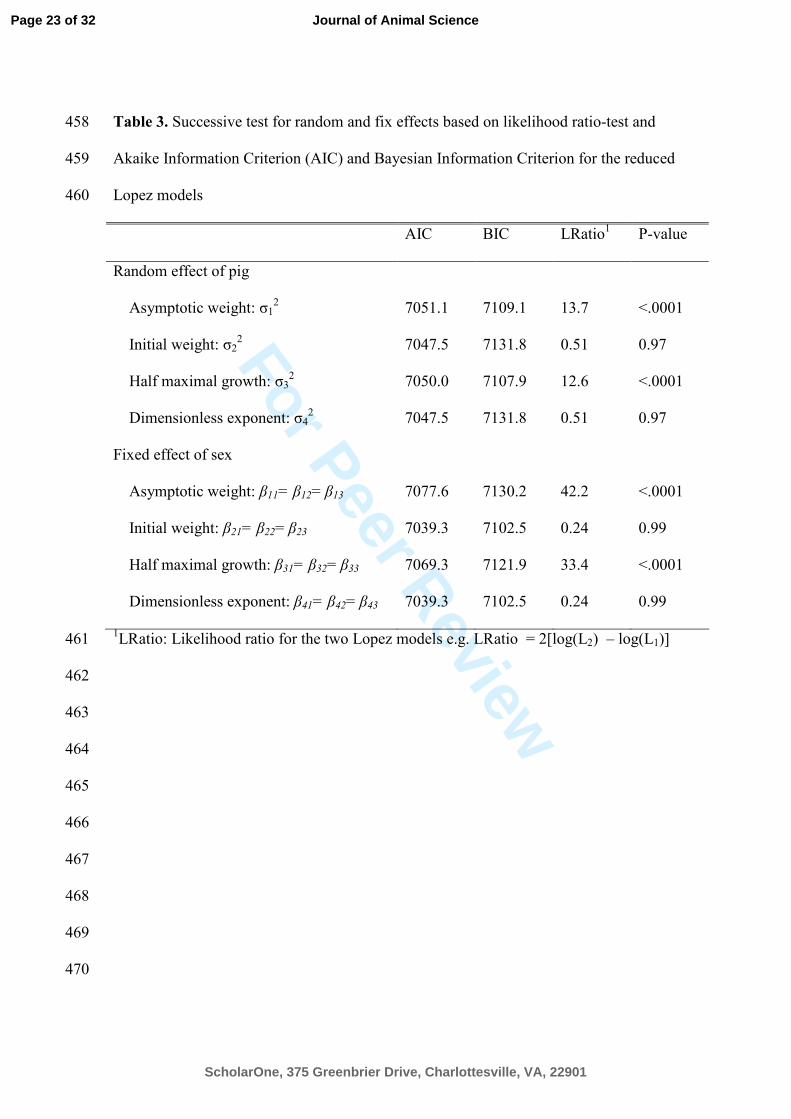
mature size (Wf) was highly significant (P < 0.0001) which was quantified by the 277

variance component (σ12).The variation between pigs in the parameter that describes 278

initial weight (W0) of pigs (σ22), was not significantly different from zero (P = 0.97). 279

The age at approximately half maximum BW (K) varies from individual to the 280

individual (σ32, P < 0.0001). The exponent (n) that determines the sigmoid shape in Eq. 281

[4] was not affected by the pig to pig variation (P = 0.97). The second main objective of 282

the study was to model and describe growth patterns of different genders of pigs, 283

therefore it is important to have an adequate quantification of the source of variation 284

imposed by each pig and to understand which of the parameters in the Lopez function 285

varies with individual pigs. Moreover, it further underlines the necessity to separate the 286

variation between pigs from the within-pig-variation when fitting nonlinear models to 287

growth data obtained from a population of pigs. Failure to include this information 288

adequately in the modeling process will produce biased estimates and SE of the 289

parameters (Pinheiro and Bates, 2000). 290

Fixed Effects. The systematic effect of sex on the mean curve parameters β= 291

(β11, β12,…, β43) that influences the shape of the estimated population growth profiles, 292

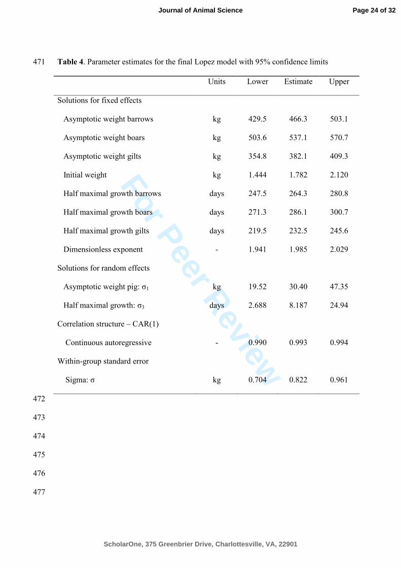
was investigated. W0 was not affected by gender (P = 0.99). The estimated birth weight 293

of 1.78 (SE=0.174) kg by the Lopez function was close to mean birth weight of 1.86 kg 294

of 40 pigs represented in the data set. Furthermore, conducting a one-way ANOVA on 295

the birth weights of these pigs also showed that the gender effect was not significant (P 296

= 0.69). This suggested that there was a good correspondence between conclusions 297

based on the Lopez-NLME analysis and the simple ANOVA. 298

The asymptotic weight of the pigs, Wf, showed systematic differences between 299

genders (P < 0.0001). A qualitative interpretation of Figure 1 and Figure 2 is that gilts 300

Page 13 of 32



For Peer Review

have a distinct growth patterns compared to other sexes and it seems that they do not 301

grow as large as the barrows or boars, which the estimates of Wf also confirm. The 302

estimates of the 3 sexes (barrow: 466 (SE=18.4), boar: 537 (SE=17.2), gilt: 382 303

(SE=13.9), kg) seem to display a reasonable mature weight of barrows, boars and gilts 304

because mean growth curves for barrows and boars were still increasing (Figure 1) 305

while the gilts size had stabilized. In fact, the highest average measured BW are 407, 306

460 and 358 kg at 641, 600 and 629 days of age for barrows, boars and gilts, 307

respectively. These estimates are much larger than previously reported in the literature 308

e.g. Knap (2000) which was partly a consequence of genetic, nutritional and 309

environmental improvements of Danish meat-type pigs and partly due the duration of 310

the experimental period as stated previously. When growth data containing only a BW 311

of less than 200 kg were analyzed by sigmoid growth functions, a caution should be 312

taken in the interpretation of the asymptotic value i.e. mature size. This problem can be 313

illustrated by fitting the final Lopez model to a subset of data where all information 314

above 365 days of age was excluded. This resulted in Wf estimates of 406 (SE=19.4), 315

471 (SE=21.2) and 354 (SE=15.4) kg for barrows, boars and gilts, respectively. Thus, 316

the value of Wf shifted downwards and it may be recommended that future studies 317

looking at estimating the mature size of animals are conducted long enough so that BW 318

stabilizes visually. 319

The age at approximately half maximum was also affected by gender (P < 320

0.0001). The dimensional exponent (n) in Lopez function was not affected by gender (P 321

= 0.99). Lopez et al. (2000) presented methods for calculating inflexion points (t*, BW

*) 322

when d2W/dt

2 is zero and the dimensional exponent is n > 1. These estimates are 323

presented in Table 5. The maximum growth rate for the boars was reached at 135 kg 324

Page 14 of 32



For Peer Review

BW which agrees very well with results obtained by Tauson et al. (1998) who reported 325

that boars of similar breed reached the maximal rate of protein retention at about the 326

same BW. It can be noted that the maximum growth rate (inflexion point) of the boars 327

are reached later in life compared to the gilts which are caused by differences in the 328

parameter values (β31, β32, β33) “the age at approximately half maximum BW”. The 329

results of the current growth analysis showing growth profiles of 9 pigs of 3 sexes with 330

the estimated populations and pig specific curves for the final Lopez model is given in 331

Figure 2. The NLME-models provide the possibility of fitting all growth profiles 332

simultaneously, and thus partition variation between pigs from variation within pigs 333

(under the assumption that all pigs are sampled from the same homogenous 334

populations). Therefore, it was possible to observe that some pig-specific growth 335

profiles deviate from the population curve whereas others follow the population curve. 336

337

Modeling Correlation in Repeated Measure Growth Data 338

The fit of the 4 growth functions to data as presented in Table 2 were improved 339

by adding the VP specification without introduction of a new parameter, which gives 340

evidence of heterogeneity of residual variance. The VP + CAR(1) gives a substantial 341

improvement of fit to data across all growth functions. This calls for a description of the 342

error structure (e.g. Λij) because measurements taken on the same animal are not 343

independent. As mentioned earlier, growth data shows an inherent underlying 344

relationship. Measures made on the individual animal are likely to be more correlated 345

than measures made on different individuals, and spatial correlation exits since 346

measurements made closely in time tend to be highly correlated compared to measures 347

made further distant in time. As a result, all growth functions yield a substantial 348

Page 15 of 32



For Peer Review

improvement of fit to data by incorporating a CAR(1)-process into the models. Wang 349

and Zuidhof (2004) discussed the same issue in their analysis of growth in chickens 350

without resolving it and encouraged development of more advanced correlations 351

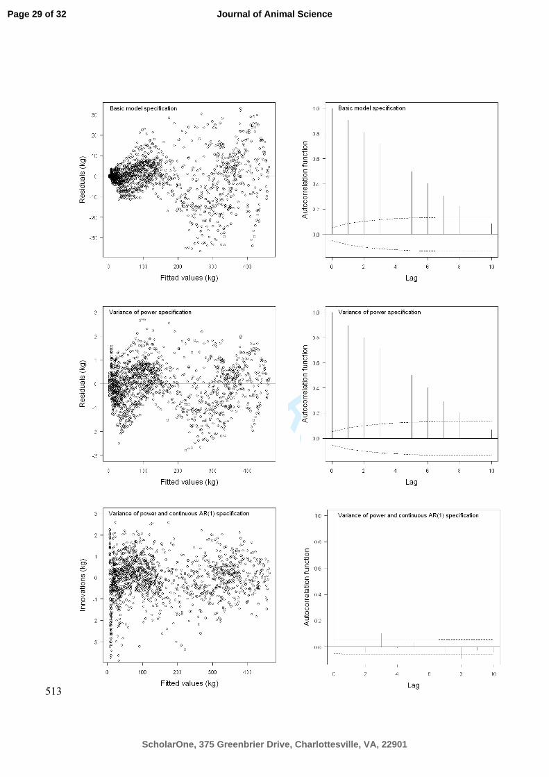
structures for NLME models. Figure 3 presents the residuals as function of fitted values 352

along with the empirical autocorrelation function for the basic model and VP. For the 353

VP + CAR(1) model specification the CAR(1) innovations are presented instead. It is 354

clear from inspection of the first row of diagnostic plots (basic model formulation) that 355

both the assumption of variance homogeneity and independent errors were violated. The 356

heteroscedastic errors were corrected by introducing the VP-specification, but this did 357

not remove the strong auto-correlation in the residuals. A combination of a VP and 358

CAR(1) specification produced innovations that were homoscedastic and independent 359

based on the empirical autocorrelation and corresponding 95% confidence bands. The 360

average autocorrelation could be calculated using Eq. 6. The average distance between 361

to measurements were 9.5 days and thus the average correlation between 2 following 362

measurements were 0.9939.5

= 0.935, which was very substantial. 363

As mentioned earlier, we have chosen to implement all models in the R-364

language utilizing the nlme-library (Pinheiro et al., 2007). NLME-modeling of growth 365

in pigs has previously been approached in SAS, utilizing the NLMIXED-procedure 366

(Criag and Schinckel, 2001; Kebreab et al., 2007). However, the NLMIXED-procedure 367

only offers a single RANDOM and no REPEATED statement (Littell et al., 2006). 368

Thus, specification of multilevel NLME-models with variance weights and correlation 369

structures, which were required to give a complete description of growth data, is not 370

possible within the framework of the NLMIXED-procedure. Most animal scientists use 371

SAS for analysis, therefore, we have implemented the multilevel NLME Lopez model 372

Page 16 of 32



For Peer Review

with VP + CAR(1) specification in SAS as well. This is possible by means of the 373

%NLINMIX macro where the latest version of the macro (nlmm8.sas) is used (Moser, 374

2004; Littell et al., 2006); however, the SAS syntax is more technical compared to the 375

nlme function in R (Appendix 1). 376

In conclusion, 4 different growth functions (Gompertz, Logistic, Bridges and 377

Lopez) have been fitted successfully to growth data obtained from 40 pigs of 3 sexes 378

originating from 17 litters. The models were specified as multilevel nonlinear mixed 379

effect models that allow inclusion of nested random effects and fixed effects of sex on 380

the parameters in the growth functions. The growth analysis has also revealed that 381

inclusion of a continuous auto-regressive process of first order considerably improved 382

the fit to data for all models. This can be attributed to removal of the serial correlated 383

errors, and thus inclusion of a continuous auto-regressive process of first order is 384

recommended when modeling frequently sampled growth data. The Lopez function has 385

provided the best fit to data and is used for estimating the population growth curves 386

related to the different sexes. The 3 sexes clearly differ in the parameters, describing the 387

asymptotic weight and the age at approximately half maximum BW. 388

389

LITERATURE CITED 390

Andersen, S., and B. Pedersen. 1996. Growth and feed intake curves for group-housed 391

gilts and castrated male pigs. Anim. Sci. 63:457-464. 392

Boisen, S., and J. A. Fernández. 1997. Prediction of the total tract digestibility of energy 393

in feedstuffs and pig diets by in vitro analyses. Anim. Feed Sci.Technol. 68:277-394

286. 395

Page 17 of 32



http://www.sciencedirect.com/science?_ob=ArticleURL&_udi=B6T42-3S124SC-15&_user=6447644&_coverDate=10%2F31%2F1997&_alid=805223647&_rdoc=15&_fmt=high&_orig=search&_cdi=4962&_sort=d&_docanchor=&view=c&_ct=19&_acct=C000034378&_version=1&_urlVersion=0&_userid=6447644&md5=23b211c8998f9cbb066cf524f68985a0

http://www.sciencedirect.com/science?_ob=ArticleURL&_udi=B6T42-3S124SC-15&_user=6447644&_coverDate=10%2F31%2F1997&_alid=805223647&_rdoc=15&_fmt=high&_orig=search&_cdi=4962&_sort=d&_docanchor=&view=c&_ct=19&_acct=C000034378&_version=1&_urlVersion=0&_userid=6447644&md5=23b211c8998f9cbb066cf524f68985a0

For Peer Review

Bridges, T. C., L. W. Turner, E. M. Smith, T.S. Stahly, and O. J. Loewer. 1986. A 396

mathematical procedure for estimating animal growth and body composition. Trans. 397

Am. Assoc. Agric. Eng. 29:1342 -1347. 398

Craig, B. A., and A. P. Schinckel. 2001. Nonlinear mixed effects model for swine 399

growth. Prof. Anim. Sci. 17:256-260. 400

Gompertz, B. 1825. On nature of the function expressive of the law of human mortality, 401

and on a new mode of determining the value of life contingencies. Phil. Trans. R. 402

Soc. 115:513-585. 403

Just, A. 1982. The net energy value of balanced diets for growing pigs. Livest. Prod. 404

Sci. 8:541-551. 405

Kebreab, E., M. Schulin-Zeuthen, S. Lopez, R. S. Dias, C. F. M. de Lange, and J. 406

France. 2007. Comparative evaluation of mathematical functions to describe growth 407

and efficiency of phosphorus utilization in growing pigs. J. Anim. Sci. 85:2498-408

2507. 409

Knap, P. 2000. Time trends of the Gompertz growth parameters in pigs. Anim. Sci. 410

70:39-49. 411

Littell, R. C., G. A. Milliken, W. W. Stroup, R. D. Wolfinger, and O. Schabenberger. 412

2006. SAS System for Mixed Models, Second Edition. SAS Institute Inc, Cary, 413

North Carolina, USA. 414

Lopez, S., J. France, W. J. J. Gerrits, M. S. Dhanoa, D. J. Humphries and J. Dijkstra. 415

2000. A generalized Michaelis-Menton equation for the analysis of growth. J. Anim. 416

Sci. 78:1816-1828. 417

Page 18 of 32



For Peer Review

Moser, E. B. 2004. Repeated measures modeling with PROC MIXED. Paper 188-29. 418

Proceedings of the Twenty-Ninth Annual SAS Users Group International 419

Conference. Cary, NC: SAS Institute Inc. 420

Oehlert, G. W. 1992. A note on the delta method. Amer. Stat. 46:27-29. 421

Pinheiro, J., and D. M. Bates. 2000. Mixed effects models in S and S-PLUS. Statistics 422

and Computing, Springer, New York, USA. 423

Pinheiro, J., D. M. Bates, S. DebRoy, and D. Sarkar. 2007. nlme: Linear and Nonlinear 424

Mixed Effects Models. R package version 3.1-83. 425

R Development Core Team. 2007. R: A language and environment for statistical 426

computing. R Foundation for Statistical Computing, Vienna, Austria. ISBN 3-427

900051-07-0, URL http://www.R-project.org. 428

Robertson, T. B. 1908. On the normal rate of growth of an individual and its 429

biochemical significance. Archiv für Entwicklungsmechanik der Organismen. 430

25:581-614. 431

Schinckel, A. P., S. Pence, M. E. Einstein, R. Hinson, P. V. Preckel, J. S. Radcliffe, and 432

B. T. Richert. 2006. Evaluation of different mixed model nonlinear functions on 433

pigs fed low-nutrient excretion diets. Prof. Anim. Sci. 22:401-408. 434

Schulin-Zeuthen, M., E. Kebreab, J. Dijkstra, S. Lopez, A. Bannink, H. Darmani Kuhi, 435

J. H. M. Thornley, and J. France. 2008. A comparison of the Schumacher with other 436

functions for describing growth in pigs. Anim. Feed Sci. Technol. 143:314-327. 437

Tauson, A. H., A. Chwalibog, , K. Jakobsen, and G. Thorbek, 1998. Pattern of protein 438

retention in growing boars of different breeds, and estimation of maximum protein 439

retention. Arch. Anim. Nutr. 51:253-262. 440

Page 19 of 32



For Peer Review

Wang Z., and M.J. Zuidhof. 2004. Estimation of growth parameters using a nonlinear 441

mixed Gompertz model. Poult. Sci. 83:847-852. 442

Wellock I.J., G.C. Emmans and I. Kyriazakis. 2004. Describing and predicting potential 443

growth in the pig. Anim. Sci. 78:379-388. 444

445

Page 20 of 32



For Peer Review

Table 1. Nutrient and energy composition of experimental diets 446

Diet

Duration

1

4-7 weeks

2

7 weeks-25 kg

3

25-45 kg

4

45-65 kg

5

65-100 kg

6

100-150 kg

7

150 kg-

Dry matter, g/kg diet 899 896 889 883 886 888 884

Nutrients, g/kg DM

Crude protein 267 240 213 204 179 162 147

Crude fat 93.7 91.3 86.3 54.5 44.4 26.8 26.1

Sugars1 27.4 31.8 36.9 35.5 32.4 31.4 30.6

Starch 317 337 358 406 458 492 529

Dietary fiber2 157 172 176 171 178 157 159

Lysine 15.6 14.0 12.4 10.8 9.51 7.88 6.33

Methionine 5.49 4.69 3.80 3.34 3.02 2.68 2.25

Cystine 3.58 3.49 3.58 3.46 3.26 3.13 2.83

Threonine 10.4 9.48 8.48 7.31 6.74 5.75 4.52

Minerals, g/kg DM

Ash 61.4 59.4 56.2 53.0 50.3 45.5 44.3

Calcium 10.2 9.4 8.7 8.2 7.9 7.7 7.3

Phosporus 7.1 6.5 6.0 5.9 6.1 5.7 6.0

Net energy, MJ/kg diet3 9.57 9.26 8.96 8.41 8.26 8.11 7.80

1Glucose, fructose, sucrose and fructans. 447

2Non-starch polysaccharides (NSP) + lignin.

448

3Estimated according to Just (1982) and Boisen and Fernandez (1997).449

Page 21 of 32



For Peer Review

Table 2. Comparison of 4 sigmoid models fitted to growth data on pigs in terms of 450

goodness-of-fit indicators, including Akaike information criterion (AIC), Bayesian 451

information criterion (BIC) and residual standard deviation (RSD) 452

Formulation Model df1

AIC BIC RSD

(kg)

Basic Gompertz 16 10724.5 10793.0 8.91

Logistic 16 11939.7 12008.2 13.8

Bridges 21 10059.3 10148.9 6.59

Lopez 21 9861.4 9950.9 6.45

VP2

Gompertz 16 10069.3 10137.8 0.78

Logistic 16 11765.4 11833.9 1.32

Bridges 21 9522.0 9611.6 0.62

Lopez 21 8950.4 9040.0 0.53

VP+CAR(1)3

Gompertz 17 7141.9 7215.7 1.52

Logistic 17 7474.2 7547.9 4.30

Bridges 22 7095.8 7190.6 1.22

Lopez 22 7051.5 7146.3 0.82

1Model degrees of freedom, which is equal to the number of parameters. 453

2Variance of power specification 454

3Variance of power and first order continuous autoregressive process 455

456

457

Page 22 of 32



For Peer Review

Table 3. Successive test for random and fix effects based on likelihood ratio-test and 458

Akaike Information Criterion (AIC) and Bayesian Information Criterion for the reduced 459

Lopez models 460

AIC BIC LRatio1 P-value

Random effect of pig

Asymptotic weight: σ12

7051.1 7109.1 13.7 <.0001

Initial weight: σ22

7047.5 7131.8 0.51 0.97

Half maximal growth: σ32 7050.0 7107.9 12.6 <.0001

Dimensionless exponent: σ42

7047.5 7131.8 0.51 0.97

Fixed effect of sex

Asymptotic weight: β11= β12= β13 7077.6 7130.2 42.2 <.0001

Initial weight: β21= β22= β23 7039.3 7102.5 0.24 0.99

Half maximal growth: β31= β32= β33 7069.3 7121.9 33.4 <.0001

Dimensionless exponent: β41= β42= β43 7039.3 7102.5 0.24 0.99

1LRatio: Likelihood ratio for the two Lopez models e.g. LRatio = 2[log(L2) – log(L1)] 461

462

463

464

465

466

467

468

469

470

Page 23 of 32



For Peer Review

Table 4. Parameter estimates for the final Lopez model with 95% confidence limits 471

Units Lower Estimate Upper

Solutions for fixed effects

Asymptotic weight barrows kg 429.5 466.3 503.1

Asymptotic weight boars kg 503.6 537.1 570.7

Asymptotic weight gilts kg 354.8 382.1 409.3

Initial weight kg 1.444 1.782 2.120

Half maximal growth barrows days 247.5 264.3 280.8

Half maximal growth boars days 271.3 286.1 300.7

Half maximal growth gilts days 219.5 232.5 245.6

Dimensionless exponent - 1.941 1.985 2.029

Solutions for random effects

Asymptotic weight pig: σ1 kg 19.52 30.40 47.35

Half maximal growth: σ3 days 2.688 8.187 24.94

Correlation structure – CAR(1)

Continuous autoregressive - 0.990 0.993 0.994

Within-group standard error

Sigma: σ kg 0.704 0.822 0.961

472

473

474

475

476

477

Page 24 of 32



For Peer Review

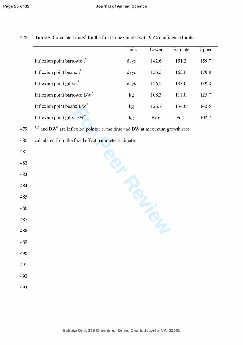
Table 5. Calculated traits1 for the final Lopez model with 95% confidence limits 478

Units Lower Estimate Upper

Inflexion point barrows: t*

days 142.6 151.2 159.7

Inflexion point boars: t* days 156.5 163.6 170.8

Inflexion point gilts: t* days 126.2 133.0 139.8

Inflexion point barrows: BW*

kg 108.3 117.0 125.7

Inflexion point boars: BW* kg 126.7 134.6 142.5

Inflexion point gilts: BW* kg 89.6 96.1 102.7

1t* and BW

* are inflexion points i.e. the time and BW at maximum growth rate 479

calculated from the fixed effect parameter estimates. 480

481

482

483

484

485

486

487

488

489

490

491

492

493

Page 25 of 32



For Peer Review

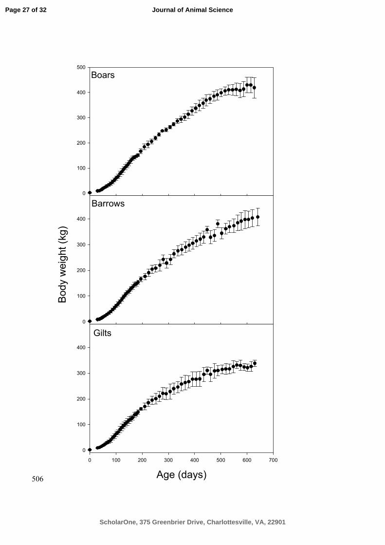
Figure 1. Average body weights (kg) as a function of age (days) and grouped by gender 494

i.e. barrow, boar and gilt, respectively. Error bars (standard deviations) are included in 495

order to shown how the variance increases as a function of age. 496

497

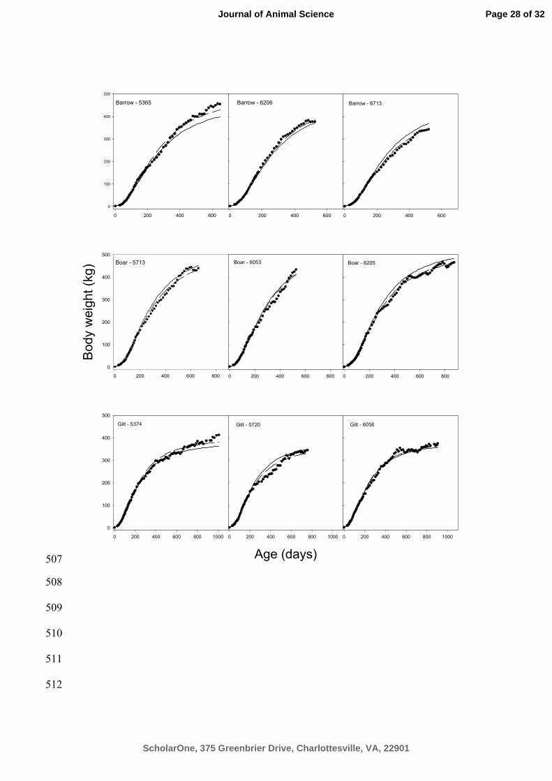
Figure 2. Selected growth profiles of 9 pigs of all sexes (symbol). Lopez function was 498

used to produce population (solid lines) and pig specific (dotted lines) curves. 499

500

Figure 3. Each row in plot region presents diagnostics plots for Lopez function 501

according to the extensions imposed on the basic model formulation. In the left column 502

the residuals or CAR(1) innovations are plotted as function of fitted values and in the 503

right column the empirical autocorrelation functions are presented. 504

505

Page 26 of 32



For Peer Review

Boars

Body weight (kg)

0

100

200

300

400

500

Barrows

0

100

200

300

400

Gilts

Age (days)

0 100 200 300 400 500 600 700

0

100

200

300

400

506

Page 27 of 32



For Peer Review

Barrow - 5365

0 200 400 600

0

100

200

300

400

500

Barrow - 6206

0 200 400 600

Barrow - 6713

0 200 400 600

Boar - 5713

0 200 400 600 800

Body weight (kg)

0

100

200

300

400

500

Boar - 6053

0 200 400 600 800

Boar - 6205

0 200 400 600 800

Gilt - 5374

0 200 400 600 800 1000

0

100

200

300

400

500

Gilt - 5720

Age (days)

0 200 400 600 800 1000

Gilt - 6056

0 200 400 600 800 1000

507

508

509

510

511

512

Page 28 of 32



For Peer Review

513

Page 29 of 32



For Peer Review

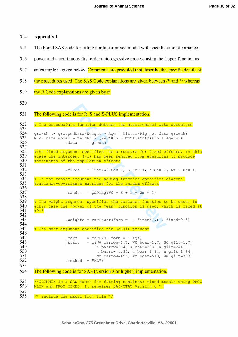
Appendix 1 514

The R and SAS code for fitting nonlinear mixed model with specification of variance 515

power and a continuous first order autoregressive process using the Lopez function as 516

an example is given below. Comments are provided that describe the specific details of 517

the procedures used. The SAS Code explanations are given between /* and */ whereas 518

the R Code explanations are given by #. 519

520

The following code is for R, S and S-PLUS implementation. 521

# The groupedData function defines the hierarchical data structure 522 523 growth <- groupedData(Weight ~ Age | Litter/Pig_no, data=growth) 524 M <- nlme(model = Weight ~ ((W0*K^n + Wm*Age^n)/(K^n + Age^n)) 525 ,data = growth 526 527 #The fixed argument specifies the structure for fixed effects. In this 528 #case the intercept (-1) has been removed from equations to produce 529 #estimates of the population effects 530 531 ,fixed = list(W0~Sex-1, K~Sex-1, n~Sex-1, Wm ~ Sex-1) 532 533 # In the random argument the pdDiag function specifies diagonal 534 #variance-covariance matrices for the random effects 535 536 ,random = pdDiag(W0 + K + n + Wm ~ 1) 537 538 # The weight argument specifies the variance function to be used. In 539 #this case the “power of the mean” function is used, which is fixed at 540 #0.5 541 542 ,weights = varPower(form = ~ fitted(.) , fixed=0.5) 543 544 # The corr argument specifies the CAR(1) process 545 546 ,corr = corCAR1(form = ~ Age) 547 ,start = c(W0_barrow=1.7, W0_boar=1.7, W0_gilt=1.7, 548 K_barrow=264, K_boar=283, K_gilt=244, 549 n_barrow=1.94, n_boar=1.94, n_gilt=1.94, 550 Wm_barrow=455, Wm_boar=510, Wm_gilt=393) 551 ,method = "ML") 552 553

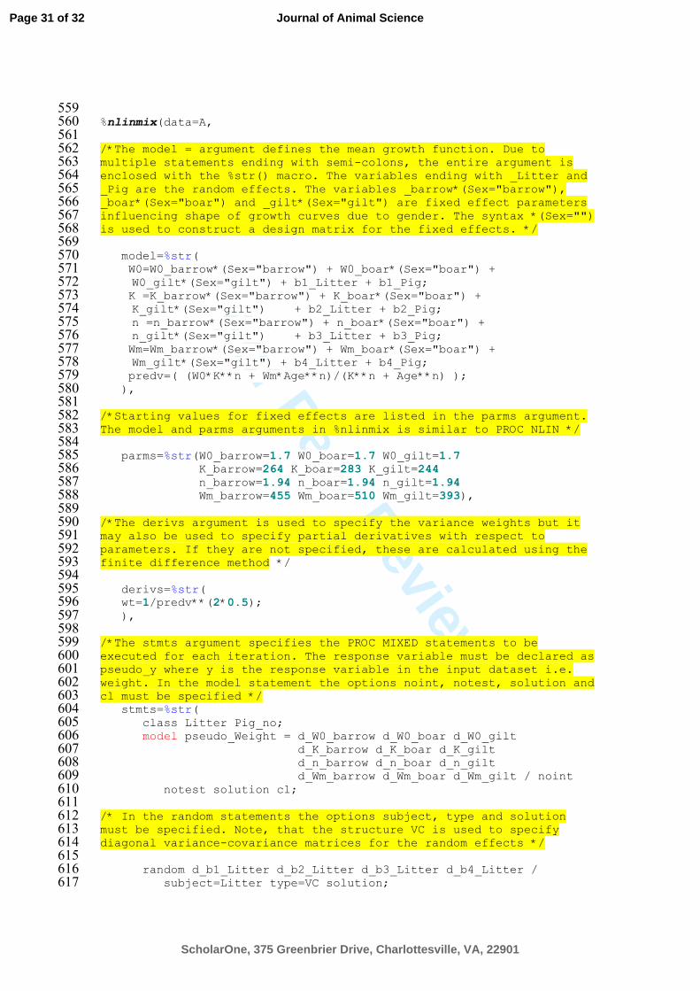
The following code is for SAS (Version 8 or higher) implementation. 554

/*NLINMIX is a SAS macro for fitting nonlinear mixed models using PROC 555 NLIN and PROC MIXED. It requires SAS/STAT Version 8 */ 556

557 /* include the macro from file */ 558

Page 30 of 32



For Peer Review

559 %nlinmix(data=A, 560 561 /*The model = argument defines the mean growth function. Due to 562 multiple statements ending with semi-colons, the entire argument is 563 enclosed with the %str() macro. The variables ending with _Litter and 564 _Pig are the random effects. The variables _barrow*(Sex="barrow"), 565 _boar*(Sex="boar") and _gilt*(Sex="gilt") are fixed effect parameters 566 influencing shape of growth curves due to gender. The syntax *(Sex="") 567 is used to construct a design matrix for the fixed effects. */ 568 569 model=%str( 570 W0=W0_barrow*(Sex="barrow") + W0_boar*(Sex="boar") + 571

W0_gilt*(Sex="gilt") + b1_Litter + b1_Pig; 572 K =K_barrow*(Sex="barrow") + K_boar*(Sex="boar") + 573

K_gilt*(Sex="gilt") + b2_Litter + b2_Pig; 574 n =n_barrow*(Sex="barrow") + n_boar*(Sex="boar") + 575

n_gilt*(Sex="gilt") + b3_Litter + b3_Pig; 576 Wm=Wm_barrow*(Sex="barrow") + Wm_boar*(Sex="boar") + 577

Wm_gilt*(Sex="gilt") + b4_Litter + b4_Pig; 578 predv=( (W0*K**n + Wm*Age**n)/(K**n + Age**n) ); 579 ), 580 581 /*Starting values for fixed effects are listed in the parms argument. 582 The model and parms arguments in %nlinmix is similar to PROC NLIN */ 583 584 parms=%str(W0_barrow=1.7 W0_boar=1.7 W0_gilt=1.7 585 K_barrow=264 K_boar=283 K_gilt=244 586 n_barrow=1.94 n_boar=1.94 n_gilt=1.94 587 Wm_barrow=455 Wm_boar=510 Wm_gilt=393), 588 589 /*The derivs argument is used to specify the variance weights but it 590 may also be used to specify partial derivatives with respect to 591 parameters. If they are not specified, these are calculated using the 592 finite difference method */ 593 594 derivs=%str( 595 wt=1/predv**(2*0.5); 596 ), 597 598 /*The stmts argument specifies the PROC MIXED statements to be 599 executed for each iteration. The response variable must be declared as 600 pseudo_y where y is the response variable in the input dataset i.e. 601 weight. In the model statement the options noint, notest, solution and 602 cl must be specified */ 603 stmts=%str( 604 class Litter Pig_no; 605 model pseudo_Weight = d_W0_barrow d_W0_boar d_W0_gilt 606 d_K_barrow d_K_boar d_K_gilt 607 d_n_barrow d_n_boar d_n_gilt 608 d_Wm_barrow d_Wm_boar d_Wm_gilt / noint 609

notest solution cl; 610 611 /* In the random statements the options subject, type and solution 612 must be specified. Note, that the structure VC is used to specify 613 diagonal variance-covariance matrices for the random effects */ 614 615 random d_b1_Litter d_b2_Litter d_b3_Litter d_b4_Litter / 616

subject=Litter type=VC solution; 617

Page 31 of 32



For Peer Review

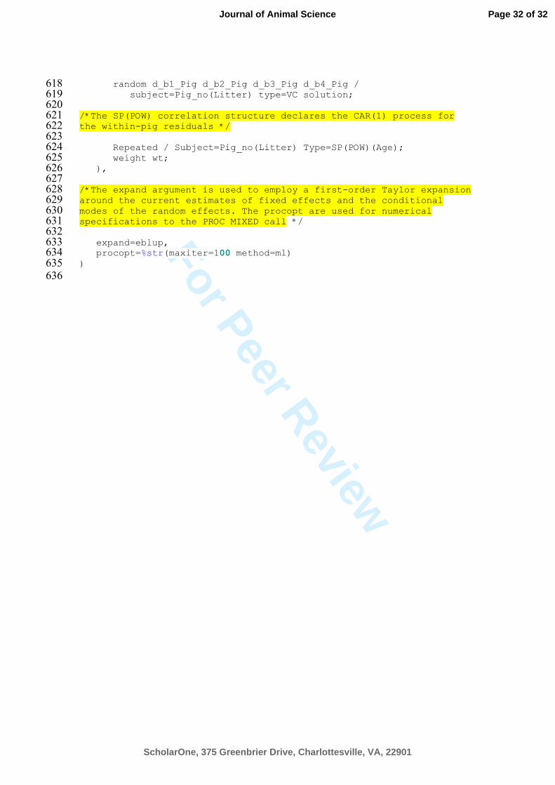
random d_b1_Pig d_b2_Pig d_b3_Pig d_b4_Pig / 618 subject=Pig_no(Litter) type=VC solution; 619

620 /*The SP(POW) correlation structure declares the CAR(1) process for 621 the within-pig residuals */ 622 623 Repeated / Subject=Pig_no(Litter) Type=SP(POW)(Age); 624 weight wt; 625 ), 626 627 /*The expand argument is used to employ a first-order Taylor expansion 628 around the current estimates of fixed effects and the conditional 629 modes of the random effects. The procopt are used for numerical 630 specifications to the PROC MIXED call */ 631 632 expand=eblup, 633 procopt=%str(maxiter=100 method=ml) 634 ) 635 636

Page 32 of 32



A multilevel nonlinear mixed-effects approach to model growth in pigs

Documents

Transcript of A multilevel nonlinear mixed-effects approach to model growth in pigs