Meteorological effects on seasonal infertility in pigs - NET
303
UNIVERSITY OF LEEDS Meteorological effects on seasonal infertility in pigs by Anna LeMoine Submitted in accordance with the requirements for the degree of Doctor of Philosophy in the Faculty of Biological Sciences School of Biology March 2013
-
Upload
khangminh22 -
Category
Documents
-
view
0 -
download
0
Transcript of Meteorological effects on seasonal infertility in pigs - NET

UNIVERSITY OF LEEDS
Meteorological effects on seasonal
infertility in pigs
by
Anna LeMoine
Submitted in accordance with the requirements for the
degree of Doctor of Philosophy
in the
Faculty of Biological Sciences
School of Biology
March 2013

Declaration of Authorship
The candidate confirms that the work submitted is her own and that appropriate credit
has been given where reference has been made to the work of others. This copy has been
supplied on the understanding that it is copyright material and that no quotation from
the thesis may be published without proper acknowledgement.
c©2012 The University of Leeds and Anna LeMoine
i

“The roots of education are bitter, but the fruit is sweet.”
Aristotle

Acknowledgements
Firstly I would like to thank my supervisors Professor Helen Miller and Dr Andy Bulpitt
for their continuous support throughout my PhD. Not only did you provide me with
academic support and encouragement, but also guidance in gaining outside help to
pursue my development. Your faith in my abilities has gotten me to the end. I would
also like to thank Dr Christopher Needham and Professor Roger Boyle for helping me
initially get to grips with the language of computing, it all seems so much less scary
now!
Thank you BQP Ltd for providing me with the data which resulted in all the work I
have produced, as well as JSR Genetics Ltd for allowing my work to branch out a bit.
Thank you Dent Ltd, in particular Steve Winfield and everyone at Guild House farm for
making it possible for me to carry out a trial to round off my PhD. It was what I needed
to get me through the final stages of my work and thanks go to my undergraduate
students for collecting the behaviour data during the trial work. We braved the weather
together!
To my funders BPEX and the Yorkshire Agricultural Society thank you for your spon-
sorship, allowing for this work to take place.
A huge thank you goes to my farm buddies Fiona Reynolds, Amy Taylor, Jen Waters
and Steven Pace for keeping me sane and on track whilst in the office. You are all
brilliant to work with and amazing friends. Also a massive thank you to all my friends
around the world who have supported me over the years, encouraging me to continue
with my work and allowing me to get distracted when it was needed.
Thank you, ’Merci’ and ’Todah’ to my parents and sisters for their moral support during
some of the more difficult times. I would not be where I am today if it was not for all
of you.
Last but not least I would like to thank my loving, supportive and extremely patient
husband Jonathan for his encouragement throughout my PhD. How you put up with
me on a daily basis I will never know, but without you I would have been at a loss.
iii

Abstract
The presence of seasonal infertility has long been recognised, but its causes are much
debated within the farming and scientific communities. Almost half of the UK breeding
herd is kept outdoors and is therefore more likely to be susceptible to seasonal infertility.
Most research on the matter has been conducted on indoor sows, and so the aim of this
thesis was to describe the effects of meteorological conditions on reproductive function
in both outdoor sows and commercial boars. The data confirm that both sows and boars
suffer from seasonal reductions in reproductive output.
Reduced farrowing rates were the major manifestation of seasonality in sows. High tem-
peratures and long days were associated with poor performance. A simulation model of
seasonal infertility was developed; with further refinement this could potentially provide
a tool for farmers, allowing them to make managerial adjustments to compensate for
low productivity in select months.
Seasonal effects on litter size were less apparent when assessed at herd level. However
individual sows were found to be more or less susceptible to reductions from summer
services, suggesting a genetic predisposition to seasonal infertility.
Sow skin temperatures and respiration rates increased with external temperature hu-
midity indices; these increases occurred at a lower threshold following cold conditions.
Together with observed thermoregulatory behaviour it appears that UK sows become
acclimatised to cold weather and are therefore more susceptible to heat stress when it
becomes warmer.
Boar semen quality was reduced over the summer and early autumn months, with a
higher proportion of abnormalities and lower sperm concentrations. However individual
boar and management parameters had a larger effect on semen quality than meteoro-
logical conditions.
More research into outdoor production systems is required and further links between
boar and sow fertility should be made. Producers need to be aware that outdoor sows
may behave differently from those on indoor units.

Contents
Declaration of Authorship i
Acknowledgements iii
Abstract iv
List of Figures x
List of Tables xiii
Abbreviations xv
Publications xvii
1 Introduction 1
2 Review of literature 3
2.1 Endocrinological basis of reproduction . . . . . . . . . . . . . . . . . . . . 3
2.1.1 Oestrous cycle . . . . . . . . . . . . . . . . . . . . . . . . . . . . . 3
2.1.2 Spermatogenesis . . . . . . . . . . . . . . . . . . . . . . . . . . . . 5
2.1.3 Seasonal breeding . . . . . . . . . . . . . . . . . . . . . . . . . . . 7
2.2 Seasonal infertility in sows . . . . . . . . . . . . . . . . . . . . . . . . . . . 9
2.2.1 Manifestations of seasonal infertility . . . . . . . . . . . . . . . . . 9
2.2.1.1 Farrowing rate . . . . . . . . . . . . . . . . . . . . . . . . 10
2.2.1.2 Litter size . . . . . . . . . . . . . . . . . . . . . . . . . . . 12
2.2.1.3 Wean to oestrus period . . . . . . . . . . . . . . . . . . . 13
2.2.1.4 Delayed puberty in gilts . . . . . . . . . . . . . . . . . . . 14
2.2.2 Factors contributing to seasonal infertility . . . . . . . . . . . . . . 14
2.2.2.1 Photoperiod . . . . . . . . . . . . . . . . . . . . . . . . . 14
2.2.2.2 Temperature . . . . . . . . . . . . . . . . . . . . . . . . . 16
2.2.2.3 Genetics . . . . . . . . . . . . . . . . . . . . . . . . . . . 20
2.2.2.4 Management and Nutrition . . . . . . . . . . . . . . . . . 21
2.3 Boar semen quality and artificial insemination . . . . . . . . . . . . . . . . 22
2.3.1 Seasonal changes in boar reproductive physiology . . . . . . . . . . 23
v

Contents vi
2.3.1.1 Season . . . . . . . . . . . . . . . . . . . . . . . . . . . . 23
2.3.1.2 Temperature . . . . . . . . . . . . . . . . . . . . . . . . . 27
2.3.2 Artificial insemination . . . . . . . . . . . . . . . . . . . . . . . . . 28
2.3.2.1 Extending semen . . . . . . . . . . . . . . . . . . . . . . . 28
2.3.2.2 Storing and transporting semen . . . . . . . . . . . . . . 30
2.3.2.3 Artificial insemination methods . . . . . . . . . . . . . . 32
2.3.2.4 Timing of insemination . . . . . . . . . . . . . . . . . . . 34
2.4 Modelling in Agriculture . . . . . . . . . . . . . . . . . . . . . . . . . . . . 36
2.4.1 The use of data mining and modelling in agricultural research . . . 36
2.4.2 Current status of modelling seasonal infertility . . . . . . . . . . . 37
2.5 Conclusions . . . . . . . . . . . . . . . . . . . . . . . . . . . . . . . . . . . 39
2.6 Aims . . . . . . . . . . . . . . . . . . . . . . . . . . . . . . . . . . . . . . . 39
3 An investigation into the factors that may cause seasonal changes inoutdoor sow herd productivity 40
3.1 Introduction . . . . . . . . . . . . . . . . . . . . . . . . . . . . . . . . . . . 40
3.2 Objectives and hypotheses . . . . . . . . . . . . . . . . . . . . . . . . . . . 41
3.3 The Data . . . . . . . . . . . . . . . . . . . . . . . . . . . . . . . . . . . . 42
3.3.1 Production data . . . . . . . . . . . . . . . . . . . . . . . . . . . . 42
3.3.2 Meteorological data . . . . . . . . . . . . . . . . . . . . . . . . . . 45
3.3.3 Pre-processing the data . . . . . . . . . . . . . . . . . . . . . . . . 45
3.4 Statistical analyses . . . . . . . . . . . . . . . . . . . . . . . . . . . . . . . 46
3.4.1 Principal components analysis . . . . . . . . . . . . . . . . . . . . 46
3.4.2 Weather parameters . . . . . . . . . . . . . . . . . . . . . . . . . . 47
3.4.3 Sow reproduction parameters . . . . . . . . . . . . . . . . . . . . . 47
3.4.3.1 Monthly effects . . . . . . . . . . . . . . . . . . . . . . . . 48
3.4.3.2 Meteorological effects . . . . . . . . . . . . . . . . . . . . 48
3.4.3.3 Individual effects . . . . . . . . . . . . . . . . . . . . . . . 49
3.5 Results . . . . . . . . . . . . . . . . . . . . . . . . . . . . . . . . . . . . . . 50
3.5.1 Descriptive statistics . . . . . . . . . . . . . . . . . . . . . . . . . . 50
3.5.2 Month effects . . . . . . . . . . . . . . . . . . . . . . . . . . . . . . 55
3.5.3 Day length effects . . . . . . . . . . . . . . . . . . . . . . . . . . . 57
3.5.4 Temperature effects . . . . . . . . . . . . . . . . . . . . . . . . . . 57
3.5.5 Other meteorological effects . . . . . . . . . . . . . . . . . . . . . . 62
3.5.6 Individual sow effects . . . . . . . . . . . . . . . . . . . . . . . . . 67
3.6 Discussion . . . . . . . . . . . . . . . . . . . . . . . . . . . . . . . . . . . . 71
3.6.1 Photoperiodic effects on reproduction . . . . . . . . . . . . . . . . 71
3.6.2 Meteorological effects on reproduction . . . . . . . . . . . . . . . . 73
3.6.2.1 Farrowing rate . . . . . . . . . . . . . . . . . . . . . . . . 73
3.6.2.2 Litter size . . . . . . . . . . . . . . . . . . . . . . . . . . . 75
3.6.3 Individual sow susceptibility . . . . . . . . . . . . . . . . . . . . . . 77
3.7 Conclusions . . . . . . . . . . . . . . . . . . . . . . . . . . . . . . . . . . . 78
4 Simulating seasonal infertility in outdoor UK sow herds 80
4.1 Introduction . . . . . . . . . . . . . . . . . . . . . . . . . . . . . . . . . . . 80
4.2 Objectives . . . . . . . . . . . . . . . . . . . . . . . . . . . . . . . . . . . . 82

Contents vii
4.3 General scope . . . . . . . . . . . . . . . . . . . . . . . . . . . . . . . . . . 82
4.4 The Data . . . . . . . . . . . . . . . . . . . . . . . . . . . . . . . . . . . . 85
4.5 Model creation . . . . . . . . . . . . . . . . . . . . . . . . . . . . . . . . . 85
4.5.1 Decision rules . . . . . . . . . . . . . . . . . . . . . . . . . . . . . . 85
4.5.2 Outputs and analyses . . . . . . . . . . . . . . . . . . . . . . . . . 89
4.5.3 Calibration of the number and length of simulations . . . . . . . . 89
4.6 Results . . . . . . . . . . . . . . . . . . . . . . . . . . . . . . . . . . . . . . 93
4.6.1 Farrowing . . . . . . . . . . . . . . . . . . . . . . . . . . . . . . . . 93
4.6.2 Litter size . . . . . . . . . . . . . . . . . . . . . . . . . . . . . . . . 94
4.6.3 Parity . . . . . . . . . . . . . . . . . . . . . . . . . . . . . . . . . . 94
4.6.4 Empty days . . . . . . . . . . . . . . . . . . . . . . . . . . . . . . . 94
4.6.5 Culling . . . . . . . . . . . . . . . . . . . . . . . . . . . . . . . . . 94
4.6.6 Changing weather conditions . . . . . . . . . . . . . . . . . . . . . 98
4.6.7 Model validation . . . . . . . . . . . . . . . . . . . . . . . . . . . . 100
4.7 Discussion . . . . . . . . . . . . . . . . . . . . . . . . . . . . . . . . . . . . 108
4.7.1 Sow herd management and seasonality . . . . . . . . . . . . . . . . 108
4.7.2 Model performance . . . . . . . . . . . . . . . . . . . . . . . . . . . 111
4.7.3 Future modelling improvements and applications . . . . . . . . . . 113
4.8 Conclusions . . . . . . . . . . . . . . . . . . . . . . . . . . . . . . . . . . . 115
5 An investigation into the factors that may influence seasonal changesin commercial boar semen quality 116
5.1 Introduction . . . . . . . . . . . . . . . . . . . . . . . . . . . . . . . . . . . 116
5.2 Objectives and hypotheses . . . . . . . . . . . . . . . . . . . . . . . . . . . 118
5.3 The Data . . . . . . . . . . . . . . . . . . . . . . . . . . . . . . . . . . . . 119
5.3.1 Stud data . . . . . . . . . . . . . . . . . . . . . . . . . . . . . . . . 119
5.3.2 Meteorological data . . . . . . . . . . . . . . . . . . . . . . . . . . 120
5.4 Methods . . . . . . . . . . . . . . . . . . . . . . . . . . . . . . . . . . . . . 120
5.4.1 Statistical analyses . . . . . . . . . . . . . . . . . . . . . . . . . . . 120
5.4.2 Decision trees . . . . . . . . . . . . . . . . . . . . . . . . . . . . . . 122
5.4.2.1 Learning features . . . . . . . . . . . . . . . . . . . . . . 122
5.4.2.2 Learning algorithm . . . . . . . . . . . . . . . . . . . . . 123
5.4.2.3 Performance metrics . . . . . . . . . . . . . . . . . . . . . 124
5.5 Results . . . . . . . . . . . . . . . . . . . . . . . . . . . . . . . . . . . . . . 125
5.5.1 Ejaculate usage . . . . . . . . . . . . . . . . . . . . . . . . . . . . . 125
5.5.2 Semen volume, sperm concentration and total sperm numbers . . . 126
5.5.2.1 Monthly effects . . . . . . . . . . . . . . . . . . . . . . . . 126
5.5.2.2 Breed effects . . . . . . . . . . . . . . . . . . . . . . . . . 127
5.5.2.3 Age effects . . . . . . . . . . . . . . . . . . . . . . . . . . 127
5.5.2.4 Collection interval effects . . . . . . . . . . . . . . . . . . 129
5.5.2.5 Interactions . . . . . . . . . . . . . . . . . . . . . . . . . . 129
5.5.3 Abnormalities . . . . . . . . . . . . . . . . . . . . . . . . . . . . . . 130
5.5.3.1 Monthly effects . . . . . . . . . . . . . . . . . . . . . . . . 130
5.5.3.2 Breed effects . . . . . . . . . . . . . . . . . . . . . . . . . 130
5.5.3.3 Age effects . . . . . . . . . . . . . . . . . . . . . . . . . . 134
5.5.3.4 Collection interval effects . . . . . . . . . . . . . . . . . . 134

Contents viii
5.5.3.5 Interactions . . . . . . . . . . . . . . . . . . . . . . . . . . 135
5.5.4 Motility . . . . . . . . . . . . . . . . . . . . . . . . . . . . . . . . . 136
5.5.5 Decision trees . . . . . . . . . . . . . . . . . . . . . . . . . . . . . . 137
5.5.5.1 Semen dose usage . . . . . . . . . . . . . . . . . . . . . . 137
5.5.5.2 Semen quality parameters . . . . . . . . . . . . . . . . . . 137
5.6 Discussion . . . . . . . . . . . . . . . . . . . . . . . . . . . . . . . . . . . . 141
5.6.1 Seasonal changes in semen quality . . . . . . . . . . . . . . . . . . 141
5.6.1.1 Semen volume, sperm concentration and total sperm num-bers . . . . . . . . . . . . . . . . . . . . . . . . . . . . . . 141
5.6.1.2 Abnormalities and motility . . . . . . . . . . . . . . . . . 144
5.6.2 The use of decision trees . . . . . . . . . . . . . . . . . . . . . . . . 149
5.7 Conclusions . . . . . . . . . . . . . . . . . . . . . . . . . . . . . . . . . . . 150
6 The assessment of heat stress in outdoor lactating sows throughoutthe year 151
6.1 Introduction . . . . . . . . . . . . . . . . . . . . . . . . . . . . . . . . . . . 151
6.2 Objectives . . . . . . . . . . . . . . . . . . . . . . . . . . . . . . . . . . . . 155
6.3 Methods . . . . . . . . . . . . . . . . . . . . . . . . . . . . . . . . . . . . . 156
6.3.1 Animals and Housing . . . . . . . . . . . . . . . . . . . . . . . . . 156
6.3.2 Animal measurements . . . . . . . . . . . . . . . . . . . . . . . . . 158
6.3.3 Meteorological measurements . . . . . . . . . . . . . . . . . . . . . 160
6.3.4 Farrowing hut measurements . . . . . . . . . . . . . . . . . . . . . 160
6.3.5 Data preparation . . . . . . . . . . . . . . . . . . . . . . . . . . . . 160
6.4 Statistical Analyses . . . . . . . . . . . . . . . . . . . . . . . . . . . . . . . 161
6.4.1 Batch statistics . . . . . . . . . . . . . . . . . . . . . . . . . . . . . 161
6.4.2 Skin temperatures . . . . . . . . . . . . . . . . . . . . . . . . . . . 162
6.4.3 Respiration rates . . . . . . . . . . . . . . . . . . . . . . . . . . . . 162
6.4.4 Farrowing huts . . . . . . . . . . . . . . . . . . . . . . . . . . . . . 162
6.5 Results . . . . . . . . . . . . . . . . . . . . . . . . . . . . . . . . . . . . . . 163
6.5.1 Batch statistics . . . . . . . . . . . . . . . . . . . . . . . . . . . . . 163
6.5.2 Skin temperatures . . . . . . . . . . . . . . . . . . . . . . . . . . . 165
6.5.3 Respiration rates . . . . . . . . . . . . . . . . . . . . . . . . . . . . 172
6.5.4 Changes in Farrowing hut conditions . . . . . . . . . . . . . . . . . 175
6.6 Discussion . . . . . . . . . . . . . . . . . . . . . . . . . . . . . . . . . . . . 178
6.6.1 Physiological signs of heat stress in sows . . . . . . . . . . . . . . . 178
6.6.2 Consequences of heat stress in sows . . . . . . . . . . . . . . . . . 182
6.6.3 Farrowing huts . . . . . . . . . . . . . . . . . . . . . . . . . . . . . 184
6.7 Conclusions . . . . . . . . . . . . . . . . . . . . . . . . . . . . . . . . . . . 185
7 Changes in outdoor sow behaviour in relation to meteorological con-ditions 186
7.1 Introduction . . . . . . . . . . . . . . . . . . . . . . . . . . . . . . . . . . . 186
7.2 Objectives and hypotheses . . . . . . . . . . . . . . . . . . . . . . . . . . . 188
7.3 Methods . . . . . . . . . . . . . . . . . . . . . . . . . . . . . . . . . . . . . 189
7.3.1 Animals and Housing . . . . . . . . . . . . . . . . . . . . . . . . . 189
7.3.2 Animal measurements . . . . . . . . . . . . . . . . . . . . . . . . . 189

Contents ix
7.3.3 Behavioural measurements . . . . . . . . . . . . . . . . . . . . . . 189
7.3.4 Meteorological measurements . . . . . . . . . . . . . . . . . . . . . 190
7.4 Statistical analyses . . . . . . . . . . . . . . . . . . . . . . . . . . . . . . . 191
7.4.1 Sow activity and location . . . . . . . . . . . . . . . . . . . . . . . 191
7.4.2 Farrowing hut usage . . . . . . . . . . . . . . . . . . . . . . . . . . 192
7.4.3 Piglet mortality . . . . . . . . . . . . . . . . . . . . . . . . . . . . . 192
7.4.4 Individual sow behaviour . . . . . . . . . . . . . . . . . . . . . . . 192
7.5 Results . . . . . . . . . . . . . . . . . . . . . . . . . . . . . . . . . . . . . . 192
7.5.1 Descriptive statistics . . . . . . . . . . . . . . . . . . . . . . . . . . 192
7.5.2 Sow activity and location . . . . . . . . . . . . . . . . . . . . . . . 193
7.5.3 Sow pairing . . . . . . . . . . . . . . . . . . . . . . . . . . . . . . . 198
7.5.4 Time spent with piglets . . . . . . . . . . . . . . . . . . . . . . . . 201
7.5.5 Farrowing hut usage . . . . . . . . . . . . . . . . . . . . . . . . . . 202
7.5.6 Piglet mortality . . . . . . . . . . . . . . . . . . . . . . . . . . . . . 203
7.5.7 Individual preferences . . . . . . . . . . . . . . . . . . . . . . . . . 204
7.6 Discussion . . . . . . . . . . . . . . . . . . . . . . . . . . . . . . . . . . . . 207
7.6.1 Activity and Location . . . . . . . . . . . . . . . . . . . . . . . . . 207
7.6.2 Sow pairing . . . . . . . . . . . . . . . . . . . . . . . . . . . . . . . 209
7.6.3 Time Spent With Piglets . . . . . . . . . . . . . . . . . . . . . . . 209
7.6.4 Piglet Mortality . . . . . . . . . . . . . . . . . . . . . . . . . . . . 210
7.7 Conclusions . . . . . . . . . . . . . . . . . . . . . . . . . . . . . . . . . . . 211
8 General Discussion 212
8.1 Seasonal infertility in sows . . . . . . . . . . . . . . . . . . . . . . . . . . . 212
8.2 Seasonal infertility in boars . . . . . . . . . . . . . . . . . . . . . . . . . . 215
8.3 Individual susceptibility to seasonal infertility . . . . . . . . . . . . . . . . 217
8.4 Modelling seasonal infertility . . . . . . . . . . . . . . . . . . . . . . . . . 218
8.5 Conclusions . . . . . . . . . . . . . . . . . . . . . . . . . . . . . . . . . . . 219
Bibliography 221
A Python code 255
B Decision trees 271
C Body scoring 284

List of Figures
2.1 Female endocrinological pathways . . . . . . . . . . . . . . . . . . . . . . . 4
2.2 Male endocrinological pathways . . . . . . . . . . . . . . . . . . . . . . . . 6
2.3 Seasonal changes in farrowing rate . . . . . . . . . . . . . . . . . . . . . . 11
2.4 Methods of artificial insemination . . . . . . . . . . . . . . . . . . . . . . . 33
3.1 Herd and Weather station map . . . . . . . . . . . . . . . . . . . . . . . . 43
3.2 Biplot of production and weather data principal component analysis results 50
3.3 Average weather conditions . . . . . . . . . . . . . . . . . . . . . . . . . . 52
3.4 Total born litter size by genotype and parity . . . . . . . . . . . . . . . . 53
3.5 Monthly farrowing rates for different genotypes . . . . . . . . . . . . . . . 53
3.6 Farrowing rate above and below 18 ◦C . . . . . . . . . . . . . . . . . . . . 54
3.7 Annual farrowing rate patterns . . . . . . . . . . . . . . . . . . . . . . . . 55
3.8 Monthly farrowing rates by parity . . . . . . . . . . . . . . . . . . . . . . 56
3.9 Monthly total born litter size by parity . . . . . . . . . . . . . . . . . . . . 56
3.10 Total born litter sizes for changing day lengths . . . . . . . . . . . . . . . 58
3.11 Total born litter size in relation to absolute day length . . . . . . . . . . . 58
3.12 Farrowing rate for changing day lengths . . . . . . . . . . . . . . . . . . . 59
3.13 Farrowing rate in relation to absolute day length . . . . . . . . . . . . . . 59
3.14 Maximum temperature effects on farrowing rate . . . . . . . . . . . . . . . 63
3.15 Average temperature effects on farrowing rate . . . . . . . . . . . . . . . . 63
3.16 Maximum temperature effects on total born litter size . . . . . . . . . . . 64
3.17 Average temperature effects on total born litter size . . . . . . . . . . . . 64
3.18 Change in temperature effects on litter size . . . . . . . . . . . . . . . . . 65
3.19 Change in temperature effects on farrowing rate . . . . . . . . . . . . . . . 65
3.20 Humidity effects on farrowing rate . . . . . . . . . . . . . . . . . . . . . . 66
3.21 Humidity effects on total born litter size . . . . . . . . . . . . . . . . . . . 66
3.22 Origin of fertile and infertile sows . . . . . . . . . . . . . . . . . . . . . . . 70
3.23 Annual proportion of infertile sows . . . . . . . . . . . . . . . . . . . . . . 70
4.1 Conceptual diagram of simulation model . . . . . . . . . . . . . . . . . . . 84
4.2 Sow farrowings over time . . . . . . . . . . . . . . . . . . . . . . . . . . . 91
4.3 Sow culls over time . . . . . . . . . . . . . . . . . . . . . . . . . . . . . . . 91
4.4 Batch parity profiles . . . . . . . . . . . . . . . . . . . . . . . . . . . . . . 92
4.5 Simulation replications for sow farrowings . . . . . . . . . . . . . . . . . . 92
4.6 Simulation replications for sow parities . . . . . . . . . . . . . . . . . . . . 93
4.7 Experimental results for farrowing rate . . . . . . . . . . . . . . . . . . . . 95
4.8 Experimental results for number of farrowings . . . . . . . . . . . . . . . . 95
x
List of Figures xi
4.9 Experimental results for born alive litter sizes . . . . . . . . . . . . . . . . 96
4.10 Experimental results for herd parity . . . . . . . . . . . . . . . . . . . . . 96
4.11 Experimental results for sow empty days . . . . . . . . . . . . . . . . . . . 97
4.12 Experimental results for number of culls . . . . . . . . . . . . . . . . . . . 97
4.13 Experimental results for sow parity at culling . . . . . . . . . . . . . . . . 98
4.14 Simulation comparison between weather conditions . . . . . . . . . . . . . 99
4.15 Average batch temperatures for validation herds . . . . . . . . . . . . . . 101
4.16 Herd 1 validation data . . . . . . . . . . . . . . . . . . . . . . . . . . . . . 103
4.17 Herd 2 validation data . . . . . . . . . . . . . . . . . . . . . . . . . . . . . 104
4.18 Herd 3 validation data . . . . . . . . . . . . . . . . . . . . . . . . . . . . . 105
4.19 Herd 4 validation data . . . . . . . . . . . . . . . . . . . . . . . . . . . . . 106
4.20 Herd 5 validation data . . . . . . . . . . . . . . . . . . . . . . . . . . . . . 107
5.1 Stud and Weather station map . . . . . . . . . . . . . . . . . . . . . . . . 121
5.2 Monthly changes in ejaculate usage . . . . . . . . . . . . . . . . . . . . . . 125
5.3 Monthly changes in semen quality parameters . . . . . . . . . . . . . . . . 128
5.4 Abnormalities by breed and month . . . . . . . . . . . . . . . . . . . . . . 133
5.5 Collection interval frequency and effects on total abnormalities . . . . . . 135
5.6 Changes in sperm motility by month, breed, collection interval and age . . 138
5.7 Ejaculate usage decision tree . . . . . . . . . . . . . . . . . . . . . . . . . 139
6.1 Ambient temperature effects on respiration rate . . . . . . . . . . . . . . . 152
6.2 Ambient temperature effects on rectal temperature . . . . . . . . . . . . . 154
6.3 Ambient temperature effects on skin temperature . . . . . . . . . . . . . . 154
6.4 Farrowing huts used in trial . . . . . . . . . . . . . . . . . . . . . . . . . . 158
6.5 Nominated skin sites for infra-red thermometry . . . . . . . . . . . . . . . 159
6.6 Average skin temperature in relation to temperature humidity index . . . 167
6.7 Skin temperature in relation to temperature humidity index . . . . . . . . 168
6.8 Average skin temperature in relation to temperature humidity index overdifferent seasons . . . . . . . . . . . . . . . . . . . . . . . . . . . . . . . . 169
6.9 Skin temperature in relation to temperature humidity index over differentseasons . . . . . . . . . . . . . . . . . . . . . . . . . . . . . . . . . . . . . . 170
6.10 Average respiration rate in relation to temperature humidity index . . . . 173
6.11 Average respiration rate in relation to temperature humidity index overdifferent seasons . . . . . . . . . . . . . . . . . . . . . . . . . . . . . . . . 173
6.12 Individual sow respiration rates for summer and winter batches . . . . . . 174
6.13 Changes in farrowing hut temperature humidity index throughout the day 175
6.14 Changes in farrowing hut temperature humidity index (THI) with exter-nal THI . . . . . . . . . . . . . . . . . . . . . . . . . . . . . . . . . . . . . 176
7.1 Photographs of different sow behaviours . . . . . . . . . . . . . . . . . . . 190
7.2 Weather data for all behaviour batches . . . . . . . . . . . . . . . . . . . . 194
7.3 Proportion of time sows spent doing activities in each month . . . . . . . 196
7.4 Proportion of time sows spent in different locations in each month . . . . 197
7.5 Body condition and temperature humidity index effects on sow pairing . . 201
7.6 Change in average litter size throughout lactation . . . . . . . . . . . . . . 204
7.7 Individual sow time spent with piglets throughout lactation . . . . . . . . 205

List of Figures xii
7.8 Individual sow time spent in huts throughout lactation . . . . . . . . . . . 206
8.1 Sperm abnormality changes over the year . . . . . . . . . . . . . . . . . . 217
B.1 Decision tree 1 . . . . . . . . . . . . . . . . . . . . . . . . . . . . . . . . . 272
B.2 Decision tree 2 . . . . . . . . . . . . . . . . . . . . . . . . . . . . . . . . . 273
B.3 Decision tree 3 . . . . . . . . . . . . . . . . . . . . . . . . . . . . . . . . . 274
B.4 Decision trees 4 to 6 . . . . . . . . . . . . . . . . . . . . . . . . . . . . . . 275
B.5 Decision tree 7 . . . . . . . . . . . . . . . . . . . . . . . . . . . . . . . . . 276
B.6 Decision tree 8 . . . . . . . . . . . . . . . . . . . . . . . . . . . . . . . . . 277
B.7 Decision tree 9 . . . . . . . . . . . . . . . . . . . . . . . . . . . . . . . . . 278
B.8 Decision tree 10 . . . . . . . . . . . . . . . . . . . . . . . . . . . . . . . . . 279
B.9 Decision tree 11 . . . . . . . . . . . . . . . . . . . . . . . . . . . . . . . . . 280
B.10 Decision tree 12 . . . . . . . . . . . . . . . . . . . . . . . . . . . . . . . . . 281
B.11 Decision tree 13 . . . . . . . . . . . . . . . . . . . . . . . . . . . . . . . . . 282
B.12 Decision trees 14 and 15 . . . . . . . . . . . . . . . . . . . . . . . . . . . . 283
C.1 Body condition scoring . . . . . . . . . . . . . . . . . . . . . . . . . . . . 284

List of Tables
2.1 UK monthly average day lengths . . . . . . . . . . . . . . . . . . . . . . . 15
2.2 Effect of season on boar sperm quality . . . . . . . . . . . . . . . . . . . . 24
3.1 Sow data variables . . . . . . . . . . . . . . . . . . . . . . . . . . . . . . . 44
3.2 Effects of parity on farrowing rate and litter size . . . . . . . . . . . . . . 51
3.3 Temperature effects on sow fertility . . . . . . . . . . . . . . . . . . . . . . 60
3.4 Random effects of monthly changes on the influence of temperature . . . . 61
3.5 Meteorological effects on sow fertility . . . . . . . . . . . . . . . . . . . . . 68
3.6 Random effects of monthly changes in the influence of meteorologicalconditions . . . . . . . . . . . . . . . . . . . . . . . . . . . . . . . . . . . . 69
3.7 Threshold effects of meteorological conditions, at sow upper critical tem-perature, on sow fertility . . . . . . . . . . . . . . . . . . . . . . . . . . . . 69
3.8 Summary of individual seasonal infertility . . . . . . . . . . . . . . . . . . 71
4.1 Summary of manifestations of seasonal infertility by country . . . . . . . . 81
4.2 Data sources for simulation model . . . . . . . . . . . . . . . . . . . . . . 85
4.3 Simulation model default biological parameters . . . . . . . . . . . . . . . 86
4.4 Simulation model experiments . . . . . . . . . . . . . . . . . . . . . . . . . 88
4.5 Model validation herds summary . . . . . . . . . . . . . . . . . . . . . . . 100
5.1 Learning features used for decision tree experiments . . . . . . . . . . . . 122
5.2 Size of decision tree datasets . . . . . . . . . . . . . . . . . . . . . . . . . 123
5.3 Proportion of types of abnormality in used and discarded ejaculate doses . 126
5.4 Semen characteristics by age . . . . . . . . . . . . . . . . . . . . . . . . . 127
5.5 Semen characteristics by collection interval . . . . . . . . . . . . . . . . . 129
5.6 Changes in percentage of abnormalities by month . . . . . . . . . . . . . . 131
5.7 Changes in percentage of abnormalities by breed . . . . . . . . . . . . . . 132
5.8 Changes in percentage of abnormalities by age . . . . . . . . . . . . . . . 134
5.9 Performance metrics of decision tree experiments . . . . . . . . . . . . . . 140
6.1 Overview of batch dates . . . . . . . . . . . . . . . . . . . . . . . . . . . . 157
6.2 Farrowing hut descriptions . . . . . . . . . . . . . . . . . . . . . . . . . . . 157
6.3 Behaviour descriptions . . . . . . . . . . . . . . . . . . . . . . . . . . . . . 159
6.4 Batch descriptive statistics . . . . . . . . . . . . . . . . . . . . . . . . . . 164
6.5 Skin temperature correlations by site . . . . . . . . . . . . . . . . . . . . . 165
6.6 Piecewise models for skin temperature . . . . . . . . . . . . . . . . . . . . 166
6.7 Piecewise model with three breakpoints for skin temperature by temper-ature humidity index . . . . . . . . . . . . . . . . . . . . . . . . . . . . . . 166
xiii

List of Tables xiv
6.8 Slopes and intercepts for skin temperature by season and temperaturehumidity index . . . . . . . . . . . . . . . . . . . . . . . . . . . . . . . . . 167
6.9 Piecewise model for skin temperature for different seasons . . . . . . . . . 171
6.10 Slopes and intercepts for skin temperature by season and temperaturehumidity index . . . . . . . . . . . . . . . . . . . . . . . . . . . . . . . . . 171
6.11 Fixed effects on Respiration rate (log) . . . . . . . . . . . . . . . . . . . . 172
6.12 Hut conditions in different batches . . . . . . . . . . . . . . . . . . . . . . 177
7.1 Summary of batch details . . . . . . . . . . . . . . . . . . . . . . . . . . . 189
7.2 Meteorological categories . . . . . . . . . . . . . . . . . . . . . . . . . . . 191
7.3 Batch descriptive statistics . . . . . . . . . . . . . . . . . . . . . . . . . . 193
7.4 Model selection for sow activity and location . . . . . . . . . . . . . . . . 195
7.5 Coefficients and odds ratios for sow activity models . . . . . . . . . . . . . 199
7.6 Coefficients and odds ratios for sow location models . . . . . . . . . . . . 200
7.7 Factors associated with the amount of time sows spent with piglets . . . . 202
7.8 Farrowing hut conditions . . . . . . . . . . . . . . . . . . . . . . . . . . . . 202
7.9 Factors associated with the amount of time sows spent in their huts . . . 203
C.1 Body scoring . . . . . . . . . . . . . . . . . . . . . . . . . . . . . . . . . . 284

Abbreviations
AAS Autumn Abortion Syndrome
AB Percentage ABnormalities
ADL Absolute Day Length
AI Artificial Insemination
AIC Akaike’s Information Criterion
ANN Artificial Neural Network
AR Abortion Rate
AUC Area Under the Curve
BADC British Atmospheric Data Centre
BPEX British Pig EXecutive
BQP British Quality Pigs
BSA Bovine Serum Albumin
BTS Beltsville Thawing Solution
C&RT Classification and Regression Tree
CDL Change in Day Length
CFU Colony Forming Unit
CL Corpora Lutea
DNA DeoxyriboNucleic Acid
DUI Deep-Uterine Insemination
FR Farrowing Rate
FSH Follicle Stimulating Hormone
FT Frozen Thawed semen
GMU Gilt Mating Unit
GnRH Gonadotropin Releasing Hormone
ICI Intra-Cervical Insemination
xv

Abbreviations xvi
IR Infra-Red
LCT Lower Critical Temperature
LH Luteinising Hormone
MAM Minimum Adequate Model
ME Metabolisable Energy
MJ Mega Joules
ML Machine Learning
MOT MOTility
MTNR1A MelaToniN Receptor 1A gene
NBA Number Born Alive
NIP Not In Pig
OS Ordnance Survey
PCA Principal Component Analysis
PCI Post-Cervical Insemination
PGF ProstaGlandin F2α
ROC Receiver Operating Characteristic
RT-PCR Reverse Transcriptase-Polymerase Chain Reaction
SC Semen Concentration
SV Semen Volume
TB Total Born
THI Temperature Humidity Index
TSN Total Sperm Number
UCT Upper Critical Temperature
UK United Kingdom
UV Ultra Violet
WCI Weaning to Conception Interval
WOI Weaning to Oestrus Interval
WP Weaned Piglets
WSI Weaning to Service Interval

Publications
Publication
TypeReference
Conference
Proceedings
LeMoine, A., Boyle, R.D. and Miller, H. The influence of pre-
service weather conditions on farrowing rate in outdoor sows. In:
Advances in Animal Biosciences, Proceedings of the British Soci-
ety of Animal Science and the Association of Veterinary Teaching
and Research Work, Nottingham.; 2011: 2(1). Page 106.
Conference
Proceedings
LeMoine, A. and Miller, H. Changes in commercial stud boar se-
men abnormality types throughout the year. In: Advances in
Animal Biosciences, Proceedings of the British Society of Animal
Science and the Association of Veterinary Teaching and Research
Work, Nottingham.; 2012: 3(1). Page 33.
Conference
Proceedings
LeMoine, A. and Miller, H. Day length and weather pattern ef-
fects on outdoor sow reproduction in the UK. In: Reproduction
in Domestic Animals., 2012. 47(5): Page 70.
xvii

Dedicated to my family and friends
xviii

Chapter 1
Introduction
Seasonal infertility is a syndrome which is known to affect pig production in numerous
ways and reduces the prolificacy of sows in summer and autumn. Although it has been
identified in countries worldwide and is quite well defined in terms of its manifestations,
it has not yet been possible to consistently predict its occurrence which varies between
years and between herds in the same vicinity. This makes it difficult to plan when to
make adjustments to counteract its effects. Much work has gone into assessing seasonal
infertility in relation to meteorological phenomena such as photoperiod and temperature,
however results are often inconclusive and provide contradicting theories. Some papers
suggest that photoperiod is the main driving force behind seasonal infertility, with long
day lengths resulting in reduced sow production (Peacock et al., 1991; Chokoe and
Siebrits, 2009). Others state that elevated temperatures are what cause sows to be less
fertile in summer (Prunier et al., 1996, 1997) and some either conclude that there is
an interaction between photoperiod and temperature (Stork, 1979; Boma and Bilkei,
2006; Auvigne et al., 2010) or do not try to separate the two parameters, calling it a
seasonal effect (Tast et al., 2002; Tummaruk et al., 2004; Almond and Bilkei, 2005).
The manifestations of seasonal infertility are not always the same and can be moderated
by parity (Xue et al., 1994). Studies show that seasonality exists either in the form of
reduced farrowing rates (Love et al., 1995; Chokoe and Siebrits, 2009), smaller litter
sizes (Peters and Pitt, 2003), extended weaning to oestrus intervals (WOI; Tummaruk
et al. 2000), elevated numbers of returns to oestrus following service (Love, 1981) or a
combination of the above (Love et al., 1993). More work is therefore warranted into
this area in order to provide a better understanding of the causes of seasonal infertility,
which may allow for corrective measures to be taken in advance.
Outdoor pig farming has become more popular in recent years, with 40% of the United
Kingdom (UK) breeding herd now housed outdoors (personal communication; The
1

Chapter 1. Introduction 2
British Pig Executive 2011). It is therefore a concern that much of the research into
seasonal infertility has been conducted on sows housed indoors and under experimental
conditions. In comparison to indoor sows, outdoor sows suffer from lower reproductive
performance under unfavourable climatic conditions (Akos and Bilkei, 2004) presum-
ably due to their direct exposure to the elements. Even at similar air temperatures
the presence of solar radiation adds an additional heat load which indoor sows would
normally be protected from. Constant exposure to outdoor conditions leads to accli-
matisation (Folk Jr, 1974) and potentially a lower tolerance to increasing temperatures.
In the UK summer temperatures rarely exceed 18 ◦C, however it is thought that only
temperatures above 22 ◦C negatively influence sow fertility (Black et al., 1993). This
could suggest that photoperiod is the main driver of seasonal infertility, however with
inconsistent occurrences of seasonal infertility every year this cannot be the only force in
effect. Increased sensitivity to warm temperatures may play a role and thus more work
is required on the reproductive biology of outdoor commercial sows (Chapters 6 and 7).
Boar effects are also of importance when considering seasonal infertility and are often
overlooked. It has been found that boars exhibit seasonal changes in their semen quality
(Frydrychova et al., 2007) and this in turn reduces reproductive output observed on the
breeding unit. Artificial insemination (AI) means that numerous sows are inseminated
with semen from the same boar and if the quality of this semen has deteriorated due
to temperature or photoperiodic effects, farrowing rates and litter sizes may also be
reduced. This directly impacts sow production on a large scale and so the identification
of factors which cause boar semen to be of reduced quality is important for defining
strategies to counteract this.
Computational methods have several benefits, including the ability to run numerous
experiments at a minimal cost as well as house and analyse large volumes of data; with
the goal of identifying patterns that may normally go undetected. Machine learning
(ML) involves supplying data that are annotated with attributes and, potentially, known
classifications and then identifying patterns in those data, modelling them according to
the annotations. The subsequent model can then be used to classify or make predictions
about new query data in the same form of that used to train the model. This thesis
considers decision tree learning in Chapter 5 to identify patterns within boar semen
quality data in relation to meteorological conditions. Using results from traditional
analyses (Chapter 3) a simulation of sow breeding herd dynamics over the year was also
created, considering managerial methods which may impact seasonal infertility in the
UK breeding herd (Chapter 4). Significant results will be used to suggest where further
work should be carried out in the area of both sow and boar reproductive biology.

Chapter 2
Review of literature
2.1 Endocrinological basis of reproduction
2.1.1 Oestrous cycle
The female domestic pig generally reaches sexual maturity at around 200 days of age,
after which she is fertile throughout the year with regular oestrous cycles occurring
approximately every 21 days (range 18 to 23), which should only be interrupted by
pregnancy (lasting on average 115 days) or lactation (in a commercial setting lasting
around four weeks; Carr 1998). Figure 2.1 summarises the endocrinological control of
reproduction beginning in the hypothalamus, which in conjunction with the anterior
pituitary gland, receives and translates both environmental and internal cues to become
the main control centre for reproductive function.
It all begins with the hypothalamus inducing the secretion of gonadotropin releasing
hormone (GnRH) in pulses, which promotes the release of follicle stimulating hormone
(FSH) and luteinising hormone (LH) from the anterior pituitary gland (Foxcroft and
de Wiel, 1982). The primary roles of FSH and LH are the stimulation of follicular
growth and ovulation respectively. First ovarian follicles grow and develop in response
to high levels of FSH in the presence of LH (Quesnel et al., 2005). The formation of pre-
ovulatory follicles is dependent on pulses of LH, which if insufficient will lead to atresia of
the follicles (Squires, 2003). Then, when fully developed, they shed their mature ova in
response to high levels of LH and a small elevation in FSH. Oestrogen levels are low for
most of the oestrous cycle forming a negative feedback loop so that the hypothalamus
can monitor levels of oestrogen in the blood and release GnRH accordingly (Quesnel
et al., 2005). Oestrogen levels start to rise from about day 17 to day 20 when they peak
3

Chapter 2. Review of literature 4
Hypothalamus
GnRH
Anterior Pituitary Gland
Ovary
Uterus
FSH/LH
Progesterone
Prostaglandin
Oestrogen
Environmental and Internal Cues
-ve
-ve
-ve/
+ve
Figure 2.1: Overview of endocrinological pathways involved in the control of oestrusin the female. Adapted from Hughes and Varley (1980) and Squires (2003).
and it is at this stage that oestrus signs are apparent and that, through a positive feed-
back mechanism, high secretion rates of FSH and LH result in the pre-ovulatory surge
of LH responsible for ovulation. The ruptured follicles are then converted into corpora
lutea (CL) in the presence of low levels of LH and FSH and actively secrete progesterone
until prostaglandins are released by the uterus around day 15 of the cycle, resulting in
luteolysis and a rapid decline in progesterone levels (Foxcroft and de Wiel, 1982). As
in other species, such as the laboratory rat, oestrus has been found to be highly syn-
chronised in female pigs even in the absence of a male (Delcroix et al., 1990). This is
thought to occur due to social interactions, resulting in cycling in the same week. This
is beneficial for farmers as it makes management easier however it cannot be guaranteed
and so techniques such as weaning sows at the same time as well as boar contact are
used to try and naturally induce oestrus at the same time for batches of sows. It is also
possible to induce cycling through the use of synthetic hormones (reviewed in Estill 2000

Chapter 2. Review of literature 5
and Hazeleger et al. 2001), a tool which can prove useful in summer months when gilts
are delaying maturation (Paterson et al., 1991) and returns to oestrus after service are
extended (Prunier et al., 1996). Under normal commercial conditions, slight differences
in normal sow oestrus behaviour can have severe consequences. It is known that the
duration of oestrus can vary from 24 to 96 hours, and that ovulation occurs 10 to 85
hours after the onset of oestrus. Dutch data have indicated that the average duration
of oestrus is longer in the summer months (53 to 60 hours) compared with the rest of
the year (46 to 50 hours; Kemp and Soede 1997). This supports work carried out in
Germany (Waberski et al., 1994) and means that timing AI can be difficult as the mo-
ment of ovulation is more variable. Longer WOI are thought to decrease the duration
of oestrus, further complicating the matter (Waberski et al., 1994; Kemp and Soede,
1996). In the event of fertilisation, the oestrogen secreted by the embryos redirects the
prostaglandins away from the ovaries and towards the uterine lumen, possibly due to
the induction of calcium cycling by the oestrogens across the endometrial epithelium
(Spencer et al., 2004). This redirection occurs between days 10 and 12 of pregnancy and
the theory behind it is based on evidence that the uterine endometrium in cyclic gilts
secretes luteolytic prostaglandin F2α (PGF) towards the uterine vasculature to induce
luteolysis, whereas during pregnancy, after secretion of anti-luteolytic oestrogens by the
pig conceptuses, secretion of PGF is into the uterine lumen where it is sequestered from
the CL (Bazer and Thatcher, 1977; Spencer et al., 2004; Bazer et al., 2010). All this
allows for the secretion of progesterone by the CL to be stimulated by maternal LH se-
cretion for the first month of gestation (Waclawik, 2011), and subsequently by prolactin
circulating in the blood (Hughes and Varley, 1980). This in turn allows for progesterone
levels to remain high throughout pregnancy, keeping the uterus in a quiescent state to
maintain the pregnancy (Hughes and Varley, 1980; Quesnel et al., 2005). Removal or
functional disruption of the CL terminates pregnancy in sows (Wrathall, 1987). Season-
ally altered LH secretion resulting in decreased progesterone secretion by CL has been
suggested as a mechanism which increases the occurrence of early pregnancy disruptions
(Tast, 2002). Therefore the effects of photoperiod on the oestrous cycle need consider-
ation when investigating seasonal infertility in sows and shall be further discussed at a
later stage.
2.1.2 Spermatogenesis
Spermatogenesis is the process of division and differentiation by which a primitive stem
cell is converted into a mature spermatozoan in the seminiferous tubules of the testes
and consists of spermatocytogenesis, meiosis and spermiogenesis. It is a complex process
involving Sertoli and Leydig cell populations and takes up to six weeks to complete in

Chapter 2. Review of literature 6
Hypothalamus
GnRH
Anterior Pituitary Gland
Sertoli
cells
FSH
Testosterone
Environmental and Internal Cues
-ve
+ve
LH
Leydig
cells
-ve
+ve
+ve
Figure 2.2: Overview of endocrinological pathways involved in spermatogenesis.Adapted from Hughes and Varley (1980) and Squires (2003).
boars (Swierstra, 1968; Hughes and Varley, 1980). This means that if damage is done
to the sperm early on, the effects may not be seen for several weeks and so the time lag
can carry the fertility problem into subsequent weeks. Boars have an infinite capacity
to produce germ cells once maturity is reached, and are considered mature once free
spermatozoa are present in the caude epididymidis, normally at around 27 weeks of
age, although maximal fertility is not obtained before 35 weeks of age. Pulsatile GnRH
production signals the anterior pituitary to produce FSH and LH that then act on the
testes to regulate spermatogenesis (Figure 2.2).
Leydig cells respond to LH and stimulate the production of testosterone, a steroid hor-
mone that diffuses into the seminiferous tubules where Sertoli cell populations reside.
Sertoli cells possess receptors for testosterone and FSH and use these hormonal signals to
regulate spermatogenesis (Walker and Cheng, 2005). The first stage of spermatogenesis,
spermatocytogenesis, involves mitotic cell division and results in the production of stem

Chapter 2. Review of literature 7
cells and primary spermatocytes. The spermatocytes are then transformed into two
secondary spermatocytes during the testosterone dependent step of meiosis I (Hughes
and Varley, 1980). These cells are subsequently converted into the anatomically larger
spermatids during meiosis II. During spermiogenesis, spermatids undergo several meta-
morphic changes under the influence of FSH, including nuclear condensation, formation
of the acrosomal cap, and development of a tail to produce spermatozoa (Gordon, 2004).
These are then released from the seminiferous epithelium into the lumen of the tubule;
although lacking motility and the capacity for fertilisation. This is gained during tran-
sit through the epididymi when the cytoplasmic droplets migrate along the tails of the
spermatozoa and fall off, resulting in an increase in cellular motility and the production
of sperm cells capable of fertilisation (Hughes and Varley, 1980; Franca et al., 2005).
2.1.3 Seasonal breeding
Seasonal breeding is known to occur in many domesticated mammalian species, including
sheep (Legan and Karsch, 1980) and deer (Asher, 1985). This highly adaptive repro-
ductive activity is timed so that birth generally occurs when conditions are optimal for
offspring survival, often between late winter and early spring when food availability and
temperatures are favourable (Chemineau et al., 2007). This means that seasonality is
related to gestation length, with short day breeders having shorter gestation lengths
than long day breeders (Chemineau et al., 2008). It is known that circulating melatonin
levels, secreted by the pineal gland in response to the number of day light hours, medi-
ate seasonality in sheep as well as other seasonal mammals (reviewed in Prunier et al.
(1996)). Seasonal differences in photoperiod are detected by the pineal gland, which
in turn releases melatonin during the periods of darkness (scotophase). The pattern of
melatonin release regulates the pulsatile release of GnRH from the hypothalamus (Mal-
paux et al., 1999), however melatonin’s mode of action is not always the same. Many
species commence breeding when days lengthen in the spring, and in these so called
long day breeders the provision of increased lighting promotes the onset of reproductive
activity as melatonin levels drop and GnRH production is no longer inhibited. In others
the onset of the breeding season relies on decreasing day length as increased melatonin
stimulates GnRH release, with sheep and goats being the more familiar short day breed-
ers in the literature (Legan and Karsch, 1980; Rosa and Bryant, 2003). The extent to
which a photoperiodic mechanism operates to regulate breeding in mammals is obviously
variable and has been the topic of much debate in domestic pigs, which will be described
in detail later on. The European wild boar (Sus scrofa) is the ancestor of the domestic
pig and is a short day breeder, generally mating between November and February, to
produce one litter each year between March and June. This is when conditions are ideal

Chapter 2. Review of literature 8
for piglet survival with warmer temperatures and high food availability (Mauget, 1982;
Chemineau et al., 2007). The mating season is preceded by a period of anoestrous during
the summer months (Mauget, 1982). Boars have been shown to exhibit a period of lower
fertility coinciding with female anoestrous, manifested as reduced ejaculate volume and
concentration as well as a lower number of motile spermatozoa (Kozdrowski and Du-
biel, 2004). Management and selective breeding have alleviated the problem of seasonal
breeding to a certain extent, but not eliminated it since seasonality is still observed in
domestic pigs (Paterson et al., 1989a; Peltoniemi et al., 1997a).
In recent years kisspeptins, peptide hormone products of the gene KiSS-1 first discovered
in 1996 (Lee et al., 1996), have been implicated in puberty and seasonal breeding. They
have been identified as potent positive regulators of hypothalamic GnRH release, acting
through receptors (KISS1R) which are expressed on GnRH neurones (reviewed by Smith
et al. 2006 and d’Anglemont de Tassigny and Colledge 2010). Work in Syrian hamsters
(a long day breeder) has shown that KiSS-1 was expressed at significantly higher levels
in hamsters kept in long days as compared to short days and that down regulation of
KiSS-1 expression in short days appeared to be mediated by melatonin. In addition,
chronic administration of kisspeptin restored testicular activity under short day condi-
tions (Revel et al., 2006, 2007). Conversely, Siberian hamsters, although exhibiting rises
in LH levels in response to kisspeptin administration, did not have a reversal of gonadal
regression under short day conditions (Greives et al., 2008). This shows inconsistencies
in the functional role of kisspeptin between species, possibly due to the restricted abil-
ity of kisspeptin to elicit an FSH response alongside the LH response (Greives et al.,
2008) or that the process is more complex. Sheep have been shown to have season-
ally varying kisspeptin levels and exposure to kisspeptin has been shown to elicit an
elevation in circulating LH which induced ovulation in anoestrous ewes (Smith et al.,
2008). Current research suggests that kisspeptin neurons have an essential role in receiv-
ing stimulatory oestrogen signals and generating the full positive feedback GnRH/LH
surge necessary for ovulation (Smith et al., 2011). The implications of kisspeptins in
pigs may be great, since work in prepubertal gilts has shown that both central infu-
sion and peripheral administration of kisspeptin-10 rapidly induced LH secretion (Lents
et al., 2008). Semi-quantitative RT-PCR has identified abundant KISS1R transcript
in several tissues of the pig and KISS1R mRNA levels in the hypothalamus have been
shown to fluctuate throughout the oestrous cycle. In comparison to cyclic sows, pre-
pubertal animals exhibited markedly lower expression, consistent with the hypothesis
that kisspeptin is involved in the initiation of puberty (Li et al., 2008) although little is
known in terms of photoperiodic cues, with respect to both direct and indirect pathways
and the intermediates involved (e.g. melatonin; Oakley et al. 2009).

Chapter 2. Review of literature 9
2.2 Seasonal infertility in sows
2.2.1 Manifestations of seasonal infertility
Wild sows can produce two litters per year if lactation is terminated abruptly through
piglet death or early weaning, and it is this trait which has been exploited by producers
of domestic pigs, so that on average 2.3 litters per sow per year are obtained in the
UK (Agricultural and Horticultural Development Board, 2011). As with any selectively
bred trait there are limitations to year round piglet production. Seasonal infertility is the
term used to describe the reduced piglet production that appears after breeding in late
summer and early autumn, coinciding with when the European wild boar experiences
total anoestrous. Many variables are thought to contribute to seasonal infertility in the
female, including ambient temperature, photoperiod, nutrition and animal husbandry.
Seasonal infertility can also manifest as a higher loss of pregnancies in autumn following
summer services (Almond et al., 1985; Wrathall, 1987). It has been noted that on
some UK farms there is depressed production at other times of the year, which coincide
with altered management on farms, such as over the Christmas period or other national
holidays (personal communication; BQP Ltd, 2010). Along with inconsistent seasonal
infertility patterns in the summer (i.e. some farms are affected whilst others are not) it
has therefore been suggested that seasonal infertility may be a consequence of altered
summer management and not photoperiod and/or temperature effects. However with
experiments showing the influences of environmental conditions on reproduction, this
theory is unlikely to be the main cause of seasonal infertility, although management
most likely does explain some of the variation between units.
In both gilts and sows seasonal infertility has four main manifestations of great economic
importance:
• Reduced farrowing rates are a result of increased numbers of gilts and sows
returning to oestrus after insemination and a higher proportion of spontaneous
abortions occurring from breedings completed during late summer and early au-
tumn (Tast et al., 2002; Bertoldo et al., 2010). This results in inefficient use of
facilities and a decreased number of piglets being produced.
• Smaller litter sizes have been reported in some studies (Domınguez et al., 1996;
Peltoniemi et al., 1999) and have been attributed to embryonic death in early preg-
nancy, resulting in fewer piglets being available for production. Lower ovulation
rates are also thought to cause this.

Chapter 2. Review of literature 10
• Extended weaning to oestrus intervals have also been associated with season-
ality (reviewed by Claus et al. 1985). High temperatures reduce feed intake during
lactation, contributing to the problem. Primipares are especially prone to suffer
from delayed oestrus after weaning, probably because they cannot cope with the
metabolic demands of lactation as well as older sows (Hurtgen and Leman, 1980;
Peltoniemi et al., 1999). Extended WOI result in more non-productive days for in-
dividual sows contributing to the decrease in the number of piglets a sow produces
in her lifetime.
• Delayed puberty in gilts expected to mature between August and November
has been associated with long days (Paterson and Pearce, 1990). This adds to the
animal’s non-productive days, however appropriate boar contact around the time
of sexual maturation has been shown to weaken this effect (Paterson et al., 1991).
2.2.1.1 Farrowing rate
Farrowing rate can be defined as the proportion of sows mated that continue on to
farrow, and has been found to be significantly reduced from services occurring in late
summer and early autumn compared to the rest of the year (Love, 1978; Hurtgen and
Leman, 1981; Love et al., 1993; Xue et al., 1994; Quesnel et al., 2005; Chokoe and
Siebrits, 2009). Failure to conceive (Love et al., 1995) and late pregnancy loss (Bertoldo
et al., 2009) have been attributed to this, although early disruption of pregnancy is key
in terms of affecting farm management on a large scale (Mattioli et al., 1987; Tast et al.,
2002). Indeed an increase in the number of returns during the summer months has been
found in many studies (Peltoniemi et al., 1999; Thaker et al., 2008; Boların et al., 2009)
and this in turn is thought to affect farrowing rates in gilts and, to a lesser extent, in
sows (Takai and Koketsu, 2008; Vargas et al., 2009). Farrowing rates are expected to
reach around 80% on average in most herds (Carr, 1998; Spoolder et al., 2009), however
during periods of seasonal infertility these have been found to drop to as low as 65% in
the UK (White, 2009) and 62% in Finland (Tast et al., 2002). Of course these figures
vary greatly with some reports of only a 3 to 5% drop in the UK (Stork, 1979; Peters
and Pitt, 2003). In America analyses of breeding records from 11 herds over two years
showed that sows and gilts mated between July and September had their farrowing rates
reduced by up to 15% as compared to the rest of the year’s average (Figure 2.3), with
multiparous sows being less affected (Hurtgen and Leman, 1980).
Another retrospective study revealed a 5 to 10% reduction in farrowing rate following
matings from August to October in Finland (Peltoniemi et al., 1999) and in Australia
farrowing rates following autumn matings dropped down to 50% in the most severe

Chapter 2. Review of literature 11
5560
6570
7580
Month of service
Farr
owin
g ra
te (
%)
Jan Feb Mar Apr May Jun Jul Aug Sep Oct Nov Dec
Hurtgen et al., 1980Peltoniemi et al., 1999
Figure 2.3: Seasonal effects on farrowing rates. Graph reproduced from the data ofHurtgen and Leman (1980) and Peltoniemi et al. (1999).
cases and reductions of 10 to 15% were commonly seen (Love et al., 1993). Variation
in the severity of seasonal infertility is at least partly explained by varying management
and environmental factors (Hancock, 1988). It is also typical for seasonal infertility to
differ between years, weeks, herds and even within the same herd amongst different
groups of pigs (Love, 1978; Love et al., 1993). The great variation in severity and the
unpredictable manifestations of the problem make it difficult to control. This means that
extra care in detecting sows which are not pregnant must be taken or severe economic
consequences will ensue as fewer piglets are produced in a given period. It also creates
herd management difficulties related to gilt and unit space availability, resulting in
inefficient use of available resources since more services may be carried out in anticipation
of reduced productivity and therefore more stock is required.
Two of the main parameters thought to be involved in reduced farrowing rates are pho-
toperiod and temperature. These shall be discussed in detail later on. Research suggests
that even at constant temperatures, seasonal photoperiod differences in farrowing rates
due to latitude differences can be observed (Gaustad-aas et al., 2004). However it should

Chapter 2. Review of literature 12
be considered that drops in farrowing rates are observed in the tropics where there is a
negligible change in day length (Tantasuparuk et al., 2000a) and so other environmental
effects must play a role. Sows exposed to temperatures greater than 35 ◦C have been
shown to exhibit lower farrowing rates (Almond and Bilkei, 2005), although cooling
methods such as water fogging and floor cooling pre-mating proved to be unsuccessful
at resolving the problem (Hurtgen and Leman, 1981; Silva et al., 2006). Farrowing rates
were found to be higher when sows were mated during the cooler season in Australia,
and during the hot and dry season compared to the hot and humid season in Vietnam
(Dan and Summers, 1996), suggesting colder conditions are preferable and that when
conditions are hot additional climate interactions involving rainfall and humidity affect
sow reproduction.
2.2.1.2 Litter size
The impact of season on litter size is equivocal and can be thought of as one of the
least significant effects of seasonal infertility in terms of its prevalence. In Thailand a
reduction in total born piglets and live born piglets occurred in sows that were mated
during the hot season (Tantasuparuk et al., 2000a). Finnish work has found a small
reduction in three week litter weights of piglets born from summer services (Peltoniemi
et al., 1999), whilst in Sweden no effects on litter size have been found (Tummaruk et al.,
2001a). Sow reproductive ability is known to be breed dependant (Gaugler et al., 1984)
which may explain differences between the studies as both the Thai and Finnish studies
used Landrace crosses, whist the Swedish study used Hampshire sows. Other studies
have found a reduction of between 0.4 and 1 piglet born from summer and autumn
inseminations with multiparous sows being most affected (Xue et al., 1994; Domınguez
et al., 1996). Modern breeds of sow have ovulation rates which often exceed uterine ca-
pacity making litter size differences difficult to observe. Even if more pre-implantation
embryos are lost, the number remaining may still be sufficient to fill the uterus to ca-
pacity. In addition ovulation rate can be affected by intrinsic factors to the individual
animal such as parity and genotype as well as external factors such as nutrition and en-
vironmental cues (Hughes and Varley, 1980). One study found that ovulation rates were
greatest in spring and lowest in autumn with sow live weight having a significant effect
(Hochereau De Reviers et al., 1997). Final litter size can be affected at several stages
of the reproductive cycle including ovulation, fertilisation, pregnancy and, for number
born alive, parturition. For successful fertilisation of the released ova, sperm must be
deposited in the uterus several hours prior to ovulation in order to allow for both sperm
maturation and transport to the oviducts (Hughes and Varley, 1980). Since signs of
oestrus are affected by season (Peltoniemi et al., 1999) this emphasises the importance

Chapter 2. Review of literature 13
of good oestrus detection in order to obtain maximum fertilisation, for if incorrect it may
contribute to reduced litter sizes from services in the summer months. Pre-implantation
embryonic losses may contribute towards the largest proportion of prenatal losses (Ash-
worth and Pickard, 1998) and since implantation of fertilised eggs begins about 12 days
post-fertilisation (Hughes and Varley, 1980) it is significant that early work has found
that pregnant gilts were susceptible to heat stress during both the first and second weeks
post-breeding, resulting in reduced conception rates and fewer viable embryos (Omtvedt
et al., 1971). Any additional embryonic losses in summer are most likely due to seasonal
influences on follicular development, and as a consequence, oocyte quality and subse-
quent luteal function (Bertoldo et al., 2010). Changes in follicular steroidogenesis and
circulating steroid concentrations (Almeida et al., 2001; Mao et al., 2001) may also affect
both the oviductal and uterine environments.
2.2.1.3 Wean to oestrus period
In most pig production units the average WOI is expected to be around five to seven
days. However, it has been found that this interval is longer during the summer months
(Legault et al., 1975), with primiparous sows being more affected than multiparous sows
(Britt and Szarek, 1983; Prunier et al., 1996; Halli, 2008). The magnitude of these
prolonged WOI during the summer months also varies within herds from year to year,
between herds, with housing system and other management and environmental factors
(Hurtgen and Leman, 1979). This can make it harder to detect oestrus and manage the
herd efficiently as services may be timed incorrectly (Kemp and Soede, 1996), resulting in
more regular returns. Almond and Bilkei (2005) found that in Large White × Landrace
sows, high temperatures (above 35 ◦C) produced longer WOI, as well as more returns to
oestrus following service. It is thought that WOI which are longer than five days result
in a higher incidence of rebreeding (Anil et al., 2005). The exact biological reason for this
is not fully understood, however it may be associated with an increase in the duration of
oestrus resulting in sub-optimal timing of inseminations in relation to ovulation (Claus
et al., 1985; Kemp and Soede, 1996) and/or higher embryonic deaths following service
in summer (Peltoniemi et al., 2000). The condition of the sow at weaning can be critical
during the summer and autumn months due to reduced voluntary feed intake in warm
temperatures causing sows to lose more reserves during lactation (Love et al., 1993).
Having lost body condition prior to weaning it can take sows a prolonged amount of
time to begin cycling again. Indeed longer lactation lengths have been shown to improve
WOI (Xue et al., 1993; Tummaruk et al., 2001b) due to sows having more time to recover
body reserves and prepare for oestrous and the subsequent pregnancy.

Chapter 2. Review of literature 14
2.2.1.4 Delayed puberty in gilts
Most studies support the opinion that gilts reach puberty at an older age during the
seasonal infertility period compared with the rest of the year (Hughes, 1982; Paterson
et al., 1989b; Paterson and Pearce, 1990; Peltoniemi et al., 1999). This relates back to
the European wild boar in its natural environment which, after reaching threshold values
in age and weight, depends on season for the occurrence of puberty. For example if the
right age and weight are reached late in the spring, the attainment of the puberty will be
delayed until the next winter (Mauget and Boissin, 1987). In an Australian study, 53%
of domestic gilts reached puberty at 225 days of age, when kept in short day lighting
conditions around the expected time of the puberty and isolated from boars, whereas
only 13% of gilts reached puberty by that age when kept in long day lighting conditions
(Paterson et al., 1991). The effect of season on puberty is also partly dependent on
other factors such as herd origin (Paterson et al., 1989a) and boar contact (Paterson
et al., 1989b, 1991). This delayed attainment of puberty has economic implications
in commercial units, increasing an animals non productive days. This is especially true
when considering that it coincides with periods of reduced farrowing rates and prolonged
WOI.
2.2.2 Factors contributing to seasonal infertility
2.2.2.1 Photoperiod
In general, seasonality is determined by changing day length as discussed in Chaper 2.1.3.
In the UK average day length peaks in July and is shortest in December, with rapidly
shortening day length between September and October (Table 2.1).
In sheep and goats short days are stimulatory of sexual activity, whilst in horses long
days are needed to stimulate oestrus (Chemineau et al., 2007). In pigs, the role of
photoperiod on reproduction has been the subject of much research, although melatonin
profiles still remain unclear. Several studies have shown a lack of circadian rhythm
in gilts (Minton et al., 1989; Diekman et al., 1992) or that nocturnal rises in serum
melatonin secretion do not affect the age at which gilts attain puberty (Bollinger et al.,
1997). It has even been suggested that pigs have raised melatonin levels during day light
hours (Peacock et al., 1991) and only one early study showed consistent rises in nocturnal
melatonin levels (Paterson et al., 1992a). However, relatively recent studies have shown
that both wild boars and domestic pigs react to changes in day length by modified
melatonin secretion, responding rapidly to a change from long days to short days (Tast

Chapter 2. Review of literature 15
Table 2.1: UK monthly average day lengths.
Month Daylight hours
January 8
February 9
March 11
April 13
May 15
June 16
July 16.5
August 16
September 14
October 11
November 10
December 8
et al., 2001a,c). Inappropriate assays had been suggested to be the most common reason
for failure to reveal a melatonin profile in earlier studies (Tast et al., 2001c), combined
with incorrect light intensity at pig level (Tast et al., 2001b). Tast et al. 2001b,c used a
kit proven to be extremely sensitive to melatonin in their experiments, along with light
intensities appropriate for the pig (at least 120 lux during the day and no more than 15
lux at night), enhancing the results they obtained.
Researchers have tried to control reproductive performance using artificial lighting regi-
mens, but not always succeeded. Work in Finland failed to improve sow farrowing rates
or WOI in a commercial unit when providing a short day regime in comparison to a
long day regime (Tast et al., 2005). Sows were either provided with constant 16 hour
days throughout the reproductive cycle or alternating 16 hour days during gestation and
eight hour days during farrowing and lactation. Since changes from short to long days
were abrupt, sows may not have had time to respond appropriately considering that
gradual changes in photoperiod would better mimic natural conditions which pigs have
been found to respond to in previous studies (Tast et al., 2001a). Work in South Africa
compared constant 10.4 hour days (experimental group) with naturally changing days
(between 10.4 hours in winter to 13.4 hours in summer; control group). It was found
that the experimental group had higher farrowing rates and larger litter sizes in early
summer (Chokoe and Siebrits, 2009). This suggests that sows may positively respond
to constant short day conditions. Controlled day length may apply to indoor farmed
pigs, however artificial lighting provides no benefit to outdoor farmers. Therefore only
by understanding the hormonal regulation of photoperiodic entrainment in sows may
Chapter 2. Review of literature 16
it be possible to alleviate the symptoms in outdoor sows. This would involve some
form of hormonal treatment to promote cycling when the body would otherwise not.
For example delayed puberty in gilts can be overcome by orally administered melatonin
(Paterson et al., 1992b). This works directly on the circadian rhythm experienced by the
sows, however manipulating the reproductive hormones directly is also possible. Large
White × Landrace sows injected with pregnant mare’s serum gonadotropin and human
chorionic gonadotropin on day one or seven post-weaning under hot summer conditions
had larger pre-ovulatory follicles than control sows given saline injections. In addition
if injected on day one post-weaning a larger proportion expressed oestrus (Franek and
Bilkei, 2008). This is in agreement with work by Bracken et al. (2006) showing that it is
possible to manipulate animals into cycling during periods of seasonal infertility. This
does however result in additional work for farmers and so simpler methods not involving
as much animal handling would be more practicable in a commercial setting.
2.2.2.2 Temperature
Increased ambient temperatures are known to affect many mammalian physiological pro-
cesses and it has been shown that reproduction in the pig is one of them (Wettemann
and Bazer, 1985). Many studies have been conducted in order to assess whether an in-
crease in temperature has a direct effect on fertility, and whether cooling alleviates the
problem. Edwards et al. (1968) found that high ambient temperatures prior to breeding
and in early gestation resulted in longer oestrous cycles and a reduced appetite in gilts.
Significantly, heat stress during the two weeks post-breeding has also been found to
result in fewer viable embryos and lower survival rates (Edwards et al., 1968; Omtvedt
et al., 1971). Sows exposed to temperatures greater than 35 ◦C have also been shown
to exhibit longer WOI and lower farrowing rates and litter sizes (Almond and Bilkei,
2005). Even at temperatures of 25 ◦C negative effects on the WOI of primiparous sows
have been found (Prunier et al., 1996). Conversely cooling methods such as water fog-
ging and floor cooling pre-mating have been shown to be unsuccessful at resolving the
problem (Hurtgen and Leman, 1981; Silva et al., 2006). Cooling is known to improve
the feed intake of sows, however this has not been shown to translate into improved
fertility. Reduced feed intake during periods of elevated temperatures is thought to
influence subsequent reproductive ability in sows, due to a deterioration in their body
condition prior to weaning (Love et al., 1993). In addition, as reviewed by Cosgrove
and Foxcroft (1996), LH pulsatile levels become less frequent and lower resulting in in-
hibitory action by GnRH (Kirkwood et al., 1987; Barb et al., 1991). Recent in vitro
work on ovarian cells from non-cycling gilts suggests that at high body temperatures
(41.5 vs 37.5 ◦C) the cells have a reduced response to hormones, with leptin and FSH

Chapter 2. Review of literature 17
failing to stimulate progesterone secretion (Sirotkin and Kacaniova, 2010). It must be
considered that 41.5 ◦C is high in terms of sow physiology and would only be presented
under severe heat stress or illness. It is thought that in temperate climates, temperature
is not the causative factor but adds to the effects of seasonal infertility by heat stressing
the animals (Auvigne et al., 2010). However in other climates it may play the prominent
role (Tantasuparuk et al., 2000a). In Australia it has been shown that when the mean
maximum temperature exceeded 32 ◦C at mating a higher than normal proportion of
infertile sows was observed (Paterson et al., 1978). Dan and Summers (1996) found that
farrowing rates were higher when sows were mated during the cooler season in Australia,
as well as during the hot and dry season compared to the hot and humid season in Viet-
nam, suggesting more climate interactions. Controlled temperature experiments have
demonstrated that indoor sows of varying parities are adversely affected by increased
temperatures (Lynch, 1977; Robinson and van Niekerk, 1978; Flowers et al., 1989; Barb
et al., 1991; Black et al., 1993; Prunier et al., 1994; Kunavongkrit and Tantasuparuk,
1995; Prunier et al., 1997; Leneveu, 1998; Quiniou and Noblet, 1999) although each
study used different temperature ranges as treatments and at varying humidities. In
addition different manifestations were observed (smaller litter sizes, reduced farrowing
rates, layer attainment of puberty or longer WOI), making it difficult to compare stud-
ies. One thing they all have in common is the use of indoor animals, highlighting the
need for more work on sows kept outdoors. The effects of temperature on boars is also
of importance and will be discussed in more detail later on.
The upper critical temperature
From the literature it is clear that depending on the country of origin, different tem-
peratures are required to be reached before reproductive problems are observed in sows.
Australian and South African summers reach much higher extremes than countries such
as the UK, so does temperature really have an influence under mild conditions? All
animals have a range of thermoneutrality at which they are able to maintain body tem-
perature without the need to exert additional energy. The temperature at which they
need to create heat to maintain thermoneutrality is termed their lower critical tempera-
ture (LCT) and the temperature at which animals need to start actively cooling down is
termed their upper critical temperature (UCT; Monteith 1974). The UCT of an animal
is not a fixed value and can be defined in different ways such as the temperature at
which the metabolic rate or evaporative heat loss increases (Ingram, 1973). Its value
will therefore differ depending on what physiological parameters are used to define it and
whether it is considered a problem for productivity (Morgan, 1998). A lactating sows
UCT is currently thought to be 22 ◦C (Black et al., 1993). However this is based on work

Chapter 2. Review of literature 18
carried out on indoor sows, and there is little emphasis in the literature on the effects
of temperature on sows kept outdoors in a commercial environment. Outdoor sows are
altogether different from indoor sows in the UK. They are exposed to extremely variable
temperatures not only throughout the year but also in a single day, in contrast to in-
door animals which are kept in near constant conditions. This may mean that outdoor
sows have become acclimatised to cooler temperatures and may therefore be adversely
affected at lower temperatures than indoor sows. Recent work in Spain has shown that
temperatures of around 20 ◦C reduce outdoor sow reproductive ability, although genetic
lines differed in their susceptibility (Bloemhof et al., 2008). This is significant for sows
in temperate climates where temperatures may occasionally reach 20 ◦C during a hot
summer, unlike in hot or tropical countries where this is a relatively frequent occur-
rence. It suggests that the UCT of outdoor lactating sows is lower than the previously
accepted UCT of lactating indoor sows. Humidity can also have a large influence on
the ability of pigs to dissipate heat. High humidity in tropical countries has been shown
to influence litter size (Tummaruk et al., 2004; Suriyasomboon et al., 2006) and sperm
quality (Suriyasomboon et al., 2004) which will have an effect on perceived sow fertility.
Humidity has also been shown to influence feed intake in gilts (Teague et al., 1968)
which could subsequently affect reproduction. In growing pigs 80% relative humidity
negatively influenced feed intake (Huynh et al., 2005). Conversely, studies have shown
that humidity does not affect body temperature (Tidwell and Fletcher, 1951; Morrison
et al., 1969), although this may be due to the temperatures studied being already well
above the animals UCT and so any effect of humidity may have been masked by this.
Temperature assessment techniques
In order to establish the UCT of an animal it is necessary to define the significant
parameters being examined. Previous work on lactating sows has defined the UCT in
terms of feed intake (Black et al., 1993), farrowing rate (Bloemhof et al., 2008) and litter
size (Bloemhof et al., 2008) by studying rectal temperature, (Kelley and Stanley, 1978;
Gourdine et al., 2006a; Williams, 2009) skin temperature and respiratory rate (Quiniou
and Noblet, 1999; Romanini et al., 2008; Williams, 2009). Rectal temperature provides
an accurate measurement of how hot sows are feeling, since heat stressed animals will
struggle to maintain their normal core temperature. This is relatively easy to measure
on indoor individually housed experimental sows, whilst for outdoor commercial sows
this becomes more difficult. Infrared thermometers provide a potential alternative since
they can be used from a distance of several meters without disturbing the animal. Work
in humans has shown that the correlation between mean skin temperature using infrared
thermometry and contact thermistors was r = 0.95 when resting and r = 0.98 during
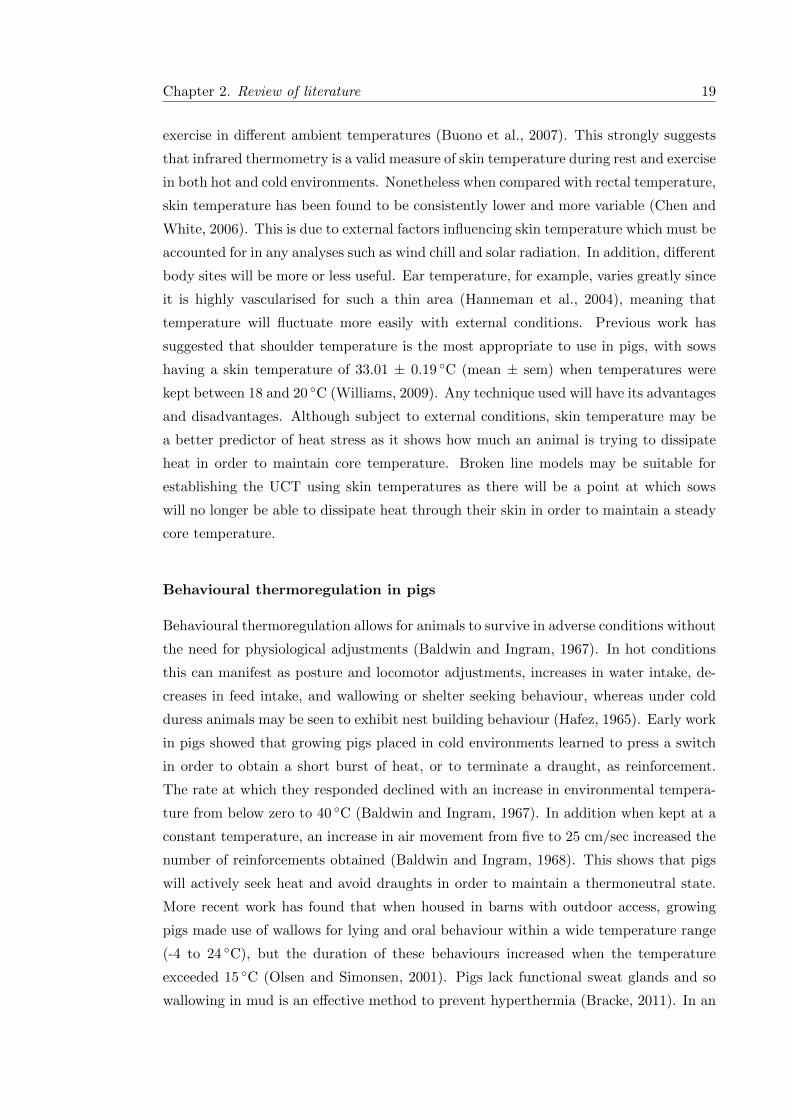
Chapter 2. Review of literature 19
exercise in different ambient temperatures (Buono et al., 2007). This strongly suggests
that infrared thermometry is a valid measure of skin temperature during rest and exercise
in both hot and cold environments. Nonetheless when compared with rectal temperature,
skin temperature has been found to be consistently lower and more variable (Chen and
White, 2006). This is due to external factors influencing skin temperature which must be
accounted for in any analyses such as wind chill and solar radiation. In addition, different
body sites will be more or less useful. Ear temperature, for example, varies greatly since
it is highly vascularised for such a thin area (Hanneman et al., 2004), meaning that
temperature will fluctuate more easily with external conditions. Previous work has
suggested that shoulder temperature is the most appropriate to use in pigs, with sows
having a skin temperature of 33.01 ± 0.19 ◦C (mean ± sem) when temperatures were
kept between 18 and 20 ◦C (Williams, 2009). Any technique used will have its advantages
and disadvantages. Although subject to external conditions, skin temperature may be
a better predictor of heat stress as it shows how much an animal is trying to dissipate
heat in order to maintain core temperature. Broken line models may be suitable for
establishing the UCT using skin temperatures as there will be a point at which sows
will no longer be able to dissipate heat through their skin in order to maintain a steady
core temperature.
Behavioural thermoregulation in pigs
Behavioural thermoregulation allows for animals to survive in adverse conditions without
the need for physiological adjustments (Baldwin and Ingram, 1967). In hot conditions
this can manifest as posture and locomotor adjustments, increases in water intake, de-
creases in feed intake, and wallowing or shelter seeking behaviour, whereas under cold
duress animals may be seen to exhibit nest building behaviour (Hafez, 1965). Early work
in pigs showed that growing pigs placed in cold environments learned to press a switch
in order to obtain a short burst of heat, or to terminate a draught, as reinforcement.
The rate at which they responded declined with an increase in environmental tempera-
ture from below zero to 40 ◦C (Baldwin and Ingram, 1967). In addition when kept at a
constant temperature, an increase in air movement from five to 25 cm/sec increased the
number of reinforcements obtained (Baldwin and Ingram, 1968). This shows that pigs
will actively seek heat and avoid draughts in order to maintain a thermoneutral state.
More recent work has found that when housed in barns with outdoor access, growing
pigs made use of wallows for lying and oral behaviour within a wide temperature range
(-4 to 24 ◦C), but the duration of these behaviours increased when the temperature
exceeded 15 ◦C (Olsen and Simonsen, 2001). Pigs lack functional sweat glands and so
wallowing in mud is an effective method to prevent hyperthermia (Bracke, 2011). In an

Chapter 2. Review of literature 20
effort to reduce metabolic heat production decreased feed intake has been observed in
sows exhibiting signs of heat stress (Lynch, 1977; Black et al., 1993) and increased water
intake when provided with chilled water (10 or 15 ◦C) compared to room temperature
water (22 ◦C) has also been found (Jeon et al., 2006). It can therefore be concluded
that sows will alter their feeding habits in order to stay comfortable which, as previ-
ously described, can have effects on subsequent reproductive output. In contrast, work
in Scotland showed that the behaviour and activity of outdoor sows was most strongly
related to the stage of reproductive cycle, with season and climate (including temper-
ature and wind speed) having relatively small effects (Buckner et al., 1998). This was
attributed to the sows being exposed to very few days when conditions exceeded their
UCT, although the fact that individual behaviour was not monitored could also be a
factor. Individuals will react differently to stress (Renaudeau et al., 2010), with increases
in physiological changes being more important for some (e.g. panting) and behaviour
more for others. Therefore in conjunction with physiological readings, the behaviour of
individual animals exposed to varying temperatures may help us understand at which
level environmental stress occurs.
2.2.2.3 Genetics
Seasonal infertility in the domestic pig is thought to have originated from the wild boar’s
breeding habits, where only one litter is produced each spring when piglet survival is
most likely (Mauget, 1982). Wiseman et al. (2006) conducted a database study to in-
vestigate whether a genetic basis for seasonal infertility exists and found that there was
no significant fluctuation in numbers born alive or successful number of services over the
course of the year, although specific breed differences were not examined. It is known
however that different breeds are more or less tolerant to external stressors, such as
temperature, explaining the use of different breeds in different climates (Gourdine et al.,
2006a; Chokoe and Siebrits, 2009). Studies have shown that different breeds have dif-
ferent reproductive performance for general traits such as WOI and number of piglets
born per litter (Gaugler et al., 1984). These may be accentuated in hot conditions with
Yorkshire sows having shorter WOI and smaller litter sizes than Landrace sows (Tan-
tasuparuk et al., 2000b; Tummaruk et al., 2000), and Creole sows better feed intakes
during lactation under warm conditions in comparison to Large White sows (Gourdine
et al., 2006a; Renaudeau et al., 2007), which could have knock on effects on subsequent
reproductive performance. However more work on comparing breed tolerances to envi-
ronmental conditions needs to be conducted, as there is limited research available on
the subject especially in relation to UK breeds. Breed choice should be an integral part
of controlling seasonal infertility, choosing those breeds shown to be least affected. The

Chapter 2. Review of literature 21
Large White is known to be highly productive and hardy, with excellent maternal traits
making it ideal in a variety of climates (such as the tropics), especially when used as
a maternal line for hybrid crosses (New South Wales Department Of Primary Indus-
tries, 2005). In the UK it is common for Landrace × Duroc sows to be used in outdoor
units due to their robustness (Edwards, 2005). This is in contrast to indoor breeds
where Landrace and Large Whites dominate, both as pure and cross breeds. Molecular
research into genes known to be involved with seasonality, such as the melatonin and
kisspeptin receptors, may provide insight into tolerances to photoperiod, rather than
simply looking at reproductive output, since expression and function between breeds
may differ. For example genotyping work has already established that effects of the
melatonin receptor 1a gene (MTNR1A) on litter size in Iberian × Meishan sows exist
in different seasons, with individuals heterozygous for MTNR1A being less prolific than
homozygous individuals in autumn and winter (Ramırez et al., 2009).
2.2.2.4 Management and Nutrition
Housing conditions of indoor herds have been found to affect sow fertility. Individual
housing is thought to maintain high farrowing rates in summer (Love et al., 1995) and
the provision of bedding can reduce the incidence of returns to oestrus (Peltoniemi
et al., 1999) probably due to less social stressors being present and a more stimulating
environment. Since there is a move towards more group housing in the industry, this
may lead to an increase in the incidence of seasonal infertility observed (Peltoniemi et al.,
2000) with analyses concluding that group housing of dry sows increases the risk of re-
breeding (Peltoniemi et al., 1999). Throughout the year pregnant sows are often restrict
fed in response to early findings demonstrating that fewer early embryonic deaths took
place in primiparous sows when fed low (< 23 MJ ME/day) compared with high (> 35
MJ ME/day) energy levels (reviewed by Aherne and Kirkwood 1985). Recent work has
shown however that feeding double the standard ration (2 vs 4 kg/day) to Large White
gilts did not affect embryonic survival (Quesnel et al., 2010). In group housing systems,
feeding 1.6 to 2 kg/day increased the WOI and reduced farrowing rates during summer
and autumn. In winter and spring, the same level of feeding did not have any adverse
effects. Higher feeding levels (2.5 to > 3.6 kg/day) had a positive effect on summer and
autumn farrowing rates and feeding level did not affect litter size (Love et al., 1995).
It has been hypothesised that the protective effect of higher feeding against seasonal
infertility might be due to increased pituitary LH support to the CL, since pituitary LH
pulses have been found to be of lower amplitude and more irregular during the seasonal
infertility period (Paterson et al., 1992a; Peltoniemi et al., 1997a). Nonetheless no direct
link between energy intake and plasma LH frequency or mean concentration has been

Chapter 2. Review of literature 22
found (Peltoniemi et al., 1997b). It should be noted that energy supplementation was
provided in the form of fat during the trial, unlike a commercial setting where increased
carbohydrates would be given in the form of a larger ration of feed. Increasing total
energy intake with carbohydrates affects insulin regulated glucose metabolism more than
by using fat, having a greater effect on the hypothalamic-pituitary-ovarian function in
the pig (Booth, 1990). This research shows that feeding levels may need to be altered
depending on the season and housing of the animals. Poor management during lactation
resulting in poor body condition at weaning can also affect subsequent fertility, as can
incorrect timing of AI or poor health status. All of these associated factors should be
considered to obtain a clear idea of the problem and how to improve the fertility of sows
during periods of seasonal infertility. Although different hormonal treatments have been
tried and tested to overcome seasonal infertility, with varying results (Kermabon et al.,
1995; Pena et al., 1998, 2000, 2001; Thaker et al., 2008), a change in management may
be much easier and cost effective to apply on site.
2.3 Boar semen quality and artificial insemination
Boar efficiency relies on the production of consistently large quantities of good quality
semen as well as high libido, yet seasonal variations in semen composition and the fer-
tilising capacity of boar spermatozoa contribute to seasonal alterations in herd fertility.
The use of AI in the UK is increasing annually (Penny and Machin, 1999), and although
AI centres try to keep semen doses as consistent as possible, it is well known that boars
suffer from decreased fertility during the summer months, with short or shortening day
lengths generally stimulating most aspects of boar fertility (Trudeau and Sanford, 1986;
Kunavongkrit and Prateep, 1990; Kozdrowski and Dubiel, 2004; Wysokiska et al., 2009).
Sperm production may fluctuate by up to 30% throughout the year (Ciereszko et al.,
2000), forcing AI centers to keep additional boars to compensate for these fluctuations.
This can influence management rigour and so a better knowledge of factors influencing
the quality of ejaculates may help improve stud efficiency. Photoperiod and tempera-
ture are thought to be the major factors affecting production during the summer months
(Quesnel et al., 2005) and so one of the most crucial aspects of AI, in respect to season-
ality, is the conditions in which boars are kept. Due to the temperate UK climate, boars
are generally kept in basic conditions without any specialist environmental control. This
is in contrast with other countries in mainland Europe, or in tropical climates, where
air cooling is becoming more popular in studs to help manage hot summer conditions.
UK boar stud accommodation may consist of stalls within barns or sheds, where the

Chapter 2. Review of literature 23
animals are individually housed or occasionally kept in pairs. The boars therefore ex-
perience temperatures similar to those outside, using straw to keep warm in winter and
natural ventilation to cool down in summer. This can pose problems since in summer it
is possible for the boar accommodation to heat up significantly and, without adequate
cooling, this may have a severe effect on the quality of semen produced. Boars are also
generally exposed to natural lighting regimes enhanced through artificial lighting during
working hours, and so are subject to natural fluctuations in semen production in relation
to the changing day light hour patterns and seasons (Table 2.2). Year on year, regard-
less of temperature, the same pattern of an increase in the number of abnormal sperm
morphologies or poor motility can be seen (personal communication; JSR Ltd, 2010).
Infertile boar stock may be used for a long period of time before negative effects are seen,
as it is only through sow returns and reduced litter sizes that subfertility is observed.
Additionally libido has been linked to fertility, mainly since causes of reduced fertility
such as heat stress and under-nutrition also tend to induce poor libido (Flowers, 1997).
This is an important point as it results in boars with high libidos and high fertility be-
ing overworked, eventually resulting in lower semen volumes and sperm concentrations
due to the short intervals between ejaculations (Kunavongkrit et al., 2005; Smital, 2009;
Wolf and Smital, 2009).
2.3.1 Seasonal changes in boar reproductive physiology
2.3.1.1 Season
Wild boar ejaculates are comparable to those of the domestic boar and have been found
to undergo significant changes at various times of the year with increases in semen
quality between September through February as compared to March through August in
temperate climates (Kozdrowski and Dubiel, 2004). Having analysed records of 1,646
boars on seven studs it was found that domestic boars were most productive in autumn
and winter in America (Rutten et al., 2000). As can be seen in Table 2.2, it has been
consistently found throughout the literature that when boars are kept in decreasing
photoperiodic conditions the volume of their semen increases (with the exception of
Sancho et al. 2004), as does the motility of the sperm, however there is equivocal evidence
as to when sperm concentration and total sperm numbers peak. Semen quality is known
to deteriorate and sperm concentration is known to decrease in domestic boars kept
in studs (Wolf and Smital, 2009). Boars may therefore naturally try to compensate
for this in autumn by increasing their ejaculate volume during the start of the rutting
season, as is the case in wild boars where semen volume, sperm concentration and
the total number of spermatozoa are highest in late autumn (Kozdrowski and Dubiel,
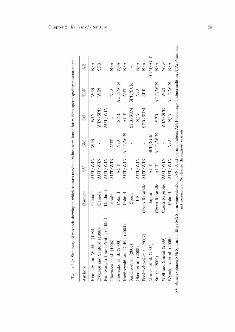
Chapter 2. Review of literature 24
Table2.2:
Su
mm
ary
ofre
sear
chsh
owin
gin
wh
ich
seaso
ns
maxim
al
valu
esw
ere
fou
nd
for
vari
ou
ssp
erm
qu
ali
tym
easu
rem
ents
Au
thor
sC
ountr
yS
VS
MS
CT
SN
AB
Ken
ned
yan
dW
ilkin
s(1
984)
Can
ada
AU
T/W
INW
INW
INW
INN
/A
Tru
dea
uan
dS
anfo
rd(1
986)
Can
ada
AU
T/W
IN-
WIN
/SP
RW
INS
PR
Ku
nav
on
gkri
tan
dP
rate
ep(1
990)
Th
aila
nd
AU
T/W
IN-
AU
T/W
IN-
-
Ch
arn
eca
etal
.(1
996
)S
pai
nA
UT
/WIN
AU
T-
N/A
N/A
Cie
resz
koet
al.
(2000
)P
olan
dA
UT
N/A
SP
RA
UT
/WIN
N/A
Koz
dro
wsk
iand
Du
bie
l(2
004)
Pol
and
AU
T/W
INA
UT
/WIN
AU
TA
UT
N/A
San
cho
etal
.(2
004
)S
pai
n-
-S
PR
/SU
MS
PR
/SU
M-
Oke
reet
al.
(200
5)U
SA
UT
/WIN
-N
/AN
/AN
/A
Fry
dry
chov
aet
al.
(2007
)C
zech
Rep
ub
lic
AU
T/W
IN-
SP
R/S
UM
SP
RN
/A
Mu
rase
etal
.(2
007
)Jap
anA
UT
SP
R/S
UM
--
SU
M/A
UT
Sm
ital
(200
9)C
zech
Rep
ub
lic
AU
TA
UT
/WIN
SP
RA
UT
/WIN
N/A
Wolf
an
dS
mit
al
(2009
)C
zech
Rep
ub
lic
AU
T/W
IN-
WIN
/SP
RW
INW
IN
Wyso
kis
kaet
al.
(200
9)P
olan
dA
UT
/WIN
N/A
N/A
AU
T/W
INN
/A
SV
:S
emen
volu
me;
SM
:S
per
mm
otil
ity;
SC
:S
per
mco
nce
ntr
ati
on
;T
SN
:T
ota
lsp
erm
nu
mb
ers;
AB
:P
erce
nta
ge
of
ab
norm
ali
ties
;N
/A
:P
ara
met
ern
otass
esse
d;
-:N
och
an
ge
thro
ugh
ou
tse
aso
ns.

Chapter 2. Review of literature 25
2004). Smital (2009) found that although maximal semen volume was produced in
November compared to April, sperm concentration was highest in March and April
and highest total sperm numbers were found in December and January and least in
August, with breed having a highly significant effect. This was confirmed by Wolf
and Smital (2009) and could be related to temperature since heat stress negatively
affects semen quality and ejaculate volume, with differences between various genetic
lines (Sonderman and Luebbe, 2008). Alentejano pigs, for example, have been found
to have significantly smaller ejaculates than some cross bred animals, whilst sperm
concentration, percentage of alive spermatozoa and sperm motility after collection were
significantly higher (Charneca et al., 1996). Other work has shown that boars kept in
stalls under natural environmental conditions experience a decrease in the percentage of
motile sperm during late summer and early autumn, and that the agglutination score
for the semen was high during this time. Additionally, having artificially inseminated
sows with semen from the study boars, it was found that farrowing rates were best
in winter and spring and very low in autumn (Murase et al., 2007). Agglutination in
semen is when spermatozoa adhere physically to each other (Lillie, 1915) and can occur
for several reasons such as a high number of dead spermatozoa in the ejaculate, a large
number of abnormal acrosomes, and bacterial contamination (Corcuera et al., 2002a),
all of which have been associated with seasonal changes in boar fertility (Brinsko et al.
2003; Murase et al. 2007; Althouse et al. 2000 respectively). Sedimentation of semen
has been found to modify seminal quality not only from initial collection but also due
to incorrect storage of doses, i.e. without agitation. In fact 48 hours of storage without
agitation resulted in significantly reduced spermatozoa viability and increased numbers
of abnormal acrosomes throughout the year (Rodrıguez-Gil and Rigau, 1995).
Okere et al. (2005) only studied two boars (one Yorkshire and one Landrace) to evaluate
libido and the quality of ejaculates on a weekly basis. Although their experiment may
contain a lot of bias as they only had one of each genotype, their findings are still of
interest; ejaculate volume was greatest in autumn, with no other traits (motility, libido)
showing seasonal changes. This is in contrast to work in Spain using eight month old
Landrace boars sired from the same father (Sancho et al., 2004). The boars were sepa-
rated into ’spring’ and ’autumn’ as decided by whether they were exposed to naturally
increasing daylight or decreasing daylight respectively. Temperature was maintained at
21 ◦C with 60 to 75% humidity and the boars were ejaculated twice weekly. No dif-
ferences in ejaculate volume were found, but semen pH was higher in ’autumn’ boars.
Conversely other research suggested that semen pH was highest in spring and early sum-
mer (Trudeau and Sanford, 1986), suggesting that vesicular gland function is affected

Chapter 2. Review of literature 26
due to the synergistic action of testosterone and oestrogen changing with day length. Us-
ing radioimmunoassays it has been shown that when comparing steroid levels in seminal
and blood plasma of mature boars kept under natural day length conditions or artificial
lighting conditions (17 hours and eight hours a day in winter and summer respectively;
reversed in respect to natural conditions), testosterone and oestrogen levels increased
during the shorter day lengths. This resulted in the expected dip during the summer
months being reversed by using the artificial lighting regime, suggesting that day length
is the main driving force in changing steroid levels (Claus et al., 1983). Oestrogen in
the forms of oestrone, oestradiol-7β and oestrone sulphate, is abundantly found in boar
semen due to the high volumes produced during ejaculation (Claus et al., 1987) and
is known to indirectly regulate LH and testosterone levels through negative feedback
loops in the hypothalamus-pituitary-testis axis (reviewed by Carreau and Hess 2010).
A study comparing entire and castrated boars (with or without supplementary steroid
injections) found that castration reduced the secretory activity of sex glands in boars
(reduced seminal plasma volume, citric acid and fructose levels) and if supplementary
testosterone was given (75 mg/week) this was not sufficient to improve production. If
both testosterone and oestrogen were given production did improve (Joshi and Rae-
side, 1973). It has also been shown that testosterone concentrations in the wild boar
change with day length, peaking in the autumn and winter when reproductive activity
re-commences (Mauget and Boissin, 1987), although some data suggest that decreasing
photoperiod impairs testicular activity as spring boars were found to have double the
sperm concentration of autumn boars and more morphological abnormalities have been
found in semen from autumn boars (Sancho et al., 2004). No seasonal differences in
motility or vitality were found re-enforcing recent work which demonstrated that motil-
ity remained relatively constant and seasonal differences in percentage of abnormalities
were less than 1% (Wolf and Smital, 2009). Other work has shown that motility is lowest
in summer and that animals exhibit a reduced libido from May to September, which co-
incides with the anoestrous period of sows (Kozdrowski and Dubiel, 2004). Frydrychova
et al. (2007) studied 22 hybrid boars over five years, collecting 1,170 ejaculates. They
found that semen volume was highest between October and December, although there
were large standard deviations around the mean values most likely due to individual
boar variation. Sperm concentration was lowest in summer and autumn versus winter
and spring. Number of sperm per ejaculate was lowest in summer and the daily output
of sperm was greatest in autumn in comparison to spring. All these studies support each
other to some extent, although differences are apparent. As with any biological system,
variation in individual boar tolerance levels is to be expected, making most whole ani-
mal studies very difficult to compare as small sample sizes are often used and different
genetic lines considered. Sow studies have shown differences in heat stress tolerance

Chapter 2. Review of literature 27
between sow lines as measured by differences in reproductive performance (Bloemhof
et al., 2008) and genetic differences in boar reproduction have also been shown (Flow-
ers, 2008). Nonetheless published large scale data analysis studies have not considered
daily temperature effects and so environmental factors may not have been evaluated to
their full potential.
2.3.1.2 Temperature
Boar semen production has been shown to be extremely sensitive to heat stress. Early
work showed that boars exposed to temperatures of 33 ◦C, as opposed to 20 ◦C, with
50% relative humidity for 72 hours, had significant differences in sperm concentration,
motility and percentage of abnormalities (McNitt and First, 1970). Sperm concentration
was not affected until 28 days after exposure to heat stress, and fertility was reduced
for up to six weeks after (McNitt and First, 1970). When boars were heat stressed (33
to 37 ◦C) for varying periods of time (six hours a day for four, five or seven days) it was
found that after five or more days of exposure, total sperm numbers fell significantly and
sperm morphology was severely affected from weeks two to five post heat stress (Cameron
and Blackshaw, 1980). Work on Yorkshire boars showed that although sperm volume was
not affected by increased temperatures, sperm motility decreased and took five weeks to
recover. Additionally sperm output decreased by over 50% and when gilts were naturally
mated with the boars, fertility rates were 23% lower in heat stressed boars compared
with control boars, although embryo survival remained unaffected (Wettemann et al.,
1979). This suggests that while overall fertility may be lower, the sperm which do go on
to fertilise ova are of good quality. Cold temperatures do not impact semen quality as
much as hot temperatures. When exposed to external temperatures as low as −30 ◦C,
boars were found to produce larger volumes of semen with lower sperm concentrations,
resulting in sperm output that was equivalent between the cold exposed boars and
temperature controlled boars. Additionally spermatozoa reserves were greater in the
experimental group when compared to boars kept indoors at 17 ◦C. This suggests that
boars build up semen reserves in response to the cold. It has been shown that when
temperature is controlled within the stud, better semen quality is achieved in the form of
increased motility and a higher percentage of normal acrosomes (Corcuera et al., 2002b).
If environmental control was not provided, the addition of straw helped maintain better
values. This highlights the importance of changes in temperature on the production of
semen, although it has been suggested that boars are in fact capable of withstanding
temperatures as high as 29 ◦C (Stone, 1982). The inclusion of temperature control within
UK boar studs may help with the consistency of semen quality throughout the year.

Chapter 2. Review of literature 28
2.3.2 Artificial insemination
2.3.2.1 Extending semen
The success of AI has been largely mediated by the success of the preservation and
dilution of semen. Spermatozoa are found in the seminal plasma, which supplies them
with the necessary nutrients required for the high metabolic demands of sperm transport
through the female reproductive tract. In order to preserve spermatozoa for prolonged
periods of time, their metabolic rate needs to be reduced making their storage envi-
ronment vital. Boar spermatozoa are extremely sensitive to cold shock, suffering from
reduced viability and motility (Pursel et al., 1973). This reaction to cold means that
ejaculates need to be kept at around 17 ◦C, however this restricts their storage capacity
since cell metabolism cannot be reduced and because contamination risks are higher
than when lower temperatures are maintained (5 ◦C). In addition, dilution lowers the
concentration of certain compounds in the seminal plasma, such as potassium ions or
plasma proteins, altering sperm viability (Gadea, 2003) and resulting in a need for them
to be compensated for by the addition of substances to the diluent formulation such as
bovine serum albumin (BSA), which has been shown to enhance motility and improve
fertility rates (Waberski et al., 1994).
Semen diluents can be categorised as either for short term preservation, commonly used
in mainland Europe and the UK, or long term preservation, commonly used in Norway
and America (Gadea, 2003). Many different brands exist with various formulae for
short and long term usage, but the more commonly used short term extenders (Kiev
and Beltsville Thawing Solution (BTS)) consist mainly of glucose for energy, added ions
for buffering action and the chelating reagent EDTA which blocks the action of calcium
as a mediator of sperm capacitation and acrosome reaction (Johnson et al., 2000; Gadea,
2003). Antibiotics are also added to extended semen since contamination can arise during
collection and processing. Semen is stored at warm temperatures in extenders containing
high glucose concentrations and nutrients similar to those of cell cuture media, and as
such bacteria can easily colonise doses. Bacterial presence in semen is thought to reduce
fertility (Diemer et al., 2003; Maroto Martın et al., 2010) as a result of effects on motility
and increased cell agglutination, with E. coli being the main causative agent (Althouse
et al., 2000). Recent work has shown that litter size is reduced by the presence of
E. coli, with a threshold of 3.5 x 10³ colony forming units (CFU)/ml (Maroto Martın
et al., 2010). This is in contrast to other work showing that this was not the case in
a commercial farm setting, with neither fertility rates nor litter sizes decreasing in the
presence of bacterial contamination (Reicks and Levis, 2008). Extended, pooled semen
doses were cultured two to five days after semen collection, however it should be noted

Chapter 2. Review of literature 29
that in this study the strains of bacteria found to infect the semen were not analysed
and so it is possible that had more research into the different strains been carried out,
different results would have been obtained. In addition no significant interaction between
bacteria and season were found in this study, suggesting that bacteria counts do not
change throughout the year. Nevertheless it is conceivable that once semen has been
transported to farms from studs, if conditions are not kept stable in summer months,
warmer temperatures may allow for increased bacterial colonisation and thus a potential
drop in fertility.
Research has also been conducted into the use of frozen thawed semen (FT), as this could
provide an advantage to the pig industry in terms of genetic evaluation and selection
programmes (Roca et al., 2006). Currently FT is not routinely used due to the fact
that very large numbers of spermatozoa (5 to 6 x 10¹⁰) are required to achieve even
relatively low fertility rates of around 70% when using Intra-Cervical insemination (ICI).
Spermatozoa in FT have shorter life spans than those in fresh or cooled semen, and so
once deposited in the sow they are only able to survive in the reproductive tract for up
to six hours (Waberski et al., 1994). Pursel et al. (1978) found that twice as many ova
were fertilised and developing normally in gilts which had been subjected to ICI with
fresh semen (97%) compared to FT (44%), since FT was removed more readily from
the reproductive tract. This was confirmed in a recent study where sows were twice as
likely to get pregnant after Post-Cervical Insemination (PCI) with cooled semen (1 x
109 cells in a 30 ml dose) than with FT (7.5 x 10⁹ cells in a 30 ml dose; Casas et al.
(2010)). Recent research suggests that FT aggravates fertility and prolificacy problems
in summer months compared with liquid semen (Boların et al., 2009) due to the increased
variation in ovulation times making it harder for the spermatozoa to survive long enough
to fertilise the ova within the female reproductive tract. Spermatozoa in FT are weak
in comparison to fresh/cooled spermatozoa, meaning that when ICI is used, they have
difficulty is crossing the cervix, resulting in only a small proportion making it to the
uterine horns (Roca et al., 2006). This would suggest that the use of FT may be
suitable with PCI or Deep-Uterine Insemination (DUI), as the semen is deposited closer
to the site of fertilisation, not only meaning that less numbers are needed, but also that
allowances can be made for the timing of insemination. Roca et al. (2003) found that
when using DUI with FT (1 x 10⁹) in comparison to DUI with fresh semen (1.5 x 10⁸)
and ICI with FT (6 x 10⁹), no significant differences were found in farrowing rates or
litter sizes when sows had an induced oestrus. Significant reductions in farrowing rates
were found however when DUI with FT (1 x 10⁹) and ICI with fresh semen (3 x 10⁹)
were compared (Roca et al., 2003). If the processing of FT could be optimised to achieve
similar results to cooled semen, this would facilitate the elimination of seasonal effects

Chapter 2. Review of literature 30
in boar semen, as semen could be collected in months when it is known to be at its best
and frozen for use during the seasonally infertile months.
Due to seasonal changes in semen quality, pooling is often seen as useful to try and
counteract the effects and compensate for under producing boars. Pooling semen can
be beneficial as it increases efficiency by allowing for a large number of ejaculates to be
processed together, and reduces inherent differences in fertility between boars. However
some boars only produce a few piglets from their ejaculate and therefore have little merit
as they are only diluting the pooled semen (Foxcroft et al., 2008). If sperm numbers
needed per dose can be reduced, it may not be necessary to pool semen and therefore it
would be possible to capitalise on the true genetic merit of superior sires. Assessment of
semen quality is done via motility scoring, morphological assessment and other checks
with minimum limits being at least 15 x 109 sperm in the ejaculate, motility of at
least 70%, no more than 30% abnormalities, including no more than 15% cytoplasmic
droplets (personal communication; JSR Ltd, 2010). This is done prior to pooling and
any semen which falls below these standards is discarded and the high sperm numbers
used compensating to some extent for reductions in fertility. By using a low dose (1.5 x
109) AI protocol to inseminate gilts with single sire semen of comparable quality, it was
found that there were differences among boars in farrowing rates and litter sizes (Ruiz-
Sanchez et al., 2006). Specific boars were found to produce smaller litters and reduced
farrowing rates, even though under normal commercial conditions their semen would
have been pooled and sold. Their reduced fertility therefore reduced the overall fertility
of the semen doses they were included in and resulted in poorer on farm performance.
This suggests that if these boars could be identified and removed, overall semen quality
would be improved and thus better farm production achieved. Although this issue is
applicable year round, it is particularly important in summer. If the boars which are
least tolerant to seasonal changes and increased temperatures could be replaced, AI may
have a smaller impact on the seasonal infertility observed in sow breeding herds. Indeed
Foxcroft et al. (2008) suggest that “the ability to differentiate relative fertility amongst
boars would have a substantial economic impact on the swine industry, by eliminating
or optimising the use of less fertile boars”.
2.3.2.2 Storing and transporting semen
Intensive exposure of sperm to ultra-violet (UV) light has been shown to induce DNA
damage (Bathgate, 2008). Although the sperm are still capable of fertilising and acti-
vating the oocyte, embryonic development is blocked after reaching the four to eight cell

Chapter 2. Review of literature 31
stages (Silva and Gadella, 2006). In summer months there is the potential for mishan-
dled semen doses to experience damage due to the effects of stronger UV light exposure,
although there is a lack of data available in the literature to confirm this. Tempera-
ture during collection and initial storage of semen is known to be very important in
maintaining the integrity of spermatozoa. Boar spermatozoa are susceptible not only to
very high temperatures but also to cold shock and so must be treated carefully before
being extended and stored. Shortly after ejaculation if semen is cooled too quickly its
viability is diminished (Johnson et al., 2000) and so it should always be kept between
15 and 17 ◦C. This is normally achieved on units where strict protocols for the han-
dling of semen are maintained, and so it is unlikely that any sort of seasonal influences
of temperature are present at the initial processing stage. It has been found however
that during August in European climates motility was significantly reduced after storage
(Charneca et al., 1996). This may be explained by the storage of semen post-extension
in climate controlled rooms. If it is extremely hot outside, indoor temperatures are
difficult to maintain at 17 ◦C and so semen is exposed to higher temperatures and the
spermatozoa begin to weaken. Semen quality is known to degrade during storage regard-
less of the temperature it is kept at (Johnson et al., 2000), which is why extenders have
been designed to try and prolong semen viability. Nevertheless if exposed to inappro-
priate temperatures, degradation is liable to occur more quickly, and if the temperature
changes remain unnoticed, sub-standard semen may be dispatched to farms. Addition-
ally, in the UK, semen transportation to units from the studs tends to occur either via
courier or postal deliveries (PIC International Group, 2009). This can lead to damage
as temperature is not controlled and the packages may not be handled appropriately.
On arrival at the farm semen should also be stored correctly and used within the recom-
mended period of time to ensure that viable sperm are being used. There is very little
literature available on the effects of semen transportation on subsequent sperm quality,
and none in regards to effects during different times of the year or in different external
climatic conditions. Research into the transportation of equine sperm has shown that
even specialised containers were unable to maintain semen at the correct temperature
when exposed to extreme external temperature of about 37 ◦C in comparison with room
temperature (Malmgren, 1998). This is a cause for concern as the semen may degrade
more rapidly in the summer months when vehicles/storage rooms experience increased
temperatures. Other results from canine semen research suggest that depending on
the type of container used to transport the semen, the membrane integrity and motil-
ity of sperm are affected (Lopes et al., 2009), which in practical terms would relate
to decreased fertility. If regulated transportation protocols were introduced during the
summer the fertilising capacity of semen may be improved, and so under hot conditions

Chapter 2. Review of literature 32
it may be applicable to invest in temperature controlled transportation systems. In ad-
dition, maintaining semen temperature at 17 ◦C during the colder winter months is an
area of interest.
2.3.2.3 Artificial insemination methods
Artificial insemination was first attempted as a practical procedure in Russia during the
early 1900’s (Foote, 2002), and has been used in pigs since the 1930’s. However it is only
in the past few decades that wide commercial application in the pig industry has taken
place, owing to standardised procedures being established (Roca et al., 2006). The most
common procedure used on farm is ICI and involves the use of a catheter to deposit a
semen dose in the posterior portion of the cervical canal (Figure 2.4). At least 2.5 x 10⁹
sperm cells are recommended for ICI, with semen extended in a liquid state for optimal
results (Roca et al., 2006), in volumes ranging from 80 to 100 mls (Buranaamnuay et al.,
2010). Intra-cervical insemination is a simple, inexpensive and quick method of AI which
is used throughout the industry, but can only make use of around 15 semen doses from a
single ejaculate, thus reducing the efficiency of each ejaculate used and increasing costs.
For this reason the industry began to research more efficient ways of inseminating sows
with a lower concentration of spermatozoa per dose. Post-cervical and deep uterine
insemination are two techniques which have been looked at extensively in the literature.
Post-cervical insemination is performed by inserting a thin and semi rigid insemination
device through a conventional catheter previously inserted in the cervical folds. This
device is about 20 cm longer than the catheter and so can pass through the rest of
the cervix and enter the uterine body (Figure 2.4). Fitzgerald and colleagues allotted
389 sows into two experimental groups balanced for parity, body condition score and
breed of sire (Fitzgerald et al., 2008). Sow matings were performed by ICI or PCI
with 3 x 10⁹ spermatozoa in each dose. Farrowing rates were generally low (below
70% for both groups), but no performance differences were observed between the two
methods, in that litter sizes and fertilising capacity were comparable. A Swiss study
also showed that although litter sizes were significantly smaller by an average of two
piglets, by using PCI with 1 x 10⁹ spermatozoa no other reproductive inefficiencies
were observed in comparison to ICI with 3 x 10⁹ spermatozoa (Roberts and Bilkei,
2005). This suggests that the smaller dose leads to less embryos being fertilised, but
the overall farrowing rates remain similar. Other studies have shown similar results
(Cordova-Izquierdo et al., 2008; Dimitrov and Zmudzki, 2009). Rozeboom et al. (2004)
evaluated the reproductive performance of sows using PCI and various concentrations
of spermatozoa in 85 ml of semen extender (0.5 x 10⁹; 1 x 10⁹; 4 x 10⁹) in comparison

Chapter 2. Review of literature 33
14
Jan
ua
ry 2
01
1
09
:43
Un
file
d N
ote
s P
ag
e 1
Figure 2.4: Schematic (not to scale) of site of semen deposition with three differentartificial insemination methods: Intra-Cervical Insemination (ICI); Post-Cervical In-semination (PCI) and Deep-Uterine Insemination (DUI). Green circles represent where
semen would be deposited.
to ICI with 4 x 10⁹ spermatozoa. They found that when PCI with less than 1 x 10⁹
spermatozoa was used, farrowing rate, total pigs born and number born alive decreased
significantly and therefore that the use of PCI was not favourable over conventional ICI.
In contrast, Serret et al. (2005) found that farrowing rates and litter sizes did not differ
between ICI with 3.5 x 10⁹ spermatozoa and PCI with as few as 5 x 10⁸ spermatozoa.
In times of seasonal infertility, when the availability of good quality sperm is reduced
due to less sexually active boars or more abnormalities within the semen, PCI could
potentially allow for semen to be distributed more successfully. In other words breeders
could make more use of the good quality sperm that they do obtain in late summer and
early autumn since smaller volumes of semen may be used. A recent study showed that
when comparing ICI (3 x 10⁹ spermatozoa/100 ml) with PCI (1 x 10⁹ spermatozoa/100
ml; 1 x 10⁹ spermatozoa/50 ml; 5 x 10⁸ spermatozoa/100 ml; 5 x 10⁸ spermatozoa/50
ml), sows submitted to PCI produced farrowing rates which averaged at 90.8%, which
did not differ significantly from the rates obtained by ICI (90.0%). Litter size did not
differ either, at between 11.4 and 11.9 piglets at farrowing (Araujo et al., 2009). This

Chapter 2. Review of literature 34
shows that half the volume of semen with a lower concentration of spermatozoa will
produce comparable results when using PCI, in comparison to ICI.
Deep-uterine insemination follows a similar procedure, with a long, thin and flexible
insemination device being inserted through the catheter so that it can target one of
the uterine horns and deposit the semen up to a third of the way into it (Figure 2.4).
This could potentially be problematic due to only one side being targeted but has been
successfully used to inseminate sows in several studies, with varying farrowing rates
with fresh semen obtained; 92% (0.5 x 10⁸; Martınez et al. 2001); 89% (1.5 x 10⁸;
Dimitrov et al. 2007); 84% (1.5 x 10⁸; Roca et al. 2003). A Spanish study showed that
when using DUI, as little as 5 x 10⁷ spermatozoa would give similar results to 3 x 10⁹
spermatozoa deposited using ICI (Martınez et al., 2001). Conversely Dimitrov et al.
(2007) found that although farrowing rate was not significantly reduced, when sows
were artificially inseminated by DUI (0.15 x 10⁹ spermatozoa in 5 ml) as compared to
ICI (3 x 10⁹ spermatozoa in 100 ml), total born litter size was significantly reduced.
The deposition of a low volume of highly concentrated spermatozoa during DUI, may
seem more convenient than using larger volumes as it diminishes the backflow of the
inseminate. However with reduced numbers of spermatozoa present, there is a tendency
for a reduction in litter size, as there are less spermatozoa available to successfully
fertilise the ova (Dimitrov et al., 2007). It has been found that sows inseminated by
DUI after induced ovulation with 7 x 10⁶ or 1.4 x 10⁷ spermatozoa in 7.5 ml diluent had
farrowing rates of 78.7% and 85.7% and litter sizes of 9.8 and 9.9 piglets respectively.
When ovulation was allowed to occur spontaneously this was reduced to farrowing rates
of 77.2% and 80.9% and litter sizes of 9.1 and 9.5 piglets respectively, although results
for 1.4 x 10⁷ were still within a comparable range (Vazquez et al., 2003). The data
therefore suggest that timing of insemination in relation to ovulation was important and
that DUI is a suitable method for inseminating sows, providing acceptable farrowing
rates at low spermatozoa concentrations without litter size being significantly different.
The concentration of spermatozoa which can be used with DUI is a lot lower than for
both ICI and PCI, which economically would be extremely beneficial if the technique
was perfected.
2.3.2.4 Timing of insemination
Timing of insemination is also a key factor affecting fertilisation rates and the overall
success of AI. Variability in the duration of oestrus in individual sows is great, making
the timing of insemination difficult to assess. Additionally the moment of ovulation
after the onset of oestrus may vary from 10 to 85 hours (Kemp and Soede, 1997).

Chapter 2. Review of literature 35
Soede et al. (1995) studied the effects of the timing of insemination relative to ovulation
on the fertilisation rate and early embryo development in 151 sows. They found that
the time of ovulation during oestrus was dependent on the duration of oestrus, that
fertilisation rate of normal embryos was dependent on the interval between insemination
and ovulation and that fertilisation results were optimal when insemination took place
between 0 and 24 hours before ovulation. Waberski et al. (1994) suggest that this is
reduced to under 12 hours prior to ovulation in gilts. Studies show that ovulation occurs
about three quarters of the way through oestrus (Almeida et al., 2000), and so recognition
of the onset of oestrus is crucial for breeding herd management in summer. Extended
WOI during periods of seasonal infertility have been reported widely in the literature
(Hurtgen and Leman, 1981; Koketsu and Dial, 1997; Almond and Bilkei, 2005; Boma
and Bilkei, 2006), and have been associated with summer weaned sows experiencing
oestrus durations extended by around eight hours compared to spring weaned sows,
although extensive variation between farms exists (Steverink et al., 1999; Belstra et al.,
2004). In contrast longer WOI have also been associated with shorter oestrus durations
(Nissen et al., 1997; Steverink et al., 1999). With conflicting reports on the duration
of oestrus during periods of seasonal infertility, it is difficult to be certain of when is
the optimal time to inseminate sows, since if it is done too early the spermatozoa will
not be sufficiently viable to fertilise the ova, and if it is done too late then the ova
may have passed their fertile life span. Considering that the success of AI has been
found to depend on the availability of sufficient sperm in the oviduct at the time of
ovulation (Garcia et al., 2007), the timing of insemination is vital. Farrowing rates for
sows receiving sperm six hours prior to the predicted time of ovulation were greater
than those of sows receiving sperm 24 hours prior to the predicted time of ovulation
(85% versus 61%), and although sperm numbers were double in the former, no effects of
time of AI or sperm numbers on subsequent litter size were found (Garcia et al., 2007).
Weaning to oestrus intervals vary not only with season, but also with body condition
of the sow and lactation length, making sow management also important for successful
AI. In Australia sows tend to have reduced appetites in the summer months due to heat
stress and so without careful management their body condition may not be optimal
(Love et al., 1995). This can result in extended WOI and consequently reduced success
of AI. The timing of insemination is important throughout the year, but with increased
variability during summer months the implications are larger and even more attention
must be paid to signs of oestrus in gilts and sows in order to ensure successful AI.

Chapter 2. Review of literature 36
2.4 Modelling in Agriculture
2.4.1 The use of data mining and modelling in agricultural research
Data mining is becoming increasingly popular in biology, proving to be a useful method
of discovering relationships between variables using the ever expanding data resources
becoming publicly available. Many biological papers using data mining have been pub-
lished, ranging from using large sets of data to model the reproductive efficiency in beef
cow herds (Blanc and Agabriel, 2008), to using ML techniques to model seal breeding in
New Zealand (Bradshaw et al., 2002). Mined information is generally represented as a
model of the dataset which can then be used on new data for prediction or classification.
Alternatively the model can be examined to help clarify unknown characteristics in the
field of study. When considering ML methods of data mining, Wu et al. (2008) found
that systems that construct classifiers, such as the decision tree algorithms C4.5 and
C&RT (classification and regression tree), were amongst the most commonly used tools
in data mining in the fields of biology and medical science. Decision trees in particular
have been used to predict the occurrence of clinical mastitis in dairy cows (Kamphuis
et al., 2010a,b) as well as for the evaluation of sow herd management (Kirchner et al.,
2004a,b). Their popularity can be attributed to the fact that decision trees are easy
to interpret when visualised, although it is known that thorough preparation of data
provides improved classification as when irrelevant, noisy or incomplete attributes and
data entries are removed the algorithm can more easily detect true patterns within the
data (Kirchner et al., 2004b). Using the C4.5 algorithm, German workers found that
both simulated and real pig farming data sets could be analysed in order to identify dif-
ferences and weak points in farm management (Kirchner et al., 2004a,b). This detection
of patterns is not always possible when using linear models (De’ath and Fabricius, 2000;
Texeira et al., 2008). In contrast to decision trees, other methods are much less accessi-
ble, using ’black-box’ approaches. This means that although the model produced may
be a very good predictor for new data, the patterns found are not accessible to the user.
Artificial Neural Networks (ANN) are an example of this and have been extensively used
in the agricultural literature to model problems such as rumen fermentation patterns
in dairy cattle (Craninx et al., 2008), tree mortality in the Norway spruce (Hasenauer
et al., 2001), maize yield in America (O’Neal et al., 2002) and to find out how forage
availability and climate affect sheep reproductive performance (Texeira et al., 2008).
These papers state that exploratory analyses and biological significances guided them
in the selection of independent variables since feature selection is essential in ANN de-
velopment and variables should not be correlated. The type, quantity and quality of
input variables can alter the success of an ANN and must therefore be carefully selected

Chapter 2. Review of literature 37
(Hasenauer et al., 2001). In addition, a major challenge with the application of ML
is the analysis of the performance achieved when using unbalanced or small datasets.
This requires even more data preparation in order to balance the data and combinations
of performance statistics to interpret the results (Pietersma et al., 2003). Analysing
stored data in this manner when it would previously go unused is a relatively cheap and
fast method of experimenting, providing accurate information on which to base animal
studies in the future.
Simulation models are developed to try and integrate knowledge relative to the biological
processes in play and their interactions. These models provide tools to assist decision
making in breeding management and help to predict the effects of changes in the levels
of biological or management factors on the reproductive efficiency of the herd. In recent
decades, several models on swine production looking at the effects on productivity of
feed management and culling, genetics and batch systems have been published (Pomar
et al. 1991a; Faust et al. 1992; Martel et al. 2008 respectively). Models can summarise
reproductive output as a single integrative variable (farrowing rate for example) and
predict its value whilst taking into account factors such as parity and body condition.
Alternatively reproductive efficiency may be considered as resulting from a dynamic
process that includes successive steps from farrowing such as lactation length and WOI.
The advantage of simulating herd processes is that by using real data, it is possible to see
how random variables may influence herd dynamics in the future, to which a cost benefit
analysis can be applied (Faust et al., 1992). Using simulation modelling, it is possible to
account for various scenarios and using the output, adjust managerial processes on the
farm to establish optimal productivity. This can help one gain a better understanding
of what to expect in a herd and the cost implications.
2.4.2 Current status of modelling seasonal infertility
Seasonal infertility is an established problem in the UK as well as internationally. Much
research has been conducted into the subject, with few successful solutions being pro-
duced, making it increasingly clear that new techniques to understand the problem must
be attempted. To date, experiments have been conducted to see whether specific factors
influence or trigger seasonal infertility such as changing lighting regimes (Kermabon
et al., 1995; Tast et al., 2005; Chokoe and Siebrits, 2009), providing different levels
of feed (Love et al., 1995; Virolainen et al., 2004) and controlling the temperature or
ventilation available to the animals (Edwards et al., 1968; Almond and Bilkei, 2005).
Additionally hormonal treatments have been investigated as a method of trying to al-
leviate the problem, with some successes (Pena et al., 1998, 2001) and some failures
Chapter 2. Review of literature 38
(Pena et al., 2000; Thaker et al., 2008), although none are really practicable in the field.
Although these studies may help to explain some of the biological mechanisms occurring
within the animal, until now they have failed to provide an answer as to how farmers
can prevent the impact of seasonal infertility within their herds. In addition, most of
them are carried out in indoor controlled environments when the problem lies mainly in
outdoor herds.
Production record analysis is also becoming more common in the literature, for example
recent research in France using pig production data, looked into the relative roles of
temperature and photoperiod on seasonal infertility (Auvigne et al., 2010). Linear mod-
els were used to establish relationships between environmental factors and reproductive
traits. No definite conclusions were made other than, with temperature varying between
years and seasonal infertility being present every year, photoperiod had a stronger role
in the trend for reduced fertility and heat stress only exasperated the problem. Other
investigations in various parts of the world have used similar techniques, including gen-
eralised linear models, regression, chi-squared tests and mixed effects analyses to assess
the occurrence of seasonal infertility and its contributing factors (Hurtgen and Leman,
1981; Britt and Szarek, 1983; Peltoniemi et al., 1999; Belstra et al., 2004; Almond and
Bilkei, 2005; Kousenidis et al., 2009). An issue with previous studies is that although
they use herd data from very large databases, they involve different types of farms with
different managerial practices, meaning that many factors have not been accounted for.
The data are often a mixture of indoor and outdoor herds, dispersed across the country
in question, and any temperature data used are often general for the country in a given
month. Many different methods of data mining exist, ranging from ML techniques to
statistical methods. There has not yet been any published work pertaining to research-
ing seasonal infertility using ML methods to model the problem, with most research
looking at a set number of factors often with confounding results and with traditional
mathematical models for sow herd management being the main types of models avail-
able in the industry (Pla, 2007). Using local weather data and production data from
a uniform group of outdoor sow herds, this work should give a new perspective to the
problem and show us how to predict when seasonal infertility will occur even if the ex-
act biological reasoning behind its occurrence is not fully understood. This will be done
through simulation modeling, creating a better understanding of how the herd changes
its productivity over the months of the year.

Chapter 2. Review of literature 39
2.5 Conclusions
From the information available it is clear that the various manifestations of seasonal in-
fertility are due to complex interactions between environmental factors and managerial
processes, which in turn are mediated by a variety of endocrine signals. These factors
include, but are not necessarily limited to photoperiod, temperature, nutrition and so-
cial interactions and affect both the sow and the boar. Most parameters can be easily
corrected for in indoor herds, however in outdoor herds photoperiodic and environmen-
tal factors such as temperature are impossible to control. This highlights the need for
perfected managerial routines which will both limit the occurrence of seasonal infertility
and also counter-balance any production losses, such as the provision of wallows and
optimised gilt management respectively. Due to complications in standardising the ex-
pression of seasonal infertility and with so many confounding factors between herds, it
becomes difficult to identify the exact causative agents on a case by case basis. The
more research conducted into different aspects of seasonal infertility the better our un-
derstanding of the problem will become, and by using ML this process should be faster
and more accessible than ever before.
2.6 Aims
The aim of this study is to investigate previously unidentified relationships between
meteorological conditions and pig reproductive performance during periods of seasonal
infertility in the UK. Using exploratory statistical methods, analyses will be conducted
on production data from outdoor sows and corresponding meteorological data. Economic
values will subsequently be placed on the results obtained and a computer simulation
created to see whether reductions in production losses resulting from services in summer
months can be predicted. In response to the initial data analyses suggesting that the
UCT of outdoor sows may be lower than previously thought, a trial was also conducted
investigating meteorological effects on UCT and behaviour of outdoor breeding sows
throughout the year. Finally, using statistical methods and decision trees, relationships
between commercial boar semen quality and meteorological conditions will also be as-
sessed, in an attempt to identify the key variables involved in altering semen quality so
that suggestions for altering stud management can be made and improvements in semen
quality obtained.

Chapter 3
An investigation into the factors
that may cause seasonal changes
in outdoor sow herd productivity
3.1 Introduction
The sustainability of pig production depends on a consistent number of pigs being sold
throughout the year, however a reduction in sow fertility is often observed from ser-
vices occurring during the summer months resulting in a reduced availability of pigs for
slaughter. This seasonal infertility has been identified in herds across the globe with the
economic impact estimated to be millions of pounds annually in the UK alone (Digby,
2007).
Most of the research conducted to date has been carried out on indoor sow herds (e.g.
Hurtgen and Leman 1981; Love et al. 1995; Tummaruk et al. 2000, 2001a, 2004; Anil et al.
2005; Almond and Bilkei 2005; Boma and Bilkei 2006; Auvigne et al. 2010) and only a
few studies have considered outdoor sows (Larsen and Jø rgensen, 2002; Bloemhof et al.,
2008). With British farmers keeping ahead of EU legislation, outdoor pig production
has become more popular in the UK. In addition, changes in consumer preferences which
can be attributed to increased perceived animal welfare for outdoor pigs have helped
drive the outdoor pig production sector. Currently more than 40% of breeding sows are
kept outdoors (personal communication; BPEX, 2011), however this type of production
exposes sows to the elements and can have significant effects on their reproduction. Of
all the factors thought to affect sow fertility, photoperiod and temperature represent
40

Chapter 3. Seasonality in sows 41
the biggest problems which cannot be controlled by managerial techniques on outdoor
farms.
The effects of day length on sow fertility are inherited from the wild boar, which is
known to be anoestrous over the summer months (Mauget, 1982). Much of the research
from European countries suggests that photoperiod plays the prominent role in seasonal
infertility, nonetheless with seasonal infertility present in countries with negligible day
length changes (Tummaruk et al., 2004) other factors must come into play. This is
especially true when considering that not all herds are affected annually and that the
degree of infertility observed changes year on year. Work into day length effects on sow
fertility has yet to define which photoperiodic regime maintains fertility, as described
in Chapter 2. It is possible that this is due to the methods used during experiments,
for example exposure lengths being too short. Sows may be influenced by longer term
changes throughout the year and so this is something which needs clarifying before more
experiments are carried out. In addition it may be the rate of day length decline which
results in reduced fertility rather than absolute day length. If a pattern for the effects
of day length on sow productivity can be identified, targeted research could then be
conducted using, for example, hormonal treatments on outdoor animals since lighting
cannot be controlled.
Outdoor sows in the UK are also exposed to temperature extremes over the changing
seasons and as such may succumb to increased fertility problems. Hot temperatures
are known to affect sow fertility (Edwards et al., 1968; Black et al., 1993), however the
temperatures needed to influence litter size or conception rate are generally thought
to be higher than the average UK summer temperatures. It is possible that outdoor
sows in the UK are affected by lower temperatures than anticipated as they may have
acclimatised to colder conditions. It would therefore be beneficial to confirm if weather
phenomena per se affect outdoor sow reproduction and if so at what level problems begin
to occur.
3.2 Objectives and hypotheses
Objectives
The objectives of this work were to establish whether seasonal changes in sow repro-
duction could be observed in a large data set and determine what the causative agents
may have been in regards to meteorological events. This included looking at sows on an

Chapter 3. Seasonality in sows 42
individual basis as well as on a herd level and relating their reproductive outputs to me-
teorological conditions. Using the results produced, hypotheses for future experimental
work were then formed (Chapter 6) and a simulation of the productivity levels which
could be expected throughout the year was created (Chapter 4).
Hypotheses
It was hypothesised that:
• High temperatures would result in lower reproductive performance
• Other meteorological conditions such as relative humidity and windspeed would
work to influence perceived temperature and thus influence reproductive perfor-
mace
• Long days would result in lower reproductive performance
• Not all sows would be affected by seasonal infertility
3.3 The Data
3.3.1 Production data
The original data provided by BQP Ltd were from 36 outdoor breeding units in the
UK, for the years 2004 to 2009. Of the herds only those located in Hampshire (n =
2), Norfolk (n = 16), Suffolk (n = 7) and Wiltshire (n = 4) were used (Figure 3.1),
due to the availability of corresponding weather data, giving a final dataset of 122,391
farrowings from 32,935 sows in 29 herds.
All herds were similarly managed. Upon site establishment, pregnant gilts were brought
onto the farm in seven batches from a gilt mating unit (GMU). Three week batch farrow-
ing was practiced on all the units and once the required herd size was established, herds
were closed. Gilts were either pure Landrace or Landrace × Duroc crosses. Landrace
gilts were inseminated with either Landrace semen to produce the grandparent line or
Duroc semen to produce the new main stream gilts. Landrace × Duroc gilts/sows were
inseminated with semen from synthetic sireline boars to produce piglets for the food
supply chain. On occasions other genotype semen was used to inseminate the sows,
such as Hampshire, and this was recorded. All gilts were naturally mated and sows

Chapter 3. Seasonality in sows 43
")
")
")
a
a a
a
a
a
aa
aa
a aa
a
a
aa
a
a
a
a
a
a
aa
a
a
a
a
#
#
#
#
## #
#
NORFOLK
SUFFOLK
WILTSHIRE
HAMPSHIRE
±Reproduced with permission from Edina spatial data© Crown copyright.
0 20 4010 Miles
Legenda Farms# Weather Stations") Day Length Sites
Figure 3.1: Map of locations of selected herds and weather stations

Chapter 3. Seasonality in sows 44
Table 3.1: Variables included in the sow dataset
Variable Values
Animal ID String and Numeric
Gilt entry date 2004 - 2009
Service date 2004 - 2009
Service type AI or Natural
Parity 1-14
Farrow date 2004 - 2009
Total born piglets 0 - 27
Piglets born alive 0 - 27
Wean date 2004 - 2009
Piglets weaned 0 - 17
Cull date 2004 - 2009
Repopulation season Spring or Autumn
Sow source Breeder
Herd location County
served by AI, unless they returned. AI was carried out in service tents by experienced
stockmen and sows then housed with a catcher boar in case they returned.
Sows and gilts were fed a standard diet at a summer base level of around 2.5 kg/day,
which rose during the last two weeks of gestation to 3.5 kg/day. Two days prior to
farrowing this was reduced to 1 kg/day. Following farrowing this was increased from 3
kg on the day of farrowing to a maximum of 10 kg/day, by 0.5 kg/day increments. Sows
were normally weaned after four weeks, and fed 4 kg for day one post-weaning, 6 kg day
two post-weaning and 8 kg day three post-weaning. This was held until service, usually
five days post-weaning, when it was dropped to 3.5 kg/day for two weeks and then back
to the base level. In winter, and depending on sow condition throughout the year, slight
variations of up to 1 kg/day may have been made.
The variables contained within the dataset can be found in Table 3.1. From these
it was then possible to create new variables to assess fertility such as farrowing rate
(FR), lactation length and average total born (TB) or born alive (NBA) litter size. In
addition to individual herd production data, unit locations were provided as well as
breeder information. Repopulation season was also provided.

Chapter 3. Seasonality in sows 45
3.3.2 Meteorological data
Having established the locations of the herds, data were obtained from the British Atmo-
spheric Data Centre (BADC) in regards to historic weather conditions for the relevant
years (2004 to 2009). Weather stations recording all of the necessary weather variables
and located nearest to the herd sites were chosen (Figure 3.1). The data were extracted
from the MIDAS dataset (UK Meteorological Office, 2006) and included: minimum and
maximum daily temperatures ( ◦C); daily rainfall (mm); daily relative humidity (%);
daily wind speed (mph) and wind direction.
Altitude data were obtained as follows.
• The Ordnance Survey (OS) Grid reference provided for each herd was converted
into OSGB36 Latitudinal and Longitudinal references using http://www.movable-
type.co.uk/scripts/latlong-gridref.html.
• The new grid references were entered into Google Earth and the herd was located
on the map.
• The elevation (altitude) data, in metres, for that location could then be found and
noted.
Absolute day length (ADL) and change in day length (CDL) data were obtained for the
counties in which the herds were located (Figure 3.1) for each day in the relevant years
from http://www.timeanddate.com/worldclock/astronomy.html. Data were converted
into minutes.
3.3.3 Pre-processing the data
Using self written programmes, data in the form of ’.txt’ and ’.csv’ files were imported
into MATLAB R© 7.11.0 (R2010b) (MATLAB, 2010) and converted into ’.mat’ files for
use. The original dataset for the 29 herds comprised 226,609 farrowings. Scatter graphs
and histograms were used in order to detect any outliers in the data, for which records
were deleted or corrected. As is common with most field data, the data were extremely
noisy with many anomalies, duplicates and omissions present which needed to be cor-
rected and adjusted for. Pigs which entered the herd or were served after the 1st of
September 2009 were removed since complete data for their last parity were unavailable.
Sows which farrowed or were weaned after the 1st of November 2009 were removed as
their last parity production data were incomplete. Outliers for any of the variables were

Chapter 3. Seasonality in sows 46
looked at individually. If data entry was found to be the cause of the faulty data, the
value was corrected (for example 100 piglets instead of 10), otherwise if the root of the
problem was an impossible concurrence of values (for example a cull at parity three, but
a litter at parity four), the complete data for the sow in which the entry was found were
removed from the dataset, to leave only those sows with complete data within biologi-
cally relevant ranges. Sow tag numbers were occasionally replicated between herds and
so a new set of sow numbers had to be generated, providing a unique number per animal.
Parities were grouped as gilts, primipares, parities two to six and parities greater than
six. Lactation length was calculated by subtracting the farrow date from the wean date
and was limited to between 21 and 35 days, and based on values in the literature records
were limited to those containing gestation lengths between 110 to 122 days (Peltoniemi
et al., 1999). Using the dates provided in the original dataset, wean to service intervals
(WSI) were calculated by subtracting the service date from the previous wean date.
Records with WSI less than or equal to zero, or greater than 365 were deleted (Takai
and Koketsu, 2008). Returns were recorded when a sow was served on two different
dates whilst staying at the same parity. Culls were recorded if a cull date was present.
The data used in the present study were from three lines of Landrace × Duroc sows.
They originated from breeder A, either as coming directly from the breeding company
(G1) or as second generation animals (G2), or originated from breeder B (G3). Other
genotypes were removed from the dataset. Humidity values greater than 100% in the
meteorological dataset were set to 100. In order to allow for analyses between meteoro-
logical conditions and sow productivity, for each service date the average daily weather
conditions from the closest weather station on the same date and for up to five weeks
prior to service and five weeks post service, were attached to the record.
3.4 Statistical analyses
All analyses were carried out in MATLAB (2010) and R 2.12.1 (R Development Core
Team, 2009).
3.4.1 Principal components analysis
Principal component analysis (PCA) was carried out using the princomp function in
MATLAB (2010) in order to establish the relative importance of the different variables
available for future analyses (Adams, 2010). This included all the collated weather
variables (for weeks one and two pre- and post-service and day of service), as well as
day length, sow parity, genotype, lactation length, WSI, gestation length, service type,

Chapter 3. Seasonality in sows 47
which season the herd was established (repopulation season), piglets weaned and herd
location. The biplot and pareto functions in MATLAB (2010) were then used to interpret
the results produced.
3.4.2 Weather parameters
Weather data are presented as monthly averages between all locations. ANOVA followed
by the Tukey multiple-mean comparison test was used to look at the effects of year and
month on temperature, daily rainfall, humidity and windspeed.
3.4.3 Sow reproduction parameters
Farrowing outcome was analysed one of two ways: as a binary outcome (farrowed or not
farrowed) with farrow record as the statistical unit when conducting logistic regression
and as a calculated herd FR with a statistical unit of ’herd’ when considering day length
effects and ’herd-day relative to service’ when considering meteorological effects. Both
TB and herd FR were found to be normally distributed using the Lilliefors test and
quantile-quantile plots. In all analyses the statistical unit for TB was farrow record
unless otherwise stated.
For mixed effects models the lme4 package (Bates and Maechler, 2009) in R was used.
Markov-Chain Monte Carlo (MCMC)-estimated P values based on MCMC sampling
were calculated using the languageR package in R (Baayen, 2009). Residuals of all
parametric models were checked to approximate to a normal distribution by visually
checking normal probability plots and by using the Shapiro-Wilk test.
The effects of altitude and genotype on FR and TB were assessed using generalised
linear mixed effects models, with a binomial and gaussian family respectively. Herd was
included as a random effect.
Initial exploratory analyses were conducted in order to establish which period of time
influenced FR, and for what duration of time certain conditions needed to last in order
to have any effect. This involved collating weather data for different lengths of time (one
to five consecutive days) and periods of time around service (up to five weeks pre- and
post-) and plotting numerous graphs with the data. ANOVA and post-hoc Tukey tests
were then used to analyse the various scenarios, for example, the effects of three days of
temperatures above 18 ◦C with and without rain in four parity groupings. Temperatures
considered were ≤ 15 to 22 ◦C and ≥ 15 to 22 ◦C.

Chapter 3. Seasonality in sows 48
3.4.3.1 Monthly effects
Generalised linear mixed effects models were used to test for the effects of parity, month
of service and year of service on FR (binomial distribution) and TB (gaussian distribu-
tion), with herd as a random effect.
Day length effects
Day length was analysed as both average ADL during the 28 days preceding service
(ranging from eight to 17 hours) and as average CDL in the same period (24 groups
ranging from -120 to +110 minutes in 10 minute increments). This time frame reflected
the month prior to oestrus, accounting for the whole of a sow’s oestrous cycle and more.
Mean TB and FR for each level of both ADL and CDL were calculated for each herd
and significant differences were tested for using one way ANOVA followed by the Tukey
multiple-mean comparison test.
3.4.3.2 Meteorological effects
The effects of meteorological variables for the period two weeks pre- and post- service
date on FR and TB were analysed. These included average, minimum and maximum
temperatures (1 ◦C increments between -10 to 33 ◦C), relative humidity (10 equal groups
ranging from 0 to 100%), rainfall (wet or dry) and wind speed which was classed as either
calm (0 mph) or windy (> 0 mph). Meteorological data were grouped for weeks one and
two pre- and post- service and for day of service. This was based on the exploratory
analyses which found that the two weeks prior to service were crucial for subsequent
FR, while previous experiments have shown that heat stress for up to two weeks post-
service influences TB (Tompkins et al., 1967; Omtvedt et al., 1971) and that post-service
stressors can result in pregnancy failure (Bertoldo et al., 2009).
The effects of individual meteorological conditions on farrowing data were analysed using
generalised linear mixed effects models with a binomial distribution. Farrow outcome
was the binary output and meteorological conditions for each week surrounding service
and day of service as the explanatory variables. Month of service, herd and parity
were included as random effects. The same was carried out for TB, using a gaussian
distribution.
In order to establish thresholds for the effects of meteorological variables on reproductive
output, FR and TB were then analysed for each level of the studied meteorological

Chapter 3. Seasonality in sows 49
variables over two day rolling averages and for the 28 day period surrounding service.
Significant differences between values were tested for using ANOVA followed by the
Tukey multiple-mean comparison test. The first point at which a significant drop in FR
or TB was found in relation to increasing temperature was defined as the UCT for the
respective reproductive parameter.
Using the defined UCT, interactions between warm weather and the other meteorological
variables were assessed. In order to assess interactions between temperature and other
meteorological factors, analyses were carried out on data when sows were exposed to
two days of temperatures above the UCT and then thresholds were selected for rainfall
(dry, wet), wind (windy, calm) and relative humidity (above or below 80%). Student’s
t-test was used to test for significance.
The effect of variation in daily temperature on FR and TB was also assessed for the six
weeks prior to service. Daily minimum temperatures were subtracted from daily max-
imum temperatures and rounded to the nearest integer. Values were then averaged to
give a mean weekly change in daily temperature, ranging from 1 to 21 ◦C. Parity effects
were also accounted for with significant differences being tested for using ANOVA fol-
lowed by the Tukey multiple-mean comparison test. Temperature data were discretised,
grouping changes of < 3 ◦C or greater than 15 ◦C together.
3.4.3.3 Individual effects
To investigate whether specific sows suffered from seasonal drops in fertility, only sows
with at least six parities were included in the analyses (n = 7474). A seasonal drop in
fertility was defined as reduced born alive litter sizes (NBA) in relation to individual
sow average NBA and/or returns to oestrus after summer services (June to September).
Sows were grouped into four categories: Unaffected (no returns or reduced NBA), re-
duced NBA (had experienced a drop of at least one piglet), returned, or both (both
returned and experienced a drop of at least one piglet subsequently). For each group
the proportion of sows in that group, their average NBA and their herd origin were
recorded. Comparisons between the properties of the groups were then made. Student’s
t-test was used to analyse for significant differences between affected (merging the three
affected groups) and unaffected sows in relation to average FR and NBA.

Chapter 3. Seasonality in sows 50
3.5 Results
3.5.1 Descriptive statistics
Principal component analysis
By using PCA it was possible to see that meteorological variables accounted for most of
the variation within the dataset, along with the month of service and month of farrowing
(Figure 3.2). This was especially true for month (related to day length), temperature
and humidity which made up the majority of the first two principal components and
accounted for over a third (40.6%) of all the variation in the data.
−0.3 −0.2 −0.1 0 0.1 0.2 0.3
−0.3
−0.2
−0.1
0
0.1
0.2
0.3
ServiceParityTB
Gestation
Lactation
Weaned
Repop
WSI
Location
Servemonth
Serveyear
Farrowmonth
wind−2hum−1 max−2 max−1 min−1 wind−1min−2 max0 avg−2 avg−1 min0 rain−2rain−1avg0 hum−2
rain0
hum0wind0
max1min1
avg1
rain1
hum1wind1max2
min2
avg2rain2
hum2
wind2
Daylength
Component 1
Com
pone
nt 2
Figure 3.2: Biplot showing the variation attributed to the first two principal compo-nents, accounting for 40% of the variation within the dataset. TB: total born piglets;Daylength: day length; Max: max ◦C; Min: min ◦C; Avg: average ◦C; hum: hu-midity; Rain: rain; Wind: wind; Gestation: gestation length; Servemonth: monthof service; Farrowmonth: month of farrowing; Serveyear: year of service; Lactation:lactation length; WSI: Wean to service interval; Weaned: number of piglets weaned;Farmlocation: county herd located in; Repop: repopulation season of herd; -2: weektwo pre-service; -1: week one pre-service; 0: day of service; 1: week one post-service; 2:
week two post-service.

Chapter 3. Seasonality in sows 51
Weather parameters
Weather did not vary significantly between years. Monthly differences were found how-
ever, with June to August temperatures being higher, and May to August humidities
lower, than the rest of the year (P < 0.001; Figure 3.3). No significant differences in
wind speed or rainfall were observed although January was the wettest month and April
the driest.
Sow reproduction parameters
Overall parity structure in the data was as follows. Gilts accounted for 30.4% of all
data, primipares for 23.6%. Multipares made up 41.4% of the data and only 4.6% of
farrowings occurred after parity six. Statistics for FR and TB across parities can be
found in Table 3.2. It should be noted that for FR, results only showed a trend towards
significance (P = 0.08), most likely due to the variability present, whereas for TB, results
were significant (P < 0.001). Parity two to six sows performed best for TB (11.90 ±0.64 piglets) and primipares best in terms of FR (82.73 ± 4.5%). Parities seven and
above did worst in terms of FR (74.19 ± 21.7%) although much variation was present,
suggesting that some sows were better producers than others. Gilts performed worst in
terms of TB (10.46 ± 0.56 piglets). A second litter drop was not found as primipares
had larger TB than gilts.
Table 3.2: Farrowing rates and total born litter sizes for four parity groupings
Parity Farrowing rate (%) Total Born
Gilts (n = 37,265) 79.5 ± 8.7a 10.5 ± 0.56a
Primipares (n = 28,837) 82.7 ± 4.5a 11.3 ± 0.52bc
Parities 2 - 6 (n = 50,718) 81.9 ± 7.3a 11.9 ± 0.64b
Parities 7+ (n = 5,571) 74.2 ± 21.7a 11.0 ± 1.53ac
Presented as mean ± standard deviation. Values within columns with different lettersdiffer significantly from each other (P < 0.001).
In terms of TB, G1 and G2 sows performed best as gilts and for parities two and three,
after which G3 sows caught up and maintained larger litter sizes until parity eight
(Figure 3.4). G2 sows were kept for shorter lengths of time but did produce the largest
TB throughout their lifetime. They were also more susceptible to seasonal drops in FR,
experiencing around a 20% drop in the summer months (Figure 3.5).

Chapter 3. Seasonality in sows 52
Jan
Feb
Mar
Apr
May
Jun
Jul
Aug
Sep
Oct
Nov
Dec
0510152025
Temperature (°C)
Mon
th
Jan
Feb
Mar
Apr
May
Jun
Jul
Aug
Sep
Oct
Nov
Dec
0.51
1.52
2.53
3.5
Daily rainfall (mm)
Mon
th
Jan
Feb
Mar
Apr
May
Jun
Jul
Aug
Sep
Oct
Nov
Dec
72747678808284868890
Relative humidity (%)
Mon
thJa
nF
ebM
arA
prM
ayJu
nJu
lA
ugS
epO
ctN
ovD
ec6
6.57
7.58
8.59
9.510
Windspeed (mph)
Mon
th
Max
imum
Min
imum
Ave
rage
A CDB
Figure3.3:
Ave
rage
mon
thly
wea
ther
valu
esfo
rth
esi
xyea
rsst
ud
ied
(2004
to2009).
A)
Min
imu
m,
maxim
um
an
dav
erage
tem
per
atu
re(◦ C
);B
)A
vera
ged
aily
rain
fall
(mm
);C
)A
vera
gere
lati
vehu
mid
ity
(%);
D)
Aver
age
win
dsp
eed
(mp
h).
Valu
esp
rese
nte
das
yearl
ym
ean±
stan
dard
erro
rs.

Chapter 3. Seasonality in sows 53
1 2 3 4 5 6 7 8 9 10 11 129.5
10
10.5
11
11.5
12
12.5
13
13.5
14
Parity
Tot
al b
orn
litte
r si
ze
G1 G3 G2
Figure 3.4: Effect of parity on total born litter size for different sow lines of Landracex Duroc sows.
Jan Feb Mar Apr May Jun Jul Aug Sep Oct Nov Dec60
65
70
75
80
85
90
95
Month of service
Far
row
ing
rate
(%
)
G1 G3 G2
Figure 3.5: Effect of month of service on farrowing rate for different sow lines ofLandrace x Duroc sows. Mean value calculated as an overall percentage for all animals
within a given month and of a given breed.

Chapter 3. Seasonality in sows 54
0 5 10 15 20 25 30 3575
76
77
78
79
80
81
82
83
Days prior to service
Far
row
ing
rate
(%
)
< 18°C>= 18°C
Figure 3.6: Effect of two consecutive days of temperatures reaching at least 18 ◦Cduring the five weeks preceding service on farrowing rate
Both G1 and G3 sows performed at near identical levels in terms of FR throughout the
year, with FR at around 85% for most of the year but dropping by around 10% from
June to August. Altitude did not significantly influence FR or TB (data not shown).
During exploratory analyses for the effects of the weather on FR it was found that
temperatures below 15 ◦C produced better FR than those above 18 ◦C (P < 0.001).
When data for temperatures above and below 15 to 18 ◦C were analysed, it was found
that two or more consecutive days of temperatures above 18 ◦C around weaning and
during late or very early lactation resulted in significantly reduced and more variable
FR (Figure 3.6) in comparison to all days having temperatures below 18 ◦C. The longer
the warm temperatures persisted the more pronounced the effects (data not shown).
This showed that a period of two days of conditions needed to be used for further
analyses and that the two weeks preceding service were crucial.

Chapter 3. Seasonality in sows 55
Jan 04 Jan 05 Jan 06 Jan 07 Jan 08 Jan 0970
72
74
76
78
80
82
84
86
88
90
Month of service
Far
row
ing
rate
(%
)
Monthly averageOverall average
Figure 3.7: Monthly changes in sow farrowing rates from 2004 to 2009.
3.5.2 Month effects
The pattern for monthly FR changes was not significant when the data were considered
on an annual basis (Figure 3.7), although dips in FR were observable from services
during the summer months with 2004 and 2005 being the worst affected. This could
not be explained by temperature since 2006 actually had the warmest summer from the
years analysed, highlighting the sporadic nature of seasonal infertility. Over the years,
average FR improved which may also explain why summer FR values remained relatively
high in comparison to earlier years.
When excluding year as a covariate, an annual pattern in FR was evident for all parities,
with services between June and August producing much lower values than the rest of
the year (Figure 3.8; P < 0.001). This meant that reduced fertility coincided with the
warmest months of the year and those with the lowest humidities, as well as those with
longer days. Older sows were the worst affected in terms of FR and gilts the least.
Services between June and October resulted in smaller TB (P < 0.05) and gilts had
significantly smaller litter sizes than other parities (P < 0.001; Figure 3.9).
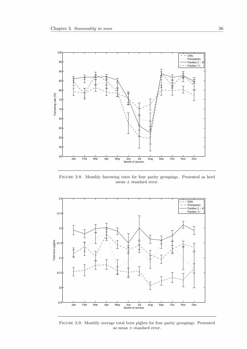
Chapter 3. Seasonality in sows 56
Jan Feb Mar Apr May Jun Jul Aug Sep Oct Nov Dec45
50
55
60
65
70
75
80
85
90
95
100
Month of service
Far
row
ing
rate
(%
)
GiltsPrimiparesParities 2 − 6Parities 7+
Figure 3.8: Monthly farrowing rates for four parity groupings. Presented as herdmean ± standard error.
Jan Feb Mar Apr May Jun Jul Aug Sep Oct Nov Dec9.5
10
10.5
11
11.5
12
12.5
13
Month of service
Tot
al b
orn
pigl
ets
GiltsPrimiparesParities 2 − 6Parities 7+
Figure 3.9: Monthly average total born piglets for four parity groupings. Presentedas mean ± standard error.

Chapter 3. Seasonality in sows 57
The years 2005, 2008 and 2009 had significantly smaller TB than 2004 (P < 0.001),
with between 0.2 and 0.5 fewer piglets.
3.5.3 Day length effects
The effects of both ADL and CDL on TB can be found in Figures 3.10 and 3.11. Overall
lengthening days resulted in litter sizes of up to one piglet per litter larger than shorten-
ing days (P < 0.001). However when broken down into 10 minute increments of change,
significant differences of 0.5 piglets were found when comparing rapidly lengthening days
to rapidly shortening days (Figure 3.10; P < 0.001). When investigating ADL, no clear
trend was observable in the data and only small changes in TB were found (Figure 3.11).
The effect of CDL on FR was very different (Figures 3.12 and 3.13). The data showed
that rapid changes in day length (whether long or short) resulted in better FR and
that periods of time without much change in day length (such as around the solstices)
resulted in FR up to 30% lower (Figure 3.12; P < 0.001). In addition for ADL, days
longer then 15 hours reduced FR by around 10% when compared to shorter days (P <
0.001) and this coincided with when average temperatures were warmer (Figure 3.13).
3.5.4 Temperature effects
Having established that the two week time frame pre-service was crucial for FR, and
on the basis that temperatures for a fortnight post-service are known to affect embryo
survival (Tompkins et al., 1967; Omtvedt et al., 1971), temperature effects on FR and TB
were conducted on the fortnight pre- and post- service. Logistic regression showed that
on the whole, increases in temperature resulted in improved farrowing rates (Table 3.3),
however during the summer months (May to August) increases in temperature resulted
in decreased farrowing rates (Table 3.4).
For most of the year temperatures are relatively cold (< 10 ◦C) and so rises in tempera-
ture result in a more comfortable thermal environment. However in the summer months
temperatures are on average higher and so rises in temperature surpass thermal neu-
trality and may result in sows becoming heat stressed. These effects were mainly found
during the second week pre-service and second week post-service, corresponding to late
lactation and implantation respectively. Temperature effects on FR were moderated by
parity (P < 0.001), with gilts being least affected by any temperature increases and
parity seven and above sows being most affected. In terms of TB, regardless of temper-
ature changes, gilts performed significantly worse than primipares and parity two to six

Chapter 3. Seasonality in sows 58
−120−110−100−90 −80 −70 −60 −50 −40 −30 −20 −10 0 10 20 30 40 50 60 70 80 90 100 11011
11.1
11.2
11.3
11.4
11.5
11.6
Total change in day length (minutes)
Tot
al b
orn
litte
r si
ze
Figure 3.10: Total born litter size for average change in day length for 28 days priorto service date. Data shown as mean ± standard error.
8 9 10 11 12 13 14 15 16 1711
11.1
11.2
11.3
11.4
Day length (hours)
Tot
al b
orn
litte
r si
ze
Figure 3.11: Total born litter size for average absolute day length for 28 days priorto service date. Data shown as mean ± standard error.

Chapter 3. Seasonality in sows 59
−120−110−100−190−80 −70 −60 −50 −40 −30 −20 −10 0 10 20 30 40 50 60 70 80 90 100 11040
45
50
55
60
65
70
75
80
85
90
Total change in day length (minutes)
Far
row
ing
rate
(%
)
Figure 3.12: Farrowing rate for average change in day length for 28 days prior toservice date. Data shown as mean ± standard error.
8 9 10 11 12 13 14 15 16 1760
70
80
90
100
Far
row
ing
rate
(%
)
Day length (hours)8 9 10 11 12 13 14 15 16 17
0
1
2
3
4
5
6
7
8
9
10
11
12
13
14
15
16
17
18
19
20
Ave
rage
tem
pera
ture
(°C
)
Figure 3.13: Farrowing rate for average absolute day length for 28 days prior toservice date. Data shown as mean ± standard error. Average temperatures for those
day lengths are given by the dashed line.

Chapter 3. Seasonality in sows 60
Table3.3:
Coeffi
cents
for
the
fixed
effec
tsof
tem
per
atu
re(a
vera
ge,
min
imu
man
dm
axim
um
;◦ C
)d
uri
ng
the
two
wee
ks
pre
ced
ing
an
dfo
llow
ing
serv
ice
on
farr
owin
gra
tean
dto
tal
born
litt
ersi
ze.
Tem
per
atu
re(◦ C
)T
ime
arou
nd
serv
ice
Far
row
ing
rate
Tot
alb
orn
Est
imat
eS
td.
Err
orP
Val
ue
Est
imat
eS
td.
Err
orP
Val
ue
Ave
rage
2w
eeks
pre
0.01
40.
004
<0.
001
0.01
10.
005
0.03
1w
eek
pre
0.00
60.
005
NS
0.00
10.
006
NS
Day
ofse
rvic
e0.
002
0.00
3NS
0.00
60.
004
NS
1w
eek
pos
t-0
.004
0.00
5NS
0.01
00.
006
0.09
2w
eeks
pos
t0.
015
0.00
4<
0.00
10.
016
0.00
60.
002
Max
imu
m
2w
eeks
pre
0.01
80.
003
<0.
001
0.01
30.
005
0.00
6
1w
eek
pre
0.00
10.
004
NS
0.00
60.
005
NS
Day
ofse
rvic
e-0
.001
0.00
3NS
0.00
40.
004
NS
1w
eek
pos
t0.
002
0.00
4NS
0.00
50.
005
0.03
2w
eeks
pos
t0.
013
0.00
4<
0.00
10.
010
0.00
5NS
Min
imu
m
2w
eeks
pre
0.00
90.
004
0.01
50.
006
0.00
5NS
1w
eek
pre
0.01
10.
004
0.00
30.
001
0.00
5NS
Day
ofse
rvic
e0.
004
0.00
3NS
0.00
50.
003
0.09
1w
eek
pos
t-0
.005
0.00
4NS
0.01
10.
005
0.03
2w
eeks
pos
t0.
004
0.00
30.
002
0.02
20.
005
<0.
001
Mod
els
con
sid
ered
the
effec
tsof
tem
per
atu
red
uri
ng
the
two
wee
kp
erio
dp
re-
an
dp
ost
-se
rvic
e.F
arr
owin
gra
tem
od
els
use
da
bin
om
iald
istr
ibu
tion
and
tota
lb
orn
litt
ersi
zem
od
els
use
da
gau
ssia
nd
istr
ibu
tion
.A
llm
od
els
incl
ud
edh
erd
,p
ari
tyan
dm
onth
as
ran
dom
effec
ts.

Chapter 3. Seasonality in sows 61
Table 3.4: Coefficients for the random effects of month of service on temperature(average, maximum and minimum; ◦C) and changes in farrowing rate and total born
litter size during the two weeks preceding and following service.
MonthFarrowing rate Total born
Average Maximum Minimum Average Maximum Minimum
January 0.357 0.360 0.322 0.244 0.252 0.211
Feburary 0.323 0.303 0.306 0.270 0.259 0.252
March 0.203 0.208 0.199 0.216 0.222 0.218
April 0.086 0.095 0.098 0.256 0.199 0.261
May -0.063 -0.07 -0.038 -0.060 -0.056 -0.045
June -0.381 -0.384 -0.316 -0.216 -0.196 -0.185
July -0.642 -0.642 -0.664 -0.245 -0.231 -0.235
August -0.600 -0.611 -0.607 -0.683 -0.671 -0.680
September 0.046 0.034 0.069 -0.308 -0.301 -0.288
October 0.127 0.119 0.129 -0.133 -0.150 -0.129
November 0.296 0.304 0.283 0.273 0.275 0.259
December 0.248 0.283 0.219 0.386 0.399 0.360
Models considered the effects of temperature during the two week period pre- and post-service. Farrowing rate models used a binomial distribution and total born litter sizemodels used a gaussian distribution. All models included herd, parity and month asrandom effects. Shaded area corresponds to when temperature had a negative effect on
both farrowing rate and litter size.
sows (10.3 piglets; P < 0.001). Parity two to six sows performed the best overall (11.75
piglets; P < 0.001). Increasing temperatures in the second week prior to service and
the second week post-service resulted in improved TB for most of the year (Table 3.3),
although from May to October negative effects were seen (Table 3.4). This was similar
to the pattern found for FR, however the negative effects of increasing temperature on
TB carried on later into the summer and early autumn, with a trend to result in smaller
TB when occuring in the week immediately post-service too.
When daily maximum temperatures reached 18 ◦C in the two weeks prior to service, FR
dropped from 84% to 78.4% (P < 0.001; Figure 3.14). Similarly maximum temperatures
above 18 ◦C during the two weeks post-service reduced FR (P < 0.001). We therefore
suggest that the UCT for outdoor sows in the UK is 18 ◦C in terms of FR. Through
increased standard errors, Figure 3.14 demonstrates that FR became more variable when
maximum temperature surpassed 25 ◦C for the days surrounding service. Graphical
analysis found that the effect of maximum temperatures above 18 ◦C on FR was present

Chapter 3. Seasonality in sows 62
only during the summer months, with winter months never achieving temperatures above
18 ◦C in order to have any effect on FR (data not shown).
When average temperatures were considered, 14 ◦C was found to be the significant value
at which drops in FR were observed (Figure 3.15). When added to the information
that maximum temperatures of 18 ◦C were required, this suggests that large changes in
temperature throughout the day need to be minimal for effects of high temperatures on
FR to occur, in that several hours at temperatures of at least 18 ◦C must be maintained
with presumably night time temperatures remaining above 12 ◦C to provide an average of
14 ◦C over the day. When minimum daily temperatures fell below freezing, significantly
better FR were produced than when minimum temperatures were between 13 ◦C and
18 ◦C (data not shown). Any subsequent increases in minimum temperature above 18 ◦C
produced more variable FR between herds.
Litter size was unaffected by maximum temperature during the two weeks prior to
service, remaining between 11.2 and 11.4 piglets, unless it exceeded 29 ◦C when TB de-
creased to 11 piglets (P < 0.001; Figure 3.16). When considering the effect of maximum
temperature post-service on TB, it was found that temperatures below freezing resulted
in TB of around 10.8 piglets compared to 11.2 piglets in temperatures above freezing
(P < 0.001). Average temperatures above 24 ◦C reduced TB from 11.3 piglets to 10.8
piglets as compared to 14 ◦C pre-service (P < 0.001; Figure 3.17). Therefore 24 ◦C was
defined as the UCT for outdoor sows in relation to TB for the lactating sow. Surprisingly
litter size was not negatively affected by high temperatures post-service when considered
on a temperature basis, however this may be due to a lack of data points available.
The effects of variation in daily temperature on TB and FR can be found in Figures 3.18
and 3.19 respectively. Due to minimal data points available for situations where the
temperature changes were less than 3 ◦C, these results showed a lot of variation for both
reproductive parameters and did not provide a reliable pattern. The same was true for
average daily changes of more than 16 ◦C and in terms of TB no significant changes were
seen in any week prior to service. A trend for larger changes in temperature to reduce
FR can be seen in Figure 3.19.
3.5.5 Other meteorological effects
Gilts were most severely affected by changes in meteorological conditions, and differ-
ences between herds did exist. Both FR and TB reduced with increasing humidity
(Figures 3.20 and 3.21 respectively).

Chapter 3. Seasonality in sows 63
−2 −1 0 1 2 3 4 5 6 7 8 9 10 11 12 13 14 15 16 17 18 19 20 21 22 23 24 25 26 27 28 29 30 31 32 33 3468
70
72
74
76
78
80
82
84
86
88
Temperature (°C)
Far
row
ing
rate
(%
)
Pre−servicePost−service
*
Figure 3.14: Effect of maximum temperature on farrowing rate for the two weekperiod pre- and post-service. Presented as mean ± standard error. * represents first
point at which a significant drop in farrowing rate was found.
−1 −2 0 1 2 3 4 5 6 7 8 9 10 11 12 13 14 15 16 17 18 19 20 21 22 23 24 25 26 2768
70
72
74
76
78
80
82
84
86
Average Temperature (°C)
Far
row
ing
rate
(%
)
Pre−servicePost−service
Figure 3.15: Effect of average temperature on farrowing rate for the two week periodpre- and post-service. Presented as mean ± standard error.

Chapter 3. Seasonality in sows 64
−1 −2 0 1 2 3 4 5 6 7 8 9 10 11 12 13 14 15 16 17 18 19 20 21 22 23 24 25 26 27 28 29 30 31 32 33 3410.6
10.8
11
11.2
11.4
11.6
11.8
12
12.2
Temperature (°C)
Tot
al b
orn
litte
r si
ze
Pre−servicePost−service
Figure 3.16: Effect of maximum temperature on total born litter size for the twoweek period pre- and post- service. Data presented as mean ± standard error.
−1 −2 0 1 2 3 4 5 6 7 8 9 10 11 12 13 14 15 16 17 18 19 20 21 22 23 24 25 2610.6
10.8
11
11.2
11.4
11.6
11.8
Average Temperature (°C)
Tot
al b
orn
pigl
ets
Pre−servicePost−service
Figure 3.17: Effect of average temperature on total born litter size for the two weekperiod pre- and post- service. Data presented as mean ± standard error.

Chapter 3. Seasonality in sows 65
2 4 6 8 10 12 14 16 18 20 225
6
7
8
9
10
11
12
13
14
Average change in daily temperature (°C) over the week
Tot
al b
orn
litte
r si
ze
Week 1 Week 2 Week 3 Week 4 Week 5 Week 6
Figure 3.18: Effect of daily temperature change on total born litter size for six weeksprior to service. Data presented as mean ± standard error.
0 2 4 6 8 10 12 14 16 18 20 220
10
20
30
40
50
60
70
80
90
100
Average change in daily temperature (°C) over the week
Far
row
ing
rate
(%
)
Week 1 Week 2 Week 3 Week 4 Week 5 Week 6
Figure 3.19: Effect of change in daily temperature on farrowing rate for six weeksprior to service. Data presented as mean ± standard error.

Chapter 3. Seasonality in sows 66
10 20 30 40 50 60 70 80 90 10079
80
81
82
83
84
85
86
87
88
Humidity (%)
Far
row
ing
rate
(%
)
Pre−servicePost−service
Figure 3.20: Effect of humidity levels on farrowing rate for the two week period pre-and post- service. Data presented as mean ± standard error.
10 20 30 40 50 60 70 80 90 10011.1
11.2
11.3
11.4
11.5
11.6
11.7
Humidity (%)
Tot
al b
orn
pigl
ets
Pre−servicePost−service
Figure 3.21: Effect of humidity levels on total born litter size for the two week periodpre- and post- service. Data presented as mean ± standard error.

Chapter 3. Seasonality in sows 67
Analyses revealed that FR was significantly reduced when humidity increased in the
week prior to service and on the day of service (Table 3.5). This was especially true
between May and August (Table 3.6). Total born litter size however was only negatively
affected by humidity in the week prior to service and this was particularly true in August
and September (Table 3.6).
The presence of rainfall pre-service resulted in reduced FR (Table 3.5), particularly in
July and August (Table 3.6) and TB was also adversely affected, particularly in August
and September. Although no set pattern for the period around service day could be
found, in general the presence of wind worked to improve both FR and TB, presumably
as a result of moderating perceived temperatures.
When the sow’s UCT had been reached, an increase in humidity did not significantly
affect TB or FR although there was a trend for improved TB in less humid conditions
(Table 3.7). Dry weather resulted in slightly improved FR (+1%) and TB (+ 0.3 piglets)
when the sows UCT had been exceeded (P < 0.001 and P = 0.002 respectively; Ta-
ble 3.7). The presence of wind improved TB by half a piglet when sows’ had reached
their UCT (Table 3.7)
3.5.6 Individual sow effects
Over a quarter of all sows were not affected by seasonal infertility (Table 3.8), suggesting
that some sows have more tolerance to temperature and photoperiodic changes than
others. Unaffected sows had significantly higher FR than sows which were affected in
some form (91.6% vs. 88.4%; P < 0.001).
As can be seen in Figure 3.22, sows which were affected by summer services came from
the same herds as those which were unaffected and so managerial differences between
herds are unlikely. It is often thought that unusual staffing patterns over holiday periods
can result in inconsistent services, however if sows from the same herds can be both
unaffected and severely affected, sow differences rather than staff differences seem more
plausible. The exceptions being herds three, 15 and 23 where very few older sows were
available for the analyses, which may explain the discrepancies.
From Table 3.8 it can be seen that 28% of sows did not suffer from seasonal infertility,
whereas 11% were affected by both returns from summer services and reduced litter
sizes. Born alive litter size was more adversely affected than sow returns, with over half
of the animals experiencing a drop of at least one piglet from summer services. With the
exclusion of 46 sows, the sows had an average NBA of eight piglets and above. Of the
remaining sows, 34 had average NBA of seven, 10 sows had average NBA of 6, one had

Chapter 3. Seasonality in sows 68
Table3.5:
Coeffi
cents
for
the
fixed
effec
tsof
rela
tive
hu
mid
ity,
rain
fall
an
dw
ind
spee
dd
uri
ng
the
two
wee
ks
pre
ced
ing
an
dfo
llow
ing
serv
ice
on
farr
owin
gra
tean
dto
tal
born
litt
ersi
ze.
Var
iab
leT
ime
arou
nd
serv
ice
Far
row
ing
rate
Tot
alb
orn
Est
imat
eS
td.
Err
orP
Val
ue
Est
imat
eStd
.E
rror
PV
alu
e
Hu
mid
ity
(%)
2w
eeks
pre
0.00
40.
014
NS
0.00
30.
018
NS
1w
eek
pre
-0.0
340.
014
0.02
-0.0
500.
017
0.00
5
Day
ofse
rvic
e-0
.024
0.00
80.
005
-0.0
040.
011
NS
1w
eek
pos
t-0
.004
0.01
5NS
0.01
70.
018
NS
2w
eeks
pos
t0.
039
0.01
40.
004
0.01
50.
017
NS
Rain
fall
2w
eeks
pre
-0.0
450.
020
0.03
-0.0
600.
025
<0.
001
1w
eek
pre
-0.0
470.
021
0.02
5-0
.052
0.02
6<
0.00
1
Day
ofse
rvic
e0.
017
0.01
9NS
-0.0
390.
024
<0.
01
1w
eek
pos
t0.
043
0.02
10.
040.
071
0.02
6<
0.00
1
2w
eeks
pos
t0.
014
0.02
0NS
-0.0
180.
025
NS
Win
dsp
eed
2w
eeks
pre
0.27
10.
153
0.08
0.12
40.
184
NS
1w
eek
pre
0.56
70.
119
<0.
001
0.53
20.
176
<0.
001
Day
ofse
rvic
e0.
127
0.03
0<
0.00
10.
125
0.03
8<
0.00
1
1w
eek
pos
t0.
279
0.14
00.
050.
247
0.16
60.
04
2w
eeks
pos
t-0
.048
0.12
7NS
0.04
20.
136
NS
Mod
els
con
sid
ered
the
effec
tsof
met
eoro
logi
cal
con
dit
ion
sd
uri
ng
the
two
wee
kp
erio
dp
re-
an
dp
ost
-se
rvic
e.R
elati
vehu
mid
ity
was
gro
up
edin
to10
equ
algr
oup
sb
etw
een
0an
d10
0%an
dra
infa
llan
dw
ind
spee
dw
ere
con
sid
ered
as
bei
ng
ab
sent
or
pre
sent.
Farr
owin
gra
tem
od
els
use
da
bin
omia
ld
istr
ibu
tion
and
tota
lb
orn
litt
ersi
zem
od
els
use
da
gau
ssia
nd
istr
ibu
tion
.A
llm
od
els
incl
ud
edh
erd
,p
ari
tyan
dm
onth
as
ran
dom
effec
ts.

Chapter 3. Seasonality in sows 69
Table 3.6: Random effects of month of service on relative humidity, rainfall andwindspeed and changes in farrowing rate and total born litter size during the two
weeks preceding and following service
MonthFarrowing rate Total born
Humidity (%) Rainfall Windspeed Humidity (%) Rainfall Windspeed
January 0.143 0.127 0.169 0.028 0.050 0.018
Feburary 0.076 0.063 0.103 0.049 0.066 0.042
March 0.091 0.034 0.083 0.124 0.108 0.057
April 0.058 0.073 0.066 0.157 0.154 0.132
May -0.039 -0.015 -0.013 0.061 0.105 0.048
June -0.114 -0.095 -0.131 -0.019 0.018 0.014
July -0.339 -0.317 -0.413 -0.002 0.019 -0.270
August -0.289 -0.314 -0.359 -0.437 -0.422 -0.416
September 0.021 0.107 0.105 -0.175 -0.167 -0.113
October 0.042 0.094 0.122 -0.127 -0.044 -0.115
November 0.173 0.139 0.161 0.143 0.092 0.133
December 0.176 0.102 0.115 0.196 0.029 0.197
Models considered the effects of meteorological conditions during the two week periodpre- and post- service. Relative humidity was grouped into 10 equal groups between0 and 100% and rainfall and windspeed were considered as being absent or present.Farrowing rate models used a binomial distribution and total born litter size modelsused a gaussian distribution. All models included herd, parity and month as random
effects.
Table 3.7: Effects of meteorological conditions on farrowing rate and total born littersize below and above upper critical temperature thresholds.
Variables Farrowing rate P value Total born piglets P value
Dry vs. Wet 81.2 79.5 < 0.001 11.3 11.0 0.002
Windy vs. Calm 79.6 80.7 NS 11.2 10.7 < 0.001
Humid vs. Arid 78.9 78.7 NS 11.0 11.2 0.09
Upper critical temperature was defined as 18 and 24 ◦C for farrowing rate and totalborn litter size respectively.

Chapter 3. Seasonality in sows 70
1 2 3 4 5 6 7 8 9 10 11 12 13 14 15 16 17 18 19 20 21 22 23 24 25 26 27 28 290
100
200
300
400
500
600
700
800
900
Herd number
Fre
quen
cy
Unaffected
Affected
Figure 3.22: Herd origin and seasonal infertility status of sows.
2004 2005 2006 2007 2008 20090
10
20
30
40
50
60
70
80
90
100
Year of service
% S
ows
NBA and Returns NBA Returns Unaffected
n = 1865 n = 2978 n = 4434 n = 4746 n = 2973 n = 540
Figure 3.23: Stacked histogram representing the proportion of services resulting inseasonal infertility in each year. NBA = Born alive litter size.

Chapter 3. Seasonality in sows 71
Table 3.8: Number of sows which for summer services (June to September) fell intothe categories of: Unaffected by seasonal infertility; Having reduced born alive litter
sizes (NBA) and returning to oestrus; Having reduced NBA; Returning to oestrus
Reproductive effects Number of sows % of total
Unaffected 2082 28
Both 807 11
Reduced NBA 4166 55
Returned 419 6
five and one three. Therefore only a very small percentage of the animals had innately
low litter sizes. There was no significant difference between the NBA of affected and
unaffected sows (11.1 vs. 11.2 piglets respectively; P > 0.05).
Over half of returns occurred in gilts and primipares, however 45% of all the sows were
parity three and above when they returned for the first time. When regarded on a
yearly basis, 50 to 60% of sows served in summer were unaffected by seasonal infertility
(Figure 3.23). This is much higher than the total number of sows which were unaffected
(28%) and is probably due to sow replication over the years since sows were present for
summer services in more than one year. Therefore unaffected sows are replicated across
the dataset. Generally there was the same pattern for fertility every year, with 2009
being the exception, probably due to it being the end of the data set (ended December
2009) and so not many sows were available for analysis, reducing the power of the results.
3.6 Discussion
3.6.1 Photoperiodic effects on reproduction
The present study has shown that seasonal infertility was present in outdoor sow herds
in the South of England for the years 2004 to 2009, with reduced FR throughout the
summer and early autumn. This is in agreement with previous work suggesting that
in the Northern hemisphere, and in temperate climates, sows are affected by seasonal
infertility presumably as a result of changing photoperiod and the associated warmer
temperatures in the summer months (Peters and Pitt, 2003; Auvigne et al., 2010). Many
studies have shown that in the summer months there is a drop in FR, with a recent
French study stating that photoperiod has a prominent role in seasonal infertility and
that heat stress only works to exacerbate the problem (Auvigne et al., 2010). However
studies have not been able to identify the main contributor towards seasonal drops in

Chapter 3. Seasonality in sows 72
sow reproductivity and in terms of photoperiodicity, results are equivocal with no exact
mechanisms being elucidated (Minton et al., 1989; Diekman et al., 1992; Diekman and
Green, 1996; Tast et al., 2001b,c,a; Tummaruk et al., 2004). In addition it is not possible
to control photoperiod on outdoor sow units and without an understanding of what may
drive seasonal fertility in the pig it is difficult to suggest any remedial action to be taken.
Sow parity was shown to moderate the effects of month on FR with gilts being least
affected and sows past their sixth parity affected the most. This is in accordance with
other studies which found that older sows had lower FR than younger animals (Tum-
maruk et al., 2000) and that when fed a high rate of feed during gestation, gilts had
significantly higher FR in summer-autumn months than primipares and multipares (Love
et al., 1995). This may be due to their inherently lower average FR (Tantasuparuk et al.,
2000b), which would benefit the most from additional feeding during gestation.
Although of the same genotype (Landrace × Duroc) differences in both TB and FR
for different sow lines were apparent. Sows which were bred on site (G2) were found to
maintain the highest overall TB but experienced the largest drops in FR over the summer
months. G1 and G3 sows had comparable FR throughout the year and although G3
sows had lower litter sizes as gilts, they had larger litter sizes at later parities. This
highlights the need to consider the source of sows used, as breeders will have different
criteria in their breeding programmes which will affect both sow productivity and the
quality of the piglets produced. This can result in different tolerance to stressors which
may affect fertility, and is supported by previous work where both genotype and sow
line differences in sow reproductivity have been found (Gourdine et al., 2006a; Bloemhof
et al., 2008).
Small effects of month of service on TB were found and so it may be that fertility is in-
fluenced by season, whereas fecundity is not. Similar results have been found previously
(Legault et al., 1975; Gaustad-aas et al., 2004) but the literature presents confound-
ing results on the effect of season on TB with some studies finding effects and others
none. This may be due to the different climates in which the studies were conducted,
with tropical climates exhibiting more profound effects of season on TB than temperate
climates. Hughes (1998) found that season had no effect on litters born in Australia,
whereas a Thai study found seasonal effects that differed between parities and years,
with gilts having the smallest litter sizes (Tummaruk et al., 2004). Studies which have
found litter size effects tend to originate from tropical or hot countries, suggesting that
high temperature plays more of a role in terms of litter size and this shall be discussed

Chapter 3. Seasonality in sows 73
later. Indeed Prunier et al. (1994) concluded that temperature may have a greater in-
fluence on sow and litter performance than photoperiod since different lighting regimes
did not result in statistically different TB.
Unlike other data analysis based research, this study took the opportunity to examine
the effects of actual day length and day length changes prior to service on both FR
and TB. The effects of photoperiod are often described in terms of month or season
of service (Love et al., 1993; Peltoniemi et al., 1999; Auvigne et al., 2010) rather than
actual hours of day light. The current study found that long days resulted in reduced
FR, corresponding to the reproductive cycle of the European wild boar which is a short
day breeder whose reproduction is stimulated by shortening day length in the autumn.
Accordingly, increasing day length in the spring and early summer drives these animals
towards anoestrous (Mauget, 1982). However the present data also implied that FR
were highest when day length was during a rapid state of change, whether increasing or
decreasing. This occurs around the equinoxes during March/April and September/Oc-
tober respectively, suggesting that domestic sows have been able to maintain maximal
fertility for a further two months into Spring, in comparison to their ancestors, and that
indeed it is long days and not lengthening days which result in reduced fertility. Long
days normally coincide with warmer temperatures and longer exposure to these higher
temperatures, therefore could it be that it is temperature which is the causative factor
of seasonal infertility in the domestic sow, rather than photoperiod? Lengthening days
resulted in higher TB, indicating that services after the winter solstice, and in particular
around the spring equinox, were better maintained and that gestation conditions were
more conducive to embryonic survival.
3.6.2 Meteorological effects on reproduction
3.6.2.1 Farrowing rate
The main manifestation of seasonal infertility was found to be reduced FR, which was
affected not only by month of service but also by temperature and parity. Although
increasing temperatures overall improved FR, in the summer months increasing tem-
peratures had a negative effect. This relates to the fact that temperatures are higher
during the summer months and as such surpass the sow’s thermoneutral limits. Far-
rowing rate significantly dropped when maximum daily temperatures reached 18◦C and
above, suggesting that 18◦C is the UCT for outdoor sows in South Eastern England.
This value is lower than the previously accepted UCT for indoor lactating sows of 22
to 25◦C (Quiniou and Noblet, 1999; Black et al., 1993) and implies that sows which

Chapter 3. Seasonality in sows 74
live outdoors may be acclimatised to cooler temperatures than indoor sows which live
in temperature controlled environments. It has been shown that pigs acclimatise to the
cold. Morphologically growing pigs have been shown to increase the amount of hair they
have and reduce the size of their ears when kept at 10◦C as opposed to 35◦C (Dauncey
and Ingram, 1986) and metabolically, heat production has been shown to increase when
kept at between 6 and 12◦C compared to 18 and 30◦C (Derno et al., 1995). Dorsal fat
insulation has also been found to be thicker in pigs kept at 12◦C in comparison to 24◦C
(Derno et al., 1995). This means that the body is adjusted to cope with the cold and
as such is less capable of dealing with subsequent warmer conditions. Similar work with
sows in Spain supports the present study’s finding; the UCT of these sows was found to
be around 19◦C and there were sow line differences present too. Large White sow lines
bred for warmer climates had a higher tolerance to heat stress in comparison with sow
lines bred for temperate climates (Bloemhof et al., 2008).
One mechanism thought to be driving reduced FR in sows is depressed voluntary feed
intake when temperatures rise (Love et al., 1993; Black et al., 1993; Prunier et al.,
1997). A sows appetite will be lower when her UCT has been exceeded as she will work
to reduce metabolic heat production, including digestive processes. This results in her
not being able to meet the metabolic demands of lactation resulting in mobilisation of
body reserves, reduced body condition at weaning and reproductive problems during the
next cycle (Baidoo et al., 1992; Prunier et al., 1997; Clowes et al., 2003; Kongsted and
Hermansen, 2009). This is supported by gilts being found to be least affected by month
of service and temperature. Gilts have not yet experienced a lactation period and as
such their body condition is likely to be acceptable at the time of farrowing if gestational
feeding is maintained. Any lactational losses may therefore not be as severe. In addition,
they have a lower energy requirement than sows as they are smaller, supported by early
work where parity one sows suffered no significant negative effects to varying energy
intakes during lactation, whereas older sows had significantly lighter litters and reduced
body condition (O’Grady et al., 1973, 1975). It should be considered however that other
research has shown multiparous sows to sustain higher lactational losses and yet maintain
reproduction to the same level as primiparous sows (Thaker and Bilkei, 2005). This may
be explained by the study not accounting for backfat losses, and only taking sow weight
as a measurement for lactational losses, which would include both fat and protein losses.
It has been shown that insulin plays a large role in follicular development (Hazeleger
et al., 2005) and so losses in protein mass rather than fat mass may influence this by
affecting insulin levels and thus glucose metabolism and hypothalamic-pituitary-ovarian
function (Booth, 1990).

Chapter 3. Seasonality in sows 75
The presence of rainfall significantly decreased reproductive performance, especially at
warmer temperatures. This is most likely due to increasing humidity when rainfall is due
to occur, which would influence the sow’s cooling abilities. In simple terms humidity can
be defined as the amount of water in the air. Warm air is able to hold more water than
cool air and so when temperatures rise humidity increases, subsequently resulting in rain
when the warmer air is cooled (UK Meteorological Office, 2012). As previously described,
increasing humidity interferes with evaporative heat loss and causes heat stress in sows.
Work on the wild boar in a natural Mediterranean environment has shown the opposite,
where years with increased rainfall resulted in more pregnant females and larger litter
sizes. However this is most likely due to increased food availability when more rain is
present (Fernandez-Llario and Mateos-Quesada, 2005). Under commercial conditions
sows have ample food available to them and so food availability is not an issue. It might
be expected that contact with rain would improve productivity, similarly to wallowing as
it should cool the skin. However sows will generally shelter during rain (Buckner et al.,
1998) and so may not benefit from this. Humidity as a factor was also found to affect FR,
contradicting other work which found that remating was not affected by temperature
and humidity combinations (Suriyasomboon et al., 2006). This does however support
the effects which can be found on litter size in response to high humidities (discussed
later on).
As previously mentioned, much of the work done on seasonal infertility has assessed
indoor sows which are not subject to the same environmental conditions as outdoor
sows. For example solar radiation may work to intensify temperature effects on sows
kept outdoors. This additional heat load will exacerbate the heat stress experienced
and may result in abortion or total foetal resorption rather than partial embryonic
losses, explaining the discrepancies between large effects on FR and small effects on TB.
Unfortunately for the current study it was not possible to measure the effects of solar
radiation, as the data were not available for the areas in which the herds were located.
However, in practice farmers are more likely to know what the temperature is and so
this is potentially of more importance in terms of addressing the problem.
3.6.2.2 Litter size
In line with Bloemhof et al. (2008), the current study found that more than two days
of temperatures reaching 24◦C pre-service were needed for negative effects on TB to
be observed, giving this as the UCT for outdoor lactating sows in terms of TB. Al-
though this is quite warm for the UK climate, it is not as hot as one would expect for
affecting TB, supporting the theory that UK outdoor sows are acclimatised to cooler

Chapter 3. Seasonality in sows 76
temperatures and therefore are affected at lower temperatures than expected. High
temperatures can suppress gonadal functions through a reduction in food consumption
(Kunavongkrit et al., 2005), preventing the stimulatory effect of leptin on progesterone
(and thus the regulation of the growth of ovarian follicles and CL development), which
has been confirmed by in vitro work where the negative effect of high temperatures on
reproductive processes was due to ovarian hormones not being produced properly and
a reduced response of ovarian cells to hormonal stimulators (Sirotkin and Kacaniova,
2010).
In the current study, minimum temperature post service affected TB only during the
summer months. Previous work has shown high post conception temperatures (> 32◦C),
during the first week (Tompkins et al., 1967) and second week (Omtvedt et al., 1971)
post-service, to be critical for embryonic survival. Only in the summer would one expect
UK minimum temperatures to reach high levels, and the lack of post,service effects on
TB may also be due to the small sample size available in the current work for when
average daily temperatures reached 24◦C or above. Hot climates have been shown to
exhibit improvements in TB (10 ± 1.1 vs. 9.1 ± 1.7 piglets) in cooler temperatures (25.2
± 2.2◦C vs. 37.2 ± 3.3◦C; Boma and Bilkei 2006), however the average temperatures
compared were higher than UK average summer temperatures and with such extreme
values embryonic mortality can be expected to be higher.
A trend for high humidity (greater than 80%) to reduce TB when daily temperatures
were above 24◦C suggests that high humidity may only become important when the
animals are already heat stressed, since it reduces their ability to lose heat and hence
adds to the heat load experienced. This was especially true for the week prior to service.
Heat stress relates to those meteorological elements that interfere with heat loss from
the animal to the environment (Bianca, 1976). In tropical conditions with temperatures
in the range of 34 to 37◦C, increasing humidity from 40 to 48% was found to have a
negative impact on reproductive performance in terms of litter size (Tummaruk et al.,
2001a). Work in grower pigs showed that they were susceptible to reduced growth at
lower temperatures when relative humidity increased from 30% to 90% and this was
attributed to a reduction in feed intake (Morrison et al., 1969), as was later confirmed
by Huynh et al. (2005). Most of the work conducted into the effects of humidity on
pig performance has been carried out in tropical countries and little in temperate cli-
mates. The combination of high ambient temperature and high humidity during the
first few weeks post-service is thought to influence TB when average temperatures re-
main high throughout the day (Tummaruk et al., 2010, 2004), however this is seldom
the case in England and even under tropical conditions the effects may not be consistent
(Suriyasomboon et al., 2006).

Chapter 3. Seasonality in sows 77
The presence of wind was generally found to improve TB, especially when sows had
reached their UCT, and so it may be that relief from heat stress during warm conditions
improves reproductive outcomes. In dairy cows wind speed has been found to positively
influence pregnancy rates (Amundson et al., 2006) and research in cattle confirms that
the effects of wind and humidity are important in evaluating the effective temperature
experienced by animals (Mader et al., 2003). Methods for cooling animals have been
trialled on indoor units. For example, it has been found that floor cooling improves the
thermal environment of indoor sows kept at temperatures exceeding 20◦C, leading to
an increase in milk production and greater piglet and litter weight gain during a 21 day
lactating period (Silva et al., 2006). This could be attributed to improved feed intake
in sows, as shown by the provision of snout coolers improving feed intake in sows kept
at temperatures of either 18 or 25◦C (Stansbury et al., 1987). When translating this
back to outdoor farms, this highlights the importance of providing wallows and huts
with ventilation so that sows are able to cool themselves down when subjected to higher
temperatures.
3.6.3 Individual sow susceptibility
Interestingly it was established that not all sows suffered from seasonal infertility. Al-
though it is known that not all herds will suffer from seasonal drops every year, it has
not been shown before that individual sows may be resistant to the problem. The results
showed that regardless of the herd and year, a certain proportion of sows (28%) never
reduced their litter size, nor returned to oestrus after service throughout their repro-
ductive lifetime. In sows which did exhibit a reduction in summer productivity, reduced
NBA was the most prominent problem. This is contrary to herd level data where FR was
the main problem observed, both in terms of photoperiodic and temperature changes.
It is important to note that only sows which had at least six parities were used for the
individual analyses and that the majority of sows with conception problems would have
already been culled by the 6th litter and so would not have been present in the analyses.
Hot temperatures and season have both previously been shown to affect NBA by in-
creasing embryonic mortality (Wildt et al., 1975) and affecting the WOI (Knox and Zas,
2001) which in turn affects successful insemination and fertilisation of ova. Feed intake is
known to be depressed in heat stressed mammals (Hansen, 2009) which leads to reduced
rates of ovulation (Hughes and Varley, 1980). This is likely to be the main contributor
to reduced NBA, since there is little evidence that photoperiod directly influences litter
size. Having smaller litter sizes is manageable as sows are still producing viable piglets.
Some sows however were found to also be affected by returns during summer services.

Chapter 3. Seasonality in sows 78
Returning to oestrus after a summer service is a common sign of seasonal infertility in
the literature and is often associated with photoperiod (Tummaruk et al., 2000; Chokoe
and Siebrits, 2009), as well as high ambient temperatures (Prunier et al., 1996; Almond
and Bilkei, 2005). It increases the number of non-reproductive days for a sow and leads
to deficiencies in piglet numbers for a given period since less sows are available to farrow.
The fact that not all sows suffered from seasonal infertility is an exciting prospect as it
suggests that some sows may be genetically superior than others in terms of susceptibility
to stressors which cause drops in fertility related to either temperature, photoperiod or
both. It is already known that different breeds of animals have different tolerances to
external stressors (Hansen, 2009; Gourdine et al., 2006a) and that sow line differences
within breeds also exist (Bloemhof et al., 2008). Some genes have already been related to
reproduction traits and their phenotypes. For example, the oestrogen receptor has been
significantly associated with litter size (Rothschild et al., 1994; Short et al., 1997) with
allelic effects varying from 1.15 pigs per litter in Meishan synthetics to 0.42 pigs per litter
in Large White lines. In a review by Rothschild (2000) several genes were implicated
in having polymorphisms which may account for improved reproductive performance
in sows. It is possible that a combination of these polymorphisms, or a previously
unidentified allelic change may be responsible for providing some sows with resistance
to seasonal infertility. It may therefore be suggested that future work could look into
this via the use of methodologies such as candidate gene analysis. In particular the
fashionable KISS1R gene may be an ideal candidate for exploration with its recent
connections to seasonality in the literature (Li et al., 2008).
3.7 Conclusions
In conclusion, the results of this study demonstrate the importance of temperature,
photoperiod and service month on the FR of outdoor lactating sows of all parities in the
UK. Temperature was concluded to have more of an influential effect on FR and TB than
photoperiod, although the two are highly correlated with each other during the summer
months. In particular it should be noted that temperature affected outdoor sows at a
lower threshold than previously thought (18◦C) and so the UCT of outdoor lactating
sows needs to be re-examined in the context of a temperate climate. In addition, other
meteorological variables affected the temperature perceived by sows and so their relative
importance needs to be established. On a herd level, litter size was only slightly affected
by month and required temperatures well above the UK summer average (24 vs. 16◦C)
for any negative effects to be observed, although these temperatures were below accepted
values for fecundity problems. With the increasingly sporadic weather found in the

Chapter 3. Seasonality in sows 79
UK, outdoor breeding herd management may therefore benefit from ensuring sows have
good hut ventilation and access to wallows throughout the year and not just during the
summer months. It should also be noted that some sows may be more resistant to the
effects of seasonal changes than others and more research into this is required.

Chapter 4
Simulating seasonal infertility in
outdoor UK sow herds
4.1 Introduction
Although the presence of seasonal infertility has been confirmed in the UK (Chapter 3),
there are no data available in the literature on how it may be predicted. Decision
making in pig farming has become more complicated in recent years, reasons for which
include intensification of production, the increase of competitiveness and the reduction
of marginal profits (Pla et al., 2003). To maintain profitability, the average farmer needs
to estimate animal and economic responses to changing production conditions and for
this reason decision oriented models are increasingly needed. In outdoor production
systems’, attempts to control the negative effects of seasonal infertility need to be better
understood, and by modelling the current state of knowledge it is conceivable that
a useful tool may be created for producers, allowing for a prediction to be made on
seasonal drops in production depending on specified managerial routines.
It has been suggested that there are three types of modelling in livestock farming systems
comprising of simulating according to a set of parameters, finding the economically
optimal solution and an action model to simulate a systems dynamics (Gouttenoire
et al., 2011). However, overlaps between these model types do exist and it is possible to
combine aspects of all three into one model. A simulation study is concerned with the
building of a model for a problem rather than working on the problem itself. It allows
the simulator to assess how a problem will manifest under different conditions and what
the expected outputs could be. Several sow models have been published which focused
on aspects of breeding such as feeding management (Pettigrew et al., 1986; Pomar et al.,
80

Chapter 4. Simulating seasonal infertility 81
1991b), lactation length (Allen and Stewart, 1983), culling and replacement rate (Pomar
et al., 1991b), farmer performance on oestrus detection (Jalvingh et al., 1992; Jorgensen
et al., 1995) and batch farrowing systems (Martel et al., 2008). However seasonal changes
in sow productivity have not been addressed in previous models, even though this is a
vital aspect of pig production in many countries. Modelling a complicated process
such as reproductive efficiency is a complex task that clearly needs to be supported by
reliable and comprehensive data. Using data from different sources, it is possible to
piece together the required evidence for creating such a model with reliable inputs and
expected outputs. It is important to note that models are naturally restricted to the
input parameters used to define them and are simplified versions of real life situations,
and so although they may not cover all aspects of a problem, they do give an idea of
what may be expected to happen.
Table 4.1: Seasonal infertility manifestations in different countries. Table adaptedfrom Penny and Machin (1999)
Country
Longerwean tooestrus
intervals
Reducedfarrowing
rates
Smallerlitter sizes
United Kingdom√ √ √
Ireland X X X
France√ √ √
Denmark√
X X
Spain X√ √
Portugal√ √
X
United States√ √ √
Australia√ √ √
√denotes that an influence was reported, X that it was not reported.
Depending on the country of origin, and whether sows are kept indoors or outdoors,
the various manifestations of seasonal infertility have been differentially identified (Ta-
ble 4.1). Countries such as the UK, France, the United States and Australia have found
that farrowing rates, litter sizes and wean to oestrus intervals are all negatively affected
by season, whereas data from Ireland suggest that seasonal infertility does not exist
there. Other countries may only exhibit one or two manifestations of seasonal infertility
and at differing times of the year (Hurtgen and Leman, 1980; Peltoniemi et al., 1999;
Halli et al., 2008; Auvigne et al., 2010). Hence, the model produced in this thesis will

Chapter 4. Simulating seasonal infertility 82
only apply to the UK or similar production systems as the parameters set within the
model are specific to UK production and meteorological conditions.
4.2 Objectives
The final outcome of this work will be a simulation model which can be used to predict
production losses during the year, as well as adaptation to modifications in herd man-
agement or changes in sow biological parameters. This will be based on data produced
in Chapter 3 as well as detailed literature searches. Several specifications for the model
were formulated:
1. It should give an account of the effect of modifications to the parity structure on
the reproductive output and productivity of sows
2. It should give an account of the effect of culling strategies on the reproductive
output and productivity of sows
3. It should account for months which experience extreme weather conditions (heat
waves and below freezing temperatures)
4.3 General scope
Built in Python 2.7, the model simulates the reproductive performance of a herd of
sows, within a three week batch farrowing system under outdoor conditions. The model
covers varying performance throughout the year, accounting for seasonal differences in
sow reproductive output. Code for the model can be found in Appendix A. The time
step of the model is the day and individual sow is the modelling unit. Sow reproductive
performance is viewed as a sequence of events (heat detection, insemination, farrowing,
weaning; summarised in Figure 4.1) and the basic steps involved in the model are listed
below.
The representation of sow biology needs to take into account the random nature of the
biological processes, which is why each sow is individually represented in the model with
biological characteristics that are randomly estimated according to distribution curves.
Different parameters within the simulation are mutable, allowing for different scenarios
to be taken into account, such as herd parity structure and batch size.
1. Animal creation

Chapter 4. Simulating seasonal infertility 83
(a) Pool of animals to last whole of simulation time are created.
(b) Batches created from this animal pool.
(c) Probability of a heat wave or cold snap is calculated and productivity param-
eters are changed accordingly (or kept at default).
2. Heat detection
(a) Gilts assumed to be sexually mature, hormonally synchronised and on heat.
(b) Sows are given a probability of coming on heat.
(c) If on heat they continue on, if not they return to the sow pool.
(d) More than 2 no heats results in culling.
3. Insemination
(a) Depending on parity and month, a probability for farrowing is given.
(b) If due to farrow they gestate, if not they return to the sow pool.
(c) More than 2 no farrows results in culling.
(d) A probability for abortion is given, if a sow aborts she is culled.
4. Farrowing
(a) Depending on month and parity distributions, a litter size is given.
(b) Lactation length is given a set distribution.
(c) Pre-weaning losses are calculated based on month of the year.
5. Weaning
(a) Number of piglets weaned is recorded.
(b) Sow parity increases by 1 .
(c) Sows over a set parity (6 for example) are culled.
(d) Sows with two previously low litter sizes at birth are culled.
(e) Other sows return to the sow pool.
(f) Depending on month and parity distributions, a WOI is given.
6. Outputs
(a) For each batch farrowing rate is calculated.
(b) For each batch average weaned litter size is calculated.
(c) For each batch the number of culled animals is calculated.
(d) For each batch total empty days is calculated.

Chapter 4. Simulating seasonal infertility 84
Inseminated
Gestation
Farrowing
Weaning
Cull
Returns Sow batch
Farrowing rate Litter size
Sow pool
No. piglets weaned Wean to oestrus interval
Sows culled Parity at weaning
n = 40/45/50 Weather conditions
n = infinity
N(116,2)
N
Parity distribution
Max parity at wean
Returns
Pre-wean mortality
Returns Abortions
Parity
Figure 4.1: Overview of simulation model and dynamics of animal movement. Textin red represents recorded variables. Text in blue represents parameters which can be
set within model.

Chapter 4. Simulating seasonal infertility 85
4.4 The Data
The model was created using the data produced in Chapter 3 along with other empirical
data from studies conducted in European countries or temperate climates (Table 4.2).
Table 4.2: Sources of data used to assign values to parameters utilised in the model
Parameter Source(s)
Farrowing rate Chapter 3
Number born alive Chapter 3
Abortion rate Wrathall (1987); Stork (1979)
Wean to oestrus interval Chapter 3
Pre-weaning mortality Chapter 3
Lactation length Chapter 3
Gestation length Chapter 3
Oestrus probability Knox and Zas (2001)
Temperature stress effects Auvigne et al. (2010)
Due to the lack of outdoor sow studies available, data from indoor studies have also
been used. Seasonal effects on the attainment of puberty (Paterson et al., 1991) have
not been modelled since it has been shown that through correct boar contact and feeding
regimens seasonal effects on the attainment of puberty in gilts can be removed (Paterson
et al., 1989b). Sources of data used can be found in Table 4.2 and default data values
are presented in Table 4.3. Heat and cold stress were modelled by adjusting parameter
values to coincide with previous research showing that under hotter conditions FR can
decrease by at least 5% (Auvigne et al., 2010), litter size by one piglet (Bloemhof et al.,
2008) and WOI can be extended by at least two days (Prunier et al., 1994). When
temperatures drop, piglet mortality has been shown to increase by at least 3% (personal
communication; BQP Ltd, 2012).
4.5 Model creation
4.5.1 Decision rules
The study aims to evaluate the effect of month of the year on sow reproductive perfor-
mance and see how altered parity structures and batch sizes may influence the results
produced. The number of sows per batch at farrowing depends on the number of sows
inseminated per batch and the conception, abortion and culling rates prior to farrowing

Chapter 4. Simulating seasonal infertility 86
Table 4.3: Default biological parameters used in the model.
Month Parity FR (%) NBA AR (%) WOI (days)Mortality
(%)
Jan
0 79.18±10.92 10.19±0.83
0.4±0.07
8.28±0.39
11.26±0.641 85.72±7.70 10.78±0.69 7.33±0.30
2-6 86.13±4.84 11.45±0.68 7.08±0.30
7+ 84.24±10.31 10.69±0.80 7.50±0.33
Feb
0 78.51±13.27 10.13±1.02
0.3±0.23
9.39±0.59
11.53±0.621 85.38±7.58 10.96±0.85 7.89±0.51
2-6 86.94±6.09 11.29±0.73 7.01±0.38
7+ 78.18±15.46 10.71±1.07 6.97±0.41
Mar
0 81.29±10.00 10.28±0.68
0.3±0.25
8.15±0.44
10.76±0.531 84.01±7.39 10.65±0.75 7.06±0.26
2-6 86.95±5.96 11.38±0.75 6.76±0.21
7+ 88.21±7.64 10.80±0.68 6.09±0.21
Apr
0 78.99 ±9.90 10.30±0.87
0.5±0.18
7.96±0.51
10.01±0.701 83.43±11.83 11.37±0.95 6.65±0.21
2-6 87.29±5.75 11.42±0.77 6.67±0.24
7+ 84.93±11.79 10.74±0.78 6.93±0.38
May
0 78.29±9.08 10.15±0.63
1.1±0.79
7.81±0.40
9.81±0.631 82.32±8.21 11.07±0.65 8.01±0.93
2-6 85.35±4.73 11.37±0.63 7.05±0.24
7+ 79.14±11.73 10.05±1.14 7.04±0.37
Jun
0 75.75±12.89 10.12±0.74
1.3±0.49
7.81±0.24
10.77±0.841 75.79±17.99 10.89±0.74 8.09±0.84
2-6 75.41±16.72 11.05±1.58 7.50±0.51
7+ 62.53±29.55 10.24±2.59 6.48±0.51
Jul
0 70.18±16.90 10.11±0.85
2.6±1.11
7.81±0.24
11.09±0.731 64.62±30.71 11.02±0.79 6.79±0.25
2-6 61.04±29.08 11.58±2.22 7.25±0.33
7+ 55.48±32.47 10.43±0.56 7.65±0.45
Aug
0 72.44±15.96 9.60±0.73
1.2±0.83
8.03±0.40
11.30±0.731 63.60±24.05 10.71±0.85 6.73±0.28
2-6 57.56±32.89 11.08±0.80 6.68±0.30
7+ 54.39±35.11 10.21±1.02 8.27±1.19
Sep
0 80.05±14.21 9.79±0.84
1.0±0.49
8.67±0.57
10.21±0.711 83.68±11.55 10.56±0.80 7.47±0.29
2-6 88.69±5.32 11.05±0.76 6.68±0.30
7+ 89.05±11.00 10.78±0.52 7.32±0.45
Oct
0 79.82±13.18 9.90±1.04
1.3±1.06
8.23±0.30
10.52±0.661 83.48±9.94 10.80±0.66 7.23±0.34
2-6 86.79±6.81 11.12±0.99 7.23±0.26
7+ 82.56±8.16 10.63±1.19 7.17±0.45
Nov
0 80.38±9.80 9.87±1.18
0.4±0.21
8.37±0.51
12.15±0.961 85.69±6.51 10.99±0.64 7.17±0.33
2-6 87.84±5.37 11.54±0.51 6.38±0.26
7+ 88.10±9.83 10.23± 2.09 6.42±0.36
Dec
0 77.33±14.72 10.30±0.89
0.3±0.14
9.16±0.98
11.27±0.641 85.60±5.92 10.98±0.74 7.01±0.30
2-6 84.62±5.40 11.45±0.72 7.31±0.33
7+ 82.37±11.03 9.91±3.02 7.02±0.29
Data presented as mean ± standard deviation. Month of service used for farrowing rate (FR),born alive piglets (NBA) and abortion rate (AR). Month of weaning used for Wean to Oestrus
Interval (WOI) and pre-weaning mortality.

Chapter 4. Simulating seasonal infertility 87
in the batch. The number of sows inseminated is dependent on the number of sows
tested for oestrus behaviour and on the oestrus detection rate. Sows tested for oestrus
behaviour are those weaned the week before oestrus detection, the replacement gilts and
sows from the previous batch which failed to show heat. It is assumed in the model that
the number of gilts included in a batch always fits the need to meet the target number
of sows at service. This assumption implies that the gilt pool is unlimited which differs
from the reality on farm. This choice was made for simplification and also because the
decision rules concerning the management of replacement gilts are not well known. Tac-
tical decision rules included in the model concern the rules for the culling of sows at each
step of the reproductive cycle. The rules for culling sows at weaning are based on parity
number and sow productivity. By default the maximum number of allowed parities is
varied between six and eight. The productivity thresholds relate to a minimum born
alive litter size of seven piglets. At oestrus detection, sows found to be not on heat twice
in a row are culled. After insemination a farrowing probability is set, which if it results
in a non-pregnancy twice in a row, the sow is culled. In addition, if the sow aborts she
is culled.
The model was run using combinations of the rules defined below (summary in Table 4.4).
• Herd either starts off with only gilts (’start up herd’) or with a defined parity
structure (Gamma (2.47, 1.14); ’established herd’)
• Batch size is either 40, 45 or 50 sows
• Sows are permitted either one or two returns before culling
• The maximum parity before culling is set to either six or eight
• Lactation length is set to either 21 or 28 days
Other parameters which were kept constant amongst all models were:
• Number of batches run (120)
• Gestation length (Normal (115.73, 2.09))
• The probability of oestrus was 0.95

Chapter 4. Simulating seasonal infertility 88
Table 4.4: Experiments conducted using the simulation model.
Experiment Herd type Max. parity No. returns Lactation length Batch size
1
Established
6
1 21 40
2 1 21 45
3 1 21 50
4 1 28 40
5 1 28 45
6 1 28 50
7 2 21 40
8 2 21 45
9 2 21 50
10 2 28 40
11 2 28 45
12 2 28 50
13
8
1 21 40
14 1 21 45
15 1 21 50
16 1 28 40
17 1 28 45
18 1 28 50
19 2 21 40
20 2 21 45
21 2 21 50
22 2 28 40
23 2 28 45
24 2 28 50
25
Start
up
6
1 21 40
26 1 21 45
27 1 21 50
28 1 28 40
29 1 28 45
30 1 28 50
31 2 21 40
32 2 21 45
33 2 21 50
34 2 28 40
35 2 28 45
36 2 28 50
37
8
1 21 40
38 1 21 45
39 1 21 50
40 1 28 40
41 1 28 45
42 1 28 50
43 2 21 40
44 2 21 45
45 2 21 50
46 2 28 40
47 2 28 45
48 2 28 50
Default productivity values used during above experiments so that (no cold snap orheat wave occurring)

Chapter 4. Simulating seasonal infertility 89
4.5.2 Outputs and analyses
The model provides information on sow productivity and time of events. Productivity
data concern the performance of individual sows (NBA; number of empty sow days; fer-
tility) and farrowing batches (number of sows at service, farrowing and weaning; culling
rate; and fertility). Data were imported into MATLAB R© 7.11.0 (R2010b) (MATLAB,
2010) for analysis and graphical presentation.
Normally distributed outputs (litter size and mean batch parity) and those which could
be transformed to follow a normal distribution (log number of empty days, square root
number of culls and square number of sows which farrowed) were analysed by N-way
ANOVA, looking at two way interactions between batch size, number of returns, lacta-
tion length, maximum parity and herd set up (established or start up). Farrowing rate
and average parity at culling were non-normally distributed and no transformation was
able to bring them to normality. Therefore these were analysed using the Kruskal-Wallis
test looking at the effects of each independent parameter (batch size, number of returns,
lactation length, maximum parity and herd set up (established or start up)) separately.
The data collected were as follows:
• Month in which batch was served and farrowed
• Which weather conditions the batch experienced (default, heat wave, cold snap)
• Number of piglets born alive per sow
• Number of sows which farrowed
• Number of sows culled
• Number of empty days
4.5.3 Calibration of the number and length of simulations
Number and length of sow herd simulations
Before being able to use the model to compare various parity structures, it was necessary
to determine the minimal length of simulation for reaching the steady state when an
established herd structure was utilised. In addition the number of replications needed
to estimate the variability of the results needed to be established. For this the approach
consisted of analysing the data obtained from 20 replications of simulation over 120

Chapter 4. Simulating seasonal infertility 90
batches (4800 services). The results were analysed according to the following list, using
Welch’s method (Welch, 1983) to establish steady state values.
• The number of sows per batch at farrowing, standing for the ability of the simulator
to maintain a constant number of sows in the herd.
• The mean parity of sows at weaning and culling, which are indicators of herd
demography.
• The number of culled sows per cycle, as indicators of sow longevity.
The average, minimum and maximum numbers of farrowing sows per batch over 20
replications are shown in Figure 4.2. The mean number of sows farrowing per batch (34.1
± 3.1) is close to the objective of 40 inseminated sows fixed in the model, considering the
seasonal variations present. The maximum number of sows never exceeded 40, which is
in agreement with the culling rules and the minimum number of sows never fell under 19.
This validates the capacity of the simulator to maintain the number of sows farrowing
per batch over a long period of time.
The minimum, maximum and mean numbers of culled sows per batch over 20 replications
are shown in Figure 4.3. Since the culling rules do not oblige some sows to be culled at
each cycle, the minimum number of sows culled could be zero. In the same way there
was no upper limit to the number of sows culled which explains why some batches had
a high culling rate during one cycle. The mean number of sows culled per batch was
approximately six.
Mean, minimum and maximum batch averages for parity are presented in Figure 4.4.
Parity followed a fifty batch cycle, increasing and decreasing as gilt populations increased
and decreased. This corresponds with an aging herd and the strict culling rules of no
sows surpassing a set parity. Sows were culled at all parities. The maximum parity at
culling was in some cases above the number set in the model due to the initial herd
distribution used.
In order to determine the number of replications needed to estimate the variability
of parameters of interest, the mean and standard deviation of the average value of
these parameters at steady state according to the number of replications performed
was visually assessed (Martel et al., 2008). Two examples of this are illustrated in
Figures 4.5 and 4.6. Both illustrate the evolution of mean and standard deviation of
the appropriate parameter and indicate that the values are relatively stable from the
beginning. Therefore five runs of the model were selected as they should be sufficient

Chapter 4. Simulating seasonal infertility 91
0 20 40 60 80 100 12015
20
25
30
35
40
45
Batch
Num
ber
of s
ows
MeanMinimumMaximum
Figure 4.2: Minimum, mean and maximum number of farrowing sows per batch over20 simulations in an established herd.
0 20 40 60 80 100 120
0
5
10
15
20
25
Batch
No.
sow
s cu
lled
MeanMinimumMaximum
Figure 4.3: Minimum, mean and maximum number of culled sows per batch over 20simulations in an established herd.

Chapter 4. Simulating seasonal infertility 92
0 20 40 60 80 100 1201
2
3
4
5
6
7
8
Batch
Ave
rage
par
ity a
t far
row
ing
MeanMinimumMaximum
Figure 4.4: Minimum, mean and maximum of the mean parity of sows at farrowingfor each batch over 20 simulations in an established herd.
0 2 4 6 8 10 12 14 16 18 2029
30
31
32
33
34
35
36
37
38
Number of replications
Num
ber
of fa
rrow
ings
per
bat
ch
Figure 4.5: Average and standard deviation of the number of farrowing sows for oneto 20 replications.

Chapter 4. Simulating seasonal infertility 93
0 2 4 6 8 10 12 14 16 18 203.4
3.6
3.8
4
4.2
4.4
4.6
4.8
5
5.2
5.4
Number of replications
Ave
rage
par
ity p
er b
atch
Figure 4.6: Average and standard deviation of sow parity for one to 20 replications.
for presenting results with any less not providing enough replication and any more not
adding value to the data.
Overall, using both graphical outputs and Welch’s method, it was found that for all
parameters to reach stability in established herds, 40 batches were needed in the warm up
period. Thus, in the experimental simulations the value of sow and herd productivity at
steady state for established herds were estimated after allowing for 40 warm up batches,
corresponding to data from 16,000 services. All other simulations corresponded to 24,000
services as the whole data set was utilised.
4.6 Results
4.6.1 Farrowing
It was found that lactation length and the number of returns allowed influenced far-
rowing rate the most (Figure 4.7). Experiments allowing for two returns resulted in
improved farrowing rates as compared to one return (P< 0.001). Experiments with

Chapter 4. Simulating seasonal infertility 94
longer lactation lengths also experienced increased farrowing rates (P< 0.001). A maxi-
mum parity of six improved farrowing rates (P< 0.001). Farrowing rates were higher in
start up herds (P< 0.001) and batch size did not have a significant effect (P = 0.157).
The results directly corresponded with the number of farrowings (Figure 4.8), although
as expected batch size had a significant effect on the number which farrowed (P< 0.001).
Larger batches (50 sows) meant that more sows were potentially available to farrow and
as such more farrowed than in smaller (40 sows) batches.
4.6.2 Litter size
Established herds had significantly larger litter sizes (P< 0.001) than start up herds
(Figure 4.9), especially when sows were only allowed one return (P< 0.001). A maximum
of parity six also resulted in larger litters (P< 0.001) and this was significantly improved
with only one return (P = 0.003) and shorter lactation lengths (P = 0.001). Batch size
did not affect litter size.
4.6.3 Parity
Average herd parity was higher (P< 0.001) in established herds (Figure 4.10) and when
a maximum parity of eight was set (P< 0.001). Longer lactations (P< 0.001) and two
returns (P< 0.001) also resulted in an increase in the parity profile of the herd. Batch
size had no significant effect on mean herd parity.
4.6.4 Empty days
The number of empty days in a herd increased in start up herds (P< 0.001) and with the
number of returns sows were permitted (P< 0.001; Figure 4.11). An older parity profile
(P< 0.001) and longer lactation (P< 0.001) also resulted in more empty days, although
batch size did not affect this (P = 0.331). An interaction between the number of returns
and lactation length meant that longer lactation lengths with two returns resulted in
almost four extra empty days (P< 0.001), regardless of maximum parity allowed.
4.6.5 Culling
More sows were culled in established herds (P< 0.001) and if the maximum parity
allowed was set to six (P< 0.001; Figure 4.12). In addition reducing the number of
returns (P< 0.001) and the lactation length (P< 0.001) increased the number of culls

Chapter 4. Simulating seasonal infertility 95
2 4 6 8 10 12 14 16 18 20 22 24 26 28 30 32 34 36 38 40 42 44 46 4865
70
75
80
85
90
95
Experiment
Far
row
ing
rate
(%
)
Established herd Start up herdMax Parity 8Max Parity 6 Max Parity 6 Max Parity 8
Figure 4.7: Mean (± standard errors) farrowing rate for each experiment. Solid redsquares highlight most productive situations and red circles highlight least productive
situations.
2 4 6 8 10 12 14 16 18 20 22 24 26 28 30 32 34 36 38 40 42 44 46 4824
26
28
30
32
34
36
38
40
42
44
Experiment
No.
sow
s fa
rrow
ed
Established herd Start up herdMax Parity 8Max Parity 6 Max Parity 6 Max Parity 8
Figure 4.8: Mean (± standard errors) number of sows farrowing for each experiment.Solid red squares highlight most productive situations, dashed red squares the second
most productive situations and red circles highlight the least productive situations.

Chapter 4. Simulating seasonal infertility 96
2 4 6 8 10 12 14 16 18 20 22 24 26 28 30 32 34 36 38 40 42 44 46 489.2
9.4
9.6
9.8
10
10.2
10.4
10.6
10.8
11
11.2
Experiment
Litte
r si
ze
Established herd Start up herdMax Parity 8Max Parity 6 Max Parity 6 Max Parity 8
Figure 4.9: Mean (± standard errors) born alive litter size for each experiment.Solid red squares highlight most productive situations and red circles highlight least
productive situations.
2 4 6 8 10 12 14 16 18 20 22 24 26 28 30 32 34 36 38 40 42 44 46 481.5
2
2.5
3
3.5
4
4.5
Experiment
Par
ity
Established herd Start up herdMax Parity 8Max Parity 6 Max Parity 6 Max Parity 8
Figure 4.10: Mean (± standard errors) herd parity for each experiment. Solid redsquares highlight highest parities and red circles highlight lowest parities.
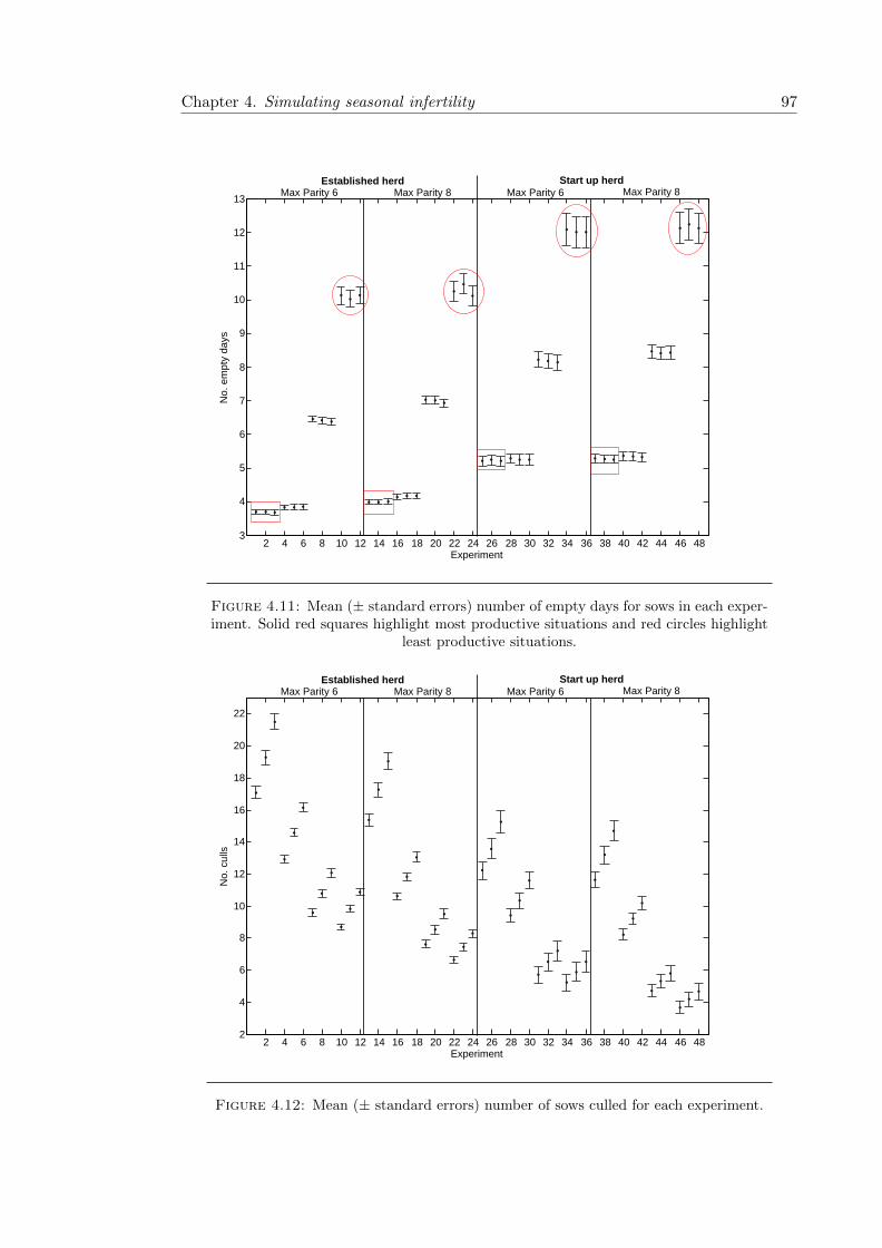
Chapter 4. Simulating seasonal infertility 97
2 4 6 8 10 12 14 16 18 20 22 24 26 28 30 32 34 36 38 40 42 44 46 483
4
5
6
7
8
9
10
11
12
13
Experiment
No.
em
pty
days
Established herd Start up herdMax Parity 8Max Parity 6 Max Parity 6 Max Parity 8
Figure 4.11: Mean (± standard errors) number of empty days for sows in each exper-iment. Solid red squares highlight most productive situations and red circles highlight
least productive situations.
2 4 6 8 10 12 14 16 18 20 22 24 26 28 30 32 34 36 38 40 42 44 46 482
4
6
8
10
12
14
16
18
20
22
Experiment
No.
cul
ls
Established herd Start up herdMax Parity 8Max Parity 6 Max Parity 6 Max Parity 8
Figure 4.12: Mean (± standard errors) number of sows culled for each experiment.

Chapter 4. Simulating seasonal infertility 98
2 4 6 8 10 12 14 16 18 20 22 24 26 28 30 32 34 36 38 40 42 44 46 481
2
3
4
5
6
7
8
Experiment
Par
ity a
t cul
ling
Established herd Start up herdMax Parity 8Max Parity 6 Max Parity 6 Max Parity 8
Figure 4.13: Mean (± standard errors) parity at culling for each experiment. Solidred squares highlight highest parities and red circles highlight lowest parities.
which took place. Larger batches increased the number of sows culled (P< 0.001),
although this was slightly moderated by maximum parity allowance (P = 0.04). Parity
at culling (Figure 4.13) followed a similar pattern to mean herd parity, being higher in
established herds (P< 0.001) and when a maximum parity of eight was set (P< 0.001).
4.6.6 Changing weather conditions
In order to assess if the model could correctly account for extreme weather conditions,
three replicates for each of default, heat wave and cold snap values were run. The model
was set to an established herd parity structure, therefore only after the first 40 batches
were readings accounted for. Results were assessed in relation to mean sow parity at
farrowing, mean number of culls and the mean number of sows which farrowed per
batch. All of these were found to be approximately normally distributed using quantile
quantile plots. Using ANOVA testing it was found that the number of culled sows did
not significantly differ under different conditions (Figure 4.14A) but the parity profile
of farrowing sows was significantly lower during periods of heat stress as compared to
default and cold snap conditions (P < 0.001; Figure 4.14C).

Chapter 4. Simulating seasonal infertility 99
010
2030
4050
6070
802468101214161820
Bat
ch
No. culled
010
2030
4050
6070
8022242628303234363840
Bat
ch
No. farrowed
010
2030
4050
6070
802
2.53
3.54
4.55
Bat
ch
Mean parity
D
efau
lt va
lues
Hea
t Wav
eC
old
Sna
p
B
C
A
Figure4.14:
Com
par
ison
ofd
iffer
ent
def
ault
wea
ther
valu
esp
rovid
edto
mod
elfo
rA
)C
ull
edso
ws;
B)
Sow
farr
owin
gs
an
dC
)A
vera
ge
pari
tyof
sow
sat
wea
nin
g.
Sta
rtin
gm
onth
was
alw
ays
Janu
ary
.

Chapter 4. Simulating seasonal infertility 100
In addition less sows farrowed during batches experiencing a heat wave as compared to
months with a cold snap (P = 0.0016; Figure 4.14B). This suggests that the model was
able to correctly adjust its productivity in response to changing conditions. Therefore
in future runs of the model it would be acceptable to allow the model to assign a heat
wave or cold snap to a particular batch. Due to time constraints models including these
changes were not run.
4.6.7 Model validation
Model verification was first performed by checking for both mathematical and logical
consistencies. Subsequently, using data from five herds in Chapter 3, results produced
from the simulation model were validated. Since the model was built from average data
across 29 herds, using specific herd data meant that the data were different to those
used to define model input parameters of the model. The five herds with the most data
points available (between 9,170 and 13,199 records) were selected, for which productivity
data can be found in Table 4.5. For each herd, average reproductive parameters were
calculated in three week batches, and the simulation run alongside used the herd specific
lactation length and beginning during the same month of the year. The model was set
to only retrieve default weather conditions.
Table 4.5: Sow productivity data for test herds
Herd 1 Herd 2 Herd 3 Herd 4 Herd 5
Farrowing rate (%) 84.0 79.7 82.6 90.9 70.5
Lactation length 26.2 24.5 26.2 25.2 26.3
Mean parity 3.0 3.3 2.8 3.2 3.5
NBA per litter 10.3 10.9 11.0 10.7 10.8
Piglets weaned 9.4 9.5 9.9 10.2 9.4
Parity of sows at culling 3.7 3.8 3.2 4.8 4.4
WCI 8.9 10.2 7.5 7.4 15.7∗ NBA: Number born alive; WCI: Wean to Conception Interval.
The χ2 goodness of fit test was carried out using the crosstab function (MATLAB, 2010)
to provide an objective measure of the goodness of fit between observed and simulated
data. This test allows to compare the distribution of the observed and simulated pop-
ulations. Large values of χ2 indicate that the null hypothesis is rather unlikely and
that there likely is a significant difference. The significance gives a quantitative measure

Chapter 4. Simulating seasonal infertility 101
0 10 20 30 40 50 60 70 80 90 100−5
0
5
10
15
20
25
Batch
Tem
pera
ture
(°C
)
Herds 3 and 5Herds 1, 2 and 4
Figure 4.15: Average temperatures in each batch for herds used to validate simulationmodel.
of the model goodness of fit. Values below 0.05 indicate that discrepancies between
observed and simulated data population are likely.
The herds were from two different locations (Norfolk and Suffolk) and as such any
temperature comparisons have been conducted using area specific temperatures for each
batch (Figure 4.15). Figures 4.16 to 4.20 show comparisons between the batch data
for the herds and the results from simulation models run using herd specific lactation
lengths.
Herd 1
The model was poorly representative of herd 1 (Figure 4.16). None of the parameters
closely matched the output from the simulation model. The percentage culled was ex-
tremely variable, with large over- and under-estimations throughout (χ2 = 865.308, P
= 0.049), suggesting that there is a difference between the model and herd data. Simi-
larly farrowing rate exhibited great underestimations. Litter size was underestimated by
nearly two piglets in some batches. Predicted empty days closely followed the herd data

Chapter 4. Simulating seasonal infertility 102
most of the time, although between batches 45 and 55 they were vastly underestimated.
Average herd parity was the only parameter which matched the herd data quite well,
although it did fail towards the end. All parameters had high χ2 values, suggesting the
model did not closely mirror herd data, even if the results were not significant.
Herd 2
The model represented herd 2 better than herd 1 (Figure 4.17). Predicted percent-
age culled followed herd data generally well and in the correct direction (χ2 = 1227.5),
however over and underestimations did occur, suggesting that the distributions were dif-
ferent (P < 0.001). Predicted and herd farrowing rates were similar in pattern, although
the magnitude of change was often overshot. Around batch 30, the temperatures the
herd would have experienced were relatively high, explaining the lower farrowing rate
observed and as such the discrepancy between herd and model data. Litter size was
underestimated throughout and did not bear any resemblance to the herd data. Pre-
dicted empty days failed to match the herd data and average herd parity was poorly
represented by the model. This was supported by high χ2 values.
Herd 3
The only predicted parameter to bear any resemblance to herd 3 data was farrowing
rate (Figure 4.18) which did produce results in the right ’direction’ as compared to the
herd data. Again, litter size was vastly under-estimated and percentage culled, empty
days and average parity were not at all comparable. None of the results produced χ2
values which suggested that the model data closely matched the herd data.
Herd 4
The model was not able to confidently predict the outcomes for herd 4 (Figure 4.19).
Farrowing rates (χ2 = 2952.0, P = 0.073) were unusually high for herd 4, potentially
due to small batches being served.
Herd 5
Similarly to herd 4, the model was a poor predictor for herd 5 (Figure 4.20), with gross
underestimations of empty days and litter size. Farrowing rate was overestimated in
the earlier batches, although from batch 50 onwards the values corresponded quite well.

Chapter 4. Simulating seasonal infertility 103
020
4060
020406080100
% Culled
Bat
ch0
2040
605060708090100
Farrowing rate (%)
Bat
ch0
2040
60789101112
Bat
ch
Number of piglets
020
4060
0510152025
Bat
ch
Empty days
020
4060
0123456
Bat
ch
Average parity
H
erd
Mod
el
AC
DE
B
Figure4.16:
Her
d1
dat
aver
sus
aver
age
offi
veru
ns
of
sim
ula
tion
mod
elfo
rA
)%
Cu
lled
(χ2
=865.3
08,P
=0.0
49);
B)
Farr
owin
gra
te(%
;χ2
=23
71.5
,NS
));
C)
Ave
rage
nu
mb
erp
igle
tsb
orn
alive
(χ2
=3720.0
,NS
);D
)A
vera
ge
nu
mb
erof
emp
tyd
ays
(χ2
=2915.0
,NS
);E
)A
vera
ge
par
ity
atfa
rrow
ing
(χ2
=3162.0
,NS
).L
act
ati
on
len
gth
set
to26.2
day
sfo
rm
od
elru
ns.

Chapter 4. Simulating seasonal infertility 104
050
100
01020304050607080
% Culled
Bat
ch0
5010
06065707580859095100
Farrowing rate (%)
Bat
ch0
5010
078910111213141516
Bat
ch
Number of piglets
050
100
051015202530354045
Bat
ch
Empty days
050
100
12345
Bat
ch
Average parity
H
erd
Mod
el
DE
AB
C
Figure4.17:
Her
d2
dat
ave
rsu
sav
erag
eof
five
run
sof
sim
ula
tion
mod
elfo
rA
)%
Cu
lled
(χ2
=1227.5
,P<
0.0
01);
B)
Farr
owin
gra
te(%
;χ2
=49
03.6
,NS
);C
)A
vera
genu
mb
erp
igle
tsb
orn
ali
ve
(χ2
=8740.0
,NS
);D
)A
vera
ge
nu
mb
erof
emp
tyd
ays
(χ2
=9506.0
,NS
);E
)A
vera
ge
par
ity
atfa
rrow
ing
(χ2
=7399.0
,NS
).L
act
ati
on
len
gth
set
to24.5
day
sfo
rm
od
elru
ns.

Chapter 4. Simulating seasonal infertility 105
050
100
01020304050607080
% Culled
Bat
ch0
5010
06065707580859095100
Farrowing rate (%)
Bat
ch0
5010
0678910111213
Bat
ch
Number of piglets
050
100
051015202530
Bat
ch
Empty days
050
100
12345
Bat
ch
Average parity
H
erd
Mod
el
AB
C
DE
Figure4.18:
Her
d3
dat
aver
sus
aver
age
of
five
run
sof
sim
ula
tion
mod
elfo
rA
)%
Cu
lled
(χ2
=702.2
.0,NS
);B
)F
arr
owin
gra
te(%
;χ2
=42
67.0
,NS
);C
)A
vera
genu
mb
erp
igle
tsb
orn
aliv
e(χ
2=
8835.0
,NS
);D
)A
vera
ge
nu
mb
erof
emp
tyd
ays
(χ2
=7826.0
,NS
);E
)A
vera
ge
pari
tyat
farr
owin
g(χ
2=
7372.0
,NS
).L
act
ati
on
len
gth
set
to26.2
day
sfo
rm
od
elru
ns.

Chapter 4. Simulating seasonal infertility 106
050
100
020406080100
% Culled
Bat
ch0
5010
065707580859095100
Farrowing rate (%)
Bat
ch0
5010
0789101112
Bat
ch
Number of piglets
050
100
024681012
Bat
ch
Empty days
050
100
0.51
1.52
2.53
3.54
4.55
Bat
ch
Average parity
H
erd
Mod
el
AC
DE
B
Figure4.19:
Her
d4
dat
aver
sus
aver
age
offi
ve
run
sof
sim
ula
tion
mod
elfo
rA
)%
Cu
lled
(χ2
=819.0
,NS
);B
)F
arr
owin
gra
te(%
;χ2
=2952.0
,P
=0.
073)
;C
)A
vera
genu
mb
erp
igle
tsb
orn
aliv
e(χ
2=
8835.0
,NS
);D
)A
vera
ge
nu
mb
erof
emp
tyd
ays
(χ2
=8633.0
,NS
);E
)A
vera
ge
pari
tyat
farr
owin
g(χ
2=
7469.0
,NS
).L
act
ati
on
len
gth
set
to25.2
day
sfo
rm
od
elru
ns.

Chapter 4. Simulating seasonal infertility 107
020
4060
80010203040506070
% Culled
Bat
ch0
2040
6080
5060708090100
Farrowing rate (%)
Bat
ch0
2040
6080
678910111213
Bat
ch
Number of piglets
020
4060
800510152025303540
Bat
ch
Empty days
020
4060
800123456
Bat
ch
Average parity
H
erd
Mod
el
AC
DE
B
Figure
4.20:
Her
d5
dat
ave
rsu
sav
erag
eof
five
run
sof
sim
ula
tion
mod
elfo
rA
)%
Cu
lled
(χ2
=680.8
,NS
);B
)F
arr
owin
gra
te(%
;χ2
=30
20.4
,NS
);C
)A
vera
genu
mb
erp
igle
tsb
orn
aliv
e(χ
2=
4692.0
,NS
);D
)A
vera
ge
nu
mb
erof
emp
tyd
ays
(χ2
=4422,NS
);E
)A
vera
ge
pari
tyat
farr
owin
g(χ
2=
3996
.0,P
=0.0
028).
Lact
ati
on
len
gth
set
to26.3
day
sfo
rm
od
elru
ns.

Chapter 4. Simulating seasonal infertility 108
The average parity in the model was found to be significantly different in distribution
to the herd (χ2 = 3996.0, P = 0.0028).
Overall performance
Visually, it is clear that in all cases the model was unable to match the herd data precisely
and as such the model is not very well validated. In addition it has been suggested that
χ2 analysis is a much more powerful method of finding differences that may exist between
simulated and observed herd distribution data than visual analysis alone (Pla, 2001).
In this study the χ2 values were high, however they were non-significant. This suggests
that although real differences are likely, because of the variability present they were not
always observed to be significant.
From visual assessment it can be said that in some cases the model was a good predictor
of farrowing rate and empty days, and for the majority of herds average parity was well
represented up until about batch 50. Litter size however was always underestimated and
the percentage culled was extremely variable. This shows how varied different farms can
be in their productivity and how hard it is to model data against them. However, should
the model allow for more farm specific inputs to be included (e.g. gestation length and
culling decisions), it may be able to better match what is happening on farms.
4.7 Discussion
The work contained within this chapter has produced a framework on which to build
a model for the prediction of seasonal infertility in outdoor sow herds. Although not
fully validated, the model demonstrates that it is possible to use real farm data to begin
to predict outcomes. Before discussing the shortcomings of the model in its current
state, it is important to highlight what the model discovered to be significant in terms
of differing managerial decisions.
4.7.1 Sow herd management and seasonality
The manner in which a herd is managed is key to producing the best profits possible. The
model showed that four week lactation lengths, as opposed to three weeks, resulted in
improved farrowing rates and therefore potentially higher profits. This supports previous
data which found that in terms of gross profit, a linear increase in profits could be seen
between lactation lengths of 21 and 35 days, although in terms of sow productivity,

Chapter 4. Simulating seasonal infertility 109
21 days provided the better results (Varley, 1989). In the UK, the law states that 28
day weaning should be practiced (Defra Publications, 2003). Nonetheless the lactation
period is often reduced to 21 days (or even less) for sows in a batch that have farrowed
late. This is normally practiced to provide better health management, with an ”all in
all out” system on indoor farms. Outdoor farms do not have the same health risks as
indoor farms since individual paddocks can be treated separately, but batch management
of a field may be complicated by having varied weanings within a batch. In order to
obtain more consistent 28 day lactation periods, better oestrus detection needs to be
conducted as this would result in less variability in farrowings. It has been suggested
that on some farms, up to 20% of sows served by AI are not in standing heat (Young
et al., 2010). If these sows are then inseminated by a catcher boar they will invariably
have different farrowing dates to those successfully served by AI. Hormonal treatments
(e.g. Regumate R©) can also result in more synchronised oestrous cycles (Hazeleger et al.,
2001) by regulating the follicular phase and as such producing closer farrowings.
In addition, allowing for two returns resulted in improved farrowing rates, as compared
to one return. This is unusual as it suggests that if a sow returns, the probablility of
her becoming pregnant is higher during the next cycle. This was not a set parameter
within the model and in real life terms sows which return are thought to be less fertile
(Tummaruk et al., 2001b; Takai and Koketsu, 2008; Vargas et al., 2009) and as such
the chances of conceiving should decrease with the number of returns. In terms of
the simulation model, a second return would have meant that the sow would have been
present in a different batch which may have had seasonally improved chances of farrowing
(such as going from a batch in March to one in April), improving overall perceived herd
productivity. Therefore the model would have benefited from adding in a different
conception probability for one or two returns, something which shall be discussed later
on.
Longer lactation periods and two returns resulted in an increase in the parity profile
of the herd. By having longer lactation lengths, and as such improved farrowing rates,
the perceived productivity of the sows is higher and so they are less likely to be culled.
This results in sows being kept for longer and hence the average herd parity increases.
The data did suggest however that overall productivity was highest if culling strategies
meant that sows did not surpass six parities. Although sows should be allowed two
returns, once they reach parity six this is no longer efficient. As sows age they peak
in their fertility, normally by parity six (Stalder, 2008), and so strict culling strategies
for older sows mean that farms can be as efficient as possible. This is supported by the
fact that farrowing rates were highest when a parity six cap was in place as were litter
sizes, although interestingly these were significantly improved with only one return and

Chapter 4. Simulating seasonal infertility 110
a shorter lactation length. Both of these parameters would result in gilts increasing their
parities more quickly. As such the improvements in litter size for sows aged between
parities two and six would have been more pronounced.
An older parity profile and longer lactation lengths resulted in more empty sow days.
As previously mentioned, older sows (past parity six) tend to have reduced fertility,
including longer WOI (Tummaruk et al., 2000) and potentially more returns. Sows
which returned more than once had additional empty days, as expected. However the
interaction found with longer lactation lengths, resulting in an additional four empty
days on average, does not fit in with the literature (Le Cozler et al., 1997). Longer
lactation lengths would be expected to reduce the chances of a sow returning to oestrus
unless the sow experienced lactational oestrus. The observed result may relate to the
length of time a sow is kept for. A longer lactation length results in a sow being kept
at a certain parity for an additional week. Combined with the fact that her conception
month may also change in that time, it is possible that she changes to a less productive
parity in a less productive month. This additive effect may therefore result in reduced
overall productivity for the simulation run.
Batch management is not frequently studied within simulation models in the literature,
the exceptions being Singh (1986) and Martel et al. (2008). Only recently has batch
farrowing become more popular within the UK, providing a better routine for farm
management to follow in terms of disease control. As such it is important that, like
the current model, future models account for batch farrowing within their design as
this will be most representative of the state of affairs on farms. Batch size increased
piglet volumes at weaning, since it had significant effects on the number of sows which
farrowed. However it was not shown to have any significant effect on other production
parameters assessed, except for the number of sows culled since through inference if more
sows are served in a batch there are more available to cull. This was slightly moderated
by allowing a maximum culling parity of eight rather than six, again since if sows are
routinely allowed to reach an older age they are less likely to be culled. As a result it
could be said that farmers should always try and produce to their maximum capacity
in order to make as much profit as possible.
The only advantage of a start up herd over an established one was producing better
farrowing rates. This may be due to easier management of groups of sows with similar
parities, due to less variability between sows in a batch. Established herds outperformed
the start up herds in every other way. For example older sows had significantly larger
litter sizes, probably due to their innately larger litter sizes as compared to gilts (Koketsu
and Dial, 1998), with a plateau being reached between parities three and six (Tummaruk

Chapter 4. Simulating seasonal infertility 111
et al., 2000). The number of empty days in a herd increased in start up herds and with
the number of returns sows were permitted. Gilts have longer WOI (Tummaruk et al.,
2000) and if permitted a second return, the additional time would be longer than for
older animals. This increases their empty days but does mean that replacement costs
may be reduced.
4.7.2 Model performance
From looking at the literature it is clear that this is the first time that seasonal changes
in sow productivity have been included in a model using a simulation approach. In
addition it is one of few models which utilise real farm data to create the model, with
the exceptions being Pla et al. (2003); Martel et al. (2008); Rodrıguez-Sanchez et al.
(2012).
The model was able to simulate a sow herd throughout the year, maintaining a reason-
able number of farrowings and a realistic number of cullings per batch. This is consistent
with the decision rules and parameters incorporated into the model. Simulation models
work by using random parameters characterised by a specific distribution and not a con-
stant value. Biological production parameters are quite similar within most models in
the literature and include conception rate, number of piglets born alive per litter, mor-
tality rates at different stages, gestation length, weaning to oestrus interval and oestrus
cycle length. The way these parameters are taken into account and valued depends on
the model structure, design and objective. For example, Singh (1986) considered em-
pirical distributions of sow farms to generate values for litter size, mortality rates and
WOI, but also random distributions for other parameters e.g. gestation and oestrous
cycle length. In agreement with the distributions used within the present model, other
models generally used normal univariate distributions for random generation of input
parameters when continuous variables were represented, although several authors used
other distributions to represent WOI (e.g. log-normal by Pettigrew et al. (1986)).
The current model utilised a simplified framework for creating the outputs. In general
there are different parameters which can be used to assess the performance of a pig herd.
For example sow parameters include prolificity, which is a summation of piglets born
alive, piglets born dead and the number which survive to weaning. The current model
used piglets born alive and those which survive to weaning. In addition the duration
of a sows cycle is important, accounting for gestational and lactational periods as well
as non-productive or empty days, which amount to the WCI and any return days. The
current model calculated all of these. The demographics of a herd in terms of parity
structure can also be important as this will in turn affect individual sow performance,

Chapter 4. Simulating seasonal infertility 112
again something which the current model looked at. It would therefore seem that the
majority of parameters assessed were of relevance when comparing them to the sow
modelling literature, however some omissions were made which shall be described in the
future work section of this discussion.
Random number generators are often used to create observations for individual animals,
such as production, survival and conception. As a result of using a random number
generator, multiple runs are needed to obtain a reliable estimate of the average results
of the herd. When the number of replications is not large enough, outputs may not be
as reliable. The present model had a moderate number of runs (5) over long simulation
cycles (120 batches). This may have accounted for some of the discrepancies observed
between the model and herd data during the validation process. Singh (1986) ran their
model for ten consecutive years, taking a sample per year and used the Student t-
distribution to test the average income and to obtain the 95% confidence interval of
the yearly average income. Pettigrew et al. (1986) replicated each alternative scenario
three times and compared them by ANOVA in a completely random design. Both these
models produced less replications than the present study, and as such this suggests that
the amount of data produced herein should have been sufficient to obtain relatively
reliable results.
Not all reviewed models in the literature are validated. For example, optimisation
models are often presented as deterministic models dealing with well defined problems.
Optimisation models are mainly interested in showing mathematical methodologies to
solve specific problems. Instead of a formal validation, some authors determine the
effect of changing conditions in some major parameters, just to gain insight into the
model behaviour (Dijkhuizen et al., 1986; Huirne et al., 1991). Alternatively, several
validation methods have been used in simulation models, although it is generally agreed
that it is difficult to achieve full validation because not all parameters are known in
practice and suitable data for validation are not always available. An alternative used
by several authors is to describe precisely the model without any other test to validate
it (Singh, 1986). In some cases, the common strategy is to perform a verification based
on a detailed description of the model and checking for the correct running of the model
at several points in the life-cycle, including the final summation of inputs and outputs.
This was done in the current model as an initial test and compares well to work done
by previous authors. For verification Allen and Stewart (1983) used two statistics, num-
ber of sows and gilts in the system and time in phase. For partial validation, Pomar
et al. (1991b) evaluated different outputs, while Allen and Stewart (1983) compared pig
weaning weights with those published in the literature. Jalvingh et al. (1992) and Pla
et al. (1998) presented a model behaviour study based on sensitivity analysis, afterwards

Chapter 4. Simulating seasonal infertility 113
they compared general results with results obtained from management information sys-
tems. No statistical evaluation was presented in previous papers, other than by Pla
et al. (1998) who considered the sow herd distribution over states calculated by the
model and the actual distribution observed. They found, as did we, that even with the
statistical χ2 test, it is not easy to assert the suitability of the model for one specific
farm. Exogenous variables such as health problems and feed differences may affect herd
dynamics and make it difficult to explain differences that may appear between actual
farm data and simulation results. Incorrect data from farms may also be responsible
for the disagreement between simulated and collected data, however by including farm
specific inputs these problems may be overcome. It is also important to note that a good
model with appropriate farm data may also give different population distributions.
The model was also able to adjust in response to variations in the weather. Lower far-
rowing rates were observed during heat waves as compared to cold snaps and the parity
profile lowered under the same conditions. Few models account for seasonal changes
in productivity, the exception being Rodrıguez-Sanchez et al. (2012) whose input pa-
rameters were based on expected seasonal changes in conception rate and mortality.
They did not however investigate how sudden extreme weather and changes in man-
agement would influence overall herd productivity. The present model was able to
add in the random effect of the presence of a heat wave or cold snap, both scenarios
which would result in reduced productivity at some level. Long term weather events
are often predicted in advance, therefore farmers would be aware if, for example, an
especially cold winter is expected or not. Long range forecasts (three months) can be
found at www.metoffice.gov.uk/publicsector/contingency-planners for both temperature
and rainfall. Although these sorts of forecasts are still in development they can provide
an insight into what may be expected in the coming months. Therefore by including
an option for predicted conditions during gestation or at farrowing within the model,
adjustments to the outputs can be made.
4.7.3 Future modelling improvements and applications
Whilst this model provides an adequate framework for simulating a sow herd with sea-
sonal changes, there are several drawbacks to it in its current form. For example only
sow effects have been considered, without the input of seasonal differences in boar semen
quality. If both were to be combined, the compounding effects of reductions in boar fer-
tility alongside reductions in sow fertility may be brought to light. In addition only one
management system (batch) has been considered. Had data from alternative farming
systems been available, this too could have been incorporated into the model. Although

Chapter 4. Simulating seasonal infertility 114
a regular occurrence in the modelling literature, a simplified management structure was
created. The model does not account for fosterings, age of gilts at first insemination
and detailed culling reasons. The inclusion of these types of parameters would better
account for replacement gilt costs for example, as well as feeding costs. Culling rules
were simplified within the current model, with no discrepancy between cullings due to
illness, age, stock numbers or fertility being made. The number of returns a sow had,
her parity and whether she aborted or had consistently low litter sizes were the reasons
provided for culling. Allen and Stewart (1983) also considered culling based on parity
limit, while other authors were more explicative detailing infertility and more culling
reasons such as lameness and disease (Singh, 1986; Pettigrew et al., 1986; Pomar et al.,
1991c). In addition, when a sow returned the probability of her conceiving from the
subsequent insemination was not altered. Had this been incorporated into the model a
more accurate picture of the effects of increased returns of productivity could have been
assessed. Adjustments for different lactation lengths of productivity would have also
improved the accuracy of the model. However due to the limited available time to work
on the model, this was not possible. Overall there are several parameters which could
be added to the model in order to produce a more accurate representation of an outdoor
sow herd throughout the year. Had more time been available, a financial aspect could
have been added to the model. By calculating the cost of the pigs weaned in relation
to seasonal price changes and other farm expenses, the profitablilty of the different sit-
uations assessed could have been discovered. This was outside the scope of the present
work but could be a useful addition to any future development of the model.
The current work used the programming language Python to create the model. This was
due to the relative ease of learning how to write the language, as well as the flexibility of
the language to perform what was needed (e.g. batch simulations with individual out-
puts). This worked effectively to produce the model and allows for the easy application
of this model on different platforms, and for free. If this were to be developed into a pro-
gramme which farmers could use, they would be able to download it onto any device that
they may have. A product for detecting oestrus in cows has been developed in Ireland
and is currently available even on mobile technology (Dairymaster UK Limited, 2012).
Most sow models in the literature are intended for research or educational purposes and
few express their aim to be used on-farm (Dijkhuizen et al., 1986; Jalvingh et al., 1992;
Pla et al., 1998). This may explain why general user interfaces (GUI) are not well elabo-
rated for farmers or advisers. A GUI for the present model could have been created had
the model been better validated and more time been available. This would have a had a
menu bar able to accept user defined input and commands and would have meant that
individual farm data could have been used to define the parameters within the model,
Chapter 4. Simulating seasonal infertility 115
providing a more accurate prediction for the farm in question. The types of parameters
which would have been involved, include average pre-wean mortality, seasonal changes
in the price of pigs, average lactation length, average gestation length and any other
parameter which is farm specific. Outputs would have then been generated specific to
the inputs provided. The use on-farm of such a model is related to its integration in
existing information systems as modules. The model interface is very important for a
practical use and in acceptance by farmers or decision-makers. In the UK, the Agrosoft
Ltd Winpig programme is used by many farmers to store information on their breeding
sows. The integration of the data recorded within this database into a model, such as an
improved version of the one created here, would be key to rolling out a GUI. This would
mean that the model could be expanded to account for different genotypes, service data
and any other parameter which may have a seasonal influence on sows.
4.8 Conclusions
The simulation model in its current form is not an adequate predictor of seasonal infer-
tility in the UK, however it does provide a good framework on which to build. Different
herds will differ in their productivity and as such increased specificity needs to be incor-
porated into any model which is to be used as a predictor for future outcomes. However,
it is important to note that in general terms, some management routines can help im-
prove productivity, including longer lactation lengths and a strict parity related culling
policy.

Chapter 5
An investigation into the factors
that may influence seasonal
changes in commercial boar
semen quality
5.1 Introduction
It is important to recognise that 50% of any reproductive output comes from the male.
Seasonal infertility is most often associated with the sow even though seasonal changes
in boar semen quality have been studied extensively, with results implicating both tem-
perature fluctuations and photoperiodic changes in reduced semen quality (McNitt and
First, 1970; Wettemann et al., 1979; Sancho et al., 2004). The quality of semen is af-
fected in the form of reduced ejaculate volumes; reduced concentrations of spermatozoa
in the semen; increased percentages of morphological abnormalities in the ejaculates; re-
duced sperm motility and reduced total spermatozoa output per ejaculate. Modern pig
production relies on AI, which to some extent eliminates the effects of seasonal changes
in boar semen however problems are still evident. A reduction in the effects of seasonal
changes is achieved through the quality control of ejaculates at the stud before dissemi-
nation to units. This involves discarding ejaculates from poorly producing boars and/or
pooling semen from several boars to meet the required standards. These measures re-
quire increased numbers of boars to be available for collection during periods of seasonal
infertility and so understanding which parameters alter semen quality, and at which time
of the year, would allow for improved managerial processes in the boar stud. As well
116

Chapter 5. Seasonality in boars 117
as temperature and photoperiod, humidity is thought to affect semen quality (Suriya-
somboon et al., 2004; Kunavongkrit et al., 2005) and large differences between breeds
have been found to exist (Swierstra, 1968; Sonderman and Luebbe, 2008). Therefore
depending on the stock required and the conditions in which boars are housed, optimal
management can be difficult to maintain.
In the UK, day length changes are large across the year with the longest day lasting over
16 hours, and the shortest around eight hours. Boars are kept indoors and although
artificial lighting is used when it is dark (extending perceived day length in winter),
boars are exposed to long day light hours in the summer through windows in their
accommodation. It is therefore conceivable that photoperiod plays a role in affecting
their semen quality since they will be subject to decreasing day length during late
summer and early autumn. For example it has been shown that even under constant
temperature and humidity, boars experienced decreased semen quality during periods
of decreasing photoperiod (Sancho et al., 2004). In equatorial countries day length
changes are negligible and so the effects of temperature and humidity are thought to
be more important. One study showed that a 21 day moving average of temperature
and humidity had a significant effect on the ejaculate volume of Duroc boars, and that
humidity affected total sperm production, with both of these traits decreasing when
temperatures exceeded 27 ◦C and humidity exceeded 40% (Suriyasomboon et al., 2004).
In the UK ambient temperatures rarely reach such high values, however changes in boar
reproductive output are still apparent during the summer and autumn months. For this
reason photoperiod may be thought of as the main driving force behind altered semen
quality parameters, although there is the possibility that UK breeds are more sensitive
to temperature changes, or that the few hot days we do experience in the UK cause
lasting damage to our boars.
Most studies investigating the effects of temperature and season on semen quality either
use small sample sizes in experiments with traditional statistics (Swierstra, 1970; Wet-
temann et al., 1979; Cameron and Blackshaw, 1980; Andersson et al., 1998; Kozdrowski
and Dubiel, 2004; Sancho et al., 2004; Okere et al., 2005; Murase et al., 2007; Frydrychova
et al., 2007) or linear models in large scale data analyses (Ciereszko et al., 2000; Corcuera
et al., 2002b; Wysokiska et al., 2009; Smital, 2009; Wolf and Smital, 2009). These have
some explanatory power of the data studied but do not necessarily allow for predictions
to be made which would be applicable across other data. Data mining using ML algo-
rithms is an emerging technique in the animal science literature (Chedad et al., 2001;
Kirchner et al., 2004a,b; Fernandez et al., 2006; Craninx et al., 2008; Texeira et al., 2008;
Chamsaz et al., 2009; Kamphuis et al., 2010b,a). It allows for patterns within data to be
identified without limiting data parameters, such as a known distribution, and the use of

Chapter 5. Seasonality in boars 118
these patterns to predict the outcome for future events. By using ML on semen quality
and meteorological data there is the potential to identify weather patterns throughout
the year and individual boar parameters which may influence semen quality. The model
created can then be used to predict under which conditions decreased semen quality can
be expected and thus lead to recommendations on how to alter stud management in
order to overcome any anticipated negative effects.
Quality parameters such as semen volume, sperm concentration and total sperm num-
bers can often be easily compensated for through pooling of ejaculates and the dilution
process. However increases in the percentage of abnormalities in an ejaculate or poor
sperm motility will result in a full ejaculate being discarded. Several morphological
abnormalities of spermatozoa exist, ranging from head and tail abnormalities to the
presence of cytoplasmic droplets, however there is little data in the literature regarding
specific abnormality type changes with month of the year. Different abnormalities are
known to affect sperm differently (e.g. motility or ability to fertilise the ova) and so
it would be prudent to investigate whether all abnormalities change with season and
whether breeders should prioritise their quality checks on specific abnormalities. By
assessing which abnormalities change under various conditions, it may be possible to
identify what causes the increased numbers found since different environmental stres-
sors will result in different morphological changes throughout the various stages of the
spermatogenesis process.
5.2 Objectives and hypotheses
Objectives
This work aimed to use decision tree analyses in order to establish the meteorological
conditions under which semen quality parameters were altered in terms of semen volume,
sperm concentration, total sperm numbers and total percentage abnormalities present.
In addition specific morphological abnormality type and sperm motility changes were
assessed for differences by month of collection, breed and age of boar and collection
interval.

Chapter 5. Seasonality in boars 119
Hypotheses
It was hypothesised that high temperatures and shortening day lengths would result in
an overall decrease in sperm quality parameters, especially in terms of increased abnor-
mality type. It was also hypothesised that all semen quality traits would be influenced
by breed, age of boar and collection interval. It was thought that decision trees would be
able to detect patterns within the data to highlight relationships between meteorological
conditions and sperm quality parameters.
5.3 The Data
5.3.1 Stud data
The study was based on data from three JSR Genetics Ltd boar studs in the UK (Fig-
ure 5.1). Stud management was similar across all sites and years, with boars housed in
buildings containing little environmental control and the boars were worked on average
once a week. Housing consisted of insulated barns with windows to provide natural day
light and ventilation when required. Semen was collected by the gloved hand method,
assessed for quality and diluted within 15 minutes of collection by trained technicians.
Cell counts were carried out after suspension in sodium citrate and ejaculates with more
than 30% total abnormalities, low motility, low sperm counts or high agglutination
scores were recorded and discarded. The data set contained individual boar and semen
quality parameters including age of boar, breed of boar, date of collection, interval since
previous collection, semen volume (SV; ml); sperm concentration (SC; × 106/ml); total
sperm numbers (TSN; × 109/ejaculate); percentage of abnormalities in semen (AB; %)
and motility (MOT; ranging from 0 for aspermic to 5 for very good). The dataset was
analysed for incorrect and missing values prior to use. The complete dataset contained
50,493 instances from 1,043 boars, over five years from 2005 to 2009. In order to prepare
the data for general analysis, scatter graphs and histograms were used to detect any
outliers, for which records were deleted or corrected if error was obvious (e.g. incorrect
decimal place). Age of boar was provided in days and so was converted to the nearest
year for analysis with anything older than five years grouped together. The data were
for different breeds: White Duroc × Pietrain, Sireline Large White, Duroc, Hampshire,
White Pietrain, Large White damline, Landrace damline and White Pietrain × Large
White. Collection interval was calculated from the data for each boar by subtracting
the date of one collection from the previous one. Average individual boar production for

Chapter 5. Seasonality in boars 120
each semen quality parameter (SV, SC, TSN) was calculated and the difference between
every ejaculate and the boar’s average recorded.
5.3.2 Meteorological data
Having established the locations of the AI centres, detailed weather data were obtained
from the BADC from neighbouring sites for the relevant years (2005 to 2009; Figure 5.1).
The weather associated with the six weeks previous to each ejaculation was collected.
This period of time was chosen as it has been shown that boar semen quality is not af-
fected immediately after heat stress and that it takes at least two weeks for the damage
to be seen and up to six weeks for semen quality to return to normal (McNitt and First,
1970; Christenson, 1973; Cameron and Blackshaw, 1980). Data included minimum, max-
imum and average daily temperatures ( ◦C), daily rainfall (mm), daily humidity (%),
daily wind speed (mph) and wind direction. Weather variables were rounded to the near-
est integer. day length data were obtained for the AI centres (Figure 3.1) for each day
in the relevant years from http://www.timeanddate.com/worldclock/astronomy.html.
Data were converted into seconds. The number of hot days (above 27 ◦C; Suriyasom-
boon et al. 2004) and the number of days with daily temperature changes exceeding
10 ◦C for the given time period were counted.
5.4 Methods
5.4.1 Statistical analyses
All statistical analyses were carried out in MATLAB R© 7.11.0 (R2010b) (MATLAB,
2010). Semen volume, SC, TSN and AB were analysed in relation to month of collection,
breed of boar, age of boar and collection interval, using N -way ANOVA with interactions
to see if there were any significant differences. Changes in motility were assessed by
month of collection, breed, age and collection interval using the χ2 test of independence
and results interpreted by means of cross tabulation frequencies. Ejaculate usage was
analysed in relation to month of collection and the percentage of different abnormality
types. Abnormality types were analysed by N -way ANOVA to determine effects of
month of collection, age of boar, breed of boar and collection interval.

Chapter 5. Seasonality in boars 121
")
#*
#*
#*
a
a
a
LINCOLNSHIRE
NORTH LINCOLNSHIRE
KINGSTON UPON HULLNORTH YORKSHIRE
0 7.5 153.75 Miles ±Reproduced with permission from Edina spatial data(c) Crown Copyright
Legenda Studs#* Weather Stations") Day Length Site
Figure 5.1: Map of locations of studs in relation to where weather and day lengthdata were collated from

Chapter 5. Seasonality in boars 122
Table 5.1: Learning features used during the various decision tree experiments con-ducted on the sperm quality data
Ref No. Learning Feature Units Key
1 Month of collection 1 to 12 Month
2 Year of collection 2004 to 2009 Year
3 Age of boar at collection Years age
4 Location of boar stud 1,2 or 3 Location
5 Breed of boar 1 to 8 breed
6Average temperature for n weeks prior to
collection◦C mx/mn/av (n)
7Average humidity for n weeks prior to
collection% h (n)
8Average wind speed for n weeks prior to
collectionmph w (n)
9 Average rainfall for n weeks prior to collection mm r (n)
10Average change in day length for n weeks prior
to collectionSeconds DL
11Average day length for n weeks prior to
collectionMinutes DC
12 Collection interval Days int
n weeks ranged from one to six. Temperature included daily maximal, minimal oraverage values.
5.4.2 Decision trees
5.4.2.1 Learning features
Data for decision tree experiments were prepared and analysed in MATLAB (2010)
using the classregtree function. Initially decision trees were inducted to discover patterns
relating to semen ejaculate use by the boar stud. The outcome parameter was either
ejaculate used (1) or discarded (0), with the learning features presented to the decision
tree presented in Table 5.1 along with the additional features of AB, SC, SV and TSN.
The classification parameters were defined as AB less than (1) or greater than (0) 20% or
30%, individual boar SV less than (0) or greater than (1) boar average, individual boar
SC less than (0) or greater than (1) boar average and individual boar TSN less than (0)
or greater than (1) boar average. The AB level was chosen as, although ejaculates with
more than 30% abnormalities are normally rejected, average values for AB were under
20% and so both these levels were explored.

Chapter 5. Seasonality in boars 123
5.4.2.2 Learning algorithm
The decision tree classification method belongs to ML and has been extensively tested
in different disciplines. The C&RT algorithm of MATLAB (2010) was used. This is a
supervised learning strategy of ML, based on the algorithms found in Breiman et al.
(1984), where detailed explanations of the decision tree rules and implementation can
be found. It creates a decision tree consisting of a root node representing the feature
which mostly influences the classification, and subsequent internal nodes containing the
other attributes. The branches characterise the attribute values and the tree ends in the
leaf nodes which indicate the classification of the decision they present.
In the present study the training set was split recursively into two sub-trees using Gini’s
diversity index as the splitting criterion. This procedure is done at each node, calculating
the influence of the target feature. In order to avoid over-fitting, 10 fold cross validation
was carried out on the training set to determine the optimum tree size. Ten fold cross
validation involves splitting the whole dataset into 10 parts, nine parts of the data set
being dedicated to training and one to testing. The training set is used to generate the
tree and the test set to estimate classification performance. This procedure is repeated
10 times so that every part of the dataset is used for both training and testing. This
approach can provide an estimate of the optimal size for the tree by giving the smallest
tree which is within one standard error of the minimal cost (lowest misclassification
rate). The tree is subsequently pruned to the prescribed level, which in MATLAB
(2010) involves an optimal pruning scheme that first prunes the branches giving less
improvement in cost. It is possible to specify the minimal number of instances per class.
This option tells the algorithm to also prune nodes which contain less than the minimum
value specified. The minimum value was varied between 20, 50 and 100 instances per
class in order to produce a tree which would be small enough to interpret with biological
relevance but was still as accurate as possible.
Table 5.2: Total number of instances used for each classification parameter assessed.Table also shows whether balancing of the data was required.
Classification parameter No. instances used Balanced?
Ejaculate usage 1230 Yes
Semen volume 50493 No
Sperm concentration 50493 No
Abnormalities (30%) 3987 Yes
Abnormalities (20%) 11504 Yes
Total sperm numbers 50493 No

Chapter 5. Seasonality in boars 124
In some instances the data were unbalanced (Table 5.2) with many more instances of
one category than another. It has been established that during classification procedures,
highly unbalanced data causes the algorithm to favour the majority class (Byon et al.,
2010) and so correcting for this is vital. It was therefore necessary to sample the data
at random for training and balance the data. This was done using sampling without
replacement until the maximum number of the minority class was reached and matched
with the same number of instances from the majority class. The number of instances the
algorithm was trained on for each of the classification parameters assessed is presented
in Table 5.2. The generated models were then tested with respect to their explanatory
power using a test data set which they had not yet encountered.
Experiments were conducted looking at each semen quality parameter individually (SV,
SC, TSN and AB (20 or 30%)) in relation to the features presented in Table 5.1. Trees
were made to include minimum leaf values of between five and 200.
5.4.2.3 Performance metrics
The classification assessments determine whether the model can be applied to other
datasets, or whether further preparation of the model will be necessary. They are calcu-
lated using a confusion matrix. The confusion matrix is a square array (N) and consists
of the numbers of true positive (TP), false negative (FN), false positive (FP) and true
negative (TN) classified examples. These are used to calculate the following performance
metrics:
Accuracy =TP + TN∑
N× 100 (5.1)
Error =FP
FP + TP× 100 (5.2)
Sensitivity =TP
TP + FN× 100 (5.3)
Specificity =TN
TN + FP× 100 (5.4)
The classification accuracy (Equation 5.1) gives evidence of how many instances were in
total classified correctly. The classification error (Equation 5.2) gives an indication of
the number of FP’s in proportion to the number of all instances which are classified as

Chapter 5. Seasonality in boars 125
positive examples. The sensitivity, or TP rate (Equation 5.3), measures the number of
correctly classified instances in relation to all positive examples and the specificity, or
TN rate (Equation 5.4), relates the number of correctly classified negative instances in
relation to all negative instances. In addition it is possible to use N to create Receiver
Operating Characteristic (ROC) curves which show sensitivity versus (1 - specificity) for
different thresholds of the classifier output and can be used to assess how the classifier
performs using the area under the curve (AUC), as values above 50% show that the
classifier output is better than a random estimation.
5.5 Results
5.5.1 Ejaculate usage
In comparison to winter and spring, ejaculate usage decreased during the summer and
autumn months by about 5% (Figure 5.2), and this was true for all breeds of boar.
Jan Feb Mar Apr May Jun Jul Aug Sep Oct Nov Dec89
90
91
92
93
94
95
96
97
98
Month of collection
% E
jacu
late
s us
ed
Figure 5.2: Percentage of ejaculates used in each month of the year. Presented asmean ± standard error across breeds.
Used ejaculates had higher SV than discarded ejaculates (223 ± 91 vs 208 ± 97 ml; P
< 0.001), and lower but less variable SC (430 ± 170 vs 450 ± 225 ×106 sperm/ml ;

Chapter 5. Seasonality in boars 126
Table 5.3: Proportion of types of abnormality in used and discarded ejaculates
Abnormality
Percentage inused ejaculate
Percentage indiscardedejaculate
P value
(n = 46,631) (n = 3,862)
Detached head 0.41 ± 0.90 0.83 ± 2.38 < 0.001
Malformed head 1.02 ± 1.74 2.42 ± 5.35 < 0.001
Damaged acrosome 0.01 ± 0.17 0.02 ± 0.24 < 0.001
Bent tail 1.84 ± 3.05 7.79 ± 11.03 < 0.001
Coiled tail 0.22 ± 0.66 0.61 ± 1.91 < 0.001
Proximal droplet 4.06 ± 4.18 12.45 ± 13.33 < 0.001
Distal droplet 5.49 ± 4.53 12.45 ± 11.38 < 0.001
Other 0.01 ± 0.27 0.03 ± 0.60 < 0.01
Total 13.18 ± 7.07 36.80 ± 18.88 < 0.001
Data presented as mean ± standard deviation.
P = 0.007). There was no significant difference between TSN for used and discarded
ejaculates. The mode motility was 5 (very good) for both used and discarded ejaculates.
The percentage of abnormalities in used and discarded ejaculates is shown in Table 5.3.
As expected both used and discarded ejaculates contained some abnormalities although
discarded ejaculates always contained significantly more as a result of stud selection
criteria. Detached heads, malformed heads and distal droplets occurred twice as often
in discarded ejaculates (P < 0.001 for all), whereas damaged acrosomes (P < 0.001),
coiled tails (P < 0.001), proximal droplets (P < 0.001) and unclassified abnormalities (P
< 0.01) were three times more frequent. Bent tails and middle droplets increased even
further, at around four times. Overall, distal droplets were the most common type of
abnormality present, followed by proximal droplets and bent tails. Damaged acrosomes,
detached heads and coiled tails accounted for less than 1% of abnormalities in both
ejaculate types. Unclassified abnormalities were hardly present in the boar ejaculates.
5.5.2 Semen volume, sperm concentration and total sperm numbers
5.5.2.1 Monthly effects
Seasonal patterns in boar semen quality over the year were found and these differed
between breeds (Figures 5.3 A to C). From December to April SV declined (240 to

Chapter 5. Seasonality in boars 127
190 ml) before increasing until it peaked in November (245 ml). A similar pattern
was found for TSN with the lowest values in April (80×109 sperm/ejaculate). Sperm
concentration showed the opposite with values peaking in April (440×106 sperm/ml)
and declining until November (405×106 sperm/ml).
5.5.2.2 Breed effects
Mean values for boar parameters by breed can be seen in Figures 5.3 A to C. Semen
volume differed between breeds with White Pietrain and Hampshire boars producing
the most (252 and 232 ml respectively) and Duroc boars the least (134 ml; P < 0.001)
resulting in them having the highest SC (634×106 sperm/ml; P < 0.001). White Pietrain
boars also had the highest TSN counts (91×109 sperm/ejaculate) but relatively low SC
(385×106 sperm/ml). White Pietrain boars were the most common breed used, reaching
significantly older ages than the other breeds (682 days compared to less than 599 days;
P < 0.001). This is probably related to their semen being of an overall good quality,
highlighted by the percentage of ejaculates used per month being high (94%).
5.5.2.3 Age effects
Boar age had a significant effect on all three semen quality parameters (Table 5.4).
Boars aged one or over five years exhibited lower SV and TSN (P < 0.001). Sperm
concentration reduced with age of boar until four years of age (P < 0.001).
Table 5.4: Effect of age on semen volume (SV), sperm concentration (SC) and totalsperm numbers (TSN), analysed for individual ejaculates.
Parameter Age (years)
1 2 3 4 5+
SV (ml) 195.0±78.5a 243.6±89.4b 267.9±98.3c 279.8±105.4d 215.9±106.7a
SC (×106
sperm/ml)435.9±27.0a 425.5±162.0b 406.1±158.4c 363.3±143.2d 341.3±150.3d
TSN (×109
sperm/ejaculate)76.3±27.0a 93.8±29.2b 98.0±29.7c 90.9±27.0d 63.9±20.5e
Results presented as mean ± standard deviation. Values followed by different letterswithin rows are significantly different from each other (P < 0.001).

Chapter 5. Seasonality in boars 128
Jan
Feb
Mar
Apr
May
Jun
Jul
Aug
Sep
Oct
Nov
Dec
120
140
160
180
200
220
240
260
Mon
th
Semen volume (mls)
Jan
Feb
Mar
Apr
May
Jun
Jul
Aug
Sep
Oct
Nov
Dec
350
400
450
500
550
600
650
Mon
th
Sperm concentration (millions/ml)
Jan
Feb
Mar
Apr
May
Jun
Jul
Aug
Sep
Oct
Nov
Dec
76788082848688909294
Mon
th
Total sperm numbers (billion)
Jan
Feb
Mar
Apr
May
Jun
Jul
Aug
Sep
Oct
Nov
Dec
12131415161718
Mon
th
Percentage of abnormalities
Ove
rall
WD
/PS
ire L
WD
HW
PD
am L
WD
am L
WP
x LW
A C
B D
Figure5.3:
Ove
rall
mon
thly
and
bre
edav
erag
eva
lues
for
A)
sem
envolu
me;
B)
sper
mco
nce
ntr
ati
on
;C
)to
talsp
erm
nu
mb
ers;
an
dD
)p
erce
nta
ge
ofab
nor
mal
itie
s.B
reed
sco
mp
rise
ofW
hit
eD
uro
c×
Pie
train
(WD
/P
);S
irel
ine
Larg
eW
hit
e(L
W);
Du
roc
(D);
Ham
psh
ire
(H);
Whit
eP
ietr
ain
(WP
);L
arge
Wh
ite
(LW
)d
amli
ne;
Lan
dra
ce(L
)d
am
lin
e;an
dW
hit
eP
ietr
ain×
Larg
eW
hit
e(W
P×
LW
).

Chapter 5. Seasonality in boars 129
5.5.2.4 Collection interval effects
Collection intervals of one week resulted in significantly higher SV than longer intervals
(Table 5.5). Two week intervals produced higher SC (P < 0.001) than one week intervals,
and the same was true for TSN (P < 0.001).
Table 5.5: Effect of collection interval (1 to 5 weeks) on semen volume (SV), spermconcentration (SC) and total sperm numbers (TSN), analysed for individual ejaculates
Parameter Collection interval (weeks)
1 2 3 4 5+
SV (mls) 227.4±90.6a 211.1±88.2b 206.9±87.0 b 198.8±85.1b 192.2±60.1ab
SC (×106
sperm/ml)418.8±164.1a 473.3±186.7b 467.4±189.8b 465.9±176.9b 481.1±163.2ab
TSN (×109
sperm/ejaculate)85.7±29.1a 89.3±31.8b 86.4±31.2ab 82.9±29.4ab 90.0±35.1ab
Results presented as mean ± standard deviation. Values followed by different letterswithin rows are significantly different from each other (P < 0.001)
5.5.2.5 Interactions
Sperm concentration: All two way interactions between breed of boar, age of boar,
month of collection and collection interval were found (P < 0.001 for all except month
× interval interactions (P = 0.06)). Overall the data showed that SC was lower when
boars got older and that this was particularly true in summer and for shorter collection
intervals. Some breeds were affected more than others.
Semen volume: Two way interactions between month of collection, collection interval
and boar breed were all significant (P < 0.001). Longer collection intervals in spring,
resulted in larger semen volumes for Hampshire boars. Age × interval interactions (P
= 0.001) and age × breed interactions (P = 0.03) were also found, suggesting that
younger boars produced even smaller volumes when long collection intervals took place
and that not all breeds were influenced by age. No interactions between age and month
of collection were found.
Total sperm numbers: All two way interactions between breed of boar, age of boar,
month of collection and collection interval were found (P < 0.001 for all except month
× breed interactions (P = 0.008)). In autumn/winter boars aged one or above five had
Chapter 5. Seasonality in boars 130
reduced TSN, and longer collection intervals improved TSN during the summer months.
Not all breeds were affected in the same manner.
5.5.3 Abnormalities
5.5.3.1 Monthly effects
Abnormalities tended to be lowest during the spring and highest in late summer and
early autumn, reaching a maximum of 17.5% in August (Figure 5.3 D; P < 0.001).
With the exception of unclassified abnormalities, changes in abnormality types differed
by month (Table 5.6). Damaged acrosomes were infrequent and so together with unclas-
sified abnormalities will no longer be presented in the data. Detached and malformed
heads occurred most frequently in the spring and summer months (P < 0.001), whereas
abnormalities of the tail such as bent, coiled and proximal or distal droplets occurred
more during late summer and autumn months (P < 0.001). Total abnormalities were
highest from July through November (P < 0.001) and lowest during February, March
and April (P < 0.001) and total percentage change over the year was up to 5% on
average.
5.5.3.2 Breed effects
The average total percentage of abnormalities varied from 13% in White Duroc/Pietrain
boars to 16.6% in Hampshire boars (P < 0.001; Figure 5.3 D). Breed differences were
also present within the abnormality type data with Hampshire boars exhibiting the
largest amount of detached and malformed heads, coiled tails and proximal droplets
(Table 5.7; P < 0.001). Duroc semen had the most distal droplets, but the fewest bent
tails. Large White boars produced the fewest detached head abnormalities along with
Landrace boars. Large White dam line and Pietrain crosses had the fewest malformed
heads. White Pietrains exhibited increased numbers of spermatozoa with distal droplets.
Overall Pietrain animals exhibited the fewest abnormalities in their semen (P < 0.001)
with all other breeds having on average at least 2% more abnormalities in a given
ejaculate.
In relation to specific abnormality types, different breeds reacted differently to season
(Figures 5.4 A to H). Most breeds had increases in cytoplasmic droplets over the summer
and autumn months, whereas bent tails only showed changes in boars with Large White
genetics. Other abnormality types showed little change over the months when compared
by breed.

Chapter 5. Seasonality in boars 131
Table5.6:
Ch
an
ges
inp
erce
nta
ge
of
ab
norm
ali
ties
by
month
Mon
th
nej
acu
late
s32
41363
241
7942
1742
1341
4046
8947
1745
3045
1642
0642
13
Ab
norm
alit
yJan
Feb
Mar
Ap
rM
ayJu
nJu
lA
ug
Sep
Oct
Nov
Dec
Det
ach
edh
ead
**0.
41±
0.96
ae
0.44
±1.2
5ac
0.42
±1.
00ad
0.44
±0.
96acd
0.47
±1.
70bcd
e0.
47±
1.23
bcd
0.46
±1.
32bcd
0.52
±1.
33bc
0.49
±1.
14bcd
0.42
±0.
92ae
0.43
±1.
19ae
0.37
±0.
91a
Malf
orm
edh
ead
**1.
08±
2.1
4bc
1.1
2±
2.2
7acd
1.00
±2.
33bd
1.19
±2.
94ace
1.24
±2.
34ac
1.27
±2.
52a
1.24
±2.
84ac
1.24
±2.
34ac
1.14
±2.
11acd
1.12
±2.
12acd
1.04
±1.
99bde
1.04
±1.
79bde
Dam
aged
acr
osom
e*0.0
0±
0.0
6b0.
01±
0.16
ab
0.01
±0.
18ab
0.01
±0.
15ab
0.01
±0.
15ab
0.02
±0.
22a
0.01
±0.
18ab
0.01
±0.
15ab
0.01
±0.
19ab
0.02
±0.
22a
0.02
±0.
21a
0.01
±0.
20ab
Ben
tta
il**
2.39
±5.
05cd
2.02
±4.2
7bd
1.96
±3.
88bf
1.84
±3.
33b
1.99
±3.
86bf
2.19
±4.
20def
2.55
±4.
80ch
2.65
±4.
98ac
2.75
±5.
38ah
2.66
±5.
05ac
2.89
±5.
51a
2.42
±5.
09ceh
Coil
edta
il**
0.2
5±
0.84
ad
0.22
±0.6
2d0.
21±
0.69
d0.
23±
0.81
cd0.
25±
0.87
ad
0.24
±0.
72bcd
0.27
±0.
95ad
0.29
±1.
07ab
0.31
±1.
00a
0.24
±0.
72bcd
0.29
±0.
89ac
0.27
±0.
96ad
Pro
xim
ald
rop
let*
*4.2
5±
5.2
5def
4.1
2±
5.0
6ef
4.12
±4.
65f
4.57
±6.
19de
4.59
±5.
68cd
4.71
±5.
88cd
5.33
±6.
61ab
5.73
±6.
96a
5.21
±6.
45b
5.05
±6.
23b
4.98
±6.
50bc
4.50
±6.
15def
Dis
tal
dro
ple
t**
5.6
2±
5.4
6abd
5.1
5±
4.67
bc
5.12
±4.
73c
5.20
±5.
09ac
5.63
±5.
33ad
5.96
±5.
55de
6.53
±6.
39f
7.03
±6.
81g
7.17
±7.
02g
6.90
±6.
31fg
6.98
±6.
50g
6.24
±6.
31ef
Oth
erNS
0.01
±0.1
80.0
1±
0.1
20.
01±
0.27
0.01
±0.
290.
01±
0.24
0.01
±0.
300.
02±
0.40
0.02
±0.
510.
02±
0.38
0.01
±0.
250.
02±
0.57
0.02
±0.
37
Tota
l**
14.
10±
10.2
4bf
13.
20±
9.4
3c12
.99
±8.
67c
13.5
8±
10.2
4bc
14.2
8±
9.97
bd
14.9
4±
10.4
3df
16.5
4±
12.1
7e
17.6
4±
12.6
1a17
.23
±12
.18ae
16.5
4±
11.3
0e16
.76
±11
.72e
14.9
8±
11.0
3d
Dat
apre
sente
das
mea
n±
stan
dar
dd
evia
tion
.M
onth
lyva
lues
wit
hin
row
sfo
rea
chabn
orm
ali
tyty
pe
sup
ersc
rip
ted
wit
hd
iffer
ent
lett
ers
diff
ersi
gnifi
cantl
yfr
omea
choth
er(N
SN
on
-sig
nifi
cant,
*P<
0.0
1,
**P<
0.0
01).

Chapter 5. Seasonality in boars 132
Table5.7:
Ch
an
ges
inp
erce
nta
ge
of
ab
norm
ali
ties
by
bre
ed
Bre
ed
nej
acu
late
s151
185
3936
6611
598
1778
534
8027
1514
01
Ab
norm
alit
yW
hit
eD
uro
c/P
i-et
rain
Lar
geW
hit
eS
ire
Du
roc
Ham
psh
ire
Wh
ite
Pie
trai
nL
arge
Wh
ite
dam
Lan
dra
ced
am
Wh
ite
Pie
trai
nx
Lar
gew
hit
e
Det
ach
edh
ead
0.47
±1.
27ac
0.33±
0.33
b0.
42±
1.16
ace
0.57±
1.18
d0.
46±
1.27
a0.
36±
1.08
bc
0.40
±0.
94ab
0.31
±0.
94be
Malf
orm
edh
ead
0.85
±1.9
6cde
1.01±
1.70
d0.
90±
1.59
cd2.
05±
3.46
a0.
89±
1.93
c0.
65±
1.67
be
0.85±
1.63
c0.
49±
1.02
b
Ben
tta
il3.5
5±
6.4
4a2.
55±
4.70
b1.
70±
2.83
d2.
37±
4.41
b1.
63±
3.30
d3.
44±
6.55
a5.
81±
8.32
c2.
36±
4.99
b
Coil
edta
il0.
18±
1.0
2ade
0.28±
1.02
b0.
30±
0.76
b0.
42±
1.10
c0.
15±
0.60
d0.
25±
0.80
be
0.25
±0.
73be
0.15
±0.
82ad
Pro
xim
ald
rop
let
2.2
5±
2.87
a5.
47±
6.51
b5.
06±
5.32
c5.
85±
6.68
d4.
36±
6.00
e4.
31±
5.54
e3.
68±
4.67
f3.
38±
4.52
f
Dis
tal
dro
ple
t5.4
2±
5.16
a6.
51±
5.55
b7.
64±
7.24
c5.
11±
5.22
a6.
46±
6.39
b7.
14±
6.62
d4.
90±
4.44
a6.
51±
5.62
b
Tota
l12.
98±
10.5
9a16
.20
±10
.89b
16.1
0±
10.8
7b16
.56
±11
.87b
14.1
3±
10.4
7c
16.2
1±
11.7
2b16
.03
±11
.30b
13.2
5±
9.81
ac
Pre
sente
das
mea
n±
stan
dar
dd
evia
tion
.B
reed
valu
esw
ithin
row
sfo
rea
chab
norm
ali
tyty
pe
sup
ersc
rip
ted
wit
hd
iffer
ent
lett
ers
diff
ersi
gn
ifica
ntl
yfr
om
each
oth
er(P
<0.0
01).
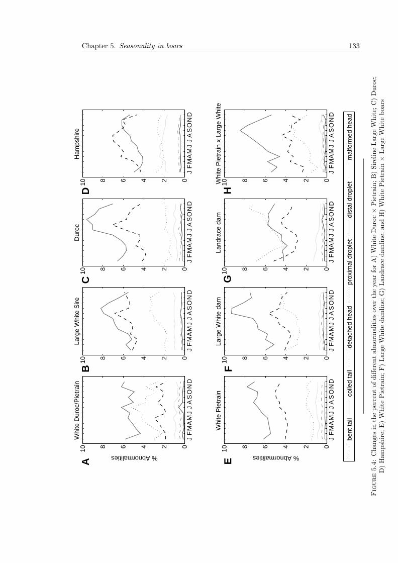
Chapter 5. Seasonality in boars 133
JF
MA
MJ
JA
SO
ND
0246810
% Abnormalities
Whi
te D
uroc
/Pie
trai
n
JF
MA
MJ
JA
SO
ND
0246810La
rge
Whi
te S
ire
JF
MA
MJ
JA
SO
ND
0246810D
uroc
JF
MA
MJ
JA
SO
ND
0246810H
amps
hire
JF
MA
MJ
JA
SO
ND
0246810
% Abnormalities
Whi
te P
ietr
ain
JF
MA
MJ
JA
SO
ND
0246810La
rge
Whi
te d
am
JF
MA
MJ
JA
SO
ND
0246810Whi
te P
ietr
ain
x La
rge
Whi
te
bent
tail
coile
d ta
ilde
tach
ed h
ead
prox
imal
dro
plet
dist
al d
ropl
etm
alfo
rmed
hea
d
JF
MA
MJ
JA
SO
ND
0246810La
ndra
ce d
am
BC
D
FG
HEA
Figure5.4:
Ch
ange
sin
the
per
cent
ofd
iffer
ent
abn
orm
ali
ties
over
the
yea
rfo
rA
)W
hit
eD
uro
c×
Pie
train
;B
)S
irel
ine
Larg
eW
hit
e;C
)D
uro
c;D
)H
amp
shir
e;E
)W
hit
eP
ietr
ain
;F
)L
arge
Wh
ite
dam
lin
e;G
)L
an
dra
ced
am
lin
e;an
dH
)W
hit
eP
ietr
ain×
Larg
eW
hit
eb
oars

Chapter 5. Seasonality in boars 134
5.5.3.3 Age effects
Total abnormalities were not significantly affected by boar age (Table 5.8), although
older boars (five years and above) had proportionally more. This may be due to the
increased variation in percentage of abnormalities observed in ejaculates from older boars
masking the effects of age (data not shown). Age did however significantly affect the
occurrence of detached and malformed heads, as well as proximal and distal droplets
(P < 0.001), but none of the other abnormalities assessed. Detached heads and distal
droplets were most common in three year old boars (P < 0.001) and malformed heads
in four year old boars (P < 0.001), although the difference between the ages was less
than 1%. Proximal droplets showed variation between ages with boars above the age of
four more than doubling their frequency from 4.5% to over 9% (P < 0.001).
Table 5.8: Changes in percentage of abnormalities by age
Age (years)
nejaculates
21057 13075 5573 647 120
Abnormality 1 2 3 4 5 P Value
Detachedhead
0.44±1.15b 0.42±0.98b 0.54±1.83a 0.53±1.03ab 0.22±1.15ab < 0.001
Malformedhead
1.08±2.51b 1.09±2.02b 1.21±2.22b 1.49±2.42ac 1.27±1.65bc < 0.001
Bent tail 2.28±4.99 2.17±4.16 2.20±3.75 2.28±2.98 1.29±2.18 NS
Coiled tail 0.26±0.90 0.25±0.88 0.26±0.73 0.24±0.75 0.08±0.61 NS
Proximaldroplet
4.90±6.77a 4.50±5.13b 4.72±4.72ab 4.35±3.93ab 9.04±8.96c < 0.001
Distaldroplet
6.06±6.12ab 6.14±5.84a 5.75±5.06b 5.88±5.14ab 4.55±4.96ab < 0.001
Total 15.17±11.99 14.72±9.87 14.84±9.78 14.88±8.35 16.51±8.75 NS
Age values within rows for each abnormality type superscripted with different lettersdiffer significantly from each other at the prescribed level.
5.5.3.4 Collection interval effects
Total abnormalities increased with collection interval. Intervals of up to a fortnight
had significantly lower total abnormalities than three weeks or more (Figure 5.5; P <
0.001). This was mainly attributed to the number of bent tails being higher for intervals
of more than three weeks (P < 0.001), proximal droplets lower for intervals of less than
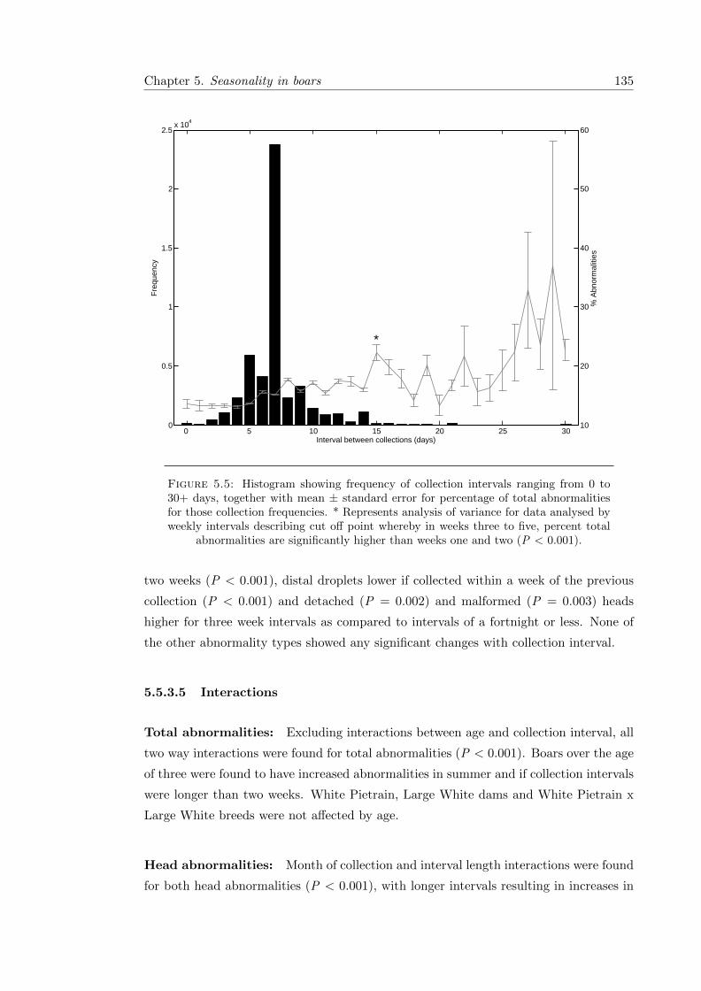
Chapter 5. Seasonality in boars 135
0 5 10 15 20 25 300
0.5
1
1.5
2
2.5x 10⁴
Fre
quen
cy
Interval between collections (days)
10
20
30
40
50
60
% A
bnor
mal
ities
*
Figure 5.5: Histogram showing frequency of collection intervals ranging from 0 to30+ days, together with mean ± standard error for percentage of total abnormalitiesfor those collection frequencies. * Represents analysis of variance for data analysed byweekly intervals describing cut off point whereby in weeks three to five, percent total
abnormalities are significantly higher than weeks one and two (P < 0.001).
two weeks (P < 0.001), distal droplets lower if collected within a week of the previous
collection (P < 0.001) and detached (P = 0.002) and malformed (P = 0.003) heads
higher for three week intervals as compared to intervals of a fortnight or less. None of
the other abnormality types showed any significant changes with collection interval.
5.5.3.5 Interactions
Total abnormalities: Excluding interactions between age and collection interval, all
two way interactions were found for total abnormalities (P < 0.001). Boars over the age
of three were found to have increased abnormalities in summer and if collection intervals
were longer than two weeks. White Pietrain, Large White dams and White Pietrain x
Large White breeds were not affected by age.
Head abnormalities: Month of collection and interval length interactions were found
for both head abnormalities (P < 0.001), with longer intervals resulting in increases in

Chapter 5. Seasonality in boars 136
summer. Collection interval and breed interactions were present for detached heads (P
< 0.001), with some breeds having more if collection intervals were longer. Breed and
month interactions were found for malformed heads, with Hampshire boars exhibiting
greater monthly changes than the other breeds (P < 0.001). In addition, as age increased
above three years the semen was more likely to have malformed heads (P = 0.007) in
summer.
Tail abnormalities: Collection interval and breed interactions were present for bent
tails with some breeds having more tail abnormalities with longer collection intervals (P
< 0.001). In addition longer collection intervals in summer resulted in increased numbers
of bent (P < 0.001) and coiled (P = 0.03) tails. Landrace and Large White damline
boars, together with White Duroc/Pietrain boars had more bent tails in summer (P <
0.001), whereas the same was true for coiled tails in Hampshire boars (P < 0.001).
Cytoplasmic droplets: Longer collection intervals in summer were found to result
in increased proximal and distal droplets (P < 0.001), although White Duroc/Pietrain
boars were most likely to be affected (P < 0.001). Collection interval and breed inter-
actions were present for proximal (P = 0.005) and distal (P = 0.01) droplets in general,
with some breeds having increased cytoplasmic droplets with longer collection intervals.
Only proximal droplets exhibited interactions between age and collection interval (P <
0.001) with boars over the age of three performing best when intervals were less than
two weeks. In addition as age increased above three years there were more proximal
(P < 0.001) and distal droplets in summer (P = 0.002). Interactions between age and
breed were found for both proximal and distal droplets (P = 0.001), showing that not
all breeds were affected by age.
5.5.4 Motility
Month of collection: In all months over 75% of spermatozoa were classified as having
very good motility (Figure 5.6 A), and at least 17% as good motility. However signifi-
cant changes in sperm motility scoring were found throughout the year with ejaculates
collected between July and December having more scores of one, two and three (P <
0.001).
Breed: Breed differences were apparent (Figure 5.6 B) with White Duroc/Pietrain
boars producing proportionally more (over 25%) motilities classed as four and White

Chapter 5. Seasonality in boars 137
Pietrain × Large White and Hampshire boars more semen with a classification of five
(over 80%; P < 0.001).
Collection interval: Regardless of collection interval over 60% of ejaculates scored
five (Figure 5.6 C). However collection intervals of more than three weeks resulted in
more scores below five, and in particular intervals of five weeks or more resulted in nearly
20% of ejaculates having a score of three or under (P < 0.001).
Age: Age of boar was found to influence sperm motility (Figure 5.6 D; P < 0.001).
Boars aged one to four had more motilities classed between one and three, although
overall they had a higher proportion of motilities classed as five than boars aged over
five years. In particular boars aged below three had at least 75% of ejaculates given a
score of five.
5.5.5 Decision trees
5.5.5.1 Semen dose usage
It was found that the algorithm was able to accurately identify patterns within the
data, with similar trees being produced after pruning. As instance number increased,
initial tree size decreased as the number of leaves and nodes dropped. Trees with five in-
stances per leaf produced a slightly smaller tree, with very similar classification decisions
(Figure 5.7 A) to trees with 20 and 100 instances per leaf (Figure 5.7 B).
The results suggest that as long as the percentage of AB was less than 30% the sample
would be used, although sperm concentration did factor into it too with ejaculates
containing less than 145 x 106 spermatozoa/ml being discarded. Only those parameters
seemed to matter even though month and year of collection, stud location, collection
interval, average motility of sperm, SV and boar age and breed had also been presented
to the algorithm. The tree accuracy was high at 90% as was the the AUC at 87.6%.
5.5.5.2 Semen quality parameters
A summary of the results produced during the different decision tree experiments can
be found in Table 5.9 and the corresponding decision trees can be found in Appendix B.
The first set of experiments aimed to classify SC (trees one to three; Figures B.1 to B.3)
in the semen samples and produced three distinct trees. Regardless of the number of

Chapter 5. Seasonality in boars 138
Jan
Feb
Mar
Apr
May
Jun
JulA
ugS
epO
ctN
ovD
ec0255075100
Mon
th o
f col
lect
ion
% motilities
WD
/PLW
SD
HW
PLW
DLD
WP
/LW
0255075100
Bre
ed o
f boa
r
% motilities
12
34
50255075100
Col
lect
ion
inte
rval
(w
eeks
)
% motilities
12
34
5+0255075100
Age
of b
oar
(yea
rs)
% motilities
01
23
45
Figure5.6:
Per
centa
geof
sper
mw
ith
diff
eren
tm
otil
ity
score
sra
ngin
gfr
om
0(a
sper
mic
/n
om
ovem
ent)
to5
(ver
ygood
)giv
enby
A)
month
of
coll
ecti
on;
B)
bre
edof
boa
r(W
hit
eD
uro
c×
Pie
trai
n(W
D/P
),S
irel
ine
Larg
eW
hit
e(L
WS
),D
uro
c(D
),H
am
psh
ire
(H),
Wh
ite
Pie
train
(WP
),L
arge
Wh
ite
(LW
D)
dam
lin
e,L
and
race
(LD
)d
amli
ne
an
dW
hit
eP
ietr
ain×
Larg
eW
hit
e(W
P/LW
));
C)
coll
ecti
on
inte
rval
an
dD
)age
of
boar.

Chapter 5. Seasonality in boars 139
Abnormalities
Used Discarded
< 29.5% ≥ 29.5%
Used Discarded
Sperm concentration
Abnormalities
Used Discarded
< 30.5% ≥ 30.5%
A) B)
≥ 145 x 106 < 145 x 106
Figure 5.7: Decision tree showing the attribute decisions made for whether or not aboar ejaculate is to be used. Trees made using either A) five instances per leaf or B)
20/100 instances per leaf.
instances included in the classifier, all trees had an accuracy of 60%, however trees one
and two were over-fitted and difficult to interpret. Tree three had a clear decision path
to follow, although the AUC was more than 5% lower than the other trees. This was as a
result of improved specificity and decreased sensitivity, when increased sensitivity is what
was required. All the trees showed collection interval to be the most important parameter
with intervals of less than 6.5 days resulting in reduced SC in tree three. Month and
age were then selected as the next determining factors with July to December resulting
in reduced concentrations in boars aged between two and four years. Meteorological
conditions were not important in classifying whether a boar would produce ejaculates
with lower SC.
Trees four to six (Figure B.4) classified SV and all three trees were identical with an
accuracy and AUC of 63.5%. Month was the main determining factor with a split
between February to July and August to January. In particular March to May resulted
in lower than average SV, although in February, June and July boars aged one or four
also suffered from reduced SV. For the remainder of the year only boars aged one or more
than four years suffered from reduced SV between 2004 and 2008 if the collection interval
was less than 10.5 days. Meteorological conditions were not implicated in predicting
changes in SV. Sensitivity was high for the decision tree produced (72.4%) suggesting
that the classifier was good at detecting true positives.

Chapter 5. Seasonality in boars 140
Table 5.9: Classification results produced from the various decision tree experimentsconducted looking at sperm concentration (SC), semen volume (SV), total sperm num-
bers (TSN) and percentage of abnormalities (AB).
Parameter ExptAccuracy
(%)Sensitivity
(%)Specificity
(%)Error
rate (%)No.leaves
No.nodes
AUC(%)
SC
1 60.1 56.4 63.9 41.4 47 93 65.9
2 60.1 54.6 66.6 41.3 31 61 64.7
3 60.3 53.2 67.7 41.7 5 9 58.1
SV
4 63.5 72.4 54.5 33.7 13 25 63.5
5 63.5 72.4 54.5 33.7 13 25 63.5
6 63.5 72.4 54.5 33.7 13 25 63.5
TSN
7 63.4 74.3 51.2 36.2 23 45 67.4
8 62.3 75.8 49.0 35.7 18 35 66.7
9 63.4 74.3 51.2 36.2 23 45 67.4
AB (20%)
10 58.6 62.9 54.3 40.4 34 67 53.3
11 58.3 63.4 53.2 40.6 13 25 50.9
12 58.3 60.7 56 41.1 14 27 56.0
AB (30%)
13 58.1 62.9 53.4 40.7 5 9 53.4
14 59.1 73 45.5 36.9 11 21 54.9
15 59.1 73 45.5 36.9 11 21 54.9
Trees seven to nine (Figures B.6 to B.7) examined TSN and tree eight produced the most
interpretable results with an accuracy matching those for the other trees (62.3% versus
63.4%). Similarly to SC, interval lengths of 6.5 were critical for establishing the first
split in the data, followed by month of collection and age of boar. October to January
in boars aged one or more than four years with collection intervals of less than 10.5 days
had reduced TSN. In other months of the year, decisions were not as clear to interpret
and again meteorological conditions did not play a major role in classifying the data.
When classifying AB with a cut off point of either 20 or 30%, age was always the
first parameter to split the data. Trees 10 to 15 (Figures B.9 to B.12) all had low
accuracies and AUCs never surpassing 56%, however trees 14 and 15 produced the most
interpretable results from all the AB trees with an AUC of 54.9%. Boars aged two to
five were separated from other ages and then average temperatures greater than 13.5 ◦C
were shown to affect them by resulting in more abnormalities. None of the trees had
the high specificities which were required, as it is better to misclassify positive instances
(having low abnormalities) than negative abnormalities and using sub standard semen.

Chapter 5. Seasonality in boars 141
5.6 Discussion
5.6.1 Seasonal changes in semen quality
5.6.1.1 Semen volume, sperm concentration and total sperm numbers
The results indicate that seasonal changes in boar semen quality from ejaculates collected
under commercial UK conditions did occur. An increase in SV and TSN during late
autumn and early winter supports other European work carried out in Poland (Ciereszko
et al., 2000; Wysokiska et al., 2009) and the Czech Republic (Smital, 2009; Wolf and
Smital, 2009), as well as patterns found in the European wild boar which has ejaculates
similar to those of domestic boars (Kozdrowski and Dubiel, 2004). These changes are
thought to be mediated by photoperiod and temperature, affecting the production of
testosterone and thus spermatogenesis and semen quality output.
The effects of day length on semen quality relate to testosterone having a stimulatory
effect on spermatogenesis and being essential for sperm maturation. In fact short days
have been shown to stimulate pubertal maturation of spermatogenesis (Andersson et al.,
1998) which may be a contributory factor towards increases in the TSN from boars
during the autumn months. Reductions in testosterone reduce spermatogenesis at the
spermatogonial level and thus result in lower sperm numbers. The synergistic effects
of oestrogen and testosterone are also thought to be responsible for changes in SV
(Joshi and Raeside, 1973) and photoperiod regulated testosterone levels are known to
affect levels of acrosomal stabilising proteins in seminal plasma, resulting in reduced
fertility in August and September due to quicker acrosome reactions (Murase et al.,
2007). However the mechanisms involved in increased testosterone production during
the autumn and winter months (Claus et al., 1983) are difficult to determine as there
is no evidence that FSH and LH levels are altered in the testes, even though these
would be primary candidates for affecting spermatogenesis due to their involvement in
sperm cell and testosterone production respectively. Oestrogen has also been shown
to be important for the long term maintenance of spermatogenesis involving germ cell
proliferation, differentiation and the final maturation of spermatids, as well as germ
cell survival and apoptosis (Carreau and Hess, 2010). The seminal changes occurring
coincide with the wild boar rutting season, when sows come into oestrus in preparation
for a spring farrowing (Mauget, 1982) and so allow for optimal semen quality to maximise
fertility and fecundity.
The present study found that SV was greatest in autumn and winter, when day length
was shortening, supporting previous work where decreasing photoperiod was found to

Chapter 5. Seasonality in boars 142
be the main contributor to improvements in SV, due to increasing testosterone levels
affecting spermatogenesis (Kennedy and Wilkins, 1984; Trudeau and Sanford, 1986;
Charneca et al., 1996; Ciereszko et al., 2000; Kozdrowski and Dubiel, 2004; Okere et al.,
2005; Frydrychova et al., 2007; Wolf and Smital, 2009; Wysokiska et al., 2009). In
addition weather conditions were not found to influence SV, reinforcing the idea that
in terms of SV photoperiod is more important than temperature. Younger boars were
more likely to have lower SV, although this then reduced again with boars which were
four years or older. No clear trend for breed was found, although Pietrain animals
were found to have higher SV than Duroc boars overall and as younger animals. In
the past Hampshires have been found to have the greatest SV (Kennedy and Wilkins,
1984), whereas they were only second after White Pietrains in the present study. White
Pietrains are a newer breed and so improvements in productivity traits can be expected.
When comparing sire and dam lines no differences in SV were found, although the
Large White sire line did produce slightly higher volumes overall than the Large White
damline. Sonderman and Luebbe (2008) reviewed the effects of interactions between
age and breed, concluding that young boars often produce inadequate volumes and that
terminal sire line boars often produce larger volumes at younger ages than maternal
lines, and continue to have larger volumes throughout their productive lives. In fact it
has been suggested that boar semen quality, as assessed by SC and SV, actually peaks
at around 3.5 years of age and then gradually declines (Smital, 2009).
Total sperm numbers were found to be lowest throughout spring and summer, supporting
recent findings where TSN were found to be lowest over the same period (Wolf and
Smital, 2009; Wysokiska et al., 2009). However the current study found SC to be lowest
in autumn, opposing previous work where SC was found to follow a similar pattern to
TSN with increases over the autumn and winter months (Kennedy and Wilkins, 1984;
Wolf and Smital, 2009; Wysokiska et al., 2009). Nonetheless it supports work which
showed that decreasing photoperiod between August and October, in comparison to
increasing photoperiod between February and mid-April, reduced SC (Sancho et al.,
2004) and that increases in SV were not sufficient to reduce SC (Ciereszko et al., 2000;
Frydrychova et al., 2007).
Sperm concentration was found to be mainly affected by collection interval with an age
and month interaction. Early work has shown that longer collection intervals increase
SC (Kennedy and Wilkins, 1984) since boars have more time to supplement their re-
serves. The decision tree analyses were able to show that collection interval was also
the main attribute which affected TSN, along with boar age. Decision trees classifying
TSN produced the most accurate results from all the parameters assessed (around 67%
for trees seven to nine) which were relatively sensitive (around 75%). This shows the

Chapter 5. Seasonality in boars 143
usefulness of decision trees in finding patterns within the data which may not have been
previously considered. Early work had shown that TSN are greatest in late winter and
early spring (Trudeau and Sanford, 1986), which supports the present findings for boars
during their most productive years (two to four years old) and has been found in more
recent studies too (Murase et al., 2007). These are periods of time when humidity tends
to be high but temperatures are lower, meaning that the effective temperature experi-
enced by the animals is more comfortable and may contribute to the improved TSN.
Heat stress has been shown to affect SC from two weeks after exposure (McNitt and
First, 1970) and results show that SC was reduced during the summer months. Inter-
estingly the decisions trees produced did not find temperature in any of the six weeks
prior to collection to affect SC. It may be that the conditions experienced in the UK are
not extreme enough to elicit a heat mediated response on SC.
The present study found no clear trend in ejaculate usage by breed, although Sonderman
and Luebbe (2008) suggest that purebred maternal lines produce more ejaculates which
are discarded. Boar maximal age varied between breeds, with White Pietrain boars being
kept longer before culling. This may be due to selection for good quality semen being
more successful in this breed, meaning that they produce high quality semen for longer.
White Pietrains also contributed the most ejaculates to the data set, suggesting that it
is used more regularly than other breeds. Due to the decision trees assessing individual
boar changes in semen quality parameters, breed differences were eliminated from the
tree models, although the linear analyses showed that differences most definitely exist.
Some breeds were more susceptible to month of collection than others, including the
Duroc which has previously been identified as being more sensitive to seasonal infertility
than Landrace, Yorkshire and Hampshire boars (Sonderman and Luebbe, 2008).
Under the commercial AI conditions of the present study, extended semen was sold in 75
ml doses with 2.5×10⁹ sperm/dose. The ejaculates collected would only be discarded if
less than 1.43 ×10⁸ sperm/ml ejaculate were present since pooling and extending semen
means that concentrations can be adjusted before sale. It is therefore impossible to
say whether any decrease in TSN or SC would actually influence fertility in the autumn
months per se, but it does show whether any boars have changed their production in this
period which can be a sign of changes in spermatogenesis which may affect the quality of
spermatozoa produced (Ciereszko et al., 2000). Low concentrations can be problematic
for studs as it reduces the number of spermatozoa available, and can result in more
pooling being necessary in order to make up the numbers. Semen pooling has been
suggested to negatively affect sow fertility due to the masking of relative differences in
individual boar fertility (Foxcroft et al., 2008) and so higher concentrations are beneficial
by permitting more single sire doses to be sold.

Chapter 5. Seasonality in boars 144
In order to obtain a fuller picture of the meteorological effects on seasonal changes in boar
semen quality it would be necessary to carry out more detailed analyses on the effects
of outside conditions on the stud environment and relate that back to boar fertility.
It should be noted that the trees produced in this study used binary classification due
to the simplicity of splitting data into two classes and analysing the results produced.
This meant that subjective levels had to be set in order to split the data. Further
experiments using the regression option would allow for levels within the data to be
chosen automatically, allowing for details within breeds and age groups and under various
meteorological conditions to be better defined. This was not possible in the present study
due to the unbalanced nature of the data across breeds etc. meaning that once organised
into a useable dataset, not enough points for regression classification were available.
5.6.1.2 Abnormalities and motility
Monthly changes in the proportion of abnormalities were found in this study, with in-
creases in AB during the summer and autumn months. This supports previous work
carried out in Spain where 75 days of decreasing photoperiod were found to have a neg-
ative impact on sperm morphology even when environmental temperature and humidity
were kept constant (Sancho et al., 2004). Work from the Czech Republic also found
that AB in semen were influenced by changing day length (Smital, 2009). However the
mechanisms behind photoperiodic influences on changes in the AB are poorly under-
stood, with little data available in the literature. This may be due to the fact that
initially decreasing photoperiod tends to coincide with increasing temperatures and so
most studies will have confounded results. It is therefore of importance that future
studies use hormonal assays to investigate the effects of photoperiod on sperm abnor-
malities in the boar. Changes in sperm morphology are however better understood in
terms of cellular senescence or factors, mainly exogenous (temperature, frequency of
semen collection, nutrition, etc.), which alter the correct development of sperm (sper-
matogenesis or spermiogenesis) or sperm epididymal maturation (Bonet et al., 1993).
The relationship between the causative factor and the abnormality observed may be
specific. For instance, a high frequency of semen collection may bring about an increase
in spermatozoa with tail abnormalities due to fast passage through the epididymis re-
sulting in insufficient sperm maturation (Bonet et al., 1991) whereas high temperatures
may result in more head abnormalities early on in the spermatogenesis cycle (Cameron
and Blackshaw, 1980) and an increased number of cytoplasmic droplets later on (Stone,
1982).

Chapter 5. Seasonality in boars 145
In the present study there was no climatic control in the boar accommodation, meaning
the boars were to some extent susceptible to outside conditions, which could be exacer-
bated without the correct ventilation and provision of cooling facilities. Increased AB
due to heat stress manifest for up to six weeks after exposure (McNitt and First, 1970)
and it is thought that there are two stages at which heat affects developing spermatozoa.
Decreased motility and an increased incidence of primary AB, such as coiled tails, are
thought to occur due to heat stress during the late primary spermatocyte, secondary
spermatocyte and early spermatid stages (McNitt and First, 1970; Wettemann et al.,
1979). Characteristics in which the effects of heat stress are observed at a later time
(concentration, total sperm numbers and total motile sperm) are thought to be pro-
duced in the middle period of the primary spermatocyte stage (McNitt and First, 1970),
although it has been suggested that this is dependent on individual boar tolerances
(Cameron and Blackshaw, 1980). Secondary AB, such as detached heads, seem to arise
from a general weakening of the spermatozoa over the entire developmental period from
the mid-primary spermatocyte to the early spermatid stages (McNitt and First, 1970).
Therefore during the summer months when temperatures are generally at their warmest,
the AB in semen may increase and the effects would be seen weeks later and therefore
in early autumn.
Breeders select boars to a certain degree on the basis of a low incidence of abnormal
spermatozoa, usually related to good testes size and form. However abnormalities cannot
be altogether eliminated and it is therefore necessary to establish a threshold at which
semen must be discarded due to excessive abnormalities being present. In most cases
this is set to 30%. Therefore as expected, in comparison to discarded ejaculates, used
ejaculates had lower percentages for most of the assessed abnormality types. However
the fold increase in different types of abnormalities in discarded ejaculates, compared
to used ejaculates, was not always the same. This suggests that some abnormalities are
more likely to occur than others and so during the assessment of semen it may not be
necessary to focus on all abnormality types, with only some of them occurring frequently
enough to cause fertility problems.
Interestingly tail abnormalities were found to increase in summer and autumn whilst
head abnormalities increased during spring and summer. This supports previous findings
(Sancho et al., 2004; Murase et al., 2007) and suggests that spermatozoa may be more
prone to tail abnormalities occurring in early spermiogenesis during periods with warm
temperatures and decreasing day length, whilst head abnormalities are more of a result
of increasing temperatures and day length, possibly due to altered sperm cell formation.
Apoptosis of germ cells is thought to be one of the primary causes as this increases with
exposure to elevated temperatures (Morgentaler et al., 1999). Indeed animals suffering

Chapter 5. Seasonality in boars 146
from cryptorchidism are rendered infertile. Abnormality formation at the testicular stage
is termed a primary malformation, whereas the development of abnormalities in the
epididymis would be secondary, and it has been suggested that most tail abnormalities
occur at this later stage (Briz et al., 1996). The epididymis is essential for normal
reproduction in mammals because sperm leaving the testis are not capable of fertilizing
an oocyte (Franca et al., 2005). Any malfunctions during passage through the epidydimis
may therefore result in immature or malformed sperm.
Immature spermatozoa with proximal or distal droplets were the most common types
of abnormal sperm in the present study, confirming earlier work carried out on boars
(Larsson et al., 1980). These occur when the cytoplasmic droplet on the sperm tail is
retained. In the current data used ejaculates contained between 4 and 5% proximal and
distal droplets respectively. Waberski et al. (1994) investigated the effect of proximal
and distal droplets on fertility in a field experiment and found a negative correlation
between the proportion of distal droplets and fertility. They concluded that the presence
of cytoplasmic droplets is a serious morphological defect that may be associated with
lowered resistance against in vitro ageing and recommended that the total percentage of
cytoplasmic droplets in ejaculates used for AI should not exceed 15%. This is in contrast
to other work suggesting that distal cytoplasmic droplets pose less of a problem than
proximal droplets (Althouse, 1998) and that disruptions to epididymal sperm maturation
due to heat stress result in more proximal droplets being retained and thus reduced
fertility (Malmgren and Larsson, 1984; Thundathil et al., 2001).
Abnormal heads have been suggested to be the most frequently occurring abnormality
type in dairy bull semen (Soderquist et al., 1996), whereas in the present boar study they
were only fourth. Their reduced fertility is thought to stem from them being unable to
traverse the female reproductive tract (Saacke et al., 1998) due to altered hydrodynam-
ics by the small geometrical differences in head morphology (Dresdner and Katz, 1981)
and obstructions such as the cervix and utero-tubual junction. Additionally difficul-
ties in attachment and oocyte penetration have also been observed in the cat (Howard
et al., 1993). Acrosomal damage can also be classified as a head abnormality and in
the present study was infrequently found, with slight increases in the autumn months
in comparison to January. Acrosin activity has been found to be reduced in autumn
months (Ciereszko et al., 2000), which coincides with increased levels of damaged acro-
somes in October and November. Yoshinaga and Toshimori (2003) found that several
mammalian acrosome molecules involved in the acrosome reaction, zona pellucida reac-
tion and oocyte penetration are formed during spermiogenesis and arranged gradually

Chapter 5. Seasonality in boars 147
and compartmentalised in a stage specific manner during sperm maturation. This sug-
gests that damage during transport through the epididymi is responsible for acrosomal
defects, potentially corresponding to heat stress in the weeks prior to ejaculation.
In the present study the occurrence of detached and malformed heads and proximal
and distal droplets were found to be influenced by age although total percentage of
AB remained unaffected. Additionally as age increased so did variation for all of the
assessed traits. Previous work has found age to influence semen characteristics. Boars
older than three and a half years displayed reduced semen quality (Smital, 2009) and
two year old boars had the maximum number of potential doses in terms of the best
semen volume and concentration (Kennedy and Wilkins, 1984). Wolf and Smital (2009)
found that the percentage of abnormal sperm increased between eight months and four
years of age, possibly due to older boars surpassing their functional age (Sonderman
and Luebbe, 2008), since lower semen quality in older boars may be associated with fat
deposition in the scrotum (Coe, 1999) and the break down of body tissues (particularly
testicular) with advancement in age (King, 1993). Young boars (under one year) have not
yet reached maturity, with the testes still developing and as such are also susceptible to
decreased semen quality (Hughes and Varley, 1980). Therefore in a commercial setting it
is necessary to only use ejaculates from boars which have been shown to reach maturity.
In addition, with boars aged between one and four being the best producers, it was
interesting to note that on average boars were only kept for two to three years (one to
two years for some breeds). It may be more cost effective to keep boars for an additional
year before culling (Rutten et al., 2000), although after four years they should be culled.
Collection interval is another managerial decision which needs to be carefully moni-
tored. The present study found that when collection intervals surpassed two weeks,
total abnormalities increased by over 5% and up to 25% in some cases. Previous work
has shown that longer collection intervals result in increased total abnormalities in an
ejaculate (Wolf and Smital, 2009) although it has been suggested that more than 30
days need to pass before significant effects are seen (Smital, 2009). When comparing
short intervals of between one and three days no significant differences were found, sup-
porting previous findings (Swierstra, 1973). Most studs work boars on average once a
week and this seems to be the optimal length of time for ensuring reduced numbers of
abnormalities, including the most common abnormalities of cytoplasmic droplets, bent
tails and detached heads, and maintaining high SV and SC. It should be noted however
that previous models have established that collection intervals of three to four days may
provide better financial returns (Rutten et al., 2000).

Chapter 5. Seasonality in boars 148
Breed often plays a large role in the resilience of animals to external conditions and
differences in semen quality assessed as sperm volume, concentration and motility have
been demonstrated (Wysokiska et al., 2009). The present study found breed differences
in respect to total abnormalities and different abnormality types. Sirelines tended to ex-
perience higher numbers of abnormalities, in particular the Hampshire and Large White
sires. Landrace dam line boars did however experience more bent tails and Duroc boars
more distal droplets. Previous work has shown that breed differences in abnormality
percentages exist at a low level of up to 1.6% between Large White and Pietrain breeds
(Smital, 2009), which is lower than the data produced from this study showing that dif-
ferences of up to 3.5% exist between Hampshire and White Duroc/Pietrain boars. This
may be attributed to the differing genetic lines assessed in the studies. Abnormality
types were also found to be breed dependent. For example Large White boars were
found to have increases in cytoplasmic droplets and bent tails in the summer/autumn
months, supporting previous work where the percentage of spermatozoa with bent tails
and cytoplasmic droplets increased between August and November in the same breed
(Murase et al., 2007). Conversely Duroc boars were found to have increases in cyto-
plasmic droplets in summer/autumn when previous work suggests that this is not the
case (Borg et al., 1993). These discrepancies may be attributed to boar age which was
on average one year older in the present study (average age of two years). As previ-
ously mentioned young boars may suffer from more abnormalities and so higher averages
throughout the year may mask seasonal changes.
Within breed variation for semen quality parameters was high, most likely due to in-
dividual boar differences which have previously been found to be a problem in semen
quality analyses (reviewed in Foxcroft et al. 2008). In their review they describe how
under normal commercial AI conditions, individual boar fertility is masked due to semen
pooling and the high concentrations used. It is therefore imperative that semen evalua-
tion for traits such as morphological abnormalities are able to detect boars which may
be more sensitive to seasonal stressors such as temperature and day length, increasing
the percentage of abnormalities in their semen and reducing their fertilising capacity.
Malmgren and Larsson (1984) found differences in individual boar susceptibility to heat
stress, resulting in different percentages of abnormal morphologies. In fact morpholog-
ical characteristics have been found to be a useful tool for assessing semen fertility in
boars, in that differences in normal sperm morphology contributed to the variance in
litter size born for multiparous sows (Xu et al., 1998). Increased abnormalities in ejacu-
lates will result in poorer quality semen and a reduced ability to fertilise eggs. This may
be contributing to the seasonal infertility phenomenon found in sow breeding herds, as

Chapter 5. Seasonality in boars 149
the period of increased abnormalities in semen coincides with the period of sow seasonal
infertility.
5.6.2 The use of decision trees
The decision tree algorithm was able to detect stud management decisions on whether to
use or discard ejaculates. The trees produced had up to two decisions to be made, with
only five nodes and three leaves in the largest tree and three nodes and two leaves in the
smallest tree, maintaining a high accuracy of 90%. It was found that semen ejaculates
would only be used if there were less than 29.5% AB and if the SC in the dose was
greater than 145×106 sperm/ml ejaculate. This closely mimics decisions made in the
boar studs as their rules outline that no ejaculates with more than 30% AB should be
used and that the semen must contain a high enough count of sperm cells, as it will
later be diluted to serve many sows. This emphasises the ability of decision trees to
identify patterns within large data sets and confirms that they may be a useful tool in
identifying if standards within a boar stud are being met. Other studies have also found
decision trees to be useful in assessing on-farm decisions, when both simulated and real
datasets were examined (Kirchner et al., 2004a,b, 2006; Kamphuis et al., 2010a,b).
When the algorithm was applied to the dataset containing meteorological variables and
semen quality parameters, the decision trees produced were not as interpretable. Clas-
sification accuracies were much lower and the trees were more complex to interpret,
although some patterns were detected. When considering AB for example, boar age was
found to be the main contributing factor to increased values, with average temperature
two and four weeks pre collection being the next parameter considered. Other me-
teorological conditions and boar parameters showed little influence in the experiments
conducted. The accuracies of the decision trees were relatively low (below 56%), suggest-
ing that it is difficult to identify what affects AB and that there is still another 40% of
the variation which has not been explained. Abnormality identification and assessment
is a subjective process, and depends on having a representative sample of each ejaculate
to quality control. It is possible that this may contribute to the unexplained variation.
Additionally the studied period used for the meteorological effects was two to six weeks
prior to collection. Different abnormalities are known to occur at different periods of the
spermatogenesis cycle, and for different reasons. Data analyses showed that malformed
heads, bent tails and proximal or distal droplets were the most commonly found ab-
normalities in the semen from the boar studs used (data not shown). Malformed heads
are produced early on in spermatogenesis (Saravia et al., 2007), suggesting that any
influencing factors would have to be present at the beginning of the cycle (around week
Chapter 5. Seasonality in boars 150
six prior to ejaculation). Proximal and distal droplets however, would most likely be
affected during transit through the epididymi (Stone, 1982) and so any weather effects
would be happening later, during the maturation process. Therefore the assessment of
AB may require a breakdown of abnormality types in order to identify any effects of
meteorological factors such as temperature.
A similar problem was true for other semen quality parameters. Even though the data
were analysed in relation to individual boar changes in production, the algorithm was
unable to detect specific patterns in the data with high accuracy. This is most likely
due to unknown factors which were not provided to the algorithm, such as collection
technician which has been shown to influence quality parameters (Kennedy and Wilkins,
1984), as well as libido and feed intake (Kunavongkrit et al., 2005). The results show
that the algorithm is able to detect relationships in boar stud datasets as the usage
reasons were easily visualised by the decision tree with understandable decision rules.
However when applied to more varied biological parameters, more data preparation may
be necessary to reduce the noise in the dataset. Kirchner et al. (2004b) found that the
pre-processing of data provided improved classification as irrelevant, noisy or incomplete
attributes and data entries were removed, allowing the algorithm to more easily detect
true patterns. Future work may consider using data from one breed and age group at a
time, which was not possible in the present study due to insufficient data.
5.7 Conclusions
Seasonal changes in semen quality parameters are present in the UK, with some breeds
being more affected than others and age of boar and collection interval also having an
influence. All quality parameters are influenced from semen volume to percentage ab-
normalities. Reduced quality was generally found during the summer and early autumn
when temperatures are higher and day length is shortening. Practical implications of
the work are that boars should be worked between the ages of one and five years, at least
once a week in order to maintain semen quality. In addition more boars should be made
available over the summer/autumn months to compensate for increases in abnormalities.
If freeze thaw technology ever becomes available in the industry, more winter/spring col-
lections could help compensate for reductions in semen quality during other times of the
year. Decision trees were found to provide a valuable method of assessing managerial
decisions on semen usage, however were less useful at predicting specific semen quality
parameter changes in relation to individual boar and meteorological attributes. They
were nonetheless convenient for identifying initial patterns in the data which may have
otherwise gone undetected.

Chapter 6
The assessment of heat stress in
outdoor lactating sows
throughout the year
6.1 Introduction
Analyses on UK outdoor commercial pig production data suggest that negative effects
on sow farrowing rates can be found when, during late lactation, average temperatures
are as low as 18 ◦C (Chapter 3). Other work from Spain has found that Yorkshire sows
had an UCT of 19.2 ◦C in regards to farrowing rate (Bloemhof et al., 2008), over 2 ◦C
lower than previously published temperatures (22 to 25 ◦C; Black et al. 1993; Quiniou
and Noblet 1999). We can therefore ask whether in the UK (and other countries with
temperate climates) we are doing enough to keep our animals cool not only in summer
but also during spring and early autumn when temperatures may reach these levels.
Most experimental work on sow reproduction has been carried out on indoor sows, with
few studies looking at the effects on sows kept outdoors in a commercial environment.
In the UK, outdoor sows are altogether different from indoor sows both genetically and
in terms of their environment since for the duration of their lifetime they are exposed to
extreme temperatures not only throughout the year but also in a single day. This is in
contrast to indoor animals which are kept in near constant conditions. This may mean
that outdoor sows have become acclimatised to cooler temperatures and therefore have
a lower tolerance for rises in ambient temperature during the summer months.
As homeotherms, pigs are generally able to maintain a steady core temperature regard-
less of external conditions and the equilibrium between the production of heat, the loss
151

Chapter 6. Heat stress in outdoor sows 152
18 20 22 24 26 28 30 320
20
40
60
80
100
120
140
Ambient temperature (°C)
Res
pira
tion
rate
(br
eath
es/m
inut
e)
Figure 6.1: The effect of ambient temperature on the respiration rate of lactatingsows as found by previous publications (Lynch, 1977; McGlone et al., 1988; Schoenherret al., 1989; Johnston et al., 1999; Quiniou and Noblet, 1999; Laspiur and Trottier,
2001; Renaudeau et al., 2001).
of heat and/or the gain of heat from external sources is maintained by thermoregula-
tion. Heat production is a result of the metabolic activity of the animal, taking into
account basal metabolic functions such as digestion and state functions such as lactation
in the post-partum sow (Chaffee and Roberts, 1971). This means that heat production
increases with additional metabolic activity, such as nursing a large litter, and can be
controlled to some extent by restricting feed intake and thus reducing ingestive and di-
gestive heat production. In contrast, heat loss is a function of the surface heat being
lost, the temperature gradient between the skin and the external surface, the conduc-
tivity of the animal (body fat, hairiness), the environment the animal is in (wind speed,
sunshine) and the animals ability to dissipate heat through sweating and panting (Mon-
teith, 1974). Pigs have a diminished ability to sweat due to their lack of functional
sweat glands (Ingram, 1965, 1967). This means that most evaporative heat loss is con-
ducted through the lungs, with respiratory rates increasing in order to dissipate more
heat (Figure 6.1).
The amount of heat that an animal is able to lose drops with increases in ambient tem-
perature, and this is true for both core (rectal; Figure 6.2) and surface (skin; Figure 6.3)
heat loss. In indoor animals this relationship has been described as being linear with
maximal ambient temperatures of 30 ◦C (Williams, 2009). However the amount of heat

Chapter 6. Heat stress in outdoor sows 153
that an animal can experience before having to actively cool down most likely follows a
broken line model and is dependent on humidity (Huynh et al., 2005).
Chaffee and Roberts (1971) conducted a thorough literature review of temperature ac-
climation in birds and mammals and described how mammals acclimatise to prolonged
exposure to cold temperatures. This has been confirmed in pigs with data showing that
when growing pigs were kept at 10 ◦C they grew more slowly, had more body hair and
had smaller ears than pigs kept at 35 ◦C (Dauncey and Ingram, 1986). This shows that
pigs kept in different environments will morphologically differ as they will adapt their
body to provide additional insulation and an altered surface area in order to increase or
decrease heat production and heat loss appropriately (Derno et al., 1995). Core body
temperature has also been found to be lower in animals kept in cold conditions (Dauncey
and Ingram, 1986). In addition, if moved from a 10 ◦C to a 35 ◦C environment pigs ex-
hibited severe hyperthermia as compared to if kept in hot conditions from the beginning,
suggesting that there is a marked difference in heat tolerance induced by living in the
cold (Dauncey and Ingram, 1986). Different breeds have also been found to differ in
their ability to cope with heat stress (Bloemhof et al., 2008) and the time it takes them
to acclimatise to changing conditions (Renaudeau et al., 2007).
Respiration rate is correlated with ambient temperature. In growing piglets low (0
to 5 ◦C) and high (20 to 25 ◦C) ambient temperatures have been shown to result in
increased respiration rates, relating to an increased need for oxygen under cold conditions
and an increased need for evaporative heat loss under warm conditions respectively
(Ingram and Legge, 1969). Therefore it can be deduced that outdoor sows, differing
both genetically and in environmental exposure to indoor sows, most likely have a lower
threshold for heat stress. This is especially true during the later stages of lactation
when metabolic demands are higher due to the additional requirements necessary for
increased milk production. Heat stress is known to negatively influence several aspects
of sow productivity including conception rates and litter sizes, most likely due to reduced
feed intake and the associated negative effects on body condition (Black et al., 1993; Love
et al., 1993). If the threshold at which outdoor sows succumb to heat stress is lower
than what we know it to be for indoor animals, methods of alleviating the symptoms
need to be provided appropriately.
Work carried out in Scotland suggests that lactating sows spend more than 70% of
their time inside farrowing huts in summer and spring and more than 80% of their time
inside during winter and autumn (Buckner et al., 1998). This is supported by work in
America, where sows spent around 80% of their time in their farrowing huts (Johnson
et al., 2008). The literature presents little data on the conditions inside farrowing huts,

Chapter 6. Heat stress in outdoor sows 154
18 20 22 24 26 28 30 3238.6
38.8
39
39.2
39.4
39.6
39.8
40
Ambient temperature (°C)
Rec
tal t
empe
ratu
re (
°C)
Figure 6.2: The effect of ambient temperature on the rectal temperature of lactatingsows as found by previous publications (Lynch, 1977; Schoenherr et al., 1989; Quiniou
and Noblet, 1999; Laspiur and Trottier, 2001; Renaudeau et al., 2001).
16 18 20 22 24 26 28 3033
33.5
34
34.5
35
35.5
36
36.5
37
37.5
38
Ambient temperature (°C)
Ski
n te
mpe
ratu
re (
°C)
Figure 6.3: The effect of ambient temperature on the skin temperature of lactatingsows as found by previous publications (Quiniou and Noblet, 1999; Renaudeau et al.,
2001; Huynh et al., 2005; Williams, 2009).

Chapter 6. Heat stress in outdoor sows 155
as experienced by the sow, and the data which are available can be contradictory. For
example work in Texas found no significant effect of insulating farrowing huts on the
temperature inside the huts or on litter performance (Johnson and McGlone, 2003),
whereas UK data have shown that insulation prevents large temperature fluctuations
within the huts, even if piglet productivity was not affected (Randolph et al., 2005).
Argentine work has shown that temperatures inside farrowing huts were significantly
reduced when huts were painted white (Echevarria et al., 2000). We can therefore ask
whether producers should be using a certain type of farrowing hut which will keep sows
more thermally comfortable during lactation.
Rectal temperature is often used as a measure of heat stress in pigs (for example Kelley
and Stanley 1978; Macari et al. 1983; Quiniou and Noblet 1999; Huynh et al. 2005) as
it is representative of core temperature, any changes in which would indicate a ther-
moregulatory challenge. However animals work to maintain their core temperature, so
changes in rectal temperature may not be apparent unless under severe duress. In ad-
dition, as stated in Chapter 2, it is an invasive method and not practicable in outdoor
roaming animals. The skin is the main heat exchanger of the body and its temperature
is determined by the core temperature and by the environment (temperature, humidity,
air velocity; Monteith 1974). Thus the skin temperature is governed by the needs of the
body to exchange heat energy and the point at which the skin can no longer emit any
more heat may be defined as the animals UCT. Infrared (IR) thermometry provides an
accurate technique for measuring skin temperature (Buono et al., 2007) but environmen-
tal conditions need to be accounted for as these will influence the results obtained. For
example increased solar radiation will result in an increase in skin temperature which is
independent of internal heat loss.
6.2 Objectives
It was postulated that outdoor sows may succumb to heat stress at lower levels than
those published in the literature for lactating sows kept indoors. Therefore the aim of
this work was to monitor how sow physiology (respiration rate and skin temperature)
changed in relation to external meteorological conditions in order to determine an UCT
for outdoor lactating sows in a temperate climate. The UCT was defined as the point
at which the sow’s skin temperature or respiration rate reached a plateau in relation to
corresponding meteorological conditions.
Temperature and humidity fluctuations in different types of farrowing hut were also
studied, in order to determine whether some huts are more effective at keeping sows

Chapter 6. Heat stress in outdoor sows 156
in a state of thermoneutrality under varying external conditions. It was hypothesised
that insulated huts would perform better in terms of reducing temperature fluctuations
within the farrowing hut.
6.3 Methods
6.3.1 Animals and Housing
All animal measures were collected between July 2011 and July 2012 at Guild House
farm in East Knapton, North Yorkshire, UK (part of Dent Ltd). A total of 380 Landrace
× Duroc sows and gilts were followed, mated to Swedish Hampshire boars (JSR Genetics
Ltd) using AI, although any returns were caught using boars. On observation of oestrus,
AI was carried out by experienced stockmen in service tents before returning sows in
groups to gestation paddocks. Due to sow deaths or sows found to be not in pig (NIP),
some sows were removed from the trial (n = 21). Sows used for this study had a high
health status, were nose ringed and ranged over 14 parities: gilts (n = 106), primipares (n
= 76), multipares (n = 177). A summary of the batch details can be found in Table 6.1.
If a lactation period spanned over two months of the year, data were presented as being
relevant for the month in which more days were included. Nine batches began with 40
animals, however in March/April 2012 the huts were moved onto a new field adjacent
to the the original one and so for batch seven only 20 huts were available for the trial
(all triangle shaped) and so only 20 sows were followed. The same facilities and routines
were kept.
The sows were introduced into their individual paddocks (14 m × 14 m) with farrowing
hut approximately five days prior to their expected farrowing date and were allowed to
farrow under normal commercial management conditions. Four hut types were used on
the farm: wooden triangle insulated huts, wooden triangle non-insulated huts, metal arc
insulated huts and metal arc non-insulated huts (Table 6.2 and Figure 6.4).
In warmer weather it was farm practice to open ventilation shafts at the back of far-
rowing huts which had functional ones. Sows had access to fresh water in the form of
individual drinking troughs connected to a mains water supply. No additional shade
was made available within the paddocks but each sow had access to a wallow located
by the drinkers. The farrowing huts faced approximately South East throughout the
duration on the study, but were moved within individual paddocks after each weaning.
Throughout the first week of lactation each hut was checked by the stockmen at least
once a day and dead piglets removed and recorded. Lactation length was on average

Chapter 6. Heat stress in outdoor sows 157
Table 6.1: Dates and sow numbers for the batches in the trial. Dates presented areapproximate start dates for farrowing, weaning, serving and ultrasound scanning in
week five following service.
Batch No. sows Farrow Wean Serve Wk5 scan
1 39 14/07/2011 08/08/2011 11/08/2011 15/09/2011
2 40 11/08/2011 05/09/2011 08/09/2011 13/10/2011
3 40 15/09/2011 10/10/2011 13/10/2011 24/11/2011
4 37 20/10/2011 21/11/2011 25/11/2011 29/12/2012
5 33 29/12/2011 30/01/2012 02/02/2012 08/03/2012
6 39 02/02/2012 05/03/2012 08/03/2012 12/04/2012
7 20 08/03/2012 04/04/2012 09/04/2012 10/05/2012
8 35 06/04/2012 09/05/2012 14/05/2012 18/06/2012
9 36 14/05/2012 13/06/2012 18/06/2012 23/07/2012
10 40 18/06/2012 18/07/2012 23/07/2012 27/08/2012
Table 6.2: Approximate farrowing hut dimensions and materials
Hut typeHeight(cm)
Depth(cm)
Length(cm)
Materials
Insulated Arc 100 140 250Galvanised steel and fibre-glass insulation
Non-insulated Arc 100 140 250 Galvanised steel
Insulated triangle 140 170 230Plywood and fibreglass insu-lation
Non-insulated triangle 140 170 230 Plywood
four weeks. Sows were fed once a day. During the first week of lactation sows were
individually fed in their paddocks and feed was estimated on sow condition and litter
size. Fenders were attached to the huts for the first week of lactation in order to keep
piglets inside the huts. One week after farrowing, division tapes between individual
paddocks were removed, grouping between nine and 14 sows together. Once grouped,
sows were group fed using feed hoppers located in the centre of the field. The farm had
a 55% replacement rate and all gilts were regumated in order to synchronise oestrus.
Ultrasound scans were conducted five weeks after service by trained stockmen in order
to identify pregnant animals.

Chapter 6. Heat stress in outdoor sows 158
Figure 6.4: Examples of the farrowing huts used in the trial. From top right goingclockwise, insulated arc, non-insulated triangle, non-insulated arc, insulated triangle.
6.3.2 Animal measurements
Parity and sow ID were noted at the beginning of each batch and using the grading
system in Appendix C sows were given a body score. After farrowing, NBA and week one
deaths were recorded. Animal measurements were taken every Monday and Thursday
from farrowing to weaning at four different time points over the day (starting at 8am,
12pm, 4pm and 8pm), following the same route around the paddock. Respiratory rate
was taken first by observing and counting flank movements for one minute timed on a
stop clock (breathes per minute; bpm). Skin temperature was then taken in triplicate
using an IR thermometer (OS425-LS, Omega, UK) on as many of the four nominated
skin sites as possible at each time point. Skin sites were only measured if free from
mud. The four skin sites used were the head, shoulder, flank and rear as illustrated
in Figure 6.5. Sows which were not safely accessible were omitted from the readings
for that time point. Alongside the regular measurements sow location and activity at
the time of taking the readings were also noted (Table 6.3). Location was defined as in
the farrowing hut, in the paddock, in the shade behind the farrowing hut, in a sunny
spot in the paddock or in the wallow. Activity of the sows was defined as lying down,

Chapter 6. Heat stress in outdoor sows 159
standing, nursing the piglets, rooting/eating or drinking. At weaning, sow body score
was taken again (Appendix C) and post-weaning, the farm records were used to obtain
service dates, week five scan results and any culls.
Head
Shoulder
Flank
Rear
Figure 6.5: Location of skin sites used for skin temperature measurements on sows.
Table 6.3: Description of behaviours
Behaviour Description
Lying down Lying either on side or front without nursing. e.g. sleeping
Standing Standing without any other activity being carried out
NursingWhen piglets are at teats, with sow grunting signifying
milk let-down
Rooting/EatingSow located either at feeder and eating or with active oral
rooting activity in the ground
Drinking Seen to be drinking either at drinker or in wallow/puddle
In farrowinghut
Sow located within a farrowing hut, even if not hers
In paddockSow located in the paddock but not seeking shade or
warmth
In shade Sow located in a shady spot of the paddock on a sunny day
In sun Sow located in a sunny spot on a colder/windier day
In wallow Sow either standing or lying down in a wallow

Chapter 6. Heat stress in outdoor sows 160
6.3.3 Meteorological measurements
A weather station (Vantage Pro2, Davis Instruments, CA, USA) was set up near the
paddocks in order to record ambient temperature ( ◦C), rainfall (mm), relative humid-
ity (%), solar radiation (W/m2), wind speed (mph) and wind direction at 30 minute
intervals. A data logger was used to store the weather data and download it for analysis
(WeatherLink, 6510USB model, Davis Instruments, CA, USA). Weather data down-
load was done on average once a fortnight. Data recording began one week before the
trial commenced and ended the day of the last weaning. Due to technical difficulties
the weather station failed to record data at various time points and so data were col-
lated from the MIDAS dataset (UK Meteorological Office, 2006) for the location of High
Mowthorpe which is within 10 km of the farm. It was only possible to get rainfall,
ambient temperature and relative humidity data from the MIDAS dataset.
6.3.4 Farrowing hut measurements
Farrowing hut temperature and humidity readings were automatically taken every 30
minutes using data loggers (Tinytag Plus 2, Gemini Data Loggers Ltd, UK). Data
loggers were randomly placed in three farrowing huts from each different type. In order
to protect them from wet conditions and damage by sows, loggers were suspended from
thick string inside two litre water bottles cut into a bell shape and wrapped in black
duct tape. Holes were drilled into the top of the bell in order to allow sufficient air flow.
Recordings began three days before the first batch of sows entered the paddock and
were stopped on the final batch day of weaning. At the end of each batch, data were
downloaded using Tinytag Explorer software and Tinytag Plus USB Download cable
(Gemini Data Loggers Ltd, UK). Loggers were removed from the huts during December
as there was no batch that month and once again in March when the field transfer
occurred.
6.3.5 Data preparation
A Temperature Humidity Index (THI) was used in order to account for both temperature
and humidity within one variable.
THI = T − (0.55− (0.0055×RH))× (T − 14.5) (6.1)

Chapter 6. Heat stress in outdoor sows 161
Equation 6.1 has previously been used for pigs (Zumbach et al. 2008; where T = Tem-
perature ( ◦C) and RH = Relative Humidity(%)) and the method of using a THI to
assess heat stress is already commonly used for feedlot cattle (Mader et al., 2002, 2003;
Amundson et al., 2006). Temperature humidity indices for livestock are derived from
human indicies and are becoming more popular in animal science research (Mader et al.,
2010).
6.4 Statistical Analyses
All statistical analyses were conducted in MATLAB 7.11.0 (R2010b) (MATLAB, 2010)
and R2.12.1 (R Development Core Team, 2009). When implementing linear models,
backwards stepwise regression was used to find the minimum adequate model (MAM).
Normality and homogeneity of models were checked for by visual inspections of plots of
residuals against fitted values when required.
6.4.1 Batch statistics
Born alive litter size, lactation length and pre-weaning mortality were found to be ap-
proximately normally distributed using normality plots and as such ANOVA testing, fol-
lowed by the Tukey test were conducted to find significant differences between batches.
Batch parity, week one deaths and WSI were found to be non-normal and as such were
analysed using the non-parametric Kruskal-Wallis test.
Wean to service interval was found to follow a lognormal distribution and so generalised
linear models after a log transformation of the data were used, looking at the effects
of week one litter size, average meteorological conditions for the last week of lactation,
lactation length (up to three, four, or more weeks), change in body score over lactation,
sow parity (gilt, primipare, multipare) and batch. After analysis the results were back-
transformed to obtain geometric means of WSI (in days).
Sow conception rates throughout the year were analysed using generalised linear models
with a binomial distribution with week five scan results as the dependant variable (0
or 1) and average weekly meteorological conditions for the two weeks prior to service
date, sow parity (gilt, primipare, multipare), WSI (less than or more than seven days),
hut type, batch and change in sow body score as the independant variables. The effects
of maximum and minimum sow skin temperature during lactation on conception rates
were also assessed using binary logistic regression.
Chapter 6. Heat stress in outdoor sows 162
Change in sow body score was analysed using linear models looking at the effects of week
one litter size, lactation length (up to three, four or more than four weeks), average THI
throughout lactation, sow parity (gilt, primipare, multipare), batch and hut type.
6.4.2 Skin temperatures
Pearson product moment correlations were calculated for the different skin sites used
(head, flank, rear and shoulder) and between skin temperature and respiratory rate.
The effects of THI on average skin temperature were analysed using piecewise general
linear regression from the segmented package in R (Muggeo, 2003), with solar radia-
tion, wind speed, rainfall, time of day and week of lactation as covariates. Piecewise
models are regression models where the relationships between the response and one or
more explanatory variables are represented by two or more straight lines connected at
unknown values (referred as breakpoints). The segmented package is able to estimate
the breakpoints within the line and then fit the lines to the data. The Davies test was
used to establish whether a break point existed and comparisons between models with
different numbers of breakpoints were done using Akaike’s information criterion (AIC).
Data were analysed for all seasons combined and each season separately. Seasons were
defined as summer (June, July, August), autumn (September, October, November),
winter (December, January, February) and spring (March, April, May).
6.4.3 Respiration rates
Respiration rate was found to be lognormally distributed and so was analysed after
log transformation. The effects of meteorological conditions on sow respiratory rates
were analysed in R using linear mixed effects models from the lme4 package (Bates and
Maechler, 2009) and the languageR package (Baayen, 2009) to estimate P values. The
initial (and final) model included THI, solar radiation, rainfall, wind speed, week of
lactation, time of day, sow activity and their interactions. Sow ID and batch were used
as random factors. To assess the validity of the mixed effects analyses, a likelihood ratio
test was performed comparing the model with fixed effects to the null model with only
the random effects.
6.4.4 Farrowing huts
In order to analyse the conditions within the four types of farrowing hut, averages across
the three data loggers placed in each type of hut were used. Summary statistics for hut
Chapter 6. Heat stress in outdoor sows 163
conditions over the course of a day were produced and stepwise linear regression was
applied to identify the relationship between the four types of farrowing hut and external
temperatures, humidities and THIs.
6.5 Results
6.5.1 Batch statistics
A summary of the batch statistics can be found in Table 6.4.
Parity profiles across batches varied between an average of 1.7 in batch seven to 4.4 in
batch eight. Born alive litter sizes were moderate with an average of 10.4 ± 0.7 (mean
± s.d.) piglets and week one litter sizes were also relatively small for a commercial unit.
There was a tendency (P = 0.08) for the NBA in batch four to be smaller than the other
batches. Lactation length averaged 26 ± 2.4 days, supporting the four week lactation
period expected on commercial UK units. Not all batches had sows which were culled
after weaning. Batch six had the highest percentage culled (20.5%) although this could
not be attributed to any of the other sow factors.
The mean WSI was about seven days. Meteorological conditions during the week prior
to weaning did not significantly affect WSI, although lactation lengths lasting over four
weeks were found to increase WSI by about two days (P = 0.04). However an interaction
between long lactation lengths and large litter sizes resulted in reduced WSI (one day;
P < 0.03). Older sows were found to have WSI of nearly one day less (P = 0.004) and
sows in batch seven were found to have, on average, WSI that were two days longer than
sows in other batches (P = 0.002).
Sows served in February had the lowest conception rates with only 55% of sows found
to be pregnant at the week 5 scans (P = 0.02), although these were not found to be
related to pre-wean meteorological conditions. If WSI were longer than seven days,
conception rates were found to be reduced (P = 0.007) and there was also a trend for
sows above parity three to have higher conception rates (P = 0.08). None of the other
factors assessed impacted on conception rates, including maximum and minimum skin
temperatures throughout lactation.
The average sow started off with a body condition score of between 3 and 3.5 and
finished with a score of between 2.5 and 3 at the end of the lactation period, although
this was improved for longer lactation lengths (P < 0.05). Some sows did actually
increase their body condition score over the lactation period, but these were found to be

Chapter 6. Heat stress in outdoor sows 164
Table6.4:
Des
crip
tive
stati
stic
sfo
rea
chof
the
batc
hes
.
Par
amet
erB
atch
Num
ber
12
34
56
78
910
Month
FJu
lA
ug
Sep
Oct
Jan
Feb
Mar
Ap
rM
ayJu
n
No.
farr
owed
3940
4037
3339
2035
3640
Par
ity2∗
4.2a
2.6b
2.3b
3.3a
b2.
4b
2.6ab
1.7b
4.4a
3.2ab
2.9a
b
(ran
ge)
(1-1
3)(1
-11)
(1-8
)(1
-11)
(1-7
)(1
-5)
(1-4
)(1
-13)
(1-8
)(1
-7)
NB
A1
11.7
10.8
9.9
10.7
9.5
109.
410
.411
.710
.8
Wk1
dea
ths2∗∗
1.58
1.89
1.37
a1.
892.
70b
2.43
1.67
2.10
2.07
1.52
Wk1
litt
ersi
ze†1∗∗
10.9
9.8
9.5
9.9
8.3a
9.1
9.2
9.0
10.4
10.0
Wk1
mor
tali
ty(%
)6.
89.
24.
07.
512
.69.
02.
113
.511
.17.
4
Mon
thL
Ju
lA
ug
Sep
Nov
Jan
Feb
Mar
Ap
rJu
nJu
l
WS
I(d
ays)
2∗
7.2
acd
efg
6.5c
def
5.8acd
efg
6.0d
eg7.
8ef
6.4a
cdefg
13.7
f6.
3acd
eg7.
0g7.
0b
Month
SA
ug
Sep
Oct
Nov
Feb
Mar
Ap
rM
ayJu
nJu
l
No.
serv
ed38
3940
3531
3120
3536
37
Con
cep
tion
rate
(%)
81.6
69.2
77.5
74.3
54.8
87.1
60.0
88.6
75.0
73.0
Pos
tw
ean
cull
s(%
)2.
62.
50
5.4
6.0
20.5
00
2.8
7.5
LL
(day
s)1∗
20.1
a25
.9bcd
e26
.1bcd
e27
.3cd
f25
.5de
24.6
e26
.4bcd
ef27
.0bcd
f28
.2f
28.9
f
Res
ult
sp
rese
nte
das
mea
nor
per
cent.
Mon
thF
:m
onth
of
farr
owin
g;
Month
L:
month
of
lact
ati
on
;M
onth
S:
month
of
serv
ice;
NB
A:
born
ali
veli
tter
size
;W
SI:
wea
nto
serv
ice
inte
rval
;C
once
pti
onra
te:
per
centa
ge
of
sow
sfo
un
dto
be
pre
gnant
five
wee
ks
aft
erse
rvic
e;L
L:
lact
ati
on
len
gth
.†
Wk1
litt
ersi
zeac
cou
nts
for
fost
erin
g.V
alu
esin
row
sw
ith
diff
eren
tsu
per
scri
pts
diff
ersi
gn
ifica
ntl
yfr
om
each
oth
er(∗P<
0.0
01;∗∗P<
0.0
5)
asass
esse
dby
AN
OV
A1
or
Kru
skal-
Wall
is2.
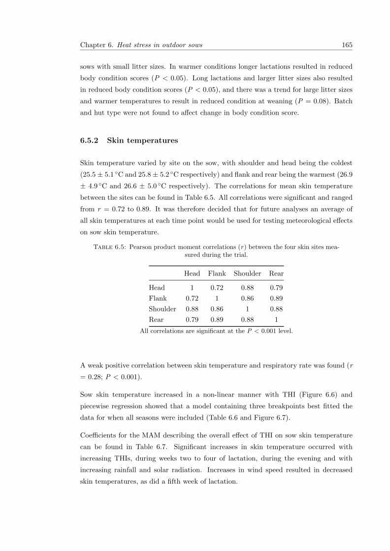
Chapter 6. Heat stress in outdoor sows 165
sows with small litter sizes. In warmer conditions longer lactations resulted in reduced
body condition scores (P < 0.05). Long lactations and larger litter sizes also resulted
in reduced body condition scores (P < 0.05), and there was a trend for large litter sizes
and warmer temperatures to result in reduced condition at weaning (P = 0.08). Batch
and hut type were not found to affect change in body condition score.
6.5.2 Skin temperatures
Skin temperature varied by site on the sow, with shoulder and head being the coldest
(25.5 ± 5.1 ◦C and 25.8 ± 5.2 ◦C respectively) and flank and rear being the warmest (26.9
± 4.9 ◦C and 26.6 ± 5.0 ◦C respectively). The correlations for mean skin temperature
between the sites can be found in Table 6.5. All correlations were significant and ranged
from r = 0.72 to 0.89. It was therefore decided that for future analyses an average of
all skin temperatures at each time point would be used for testing meteorological effects
on sow skin temperature.
Table 6.5: Pearson product moment correlations (r) between the four skin sites mea-sured during the trial.
Head Flank Shoulder Rear
Head 1 0.72 0.88 0.79
Flank 0.72 1 0.86 0.89
Shoulder 0.88 0.86 1 0.88
Rear 0.79 0.89 0.88 1
All correlations are significant at the P < 0.001 level.
A weak positive correlation between skin temperature and respiratory rate was found (r
= 0.28; P < 0.001).
Sow skin temperature increased in a non-linear manner with THI (Figure 6.6) and
piecewise regression showed that a model containing three breakpoints best fitted the
data for when all seasons were included (Table 6.6 and Figure 6.7).
Coefficients for the MAM describing the overall effect of THI on sow skin temperature
can be found in Table 6.7. Significant increases in skin temperature occurred with
increasing THIs, during weeks two to four of lactation, during the evening and with
increasing rainfall and solar radiation. Increases in wind speed resulted in decreased
skin temperatures, as did a fifth week of lactation.

Chapter 6. Heat stress in outdoor sows 166
Table 6.6: Piecewise regression model results for temperature humidity index effectson sow skin temperature, with differing numbers of estimated breakpoints.
No. breakpoints Estimated breakpoints C.I. (95%) AIC
1 14.61 ◦C 13.53 - 15.69 36360
215.77 ◦C 14.92 - 16.62
3579020.15 ◦C 19.29 - 21.00
3
4.70 ◦C 3.04 - 6.37
3576015.68 ◦C 14.98 - 16.38
20.02 ◦C 19.20 - 20.83
All models included temperature humidity index (THI), solar radiation, rainfall, windspeed, lactation week and time of day. C.I: Confidence Interval and AIC: Akaike’s
Information Criterion.
Table 6.7: Coefficients from piecewise regression model for temperature humidityindex effects on sow skin temperature, with three breakpoints along the regression line.
Estimate Std. Error t value P value
(Intercept) 21.510 0.263 81.923 < 0.001
THIout 0.304 0.089 3.396 < 0.001
lactweek2 0.343 0.123 2.788 0.005
lactweek3 0.341 0.122 2.797 0.005
lactweek4 0.440 0.149 2.940 0.003
lactweek5 -0.667 0.443 -1.505 0.132
timeofday2 -2.339 0.136 -17.184 < 0.001
timeofday3 -2.564 0.137 -18.724 < 0.001
timeofday4 0.328 0.138 2.375 0.018
solar 0.003 0.000 10.170 < 0.001
rain 0.875 0.159 5.517 < 0.001
wind -0.334 0.019 -17.578 < 0.001
Model included temperature humidity index (THI), solar radiation, rainfall, wind speed,lactation week and time of day
Breakpoints were found at THIs of 4.7, 15.7 and 20.0 ◦C with varying slopes between
each breakpoint (Table 6.8 and Figure 6.7). The confidence intervals around these
breakpoints were quite narrow, providing more confidence in the values produced. It
was clear that the final increase in temperature occurred at 20 ◦C (Figure 6.7), suggesting
this to be the UCT of outdoor lactating sows.

Chapter 6. Heat stress in outdoor sows 167
−2 −1 0 1 2 3 4 5 6 7 8 9 10 11 12 13 14 15 16 17 18 19 20 21 22 23 2416
18
20
22
24
26
28
30
32
34
THI (°C)
Ski
n te
mpe
ratu
re (
°C)
Figure 6.6: Sow skin temperatures for different temperature humidity indicies (THI).Presented as mean ± standard error.
Table 6.8: Slopes with 95% confidence intervals (CI) for temperature humidity indexfrom a piecewise regression model with three breakpoints.
Slope St.Err. t value Lower CI (95%) Upper CI (95%)
1 0.30450 0.08967 3.3960 0.1287 0.4803
2 0.69100 0.02060 33.5300 0.6506 0.7313
3 -0.03309 0.11320 -0.2923 -0.2550 0.1888
4 1.16400 0.19130 6.0860 0.7890 1.5390
Model included temperature humidity index (THI), solar radiation, rainfall, wind speed,lactation week and time of day.
When considering the effects of THI on skin temperature for different seasons of the
year, the whole temperature range was not available for every season and so direct
comparisons for all temperatures were not possible (Figure 6.8). It was found that a
model containing one break point best fit the seasonal data as compared to models
with more than one breakpoint (AIC = 35445; Figure 6.9), although the data for other

Chapter 6. Heat stress in outdoor sows 168
●● ● ●● ● ●●● ● ●●●
●●● ●●●● ●● ● ●● ● ●●● ●● ●● ●●● ●● ●● ● ●●● ●● ● ●●●●● ●● ● ● ●●●
●● ● ●● ●● ●● ● ●●● ● ● ●
●● ● ● ●● ●●● ●● ● ●● ●● ●● ●● ●
●● ● ● ●● ● ● ●● ●● ●● ●● ●●● ● ●● ●●● ● ● ●● ●● ● ●●● ● ● ●●● ● ● ●
● ● ● ●● ●● ●● ●
●● ● ●● ●● ●● ● ●●●● ●●●●● ●● ● ● ●● ● ●● ● ●● ● ●● ●● ● ● ●● ●●● ● ●● ●●● ●● ●●●● ●●●● ●● ●●●●● ●
● ●●●● ● ●●●●
● ● ● ●●● ●●● ●●● ●●● ●●●● ● ● ●● ● ●● ● ●● ●● ●●● ●● ● ●●●● ●● ●● ● ● ● ●●● ● ●●● ●● ● ● ● ● ●●●● ●● ●● ●●● ●●● ● ●●● ● ●●● ● ●● ●● ●● ●● ●● ●●● ●
● ●●● ● ●● ●● ● ●● ● ●● ● ● ● ●●● ● ●● ● ●● ● ● ●●●●● ●● ●● ● ●● ●●●● ●● ● ●● ●● ●●●● ●● ●●●● ●● ●●●● ● ● ●● ● ● ●●● ● ●● ● ●● ●● ●●● ●● ● ● ● ● ●● ●●● ●● ● ●● ● ●● ●● ● ●● ●●●● ●● ●●● ●● ●●● ●●● ● ●● ●●● ● ●● ●● ●● ● ●●●●● ●● ●● ● ●●● ●● ●● ● ●●● ●● ●●● ● ● ● ●●● ●●●● ●● ● ●●● ●● ●● ● ●● ●● ●●● ●● ●● ● ●●● ●● ● ●●● ●●● ●●●●● ●● ● ●●●● ●● ●● ●● ●● ● ● ●●●●● ●● ● ●● ●● ●●● ●●● ●●●●●● ● ● ● ●●● ● ● ●● ●● ●●● ● ●●● ●● ●● ● ●●● ● ●●●●●●● ●●● ● ● ●● ●●●● ●● ● ●● ●●●●● ●● ●●● ●● ● ●● ●●●● ●● ● ●●● ● ●●●●● ●● ●● ● ●●● ●●● ●● ●●●●● ● ●●● ●●● ●●● ●●● ● ● ●● ●●● ●● ●● ●●● ●● ●●●● ● ●●● ●● ● ● ●●● ●● ●● ●● ● ● ●● ● ● ●● ●●● ●● ●● ●● ● ●●● ●● ●●● ●● ●● ●● ● ●● ● ●● ●● ●●● ●● ● ● ●●●●●●● ● ●● ●● ● ● ●● ● ●● ●●● ●●● ●● ●● ●● ● ●● ●●● ● ●●● ● ●●● ● ● ● ●●● ●● ●●●●● ● ● ●● ● ●● ● ● ●● ●● ● ● ●● ●● ●● ● ● ●● ● ● ●●● ●●● ● ●● ● ●●● ● ●● ●●● ● ●● ● ● ●●● ● ●●● ● ●● ●● ●● ●● ● ●● ●● ● ●● ●● ● ●● ●● ●● ● ●● ●●● ● ● ●●● ● ● ●● ●●● ●●● ● ●● ● ●●● ● ●● ●● ●●● ●● ●● ●●● ●● ● ●●● ● ●● ●● ● ● ●●● ●● ●●● ●● ● ●●●● ●● ● ● ●● ●●●● ●●●● ●● ● ●● ●● ●● ● ●● ●● ● ● ●●● ● ●● ●● ● ● ●●●●●●● ● ● ●●● ●●● ● ●● ● ● ● ●●●● ● ●●● ●●● ● ●●●● ● ●●● ●● ● ● ●●● ●● ●● ● ●● ●●● ●● ● ● ●●● ●●● ●●● ● ●●● ●●● ● ● ●● ● ●●●● ● ● ● ●●●● ●●●● ●● ●●● ● ● ●● ●● ●● ●●● ● ●●● ●● ●●● ●●● ●● ● ●●● ● ● ● ●● ● ● ●● ● ●● ●●●● ● ● ●● ● ●●●●●● ● ●●● ●● ●●● ●●●● ●●● ●●● ● ● ●● ●● ● ●●● ●●● ●● ●● ●● ● ●●● ●●●● ●●● ● ● ●●●●●● ●●●●●● ● ● ●●●● ● ●● ● ● ● ●●●● ●● ●●● ●●● ●● ● ●● ● ●● ●● ●● ● ● ●● ● ●● ●● ●● ●●● ● ●●● ● ●●● ● ●●● ● ● ●● ●● ●● ●● ●● ●●● ● ● ●● ●● ●● ●● ●● ●●●●● ●● ●● ● ●● ● ● ●●● ●● ●● ●● ● ●● ●● ●● ●● ● ●●● ●●● ● ●● ●●● ● ●●● ● ●● ●●●●● ● ● ● ● ●● ●● ● ● ●● ●● ●● ●●● ●● ●● ●● ● ●●● ●●●●● ●● ● ●●● ●●● ●● ●●●●● ● ● ● ● ●●● ●● ●●●● ● ●● ●●● ● ●● ●● ●● ● ●●● ●● ●●● ● ● ●●● ● ● ●● ●● ● ●●● ● ●● ● ●● ●● ●●●● ●● ●●● ● ● ● ● ●●●● ●●●● ● ●● ●●●● ●● ●● ●● ● ●● ●● ●●● ● ●● ●●●● ● ●● ●● ● ●● ●● ●● ●●● ●●● ● ● ●●● ●● ●● ● ●●● ● ●● ●● ●●● ● ●●● ● ●●● ● ●● ●● ●● ●● ● ●●● ● ●●● ● ●● ●●● ●●● ●● ●● ● ●● ●● ● ●●● ● ●● ● ●●● ●●● ● ● ●● ● ●● ●● ●● ●●● ●● ●●● ● ●● ●● ●● ●●●●● ● ● ● ●● ● ● ● ●●● ●● ● ●●●● ● ● ●● ● ●● ●● ●● ●● ●● ● ●● ●● ● ●● ●● ●● ● ●● ● ●● ●●● ●●● ●●● ●● ● ●● ●●●● ● ●●● ● ●●● ● ●●● ●●● ● ●● ●● ●● ●● ● ●● ●● ●●● ● ●●● ● ●● ●● ●● ● ●● ●●● ●● ●●● ● ●● ●●● ●● ●● ●● ●● ● ● ● ●●●● ●●● ● ● ●● ● ●●● ● ●● ●● ●● ● ●● ● ●●● ●● ●● ●● ●●● ● ●● ●● ●● ●● ●●● ●● ● ●● ●● ●● ● ● ●● ●● ●● ●●● ●●● ●● ●● ● ●● ● ●● ● ●●● ●● ●● ●● ● ●●● ●● ● ● ● ●●●●● ●●● ●● ●● ●●● ● ● ●●● ●● ●●● ● ● ●● ●● ● ●●●● ●● ● ●●● ● ● ●● ●● ●●● ●●● ●● ●● ● ● ● ●● ●●● ●●● ●● ●●● ●●● ●●●● ● ● ●● ●●● ●●● ●● ●● ●●● ●● ● ●●●● ● ● ●●● ● ●●● ●● ● ●●●●● ● ● ●● ●●● ● ● ● ●●● ● ●● ●●●● ● ●●● ● ●●●● ● ●●●● ●● ●●● ●●●●●● ● ● ●● ●● ●● ●●● ●● ●● ●● ●● ●● ●● ● ●●● ●● ●● ●●● ●● ●● ● ●● ● ● ●●● ●● ● ● ●●●● ● ● ●● ●●● ●●●● ● ●● ●● ● ●●●● ● ●● ●●● ● ●●● ●● ● ●● ●●● ● ●●● ●● ●● ●●● ● ●● ● ●●● ● ● ●● ●●● ● ● ● ●●●● ●●● ● ●● ●●●● ●● ●●●●● ● ● ●●● ● ● ● ●● ●● ● ●● ● ●● ●●● ● ● ●● ●●● ●● ●●● ●●● ●● ● ● ●●● ●● ● ● ●●●● ● ●● ●● ● ●● ●●●● ●● ●● ●● ●● ●● ● ● ●● ●●● ●●●● ● ● ●● ●● ●● ●●●● ● ● ● ●● ●● ●● ● ●● ● ●●●● ● ●● ●●● ● ●●●● ●● ●● ● ●● ●●● ●● ● ●●●● ● ●●●●● ● ●●●●● ● ●● ●● ●●● ● ● ●● ●●● ● ●●● ●● ●●● ● ● ●●● ●●● ● ●● ●●●● ● ●● ●●● ● ● ● ●● ● ●●● ●● ●●● ● ●●● ● ●● ● ●● ● ●● ●●● ●● ● ●● ● ●● ●●●● ● ●● ●●● ● ●●● ●●●●● ● ●● ● ●●●● ●●● ● ●● ●●● ●●●● ●● ●●● ●● ●● ● ● ●● ●● ●●●●● ● ● ●●●● ●● ●● ● ●●● ● ●●● ● ●●●● ●●● ●●● ● ●● ● ●●● ● ● ●● ● ● ●●● ●● ● ●●● ● ●● ●●●● ●●● ● ● ●●●● ● ●● ●●●● ●●●●● ●● ● ● ●● ●● ● ● ●●● ● ● ●● ●● ●● ●●● ●●● ● ● ●●● ●●● ● ● ●●● ● ●●●● ●● ●● ●● ●● ●●● ● ●● ● ●● ●●●● ● ●● ●● ●● ●●● ●●● ● ●● ●● ●● ●● ● ●● ●●● ● ●● ● ●●● ●●●● ●● ●●● ●●● ● ●● ●● ● ●● ●● ● ●●●●● ● ●●● ●● ● ●● ● ●● ● ●● ● ●● ● ●●●● ●●● ●● ●● ● ●● ● ● ●● ● ●● ●●● ● ●●●● ● ●●● ●●●● ●●● ●● ●● ●● ●● ●● ● ●● ● ●● ●● ● ●● ●● ●●● ●●● ●● ● ●● ●● ● ● ● ●● ●● ●● ●●● ● ● ●● ●● ●● ● ●●● ●●●● ●● ● ● ● ●●● ●●●●● ●● ●● ● ● ● ●●● ● ●●● ● ●●● ● ●● ● ●●● ● ●● ● ●● ● ● ●●●● ● ● ●●● ● ● ● ●●●●● ●● ● ●●●● ●● ●●●● ●●● ●●●●● ● ●● ● ●● ●● ●● ● ●●●● ●● ●● ●● ●●● ●● ● ●● ● ● ●●●● ● ● ●● ● ●●● ●● ●● ● ● ●● ●● ●●●● ● ● ●● ● ●●● ●●●●● ● ●●● ●● ●●● ●● ●● ●● ●● ●●● ● ●●● ● ● ●●● ● ●● ●● ● ●● ●● ●● ●●● ●●●● ●● ● ●● ● ●● ●● ●●● ●●●● ● ● ●● ● ●●● ● ●● ●●● ● ●● ●●● ●●●●● ● ● ●● ● ●● ● ●●●● ●●●● ●●●● ● ● ●● ● ●●● ●● ● ● ●●● ●●● ●●● ●● ● ● ● ●● ●● ●● ●● ● ● ● ● ●● ●● ●● ●● ● ● ● ●● ● ● ●●● ●●● ●● ●● ●●●● ●● ●●● ●●● ● ●● ● ●●● ●● ●● ● ● ●● ●● ● ●● ●● ● ●●● ● ●● ●● ● ●●● ●● ●● ●● ●● ●● ●●●● ●●● ●●● ●● ● ●●● ● ●● ●●● ●● ●●● ●●●● ● ●●● ● ●●● ● ● ●●● ●●●● ● ●●● ●● ● ● ● ● ● ●● ●● ● ●●● ●●●● ● ● ●●● ● ●● ●● ●● ●● ● ● ●●● ● ●●● ●●● ●● ●● ●● ● ●● ●● ●● ●● ● ●● ● ●● ●●● ●● ●● ● ●● ●●● ● ●●●●● ● ● ●● ● ●●● ● ● ●● ●● ●● ●●● ●●●● ● ● ● ●●● ●● ● ●● ● ●●●●●● ●● ● ●●●●● ● ●● ●●● ● ● ●● ● ● ●●●● ●●●● ●●● ● ● ●●●● ● ●● ●● ●●● ● ●● ● ● ●● ●●● ●● ●●●● ●● ● ● ●●● ● ● ● ●● ●● ●● ● ●● ●●●● ●● ●● ● ●●● ●● ●● ● ●● ●● ● ●● ●●● ●● ●●●● ● ●● ●● ●● ●● ● ● ●● ●● ●●● ●●● ●● ● ● ●● ● ● ●● ●●●●●● ●● ●● ●● ●● ●●● ●● ●●● ●● ●● ●●● ● ● ●● ●● ●● ●● ● ●●● ● ● ●● ●● ● ●● ●● ●●● ●●● ● ●● ●● ●● ●● ● ●● ●●● ●● ●●● ● ●●● ●● ●● ●● ●● ●●● ● ●● ●● ●●●● ●●●● ●●● ● ●● ●●● ●● ●●● ●● ● ●● ●●● ● ● ●● ●● ● ● ●●●● ● ●●● ●●● ●●●● ● ● ●●● ● ●● ●● ●●●●● ●●● ● ●●● ●● ●● ●● ●● ●●●● ●● ● ●● ● ●● ● ● ● ●●● ●●●● ●● ●●●● ● ● ●●● ●● ●● ● ●● ●● ●● ●● ● ●● ● ●● ●● ●● ●●● ● ● ●●● ●●● ●●●● ●● ● ●● ●●● ●●● ● ●●●● ●● ● ● ●●● ●● ●●● ●● ● ● ● ●●● ●● ●●● ● ● ●●● ●● ●● ●●● ●● ●● ●●● ●● ●● ●● ● ● ● ● ●● ●● ● ● ●●● ●●● ●● ● ● ●● ●●●● ●●● ● ●●●●● ●● ● ● ●●● ●● ● ●● ●●● ●● ●●● ● ●● ●● ●● ● ●●● ●● ● ●●● ●● ●●●●●● ●● ● ●● ●● ●●● ● ● ●● ●●●●●● ●●●● ● ●●● ●●●● ● ●● ●● ●● ● ●● ●● ●● ●● ●● ●●● ●● ●● ● ● ● ●● ●● ● ●●●● ●● ● ●●● ●●● ● ●● ●● ● ●● ● ●●●● ● ●●●● ● ●● ●● ●● ●● ● ●●● ●●●● ●● ●● ●●● ● ●● ● ●●● ●● ● ● ●● ● ●●● ● ●● ●● ● ●● ●● ●● ● ●●●● ● ● ●●● ●● ●● ● ●●●● ● ●● ●●● ● ●● ●●● ● ●●● ●●● ●●●●● ●● ●● ● ● ●● ●● ●● ● ●● ●●● ●●● ● ●● ●●● ●● ● ● ● ●● ●●● ● ●● ●● ● ●● ● ●● ● ● ●● ● ●● ●● ●●● ●● ●● ● ●● ●● ●●●● ●●● ●● ●●● ● ● ● ●● ●●● ●●● ●● ● ● ●● ●●● ●● ● ●● ●●● ●● ● ●●● ●● ●● ●● ● ●● ●● ●● ●● ● ●●●●●● ●● ●● ●● ● ●●● ● ● ● ●● ● ●● ●●●● ●● ●● ● ● ● ●● ●● ●●● ●● ● ● ● ● ●● ●● ● ●● ● ●● ● ●●●●● ● ● ●● ●● ●● ● ● ●● ●● ● ●● ● ●●● ● ●● ● ●● ● ●● ●● ●● ●● ● ● ●● ●●●● ● ●● ●●● ● ●● ● ●●● ●● ●● ●● ●● ●●● ● ●● ● ● ●●●● ● ●● ● ●● ●●● ●●● ● ● ●●●● ●● ● ● ● ●●●● ●● ● ●● ● ●● ● ●●●● ●● ● ●●● ●● ●● ●● ● ●●●●● ●● ● ●●● ●● ● ●●● ●●●●● ● ●●● ● ●●● ●● ●●● ●● ● ●●● ● ● ● ●●● ● ●● ●● ●● ● ● ● ●● ●●●● ● ●●● ●● ● ● ●●● ● ●●● ●●●● ●● ●●● ●● ●● ●● ●●● ●● ● ●● ●●●● ●●● ●● ● ●●● ●● ●● ● ●● ● ● ●● ●● ● ●● ● ●● ● ●● ●● ● ●● ●● ●● ● ● ●● ● ●● ● ●● ● ●●● ● ●● ● ●● ● ●●● ●● ● ● ●●●● ● ●● ●● ● ●● ●● ●●●● ●●● ● ●● ●● ●● ●● ●● ● ●● ●● ● ●●● ●● ●● ●●● ● ● ●●● ●● ●● ●● ● ●● ●● ● ●●●● ●● ●● ● ●● ●● ● ●●●●●● ●● ● ●● ●● ●● ●● ● ●● ● ●● ●●● ● ●● ●● ● ●● ●● ● ● ●●● ●● ●● ●● ●●● ● ●●● ●● ●●● ●●● ● ●●● ●●● ● ●●● ● ●● ●●● ●● ● ●● ●● ●●● ● ●● ●● ●● ● ● ●● ●●● ●●● ● ●●● ●●●● ● ● ●●●●● ● ● ● ●● ●●● ● ●● ●● ● ●● ●● ●● ●● ● ● ● ●● ● ● ●● ●●● ●●● ●● ●●●● ●●● ●● ●● ●● ●●●● ●● ●●● ● ●● ● ●● ● ● ●● ●● ● ● ●● ●●● ●● ●● ● ●● ●●●● ● ●●●●●● ● ●●● ● ● ● ●●● ●●● ●● ● ● ●● ● ● ●● ●●● ●● ●●●● ●● ●● ● ●● ●●●● ●● ●●● ●● ● ● ●● ●● ●● ●●● ● ●●●●● ● ●● ●●● ●● ●●● ● ●●● ●● ● ●● ●● ● ●● ●● ●● ●●● ●● ●●● ●● ●● ● ●●● ●● ●●● ● ●● ●● ● ● ●● ● ●● ●●● ●● ●● ●● ●● ●●● ● ●●● ● ●● ● ●● ● ● ●● ●●●● ●● ●●●● ●● ●●● ●● ●●●● ●● ●● ●● ●● ●● ●● ●● ●●● ●●●●● ● ●●● ●● ● ●● ●●● ●●●●● ● ●● ●● ● ● ●●●● ●● ● ●● ● ●● ● ●●● ● ●●● ● ●● ●● ● ●● ●●● ●● ● ●●● ●● ● ●●● ● ●●●● ●● ●● ●●● ●● ● ●●●● ●● ●● ●●●● ● ●●● ●● ●● ● ● ●● ●●● ● ●● ● ● ●●● ● ● ●●● ●● ●●● ● ●●● ● ● ●● ●● ●●● ● ● ●● ● ●● ●● ●● ● ● ●●●● ●● ●●●● ● ●● ●●●● ●● ●● ●● ●●● ● ● ●● ● ●●● ● ● ●● ● ● ●●●● ●● ● ●● ●●● ● ●●●● ● ●● ● ●● ●● ●● ●● ●● ●●● ● ●● ● ●●● ●● ● ●●●● ●● ●● ●● ● ●● ●● ●● ●●● ● ● ●● ●●● ●● ●● ●● ●●● ● ●● ●●●●● ●● ●● ●● ● ●● ●●● ● ●● ●●●●● ●●● ●● ● ● ● ●● ●● ●● ●●● ● ●● ●●● ● ●●● ●● ●● ● ●●●● ●● ●●●● ●● ●● ●●● ●●● ●● ●● ● ●● ● ●● ● ●●● ●●●● ●●● ●● ●● ●●●● ●● ● ●● ●● ●● ●● ● ●● ● ● ●●● ● ●● ●●● ● ●● ●● ●● ●● ●● ●● ● ● ● ●● ●● ● ●●● ●● ●●● ● ●●● ●● ●●● ●● ● ● ●● ●● ●● ●● ●● ●●●●● ●●● ●● ● ● ●● ● ●●● ●●●● ●● ●● ● ● ● ●●●● ●● ● ●● ● ●● ●● ●● ●●●● ●●● ●●● ● ●●●● ●●● ●●● ● ● ●● ● ● ●●●● ●●● ●● ●●●●● ●● ●● ●● ●●●●● ●●●● ● ● ●● ● ● ● ●● ● ●● ● ● ●●● ● ● ●● ●●●● ● ●● ●●● ●●● ● ● ●● ●● ● ●●● ●● ●● ● ● ●● ●● ●●●●● ●●● ●●● ●● ●● ●●●● ● ●● ● ●● ● ●● ● ●● ●● ● ●● ●● ● ●●● ● ●● ● ● ● ●●● ● ●●● ●●● ● ●●●● ●● ●● ● ●●● ●●● ●● ●● ●● ● ● ●● ● ● ● ●● ● ●●●● ● ●● ●● ●● ●●● ● ●● ●● ●● ●● ●● ●● ● ●● ● ●● ●●● ● ●● ● ● ●● ● ●●●●● ●●●● ●● ●● ● ●● ● ●● ● ●● ●●●● ● ●●● ●● ●●● ● ●● ●● ●● ●● ● ● ●● ● ●●● ● ●● ● ●● ●● ● ● ● ●● ●●● ● ●● ●● ● ●● ●●● ●● ●●● ●●●●● ● ●● ● ●●● ● ●●● ●● ● ●●● ● ●● ●● ● ●● ●● ● ●● ●●● ●●● ● ● ●●● ●● ● ●●● ●●●● ●● ● ●● ●●● ●● ● ●●●● ●● ● ● ●● ●● ● ● ●● ●●● ●● ●● ●● ● ●● ●● ●●● ●● ● ● ●● ●● ●●● ●● ● ● ●●● ● ●●● ● ●● ●● ●●● ● ●● ● ●● ● ●●● ● ●● ●● ● ● ● ●●● ●● ● ● ●●● ●● ●● ●● ●● ● ●●● ●● ● ● ●● ●●● ● ● ● ● ●● ●● ●● ●●● ●● ●● ●●●● ●● ● ●●● ●●● ● ●● ●● ● ● ●●●● ●●● ● ●● ● ●●●●● ●● ● ●● ●● ●● ●● ●●● ●●● ● ● ●● ●●● ●● ● ●● ●●●●●● ●●●● ●● ●● ●● ● ●● ●● ●● ●● ●●●● ● ●● ● ●● ●●● ● ●● ● ●●● ● ●● ●● ●● ● ●● ● ●●● ●●●● ●●● ● ●●●● ●●● ● ●●●● ● ●● ● ● ●● ●●● ● ● ● ●● ●● ●● ●● ●● ●● ●● ●● ●● ● ●● ●● ●●● ● ● ●● ●● ●●● ● ●● ● ● ●● ● ●● ●● ●● ●● ●● ●● ●●●●● ● ● ●● ●● ●● ● ●● ●●● ●● ●● ● ● ●● ●● ●● ●● ●● ●● ●● ● ●●● ●● ●● ●● ● ●● ● ●● ●● ● ● ● ●●●● ●● ●● ●●● ● ●● ● ●●●● ● ● ● ●● ●● ●●●●● ●● ●●●● ●● ● ●●● ● ● ●●● ●● ●●●● ●●●● ●● ●● ● ● ● ●●● ●●● ● ●● ●● ● ●●● ●●● ●● ●● ●● ● ●● ● ● ●●● ●● ●● ●● ● ●● ●● ●●● ● ● ●● ●●● ●●● ●● ●●● ●● ●●●● ● ● ● ●● ●●●● ●● ●● ●● ● ● ● ●● ●● ● ●● ●● ● ●● ● ●● ● ●● ●● ● ●● ●● ● ●●● ● ● ●●●●● ●● ●● ●● ● ●● ●● ● ●●●●● ● ●●● ●● ●●● ● ●●● ●● ●● ●●● ● ● ●●●● ●●● ● ●● ●● ●●●● ●● ●● ●● ●● ● ● ●● ●● ●●● ●● ● ●● ●● ●● ● ● ● ●●●● ● ●● ●● ● ●● ●●● ● ● ●● ●● ●● ● ●●● ●●● ●● ● ●● ●● ●● ●● ●● ● ●●● ●● ●● ●●● ●● ●●●● ●● ●● ● ●● ● ●● ●● ● ● ● ●●● ● ●● ●●● ● ●● ● ●●● ●● ● ● ●● ● ●●● ●●● ●● ●●●● ●●● ●● ●● ●● ●● ● ●●●● ●● ●● ●● ●● ●● ●●● ●●● ● ●● ●●● ●● ●● ●● ●● ●●● ● ●● ● ●● ● ●● ●● ● ●● ●●● ●●●● ●● ● ● ●● ● ●● ● ● ●●●●●●● ● ●● ● ●●● ● ●●● ●● ●●● ●● ●●● ● ●●● ● ● ●● ●●● ●● ●● ●● ● ●● ●●● ●●●● ● ●●●● ●●● ●● ● ●● ● ●● ●● ● ● ●●● ●● ● ● ● ● ●● ●●● ●●● ●● ● ●● ●● ●●● ●● ● ●● ● ●● ● ● ● ●● ●● ●● ●● ● ●●● ● ● ●●●● ●● ●● ●● ●● ● ●●● ●●●●● ●●●●● ●● ●●●●●● ●● ● ● ●●●● ●● ●●●● ● ●●● ●● ●● ●● ● ● ●●● ●●● ● ●●● ● ●●●● ● ●●● ●● ●●●●● ●● ● ● ●●● ●● ●●● ● ●● ● ●●● ●●● ●●● ●● ● ●●●● ●● ● ● ●● ●● ● ● ● ● ●● ● ●● ● ●● ● ●● ● ● ●●● ●● ●● ● ● ●●●● ● ●● ●● ●●● ●●● ● ● ●● ●● ● ●● ●●●●● ●● ●● ● ● ●● ●● ● ● ● ●● ● ● ●●● ●● ●● ● ●● ● ●● ● ●● ●● ●● ● ●●● ●●●● ●●●● ●● ● ●● ● ●● ●● ● ●● ●●●● ●●●● ● ● ●● ● ●● ● ● ●● ●● ●● ● ● ●●● ●●● ●● ● ●● ● ●●● ●● ● ●● ● ● ●● ●● ● ●● ●● ● ●●● ● ●● ● ● ●●● ●●● ●● ●● ● ● ●● ●● ●●●● ● ●● ●● ●● ● ●●●● ●●● ●●● ● ●● ●● ● ●● ●● ●● ●● ●●● ●● ● ●● ●●● ●● ●● ●●● ● ● ●●● ● ●●
●● ●●●●● ● ●● ●●● ● ●● ●● ●● ● ●● ●●● ●●● ●● ●● ●● ●● ● ●● ● ● ●●● ● ●●● ●● ●●● ●● ●●● ●● ●● ●● ●● ●● ● ●● ●●● ●●● ●● ● ●● ●●●● ●● ● ● ●● ● ● ● ●●● ●● ● ●● ●●● ●● ● ● ● ●●
●●● ●●● ●● ●● ● ●●●● ●● ●●●●● ● ●●● ● ●● ● ●● ●● ●●● ●● ●● ● ● ● ●●● ● ●●● ● ●●●● ● ●● ●●●● ●● ●●●● ●● ●● ●● ● ● ●● ●● ●● ●●● ●●● ●● ● ● ●● ● ●● ● ● ● ● ●● ●● ● ●●●● ● ●●● ●● ● ● ● ● ●● ●● ● ●● ● ●●● ● ●● ●● ● ●●● ● ●● ●● ●● ●●● ● ●● ●●● ●●● ●● ● ●● ●● ● ●● ● ●● ● ● ● ●● ●● ●● ● ●●● ●●● ●● ● ●● ● ●● ●●
●●●● ● ●● ● ●●● ● ●● ● ●● ●● ●● ●● ● ● ●● ● ●●● ● ●●● ●● ● ●● ●● ● ●● ●●● ●●● ●●●● ● ● ●● ●● ● ● ● ●● ●● ●● ● ●●● ●● ● ● ●●
−5
05
1015
2025
010203040
Ext
erna
l TH
I (°C
)
Average skin temperature (°C)
Figure6.7:
Sow
skin
tem
per
atu
res
for
diff
eren
tte
mp
eratu
rehu
mid
ity
ind
icie
s(T
HI)
wit
hli
ne
of
bes
tfi
tan
d95%
con
fid
ence
inte
rvals
aro
un
dth
ees
tim
ate
db
reakp
oin
tva
lues
.

Chapter 6. Heat stress in outdoor sows 169
−2 −1 0 1 2 3 4 5 6 7 8 9 10 11 12 13 14 15 16 17 18 19 20 21 22 23 2416
18
20
22
24
26
28
30
32
34
THI (°C)
Ski
n te
mpe
ratu
re (
°C)
SummerAutumnWinterSpring
Figure 6.8: Sow skin temperatures for different temperature humidity indicies (THI)for the different seasons of the year. Presented as mean ± standard error.
models have not been presented. This most likely represents the narrower range of THIs
available during separate seasons.
Coefficients for the MAMs can be found in Table 6.9 where it can be seen that skin
temperature was not only affected by THI but also other meteorological conditions,
time of day and week of lactation. Wind had a cooling effect on skin temperature and
both rainfall and solar radiation resulted in increased skin temperatures. Compared
to week one, sows during weeks two to four of lactation tended to have higher skin
temperatures and during the day skin temperatures were cooler than in the morning.
In summer, colder THIs resulted in a steeper decrease in skin temperature and warmer
THIs in a more gradual increase in skin temperature (Table 6.10). In addition spring
had the steepest increase in THI following the breakpoint. This suggests that following
periods of cooler weather, sows react to hot temperatures more adversely than after
periods of warmer THIs.
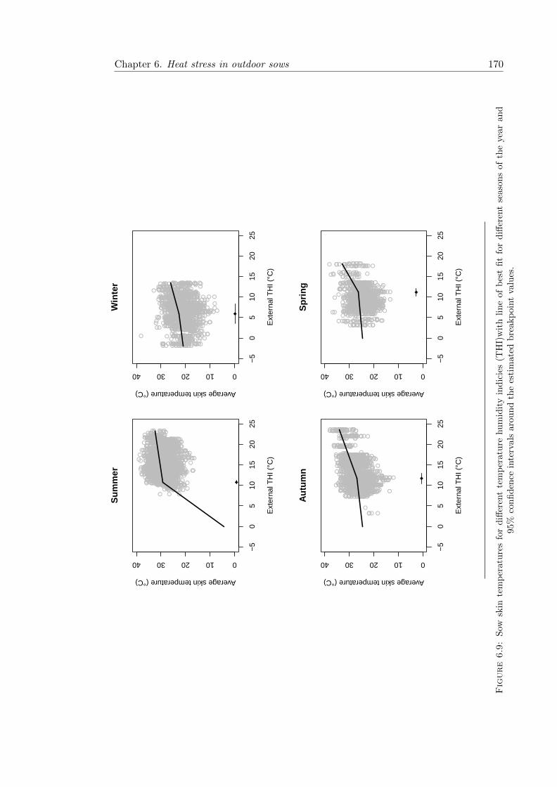
Chapter 6. Heat stress in outdoor sows 170
● ●●
●● ● ●● ●● ●● ●● ●●● ●● ●●●●●● ● ●● ●●●● ●● ●● ●● ●● ●● ●● ● ●●● ● ●●● ● ● ●● ●●● ● ●●● ●● ●●● ●● ● ● ●●●● ●● ●● ● ●●● ● ●●● ● ●●● ● ●●●● ●● ●● ●●●● ● ●● ●● ●● ●●● ●● ● ●●●●● ● ●●● ●● ● ●● ●●● ●●●● ●●● ●● ● ●● ● ●● ●● ● ●● ●● ●●● ●●● ●● ●●● ●● ●●● ●● ●● ●● ●●● ●● ● ●● ● ● ●● ●●●● ● ●●● ● ●● ●● ● ●● ●● ●● ● ●● ●●● ● ●● ●●● ●●●●● ●● ●●● ●●● ● ●● ● ●●● ●● ●● ● ● ●● ●● ● ●● ●● ● ●●● ● ●● ●● ● ●●● ●● ●● ●●● ●●● ●●● ●● ● ●●● ● ●● ●●●● ● ●●● ● ●●● ● ● ●●● ●●●● ● ●●● ●● ● ● ●●● ●●●●● ● ● ● ●●● ●●●● ● ● ●●● ●●● ●● ● ● ●● ● ● ●● ●●●●●● ●● ●● ●● ●● ●●● ● ● ●● ●● ●● ●● ● ●●● ● ● ●● ●●● ●● ●● ● ●● ●●● ●● ●● ●● ●● ●● ● ●● ●●● ●● ● ●● ●●● ● ● ●● ●● ●● ●●●● ● ● ●●● ● ●●●● ●●● ● ●●● ●● ●● ●● ●● ●●●● ●● ● ●● ● ●● ● ● ● ●●● ●●●● ●●● ●● ●● ●● ● ●●● ●● ●● ● ● ● ●●● ●● ●●● ● ● ●●● ●● ●● ●●● ●● ●● ●●● ●● ●● ●● ● ● ● ● ●● ●● ● ● ●● ●● ● ●●● ●● ● ●●● ●● ●●●●●● ●● ●●● ● ●●● ●●●● ● ●● ●● ●● ● ●● ●● ●● ●● ●● ●●● ●● ●● ● ●● ●● ●● ●● ● ●●● ●●●● ●● ●● ●●● ● ●● ● ●●● ●● ● ● ●● ● ●●● ● ●● ●● ● ●● ●● ●● ● ●●●● ● ● ●●●●● ● ●● ●●● ● ●● ●●● ● ●●● ●●● ●●●●● ●● ●● ● ● ●● ●● ●● ● ●● ●●● ●●● ● ●● ●●● ●● ●● ●● ● ●● ● ●● ● ● ●● ● ● ●●● ●●● ●● ●●● ● ●●● ●● ● ●● ●●● ●● ● ●●● ●● ●● ●● ● ●● ●●● ●● ●● ●● ● ●●● ● ● ● ●● ●● ●● ● ● ● ●● ●● ●●● ●● ● ● ● ● ●● ●● ●● ● ●● ● ●●● ● ●● ● ●● ● ●● ●●● ●● ●● ●● ●● ●●● ● ●● ●●● ●● ● ● ● ●●●● ●● ● ●● ● ●● ● ●● ●●●●● ● ●●● ● ●●● ●● ●●● ●● ● ●●● ● ● ● ●●● ● ●● ●● ●● ● ● ● ●● ●●●● ● ●●● ●● ● ● ●●● ● ●●● ●●●● ● ● ●● ●●●● ●●● ●● ● ●●● ●● ●● ● ●● ● ● ●● ●● ● ●● ● ●● ● ●● ●● ● ●● ●● ●● ● ● ●● ● ●● ● ●● ● ●●● ● ●● ● ● ● ●●●● ● ●● ●● ● ●● ●● ●●● ●●● ● ●● ●● ●● ●● ●● ● ●● ●● ● ●●● ●● ●● ●●● ● ● ● ● ●●●● ●● ●● ● ●● ●● ● ●●●●●● ●● ● ●● ●● ●● ●● ● ●● ● ●●● ●● ●● ● ● ●●● ●● ●● ●● ●●● ● ●●● ●● ●●● ●●● ● ●●● ●●● ● ●●● ● ●● ●●● ●● ● ●● ●● ●●● ● ●● ●●●●● ● ● ● ●● ●●● ● ●● ●● ● ●● ●● ●● ●● ● ● ● ●● ● ● ●● ●●● ●●● ●● ●●●● ●●● ●● ●● ●● ●●●● ●● ●●● ● ●● ● ●● ● ● ●● ●● ● ● ●● ●●● ●● ●● ● ●● ●●●● ● ●●●●●● ● ●●● ● ● ● ●●● ●●● ●● ● ● ●● ● ● ●● ●●●● ●● ●●● ●● ● ● ●● ●● ●● ●●● ● ●●●●● ● ●● ●●● ●● ●●● ● ●●● ●● ● ●● ●● ● ●● ●● ●● ●●● ●● ●●● ●● ●● ● ●●● ●● ●●● ● ●● ●● ● ● ●● ● ●● ●●● ●● ●● ●● ●● ●●● ● ●●● ● ●● ● ●● ● ● ●● ●●●● ●● ●●●● ●● ●●● ●● ●●●● ●● ●● ●● ●● ●● ●● ●● ●●● ●●●●● ● ●●● ●● ● ●● ●●● ●●●●● ● ●● ●● ● ●●● ●● ● ●●● ● ●●●● ●● ●● ●●● ● ●● ●● ●●●● ● ●●● ●● ●● ● ● ●● ●●● ● ●● ● ● ●●● ● ● ●●● ●● ●●● ● ●●● ● ● ●● ●● ●●● ● ● ●● ● ●● ●● ●● ● ● ●●●● ●● ●●●● ● ●● ●●●● ●● ●● ●● ●●● ● ● ●● ● ●●● ● ● ●● ● ● ●● ●● ●● ●● ●● ●●● ● ● ●● ●●● ●● ●● ●● ●●● ● ●● ●●●●● ●● ●● ●● ● ●● ●●● ● ●● ●●●●● ●●● ●● ● ● ● ●● ●● ●● ●●● ● ●● ●● ● ● ●●●● ●● ●●●● ●● ●● ●●●● ●●● ●● ●● ●●●● ●● ● ●● ●● ●● ●● ● ●● ● ● ●●● ● ●● ●●● ● ● ●●● ● ●●● ●● ●●● ●● ●● ●● ●● ●● ●● ●●●●● ●●● ●● ● ●●● ●● ●● ●● ● ●● ●● ●● ●●●● ●●● ●●● ● ●●●● ●●●●● ●●● ●● ●●●●● ●● ●● ●● ●●●●● ●●●● ● ● ●● ● ● ● ●● ● ●● ● ● ●●● ● ● ●● ●● ●●●● ●●● ●●● ●● ●● ●●●● ● ●● ● ●● ● ●● ● ●● ●● ● ●● ●● ● ●● ● ●●●● ●●● ●● ●● ● ● ●● ● ● ● ●● ● ●●●● ● ●● ●● ●● ●● ●● ●● ●●● ● ●● ● ● ●● ● ●● ●● ● ●● ● ●● ● ●● ●●●● ● ●●● ●● ●●● ● ●● ●● ●●● ● ●● ●● ●● ● ●●● ●● ● ●●● ● ●● ●●● ● ●●●●● ●● ● ●● ●●● ●● ● ●●●● ●● ● ● ●● ●● ● ● ●● ●●● ●● ●● ●● ● ●● ●● ●●● ●● ● ●● ●● ●●● ● ●● ● ●● ● ●●● ● ●● ●● ● ● ● ●●● ●● ● ● ●●● ●● ●● ●● ●● ● ●●● ●● ● ● ●● ●●● ● ●● ●● ●● ●●● ●● ●● ●●●● ● ●● ●● ● ● ●●●● ●●● ● ●● ● ●●●●● ●● ● ●● ●● ●● ●● ●●● ●●● ● ● ●● ●●● ●● ● ●● ●●●●●● ●●●● ●●● ● ●●●● ● ●● ● ● ●● ●●● ● ● ● ●● ●● ●● ●● ● ● ●● ●● ●●● ● ●● ● ● ●●● ● ● ●● ●● ●● ● ●● ●●● ●● ●● ● ● ●● ●● ●● ●● ●● ●● ●● ● ●●● ●●● ● ● ● ●● ●● ●●●●● ●● ●●●● ●● ● ●●● ● ● ●●● ● ● ●● ●● ● ●●● ●●● ●● ●● ●● ● ●● ● ● ●●● ● ●●● ●● ●●● ●● ●●●● ● ● ● ●● ●●●● ●● ●● ●● ● ● ● ●● ●● ● ●● ●● ● ●● ● ●● ● ●● ●● ● ●● ●● ● ●●● ● ● ●●● ● ●●●●● ● ●●●● ●● ●●● ● ● ● ●● ●● ●●● ●● ● ●● ●● ●● ● ● ● ●●●● ● ●● ●● ● ●● ●●● ● ● ●● ●● ●● ● ●●● ●●● ●● ● ●● ●● ●● ●● ●● ● ●●● ●● ●● ●● ●● ●●●● ●● ●● ● ●● ● ●● ●● ● ● ●●● ●● ●● ●● ●● ●● ● ●●●●● ●● ●● ●● ●● ●●●● ●●●● ●● ● ● ●● ● ●● ● ● ●●●●●●● ● ● ●●● ● ●●● ●● ●●● ●● ●●● ● ● ●● ●●● ●● ●● ●● ● ●● ●●● ●●●● ● ●●●● ●●● ●● ● ●● ● ●● ●● ● ● ●●● ●● ● ● ● ● ●● ●●● ●●● ●● ● ●● ●● ●●● ●● ● ●● ● ●● ● ● ● ●● ●● ●● ●● ● ●●● ● ● ●●● ● ●●● ●●●●● ●●●●● ●● ●●●●●● ●● ● ●●●● ●● ●●●● ● ●● ● ● ●●● ●●● ● ●●● ● ●●●● ● ●●● ●● ●●●●● ●● ● ● ●●● ●● ●●● ● ●● ● ●●● ●●● ●●● ●● ● ●●●● ●● ● ● ●● ●● ● ● ● ● ●● ● ●● ● ●● ● ●● ● ● ●●● ●● ●● ● ● ●●●● ● ●● ●● ●●● ●●● ● ● ●● ●● ● ●● ●●●●● ●● ●● ● ● ●● ●● ● ● ● ●● ● ● ●●● ●● ●● ● ●● ● ●● ● ●● ●● ●● ● ●●● ●●●● ●●●● ●● ● ●● ● ●● ●● ● ●● ●●●● ●●●● ● ● ●● ● ●● ● ● ●● ●● ●● ● ● ●●● ●●● ●● ● ●● ● ●●● ●● ● ● ●●● ●●● ●● ●● ● ● ●● ●● ●●●● ● ●● ●● ●● ● ●●●● ●● ●● ●● ●●● ●● ● ●● ●●● ●● ●● ●●● ● ● ●●● ● ●● ●● ●●●●● ● ●● ●●● ● ●● ●● ●● ● ●● ●●● ●●● ●● ●● ●● ●● ● ●● ● ● ●●● ● ●●● ●● ●●● ●● ●●● ●● ●● ●● ●● ●● ● ●● ●●● ●●● ●● ● ●● ●●●● ●● ● ● ●● ● ● ● ●●● ●● ● ●● ●●● ●● ● ● ● ●●●●● ●●● ●● ●● ● ●●●● ●● ●●●●● ● ●●● ● ●● ● ●● ●● ●●● ●● ●● ● ● ● ●●● ● ●● ●●●● ●● ●●●● ●● ●● ●● ● ● ●● ●● ●● ●●● ●●● ●● ● ● ●● ● ●● ● ● ● ● ●● ●● ● ●●●● ● ●●● ●● ● ●● ● ●●● ● ●● ●● ●● ●●● ●●● ●●● ●● ● ●● ● ●● ●● ●●●● ● ●● ● ●● ●● ● ● ●
−5
05
1015
2025
010203040
Sum
mer
Ext
erna
l TH
I (°C
)
Average skin temperature (°C)
●● ● ●
●●● ● ● ●● ●●●● ●●●● ●● ● ● ●● ● ●● ●●●● ● ● ● ●● ●● ●● ● ● ●● ● ●●● ● ●● ●● ●●●● ●● ●●● ● ● ●● ● ●●● ● ●●● ● ●● ●● ●● ●● ●● ●● ● ●●● ●● ●●● ● ●● ●● ● ●●● ● ●●● ●●● ●● ● ●● ●● ●● ● ●● ●●● ●● ●●● ● ●● ●●● ●● ●● ● ● ● ● ●●●●● ●●● ●●● ● ● ●● ●● ●●● ●●● ●● ●●● ●● ● ●● ●●●● ●● ●● ● ●● ● ● ●●● ●● ● ● ●●● ● ●●● ● ●●● ●● ●● ●●● ● ●●●●●● ● ●●● ●● ●● ● ●● ●●● ●● ● ● ●●● ●●● ● ●● ●●●● ● ●● ●●● ● ● ● ●● ● ●●● ●● ●● ● ●● ● ●● ●●● ●● ● ●● ● ●● ●●●● ● ●● ●●● ● ●●● ●●●●● ● ●● ● ●●●● ●●● ● ●● ●● ● ● ●● ●● ●●●● ● ● ●●● ●●●●● ●● ● ● ●● ●● ● ●●● ●●● ● ● ●●● ● ●●●● ●● ●● ●● ●● ●●● ● ●● ● ● ●● ●● ● ●● ●●● ● ●● ● ●●● ●●●● ●● ●●● ●●● ●● ●● ● ●● ● ● ●● ● ●● ●● ●● ●● ●● ● ●● ● ● ● ●●● ● ●●● ● ●●● ● ●● ● ●●● ● ●● ● ●● ● ● ●●●● ● ● ●●● ● ● ● ●●● ● ●●●● ●● ●●●● ●● ●●●● ● ● ●● ● ●●● ●● ●● ● ● ●● ● ●● ●● ●●● ●● ●● ●● ●● ●●● ● ●●● ● ●● ● ● ●● ● ●● ● ●●●● ●●●● ●●●● ● ● ●● ● ●●● ●● ● ● ●●● ●●● ●●● ●● ● ● ● ●● ●● ●● ●● ● ● ●●● ●●● ●● ●● ●●● ● ● ●● ●● ●● ●● ● ● ●●● ● ●●● ●● ●● ● ●● ● ●● ●●● ●● ●● ● ● ●●●● ● ●●● ● ● ●● ●● ●● ● ●●● ●● ● ●● ● ●●●●●● ●● ● ●●●●● ● ●● ●●● ● ● ●● ● ● ●●●● ●●●● ●●● ● ● ●●●● ●● ●●●● ●● ● ● ●●● ● ● ● ●● ●● ●● ● ●● ●●●● ●● ●●●● ● ●● ●● ●● ●● ● ● ●● ●● ●● ●● ●●● ●● ●● ● ● ●● ●● ●●● ●●● ● ●● ●● ●●● ● ● ●●●● ● ●●● ●● ●● ●●●●● ● ● ●● ● ●●● ●●● ●● ● ● ●● ●●●● ●●● ● ●●●●● ●● ● ● ●●● ●● ● ●● ●●● ●● ●●● ● ●● ● ●● ●● ● ●●●● ●● ● ●●● ●●● ● ●● ●● ●● ●● ● ●●● ●● ●● ● ●●●● ●● ● ●● ●●● ●● ● ●● ● ●●●●● ● ● ●● ●● ●● ● ● ●● ● ● ●● ● ●●●● ● ●●●●●● ●● ● ●●● ●● ● ●● ● ●●● ●● ●● ●●● ● ●● ●●● ●● ● ● ●● ●●● ●●● ● ●●● ●●●● ● ● ●● ●● ●●● ●● ●●●● ●● ●● ●●●● ●● ● ●● ● ●● ● ●●● ● ●●● ● ●● ●● ● ●● ●●● ●● ● ●● ● ●●●● ●● ●● ● ●● ●●● ● ●●●● ● ●● ● ●● ●●● ● ●● ● ●●● ●● ● ●●●● ●● ●● ●● ●● ●● ●● ●●● ●●● ●● ●● ● ●● ● ●● ● ●●● ●● ●● ●● ●● ●● ●● ● ● ● ●● ●● ● ●●● ●● ● ●● ●● ● ●●● ●● ● ● ●●●● ●● ● ●● ●●● ● ● ●● ● ●●● ● ●● ●●● ●●● ● ● ●● ●● ● ●●● ●● ●● ● ● ●● ●● ●● ● ●● ● ● ● ●●● ● ●●● ●●● ●● ● ●●● ●●● ● ● ●● ● ●● ●● ● ●●●●● ●●● ●● ●● ● ● ●● ● ●●● ● ●● ● ●● ●● ● ● ● ●● ● ●● ●●● ●● ●●● ●●●●● ● ●● ● ● ●● ● ●● ●● ● ●● ●●● ● ● ● ●● ●● ●●● ●● ● ● ●●● ● ●● ● ● ● ●● ●● ● ●● ●● ●● ●● ●●●● ● ●● ● ●● ●●● ● ●● ● ●●● ● ●● ●● ●● ● ●● ● ●●● ●●●● ●●● ● ●●●● ●●●● ●● ●● ●● ●● ●● ● ●● ●● ● ●● ● ●● ●● ●● ●● ●● ●● ●●● ●● ●● ● ●● ● ●● ●● ● ● ● ●●●● ●● ●● ●●● ● ●● ● ●●● ●●●● ●●●● ●● ●● ● ● ● ●●● ●●●● ●● ●● ● ●● ●● ●●● ● ● ●● ●●● ●● ●● ●● ●● ● ●● ●● ●● ●●● ● ●●● ● ● ● ●●●● ●●● ● ●● ●● ●●●● ●● ●● ●● ● ●●● ● ●● ●●● ● ●● ● ●● ●● ● ●●● ●●● ●● ●●●● ●●● ●●● ●● ●● ●● ●● ●● ●●● ●●● ● ●● ●●● ● ●
● ● ● ●● ●● ● ●● ●● ● ●●● ● ●● ● ● ●●● ●●● ● ●● ●● ● ●●
●● ● ●●●● ● ●● ● ●● ●● ● ●● ● ●●● ● ●● ●● ●● ●●● ●●● ●● ● ●● ●● ● ●● ● ●● ● ● ● ●● ●● ●● ●
●● ● ●● ● ●● ●● ●● ● ●●● ● ●●● ●● ● ●● ●● ● ●● ●●● ●●● ●●●● ● ● ●● ●● ● ● ● ●● ●● ●● ● ●●● ●● ● ● ●●
−5
05
1015
2025
010203040
Aut
umn
Ext
erna
l TH
I (°C
)
Average skin temperature (°C)
●● ● ●● ● ●●● ● ●●● ●●● ●●●● ●● ● ●● ● ●●● ●● ●● ●●● ●● ●● ● ●●● ●● ● ●●●●● ●● ● ● ●●● ●● ● ●● ●● ●● ● ●●● ● ● ●●● ● ● ●● ●●● ●● ● ●● ●● ●● ●● ●●● ● ● ●● ● ● ●● ●● ●● ●● ●●● ● ●● ●●● ● ● ●● ●● ● ●●● ● ● ●●● ● ● ●● ● ● ●● ●● ●● ●●● ● ●● ●● ●● ● ●●●● ●●●●● ●● ● ● ●● ● ●● ● ●● ● ●● ●● ● ● ●● ●●● ● ●● ●●● ●● ●●●● ●●●● ●● ●●●●● ● ● ●●●● ● ●●●● ● ● ● ●●● ●●● ●●● ●●● ●●●● ● ● ●● ● ●● ● ●● ●● ●●● ●● ● ●●●● ● ● ● ●●●● ●● ●● ●●● ●●● ● ●●● ● ●● ●● ●● ●● ●● ●●● ●● ●●● ● ●● ●● ● ●● ● ●● ● ● ● ●●● ● ●● ● ●● ● ● ●●●●●●●● ●● ● ●● ●● ●●●● ●● ●● ●● ● ● ●●● ● ●● ● ●● ●● ● ● ●● ●●● ●● ● ●● ● ●● ●● ● ●● ●●●● ●● ●●●● ● ●● ●● ●●●●● ●● ●● ● ●●● ●● ●● ● ●●● ●● ●●● ● ● ● ●●● ●●●● ●● ● ●●● ●● ●● ● ●● ●● ●●● ●● ●● ● ●●● ●● ● ●●● ●●● ●●●●● ●● ● ●●●● ●● ●● ●● ●● ● ● ●●●●● ● ●● ● ●● ●● ●●● ●●● ●●●●●● ● ● ● ●● ●● ●●● ● ●●● ●● ●● ● ●●● ● ●●●● ●● ●●●●● ●● ●●● ● ●●● ● ●●●●● ●● ●● ● ●●● ●●● ●● ●●●●● ● ●●● ●●● ●●● ●●● ● ● ●● ●●● ●● ●● ●●● ●● ● ●● ●● ● ● ●● ● ● ●● ●●●● ●● ● ●● ●● ●●● ●● ● ● ●●●●●●● ● ●● ●● ● ● ●● ● ●● ●●● ●●●● ● ●●● ● ●●● ● ● ● ●●● ●● ●●●●● ● ● ●● ● ●● ● ● ●● ●● ● ● ●● ●● ●● ● ● ●● ● ● ● ●● ● ●●● ● ●● ●●● ● ●● ● ● ●●● ● ●●● ●● ● ●● ●● ● ●● ●● ● ●●● ● ●● ●● ●●● ●● ●● ●●● ●● ● ●●● ● ● ●●● ●● ● ●●●● ●● ● ● ●●● ● ●● ●● ● ● ●●●● ● ●●● ●● ● ● ●●● ●● ●● ● ●● ●●● ●● ● ● ●●● ●●● ●● ● ● ●●●● ●●●● ●● ●●● ● ● ●● ●● ●● ●●●● ●●● ●● ● ●●● ● ● ● ●● ●● ● ●●●●●● ●● ● ●●● ●●●●● ● ●● ● ● ● ●●●● ●● ●●● ●● ●● ●● ●●● ● ● ●● ●● ●● ●● ●● ●●● ● ● ●● ● ●●● ●● ●● ●● ● ●● ●● ●●● ●● ●● ●● ● ●●● ●●●●● ●● ● ●● ● ●● ●● ●● ● ●●● ●● ●●● ● ● ●●● ● ● ●● ●● ● ●●● ● ● ●●●● ●●●● ● ●● ●●●● ●● ●● ●● ●●●● ● ● ●●● ●● ● ●● ●●● ●● ● ●● ● ●●● ●●● ● ● ●● ● ●● ●● ●● ●● ●● ●●●●● ● ● ● ●● ● ● ● ●●● ●● ● ●●●● ● ● ●● ● ●● ●● ● ●● ● ●● ●●● ●●● ●●● ●● ● ●● ●●●● ● ●●● ●● ●● ●● ●● ● ●● ●●● ● ●● ●● ●● ● ●●●● ●●●●●● ● ● ●● ●● ●● ●● ●● ●● ● ●●● ●● ●● ●●● ●● ●● ● ● ●● ● ●●● ● ● ●● ●●● ● ● ● ●●●● ● ●● ●● ● ● ●●●● ● ●● ●● ● ●● ●●● ●● ● ● ●● ●●● ●●●● ● ● ●● ●● ●● ●● ● ●● ● ●●●● ●● ●●●● ● ●●●●● ● ●●●●● ● ●●● ● ● ●● ●●● ●●●● ●● ●● ●●● ● ● ●● ●● ●● ●●●●● ● ●● ●● ●● ● ●● ● ●● ● ●●●● ●● ●● ●● ● ●●● ●●●● ●● ● ● ● ●●● ●●● ●●●● ● ●● ● ●● ●● ●● ● ●● ●●● ●●●● ●● ● ●● ● ● ●●● ●●● ●● ●● ●● ● ●●● ● ●● ●● ●●● ● ●● ● ● ●● ●● ●● ●● ● ●● ●
● ●● ●● ●● ●● ● ●● ● ●● ●● ● ●●● ●● ●●● ●● ●● ● ●●●● ● ●●●● ●● ●● ●●● ●● ●● ● ●● ●● ●● ● ● ●● ●●● ●●● ●● ● ● ●● ● ●● ●●● ●●● ● ● ●●
−5
05
1015
2025
010203040
Win
ter
Ext
erna
l TH
I (°C
)
Average skin temperature (°C)
● ●● ●● ● ● ● ●●● ● ●●● ●●
● ●● ●● ● ●● ●● ●● ●●●● ● ● ●●● ●● ● ●●● ●● ●●●● ●● ●● ●● ●
● ● ● ●● ●●● ●●● ● ● ●● ●●●● ●● ●●● ●● ● ●● ●●●● ●●● ● ●●● ●● ● ● ●●● ●● ●● ●● ●● ● ●●● ●● ●●● ●● ●● ●● ● ●● ●● ●● ● ●● ●●● ●●● ● ● ●● ●● ●● ●● ● ●● ● ●● ● ●● ●●● ● ● ●●● ● ● ●● ●●● ●●● ● ●● ●● ● ● ●●● ●● ●●● ● ●● ●● ●● ● ●●●●● ● ● ●●● ●●● ● ●● ● ● ● ●●●● ● ●●● ●●● ● ●●●● ● ●●● ●●● ● ● ●● ● ●●●● ● ● ●●● ●● ●●● ● ●●● ●● ●●● ●●●● ●●● ●●● ● ● ●● ●● ● ●●● ●●● ●● ●●● ●●● ● ● ●●●●●● ●●●●●● ● ● ●● ●● ● ●● ● ●●● ● ●●● ● ●●● ●● ●● ●● ●● ●●●●● ●● ●● ● ●● ●● ●● ●● ● ●●● ●●● ● ●● ●●● ● ●●● ● ●● ●●●●● ● ● ● ● ●● ●● ● ● ●● ●●● ●● ●●●●● ● ● ● ● ●●● ●● ●●●● ● ●● ●●● ●● ●● ●●● ● ●● ●●●● ● ●● ●● ● ●● ●● ●● ●●●● ●● ●●● ● ●●● ●● ● ●●● ● ●●● ● ●● ●● ●● ● ●●● ●● ●● ●● ●● ● ●● ●● ● ●●● ●●● ● ●●● ●● ● ● ● ●●●● ●●● ● ● ●● ● ● ● ●●● ●● ●● ●● ●●● ● ●● ●● ●● ●● ●●● ●● ● ●● ●● ●● ● ● ●● ●● ●● ●●● ●●● ●● ●● ● ●●● ●● ●● ●● ● ●●● ●● ●● ●●● ● ● ●●● ●● ●●● ● ● ●● ●● ● ●●●● ●● ● ●● ● ● ● ●● ●● ●●● ●●● ●●●● ● ● ●● ●●● ●●● ●● ●● ●●● ●● ● ●●●● ● ● ●●● ● ●●● ●● ● ●●●●● ● ● ●● ●●● ● ● ● ●●●●● ● ●●● ● ●●●● ● ●● ●●● ●●●● ● ●● ●● ● ●●●● ● ●● ●● ●●● ●● ● ●● ●●● ● ● ● ●● ●● ● ●●●● ● ● ●● ●●● ●● ●●● ●●● ●● ● ● ●●● ● ● ●● ●● ●●●● ● ●●●● ● ●● ●● ●●●● ●●● ●●● ● ●● ● ●●● ● ●●● ● ●● ●●●● ●●● ● ● ●●●● ● ●● ●● ●●● ● ● ●●● ● ●● ●● ● ●● ●●● ● ●●●● ● ●● ●● ● ● ● ●● ●● ●● ●●● ● ● ●●●● ●● ●● ● ●●● ●●●●● ● ●● ●● ●●● ●●●● ● ● ●● ● ●● ● ● ● ●● ●● ●● ●● ● ● ● ●● ●● ●● ●● ●●●● ●● ●●● ● ● ●● ●● ● ●●● ●●●● ● ● ●●●● ●● ●● ● ●●● ●● ●● ●●● ●● ●●● ● ●●●● ● ●● ●● ●●●● ●●●● ●● ● ●● ●●● ● ● ●●● ●●● ●●●●●● ●●● ●●● ● ●●● ●● ●●● ● ● ●● ●●●●●● ●● ● ● ● ●● ●●● ●●● ●● ● ● ●● ●●●● ● ●● ●●● ● ● ●●●● ●● ● ●●● ●● ●● ●● ●● ●●● ●● ●● ●● ●●● ●●●● ●● ●● ●● ● ●● ●●
● ● ●●● ●● ● ●●● ● ●● ●● ●●● ●● ● ●●● ●● ● ●●● ●●●● ● ● ●● ● ●● ● ●● ●● ● ●● ●● ●●● ●● ●● ●● ● ●●● ●● ●●
−5
05
1015
2025
010203040
Spr
ing
Ext
erna
l TH
I (°C
)
Average skin temperature (°C)
Figure6.9:
Sow
skin
tem
per
atu
res
for
diff
eren
tte
mp
eratu
rehu
mid
ity
ind
icie
s(T
HI)
wit
hli
ne
of
bes
tfi
tfo
rd
iffer
ent
seaso
ns
of
the
yea
ran
d95
%co
nfi
den
cein
terv
als
aro
un
dth
ees
tim
ate
db
reakp
oin
tva
lues
.

Chapter 6. Heat stress in outdoor sows 171
Table 6.9: Coefficients from piecewise regression models of the effects of season ontemperature humidity index and sow skin temperature throughout the year.
Estimate Std. Error t value P value
Summer 25.871 0.398 64.950 < 0.001
Autumn 20.981 0.356 58.863 < 0.001
Winter 20.958 0.214 98.082 < 0.001
Spring 22.284 0.374 59.620 < 0.001
THI.sum 0.296 0.0262 11.330 < 0.001
THI.aut 0.536 0.0249 21.521 < 0.001
THI.win 0.359 0.028 12.762 < 0.001
THI.spr 0.449 0.040 11.343 < 0.001
lactweek2 0.298 0.120 2.476 0.013
lactweek3 0.365 0.122 2.989 0.003
lactweek4 0.288 0.148 1.944 0.052
lactweek5 -0.506 0.432 -1.172 0.241
noon -1.622 0.135 -12.001 < 0.001
afternoon -2.136 0.135 -15.751 < 0.001
evening 0.034 0.137 0.251 0.802
solar radiation 0.001 0.000 2.650 0.008
rainfall 0.530 0.156 3.398 < 0.001
wind speed -0.269 0.020 -13.594 < 0.001
Models included temperature humidity index, season, lactation week (week 1 as inter-cept), time of day (morning as intercept), solar radiation, rainfall and wind speed.
Table 6.10: Slopes with 95% confidence intervals from piecewise regression models ofthe effects of temperature humidity index on skin temperature for different seasons.
Slope Estimate St.Error t value Lower CI (95%) Upper CI (95%)
Summer1 2.318 0.471 4.922 1.395 3.241
2 0.249 0.029 8.650 0.193 0.305
Autumn1 0.179 0.115 1.554 -0.047 0.406
2 0.620 0.036 16.920 0.548 0.692
Winter1 0.207 0.069 2.977 0.071 0.343
2 0.485 0.059 8.204 0.369 0.601
Spring1 0.139 0.073 1.885 -0.006 0.284
2 0.965 0.105 9.231 0.760 1.170
Models included temperature humidity index, season, lactation week, time of day, solarradiation, rainfall and windspeed.

Chapter 6. Heat stress in outdoor sows 172
6.5.3 Respiration rates
Coefficients of terms for the relationship between respiration rate and external conditions
are shown in Table 6.11.
Table 6.11: Coefficients for the fixed effects of the linear mixed effects model for thelog of respiration rate.
Estimate Std. Error t value P value
(Intercept) 3.0006 0.0629 47.66 <0.001
THI 0.0215 0.0024 9.06 <0.001
rain 0.2157 0.2804 0.77 NS
sun -0.0005 0.0002 -2.53 0.011
wind -0.0058 0.0066 -0.87 NS
time -0.0630 0.0018 -3.57 <0.001
activity -0.0964 0.0241 -4.01 <0.001
week -0.0207 0.0179 -1.16 NS
THI:rain -0.0195 0.0242 -0.80 NS
THI:sun 0.0000 0.0000 3.43 <0.001
rain:sun -0.0020 0.0047 -0.42 NS
THI:wind -0.0009 0.0006 -1.56 NS
rain:wind -0.0935 0.0514 -1.82 0.069
sun:wind 0.0000 0.0000 -0.61 NS
time:activity 0.0251 0.0097 2.59 0.01
time:week 0.0331 0.0067 4.93 <0.001
activity:week 0.0231 0.0089 2.59 0.01
THI:rain:sun 0.0002 0.0004 0.44 NS
THI:rain:wind 0.0096 0.0045 2.16 0.031
THI:sun:wind 0.0000 0.0000 2.16 0.031
rain:sun:wind 0.0012 0.0010 1.17 NS
time:activity:week -0.0116 0.0036 -3.23 0.001
THI:rain:sun:wind -0.0001 0.0001 -1.08 NS
Data presented as log values. Parameters included in model were temperature humid-ity index (THI; ◦C), rainfall (mm), solar radiation (W/m2), wind speed (mph), timeof day (morning, noon, afternoon, evening), activity (lying down, standing, nursing,
rooting/eating or drinking), week of lactation and their interactions.
The mean respiration rate was 20.1 bpm (log 3) and increased with THI (Figure 6.10;
P < 0.001). This effect was amplified with increasing solar radiation (P < 0.001).
Although rain and wind did not have significant effects on respiration rate as single
factors, increasing levels of wind in combination with increased rain resulted in a trend

Chapter 6. Heat stress in outdoor sows 173
−2 −1 0 1 2 3 4 5 6 7 8 9 10 11 12 13 14 15 16 17 18 19 20 21 22 23 2415
20
25
30
35
40
45
THI (°C)
Res
pira
tion
rate
(br
eath
es/m
in)
Figure 6.10: Sow respiration rates (bpm) for different temperature humidity indicies(THI). Presented as mean ± standard error.
−2 −1 0 1 2 3 4 5 6 7 8 9 10 11 12 13 14 15 16 17 18 19 20 21 22 23 2410
15
20
25
30
35
40
45
50
THI (°C)
Res
pira
tion
rate
(br
eath
es/m
in)
SummerAutumnWinterSpring
Figure 6.11: Sow respiration rates (bpm) for different temperature humidity indicies(THI) for the different seasons of the year. Presented as mean ± standard error.

Chapter 6. Heat stress in outdoor sows 174
05
1015
2025
3035
40020406080100
Sow
(ar
bitr
ary
num
ber)
Respiration rate (bpm)B
atch
1 (
July
)
05
1015
2025
3035
40020406080100
Sow
(ar
bitr
ary
num
ber)
Respiration rate (bpm)
Bat
ch 4
(N
ovem
ber)
A B
Figure6.12:
Ind
ivid
ual
resp
irat
ion
rate
s(b
reat
hes
/m
inu
te;
bp
m)
for
sow
sin
A)
asu
mm
erb
atc
han
dB
)a
win
ter
batc
h.
Pre
sente
das
mea
n±
stan
dard
dev
iati
on
.

Chapter 6. Heat stress in outdoor sows 175
for lower respiration rates, and this became significant if the THI was also increasing (P
= 0.031). If THI and solar radiation were high, wind also helped to reduce respiration
rates (P = 0.031). Sow respiration rate decreased throughout the day during the first
week of lactation however during the following weeks it increased as the day progressed.
Sows which were lying down had lower respiration rates than those which were standing
or active and this was amplified later on into the day and into lactation (P = 0.0012).
It was also found that individual sows behaved differently, with some having lower
respiration rates than others. In the spring and summer batches respiration rates were
generally higher (Figure 6.11) and more variable (Figure 6.12).
6.5.4 Changes in Farrowing hut conditions
Farrowing hut THI changed over the course of the day (Figure 6.13) with the warmest
temperatures around midday and the coldest overnight. A similar pattern was followed
for all hut types.
Midnight 4am 8am Noon 4pm 8pm4
6
8
10
12
14
16
18
20
22
Time of day
Tem
pera
ture
Hum
idity
Inde
x (°
C)
Insulated triangleInsuated arcNon−insulated arcNon−insulated triangle
Figure 6.13: Temperature humidity index values for four different hut types over thecourse of 24 hours. Values average over the whole year.

Chapter 6. Heat stress in outdoor sows 176
−5
05
1015
2025
−5051015202530
Insu
late
d tr
iang
le
Logger THI (°C)
Ext
erna
l TH
I (°C
)−
50
510
1520
25−
5051015202530In
sula
ted
arc
Logger THI (°C)
Ext
erna
l TH
I (°C
)
−5
05
1015
2025
−5051015202530
Non
−in
sula
ted
arc
Logger THI (°C)
Ext
erna
l TH
I (°C
)−
50
510
1520
25−
5051015202530N
on−
insu
late
d tr
iang
le
Logger THI (°C)
Ext
erna
l TH
I (°C
)
AB
CD
Y =
(0.
90 x
X)
- 3.
9°C
Y =
(1.
01 x
X)
- 2.
7°C
Y =
(1.
07 x
X)
- 2.
0°C
Y =
(1.
08 x
X)
- 1.
5°C
Figure6.14:
Lin
ear
rela
tion
ship
bet
wee
nfa
rrow
ing
hu
tte
mp
eratu
rehu
mid
ity
ind
ex(T
HI)
an
dex
tern
al
TH
Ifo
rA
)In
sula
ted
tria
ngu
lar
hu
ts;
B)
Insu
late
dar
cs;
C)
Non
-in
sula
ted
arcs
;D
)N
on
-in
sula
ted
tria
ngula
rhu
ts.
Ineq
uati
on
s,Y
isth
ehu
tT
HI
an
dX
the
exte
rnal
TH
I.

Chapter 6. Heat stress in outdoor sows 177
Table6.12:
Far
row
ing
hu
tco
nd
itio
ns
for
the
diff
eren
thu
tty
pes
thro
ugh
ou
tth
etr
ial
Huttype
Batch
1a
23
45
67
89
10a
Temperature(◦C)
Insulatedtriangle
17.5
(6.7-37.2)
16.4
(7.0-31.9)
15.1
(1.9-37.4)
12.8
(1.9-24.3)
5.9
(-5.1-
19.12))
7.2
(-5.0-27.9)
12.1
(-0.8-37.6)
11.2
(-0.3-23.6)
14.7
(3.7-33.1)
18.1
(9.7-28.9)
Insulatedarc
18.9
(8.4-39.9)
16.7
(5.0-30.6)
16.0
(2.7-39.2)
12.9
(2.7-26.6)
6.3
(-5.6-23.6)
6.8
(-5.0-23.3)
-9.9
(-2.9-33.4)
16.1
(4.0-42.0)
18.7
(6.6-36.5)
Noninsulatedarc
19.0
(8.1-46.1)
17.6
(4.7-46.1)
15.4
(1.5-36.2)
11.8
(1.5-24.4)
4.9
(-7.1-22.3)
6.6
(-7.1-26.2)
-10.8
(-3.4-28.8)
15.9
(3.4-42.3)
18.3
(7.8-31.1)
Noninsulatedtriangle
17.9
(6.5-38.0)
16.3
(5.1-32.5)
14.7
(1.7-35.8)
11.6
(1.7-21.7)
4.5
(-6.1-14.6)
6.7
(-6.1-27.8)
10.2
(-0.9-35.7)
11.3
(2.1-29.9)
15.5
(3.4-39.9)
18.0
(7.8-31.7)
Humidity(%)
Insulatedtriangle
77.1
(30.5-100)
78.9
(32.5-100)
78.6
(27.8-100)
86.2
(38.9-100)
89.0
(37.0-100)
85.3
(34.9-100)
75.3
(20.4-100)
79.5
(29.6-100)
80.5
(29.6-100)
82.2
(43.0-100)
Insulatedarc
72.8
(27.8-100)
76.8
(30.1-100)
75.0
(26.6-100)
86.6
(40.0-100)
87.5
(37.4-100)
85.1
(37.4-100)
-81.8
(21.0-100)
78.3
(20.5-100)
80.1
(29.1-100)
Noninsulatedarc
73.8
(14.7-100)
75.7
(14.7-100)
78.9
(32.7-100)
90.9
(42.9-100)
31.4
(29.3-100)
87.9
(38.2-100)
-80.9
(25.1-100)
78.1
(26.6-100)
83.3
(43.7-100)
Noninsulatedtriangle
76.5
(29.6-100)
79.3
(30.0-100)
80.4
(30.3-100)
90.8
(47.8-100)
91.9
(53.9-100)
88.5
(42.2-100)
79.7
(14.9-100)
81.3
(25.3-100)
80.8
(27.5-100)
84.9
(34.2-100)
THI(◦C)
Insulatedtriangle
b16.9
(6.7-28.8)
16.0
(7.6-25.6)
14.8
(2.4-28.9)
12.8
(2.4-21.9)
6.3
(-5.1-18.2)
7.6
(-4.6-23.5)
12.1
(0.4-28.8)
11.4
(-0.1-20.7)
14.5
(4.3-27.4)
17.6
(9.8-25.9)
Insulatedarc
18.0
(8.4-31.0)
16.2
(5.2-25.3)
15.5
(2.9-29.8)
12.9
(2.9-22.6)
6.7
(-5.6-20.7)
7.4
(-4.5-21.1)
-10.0
(-2.8-26.7)
15.5
(4.0-31.9)
17.9
(6.6-29.4)
Noninsulatedarc
b18.0
(8.1-32.1)
16.9
(4.9-31.2)
15.0
(1.8-28.5)
11.9
(1.8-22.4)
5.3
(-7.1-19.8)
7.0
(-7.1-22.3)
-10.9
(-3.3-24.5)
15.4
(3.6-31.8)
17.7
(8.6-27.0)
Noninsulatedtriangle
17.1
(6.5-30.3)
15.9
(5.1-25.6)
14.4
(2.1-28.8)
11.7
(2.1-20.5)
4.9
(-6.1-14.6)
7.0
(-6.1-23.8)
10.1
(-0.8-26.9)
11.3
(2.3-24.6)
14.5
(3.9-31.3)
17.5
(7.8-26.4)
Res
ult
spre
sente
das
mea
n(r
ange
inb
rack
ets)
.A
llsi
ngle
an
din
tera
ctio
neff
ects
are
sign
ifica
nt
(P<
0.0
01)
un
less
oth
erw
ise
state
d.
aT
hes
eb
atch
esd
idn
oth
ave
sign
ifica
nt
diff
eren
ces
inhu
tte
mp
eratu
re.
bT
emp
eratu
rehu
mid
ity
index
(TH
I)d
idn
ot
diff
erb
etw
een
thes
ehu
tty
pes
.-
Bat
chse
ven
only
had
tria
ngle
shap
edhu
tsan
dso
data
for
arc
sare
mis
sin
g.

Chapter 6. Heat stress in outdoor sows 178
Farrowing hut THI was found to be linearly correlated with external THI (R2 = 0.84; P
< 0.001), and an interaction with farrowing hut type existed (Figure 6.14; P < 0.001).
Each hut type had a slightly different relationship with external THI (Figure 6.14).
When considering temperature, humidity and THI in the different hut types, for the
different batches, it was found that batch, hut type and their interactions were significant
for both temperature and humidity (P < 0.001 for all) and that for THI, batch and its
interactions with hut type were significant (P < 0.001 for both; Table 6.12).
Throughout the year insulated arcs were the warmest hut type with temperatures peak-
ing in the summer and non-insulated triangles the coldest with winter batches suffering
from the coldest conditions (Table 6.12). Humidity followed the opposite pattern with
insulated arcs being the least humid and non-insulated triangles the most. Insulated
triangles and non-insulated arcs did not have THI which differed, probably due to the
crossing over of temperature and humidity values.
6.6 Discussion
6.6.1 Physiological signs of heat stress in sows
This experiment has shown that sows increase their skin temperature in response to
increasing ambient THI, presumably to increase heat loss. Following a linear increase
of skin temperature from a THI of 5 ◦C, a plateau in skin temperature was reached and
maintained between 15 and 20 ◦C. This may correspond to the sows’ thermoneutral
zone whereby sows are able to maintain a steady core temperature and as such there
is no need to increase heat loss via the skin. Sow skin temperature was then found to
linearly increase with THI when 20 ◦C was surpassed, which may correspond to when
sows become heat stressed and as such actively work to dissipate heat. This is in contrast
to what was expected, as it was thought that a final plateau would be reached which
would represent the sow’s UCT where skin temperature was no longer able to increase
in response to rising ambient temperatures. This does however support previous work
where flank and back temperatures increased with increased ambient temperature (34.6
to 37.4 ◦C between 18 and 29 ◦C), although udder temperature reached a plateau at
25 ◦C (Quiniou and Noblet, 1999).
In the present study the maximal THI reached during the year did not surpass 25 ◦C
and so information on the final skin temperature plateau of outdoor sows may not have
been acquired. When conducting experiments in a commercial outdoor environment,
with no control on external conditions and only the ability to monitor them, not all

Chapter 6. Heat stress in outdoor sows 179
scenarios can be achieved. The fact that the THI at which sows began to increase their
skin temperature for a second time following the plateau was 20 ◦C implies that this is a
critical value for outdoor sows. It is lower than the cited values of 22 to 25 ◦C in indoor
sows (Black et al., 1993), showing that differences between sows kept in indoor and
outdoor conditions do exist. It is however warmer than the implicated value of 18 ◦C
in Chapter 3, which was established from analyses of data from outdoor production
units. However the aforementioned chapter used historical data from a different group
of herds, in a different part of the country. In addition the weather data were more
generic across the herds studied, using one weather station for several herds. Differences
may therefore arise from the different genetic pools, the average conditions to which the
sows were exposed to and the generalisation of weather conditions across several herds.
In addition the use of data to discover trends in reproductive ability is only a platform
for creating trials on which empirical data can be collected and analysed, which is what
has been done in the present study.
The reaction of sows to increasing temperatures was also found to differ throughout
the year. Compared to summer, in spring sows increased their skin temperature more
rapidly in response to rising THI, suggesting that following the winter period when tem-
peratures are colder, sows become acclimatised to the cooler conditions and thus react
more adversely to rising temperatures in spring. This supports previous work in piglets
where exposure to cold temperatures resulted in pigs which not only were morphologi-
cally adapted to a colder environment (smaller ears, more hair and fat insulation) but
also pigs which suffered from a more adverse reaction to increased temperatures fol-
lowing cold exposure (Dauncey and Ingram, 1986; Derno et al., 1995). With the use
of large scale outdoor production being relatively new in the UK and otherwise only
really practiced in some parts of the US, there is no literature available on the acclima-
tisation of lactating sows under outdoor production systems. It should be considered
however that sow genetics have changed to accommodate for the harsher environment
which outdoor sows are exposed to and so it is plausible that heat tolerances have also
changed. Data suggest that sow line differences in heat tolerance exist between sows
bred for hot and temperate climates (Bloemhof et al., 2008) and in growing pigs kept in-
doors, short- and long-term physiological reactions during heat acclimatisation differed
between Creole and Large White breeds (Renaudeau et al., 2007). Unfortunately in the
present study, data on the physical characteristics of sows were not collected. It would
have been interesting to see whether differences in hair length and ear size did exist for
example between sows which as gilts had been reared outside in winter or in summer.
Physiological signs of heat stress occur at moderate temperatures in modern pigs since
these animals have high metabolic activity and high heat production (Huynh et al.,

Chapter 6. Heat stress in outdoor sows 180
2005). As seen in the present study, the animals first level of defense against heat stress
is to increase respiratory rates. When this is no longer sufficient, core temperature
starts to increase (Brown Brandl et al., 2011). Skin temperature is affected by both
internal and ambient temperature (Renaudeau et al., 2010) and so assuming that under
thermoneutral conditions sows maintain their core temperature, rises in core temper-
ature under heat stressed conditions will translate into increased skin temperature as
the animal works to dissipate the heat. Much of the heat transfer between a pig and
its environment occurs through its skin (Ingram, 1973) and most of the heat lost from
the skin to the surrounding environment is produced in the inner core of the body. By
vasodilation and vasoconstriction, the animal is capable of increasing or decreasing skin
temperature (Fialho et al., 2004). As seen during this experiment, increases in skin
temperature have been reported at high ambient temperatures, presumably in response
to increased blood flow to the skin from the core as a specific response to heat expo-
sure, contributing to maintain a gradient between skin and ambient temperature and
hence to maintain sensible heat loss (Quiniou and Noblet, 1999; Renaudeau et al., 2001;
Collin et al., 2002; Renaudeau et al., 2003). This results in a redirection of blood flow
from peripheral organs to the skin (Black et al., 1993) and in Large White × Landrace
sows exposed to 28 compared to 20 ◦C it was shown using transit time ultrasonic flow
probes that mammary blood flow increased by approximately 5%, most likely due to an
increased proportion of blood flow to the skin capillaries in order to dissipate body heat
(Renaudeau et al., 2003).
In addition respiration rate was correlated with ambient temperature, supporting pre-
vious work where respiratory rate increased with ambient temperature (26 to 124 bpm
between 18 and 29 ◦C; Quiniou and Noblet 1999) but contradicting early work where,
for up to four days post farrowing, no significant differences in rectal temperature or
respiratory rate between sows kept at 20.5 or 29.8 ◦C were found (Kelley and Stanley,
1978). Low (0 to 5 ◦C) and high (20 to 25 ◦C) ambient temperatures have been shown
to result in increased respiration rates, relating to an increased need for oxygen under
cold conditions and an increased need for evaporative heat loss under warm conditions
respectively (Ingram and Legge, 1969). Early work has shown that a combination of
high ambient temperature, humidity and solar radiation results in high respiration rates
and that this can occur for exposure lengths of as little as 15 minutes (Tidwell and
Fletcher, 1951). In accordance with previous work, individuals differed significantly in
respiration rates during the same period of time. This suggests that individuals differ
in their ability to cope with factors which tend to increase body temperature. In order
to maintain the same body temperature certain individuals had to increase respiration

Chapter 6. Heat stress in outdoor sows 181
significantly more than others. This did not appear to relate to milk production, as sows
with larger litters did not have significantly higher respiration rates (data not shown).
Other meteorological conditions were found to influence both sow skin temperature and
respiratory rates. Increased solar radiation resulted in higher skin temperatures, as
did the presence of rain. The effects of solar radiation on beef cattle are well defined
and have been shown to interact with increased THI to reduce feed intake and increase
water intake and heat load (Arias and Mader, 2011; Mader et al., 2003, 2002; Amundson
et al., 2006). Even in the harp seal it has been shown that skin temperature is dependent
on solar radiation (Oritsland and Ronald, 1973). Using a computer simulation, Fialho
et al. (2004) found that in pigs when skin was exposed to sunlight, with a maximum
solar radiation intensity of 894 W/m2 at noon and no shade available, body temperature
increased sharply above the UCT during the day, inhibiting both feed intake and growth.
The effect of solar radiation on skin temperature in the present study was not quite so
dramatic, with a very shallow slope of increase, and respiration rate only increased if THI
were also elevated. The presence of rain was also found to increase skin temperature,
most probably because moisture in the air increases humidity which in turn interferes
with evaporative heat loss, especially at higher temperatures (Ingram, 1973). Conversely,
wind reduced skin temperatures since increased air movement will result in increased
convective heat loss (Monteith, 1974). In fact it was found that the presence of both
rain and wind reduced sow respiratory rates, since wet skin exposed to windy conditions
will result in higher surface heat loss than respiratory heat loss due to the increase in
humidity.
Sows’ skin temperatures increased until the fourth week of lactation, whereafter they
began to decrease. Producing milk for increasingly larger piglets places a huge metabolic
strain on the sow (Valros et al., 2003) resulting in increased body temperatures (Prunier
et al., 1997). However by the fifth week of lactation outdoor piglets suckle less frequently
and consume more solid feed (Hotzel et al., 2004), therefore sows will be nursing less
frequently and so the previous metabolic strain will be reduced. Sow skin temperature
was found to be highest in the evening, and during the later weeks of lactation respira-
tion rates progressively increased throughout the day. This suggests a build up of heat
throughout the day when the sows are most active, which is then able to dissipate in the
evening when sows are resting. In general longer lactation periods resulted in improved
body condition, a surprising result since body weight loss has been shown to signifi-
cantly increase in the later stages of lactation (Hulten et al., 2002). Nonetheless body
condition score did reduce if temperatures were elevated throughout lactation, support-
ing work by Quiniou and Noblet (1999) who found that backfat thickness significantly
reduced throughout lactation as ambient temperature increased, although there was a

Chapter 6. Heat stress in outdoor sows 182
less obvious difference in weight loss for the same period of time. Data on backfat losses
are equivocal, with some studies claiming that backfat losses were reduced if sows were
weaned early (Willis et al., 2003), whereas on organic farms with seven weeks lactation
backfat levels remained good (Kongsted and Hermansen, 2009). This may relate back
to outdoor piglets being more independent and therefore the lactational load in outdoor
sows being lower during late lactation. This would mean that over an extended lactation
period sows would be able to build up their reserves once more, since they have access to
feed ad libitum. Body condition scoring is not as good a measure of condition as ultra-
sonic backfat measuring or weighing, since it is a subjective measure. Although Coffey
et al. (1999) associated specific backfat levels with body condition scores, subsequent
work has shown backfat levels and body scores to be poorly correlated (Young et al.,
2001; Maes et al., 2004). However when carried out by the same individual, it is an
adequate estimator of sow metabolic state if other facilities are unavailable (Fitzgerald
et al., 2009). Excessive sow handling was not possible in the current study due to a lack
of available personnel and as such body condition scoring by sight was the only available
option.
6.6.2 Consequences of heat stress in sows
Although evidence of sows working to dissipate more heat as temperatures rose was
found, this did not necessarily translate into obvious negative effects on productivity. For
example conception rates were not found to be related to the weather. It would normally
be expected that summer conception rates would be lower than winter conception rates
due to the negative effects of increased temperatures (Love et al., 1995). Under hot
conditions, sow feed intake is generally reduced (Black et al., 1993; Love et al., 1993;
Prunier et al., 1997). This results in an inability to meet the metabolic demands of
lactation resulting in mobilisation of body reserves, reduced body condition at weaning
and hence reproductive problems (Baidoo et al., 1992; Prunier et al., 1997; Clowes
et al., 2003; Kongsted and Hermansen, 2009). It is important to note however that in
the present study the sows were served outside in service tents. They were therefore
often served in cold conditions, such as during batch five which had the lowest overall
conception rate. Adverse working conditions could affect the quality of service due to
the service-man rushing to complete the job. This could balance out annual conception
rates, resulting in the non-significant results observed and masking the negative effects
of heat stress on sows conception rates. So although not directly related to the weather,
management changes due to the weather may have an influence. The storage of semen
within service tents may also be of importance. Although kept in insulated boxes, the
sows served first would most likely receive better quality semen than those served last,

Chapter 6. Heat stress in outdoor sows 183
since the semen would have either cooled down or warmed up during the time it took
to serve all the animals. This suggests that in order to optimise sow productivity, the
working conditions of farm staff on outdoor units need to be improved. Large production
units will have several members of experienced staff, however staff turnover can be high
(personal communication; Dents, 2012). This high turnover generally occurs in winter
as the working conditions deteriorate and people leave. Although service tents will be
marginally warmer than no shelter due to there being a windbreak for example, more
permanent facilities with temperature control could result in improved sow reproductive
outputs. This would be as a result of staff being more comfortable and taking more time
to work with the sows, as well as the maintenance of experienced staff for longer periods
of time. There is no doubt that this would come at an additional cost to producers,
however in the long term the financial gain could be significant. Staff would stay for
longer and become more experienced, reducing recruitment costs, and sow outputs would
be more consistent, resulting in increased profits. In addition, the current data set
was relatively small and not balanced for parity. Therefore proportion values such as
conception rates may not produce as informative data as one could expect from large
data sets such as that used in Chapter 3.
Wean to service interval was not affected by meteorological conditions either. It was how-
ever found to be extended following longer lactation lengths and since change in body
condition score was not found to be affected by lactation length, nutritional deficits
are an unlikely cause and so lactational oestrus may be a candidate. The inhibition
of the hypothalamic-pituitary-ovarian axis during lactation is mainly due to suckling
induced neuroendocrine changes (Quesnel and Prunier, 1995), with sow nutrition nor-
mally playing more of a role after about three weeks of lactation. Sows generally return
to heat five days post-weaning due to the cessation of these stimuli. Therefore any
factors which affect suckling during lactation, such as the death of a high proportion
of the litter reducing the litter size or multisuckling with some sows taking on more
piglets than others, can mimic the effects of weaning and result in lactational oestrus.
In outdoor environments nursing frequency decreases markedly by the fifth week of lac-
tation (Wallenbeck et al., 2008), coinciding with an increase in the piglets intake of solid
feed (Damm et al., 2003). This increases the chances of lactational oestrus occurring
since suckling is limited and the fact that sows with larger litters did not experience
longer WSI, even for longer lactation lengths, supports this. A larger litter would mean
more stimuli for milk production would have been present and so oestrus would have
been inhibited. It was found that batch seven sows had significantly longer WSI than
sows in the other batches. This was potentially due to the lower parity profile of the
batch, since younger sows were found to have longer WSI. It has been consistently found

Chapter 6. Heat stress in outdoor sows 184
within the literature that older sows have shorter WSI (Hulten et al., 2002; Kongsted
and Hermansen, 2009; Koketsu et al., 1997) and are able to withstand higher lactational
losses before negative effects on reproduction are observed (Thaker and Bilkei, 2005).
In addition this was a period of field changeover and so the quality of oestrus detection
may have been lower with the farmers being busy with other things on the farm. This
would result in heats being missed and sows being noted as having an extended WSI.
In accordance with previous findings, longer WSI resulted in poorer conception rates
(Tummaruk et al., 2000, 2010; Kemp and Soede, 1996). The timing of insemination
relative to ovulation has been implicated in this since the duration of oestrus decreases
as WSI increases making it more difficult for insemination to be timed optimally (Kemp
and Soede, 1996).
The present study was conducted by one person, working by themselves on an outdoor
commercial unit. This restricted the measurements which could be taken. It is not safe
to handle a loose sow alone and as such any measurements which may have involved sow
contact could not take place. For this reason IR thermometry was used rather than any
sort of contact probes, rectal thermometers and measurements such as backfat thickness
were unobtainable. Had there been the opportunity, these readings could have increased
the robustness of the data obtained on skin temperature and the effects of fat insulation.
In addition due to the method of sow feeding (feed was estimated by scoops and thrown
on the ground or ad lib to groups in feed hoppers) feed intake could not be recorded.
This could have yielded interesting data in relation to feed intake and heat loss as done
by many previous investigators (e.g. Noblet et al. 1993; Kirkwood et al. 1987; Quiniou
and Noblet 1999; Renaudeau et al. 2001).
6.6.3 Farrowing huts
Farrowing hut THI was closely correlated with external THI, with maximum values
reached after midday. This is in line with ambient temperature which generally peaks
at midday when the sun is highest in the sky. Insulated arcs maintained higher tem-
peratures during cold conditions and non insulated triangles became the coldest. No
effects on sow productivity were found and there is no literature available on the effects
farrowing hut temperatures may have on sow reproductive performance, although piglet
survival has been studied (McGlone and Hicks, 2000; Johnson and McGlone, 2003). The
effects of hut type on piglet survival have also been assessed in Chapter 7.
All of the hut types became extremely hot in the summer, which during the first week
of lactation especially is problematic for sows, since they need to spend time with their
litter inside their huts and therefore may be susceptible to increased heat stress. However

Chapter 6. Heat stress in outdoor sows 185
no differences in hut type on conception rates were observed, most likely due to all hut
types reaching extreme values even if some were slightly more extreme than others.
In hotter weather sows spent less time inside their huts (Chapter 7) and so negative
effects of high hut temperatures on reproduction were most likely moderated. This
suggests that hut type is not necessarily critical for sow reproductive ability, since in
the later weeks of lactation sows spend more time outside their huts, especially in warm
weather. Since it is during these later weeks of lactation and post-weaning that heat
stress effects on reproductive ability occur, as long as sows have the ability to exit their
huts, hut conditions should have little effect on subsequent reproductive performance.
It has previously been found that arcs perform better in terms of piglets survival than
huts with four straight walls (McGlone and Hicks, 2000; Honeyman and Roush, 2002)
and no significant differences between insulated and non insulated huts have been found
(Johnson and McGlone, 2003). The present study suggests that insulated huts helped
maintain a more constant temperature within the hut, though the relevance of this is
negligible with all hut types experiencing similar temperature ranges within each batch.
6.7 Conclusions
In conclusion, outdoor sows were susceptible to heat stress at lower thresholds than
those cited for indoor sows, and this differed with season. Sows acclimatised to colder
conditions, such as those experienced in winter and as such became heat stressed when
temperatures subsequently rose. This was evident from changes in both skin temper-
ature and respiration rate. Other meteorological conditions worked to moderate the
temperature perceived. This heat stress did not translate into reduced reproductive
performance in terms of WSI, which was instead negatively affected by long lactation
lengths and large litter sizes, possibly as a result of reduced body condition. The oc-
currence of lactational oestrus in outdoor units may have contributed to the negative
reproductive outputs and is something which requires additional research. Conception
rates appeared to be unaffected by heat stress, although this most likely related to
management conditions and a lack of sufficient data points for when conditions were
hot. Farrowing hut conditions reached extreme values in winter (very cold) and in sum-
mer (very hot) which may have resulted in environmental stress to sows residing within
them. Farmers need to ensure that they provide plenty of straw for warmth in winter
and, more importantly, ventilation and wallow access in summer to ensure that sows are
able to remain comfortable although this is unlikely to impact upon their reproductive
performance.

Chapter 7
Changes in outdoor sow
behaviour in relation to
meteorological conditions
7.1 Introduction
The primary role of a domestic sow is to successfully raise as many healthy piglets as
possible and although piglet mortality has dropped in the last century it still contributes
to large economic losses on farms (Lay et al., 2002). In the UK over 40% of breeding
sows are kept outdoors, resulting in a less intensive method of farming as well as poten-
tially even greater piglet losses. This is because outdoor sows have more responsibility
in terms of caring for piglets since there are few managerial techniques implemented
outdoors which work to encourage piglet survival. Therefore behavioural studies are im-
portant in assessing sow-piglet interactions during the lactation period, especially when
considering that starvation and crushing by the sow are the most common causes of
pre-weaning losses (Valros et al., 2003), most of which occur within the first week of the
piglets’ life when they are most vulnerable to external conditions and still acquiring the
energy and immunity which is critical for their survival (Fraser, 1980; Lay et al., 2002;
Edwards, 2002). Sow behaviour may therefore be the key to identifying environmental
and individual factors, which if defined can be optimised to help minimise negative ef-
fects on piglet survival and thus maximise the profits produced from outdoor production
systems.
Outdoor sows are also exposed to a wide range of climatic conditions that would be
expected to influence their comfort levels and therefore behaviour in some way (Buckner
186

Chapter 7. Outdoor sow behaviour 187
et al., 1998). Although the behaviour of domestic pigs has been widely researched, few
studies have focused on the effects of weather conditions on the behaviour of outdoor
lactating sows. Those which have, have failed to note specific information on sows such
as body condition and parity (Buckner et al., 1998; Johnson et al., 2008) which may have
an effect on individual preferences (Wallenbeck et al., 2008), maternal care (Thodberg
et al., 2002) and reproductive ability (Kongsted and Hermansen, 2009). Behaviour also
plays an important role in animal welfare and in conjunction with physiological mea-
surements can improve our understanding of how stressed sows are feeling. For example
shelter seeking behaviour may be a sign of cold stress, whereas wallowing (Curtis, 1985)
or rooting near the wallow (Olsen, 2001) suggest that sows are heat stressed, as do shade
seeking behaviours (Blackshaw and Blackshaw, 1994) and postural adjustments (John-
son et al., 2008). Studies into behavioural thermoregulation in pigs have shown that
piglets will learn to operate a switch which will provide warmth in cold environments,
or alleviate heat stress in hot environments (Baldwin and Ingram, 1967, 1968). This
shows that pigs endeavor to create a comfortable environment for themselves and that
behaviour plays a large part in their thermoregulatory control and may provide insight
into changes in sow reproductive physiology.
High ambient temperatures, above the thermoneutral zone of the sow, also decrease food
consumption (Prunier et al., 1997; Quiniou and Noblet, 1999) in order for the sow to
reduce the production of heat through the metabolic processing of feed (Noblet et al.,
1994). This in turn will affect sow condition and preparation for a subsequent pregnancy.
Data suggest that when sows are exposed to temperatures above 27 ◦C a significant
decrease in piglet growth is seen, indicating that milk yields are affected (Stansbury
et al., 1987; Quiniou and Noblet, 1999) potentially due to a redirection of blood flow to
the skin and away from other tissues such as the mammary gland (Black et al., 1993).
Sow body condition and parity may also have an effect on thermoregulatory behaviours,
since it has been shown that pigs with higher body weights use less heat reinforcement
and ultimately, therefore, may have a lower overall heat requirement (Swiergiel and
Ingram, 1986; Huynh et al., 2005).
Huynh et al. (2005) found that the effects of high temperatures on confined finishing
pigs were exaggerated by high humidities; therefore it is necessary when studying the
effects of weather, and specifically temperature, on pigs to take humidity into account.
For this reason a temperature humidity index (THI) has been used to determine a
combined effect rather than looking at each factor in isolation (Fitzgerald et al., 2009).
Air movement and rainfall have also been implicated in thermoregulatory behaviour in
eight week old pigs, which sought shelter in wind and rain providing temperatures were
below 5 ◦C (Ingram and Legge, 1970). This was dependent on whether the pigs were fed

Chapter 7. Outdoor sow behaviour 188
a restricted diet, as they found that hunger and the desire to find food made the pigs
more tolerant of certain climatic conditions. Wind had the greatest effect on the pigs’
choice of a sheltered habitat (Ingram and Legge, 1970; Sallvick and Walberg, 1984),
with a preference for low wind velocities. Rainfall can also affect behaviour, causing an
increase in redirected oral activities towards either pen mates or the pen itself, depending
on where the pigs are located (Olsen, 2001). This can be problematic in a grouped sow
paddock as it may represent an increase in aggressive behaviour.
Something which has not been recorded previously but is a crucial aspect of this present
research is the monitoring of the behaviour of individual sows, as different sows are likely
to respond differently to each other, to their piglets and to their environment. Farrowing
hut insulation may also contribute to the amount of time a sow chooses to stay in her
hut, which may in turn influence pre-weaning mortality in piglets. Equivocal data in
the literature make it difficult to decide whether hut insulation is beneficial (Edwards,
1995; Randolph et al., 2005) but does suggest that it may play a role in influencing the
time the sow chooses to spend inside the hut which, especially during the first week of
lactation, is vital for piglet survival. Sows staying inside their huts to suckle their piglets
may experience excessive heat stress if temperatures are high and piglets may succumb
to starvation if the sow puts her own comfort before the care of her litter. Stage of
lactation also plays a role in the amount of time a sow spends in the farrowing hut and
so must be considered (Johnson et al., 2008). In addition, cold stress has not been seen
as an issue for sow reproductive ability, and it has been said that providing a sow is
sheltered and able to construct a nest from a large quantity of straw she should not be
adversely affected by the cold and neither should her piglets (Algers and Jensen, 1990).
However with piglets having such a high LCT during the first week of life, it could be
presumed that cold conditions would in fact result in increased piglet mortality.
7.2 Objectives and hypotheses
The objectives of this study were to determine if varying weather conditions and far-
rowing hut types affected the behaviours displayed by outdoor lactating sows, as well
as piglet survival during the pre-weaning period. It was postulated that sow behaviour
would change depending on the weather conditions and that piglet survival would also
be altered during the lactation period depending on the conditions.

Chapter 7. Outdoor sow behaviour 189
7.3 Methods
7.3.1 Animals and Housing
A total of 146 Landrace × Duroc sows and gilts were used with the same managerial
routines and procedures as in Chapter 6. For this trial two parity groupings were
considered: Gilts (n = 43) and multipares (n= 103). Animal measures were collected in
four batches during November 2011, January 2012, June 2012 and July 2012 (Table 7.1).
Hut types were either insulated with fibreglass or non-insulated. Hut shape was not
considered. Batches were assumed to be similar since sow genotype, farm location and
management were identical year round and so any differences found were assumed to be
related to month and thus meteorological conditions.
Table 7.1: Trial details including the number of sows followed and the approximatestart dates for farrowing and weaning.
Batch No. Batch month No. sows Farrow Wean
1 November 37 20/10/2011 21/11/2011
2 January 33 29/12/2011 30/01/2012
3 June 36 14/05/2012 13/06/2012
4 July 40 18/06/2012 18/07/2012
7.3.2 Animal measurements
Using the grading system in Appendix C at the beginning and end of each batch, sow
body scores were recorded. Parity and sow ID were also noted at the beginning, along
with which hut type the sows had been allocated. After farrowing, born alive litter size
and week one deaths were recorded. In addition a piglet count was done once a week
for every litter, although this became more difficult after week two of lactation due to
the sows spending more time in pairs or groups and piglets therefore being grouped
together. Therefore conservative estimates were made several times throughout the day,
when possible while sows were nursing. At the end of the day the number which arose
most frequently was considered the litter size.
7.3.3 Behavioural measurements
Data were collected in one hour scan samples (Altmann, 1974) from 8am to 8pm at
least once a week (normally Thursdays) from the day the sows entered the paddocks

Chapter 7. Outdoor sow behaviour 190
A B
C D
E
Figure 7.1: Photographs of sows A) Nursing; B) Drinking; C) Rooting/Eating; D)Pairing up in a farrowing hut and E) Wallowing.
and throughout lactation until weaning. Measurements taken were sow location and
behaviour at the given time. Location was defined as in the farrowing hut, in the
paddock, in the shade or in the wallow. Behaviour of the sows was defined as lying
down, standing, nursing, rooting or eating and drinking (Figure 7.1 and Table 6.3 in
Chapter 6). It was also noted whether the piglets were with the sow or not (piglets within
3 m radius of sow and/or interacting with sow) and when in huts whether the sows paired
up after the division tapes had been removed between paddocks. It was assumed that
sows remained in their huts for most of the time during the night (Buckner et al., 1998).
7.3.4 Meteorological measurements
Meteorological and farrowing hut measurements were recorded as per Chapter 6. As in
Chapter 6, a THI was used to account for both temperature and humidity within one
variable. In order to carry out the analyses the weather data were sorted into discrete
categories (Table 7.2).

Chapter 7. Outdoor sow behaviour 191
Table 7.2: Categories used to discretise weather variables for analysis.
Variable Discretisation
Temperature◦C
≤0, 1-5, 6-10, 11-15, 16-20 and >20
Humidity(%)
0-10, 11-20, 21-30, 31-40, 41-50, 51-60, 61-70, 71-80, 81-90and 91-100
THI ◦C ≤0, 1-5, 6-10, 11-15, 16-20 and >20
Wind speed(mph)
0, 1-2, 3-4, 5-6, 7-8 and >8
Rainfall (cm) 0 and >0
Solarradiation(W/m 2)
0, 1-50, 51-100, 101-150, 151-200, 201-250, 251-300,301-350, 351-400, 401-450, 451-500 and >500
7.4 Statistical analyses
All analyses of the data were carried out in MATLAB R© 7.11.0 (R2010b) (MATLAB,
2010) and R 2.12.1 (R Development Core Team, 2009). Descriptive statistics and graphs
were produced in MATLAB (2010). Single effects for monthly changes in normally
distributed variables were assessed using ANOVA testing to discover population mar-
gin mean differences, whereas non-normally distributed variables were tested using the
Kruskal-Wallis test. Binary stepwise logistic regression in R was used for selecting the
MAM to describe data with binary outcomes (with/without piglets, paired/unpaired
sows, in/outside farrowing hut). Multinomial stepwise logistic regression in R was used
for selecting the MAM to describe data with several outcomes (activity, location). Due
to sow breed and herd management being the same throughout, it was assumed that
batches were similar to each other and so batch was not included in the analyses, so
that monthly differences could be perceived.
7.4.1 Sow activity and location
Sow behaviour in terms of sow location and activity was analysed in relation to mete-
orological conditions, parity grouping (gilt or multiparous) and week of lactation (pre-
farrowing, 1, 2, 3, 4 or 5) using multinomial logistic regression. A backwards elimination
procedure from a full model containing all the possible effects was carried out. Likeli-
hood ratio tests were used to determine covariate significance in each model and Akaike’s
Information Criterion (AIC) for model selection. Using binary logistic regression, the

Chapter 7. Outdoor sow behaviour 192
frequency of sow pairing in huts was analysed in relation to THI and body condition.
In addition the proportion of time sows spent with their piglets was analysed in relation
to month, sow parity grouping, activity and THI.
7.4.2 Farrowing hut usage
The amount of time sows spent inside their farrowing huts was analysed by binary logistic
regression in relation to hut type (insulated or non-insulated) and weather conditions,
using week of lactation as a covariate. N-way ANOVA testing was used to find differences
in average temperature, humidity and THI in different farrowing hut types for different
batches.
7.4.3 Piglet mortality
The effects of parity grouping, farrowing hut type, month and their interactions on piglet
mortality were investigated using ANOVA testing to discover population margin mean
differences. Pearson’s product moment correlation coefficient was used to assess the
relationship between born alive litter size and overall litter mortality.
7.4.4 Individual sow behaviour
Based on methods used by Benson-Amram et al. (2011) individual variability in sow
location (hut or paddock) and time spent with piglets were investigated using likeli-
hood ratio tests to compare models with and without the ID of the sow as a random
effect. Week of lactation and month were included as covariates. Correlation coefficients
between individual sow time spent in hut and piglet mortality were also analysed.
7.5 Results
7.5.1 Descriptive statistics
Month statistics can be found in Table 7.3. January and July had the lowest parity
profiles, although this was not statistically significant. January had the shortest lactation
length. There were only four gilts in July, as compared to 15 in November. Pre-weaning
mortality was highest in November and January, corresponding to when temperatures
were on average lower.

Chapter 7. Outdoor sow behaviour 193
Table 7.3: Descriptive statistics for single effects in each month.
ParameterBatch number
1 2 3 4
Farrow month Oct Jan May Jun
Lactation month Nov Jan Jun Jul
Total sows 37 33 36 40
No. gilts 15 14 10 4
Average parity (range)2, NS 3.3 (1-11) 2.4 (1-7) 3.2 (1-8) 2.9 (1-7)
Total piglets born 396 315 420 430
Average born alive litter size1, NS 10.7 9.5 11.7 10.8
End Wk1 piglets 133 207 115 386
End Wk2 piglets 341 261 373 385
End Wk3 piglets 330 264 365 378
End Wk4 piglets 335 244 348 362
End Wk5 piglets 327 - 346 74∗
Average weaned litter size1, P=0.0245 8.8b 7.4a 9.6b 9.0b
Pre-wean mortality (%)1, NS 19.2 20.6 17.6 16.7
Lactation length (days)1, NS 27.3 25.5 28.2 28.9∗Only ten litters remained for the fifth week of lactation. Values within rows withdifferent letters differ significantly from each other as assessed by ANOVA1 or Kruskal-
Wallis2. NS means no significant differences were found.
Climatic conditions for the four months can be found in Figures 7.2 A to D. July was
the hottest month with an average of 14 ◦C. January was the coldest with an average
of 5 ◦C. Solar radiation was highest in the summer months, reaching 1000 W/m 2 in
the first lactation week in June, compared to around 200 W/m 2 throughout January.
June and July both experienced unusually wet weeks for the summer and wind speed
averaged 3 mph over all months studied.
7.5.2 Sow activity and location
Sow activity changed over the year (Figure 7.3). Overall sows were found to be most
active during daylight hours, which when extended in the summer, resulted in more time
spent active than in the winter when it was dark after 5pm in the evening. For example
sows were found to spend more time eating/rooting after 5pm during the summer, and
hence the proportion of time spent lying down was reduced (75% in summer as compared

Chapter 7. Outdoor sow behaviour 194
12
34
5246810121416
Average THI (°C)
12
34
50
200
400
600
800
1000
1200
Max Solar radiation (W/m2)
12
34
50
0.02
0.04
0.06
0.080.
1
0.12
0.14
Wee
k of
lact
atio
n
Average daily rainfall (cm)
12
34
51.
52
2.53
3.54
4.55
5.5
Wee
k of
lact
atio
n
Average windspeed (mph)
Nov
embe
r Ja
nuar
y Ju
neJu
ly
AB
CD
Figure7.2:
Su
mm
ary
ofw
eath
erco
nd
itio
ns
for
allw
eeks
of
lact
ati
on
for
the
fou
rm
onth
s.A
)A
vera
ge
tem
per
atu
rehu
mid
ity
ind
ex;
B)
Maxim
um
sola
rra
dia
tion
;C
)A
vera
ged
aily
rain
fall
;D
)A
vera
ge
win
dsp
eed
.P
lease
note
that
inJu
ly,
sola
rra
dia
tion
data
wer
em
issi
ng
for
the
last
thre
ew
eeks.

Chapter 7. Outdoor sow behaviour 195
to 90% in winter). Sows were seen to spend less time drinking in the summer, although
this may be confounded by the additional time they spent in wallows.
In terms of sow location (Figure 7.4), sows spent more time within the farrowing huts
over the winter and more time in the wallows or shade in the summer. The length of
time spent in the pasture was also extended in the summer with over 40% of sows being
found in the pasture from 6pm until 8pm in July, as compared to less than 10% of sows
being found in the pasture between 6pm and 8pm in January.
Stepwise analyses of models for sow activity showed that a combination of THI, time
of day, solar radiation, rainfall, wind speed and lactation week best fitted the data
(Table 7.4). For sow location the MAM was similar, including all the same factors as
for activity but also sow parity and wind direction.
Results from the MAM for sow activity can be found in (Table 7.5). Using nursing as the
reference activity, sows were less likely to stand, eat or drink after 5pm in the evening.
Table 7.4: Multinomial logistic regression model selection for sow activity and loca-tion.
Model covariates Degrees of freedom AIC ∆AIC
Act
ivit
y
T,THI,S,R,WS,LWk 160 13942 0
T,S,R,WS,WD,LWk 200 13971 29
T,THI,S,R,WS,WD,LWk 220 13976 34
T,P,THI,S,R,WS,WD,LWk 224 13977 35
T,THI,S,R,WS,WD 204 14002 60
P,THI,S,R,WS,WD,LWk 176 14051 109
Loca
tion
T,P,THI,S,R,WS,WD,LWk 168 10168 0
P,THI,S,R,WS,WD,LWk 132 10183 15
T,THI,S,R,WS,WD,LWk 165 10192 24
T,P,THI,S,R,WS,LWk 123 10239 71
T,P,S,R,WS,WD,LWk 153 10282 114
T,P,THI,S,R,WS,WD 156 10309 141
T,P,THI,S,WS,WD,LWk 165 10331 163
T,P,THI,R,WS,WD,LWk 132 10414 246
Possible covariates are six increasing groups of temperature humidity indices (THI;◦C), 14 increasing groups of solar radiation (S; W/m2), presence/absence of rainfall(R), time of day between 8am and 8pm (T), week of lactation (LWk), eight increasinggroups of wind speed (WS; mph), wind direction (WD) and sow parity (P; gilt ormultiparous). Models are ranked by their AIC value. ∆AIC is the difference between
each model’s AIC value and the AIC value of the best supported model.

Chapter 7. Outdoor sow behaviour 196
89
1011
1213
1415
1617
1819
20020406080100
Proportion of time doing activity (%)
Nov
embe
r
89
1011
1213
1415
1617
1819
20020406080100
Janu
ary
89
1011
1213
1415
1617
1819
20020406080100
Proportion of time doing activity (%)
Tim
e (2
4 ho
ur c
lock
)
June
89
1011
1213
1415
1617
1819
20020406080100
Tim
e (2
4 ho
ur c
lock
)
July
Sta
ndin
gLy
ing
dow
nE
atin
g/ro
otin
gM
ilkin
gD
rinki
ng
A C
B D
Figure
7.3:
Th
ep
rop
orti
onof
tim
eso
ws
spen
t(f
rom
bott
om
of
yaxis
)st
an
din
g,
lyin
gd
own
,ea
tin
g/ro
oti
ng,
nu
rsin
gan
dd
rin
kin
gin
A)
Nov
emb
er;
B)
Janu
ary
;C
)Ju
ne;
an
dD
)Ju
ly.

Chapter 7. Outdoor sow behaviour 197
89
1011
1213
1415
1617
1819
20020406080100
Proportion of time in location (%)
Nov
embe
r
89
1011
1213
1415
1617
1819
20020406080100
Janu
ary
89
1011
1213
1415
1617
1819
20020406080100
Proportion of time in location (%)
Tim
e (2
4 ho
ur c
lock
)
June
89
1011
1213
1415
1617
1819
20020406080100
Tim
e (2
4 ho
ur c
lock
)
July
Pas
ture
Sha
deW
allo
wF
arro
win
g hu
t
B
CA
D
Figure7.4:
Th
ep
rop
orti
onof
tim
eso
ws
spen
t(f
rom
bott
om
of
yaxis
)in
past
ure
,sh
ad
e,w
all
owan
dfa
rrow
ing
hu
tin
A)
Nov
emb
er;
B)
Janu
ary
;C
)Ju
ne;
an
dD
)Ju
ly.

Chapter 7. Outdoor sow behaviour 198
Until then sows were more likely to be standing, eating or drinking. As THI increased,
the odds ratio for sows standing increased.
When THI reached 20 ◦C or above sows were six times more likely to be drinking than
nursing when THI were below 0 ◦C. Lying and eating behaviours increased with tem-
peratures too. Sows were more likely to eat/root when solar radiation levels were below
350 W/m2 as compared to 0 W/m2. Otherwise no clear trend was observed. Sows were
more likely to stand, eat or drink if it was raining, and just as likely to be lying down.
No strong associations with wind speed were found. As the weeks progressed, sows were
more likely to eat/root/drink than during week one. Lying and standing behaviour did
not really change over the weeks of lactation.
Results for the MAM for sow location can be found in (Table 7.6). Data for wind
direction are not presented since no clear trends could be found even though statistically
the model required it. It was noted however that sows were less likely to wallow if there
was a North-Westerly wind. In comparison to time spent in the paddock, it was found
that at noon sows were more likely to spend time in the shade, wallow or farrowing hut.
Sows were also more likely to be in their huts after 6pm. In relation to below freezing
THI, sows were much more likely to be in the wallow when the THI was above 0 ◦C
and were more likely to be in the shade when above 11 ◦C. In addition sows were less
likely to spend time in their farrowing huts when temperatures were above 11 ◦C. Solar
radiation readings greater than 350 W/m2 resulted in more time spent in the shade and
much less time in the farrowing hut. Increased wind speed also seemingly increased time
spent in the shade, though this is most likely related to the fact that the only shade
in the paddocks was produced from the farrowing huts and so the sows were using the
huts as wind shelters and hence happened to also be in the shade. Sows were four times
more likely to remain in their farrowing huts when it rained and multipares were nearly
twice more likely to wallow than gilts. As compared to first week of lactation, time spent
inside farrowing huts decreased most during the last two weeks of lactation.
7.5.3 Sow pairing
Out of all the sows, 102 paired up at least once during their lactation period. During
June, for example, 29 sows paired up as compared to around 20 in the other months.
This correlates with when there was high rainfall and thus sows sheltered in nearby huts.
It was found that both THI and body condition score had an influence on the frequency
of sow pairing. At lower THI values, sows were more likely to pair up in their huts (P <
0.01; Figure 7.5). Body condition score also affected the frequency of pairing: as body
score increased the frequency of pairing decreased (P = 0.02). An interaction between

Chapter 7. Outdoor sow behaviour 199
Table 7.5: Coefficients and odds ratios for a multinomial logistic model regressingsow activity on meteorological conditions, week of lactation and time of day.
Standing∗ Lying∗ Eating/rooting∗ Drinking∗
Parameters Est. S.E. O.R. Est. S.E. O.R. Est. S.E. O.R. Est. S.E. O.R.
Time1
9am 1.10 0.38 3.00 0.93 0.35 2.53 0.82 0.36 2.28 0.24 0.71 1.27
10am 0.41 0.36 1.50 0.43 0.32 1.53 0.64 0.33 1.89 0.99 0.56 2.68
11am 0.28 0.35 1.32 0.28 0.31 1.33 0.11 0.32 1.12 0.29 0.61 1.33
12pm 0.73 0.38 2.07 0.70 0.34 2.01 0.22 0.35 1.25 0.76 0.61 2.13
1pm 1.17 0.42 3.21 1.30 0.39 3.66 0.96 0.40 2.62 1.08 0.65 2.93
2pm 0.93 0.39 2.54 0.84 0.35 2.32 0.64 0.36 1.91 0.59 0.62 1.80
3pm 0.74 0.39 2.09 0.80 0.35 2.23 0.75 0.36 1.57 0.86 0.61 2.35
4pm 0.09 0.35 1.09 0.10 0.31 1.10 -0.31 0.32 0.73 0.01 0.60 1.01
5pm -0.09 0.38 0.92 0.34 0.34 1.40 -0.10 0.35 0.91 -0.30 0.69 0.74
6pm -0.75 0.42 0.47 0.54 0.35 1.72 -0.03 0.37 0.97 -0.25 0.72 0.78
7pm -0.76 0.39 0.47 0.35 0.33 1.41 -0.30 0.34 0.74 -0.35 0.68 0.71
8pm -1.30 0.41 0.27 0.13 0.34 1.14 -0.97 0.37 0.38 -0.21 0.64 0.81
THI2
1-5 0.23 0.61 1.25 -0.32 0.56 0.73 -0.05 0.62 0.95 0.12 1.14 1.13
6-10 0.69 0.60 1.99 0.58 0.54 1.79 0.49 0.60 1.63 1.41 1.04 4.11
11-15 1.22 0.61 3.40 0.82 0.56 2.27 1.01 0.61 2.73 1.31 1.07 3.71
( ◦C) 15-20 1.66 0.67 5.27 0.83 0.61 2.29 0.83 0.66 2.29 1.34 1.17 3.82
> 20 1.69 0.78 5.41 1.18 0.69 3.25 0.84 0.74 2.31 7.80 1.31 6.02
Solar
1-50 -0.46 0.36 0.63 -1.01 0.33 0.36 1.12 0.39 3.07 -0.08 0.59 0.92
51-100 -0.66 0.38 0.52 -1.41 0.35 0.24 1.15 0.41 3.16 -0.09 0.61 0.91
101-150 -0.73 0.43 0.48 -1.28 0.39 0.28 1.45 0.44 4.26 -1.64 0.93 0.19
151-200 -2.71 0.55 0.07 -1.45 0.44 0.23 1.01 0.49 2.76 -0.67 0.80 0.51
201-250 -1.75 0.61 0.19 -1.41 0.55 0.25 1.49 0.59 4.45 -0.47 0.97 0.62
251-300 -2.79 0.61 0.06 -1.84 0.52 0.17 0.45 0.57 1.57 -0.70 0.90 0.50
radiation3 301-350 -1.98 0.68 0.14 -0.83 0.60 0.44 0.97 0.64 2.63 -0.53 1.00 0.59
(W/m2) 351-400 -2.89 0.97 0.06 -2.38 0.77 0.09 -0.62 0.87 0.50 -10.50 110.87 0.00
401-450 -1.94 0.54 0.14 -2.25 0.50 0.10 0.48 0.54 1.62 -11.60 92.80 0.00
451-500 -2.56 1.53 0.10 -0.30 1.13 0.74 2.78 1.18 0.16 -9.03 0.01 0.00
>500 -3.34 0.53 0.04 -2.41 0.46 0.09 0.01 0.51 1.01 -2.34 0.92 0.09
Rain4 Present -0.68 0.26 0.50 -0.17 0.23 0.84 -1.49 0.25 0.23 -0.81 0.47 0.44
Wind speed5
1-2 -0.39 0.55 0.67 -0.66 0.50 0.52 -0.66 0.52 0.51 -1.39 0.84 0.25
3-4 -0.43 0.57 0.65 -0.56 0.51 0.57 -0.52 0.53 0.59 -0.19 0.86 0.30
5-6 -0.26 0.57 0.77 -0.53 0.51 0.59 -0.16 0.53 0.85 -1.01 0.85 0.36
(mph) 7-8 -0.03 0.59 0.97 -0.22 0.53 0.80 -0.12 0.56 0.89 -0.88 0.89 0.42
>8 -0.48 0.76 0.62 -0.66 0.70 0.51 -0.41 0.74 0.66 -0.77 1.10 0.46
Lactation
PF 0.00 0.00 1.00 0.00 0.00 1.00 0.00 0.00 1.00 0.00 0.00 1.00
2 -0.02 0.45 0.98 -0.47 0.42 0.62 0.38 0.47 1.46 0.04 0.68 1.05
3 -0.20 0.47 0.82 -0.47 0.43 0.63 0.68 0.48 1.97 0.31 0.71 1.35
week6 4 -0.25 0.46 0.78 -0.49 0.43 0.61 0.88 0.47 2.41 0.37 0.70 2.83
5 -0.43 0.54 0.65 -0.37 0.49 0.69 1.04 0.53 2.83 0.66 0.83 1.94
PF: Pre-farrowing. ∗Reference activity is nursing. 1Reference time is 8am. 2Referencetemperature humidity index (THI) is below freezing. 3Reference is 0 W/m2. 4Reference
is no rain. 5Reference is no wind. 6Reference is week 1 of lactation.

Chapter 7. Outdoor sow behaviour 200
Table 7.6: Coefficients and odds ratios for a multinomial logistic model regressingsow location on meteorological conditions, week of lactation, parity and time of day.
In shade∗ In wallow∗ In hut∗
Parameters Est. S.E. O.R. Est. S.E. O.R. Est. S.E. O.R.
Time1
9am -2.31 1.09 0.10 -0.29 0.33 0.75 0.22 0.16 1.25
10am -1.54 0.97 0.21 -0.48 0.32 0.62 -0.06 0.16 0.94
11am -0.99 0.87 0.34 0.07 0.31 1.07 0.13 0.16 1.13
12pm 0.87 0.95 2.40 2.56 0.30 1.29 0.34 0.16 1.41
1pm -1.21 1.06 0.30 0.15 0.31 1.16 0.05 0.16 1.06
2pm -0.45 1.21 0.64 -0.04 0.31 0.96 0.08 0.16 1.08
3pm -0.27 1.08 0.76 0.09 0.30 1.10 -0.22 0.16 0.81
4pm -2.15 1.22 0.12 -0.40 0.32 0.67 0.01 0.17 1.01
5pm -0.23 1.05 0.79 -0.18 0.33 0.84 -0.25 0.17 0.78
6pm 1.36 0.99 3.89 -0.13 0.33 0.88 0.38 0.18 1.47
7pm 0.66 1.12 1.94 -0.22 0.32 0.80 0.23 0.17 1.26
8pm -0.17 1.19 0.85 -0.64 0.38 0.52 0.58 0.18 1.79
THI2
1-5 -15.21 0.00 0.00 14.61 0.64 >100 -0.33 0.30 0.72
6-10 -1.62 1.12 0.19 15.77 0.31 >100 -0.16 0.28 0.85
11-15 0.69 0.58 9.03 16.16 0.25 >100 -1.21 0.29 0.30
( ◦C) 15-20 -0.90 0.69 1.99 17.03 0.29 >100 -1.08 0.31 0.30
> 20 0.66 0.76 1.94 17.83 0.33 >100 -1.21 0.37 0.29
Solar
1-50 -20.65 0.00 0.00 -1.50 0.47 0.22 -1.59 0.17 0.20
51-100 -20.80 0.00 0.00 -1.36 0.43 0.26 -1.89 0.17 0.15
101-150 1.53 1.26 4.60 -1.23 0.48 0.29 -1.97 0.19 0.14
151-200 -0.40 1.64 0.67 -1.07 0.53 0.34 -1.52 0.20 0.22
201-250 0.95 1.69 2.59 -1.12 0.55 0.33 -2.34 0.25 0.10
251-300 -13.84 0.00 0.00 -1.78 0.68 0.17 -1.97 0.25 0.14
radiation3 301-350 1.58 1.82 4.87 -1.62 0.57 0.20 -1.47 0.25 0.23
(W/m2) 351-400 6.49 1.89 >100 -0.85 0.69 0.43 -3.40 0.78 0.03
401-450 2.93 1.55 18.66 -2.03 0.58 0.13 -2.07 0.25 0.13
451-500 5.54 2.21 >100 -0.08 0.77 0.92 -2.92 0.45 0.05
>500 5.67 1.54 >100 -1.07 0.48 0.34 -1.91 0.24 0.15
Rain4 Present -1.88 1.57 0.15 -0.92 0.47 0.39 1.48 0.13 4.40
Parity5 Multipare -1.08 0.39 0.34 0.59 0.17 1.81 0.22 0.07 1.25
Wind speed6
1-2 9.83 0.48 >100 0.42 0.67 1.52 0.15 0.21 1.16
3-4 11.43 0.42 >100 0.22 0.66 1.24 0.25 0.24 1.28
5-6 10.99 0.51 >100 -0.12 0.67 0.89 0.20 0.24 1.22
(mph) 7-8 7.75 0.79 >100 -0.10 0.67 0.91 0.42 0.25 1.52
>8 0.96 0.00 2.62 -1.35 1.25 0.26 0.98 0.32 2.67
Lactation
PF 0.00 0.00 1.00 0.00 0.00 1.00 0.00 0.00 1.00
2 -2.72 1.04 0.07 -0.51 0.64 0.59 -0.91 0.20 0.40
3 -1.58 0.94 0.21 -0.17 0.64 0.84 -1.48 0.21 0.22
week7 4 -0.49 1.02 0.62 -0.34 0.64 0.71 -1.77 0.21 0.17
5 -1.68 1.11 0.19 -0.15 0.66 0.86 -1.80 0.24 0.17
PF: Pre-farrowing. ∗Reference location is in paddock. 1Reference time is 8am.2Reference temperature humidity index (THI) is below freezing. 3Reference is 0 W/m2.4Reference is no rain. 5Reference is gilt. 6Reference is no wind. 7Reference is week 1
lactation.

Chapter 7. Outdoor sow behaviour 201
1 1.5 2 2.5 3 3.5 4 4.5 50
10
20
30
40
50
60
70
80
90
100
Body condition score
Pro
port
ion
paire
d (%
)
THI <= 0°CTHI > 0 & <= 5°CTHI > 5 & <= 10°CTHI > 10 & <= 15°CTHI > 15 & <= 20°CTHI > 20°C
Figure 7.5: The proportion of sows which paired up in huts, grouped by body condi-tion score at farrowing, for different temperature humidity indices.
THI and body score was also found. Only 3% of sows with a body condition score above
3 paired up at temperatures above 15 ◦C. At THI below 5 ◦C, 65% of sows with a body
condition score of less than 4 paired up (P = 0.02). However it should be noted that
not many sows had a body condition score of 4 or above.
7.5.4 Time spent with piglets
Results for the factors included in the MAM for sow time spent with piglets can be found
in Table 7.7. Parity was not found to be a significant predictor of the mean proportion
of time spent with piglets (P = 0.81). In July there was a tendency for sows to spend
less time with their piglets as compared to November (P = 0.07), which corresponded
with results that as THI got higher sows were more likely to spend time away from their
piglets than when conditions were below 0 ◦C (P < 0.05). Sows were 50% more likely to
spend time with their piglets when lying down or nursing as compared to when standing
(P < 0.001), and were less likely to spend time with their piglets when drinking (P <
0.001).

Chapter 7. Outdoor sow behaviour 202
Table 7.7: Factors associated with the amount of time sows spent with piglets.
Explanatory variable Coefficient S.E. Odds ratio P Value
July vs November -0.17 0.09 0.85 0.07
Lying down vs standing 1.35 0.08 3.86 < 0.001
Nursing vs standing 3.93 0.46 50.6 < 0.001
Drinking vs standing -0.99 0.23 0.37 < 0.001
THI 0 - 5 vs < 0 ◦C -0.73 0.24 0.48 0.002
THI 10 - 15 vs < 0 ◦C -0.52 0.27 0.59 0.05
THI 15 - 20 vs < 0 ◦C -0.59 0.27 0.55 0.03
THI 0 > 20 vs < 0 ◦C -0.75 0.31 0.47 0.02
P Values based on binary logistic regression analysis.
7.5.5 Farrowing hut usage
It was found that sows spent the same amount of time in their farrowing huts regardless
of whether they were insulated or not (P = 0.19), even though in comparison to insulated
huts, non-insulated huts were on average colder (THI) when external conditions were cold
and hotter (THI) when external conditions were hot (Table 7.8; P < 0.001). Maximum
temperatures in insulated huts reached a higher level in July than non-insulated huts, due
to them retaining more heat, however their humidities remained lower and so perceived
temperatures (THI) would have been similar in both hut types.
Table 7.8: Average farrowing hut conditions over the four months studied.
Batch Hut type Ave. temp Min. temp Max. temp Ave. humidity Ave. THI
NovInsulated 12.83 1.92 26.56 86.39 12.88
Non-insulated 11.72 1.55 24.42 90.88 11.80
JanInsulated 6.00 -5.59 23.55 88.17 6.46
Non-insulated 4.62 -7.14 22.95 91.59 5.02
JunInsulated 15.30 3.69 42.03 79.61∗ 14.89
Non-insulated 15.69 3.29 42.31 79.46∗ 15.19
JulInsulated 18.40 6.56 36.50 81.07 17.76∗
Non-insulated 18.15 7.76 31.72 84.08 17.60∗
Absence of ∗ represents significant effects of hut type, month and interactions on averagetemperature, humidity and temperature humidity index (THI) inside huts (P < 0.001).

Chapter 7. Outdoor sow behaviour 203
Table 7.9: Factors associated with the amount of time sows spent in their huts.
Explanatory variable Coefficient Std. Error Odds ratio P Value
Solar radiation > 0 vs 0 W/m 2 -1.70 to -2.62 0.146 to 0.42 0.08 to 0.18 <0.001
THI 11 - 15 vs < 0 ◦C -0.84 0.27 0.43 0.002
THI 16 - 20 vs < 0 ◦C -0.49 0.29 0.61 0.09
Rain vs no rain 1.34 0.12 3.80 <0.001
Windspeed > 8 mph vs no wind 0.50 0.30 1.65 0.09
Lactation week 2 vs week 1 -0.98 0.20 0.38 <0.001
Lactation week 3 vs week 1 -1.37 0.20 0.26 <0.001
Lactation week 4 vs week 1 -1.56 0.20 0.21 <0.001
Lactation week 5 vs week 1 -1.50 0.22 0.22 <0.001
P Values based on binary logistic regression analysis.
It should also be noted that temperatures reached extremely high levels in both hut
types during the hotter months of the year.
Results for the factors in the MAM for sow time spent inside farrowing huts can be found
in Table 7.9. Sows spent significantly more time in their huts during the first week of
lactation as compared to the following weeks (P < 0.001) and also spent more time inside
their huts when there was no solar radiation (P < 0.001). When it was raining sows were
nearly four times more likely to stay in their huts (P < 0.001). Temperatures (THI)
between 11 and 15 ◦C resulted in sows spending less time in their huts as compared to
THI below freezing (P = 0.002) and there was a tendency for the same to be true at THI
of between 16 and 20 ◦C (P = 0.09). Strong winds tended to result in sows spending
more time inside their huts (P = 0.09).
7.5.6 Piglet mortality
Average piglet mortality over the whole lactation period for all sows was 19.4%. No
significant effects of parity grouping, month or hut type on overall mortality were found.
A weak positive correlation between born alive litter size and overall mortality (R2 =
0.27; P < 0.001) was found. Litter size decreased most rapidly during the first two weeks
of lactation (Figure 7.6) and during the first week of lactation litters born in January
were found to have lower mortality rates (3.75%) than those born in July (9.44%; P =
0.035). Litters residing in insulated arcs had lower mortality rates (3.53%) than those
in non-insulated huts (10.63%; P = 0.004). During the second week of lactation litters
born in January had higher mortality rates (12.1%; P = 0.002) than all other months

Chapter 7. Outdoor sow behaviour 204
1 2 3 46.5
7
7.5
8
8.5
9
9.5
10
10.5
11
11.5
Week of lactation
Ave
rage
litte
r si
ze
NovemberJanuaryJuneJuly
Figure 7.6: Average litter size throughout lactation, starting at the end of week one,for different months of the year. Presented as mean ± standard error.
(< 6%), with a trend for this to be worse in insulated huts (P = 0.085). January litters
also remained smaller after the second week of lactation (P = 0.035). From comparing
graphs between average weather conditions in each lactation week (Figure 7.2) and
weekly mortality (Figure 7.6), no correlation between mortality and conditions could be
seen, except for in January when cold temperatures coincided with high piglet mortality
during the second week of lactation.
7.5.7 Individual preferences
Individual sows varied in the amount of time they spent with their piglets (P < 0.001;
Figure 7.7). Some sows showed high levels of variability in the amount of time they
spent with piglets across the weeks of lactation (sows with large standard errors), but it
was also apparent that relatively low variance in some sows took place (sows with small
standard errors). Interestingly, sows with low variance tended to spend more time with
their piglets, on average.
The amount of time which sows spent inside their farrowing huts also varied by individual
(P < 0.001; Figure 7.8), especially in June and July. Some sows showed high levels of

Chapter 7. Outdoor sow behaviour 205
510
1520
2530
3540
020406080100
Sow
ID
% Time with piglets
Nov
embe
r
4550
5560
6570
7580
020406080100
Sow
ID
Janu
ary
8590
9510
010
511
011
512
0020406080100
Sow
ID
% Time with piglets
June
125
130
135
140
145
150
155
160
020406080100
Sow
ID
July
A C
B D
Figure
7.7:
Mea
n±
stan
dar
der
ror
ofp
rop
orti
onof
tim
esp
ent
wit
hp
igle
tsov
erfi
ve
wee
ks
of
lact
ati
on
for
each
ind
ivid
ual
sow
inth
efo
ur
batc
hes
(A-
D).
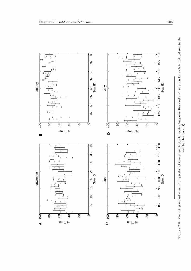
Chapter 7. Outdoor sow behaviour 206
510
1520
2530
3540
020406080100
Sow
ID
% Time
Nov
embe
r
4550
5560
6570
7580
020406080100
Sow
ID
% Time
Janu
ary
8590
9510
010
511
011
512
0020406080100
Sow
ID
% Time
June
125
130
135
140
145
150
155
160
020406080100
Sow
ID
% Time
July
A CDB
Figure7.8:
Mea
n±
stan
dar
der
ror
ofp
rop
orti
onof
tim
esp
ent
insi
de
farr
owin
ghu
tsov
erfi
vew
eeks
of
lact
ati
on
for
each
ind
ivid
ual
sow
inth
efo
ur
batc
hes
(A-
D).
Chapter 7. Outdoor sow behaviour 207
variability in the amount of time they spent in their huts across the weeks of lactation
(sows with large standard errors), but it was also apparent that relatively low variance
in some sows took place (sows with small standard errors). No relationship between the
amount of time a sow spent in her hut and litter mortality could be found.
7.6 Discussion
7.6.1 Activity and Location
The amount of time spent in different locations was found to be dependent on a number
of different factors, including meteorological conditions. Sows were less likely to use their
farrowing huts when it was warm outside and this was true for both insulated and non-
insulated huts. Under warmer external conditions, farrowing huts became extremely
hot making it uncomfortable for the sows to remain inside, whereby they sought shade
and wallows instead. This sort of behavioural thermoregulation is well documented
in the pig (reviewed in Bracke 2011). It was however variable amongst individuals,
with some sows during the warmer months spending more time inside their huts than
others. In colder weather pigs have been reported to seek shelter more often (Ingram and
Legge, 1970). This was confirmed in the present study on both a group and individual
level, since in January sows spent on average twice as much time inside their huts
than in July. Some of the adverse effects of cold climatic conditions can be avoided
by providing sows with farrowing huts containing a sufficient amount of straw (Algers
and Jensen, 1990). This may explain some of the variation in farrowing hut use since
during the latter weeks of lactation farmers did not provide straw as regularly as during
the early weeks of lactation. High solar radiation also resulted in more shade seeking
behaviour, presumably to avoid direct sunlight which leads to an increased heat load
and can cause burning. Interestingly, wallowing did not increase with solar radiation.
This was unexpected as sows will normally increase their wallowing behaviour in strong
sunlight in order to prevent sunburn (Bracke, 2011). Sows spent more time sheltering
within or behind farrowing huts when wind velocities were high than when there was no
wind. This supports previous findings where air movement had a pronounced effect on
habitat choice (Ingram and Legge, 1970) and that pigs avoided high winds regardless
of temperature (Sallvick and Walberg, 1984). High wind speeds increase heat loss from
an animal to the environment (Mader et al., 2003) and so sows will generally avoid
this when possible, especially under colder conditions. Compared to when there was no
wind present, sows were also less likely to wallow if speeds were above 5 mph, possibly
due to the higher level of wind being sufficient enough to provide cooling under warmer
Chapter 7. Outdoor sow behaviour 208
conditions without the need for wallowing. The presence of rain significantly increased
the chance of sows spending time inside their farrowing huts, supporting other studies
where rainfall caused pigs to seek shelter (Buckner et al., 1998). This resulted in an
increase in lying and nursing behaviour suggesting an effect on the amount of time that
sows spent with their piglets.
Stage of lactation affected sow location and behaviour, with sows spending significantly
less time inside their farrowing huts as lactation progressed and more time eating/rooting
during the later weeks of lactation, supporting work by Buckner et al. (1998). However,
week of lactation was not found to directly impact the amount of time the sows spent
with their piglets, with the activity being carried out and climatic conditions being
more important. This fails to support the idea that sows go through a gradual weaning
process, reducing the amount of time they spend with their piglets along with decreasing
the number of sucklings, throughout the weeks of lactation (Houwers et al., 1992). This
may however be due to the piglets spending more time with the sows, i.e. if a sow is
rooting in the paddock her piglets may follow her and mimic her behaviour. In this case
the amount of time the sow has spent with her piglets will not change over lactation
weeks since they are seen as being together, however the time spent interacting with
piglets may be lower (Hotzel et al., 2004). This was not measured in the current study,
other than for when nursing, and so cannot be confirmed.
Time of day also affected sow activity and location since sows were less likely to conduct
standing activities after 5pm and more likely to be in their farrowing huts. This corre-
sponds with sows being less likely to be in their huts when there was some solar radiation
(day time). In winter, day length was shorter and so sows spent more time in the dark
and hence more time in their farrowing huts. This may have contributed to the higher
piglet mortalities as there would have been a higher chance of crushing since increased
close contact with the piglets would have occurred. Piglet crushing has been related to
individual differences in sow behaviour (Wechsler and Hegglin, 1997) which in turn is
connected to the number of postural adjustments a sow makes and the responsiveness
of a sow to her piglets’ distress calls (Andersen et al., 2005). Had the cause of death
been recorded in the present study it may have been possible to determine this although
interestingly, for example, in November and January sows eight and 77 (which spent
over 75% of their time in their huts and with their piglets) had over 14% mortality rates
whereas sows 25 and 62 (which spent less time in their huts and with their piglets) had
0% mortality.

Chapter 7. Outdoor sow behaviour 209
7.6.2 Sow pairing
Lower THIs experienced by batch two resulted in the frequency of pairing within far-
rowing huts to rise considerably, providing evidence that this is used as a behavioural
thermoregulatory mechanism. This was particularly evident when THIs fell below 5 ◦C
as sows sought to gain body heat from others. This is supported by previous findings
(Huynh et al., 2005), that indicated a negative correlation between ambient temperature
and huddling behaviour in order to reduce heat loss to the environment in growing pigs.
Over the course of lactation however, increased piglet growth rate will lead to higher
milk production (Valros et al., 2003) and thus a rise in body temperature which may
counteract falls in ambient temperature. Had piglet growth rate been monitored it may
have been possible to see this relationship. As body condition score increased, the pro-
portion of paired sows decreased and the greatest proportion of paired sows had a body
condition of 3. This differed to the expected result of the lowest rated sows being worst
affected by the cold and thus pairing up most, as has previously been found in cows
(Graunke et al., 2011). However, with the majority of sows having a body condition
score of 3, the probability of this happening was lower.
7.6.3 Time Spent With Piglets
Sow activity and the THI affected the amount of time the sows spent with their piglets,
although this did vary between individuals with some sows spending more time with
piglets than others even during the same meteorological conditions. Previous work has
found that the time spent with piglets and the frequency with which a sow feeds her
piglets decreases as the piglets grow (Houwers et al., 1992) and although no direct
evidence of this was found in the present study, the amount of time a sow spent in
the farrowing hut decreased with the progression of lactation. During the first week
of lactation piglets had to remain in the huts due to the fender blocking their exit.
After the fender was removed piglets were then able to participate in more exploratory
behaviour, normally in close proximity to the sow. This meant that although with her
piglets, the sow was not interacting with them as much and this information may not
have been reflected in the present data. A change in the amount of time sows spend
with their piglets over lactation is normally regarded as evidence of an on-going weaning
process (Wallenbeck et al., 2008) which was observed in the present study in terms of
piglets actively eating sow feed for example.
Overall, the amount of time that sows from the summer batches spent with their piglets
was lower and more varied across the weeks of lactation than the sows observed in winter.
Chapter 7. Outdoor sow behaviour 210
This corresponded to the lower THI experienced by the first two batches; therefore sows
consistently spent time within the farrowing huts with their piglets in order to escape
the cold. Parity did not have a significant effect on sow behaviour which is contrary
to the findings of Thodberg et al. (2002) who found that maternal behaviour actually
developed over parities and as such a difference between gilts and older sows with regards
to maternal care would have been expected. This discrepancy between studies could
result from the present study’s parity groupings (gilts and multipares) which did not
consider intermediate parity groupings.
7.6.4 Piglet Mortality
Sows in January had a higher rate of overall piglet mortality, particularly in week two,
which could not be attributed to a lack of experience as no parity effects were found.
The dramatic drop in piglet numbers seen in the second week of lactation of batch two
corresponded to very low THI, suggesting that postnatal hypothermia was a significant
cause of piglet mortality (Johnson and McGlone, 2003) if piglets were unable to recover
from it. Baxter et al. (2009) found that piglet rectal temperature was directly correlated
to piglet survival in outdoor environments, however the relationship of this with external
conditions was not assessed. Hypothermia can contribute to increased mortality rates
as it predisposes piglets to effects from other potential causes of death such as starvation
and crushing (Lay et al., 2002). Smaller piglets have a larger surface area to volume ratio
and will readily lose heat to the environment in cold conditions if they do not obtain heat
from huddling with the sow or with littermates, so piglets of a lower birth weight will
be more likely to succumb to the effects of below freezing temperatures. This decrease
in the THI (average of 0 ◦C) also caused sows to share farrowing huts more frequently
which could have led to an increase in the number of crushing incidences as space within
the huts was limited.
Hut type was not found to affect overall piglet mortality throughout lactation, how-
ever during the first week of lactation insulated huts had lower mortality rates than
non-insulated huts. Insulation was found to reduce the effects of external temperature
fluctuations, which were vital during the first week of lactation when piglets were most
vulnerable to temperature, but the changes were not sufficient to improve piglet sur-
vival overall, something which has previously been found (Edwards, 1995; Johnson and
McGlone, 2003). This could be due to the volume of straw provided which although
regularly topped up during the first week of lactation, was not monitored as closely in
following weeks. This meant that some huts may have benefited from more straw than
others, maintaining higher temperatures for the piglets. In addition litter size may have

Chapter 7. Outdoor sow behaviour 211
both a negative and positive effect. Large litters may be subjected to more crushing,
however they would also result in added heat within the nest and potentially less deaths
by hypothermia. This factor was not controlled for across hut types and so cannot be
confirmed.
7.7 Conclusions
The present results suggest that meteorological conditions affected which location lac-
tating sows chose to spend their time. This in turn influenced the activities carried
out by the sows as the two were related and certain behaviours were more likely to
be undertaken in particular locations. Sows spent most of their time resting or eating
but did show signs of behavioural thermoregulation, such as pairing and shelter seeking
behaviour in cold, wet or windy conditions. This may have affected the survival rate of
piglets as low THI led to an increased level of piglet mortality whether directly through
piglet hypothermia or indirectly through changes in maternal sow behaviour. Hut insu-
lation improved piglet survival during the first week of lactation and no evidence of sow
learned behaviour over subsequent lactations was found, although individual behaviour
did differ between sows.

Chapter 8
General Discussion
Seasonal infertility is thought to cost the UK pig industry millions of pounds annually,
although its presence is much debated amongst the farming and scientific communities.
Outdoor farming in the UK has increased in recent years, exposing more sows to the
elements and as such potentially placing them at a higher risk of seasonal infertility. The
work within this thesis was therefore conducted to try and elucidate whether seasonal
infertility really does exist in outdoor UK sow herds and if so, what the main causes
and manifestations of this phenomenon are and whether its occurrence can be antici-
pated. From the results produced it is clear that seasonal influences on the fertility of
sows residing outdoors exist in the UK. These are certainly mediated by temperature
(Chapters 3 and 6), meteorological conditions such as rainfall and wind (Chapters 3, 6
and 7) and most likely photoperiodic effects too (Chapter 3). Seasonal changes in boar
fertility may also contribute towards the seasonal infertility observed on farms in the
UK (Chapter 5), and the modelling of such a complex phenomena is possible, albeit
with some limitations (Chapter 4).
8.1 Seasonal infertility in sows
The occurrence of seasonal infertility in the UK and other European countries is some-
thing which has been repeatedly reported over past (Stork, 1979; Wrathall et al., 1986;
Hancock, 1988) and recent decades (Peltoniemi et al., 1999, 2000; Bassett et al., 2001;
Tast et al., 2002; Peters and Pitt, 2003; Almond and Bilkei, 2005; Auvigne et al., 2010).
The current data showed that seasonal infertility was present in the UK during the
period studied regardless of weather conditions, although this varied by farm and by
year. This is consistent with recent data from France showing that yearly patterns of
212

Chapter 8. General Discussion 213
seasonal infertility were clear in pigs housed indoors (Auvigne et al., 2010) and corre-
sponds to cycles in the ancestors of the modern pig (the wild boar) which have been
shown to breed seasonally in response to photoperiod, food availability and meteoro-
logical conditions (Mauget, 1982). The apparent spatial and temporal irregularity of
seasonal infertility is also consistent with the literature (Stork, 1979; Auvigne et al.,
2010) and is something which tends to refute photoperiod as the main driver of seasonal
infertility. For a long time, the presence of a circadian rhythm in the domestic pig was a
controversial topic with authors providing conflicting evidence. Circadian rhythms have
been shown to exist in many domestic species such as the sheep and deer (reviewed in
Chemineau et al. 2008), although in pigs this has always been somewhat debated since
several early studies showed a lack of circadian rhythm in gilts (Minton et al., 1989;
Diekman et al., 1992). However recent research from Norway has shown a clear seasonal
alteration in the circadian melatonin rhythm of gilts (Tast et al., 2001a,c), suggesting
that previous work may not have been standardised or sensitive enough to detect the
changes present. All the experimental animals exhibited a distinct circadian pattern
in melatonin secretion, with high concentrations occurring during the scotophase. In
addition the melatonin response to the scotophase did not differ between wild boars and
domestic gilts in any season. Nonetheless if photoperiod was the main driver of seasonal
infertility, as suggested by several authors (Halli et al., 2008; Tast et al., 2001c), then
surely all farms would exhibit signs of seasonal infertility every year, and neighbouring
farms would be similarly affected. Even authors who claim that photoperiod is the main
driver of seasonal infertility have found it difficult to show that altering lighting regimes
improve sow reproductive ability (Halli et al., 2008).
In this study it was found that longer days resulted in reduced farrowings rates (Chap-
ter 3). Rapid changes in day length also improved farrowing rate regardless of whether
they were lengthening or shortening. This occurs around the equinoxes and suggests
that it is long days and not lengthening days which result in reduced fertility. Long
days normally coincide with warmer temperatures and longer exposure to these higher
temperatures. As such, in the UK it can be said that temperature changes are the
main driver of seasonal infertility in outdoor sows. It has previously been concluded
that temperature may have a greater influence on seasonal infertility than photoperiod
(Prunier et al., 1996). It should be noted that even in countries with little change in day
length, seasonal differences in fertility are still observed. For example Gourdine et al.
(2006b) found that in Guadeloupe although day length in the warm and hot seasons
were both above 11.5 hours, seasonal effects on farrowing rate and wean to conception
interval could still be observed. These countries generally experience very hot condi-
tions, something which results in reduced sow fertility (Wettemann and Bazer, 1985;

Chapter 8. General Discussion 214
Suriyasomboon et al., 2006).
A lower tolerance for increased temperatures in outdoor sows was found in the present
thesis (18 to 20 ◦C; Chapters 3 and 6 respectively), as compared to the literature available
on sows kept indoors (22 to 25 ◦C; Black et al. 1993; Quiniou and Noblet 1999). This
suggests adaptation to the cold since in the UK sows are generally exposed to the
cold when kept outdoors, with mild average temperatures the majority of the year and
winters which regularly reach below 0 ◦C. Therefore rises in temperature can have a
more pronounced effect on sows in terms of their reproductive ability. It has been
shown that pigs respond more adversely to increased temperatures following a period
of cold (Dauncey and Ingram, 1986) since they have adapted to the colder environment
(Heldmaier, 1974; Derno et al., 1995) and this is proposed as a mechanism for seasonal
infertility in outdoor pigs.
Evidence of increasing temperatures affecting sow thermoregulatory systems was evident
from increased skin temperatures and respiration rates (Chapter 6). This corresponds
with previous work showing that sows had increased skin temperature with increased
ambient temperature (Williams, 2009) and similar situations in growing pigs (Huynh
et al., 2005) and piglets (Collin et al., 2002). However, for this to have subsequent effects
on reproduction, it is generally thought that higher temperatures are required (Quiniou
and Noblet, 1999). This is because the negative effects of temperature on reproduction
are thought to be linked to a reduction in sow feed intake under hot conditions (Black
et al., 1993), which results in a deterioration in the body condition of sows prior to
weaning (Love et al., 1993), which was confirmed in Chapter 6 when sows in warmer
weather with longer lactation lengths had reduced body condition scores. Reduced feed
intake is also said to decrease the frequency and level of LH pulses, resulting in inhibitory
action by GnRH (Barb et al., 1991; Kirkwood et al., 1987). When heat stressed, ovarian
cells may also have a reduced response to hormones, with leptin and FSH failing to
stimulate progesterone secretion (Sirotkin and Kacaniova, 2010). Therefore even though
temperatures may have still been considered mild at 20 ◦C, if sows have habituated to
colder temperatures, this is enough to cause them to react adversely. Feed intake could
not be monitored in the present study, neither during the data modelling chapters, due
to the data being historic without that parameter being collected, nor during the farm
trial chapters, due to method of sow feeding carried out on the farm not allowing for
feed intake to be recorded. Feed intake data could have provided valuable information,
allowing for relationships between changes in meteorological conditions and reproductive
output to be linked with changes in the nutrition which sows were receiving.

Chapter 8. General Discussion 215
During Chapter 6 it would have also been useful to have collected rectal temperatures
from the sows. Heat stress is most often defined in terms of the transference of heat from
the animals core to the surface (Mount, 1975) and so having all parameters would have
produced more reliable results. Due to the working conditions during the study this
was not practicable. However skin temperature has been shown to be reliable if other
environmental factors are accounted for (Hanneman et al., 2004) and since respiration
rate was also collected a degree of confidence in the results produced can be maintained.
Behavioural thermoregulation also corresponded with physiological changes in the sow
(Chapter 7). Sows spent less time inside their huts when temperatures were higher and
more time in wallows. This could have resulted in negative effects on piglet production,
and had the causes of death been recorded this would have been possible to confirm.
More effective managerial methods need to be established in order to help sows maintain
high reproductive output throughout the year. Using insulated huts may help improve
conditions during the first week of lactation when sows spend most of their time within
their huts with their litters (Chapter 7), and also improve piglet survival as sows are
less likely to leave the piglets without feed due to heat stress (Chapter 7). Sows also
took shelter in the rain and when wind speeds were high, all of which correspond with
other data on outdoor sow behaviour in the UK (Buckner et al., 1998). More frequent
observations during the day would have improved the level of data obtained, however
with other measurements being taken and the size of the field to be covered, this was
not possible to do on an individual sow level. Litter weight change would have also been
interesting to observe, to relate sow milk production to temperature and weight loss,
however farm practices did not permit this.
8.2 Seasonal infertility in boars
The results indicate that seasonal changes in boar semen quality from ejaculates col-
lected under indoor commercial UK conditions did occur and that these changes were
primarily mediated by age and breed of boar (Chapter 5), with no exact meteorological
causes identified. Semen volume was found to be greatest in autumn and winter, when
day length was shortening, supporting previous work where decreasing photoperiod was
found to be the main contributor to improvements in semen volume, due to increasing
testosterone levels affecting spermatogenesis (Kennedy and Wilkins, 1984; Trudeau and
Sanford, 1986; Charneca et al., 1996; Ciereszko et al., 2000; Kozdrowski and Dubiel,
2004; Okere et al., 2005; Frydrychova et al., 2007; Wolf and Smital, 2009; Wysokiska
et al., 2009). Weather conditions were not found to influence semen volume, reinforcing
the importance of photoperiod as opposed to temperature for this trait. In order to

Chapter 8. General Discussion 216
obtain a fuller picture of the meteorological effects on seasonal changes in boar semen
quality it would be necessary to monitor the indoor environment the boars were kept in
as well as the external meteorological conditions.
Short days have also been shown to stimulate pubertal maturation of spermatogenesis
(Andersson et al., 1998) which may be a contributory factor towards increases in the
total sperm numbers from boars during the autumn months. Total sperm numbers were
found to be lowest throughout spring and summer, supporting recent similar findings
(Wolf and Smital, 2009; Wysokiska et al., 2009). The sperm concentration data also sup-
port work which showed that decreasing photoperiod between August and October, in
comparison to increasing photoperiod between February and mid-April, reduced sperm
concentration (Sancho et al., 2004) and that increases in semen volume were not suffi-
cient to reduce sperm concentration (Ciereszko et al., 2000; Frydrychova et al., 2007).
Overall sperm concentration was found to be mainly affected by collection interval with
an age and month interaction. The seminal changes found in the present study coincide
with the wild boar rutting season, when sows come into oestrus in preparation for a
spring farrowing (Mauget, 1982) and so allow for optimal semen quality to maximise
fertility and fecundity.
Large breed differences in all semen quality parameters were found in the present work
and within breed variation for semen quality parameters was high, most likely due to
individual boar differences which have previously been found to be a problem in semen
quality analyses (reviewed by Foxcroft et al. 2008). Breed often plays a large role in
the resilience of animals to external conditions and differences in semen quality have
been demonstrated elsewhere (Wysokiska et al., 2009). Considering these differences,
the industry may need to establish which breeds are more economically viable during
summer months, although this may mean changing consumer demand. In addition, hav-
ing reviewed artificial insemination (Chapter 2) it could be suggested that if freeze-thaw
technology for boar semen was perfected, a change in the way semen is collected over the
year may be possible, with higher throughput during winter in order to compensate for
summer reductions in fertility. This also links into the practice of semen pooling carried
out by many AI centres. Semen pooling has been suggested to negatively affect sow
fertility due to the masking of relative differences in individual boar fertility (Foxcroft
et al., 2008), and so by increasing boar numbers over winter when semen is at its best,
more single sire doses may be obtainable.
The present study found that when collection intervals surpassed two weeks, total abnor-
malities increased by over 5% and up to 25% in some cases. Previous work has shown
that longer collection intervals resulted in increased total abnormalities in ejaculates

Chapter 8. General Discussion 217
Feb Mar Apr May Jun Jul Aug Sep Oct Nov Dec Jan
Figure 8.1: Summary of overall increases and decreases in different sperm abnormalitytypes for different months of the year.
(Wolf and Smital, 2009) although it has been suggested that more than 30 days need
to pass before significant effects were seen (Smital, 2009). It should be noted however
that previous models have established that collection intervals of three to four days may
provide better financial returns (Rutten et al., 2000). Abnormality types were also more
or less common during different times of the year (Figure 8.1) suggesting that they were
influenced by different parameters, which were not elucidated in the present thesis.
Even with the quality control systems set up at boar studs for the dissemination of se-
men to farms, seasonal infertility in boars can have a negative effect on sow reproductive
output. Most farms still have catcher boars whose semen is not checked prior to every
insemination. If these boars are influenced by seasonal infertility, which is going unno-
ticed, the effects may be even more pronounced. With sows failing to conceive more
often in summer, a greater number may be served by catcher boars and as such may
be more likely to receive poorer quality semen which will increase the chance of smaller
litters. A study looking at reproductive output in sows only artificially inseminated
as opposed to those also put in a pen with a catcher boar post-insemination could be
enlightening.
8.3 Individual susceptibility to seasonal infertility
Over 25% of sows were never affected by seasonal infertility, with no returns or reduc-
tions in litter size from summer services throughout their lifetimes (Chapter 3). This
may suggest a genetic tolerance to environmental stressors which would normally in-
duce a negative effect on reproduction, something which has been previously reported

Chapter 8. General Discussion 218
for different sow lines of the same breed (Bloemhof et al., 2008). This is supported
by the fact that sows exhibited individual behaviours (Chapter 7) and physiological
responses (Chapter 6) to changing environmental conditions and that individual boars
within breeds had better overall performance than others (Chapter 5). If work could
be conducted to trace back genetic lines for individual animals it may be possible to
eliminate seasonal infertility from the UK pig herd. Other traits such as litter size have
been found to be genetically controlled, so why not seasonal influences? As discussed
in Chapter 3, research into emerging genes such as the kisspeptin gene could provide
researchers with new details on how seasonality is controlled and what sort of genetic x
environment interactions may exist in the pig.
8.4 Modelling seasonal infertility
The majority of data available in the literature has been conducted on sows which were
kept indoors, whereas in the UK there is now a drive towards increased outdoor breeding.
This work is therefore novel in the area of modern sow reproduction. The majority of
the research conducted herein utilised data modelling methodologies. Breeders and
farmers amass large quantities of data which generally go unused to their full potential.
When combined with other data, such as meteorological conditions, this can prove to
be a powerful tool for elucidating patterns within the data collected. Nonetheless the
importance of good quality data for modelling and analysis cannot be overestimated,
however this can be difficult to ensure when data is collected in the field. Data clean up
is therefore vital, something which previous authors who used production data for their
research have also concluded (Kirchner et al., 2004a; Auvigne et al., 2010).
In Chapter 5, decision tree modelling was able to detect stud management decisions on
whether to use or discard ejaculates. This emphasises the ability of decision trees to
identify patterns within large data sets and confirms that they may be a useful tool
in identifying if standards within a boar stud are being met. Other studies have also
found decision trees to be useful in assessing on farm decisions, when both simulated and
real datasets were examined (Kirchner et al., 2004a,b, 2006; Kamphuis et al., 2010a,b).
When the algorithm was applied to the more variable dataset containing meteorological
variables and semen quality parameters, the decision trees produced were not so effective.
More data preparation may have been necessary to reduce the noise in the dataset to
allow the algorithm to more easily detect true patterns within the data (Kirchner et al.,
2004b).

Chapter 8. General Discussion 219
The more parameters provided for the records studied, the more information can be ex-
tracted from the data. For example if specific sire and dam line data had been accessible
for Chapter 3, as well as age of first service and sow body condition, a more detailed
and rounded view of effects could have been obtained, and genetic effects could have
been included within the models produced. Record keeping by farmers may need to be
expanded so that more detailed and accurate records can be maintained. These could
then be potentially fed into a system for predicting performance, seasonal or otherwise.
Several pig record keeping systems are available, such as PigExpert in Germany, PigCom
and WinPig in the UK and PigChamp in the USA. Farmers need to see these as more
of a tool for optimising production and as such create more accurate records for their
breeding herds.
The simulation model produced in Chapter 4 shows that sow production can be antici-
pated in advance using previously recorded data, although the model itself still requires
improvement. The types of additions and improvements which could be made have been
been discussed in detail in Chapter 4. Modelling complex systems such as reproductive
biology is difficult since so many factors can affect the results produced. However, even
simple models can provide valuable information which can help on farm decisions. By
improving the model and incorporating a way of inputting individual farm data from
a database, a powerful online tool could be developed which farmers nationwide could
use.
8.5 Conclusions
Seasonal infertility exists in outdoor UK sow herds. This may be a result of sows adapt-
ing to colder environments when kept outdoors and as such being affected by temperature
rises more adversely than indoor animals. This highlights the need for farmers to provide
outdoor sows with methods to keep themselves comfortable throughout the year and not
only during the summer months. Individual sows may be more tolerant to these changes
than others and as such improved monitoring of sow reproductive output during periods
of seasonal infertility, and stricter culling rules for sows exhibiting increased problems
may help eliminate some of the seasonal infertility observed on farms. In addition ge-
netic research into seasonality may reveal sow lines which are more tolerant of changes
in environmental conditions and as such have a lower likelihood of exhibiting signs of
seasonal infertility. Reductions in boar semen quality over the summer months may also
be adding to the reduction in sow reproductivity seen on farms, especially through the
use of catcher boars. It may be possible to predict the occurrence of seasonal infertility
in a herd through the use of modelling, although farm specific inputs would need to be

Chapter 8. General Discussion 220
provided, since every farm is different. Future development of such a model is therefore
required.

Bibliography
Adams, R., 2010. Bat reproduction declines when conditions mimic climate change pro-
jections for western North America. Ecology 91 (8), 2437–2445.
Agricultural and Horticultural Development Board, 2011. BPEX annual technical report
2010-2011. Tech. rep.
Aherne, F. X., Kirkwood, R. N., 1985. Nutrition and sow prolificacy. Journal of Repro-
duction and Fertility supplement 33, 169–183.
Akos, K., Bilkei, G., 2004. Comparison of the reproductive performance of sows kept
outdoors in Croatia with that of sows kept indoors. Livestock Production Science
85 (2-3), 293–298.
Algers, B., Jensen, P., 1990. Thermal microclimate in winter farrowing nests of free-
ranging domestic pigs. Livestock Production Science 25 (1-2), 177–181.
Allen, M. A., Stewart, T. S., 1983. A simulation model for a swine breeding unit pro-
ducing feeder pigs. Agricultural Systems 10 (4), 193–211.
Almeida, F. R. C. L., Mao, J., Novak, S., Cosgrove, J. R., Foxcroft, G. R., 2001. Effects
of different patterns of feed restriction and insulin treatment during the luteal phase on
reproductive, metabolic, and endocrine parameters in cyclic gilts. Journal of Animal
Science 79, 200–212.
Almeida, F. R. C. L., Novak, S., Foxcroft, G. R., 2000. The time of ovulation in relation
to estrus duration in gilts. Theriogenology 53, 1389–1396.
Almond, G. W., Friendship, R. M., Bosu, W. T. K., 1985. Autumn abortions in sows.
Canadian Veterinary Journal 26, 162–163.
Almond, P. K., Bilkei, G., 2005. Seasonal infertility in large pig production units in an
Eastern-European climate. Australian Veterinary Journal 83 (6), 344–346.
Althouse, G. C., 1998. Cytoplasmic droplets on boar sperm cells. Swine Health and
Production, 128.
221
Bibliography 222
Althouse, G. C., Kuster, C. E., Clark, S. G., Weisiger, R. M., 2000. Field investigations
of bacterial contaminants and their effects on extended porcine semen. Theriogenology
53, 1167–1176.
Altmann, J., 1974. Observational study of behavior: sampling methods. Behaviour 49,
227–267.
Amundson, J. L., Mader, T. L., Rasby, R. J., Hu, Q. S., 2006. Environmental effects on
pregnancy rate in beef cattle. Journal of Animal Science 84 (12), 3415–20.
Andersen, I. L., Berg, S., Bø e, K. E., 2005. Crushing of piglets by the mother sow
(Sus scrofa) - purely accidental or a poor mother? Applied Animal Behaviour Science
93 (3-4), 229–243.
Andersson, H., Wallgren, M., Rydhmer, L., Lundstrom, K., 1998. Photoperiodic effects
on pubertal maturation of spermatogenesis, pituitary responsiveness to exogenous
GnRH, and expression of boar taint in crossbred boars. Animal Reproduction Science
54, 121–137.
Anil, S. S., Larriestra, A., Deen, J., Anil, L., 2005. A path analysis of the factors
associated with seasonal variation of breeding failure in sows. Canadian Journal of
Animal Science 85, 317–325.
Araujo, E. B., da Costa, E. P., da Costa, A. H. A., Lopes, F. G., Macedo, G. G.,
de Paula, T. A. R., 2009. Reproductive performance of sows submitted to intrauterine
insemination. Revista Brasileira de Zootecnia 38 (8), 1460–1467.
Arias, R., Mader, T. L., 2011. Environmental factors affecting daily water intake on
cattle finished in feedlots. Journal of Animal Science 89 (1), 245–51.
Asher, G. W., 1985. Oestrus cycle and breeding season of farmed fallow deer, Dama
dama. Journal of Reproduction and Fertility 75, 521–529.
Ashworth, C., Pickard, M., 1998. Progress in Pig Science. Nottingham University Press,
Nottingham.
Auvigne, V., Leneveu, P., Jehannin, C., Peltoniemi, O. A. T., Salle, E., 2010. Seasonal
infertility in sows: A five year field study to analyze the relative roles of heat stress
and photoperiod. Theriogenology 74 (1), 60–66.
Baayen, R. H., 2009. languageR: Data sets and functions with ”Analyzing Linguistic
Data: A practical introduction to statistics”.

Bibliography 223
Baidoo, S. K., Aherne, F. X., Kirkwood, R. N., Foxcroft, G. R., 1992. Effect of feed
intake during lactation and after weaning on sow reproductive performance. Canadian
Journal of Animal Science 72 (4), 911–917.
Baldwin, B., Ingram, D. L., 1967. Behavioural thermoregulation in pigs. Physiology &
Behavior 2 (1), 15–16.
Baldwin, B., Ingram, D. L., 1968. Factors influencing behavioral thermoregulation in
the pig. Physiology & Behavior 3 (3), 409–415.
Barb, C. R., Estienne, M. J., Kraeling, R. R., Marple, D. N., Rampacek, G. B., Rahe,
C. H., Sartin, J. L., 1991. Endocrine changes in sows exposed to elevated ambient
temperature during lactation. Domestic Animal Endocrinology 8 (1), 117–27.
Bassett, J. M., Bray, C. J., Sharpe, C. E., 2001. Reproductive seasonality in domestic
sows kept outdoors without boars. Reproduction 121, 613–629.
Bates, D. M., Maechler, M., 2009. lme4: Linear mixed-effects models using S4 classes.
Bathgate, R., 2008. Functional integrity of sex-sorted, frozen-thawed boar sperm and its
potential for artificial insemination. Theriogenology 70 (8), 1234–41.
Baxter, E. M., Jarvis, S., Sherwood, L., Robson, S. K., Ormandy, E., Farish, M., Smurth-
waite, K. M., Roehe, R., Lawrence, A. B., Edwards, S. A., 2009. Indicators of piglet
survival in an outdoor farrowing system. Livestock Science 124 (1-3), 266–276.
Bazer, F. W., Thatcher, W. W., 1977. Theory of maternal recognition of preg-
nancy in swine based on estrogen controlled endocrine versus exocrine secretion of
prostaglandin F2α by the uterine endometrium. Prostaglandins 14, 397–400.
Bazer, F. W., Wu, G., Spencer, T. E., Johnson, G. A., Burghardt, R. C., Bayless,
K., 2010. Novel pathways for implantation and establishment and maintenance of
pregnancy in mammals. Molecular Human Reproduction 16 (3), 135–52.
Belstra, B. A., Flowers, W. L., See, M. T., 2004. Factors affecting temporal relationships
between estrus and ovulation in commercial sow farms. Animal Reproduction Science
84, 377–394.
Benson-Amram, S., Heinen, V. K., Dryer, S. L., Holekamp, K. E., 2011. Numerical as-
sessment and individual call discrimination by wild spotted hyaenas, Crocuta crocuta.
Animal Behaviour 82 (4), 743–752.
Bertoldo, M., Grupen, C. G., Thomson, P. C., Evans, G., Holyoake, P. K., 2009. Identifi-
cation of sow-specific risk factors for late pregnancy loss during the seasonal infertility
period in pigs. Theriogenology 72, 393–400.

Bibliography 224
Bertoldo, M., Holyoake, P. K., Evans, G., Grupen, C. G., 2010. Oocyte developmental
competence is reduced in sows during the seasonal infertility period. Reproduction,
Fertility and Development 22 (8), 1222–1229.
Bianca, W., 1976. The significance of meteorology in animal production. International
journal of biometeorology 20 (2), 139–56.
Black, L. J., Mullan, B. P., Lorschy, M. L., Giles, L. R., 1993. Lactation in the sow
during heat stress. Livestock Production Science 35, 153–170.
Blackshaw, J. K., Blackshaw, A. W., 1994. Shade-seeking and lying behaviour in pigs
of mixed sex and age, with access to outside pens. Applied Animal Behaviour Science
39 (3-4), 249–257.
Blanc, F., Agabriel, J., 2008. Modelling the reproductive efficiency in a beef cow herd:
effect of calving date, bull exposure and body condition at calving on the calving-
conception interval and calving distribution. Journal of Agricultural Science 146, 143–
161.
Bloemhof, S., van Der Waaij, E. H., Merks, J. W. M., Knol, E. F., 2008. Sow line differ-
ences in heat stress tolerance expressed in reproductive performance traits. Journal of
Animal Science 86 (12), 3330–7.
Boların, A., Hernandez, M., Vazquez, J. M., Rodrıguez-Martınez, H., Martınez, E. A.,
Roca, J., 2009. Use of frozen-thawed semen aggravates the summer-autumn infertility
of AI weaned sows in the Mediterranean region. Journal of Animal Science 87, 3967–
3975.
Bollinger, A. L., Wilson, M. E., Pusateri, A. E., Green, M. L., Martin, T. G., Diekman,
M. A., 1997. Lack of a nocturnal rise in serum concentrations of melatonin as gilts
attain puberty. Journal of Animal Science 75, 1885–1892.
Boma, M. H., Bilkei, G., 2006. Seasonal infertility in Kenyan pig breeding units. The
Onderstepoort Journal of Veterinary Research 73 (3), 229–32.
Bonet, S., Briz, M., Fradera, A., 1991. The sperm quality and fertility of boars after two
different ejaculation frequencies. Scientia gerundensis 17, 77–84.
Bonet, S., Briz, M., Fradera, A., 1993. Ultrastructural abnormalities of boar spermato-
zoa. Theriogenology 40, 383–396.
Booth, P. J., 1990. Metabolic influences on hypothalamic-pituitary- ovarian function in
the pig. Journal of Reproduction and Fertility supplement 40, 89–100.

Bibliography 225
Borg, K. E., Lunstra, D. D., Christenson, R. K., 1993. Semen characteristics, testicular
size, and reproductive hormone concentrations in mature duroc, meishan, fengjing,
and minzhu boars. Biology of Reproduction 49 (3), 515–21.
Bracke, M. B. M., 2011. Review of wallowing in pigs: Description of the behaviour and
its motivational basis. Applied Animal Behaviour Science 132, 1–13.
Bracken, C. J., Safranski, T. J., Lucy, M. C., 2006. Ovarian follicular development, es-
trus, and ovulation in seasonally anestrous sows treated seven days post weaning with
equine and human chorionic gonadotropins. Journal Of Swine Health And Production
14 (4), 207–209.
Bradshaw, C. J. A., Davis, L. S., Purvis, M., Zhou, Q., Benwell, G. L., 2002. Using
artificial neural networks to model the suitability of coastline for breeding by New
Zealand fur seals ( Arctocephalus forsteri ). Ecological Modelling 148, 111– 131.
Breiman, L., Friedmann, J. H., Ohlsen, R. A., Stone, C. J., 1984. Classification and
Regression Trees. Wadsworth, Belmont, USA.
Brinsko, S. P., Blanchard, T. L., Rigby, S. L., Love, C. C., Varner, D. D., 2003. Effects
of dead spermatozoa on motion characteristics and membrane integrity of live sper-
matozoa in fresh and cooled-stored equine semen. Theriogenology 59 (3-4), 735–42.
Britt, J. H., Szarek, V. E., 1983. Characterization of summer infertility of sows in large
confinement units. Theriogenology 20 (1), 133–140.
Briz, M., Bonet, S., Pinart, B., Camps, R., 1996. Sperm malformations throughout the
boar epididymal duct. Animal Reproduction Science 43 (4), 221–239.
Brown Brandl, T. M., Nienaber, J. A., Eigenberg, R. A., Xin, H., 2011. Heat and mois-
ture production of growing-finishing gilts as affected by environmental temperature.
In: Proceedings American Society of Agricultural and Biological Engineers (ASABE)
Annual International Meeting, August 7-10, Louisville, Kentucky.
Buckner, L. J., Edwards, S. A., Bruce, J. M., 1998. Behaviour and shelter use by outdoor
sows. Applied Animal Behaviour Science 57 (1-2), 69–80.
Buono, M. J., Jechort, A., Marques, R., Smith, C., Welch, J., 2007. Comparison of
infrared versus contact thermometry for measuring skin temperature during exercise
in the heat. Physiological measurement 28 (8), 855–9.
Buranaamnuay, K., Tummaruk, P., Techakumphu, M., 2010. Intra-uterine insemination
with low numbers of frozen-thawed boar spermatozoa in spontaneous and induced
ovulating sows under field conditions. Livestock Science 131 (1), 115–118.

Bibliography 226
Byon, E., Shrivastava, A., Ding, Y., 2010. A classification procedure for highly imbal-
anced class sizes. IIE Transactions 42 (4), 288–303.
Cameron, R. D. A., Blackshaw, A. W., 1980. The effect of elevated ambient temperature
spermatogenesis in the boar. Journal of Reproduction and Fertility 59, 173–179.
Carr, J., 1998. Garth pig stockmanship standards. 5M Enterprises Limited. Sheffield,
UK.
Carreau, S., Hess, R., 2010. Oestrogens and spermatogenesis. Philosophical transactions
of the Royal Society of London. Series B, Biological sciences 365 (1546), 1517–35.
Casas, I., Sancho, S., Briz, M., Pinart, E., Bussalleu, E., Yeste, M., Bonet, S., 2010.
Fertility after post-cervical artificial insemination with cryopreserved sperm from boar
ejaculates of good and poor freezability. Animal Reproduction Science 118 (1), 69–76.
Chaffee, R. R. J., Roberts, J. C., 1971. Temperature acclimation in birds and mammals.
Annual Reviews in Physiology 33, 155–202.
Chamsaz, M., Asadpour, S., Perai, A. H., Khatibjoo, A., 2009. Neural network model
as a new powerful tool to describe and predict hatchability of broiler breeder eggs.
Journal of Animal and Veterinary Advances 8 (7), 1349–1352.
Charneca, R., Milhano, A., Neno, C., Nunes, J. T., 1996. Quantitative and qualitative
evaluation of Alentejano swine breed boars semen. CIHEAM - Options Mediterra-
neennes, 93–98.
Chedad, A., Moshou, D., Aerts, J. M., Hirtum, A. V., Ramon, H., Berckmans, D., 2001.
Recognition system for pig cough based on probabilistic neural networks. Journal of
Agricultural Engineering Research 79 (4), 449–457.
Chemineau, P., Guillaume, D., Migaud, M., Thiery, J. C., Pellicer-Rubio, M. T., Mal-
paux, B., 2008. Seasonality of reproduction in mammals: intimate regulatory mecha-
nisms and practical implications. Reproduction in Domestic Animals 43 (Suppl, 40–47.
Chemineau, P., Malpaux, B., Brillard, J. P., Fostier, A., 2007. Seasonality of reproduc-
tion and production in farm fishes, birds and mammals. Animal 1, 419–432.
Chen, P. H., White, C. E., 2006. Comparison of rectal, microchip transponder, and
infrared thermometry techniques for obtaining body temperature in the laboratory
rabbit (Oryctolagus cuniculus). Journal of the American Association for Laboratory
Animal Science 45 (1), 57–63.
Bibliography 227
Chokoe, T. C., Siebrits, F. K., 2009. Effects of season and regulated photoperiod on the
reproductive performance of sows. South African Journal of Animal Science 39 (1),
45–54.
Christenson, R. K., 1973. Effect of temperature on reproduction in the boar. In: Pro-
ceedings of the George A. Young Conference on Advances in Swine Repopulation and
the Thirteenth Annual Nebraska S.P.F. Conference July 23 and 24.
Ciereszko, A., Ottobre, J. S., Glogowski, J., 2000. Effects of season and breed on sperm
acrosin activity and semen quality of boars. Animal Reproduction Science 64 (1-2),
89–96.
Claus, R., Hoang-Vu, C., Ellendorff, F., Meyer, H. D., Schopper, D., Weiler, U., 1987.
Seminal oestrogens in the boar: origin and functions in the sow. Journal of Steroid
Biochemistry 27 (1-3), 331–335.
Claus, R., Schopper, D., Wagner, H. G., 1983. Seasonal effect on steroids in blood plasma
and seminal plasma of boars. Journal of Steroid Biochemistry 19 (1C), 725–729.
Claus, R., Schopper, D., Wagner, H. G., Weller, U., 1985. Photoperiodic influences on
reproduction of domestic boars. I. Light influences on testicular steroids in peripheral
blood plasma and seminal plasma. Journal of Veterinary Medicine: Series A 32, 86–98.
Clowes, E. J., Aherne, F. X., Schaefer, A. L., Foxcroft, G. R., Baracos, V. E., 2003.
Parturition body size and body protein loss during lactation influence performance
during lactation and ovarian function at weaning in first-parity sows. Journal of Ani-
mal Science 81 (6), 1517–1528.
Coe, P. H., 1999. Associations among age, scrotal circumference, and proportion of mor-
phologically normal spermatozoa in young beef bulls during an initial breeding sound-
ness examination. Journal of the American Veterinary Medical Association 214 (11),
1664–7.
Coffey, R. D., Parker, G. R., Laurent, K. M., 1999. Assessing Sow Body Condition.
Tech. rep., University of Kentucky Cooperative Extension Service, Lexington.
Collin, A., Vaz, M.-j., Le Dividich, J., 2002. Effects of high temperature on body tem-
perature and hormonal adjustments in piglets. Reproduction Nutrition Development
42, 45–53.
Corcuera, B. D., de Alba Romero, C., Hernandez-Gil, R., Sagues, A., 2002a. Identifying
abnormalities in boar semen. Pig Progress 18 (5), 24–27.

Bibliography 228
Corcuera, B. D., Hernandez-Gil, R., de Alba Romero, C., Martn Rillo, S., 2002b. Rela-
tionship of environment temperature and boar facilities with seminal quality. Livestock
Production Science 74 (1), 55–62.
Cordova-Izquierdo, A., Amaya-Mejıa, S. E., Cordova-Jimenez, M. S., Cordova-Jimenez,
C. A., 2008. Comparison of two methods of artificial insemination in sows. Journal of
Animal and Veterinary Advances 7 (1), 110–112.
Cosgrove, J. R., Foxcroft, G. R., 1996. Nutrition and reproduction in the pig: Ovarian
aetiology. Animal Reproduction Science 42 (1-4), 131–141.
Craninx, M., Fievez, V., Vlaeminck, B., de Baets, B., 2008. Artificial neural network
models of the rumen fermentation pattern in dairy cattle. Computers and Electronics
in Agriculture 60, 226–238.
Curtis, S. E., 1985. Physiological responses and adaptations of swine. In: Yousef, M. K.
(Ed.), Stress physiology in livestock. Volume II. Ungulates. Vol. 2. CRC Press, Inc.,
pp. 59–65.
Dairymaster UK Limited, 2012. MooMonitor.
URL http://www.dairymaster.co.uk/heat-detection/
Damm, B. I., Pedersen, L. J., Jessen, L. B., Thamsborg, S. M., Mejer, H., Ersbø ll,
A. K., 2003. The gradual weaning process in outdoor sows and piglets in relation to
nematode infections. Applied Animal Behaviour Science 82 (2), 101–120.
Dan, T. T., Summers, P. M., 1996. Reproductive performance of sows in the tropics.
Tropical Animal Health and Production 28 (3), 247–256.
d’Anglemont de Tassigny, X., Colledge, W. H., 2010. The role of kisspeptin signaling in
reproduction. Physiology 25 (4), 207–17.
Dauncey, M. J., Ingram, D. L., 1986. Acclimatization to warm or cold temperatures and
the role of food intake. Journal of Thermal Biology 11 (2), 89–93.
De’ath, G., Fabricius, K. E., 2000. Classification and regression trees : A powerful yet
simple technique for ecological data analysis. Ecology 81 (11), 3178–3192.
Defra Publications, 2003. Code of Recommendations for the Welfare of Livestock: Pigs.
Delcroix, I., Mauget, R., Signoret, J. P., 1990. Existence of synchronization of reproduc-
tion at the level of the social group of the European wild boar (Sus scrofa). Journal
of Reproduction and Fertility 89, 613–617.
Bibliography 229
Derno, M., Jentsch, W., Hoffmann, L., 1995. Effect of long time exposure to different
environmental temperatures on heat production of growing pigs. Livestock Production
Science 43 (95), 149–152.
Diekman, M. A., Brandt, K. E., Green, M. L., Clapper, J. A., Malayer, J. R., 1992.
Lack of a nocturnal rise of serum melatonin in prepubertal gilts. Domestic Animal
Endocrinology 9 (2), 161–167.
Diekman, M. A., Green, M. L., 1996. Serum concentrations of melatonin in prepuber-
tal or postpubertal gilts exposed to artificial lighting or sunlight. Journal of Animal
Science (97), 923–928.
Diemer, T., Huwe, P., Ludwig, M., Hauck, E. W., Weidner, W., 2003. Urogenital infec-
tion and sperm motility. Andrologia 35 (5), 283–7.
Digby, S., 2007. Seasonal infertility: a cost... but also an opportunity.
URL http://www.thepigsite.com/swinenews/13487
Dijkhuizen, A. A., Morris, R. S., Morrow, M., 1986. Economic optimization of culling
strategies in swine breeding herds, using the PorkCHOP computer program. Preven-
tive Veterinary Medicine 4 (4), 341–353.
Dimitrov, S., Jeliazkov, E., Levis, D., 2007. Deep intrauterine and transcervical insemi-
nation of sows and gilts. Trakia Journal of Sciences 5 (1), 40–46.
Dimitrov, S., Zmudzki, J., 2009. Post-cervical insemination of sows with low sperm
concentration dose in the commercial pig farm. Bulletin of The Veterinary Institute
in Pulawy 53, 225–228.
Domınguez, J. C., Pena, F. J., Anel, L., Carbajo, M., 1996. Swine summer infertility
syndrome in North West Spain. The Veterinary Record 139, 93–94.
Dresdner, R. D., Katz, D. F., 1981. Relationships of mammalian sperm motility and
morphology to hydrodynamic aspects of cell function. Biology of Reproduction 25 (5),
920–930.
Echevarria, A., Parsi, J., Trolliet, J., Rinaudo, P., Ambrogi, A., Dolso, I., Vazquez, M.,
Sbaffo, A., 2000. Internal temperatures and sows productivity in outdoor farrowing
huts with different external paints. Investigacion Veterinaria 2 (1), 39–47.
Edwards, R. L., Omtvedt, I. T., Tuesman, E. J., Stephens, D. F., Mahoney, W. A., 1968.
Reproductive performance of gilts following heat stress prior to breeding and in early
gestation. Journal of Animal Science 27, 1634–1637.

Bibliography 230
Edwards, S. A., 1995. Effect of outdoor farrowing hut insulation on piglet mortality and
growth. Farm building progress 117, 33–35.
Edwards, S. A., 2002. Perinatal mortality in the pig: environmental or physiological
solutions? Livestock Production Science 78, 3–12.
Edwards, S. A., 2005. Product quality attributes associated with outdoor pig production.
Livestock Production Science 94 (1-2), 5–14.
Estill, C. T., 2000. Current concepts in estrus synchronization in swine. Journal of
Animal Science 77, 1–9.
Faust, M. A., Tess, M. W., Robison, O. W., 1992. A bioeconomic simulation model for
a hierarchical swine breeding structure. Journal of Animal Science 70, 1760–1774.
Fernandez, C., Soria, E., Martn, J. D., Serrano, A. J., 2006. Neural networks for animal
science applications: Two case studies. Expert Systems with Applications 31, 444–450.
Fernandez-Llario, P., Mateos-Quesada, P., 2005. Influence of rainfall on the breeding
biology of Wild boar (Sus scrofa) in a Mediterranean ecosystem. Folia Zoologica 54 (3),
240–248.
Fialho, F. B., Bucklin, R. A., Zazueta, F. S., Myer, R. O., 2004. Theoretical model of
heat balance in pigs. Animal Science 79, 121–134.
Fitzgerald, R. F., Jones, G. F., Stalder, K. J., 2008. Effects of intrauterine and cervical
artificial-insemination catheters on farrowing rate and litter size. Journal of Swine
Health and Production 16 (1), 10–15.
Fitzgerald, R. F., Stalder, K. J., Dixon, P. M., Johnson, A. K., Karriker, L. A., Jones,
G. F., 2009. The accuracy and repeatability of sow body condition scoring. The Pro-
fessional Animal Scientist 25, 415–425.
Flowers, B., Cantley, T. C., Martin, M. J., Day, B. N., 1989. Effect of elevated ambient
temperatures on puberty in gilts. Journal of Animal Science 67, 779–784.
Flowers, W. L., 1997. Management of boars for efficient semen production. Journal of
Reproduction and Fertility supplement 52, 67–78.
Flowers, W. L., 2008. Genetic and phenotypic variation in reproductive traits of AI
boars. Theriogenology 70, 1297–1303.
Folk Jr, G. E., 1974. Adaptation and heat loss: The past thirty years. In: Montieth,
J. L., Mount, L. E. (Eds.), Heat loss from animals and man: Proceedings of the twen-
tieth Easter school in agricultural science, University of Nottingham. Butterworths,
London, pp. 119–146.

Bibliography 231
Foote, R. H., 2002. The history of artificial insemination: Selected notes and notables.
American Society of Animal Science, 1–10.
Foxcroft, G. R., de Wiel, D. F. M., 1982. Endocrine control of the oestrous cycle. In: Fox-
croft, G. R., Cole, D. J. A. (Eds.), Control of Pig Reproduction. Vol. 8. Butterworth-
Heinemann, pp. 161–177.
Foxcroft, G. R., Dyck, M. K., Ruiz-Sanchez, A. L., Novak, S., Dixon, W. T., 2008.
Identifying useable semen. Theriogenology 70 (8), 1324–1336.
Franca, L. R., Avelar, G. F., Almeida, F. F. L., 2005. Spermatogenesis and sperm
transit through the epididymis in mammals with emphasis on pigs. Theriogenology
63, 300–318.
Franek, S. P., Bilkei, G., 2008. Effect of gonadotropins during hot summer season given
at different times after weaning on selected reproductive indicators of the sow. Acta
Veterinaria Brunesis 77, 193–198.
Fraser, D., 1980. A review of the behavioural mechanism of milk ejection of the domestic
pig. Applied Animal Ethology 6 (3), 247–255.
Frydrychova, S., Lustykova, A., Cerovsky, J., Lipensky, J., Rozkot, M., 2007. Seasonal
changes of boars semen production. Research in Pig Breeding (1), 31–33.
Gadea, J., 2003. Review : Semen extenders used in the artificial insemination of swine.
Spanish Journal of Agricultural Research 1 (2), 17–27.
Garcia, J. C., Abad, M., Kirkwood, R. N., 2007. Effect of sperm numbers and time of
insemination relative to ovulation on sow fertility. Animal Reproduction Science 100,
397–401.
Gaugler, H. R., Buchanan, D. S., Hintz R, L., Johnson, R. K., 1984. Sow productiv-
ity comparisons for four breeds of swine: Purebred and crossbred litters. Journal of
Animal Science 59 (4), 941–947.
Gaustad-aas, A. H., Hofmo, P. O., Karlberg, K., 2004. Reproductive performance of
gilts and sows in temperate versus subarctic and arctic zones of Norway. Animal
Reproduction Science 80, 291–301.
Gordon, I., 2004. Reproductive technologies in farm animals. CAB International,
Wallingford, UK.
Gourdine, J. L., Bidanel, J. P., Noblet, J., Renaudeau, D., 2006a. Effects of breed and
season on performance of lactating sows in a tropical humid climate. Journal of Animal
Science 84, 360–369.

Bibliography 232
Gourdine, J. L., Quesnel, H., Bidanel, J. P., Renaudeau, D., 2006b. Effect of season,
parity and lactation on reproductive performance of sows in a tropical humid climate.
Asian-Australian Journal of Animal Science 19 (8), 1111–1119.
Gouttenoire, L., Cournut, S., Ingrand, S., 2011. Modelling as a tool to redesign livestock
farming systems: a literature review. Animal 5 (12), 1957–71.
Graunke, K. L., Schuster, T., Lidfors, L. M., 2011. Influence of weather on the behaviour
of outdoor-wintered beef cattle in Scandinavia. Livestock Science 136 (2-3), 247–255.
Greives, T. J., Kriegsfeld, L. J., Demas, G. E., 2008. Exogenous kisspeptin does not al-
ter photoperiod-induced gonadal regression in Siberan hamsters (Phodpus sungorus).
General and Comparative Endocrinology 156, 552–558.
Hafez, E. S. E., 1965. Behavioral thermoregulation in mammals and birds (A Review).
International journal of biometeorology 7 (3), 231–240.
Halli, O., 2008. Effect of environment and management on reproductive efficiency of
sows with special emphasis on control of seasonal infertility. Ph.D. thesis, University
of Helsinki.
Halli, O., Tast, A., Heinonen, M., Munsterhjelm, C., Valros, A., Peltoniemi, O. A. T.,
2008. Short or long day light regimes may not affect reproductive performance in the
sow. Reproduction in Domestic Animals 43 (6), 708–12.
Hancock, R. D., 1988. Clinical observations on seasonal infertility in sows in Cornwall.
The Veterinary Record 123 (16), 413–416.
Hanneman, S. K., Jesurum-Urbaitis, J. T., Bickel, D. R., 2004. Comparison of methods
of temperature measurement in swine. Laboratory animals 38 (3), 297–306.
Hansen, P. J., 2009. Effects of heat stress on mammalian reproduction. Philosophical
transactions of the Royal Society of London. Series B, Biological sciences 364 (1534),
3341–50.
Hasenauer, H., Merkl, D., Weingartner, M., 2001. Estimating tree mortality of Norway
spruce stands with neural networks. Advances in Environmental Research 5, 405–414.
Hazeleger, W., Kirkwood, R. N., Soede, N. M., 2001. Synchronisation of the reproductive
cycle in pigs. Archiv Tierzucht, Dummerstorf 44, 71–76.
Hazeleger, W., Soede, N. M., Kemp, B., 2005. The effect of feeding strategy during the
pre-follicular phase on subsequent follicular development in the pig. Domestic Animal
Endocrinology 29 (2), 362–70.

Bibliography 233
Heldmaier, G., 1974. Cold adaptation by short daily cold exposures in the young pig.
Journal of Applied Physiology 36 (2), 163–8.
Hochereau De Reviers, M. T., Lagantm, H., Despres, P., Venturi, E., Brunte, L., Perreau,
C., Wianny, F., Legault, C., 1997. Facteurs de variation de lage a la puberte, du taux
dovulation et de la survie embryonnaire precoce chez la cochette: type genetique,
poids vif, saison et consanguinite. Journees de la Recherche Porcine en France 29,
109–113.
Honeyman, M. S., Roush, W. B., 2002. The effects of outdoor farrowing hut type on
prewean piglet mortality in Iowa. American Journal of Alternative Agriculture 17 (2),
92–95.
Hotzel, M. J., Pinheiro Machado F, L. C., Wolf, F. M., Costa, O. A. D., 2004. Behaviour
of sows and piglets reared in intensive outdoor or indoor systems. Applied Animal
Behaviour Science 86 (1-2), 27–39.
Houwers, H. W. J., Bure, R. G., Koomans, P., 1992. Behaviour of sows in a free-access
farrowing section. Farm building progress, 9–11.
Howard, J. G., Donoghue, A. M., Johnston, L. A., Wildt, D. E., 1993. Zona pellucida
filtration of structurally abnormal spermatozoa and reduced fertilization in teratosper-
mic cats. Biology of Reproduction 49 (1), 131–139.
Hughes, P. E., 1982. Factors affecting the natural attainment of puberty in the gilt. In:
Foxcroft, G. R., Cole, D. J. A. (Eds.), Control of Pig Reproduction. Butterworth-
Heinemann, pp. 117–133.
Hughes, P. E., 1998. Effects of parity, season and boar contact on the reproductive
performance of weaned sows. Livestock Production Science 54 (2), 151–157.
Hughes, P. E., Varley, M. A., 1980. Reproduction in the pig. Butterworth & Co. Ltd.,
Boston.
Huirne, R. B. M., Dijkhuizen, A. A., Renkema, J. A., 1991. Economic optimization of
sow replacement decisions on the personal computer by method of stochastic dynamic
programming. Livestock Production Science 28 (4), 331–347.
Hulten, F., Valros, A., Rundgren, M., Einarsson, S., 2002. Reproductive endocrinology
and postweaning performance in the multiparous sow. Part 1. Influence of metabolic
status during lactation. Theriogenology 58 (8), 1503–1517.
Hurtgen, J. P., Leman, A. D., 1979. Use of PMSG in the prevention of seasonal post-
weaning anestrus in sows. Theriogenology 12 (4), 207–214.

Bibliography 234
Hurtgen, J. P., Leman, A. D., 1980. Seasonal influence on the fertility of sows and gilts.
Journal of the American Veterinary Medical Association 177 (7), 631–635.
Hurtgen, J. P., Leman, A. D., 1981. The seasonal breeding pattern of sows in seven
confinement herds. Theriogenology 16 (5), 505–511.
Huynh, T. T. T., Aarnink, A. J. A., Verstegen, M. W. A., Gerrits, W. J. J., Heetkamp,
M. J. W., Kemp, B., Canh, T. T., 2005. Effects of increasing temperatures on physi-
ological changes in pigs at different relative humidities. Journal of Animal Science 83,
1385–1396.
Ingram, D. L., 1965. Evaporative cooling in the pig. Nature 207 (4995), 415–6.
Ingram, D. L., 1967. Stimulation of cutaneous glands in the pig. Journal of Comparative
Pathology 77, 93–99.
Ingram, D. L., 1973. Heat loss and its control in pigs. In: Montieth, J. L., Mount,
L. E. (Eds.), Heat loss from animals and man: Proceedings of the twentieth Easter
school in agricultural science, University of Nottingham. Butterworths, Nottingham,
pp. 233–254.
Ingram, D. L., Legge, K. F., 1969. The effect of environmental temperature on respira-
tory ventilation in the pig. Respiration Physiology 8 (1), 1–12.
Ingram, D. L., Legge, K. F., 1970. Thermoregulatory behaviour of young pigs in a
natural environment. Physiology & Behavior 5 (9), 981–987.
Jalvingh, A. W., Dijkhuizen, A. A., van Arendonk, J. A. M., 1992. Dynamic probabilistic
modelling of reproduction and replacement management in sow herds. General aspects
and model description. Agricultural Systems 39 (2), 133–152.
Jeon, J. H., Yeon, S. C., Choi, Y. H., Min, W., Kim, S., Kim, P. J., Chang, H. H., 2006.
Effects of chilled drinking water on the performance of lactating sows and their litters
during high ambient temperatures under farm conditions. Livestock Science 105 (1-3),
86–93.
Johnson, A. K., McGlone, J. J., 2003. Fender design and insulation of farrowing huts:
Effects on performance of outdoor sows and piglets. Journal of Animal Science 81,
955–964.
Johnson, A. K., Mitloehner, F. M., Morrow, J. L., McGlone, J. J., 2008. Effects of
shaded versus unshaded wallows on behavior, performance, and physiology of the
outdoor lactating sow. Journal of Animal Science 86 (12), 3628–34.
Bibliography 235
Johnson, L. A., Weitze, K. F., Fiser, P., Maxwell, W. M., 2000. Storage of boar semen.
Animal Reproduction Science 62 (1-3), 143–72.
Johnston, L. J., Ellis, M., Libal, G. W., Mayrose, V. B., Weldon, W. C., 1999. Effect of
room temperature and dietary amino acid concentration on performance of lactating
sows. NCR-89 committee on swine management. Journal of Animal Science 77, 1638–
1644.
Jorgensen, E., Dethlefsen, C., Kristensen, A. R., 1995. Systems for monitoring and
decision support with respect to sow longevity. Tech. rep.
Joshi, H. S., Raeside, J. I., 1973. Synergistic effects of testosterone and oestrogens on
accessory sex glands and sexual behaviour of the boar. Journal of Reproduction and
Fertility 33, 411–423.
Kamphuis, C., Mollenhorst, H., Feelders, A., Pietersma, D., Hogeveen, H., 2010a.
Decision-tree induction to detect clinical mastitis with automatic milking. Computers
and Electronics in Agriculture 70 (1), 60–68.
Kamphuis, C., Mollenhorst, H., Heesterbeek, J. A. P., Hogeveen, H., 2010b. Detection
of clinical mastitis with sensor data from automatic milking systems is improved by
using decision-tree induction. Journal of Dairy Science 93 (8), 3616–27.
Kelley, K. W., Stanley, E. C., 1978. Effects of heat stress on rectal temperature, respi-
ratory rate and activity rates in peripartal sows and gilts. Journal of Animal Science
46, 356–361.
Kemp, B., Soede, N. M., 1996. Relationship of weaning-to-estrus interval to timing of
ovulation and fertilization in sows. Journal of Animal Science 74, 944–949.
Kemp, B., Soede, N. M., 1997. Expression of oestrus and timing of ovulation in pigs.
In: Foxcroft, G. R., Geisert, R. D., Doberska, C. (Eds.), Proceedings of the Fifth
International Conference on Pig Reproduction. Journals of Reproduction and Fertility
Ltd, Kerkrade, pp. 91–103.
Kennedy, B. W., Wilkins, J. N., 1984. Boar, breed and environmental factors influencing
semen characteristics of boars used in artificial insemination. Canadian Journal of
Animal Science 64, 833–843.
Kermabon, A. Y., Prunier, A., Djiane, J., Salesse, R., 1995. Gonadotropins in lactating
sows exposed to long or short days during pregnancy and lactation: Serum concen-
trations and ovarian receptors. Biology of Reproduction 53, 1095–1102.

Bibliography 236
King, G. J., 1993. Reproduction in domesticated animals, 6th Edition. Elsevier Health
Sciences.
Kirchner, K., Tolle, K., Krieter, J., 2006. Optimisation of the decision tree technique
applied to simulated sow herd datasets. Computers and Electronics in Agriculture
50 (1), 15–24.
Kirchner, K., Tolle, K. H., Krieter, J., 2004a. Decision tree technique applied to pig
farming datasets. Livestock Production Science 90 (2-3), 191–200.
Kirchner, K., Tolle, K. H., Krieter, J., 2004b. The analysis of simulated sow herd datasets
using decision tree technique. Computers and Electronics in Agriculture 42 (2), 111–
127.
Kirkwood, R. N., Lythgoe, E. S., Aherne, F. X., 1987. Effect of lactation feed intake and
gonadotrophin-releasing hormone on the reproductive performance of sows. Canadian
Journal of Animal Science 67, 715–719.
Knox, R. V., Zas, S. L., 2001. Factors influencing estrus and ovulation in weaned sows
as determined by transrectal ultrasound. Journal of Animal Science 79, 2957–2963.
Koketsu, Y., Dial, G. D., 1997. Factors influencing the postweaning reproductive per-
formance of sows on commercial farms. Theriogenology 47 (7), 1445–1461.
Koketsu, Y., Dial, G. D., 1998. Interactions between the associations of parity, lactation
length, and weaning-to-conception interval with subsequent litter size in swine herds
using early weaning. Preventive Veterinary Medicine 37 (1-4), 113–120.
Koketsu, Y., Dial, G. D., King, V. L., 1997. Influence of various factors on farrowing
rate on farms using early weaning. Journal of Animal Science 75, 2580–2587.
Kongsted, A. G., Hermansen, J. E., 2009. Sow body condition at weaning and repro-
duction performance in organic piglet production. Acta Agriculturae Scandinavica,
Section A - Animal Science 59 (2), 93–103.
Kousenidis, K. V., Kipriotis, E. A., Maglaras, G., 2009. Seasonal subfertility in pigs:
The effect of elevated service numbers on the expression of the syndrome. Journal of
Animal and Veterinary Advances 8 (2), 255–264.
Kozdrowski, R., Dubiel, A., 2004. The effect of season on the properties of wild boar
(Sus scrofa L.) semen. Animal Reproduction Science 80, 281–289.
Kunavongkrit, A., Prateep, P., 1990. Seasonal effect on boar semen quality. In: Pro-
ceedings of the 11th IPVS Congress, Lausanne. Lausanne, p. 441.

Bibliography 237
Kunavongkrit, A., Suriyasomboon, A., Lundeheim, N., Heard, T. W., Einarsson, S.,
2005. Management and sperm production of boars under differing environmental con-
ditions. Theriogenology 63 (2), 657–67.
Kunavongkrit, A., Tantasuparuk, W., 1995. Influence of ambient temperature on repro-
ductive efficiency in pigs: (2) Clinical findings and ovarian response in gilts. The Pig
Journal 35 (2), 48–53.
Larsen, V. A., Jø rgensen, E., 2002. Reproductive performance of outdoor sow herds.
Livestock Production Science 78, 233–243.
Larsson, K., Darenius, K., Johansson, K., 1980. Sperm morphology and in vitro viability
in diluted semen. Nordisk Veterinaer Medicin 32 (12), 533–542.
Laspiur, P. J., Trottier, N. L., 2001. Effect of dietary arginine supplementation and en-
vironmental temperature on sow lactation performance. Livestock Production Science
70 (1-2), 159–165.
Lay, D. C., Matteri, R. L., Carroll, J. A., Fangman, T. J., Safranski, T. J., 2002.
Preweaning survival in swine. Journal of Animal Science 80 (E. Suppl. 1), 74–86.
Le Cozler, Y., Dagorn, J., Dourmad, J. Y., Johansen, S., Auma, A., 1997. Effect of
weaning-to-conception interval and lactation length on subsequent litter size in sows.
Livestock Production Science 51, 1–11.
Lee, J. H., Miele, M. E., Hicks, D. J., Phillips, K. K., Trent, J. M., Weissman, B. E.,
Welch, D. R., 1996. KiSS-1, a novel human malignant melanoma metastasis-supressor
gene. Journal of the National Cancer Institute 88, 1731–1737.
Legan, S. J., Karsch, F. J., 1980. Photoperiodic control of seasonal breeding in ewes:
Modulation of the negative feedback action of estradiol. Biology of Reproduction 23,
1061–1068.
Legault, C., Dagorn, J., Tastu, D., 1975. Effets du mois de mise-bas, du numero de
portee et du type genetique de la mere sur les composantes de la productivite de la
truie dans le elevages Francais. Journees de la Recherche Porcine en France, 43–52.
Leneveu, P., 1998. Suivi echographique de 68 elevages de truies sur 14 mois Resultats,
analyse et etude de l’infertilite d’ete en fonction de la temperature ambiante. Journees
de la Recherche Porcine en France 30, 423–427.
Lents, C. a., Heidorn, N. L., Barb, C. R., Ford, J. J., 2008. Central and peripheral
administration of kisspeptin activates gonadotropin but not somatotropin secretion in
prepubertal gilts. Reproduction 135 (6), 879–87.

Bibliography 238
Li, S., Ren, J., Yang, G., Guo, Y., Huang, L., 2008. Characterization of the porcine
Kisspeptins receptor gene and evaluation as candidate for timing of puberty in sows.
Journal of Animal Breeding and Genetics 125 (4), 219–27.
Lillie, F. R., 1915. Sperm agglutination and fertilization. Biological Bulletin 28 (1), 18.
Lopes, G., Simoes, A., Ferreira, P., Martins-Bessa, A., Rocha, A., 2009. Differences
in preservation of canine chilled semen using different transport containers. Animal
Reproduction Science 112 (1-2), 158–63.
Love, R. J., 1978. Definition of a seasonal infertility problem in pigs. The Veterinary
Record 103 (20), 443–446.
Love, R. J., 1981. Seasonal infertility in pigs. The Veterinary Record 109, 407–409.
Love, R. J., Evans, G., Klupiec, C., 1993. Seasonal effects on fertility in gilts and sows.
Journal of Reproduction and Fertility supplement 48, 191–206.
Love, R. J., Klupiec, C., Thornton, E. J., Evans, G., 1995. An interaction between
feeding rate and season affects fertility of sows. Animal Reproduction Science 39,
275–284.
Lynch, P. B., 1977. Effect of environmental temperature on lactating sows and their
litters. Irish Journal of Agricultural Research 16 (2), 123–130.
Macari, M., Ingram, D. L., Dauncey, M. J., 1983. Influence of thermal and nutritional
acclimatization on body temperatures and metabolic rate. Comparative Biochemistry
and Physiology 74A (3), 549–53.
Mader, T. L., Davis, S., Gaughan, J. B., Brown Brandl, T. M., 2003. Wind speed and
solar radiation adjustments for the temperature-humidity index. Tech. rep., University
of Nebraska, Lincoln.
Mader, T. L., Holt, S. M., Hahn, G. L., Davis, M. S., Spiers, D. E., 2002. Feeding
strategies for managing heat load in feedlot cattle. Journal of Animal Science 80,
2373–2382.
Mader, T. L., Johnson, L. J., Gaughan, J. B., 2010. A comprehensive index for assessing
environmental stress in animals. Journal of Animal Science 88 (6), 2153–65.
Maes, D., Janssens, G., Delputte, P., Lammertyn, A., Dekruif, A., 2004. Back fat mea-
surements in sows from three commercial pig herds: relationship with reproductive
efficiency and correlation with visual body condition scores. Livestock Production
Science 91 (1-2), 57–67.

Bibliography 239
Malmgren, L., 1998. Effectiveness of two systems for transporting equine semen. Theri-
ogenology 50, 833–839.
Malmgren, L., Larsson, K., 1984. Semen quality and fertility after heat stress in boars.
Acta Veterinaria Scandinavica 25 (3), 425–435.
Malpaux, B., Thiery, J. P., Chemineau, P., 1999. Melatonin and the seasonal control of
reproduction. Reproduction Nutrition Development 39, 355–366.
Mao, J., Treacy, B. K., Almeida, F. R. C. L., Novak, S., Dixon, W. T., Foxcroft, G. R.,
2001. Feed restriction and insulin treatment affect subsequent luteal function in the
immediate postovulatory period in pigs: progesterone production in vitro and messen-
ger ribonucleic acid expression for key steroidogenic enzymes. Biology of reproduction
64 (1), 359–67.
Maroto Martın, L. O., Munoz, E. C., de Cupere, F., van Driessche, E., Echemendia-
Blanco, D., Rodrıguez, J. M. M., Beeckmans, S., 2010. Bacterial contamination of
boar semen affects the litter size. Animal Reproduction Science 120 (1-4), 95–104.
Martel, G., Dedieu, B., Dourmad, J. Y., 2008. Simulation of sow herd dynamics with
emphasis on performance and distribution of periodic task events. Journal of Agricul-
tural Science 146, 365–380.
Martınez, E. A., Vazquez, J. M., Roca, J., Lucas, X., Gil, M. A., Parrilla, I., Vazquez,
J. L., Day, B. N., 2001. Successful non-surgical deep intrauterine insemination with
small numbers of spermatozoa in sows. Reproduction 122, 289–296.
MATLAB, 2010. Version 7.11.0 (R2010b). Natick, Massachusetts.
Mattioli, M., Prandi, A., Camporesi, A., Simoni, A., Seren, E., 1987. Investigations
on swine summer infertility in Italy. In: Mattioli, M., Seren, E. (Eds.), Definition of
the Summer Infertility Problem. Commission of the European Communities, Brussels.
Brussels, pp. 33–43.
Mauget, R., 1982. Seasonality of reproduction in the wild boar. In: Foxcroft, G. R., Cole,
D. J. A. (Eds.), Control of Pig Reproduction. Butterworths, London, pp. 509–523.
Mauget, R., Boissin, J., 1987. Seasonal changes in testis weight and testosterone con-
centration in the european wild boar (Sus scrofa L.). Animal Reproduction Science
13 (1), 67–74.
McGlone, J. J., Hicks, T. A., 2000. Farrowing hut design and sow genotype
(Camborough-15 vs 25% Meishan) effects on outdoor sow and litter productivity.
Journal of Animal Science 78, 2832–2835.
Bibliography 240
McGlone, J. J., Stansbury, W. F., Tribble, L. F., Morrow, J. L., 1988. Photoperiod and
heat stress influence on lactating sow performance and photoperiod effects on nursery
pig performance. Journal of Animal Science 66, 1915–1919.
McNitt, J. I., First, N. L., 1970. Effects of 72-hour heat stress on semen quality in boars.
International Journal of Biometeorology 14 (4), 373–80.
Minton, J. E., Davis, D. L., Stevenson, J. S., 1989. Contribution of the photoperiod
to circadian variations in serum cortisol and melatonin in boars. Domestic Animal
Endocrinology 6 (2), 177–181.
Monteith, J. L., 1974. Specification of the environment for thermal physiology. In: Mon-
teith, J. L., Mount, L. (Eds.), Heat loss from animals and man: Proceedings of the
twentieth Easter school in agricultural science, University of Nottingham. Butter-
worths, London, pp. 1–18.
Morgan, K., 1998. Thermoneutral zone and critical temperatures of horses. Journal of
Thermal Biology 23 (1), 59–61.
Morgentaler, A., Stahl, B., Yin, Y., 1999. Testis and temperature: An historical, clinical
and perspective. Journal of Andrology 20 (2), 189–195.
Morrison, S. R., Heitman, H., Bond, T. E., 1969. Effect of humidity on swine at tem-
peratures above optimum. International Journal of Biometeorology 13 (2), 135–9.
Mount, L. E., 1975. The assessment of thermal environment in relation to pig production.
Livestock Production Science 2, 381–392.
Muggeo, V. M. R., 2003. Estimating regression models with unknown break-points.
Statistics in medicine 22 (19), 3055–71.
Murase, T., Imaeda, N., Yamada, H., Miyazawa, K., 2007. Seasonal changes in semen
characteristics, composition of seminal plasma and frequency of acrosome reaction
induced by calcium and calcium ionophore A23187 in Large White boars. The Journal
of Reproduction and Development 53 (4), 853–865.
New South Wales Department Of Primary Industries, 2005. Breeds of pigs - Large White,
Primefact 62 - November 2005.
URL http://www.dpi.nsw.gov.au
Nissen, A. K., Soede, N. M., Hyttel, P., Schmidt, M., D’Hoore, L., 1997. The influence
of time of insemination relative to time of ovulation on farrowing frequency and litter
size in sows, as investigated by ultrasonography. Theriogenology 47, 1571–1582.

Bibliography 241
Noblet, J., Fortune, H., Shi, X. S., Dubois, S., 1994. Prediction of net energy value of
feeds for growing pigs. Journal of animal science 72 (2), 344–54.
Noblet, J., Shi, X. S., Dubois, S., 1993. Metabolic utilization of dietary energy and
nutrients for maintenance energy requirements in sows: basis for a net energy system.
The British Journal of Nutrition 70 (2), 407–19.
Oakley, A. E., Clifton, D. K., Steiner, R. A., 2009. Kisspeptin signaling in the brain.
Endocrine reviews 30 (6), 713–43.
O’Grady, J. F., Elsley, F. W. H., MacPherson, R. M., McDonald, I., 1973. The response
of lactating sows and their litters to different dietary energy allowances. 1. Milk yield
and composition, reproductive performance of sows and growth rate of litters. Animal
Production 17 (01), 65–74.
O’Grady, J. F., Elsley, F. W. H., MacPherson, R. M., McDonald, I., 1975. The response
of lactating sows and their litters to different dietary energy allowances. 2. Weight
changes and carcass composition of sows. Animal Production 20 (02), 257–265.
Okere, C., Joseph, A., Ezekwe, M., 2005. Seasonal and genotype variations in libido,
semen production and quality in artificial insemination boars. Journal of Animal and
Veterinary Advances 4 (10), 885–888.
Olsen, A. W., 2001. Behaviour of growing pigs kept in pens with outdoor runs I. Effect
of access to roughage and shelter on oral activities. Livestock Production Science 69,
255–264.
Olsen, A. W., Simonsen, H. B., 2001. Behaviour of growing pigs kept in pens with
outdoor runs II. Temperature regulatory behaviour, comfort behaviour and dunging
preferences. Livestock Production Science 69, 265–278.
Omtvedt, I. T., Nelson, R. E., Edwards, R. L., Stephens, D. F., Turman, E. J., 1971.
Influence of heat stress during early, mid and late pregnancy of gilts. Journal of Animal
Science 32, 312–317.
O’Neal, R., Engel, B. A., Ess, D. R., Frankenberger, J. R., 2002. Neural network predic-
tion of maize yield using alternative data coding algorithms. Biosystems Engineering
83, 31–45.
Oritsland, Ronald, K., 1973. Effects of solar radiation and windchill on skin temperature
of the harp seal, Pagophilus Groenlandicus (Erxleben 1777). Comparative Biochem-
istry and Physiology 44 (A), 519 – 525.

Bibliography 242
Paterson, A. M., Barker, I., Lindsay, D. R., 1978. Summer infertility in pigs: its inci-
dence and characteristics in an Australian commercial piggery. Australian Journal of
Experimental Agriculture and Animal Husbandry 18, 698–701.
Paterson, A. M., Hughes, P. E., Pearce, G. P., 1989a. The effect of limiting the number
of days of contact with boars, season and herd of origin on the attainment of puberty
in gilts. Animal Reproduction Science 18, 293–301.
Paterson, A. M., Hughes, P. E., Pearce, G. P., 1989b. The effect of season, frequency
and duration of contact with boars on the attainment of puberty in gilts. Animal
Reproduction Science 21 (2), 115–124.
Paterson, A. M., Martin, G. B., Foldes, A., Maxwell, C. A., Pearce, G. P., 1992a.
Concentrations of plasma melatonin and luteinizing hormone in domestic gilts reared
under artificial long or short days. Journal of Reproduction and Fertility 94, 85–95.
Paterson, A. M., Maxwell, C. A., Foldes, A., 1992b. Seasonal inhibition of puberty
in domestic gilts is overcome by melatonin administered orally, but not by implant.
Journal of Reproduction and Fertility 94, 97–105.
Paterson, A. M., Pearce, G. P., 1990. Attainment of puberty in domestic gilts reared
under long-day or short-day artificial light regimens. Animal Reproduction Science
23, 135–144.
Paterson, A. M., Pearce, G. P., D’Antuono, M. F., 1991. Seasonal variation in attainment
of puberty in isolated and boar-exposed domestic gilts. Animal Reproduction Science
24 (3-4), 323–333.
Pena, F. J., Domınguez, J. C., Carbajo, M., Anel, L., Alegre, B., 1998. Treatment
of swine summer infertility syndrome by means of oxytocin under field conditions.
Theriogenology 49, 829–836.
Pena, F. J., Domınguez, J. C., Pelaez, J., Alegre, B., 2000. Intrauterine infusion of PGF
2α at insemination enhances reproductive performance of sows during the low fertility.
The Veterinary Journal 159, 259–261.
Pena, F. J., Gil, M. C., Pena, F., 2001. Effect of vulvomucosal injection of d-cloprostenol
at weaning and at insemination on reproductive performance of sows during the low
fertility summer season under field conditions. Animal Reproduction Science 68, 77–
83.
Peacock, A. J., Evans, G., Love, R. J., 1991. The role of melatonin in seasonal infertility
of pig. Advances in Pineal Research 6, 189–198.

Bibliography 243
Peltoniemi, O. A. T., Love, R. J., Heinonen, M., Tuovinen, V., Saloniemi, H., 1999.
Seasonal and management effects on fertility of the sow: a descriptive study. Animal
Reproduction Science 55, 47–61.
Peltoniemi, O. A. T., Love, R. J., Klupiec, C., Evans, G., 1997a. Effect of feed restriction
and season on LH and prolactin secretion, adrenal response, insulin and FFA in group
housed pregnant gilts. Animal Reproduction Science 49 (2-3), 179–90.
Peltoniemi, O. A. T., Love, R. J., Klupiec, C., Revel, D. K., Evans, G., 1997b. Altered
secretion of LH does not explain seasonal effects on early pregnancy in gilts. Animal
Reproduction Science 49, 215–224.
Peltoniemi, O. A. T., Tast, A., Love, R. J., 2000. Factors effecting reproduction in
the pig: seasonal effects and restricted feeding of the pregnant gilt and sow. Animal
Reproduction Science (60-61), 173–184.
Penny, R. H. C., Machin, D. H., 1999. Pig Reproduction: Problems, Practices and
Principals. Cambac Associates Publications, Oxford.
Peters, A. R., Pitt, R. L., 2003. Seasonal infertility in outdoor pigs in the East of
England. The Pig Journal 52, 13–27.
Pettigrew, J. E., Cornelius, S. G., Eidman, V. R., Moser, R. L., 1986. Integration of
factors affecting sow efficiency: A modeling approach. Journal of Animal Science 63,
1314–1321.
PIC International Group, 2009. AI: Critical factors for success (Booklet).
Pietersma, D., Lacroix, R., Lefebvre, D., Wade, K. M., 2003. Performance analysis for
machine-learning experiments using small data sets.
Pla, L. M., 2001. A Markov sow herd model for on-farm decision support. Ph.D. thesis,
University of Lleida.
Pla, L. M., 2007. Review of mathematical models for sow herd management. Livestock
Science 106, 107 – 119.
Pla, L. M., Conde, J., Pomar, J., 1998. Sow model for decision aid at farm level. In:
Giron, F. J. (Ed.), Applied Decision Analysis. Kluwer Academic Publishers, Boston,
pp. 47–62.
Pla, L. M., Pomar, C., Pomar, J., 2003. A Markov decision sow model representing the
productive lifespan of herd sows. Agricultural Systems 76 (1), 253–272.

Bibliography 244
Pomar, C., Harris, D. L., Minvielle, F., 1991a. Computer simulation model of swine
production systems: I. Modeling the growth of young pigs. Journal of Animal Science
69, 1468–1488.
Pomar, C., Harris, D. L., Minvielle, F., 1991b. Computer simulation model of swine
production systems: II. Modeling body composition and weight of female pigs, fetal
development, milk production, and growth of suckling pigs. Journal of Animal Science
69, 1489–1502.
Pomar, C., Harris, D. L., Savoie, P., Minvielle, F., 1991c. Computer simulation model
of swine production systems: III. A dynamic herd simulation model including repro-
duction. Journal of Animal Science 69, 2822–2836.
Prunier, A., Dourmad, J. Y., Etienne, M., 1994. Effect of light regimen under various
ambient temperatures on sow and litter performance. Journal of Animal Science 72 (6),
1461–1466.
Prunier, A., Messias De Braganca, M., Le Dividich, J., 1997. Influence of high ambient
temperature on performance of reproductive sows. Livestock Production Science 52,
123–133.
Prunier, A., Quesnel, H., Messias De Braganca, M., Kermabon, A. Y., 1996. Environ-
mental and seasonal influences on the return-to-oestrus after weaning in primiparous
sows: a review. Livestock Production Science 45, 103–110.
Pursel, V. G., Johnson, L. A., Schulman, L. L., 1973. Effect of dilution, seminal plasma
and incubation period on cold shock susceptibility of boar spermatozoa. Journal of
Animal Science 37, 528–531.
Pursel, V. G., Schulman, L. L., Johnson, L. A., 1978. Distribution and morphology
of fresh and frozen-thawed sperm in the reproductive tract of gilts after artificial
insemination. Biology of Reproduction 19, 69–76.
Quesnel, H., Boulot, S., Le Cozler, Y., 2005. Les variations saisonnieres des performances
de reproduction chez la truie. INRA Productions Animales 18 (2), 101–110.
Quesnel, H., Boulot, S., Serriere, S., Venturi, E., Martinat-Botte, F., 2010. Post-
insemination level of feeding does not influence embryonic survival and growth in
highly prolific gilts. Animal Reproduction Science 120 (1-4), 120–124.
Quesnel, H., Prunier, A., 1995. Lovulation apres le tarissement des truies: mecanismes
physiologiques et facteurs de variation. INRA Productions Animales 8 (3), 165–176.

Bibliography 245
Quiniou, N., Noblet, J., 1999. Influence of high ambient temperatures on performance
of multiparous lactating sows. Journal of Animal Science 77, 2124–2134.
R Development Core Team, 2009. R: A Language and Environment for Statistical Com-
puting. R Foundation for Statistical Computing, Vienna, Austria.
URL http://www.r-project.org
Ramırez, O., Tomas, A., Barragan, C., Noguera, J. L., Amills, M., Varona, L., 2009.
Pig melatonin receptor 1a (MTNR1A) genotype is associated with seasonal variation
of sow litter size. Animal Reproduction Science 115, 317–322.
Randolph, C. E., O’Gorman, A. J., Potter, R. A., Jones, P. H., Miller, B. G., 2005.
Effects of insulation on the temperature within farrowing huts and the weaning weights
of piglets reared on a commercial outdoor pig unit. The Veterinary Record 157, 800–
805.
Reicks, D. L., Levis, D. G., 2008. Fertility of semen used in commercial production and
the impact of sperm numbers and bacterial counts. Theriogenology 70 (8), 1377–9.
Renaudeau, D., Anais, C., Tel, L., Gourdine, J. L., 2010. Effect of temperature on
thermal acclimation in growing pigs estimated using a nonlinear function. Journal of
Animal Science 88 (11), 3715–24.
Renaudeau, D., Huc, E., Noblet, J., 2007. Acclimation to high ambient temperature in
Large White and Caribbean Creole growing pigs. Journal of Animal Science 85 (3),
779–90.
Renaudeau, D., Noblet, J., Dourmad, J. Y., 2003. Effect of ambient temperature on
mammary gland metabolism in lactating sows. Journal of animal science 81 (1), 217–
231.
Renaudeau, D., Quiniou, N., Noblet, J., 2001. Effects of exposure to high ambient
temperature and dietary protein level on performance of multiparous lactating sows.
Journal of Animal Science 79, 1240–1249.
Revel, F. G., Ansel, L., Klosen, P., Saboureau, M., Pevet, P., Mikkelsen, J. D., Simon-
neaux, V., 2007. Kisspeptin: a key link to seasonal breeding. Reviews in Endocrine
and Metabolic Disorders 8 (1), 57–65.
Revel, F. G., Saboureau, M., Masson-Pevet, M., Pevet, P., Mikkelsen, J. D., Simonneaux,
V., 2006. Kisspeptin mediates the photoperiodic control of reproduction in hamsters.
Current Biology 16, 1730–1735.

Bibliography 246
Roberts, P. K., Bilkei, G., 2005. Field experience on post-cervical artificial insemination
in the sow. Reproduction in Domestic Animals 40, 489–491.
Robinson, R. D. V., van Niekerk, B. D. H., 1978. Effect of ambient temperature on
farrowing rate in pigs. South African Journal of Animal Science 8, 105–109.
Roca, J., Carvajal, G., Lucas, X., Vazquez, J. M., Martınez, E. A., 2003. Fertility of
weaned sows after deep intrauterine insemination with a reduced number of frozen-
thawed spermatozoa. Theriogenology 60 (1), 77–87.
Roca, J., Hernandez, M., Carvajal, G., Vazquez, J. M., Martınez, E. A., 2006. Factors
influencing boar sperm cryosurvival. Journal of Animal Science 84 (10), 2692–9.
Rodrıguez-Gil, J. E., Rigau, T., 1995. Effects of slight agitation on the quality of refrig-
erated boar sperm. Animal Reproduction Science 39 (2), 141–146.
Rodrıguez-Sanchez, S. V., Pla-Aragones, L. M., Albornoz, V. M., 2012. Modeling tactical
planning decisions through a linear optimization model in sow farms. Livestock Science
143 (2-3), 162–171.
Romanini, C. E. B., Tolon, Y. B., Naas, I. D. A., de Moura, D. J., 2008. Physiological
and productive responses of environmental control on housed sows. Scientia Agricola
65 (4), 335–339.
Rosa, H. J. D., Bryant, M. J., 2003. Seasonality of reproduction in sheep. Small Rumi-
nant Research 48, 155–171.
Rothschild, M. F., 2000. Advances in pig molecular genetics, gene mapping and ge-
nomics. Tech. rep., Iowa State University, Ames.
Rothschild, M. F., Jacobson, C., Vaske, D. A., Tuggle, C. K., Short, T. H., Sasaki,
S., Eckardt, G. R., Mclaren, D. G., 1994. A major gene for litter size in pigs. In:
Proceedings of the 5th World Congress on Genetics in Applied Livestock Production.
pp. 225–228.
Rozeboom, K. J., Reicks, D. L., Wilson, M. E., 2004. The reproductive performance
and factors affecting on-farm application of low-dose intrauterine deposit of semen in
sows. Journal of Animal Science 82, 2164–2168.
Ruiz-Sanchez, A. L., O’donoghue, R., Novak, S., Dyck, M. K., Cosgrove, J. R., Dixon,
W. T., Foxcroft, G. R., 2006. The predictive value of routine semen evaluation and
IVF technology for determining relative boar fertility. Theriogenology 66 (4), 736–48.
Rutten, S. C., Morrison, R. B., Reicks, D. L., 2000. Boar stud production analysis.
Journal of Swine Health And Production 8 (1), 11–14.

Bibliography 247
Saacke, R. G., DeJarnette, J. M., Bame, J. H., Karabinus, D. S., Whitman, S. S.,
1998. Can spermatozoa with abnormal heads gain access to the ovum in artificially
inseminated super- and single-ovulating cattles? Theriogenology 50, 117–128.
Sallvick, K., Walberg, K., 1984. The effects of air velocity and temperature on the
behaviour and growth of pigs. Journal of Agricultural Engineering Research 30 (Jan-
uary), 305–312.
Sancho, S., Pinart, E., Briz, M., Garcia-Gil, N., Badia, E., Bassols, J., Kadar, E.,
Pruneda, A., Bussalleu, E., Yeste, M., Coll, M. G., Bonet, S., 2004. Semen quality
of postpubertal boars during increasing and decreasing natural photoperiods. Theri-
ogenology 62 (7), 1271–1282.
Saravia, F., Nunez Martınez, I., Moran, J. M., Soler, C., Muriel, A., Rodrıguez-Martınez,
H., Pena, F. J., 2007. Differences in boar sperm head shape and dimensions recorded
by computer-assisted sperm morphometry are not related to chromatin integrity. The-
riogenology 68 (2), 196–203.
Schoenherr, W. D., Stahly, T. S., Cromwell, G. L., 1989. The effects of dietary fat or
fiber addition on yield and composition of milk from sows housed in a warm or hot
environment. Journal of Animal Science 67, 482–495.
Serret, C. G., Alvarenga, M. V. F., Coria, A. L. P., Dias, C. P., Corcini, C. D., Correa,
M. N., Deschamps, J. C., Bianchi, I., Lucia, T., 2005. Intrauterine artificial insemina-
tion of swine with different sperm concentrations, parities, and methods for prediction
of ovulation. Animal Reproduction 2 (4), 250–256.
Short, T. H., Rothschild, M. F., Southwood, O. I., Mclaren, D. G., Vries, A. D., Eckardt,
G. R., Tuggle, C. K., Helm, J., Vaske, D. A., Mileham, A. J., Plastow, G. S., 1997.
Effect of the estrogen receptor locus on reproduction and production traits in four
commercial pig lines. Journal of Animal Science 75, 3138–3142.
Silva, B. A. N., Oliveira, R. F. M., Donzele, J. L., Fernandes, H. C., Abreu, M. L. T.,
Noblet, J., Nunes, C. G. V., 2006. Effect of floor cooling on performance of lactating
sows during summer. Livestock Science 105, 176 – 184.
Silva, P. F. N., Gadella, B. M., 2006. Detection of damage in mammalian sperm cells.
Theriogenology 65 (5), 958–78.
Singh, D., 1986. Simulation of swine herd population dynamics. Agricultural Systems
22 (2), 157–183.
Sirotkin, A. V., Kacaniova, M., 2010. The effect of high temperature on swine ovarian
function in vitro. Veterinarni Medicina 55 (8), 377–382.

Bibliography 248
Smital, J., 2009. Effects influencing boar semen. Animal Reproduction Science 110 (3-4),
335–46.
Smith, J. T., Clifton, D. K., Steiner, R. A., 2006. Regulation of the neuroendocrine
reproductive axis by kisspeptin-GPR54 signaling. Reproduction 131 (4), 623–30.
Smith, J. T., Li, Q., Yap, K. S., Shahab, M., Roseweir, A. K., Millar, R. P., Clarke, I. J.,
2011. Kisspeptin is essential for the full preovulatory LH surge and stimulates GnRH
release from the isolated ovine median eminence. Endocrinology 152 (3), 1001–1012.
Smith, J. T., Rao, A., Pereira, A., Caraty, A., Millar, R. P., Clarke, I. J., 2008. Kisspeptin
is present in ovine hypophysial portal blood but does not increase during the preovu-
latory luteinizing hormone surge: evidence that gonadotropes are not direct targets
of kisspeptin in vivo. Endocrinology 149 (4), 1951–1959.
Soderquist, L., Janson, L., Hrd, M., Einarsson, S., 1996. Influence of season, age, breed
and some other factors on the variation in sperm morphological abnormalities in
Swedish dairy A.I. bulls. Animal Reproduction Science 44 (2), 91–98.
Soede, N. M., Wetzels, C. C. H., Zondag, W., de Koning, M. A. I., Kemp, B., 1995.
Effects of time of insemination relative to ovulation, as determined by ultrasonography,
on fertilization rate and accessory sperm count in sows. Journal of Reproduction and
Fertility 104, 99–106.
Sonderman, J. P., Luebbe, J. J., 2008. Semen production and fertility issues related to
differences in genetic lines of boars. Theriogenology 70, 1380–1383.
Spencer, T. E., Burghardt, R. C., Johnson, G. A., Bazer, F. W., 2004. Conceptus signals
for establishment and maintenance of pregnancy. Animal Reproduction Science 82-83,
537–50.
Spoolder, H. A. M., Geudeke, M. J., van Der Peet-schwering, C. M. C., Soede, N. M.,
2009. Group housing of sows in early pregnancy: A review of success and risk factors.
Livestock Science 125 (1), 1–14.
Squires, E. J., 2003. Applied animal endocrinology. CAB International, Wallingford,
UK, Guelph.
Stalder, K., Feb. 2008. Parity structure of breeding herd can have effect on efficiency
and profitability. National Hog Farmer.
Stansbury, W. F., McGlone, J. J., Tribble, L. F., 1987. Effects of season, floor type,
air temperature and snout coolers on sow and litter performance. Journal of Animal
Science 65, 1507–1513.

Bibliography 249
Steverink, D. W. B., Soede, N. M., Groenland, G. J. R., van Schie, F. W., Noordhuizen,
J. P. T. M., Kemp, B., 1999. Duration of estrus in relation to reproduction results in
pigs on commercial farms. Journal of Animal Science 77, 801–809.
Stone, B. A., 1982. Heat induced infertility of boars: The inter-relationship between
depressed sperm output and fertility and an estimation of the critical air temperature
above which sperm output is impaired. Animal Reproduction Science 4 (4), 283–299.
Stork, M. G., 1979. Seasonal reproductive inefficiency in large pig breeding units in
Britain. The Veterinary Record 104 (3), 49–52.
Suriyasomboon, A., Lundeheim, N., Kunavongkrit, A., Einarsson, S., 2004. Effect of
temperature and humidity on sperm production in Duroc boars under different hous-
ing systems in Thailand. Livestock Production Science 89 (1), 19–31.
Suriyasomboon, A., Lundeheim, N., Kunavongkrit, A., Einarsson, S., 2006. Effect of
temperature and humidity on reproductive performance of crossbred sows in Thailand.
Theriogenology 65 (3), 606–28.
Swiergiel, A. H., Ingram, D. L., 1986. Effect of diet and temperature acclimation on
thermoregulatory behaviour in piglets. Physiology & Behavior 36 (4), 637–642.
Swierstra, E. E., 1968. A comparison of spermatozoa production and spermatozoa output
of Yorkshire and Lacombe boars. Journal of Reproduction and Fertility 17, 459–469.
Swierstra, E. E., 1970. The effect of low ambient temperatures on sperm production, epi-
didymal sperm reserves, and semen characteristics of boars. Biology of Reproduction
2, 23–28.
Swierstra, E. E., 1973. Influence of breed, age and ejaculation frequency on boar semen
composition. Canadian Journal of Animal Science 53, 43.
Takai, Y., Koketsu, Y., 2008. Number of services and the reservice intervals in relation to
suboptimal reproductive performance in female pigs on commercial farms. Livestock
Science 114, 42 – 47.
Tantasuparuk, W., Lundeheim, N., Dalin, A. M., Kunavongkrit, A., Einarsson, S.,
2000a. Effects of lactation length and weaning-to-service interval on subsequent far-
rowing rate and litter size in Landrace and Yorkshire sows in Thailand. Theriogenology
54, 1525–1536.

Bibliography 250
Tantasuparuk, W., Lundeheim, N., Dalin, A. M., Kunavongkrit, A., Einarsson, S.,
2000b. Reproductive performance of purebred Landrace and Yorkshire sows in Thai-
land with special reference to seasonal influence and parity number. Theriogenology
54, 481–496.
Tast, A., 2002. Endocrinological basis of seasonal infertility in pigs. Ph.D. thesis, Uni-
versity of Helsinki.
Tast, A., Halli, O., Ahlstrom, S., Andersson, H., Love, R. J., Peltoniemi, O. A. T., 2001a.
Seasonal alterations in circadian melatonin rhythms of the European wild boar and
domestic gilt. Journal of Pineal Research 30, 43–49.
Tast, A., Halli, O., Virolainen, J. V., Oravainen, J., Heinonen, M., Peltoniemi, O. A. T.,
2005. Investigation of a simplified artificial lighting programme to improve the fertility
of sows in commercial piggeries. The Veterinary Record 156, 702–705.
Tast, A., Love, R. J., Evans, G., Andersson, H., Peltoniemi, O. A. T., Kennaway,
D. J., 2001b. The photophase light intensity does not affect the scotophase melatonin
response in the domestic pig. Animal Reproduction Science 65, 283–290.
Tast, A., Love, R. J., Evans, G., Telsfer, S., Giles, R., Nicholls, P., Voultsios, A.,
Kennaway, D. J., 2001c. The pattern of melatonin secretion is rhythmic in the domestic
pig and responds rapidly to changes in daylength. Journal of Pineal Research 31, 294–
300.
Tast, A., Peltoniemi, O. A. T., Virolainen, J. V., Love, R. J., 2002. Early disruption
of pregnancy as a manifestation of seasonal infertility in pigs. Animal Reproduction
Science 74, 75–86.
Teague, H. S., Roller, W. L., Grifo Jr, A. P., 1968. Influence of high temperature and
humidity on the reproductive performance of swine. Journal of Animal Science 27,
408–411.
Texeira, M., Paruelo, J. M., Jobbagy, E., 2008. How do forage availability and climate
control sheep reproductive performance? An analysis based on artificial neural net-
works and remotely sensed data. Ecological Modelling 217, 197–206.
Thaker, M. Y. C., Bilkei, G., 2005. Lactation weight loss influences subsequent repro-
ductive performance of sows. Animal Reproduction Science 88, 309–318.
Thaker, M. Y. C., Bilkei, G., Kovac, G., 2008. Gonadotropin treatment prevents seasonal
infertility in the sow (A Short Communication). Folia Veterinaria 52 (2), 106–108.

Bibliography 251
The British Pig Executive, 2011. The British Pig Industry. Tech. rep.
URL www.bpex.org.uk
Thodberg, K., Jensen, K. H., Herskin, M. S., 2002. Nest building and farrowing in sows:
relation to the reaction pattern during stress, farrowing environment and experience.
Applied Animal Behaviour Science 77 (1), 21–42.
Thundathil, J., Palasz, a. T., Barth, a. D., Mapletoft, R. J., 2001. The use of in vitro fer-
tilization techniques to investigate the fertilizing ability of bovine sperm with proximal
cytoplasmic droplets. Animal Reproduction Science 65 (3-4), 181–92.
Tidwell, A. L., Fletcher, J. L., 1951. The effect of summer environment on the body
temperature and respiration rate of swine. Journal of Animal Science 10, 523–532.
Tompkins, E. C., Heidenreich, C. J., Stob, M., 1967. Effect of post-breeding thermal
stress on embyronic mortality in swine. Journal of Animal Science 26, 377–380.
Trudeau, V., Sanford, L. M., 1986. Effect of season and social environment on testis
size and semen quality of the adult Landrace boar. Journal of Animal Science 63 (4),
1211–1219.
Tummaruk, P., Lundeheim, N., Einarsson, S., Dalin, A. M., 2000. Reproductive per-
formance of purebred Swedish Landrace and Swedish Yorkshire sows: I. Seasonal
variation and parity influence. Acta Agriculturae Scandinavica, Section A - Animal
Science 50, 205–216.
Tummaruk, P., Lundeheim, N., Einarsson, S., Dalin, A. M., 2001a. Effect of birth litter
size, birth parity number, growth rate, backfat thickness and age at first mating of
gilts on their reproductive performance as sows. Animal Reproduction Science 66,
225–237.
Tummaruk, P., Lundeheim, N., Einarsson, S., Dalin, A. M., 2001b. Reproductive perfor-
mance of purebred Hampshire sows in Sweden. Livestock Production Science 68 (1),
67–77.
Tummaruk, P., Tantasuparuk, W., Techakumphu, M., Kunavongkrit, A., 2004. Effect of
season and outdoor climate on litter size at birth in purebred Landrace and Yorkshire
sows in Thailand. The Journal of Veterinary Medical Science 66 (5), 477–82.
Tummaruk, P., Tantasuparuk, W., Techakumphu, M., Kunavongkrit, A., 2010. Seasonal
influences on the litter size at birth of pigs are more pronounced in the gilt than sow
litters. Journal of Agricultural Science 148, 421–432.

Bibliography 252
UK Meteorological Office, 2006. MIDAS Land Surface Stations data (1853-current),
[Internet]. British Atmospheric Data Centre. British Atmospheric Data Centre.
URL http://badc.nerc.ac.uk/data/ukmo-midas
UK Meteorological Office, 2012. Why does it rain?
URL http://www.metoffice.gov.uk/learning/rain/why-does-it-rain
Valros, A., Rundgren, M., Spinka, H., Saloniemi, H., Rydhmer, L., Hulten, F., Uvnas-
Moberg, K., Tomanek, M., Krejcu, P., Algers, B., 2003. Metabolic state of the sow,
nursing behaviour and milk production. Livestock Production Science 79, 155–167.
Vargas, A. J., Bernardi, M. L., Paranhos, T. F., Gonc, M. A. D., Bortolozzo, F. P.,
Wentz, I., 2009. Reproductive performance of swine females re-serviced after return
to estrus or abortion. Animal Reproduction Science 113, 305–310.
Varley, M. A., 1989. Factors affecting the reproductive performance of sows. In:
Aumaıtre, A. (Ed.), The production of pig meat in Mediterranean Countries. Paris:
CIHEAM, pp. 101–106.
Vazquez, J. M., Martınez, E. A., Parrilla, I., Roca, J., Gil, M. A., Vazquez, J. L., 2003.
Birth of piglets after deep intrauterine insemination with flow cytometrically sorted
boar spermatozoa. Theriogenology 59 (7), 1605–14.
Virolainen, J. V., Tast, A., Sorsa, A., Love, R. J., Peltoniemi, O. A. T., 2004. Changes
in feeding level during early pregnancy affect fertility in gilts. Animal Reproduction
Science 80, 341–352.
Waberski, D., Weitze, K. F., Gleumes, T., Schwarz, M., Willmen, T., Petzoldt, R., 1994.
Effect of time of insemination relative to ovulation on fertility with liquid and frozen
boar semen. Theriogenology 42 (5), 831–840.
Waclawik, A., 2011. Novel insights into the mechanisms of pregnancy establishment: reg-
ulation of prostaglandin synthesis and signaling in the pig. Reproduction (Cambridge,
England) 142 (3), 389–99.
Walker, W. H., Cheng, J., 2005. FSH and testosterone signaling in Sertoli cells. Repro-
duction 130 (1), 15–28.
Wallenbeck, A., Rydhmer, L., Thodberg, K., 2008. Maternal behaviour and performance
in first-parity outdoor sows. Livestock Science 116 (1-3), 216–222.
Wechsler, B., Hegglin, D., 1997. Individual differences in the behaviour of sows at the
nest-site and the crushing of piglets. Applied Animal Behaviour Science 51, 39–49.

Bibliography 253
Welch, P. D., 1983. The statistical analysis of simulation results. In: The computer
performance modeling handbook. pp. 268–328.
Wettemann, R. P., Bazer, F. W., 1985. Influence of environmental temperature on pro-
lificacy of pigs. Journal of Reproduction and Fertility supplement 33, 199–208.
Wettemann, R. P., Wells, M. E., Johnson, R. K., 1979. Reproductive characteristics of
boars during and after exposure to increased ambient temperature. Journal of Animal
Science 49, 1501–1505.
White, M., 2009. NADIS BPEX commentary - September 2009.
URL http://www.bpex.org
Wildt, D. E., Riegle, G. D., Dukelow, W. R., 1975. Physiological temperature response
and embryonic mortality in stressed swine. American Journal of Physiology 229 (6),
1471–1475.
Williams, A. M., 2009. Effects of heat stress on reproduction and productivity of primi-
parous sows and their piglets performance. Masters of science, University of Missouri-
Columbia.
Willis, H. J., Zak, L. J., Foxcroft, G. R., 2003. Duration of lactation, endocrine and
metabolic state, and fertility of primiparous sows. Journal of Animal Science 81, 2088–
2102.
Wiseman, J., Lewis, T., Woolliams, J., 2006. Seasonal infertility in the domestic pig -
Myth or Menace? Is there a genetic basis? The Pig Journal, 55–66.
Wolf, J., Smital, J., 2009. Quantification of factors affecting semen traits in artificial
insemination boars from animal model analyses. Journal of Animal Science 87 (5),
1620–7.
Wrathall, A. E., 1987. Investigations into the Autumn abortion syndrome in British
pig herds. In: Mattioli, S. M. (Ed.), Definition of the Summer Infertility Problem.
Commission of the European Communities, Brussels. Commission of the European
communities, Brussels, pp. 45–60.
Wrathall, A. E., Wells, D. E., Jones, P. C., Foulkes, J. A., 1986. Seasonal variations in
serum progesterone levels in pregnant sows. The Veterinary Record 118 (25), 685–687.
Wu, X., Kumar, V., Quinlan, R. J., Ghosh, J., Yang, Q., Motoda, H., McLachlan, G. J.,
Ng, A., Liu, B., Yu, P. S., Zhou, Z.-H., Steinbach, M., Hand, D. J., Steinberg, D.,
2008. Top 10 algorithms in data mining. Knowledge and Information Systems 14,
1–37.

Bibliography 254
Wysokiska, A., Kondracki, S., Kowalewski, D., Adamiak, A., Muczyska, E., 2009. Effect
of seasonal factors on the ejaculate properties of crossbred Duroc x Pietran and Pietran
x Duroc boars as well as purebred Duroc and Pietran boars. The Bulletin of the
Veterinary Institute in Pulawy 53, 677–685.
Xu, X., Pommier, S., Arbov, T., Hutchings, B., Sotto, W., Foxcroft, G. R., 1998. In
vitro maturation and fertilization techniques for assessment of semen quality and boar
fertility. Journal of Animal Science 76, 3079–3089.
Xue, J. L., Dial, G. D., Marsh, W. E., Davies, P. R., 1994. Multiple manifestations of
season on reproductive performance of commercial swine. Journal of the American
Veterinary Medical Association 204 (9), 1486–1489.
Xue, J. L., Dial, G. D., Marsh, W. E., Davies, P. R., Momont, H. W., 1993. Influence of
lactation length on sow productivity. Livestock Production Science 34 (3-4), 253–265.
Yoshinaga, K., Toshimori, K., 2003. Organization and modifications of sperm acrosomal
molecules during spermatogenesis and epididymal maturation. Microscope Research
Technology 61, 39–45.
Young, B., Dewey, C. E., Friendship, R. M., 2010. Management factors associated with
farrowing rate in commercial sow herds in Ontario. Canadian Veterinary Journal
51 (February), 185–189.
Young, M. G., Tokach, M. D., Goodband, R., Nelssen, J. L., Dritz, S. S., 2001. The
relationship between body condition score and backfat in gestating sows. Tech. rep.,
Swine Day.
Zumbach, B., Misztal, I., Tsuruta, S., Sanchez, J. P., Azain, M., Herring, W., Holl, J.,
Long, T., Culbertson, M., 2008. Genetic components of heat stress in finishing pigs:
development of a heat load function. Journal of Animal Science 86 (9), 2082–2088.

Appendix A
Python code
Below is the Python code for the simulation model from Chapter 4. It was run using
Python 2.7 on an Intel(R) Core(TM)2 Duo CPU computer, using Microsoft Windows
XP.
Code
from SimPy.Simulation import Simulation, Process, activate, hold, Monitor
from SimPy.SimPlot import ∗from random import expovariate, seed, gammavariate, uniform, gauss
import csv
import sys
import time
class Animal(object):
pass
## Model components ————————
””” generate Batch of Pigs ””” class Batch(Process): def generate(self, number, bMon1,
bMon2, bMon3, bMon4, bMon5, bMon6, bMon7, bMon8, bMon9, bMon10, bMon11):
””” Set whether a heat wave/cold snap occurs””” currentmonth = months[self.sim.now()]
probweather = uniform(0, 0.2) # set a probablility
if currentmonth == ’Jan’ or currentmonth == ’Feb’ or currentmonth == ’Mar’ or cur-
rentmonth == ’Nov’ or currentmonth ==’Dec’ or currentmonth == ’Oct’:
255

Appendix A. Python Code 256
if probweather<0.1:
weathervar = 0
print(”Default values used in %s” % (currentmonth))
else:
weathervar = 2
print(”Cold snap occurred in %s” % (currentmonth))
elif probweather <0.1: # check probability
weathervar = 0
print(”Default values used in %s” % (currentmonth))
else:
weathervar = 1
print(”Heat wave occurred in %s” % (currentmonth))
””” Select pigs from list that are not in use ””” batchlist = []
i=0
for j in range(len(piglist)):
if(piglist[j].inuse == 0 and piglist[j].culled == 0):
batchlist.append(j)
piglist[j].inuse = 1
i = i + 1
if(i == batchSize): ## have we got enough yet?
break ## if so break off
””” create a process for each pig in batch ””” for i in range(number):
p = Pig(”%s: Pig%03d %04d” % (self.name,i,batchlist[i]),sim=self.sim)
self.sim.activate(p, p.pigCycle(weathervar, batchlist[i], bM1=bMon1, bM2=bMon2, bM3=bMon3,
bM4=bMon4, bM5=bMon5, bM6=bMon6, bM7=bMon7, bM8=bMon8, bM9=bMon9,
bM10=bMon10, bM11=bMon11))
yield hold, self, 0
class Pig(Process):
””” Carry out processes on the pigs ””” def pigCycle(self, weathervar, pig, bM1, bM2,
bM3, bM4, bM5, bM6, bM7, bM8, bM9, bM10, bM11):
piglist[pig].weather = weathervar
bM11.observe(piglist[pig].weather)
””” setting arrival time based on whether sow has returned or not”””

Appendix A. Python Code 257
piglist[pig].arrive = self.sim.now() ## arrival time (oestrus check)
if piglist[pig].regReturn == 0:
piglist[pig].firstarrive = piglist[pig].arrive ## first arrival time
””” does pig come on heat (if a sow) ””” probOestrus = uniform(0,1) # set a probability
if piglist[pig].parity >0 and piglist[pig].regReturn <retNum and probOestrus >pOest:
# note as a return if not on heat
piglist[pig].regReturn += 1
piglist[pig].inuse = 0 ## pig returns to pool
print(”%7.4f, pig %03d, No oestrus” % (self.sim.now(), pig))
bM5.observe(piglist[pig].culled,self.sim.now())
bM6.observe(piglist[pig].AI,self.sim.now())
return
elif piglist[pig].parity >0 and piglist[pig].regReturn >= retNum: # if returned twice cull
animal
piglist[pig].culled = 1
piglist[pig].cullparity = piglist[pig].parity
piglist[pig].inuse = 0 ## pig returns to pool
print(”%7.4f No oestrus, culling pig %03d, parity %02d” % (self.sim.now(), pig, piglist[pig].parity))
bM5.observe(piglist[pig].culled,self.sim.now())
bM6.observe(piglist[pig].AI,self.sim.now())
bM10.observe(piglist[pig].cullparity,self.sim.now())
return
else:
print(”%7.4f, pig %03d on heat” % (self.sim.now(), pig))
piglist[pig].AI = 1
piglist[pig].servemonth = Num month[months[self.sim.now()]]
bM6.observe(piglist[pig].AI,self.sim.now())
bM7.observe(piglist[pig].servemonth)
””” what parity and month to use for seasonal settings ””” partouse=0
if piglist[pig].parity == 0:
partouse = 0
elif piglist[pig].parity == 1:
partouse = 1
elif piglist[pig].parity >= 2 and piglist[pig].parity <7:
partouse = 2

Appendix A. Python Code 258
elif piglist[pig].parity >6:
partouse = 3
daytouse = piglist[pig].arrive
print(”In month %s” % (months[daytouse]))
””” setting value for farrowing probablility distribution ””” probpreg = uniform(0,1) #
set a probablility
threshMean = allweather[weathervar][partouse][months[daytouse]][’PR’][0]
threshSD = allweather[weathervar][partouse][months[daytouse]][’PR’][1]
individualPregThresh = gauss(threshMean, threshSD)
””” deciding whether pig is pregnant/returning or to be culled”””
””” this is assuming that farrowing rate is the same as pregnancy rate and abortions
are also included ”””
if probpreg >= individualPregThresh and piglist[pig].regReturn <retNum:
print(”%7.4f %s: Not farrowing” % (self.sim.now(), self.name))
piglist[pig].inuse = 0 ## pig returns to pool
piglist[pig].regReturn += 1 ## pig returns
yield hold, self, 35 ## hold pig for 35 days to account for return time (from scanning)
if piglist[pig].regReturn == 1: ## depending on no. returns choosing arrive/firstarrive
time
piglist[pig].returndays = round(self.sim.now() - piglist[pig].arrive)
elif piglist[pig].regReturn >1:
piglist[pig].returndays = round(self.sim.now() - piglist[pig].firstarrive)
bM3.observe(piglist[pig].farrow,self.sim.now())
bM5.observe(piglist[pig].culled,self.sim.now())
piglist[pig].AI = 0 # reset AI for next batch
return
elif probpreg >= individualPregThresh and piglist[pig].regReturn >= retNum:
print(”%7.4f %s: Not farrowing, Culling pig %03d, parity %02d” % (self.sim.now(),
self.name, pig,
piglist[pig].parity))
piglist[pig].culled = 1 # cull pig
piglist[pig].cullparity = piglist[pig].parity
piglist[pig].inuse = 0 ## pig returns to pool
bM3.observe(piglist[pig].farrow,self.sim.now())
bM5.observe(piglist[pig].culled,self.sim.now())

Appendix A. Python Code 259
bM10.observe(piglist[pig].cullparity,self.sim.now())
piglist[pig].AI = 0 # reset AI for next batch
return
else:
probabort = uniform(0,1) # set a probablility
abMean = allweather[weathervar][partouse][months[daytouse]][’AB’][0]
abSD = allweather[weathervar][partouse][months[daytouse]][’AB’][1]
individualabortThresh = gauss(abMean, abSD)
if probabort <= (individualabortThresh/100):
print(”%7.4f %s: Aborted” % (self.sim.now(), self.name))
piglist[pig].culled = 1 # cull pig
piglist[pig].cullparity = piglist[pig].parity
piglist[pig].inuse = 0 ## pig returns to pool
bM5.observe(piglist[pig].culled,self.sim.now())
bM10.observe(piglist[pig].cullparity,self.sim.now())
else:
print(”%7.4f %s: Will farrow” % (self.sim.now(), self.name))
piglist[pig].farrow = 1
piglist[pig].totalfarrows += 1 #tally every time sow farrows
bM3.observe(piglist[pig].farrow,self.sim.now())
””” Set a gestation length and record it ”””
yield hold, self, gauss(gestMean,gestSD) # hold pig for so many days gestation
piglist[pig].farrowmonth = Num month[months[round(self.sim.now())]]
bM8.observe(piglist[pig].farrowmonth)
piglist[pig].gestation = round(self.sim.now() - piglist[pig].arrive) ## gestation length
””” depending on sow parity set litter size born alive ””” NBAmean = allweather[weathervar][partouse][months[daytouse]][’nba’][0]
NBAsd = allweather[weathervar][partouse][months[daytouse]][’nba’][1]
pigNBA = gauss(NBAmean, NBAsd)
piglist[pig].born = pigNBA
print(” Pig %05d, parity %02d, had %02d piglet(s)”
% (pig, piglist[pig].parity, round(piglist[pig].born)))
””” add up total number of piglets born to sow””” piglist[pig].totalborn += piglist[pig].born
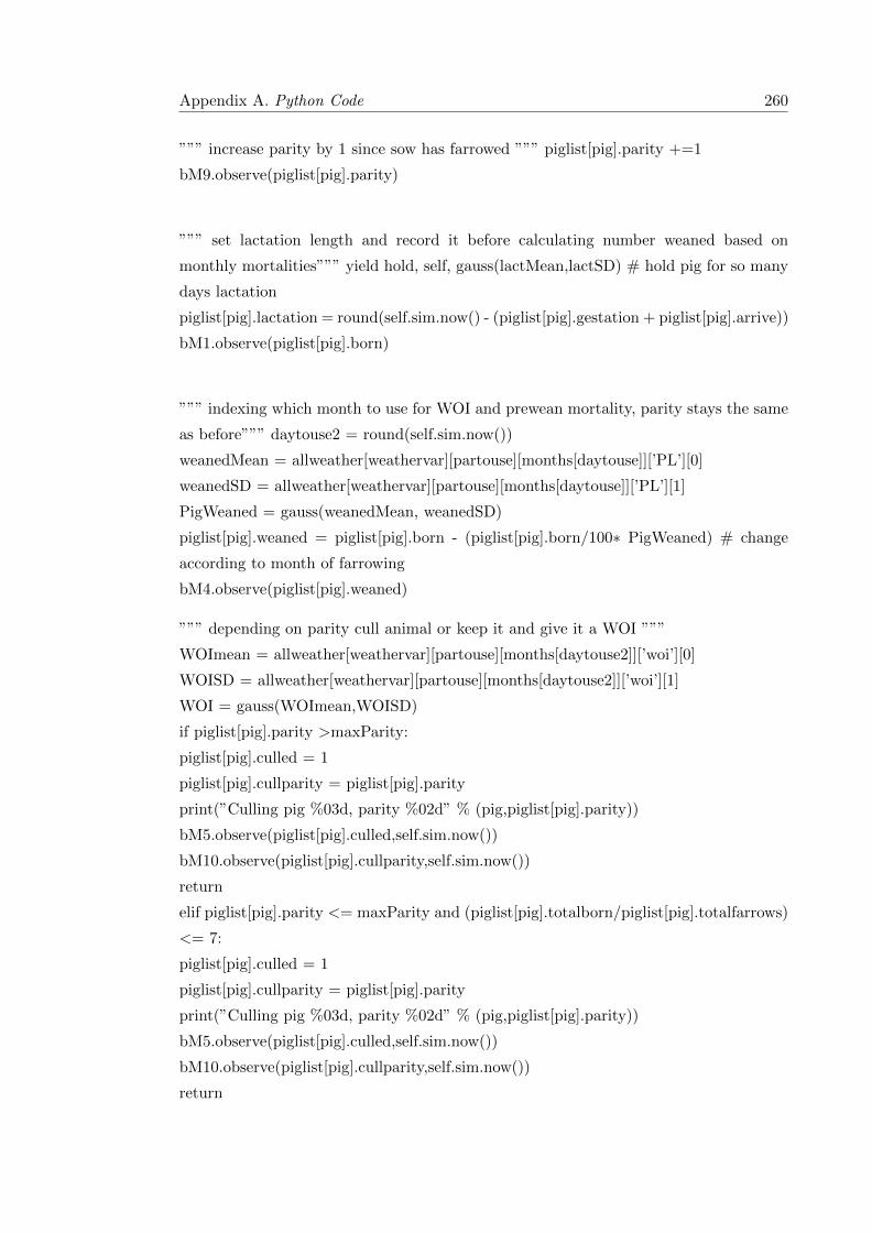
Appendix A. Python Code 260
””” increase parity by 1 since sow has farrowed ””” piglist[pig].parity +=1
bM9.observe(piglist[pig].parity)
””” set lactation length and record it before calculating number weaned based on
monthly mortalities””” yield hold, self, gauss(lactMean,lactSD) # hold pig for so many
days lactation
piglist[pig].lactation = round(self.sim.now() - (piglist[pig].gestation + piglist[pig].arrive))
bM1.observe(piglist[pig].born)
””” indexing which month to use for WOI and prewean mortality, parity stays the same
as before””” daytouse2 = round(self.sim.now())
weanedMean = allweather[weathervar][partouse][months[daytouse]][’PL’][0]
weanedSD = allweather[weathervar][partouse][months[daytouse]][’PL’][1]
PigWeaned = gauss(weanedMean, weanedSD)
piglist[pig].weaned = piglist[pig].born - (piglist[pig].born/100∗ PigWeaned) # change
according to month of farrowing
bM4.observe(piglist[pig].weaned)
””” depending on parity cull animal or keep it and give it a WOI ”””
WOImean = allweather[weathervar][partouse][months[daytouse2]][’woi’][0]
WOISD = allweather[weathervar][partouse][months[daytouse2]][’woi’][1]
WOI = gauss(WOImean,WOISD)
if piglist[pig].parity >maxParity:
piglist[pig].culled = 1
piglist[pig].cullparity = piglist[pig].parity
print(”Culling pig %03d, parity %02d” % (pig,piglist[pig].parity))
bM5.observe(piglist[pig].culled,self.sim.now())
bM10.observe(piglist[pig].cullparity,self.sim.now())
return
elif piglist[pig].parity <= maxParity and (piglist[pig].totalborn/piglist[pig].totalfarrows)
<= 7:
piglist[pig].culled = 1
piglist[pig].cullparity = piglist[pig].parity
print(”Culling pig %03d, parity %02d” % (pig,piglist[pig].parity))
bM5.observe(piglist[pig].culled,self.sim.now())
bM10.observe(piglist[pig].cullparity,self.sim.now())
return

Appendix A. Python Code 261
else:
piglist[pig].woi = WOI
print(”Pig %03d, now parity %02d” % (pig,piglist[pig].parity))
piglist[pig].inuse = 0 ## pig returns to pool
yield hold, self, piglist[pig].woi # hold for so many days from weaning
piglist[pig].empty = piglist[pig].woi + piglist[pig].returndays
print(”Pig %03d, had %02d empty days” % (pig,piglist[pig].empty))
piglist[pig].returndays = 0 # reset return days for next time
piglist[pig].AI = 0 # reset AI for next batch
piglist[pig].farrow = 0 # reset farrow for next batch
piglist[pig].regReturn = 0 # reset number of returns to 0 after farrowing
bM2.observe(piglist[pig].empty)
bM5.observe(piglist[pig].culled,self.sim.now())
## Model ———————————–
class FarmModel(Simulation):
def run(self):
””” PEM ”””
”””seed(aseed) ”””
batchMonitor1 = [Monitor() for j in range(NoBatches)] # litter size
batchMonitor2 = [Monitor() for j in range(NoBatches)] # empty days
batchMonitor3 = [Monitor() for j in range(NoBatches)] # farrow rate
batchMonitor4 = [Monitor() for j in range(NoBatches)] # piglets weaned
batchMonitor5 = [Monitor() for j in range(NoBatches)] # sows culled
batchMonitor6 = [Monitor() for j in range(NoBatches)] # sows inseminated
batchMonitor7 = [Monitor() for j in range(NoBatches)] # serve month
batchMonitor8 = [Monitor() for j in range(NoBatches)] # farrow month
batchMonitor9 = [Monitor() for j in range(NoBatches)] # sow parity
batchMonitor10 = [Monitor() for j in range(NoBatches)] # sow cull parity
batchMonitor11 = [Monitor() for j in range(NoBatches)] # weather status
for i in range(NoBatches):
b = Batch(name=’batch%02d’% (i), sim=self)
self.activate(b, b.generate(number = batchSize,bMon1=batchMonitor1[i],
bMon2=batchMonitor2[i],bMon3=batchMonitor3[i],
bMon4=batchMonitor4[i],bMon5=batchMonitor5[i],

Appendix A. Python Code 262
bMon6 = batchMonitor6[i],bMon7 = batchMonitor7[i],
bMon8 = batchMonitor8[i],bMon9=batchMonitor9[i],
bMon10=batchMonitor10[i], bMon11=batchMonitor11[i]), at=i∗TBBatches)
self.simulate(until=maxTime)
return(batchMonitor1, batchMonitor2, batchMonitor3, batchMonitor4,batchMonitor5,
batchMonitor6,batchMonitor7,batchMonitor8,batchMonitor9,batchMonitor10,batchMonitor11)
## Experiment data ————————-
batchSize = 40 # pigs in a batch
maxTime = 2920.0 # days
poolsize = 5000 # size of original sow pool
TBBatches = 21 # time between batches
NoBatches = 120
maxParity = 6 # maximum parity as cut off point
retNum = 2 # maximum number of returns allowed
pOest = 0.95 # probability of oestrus
gestMean = 115.73 # mean gestation length
gestSD = 2.09 # standard deviation for gestation length
lactMean = 21 # mean lactation length
lactSD = 0.1 # standard deviation for lactation length
postweanloss = 4 # % piglets lost before slaughter
emptydaycost = 2 # cost (in pounds) of each empty day
pigprice = 100 # worth of each pig at slaughter
””” Creating a list of dictionaries for each parity grouping by month of the year”””
””” woi = wean to oestrus interval, nba=piglets born alive, PR = pregnancy/farrowing
rate, PL = percent losses prewean”””
par0 = ’Jan’:{’woi’:[8.28,0.39],’nba’:[10.19,0.83],’PR’:[0.79,0.11],’PL’: [11.26,0.64],’AB’:
[0.4,0.07]}, ’Feb’:{’woi’:[9.39,0.59],’nba’:[10.13,1.02],’PR’:[0.79,0.13],’PL’:[11.53,0.62],’AB’:
[0.3,0.23]}, ’Mar’:{’woi’:[8.15,0.44],’nba’:[10.28,0.68],’PR’:[0.81,0.10],’PL’:[10.76,0.53],’AB’:
[0.3,0.25]}, ’Apr’:{’woi’:[7.96,0.51],’nba’:[10.30,0.87],’PR’:[0.79,0.10],’PL’:[10.01,0.70],’AB’:
[0.5,0.18]}, ’May’:{’woi’:[7.81,0.39],’nba’:[10.15,0.63],’PR’:[0.78,0.09],’PL’:[9.81,0.63],’AB’:
[1.1,0.79]}, ’Jun’:{’woi’:[7.82,0.40],’nba’:[10.12,0.74],’PR’:[0.76,0.13],’PL’:[10.77,0.84],’AB’:
[1.3,0.49]}, ’Jul’:{’woi’:[7.81,0.24],’nba’:[10.11,0.85],’PR’:[0.70,0.17],’PL’:[11.09,0.73],’AB’:
[2.6,1.11]}, ’Aug’:{’woi’:[8.03,0.40],’nba’:[9.60,0.73],’PR’:[0.72,0.16],’PL’:[11.30,0.73],’AB’:
[1.2,0.83]}, ’Sep’:{’woi’:[8.67,0.57],’nba’:[9.79,0.84],’PR’:[0.80,0.14],’PL’:[10.21,0.71],’AB’:
[1,0.49]}, ’Oct’:{’woi’:[8.23,0.30],’nba’:[9.90,1.04],’PR’:[0.80,0.13],’PL’:[10.52,0.66],’AB’: [1.3,1.06]},

Appendix A. Python Code 263
’Nov’:{’woi’:[8.37,0.51],’nba’:[9.87,1.18],’PR’:[0.80,0.10],’PL’:[12.15,0.96],’AB’: [0.4,0.21]},’Dec’:{’woi’:[9.16,0.98],’nba’:[10.30,0.89],’PR’:[0.77,0.15],’PL’:[11.27,0.64],’AB’: [0.3,0.14]}}par1 = {’Jan’:{’woi’:[7.33,0.30],’nba’:[10.78,0.69],’PR’:[0.86,0.08],’PL’: [11.26,0.64], ’AB’:
[0.4,0.07]}, ’Feb’:{’woi’:[7.89,0.51],’nba’:[10.96,0.85],’PR’:[0.85,0.08],’PL’:[11.53,0.62],’AB’:
[0.3,0.23]}, ’Mar’:{’woi’:[7.06,0.26],’nba’:[10.65,0.75],’PR’:[0.84,0.07],’PL’:[10.76,0.53],’AB’:
[0.3,0.25]}, ’Apr’:{’woi’:[6.65,0.21],’nba’:[11.37,0.95],’PR’:[0.83,0.12],’PL’:[10.01,0.70],’AB’:
[0.5,0.18]}, ’May’:{’woi’:[8.01,0.93],’nba’:[11.07,0.65],’PR’:[0.82,0.08],’PL’:[9.81,0.63],’AB’:
[1.1,0.79]}, ’Jun’:{’woi’:[8.09,0.84],’nba’:[10.89,0.74],’PR’:[0.76,0.18],’PL’:[10.77,0.84],’AB’:
[1.3,0.49]}, ’Jul’:{’woi’:[6.79,0.25],’nba’:[11.02,0.79],’PR’:[0.65,0.31],’PL’:[11.09,0.73],’AB’:
[2.6,1.11]}, ’Aug’:{’woi’:[6.73,0.28],’nba’:[10.71,0.85],’PR’:[0.64,0.24],’PL’:[11.30,0.73],’AB’:
[1.2,0.83]}, ’Sep’:{’woi’:[7.47,0.29],’nba’:[10.56,0.80],’PR’:[0.84,0.12],’PL’:[10.21,0.71],’AB’:
[1,0.49]}, ’Oct’:{’woi’:[7.23,0.34],’nba’:[10.80,0.66],’PR’:[0.83,0.10],’PL’:[10.52,0.66],’AB’:
[1.3,1.06]}, ’Nov’:{’woi’:[7.17,0.33],’nba’:[10.99,0.64],’PR’:[0.86,0.07],’PL’:[12.15,0.96],’AB’:
[0.4,0.21]}, ’Dec’:{’woi’:[7.01,0.28],’nba’:[10.98,0.74],’PR’:[0.86,0.06],’PL’:[11.27,0.64],’AB’:
[0.3,0.14]}} par2 6 = {’Jan’:{’woi’:[7.08,0.30],’nba’:[11.45,0.68],’PR’:[0.86,0.05],’PL’: [11.26,0.64],
’AB’: [0.4,0.07]}, ’Feb’:{’woi’:[7.01,0.38],’nba’:[11.29,0.73],’PR’:[0.87,0.06],’PL’:[11.53,0.62],’AB’:
[0.3,0.23]}, ’Mar’:{’woi’:[6.76,0.21],’nba’:[11.38,0.75],’PR’:[0.87,0.06],’PL’:[10.76,0.53],’AB’:
[0.3,0.25]}, ’Apr’:{’woi’:[6.67,0.24],’nba’:[11.42,0.77],’PR’:[0.87,0.06],’PL’:[10.01,0.70],’AB’:
[0.5,0.18]}, ’May’:{’woi’:[7.05,0.24],’nba’:[11.37,0.63],’PR’:[0.85,0.05],’PL’:[9.81,0.63],’AB’:
[1.1,0.79]}, ’Jun’:{’woi’:[7.50,0.51],’nba’:[11.05,1.58],’PR’:[0.75,0.17],’PL’:[10.77,0.84],’AB’:
[1.3,0.49]}, ’Jul’:{’woi’:[7.25,0.33],’nba’:[11.58,2.22],’PR’:[0.61,0.29],’PL’:[11.09,0.73],’AB’:
[2.6,1.11]}, ’Aug’:{’woi’:[6.68,0.30],’nba’:[11.08,0.80],’PR’:[0.58,0.33],’PL’:[11.30,0.73],’AB’:
[1.2,0.83]}, ’Sep’:{’woi’:[7.10,0.30],’nba’:[11.05,0.76],’PR’:[0.89,0.05],’PL’:[10.21,0.71],’AB’:
[1,0.49]}, ’Oct’:{’woi’:[7.23,0.26],’nba’:[11.12,0.99],’PR’:[0.87,0.07],’PL’:[10.52,0.66],’AB’:
[1.3,1.06]}, ’Nov’:{’woi’:[6.38,0.26],’nba’:[11.54,0.51],’PR’:[0.88,0.05],’PL’:[12.15,0.96],’AB’:
[0.4,0.21]}, ’Dec’:{’woi’:[7.31,0.33],’nba’:[11.45,0.72],’PR’:[0.85,0.05],’PL’:[11.27,0.64],’AB’:
[0.3,0.14]}} par7 = {’Jan’:{’woi’:[7.50,0.38],’nba’:[10.69,0.80],’PR’:[0.84,0.10],’PL’: [11.26,0.64],’AB’:
[0.4,0.07]}, ’Feb’:{’woi’:[6.97,0.41],’nba’:[10.71,1.07],’PR’:[0.78,0.15],’PL’:[11.53,0.62],’AB’:
[0.3,0.23]}, ’Mar’:{’woi’:[6.09,0.21],’nba’:[10.80,0.68],’PR’:[0.88,0.08],’PL’:[10.76,0.53],’AB’:
[0.3,0.25]}, ’Apr’:{’woi’:[6.93,0.38],’nba’:[10.74,0.78],’PR’:[0.85,0.12],’PL’:[10.01,0.70],’AB’:
[0.5,0.18]}, ’May’:{’woi’:[7.04,0.37],’nba’:[10.05,1.14],’PR’:[0.79,0.12],’PL’:[9.81,0.63],’AB’:
[1.1,0.79]}, ’Jun’:{’woi’:[6.48,0.51],’nba’:[10.24,2.59],’PR’:[0.63,0.30],’PL’:[10.77,0.84],’AB’:
[1.3,0.49]}, ’Jul’:{’woi’:[7.65,0.45],’nba’:[10.43,0.56],’PR’:[0.55,0.32],’PL’:[11.09,0.73],’AB’:
[2.6,1.11]}, ’Aug’:{’woi’:[8.24,1.19],’nba’:[10.21,1.02],’PR’:[0.54,0.35],’PL’:[11.30,0.73],’AB’:
[1.2,0.83]}, ’Sep’:{’woi’:[7.32,0.45],’nba’:[10.78,0.52],’PR’:[0.89,0.11],’PL’:[10.21,0.71],’AB’:
[1,0.49]}, ’Oct’:{’woi’:[7.17,0.45],’nba’:[10.63,1.19],’PR’:[0.83,0.08],’PL’:[10.52,0.66],’AB’:
[1.3,1.06]}, ’Nov’:{’woi’:[6.42,0.36],’nba’:[10.23,2.09],’PR’:[0.88,0.10],’PL’:[12.15,0.96],’AB’:
[0.4,0.21]}, ’Dec’:{’woi’:[7.02,0.29],’nba’:[9.91,3.02],’PR’:[0.82,0.11],’PL’:[11.27,0.64],’AB’:
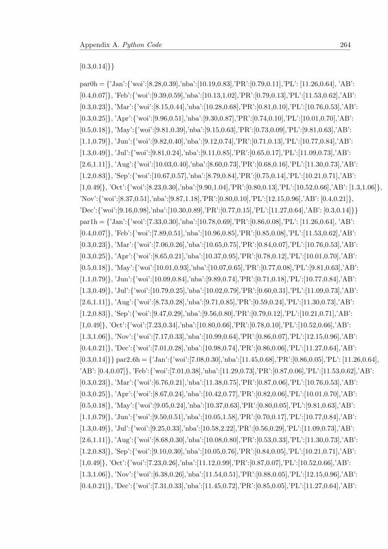
Appendix A. Python Code 264
[0.3,0.14]}}
par0h = {’Jan’:{’woi’:[8.28,0.39],’nba’:[10.19,0.83],’PR’:[0.79,0.11],’PL’: [11.26,0.64], ’AB’:
[0.4,0.07]}, ’Feb’:{’woi’:[9.39,0.59],’nba’:[10.13,1.02],’PR’:[0.79,0.13],’PL’:[11.53,0.62],’AB’:
[0.3,0.23]}, ’Mar’:{’woi’:[8.15,0.44],’nba’:[10.28,0.68],’PR’:[0.81,0.10],’PL’:[10.76,0.53],’AB’:
[0.3,0.25]}, ’Apr’:{’woi’:[9.96,0.51],’nba’:[9.30,0.87],’PR’:[0.74,0.10],’PL’:[10.01,0.70],’AB’:
[0.5,0.18]}, ’May’:{’woi’:[9.81,0.39],’nba’:[9.15,0.63],’PR’:[0.73,0.09],’PL’:[9.81,0.63],’AB’:
[1.1,0.79]}, ’Jun’:{’woi’:[9.82,0.40],’nba’:[9.12,0.74],’PR’:[0.71,0.13],’PL’:[10.77,0.84],’AB’:
[1.3,0.49]}, ’Jul’:{’woi’:[9.81,0.24],’nba’:[9.11,0.85],’PR’:[0.65,0.17],’PL’:[11.09,0.73],’AB’:
[2.6,1.11]}, ’Aug’:{’woi’:[10.03,0.40],’nba’:[8.60,0.73],’PR’:[0.68,0.16],’PL’:[11.30,0.73],’AB’:
[1.2,0.83]}, ’Sep’:{’woi’:[10.67,0.57],’nba’:[8.79,0.84],’PR’:[0.75,0.14],’PL’:[10.21,0.71],’AB’:
[1,0.49]}, ’Oct’:{’woi’:[8.23,0.30],’nba’:[9.90,1.04],’PR’:[0.80,0.13],’PL’:[10.52,0.66],’AB’: [1.3,1.06]},’Nov’:{’woi’:[8.37,0.51],’nba’:[9.87,1.18],’PR’:[0.80,0.10],’PL’:[12.15,0.96],’AB’: [0.4,0.21]},’Dec’:{’woi’:[9.16,0.98],’nba’:[10.30,0.89],’PR’:[0.77,0.15],’PL’:[11.27,0.64],’AB’: [0.3,0.14]}}par1h = {’Jan’:{’woi’:[7.33,0.30],’nba’:[10.78,0.69],’PR’:[0.86,0.08],’PL’: [11.26,0.64], ’AB’:
[0.4,0.07]}, ’Feb’:{’woi’:[7.89,0.51],’nba’:[10.96,0.85],’PR’:[0.85,0.08],’PL’:[11.53,0.62],’AB’:
[0.3,0.23]}, ’Mar’:{’woi’:[7.06,0.26],’nba’:[10.65,0.75],’PR’:[0.84,0.07],’PL’:[10.76,0.53],’AB’:
[0.3,0.25]}, ’Apr’:{’woi’:[8.65,0.21],’nba’:[10.37,0.95],’PR’:[0.78,0.12],’PL’:[10.01,0.70],’AB’:
[0.5,0.18]}, ’May’:{’woi’:[10.01,0.93],’nba’:[10.07,0.65],’PR’:[0.77,0.08],’PL’:[9.81,0.63],’AB’:
[1.1,0.79]}, ’Jun’:{’woi’:[10.09,0.84],’nba’:[9.89,0.74],’PR’:[0.71,0.18],’PL’:[10.77,0.84],’AB’:
[1.3,0.49]}, ’Jul’:{’woi’:[10.79,0.25],’nba’:[10.02,0.79],’PR’:[0.60,0.31],’PL’:[11.09,0.73],’AB’:
[2.6,1.11]}, ’Aug’:{’woi’:[8.73,0.28],’nba’:[9.71,0.85],’PR’:[0.59,0.24],’PL’:[11.30,0.73],’AB’:
[1.2,0.83]}, ’Sep’:{’woi’:[9.47,0.29],’nba’:[9.56,0.80],’PR’:[0.79,0.12],’PL’:[10.21,0.71],’AB’:
[1,0.49]}, ’Oct’:{’woi’:[7.23,0.34],’nba’:[10.80,0.66],’PR’:[0.78,0.10],’PL’:[10.52,0.66],’AB’:
[1.3,1.06]}, ’Nov’:{’woi’:[7.17,0.33],’nba’:[10.99,0.64],’PR’:[0.86,0.07],’PL’:[12.15,0.96],’AB’:
[0.4,0.21]}, ’Dec’:{’woi’:[7.01,0.28],’nba’:[10.98,0.74],’PR’:[0.86,0.06],’PL’:[11.27,0.64],’AB’:
[0.3,0.14]}} par2 6h = {’Jan’:{’woi’:[7.08,0.30],’nba’:[11.45,0.68],’PR’:[0.86,0.05],’PL’: [11.26,0.64],
’AB’: [0.4,0.07]}, ’Feb’:{’woi’:[7.01,0.38],’nba’:[11.29,0.73],’PR’:[0.87,0.06],’PL’:[11.53,0.62],’AB’:
[0.3,0.23]}, ’Mar’:{’woi’:[6.76,0.21],’nba’:[11.38,0.75],’PR’:[0.87,0.06],’PL’:[10.76,0.53],’AB’:
[0.3,0.25]}, ’Apr’:{’woi’:[8.67,0.24],’nba’:[10.42,0.77],’PR’:[0.82,0.06],’PL’:[10.01,0.70],’AB’:
[0.5,0.18]}, ’May’:{’woi’:[9.05,0.24],’nba’:[10.37,0.63],’PR’:[0.80,0.05],’PL’:[9.81,0.63],’AB’:
[1.1,0.79]}, ’Jun’:{’woi’:[9.50,0.51],’nba’:[10.05,1.58],’PR’:[0.70,0.17],’PL’:[10.77,0.84],’AB’:
[1.3,0.49]}, ’Jul’:{’woi’:[9.25,0.33],’nba’:[10.58,2.22],’PR’:[0.56,0.29],’PL’:[11.09,0.73],’AB’:
[2.6,1.11]}, ’Aug’:{’woi’:[8.68,0.30],’nba’:[10.08,0.80],’PR’:[0.53,0.33],’PL’:[11.30,0.73],’AB’:
[1.2,0.83]}, ’Sep’:{’woi’:[9.10,0.30],’nba’:[10.05,0.76],’PR’:[0.84,0.05],’PL’:[10.21,0.71],’AB’:
[1,0.49]}, ’Oct’:{’woi’:[7.23,0.26],’nba’:[11.12,0.99],’PR’:[0.87,0.07],’PL’:[10.52,0.66],’AB’:
[1.3,1.06]}, ’Nov’:{’woi’:[6.38,0.26],’nba’:[11.54,0.51],’PR’:[0.88,0.05],’PL’:[12.15,0.96],’AB’:
[0.4,0.21]}, ’Dec’:{’woi’:[7.31,0.33],’nba’:[11.45,0.72],’PR’:[0.85,0.05],’PL’:[11.27,0.64],’AB’:

Appendix A. Python Code 265
[0.3,0.14]}} par7h = {’Jan’:{’woi’:[7.50,0.38],’nba’:[10.69,0.80],’PR’:[0.84,0.10],’PL’: [11.26,0.64],
’AB’: [0.4,0.07]}, ’Feb’:{’woi’:[6.97,0.41],’nba’:[10.71,1.07],’PR’:[0.78,0.15],’PL’:[11.53,0.62],’AB’:
[0.3,0.23]}, ’Mar’:{’woi’:[6.09,0.21],’nba’:[10.80,0.68],’PR’:[0.88,0.08],’PL’:[10.76,0.53],’AB’:
[0.3,0.25]}, ’Apr’:{’woi’:[8.93,0.38],’nba’:[9.74,0.78],’PR’:[0.80,0.12],’PL’:[10.01,0.70],’AB’:
[0.5,0.18]}, ’May’:{’woi’:[9.04,0.37],’nba’:[9.05,1.14],’PR’:[0.74,0.12],’PL’:[9.81,0.63],’AB’:
[1.1,0.79]}, ’Jun’:{’woi’:[8.48,0.51],’nba’:[9.24,2.59],’PR’:[0.58,0.30],’PL’:[10.77,0.84],’AB’:
[1.3,0.49]}, ’Jul’:{’woi’:[9.65,0.45],’nba’:[9.43,0.56],’PR’:[0.50,0.32],’PL’:[11.09,0.73],’AB’:
[2.6,1.11]}, ’Aug’:{’woi’:[10.24,1.19],’nba’:[9.21,1.02],’PR’:[0.49,0.35],’PL’:[11.30,0.73],’AB’:
[1.2,0.83]}, ’Sep’:{’woi’:[9.32,0.45],’nba’:[9.78,0.52],’PR’:[0.84,0.11],’PL’:[10.21,0.71],’AB’:
[1,0.49]}, ’Oct’:{’woi’:[7.17,0.45],’nba’:[10.63,1.19],’PR’:[0.83,0.08],’PL’:[10.52,0.66],’AB’:
[1.3,1.06]}, ’Nov’:{’woi’:[6.42,0.36],’nba’:[10.23,2.09],’PR’:[0.88,0.10],’PL’:[12.15,0.96],’AB’:
[0.4,0.21]}, ’Dec’:{’woi’:[7.02,0.29],’nba’:[9.91,3.02],’PR’:[0.82,0.11],’PL’:[11.27,0.64],’AB’:
[0.3,0.14]}}
par0c = {’Jan’:{’woi’:[8.28,0.39],’nba’:[10.19,0.83],’PR’:[0.79,0.11],’PL’: [14.26,0.64],’AB’:
[0.4,0.07]}, ’Feb’:{’woi’:[9.39,0.59],’nba’:[10.13,1.02],’PR’:[0.79,0.13],’PL’:[14.53,0.62],’AB’:
[0.3,0.23]}, ’Mar’:{’woi’:[8.15,0.44],’nba’:[10.28,0.68],’PR’:[0.81,0.10],’PL’:[13.76,0.53],’AB’:
[0.3,0.25]}, ’Apr’:{’woi’:[7.96,0.51],’nba’:[10.30,0.87],’PR’:[0.79,0.10],’PL’:[10.01,0.70],’AB’:
[0.5,0.18]}, ’May’:{’woi’:[7.81,0.39],’nba’:[10.15,0.63],’PR’:[0.78,0.09],’PL’:[9.81,0.63],’AB’:
[1.1,0.79]}, ’Jun’:{’woi’:[7.82,0.40],’nba’:[10.12,0.74],’PR’:[0.76,0.13],’PL’:[10.77,0.84],’AB’:
[1.3,0.49]}, ’Jul’:{’woi’:[7.81,0.24],’nba’:[10.11,0.85],’PR’:[0.70,0.17],’PL’:[11.09,0.73],’AB’:
[2.6,1.11]}, ’Aug’:{’woi’:[8.03,0.40],’nba’:[9.60,0.73],’PR’:[0.72,0.16],’PL’:[11.30,0.73],’AB’:
[1.2,0.83]}, ’Sep’:{’woi’:[8.67,0.57],’nba’:[9.79,0.84],’PR’:[0.80,0.14],’PL’:[13.21,0.71],’AB’:
[1,0.49]}, ’Oct’:{’woi’:[8.23,0.30],’nba’:[9.90,1.04],’PR’:[0.80,0.13],’PL’:[13.52,0.66],’AB’: [1.3,1.06]},’Nov’:{’woi’:[8.37,0.51],’nba’:[9.87,1.18],’PR’:[0.80,0.10],’PL’:[15.15,0.96],’AB’: [0.4,0.21]},’Dec’:{’woi’:[9.16,0.98],’nba’:[10.30,0.89],’PR’:[0.77,0.15],’PL’:[14.27,0.64],’AB’: [0.3,0.14]}}par1c = {’Jan’:{’woi’:[7.33,0.30],’nba’:[10.78,0.69],’PR’:[0.86,0.08],’PL’: [14.26,0.64],’AB’:
[0.4,0.07]}, ’Feb’:{’woi’:[7.89,0.51],’nba’:[10.96,0.85],’PR’:[0.85,0.08],’PL’:[14.53,0.62],’AB’:
[0.3,0.23]}, ’Mar’:{’woi’:[7.06,0.26],’nba’:[10.65,0.75],’PR’:[0.84,0.07],’PL’:[13.76,0.53],’AB’:
[0.3,0.25]}, ’Apr’:{’woi’:[6.65,0.21],’nba’:[11.37,0.95],’PR’:[0.83,0.12],’PL’:[10.01,0.70],’AB’:
[0.5,0.18]}, ’May’:{’woi’:[8.01,0.93],’nba’:[11.07,0.65],’PR’:[0.82,0.08],’PL’:[9.81,0.63],’AB’:
[1.1,0.79]}, ’Jun’:{’woi’:[8.09,0.84],’nba’:[10.89,0.74],’PR’:[0.76,0.18],’PL’:[10.77,0.84],’AB’:
[1.3,0.49]}, ’Jul’:{’woi’:[6.79,0.25],’nba’:[11.02,0.79],’PR’:[0.65,0.31],’PL’:[11.09,0.73],’AB’:
[2.6,1.11]}, ’Aug’:{’woi’:[6.73,0.28],’nba’:[10.71,0.85],’PR’:[0.64,0.24],’PL’:[11.30,0.73],’AB’:
[1.2,0.83]}, ’Sep’:{’woi’:[7.47,0.29],’nba’:[10.56,0.80],’PR’:[0.84,0.12],’PL’:[10.21,0.71],’AB’:
[1,0.49]}, ’Oct’:{’woi’:[7.23,0.34],’nba’:[10.80,0.66],’PR’:[0.83,0.10],’PL’:[13.52,0.66], ’AB’:
[1.3,1.06]}, ’Nov’:{’woi’:[7.17,0.33],’nba’:[10.99,0.64],’PR’:[0.86,0.07],’PL’:[15.15,0.96],’AB’:
[0.4,0.21]}, ’Dec’:{’woi’:[7.01,0.28],’nba’:[10.98,0.74],’PR’:[0.86,0.06],’PL’:[14.27,0.64],’AB’:

Appendix A. Python Code 266
[0.3,0.14]}} par2 6c = {’Jan’:{’woi’:[7.08,0.30],’nba’:[11.45,0.68],’PR’:[0.86,0.05],’PL’: [14.26,0.64],
’AB’: [0.4,0.07]}, ’Feb’:{’woi’:[7.01,0.38],’nba’:[11.29,0.73],’PR’:[0.87,0.06],’PL’:[14.53,0.62],’AB’:
[0.3,0.23]}, ’Mar’:{’woi’:[6.76,0.21],’nba’:[11.38,0.75],’PR’:[0.87,0.06],’PL’:[13.76,0.53],’AB’:
[0.3,0.25]}, ’Apr’:{’woi’:[6.67,0.24],’nba’:[11.42,0.77],’PR’:[0.87,0.06],’PL’:[10.01,0.70],’AB’:
[0.5,0.18]}, ’May’:{’woi’:[7.05,0.24],’nba’:[11.37,0.63],’PR’:[0.85,0.05],’PL’:[9.81,0.63],’AB’:
[1.1,0.79]}, ’Jun’:{’woi’:[7.50,0.51],’nba’:[11.05,1.58],’PR’:[0.75,0.17],’PL’:[10.77,0.84],’AB’:
[1.3,0.49]}, ’Jul’:{’woi’:[7.25,0.33],’nba’:[11.58,2.22],’PR’:[0.61,0.29],’PL’:[11.09,0.73],’AB’:
[2.6,1.11]}, ’Aug’:{’woi’:[6.68,0.30],’nba’:[11.08,0.80],’PR’:[0.58,0.33],’PL’:[11.30,0.73],’AB’:
[1.2,0.83]}, ’Sep’:{’woi’:[7.10,0.30],’nba’:[11.05,0.76],’PR’:[0.89,0.05],’PL’:[10.21,0.71],’AB’:
[1,0.49]}, ’Oct’:{’woi’:[7.23,0.26],’nba’:[11.12,0.99],’PR’:[0.87,0.07],’PL’:[13.52,0.66],’AB’:
[1.3,1.06]}, ’Nov’:{’woi’:[6.38,0.26],’nba’:[11.54,0.51],’PR’:[0.88,0.05],’PL’:[15.15,0.96],’AB’:
[0.4,0.21]}, ’Dec’:{’woi’:[7.31,0.33],’nba’:[11.45,0.72],’PR’:[0.85,0.05],’PL’:[14.27,0.64],’AB’:
[0.3,0.14]}} par7c = {’Jan’:{’woi’:[7.50,0.38],’nba’:[10.69,0.80],’PR’:[0.84,0.10],’PL’: [14.26,0.64],
’AB’: [0.4,0.07]}, ’Feb’:{’woi’:[6.97,0.41],’nba’:[10.71,1.07],’PR’:[0.78,0.15],’PL’:[14.53,0.62],’AB’:
[0.3,0.23]}, ’Mar’:{’woi’:[6.09,0.21],’nba’:[10.80,0.68],’PR’:[0.88,0.08],’PL’:[13.76,0.53],’AB’:
[0.3,0.25]}, ’Apr’:{’woi’:[6.93,0.38],’nba’:[10.74,0.78],’PR’:[0.85,0.12],’PL’:[10.01,0.70],’AB’:
[0.5,0.18]}, ’May’:{’woi’:[7.04,0.37],’nba’:[10.05,1.14],’PR’:[0.79,0.12],’PL’:[9.81,0.63],’AB’:
[1.1,0.79]}, ’Jun’:{’woi’:[6.48,0.51],’nba’:[10.24,2.59],’PR’:[0.63,0.30],’PL’:[10.77,0.84],’AB’:
[1.3,0.49]}, ’Jul’:{’woi’:[7.65,0.45],’nba’:[10.43,0.56],’PR’:[0.55,0.32],’PL’:[11.09,0.73],’AB’:
[2.6,1.11]}, ’Aug’:{’woi’:[8.24,1.19],’nba’:[10.21,1.02],’PR’:[0.54,0.35],’PL’:[11.30,0.73],’AB’:
[1.2,0.83]}, ’Sep’:{’woi’:[7.32,0.45],’nba’:[10.78,0.52],’PR’:[0.89,0.11],’PL’:[10.21,0.71],’AB’:
[1,0.49]}, ’Oct’:{’woi’:[7.17,0.45],’nba’:[10.63,1.19],’PR’:[0.83,0.08],’PL’:[13.52,0.66],’AB’:
[1.3,1.06]}, ’Nov’:{’woi’:[6.42,0.36],’nba’:[10.23,2.09],’PR’:[0.88,0.10],’PL’:[15.15,0.96],’AB’:
[0.4,0.21]}, ’Dec’:{’woi’:[7.02,0.29],’nba’:[9.91,3.02],’PR’:[0.82,0.11],’PL’:[14.27,0.64],’AB’:
[0.3,0.14]}}
allmonths =[par0,par1,par2 6,par7] allmonthshot =[par0h,par1h,par2 6h,par7h] allmonth-
cold =[par0c,par1c,par2 6c,par7c] allweather = [allmonths, allmonthshot, allmonthcold]
days = range(2920) month = ([’Jan’]∗31+[’Feb’]∗28+[’Mar’]∗31+[’Apr’]∗30+[’May’]∗31
+[’Jun’]∗30+[’Jul’]∗31+[’Aug’]∗31+[’Sep’]∗30+[’Oct’]∗31+[’Nov’]∗30+[’Dec’]∗31)∗8months = dict(zip(days,month))
Num month = {’Jan’:1,’Feb’:2,’Mar’:3,’Apr’:4,’May’:5, ’Jun’:6,’Jul’:7,’Aug’:8,’Sep’:9,’Oct’:10,
’Nov’:11,’Dec’:12}
## Experiment ——————————
## create a pool of pigs

Appendix A. Python Code 267
piglist = [Animal()for i in range(poolsize)] # list of pig objects in animal class
for j in range(len(piglist)): # give pigs attributes
piglist[j].ident = j
piglist[j].parity = 0 # round(gammavariate(2.48, 1.14)) for established herd
piglist[j].born = 0 # set litter size to 0
piglist[j].weaned = 0 # set weaned piglets to 0
piglist[j].farrow = 0 # set to 0
piglist[j].woi = 0 # set WOI
piglist[j].inuse = 0 # pig starts off not in use
piglist[j].culled = 0 # pig starts off not culled
piglist[j].arrive = 0 # arrival time
piglist[j].firstarrive = 0 # first arrival time
piglist[j].gestation = 0 # gestation length
piglist[j].lactation = 0 # lactation length
piglist[j].regReturn = 0 # number of times returned normally
piglist[j].returndays = 0 # to tally how many days held for returns
piglist[j].empty = 0 # to tally how empty days
piglist[j].totalborn = 0 #total number of piglets born to sow
piglist[j].totalfarrows = 0 # number of times sow has had a litter
piglist[j].AI = 0 # if sow inseminated after oestrus or not
piglist[j].servemonth = 0 # set service month
piglist[j].farrowmonth = 0 # set farrow month
piglist[j].abortion = 0 # set farrow month
piglist[j].cullparity = 0 # set farrow month
piglist[j].weather = 0 # set weather
mymodel = FarmModel()
littersize, emptydays, farrowsows, litterweaned, culledsows, AIsows, Smonth, Fmonth,
Parities, Cullpars, Weather = mymodel.run()
## Results ————————
lFR = []
lEmptyCost =[]
lSowCullsper =[]
lSowCulls =[]

Appendix A. Python Code 268
lPigstomarket = []
lMonth = []
tot far = []
mean par = []
cull par = []
LitterSize = []
Profit =[]
lEmptydays=[]
WS=[]
for batch in range(NoBatches):
SM = Smonth[batch][1][1]
FM = Fmonth[batch][1][1]
Total farrow = farrowsows[batch].total()#total number of sows which farrowed in batch
Mean parity = (Parities[batch].total()/batchSize)#average sow parity in batch
if culledsows[batch].total() >0:
Mean cullparity = (Cullpars[batch].total()/culledsows[batch].total())#average sow par-
ity when culled in batch
else:
Mean cullparity = -1 # none culled
Weatherstats = Weather[batch].mean()
FR = (farrowsows[batch].total()/AIsows[batch].total())∗100 # FR for that batch
EmptyCost = (emptydays[batch].total()∗emptydaycost) # cost of empty days assuming
2 pounds a day lost
SoldPigs = (litterweaned[batch].total()- (litterweaned[batch].total()/100∗postweanloss))
# 4% lost before market
PigWorth = SoldPigs∗pigprice # money made per pig assuming ’pigprice’ pounds per
pig
ProfitPerBatch = PigWorth - EmptyCost # assuming everything else is kept the same
SowCullsper = (culledsows[batch].total()) # percent of culled sows in batch
SowCulls = culledsows[batch].total() # number of culled sows in batch
LS = littersize[batch].total()/farrowsows[batch].total()#total piglets born in batch
ED = emptydays[batch].total()/batchSize
lFR.append([FM,FR]) # with ’SM’ or ’FM’ instead of ’batch’ get it by month rather
than batch
tot far.append([FM,Total farrow])
mean par.append([FM, Mean parity])
cull par.append([SM, Mean cullparity])
lEmptyCost.append([SM,EmptyCost])

Appendix A. Python Code 269
lSowCullsper.append([SM,SowCullsper])
lSowCulls.append([SM,SowCulls])
lPigstomarket.append([FM,SoldPigs])
LitterSize.append([FM,LS])
Profit.append([SM,ProfitPerBatch])
lEmptydays.append([SM,ED])
WS.append([SM,Weatherstats])
f = open(’FR batch.txt’, ’w’)
for item in lFR:
f.write(”% s % s \ n” % (item[0], item[1]))
f.close()
f = open(’Weather stat.txt’, ’w’)
for item in WS:
f.write(”% s % s \ n” % (item[0], item[1]))
f.close()
f = open(’LS batch.txt’, ’w’)
for item in LitterSize:
f.write(”% s % s \ n” % (item[0], item[1]))
f.close()
f = open(’ED batch.txt’, ’w’)
for item in lEmptydays:
f.write(”% s % s \ n” % (item[0], item[1]))
f.close()
f = open(’Profit batch.txt’, ’w’)
for item in Profit:
f.write(”% s % s \ n” % (item[0], item[1]))
f.close()
f = open(’Culls batch.txt’, ’w’)
for item in lSowCullsper:
f.write(”% s % s \ n” % (item[0], item[1]))
f.close()
f = open(’Culls calib.txt’, ’w’)
for item in lSowCulls:
f.write(”% s % s \ n” % (item[0], item[1]))
f.close()
f = open(’EmptyCost batch.txt’, ’w’)
for item in lEmptyCost:
f.write(”% s % s \ n” % (item[0], item[1]))

Appendix A. Python Code 270
f.close()
f = open(’Pigsold batch.txt’, ’w’)
for item in lPigstomarket:
f.write(”% s % s \ n” % (item[0], item[1]))
f.close()
f = open(’Farrowed calib.txt’, ’w’)
for item in tot far:
f.write(”% s % s \ n” % (item[0], item[1]))
f.close()
f = open(’Parity calib.txt’, ’w’)
for item in mean par:
f.write(”% s % s \ n” % (item[0], item[1]))
f.close()
f = open(’Parity culling.txt’, ’w’)
for item in cull par:
f.write(”% s % s \ n” % (item[0], item[1]))
f.close()

Appendix B
Decision trees
The following pages present the decision trees produced in Chapter 5 for rules concerning
the effects of meteorological and managerial influences on semen quality.
Trees are presented in the same number order as in Table 5.9 from Chapter 5. Figures B.1
to B.3 represent trees produced from sperm concentration (SC) experiments. Figure B.4
represents experiments concerning semen volume (SV). Figures B.5 to B.7 show results
from experiments involving total sperm numbers (TSN). Figures B.8 to B.10 present
results for experiments with 20% abnormalities (AB) as a cut off point. Figures B.11
and B.12 present results for experiments with 30% abnormalities (AB) as a cut off point.
Within the figures for SC, SV and TSN branches ending with a 0 signify that the quality
of the parameter examined was above average, whereas a 1 signifies that the quality was
below average. For the AB figures, the opposite is true. Table 5.1 in Chapter 5 shows
what the various node key definitions are.
271

Appendix B. Decision trees 272
FigureB.1:
Dec
isio
ntr
eefo
rsp
erm
con
centr
ati
on
,u
sin
g5
as
the
min
imu
mle
af
size
.

Appendix B. Decision trees 273
FigureB.2:
Dec
isio
ntr
eefo
rsp
erm
con
centr
ati
on
,u
sin
g20
as
the
min
imu
mle
af
size
.

Appendix B. Decision trees 274
FigureB.3:
Dec
isio
ntr
eefo
rsp
erm
con
centr
ati
on
,u
sin
g200
as
the
min
imu
mle
af
size
.

Appendix B. Decision trees 275
FigureB.4:
Dec
isio
ntr
eefo
rse
men
volu
me,
usi
ng
5,
20
or
100
as
the
min
imu
mle
af
size
.

Appendix B. Decision trees 276
FigureB.5:
Dec
isio
ntr
eefo
rto
tal
sper
mnu
mb
ers,
usi
ng
5as
the
min
imu
mle
af
size
.

Appendix B. Decision trees 277
FigureB.6:
Dec
isio
ntr
eefo
rto
tal
sper
mnu
mb
ers,
usi
ng
20
as
the
min
imu
mle
af
size
.

Appendix B. Decision trees 278
FigureB.7:
Dec
isio
ntr
eefo
rto
tal
sper
mnu
mb
ers,
usi
ng
200
as
the
min
imu
mle
af
size
.

Appendix B. Decision trees 279
FigureB.8:
Dec
isio
ntr
eefo
r20%
ab
norm
ali
ties
,u
sin
g5
as
the
min
imu
mle
af
size
.

Appendix B. Decision trees 280
FigureB.9:
Dec
isio
ntr
eefo
r20%
ab
norm
ali
ties
,u
sin
g20
as
the
min
imu
mle
af
size
.

Appendix B. Decision trees 281
FigureB.10:
Dec
isio
ntr
eefo
r20%
ab
norm
ali
ties
,u
sin
g200
as
the
min
imu
mle
af
size
.

Appendix B. Decision trees 282
FigureB.11:
Dec
isio
ntr
eefo
r30%
ab
norm
ali
ties
,u
sin
g5
as
the
min
imu
mle
af
size
.

Appendix B. Decision trees 283
FigureB.12:
Dec
isio
ntr
eefo
r30%
ab
norm
ali
ties
,u
sin
g20
or
200
as
the
min
imu
mle
af
size
.

Appendix C
Body scoring
Body condition can be estimated using a universally recognised scale of 1 - 5, as shown
in Table C.1 and Figure C.1.
Table C.1: Body condition score guidelines. Adapted from Carr (1998).
Score Condition Description
5 Overfat Hips and backbone heavily covered
4 Fat Hips and backbone cannot be felt
3.5 Good condition Hips and backbone only felt with difficulty
3 Normal Hips and backbone only felt with firm palm pressure
2.5 Somewhat thin Hips and backbone felt without palm pressure
2 Thin Hips and backbone noticeable and easily felt
1 Emaciated Hips and backbone visible
Figure C.1: Body condition score guidelines. Taken from Carr (1998)
.
284