Indian Meteorological Society, Chennai Chapter Newsletter ...

Indian Meteorological Society, Chennai Chapter Newsletter Vol.15, Issue No.2, December 2013

Contents

1. Impact of Monsoon 2013 on the water supply to Chennai city by

the Chennai Metropolitan Water Supply and Sewerage Board

B.Chandra Mohan

2. Monsoons- 2013

S.R.Ramanan

3. Climate Calendar of India 2014 M.S.Narayanan & R.Uma

4. Elevation measurements using differential GNSS technology

B.Amudha

5. wXword

S.R. Ramanan

6. An Analytical Tool for depicting Rainfall Characteristics of

Tropical Cyclones over North Indian Ocean - TCRAIN

S.Balachandran

B.Geetha

K.Ramesh &

N.Selvam

EDITORIAL BOARD

Editor : Dr. B. Geetha Members : Dr.N.Jayanthi, Prof.N.Sivagnanam,

Dr.V.Geethalakshmi & Shri K.V.Balasubramanian

BREEZE Vol.15, No.2, December 2013

1

From the Chairman’s Desk…

Dear Members of IMS Chennai Chapter and Readers of Breeze,

It is my privilege to update you on the activities of the chapter, since the release of the previous issue of BREEZE (Vol.15, Issue 1). The focus of the chapter’s activities during the last six months has been on the conduct of International Tropical Meteorology (INTROMET) Symposium on Monsoons – Observations, Prediction and Simulation slated for 21-25 February 2014 at SRM University, Kattankulathur (near Chennai) under the joint auspices of the Indian Meteorological Society and the SRM University. Arrangements for a grand conduct of this mega event are in full swing. Two Local Organising Committee meetings were held.

A half-a-day seminar on “Monsoons 2013” was conducted on 08th January

2014. As many as 6 lectures on various aspects of southwest and northeast monsoons 2013 were covered during this seminar. In addition to 3 IMD scientists, two civil administrators and a research scholar delivered lectures. Dr. T.S. Sridhar, I.A.S., Additional Chief Secretary & Commissioner of Revenue Administration, Govt. of Tamil Nadu, Chennai spoke on Revenue administrative perspective of monsoons of 2013 and Dr. B. Chandra Mohan, I.A.S., Managing Director, Chennai Metropolitan Water Supply and Sewerage Board, Chennai spoke on the Impact of monsoon 2013 on water supply to Chennai city.

A Climate Calendar-2014 was prepared under the joint auspices of the Indian

Meteorological Society, Chennai Chapter and the SRM University. Copies of the same have been sent to the other IMS Chapters and Fellows of IMS.

The 4th Local council meet of the chapter for the biennial term 2011-2013

(extended upto March 2014) was held on 30th January 2014. Elections for the Chennai chapter local council for the term 2014-2016 are being planned to be held in parallel with the elections for the National council to be held in March/April 2014 about which circulars have been and also being issued as and when information is received from the returning officer.

The next issue of Breeze is likely to be released by the new editorial board to

be constituted by the incoming committee. Thank you for your cooperation for the current council till date. With best regards R. Suresh Chairman, IMS Chennai Chapter, Chennai.

Membership details of IMS-Chennai Chapter (as on December 2013)

Life Members: 145; Ordinary Members: 4; Total : 149

Those who wish to become members of IMS, Chennai Chapter may please mail to

e-mail : [email protected]

Disclaimer : The Editor and IMS Chennai Chapter are not responsible for the views

expressed by the authors.

mailto:[email protected]


2

THE IMPACT OF MONSOON 2013 ON THE WATER SUPPLY TO CHENNAI CITY

BY CHENNAI METROPOLITAN WATER SUPPLY AND SEWERAGE BOARD

by

B. CHANDRA MOHAN, I.A.S.,

Chennai Metropolitan Water Supply and Sewerage Board, Chennai

Preamble

Chennai Metropolitan Water Supply and Sewerage Board (CMWSSB) is depending

mainly on surface water, partly on groundwater and water from two desalination plants for its

water supply to Chennai city. The main water sources for Chennai city are as follows:

1. Poondi, Cholavaram, Redhills and Chembarambakkam Reservoirs.

2. Krishna River water received in the Poondi reservoir through Kandaleru-Poondi Canal.

3. Veeranam Lake in Cuddalore District.

4. Desalination Plants at Kattupalli near Minjur (100 MLD) and Nemmeli near

Mahabalipuram (100 MLD)

5. Ground water sources from Wellfields in the Araniyar-Koratalaiyar River

Basin and from Neyveli aquifer.

The water storage in the reservoirs and recharge of groundwater are mainly depending on

monsoon rains. The failure of Southwest monsoon this year combined with the failure of the

Northeast monsoon during the year 2013 has its impact on water supply to the Chennai city

after April 2014.

Impact of monsoon 2013

The average annual rainfall for the year 2013 in Chennai city is 1200 mm. But during the

year 2013, the Chennai city has received only 1086 mm. Due to the poor monsoon, the water

storage in the reservoirs and the groundwater level is comparatively less than the previous

year.

Comparison of rainfall between Normal and Actual for the year 2013

Period Normal Rainfall

in mm.

Actual Rainfall

in mm.

Deficit

Southwest Monsoon

- 2013

450 616 + 37%

Northeast Monsoon -

2013

750 437 - 41%

Total 1200 1086 - 10%

The CMWSSB has maintained daily water supply of 831 MLD up to 21.05.2013.

Considering the storage position in reservoirs, CMWSS Board is now maintaining the same

quantity (90 mld) as supplied prior to 21.05.2013 and without any changes in eight zones of

newly added areas.

However, re-organization arrangements in respect of water supply distribution have made

in the remaining seven zones of old Chennai City for providing alternate day supply with

effect from 22.05.2013.


3

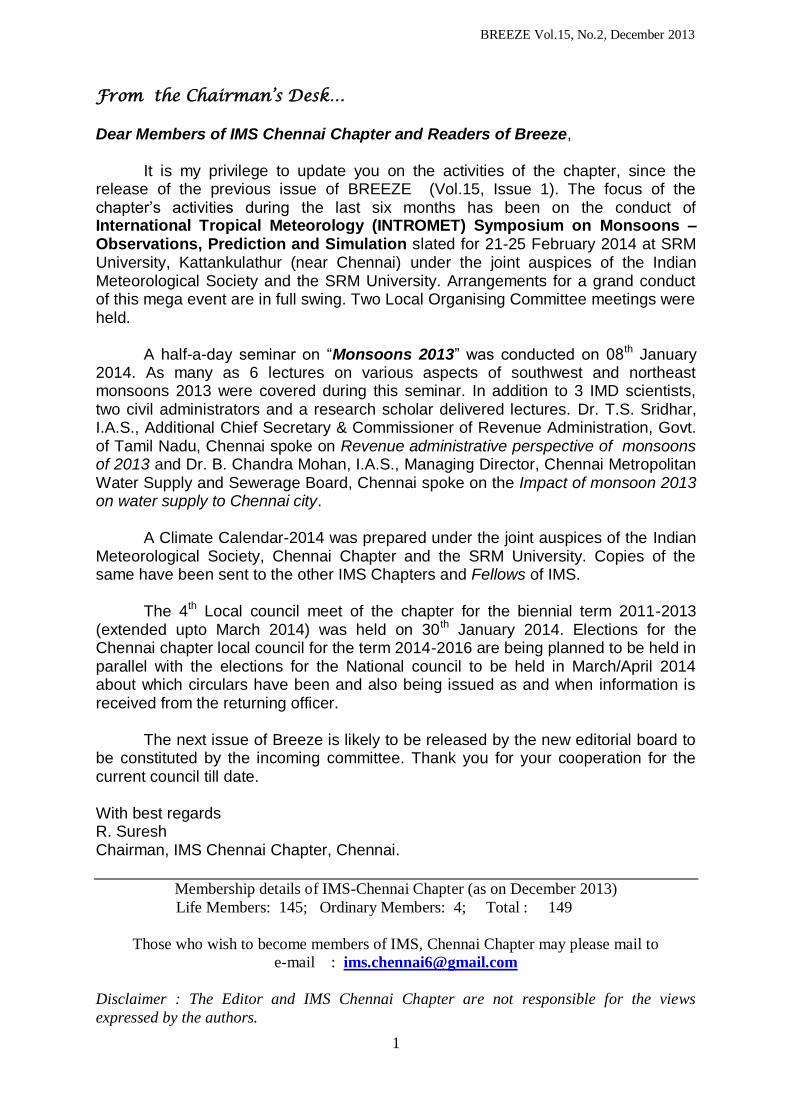
Comparison of water storage in the reservoirs between 2013 and 2014

Reservoir Full

Capacity

in ‘Mcft’

Storage as

on

02.01.2013

in ‘Mcft’

Storage as

on

02.01.2014

in ‘Mcft’

Storage

difference in

‘Mcft’

Poondi 3,231 1,523 138 -1,385

Cholavaram 881 471 169 -302

Redhills 3,300 2,166 2,160 -6

Chembarambakkam 3,645 1,241 870 -371

Total 11,057 5,401 3,337 -2,064

Veeranam 1,465 491 720 +229

Grand Total 12,522 5,892 4,057 -1,835

As on 02.01.2014, the storage in the reservoirs (Excluding Veeranam) is 3,337 mcft

against the full capacity of 11,057 mcft and the storage as on the same day last year is 5,401

mcft i.e. present storage is 2,064 mcft less than last year‟s storage.

The present pattern of average drawal of water from various sources and distribution of water

to City and Industries is as follows:

Sl.No. Source of Drawal Quantity in ‘MLD’

1 Redhills Lake 55

2 Poondi Lake 15

3 Veeranam Lake 180

4 Desalination Plant (Minjur) 100

5 Desalination Plant (Nemmeli) 80

6 Well fields (Department wells only) 35

7 Chembarambakkam Lake 80

8 Added Areas (Own source) 30

Total 575

Past experience

During earlier drought period in the years between 2001 and 2004 the reservoirs had

gone completely dry. Then the water supply was managed by extracting more ground water

from the well fields, by hiring agriculture bore wells, transporting about 25 MLD of

groundwater from distant sources such as Chengleput, Neyveli, Gummidipoondi etc. through

water tankers and by transporting average quantity of 2 MLD through railway wagons from

Erode and Mettur.

Water Management strategies by CMWSSB to meet the present scenario

The CMWSSB has planned the following contingency measures to increase the water sources

to meet and maintain the Chennai city‟s present water requirement after April 2014.

By drilling additional 6 bore wells in the well fields and 10 bore wells in the Neyveli

aquifer.

By transporting 20 MLD of groundwater from distant sources through water tankers.


4

By hiring agriculture wells in the well field area it has been proposed to by 40 MLD

of groundwater.

To request Andhra Pradesh Government to increase the discharge at Kandaleru

Reservoir so that a minimum of 800 cusecs can be realized at Zero Point from

Krishna water source after permanent restoration of the Kandaleru-Poondi Canal at

Ubbalamadagu from January 2014 till June 2014.

Action has to be initiated for more fillings in the Veeranam lake for maintaining the

city supply after April 2014.

Conclusion

As CMWSSB has implemented the Hon‟ble Chief Minister‟s long term perspective to

commission of the New Veeranam Project in 2004 and commissioning of Desalination Plants

(Kattupalli & Nemmeli) as a drought proof measure, the piped water supply will be continued

with the additional groundwater extraction from the well field area, hiring of agri wells,

transport of water from distant sources and additional quantity from Krishna water source.

******

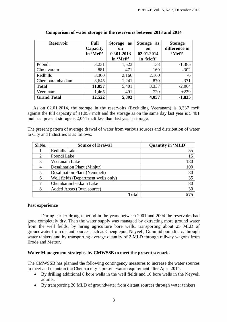
Weather wonders ….

9th January 2014: Partly frozen Niagara Falls (USA) (Courtesy: www.ibtimes.com)

http://www.ibtimes.com/


5

MONSOONS - 2013

by

S.R.RAMANAN

Area Cyclone Warning Centre, Regional Meteorological Centre, Chennai – 600 006.

e-mail: [email protected]

Indian Summer Monsoon 2013 ended with positive departure of six percent above Long

Period Average (LPA). Cyclonic Storm “Mahasen” (10-16May) that formed in Bay of Bengal

helped in strengthening the cross equatorial flow. This led to the early onset on monsoon over

Andaman & Nicobar Islands (3 days ahead of normal date of 20 May). The monsoon onset over

Kerala was on 1 June (normal date). Due to the active phase of Madden Julian Oscillation and

northward movement of east-west shear line, there was a rapid progress of monsoon. After onset

over Kerala, monsoon rapidly covered the south peninsula and north east India by 9 June and

covered the entire country by 15 June (one month ahead of the normal date). Strong cross equatorial

flow prevailed during June and July. It weakened during second half. The second and third initial

weeks had positive departures of 34 & 89 percent. The third week‟s seasonal total was 54 percent

above normal. After this week, only four weeks during the rest of the season had meaningful positive

departures and other weeks were either just normal or below normal. Yet the initial surge helped in

maintaining the seasonal figure to be on the positive side of the LPA. The month wise performance

was 132 percent of LPA and July was 106 percent. August recorded 98 percent and September 86

percent of LPA.

There are four homogenous regions and north east India alone had a negative figure of 72

percent of LPA. The other regions viz., northwest India recorded 109 percent, central India 123 and

south peninsula 115 percent of LPA. A sub division wise analysis indicates that out of 36

meteorological sub divisions, 14 sub divisions (comprising 48 percent of total area of the country)

recorded excess. 16 sub divisions (occupying 38 percent of the country‟s area) received normal

rainfall and remaining 6 subdivisions (with areal spread of 14 percent of country‟s area) received

deficient rainfall. Out of 641 districts, 100 districts had meteorological drought (26-50 percent

deficit) and 39 recorded severe drought.

During this season Tamil Nadu / Puducherry subdivision recorded normal rainfall. It

recorded a rainfall of 321.6 mm against a normal figure of 317.2 mm. All sub division‟s

performance in the southern region is given in the following table.

Sub division Actual

(mm)

Normal

(mm)

Departure

(Percentage)

Telengana 949.7 755.2 +26

Coastal Andhra Pradesh 524.1 581.1 -10

Rayalaseema 420.3 398.3 +6

Coastal Karnataka 3620.8 3083.8 +17

North Interior Karnataka 533.1 506.0 +5

South Interior Karnataka 826.6 660.0 +25

Tamil Nadu/Puducherry 321.6 317.2 +1

Kerala 2562.5 2039.6 +26

Lakshadweep 1057.2 998.5 +6

During this season there were 2 monsoon depressions and 16 low pressure areas against a normal of

6 monsoon depressions and 6 monsoon lows.



6

Withdrawal was on 9 September (normal date is 1 September) over west Rajasthan. After

19 September withdrawal was stalled due to the formation of 2 low pressure areas and their

westward movement towards central India.

The normal onset date for onset of easterlies is around 14 October. However due to the

presence of VSCS “Phalin”, it became clear that it would be delayed, Withdrawal from the entire

counting on 21 October 2013. A low pressure , which formed on 20 October 2013 in central parts

south bay off moved westwards and it could be located in the south bay off TN-SAP coast. This

system heralded the monsoon. So, we had the withdrawal of Southwest monsoon over the entire

country and the simultaneous commencement of Northeast monsoon 2013 over Tamil Nadu, Kerala

and adjoining areas of Andhra Pradesh and Karnataka.

The well marked low pressure after crossing the AP coast was moving inside AP and

weakened in to low on 26 October. Since it moved towards, TN came under the grip of westerlies

again. The situation was reminiscent of south west monsoon period in Tamil Nadu. Receipt of good

rainfall was restricted only on the day of commencement of Northeast monsoon rains. As it moved

towards AP, all the three subdivisions of AP got good rains. The two subdivisions which matter in

north east monsoon period viz., CAP and Rayalaseema had very good weekly departures of 100

&80 percent. As far as week ending 23/10/2013, Tamil Nadu/Puducherry, South Interior Karnataka

& Kerala recorded departures of 25,52 and 79 percent respectively. The reason for Kerala getting

good rains is due to bay system drawing Arabian Sea current.

After the initial week during the commencement of NEM rains, Tamil Nadu/Puducherry

experienced less rainfall activity mainly due to the reversal of winds. Tamil Nadu had to wait for

three more weeks to experience meaningful rainfall activity. A Tropical depression (named as

“Wilma” by Pagasa). It formed in the Philippines Sea near Mindano islands on 04/11/2013, further

moved westwards through South China Sea. It made landfall in Vietnam on 07/11/2013 and moved

across Cambodia and emerged in Gulf of Thailand and adjoining Tenasserim coast on 08/11/2013 as

a low pressure area. It further moved in a west north westerly direction and concentrated in to a

depression on 13 November (700 Km east south east of Chennai). It continued to move westwards

and ultimately made the landfall near Nagapattinam between 07 & 08 UTC of 16/11/2013.

TS “Podul” formed on 11 November 2013 and dissipated on 15 November 2013. When

the system became a depression, it was 1175 Km south east of Koror, Palau. After making the

landfall in Philippines moved across South China Sea and made landfall in Vietnam on 15

November and travelled across Cambodia and Thailand and remnant energy of TS “Podul” emerged

in the Andaman Sea on 17 November. The system moved westwards and became a depression on 19

May (700 Km east north east of Chennai). It later intensified in to TC “Helen” on 20 November over

West Central Bay. It made landfall close to Masulipatnam on 22 November. Since the system was

drawing Arabian Sea currents the PDP of Kerala for the week ending 27/11/2013 was 102, South

Interior Karnataka 34 and for CAP, it was 67 percent.

Close to the heels of formation of TS “Helen” another system formed. The system

formed in the South China Sea, east of Malay Peninsula on 19/11/2013. Generally, when they form

in this low latitude during late November, they would head towards TN coast. At the time of

formation itself, the system showed that it had all the potential to become a strong system. The

system rapidly strengthened and it was a very Severe Cyclonic Storm “Leher” on 25/11/2013.

Afterwards, the system was moving towards AP coast and weakened in to depression before land fall

due to strong wind shear aloft and colder Sea Surface Temperature. CAP received 58 percent more

rain for the week ending 04/12/2013 and Kerala had 51 percent more rain due to this system and due

to an upper circulation over Lakshadweep area.


7

A trough of low pressure could be located over South west Bay off Srilanka & Tamil Nadu coast

on 1 December. On 3 December, the system became a well marked low pressure area. It

concentrated in to depression on 6 December. It was situated between two Anti cyclones. The

system gradually intensified in to Cyclonic Storm “Madi”. The system was steered to the north due

the high pressure situated in the west. After moving pole ward, the system was weakened due to

strong wind shear aloft. Later the high pressure, which was lying in the west, became the dominant

steering force and the system started to move in a south westerly direction towards Tamil Nadu

coast. The weakned system made the landfall over vedaranyam during evening of 12 December and

reemerged in Palk Strait and finally made the landfall near Tondi during late night period. There

were widespread rains over Tamil Nadu/Puducherry subdivision on that day and weekly departure

figure (For week ending 18/12/2013) was 21 percent.

At the end of the season CAP was the only sub division with excess rainfall. This was

mainly due to the good performance of well marked low pressure area during the initial days during

the commencement of Northeast monsoon rains. Subsequent systems, which were heading towards

AP coast also contributed for the good performance. As far as Tamil Nadu/Puducherry subdivision is

concerned, the systems which were heading towards AP coast took the moisture away. Though two

depressions made landfall in Tamil Nadu, they hardly stayed for a day. So Tamil Nadu/puducherry

subdivision ended with deficit figures. Kerala ended with negative figures, but within the limits of

normal rains. Rayalaseema and South Interior Karnataka ended with deficit figures, as no system

passed through that region.

*********


8

CLIMATE CALENDAR OF INDIA 2014

by

M.S.NARAYANAN and R.UMA

SRM University, Kattankulathur


• A Climate Calendar of India – 2014 has been prepared with the joint efforts of the

SRM University and the Indian Meteorological Society (IMS). This is an attempt to create

awareness and popularize meteorology / climate among public in general and students in

particular.

• This was released on 27 December 2013 during the DST INSPIRE camp held at

SRMUniversity for ~ 200 bright HSC students of Tamil Nadu schools.

• With the Climate Change / Global Change controversies, the recently released 5th

Report of the International Panel on Climate Change (IPCC) on Global Change and

discussions thereon taking place so regularly in media, it was thought appropriate that we

know first and foremost, our present climate – at least of our own country.

• This Table top Climate Calendar has a total of 26 pages. On the reverse of the cover

page, some information about SRMUniversity and IMS are given, besides a short highlight

of the calendar‟s contents.

• Two pagesare assigned for each calendarmonth. The front side, besides showing day

– date has also

- Monthly maps of India depicting climatic contours of Temperature and Rainfall

- An INSAT image depicting the typical weather of the month eg.,

(i) Widespread fog over north India during January

(ii) Western Disturbance during February

(iii)Norwesters in eastern India during March / April

(iv) Various facets of southwest monsoon – onset, active, break etc. during June -

September

(v) Tropical Cyclone during November etc

This page also includes some significant climate Records and Events of interest.

• On the reverse side, a brief description is given of the weather event whose INSAT

image is shown on the front side. It has a Table showing important Climatic information of

10 select stations of India (6 Metros + Pune, Ahmedabad + 2 Hill stations).

• Most importantly, in this reverse side we have described in short about the

variousweather instruments (with photograph of their discoverers) that are used to measure /

analyse weatherparameters routinely – vizThermometers, Barometers, Rain gauge, Surface

observatory / AWS, Meteorological Tower, Meteorological Rockets, Weather Radar,

Meteorological Satellites, Super Computers and Numerical Weather Prediction (NWP). At

the end, we have included a list of important Indian Organisations / Institutions and

Universities involved in Weather and Climate studies.



9

• The various data and maps included in the Calendar have been provided by the

various units of the India Meteorological Department (IMD). Some information have also

been taken from internet sources.

• This calendar is to be distributed to the delegates of the INTROMET conference to be

held during February 21 – 25, 2014 at SRM University. Now it is being sent to

- Some select Schools in Tamil Nadu, and

- IMS Chapters, Fellows and Various Institutions involved in Met / Ocean / Climate

Research in India.

• A photograph taken during the release ceremony, and a few sample pages of the

calendar are included at the end of this article. The contents of the Calendar are provided in

full at the URL link:

https://drive.google.com/folderview?id=0B0_CpHFxoErreExjRzNoTWVzdUk&usp=sharing

• We would highly appreciate receiving your critical comments and suggestions.


10

Weather wonders …

Devastating, yet, Spectacular Weather events on 12th

October 2013 –

Three Tropical Cyclones (Phailin, Nari and Wipha) heading for menacing Asia

Courtesy: http://qz.com/author/zachseward/

Source: ercportal.jrc.ec.europa.eu/


11

ELEVATION MEASUREMENTS USING DIFFERENTIAL GNSS TECHNOLOGY

by

B. AMUDHA

Regional Instruments Maintenance Centre, Regional Meteorological Centre, Chennai-600 006.


IMD network of AWS

Automation of the surface observational network is being implemented by India

Meteorological Department (IMD) in a phased manner. As on 31.12.2013 there are 675

Automatic Weather Stations (AWS) and around 1150 Automatic Rain Gauges (ARG) installed in

the entire length and breadth of the country. Technical information about the IMD network of

AWS and ARGs has been provided by the author in earlier articles published in the newsletter

Breeze (Details given under References). In any national meteorological service, a variety of

challenges go hand-in-hand with the implementation phase of automation in any type of

observational network. Diverse types of bottlenecks are experienced for which effective way out

options need to be identified. The focus of this article is to emphasise one such area for which

contemporary solutions have come to aid.

Sensors and measurement of atmospheric pressure

An AWS is configured to measure with the help of sensors interfaced in the system and

report air temperature, hourly maximum and minimum temperatures, relative humidity, station

level atmospheric pressure(SLP), hourly and the day‟s cumulative rainfall, wind speed and wind

direction. The accuracy of the pressure sensor used by IMD in AWS is ±0.3 hPa. Its reliability

and consistency in performance under field conditions is very good. The pressure sensor is

mounted adjacent to the datalogger inside the NEMA enclosure of an AWS typically at a height

of 1.5m above ground level. Hourly Mean Sea Level Pressure (MSLP) is generated at the Earth

Station in Pune using the SLP, air temperature, vapour pressure, elevation of the site etc. The

height above mean sea level (m.s.l) or in other words, elevation of all the AWS sites needs to be

incorporated to a high degree of accuracy in the generic algorithms used to generate MSLP from

the SLP of a station. AWS data is now assimilated into the NWP models and plotted in synoptic

charts for operational weather forecasting. Accuracy in MSLP reported by a coastal station

which has an AWS but does not have a conventional surface observatory is crucial while

analysing the isobaric pattern in a synoptic chart, more so during the passage of cyclonic storms

(CS). The likely place of landfall of the CS could be determined precisely based on the fall in

MSLP of such coastal AWS.

Challenges in obtaining accurate elevation of sites

When 100 AWS of Sutron-make were installed all over India during 2006-07, one third of the

AWS were collocated for validation purposes with conventional surface observatories for which

elevation was known as they were predetermined using standard surveying techniques. For the

other AWS sites the elevation was obtained from official / government records of the

organisations in whose premises the AWS were installed. Obtaining accurate elevation details of

a large number of sites through Survey of India is a costly and long drawn process. So, if details

of elevation were not readily available, handheld digital modules like Garmin and Trimble using

the satellites of the Global Positioning System (GPS) were used to determine the same. The

geocoordinates like latitude and longitude obtained from these instruments were accurate and

very much reliable. However, due to limitations in the positioning accuracy (of the order of 10

metres) of the GPS instruments procured, the elevation obtained was found to be incorrect in the

case of a few sites which was inferred based on the erroneous MSLP reported by the station.



12

During data validation procedures digital pressure standards traceable to national standards are

utilised to compare and check the measurement of SLP by pressure sensors on-site. Such an

exercise in all AWS sites has led to the firm belief that SLP is correctly measured by the sensor

within the tolerance limits specified by the World Meteorological Organisation. Hence it was

affirmed that the elevation of the site needs to be known precisely to avoid errors in conversion

of the SLP to MSL.

In the case of uneven natural terrain conditions and land-filled sites, the history of which is

not known at first sight when a site is selected for installation of an AWS, a significant change in

elevation of a few metres between two locations separated by even a short distance has been

observed. So it is imperative to have authentic elevation measurements done exactly in the

locations where AWS are planned to be installed rather than take the value available in records

for granted.

GPS / GNSS technology

Understanding the importance of documenting and utilising the accurate elevation of AWS

sites, modern online tools like Google Earth maps were also tried with limited success. As the

density of the AWS located in geographically diverse and remote terrain is increasing manifold,

obtaining the height above m.s.l of new sites accurately became an important pre-requisite

component of the meta database while planning the augmentation of the observational network.

It was then decided to tap the options available from state-of-art satellite technology. The

constellation of satellites of the Global Navigation Satellite System (GNSS) / GPS provides sub-

metre accuracy positioning information including the height above m.s.l. of any geographic

location. The Medium Earth Orbit (MEO) satellites have a circular orbit approximately at a

height of around 20-25,000 km around the earth and their timings are very accurate, maintained

by cesium / rubidium atomic clocks. The orbit ephemerides are clearly known. The satellites

operate in L band (1-2 GHz) and in three particular frequencies viz., L1 ( 1575.42 MHz), L2

(1227.60 MHz ) and L5 (1176.45 MHz ) using code division multiple access technique. GPS

satellites are operated by USA and its Russian equivalent is the GLONASS (Global Navigat ion

Satelllite System). As of now, we in India depend on these satellite coverages and use their

services to obtain accurate positioning information. GNSS is a commonly used acronym for

GPS, GLONASS and other equivalents of China (Compass) and European Union (Galileo).

India through Indian Space Research Organisation (ISRO) with its self-reliant vision of

having a Regional Navigation Satellite System has launched the first of its series of seven

navigational satellite IRNSS-1A on 1st July 2013. It is geosynchronous at 55°E with an

inclination of 29°. In addition we have GAGAN, an inter-operable GPS aided satellite based

augmentation system (SBAS) helpful for air navigation.

Radio signals continuously transmitted by the GNSS satellites pass through different layers of

the atmosphere and are received by numerous reference (base) stations whose position is known

to the highest degree of accuracy using conventional surveying techniques. The user equipment

(receiver and antenna) also receives the signals from multiple GNSS satellites. In differential

GNSS, the base station determines ranges to GNSS satellites in view and for each satellite,

recovers the information that was transmitted and determines the time of propagation viz., the

time it takes for the signals to travel from the satellite to the receiver. This information and the

difference in ranges between the satellites is communicated to other receivers which incorporate

the corrections into their position calculations and then compute their position and time.


13

Omnistar-HP subscription services

Commercial SBAS like Omnistar-HP is used in India to have access to the corrections

provided by their high performance range correcting systems. Omnistar uses dual frequency

receivers and is able to provide accuracies of 6 to 10 cm in elevation. Differential positioning

requires a data link between base stations and other receivers if corrections need to be applied in

real-time. At least four GNSS satellites need to be in view at both the base station and the

receivers. Positioning based on standalone GNSS service is accurate to within a few metres and

the less number of satellites available with one GNSS service is not sufficient for us. On an

average, there is a variation of 1 hPa for every 10 metres height difference in the vertical

atmosphere and very high accuracy in elevation measurements are needed. Hence differential

GNSS technique is used. The absolute accuracy of the receiver‟s computed position will depend

on the absolute accuracy of the base station‟s position. One has to subscribe and obtain licence

for the period (1 to 2 years as applicable) we require. Only then the receiver will be able to

access and utilise the Omnistar services.

When used with NovAtel‟s GPS antennas, the Propak-V3 receiver provides superior

tracking performance, positioning accuracy and reliability. The antenna is compatible with

Omnistar-HP. Omnistar uses geostationary satellites in 8 regions covering most of the landmass

of each inhabited continent on Earth. It uses 100 reference stations, 6 high performance satellites

and two global network control centres for errror corrections.

IMD’s procurement

Accordingly, during the year 2012, O/o Dy.Director General of Meteorology(Surface

Instruments), Pune procured the following equipment viz., a) a GPS-702-GG-L1/L2 GNSS

antenna (Fig.1a) offering combined GPS + GLONASS signal reception facility, b) a Propak V3

triple frequency GNSS receiver (Fig.1b), c) tripod stand(Fig.1c), d) power supply (12V/5 Ah),

and e) a note pad computer containing NovAtel CDU software interface (Version 3.9.0.7, Build

6168) for communication with the receiver. A screen shot of the software while using it to track

the satellites and obtain the correct geocoordinates and elevation of a site is shown in Fig.2.

Using these equipments survey of all AWS sites was initiated first in the state of

Maharashtra. Remarkable improvement in accuracy levels with errors less than 0.3 hPa was

evident in the conversion of SLP to MSLP of AWS in Maharashtra after incorporating in the

Earth station software the elevations of sites obtained through the GNSS receiver equipment.

Similar such survey was completed for Tamil Nadu (TN) and south Andhra Pradesh(AP) during

the year 2013. The advantage is that the accurate elevation of the pressure sensor above m.s.l is

known. Hence reduction of SLP to MSL is most accurately obtained. Shri. Anjit Anjan,

Scientist-C from O/o DDGM(SI), IMD, Pune imparted training on operation of the sub-metre

accuracy GNSS receiver equipments to officers and staff of RMC Chennai on 1.1.2013. After

familiarisation, team members of Regional Instruments Maintenance Centre (RIMC) successfully

completed survey of 64 sites (in TN and south AP) including surface observatories during

1.1.2013 to 8.5.2013.


14

1(a) (b) (c)

Fig.1(a) Pin wheel antenna b) Propak V3 receiver and c) Tripod stand used to mount the

antenna

Fig.2 Screen shot of the tracking of satellites using NovAtel CDU GNSS receiver software

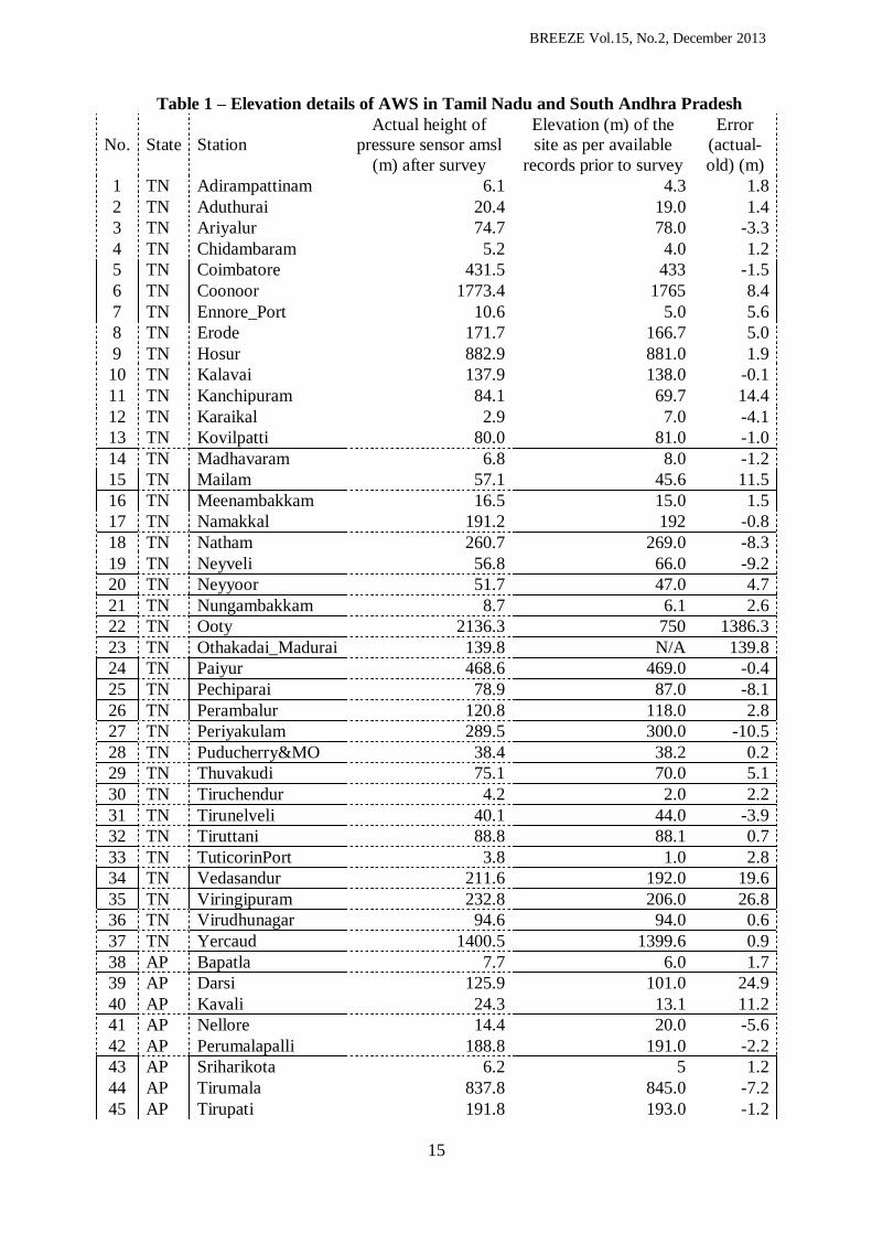
Table 1 provides the details of 45 stations and their elevations prior to and after the

survey. It is clear from Table 1 that for a few stations there is a marked deviation between the

elevations available prior to and after the survey. Others have negligible errors in elevat ion. This

can be attributed to the comparatively uniform terrain in the coastal areas of TN and south AP

and the gradual increase in elevations as one proceeds westwards due to the variability in

topography under the influence of the western ghats. The same situation cannot be expected in

other States when there is high region-specific variability in topopgrahy and hence the survey is

crucial in such regions. Problems in reduction of slp to msl in few sites (like Vedasandur,

Mailam, Kanchipuram, Vrinjipuram, Othakadai(Madurai), Periyakulam, Darsi, Kavali, where the

accurate elevation was not known have been sorted out now.


15

Table 1 – Elevation details of AWS in Tamil Nadu and South Andhra Pradesh

No. State Station

Actual height of

pressure sensor amsl

(m) after survey

Elevation (m) of the

site as per available

records prior to survey

Error

(actual-

old) (m)

1 TN Adirampattinam 6.1 4.3 1.8

2 TN Aduthurai 20.4 19.0 1.4

3 TN Ariyalur 74.7 78.0 -3.3

4 TN Chidambaram 5.2 4.0 1.2

5 TN Coimbatore 431.5 433 -1.5

6 TN Coonoor 1773.4 1765 8.4

7 TN Ennore_Port 10.6 5.0 5.6

8 TN Erode 171.7 166.7 5.0

9 TN Hosur 882.9 881.0 1.9

10 TN Kalavai 137.9 138.0 -0.1

11 TN Kanchipuram 84.1 69.7 14.4

12 TN Karaikal 2.9 7.0 -4.1

13 TN Kovilpatti 80.0 81.0 -1.0

14 TN Madhavaram 6.8 8.0 -1.2

15 TN Mailam 57.1 45.6 11.5

16 TN Meenambakkam 16.5 15.0 1.5

17 TN Namakkal 191.2 192 -0.8

18 TN Natham 260.7 269.0 -8.3

19 TN Neyveli 56.8 66.0 -9.2

20 TN Neyyoor 51.7 47.0 4.7

21 TN Nungambakkam 8.7 6.1 2.6

22 TN Ooty 2136.3 750 1386.3

23 TN Othakadai_Madurai 139.8 N/A 139.8

24 TN Paiyur 468.6 469.0 -0.4

25 TN Pechiparai 78.9 87.0 -8.1

26 TN Perambalur 120.8 118.0 2.8

27 TN Periyakulam 289.5 300.0 -10.5

28 TN Puducherry&MO 38.4 38.2 0.2

29 TN Thuvakudi 75.1 70.0 5.1

30 TN Tiruchendur 4.2 2.0 2.2

31 TN Tirunelveli 40.1 44.0 -3.9

32 TN Tiruttani 88.8 88.1 0.7

33 TN TuticorinPort 3.8 1.0 2.8

34 TN Vedasandur 211.6 192.0 19.6

35 TN Viringipuram 232.8 206.0 26.8

36 TN Virudhunagar 94.6 94.0 0.6

37 TN Yercaud 1400.5 1399.6 0.9

38 AP Bapatla 7.7 6.0 1.7

39 AP Darsi 125.9 101.0 24.9

40 AP Kavali 24.3 13.1 11.2

41 AP Nellore 14.4 20.0 -5.6

42 AP Perumalapalli 188.8 191.0 -2.2

43 AP Sriharikota 6.2 5 1.2

44 AP Tirumala 837.8 845.0 -7.2

45 AP Tirupati 191.8 193.0 -1.2


16

Field usage aspects

Measurements using the GPS/GNSS antenna and receivers are best done in clear sky

conditions and with maximum number of satellites in the field of view while undertaking the

survey. Ideally around 10 to 11 satellites (11 in Fig.2) give the maximum accuracy. A minimum

of time of 30 minutes is required for the accuracy to reach ± 0.1m. Hence, as soon as one reaches

the site, the GNSS equipment is set up for synchronisation to commence. A 12V/5 Ah battery is

required for powering up the receiver. Sometimes under cloudy sky conditions the number of

satellites in the field of view may be only 7 or 8 and the accuracy will also vary from ±0.2 to

0.4m. While in the site, during the 30 minutes time, three-four snap-shots of the image

containing the lat/lon/elevation details are taken and the best with the least error is taken as

representative of the site. A digital hand-held pressure standard (DPI-740) is also carried to sites

to validate the data from the pressure sensor of AWS and to note deviations if any, for corrective

action. The accurate geocoordinates for AWS in TN and south AP have been fed into the

database of earth station. The MSLP conversion is now accurate and so the synop message

generated is in consensus with the isobaric analysis while plotting and analyzing MSLP synoptic

chart.

The survey of AWS sites in Kerala also has since been completed and is pending in

north AP and Karnataka due to formalities in renewing the licence with Omnistar. Yearly

calibration of pressure sensor of AWS added with accurate elevations of sites will generate

correct MSLP.

Around 2000 AWS are envisaged in the next few years by IMD and site surveys using

GNSS receivers for obtaining correct height above m.s.l are mandatory. Hence IMD has planned

to procure more number of GNSS receivers. Each of the Regional Meteorological Centres needs

to undertake this type of survey of the sites before finalising them for installation of AWS in their

respective regions to ensure reliability in MSLP data.

It may be mentioned here that various other organisations install their own AWS and

might require the use of this receiver procured by IMD for accurate reporting of atmospheric

pressure above m.s.l. IMD will be able to provide assistance in this regard to such organisations.

References

Amudha B., Overview of Automatic Weather Stations in IMD, Breeze, Vol.11,2, pp.1-4,

December 2008.

Amudha B., Satellite based Automatic Rain Gauge Stations of India Meteorological Department,

Vol.14, 1, pp.13-15, June 2012.

http://www.novatel.com/

Manual of Propak V3 receiver.

Instructions Note on usage of GPS /GNSS equipment prepared by RIMC Chennai, July 2013.


17

WXWORD 1

2

3

4

5

6

7

8

9

10

11

12

13

14

15

16

17

18

19

20

21

22

23

24

ACROSS:

1 : Water in Latin

2 : Action of drawing liquid into a tube or porous material

5 : Transfer of energy through vacuum

7 : Cloud Cover is measured in ----------.

8 : Term used for professional body of lawyers is a unit of measurement in

Meteorology

9 : You call it a -----------process in an insulated system.

12 : Acronym for an agency held by Navy and Air Force in Pearl Harbour

13 : Acronym for procedure of shifting files from one host to another in internet

14 : State of the atmosphere when isotherm and isobar run parallel to each other

17 : German physicist known for his contribution to scattering

19 : Longest of the five notable latitudinal circles

21 : Hidden and it matters when change of state of substance occurs

23 : This programming language reminds us of measuring unit in Meteorology

24 : Geo physical entity distinct from earth and sky

DOWN:

1 : ------foresting is an integrated approach of using the interactive benefits

by combining trees, shrubs with crops.

3 : Sapphire in Thai means second strongest ever cyclone to make landfall in

India

4 : Directional antenna in synonym with typhoon that impacted Ryukyu islands

in the year 2000

5 : Well-known palindrome in meteorology

6 : ---------- of a planet is typically elliptical

10 : Reference from which measurements are made

11 : One of shortest in the five notable latitudinal circles

15 : Synonym with impenetrable

16 : Father of thermodynamics

18 : Rate of flow of energy across unit area

20 : Acronym for zonal flow in tropical stratosphere

22 : Acronym of advent in flight schedule

-S.R.RAMANAN

Regional Meteorological Centre, Chennai


18

AN ANALYTICAL TOOL FOR DEPICTING RAINFALL CHARACTERISTICS OF

TROPICAL CYCLONES OVER NORTH INDIAN OCEAN - TCRAIN

by

S.BALACHANDRAN, B.GEETHA, K.RAMESH and N.SELVAM

Cyclone Warning Research Centre, Regional Meteorological Centre, Chennai-600 006.

Email: [email protected]

India, having an extensive coastline is vulnerable to the destructive features of Tropical

Cyclones (TCs) that form over the North Indian Ocean (NIO) basin comprising of the Bay of

Bengal (BOB) and the Arabian Sea (AS). Torrential rains associated with landfalling TCs cause

fresh water flooding and extensive damages to crops in the respective coastal areas so much so,

that, rainfall prediction is a highly warranted aspect of TC forecasting. However, Quantitative

Prediction Forecasts for TCs is a highly challenging aspect as precipitation distribution around a

TC display complex asymmetric structure owing to TC translational speed, environmental wind

shear and TC specific structural and dynamical aspects.

Characterisation of rainfall associated with TCs based on intensity stratification is an

important step towards understanding the symmetry and/or asymmetry of TC rainfall distribution

during the life cycle of the TC. Frequency distribution of rain rates would give valuable

information on highly probable rain rates associated with different intensity stages of the TC;

azimuthally averaged radial profiles of mean rain rates would provide information on rainfall

variability at different radial distances from the TC centre; and quadrant-wise mean rain rates

would depict the asymmetry in the radial rainfall structure.

TCRAIN is a Tropical Cyclone Rainfall Analytical tool that provides rainfall

characteristics of 43 Tropical Cyclones that formed over North Indian Ocean during the period

2000-2010 in graphical / pictorial form through a menu-driven user interface. Three products,

viz., the (i) Frequency distribution of rain rates within 500 km from the TC centre (ii)

Azimuthally averaged radial profiles of mean rain rates within 500 km from the TC centre and

(iv) Quadrant-wise mean rain rates within 200 km from the TC centre are presented for five

different stages of intensity during the life cycle of each cyclone. The products are generated

using 3-hourly Tropical Rainfall Measuring Mission (TRMM) rainfall data at a spatial resolution

of 0.25⁰ x 0.25⁰ grid.

The rainfall analysis is carried out using the TRMM based precipitation data (3B42 V6)

having a spatial coverage of 50⁰S to 50⁰N at 0.25⁰ x 0.25⁰ resolution at 3 hourly intervals. The

3B42 processing has been designed to maximise data quality and has been recommended for

research work (http://disc.sci.gsfc.nasa.gov/).

According to India Meteorological Department‟s (IMD) classifications based on

maximum sustained surface wind speeds, low pressure systems are categorised as Well marked

low (<17 knots), Depression (D, 17-27 knots), Deep Depression (DD, 28-33 knots), Cyclonic

Storms (CS, 34-47 knots), Severe Cyclonic Storms (SCS, 48-63), Very Severe Cyclonic Storm

(VSCS, 64-119 knots), and Super Cyclonic Storm ( SuCS, >120kts).

During the period 2000-2010, 43 TCs (CS and higher categories) have affected the NIO

basin. Using the IMD‟s best track data of TCs which contain information on instantaneous

position, intensity and direction of motion of the TC, the life cycle of a TC is stratified based on

intensity during the growth and decay of the TC and grouped into 5 stages as follows: The

growing phase of the life cycle of the TC is classified into 3 intensification stages indicated by


http://disc.sci.gsfc.nasa.gov/


19

a prefix ‘i’; the intensity categories of D, DD are categorised as Stage-1 (Intensification stage 1

and indicated as iD); the category CS is categorised as Stage-2 (Intensification stage 2 and

indicated as iCS); the categories of SCS, VSCS and SuCS are grouped under Stage-3

(Intensification stage 3 & indicated as iSCS) and the decaying phase (i.e., when the intensity

category of the TC changes from the peak category to lower categories) of the TC is classified

into two stages of weakening indicated by prefix „w‟; the intensity category of CS during the

decaying phase is classified under Stage-4 (Weakening stage 1 and indicated as wCS) and the

categories of DD and D during the decaying phase as Stage-5 (Weakening stage 2 and indicated

as wD).

Whereas the IMD‟s best track data are available at 3-hourly interval for 00, 03, 06, 09,

12, 15, 18 and 21 UTC, the precipitation data are centered at 0130, 0430, 0730, 1030, 1330,

1630, 1930 and 2230 UTC. Hence, the location and direction of movement of the TCs at TRMM

Observation times are determined by interpolation from the IMD‟s Best Track dataset.

For the purpose of computations, a moving coordinate system with the TC centre as the

origin and direction of motion of the TC as the reference direction is considered. For each instant

of time, the centre of the coordinate system is first shifted to the centre of the TC at that instant

and then the coordinate system is rotated such that the direction of motion of the TC at that

specific instant of time coincides with the 0⁰ azimuth which is taken as the positive Y-direction

for the purpose of plotting. For this purpose, every grid point in the world co-ordinate system

(longitude, latitude) are represented in polar co-ordinates (r,θ), in terms of radial distance from

the TC centre (r) and oriented at an angle (θ) with reference to direction of motion of the TC

[taken as the 0⁰ azimuth]. All 0.25⁰x0.25⁰ rainfall data are then represented in terms of radial

distance from the TC centre and with reference to the direction of motion of the TC.

For each stage of intensity of a TC, all three hourly rainfall data are grouped together and

the composited mean rainfall characteristics are determined for that stage. FORTRAN programs

developed for the purpose and GrADS software package are used for computations and plotting.

The methodology of computation is as follows:

(i) The percentage frequency distribution of rain rates is determined by considering all rain rates

within 5⁰ radius (≈500 km from the TC centre) in respect of all the 3-hourly instances of

observation grouped under the specific intensity category. For this purpose, the rain rates are

classified into nine classes (including no rain category) as 0.0, 0.0-0.1, 0.1-0.2, 0.2-0.5, 0.5-1.0,

1.0-2.5, 2.5-5.0, 5.0-10.0 and >10.0 mm/hr and the frequency distribution in each class is

determined and expressed in percentage.

(ii) Radial profile of mean rain rates is obtained by first azimuthally averaging rain rates within

an annulus of very small thickness [0.1⁰ (≈10 km)] for a particular radial distance r, and then

determining the same for all radial distances from the TC centre up to 5⁰ radius (≈500 km from

the TC centre) for each instant of observation and then determining the mean of all the mean rain

rates corresponding to each radial distance (annulus at that radius) in respect of all observations

in the specific intensity category. For this purpose, for each observation, the origin is shifted to

the TC centre. Then an area within 5⁰ radius (≈500 km) from the TC centre (origin) is taken and

divided in to 50 annular rings of 0.1⁰width (≈10 km). Each data point within 5⁰ radius from the

TC centre is then expressed in terms of radial distance from the centre (r) and all rain rates

within each annulus of radius r are considered for determining the azimuthally averaged rain rate

at the radial distance r of the annulus from the TC centre. Fig.2 depicts the methodology of

determining the azimuthally averaged radial profile schematically. Thus, as we go from the TC

centre (r=0⁰) to outer most radius of r=5⁰ in steps of 0.1⁰, a profile of 50 radial mean rates

corresponding to 50 annuli are obtained. Similarly, instantaneous profiles are obtained for all


20

observations grouped under a specific intensity stage from which the mean profile of azimuthally

averaged mean rain rate for that intensity stage is determined. Similar profiles are obtained for

all intensity stages during the life cycle of the TC.

Fig.2 Schematic representation of steps for determination of azimuthally averaged radial

profile of mean rain rate

(iii) The Quadrant-wise mean rain rates are obtained by averaging all rain rates within 2⁰ radius

(≈200 km) from the TC centre with the direction of motion of the TC as the reference direction

for each instant of observation and then determining the mean rain rate in each quadrant in the

specific intensity category of the TC. For this purpose, the co-ordinate system is rotated through

an angle θ1 which is the direction of TC movement measured clockwise from the reference

direction (North, which is taken as 0⁰ azimuth as per meteorological convention) such that the

direction of movement of the TC is now oriented along 0⁰ azimuth, the reference direction. Then,

in the rotated configuration, the mean of all rain rates in the quadrant 0⁰-90⁰ (measured

clockwise from the direction of movement of the TC) from the TC centre up to 2⁰ radius is

determined which gives the mean rain rate in the Right Forward quadrant. Similarly, mean of

all rain rates in the quadrant 90⁰-180⁰ within 2⁰ radius gives the mean rain rate in the Right Rear

quadrant, that in quadrants 180⁰-270⁰ and 270⁰-360⁰ correspond to Left Rear and Left Forward

quadrants respectively. Fig.3 depicts the steps schematically.

Fig.3 Schematic representation of steps for determination of quadrant-wise mean rainrates


21

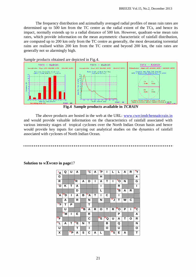
The frequency distribution and azimuthally averaged radial profiles of mean rain rates are

determined up to 500 km from the TC centre as the radial extent of the TCs, and hence its

impact, normally extends up to a radial distance of 500 km. However, quadrant-wise mean rain

rates, which provide information on the mean asymmetric characteristic of rainfall distribution,

are computed up to 200 km only from the TC centre as generally, the most devastating torrential

rains are realised within 200 km from the TC centre and beyond 200 km, the rain rates are

generally not so alarmingly high.

Sample products obtained are depicted in Fig.4.

Fig.4 Sample products available in TCRAIN

The above products are hosted in the web at the URL: www.cwrcimdchennaitcrain.in

and would provide valuable information on the characteristics of rainfall associated with

various intensity stages of tropical cyclones over the North Indian Ocean basin and hence

would provide key inputs for carrying out analytical studies on the dynamics of rainfall

associated with cyclones of North Indian Ocean.

Solution to WXWORD in page17

1A Q U A

2C A

3P I L L A R

4Y

G H A

R 5R A D I A T I

6O N G

7O K T A I R I

D L 8B A R

9A

10D I A B

11A T I C I

A R N N 12

J T W C 13

F T P T

U 14

B A R O T R 15

O P I 16

C

17

M I E R P A 18

F C 19

E 20

Q U A T O R 21

L A T 22

E N T B Q N

U T I O U O

X 23

P A S C A L 24

S E A T

http://www.cwrcimdchennaitcrain.in/


22

INDIAN METEOROLOGICAL SOCIETY

CHENNAI CHAPTER

Email ID: [email protected]

COUNCIL MEMBERS 2011-2014

Chairman : Dr. R. Suresh

Ph.No.044-22561636

Mobile: 94450 21763

E-mail : [email protected]

Immediate Past Chairman : Dr. Y.E.A. Raj Ph.No.044-28276752 / 2823 0091 Extn.: 222

Mobile: 94452 46157


Secretary : Dr. B. Geetha

Ph.No.044-28230091 Ext.205

Mobile: 98405 31621


Joint-Secretary : Dr. S.R. Ramanan

Ph.No.044-28229860

Mobile: 94447 50656


Treasurer : Shri N. Selvam

Ph.No.044-28230091 Ext.205

Mobile: 94442 43536


Members

Prof. N. Sivagnanam

Mobile: 94448 70607


Shri V.K. Raman

Ph: 044-2491 9492

Email : [email protected]

Dr. S. Gomathinayagam

Ph: 044-22463981/82/83/84

Mobile: 9444051511


Shri R. Nallaswamy

Mobile: 94447 13976


Dr. B.V. Appa Rao

Ph: 08623-222422


Shri M.N. Santhanam

Ph.No.044-22561515 Ext.4276

Mobile: 94446 77058


Dr. G. Latha

Ph: 044-6678 3399


Smt V. Radhika Rani

Ph.No.044-28230091 Ext.251

Mobile: 94441 28765




Indian Meteorological Society, Chennai Chapter Newsletter ...

Documents

Transcript of Indian Meteorological Society, Chennai Chapter Newsletter ...