\;VMO olt-

woRLD METEOROLOGICAL ORGANIZATION, -"-··-~-·- .

PROCEEDINGS of the

REGIONAL SEMINAR ON MODERN METHODS AND EQUIPMENT FOR DATA PROCESSING

FOR CLIMATOLOGICAL PURPOSES IN AFRICA.

(Cairo, January 1970)

I WMO - No. 317 I Secretariat of the World Meteorological Organization • Geneva • Switzerland

1972 s- ~) l , s b (b)~ S J \. :;"·> \ G s . t! \t . '' ·:) ', , . 3 .c; :;· , . So1!, -~ 1 "'

(;J;i t :~ VV~H)- ., \11

©-1972, World-Meum~rological Organization

NOTE

The designations employed and the presentation of the material in this publication do not

imply the expression of any opinion whatsoever on the part of the Secretariat of the World

Meteorological Organization concerning the legal status of any country or territory or of its

authorities, or concerning the delimitation of its frontiers. ·

- i -

TABLE OF CONTENTS

Foreword by the Secretary-General of WMO • • • • • • • • • • • • • • • • • • • iii

List of participants • • • • • • • • • • • • • • • • • • • • • • • • • • • • • v

Opening ~peeches by:

Dr. Ahmed Moustafa, Minister of Scientific Research . . . . . . . . . M. F. Taha •• . . . . • • • Ill . . . . . . . . . . . . . . . . . M. Seck . . . . . . . . . . . . . . . . . . . . . . . . . . . . G. Somers . . . . . . . . . . . . . . . . . . . . . . . G. Tarakanov • . . . . . . . . . . . . . . . . . . . . . . . . . . . R. Bergg.ren • • . . . . . . . . . . . . . . . . . .

FIRST WEEK - ELEMENTARY CLIMATOLOGY AND STATISTICAL THEORY

Lectures by:

R. Bergg.ren

N. K. Kljukin

R. Arlery

G. Tarakanov

R. Arlery

B. Eriksson * B. Eriksson * B. Eriksson * G. Tarakanov

R. Arlery

Introductory lecture (summary) . . . . . . . . . . . Main problems of modern data processing for climatological purposes • • •••••••• . . Observation and recording of elements, meteoro­logical log books, scrutiny of data, meteorolo­gical journals • • • • • • • • • • • • • • • •

Quality and duration of meteorological sequences

. . .

• ! •

. . Climatological summaries, means, extreme values, frequencies, diurnal and interdiurnal variability, climatic series •••••••••••••••••••

Elementary statistical theory PART I

Elementary statistical theory PART II •

Elementary statistical theory PART III . . . . . . Statistical forecasting • . . . . . . . . . . . Homogeneity, variability, mean climatic maps . . . .

~tures presented by R. Berggren

1

3

7

9

13

15

21

23

49

53

59

63

81

101

113

125

N. K. Kljukin

- ii -

Methods of summarizing data and of computing compound statistics for the compilation of climatic reference data • • • • • • • • • • • . . . .

SECOND WEEK - MODERN METHODS AND EQUIPMENT FOR DATA PROCESSING

N. K. KljUkin Methods, equipment and economical efficiency of machine processing of hydrometeorological data

129

173

B. Eriksson * Survey of data processing machines • • • • • • • • • 207

R. Arlery

B. Eriksson * M. El-Sawy

M. s. Harb

H. Zohdy

M. K. Naguib

S. S. Abd El-Hadi

A. Boukli.-Hacene

M. S. Harb

M. Seck

w. Boer

A. Boukli-Hacene

M. Ayadi

Methods for data processing for climatological purposes . . . . . . . . . ~ . . . . . . . . Principles of computer programming . . • •

The use of punch cards in forecasting • . . . . . Data processing in the U.A.R. . . . . . . . . . . . Harmonic and Fourier analyses • . . . • • . . • •

Climatological elements •••• . . . . . . . . . . . LECTURES BY PARTICIPANTS

Computation of different climatic parameters . . . . Statistics - Analysis of variance . . . . . . Analysis and presentation of surface wind observations • • • • • • • • • • • • • • tt • • • • •

Machine processing of climatological data recorded in Senegal • • • • • • • • • • • . . . . . . Methods to estimate the main parameters of frequency distributions of meteorological elements on the basis of very short observa­tional series • • • • • • • • • • • • • • • • . . Practical work study of the rain distribution at

-stati-on -Algiers Universi-ty-- • •• - •- •• -•• -.

Determining the intensity of a phenomenon recorded on a chart with curved ordinate axis . . . .

Conclusions of the Seminar . . . . . . . . . . ~ . . . . . . . . . . . . . . . * Leo_tures presented by R. Berggren

217

223

241

255

261

271

277

285

293

297

303

311

319

327

- iii -

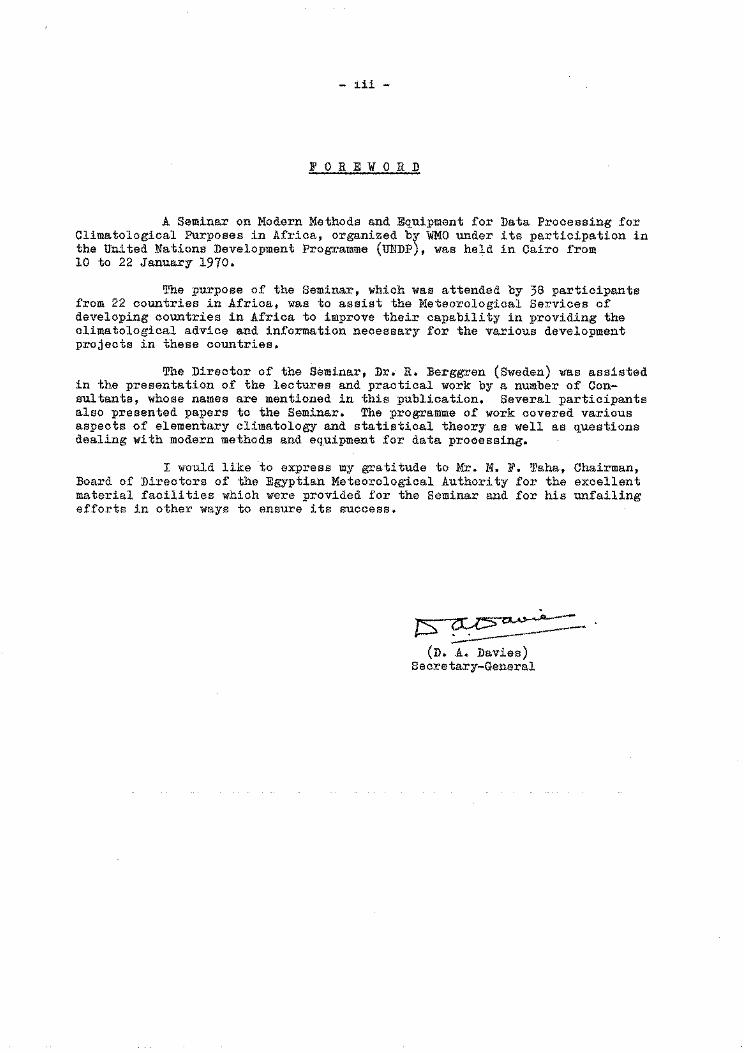
FOREWORD

A Seminar on Modern Methods and Equipment for Data Processing for Climatological Purposes in Africa, organized by WMO under its participation in the United Nations Development Programme (UNDP), was held in Cairo from 10 to 22 January 1970.

The purpose of the Seminar, which was attended by 38 participants from 22 countries in Africa, was to assist the Meteorological Services of developing countries in Africa to improve their capability in providing the climatological advice and information necessary for the various development projects in these countries.

The Director of the Seminar, Dr. R. Berggren (Sweden) was assisted in the presentation of the lectures and practical work by a number of Con­sultants, whose names are mentioned in this publication. Several participants also presented papers to the Seminar. The programme of work covered various aspects of elementary climatology and statistical theory as well as questions dealing with modern methods and equipment for data processing.

I would like to express my gratitude to Mr. M. F. Taha, Chairman, Board of Directors of the Egyptian Meteorological Authority for the excellent material facilities which were provided for the Seminar and for his unfailing efforts in other ways to ensure its success.

. rs~~

(D. A. Davies) Secretary-General

Honorary President

Mr. M.F. Taha

Director of the Seminar

Dr. R. Berggren

WMO Secretariat

Dr. G. Tarakanov (eo-Director)

Mr. A.M. Ela.mly

Consultants

Mr. R. Arlery

Dr. N.K. Klju.kin

Invited Lecturer

Dr. W. Boer

Lecturers from U.A.R. Meteoro­logical Department

Dr. M.S. Harb

Mr. M.K. Naguib

Mr. S.S. Abd El-Hadi

Mr. M. El-Sawy

Mr. H. Zohdy

- V -

LIST OF PARTICIPANTS

Under-Secretary of State Director General Meteorological Department, U.A.R.

Associate Professor Swedish Meteorological and Hydrological Institute Stockholm, Sweden

Special Assistant to the Secretary­General of WMO for Technical Policies and Programmes

WMO Regional Representative for Africa

Service Meteorologique National Paris, France

Hydrometeorological Services Moscow, U.S.S.R.

Meteorological Services, Potsdam

Local Secretariat

Mr. A.N. El-Guindy

Mr. M. Koubaisy

Name of Member

Algeria

Cameroon

Congo (Republic of)

Congo (Democratic Republic of')

Dahomey

Ghana

Ivory Coast

Kenya

Kenya, Uganda and Tanzania

Libyan Arab Republic

Madagascar

Nigeria

Rwanda

Senegal

Sierra Leone

Somalia

Sudan

Tanzania

To go

Tunisia

- vi -

Meteorologist International Affairs Division Meteorological Department, U.A.R.

Senior Observer International Affairs Division Meteorological' Department, U.A.R.

Name(s} of Partici2ant(s}

Mr. A. Boukli-Hacene

Mr. v. Nyoue

Mr. A. Loubello Mr. E. Ghoma

Mr. E. Pini

Mr. N. Totah

Mr. S.E. Tandoh

Mr. J. Djigbenou

Mr. S.E.L. Mukhwana

Mrs. G. Mwebesa

Mr. A.A. Sherif Mr. A.S. Asibi

Mr. J .P. Andrianifahanana

Mr. E.O. Adubifa

Mr. F. Kanyabogoyi Mr. s. Muganza

Dr. M. Seck

Mr. A.E. Massaquoi

Mr. A.A. Odawa

Mr. A.M. Gasm El-Seed

Mr. J. Ndimbo

Mr. S.C. Blivi

Mr. M. Ayadi

- vii -

Name of Member Name(sl of ParticiEant(s)

Uganda Mr. G.K. Kaggwa

Upper Volts. Mr. A. Kabre Mr. E. Souly

U.A.R. Mr. A.A. Abdel-Halim Mr. N. El-Sharkawi Mr. H. Zidan Mr. A. El-Habashi Mr. R. Youssef Mr. K. El-Safi Mr. s. Koudsy

- l -

. Addresf:l by Dr. Ahmed Moust~f'a . Minister of'.Scientific Research, U.A.R.

It gives.me pleasure t~ welcome you in our cotintry and to greet you on . ' behalf' of. the Government of the United Arab Republic, on the occasion of your

presence in Cairo to participate in the Seminar on the Modern Methods and Equipment for Data Processing for Climatolog:lcal.Pilrposes in Africa, organized by.the World Meteorologicai Organizatioh in the framework of' the Tecbrlical Assistance component of' the United Nations Development Programme in collaboration with the Meteorological Department of' the United Arab Republic.

The subject of the seminar is characterized by its particular importance in the field of the economic development programme for the developing countries in general and in the African countries in particular. This is due to the character of' the climatological information which is considered as one of' the most important bases for the successful planning of most of the economic development projects aimed at raising the standard of the developing countries, and in particular those concerned with the exploitation of' the natural resources of' the countries.

In the United Arab Republic we have a deep faith in the importance of' con­vening such seminars, not only because of their great value in the training of' per­sonnel engaged in the different technical and scientific fields, but also they are considered as one of the most important means in strengthening the relationships between specialists of different countries. This latter aspect is of' particular importance to African countries whose similar circumstances necessitate close co­operation of their specialists in various fields to accomplish progress on a solid basis.

The United Arab Republic, being a member of' the Organization of African Unity, is fully aware of' the deep concern and the real hopes of the different coun­tries of the continent for strengthening the co-operation between them for a better life for their people. In response to the policy laid down by President Nasser which aims in the first place for the realization of the aspirations of the African Unity, for the economic, social and cultural progress of the African countries, we will do our best to make this seminar a success. In response also to this policy the doors of the Meteorological Department and its Institute for Research and

- 2 -

Training are open to receive free of charge from African countries personnel engaged

in the field of meteorology with the aim of exchanging experience and outcome of

scientific research.

May I thank the United Nations Development Programme and the World Meteoro­

logical Organization for organizing this seminar and the distinguished scientists

who will participate with their knowledge and experience. I wish you every success

and hope your time will permit you besides your important commitments to enjoy your

stay with us in Cairo and to return to your respective countries with happy

memories.

- 3 -

Address by Mr. M. F. Taha Honorary President of the Seminar

Your Excellency the Minister of Scientific Research, Ladies and Gentlemen,

It is my pleasant duty and indeed equally my honour to address you on the occasion of convening here in Cairo the Regional Seminar on Modern Methods and Equip­ment for Data Processing for Climatological Purposes in Africa.

I would like to start by thanking Dr. Ahmed Moustafa, the Minister of Scientific Research, the Ministry to which' the Meteorological Department belongs, for presiding over this opening ceremony on behalf of the Government of the United Arab Republic.

The science of meteorology is of vital importance and its applications to the various aspects of life and human activities are outstanding. It is difficult to find any aspect of public or private life which is not affected in some degree by weather or climate.

Meteorology provides through weather records fundamental climatological data which are prerequisite for sound short and long-term planning programmes for national economic development as well as the effective exploitation of natural resources. This fact has been wisely recognized by Resolution 196 carried by the United Nations Regional Economic Commission for Africa which met in Addis Ababa during February last year.

We all know that very few of the considerable natural resources existing in Africa are fully utilized. We also know that many of the national and regional projects established in the different parts of this rapidly developing continent are not based on sound climatological information.

This situation challenges the Meteorological Services in Africa with increasing demands for sound processed and analysed climatological data to meet the needs of the variety of economic development programmes and the effective use of natural resources which cover aviation, shipping, fishery, agriculture including land reclamation, housing, industry, transport, electric power and tourism.

- 4 -

These Services are also challenged with the problem of dealing with the

progressive increase of the immense amount of meteorological data which has been

accumulated during the last decades. This fact is due to the expansion of the net­

works of meteorological stations and the developments of the observational programmes

which are being forced to cover the needs of the wide variety of economic development

projects.

To meet these challenges the Services have to apply modern methods and

equipment for data processing in place of the slow classic manual methods such as

sorting, counting, arithmetical computation, etc. The use of electro-mechanical

processing machines and electronic computers is no doubt the only way by which the

upsurge of the climatological data can be treated.

This matter has been the subject of much thought in the U.A.R. Meteoro­

logical Department. I am glad to say that this Department has succeeded in obtaining

the approval of the World Meteorological Organization and the United Nations Develop­

ment Programme to convene this present seminar for Africa.

From our experience with preceeding seminars organized for Africa in the

different fields of meteorology, I am sure that the present seminar will promote the

knowledge of the participants in the field of climatology.

I have great confidence in the value of assembling together African par­

ticipants to exchange knowledge and experience acquired by their modern services and

to receive training under the direction and guidance of very highly qualified consul­

tants.

I am extremely glad to see among us here today Mr. Mansour Seck, the

President of the WMO Regional Association for Africa, and Mr. Moncef Ayadi, member of

the WMO Executive Committee who have both repeatedly shown their keen interest in

promoting meteorology in our Region. I would like also to say how happy I am to

meet some of my old and valued friends from the different parts of Africa and to

meet for the first time some new ones.

We are fortunate to have Dr. R. Eerggren from Sweden who has accepted to

serve us as the Director of the Seminar. I am confident that with his long experience

and competence in the field of climatology, the work of the seminar will be most

efficient and successful. The wise and careful selection by the World Meteorological

Organization of the highly qualified consultants for this seminar will no doubt

ensure its successful accomplishment.

- 5 -

The participation of Dr. G. Tarakanov, the Special Assistant to the Secretary-General of WMO for Technical Policies and Programmes and Mr. A. M. Elamly, the WMO Regional Representative for Africa demonstrates the great interest which Mr. David Arthur Davies, the Secretary-General of WMO has in this seminar. May I therefore ask these officers to convey to Mr. Davies on your. behalf our deep appreci­ation for the great interest he has always shown in promoting meteorology in Africa.

I must also thank the United Nations Development Programme Resident Representative in Cairo for the unfailing efforts and assistance which he has always given in the development of the U.A.R. Meteorological Department as well as in arranging this seminar.

Finally I wish all the members of the seminar every success in their work and I sincerely hope that they will enjoy their stay in Cairo. I feel sure that they will make new friends and establish closer contacts with their colleagues in our international family of meteorologists.

Needless to say the Meteorological Department will make every effort to make your stay with us both useful and pleasant.

- 7 -

Address by Mr. M. Seck President of Regional Association I (Africa)

Your Excellency, Dear Colleague Mr. Taha, Ladies an~ Gentlemen,

It is an honour and pleasure for me to.address you, in my capacity as President of Regional Association I (Africa) on this occasion of the opening of the Seminar on Modern Methods and Equipment for Data Processing for Climatological Purposes in Africa.

I would like first and foremost to thank the authorities of the United Arab Republic for their kindness in inviting us to Cairo where WMO and Regional Associa­tion I in particular have always received traditional warm hospitality in the course of many seminars previously held in this country.

I also wish to associate myself with the people of the U.A.R. and the World Meteorological Organization in welcoming all delegates to this seminar. May I also take this opportunity to extend to you my best wishes for a happy and pros­perous New Year.

And now concerning our programme, the U.A.R. because of its advanced state of development has, as on previous similar occasions, initiated the organization of this seminar at the instigation, of course, of our good friend and father of meteoro­logy in Africa, Mr. Taha, who has never ceased to show his competence, experience and continuing devotion to the advancement of meteorology particularly during sessions of Congress and the Executive Committee. In the course of the next few days you will derive the benefits of fruitful discussions with a view to enhancing the meteoro­logical services in which climatological information is playing an increasingly important role.

1.

2.

During our work we must:

Extract the fundamental meteorological parameters necessary for the study of climate and.its application;

Usefully analyse well adapted statistical and olimatological formulae;

3·

- 8 -

Attend demonstrations and possibly operate efficient and rapid equipment

kindly put at our disposal by the U.A.R. Meteorological Service and foreign

companies.

Before concluding my speech, I would also like to emphasise the role

played by the UNDP in the expansion of meteorological services in Africa. Fully

conscious of the importance to development of training personnel, the UNDP together

with WMO ha~ in the absence of systematic refresher courses, considered it necessary

to inform the people in charge of meteorological services in Africa of the modern

equipment available for data processing for climatological purposes. I would like

to thank the administration of the UNDP, the WMO Secretariat, and particularly its

Technical Co-operation Department, and also Mr. Elamly, the WMO Regional Representa­

tive for Africa, for having organized such an interesting seminar for our Association,

I feel sure that all delegates here will contribute to the work of the

seminar by informing us of the different climatological techniques used in their

respective services. This then is a tangible proof of true international co­

operation. In this respect I am sincerely grateful to the eminent lecturers at the

seminar, particularly my distinguished and former professor, Mr. Arlery of France,

for having agreed to share their knowledge and experience in the service of Africa.

I hope, indeed I am certain that these two weeks of work before us will

be crowned with success and that this seminar will be a source of prosperity for

meteorology in Africa.

Thank you.

- 9 -

Address by Mr. Gordon Somers Deputy Resident Representative of UND~Office in U.A.R.

Your Excellency, esteemed delegates, ladies and gentlemen,

It gives me great pleasure to be present at what will possibly be a memor­able gathering to discuss the question of data processing and climatic control. I bring the symposium the greetings of Mr. Pavicic, the Resident Representative of the UNDP in the U.A.R., who would have wished to have been present in person, but unfor­tunately was called to Asswan on other business.

It would be presumptious of me to attempt to discuss at any length the developments in the field of meteorology or even the utilization of computer techno­logy to this increasingly important field in the presence of such a ·learned gathering. However, I cannot resist the opportunity to mention some of the factors that are always uppermost in the policy considerations of the UNDP, particularly as they relate to a greater awareness of the role of meteorological research in economic and social development. Much of what I say will probably be repetitive to those who participated in or have read the proceedings of the CEA Seminar on the "Role of Meteorological Services in Economic Development in Africa", held in Ibadan, Nigeria in September 1968. I believe however it would be correct to say that that seminar attempted to catalogue the factors which make meteorological services important to economic and social development. In the past, many laymen like myself have only associated meteorological research with the umbrella and raincoat not always realizing the significance of the climate to economic and social well-being.

It is in a way a challenge to such conventions as t~is one to better dis­seminate information on the unique role that climate conditions have to our develop­ment.

When we talk about natural resources, or better yet the natural condition and its exploitation we are primarily discussing matters related to meteorological research. In countries like the U.A.R. which constantly grapple with the omnipresent desert and all that that implies, there is always the need to understand how one can better develop and use meteorological research.

- 10 -

The agriculturist, the industrial planner, the town-planner, the communica­

tion expert, whether he be concerned with rail, road, surface or air, all are in­

terested in information made available from the meteorological services.

Assuming that the world of the 1970's is now convinced of the importance

of meteorological research the next hurdle to be overcome is in applying other

technological growth to problems of meteorology in economic proportions. We have

seen the development of satellites which could never have been realized if all other

technologies were not used and built upon. Fortunately we have also seen the

development of the World Weather Watch system which, I believe, only begins to

scratch the surface in the ultimate limits of this field.

The computer industry is a relatively new endeavour in man's long trek in

the search of mastering his environment. Certainly, with the use of data processing

the meteorological forecaster is better able to process his information with greater

rapidity and accuracy. This constitutes a vast improvement on the manual system.

I can say quite frankly, that the UNDP as an organization involved in the

process of development planning constantly watches such growth and is always ready

and willing to support governments in such deserving and urgent fields. Of course,

I am certain that we will all agree that in terms of need the UNDP alone cannot

always respond as readily or in the desired magnitude to the needs of the moment, but

since these undertakings are joint efforts we can only hope that priorities will be

readily recognized by the various governments.

Within its structure, the UNDP system has been assisting many governments

on a limited scale since the inception of its Technical Assistance Programme in 1949.

However, since 1959, with the birth of the Special Fund component, the UNDP through

the World Meteorological Organization as the executing agency has been trying to

increase the awareness of need in this field.

To date, over the last ten years, the UNDP has supported a total of 19

meteorological projects throughout the world with a contribution of US $ 19 million.

Of these 19 projects, 16 were national undertakings and 3 regional. Of the 16 pro­

jects, 10 were supported in Africa and Asia. This has in fact meant an expenditure

approaching US I 9 million. There is at present one operational project in Africa:

"the Hydrometeorological Survey of the Catchments of Lakes Victoria, Kioga and

Albert", in which the Sudan, Kenya, Uganda, the United Republic of Tanzania and the

United Arab Republic are participating. I am certain that the delegates to this

- ll -

symposium are quite familiar with the aims of this regional venture. In the U.A.R. the UNDP has been assisting the Government during the past 5 years in establishing a Meteorological Institute for Research and Training. The Government seeks to streng-then its meteorological services by training a number of operational forecasters, meteorological observers and specialists in electronic meteorological observations and instrumentation. Research is being carried out in the fields of dynamic meteo­rology and forecasting, micrometeorology and physical climatology. It would however, be both inaccurate and misleading to imply that the UNDP and WMO are solely respon­sible for the meteorological undertakings of the programme. If it were not for the national efforts, we might all still be floundering in the dark ages in the field of meteorology. To the US $ 19 million contributed by the UNDP, governments have pro­vided some US $ 28 million.

I wish to conclude my statement with a somewhat sombre appeal to the delegates of this esteemed body: by now we are all quite aware of the longevity of the task ahead of us in planning for economic development. Although, we may some­times be attracted by the splendour attached to national undertakings, particularly in the new fields of science and technology, we must also realize that much of the splendour is only a facade and it is in our better interests to mount concrete and attainable schemes.

I therefore, make a special, though not unique appeal for greater regional co-operation in such areas where we are as yet in the stages of infancy with regard to scientific research and technological development. I am sure we can all accept the wisdom in this, particularly when we are dealing with scarce and limited resources.

Again, I wish to thank your Excellency, and this esteemed gathering, on behalf of Mr. Pavicic and the UNDP for permitting me to participate at this symposium.

- 13 -

Address by the Representative of the Secretary-General of the World Meteorological Organization

G. Tarakanov

Your Excellency the Minister, Mr. President, Ladies· and Gentlemen,

I should first of all like to express, on behalf of Mr. David Arthur Davies, the Secretary-General, the deep appreciation of the World Meteorological Organization for the kind invitation of the Government of the United Arab Republic to hold this seminar in Cairo. The authorities of the United Arab Republic, and in particular, Mr. Taha have always been supporters of the World Meteorological Organization and have shown great interest in the development of meteorology particularly in Africa •. The organization of this seminar is yet another demonstration of this.

It is indeed fitting that this meeting should take place here where the Meteorological Department has developed in a very remarkable way in all the fields of meteorology and has been equipped with modern facilities particularly in the field of climatology. These facilities both technical and material will, no doubt, contribute greatly to the success of the seminar.

I should also like to convey to the participants the best wishes of Mr. Davies, who regrets that due to other urgent commitments he is unable to attend personally.

Seminars have proved to be very efficient media for training personnel in the different fields of meteorology. The present seminar has been organized as one of the WMO regional projects financed by the United Nations Development Programme. Its main purpose is to familiarize participants with modern methods and equipment for data processing for climatological purposes. It is not my intention nor would it be proper for me, to go into the technical details of the seminar. We will all have ample opportunity to acquaint ourselves with this aspect during the next two weeks. Nevertheless, I would like to stress at this stage the important role of the applica­tion of climatological data for economic development, a subject which will no doubt be highlighted during this seminar.

In this connexion, I should like to say how happy we are in the WMO Secretariat to have obtained the services of such highly qualified consultants. I should also like to mention that both my colleague, Mr. Elamly, the WMO Regional

- 14 -

Representative for Africa and I are very pleased to meet the participants, many

of them old friends, who have come from numerous countries of Africa.

In conclusion, I should like again, on behalf of the Secretary-General of

WMO, to express to you, your Excellency, Mr. Taha, and also to those officials in

the U.A.R. who have been directly or indirectly concerned ~ith the organization of

this seminar, our sincere thanks for the excellent facilities which have been pro­

vided and for the thorough preparatory work with regard to the arrangements for the

seminar. We are confident that the seminar will be a great success.

- 15 -

Address of Dr. R. Berggren Director of the Seminar

Your Excellency the Minister, Mr. President, Ladies and Gentlemen,

The work of the Meteorological Services of the world has, to a large extent, been dominated by the many problems related to forecasting the weather for the gen­eral public, for aviation, for shipping and so on. Indeed for many, weather fore­casting has been their only function. Cli~atology on the other hand has been regarded as a science in which one adds 31 values together, divides the total by 31 and thereby arrives at a monthly mean value. There is no doubt that in the early years of clima­tology there was a tendency to overemphasize this type of work, Latterly however, with the development of advanced statistical techniques and the introduction of more sophisticat~d mechanical aids the picture has changed beyond recognition. It is now accepted that quite apart from weather forecasting as such it is now possible to pro­vide climatological predictions which can and should be used as a basis for planning and design purposes wherever weather is an important contributory factor ~ and there are of course numerous human activities which are significantly influenced by the weather. I would like to give only a few examples of applied climatology to illus­trate the trend in this very. important field. Naturally, many of the examples which I quote will reflect the fact that I come from a northern country but I feel confident that these examples demonstrate that climatology is no longer confined to the deter­mination of mean values,

Let us first take aviation. Taking into account such factors as the dis­tribution of wind, cloud base, visibility, and temperature the climatologist can advise on locations and lengths of airport runways. He can moreover give an indica­tion of the regularity of air traffic using a given airport by providing climato­logical information concerning weather phenomena that are ~ikely to be troublesome to aircraft landing and taking off, He can also advise on the best choice of alter­nate aerodromes and route segments, and even assist aircraft designers from astute analyses of collected meteorological data.

The building industry is another example. There has been a tendency in many countries to neglect the fact that the earth receives large amounts of energy in the form of radiation from the sun. Office buildings today look the same whether they are built in northern regions, in Rome or in Brasilia. This fact however has

1\

- 16 -

presented the air-conditioning engineers with many problems related to the removal

of surplus heat during the summer seasons. The climatologist is in a position to

provide information on the amounts of energy involved and their daily and periodic

variations. He is also able to compute and analyse statistically derived quantities,

such as cooling power.

This apart some building structures are extremely vulnerable to wind forces

and it has become necessary for building constructors to consult the climatologists

for information on the possibilities of high winds and their expected frequencies.

Nor is it only a question of wind force exerted directly on the windward side of a

building. Difficulties may frequently suddenly arise on the leeward side of a

building due to the effect of suction. Finally, the frequencies of gusts are of para­

mount importance: structures such as bridges can suffer damages due to resonance

phenomena.

The electric power industry is also on occasion sensitive to weather. In

the first place power lines can suffer structural damage due to wind effects and ice

accumulation. Secondly, the consumption of electricity is dependent on meteorological

factors. In both cases the climatologists can give valuable information which can

be useful in solving design problems.

The increasing use of heavy and complex machinery in construction work has

made these types of enterprise more sensitive to the weather. Let us take one ex­

ample. To reduce the cost of building highways it has been necessary in many coun­

tries to make use of heavy machinery. In some cases these machines put heavy stress

on the carrying power of the underlying ground. Failure to take due account of the

nature and frequency of weather conditions at the construction site might well mean

economic disaster for the construction company concerned.

Finally, in many parts of the world air and water pollution are rapidly

becoming serious problems. In this field climatologists have a natural position as

suppliers of relevant data. In Sweden for instance, we are currently trying to

develop a kind of ventilation climate for the whole country in an effort to help the

responsible authorities in their decisions regarding the locations of certain indus­

tries, such as atomic power plants and paper mills.

I have said nothing so far about the importance of climatology to agri­

culture. This is not because its importance in this respect is less than in the

other fields I have mentioned but rather because the importance of climatology to

- .17 -

agriculture has already been fully recognized. This does not mean, however, that everything which can be done is being done. Far from it: there are many areas of agriculture (irrigation, pests and diseases, plant production, etc.) where climato­logical information and prediction could be used more effectively than at present.

Taking a broad view, there are innumerable areas of human activity where climatological information and prediction can be better us.ed than it is today. It has been estimated that the cost-benefit ratio for climatology is at least- I repeat - at least - of the order of 1 to lOO which means that investments are re­imbursed a hundredfold.

- 61 -

- 21 -

INTRODUCTORY LECTURE (SUMMARY)

by

Dr. R. Berggren

I wish simply to make a few comments concerning the work before us.

In the first place as indicated in the title of the seminar we will assume

that we already have sets of climatological data available for data processing.

Hence, we will not be discussing questions such as the training of observers, and

the taking of observations.

We should also bear in mind that among the participants of this seminar

there is a certain inhomogeneity because of the differing education and training

backgrounds and interests, etc. For this reason the lectures have been adjusted to

some average level which will mean that for all of us present there will be some

elements of the lectures which may be boring since they will not convey any new

information and others which may be on the difficult side as far as the mathematical

treatments are concerned.

There will also ~e some manual exercises in the calculation of different

statistical parameters. I personally believe that it is important to go through

this tedious work for several reasons. Firstly, it is the "best way to learn how the

statistical formulae operate. Secondly, even though most of us are looking forward

to the day when computers will carry out this time-consuming and tiring work for us,

one must also remember that the computers themselves have to be instructed on the

correct ways to solve the scientific problems. Thirdly, when testing a programme

it is necessary to check the results of the computations against ~anually computed

values.

I would also like to emphasize that the failure or success of a training

seminar of the type on which we are about to embark depends not only upon the

lectures and the technical arrangements but also to a large degree upon the active

participation of all of us in the work. You can all assist by asking questions,

expressing your views, giving lectures, and suggesting individual problems for

discussion.

- 22 -

Finally a word of warning about putting too much faith in a computer. A

computer solves no climatological problems as such. We must supply the programmer

with specific instructions concerning the solutions required. Thus, we ourselves

must be thoroughly acquainted with the practical solutions of statistical problems

in climatology. One excellent way to arrive at an optimal solution might be for us

to write our own programmes.

.... 23 -

MAIN PROBLEMS OF MODERN DATA PROCESSING FOR CLIMATOLOGICAL PURPOSES

by

N.K. Kljukin

Automation of the collection, control, processing, storage, copying and distribution of hydrometeorological data is conditioned by the need to provide the various sectors of the national economy and different research institutes with more detailed, accurate and comprehensive information.

This necessity may appear to be paradoxical since, with technological pro­gress, one might expect many weather and climatic factors to be neglected. However, in reality this is not the case: development and improvement of technology, large­scale construction, urbanization, ever increasing needs of agr~cultural products, and many other spheres which influence or are influenced by climate and weather demand much wider and more thorough investigations of hydrometeorological conditions using effective research methods. Examples of the latter are meteorological satellites and radars which ensure the safety and economic efficiency of certain activities (References 1, 4, 11, 19, 25, 31, 52, 55, 56, 57).

A tendency towards a continuous increase in the volume of information about the hydrometeorological regime is therefore natural. Indeed the main purpose of developing new observing devices and improving methods of data collection, control and processing is to increase the volume of reliable hydrometeorological information to the maximum possible extent compatible with the time-dependent requirements of the national economy and research institutes. In this light the magnitude of the in­crease in volume of reliable hydrometeorological information can be considered as the basic criterion for evaluating the effectiveness of measures to develop the observa­tion network, data collection, control and processing systems. Using this criterion, the disparity between the value of stations established in the relatively well investigated regions and those in little known areas is clear. In the latter case an increase in volume of information made available would be ten times more effective than an equivalent increase in the former even though more expensive stations might be necessary.

A sharp increase in the volume of information results from the introduction of efficient new observing devices, e.g., meteorological satellites. Hence, greater

- 24 -

expenditure to develop new types of observations is justified. The publication of

new types of reference material comprising data at both isolated observation points

and for extensive area coverage provides an enormous increase in volume of information

and is therefore of great value. Any reliable prognosis, for example, a climate­

logical forecast increases the volume of information, since it allows future hydro-

meteorological conditions to be estimated. Automatic data control and processing

using objective numerical methods allows considerable increase in the volume of

information (to say nothing of a decrease of the time needed for presenting this

information to the users). Hence the introduction of these methods is extremely

important. Even where the introduction of new methods does not result in an in­

crease of volume of reliable information, there are other significant advantages such

as rapidity of presentation of information to users, economy, reliability of archival

storage for the future utilization of information, impossibility of deterioration or

loss of information, etc.

The system of automatic preparation, collection, control, processing,

archival storage and distribution of hydrometeorological data is therefore firmly

based. Added to this. the volume of information acquired over the past few decades

is so large as to be veritably impossible to collect, control, process and analyse

by manual, non-automated methods and make it available to the users in due time.

Information about the hydrometeorological regime has two characteristic

features: firstly, its large and rapidly increasing.volume and, secondly, the neces­

sity for permanent archival storage and regular use of original (raw) data, which do

not lose their value in the course of time as distinguished from many other types of

information.

However, the Hydrometeorological Services of many countries have been un­

able to use in full measure this ever growing flow of information for the very reason

that they still employ low productivity manual labour in a number of operations and

at the same time expensive and bulky information-carrying media. It has therefore

become necessary to elaborate a technological scheme of collection, processing,

retrieval, storage, exchange and distribution of hydrometeorological information at

all divisions of the Hydrometeorological Seryices for the.introduction of automatic

methods.and computer programmes to achieve the aim of a climatological service, i.e.,

to provide appropriate hydrometeorological information to sectors of the national

economy and research institutes (see Block-Diagram).

-

--.

- 25 -

BLOCK-DIAGRAM

FOR HYDROMETEOROLOGICAL DATA PROCESSING BY MACHINE METHODS

I. At the observation point

(a) with automatic equipment

Output of impulses from sensors for sending information to the data-processing centre through communication channels or for its recording on the intermedi-ate technical medium

Transmission Sending of of original original data data to the recorded on data-process- the technical ing centre medium to the through com- data-process-munication ing centre channels

(b) with non-automatic or semi-automatic equipment

Initial treatment of some data prior to their recording on the technical medium. Recording of digital {discrete) data on the intermediate technical medium by automatic means (for automated types of observations) or by the observer. Data recording on the technical medium in the analogue or digital form (by recorders)

Sending of original data on the technical media or their trans-mission through com-munication channels to the data-process-ing centre

II. At the data-processin~ centre

Input of data received through communication channels or on the technical media into an electronic computer: decoding, control, initial data processing and com-pletion of data

Output of the results of origi- Recording of corrected original data on nal data processing to print the compact and sufficiently durable (diagrams, charts). Compilation technical medium (microfilm) for archi-of reference materials contain- val storage, statistical analysis, ex-ing original data of observations change and satisfaction of users' requests

Statistical analysis, compilation of reference mate-rials and handbooks containing statistical data

I· Publication, reproduction, copying, microfilming l I

l Transmission of the original

~ Archiving Scientific-technical

and processed information to storage information the users and to other centres

I I

' I

- 26 -

This scheme has been elaborated on the basis of the following main

principles:

1.

2.

).

4.

To provide as completely as possible automatic processing, control, trans­

mission, transformation and archival storage of data (which should be re­

corded on suitable technical media for input into an electronic computer at

the earliest stage of the technological process).

The technological process should be planned so that after data recording on

the technical medium all laborious operations would be conducted by machine

methods for maximum scientific, technical and economic effectiveness.

Data should be processed at only a few data-processing centres (on the·basis

of maximum possible centralization) for more rational and efficient use of

the universal electronic computers and other equipment.

As the simultaneous introduction of the completely automatic system of data

processing of all types of observations to all divisions of the Hydrometeo­

rological Services is not possible, the technological scheme must be suf­

ficiently flexible to facilitate the automation of a larger number of

different operations.

Let us consider the block-diagram of machine processing of hydrometeoro­

logical data. It can be seen that the block-diagram includes operations

carried out at the observation point and at the data-processing centre. Any auto-

matic or non-automatic hydrometeorological station, post, expedition, research or

other vessel, even an individual sensor, device or set of devices, etc., i.e., any

installation which carries out a set of observations of any volume and complexity,

may be considered as an observation point.

A data-processing centre is any centre, where it is most convenient for

scientific, technical and economic reasons to process data of certain types of obser­

vations by machine methods. Thus according to the block-diagram a data-processing

centre may be world, regional, or territorial (national); research institutes,

research vessels, etc., may also be data-processing centres.

- 27 -

Explanations of some main blocks of the diagram are given below.

Data recording on the technical media

As has been mentioned above, the only possibility of full and sufficiently rapid use of data accumulated over the years and of the ever growing amount of infor­mation lies in the introduction of modern machine methods of data preparation, pro­cessing and storage. Hence the need for technical media which can be fed into a computer is evident. However, the choice of the optimum technical media does not solve the problem completely, since data must first be entered on the media.

The problem of entering data on the technical media is far from simple, since so far, meteorological information is obtained for the most part by visual reading from observing instruments or by a meteorologist's visual observations with subsequent records of results of measurements (observations) in log-books.

Under such circumstances transferring data onto the technical media (e.g., information from tables) is a rather expensive and laborious operation. The cost of ~ne 80-colu~ punch-card c~ntaining information transferred from tables is on average 2.2 kopecks.

The preparation of digital information in this way for processing by the electronic computers can only be applied and justified in a few specific cases.

However, as we have seen, the volume of hydrometeorological information is extremely large. At the present time Hydrometeorologioal Services throughout the world annually record on the technical media information equivalent to several hundreds of millions of 80-column punch-cards.

Economic efficiency of the whole system of mechanized processing and the use of hydrometeorological data therefore depends to a large extent, on a successful solution to the problem of data recording on the technical medium and the optimum choice of the medium.

Results of experimental work of the Hydrometeorological Service of the u.s.s.R. and experience of some foreign Services (References 9, 17, 27, 28, 32) at the present time make it possible to recommend the following solutions to the prob­lems concerning the choice of the technical medium and methods of recording data on them:

- 28 -

(a) Main intermediate technical medium is a paper punched tape;

(b) Main durable technical medium- microfilm (discs or plates) with binary

code. This medium should be further improved to increase its compactness

and to speed up recording and reading;

(c) Magnetic media (tapes, discs) are recommended for discontinuous archival

storage of data;

(d) Basic method of automatic data recording on the intermediate technical

medium (paper punched tape) may be of two types: either using punching

devices immediately in automated observing instruments or by teletype

through communication channels;

(e) Auxiliary methods (which should be replaced gradually by basic methods) =

data recording on the intermediate technical medium directly at the obser-

vation point. This method is applied to record, when necessary, additional

information on punched tape, obtained by automatic observing instruments.

It is also convenient to use automatic or semi-automatic conversion of data

from analogue form (curves of recorders which are not equipped with punching

devices, charts, etc.) to digital form and output to the intermediate tech­

nical medium;

(f) Automatic method of data recording on the durable technical medium (micro­

film) simultaneously with control and initial processing of data obtained

by the data-processing centre through communication channels or on the

intermediate technical medium;

(g) Coding according to the rules suitable for automatic observing instruments

(Reference 10), transmission through communication channels and data­

processing by electronic computers:

in all possible cases data are coded in physical values;

report is distinctly divided into part formed by data obtained from

automatic observing instrument and part formed by hand;

at the beginning of the report data needed for both operational and

regime purposes are given, later - those for regime purposes only;

each group of the report (they may vary with quantity of characters)

has its own number;

for code compilation only teletype digital register should be used;

- 29 -

(h) Use should be made of the following basic equipment:

teletype or manual mechanical tape punchers at the station; if provision

is made in the scheme - data transmission through communication channels,

automatic recording on the technical media at the data-processing centres by autonomous devices or by electronic computers;

manual mechanical tape punchers at the posts, i~ the expeditions, etc.,

for manual tape punching;

semi-automatic devices for curve reading, conversion to digital form and

output into print and punched tape;

set of devices for microfilming, copying and processing of microfilms

(or other durable media) with binary code;

recorders equipped with punching devices to record data on punched tape.

Automatic quality control of information by electronic computers

So far the quality of hydrometeorological information at all stages of its

collection and generalization has been maintained on the proper level largely by

visual control. Control is conducted at the observation point, in the compilation

of standard reference tables and analysis of weather maps and prior to the archival

storage of data recorded on the technical media.

This conventional type of control needs laborious manual operations, it is

subjective by its character and is incapable of finding systematic errors. Also

rough random errors may occur with this type of control.

In connexion with the ever growing volume of information and the need for its

mme complete use for scientific investigations and numerical predictions, the prob­

lem of objective quality control of data becomes still more important.

At present the algorithms and computer programmes for automatic control

have been successfully developed (References 2, 3, 12, 16, 22, 32, 41, 42, 43, 44,

48, 49).

The following basic principles for automatic data control can be recommended:

(a) Test for observance of the codes or revealing, valU.I·II which are not provided for in the codes;

(b) Test for incompatibility of data within a summary, i.e., revealing inadmis­

sible discrepancies between some elements at the time of observation;

- 30 -

(c) Control by means of use of certain regular relations between some elements,

for instance, equation of hydrostatics;

(d) Test for consistency of data in space using statistical parameters (e.g.,

mean value, dispersion, regression equation for the first stations, etc.),

cartographical constructions (objective analysis);

(e) Test for consistency in time of those meteorological elements which have

physical dimension (temperature, atmospheric pressure, humidity character­

istics) in the course of total analysis of temporal variation;

(f) Test for consistency of these values with local climatic norms or extrema;

(g) Control by means of comparison with the first derivatives with respect to

time and space, if these derivatives are sufficiently constant;

(h) Control by check sums accumulated over a certain period;

(i) Control should not be too complicated or expensive (considering cost of

machine time); it should only maintain an acceptable level of data quality.

Hence it is reasonable, if possible, to combine control operations for

operational and regime purposes;

(j) Original information should not deteriorate with the control. Doubtful

data must therefore be put into print for specialists' analysis.

Classification of reference materials, data processing and compilation of reference handbooks

The possibility of recording and entering meteorological information on

compact technical media (magnetic tape, punched tape, microfilm, etc.) cannot as yet

meet the requirements of a large number of users who need these data for direct

reading, e.g., for references in the solution of various operational and scientific

problems.

Moreover, periodical and non-periodical publication of reference handbooks

meet a considerable part of the users' requirements and thus permit time saving ex­

pense and effort for those branches of the Hydrometeorological Services which operate

ail "inquiry-answer" system.

- 31 -

For this reason, many countries with the introduction of data recording on the technical media and high speed computers did not reduce but rather increased the volume of reference handbooks and amount of information contained therein.

The availability of different technical media and computer memory speeds up the preparation of reference handbooks and makes it possible to publish new types of reference material which include not only the original observational data of high quality, but also the generalized characteristics obtained by compound algorithms and the results of observations by new methods (References 31, 32, 34, 35, 38, 59).

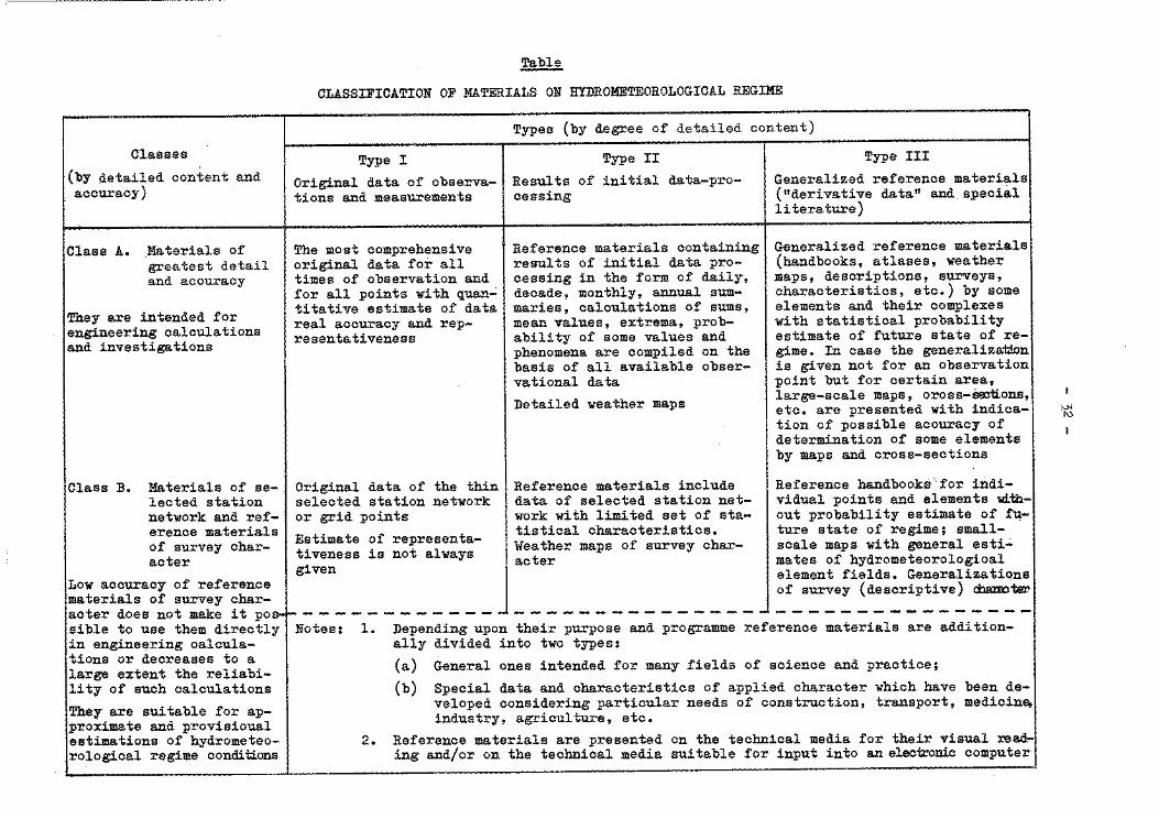
The classification of hydrometeorological regime reference materials is given in the Table.

Materials of Class A including comprehensive original data of observations for sufficiently dense (for this purpose) station networks or for grid points with quantitative estimates of their representativeness (Type I), results of initial data processing with sufficient sets of statistical characteristics (Type II), and gener­alized materials containing results of high-order statistical analysis (Type III) are of the highest importance to users. In the preparation of materials of Class A information concerning the representativeness of observations at some points, real accuracy and possibility of spatial and temporal distribution of data of the obser-vations with quantitative estimates of the errors are of special value. This is so because users are generally interested in hydrometeorological data not for the obser­vation point itself but for territory more or less distant from the observation point.

Hence the need arises for presenting material not only for individual obser­vation points but also for certain .areas in the form of climatological element fields (or their complexes) and therefore for the use of new observational devices such as meteorological satellites, radars, snow reconnaissance and other similar surveys and so on.

Generalized materials of Class A, Type III, not only determine or describe the state of some elements (or groups of elements) of the hydrometeorological regime but also reveal complex inter-relationships and on this basis provide probability estimates of the future state of the regime (and further - a climatological prognosis with an indication of time of realization of the expected regime state).

Large-scale maps of materials should be prepared on the basis of objective analysis. They should also make it possible to estimate an element (or complex of

Classes

(by detailed content and accuracy)

Class A. Materials of greatest detail and accuracy

They are intended for engineering calculations and investigations

Class :B. Materials of se­lected station network and ref­erence materials of survey char­acter

Low accuracy of reference materials of survey char-

~

CLASSIFICATION OF MATERIALS ON HYDROMETEOROLOGICAL REGIME

Types (by degree of detailed content)

Type I Type II

Original data of observa- Results of initial data-pro-tions and measurements cessing

The most comprehensive original data for all times of observation and for all points with quan­titative estimate of data real accuracy and rep­resentativeness

Original data of the thin selected station network or grid points

Estimate of representa­tiveness is not always given

Reference materials containing results of initial data pro­cessing in the form of daily, decade, monthly, annual sum­maries, calculations of sums, mean values, extrema, prob­ability of some values and phenomena are compiled on the basis of all available obser­vational data

Detailed weather maps

Reference materials include data of selected station net­work with limited set of sta­tistical characteristics. Weather maps of survey char­acter

Type III

Generalized reference materials ("derivative data" and. special literature)

Generalized reference materials (handbooks, atlases, weather maps, descriptions, surveys, characteristics, etc.) by some elements and their complexes with statistical probability estimate of future state of re­gime. In case the generaliza~n is given not for an observation point but for certain area, large-scale maps, cross-~uons, etc. are presented with indica­tion of possible accuracy of determination of some elements by maps and cross-sections

Reference handbooks'for indi­vidual points and elements wlth­out probability estimate of f~­ture state of regime; small­scale maps with general esti~ mates of hydrometeorological element fields. Generalizations of survey (descriptive) ~ter

:~~~~ ~~e:s:0!h::k~i!!c~~;-rN~t~s~ -1~ -D~p~n~i~g-u;o~ ~h~i~ ;~p~s~ :0~ ;r~~~~ ~e;e~e~c~ ~a~e~i~l~~r~ :d~i~i~n:-

in engineering calcula- ally divided into two types: tions or decreases to a ( ) . . . . large extent the reliabi- a General ones 1ntended for many f1elds of sc1ence and pract1ce;

lity of such calculations (b) Special data and characteristics of applied character which have been de-

They are suitable for ap­proximate and provisional estimations of hydrometeo­rological regime conditions

2.

veloped considering particular needs of construction, transport, medicin~ industry, agriculture, etc.

Reference materials are presented on the technical media for their visual read­ing and/or on the technical media suitable for input into anelecwonic computer

>-"' 1\)

- 33 -

elements) at any point of a territory with quantitative accuracy (References 5, 8, 13, 14, 15, 18, 20, 21, 40, 45, 51, 53, 54). Data of Class A are suitable for engineering calculations.

Materials of Class B include original data of sparse station networks or some grid points (generally without estimates of representativeness) and also gener­alizations of survey {descriptive) character with small-scale maps. These materials are suitable for general estimates of the hydrometeorological regime conditions for use in planning or for preliminary decisions. Use of materials of this class are made, if necessary, in practice and for engineering calculations, but the accuracy of these latter and hence the efficiency of the hydrometeorological service is lower.

An analysis of current practicesindicates that many countries still prepare mainly reference materials of Class B. At best, comprehensive reference materials of Types I-II {data of observations - results of initial data processing) published at the present time do not normally include quantitative estimates of the accuracy and representativeness of observations.

Published reference material of Type III (results of special statistical analysis and generalization) present as a rule the probability characteristics of individual elements rather than of their complexes, which in reality affect conditions of human life, growth of agricultural crops, different machinery, etc.

Cartographical constructions are usually on a small scale; they are drawn using subjective methods and do not contain any indications of the true accuracy of the hydrometeorological parameters determined from reference material over widely different geographical locations. Material of Class A should, therefore, be given a much greater priority than at present.

Let us now consider in detail the preparation and publication of reference material including the results of statistical analyses.

In this connexion, the ever growing volume of information makes reference materials difficult to use because of their bulkiness. For instance in the 1930s the climatological handbook for the territory of the u.s.s.R. was published in three ~olumes; in the forties and fifties in 28 volumes, and in the sixties in 170 volumes.

Thus in preparing reference material, it has become necessary to use new procedures for presenting the information and to "compress" the data in the form of

- 34 -

initially generalized characteristics, including distribution parameters of individual

elements and their complexes, and spatial and temporal structure parameters (Refer­

ences 5, 6, 7, 15, 31, 36, 37, 51, 53; 58).

Periodical publication of the material and its permanent storage on the

technical media form the basis for the further statistical development and compila­

tion of generalized reference materials of Class A to meet the different needs

(general and applied) for both local and large territories. The material which

takes into account regularities of formation as well as variations of the regime par~

meters and gives probabilities and prognostic estimates of regime conditions, must be

presented in a compact, convenient form.

In addition to statistical "compression" of information in preparing com­

pact reference materials of new types, the presentation of data. in the analogue form,

i.e., charts, diagrams, sections, etc., is important as the analogue form exceeds the

digital .form for compactness of information "packing" to a large extent.

General climatic and agroclimatic maps should also be an important facet in

the development of reference materials on the hydrometeorological regime. These maps

should be constructed according to the responsibility zones of the territorial

(national) centres for regions, countries, hemispheres and for the world and should

have suitably large scales for use in engineering calculations and investigations.

The construction of the maps should be based on the utilization of all

information obtained from ground-based observing stations (at individual observation

points and from movable observing devices), from satellites, rada.rs, aircraft, etc.

This information must undergo statistical and objective analysis in the light of the

physical relations and regularities and the local peculiarities in the large-scale

cartographical constructions. The results of statistical analysis may be presented

by graph plotters in the form of charts of corresponding scales, profiles and mono­

graphs.

In this way it will be possible to make the necessary data available in the

compact, analogue form which meets the requirements of users and investigators.

Together with data presentation in the analogue form, provision should be

made for the digital presentation of the most important data (at the grid points, key

local regions and points, etc.) on the technical media. This practice allows the

calculation of derivative values and the inclusion of the necessary hydrometeorological

- 35 -

data directly in computational algorithms. Applied and scientific problems can then be solved by the electronic computers without resorting to the bulky original information.

At the present stage of scientific and technical development it is impos­sible to produce accurate forms or layouts of reference mate~ial which contain results of statistical analysis meeting the necessary requirements.

As appropriate scientific and technical investigations are completed, forms and layouts corresponding to the third stage of development of presentation of data on hydrometeorological regime will be produced.

The following conclusions concerning the preparation of reference handbooks can therefore be made:

(a) Periodical and non-periodical reference handbooks should be prepared and published regardless of the availability of original data recorded on the technical media in archives;

(b) Attention should be largely paid to the preparation of reference materials of Class A.

The form and content of reference handbooks should meet a considerable number of users' requirements and thus greatly diminish the number of oper­ations under the "inquiry-answer" system. It is necessary therefore to take into consideration the sp~eific needs of the users in the development of these forms. However, to avoid unnecessary expense the volume of reference handbooks should not be too large for data processing and repro­duction: in the development of forms and circulation single requests, which are cheaper to be satisfied under the "inquiry-answer" system, should be considered as well as the mass requests;

(c) After the introduction of new advanced methods of data recording on the technical media, reference handbooks and tables of original data of obser­vations will not be generally used as information sources for data trans­ferring onto technical media (for instance, punch-card) or for complicated manual calculations; they will be used for references and information purposes only;

- 36 -

(d) The preparation of reference materials by electronic computers allows the

rapid computation of new statistical characteristics ·and results of analyses

which have not been possible up to now;

(e) New type reference materials should have the following distinctive features:

they should include only those original (raw) data of observations which

are needed for reference and information work;

they should include data and additional statistical characteristics

required by users, not only for individual points (stations) but also

for large areas (fields of meteorological elements and their complexes);

(f) Reference materials should also include results of observations from meteo­

rological satellites, radars and movable observing devices such as air­

craft, etc;

(g) Pe:dodici ty of publication of reference materials may range from a month to

ten years. Longer intervals are not desirable as information ages rapidly;

(h) In accordance with the WMO recommendations reference materials (particularly

of Type I) are prepared for immediate visual reading as well as on technical

media suitable for input into an electronic computer. It will, in some

cases, permit the compact summarized information (mostly calculated data)

to be used for special calculations rather than bulky original (raw) obser­

vation data;

(i) Conside:t'ing the need to compile detailed and accurate material of Class A

which includes all availab;Le information and kr).owledge of the local

peculiarities, it is reasonable to expect materials for local regions to be

prepared immediately at the territorial (national) centres. ·It then makes

it possible to combine the total information available for certain terri­

tories for use by the specialists who are studying the operational require­

ments of these. territories and by the different branches of national economy

and hydrometeorological research institutes.

Reference materials for extensive territories such as the European part of

the U.S.S.R., the Soviet Union Republics of. Central Asia, Siberia, .the .Far East, etc.,

are compiled at the regional centres and world centres (Hydrometeorological Centre of

the U.S.S.R.) and the territorial (national) centres can obtain them for use.

- 37 -

As some important scientific and technical problems have not yet been solved, the compilation of reference materials to meet modern requirements needs further thorough study and development at all levels (territorial (national) centres -regional centres - special research institutes - world centres).

Archival storage and retrieval of information in the information-retrieval system. Operative copying. Scientific-technical information

At present the scientific-information services in the broadest sense are an integral part of scientific investigations and presentation of results for different purposes (Reference 47).

The main purposes of the scientific-information activity are as follows:

(a) Collection of scientific documents;

(b) Analysis and synthesis of information;

(c) Archival storage and retrieval of information;

(d) Reproduction and distribution of information materials.

Sometimes the term "documentation" which the International Federation of Documentation defines as "collection and storage, classification and selection, dis­tribution and utilization of information of all kinds" is used.

Development of these goals is one of the problems of processing and archival storage of hydrometeorological information.

The problem of archival storage of information is much more complicated for Hydrometeorological Services than for many other fields of science due to the large volume of annual flow of information and necessity for its archival life for an indeterminable period.

Let us then consider the most up-to-date means of archival storage of infor­mation in the light of their suitability for hydrometeorological practices.

The problem of compact and continuous archival storage of information can be divided into two parts:

(a) Storage of information in a form which can be readily used by electronic computers with automated input (i.e., information recorded on .the technical media);

- 38 -

(b) Storage of information in a form which is suitable for visual reading,

manual treatment or manual input into the electronic computers.

In spite of great progress in developing computing techniques, both these

aspects of the archival storage of information are of high practical importance and

must be used by the Hydrometeorological Services and the World Weather Watch.

On the basis of scientific and methodical work already carried out in this

direction and bearing in mind our experience and that of other countries (Refer­

ences 28, 33) one can draw the following conclusions:

(a) Microfilm (discs, plates) with a binary code is recommended as a basic

type of information-carrying medium for permanent archival storage;

(b) SO-column punch-cards, paper punched tapes, punch-cards for graphite marks

can be used as the auxiliary or intermediate technical media;

(o) Archival storage of sheet originals (tables, books, maps, etc.) is accept­

able with sufficient number of archives, because their immediate use is

still convenient in some oases;

However, 35-mm microfilms are the basic media for archival storage of infor­

mation recorded on sheet originals. 16-mm microfilms can be used as well;

in rare cases 70-mm microfilms requiring very high resolution and large

sheet size can be used too;

(d) It is recommended that the archives be equipped with small mechanized

devices;

(e) It is recommended that the information-retrieval system be created on the

basis of a special classification which combines the systems of U.D.C.

(Universal Decimal Classification) and L.D.C. (Local Decimal Classification);

(f) Information-retrieval systems can be largely realized by means of cards

with edge perforation, machineable punch-cards and microfilms of an auto­

mated device of the "POISK'' type;

(g) Delay of data presentation to the users often results from faults in the

organization of operational copying. Hence the following most important

principles and methods for copying material-s should be widely.introduced:

- 39 -

miniaturization of sheet materials mostly by microfilming of originals

on non-perforated 35-mm film, in some cases - on 16-mm film, rarely -

on 70-mm film;

reproduction and transmission of copies of microfilms to other centres

and to users;

photo-offset, electrographioal and diazographical reproduction of sheet

originals or enlarged prints of microcopies;

in comparatively rare oases - publication of collections of papers,

handbooks, monographs, etc.

The use of facsimile print and photo-telegraph is the most convenient

method for the urgent presentation of materials to users.

Scientific-technical effectiveness of automated systems and their separate units

The introduction of the proposed technological scheme will allow:

the reduction of the time from the moment of observation to the data

processing stage by electronic computers for scientific and practical

purposes and also the time needed for publishing handbooks containing

original data of observations from l-3 years as at present to l-2 months;

raising the coefficients of use of results of the observations for hydro­

meteorological regime studies and practical use of hydrometeorological

data from 0.2-0.3 as at present to 0.9-1.0 using all available data;

utilization by a computer of those algorithms which are not presently

accessible due to their labour-consuming character for calculations and

subsequently for the development of new procedures and preparing prog­

noses of hydrometeorological regimes.

All these steps will greatly improve the hydrometeorological services to

the national economy and the different research institutes. In other words they

will increase the scientific-technical effectiveness of the system.

At the same time, preliminary calculations show the economic effectiveness

of the separate units of the system.

The introduction of system design will allow an approximately threefold

reduction in the cost of processing data obtained from one hydrological post per year.

Also the proposed technological scheme will reduce the time needed for data processing

two hundredfold.

- 40 -

Results of the experimental recording of basic meteorological data of obser­

vations on punched tape during five months of 1968 at 48 stations showed that punching

could be made almost twice as rapidly as manual compiling and checking of Table TM-I

(although full possible speed of teletype T-51 puncher has not been obtained yet).

Therefore, the introduction of table compilation by machine methods will save forty

man-hours per week; this time could be used for carrying out some extra observations

and so on.

Preliminary results also show that the cost of processing and checking

basic meteorological observation data and compiling Tables TM-I using the electronic

computer "Minsk-22" is more than that of the manual operations. However, further

optimization of algorithms and programmes of data checking and processing will make

it possible to reduce the cost of machine data processing.

From tentative information on the time needed for processing and checking

of one Table TM-I at the data-processing centre, machine methods of data processing

by "Minsk-22" using current experimental algorithms and programmes take only half the

time required using corresponding manual methods.

Thus an automated system provides considerable scientific-technical effec­

tiveness which in turn allows labour saving operation, a speeding up of the presenta­

tion of materials to the users, and an increase in the completeness and quality of

these materials, i.e., general improvement of hydrometeorological service providing

different organizations of the national economy and different research institutes

with hydrometeorological data.

Moreover preliminary results of tests of separate units of the system sug­

gest that even at the early stage of introducing new technology both scientific­

technical and direct economic benefits can be obtained. There is therefore great

potential to increase the effectiveness of the system as a whole and of its separate

units at the stage of adoption and improvement of new technological processes and

equipment.

Conclusions. Trends in further investigations and operations

1. Preliminary results show that the introduction of the proposed methods will

provide:

(a) Scientific-technical benefits due to the increase in completeness and , __

- 41 -

quality of hydrometeorological data and in their operational presentation to the users;

(b) Indirect economic benefits related to the utilization of hydrometeorological data in the solution of a number of problems in the fields of planning, construction, transport, energetics, industrial and agricultural production, output of minerals, fisheries, production of material values and also in the implementation of scientific and practical goals in other fields;

(c) Direct economic effe.ct due to reduction of labour costs.

2. In some cases current modern methods are not sufficiently effective. Hence further scientific research and experimental-design investigations along the following lines are required:

(a) Testing of data recording on intermediate technical media: paper punched tape using mechanical punchers; cards with code field; punched cards with graphite or other "sensitive" marks.

Statistical analyses of data will show the level of errors and facilitate the choice of an optimum intermediate technical medium and methods of data recording for the different types of hydrometeorological observations;

(b) Improving devices for obtaining a durable medium, particularly with a view to increasing the speed of recording information on this medium and the reliability of recordings and readings using independent serial facilities which do not need special adjustments for each type of medium;

(c) Developing and introducing methods and devices to eliminate laborious manual operations in the treatment of data from recorders. The most accessible and reliable techniques are as follows:

semi-automatic reading of curves and their conversion to digital form for processing by the electronic computers; equipping recorders with punching devices to obtain the necessary punched tape for further processing by electronic computer;

(d) Testing and introduction of autonomous devices for re-recording information from one medium to another thus saving machine time;

- 42 -

(e) Evaluating the advisability of introducing analogue and analogue-digital

electronic computers and systems for some types of data processing and

their inclusion in the general technological scheme;

(f) Developing unified codes for recording observational data on the technical

media;

(g) Improving methods of automatic data control to increase economic effective-

ness;

(h) Optimizing algorithms of initial data processing and forms of presentation

of original data to increase the effectiveness of hydrometeorological

service and reduce the cost of data processing, archival storage, repro­

duction and distribution;

(i) Developing and improving methods of statistical analysis for compiling

reference materials containing probability calculations and prognoses for

some elements of the hydrometeorological regime and their complexes not

only for individual observation points but more particularly for extensive

areas;

(j) Developing and improving programmes for the electronic computers especially

those using automatic programming methods;

(k) Developing of special information-retrieval systems using modern technical

means for Hydrometeorological Services;

(1) Testing and utilizing, in accordance with the goals of the Hydrometeoro­

logical Services, reproduction techniques for all units of the system to

eliminate the laborious manual operations in copying, reproducing and

publishing. Development and introduction of methods of microfilming of

materials in the analogue form (maps, diagrams, photographs, etc.) without

loss of information;

(m) Testing and improving the technological scheme of collection, processing,

retrieval, archival storage, reproduction, distribution and exchange of

data;

- 43 -

(n) Compilation of scientific-methodical handbooks for the introduction of

approved methods. Recommendations to other organizations which conduct

hydrometeorological work.

The implementation of these measures will provid~ a further increase in

the scientific, technical and economic effectiveness of the system of complex auto­

mation of Hydrometeorological Services.

*

* *

~

- 44 -

REFERENCES

l. Anapolskaya L.E. and Gandin L.S., 1958: Procedures for determination of calculated velocities of wind pressures on buildings. Meteorology and Hydrology, No. 10.

2. Beloussov S.P., 1965: Experiments on use of automatic processing of aero­logical telegrams for operational numerical prognosis. Proceedings of the Hydrometeorological Centre of the U.S.S.R., No. 10, Moscow.

3. Birman B.A., 1967: Automatic control of marine meteorological informa­tion using an electronic computer. Express-Information No. 9, Hydro­meteorological Centre of the U.S.S.R., Obninsk Branch.

4. Blinova E.N., 1967: General atmospheric circulation and long-term hydrodynamical atmospheric prognosis. "Meteorology and Hydrology for Fifty Years of the Soviet Power 11 , Leningrad.

5, Borisenkov E.P., 1963: Physico-statistical methods of analysis and pre­calculations of meteorological fields. Proceedings of the Arctic and Antarctic Research Institute, Vol. 263, Leningrad.

6. Borisenkov E.P., ed., 1966: Introduction to statistical methods of hydro­meteorological information processing by an electronic computer. The Arctic and Antarctic Research Institute, Leningrad.

1. Bruks K. and Caruzers N., 1963: Use of statistical methods in meteorology. Leningrad.

8, Budyko M.I., 1968: Radiation factors of recent climate changes. Izves­tiya Akademii Nauk s.s.s.R. (Bulletin of the Academy of Sciences of the U.S.S.R.), Geographical Series, No. 5.

9. Vaisman G.M., 1967: Automation and telemechanics in meteorology. Leningrad.

10. Vaisman G.M., 1967: Composition of the report from completely automatic or semi-automatic stations. Abstracts of reports submitted to the inter­institute scientific seminar on automation of collection, processing and distribution of hydrometeorological information, 24 August 1967. The Aeroclimatological Research Institute, Moscow.

11. Vetlov I.P., 1967: Meteorological investigations using artificial earth satellites. "Meteorology and Hydrology for Fifty Years of the Soviet Power", Leningrad.

12. Vildanova M.I., 1967: Automatic control of coastal hydrometeorological information. Express-Information No. 10, Hydrometeorological Centre of the U.S.S.R., Obninsk Branch.

13. Vitels L.A., 1962: Anomalies of solar activity cyclic variation and trends in recent climatic fluctuations. Proceedings of the Main Geophysical Observatory No. 133, Leningrad.

14. Gandin L.S. and Kogan R.L., 1967: On the economical approach to location of station network. "Problems of acquisition and processing of information about physical state of ocean", Sevastopol.

- 45 -

15. Golzberg I.A. et al., 1968: Microclimate of the U.S.S.R. Leningrad.

16. Grigor'ev V.I., 1967: Automatic control of results of water-meter obser­vations in their processing by an electronic computer. Express-Information No. 10, Hydrometeorological Centre of the U.S.S.R., Obninsk Branch.

17. Grigor'ev V.I., Dement'ev N.F., and Tikhov V.A., 1967: Results of the experimental works on use of punch~cards for graphite marks as hydro­meteorological information technical media. Express-Information No. 9, Hydrometeorological Centre of the U.S.S.R., Obninsk Branch.

18. Gruza G.V., 1968: Some general problems of the theory of weather forecasting on the basis of statistical data. Proceedings of the Central Asian Hydro­meteorological Research Institute No. 29(44).

19. Davitaja F.F., 1967: Results and prospects of studies of agroclimatic resources of the s.s.S.R. "Meteorology and Hydrology for Fifty Years of the Soviet Power", Leningrad.

20. Dzerdzeevsky B.L., 1968: Climatic fluctuations and problem of over-long prognosis. Izvestiya Akademii Nauk S.S.S.R. (Bulletin of the Academy of Sciences of the U.S.S.R.), Geographical Series No. 5, Moscow.

21. Dzerdzeevsky B.L., 1968: Circulation processes in the atmosphere of the northern hemisphere in the twentieth century. International Geophysical Year, Materials of Meteorological Investigations. The Geographical Institute of the Academy of Sciences of the U.S.S.R., Moscow.

22, Dobryshman E.M., 1967: Some questions on hydrometeorological data pro­cessing. Proceedings of the Hydrometeorological Centre of the U.S.S.R., No. 1, Moscow.

23. Drozdov O.A., 1967: Climatic fluctuation studies. "The A.I. Voejkov Main Geophysical Observatory for Fifty Years of the Soviet Power", Leningrad.

24. Drozdov O.A. and Grigor'eva A.S., 1969: On the cycles of variations of amount of atmospheric precipitation throughout the territory of the U.S.S.R. Proceedings of the Main Geophysical Observatory, No. 245, Leningrad.

25. Ivanov R.N. and Staburova S.N., 1968: Use of teletype communication in the system of inter-branch territorial information bodies. Scientific­Technical Information, Series I, No. 6.

26. Kljukin N.K., 1965: On the new principles of preparation of hydrometeoro­logical data for processing using an electronic computer. "Automatic input of characters into an electronic computer", Vilnus.

27. Kljukin N.K., 1966: Preparation of hydrometeorological data for processing by electronic computers. Meteorology and Hydrology No. 6.

28. Kljukin N.K., 1967: regime information. Institute, No. 46.

System of automatic processing of hydrometeorological Proceedings of the Aeroclimatological Research

29. Kljukin N.K., 1967: Characterization·of hydrometeorological regime infor­mation, some principles of its processing and storage. Proceedings of the Hydrometeorological Centre of the U.S.S.R., No. 1, Moscow.

- 46 -

30. Kljukin N.K., Sapozhnikova S.A. and Filippov v.v., 1967: Use of computing techniques in the development of basic climatological characteristics. Proceedings of the Aeroclimatological Research Institute, No. 46, Moscow.

31. Kljukin N.K. and Filippov v.v., 1967: Review of present state of means and methods of mechanized meteorological information processing in different

countries. Express-Information No. 13, Hydrometeorological Centre of the

U.S.S.R., Obninsk Branch.

32. Kljukin N.K., 1968: World centre for hydrometeor,ological data collection, processing and storage. Meteorology and Hydrology, No. 10.

33. Kolotovkin I.V., Koshinsky S.D. and Pakhomov V.I., 1967: On the problem of input and meteorological regime information processing using the elec­tronic computer "Ural-14b11 • Proceedings of Novosibirsk Regional Hydro­meteorological Centre, No. 1(5).

34. Koshinsky S.D., Radtchenko G.V. and Rusanov V.I., 1966: Mechanized develop­

ments of meteorological complexes: temperature and relative humidity of air

for different values of wind velocity and low cloud. Proceedings of the Aeroclimatological Research Institute (Novosibirsk Branch) No. 42(2).

35. Lebedev A.N., 1965: Application of nomogram method to the climatic regu­larity studies at the tropical and equatorial latitudes. Proceedings of the Main Geophysical Observatory, No. 182, Leningrad.

36. Lebedev A.N. and Mikhajlenko M.M., 1968: Procedures of summarization and graphical representation of temperature and relative humidity of air. Proceedings of the Main Geophysical Observatory, No. 232, Leningrad ..

37. Lobanova V.Ya., 1967: Experience of use of computers for accumulation of statistical generalization of information about clo11diness obtained from meteorological satellites. Proceedings of the Aeroclimatological Research Institute, No. 39, Moscow.

38. Logvinov K.T., 1967: Preparation of sounding rocket data for mechanized developments. Proceedings of the Aeroclimatological Research Institute, No. 39, Moscow.

39. Mamontov N.V., 1965: Statistical characteristics of two-dimensional dis­tributions of temperature and relative humidity of air in the south-eastern

part of the Western Siberian lowland. Proceedings of the Aeroclimatological Research Institute (Novosibirsk Branch), No. 1.

40. Makurin N.V., 1966: Control of data from temperature soundings in the atmosphere using an electronic computer. Proceedings of the Arctic and Antarctic Research Institute, No. 277, Leningrad.

41. Makhover Z.M. and Ovsiannikov v.v., 1967: On the system of automatic con­trol and processing of hourly meteorological observational data using an electronic computer. Express-Information No. 10, Hydrometeorological Centre of the U.S.S.R., Obninsk Branch.

42. Makhover Z.M. and Ovsiannikov v.v., 1968: On the problem of control and processing of hourly meteorological data. Proceedirlgs of the Aeroclimato­logical Research Institute, No. 51, Moscow.

- 47 -

43. Mertzalova O.B., 1967: Technological scheme of aerological material motion with mechanized control and statistical processing of data. Express­Information No. 13, Hydrometeorological Centre of the U.S.S.R., Obninsk Branch.

44. Mednikova E.S. and Tchernin K.E., 1966: Graphical representation of co­ordinate grid on the screen of electron-beam tube using an electronic com­puter. Proceedings of the Arctic and Antarctic Research Institute, No. 277, Leningrad.

45. Mikhajlov A.I. and Polushkin V.A., 1963: The theory of scientific infor­mation - a new independent branch of science. Scientific-Technical Information No. 3.

46. Mikhajlov A.!., Tcherny A.I. and Giliarevsky R.S., 1965: Fundamentals of scientific information, Moscow.

47. Nazarova I.V., 1967: Automatic control of main daily observations. Express­Information No. 13, Hydrometeorological Centre of the U.S.S.R., Obninsk Branch.

48. Nazarova I.V. and Aristova L.N., 1967: meteorological observations by temporal Information No. 13, Hydrometeorological Branch.

An experiment in the control of data interpolation. Express­Centre of the U.S.S.R., Obninsk

49. Roger J., 1963: Use of computers at documentation centres and speci~l libraries. Unesco Bulletin for Libraries, Vol. XVII, No. 5.

50. Rubinshtein E.S., 1967: Goals and methods of climatic mapping. "The A.I. Voejkov Main Geophysical Observatory for Fifty Years of Soviet Power", Leningrad.

51. Sal'man E.M~, Gashina S.B., Divinskaya B.Sh. and Alter-Zalik Yu.Zh., 1968: Principles of the system of radar observations of clouds, cloud systems and dangerous phenomena using a network of radar meteorological stations. Proceedings of the Main Geophysical Observatory, No. 231, Leningrad.

52. Saposhnikova S.A., 1967: Use of climate-formation regularities in the climate service. Proceedings of the Aeroclimatological Research Institute, No. 46, Moscow.

53. Semendiajev K.A., 1967: Automatic construction of isoline maps. Proceedings of the Hydrometeorological Centre of the U.S.S.R., No. 1, Moscow,

54. Sotchava V.B., 1964: Complex mapping of geographical environment. Siberian Geographical Collection of Papers, No. 3, Moscow-Leningrad.

55. Fedorov E.K., 1967: The Soviet Hydrometeorological Service by the Fiftieth Anniversary of the Great October Socialistic Revolution. "Meteorology and Hydrology for Fifty Years of the Soviet Power", Leningrad.

56. Fedorov E.K., 1967: Active influence on meteorological processes. "Meteo­rology and Hydrology for Fifty Years of the Soviet Power", Leningrad.

- 48 -

57. Philippov v.v., 1965: Experience of multi-factor dispersion analysis of air temperature from ship observations. Proceedings of the Aeroclimato­logical Research Institute, No. 33, Moscow.

58. Fridberg G.I., 1960: Microfilming in the institutions of scientific­technical information. "Problems of organization and procedures of scientific-technical information and propaganda", Moscow.

59. Frank o., 1966: Development and present state of microfilming technique.

"Methods and means of document copying", No. 3, VINI'l'I, Moscow.

- 49 -

OBSERVATION AND RECORDING OF ELEMENTS, METEOROLOGICAL LOG-BOOKS, SCRUTINY OF DATA, METEOROLOGICAL JOURNALS

by

R. Arlery

Reference shall be made to certain parts, indicated in parenthesis (GCP --0, of the Guide to Climatological Practices. A few suggestions should be taken into consideration for the automatic data processing; some precautions should also be observed in the stage of collection and initial recording of data.

Climatological observations (GCP 3.1.2, 3.2, 3.4.2, 3.4.3)

The various types of obser~ations are described without any distinction between surface and upper-air observa.tions.

Visual observations: appreciation of forms or nature (cloud, state of the sky, etc.), estimation of distances (visibility, height of cloud base, etc.), iden­tification of hydrometeors (snow, ice pellets, rain, etc.), evaluation of intensities of certain phenomena (light, medium, strong, etc.), etc.

Simple readings of currently used instruments, in instantaneous values (thermometer, barometer, etc.) or in cumulative values (sunshine recorder, raingauge, evaporimeter, etc.).

Readings associated with the use of psychrometric tables (psychrometer) or reduction tables (sea-level pressure).

Readings on dials (anemometer, wind vane).

Readings on diagrams of recording equipment (instantaneous values for mean values over short periods of time); time marching.

In the case of automatic climatological stations, recording of values on perforated tapes associated with periodic recordings.

- 50 -

Log-book (GCP 3.4.4)

1 Distinction to be made between surface observations and upper-air obser-

vations.

Entries in numerical values and coded values.

The order in which the entries are made. Uniformity of the units. Res­

pecting of the prescribed hours. Utilization of standard symbols. Keeping of the

log-book, etc.

Meteorological recordings (GCP 3.4. 3)

Generally one should beware of the impression of security given by the

automatic functioning of the recorders. As with any instruments with mechanical or

electrical transmissions they may go out of order unexpectedly. When properly

calibrated before installation and subject to frequent check~ by means of measure­

ments with direct reading instruments, the recorders can permit quite valuable inter­

polations between the observations. But, if one wishes to ~void gaps and to prevent

malfunctioning of the recorders, it is also necessary, besid~ checking, to clean

them at frequent and regular intervals.

In these instruments the sensor is subjected to the action of the variations

of the element observed. As a result mechanical deformations of the sensor may

occur or its electrical resistance or other properties may be modified. The trans­

mitting system (mechanical, electrical or electronic) amplifies these distortions

and transmits them to the recording equipment (a stylus, needle, etc.). The actual

recording involves a diagram brought into motion by a clockwork at a determined speed

before the stylus or needle.

The clockwork with which these instruments are equipped may have irregu­

larities in functioning, particularly if they are placed outside the building, and

thus subject to great variations of temperature. On the other hand the paper of

these diagrams is usually a hygroscopic material which varies in length with the

increase in the humidity. It is, therefore, mandatory to trace the time marks

regularly, for instance, one for each of the three-hourly observations on the daily

diagram.

- 51 -

Beside faulty functioning of the recorders, due tp clockwork trouble or to excessive friction caused by the pressure of the stylus on the diagram there might be other causes for errors in recording. Friction may be caused by dust which collects at the extremities of the axis and the joints of the transmission levers; or, in electrical equipment, corrosion of the contact surfaces may increase the resistance of the circuits and introduce errors in the measurements.

Beside the usual recorders one should also mention the automatic observing equipment, designed and built to make climatological observations, in remote areas during certain periods, without a human observer. This type of equipment may be used for the climatological study of large uninhabited or uninhabitable regions: thus, in arid regions the automatic climatological stations may be located in the most appropriate (climatically speaking) places instead of in individual places (oases), imposed by practical necessities, which are not always sufficiently rep­resentative of the microclimate.

On the subject of recorders some mention should be made of the transfer of data from autographic records and of the filing of the diagram (GCP 3.4.5).

Scrutiny of data (GCP 4.3)

Before considering the scrutiny of data one should mention the conditions to be fulfilled to eliminate the possibilities of introducing errors: providing appropriate guidance for new observers, avoiding bad habits, ensuring the silence and the absence of distractions in the observation rooms (by removing the telephone or anything else which might distract the observer from his continuous tasks).

The general problem of the scrutiny of data also raises the question of the level(s) at which the corresponding operations should be carried out.

Meteorological journals (GCP 3.4.4.1)

Annual or pluriannual meteorological journals are traditionally kept up to date at certain stations, particularly at those which are long established. These documents, where in theory the data are entered after a thorough checking, are a use­ful means of preserving the data. Their format is normally standardized thus facilitating the manual operations of the local climatology. They also have the

- 52 -

advantage of containing valuable background data of the station. On the other hand

they are not particularly adaptable for regional synthesis or for transmission

of data. (The photocopy reproduction, while being the most practical means of

supplying data is often too costly and is being replaced by microfilming, which in

turn is not always appreciated by the users.)

The tendency is to replace these journals by printed monthly forms which

can be reproduced easily (particularly if filled on a translucid paper) for tr~ns­mission to the regional or central authorities of the Meteorological Services or for

periodic broadcasts to the public, according to requirements.

Guidance on these monthly forms is contained in the Guide to Climatological

Practices (GCP 3.4.4.2).

- 53 -

QUALITY AND DURATION OF METEOROLOGICAL SEQUENCES

by

G. Tarakanov

The reliability of climatic indices derived from statistical meteorological data depends to a large extent on the quality of the initial data. The climatic indices will reflect the character of the climate correctly only if the meteorolo-gical sequences satisfy definite requirements.

of the sequences.

The basic requirement is homogeneity

A sequence is homogeneous when its characteristics vary from one year to another or over several years in accordance with the natural variation of processes influencing the weather and climate of the region concerned. It is obvious there­fore that a meteorological sequence will be homogeneous when the surrounding land­scape, the type of instruments and methods of observation used are unchanged over the period in question. In other cases relatively simple techniques oan be used to detect and correct non-homogeneity of the sequences.

If the natural variability of a meteorological element from year to year is less than a variability caused by the non-homogeneity of the sequence, the latter can be detected by a simple comparison of the data observed at the station over different years.

When increases in the values of meteorological elements, caused by non­homogeneity, are less than the natural variability of the element, the non-homogeneity can be detected by comparison of the given sequence with those of corresponding elements for a neighbouring station. As a general rule the trend of a meteorological element at a neighbouring station must be the same since climatic changes occur simultaneously over a wide area. Thus where we have two homogeneous sequences from two neighbouring stations, the meteorological element variations from year to year at these stations have similar characteristics. These characteristics form a con­stant relationship between the two sequences. If from a certain time the charac­teristics of this relationship are changed, a disturbance of homogeneity of one or other of the sequences is immediately apparent from the comparison.

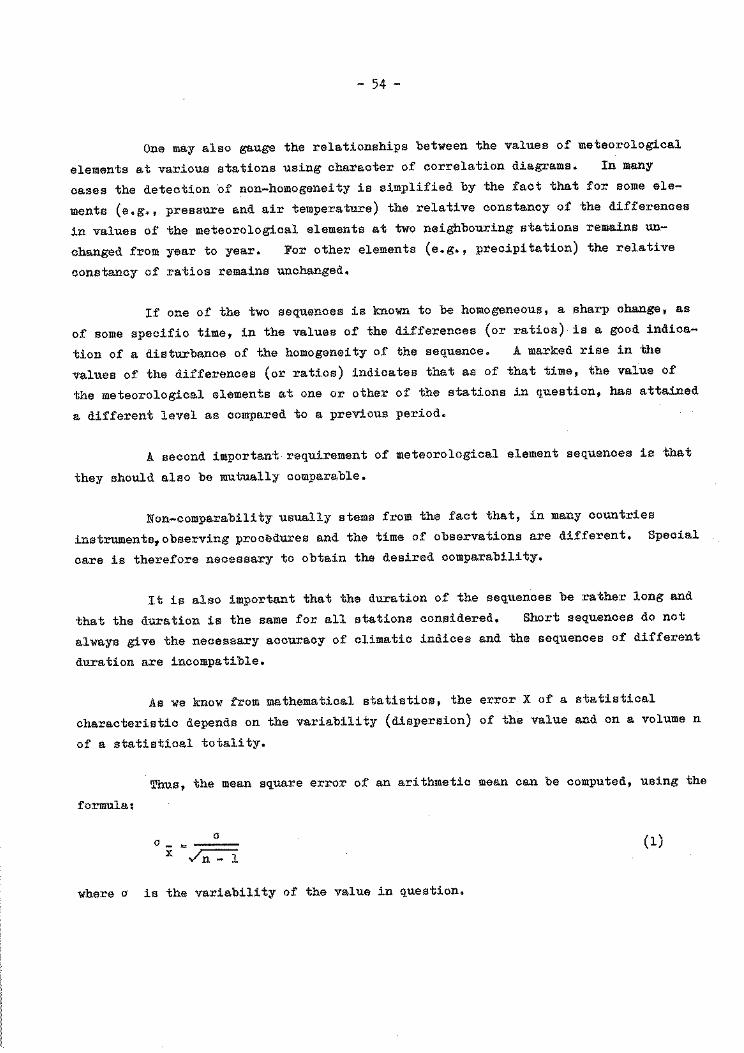
- 54 -

One may also gauge the relationships between the values of meteorological

elements at various stations using character of correlation diagrams. In many

cases the detection of non-homogeneity is simplified by the fact that for some ele­

ments (e.g., pressure and air temperature) the relative constancy of the differences

in values of the meteorological elements at two neighbouring stations remains un­

changed from year to year. For other elements (e.g., precipitation) the relative

constancy of ratios remains unchanged.

If one of the two sequences is known to be homogeneous, a sharp change, as

of some specific time, in the values of the differences (or ratios) is a good indica­

tion of a disturbance of the homogeneity of the sequence. A marked rise in the

values of the differences (or ratios) indicates that as of that time, the value of

the meteorological elements at one or other of the stations in question, has attained

a different level as compared to a previous period.

A second important requirement of meteorological element sequences is that

they should also be mutually comparable.

Non-comparability usually stems from the fact that, in many countries

instruments,observing procedures and the time of observations are different. Special

care is therefore necessary to obtain the desired comparability.

It is also important that the duration of the sequences be rather long and

that the duration is the same for all stations considered. Short sequences do not

always give the necessary accuracy of climatic indices and the sequences of different

duration are incompatible.

As we know from mathematical statistics, the error X of a statistical

characteristic depends on the variability (dispersion) of the value and on a volume n

of a statistical totality.

Thus, the mean square error of an arithmetic mean can be computed, using the

formula:

a (1)

where a is the variability of the value in question.

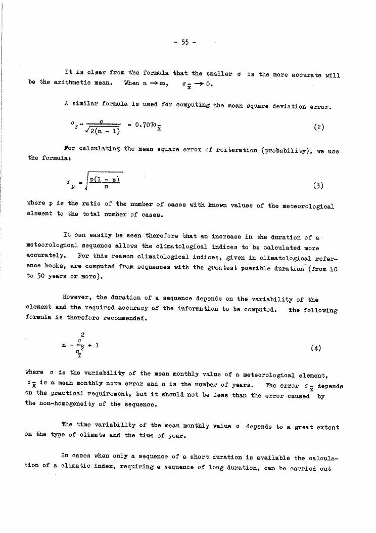
- 55 -

It is cl~ar from the formula that the smaller a is the more accurate will be the arithmetic mean. When n ~eo, a-~ D.

X

A similar formula is used for computing the mean square deviation error.

a = -====::­a /2(n - 1)

For calculating the formula:

a = J p(l - p) P n

D.1D7a­x (2)

the mean square error of reiteration (probability), we use

(3)

where p is the ratio of the number of cases with known values of the meteorological element to the total number of cases •.

It can easily be seen therefore that an increase in the duration of a meteorological sequence allows the climatological indices to be calculated more accurately. For this reason climatological indices, given in climatological refer­ence books, are computed from sequences with the greatest possible duration (from 10 to 50 years or more).

However, the duration of a sequence depends on the variability of the element and the required accuracy of the information to be computed. The following formula is therefore recommended.

2 a

n = 2 + 1 ax

(4)

where a is the variability of the mean monthly value of a meteorological element, a- is a mean monthly norm error and n is the number of years. The error a- depends X

X on the practical requirement, but it should not be less than the error caused by the non-homogeneity of the sequence.

The time variability of the mean monthly value a depends to a great extent on the type of climate and the time of year.

In cases when only a sequence of a short duration is available the calcula­tion of a climatic index, requiring a sequence of long duration, can be carried out

- 56 -

using a special .method of. climatological data processing called "the adduction of

sequences".

The theory of sequence adduction is based on the fact that there is a

definite relationship between values of the same meteorological element at different

stations. The following form of regression equation is therefore used.

(Jb

BN = Bn + r(a, b) Oa (~ - An) (5)

where AN and An are the average values of the meteorological element at long

sequence station A over the long period N years and short period n years respectively,

Bn is the average value of the meteorological element at the short sequence station B

over n years; r{a, b) is the correlation coefficient between values of the element

at stations A and B; a , ab are the mean square deviations of the element at a "

stations A and B respectively. BN is the average value of the element at station B,

adduced for the long period {over N years).

Where r(a, b)> 0.5, good results can be obtained using the more simple

expression:

(Jb

B' "" B + r;;a N n (AN - An) {6)

This method of sequence adduction can be further simplified in two special

cases:

(1)

(2)

when ab ;;;

when ~b '01:

n

(J a

(Ja

An

(the variabilities at both stations are equal)

(the relative variabilities are equal)

In the first case formula (6) becomes

B!_ c A + (B - A ) -N n n n

and is referred to as "THE METHOD OF DIFFERENCES".

(7)

- 57 -

The second case gives us the expression:

B , n (8) BN=rAN

n

and is known as "THE METHOD OF RATI0 11•

It is worth noting that all these methods give good results in satisfying the so called "criterium of adduction appropriateness" which we will discuss later.

- 59 -

CLIMATOLOGICAL SUMMARIES, MEANS, EXTREME VALUES, FREQUENCIES, DIURNAL AND INTERDIURNAL VARIABILITY,

CLIMATIC SERIES

by

R. Arlery

Climatological summaries

Qs~ ~f_s~~a~i~s

Their preparation is not an end in itself. They contribute to the pre­

servation of data. They facilitate the provision of information for the public.

They should therefore be prepared in a form which meets the technical requirements

and the needs of possible users.

Types of climatological summaries

]!a.!lz ~u.!!m.!.r!e~

These refer to a group of stations (problem of the order of presentation

of these stations),

They contain values observed at certain hours and values which are repre­

sentative of the day: means (pressure, temperature, humidity), maximum and minimum

(of certain elements), totals (radiation, sunshine, totals of precipitation, duration

of precipitation, evaporation) an indication of the presence or otherwise of

occasional phenomena (fog, thunderstorm, snow, hail, dew, etc.).

The division of the day (0 to 24 h, 6 h to 6 h GMT) is a delicate matter;

apparent anomalies may result from this conventional division.

!1.onthlz !lll.2:..!.Il!!.u.!.l_s~m.!!a~i~s

These refer to one station or to a group of stations.

They contain mean values of the principal elements, for the month, either

measured at a fixed time or meaned for the day. Extreme values for the month (pos­

sibly with date of occurrence). Monthly ·totals of cumulative elements (possibly

- 6o -

with the maximum in a day). Frequencies of given values (selection of ranges).

Numbers of days with particular phenomena. Possibilities of automatic preparation.

Filling in gaps.

Nature of certain summaries adopted for specific purposes

The report of the Working Group on Climatological Summaries, discussed at

the CCl-V (Geneva, October 1969) shall be taken as a basis for consideration.

of: CCl-V/Doc. 5 (18.6.1969) and the results of the discussions:

Aeronautical climatological summaries (see Guide to Climatological Prac­

tices, Chapter 12, Annex 12 B).

Summaries which may best satisfy the hydrometeorological requirements.

Summaries satisfying the requirements of agricultural meteorology.

Summaries satisfying the requirements of marine meteorology.

Mean values, extremes, freguencies

A brief mention will be made of the definitions and the best selection

among these characteristics depending on the element under consideration, publication

envisaged or the probable use of the information to be supplied.

Diurnal and interdiurnal temperature variation

An effort will be made to visualize the concept of the variability as it

may be shown experimentally on a continuous recording diagram, leaving aside for the

moment the way in which this variability will be expressed in values. The ways of

empirical appreciation of this variability will be sought, i.e. by means of indica­

tions contained in the monthly climatological summaries. A discussion will be held

on the periods, natural or conventional, which should be taken into consideration

for getting an idea of the importance of the variability. The distinction will be

made between the diurnal and interdiurnal variations and the corresponding varia­

bilities. The imperative necessity to respect the terminology will be studied.

- 61 -

Climatic series

A sequence of values of a climatological element in chronological order is not necessarily a climatic series. The chronological list of average daily tempera­tures, for instance, does not constitute a climatic series in the sense of this expression.

On the other hand, the series of 30 mean monthly temperatures for the month of January over 30 consecutive years of observations constitutes a climatic series. The 30 values of daily rains on 10 January over 30 years also form a climatic series, but the 90 monthly totals for the months February, March and April do not constitute a climatic series whereas, under certain conditions, the 30 cumula­tive totals for rains in February, March and April may be considered as forming a series. The climatic series is a series formed of values of a meteorological element observed or calculated for the same time or for the same time interval for each of the years in a homogeneous sequence of years. The basic characteristics of a climatic series are homogeneity, successive independent terms and the absence of any variation in the individual years which make up the series. These conditions are dictated by the need to be able to consider these series as samples, selected at random, which permits to subject them to statistical analysis. A series of yearly maxima or minima may, in this repect, represent a good example of the climatic series, although some reservations may be made (for an element such as wind, if a maximum speed occurring on 31 December of one year is followed next year by a yearly maximum occurring on 1 January it is possible that the latter is not independent from the previous years maximum). When a mixture of climatic series may be con­sidered a homogeneous population (of: previous example of cumulated rains of February, March and April) it is necessary to well define it before applying any particular statistical treatment.

The variables of a climatic series may be stepped (number of days with fog in January, or of precipitations of more than 1 mm, etc.) or continuous (average monthly temperature in July, the total spring precipitation over 30 consecutive year~.

A climatic series is nothing but a sample, extracted from a simple popula­tion which presumably behaves as if it were infinite and had such climatological pro­perties that the climatic series available is representative of that supposedly in­finite population. The elements of the series are, in the final resort considered as selected at random in a fashion entirely independent of the value of the terms of the infinite population.

Descriptive statistics

In.:£r.£d:Ep,ii.£,n

- 63 -

ELEMENTARY STATISTICAL THEORY (I)

by

B. Eriksson *

-1-

The science of statistics provides the means for the analysis of numerical data. In the first place it allows us to describe the main characteristics of the data material, and secondly it enables us to draw inferences. I~ for example, certain results have been obtained from a limited selection of data it is possible, using mathematical models constructed by the statisticians, to say how universal the results are. For a climatologist who, among his many tasks, has to provide descrip­tions of the climate in his country, a good knowledge of the proper methods in descriptive statistics is of the greatest importance •

. Qa~!e_a~d_p.£.P~l~t!o~

Modern statistical methods have been developed on the basis of the idea that the empirical observational material can be looked upon as a sample from a population. As a rule the properties of the population are not known but the sample gives a picture of the population. Even in climatology we have to consider our data as samples and we have to ask: What is the population? If we study the daily tem­perature in Cairo on 1 January during the period 1961-1969 these data form a sample. The population from which these data are taken includes all the temperatures which have occurred and will occur in Cairo on 1 January. Thus the popul~tion is something which as such we cannot study. A common type of sample dealt with in statistical analysis is the random sample. Many statistical methods postulate that the s~mple has been obtained from random sampling. In random sampling every individual in the population has the same chance of being selected as part of the sample. Thus in climatology, since most often we do not have access to the whole population, we seldom deal with true random samples. However, if we select the data properly, the sample may behave like a random sample.

1~ fr~~e~c~ ii~t£i£u,ii.£,n

The aim of descriptive statistics is to provide techniques for presenting in a clear way the essential character of the data we deal with. It is necessary to

~ture presented by R. Berggren

Year +1

1870 15.2

1880 17.2

1890 13.7

1900 13.0

1910 13.4

1920 14.8

1930 15.1

1940 16.3

Class number

1

2

3

4

5 6

7 8

9 10

11

_ <>4 -

TA:BLE 1

January mean temperatures (°C) in Alexandria for the years 1871-1950 (from World Weather Records)

+6 10-yearl

+2 +3 +4 +5 +7 +8 +9

13.8 15.8 14.1 12.6 14.1 13.8 13.3 15.6

13.4 14.6 12.1 13.7 14.7 13.7 13.5 14.2

15.0 13.4 14.0 14.7 12.6 15.3 13.1 14.1

13.7 13.1 12.9 12.0 13.9 13.0 13.9 13.3

13.6 14.4 14.3 14.4 13.6 15.0 14.6 15.2

14.2 14.3 13.6 13.3 14.6 15.0 16.0 13.7

14.3 14.5 14.4 14.3 16.1 13.3 14.5 15.2

13.1 14.6 14.4 13.9 15.6 14.1 15.9 13.3

TA:BLE 2

Frequency distribution of January mean temperature Alexandria 1871-1950

+10 mean value

12.3 14.1

13.2 14.0

14.8 14.1

13.2 13.2

14.5 14.3

14.5 14.4

14.3 14.6

13.5 14.5

Class Absolute Relative Cumulative rela-interval °C frequency frequency tive frequency

12.0-12.4 3 3-7 3·7

12.5-12.9 3 3·7 7-4

13.0-13.4 15 18.8 26.2

13.5-13.9 15 18.8 45.0

14.0-14.4 14 17.5 62.5

14.5-14.9 14 17.5 80.0

. 15.0-15.4 8 10.0 90.0

15.5-15.9 4 5.0 95.0

16.0-16.4 3. 3.7 98.7

16.5-16.9 0 o.o 98.7

17.0-17.4 1 1.3 100.0 I

[ 80 100.0 __ _j ~

L__ -----

- 65 -

concentrate the raw data so that the relevant information is stressed, Let us first deal with the simplest case that is, when only one variable is to be studied. A common basic tool for concentrating the data is a freguency table. .The climate­logical data are ordered in a number of groups or classes: the number of classes to be chosen depends upon the number of observations in the sample. The smaller the sample the fewer should be the number of classes. If the number of classes is large there may be many into which few or even no cases fall and hence we do not obtain the simplification of the data which we require. On the other hand, witp too few classes there is the risk that essential information will be lost. As an example we can use the data given in Table 1. The number of observations is 80 and a pro­per number of classes is around 10. Table 2 shows the number of cases in each class when the class width is 0.5°0, The number of observations in each class we call the frequency and the frequencies form a freguency distribution.

When small data amounts are treated, for instance in a pilot study, manual methods can be used since it is easy to mark every observation in the class to which it belongs. On the other hand, if the number of observations is large, e.g. all maximum temperatures in Cairo during January 1931-1960, mechanical methods are superior, Card sorting and counting machines are practical but of course computers offer more interesting possibilities.

The type of distribution which we find in our example is very common in climatology. The lowest frequencies are found in the outer classes and the highest in the middle of the temperature interval. However, certain meteorological vari­ables have distributions of quite another character. The frequency distribution of daily rainfall amounts, for example, has its highest values in the lower half of the interval and the distributions of daily cloud amounts, sunshine duration and visi­bility show large deviations from the type shown in Table 2.

A graphical picture of an empirical distribution is plotted in Figure 1. Such a picture is called a histogram.

Instead of giving the absolute frequencies one can divide the frequencies by the total number of observations and express the frequencies in percentages. When relative frequencies are given it is very important to state the total number of values from which the percentages are computed.

A relative frequency can be interpreted as the climatological probability or. the empirical probability. For example, the probability that the mean monthly

- 66 -

temperature in Alexandria in January will be between 15.0 and 15.4°C is 0.1 or 10%

(assuming that no climatic changes occur). A mathematical probability is defined

from mathematical models.

In order to answer questions of the type: How large is the probability

that the variable in question will fall above or below a certain value?, . the

cumulative frequency distribution is valuable. Table 2 gives also the cumulative

frequency distribution for the monthly mean temperatures in Table 1. We can see

that the empirical probability of mean temperatures less than 16°C is 0.95. From

the table we also can read, for example, that the probability of temperatures above

or equal to 14.5°C is 0.2. Figure 2 illustrates the cumulative frequency curve.

Straight lines have been drawn between the points, implying that an approximation

has been made that the values are evenly distributed in each class •

.Q.egt!_al zalu~s

Very often it is impracticable to give the distribution and the charac­

teristics of the data are given by some few numbers. These numbers which give con­

densed information are called empirical parameters or statistics. For the notation

of parameters calculated from samples, letters like i, s, r, g, will be used but

for the corresponding parameters in the population Greek letters l..l, a, p , y , etc.

will be used throughout.

It is natural to give a value in the middle of the distribution as a

characteristic feature. One of the best and most often used is the arithmetic mean

value. For all climatologists this is a very well known parameter which is defined:

-X 1 N - I: N . x.

~ = 1 ~ (1.1)

It is easy to calculate, is based upon all N observations in the sample and has

many useful properties. If the frequency distribution is given, the mean can be

rapidly calculated using the short formula:

-X 1 k N . I: f.x.

J = 1 J J (1. 2)

where x. is the value of x at the midpoint of class j. Thus an approximation has J

been effected: all the values in class j are replaced by the value in the midpoint

of the class. In our example the value of i from Table 1 is 14.14°C and hence using

this method we get the value 14.2°C.

- 67 -

Another type of central value which is not commonly used in climatology is the mode. The mode is the most probable value of the variable, that is to say the value for which the frequency distribution has its maximum value. This is sometimes used in the case of wind directions.

If we order the observations, starting with ~he lowest, the median is the value in the middle. With (2n + 1) observations the median is the (n + l)th value, above and below which there are n values. From Table 1 we can find that the median is 14.2°0 and almost the same as the mean value.

An approximative value of the median can be interpolated from Figure 2. From this graph we can see that the median is a value between 14.1 and 14.2.

The median is a statistic falling within a group of values called per­centiles. A percentile value tells how many per cent of the data fall below a certain percentage. If the frequency distribution is divided in five equal parts we get the percentiles P20 , P

40, P60 and P80 • These values are also called quin­

tiles and are used in the monthly climat reports of monthly precipitation amounts. From Figure 2 we can find that the values 13.3, 13.9, 14.4 and 15.0 divide the dis­tribution into five equal parts, each of which contains 20% of the observations.

N,e~s]!'~S _of. .2:,i,EP~r.[i.£n .

Two samples can be very different even if the mean values are the same. For example the mean temperature in Alexandria during January is the same as the mean temperature in southern Sweden in June but the temperature climate is quite different. The dispersion of the temperature values is much larger in Sweden than in Alexandria. A measure of the variability is therefore of great importance. To obtain this the simplest way commonly used in climatology is to give the highest and lowest values in the sample. The difference between these two extremes is called the range. However, this measure is not very suitable from a statistical point of view. The value of the range is very unstable. When the size of the sample in­creases the range too will increase. A measure which has many useful properties is the variance or the mean square deviation from the arithmetic mean value. It is defined as:

82 X

l N

N • E (x. _ x)2 l. = 1 l.

(1. 3)

- 68 -

It is more practical, however, both for manual calculations with a mechanical desk

calculator or when writing a programme for a computer to rewrite the expression

above and use the following formula:

2 1 l: sx = N

2 _2 X. - X ~

(1. 3 I)

The positive SQUare root of the variance is called the standard deviation,

which has the same unit as x. When the number of observations is large and the data

have been grouped, the variance can be computed directly from the freQuency dis­

tribution according to the formula:

2 1 sx = i

k l: f( -2 • J. x. - x)

J = 1 J

(1.4)

In our example we find that s2 = 0.97 ( 0 c) 2 and s = 0.98°C. Using the X X

short method in accordance with eQuation (1.4) we arrive at exactly the same results.

TABLE 3

Number of cases (in %) in different intervals (from Table 1 and Figure 2)

(i-s) - (x+s) (x-2s) - (x+2s) 13.16 - 15.12 12.18 - 16.10

Original data (Table 1) 71 95

Grouped data (Figure 2) 68 94

(i-3s) - (x+3s) 11. 20 - 17. 08

99

99

We may note the number of observations in the intervals x - s to x + s,

x - 2s to x + 2s and x - 3s to x + 3s. The figures are shown in Table 3. It is

rare that values are found at a longer distance from the mean than three times the

standard deviation. It is possible to show that one gets a better estimate, a so­

called unbiased estimate, of the variance of the population if in the formulae 1.3

and 1.4 we divide by (N - 1) instead of N. This refinement is rather unimportant

if N is not a small number. If we want to calculate the variance of a variable which

is the sum of two other variables, e.g., z = x + y we obtain the expression:

2 s2

2 2 2 s + s + -N X y

- 69 -

N E (x. - x) (y. - y)

i = 1 1 1 (1.5)

The quantity _Nl E (x. - x) (y. - y) is called the covariance of x and y. 1 1 Suppose we have the variables x1 , x2 , x

3, ••• xn' all of which have the same vari-

ance s 2 and the covariance between any two of them is zero we have:

2 2 s( ) = n s xl + x2 + ••• xn

2 1 2 sx = -;j2 (n s )

Thus we have:

s s- =-X JTj (1.6)

In Table 1 there are 8 ten-year means calculated. If the formula above is valid we should expect the standard deviation of the 10-year means to be ~ = 0.3°. But if we calculate the standard deviation directly from the values ,flO in the table we get a somewhat higher value 0.5°. The discrepancy between the two values may be due to the fact that the assumption made (regarding the covariances) is not fulfilled or that a sample size of only 8 values is too small for a good estimate of the true standard deviation •

.§.k~WB_e~s

'l'wo distributions having the same means and variance can be different. The distributions may have a different skewness. As a measure of skewness the fol­lowing expression is recommended:

g 1 1 ;3" N

N . E (x. - x)3

1 = 1 1 (1. 7)

The computed value depends very much upon a few of the values farthest from the mean and it is difficult to find stable estimates. A distribution is said to be positively skew if the bigger tail is on the right and negatively akew when the bigger tail is on the left. In climatology we meet many variables having skew distributions: daily rainfall amounts form a distribution which is strongly posi­tively skew, and the distribution of minimum temperature is negatively skew.

Date

l 2

3 4 5 6

7 8

9 10

ll

12

13 14 15 16

17 18

19 20 21 22

23 24 25 26

27 28

29 30 31

- 70 -

'!'ABLE 4

Sunshine (s) and cloudiness (N) in Stockholm during June, July and August 1969

June July s N s N

hours aetas hours aetas

0 8.0 3·5 7.0

0 8.0 5.5 5.3

0 8.0 0.4 8.0

0 8.0 14-5 4.0

4-7 6.7 11.6 3-7

14-5 2.3 16.2 .2.0

13-3 4-3 8.7 7-3

13-4 4.0 2.7 5-7

14.3 2.3 3·7 1·3 15.5 l.O 15-3 1.3

14.8 1.3 14-9 2.0

14-9 3-7 8.7 4-7

15-7 l.O 6.9 5.3

15.9 l.O 15.4 l.O

15.3 l.O 14.5 1.3

15.8 l.O 16.3 1.7

16.2 1.7 12.2 4·3 16.2 1.7 13.9 2.3

16.5 0.3 14.8 2.7

16.3 l.O 5.2 5.3

16.3 0.3 7.8 4·3

15.3 2.7 ll. 5 6.0

15.4 1.7 15.4 0

16.6 0.7 13.4 4-3

10.8 3-7 0.7 6.7

16.7 l.O 16.3 0.7

16.3 l.O 15.9 0

16.4 l.O 15.5 0.3

16.1 1.3 15.1 0.3

12.0 4-3 14.9 0

15.2 0

August s N

hours aetas

14.9 0

14.1 1.3

14.9 l.O

15.2 0.3

14.9 0.7

15.0 0.7

13.7 1.7

11.6 2.7 I

14.2 1.3 I

14.7 2.0

14.2 l.O I

13.8 0.7 I

12.0 3.0 ' 10.2 3.0

5.1 5·7 I I

12.2 2.7 !

14.1 l.O I

13.9 l.O '

13.9 1.3

2.9 7.0 I

0 7-3 9.7 5.0

I 10.7 2.0

I 4-9 5.3 8.2 5.0

I 4.3 5-3 0.3 8.0 I

i

0.8 7-7 I

9.7 3·3 I

0 7.7

13.2 1.3

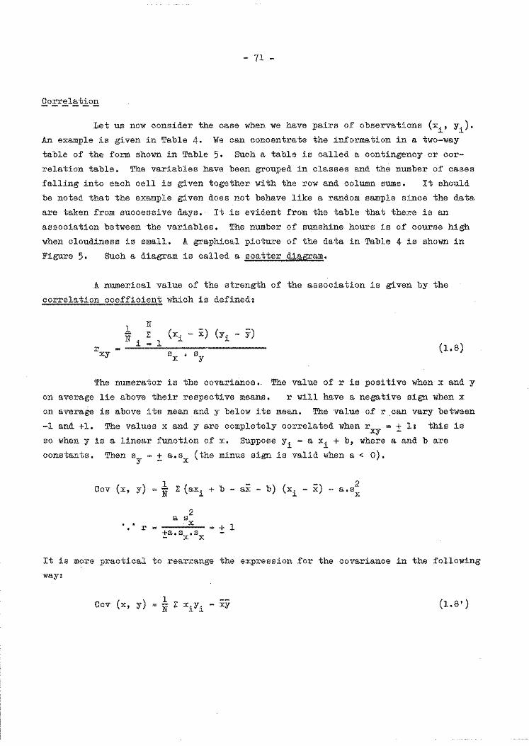
- 71 -

QoE_r~l§:.t,;ho_£

Let us now consider the case when we have pairs of observations (x., y.). ~ ~

An example is given in Table 4. We can concentrate the information in a two-way

table of the form shown in Table 5. Such a table is called a contingency or cor­

relation table. The variables have been grouped in classes and the number of cases

falling into each cell is given together with the row and column sums. It should

be noted that the example given does not behave like a random sample since the data

are taken from successive days. It is evident from the table that there is an

association between the variables. The number of sunshine hours is of course high

when cloudiness is small. A graphical picture of the data in Table 4 is shown in

Figure 5, Such a diagram is called a scatter diagram.

A numerical value of the strength of the association is given by the

correlation coefficient which is defined:

r xy

l N

N E i

(x. - i) (y. - y) l ~ ~

s • s X y

(1.8)

The numerator is the covariance. The value of r is positive when x and y

on average lie above their respective means. r will have a negative sign when x

on average is above its mean and y below its mean. The value of r .can vary between

-1 and +l. The values x and y are completely correlated when rxy

so when y is a linear function of x. Suppose y. = a x. + b, where ~ ~

constants. Then sy + a.s (the minus sign is valid when a< o). - X

Cov (x, y) = ~ E (ax. + b - ai - b) (x. - i) - a. s2

~ ~ X

2 a s X = + l r =

+a. sx. sx

= + 1: this is

a and b are

It is more practical to rearrange the expression for the covarianoe in the following

way:

Cov (x, y) l N l: xiyi - xy (1. 8')

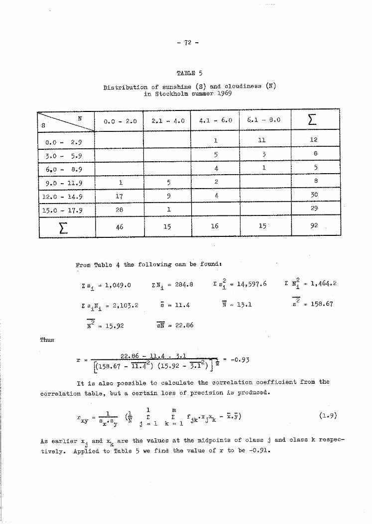
- 72 -

TA:SLE 5

Distribution of sunshine (s) and cloudiness (N) in Stockholm summer 1969

~ o.o - 2.0 2.1 - 4.0 . 4.1 - 6.0 6,.1 - 8.0

o.o - 2.9 1 11

3.0 - 5·9 5 3

6.o - 8.9 4 1

9.0 - 11.9 1 5 2

12.0 - 14.9 17 9 4

15.0- 17.9 28 1

L 46 15 16 15

From Table 4 the following can be found:

l: s. = 1,049-0 J.

EN. = 284.8 J.

I: s.N. = 2,103.2 J. J.

s = 11.4

2 N = 15.92 Si = 22.86

Thus

r 22.86 - 11.4 . ~.1

ff( -2 -2 ~158.67 - 11.4 ) (15.92 - 3.1 )

2 Esi = 14,597.6

:t 2

N = 13.1

-0.93

[

12

8

5

8

30

29

92

2 E N. = 1,464.2

J.

2 = 158.67 s

It is also possible to calculate the correlation coefficient from the

correlation table, but a certain loss of precision is produced.

rxy =. __ 1_ s • s

X y (1 1 m - r N I: f x - -)

j = 1 k = 1 jk" j~ - x.y (1.9)

As earlier xj and ~ are the values at the midpoints of class j and class k respec­

tively. Applied to Table 5 we find the value of r to be -0.91.

- 73 -

E,e,gr~s§_i,£n

In many cases it is natural to consider one of the variables to be depen­

dent and the other to be independent. If it is a forecast problem we normally call

the dependent variable the predictand and the independent variables predictors.

In the example for sunshine and cloudiness data if we want to establish

a relationship between the two variables we then consider sunshine as the dependent

variable. This relationship can be used to estimate the number of sunshine hours

from the cloud amount observations for stations not having a sunshine recorder.

This type of problem is usual in climatology. Another similar example .is the

following. Suppose we have two meteorological stations some distance apart. If for

some reason (e.g., economic) one of the stations has to discontinue its meteoro­

logical observations, it is possible to obtain estimated values for that station

using an interpolation equation established from the data during the years when both

stations were working synchronously. Such an equation is called a regression equa­

~ and the coefficients entering the formula are called regression coefficients.

The simplest type of regression equation is a linear one of the form:

y. = a + bx. + z. ~ ~ ~

(1.10)

where z. is the error or the residual. Figure 4 illustrates the values z .• The ~ ~

most common way to determine the regression coefficients is to minimize the quantity

Q = N E

i = 2 z .•

1 ~ The method is the least square method.

of Q we have to solve the two equations

~ Cl a 0

N

and ~ 'db

0

To find the minimum value

(l.ll)

Q I: (y.- a- bx.) 2 ~ 1

and we obtain the so-called normal equations: i = l

N i ~ l (yi - a - bxi) = 0 ~

E xi(yi- a- bx.) = 0 l (1.12)

i ~

From these we can solve for a and b

b

a

Cov (x, y) s2

s r.J..

s X

X

Y - bx - s y-r.J...b s

X

The regression equation is

-y,o- y s -) r ..Jl. (x - x sx

- 74 -

where Y is the best linear estimate of y with the aid of x.

(1.12')

(1.13)

The quantity k E z~ is the residual variance, the scatter about the

regression line. The value can be computed from:

s2 y.x

2 2 s (l - r )

y (1.14)

The total variance s 2 can be split into two parts, the "unexplained" .or residual y

variance s 2 and the "explained" part of the variance s2r 2• y.x y If r = 0.7 it means

that 49% of the total variance can be "explained" from the linear association with

one independent variable. With an r-value of 0.5 only i of the variance is

"explained". Thus the square of the correlation coefficient is able to give a

simple interpretation.

In our example we find the slope of the regression line to be

b 22 •86 - ll.4.3.l l 98 Th 1° thr h th 0 t (-N -S) d 0 h = 15 •92 _ 9

.6 = - • • e ~ne goes oug e po~n , an ~s s own

in Figure 5. The residual variance is 28.7(1 - 0.86) = 4.0 and the variance

reduction is 86 per cent.

From the scatter diagram there is some indication that a linear regression

is not the best. We can try a second degree polynomial.

s 2 b0 + b1N + b2N + z (1.15)

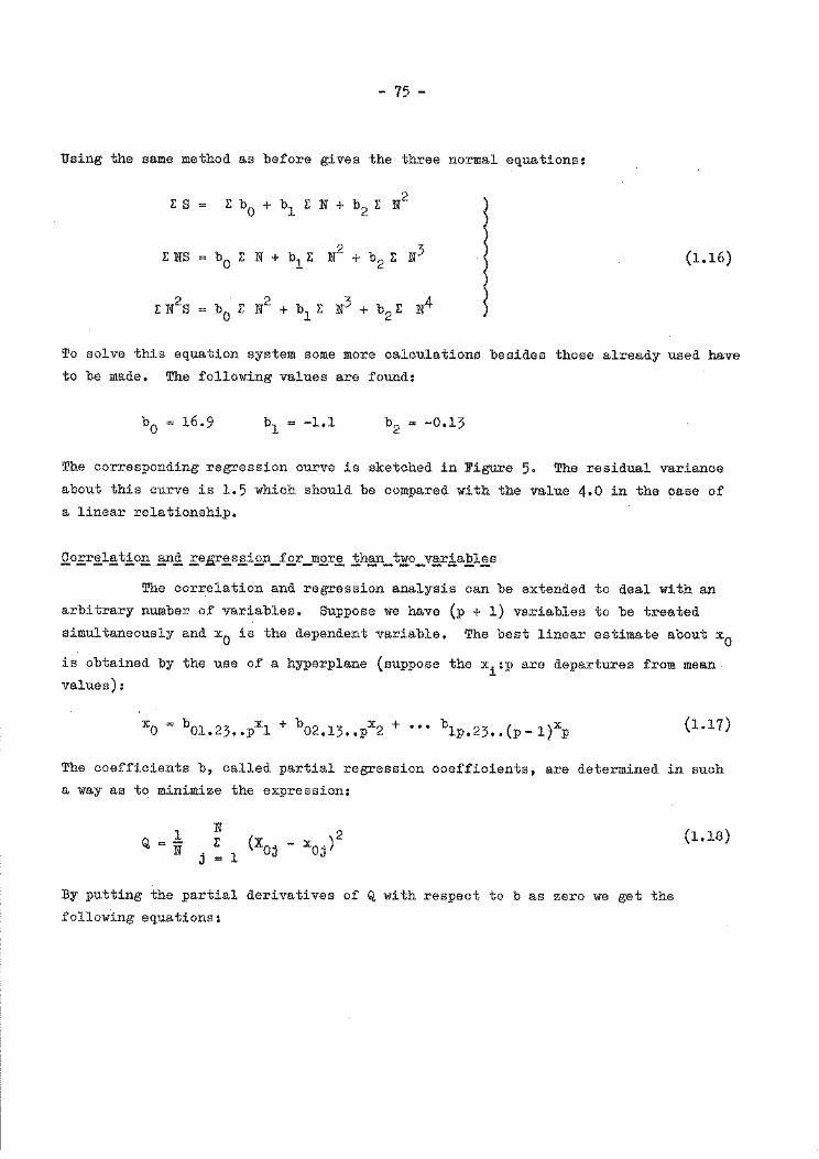
- 75 -

Using the same method as before gives the three normal equations:

E S = E b0 + bl E N + b2 E N 2

~ E NS = b0 E N + b1 E N

2 + b2 E N3 l (1.16)

E N2S = b0 E N2 + b1 E N3 + b2 E N4 l To solve this equation system some more calculations besides those already used have to be made. The following values are found:

b0 = 16.9 bl = -1.1 b2 = -0.13

The corresponding regression curve is sketched in Figure 5. The residual variance

about this curve is 1.5 which should be compared with the value 4.0 in the case of

a linear relationship.

Qo£r~l~tio~ ~n£ £e~~s~i£n_f£r~m£r~ !h~n_t~o_v~ria~l~s

The correlation and regression analysis can be extended to deal with an

arbitrary number of variables. Suppose we have (p + 1) va.riables to be treated

simultaneously and x0 is the dependent variable. The best linear estimate about x0 is obtained by the use of a hyperplane (suppose the x.:p are departures from mean

~

values):

x = b xl + b02 13 x2 + ••• bl 23 ( l)x 0 01.23 •• p ••• p P• •• p- .· P (1.17)

The coefficients b, called partial regression coefficients, are determined in such

a way as to minimize the expression:

1 Q = i

j

N E 1 (xoj - xoj)2

By putting the partial derivatives of Q with respect to b as zero we get the

following equations:

(1.18)

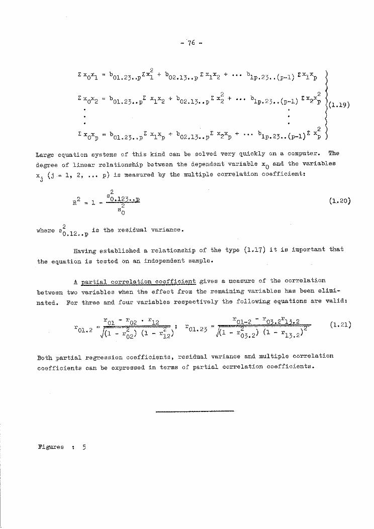
E XOXl

E XOX2

-76 -

2 b01.23 •• prxl + b02.13 •• p I: xlx2 +

2 b01.23 •• pr xlx2 + b02.13 .. pi: x2 + •••

b ( )I;XX lp.23 •• p-1 1 p

2 b ( ) Ex x lp.23 •• p-1 2 p

2 E xOxp = b01.23 •• pr xlxp + b02.13 •• pr x2xp + ••• blp.23 •• (p-l)I: xp

Large equation systems of this kind can be solved very quickly on a computer.

l )(1.19)

~ ~ The

degree of linear relationship between the dependent variable x0 and the variables

x. (j = 1, 2, ••• p) is measured by the multiple correlation coefficient: J

R2 1 -

2 s 0.123 •• p 2

so

where s 02

12 is the residual variance. • 8 GIP

(1.20)

Having established a relationship of the type (1.17) it is important that

the equation is tested on an independent sample.

A partial correlation coefficient gives a measure of the correlation

between two variables when the effect from the remaining variables has been elimi­

nated. For three and four variables respectively the following equations are valid:

rOl - r02 • rl2 ;

r01.2 =j(l- r;2

) (1- r~2) rOl-2 - r03.2rl3;2

r01.23 = j(l - r~3.2) (1 - rl3.2)2 (1. 21)

Both partial regression coefficients, residual variance and multiple correlation

coefficients can be expressed in terms of partial correlation coefficients.

Figures : 5

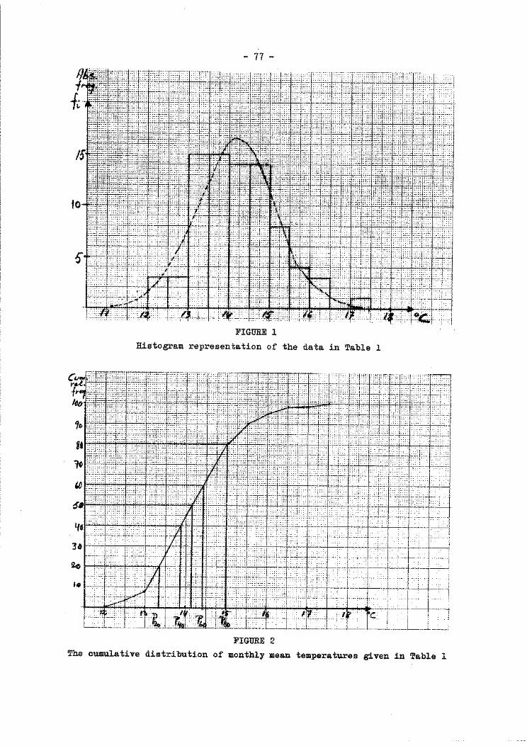
- 77 -

_T:l{L.J]L:i"'G j_, 4-c-ck-.-l:-·L'-fJ-~12Jit.llEJ2jl~T __ j •• _.-u~--!··r··ll<-1~j- -·•- .. 1

FIGURE 1 Histogram representation of the data in Table 1

FIGURE 2 The cumulative distribution of monthly mean temperatures given in Table 1

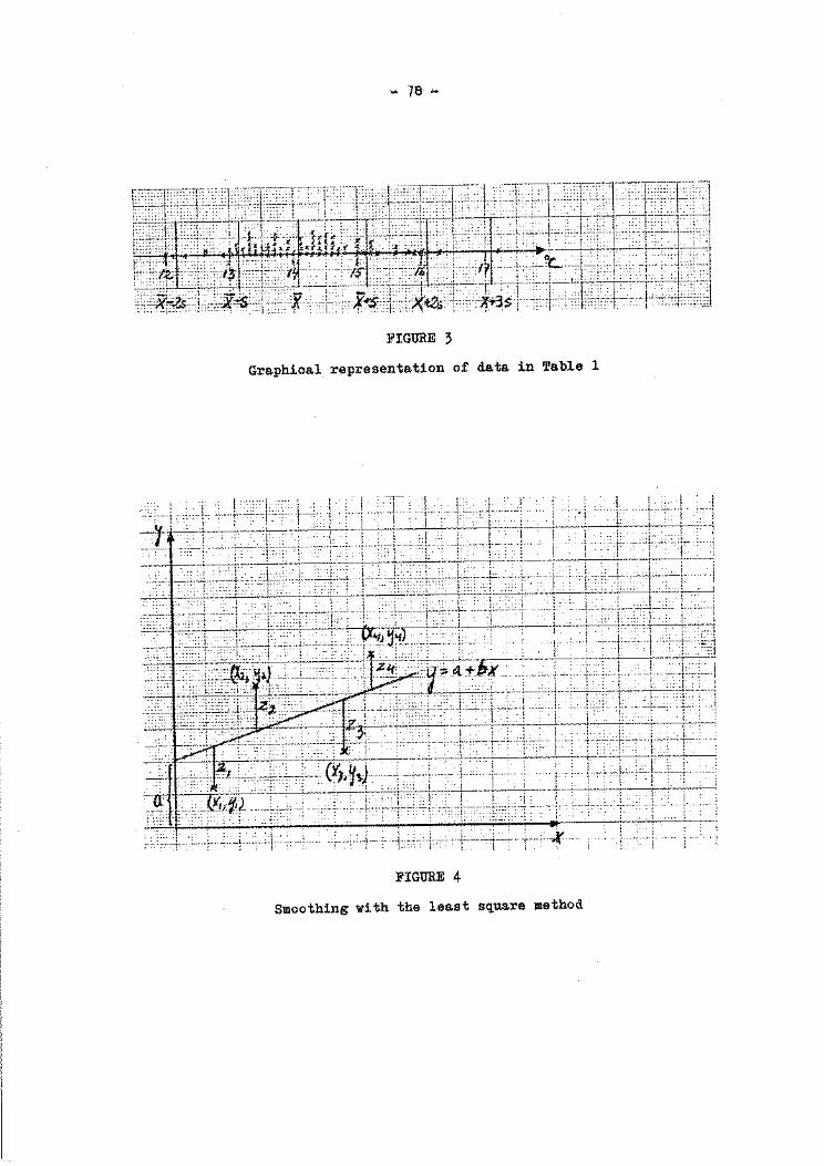
... 1e

FIGURE 3

Graphical representation of data in Table 1

,.--+ i __ r-:-~+<-t--+ -: -+- :-r: _:_)---. .,+~:~"+-:: < l :~-I '-::!: --1-~l-1- ·- :!

---- +~:-:h+-+- ---:1:-:-' :J-·7::+:-~~1:~:: --h., ·t: =- r l :- : 'i -:T-: -·r ,--j:·-+dH -h+-++-J-~:T·r-:·"- -1----~--·bt::+~::-H--::--l--

---~ ~-h-~~+. t8_:-~ 1-:-~:- \ r -l ~ +~---f ~"-+ :~

~~-~ Ii! i-:~:fTj_-. f ... ~L t ~ i H T . i --·':-"~- ::•F++~ -~1:-+d':~-:~--!

:~'; t ,~-t::j'---' i _;- ~

tlJtL:_ _ _L ___ - -(X IJ . . . ----Lee~, . ' -,-, .l•J•l· ~-··-•·- -··-'···· ' ' ' '·: ,. ' .

···· ~1~r · , ·· :-· ·· ~i ... ~: ,! +1 de A r • t:-r"C: --r .. ~:_;q_,'---+ +::_4: -·~:- -j-- ,_ +~_,+,-'--,-F-~+~----~---: -.r --- i

FIGURE 4

Smoothing with the least square method

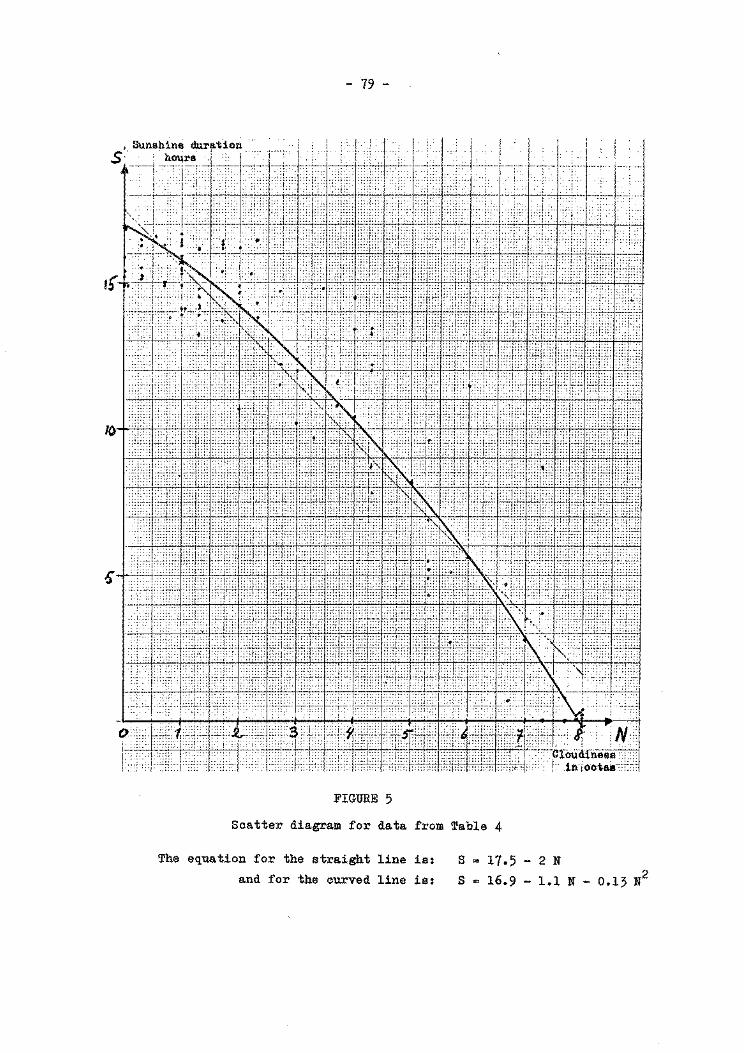
- 79 -

I, ' I ·. ; I . I :

,-··rrJJ-·· 1·; ·: ··-·

. :~--:~:-::···

lo+·•·:::'.l.•••:···:!::: ::·::l::.:::::·l::;:::::·l::::i:•.T::•:·:::I:':'k.iN .·•1::.::.::•1• .. :.::.I::•:::::•I•.::•::::J::;; :J:::::•::J:::J;:::I:::;::::·I::::;•:•:I

.) ·I.:•·· 1:: :: l:.::::::r.:;:::t•tJ::;;::J :•;•::J:•t:t::~ •:t:::;::::l :::;;:;:~ ::·:::J ~: :·· :•::r::•::•r•:r:./::::•::~::·••::::1

I ,. ;·.:·

FIGURE 5

Scatter diagram for data from Table 4

The equation for the straight line is:

and for the curved line is:

s s

17.5 16.9

2 N 2

1.1 N - 0.13 N

- 81 -

ELEMENTARY STATISTICAL THEORY (II)

by

B. Eriksson *

Theoretical freguency distribution

,!n,1r,2_d]:c,1i,2_n

The theories and methods of statistical analysis originate from the cal­culus of probability. From this many theoretical distributions have been derived.

Statistical theory allows inferences to be drawn from calculated empirical parameters concerning the size of the population parameters. It is natural to look upon a calculated mean value as an estimate of the unknown population mean. The reliability of this approximation depends upon the size of the sample and the scatter about the centre. Statistical theories also make it possible to indicate an interval, with a certain selected degree of reliability, inside which the true value, the parameter of the population, is located. Another common type of problem is to decide whether the difference between two means is sufficiently large to be significant; in other words that it confirms real sources of variation, or whether the difference is due only to chance variations in the restricted observational material.

~o~e-~~a~ent~l~.2_f_y~o~a~i!i,!y

The classical definition of the idea of probability is as follows. Suppose an event to occur in N mutually and equally likely ways. If m of these have an attribute A, the probability of event A, p(A), is the fraction m/N. The quantity is a non-negative number smaller than or equal to unity. A probability equal to 1 means that the event always will occur. The probability of composite events is cal­culated according to the rules of addition and multiplication of probabilities. If we study two events A and B, the probability that either A or B will occur is, if the events are mutually exclusive events, equal to the sum of the probability that A will occur plus the probability that B will occur.

p(A or B) = p(A) + p(B) (2.1)

* Lecture presented by R. Berggren

- 82 -

If the events are non-exclusive we have to subtract the probability that both will

occur.

p(A or B) = p(A) + p(B) - p(A and B) (2.1')

The probability that both A and B will occur is found by multiplication of the

probabilities of the individual events. When the two events are independent of each

other we can write:

p(A and B) = p(A)p(B) (2.2)

If the events are dependent on each other we must count with conditional prob­

abilities. We use the notation pB(A) to express the probability that A will occur

when B alread.y has occurred. The multiplication law reads:

p(A and B) = p(A)p.A.(B) = p(B)pB(A) (2.2')

Simple examples of probability problems are found in games of chance, such as cards.

dice or roulette.

£r.£b.§:.bili tx ,£i,!!tE,i}!,u,ii.Q,n,.§. ·

Suppose a variable x can have the values x1 , x2 ••• xn and only these.

The probability of x. is f:.. Such a variable is called a..stochastic variable and f. ~ ~ ~

is called the discrete probability function. The corresponding discrete cumulative

probability function is:

F(k) p(x ~ ~) K L:

i = 1 f. ~

(2.3)

For a continuous variable x the probability of a certain x-value is zero. The pro­

bability of finding x within a given small interval, ~x, is:

p [Cx0 -~~x)< x< (x0 +~~x)J =f(x0)~x (2.4)

f(x) is termed the probability density function. The corresponding cumulative

probability is:

u F(u) p(x < u) = J f(x)dx (2.5)

-oa

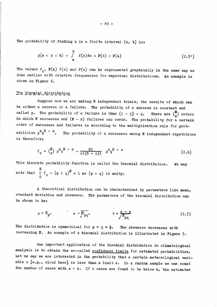
- 83 -

The probability of finding x in a finite interval (a, b) is:

b p(a < x < b) J f(x)dx F(b) - F(a) (2.5')

a

The values fi' F(k) f(x) and F(u) can be represented graphiqally in the same w~y as done earlier with relative frequencies for empirical distributions. An example is shown in Figure 6.

!h~ ~i~o~i~l_dis!~~b~tio~

Suppose now we are making N independent trials, the results of which can be either a success or a failure. The probability of a success is constant and called p. The probability of a failure is thus (1 - p) = q. There are (:) orders in which N successes and (N -.x) failures can occur. The probability for a certain order of successes and failures is according to the multiplication rule for prob-

abilities pxqN - x

is tl;lerefore:

The probability of x successes among N independent repetitions

fx = (~) pxqN - X Nl xl{N XJ!

X N - X p q

This discrete probability function is called the binomial distribution.

note that N E f = (p + q)N = 1 as (p + q) is unity. Q X

(2.6)

We may

A theoretical distribution can be characterized by parameters like mean, standard deviation and skewness. The parameters of the binomial distribution can be shown to be:

ll = Np' a=~, .9.....'::'..J? y = p;;_

The distribution is symmetrical for p = q = i. The skewness decreases with

(2.7)

increasing N. An example of a binomial distribution is illustrated in Figure 7.

One important application of the binomial distribution in climatological analysis is to obtain the so-called confidence limits for estimated probabilities. Let us say we are interested in the probability that a certain meteorological vari­able x (e.g., cloud base) is less than a limit k. In a random sample we can count the number of cases with x < k. If c cases are found to be below k, the estimated

- 84 -

value of the probability of x being less thank is the proportion p = c/N, where N

is the sample size. We want to know how good this estimate is of the population

parameter 11 • The sampling distribution of p is the binomial one.

f = (N) nx (1 - 1t )N - x for x = 0, 1, 2, • • • N X X

We now try to find proportions p1 and Pu

the true value is inside the interval p1 commonly chosen value of a is 2~ or 5%.

given by the expressions:

so that, with a certain degree of confidence,

to Pu• Prob(p1 < 1t<Pu) = 1 - 2a. A

The lower and upper values, p1 and pu' are

a = Prob(x ~ c) N E

X = C

N

(N) x (l _ )N - x X pl pl

1- a= Prob(x> c)= E (N) px (1- p )N- x X = C + 1 X U U

Convenient graphs to find p1 and pu for different sample sizes and proportions are

found in statistical textbooks. It is necessary to stress that the method is only

valid for random samples. As an example we can choose N = 30, c = 6 and a = 0.05.

With a confidence of 90 per cent the true proportion is between 0.09 and 0.32.

Ro!s~on £i~t£i~uii£n

From the binomial distribution function we can arrive a·t other distribu­

tions. One of interest in climatology is the Poisson distribution. It is valid

for discrete variables. When N in the binomial distribution becomes large and p is

very small with ~ = Np constant a passage to the limit gives the function:

f X

-~ x e IJ ·--, r Xo

The variance is the same as the mean.

F(x) t

X

E t e-ll jJ.•-

0 tt

(2.8)

The distribution function is:

(2.8 1 )

The Poisson distribution applies to relatively rare events, e.g., annual

hail frequency, typhoon frequency. As an example, .we have examined the occurrence

of daily precipitation amounts greater than 20 mm in Stockholm. During the

period 1911-1968, 150 days over the 58-year period were found. This gives a mean

- 85 -

value of 2.586 days per year. Using this mean value in equation (2.8), the expected number of years having heavy rain during 0, 1, 2, etc., days in a year is calculated and shown in the table below. The assumption made is that the probability of heavy rainfall is constant from one year to another.

TABLE 6

Observed and estimated frequencies of daily precipitation l;l.mounts in St'ockholm exceeding 20 mm

Period 1911-1968

Number of days in a year with more than 0 1 2 3 4 5 6 7 20 mm

Observed number of years with given 6 11 13 14 6 4 2 1 number of days

Estimated frequency from Poisson 4.37 11.28 14.60 12.67 8.13 4.20 1.80 0.73 distribution

8

1

0.22

It can be seen that in general there is a close agreement between the observed and the expected number of years. The two distributions are shown in Figure 8.

1h~ ~O£m~l_dis!rib~tiO£

I

i

I

The binomial distribution will spread out indefinitely when N is increased. In order to hold the standard deviation constant during the limiting process a change of variables is appropriate. The variable u = X~p will have zero mean and unity

pq variance. The distribution of u can be represented by a step curve. When N is increased indefinitely the steps can be made smaller and the number increased. Using the Stirling formula for Nt it is possible to show that the step curve approaches a continuous curve with the equation:

2 u

l -2 f(u) = ffi · e (2.9-)~_

u

o.o 0.1 0.2 o. 3 . 0.4

0.5 0.6 0.7 0.8 0.9

1.0 1.1 1.2 1.3 1.4

1.5 1.6 1.7 1.8 1.9

2.0 2.1 2.2 2.3 2.4

2.5 2.6 2.7 2.8 2.9

3.0 3·5 4.0

.....

- 86 -

TABLE 7

The probability density and the cumulative distribution for the normal distribution

X f(u)

j..l 0.3989 f.i+ O.lcr o. 3970 11+ 0.2a 0.3910 I"+ 0.3a 0.3814 f.i+ 0.4a 0.3683

I"+ O. 5 a 0.3521 f.i+ o.6a 0.3332 f.i+ 0.1a 0.3123 I"+ 0. 8 a 0.2897 f.i+ 0.9a 0.2661

f.i+ l.Oa 0.2420 f.t+ l.la 0.2179 !"+ l.2a 0.1942 f.i+ 1.3a 0.1714 f.i+l.4a 0.1497

f.i+ 1.5a 0.1295 f.i.+ l.6a 0.1109 fJ.+ 1.7a 0.0904 f.l+ l.8a 0.0790 fJ.+ l.9a 0.0656

fJ.+ 2.0 a 0.0540 f.i+2.la 0.0440 fJ.+ 2.2 a 0.0355 f.l+ 2.3a 0.0283 ~t+ 2.4a 0.0224

f.l+ 2.5 a 0.0175 !"+ 2.6a 0.0136 f.l+ 2.7 a 0.0104 !"+ 2.8a 0.0079 f.i + 2.9 a o.oo6o

f.l+ 3.0a 0.0044 f.l+ 3.5a 0.0009 ~" + 4. oa 0.0001

F(u)

0.5000 0.5398 0.5793 0.6179 0.6554

0.6915 0.7257 0.7580 0.7881 0.8159

0.8413 0.8643 0.8849 0.9032 0.9192

0.9332 0.9452 0.9554 0.9641 0.9713

0.9772 0.9821 0.9861 0.9893 0.9918

0.9938 0.9953 0.9965 0.9974 0.9981

0.9986 0.9997 0.99997

2 u

u

-3.090 -2.576 -2.326 -1.960 -1.654

-1.282 -1.036 -0.842 -0.674 -0.524

-0.385 -0.253 -0.126 o.ooo 0.126

0.253 0.385 0.524 0.674 0.842

1.036 1. 282 1. 645 1.960 2.326

2. 576 3.090

u

F(u)

0.001 0.005 0.010 0.025 0.050

0.100 0.150 0.200 0.250 0.300

0.350 0.400 0.450 0.500 0.550

0.600 0.650 0.700 0.750 0,800

0.850 0.900 0.950 0.975 0.990

0.995 0.999

U=~ a '

-2 _Le f(u) = f2n F(4) = f f(t dt) -00

- 87 -

f(u) is the probability density function and the appearance of the normal curve is shown in Figure 9, It is a symmetrical function with inflexion points at -1 and +1. The total area under the curve f(u) is unity.

2 +oo u l 5!

-2 e

-oo

l (2.9')

We have passed from a discrete probability function to a continuous density function, The probability of finding values between u1 and u2 is:

Prob{u1 < u < u2)

u2

J f(u) du ul

(2.10)

Since the distribution depends only on u it can be tabulated, To be able to use such a table for variables not having zero mean arid standard deviation = l the variable. x has to be normalized according to the expression:

u .!.....::.Ji a (2.11)

In Table 7 values of f(u) arid F(u) for the normal distribution are given for some values of u. Due to the symmetry, it is not necessary to tabulate for negative u~values. An example shows how to use this table. Given a normal distribution with ~ ~ 4 and standard deviation 5, what is the probability that a value x, randomly drawn from this distribution, is less than 2? x < 2 corresponds to

L.:.....& u < 5 = -0.4. The value F(0.4), according to Table 7, is 0.6554, thus,

F(-0.4) is 1.0000

0.3446.

0.6554 = 0.3446. The probability for x being less than 2 is

From the table we may note the following rules:

P ( I x - ~ I < a) = 0. 68 3

P(l X -~1< 2a) ., 0,954

P ( I x - ~ I < 3a) = 0 • 997

For a variable with a normal distribution, about 2/3 of the values are between ~-a and~+ a. About 5% of the values are outside the interval~- 2a , ~ + ·2a and more than 99% of the values are found within the interval~ - 3a , ~ + 3a •

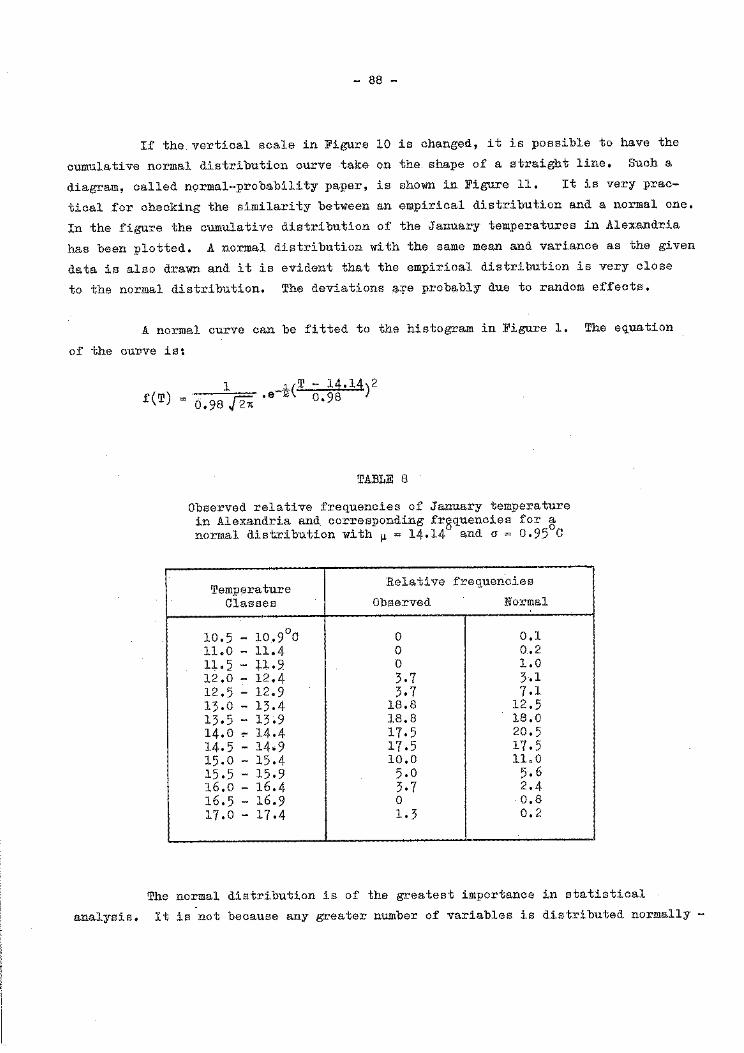
- 88 -

If the.vertical scale in Figure 10 is changed, it is possible to have the

cumulative normal distribution curve take on the. shape of a straight line. Such a

diagram, called nQrmal-probability paper, is shown in Figure 11. It is very prac-

tical for checking the similarity between an empirical distribution and a normal one.

In the figure the cumulative distribution of the January temperatures in Alexandria

has been plotted. A normal distribution with the same mean and variance as the given

data is also drawn and it is evident that the empirical distribution is very close

to the normal distribution. The deviations a.+e probably due to random effects.

A normal curve can be fitted to the histogram in Figure 1. The equation

of the cuTive is:

f(T)

TABLE 8

Observed relative frequencies of January temperature in Alexandria and corresponding frequencies for a normal distribution with ~ = 14.14° and a= 0.95°C

Temperature Relative frequencies

Classes Observed Normal

10.5 - l0.9°C 0 0.1 11.0 - 11.4 0 0.2 11.5 - 11.2 0 1.0 12.0 - 12.4 3·7 3.1 12.5 - 12.9 3.7 7.1 13.0 - 13.4 18.8 12.5 13.5 - 13.9 18.8 18.0 14.0 .,.. 14.4 17.5 20.5 14.5 - 14.9 17.5 17.5 15.0 - 15.4 10.0 ll. 0 15.5 - 15.9 5.0 5.6 16.0 - 16.4 3·7 2.4 16.5 - 16.9 0 0.8 17.0 - 17.4 1.3 0,2

The normal distribution is of the greatest importance in statistical

analysis. It is not because any greater number of variables is distributed normally -

- 89 -

many cannot be approximately described by a normal distribution. It is possible to show that the distribution of sample means is normal with mean ~ and standard

deviation a;f~, where N as usual is the sample size. Even if the population from

which the samples are taken is non-normal this theorem, the so-called central limit theorem, is valid.

In general the value of a is not known and must be estimated from the i- ~· . The distribution of u = -----1 is not the normal, but the Student aN

sample.

t-distribution. However, for large values of N the t-distribution approaches the normal distribution. Going back to the data in Table 1 and assuming firstly, that the distribution is normal - an assumption we have found to be valid - and secondly; that no climatic fluctuations take place, we can make the following inferences:

(a) The best estimate of a January mean temperature is 14.1°0 but small deviations from this value occur.

(b) With a confidence of 95% the temperature will fall inside the interval 14.14- 2 x 0.98 < T < 14.14 + 2 x 0.98, i.e., 12.1- 16.1°.

(c) In two-thirds of all cases the 10-year mean is within the

interval 14.14 - 0•98 < T < 14.14 + .2..:..2.§. , i.e., llO ./10

1).8- 14.4°.

(d) With a confidence of 95% the temperature for the period 1951-60, which is

not included in

14.14 + 2 0.98 jlO'

the sample, will be in the interval 14.14 - 2 °~ , 0 . ~ 10

i.e., 13.5 to 14.7 • The value really observed.

was 13.7°, thus in agreement with the statement above.

!~ ,2_x,!r_!m!, _!a,!.U!, .9:_i.[t£i]lu,1i.2,n

In applied climatology, the annual highest or l~west extremes are often of interest. Engineers who are designing structures want to know the probability that certain values will be exceeded and whether a structure can withstand all other values in the year. The distribution functions of annual extremes most commonly used are the Fisher-Tippet Type I and Type II. The Type I distribution function

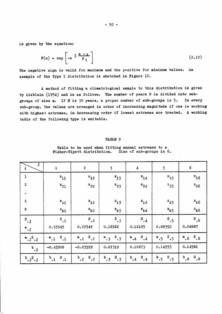
- 90 ..;.

is given by the equation:

[ + .!...::..I!.. J F(x) = exp -e - ~ 1 _ (2.12)

The negative sign is valid for maximum and the positive for minimum values.

example of the Type I distribution is sketched in Figure 12.

An

A method of fitting a climatological sample to this distribution is given

by Lieblein (1954) and is as follows. The number of years N is divided into sub­

groups of size m. If N is 30 years, a proper number of sub-groups is 5. In every

sub-group, the values are arranged in order of increasing magnitude if one is working

with highest extremes, in decreasing order if lowest extremes are treated. A working

table of the following type is suitable.

~ 1

2

. i

k

s.j

a . •J

a .js .j

b .j

b .s j • J • L _____

TABLE 9

Table to be used when fitting annual extremes to a Fisher-Tipett distribution. Size of sub-groups is 6.

1 2 3 4 5

xll xl2 xl3 xl4 xl5

x21 x22 x23 x24 x25

xil xi2 xi3 xi4 xi5

~1 ~2 xk3 ~4 xk5

s.l s.2 s.3 s.4 s.5

0.35545 0.22549 0.16562 0.12105 0.08352

a.l s.l a.2 s.2 a.3 s.3 a.4 s.4 a • 5 s.5

-0.45928 -0.03599 0.07319 0.12673 0.14953

b.l s.l b.2 s.2 b.3 s.3 b.4 s.4 b.5 s.5

6

x16

x26

xi6

xk6

s.6

0.04887

a.6 s.6

0.14581

b.6 s.6

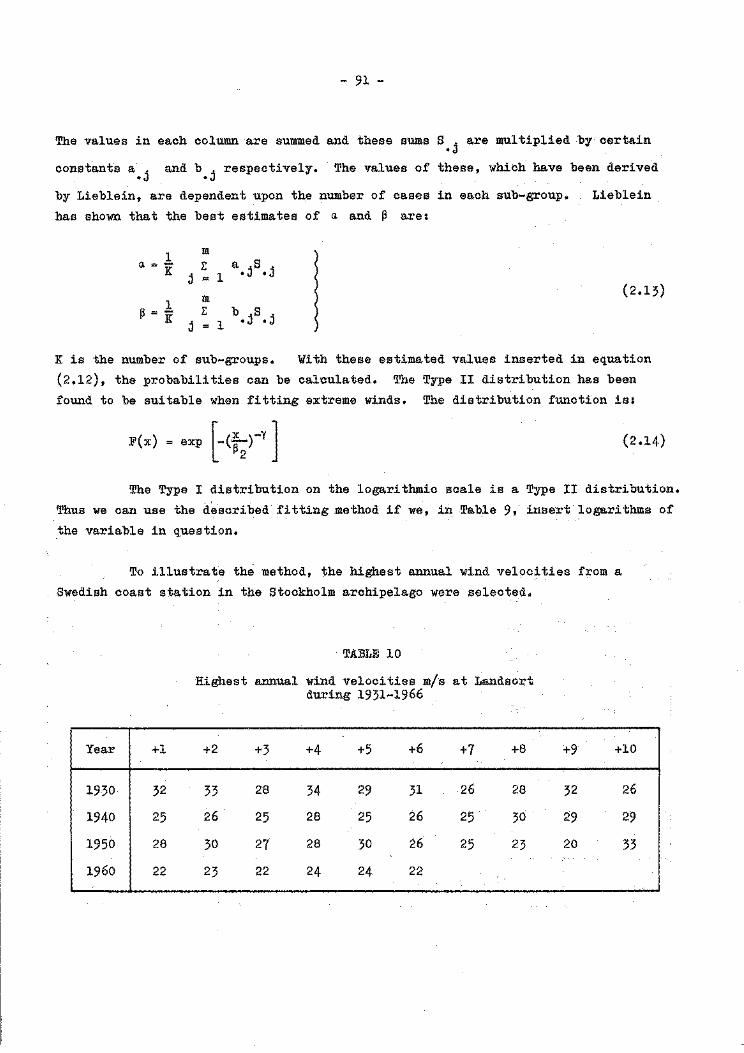
- 91 -

The values in each column are summed and these sums S . are multiplied by certain •J

constants a. • and b j respectively. The values of these, which have been derived •J •

by Lieblein, are dependent upon the number of cases in each sub-group.

has shown that the best estimates of a and ~ are:

l m E a. S a==K . l .j .j

J =

l m ~=if E b .S j

j = l •J •

Lieblein

(2.13)

K is the number of sub-groups. With these estimated values inserted in equation

{2.12), the probabilities can be calculated. The Type II distribution has been

found to be suitable when fitting extreme winds. The distribution function is:

F{x) exp [-<~r l (2.14)

The Type I distribution on the logarithmic scale is a. Type II distribution.

Thus we can use the described fitting method if we, in Table 9, insert logarithms of

the variable in question.

To illustrate the method, the highest annual wind velocities from a.

Swedish coast station in the Stockholm archipelago were selected.

Year +1

1930 32

1940 25

1950 28

1960 22

TABLE 10

Highest annual wind velocities m/s at Landsort during 1931-1966

+2 +3 +4 +5 +6 +7 +8

33 28 34 29 31 26 28

26 25 28 25 26 25 30

30 27 28 30 26 25 23

23 22 24 24 22

+9 +10

32 26

29 29

20 33

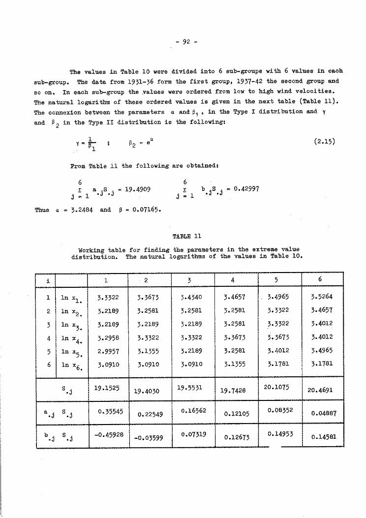
- 92 -

The values in Table 10 were divided into 6 sub-groups with 6 values in each

sub-group. The data from 1931-36 form the first group, 1937-42 the second group and

so on. In each sub-group the values were ordered from low to high wind velocities.

The natural logarithm of these ordered values is given in the next table (Table 11).

The connexion between the parameters ~ and ~ 1 , in the Type I distribution and y

and ~ 2 in the Type II distribution is the following:

Thus a

i

1

2

3

4

5

6

a .j

b.j

1 y "" '!r:"'

1 ~2 = ea.

From Table 11 the following are obtained:

6 6 E

j = 1 a .S . = 19.4909

•J •J E b .s . = 0.42997

• J • J j .. 1

3.2484 and ~ = 0.07165.

TABLE 11

Working table for finding the parameters in the extreme value distribution. The natural logarithms of the values in Table 10.

1 2 3 4 5

ln x1• 3.3322 3.3673 3·4340 3.4657 . 3.4965

ln x2• 3.2189 3.2581 3.2581 3.2581 3·3322

1n x3• 3.2189 3.2189 3.2189 3.2581 3·3322

ln x4• 3.2958 3·3322 3·3322 3.3673 3.3673

1n x5• 2.9957 3.1355 3· 2189 3.2581 3.4012

1n x6• 3.0910 3.0910 3·0910 3·1355 3.1781

s.j 19.1525 19.4030 19.5531 19.7428 20.1075

s.j 0.35545 0.22549 0.16562 0.12105 0.08352

s.j -0.45928 -0.03599 0.07319 0.12673 0.14953

(2.15)

6

3.5264

3.4657

3.4012

3.4012

3.4965

3.1781

20.4691

0.04887

0.14581 -

- 93 -

~ 2 is found to be 25.75 and y is 13.95. The distribution function with these parameters is drawn in Figure 10. From this curve we can read that for F = 0.98 the x-value is 34 m/s. This means that the value 34 m/s is expected to be exceeded twice during a lOO-year period.

Qthe£ !h~o£e!i£a! ii~t£i~u!i~n~

There are some other theoretical distributions that are of interest in climatology. They will be mentioned here only very briefly.

The gamma distribution has been found to give good results with zero-bounded continuous variables like precipitation data.

The x2-distribution is used when two series of frequencies~ one observed, fe' and one theoretical, ft, are compared to see if the difference between them is

large enough to be considered significant. The quantity

k

x2 = I: i = 1

(f . - ft .. )2 e~ ~

fti has an x2-distribution. textbooks of statistics.

Tables of the x2-distribution function are found in

The Fisher's F-distribution is used for testing statistically whether two

estimates of variances si and s~ are significantly different. The quotient si/s~ has a sampling distribution which is the F-distribution.

Figures : 8

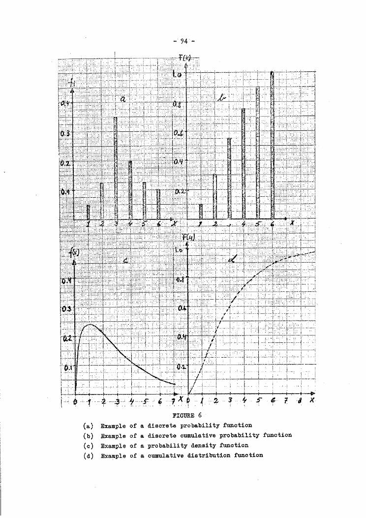
- 94'-

~-~---. . . . .! !

Tl~i~h-S/~-+-~-d-+i;f:o::::+++·-~·lJ· .. _. ... . . • : /T-" -1'-'·-+:·_:··+,.j +---,- l · -- l

• :. ~-.I:. :: . 1

1· H:r~:'>:f/'~-r,.ct::'- ------1 ! -! i ·j· : ~7·! -:~ ___ :_:_;:---:

·-~ . I . . . I ·--- ---·---, - ...

.I· . ,,,-.: ;-· ·-~:·:-- :··

-;

! : )----· ... , . --···j

! :

! ·!:·

l '!

+ + S" . ;:. 'I ·I X. i _:~ ·'·1· -*---~- t. -r: ' ... fx~ { ·····~. 3

(a) (b)

(c) (d)

FIGURE 6

Example of a discrete probability function

Example of a discrete cumulative probability function

Example of a probability density function

Example of a cumulative distribution function

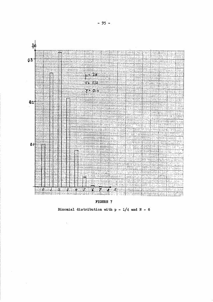
- 95 -

~

o.~ !ijr~~~~~liliil~ii!lli;-=r~~~

~~= ~ ~r~ ·~ ~ m~~~~~~~~~~~~;ri:~~g;m~~~~~t~~~=jP~~1f,f#~~IN -:~~:~ ~· :~~ ~~ ~; -; ~~;~~~~~~t~=~~~::~~--t\_;;~~8~~~.~i~~~-:;;;~;~l::tr:~:;-~f:4 =-~~1:-~~ ~i: ~.:: c!: Ec~: '~ -=~~"i:::C:.C::~:~~~~:·:e: ['."•=:=~·:r:::·=;::::~:~t~=:r:~F~i::L "t:O:'<L'~'O: L:_ __ ! ~;?::' ~= ~=: :;t 1:~: ': ..-.:::---:~~:~~_.-:::::==--==§:-==:c~-==~:d~:::::-:::r::?'~::~-l:::..:=:~~·?=:n:::;~·~:I:'-'-i~::~ :~~~~;:~:::c: ~; ;:;: .:

o. i~ :,ji't ~~~ ]~~~~l[m;m~,2~-~==t,sJcHSHbH ~:o!:': i ::::::F~ ::.==; :f: ·~~ C:• ~~ i• ~::?::"'=:::::~i-=:~~=-:§.:~?L:':: ':L'·~~?:;~::-:~::0f:::~-::'E::::::--:-t~;::~. !~' :;: ;:~,: :·~

~~=: ~ ~~ .~~ ~~t~~ ~~~;~m 0~=~~~~~~~~i~~~~~~~;:·;:~1~H~~~~~~~7:s7-~

i 1r~ il-~~ f; •~, 1~ ~~i~~~~~G.;~~i~j~i~~~[i:'~ 0.B~f~~~·~ ~=.=~=~=~!.~==:i:£:~~-=~~~~~r1~~~r~~·~fffi~;~~~~~~~-~;·-~~·~m~;:i:f~~~ij~~;~;~~~~~:l::.~i:::·i- :~-:.~,;:~·;_;:~:

FIGURE 7

Binomial distribution with p 1/4 and N 8

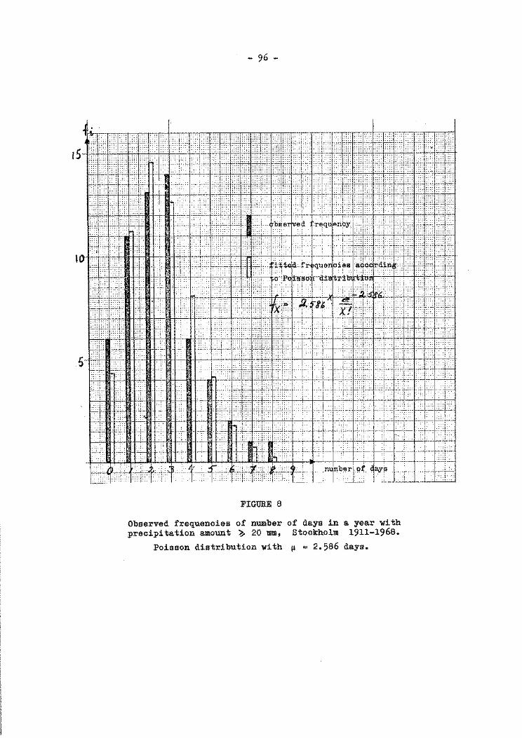
- 96 -

FIGURE 8

Observed frequencies of number of days in a year with precipitation amount ~ 20 mm, Stockholm 1911-1968.

Poisson distribution with ~ = 2.586 days.

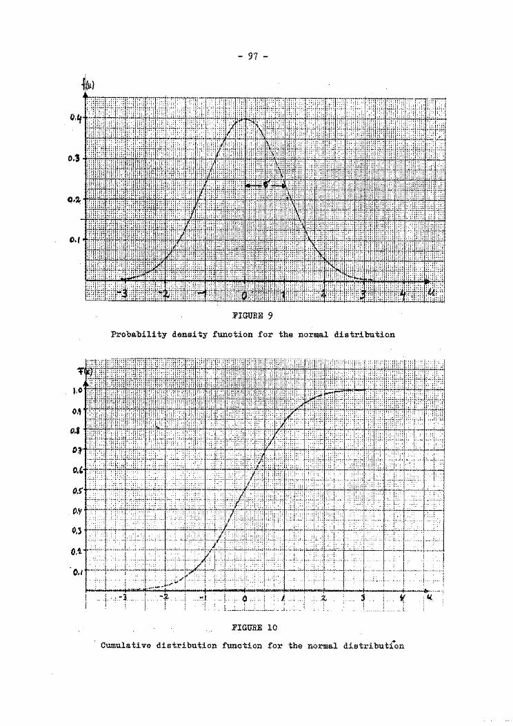
- 97 -

~(ll)

..... .,,,,,, , . c·- , . . . '''''"' ... , ... ., . . , .. ,c-c-rc;-;-,.-j·: ... 1 ..... 1... .. .. :SSJ:g-~-· ----·-- ~-· :! :::, :.:·1..·: : !·•:: ,· ·! : :·.:' · : · ::.::''I :i :;.!;:.·::' '· · · :;,:,:·,.,,,; .. : · ,

o JI\-r:r·:~;:::;~ >1:r;: ~::.:: ~: \1.~ ::· :::t::t:i~ ),h::IT::'r::;:ti\f "'? ;:~; ;J; ::.·"tu. ·J2 ~;r;. ::i::: :; 1:::.

···1!111&f~ill~!~~~~~~~~~,1

1!!!!~iil]!!i -~*~l ~i~l*~ :;tb~tmt~:~~mti,::~r* ,uu;,: rt\,1;1~ %~tm1m~ :ili~tH ~drr~ ~tlt+~~~n~ :ffi#1~rr ;J~ :tiniW :~:;!;

FIGURE 9

Probability density function for the normal distribution

o., o.J L::::'t'f:'¥.:::r::~r :"'l'::'l n: l':' :I :.:::t:::t~i .. ::.J..:: 1.:-

0.1-l<:::'k'"·'"l.:': j,:--'£!~ . .1.::' I ~~4 '-'-'1 'i'l

M

O,l

o.t

I ·I !

FIGURE 10

I

1111Ut L-.-f- 4---+----·--'"--: i if ! ~

. ___ .l ____ -~- .L _ .

Cumulative distribution function for the normal distribution

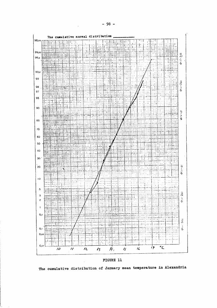
- 98 -

~ ~ 'X

. ": l::-: $ .. I 'i,, ..

99,5 1.~ ...t~ !.:.

~ ~ .,... l.. • ... • --·

.••. !, ; : _, ...

99 :- ~ : i ; ; ;

" ! ; ' I '

-o

96 ~

" 97

-$

95

90 :0 +

'X

w i

70

60

50

40

30'

20 .. , . . ! : :-:->--,.: t.. : . 'I. ~-:-eT-:-:-.. f . . .. , •••-• +H< "''£_,, _ _., <• ,,;,;;J;, •• I,, .. ••• ~·• 'I '

·::,::~ .. ::: -: !:: '·. ~~ ::t ': .· !.·. $ __ ,.. __ ...... -.... j ...... , ............ r----- ,

10 ~j- -··- -~'--·----'-·-::... __ _

; ... .... . sJ[tjr"J;:;i;thliii~(t!"~;~ ~ ., .. 1 ... · .. ,. · • --j· .t ... , , ..

0,5 .. :, ::~ ~~:+;~~ .;~~i;~:: :~~:b~~ :.~~.:.: : :.:. . .:..:..:..:1~.; .. : ; :._;; L~ ~~ ............... "!····~· I -··-·-r--· -- -· ........... 1·---- -----. --~ .1 ~ ::::;::·: :::: :::: ::::1:::

o., ::::!:'" ::::;-:::T'''l:~:=~.,.

'·"' ,., if -. I ' ~ • 1 r 0,0 I · • . __.__.____

/0 If n., 13 /lj, Is IL 11 oc_

FIGURE 11

The cumulative distribution of January mean temperature in Alexandria

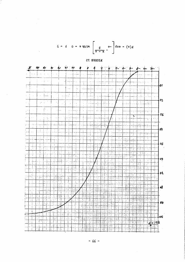
~ 9 o = » qq. 'J:.M. [_a __ a-] dxa (x)JI 1l - X

~-· __ ;

..J'If

' . i i · + -,--1 ··· I·--:··+--·-·!- --·+-~ .-¥1-- · i · -· ! -~.· .• ·---·,,--. -,_-.· ,:,, ---T~--~.:~, ... -.. -... ,-.... ·.--.-r~-----·._.------··-:···:· 'tt: I ~-/' l . , -,-T-·--- --·--JL=r-~· ·:- · ~- ~

1 ! · I·--, t·' ·--'··~ ·z1· :- i +---. ! ; ...... i . LJ · ··--·- ~ --~--:,-----, 1/-1 ·- --.. -· --·-- · -·---~ -· · ~

-t-_+-!1 ----,--+1-· J . ·! ' ....... :Lj., f j .: .. j i I. ·! ; : . ; ! I

··! · · I i · ···-···· 1 -· · · , l ·: 1 1-------+·· · --,---:··-+=_-,.+-l, --+O' --+j-.---l---'-. ~ ·1···.··. ... .. ·······-·t-:c:· -· '·· .. ~~---·--''-··· ····:. ! ; . I : ·'. : : . . .

- 66 -

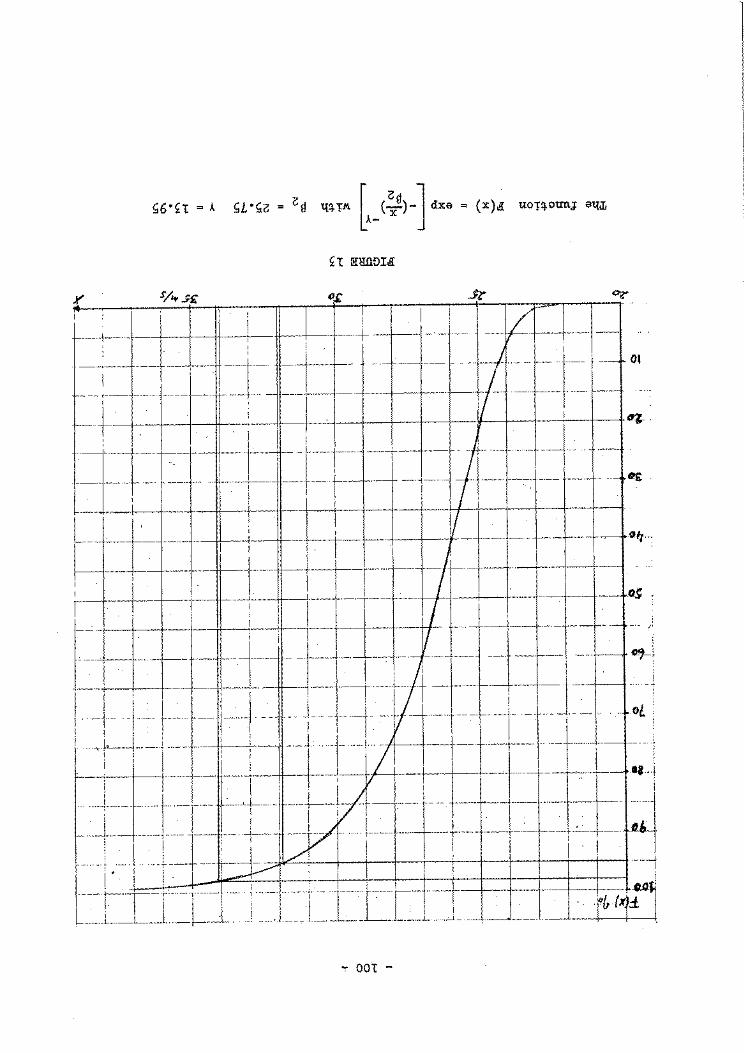
~ oot -

Time series

1,n.,ir.2,d];c,!i.2,n

- 101 -

ELEMENTARY STATISTICAL THEORY (III)

by

B. Eriksson *

Most of the data a climatologist is working with consists of observations

equally spaced along the time axis. The time interval varies from hours or days to

years. Such data form time series. The statistical analysis of time series attempts

to understand the basic characteristics, such as trends and periodicities, and to

predict the behaviour of the series in the future. The total variation can be looked

upon as the sum of certain oscillations, some periodic, e.g., diurnal and annual, and

some irregular.

Qo£r~l.2.~a~ ~n~ ~e£s!s_!eac~

Looking at a time series we often find a tendency of the terms which are

close together to be more alike than terms which are more separated. This tendency

we often call persistence -or coherence. This fact in itself is evidence that there

is some predictability about the series. It is natural therefore to endeavour to

obtain a measure of the persistence by calculating correlation coefficients, commonly

called autooorrelation coefficients.

The values at a certain time are correlated with the value.s some time-steps

later. In order to eliminate the regular trends the values may be normalized, e.g.,

the mean or normal value is subtracted and this departure is divided by the standard

deviation. The autocorrelation for a series of normalized x-values is simply found

according to the formula:

rL = k t xt - xt + L t = 1

L is the time step and is called the lag.

(3.1)

If L is small, meteorological data

normally show positive autocorrelations. In other words, persistence is a common

property in climatological series. A graphical picture where rL is plotted as a

function of L is called a correlogram. Figure 14 shows a correlogram calculated from

daily temperature.

* Lecture presented by R. Berggren

•

- i02 -

For discontinuous variables or qualitative variables like "precipitation

day-dry day" the persistency of the time series can be expressed with the aid of

conditional probabilities. As an example we can look upon a series of days with

precipitation, denoted by 1, and days without precipitation, denoted by 0 •. The

general probability for state 1 is the number of wet days divided by the total number

of days. Let us call this probability p(l). The probability of a dry day is

p(O) = 1- p(l). Conditional probabilities indicated p1(1) (p0(o)) give the proba­

bility for a wet (dry) day when preceeding day was wet (drY,)• An index of persis­

tence is given by the following expression:

r{l) .. 1 -11 - pl (1)-12

~ - p(l) J (3.2)

The value of r is zero if p(l) and p1(1) are the same and the value 1 if p1(1) = 1, that is to say, the value today gives complete information of the state tomorrow.

Some values of r calculated for Stockholm are given below.

TABLE 12

Indices of persistence. Stockholm 1931-60

Months J F M A M J J A s 0 N D

Index r(l) 0.58 0.45 0.61 0.48 0.45 0.35 0.43 0.46 0.43 0.52 0.47 0.57

r(o) 0.60 0.50 0.59 0.51 0.48 0.35 0.42 0.43 0.48 0.51 0.46 0.55

The differences between persistency indices for wet (r(l)) and dry (r(o))

days can be shown to be due to random effects.

A time series having the property that all information of the state on

day d is given by the state on day (d - 1) is called a Markov chain of first order.

For such a series we must have:

P1(1) = p11 (1) plll(l) . . . . . . l (3.3)

Po(o) = Poo<o) = Pooo<o)

-103-

The result of such an investigation regarding wet and dry days is sum­marized in Figure 15. It is seen that the simple Markov chain model is not valid exactly. Some additional information is gained if the conditions on day d - 2, d- 3, etc., also are considered.

1h~ ~fe£t_of ~e~s!s!e~c~ ~n_the_a£C~~cz ~f_m~a~ ~alu~s a

The variance of means from random samples has been shown to be lN. However, if we form means from successive values of a time series, which is commonly done in climatology, the standard deviation of the means is larger if there is persistence in the series. The standard deviation of the arithmetic mean of N con­secutive values, each of variance a 2 , is:

a [ [N-1 N-2 aN=/ff jl+2 --w-r1 +-N-r2 + ••• + i rN - 1] a

=JN' ( 3-4)

N' can be called the number of independent days during the N-day period. Table 13 gives an example of the values of N' computed from mean temperatures. Low values of N' imply a high degree of persistence. A seasonal variation of persistence may be noted.

Monthly period

5

10

20

30

TA:BLE 13

Effective number of observations in mean values of consecutive daily mean temperatures {Stockholm 1901-60)

Jan. Feb. Mar. Apr. May Jun. Jul. Aug. Sep. Oct. Nov.

1.6 ' 1.4 1.2 1.3 1.6 1.6 1.4 1.5 1.6 1.6 1.6

1.9 1.5 1.3 1.6 2.1 2.1 2.0 1.9 1.7 1.8 2.5

2.6 1.9 1.6 2.3 3-4 2.9 2.2 2.4 3.0 2.9 3.2

3.1 2.3 2.0 3.1 4·5 4.0 2.8 2.9 3.8 4-4 4-5

~~d!c!i~n_of !i~e_s~r!e~ ~-lin~a~ ~e~~s~i~n

Dec.

1.6

.2.4

2.8

3·3

We can try to predict the value of x at time t with the aid of known values at times t- 1, t - 2, ••• by an equation of the form:

xt = alxt- 1 + a2xt- 2 + ••• ~xt- k + zt (3.5)

- 104 -

a1 , a 2, ••• ~are regression coefficients and zt is the error. The values ai are

functions of the autocorrelation coefficients. We can look at a very simple example.

Assume that the information.of xt is given by xt _ 1 and the values xt _ 2 , etc., give

no additional information

xt = axt - 1 + zt (3.6)

If we multiply by xt and then take the expectations and assuming no correlation - V

between the error z and the values of x we get r = a.r 1, which gives a = r 1 V V-

V and rv = r 1 •

In this Markovian model the autocorrelation function is very simple. Using

this model to forecast the value of x for t = 1, 2, 3, 4 and 5 days with the aid of

todays value x0

we expect the following residual variances:

2 az

t

2 2) a (1 - rt (3.7)

If instead we forecast say that todays value is the prognosis, e.g., we put xt = x0 the variance of the error zt is

2 lr- 2 2 azt = i L_(xt- xo) = 2a (1- rt) (3.8)

With the numerical value of r 1 = 0.8 (a suitable value in Scandinavia if x

is the daily mean temperature) we find the following residual variances:

t days 1 2 3 4 5 Method

rt o.e 0.64 0.51 0.41 0.33

2 a zt

36 59 xt = rt.xo - 2 • lOO 74 82 89 a ,

a2 zt

40 72 98 118 134 xt = xo - 2 • lOO a

- ---- --·-- -·-- - -· --~-

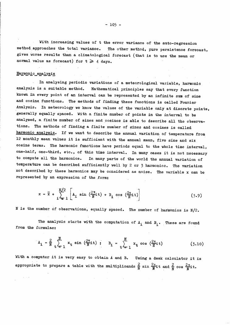
- 105 -

With increasing values of t the error variance of the auto-regression method approaches the total variance. The other method, p~e persistence forecast, gives worse results than a climatological forecast (that is to use the mean or normal value as forecast) for t ~ 4 days.

Ha£~n!c_a~aly~i~

In analysing periodic variations of a meteorological variable, harmonic analysis is a suitable method. Mathematical principles say that every function known in every point of an interval can be represented by an infinite sum of sine and cosine functions. The methods of finding these functions is called Fourier Analysis. In meteorology we know the values of the variable only at discrete points, generally equally spaced. With a finite number of points in the interval to be analysed, a finite number of sines and cosines is able to describe all the observa­tions. The methods of finding a finite number of sines and cosines is called harmonic analysis. If we want to describe the annual variation of temperature from 12 monthly mean values it is sufficient with the annual mean, five sine and six cosine terms. The harmonic functions have periods equal to the whole time interval, one-half, one-third, etc., of this time interval. In many cases it is not necessary to compute ~11 the harmonics. In many parts of the world the annual variation of temperature can be described sufficiently well by 2 or 3 harmonics. The variation not described by these harmonics may be considered as noise. The variable x can be represented by an expression of the form:

X= X+ it-2

1 [Ai sin (~it)+ :Si cos (

2;it)J (3.9)

N is the number of observations, equally spaced. The number of harmonics is N/2.

The analysis starts with the computation of A. and :S .• These are found 1 1 from the formulae:

2 N Ai = N \ x sin ( 2nit)

t'=. 1 t N :si N

\ X COS (E2!.• t) t4rl t N

1 (3.10)

With a computer it is very easy to obtain A and :a. Using a desk calculator it is

appropriate to prepare a table with the multiplicands~ sin ;;it and~ cos ~it.

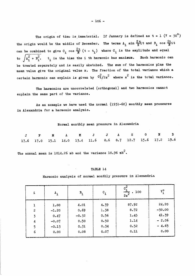
- 106 -

The origin of tim~ is immaterial. If January is defined as t = 1 (~ = 30°)

the origin would be the middle of December. The terms Ai sin 2N\t and Bi cos ~it

can be combined to give C i cos 2Nn ( t - t 1 ) where Ci is the amplitude and equal

to ~Ai + Bi· ti is the time the i th harmonic has maximum. Each harmonic can

be treated separately and is easily sketched. The sum of the harmonics plus the

mean value give the original value x. The fraction of the total variance which a

certain harmonic can explain is given by Cfj2s2 where s2 is the total variance.

The harmonics are uncorrelated (orthogonal) and two harmonics cannot

explain the same part of the variance,

As an example we have used the normal (1931-60) monthly mean pressures

in Alexandria for a harmonic analysis.

J

17.6

F

17.0 M

15.1

Normal monthly mean pressure in Alexandria

A

14.0

M

13.4

J

11.6

J

8.6

A

8.7

s 12.7

0

15.6

The annual mean is 1014.26 mb and the variance 10.96 mb2•

TABLE 14

Harmonic analysis of normal monthly pressure in Alexandria

c~ i A. Bi ci

J.

J. - 2 • lOO 2s

1 1.80 4.01 4. 39 87.92

2 -1.20 0.69 1.38 8.72

3 0.47 -0.32 0.56 1.45

4 -0.07 0.50 0.50 1.14

5 -0.13 0.31 0.34 0.52

6 o.oo 0.08 0.07 0.11

N

17.2

'!!~ J.

24.20

-30.00

41.39

- 2.06

- 4.65 o.oo

D

19.6

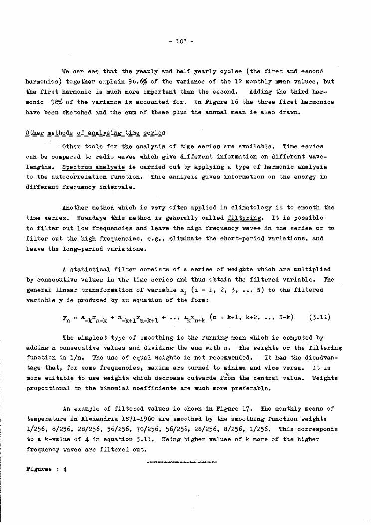
- 107 -

We can see that the yearly and half yearly cycles (the first and second

harmonics) together explain 96.6% of the variance of the 12 monthly mean values, but

the first harmonic is much more important than the second. Adding the third har­

monic 98% of the variance is accounted for. In Figure 16 the three first harmonics

have been sketched and the sum of these plus the annual mean is also drawn.

Qthe£~e!h~d~ ~f_aaaly~ia~t1m~ ~e£i~s

Other tools for the analysis of time series are available. Time series

can be compared to radio waves which give different information on different wave­

lengths. Spectrum analysis is carried out by applying a type of harmonic analysis

to the autocorrelation function. This analysis gives information on the energy in

different frequency intervals.

Another method which is very often applied in climatology is to smooth the

time series. Nowadays this method is generally called filtering. It is possible

to filter out low frequencies and leave the high frequency waves in the series or to

filter out the high frequencies, e.g., eliminate the short-period variations, and

leave the long-period variations.

A statistical filter consists of a series of weights which are multiplied

by consecutive values in the time series and thus obtain the filtered variable. The

general linear transformation of variable xi (i = 1, 2, 3, ••• N) to the filtered

variable y is produced by an equation of the form:

Yn = a_kxn-k + a-k+lxn-k+l + ••• akxn+k (n k+l, k+2, ••• N-k) (3.11)

The simplest type of smoothing is the running mean which is computed by

adding n consecutive values and dividing the sum with n. The weights or the filtering

function is 1/n. The use of equal weights is not recommended. It has the disadvan­

tage that, for some frequencies, maxima are turned to minima and vice versa. It is

more suitable to use weights which decrease outwards fibm the central value. Weights

proportional to the binomial coefficients are much more preferable.

An example of filtered values is shown in Figure 17. The monthly means of

temperature in Alexandria 1871-1960 are smoothed by the smoothing function weights

1/256, 8/256, 28/256, 56/256, 70/256, 56/256, 28/256, 8/256, 1/256. This corresponds

to a k-value 9f 4 in equation 3.11. Using higher values of k more of the higher

frequency waves are filtered out.

Figures : 4

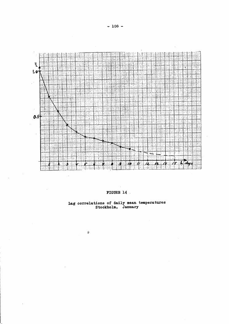
- 108 -

::;:::t:: [ :: : 1:: :t ::::l's-.1 " ... "" ............. " .. . '"!::: :··· .. . .. ::: ~ :/'I:::; y }': ;;;:!:::J:T :: .:·• • • .. ... .. • , , . .

:+': ::1:: ' :: :C:br i: 1:::: ,~~ .,,, ,, ::~!:.:.;:tc:.: I ; ' : r 1

f:T 1 1, .:re . .:elF :::::: :::: :::::: r : :<::.: : ::. :: ::: ......... ':'!::: L:: t: i . ::} ::::: 't: [ I .. j:~· !:'"' :;.:cf;7:.;

rt''%''[ ',ii+:r :::, ''ii!i:iii~~s:- •• '~ ~2~ ± ~~• .:··~st-r~ilifHl&l1,·:!•:•t••HGt~f:,,jPf:~~l~:~lr:l·:rrm•w=r-ftlJffEfi3ffJtfJC

FIGURE 14

Lag correlations of daily mean temperatures Stookholm, January

1.\>

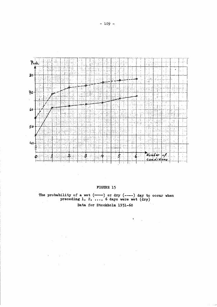
- 109 -

· ----T--: -~ 1-,

:cc--f-,---'--:--+---"-... c---. ~-+-"-1

! 4o 1: :== •+ : i '' J :I ·: I ': I : t : ... I 'I . : I ' I 1 +- :· I : ··.1 : ~ I· I · I ·j' .

' · , • = 1 = r 1 , · t · 1 · 1 =· J 1 · 1 · 1 1 ·· 1.., · J ·····1 · · ·1 1 - • · I . . .. . . . .. . . . . . -' • ' ~ I . 1 · I ! I

~--r----:

FIGURE 15

The probability of a wet (----) or dry (----) day to occur when preceding 1, 2, ••• , 6 days were wet (dry)

Data for Stockholm 1931-60

'I

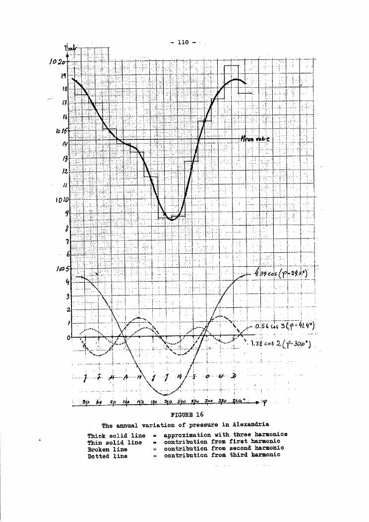
- 110 - '

/0 '),,!- I ~ · ~'-'-+· .-+--,--:+---+--+-,--i.........,-

... _ .. : .. ------l -· ...... ; , I

0 \· '•,;L \ :

---~.;: '-"-;.-.lr-= ... i ... j,. : • \.'3~ (..coS .2-(f-30,0°) , ,_.....,.,.. I

' ' l -- . ~------:· ---~ -- . ,_ ... \ ; . f!

, _____ L -·-+- A--~---11\0.t' .... ,'. ·. 4 . --~- -o-- --¥·. ~ I . : . . .

. . •· - . : -- --- ; ..... ·' . ; .... : ... : - . : ... --; ..

_:;!p 4 q~ 1+ 1f'O l(ll '?flt :~,IJo ?-P> ~ ~';<> ~t.o. o ; • ''f

FIGURE 16

The annual variation of pressure in Alexandria

Thick solid line • approximation with three harmonics Thin solid line • contribution from first harmonic Broken line = contribution from second harmonic Dotted line = contribution from third harmonic

; . -------.---

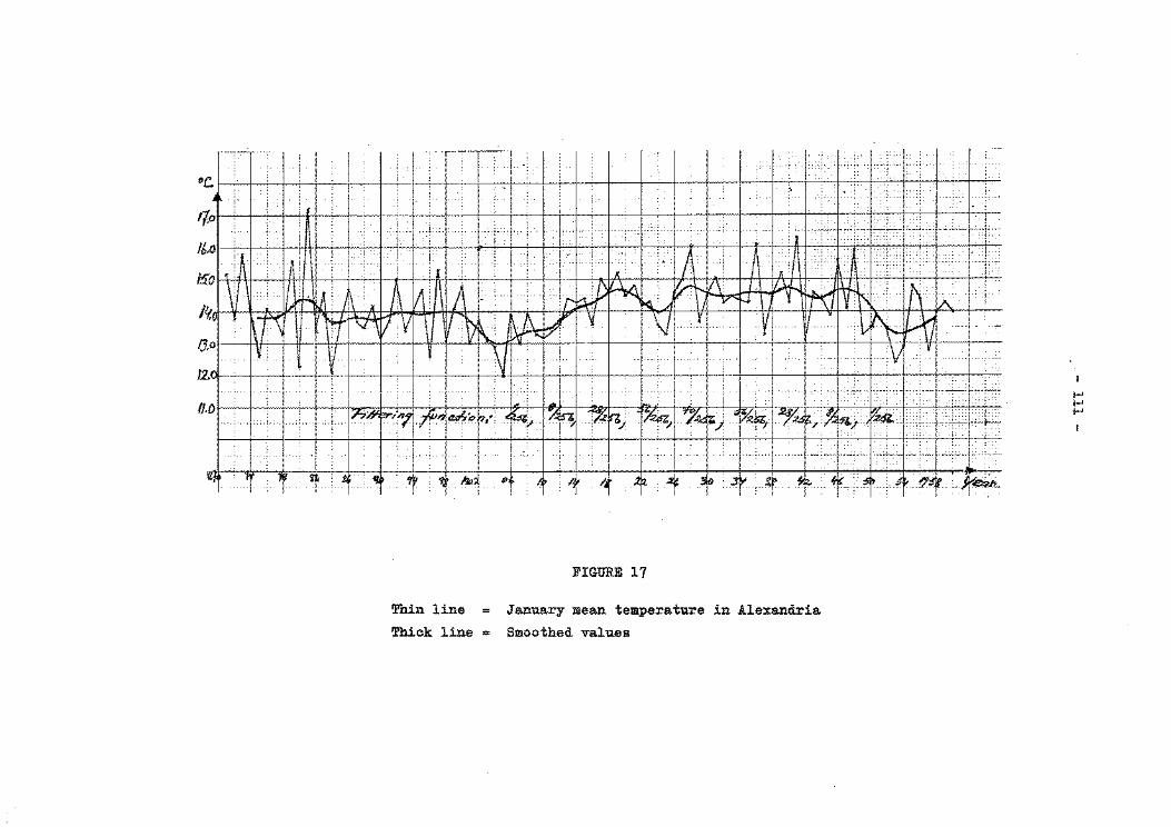
Df: .. . : . . ··I . : I I' ~ , ... , ~ I I . I . I . I . I I H ., '> I' ,. Hl HI I ; . I ' I . : I : I , I. : I H- . . I H- . ,----t-T-- . . .. · ........ :· '

i

... !· rt' r.o

1 ~

.: j.: i ! i

j ... I .. OH,. I HO. H.. . ... , ... . . . .

I . .

t j·. (I I J· ' ... , :H;·:::[;q~ .. r-: J ~-I .•.•• HI-:+--H:~::-:!t-: .. h!:-ccj_c_c_(-: .. (: .. I H.~- ·1H · ·1· H. ·1 : · 1 A 1 · 1 A 1 1\1 · rr 1 :, ... ,. ' . • .. i . : .. : •... < ··. ' > . : •. ! . •. · ... : . '· •• ,' •. ::{ • :: ., ...

I A. ' . . : K . ' ' . . .. . .... ' ...

·~·Jm;•··Wiffrfbf\Ft1Mtf\klf\F. :~ IJ.or~:

~~, 1vllf I, IH1.·l~J 1 t I inf 111-1-l"l.l+· ····I Ll ! 1~44~t·· r ITI··wr Plff i*l?ttrtltbCft '"on .

< - I j

~4 : ~. • ~ ' + L 1~4If~--'f--~ 1111 "f 4' • /t ~ ~ t·t ~ ~-·1···1·1·~'L· · * ·· ""t ·· : .. · ; "'f" · ··r· .:. · .,;: ... :.. J? ·· --Xr""~~-1 • I · : ·: · ·.

FIGURE 17

Thin line = January mean temperature in Alexandria

Thick line = Smoothed values

1-' 1-' 1-'

- 113 -

STATISTICAL FORECASTING

by

G. Tara.kanov

Structural and correlation functions

Structural and correlation functions are extremely important character­istics of the statistical structure of meteorological fields. They are used for many purposes in meteorology and climatology but are particularly useful in making statistical forecasts. It is therefore essential to know what these functions are.

Let us consider a homogeneous isotropic field with two arbitrary points r 1 and r 2 on a surface (for example: isobaric surface), and at which the values of a meteorological element fare lcnown. Then the structural function Bf (r1 , r 2) is the average square of the difference of the values of the meteorological element f at points r 1 and r 2, and can be written as follows:

Bf(rl' r2) (_r(rl) - f(r2)] 2 (1)

where the line above the formula [f(r1) - f(r2 ~ 2 denotes average.

For some purposes it is useful to consider the structural function of the deviations of the element f from its average value f.

If we therefore denote:

f(r) - as the norm (average value) of the element f at the point r, and,

fJ(r)- as the anomaly of the element fat the same point (deviation from the norm),

we arrive at the following expression:

f1(r) = f(r) - f(r) (2)

Thus, if the structural function for the deviation of the element f from its norm is bf(r1 , r 2), we obtain:

bf(rl' r2) [f' (r1 ) - f' (r2 )] 2

(3)

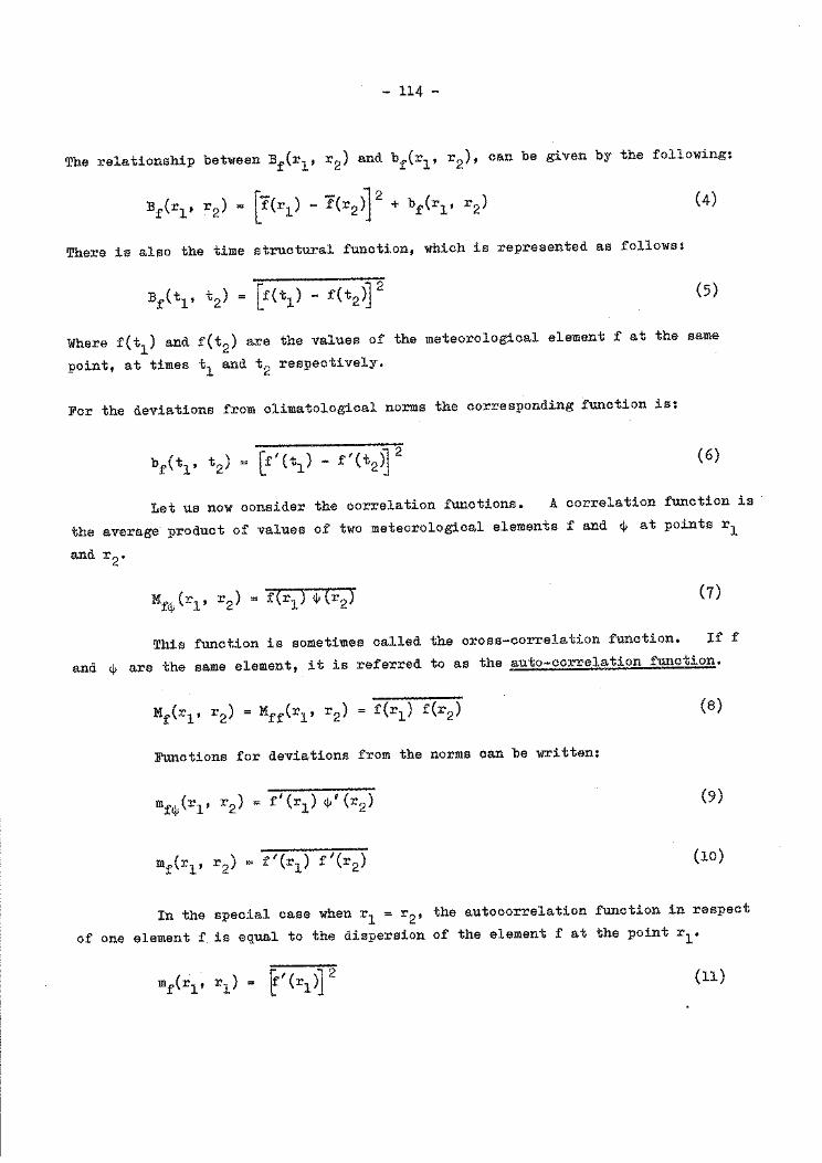
- 114 -

The relationship between Bf(r1 , r 2) and bf(r1 , r 2), can be given by the following:

Bf(rl, r2) [r(rl) - f(r2)l2 + bf(rl, r2) (4)

There is also the time structural function, which is represented as follows:

Bf(tl, t2) = [f(tl) - f(t2)] 2 (5)

Where f(t1) and f(t2) are the values of the meteorological element f at the same

point, at times t 1 and t 2 respectively.

For the deviations from climatological norms the corresponding function is:

bf(tl, t2) = ~'(tl)- f'(t2~ 2 (6)

Let us now consider the correlation functions. A correlation function is

the average product of values of two meteorological elements f and (jJ at points r 1

and r 2•

Mf(jl(r1 , r 2) = f(r1 ) 1jJ(r2) (7)

This function is sometimes called the cross-correlation function. If f

and (jJ are the same element, it is referred to as the auto-correlation function.

Mf(r1 , r 2) = Mff(r1 , r 2) = f(r1) f(r2) (8)

Functions for deviations from the norms can be written:

mf(jl(r1 , r 2) = f 1 (r1 ) (jl' (r2) (9)

mf(rl' r2) f'(r1 ) f'(r2) (10)

In the special case when r 1 = r 2, the autocorrelation function in respect

of one element f is equal to the dispersion of the element fat the point r 1•

mf(rl, rl) = ~'(rl)] 2 (11)

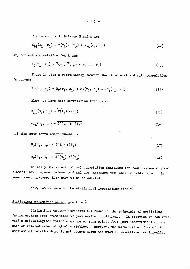
- 115 -

The relationship between M and m is:

MN(r1 , r 2) = f(r1 )~(r2 ) + mfq,(r1 , r 2) (12)

or, for auto-correlation functions:

Mf(r1 , r 2) = f(r1 ) f(r2) + mf(r1 , r 2) (13)

There is also a relationship between the structural and auto-correlation functions:

Bf(r1 , r 2) = Mf(r1 , r 1 ) + Mf(r2, r 2) - 2Mf(r1 , r 2) (14)

Also, we have time correlation functions:

Mfq,(t1 , t 2) = f(t1 ) q, (t2) (15)

mfq,(t1 , t 2) = f'(t1) q,' (t2) (16)

and time auto-correlation functions:

Mf(t1 , t 2) = f(t1 ) f(t2) (17)

mf(t1 , t 2) = f'(t1 ) f'(t2) (18)

Normally the structural and correlation functions for basic meteorological elements are computed before hand and are therefore available in table form. In some cases, however, they have to be calculated.

Now, let us turn to the statistical forecasting itself.

Statistical relationships and predictors

Statistical weather forecasts are based on the principle of predicting future weather from statistics of past weather conditions. In practice we can fore­cast a meteorological variable at one or more points from past observations of the same or related meteorological variables. However, the mathematical form of the statistical relationships is not always known and must be established empirically.

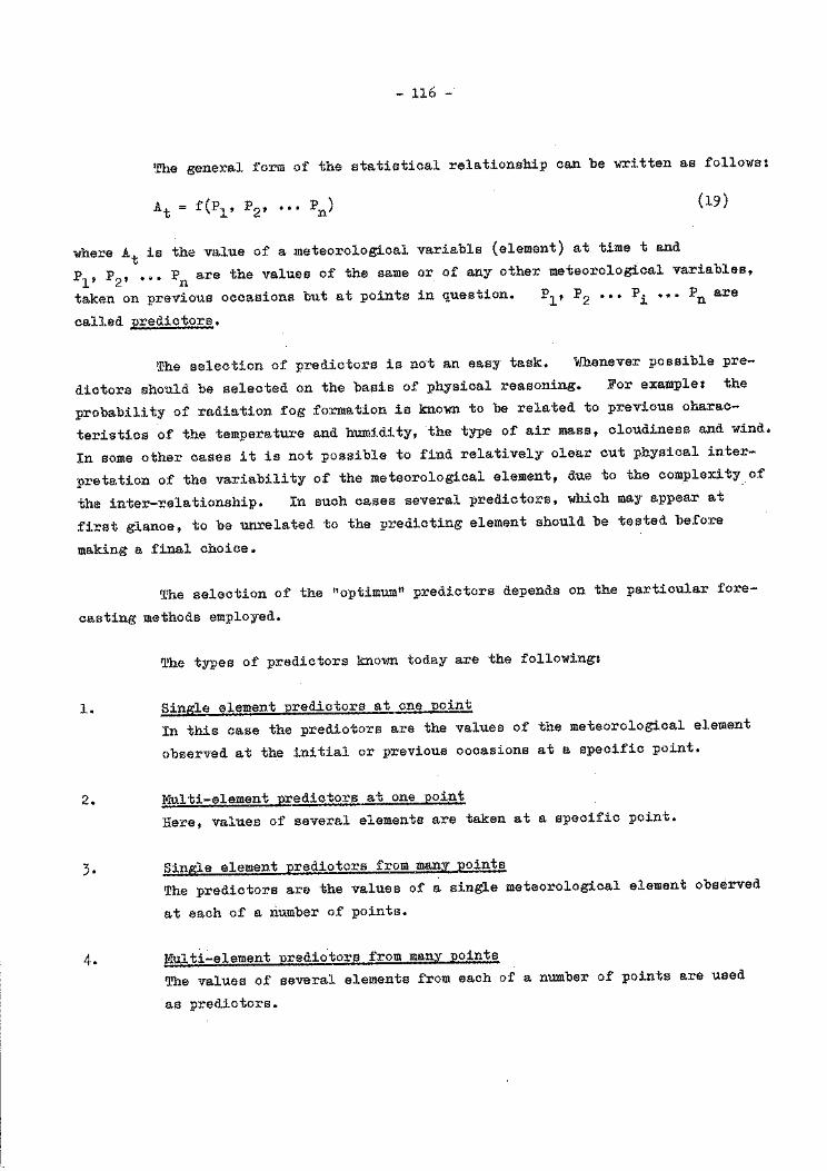
- 116 -

The general form of the statistical relationship can be written as follows:

At= f(P1 , P2 , ••• Pn) (19)

where At is the value of a meteorological variable (element) at time t and

P1 , P2, ••• Pn are the values of the same or of any other meteorological variables,

taken on previous occasions but at points in question.

called predictors.

Pl' P2 ••• Pi ••• Pn are

The selection of predictors is n~t an easy task. Whenever possible pre­

dictors should be selected on the basis of physical reasoning. For example: the

probability of radiation fog formation is known to be related to previous charac­

teristics of the temperature and humidity, the type of air mass, cloudiness and wind.

In some other oases it is not possible to find relatively clear cut physical inter­

pretation of the variability of the meteorological element, due to the complexity of

the inter-relationship. In such cases several predictors, which may appear at

first glance, to be unrelated to the predicting element should be tested before

making a final choice.

The selection of the "optimum" predictors depends on the particular fore­

casting methods employed.

1.

2.

3·

4·

The types of predictors known today are the following!

Single element predictors at one point

In this case the predictors are the values of the meteorological element

observed at the initial or previous occasions at a specific point.

Multi-element predictors at one point

Here, values of several elements are taken at a specific point.

Single element predictors from many points

The predictors are the values of a single meteorological element observed

at each of a number of points.

Multi-element predictors from many points

The values of several elements from each of a number of points are used

as predictors.

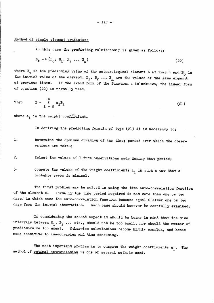
- 117 -

Method of single element predictors

In this case the predicting relationship is given as follows:

Bt =<V (BO' Bl' B2 • • • Bn) (20)

where Bt is the predicting value of the meteorological element b at time t and B0 is the initial value of the element, B1 , B2 ••• Bn are the values of the same element at previous times. If the exact form of the function~ is' unknown, the linear form of equation (20) is normally used.

Then B i

n E a.B.

0 l. l. (21)

where ai is the weight coefficien-t._

1.

2.

3·

In deriving the predicting formula of type (21) it is necessary to:

Determine the optimum duration of the time; period over which the obser­vations are taken;

Select the values of B from observations made during that period;

Compute the values of the weight coefficients ai in such a way that a probable error is minimal.

The first problem may be solved in using the time auto-correlation function of the element B. Normally the time period required is not more than one or two days; in which case the auto-correlation function becomes equal 0 after one or two days from the initial observation. Each case should however be carefully examined.

In considering the second aspect it should be borne in mind that the time intervals between B1 , B2 ••• etc., should not be too small, nor should the number of predictors be too great. Otherwise calculations become highly complex, and hence more sensitive to inaccuracies and time consuming.

The most important problem is to compute the weight coefficients ai. The method of optimal extrapolation is one of several methods used.

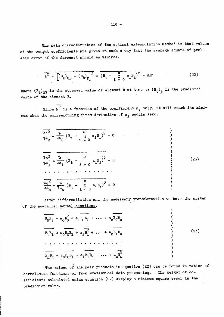
- 118 -

The main characteristics of the optimal extrapolation method is that values

of the weight coefficients are given in such a way that the average square of prob­

able error of the forecast should be minimal.

02 [(Bt)OB - (Bt)p] 2 = (Bt - i ! 0 aiBi)2 = min (22)

where (Bt)OB is the observed value of element B at time t; (Bt)p is the predicted

value of the element B.

Since~ is a function of the coefficient ai only, it will reach its mini­

mum when the corresponding first derivative of ai equals zero.

d02 d - =- (B -'dao qao t i

n I: a.B )2

0 ~ i

ao2 a - n -­--oal = ~ (Bt - I: aiBi)2

1 i = 0

"do 2

ea n

c =~

n ( B -

t i

n I: a B )2

0 i i

0

= 0 (23)

0

After differentiation and the necessary transformation we have the system

of the so-called normal eguations.

2 BOBt = aOBO + alBOBl + ••• + anBOBn

2 BlBt = aOBOBl + alBl + ••• + anBlBn

• • • • 0 • • •

BnBt = aOBOBl + alBlBn + ••• + a B2

nn

(24)

The values of the pair products in equation (22) can be found in tables of

correlation functions or from statistical data processing. The weight of eo-

effieients calculated using equation (22) display a minimum square error in the

prediction value.

- 119 -

Multi-element predictors in one point

The predicting relationship may be calculated using the following expression:

At= F(P1 , P2 , ••• Pn) (25)

where P1 , P2 ••• Pn are the various atmospheric state characteristics at the point where the forecast is being made either at the initial or in past moments of time.

As we have seen, the first method by extrapolation procedures can be applied to meteorological elements displaying a regular variation with time. However, forecasters often deal with weather phenomena such as air mass thunderstorms or radiation fog, the occurrence and termination of which are sharply defined. cases the predicting relationship given in equation (23) is more useful.

In such

Before establishing a working formula for a predicting element a choice of the characteristics of the initial state of the atmosphere (P1 , P2 ••• Pn) should be made. This choice is normally based on a general understanding of the mechanism of predicting phenomena in question, theoretical deduction and also on the experience of the forecaster.

To explain this method in more detail we 'will look at a specific example. Let us assume that we have to predict low level cloudiness (not frontal) at night using data recorded at the station before 6 p.m. The first necessary condition for cloud formation is high humidity in the surface layer of the air. Thus some mois­ture characteristics should be used as predictors. For example the relative humidity R and its variation over the last few hours may be included.

A second obvious condition is a decrease in temperature in the cloud for­mation layer. Since this decrease in temperature is transferred downwards by heat exchange in the underlying surface, the rate of decrease must depend on the wind velocity and the wind direction. Low aloud formation is therefore more probable when the wind direction d is such that the maximum positive advection is produced (i.e.: maximum heat loss from the air-mass).

For the sake of simplicity we will confine ourselves to these three pre­dictors: R; A R and d. The predicting relationship can then be written in the

- 120 -

following general form:

p f(R, b. R, d) (26)

where P is a probability of low cloud formation.

The next step is to verify the assumed relationships by building up cor­

relations At (P1 ); At (P2); At (P3). In our example we have to take data of

observations made over the same period during previous years 'and select cases when

the station was in the same air-mass during the evening and night. Tables similar

to the following can be prepared:

The probability of low cloudiness formation at different values R

R% N /N + -

p

96-100 64/16 0.8

90-95 30/10 0-75 L_ _____ ------- '----

N+ denotes the number of cases when cloudiness was observed and N indi­

cates no cloud observed.

The probability is calculated by means of the simple formula:

p N+ (27)

N+ + N

Similar tables should be prepared for b. R and d.

The correlation if it exists will be apparent from an examination of the

tables.

Having established the relationships we may write a linear combination as

follows:

At= Cl At(Pl) + C2 At(P2) + ••• + Cn At(Pn) (28)

- 121 -

where c1 , c2 ••• Cn are the weight coefficients and At(P1 ), At(P2) ••• At(Pn) are the functions expressing the correlation between probability values of the predicting element and the predictors.

Normally At is given in the form of probability.

The weight coefficients may be calculated as described before.

The method of single element predictors at several points

The predicting~relationship is given in the following formula:

llt = <j,(llOL' llll ••• llnl' ll02' lll2 ••• lln2' llOK' lllK ••• BnK) ( 29)

This method is generally used for predicting the pressure and height of an isobaric surface. There are of course many ways o'f using equation (29) as a working formula. In this case we shall limit ourselves to one of the most promising which is the use of empirical influence functions. The variation of geopotential heights for a time period fl t may be presented as follows:

flH = n !:

i = G .• ~.

1 l. "'i (30)

where G is the Green or influence function, and q, is the function of the space dis-tribution of. geopotential heights of an isobaric surface; Gi and <Vi are the values of the.functions G and <V in i points in the vicinity of the i = 0, for which the forecaE!t, is being .made. In this case, q,l' q,2' <Vi' • • • <Vn are the predictors,

and the function G denotes the influence of these predictors on the variations of the geopotential heights.

The values of G1 , G2 , ••• Gi ••• Gn may be determined theoretically or statistically. Since we are talking now of statistical forecasting we shall refer to the latter.

The values determined statistically are called empirical influence functions and denoted by a1 , a 2 , ••• an.

AH = i

n I ai <Vi

1 ( 31)

- 122 -

When deriving.a working formula two basic problems have t~ be solved:

(a) To select points (number and location) from which values of ~ should be

taken;

(b) To determine the optimal values of the coefficients a1 , a2 , ••• an.

Experience shows that the area of the influencing region is cf the order of

magnitude of 106- 107 km 2,i.e. a circular area with a radius of about 1,000 km

around the forecasting point.

The points i inside this area are usually selected from operational meteo­

rological upper-air observing stations in the light of the result of the preliminary

interpolation into grid points. The distance between the grid points should be in

the range of 250 - 500 km.

The coefficients a, are calculated as described earlier.

Multi-element predictors at several points

In this case the predicting relationship can be expressed in the general

form:

At = f(P1 , P2, Pn) (32)

where P1 , P2, ••• Jn are the characteristics of the state of the atmosphere at a

number of points at the selected initial and pre-initial times. In selecting the

predictors, general physical considerations and experience as well as the results of

a statistical analyses of the meteorological fields are useful indicators.

Again there are many ways of developing this method. The method of

similar selections with the aid of a computer seems to be the most promising approach.

However, this method is still in its development stage and is not yet operational.

The b.asic assumption in using this method is that for short periods of time (!!. t) the

weather conditions, :ina specific region at time t + llt, are a direct result of the

atmospheric conditions existing at the initial time t.

Let us assume that we have defined a number (N) of combinations of weather

conditions (weather complexes); its successful forecast is most important. For

- 123 -

aviation, for example, such complexes may include various combinations of visibility and heights of cloud base, for railway transport- quantity and type of precipitation, and so on. Then, using synoptic chart archives we can compose the (N) groups. Each of these groups will have ni cases with one of the selected combinations of weather conditions. Thus, a special catalogue containing these specific charts may be compiled.

With such a catalogue the task of the forecaster is simply to recognize the group to which the atmospheric conditions at the forecast time apply and to describe the weather conditions observed on similar previous occasions. However, this is not always an easy task since the influence and types of criteria to be used for this purpose are still unknown. Moreover criteria of similarity already suggested by some scientists are of a general nature and cannot as yet be used for forecasting purposes.

Nevertheless, for a successful solution of the task one should seek some objective characteristics of the atmospheric conditions which, being quasi constant within one group would change sharply in the case of another group. This problem is the same as the so called "problem of image recognition11 , which is one of the basic problems of the modern kibernetics.

As we all know, this science has and is making rapid progress. Recent developments in the computerized selection of analogies are very promising. There is no doubt that this method will play a significant role in weather forecasting in the future.

- 125 -

HOMOGENEITY, VARIABILITY, MEAN CLIMATIC MAPS

by

R. Arlery

Homogeneity

]_e.f.iE_i_ii.2_n

The scrutiny of a series of observations sometimes reveals sudden changes

in values which are maintained or progressive systematic changes in the values. The

series is called homogeneous if it can be proved that these anomalies are due to

climatic changes exclusively. Generally, it is very difficult to maintain that a

series is homogeneous and one should always check first if there are indications of

its non-homogeneity.

Ya£i£U~£a~s~s_of E_OE_-ho~o~eE_eitx

Relocation of a station, changes in the environment, replacement of the

equipment, ageing of the thermometers, changes in the instructions.

lioE_-ho~o~eE_eitx £h~cks

If, as a result of the statistical tests the homogeneity of an isolated

series is in doubt, before actually ascribing the changes in the series to the

climatic changes a thorough and detailed scrutiny of the station's history is

essential.

If the conditions permit, it is preferable to make comparisons with a

neighbouring station the homogeneity of which is beyond doubt, or to compare the

observations made simultaneously at a number of stations, all located fairly close

to each other and in similar topographic conditions. These studies of correlations

are often conducted using the classical methods of constant differences or con­

stant ratios.

In ·certain cases the graphical comparisons are sufficient (plotting annual

values, curves of accumulated values or "double mass" curves, etc.).

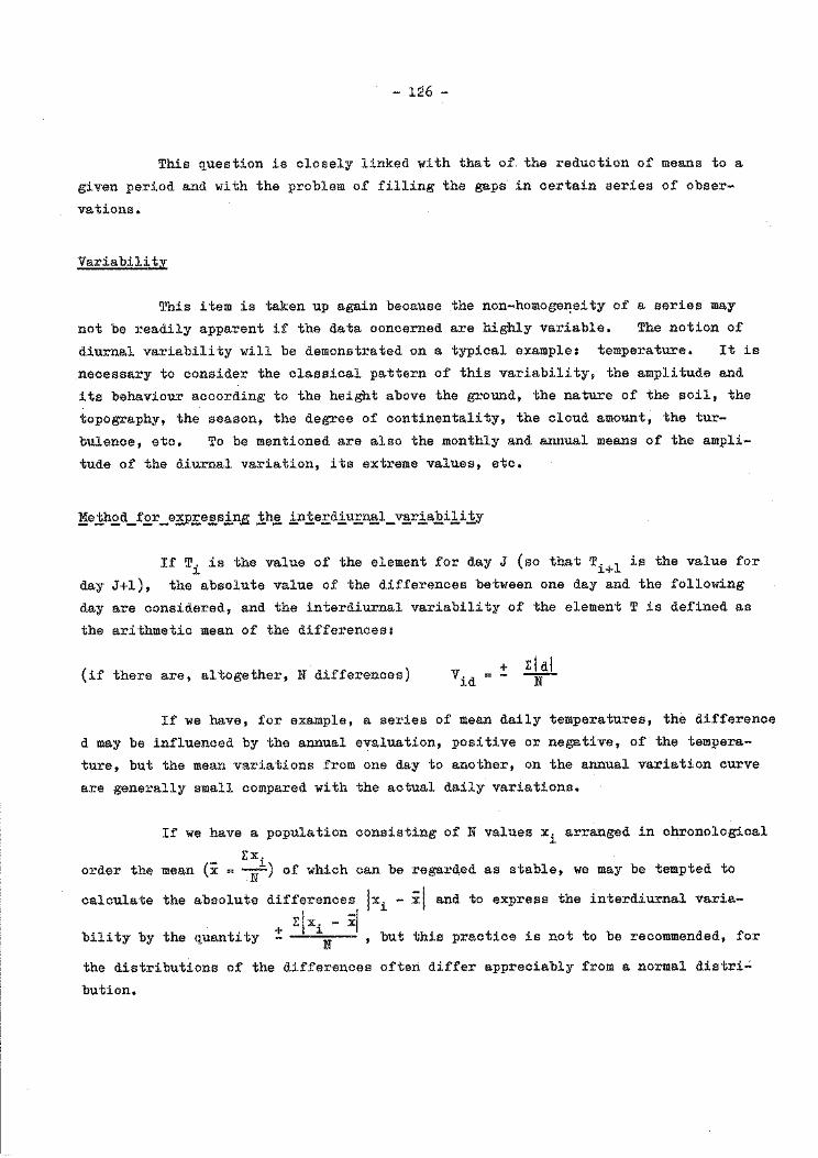
- 126 -

This question is closely linked with that of the reduction of means to a

given period and with the problem of filling the gaps in certain series of obser­

vations.

Variability

This item is taken up again because the non-homoge~eity of a series may

not be readily apparent if the data concerned are highly variable. The notion of

diurnal variability will be demonstrated on a typical example: temperature. It is

necessary to consider the classical pattern of this variability, the amplitude and

its behaviour according to the height above the ground, the nature of the soil, the

topography, the season, the degree of continentality, the cloud amount, the tur-

bulence, etc. To be mentioned are also the monthly and annual means of the ampli-

tude of the diurnal variation, its extreme values, etc.

~e!h£d_f£r_e~£e~siPE !~ in!e£diu£n~l_v~ria~i!i!Y

If T. is the value of the element for day J (so that T. 1 is the value for 1 1+

day J+l), the absolute value of the differences between one day and the following

day are considered, and the interdiurnal variability of the element T is defined as

the arithmetic mean of the differences:

(if there are, altogether, N differences) vid =:!: Ekdl

If we have, for example, a series of mean daily temperatures, the difference

d may be influenced by the annual evaluation, positive or negative, o£ the tempera­

ture, but the mean variations from one day to another, on the annual variation curve

are generally small compared with the actual daily variations.

If we have a population consisting of N values xi arranged in chronological

E~ order the mean (i = -w-) of which can be regarded as stable, we may be tempted to

calculate the absolute differences lxi -

Elx. - ~ the quantity :!: 1

u , but

xl and to express the interdiurnal varia-

bility by this practice is not to be recommended, for

the distributions of the differences often differ appreciably from a normal distri~

bution.

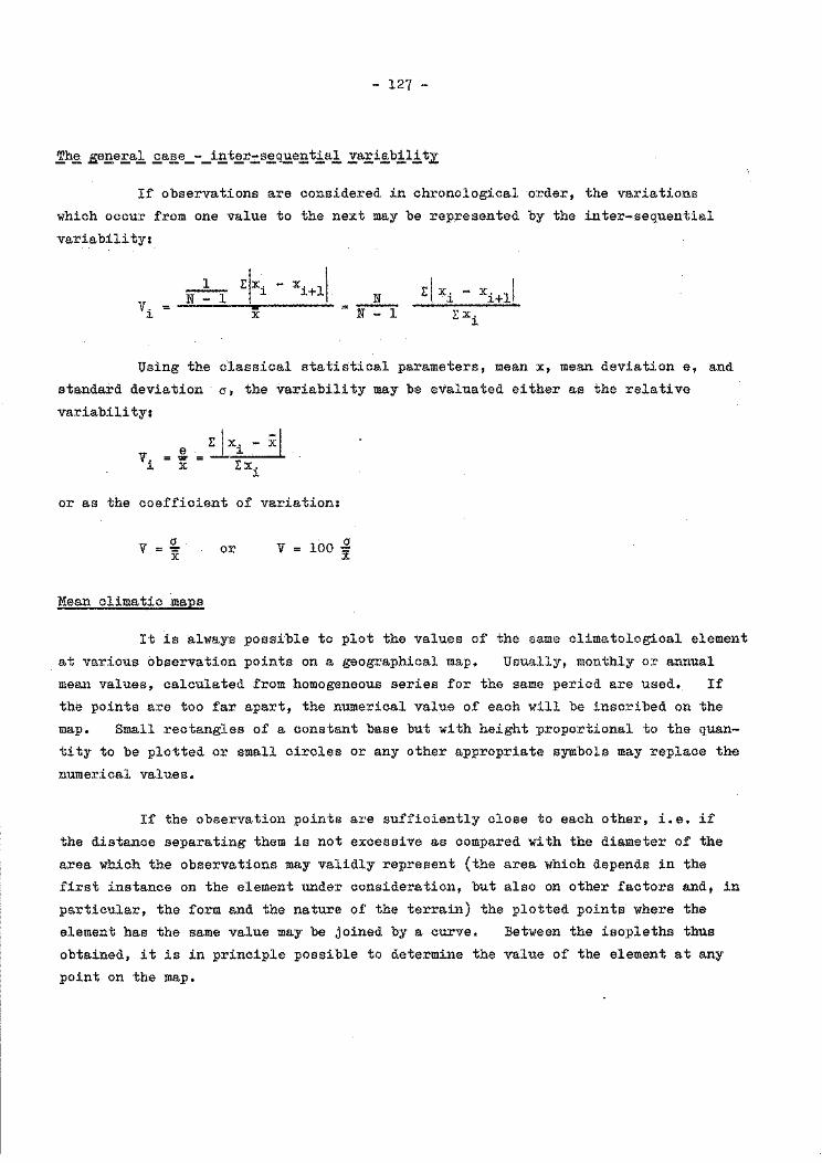
- 127 -

!h~ ~e~e£al £a~e_-_i~t~r=s~~e~tial ~a£i~bilitz

If observations are considered in chronological order, the variations

which occur from one value to the next may be represented by the inter-sequential

variability:

vi _1 Elx.- x. I N - 1 1 1+l

X

_N_ N - 1

Ej xi - xi+ll

EXi

Using the classical statistical parameters, mean x, mean deviation e, and

standard deviation a, the variability may be evaluated either as the relative

variability:

vi e -X

E I xi - xl I: xi

or as the coefficient of variation:

V a i

Mean climatic maps

or V lOO .Q x

It is always possible to plot the values of the same climatological element

at various observation points on a geographical map. Usually, monthly or annual

mean values, calculated from homogeneous series for the same period are used. If

the points are too far apart, the numerical value of each will be inscribed on the

map. Small rectangles of a constant base but with height proportional to the quan­

tity to be plotted or small circles or any other appropriate symbols may replace the

numerical values.

If the observation points are sufficiently close to each other, i.e. if

the distance separating them is not excessive as compared with the diameter of the

area which the observations may validly represent (the area which depends in the

first instance on the element under consideration, but also on other factors and, in

particular, the form and the nature of the terrain) the plotted points where the

element has the same value may be joined by a curve. Between the isopleths thus

obtained, it is in principle possible to determine the value of the element at any

point on the map.

- 128 -

The accuracy of the curves is reduced by the standard error affecting each

of the mean values used which sets a limit for the number of isopleths that may be

traced.

The interpolations may be made in assuming that the value of the element

under consideration is subject to linear variation with distance; this supposes

that the region concerned is climatically homogeneous.

Usually, account is taken of the influence of the altitude on the elements

for which the laws of variation have been adopted; the values of the element

"reduced to sea level 11 (pressure, temperature) become comparable and may be inter­

polated.

Consideration will be given to various elements greatly influenced by the

local conditions for which the path of the isopleth is often uncertain. Mention

will be made of the maps of isanomalies established by plotting for each station the

differences between the value obtained at the station and the mean value calculated

for the corresponding parellel (to bring out the influence of the geographic factors).

Finally, reference shall be made to the Guide to Climatological Practices

(Chapter 7 - Annex 7 B) for consideration of the various aspects of the preparation

of the climatic maps in general (presentation, scale, projection) principles to be

applied in establishing maps for various elements, accuracy of climatic maps and

the most frequent errors.

- 129 -

ME~HODS OF SUMMARIZING DA~A AND OF COMPUTING COMPOUND S~A~IS~ICS FOR THE COMPILATION OF

CLIMATIC REFERENCE DATA

by

N. K. Kljukin

Suitable representation of the space-time fields, not only of each climatic element but also of compound statistics relating t9 these elements, is one of the most important long-term tasks of applied climatology. This necessitates summarizing data, i.e. presenting the data in a compact form, convenient for reference, analysis and practical use.

Such a programme for the development of applied climatology (which is however, closely linked with the development of theoretical climatology) is governed by the following considerations

For practical purposes and for investigations there is an ever increasing need for more detailed and more fully summarized data relating to the present and future meteorological situation;

In this connexion it was found that it is impossible to meet the require­ments of a considerable number of inquiries, using limited data for each climatic element, as has frequently been done in the past;

Present-day inquiries, in the practice of hydrometeorological and related sciences, make it necessary to obtain and use a considerably greater amount of data. On the basis of this data, statistics should be given, taking into account natural combinations of climatic elements, which in their complex interactions with and interdependence on the environment, have a direct influence on solid objects, and on the processes of animal and human activity;

As a consequence, it has become impossible to use former methods for the representation of data.

Thus, the mean values of each elemen·t which, formerly, were most frequent­ly used, are now only of subsidiary importance. Tables giving distributions at each station, i.e. frequency tables, which without sufficient grounds, were sometimes

- 130 -

considered as being equivalent to probability tables, greatly increased the volume

of data, and in some cases made the usual tables so cumbersome, that publication,

analysis, summarizing and full use of the tables was impracticable.

Practical and theoretical climatology makes use, to a certain extent

(frequently quite insufficient), of the following basic methods, as a solution of

the problem of summarizing data and compound statistics representative of climato­

logical conditions.

1.

2.

3.

4-

5·

Spatial classification, taking into account natural conditions and

anthropological influences and also the variability of the element or

compound elements under investigation;

Distribution in time of elements or compound elements, taking into account

the temporal and spatial variability, due to the influence of external

factors, associated with the inherent nature of the processes and

phenomena under investigation;

Representation of compound climatic statistics, consisting of 2 to 4 and

sometimes more elements using the basic parameters of statistical distri­

bution (Reference 10) and, in some oases expressing the selected compound

statistic in non-dimensional units;

Establishment and use of relationships for complex statistics of each

element and their components, with simple popular statistics;

Wide use of the analogue form of representing data (maps, graphs, noma­

grams, etc.). Analogue forms, by their nature, are best for showing

visually the laws governing, and the progress of any given process (i.e.

give an analogue of it). At the same time, the analogue form of represen­

ting of climatic data is usually much more compact than data given as

figures.

We shall consider some of the methods, illustrating ways of solving the problem of

summarizing climatological data and compound statistics representative of climate­

logical conditions.

- 131 -

The following methods a~e examples of spatial distribution of values.

1. Values, representative of climatological conditions, according to the geographical position of the place of observation. This method was in use for many years (reference 3, 5, 6, 7, 17, 18, 19, etc.) and was used in agroclimatology and in climatology for the building industry, for transport and for industry in general.

For values of this kind, the following sequence is adopted 1

Coefficients of the variability of an element or compound element for typical positions and their relationship to local (e.g. geomorphological, geobotanical, etc.) conditions, are determined for the region under investigation, based on actual observations (especially for key position);

On sufficiently large-scale maps typical locations are chosen and areas are determined containing a given type of geographical unit in the region under consideration;

The coefficients which are found or the simple values of the element, . found from actual observations and coefficients are entered on the map.

Such maps can be used directly for calculations for engineering, agro-teohnical, etc. purposes, where climatological data for an area are necessary for electric trans­mission lines, routes for roads, etc.

On the basis of such charts, areas having certain definite .climatological

features can be assessed. An example of such an assessment is given in Table 1 (5).

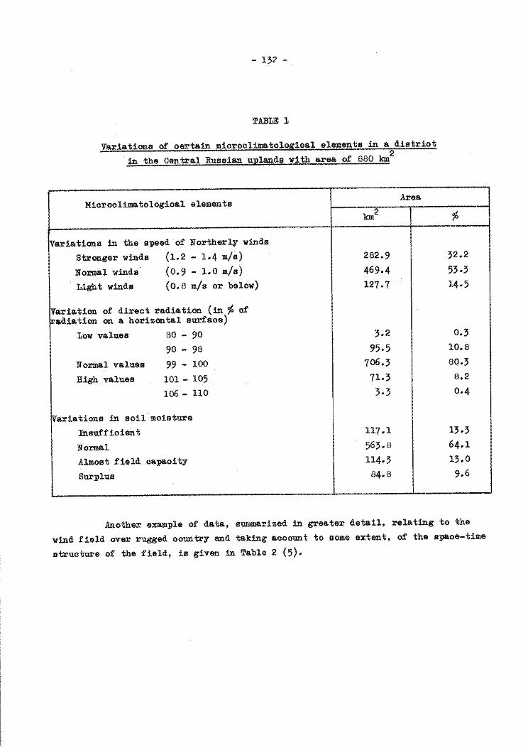
- 132 -

TABLE l

Variations of certain microclimatological elements in a district 2

in the Central Russian uplands with area of 880 km

Microclimatological elements

Variations in the speed of Northerly winds

Stronger winds (1.2 - 1.4 m/s)

Normal winds (0.9 - 1.0 m/s)

Light winds (0.8 m/s or below)

Variation of direct radiation (in % of ~adi~tion on a horizontal surface)

Low values 80 - 90

90 - 98

Normal values

High values

99 - 100

101- 105

106- 110

rariations in soil moisture

Insufficient

Normal

Almost field capacity

Surplus

km2

282.9

469.4 127.7

3.2 95.5

706.3 71.3 3-3

117.1 563.8 114.3

84.8

Area

%

32.2

53-3 14-5

0.3 10.8

80.3 8.2

0.4

13.3 64.1 13.0

9.6

Another example of data, summarized in greater detail, relating to the

wind field over rugged country and taking account to some extent, of the space-time

structure of the field, is given in Table 2 (5).

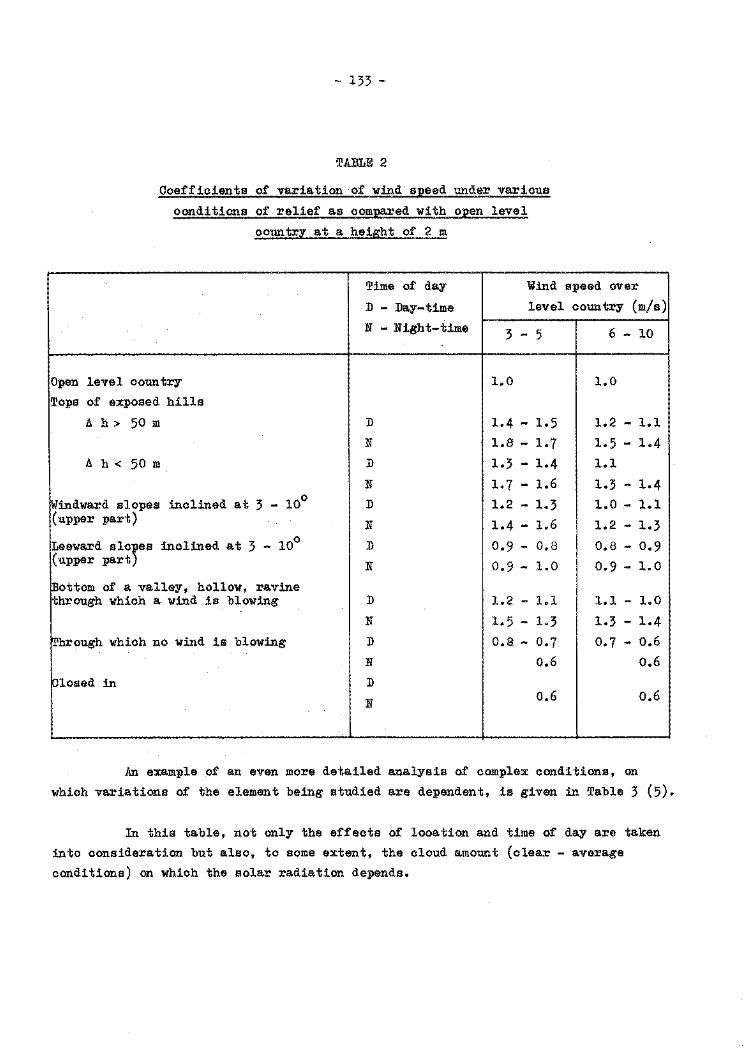
- 133 -

TABLE 2

Coefficients of variation of wind speed under various

conditions of relief as compared with open level

country at a height of 2 m

Time of day Wind speed over

D - Day-time level country (m/s)

N - Night-time 3 - 5 6 - 10

Open level country I I 1.0 1.0

Tops of exposed hills

lJ. h > 50 m I D 1.4 - 1.5 1.2 - 1.1

N 1.8- 1.7 1.5 - 1.4

lJ. h < 50 m I D 1.3 - 1.4 1.1

N 1.7 - 1.6 1.3 - 1.4

~indward slopes inclined at 3 - 10° D 1.2 - 1.3 1.0 - 1.1 (upper part) N 1.4 - 1.6 1.2 - 1.3

0 D 0.9 - 0.8 0.8 - 0.9 Leeward slo)es inclined at 3 - 10 (upper part N 0.9- 1.0 0.9 - 1.0

!Bottom of a valley, hollow, ravine through which a wind is blowing I D 1.2 - 1.1 1.1 - 1.0

N 1.5 - 1.3 1.3 - 1.4

~hrough which no wind is blowing I D o.s- 0.7 o. 7 - 0.6

N 0.6 0.6

~losed in I D

N I 0.6 I 0.6

An example .of an even more detailed analysis of complex conditions, on

which variations of the element being studied are dependent, is given in Table 3 (5).

In this table, not only the effects of location and time of day are taken

into consideration but also, to some extent, the cloud amount (clear - average

conditions) on which the solar radiation depends.

Region

Hilly country in the European territory of the u.s.s.R.

Hilly country Central Asia

- 134 -

TABLE 3

Variations of day-time (TD) and night-time (~Tl

air temperatures (°C) in hilly country. July.

Top, upper third Wide valley of slope

Parameter Average Clear Average Clear condi- weather condi- weathez tions tions

TD + -0.5 + -0.5,-1 + -0.5 + -0.5,-1

TN 1-2 2 -1,-2 -2,-3

(TD - TN) -1,-2 -2,-3 1-2 2-3

TD -0.5 -0.5,-1 0.5 0.5,-1

~ 2-3 3 -2,-3 -3,-4

(TD - TN) -2,-3 -3,-4 2-3 3

Closed valley Hollow

!Average Clear condi- weather tions

0.5 0.5,-1

-2 -3

2 3

0.5 0.5,-1.

-3 -4.-5

4-5 5-6

NOTE: Negative values mean a decrease in TD' TN and (TD - TN) as compared with

open level country. Positive values mean an increase.

An excellent example of the spatial distribution of soil moisture condi­

tions in hilly country in various zones is given in Table 4 (7).

In themselves, soil moisture or the supply of moisture are complex

quantities depending, in connexion with suitable agro-techniques over level country,

on combined climatological conditions (temperature, precipitation, humidity, wind

etc)., the nature of the soil and ground, the nature of the vegetation, the hydro­

geological features of the region, etc.

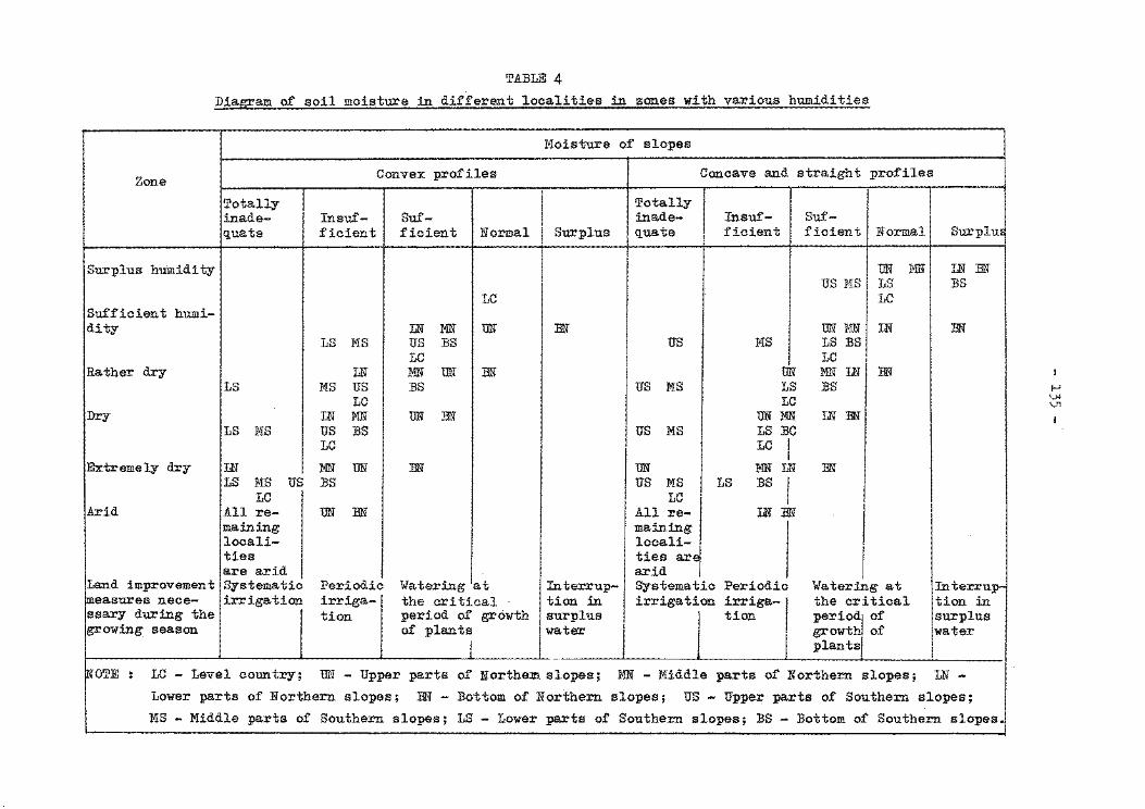
TABLE 4

Diagram of soil moisture in different localities in zones with various humidities

Moisture of slopes

Zone I Convex profiles Concave and straight profiles

Totally Totally inade- Insuf- Suf- inade-

I Insuf- Suf-

quate ficient ficient Normal Surplus quate ficient ficient I Normal SurplUE

Surplus humidity UN MU LN BN US MS LS :BS

LC LC Sufficient humi-~

I I UN }JN I LN I dity LN MN UN BN BN LS MS us :BS us MS LS :BS

LC LC Rather dry I I LN MN UN BN UN :1-lN LN I BN

LS MS us :BS us MS LS :BS I LC LC

Dry I I LN MN UN BN UNMN LN BN LS MS us :BS us MS LS :BC

LC LC I Extremely dry ILN I MN UN BN UN MN LN BN

LS MS us :BS us MS LS :BS I LC LC Arid !All re- UN BN All re- LN BN

maining maining locali- locali-ties ties ar, are arid arid

Land improvement Systematic Periodic Watering at Interrup- Systematic Periodic Watering at Interrup !measures nece- irrigation irriga-~ the critical · tion in irrigation irriga- the critical tion in ssary during the I tion period of growth surplus

I tion period' of surplus

growing season of plants water growth of water

I plants

~OTE : LC - Level country; TIN - Upper parts of N.orthem slopes; MN -Middle parts of Northern slopes; LN -

Lower parts of Uorthern slopes; J3N - :Bottom of Northern slopes; US- Upper parts of Southern slopes;

MS -Middle parts of Southern slopes; LS - Lower parts of Southern slopes; :BS - :Bottom of Southern slopes.

I I-' \jJ

V1

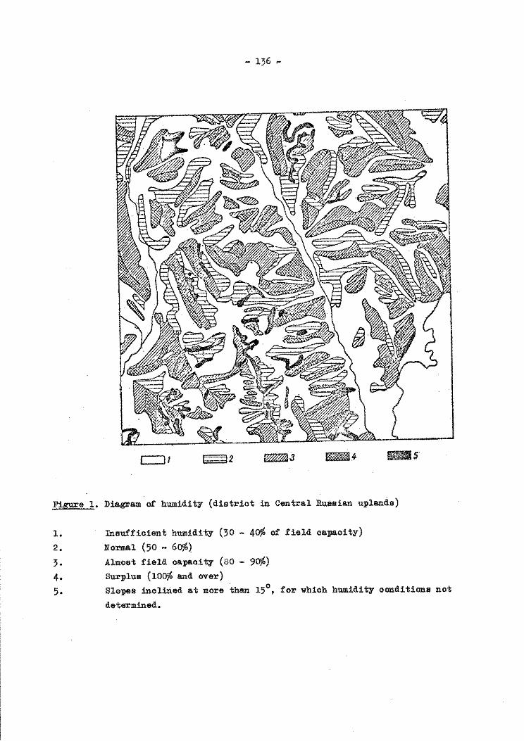
Fi~e 1.

1.

2.

3-4. 5.

- 136 -

c:::J 1 ~2 ~3 ~.4 lills·

Diagram of humidity (district in Central Russian uplands)

Insufficient humidity (30 - 4o% of field capacity)

Normal {50 - 6o%)

Almost field capacity (80 - 9o%)

Surplus {lOo% and over)

Slopes inclined at more than 15°, for which humid! ty conditions not

determined.

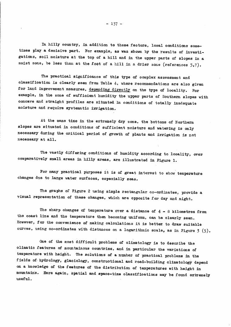
- 137 -

In hilly country, in addition to these factors, local conditions some­times play a decisive part. For example, as was shown by the results of investi­gations, soil moisture at the top of a hill and in the upper parts of slopes in a moist zone, be less than at the foot of a hill in a drier zone (references 5,7).

The practical significance of this type of complex assessment and classification is clearly seen from Table 4, where recommendations are also given for land improvement measures, depending directlz on the type of locality. For example, in the zone of sufficient humidity the upper parts of Southern slopes with concave and straight profiles are situated 'in conditions of totally inadequate moisture and require systematic irrigation.

At the same time in the extremely dry zone, the bottoms of Northern slopes are situated in conditions of sufficient moisture and watering is only necessary during the critical period of growth of plants and irrigation is not necessary at all.

The vastly differing .conditions of humidity according to locality, over comparatively small areas in hilly areas, are illustrated in Figure 1.

For many practical purposes it is of great interest to show temperature changes due to large water surfaces, especially seas.

The graphs of Figure 2 using simple rectangular co-ordinates, provide a visual representation of these changes, which are opposite for day and night.

The sharp changes of temperature over a distance of 4 - 8 kilometres from the coast line and the temperature then becoming uniform, can be clearly seen. However, for 'the convenience of making calculations it is better to draw suitable curves, using co-ordinates with distances on a logarithmic scale, as in Figure 3 (5).

One of the most difficult problems of climatology is to describe the climatic features of mountainous countries, and in particular the variations of temperature with height. The solutions of a number of practical problems in the fields of hydrology, glaoiology, constructional and road-building climatology depend on a knowledge of the features of the distribution of temperatures with height in mountains. Here again, spatial and space-time classifications may be found extremely useful.

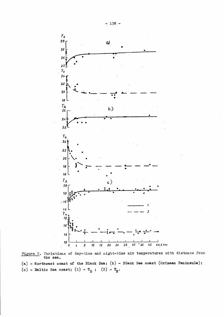
TA t.8"

26

2.2

TH 24-

Z2

20

18

TA

• • "t....

":" 138 -

a)

•

-- ·- --

..

__. •• •

• •

..__ - -- --

"~ . . .. . 24 • • •••

:u.

b)

TH 24

2.2 ~" •

• • 201-\.

18 I 16

18

,, 16

14 TH 18

16

J"-•

•

•

-• .. •

•

~--..:__ • ~ -- --:.-; 1-t •

•

..___ •

• •

-·--

• • • • ,

---2

--. !....a • •

.... .--. -f2L_~-L~--~~-7~~~~~«17

0 " 8 12 16 2.0 24 28 ~2 ~0 ~4 s 1</>f

Figure 2. Variations of day-time and night-time air temperatures with distance from the sea.

(a) -Northwest coast of the Black Sea; (b) -Black Sea coast (Crimean Peninsula);

(c) - Baltic Sea coast; (1) - TD ; (2) - TN.

- 1.~9 -

6

-36 5

-32 4

-·24 -----~---------3

-20 ~--------2

-1&

-12

-8 :---------- I

-4

L----~----~--~~---~-~ -2 o 4- 8 12 16 20s xM 0,01 -1 0.1

0 1

8

s

~

3

2

I

ttg s 10 kM

Figure 3. Variations of the average of the absolute minimum air temperatures for each year, with distance from the sea. (a) - Distance in km; (b) - Distance on a logarithmic scale; (1) - South-east coast of the Black Sea; (2) - South coast of the Crimea; (3) - Baltic Sea coast; (4) -Coast of the Gulf of Finland; (5) - The banks of Lake Onega; (6) - The banks of Lake Baikal.

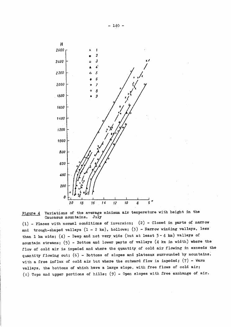
- 140 -

,., 2600 r X 1

11 2

2400 1- c 3 xl

• 4' I 2 200 I- e:. 5

xfx • 6 2000 1- et 7 t/

0 8 /"' 1800 1- • 9 X <,c. .,.,

I

1600 1- I I 1400r 1./' 1200

1000

800

600

40lJ

200

0. __J

20 18 16 14- 12 10 8 50

Figure 4 Variations of the average minimum air temperature with height in the Caucasus mountains. July

(1) - Places with normal conditions of inversion; (2) - Closed in parts of narrow

and trough-shaped valleys (1- 2 km), hollows; (3) -Narrow winding valleys, less

than 1 km wide; (4) - Dee:p and not very wide (but at least 3- 4 km) valleys of

mountain streams; (5) - Bottom and lower parts of valleys (4 km in width) where the

flow of cold air is impeded and where the quantity of cold air flowing in exceeds the

quantity flowing out; (6) - Bottoms of slopes and plateaux surrounded by mountains,

with a free influx of cold air but where the outward flow is impeded; (7) -Warm

valleys, the bottoms of which have a large slope, with free flows of cold air;

(s) Tops and upper portions of hills; (9) - Open slopes with free exchange of air.

- 141 -

Figure 4 show$ exampl~s of the distribution of temperature with height for typical locations in vario~ mountainous regions (5).

One can hardly imagine the quantity of paper which would be needed to give this compact information for existing stations, in the form of ordinary figures. But even if this were done, the information would be found to be representative of certain points only, where observations are made. At the same time, for practical requirements, data are usually necessary not only (or even not as much as) at points where observations are made, but for areas in the region being studied or dealt with.

However, summarizing climatological data by means of classification under homogeneous headings requires objective definitions of this homogeneity and a knowledge of the space-time structure of the fields of the meteorological elements which it is intended to describe. Without this, systematic errors are possible, due to combining initial data which are not sufficiently homogeneous (10).

2. Taken as an example of the nomogram method, we may consider, the classifi-cation of the distribution in time of elements or compound elements, with regard to time and space variability, the establishment and use of relationships between complex statistics and simple statistics and the summarization of data, using the analogue form for their representation. Nomograms of this type indicate the possi­ble magnitude of the required probability of occurrence when the mean for a given period is known.

In view of the faot that at present there are no methods for making sufficiently accurate climatic forecasts (although they are urgently required), climatologists are obliged to fall back on statistical methods which enable the distribution and graphs of the probability of occurrence to be obtained from the basic statistical parameters.

Mean value n

- L xi i = 1

X

Standard Deviation

(] = rf (xi ji ~= 1

(1)

- i)2 (2)

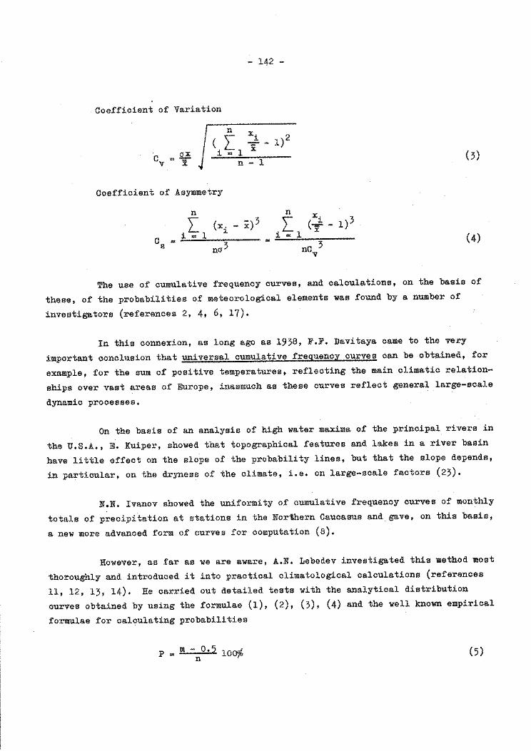
- 142 -

Coefficient of Variation

n x. ~

(i ~1 i -

CV £..! i n - 1

Coefficient of Asymmetry

n

L (x. - i)3

c = i "' 1 ~

na3 s =

1)2

n [ <~i - 1)3

i = 1 X

ne 3 V

(3)

(4)

The use of cumulative frequency curves, and calculations, on the basis of

these, of the probabilities of meteorological elements was found by a number of

investigators (references 2, 4, 6, 17).

In this connexion, as long ago as 1938, F.F. Davitaya came to the ve£y

important conclusion that universal cumulative frequency curves can be obtained, for

example, for the sum of positive temperatures, reflecting the main climatic relation­

ships over vast areas of Europe, inasmuch as these curves reflect general large-scale

dynamic processes.

On the basis of an analysis of high water maxima of the principal rivers in

the u.s.A., E. Kuiper, showed that topographical features and lakes in a river basin

have little effect on the slope of the probability lines, but that the slope depends,

in particular, on the dryness of the climate, i.e. on large-scale factors (23).

N.N. Ivanov showed the uniformity of cumulative frequency curves of monthly

totals of precipitation at stations in the Northern Caucasus and gave, on this basis,

a new more advanced form of curves for computation (8).

However, as far as we are aware, A.N. Lebedev investigated this method most

thoroughly and introduced i.t into practical climatological calculations (references

11, 12, 13, 14). He carried out detailed tests with the analytical distribution

curves obtained by using the formulae (1), (2), (3), (4) and the well known empirical

formulae for calculating probabilities

p (5)

...; 143 -

p m il'+T lOO% ( 6)

(7)

where m is the serial number of a term of the series, n is the number of observations in the series.

Based on these investigations A.N. Lebedev reached the conclusion that the best results are given by the empirical formula (8), recommended by G.A. Alekseev {1). In this connexion it is particularly convenient to make use of the graphico-analytical method proposed by G.A. Alekseev and tables for the calculation of probability in accordance with the formula:

p m - ~·~5 lOO% (8)

A.N. Lebedev came to the conclusion that "The application of empirical formulae requires the accurate quantitative determination of values of the magnitudes of phenomena which occur only rarely, including some which are not yet observed".

"The graphico-analytical method, developed by Alekseev, is of great practical and theoretical interest. By means of this method he succeeded in obtaining more reliable data for three basic parameters for distributions, C , a , x, at the expense · S X of very little technical effort. Being less accurate, use of this method enables the extremely cumbersome and labour-consuming calculations by the formulae (l) - (4) to be avoided" (13).

An example of the calculation of the probabilities from formula (4) is given in Table 5 (13), while a table for the calculation of the probabilities by G.A. Alekseev's formula is given in Annex 1.

The nomograms, constructed and analysed by A.N. Lebedev, for obtaining values having a given probability of occurrence, when the mean value is known, are extremely conveniex1t and compact but also contain a vast amount of information.

By classifying such nomograms, Lebedev succeeded in obtaining the prob­ability of occurrence of given values of many elements over very large terrirories such as for example, the European territory of the U.S.S.R. (12), and Africa (9, 14).

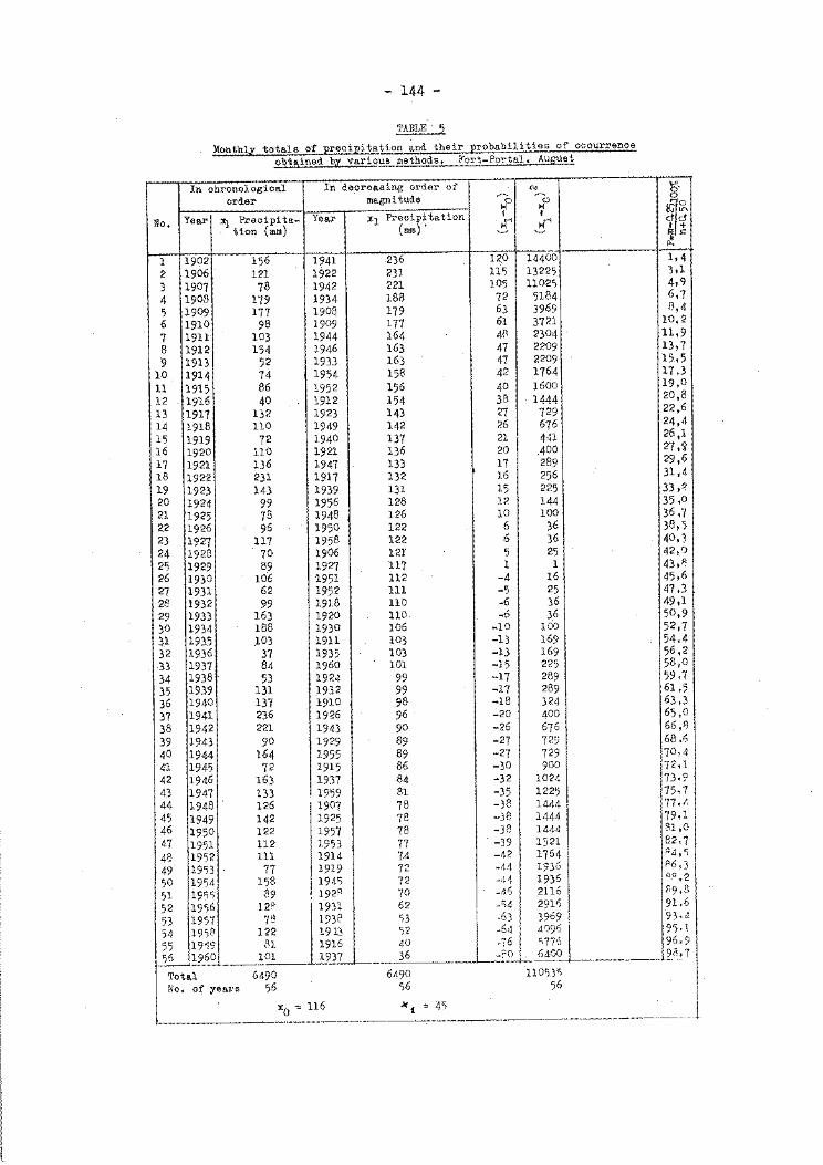
- 144 -

TABLE· 5_

Monthly totals of precipitation and their probabilities of occurrence

obtaine.d by various methods, Fort-Portal, Aucust

In chronological In decreasing order of N

order magnitude ~0 0 " H

Year x1 Precipitation I I No, Year x1 Preoipi ta- r-1 K'

tion (mm) (mm)· H ~ ~

1 1902 156 1941 236 120 14400 2 1906 121 1922 231 1i~ 13225 3 1907 78 1942 221 105 1102')

4 1908 179 1934 188 72 5184 5 1909 177 190$ 179 63 3969 6 1910 98 1909 117 61 3721 7 1911 103 1944 164 411 2304 8 1912 154 1946 163 47 2209

9 1913 52 1933 163 41 2209 10 1914 74 1954 158 42 1764 11 1915 86 1952 156 40 1600 12 1916 40 1912 154 38 1444 13 1917 132 1923 143 27 729 14 1918 llO 1949 142 26 676 15 1919 72 1940 137 21 441 16 1920 no 1921 136 20 400 17 1921 136 1947 133 17 289 18 1922 231 1917 132 16 256 19 1923 143 1939 131 15 225 20 1924 99 1956 128 12 144 21 1925 78 1948 126 10 100 22 1926 96 1950 122 6 36 23 1927 117 1958 122 6 36 24 1928 70 1906 121 5 25 25 1929 89 1927 117 1 1 26 1930 106 1951 112 -4 16 27 1931 62 1952 111 -5 25 213 1932 99 1918 110 -6 36 29 1933 163 1920 110 -6 36 30 1934 188 1930 106 -10 100 31 1935 103 1911 103 -13 169 32 1936 37 1935 103 -13 169 33 1937 84 1960 101 -15 225

34 1938 53 1924 99 -17 289 35 1939 13i 1932 99 -17 289 36 1940 137 1910 98 -18 324 37 1941 236 1926 96 -20 400 38 1942 221 1943 90 -26 676 39 1943 90 1929 89 -27 729 40 1944 164 1955 89 -27 729 41 1945 72 1915 86 -30 900 42 1946 163 1937 84 -32 1024 43 1947 133 1959 81 -35 1225 44 1948 126 1907 78 -38 1444 45 1949 142 1925 78 -38 1444 46 1950 122 1957 78 -38 1444 47 1951 112 1953 77 -39 1521 48 1952 111 1914 74 -42 1764 49 19'i3 77 1919 72 -4-1 193li

50 1954 158 194'i 72 -41 1936 51 1955 ·'39 ' 192Q 70 -46 2116 52 19'i6 12° 1 1931 62 _;4 2916

53 1957 79 1938 'i3 -63 3969 54 1951' 122 1913 'i2 -641 J096

55 1959 81 1916 40 -76 'i7/'S

56 1960 101 1937 36 .PQ 6400 -

Total 6490 6490 110'i3'i

No, of years 56 'i6 56

xo ~ 116 )C f = 45

f:j-0

,~ dd I + ~ s:: 11.

1,4 3,1 4,9 6,7 13,4

10,2 11,9 13,7 15,5 17,3 19,0 20,8 22,6 24,4 26,1 27,9 29,6 31,4 33,~

35,0 36.7 38,5 40,3 42,0 43,.A 45,6 47.3 49,1 50,9 52,7 54,4 56,2 58,0 59.7 61,5 63,3 65,0 66,1J 68.6 70,4 72,1 73·9 ?5.7 f1,<1

79,1 81,0 82.7 RJ,f)

P6,3 ~.Q t 2 89.8 91.6 9).J 9').1 96·9

- 2_il. 7

I

- -~ - --- ---------- ---- l

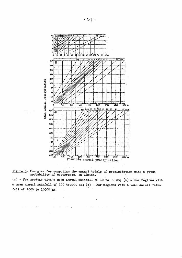
- 145 -

/llll .kl

:_71!

~

JD

w~~~~~~~~. 0 20 ~ 60 fA1 J00 .12f 1'10~ 200 210 240 Z60 280M~

~UH. 95 2000 .. oo ea '10 «~ lfll JO zo 10 ---:1rma:x 7

g ..-1 +' r3 +' •rl p,

•rl 0 (I)

J:

1 ~ ~

1800

1600

J41

1200

1000

eoo

600

D

)

0

f-6) I V I/ .I/ .I J ~

~ ~ I J /

/ V ~

/ 1/ ~ ~ ~ V

I I I~ ~ f'i /V 1 Jr.i~r2lL t/

~ ~ V V -

~ ~ V V

~ V 17 ~ IL/ j;; I/

V //

/

ov1 ~~~s L~~ -·- __

~~~~-;( Ll__._w.. t;:=C:~LL J.... 0 lj()O &!0 16ti0 zooo 2400

V /

V /

--· ~~·-2600 32001!11

Figure 5. Nomogram for computing the annual totals of precipitation with a given probability of occurrence, in Africa.

(a) - For regions with a mean annual rainfall of 10 to 90 mm; (b) - For regions with a mean annual rainfall of 100 to2000 mm; (c) - For regions with a mean annual rain­fall of 2000 to 10000 mm.

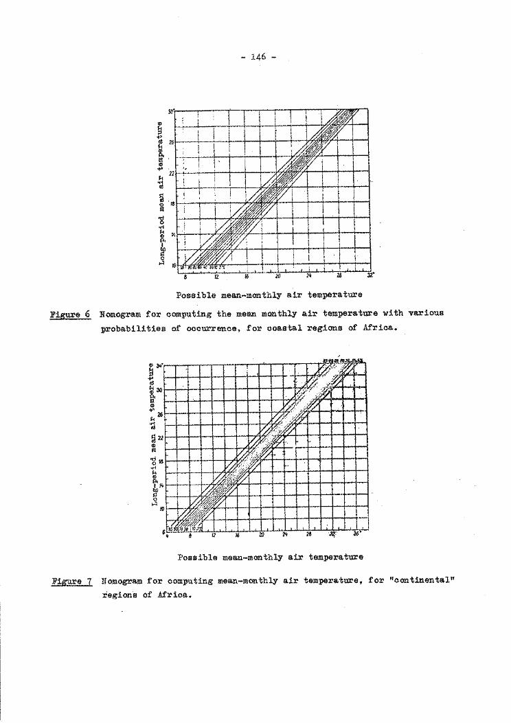
Cl)

~ al

~ Cl) .... !:: al

od 0 orl

- 146 -

~ ~~tl : i )(.~~/ i I ! I ! I I

0 H

Possible mean-monthly air temperature

Figure 6 Nomogram for computing the mean monthly air temperature with various

probabilities of occurrence, for coastal regions of Africa.

~ 34' . 1/~fS!~.~~ +> ./r// J .. L. ·•

al ~- a ~ ~~ ·~ .~ . & ~.}-· .· :;v.. El · :.;/ ;:,?./ I

$ !0/_,o;ti_ ~ 26 0. / · ... ;.2·~· .£...+--+--4--1--1

!: ~1~U l I FH ·~ ~z .

Cll I l7-~~ ~fJ# 1 "/-"(')'?~r/ ~ ~.w~~~~r-~~~~~-+-~~ 0 . / J.-:,)0

H 10 0-rw~ ~-~,~f~t~1-+-~~-+~~~+-~~ ~WA --J:jsi\?.JI"i",!.T.! e ,--- 8 12 u; ZIJ 2'1 ·- 2a-~·-w---as•

Possible mean-monthly air temperature

Figure 7 Nomogram for computing mean-monthly air temperature, for "continental"

regions of Africa.

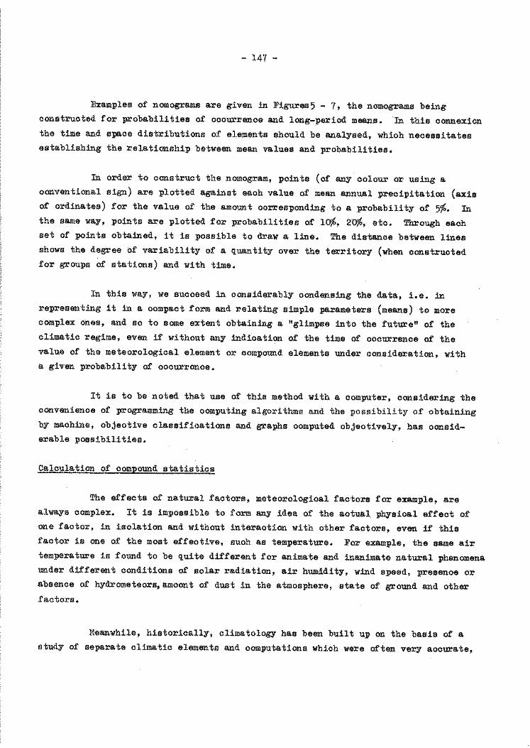
- 147 -

Examples of nomograms are given in Figures5- 7, the nomograms being constructed for probabilities of occurrence and long-~eriod means. In this connexion the time and space distributions of elements should be analysed, which necessitates establishing the relationship between mean values and probabilities.

In order to construct the nomogram, points (of any colour or using a conventional sign) are plotted against each value of mean annual precipitation (axis of ordinates) for the value of the amount corresponding to a probability of 5%. In the same way, points are plotted for probabilities of 10%, 2'0%, etc. Through each set of points obtained, it is possible to draw a line. The distance between lines shows the degree of variability of a quantity over the territory (when constructed for groups of stations) and with time.

In this way, we succeed in considerably condensing the data, i.e. in representing it in a compact form and relating simple parameters (means) to more complex ones, and so to some extent obtaining a "glimpse into the future" of the climatic regime, even if without any indication of the time of occurrence of the value of the meteorological element or compound elements under consideration, with a given probability of occurrence.

It is to be noted that use of this method with a computer, considering the convenience of programming the computing algorithms and the possibility of obtaining by machine, objective classifications and graphs computed objectively, has consid­erable possibilities.

Calculation of compound statistics

The effects of natural factors, meteorological factors for example, are always complex. It is impossible to form any idea of the actual physical effect of· one factor, in isolation and without interaction with other factors, even if this factor is one of the most effective, such as temperature. For example, the same air temperature is found to be quite different for animate and inanimate natural phenomena under different conditions of solar radiation, air humidity, wind speed, presence or absence of hydrometeors,amount of dust in the atmosphere, state of ground and other factors.

Meanwhile, historically, climatology has been built up on the basis of a study of separate climatic elements and computations which were often very accurate,

- 148 -

even scrupulously so, but which were in fact, carried out for separate elements.

Although the values of each element are necessary, in some cases, for practical

purposes, the period which may have been necessary in the initial stages of the

development of climatology, was excessively long and these averages for separate

elements still remain in many climatological summaries and works.

The quantity here determined is undoubtedly time-consuming when computa­

tions of compound quantities are performed manually. However~ methods for the

study of the compound effect of natural factors, described by two or more elementary

factors (for example, meteorological elements), elaborated in separate studies,

have been known for a long time.

The hydro-thermal coefficient due to G. T. Seljaninov (conditional

humidity· balance) which takes into account air temperature and precipitation, is the

classical example in this field which, so far, has not lost its significance.

According to his investigations, the sum of the temperatures during the period with

temperature above 10°C divided by 10 can be approximately considered as an index

of the expenditure of humidity in the field. Having taken the ratio of the total

precipitation to the aforesaid sum of temperatures for the same period we obtain

the conditional humidity balance for any interval of time. In this way the length

of arid periods (humidity balance for the month less than 0.5) and dry periods

(humidity balance for the month less than 1.0) was successfully estimated at more

than 300 stations in the Soviet Union, 317 stations in Asia, 261 stations in Africa,

548 stations in North and Central America, etc. (15).

The various methods of calculating effective temperatures, effective­

equivalent temperatures, etc. taking into account the complex influence of tempera­

ture, humidity, and wind speed is of considerable practical and scientific interest.

In recent years, with the increased requirements of aviation, for accurate

and detailed aviation-climatic interpretations of take-off and landing conditions,

compound statistics describing complex meteorological conditions for aviation, have

begun to be widely used. Such, for example, are the compound statistics for

combined height of base of low cloud below 200 m (h<200 m) and visibility less than

2 km (V<2 km), when the ranges of these two elements are given, or they are

observed simultaneously or one of the elements lies within the range associated with

any value of the other. This compound statistic is designated by the symbol K2oo

and after preliminary processing (combining the two given elements) all further

calculations are carried out using the quantity K200 • For example, the frequency

- 149 -

of the compound statistic, the·frequency of continuous duration of K200 with a given probability of occurrence, the maximum possible duration, etc. are calculated. (21).

In the Technical Regulations of the World Meteorological Organization (20), provision is made for the compilation of compound climatological summaries for airports (Annex 2).

In the summary model "A", the mean numbers of occurrence of combinations of various values of visibility and height of base of low 'cloud are given (Ns~5/8).

In the summary model "B", the distribution of wind speeds according to direction is given.

In the summary model 11 C11 , information with regard to complex weather conditions (height of base of low cloud 0-30, 30-60, 60-150 m and/or visibility 0.0 - 0.4, 0.4-0.8, 0.8 - 1.6 km) with certain values of wind speed and direction, is given.

However, producing these climatological summaries by hand requires a great deal of work and time. Thus, using Makhover 1 s data, in regions where complex weather conditions occur fairly frequently, an algorithm for preparing the tables and the times required is as follows:

(a) All tables are prepared by means of extracting statistics (elements) from the daily records of weather in the form of a series of messages in the synoptic code (KN-01);

(b) The tables are prepared by entering hourly values and remarks in the working table. After completion of the extractions, the totals are found and hence the means of a number of years of observation (5-year means and 10-year means). These mean values are transferred to the final version of the table.

(c) Algorithm of the summary model A. Combined cloud heights and visibilities are entered in each column. Time required - 4 hours for 1 calendar month. For 5 years' extractions the time required is 240 hours, and for 10 years' extraction, 480 hours.

(d) Algorithm of the summary model B. Extractions are carried out, as for model A, for wind speed and direction. Time required: 240 hours for 5 years' data and 480 hours for 10 years' data.

- 150 -

(e) Algorithm of the summary model C.

Before extraction is started the data are sorted according to cloud

height and/or visibility less than prescribed limits (i.e. cloud heights

below 150 m and/or visibility less than 1.6 km). These data are under­

lined with a coloured pencil (preferably using different colours for the

various ranges). Then, from the marked data a pattern is formed. The

necessary wind direction is found, then we find the column for the speed

and so, combining speed and direction we enter the _observed complex

conditions in the appropriate square. Time required - 5 hours per calendar

month. For 5 years' extractions, 300 hours; for 10 years 600 hours.

Hence, it is clear that with the previously prevailing hand processing

methods, it was quite impossible to compute complex quantities consisting of many

factors. These difficulties are removed if the summaries are prepared by computer.

But there remain difficulties associated with the collection of an adequate series

of statistics (especially with regard to the low frequencies of each of the compound

elements) and with the compact presentation to the results of calculations. It is

possible that the way to a solution to these problems lies in the following proced­

ures; searching for relationships between compound, complex and rarely occurring

quantities, and simple. frequently occUrring quantities, in this way obtaining an

adequate series of statistics, analogue and analogue-digital representation of the

final data. But here again there are many unsolved. problems wh:i.ch await investiga­

tion by means of computer.

Thus methods for a s:ummarized, compact representationof data, methods for

the representation of data not only at points of observation, but in the form of

fields of meteorological elements and complex quantitie~ computations of complex

quantities consisting of many factors relating to climatological effects, are

already giving good results.

The great value of such a method for summarizing and presenting information

in a compact form for scientific and applied purposes such as, for example, planning

the storage of agricultural crops, preparing a land survey, building towns, construc­

tion and operation of aerodromes, roads and electric transmission lines, transport,

etc. is obvious. But present day climatology, equipped with powerful computing

_techniques, should speedily and confidently introduce known progressive methods and

relentlessly develop new methods.

- 151 -

REFERENCES

1. Alekseev G.A. Graphanalytioal means of determination of the parameters of distribution curves and their raduo·tion to long periods of observation. GGI Proceedings, No. 73, 1960.

2. Baranov A. I. Low-air temperatures in Crimea. Annals of the State Nikitskij Botanical Garden, Vol. XVII, No. 3, 1923.

3. Voejkov A.I. New data on daily amplitude of the air temperat'ure, parti­cularly under. the influence of the topographic conditions. Selected essays, Vol. III, Izd. Akad. Sciences of the u.s.s.R., Moscow-Leningrad, 1952·

4. Gol 1oberg I.A. Tabulation of the probability of various meteorological elements. Publications of the Main Geophysical Observatory (GGO), No. 85 1958.

5. Gol'oberg I.A. Mioroclimate of the U.S.S.R. Gidrometeoizdat, Leningrad, 1967.

6. Davitaja.F.F. Climate zones of the grapes in the u.s.s.R. Methods of agroclimatic zoning. Gidrometeoizdat, Leningrad~Moscow, 2nd edition, 1948.

7. Zubenok L. I. Moist.ening characteristics· of the territory of the U. s. S.R. GGO Publications; No. 179, 1965. ·

8. Ivanov N.N. The precipitation probability curves for the steppe and forest steppe belts of the European territory of the U.S~S .. R. Annals of the Geroen Pedagogic Institute, No. 73, 1948.

9. Climatic guide to Africa, Part I. Air temperature, precipitation, Edited by Dr. Lebedev. Gidrometeoizdat, Leningrad, 1968.

10. Kljukin N .K., Sapoznikova S.A., Filippov V. V. About transforming the main climatologioal.conoepts into calculation methods by means of computers. Proceedings of the Institute of Scientific Research in Agroolimatology, No. 46, Gidrometeoizdat, 1967.

- 152 -

11. Lebedev A.N. Reliability of the dates at which the mean air tempe~ature

over virgin and fallow lands goes through 0, 5, 10 and 15° in the

springtime. Proceedings of the Main Geophysical Observatory, ,o. 65 (127),

1956.

12. Lebedev A.N. Diagrams and charts for calculation of climatic character­

istics of different probability over the European t~rritory of the

U.S.S.R. Gidrometeoizdat, Leningrad, 1960.

13. Lebedev A. N. Application of the nomograms method to the investigations

of climat~o regularities in tropical and equatorial latitudes. Proceed­

ings of the Main Geophysical Observatory, No. 182, 1965.

14. Lebedev A.N. Certain peculiarities of the thermal regime of Africa.

Proceedings of the Main Geophysical Observatory, No. 182, 1965.

15. World agroolimatic guide. Gidrometeoizdat, Leningrad-Moscow, 1937·

16. Sapoznikova S.A. Microcli~ate and local climate. Gidrometeoizdat,

Leningrad, 1950.

17. Sapoznikova S.A. On the methodics of calculation of the probabi11ty of

ten day average air temperatures. Central Weather Institute (CIP)

Publications, No. 41 (68), 1955.

18. Seljaninov G.T. On the methodics of agricultural climatography,

Publications of agricultural meteorology, No. XXII, 1930.

19. Seljaninov G.T. Special;i.zat:j.on of tl).e agricultural districts on the

climatic basis. Map of the agroclimatic zones of the u.s.S.R. "Plant

growing in the U. S. S.R." Vol. I, Part I, Leningrad, 1933.

20. Technical Regulations of the World Meteorological Organization.

Meteorological Service for International Air Navigation, Vol. II, Geneva

1966.

21. Titov V.I. Probability of the meteorological conditions affecting air

navigation and their stability in the European territory of the u.s.s.R.

- 153 -

Publications of the Institute for Scientific Research in Aeroclimatology,

No. 46, 1967.

22. Cottle, H.J. Vegetation on North and South slopes of mountains in

South-Western Texas. Ecology, Vol. 13, No. 2, 1932.

23. lOO Frequency curves of North American rivers. Kuiper E.J., Hydraul.

Div. Proc. Amer. Soc. Civil Engrs. 1957, 83 No. 15.

Annexes : 2

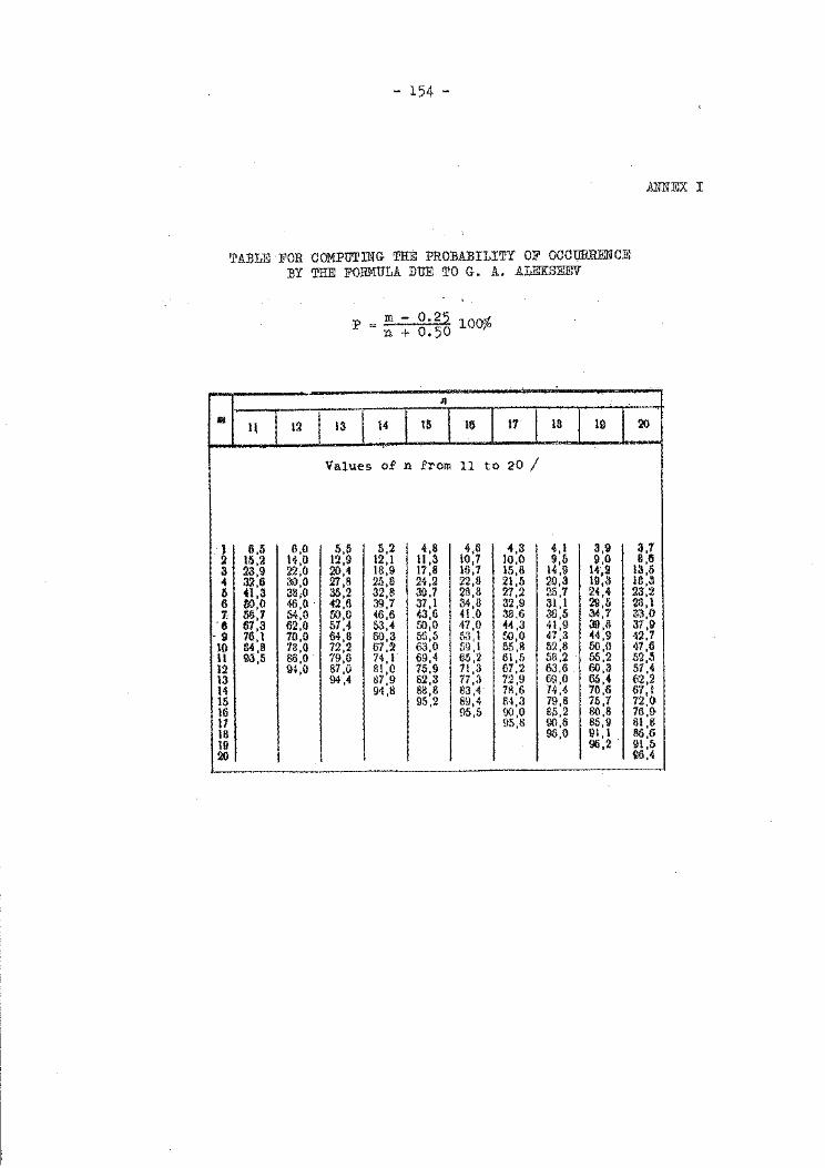
A

·~ 3 4 5 6 7:

'8 • 9 10 11 12 13 l4 15 16 11 18 19 20

- 154 -

ANNEX I

TABLE FOR COMPUTING THE PROBABILITY OF OCCURRENCE BY THE FORMULA DUE TO G. A. ALEKSEEV

lOo%

n

1\ 12 13 I 14 15 16 17 16 19 20

Values of n from 11 to 20 /

6,5 6,0 5,5 5,2 4,8 4,6 4,3 4,1 3,9 3,7 15,2 14,0 12,9 12,1 11,3 10,7 10,0 9,5 9,0 11,15 23,9 22,0 20,4 18,9 17,8 16,7 15,8 H,9 Hl! 13,5 32,6 30,0 27,8 25,6 24,2 22,8 21,5 21),3 19:3 13,3 41,3 38;0 35,2 32,8 30,7 28,8 27,2 25,7 24,4 23,2 00,0 46 0 . ~2.6 39,7 37 ,I 34,6 32,9 31,1 29,5 23,1 58,7 M:o W,O 46,6 <13,6 41,0 38,6 38,5 34,7 330 67,3 62,0 57,4 53,4 50,0 47,0 4<1,3 41,9 39,8 31:\) I

76,1 70,0 M,B 60,3 &.,5 M,! 000 47,3 44,9 42,7 !14,8 78,0 72,2 6'1,2 63,0 li9,1 55) 52,6 50,0 47,6 93,5 86,0 79,6 74, I 69,4 tl5,2 61,5 5>'3,2 55,2 52,5

9~,0 87,0 81,0 75,9 71,3 67,2 63,6 60,3 57,4 94,4 il7,9 62,3 77,3 72,9 69,0 65,4 62,2

94,!1 88,8 83,4 71l,6 74.~ 70,6 67,1 95,2 89,4 84,3 79,8 75,7 72,0

95,5 90,0 81i,2 80,8 76,9 95,8 00,6 85,9 81,8

96,0 91 ,I 86,6 I 00,2 91,1) I ~.4

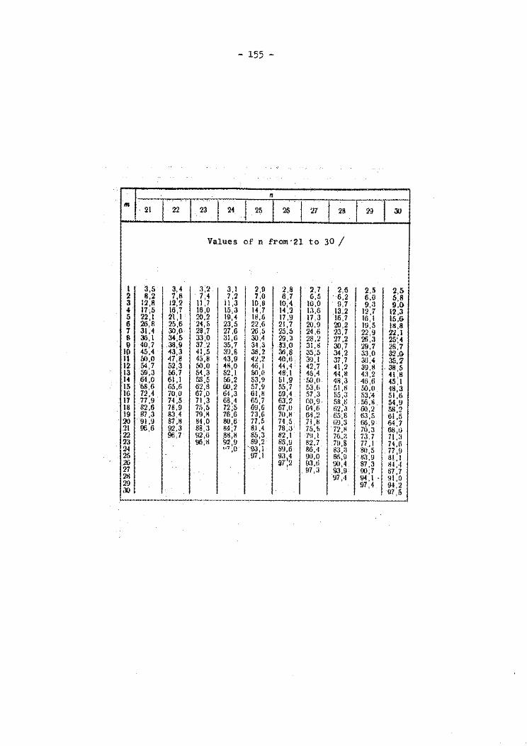
- 155 -

n ,. . 21 2'2 23 I 24 ~ 25 26 Zl 28 I 29 I 30

Values of n from·21 to 30 /

1 3,5 3,4 .1,2 3,1 2,9 :2,8 2,7 2,6 2,5 2,5 2 8,2 7,8 7 4 7,2 7,0 6,7 6,5 6,2 6.,0 5,8 3 12,8 12,2 11 :7 11,3 IO,tl 10,4 10,0 9,7 9,:! 9,0 4 17 5 16,7 16,0 15,3 14,7 14,2 1.1,6 13.,2 12.7 12,3 ' 5 22:1 21,1 20,2 19,4 18,6 17,9 17,3 16,7 Hl,l 15,& 6 26,1! 25,6 24,5 23,5 22,1) 21,7 20,9 20,2 1\1,5 18,8 ., 31,4 30,0 '..!8,7 27,6 26,5 25,5 24,6 23,7 22,9 2'~, I • 8 361 34,5 33,0 31 ,ll 30,4 29,3 28,2 27,2 26,3 25',4 9 40:7 38,9 37,2 35,7 34,3 ~3,0 31 ,S 30,7 29,7 28,7

10 45,4 -43,3 41,5 3\l,B 38,2 36,8 35,5 34,2 3.1,0 32,(> 11 50,0 47,8 45,8 43,9 42,2 40,11 39, I 37,7 3H,4 35, 2' 12 54,7 52,3 50,0 4!!,0 46, I '44,4 42,7 41,2 39,!1 . 38,5 13 59,3 56,7 54,3 52,1 50,0 48, I 46,4 44,11 4:!,2 41 ,B 14 64,0 61,1 58,5 56,2 53,9 51,9 50,0 48,3 46,6 -45, I 15 68,6 65,6 62,8 60,2 57,9 55,7 53,(i 51 ,H 50,0 48,3 16 72,4 70,0 67,0 64,3 61 ,!1 59,4 57,3 55,3 53,4 51,6 17 77 9 74,5 71,3 68.,4 !i5,7 !i3,2 li0,9 59 8 56,S 54,9 18 82:6 78,9 75,5 72;5 139,6 67,0 64,6 fi2::l 00,2 58,2 19 87,3 83.4 79,11 76,6 73 6 70,H 6H,2 65,8 63,5 . 6\ 5 20 91,9 87,8 84,0 80,6 77:5 74,5 71 ,ll Ci9,3 56,9 64) 21 96,6 92,3 88,3 84,7 8.1 ,4 7S,a 75.,5 72,H 70,3 68,1) 22 96,7 !12,1i .8H,H 85 3 82, I 7\1, I 76.:l 73,7 71,3 23 96;tl 92 !J 89:2 !lS,H B2 7 79 s 77.,1 74,6 24 1•7:0. 93,1 89,6 86:1 83::1 80,5 77 ,!I 25 .!J7 ,I 93,4 \10,0 135,1.1 83 9 81, I 26 97,2 !13,1i \)(1,4 87:3 ~4 ,-I : 27 !17,3 93,9 \)(), 7 87,7 2tl !J7 ,.1 !If I · 9!,0 2\l 97:4 9·1,2 30 !17,5

~-

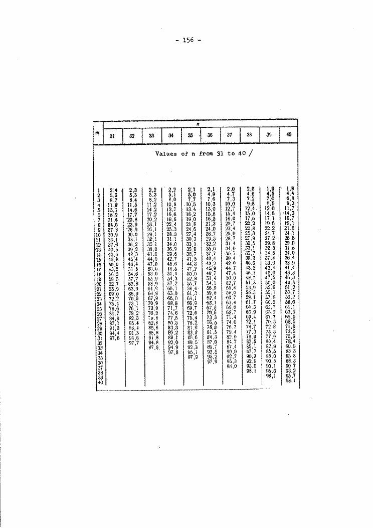
- 156 -

n

m 31 32 33 34 35 36 37 3S 39 40

Values o£ n from 31 to 40 /

1 2:4 . 2,3 . 2,2 2,2 2'1 2,1 2,0 2,0 1,9 . l,ll 2 5,6 5,5 5.3 5,1 s:o 4,9· 4,7 4,6 4,5 4,4 3 8,7 8,4 8,2 8,0 7,7 7,6 7,3 7.2 7,0 6,8 4 11,9' 11,5 11,2 10,8 10,5 10,3 10,0 9;8 9,5 9,3 5 15,1 14,6 14.2 13,7 13.4 13,0 12,7 12,4 12,0 11,7 6 18,2 17,7 17,2 16,6 162 15 8 15,4 15.0 14,6 •14,2 7 21.~ '20,8 20,2 19,6 19:0 18:5 18.0 17,6 17,1 16,7 B 24.6 23,9 23,1 22,4 21,8 . 21,3 20,7 20,2 19,6 19,1 !J 27.8 26.9 26.1 25,3 24.6 24.0 23.4 22,8 22.2 21.6

10 30.9 30.0 29.1 28.3 27,4 26,7 26,0 25,3 24,7 24,1 11 . 34,1 33,1 32.1 31.1 30,3 29,5 28,7 :n .9 '27,2 26,5 12 37,\3 36,2 .353 34.0 33.1. •32,2 31.4 30,5 29.8 29,0 13 40.5 39,2 38.0 36,9 35~9 35,0 34,0 ,33,1 .12,3 31,5 14 43.6 42,3 41.0 39,8 38,7 3i,7 36.i 35,7 34,8 34,0 15 46:8 45:4 44,0 42,7 41,5 40,4 39.4 38.3 37,1 36,4 16. 50.0 48,4 47.0 45.6 44,3 ·43,2 42.0 40.9 39,9 38.9 17 53.2 51.5 so.u 48.5 47.2 45',9 44,7 4.'!,5 42,4 41,4 18 56,3 54.6 . 53.0 51,4 so:o 48,7 47,4 4G, I 45,0 43.1)

19 .59,5 57,7 55.9 54,3 52,S 51,4 50.0 48,7 ·47 ,5 4fi,3 20 62.7 . 60.8 58,9 57.2 55,7 54.1 52,7 51,.) 50,0 48.8

21 65.9 63,9 61 .~ 60.1 5!l,4. 56,9 5.5.4 53,9 52,6 51,2

22 690 66,9 fi.l,S 63.0 61,3 59;5 [>l'i.O 56.5 55,1 53,7 23 72:2 70,0 67,9 {;6,0 . 64,1 62,4 <10. 7 59.1 &7,6 .56.2 24 75,4 73,1 70 9 68.8 66,11 -55,1 63,4 61.7 160.2 S8,ti

25 78,6 76,1 i3:9 71 ,T 69.7 67,6 M.O fA.3 62,7 61.1 26 81,7 79.2 76,9 74.,6 72,6 70,6 68.7 66.9 !)T>,2 03,6 27' 64,9 82,3 ;~.8 77,5 75,4 73,3 71.4 69.4 67,7 ffi,O

28 87.1 85.4 S:Z,R 80.5 .. 78.2. 7'6,(1 74,0 72,1 70,3 68,5 29 91,3 83,-l 85,8 83 3 81.0 78,8 76,7 R? 72.8 71,0

30 94,4 91,5 86,B 86:2 83,8 81.5 79.4 77.3 75.:3 73.5

31 97,6 94,6 91,8 89.·1 SR,6 84 .• 3 82.0 79.9 77,9 75,!:1 32 97,7 94,R 92,0 89.[> 87,0 R~.7 82.5 80.4 78,4 33 97 ,8. 94.9 92.3 8Y,7 87.4 85,1 82,9 80,9 34 97,8 95,1 92.5 90,0 87,7 t<.'i,5 83,3

."35 97,9 95,2 112.7 90;3 ss.o 85,8 36' 97,9 95.3 92,9 00,5 88,3 37 91?,0 95.5 93,1 90.7 38 98,1 9&.5 93,2 39 98,1 95,7 40 98.1 I '--·-- ··--····

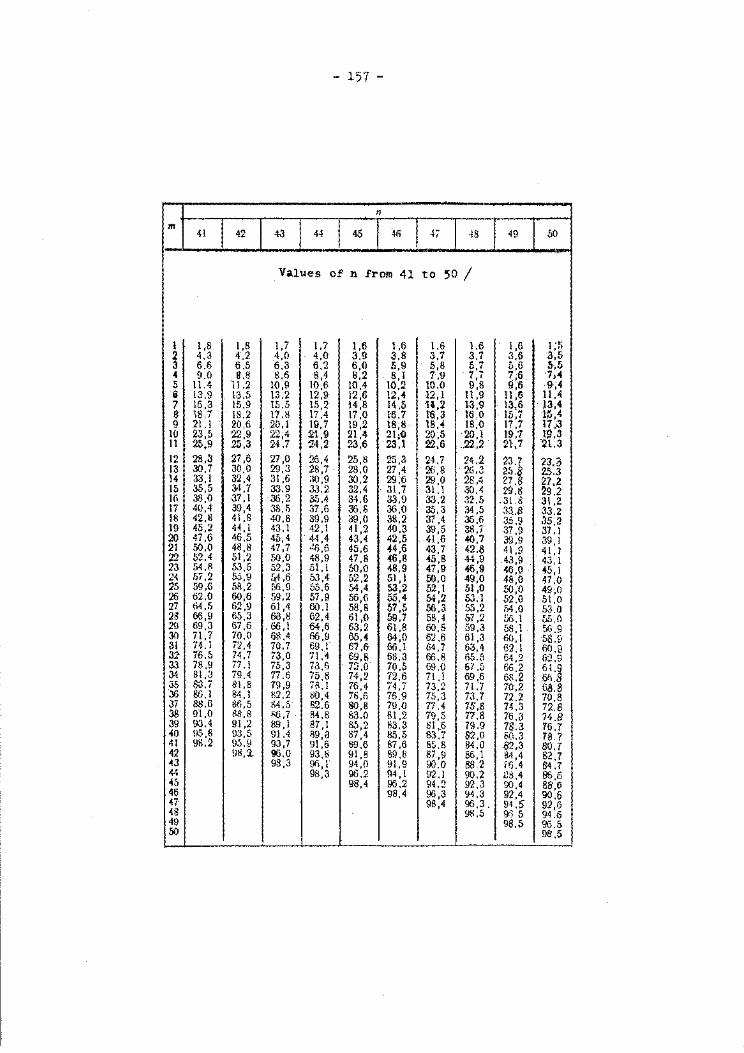
- 157 -

11

m I 42 1 43 I 44 I 45 I 4n I 4~ I ~8 I 49 I 50 41

Values of n from 41 to 50 /

1 1,8 1,8 I ,7 1.7 1,6 1,6 ],6 1.6 I ,6 1;5 2 4 . .3 4.2 4,0 4,0 3.9 3,8 3,7 3,7 3,.6 3,5 3 6,6 6.5 6.3 6.2 6,0 5,9 5,8 5,7 5,6 5·,5 4 9.0 8.8 !l,6 8,4 6,2 8,1 7,9 7,7 7;6 ·7,4 s 11.4 11.2 10,9 10,6 10,4 10,2 . 10.0 9,8 9,6 9;4 6 13.9 1.3,5 13.2 12,.9 12,6 12,4 ·12, 1 11,9 11,6 11 ·" 7 16,3 15.9 15,5 15,2 H,S 14,5 11,2 13,9 13,6 13,4 8 18,7 18.2 17,8 17,4 17,0 16,7 1$,3 16,0 15,i 15,4 9 21.1 20.6 . . 20,1 111,7 19,2 18 8 18,4 18,0 17,7 17;3

10 23,5 22,9 22;4 21.,9 21,4 21.:-o 2Q;5 20,1 19,7 1!},3 11 25,9 25,3 24,7 '24,2 23,6 '23,1 22,6 .. 22.2 21,7 21;3 12 28,3 27,6 27,0 26,4 25,8 25,3 24.7 24.2 23.7 23.3 13 30.7 30,0 29,3 28,7 28,0 27,4 26,8 2G.3 25.8 25.3 14 33, I 32,4 31,6 ao,9 30,2 29,6 29,0 28,4 27,8 27,2 15 35,5 34,7 33.9 33,2 32,4 31,7 31.1 30,4 29,8 29.2 )() 38,0 37,1 36,2 35,4 34.6 3.3,9 33.2 32.5 . 31.8 31.2 17 40,4 30,4 38,5 37,6 36,8 36,0 35 . .3 34,5 33 .. 8 33.2 18 42,1l 41,8 40,8 39,9 39,0 38,2 37,4 36,6 35,9 35.2 19 45,2 44,1 43,1 42, I 41,2 40,3 39,5 38,7 37,9 37' l 20 47,6 46,5 45,4 44,4 43,4 42,5 . 41,6 40,7 39,9 39,} 21 50,0 48,8 47,7 .!f),6 45,6 44,6 43,7 42.8 41,9 41, I 22 52,4 51,2 50,0 48,9 47,8 46,8 45,8 44,9 .43,9 . 43,1 23 54,B 5.>,5 52,3 51,1 50,0 48,9 47,11 «>,9 46,0 45,1 24 ,')7 ,2 55,9 [f1 ,6 53,4 52,2 51,1 ro.o 49,0 48,0 47,0 '25 59,6 58,2 56,9 55.6 54,4 53,2 52,1 51,0 50,0 49,0 26 62,0 60,6 59,2 57,9 56,6 55,4 54,2 53,1 52,0 51,0 '27 64,5 62,\l 61,4 60,1 58,8 57,5 56,3 55,2 .'i4,0 f>3.0 2g 66,9 65,3 68,8 62,4 61,0 59,7 5B,4 &7,2 56.1 55,0 29 69,3 67,6 . 66,1 64,6 63,2 61,8 60.5 59,3 58,1 513.9 30 71 '7 70,0 68,4 66,9 65,4 64;0 6:2,6 61,3 60, I 58.9 31 74.1 72,4 70,7 69,1 67,6 66,1 64,7 63.4 62,1 60.9 32' 76.5 74,7 73,0 71,4 69,8 68,3 66.8 65.5 64,2 62.9 33 78,9 77.1 75,3 73,6 72,0 70,5 69,0 67.5 66.2 61.9 34 81,3 79,4 77.6 75,t! 74,2 72,6 71, I 69,6 68.2 611.8 35 83,7 81,8 79,9 iR,l 76,4 74,7 73,2 71.7 70,2 68.8 36 86, I 84, I !\2.2 80,4 78,ii 76.9 75,3 73,7 72.2 70.8 37 88.6 86,5 !>4,5 82.6 80,8 79.0 7i .4 75,8 74,3 72.8 38 91,0 t\8,8 ~6,7 R-4,8 83,0 81,2 79,5 77,8 76.3 74.8 39 93,4 91,2 89, I 87,1 85,2 83,3 81,6 79.9 7S.3 76.7 -40 !l.:>,8 93,5 91,4 fl9,a 87,4 85,5 83,7 82,0 80.3 78.7 41 91>,2 95,9 93,7 91,6 89,6 87,6 85,8 84,0 82,3 80.7 42 !J8, 2. 96,0 93,8 91,8 89,8 87,9 86,1 84,4 82,7 ~3 98,3 00, I 94,0 91,9 90.0 88.2 f·!j. 4 84.7 44 98,3 96,2 94,1 92.1 90,2 C8,4 86,6 -45 98,4 96.2 94.2 92,3 00,4 88,D 46 98,4 96,3 94,3 92,4 90,6 47· 98,4 96,3. 94.5 92,G 48 9H.5 9<3 5 94.5 49 98,5 96.5 50 98.5

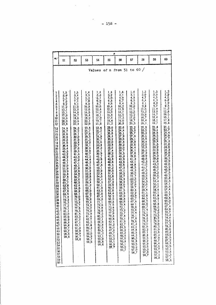
- 158 -

n

Ill' SI 52 53 54 55 56 57 58 59 6i}

Values of n from 51 to 60 /

1 1,5 . 1,5 1 ,4 I ,4 1,4 1,4 l ,4 1.3 1,3 1,3 2 3,4' 3,4 3,3 3,3 3,2 3,1 J, I 3,0 .3,0 2,9 3 5,3 5,2 5,2 ·5,1 5,0. 4,9 4,8 4,7 4,6 ~.5

4 7,3 7,1 7,0 6,9 6,8 6,7 6,5 6,4 6,3 6,2'

.5 9,2 9,1 8,9 8,7 8,6 8,4 8,3 8 .. 1. 8,0 7.9 6 11,2 11,0 10,8 10,6 10,4 10,2 10,0 9,8 9,7 9,5 7 13,1 12,9 12.6 12,4 12,2 11,9 11,7 11,6 11,4 11,2

8 15,1 14,8 i4,5 14,2 .14,0 13,7 13,5 13,3 13,0 12.8 9 17,0 16,7 16,4 16,1 15,8 15,.5 15,2 15,0 14.7 14.S

10" 18,9 18,6 18,2. 17,9 17,6 17.3 17,0 16,7 16,4 16.1 11 20,9 20,5 20,1 . . 19,7 !9,4 19,0 18,7 18,4 18,1 17.8 12 22,8 22,4 22,0 :.!1,6 21,2 20,8 20,3 20.1. 19.7 19.+

13 24,8 24,3 23,8 23,4. 23,0 22,6 22.2 21,8 21,4 21,1 14 26,7 26,2 25,7 25,2 24,8 24,4 23,9 23,5 23,1 22,7

15 28,6 2ll' I '21 ,6. 27' 1 26,6 25,1 25,7 25,2 24,8 24,4

16 30,6 W,O 29,5 28,9 j28,4 21'.9 27,4 26,fl 26,5 26,0

t1 32.5 3.1 ,9. 31,3 30,7 30,2 29,6 29.1 28,6 28,2 21,1

18 34,5 33,8 33,2 32,6 i32,0 31,4 30,9 30,4 29,8 29,3

19 36,4 3-S,T 35,1

~· 33,8 33,2 32,6 32,0 31,5 31,0

20 38.4 ·37.6 36,9 . :3 35,6 35,0 34,4 33,8 33,2 32,6

21 40,3 ·395 38,8 38,1 31.,4 a6,7 36,1 35,.3 34,9 34,3

22 42,2 4(4 40,7 JJ,9 . ~.2 38,5 37,8 37,2 36,6 36,0

23 44,2 43,3 42,5 41,7 41,0 40,3 39,6 30.9 3",3 37,6

24 46,1 45,2 44,4 4g,6 42,8 42,0 41,3 40,6 39,9 39,3

25 48,1 47,1 46,3 4 ,4 #,6 43,8 43,1 42,3 41,6 40,9

26 W,O 49,1 48 1 41,3 46,4 45,6 44,8 4 ~.o 43,3 42,6

'El 51,9 51,0 so:o 49,1 48,2 47,3 46,5 45,7 45,0 44,2

28 s:t9 52,9 51,9 50,9 W,O 49,1 48,3 47,5 46,7 45,9

29 55,8 54,!1 53,8 52,8 51,8 509 50,0 49,2 ·1.8,3 47,5

30 57,8 56,1 55·,6 M,6 53,6 52) 51,7 50,9 50,0. 49,2

31 1i9,7 58,6 57,5 55,4 55,4 54,4 o53,5 52,6 '51,7 50,8

32 61 7 60,5 59,4 58,.3 57,2 56,2 55,2 54,3 5.1,4 52,5

33 63'6 62,4 61,2 60,1 59,0 58,0 57,0 56.0 55,1 54,1

34 65:5 64,3' 63,1 61,9 60,8 597 58,7 57,7 56,7 S.'i,B

35 67,5 66,2 65,0 "638 62,6 61 :s 60,4 59,4 58,4 57,4

35 69,4 68,1 li7,0 65:6 64,4 63,3 62,2 51.1 60,1 59.1

37 71,4 70,0 63,7 (!7,4 662 65,0 63,9 52,8 61,8. 60,71

3S 73.3 71,9 10,6 69,3 68,0 66,8 6<">,7 64,5 6.'3,5 62,4

39 75,3 73,8 72,4 71,1 69,8 68,6 67,4 66,2 65,1 64,0

40 77,2 75,7 74,3 72,9. 71,6 70,4 69 I 6H,O 66,8 05,7

41 79,1 n.6 76,2 74,8 73,4 72,1 70,9 69,7 68,5 67,4

42 81.1 79,5 78,0 76,6 75,2 73,9 72,6 71,4 i0,2 6Y:O

43 83,0 81,4 79,9 78,5 77,0 75,7 74.4 73,1 71,9 70,7

44 85,0 83,3 81,8 80,5 78,8 77,4 76.1 74,8 73,5 7'2,3

45 86,9 8.5,2 83;7 82,1 80,6 79,1 77,8 76,5 75.2 74,11

46 88,8 87, I 85,5 84,0 82,4 81.0 79,6 i8,2 76,9 7b,6

47 90,8 89,1 87,-4 85,8 84,2 82,7 81,3 ;g,r, 78.6 77,3

4& 92,7 91,0 89,3 87,6 85,0 84,5 83,1 81,1\ 80,3 78,9

(!) 941 92,9 91,1 89,5 87,9 86,3 84,8 83,3 81,9 80.6

50 96:6 94,8 93,0 91,3 89,7 88,2 86,5 85,1 83,6 8'22

51 98,6 96,7 94,9 93,1 91.5 89,8 R8,3 86,8 8.5.3 83:-,J

52 98,6 96,7 950 93.3 91,6 90,:.> 88,5 87,0 85,.')

53 98,6 . oo:s . 95,1 93,4 91,8 90,2 88.7 87.2 54 98,6 96,9 96,1 93.5 91,9 90,4 t>tU

S.':i 9S".i 96,9 95,2 93,6 92,0 90,5

56 93,7 97,0 95,3 93,7 92 ,I

57 98.7 97,0 95,4 93,8

58 98,7 97,1 9.5 ,.'i

59 98,8 9i ,1 .

60 nS.IS

~~- ------- --

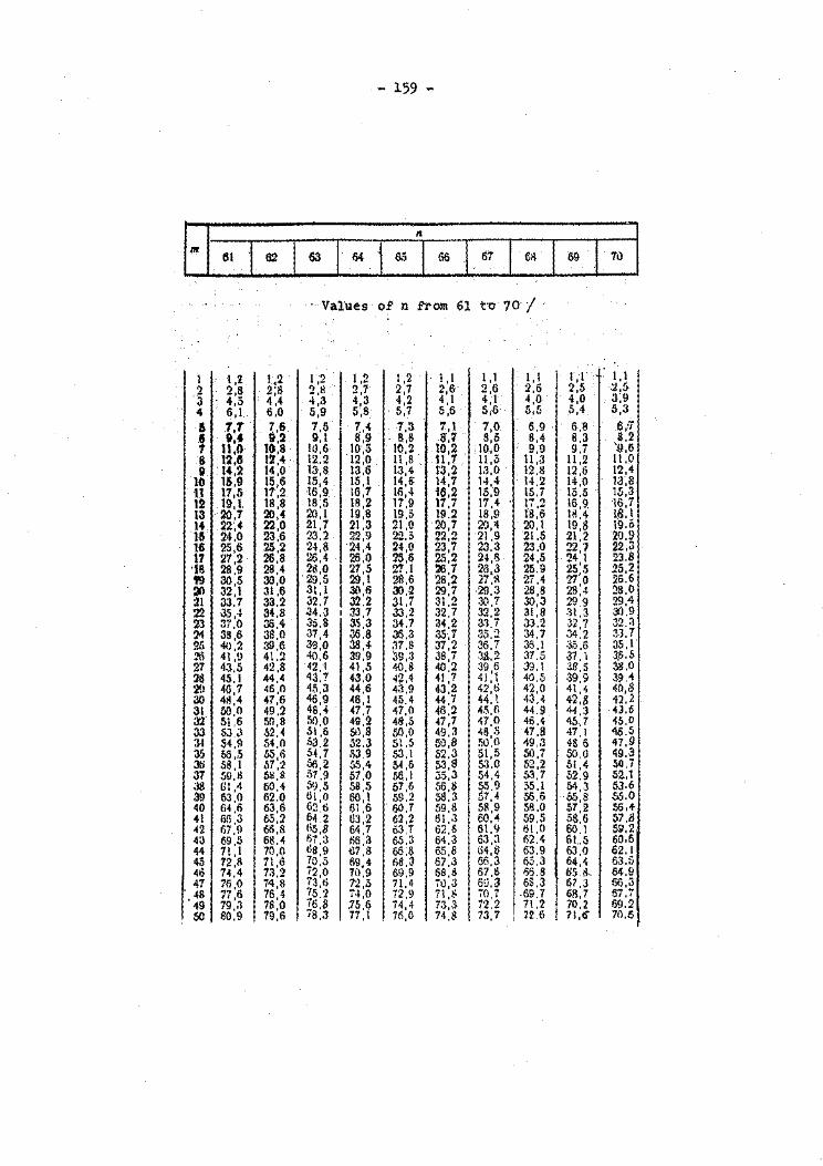
- 159 -

H 01 162 I., 1 .. j ""1 .. I" 1 .. 1 .. I,.] Values o.f' n from 61 to 70 /

t ~J 1,2 1 ? 1,2 1,2 1,1 1,1 1,1 1,1 1,1 2 2;8 2:ti 2,7 2,7 2,6 2,6 2,6 2,5 ·-~,5

3 4,5 4.4 4,3 4,3 4,2 4,1 4,1 4,0 4,0 . 3,9 4 6,1 6,0 5,9 s.s. 5,7 5,6 5;6 5,5 5,4 5,3

a .1.1 · 7,6 7,5 7,4 7,3 1,1 7,0 6,9 . . 6:8. 6;7 e flf 9,2 9,1 8,9. . 8,8 5.'1 8,5 8,4 8,3 8.2 7 ll :o 10,8 10,6 10,5 10,2 10,2 .to,o 9,9 9.7 '9.6' .8 12,8 12,4 12,2 12,0 11 ;8 n.1 · 11,5 ti,J 11.2 11.0 g '14,2 14,0 13·,8 13,6 13,4 1'3,2 1.3,0 12,1.1 12,6 12,4

10 15,9 15,6 15,4 15,1 14,8 14,7 14,4 14.2 14,0 13',8 t1 17,5 17 2 ·16,9 16,7 16,4 i6,2 15,9 15.7 15.5 . 1[1,3 12 19,1 1s:a 18 5 18,2 17,9 17,7 17,4 1.7.2 16,9, 16.7 13 '20,7 20,4 20:1 19,8 19,5 19.2 18,9 18,6 1il.4 18,1 14. ~.4 22,0 21,7 21,3 21,0 20,7 2".1;4 20,1 19,8 19.5 Ul 24,0 23,6 23.2 22,9 22.5 ~.2 21.9 21.5 21,2 20.!1 16 25,6 25,2 24,8 ~4,4 24,0 23,7 23.3 23,0 22,7 22.3 17 27 2 26,8 26,4 26,0 25,6 25,2 24,$ 24.5 24 1 23.8 ·Is 28:9 28,4 28,0 127,5 27.1 :26,7 26,3 25.9 25'.5 25,2 1'9 30,5 30,0 '29,5 29,1 28,6 28,2 27.~ 27.4 21'0 :26.6 :10 32,1 31,6 31.1 30,6 30,:2 29,7 29,3 28,8 28:4 28,0 :Zl 33.7 33,2 32,7 32.2 31.1 31.2 .'30,7 30,3 29.9 29,4 22 35 ·I 34,8 .'.14,3 I 33,7 33.2 32.7 32,2 31,8 :n.a ll.9 23 3(0 36.4 .35, S 3.S ,3 34,7 34,2 33,7 33.2 32,7 32.3 24 38,6 38,0 37,4 36.8 35,3 35,7 35.2 34.7 34.2 33.7 25 4(),2 39,6 39,0 38,4 37.8 37,2 ~6.7 36,1 :3.j,6 35, I 26 41,!.1 41,2 40.6 39,9 39,3 38,7 3&,2 37.5 37. l 3.5.5 27 4.3,5 42,8 42,'1 41,5 40.8 40,2 :39,6 39.1 38,5 38.0 2d 45.1 44.4 '13. ?' 43,0 42.4 41,7 41,1 40.5 ·'39,9 J!H 2!1 46,1 46,0 45,3 44.6 43.9 43,2 42,6 42,0 41,4 40,8 ao 41!,4 47,6 46,9 ~6.1 45.4 44,7 44,1 43,-4 42,8 42.2 31 50,0 49,2 48,4 lr7,7 17.0 46.2 4.5.6 44.9 4-(3 43.6 32 51,6 !i0,8 50,0 49,2 48.5 47,.7 47,0 46,4 45,7. 45.0 3J SJ.J ~2.4 51,6 51),8 50.0 49,3 48 .') 47.8 47.1 ~6.5 3-1 54,9 54.0 53,2 52.3 51.5 50,8 .~o~o 49,3 48 5 47,9 :).5 56,5 556 54,7 SJ.9 . 53.1 52.3 ~l·5 50,7 50.0 ~9.3 31i 5S,l 57'2 56,2 5.5,4 54,6 5.3,8 ;).>,0 52,2 51.4 S0,7 37 59.8 s~:s .'l7.9 57,0 5(\,1 .3.5,3 54,4 5.3, 7 52.9 52..1 38 Gl,4 60.4 5<),5 .58,5 57,6 56,1) rr::.9 55.1 54,3 53.6 39 63,0 62.() 61,0 60,1 .59,2 58.3 ;>7,4 56.6 55,8 55.0 40 64,6 63,6 62.1i 61,6 . 1)0, 7 59,8 58,9 58.0 57,2 56.+ 41 1'16,3 65,2 64.2 [)3,2 62,2 61,·3 60.<4 59.5 58.6 57.8 -42 67,9 60,8 li5 8 64 7 63.7 62,8 61,<:1 61,0 60.1 t)g,2 4;) 69,5 68,4 67':3 ti6'3 65,3 64,3 63,:1 62.4 61 .. 5 60.6 44 71,1 70,(1 t>s:9 u7:s 66.8 65,8 64.6 63.9 63.0 62. I 45 72,R 71,6 70 5 69 4 1)8,3 67,3 66,3 65.3 64,4 63.5 46 7-4,4 73,2 12:o 7t):9 69,9 68,11 67.S 156.8 65.8- 64.9 47 76,0 74,8 7'3,6 72,5 71.4 70,3 6!1.3 6S.3 67.3 66,3

·. 48 77,6 76,4 75 •) ~.\ 0 72,9 71,!.' 70,7 .69.7 68,7 67.7 49 79,.) 78,0 ZB:ii .75:6 74,4 7.1.3 i:2,2 71.'2 70.2 69.2 50 80,9 19,6 18,:3 77 ,I 76,0 74.8 73,7 ' 72.6 71 ,er 70.5

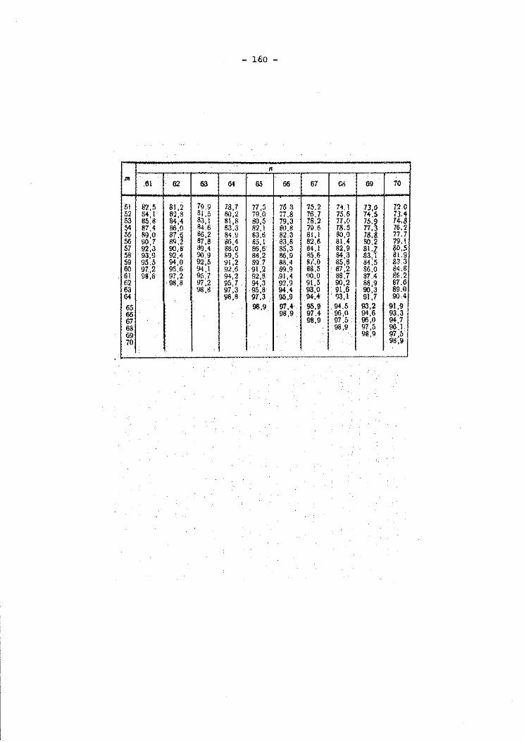
- 160 -

n -m

.61 62 63 64 65 66 67 6il 69 .· 10

51 b'2,5 81.2 79.9 iB, 7 77,5 76.:3 7S,2 74.1 73,0 72.0 52 84 I 8:2 8 81,5 80,:2 79,0 77.8 7.fi.7 75.6 74.5 13.4 53 lls:s 84:4 83, I 81,8 80.5 79.3 7.8.2 77,0 75.9 74-.8 54 87,4 86,0 84 6 83,3 82.1 80,8 70.6 T8.5 77.3 76.'2 55 R9,0 87.~ 86'2 84,\l 83,6 82.3 81, I 80,0 78.8 77.7 56 90,7 89.~ a1:a l\6,4 85,1 83,8 82,6 81,4 80.2 79,1 57 92,3 90,8 89,4 88,0. 86,6 85,3 84,1 82,9 81.] . 80.5 58 . 93,9 92,4 90,9 S9,5 88 .. 2 86,9 )35,6 84.,3 83,1 . 81.9 59 95,5 94,0 92,5 91,2 89.7 81!,4 S'i.O 85,8 84 5 . 83.3 60 97,2 95,6 94, I 9:2,6 91,2 89.9 88.5 ' 87,2 86:0 84.8' 61 98,8 97,2 9ii,7 94,2 92,8 .91,4 90,0 88,7 87.4 86,2 62 . 91:1,8 g~ ? 95,7 94,3 92,9 91,5 90,2 88,9 87,6 I,~

63 98,1:! 97,3 95,8 ~.4 93,0 . 91,6 90,.3 89.0 64 98,8 97,3 95,9 94,4 ''}3, 1 91,7 90;4

65 98,9 91,4 95,9 94,5. 93,2 91,9 66 98,9 97,4 '96,0 94,6 93,3 67 98,9 97,5 96,0 94,7 68 98,9 . 97,5 96,1 69 98,9 97,5 70 98,9

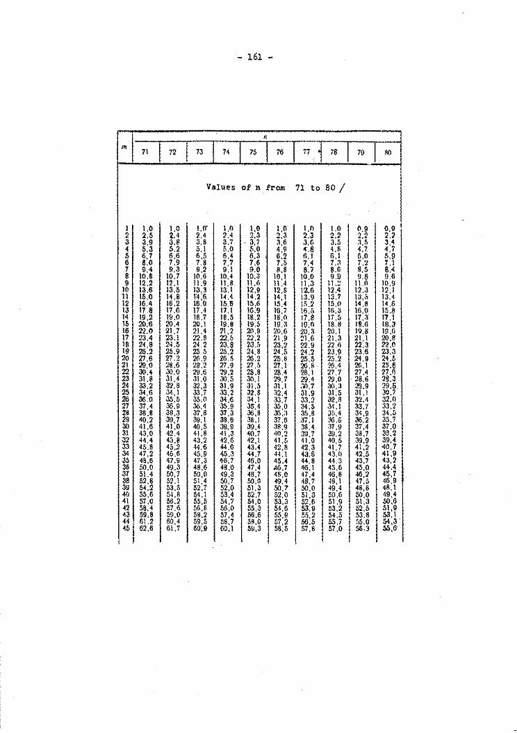
- 161 -

11

m. 71 72 1 73 74 75 76 77 78 71) 80

Values of n from 71 to 80 /

1 1.0 1,0 1,0' 1,0 1,0 1,0 1,0 1.0 09 0,9 I 2 2.5 2.4 2.4 2.4 2,3 2,3 2.3 2.2 2.2 2.2 3 3.9 3.8 3,8 3,7 . 3,7 3,6 3,6 3.5 :1,5 3,4 4 5,3 5.2 5.1 5.0 5.0 4.9 4.8 4,8 4.7 4,7 5 6,7 6.6 6.5 6.4 6.3 6.2 6,1 li,l 6,0 5,9 6 8,0 7.9 . 7.8 7,7 7,6 7 .. 'J 7,4 7.3 " ') 7,1 1, • . 7 9,4 9.3 9,2 9.1 9.0 a,s 8.7 8.6 S,5 S.4 8 10,8 10.7 10,6 10.~ 10.3 10, I 10.0 9.9 !1.8 !1.6 9 12,2 12 .I 11.9 11,8 11.6 11.4 11,3 11.2 11,0 IO,!l

10 13.6 13.5 13,3 13.1 l2,9 l2,S 12.6 12.4 12.3 12.1 11 15,0 14.8 1'4 6 J.4 .4 14.2 14.1 13.9 13.7 13,.; 13,4 12 16.4 16,2 15:o 15.S 15.6 15.4 1ii.2 15.0 14,8 14,6 13 17.8 17.6 17.4 17. I 10;9 16,7 16,5 16,3 16,0 15.8 14 19,2 19,0 18.7 18.5 18.2 1S,O 17,8 17,5 17 ,.3 17. I 15 20.6 20.4 20.1 19,8 19.5 19.3 l!J ,0 IB.8 18.6 18.3 16 2'2.0 21,7 21.4 21,2 20.9 20,6 :20.3 20. I 1!1.8 1!J .6 17 23.4 23.1 22.8 22,5 22,2 21.9 21.6 :21,3 :21,1 20.8 18 24,8 24.5 24.2 23,8 ~3.5 23,2 22.9 21.6 22,·3 2<?,0 19 26.2 25,9 25.5 25,2 24,8 24.5 24.2 23,9 23.6 2.1,3 20 Z7.6 27.2 26.9 26.5 26.2 25.8 25.5 25.2 24,9 24.5 21 29,0 28.6 2S.2 27.9 27,5 . 27,1 26.R ::?6.4 2G,1 25.6 22 30,4 30,0 29.6 :?9.2 28.8 28.4 28. I 27.7 27 .il 27 .o 23 31.8 31.4 31.0 30.5 30,1 29.7 29.4 29.0 28,6 2U 24 33.2 32,8 32,3 31,9 . 31,5 31.1 30,7 30,3 2!!.9 29.5 25 34,6 34,1 33,7 33,2 32.8 32.4 31.9 31,5 31,1 30,7 26 36.0 35,5 35,0 34,(i 34' 1 33,7 33.2 32.f! 32.4 32,0 27 37,4 36,9 36,4 35.9 35,4 35,0 34.5 34 .I 33,'1' 33,2 ~ 38,8 38,.3 37,8 37,3 36,8 35,3 35.8 3.'i,4 34,9 34.5 29 40,2 39,7 39,1 38,6 38,1 37,6 .37' 1 :l6.6 36.2 35,7 30 41.6 41,0 40,5 39,9 39,4 38,9 38.4 .37 .Y 37,4 37,0 31 43,0 42,4 41,8 41,3 40.7 40,2 39.7 39,2 38.7 3B 2 32 44,4 43.8 43.2 42,5 42,1 41,5 41,0 40,5 39.9 39:4 J3 45.8 45,2 44.6 44.0 ~3.>4 42,8 42.3 41,7 41,2 40,7 34 47.2 46.6 45,9 45,3 44.7 44,1 43.6 43,0 42,5 41,9 35 48.6 47.9 47,3 46.7 46,0 45.4 44,8 44.:3 -13.7 43,2 36 ,50,0 49,3 48.6 48.0 47.4 .16,7 46,1 45.6 45,0 44,4 37 51,4 50,7 50,0 49,3 48;7 48,0 47.4 46,8 46,2 45,7 38 52.8 52.1 51,4 50,7 50,0 49.4 48,7 48, I 47,5 46,9 39 5C2 53.5 52.7 52,0 51,3 50.7 50,0 49,4 48,8 48,1 40 55,6 54.8 54. l 53.4 52,7 . 52,0 51,3 50,6 50,0 49,4 41 57.0 56.2 55,5 54,7 54.0 53,3 52,6 51,9 51,3 50,6 42 58,4 57.6 56,8 56.0 55,3 54,6 53,9 53,2 52.5 51,9 43 .59.8 59.0 58,2 57,4 56.6 55,9 5.5,2 54,5 53,8 53,1 44 ' 61.2 60,4 59.5 58,7 58,0 57,2 56,5 55.7 :-,rl.o 54,3. 45 i 62,6 61,7 60',9 60,1 59,3 56,5 57,8 57,0 56.3 5S,6

'

- 162 -

n m

71 72 73 74 75 76 77 78 79 80

46 64,0 63,1 62,3 61,4 60,6 59,8 59,(1 58,3 .')7 ,6 56,8 47 65,4 64,5 63,6 62,8 61,9 61,1 60,3 ,)g,{i 58,8 ss. 1 48 66,8 65,9 65,0 64,1 63,3 62,4 61,6 (j(l,8 fiO, 1 59.3 49 68,2 67,2 66,3 65,4 64,6 63,7 62,9 62, I 61.3 60.6 50 69,6 68,6 67.7 66,8 65'9 65;0 64,2 63,4 ·62,G 61.8 51 71,0 70,0 69,1 68, l 67:2 66,4 65,5 64,7 63,8 63.0 52 72,4 .71 ,4 70 ,.4 69,5 61\,6 67,7 66,8 65,-9 G5,1 .64,3 53 73,8 72,8 71,8 m:, a 69,9. 69,0 68, I 67,2 fi5 4 65,5 54 75,2 74,1 .73;1 72,2 71,2 70,3 69,4 68,5 67:6 66.8 55 76,6 75,5 74,5 73,5 72,5 71,6 70,7 69,8 6H,!I 68,0 56 78,0 76,9 75,9 74,8 7B,9 72,9 -71,9 71,0 70,1 60,3 57 79,4 78,3 77,2 ;76,2 75.2. 74,2 '73,2 72,3 71,4 70,5 5ll 80.,8 79,7 78,6 77,5 76,5 75,5 74,5 73,6 72,7 71,1 59 62,2 81,0 79,9 78,9 77,8 76,8 .75,8 74,9 73,9 '.73.0 60 83,6 82,4 81,3 80,2 79,1 ,78,1 77,1 76, I 75,2 74,2 61 85,0 8.1,8 82,7 81,6 80,5 79,4 78,4 77,4 76,4 75.5 62 86;4 85,2 84,0 82,9 81,8 00,7 79,7 78,7 77.7 76,7 63 67,8 86,6 85,4 S4.,2 83, I 8!2,0 81,0 79,9 i8,9 i8,0 64· 89,2 87,9 86,7 85,6' 84,4 83,3 82,3 81,2 80,2 79,2 65 90,6 !19,3 88, I 86,9 85,8 84,7 83,6 82,Z. 81,5 80,4 6fi 92,0 90,7 !l9,5 AA,.l 87,1 86,1 84,8 1>3,8 ' 82,7 81.7 67 93,4 92,1 90,8 89,6 88,4 87,3 86, I 85,0 !?4,(1 82,9 6S 94,8 93,5 92,2 00,9 !i9-; 7 88,6 B7 ,4, 86,3 85.2 81,2 fi9 96,2 94,!\ ,93,5 92,3 91, I 89,9 88,7 87,6 86,5 85,4 ,70 07,6 96,2 94,9 93,6 92,4 91,2 90,0 8B.9 87,7 86,6 71 !19.0 97,6 96,3 95,0 W,7 92,5 91.3 90,1 89,0 ,87,9 72 99,0 '97,6 96,3 95,0 93,8 92.6 91.4 90,2 89,1 73 93,0 97,7 96,4 95,1 93,9 92.7 91,5 90,4 74 99,0 97,7 96,4 95,2 94,0 Y2,8 9l.,6 75 99,0 97,7 96,5 95,2 94.0 92,8 7(1 99,0 97,8 96,5 95,3 94 ,I 77 99,0 97.8 96,6 95.3 7R 99,0 97,8 96.G 19 !19 .1 ~7.8 80 ' 9:1

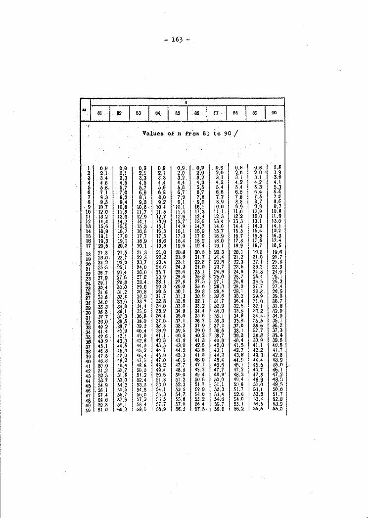
- 163 -

n M

81 . 1 82 1 83 1 8~1 R.') ., 86 I f7 AR 89 I 00 .

f

Values o£ n from 81 to 90 /

' 1 0,9 0,9 0,9 0,9 0,9. .. 0,9 . 0,9 0.8 O,ti 0,8 2 2, I 2, I 2,1 2 I 20 2,0 2,0 2.0 2.0 ·. 1.9 3 3,4 3,3 3,3 3:3 a:2 3,2 . 3,1 3.1 3,1 3.() 4 4,6 4,5 4,5 4,4 4.4 4,3 4,3 4,2 4.2 4,1 5 5,8. 5,7 5,7 5,6 5,.6 5,5 . 5,4 5,4 5,3 5.3 6 7' 1 7,0 6,9 6,8 6,7 6,7 «\.6 6.5 6.4 6.4 7 8,3 8,2 8,1 8,0. 7,9 7,8 7.7 7.6 7,5 75 8 9,5 9,4 9,3 9,2 9,1 ·90 8,9 8.8 8, 7 8,6

9 10,7 10,6 10,5. 10,4 10,1 to: 1 10,0 9.9 9,8 9,7 10 12,0 11,8 11,7 11,5 11,4 11,3 11;1 11,0 10,9 10,8 1l 13,2 13,0 12,9 12,7 12,6 . 12,4 12.3 12;2 12.0 11.9 12 14,4 14,2 14,1 13,9 13,7 13,6 13,4 13,3 13.1 1·>.0 13 .15,6 15,5 15,3 15,1 14,9 14,7 14,6 14,4 14,3 14. I 14 16,9 16,7 16,5 16,3 16,1 15,9 15,7 15,5 15,4 15,2 15 18,1 17,9 17,7 17,5 17,3 17,0 16,9 16,7 16.5 16.3 16 19,3 ·t9, I 18,9 18,6 18,4 18;2 18,0 17,8 17,6 17.-1 17 20,6 20,3 20,1 19,8 19,6 19,4 19,1 18,9 IS,7 18,5

18 21,8 21,5 21,3 .21,0 :20.8 20,5 :10,3 20,1 l!l.S l!:l.fl 19 23.0 22,7 22.5 22.2 21..9 21,7 21,4 21,2 21,0 211.7 10 24.2 :n.!l. 23,7 23,4- 23.1 22,8 22.1i 22.:! 2:l, I . 21.8 21 25.5 25, I 24.!1 24 .fl 24,3 24,0 n.7 :?a.fl 23.2 2'1.9 22 26.7 2!i,4 26,0 25,7 25.4 2b.l 24;!1 24,fi. 24.3 24,0

23 27.9 27.6 !?7,2 . 26.9 26.1l 26;3 26.0 2.S,7 25,4 25. I

24- 29:1 28,8 28.4 28.1 27,tl 27,{• 27, I 26.8 26.11 21'>.2 'lS 30.4 30.0 '29,() 29,3 :~.0 28,1; 28 .. 1 2S,O 27.7 27.4

2Ji 31.6 . 31.2 ;J0,8 80,5 30,1 29.8 29.4 '29. 1 28.8 28.& 27 32.8 3Z.4 32,0 31.7 31,3 30,!1 30.1\ 30,2 2<J.,9 29,(i

2S 34.0 33,6 :~,·u 32.6 32.5 32.1 .'31. 7 36.4 31,0 30.7 29 3.5 .. 3 34.8 34. i 34.0 J.3,fi 3.3,2 32,\J :.JVi I ,')2,} 31.8 30 35.5. 3G, I 3.5,6 35,2 34.8 3~.4 :.lq ,0 3J.G 33.2 :i2.!J 31 J7.7' 37,3 36.8 ~.~ 36,0 3[1,1\ 3[ •. 1 34.8 34,4 34,0

32 39.0 38 . .5 38.0 37,6 37.1 ~.7 36.3 3:;,9 :IS.5 35, I .13 ~0.2 39.1 39,:2 38.!! 38.3 37.9 37.4 37.0 36.6 ;%,2

.34 41.4 40:9 40,4 ,)9.9 3\!,5 39.0 38,6 38. I 37,7. 37,3

~ 42.6 42,1 4l.ll ~1.1 ·10,6 ,40,2 o'39. 7 39,3 38.8 3~.4 43.9 43,3 42.8 4'l " 41.8 41,3 40.\1 -40,4 30,9 39,5 .. ..~

37 45,1 44,5 ~4.0 4.1.5 43,0 4:.? 5 42,0 . 4 J.,'i 41.1 40,() 38 46.3 45,8 45.2 44,7 44.2 43:6 4\l,l 42.7 42.2 41.7 39 47,5 47,0 ~6.4 45,!! 45,3 44.11 4~ ,:I 4.3,8 4:3,3 42.8 40 46.8 48,2 47,6 47.0 46,5 '16.0 45,4 44 ,!1 44,4 ~3.9

41 50.0 49,4 48,13 4B,2 ~7. 1 47, I 46,fi 4!i, I 45.5 ·15,11 42 51.2 ~.7 SO,ll 41;.4 46.6 411.3 47,7 47.2 41i.1 "16.1 43 52.5 51.8 51.2 50,6 50,0 4!!.4 48,!1' 48.:3 47,8 q7 .2 44 53,7 .13,0 . 52.4 51,8 51.2 50,fi 50.0 4\1,4 4!!.\1 "!8. :1 45 . 54,9 54.2 53.ti .)3,0 52.3 .'il.7 51.1 Sfl,6 5(1,0 •19 •. 'i 46 '56.1 &5.5 54.8 f>1. I S3,!i !'i2.9 ~4!.3 ;",\, i 51.1 50.0 47 57.4 .'ili,7 55.0 5!:1,3 M,7. M.O .'i:3,4 51.ti. 52.2 Sl.7 48 SS.G 1\1,9 57,2 ~oj •• S 55.8 SS.2 54-.ti M.O s:u 52.8

. 49 S!i.!\ 59, I 58.4 ' 57.7 57,0 56.~ 55,7 55, I M,S 53.9 50 61.0 603 59.6 I 58.9 58.~ 57,!'!· 55,9 .56,2. SS.n 55,0

- 164 -

n

m ' 81 82 83 64 85 86 87 88 89 00

51 62.3 61 [, 60.8 60.1 · sg..4 58.7 58,0 57,4" 56,7 S(l 52 63.~ 62) 62,0 61.2 60,5 59.8 59.j 58,5 57.8 51.2 53 64.7 63.9 63,2 62,4 61.7 61,0' . 60·3 59.6 58.9 S8.3 54 65,0 6[>,2 64.4 63,6 62,9 . 62,1 61.4- Co,7 60,) 59,4 .55 67,2 . flG,4 6fJ,6 64.8 64,0 63.3 '62.6 61,!l 61,2 60,5 56 68,4 67.6 66,8 G5,0 65,2 G4.li 63,7 63.0 6:.!,3 61.6 57 69.6 68,8 68.0 67,2 G6.4 65.6 64.9 64.1 63,4 62,1 58 70.9 70,0 69.2 68,3 67,5 66 8 ·6.6,0 65,3 64,5 6'3.8 59 72. I 71.2 70.4 69.5 68.7 67:9 . 67,1 66,4 . 6S.G . 6<..9 60 73;3 72,4 n:~· 70.7 69.9 69.1 68.3 67.5 '·6!;,8 66.0 61 7+,5 73.6 71,9 71, I . 70,2 69,4 68,6 67.9 67.1 62 75.8 74.8' 74.0 73,1 72.2 71,.4 10,6 6\!.8 69,0 68.2 63 77.0 76,1 75.2 74 .. 1 73,4 72,5 71.7 70,9 70,1 69.3 64- 78.2 77,3 16.3 75.4 74.6 13,7 '72.9 72,0 71,2 70,4 65 1 79.4 78,5 77.5 76:{) 75.1 74.9 74,0 73.:Z 12.4 71,6 66 I 80.7 7!1,6 78,7 77.8 76.9 76.0 75. I 74,:J 73,5 72.7 67 81.9 80.9 79,9 79;0· 78.1' 77.2 ··76:3 7.5A 74' 6 . 73.8

68J 83.1 .!l2. I 81. I 80,2 J9,2 78,3 77,4 7(i.(j 1s:1 74.9 69 84.4 83 . .3 82,3 81,4 80;4 79,5 78.6 17,7 '76.S · 7{\,0 . 70· i '85.6 84.5 83,5 82,5 81.6 BO,fi. 79,7 78,8 77,9. 77 .I I 71 : 86.8 !15,8 84,7' 83.7 8'2,7 81.8 80,9 79,9 79,1 78,2 1

72 I ss·.o 87.0 85,9 84,9 83;9 83,0 82,0 81, I . 80 2 79,.3 73 ' 89.3 88.2 87,1 86, I SS, 1 84,1 "83~ 1 B2,2 81:3 80.4 741 90.5 89,4 .88,3 87,3. 86,3 85,3 R4 .. 3 . !!3,3 82,4 81,5 1f> 91.7 00,6 ' .8!1,5 88;5 S7,4 86,4 as:4- 84,5' 1!3,5 82,6 76 i 92,9 m.s · 90,7 "89,6 88,6 87,6. 86,6 115 6 64,6 83,7 17! 94.2: '93;(1 91,9 90,8 89,8 88,7 87,7 ' 86:7. ,~5 .. 8 84,8 78 95,4 94,2. 93,1 92,0 90,9 89,9 88,9 87,9 !16,9 85.9 79 96~6 95,5 94,3 93,2 92,1 91,0 90,0 89,0 88;0. 87;0 80 97,9 96,7 9.5;5 94,4 93,3 9'2,2 91 '1 90,1 89,1 88;1 l:!l 99,1 97,9 96,7 95,6 94,4 93,4 92,3 91,2 90,2 89,2 82 99,1 97,9 .95,7 95,6. 94,5 93,4 92,4 ' 91,3 90,3 83 99,1 97,9 . 96,8 95,7 94,6 93,5 ' 92,5 91,4 84 99,1; 98,0 96,8. 95,7 94;6 93;6 92,5 85 99,1 ' 98,Q.. 96,9 9-5,8 94,7 93,7 86 99,1. 98,0 96,9 95,8 94,8 87 99,1 98 .. 0. 96,9 95,9 8!S '

99,2. 98,0 97,0 89 99,2 98, I 90 99,2

- ------------

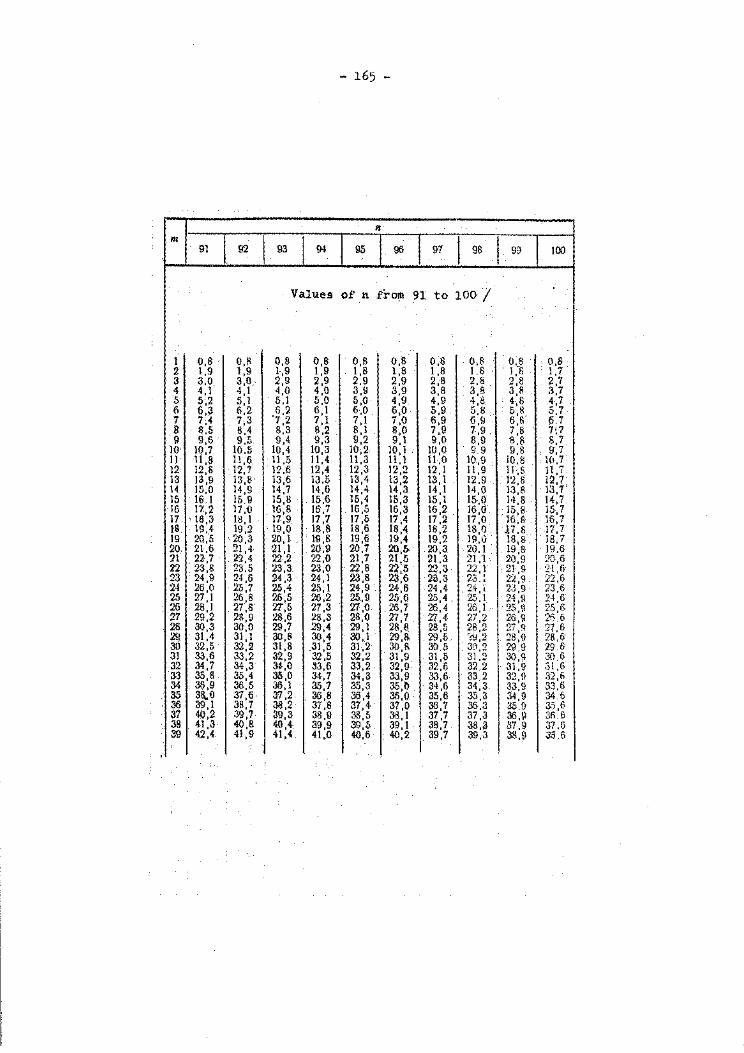
- 165 -

n m

1 93 I I 91 92 94 95 96 97 96 99 100

Values of n from 91 to 100 /

I 0,8. O,R 0,8 O,B 0,8 0,8 0,8 0,8 ·N . 0,8 2 1,9 1,9 1,9 1,9 1,8 1,8 1,8 1,8 1,7 3 3,0 3,0 2,9 2,9 2,9 2,9 2,8 2,8 2,8 2,7 4 4,1 4,1 4,0 4,0 3,9 3,9 3,8 3,8 3,8 3,7 5 5;2 5,1 5.1 5,0 5,0 4,9 4,9 4,8 4,6 .4,7 . 6 6,3 6,2 6,2 6,1 6,0 6,0 5,9 5,8 5,8 5,7 7 7;4 7;3 '7 2 7,1 7,1 7,0 6,9 6,9 6,8 6.1 8 8.5 8,4 8:3 8,2 8,1 8,0 7,9 7,9' 7,8 ' 7:7 9 9,6 9,5 9,4 9,3 9,2 9,1 9,0 8,9 B,8 8,7

10· 10,7 10.5 10,4 10,3 10,2 10,1 . 10,0 . 9.9 9,8 • 9,7 IJ 11,8 11,6 11,5 11,4 11,3 11,1 11,0 10,9 10.8 ·10.7 12 12,6 12,7 12.6 12,4 12,3 12,2 12,1 11,9 1rs 11,7 13 13,9 13;8· 13,6 13.5 13,4 13,2 13,1 12.9 12:8 12,7 14 15,0 14,9 14,7 14,6 14,4 14,3 14,1 14,0 13.~ 13,7' 15 16.1 15,9 15,8 15,6 15,4 15,3 15,1 15,0 14,8 . 14,7.

·16 17.,2 17,0 16,8 16,7 16,5 16,3 16,2 16,0. . 15,8 15,7 17 . 16,3 1!!,1 17-,9 17,7 17,5 17,4 17,2 17,0 16;8 16,7 18. 19 .. 4 19,2 19,0 18,8 18,6 .18,4 18,2 18,1) l7.8 17,7 19 20,5 20 3 20,1 . 19,8 19,6 19,4 19,2 19.0. 18,8. 18,7 20 21,6 21:4. 21,1 20.9 20,7 20& 20,3 20,1 19,8 19 .. 6 21 22,7 . 22,4 . 22,2 22,0 21,7 2(5 21,3 21,1 20,9 20,6 22 . 23,8 23.5 . 23,3 23,0 22,8 225 22,3 22,1 21,9 21,6 23 24,9 24,6 24,3 24,1 23,8 23'6 2B,3 23.: 22,9 22.6 24 26,0 25,7 25,4 25,1 24,9 . 2<6 24,4 . 24, i 23,9 23,6 25 27,1 ~H· 26,5 26,2 25.,9 25 6 25,4' 251 24,9 2-1,6 26 28,1 27;5 27,3 27,0 26'7 26,4 26) . 25,9 25.6 27 29,2 28,9 :.!8,6 :.!8,3 28,0 27) 274 27,2 26,9 26,6 28 30,3 30,0 29,7 29,4 29,1 28,8. 2B:s 28,2 27,9 27,6 29 31,4 31,1 30,8 . 30,4 30,1 29,8, 29,5 r<Y,2 :!8,9 28,6 30 32,5 32,2 31,8 .31,5 31,2 30,R 30,5 30,2 29.9 29.6 31 33,6 33,2 32,9 32,5 32,2 31,9 31,5 31,2 30,9 306 32 34,7 34,3 3t,O 33,6 33,2 32,9 32,6 32,2 31,9 31,6 3.3 35,8 35,4 35,0 34,7 34,3 33,9 33,6 33,2 32,!1 32,6 34 . 36,9 36,5 36,1 35,7 35,3 35,0 34,6 34,3 33,9 33,6 35 38,.0 37,6· 37,2 . . 36,8 36,4 36,() 35,6 35,3 34,9 34.6 36 39,1 38,7 38,2 37,8 37,4 37,0 36,7 36,3 35,!1 3.), 6 37 40,2 39,7 39,3 38,9 38,5 38,1 37,7 37,3 36,9 3n.5 38 41,3 40,8 40,4 39,9 39,5. 39,1 38,7 38,3 37,9 37.6 39 42,4 41,9 41,4 41,0 40,6 40,2 39,7 39.3 38,9 ~5.6

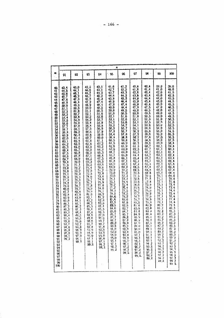
- 166 -

11

Ill 91 92 93 94 95 00 . 97 9!1 99 lOO

<10. ·~.4 43,0 42 5 42,1 41,6 41,2 40,11 40'4 39,0 3H,6 41 «.6 44,1 43:6 43,1 42,7 42,2 41,8 41:4 41,0 40,6

42 ~5.6 ~.1 44,1 44 2 4:1,7 43,3 42,8 42,4 42,0 41,5

43 ~.7 46,2 45 7· ..s:2 ~4.8 44,3 43,& 43,4 43,0 42,5

4.4 47,8 47,3 -!6:8 46,3 41i,8 45,3 44,g 44,4 44.-0 43 5

45 .fS,9 48,4 47,9 47,4 46,9 46,4 45,9 45,4 41),0 4(5

~6 50,0 49,5 48,9 48,4 -17,9 47,4 46,9 <46,4 46,0 45,5

47 51,1 50,5 50,0 49,5 49,0 411,4 47,!1 47,5 47,0 46,5. 48 52,2 51,6 51, I 50,5 50,0 49,5 49,0 48,5 48,0 47,5

49 53,3 52,7 52,1 51,6 51,0 50,5 50,0 4!1,5 49,0 48,5

50 54,4 53,8 53,2 52,6 52,1 51,6 51,0 50,5 50,0 49,5

51 55,5 54,9 54,3 5.1, 7 53,1 52,6 52, I 51,5 51,0 . 50,5

52 56,6 55,9 55,4 5-1,8 54,2 1}3,6 53,1 52,5 52,11 51,5

53 57.~ fl7,0 56,4 55,8 55,2 M,7 54' 1 53,6 53ll 52,5 54 58,7 58, I 57,5 56,9 56,3 55,7 55, I 54,6 5(0 53,5 55 &9,8 59.2 58,6 57,9 57,3 56,7 56,2 556 55,0 54,5

66 00,9 60,3 59,6 59,0 58,4 57,8 57,2 so:6 50,0 55,5 1>7 62,0 61,-1 60,7 60,0 59,4 . 58,8 5U,2 57,6 57,0 56,5 58 63,1 62,4 61,8 1\1,1 60,5 59,1:1 &.J, 2 511,6 5H,O 57,5 59 64,2 6J,5 62,8 62,2 61,5 ll0,9 60.~ 59 6 5(),0 58,4

60 65,3 64,6 63,9 6:3,2 6:2,6 61,9 Gl .:~ ro:1 601 59 4

61 00,4 65,7 t~5,0 6~,3 1\3,6 63,0 fi'2,3 61,7 61: I 60'4

62 67,5 oo.a f.li,O 65,3 64,7 64,0 63,3 62,7 62,1 61:4

63 69,6 67,8 67,1 66,4 ()5 7 65,0 lit, 1 tl;l, 7 63,1 62,4

M 69,7 6S,!J 6t!,:.2 67,5 66'11 Gti, I U5,4 li4 '7 61, I 63,4

65 70,8 70,0 6~,3 6A,5 o7:tl 67, I flti,-1 6.S,i •65,1 64,4

66 71,9 71.1 70,.1 6\J,G liti,!J li!l,l (i7,-l liG,1 lio.l 65,4 67 73,0 72,2 71,4 70 () 69,!1 6!1,2 66,5 lii ,!l 67 ,I 00,4

G8 74,0 73,2 72,5 71 '7 . . 70,!1 70.~ 69,5 6\!,11 68, I 67,-f fi9 75, I 74,3 73,5 72) 72.0 71,2 70,5 !l9,8 ti!l,l G8,4

70 76,2 75,-1 74 6 7.1,!1 7.1,0 723 71,5 70.8 70, l 68,4

71 77,3 71i,5 75) 74 \) 74, I 73::) 72,ti 71.11 71, I 70,4 I

72 78,4 77,6 7fi,7 75:9 75, I 71,1\ 73.6 i2. s 12' 1 11,4.-73 79,5 78,7 77,8 '17,0 76,2 1:' •. 4- 74,(i 73.9 7.1, I 72,4

74 80,6 79,7 78,!1 ?il,O 77' 2 7!1,4 75, fi 7~.\J 74,1 73,4 75 81,7 80,8 7\I,!J 7•1 I 76,:1 775 ~n 75,\J 75.1 74,4

76 82,1l lll,!l Ill ,0 hl)' 2 T\I,:J 78:s 7ti.!l 71U 75,4

77 83,9 1<3,0 82, l 81:-2 &1,4- 79,!i 7!l, 7 77,\J 77 ,I 7u,4

78 85,0 84,1 8J, 2 82.:1 81 ,4- 80,6 79,7 711,9 78 ,I 17.1.

79 !16' 1 85, I 84,2 83 3 82,5 1!1,6 i\u,s 7!1, \) i\1, I ill,+

80 87,2 86,2 8.'i,.1 81:4 8).5 82.ti I &1.8 1!().9 H0,2 79.4 R\ RS,3 · !l7 ,J 86,4 85 5 84,6 83,7 82.8 8;.>..0 81.2 BO,:l

132 !!!J,3 111!,4 87,4 86:~ 85,6 ll4,7 81.8 8.3 ll ll'l.2. 81 ,.1

83 90,4 K\1,5 llll,S g7 ,ti 00,7 85.7 184-,0 B4 .11 83.2 81,3

S1 91,5 !J0,5 8!1' li !\R,Ii 87,7 86,8 8~. 'J ~!J,II 81,2 81.3

85 !12,G 01,6 90,1\ 8\l, 7 88,7 87,8 !iii,!J 86.0 85.2 d1 3

1:!6 93,7 !12, 7 ()I, i \10,7 89.8 88,!J 67 ,!1 t!7, I &fi,2 8S:J 87 !14,8 !J;j 8 92.!! 91,8 90.8 &1,9 g~.u S!l.l 87,2 dll '3 1:18 9f>,8 !H:9 i)J. \l 9'l <J 9l.!J !)(J '!I 911,11 tl\1.1 !:la .2 S7 3 tl!l \17,0 95,9 !14 ,!l 9~:9 91,9 92,11 !ll,ll 'JO.l 89,2 8S.J 00 \!8, 1 97,0 91l.O %0 9'1,0 9J,O 92, I 91.1 S111.2 89 J

91 99,2 9R.I !17. I !lG:o 91i,O 9'4,0 93. I 9Z,I !Jl, 2 90'3

92 99,2 fJS, I \17, I 9fi. I 95, I· !H,I 93 I 92,2 91 ,J

!13 ~.2 08,2 ()7. l 96, I SS, I !l4 2 !H.:? 92 :; 04 99,2 !13. 2 97,2 %', 2 95,2 '14-,2 93 l 95 ~~.2 !Jil,2 S7, 2 ':l6.2. ~),l) I :1 '34 '.'\

96

I 99,2. 98 .l. 97,2 90.2 ';)S 3

!17 99, 2. 9~.2 97 2 'Jii 3

\l!l

I 99.2 %'2 97 3

9\J I 99.2 98 J

lOO 5~ '2.

----

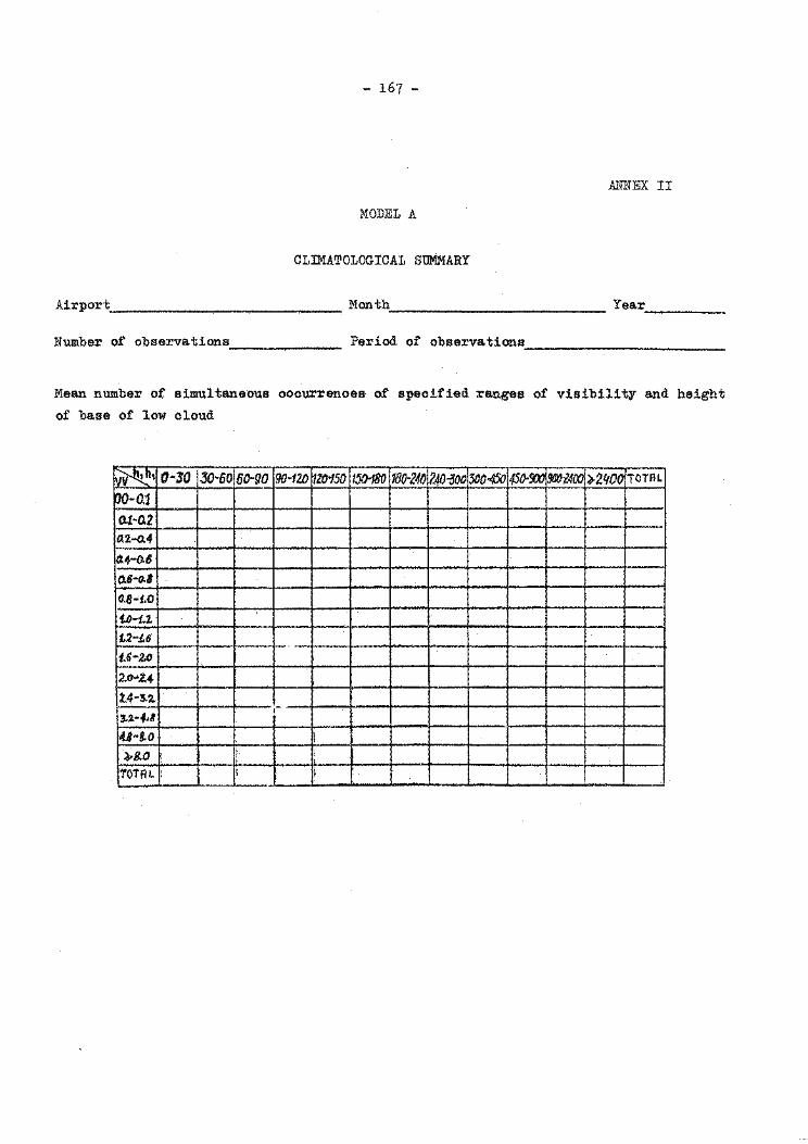
- 167 -

ANNEX II

MODEL A

CLIMATOLOGICAL SUMMARY

Airport Month Year ________ __

Number of observations ____________ __ Period of observations ________________________ _

Mean number of simultaneous occurrences of specified ranges of visibility and height

of base of low cloud

~~ O·JO 30-60 6c-go rJ(J.12D ~20150 15fHBO 180·24(} 240-500 31J0-4SO 45o-I)(X, !Jfl0i4CO ).2lf0_2_ TOTAL

00-0.1 ru-a2 tU..a.4

,a.4-0.8

0.6-o.l

0.8-:t.O

t.o-1.1·

£2-1.6

1.6-z.o 2.o--.Z.•

2.4-!.2.. 12.·4·8

,-

4J~a.o ! ~8.0 ' '

TOTAL : I --

- 168 -

MODEL B

CLIMATOLOGICAL SUMMARY

Airport Month Year ________ _

Number of observations. ______________ __ Period of observations ______________________ ___

Number of occasions of concurrent wind speed and direction

WIND IHND SPEED IN m/ s DI-REC-· ip(rOJ ~-o-3 ~.,05 ~-07 08-09 V-II . '2-13 ~~/9 20-23 ~11-27 28~31 "»32 'ID TAL TION

oz-o.3 05-0]

08•/0

11-:-13

14·16

17~19

20.;22

23-2j

26-28

29-31

32-34

(}t35;3f CALM .

VARI ABLE 'fCYI'AL

--··---- •--·--w

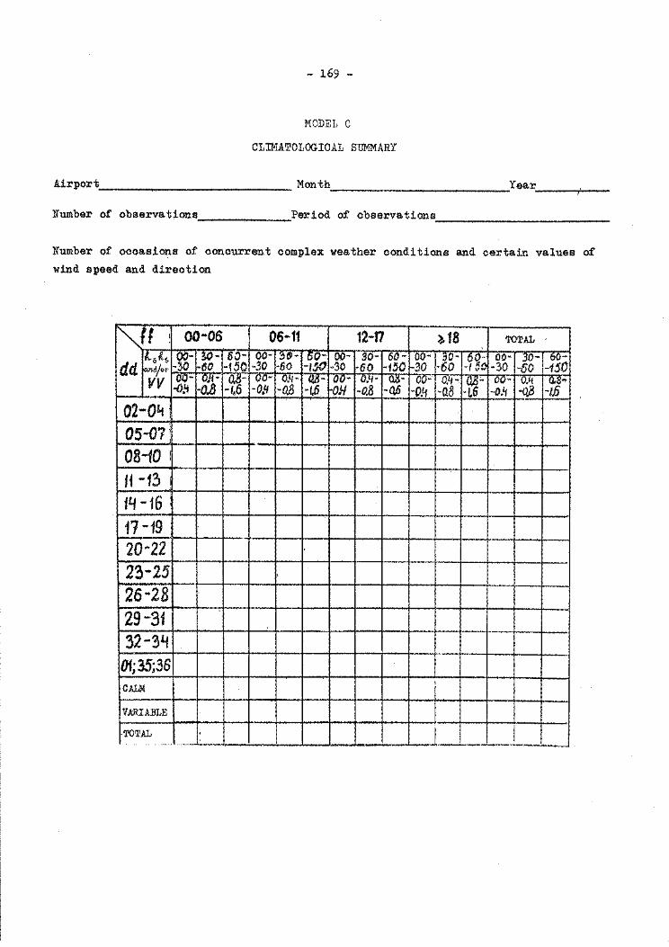
- 169 -

MODEL C

CLIMATOLOGICAL SUMMARY

Airport Month Year ______ +----

Number of observations Period of observations ________________________ __

Number of occasions of concurrent complex weather conditions and certain values of wind speed and direction

"'11 I 00-06 06-11 12-l7 ~18 TOTAL ,

I 11--s~$ oo- 30- 6J- oo- ~(j- 60- oo- .90- 60- oo- ~0- -9~; oo- ~D- 60-1

dd ~ndjo1· -30 60 -1.50 -30 ·60 -jjO -30 -60 -1.50 -30 ·60 -30 -60 -150 vv ~g- 01!- -~- oo- 0.4- ~- oo- 0.~- ~- ou- 0,4- -'tf oo- 0.'1 (I.~ .. -o.'i -OA -O.If -0,8 -1.6 OH -0.8 -a.6 -0.4 -Q8 -o.4 ..q8 -1.6 '

02-0l.t os-o7; '

08-10 I

H -13 14-16 17-19 20-22 23-25 26-28 29-3i 32 -3'i -

01;35;36 I

CALM I

VARIABLE

·TOTAL . I . -· - ··--·· --··-· ------

.. 1L1 -

- 173-

METHODS, EQUIPMENT AND ECONOMICAL EFFICIENCY OF MACHINE PROCESSING OF HYDROMETEOROLOGICAL DATA

by

N. K. Kljukin

Preparatory stages of machine data processing

Nowadays high~speed electronic computers can perform thousands of millions of arithmetic operations per second, making it possible to solve complex problems in a short time.

However, the efficiency of electronic computers is far in advance of the system used for the preparation of the information to be processed by these machines. In meteorological data processing, a vast volume of information has to be used and the greatest difficulty is to decrease the gap between the speed and the cost of processing (computations) itself, and the speed and cost of preparing data for processing. Special difficulties arise when selecting a suitable technical informa­tion carrier and recording data on this carrier. By the technical information carrier is meant a physical medium capable of carrying information in a form convenient for automatic input to the computer and for storage during a certain period of time. The complexity of the problem is increased by the fact that hydrometeorological informa­tion has certain important specific features, uncommon in other types of information.

They include

(a) ·The volume of data. At the present time the volume of data is 12 estimated to be of the order of 10 bits, and will reach twice

as much in 8-10 years: with the development of new observation techniqu~s (meteorological satelli-tes, meteorological rad.ars, etc.) it is possible that this increase will be even greater.

(b). Necessity cif permanent storage of processed and raw information

(results of direct observations) since these data do not lose their practical value with time.

(c) Necessity of wide (international) exchange of information on tec:i:m:L6al carriers.

- 174 -

We shall now consider the preparatory stages of machine data processing.

Systems of data coding

Information to be processed by a machine must be expressed in a certain

code for recording on the technical carrier. A system of symbols and rules for the

expression of information is recognized to be a code.

In hydrometeorological information processing the following codes are used.

(a) Analogue codes

Information is recorded in accordance with the continuous registration of

the values.

(b) Digital codes

Information is recorded discretely in the form of digits with a designed

time step and/or according to changes in the value recorded.

(c) Alphanumeric codes

Information is recorded discretely in the form of letters, words, combin­

ations of words, phrases, text and digits.

Digital codes are most widely used in the machine processing of hydro­

meteorological information. Let us consider the more common of these.

Digital codes based on decimal system calculus are in widespread use. The

number of digits (i.e. the base of a system) is 10, from 0 to 9.

In the decimal system each digit of a number has its own meaning (1, 3, 8) 1

with respect to position. For example: 8 x 10 = 80, if digit 8 is in the tens

column.

Digital codes based on decimal system calculus are most suitable for the

manual coding of data or for operations-an_smarl computers with manual input. Also

they are widely used for operating and punch-card calculating machines.

- 175 -

However, the decimal system is not suitable for the majority of electronic computers. Instead a binary system with 2 as the base is usually used. In the binary system one of two digits 0 or 1 is admissable in each category. The category of a binary number is called a '1bit" (abbreviation of a .E,inary digit). In Table 1 an example of expressing some decimal numbers in the binary system is given.

One of the methods of converting numbers from the. decimal system to the binary one is the consecutive division of a decimal number by two. Incomplete quotients a.re written down in a column till 1 or 0 is obtained. For near odd numbers 1 is written down, near even ones - 0 (Table 1).

A number in the binary system is obtained by means of reading these bits upwards, for example, a. decimal number 117 in the binary system is expressed as the number 11110101 (Table 1).

For convenience, since people are used to counting in the decimal system, special "man-machine-man" coding systems a.re prepared, where each decimal digit is independently expressed in the binary system. These binary-decimal codes which make it possible for a pe:t'SOn to work in the decimal system (with which he is familiar), are suitable for machine conversion of information to the binary system, information p~ocessing and inverse conversion to the decimal system for output printing.

O:t' the many binary-decimal codes we shall consider code "8, 4, 2, 111 •

Fo'lir binary bits are necessary for the most abbreviated expression of a. decimal digit in the binary code. In the above code ea.ch decimal digit is expressed by four bits. The structure of the code is such tha.t 0 a.nd 1 a.re spaced in a harmonious easily remembered order (Table 1). Since each decimal number in the binary-decimal code is coded independently, a. binary-decimal number 0001 0001 0111

1 1 7 will correspond to the decimal number 117.

A redundance method is used for making noise-protected codes which permit the detection and correction of errors arising during the transmission and processing of data, i.e. 4 and more bits are used for the expression of each decimal number. One such noise-protected code is an International Teletype Code (TTC-2) (Table 2).

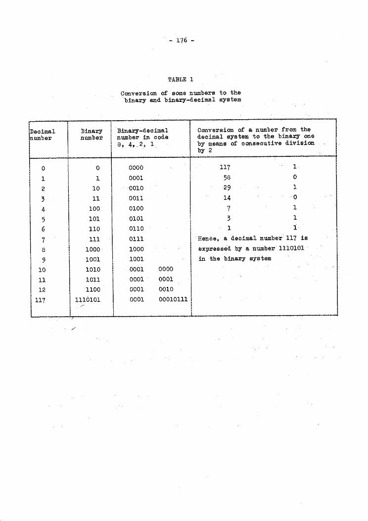
Decimal Binary number number

0 0

1 1

2 10

3 11

4 100

5 101

6 110

7 111

8 1000

9 1001

10 1010

11 1011

12 1100

117 1110101 /

/

- 176 -

TABLE 1

Conversion of some numbers to the binary and binary-decimal system

Binary-decimal Conversion of a number from the number in code decimal system to the binary one 8, 4,,2, 1 by means of consecutive division

by 2

0000 117 1

0001 58 0

0010 29 1

0011 14 0

0100 7 1

0101 3 1

0110 1 i

0111 Hence, a decimal number 117 is

1000 expressed by a number 1110101

1001 in the binary system

0001 0000

0001 0001

0001 0010

0001 00010111

___ L....______.____~--~ ------ ----~

- 177 -

In this code each decimal digit or sign is expressed by five bits. Since five bits are not sufficient to express all th~ digits, letters and signs, the code has two registers, i.e. in letters and in digits. This code is adequate for the representation of information on teletype tape. The system of punching is simple and easy to remember, and hence, it is easy f9r the operator to check whether the punching is correct, a.n,d to visualize the information by 11ll'eading" the tape. The tape punched in this code is suitable for processing by the com~uter. Code ITC-2 is therefore used in hydrometeorology not only for data transmission via. communication channels, but also for the compilation of messages from automatic meteorological stations and for recording the results of observations on punched ta~e as an initial technical carrier.

The following codes can be called alphanumeric

(a) Codes using letters and digits.

(b) Systems of recording information using digit~, signs, letter abbreviations of any spoken language on forms, observational registers, tables, etc.

The use of these codes is convenient for coding by an operator and for manual processing. Many current hydrometeorolog!cal codes are.~eveloped according to this system. However, this system makes the processing of information by computers difficult, particularly with respect to item (b).

It is only over the past few years that machines suitable for reading alphanumeric texts and feeding them into a computer have begun to appear. However, the use of alphanumeric codes is not economic and hence they are not widely appli­cable to the systems of automatic processing of mass hydrometeorological information. For this reason the introduction of automatic methods of data. processing necessitates improvements in the hydrometeorological codes, i.e. their conversion to digital codes so that they are suitable for machine processing.

Technical carriers for hydrometeorolo~ical information

With a view to modernizing h~drometeorological practices, the following classification of technical carriers can be suggested in light of their purposes and properties (Table 3).

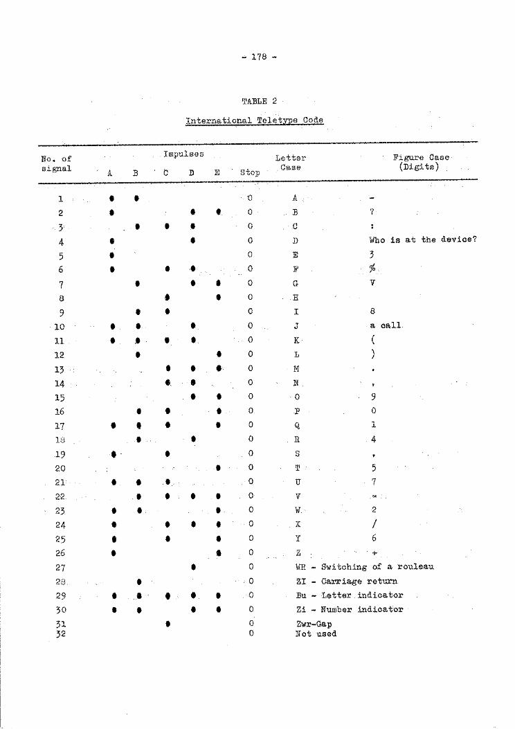
..... 178-

TA:BLE 2

International TeletlEe Code

No. of Impulses Letter Figure Case signa],.

A :B c D E Stop Case (Digits)

1 • • 0 A .

2 • • • 0 :B ?

3' • • • 0 c 4 • • 0 D Who is at the device?

5 • 0 E 3

6 • • • 0 F % 7 • • • 0 G V

8 • • 0 H

9 • • 0 I 8

10 • • • 0 J a call

11 I • • • 0 K (

12 I • 0 1 )

13 • • • 0 M

14 •• • 0 N

15 • • 0 0 9

16 I • • 0 p 0

17 • • • • 0 Q. 1

13 • • 0 R 4

19 • • 0 s 20 • 0 T 5

21 • • • 0 u 7 22 • • • • 0 V =

23 • • I 0 w 2

24 • I • • 0 X I 25 • • • 0 y 6

26 • • 0 z +

27 • 0 WR - Switching of a rouleau

28 • 0 ZI - Carriage return

29 • I • • • 0 :Bu - Letter indicator

30 I I • • 0 Zi - Number indicator

31 • 0 Zwr-Gap 32 0 Not used

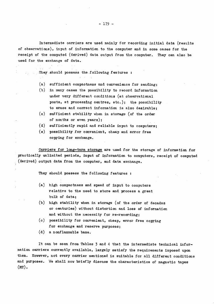
- 179 -

Intermediate carriers are used mainly for recording initial data (results of observations), input of information to the computer and in some cases for the receipt of the computed (derived) data output from the computer. They can also be used for the exchange of data.

They should possess the following features

(a) sufficient compactness and convenience for sending; (b) in many cases the possibility to record information

under very different conditions (at observational posts, at processing centres, etc.); the possibility to erase and correct information is also desirable;

(c) sufficient stability when in storage (of the order of months or even years);

(d) sufficiently rapid and reliable input to computers; (e) possibility for convenient, cheap and error free

copying for exchange.

Carriers for long-term storage are used for the storage of information for practically unlimited periods, input of information to computers, receipt of computed (derived) output data from the computer, and data exchange.

They should possess the following features :

(a) high compactness and speed of input to computers relative to the need to store and process a great bulk of data;

(b) high stability when in storage (of the order of decades or centuries) without distortion and loss of information and without the necessity for re-recording;

(c) possibility for convenient, cheap, error free copying for exchange and reserve purposes;

(d) a nonflammable base.

It can be seen from Tables 3 and 4 that the intermediate technical infor­mation carriers currently available, largely satisfy the requirements imposed upon them. However, not every carrier mentioned is suitable for all different conditions and purposes. We shall now briefly discuss the characteristics of magnetic tapes (MT).

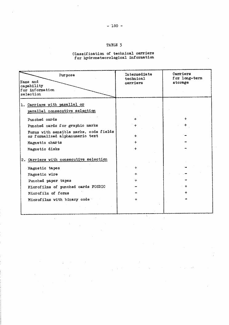
- 180 -

I!'ABLE 3

Classification of technical carriers for hydrometeorological information

~ Intermediate carriers technical for long-term carriers storage

y n

n

1. Carriers with parallel or I

parallel consecutive selection

Punched cards + +

Punched cards for graphic marks + +

Forms with sensible marks, code fields or formalized alphanumeric text + -

1

Magnetic charts + -

Magnetic disks + -

2. carriers with consecutive selection

Magnetic tapes + -

Magnetic wire + -

Punched paper tapes + -

Microfilms of punched cards FOSDIC - +

Microfilm of forms - +

Microfilms with binary code + -

- 181 -

·Magnetic tapes are used both for storage and sending data (data exchange

by mail).

Estimations of information stability on magnetic tapes vary. For example,

the USA and Norway Services consider that the use of magnetic tapes largely over­

comes the problems of data storage and exchange (under conditions of storing several

copies and re-recording the MT's approximatley every 2 to 3 years).

However, a clear estimation of the negative properties of the magnetic

tape during its long-term storage was carried out by the Goddard Canter {USA). In

a publication devoted to this problem it stated that since the introduction of space

research programmes at Goddard Space Flight Canter, 100,000 magnetic tapes have

been stored. The annual increase is equivalent to 35,000 magnetic tapes.

The storage of these tapes has the following drawbacks

(a) the high cost conditioned by the high cost of the material;

(b) "self-reprinting" from one layer to another during long-

period storage of tapes;

(c) mechanical destruction of tapes;

(d) erasing of information under the influence of magnetic fields;

(e) sensitivity to environment.

A project is therefore being discussed at the Center to establish a data

storage system using a photographic storage medium which will be cheaper and more reliable compared to the magnetic tape.

Everything suggests that coupled with MT's which are convenient for pro­

cessing, exchange and short-term storage, it is necessary to use compact long-term

technical information carriers.

Combining the functions and properties of the intermediate and long-term

carriers is certainly desirable, since if this were so there would be no need to

re-record from one carrier to another (there will be no additional errors), nor to

invest money in both re-recording and operational equipment, etc. The combination

of so many functions and properties is one of the reasons for the wide use of punch

cards.

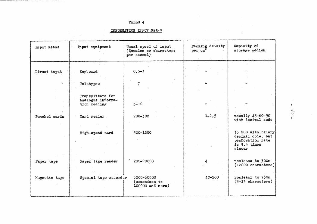
TABLE 4

INFORMATION INPUT MEANS

Input means Input equipment Usual speed of input (decades or characters per second)

'

Direct input Keyboard 0,5-1

Teletypes 7

Transmitters for analogue informa-tion reading 5-10

Punched cards Card reader 200-300

High-speed card 500-1200

Paper tape Paper tape reader 200-20000

!.fagnetic tape Special tape recorder 6000-60000 (sometimes to 100000 and more)

Packinf density per cm

-

-

-1-2,5

4

40-200

Capacity of storage medium

-

-

-

usually 45-80-90 with decimal code

to 200 with binary decimal code, but perforation rate is 3,5 times slower

rouleaux .to 300m (12000 characters)

rouleaux to 730m (3-15 characters)

1-' ro F\)

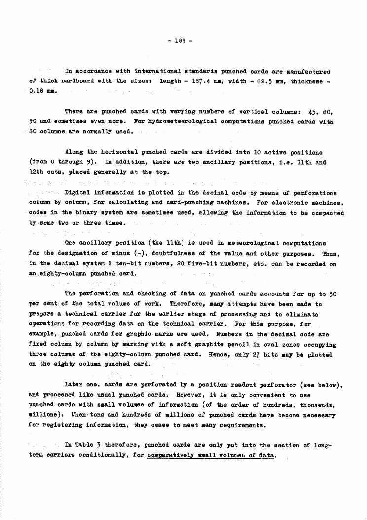
- 163 -

In accordance with international standards punched cards are manufactured of thick cardboard with the sizes& length- 187.4 mm, width- 82.5 mm, thickness-0.18 mm •.

There are punched cards with varying numbers of vertical columns: 45, 80, 90 and sometimes even more. For lcy'drometeorological computations punched cards with 80 -col'umns are n.ormally used.

Along the horizontal punched cards are divided into 10 active positions (from 0 through 9). In addition, there are two ancillary positions, i.e. 11th and 12th cuts, placed generally at the top.

Digital information is plotted in the decimal code by means of perforations column by column, for calculating and card-punching machines. For electronic machines, codes in the binary system are sometimes used, allowing the information to be compacted by some two or three times.

One ancillary position {the 11th) is used in meteorological computations for the designation of minus (-), doubtfulness of the value and other purposes. Thus, in the decimal system 8 ten-bit numbers, 20 five-bit numbers, eto. can be recorded on an eighty-column punched card.

The perforation and checking of data on punched cards accounts for up to 50 per cent- of .the total volume of work. Therefore, many attempts have been made to prepare a technical carrier for the earlier stage of processing and to eliminate operations for record-ing data on the technical carrier. For this purpose, for example, punched cards for graphic marks are used. Numbers in the decimal code are fixed column by column by marking with a soft graphite pencil in oval zones occupying three columns of the eighty-column punched card. Hence, only 27 bits may be plotted on the eighty column punched card.

Later one, cards are perforated by a position readout perforator {see below), and processed like usual punched cards. However, it is only conve:m:ient to use pun.ched cards with small volumes of information (of the order of hundreds, thousands, millions). When tens and hundreds of millions of punched cards have become necessar,y for registering information, they cease to meet many requirements.

In Table 3 therefore, punched cards are only put into the section of long­term carriers conditionally, for comparativelY small volumes of data.

- 184 -

The microfilm FOSDIC is not quite suitable since to obtain a film it is

necessary first to prepare the proper number of punched cards and then to photograph

them. It makes work difficult although FOSDIC film is eminently suitable for storage

and other purposes.

Microfilm with the binary code is free of the deficiency mentioned above

and is produced directly at the output from the computer by means of a special device.

It meets all modern requirements.

Methods of recording data on technical information carriers

The method of recording data on punched cards from tables and observational

note-books is still a major problem at the Processing Centres, which still carry out

this operation by means of manual perforation and checking.

· Some services (Iceland, USA, Eire, Japan) divide the operation of punohed

card preparation partially or completely among observation posts or district obser­

vatories.

In Austria, Canada, New Zealand and the United Kingdom information

obtained via communication channels is partially recorded automatically on punched

cards using teletype perforated paper tape as an intermediate technical carrier.

Several services record data on punched cards at the observation stations.

Other services record data at stations on punched cards with "sensitive"

marks for further automatic perforation (New Zealand).

The USA Meteorological Service uses pluviographs with a perforating

attachment which performs not only the recording of a curve on tape, but also on ~

intermediate technical carrier, i.e. on a 16-strip perforated tape.

Records made by the anemograph without a perforating attachment are read

out, converted to a digital form and transferred to wide printing and eighty-column

punched cards using a semiautomatic device with a tracking system controlled by an

operator.

The readout of data from isoline charts, conversion to digital form, inter ..

- 185 -

polation with a given discontinuity in points of a regular grid, and data output to wide printing and eighty-column punched cards are also performed by a semi-automatic device (an interpolator) the tracking system of which is again controlled by an operator.

However, in spite of the availability of all this equipment, the USA Meteorological Service cannot at present entirely dispense with the usual manual data perforation from observation note-books, tables, etc. on eighty-column punched cards. 35 operators fulfil this work at the National Weather Record Canter.

As a result of experimental work and experience gained the following recommendations can be given :

(a) majority intermediate technical carriers : perforated paper tape, magnetic tape, and with small volumes of

data - punched cards;

(b) majority long-term technical carrier: microfilm with the binary code;

(c) the two main methods of recording data on an intermediate technical carrier during an automatic process are:

on perforated paper tape directly from an automatic observation instrument using a perforating attachment from communication channels (by teletype);

(d) ancillary methods (which should be gradually replaced by the main ones): recording of data on a primary technical carrier directly at observational posts. This method can also be used where necessary for recording additional information on perforated tape, received from automated means of observation.

It may also be convenient to apply automatic or semiautomatic conversion of data from carriers in the analogue form (curves of recorders without perforating attachments, isolines, charts, etc.) to a digital form, for output to an intermediate technical carrier;

- 186 -

(e) recording of data on a long-term technical carrier

(microfilm) automatically from the computer, together

with the checking and initial processing of data

received at the Processing Centre via communication

channels on a primary or intermediate technical carrier;

(f) coding based on principles suitable for automated methods of

observation, transmission via communication channels and

processing of data by the computer.

Automatic Checking of Observational Data

The problem of automatic ohecking increases sharply with a rapid growth

in the volume of information and with the increase of requirements for complete and

precise data for research and operational applications.

A solution has become possible with the introduction of high-speed digital

computers with a large-capacity operational and file memory.

Experimental programmes are already being used in a number of countries

(United Kingdom, Hungary, Canada, USSR, USA, Federal Republic of Germany, Japan).

Among them, programmes for the automatic checking of operational aerological infor­

mation for numerical prediction and also special programmes for precipitation

checking have been the most fully investigated (United Kingdom).

It is however obvious that the work already done has not solved the

problem of automatic checking completely. However, it is important nevertheless

that we can suggest the following main principles of machine checking as a first

approximation:

(a) Checking for observing codes or revealing such values

which are not envisaged by codes;

(b) Checking for incompatibility of data within one report

i.e. to reveal contradictions between individual elements

at the observation times;

(c) Checking by applying known relationships such as the

hydrostatic equation, between separate elements;

- 187 -

(d) Checking for the space agreement of data using statistical

parameters (for example, means, regression equations, etc.),

cartographic constructions, interpolation ratios (of the

objective analysis) ;

(e) Checking for agreements in time by analysis of the time trends;

(f) Checking for agreement with local climatic normal or extreme values.

The checking should not be over complex or expensive and should provide

only an adequate level of data quality.

Original information should not be distorted during the process of

checking. Therefore, doubtful data should be put to printing for analysis by a

specialist.

Machine Data Processing

Following the preliminary stages (coding, recording on a technical carrier,

checking) the machine processing of data involves the following operations:

Physical (scientific) statement of the problem or elaboration

of a meaningful algorithm;

- Mathematical description of a computational problem (the

compiling of a mathematical algorithm);

Compiling of a computational algorithm, i.e. the system of

formal rules describing exactly the process of the work by

a computer;

Compiling of machine processing programmes, i.e. consecutive

recording of commands for a machine realizing the given

computational algorithm;

Input of initial data and programme to the machine, solution

of the proble~output of results in' the required form;

..:. 188 -

Completion of data processing either manually or with the aid

of any ancillary device in oases of incompatibility of require­

ments with respect to form or content of the results;

Analysis of computed data by specialists, issue of data to the

consumer.

Now we shall consider some aspects of these operations.

The physical (scientific) statement of the problem or elaboration of a

meaningful algorithm for machine processing of data, (for example, climatologioal

data) is usually necessary for practical and/or research requirements. These

objectives are similar to those of manual processing, but the ~pplioation of machines

provides for more comprehensive and profound research. At the same time the require­

ments posed by science and practice complicate the problems of processing.

The first stage: Climatologioal calculations of norms

Norms are used for the estimation of a preceding period of time (which is,

in a number of oases, necessary and quite justified) and for the estimation for a

subsequent period. In this case it is supposed that a subsequent period will be

similar to a preceding one, but since this is not always so, such applications of

norms are groundless. This initial stage which is limited to the calculation of

norms only, is characterized by the application of manual methods of processing and

partially by calculating and card-punching machines.

The second stage: Climatologioal computation of probabilities, reliability and

other statistical characteristics, which allow an assessment of the probability of

future events albeit without indicating the time of occurrence. For example, the

computed annual sum of 800 mm precipitation at 1% reliability might be realized next

year or in 10, 50, 80 or 99 years. In all oases the calculations will be correct

and correspond to statistical laws. Such computations meet many practical needs and,

as such are necessary and useful.

For the solution of a number of problems, however, calculations of proba­

bility are not sufficient since, for example, in the planning of water-economic

measures for agriculture, etc., the particular period when (a year, five years,· a

d~cade) water will be plentiful is highly relevant.

- 189 -

It is important therefore, to bear in mind that calculations are usually based only on a previous series of observations and statistical laws, and do not take into account the laws of casual relations tendency of a process (in our example the tendency of climatic change). Moreover, climatic parameters axe usually given at the observation point or with space interpretation of low accuracy. This stage requires wide use of mathematic means, calculating, card-punching and electronic computers.

The third stage: Climatological forecasts are based not only on statistical laws, but also on the laws of causality of phenomena revealing the tendency of process development. On the basis of the above and using computational statistical methods (i.e. methods of the second stage) the climatologioal forecast should specify expected changes in climate or separate parameters and at the same time indicate the time of occurrence.

In this case relations in the atmosphere and the complex interactions of the Earth's atmosphere with extraterrestrial (including cosmic) influences should be taken into account.

At the same time, climatologists are facing a problem of vital importance for mankind, i.e. a problem of calculating and forecasting climatic changes as a result of active anthropogenic influences.

The importance and urgency of the problem is explained by the following considerations

(a) Even at the present time, scientific methods and techniques for premeditated active influences on some atmospheric processes are sufficiently effective. They will moreover probably be one of the principal areas of study with the development of science and techniques in the future.

(b) Unpremeditated anthropogenic influences in a number of cases have already been responsible for the formation of important climatic conditions in densely populated regions. In the future, these unpremeditated influences will become more significant factors in climate formation since it is expected that the energy produced by mankind will be comparable in the coming decades with that coming to the Earth from the Sun.

- 190 -

Climatic changes arising from unpremeditated influences are practically

irreversible (or, at least, not easily controlled) and are at the same time unfav­

ourable to mankind. Here the importance of quantitative estimates and forecasts of

such changes is understandable.

It is only recently that the science of climatology has progressed to the

stage of climatological forecasting and although attempts to prepare such forecasts

are relatively few the future will bring a more precise synthesis of climatological

computations and consequently more accurate climatological forecasts.

Mathematical description of computational problems

A brief list of parameters calculated by machines is given below.

2!!!!~!!~!!_R~!~~!~~!-~f-~~!~2~~!~~!~!!~~~!~~!!!!~~-!~~!~!

(a) moments of the first order (means);

(b) frequency and reliability;

(c) parameters of statistical distribution (mode, median, root­

mean-square deviations, variance, coefficients of asymmetry

and excess, parameters of the ellipse of vector value dispersion);

(d) structure parameters (space square tifferences, horizontal

and vertical coefficients of correlation, cross-correlation

and autocorrelation);

(e) criteria for agreement between empirical and theoretical

distributions;

(f) computations with interpolation formulae

22~P~~~~!2~_2!-~!~!Y!~!!!~-~! :

(a) density;

(b) vapour pressure and saturated vapour pressure;

- 191 -

(c) specific humidity and absolute humidity;

(d) vertical and horizontal gradients;

(e) climatic indices of continentality, rigour, temperature, humidity, etc. ;

(f) temperature contrasts of the type sea-atmosphere;

(g) interlayer differences.

For the time being we cannot indicate mathematical algorithms of the third order, i.e. prediction of climate, but it should be expected that as far as their complexity is concerned, they will be comparable with the algorithms of operative numerical prediction, and that the volume of data used for this purpose will of necessity exceed that routine information.

Compiling computational algorithms

A computational algorithm or "a system of formal rules simply determining the process of performing given operations" divides the mathematical description of a problem into its simplest operations spaced in sequences suitable for computations on the machine. It serves also as a transient stage in the man-machine system and facilitates the contacts with the machine. Simplicity (determinancy) is a charac­teristic property of algorithms of problems for the computer. A computational algorithm is compiled on the basis of a mathematical algorithm (formula, a numerical method of problem solution) and is in turn the initial material for compiling machine programmes.

Compiling machine processing programmes (for electronic digital computers)

A programme for solving problems on a computer is the sequential writing of commands for the machine. The programme written beforehand by a programmer on sheets of paper in an appropriate code is carried over on technical carriers (for example, on punched paper tape, a punched card), and fed into the computer. Programmes are stored in the machine memory and on technical carriers.

- 192 -

At present the following methods of programming are most widely used

(a) programming in the command system of a given machine;

(b) automated methods of programming.

iifhen programming commands for machines, compiling and debugging of the

programmes require a period of the order of 3 to 6 months, and sometimes a year of

work for a qualified programming engineer. Also the programme is suitable only for

a given type of electronic digital computer and for this reason methods of automatic

programming are being continually developed.

In meteorological practice a number of autocodes and algorithmic languages

(autocode "Engineer", algorithmic languages ALGOL, FORTR.MT, CABOL) are used .•

Unfortunately, they are not always suitable for solving hydrometeorological problems.

Consequently research on more modern methods of automatic programming is being

carried out. For example, the language "METO" used for the solution of statistical

problems has been developed by the Meteorological Office of the United Kingdom.

In conclusion, it should be noted that compiling programmes is one of the

most labour-consuming and expensive operations which often determine the efficiency

of machine processing. Further insistent search therefore, is absolutely essential

with a view to simplifying and automating the programming processes.

Input of initial data to the computer, solution of problems, output of results

vfuen solving problems by processing hydrometeorological data, information

amounting to tens and hundreds of millions of decimal digits have to be fed into the

machine. Because of this, the requirements for technical carriers and input devices

are high.

As stated above, the automatic checking and solution of problems require

computations with rather complex formula and the performance of logical operations.

It demands adequate machine speed (computation speed) and a large "memory".

The output of results should be performed in the alphanumeric form for

printing and recording on technical carriers, or in the analogue form on various

maps, graphs and diagrams, etc. Much of the information in printing and graphical

form is published. This necessitates special requirements for devices for data input

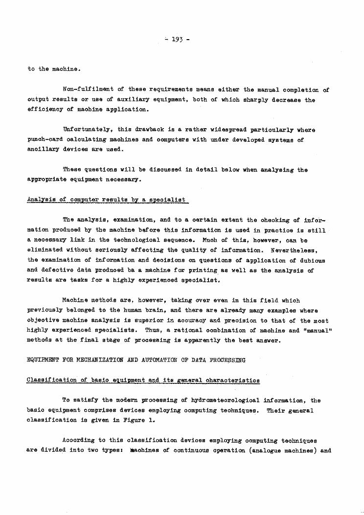
- 1.93 -

to the machine.

Non-fulfilment of these requirements means either the manual completion of output results or use of auxiliary equipment, both of which sharply decrease the efficiency of machine application.

Unfortunately, this drawback is a. rather widespread particularly where punch-card calculating machines and computers with under developed systems of ancillary devices are used.

These questions will be discussed in detail below when analysing the appropriate equipment necessary.

Analysis of computer results by a specialist

The analysis, examination, and to a certain extent the checking of infor­mation produced by the machine before this information is used in practice is still a. necessary link in the technological sequence. Much of this, however, can be eliminated without seriously affecting the quality of information. Nevertheless, the examination of information and decisions on questions of application of dubious and defective data produced ba a machine for printing as well as the analysis of results are tasks for a highly experienced specialist.

Machine methods are, however, taking over even in this field which previously belonged to the human brain, and there are already many examples where objective machine analysis is superior in accuracy and precision to that of the most highly experienced specialists. Thus, a rational combination of machine and "manual" methods at the final stage of processing is apparently the best answer.

EQUIPMENT FOR MECHANIZATION AND AUTOMATION OF DATA PROCESSING

Classification of basic equipment and its general characteristics

To satisfy the modern processing of hydrometeorological information, the basic equipment comprises devices employing computing techniques. Their general classification is given in Figure 1.

According to this classification devices employing computing techniques are di vide.d in to two types: lila.chines of continuous operation (analogue machines) and

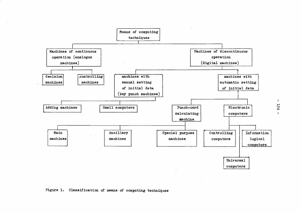
Means of computing

techniques i

I Machines of continuous

operation (analogue

machines)

' I I I decision I l".contr~lling J machines with

machines machJ.nes manual setting

I [ Adding machines I

Main

machines

of in! tial data

(key punch machines)

I I Small computers I

Ancillary

machines

I

I Machines of discontinuous

I calculat:i.ng

iiachine

Special purpose

machine~

I

operation

(digital machines) I

I machines with

automatic setting

of initial data

I I

I computers c 1

Controlling

computers

Universal

computers

Information

logical

comnuters

Figure 1. Classification of means of computing techniques

1-'

"' ~

- 195 -

machines of discontinuous operation. Machines of continuous operation work using

analogues of many physical phenomena and processes, which allow the simulation of these processes and phenomena. The machine does not obtain digital images of values,

but rather their images in the form of continuous variables, for example, in the

form of tensions of electric current. Analogue machines have high speed, but low

accuracy. Their applications to hydrometeorology are confined generally to a few

hydrological computations.

Machines of discontinuous operation (digital machines) are more widely

used. They are divided into two groups:

machines with manual setting of initial data (key punch machines),

and

machines with automatic setting of initial data.

Manual input, rather low speed, and the absence of "memory" rule out any

serious prospects of using machines with manual setting of data.

Digital machines with automatic setting of data are the basis for the mechanization and automatization of processing hydrometeorological information and

are divided into two large groups :

punch card calculating machines, and

electronic computers.

Let us dwell in more detail upon characteristics of these machines.

Punch-card calculating machines

Punch-card calculating machines automatically take the initial data which

is written on punched cards. Thus this group of machines is characterized by its technical carrier, i.e. a punched card. The detailed classification of punch-card calculating machines is given in Figure 2.

Auxiliary punch-card calculating machines, (i.e. a puncher and a controller) are

used only to compile and check punched cards:" they require manual setting of initial

data.

- 196 -

Punch-card calculating

machines

I I Alphanumerical . Digital machines

machines

I

1 .Ancillary Main machines Special purpose -~ machines machines

r I I

Puncher Controller Summary card Decoding

puncher machine

I Sorting Tabulator ·card-selecting Reproducer machine machine

Computing Electronic I puncher calculator

Figure 2. Scheme of the complex of Punch-card calculating machines

Electromechanical punchers and controllers used in processing Centres have

a limited technical speed of the order of 300 cards per hour, although their real

output is 1/~ to 1/3 this speed. The puncher can automatically duplicate punched

cards at a speed of some 250 to 300 cards per hour.

Desk-size mechanical punchers (for example, Bull puncher) with a somewhat

lower output are used to punch small amounts of data at points of observations.

The main punch-card calculating machines have the following characteris-tics.

A sorting machine which distributes punched cards to receiving pockets

- 197 -

(usually 13 pockets) and calculates the number of cards dispensed into each pocket. During one operation of input to the eomputer the sorting is performed for one position (some machines for two positions). The technical speed of the sorting is 18 to 20 thousand cards per hour, the actual speed being closer to 15 thousand.

The main purpose of a card selecting machine is to combine two card groups into one (the combining of punched cards) and the selection of cards by predetermined indicators. It has two magazines for input cards and four magazines for sorted cards. The combining is carried out at a speed of about 30,000 cards per hour for 16 columns.

A tabulator performs calculating operations and printing, i.e. tabulation. The alphabetic tabulator may print not only digits but also texts. The tabulator is mostly suitable for calculations involving subtraction and addition, and for printing initial data and results. Multiplication and division are generally per­formed by a special electronic calculating attachment: the speed of its multipli­cation operation is 150 eight-digit numbers per minute. The output of the tabulator is of the order of 6,000 cards per hour at line printing, and if printing only results, ita output reaches 9,000 cards.

A calculating puncher carries out four arithemetic operations and recorda the results on cards. Ita output is not high, for example, when multiplying it accounts for 1,000 products per hour.

Special purpose punch-card calculating machines

A reproducer performs the following operations:

(a.) producing card copies

(b) checking of two similar card sets

(c) distribution of data from one card to several cards (d) recording of data on one card from several cards.

The output is about 4,000 cards per hour.

The summary puncher is a machine connected to the tabulator for automatic recording of computed results on cards. The output is 100 to 120 per hour.

An electronic calculator consists of a device for input and output of cards as well as an electronic calculator itself. It is used along with other

- 198 -

punch-card calculating machines to increase the speed of calculating logarithms,

rooting, division and multiplication. The computed results are perforated on cards

with initial data or on new cards. The speed of operation is of the order of lOO

cards per minute.

A position reading puncher reads graphical marks from cards on which

original data are written with a graphite pencil. Using a given scheme the puncher

automatically makes punches in either of eighty columns of the same card, after

which cards are processed in the usual way.

Punch-card calculating machines have played a major role in the early

stages of the mechanized processing of hydrometeorological data. Now, however, due

to the fact that the amount of information is increasing and processing algorithms

are becoming more complex they do not, as can be seen below, keep up with

electronic machines and will be of little use when fully automatized systems are

developed. Their use is suitable for separate auxiliary operations (a kind of simple

sorting) only, or for simple computations of small data amounts, but even here they

are as a rule used in conjunction with an electronic computer.

Electronic Digital Computers with Automatic Setting of Initial Data

These computers, in contrast to analogue computers, perform computations

with digital values and with practically unlimited accuracy. Many electronic digital

computers function in multiprogramme conditions i.e. solve a number of problems at

a time. Already three main types of electronic digital computers and their respec­

tive constructive features have been clearly defined.

Universal electronic digital computers for the solution of complex mathe­

matical and engineering problems are characterized by very powerful calculators

which are capable of performing up to several millions of arithmetic operations per

second. The speed of input and output is essentially lower than that of the

computational speed. This type of computer, therefore, is intended for the solution

of problems involving a large number of computations using relatively small amounts

of initial information.

Information and logical electronic digital computers are also universal

machines, i.e. they are capable of solving a wide variety of problems, but they

are especially adapted for the rapid retrieval of information in large files. They

are characterized by rather large accumulators of information ("memories") and a

- 199 -

powerful system of different devices for information input and output.

Controlling electronic digital computers intended for controlling processes of production and the rate of processes are characterized by the presence of special devices aimed at establishing relations between a production object, computer and again production object.

For climatological purposes information and logical electronic digital computers and the universal electronic digital computers with a well developed system of peripherals are the most suitable.

We shall now discuss a structure system for the digital computer (Figure 3) and the requirements for the computer in -~he light of the problems to be solved in the processing of hydrometeorological information.

A data-preparation device records data on the technical carrier. Not all data-preparation devices form a part of the computer system since the recording of data on technical carriers is not always performed at the Processing Centre where electronic digital computers are located.

The following wide set of data preparation devices is used.

1. Devices for punched paper tape preparation :

(a) punched tape punchers in conjunction with the computer

(b) punchers suitable for location at large stations with communications (for example, teletype apparatus)

(c) punchers suitable for location at small stations without communication: (for instance, simple, inexpensive and reliable mechanical tape punchers)

(d) devices for automatic rerecording on standard punched tape from other technical carriers (special punched tapes I for recorders, etc.).

2. Devices for card preparation.

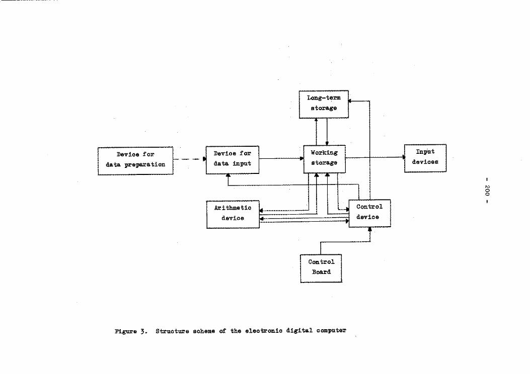
Devioe :for

data preparation 1----

Device :for

data input

T

Arithmetic

device

..

t..

~

Long-term

storage

Working

storage

~

Lt -.: r

r Control

Board

Figure 3. Structure scheme o:f the electronic digital computer

I Control

device

InpUt

devices

1\)

0 0

- 201 -

3. Device• for automatic punching for cards with graphical marks.

4. Devices for recording source information on magnetic wire and tape.

5. Self-contained devices for data rerecording from some (intermediate)

technical carriers on other more compact and productive intermediate technical carriers (for instance, on tape, magnetic discs).

6. Automatic self-contained devices for recording source observational data on intermediate magnetic carriers.

7• Devices for recording information on microfilms with the binary code.

Data input devices. Electronic digital computers for processing of data for olima.tological purposes should be provided with devices for input from appropriate technical carriers selected for the given centre and prepared by the above-mentioned devices of data preparation. Also, the availability of the following devices is essential:

1. Devices for direct data input from communication channels.

2. Devices for data input from analogue types of carriers, in particular, recorder tapes, chart isolines.

3. In special oases - devices for data input from forms with sensitive marks or from alphanumeric records.

Since the speed and reliability of operation of information-logical electronic digital computers depend in many oases on the reliability of input data, it is desirable to have two sets of main data input devices in service.

Working Storage

The information read out from technical carriers is recorded in a working

storage unit by means of input devices. The working storage which is characterized by a high speed and a high degree of operation reliability, stores initial data during the period required for their processing as well as the programmes for

problem solution. It also accumulates intermediate and computed results until the termination of a given cycle of processing and output of results.

The programmes for climatological processing as well as the amount of

- 202 -

initial information place high requirements on the capacity of the working storage.

Moreover, it is important that the working storage is provided with a "memory"

reserve for the operation of the electronic digital computer in multiprogramme

conditions. The working storage should be of the order of 50,000 and certainly no

less than 5,000 24-48-digit machine words. To increase the possibilities of the

computer operation, a "memory" of somewhat less speed, but with larger capacity,

for instance, magnetic drums is used in some electronic digital computers.

An arithmetic device performs arithmetic and logical operations and is

closely connected with the working storage. When problems are solved, data to be

processed are fed from the working storage to the arithmetic device, and the results

of computations, selection, etc. from the arithmetic device to the working storage.

The number of computational operations when processing and checking source

meteorological information as well as clima.tological calculations is not too great.

For this reason, the speed of the arithmetic device is of the order of 50,000

operations per second, and at small processing centres machines with a speed of

5,000 to 10,000 operations per second can be used.

A control device governs the computer according to a programme. Commands

from the working storage, where the programme is stored, are fed to the control

device where special control signals to be sent to blocks of the electronic digital

computer are generated (see Figure 3).

Long-term stora.~e. In order that the electronic digital computer,

(particularly, the information-logical type) can function, it is necessary to store

in the "memory" a. large amount of information (hundreds of millions of numbers). At

the same time "a. rapid memory" (the working storage) of modern computers does not

generally exceed several thousandsof numbers. The construction of a working storage

with a large capacity involves many technical problems. Therefore, together with the

"rapid memory" (the working storage), long-term s·horage devices with practically

unlimited capacity, are used in the electronic digitia.l computer, but because of the

high speed of operation of the computer they are not capable of exchanging informa­

tion with the control and arithmetic devices. The long-term devices accomplish this

operation via. the working storage.

The capacity of the long-term storage for solving climatological problems

should be of the order of 1 to 2 million machine words at least.

- 203 -

Modern long-term storage is usually in the form of tapes or magnetic discs.

Devices of data output. For climatological purposes a variety of data output devices is required:

1. An alphanumeric wide-sheet printer with the possibility for accurate printing on roll forms and with a printing quality allowing direct offset issue of

printed information.

2. Output devices on intermediate and long-term technical carriers (cards, punched paper tape, microfilm with the binary code).

3. A device for data output in the discrete and analogue forms to communications channels.

4. Output devices in the digital and analogue forms to the screen of an electronic-beam tube for visual analysis and photographing with special photo and motion-picture attachments.

5. A data output device in the digital and analogue forms as graphs, charts, diagrams with smooth curves of no more than 0.5 mm in thickness at no more than 0.5 mm intervals, plotted on sheets with a size no less than 1 m by 1 m. Curves, coordinates of graphs, coordinate grids of charts should be figured and provided with appropriate explanatory inscriptions (symbols).

The quality and completeness of information plotted by the machine should allow their direct issue by the offset method.

The control board is used by an operator to control the electronic digital computer (start, stop, manual input of some commands or data, etc.). A number of modern commercial electronic. digital computers e.g. the Minsk-32 electronic digital computer, largely satisfy requirements, apart from some ancillary devices.for data input and output. It should be noted that the economic efficiency of machine processing depends in many respects on the completeness and operational quality of a set of ancillary devices. It is evident therefore, that the ancillary devices determine to a large degree the number of expensive manual operations for the preparation and "completion" of computed results.

- 204 -

TECHNICAL .AND ECONOMIC EFFICIENCY OF USING DIFFERENT TYPES OF MATii EQUIPMENT

Machine processing of hydrometeorological data may be performed by means

of punch-card, key punch and electronic computational techniques.

The limits of reasonable use of these types of computational techniques

are significantly determined by the amount of processed information and the

complexity of processing algorithms.

The USA conducted research in the field of hydrology and found that

computations carried out by the electronic computer for the analysis of 282 equations

took about 7 hours of machine time. Research cost amounted to about U.S.$ 1,500.

If all the research were based on manual calculations or on using the punch-card

calculating machines, the cost would have exceeded U.S.$ 5,000.

The computation of a time correlation function of a meteorological element

for 1 station with a volume of information amounting 44,000 cards, carried out by a

"Minsk-22" electronic Computer is 8 times cheaper than by punch-card calculating

machine and is almost 150 times faster (Table 5).

On the basis of the analysis on the comparative efficiency of using punch­

card calculating machines and electronic computers for statistical processing one

can conclude :

the application of punch-card calculating machines is reasonable provided

the amount of information with simple processing algorithms does not exceed 150,000

cards, (with rather complex algorithms several thousands of cards);

the application of punch-card calculating machines for processing a

file which is over the above mentioned limits, is not reasonable from both economic

and technical points of view; in such cases the use of electronic computers is

required;

to compensate for the efficency of electronic computers when

processing large amounts of information it is necessary to increase the stock of

punch-card calculating machines. It also requires an increase of floor area.,

operating staff, etc.;

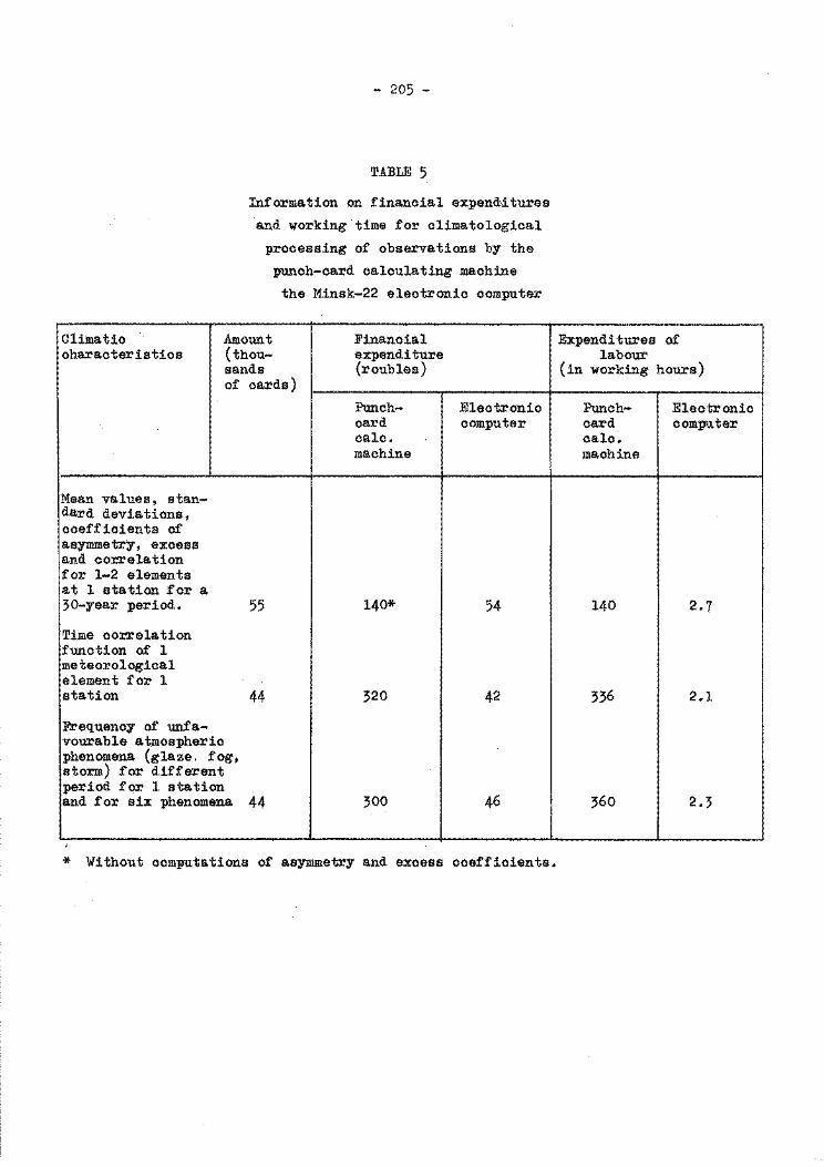
- 205 -

TABLE 5

Information on financial expend~tures

and working time for climatological

processing of observations by the.

punch-card calculating machine

the Minsk-22 electronic computer

Climatic Amount Financial characteristics (thou- expenditure

sands {roubles) of cards)

Punch- Electronic card computer calc. machine

Mean values, stan-dard deviations, coefficients of asymmetry, excess and correlation for 1-2 elements at 1 station for a. 30-year period. 55 140* 54

Time correlation function of 1 meteorological element for 1 station 44 320 42

Frequency of unfa-voura.ble atmospheric phenomena. (glaze. fog, storm) for different period for 1 station a.nd for six phenomena 44 300 46

* Without computations of asymmetry and excess coefficients.

Expenditures of labour

(in working hours) .

Punch- Electronic card computer calc. machine

140 2.7

336 2.1

360 2.~

- 206 -

automatization percentage for calculating and card-punching machines is

approximately 50 per cent, and for electronic computers in the order of 98 per cent.

Moreover, the high level of mechanized statistical processing achieved by

electronic computers also results in:

an increase in computational accuracy

an increase of effectiveness in using results

a considerable increase of quantitative and qualitative indices for

information use.

In only a few cases (sorting of data recorded earlier on cards, some

preparatory operations) is the use of punch-card calculating machines profitable

together with electronic computers.

CONCLUSIONS

The proposed methods of machines processing if introduced will give:

(a) scientific and technical benefits due increased completeness

and quality of hydrometeorological information and also

greater effectiveness in their use by consumers;

(b) indirect economic benefits through use by consumers in

determining more reasonable and desirable solutions to

national economic problems on design, building, transport,

energetics, industry, extraction of minerals, production of

food products and their storage, fish industry and other kinds

of activities in the sphere of material production as well as

in scientific and practical problems in other spheres;

(c) direct economic effect due to lower production costa.

However. in many cases the methods currently in use are not optimal and the

existing technical means to develop improved methods are not always sufficiently effec­

tive. It is necessary, therefore, to continue research and development work in this

area.

- 207 -

SURVEY OF DATA PROCESSING MACHINES

by

B. Eriksson *

Some problems in connexion with the introduction of automatic data processing at a olimatological division

Introduction

Before it is possible to come to a decision to change the system of data

processing being used for treating the material that is continously flowing to a

climatological division, it is necessary to make a thorough analysis of many factors.

The goal of the work at a climatological division is, without doubt, to be able to

provide information for use in applied climatology and research in a form acceptable

to the consumers. The consumer of climatological information does not always know

what information is available nor how it should be presented if it is to be of

maximum use. A climatological division therefore ought to inform users of its

capabilities. These capabilities can be increased by the introduction of modern

methods and machines for the treatment of climatological data. The goal for a

change from a data processing system based on manual methods mainly using paper,

pencil, and simple adding machines to a system which makes use of more advanced

methods must be to arrive at a rationalization of the work so that on the one hand

an economical profit or better exploitation of available economical resources is

achieved and on the other hand that better raw and refined products, for use in

applied and research fields, are produced.

When planning the introduction of new methods a long term view should be

taken. It is not certain that a change to the use of advanced electronic machines

gives immediate economic advantages. Improved climatological service, will result

from the in·troduction of modern data processing equipment, but due to the fact that

long series of data on media that can be read by the machines are not available,

the improvement may be a gradual process. In the first place, after some years,

when one has collected many years of climatological data on suitable media, one

can perform statistical analysis on the machines, as well as computations of

probabilities and duration of certain phenomena or combinations of different

variables. The great advantages of a machine system which can deal with large

amounts of data in a very short time with very little manual contribution will be

~ture presented by R. Berggren

- 208 -

obvious when large amounts of data are transferred to suitable technical media. The

data processing problems of a climatological division should not be regarded

separately but together with the whole data processing needs at the hydrometeorolo­

gical institute. The demands and needs for data processing facilities vary at

~tutes working in the fields of synoptic and aerological meteorology, hydrology,

climatology or research. The division working with numerical routine forecasts

for example has not the same requirements for data processing machines as a

climatological division. In most countries the climatological divisions are

smaller departments than the forecasting sections and the requests from the clima­

tologists for machine equipment do not perhaps carry great weight. In many

countries the daily forecasts are considered more important than climatological

information. Very few climatological divisions are big enough to merit the sole

use of its own computer. Thus many climatological divisions have to make use of a

machine system which has been provided primarily for daily weather forecasts. If

the meteorological institute has not the size or the economical resources required

to keep a machine system for data processing fully busy, there is the possibility

of renting time on a machine from a computer company. If the results of an

investigation of the different data processing systems indicate that a change to a

system based upon electromechanical or electronic machines would be profitable, there

are still a number of questions which must be answered.

The choice between punch-card machines and a computer 2Ystem

The passing from data processing based mainly upon manual methods to a

system that uses data processing machines can be done in one or many steps. One

step is to pass first to machines based on the punch-card and subsequently at a

later date to data processing on a computer. One may also pass directly from manual

systems to systems built up around a computer. Whether one short step or a some­

what longer one is better depends upon many circumstances, including economic

factors, the access to skilled staff that can run the machines, maintenance and

service facilities and whether there are similar machines at the locality or in the

country to permit back-up possibilities in case of machine breakdown. It is

difficult to give any general advice as the conditions vary greatly from one

country to another. Let us try to analyse the advantages and disadvantages of

the two types of data processing systems - the one which uses different types of

punch-card machines and the one which is built up around a computer.

- 209 -

A system of the first kind requires many different types of punch-card machines. Key-punch and verifier, reproducing, sorting and collating machines are required. These machines work at high speed but they are all specialized and many machines rather than one single calculating machine are needed. Moreover all of these machines are ex~ensive to buy or hire. A user must have large amounts of data to be able to keep its own machine-park. Also the card-machines require skilled operato:rs in order to work effectively. The calculations which can be performed on a tabulating machine are of a rather simple character: addition, subtraction and in certain cases multiplication can be done. In climatological work a tabulator can be used for accumulation, for preparing frequency tables and for printing of climatological summaries. For scientific purposes punch-card machines are less effective. Since more and more electronic computers are coming onto the market the electromechanical punch-card machines are becoming less important. Today, a data processing system with a computer seems to be a better solution in many cases. The c.ost of a medium-sized general purpose computer is not so much higher than a punch-card installation. As the speed of the computations that a computer can do has increased, the cost per computation performed has steadily decreased during the past two years. In fact the cost of a mathematical operation done by a computer is less than having it done in any other way. Because of the great flexibility with which an electronic data processing (EDP) system can be built and the endless possibilities for solving complicated computations there are many strong arguments for the choice of an EDP-system.

Choice· of computer and devices for. input and output

Suppose that the investigation regarding data processing systems has led to a decision that an EDP-system should be used. The need to examine the different types of computers and accessories then arises. Most computers can be delivered in different sizes and there are many possibilities to tailor a system to suit best the problems in question. When choosing between different manufacturers one should take into account not only the price and the speed with which additions or multiplications are done"but also such factors as how maintenance and service can be arranged as well as whether programming systems (so-.called soft-ware) are inclu­ded in the price, whether these systems are well tested and whether the manufacturer gives aid in training programmers. It can be of value to choose a type of computer already existing in th~ country.

Regarding the need for high speed of the central processing unit the

- 210 -

demands are different from different users in a meteorological institute. The

forecasting division which needs a computer for objective analysis and numerical

forecasts wants a computer with very short addition and multiplication times as

even a simple atmospheric model requires many additions and multiplications to

calculate a 24-hours forecast for one level only. A climatological and even a

hydrological division have data processing problems of a rather different nature.

They have large data amounts to be fed into the machine, rather simple calculations

to be performed, the results printed out and data stored. The need regarding the

speed of the computations from the climatologists point of view is less but the

need for high speed of the devices for input and output is higher. A compromise

between the needs of the different sectors of an institute is therefore necessary.

In the beginning a computer system can be built from a rather small

initial system completed later by for instance larger internal storage, more

magnetic tape stations, a plotter and so on. A small to medium-sized computer

system might have the configuration shown in the Figure.

The central processing unit consists of three main parts, the control unit

the arithmetic unit and the high-speed core memory. The internal storage of a

medium-sized computer can hold 20,000 to 30,000 words. The number of binary

positions in a computer word varies, a common number being between 24 and 48. The

addition time of a computer of medium speed is about 10 microseconds. For a fast

computer the time for addition of two numbers can be 1 microsecond or even less.

The time for multiplication performed by a medium-fast computer is 30-50 micro­

seconds. For each computer there is a console panel with keys used to start and

stop and to direct certain courses during a run of programme. An electrical type­

writer is coupled with the machine. On this type-writer information is written for

the operator. Orders can be given to load the card reader with cards, to put a

certain magnetic tape in a tape station, etc.

Facilities for input and output are necessary devices. The electrical

typewriter' can only be used for output and input of very small amounts of informa­

tion since the speed·of writing is very low. On the input side a paper tape reader

is a rather important or necessary equipment since most data arrive at the tele­

communication centre on teletype machines that produce a 5-channel telex tape. A

paper tape reader normally reads 1000-2000 characters/second. A card reader is also

a common device for feeding data and programmes into the computer and data from

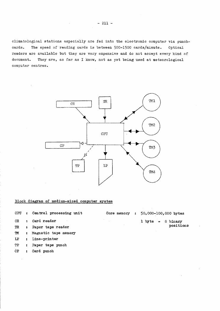
- 211 -

climatological stations especially are fed into the electronic computer via punch­

cards. The speed of reading cards is between 500-1500 cards/minute. Optical

readers are available but they are very expensive and do not accept every kind of

document, They are, as far as I know, not as yet being used at meteorological

computer centres.

CR 'ffi

CPU

CP ]<!-- / /

/

ES I LP

I

1//

Block diagram of medium-sized computer system

CPU

CR

TR

'I'M

Central processing unit

Card reader

Paper tape reader

Magnetic tape memory

LP : Line-printer

TP : Paper tape punch

CP : Card punch

Core memory

G

50,000-100,000 bytes

1 byte 8 binary positions

- 212 -

Magnetic tape is used both as an input and output device and most computer

systems, apart from the smallest are equipped with magnetic tape stations. The

number of stations can be large. For a medium system 4-6 stations ought to be

sufficient for meteorological and climatological applications. The speed of

transfer between the internal storage and the magnetic tape is very high, normally

30,000 - 60,000 characters/second.

A very valuable output device is the line-printer. It operates with

speeds around 1000 rows/minute. On the line-printer the climatologists can produce

their tables and summaries for monthly bulletins, yearbooks and so on. The tables

can be manifold.

Many other facilities can be added to a computer system. Magnetic discs

and magnetic drums may be used as external memories. The magnetic tape may also be

regarded as an external memory. The advantage of discs and drums compared with

magnetic tape is that there is almost direct access to the information stored on

these media. The time to obtain access to information on a magnetic tape may be

relatively long i£ a large part of the tape has to be read before the required

information is found. Further devices for output are among other things, plotters,

paper tape and card punchers.

A machine configuration of the size shown in the figure may be too large

for a small meteorological institute. The possibility ·to rent time from a computer

firm, if available, can be tried or agreements might be made with other

authorities or companies to share a computer. After some years when the climatolo­

gists have gained experience and have trained staff at their disposal one normally

finds that more and more tasks can be taken over by the computer and the need for

computer time rises steadily.

Planning and training of staff before shifting over to automatic data processing

When the decision has been taken to go over to an EDP-system at a clima­

tological division there follows an intensive period of further planning and

training of staff. The training of persons belonging to the division is very

important. The changing of the working routines affects many categories of personnel;

observers at the climatological stations will in some ways come into contact with

the new data processing system, assistants at the division who previously carried

out many of the calculations will receive new tasks, and the climatologists will

have to reconsider their methods of calculation and publication of climatological

- 213 -

data in light of the new system. The tasks of certain staff will disappear completely and other new tasks will require doing.

Media for input

An important question to be settled is: the medium on which the cllma­tological data should be fed into the computer. If, for example the computer can accept both paper tape, cards and magnetic tape, which media is the most appropriate for input? Most climatological divisions have up to now used punch­cards for the input. However, this is not necessarily the most suitable since the storage density is low and the archival life is rather short. Over the past

few years magnetic tape (manual and automatic) has been a good alternative to the punch-card and paper tape. The devices for the registration on magnetic tape are rather more expensive to buy or hire than the corresponding paper-tape or card punching machines, but magnetic tape is the most rapid and the cheapest medium for data registration. The advantages of the magnetic tape over paper tape and punch­card are many the storage density is much higher and the reading into the computer

is much more rapid. Thus expensive computer time is saved, less archive space is needed and moreover it is much easier to transport the registered information from the punching room or the archives to the computer room.

Fitting log-books to the EDP-system and the punching

Irrespective of which medium is selected for input one has to punch or write the climatological data on the medium. At the automatic meteorological

stations this is of course done automatically on paper or magnetic tape. Each obser­vation hour certain parts of the observations are received from the synoptic stations on telex tape from the teletypes. This information can be used directly for climatological purposes. There are however a number of observations which have to be transfered to the computer medium. This transference procedure is both expensive and time-consuming, and is generally performed centrally at the climatological

division from the log-books, sent to the meteorological institute by mail. It is possible to carry out the registration of the data on the medium at the observing station, providing it is done simply and cheaply. If the punch-card is used for input the mark-sensing card can be used.

Log-books in which observers note their weather observations have to be adapted to the automatic data-processing system. The source documents from which

- 2l.4 -

the punching is carried out must be constructed in such a manner that the punching

is made easy. The observations in the log-book should be written in the order in

which they are to be punched. Observers must be trained to record the observations

in accordance with given rules: it is more essential that fixed rules are obeyed in

an automatic data processing system than in a manual processing system. When

the observations are treated manually it is relatively easy to discover whether a

reading has been written in a wrong column, but with a computer programme it is

much more difficult to find errors of this nature. A manual inspection of the log­

books is recommended before they are sent to the punching section. The punching

staff must receive training on the type of machine provided for the transformation

of the data to the appropriate media.

The checking of the punched data is also important. Verification can be

effected in at least three different ways. The verification of the punching should

be done manually even if it is possible to write control programmes such that

certain punching mistakes can be found by the computer. One manual method is to

punch the data again on a special machine called a verifier. Another method is

list the punch-cards (when punching on a paper tape machine an out-print is received

at the same time as the tape is punched) and proof-read these lists against the log­

books. A third method is to compute control sums and carry out the punching on a

machine equipped with a device to accumulate the numbers being punched. If the

control sum does not agree with the sum received at the punching a signal is given.

Programme writing for climatological calculations

It is not enough to have punched and verified data on the appropriate

medium and access to computer time. The most important part of a computer system

is the programme giving the computer detailed step by step instructions what to do

with the data to be treated. Designing the programmes for the climatolcgical data

processing is very important and the planning must be done in co-operation with all

climatological and programming experts available. If the computer system can use

different programming languages one has to choose one or more which give the most

effective programmes in relation to the time needed for writing them.

One of the climatological division staff should receive training in the

art of writing computer programmes. At many meteorological institutes meteorolo­

gists are trained to undertake programming work. To leave the programming to

professionals unacquainted with climatology is not a good solution. Proper computer

know-how at a climatological division is invaluable. It does not take very long to

- 215 -

learn programming. The first programmes to be written are those which perform most of the necessary computations previously done manually. After that programmes for more advanced treatment of the climatological data and computations and investiga­tions which were not possible before the introduction of the EDP-system may be written. Certain other changes in the ordinary climatological routines may also be appropriate in a new data processing system. Tables in the monthly and annual climatological summaries, might be re-arranged to better suit the printing equip­ment of the computer system.

Programmes have to be thoroughly tested on different kinds of da·ta before the changeover to the new system takes place. Even after the new system is opera­tional it might be necessary to modify and improve the programmes. In such cases it is a distinct advantage that the person who has written the programme belongs to the regular climatological staff. When programmes are found to function well, they can be used for many years.

As soon as a library of data is available on magnetic tape, climatological research and investigation can be done effectively and economically on the computer. New programmes have to be written and staff with a good knowledge of computer programming are needed at a climatological division even before the first introduc­tory period has been completed.

Operating the computer

If the machines used in the automatic data processing system have been bought or hired by the meteorological institute, staff must be trained to operate the computer and its various components. Programmers have to write detailed instructions as to how the programmes are to run, how and what data are to be fed into the computer, how the results should be delivered from the computer, action to be taken when errors are signalled by the computer and so on. These operators, who might be selected from the staff who originally carried out the work taken over by the computer, must be trained how to use the keys of the console of the computer, feed punch-cards into the card reader, mount and dismount magnetic tapes in the tape stations, mount paper in the line-printer etc.

The technical servicing and maintenance of the computer system should be

done by specially trained technicians, who are normally supplied by the manufacturer of the computer.

- 216 -

Conclusions and summary

A change over from manual processing of climatological data to EDP requires

very careful planning and a number of choices between different alternatives has

to be made. The more carefully the planning is done, the easier it is to

change over to the new system.

The introduction of modern data processing methods represents a radical

change in a climatological division. A large part of the manual work is taken over

by machines. Some of the staff who have been occupied with the previously manual

operations have to be trained for other duties as new tasks are added. Data has to

be·punched, programmes must be written and tested, and machines have to be operated.

A special organization is necessary to feed the computer, which devours information

like a hungry monster. Every minute of computer time costs a great deal of money

and as such must be used efficiently to facilitate the work of the forecasters, to

help the climatologists to be able to provide the necessary climatological informa­

tion tq society for planning and the improvement of the production and economy of

the country.

An attempt to summarize the advantages and disadvantages of using advanced

machines for data processing of meteorological data follows.

The main disadvantage with EDP machines is that they are expensive. If

the country has a surfeit of cheap labour it is unlikely that the introduction of a

computer system will involve immediate economic return. Also the machines are

highly technical and engineers who are able to maintain ·the complicated equipment

must be available. Moreover many computers need special rooms where the temperature

and humidity conditions can be kept constant.

The advantages with EDP are many, especially in the long term. In a

climatological division computations are not as a rule very complicated but on the

other hand there is a huge amount of data to be processed. With the introduction of

EDP, climatological observations can be controlled systematically and the publica­

tion of climatological summaries can be made at an early date. The tables written

by the line-printer or tabulator can be published directly without proof-reading.

Special investigations asked for can be performed simply by writing a programme for

the computer if the necessary data are available on suitable media. Meteorological

and climatological research is greatly stimulated and made easier by the introduc­

tion of a computer system.

- 217-

METHODS FOR DATA PROCESSING FOR CLIMATOLOGICAL PURPOSES

Use of data obtained by recording instruments

by

R. Arlery

By force of circumstances whether they be economic or technical, it will

be impossible for a long time to come for most Meteorological Services to convert

the present network of stations with recording instruments to an ultra-modern network,

allowing data to be stored on technical carriers (punched tapes or magnetic tapes)

and fed directly into conventional electronic equipment. Thus, the use of data

obtained from recording instruments remains one of the present-day problems, and,

in addition to making it desirable to examine future prospects, justifies a study of

the means for making the best possible use of the recordings which are available

within the Services, and of which no use has.yet been made.

Automatic reading of charts

This is clearly the solution for the future, but it cannot generally be

applied to existing climatological records. Such automatic reading implies that

the recordings should have been made in accordance with well-defined and rigid stan­

dards, in order to obviate difficulties due to smudging, breaks in the recording,

several traces on the same chart, different coloured inks, etc., and in order to

eliminate certain inconsistencies such as a "trace" consisting of points, curvilinear

scales, or vertical traces in recordings of precipitation where siphoning is used.

Thus, in general, charts intended for automatic reading, should be carefully designed

beforehand, bearing in mind the method of automatic reading to be used.

Semi-automatic reading

This usually concerns equipment in which the positions of a certain number

of points on the trace, which are regularly spaced with regard to time, are found

manually. By means of a suitable device, the chart may be made to move automatically

in the direction along the axis of abscissae and the operator has only to record the

points on the trace, by operating a pedal for example. By this means, the co­

ordinates of each point are punched on a card. The necessary precautions should be

taken with regard to the use of the reading table, checking the zero position, choice

- 218 -

of suitable scales for abscissae and ordinates, the beginning and end of the re­

cording, checks during the process of analysis, treatment of recordings consisting

of several traces, etc.

Analysis by completely manual methods

The selection of data to be obtained from recordings by purely manual

methods is a somewhat delicate matter. We should not be too ambitious and we should

avoid imposing work which is too exacting, thereby running the risk of the work being

performed with insufficient care. However, we should also bear in mind that

analyses, carefully carried out, may help staff to improve their knowledge and widen

their experience in matters concerning loc~l climatology. When reduced to such

manual analysis, it is thus preferable, in order to limit the amount of work and to

facilitate checking, to arrange for the work to be done at the station itself, rather

than carrying out all such work at a specialized centre. On the other hand, this

makes it necessary to arrange the work on an extremely rational basis.

We shall take one single example concerning the acquisition of the basic

data necessary for the study of the intensity of precipitation.

!,n,!.l,Ys.!,s_of £!:.a!l.Y!_a!nfall_c,ha!,t!!,

The determination of the intensity of precipitation by the analysis of

recording raingauge charts may be considered in various ways, depending on the prob-

lems to be solved. We shall discuss, very briefly, the various possible methods,

but we shall place most stress on a simplified method, making no claims to giving a

detailed and complete study of the frequency-intensity-duration relationships for all

periods of rainfall at a given place.

We shall pay particular attention to finding the most economical methods

for determining the probable frequency of the intensity of precipitation exceeding

any given value. We shall moreover reduce the complexity of the processing by

assigning a limit to the value corresponding to the time interval used to determine

the mean maximum intensity.

For each selected time interval, it is necessary to find and record all

amounts of precipitation which exceed the given limit, without overlapping of the.

time intervals. It is then a simple matter to convert amounts to mean intensities,

using the same unit (usually millimetre per hour), over 10 minutes, 15 minute~, half

an hour, one hour, etc.

- 219 -

The first difficulty clearly lies in determining a priori the limits which

it would be appropriate to select. These limits depend, of course, on regional

conditions and, unless we already have some approximate knowledge of the phenomena

under consideration, it will be necessary to determine the limits by trial and error,

at least during the initial phase of the investigation. Very often it is sufficient

to adopt limits such that the intensities occur, on average, about 10 times per year,

during a first sampling extending over a few years.

Once these limits have been adopted, the operator is able to identify,

without too much difficulty, falls in which the limits will probably have been ex-

ceeded. He must then determine whether, for each time interval, the amount actually

recorded exceeds the given limit: if it does, he proceeds to analysis, after having

checked, by comparison with direct measurements with an ordinary raingauge, that the

recording does not require correction.

Analysis is facilitated if we have suitable transparent scales, gradua·bed

for the various time intervals which we have to consider on the chart. The pro­

cedure is then as follows, for each time interval:

(a) Slide the scale along the chart, to identify the absolute maximum; if this

maximum exceeds the limit, note the time of the beginning of the interval

and also the amount of precipitation during this interval.

(b) Slide the scale along the chart to see if there is a second maximum (less

than the first), making sure that there is no overlap of the new time

interval and the time interval for the first maximum. In the same way as

before, note whether this second maximum also exceeds the limit. Continue

these operations on the same chart, until all the successive maxima which

exceed the limit have been noted, taking care that there is no overlap in

the time intervals with which these various maxima are associated.

(c) Change the time interval and proceed as before, making sure that each

maximum noted for a given interval and exceeding the limit for one or

several longer time intervals, does in fact give a maximum for this (or

these) longer interval(s).

- 220 -

It is best to set out the data on a printed form prepared for the purpose,

which would have, for example, for each time interval dt, three columns for:

J = Day and month

H = Time, GMT, of beginning of the interval dt

Q = Amount of precipitation (water) during this interval dt.

It should be noted that, only rarely will the time of commencement of

precipitation coincide with the time of the beginning of one of the time intervals

under consideration (in certain cases it could be later). Similarly continuity of

precipitation is not essential; a selected interval (for which a maximum has been

noted) may include the whole or part of several separate falls. In the case of a

defective record, the dates of the beginning and end of the period during which it

was impossible to determine maxima, should be shown, so that this period may sub­

sequently be deducted from the total time to which the statistics refer.

The work involved in preparing these summaries is not at all irksome if

done day by day. However, even if undertaken for a whole year at a time, it does

not assume large proportions, the heaviest part of the work being, in fact, to find

amongst the collection of daily charts those which need to be analysed.

As soon as a sufficient number of years' observations are available, using

the above summaries, "frequency-intensity-duration" statistics for precipitation are

prepared as follows:

For each time interval dt, the maximum amounts during the N years are

arranged in decreasing order of magnitude, regardless of the dates of occurrence. In

the ranking list thus obtained, the value of rank N represents the amount equalled or

exceeded N times inN years, i.e., the amount equalled or exceeded, on average, once

per year. In the same way, the value of rank 2N is the amount equalled or exceeded

on average twice per year; the value of rank N/2 is the amount equalled or exceeded

once every two years; and so on, thus: rank N/5 corresponds to an average frequency

of once in five years, N/10 to once in ten years, etc. However, it will immediately

be seen that there should be data for a large number of years, in order that the

assigning of frequencies such as once in ten years have any meaning. The value of

rank N/10 will be the second in the ranking list if the number of years is only 20.

With regard to the first value in the list, all that can be said about it is that

it is the highest value observed during the period under consideration; it is an

indication only, and of course cannot be used to make a correct estimation of an

average frequency in N years.

- 221 -

In spite of these doubts concerning maximum intensities with a low frequency of occurrence, we may determine· empirically the average freque~cies of the maximum amounts which have fallen in a time dt and these may easily be converted to hourly intensities (simply by dividing by dt expressed in hours or fractions of an hour). If we take T as the average return period (or average period of recurrence) and Idt the average maximum intensity associated with this return period, we can plot on a diagram, for each dt, values of Idt corresponding to various return periods. In this way we obtain a set of curves for the "frequency-intensity-duration" relation­ships for precipitation. The nature of these curves is such that in many cases, for a given dt, there is an approximately linear relationship between the logarithm of the average maximum intensity in an interval dt and the logarithm of the return period. If we choose logarithmic scales for the co-ordinates of the variables, the "frequency-intensity-duration" graphs for precipitation are a set of straight lines, which facilitates any adjustments which need to be made. However, we should not lose sight of the fact that this is merely a simplified theory and we should not accept without question the results so obtained.

- 223 -

THE PRINCIPLES OF COMPUTER PROGRAMMING

by

B. Eriksson *

The principles of computer programming

1.n.!r.2_d,!!c_1i.2_n

A climatologist must know the fundamentals of programming so that he can

use a computer. To be sure, a climatological division can commission a professional

computer bureau to write climatological programmes, but the dialogue between clima­

tologist and professional programmer will be much easier if the former has some idea -

evert if only a rudimentary one - how his problems can be solved with the aid of a

computer.

In the early days of the computer era the computers had to be programmed in

machine codes, which is the basic language of the computer. Writing major programmes

in machine code is a task which calls for a great deal of care. A programme can be

very effective, and if it has to be run very frequently - daily or several times

daily- its effectiveness is of the utmost importance. In the case of programmes

used rather seldom, once a month or so, effectiveness is not as important as ease of

writing~ Although machine coding is used very seldom nowadays, a knowledge of its

principles is nevertheless useful when automatic coding systems are operated.

There are many and varied types of computer from small ones no bigger than

a mechanical desk calculator to huge ones occupying a large room. All, however,

have certain features in common.

Storage, stored programmes

In order to understand the principles of machine coding, let us take a very

simple but imaginary computer which has properties in common with all real computers.

A computer must have an internal or primary memory, an arithmetic unit, a control

or steering unit and devices for input and output. The structure of a computer is

shown in the block diagram below:

* Lecture presented by R. :Berggren

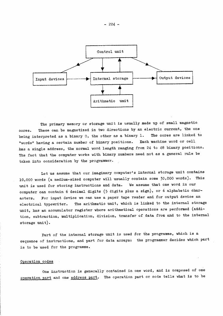
- 224 -

Control unit

Input devices Internal storage Output devices

Arithmetic unit

The primary memory or storage unit is usually made up of small magnetic

cores. These can be magnetized in two directions by an electric current, the one

being interpreted as a binary 0, the other as a binary 1. The cores are linked to

"words" having a certain number of binary positions. Each machine word or cell

has a single address, the normal word length ranging from 24 to 48 binary positions.

The fact that the computer works with binary numbers need not as a general rule be

taken into consideration by the programmer.

Let us assume that our imaginary computer's internal storage unit contains

10,000 words (a medium-sized computer will usually contain some 30,000 words). This

unit is used for storing instructions and data. We assume that one word in our

computer can contain 6 decimal digits (5 digits plus a sign), or 6 alphabetic char­

acters. For input device we can use a paper tape reader and for output device an

electrical typewriter. The arithmetic unit, which is linked to the internal storage

unit, has an accumulator register where arithmetical operations are performed (addi­

tion, subtraction, multiplication, division, transfer of data from and to the internal

storage unit).

Part of the internal storage unit is used for the programme, which is a

sequence of instructions, and part for data arrays: the programmer decides which part

is to be used for the programme.

Operation codes

One instruction is generally contained in one word, and is composed of one

operation part and one address part. The operation part or code tells what is to be

- 225 -

done, while the address part usually indicates which word will be affected by the

operation. In our case, the format of the instructions is OPADRS. The first two

positions OP are the operation part, and ADRS the address part. The instructions

are normally obeyed in order. If the computer starts with the instruction stored in

the cell with address 200, it normally continues with the instruction in cell 201,

and so on.

OP

00

01

04

40

06

46

22

23

63

26

70

71

Some examples of operation codes are given below:

Address

AAAA

AAAA

AAAA

AAAA

AAAA

AAAA

AAAA

AAAA

AAAA

AAAA

AAAA

AAAA

Meaning

Add to the accumulator register the content of the

cell with address AAAA.

Enter zero in the accumulator register and then trans­

fer to the register a copy of the content of cell AAAA.

The value in the accumulator register is multiplied by

the value stored in cell AAAA and the result entered

in the register.

From the value of the accumulator register is sub­

tracted the value stored in cell AAAA.

The content of the accumulator register is written in

cell AAAA.

Similar to code 06, but is also entered in the register.

Jump to cell with address AAAA.

Jump to cell AAAA if the content of the accumulator

register is ~ 0.

Jump to cell AAAA if the content of the accumulator

register is < 0.

If this instruction is placed in a cell with address

1, the address (1 + 1), together with the operation

code 22, is transferred to word AAAA and a jump is

made to cell (A + 1).

Read 6 characters from the paper tape reader to the

accumulator register and store in word AAAA.

Write on the electric typewriter a copy of the con­

tent of cell AAAA.

- 226 -

OP Address Meaning

25 AAAA The computer stops. When the starting key is pressed

down, a jump is made to cell AAAA.

With the aid of these instructions we can make some simple programmes.

In the first example we want to read two numbers x and y from a paper tape, store

these numbers in two words and write the sum.

In cell number

1000

1001

1002

1003

1004

1005

The programme will look like this:

Instruction

700100

700101

000100

060102

710102

251000

Comments

The first number on the paper tape is read and

stored in word lOO.

The second number on the tape is read and stored in

word 101.

The value x is added to the accumulator register,

which already has the number y.

The sum of x and y is stored in cell 102.

The sum is written on the typewriter.

The computer stops. When the starting key is

pressed down, two new numbers are read.

The programme has been read into the internal storage unit with the aid of

a special programme. A necessary assumption for the results to be correct is that

the numbers have been punched correctly on the tape. In this case, they must be

punched with 6 or 5 digits and a sign.

Jumps

Instructions are obeyed in order, but an exception to this rule is the

jump-instruction, compelling a jump to another instruction whose address is given in

the address part of the jump-instruction.

The jump-instruction can be conditional or unconditional. The conditional

one 'leads to a jump only if a certain condition is fulfilled. For our imaginary

computer the three instructions 22, 23 and 63 have been defined.

- 227 -

With the aid of jump-instructions programmes containing "loops" can be

constructed. A loop is a part of the programme that is executed many times. Let

us now suppose we want to write a programme that reads pairs of numbers xi, yi from

a paper tape, takes the sum of x and y and prints it. All x-values are assumed to

be positive numbers, a negative number of x being used as a stop signal.

Instruction stored in cell

3000

3001

3002

3003

3004

3005

3006

3007

Constants

Instruction

705000

633007

705001

005000

065002

715002

223000

253000

Comments

A number from the paper tape is read and stored in

cell 5000.

If the number just read is negative, a jump is made

to cell 3007.

Next number, y, is read.

To the content of the accumulator register, y, is

added the value x.

The sum of x. and y. is stored in cell 5002. ~ ~

,·The sum is written.

A jump back to the first instruction.

The computer stops.

Generally one needs a number of constants in a programme. These have to

be stored in certain cells. Let us now examine a programme that reads a sequence of

numbers xi from the paper tape, and writes those numbers that are ~ 0 and~ 1000.

The first number (n) on the tape we assume to be the quantity of numbers xi. The

block diagram for this computer operation is shown in Figure 1. A certain cell

(4001) is used to count how many x-values have been read.

The machine code is as follows:

1999 704000 Read the first number, n, and store in cell 4000,

2000 464001 Enter zero in the accumulator register.

2001 464001 Zero is written in cell 4001.

2002 704002 A number is read from the paper tape and stored,

No

- 228 -

Read the first number

n

Zero entered in cell

4001

Read x

Print x

Increase

Yes

Yes

the content of ~------------~ cell 4001 by l

FIGURE l

Block scheme

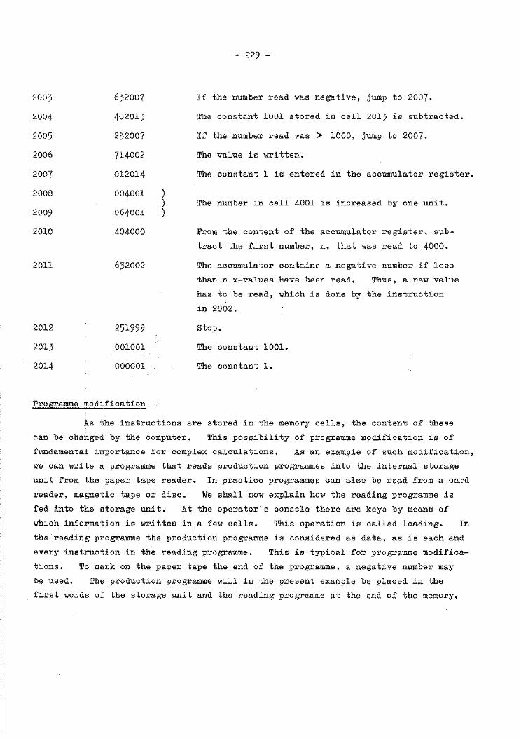
- 229 -

If the number read was negative, jump to 2007. 2003

2004

2005

2006

2007

2008

2009

2010

632007

402013

232007

714002

012014

004001

064001

404000

The constant 1001 stored in cell 2013 is subtracted.

If the number read was > 1000, jump to 2007.

The value is written.

The constant l is entered in the accumulator register.

2011

2012

2013

2014

632002

251999

001001

000001

Programme modification

l The number in cell 4001 is increased by one unit.

From the content of the accumulator register, sub­

tract the first number, n, that was read to 4000.

The accumulator contains a negative number if less

than n x-values have been read. Thus, a new value

has to be read, which is done by the instruction

in 2002.

stop.

The constant 1001.

The constant l.

As the instructions are stored in the memory cells, the content of these

can be changed by the computer. This possibility of programme modification is of

fundamental importance for complex calculations. As an example of such modification,

we can write a programme that reads production programmes into the internal storage

unit from the paper tape reader. In practice programmes can also be read from a card

reader, magnetic tape or disc. We shall now explain how the reading programme is

fed into the storage unit. At the operator's console there are keys by means of

which information is written in a few cells. This operation is called loading. In

the reading programme the production programme is considered as data, as is each and

every instruction in the reading programme. This is typical for programme modifica-

tions. To mark on the paper tape the end of the programme, a negative number may

be used. The production programme will in the present example be placed in the

first words of the storage unit and the reading programme at the end of the memory.

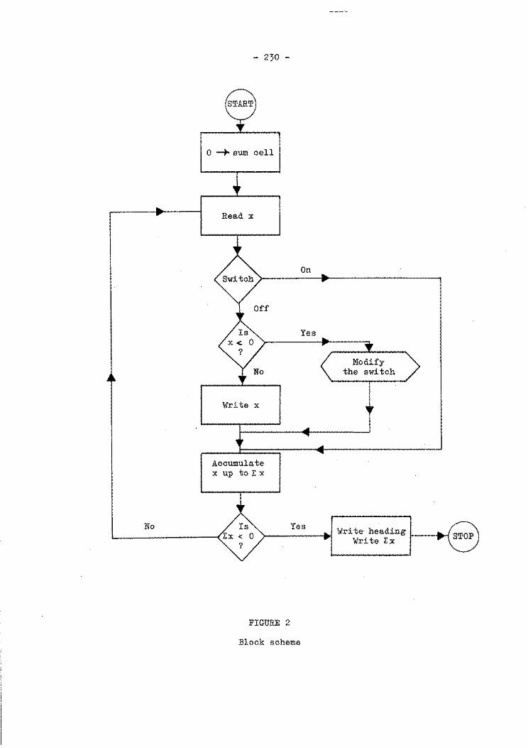
No

- 230 -

0-+ sum cell

Read x

Write x

Accumulate x up toE x

FIGURE 2

On

Yes

Yes

Block scheme

Write heading I .. I Write Ix

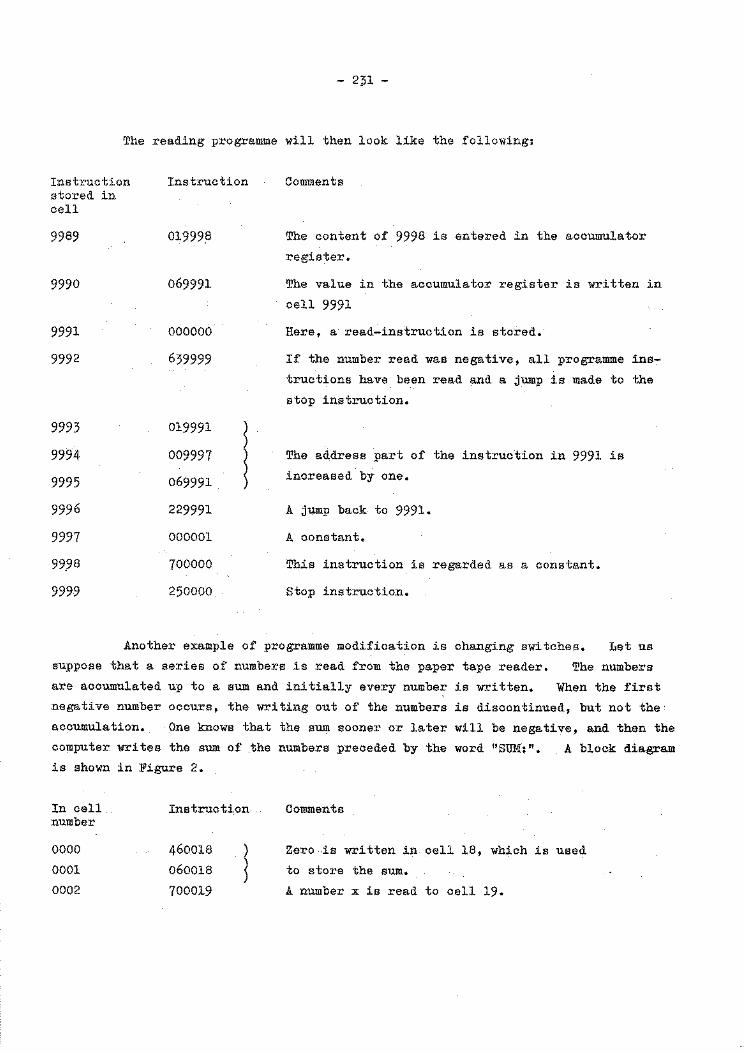
- 2;31 -

The reading programme will then look like the following:

Instruction stored in cell

9989

9990

9991

9992

9993

9994

9995

9996

9997

99.98

9999

Instruction

019998

069991

000000

639999

019991 ~ 009997 l 069991

229991

000001

700000

250000

Comments

The content of 9998 is entered in the accumulator

register.

The value in the accumulator register is written in

cell 9991

Here, a read-instruction is stored.

If the number read was negative, all programme ins­

tructions have been read and a jump is made to the

stop instruction.

The address part of the instruction in 9991 is

increased by one.

A jump back to 9991.

A constant.

This instruction is regarded as a constant.

Stop instruction.

Another example of programme modification is changing switches. Let us

suppose that a series of numbers is read from the paper tape reader. The numbers

are accumulated up to a sum and initially every number is written. When the first

negative number occurs, the writing out of the numbers is discontinued, but not the·

accumulation. One knows that the sum sooner or later will be negative, and then the

computer writes the sum of the numbers preceded by the word "SUM:". A block diagram is shown in Figure 2.

In cell Instruction Comments number

0000 460018 ) Zero is written in cell 18, which is used

0001 060018 ~ to store the sum.

0002 700019 A number x is read to cell 19.

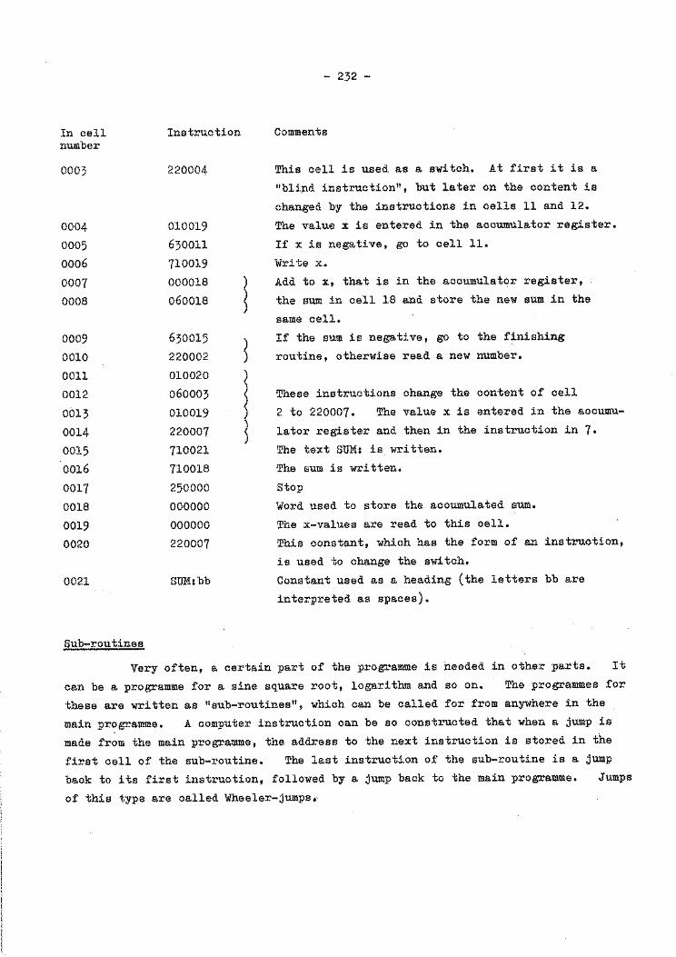
In cell number

0003

0004

0005

0006

0007

0008

0009

0010

0011

0012

0013

0014

0015

0016

0017

0018

0019

0020

0021

Sub-routines

Instruction

220004

010019

630011

710019

000018

060018

630015

220002

010020

060003

010019

220007

710021

710018

250000

000000

000000

220007

SUM:bb

l ) )

)

l ~

- 232 -

Comments

This cell is used as a switch. At first it is a

"bli;nd instruction", but later on the content is

changed by the instructions in cells 11 and 12.

The value x is entered in the accumulator register.

If x is negative, go to cell 11.

Write x.

Add to x, that is in the accumulator register,

the sum in cell 18 and store the new sum in the

same cell.

If the sum is negative, go to the finishing

routine, otherwise read a new number.

These instructions change the content of cell

2 to 220007. The value x is entered in the accumu­

lator register and then in the instruction in 7•

The text SUM: is written.

The sum is written.

Stop

Word used to store the accumulated sum.

The x-values are read to this cell.

This constant, which has the form of an instruction,

is used to change the switch.

Constant used as a heading (the letters bb are

interpreted as spaces).

Very often, a certain part of the programme is needed in other parts. It

can be a programme for a sine square root, logarithm and so on. The programmes for

these are written as "sub-routines", which can be called for from anywhere in the

main programme. A computer instruction can be so constructed that when a jump is

made from the main programme, the address to the next instruction is stored in the

first cell of the sub-routine. The last instruction of the sub-routine is a jump

back to its first instruction, followed by a jump back to the main programme.

of this type are called Wheeler-jumps.

Jumps

- 233 -

Let us now examine a section of a main programme and a sub-routine.

Main programme

0498

0499

0500

0752

0753

0754

Sub-routine

5000

5450

265000

265000

000000

225000

A Wheeler-jump to a sub-routine that starts in

cell 5000.

A jump to the same sub-routine.

In this cell write a jump-instruction back

to the main programme. The first time the

instruction 220500 is stored here, and in the

second the sub-routine is called upon in

cell 5000 and written 220754.

Jump back to 5000 where a new jump-instruction

to the main programme is given.

The operation list we have used to demonstrate some of the fundamentals of

programming is very meagre. In a real computer the number of instructions may be

lOO or more. In any case, machine coding is rarely used nowadays. A computer can

carry out many laborious tasks. Automatic coding systems that are more "human" have

been constructed. But in order to understand what he is doing when using an auto­

matic coding system, the programmer should have a thorough knowledge of the principles

of machine coding.

Automatic coding

A programme written in computer language is called an object programme,

and is constructed to suit the computer. With the aid of automatic coding the

programmer writes symbolic programmes called source programmes. Instead of computer

instructions, the source programme uses symbolic instructions or statements. These

the computer can translate into an object programme. In the most commonly used

systems of automatic coding this is done once and for all in a special computer run,

the "compiling". Figure 3 shows a flow chart. The compiler programme is generally

delivered by the manufacturer.

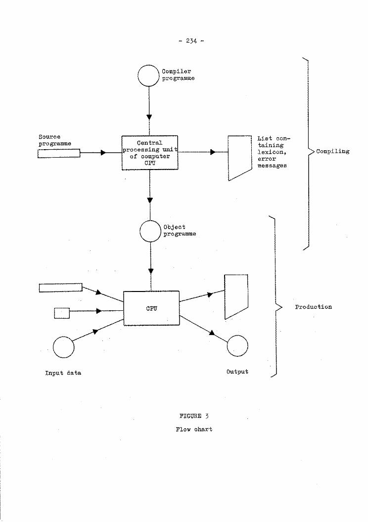
Source programme Central

- 234 -

Compiler programme

[ J ~ !processing uni t 1 ., I

~----------~.~- of computer CPU

D • CPU

Input data

Object programme

FIGURE 3

Flow chart

Output

List con­taining lexicon, error messages

Compiling

Production

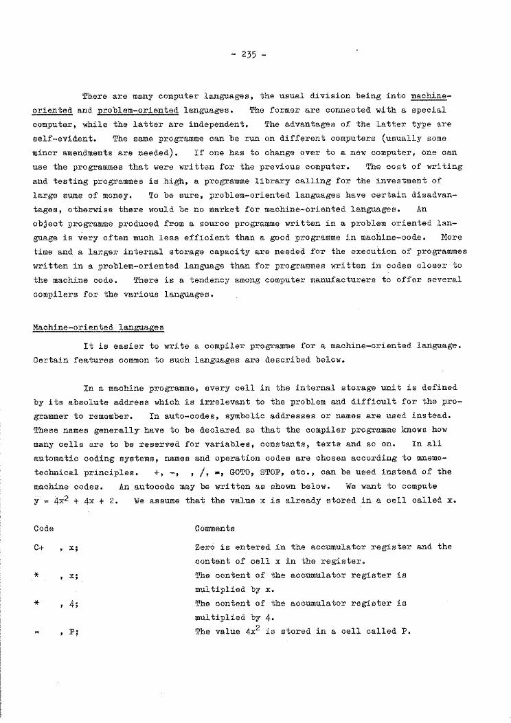
- 235 -

There are many computer languages, the usual division being in·to machine­

oriented and problem-oriented languages. The former are connected with a special

computer, while the latter are independent. The advantages of the latter type are

self-evident. The same programme can be run on different computers (usually some

minor amendments are needed). If one has to change over to a new computer, one can

use the programmes that were written for the previous computer. The cost of writing

and testing programmes is high, a programme library calling for the investment of

large sums of money. To be sure, problem-oriented languages have certain disadvan-

tages, otherwise there would be no market for machine-oriented languages. An

object programme produced from a source programme written in a problem oriented lan-

guage is very often much less efficient than a good programme in machine-code. More

time and a larger internal storage capacity are needed for the execution of programmes

written in a problem-oriented language than for programmes written in codes closer to

the machine code. There is a tendency among computer manufacturers to offer several

compilers for the various languages.

Machine-oriented languages

It is easier to write a compiler programme for a machine-oriented language.

Certain features common to such languages are described below.

In a machine programme, every cell in the internal storage unit is defined

by its absolute address which is irrelevant to the problem and difficult for the pro-

grammer to remember. In auto-codes, symbolic addresses or names are used instead.

These names generally have to be declared so that the compiler programme knows how

many cells are to be reserved for variables, constants, texts and so on. In all

automatic coding systems, names and operation codes are chosen according to mnemo­

technical principles. +, -, , /, ., GOTO, STOP, etc., can be used instead of the

machine codes. An autocode may be written as shown below. We want to compute

y = 4x2 + 4x + 2. We assume that the value x is already stored in a cell called x.

Code

C+ ' x;

* t x;

* ' 4;

, P;

Comments

Zero is entered in the accumulator register and the

content of cell x in the register.

The content of the accumulator register is

multiplied by x.

The content of the accumulator register is

multiplied by 4.

The value 4x2 is stored in a cell called P.

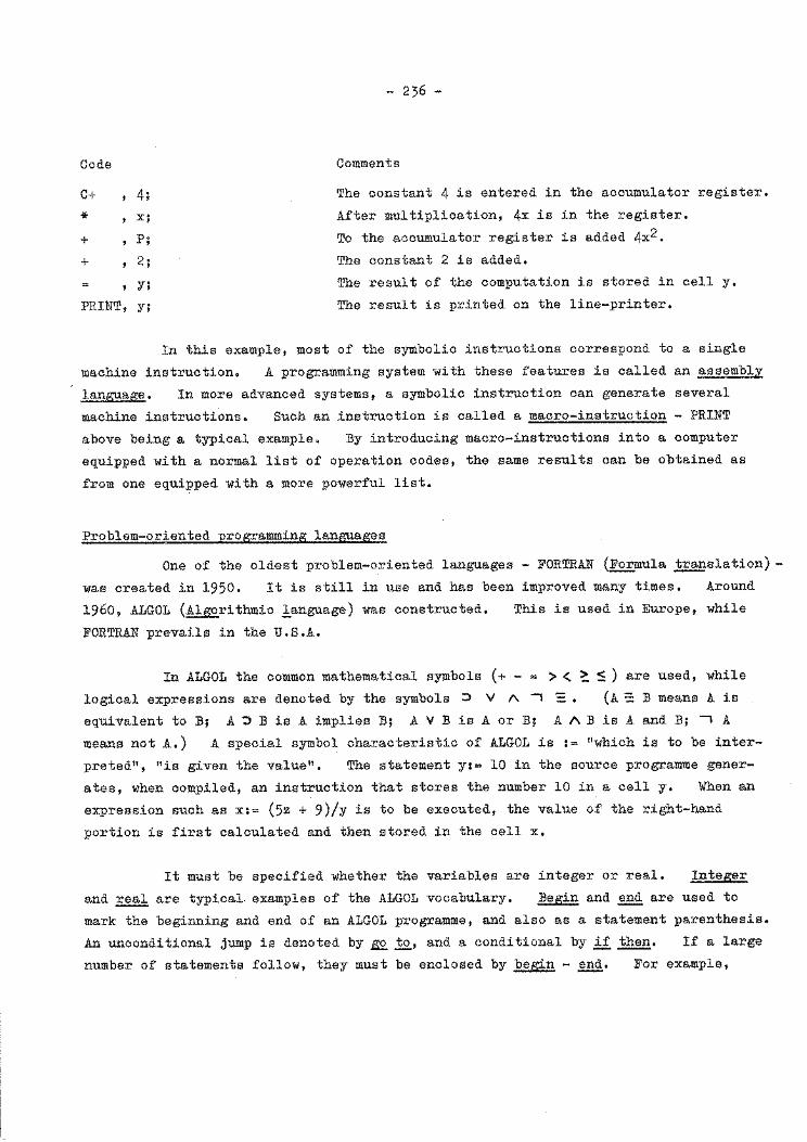
Code

C+ ' 4;

* ' x;

+ ' P;

+ ' 2; y;

PRINT, y;

- 236 -

Comments

The constant 4 is entered in the accumulator register.

After multiplication, 4x is in the register.

To the accumulator register is added 4x2.

The constant 2 is added.

The result of the computation is stored in cell y.

The result is printed on the line-printer.

In this example, most of the symbolic instructions correspond to a single

machine instruction. A programming system with these features is called an assembly

language. In more advanced systems, a symbolic instruction can generate several

machine instructions. Such an instruction is called a macro-instruction - PRINT

above being a typical example. Ey introducing macro-instructions into a computer

equipped with a normal list of operation codes, the same results can be obtained as

from one equipped with a more powerful list.

Problem-oriented programming languages

One of the oldest problem-oriented languages - FORTRAN (E££mula ~alation) -

was created in 1950. It is still in use and has been improved many times. Around

1960, ALGOL (~rithmic language) was constructed. This is used in Europe, while

FORTRAN prevails in the U.S.A.

In ALGOL the common mathematical symbols (+ - = > < ~ !: ) are used, while

logical expressions are denoted by the symbols :::> V 1\ 1 =: • (A := E means A is

equivalent to B; A ~ E is A implies E; A V B is A or B; A AB is A and E; -, A

means not A.) A special symbol characteristic of ALGOL is := "which is to be inter-

prated", "is given the value". The statement y:= 10 in the source programme gener-

ates, when compiled, an instruction that stores the number 10 in a cell y. When an

expression such as x:= (5z + 9)/y is to be executed, the value of the right-hand

portion is first calculated and then stored in the cell x.

It must be specified whether the variables are integer or real. Integer

and ~ are typical examples of the ALGOL vocabulary. Eegin and end are used to

mark the beginning and end of an ALGOL programme, and also as a statement parenthesis.

An unconditional jump is denoted by££ to, and a conditional by k£ then. If a large

number of statements follow, they must be enclosed by begin - end. For example,

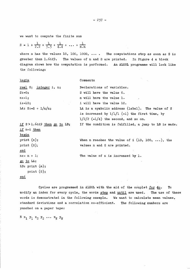
- 237 -

we want to compute the finite sum

1 1 1 1 s = 1 + 2:2 + 3.3 + 4.4 + ••• + n:n where n has the values 10, lOO, 1000, ••• • The computations stop as soon as S is

greater than 1.6449. The values of n and S are printed. In Figure 4 a block

diagram shows how the computation is performed.

the following:

An ALGOL programme will look like

begin

~ S; integer i, n;

S:=O;

n:,l;

i:=10;

LA: S:=S + 1/n/n;

if S > 1. 6449 then ~ .1£ LB;

if n=i ~

begin

print (n);

print (s);

~ n:= n + 1~

~to LA;

LB: print (n);

print (s);

~

Comments

Declarations of variables.

S will have the value 0.

n will have the value 1.

i will have the value 10.

LA is a symbolic address (label). The value of S

is increased by 1/1/1 (=1) the first time, by

1/2/2 (=1/4) the second, and so on.

If the condition is fulfilled, a jump to LB is made.

When n reaches the value of i (10, 100, ••• ), the

values n and S are printed.

The value of n is increased by 1.

Cycles are programmed in ALGOL with the aid of the couplet 1£E ~· To

modify an index for every cycle, the words step and until are used. The use of these

words is demonstrated in the following example. We want to calculate mean values,

standard deviations and a correlation co-efficient.

punched on a paper tape:

N xl Y1 x2 Y2 ••• ~ YN

The following numbers are

8 s:-o n:=l i:•lO

1 S:=S + n:ri

Print n and S

Multiply i by 10

Increase the value of n

with 1

- 238 -

FIGURE 4

Block Diagram

Print n and S

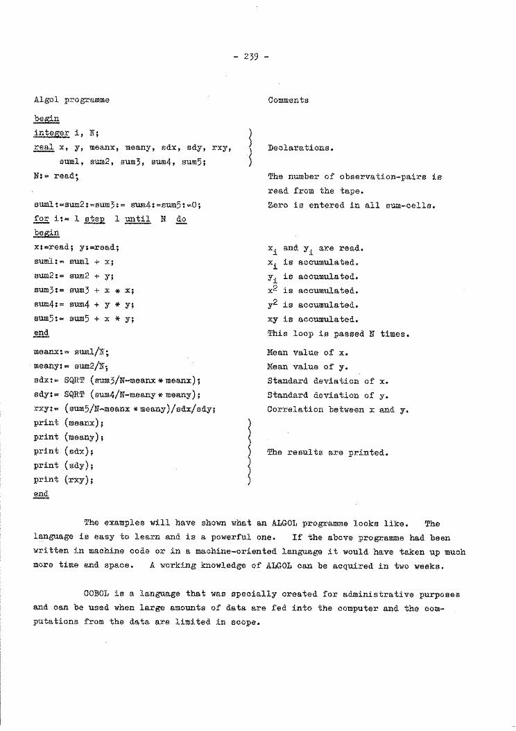
Algol programme

begin

integer i, N;

~ x, y, meanx, meany, sdx, sdy, rxy,

suml, sum2, sum3, sum4, sum5;

N:= read;

suml:=sum2:=sum3:= sum4:=sum5:=0;

.f.2E. i:= 1 step 1 ~ N do

begin

x:=read; y:=read;

suml:= suml + x;

sum2:= sum2 + y;

sum3:= sum3 + x * x;

sum4:= sum4 + y * y;

sum5:= sum5 + x * y;

.!ill£

meanx:= suml/N;

meany:= sum2/N;

sdx:= SQRT (sum3/N-meanx * meanx);

sdy:= SQRT (sum4/N-meany*meany);

rxy:"' (sum5/N-meanx *meany)/sdx/sdy;

print (meanx);

print (meany);

print ( sdx);

print (sdy);

print (rxy);

.!ill£

- 239 -

l Comments

Declarations.

The number of observation-pairs is

read from the tape.

Zero is entered in all sum-cells.

xi and yi are read.

xi is accumulated.

yi is accumulated.

x2 is accumulated.

y2 is accumulated.

xy is accumulated.

This loop is passed N times •

Mean value of x.

Mean value of y.

Standard deviation of x.

Standard deviation of y.

Correlation between x and y.

The results are printed.

The examples will have shown what an ALGOL programme looks like. The l~nguage is easy to learn and is a powerful one. If the above programme had been written in machine code or in a machine-oriented language it would have taken up much more time and space. A working knowledge of ALGOL can be acquired in two weeks.

COBOL is a language that was specially created for administrative purposes and can be used when large amounts of data are fed into the computer and the com­putations from the data are limited in scope.

- 240 -

Comparisons of different programming languages

When choosing between different programming systems, ~t is not easy to get

an objective opinion from an expert. A person who has learnt a certain language

develops an emotional attachment to it.

Ease of learning is important. A problem-oriented language can be learnt

quite quickly, but a certain amount of time is needed for training before a pro­

grammer can be said to be fully familiar with the system. It is easier to write and

test programmes written in a language such as ALGOL than those written in machine­

oriented languages. In programming much time can be saved through using probVem­

oriented languages. The ease with which a programme can be read is another point in

favour of languages like FORTRAN, ALGOL, and COBOL.

Autocoding systems do, however, have certain disadvantages. Compilation

(the translation from source to object programme) can take quite a long time, its

speed varying greatly from one computer to another, and from one language to another.

The compiler programme is usually quite large and considerable internal

storage capacity is needed, as well as certain external memory facilities. For

problems that need large areas of the core memory, the use of problem-oriented

languages is not practical if the internal storage capacity is limited. The com­

piler cannot economize with the number of cells available in the memory unit, unlike

the programmer who writes in a machine-oriented language by means of which he can

influence the operation of the computer in detail. This is also true of the number

of instructions needed and of the dimensions of those portions of the memory unit that

are used for input and output. The right choice of programming systems can lead to

major savings. The development of new computer languages is a very rapid process.

- 241 -

THE USE OF PUNCH-CARDS IN FORECASTING

by

M. El-Sawy

The recent activity in forecasting using either dynamical or statistical

methods is one of the by-products of computer machine development. If the dynamics

of the atmosphere were perfectly understood, and if the past history of the atmos­

phere were perfectly known, dynamic forecasting and statistical forecasting procedures

would lead to identical predictions. The application of statistically established

forecasting relationships to current situations can be carried out entirely by auto­

matic computing machines. Thus, if we are given a £Fedictand. we must first choose

the observable quantities to use as predictors. We must next, if we are establishing

a formula, choose mathematical form, without specifying any precise formula. Then

we must choose a sample of data from the recorded history of the predictand and the

predictors. Finally we must specify a rule by which the chosen data shall determine

the precise formula.

In the establishment of the empirical relationship, the number of

degrees of freedom is equal to the number of constants or coefficients of predictors

if this relationship is linear.

One fundamental principle is that the statistical forecaster should

bear in mind that the number of these constants must be small compared with the number

of independent observations of the predictand used in the establishment of the fore­

casting relationship.

To have a recorded history of predictand and predictors the meteoro­

logical data should be properly stored, archived and catalogued for this purpose as

well as for the other purposes of meteorological research. The choice of media on

which this data is to be recorded is a matter of convenience~

In countries planning to introduce the storing of meteorological data,

it is preferable for them to choose the media in accordance with the input devices

available with the computer they have or they are planning to have in the future.

One of the most widely used media for this purpose is the punch-card. This media is

also one of those recommended for the World Weather Watch. The punch-card though not

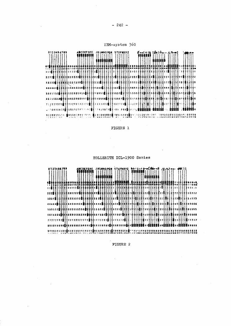
- 242 -

I:BM-system 360

XYZ '-.!.~!_-:!::!~ tl.-tt~J.,.r /,.,._1 ,_,,....,

::::mmmnlndnm: :' 1111 11~ : :l\1\·\r : ::::!lrllrl: !l~l~lr ·IU2 2 !12 11

U 3 Ulfllll·rl3 3 U I 444444, 44444444

U515H _ 55BSH~~

SlooG&&I &6&666B~~R

1'; 11 n 111 tIn n n nrn ,·:,'SUHH~ aU'~a~n'·.:n

'"'IJj 4444

5 55 55

6 ~ &li&l

1171111

·, ·~ fl j ~ I ~ 1

ll

444

55 55

iUI~

llJ11J

'•Br·Pas

3 33 3 I 333 u

444 4 4 44 4 •• 1UlJL ~ 55 5 5 55 5 5 s

6 ~ H 6 6 Hi· s.,JJJU~. lilT l 111 ,., il :l '! ~- ;:,

93J99S9&~~ I9999J~~9•9q1 'J ~~S99SS9I'9!11!99I!~· lJJJ9uq•ln• 1999~99999999~··99~9~ '.• I&~ f • f <· • ,,.,,, .r • •t,•l '' '< ~ ~ ltliTI1:ti.G'Il": "- J~" 1: J-~~ l"'·~'•1'.1~· .. ~:t.••'oll • .·.1~1fi.1M\.,~tl!ir.11/0if 1713'J4l'.lh1JIII,.ll!l

FIGURE 1

HOLLERITH ICL-1900 Series

~lr ..... !!m1r, · !r · ·:· ~ .... ~ .... r~<J~·~: .. ~~::~ 11 11111 I I I 11 I 11 111'1

!!! 112721 ll I 1 !! 22 !2 2Zl2l

UJ3 UJ3333 UJ I 3 ] 33 lJ l3 IOU ..... 44444444 44 .. 444 4 44 u 44 444U

SS55H 5555U555 55 S5 5 S5 55 I .~5 55 H 55555

6&66&U 51&66&&111 11£116 &UU ' • 6 6 6 81 I &Ill

111111J1 1111J111111 1711111 71Jil7 71 ll n 71711

11!888111 1,11111188888 88881118 1111181 ' 8A .. 11 ..... U9999&9 99 99999999999 9 9 99 99999 u 99H9 9 9 9 ' ' H '1 ~9U99UU919! 9191 i U UtU99t U ' : J .. ~ ~ ~~~ :~~''')'''''~-·~~·~~~~~:,na»~t"n•••v••••••4~~ ·~~~-•~~~~-~•~•~•~ca~e•~••NJI»nM~NnMN•

FIGURE 2

- 243 -

perhaps very sophisticated, is in most respects especially suited for use in the

research stages of statistical forecasting. They are easy to replace, supplement,

and use in permutations, which is not always the case with other input media.

The SO-column punch-card, recommended by Technical Regulation 8.2.1.3

is provided by a number of manufacturers including Bull (France), Hollerith (United

Kingdom) and IBM (U.S.A.) and is widely used for many purposes, including meteorology.

The dimensions of the SO-column punch-card are standardized very accu­

rately to make possible the automatic processing of data. The dimensions are:

height 82 mm, width 187 mm, thickness 0.18 mm. Data are usually entered on these

cards by punching holes through the use of punching machines. These holes are, in

principle, usually rectangular in shape, the position of each hole with respect to

the horizontal rows and vertical columns of the card is a function of the information

represented by the hole. The card is divided from left to right into 80 columns,

each column containing 12 possible punching positions. In the conventional punch­

card notation which is almost universally used in meteorological applications, the

numerics l to 9 are recorded as holes in the positions, thus a hole in the lowest

position of the column represents the number 9, a hole in the next position above

represents the number 8, and a hole in the highest position represents the number 1.

The remaining highest column positions 0, 11, 12 are the tenth, eleventh and twelfth

from the bottom and they are called the zone positions. The 0 position is considered

to be both a numeric and zone position.

The alphabetic characters are represented by two punches in a single

vertical column, o~e numeric and the other a zone punch,

The special characters are represented by one, two or three punches in

a single column and consist of punch configurations not used for numeric or alphabetic

data. Figures 1 and 2 provide an understandable picture of the different cardings

of the punched cards.

To clarify the usage of punch-cards in statistical forecasting, the

following mathematical problem in simplifying a linear regression formula can be

taken as an example.

- 244 -

Object of screening procedure

In multiple linear regressions, the predictand X is expressed as a linear 0

combination of a set of predictors X .• ~

When the correlations between the predictors

are large, there is much duplication of the available information, and the one most

highly correlated with the predictand gives almost as much information about the

latter as can be obtained from all the predictors. When the correlations between

predictors are all small, the partial correlation coefficients will differ little

from those of zero order. In both cases a method of successive elimination gives

practically the same result with much less effort. This procedure of successive

elimination of predictors is similar to scale analysis in dynamic forecasting, with

the exception that the latter does not exclude the effect of the eliminated predictors.

This procedure in statistical forecasting is known as the screening procedure. The

object of the screening procedure is to select from a set of M possible predictors

only those which contribute significantly and independently to the prediction of X0

•

Following E.N. Lorenz (1) scheme we can write.

The theoretical background

Let xi

X a

Xi(a)

Xb(a)

Xi(a,b)

Xc(a,b)

xi(a,b,c)

" xi

xi

= an individual value of the predictand (i = 0) or any predictor (i = l, 2, ••• , M)

an individual value of the first predictor selected (a = l, 2, ••• , M)

= an individual value of X. with least squares specifi­cation by (a) removed ~

an individual value of the second predictor selected with least squares specification by (a) removed (b=l,2, ••• ,M,bfa)

= an individual value of X. with least squares specifi­cation by (a) and (b) reffioved

an individual value of the third predictor selected with least squares specification by (a) and (b) removed (c = l, 2, ••• ,M, c fa, c f b)

an individual value of X. with least squares specifi­cation by (a), (b) and ~(c) removed

a least squares estimate of X. ~

the mean over all observations of Xi in the sample

(1) E.N. Lorenz, Prospects for Statistical Weather Forecasting, January 1959,

Massachusetts Institute of Technology, Department of Meteorology.

- 245 -

It is convenient to deal only with deviations from the mean of each Xi.

Therefore in the following let Xi = 0. The covariance between Xi and Xj in the

sample is then given by XiXj, and the variance of Xi by Xf.

The procedure involves an iterated sequence of selections and reductions.

Although several of the steps described below are by-passed in the actual computations

(see section on computations), they are included here for completeness.

Step 1. Examine the square of the correlation coefficient between each predictor

(i = 1, 2, ••• , M) and the predictand,

x.x-2 ~ 0

x2 x2 i 0

(1)

Let the predictor with the highest value be Xa'

Step 2.

given by

The least squares estimate of X. (i ~

" xi xi xa

x2 a

X a

O, 1, 2, ••• ,M) based on X is a

A new value of each X., one with the least squares specification by X removed, is ~ a

computed from

" x:-x

X.( ) =X. -X. =X-~ a X

~ a ~ ~

x2 a

a

Similarly,

" X. X

J a (j = 1, 2, ••• , M) xj(a) = xj - xj = xj - X x2

a

a

Therefore

xi(a) J:Cj(a) xi xj

- 246 -

X.X X X. ~ a a J

x2 a

(2)

In particular, the covariance between any predictor with specification (a)

removed and the predictand with specification (a) removed is given by

xi(a) xo(a) X. X ~ 0 [~] rx

~ a (3)

and the variance of any predictor (or the pred.ictand) with specification (a) removed

is given by

2 Xi(a) X~

J.

-_x:-x2 J. a

x2 a

(4)

It should be noted that these new functions X.( ) are all independent of X since J. a a

X. ( ) X ~ a a rx

~ a xi xa

x2 a

X X a a 0

Consequently all the predictive information contained in X has been removed from . a each Xi(a)' and the contribution to prediction by each of the remaining predictors

may now be considered independently of Xa.

Step 3· Step l is now repeated, but this time the predictors Xi(a) are considered.

Examine the square of the correlation coefficient,

xiW

2 Xi(a)

X 2 oW

2 ( xo(a)

Let that predictor with the highest value be Xb(a)"

(5)

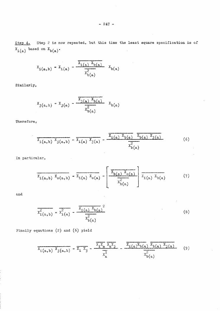
- 247 -

Step 4. Step 2 is now repeated, but this time the least square specification is of

Xi(a) based on Xb(a)·

X( )-X( -i a,b - i a)

Similarly,

X( =X( -ja,b) ja)

Therefore;

xi(a) xb(a) -2--

xb(a)

xj(~(a) 2

Xb(a)

Xb(a)

xb(a)

Xi(a,b) xj(a,b) = xi(a) xj(a) -Xi(a) xb(a) xb(a) xj(a)

-2--

xb(a)

In particular,

_ [- Xb(~~(a) ]

b(a)

xi(a) xb(a) xi(a,b) xo(a,b) = xi(a) xo(a)

and

2 -2--

xi(a,b) = xi(a) -

2 xi(a) xb(__a)_

2 xb(a)

]'inally equations ( 2) and ( 6) yield

X.( b) X.( b)= X.X.-l a, J a, l J

xixa xaxj

x2 a

xi(a)xb(a) xb(a) xj(a)

x~(a)

(6)

(7)

(8)

(9)

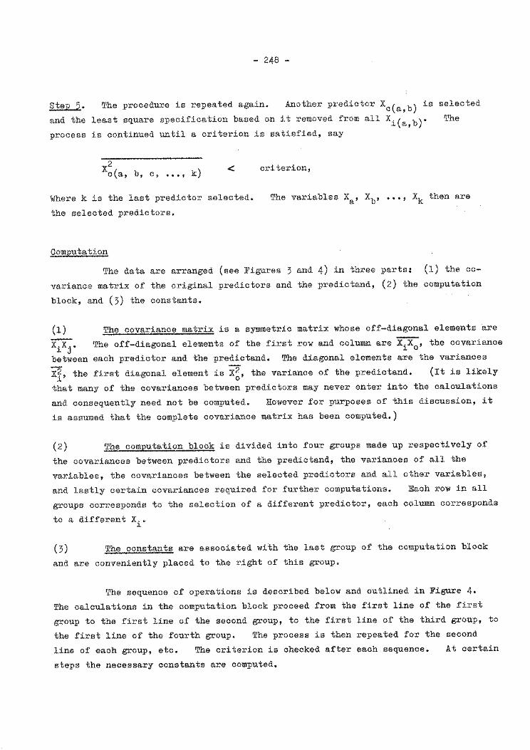
- 248 -

Step 5. The procedure is repeated again. Another predictor Xc(a,b) is selected

and the least square specification based on it removed from all Xi(a,b)" The

process is continued until a criterion is satisfied, say

x2 c(a, b, c, ••• , k) <

Where k is the last predictor selected.

the selected predictors.

Computation

criterion,

The variables Xa' Xb' ••• , Xk then are

The data are arranged (see Figures 3 and 4) in three parts: (1) the eo­

variance matrix of the original predictors and the predictand, (2) the computation

block, and (3) the constants.

(1) The covariance matrix is a symmetric matrix whose off-diagonal elements are

~. The off-diagonal elements of the first row and column are x:x-, the covariance ~ J ~ 0

between each predictor and the predictand. The diagonal elements are the variances

x?, the first diagonal element is x?, the variance of the predictand. (It is likely ~ 0

that many of the covariances between predictors may never enter into the calculations

and consequently need not be computed. However for purposes of this discussion, it

is assumed that the complete covariance matrix has been computed.)

(2) The computation block is divided into four groups made up respectively of

the covariances between predictors and the predictand, the variances of all the

variables, the covariances between the selected predictors and all other variables,

and lastly certain covariances required for further computations. Each row in all

groups corresponds to the selection of a different predictor, each column corresponds

to a different xi.

(3) The constants are associated with the last group of the computation block

and are conveniently placed to the right of this group.

The sequence of operations is described below and outlined in Figure 4.

The calculations in the computation block proceed from the first line of the first

group to the first line of the second group, to the first line of the third group, to

the first line of the fourth group. The process is then repeated for the second

line of each group, etc. The criterion is checked after each sequence. At certain

steps the necessary constants are computed.

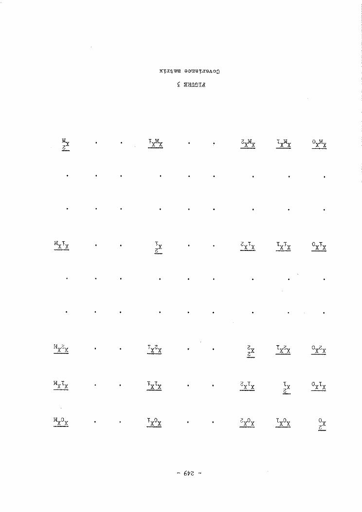
- 617<:: -

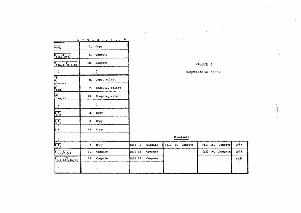
1 = 0 1 2 . . i - ..

=-=-x1xo . 1. Copy

1i(a)XO(a) 6. Coapute

Xi (a b)XO(a b) . 12. Compute

2 ~~ ~- Copy, select

'2--~~(a) 7. Compute, select

2 ~~(a,b) 13. Compute, select

~ 3 •. Copy

~ 8. Copy

=-x 1 c

14. Copy

y;: 4. Copy

~1(a)~(a) 10. C0111pute

~i(a b)Xc(a b) 17. Compute

11 -

(kl) 5. Compute (pl)

(k2) 11. Compute

(k3) 18. Compute

FIGURE 4

Computation block

Constants

9. Compute (ql) 15. Colllpute

(q2) 16. ,CoiiJ)ute.

(rl)

(r2)

(r3)

rv V1 0

- 251 -

Each step in the computations was derived from a particular equation in

the section on theoretical background. These equations are noted in parentheses

but need not be referred to in order to perform the calculations. After the

covariance matrix of all predictors and the predictand has been computed (see

FigQ~e 3), the sequence of operations is:

l.

2.

3·

4·

5·

6.

1·

.

Copy the first column of the matrix into X.X ~ 0

Copy the diagonal of the matrix into xi. Examine x.x2 ~

X~ ~

for

i = l, 2, ••• , M LSee equation (127. value of this ratio be X •

Let Xi associated with the highest

a

Copy column X of the matrix into X.X of the third group. a ~ a

Copy column Xa of the matrix into XiXa of the fourth group.

Compute

Compute

kl X X

2-..l!:

x2 a

xi(a)xo(a) = xixo - (kl) xixa

for all i LSee equation (3l7.

Compute

~ 2 xi(a) = xi

x:x-2 ~

x2 a

for all i LSee equation (427·

Examine

xi(a/o(a) 2

-2-

xi(a)

fori = 1, 2, ••• , M LSee equation (5l7. highest value of this ratio be Xb(a)'

Let Xi(a) associated with the

- 252 -

8. Copy column Xb of the matrix into XiXb.

9. Compute

pl xbxa

x2 a

10. Compute

xi(a)xb(a) = xixb - w~ xixa

for all i LSee equation (217.

11. Compute

k2 Xo(a)Xb(a)

2 xb(a)

12. Compute

xi(a,b)xo(a,b) = xi(a)xo(a) - (k2 ) xi(a)xb(a)

for all i LSee equation (717•

13. Compute

14.

x2 - x2 -i(a,b) - i(a)

2 xi(a)Xb(a)

2 xb(a)

for all i LSee equation (817.

Examine

xi(a, b)X o(a, b)

x2 i(a,b)

for i = 1, 2, ••• , M.

this ratio be Xc(a,b)'

Let Xi(a,b) associated with the highest value of

Copy column X of the matrix into X.X • c ~ 0

15. Compute

ql

16. Compute

q2

17 Compute

XX' c a

x2 a

. xcCalbCa)

2 xb(a)

- 253 -

xi(a,b)xc(a,b)

LSee equation (9l7.

xixc - (ql) xixa - (q2) xi(a)xb(a)

18. Compute

k3 Xo(a,b)Xc(a,b)

x2 c(a,b)

At this point three predictors have been selected. The process of selecting and reducing is continued in a similar manner until the desired criterion

is satisfied. The criterion is determined by x 2( b )' the first column in o a, ,c, ••• in the second group of the computation block, which contains successively the total variance of the predictand the remaining variance after (a) has been removed the remaining variance after (a) and (b) have been removed, etc.

For reference, the constants and equations required in the last group of the computation block are tabulated on the next page for the first four selections.

- 2~4 -

kl • I.OJ.a • k2 .. J.O(a)Xa,(a)

""l • z!ca>

~(a1 b)J:c(a 1 b) i X

k3 "' k4 = O(a,b,c) d(a,b,c)

' z!ca,b)

x2 d(a,b,c)

pl Xa,Xa .. -x2

a

i'"'i""" X . Xa, ql

c a ' q2 c (a) (a) .. -- =

x2 -2--

a Xbca>

xdxa xd(a)~(a) X X

rl • -- r2 = r3 = d(a 1b) c(a 1 b)

x2 , -2-- ' r-

a xb(a) c(a,b)

xixa xixa

xi(a)~(a) x1~ - (pl) x1xa

11(a, b)Xc (a, b) = xixc - (ql) xixa - (q2) xi(a)xb(a)

--X X 1(a,b,c) d(a,b,c) = x1x4 - (rl) x1x8 - (r2) x1 (a)xb(a)

-{r3} xi(a,b)xc(a,b)

- 255 -·

DATA PROCESSING IN THE U.A.R.

by

M.S. Harb

Introduction

In the U.A.R. Meteorological D~partment as in any Meteorological Service

an immense amount of meteorological data has been assembled during the past decades.

Moreover the rate of increase of such data is mounting steadily due to the increase

in the number of stations and the expansion of observational programmes. The new

and more complex problems arising from the application of meteorological data in

scientific and practical work require special treatment of the source material data

and indeed a great volume of climatic information. Such information in the past

required laborious manual operations, i.e., sorting, counting, arithmetical computa­

tions, etc. Since, however requirements in climatology are increasing rapidly and

as manual methods of processing such data are time consuming and inefficient, the

Meteorological Department has introduced punch-cards and punch-card machines for pro­cessing the large amounts of meteorological data.

The SO.;.column punch-card

The punch-card used·in the. Meteorological Department is the SO-column

punch~oard which is recommended by Technical Regulation s.2.1.3. The cards are pro­

vided by Hollerith manufacturers. Almost all existing systems for mechanical data

processing make use of or can be used in connexion with the SO-column punch-card.

The standard dimensions of the card are lS7 mm by S2 mm by O.lS mm.

Data are entered on these cards by punching rectangular holes, the positions

of which with respect to the horizontal and vertical co-ordinates of the card are a

function of the information represented. The card is divided from left to right into SO columns, each column allowing 12 punch positions. In the conventional punch-card

notation, generally used in meteorological applications, the numbers from 0 to 9 are

recorded as holes in the ten lower positions, the eleventh position from the bottom

and the highest position are known as the X and R (or 11 and 12) over punches which

may be used with no lower punch in a specific column or in combination with a punch in

one of the positions from 0 to 9 (i.e., for coding negative signs).

- 256 -

Punch-card machines

The machines used in the U.A.R. Meteorological Department may be broadly

grouped into one category - the electromechanical machines which are programmed exter­

nally by setting switches either manually or by the insertion of an appropriate con­

trol panel with wiring to complete the desired electrical circuits. The electro­

mechanical machine is a relatively specialized low capacity piece of equipment. Each

is designed for a special data processing function or group of functions. For com­

plete data processing it is usually necessary to use several types of machines each

performing its own specific task. The work is moved sequentially from machine to

machine by an operator.

Electromechanical machines used in the U.A.R. Meteorological Department are

manufactured by the I.C.L. Company and are of the following five main types:

1.

2.

3·

4·

Key-punch machines

They are of the electromechanical models 29-3 or 29-4· They are electri-

cally driven with automatic feeding and ejection and are suitable for large

volume production. Model 29-3 can be used for numerical punching only,

while model 29-4 can be used for both alphabetical and numerical punching.

Verifying machines

They are of the electromechanical model 29-3. They do not however punch

holes in the card but test for the presence or absence of a punched hole.

They are used to verify the punching and react automatically if there is

lack of agreement between the original and the second punching operation.

Sorting machines

Are of the 302-0 model and are used for arranging cards in any desired

sequence, or for segregating particular categories of data. They operate

on one card column at a time only, grouping the cards into a separate poc­

ket for each of the twelve possible punches in the card column. They are

equipped with mechanical visual counters.

Tabulating machines

Are of the 855-0 and the 906-0 models. The latter have four times the

capacity of the former. They are used for the following major functions:

(a) Preparing frequency tables;

5.

- 257 -

(b) Preparing sums of quantitative measurement for the purpose of extrac­

ting their means or performing other computations;

(c) Preparing printed paper copies of punch-card records, entirely or

selectively;

(d) Data editing for chronological or synoptic continuity;

(e) Preparation of final copies of climatological summaries.

Reproducing and gang-punching machine

is of the 234-0 model and is used in:

(a) Reproducing or copying data from one set of cards to another;

(b) Copying data from a master card onto cards behind.

Punch-card design

Punch-card systems have been planned taking the following principles into

consideration:

(a) Information entered on each punch-oard consists of:

(i) Identification groups (13 columns always from the left side of

all cards);

(ii) Quantitative data (values of meteorological elements either

observed, recorded or estimated);

(iii) Qualitative data (in codes as present and past weather, etc.);

The table gives the punch-card layout and their fields of use as technical

carriers of meteorological data in the U.A.R.

(b) All potentially useful data are transferred from observational formats,

log books, meteorological registers, etc., to punch-cards.

are normally preserved;

Decimals

(c) Punch-cards and observational formats (log books, registers, etc.)

are, as far as possible, of the same design and the content in both

media are of the same order. This principle is very important from

the view point of labour economy since the time required for punching

and checking data is greatly reduced;

- 258 -

(d) As routine publications in climatology (climatological year books) are

produced by punch-card methods, the punch-cards are designed to main­

tain the same format for a long period.

The development of scientific and applied climatology, as well as

changes in the synoptic codes necessitate either the introduction of

additional types of punch-cards or revision of the existing cards. As

an example additional punch-cards for the 250mb, 9, 8, 7, 6 ••• 2mb

levels, have been introduced in the upper-air punch-card layout since

1 January 1969.

(e) The number of punch-card types carrying basic meteorological data is

the least possible number. This is obvious from the table which shows

that for surface data two punch-cards are used (Nos. 5 and 7). For

upper-wind and upper-air data a series of punch-cards is used; each

series contains a number of punch-cards on one punch-card.

Scrutiny of meteorological data

All observational material is checked before entering on the punch-card media

to ensure the quality of observations. The meteorological department issues a set

of rules for the scrutiny of forms, autographic records, etc., to cover the following

steps:

(a) Detection of systematic errors, non-systematic errors, instrumental

failures and unrepresentative values arising from unsuitable exposure

or installation of instruments;

(b) Interpolation of missing values by an experienced meteorological officer;

(c) Checking of arithmetic computations.

Climatic elements

Any attempt to describe the climate of any locality can be expressed in

terms of meteorological (climatic) elements. In the U.A.R. Climatological Division

climatic elements are regarded as those elements related to surface and upper-air

observations. Most of these elements can be grouped into the following three groups:

Group 1. Elements related to the physical properties of the atmosphere,

e.g. wind (direction and speed), temperature and moisture,

atmospheric pressure.

Group 2.

Group 3·

Table : 1

- 259 -

Elements related to weather phenomena developing or occurring in the atmosphere, e.g. precipitation (amount and type),

present and past weather, horizontal visibility and cloudiness (amount, type, base).

Elements related to radiation, e.g. solar and sky radiation,

duration of bright sunshine and the amount of incoming and outgoing radiation.

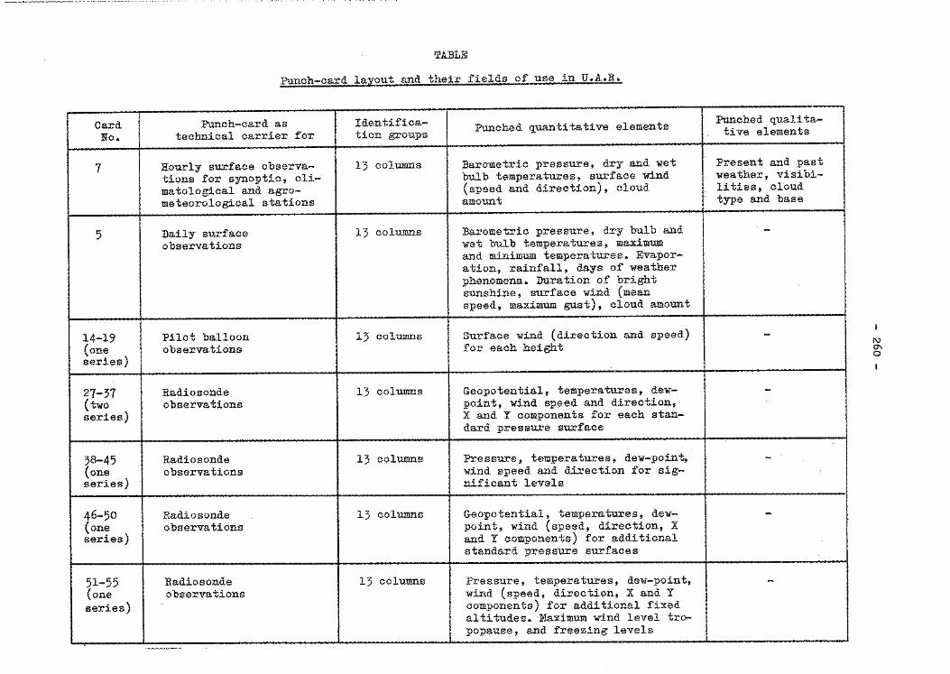
Card No.

7

5

14-19 (one series)

27-37 (two series)

38-45 (one series)

46-50 (one series)

51-55 (one series)

TABLE

Punch-card layout and their fields of use in U.A.R.

Punch-card as Identifica- Punched quantitative elements technical carrier for tion groups

Hourly surface observa- 13 columns Barometric pressure, dry and wet tions for synoptic, cli- bulb temperatures, surface wind matological and agro- (speed and direction), cloud meteorological stations amount

Daily surface 13 columns Barometric pressure, dry bulb and observations wet bulb temperatures, maximum

and minimum temperatures. Evapor-ation, rainfall, days of weather phenomena. Duration of bright sunshine, surface wind (mean speed, maximum gust), cloud amount

Pilot balloon 13 columns Surface wind (direction and speed) observations for each height

Radiosonde 13 columns Geopotential, temperatures, dew-observations point, wind speed and direction,

X and Y components for each stan-dard pressure surface

Radiosonde 13 columns Pressure, temperatures, dew-point, observations wind speed and direction for sig-

nificant levels

Radiosonde 13 columns Geopotential, temperatures, dew-observations point, wind (speed, direction, X

and Y components) for additional standard pressure surfaces

Radiosonde 13 columns Pressure, temperatures, dew-point, observations wind (speed, direction, X and Y

components) for additional fixed altitudes. Maximum wind level tro-popause, and freezing levels

Punched qualita-tive elements

Present and past weather, visibi-lities, cloud type and base

-

-

-

-

-

-

1\) (]'\

0

I

- 261 -

HARMONIC AND FOURIER ANALYSES

by

H. Zohdy

Harmonic analysis

The study of the statistical structure of meteorological elements has been

extended remarkably during the past few years. The statistical structure of some

elements helps in determining the statistical regularity which is related not only

to restricted examples of data but also to any population. This knowledge is a

useful tool in the analysis of time series.

Fourier analysis

Fourier analysis can be used to represent the periodic characteristics of

any given function with respect to time and space.

For different kinds of Fourier analysis, there are four ways of distin­

guishing among Fourier techniques. They can be summarized as follows:

l.

2.

).

4.

The phenomenon is treated periodically, i.e., all the frequencies involved

in the phenomenon are integral multiples of a single frequency.

The phenomenon is aperiodic. In this case, the frequencies involved

could be either discrete or continuous.

The times involved are either discrete and equi-spaced or continuous.

The data analysed could be regarded as unique or as statistical samples.

Since the measured values (the data) reflect not only the phenomenon

studied but also measurement errors and, usually the sources of fluctuations, the

data will always be aperiodic.

An example of using Fourier analysis is given here following the techniques

mentioned in (l) above.

- 262 -

Mathematical Aspects

Consider a series S(x) consisting of 2n+l terms.

s(x) = Ao+ Al cos X+ A2 cos 2 ~ + •••••••••• +An cos n X

+ B1 sin x + B2 sin 2 x + •••••••••• + Bn sin n x (1)

We want to determine the coefficients Ak and Bk in such a way that S(x) approximates

as accurately as possible to a given function F(x) in a given interval. As a matter

of convenience we choose this interval to be

-n~x~n

Let the error in the approximation be E: (x)

E (x) = F(x) - s(x) (2)

The approximation is good if e(x) is small everywhere in the interval. The

simplest method to formulate this in a mathematical way is to require the coefficients,

Ak and Bk' to be determined in such a way that the mean square error

M = ~n £: [e(x)J 2 dx (3)

to be a minimum.

This requirement is, however, not completely sufficient for the determin­

ation of the coefficients in the series. We also require the coefficients to be

final. By this we mean that a. coefficient Ak in _S(x) should not change if we

increase the number of terms in the series. This implies that the coefficients are

mutually independent.

To find the minimum of the mean square error we may, therefore, take

derivatives of M with respect to Ak and Bk as independent variables. This gives,

using (2)

'aM _ 1 n ~~ - 2n £u 2

'bM _ ....1. Jn 2 dBk - 2n -n

[F(x) - S(x)] Cos kx dx

[F(x) - s(x)J Sin kx dx

k = 0, 1, 2, ••••••••••••••••• , n

0

0

or f F(x) Cos kx dx

and f F(x) Sin kx dx

- 263 -

f S(x)

f S(x)

Cos kx dx

Sin kx: dx

where all the integrals are tobe taken over the interval (-n,11)

The integration of the right hand sides of both (4) and (5) expresses a

characteristic property of trigonometric functions, the so-called orthogonality,

Where for k > 0, we have

and

11 f Cos kx -11 dx = 0

1:11

Cos kx Sin kx

1t f Sin kx -1t

dx =0

dx = 0

li'urthermore we have for m ~ k > 0

11 f Cos mx Cos ikx -1t dx = 0

11 f Sin mx Sin kx dx -11

Due to orthogonality (4) and (5) reduce to

f F(x) Cos kx dx = ~ f Cos2

kx dx

f F(x) Sin kx dx = Bk J Sin2 kx dx

where the normalizing factors of Ax: and Bk are

f . 2 f . 2 Cos kx dx = Sin kx dx = 11

and from (6), (7), and (8) we have

1 JF(x) Ak = it cos kx dx

= 0

( 4)

(5)

(6)

(7)

(8)

(9)

Bk 1 !F(x) Sin kx dx = 'jf (10)

If we put k = 0 in (9), we have

1 fF(x) dx A = -0 24 (11)

It is clear .from (11) that A0 represents the mean value of the function F(x) in the interval (-11 111)

It is natural that with increasing n the approximation will become better

and that for n ~ oo we will obtain exact agreement between the furiction and the

series; we may thus write

- 264 -

F(x) 00 00

= A0 + l: A_ Cos nx + l: B Sin nx 1 --h 1 n

To simplify the computation of the coefficients, with a high degree of

accuracy, the coefficients of Fourier series, using (9) and (10), can be written in

the finite difference form

1 n 2" A =- l: F(xi) xi = - i

0 n 1 n

2 :p. A = - I: F(xi) Cos kx1 k n i=l

n 2

F(xi) B - - l: Sin kxi k - n i=l

where n is the number of intervals in the period concerned.

Example of the application of Fourier series:

The monthly mean temperature (in °C) of the station Helwan during the

period (1947-1960) are:

Jan. Feb. Mar. Apr. May June July Aug. Sept. Oot. Nov. Dec.

0 13.7 c 14.9 17.3 20.9 24.8 27 28.1 27.9 25.8 23.5 19.3 15.3

The number of intervals in this case n = 12

For convenience in the calculations, we add the mean temperature of

January to the 12 intervals to give the interyal number 13 so that we do not change

the shape of the cycle, i.e. the intervals start with January and end with January.

This makes the number of intervals = 13.

Ao

X = 2Jt I 13 = 27° 41 t

13-7+14.9+17.3+20.9+24.8+27+28.1+27.9+25.8+23.5+19.3+15.3+13.7 13

20.9°C

The actual deviation,oe. , from the mean A0, at every interval i.s given by

subtracting A0 from the values at every interval.

"1

-7.2

- 265 -

"2 a 3 "4 a5 a6 a.7 a 8 a 9 alo an a 12

-6 .• 0 -3.6. 0 3.9 6.1 7.2 7.0 4.9 2.6 -1.6 -5.6

A1 = 1~ [a1 cos (27°41') + a2 Cos (55°22 1 ) +a 3 Cos (83°03') + ••••

+ a13 Cos (332°12')~ = -7.5

:a1 = 1~ [a; Sin (27°41') + a 2 Sin (55°22') + a3 Sin (83°03') + ••••

+ a13 Sin (332°12')] = 0.9

A2 = 1; [a1 Cos (55°22') +a 2 Cos (110°44') + ••••••••••

+a 13 Cos (664°24')] = -0.1

B2 = 1; [\Sin (55°22') +a 2 Sin (110°44') + ••••••••• ,

+ a13 Sin (664°24')] = 0.2

a.rid so on for the coefficients of the higher order

A3

= 0.3

A4 = 0.2

A5

=;-0.2

A6 = 0~3

]3 = 0.1

:a4 =-0.1

:a5 =-:-0.1

B6 = 0.3

Fi~e 1 shows the curve of the actual deviation (a) (heavy line)

a.l3

-7.2

together with the curves of the first two "terms in Fourier expansion (dashed lines), while Figure 2 shows the curves of the second two terms but on a magnified scale.

Figure 1 reveals the one-year periodicity of the temperature while Figure 2 indicates that there exists also a six-month periodicity since the wave repeats itself every six months illustrating the seasonal change in temperature. Such .a distribution rev~als that the temperature function could be represented by thefirs"ji.ha.rmonic.to a,. good deg.t'ee of approximation.

- 266 -

Figure 3 shows the relation between the sum of the square of the

amplitudes of terms of the same rank with the rank. The figure reveals that the

amplitude of the two terms of rank 1 are of the greatest weight in the expansion,

and also that the weight of the amplitude of the terms of odd ranks is greater than

that of even ranks. The term of greater weight in the series shows more contribu­

tion of the harmonic to the special characteristics.

Further applications of harmonic analysis (introduction to power spectrum):

Definitions

1. Autocorrelation function

Autocorrelation means co~relation with itself. The autooorrelation

function of any parameter x is given by

B(ti,ti+t) (xi - i). (xi+ - i) "·

where x1 is the value of the parameter at the time ti and xi+t is the value of the

same parameter at the time (ti +t ).

2. Autocorrelation coefficients

They are correlation coefficients between a time series of a certain

parameter (x) and the same time series of the same para~eter (x) in an interval of

time (t). The interval of time (t) is called the lag (t = O, 1, 2, •.•••..••• ,1 m)

where t is the maximum lag used. The autocorrelation coefficient is expressed in m

the form:

R .....,..M!_l a..._, B(OJ

where B(") is the autooor.r~lation function, and

( ) ' 2

B 0 is the variance = a •

The autocorrelation coefficient gives the possibility to recognize the

degree of dependenoe of the value of a parameter in a certain time interval of the

- 267 -

time series upon the value of the same parameter in another time interval of the same time series.

3. Auto-covariance function

Consider the series x(ti), where i function for this series is defined as

1, 2, •••••••••• N. The auto-covariance

1 N-"' A (,;) = -N E x(t.). x(tiH)

X -,; i=l 1

The variable ,; is the lag.

Power spectrum

The Fourier cosine transformation of the auto-covariance function spectrum is the power spectrum of the x(ti) series. The power spectrum is obtained from the following expression.

2 "Cm-1

'"" 1 [ Ax (o) + Ax (,;m) Cos <~"oB Px (fo) = r I: Ax (,;) Cos ,; m ,; +-

0 "' m "'=1 m

The variable f, known as the frequency is defined by f = ~ "'m

Thus 0 ~ f .s. 0. 5 P (f) is known as the row value of the spectral density. It is X

normally smoothed as follows

...., Px (f,;) = 0.25 P(~ _1) + 0.50 P(f,;) + 0.25 P(f'C+l)

,; where f-c = ~

m

P (o) X

p (0.5) X

0.50 [Px (f1) + Px (o~ = 0.50 [p (0.5) + p (~ )l

X X m-l'J

Without going into detail, the information value of the spectrum is that it shows the contribution of the harmonic to the total variance. The power spectrum of a

- 268 -

time series shows the contribution of oscillations with various frequencies to the

variance of a time series.

R E F E R E N C E S

l. Courant, R. and Hilbert, D., 1962, "Methods of mathematical physics"

Volume 1 pp. 69-73·

2. Van Wijk, W.R., 1963, "Physics of plant environment"pp. 134-138.

3. Blackmann, R.B. and Tukey, J.W., 1959, "The measurement of power spectra",

Dover publications, New York.

4. Panofsky, H.A., and Brier, G.W., 1958, "Some applications of statistics to

meteorology", Penn. St. Univ. Press

Figures: 3

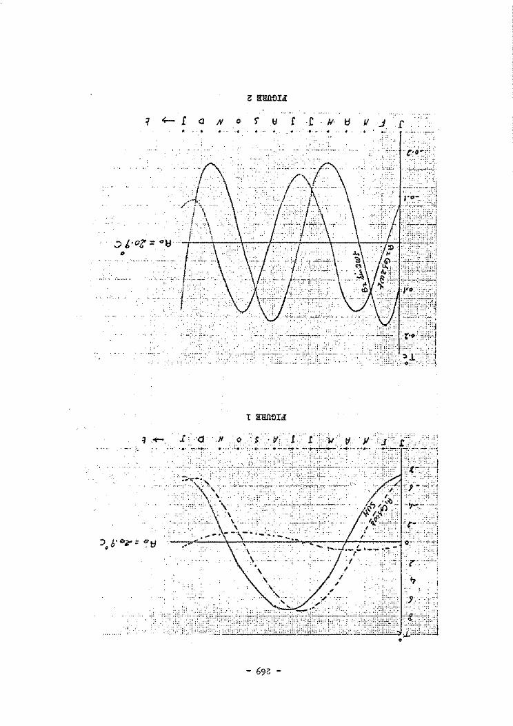
Q N r .r . ' . ... . .. . ...

·p\···· ·/' '"' .. ' 1 t

. I . \ .. ,., .,'t I .. \

.. . ··· ... --·· ~:..:--~·--:-~·· ..

" .. •:·· .. ···-·---- . --~·-··· . .:_~:-:~. ~ ~.-.:..--.~·

t :ll:liO:OIJI

- 69C: -

11 1. • '.~ N

r ... .: .. .., __ .. . '

'·· '' ...

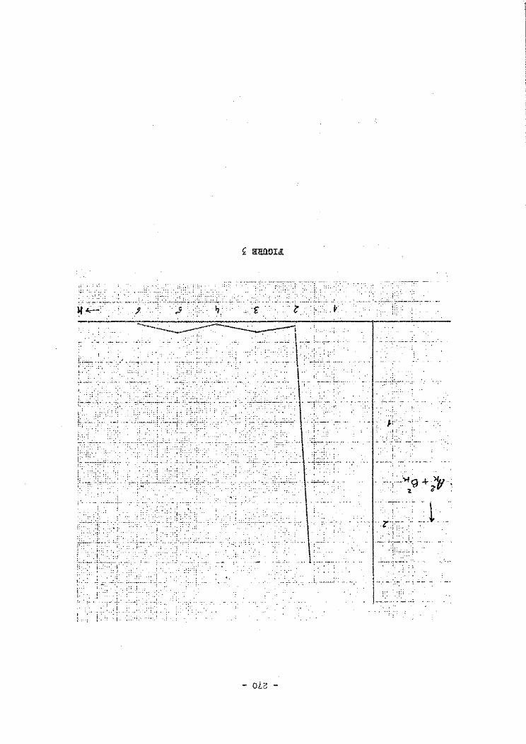
)f~:'

i. :·:-:,·

F -~::/-::~·: .. ~- -..

i · ... -- . ··---- .....

L . .': . . . . . . ' ----··r·-. . . < :~: : .....

;+~-;:L_.-~.: .. :- .. r:: ': .. .,

.j.

. i" .

i~~~-t~~:~~-· -···

i: l·.

I I,.

: : ~ . .. "

'I .. . :·r.·

" ., ..

. : ...: ... ~__;..;~ ... : .:.. .. :~.~=-~-: .. :. . ,, .,.r; ~,:

- . ·_: -~- ~·-

..1. ... ':·;.:.::·:· . ··-·

: .· .. ·. . .. ·; .,

-.

- OLo -

- 271 -

CLIMATOLOGICAL ELEMENTS

by

M.K. Nagu.ib

The condition of the atmosphere at any time in a given place, the weather, is expressed as a combination of several elements: temperature, precipitation, hum­idity, winds, air pressure, etc. These are the elements of we~ther. But since climate is a composite or generalization of the variety of day to day weather con­ditions, then the climatological elements are also the weather elements.

It is not possible to enumerate all the elements, because their number can be increased arbitrarily, but the following may be mentioned:

1. Radiation, incoming and outgoing,

2. Temperature of air and the surface of the earth,

3. Wind direction and velocity,

4. Humidity and evaporation,

5. Cloudiness and sunshine,

6. Precipitation,

7. Snow cover, 8. State'of the ground and sea,

9. Atmospheric pressure,

10. Air pollution.

In general these items do not really represent single elements, but groups of elements. For example the incoming radiation is divided into two main parts: direct radiation from the sun and radiation from the sky. Each part can also be subdivided into any number of elements.

It is possible, also for some purposes, to classify the elements from another point of view:

1.

2.

Primitive elements which are directly observed or estimated like temperature, precipitation, wind, cloudiness, etc.,

Combined elements, some of which can be determined instrumentally_like c.ooling power, drying power, equivalent temperature, etc.

3·

- 272 -

Derived elements like turbidity factor and coefficient, lapse rates of

temperature, anomalies, frequencies, etc.

The climatic picture may be created by the averages of several climatic

elements particularly temperature and precipitation or by portrayal of the various

types of weather which together comprise climate. Temperature and precipitation are

mentioned to be the two most important elements owing to their practical significance.

However, a complete description of the climate of a region should comprise not only

the means and the seasonal and diurnal variations of the climatic elements, but also

information about their extremes and about the frequencies with which the various

values occur, Koppen used the two most important elements, temperature and precipi­

tation for giving a picture of the different climates on the earth.

earth.

Climatic elements vary from place to place and from season to season on the

This is due to latitude, sun, distribution of land and water, the great semi-

permanent high and low pressure cells, winds, altitude, mountain barriers, ocean cur­

rents, storms of different kinds, etc. These are considered as controls to climate.

In every sector dealing with climatology there are large volumes of data

for utilization in furthering this science. Series of climatological data may be

treated as statistical series and thus statistical procedures are applied. When

large masses of data are involved, it is advisable to resort to mechanical processing.

Some of the statistical procedures have been explained during this seminar.

Climatological data are obtained from climatological stations. This is in

accordance with the Technical Regulations of the World Meteorological Organization.

All stations at which meteorological observations of value to climatological purposes

are carried out, regardless of the purpose for which they have been established,

should be considered as climatological stations. A climatological network is com­

posed of olimatological stations. Climatological data are not only required from

surface stations but also from upper-air stations.

The forms in which these data exist include: journals, log books, monthly

or annual forms prepared from original records, punch-cards, paper tapes, magnetic

tapes, microfilms, microcards, analysed maps and diagrams, etc.

Data should be entered in a specially designed journal with which should

also be kept a record of all changes in the equipment of the station or in the expo­

sure of the instruments together with notes of the times when the instruments have

been checked, adjusted or repaired.

- 273 -

Checking of the observed material is essential to ensure the quality of

observations. Errors must be corrected. Special attention should be given to data

received from s'tations manned by inexperienced observers. In order to ensure the

application of homogeneous checking methods, meteorological services prepare sets of

rules covering the scrutiny of forms, autographic records, etc. These rules cover

procedures regarding detection of systematic and nonsystematic errors, correction of

errors where feasible, detection of instrument failure and unrepresentative values,

interpolation of missing values, and checking of the arithmetic.

Climatological data should be suitably protected against excessive heat,

rapid temperature fluctuations, high humidity, dust and destruction by insects. Non­

inflammable microfilm reduces the volume of the stored data and gives protection

against fire risk. We must bear in mind that basic climatological data are often

irreplaceable and every precaution should be taken to protect them from destruction.

As many copies as possible should be made and retained in different places from the

originals.

Storing data using microfilm permits additional copies to be made for loan,

sale or other purposes. Punched tapes and magnetic tapes are the most advanced

systems for storage, reproduction and processing of data.

To meet research requirements and for the provision of climatological infor­mation there is a world-wide and increasing demand for climatological data. These

data are considered as part of a nation's wealth and of great value in many aspects

of the nation's economy and future development.

In the U.A.R. climatological data are collected from our climatic network. The processing of these data has been dealt with in a special lecture presented by

Dr. Saad El-Din Harb.

SwNVdiOiwHVd X[ S~HnwO~~

- ~Le: -

- 277 -

COMPUTATION OF DIFFERENT CLIMATIC PARAMETERS

by

S.S. Abd El-Hadi

The following pages illustrate the practical computation of the arithmetic

mean, the 2nd, 3rd and 4th moments of the January daily minimum temperature at

Alexandria during the period 1960-1969, after grouping the data into class intervals,

the skewness; and calculating the frequency distributions in the class intervals

assuming normal distribution. These comprise:

(a) A series of observations for the January daily minimum temperature at

Alexandria during the period 1960-1969 (Table 1).

(b) A frequency table grouping the data for daily minimum temperature at

Alexandria into class intervals of 1°C during the same period and. com­

putation of the mode and median (Table 2).

(c) Computation of the deciles and quartiles.

(d) The practical computation of the arithmetic mean and moments about the

mean m2 , m3

, m4

, of the January daily minimum temperature at Alexandria

during the period 1960-1969 (Table 3).

(e) Methods of calculation of the absolute frequency o£ daily ~inimum temper­

ature at Alexandria during the same period assuming normal distribution

(Table 4).

(f) The frequency polygon and normal distribution curve of the same element

during the same period.

- 278 -

TABLE 1

Series of observations for the Januarx daily minimum temperature at Alexandria during the period 1960-1969

Day Year 60 61 62 63

1 08.2 08.5 14.8 09.5 2 08.3 11c9 10.0 12.3 3 10.9 08.6 09.7 12.3 4 08.2 09.7 10.8 10.2 5 08.8 11.7 10.5 09.5 6 10.7 11.5 12.4 08.1 7 11.8 09.3 10.5 07.1 8 09.9 10.8 10.7 10.2 9 11.3 09.7 10.1 11.1

10 07.9 11.6 10.3 14.5 11 08.3 12.6 10.5 11.5 12 06.9 10.7 10.4 09.0 13 11.7 10.8 09.5 09.1 14 09.6 08.5 10.5 07.6 15 11.9 09.2 10.6 11.5 16 10.2 10.6 08.8 10.0 17 06.9 09.3 11.0 13.2 18 10.5 11.0 08.6 07.6 19 14.5 09.4 08.8 04.6 20 11.5 09.6 13.8 05.1 21 12.5 07.3 14.5 05.4 22 13.6 06.4 09.7 09.6 23 08.8 04.6 08.2 13.0 24 06.3 06.3 09.6 10.6 25 08.5 05.6 09.0 09.0 26 12.3 09.0 07.7 07.9 27 08.5 08.2 09.8 05.8 28 08.3 08.2 08.6 05.4 29 08.8 13.0 18.3 02.9 30 06.4 11.6 04.6 04.3 31 05.4 09.0 04.8 11.0

Absolute maximum in the sample M = 14.9°0.

Absolute minimum in the sample m = 2.5°0.

64 65

08.6 11.7 06.7 07.5 04.5 08.8 06.0 08.2 08.0 05.6 06.1 05.6 06.2 05.2 06.6 09.6 06.8 11.8 08.2 10.8 06.7 09.2 11.6 09.2 08.8 09.4 08.5 09.7 10.4 07.0 11.5 09.6 11.5 08.6 07.5 10.4 04.5 12.5 04.7 08.6 05.4 06.8 10.7 06.0 10.6 10.2 09.5 08.0 10.1 07.5 11.1 10.8 08.6 09.2 08.2. 06.6 08.0 07.4 12.0 11.4 12.6 11.0

The range of variation (difference) = M - m = 12.4°0.

66 67

10.5 06.6 06.2 07.0 09.9 09.6 09.8 09.0 10.5 o6.o 07.8 09.4 07.8 08.0 04.2 05.1 08.0 08.0 07.4 05.1 08.5 04.0 07.0 04.4 07.0 07.2 04.8 08.0 04.3 09.6 07.4 09.9 03.6 09.6 06.8 09.2 05.0 08.6 05.6 08.7 09.0 06.6 09.3 03.4 09.5 04.8 08.8 08.8 11.8 07.1 09.3 06.2 05.7 09.8 10.4 12.9 10.4 12.0 09.8 09.4 09.5 09.2

Taking a class interval of 1°0 we obtain the following frequency table.

68 69

09.4 10.0 09.8 09.0 14.9 07.6 11.0 07.5 09.8 08.0 10.0 05.7 08.5 09.2 04.4 08.1 06.7 07.2 06.7 07.4 02.5 06.4 o6.o 11.8 09.7 12.6 05.6 08.4 05.6 05.8 10.8 08.1 12.7 06.6 07.7 09.9 06.6 09.7 06.5 11.0 06.8 10.4 08.5 09.4 04.0 08.3 08 •. 8 09.8 06.9 09.0 04.6 11.2 07.0 11.5 09.2 08.9 09.6 10.1 03.6 09.1 11.4 08.4

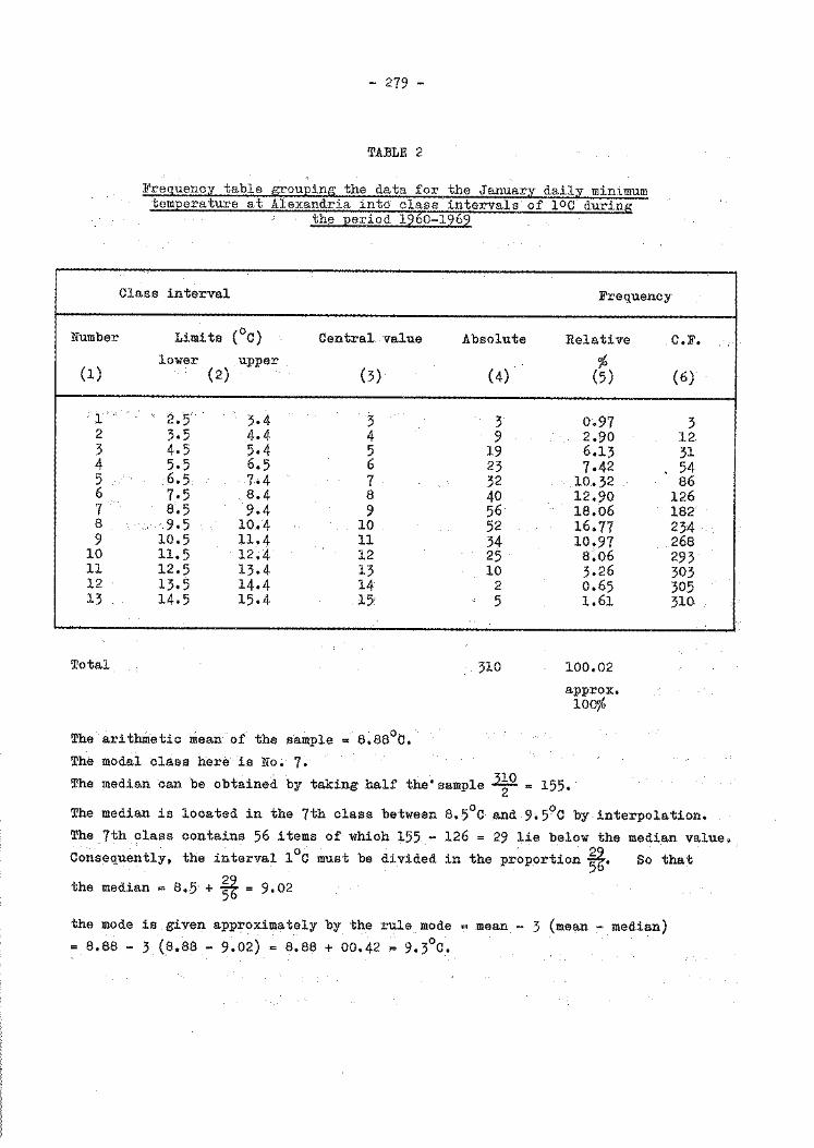
Number

(1)

- r· .. 2 3 4 5 6 7 8 9

10 11 12 13

Total

- 279 -

TABLE 2

Frequency table grouping the data for the January daily minimum temperature at Alexandria into class intervals of roe during

the period 1960-1969

Class interval

Limits (°C) Central value lower upper

(2) (3)

2.5 3·4 3 3.5 4·4 4 4.5 5·4 5 5.5 6.5 6 6.5 7•4 7 7.5 8.4 8 8.5 9.4 9 9.5 10.4 10

10.5 11.4 11 11.5 12.4 12 12.5 13.4 13 13.5 14.4 14 14.5 15.4 15

-~~------

Absolute

(4)

3 9

19 23 32 40 56 52 34 25 10

2 5

310

Frequency

Relative

% (5)

0-.97 2.90 6.13 7.42

10.32 12.90 18.06 16.77 10.97 8~06 3.26 0.65 1.61

100.02

approx. lOO%

The arithmetic mean of the sample = 8.88°0. The modal class hereis No. 7. The median can be obtained by taking half the'sample 3~0 = 155.

C.F.

(6)

3 12 31 54 86

126 182 234 268 293 303 305 310

The median is located in the 7th class between 8.5°C and 9• 5°C by in.terpolation. The 7th class contains 56 items of which 155 - 126 = 29 lie below the median value. Consequently, the interval 1°C must be divided in the pr~portion ~· So that

the median = 8.5 + 3t = 9.02

the mode is given approximately by the rule mode = mean - 3 (mean - median) . 0 .

= 8.88 - 3 (8.88 - 9.02) = 8.88 + 00.42 = 9.3 c.

- 280 -

Computation of the deciles and guartiles

According to the same principle for computing the median, the entire

sample can be divided into an arbitrary number of equal parts, which are symmetric

about the median. It is usual to divide the sample into ten, or into four, parts.

These parts are called, respectively, deciles and quartiles. In the example in

Table 2, the limits of the deciles are given by the cumulative sums 1~ = 3ig = 31

with the following results:

Decile No.: 1

Decile limit: 31

2

62

3

93

4

124

5

155

6

186

7

217

8

248

9

279

10

310

The first decile contains 31 items, therefore it is the boundary between

classes Nos. 3 and 4 and is equal to 5.5°C.

The second and first deciles together contain 62 items,

second decile lies within class No. 5 which contributes 62 - 54 = upper temperature of the second decile lies at= 6.5 + 6.75°C.

therefore the

8 items. The

This process is

carried out for the remaining deciles, with the following results:

Absolute min. : 2.5°C Decile 6 : 9.58

Decile 1 : 5.5 Decile 7 : 10.17

Decile 2 : 6.75 Decile 8 : 10.91

Decile 3 : 7.68 Decile 9 : 11.94

Decile 4 : 8.45 Absolute max. : 14.9

Decile 5 (Med.) : 9.02

The deciles divide the sample into equal parts of 10 percent each; the

quartiles, into parts of 25 percent each. In the example in Table 2, n = 310. The

cumulative sums for the quartiles would therefore be: 77.5, 155, 232.5 310.

The quartiles can be computed as before:

Absolute min.

2.5°C

Difference 4·73°C

Lower quartile

7.23°C

Median

9.02°0

1.79°C 1.45°C

Upper quartile

10.47°0

4·43°0

Absolute max.

14.9°C

It is characteristic of the element under investigation that 50 percent of

all observations lie within the range 3.24°0, i.e. between 7.23°0 and 10.47°0. The

other 50 percent, however, are distributed over a range of 9.16°0. This result

shows clearly the rarity of large deviations from the median value.

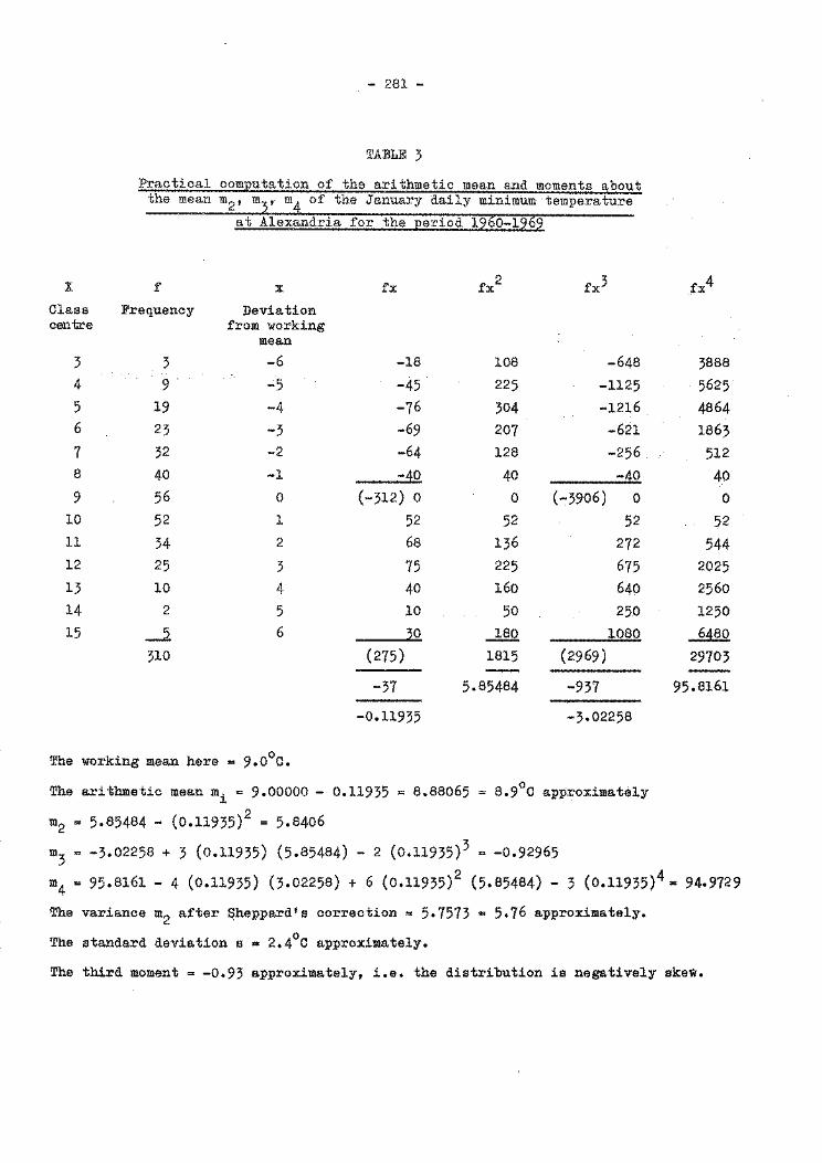
- 281 -

TABLE 3

Practical computation of the arithmetic mean and moments about the mean m2, m

3, m

4 of the January daily minimum temperature

at Alexandria for the period 1960-1969

X f X fx fx2 fx3

Class Frequency Deviation centre from working

mean

3 3 -6 -18 108 -648

4 9. -5 -45 225 -1125

5 19 -4 -76 304 -1216 6 23 -3 -69 207 -621

7 32 -2 -64 128 -256 8 40 -1 -40 40 -~0

9 56 0 (-312) 0 0 (-3906) 0 10 52 1 52 52 52 11 34 2 68 136 272 12 25 3 75 225 675 13 10 4 40 160 640 14 2 5 10 50 250 15 __j, 6 3..Q. 180 1080

310 (275) 1815 (2969) --37 5.85484 -937 --

-0.11935 -3.02258

The working mean here = 9.0°C.

The arithmetic mean mi = 9.00000 - 0.11935 = 8.88065 = 8.9°C approximately 2 m2 = 5.85484 - (0.11935) = 5.8406

m3

= -3.02258 + 3 (0.11935) (5.85484) - 2 (0.11935) 3 = -0.92965

fx4

3888

5625

4864

1863

512

40

0

52

544 2025

2560

1250

~ 29703 -

95.8161

m4

= 95.8161 - 4 (0.11935) (3.02258) + 6 (0.11935)2

(5.85484) - 3 (0.11935) 4 = 94.9729

The variance m2 after ~heppard's correction= 5.7573 a 5.76 approximately.

The standard deviation s • 2.4°C approximately.

The third moment = ~0.93 approximately, i.e. the distribution is negatively skew.

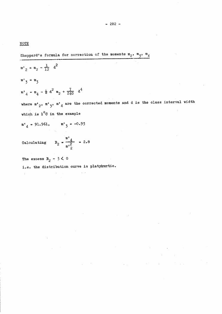
- 282 -

~

Sheppard's formula for correction of the moments m2 , m3, m

4

m'2 = m2- JL d2 12

m' -m 3 - 3

I 2 m 4 = m4 - t d m2 + _]_ d4 240

where m• 2 , m•3

, m•4

are the corrected moments and d is the class interval width

which is l°C in the example

m' 4 = 91.961,

Calculating

m• 3 = -0.93

m' .:....L .. 2.8 B .. 2

2 m' 2

The excess B2 - 3 < 0

i.e. the distribution curve is platykurtic.

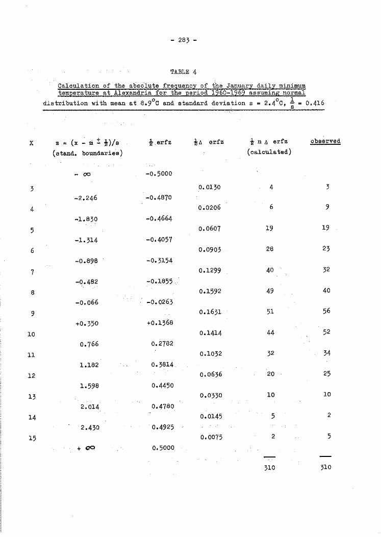
X

3

4

5

6

7

8

9

10

ll

12

13

14

15

- 283 -

TABLE 4

Calculation of the absolute freguency of the January daily minimum temperature at Alexandria for the period 1960-1969 assuming normal

dlstribution with mean at 8.9°C and standard deviation s = 2.4°C, 1. = 0,416 s

z = (x - ~ ± i)/s i-erfz ill erfz i n ll erfz observed

(stand. boundaries) (calculated)

- 00 -0.5000

0.0130 4 3

-2.246 -0.4870 0.0206 6 9

-1.830 -0.4664 0.0607 19 19

-1 • .314 -0.4057 0.0903 28 23

-0.89.8 -0.3154 0.1299 40 32

-0.482 -0.1855 0.1592 49 40

-o.o66 -0.0263 0.1631 51 56

+0.350 +0.1368 0.1414 44 52

0.766 0.2782 0.1032 32 34

1.182 0.3814 0.0636 20 25

1.598 0.4450 0.0330 10 10

2.014 0.4780 0.0145 5 2

2.430 ·o.4925 0.0075 2 5

+00 0.5000

- -310 310

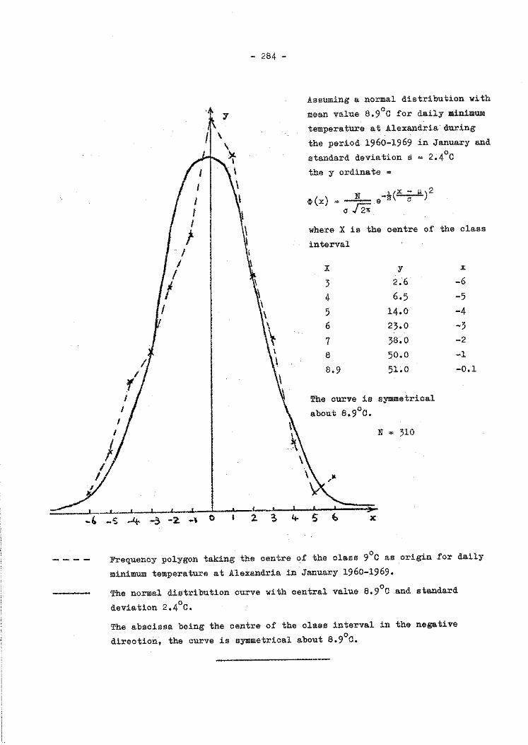
·it. y

\

J...._ ' l

-la -S -Lt ~ -2. _, 0

\

~ ' \

\ \ I

~ .\ ,\

- 284 -

Assuming a normal distribution with

mean value 8.9°0 for daily minimum

temperature at Alexandria during

the period 1960-1969 in January and

standard deviation s = 2.4°0

the y ordinate =

~(x) = ___ N ___ e-~(~)2 a J2n

where X is the centre of the class

interval

X y

3 2.6

4 6.5

5 14.0

6 23.0

7 38.0

8 50.0

8.9 5LO

The curve is symmetrical

about 8.9°0.

N = 310

X

-6

-5

-4 -3

-2

-1

-0.1

23 4-5 (,. X

Frequency polygon taking the centre of the class 9°0 as origin for daily

minimum temperature at Alexandria in January 1960-1969.

The normal distribution curve with central value 8.9°0 and standard

deviation 2.4°0.

The abscissa being the centre of the class interval in the negative

direction, the curve is symmetrical about 8.9°0.

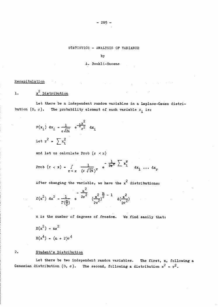
- 285 -

STATISTICS - ANALYSIS OF VARIANCE

by

A. :Soukli-Hacene

Recapitulation

1. x2 Distribution

Let there be n independent random variables in a Laplace-Gauss distri­bution (o, a). The probability element of each variable xi is:

2.

F(xi) dxi

2 Let r

1 =-

a,J2;

LX~

2 1X -2-e

02 dxi

and let u~;~ calculate Prob (r < x)

Prob (r < x) J r<x

1

(a f2i)r

- 1 \ r e 2o-r L x. l.

dx1 ..• dxr

After changing the variable, we have the x2 distributions:

2 X

--2 f(x2) dx2 = _1_. e 2a

r(~) ( x

2 )~ - 1

2a 2

n is the number of degrees of freedom.

E(x2)

E(x4)

2 no

(n + 2)a4

Student's Distribution

2 d(..L)

20 2

We find easily that:

Let there be two independent random variables. The first, x, following a Gaussian distribution (o, a). The second, following a distribution x2 = r 2•

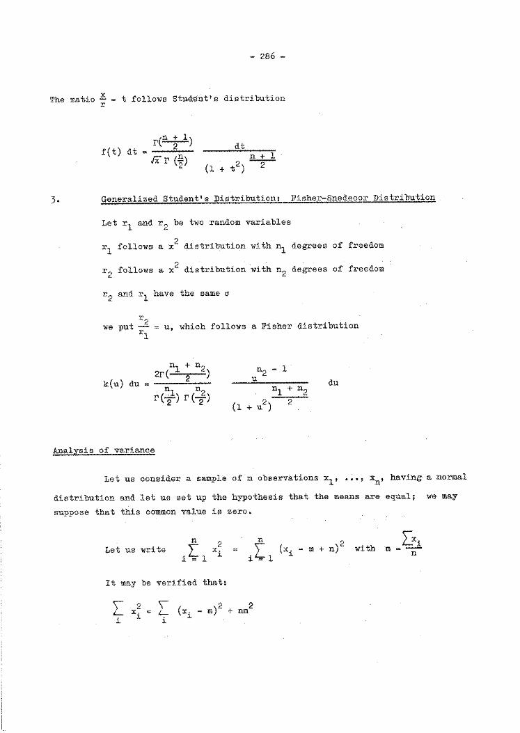
- 286 -

The :~m 'W.o 2S r

t follows Stud:ent' s distribution

f(t) dt I'(~)

lit I' (~) dt

n + 1 (l + t 2 ) -2-

3· Generalized Student's Distribution: Fisher-Snedecor Distribution

Let r 1 and r 2 be two random variables

r1

follows a x2 distribution with n1 degrees of freedom

r 2 follows a x2 distribution with n2 degrees of freedom

r 2 and r 1 have the same a

r we put ~ = u, which follows a Fisher distribution

rl

k(u) du

n + n 2I'(l2 2)

n n r(2l)r(i)

Analysis of variance

n2 - l u

nl + n2

(1 + u2) 2

du

Let us consider a sample of n observations x1 , ••• , xn' having a normal

distribution and let us set up the hypothesis that the means are equal; we may

suppose that this common value is zero.

n Let us write .L X~

1 = l 1

It may be verified that:

LX~ i

\ 2 L (x. - m) + i 1

Ln 2

(x. - m + n) i = 1

1

2 nm

with [xi

m =-n

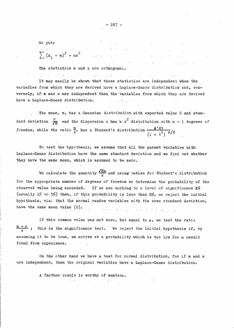
We put:

L (xi - m)2 2 ns

- 287 -

The statistics m and s are orthogonal.

It may easily be shown that these statistics are independent when the

variables from which they are derived have a Laplace-Gauss distribution and, con­

versel,y, if m. and s are independent then. the variables from which they are derived

have a Laplace-Gauss distribution.

·The me.an, m, has a Gaussian distribution with expected value 0 and stan-

dard deviation a

'Fn and the dispersion s has a x2 distribution with n- 1 degrees of

freedom, while the ratio ~. s has a Student's distribution A'd~ ; 2 (1 + t ) n

To test the hypothesis, we assume that all the parent variables with

Laplace-Gauss distribution have the same standard deviation and we find out whether

they have the same mean, which is assumed to be zero.

We calculate the quantity mm .. and using tables for Student's distribution s

for the appropriate number of degrees of freedom we determine the probability of the

observed value being exceeded.

(usually 1% or 5%) then, if. t~is

hypothesis, viz. that the normal

have the same mean value ( 0).

If we are working to a level of significance K%

pr~bability i~ ],ess than K(0, we reject the initial

random variables with the same standard deviation,

If this common value was not zero, but equal to 1.1, we test the ratio

~ ; this is the significance test. s We reject the initial hypothesis if, by

assuming it to be true, we arrive at a probability which is too low for ~ result

found from experience.

On the other hand we have a test for normal distribution, for if m and s

are independent, then the original variables have a Laplace-Gauss distribution.

A further result is worthy of mention.

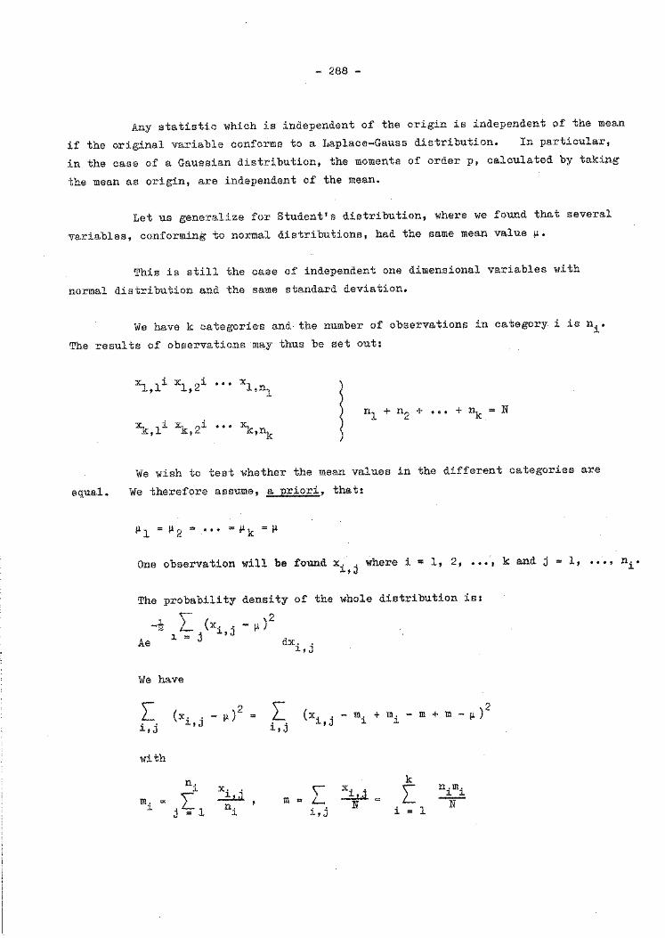
- 288 -

Any statistic which is independent of the origin is independent of the mean

if the original variable conforms to a Laplace-Gauss distribution. In particular,

in the case of a Gaussian distribution, the moments of order p, calculated by takipg

the mean as origin, are independent of the mean.

Let us generalize for Student's distribution, where we found that several

variables, conforming to normal distributions, had the same mean value~·

This is still the case of independent one dimensional variables with

normal distribution and the same standard deviation.

We have k categories and the number of observations in category i is n .• ~

The results of observations may thus be set out:

equal.

X i · 1,1 xl 2~ ••• xl

l ' ,nl

X i X · nl + n2 + ••• + ~ = N

k,l k 2~ ••• xk ' ,nk

We wish to test whether the mean values in the different categories are

We therefore assume, a priori, that:

~1=~2=···=jJ.k=~

One observation will be found x .. where i = 1, 2, ••• , k and j ~.J

The probability density of the whole distribution is:

-~ L (x. · - ~ )2

Ae . ~.J

~ = J dxi,j

We have

[ i,j

with

m. ~

(x. . _ 11 )2 ~.J ,..

ni

.L J = 1

2.z..j_ ni

[ i,j

m

2 (xi, j - mi + mi - m + m - ~ )

\ L i,j

2.z..j_ N

k

[ i = 1

nimi -N-

1, ... , ni.

which gives

L i,j

(xi . _ 1.1 )2 t J

[ i,j

[ i,j

(x. j - m. ) 2 +

~, ~

- 289 -

(x .. _ m )2 \ ~, J i + L (mi ... m)2 + L i,j i,j

L ni i

( 2 2

mi - m) + N(m - fl)

(m - fl)2

and it may easily be verified that the rectangular terms are zero.

Let us take, for example: [ i,j

(x .. - n.) (m.- m) ~,J ~ .· ~

Expanding we have:

L i,j

(xi,j - ~i) (mi - m) [ i,j

2 (x .. m. - x .. m - m. + m m.) ~,J ~ ~,J ~ ~

[ i,j

x. m 2 ~, j i - Nm - L i

2 2 ni mi + Nm L ni m~- L n mi 0

Let us put:

[ (x .. - m.) 2 = s• 2

i,j ~, J ~

[ 2 2 n. (m. - m) = s' i ~ ~

and we put also:

x .. -m. ~,J ~ s•ei,j

ni => ~ e .. = o

.L 1 ~,J J =

i.e., k equations

[ i,j

2 e. . ~,J

1, thus altogether k + 1 equations between the N(e1 .). , J

remain therefore (N - k - 1)8 .. which are independent. ~,J

There

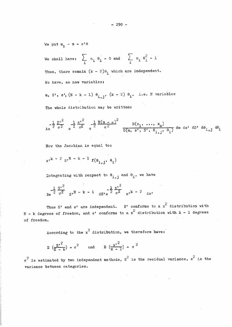
We put m. -m= s'8 ~

We shall have: L n. e. i 1. ~

- 290 -

0 and \ 2 L ni 8 i i

1

Thus, there remain (k - 2)8. which are independent. ~

We have, as new variables:

m, S', s', (N- k- 1) 8 .. , (k- 2) 6., i.e. N variables ~, J ~

The whole distribution may be written:

l 8' 2

Ae-2 -;;-2 l s'

2

e2~ -~ N(m _ f! )2

e o2

Now the Jacobian is equal to:

,k- 2 S'N- k- 1 f(e .. , s ~,J eJ

D(m, s', S' e e ) dm ds' dS' de .. de. ' i,j' i l.,J ~

D(x1 , ••• , xn)

Integrating with respect to e .. and e., we have ~,J ~

1 8 12

Be-2 ~ 8 ,N - k - 1 l s'2

dS'e-2 -;;-2 s'k - 2 ds'

Thus S' and s' are independent. S' conforms to a x 2 distribution with

N - k degrees of freedon, and s' conforms to a x2 distribution with k - l degrees

of freedom.

According to the x2 distribution, we therefore have:

8'2 E (if":'"k)

2 0 and

I 2 E (/_ 1)

2 0

o2 is estimated by two independent methods, s2 is the residual variance, s 2 is the

variance between categories.

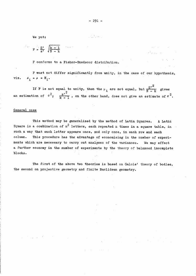
viz. l!i

- 291 -

We put:

. · S' Jk ... ·1 F=- ---s' N- k

F conforms to a Fisher-Snedecor distribution.

F must not differ significantly from unity, in the case of our hypothesis,

I! = Ni.

If F is not equal to unity, then the I!. are not equal, 2 ~

8'2 but N _ k gives

an estimation of 02• '

s' ~ , on the other hand, does not give an estimate of a

2•

General case

This method may be generalized by the method of Latin Squares. A Latiri Square is a combination of n2 letters, each repeated n times in a square table, in such a way that each letter appears once, ~d only once, in each row and each column. This procedure has the. advantage of economising in the number of experi-ments which are necessary to carry out analyses of the variances. We may effect a further economy in the number of experiments by the theory of balanced incomplete blocks.

The first of the above two theories is based on Galois' theory of bodies, the second on projective geometry and finite Euclidean geometry.

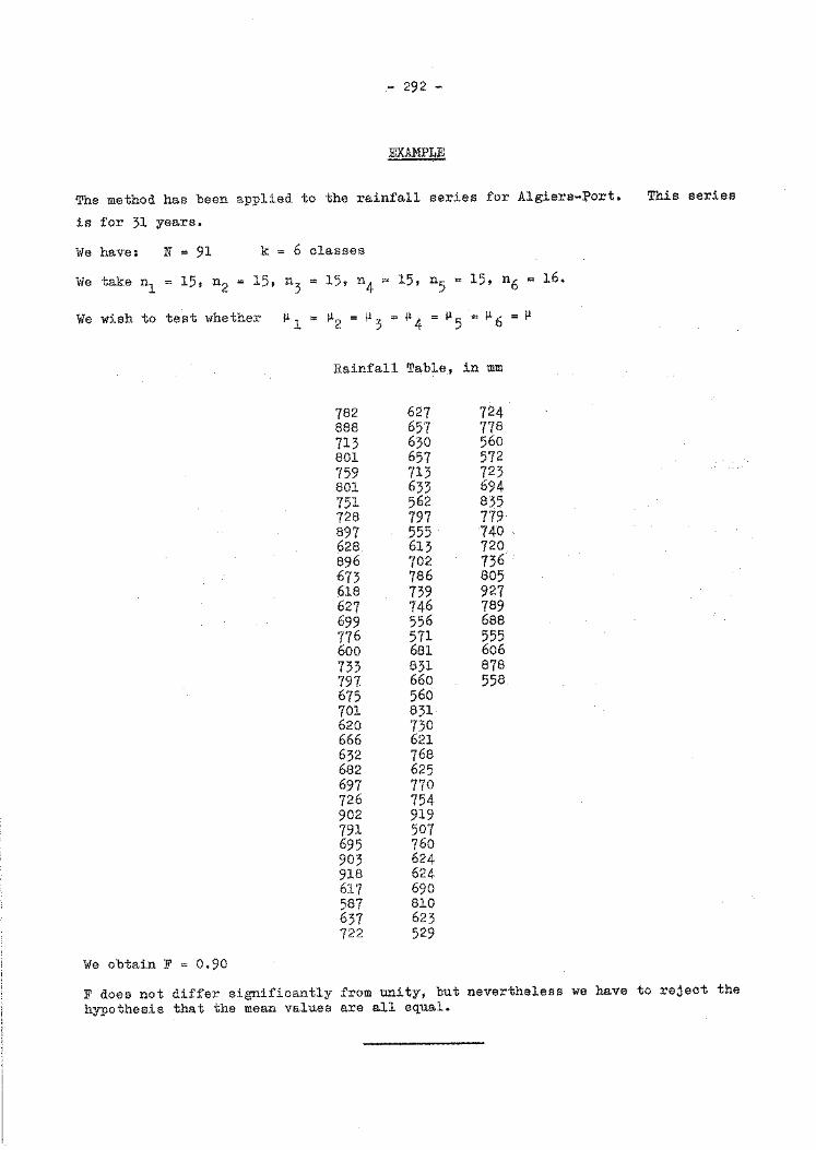
- 292 -

EXAMPLE

The method has been applied to the rainfall series for Algiers-~ort.

is for 31 years.

We have: N = 91 k = 6 classes

We take n1 = 15, n2 = 15, n3

15, n4 = 15, n5

= 15, n6 = 16.

We wish to test whether ~ 1 ~2 = ~ 3 = ~ 4 = ~ 5 = ~ 6 = ~

Rainfall Table, in mm

782 627 724 888 657 778 713 630 560 801 657 572 759 713 723 801 633 694 751 562 835 728 797 779 897 555 740 628 613 720 896 702 736 673 786 805 618 739 927 627 746 789 699 556 688 776 571 555 600 681 606 733 831 878 797 660 558 675 560 701 831 620 730 666 621 632 768 682 625 697 770 726 754 902 919 791 507 695 760 903 624 918 624 617 690 587 810 637 623 722 529

We obtain F = 0.90

This series

F does not differ significantly from unity, but nevertheless we have to reject the hypothesis that the mean values are all equal.

- 293 -

ANALYSIS AND PRESENTATION OF SURFACE WIND OBSERVATIONS

by

M.S. Harb

In every meteorological service surface wind observations are taken using different types of instruments, some of which (e.g. cup anemometers) allow J,~or actual visual observations while others (e.g. Dines Pressure T1lbe Anemograph) allow complete records of- the ·surface wind during the wl;iole day (direction and speed) to be taken.

Meteorologists and users of climatic data are mostly interested in two aspects of the surface wind, the direction from which the surface wind blows and its speed. The direction is usually indicated by the compass points and measured, from the north on the scale from 000 - 360° points while the speed is given either in m/sec, knots, etc~

The percentage· frequencies of surface wind blowing from diffl;lrent dil!'ections, within certain spe'ed limits, are of vi tal importance and· are considered as basic information in all the applied fields related to meteorology, particularly the fol­lowing:

Agriculture

Industry ail:d trade

- Air transport · - · · SeB: transport

-Land transport

- Tourism Recreation and sport

Disasters

Science and research

Individual need

Service and its value to the community Future developments and future projects.

The processed '~urface wind. data are required either. in the form of tables or in graphic representation such as wind roses.

- 294 -

In the U.A.R., the climatological division has introduced a special form

(see annex) which serves both purposes. It includes a ·table for processed climatic

data of wind and a space for wind rose presentation for four months of the year

or for three months, the relevant season or for the four seasons of the year, accor­

ding to the included climatic data.

The elements used in preparing this table are the percentage frequencies

of surface wind, blo.wing from different directions within special speed ranges.

These frequencies are computed from the analysis of the daily records of surface

wind instruments installed in the meteorological stations. Themean hourly values

are extracted for every hour of each day of the month and they refer to a period of

60 minutes centred at the hour. Sorting of surface wind direction and surface wind

speed within specified ranges of direction and speed is carried out mechanically by

the sorters in the processing machine section.

The number in hours of "variable" winds is the number of cases when the

surface wind showed no definite direction over the period of the 60 minutes centred

at the hour or when the wind vane was sticking over that period due to the lightness

of the wind and therefore not responding to the variation in wind .direction; in

such cases the mean wind speed over this period is normally less than 5 knots. The

number in hours of calm winds is the number of cases where the surface wind has a

mean speed of less than one knot over that period whatever the surface wind direction

over the same period may be.

Construction of wind roses is carried out directly using the already pro­

cessed data shown in the table below in the relevant square of the month or of the

season. To facilitate the process the directions of the surface wind are already

indicated in each square with the aid of a calibrated ruler (in centimetres and

millimetres) and using a relevant scale. Three categories of speeds can be pre­

sented in this form. They are:

Category Speed Range

lst l-10 knots

2nd 11-27 knots

3rd 28-47 knots

- 295 -

The thickness of the line showing the percentage frequencies of direction

represents these three categories. This line starts from the circumference of the

small circle centred in each square. Percentage frequency of calms and variables

are indicated in upper and lower semi-circles respectively.

This form can be widely used in different meteorological services using

appropriate ranges of directions, i.e. for countries using eight compass points, or

16 compass points the appropriate table at the bottom of this form can be used.

Annex : 1

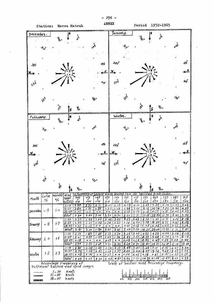
- 296 -

Station: Mersa Matruh ANNEX Period 1952-1965

1t.tnua-{i] f 0 v\ ~

]Jecemhe-t • T 1" . 'l·

,.., • ~ .. 0 .

0 • 11 -.t,J'. 0~ o'lf'> . .

~.s-Q

~Qs· .

2as ~ I c7f jJ'l· o7f

~. ~-r::1. . ._L ~ ~ . .\-I· o

·~ " ,;tl'/1~ '•s 11

. .,_1J6 ~,~ 14

' ,t? . . <$-." '!,'},~ <ts• .

•~o,

"' fs ~- ~.

f e!Ytulfl&1 • .J M • Wintet. o~"~ ~ ~~ '0-· . . .

Jo<s- . . v.e, ~"'. . . ovf> 0

285

~ ol!i <eJ

;;r~ tJ75

tit-· . ~ .:tf..t;.. . 1·.1 ~ . .£.. 1:3, 0 t'J

1

" 71~ 1.6, le$ z.S? Ios•

' • "'{' . ~,.. .. tt? . . "'-&-•

0 b ~ ts ~d fs -' ~ tn,o

( p11 W:i~ie~Jile Wind %tt.tt9ktMcyo,. ttifacewin7KDliJ"'~!l.I.i.EJn "!!U--;~rrnecr-,~.ec u~.-. . __ Mo~H !·--'1 1 Sneed 3115 CJ/5 cifS DH fc'i I.HT15.5 195 J.~'i .2551,1.[{5 3/!i

.. 11~ o 11 r· / .., / _, / 1 ; / / .-· / /

y.; ;la I{K(ft,ts) ~>1.11 ~If¥ o'711 · /ol< IYI 16 'I~:!L. 22. 'I _!£!_ __ EJ _. :~!!- ..;!!!., •

·;pecembd ,, · 9

p-anual!.J .,.g

Febwaxj I ), · o

-!;=~~%-· -i~H= 4: ;,1-+~~ ·1--~.~:J .. , t:-;;-- -t:is.1t-t-i~··;_2-~,~f- -f~A~ +F~'-· -~_-:--r-1:- {j~--1 • o 1,11.;1· o: • ' -~~~:. ;,--- r;::;;- -:~:;;~:~-:~=- ~:ir1 I~~I~ ~~::11. -~~z'C ~Y.:.Jt: :~'il:~ ,~:~~zJ

'Toto 7-:Z.II -~.~o 3-oc 3.3o li·J•• 6·£.::..J 7·7t' 1~'./IJ 2.2-Vo 11-'7~ l).&o 1·50

~, ~--). %- __ • _ 9 !f H.~r?-Y~r·U __ }_ ~--~ __ }_lW-~1~Tf]. _].:_~!'_t!L!!. __ · .~~-:TI_i:.?I 1·7 ~-_j~ o-116 !!..:.HL.l:.Z.L .. tJ..l+L?~ 9:~g_ 16-t!!...~ . .!Q·?!J~. '~:Xf._ ~:~.!.

2.8 117 o·O) <1'·<•2 .,.,. o-o o-<> o.oJ d·/2 •·•6 O·!.>ti I o·;{lf o.o; o.fO

'rata?' 3-Bv- ·3·"• ·J·8l> I:.:J-.l'-' ,3.;;:;=·'_5'.'~'PTI':"~~"'1t6~o!2s-i0113:;y" =-~rl'J· r-2~' ~-~..!...'!._ . . X-JJ ....!.:$.3 !-~~- _i·Jl]TF 3-lfTio_ ~--LiiZJ6·U±' N-1/i(~:IJ.f __ TII.:t;t._.

j.f !4-.2.1_ r-1-:.ol- O•cSl ~·o/J /•t/0 t /• yq-1-j'::_~_Q ,) J,}~ , ~~i_~ !_· }tf L..:·:~<j.J.:.~· ... f.. !J.B-'17 o~]J. o·o o-t> tl•f/7 o-o "'"8-,--;.-.!6 •·JIJ, fi:..!/J.: o-68 •·Hd'f 1{-o

~- ::'s: ;;~5:-~~-- :_;~f-~~±ff_f~:r;~~ .~J1B5¥.!JJ:~¥:{tif,i~ + I 1 2 ,,.3 ~J=~~ .. J:.:Z.~- .J· rJ . .2. __ .E.:JL .J..:.a_ ...... l:J-.~.l.::~LjJ..:.H.t' .. 8.:!fJ..La.:7:,2_ 1 ,"~-. 6~f~ .. : .. u_ !J.:.-z.'!...

'Winttlt ' 28-117 11·"5' •·"I o.o L'·c.1 •-o c-oil o·f7 6-lfi :o·6'/ o-/.11 Q.;il 0·/9 1 f"::' " --" ===--==~~F===~ •=·o~~""'"=--·-Lc"~"-'~"1·"=~-=-=- .,--;:-·-· -'"=-·"·--=~==-='

="-=: ~e~cent~9e r~;~;~~z~6:r 3

.01 2

•3:= ::.~-~-~j;f~~t~~~~!~~af~~,~~~7~.:;,~~~;.1.t ..

1Ji/fe<tenf SUJtface wind spePd Jurn1tJ~.

1-10 knot> IJ -2.7 l<nof:s 28-'17 knots - :!: ·, n! h,,~~wh.JmJUuJ

l!t ~ }O't'l 3..>_/1, #'"~% §tt J/, (,,% ~

- 297 -

MACHINE PROCESSING OF CLIMATOLOGICAL DATA RECORDED IN SENEGAL

by

M. Seck

Introduction

The aim of this document is to inform delegates about the methods and equip­ment used in processing data for climatological purposes in Senegal.

The Senegalese Meteorological Service, technically assisted by the Air Traffic Security Agency (Agence pour la Securite de la Navigation Aerienne - ASECNA) in Africa and Madagascar, publishes a variety of climatological data taken from con­ventional meteorological registers. We shall successively examine the recording system, with its advantages and disadvantages, and then the data contained in the various documents and the way in which these data are processed depending on the possibilities of the service and the needs of the users.

Recording Slstem

Since 1966, Senegal has abandoned the old recording system using documents such as DWR and others in favour of machine cards which, in this case, are based on the "mark sensing" system rather than on direct punching.

The observer starts by filling in the holes, with a special black pe~cil intended for this type of work, against each figure that corresponds to an indicated value. These cards are collected at the NMC at Dakar-Yoff which feeds them into the electromagnetic reader for punching.

1.

This procedure has both advantages and disadvantages.

The advantages of mark sensing cards

There is less chance of errors creeping in as the cards are prepared by the observer himself, directly from the register. Moreover there are no errors due to transmission, coding and decoding.

2.

- 298 -

Stations within the country no longer need despatch files which make

the collection of documents so much more difficult.

The graphite system is cheaper as the climatological staff needed is

smaller than that needed for the old system involving documents

(Monthly Climatological Report, DWR, etc.).

It is possible to prepare as many cards as are required (R, Q, S, T, et.c.)

Disadvantages

The areas covered in graphite are bigger than the punched holes; the

number of·columns giving basic information contained on a card drops

from 80 to 54.

The graphite coating, which remains after automatic punching, cakes up

the machine leading to electronic break-downs, and so it must be

cleaned frequently.

Recorded data

There are several kinds of recorded data, different cards being used

depending on the nature.

1. s66 cards: which contain:

Synoptic observations

Hourly observations for certain aerodromes:

IIiii Nddff VVwwW PPPTT NC1hCMCH

The main cloud layer

Dry bulb temperature

Wet bulb temperature

Relative humidity

Vapour pressure

Dew-point temperature

Air pressure

2.

3·

4.

- 299 -

o66 cards: which contain:

Daily observations (2 cards per day per station), including:

precipitation (quantities and duration by day and by night)

sunshine a.m. and p.m.

actinometric data (not yet carrie4 out)

maximum and minimum air pressure, a.m. and p.m.

maximum and minimum temperatures

raingauges

maximum wind speed

extremes of relative humidity

extremes of temperature

evaporation

minimum visibility

minimum cloud base

duration of fog

raingauge readings from auxiliary stations (daily readings:

3 cards per month per station).

v66/l cards:

Give upper winds (speed and direction) up to 10 mb (25 selected levels).

v66; 2 cards:

If the height reached by the sounding is 50 mb or higher.

v6613 cards:

If the height reached by the sounding .is lOO mb or higher.

Cards v66/l' v66; 2 and v6613 are very much alike and are used regardless

of the method of sounding (radar, optical theodolite and radio theodolite).

R66 cards: for radio-soundings contain:

Altitude

5.

6.

(

7.

Temperature

Mixing ratio

- 300 -

Wind at 23 levels oetween ground level and 10 mb

Pressure

0° and -10° isotherms

The tropopause(s).

The R66 cards are supplemented by T66 which give the isotherms (zero,

minus ten and one or more tropopauses).

w66 cards:

These give wind at 23 levels, and the various significant points of the

sounding relating to the wind.

r 66 cards:

These allow for the recording of certain significant points (front and

back) of temperature and humidity (temperature inversion base and top).

Data processing

In this part of the document, we shall simply mention the type of equipment

that we have. We shall not enter into great detail in the description and operation

of our equipment, nor shall we criticise it, for this would involve long, often

classical, and therefore well known, theories.

So, once the graphite has been applied, the cards are fed to a punch after

which it is possible to print out or list the data. For the moment, we have:

The 11Resume mensual d 1 observations" (Monthly summary of observations)

(see publication)

The rain data supplement (see publication)

Synoptic observations and daily readings

Upper air observations comprising:

- 301 -

Altitude Temperature Mixing Ratio Winds (23 selected levels)

Monthly Standard Monthly Standard Average Standard Resultant: E : W : N : s Mean Deviation Mean Deviation Deviation components

. : : : . : : . . . . : : . : .

Obviously, certain data are no longer calculated manually, but by computer.

Once the cards have been fed successively into the punch, the card reader, the col­

lator and the sorters (2), they go on to the tabulator which operates at 80 lines/

minute. If we want to carry out more complex operations (standard deviations,

averages, variance, etc.), we use a computer with the following characteristics:

l.

2.

3.

4.

~:

IBM/11.30 with 16,000 storage locations (16 k) originally we had 8,000 (8 k).

Input/Output:

punched cards, or

discs

we have neither punched nor magnetic tapes.

Printer:

The printer connected to the computer has a print-out rate of lOO lines/

minute, which is very fast.

Langu.ages used:

Assembler

Gap

FORTRAN

Comet.

FORTRAN is used most, but it has the disadvantage of signs (+ or -). We

then move over to Assembler. Comet is occasionally used to back up FORTRAN. We

are also beginning to programme in Gap.

Apart from the systematic programmes mentioned at the beginning of this part

(RMO, Rainfall supplements, etc.) we also prepare other publications for commercial

purposes.

- 303 -

METHODS TO ESTIMATE THE MAIN PARAMETERS , OF FREQUENCY DISTRIBUTIONS OF METEOROLOGICAL ELEMENTS

ON THE BASIS OF VERY SHORT OBSERVATIONAL SERIES

by

w. Boer

In the operational activities of Meteorological Services the necessity fre­quently arises to supply some information on selected meteorological parameters for a selected site or a selected area without having available sufficient meteorological observations for this site or for these parameters (frequently not even for both). The desired information is for national economic planning in most cases related to the so called "meteorological risk", i.e. to the probability of the occurrence of an adverse "meteorological event" (or, respectively: the probability of the non-occurence of a favourable "meteorological event") during a certain season (or the whole year) and in a selected area. A "meteorological event" is understood to be, generally speaking, the passing beyond (below or above) a certain threshold value of a meteoro­logical element (e.g. reaching or exceeding of a selected value of the diurnal maxi­mum of the air temperature or of a selected value of the 24-hour precipitation sum, etc.), or the simultaneous exceeding (below or above) of a selected threshold of two or more meteorological elements (e.g. of the visibility and of the height of the base of low cloud at an aerodrome, etc.), or, further, the probability of the uninter­rupted duration of such exceeding (below or above) (for instance, the sequence of very hot and humid days, say with air temperature permanently above 20°C and relative humidity above so%, the duration of drought periods, etc.), all these parameters should be economically relevant to a certain technological, agricultural or other national-economical process.

Such meteorological information is required for long-term national­economical planning as well as for the conception and design of certain production processes or certain technical equipment (including houses and towns) for which the disturbing parameter "meteorological environment" must be eliminated, or at least, taken into account.

In a very general sense, the problem is to derive, from rather short obser­vational series, certain statistical parameters of the frequency distribution of the required meteorological parameter, although the volume of the sample is normally too small to allow for statistically significant statements. A statistically significant

- 304 -

statement for meteorological observational series is not generally feasible unless

there is available at least a 10-year series or an even remarkably longer one. The

information needed for the national economy ls in most cases, however, required much

earlier, i.e. not only after 10 years or a longer period, for the decision making

process.

Such obstacles can in certain cases be overcome provided a reasonably long

observational series is available for another meteorological parameter to which the

required parameter can be related with reasonable reliability. Statistically this

is a regression problem. 'When there is a stochastic relation conclusions can be

drawn from a known sample for an unknown or insufficiently known sample and even

possibly for the population.

The statistical methods and tests that should be applied as a tool and -

if po~sible ~ using machine processing techniques are presented in other lectures of

this Seminar especially in those of Dr. Eriksson and Dr• Tarakanov. They need not

be repeated here.

l.

2.

3·

However in any case some basic conditions must be fulfilled:

At least one (or rather more than one) long and homogeneous observational

series to which the rather short observational series can be referred must

be available.

The rather short observational series must be of a strictly homogeneous

nature.

There must exist between the parameters to be referred to each other a physically based relation, not only a formal statistical one.

The following three examples show some special applications and the prac­

tical handling (on a physical background) of statistical methods:

to obtain olimatologioal normals,

to obtain olimatologioal values, on the topoclimate of a selected site,

to obtain climatological vaiues for an unmeasured or insufficiently

measured element.

- 305 -

\

Estimation of climatological normal values for a newly established station

Provided climatological normals of the parameter in question are available

for a selected area with a certain number of stations, then climatological normal

values can be generally estimated for further stations or sites for which no measured

data are available,

In the first instance, it is possible to derive from a relevant climato­

logical chart by interpolation a value for the desired site, e.g. a value for the

normal monthly average temperature of a selected month. In such a case one can

generally obtain no more than a comparatively rough approximation to the real normal

value for the specific site, since the local peculiarities (influence of the special

local climatic features) cannot be derived from a climatological chart which in

principle can only show macroscale spatial variations.

If observations are available for at least a period of one year for the

site in question (for which an assessment is required) the whole procedure can be

refined substantially. The first step is to determine by calculation the observa­

tional data of neighbouring stations or from suitable distribution cards for each

month a probable deviation from the normal value (or the probable ratio, should the

respective parameters so require) for the station in question, then - in the reverse

direction - from these probable deviations (or ratios) and using the values observed

at the station, a preliminary normal value is determined for the various months and

for the year.

The deviation of these preliminary normal values from the corresponding

mean values of the respective climatic area is then determined. This ."area mean" of the normal value is obtained either from the corresponding climatological charts or

it is calculated as the arithmetic mean of the normal value of neighbouring stations,

which must however, be situated in the same climatic area. The assumption can be

made (which is corroborated by experience) that deviations of the normal value of an

individual station from the "area mean" of the normal value - according to the local

climatic conditions of that station - are either constant over the whole year or show

a steady annual variation, Irregularities of these deviations (which are unlikely)

are corrected by altering the "preliminary normal value", which then leads to the

final normal value. This procedure is illustrated by the example given in the Table.

Based solely on the observation of one year (1952) - which was a pure chance selec­

tion- the normal values of the monthly mean temperature with a maximum error of 0,3°

were obtained for the station Halle (for which a complete series of homogeneous

- 30,6 -

observations was available). With further observations at hand, the degree of a

approximation can be continuously improved using the same method. The local peculi­

arities of the site (in question) have been taken into account with this procedure.

If further refinement is needed the statistical structure could be taken into account,

e.g. by means of the structure function of the field of the quantity in question.

Assessment of the areal differences of characteristic parameters within the local climatic scale

For a number of planning problems it is rather important to know something

of the climatic differences in comparatively small areas. This applies particularly

to many major building sites, and also to detailed agricultural and horticultural

crop planning. Such local climatic (topoclimatic) differences are not normally

available from a meteorological station network which has only to serve the investi­

gation of macroscale meteorological phenomena and processes. 11Macroscale 11 in the

sense quoted here means a scale of some ten to fifty kilometres. It should, however,

be noted that measured values of each meteorological station are in any case an

"ensemble" of the effects of all meteorological scales, particularly the macro­

meteorological and local meteorological ones. The most secure approach to gather

information on local climatic differences is by means of a very dense station network

(special network) being maintained for a longer period of time (at least 5, or pre­

ferably 10 years). The expenditure of personnel and material required for the estab­

lishment of such a special network, for its maintenance and for the processing of the

data obtained is nevertheless remarkable. Further, in general too much time passes

before the required information is available. For this reason there is reluctance

to establish such special networks. The method mainly used to get information on

local climatic differences is to obtain these differences for selected synoptic

situations (chiefly with low wind speeds and cloudless sky) by measuring runs, e.g. of

the nocturnal temperature minima.

This method, though furnishing some clue on the order of magnitude of the

local climatic differences, has, however, some disadvantages, namely: the state­

ments generally refer only to selected special states of weather, and do not normally

reflect the "climate" adequately, i.e. the entirety of all states and developments of

the weather (of a given area) occurring with different frequencies.

The drawbacks of both the methods mentioned above (too great an expenditure,

rather long duration, or insufficient representation of the climate) are largely

avoidable if a method which was worked out in our country by MADE and his staff is

- 307 -

applied. The idea of this method is to establish a special network which should, if

possible, be furnished with recording instruments, and operated for only a short

period (i.e. not more than 2 years). From the data obtained from these stations at

a maximum possible number of observation hours for the desired meteorological element

(e.g. air temperature), the frequency distribution is calculated for short periods -

preferably months. At the same time, for stations of the meteorological basic net­

work in the vicinity of the investigated area, an identical evaluation (frequency

distribution) for the respective element is carried out. A comparison of the fre­

quency distribution serves to find out for which stations of the meteorological basic

network and of the special network the frequency distributions are sufficiently simi­

lar to each other within a given tolerance.

The comparison is most easily made by graphical means with the cumulative

frequency di~tributions being plotted into the normal probability paper. In such

a way it can be found which of the basic network stations having available long-term

observational series may be taken as representative for the investigated meteoro­

logical elements and for which parts of the terrain. Measuring runs must serve to

determine which stations of the special network are representative and for which

parts of the terrain (e.g. valley bottom, slope, surrounding elevated plain, etc.).

In this way the desired climatological information can be obtained for any part of

the terrain.

1.

2.

The following scheme may serve to illustrate the procedure:

A, B, C denote stations of the meteorological basic network

a, b, c denote stations of the special network

a, ~' y denote selected parts of the terrain

* * FA {u) = Fb (u)

Frequency distribution of station A for the meteorological parameter u

approximately equal to the frequency distribution of station b (in the

short period).

* short period

b representative for parts of the terrain a.

3·

- 308 -

FA (u)-+ I (a)

Frequency distribution of station .A for the meteorological parameter u

(long period) furnishing the climatological information (I) for part a

of the terrain.

The following illustrates the application of this method for a routine

operational example from the German Democratic Republic. I must apologize that no

example could be worked out for a terrain and parameters usually asked for in .Africa

but the time was too short for me to get one. Nevertheless as an illustration of

the method it might be good enough. .Any meteorological parameter showing marked

differences due to topography built up areas or other local factors can easily be

substituted instead.

Estimation of relevant statistical parameters for a meteorological element measured only over a short period by means of another element measured over a longer period and physically related to the former

For a number of operational problems information is required on parameters

for which there are no, or only short-term, measurements available from just a few

stations~ Now, if there is a physical relation to a different parameter, for which

measurements are available from a large network and for a long period of time, then

it is generally possible to calculate the regression by the usual relevant statistical

methods shown in other papers of the seminar, provided parallel measurements were

carried out for a common period at a number of stations. The same is true if only

one station is of interest.

An example is given for the percentage snow share in lowland precipitation

of the GDR. On the basis of scheduled measurements (at observation hours) at clima­

tological stations (i.e. a limited number of stations) the calculation of the snow

share in the annual precipitation sum was possible only for a rather short period.

For many stations, however, observations of the number of days with precipitation and

the number of days with snowfall were available for a much longer period. The

desired information (in this case: a climatological chart of the snow share in the

annual precipitation sum for the whole territory of the GDR) required relevant values

of all the precipitation stations to be included for the plotting of the chart. It

can be shown that the frequency distributions of the percentage snow share in the

annual precipitation sum (short period) and for the percentage share of the days with

snowfall on all the precipitation days (short period) and for the percentage share

- 309 -

of the days with snowfall on all precipitation days (long period) were largely

identical and that they differed only by a constant difference. These frequency

distributions are nearly parallels drawn on normal probability paper. The para­

meter "number of days with snowfall" (obtainable for all the precipitation stations

and for the long period) as compared with the number of precipitation days was then

(by including a constant correction) simply transformed into the parameter "snow

share in the annual precipitation sum" for the long period, and - based upon these

values - the climatological chart was drawn up.

From scientific references a large number of corresponding examples for

other meteorological parameters are known. Mention can be made, for example, of the

calculation of global radiation from data of cloud coverage. Another very instruc­

tive example was given by Mr. Thoro (u.S.A.) at the vmo Symposium on "Town climates

and building climatology", Erussels, October 1968. In this case the maximum wind

velocity for the design of buildings and structures in the whole area of the

Caribbean Sea affected by tropical storms was derived from the frequency of the occur­

rence of such storms in one-degree-fields (read from historical weather maps) on the

basis of the relationship between storm frequency and the maximum wind velocity obser­

ved over many years at stations in the southern part of the U.S.A.

Antonik, E., Eoer, W.

Eoer, W.

Eoer, W.

Made, A.

WMO

Table : 1

REFERENCES

Der Schneeanteil am Niederschlag in Gebiet der Deutschen Demokratischen Republik (The snow share in annual preci­pitation sums in the territory of the German Democratic Republic). Z-Met. Ed 16 (1962) S. 231-239·

Einige Bemerkungen zu klimatologischen Normalwerten der Monatsmittettemperatur fur den zeitraum 1901 bis 1950 (Some remarks on climatological normals of monthly mean temperature for the period 1901 to 1950). Z-Met. Ed 10 (1956) S. 1-11.

Technische Meteorologie (Technical Meteorology). Leipzig 1964.

Ubder die Methodik der meteorologischen Gelande vermessung (on the method of topometeorological measurements). Deutsche Akademie Sitzungsberichte Ed. V, H.5 Leipzig 1956.

Lectures at the Symposium on "Town climates and building climatology", Erussels, Technical Note.

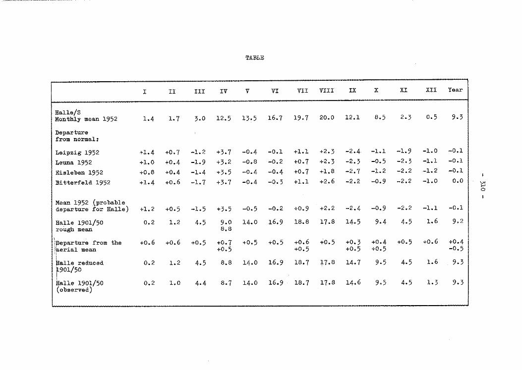
TABLE

I II III IV V VI VII VIII IX X XI XII Year

Halle/S Monthly mean 1952 1.4 1.7 3·0 12.5 13.5 16.7 19.7 20.0 12.1 8.5 2.3 0.5 9-3

Departure from normal:

Leipzig 1952 +1.4 +0.7 -1.2 +3.7 -0.4 -0.1 +1.1 +2.3 -2.4 -1.1 -1.9 -1.0 -0.1

Leuna 1952 +1.0 +0.4 -1.9 +3.2 -0.8 -0.2 +0.7 +2.3 -2.3 -0.5 -2.3 -1.1 -0.1

Eisleben 1952 +0.8 +0.4 -1.4 +3.5 -0.4 -0.4 +0.7 +1.8 -2.7 -1.2 -2.2 -1.2 -0.1

:Sitterfeld 1952 +1.4 +0.6 -1.7 +3-7 -0.4 -0.3 +1.1 +2.6 -2.2 -0.9 -2.2 -1.0 0.0 1 V.J 1-' 0

I Mean 1952 (probable departure for Halle) +1.2 +0.5 -1.5 +3.5 -0.5 -0.2 +0.9 +2.2 -2.4 -0.9 -2.2 -l.l -0.1

Halle 1901/50 0.2 1.2 4.5 9.0 14.0 16.9 18.8 17.8 14.5 9.4 4.5 1.6 9.2 rough mean 8.8

)fe~ture from the +0.6 +0.6 +0.5 +0.7 +0.5 +0.5 +0.6 +0.5 +0-3 +0.4 +0.5 +0.6 +0.4 er~al mean +0.5 +0.5 +0.5 +0.5 -0.5

a.lle reduced 0.2 1.2 4-5 8.8 14.0 16.9 18.7 17.8 14.7 9.5 4.5 1.6 9-3 901/50

Halle 1901/50 0.2 1.0 (observed)

4·4 8.7 14.0 16.9 18.7 17.8 14.6 9.5 4.5 1.3 9·3

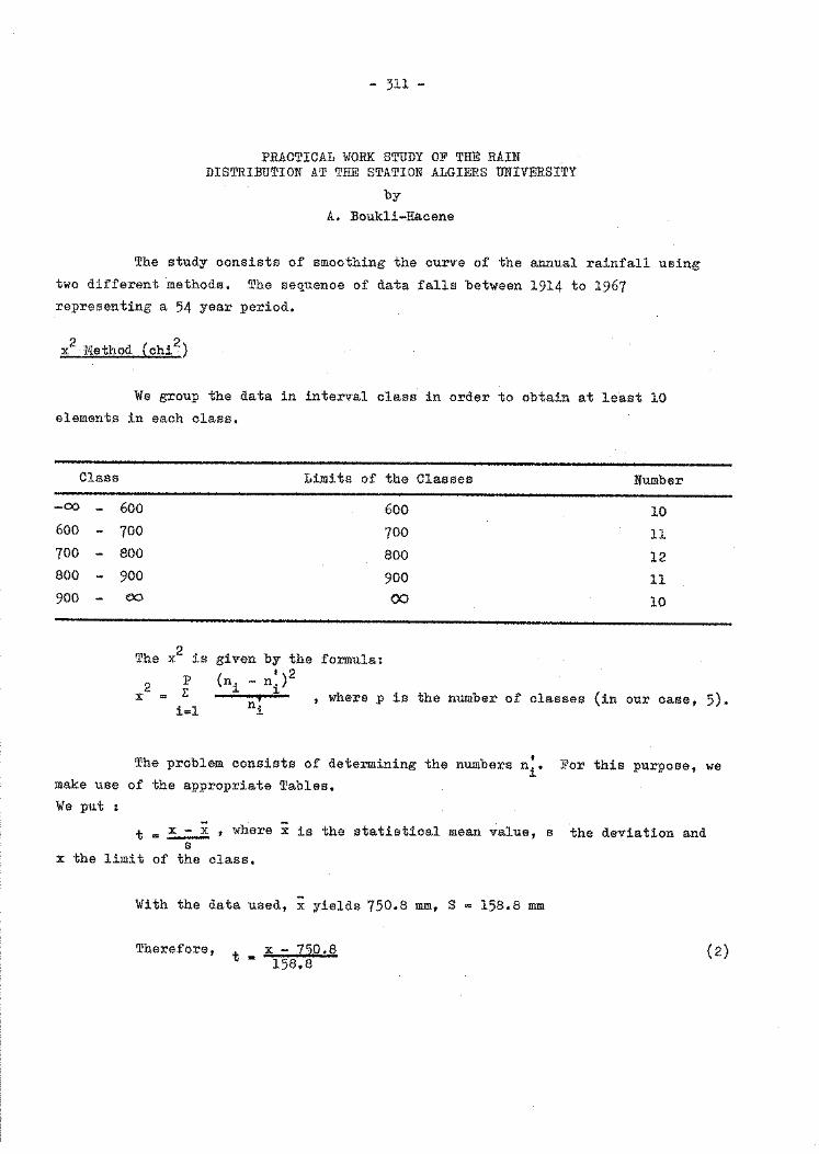
- 311 -

PRACTICAL WORK STUDY OF THE RAIN ~ DISTRIBUTION AT THE STATION ALGIERS UNIVERSITY

by

A. Boukli-Hacene

The study consists of smoothing the curve of the annual rainfall using two different methods. The sequence of data falls between 1914 to 1967 representing a 54 year period.

2 ( 2 x Method chi )

We group the data in interval class in order to obtain at least 10 elements in each class.

Class Limits of the Classes Number

-oo - 600 600 10 600 - 700 700 11 700 - 800 800 12 800 - 900 900 11 900 - 00 CO 10

The x 2 . ~s given by the formula:

p I 2 (n. -n.) 2 X = E ~ ~

ni , where p is the number of classes (in our case, 5).

i=l

The problem consists of determining the numbers n~. For this purpose, we ~

make use of the appropriate Tables. We put :

t .. x - x , where x is the statistical mean value, s the deviation and s

x the limit of the class.

With the data used, x yields 750.8 mm, S

Therefore, t x - 750.8 - 158.8

158.8 mm

(2)

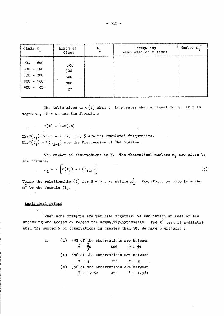
- 312 -

CLASS xi Limit of t. Frequency Number n. Class ~ cumulated of classes ~

-00 - 600 600

600 - 700 700 700 - 800 800 800 - 900 900 900 - 00 00

The table gives usn (t) when t is greater than or equal to 0. If t is

negative, then we use the formula :

n(t) = '1-n(-t)

Then(t.) fori= l, 2, ••• , 5 are the cumulated frequencies. ~

Then(\) -n(t1 _1 ) are the frequencies of the classes.

I

The number of observations is N.

the formula.

The theoretical numbers n'. are given by ~

n. = N rn(t.) -n (t. 1)]

~ L ~ ~-(3)

Using the relationship (3) for N = 54, we obtain n.. Therefore, we calculate the 2 ~

x by the formula (1).

Analytical method

When some criteria are verified together, we can obtain an idea of the

smoothing and accept or reject the normality-h:ypothesis. The x2 test is available

when the number N of observations is greater than 50. We have 5 criteria

1. (a) 49% of the observations are between - 2 - 2 x- ~ and x + ~

(b) 68% of the observations are between

X - S and X+ S

(c) 95% of the observations are between

x - 1.96s and x + 1.96s

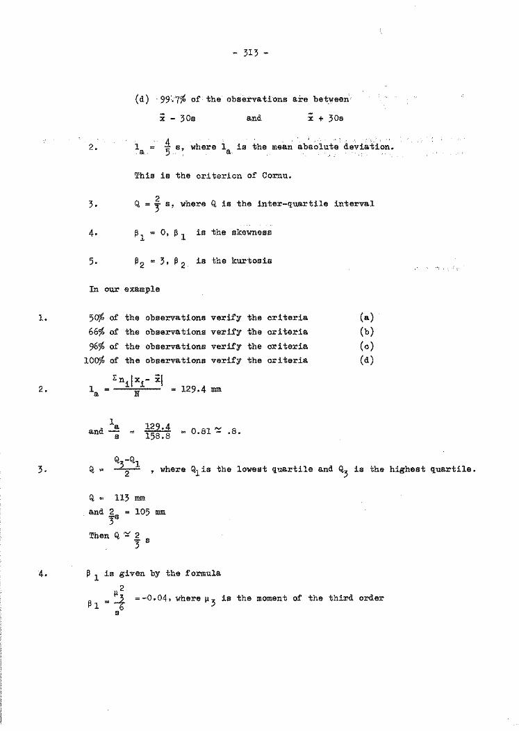
1.

2.

3.

- 313 -

(d) . 99·7% of the observations are between·

x - 30s and i + 30s

2. la = ~ s, where la is the mean absolute deviation.

This is the criterion of Cornu.

3. Q = J s, where Q is the inter-quartile interval

4· ~ 1

= O, ~ 1 is the skewness

5. ~ 2 = 3, ~ 2 is the kurtosis

In our example

5o% of the observations verify the criteria

66% of the observations verify the criteria

96% of the observations verify the criteria

lOO% of the observations verify the criteria

1 = Z nijxi- ij

a N

1 and _!. s =

~ 158.8

= 129.4 mm

0.81 ~ .8.

(a.) (b)

(c) (d)

Q = Q3-Ql -2- , where Q1is the lowest quartile and Q

3 is the highest quartile.

Q = 113 mm

and 2 = 105 mm 38 Then Q ':! _g

8 3

4. ~ 1 is given by the formula

2

11 _

11 3 = -0. 04, where 11 3 is the moment of the third order 1'1- b

a

- 314 -

1.1.

5. ~ 2 = -1 = 2.4, 1.1. 4

is the mo!llent o;f the fourth or!ler,, s

The different criteria are verified. We may then conclude that the curve of rain at

the station,.Algi.ers University can be represented by a normal curve.

Tables : 3

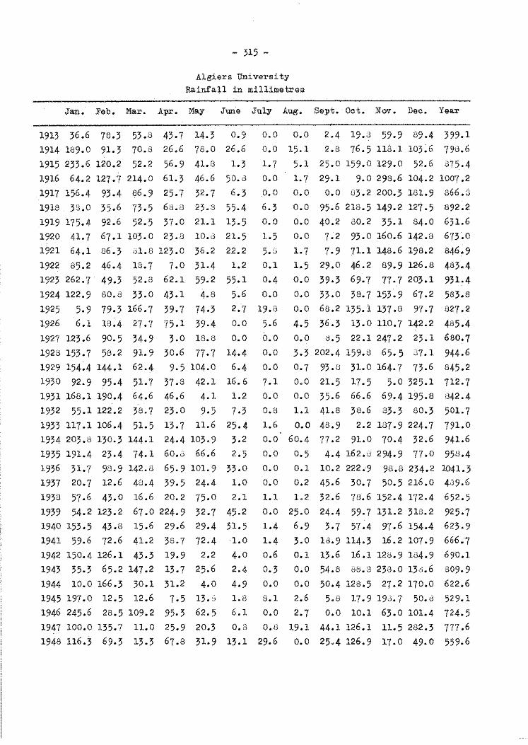
- )15 -

Algiers University Rainfall in millimetres

Jan. Feb. Mar. Apr. May June July Aug. Sept. Oct. Nov. Dec. Year

1913 36.6 78.3 53.8 43-7 14.3 0.9 o.o o.o 2.4 19.3 59.9 89.4 399.1 1914 189.0 91.3 70.8 26.6 78.0 26.6 o.o 15.1 2.8 76.5 118.1 103~6 798.6 1915 233.6 120.2 52.2 56.9 41.8 1.3 1.7 5.1 25.0 159.0 129.0 52.6 375-4 1916 64.2 127.7 214.0 61.3 46.6 50.8 0.0 1.7 29.1 9.0 298.6 104.2 1007.2 1917 156.4 93-4 86.9 25.7 32.7 6.3 o.o o.o o.o 83.2 200.3 181.9 866.3 1918 33.0 35.6 73-5 68.8 23.3 55.4 6.3 o.o 95.6 218.5 149.2 127.5 892.2

1919 175-4 92.6 52.5 37.0 21.1 13.5 o.o o.o 40.2 80.2 35.1 84.0 631.6 1920 41.7 67.1 103.0 23.8 10.a 21.5 1.5 0.0 7-2 93.0 160.6 142.8 673 .o 1921 64.1 86.3 dl. 8 123 .o 36.2 22.2 5.J 1.7 7-9 71.1 148.6 198.2 846.9 1922 85.2 46.4 18.7 7.0 31.4 1.2 0.1 1.5 29.0 46.2 89.9 126.8 483.4 1923 262.7 49.3 52.8 62.1 59.2 55.1 0.4 o.o 39.3 69.7 77·7 203.1 931.4 1924 122.9 80.8 33.0 43.1 4-8 5.6 o.o o.o 33.0 38.7 153.9 67.2 583.8 1925 5.9 79.3 166.7 39.7 74·3 2.7 19.8 0.0 68.2 135.1 137.8 97-7 827.2 1926 6.1 18.4 27-7 75.1 39.4 o.o 5.6 4.5 36.3 13.0 110.7 142.2 485.4 1927 123.6 90.5 34-9 3.0 18.8 o.o o.o o.o d.5 22.1 247.2 23.1 680.7

1928 153-7 58.2 91.9 30.6 77-7 14-4 o.o 3.3 202.4 159.8 65.5 J7.1 944.6 1929 154-4 144.1 62.4 9-5 104.0 6.4 o.o 0.7 93.8 31.0 164.7 73.6 845.2 1930 92.9 95.4 51.7 37.8 42.1 16.6 7.1 o.o 21.5 17.5 5.0 325.1 712.7 1931 168.1 190.4 64.6 46.6 4.1 1.2 o.o 0.0 35.6 66.6 69.4 195.8 842.4 1932 55.1 122.2 38.7 23.0 9-5 7-3 0.8 1.1 41.8 38.6 33.3 80.3 501.7 1933 117.1 106.4 51.5 13.7 11.6 25.4 1.6 0.0 48.9 2.2 187.9 224.7 791.0 1934 203.8 130.3 144-1 24.4 103.9 3.2 0.0 60.4 77.2 91.0 70.4 32.6 941.6 1935 191.4 23.4 74.1 60. i3 66.6 2.5 o.o 0.5 4-4 162.d 294-9 77.0 958.4 1936 31.7 98.9 142.8 65.9 101.9 33.0 o.o 0.1 10.2 222.9 98.8 234.2 1041.3 1937 20.7 12.6 48.4 39-5 24.4 1.0 o.o 0.2 45.6 30.7 50.5 216.0 439.6 1938 57.6 43.0 16.6 20.2 75.0 2.1 1.1 1.2 32.6 78.6 152.4 172.4 652.5 1939 54.2 123.2 67.0 224.9 32.7 45.2 0.0 25.0 24.4 59.7 131.2 313.2 925.7 1940 153-5 43.8 15.6 29.6 29.4 31.5 1.4 6.9 3.7 57-4 97.6 154.4 623.9 1941 59.6 72.6 41.2 38.7 72.4 1.0 1.4 3.0 18.9 114.3 16.2 107.9 666.'7 1942 150.4 126.1 43-3 19.9 2.2 4.0 0.6 0.1 13.6 16.1 128.9 184.9 690.1 1943 35.3 65.2 147.2 13.7 25.6 2.4 0.3 o.o 54.8 88.3 233.0 13d.6 809.9 1944 10.0 166.3 30.1 31.2 4.0 4.9 0.0 o.o 50.4 128.5 27.2 170.0 622.6 1945 197.0 12.5 12.6 7·5 13.~ 1.8 8.1 2.6 5.8 17.9 19,3. 7 50. a 529.1 1946 245.6 28.5 109.2 95-3 62.5 6.1 o.o 2.7 o.o 10.1 63.0 101.4 724.5 1947 100.0 135-7 11.0 25.9 20.3 0.8 0.8 19.1 44.1 126.1 11.5 282.3 777.6 1948 116.3 69.3 13.3 67.8 31.9 13.1 29.6 o.o 25.4 126.9 17.0 49.0 559.6

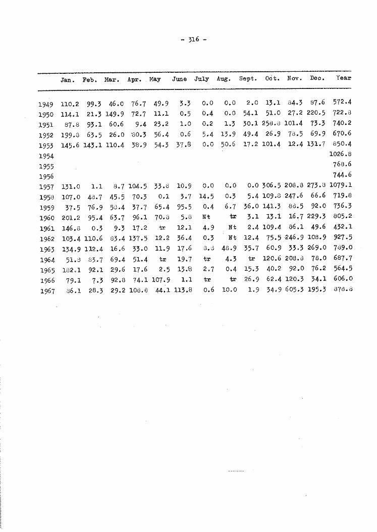
- 316 -

Jan. Feb. Mar. Apr. May June July Aug. Sept. oat. Nov. Dec. Year

1949 110.2 99.3 46.0 76-7 49.9 3.3 o.o o.o 2.0 13.1 84.3 87.6 572.4

1950 114.1 21.3 149· 9 72.7 11.1 0.5 0.4 0.0 54.1 51.0 27.2 220.5 722.8

1951 87.8 93.1 60.6 9.4 23.2 1.0 0.2 1.3 30.1 258.8 101.4 73·3 740.2

1952 199.3 63.5 26.0 '80.3 56-4 0.6 5-4 13.9 49.4 26.9 7o.5 69.9 670.6

1953 145.6 143.1 110.4 3S.9 54.3 37.8 0.0 50.6 17.2 101.4 12.4 131.7 850.4

1954 1026.8

1955 768.6

1956 744.6

1957 131.0 1.1 8.7 104.5 33.8 10.9 0.0 0.0 0.0 306.5 208.8 273.G 1079.1

1958 107.0 4i3.7 45·5 70.3 0.1 3.7 14.5 0.3 5·4 109.8 247.6 66.6 719.8

1959 37-5 76.9 5J.4 37·7 65.4 95.5 0.4 6.7 36.0 141.3 88.5 92.0 736.3

1960 201.2 95·4 63.7 96.1 70.8 5.8 Nt tr 3.1 13.1 16.7 229.3 805.2

1961 146.8 0.3 9.3 17.2 tr 12.1 4-9 Nt 2.4 109.4 86.1 49.6 432.1

1962 103.4 110.6 83.4 137.5 12.2 36.4 0.3 Nt 12.4 75.5 246.9 108.9 927.5

1963 134.9 112.4 16.6 33.0 11.9 17.6 i:l.G 48.9 35·7 60.9 33.3 269.0 789.0

1964 51.3 83.7 69.4 51.4 tr 19.7 tr 4-3 tr 120.6 208.0 78.0 687.7

1965 182.1 92.1 29.6 17.6 2.5 13.8 2.7 0.4 15.3 40.2 92.0 76.2 564.5

1966 79.1 7.3 92.8 74.1 107.9 1.1 tr tr 26.9 62.4 120.3 34.1 606.0

1967 06.1 28.3 29.2 108.8 44.1 113.8 0.6 10.0 1.9 34.9 605.3 195.3 878.8

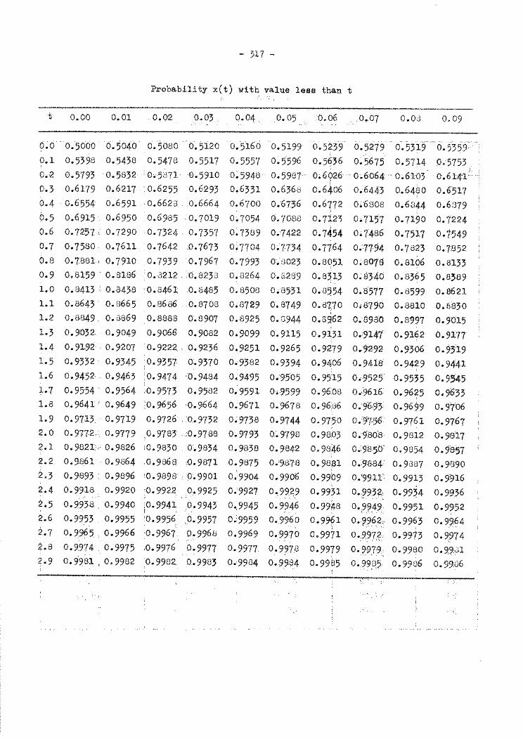
- )17 -

Probability x(t) with value less than t

t 0.00 0.01 o. 02. 0.03 0.04 o. 05 0.06 0.07 O.OJ 0.09

0~0 .,.

0.5000 0.5040 o.5o8o 0.5120 0.5160 0.5199 0.5~39 0.5279 0.5319 o. 5359 0.1 o. 5398 0.5438 0.5478 0.5517 0.5557 0.5596 0.56~6 o; 5675 o. 5Tl4 o. 5753 . 0.2 ·0. 5793 0.5832 :o~5s71· 0~5910 o:594s o~59B7 o.6926 ··o.6064·-o.6103 0.6141' .. 0.3 0.6179 0.6217 . 0.6255 0.6293 0.6331 0.6368 o.64o6 0.6443 0.64?0 0.6517 0.4 0.6554 0.6591 ·0.6628 0.6664 0.6700 0.6736 0.6772 0~6808 0.6844 0.6379 0.5 0.6915· 0.6950 .0.6985 0.7019 0~7054 0.7088 0.712? 0·7157 0.7190 0.7224 0.6 0.7257 t 0.7290 0.7324 0.7357 0.7389 0.7422 0.7454 o. 7'486 0.7517 0.1549 0.7 0.7580 o. 7611 o. 7642 .0. 7673 0~ 7704 0.7-734 o. 7764 0.7794 0.7823 o. 7852 0.8 0.1881. 0.7910 0.7939. 0.7967 0.7993 008023 0.8051 0~ 8018 0.8106 0.8133 0.9 0.8159 o. 8186 o. 8212 . o. 8233 o.a264 0.8289 0.8313 o. 8340 0.8365 0.8389 1.0 0.8413. 0.8438 ·0.8461 0.8485 0.8508 0.;8531 0.8554 0.8517 0.8599 o. 8621 1.1 0.8643 0.8665 0.8686 0.8708 0.8729 0.8749 o. 8170 o. 8790 0.8810 O.b830 1.2 0.8849. 0.8869 0.8888 0.8907 0.8925 O.G944 o. s962 0~ 8980 0.8997 0.9015

' 1.3 o. 9032. o. 9049 o. 9066 0.9082 0.9099 0.9115 o. 9],31 0.9147 0.9162 0.9177 1.4 o. 91-92 0.9207 o. 9222 .. o. 9236 0.9251 0.9265 o. 9279 0.9292 0.9306 o. 9319 1.5 0.9332 0.9345 0.9357 o. 9370 0.9382 0·9394 o. 9406 0.9418 0.9429 o. 9441 1.6 0.9452 . 0.9463 0.9474 ·0.9484 0.9495 0.9505 0.9515 0·9525 0.9535 0.9545 1.7 0.9554 o. 9564 o. 9573 0.9582 0.9591 0.;9599 o. 9608 0.9616 o. 9625 o. 9633 1.8 0.9641 · o.9649 ;o.9656 0.9664 0~ 9671 o. 9678 o. 96.86 0.'96·93 0.9699 o. 9706 1.9 0.9713.. 0.9719 0.9726 0..9732 0:9738 0.9744 o. 9750 0.97-56 o. 9761 0.9767

;

2.0 o. 9772 .. o. 9779 ,o. 9783 0. 9788 0.9793 0.9798 0.9803 0.9808 0.9812 0.9817 ?.1 0.98.21; 0.9826 :0.9830 0.9834 0.9838 0.9842 o. 9846 o~-9850 o. 9854 0.9857 2.2 0.9861 o. 9864 o. 9868 :0.9871 0.9875 0.9&78 0.9881 0.·9'8·84 o. 9887 o. 9890 2.3 o. 9'893 : o. 9896 ·o. 9898 o. 9901 0.9904 0.9906 0.9909 0.'9911' o. 9913 0.9916 2.4 0.9918 o. 9920 o. 9922 . 0.9925 0.9927 o., 99.29 0.9931 0.~~932: o. 9934 o. 9996 2.5 0.9936 0.9940 ,0.9941 . I 0.9943 0.9945 0.9946 0.99?1-8 0.9~.49· o. 9951 0.9952 2.6 0.9953 0.9955 '0.9956 .0.9957 0.9959 0.9960 o. 9961 o. 9962, o. 9963 0.9964

. . '··· '. · . 2.7 o. 99.6 5. 0.9966 0.9967. 0.9968 0.9969 0.9970 0.9971 0.:9,9_7? o. 9973 0.99'74 2.8 0.9.974 0.9975 .0. 9976 0.9977 0.9977 0.9978 0.9979 o. 9979. o. 9980 0.9,9J1 2.9 0.~981 0.9982 ·0.993~ D.99B3 0.9984 0.9984 0.99135 o. 9985 0.9986 o. 99,136 ' . ~ . .. ! l

' ::-:

'

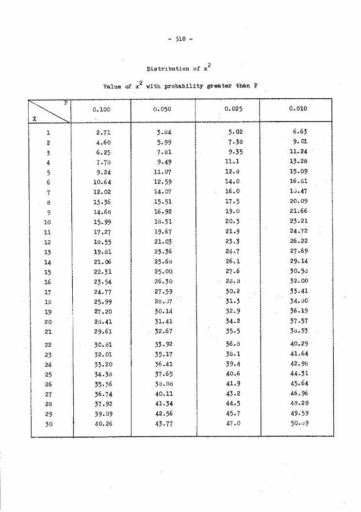
- 318 -

Distribution of x 2

Value of x2 wlth probability greater tna.n J;'

~ 0.100 0.050 0.025 0.010

l 2.71 3.84 5.02 6.63

2 4.60 5·99 7.38 9. 01

3 6.25 7.81 9.35 11.24

4 7-78 9.49 11.1 13.28

5 9.24 11.07 12.8 15.09

6 10.64 12.59 14.0 16.61

7 12.02 14.07 16.0 1J.47 ' 8 13.36 15.51 17.5 20.09

9 14.68 16.92 19.0 21.66

10 15.99 18.31 20.5 23.21

11 17.27 19.67 21.9 24.72 I

12 18.55 21.03 23.3 26.22

13 19.81 23.36 24.7 27.69 ' '

14 21.06 23.68 26.1 29.14

15 22.31 25.00 27.6 30. 5d

16 23.54 26.30 28.8 32.00

17 24-77 27.59 30.2 33-41 18 25.99 28. J7 31.3 34.30

19 27.20 30.14 32.9 36.19

20 28.41 31.41 34.2 37.57 21 29.61 32.67 35.5 3d.93 I

22 30.81 33.92 36.8 4.0.29

23 32.01 35.17 38.1 41.64

24 33.20 36.41 39.4 42.9B

25 34.38 37.65 40.6 44.31

26 35.56 ?8.88 41.9 45.64

27 36.74 40.11 43.2 46.96 28 37-92 41.34 44.5 48.28

29 39.09 42.56 45.7 49.59

30 40.26 43-77 47 .o 50.d9

------- -----~-- ------~--------- '----- I

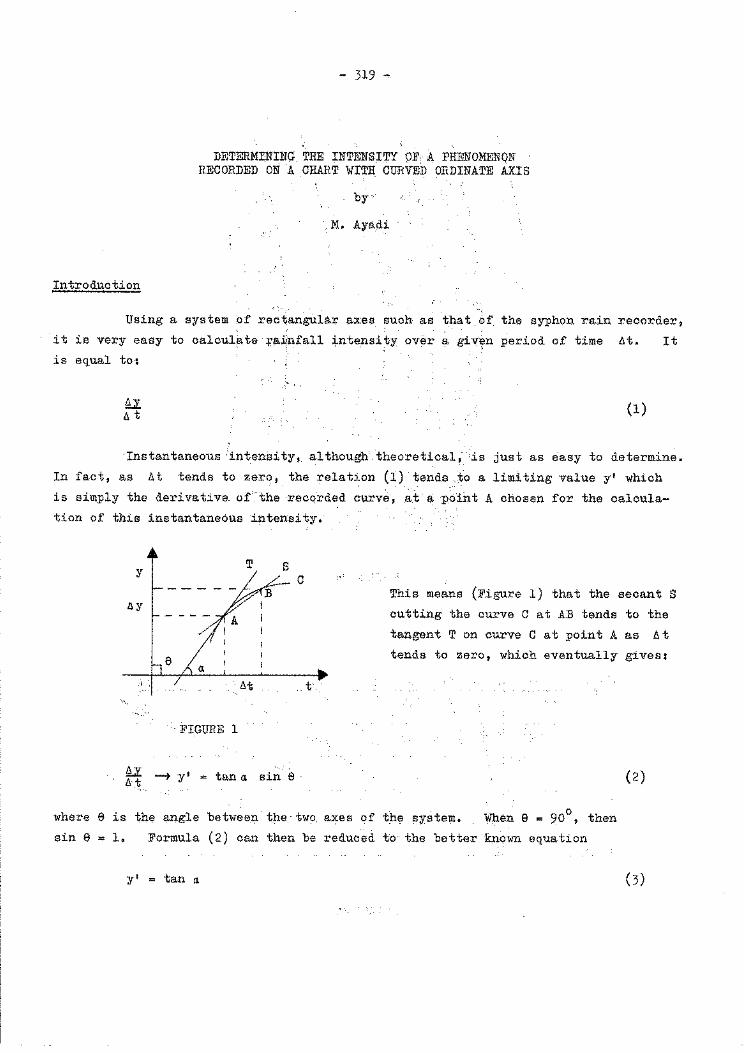
Introduction

- 319 ...,

DETERMI:NING THE ;I:NTENSITY QF; A PHENOMENQN RECORDED ON A CHART WITH CURVED ORDINATE AXIS

by'

M. Ayadi

Using a system of rectangular axes such as that of the syphon rain recorder,

it is very easy to calculate :rajJnfall ~ntensity over a giv~n period of time H. It

is equal to:

~ ld (1)

Instantaneous :intensity, although theoretical; 'is just as easy to determine.

In fact, as lit tends to zero, the relation (1) tends .to a limiting value y' which

is simply the derivative. of'the recqrded curve, a.t a point A chosen for the calcula­

tion of this instantaneous intensity.

y

Ay

'<'-,

~ li· t

T s c

lit .. t

··FIGURE 1

--. y' = tan a sin e .

This means (Figure l) that the secant S

cutting the curve C at AB tends to the

tangent T on curve C at point A as lit

tends to zero, which eventually gives:

(2)

where e is the angle between the·two axes of the system. When e = 90°, then

sin e = l. Formula (2) can then be reduced to the better known equation

y' = tan a ( 3)

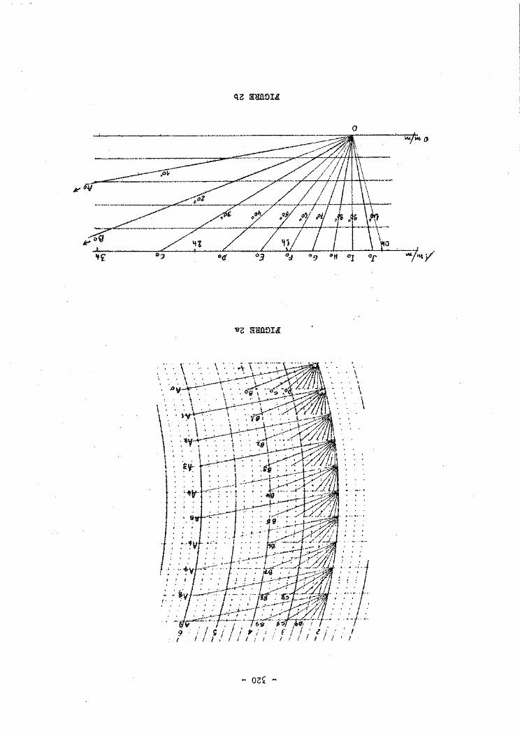
0

- oc:~ -

- 321 -

Determining instantaneous intensity in the case of a system of axes with curved ordinate axis

1. We have seen that when 9 = 90°, formula (2) may be reduced to the simpler

formula (3).

If et 90°, formula (2) should be left in its full form. The problem of

determining the instantaneous intensity of a phenomenon recorded on a chart with a ~~

curved ordinate axis is more complex in that the angle e in formula (2) varies from

one point to another along the curved ordinate axis.

2. We shall try, by using the chart with curved ordinates of a tipping-bucket

recording raingauge; to find a method whereby we can rapidly obtain the instantaneous

intensity of rainfall.

Figure 2b shows part of the chart under consideration, on an enlarged scale.

A pencil of straight lines originating from 0 form angles of 10°, 20°, 30°, etc., with

the horizontal. This pencil of lines cuts the upper horizontal of the millimetre of

rain in question at points A0 , B0 , c0 , etc.

In this figure we can see that the 40°,line cuts the upper horizontal at

point D0 , and that OD0 = lh 40m, likewise OE0 = lh l?m, OF0 = lh approximately,

OG0 = 42m, and so on.

If we repeat this operation every 10°, from 10° to 100° and for all the

millimetres of rain shown on the chart in question (Figure 2a), we obtain a series

of points.

AO' !oi CO' DO " • • • • • ' • ' • • JO

Al' Bl' Cl, • • • • • • • • • • • •

• • • • • • • • • lt • • • • • • • •

A9' B9' c9, • • • • • • • • • • • •

Now let us transfer these points to graph paper ruled off in millimetres

and on which the ordinate axis is graduated in hours. Plot on a vertical (0} all

the points with suffix (0), and on a vertical (l) all the points with suffix (1 )

- -;'2.'2. -

FlG'Ult'E 3

n"' rnteneitY

"

4 n

2

\ \ I I I I //Ill/ / /'

'n

1 I

I ,1'

o' ,

f

z..5

' 2. n

\\1/////////// / // ~.4 5 .6 1 8

400o \I I l///1/$57/777~~~

1. n

0 1. 2 -; 4 5 6 1 8 9 1.0

- 323 -

and so forth, By joining the points of the same letter we obtain a series of

parellel, unequally spaced straight lines.

to a given angle.

Each of these straight lines corresponds

Let us take a unit of intensity equal to 3mm/hour and let us plot the

intensity lines (1), (2), ••• on this same squared paper. Theyf~rill a pencil of

straight lines converging on the origin 0.

The verticals O, 1, 2, ••• 10, represent millimetres of rain.' and:·the hori­

zontals, l hour, 2 hours, etc., w.ere omitted in order to avoid h.aYin,g .too many lines on Figure 3.

3. We have just devised a diagram having: ·

(a) Equally spaced vertical straight lines representing.millimetres of rain; ~·· " .

{b) Horizontal straight lines representing the number of .pQu:ts;

(c) Parallel, slightly inclined and unequally spaced'strai~h·t lines, 10°, 20°,

••• 100°' repre,sent'ing the angle of. the tangent .. to th.e raintall curve at a gi·ven point; - · .. >"

'~-'\

(d) Straight, lines c_on.yerging .on point 0 ·ari?- representing tb,~ .:intensity of rainfall..

4. The diagram in Figure 3 is not very practical to use.

If, for example, we want to determine the intensity of rainfall at point M,

situated between the fourth and fifth mHlimetre on the chart, and at which the

tangent on the recorded curve makes an angle of 70° with the horizontal, we find on

the diagram in Figure 3 that the intensity that we are trying to find is indicated by

the value of the intensity line which passes through the point of intersection of the

vertical between the values 4 and 5 for the abscissae and the 70° line.

Moreover, the problem becomes more complicated when the recording is from the top of the chart to the bottom.

- 324 -

J 90° 80°

~~==~~~~~~~~~\~~=~,~~10°

0 1 2 3 4 5 6 7 8 9 10

FIGURE 4

- 325 -

5. To avoid all these practical· difficulties, the diagram of Figure 3 has been

transformed and replaced by the finalized diagram shown in Figure 4, which has to be

on some totally transparent material such as perspex.

The finalized diagram was very simply obtained by transposing the series

of. straight lines shown in Figure 3.

(a) . 0 0 . . ' 0 . • . The straight lines representing the angles 10 ,' 20, ••• 100 •were replaced

by converging straight lines forming the required angles with the horizontal;

(b) The vertical lines representing the measure of rainfall have been replaced

by arcs of concentric circles;

(c) The horizontal straight lines representing hours have been omitted;

(d) The converging straight lines representing rainfall intensity have been

transposed point by point to give a network of curved lines in the final

diagram.

6. In this form, the final diagram has advantages which eliminate all the

difficulties involved in measuring intensity. It is very easy to use. To find the

intensity at point M mentioned above, and situated on the recorded rainfall curve,

the diagram is placed on the chart in such a way that I coincides with M. The

angle p that the tangent makes with the horizontal is easily found with the aid of

this same scale, which serves also as a protractor, and the required intensity can be

read off on the intensity curve which passes through the point at which' the tangent makes

an angle P with the horizontal and which is situated between the fourth and fifth arcs.

For the parts of the recording sloping downwards we proceed in the same man­

ner but working on the reverse side of the diagram, using a light table.

Remarks

The choice of a unit of intensity equal to 3mm/hour is arbitrary.

This method can be applied to other parameters as well as rainfall.

- 326 -

The precision of intensity measurements depends on the quality of the rain

recorder and the recording.

Conclusion

This study offers an example of how the many problems racing meteorologists

can be solved. It shows how a given subject can be tackled to give a result of

true practical and even scientific value.

- 327 -

CONCLUSIONS OF THE SEMINAR

1. It was generally agreed that the Seminar had been sucessful in achieving its objectives. The participants expre.ssed their ,hopes that the .conclusions of the Seminar would be followed up by appropriate action by WMO and by the Members concerned.

2. It was recommended that the proceedings of the Semina,r should be published by WMO so that all the Members of the Region would get the maximum benefit of the Seminar •. Those proceedings should. include both the theoretical and practical parts of the Seminar and the c~nsul tan ts should consider a~ending their lectures in the. light of the various discussions which were held during the Seminar.

3· The participants expressed tneir conviction that the African Meteorologi-cal Services should introduce, if this has not already been done, modern methods and equipment such as electro-mechanical machines and electronic .computers for climat­logical data processing in order to cope with the increasing demands for such data for the different sectors of the national economic development, particularly at the planning stages of the development projects. It was pointed out that eventually electronic computers would be indispensible for climatological data processing and that African countries should make their plans accordingly. In this connexion some countries may consider the possibility of having joint data processing centres.

4· The participants expressed their hope that WMO and UNDP would assist the African Meteorological Services to equip themselves with modern equipment for clima­tological data processing, if so requested.

5. The participants stressed the. necessity to include i~ the e.ducation and training programmes of meteorological personnel, appropriate .coUJ;'ses on "modern methods and equipment for climatological data processing11 •

6.. .The .pai,-"ticipants e;x:p:ressed .the desire .that IVMO should issue apprQpriate publicatio;ns on the following suojects, preferably inc EngJ,ish and Frencp:

(a) Statistical forecasting

(b) Scrutinizing of climatological data

- 328 -

7. The participants stressed the need to give more serious attention to the

subject of extreme climatological conditions, particularly those seriously affecting

the national economy.

G. It was noticed that an immense amount of synoptic data is available in the

form of teleprinter tapes, and it was pointed out that it would be of great advan­

tage to store such data at National and/or Regional Meteorological Centres in a

suitable form for later transfer to a more permanent and compact technical medium

such as magnetic tapes and microfilms with binary codes.

9. As this Seminar was the first of its kind to be organized for Africa in

the field of climatology, the participants made the following comments to be taken

into consideration when organizing similar future Seminars :

(a) Members of the Region should be informed sufficiently

well in advance of the scope of the Seminar and be

provided with relevant documents to be able to choose

the most suitable participants.

(b) Every effort should be made to avoid overlapping in the

lectures and to balance the theoretical and practical

sides of the Seminar.

(c) Practical exercises and examples should, as far as

possible, be based on the conditions of the Region concerned.

10. The participants expressed their gratitude to the UNDP, WMO, to

Dr. Berggren the Director of the Seminar, and to the lecturers for organizing this

Seminar, the usefulness of which is beyond any doubt for the improvement of storage

and processing of olimatological data in African countries.

11. The participants also expressed their gratitude to the United Arab

Republic and to Mr. M. F. Taha the Director General of the Meteorological Department

in Cairo and expressed their thanks for the excellent work which was achieved in

this Seminar with their help.