PROCEEDINGS OF THE WORKSHOP on the ACSYS SOLID PRECIPITATION

CLIMATOLOGY PROJECT

(Reston, VA, USA, 12-15 September 1885)

I» ® ICSU UNESCO

The World Climate Programme launched by the World Meteorological Organization (WMO) includes four components:

The World Climate Data and Monitoring Programme The World Climate Applications and Services Programme The World Climate Impact Assessment and Response Strategies Programme The World Climate Research Programme

The World Climate Research Programme is jointly sponsored by the WMO, the International Council of Scientific Unions and the Intergovernmental Oceanographic Commission of Unesco.

NOTE

The designations employed and the presentation of material in this publication do not imply the expression of any opinion whatsoever on the part of the Secretariat of the World Meteorological Organization concerning the legal status of any country, territory, city or areas, or of its authorities, or concerning the delimitation of its frontiers or boundaries.

World Climate Research Programme

PROCEEDINGS OF THE WORKSHOP ON THE

ACSYS SOLID PRECIPITATION CLIMATOLOGY PROJECT

(Reston, V A, USA, 12-15 September 1995)

May 1996

TABLE OF CONTENTS

Page no.

FOREWORD (Scope and purpose ofthe workshop) . . . . . . . . . . . . . . . . . . . . . . . . . . . . v

WORKSHOP SUMMARY . . . . . . . . . . . . . . . . . . . . . . . . . . . . . . . . . . . . . . . . . . . . . . . vu

SESSION 1 -In situ measurements of solid precipitation in the Arctic region . . . . . . . 1

In situ measurements of solid precipitation in high latitudes: the need for correction . . . . . 3 B. Goodison and D. Y ang

Point measurements of solid precipitation V. Golubev and E. Bogdanova

18

Method of measurements .and corrections ofsolid precipitation in the Russian Arctic . . . . 30 N. Briazgin

Correcting precipitation measurements in Switzerland B. Sevruk

33

In situ solid precipitation measurement adjustments: the US experience . . . . . . . . . . . . . . 38 P. Groisman, D. Easterling, R. Quay le, V. Golubev and E. Peck

Daily precipitation measured at the "North Pole" stations (Abstract only) . . . . . . . . . . . . 42 R. Colony

Snow measurements during the SEVER programme (Abstract only) R. Colony

43

Snow course measurements from the "North Pole" stations (Abstract only) . . . . . . . . . . . 44 R. Colony

ii

SESSION 2 -Model-derived precipitation climatologies for the Arctic . . . . . . . . . . . 47

A preliminary look at model-derived precipitation climatologies from the UKMO and ECMWF NWP models . . . . . . . . . . . . . . . . . . . . . . . . . . . . . . . . . . . . . . . . . . . . . . . 49

H. Cattle and J. F. Crossley

Model-derived precipitation climatologies for northern high latitudes . . . . . . . . . . . . . . . . 59 J. Walsh

Aerological estimates of precipitation minus evaporation over the Arctic . . . . . . . . . . . . . 71 M. Serreze and R. Barry

Snow mass variation over the northern polar region as simulated with AMIP general circulation models . . . . . . . . . . . . . . . . . . . . . . . . . . . . . . . . . . . . . . . . . . . . . . . . . . . . . . 75

V. Kattsov and V. Meleshko

SESSION 3 - Remote sensing of solid precipitation . . . . . . . . . . . . . . . . . . . . . . . . . . 81

Remote sensing ofsnow in the cold regions . . . . . . . . . . . . . . . . . . . . . . . . . . . . . . . . . . . 83 T. Carron

Satellite snow-cover mapping: a brief review . . . . . . . . . . . . . . . . . . . . . . . . . . . . . . . . . . 93 D. Hall

Interactive multisensor snow and ice mapping system B. Ramsay

Use of satellite data for operational sea ice and lake ice monitoring C. Bertoia

101

106

Monitoring Swiss alpine snow cover variations using digital NOAN A VHRR data . . . . . 110 M. Baumgartner, T. Holzer and G. Apfl

Mapping fractional snow covered area and sea ice concentrations A. Nolin

An analysis ofthe NOAA satellite-derived snow-cover record, 1972- present D. Robinson and A. Frei

115

126

iii

SESSION 4 - Hydrological modelling of Arctic river run-off. . . . . . . . . . . . . . . . . . . 131

Hydrological modelling of Arctic river run-off . . . . . . . . . . . . . . . . . . . . . . . . . . . . . . . . 133 S. Bergstrom

Hydrological modelling of Arctic river run-off . . . . . . . . . . . . . . . . . . . . . . . . . . . . . . . . 144 Yu. Vinogradov

Some useful inferences from past attempts to estimate the precipitation and run-off in the Canadian Arctic Basin . . . . . . . . . . . . . . . . . . . . . . . . . . . . . . . . . . . . . . . . . . . . . 159

S. Solomon, E. Soulis and M. Lee

The measurement and modelling of Arctic hydrologic processes D. Kane

APPENDICES:

A. List of participants B. Final programme C. Working Group reports

178

V

FOREWORD

(Scope and Purpose of the Workshop)

The third session of the Scientific Steering Group (SGG) of the Arctic Climate System Study (ACSYS), meeting in GOteborg, Sweden in November 1994, decided that an ACSYS Solid Precipitation Climatology Project Workshop should be held in order to defme an optimum strategy for accurate determination of the rate and variability of freshwater input into the Arctic Ocean by precipitation and runoff. Candidate strategies for mitigating shortcomings of the existing hydrological data and for enhancing current models were identified. The ~reeting organizers (R.G. Barry, R. l.awford, V. Vuglinsky and J.E. Walsh) proposed a list of experts who were invited to prepare a series of status reports on the central hydrological questions in ACSYS. Additional shorter contributions were solicited, or submitted, on related topics. Appendix A contains the list of meeting participants. The final programme of the workshop is given in Appendix B. Three working groups examined (1) the utility of adjusted station precipitation and snowfall data as well as the remote sensing of snow cover pararreters, (2) the output of precipitation fields from numerical weather prediction models and (3) the role of hydrological modelling, in formulating an optimum strategy.

This report provides an overview of the main scientific objective, the findings of the three working groups, and the recommendations agreed upon by the participants. These recommendations form the basis of the strategy proposed here for achieving the ACSYS hydrological objectives. The presented papers are also included.

The convenors wish to thank Linda Housel, Dr. Harry Lins and Dr. George Leavesley of the US Geological Survey Water Resources Division for their assistance in hosting the workshop at the USGS Headquarters in Reston, Virginia, USA, Dr. Victor Savtchenko, World Climate Research Programme, ICSU/IOC/WMO, for his coordination and support of the meeting, and Dr. Paul Twitchell, International GEWEX Project Office, for supplemental support.

Roger G. Barry John E. Walsh eo-convenors

vii

WORKSHOPS~RY

(a) Introduction

The overall goal of ACSYS is to ascertain the role of the Arctic in global climate. Its three principal scientific objectives concern:

i. understanding the interactions between the Arctic Ocean circulation, ice cover and the hydrological cycle;

ii. initiating long-term climate research and monitoring programmes for the Arctic; ill. providing a scientific basis for an accurate representation of Arctic processes in global climate

models.

The hydrological programme of ACSYS emphasizes the compilation of Arctic hydrological databases for precipitation and for runoff, and the development of hydrological models for selected Arctic river basins. Its specific objectives are:

i. Determining the elements of the freshwater cycle in the Arctic region and their time and space variability;

ii. Quantifying the role of atmospheric, hydrological and land surface processes in the exchanges between different elements of the hydrological cycle;

ill. Developing mathematical models of the hydrological cycle under specific Arctic climate conditions, suitable for inclusion in coupled climate models; and

iv. Providing an observational basis for the assessment of long-term trends of the components of the freshwater balance in the Arctic region under changing climate.

The ACSYS Scientific Steering Group, meeting in Goteborg, Sweden (SSG-III November 1994) noted the importance of determining the freshwater inputs of precipitation and runoff into the Arctic Ocean. Table 1 summarizes the freshwater budgets of the Arctic Ocean as estimated by Aagaard and Cannack (1989). Current aerological estimates indicate that net precipitation minus evaporation over the Arctic Ocean is about 16 cm/year (Serreze et al., 1996), or 75% greater than their estimate. The runoff-contribution is equivalent to about 35 cm/year, for an area of 9.55 x 106 km2

• Figure 1 illustrates the Arctic drainages and their magnitudes of mean annual run-off (Lawford, 1995). The freshwater inputs considerably exceed the calculated oceanic transports of low salinity water. However, there is apparently a larger positive imbalance (16 cm) than estimated by Aagaard and Carmack (1989). Since the runoff is unlikely to be underestimated, due to the ungauged river contribution, the sources of this discrepancy are likely to be in the oceanic terms (Barry et al., in press). For example, Steel et al. (in press) propose that the outflow through the Canadian Archipelago may exceed that due to sea ice via the Fram Strait.

Table 1 Freshwater budget of the Arctic Ocean (from Aagaard and Carmack (1989))

Source or Sink Transport, km3 yr"1 Yield, cm yr·1

Ice export through Fram Strait -2790 -29

Water export through Fram Strait -820 -9

Runoff 3300 35

Precipitation less evaporation 900 9

Water import through Bering Strait 1670 18

Water export through Canadian Archipelago -920 - 10

Import with Norwegian Coastal Current 250 3

Saline water import through Barents Sea -540 -6

Saline water import with West Spitsbergen Current - 160 -2

Net 890 9

Note: Freshwater fractions are relative to a standard salinity of 34.80. Yield calculated for an area of9.55 x 106 km2

• Values are positive for sources and negative for sinks.

viii

@NOFF '\JAL UE5 (mm_)

GB o-9o

Ill 100-190

11 :200-:290

• :lOO-J90

Figure 1: Run off (mm) for Arttic dreinages (from Lawford, 1995)

ix

(b) Workshop Structure

'The Workshop included invited and contributed presentations addressing four topics: in situ measurements of solid precipitation in the Arctic and their adjustment for errors, model-derived estimations of Arctic precipitation, the remote sensing of solid precipitation and snow on the ground, and hydrological modelling of Arctic river runoff. 'The rermte sensing contributions were provided during a half-day combined session with a group discussing NASA Earth Observing System (EOS) Moderate-resolution Imaging Spectroradiometer (MODIS) snow and ice algorithms. Subsequently, the ACSYS participants divided into three working groups to develop assessments and recommendations concerning: in situ and remote sensing measurements, model­derived precipitation climatologies, and runoff rmdelling. The composition of the groups and the questions they addressed are shown below. During a final plenary session, the group recommended an overall strategy directed to achieving the objectives of the ACSYS hydrological programme.

Working Groups

MiPt~@g1J~~Pi. In situ and remotely sensed observations Chair Barry Goodison

Recorder David Legates

(Roger Barry)

Nicolai Briazgin

Thomas Fuchs

Victor Golubev

Pavel Groisman

(Eugene Peck)

W9rl®i'Gr9#p ~ Model-derived climatologies Chair Howard Cattle

Recorder John Walsh

(Roger Barry)

(Roger Colony)

Vladimir Kattsov

Mark Serreze

lY~f~g qf§qp ~ ? Hydrological modelling Chair Valeriy Vuglinski

Recorder Sten Bergstrom

DougKane

(Rick Lawford)

George Leavesley

(Dennis Lettenmaier)

Victor Savtchenko

Shully Solomon

Yuriy Vinogradov

X

Working Group Questions

The overall goal is to define an optimum strategy for determining freshwater inputs into the Arctic Ocean from precipitation and runoff and their variability. The groups should also consider whether current GEWEX plans will satisfy, or make a useful contribution to, this goal.

Will adjusted data be adequate (space/time) to define inputs? How to adjust historical/future data? Who should take the lead? What can remote sensing add (Passive Microwave; MODIS)? How best to merge remotely sensed with in situ data? Are existing/planned operational products adequate? If not, what is needed and who does it? Are data archives accessible? What is needed? (Note: ACSYS plans Arctic precipitation data archive, 1978 to present at GPCC.)

Do current/near-term models have capability to predict Arctic precipitation? Do we need nested models? Coupled models? Better surface hydrology, sea ice treatments? What outputs can be provided? By whom? When? What, if any, observations should be assimilated? AMIP lessons? Re-/Re-analysis needed? When? How to verify?

Can current models be scaled-up to Arctic basins? Should all Arctic drainages be included in ACSYS programme for climate studies as well as runoff? Is it useful/necessary to model all major drainages (remainder- what is their contribution)? What is needed to define sector/basin-wide runoff? (Note: ACSYS plans Arctic Runoff Data Base, 1978 to present at GRDC) Problems in access, standardization? What climate/other data are needed? Can hydrologic modelling provide other useful estimates (evaporation, ... )? What is the significance of permafrost, glaciers?

(c) Workshop Findings

The submitted invited and contributed papers are presented in the following sections. Appendix C contains the reports of the Working Groups. The principal findings of the Groups are summarized below.

Working Group 1: In situ and Remotely Sensed Observations

A necessary first step is to compile existing surface measurements of rainfall and snowfall in the Arctic region (the exact boundaries of the Arctic were not specified). Known and potential sources are identified; they include conventional gauge IreaSurements of precipitation and stick measurements of new snow on the ground at synoptic and climatological stations on land and at Arctic drifting stations, and observations made at short­term research sites that will aid validation studies.

Adjustments to the measurements are necessary in view of biases in catch caused by gauge and shield design, gauge height and siting, the effects of wind and blowing snow, the use of fences at exposed sites, losses due to evaporation/sublimation and the wetting of the gauge and collector. Correction procedures have been

xi

developed by national agencies and WMO has organized a substantial effort to intercompare solid precipitation measurements (WMO, in preparation). Those conclusions and recommendations need to be carefully considered for adoption, as appropriate. Bias adjustments necessitate the availability of concurrent meteorological data (air temperature, wind speed and precipitation type) on at least a daily basis. Metadata documenting station location and elevation site characteristics and gauge type are essential. An ACSYS working group needs appointing to evaluate current bias-adjustment algorithms and ensure consistent estimates of precipitation across national boundaries.

The Global Precipitation Climatology Centre (GPCC) in Offenbach!Main, Germany is recommended as the designated archive for Arctic precipitation and supplemental data in support of ACSYS. Both measured and gauge-bias adjusted data should be archived for the period 1979 to present. Continuation of the work of the NSIDC/WDC-A for Glaciology in Boulder, Colorado, USA to assemble snow depth and water equivalent data for the Arctic region is encouraged.

Current remote sensing products provide only weekly maps of northern hemisphere snow cover extent (those began. in 1966). During 1996 to 1998 NOAA-NESDIS will develop an. Interactive Multisensor Snow and Ice Mapping System. This will incorporate visible, infrared and passive microwave data, the US Air Force daily snow analysis and the National Ice Center Arctic ice analysis and when the system is implemented, will provide high resolution digital products on a daily basis.

Algorithms to estimate snow/water equivalent (SWE) on land, from passive microwave data are still under development. The NSIDC Distributed Active Archive Center (DAAC) archives Special Sensor Microwave Imager (SSM/1) data (1987 to present) and is producing 25 km resolution northern hemisphere daily maps of SWE using current algorithms. Passive microwave sensors with improved resolution will be available on an EOS platform, ADEOS-2 and METOP. MODIS daily and weekly snow extent maps will be produced also, beginning in 1998. Weather radar can provide information on summer and winter precipitation in Arctic land and coastal areas, for intercomparison with gauge measurements. Studies conducted under EOS, GEWEX programmes and by operational agencies to develop products merging surface observations with remotely sensed data will assist ACSYS, but efforts to obtain routine data concerning SWE on Arctic sea ice are needed.

Working Group 2: Model-derived climatologies

This group considered the precipitation fields sinwlated by atmospheric models used in climate simulations and in short-range numerical weather prediction (NWP).

The climate simulations of the Atmospheric Model Intercomparison Project (AMIP) appear to contain significant positive biases of precipitation in the Arctic, although uncertainties in the validation data can significantly limit assessments of simulated precipitation and evaporation. While there remains a need for the identification of the best AMIP sinrulations and a diagnosis of the reasons why some AMIP models were more successful in the Arctic, similar m:xiels run in the NWP data-assimilation-and-forecast mode have the advantage ofuseful observational input to produce internally consistent fields. The so-called "re-analysis" projects now underway at three centers (ECMWF, NMC, NASA Goddard) are using this approach to provide, on a daily basis, gridded fields of precipitation and other hydrologic variables. The biases of climate model (e.g. AMIP) sinrulations are sufficiently large that one must regard the atmospheric re-analyses as a useful basis for building an appropriate strategy for the ACSYS hydrological programme.

The AMIP experience points to the need in ACSYS for an intercomparison, verification and critical appraisal of the re-analysis datasets (especially precipitation) over the region of relevance to ACSYS. This effort should include an intercomparison of the re-analysis products from different parts of the assimilation/forecast cycle (e.g. 0-12 hour forecast against 12-24 hour forecast) and, by implication, consideration of the issues from spin-up of the forecast precipitation fields. Because of the general sparseness of the Arctic precipitation station network, as well as problems of representivity, it is important that verification efforts draw on all available relevant information. This information should include components from other parts of the ACSYS hydrological programme: (1) a database of adjusted precipitation measurements from Arctic stations for the years COIDiron to the current re-analysis projects (i.e., 1979 to 1989), (2) a database of Arctic-relevant satellite products, in particular snow extent and snow depth/water equivalent, accompanied by uncertainty estimates,

xii

and (3) water vapor budget evaluations based on rawinsonde data. It may also be feasible to address, for example, the validity of the re-analysed evapotranspiration using historical climatological charts.

Initial efforts to assess Arctic re-analyses are being and will be made by individual investigators. Coordination of these efforts and interaction with the re-analysis centers would be enhanced by the formation of an ad hoc working group consisting of ACSYS participants and representatives of the re-analysis centers. It was recoll1lrended that ACSYS organize such a working group in the near future. It was also recommended that a commitment to participate in an assessment of Arctic re-analyses be obtained from one of the major centers.

Present re-analyses incorporate all station-based upper air observations from the Arctic and elsewhere. There is a need to ascertain which, if any, ice island smmding and Arctic buoy data are in the data input stream and to detennine whether unadjusted TOVS soundings from the Arctic are incorporated. Preliminary roles for ACSYS are (1) the identification of systematic errors (e.g. in surface temperature) in the re-analysed Arctic fields, and (2) the provision of corresponding enhanced datasets for future re-analyses for the Arctic. A recoll1lrended vehicle for facilitation of these efforts is the proposed ad hoc working group.

Three particular strategies may be envisaged for producing fields of precipitation for ACSYS over the Arctic region:

i. Use of adjusted station data alone, coupled with methods based on precipitation frequency over the data-sparse ocean area; station sparseness and representativeness are key limitations.

ii. Use of re-analysis data alone, following verification and possibly ad hoc data calibration against station and other data; an over-reliance on parameterization schemes of individual models and under-reliance on the precipitation network itself are major disadvantages.

iii. A suitably formulated combination of adjusted station and re-analysis data, for example using optimal interpolation of station data against re-analysis data used as background fields.

The third alternative may need development of new techniques, but it is the preferred approach in that it has the potential to make the best use of all available data. It is recommended that this task be undertaken in consultation with the GPCC. It should refer to and build upon the assessments by the proposed ad hoc working group.

Application of re-analysis-based fields of precipitation to the forcing of surface hydrological models will need to use downscaling techniques in order that the resolution of the forcing and the models be compatible. For this purpose, a strategy that merits consideration in ACSYS is the use of circulation downscaling statistics, in which high-resolution topography is used in conjunction with coarse-resolution model output and statistical relationships between variables on the two scales.

The Group did not see a need for fully coupled (atmosphere-ocean) models as a component of the ACSYS precipitation climatology prograll1lre.land surface and sea ice/ocean models may indeed provide the optimum estimates of evapotranspirationlevaporation when forced by the re-analysis derived products, but, of course, without the opportunity for physical feedback to them.

It is certain that improvements can and will be made in the sea ice and land surface representations used in the mxiels providing future re-analysis programmes. However, the representation of other model elements (e.g., clouds) also needs to be addressed in order to successfully model the Arctic. While the ACSYS atmJspheric progranune will address the formulation of clouds and precipitation processes in climate models, and the ACSYS hydrological programme (in collaboration with GEWEX) improved land surface schemes, a particular ACSYS contribution to future re-analyses is the inclusion of more realistic sea ice boundary conditions. Feasible enhancements of present models are specifications of sea ice concentration and albedo in accordance with observations. Such specifications will require that the atmospheric models used are configured for more than one type of surface within a grid cell.

xiii

The group recommended that:

Jntercomparison and critical appraisal of re-analysis products are needed, drawing upon all available information (in particular station data, remote sensing and water vapor budgets). Such appraisals should aim at feeding back to future re-analysis efforts as well as at an assessment of the suitability of re-analysis fields over the Arctic for ACSYS purposes.

An ad hoc working group should be formed with membership from the ACSYS community and, if possible, the re-analysis centers. An operational center to serve as a "primary contact" needs to be identified, and commitments to this effort by both ACSYS and the center need to be obtained.

Consideration should be given to developing a strategy to construct Arctic precipitation datasets based on the currently-running atmospheric re-analysis project precipitation products used as background fields against data. Development of such a strategy may be carried out by the proposed ad hoc working group (or a sub-group) in liaison with the GPCC.

There is a need to explore strategies for downscaling atmospheric model precipitation for application to more local hydrological models. The downscaling should incorporate orography, for which existing elevation databases imply scale limitations of several hundred metres. WCRP/GEWEX should promote this issue, which is not unique to high latitudes.

Efforts should be made within the ACSYS hydrological programme to ensure that it archives:

1) a database of adjusted station precipitation for Arctic stations

2) satellite products on snow extent and snow/depth water equivalent, accompanied by uncertainty estimates.

Working Group 3: Hydrological Modelling

The group evaluated existing measurments of discharge into the Arctic and concluded that hydrometric stations on the large rivers of Eurasia and North America provide reliable long-term data for about 75% of the mean freshwater inflow. The ungauged inflow needs to be estimated by modelling, or by interpolation. Conceptual trodels can be scaled-up to Arctic river basins. However, for global warming scenarios, assessment of changes in the large river basins requires study of processes in middle latitudes; such work requires the establishment of a joint ACSYS/GEWEX project.

ACSYS should concentrate on sxmll Arctic river basins to determine parameters for conceptual models and with emphasis on typical high-latitude processes. Runoff data should be archived in the ACSYS Runoff Data Base for hydrological modelling. Hydrological models can also be used to assess other components of the hydrological regime (evaporation, soil moisture, snow storage, etc.). A group to coordinate ACSYS hydrological modelling should be established.

xiv

(d) Overall Strategy

The participants discussed in plenary session the reconunendations of the three working groups and reconunended the following overall strategy for detennining Arctic freshwater inputs:

I. meteoric precipitation over the Arctic Ocean and Arctic drainage basins should be detennined from adjusted station data optimally interpolated using the NWP re-analysis products. This strategy can provide monthly precipitation fields.

ii. runoff into the ocean will be detennined from data for the major rivers supplemented by hydrological model output for the ungauged rivers; the models will be calibrated using the station precipitation data and NWP-derived fields. The runoff models will need to be tested for a range of watersheds having adequate data. Model sensitivities will be assessed using seasonal and interannual variations of the forcing data

iii. the ACSYS hydrological progranune should take steps to become recognized as a special regional programme of GEWEX.

References

Aagaard, K. and Carmack, E. C., 1989: The role of sea ice and other freshwater in the Arctic circulation. J. Geophys. Res. 94, C10: 14,485-14,498.

Barry, R.G., Serreze, M.C. and Walsh, J.E., 1996: Atmospheric components of the hydrologic cycle. In: P.E. Lemke, ed., Dynamics of the Arctic Climate System (ACSYS Conference, Goteborg, Sweden, 1994), in press.

Lawford, R.G., 1995: Some aspects of the hydroclimatolgy of north-flowing high latitude rivers. International GEWEX Workshop on Cold-Season/Region Hydrometeorology, Surrunary Report and Proceedings, Banff, Alberta, Canada. International GEWEX Project Office Publication Series No. 15 (UCAR, Boulder, CO), pp. 217-224.

Serreze, M.C., Barry, R.G., Rehder, M.C. and Walsh, J.E., 1995: Variability in atmospheric circulation and moisture flux over the Arctic. Phi/. Trans. Roy. Soc., London, A 352: 215-225.

Steel, M., Thomas, D., Rothrock, D. and MartinS., 1996: A simple model study of the Arctic Ocean freshwater balance, 1979-1985. J. Geophys. Res, in press.

WMO: WJ\1'0 Solid Precipitation Measurement lntercomparison, Final Report (in preparation).

1

SESSION 1 - IN SITU MEASUREMENTS OF SOLID PRECIPITATION IN THE ARCTIC REGION

3

IN-SITU MEASUREMENT OF SOLID PRECIPITATION IN HIGH LATITUDES: THE NEED FOR CORRECTION

Barry E. Goodison Atmospheric Environment Service, Downsview, Ontario, Canada

Daqing Yang Department of Geography, McMaster University, Hamilton, Ontario, Canada

INTRODUCTION

Knowledge of the amount and the spatial and temporal distribution of high latitude precipitation has been a challenge for decades and is still a major challenge in our current efforts to quantify the water and energy cycle of northern regions (e.g. Rasmusson, 1968,1971; Hare and Hay, 1971; Woo et al., 1983; Walsh et al., 1994). The lack of observing stations over the Arctic Basin certainly limits our ability to determine precipitation from conventional station measurements. Remote sensing of snow water equivalent over terrestrial and sea-ice surfaces may help fill this void in the future as new microwave approaches are developed. Re-analysis of atmospheric models may also provide improved regional estimates. However, we still must rely on the conventional station precipitation measurements for development and/or validation of regional precipitation fields in northern latitudes. The major factors which contribute to uncertainties in the estimation of this precipitation field over land areas include the sparseness of the precipitation network, the uneven distribution of measurement sites, biased toward coastal and the low-elevation areas, and the difficulty in measuring solid precipitation with precipitation gauges in windy and cold environments.

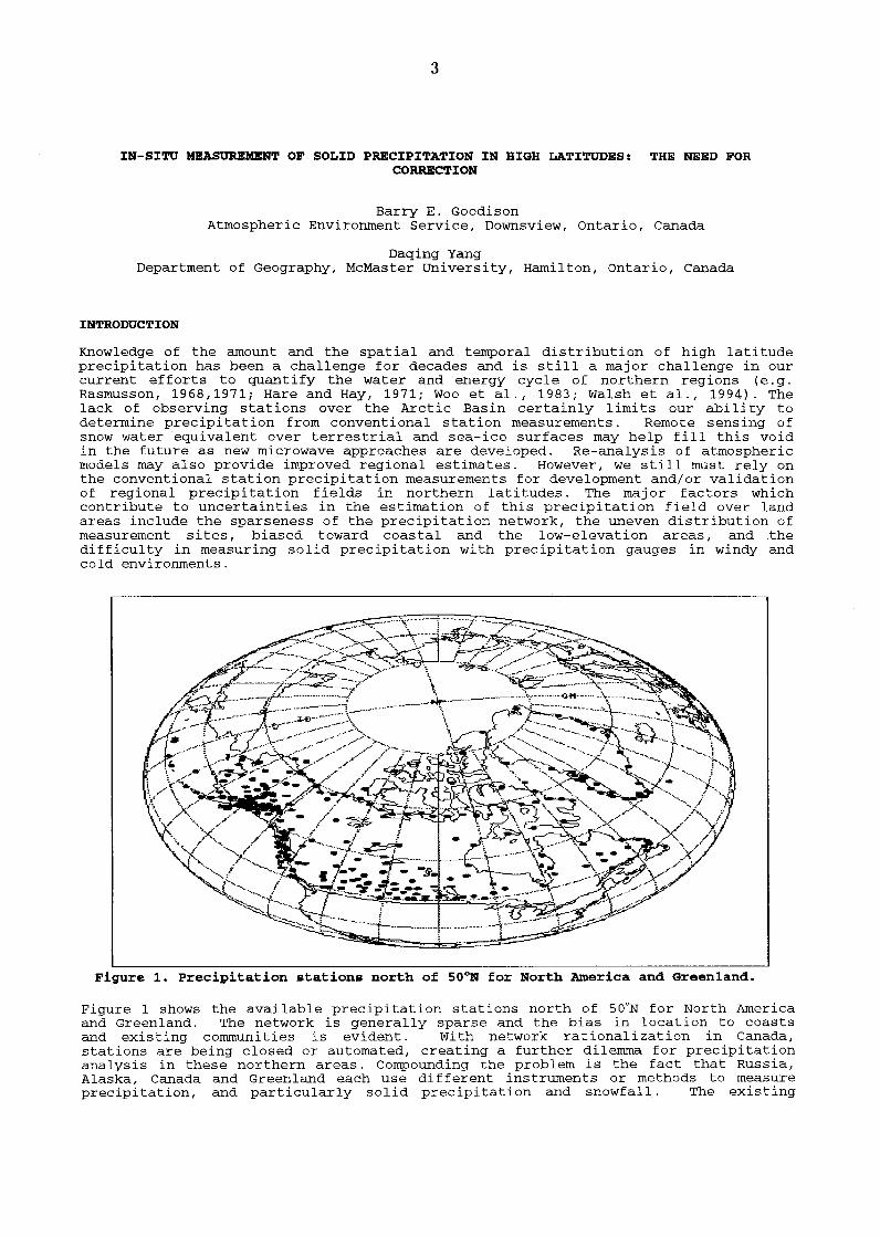
Figure 1. Precipitation stations north of 50°N for North America and Greenland.

Figure 1 shows the available precipitation stations north of SOON for North America and Greenland. The network is generally sparse and the bias in location to coasts and existing communities is evident. With network rationalization in Canada, stations are being closed or automated, creating a further dilemma for precipitation analysis in these northern areas. Compounding the problem is the fact that Russia, Alaska, Canada and Greenland each use different instruments or methods to measure precipitation, and particularly solid precipitation and snowfall. The existing

4

precipitation network in the Arctic regions includes about 100 station in northerncanada, 25 in Alaska, 20 in Greenland and more than 100 in Arctic zone of Russia (WMO, 1994). Many different instruments and observation methods are used for precipitation observation in the regions. Table 1 summarizes the primary national precipitation gauges and the associated information on wind shield and gauge installation.

The challenge then, for programs such as ACSYS, is to reconcile these different observation sources and to assemble a consistent data set for climatological and hydrological studies. Errors of up to 80 - 100% have been documented in in-situ snowfall measurements in the high latitude regions. There is little we can do about station location and local sitting issues. But can we do anything to adjust our existing, and future, data for systematic errors in measurement? One step is to have a methodology for adjusting solid precipitation data from the operational meteorological and hydrological networks. The results from the WMO/CIMO Solid Precipitation Measurement Intercomparison can provide some of this methodology.

This paper will demonstrate the magnitude of the problem of measuring solid precipitation in different northern countries and will summarize some of the results from the WMO Intercomparison with emphasis on the national precipitation gauges used in the Arctic regions. We will also giver some examples of adjustments of measured precipitation, based on the application of the WMO Intercomparison results, on the archived data in the high latitude regions of Alaska and northern Canada. Some considerations that ACSYS might consider in developing a strategy for precipitation measurement in the northern latitudes are also given for discussion.

Table 1. List of national standard (manual) gauges currently used for snowfall measurement in the high latitude regions.

Country Region Name Mat Ori. Gauge Wind Height Min. No. of of Area Height Shield Above meas. of Gauge Gauge (cm2) (cm) Ground Gauges

Canada NWT/Yukon Nipher copper 127 52 Canadian 2m 0.2 -100 Nipher

USA Alaska NWS 8" copper 324 68 Alter 1m 0.13 -130 standard steel

Russia Siberia Tretyakov galv. 200 40 Tretyakov 2m 0.1 -100 iron

Denmark Greenland Hellmann galv. 200 43 ? 1.5m 0.1 -35 iron

Finland Tretyakov galv. 200 40 Tretyakov 1.5m 0.1 -634 iron

Norway Norwegian copper 225 25 Nipher 1.5m ? -775

Sweden SMHI alum. 200 35 Nipher 1.5m ? -900 Iceland Icelandic galv. 200 56 Nipher 1. 5m ? -750

THE WMO SOLID PRECIPITATION MEASUREMENT INTERCOMPARISON

The WMO Solid Precipitation Measurement Intercomparison was initiated in 1986. The goal of the study was to assess national methods of measuring solid precipitation against methods whose accuracy and reliability were known, including past and current procedures, automated systems and new methods of observation. Countries which participated, operated the reference standard and have submitted complete data summaries for analysis include: Canada, China, Croatia (originally Yugoslavia), Denmark, Finland, Germany (originally German Democratic Republic), Japan, Norway, Russia (originally USSR), Sweden and the United States. Other countries collecting and submitting comparative data for at least one winter included Bulgaria, India, Romania and Slovakia (originally Czechoslovakia), and the United Kingdom.

The Intercomparison was designed to: determine wind related errors in national methods of measuring solid precipitation, including consideration of wetting and evaporative losses; derive standard methods for correcting solid precipitation measurements; and, introduce a reference method of solid precipitation measurement for general use to calibrate any type of precipitation gauge. The experiment,

5

conducted by Members at sites selected in their own country, ran from 1986/87 through 1992/93.

Reference Method for Snowfall Measurement:

The reference measurement for the WMO Intercomparison experiment is critical. The octagonal, vertical double fence shield (with manual Tretyakov gauge) was designated as the Intercomparison Reference (DFIR) by the Organizing Committee (WMO/CIMO, 1985; Goodison et al., 1989). An artificial shield was selected since natural bush sheltering would not be available in all climatic regions, such as the Arctic. The DFIR is a secondary standard. Errors in measurement using the DFIR and correction procedures are given in Golubev (1986) and Yang et al. (1993). Initial results from the experiment are given in WMO/CIMO (1992), Aaltonen et al. (1993), Gunther (1993) and Metcalfe and Goodison (1993). Errors in solid precipitation measurement have been quantified for over 20 different gauge and shield combinations.

Figure 2 shows one of the problems in measuring precipitation, and the need for a reference standard. In this case, the Universal Belfort gauge (an automatic recording gauge) was operated unshielded, with an Alter shield and with a Canadian large Nipher shield. For the month, during which only snow fell, the DFIR and Nipher shielded gauges recorded almost twice that measured by the unshielded gauge. Proper shielding of a gauge is critical; information of the gauge type and the type of shielding used is essential if historical data are to be corrected. The need for metadata cannot be overemphasized.

Wetting and Evaporative Losses:

Evaporation and wetting losses from manual gauges contribute significantly to the undermeasurement of solid precipitation. Aal tonen et al. ( 1993) reported on the comprehensive Finnish assessment of evaporation losses; average daily losses varied by gauge type and time of year. Losses in April of over 0.8 mm/day were measured in some gauges. Average losses for winter periods, ranging from 0.1-0.2mm/day, were much less than during summer periods.

50

45

40

35

e .§. 30 z 0 i= 25 <( ...... ii: u 20 w a: D..

~-~--------------J // ' ,.--------------J

,.,:,~

;.:""

/

/ ,..,..-'

/

A/S BELFORT

r-----------uis BELFORT-­/

N/S "' NIPHER SHIELDED AJS "' AL TEA SHIELDED U/S "' UNSHIELDED

" / _ _,

10 11 12 13 14 15 16 17 18 19 20 21 22 23 24 25 26 27 28 29 30 31 JANUARY 1987

Fig. 2. Gauge measurements (uncorrected) of snowfall at Kortright Center for January 1987.

Wetting loss varies by precipitation type, gauge type and the number of times the gauge is emptied. Wetting loss is cumulative and it can become a very large value for the year. Average wetting loss can be up to 0.2mm per observation. At some Canadian synoptic stations, wetting loss was calculated to be 15-20% of measured winter precipitation (Metcalfe and Goodison, 1993).

6

Trace precipitation:

For most manual gauges, a precipitation event of less than 0 .1mm is beyond the resolution of the measuring cylinder and hence is recorded as trace precipitation ("T" for trace). Officially, all of the trace precipitation events are treated as zero; they are not included in the monthly totals. The day during which trace precipitation is reported is counted as a precipitation day.

A large number of trace precipitation events was reported in Alaska and northern Canada. According to Benson (1983), trace precipitation at 14 weather stations in Alaska accounted for 12 to 65% of the total number of days on which precipitation was recorded, with generally more days recording trace in winter than summer. The number of trace observations in winter at some stations can be as high as 80% of the total. The percentage of traces is inversely proportional to the amount of measured precipitation. Yang et al. (1995a) estimated the trace adjustment to be 9. 8mm and 9.3mm at Barrow Alaska for 1982 and 1983, or 12% and 13% of the annual precipitation.

For the Canadian Nipher snow gauge, a precipitation event of less than 0. 2mm is treated as a trace. Metcalfe et al. (1993) reported that some Canadian Arctic stations have reported over 80% of all precipitation observations as trace amounts and that there has been an increasing trend of trace precipitation reported in the high Arctic regions. For instance, at Resolute Bay, NWT, the average number of trace recorded each year has continued to increase from around 300 in 1950 to well over 700 in 1993. The annual correction for the trace precipitation at Resolute is estimated to be 25-35mm for the period of 1948 to 1991.

Wind-Induced Error:

Many studies have indicated that wind speed is the most important environmental factor contributing to the undermeasurement of solid precipitation (Goodison et al., 1981,1989). The effect of wind on gauge catch can be reduced by the use of naturally sheltered locations, or by using artificial shielding. Goodison (1978) showed that for most gauges, the catch ratio to "true precipitation" as a function of wind speed decreases exponentially with increasing wind speed. Deviations from the DFIR measurement varied by gauge type and precipitation type. Some results from the Intercomparison, emphasizing polar countries, are summarized below to emphasize the magnitude and variability between gauge types (and shielding) and precipitation type in the undermeasurement of solid precipitation.

One must be very careful when analyzing ratios and differences between gauges. small absolute differences between gauges and the reference gauge (DFIR) could create significant large variations in the catch ratios (e.g. a 0.2mm difference of Tretyakov gauge vs. DFIR with a DFIR catch of 1mm gives a ratio of 80% versus 96% for a 5mm event) . To minimize this effect, the daily totals when the DFIR measurement was greater than 3.0mm were used in the statistical analyses.

Valdai, Russia was the only site where the DFIR, a secondary reference, was compared to gauges sited in bushes (cut to gauge height), the latter deemed to provide the best estimate of "true" snowfall. Table 2 compares precipitation totals for November 1991 to March 1992 for the DFIR, the bush gauge and some of the other gauges operated at Valdai.

The measurements show the need to correct the DFIR to the "ground true" value of the bush gauge to account for the effect of wind and other environmental factors (e.g. temperature). Methods to correct the DFIR were developed and applied (WMO/CIMO, 1992; Yang et al., 1993) before comparing the catch of national gauges to the DFIR.

Finland conducted the most extensive comparison of gauge types and shielding at a single site (8 manual, 3 autogauges). Table 3 shows the average percentage catch for selected gauges (allowing for wetting loss) compared to the corrected DFIR. Gauge catch decreased with increasing wind speed for all gauges, with the relationship varying by gauge type, shielding, precipitation type and, in some instances, air temperature. Shielded gauges caught more than their unshielded counterparts.

A comprehensive analysis (Yang et al., 1995a,b) of measurements for the same gauge tested in different countries is also being done by using the compiled WMO Intercomparison datasets, which represent a wide range of terrain, exposure and snow condition. Comparison of the average catch ratios vs wind speed for several gauges, both shielded and unshielded, is shown later.

7

Table 2: Precipitation totals (rain and snow) mea~ured by different gauges at Valdai, Russia, November 1991-March 1992 (WMO/CIMO, 1992)

Gauge type Total Precip. (mm) % of bush total

Tretyakov in bushes DFIR (Tretyakov) DFIR (Canadian Nipher) Canadian Nipher shielded Tretyakov 8" USA Alter shielded 8" USA unshielded

367 339 342 314 258 273 208

100 92 93 86 70 75 57

Table 3: Average gauge catch (%) compared to DFIR (corrected to bush value) for snowfall at Jokioinen, Finland, 1987-1993.

Gauge

DFIR Canadian Nipher Shielded Tretyakov (shielded) Tretyakov (unshielded) Swedish Norwegian

Catch(%)

100 82 74 46 69 66

GAUGES OF NORTHERN COUNTRIES

Canadian Nipher snow gauge

Gauge Catch(%)

Danish Hellmann (unshielded) 48 Hungarian Hellmann (unshielded) 46 Geonor (Alter shield) 62 Tipping Bucket (heated) 62 Wild (shielded) 57 Wild (unshielded) 40

The Canadian Nipher Shielded Snow Gauge System is the standard Canadian instrument for measuring snowfall amount as water equivalent. The accuracy of this snow gauge and others used in Canada was first defined by Goodison (1978). Results from the WMO Intercomparison indicate results similar to those found previously and show the catch of the Canadian Nipher shielded gauge to be almost the same as the WMO reference standard (Goodison and Metcalfe, 1992). The unique design of the Canadian Nipher shield minimizes disturbance of the airflow over the gauge and eliminates updrafts over the orifice. This results in an improved catch by the gauge, for wind speeds ,up to 7 ms-1

, measured at gauge height, relative to other shielded and unshielded gauges (Goodison et al., 1983).

Tretyakov gauge

The Tretyakov gauge is the standard precipitation gauge currently used in Russia and Finland. Table 4 summarizes the average catch ratio of the shielded Tretyakov gauge at 11 WMO test sites. The ratio changes as a function of wind and varies according to the proportion of snow, rain and mixed precipitation. The variability between stations shows that it is necessary to analyze and understand the wind and precipitation data at both the intercomparison station and at the climate stations before applying the intercomparison results to a regional or national station network.

Detailed analysis (Yang et al., 1995b) of daily data confirmed that wind speed is the most important factor for gauge catch when precipitation is classified as snow, snow with rain, rain with snow and rain. Air temperature has a secondary effect on gauge catch. Gauge catch decreases with increasing wind speed on the precipitation day and increases with rising air temperature. However, compared to the wind influence, the effect of air temperature on the gauge catch of snow is small. For instance, an air temperature change of 10°C only results in a 3% change of the gauge catch whereas a wind speed increase of 1 m/s causes a 9% decrease of catch compared to the DFIR.

8

Table 4. Summary of the Intercomparison of shielded Tretyakov gauge against the DFIR at 11 WMO sites.

Station

Valdai

Reynolds

Danville

Jokioinen

Harzgerode

Bismarck

Joseni

Parg

Peterborough

Regina

Kortright

Snow Snow/Rain Rain/Snow Rain Bvent Ws DFIR Tret Event Ws DFIR Tret Event Ws DFIR Tret Event Ws DFIR Tret

Catch Catch Catch Catch

(day! lmls 1 fmml 1%/ (day/ fm/s / lmml 1%/ I day/ fmls I mm/ f%/ (day/ fmls / fmm/ f%1

304 4.1 1181.7 63.1 85 4.6 584.9 71.2 75 4.5 489.7 86.3 230 3.8 1259.2 91.4

50 2.5 105.6 84.4 27 3.8 71.4 88.5

157 1.5 1036.2 91.6 21 1.0 999.5 95.0

8 4.4 29.3 85.4 40 2.7 206.4 92.0

18 1.4 348.7 94.5 30 1.0 446.3 94.3

334 2.6 740.9 67.2 149 3.1 405.6 72.5 131 2.9 414.3 84.5 567 2.5 1694.4 86.6

42 3.0 112.7 72.2 53 3.9 110.2 78.5 127 4.2 538.8 82.4 172 4.2 475.3 81.3

32 3.3 94.6 65.4 16 3.1 53.3 67.8

94 1.1 194.0 85.8 14 1.3 39.8 92.9

65 1.0 486.9 91.0 16 1.2 250.1 90.3

3 3.3

11 2.2 53.6 86.9 34 1.2

9.3 71.6

85.0 90.6

31 1.5 550.8 90.7 141 1.6 1573.8 88.2

76 2.0 262.0 81.1 31 2.0 172.3 90.6 20 2.3 219.4 95.0

117 3.5 199.1 59.4 36 4.3 76.9 63.1

80 1.9 581.9 95.0

5 3.9 5.1 97.4

107 2.5 274.7 83.1 25 2.7 198.4 85.3 1 4.2 31.9 91.8 64 2.3 342.6 90.0

The beneficial effect of using a wind shield, Tretyakov shield in this case, on gauge catch is clearly shown in Figure 3. For the unshielded Tretyakov gauge, the variation of daily catch ratio of snow as a function of daily mean wind speed at the gauge orifice height of 1.5m has been derived from the Intercomparison data collected at the Jokioinen experimental station in Finland (Elomaa, 1994). The unshielded gauge has a catch ratio of 10-20% lower at Jokioinen compared to that for a shielded gauge at the same wind speed . At high winds, the catch ratio of the unshielded gauge can be an absolute 30% less than the shielded one. It is critical to know the shielding employed at a site if adjustments of historical data are to be made. Figure 3 also shows the variability in catch that can occur, depending on local siting and other environmental factors. Derived regression relationships can identify and incorporate other effects.

0::: l..;_

0

Q) 0') :_") 0

(..!)

> 0

_y 0 >-

+­(]) !..... , .....

120~------------------------------------------------~

shieided + Lmshielded

100-l----0~.----+,--------------------------------------------------4

80 J_ ___ ~_. __ f'·~··:_~_:~-~~-:~~-·~,~~~:~,·~-'~~~f~~t~3---------------------------------------~ > L .. l ~!:::t

~

'-'g Cl,..., ~ ••• : !-.' * + ~ 'f:·;·: c.b, .. ,:

6 0 -+----------.. ,._.+_.=.+:---+'-.. -----,-· ···T"f""...---0-... '_...r:::..._·::l _,.E .. 'e---------------1 + ++ + UP o

+ +t·+ + + . + -EJ+·

:-·.f:":.J 0 + ~["j 40 +-----------------+~--~-i--~--~~-------,~~~--~C-1----,~--------~ + .. ,.++

-13~-:+-+ ·+ +

+ +

+

0~-------------.------.------.------.------.------.-----~

0 A ; 2 3 4 5 6 7 8

Daily Mean Wind Speed at 1 .5m (m/s)

Fig. 3. Daily catch ratio of shielded and unshielded Tretyakov gauge versus daily wind speed at 1.5m at Jokioinen WMO Intercomparison site.

9

U.S. NWS 8" standard gauge

The NWS 8" standard nonrecording gauge has been used as the official precipitation measuring instrument at the U. s. climatological station network, including Alaska. The gauge is mounted at 1m above the ground surface and, at some of the stations, the gauge is equipped with an Alter-shield for snowfall measurements.

During the WMO Intercomparison, this gauge was tested at the Valdai hydrological Research Station in Russia, at two stations in the USA. The daily gauge catch of snow as a function of daily wind speed at the level of the gauge orifice has been derived from the compiled Intercomparison data collected at the WMO sites for a number of winter seasons (Yang et al, 1995b). Figure 4 shows the relationship for the shielded NWS 8" gauge based on data from sites in Russia and the USA. The results indicates a clear difference of the catch of snow between the shielded and unshielded gauges, e.g., at a gauge height wind speed of 5m/s, the shielded and unshielded gauges recorded 55% and 29%, respectively, of the corrected DFIR. Thus, it is easy to understand that the combination of the precipitation data measured by shielded and unshielded gauges in Alaska will produce an inhomogeneous precipitation time-series and lead to incorrect spatial interpretation.

,-, 140 ~ CJ Reynclds ·~· Va!dal .__. C::": 120 ....._ Cl

.............. 100

,-, ..r::. !a 80

::5 ,_.. LL.I 60 (.!) =:1 <::( (..? 40

i:O 20

!/l :s: --:z: 0

0 2 3 4 5 6 7 8 9 DAlLY WlND SPEED .P, T GAUGE HEiGHT (m/ s)

. Fig. 4. Daily catch ratio of the NWS 8" non-recording gauge to the DFIR as a function of daily wind speed at the gauge height.

Hellmann gauge

The Hellmann gauge is one of the most widely used precipitation gauges around the world. It is the standard gauge in 30 countries and the total number of gauges is about 30,000. Hellmann gauge is a no-recording gauge for both rain and snow measurement. Although there are various versions of the gauge, e.g. German, Danish, Polish and Hungarian, the designs of the versions of the gauge are very similar (Sevruk and Klemm, 1989) . A metal cross is installed in the Danish Hellmann gauge to minimize snow being blown out of the gauge. In some countries they are equipped with a wind shield at climate stations in mountain regions or at high latitudes.

Many experimental studies on Hellmann gauges have been conducted and reported, primarily for rain (Sevruk, 1981; 1982; Sevruk and Hamon, 1984; Sevruk and Klemm, 1989) with results being used to correct the archived precipitation in Switzerland (Sevruk et al., 1993). During the WMO Intercomparison, the Hellmann gauge was tested against the DFIR in Russia, Finland, Germany and Crotia.

At Jokioinen Finland, two unshielded Hellmann gauges of Hungarian and Danish design were installed at 1. 5m above the ground. Intercomparison shows that both gauges caught almost the same amount of precipitation (Table 5).

At the Harzgrode WMO test site in Germany, German Hellmann gauges were operated with a Tretyakov wind shield and unshielded and tested against the DFIR for a number of years. The results indicated that for the entire test period the unshielded German Hellmann gauge caught 44% of the DFIR for snow and 88% of the DFIR for rain, while the shielded German Hellmann gauge measured 62% of the DFIR for snow and 90% of the DFIR for rain. At this site, a Tretyakov wind shield increased the average catch

10

years. The results indicated that for the entire test period the unshielded German Hellmann gauge caught 44% of the DFIR for snow and 88% of the DFIR for rain, while the shielded German Hellmann gauge measured 62% of the DFIR for snow and 90% of the DFIR for rain. At this site, a Tretyakov wind shield increased the average catch ratio of the German Hellmann gauge by 18% for snow, 12% for snow with rain and 4% for rain with snow and rain.

Table 5. S11IDDI&rY (total and % of the DFIR) of daily observed precipitation for Hungarian and Danish Hellmann gauges (unshielded) at Jokioinen WMO Intercomparison station

Type of Precip

Snow

Snow/Rain

Rain/Snow

Rain

# Events (day)

266

150

132

526

-2.3

1.0

3.2

11.3

Tmin (Oc)

-6.0

-1.6

-0.1

7.0

Ws{@ 3m) (m/s)

2.7

3.0

2.9

2.4

DFIR

620.2 100.0

406.2 100.0

414.8 100.0

1616.1 100.0

Hellmann Gauge Cat l.Sm) Hungarian Danish

263.2 42.4

239.8 59.0

336.9 81.2

1456.6 90.1

264.8 (mm) 42.7 (%)

226.6 (mm) 55.8 (%)

320.4 (mm) 77.2 (%)

1413.6 (mm) 87 0 5 (%)

Figure 5 shows the regression of the daily catch ratio of snow as a function of daily wind speed for the unshielded Hellmann gauge (Yang et al., 1994). The data are from 4 intercomparison sites, with gauges at different heights. Although wind speed alone accounts for 69% of the variation, other environmental and site factors contribute to the variability in the observations. Also, this is a plot of daily values. Also, there may not have been precipitation during the entire day, so the average daily wind speed may not be the same as the wind speed during the precipitation event. But this is what we must try to deal with when correcting archived data - we will not have wind speed during the storm itself.

120 ..--.. ~...::: ..._.., 0::: 100 w... 0

.......... 80

CJ +-8--=---=----------------·-----------------------------------l

G~i=.aoB =o (::~:::; ;:::~ c;

c:: c 0 60 E (J.)

:::r: T.l 40

CD ""Cl

(J.)

:.c 20 u; c::

:J 0

0 0 1 2 3 4 5 6 7 8 9

Wind Speed at Gauge Height (m/s)

Figure 5. Daily Catch ratio of snow as a function of daily wind speed at gauge height of the unshielded Hel1mann gauge.

Compared to Nipher snow gauge (Goodison and Metcalfe, 1992), Tretyakov gauge (Yang et al., 1995a) and the NWS 8" standard gauge (Yang et al., 1995b) , the catch of the Hellmann gauge, regardless of the different versions, is generally very low (Fig.6). For example, the average catch ratio for snow range from 42 to 89% at the 4 WMO sites and at the daily mean wind speed of 5m/s, the gauge catches only 30% snow of the DFIR. The problem is that when a gauge catches a low amount, any adjustment factor becomes large since it is the inverse of the ratio. For example, if a gauge catches 20%, the adjustment is 5 times the measured amount, while at 25% catch it is only 4

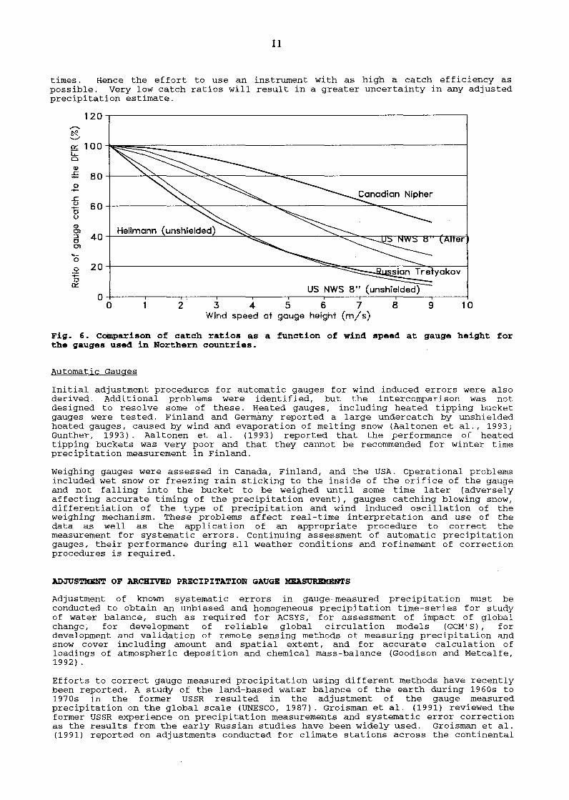
11

times. Hence the effort to use an instrument with as high a catch efficiency as possible. Very low catch ratios will result in a greater uncertainty in any adjusted precipitation estimate.

120~--------------------------------------------------------.

oc 100~~~~~==------------------------------------------j G:: 0 IV

£ 80+---""'c""'c---.=:...'<:2'-.;:------:::::.. ...... ::::---------------------j 0 -..c. 0 ..... 0 u

g, Hellmann (unshielded) ~ 401-~-~--i~~---L--~~~-------~~~~==--n~~~~~~n+.e~r~

Ol

US NWS 8" (unshielded) 0+-----.-----.-----.-----.-----.-----.-----.-~------~~----~

0 2 3 4 5 6 7 8 9 10 Wind speed at gauge height (m/s)

Fig. 6. Comparison of catch ratios as a function of wind speed at gauge height for the gauges used in Northern countries.

Automatic Gauges

Initial adjustment procedures for automatic gauges for wind induced errors were also derived. Additional problems were identified, but the intercomparison was not designed to resolve some of these. Heated gauges, including heated tipping bucket gauges were tested. Finland and Germany reported a large undercatch by unshielded heated gauges, caused by wind and evaporation of melting snow (Aaltonen et al., 1993; Gunther, 1993). Aaltonen et al. (1993) reported that the performance of heated tipping buckets was very poor and that they cannot be recommended for winter time precipitation measurement in Finland.

Weighing gauges were assessed in Canada, Finland, and the USA. Operational problems included wet snow or freezing rain sticking to the inside of the orifice of the gauge and not falling into the bucket to be weighed until some time later (adversely affecting accurate timing of the precipitation event), gauges catching blowing snow, differentiation of the type of precipitation and wind induced oscillation of the weighing mechanism. These problems affect real-time interpretation and use of the data as well as the application of an appropriate procedure to correct the measurement for systematic errors. Continuing assessment of automatic precipitation gauges, their performance during all weather conditions and refinement of correction procedures is required.

ADJUSTMENT OF ARCHIVED PRECIPITATION GAUGE MEASUREMENTS

Adjustment of known systematic errors in gauge-measured precipitation must be conducted to obtain an unbiased and homogeneous precipitation time-series for study of water balance, such as required for ACSYS, for assessment of impact of global change, for development of reliable global circulation models (GCM'S), for development and validation of remote sensing methods of measuring precipitation and snow cover including amount and spatial extent, and for accurate calculation of loadings of atmospheric deposition and chemical mass-balance (Goodison and Metcalfe, 1992).

Efforts to correct gauge measured precipitation using different methods have recently been reported. A study of the land-based water balance of the earth during 1960s to 1970s in the former USSR resulted in the adjustment of the gauge measured precipitation on the global scale (UNESCO, 1987). Groisman et al. (1991) reviewed the former USSR experience on precipitation measurements and systematic error correction as the results from the early Russian studies have been widely used. Groisman et al. (1991) reported on adjustments conducted for climate stations across the continental

12

United States from 1950 to 1987, with consideration of the effects of wind and wetting losses on gauge catch. The "corrected" estimates were obtained using site specific information including wind speed, air temperature, gauge height and sheltering. Wind speed during precipitation was estimated from mean monthly wind speed using a procedure outlined by Sevruk (1982).

Adjustments have also been conducted for Switzerland (Sevruk et al., 1993), and other study areas (Peck, 1991; Groisman Easterling, 1994). The adjustments were based on a variety of studies with the Tretyakov gauge, other types of precipitation gauges, pit gauge, snow boards and snow cover data. Generally two techniques were developed and used in the analysis of monthly data. The first method (Peck, 1991; Groisman et al., 1991, 1994) simply used a constant adjustment factor, obtained from an intercomparison experiment at other sites, for each month or season; the results of this adjustment did not have any impact on climate change studies, such as trend analysis, since the monthly and annual totals were only changed. The other technique required monthly wind speed and air temperature to estimate the adjustment factors, by using the correlation between monthly mean wind speed and the mean wind speed during precipitation days (Sevruk, 1982).

The WMO Solid Precipitation Measurement Intercomparison provided the opportunity to develop improved adjustment procedures for a number of precipitation gauges commonly used around the world. Currently, there are on-going efforts to test the adjustments of historical national gauge measurements for wind and wetting losses. To apply the adjustments, wind speed at gauge height is required; it can be measured or derived using a mean wind speed reduction procedure. This is site dependent; estimation will require a good knowledge of the station and gauge location. Hence, there must be a reliable metadata record.

350~--------------------------------------------~

,_ DFIR ~ C/DFIR

3oo 1 ts:sreiNA_T_COJ~uCER

250 ,..

200

150

100

1990/91

Fig. 7. Annual measured and corrected snowfall precipitation for three different measurement methods at Dease Lake for 1987/88 to 1990/91 winter period: DFIR; corrected DFIR ot 'true precipitation' (C/DFIR); Nipher gauge (NAT); corrected Nipher gauge (C/NAT); fresh snowfall ruler using 100 kg/m3 (RULER), corrected ruler using 80kg/m3 (C/RULER).

Canada has conducted preliminary tests in applying adjustment procedures on its digital archive data. Figure 7 shows the result of adjusting the Dease Lake synoptic station annual snowfall precipitation as measured by the Canadian standard methods of snowfall measurement (ruler and Nipher gauge) and by the DFIR operated at the site for 1987/88-1990/91. Average winds at this station are less than 3ms·1

; hence the Nipher gauge showed only a 5-10% undercatch compared to the DFIR. However, ruler measurements, using a density of 100kgm-', overestimated precipitation by as much as 20%. Metcalfe and Goodison (1993) showed that by applying adjusting gauge measurements for wind, wetting loss and trace precipitation (assigning a non-zero value), and ruler measurements for variations in regional fresh snowfall density, the corrected values were within a few percent of the corrected DFIR.

Figure 8 (Metcalfe et al, 1994) compares corrected and uncorrected Canadian Nipher gauge data for Resolute, NWT for 1963-1992, applying adjustments for wind, wetting loss and trace precipitation to 6-hourly archived data. Plotted along with these are

13

adjusted annual precipitation amounts based on special snow surveys reported by Woo et al. (1983). Both the corrected annual precipitation and the snow course totals exhibit good agreement. Most important, however, is that both methods in~icate ~hat actual annual precipitation is 50 100% greater than measured at thls statlon. similar increases resulted when precipitation corrections were made at other Arctic stations. Increases in corrected annual precipitation totals were less dramatic for other NWT stations located south of 65°N. For example, at Yellowknife corrections increased average annual precipitation by 26% and at Norman Wells by 19%. Both these sites are more sheltered than Resolute and the effect of wind on gauge catch is less.

e .§_ z 0

< !:::::: c... Q UJ a: c... .....J

~ :z ~

500

450

400

350

ANNUAL PRECIPITATION RESOLUTE BAY, N.W.T.

01~---r-------.-------,--------r-------,--------.-------.--~ 1 975-76 1 976-77 1 977-76 1 976-79 1 979-60 1 960-61 1 961 -62

YEAR (Sept.- Aug.)

-Woo/McMaste..-

----Niphe..-........ Ruler-

Figure 8 Comparison of AES archived annual total precipitation, corrected annual total precipitation from gauge and ruler measurements and annual precipitation estimates (range) from special snow survey data (Woo et al., 1983) at Resolute Bay, NWT.

The primary reason for the larger differences between measured and corrected precipitation at High Arctic stations is the number of traces recorded annually at these locations. At Resolute Bay the average number of traces recorded each year has continued to increase from around 300 in 1950 to well over 700 in 1993. A large number of these trace observations are a result of the occurrence of ice crystals. There is some speculation that this trend in ice crystal occurrence may be directly or indirectly related to a systematic increase in Arctic haze and to changes in the Arctic winter boundary layer (Bradley et al., 1993).

The correction of six hourly archived precipitation measurements for known systematic errors will provide significantly improved estimates of actual precipitation than are currently available. It is anticipated that anomalies currently existing between various hydrologic data sets will be minimized after correction of the precipitation archive. ACSYS will require an adjusted precipitation data base if it is to be successful in its studies of the Arctic climate system.

Yang et al. ( 1995c) have reported on the adjustment of the NWS 8" daily gauge measurements at Barrow Alaska for 1982 and 1983, by applying the WMO Intercomparison result for that gauge (Yang et al, 1995b). Figure 11 shows the monthly summary of the adjustments for trace amount, wetting loss and wind-induced errors. Monthly adjustment factors varied from 1.15 to 2.76 in 1982 and from 1.36 to 3.23 in 1983. It is important to note that there is a seasonal variation of the adjustment factor, that is, a high value for snow data in the cold season from September to May and a low value for rain data in the warm season from June to August, due to the higher wind-loss for snow than for rain and due to the smaller amount of absolute precipitation in the cold season than in the warm season. It is even more important to recognize the importance of the intra-annual variation of the monthly adjustment factors due to the fluctuation of wind speed, frequency (or percentage) of snowfall, number of trace precipitation observations, amount of gauge-measured precipitation

14

and air temperature. In 1982, during the cold period of January to May and of September to December, the percent of snowfall in each month was 100% except in September with 68% and the average AF was 1.90. In the warm period of June to August, rainfall dominated with snowfall being less than 10% in each month and the mean AF was 1.19. In 1983, the average AF in the cold season was 1.88 and the mean AF in the warm season was as high as 1.41 mainly because of the higher percent of snowfall (55% and 40%) in June and July. Use of the same monthly average adjustment factor every year can produce erroneous estimates of precipitation, since monthly climate conditions can be very different from year to year. The study at Barrow showed that the wind-induced error was the largest systematic error, estimated to be about 33% of measured annual precipitation. Trace and wetting losses were not negligible, accounting for 12-13% and 9.5-14.4%, respectively, of the archived annual total.

..iAN !ot'!AR MAY jlJL SPT NOV FEB APR JUN AUG OCT DEC

45

40

35

E .'50 $

c 25 ~Q

=E 20 ·c. ·r:s "' 15 ....

0..

1 0

5

0 JAN MA.R MAY JUL. SPT NOV

F'£13 APR JUN AUG OCT DEC

Fig. 9. Adjustments of gauge-measured precipitation at Barrow Alaska, for 1982 (top) and 1983 (bottom).

CONSIDERATIONS BY THE ACSYS COMMUNITY

The goal and objectives of the WMO experiment were successfully achieved. Data from all experiment sites confirm that solid precipitation measurements must be adjusted for wetting loss (for volumetric measurements), trace amount and undercatch due to wind speed before one can estimate precipitation at ground level.

To achieve improved measurement and adjustment of solid precipitation in Arctic regions ACSYS should consider some of the results and recommendations from the WMO Intercomparison, namely that:

15

(1) methods developed from the WMO Intercomparison for adjusting systematic errors ~-' precipitation measurement that are now available for different types of gauges and for different types of precipitation and various time intervals should be adopted and applied to current and archived data;

(2) both measured and corrected precipitation data should be reported and archived;

(3) trace precipitation should be treated as a non-zero event;

(4) gauges should be shielded either naturally (e.g., forest clearing) or artificially (e.g., Alter, Canadian Nipher type, Tretyakov) to minimize the adverse effect of wind speed;

(5) use of heated tipping-bucket gauges for winter precipitation measurement be carefully assessed; their usefulness is severely limited in regions temperatures fall below OC for prolonged periods of time;

should where

(6) additional wind speed measurements be taken at the level of the gauge orifice and hourly mean wins be archived in order to correct for wind-induced errors.

(7) the timing and the type of precipitation be recorded by automatic instruments l2

order to conduct the correction on the basis of an event of precipitation.

However, for ACSYS there are additional aspects which must be considered. Before embarking on the adjustment, analysis, application of precipitation data, we must have a very clear understanding of the science question we are trying to answer. Only by having a clear understanding of the question can we decide on the appropriate temporal and spatial scale for the analysis, and hence the most appropriate adjustment procedures. Do we need a gridded product to be compatible with model outputs? What is the period of record to be used? Do we have the metadata to do a good job of implementing adjustments? Are we concerned about solid precipitation only, i.e. snowfall, or total precipitation. There are errors and biases in measuring rain as well. But the first issue is having a clear understanding of the science question being addressed.

In the adjustment of measured point precipitation, are the WMO results sufficient, or do some countries feel there needs to be additional data collected at higher latitudes? ACSYS provides a great opportunity to test the application of adjustment procedures and to test the corr~atibility of adjusted data across national boundaries. If national data bases are to be used, one might argue that national hydromet services are in the best position to take an active role in adjusting their own precipitation measurements.

Analyses for ACSYS will rely on digital data. But network data are sparse in our Arctic regions. There are, however, many data sets that were collected during past Arctic experiments. These data must be "rescued" and entered into digital archives, as appropriate. All such data must be first assessed for their quality and the availability of appropriate metadata. In Canada, through the EOS/CRYSYS project, the historical snow course data have been rescued and digitised for research purposes. There are other glaciological data which could contribute to the definition of precipitation at high latitudes.

Finally, precipitation networks are at risk as countries both automate or close observing stations. New observation methods will introduce data incompatibilities. These must be identified and accounted for in any analysis of precipitation. Creation of a homogeneous precipitation time series, suitable for climatological and hydrological analyses in the Arctic is essential. But the task will be challenging.

But let us all think about "What is the science question, what is it that we are trying to answer" as we debate the creation of spatially and temporally homogeneous time series of precipitation in our northern regions.

ACKNOWLEDGMENTS:

This international effort would not have been possible without the cooperation of the participating countries and the many observers at the stations where the WMO Intercomparison was conducted for a number of years.

16

REFERENCES

Aaltonen, A., E. Elomaa, A. Tuominen, and P. Valkovuori, 1993: Measurement of precipitation. Proc Symp. on Precipitation and Evaporation (ed. B. Sevruk and M. Lapin), Vol.l, Bratislava, Slovakia, Sept. 20-24, 1993, Slovak Hydrometeorlogical Institute, Slovakia and swiss Federal Institute of Technology, Zurich, Switzerland, 42-46.

Elomaa, E. J., 1993: Experiences in correcting point precipitation measurement in Finland. Proc. Eighth Symposium on Meteorological Observation and Instrumentation, Anaheim, California, January 17-22, 1993, American Meteorological Society, Boston, 346-350.

Golubev, v., 1986: On the Problem of Standard Conditions for PrecipitationGauge Installation. In, Proc. Int. Workshop on the Correction of Precipitation Measurements, WMO/TD No. 104, WMO Geneva, 57-59.

Goodison, B.E., H.L., Ferguson and G.A., McKay, 1981: Comparison of point snowfall measurement techniques. In, Handbook of Snow, D.M. Gray and M.D. Male, Ed, Pergamon Press, 200-210.

Goodison, B.E., B. Sevruk and s. Klemm, 1989: WMO solid Precipitation Measurement Intercomparison: Objectives, Methodology, Analysis. In, Atmospheric Deposition (Proc. Baltimore Syrnp, May 1989) IAHS publ. No. 179, Wallingford, U.K., 57-64.

Goodison, B.E., and J. R. Metcalfe, 1992: The WMO solid precipitation intercomparison: Canadian assessment. In, WMO Technical Conference of Instruments and Method of Observation, WMO/TD, No. 462, WMO, Geneva, 221-225.

Groisman, P.Ya., and D.R. Easterling, 1994: Variability and trends of precipitation and snowfall over the United States and Canada. J. Climate, 7, 205.

total 184-

Groisman, P. Ya., V. V. Koknaeva, T .A. Belokrylova and T .R. Karl, 1991: Overcoming biases of precipitation measurement: A history of the USSR experience. Bulletin of American Meteorological Society, Vol.72, No.ll, 1725-1732.

Gunther, Th., 1993: German participation in the WMO Solid Precipitation Intercomparison: Final results. Proc. Sym. on Precipitation and Evaporation (ed. B. Sevruk and M. Lapin), Vol.l, Bratislava, Slovakia, Sept. 20-24, 1993. Slovak Hydrometeorlogical Institute, Slovakia, and Swiss Federal Institute of Technology, Zurich, Switzerland, 93-102.

Hare, F.K. and J.E. Hay, 1971: Anomalies in the large-scale annual water balance over northern North America. Canadian Geographer, 15, 79-94.

Milkovic, J., 1989: Preliminary results of the WMO field intercomparison in Yukoslavia, Proc. International Workshop on precipitation Measurement, St.Moritz, swi tzerland, Department of Geography, Swiss Federal Institute of Technology, ETH Zurich, 145-149.

Metcalfe, J.R. and B.E. Goodison, 1993: Correction of Canadian winter precipitation data. In, Proc. Eighth Symp. on Meteorological Observations and Instrumentation. 17-22 January, 1993, Anaheim, Calif. AMS, Boston, 338-343.

Rasmusson, E.M., 1968: Atmospheric water vapor transport and the water balance of North America. II. Large-scale winter balance investigations. Mon. Weather Rev. 96, 720-734.

Rasmusson, E .M., 1971: A study of the hydrology of Eastern North America using atmospheric vapor flux data. Mon. Weather Rev. 99, 119-135.

Sevruk, B., 1981: Methodological investigation of systematic error of Hellmann rain gauges in the summer season in Switzerland (in German). Versuchsanstalt fur Wasserbau, Hydrologie and Glaciology, ETH-Zurich, Mitt. 52, 296pp.

Sevruk, B., 1982: Method of correction for systematic error in point precipitation measurement for operational use. corrections in Switzerland. Proc. Symp. on Precipitation and Evaporation (ed. B. Sevruk and M. Lapin), Vol.l, Bratislava, Slovak Hydrometeorlogical Institute, Slovakia and Swiss Federal Institute of Technology, Zurich, Switzerland, 155-156. WMO-No.589, WMO, Geneva, 9lpp.

17

Sevruk, B., and W.R. Hamon, 1984: International comparison of national precipitation gauges with a reference pit gauge. WMO Instrument and Observing Methods Report No.17, WMO, Geneva, 111p.

Sevruk, B., and S. Klemm, 1989: Types of standard precipitation gauges. In, Measurements Precipitation Measurement, WMO/IAHS/ETH Workshop on Precipitation

(ed. B. sevruk), st.Moritz, Switzerland, December 3-7, 1989, 227-233.

WMO/CIMO, 1985: International Organizing Committee for the WMO Solid Precipitation Measurement Intercomparison, Final Report of the First Session, WMO, Geneva, 31pp.+ Appendices.

WMO/CIMO, 1993: International Organizing Committee for the WMO Solid Precipitation Measurement Intercomparison, Final Report of the Sixth Session, Toronto, Canada, WMO, Geneva, 140pp.

Woo, M., R. Heron, P. Marsh and P. Steer, 1983: Comparison of weather statio snowfall with winter snow accumulation in high Arctic basins. Atmosphere-Ocean, 21, 312-322.

Yang, D., J.R. Metcalfe, B.E. Goodison, and E. Mekis, 1993: An evaluation of the double fence intercomparison reference gauge. In, Proc. Eastern Snow Conference, 50th Meeting, Quebec City, June 8-10, 1993, 105-111.

Yang, D., B. Sevruk, E. Elomaa, V. Golubev, B. Goodison and Th. Gunther, 1994: Wind­induces error on snow measurement: WMO Intercomparison Results. In, Proc. International Conference on Alpine Meteorology, Sept. 22-25, 1994, Lindau, Slovakia, 61-64.

Yang, D., B.E. Goodison, J.R. Metcalfe, V.S. Golubev, E. Elomaa, Bates, T. Pangburn, c. L. Hanson, D. Emerson, V. Copaciu and J. Accuracy of Tretyakov precipitation gauge: results of WMO Hydrological Processes, 877-895.

Th. Gunther, R. Milkovic, 19 9 Sa: Intercomparison.

Yang, D., B.E. Goodison, J. R. Metcalfe, V.S. Golubev, R. Bates, T. Pangburn and c. Hanson, 1995b: Accuracy of NWS 8" standard non-recording precipitation gauge: result of WMO Intercomparison. In, the 9th Conference on Applied Climatology, Jan. 15-20, Dallas, Texas, AMS Boston, 29-32.

Yang, D., B.E. Goodison., J.R. Metcalfe., 1995c: Adjustment of daily precipitation measured by NWS 8" nonrecording gauge at Barrow, Alaska: Application of WMO Intercomparison result. Proc. Ninth Symposium on Meteorological Observation and Instrumentation, Charlotte, NC, March 27-31, 1995, AMS Boston, 295-300.

18

POINT MEASUREMENTS OF SOLID PRECIPITATION

Golubev, V.S. 1, E.G. Bogdanova2

1 State Hydrological Institute, St.Petersburg, Russia

2Main Geophysical Observatory, St. Petersburg, Russia

INTRODUCTION

In general, methods for regular precipitation measurements were not changed greatly since ancient time till nowadays. These measurements are based on the idea of taking precipitation samples in an open vessel with the specified area of the horizontal receiving opening after which the selected sample is measured in length, volume or mass.

This method of precipitation sampling has no physical validation, strictly speaking. Therefore, the results of regular instrumental observations cannot be taken as absolutely correct. Moreover, due to change in the environmental conditions at the selection of the instrument is removed to another place, or if some type of the instrument is replaced by another type, the observation series becomes incompatible and its relative homogeneity is broken.

In general, precipitation measurements at the hydrometeorological network have high systematic errors. Nevertheless, only during the last 30 or 40 years, when it became possible to estimate all water balance components by independent methods, it was clear that these errors should be taken into account in all climatological, hydrological and other water balance generalizations. The amount of precipitation measured by standard network instruments is usually less than actual value, fallen onto the underlying surface at the observation point. The total systematic error of measurements contains several partial components of different physical nature and amount. Firstly, wind effect makes it impossible to catch the whole amount of precipitation. Then, the amount of precipitation in the precipitation gauge cannot be completely, e.g. some amount may evaporate, some portion of precipitation may be splashed out of the gauge in case of a severe storm, some snow may be blown away. And, finally, some water may be left on the walls of precipitation gauge when it is poured out to the measuring vessel, thus it is not taken into account in the results of measurements. In winter, in case of a snow cover, one more kind of systematic errors typical of this method of measurements should be taken into account. A strong wind takes the ice particles from the snow cover surface and keeps them in the air. When the height of these ice particles fly is above the receiving opening of the precipitation gauge, it catches these particles together with snow flakes which fall from the clouds. These ice particles of deflation origin which fall into the gauge are termed "false" precipitation. This false precipitation in its pure from can be discovered in the precipitation gauge ifthere is no snow fall and the elevation ofthe snow transport by wind is above the elevation of the receiving opening ofthe gauge.

19

The false precipitation is mentioned in introductory sections in numerous publications on the systematic errors of precipitation measurements but its quantitative assessment is usually missing. The main reason of a poor knowledge of this error is associated with great technical difficulties and costly experiments. The available instruments for estimating a vertical distribution of snow transport are complicated and far from being perfect; besides, it is extremely methodologically difficult to get reference precipitation values free from the great errors in case of severe blizzards.

GENERAL METHODOLOGY FOR CORRECTION OF PRECIPITATION MEASUREMENTS

The actual amount of precipitation (P) can be .obtained from the data on standard observations by standard precipitation gauges (P") introducing some corrections to the results of measurements which take into account systematic errors of the applied method. The base equation for correction is as follows:

where:

P=KP', (I)

K is the so-called wind coefficient which corrects the distorting wind effect on the receiving surface of the instrument.

The amount of precipitation caught by the gauge (P') is a sum of the measured amount (P") and corrections taking into account systematic errors of different origin:

where:

P' = P" + P(w) + P(s) + P(e) + P(b)- P(f), (2)

P(w) is correction compensating precipitation losses for wetting the inner walls of the precipitation gauge; P(s), P(e), P(b) are corrections which take into account the precipitation losses for splashing out of the precipitation gauge, for evaporation from it and for blow it out of the gauge, respectively; P(t) is correction which makes it possible to take into account false precipitation in the total amount of the solid precipitation caught by the precipitation gauge, i.e. water layer which was formed by the melt of ice particles of deflation origin.

The above corrections are closely interrelated with the characteristics of the instrument itself, place of its installation, as well as with the precipitation type, structure, weather conditions during and the precipitation fall, and with the methodology for making observations.

A great experience is available on the results of regular precipitation measurements at hydrometeorological networks in many countries. Different methodologies and inadequate assessments for comparison of the final results, however, make it impossible to get the required knowledge.

20

WIND EFFECT ON PRECIPITATION CATCH

At present, there groups of methods have been developed which can be applied for the assessment of wind effect on the instrument capacity to catch precipitation.

The first group of methods, rather numerous, is based on the model where empirical relations between .nd coefficient of the particular instrument, wind velocity and type of precipitation are applied (Struser et al., 1965; Bogdanova, 1965; Golubev, 1973; Mendel, 1985 and others). In some schemes the type of precipitation is augmented by characteristics of structure expressed by the intensity of rainfalls or air temperature during the snowfall. These methods are rather universal and can be applied for current results and data collected during previous years. Publications of Golubev (1973, 1986) and Struser et al. (1965, 1975) can be noted here.

Golubev suggests to use the following equation for the computation of the wind coefficient:

where:

(3)

Ao is empirical coefficient which depends on the type of precipitation and type of the precipitation gauge (Fig.l ); m is coefficient which takes into account the difference between the actual and standard densities of the air; U is wind velocity at the height of the receiving of the precipitation gauge.

Another equation was proposed by Struser et al. It is as follows for rainfalls:

where:

K = 1/(1 - 0.00038 NU), (4)

N is a parameter of the liquid precipitation structure. It characterizes (%) the fine-drop portion of rains which fell with the intensity of no more than 0.03 mm/min in the total amount ofthe rainfaH.

For snowfall the equation is modified as follows:

K = 1 + [0.35- 0.25 exp (0.045 t)] ui.2, (5)

where: t is air temperature.

The second group of methods is presented by models based on empirical relations between the actual and measured precipitation (measured by two instruments which differ by aerodynamic features) instead of wind velocity. These methodologies are most developed by Hamon (1972) and Struser ( 1969). These methodologies, however, are usually not applicable to observation data collected in the past.

The third group of methods is bases on physical and mathematical models (Folland, 1988) supported by the results of precipitation gauge experiments in aerodynamic tubes and by the actual

fn K

2.

0 5

/ /

/· /

21

/ /

/ /

/

/ /

/ /

/

/

/

/

/

/

,.I /

/

/2. /

/5 /

/ I

I I

/ / /

I /

/

/ /

/

/ /

/ /

10

/ /

/ /

/ /

/ /

15

/

/ /

/

/ /

20

/

/

/

/ /

25

/

_,.4 /

u Figure 1. Wind coefficient (K) for Tretjakoff precipitation gaug_; at different

wind speeds (U, m/s) for dry snow (1), sleet (2), moderate rain (3) and rain storm ( 4) (according to Golubev, 1973).

22

data weather conditions and spectral characteristics of precipitation gauges according to the size and velocity fall. From the theoretical point of view, the methodologies of this group are most validated, but their practical application is limited due to inadequate regime data on the spectral characteristics of precipitation and on the turbulent structure of the air flux at the site of the precipitation gauge.

Empirical solutions derived for the first and the second groups of methodologies have two common drawbacks. Firstly, each author took the actual precipitation value from his own experience and selected it among the results of control measurements. There was no reference method for precipitation measurements and there was no intercomparison between different methods for control measurements. Secondly, the characteristics ofthe precipitation structure were taken into account indirectly. This solution, quite valid for mean long-term data, may ·give great errors for short intervals, e.g., for day, 1 0-day or a month period.

Therefore, it is reasonable to note the importance of intercomparison of solid precipitation measurements made by several national services under the auspices of the WMO during 1986-1994. The results of those intercomparisons may serve as a reliable basis calibrating the developed national methods.

FALSE PRECIPITATION IN PRECIPITATION GAUGE

On the basis of the physical analysis of the processor false precipitation appearance in the precipitation gauge, Struser suggested a theoretical approach to its quantitative assessment in 1971 (Struser, 1971 ), proceeding from the research results of Diunin (1956). Moreover, he made the following assumptions:

-velocity ofuniform fall of the blizzard particles in the air should be equal on average to 0.3 m/s at any air temperature;

- the vertical wind profile of the blizzard flux should be the same as that of the air flux without any solid suspended particles, i.e. close to logarithmic;

- the solid yield of blizzard varies over elevation according to hyperbolic law; - wind coefficient of the deflation particles catch in the precipitation gauge at any air temperature, when a blizzard occurs, is equal to wind coefficient for snowfalls when the air temperature is ( -20) 0 C.

The amount of false precipitation caught by the precipitation gauge is computed, proceeding from the information on the blizzard duration T(f) and intensity of blizzard particles catch in the precipitation gauge J'(f):

P(f) = J'(f) T(f), (6)

The equation proposed by Struser for the assessment of the intensity of false precipitation caught by Tretjakoff precipitation gauge during the overall blizzards is as follows:

where:

23

J'(t) =(s Q)/(U K), (7)

Q is integral transfer of deflation particles with the snow, computed by the formula of Kotliakov ( 1961 ); U is wind speed at the elevation of the precipitation gauge 2m above the land surface; K is wind coefficient ofthe precipitation gauge for solid precipitation falling at temperature of(-20)° C; s is coefficient of coordination of the dimensionalities, equal to 0. 0675 at J'(f) in mm/hour, Q in g/(m s) and U in m/s.

The formula of Kotliakov for the computation of the integral snow transfer according to the values of wind speed 2 m above the land surface, is as follows:

Q = 0.49 (U2.2- 4.22.2 ). (8)

If equation (8) is substituted into equation (7) and then into equation (6), the formula is derived for the assessment of the false precipitation amount caught by the precipitation gauge during the overall blizzard:

P(t) = [0.033 (U2·2 - 4.22·2 ) T(f)]/(U K). (9)

It follows from a numerical analysis of equation (9) , that during snowfalls the total blizzard is developed at wind speeds exceeding 4.2 m/s. The amount of false precipitation blown into Tretjakoff precipitation gauge attains its maximum at wind speed of about 10 m/sand attains 0.1 mm/hour (Fig.2). Thus, if the total blizzard is no longer than 24 hour the amount of false precipitation in the gauge would hardly exceed 2.5 mm.

The blizzard accompanied by ground wind is developed in general at wind speeds exceeding 8.5 m/s. The amount of false precipitation into the precipitation gauge during this kind of the blizzard can be estimated by the following equation:

P(t) = [8.9 10-6 (U5·1 - 8.55·1) T(f)]/(U K). (10)

The intensity of blowing false precipitation into Tretjakoff precipitation gauge during the blizzard accompanied by ground wind begins to exceed the similar indices during the total blizzard at wind speeds higher than 18 m/s.

24

]'(f) I I

I 2. I ---- I

I I

I

0.2. I I

I I

I I

I I

0.1 /

/ /

/ /

/ /

/ /

0 5 10 15 20 25 u

Figure 2. Intensity of false precipitation blow into Tretjakoff precipitation gauge (J'(f), mm/hour) at different wind speeds (U, m/s) during general blizzards (l) and blizzards accompanied by ground wind (2).

0,2.

0,1

0

• -1 '<-2 o-3

5

25

JO 15 Sw So

Figure 3. Wetting loss (P(w), mm) as a function ofthe ratio of the total area of inner walls (Sw, cm) of precipitation gauge collector and the orifice area (So, cm) for various materials.

1 - galvanized steel sheet, 2 - lacquered steel sheet, 3 - polished metal or glass.

P(e)

0,10

0,01

• - t 0- z

\,_06 "t K- 3

o.olc

O.lll •

0

-o.u

26

......

-004+-----~----~--~~--~----~----~--~ . 0 10 20 H 40 so ~0 DU-

Figure 4. Intensity of evaporation (P(e), mm/hour) from the precipitation gauge container as a function of the product of the saturation deficit (D, hPa) and wind speed (U, m/s)_

1 - Tretjakov gauge, 2 - Hellmann gauge, 3 - Nipher gauge (Russian).

27

dP I

I 1 a::. 3 o

I ----2 I

2,5 I I

I I

2.0 I I

I I

1,5 I I

I a:: \0 I / a.=- 30 I /

1,0 /

I / /'

I /' /

I / /

I /

0,5 /

I / / a..= 10 I ......-::

/. I ....-:::

I.&.--::. .&

0 ·5 10 l5 u'" Figure 5. Relative error of precipitation measurements ( d P, in shares of P)

explained by non-horizontal position of the receiving surface of the precipitation gauge at different wind speed (U, m/s) and for inclination angles of the receiving surface (a) equal I 0 and 3°. The velocity of the equal fall of precipitation particles is 1.0 m/s (1) and 0.3 m/s (2);

28

WETTING, EVAPORATION, SPLASH AND BLOW OUT

The history of studying systematic errors of precipitation measurements is several centuries old and it is hardly possible to mention everybody who noted inaccuracies associated with losses of precipitation caught in the vessel or lost for wetting the walls of the vessel, or evaporated, splashed or blown out of the vessel. Moreover, some scientists, discovering errors, improved the design of the precipitation gauge thus reducing the errors. Hence, the errors associated with splash and blow out of standard network precipitation gauges are not available.

The errors related to precipitation losses for wetting of the vessel and for evaporation are well­gauged and in general they are not significant (Figs 3 and 4). A reliable estimation of errors, however, for particular cases may be a complicated problem. This mainly concerns small precipitation values or traces of precipitation. Besides, in case of every-day precipitation the vessel is not dries and reduced to a zero. When the air temperature rises above 20° C, and short rains occur many times during 24 hours, the total precipitation losses for wetting and evaporation tend to increase in several times.

Khodakov (1964) noted one more possible error at precipitation measurements. This error is associated with the disturbance of a horizontal position of the receiving surface of the precipitation gauge. Estimates made for a dry snow and for blizzard particles with equal fall velocities of 1 rnls and 0.3 m/s respectively show (Fig. 5) that during blizzards the warp ofthe instrument within 1-3 degrees can greatly affect the reliability of measurements. In the total volume of measurements, this error may be related to random errors because it may be both positive and negative, depending on the wind direction.

The stated methodology of precipitation measurement correction may be applied to the regular observation data in the Arctic basin. However, to carry out the precipitation correction and to obtain the assessments of reliability of the correction results, it is desirable to make the preliminary climatological generalizations concerned with the observation sites and to carry out the special experiments at one or two stations to calibrate the precipitation measurement devices used in the basin and to make the calculation scheme parameters and formulas more accurate.

The results of the similar studies early obtained by Briazgin (1972, 1976) and others instil hope of the successful solution of problem on the precipitation measurement correction.

REFERENCES

Bogdanova, E.G., 1965: Investigation ofwind effect for precipitation measurements. Trudy GGO, issue 195, 40 - 62 (in Russian). Briazgin, N.N., 1972: Experimental investigations of precipitation gauge errors in the Arctic region. Problemy Arktiki i Antarktiki, vol. 39, 96- 102 (in Russian). Briazgin, N.N., 1976: Reduction of series of raingauge measurements to the series of precipitation­gauge measurements and correction of monthly precipitation in Arctic region. Trudy AANII, vol. 328, 44 - 52 (in Russian). Diunin A.K., 1956: Structure of blizzard snow and the laws of snow flux. In: Voprosy ispolzovania snega i borba so snezhnymi zanosami i lavinami. Izd. AN SSSR, Moscow, pp. 106 - 119 (in Russian). ·

Fol_land, C.K., 1988: Numerical models ofthe rain gauge exposure problem, field experiments and an Improved collector design. Q.J.R. Meteorol. Soc., 114(484), 1485-1516.

29

Golubev, V.S., 1973: Methodology for correction of monthly precipitation and precipitation for particular date and results of its verification. Trudy GGI, vol. 207, 11 - 27 (in Russian). Golubev, V. S., 1986: Random and systematic errors of precipitation measurements by network instruments. In: Correction of Precipitation Measurements, B.Sevruk (ed.). Zurcher Geogr. Schriften, No 23, 131 - 140, Zurich. Hamon, 0., 1972: Computing actual precipitation. Paper prepared for presentation at the WMO­IAHS Symposium on Distribution ofPrecipitation in Mountainous Areas. Ceilo, Norway, 31 July-5 August 1972. Khodakov, V.G., 1964: On a possible errors of precipitation measurement. Meteorologiya i hydrologiya, No 6, 51 - 52 (in Russian). Kotliakov, V.M., 1961: Snow cover of the Antarctic region and its effect on the update glaciation ofthe continent. Izd. AN SSSR, Moscow, 243 pp. (in Russian). Mendel, 0., 1985: Correction ofmeasured precipitation data and their application in Central and Eastern Europe. Pro c. Correction of Precipitation Measurements, Zurich, April 1985. Struser, L.R., 1969: Method for measuring correct values of solid precipitation. Trudy GGO, vol. 244, 41 - 47 (in Russian). Struser, L.R., 1971: About methods of the taking into consideration of precipitation gauge errors due to the catch offalse precipitation during blizzards. Trudy GGO, vol. 260, 35 - 60 (in Russian). Struser, L.R., Bogdanova E.G., 1975: Methodology for the taking into consideration of blizzards influences under precipitation norms correction. Trudy GGO, vol. 341, 18 - 31 (in Russian). Struser, L.R., Nechaev I.N., Bogdanova E.G., 1965: Systematic errors of precipitation measurements. Meteorologiya i hydrologiya, No. 10, 50 - 54 (in Russian).

30

METHOD OF MEASUREMENT AND CORRECTION OF SOLID PRECIPITATION IN THE RUSSIAN ARCTIC

N .N. Briazgin Arctic and Antarctic Research Institute

St. Petersburg

Measurements of precipitation in the Arctic are made with large errors, especially when solid precipitation is IreaSured during strong winds and snow stonns. Wild gauges with Nipher shields were used at Arctic stations until1954. This was replaced by the Tretyakov gauge during 1952 to 1954, which continues in use up to the present. Investigations show that IreaSured solid precipitation is lower with the Wild gauge than with the Tretyakov gauge, as a result of their different designs. Table 1 shows precipitation amounts as measured at the Arctic station Dixon by a Wild gauge for January 1946 to October 1952 and by a Tretyakov gauge during November 1952 to December 1959. Significant differences appear only in winter and range from x 3 to x 18. Especially large differences are noted during strong snow storms. In summer, the two gauges show little difference throughout most of the Arctic.

There are about 20 polar stations like Dixon. At these stations, snow is often blown into the gauge; at other stations, such false precipitation is less frequent and more southern stations (Khatanga, Khokurdach) are seldom affected and IreaSurement errors there are less. The same problem exists with precipitation measurements in Finland, where the Wild gauge was used between 1909 and 1981, and the Tretyakov gauge from 1982 to the present. It was found that the Tretyakov gauge increased the catch of solid precipitation by 27% compared with the Wild gauge during September -May (Heino, 1994).

The problem of correcting precipitation measurements has long been recognized. At the initiative of the World Meteorological Organization, an intercomparison of all gauges was carried out during 1960 to 1970. It appears that worldwide there is no ideal gauge.

Measurements of precipitation in the Arctic must be corrected before records are entered into a computer database and climatic investigations are made. AARI has its own correction procedures and articles describing these are available (Briazgin, 1975; AARI, 1980). Figure 1 shows the dependence of catch on wind speed for daily (line 1) and monthly (line 2) totals. Precipitation measured by the Wild gauge during 1940 to 1955 is adjusted to the amounts that would be recorded with a Tretyakov gauge. Precipitation is a discrete event; for example, following 12 hours snowfall, the wind speed may rapidly increase. For this reason the use of average values is necessary.

Table 2 gives an example of the size of precipitation corrections at two Arctic stations. There are no snow courses for IreaSuring solid precipitation as there is no sheltering tree/shrub cover. Attempts have been made to measure the water equivalent in the snow cover but snow on the ground is redistributed by wind and snowstorms. Procedures for correcting precipitation are not currently in use at Russian Arctic stations; since 1966, only the correction for wetting of the Tretyakov gauge. AARI's correction method is used for research and for climatological purposes. New methods need to be developed in order to organize field experiments on gauge measurements in the Arctic.

31

KM 1.0

0.9

0.8

0.7

0.6 1

0.5 2

0.4

0.3

0.2

0.1

2 4 6 8 10 12 14 16 18 20 22 24 26 28 30

V(~)

Figure 1 Underestimation factors (KM) for (1) daily and (2) monthly precipitation, versus wind speed (rnls).

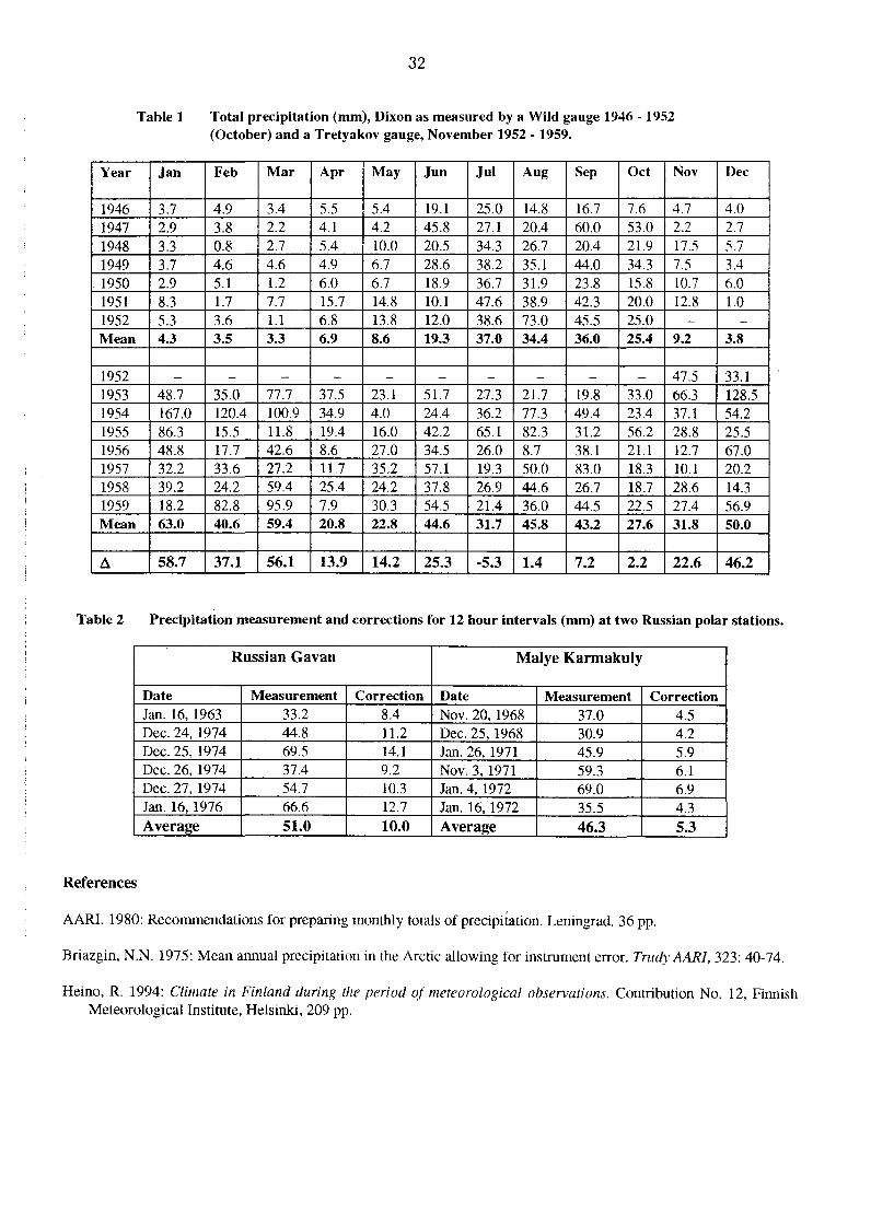
Year

1946 1947 1948 1949 1950 1951 1952 Mean

1952 1953 1954 1955 1956 1957 1958 1959 Mean

~

32

Table 1 Total precipitation (mm), Dixon as measured by a Wild gauge 1946 -1952 (October) and a Tretyakov gauge, November 1952- 1959.

Jan Feb Mar Apr May Jun Jul Aug Sep Oct Nov

3.7 4.9 3.4 5.5 5.4 19.1 25.0 14.8 16.7 7.6 4.7 2.9 3.8 2.2 4.1 4.2 45.8 27.1 20.4 60.0 53.0 2.2 3.3 0.8 2.7 5.4 10.0 20.5 34.3 26.7 20.4 21.9 17.5 3.7 4.6 4.6 4.9 6.7 28.6 38.2 35.1 44.0 34.3 7.5 2.9 5.1 1.2 6.0 6.7 18.9 36.7 31.9 23.8 15.8 10.7 8.3 1.7 7.7 15.7 14.8 10.1 47.6 38.9 42.3 20.0 12.8 5.3 3.6 1.1 6.8 13.8 12.0 38.6 73.0 45.5 25.0 -

4.3 3.5 3.3 6.9 8.6 19.3 37.0 34.4 36.0 25.4 9.2

- - - - - - - - - - 47.5 48.7 35.0 77.7 37.5 23.1 51.7 27.3 21.7 19.8 33.0 66.3 167.0 120.4 100.9 34.9 4.0 24.4 36.2 77.3 49.4 23.4 37.1 86.3 15.5 11.8 19.4 16.0 42.2 65.1 82.3 31.2 56.2 28.8 48.8 17.7 42.6 8.6 27.0 34.5 26.0 8.7 38.1 21.1 12.7 32.2 33.6 27.2 11.7 35.2 57.1 19.3 50.0 83.0 18.3 10.1 39.2 24.2 59.4 25.4 24.2 37.8 26.9 44.6 26.7 18.7 28.6 18.2 82.8 95.9 7.9 30.3 54.5 21.4 36.0 44.5 22.5 27.4 63.0 40.6 59.4 20.8 22.8 44.6 31.7 45.8 43.2 27.6 31.8

58.7 37.1 56.1 13.9 14.2 25.3 -5.3 1.4 7.2 2.2 22.6

Dec

4.0 2.7 5.7 3.4 6.0 1.0

-

3.8

33.1 128.5 54.2 25.5 67.0 20.2 14.3 56.9 50.0

46.2

Table 2 Precipitation measurement and corrections for 12 hour intervals (mm) at two Russian polar stations.

Russian Gavan Malye Karmakuly

Date Measurement Correction Date Measurement Correction Jan. 16, 1963 33.2 8.4 Nov. 20, 1968 37.0 4.5 Dec. 24, 1974 44.8 11.2 Dec. 25, 1968 30.9 4.2 Dec.25, 1974 69.5 14.1 Jan. 26, 1971 45.9 5.9 Dec. 26, 1974 37.4 9.2 Nov.3, 1971 59.3 6.1 Dec.27, 1974 54.7 10.3 Jan. 4, 1972 69.0 6.9 Jan. 16, 1976 66.6 12.7 Jan. 16, 1972 35.5 4.3 Average 51.0 10.0 Average 46.3 5.3

References

AARI. 1980: Recommendations for preparing monthly totals of precipitation. Leningrad. 36 pp.

Briazgin, N .N. 1975: Mean annual precipitation in the Arctic allowing for instrument error. Trudy AARI, 323: 40-74.

Heino, R. 1994: Climate in Finland during the period of meteorological observations. Contribution No. 12, Finnish Meteorological Institute, Helsinki, 209 pp.

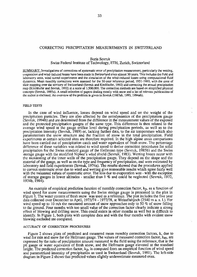
33

CORRECTING PRECIPITATION MEASUREMENTS IN SWITZERLAND

Boris Sevruk: Swiss Federal Institute of Technology, ETH, Zurich, Switzerland

SUMMARY: fuvestigations of corrections of systematic error of precipitation measurement, particularly the wetting, evaporation and wind-induced losses have been made in Switzerland since almost 30 years. This includes the field and laboratory tests, wind tunnel experiments and the simulation of the wind-induced losses using computational fluid dynamics. Mean monthly corrections were assessed for the 30-year reference period, 1951-1980, with the aims of their mapping over the territory of Switzerland (Sevruk and Kirchhofer, 1992) and correcting the annual precipitation map (Kirchhofer and Sevruk, 1992) at a scale of 1:500.000. The correction methods are based on simplified physical concepts (Sevruk, 1985a). A small selection of papers dealing mostly with snow and a list of relevant publications of the author is enclosed. An overview of the problem is given in Sevruk (1987ab, 1993, 1994ab).

FIELD TESTS

In the case of wind influence, losses depend on wind speed and on the weight of the precipitation particles. They are also affected by the aerodynamics of the precipitation gauge (Sevruk:, 1994b) and are determined from the difference in the measurement values of the exposed and the protected precipitation gauges of the same type. This difference is then related to the average wind speed at the gauge orifice level during precipitation periods, as well as to the precipitation intensity (Sevruk:, 1989) or, lacking further data, to the air temperature which also parameterizes the snow structure and the fraction of snow in the total precipitation. Field experiments at certain selected sites are therefore required. In the high alpine areas comparisons have been carried out of precipitation catch and water equivalent of fresh snow. The percentage difference of these variables was related to wind speed to derive correction procedures for solid precipitation for the Swiss standard gauge of the Hellmann type (Sevruk:, 1985b) and the Swiss storage gauge with the modified Nipher's wind shield (Sevruk, 1983). Wetting losses occur with the moistening of the inner walls of the precipitation gauge. They depend on the shape and the material of the gauge, as well as on the type and frequency of precipitation, and were estimated by laboratory and field experiments (Sevruk:, 1974a). The results showed that the procedures applied to correct systematic error due to wind and wetting give reasonable results which agree fairly well with the measured values of systematic error. The loss due to evaporation was - with the exception of storage gauges in lower altitudes - smaller than 1 % and could be neglected (Sevruk, 1972, 1974b, 1984).

An example of empirical prediction function of monthly correction factor, kp. as a function of wind speed for snow measurements using the Swiss storage gauge is presented in the plot in Figure 1. The water content of fresh snow was used as a reference. The plot includes the five year data collected over December to April, 1973n4- 1977n8, at Weissfluhjoch (2540 m a. s.l.). For wind speed up to 10 m/s the measured amount of snow approaches only to 50 % of snow falling to the ground. Four months with too small value of the correction factor clearly indicate a strong effect of blowing and drifting snow. This could exists in other months as well but is difficult to identify. In Figure 1, both plots with complete data and with the four months with evident snow blowing excluded are compared.

ACCURACY OF CORRECTION PROCEDURES

Figure 2 shows plots of predicted and measured mean monthly correction factors, k, due to wind for rain and snow for the Hellmann gauge. The values of measured correction factor, km, are expressed by the ratio of precipitation amount measured in the field using the reference, that is the pit gauge or water equivalent of fresh snow, and the Hellmann gauge elevated at the standard height. The predicted correction factor, kp. is computed from an empirical function of wind speed and parametrized intensity of precipitation as used in Switzerland (Sevruk:, 1981). The left-side diagram in Figure 2 shows that predicted values slightly underestimate measured ones.

Figure 1

Figure 2

3

km

2.5

2

1.5

. 5

y = .069x + .916, r2 = .266

WEISSFLUHJOCH

o+-~~--~~~--~~~--~~ 0 2 3 4 5 6 7 8 9 10

U [m s-1]

34

3 km y = .07x + .974, r2 = .334

WEISSFLUHJOCH 2 · 5 SELECTION

2

1.5

.5

0+-~~--~~~--~~~--:-~ 0 2 3 4 5 6 7 8 9 10

u (ms-1]

Plots of monthly correction factor, km, against wind speed. Uhp· at the level of the gauge orifice for the Swiss storage gauge at Weissfluhjoch (2540 m a. s.l.). Left: complete data set, right: four months with very low km values indicating blowing and drifting snow are excluded. The regression equation is

placed on the top of each diagram. The variable x indicates wind speed in m s-1 ( Sevruk, 1983).

1.08 1.8 km km 10 1.07 1.7

1.06 1.6

1.05 1.5

1.04 1.4

1.03 1.3 8

1.02 1.2

1.01 1.1

1~~--~--~~--~--~~--~ 1.01 1.02 1.03 1.04 1.05 1.06 1.07 k 1.08

p 1 1.1 1.2 1.3 1.4 1.5 1.6 1. 7 1.8

kp

Plots of predicted correction factors due to wind, kp. against the measured correction factors, km for rain (left) and snow (right). Left diagram refers to mean monthly rain totals at two different stations (crosses and points) (Sevruk (1981). The measured correction factors were obtained from measurements of the pit gauge (reference) and the elevated Hellmann gauge. Right diagram refers to average values of snow measurements from seven stations using Hellmann gauges and the water content of fresh snow as a reference. The data set was subdivided into temperature intervals of 1° C for the range from -1 to -10° C and wind speed from 1.2 to 3 .0 m s-1 ( Sevruk, 198Sb).

APPLICATION OF CORRECTIONS

To apply the corrections, it is of prime importance to consider whether all the variables required are available at the gauging site. Thus the correction methods depend on the type of precipitation gauge and the measurement station which differ in the availability of meteorological data on wind and air temperature and particularly, the wind exposure. At protected sites (e.g. forest clearings, parks, village centres or farms) corrections are normally low, whereas at exposed sites (e.g. open windward slopes, mountain passes or lake shores) they are high. While these data are directly available at the 104 Swiss climatological stations, they have to be inferred for the 230 precipitation stations. The assessment of exposure class is based on site history recorded in the archives of the Swiss Meteorological Institute, documented by photos, sketches, and written reports, as well as on topographical maps at a scale of 1 :25000. Four classes of exposure were used: open site, mostly open and mostly protected site and protected site (Sevruk and Zahlavova, 1994).

35

Problems arise when determining the wind speed. It is only measured at climatological stations, at a height of more than 10 m above ground, as in most cases only three times per day. For the remaining sites, the wind speed had therefore to be estimated. In addition, the wind speed had to be convened into the height of the precipitation gauge above ground, as well as into the periods of precipitation.

Using the similarity principle, the average annual wind speed was transferred from measured to unmeasured sites, taking into consideration the regional wind fields. The reduction of wind speed to the level of the precipitation gauge orifice was based on the logarithmic wind profile and the average vertical angle of obstacles around the gauging site, as measured in the eight directions of the wind rose, using a simple optical instrument. This angle characterises the average vertical elevation above the horizon of the surrounding obstacles and is a good measure of the gauge site protection against wind. It can be estimated by means of the gauge site exposure class as mentioned above (Sevruk and Zahlavova, 1994). Empirical coefficients were used for the reduction to precipitation periods, assuming that depending on the region, the wind speeds during precipitation were equal to or greater than the climatic values.

The above mentioned procedures have been used for the Hellmann gauges only. For the storage gauges fitted with a wind shield, a different method was applied. Because no wind speed data were available, the corrections were estimated from an empirical function based on intercomparison measurements, using the gauge site altitude and exposure degree as variables (Sevruk and Kirchhofer, 1992).

The wetting losses for the Hellmann gauge amount to an average of 0.3 mm on a rainy and 0.15 mm on a snowy day (Sevruk, 1974a, 1985c). The monthly number of days with rain and snow was estimated from the number of precipitation days of a particular period using the portion of snow in total precipitation. The latter depends on temperature or the altitude. The relevant relationships have been derived for the Swiss conditions (Sevruk, 1985a). To assess the altitude dependency of the air temperature, a data set of 104 climatological stations was used (period 1971-1980). The average monthly fraction of snow was determined in a similar way, though only 54 stations for the span of 1959-1970 were available for the regression analysis.

The correction values increase absolutely and relatively with increasing altitude, from approximately 100 mm to 700 mm; this corresponds to 5-25 % of the measured values. At lower altitudes, the wind speed tends to be low as a result of the greater roughness (forests and built-up areas) and the topographic barriers. The small fraction of snow and the substantial wind protection of the stations also have a positive effect. Compared to this, the correction values in the snow-rich and wind-exposed high alpine regions are excessively high. The magnitude of the corrections, however, is also influenced by the type of instrument used. For the Hellmann precipitation gauge (without wind shield) they are considerably greater than for the storage gauge fitted with a wind shield.

The comparison of correction values for selected, small square areas of 25 km x 25 km situated in nine different regions of Switzerland showed a range from 8-10 % in the six regions (Winterthur-Zurich; Fribourg Alps; Orbe-Eschallens; Basel-Land; Oberaargau-Emmental and Valle Maggia) to approximately 20% in Saastal (Valais). The relative small correction values as for the high altitude areas (Fribourg, Unterengadin) are due to the use of storage gauges as preferred in such region.

The results show that the correction of systematic error of precipitation measurement can be estimated even for gauge sites with missing input variables, such as wind speed, temperature and portion of snow in total precipitation. These variables can be derived by analogy and regionalized vertical gradients. Based on such procedures and kriging, the correction can be computed and isolines drawn over a territory of a country.

WIND TUNNEL EXPERIMENTS

The results of a series of wind tunnel tests indicate that different types of precipitation gauges show different parameters of wind field deformation above the gauge orifice, particularly the

36

maximum wind speed increase and the turbulence vary considerably. The range of the former was from 25 to 50 % for seven types of gauges (Sevruk et al., 1989). This reveals some basic principles of the physics of precipitation gauges (Sevruk et al., 1994). The results confirm the fact that the wind-induced loss of precipitation measurement depends on construction parameters of precipitation gauges and they can assist: (i) to explain differences between precipitation values as measured at the same spot in the field using different types of precipitation gauges, (ii) to check the results of computations of the flow over gauges, (iii) to develop and to improve the correction procedures for wind-induced losses and (iv) to develop better precipitation gauges.

NUMERICAL SIMULATION OF WIND-INDUCED LOSSES

In addition to the field experiments, the wind-induced error was estimated using a complex three-dimensional numerical procedure in two steps: Firstly, the air flow around the gauge was simulated using PHOENICS software (k-e turbulence model) and compared with the direct measurements in the wind tunnel. The comparison showed a good agreement. Secondly, the trajectories of water drops of different sizes were computed in the simulated flow fields and combined into different drop size distributions to correspond with real rainfall events. The integration resulted in a formula giving the integral wind-induced error as a function of the wind speed, the rate of rainfall, and the drop size distribution (Nespor, 1995). A comparison of results with empirical models for different types of gauges showed a fairly well agreement. It explained also the different magnitude of wind-induced error among different types of gauges as a function of the gauge construction parameters, particularly the gauge diameter. For instance, between the two different types of gauges used in Switzerland, the slightly robust ASTA gauge shows a greater computed wind-induced error than the smaller Hellmann gauge, the same tendency as observed in field measurements.

CONCLUSIONS

The agreement of results of field and laboratory experiments, numerical simulations and wind tunnel tests, confirms the existence of the systematic errors of precipitation measurements due to wind, wetting and evaporation. There is a need for the world-wide application of corrections, particularly for solid precipitation measurements. The correction methods are based on simplified physical concepts and were derived by using intercomparison measurements with the WMO reference gauges. They depend on the type of precipitation gauge used, the form, structure and frequency of precipitation events and the wind speed at the level of the gauge orifice. For stations in the Swiss midland and in the valleys of Ticino, Valais, Central Switzerland and Engadin only small corrections of annual precipitation totals, up to 10 %, need to be made, larger ones are required for stations in northern and western Switzerland, the Jura and the lower alpine regions, and major corrections are necessary for the stations in the high alpine regions.

References

Nespor, V., 1995: Investigation of wind-induced error of precipitation measurements using a three-dimensional numerical simulation. Swiss Federal Institute of Technology, ETH, Zurich, Diss. No. 11 060, 110 p.

Kirchhofer, W. and B. Sevruk, 1992: Mean annual corrected precipitation amounts 1951-1980. In: M. Spreafico, R. Weingartner and Ch. Leibundgut (Editors). Hydrological Atlas of Switzerland, Part 2.2, Landestopographie Bern.

Sevruk, B., 1972: Evaporation losses from storage gauges. In: Distribution of precipitation in mountainous areas. WMO-Publ. 326(2), 96-102.

Sevruk, B., 1974a: Correction for the wetting loss of a Hellmann precipitation gauge. Hydrol. Sci. Bull., 19 (4), 549-559.

Sevruk, B., 1974b: Evaporation losses from containers of Hellmann precipitation gauges. Hydrol. Sci. Bull., 19 (2), 231-236.

37

Sevruk, B., 1981: Methodical investigation of systematic error of Hellmann rain gauges in the summer half-year in Switzerland (in German). Trans. Versuchsanstalt fiir Wasserbau, Hydrologie and Glaciology, Swiss Federal Institute of Technology, ETH ZUrich, No. 52, 297 pp. Ziirich.

Sevruk, B., 1983: Correction of measured precipitation in the Alps using the water equivalent of new snow. Nordic Hydrology, 14 (2), p. 49-58.

Sevruk, B., 1984a: Comparison of evaporation losses from standard precipitation gauges. In: Proc. TECEMO/WMO, September 24-28, 1984, Noordwijkerhout. Instruments and Observing Methods Rep., No. 15,57-61.

Sevruk, B. 1985a Correction of precipitation measurements: Swiss experience. In: B. Sevruk (Ed.) Proc. Workshop on the Correction of Precipitation Measurements. WMO/ID-No. 104, p. 187-196.

Sevruk, B., 1985b: Conversion of snowfall depths to water equivalents in the Swiss Alps .. In: B. Sevruk (Ed.) Proc. Workshop on the Correction of Precipitation Measurements. WMO/fD-No. 104, 81-88.

Sevruk, B., 1985c: Correction of monthly precipitation for wetting losses. WMO Instruments and Observing Methods Rep., No. 22, WMO/fD. No. 50, 7-11.

Sevruk, B., 1987a: Point precipitation measurements: why are they not corrected? In: J. C. Rodda and N. C. Matalas (Eds.), Proc. Water for the Future: Hydrology in Perspective, Internat. Assoc. Hydrol. Scie., IAHS, Publ. No. 164, 477-486.

Sevruk, B., 1987b: On difficulties of checking storage gauges. In: Proc. 13th Conference of Carpathian Meteorology. Institute of Meteorology and Hydrology, Bucharest, 169-174.

Sevruk, B., 1989: Wind-induced measurement error for high-intensity rains. In: B. Sevruk (Editor) Precipitation Measurement. Proc. International Workshop on Precipitation Measurement, St. Moritz, Switzerland, 3.-7. December, 1989. Institute of Geography, Swiss Federal Institute of Technology, ETH Zurich, p. 199-204.

Sevruk, B., 1993a: Checking precipitation gauge performance. In: S. Couling (Ed.). Measurement of airborne pollutants. Butterworth Heinemann, Oxford, p. 89-107.

Sevruk, B., 1993b: The effect of dimensions and shape of precipitation gauges on the wind-induced error. In: S. Couling (Ed.). Measurement of airborne pollutants. Butterworth Heinemann, Oxford, p. 231-246.

Sevruk, B., 1994: Spatial and temporal inhomogeneity of global precipitation data In: M. Desbois and F. Desalmand (Eds.) Global precipitation and climate change. NATO ASI Series, Springer Verlag, Berlin, Vol. I 26, 219-230.

Sevruk, B., J.-A. Hertig and R. Spiess, 1989: Wind field deformation above precipitation gauge orifices. Internat. Assoc. Hydrol. Scie., IAHS Publ. No. 179, 65-70.

Sevruk, B., J.-A. Hertig and R. Tettamanti, 1994: The effect of orifice rim thickness on the wind speed above precipitation gauges. Atmosph. Envir., 28(11), 1939-1944.

Sevruk, B. and W. Kirchhofer, 1992. Mean annual corrections of measured precipitation amounts 1951-1980. In: M. Spreafico and R. Weingartner (Editors). Hydrological Atlas of Switzerland, Part 2.3, Landestopographie Bern.

Sevruk B. and L. Zahlavova, 1994: Classification system of precipitation gauge site exposure: Evaluation and application. Internat. J. Climatol., 14(6), 681-689.

38

IN SITU SOLID PRECIPITATION MEASUREMENT ADJUSTMENTS: THE U.S. EXPERIENCE

Pavel Ya. Groisman, University ofMassachusetts, Amherst, Massachusetts, USA David R. Easterling & Robert G. Quayle, National Climatic Data Center, Asheville,North Carolina, USA

Valentin S. Golubev, State Hydrological Institute, St. Petersburg, Russia, and Eugene L. Peck, HYDEX, Vienna, Virginia, USA

Adjustment procedures for reducing the bias in precipitation point measurements of standard US. rain gauges are discussed The procedures presented here employ information about wind speed variations over the gauge orifice during precipitation events, and extensive metadatafiles which trace the history of precipitation measurements at each site throughout the period of instrumental observations (gauge type, exposure, and site climatology).

INTRODUCTION. The existing U.S. rain gauge network measures

snowfall with a bias of up to 50% percent or more (Larson and Peck 1974, Groisman and Legates 1994). The main factor is wind-induced turbulence over the gauge orifice. Because of these large systematic errors, there exists the possibility that changes of these errors with time may adversely affect the homogeneity of the frozen precipitation time series and the hydrological studies that rely upon these time series (Legates 1995, Groisman and Legates 1995). The installation of wind shields and the changes in exposure of the gauges can be a problem for climate change studies by introducing systematic non-climatic changes into measured precipitation totals (Karl et al. 1993). After spatial averaging, it can be expected that the random errors connected with such shifts will be decreased and compensate each other. However, this is not so when systematic changes in the measurement procedures occur countrywide, and several systematic changes have occurred during the last century in the North American meteorological primary networks (Karl et al. 1993, Groisman and Easterling 1994).

ADJUSTMENT PROCEDURE. A typical adjustment procedure of precipitation

time series is based on methods developed by American, Swiss, and Russian climatologists (Bogdanova 1966, Golubev 1969, WWB 1974, Larson and Peck 1974, Sevmk 1982, Legates 1987). The formulas of such adjustments a.re: Adjusted Precipitation=

K(W,h,H)*(Measure Precipitation + ~P), (1) where K is a function of wind speed, W, gauge and anemometer elevations, h and H, specific for each type of gauge and precipitation type (liquid, mixed, or frozen); in ~p we accumulate a set of additive adjustments specific for gauge type and observational practice. Sometimes instead

of precipitation type surface air temperature is substituted (Allemp et al. 1995).

The adjustments for frozen precipitation measured by standard U.S. rain gauges are large and are based on the relationships between snow undercatch by the gauge and wind speed over its orifice during the precipitation event (Larson and Peck 1974, Peck 1993, Golubev 1993). These relationships are described by steep functions of wind speed for each type of gauge. Therefore, a knowledge of the wind speed over the gauge orifice during precipitation events, w, is critical to the proper evaluation of adjustments. This speed is not measured by the operational network, but

is available only from special experiments. We use the following formula for this wind speed:

w = W*f(a)*A*ln(h/z.o)/In(H/z.o), (2) where W is the mean daily wind speed recorded (or interpolated) at the height H of the wind gauge; h is the elevation of the gauge orifice; Zo is the meteorological dynamic roughness parameter of the ground; A is an amplification coefficient of the wind during precipitation events as compared to the mean daily wind speed (we constmcted maps of these coefficients for the U.S. for each type of precipitation); and f( a) is a function of a, the mean vertical angle from the gauge orifice to the top of obstmctions, derived by Fedorova (1966). The information about a, H, z0, h. the type of the gauge, and the set of supplementary fields necessary for precipitation adjustments are derived from the metadata files. These metadata consist of topography of the stations, descriptions of the rain and wind gauges used, gauge exposure (information about wind obstacles, their distance from the gauge, and their height), gauge elevation, and changes in these variables with time. The metadata files are completed for approximately 1500 U.S. stations (including all Alaskan stations). They provide the information necessary for estimation ofnonclimatic changes in the gauge catch.

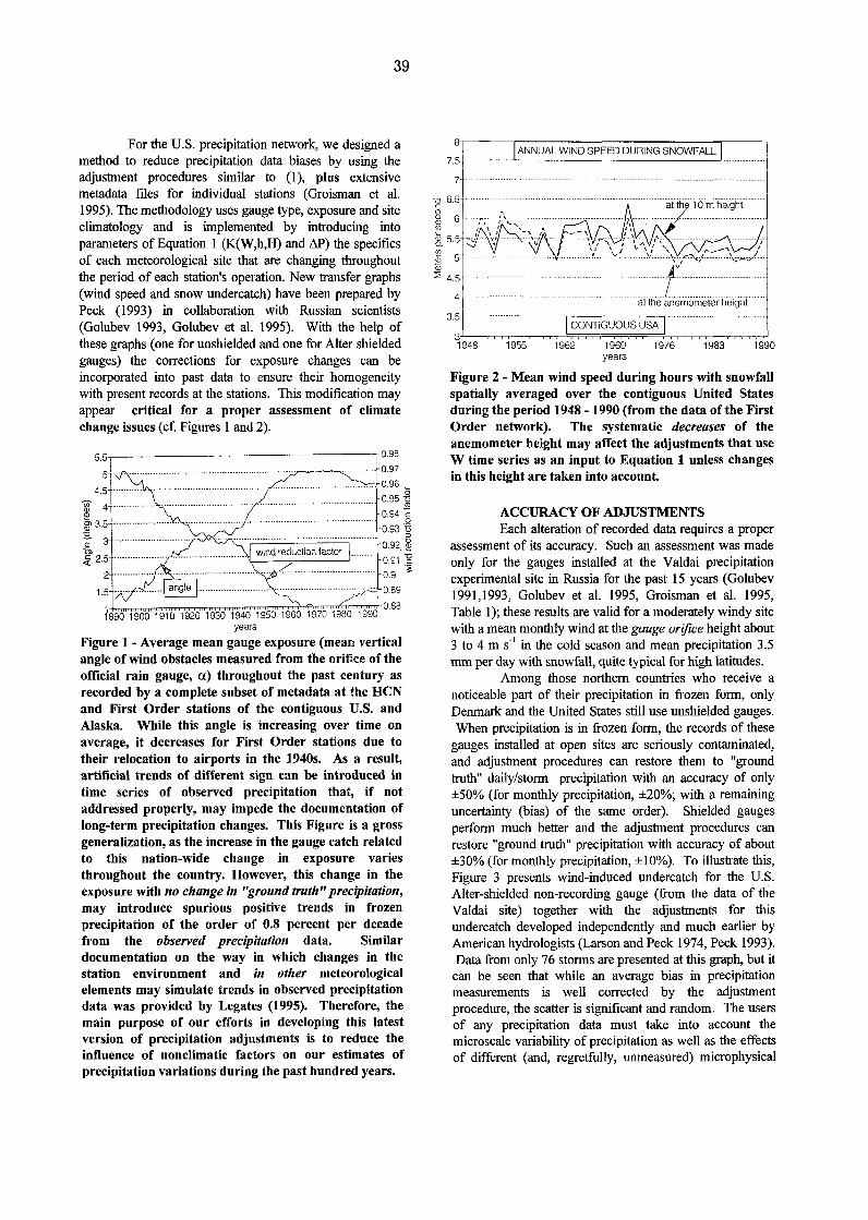
39

For the U.S. precipitation network, we designed a method to reduce precipitation data biases by using the adjustment procedures similar to (1), plus extensive metadata files for individual stations (Groisman et al. 1995). The methodology uses gauge type, exposure and site climatology and is implemented by introducing into parameters of Equation 1 (K(W,h,H) and M>) the specifics of each meteorological site that are changing throughout the period of each station's operation. New transfer graphs (wind speed and snow undercatch) have been prepared by Peck (1993) in collaboration with Russian scientists (Golubev 1993, Golubev et al. 1995). With the help of these graphs (one for unshielded and one for Alter shielded gauges) the corrections for exposure changes can be incorporated into past data to ensure their homogeneity with present records at the stations. This modification may appear critical for a proper assessment of climate change issues (cf. Figures 1 and 2).

5_5-,-----------------1 o.es

4.~ -----------------------:·-:::::::::::::::::::::~ ~:::~ w 4 --------------- ------------- 0.94-;::: Q) 0 g, 3.5 ---------------------- -- - -------------------- ----------- ----------- ---- - ------------- 0.93 -~

i 2.: ::::::::::::::::::::--::::::: ____ : _____ ::: ___ :::::r~;~~-;~~~~;~~~-;~~;~;-r::::::: ~::~ ~ -·-·w -- --------------------- 0.9 -~

1.5 ------ -- ------- angle -------------------- ----------------= 0.89

1s9o 1900 1910 1920 1930 1940 19SO 1960 197o 1980 i9eo 0

'88

years

Figure 1- Average mean gauge exposure (mean vertical angle of wind obstacles measured from the orifice of the official rain gauge, a) throughout the past century as recorded by a complete subset of metadata at the HCN and First Order stations of the contiguous U.S. and Alaska. While this angle is increasing over time on average, it decreases for First Order stations due to their relocation to airports in the 1940s. As a result, artificial trends of different sign can be introduced in time series of observed precipitation that, if not addressed properly, may impede the documentation of long-term precipitation changes. This Figure is a gross generalization, as the increase in the gauge catch related to this nation-wide change in exposure varies throughout the country. However, this change in the exposure with no change in "ground truth" precipitation, may introduce spurious positive trends in frozen precipitation of the order of 0.8 percent per decade from the observed precipitation data. Similar documentation on the way in which changes in the station environment and in other meteorological elements may simulate trends in observed precipitation data was provided by Legates (1995). Therefore, the main purpose of our efforts in developing this latest version of precipitation adjustments is to reduce the influence of nonclimatic factors on our estimates of precipitation variations during the past hundred years.

ANNUAL WIND SPEED DURING SNOWFALL

4-

35 - ............. ,CONTIGUOUS USA ~-31~~~~~~~~rn~~~~~~~~~~ 1948 1955 1962 1969

years 1976 1983 1990

Figure 2 - Mean wind speed during hours with snowfall spatially averaged over the contiguous United States during the period 1948-1990 (from the data of the First Order network). The systematic decreases of the anemometer height may affect the adjustments that use W time series as an input to Equation 1 unless changes in this height are taken into account.

ACCURACY OF ADJUSTMENTS Each alteration of recorded data requires a proper

assessment of its accuracy. Such an assessment was made only for the gauges installed at the Valdai precipitation experimental site in Russia for the past 15 years (Golubev 1991,1993, Golubev et al. 1995, Groisman et al. 1995, Table 1); these results are valid for a moderately windy site with a mean monthly wind at the gauge orifice height about 3 to 4 m s-1 in the cold season and mean precipitation 3.5 mm per day with snowfall, quite typical for high latitudes.

Among those northern countries who receive a noticeable part of their precipitation in frozen form, only Denmark and the United States still use unshielded gauges. When precipitation is in frozen form, the records of these

gauges installed at open sites are seriously contaminated, and adjustment procedures can restore them to "ground truth" daily/storm precipitation with an accuracy of only ±50% (for monthly precipitation, ±20%; with a remaining uncertainty (bias) of the same order). Shielded gauges perform much better and the adjustment procedures can restore "ground truth" precipitation with accuracy of about ±30% (for monthly precipitation, ±10%). To illustrate this, Figure 3 presents wind-induced undercatch for the U.S. Alter-shielded non-recording gauge (from the data of tlie Valdai site) together with the adjustments for this undercatch developed independently and much earlier by American hydrologists (Larson and Peck 1974, Peck 1993). Data from only 76 storms are presented at this graph, but it

can be seen that while an average bias in precipitation measurements is well corrected by the adjustment procedure, the scatter is significant and random. The users of any precipitation data must take into account the microscale variability of precipitation as well as the effects of different (and, regretfully, unmeasured) microphysical

40

properties of snowflakes in different storms. The scatter shown in Figure 3 is an illustration of this variability in the adjustment procedure.

wind speed (m/sec)

E. Peck formula

Figure 3 - Wind undercatch of the Alter-shielded non­recording U.S. gauge as determined from 76 snow storms at the Valdai precipitation polygon, Russia; and the undercatch modeled by Peck (1993). The data have been adjusted with a wetting correction. All negative values on this graph (i.e., overcatch) are related to very light precipitation events (less then 5 mm per storm). Adapted from Groisman et al. (1995).

EXAMPLE

Duluth International Airport (MN) First Order station. During the past 45 years at this station, the anemometer height was changed twice, rain gauge height and type were changed four times; and the exposure of the rain gauge changed several times. Especially important for the solid precipitation catch was the 1960 installation of an Alter wind shield for the rain gauge. It has remained in operation since 1960, with a short interruption in 1975-1976 (and measured January precipitation was about half of its bias­adjusted value during this interruption). Mean January wind speed over the gauge orifice, w, at this station changes through the time following the changes in the gauge exposure and W. W is quite stable for periods of constant height of the anemometer. Therefore, when we replace the monthly wind speed, W, with its long-term mean values and recalculate the corresponding wind adjustment coefficients using these long-term mean values, the time series of adjusted monthly precipitation does not show a notable change. This supports the hypothesis that reliable precipitation adjustments can be obtained from long-term mean values of W from First Order stations. As a large scale generalization, we believe these results for First Order stations can be interpolated to neighboring cooperative stations that do not have wind measurements. But we have found that metadata (especially information about gauge shielding) is critical for proper evaluation of the "ground truth" from the conventional precipitation measurements. Climatological wind data over the United States are readily

available from less than 300 locations. The robustness of our adjustment procedure (for monthly precipitation) to the use of long-term climatological values of wind, instead of the actual values, as shown in this Figure, suggests that this deficiency of the U. S. network will not substantially affect the accuracy of the bias-adjusted precipitation data. On the contrary, the accuracy of point measurements of solid precipitation by unshielded gauges represents a major concern. Users of these observations must be aware of this and use these data accordingly.

Wind Speed

Wind Adjustment ::oefficient

M~asured

and Adjusted

Precipitation

(b)'·-~-~

___ climaioiOQical wmd..lldJustmants __ ·--- _ --· _ --1

Figure 4 - January wind speed and precipitation at Duluth International Airport, MN: (a) wind speed at 16.2 m above the ground (the anemometer elevation in the 1950s) and over the orifice of the official rain gauge during precipitation events; (b) wind adjustment coefficients for monthly precipitation, i.e., K(W,h,H) functions in Equation 1 based on the work of Larson and Peck (1974); (c) mean monthly precipitation measured and adjusted for wind and wetting losses from the gauge. Two types of wind data, W, were used: the long-term mean monthly climatological wind at the height of the anemometer (dashed lines), and actual mean monthly wind speeds for each year-month (solid lines). For the adjusted precipitation time series in (c) these two lines coincide (r=0.997), and appear to be one line. Comparison of adjusted and unadjusted precipitation time series in this example shows that the interannual variability dominates over the decadal or longer variability in these time series as in any other point precipitation record throughout the world. Therefore, systematic changes in precipitation catch related to exposure and other factors described above are often not evident. When precipitation data are averaged over time and/or spatially, all these systematic biases and inhomogeneities stay in the data and can contaminate studies of climate change and hydrology.

41

Table 1. Accuracy of precipitation bias adjustments(%) applied to observations made by different gauges at the Valdai experimental site. Data for U.S. gauges are preliminary (Golubev 1991. 1993, Groisman et al. 1995).

Gauge Type

WMO standard for solid precipitation intercomparison Russian standard gauge (Tretiak:ov shielded gauge) U.S. 8" non-recording gauge with Alter wind shield U.S. 8" non-recorded unshielded gauge Mean daily precipitation (mm)

REFERENCES:

Allerup, P., Madsen, H., and Vejen, F. E., 1995: A comprehensive model for correcting point precipitation. Nordic Hydrology, 26, (in press).

Bogdanova, E. G., 1966: Investigation of precipitation measurement losses due to the wind (in Russian). Trans. of Main Geophys. Observ., Leningrad, 195,40-62 (in Russian; English translation, # 70-59013, is available from the U.S. National Technical Information Service, Operations Division, Springfield, VA 22151).

Fedorova, E. A., 1966: Calculation of wind speed at the level of the precipitation gauge considering the degree of station protection. Trans. of Main Geophys. Observ., 195, 63-69 (in Russian; English translation, #5828.4F(7079), is available from the National Lending Library for Science and Technology, Boston Spa, Yorkshire, UK).

Golubev, V. S., 1969: Research on precipitation measurement accuracy. Trans. of State Hydrol. Inst., 176, 149-164 (in Russian).

------• 1991: Preliminary estimates of accuracy of the raingauge in double fence shield. Meteorologia i Gidrologia, No.2, 116-121 (in Russian; In English in Soviet/Russian Meteorology and Hydrology, 1991, No.2).

______ 1993: Experience of correction of precipitation point measurements and analysis of correction procedures. AMS Proc., Eighth Symposium on Meteorological Observations and Instrumentation, Anaheim, CA, 325-328.

-----• Groisman, P. Ya., and Quayle, R. G., 1992: An evaluation of the U.S. standard 8-inch

nonrecording rain gage at the Valdai polygon, USSR. J. Atmos. Oceanic Technol., 49,624-629.

-----• Koknaeva, V. V., Simonenko, A. Yu., 1995: Results of atmospheric precipitation measurements by national standard gauges of Canada, USA, and Russia. Meteorologia i Gidrologia, No. 2, 102-110 (in Russian; in English in Russian Meteorology and Hydrology, 1995, No. 2).

Daily Monthly precipitation precipitation (±%) in cold season (±%) frozen mixed

11 10 39 21 46 22 50 30 3.5 6.0

6 10-12 NIA NIA NIA

Groisman, P. Ya. and Easterling, D. R., 1994: Variability and trends of precipitation and snowfall over the United States and Canada, J. Climate, 7, 184-205.

_______ and Legates, D. R., 1994: The accuracy of United States precipitation data. Bull. Amer. Meteorol. Soc., 75,215-227.

_____________________ 1995:Documenting

and detecting long-term precipitation trends: where we are and what should be done. Climate Change, (in press).

______ , D.R. Easterling, R.G. Quayle, V.S. Golubev, A.N. Krenke, A.Yu. Mikhailov, 1995: Reducing biases in estimates of precipitation over the United States: phase three adjustments. J. Geophys. Res., (in press).

Karl, T. R., Quayle, R. G., and Groisman, P. Ya., 1993: Detecting climate variations and change: New challenges for observing and data management systems. J. Climate, 6, 1481-1494.

Larson, L. W., and Peck, E. L., 1974: Accuracy of precipitation measurements for hydrologic modeling. Water Resour. Res., 10, 857-863.

Legates, D. R., 1987: A climatology of global precipitation. Publ. Climatal., 40(1), 84 pp.

_______ 1995: Precipitation measurement biases and climate change detection. AMS. Proc., Sixth Symposium on Global Change Studies, Dallas, TX, 168-173.

Peck, E. L., 1993: Adjusted precipitation records: methods and example. Report of HYDEX Corporation to National Climatic Data Center in the framework of the NOAA Project "Development of North American Unbiased Precipitation Data Set for GCIP", 36 pp. + Appendices.

Sevruk, B., 1982: Methods of correction for systematic error in point precipitation measurement for operational use, Operational Hydrology Report No. 21, Publ. 589, World Meteorological Organization, Geneva, Switzerland, 91 pp.

World Water Balance and Water Resources of the Earth (WWB), 1974: Gidrometeoizdat, Leningrad, 638 pp. (in Russian; published in English by UNESCO Press, 1978).

42

Daily Precipitation Measured at the "North Pole" Stations

R. Colony Director, International ACSYS Project Office, Oslo, Norway

The Soviet Union had a long tradition of conducting scientific investigations from drifting ice stations. First demonstrated by Papanin in 1937-38, the "North Pole" (NP) series manned scientific stations on drift ice were a regular feature of Soviet arctic science from 1950 through 1991. In all, thirty one NP ice stations were occupied for a mean duration of about two and a half years. For many years two, and sometimes three, stations were in simultaneous operation. For the most part, the stations were confined to the central Arctic Basin.

Daily precipitation was measured as part of the standard meteorological programme carried out at all NP stations. In 1954 (NP- 3) the Tretyakov precipitation meter (PM- 1) was introduced and precipitation was measured twice daily, at 06:00 and 18:00 Moscow time. For the period 1954 - 1991, 68 station years of precipitation observation, both amount and type, were reported by the NP stations.

The Arctic and Antarctic Research Institute (AARI), Russian Federation, in cooperation with the Environmental Research Institute of Michigan (ERIM), USA, created an electronic data base of precipitation measurements taken at the NP stations. This data base is now under review by scientists from both AARI and ERIM. By early 1996, the data base should be ready for submission to a World Data Center and available to the international community. A preliminary analysis of the mean seasonal cycle of precipitation is in agreement with a Gorshkov analysis ("Atlas ofthe Arctic Ocean", 1980).

The precipitation measurements from the NP stations are almost alone in defining the climate of the Arctic Basin. Fortunately this data set is complemented by the complete meteorological measurements made at the NP stations. These include standard surface observations, atmospheric soundings, cloud observations, and radiation measurements. Additionally, snow accumulation and melt was routinely measured at all NP stations. The accuracy of in situ solid precipitation measurements has always been held in question. Covariance studies of precipitation and other geophysical parameters should help quantify these errors.

43

Snow Measurements During the SEVER Program

R. Colony Director, International ACSYS Project Office, Oslo, Norway

In 1948 the Soviet Union began a series of comprehensive airborne hydro graphic surveys of the Arctic Ocean and adjacent Siberian marginal seas. The annual surveys were conducted from mid-March through early May when weather and ice conditions favored aircraft landings on unattended ice floes. From 1948 through 1988 hydrographic measurements were made at about 4,000 individual sites. In the mid 1950's and again in the 1970's the central Arctic Basin was annually sampled at about 150 sites, in other years the SEVER Program focused on the Kara, Laptev, East Siberian, and Chukchi Seas. During the early part ofthe program snow and ice thickness were regarded as operational issues bearing on the safety of aircraft landings. Midway through the program Dr. Ilya Romanov recognized the scientific value of snow and ice measurements. Beginning in the early 1960's Dr. Romanov and his associates at the Arctic and Antarctic Research Institute began a systematic program of snow and ice measurements ancillary to the SEVER Program. Additionally, they began archiving the earlier snow and ice thickness measurements. Their snow and ice thickness subproject was regarded as extracurricular to the hydro graphic work and not an official part of SEVER, thus for many years the data resided in personal archives.

In 1994 the Environmental Research Institute ofMichigan (ERIM), USA, negotiated with Dr. Romanov to make his archived snow data available to the international community. ERIM and Dr. Romanov agreed to create a uniform data base and submit it to the World Data Center (A) for Glaciology, USA At present, the data base contains all measurements related to 11 snow parameters and one ice parameter (thickness of runway ice). The snow parameters are: 1) height on runway; 2) height on prevailing ice; 3) sastrugi height on runway; 4) fractional area of sastrugi on runway; 5) sastrugi height on prevailing ice; 7) length of drifts; 8) height of drifts; 9) height of snow at hummocks (windward); 1 0) height of snow at hummocks (leeward); and 11) density. Not all parameters were measured at each landing site. In addition to snow and ice parameters, some metadata were attached to the data set. The field measurements were all made according to Dr. Romanov' s specifications, thus minimizing the subjective decisions of independent data collectors. All measurements were made in the spring and can be regarded as the annual total snow accumulation prior to significant liquid precipitation and prior to the summer melt.

The principal results and many spatial patterns of snow statistics were privately published by Dr. Romanov in his monograph "Ice Cover of the Arctic Basin" (1993, English translation) and atlas "Morphometric Characteristics of Ice and Snow in the Arctic Basin" ( 1993, Russian/English). A revised and expanded edition will be available in early 1996, published by Backbone Press, New York. In addition, Dr. Romanov has published selections of these data in the Russian scientific literature.

The creation of an electronic data base for the SEVER snow measurements will serve many purposes. The data are sufficient for preliminary studies of large scale spatial statistics and interannual variability of annual snow accumulation in the Arctic Basin and marginal seas. However, their true value will be evident when compared to complementary geophysical data and analysis, e.g. contemporaneous meteorological measurements and synoptic analysis.

44

Snow Course Measurements from the "North Pole" Stations

R. Colony Director, International ACSYS Project Office, Oslo, Norway

The "North Pole" (NP) drifting ice stations maintained by the Soviet Union from 1950 through 1991 are an important source of climate data for the Arctic Ocean. The usual station platform was a multi-year sea ice floe, although low tabular icebergs were occasionally occupied. For forty years scientists at a succession ofNP stations monitored basic meteorological elements, sea ice properties, and snow conditions in the central Arctic Basin. The standardized snow program at the stations included the repeated measurement of snow height along a prescribed course.

When a drifting station was established, the snow course was marked by implanting posts at the start, mid-point, and end of the route. Most often the course length was 1,000 meters (m), although some 500 m snow courses were also maintained. The courses were always limited to the level ice, avoiding hummocked areas. Snow height along the course was measured every 10 m with a resolution of 1 centimeter. Snow density was sampled every 100 m. At most stations the snow course measurements were repeated every 30 days; some of the later ice stations used a I 0 day repeat period. The measurements were continued throughout the year, except during the snow free part of the summer.

The 10 m spaced measurements sample the profile of snow height along the course and 30 day successive measurements can be used to sample the evolution of the profile. It is important to note that repeat measurements were not at exactly the same location because the course was defined only in terms of the implanted poles. However, the location offset is thought to be less that a few meters. The snow course data are complemented by daily measurements of snow height at three fixed stakes located on the meteorological grounds. The snow stake data can be used to study the evolution of snow height at specific fixed locations.

The Arctic and Antarctic Research Institute (AARI), Russian Federation, in cooperation with the Environmental Research Institute of Michigan (ERIM), USA, has created an electronic data base of snow course and snow stake measurements taken at the NP stations. The data base is now under review by scientists at AARI and ERIM. By early 1996 the data base should be ready for submission to a World Data Center and available to the international community.

The snow height profile data can be used to estimate small scale spatial statistics. For example, an autocovariance study shows the typical variance of snow height on an ice floe is 150 cm2 and the length scale for height variability is less than 10 m. As the NP stations were occupied throughout the year, the seasonal cycle of many statistics can also be estimated, e.g. mean monthly snow height on level multiyear ice. Successive measurement of the profiles are interesting on two accounts: precipitation measured at the station can be compared to changes in the profile; and 10 m wind speed measurements can be related to the evolution of the shape of the profile. Preliminary studies indicate that monthly measured precipitation is poorly correlated with monthly changes of mean snow height along the course. Individual correlations of successive height profiles show a bimodal distribution. One mode is at high correlation and the

45

other at almost zero correlation, suggesting that the profile is either easily recognized in successive months or that the profile is completely changed within the 30 day period. Again, complementary data sets of wind, snow stake data, and measured precipitation make the North Pole snow course measurements particularly interesting and important.

47

SESSION 2 - MODEL-DERIVED PRECIPITATION CLIMATOLOGIES FOR THE ARCTIC

49

A PRELIMINARY LOOK AT MODEL-DERIVED PRECIPITATION CLIMATOLOGIES FROM THE UKMO AND ECMWF NWP MODELS

1. INTRODUCTION

H CATTLE AND J F CROSSLEY

OCEAN APPLICATIONS BRANCH METEOROLOGICAL OFFICE

BRACKNELL, UNITED KINGDOM

It has been recognised for some time now that the output of Numerical Weather Prediction (NWP) models has the potential to provide estimates of fields of the surface forcing of the ocean, including surface precipitation. The NWP model-based re-analyses currently underway at the European Centre for Medium Range Weather Forecasts (ECMWF), by the U.S. National Meteorological Centre/National Centre for Atmospheric Research and the U. S. National Aeronautic and Space Centre's Goddard Space Science Laboratory will all provide the potential for more or less consistent climatological datasets of such forcing. An important task will be to verify and intercompare these datasets and the associated meteorological fields from which they are derived so as to assess their consistency both internally and with one another and with externally-derived datasets. For the Arctic, this is an integral component of the strategy of the WCRP Arctic Climate System Study (ACSYS), as described in the ACSYS Scientific and Interim Implementation Plans (WCRP, 1992 and 1994).

This note describes results of a brief initial examination of the potential for deriving precipitation climatologies over the Arctic from two NWP models, those run at ECMWF and the United Kingdom Meteorological Office (UKMO). It is based on short climatologies derived from the existing NWP model archives and as such must be considered a very preliminary study. In the next section, the models and data sources are summarised. This is followed by a description of the results of the study in sections 3 and 4. Conclusions are given in section 5.

2. MODELS AND DATA

The data employed were taken from the operational archives of runs of the ECMWF spectral NWP model and the UKMO Unified Model (Cullen, 1993). In operational mode, both models are run through a data assimilation and forecast cycle. In the assimilation phase, meteorological surface and upper air data (including data from satellites) are assimilated into the models as they run to produce analyses at given times, providing the initial conditions from which the forecast integrations are carried out. In the case of the UKMO model, a 6 hourly assimilation phase is followed by a forecast (of up to 5 days) starting from 00, 06, 12 and 18Z. ECMWF uses a 6 hourly assimilation phase, with forecasts of up to 10 days run at 12Z. In the present context, it is important to note that precipitation data are not assimilated, and that the model

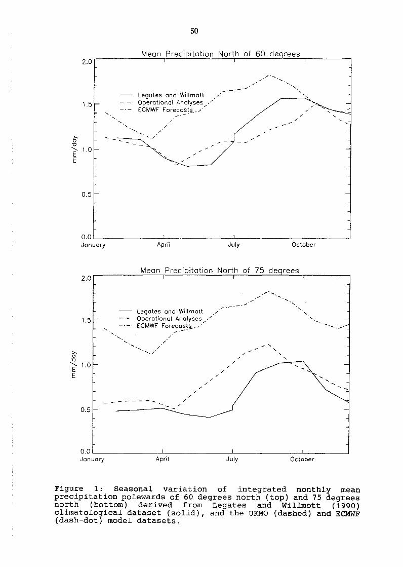
50

Mean Precipitation

2.0 t I

.......... /

/

---~./ ' Legates and Willmott ' /

1.5 Operational Analyses/''

' ECMWF F areca~!§...__..

' ' /

' /

/ /

>, ...... / /

0 /

"0 .......... 1.0 ,.. E ,..

/

E

0.5

O.OL-------------~---------------L--------------~--------~

>, 0

"0

January

2.0

1.5

E- 1.0

E

0.5

April July October

Mean Preci itation North of 75 de rees

Legates and Willmott / Operational Analyses// ECMWF Foreca~!§.. . ..--" -· /

/

/

/ /

-------

April

/

_____ ..,

/ /

/ /

July

/

October

Figure 1: Seasonal variation of integrated monthly mean precipitation polewards of 60 degrees north (top) and 75 degrees north (bottom) derived from Legates and Willmott (1990) climatological dataset (solid}, and the UKMO (dashed) and ECMWF (dash-dot) model datasets.

51

precipitation fields arise from the internal calulations from the parametrisations within the models. Both models employ comprehensive physical parametrisation schemes, including representation of solid and liquid precipitation and, in the current versions, explicit representation of cloud liquid water and ice.

For this study, data for total precipitation accumulated and averaged over the first 24 hours of the forecast run were extracted from the ECMWF archives. Over the period for which the data were extracted (1986 to 1994), the model resolution has varied. A horizontal resolution of T106 (approximately 1 degree) with 19 levels in the vertical was in use operationally from 1 January 1985 until 17 September 1991, since which a horizonal resolution of T213 with 31 vertical levels has been employed. However, the archive data utilised for this investigation were those held on a 2.5 degree latitude-longitude grid. UKMO Unified Model data were available for the (relatively short) period for June 1991 to June 1995 as accumulations over the 6 hours of the assimilation cycle. The data are held on the grid of the model which has a resolution of 0. 83 degrees of latitude by 1. 25 degrees longitude and which, for purposes of comparison, were interpolated, after extraction, to the same 2.5 degree grid of the ECMWF archive.

Other data employed in the study were the fields from the Legates and Willomott (1990) precipitation climatology (interpolated to the ECMWF 2.5 degree grid) and from the UKMO climatological data archive.

3. COMPARISON OF FIELDS OF TOTAL PRECIPITATION

Figure 1 summarises the seasonal cycle of precipitation polewards of 60 and 75 degrees north as described by the Legates and Willmott (1990) climatology and by the U~lO and ECMWF model data. It is evident that there is a substantial discrepancy in the total precipitation amounts described by the ECMWF model, compared to the Legates and Willmott and UKMO datasets. Indeed, polewards of 75 degrees north, the ECMWF total precipitation amounts to some twice that of the other two datasets. We note here that there is, of course, a particular inconsistency in the derivation of the NWP model data which are for different parts of the analysis/forecast cycle. Further, it is known that precipitation is particularly affected by variation as the model forecast spins up and will be affected by the assimilation process, which will also affect the totals. Interestingly the total precipitation the the UKMO model run in data assimilation mode, is not dissimilar to that derived from a run of the atmospheric model in climate mode, coupled to ocean and sea ice models (Cattle and Crossley, 1995) . This can be seen by comparison of the appropriate curves of figures 1 and 2 (note the change of scale). However, this may be fortuitous (see also the paper by Walsh). All three of the datasets shown in figure 1 are consistent in showing a minimum in total precipitation in spring/early summer and a maximum in late summer/fall. However, the dates of the minima vary from as early as March in the ECMWF model to as late as June for the Legates and Willmott dataset.

52

Likewise the dates of the maxima between the datasets vary from August to October.

1.5

- HC model 10 year mean

1.0

0.5

O.OL-------------~-------------L------------~--------~ January April July October

Figure 2: Comparison of the seasonal variation of integrated monthly mean precipitation polewards of 75 degrees north derived a coupled atmosphere-ocean climate model version of the UKMO Unified Model (see Cattle and Crossley, 1995)

Figure 3 shows the fields over the north polar region from the Legates and Willmott dataset for winter (December, January February), spring (March, April, May), summer (June, July, August) and autumn (September 1 October 1 November) . In winter and spring a marked area of low precipitation (less than 0.5 mm/day) extends across much of the Arctic from Northern Canada to central Russia. Higher values are associated with the extension of the trough from the Icelandic low pressure system into the Barents and Kara seas. In summer, relatively low values (of between 0.5 and 1 mm/day) are still found over the pole and the Canadian side of the Arctic basin. A transitional return to the lower winter values is evident in autumn. Data from the UKMO (figure 4) and the ECMWF (figure 5) models show similar overall patterns and seasonal variation, but, as reflected in figure 1, with substantially higher levels of precipitation from the ECMWF model dataset.

4. COMPARISON WITH STATION DATA

Figures 6 (b) and 7 show a comparison of station data extracted from the UKMO climatological data archive with nearest

0

0

53

0.5 2 7 15 0 0.5 2 7 15

0.5 2 7 15 0 0.5 2 7 15

Figure 3: Precipitation fields for the Arctic derived from Legates and Willmott (1990). Top left: winter (December, January February); top right: spring: (March, April, May); bottom left summer: (June, July, August); bottom right: autumn (September, October, November)

54

0 0.5 2 7 15 0 0.5 2 7 15

0 0.5 2 7 15 0 0.5 2 7 15

Figure 4: As for figure 3, but derived from UKMO model output.

55

·~.:-0 0.5 2 7 15 0 0.5 2 7 15

ECMWF ECMWF Forecasts

0 0.5 2 7 15 0 0.5 2 7 15

Figure 5: As for figure 3, but derived from ECMWF model output.

'

.p

' ' / y

1. REYKJAVIK

2. SVALBARD

3. EUREKA

4. ANCHORAGE

5. BARROW

6. ANADYR

7. DZARDZAN

8. OSTROV DIKSON

9. POLAR GMO IM.E.T

'

I

I I

I T I

I ,_ I,

1 _____ 1

..... -, ,- .......

lq 't"c;:)

' 1 ___ 1 ~ ' - ....... / ,/""' \ I ' /

/' \ I '

' ' ' / V

/

/ ' ' ' / /

/

' \

' / ")'

/ ' '

\

I \

..l-

I ', \ I // \ ~ _ ~\

- - _t ' \ I / *-~ 1- ' I I/ - - Cf 1o I - ::)(:::- I I

-,,,,- -·-1 I

/ I I ' ~--/ I I ',2~ --

I )/

I ' ' &<:._.r,r-1 - - -~ ' ' '

/

;(

'" ' ' '

~ I

..1- ~

Figure 6: Left: Location of stations for intercomparison. Right: Comparison of seasonal variation of monthly mean precipitation from station data (dots) and 'nearest grid point' data from the Legates and Willmott ( 1990) climatological dataaet (solid) and the UKMO (dashed) and ECMWP (dash-dot) model data for (from top to bottom) staticns 1 to 3.

SVALBARD LUFTHAVN

--

•r- -

•r- -

f •r- -

.-· •r-

0 0 10 "

EU N.W.T. 10

•I-

·-! !

•I-

2~

0 0

'.-- Leqct .. GftdWillmott """' - Opoorolianal AnalpR ·---,- Ob-loOIII ----,_c_:~r~..!!'9~

'

l .... ~.,...~lmotl Op~rotlonal MolyMII Obi-t;,.,. £CWWF Fotote:O.ll

----------

i.eoge\11 oN Wfi\lmotl (lpl ... tton.t~ oo-iiont [CWWf'Fgqo:aala

ANCHORAGE ltiT.

/

/

.. -····· ...... ---·

.. ··

BAARO'IIU_W. POST W. ROGERS

-·-

ANAOYR'

' ' ·,. I --...... ,.

-. -

·· ..... .

....... -------... -·· ····:;·---- ...... ::"'

-

-

-

12

·-•r-

f ~

' •I-

21-

0 0

f

2-

10

L•got .. _WiMmotl OperoliooMI Ana.,.... ObHIVOit-ECIIIIWF Forote:ol\1

uqo\u-WillmoU Op1rotionol Anol)"'ll Ob••,..,• lion• Ec~rrot•c:a.ll

OZAROZAN

OSTROV OIKSON

- ·- ....... ·.: .. .- --~---..:-::.· =-::.· ..;-=-~-7-:;-;-:=-~-=-=---:~ ..... -~

lepln Qnlll1irlllmoll OparotionoiAna~ 001-liooll £CWW!' Foreco1U

POLAR GloiO IM.E.T. KRENI<El...JA

--------~~:-

--- -~-~---~-~-~-~~~--~-~-~ ~

Figure 7: As for figure 6(right) but for stations 4 to 6 (left) and 7 to 9 (right) of figure 6(left)

-

-

-

---=----:_....,. __ _

---·---. -· -.......... -. __ _,-.;.; ... ~.:.:_·:..::.·-~--:..

58

grid point data from the Legates and Willmott climatology and UKMO and ECMWF model datasets for the stations shown on the left hand side of figure 6. Few of the stations lie in the central Arctic and all are land-based. Though in many cases there is general agreement on the phase of the seasonal cycle, there are evident (and not necessarily consistent) discrepancies between the various datasets. Overall, the observed station data show lower values than the climatologies, probably reflecting the difficulties involved in catching solid precipitation. Not surprisingly from the results discussed in section 3 above, of the model data, those for the ECMWF model tend to be the higher though this is not universally the case.

5. CONCLUSIONS

Overall, the total climatological precipitation rate over the Arctic derived from accumulation through the UKMO 6 hour assimilation and ECMWF 24 hour forecasts show not dissimilar geographical patterns in the seasonal means to those deduced by Legates and Willmott (1990). All three datasets show a broadly consistent seasonal phasing of precipitation, with a minimum in spring/early summer and a maximum in late summer/autumn. The rise to summer values starts earlier in the ECMWF and UKMO model datasets. However, the ECMWF data show values which are generally higher than either the UKMO or Legates and Willmott data by up to twice as much. in the integrated mean polewards of 75 degrees north. Not surprisingly, 'nearest grid point comparisons with station data reveal substantial discrepancies, with station data tending to show the lowest values.

This is very much a preliminary investigation and further work needs to be done to establish a proper comparison between models and between models and the observed data. In particular, issues of 'spin up' of the precipitation fields, as well as consistency of comparison need to be addressed. The re-analyses currently underway should give an improved basis on which to assess the quality of the model data.

6. REFERENCES

Cattle, H and Crossley, J. , 1995: Modelling Arctic climate change. Phil. Trans. R. Soc. Lond. A, 352, 201-213.

Cullen, M.J.P., 1993: The unified forecast/climate model. Meteorological Magazine, 122 1 81-94.

Legates 1 D. R. and Willmott 1 C. J. , 1990: Mean seasonal and spatial variability in gauge-corrected global precipitation. Int. J. Climatol. 1 10, 111-127.

WCRP, 1992: Scientific concept of the Arctic Climate System Study (ACSYS). WCRP-72, WMO/TD-No. 486.

WCRP, 1994: Arctic Implementation Plan.

Climate System Study (ACSYS) WCRP-85, WMO/TD-No. 627.

Initial

59

MODEL-DERIVED PRECIPITATION CLIMATOLOGIES FOR NORTHERN HIGH LATITUDES

1. INTRODUCTION

John E. Walsh

Department of Atmospheric Sciences University of Illinois Urbana, IL 61801

One of the scientific foci of the Arctic Climate System Study (ACSYS) is the freshwater budget of the Arctic region. The Arctic freshwater budget, driven by precipitation over the Arctic Ocean and surrounding land areas, is poorly quantified because of the sparseness of in situ measurements. The inadequacy of the spatial sampling is compounded by the large errors and uncertainties in the instrumental measurements of solid precipitation, especially in environments that are windy as well as cold. The difficulties of using station data to obtain accurate areal means of precipitation in Arctic regions has raised the possibility that the most accurate areal means may be obtained from numerical models of the atmosphere. These models can be run with or without the assimilation of atmospheric data in simulations of climate and climate change. The validity of climate change will indeed depend, to a large extent, on the accuracy of the simulations of the present-day precipitation climatology by these models.

Models offer additional advantages with regard to diagnoses of the freshwater budget of the Arctic. Moisture budget components such as precipitation, evaporation, atmospheric moisture flux convergence, and runoff are readily available on regular grids from model simulations, permitting the closure of the moisture budget over arbitrary temporal and spatial domains. Such closure is exceedingly difficult to achieve observationally in the absence of data on evapotranspiration and, in many regions, runoff.

The following sections contain an assessment of model simulations of the Arctic hydrologic cycle. The emphasis will be on the simulated precipitation. The observational inadequacies noted above make such assessments difficult, especially with regard to temporal variations. Nevertheless, the observational database is sufficient to permit some first-order conclusions about the capabilities and deficiencies of model simulations of the Arctic hydrologic budget.

2. MODEL CLIMATOLOGIES

a. Climate model output

A unique source of climate model output is the Atmospheric Model Intercomparison Project (AMIP), which was organized in 1990 by the Working Group on Numerical Experimentation of the World Climate Research Programme in an attempt to promote systematic evaluations and comparisons of atmospheric general circulation models (AGCMs). Approximately thirty-five groups from the international modeling community, as well as about twenty other groups performing diagnostic subprojects, are participating in the systematic intercomparison of AGCMs run under common initial and boundary conditions (Gates, 1992). Because the ocean surface temperatures and sea ice boundary conditions are prescribed in the AMIP simulations, the models do not include ocean mixed layers or ocean dynamics. The models determine their own surface temperatures and snow cover over land areas, where each model has its own specification of surface properties such as albedo, roughness, vegetation and emissivity. The formulations of physical processes (including cloud formation, precipitation and evaporation) vary from model to model, as do the horizontal resolution, number of levels, and the choice of spectral or grid-point representations of the model dynamics in the horizontal. A comprehensive summary of the structure and parameterizations in the various models is provided by Phillips (1994). The AMIP models were run for a 10-year period, 1979-1988, with the ocean boundary conditions varying temporally in accordance with the observed fields from this period. While the prescribed ocean boundary conditions influence the computed evaporation rates to some extent, the model-determined surface winds and air temperatures introduce several degrees of freedom into the evaporation rates computed over ocean areas.

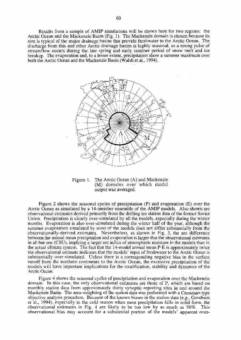
60

Results from a sample ofAMIP simulations will be shown here for two regions: the Arctic Ocean and the Mackenzie Basin (Fig. 1). The Mackenzie domain is chosen because its size is typical of the major drainage basins that provide freshwater to the Arctic Ocean. The discharge from this and other Arctic drainage basins is highly seasonal, as a strong pulse of streamflow occurs during the late spring and early summer period of snow melt and ice breakup. The evaporation and, to a lesser extent, precipitation show a summer maximum over both the Arctic Ocean and the Mackenzie Basin (Walsh et al., 1994).

Figure 1. The Arctic Ocean (A) and Mackenzie (M) domains over which model output was averaged.

Figure 2 shows the seasonal cycles of precipitation (P) and evaporation (E) over the Arctic Ocean as simulated by a 14-member ensemble of the AMIP models. Also shown are observational estimates derived primarily from the drifting ice station data of the former Soviet Union. Precipitation is clearly over-simulated by all the models, especially during the winter months. Evaporation is also over-simulated during the winter half of the year, although the summer evaporation simulated by most of the models does not differ substantially from the observationally-derived estimates. Nevertheless, as shown in Fig. 3, the net difference between the annual mean precipitation and evaporation is larger that the observational estimates in all but one (CSU), implying a larger net influx of atmospheric moisture in the models than in the actual climate system. The fact that the 14-model annual mean P-E is approximately twice the observational estimate indicates that the models' input of freshwater to the Arctic Ocean is substantially over-simulated. Unless there is a corresponding negative bias in the surface runoff from the northern continents to the Arctic Ocean, the excessive precipitation of the models will have important implications for the stratification, stability and dynamics of the Arctic Ocean.

Figure 4 shows the seasonal cycles of precipitation and evaporation over the Mackenzie domain. In this case, the only observational estimates are those of P, which are based on monthly station data from approximately thirty synoptic reporting sites in and around the Mackenzie Basin. The area-weighting of the station data was performed with a Cressman-type objective analysis procedure. Because of the known biases in the station data (e.g., Goodison et al., 1994), especially in the cold season when most precipitation falls in solid form, the observational estimates in Fig. 4 are likely to be too low by as much as 50%. This observational bias may account for a substantial portion of the models' apparent over-

61

3.20 ARCTIC OCEAN: Precipile.lion (mm/ de.y) 1.20

~BMRC 2.80 ~ccc 1.00

~ CSIRO o+o-t-0 csu -oNJJ 0.80 ............... ECMWF -GFDL

-GLA 0.60 ............... GFSC ~MGO -MPI 0.40 ~MRI ~NlJC ~SUNYA 0.20 -- Obs.

-0.00

-0.20

ARCTIC OCEAN: Evapore.t!on (rnm/de.y)

~BMRC ~ccc -csmo ~csu ...,.......... DNM .,...,......,.. EC'M1fF - GFDL

- GLA ;---..,._........., - GFSC

--MGO ,..--....:_---.. .............._ MP!

J</t~-14-- ~ MRI ~NMC ~SUl'<'YA

~~,LL.~~___,~._, --Ob~.

0.00 +-----.--.---.-.--.-.-,-----.--.,-'C'T--, 2 3 4 5 6 7 8 9 10 11 12

J.lonth

-0.40 2 3 4 5 6 7 8 9 10 11 12

Month

Figure 2. Seasonal cycles of precipitation <md evaporation over the Arctic Ocean as simulated by AMIP models (solid lines) anu estimated from observational data (dashed lines). (Figure provided by V. Kattsov and V. Meleshko.)

3.00 OCEAN: ANNUAL MEAN DIFFERENCE P-E (mm/day)

2.50

2.00

1.50

1.00

0.50

Figure 3. Annual means of P - E (Precipitation minus Evaporation) as simulated by A.MIP mcx:lels and estimated from observations (left bar). (Figure provided by V. Kattsov and V. Meleshko.)

4.0 5.0 ---G--- c vs_ bmr

3.5 --a-- evs_ccc

4.0 -.o-- evs_cnr >-. >-. ro 3.0 <':l __,.__ cvs_col "d :!2. ......... 3.0 E E ---t- evs_csi

E 2.5 E '-..../

---,<r- cvs_csu

c:: c:: 2.0 --o- cvs_dcr 0 0 ...... . ..... 13 ..... --o--- evs ec2 ro

I-< 0.. 0 1.0 --•·- cvs_gfd 0... (.) 1.5 ro Q)

P: > -•-cvs_gla j:.Ll

0.0 ---+---- c.vs_gsf

--•- cvs_jma

0.5 -" ~ "' c t.O 0. > ~

-1.0 c .D ~ 0.. "' " :; CO 0. ;:) > 1l ;; " ~ "' ~

:J :J " u

0 ~ " "' ~ " "' 0 0 ~ lL :o;: :o;: ~ <.: Ul 0 z 0 lL ;::;: <.: ;::;: ~ <.: (/) z 0

Month Month m N

4.5 5.0 ---e----- e vs lmd

4.0 -B-- cvs_mgo

4.0 --o-------cvs _rnpi ,--... >-. 3.5 >-.. ("j ro -x--- cvs mn u '0 -

......... ......... 3.0 E 3.0 E ---+--~ cvs - ne a ,..... c:: E -8-cvs_nmc

c:: 2.5 c:: 2.0 -o-- cvs_nrl 0 .s ..... ..... C':l ro --o--- cvs_sun 2.0 I-< 0.. 0 1.0 -e-- cvs ucl 0... u ro Q) 1.5 > '-< -•-cvs_uga

0... j:.Ll

1.0 0.0 -+-cvs uiu

-A..- cvs_ukn1

0.5 -1.0 " .D P. "' " :; "" c.. 2 > ~ c: .0 :;; ~ >- c:: ~ CO 0. ;:) > ~ ~ " ~ "' ~ :J C) 0 ~ "

c. "' ~ " " 0 0 u. <.: ::;;: -<>:: C/) z 0 lL ;::;: ...: ~ ...: C/) z 0

Figure 4. Seasonal cycles of precipitation and evaporation over the Mackenzie domain as simulated by AMIP models. Observational estimates of monthly p are shown by dashed line.

63

simulation of precipitation in Fig. 4, although the fact that most models simulate more precipitation than is observed even in summer suggests that at least some of the bias is real. Since budget-derived estimates of evaporation for this region would be residuals incorporating the errors in other quantities (precipitation, moisture flux convergence, moisture storage), we do not believe that such estimates of evaporation are, at this time, adequate for a meaningful comparison with model-derived estimates.

Figure 5 shows the seasonal cycles of model-derived precipitation and evaporation over the Greenland ice sheet. While most models show a maximum of Greenland precipitation in the late summer and early autumn, when the surrounding sea ice coverage is a minimum, the seasonal cycle is weak in all but a few models. Evaporation shows a summer maximum in most of the models, although E is much small than Pin the summer (and other seasons) in all models. The net P-E is indeed larger than observational estimates in all the models, as shown in Fig. 5. The positive bias is substantial in some cases, as the annual mean values of P-E of the ECMWF, GLA and SUNYA models are more than twice the observational estimates. However, the models' net snow accumulation over the 10-year period shows a smaller bias relative to the observational estimates because much of the model precipitation falls as rain around the Greenland periphery.

Several recent studies have addressed model simulations of snow cover in the present climate. Foster et al. (1994) compared output of the UKMO, MPI and GSFC models for the AMIP decade (1979-1988) with corresponding observational data on snow coverage: the SMMR satellite passive microwave data and the NOAA weekly snow charts based largely on visible imagery. Comparisons were also made with the snow depth climatology compiled by the U.S. Air Force Environmental Technical Applications Center and with snow-mass estimates obtained from the SMMR passive microwave data (Chang et al., 1987). The model­simulated snow extent was generally within 10% of the NOAA values for each calendar month, although the UK model showed a rather consistent negative bias during winter. The SSMR­derived snow extents were also smaller than the NOAA values by 5-10%. Foster et al. attribute the SMMR bias to the inability of the microwave signal to provide information about shallow snow cover, since upwelling microwave radiation from the ground is largely unaffected by snow that is less than 3 cm deep. All three models examined by Foster et al. showed large negative biases in October ( -40--50% ), implying that the autumn onset of the snow expansion is difficult for the models to capture. All three models also showed a tendency to over-estimate snow mass relative to the Air Force and SMMRdata. The over-estimates were especially apparent during the summer and early autumn because the simulated snow fails to melt in some area (e.g., the Alaska Range), where it does vanish seasonally in the present climate. Thus the models' annual accumulation exceeds their annual melt in these regions. By contrast, Foster et al. find that the GSFC and MPI models produce too little snow mass during the winter months despite their realistic snow extents.

The assessment of the simulated snow climatology has been extended to a set of 16 models by Robinson and Frei of Rutgers University. Figure 6 summarizes the simulated January snow coverage, relative to the corresponding observational data, for three regions: North America, western Eurasia (west of 75°E) and eastern Eurasia (east of 75°E). In an aggregate sense, the models underestimate snow cover over North America and overestimate snow cover over eastern Eurasia. In all three cases, the biases are 5-10% of the total land area. Over North America and eastern Eurasia, the year-to-year variability (std = standard deviation in Fig. 6) is comparable to the observed; the models show considerably less variability than observed over western Eurasia.

The study by Robinson and Frei also addressed the interannual variability of the simulated snow fluctuations in the context of the observed variability. Little correspondence was found between the simulated and observed fluctuations, implying that either (1) sea surface temperatures do not exert significant control on the high-latitude precipitation that determines snow cover, or (2) the models are not capturing the SST forcing if it is indeed significant in reality. It should be noted that these conclusions are based on a study of data and model results for only January. An extension of the analysis to other months and seasons is underway.

4.80

4.40

4.00

3.60

3.20

2.80

2.40

2.00

1.60

1.20

0.80

0.4-0

0.00 1

64

GREENLAND: Precipitation (mm/day)

2 3 4 5 6 7 8 9 10 11 12 Month

,..........BMRC ............... ccc - CSIRO 0++-H csu .....,..__. DNM ............... ECMWF .............., GFDL

---.. GLA ...,.......,... GFSC -MGO _.......MPI D++H MRI ~NMC ~SUNYA

1.20 GREENLAND: Evaporation (mm/day)

,..........BMRC 1.00 ......._... ccc

- CSIRO ............... csu

0.80 ,........_._. DNM

0.60

0.40

0.20

-0.20

......-+-.-. ECMWF -GFDL

-GLA .............., GFSC .............., MGO

...-"5-.... ~MPI '"'"-_!~..IQ'<'- ~ MRI

.....__~~--" ~ NMC

1 2 3 4 5 6 7 8 9 10 11 12 Month

~SUNYA

Figure 5. Seasonal cycles of precipitation and evaporation over Greenland as simulated by AMIP models. (Figure provided by V. Kattsov and V. Meleshko.)

North America E. Eurasian (E. of 75 Lon) W. Eurasian (W. of 75 Lon)

100 -----.---

80

~~~~ ~~ ~ ~ QJ

8 60 ';( ~

~~9~ X c

~

.jJ 40

* ~ X ~

8 * 0. 20

~ $ -~-0

~ i -~ 'd ~ i ·g 'd

a i ·a 'd

~ Qj

""' j Cl) .jJ

~ Qj .jJ

bl 11)

~ t1l Ill <1) bl !r)

~ :a ~ ~ 0 :a ~ ~

l.l ~ H ~ ~ 1-l ~

•ri '" '" ~ ~ ~ ~

Figure 6. Distribution of snow cover statistics from 16 AMIP model simulations of the 1980-1988 period. From left to right, plotted symbols show the maximum, mean, median, minimum, range, standard deviation and variance of the 16 values. Median is given by line through center of box; top and bottom of box represent first and third quaniles, respectively. Top and bottom whiskers represent the upper and lower ranges. Observed values from NOAA snow charts are marked by an "X". (Figure provided by D. Robinson and A. Frei, Rutgers University.)

O"l <:Jl

66

b. Data assimilation products

The application of climate models to precipitation estimation is clearly limited, even when the models are run with specified SSTs as in AMIP, because of the model deficiencies and associated errors in the simulations. A more promising strategy for precipitation estimation is the use of atmospheric models in a data assimilation mode, as is typically done in numerical weather prediction. By constraining a simulation with observational data at frequent intervals (e.g., 6 hours, 12 hours), the likelihood increases that the model will capture the distribution of atmospheric moisture flux convergence and precipitation. An example of results from this approach is shown in Fig. 7, which is the field of precipitation for April 1993 produced by averaging 24-to-48 hour forecasts from a regional weather prediction model of the Canadian Meteorological Center (CMC). As the CMC contributors note, "the model results are excellent" with the exception of slight overestimates of precipitation on the west coast and in eastern Canada. Consequently, "the total precipitation forecast by this model could be used as an estimate of monthly precipitation in data-sparse areas, particularly in the north" (Environment Canada, 1993, p. 11).

An even more promising approach to precipitation estimation is the so-called "reanalysis" of historical data by the incorporation of observations into a "frozen" state-of-the-art prediction model. Such efforts are now underway at the European Centre for Medium-Range Weather Forecasts (ECMWF), the U.S. National Meteorological Center (NMC) and NASA's Goddard Space Flight Center. The NMC reanalysis, which incorporates observations at 6-hour intervals, will span a 40-year period, 1957-1996. Variables that are archived in the NMC reanalysis include precipitation, evaporation, the surface energy fluxes (including solar and longwave radiation) and the fields of air temperature, wind, geopotential and humidity at various levels. Figure 8 shows the NMC reanalyses of precipitation (P) and evaporation (E) averaged over January and July of 1985 for northwestern Canada, including the Mackenzie drainage basin. The reanalysis clearly captures the January maximum of precipitation over the coastal mountains, where the monthly totals exceed 30 cm; the January precipitation totals are less than 3 cm over much of the Canadian subarctic. In July, a maximum of 15-20 cm occurs well inland, although the monthly totals along the Arctic coast are only 2-3 cm. As shown in Fig. 8b, the monthly evaporation is close to zero over the entire domain during January, but the July totals range from approximately 3 cm along the Arctic coast to 9-12 cm over the southeastern quadrant of the domain. Corresponding plots for July 1986 show even more precipitation and more evaporation over the southeastern quadrant.

Figure 9 shows the seasonal cycle of precipitation averaged over the Mackenzie domain for the NMC reanalyses and station measurements. The summer maximum, which dominates the seasonal cycles of both the reanalyses and the station data, is undoubtedly real. It is apparent, however, that precipitation is greater in the reanalyses. The 12-month totals are 17.6 cm for the reanalyses and 11.4 cm for the station data. The lower values obtained from the station data may well be an indication of the undercatch of precipitation by the gauges at the observing sites, although it is noteworthy that the largest discrepancies between the reanalyses and station data occur during the spring and summer. Most precipitation during these seasons occurs in liquid form, especially during summer.

3. CONCLUSION

This paper has examined two types of model-derived precipitation climatologies for northern high latitudes. The first, the output of atmospheric GCMs, shows a tendency of the models to over-simulate Arctic precipitation. To the extent that the data on evaporation permit observational estimates, it appears that the models also over-simulate evaporation, at least during the winter half of the year. The biases of precipitation appear to exceed the observational uncertainties and will need to be addressed by the modeling community before simulations of the Arctic hydrologic cycle can be viewed with confidence.

The second set of simulations, those which are anchored to observations by the assimilation of data at frequent intervals, offer more immediate promise for estimation of

67

TOTAL FORECAST PRECIPITATION (MM) (24- 48 H)

Figure 7. Total precipitation (mm) over Canada as obtained from 24-48 hr forecasts of Canadian Meteorological Center's RFE (Regional Finite Element) model. [Figure from Environment Canada (1993, .li, p. 11).]

68

NMC Reanalysis P(mm/day) for Jan 85 NMC Reanalysis E(mm/day) for Jan 85

70N 70N

68N 68N

66N 66N (I)

-g 64N 64N

~ 62N 62N _J

60N 60N

58N 58N

56N 56N

NMC Reanalysis P(mm/day) for Jul 85 NMC Reanalysis E{mm/day) for Jul 85

70N 70N

68N 68N

66N 66N (I)

-g 64N 64N

~ 62N 62N _J

60N 60N

58N 58N

51>~ 56N

1 1 1 1 Longitude Longitude

Figure 8. NMC reanalyses of precipitation(?) and evaporation (E) for January and July, 1985. Contour interval is 1 mm day-1.

C\1 -

0

•

I

2

•

Precipitation over the Mackenzie Basin

•

I

4

NMC

I

6

Month

I

8

I

10

Figure 9. Seasonal cycle of precipitation (mm day-I) over Mackenzie domain .from NMC reanalyses (asterisks connected by linear segments) and area-weighted station measurements fsolid circles).

1985 1986 Mean

1

12

70

various components of the Arctic hydrologic cycle: precipitation, evaporation and regional atmospheric moisture advection and convergence. Reanalysis efforts are now in their early phases, and the results presented here are among the first products of state-of-the-art reanalyses. The early results support the hypothesis that station-derived estimates of regional precipitation are too low in the Arctic. Validation of these products is clearly needed, and there will undoubtedly be further iterations of reanalyses. Near-term priorities are comparisons of the reanalyzed Arctic hydrologic fields from several reanalysis projects and rigorous assessments of their shortcomings. The potential value of these gridded fields is sufficiently high that the emphasis accorded this strategy in the ACSYS Initial Implementation Plan appears to be warranted.

References

Chang, A. T. C., J. L. Foster, and D. K. Hall, 1987: Nimbus-7 SMMR derived global snow , cover parameters. Ann. Glacial., 9, ~9-44.

Environment Canada, 1993: Forecast almost as good as observations? Climatic Perspectives (Canadian Climate Center), 15, 11.

Foster, J., G. Liston, R. Koster, R. Essery, H. Behr, L. Dumenil, D. Verseghy, S. Thompson, D. Pollard and J. Cohen, 1994: Intercomparison of snow cover and snow mass in North America from general circulation models and remote sensing. Proceedings, Sixth Conference on Climate Variations, Amer. Meteor. Soc., Boston, MA, 73, 207-211.

Gates, W. L., 1992: AMIP: The Atmospheric Model Intercomparison Project. Bull. Amer. Meteor. Soc., 73, 1962-1970.

Goodison, B. E., E. Elomaa, V. Golubev, T. Gunther and B. Sevruk, 1994: WMO Solid Precipitation Measurement Intercomparison: Preliminary Results. World Meteor. Org., TD-588, 15-20.

Phillips, T. J., 1994: A Summary Documentation of the AMIP Models. UCRL-ID-116384, Lawrence Livermore National Lab., Livermore, CA, 113 pp.

Walsh, J. E., X. Zhou, D. Portis and M. Serreze, 1994: Atmospheric contribution to hydrologic variations in the Arctic. Atmosphere-Ocean, 32, 733-755.

71

AEROLOGICAL ESTIMATES OF PRECIPITATION MINUS EVAPORATION OVER THE ARCTIC

Mark C. Serreze, Roger G. Barry

Cooperative Institute for Research in Environmental Sciences Division of Cryospheric and Polar Processes

Campus Box 449, University of Colorado, Boulder, CO

John E. Walsh

Department of Atmospheric Sciences, University of Illinois, Urbana, IL

1. INTRODUCTION

Arctic precipitation data bases are prone to considerable uncertainty. Records are available for coastal and inland stations (Vose et al., 1992), but precipitation gauges "catch" only a fraction of snow in areas where wind-driven snow is common, resulting in a negative bias. For example, Woo ( 1983) notes that individual drainage basins in the Canadian High Arctic can receive 130-300% as much snow as reported by conventional synoptic stations in the area. Even in summer, estimates may be low due to occult precipitation (fog, dew) and the neglect of trace values. As most Arctic stations are at low altitude, the tendency for precipitation to increase with elevation probably also results in an underestimate of regional averages. Some of these problems are reviewed by Groisman et al. (1991 ). Over the Arctic Ocean, precipitation data are meager. Limited measurements exist from Arctic drifting stations. In addition, there are measurements of snow depth on the Arctic Ocean ice from a Russian program of aircraft landings (Romanov, 1993).

2. AEROLOGICAL METHOD

These problems may be in part overcome via the "aerological" approach, in which humidity and wind profiles from station rawinsonde networks can be used to estimate precipitation minus evaporation, or P-E as (e.g. Alestalo, 1983)

P- E ... -V·F- oQ/ot

where -V·F is the horizontal convergence of the vertically-integrated water vapor flux (F) into a domain and oQiot is the time change in precipitable water (Q, the vertical integral of specific humidity) over the domain. Over annual time scales for which oQ/ot can be assumed to be zero, the flux convergence is equivalent to P-E. P-E represents the net freshening (or salination) of the ocean or the net gain (or loss) of water by the land through surface exchanges with the atmosphere. As such, it is arguably a more relevant hydrologic variable than precipitation alone.

We have used the aerological approach in conjunction with extensive Arctic rawinsonde archives to assess the atmospheric moisture budgets of the Mackenzie River drainage, the Arctic Ocean and the north polar cap (the region north of 70 oN). Details of the rawinsonde data bases and techniques are provided in several recent papers (Serreze et al., 1994a,b,c; Walsh et al., 1994). The primary disadvantage of the aerological approach is that it must be applied to domains larger than about 1.0x 106 km2 - for smaller regions, the flux convergence estimates can be strongly influenced by

72

errors in the rawinsonde wind measurements (Rasmusson, 1968). Errors in humidity data at low temperatures and humidities have only a minor effect (<5%) on the convergence estimates. However, errors may be introduced if large changes in the flux occur between points at which it is evaluated. Nevertheless, the rawinsonde network in the 50°-70°N zone is denser than any other 20° latitude sector of the globe. The aerological approach neglects the atmospheric flux of water in the liquid and solid phases because the liquid/ice flux is generally significant only in localized areas or for short time periods, e.g., over warm ocean currents and in cumulus clouds in the tropics.

3. POLAR CAP P-E

Over the 197 4-1991 period, annual P-E, expressed as water equivalent averaged over the domain, has a mean of 163 mm (Serreze et al., 1994a), considerably higher than the value of 120 mm for the same domain reported by Peixoto and Oort (1992), based on an earlier rawinsonde database from 1963-1973. The flux convergence is positive for all months, ranging from a low of about 10 mm for December through February to a high of 22 mm in September, when P-E also obtains its annual maximum (26 mm).

Annual P-E is strongly determined by large poleward vapor fluxes across the 70°N latitude circle near the prime meridian, reflecting transient-eddy transports associated with the primary North Atlantic cyclone track (Serreze et al., 1994a; Walsh et al., 1994). Large poleward fluxes are also found near Baffin Bay, associated with frequent cyclonic activity in this region. The only area of net moisture outflow is over the Canadian Arctic Archipelago, reflecting persistent northerly winds east of the western North American ridge. Annual P-E ranges from a low of 125 mm in 1978 to a high of 203 mm in 1981 (Figure 1). Hence, P-E ranges by about 25% on either side of the long-term mean of 163

250

200 -.. E >= .._

'--"'

IV 150 u c IV 0"\ .._ IV > c 100 0 u X :J

c:;:: 50

0

r- r-- r-- -r--

r--,......... r-- r-- - -- r-- r-- -- r-- r--

- r--- -- r-- r-- r-- -

r-- ,.-- - r--- r-- r- -r-- --

- r-- r-- r--r-- r-- -- r-- - - r-- r--r-- - -

- r--r--- r--

- r-- r-- - - - - r-- - r----r-- - f--

I I J 1 j_ ~ l J I I I I I

74 75 76 77 7B 79 BO B1 B2 B3 B4 BS B6 B7 BB B9 90 91 Year

Figure 1 - Time series of seasonal vapor flux convergence and annual P-E for the north polar cap (north of 70 ON), 1974-1991. For every year, the total length of each bar is annual P-E. From bottom to top, the individual bar segments represent the vapor flux convergences for winter (January-March), spring (Aprii-May), summer (June-August) and autumn (September-November). These seasonal definitions facilitate evaluation of seasonal contributions of the flux convergences to annual P-E for standard calendar years (from Serreze et al., 1994d).

73

mm. There is no apparent trend in P-E over the 18-year period but some indication of a multi-year cycle that needs to be tested with a longer record. For any season, large flux convergences are favored by a meridional "winter type" circulation, characterized by strong eastern North American and East Asian troughs. In turn, this is associated with a more dominant North Atlantic cyclone track, resulting in strong poleward moisture transports. The ability of general circulation models to adequately portray the present Arctic hydrologic budget would appear to strongly depend on their ability to correctly represent this cyclone track and its variability.

4. REGIONAL P-E

Annual P-E for the Mackenzie basin (Walsh et al., 1994) has a mean of 247 mm and exhibits a summer minimum. The range of interannual variations over the 1973-1990 study period is roughly +I-50% of the annual means and more than twice the monthly means.

The annual flux convergence for the Arctic Ocean is considerably smaller at 173 mm, also differing from the Mackenzie drainage in exhibiting a late summer maximum. Although comparisons with other studies are complicated by differences in the spatial domain over which P-E is calculated, the Arctic Ocean value is close to the mean of 169 mm cited by Burova (1983). Aagaard and Carmack (1989) have summed the sources and sinks of freshwater for the Arctic Ocean and arrive at an unresolved annual freshwater excess of 90 mm. Substitution of the improved estimate of P-E for the Arctic Ocean, which in magnitude is almost half of the estimated total runoff term (350 mm), now results in a larger freshwater excess of about 170 mm.

5. VALIDATION

The aerological estimates for the Mackenzie basin suggest that station reports underestimate precipitation during the winter months by amounts equivalent to several cm yr-1. Interannual variations in the flux convergence nevertheless correspond well with year-to-year variations of station­averaged precipitation in the Mackenzie domain, but the correlations with both of these variable account for less than half of the interannual variance of the Mackenzie discharge. More comprehensive assessments of linkages between river discharge and other hydrologic components are clearly in order.

Published climatological estimates of monthly evaporation from the Korzun (1977) atlas have been used to obtain P as a residual from the P-E estimates for the polar cap region (Serreze et al., 1994b). The resulting annual total P of 266 mm compares well with the estimate of 293 mm for the same domain redigitized from from the Gorshkov (1983) atlas, based on Soviet data up to 1980. Using a linear temperature adjustment (Ross and Walsh, 1987), the fraction of P represented by snowfall (S) has also been estimated, allowing for some comparisons with the snowfall climatology of Maykut and Untersteiner (1971), which is used as the basis for snow cover input in most sea ice models. Using the same mean snowpack density of 330 kg m-3 employed by Maykut and Untersteiner (1971) (which accounts for settling and aging of the snowpack) to the water equivalent snowfall yields an accumulated snow depth of 579 mm, as compared to 400 mm reported by Maykut and Untersteiner ( 1971 ). As their estimate is representative of the sea ice covered regions of the Arctic and ours includes oceanic regions over the Atlantic side of the Arctic where precipitation appears to be comparatively high (Gorshkov, 1983) this difference is not surprising.

6. CONCLUSIONS

In light of the uncertainties in Arctic precipitation data bases, especially during the winter season, the aerological approach represents an attractive method for assessing variations in Arctic moisture budgets. The primary disadvantage of the aerological method is that it must be applied to domains larger than about 1.0x I 06 km 2• As such, the approach is best suited for analysis of large areas

74

such as the north polar cap or large watersheds, such as the Mackenzie basin. Plans are underway to extend our analyses to the Yenisei, Lena and Ob-Irtysh basins, with the P-E values used to validate hydrologic models.

Acknowledu;ements: This study was supported by NSF grants DPP-9214838, DPP 9113673 and ATM-9315351. The NSIDC staff is thanked for computer support.

7. REFERENCES

Aagaard, K. and E.C. Carmack, 1989: The role of sea ice and other fresh waters in the Arctic circulation. J. Geophys. Res., 94(CIO), 14,845-14,498.

Alestalo, M., 1983: The atmospheric water vapor budget over Europe. Variations in the Global Water Budget. A. Street-Perrott, M. Beran and R. Ratc1iffe, eds., D. Riedel, 67-79.

Burova, L.P. 1983: Vlagooborot v atmosfere Arktike (Moisture exchange in the Arctic atmosphere). Gidrometeoizdat, Leningrad, 128 pp.

Gorshkov, S.G., 1983. World Ocean Atlas, Vol. 3: Arctic Ocean. Department of Navigation and Oceanography, Ministry of Defense, USSR. Pergamon Press, 184 pp.

Groisman, P.Y., V.V. Koknaeva, T.A. Belokrylova and T.R. Karl, 1991: Overcoming biases of precipitation: A history of the USSR experience. Bull. Am. Meteor. Soc., 72, 1725-733.

Korzun, V .1., 1977: Atlas of World Water Balance. Leningrad, Gidrometeiozdat, 164 pp. Maykut, G.A. and N. Untersteiner, 1971: Some results from a time-dependent thermodynamic model

of sea ice. J. Geophys. Res., 7(6), 1550-1575. Peixoto, J.P and A.H. Oort. 1992: Physics of Climate. Amer. Inst. Phys., New York, 520pp. Rasmusson, E.M., 1968: Atmospheric water vapor transport and the water balance of North America.

11. Large-scale water balance investigations. Mon. Wea. Rev., 96, 720-734. Romanov, LP., 1993: Atlas, Morphometric Characteristics of Ice and Snow in the Arctic Basin. St.

Petersburg (privately published), 152 plates. Ross, B. and J.E. Walsh, 1987: A comparison of simulated and observed fluctuations in summertime

Arctic surface albedo. J. Geophys. Res., 92, 13115-13125. Serreze, M.C., R.G. Barry and J.E. Walsh. 1994a: Atmospheric water vapor characteristics at 70°N. J.

Climate, 8(4), 719-731. Serreze, M.C., M.C. Rehder, R.G. Barry, J.E. Walsh and D.A. Robinson 1994b: Variations in

aerologically-derived Arctic precipitation and snowfall. Ann. Glaciol. (in press). Serreze, M.C., M.C. Rehder, R.G. Barry, J.D. Kahl and N.A. Zaitseva, 1994c: The distribution and

transport of atmospheric water vapor over the Arctic Basin. lot. J. Climatal. (in press). Serreze, M.C., R.G. Barry, M.C. Rehder and J.E. Walsh, 1994d: Variability in atmospheric circulation

and moisture flux over the Arctic. Transactions A of the Royal Philosophical Society (in press).

Vase, R.S., R.L. Schmoyer, P.M. Steurer, T.C. Peterson, R. Heim, T.R. Karl and J.K. Eischeid, 1992: The Global Historical Climatology Network: Long-Term Monthly Temperature, Precipitation, Sea Level Pressure, and Station Pressure Data. Oak Ridge National Laboratory, Environmental Sciences Division Publication No. 3912, 99 pp. plus appendices.

Walsh, J.E., X. Zhou, D. Portis and M.C. Serreze. 1994: Atmospheric contributions to hydrologic variations in the Arctic. Atmos.-Ocean., 32(4), 733-755.

Woo, M., R. Heron, P. Marsh and P. Steer, 1983. Comparison of weather station snowfall with winter snow accumulation in high Arctic basins. Atmosphere-Ocean, 21(3), 312-325.

75

SNOW MASS VARIATION OVER THE NORTHERN POLAR REGION AS SIMULATED WITH AMIP GENERAL CIRCULATION MODELS

V. M. Kattsov and V. P. Meleshko

Voeikov Main Geophysical Observatory, St.Petersburg, Russia

1. INTRODUCTION

It has long been recognized th(lt snow can play an important role both in high-latitude heat and water budgets. In addition to direct fresh water input into the ocean in the form of precipitation, snow can influence the thermohaline circulation through iceberg discharge from ice sheets, where it is accumulated. In turn, the ice sheets can be of major importance in climate variations due to their specific inertia properties, as well as a possible cause of sea level change on time scales of decades or longer.

The AMIP 10-year simulations (Gates, 1992) with observed SST and sea-ice forcing provide a good opportunity to assess current AGCMs' ability to reproduce snow cover variation both over the sea ice and the ice sheets. In the present study, two regions are chosen to perform a diagnostic analysis: the Arctic ocean bounded with the 70th latitude and Greenland. Some relevant results, in particular those concerning precipitation and evaporation over the above regions, can be found in the papers by Kattsov et al. (1994) and Walsh et al. (1995).

2. PARAMETERIZATION OF SNOW COVER IN AGCMS.

Current AGCMs incorporate snow cover parameterizations of varying degree of sophistication (Phillips, 1994). When surface air temperature (or a combination of ground and/or lower atmospheric level temperatures) goes below a freezing point (or a specified lower temperature value), it is assumed that precipitation falls as snow which covers (uniformly, as a rule) the grid box area. Prognostic snow mass is determined from budget equations incorporating precipitation, snow melt (runoff) and evaporation (sublimation). Snow conductivity and heat capacity may depend on snow density which in turn depends on the accumulated snow mass. Some parameterizations assume a gradual transition of physical properties of deep snow to ice. Besides nonradiative thermal properties, snow cover may affect model surface albedo and rouglmess. In some models, snow accumulation on sea ice is not allowed at all. This may be also prescribed.

3. RESULTS

3.1 Arctic ocean

Snow mass (kg/m2) decadal averages over the Arctic ocean are presented at Figure 1. The GFDL/ DERF model demonstrates permanent increasing of snow mass in the Arctic ocean. The observational

76

200

190

180

170

160

150 140

130

120

110

100

90

80 70

60

50

40

I 30

20

10

0 Obs. BMA CCC CNR CSI CSU DNM ECM GFD GLA GSF .JMA MGO MPI MAl NCA NMC NRL SUN UCL UGA UKM

Models

Figure 1 - Decadal means of snow mass {kg/m2) over the Arctic ocean. Observational estimate for the central Arctic climate is shown at left.

200.00

176.00

160.00

126.00

100.00

7~.00

50.00

26.00

0.00 0 12 24 36 ol8 eo

llonth

Figure 2 - Monthly means of snow mass (kg/m2) for 9 models allowing its accumulation over sea ice. Dashed line is an observational estimate.

6000

.tOOO

2000

77

...... BWRC -ccc -csmo

.................. csu ,.~ _...._ DNll

-GFDL

-GLA -crsc

~~::::::::::~......,_...__..._,. ..- YGO -m

~--~ ..... YRI ~NYC N&HSUNYA o.. ... CNRll

--· ECYWJ' --· JVA H++ .. NCAR --· NRL +++-++ UCLA ··-· UGAYP --· UIUC

-ftiDOct;----r--~--~--~--T---T---r-~~~ --•UKKO

Year

Figure 3 - Changes of snow mass (kg/m2) over Greenland during 10 y.~ars of AMIP simulation. The shaded area is a range of observationally-derived estimates of iceberg discharge from Greenland.

60000

50000

40000

30000

20000

10000

0 BMR CCC CNR COL CSI CSU DNM ECM GFD GLA GSF JMA MGO MPI MRI NCA NMC NRL SUN UCL UGA UKM

Models Figure 4_:-_Areally-averaged initial values of snow mass (kg/m2) over Greenland for each simulation.

78

estimate for the central Arctic (shown at left) is derived from drifting ice stations data (Orvig, 1970, p. 269).

The corresponding monthly means for 9 models allowing snow accumulation over sea ice (BMRC, CCC, CNRM, CSIRO, DNM, GLA, MGO, MRI, NMC) demonstrate significant spread in amplitude (Figure 2). The dashed line is the above mentioned observational estimate but for the seasonal cycle. The initial value of snow mass is too high in the CCC model; however, by the third year of integration, this has been normalized.

3.2 Greenland

Figure 3 shows model-derived changes of snow mass averaged over Greenland (the differences between the areally-averaged annual means for an individual year and the areally-averaged initial values for each simulation; the latter can be seen at Figure 4). The shaded area in Figure 3 is a range of observationally-derived estimates of ice discharge from Greenland ice sheet (WWB, 1974; IPCC, 1990). According to WWB, 1974, the discharge amounts to as much as 445 krn3/yr (water equivalent). IPCC, 1990, gives a lower value of 255 xl012 kg/yr, its estimated accuracy being 30%. Both estimates are based on the assumption that the mass balance of the ice sheet is zero.

If we believe the above estimates, then some models (BMRC, GLA) simulate a pronounced negative mass balance of Greenland ice sheet, whereas some other models (SUNYA, GFDL/DERF) demonstrate just the opposite. On the other hand, in this region SUNYA and GLA show the highest values of decadal mean differences between precipitation and evaporation (Kattsov et al., 1994), while the corresponding values for GFDL/DERF and BMRC are close to each other and rather moderate (although almost twice as large as the observed value). This fact reflects the importance of snow melt (runoff) as a component of mass balance over Greenland ice sheet.

4. CONCLUSIONS

However some models do include snow mass over sea ice as a prognostic variable, much remmins to be done as far as refining is concerned of the relevant parameterizations.

The computed snow mass balance over the Arctic ocean and Greenland show significant model­to-model scatter exceeding the range of uncertainty of observational estimates.

The results of simulation supported with available observed data suggest that there are three major terms of comparable significance that determine snow mass balance over Greenland: precipitation, snow melt (runoff), and iceberg discharge. The latter cannot be estimated by current GCMs, without invoking an assumption on the value of the ice-sheet mass balance.

79

References

Gates, W. L., 1992: AMIP: The atmospheric model intercomparison project. Bull. Amer. Meteor. Soc., 73, 1962-1970.

IPCC, 1990: Climate Change: The IPCC Scientific Assessment (J. T. Houghton, G. J. Jenkins and J. J. Ephraums, Eds.), Cambridge Univ. Press, Cambridge, U.K., 365 pp.

Kattsov, V. M., T. V. Pavlova and V. A. Govorkova, 1994: Heat and water budgets over the northern polar region as estimated from 14 atmospheric general circulation models. Proceedings, Arctic Climate System Study (ACSYS) Conference (Goteborg, Sweden), World Climate Research Programme, in press.

Orvig, S. (Ed.), 1970: Climates of the Polar Regions (Russian translation, 1973). Gidrometeoizdat, Leningrad, 444 pp.

Phillips, T. J., 1994: A summary documentation of the AMIP models. Program for Climate Model Diagnosis and Intercomparison (PCMDI) Report No. 18, Univ. of California, LLNL, Livermore, CA 94550, 343 pp.

Walsh, J. E., V. Meleshko, X. Tao and V. Kattsov, 1995: AMIP model simulations of the polar regions. Proceedings, AMIP Scientific Conference (Monterey, USA, May 15-19), in press.

WWB, 1974: World Water Balance and Water Resources of the Earth (V. I. Korzun, Ed.), Gidrometeoizdat, Leningrad, 638 pp. (in Russian).

-81

SESSION 3 - REMOTE SENSING OF SOLID PRECIPITATION

1 ABSTRACT

83

REMOTE SENSING OF SNOW IN THE COLD REGIONS

by

Thomas R. Carrell

National Operational Hydrologic Remote Sensing Center Office of Hydrology

National Weather Service 1735 Lake Drive West

Chanhassen, Minnesota 55317-8582

The National Weather Service {NWS) maintains the National Operational Hydrologic Remote Sensing Center, based in Minneapolis, to generate operational hydrologic products from in situ and remotely sensed snow cover data sets. The Center maintains an Airborne Snow Survey Program, a Satellite Hydrology Program, and a Snow Estimation and Updating Program. In all three programs, the Center relies heavily on the use of multiple Geographic Information Systems (GIS) to process, analyze, and distribute spatial snow cover data sets. Real-time, airborne snow water equivalent data and satellite areal extent of snow cover data are used operationally by the National Weather Service, the U.S. Army Corps of Engineers and other Federal, state, and private agencies when issuing spring flood outlooks, water supply outlooks, river and flood forecasts, and reservoir inflow forecasts. The remotely sensed and interpolated, gridded, snow water equivalent data products are generated by hydrologists in the Minneapolis office and distributed electronically, in near real-time, to NWS and non-NWS end-users in both alphanumeric and graphic format. The reliable, real-time, snow water equivalent information is critical to water managers and disaster emergency services officials who are required to make decisions with regard to snowmelt flooding, reservoir regulation, and water supply allocation.

2 AIRBORNE SNOW SURVEY PROGRAM

The ability to make reliable, airborne gamma radiation snow water equivalent measurements is based on the fact that natural terrestrial gamma radiation is emitted from the potassium, uranium, and thorium radioisotopes in the upper 20 cm of soil. The radiation is sensed from a low-flying aircraft flying 150 m above the ground. Water mass in the snow cover attenuates, or blocks, the terrestrial radiation signal. Consequently, the difference between airborne radiation measurements made over bare ground and snow covered ground can be used to calculate a mean areal snow water equivalent value with a root mean square error of less than one cm. Each flight line is typically 16 km long and 300 m wide covering an area of approximately 5 sq km. Consequently, each airborne snow water equivalent measurement is a mean areal measure integrated over the 5 sq km area of the flight line. The techniques used to make airborne snow water equivalent measurements in a prairie, forest, and mountain

84

snowpack environment have been reported in detail by Carroll and Carroll (1989A, 19898, 1990). The physics and calibration of the airborne gamma radiation spectrometer were developed under contract by EG&G, Inc. in Las Vegas and have been described by Fritzsche (1982). Details of the system hardware and radiation spectral data collection and analysis procedures have been described by Fritzsche (1982) and others and will not be discussed here.

Airborne snow water equivalent measurements are made using the relationship given in equation (1).

SWE =

where:

1

A

Co ln

c 100 + 1.11 M -2

- 1 n g cm 100 + 1.11 Mo

C and Co = Uncollided terrestrial gamma count rates over snow and bare ground,

M and Mo = Percent soil moisture over snow and bare ground,

A = Radiation attenuation coefficient in water, cm2/g

(1)

Extraneous radiation is contributed to the spectra by the Compton tails associated with the peaks of higher energy, the cosmic radiation component, the aircraft and fuel, the pilots, and the detection system itself. The raw radiation count rates for various photopeaks must be "stripped" of the extraneous sources to give the pure, uncollided radiation count rates (Fritzsche, 1982). Air mass between the airborne sensors and the terrestrial radiation source also attenuates the radiation signal. Consequently, air temperature, air pressure, and radar altitude are recorded continuously to calculate and compensate for the intervening air mass. After the appropriate photopeaks have been stripped of extraneous radiation, they are normalized to a standard air mass of 17 g/cm2.

2.1 Airborne Measurement Error and Simulation

The principal sources of error in airborne snow water equivalent calculation using the relationship given in equation (1) are: (1) errors in the normalized count rates (C, Co), (2) errors in the estimate of mean areal soil moisture over the flight line (M, Mo), and (3) errors in the radiation attenuation coefficient (A) derived from calibration data.

Carroll and Carroll (19898) simulated the principle sources of error for airborne measurements made over forested watersheds with as much as 60 cm of snow water equivalent. The results indicate that airborne snow water equivalent measurements can be made in forest environments with 60 cm of water equivalent with an error of approximately 12 percent. The simulated results agree closely with the empirical errors derived from ground snow survey data collected in a forest environment with 48 cm of snow water equivalent (Carroll

85

and Vose, 1984). In addition, the simulation technique can be used to assess the effect of the principle sources of error on airborne measurements made over agricultural environments with 2.0 to 15.0 cm of snow water equivalent. The results indicate that the error of the airborne snow measurement is, in part, a function of snow water equivalent and ranges from 4 to 10 percent. Again, the errors derived from the simulation agree closely with the errors derived using airborne and ground-based snow survey data collected over an agricultural environment (Carrell, et al., 1983). The simulation procedure and assumptions are described in detail by Carrell and Carrell (1989A and 19898).

The airborne flight line database has the longitude/latitude coordinates for each flight line identified. Immediately after each airborne snow survey, the snow water equivalent derived for each flight line and the longitude/latitude for the flight line mid-point are used in a GIS to generate a contoured surface of snow water equivalent for the region of the survey. Additionally, the digitized hydrologic basin boundary vector file has been used to generate a raster polygon of each hydrologic basin. A cross-tabulation analysis is conducted on the snow water equivalent data plane and the basin boundary polygon data plane. The result is an average snow water equivalent for each basin polygon. The GIS produces an alphanumeric cross-tabulation analysis and both digital and hardcopy calor contour maps for distribution to end-users electronically or in over-night mail. In this way, the end-user is able to obtain, in near real-time, for each airborne snow survey: (1) a calor contour map of snow water equivalent, (2) a calor map giving the mean areal snow water equivalent for each basin in the region, and (3) an alphanumeric listing of the mean areal snow water equivalent by basin. The data are made available electronically and in calor hardcopy format.

3 SATELLITE HYDROLOGY PROGRAM

In the operational satellite snow cover mapping program, AVHRR data are ingested, radiometrically calibrated, and geographically registered to one of 23 windows. During the summer of 1991, 7 additional windows were added to northern Canada and Alaska to facilitate satellite areal extent of snow cover mapping in those regions. A snow/no-snow/cloud cover byte plane image classification is generated on a digital image processing system and exported to a GIS where digital elevation model (DEM) and hydrologic basin boundary maps reside. DEM and basin boundary data sets have been prepared for 6 windows, in the West, each of which are approximately 1000 km by 1000 km. Percent areal extent of snow cover statistics are calculated for each of approximately 5 elevation zones in each of approximately 400 major river basins in the western U.S. Ten additional windows contain basin boundary data sets and are used to map snow cover for the Upper Midwest, the Great Lakes, New England, and southern Canada. During the 1993 snow mapping. season, over 4,000 river basins in North America were mapped on multiple occasions using AVHRR and GOES satellite data.

The snow/no-snow/cloud classified images are the operational output from the satellite data receive station and the image processing system. The classified image is shipped to the GIS where basin boundary polygons reside as described above. Satellite areal extent of snow cover is of critical hydrologic interest in the mountainous West as a function of elevation zone.

86

Consequently, the GIS is used with the 30 arc-second DEM database to generate sub-polygons within each basin polygon that define up to five elevation zones within the each basin. In this way, hydrologists can define specific elevation zones to obtain the percent of areal extent of snow cover, for example, in specific elevation zones that might be defined as 1000 m to 1500 m, 1501 m to 2000 m, 2001 m to 2500 m.

Techniques used to map areal extent of snow cover using AVHRR data are described by Holroyd and Carroll (1990) and Holroyd, et al. (1989) and will not be reviewed here. The refinements to the AVHRR snow mapping techniques have been described and incorporated into the NWS operational snow mapping procedures. The major refinements include: (1) scaling of AVHRR data in bands 1, 2, and synthetic band 6, (2) terrain corrections, and (3) change detection.

Data scaling of bands 1 and 2 within the 0-255 byte data range was originally giving an albedo resolution of 0.5 percent. The comparatively low resolution represented only a 5-bit data range and did not take advantage of the full byte range available for electronic transmission or the 10-bit resolution of the spacecraft data stream. Consequently, bands 1 and 2 have been rescaled to an albedo resolution of 0.25 percent.

The original data scaling of band 6 (i.e., band 3 minus band 4) within the 0-255 byte data range produced a saturation of band 3 and occasionally band 4 at radiative temperatures of 46 degrees Celsius or higher. Modifications were made to arbitrarily classify all pixels as snow-free having a band 3 value greater than 245 (40 degrees Celsius or higher) which is physically reasonable.

Classified images from the early morning NOAA-10 satellite accentuate the snow on the east-facing slopes and under represent snow on the west-facing slopes. Similarly, images from NOAA-11 in the early afternoon and NOAA-9 in the late afternoon have snow cover apparently enhanced on the sunlit slopes and diminished on the shaded slopes.

In order to correct the images in rugged terrain, 30 arcsecond digital terrain data were resampled to the 901 m pixel size and projection of the AVHRR imagery. Slope and aspect of the terrain were then calculated. The solar incidence angle, i, was then calculated by:

cos(i) = cos(z)cos(s) + sin(z)sin(s)cos(A-a) (2)

where z is the solar zenith angle, s is the terrain slope angle, a is the terrain aspect angle, and A is the solar azimuth angle. Band 1 values are divided by cos(i) to give the brightness values appropriate to flat terrain and a vertical sun. These terrain corrections reduce the solar azimuth bias associated with the areal extent of snow cover. Of course, the corrections are not perfect because substantial variability of solar incidence angle exists within each pixel as a result of terrain variability.

The GIS is used to generate a cross-tabulation analysis using the snow/no-snow/cloud data plane and the elevation zone basins to give an alphanumeric output of percent of snow, no-snow, and cloud for each elevation zone in each basin. The results are summarized in image and alphanumeric format for electronic distribution to the end-user.

87

4 AIRBORNE AND SATElliTE END-USER SNOW COVER PRODUCTS

Airborne snow surveys are typically conducted from January through March each year using two aircraft simultaneously to provide data to support spring snowmelt flood outlooks and water supply forecasts. Maps and a user's guide are available that give the current airborne flight line network, the details of the airborne snow water equivalent measurement technique, and the procedures to access electronically the snow water equivalent data in real-time. Hydrologic bastn boundaries are shown and a GIS is used to calculate a mean areal snow water equivalent for each hydrologic basin. The observed, airborne mean areal snow water equivalent is used by the NWS River Forecast Centers to update the simulated snow water equivalent generated by the snow accumulation and ablation model.

The alphanumeric and graphic airborne and satellite snow cover data are distributed over both the National Weather Service computer network and the Remote Sensing Center's electronic bulletin board system approximately 4 hours after the snow survey aircraft land anywhere in the country and 36 hours after the morning and afternoon NOAA satellite overpasses. Areal extent of snow cover maps derived from AVHRR satellite data are generated for all 17 windows approximately once a week, the effect of cloud contamination notwithstanding. Over 4,000 NWS basins are currently mapped in the U.S. (including Alaska) and southern Canada. Additional basins are being added in the West and southern Canada for use in future snow cover mapping.

5 SNOW ESTIMATION AND UPDATING PROGRAM

The National Operational Hydrologic Remote Sensing Center currently ingests the real-time, ground-based snow observation data available across the country on a daily basis between January and June of each year. The Snow Estimation and Updating System (SEUS) is used to develop gridded estimates of snow water equivalent that are then provided to end-users (Day, 1990; McManamon, et al., 1993a, 1993b). NWS River Forecast Centers {RFC) compute areal estimates of snow water equivalent over basin subareas and use this information to update the snow states of the conceptual snow model used in flood and water supply forecasting.

The SEUS consists of three components: {1) the calibration component analyzes historical data and develops the parameters needed to estimate gridded snow water equivalent, {2) the operational component accesses real-time data and uses the calibration parameters to determine gridded snow water equivalent, and (3) the updating component updates the snow water equivalent in the conceptual model based on the relative uncertainties of the simulated model snow states and estimates of the snow states developed using the snow observations.

Much of the methodology involves managing and analyzing point, line, and gridded data. The SEUS uses the Geographic Resources Analysis Support System (GRASS) GIS to perform these tasks. GRASS is a raster-based, public domain GIS developed for UNIX platforms by the U.S. Army Construction Engineering Research Laboratory. Part of the appeal of using GRASS to develop the SEUS is its modularity and the availability of the source code, so that additions and

88

modifications can easily be made to its existing capabilities. GRASS has many low-level commands that provide the user with the capability to tailor the GIS to the exact function that needs to be performed. In order to isolate the user from as many of the details of the GIS as possible, all the GRASS commands for a particular function are packaged in scripts and accessed through a graphical user interface.

The SEUS, based on the GRASS GIS, provides the tools necessary to ingest, process, analyze, display, distribute, and archive the ground-based and airborne snow water equivalent observations. Additionally, satellite areal extent of snow cover data are used in the GIS to constrain the SEUS interpolation algorithms to the geographic regions where snow cover is present.

6 PRODUCT GENERATION AND DISTRIBUTION

Composite use of ground-based and airborne snow water equivalent data along with multi-source satellite data is now accomplished through the newly developed NOHRSC Operational Product Processing System (OPPS) (Hartman, et al, 1995) OPPS ingests and databases classified (i.e., snow, ground, cloud, and unknown) satellite areal extent of snow cover rasters and all identified point and line samples of snow water equivalent and snow depth. OPPS generative capabilities include user-prioritized composite raster generation and multi-source gridded estimates of snow water equivalent and snow depth. OPPS spatial estimation processes for snow water equivalent and snow depth combine point and line data with composited satellite areal extent of snow cover rasters. OPPS can: (1) output rasters in any of several common GIS formats, (2) create displayable images with user-defined vector overlays, and (3} integrate raster data within basin boundaries to produce alphanumeric data products. OPPS products can be stored and distributed using the NOHRSC electronic bulletin board system, FTP'd over Internet to interested cooperators, and sent to NWS offices over AFOS. OPPS was developed to meet the following design objectives:

1. To streamline, to the greatest extent possible, the production of snow estimation products in an operational environment,

2. To integrate, in an automated and objective manner, a wide variety of input data sources used to produce snow estimation products,

3. To develop and employ state-of-the-art spatial data processing algorithms tailored to the task of producing snow estimation products from integrated input data sources, and

4. To automate the dissemination of generated products.

A major objective in the design of OPPS was to automate data integration. Primarily through the use of spatial interpolation techniques and polygon membership modeling, OPPS is capable of integrating raster data with point, line and areal vector data. The integration of variable resolution raster

89

data is supported by run time data sub- and super-sampling functions allowing OPPS to define a range of output product resolutions without regard to the resolution of the input data.

The spatial integration of raster and vector data is supported by automated procedures which exploit the temporal distribution of the input data. Many OPPS processes are designed to evaluate data within windows of opportunity centered on a target date. Because OPPS is designed to address snow estimation on a continental scale, there is a strong possibility that suitable input data are not available for a given instant in time. For example, processes whi~h require satellite image derived maps of areal extent of snow cover are often hampered by cloud cover. By integrating the cloud-free portions of multiple snow cover maps acquired during a window of opportunity, OPPS can minimize the impact that cloud cover has on the snow estimation process. Similar mechanisms were designed into OPPS for the treatment of each input data source.

OPPS consists of a series synchronized programs communicating with one another through an INFORMIX database server and system calls. The OPPS programs fall into three classes: Database, Analysis, and Product Development. The OPPS programs are supported by the OPPS database consisting of static and dynamic tabular and graphic data. The dynamic portion of the OPPS database is constantly updated by a wide variety of inputs. The remainder of this paper describes, in some detail, the OPPS components and their relationships in the production of OPPS outputs. OPPS is designed to integrate data from a variety of sources, data- types, structures, and formats. OPPS can handle both raster and vector data types. Raster data can be variable in resolution. Vector data may be either point, line or closed polygon structures. To minimize distortions associated with map-projected coordinates, OPPS requires that all of its inputs be in geodetic (longitude and latitude or Earth) coordinate pairs. All calculations are performed in the geodetic coordinate system. The World Geodetic System 1984 (WGS 84) horizontal datum and the National Geodetic Vertical Datum of 1929 (NGVD 29) were selected for OPPS on the basis of the availability of digital elevation model (DEM) data. Many of the analysis programs in OPPS model orographic processes and, as such, are highly dependent upon DEM data. The highest quality of DEM data available in national coverage are in the WGS 84 and NGVD 29 datums. Point observations of snow water, snow depth, precipitation, and surface air temperature are actively and passively acquired over Internet and are automatically ingested into the INFORMIX database. As airborne survey data become available, they also are ingested into the INFORMIX database.

Raster data inputs include areal extent of snow cover thematic rasters derived from the reclassification of satellite images acquired from the GOES and NOAA polar arbiter satellites. Snow cover rasters are produced on a daily basis and are registered with the OPPS database as they become available. OPPS is capable of ingesting raster data in GRASS, ARC/INFO, and Global Imaging formats. OPPS will be capable of ingesting raster data conforming to the SOTS raster profile in the near future. Point observation data are registered and stored as INFORMIX database records. OPPS is capable of ingesting flat files into the INFORMIX database. All line and areal vector structures are stored in OPPS as individual binary flat files whose headers are stored in the INFORMIX database. Since many spatial data analysis systems (i.e., GIS) are capable of exporting flat files, the OPPS

approach for dealing with these types of data allows a great deal of flexibility.

In its present state OPPS consists of the following analysis programs:

1. Raster Compositing: this program generates composites from existing rasters in the OPPS database,

2. Areal Extent of Snow Cover by Elevation: this program produces a new raster in which the snow pixels in an areal extent of snow cover raster are represented by DEM elevation values,

3. Inverse Distance Interpolation: this program accepts point and flight line observations as the x, y, and z sample data inputs into the inverse distance weighted mean spatial interpolation algorithm,

4. Temperature Interpolation: this program generates an inverse distance weighted mean interpolation of mean daily surface air temperature,

5. Degree Day Accumulation: this program sums the daily positive differences between interpolated surface air temperature and a specified base temperature for each pixel,

6. Orographic Interpolation: this program estimates snow water equivalent or snow depth in areas in which there are orographic dependencies.

7. Basin Analysis: this program will, on a basin-by-basin analysis, compute mean areal snow values {i.e., snow water equivalent, snow depth, etc.) by predefined elevation bands.

OPPS generates a variety of gridded products derived from raster and vector inputs using processes designed specifically for snow distribution estimation. Basin-integrated values can be summarized into coded Standard Hydrometeorological Exchange Format {SHEF) alphanumeric products specifically tailored to a specific user's needs. OPPS is capable of exporting these rasters into a variety of formats including GRASS, ARC/INFO ASCII grids, and Global Imaging {essentially a flat binary raster with an 80 byte header).

The NOHRSC is an operational center within the National Weather Service Office of Hydrology which has, as one of its major responsibilities, the task of mapping snow cover characteristics for all of the United States and portions of Canada. While the NOHRSC has always employed state-of-the-art techniques in accomplishing this task, OPPS, for the first time, allows the snow hydrologist access to the full value of the available ground-based, airborne, and satellite snow cover input data. Through the integration of a broad variety of input data sources, the exploitation of temporal processes, and the design and implementation of data management and analysis programs tailored to snow distribution analysis OPPS, is capable of providing and distributing near-real time analysis of the highest quality currently available.

91

7 SUMMARY

Techniques are currently being developed using GIS methodology to incorporate DEM data and forest canopy cover data into the satellite snow cover classification procedures to better estimate snow cover in areas where the snow surface is obscured from view by: (1) cloud cover, or (2) dense forest canopy. Research is also continuing toward improvement of normalization procedures to include corrections for within image effects of terrain and for effects of atmospheric scattering and absorption.

Techniques and procedures are currently being implemented in the West to generate operational, gridded snow water equivalent data sets using: (1) ground-based point snow water equivalent data, (2) airborne line snow water equivalent data, (3) satellite areal extent of snow cover data, (4) digital elevation data, and (5) forest canopy cover data sets. The system uses a GIS to store, analyze, and display point, line and gridded data. The SEUS consists of three components, a calibration component that is used to estimate parametric information and develop derived data planes, an operational component that performs the interpolation of the snow observations in real-time and an updating component that combines the estimated snow water equivalent developed using the system with the model simulated snow water equivalent. Preliminary results indicate that the updating process improves streamflow and water supply forecasting.

As a result, water managers and disaster emergency services officials can have available gridded snow water equivalent data sets that optimally integrate all of the available ground-based, airborne, and satellite snow cover information available. Hydrologists responsible for generating operational river and flood forecasts, water supply forecasts, and spring snowmelt flood outlooks can use the gridded data sets generated using a GIS in user-specific, conceptual hydrologic modeling procedures.

8 REFERENCES

Carroll, S.S. and Carroll, T.R. (1989A) Effect of uneven snow cover on airborne snow water equivalent estimates obtained by measuring terrestrial gamma radiation. Water Resources Research. 25 (7), 1505-1510.

Carroll, S.S. and Carroll, T.R. (19898) Effect of forest biomass on airborne snow water equivalent estimates obtained by measuring terrestrial gamma radiation. Remote Sensing of Environment. 27 (3), 313-319.

Carroll, S.S. and Carroll, T.R. (1990) Simulation of airborne snow water equivalent measurement errors in extreme environments. Nordic Hydrology. 21, 35-46.

Day, Gerald N., (1990) A Methodology for Updating a Conceptual Snow Model With Snow Measurements. NOAA Technical Report NWS 43, Department of Commerce, Silver Spring, MD, March 1990.

92

Fritzsche, A.E. (1982) The National Weather Service gamma snow system physics and calibration. Publication No. NWS-8201, EG&G, Inc., Las Vegas, NV, pp.37.

Hartman, R.K., Rost, A.A., Anderson, D.M. (1995) Operational processing of multi-source snow data. Presented at the 63rd Annual Western Snow Conference; Sparks, Nevada; 1995 April 17-19.

Holroyd, E.W. and Carrell, T.R. (1990) Further refinements in the remote sensing of snow-covered areas. Presented at the American Society of Photogrammetry and Remote Sensing annual meeting; Denver, CO; 1990 March.

Holroyd, E.W.,III, Verdin, J.P., and Carroll, T.R. {1989) Mapping snow cover with satellite imagery: comparison of results from three sensor systems. Proceedings of the 57th Western Snow Conference; Fort Collins, CO; April 18-20; pp.10.

McManamon, A., Day, G.N., Carrell, T.R. (1993a) Estimating snow water equivalent using a GIS. Presented at the Federal Interagency Workshop on Hydrologic Modeling: Demands for the 90s; Fort Collins, Colorado; 1993 June 7-9.

McManamon, A., Day, G.N., Carrell, T.R. (1993b) Snow Estimation -A GIS application for water resources forecasting. Presented at the American Society of Civil Engineers International Symposium on Engineering Hydrology; San Francisco, California; 1993 July 25-30.

93

SATELLITE SNOW-COVER MAPPING: A BRIEF REVIEW

INTRODUCTION

Dorothy K. Hall Hydrological Sciences Branch

Laboratory for Hydrospheric Processes NASNGoddard Space Flight Center

Greenbelt, MD 20771

Satellite snow mapping has been accomplished since 1966, initially using data from the reflective part of the electromagnetic spectrum, and now also employing data from the microwave part of the spectrum. Visible and near-infrared sensors can provide excellent spatial resolution from space enabling detailed snow mapping. When digital elevation models are also used, snow mapping can provide realistic measurements of snow extent even in mountainous areas. Passive-microwave satellite data permit global snow cover to be mapped on a near-daily basis and estimates of snow depth to be made, but with relatively poor spatial resolution (approximately 25 km). Dense forestcover limits both techniques and optical remote sensing is limited further by cloudcover conditions. Satellite remote sensing of snow cover with imaging radars is still in the early stages of research, but shows promise at least for mapping wet or melting snow using C-band (5.3 GHz) synthetic aperture radar (SAR) data.

Algorithms are being developed to map global snow and ice cover using Earth Observing System (EOS) Moderate Resolution Imaging Spectroradiometer (MODIS) data beginning with the launch of the first EOS platform in 1998 (Hall et al., in press). Digital maps will be produced that will provide daily, and maximum weekly global snow, sea ice and lake ice cover at 1-km spatial resolution. Statistics will be generated on the extent and persistence of snow or ice cover in each pixel for each weekly map, cloudcover permitting. It will also be possible to generate snow- and ice-cover maps using MODIS data at 250- and 500-m resolution, and to study and map snow and ice characteristics such as albedo.

Algorithms to map global snow cover using passive-microwave data have also been under development. Passive-microwave data offer the potential for determining not only snow cover, but snow water equivalent, depth and wetness under all sky conditions. A number of algorithms have been developed to utilize passive-microwave brightness temperatures to provide information on snow cover and water equivalent (Kunzi et al., 1982; Chang et al., 1987; Goodison and Walker, 1994). The variability of vegetative

94

cover and of snow grain size, globally, limits the utility of a single algorithm to map global snow cover.

1HE USE OF OPTICAL REMOTE SENSING TECHNIQUES FOR MAPPING SNOW COVER

The National Oceanographic and Atmospheric Administration (NOAA) maps snow cover for North America using satellite data (Matson, 1991). Snow charts are digitized weekly using the National Meteorological Center's standard-analysis grid, an 89 X 89 cell Northern Hemisphere grid with polar-stereographic projection. Cell resolution ranges from 16,000- 42,000 km2

• Only cells with at least 50 percent snow cover are mapped as snow (Robinson et al., 1993). Regional snow products are produced by NOAA's National Hydrologic Remote Sensing Center for more than 4000 drainage basins in the western United States and Canada on a weekly basis during the snow season using Advanced High Resolution Radiometer (AVHRR) and ancillary data (Carron et al., 1989; Carron, 1990; Rango, 1993; also see paper by T. Carron in this volume). Landsat data, both from the multispectra1 scanner (MSS) and the thematic mapper (TM), are suitable for measuring snow cover at resolutions of 80 m and 30 m, respectively, and the TM bands are suitable for separating snow and clouds, but TM data are only acquired on a 16-day repeat cycle (cloud-cover permitting) and are therefore not very useful for operational studies. This is especially true because during the melt season, when the snowpack is changing rapidly, a maximum of one image every 16 days is not adequate for operational use.

Planned MODIS algorithm for mapping snow MODIS is an imaging radiometer that uses a cross-track scan mirror and collecting

optics, and a set of individual detector elements to acquire imagery of the Earth's surface and clouds in 36 discrete spectral bands. MODIS will acquire data of the land, atmosphere and oceans on a daily or near-daily basis. Spatial resolution of MODIS varies with spectral band and is 250, 500 or 1000 m. The spectral bands cover parts of the electromagnetic spectrum from about 0.4- 14.0 Jlm, thus spanning the visible and thermal-infrared parts of the spectrum. The wide swath (± 55°) of the MODIS instrument will be suitable for large-area coverage. Further information on the MODIS can be found in Salomonson and Barker (1992).

A threshold-based algorithm, designed to map global snow cover, has been developed based on heritage algorithms devised by Kyle et al. (1978), Bunting and d'Entremont (1982) and Dozier (1984). This algorithm is called SNOMAP. The intent in selecting the thresholding approach to mapping snow is to utilize proven methods to map global snow and ice for the EOS at-launch global snow-cover product. More advanced snow-and ice-mapping techniques are also being investigated (e.g. Rosenthal, 1993) for use in developing post-launch products. Such advanced methods are currently useful on local and regional scales for snow and ice mapping.

SNOMAP is an algorithm designed to identify snow, if present, in each MODIS pixel each day. If snow is present in any pixel on any day during a 7-day period, that pixel will be considered to be snow covered; results will be composited for 7 days. There will

95

be a daily and a weekly snow-cover product. The weekly snow-cover product will represent maximum snow cover for the previous 7 -day period (Riggs et al., 1994; Hall et al., in press).

SNOMAP has been tested on approximately 25 Landsat TM scenes. Study of these SNOMAP-derived maps has helped us to identify various sources of error. Additionally, field studies conducted in Montana, Saskatchewan and Alaska have allowed us to validate the algorithm when used on TM scenes acquired nearly simultaneously with the field measurements. Errors are associated with mapping snow in deep shadows of clouds and mountains. There are also errors associated with mapping snow under low­solar-elevation angles using SNOMAP, and with mapping snow in mountainous terrain unless a digital elevation model (DEM) is available (Hall et al., 1995). And, under certain conditions, cumulus clouds can be mistaken for snow, using SNOMAP, and mapped as snow cover whether or not snow is undemeath·the clouds.

Unique aspects of the MODIS-derived global snow maps include: fully-automated production, anticipated improved spectral discrimination between snow and other features, relative to what is available today for global snow mapping, and statistics describing snow­cover persistence in each pixel of the weekly product. A cloud mask, being developed by other MODIS investigators, will be used as will a water mask.

Having its heritage with the Normalized Difference Vegetation Index (NDVI) (Tucker, 1979), and band-ratioing techniques (Kyle et al., 1978; Bunting and d'Entremont, 1982 and Dozier, 1984), the Normalized Difference Snow Index (NDSI) is the primary component of SNOMAP that is used to identify snow. The utility of the NDSI is based on the fact that snow reflects visible radiation more strongly than it reflects radiation in the middle-infrared part of the spectrum. Since the reflectance of clouds remains high in the middle-infrared region of the spectrum, and the reflectance of snow drops to near-zero values, the NDSI also functions as a snow/cloud discriminator. For the Landsat TM, TM band 5 (1.55- 1.75 ~m) acts as a snow/cloud discriminator band.

THE USE OF PASSIVE-MICROWAVE DATA FOR MAPPING GLOBAL SNOW COVER

Passive-microwave algorithms are very useful for measuring snow-covered area and snow depth in parts of the world where the vegetative cover is not dense. However, where dense forest cover exists, passive-microwave data are less accurate for mapping snow and for estimating snow-water equivalent (Hall et al., 1982; Foster et al. 1994 and Foster, 1995).

The intensity of the microwave radiation that is emitted from a snowpack depends on the physical temperature, grain size, density and the underlying surface conditions of the snowpack. By knowing these parameters, the radiation that emerges from a snowpack can be derived by solving the radiative transfer equation (Chang et al., 1976; Foster et al., 1987). The snow grains scatter the electromagnetic radiation incoherently and are assumed to be spherical and randomly spaced within the snowpack. Although snow particles are generally not spherical in shape, their optical properties can be simulated as

96

spheres by utilizing Mie theory (Chang et al., 1976). The scattering effect is more pronounced at the shorter wavelengths and for larger particle sizes and drier snow.

The Nimbus series of spacecraft provided passive microwave snow-cover observations beginning in the early 1970s. The Scanning Multichannel Microwave Radiometer (SMMR) data set extends from 1978 to 1987. These passive-microwave observations have been used to map snow-covered area on a hemispheric scale at a scale of 1/2° latitude by 1/2° longitude. Several investigators have attempted to produce reliable global snow-cover algorithms using theoretical calculations (Kunzi et al., 1982; Hallikainen, 1984 and Chang et al., 1987).· For example, Chang et al. (1987) developed an algorithm that assumes a snow density of 0.30 and a snow grain size of 0.35 mm for the entire snowpack. The difference between the SMMR 37-GHz and 18-GHz channels is used to derive a snow depth/brightness temperature relationship for a uniform snow field that is expressed as follows:

SD = 1.59 * (T B18H - T B37H)

where SD is snow depth in cm, H is horizontal polarization, and 1.59 is a constant derived by using the linear pmtion of the 37 -GHz frequencies. If the 18-GHz brightness temperature is less than the 37 GHz-brightness temperature, the snow depth is zero and no snow cover is mapped (Foster et al., 1987). This algorithm was used to produce maps of Northern Hemisphere snow-covered area and depth. These maps compare favorably with the NOAA maps except that the SMMR maps may underestimate the snow-covered area relative to the NOAA maps.

Analysis of global passive microwave snow data has revealed that the algorithms tend to underestimate snow mass due, primarily, to the effects of vegetation, especially dense conifers (Hallikainen et al., 1984; Foster et al., 1994). Forests not only absorb some of the radiation scattered by snow crystals, but they emit microwave radiation. Foster et al. (1994) have used a vegetation index derived from satellite data to account for forest cover in a given pixel, and to thus improve estimates of snow depth, especially in North America, using algorithms designed to estimate snow depth globally.

Combining visible/near-infrared and passive-microwave data for snow mapping in the EOS era

Both optical and passive-microwave data should be used in synergy to provide optimum results in snow-cover mapping. In the future, when data sets are gridded to a common grid, this will enable comparison and accurate registration of the data sets. The passive-microwave data are invaluable under conditions of darkness and persistent cloud cover, while the optical data provide a high-resolution view of snow cover. The high­resolution optical data are particularly important near the snowline when thin, dry, or wet snow may not be mapped using passive-microwave techniques, or when snow and frozen ground have similar microwave signatures (see, for example, Salomonson et al., 1995).

The Advanced Microwave Sounding Radiometer (AMSR) is a passive-microwave sensor that will be launched early in the next century and will provide improved spatial resolution relative to the currently-operating Special Sensor Microwave Imager (SSMI). AMSR is a Japanese instrument that senses from 40 GHz to 6.0 GHz with a spatial

97

resolution ranging from 5 to 20 kd and an incidence angle of 45°. It is anticipated that algorithms will be developed to utilize both MODIS and AMSR data to provide optimum snow maps.

THE USE OF IMAGING RADAR DATA FOR MAPPING SNOW COVER

The dielectric properties of snow at a given microwave frequency are generally dependent on the relative proportion of liquid and solid water in the snow by volume. Even a thin layer of liquid water will cause the radar signal to be absorbed. Snow that contains a large amount of liquid water has a high dielectric constant (>35 below 20 GHz) relative to that of dry snow. The dielectric properties of the snow mixture are not only influenced strongly by snow wetness, but by the inhomogeneity in the snow volume introduced by the highly-conductive water particles.

The amount of backscatter received by a radar antenna is the sum of surface scattering at the air/snow interface, volume scattering within the snowpack, scattering at the snow/soil interface and volumetric scattering from the underlying surface (if applicable). In a dry snowpack, the microwave scattering is governed by snow depth and density. Volume scattering in dry snow results from scattering at dielectric discontinuities created by the differences in electricaL properties of ice crystals and air (Leconte et al., 1990).

At present, the European ERS-1 and -2, and the Japanese JERS-1 satellites are operating, and Canada's RADARSAT is planned for launch later this year. Because the satellite-borne C-band (5.3 GHz) and L-band (1.275 GHz) wavelengths (5.7 and 23.5 cm, respectively) are much larger than the average snow crystal or grain, it is unclear whether or not C- and L-band synthetic aperture radar (SAR) data are potentially useful for monitoring and measuring dry snow. However, studies have shown that there can be a high contrast between snow-free ground and ground covered with wet snow (Matzler and Schanda, 1984) thus making it possible to distinguish wet and dry snow, and to measure snow-covered area when the snow is wet using ERS-1 data. For example, Way et al. (1990) noted a possible increase in backscatter due to snow becoming moist under thawing conditions in central Alaska. This effect was also observed in northern Alaska using ERS-1 data by Hall (in press).

CONCLUSION

The outlook for improving snow mapping in the near future is excellent Refinements of passive-microwave algorithms for mapping snow cover and snow depth are leading to improved estimates of these parameters globally. Additionally, EOS will allow an enhanced ability to map global snow cover using future MODIS and AMSR data due to improved spatial and spectral resolution. Algorithms will be developed that use data from both sensors to optimize results. These data will be available as input to general circulation models and hydrologic models.

Long-term studies of global snow cover will also be possible with the EOS data, and will extend the satellite record of North America snow cover that dates back to 1966. Satellite-borne SAR data are still being studied for their utility in snow mapping and in

98

determining snow water equivalent. If, in the future, higher-frequency SAR sensors are flown on satellites, such data may be more useful for the study of seasonal snow cover than are the currently-available C-band SAR satellite data.

ACKNOWLEDGMENTS

The author wishes to thank Dr. Jim Foster for his review of this paper.

REFERENCES

Bunting, J.T. and d'Entremont, R.P., 1982: Improved cloud detection utilizing defense meteorological satellite program near infrared measurements, Air Force Geophysics Laboratory, Hanscom AFB, MA, AFGL-TR-82-0027, Environmental Research Papers, No. 765, 91 pp.

Carron, T.R., Baglio, J.V., Jr., Verdin, J.P. and Holroyd, E.W.,III, 1989: Operational mapping of snow cover in the United States and Canada using airborne and satellite data, Proceedings of the 12th Canadian Symposium on Remote Sensing, V.3, IGARSS'89, 10-14 July 1989, Vancouver, Canada.

Carron, T.R., 1990: Operational airborne and satellite snow cover products of the National Operational Hydrologic Remote Sensing Center, Proceedings of the forty-seventh Annual Eastern Snow Conference, 7-8 June 1990, Bangor, Maine, CRREL Special Report 90-44.

Chang, A.T.C., Gloersen, P., Schmugge, T., Wilheit, T. and Zwally, H.J., 1976: Microwave emission from snow and glacier ice, Journal of Glaciology, 16:23-39.

Chang, A.T.C., Foster, J.L. and Hall, D.K.,1987: Nimbus-7 derived global snow cover parameters, Annals of Glaciology, 9:39-44.

Foster, J.L., Hall, D.K. and Chang, A.T.C, 1987: Remote sensing of snow, EOS Transactions of the American Geophysical Union, 68:681-684.

Foster, J.L., Chang, A.T.C. and Hall, D.K., 1994: Snow mass in boreal forests derived from a modified passive microwave algorithm, Proceedings of the European Symposium on Satellite Remote Sensing, 26-30 September 1994, Rome, Italy.

Foster, J.L., 1995: Improving and evaluating remotely-sensed snow/microwave algorithms and snow output from general circulation models, Ph.D. dissertation, Department of Geography, University of Reading, Reading, England.

99

Goodison, B.E. and Walker, A.E., 1994: Canadian development and use of snow cover information from passive microwave satellite data, Proceedings of the ESAINASA International Workshop, B.J. Choudhury, Y.H. Kerr, E.G. Njoku and P. Pampaloni (eds.), pp.245-262.

Hall, D.K., Foster, J.L., Chien, J.Y.L. and Riggs, G.A., 1995: Determination of actual snow-covered area using Landsat TM and digital elevation model data in Glacier National Park, Montana, Polar Record, 31(177):191-198.

Hall, D.K. in press: Remote sensing of snow and ice using imaging radar, in Manual of Remote Sensing, 3rd. edition.

Hall, D.K., Foster, J.L. and Chang, A.T.C., 1982: Measurement and modeling of microwave emission from forested snowfields in Michigan, Nordic Hydrology, 13:129-138.

Hall, D.K., Riggs, G.A. and Salomonson, V. V., in press: Development of methods for mapping global snow cover using Moderate Resolution Imaging Spectroradiometer (MODIS) data, Remote Sensing of Environment.

Hallikainen, M., 1984: Retrieval of snow water equivalent from Nimbus-7 SMMR data: effect of land-cover categories and weather conditions, IEEE Journal of Oceanic Engineering. OE9:372.

Kunzi, K.F., Patil, S. and Rott, H.,1982: Snow-cover parameters retrieved from Nimbus-7 SMMR data, IEEE Transactions on Geoscience and Remote Sensing, GE20:452-467.

Kyle, H.L.,. Curran, R.J., Barnes, W.L. and Escoe, D., 1978: A cloud physics radiometer, Third Conference on Atmospheric Radiation, Davis, "CA, pp.1 07-109.

Leconte, R., Carroll, T. and Tang, P., 1990: Preliminary investigations on monitoring the snow water equivalent using synthetic aperture radar, Proceedings of the Eastern Snow Conference, 7-8 June 1990, Bangor, Maine, pp.73-86.

Matson, M., 1991: NOAA satellite snow cover data, Paleogec;graphy and Paleoecology, 90:213-218.

Matzler, C. and E. Schanda, 1984: Snow mapping with active microwave sensors, International Journal of Remote Sensing, 5(2):409-422.

Rango, A., 1993: Snow hydrology processes and remote sensing, Hydrological Processes, 7:121-138.

100

Riggs, G.A., Hall, D.K. and Salomonson, V.V., 1994: A snow index for the Landsat Thematic Mapper and Moderate Resolution Imaging Spectroradiometer, Proceedings of the International Geoscience and Remote Sensing Symposium, IGARSS '94, 8-12 August, 1994, Pasadena, CA, pp.1942-1944.

Robinson, D.A., Dewey, K.F. and Heim, R.R., Jr., 1993: Global snow cover monitoring: an update. Bulletin of the American Meteorological Society, 74:1689-1696.

Rosenthal, C.W., 1993: Mapping montane snow cover at subpixel resolution from the Landsat thematic mapper, M.A. thesis, Department of Geography, University of California at Santa Barbara, 70 p.

Salomonson, V.V. and Barker, J.L., 1992: EOS Moderate Resolution lmaging Spectroradiometer: phase CID status and comments on calibration and georeferencing approaches, Proceedings of the 15th Annual Guidance and Control Conference, 8-12 February 1992, Keystone, Colorado, pp.l-14.

Salomonson, V.V., Hall, D.K. and Chien, J.Y.L., 1995: Use of passive microwave and optical data for large-scale snow-cover mapping, Proceedings of the Second Topical Symposium on Combined Optical-Microwave Earth and Atmosphere Sensing, 3-6 April, 1995, Atlanta, GA, pp.35-37.

Tucker, C.J., 1979: Red and photographic infrared linear combinations for mapping vegetation, Remote Sensing of Environment, 8:127-150.

Way, J., Paris, J., Kasischke, E., Slaughter, C., Viereck, L., Christensen, N., Dobson, M., Ulaby, F., Richards, J., Milne, A., Seiber, A., Ahern, F., Simonett, D., Hoffer, R., Imhoff, M. and Weber, J., 1990: The effect of changing environmental conditions on microwave signatures of forest ecosystems: preliminary results of the March 1988 Alaskan aircraft SAR experiment, International Journal of Remote Sensing, 11(7):1119-1144.

101

National oceanic and Atmospheric Administration National Environmental satellite, Data, and Information Service

Interactive Multisensor snow and Ice Mapping system

Presented by

Bruce H. Ramsay Interactive Processing Branch (E/SP22)

Room 510, NOAA Science Center 5200 Auth Road

Camp Springs, Maryland 20748

current Process

The purpose of the snow and ice charting performed by the Synoptic Analysis Branch is to produce timely, high quality analyses depicting northern hemispheric snow and ice cover. The primary data source is visible imagery acquired from NOAA-n polar orbiting satellites and is stored in hardcopy. Secondary data sources include on-line GOES, GMS, and METEOSAT imagery, hardcopy Air Force snow analyses, and surface observations. Data needs are season dependent. Snow and ice cover identification is made by the manual inspection of hardcopy imagery and graphics products, on-line imagery loops, and the previous week's analysis. Chart quality is predicated on the availability of clear sky visible imagery and the meteorologist's experience. After all boundaries have been identified, a finalized hardcopy snow and ice chart is manually prepared by the analyst by transferring the boundary lines to the chart. An electronic version of the finalized snow and ice chart is made for archival storage through the digitization of a gridded acetate overlay of the chart. Quality control is either self-imposed by the meteorologist performing the analysis or by the focal point meteorologist. Upon completion, which takes up to 10 hours during the snow season, the hardcopy snow and ice chart is faxed to users such as the National Meteorological Center, Climate Analysis Center, Department of Agriculture, Universities, Foreign Governments, and a number of other customers.

During the NOAA-K,L,M time period, there will be several automated snowmaps of differing accuracy. These include the Advanced Very High Resolution Radiometer (AVHRR)/3 snowmap from NOAA-K, L, and M, the Advanced Microwave Sounding Unit (AMSU) snowcover map, the Special Sensor Microwavejimager (SSM/I) snowmap, and the Air Force three-dimensional (3-D) Nephanalysis snow product. All of the products are daily except the AVHRR snowmap, which will be produced weekly. In addition, clear sky imagery from both the POES and GOES show the snowline very well. The problem is that visible and infrared techniques suffer from persistent cloudcover near the snowline. This makes observations difficult and infrequent. The microwave snow products are mostly independent of cloudcover: all may be inaccurate under certain circumstances or over specific types of terrain. With several products of varying accuracy, it is

102

advantageous to allow an analyst to assess each snowcover map and from them to interactively produce a composite that is a more accurate snowcover map.

Proposed System

The ultimate objective is an interactive system for producing daily global snowmaps on Hewlett Packard 755 UNIX-based workstations from a variety of satellite imagery and derived mapped products in one hour or less, with greater accuracy, for the operational use of the Synoptic Analysis Branch. An analyst working at the workstation must have available image editing tools, such as the capability to draw, erase, and label snowlines on an overlay map. The editing software must allow toggling at will between two or more snowmaps. The software must also allow toggling between snowmaps and other mapped data sets, such as elevation maps, vegetation type maps, land use maps, etc. The workstation software must write out to disk a final snowmap with appropriate header information and with an ancillary map containing information about data sources (SSM/I, AVHRR, etc.), and quality flags.

Attachments

103

National oceanic and Atmospheric Administration National Environmental satellite, Data, and Information Service

Interactive Multisensor snow and Ice Mapping system overview

Background

Product

Customers

SAB NMC CAC

Suppliers

IPD SSD NIC

Process

Critical Design Review

Objectives

Product

System

System Overview

Weekly northern hemisphere snow and ice map - since 1966

Production of weekly map Input to numerical models Long term map data aggregation

AVHRR, SSM/I, USAF Snow Analysis GOES, METEOSAT, GMS Arctic Ice Analysis

Multiple independent systems Manual interpretation, id snowline Manually prepared hardcopy Electronic map via digitization Time required - 8 to 12 hours

Daily global ~now and ice map Produced in one hour or less Improved accuracy

Modular development Single platform Common user interface

Input Files Image, overlay data

User Interface Push-button, menu-driven

Graphics Abilities Display, edit, zoom, loop, toggle Difference, data sources, overlays

Output Files Full resolution analysis map NMC map - GRIB format Coarse analysis map

104

National oceanic and Atmospheric Administration National Environmental Satellite, Data, and Information service

Interactive Multisensor snow and Ice Mapping system system Development Objectives and Milestones

critical Design Review

Prepare Statement of Work for CDR, Phase I Critical Design

Phase I System Development

Develop Initial Operating Capability, e.g.: SSMI, USAF, NIC maps and imagery Create, edit, display maps on HP-755 Overlays Save in 1024x1024, 89x89 formats

Training Test IOC Prepare SOW for Phase II

Phase II system Development

Develop essential components, e.g.:

1994 - 1995

1995- 1996

1996- 1997

AVHRR, GOES, GMS, METEOSAT, AMSU data and imagery Monthly mean, anomaly, frequency (89x89) Log files (anomaly and problem reports)

Training Parallel system test (daily vs. weekly) Prepare sow for Phase III

Phase III System Development

Develop remaining components, e.g.: Plot weather station data, forecast fields Loop maps and images Differencing between same source data

Training System test Implement operational system

1997- 1998

* Funding, facilities, and staff provided by the National Meteorological Center, Polar Program Office (NOAA-KLM), and the Satellite Services Division. Phase I contracting support provided by SMSRC, Inc. Phase II contracting support is pending budget and procurement action.

105

National Oceanic and Atmospheric Administration National Environmental Satellite, Data, and Information Service

Interactive Multisensor Snow and Ice Mapping System Phase-1 Processing Flow Diagram

c E M s c

H p

w 0 R K s T A T I 0 N

SSM/i EDR Re1ormatter

I

• Surla"" Type · SnotN / lcr E.Dpt .. •c. Concantn~tiof\ · Jullan Dale · Surta=e iemp.

~ !'ul: Res. I

,02.C). 1C2.C Snowll~t ...

Malysis !=ite

Otslri~u:•on

lt· U:.e!"'.

Last Update: 8!9!95 D. Simone

·Sn""'· O.pth ·)Cl' Cov•r

·Ice Edpo

~~ I FTP On::e Weekly I~ FTP On::e Daily Vt @ 600 Local-

@ ~200 Local Thur5c!avs ························· ····························································································· ···········-·····--:·············--0

USAF Snow/Ice Reforrr.a:ter

Interactive Snow & Ice

Mapping Program

' E\aetronic OiS1ritnnton

toNMC

FU~u•• AL1torr.a1eC: ,c..,chivr & S!•1rs11:.al

Jot'- Submiss.ion

NIC Sea Ice Reformatter

• U.Vlon Grid • Coestlines .. ~olltic:a: Boundaries ·Rivers · Ele-vation Contou!S • a.se (EIIan~; Map

1 Snow/ice Charts

I

106

Use of Satellite Data for Operational Sea Ice and Lake Ice MOnitoring

First MODIS Snow and Ice Workshop September 13-14, 1995

Cheryl Bertoia U.S. National Ice Center 4251 Suitland Road, FOB 4

Washington, D.C. 20395-5120 Voice: 301-457-5314 ext. 302 Fax: 301-457-5300

cbertoia@icecen.fb4.noaa.gov

The U.S. National Ice Center (NIC) is a tri-agency funded organization responsible for providing global sea ice and Great Lak~s ice data to military, government, foreign and commercial customers. Sponsoring organizations include the Navy, the National Oceanic and Atmospheric Administration and the U.S. Coast Guard. Satellite derived data are the primary data source for NIC ice analyses and forecast products. During the past fifteen years, analysis techniques have progressed from manual procedures to the integration of multiple sources in a digital workstation environment.

Data Sources

Primary sources of satellite data used at the NIC are the visual and infrared sensors aboard NOAA's polar orbiting TIROS~N series satellites and the visual, infrared and passive microwave sensors aboard the Defense Meteorological Satellite Program satellites (DMSP). Synthetic Aperture Radar. (SAR) data from the European Remote Sensing Satellite (ERS-1) have been evaluated over the past three years in an operational demonstration in preparation for use of the more global Radarsat data set.

Products

The NIC routinely produces weekly global scale (1:7,500,000) sea ice analyses of the Arctic and Antarctic as well as regional scale (1:5,000,000) analyses of operationally significant seas. Great Lakes seasonal ice charts and Alaskan regional analyses are produced twice weekly at a scale of 1:3,000,000. Routinely produced ice charts and products are available via either auto-polling facsimile or mail and include ice edge, inner pack concentration boundaries and ice type

107

identification in standard World Meteorological Organization (WMO} ice symbology. Historical data dating back to 1972 are archived at both the National Snow and Ice Data Center (NSIDC) and the National Climatic Data Center (NCDC) . Sea ice support at a higher level of detail is provided upon request for government supported vessels. These specialized requirements range from the depiction of an ice edge for avoidance and safety of navigation to the location and orientation of open water or thin ice-covered polynyas for oceanographic buoy deployments.

Workstation Environment

The bulk of effort in recent years at the NIC has been to develop methods to ingest all data sources digitally using various software packages hosted on Sun workstations. The Naval Satellite Image Processing System (NSIPS) has been adopted as the main image analysis platform and the ingest machine for the NOAA AVHRR data. This PV Wave based system was developed by the Naval Research Laboratory, Stennis Space Center, and has been adapted for use in ice analysis. Current efforts include fine tuning of an egg tool, which allows depiction of the WMO egg code, and adding several ice enhancement curves and multi-channel depictions for AVHRR imagery. NSIPS will be modified to allow ingest of Radarsat images from the Tromso, Gatineau and Alaskan satellite stations. The DMSP OLS images are processed using two commercially available Terascan systems.

Digital Prototype Product

The NIC recently began generating its fi~st fully digital prototype ice product in the Great Lakes. Ingest and analysis of AVHRR and ERS-1 SAR are accomplished and combined with shore station reports and aerial reconnaissance information to produce a digital data field. This information is then transferred into a SUN SPARC station hosting the Geographic Resources Analysis Support System (GRASS) software. This Army Corps of Engineer's GIS displays the information on a UTM projection with 1/8 degree resolution. An analyst tags a portion of the analysis for conversion to ASCII files which are electronically transferred to NOAA's supercomputer for digital input for National Meteorological Center ETA model runs and National Environmental Satellite Data and Information Service Great Lakes Sea Surface Temperature (SST) algorithms. The data field is available to our customers by request via Internet or output from the NIC autopolling system.

Future plans for the NIC include developing a digital product

108

suite and increasing reliance on SAR data when global Radarsat data become available. This Canadian satellite, scheduled for launch on October 4, 1995, was specifically designed for operational sea ice analysis. SAR imagery is the only high resolution data source capable of penetrating the perpetual cloud cover and illumination conditions unique to the polar regions. Radarsat's C band (5.3 GHz) HH polarized SAR sensor will provide complete arctic coverage at 100 meter resolution. RADARSAT's beam steering capabilities allow coverage over a 500 km swath at 100 meter resolution.

109

Research Needs

The projected volume of data received from Radarsat precludes manual analysis of the type employed with ERS-1/2 SAR. The NIC anticipates eventually receiving over thirty 500 km2 Radarsat scenes daily, a data volume of about 3 gigabytes. In order to effectively use Radarsat imagery, automated methods of analysis must be developed. A logical first step is to develop computer assists to the manual analysis process currently employed.

In the ERS era, the NIC directly benefitted from NASA funded SAR research and hopes the trend will continue with Radarsat. NASA funded developmental work at the University of Kansas has resulted in the development of an intelligent ice classification system which addresses ice classification in the summer and in the marginal ice zone. Working with ERS-1 data, they have begun development of an expert system which uses climatology and ice analysis rules to further refine the assignment of backscatter based ice classes. The NIC, working with Ice Services Environment Canada, is working with the University of Kansas to transition some of this work to an operational setting, beginning with development of a rules base for ice classification in the Beaufort Sea.

Long term plans call for development of intelligent methods for fusing all data sources, including visible, infrared, passive and active microwave imagery and ground truth observations in a manner which aids the analyst in determining ice extent and classification.

110

Monitoring Swiss Alpine Snow Cover Variations Using Digital NOAA-A VHRR Data

Michael F. Baumgartner, Thorbjorn Holzer, Gabriela Apfl

Dept of Geography, Univ. of Berne, Switzerland; Hallerstr. 12, CH-3012 Berne, Tel: (++) 31 631 80 20; Fax:(++) 31631 8511; E-mail: BAUMGAR1NER@giub.unibe.ch

Abstract -- Within a research project and the programrn for a Hydrologic Atlas of Switzerland, charts of the extent and the variations of the snow cover in Switzerland for two hydro logically and meteorologically different years were derived from digital NOM­A VHRR data. During the two years, 32 satellite scenes were classified using supervised classification techniques. For the generation of the snow cover charts, up to 12 categories (several sub-categories for vegetation, water, snow, and clouds) were used. The final results were thematic maps differentiating between snow covered and non-snow covered (aper) areas. The snow cover charts were geocoded to the Swiss reference system using a ground-control-point approach allowing the superimposition onto a Digital Elevation Model (DEM) and a digital boundary map of Switzerland within a Geographic Information System (GIS). Based on this data set, the snow coverage and its variations as well as the snowline for the two years under investigation were determined for several river basins in Switzerland. Furthermore, snow cover depletion curves for the two ablation periods, separately for several elevation zones, were generated which were necessary for snowmelt runoff computations in the Rhine-Felsberg basin using the SRM Model.

INTRODUCTION

For a long time, snow cover was a neglected component in the climate system [ J]. Recently it became clear, that 80% of the fresh water stems from mountaineous regions. Therefore, it is obvious that alpine snow cover variations are of fundamental importance in hydrology and regional climatology - especially in the context of the climate-change discussion. Since the mid eighties, weather patterns over Europe have changed considerably influencing the snow cover duration in the Alps and surrounding lowlands. A comparison of NOAA-A VHRR images have shown a drastical reduction of snow covered areas: the prealpine lowlands, the Vosges, the Black Forest, and the Jura used to be snow covered for 40 to 60 days per year whereas today the duration is reduced to a few snow days mainly during end of February and March. As a single event, this situation might be neglected but not if it is lasting for a longer period. The reduction of snow days can be observed since 1988 which is unusual in climate history in Europe during the last 700 years

[2][3}. Therefore, the influence of these changes on the hydrologic cycle, the water resources management, the vegetation. the regional climatology, and tourism is of major concern. In the context of a research project and of the Hydrologic Atlas of Swit=erland, the snow cover accumulation and ablation patterns for nvo selected years were studied: the hydrologic year 1983/84 represents a snow-rich year with a large snow cover extent whereas the year 1992/93 was a average year concerning precipitation but with higher temperatures and, therefore, with a significantly smaller snow cover extent (especially in lower elevations). The paper shows, how snow cover charts, separately for the accumulation and ablation period, can be derived from digital NOA.A-A VHRR data. For selected basins, snow cover depletion curves, snowline variations, and snowmelt runoff computations are derived. Furthermore, snow depths data are used for an intercomparison of ground measurements and satellite-derived results. The computations were carried out using the Alpine Snow Cover Analysis System (ASCAS) [4] which integrates the sofuvare modules image processing, GJS, database, and snow melt runoff modelling.

GENERATION OF SNOW COVER CHARTS

- Image processing: the NOAA-A VHRR data are retrieved from the archives of the receiving station [5] at the Department of Geography (Univ. of Berne, Switzerland). Based on a classification-by­supervised-learning technique [6], snow cover charts are derived (7]. These raster-based charts - or thematic maps - are geocoded to the Swiss reference system (an oblique Mercator projection) and, fmally, are vectorized. These procedures are repeated for a time series of satellite recordings (in this case 32 scenes) during the two selected years. - GIS analyses: the vectorized snow cover charts are tra.nsfered from the image processing to the GIS module within ASCAS for further spatial and temporal analyses [7). Additionally, topographic, climatologic, and hydrologic data were integrated in the GIS (elevation lines, basin boundaries, location of meteorologic stations, and stream gauges, etc.) by digitizing from topographic maps. In a first step,

111

elevation zones with an equidistance of 500 m were derived based on the intersection of elevation lines and basin boundaries. Secondly, the layers elevation zones were splitted with the layer basin boundaries and the snow cover charts resulting in a map (or a statistical table) indicating the snow coverage (in % or in km2

)

within a basin and an elevation zone. Repeating these precedures for selected dates, e.g. an ablation (or accumulation) period, the temporal and spatial variations of the snow coverage and the snowline can be extracted and graphically be displayed. Comparing snow cover accumulation and ablation patterns during the winter 1983/84 and 1992/93, it can be noted that the snow cover extent in 1992/93 was drastically smaller and its duration much shorter than in 1983/84. Lower and middle elevations (below 1200 to 1500 m a.s.l.) showed only a few days with a snow cover. The variations of the snow line elevation (Figure 1) support these findings: by superimposing the snow cover charts with a DEM, the elevation dependent snowline variations show that in 1983/84 the snowline reached for four weeks down to the lowlands (in average) whereas in 1992/93 only two snowfall events caused a descent of the snow line to the lowlands (500 m a.s.l.). All the years since 1988 show a similar behaviour of the snow1ine variations. - Snow depths: by comparing these results with snow depths data from meteorological stations it can be seen (Figure 2) that the snow depths of most stations in the Swiss lowlands did significantly decrease (e.g. the station La Dole in Figure 2) between the two years. In higher alpine regions (e.g. the station Saentis in Figure 2) such a decrease can not be detected which suggests that no major change in the amount of precipitation occured up to now.

HYDROLOGIC MODELLING

The snow cover depletion curves [8] for the snowmelt periods of 1984 and 1993, derived from the snow cover charts by interpolation, show the different ablation patterns between the two years (Figure 3). In the latter one, snowmelt takes appoximately three to four weeks earlier place than in 1984 caused basically by a lower snow water equivalent as a consequence of slightly higher temperatures and, therefore, by less snowfall and a shorter duration of the snow coverage. These differences are influencing the snowmelt runoff and, therefore, production schemes of hydroelectric power companies. Using the SRM snowmelt runoff model [9], snowmelt runoff was simulated for the Rhine-Felsberg basin (Switzerland, 3400 km2

). SRM is based on the degree-day method and asks for snow cover (from remote sensing data), precipitation, and temperatur (minimum, maximum) on a daily basis as input variables.

The simulated runoff reflects the statements made above: the ablation period 1984 is characterized by an increase ofthe runoff during May, a peak runoff in June, and a typical recession flow during the summer months (Figure 4). In comparison, the snowmelt runoff during the summer half year 1993 (Figure 4) shows significant differences: the increase of snowmelt runoff starts rather early (end of April) but is interrupted by the inflow of cold air masses causing snowfall even during May and June. The snowmelt was often influenced by heavy rainfall especially during summer which was unusual for this time of the year in the past. Due to these rainfall events, the recession flow is interrupted by significant runoff peaks. A typical peak runoff can not be detected as it was usual for alpine regimes. Since 1988, snowmelt runoff is more evenly distributed during the April-through-September period.

CONCLUSIONS

The paper has shown, how snow accumulation and ablation charts for alpine regions can be derived from digital NOAA-AVHRR data using digital image processing and GIS techniques. Due to the higher temperatures during the past hydrologic years, the snowline was for 1992/1993 significantly higher (> 1000 m a.s.l.) than for 1983/84 (-500 m a.s.l.). Consequently, in lower and middle elevations a lower snow water equivalent was calculated for 1992/93. The duration of the snow cover was drastically reduced from 40 to 60 snow days to a few days and ablation took three to four weeks earlier place than before 1988. Snowmelt runoff patterns in spring and summer 1993, computed with the SRM model, differ clearly from those in 1984: no typical peak runoff due to snowmelt but many peaks due to rainfall events, and a more evenly distributed seasonal runoff were detected. The investigations support the idea that after 1988, the situatution regarding alpine snow coverage has changed. Evaluations in other Swiss basins show similar results. The consequences for vegetation and the regional climate as well as for hydroelectric power generation are investigated in a continuation of this project. Currently, a comparison between several basins in the Austrian, French, and Swiss Alps is under investigations. Since the algorithms for extracting snow cover charts are rather expensive, algorithms for an automatic snow cover chart generation are developed which is needed for a permanent monitoring ofthe snow cover situation in the Alps.

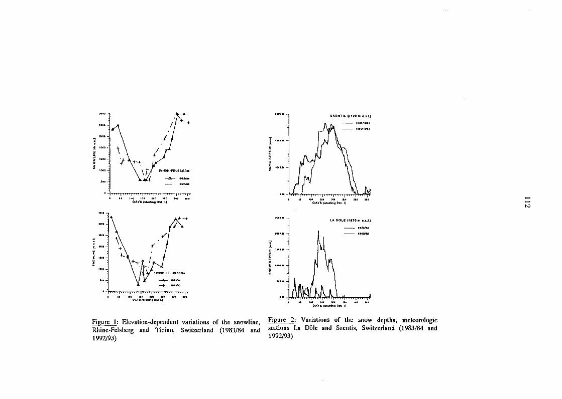
"' : !. .. 3 ~ z "

a: ,;

!. ~ z ~ 0

:

uoo

+.+

RHEIN·FELSBERO

-A- IU3/&4 ... -+ 111218:3

0 ~TTTfrrTI I' •• I I I I I,, I I I 'TT"'TTT'f'"

D ID hoD 160 )00 ,..D

DAY& (slarling 0111 1.)

not

ltfl

....

....

....

.... ...

" 111 110 NI Ml 101 1\1 DA'I'IjllllliiiiiDkil.J

Figure 1: Elevation-dependent variations of the snowline, Rhine-Felsbcrg and Ticino, Switzerland (1983/84 and 1992/93)

( UOIII !. "' X

t: .. 0

~ 0 z ..

.. !. " X t: ... 0

~ 0 z Ill

KOIIO

110100

1101.01

111.11

..

..

SAENTIS 124110 M a.s.l.)

"' ... ... "'' ... OAY6 (11arting Oc:l. I)

LA DOLE {1170 m a.a.l) ... , .. -- IIU/e:J

'" , .. ... .. . ... •• DAVB (alaf11ng Ocl. I)

Figure 2: Variations of the snow depths, meteorologic stations La Dole and Sacntis, Switzerland (1983/84 and 1992/93)

.... !: ..... i • ..... ;

.....

••

...

4UI .... tM.M tt'l• Mlt ...... •• ••r• <••.,••• AptHI.I914)

"" .. ~" ~" -· ...... ,,,,,, (•.,••• Aptill,lttl)

Figure 3: Conventional snow depletion curves for the Rhine­Felsbcrg basin (Switzerland), 1983/84 and 1992/93

.....

.. _ .. "¥

~· .. :! ,. ....

......

...... I .!. .. 1 ,. ....

1.10

. ..•

.., .. lld

U'flptld

'.

"''' M.QO IM(IIJ lltllll9 "081'1 ••••" •r••r• (ll•rli•l April I, 191.1)

.. .... ,td

41111 .... • ... ,. 11111110

""•" .t 4•r• (tttrli•l Apriii,I,IIJ tol-'0

Figure 4: Snowmclt runoiT simulations ami measurements for the Rhinc-Felsbcrg basin Switzerland (1983/84 and 1992/93) based on the SRM model

--~

REFERENCES:

[1] NRC, "Opportunities in the Hydrologic Sciences," National Research Council, Washington D.C.:

National Academic Press, 1991. [2] C. Pfister, "Klimageschichte der Schweiz 1525-1860. Das Klima der Schweiz von 1525-1860 und seine Bedeutung in der Geschichte von Bevolkerung und Landwirtschaft," Academia Helvetica 6, Bern: Paul

Haupt, 1988. [3] H. Flohn, A. Kapala, H.R. Knoche, H. Machler, "Water vapour as amplifier of the greenhouse effect: new aspects," Meteoro/ogische Zeitschrift, Neue Folge, No. 1, 1992, pp.l22-l38. [4] M.F. Baumgartner and G. Apfl, "Towards an integrated geographic analysis system with remote sensing, GIS, and consecutive modelling for snow cover monitoring," Int. Journal of Remote Sensing, Vol. 15, No. 7, 1994, pp.1507-1518. [5] M.F. Baumgartner and M. Fuhrer, "A Swiss A VHRR and Meteosat receiving station," Proc. ofthe 5th EuropeanAVHRR User's Meeting held

114

in Tromso, Norway on the 25th-28th June 1991, EUMETSA T P-09 (Darmstadt: Eumetsat), pp.23-33. [6] R.O. Duda and P.E. Hart, "Pattern Classification and Scene Analysis," New York: Wiley Interscience, 1973. (7] M.F. Baumgartner and G. Apfl, "Monitoring snow cover variations in the Alps using the Alpine Snow Cover Analysis System," In: Mountain Environments in Chaning Climates, M. Beniston (Ed.), London: Routledge Publishing Company, 1994, pp.108-120. (8] J. l\1artinec, 1985: "Snowme1t runoff models for operational forecasts," Nordic Hydrology, Vol. 16, 1985, pp.129-136. [9] J. Martinec, A. Rango, R. Roberts, "The Snwomelt Runoff Model (SRM) User's Manual," Ed.: M.F.Baumgartner, Geographica Bernensia, P-29, Dept. of Geography, Univ. of Berne, Switzerland, 1994.

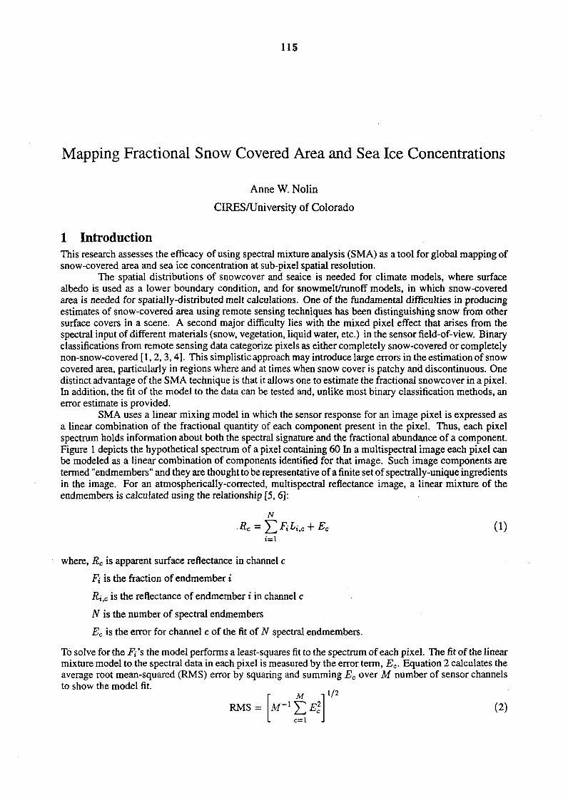
115

Mapping Fractional Snow Covered Area and Sea Ice Concentrations

1 Introduction

Anne W. Nolin

CIRES/University of Colorado

This research assesses the efficacy of using spectral mixture analysis (SMA) as a tool for global mapping of snow-covered area and sea ice concentration at sub-pixel spatial resolution.

The spatial distributions of snowcover and seaice is needed for climate models, where surface albedo is used as a lower boundary condition, and for snowmelt/runoff models, in which snow-covered area is needed for spatially-distributed melt calculations. One of the fundamental difficulties in producing estimates of snow-covered area using remote sensing techniques has been distinguishing snow from other surface covers in a scene. A second major difficulty lies with the mixed pixel effect that arises from the spectral input of different materials (snow, vegetation, liquid water, etc.) in the sensor field-of-view. Binary classifications from remote sensing data categorize pixels as either completely snow-covered or completely non-snow-covered [1, 2, 3, 4]. This simplistic approach may introduce large errors in the estimation of snow covered area, particularly in regions where and at times when snow cover is patchy and discontinuous. One distinct advantage of the SMA technique is that it allows one to estimate the fractional snowcover in a pixel. In addition, the fit of the model to the data can be tested and, unlike most binary classification methods, an error estimate is provided.

SMA uses a linear mixing model in which the sensor response for an image pixel is expressed as a linear combination of the fractional quantity of each component present in the pixel. Thus, each pixel spectrum holds infonnation about both the spectral signature and the fractional abundance of a component. Figure 1 depicts the hypothetical spectrum of a pixel containing 60 In a multispectral image each pixel can be modeled as a linear combination of components identified for that image. Such image components are tenned "endmembers" and they are thought to be representative of a finite set of spectrally-unique ingredients in the image. For an atmospherically-corrected, multispectral reflectance image, a linear mixture of the endmembers is calculated using the relationship [5, 6]:

N

Re = L FiLi,c + Ee i=l

where, Re is apparent surface reflectance in channel c

Fi is the fraction of endmember i

Ri,e is the reflectance of endmember i in channel c

N is the number of spectral endmembers

Ee is the error for channel c of the fit of N spectral endmembers.

(1)

To solve for the Fi 's the model perfonns a least-squares fit to the spectrum of each pixel. The fit of the linear mixture model to the spectral data in each pixel is measured by the error term, Ee. Equation 2 calculates the average root mean-squared (RMS) error by squaring and summing Ee over M number of sensor channels to show the model fit.

[

M ]1/2 RMS = M- 1 ?; E; (2)

0.8

0.6

R

0.4

0.2 Vegetation

0.5

116

Pure and combined cnLimcmber spectra

·_:. .. '•

1.5 wavelength, ~m

2 2.5

Figure 1: Reflectance spectra (from Mammoth Mountain A VIRIS image) of snow and vegetation and the

simulated spectrum of a linear combination of 40% vegetation and 60% snow

Spectral endmembers are chosen from each image and, though the same category of endmember may be the same for many images (eg. rock, snow, vegetation), their spectral characterization is expected to differ from one image to another because of changes in solar illumination, differences in rock, vegetation or snow-type and so on. After atmospheric correction of the image data, using the SS model, a principal components analysis (PCA) is performed on the multispectral data. PC images are examined and the locations of pixels having the highest value in each PC image are marked. These marked pixels are then located in the reflectance images and the reflectance spectra of these pixels are used as the endmember spectra. The spectral unmixing model is iteratively run (each time solving for the fraction of each endmember in each pixel) with successively fewer endmembers until both the overall RMS error is minimized and the fraction of each endmember lies between the values of 0 and 1.

As part of the Earth Observing System (EOS) project, the Moderate Resolution Imaging Spectrom­eter (MODIS) will be used to collect data in 36 channels (20 visible and near-infrared channels). Digital maps of global snow-covered area will be produced from MODIS data starting with the launch of EOS in 1998. Towards this end, a global snow-mapping algorithm, SNOMAP, is under development. One proposed approach entails using a normalized difference snow index (NDSI) to produce a binary classification of snowcover. This index, tested with Landsat Thematic Mapper (TM) data, makes use of the fact that snow reflectance is high in the visible and low in the near-infrared. Preliminary tests of the NDSI indicate that it agrees to with 95% with a sub-pixel resolution snowcover map derived with a more complex algorithm [7]. The latter algorithm, based on spectral mixture analysis [8], calculated the fraction of snow-covered area in each pixel providing a higher degree of accuracy for snow mapping. While spectral mixture analysis is a promising tool for snow mapping at regional scales, it is not clear that this more complex method can be justified for use at the global scale.

2 Approach

2.1 Mapping Alpine Snow Cover

Remote Sensing Data

117

• TM image of Glacier National Park, Montana (March 14, 1995)

• AVIRIS image of Mammoth Mountain, California (January 11, 1993)

In this research, multispectral remotely sensed data from both Land sat Thematic Mapper (TM) and Airborne Visible/Near-Infrared Imaging Spectrometer (AVIRIS) sensors were used as proxy data for MODIS. TM data represent the data having the closest spectral match to the MODIS data and these data have already been used to test both a SMA-based and NDSI-based snow mapping algorithm. So, it is appropriate to use TM data for comparison of the two techniques. Landsat TM has a 30 m spatial resolution while MODIS has 250 m to 1 km spatial resolution.

AVIRIS has a spatial resolution of 20 m a spectral range from 400-2450 nm and a nominal spectral resolution of 10 nm. It is flown in a NASA ER-2 aircraft at an altitude of 20 kmand has a swath width of 12 km. To better characterize the full number of spectral bands that may be used for snow mapping, AVIRIS channels were convolved to MODIS spectral resolution (based on current band characteristics) and results of each algorithm were compared on a spectral basis.

Both regions can be characterized as rugged, mountainous terrain with snow, rock and alpine and subalpine vegetation present. The AVIRIS image is of Mammoth Mountain on January 11, 1993, acquired shortly following a snowfall of about 10-20 cm. The snowpack at the time was approximately 2-3 m deep over most of the mountain. The Glacier National Park TM image, acquired on March 14, 1991, also shows abundant fresh snow.

Because of disk space and computational limitations, subscenes of each image were used. The AVIRIS image was subset so that Mammoth Mountain would be centered in the image. This image is 504 x 342 pixels representing an area 6900km2 . In the Mammoth Mountain image, AVIRIS channels were convolved to MODIS spectral resolution to create a 20-band synthetic image. Using spectral endmembers chosen from the principal components transformation of the data, the spectral mixture algorithm was applied to the MODIS/AVIRIS synthetic image.

The Glacier National Park image was subset to create a 2500 x 2500 pixel image representing an area of about 562,500 km2 . both the SMA and NDSI methods were used to determine snow covered area.

2.2 Mapping Sea Ice Concentrations

The SMA model was also used in to test its ability to perform sea ice mapping. Two TM images of the Beaufort Sea region of the Canadian Arctic, acquired within a two-day period (April 16, 1992 and April18, 1992) were used in this part of the analysis. As with the alpine snow images, a PC transformation was run to determine the endmembers for each image. Both images show the pack ice in spring and open water is visible in the cracks between large pieces of sea ice. No wet snow is visible in the April 16 image but, in the April 18 image, melt is just beginning to occur in the snow overlying some of the sea ice. Some clouds are visible in the bottom and the very top of the April 18 image.

2.3 Atmospheric Correction

For each-TM image, the uncalibrated data were converted from raw DN values to values of apparent surface reflectance for each of six spectral bands. First, the atmospheric transmittance and path radiance values were calculated for each of the TM spectral bands using the 5S code /citetanre. An example of these values, for the Glacier N. P. image are given in Table 1.

Then, using the transmittance and path radiance values along with the calibration coefficients (gains and offsets) for each TM band, the conversion from DN to reflectance was performed in a single step.

p =((offset+ (gain* DN))- Lpath)/(Lsun * t1 * t2) (3)

118

Table 1: Transmittance, path radiance and solar radiance values used in the atmospheric correction of the

Glacier National Park TM scene

Band Number Path Radiance Solar Radiance Tup Tdown

1 1.747 38.5 0.902 0.822

2 1.043 43.1 0.955 0.913

3 0.475 39.3 0.976 0.954

4 0.013 37.3 0.992 0.984

5 0.018 12.3 0.999 0.999

7 0.001 5.9 1.000 1.000

Where, p is apparent surface reflectance, Lpath is path radiance, Lsun is solar radiance at the top of the atmosphere, t 1 and t2 are the upward and downward transmittances, respectively. In the process of being atmospherically corrected, each TM band is converted from a byte image to a floating point image (thereby increasing its size four-fold).

AVIRIS data were also atmospherically corrected and converted to apparent surface reflectance. This task was accomplished using ATREM, the atmosphere removal program of Gao [9].

3 Results

3.1 Alpine Snow Cover Mapping

The atmospherically-corrected TM image subset (2500 x 2500 pixels) was used for both the spectral mixture analysis and analysis with the NDSI algorithm. In the spectral mixture analysis, three endmembers were chosen: snow, vegetation and shade. These were obtained after running a principal components transformation on the image and examining the scatterplots of the principal components to identify the purest pixels for each endmember and the total number of endmembers. After the image was unmixed into its endmember components, the scaled snow fraction was computed by dividing the snow image by the sum of the snow and vegetation images (see Figure 2). Best results appear to have been obtained for both the snow and shade fraction images with virtually all concentration values falling within the range from 0.0 to 1.0.

Slightly negative values mean that there was some endmember that should have been included that wasn't. However, when additional endmembers were added, the RMS error would increase to an unacceptable level because the added endmember resulted in a greater lack of fit of the model to the data. Slightly super-positive values (greater than 1.0) mean that these pixels were more "pure" than the ones chosen for the endmembers. Changing the endmembers to these "purer" pixels resulted in a worse fit of the model to the data because those pixels were actually less representative of the endmember. The results presented here represent the best fit of the model to the data: Because of the lack of pixels containing only vegetation, this endmember is not particularly representative of "pure" vegetation. This resulted in a greater number of negative and super-positive values in this image. However, the overall RMS error with those chosen endmembers was less than 1

For comparison with the spectral mixture model results, the SNOMAP algorithm was applied the Glacier National Park TM image. The resulting image is shown in Figure 3.

The NDSI binary classification resulted in a total snow covered area of3979 km2 , slightly exceeding the SMA-derived snow covered area estimate of 3820 km2 , only a 4.2% difference between the two results. Though this difference is not particularly large, it could, depending on the snow depth and spatial distribution, result in a substantially different estimate for the snowmelt/runoff from the snowpack. The snow fraction image produced using SMA is able to show the varying spatial distribution of the snowpack whereas the NDSI binary classification cannot.

119

Figure 2: Scaled snow fraction image for Glacier National Park, Montana.

Using spectral endmembers chosen from the principal components transformation of the data, the spectral mixture algorithm was applied to the 20-band MODIS/AVIRIS synthetic image and the results are shown in Figures 4-6.

The snow fraction image has values ranging from 0.0 to 1.0. This closely agrees with results from the application of the spectral mixture model to the original AVIRIS data (which have been validated using aerial photographs [10]. Summing the fractions of snowcover in each pixel gives the total snow covered area for the scene. From the MODIS/ AVIRIS synthetic image, the total snow covered area was calculated to be 38.1 km2 and the total from the original AVIRIS image was 37.3 km2• Overall RMS error for the unmixed MODIS/ A VIRIS scene was 1.1%. Pixels that are insufficiently illuminated have higher RMS error values as do the brightest snowcovered pixels. In general, the spectral mixture model was able to fit the data with very low error.

NDSI estimates of total snow covered area for Mammoth Mountain were significantly lower than those obtained from using the SMA method. The reason for the difference in estimates is the large number of shaded pixels evident in the image, many of which are assigned values of no snow from the SNOMAP algorithm. The NDSI method is not able to express the spatial distribution of snowcover in this rugged alpine area. SMA results from the MODIS-convolved AVIRIS image compared closely with SMA results from the original AVIRIS image.

3.2 Sea Ice Concentration Mapping

In the Beaufort Sea TM image from 04/18/92, four endmembers were found to best characterize the spectral variability in this six-band image: sea ice, liquid water, cloud, and wet snow. Figures 7-10 show the fractional proportions of each of these endmembers with white pixels having concentrations near unity and dark pixels having the lowest concentrations. RMS error was very low for this unmixing result ( 0.4% ).

The SMA method was able to map a wide range of sea ice concentrations in this image. In addition, the it appears that the SMA technique can discriminate between thin ice and thick ice since the combination of open water and sea ice fractions appear to have a spatial distribution like that of thin ice. While, currently

120

Figure 3: SNOMAP-derived binary classification of snowcover for Glacier National Park, Montana. White

pixels represent 100% snowcover and black pixels represen t 0% snowcover.

there is no comparison with estimates of sea ice concentrations and ice types from an NDSI-like method, we expect to produce this comparison in the near future.

The SMA method was also applied to the 04/16/92 sea ice image. Two endmembers were found to describe the range of spectral variations in each pixel: sea ice and liquid water. No clouds were apparent in this image and it appears that surface melt was insignificant. Overall RMS error was about 0.5%.

A test was performed to determine if endmembers could be transferred from one image to another. Because the Beaufort Sea TM images are close in both space and time, it was thought that the seaice and liquid water endmembers from the 4/18/92 image could be used to map those components in the 4/16/92 image. However, the average RMS error for the newly analyzed 4/16/92 image jumped to 10%, an increase of more than one order of magnitude. This case study demonstrates that spectral endmembers need to be chosen from the image data themselves for best results.

3.3 Automated Selection of Endmembers

Further analysis needs to be performed to determine how endmembers can best be selected. This is perhaps the largest constraint on the use of this method as an operational approach to sub-pixel snow and sea ice mapping. Constrained Energy Minimization (CEM), a newly developed technique used for mapping geologic materials has shown promise for discriminating between a spectrum of interest, "foreground", and the spectra of other components in the image, "background". One of the apparent advantages of mapping snow and ice with the CEM technique is that these components have high signal-to-noise and high contrast with other image components. Future research on snow cover mapping will explore the use of the CEM technique.

121

Figure 4: Snow fraction image for the MODIS-convolved AVIRIS data, Mammoth Mountain, California.

The originalAVIRIS data were acquired on January 11, 1993. North is to the upper right of the 10 kmx 12 km

image. Mammoth Mountain isthe large snow-covered region in the center of the image; ski runs are evident

on in the north side of the mountain.

4 Conclusions Snow cover in both the Mammoth Mountain and Glacier National Park images were mapped using the SMA method. Results from the MODIS-convolved AVIRIS image from Mammoth Mountain compared closely with SMA results from the original AVIRIS image. A comparison of SNOMAP-derived snow covered area produced value 4.2% larger than that calculated using the SMA technique. Though this difference is not particularly large for the 2500 x 2500 image, for snowmelt runoff models, it is crucial to have an accurate measure of the spatial distribution of the fraction of snowcover. Thus, for certain applications such as snowmelt runoff modeling in alpine regions, a binary classification does not provide sufficient information on the spatial distribution of snowcover: One area of significant disagreement between the SMA and NDSI methods was mapping shaded snow. In many pixels in the Glacier National Park image, the NDSI method incorrectly identified shaded snow pixels as non-snowcovered while the SMA method mapped them as containing some fraction of snowcover. So, while the results between the two techniques agreed fairly closely, the accuracy of the NDSI method is in doubt for shaded pixels.

A second important consideration is the possibility that the SNOMAP threshold (currently set at 0.4) may systematically bias the classification results in ways that are not currently understood. For example, if a region has a uniformly patchy snowcover such that each pixel in the image had a snowcover fraction of 0.5, the SNOMAP algorithm may map all those pixels as having zero snowcover. What is needed is a more thorough validation effort for the SNOMAP algorithm to identify possible biases and significant shortcomings.

The SMA method appears to be effective for mapping the spatial distribution of sea ice at a sub­pixellevel. Because the range of possible spectral endmembers is small in Arctic scenes this technique holds great promise for accurately characterizing the fine-scale spatial distribution ofsea ice, open water,

122

Figure 5: Vegetation fraction image for the MODIS-convolved AVIRIS data, Mammoth Mountain, Califor­

nia.

clouds, and snow. Cryospheric components in both alpine and arctic were mapped at sub-pixel resolution using the

SMA technique. However, because of the need for interactive endmember selection for each image, this technique is remains in a "pre-operational" phase. That is, until automated endmember selection can be carried out in an accurate and computationally reasonable fashion, the SMA method will not be appropriate for global operational snow and ice cover mapping. Future work on this project will focus on developing an automated endmember selection process and work-in-progress indicates that this is a promising line of research.

References

[1] A. Rango, "Assessment of remote sensing input to hydrolog1~ mucids," Wat. Res. Bull., vol. 21, pp.423-432, 1985.

[2] J. Dozier and D. Marks, "Snow mapping and classification from Landsat Thematic Mapper data," Ann. Glaciol., vol. 9, pp. 1-7, 1987.

[3] J. Martinec and A. Rango, "Interpretation and utilization of areal snow-cover data from satellites," in Proc. IAHS Third Int. Assembly, Baltimore, MD, IAHS, 1987. IAHS Publ. 186.

[4] J. Dozier, R. E. Davis, and A. W. Nolin, "Reflectance and transmittance of snow at high spectral resolution," in IGARSS '89, Quant. rem. sens.: an economic tool for the Nineties, (Canada), pp. 662-664, IGARSS '89 12th Can. Symp. on Rem. Sens., 1989. No. '89CH2768-0.

[5] J. B. Adams, M. 0. Smith, and P. E. Johnson, "Spectral mixture modeling: a new approach to analysis ofrock and soil types at the Viking Lander 1 site," J. Geophys. Res., vol. 91, pp. 8098-8112, 1986.

123

Figure 6: RlviS error image for for the MODIS-convolved AVIRIS data, Mammoth Mountain, California.

[6] D. A. Roberts, M. 0. Smith, J. B. Adams, and D. E. Sabot, "Isolating woody plant material and senescent vegetation from green vegetation in AVIRIS data," in Proc. 2nd Ann. JPLAirborne Vis.Jlnfr. /maging Spectro. (AVIR IS) Workshop (R. 0. Green, ed.), (Pasadena, California), pp. 42-57, Jet Propulsion Laboratory, 1990. JPL Publication 90-54.

[7] D. K. Hall, J. L. Foster, J. Y. L. Chien, and G. A. Riggs, "Determination of actual snow-covered area using Landsat TM and digital elevation model data in Glacier National Park, Montana," Polar Record, vol. 31, pp. 191-198, 1995.

[8] W. Rosenthal, "Mapping montane snow cover at subpixel resolution from the Landsat Thematic Mapper," Master's thesis, University of California, Santa Barbara; 1993.

[9] B.-C. Gao, K. Heidebrecht, and A. F. H. Goetz, "Software for the derivation of scaled surface re­ftectances from AVIRIS data," in Summ. 3rd Ann. JPL Airborne Geosci. Workshop (R. 0. Green, ed.), (Pasadena, California), pp. 101-103, Jet Propulsion Laboratory, 1992. JPL Publication 92-14, Vol. 1.

[10] A. W. Nolin, "Snowcover mapping with the Airborne Visible/Infrared Imaging Spectrometer," in Pro­ceedings of the International Geoscience and Remote Sensing Symposium '94, (Pasadena), pp. 2081-2083, IEEE, 1994. 94CH3378-7.

124

Figure 7: Sec. ice fraction image from the Beaufo:-t Sea TM image. 04/1 S/9:?..

Figure 8: Open water fraction image from the Beaufort Sea T?\1 irr.age, 04/18/9:?..

125

Figure 9: Cloud fra:::tion irr:afe from the Sea'Jfo:c Sea n1 ir.12.ge. ~;.1.; ~ ~:.:

126

AN ANALYSIS OF THE NOAA SATELLITE-DERIVED SNOW COVER RECORD, 1972-PRESENT

Introduction

David A. Robinson & Allan Frei Deparbnent of Geography

Rutgers University New Brunswick, NJ 00903

The large-scale distribution of snow cover over northern hemisphere lands has been a topic of increasing attention in recent years. This interest has been spurred, at least in part, by concerns associated with potential changes in the global climate system associated with anthropogenic and natural causes. Satellite observations using visible satellite imagery permit a hemispheric analysis of snow extent. For almost three decades the National Oceanic and Atmospheric Administration (NOAA) has been using visible imagery to produce weekly charts depicting the extent of snow cover over northern hemisphere lands. These charts constitute the longest satellite-derived environmental dataset available on a continuous basis and produced in a consistent manner. We will briefly describe the NOAA charts and then provide an update on the variability of snow extent over the hemisphere from January 1972 through August 1995. Concentration will be on snow kinematics, as found formerly in Matson & Wiesnet (1981), Dewey & Heim (1982), Barry (1990), Robinson et al. (1991), Iwasaki (1991), Gutzler & Rosen (1992), and Masuda et al. (1993). Recent studies that use NOAA snow data to investigate snow cover synergistics within the climate system include, for example, Leathers & Robinson (1993; 1995), and Karl et al. (1993). · ·

NOAA Snow Charts

Weekly snow charts produced by NOAA depict boundaries between snow-covered and snow-free land surfaces. They are produced from visual interpretation of photographic copies of visible-band satellite imagery, primarily Advanced Very High Resalution Radiometer (AVHRR) data. Charts show snow boundaries on the last day that the surface in a given region is observed. Since cloud cover can mask the surface, this is often not the last day of the chart week. On average, charts tend to represent the fifth day of a week. Charts are digitized on a weekly basis to the National Meteorological Center Limited­Area Fine Mesh (LFM) grid (cf. Matson et al., 1986, and Robinson, 1993 for further details on NOAA charts). While NOAA charts have been produced since 1966, early ones tended to underestimate snow extent, particularly during fall. Charting accuracy improved considerably in 1972, when VHRR and later A VHRR data began to be used. Data since 1972 are considered to be of high enough quality for use in climate studies (Wiesnet et al., 1987).

For our investigation, monthly means of snow cover area are calculated using a routine described fully in Robinson (1993). The Rutgers routine calculates weekly areas from the digitized snow files and to then obtain a monthly value, weights them according to the number of days of a chart week falling in the given month. A chart week is considered to center on the fifth day of the published chart week. Prior to the calculations, the digital files are standardized to a common land mask that includes those and only those LFM cells at least half covered by land. This corrects an inconsistency in the original NOAA files.

127

Snow Cover: 1972-present

Mean annual northern hemisphere snow cover is 25.4 million km2. On average, 14.7 million km2lies over Eurasia and 10.6 million km2 over North America (including Greenland). In figure 1, the variability of snow cover over the Northern Hemisphere between January 1972 and August 1995 is expressed through anomalies of individual months and twelve-month running means. Monthly anomalies of greater than 4 million km2 have been observed occasionally throughout the past 24 years, although they are generally less than 2 million km2.

Two pronounced snow regimes are evident during the period of record. Between 1972 and 1985, twelve­month running means of snow extent fluctuated around a mean of approximately 25.9 million km2. A rather abrupt transition occurred in the 1986/87 period to a new regime from 1988 to the present where snow extent fluctuates around a running mean of about 24.2 million km2. This recent interval is marked by a decrease in spring and early summer snow extent compared to the earlier period (figure 2). Changes are evident over both North America and Eurasia. Individual years of fall and winter snow cover vary around means that have remained more stable during the satellite era.

Zones exhibiting year-to-year variability in snow cover extent have been identified for each month of the year. Figure 3 shows these "action" areas for November and April, defined as locations where the surface is snow covered between 10% and 90% of the time in at least one third of the years between 1972 and 1994. This rather broad criterion excludes those regions where snow cover is extremely common or rare during a particular month. The variable zone in November straddles the US/Canadian border from coast to coast, and plunges into the US Rockies and high Plains. The Eurasian zone lies within approximately 5° of the 50th parallel, except in Europe where it curves poleward. The Himalayan/Tibetan region also has variable cover, which is also the case in April. The variable zone in April across the remainder of Eurasia lies between approximately 50° and 60°N. April snow extent is also variable in southern Canada and the US Rockies, a considerably smaller North American zone than in November.

Within these variable zones, Principal Components Analysis (PCA) has been used to identify regions of coherent snow cover; that is, areas within which snow time series for grid points are highly correlated to each other. An orthogonal varimax rotation of the components has been performed to allow for more clear visualization. Regional signals are found to be dominant over continent-wide signals in all months. The first two components for November and April are shown in figure 3. Together, the two November components explain 26% of the hemispheric variance. Component 1 centers on the northern US Rockies and the northern US high plains and western Canadian prairie. Component 2 covers much of the variable zone in eastern Asia. In April, component 1 is found in western Asia, and component 2 covers a region spanning North America, along and just north of the US/Canadian border. Together, these two components explain 27% of the hemispheric variance in April.

Conclusions

Given the relatively short time in which hemispheric monitoring of snow cover has been possible from space, it is difficult to fully understand the significance of the apparent stepwise change in snow extent in the middle 1980s. It is certainly premature to ascribe the less-extensive regime in recent years to a global warming. However it is noteworthy that the extent of snow cover appears to be inversely related to hemispheric surface air temperature (Robinson & Dewey, 1990), and, particularly in spring, feedbacks associated with the extent of the snowpack may be strongly influencing temperature (Groisman et al., 1994). Further studies using the NOAA set in conjunction with other climatic information are needed to better understand the synergistic relationships between hemispheric-scale atmospheric circulation and thermal variations and continental snow extent before any meaningful projections of future climatic states can be made.

128

Figure 1. Anomalies of monthly snow cover extent over northern hemisphere lands (including Greenland) between January 1972 and August 1995. also shown are twelve-month running anomalies of hemispheric snow extent, plotted on the seventh month of a given interval. Anomalies are calculated from a mean hemispheric snow extent of 25.4 million km2 for the full period of record.

Nonhern Hemisphere Fall

23...-----------.

22

21

20

19

18

Nn•~•~••o~Nft•M•~••o-""•

~~~~~~~~--------·-····· Northern Hemisphere Spring

35...,.-----------. 34

32

31

~ 30

2 @ 29

:t 28

N"·~·~--O~N~~M·~-·0-~ft·­~~~~~~~~---~------····-·

Northern Hemisphere Winter

49....------------T" 41

Northern Hemisphere Summer

10-r----=--------r

9

Figure 2. Extent of seasonal snow cover over northern hemisphere lands (including Greenland) since 1972.

129

(a) (b)

Figure 3. Land areas in white are zones of variable snow extent in November (a) and April (b) (cf. text for explanation). Contours within these zones show the first (solid) and second (dashed) principal components. Contours are plotted at 0.1 increments, starting at r2=0.3.

130

NOAA will soon be discontinuing production of the weekly snow charts and replace them with daily ones. While still incorporating visible imagery, the new product will rely heavily on satellite passive microwave-derived estimates of snow extent. Plans are to conduct at least a twelve-month comparative study of the two products before discontinuing the current visible-only one. The appearance of MODis­derived snow charts later in this decade will be a welcome addition to hemispheric snow charting efforts. The MODIS channels will provide the ability to better discriminate between snow and clouds. And perhaps with the development of procedures incorporating multiple visible and near infrared channels, snow will be identified more accurately in cloud-free areas. Together, the NOAA and MODIS products will provide an· unprecedented means of assessing the seasonal and interannual fluctuations of this influential component of the climate system.

Acknowledgments

Thanks to D. Garrett at the NOAA Climate Analysis Center for providing continuous updates of the raw digitized NOAA snow chart data, and to J. Wright for running the Rutgers routine on these files. This work is supported by NSF grants ATM-9314721 and SBR-9320786 and NASA grant NAGW-3568.

References

Barry, R.G., 1990: Evidence ofrecent changes in global snow and ice cover. Geofournal, 20, 121-127. Dewey, K.F. & R. Heim Jr., 1982: A digital archive of northern hemisphere snow cover, November 1966

through 1980. Bull. Am. Met. Soc., 63, 1132-1141. Groisman, P. Ya., T.R. Karl & R.W. Knight, 1994: Observed impact of snow cover on the heat balance

and the rise of continental spring temperatures. Science, 263, 198-200. Gutzler, D.S. & R.D. Rosen, 1992: Interannual variability of wintertime snow cover across the Northern

Hemisphere, J. Clim., 5, 1441-1447. Iwasaki, T., 1991: Year-to-year variation in snow cover area in the Northern Hemisphere. J. Met. Soc.

Japan, 69, 209-217. Karl, T.R., P.Y. Groisman, R.W. Knight & R.R. Heim, Jr., 1993: Recent variations of snow cover and

snowfall in North America and their relation to precipitation and temperature variations. J. Clim.J 6, 1327-1344.

Leathers, D.J. & D.A. Robinson, 1993: The association between extremes in North American snow cover extent and United States temperatures. J. Clim., 6, 1345-1355.

Leathers, D.J. & D.A. Robinson, 1995: Abrupt changes in the seasonal cycle of North American snow cover. Proc. Fourth Conf. Polar Meteor. Oceanog., Dallas, AMS, 122-126.

Masuda, K, Y. Morinaga, A. Numaguti & A. Abe-ouchi, 1993: The annual cycle of snow cover extent over the Northern Hemisphere as revealed by NOAA/NESDIS satellite data. Geographical Reports of Tokyo Metropolitan Univ., 28, 113-132.

Matson, M., C.F. Ropelewski and M.S. Varnadore, 1986: An Atlas of Satellite-Derived Northern Hemisphere Snow Cover Frequency. NOAA Atlas, 75pp.

Matson, M. & D.R. Wiesnet, 1981: New data base for climate studies. Nature, 289,451-456. Robinson, D.A. ,1993: Monitoring northern hemisphere snow cover. Snow Watch '92: Detection

Strategies for Snow and Ice. Glaciological Data Report, GD-25, 1-25. Robinson, D.A. & K.F. Dewey, 1990: Recent secular variations in the extent of northern hemisphere

snow cover. Geophys Res. Lett., 17, 1557-1560. Robinson, D.A., F.T. Keimig & K.F. Dewey, 1991: Recent variations in Northern Hemisphere snow

cover. Proc. 15th Annual Climate Diagnostics Workshop, Asheville, NC, NOAA, 219-224. Wiesnet, D.R., C.F. Ropelewski, G.J. Kukla & D.A. Robinson, 1987: A discussion of the accuracy of

NOAA satellite-derived global seasonal snow cover measurements. lArge Scale Effects of Seasonal Snow Cover, IAHS Publ. 166, 291-304.

131

SESSION 4 - HYDROLOGICAL MODELLING OF ARCTIC RIVER RUN-OFF

133

HYDROLOGICAL MODELLING OF ARCTIC RIVER RUNOFF

ABSTRACT

Sten Bergstrom Swedish Meteorologkal and Hydrological Iristitute

Norrkoping, Sweden

An overview of the current state of knowledge in hydrological modelling feasible for the simulation of runoff in Arctic areas is given. Problems related to data needs and the physical descriptions in the models are discussed. Examples of effects of river regulation on runoff are given and a large scale application, covering the full drainage basin of the Gulf of Bothnia is shown. It is concluded that there exist useful models and that the most important problem in Arctic applications is the poor data coverage. Among modelling problems the modelling of glacier mass balances is pointed out as the most difficult one to solve.

1. OVERVIEW OF THE CURRENT STATE OF KNOWLEDGE

1.1 Model structures

The first computer based hydrological models appeared in the late 1960-ies and since then numerous models have been developed for various purposes. It was soon realized that different problems have different requirements on the models. The earliest focus was on operational runoff simulation and hydrological forecasting and surprisingly good results were obtained by very simple models (Nash and Sutcliffe, 1970). This simplicity in model structures was, among others, a neccessity due to the limited data that normally were available. As the models had some physical background, but subroutines based on a lot of empirism, they were often referred to as conceptual models. All conceptual hydrological models have empirical coefficients (parameters) which are given optimal values by calibration of the model against observed data.

Examples of conceptual hydrological models with subroutines for snow conditions, and thus feasible for Arctic applications, are the Canadian UBC model (Quick and Pipes, 1976), the Danish NAM model (Nielsen and Hansen, 1973), the Japanese TANK model (Sugawara, 1979), the Swedish HBV model (Bergstrom, 1976; Bergstrom, 1992), the Swiss-American SRM model (Rango and Martinec, 1979) and two models from the USA; the SSARR model (U.S. Army Corps of Engineers, 1976) and the NWSRFS (Anderson, 1973). A very recent overview of runoff models can be found in the work by Sing (1995).

Contrasting the conceptual models are the models referred to as physically based. These models have a higher order of physical description and are intended for a wider span of applications than the conceptual ones. Best known among the physical category of models is the SHE model

134

(Bathurst, 1986). It is often stated that these models are more feasible for applications were man is interacting with the natural conditions, such as changing land use and climate change. The debate between the shoals of conceptual modelling and physically based modelling has, however, been vivid (See, for example, Beven, 1989 or Bergstri:im, 1991). While it, for example, is often argued that physically based modelling is the only valid approach for modelling of river flow in rivers completely lacking data, conceptual models are often used this way already today.

WMO has performed a few well controlled modelling intercomparison projects related to operational runoff modelling (WMO, 1975 and 1986) which are highly relevant for the discussion on model complexity. The last of the two intercomparisons concerned snowmelt modelling and covered a span from simple degree-day methods to complete energy balance models. One of the conclusions is worth quoting: "On the basis of available information, it was not possible to rank the tested models or classes of models in order of performance. The complexity of the structure of the models could not be related to the quality of the simulation results." This statement has since then been challanged many times but it is still valid for operational applications in large basins with normal data coverage.

There should not be a conflict between the use of physically-based process oriented models and the simpler more empirical conceptual ones. We just have to realize that they are developed for different purposes and should be applied accordingly. Physically based models are normally more feasable as research tools for process studies in the small scale where physical parameters are well under control and their variability is small while conceptual models are more basin-oriented. In the following I will concentrate on the conceptual family of models.

1.2 The conceptual model and its application

The structure of a conceptual hydrological model can usually be divided into the following three distinct components:

Subroutines for accumulation and melting of snow and glaciers.

A soil moisture accounting subroutine.

Subroutines for storage-discharge relationsships in the basin including implicit or explicit modelling of aquifers, lakes and river routing.

With these subroutines the models can simulate river flow from meteorlogical data with good accuracy. Figure 1 illustrates one example of a model simulation from a mountainous basin north of the Arctic circle in Sweden. The simulation is made by the Swedish HBV model (Bergstri:im, 1976; Bergstri:im, 1992).

135

25 150 o~~~~y-~~~~~~~~~~~~~~~~~~~o

SM (mm) SOIL MOISTUR

1

RUNOFF

Figure 1. Example of a model simulation covering two years of inflow to the Sourva reservoir in upper river Lulealven in northern Sweden. The thin irregular line represents observed inflow to the reservoir while the thick smoother line is the model simulation. The drainage basin is 4650 km2 and is located entirely to the north of the Arctic circle. The simulation is made by the Swedish HBV model. Note the heavy snow accumulation and the short period available for snowmelt and evapotranspiration.

136

If we look at applications of conceptual hydrological models we may classify them into three groups; 1) applications within the range of model calibration, 2) applications outside the range of calibration and 3) applications without any calibration of the model at all.

Model applications within the range of calibration are dominating. Here we find conventional runoff simulations which may be used to fill in gaps in runoff records, for extension of records or for data control. We also fmd short and long term hydrological forecasting, water balance studies, simulations of groundwater recharge and some hydrochemical applications.

While most applications within the range of model calibration are quite straightforward and can be done with a high degree of confidence, the use of conceptual models outside the range of calibration is more controversial. Nevertheless it is sometimes necessary, when no other reliable methods are at hand. Examples where models are used this way are simulations of design floods, studies of the effects of climate change or changing land use and hydrochemical studies of the effects of changing atmospheric deposition.

The last, and most difficult type of application, is to use models without calibration. This is necessary if runoff data are lacking. Although it is often stated that uncalibrated applications require completely physically based models a lot can be achieved by conceptual model with generalized parameters. This is, of course, an appealing approach if runoff data for remote Arctic basins are required.

1.3 Data needs

Conceptual models show their strength in the limited data demand and thus great applicability in operational hydrology. Most models can operate on standard meteorological observations from the national networks, in many cases just precipitation, air temperatures and estimates of the potential evapotranspiration. This means that snowmelt and glacier melt is usually modelled by simple degree~day approaches and that no full energy balance of the snowpack or the soil is considered. Thus the effects of frozen grounds are often neglected.

The time resolution of the models may range from daily values to hourly values. Lower resolution can sometimes be accepted but it has proved to be difficult to model snow conditions with a lower resolution in meteorological data than 24 hours.

Runoff data are output of the models but also the foundation for model calibration. Daily data are often used but these data do not neccesarily have to be of the same time resolution as the meteorological data. In very large river systems monthly runoff data may suffice.

As model calibration is a very important component of an application of a conceptual hydrological model, long homogeneous records of meteorological variables and runoff are needed. Generally, at least five years of record are needed for this procedure, but the optimal length is depending on the variability of the climate and on the hydrological conditions.

137

2. PROBLEMS IN MODELLING OF THE FRESH WATER INPUTS TO THE ARCilC OCEAN

The technical and scientific problems that have to be addressed to improve the modelling of fresh water inputs to the Arctic Ocean kan be separated into problems related to input data and problems related to the modelling of the hydrological processes of the Arctic region.

2.1 Input problems

The input problems are probably the most important ones and the worst ones to overcome. First of all we have to face a situation with very poor coverage of climate stations due to low population density. This means that there will be great interpolation problems of meteorological data. There will also be problems with extrapolation of low level data to higher altitudes when montainous areas are to be modelled.

The climate of the Arctic region creates technical problems at the climate station itself. It is not easy to measure solid precipitation continously at a remote wind-blown Arctic site. Undercatch may be dramatic. Experience has shown that it is often more favourable to chose a less representative but more sheltered site and to accept the observed precipitation as an index value. Thus the problem of representativeness is solved by model calibration.

Remote sensing data are often suggested as a support to overcome the input problem. Present satellite systems are still, however, rather limited when it comes to delivering records of the water equivalents of snow. The models further need long records, which means that data from the satellites have to be stored for some years to be of real use.

Runoff data may suffer from a large number of error sources and therefore they have to be used with great care. The measurements themself can be very difficult under arctic conditions with frequent ice-jarnmings and other problems which effect the measuring sites. While meteorological data can often be made available through international agreements this is not always the case with runoff data. It may even be difficult to identify the agency or company responsible for the measurements.

In many of the rivers of the north hydropower development is a very significant hydrological factor (See, for example, Dynesius and Nilsson, 1994). This is an advantage because it means that observations of runoff have been maintained. But it is also a problem because it disturbs the runoff records. Large volumes of water is stored in spring, summer and autumn to be release for power production in winter.

The effects of river regulation on strearnflow can be dramatic as shown in Figure 2, which shows regulated and reconstructed natural discharge in the lower parts of river Lulealven in northern Sweden. The short term irregularities are caused by short term regulations to meet the day to day fluctuations in power demand. The peak in the regulated flow in 1993 was created when the spillways had to be used as the reservoirs were full. The long-term effects of hydropower development is a successive change in runoff regimes as shown in Figure 3 from river Lulealven, which is rather drastic in this respect.

2500

2000

1500

1000

500

138

Lulealven. Boden Q (m 3/sl

_,,Natural

Regulated I

Figure 2. Comparison between the regulated river flow in lower river Lulealven in northern Sweden and reconstructed natural flow for the years 1992 and 1993. Note that the peaks nearly coincide in August 1993 when the reservoirs were full and water was evacuated via the spillways.

en ......... (")

E

2000

I 1500 -+-- -

I I

1000

I I. I i I I I ,

500 11 I I

11 ! li . 1 r ~ ~ J

I.\,

I: !

0 ~----------------------------------------------~ 1920 1930 1940 1950 1960 1970 1980 1990

Figure 3. Monthly runoff record from lower river Lulealven for the period 1950 - 1990 illustrating the effect of hydropower development on river flow. Note the gradually decreasing annual amplitude as the storage volume of the reservoirs in the basin is increasing.

139

2.2 Modelling problems

The long experience by conceptual hydrological models has shown that we have good modelling tools and that they are surprisingly general. This means that the same model structures have proved capable of simulating runoff under quite different climatological conditions. The HBV model has, for example, been applied in some 35 countries all over the world. Among areas with Arctic conditions Greenland and Spitsbergen are worth mentioning (Bergstrom, 1992).

As demonstrated several times, snow accumulation and melt can usually be modelled with acceptable precision by rather simple empirical approaches (see, for example, WMO, 1986) provided the meteorological data coverage is reasonable. But, as the summer period is very short in the Arctic area, a small modelling error· in snowmelt or the amount of winter precipitation may generate a erroneous carry-over of snow from one year to another. This will result in a biased snowpack and poor simulation of inflows. The same problem may arise from errors in the extrapolation of precipitation data to higher altitudes in mountainous areas.

The most important modelling problem in the Arctic area is, however, related to the glaciers. While it has proved to be relatively easy to model short-term glacier melt the modelling of the mass balance is more difficult. This might be critical if long-term simulations of fresh water inflow to the Arctic Ocean is required. The problem of modelling of the mass balance of glaciers in Iceland, Norway and Greenland was recently approached by J6hannesson et al. (1995) with encouraging results.

Permafrost has been suggested as another potential modelling problem. It is, however, unclear how serious this is as long as we are only modelling runoff. Experience from Scandinavia has shown that we do not need to include the effects of frozen grounds, probably because the melt rates are relatively low compared to the infiltration capacity of our soils, even if they are frozen. It is, however, not unlikely that we will encounter serious modelling problems in areas with other geological conditions and extensive permafrost.

The present conceptual hydrological models are stationary which means that they are not sensitive to changes in land use in the catchment. Their climatological sensitivity may also be rather limited, for example as concerns ice conditions on lakes and evapotranspiration. This has to be seriously considered if the models are to be used for studies of the impact of climate change on the runoff to the Arctic Ocean. These problems were considered by the recently finished Nordic project on Climate change, water resources and energy production. The standard HBV model used in the Nordic countries was redesigned to account for changing evapotranspiration with temperatures and changing ice conditions in the lakes. Changing vegetation was not considered in this particular project (Lindstrom et al., 1994).

2.3. Modelling without calibration

The difficulties in obtaining reliable runoff data may force us to run the hydrological models without a complete calibration of their parameters. This is a drawback with conceptual models, but one may argue whether the physically based approach does not suffer from the same limitation.The problem can, however, be reduced if a robust model structure with few empirical coefficients is used. Values for these coefficients can be set by calibration of the model to rivers in the neighbourhood or to rivers of similar character elsewhere.

140

If the problem of uncalibrated applications of hydrological models could be solved fully, it would be a significant break-through in applied hydrology. This requires that we are able to relate values of the empirical model parameters to the physical properties in the basin and to the local variabilities in these properties and that we have input data which are much more representative than those available today.

2.4 Is size a problem?

The conceptual hydrological modelling started in well defined small research basins and the respect for scale problems was great in the beginning. It was, however, soon realized that the problem of size was overestimated. One reason for this is the semi-empirical character of the conceptual model, which helps us compensate local errors by averageing and model calibration.

At present the climate and the environmental problems of the Baltic Sea is in focus for many research programmes and attempts have been made to model river runoff into its different basins in full or in parts. The northern part of the Baltic basin (the Gulf of Bothnia basin), covering a land area of approxomately 490 000 km2 in northern Sweden and northern Finland, may partly be considered as Arctic (Figure 4). This basin has now been modelled by the Swedish conceptual HBV model with encouraging results (Figure 5). This example shows that we need not be too afraid of large scales but it also illustrates that river regulation may have strong influence on our records, even in remote areas.

Figure 4. The drainage basin of the Gulf of Bothnia. Open circles represent temperature stations, filled circles precipitation stations. The basin is more than 100 times larger than the Sourva basin modelled in Figure 1. From Carlsson and Sanner (1994).

Figure 5.

141

20000

18000

16000

14000

12000

"' ., ......... 10000 E

8000

6000

4000 3'-~ 2000 '

''

" " . '

j I Q l[[[[jj[j[j[ljj[j[[[fj[[l[[jj[[j[jjjl[j[j[j]jjjjl[jjj[lll•-i!''''''[jl[,lj[j[[jl[llllliolillilll!llii[il\[ii~illo![[i[[iii'illtlll,.l

1981 1982 1983 1984 1983 1986 1987 ~388 1989 1990 1991

------------ Measured regulatec -- Sir::ulated nacural

A model simulation of inflow to the Gulf of Bothnia and measurements in the rivers. Note the effect of hydropower development on base flow and peaks. From Carlsson and Sanner (1994).

3. CONCLUDING REMARKS

Hydrological models have proved to be very cost-efficient tools for many water resources applications. Their best merits are that they are cheap compared to measurements and that they help us combine hydrometeorlogical information in a clever way. Thus we can make optimal use of regionally scattered runoff data and climatological records. Sometimes models are the only realistic way of obtaining inflow data to the oceans.

The main problem in hydrological modelling of fresh water inflow to the Arctic Ocean lies in the input data. These enormous land areas are poorly covered and hydrometeorological measurements have to overcome very difficult technical problems in a very tough climate.

Although hydrological models have proved to behave very well under Arctic conditions, provided the input problem can be solved, special attention has to be given to the problem of modelling of the glacier mass balance and year-to-year carry over of the snowpack. Another issue that might be important is the effect of permafrost on runoff.

If large remote areas are to be modelled we have to face situations where river flow data are missing completely. This problem can be overcome by use of a robust hydrological model with few empirical coefficients which are generalized from applications to other river systems. The scale problem is not a major one as long as simple conceptual models are used and the data coverage is reasonable.

142

The conceptual hydrological models have very modest requirements on computer resources. Most applications today can be carried out on ordinary personal computers.

One important advantage of using hydrological models to estimate inflow of fresh water to the sea is the short lead time. While meteorological data may be available with short notice there may be a lag of years between the collection of hydrological date and the time at which they are available. There are also areas where data are lacking completely or are not made available for political, bureaucratic or commerciel reasons. In that situation a good hydrological model might be invaluable.

Finally, going for modelling when estimating runoff does not mean that the homogeneity problems are solved. It only means that we have to shift focus from the homogeneity in our runoff records to the homogeneity of the climatological records used as input to the model.

REFERENCES

Anderson, E. A., 1973: National Weather Service River Forecast System- Snow accumulation and ablation model. NOAA TechnicalMemorandumNWS HYDR0-17, U.S. Dept. of Commerce, Silver Spring, MD, 217 pp.

Bathurst, J.C., 1986: Physically-based distributed modelling of an upland catchment using the Systeme Hydrologique Europeen. Journal of Hydrology, 87: 79-102.

Bergstrom, S., 1976: Development and application of a conceptual runoff model for Scandinavian catchments, Swdish Meteorological and Hydrological Institute, SMHI, Report No. RHO 7, Norrkoping.

Bergstrom, S., 1991: Principles and confidence in hydrological modelling. Nordic hydrology, Vol. 22, 123-136.

Bergstrom, S., 1992: The HBV model - its structure and applications. SMHI Reports RH, No. 4, Norrkoping.

Beven, K., 1989: Changing ideas in hydrology - The case of physically-based models. Journal of Hydrology, 105: 157-172.

Dynesius, M and Nilsson, C., 1994: Fragmentation and flow regulation of river systems in the northern third of the world. Science, Vol. 266, pp 753-762.

J6hannesson, T., Sigurdsson, 0., Laumann, T. and Kennet, M., 1995: Degree-day mass balance modelling with applications to glaciers in Iceland, Norway and Greenland. Journal of Glaciology, (In press).

Lindstrom, G., Gardelin, M., and Persson, M., 1994: Conceptual modelling of evapotranspiration for simulation of climate change effects. Swedish Meteorlogical and Hydrological Institute, Reports RH No. 10. Norrkoping.

143

Nash, J.E. and Sutcliffe, J.V., 1970: River flow forecasting through conceptual models. Part I - a discussion of principles. Journal of Hydrology, 10: 282-290.

Nielsen, S. A. and Hansen, E., 1973: Numerical simulation of the rainfall-runoff process on a daily basis, Nordic Hydrology 4, pp 171-190.

Quick, M. C. and Pipes, A., 1976: A combined snowmelt and rainfall runoff model. Canadian Journal of Civil Engineering, vol. 3, No. 3, 99 449-460.

Rango, A. and Martinec, J., 1979: Application of a snowmelt-runoff model using Landsat data. Nordic Hydrology, vol. 10, No. 4, pp 225-238.

Singh, V. J. (editor), 1995: Computer Models of Watershed Hydrology. Water Resources Publications.

Sugawara, M., 1979: Automatic calibration of the TANK-model. Hydrological Sciences Bulletin, 24, 3.

U.S. Army Corps of Engineers, 1976: Development and application of the SSARR model. Summaries of technical reports, North Pacific Division, Portland, Oregon.

WMO, 1975: lntercomparison of conceptual models used in operational hydrological forecasting. Operational Hydrology Report No. 7, Geneva.

WMO, 1986: Intercomparison of models of snowmelt runoff. Operational Hydrology Report No. 23, Geneva.

144

HYDROLOGICAL MODELLING OF ARCTIC RIVER RUN-OFF

Yu. B. Vinogradov State Hydrological Institute

St. Petersburg, Russia

During recent years the "HYDROGRAPH" Model (Version "SHI-90") has been greatly modified at the State Hydrological Institute (SHI). The concept of the model basis, the model algorithms and peculiarities have been described in details in (Vinogradov, 1988). The general diagram ofthe distributed modelling system "HYDROGRAPH" (Version "SHI-95") is shown in Fig.1, the system elements are given in Fig.2 and the structure of the algorithm of the main modules "Litho-pedo-phyton" (LPP) is shown in Fig.3.

During the "HYDROGRAPH" Model design two basic ideas were realised: - necessity to attain a conventional balance in search of the simplest decisions at the attempt

to reflect the natural processes and laws in the most adequate way; - following the universality principle, i.e. the whole set of possible situations during the

process ofrunoffformation, basins of any size (from a runoffplot up to the Amazon river basin), any phisiographic zone, possibility of combination with erosion and basin pollution models, orientation to minimum standard information.

The universality principle should not contradict the peculiarities of runoff formation under some rather specific conditions and, primarily, under Arctic conditions, i.e. in the permafrost zone and in the zone of intensive phase transition ofwater in soils.

It is reasonable to accept the viewpoint of V. Klemes (Klemes, 1986) which is a paradox at the first sight, i.e. that "hydrologic models make such ideal tools for the preservation and spreading of hydrologic misconceptions". In fact, we witness a great number of case studies when purely computational and technical aspects suppress and supersede a hydrological ideology and hydrological problems out of our models, and we cannot get away from "amateurishness in hydrology" using means of applied mathematics or other scientific disciplines.

Consequently the essence and algorithms of the "HYDROGRAPH" Model differ greatly from many other models. This difference mainly concern very important problems, e.g. surface and subsurface runoff formation, dynamics of soil moisture and phase water transitions in soil, runoff transformations before it reaches the channel and in the channel.

The following specific features of the model should be noted. The model is free from making abundant and unjustified computations which are usually too time-taking in similar models.

Here some erroneous ideas should be mentioned on the adequacy of idealised processes described by hydrodynamic equations widely applied in some runoff models. In this case not the very essence of the equation of mass and impulse conservation is meant but the form of using these equations. In fact, nobody would ever solve the equations ofNavier-Stokes for the computation ofwater flow over weirs (trough in principle it is possible to make for those who would prefer to use a cannot to shoot sparrows), which can be done quite easily by using the hydraulic equations.

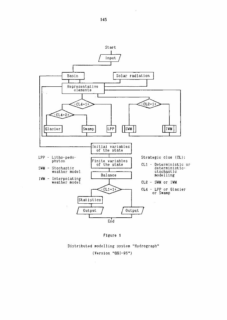
LPP -

SWM -

IWM -

145

Start

Litho- pedo- Strategic clue (CL): phyton

CL1 - Deterministic or Stochastic deterministic-weather model stochastic

modelling Interpolating weather model CL2 - SWM or IWM

CL4 - LPP or Glacier or Swamp

End

Figure 1

Distributed modelling system "Hydrograph"

(Version "GGI-95")

146

Evaporation Heat

sur[ act re en ion Regulating capacity of sufface runo

1 Regulo;t£inff 1 caprcl y

2 so1 runo

3

4 2

5

6 3

7

8

g 4

~-v

2 6

3

4 N I

ReEu-1 a 1ng 5

cq.ra 6 Cl Y

8 of

"' una er I

ground runoff 8 g

g

10 10

1 J 11

12 12

13 13

14

15 c h a n n e 1 Ocean

(f iqures means orders of the water cour:3e J

Figure 2. Elements of modelling system

START

SOLUBLE POLLUTANT

EROSION AND INSO­LUBLE POLLUTANT

END

147

Figure 3

Block-diagram of algorithm of module "LITHO-PEDO-PHITON"

148

By this is meant idea is that the river basin is not a set of different surfaces with streams running down these surfaces, but the river basin is a system of runoff elements. According to my idea, these runoff elements are restricted by micro-watershed-divide reaches of surface and subsurface basins exposed by their open "water-discharging" parts to the overland (beyond channel) or subsurface drainage network. The size of surface runoff elements. varies in the inverse relations from 1 o-2 to 104 m2

, depending on the slope; subsurface elements, are larger than surface ones. For runoff elements, the water outflow from that element is non linearly connected with the volume of water accumulated by the capacity of that element It should be noted, that the runoff elements do not make some ideal situation most suitable for computations, but they can be easily identified to· natural formations.

A balance ratio is observed for each runoff element:

dW I dt=S-R (1)

where: W(m3) is water volume accumulated by the runoff elements; S and R are water inflow

and outflow (m3/s), respectively; t(s) is time. If the analysis is proceeded, it is important to select the approximation of relationships between W and R. In our opinion, a quite suitable equation is used for a long time (Vinogradov, 1967):

R = /3[ exp(aW) -1] (2)

where a and ~ are characteristics of runoff element . A great variety of surface and subsurface (at different levels) runoff components make a

river basin or a certain portion of the basin territory. Equations (1) and (2) may be applied to the whole basin, but the coefficients of a and f3 should be replaced by

a=aln, b=n/3,

where: n is the number of runoff elements on the specified area. If we assume, that the total number of these runoff components is pr9portional to area F, we obtain

a=a*/F,

where a"' is used as a conventional constant for each type (level of transformation) of runoff,

and b"' is landscape parameter. A combination of equations (1) and (2) and its subsequent solution leads to the equation

of a hydrograph of water inflow to the channel network (total hydrograph of water flow from all runoff components at the specified level on the specified territory):

R= S+b -b 1 + [ ( S- Ro) I ( b + Ro)] exp[ -aAt( S +b)]

(3)

Here R 0 is the initial value of R and ~t is the design time interval. The Table shows a system of runoff transformation before it reaches the channel, as accepted in the "HYDROGRAPH"

149

Table

System of runoff transformation before reaching the channel

Runoff Numeric Typical Order of

requlating value n response Type of runoff the water

structure in a*=10° time at course

b* = 1 o- 6

Surface 3.0 1 7 m in Surface 1

DSL - 1 2.5 53 m in Soil 1

DSL - 2 2.4 1.1 hr Soil 1

DSL - 3 2.3 1.4 hr Soil 1

DSL - 4 2.2 1 . 8 hr Soil 1

DSL - 5 2. 1 2.2 hr Soil 1

DSL - 6 2.0 2.8 hr Soil

DSL - 7 1.9 3.5 hr Soil 1

DSL - 8 1 . 8 4.4 hr Soil 1

DSL - 9 1.7 5.5 hr Soil 1

RCUR - 1 1 . 5 8.8 hr Rapid ground 1

RCUR - 2 1.0 1.2 days Rapid ground 2

RCUR - 3 0.5 3.7 days Rapid ground 3

RCUR - 4 0.0 12.0 days Ground 4

RCUR - 5 -0.5 1 . 2 mo Ground 5

RCUR - 6 -1.0 3.8 mo Ground 6

RCUR - 7 -1.5 1.0 yr Underground 7

RCUR - 8 -2.0 3.2 yr Underground 8

RCUR - 9 -2.5 10 yr Underground 9

RCUR - 10 -3.0 32 yr Deep underground 10

RCUR - 11 -3.5 100 yr Deep underground 11

RCUR - 12 -4.0 320 yr Deep underground 12

RCUR - 13 -4.5 1000 yr Historical underground 13

RCUR - 14 -5.0 3200 yr Historical underground 14

RCUR - 15 -5.5 10000 yr Historical underground 15

DSL - Disign soil layer

RCUR - Regulating capacity of underground runoff

150

Model, with some determinations and specification of appropriate hierarchies of regulating capacities (RC) and orders of watercourses according to Horton-Strahler system.

The proposed transformation system directly combines the water discharge R from RC with water volume Win the RC:

1 W =-In( RIb+ 1)

a (4)

It is quite evident and important that W is nothing else but underground water storage at the specified level capable to drainage by the watercourses of the specified order. Moreover, many additional opportunities of the described model are discovered. In particular, it becomes possible to combine the value of W and geohydrological data. Interrelationships between surface and subsurface waters (the problem as old as the hills) are quite obvious here. Some time characteristics of the RC seem to be useful.

A characteristic time of RC response r •, which is the maximum value of this time at the given combination of a and b values at Rlb~O is as follows:

(5)

The value of r • is of a particular interest for the regulating capacities of underground runoff (RCUR).

If we follow the practice of the assessment of the time of dynamic systems relaxation, when the duration of some characteristic reduction at the system output is computed

(discharge out of RC in our case) from the initial R 0 value up to Role , where e is the base of the natural logarithm, then

•1

Rolb+e r = r n ---=---

Rolb+1 (6)

It is also possible to estimate the duration of flow of the half of water volume out of the RC ("half-life period"), then

(7)

Bearing in mind the first two opportunities, it is possible to compute the concentrations of pollution of appropriate ground water levels and to estimate the time of their purification.

It is quite unjustified to apply the equations of water conductivity (soil moisture diffusion), also widely applied in the practice of not very successful modelling. The greatest paradox at the use of this equation is in the fact that during computations not the equation controls the situation, but its coefficients do, which are to a great extent non linearly dependant on moisture content. A change in diffusion coefficient in 104 and coefficient of moisture conductivity in 106-10 7 times (Gardner, 1960) corresponds to the range of natural variations in soil moisture content. The situation is even worse for the equation because it is quite inapplicable for a

151

description of soil moisture behaviour, in particular, it contradicts the event of moisture suspension and the experimentally established effect of Hallar (Hallar, 1966; Vinogradov, 1988).

For real design time intervals (DTI) it would be quite sufficient to accept the following condition: moisture which penetrates the design soil layer (DSL) leaves this layer only when its maximum water-bearing capacity is satisfied (the least or field water bearing capacity). The only limit is the condition that the water layer exceeding the product of its filtration coefficient by the value of the DTI cannot move to the lower DSL. Otherwise, soil runoff occurs, and if the amount of water is abundant, the upper DSL is filled with water.

The account of the slope effect on many hydrometeorological processes is another important problem. Besides a direct influence of the plane slope angle on the direct solar radiation, the slope effect on the heat and moisture dynamics appears to be much more important that it seem at first sight. The area of moisture and heat exchange between the slope and the atmosphere finally affecting the amount of evaporation and heat penetration into soil tends to increase with the greater steeples of the slope. In should be also noted that in case of any a>O, the coordinate systems suitable for heat and moisture fluxes description do not coincide, which should be taken into account.

There is one more interesting problem, i.e. since rainfall duration differs from the duration of the design time interval, the surface runoff layer <Hq) for that interval should be determined from the appropriate stochastic equation directly considering the rainfall duration (T):

(8)

where Hare precipitation layer,/0 is filtration coefficient. Standard network meteorological data (air temperature and humidity deficit, precipitation,

rainfall duration) are to be used in the model with a simultaneous application of methods providing a higher model efficiency. These methods include the use of effective temperature and humidity deficit different from standard data by one more addend proportional to direct solar radiation computed for the specified latitude, elevation, slope and exposure. It is very important that the input meteorological elements are to be specified at representative elements (nodes of the space grid); this specification is to be made for the temperature taking into account climate elevation gradients and for precipitation resulted from interpolating not direct value but those relative to the total annual precipitation estimated quite independently.

A particular emphasis should be made on the "Arctic" blocks of the model. For LPP (see Fig.3) these are blocks "System", "Coefficients of the system of equations", "Solution of the system of equations", "Phase" and "Dualism", connected with the principal block "Energy". In general , the contents of these blocks are based on the algorithms providing computation of the thermal energy dynamics in "show-soil" system at the available phase transitions and constantly variable characteristics of phase transitions and constantly variably characteristics of the DSL, such as heat capacity, heat conductivity and water permeability.

All physical characteristics, moisture content and temperature of the DSL are constant at each point of the layer and they are subject to. spasmodic variations at the boundaries of the layers. Hence, the continuous profiles of soil moisture content or soil temperature are substituted by stepped histograms of their distributions over depths (a step in the scheme of finite differences is replaced by the averaging interval), and a system of ordinary differential equations is observed instead of the equation of heat conductivity (in partial derivatives). The following parameters serve as initial and boundary conditions: arbitrary histograms of

152

temperature and moisture content in the DSL; heat flux between the atmosphere and soil surface ; averaged (climatic) annual variation of soil temperatures at the definite depth.

Other simplifications (in fact , an analytical approach is used instead of the numeric solution , but for slightly modified system) make it possible to get the result with the account of peculiarities connected with phase transformations. These simplifications are attained at the use of four major ways.

The first way. It is assumed that the effective air temperature is constant during the DTI, and the temperature ofthe upper DSL (or snow cover) is time variable. Ifthese conditions are valid for any DSL, i.e. if we assume that the lowest DSL would be in contact with the above and lower soil layers which would be of the constant temperature during the DTI, then the system would consist of the equations of the following type:

(9)

Here U is the amount of heat energy in the DSL, ~ are coefficients of heat exchange

between DSLs and E>, E> are current and mean temperatures of the DSL during the DTI. The second way. The system of equations oftype (9) may be used for computations only

at the absence of phase transitions. The available phase transitions lead to the fact that individual DSLs proceed to waste heat energy, keeping the values of E> = 0, U=O - constant. The way out is to express the results of computations through AU which is either equal to the difference of U-U0, where U0 is the initial value of U, or deterrninnes the losses of energy for phase transitions, or present the sum of the first and the second ones . This way makes it possible to provide a stability of the design system of equations, changing its coefficients only, if necessary.

The third way. This way is closely connected with two previous ones and it concerns the explanation of mean values of E>, or U=cAZE>, which is more exact, where c is specific volumetric heat conductivity of the DSL, and L1Z is the DSL depth, measured perpendicularly

to the slope surface. We assume that U = U0 + kilU, where k=0.8, is the values derived from

the solution of the simplest test problems. The value of U may be termed as effective mean value.

The fourth way. When during the same DTI the temperature of the DSL tends to change and then a phase transition occurs or vice versa (dualism), then we have to decide what process prevails and the other process is neglected.

Finally, we have a system of linear algebraic equations with three-diagonal-band matrix , the system which is easily and quickly solved:

(10)

where N, M, L are parametric complexes compiled out of c, AZ values and coefficients of heat conductivity of the DSL.

If compared with the DSL, an additional "design layer" - snow cover, gives the greatest trouble to a hydrologist, because unlike other layers, it can appear and disappear, it is variable in its depth and density. Besides, there is one more hydrometeorological trouble there, i.e. solid precipitation measurements are not perfect, these measurements are accompanied by uncertain errors and they are made at extremely sparse network which is too sparse in mountains . The most complete snow cover parameters obtained at the end of each design time interval are as

153

follows : water storage he, factor ofwater saturation rate f3 = h; I h; (h; is liquid water and h; is "solid" water), heat energy storage Uc and the temperature appropriate to this heat energy

storage E>c, density Ye, layer of melting H5 and layer producing runoff Hr. Proposals for a computation of heat conductivity coefficients for a dispersed medium

under the conditions of its saturation with water and of phase transitions are of a particular interest. The design equations in the finite forms are as follows: for dry soil:

m= 2.5;

for soil completely filled with water:

for soil completely filled with ice:

for soil completely filled with water:

A= (A;,. -Am)(w·r +~, n=0.75;

for soil completely filled with ice:

A= (A:, -Am)(w*t +)..,, n=0.75;

for snow cover:

Ac = [ 1 + exp(O.IE>c)(l- y; I p*) ][2.2(y; I p*)25 + 0.02 ].

The following symbols are used in these equations: Ao, X, A* - coefficients of heat conductivity of the soil matter, water [0.58 Wlm 0 C] and ice [2.22 Wlm 0C]; E - soil porosity;

w·, w* - water saturation rate and ice saturation rate of soil (in parts of e); E>c, Ye* -

temperature and density of the snow cover; p* -ice density (920 kg/m3).

A very important item should be noted : the model parameters should be specified a priori. The possibility of this a priori assessment is explained by the generalized information on the numeric values of parameters which have a clear physical sense and which are determined in laboratories or in the field and which are connected with the type of landscapes as runoff producing complexes under various physiographic features. A parameter is here a numeric coefficient in the algorithm system of the model which is specified relative to the particular landscape as a constant but which is variable from landscape to landscape. Thus, the information on the geographic peculiarities of the territory is involved in the parameters .

Information on the vertical structure of the landscape may be checked with the help of a typical section (column) taken from the bedrock up to the top cover with the presentation of generalized characteristics (model parameters) of the mountain rocks, soils and plants. Taking into account trends in terminology, the following term of this section may be recommended: litho-pedo-phyton (Vinogradov, 1988). This term is also used for the main modules of the "HYDROGRAPH" model system (Fig . 3).

154

Numeric experiments are applied for a correction of some specially selected parameters when the model is used in the optimisation mode. The model calibration in its explicit form (i.e. when a simultaneous assessment is made for a number of parameters) is inadmissible because it leads to inter compensations at the assessment of parameters and finally to unstable results. Assessment of some parameters by solving inverse problems at the minimisation of the appropriate quality criterion is possible not only at the comparison of the computed and observed runoff hydrographs but at the use of data on water equivalent of the snow pack or soil temperature and soil moisture content.

Out of 30 model parameters, 24 parameters are slightly variable, easily generalised and not affecting the computation results greatly. The following parameters are most effective:

(I) filtration coefficients; (2) maximum water-bearing capacity of soil; (3) maximum and minimum parameters of evaporativity; (4) hydraulic parameter ofRCUR (b*), and the portion ofRCUR for the watercourse

recharge. The first parameter is of a particular importance for the computation of surface runoff

layer, the second parameter - for the computation of the subsurface runoff layer, the third and the fourth ones - for the total water balance, the fifth and the sixth ones - for the time redistribution of subsurface runoff.

The model parameters may be distributed over area and over the soil depth. The regulated system of computed representative points (CRP) is arbitrarily combined with the basin map. In our case, the points are distributed in the centres of equal circles which are scattered over the area with the maximum density (hexagonal package). The CRPs are characterised by the coordinates, elevation above m.s.l., orientation, slope and may be in general identified to the "point" on the locality. Meteorological information from meteorological station is interpolated in the CRPs. Since the CRPs fall within some RPC, the parameters of that RPC are given to these CRPs.

All computations for each CRP are repeated in several versions in accordance with the space heterogeneity of water equivalent of the snowpack over the slope. To this end ,the precipitation layer interpolated at the CRPs is multiplied by coefficient K = 1 + UpCv, where UP is a quintile of the normalised standard distribution, and Cv is space coefficient of variation of the CRPs, the UP values of snowpack. After the three-fold increase of the CRPs, the UP values are as follows: -0.967, 0, 0.967; after five-fold increase they are as follows: -1.282, -0.524, 0, 0.524, 1.282. Runoffvalues for the computed time interval for all the three or five versions are averaged. This approach is explained by the wish to consider space heterogeneity of the snowpack depth and proves the so called "mosaic" snow landscape.

The soil is divided into I 0 design layers (DLS) over its depth; these layers are usually (not obligatorily) equal and are 0.1 m deep.

The model makes it possible to compute the runoff hydrograph at the outlet and to follow the dynamics of snowpack, soil temperature and soil moisture content in any CRP. In fact, any time period may be taken for computations, but it is more suitable to use 24-hour and shorter intervals.

Different numeric coefficients are present in the model algorithm. These are: constants (of density, specific mass heat-bearing capacity, coefficients ofheat conductivity ofwater and ice, etc.), conventional constants, basin characteristics (length, area, depth of organogenic layers, etc.), parameters of RFC (density, specific mass heat-bearing capacity, coefficient of heat conductivity of soil particles; porosity, maximum water-bearing capacity, filtration coefficient of DL filtration, amount of water-intercepted by the top cove; parameters of evaporativity; phenological dates; runoff transformation parameters; ravine area, etc.).

155

A parameter is a numeric coefficient in the algorithmic model system, specified relative to particular object as a constant but varying from one RFC to another RFC and from one basin to another basin. Thus, parameters contain information on the geographic peculiarities of the terrain.

Some brief information on the number of different values included into the "HYDROGRAPH" model is given below:

Constants 7 Input elements 4 Conventional constants 30 Variables of the state 12 Correction coefficients 13 Variables in algorithms more than 100 Strategic clues 5 Number of design layer of soil 10 Characteristics RE 6 Number of regulating capacities up to 15 Parameters 30 of underground outflow

The total number of values in the computing system available tends to increase proportional to the number of DLS, regulating capacities of underground outflow, representative elements.

As noted above, the model blocks where phase transitions of soil moisture are computed are most important for the Arctic zone. The model capacity has been estimated as reliable in the permafrost zone as well as for the conditions of soil thaw in tundra landscapes.

A problem arises, however, on the specification of temperature boundary conditions at the depth of 1. 6 m. Peculiar features are observed when the temperature is about occ at this depth which is quite typical of the local permafrost areas. In case of inadequate data two similar versions of temperature specification (about + 1 cc and -1 cc) may lead to great differences in the final results.

In general, the problem of generalisation and specification of model parameters and input meteorological information for the Arctic zone is quite independent and is from being simple.

As to peculiarities of runoff formation in this zone, two almost contradictory facts should be noted, i.e. spring snow melt and rainfall floods occur in case of about 100% outflow down the frozen soil and nevertheless the underground recharge is quite significant. A complete picture of surface and subsurface water interaction is not yet clear.

Runoff hydrographs modelling was made for the Sula river and its tributary - Nyashenny brook at Kotkino (Pechora basin).

The Sula river: drainage area - 8500 km2, maximum elevation - 160 m, elevation at the outlet - 16m, number of RE- 18, birch and spruce open woodland - 30%, bush and moose tundra - 70%.

The Nyashenny brook: drainage area- 16.1 km2, maximum elevation- 71 m, elevation at the outlet- 16 m, number ofRE- 1, tundra area- 100%.

Figs 4 and 5 show continuous runoff hydro graphs for two rivers in 1979. A good agreement between the computed and observed hydrographs shows a stability and

efficiency of the model algorithm. It should be noted that this agreement was achieved only after multiplying the precipitation depth by coefficient 1.2 during snowfalls which corresponds to a popular viewpoint on the underestimation of solid precipitation measured in the Arctic tundra. The accuracy of maximum discharge computation, dates of maximum discharge occurrence and annual runoff depth are given in the Table below. Most of the model peaks correspond to the observed ones. In some cases there is a shift in the date. It is explained by

J .(~ 0 ()

:1. ~?00

1.000

BOO

I I ! ! ! I

. . l . !. J... . ' 1. l ' 4 \ . 1 . \ \ \ :- I : . : : : ------- . - 2 . . . . . . · · · · · · · · · · · · · · · · · · · -~ · · · · · · · · · · · · · · · · · · · · ·t · · · · · · · ·· · · · · · · · · ·: · · · · · · · · · · · · · · · · · · · · · :· · · · · · · · · · · · · · · · · · · · · · j · · · · · · · · · · · · · · · · · · · · · ·r · · · · · · · · · · · · · · · · · · · · · r · · · · · · · · · · · · · · · · · · . . I . . . . . : : : : : : . . : .

····················.········

() () 0 .................... , ................ . ,, :

.. :.~ () 0

:.:-:· () 0

................ , .................... : ......... j··· ',i!l\.1········· ······ .. ············· ........ . ; ·, :.·~ I . . . .., : . i :"11 j1 -1\ 1 I ·

. . . . . . . . . . . . . . . . . . . .. . . . . . . . . . . . . . . .. . . . . . . . . . ........ :-~;\ ~~~ {~~· :. .. . . . : . ............... I!\ :. . . ·~........ - ....................•...............

: \ 1~ ·\ 1 \ I •'. :,•, ~~r•J, 1•1; I

: 1o'' •I \•, I •.•. , .- .:l,f I I ...

• I .. • ,l I •I I k ·- ., : ~---·-f'· . .:-_::~.,;_~;..-:~":":~ll : '·."~·-.f' .: \\_.

'• .. •' 1,~-:_:..::..=..~-·--.:..::..::.::. 0 -----------· ---------- : ____ _:_.. T

() lOO :1. ~:·:·; () ~:-:·: () () :.:·:·: ~-:·; () ::~ () () :::: ~~-:-; () .•) 0 ()

1 -observed 2 - simulated

Figure 4. Observed and simulated hydrographs for Sula River at Kotkino, 1979

(" .. ".'

,··,

Q , M3/o

-------!---~-----:-------:---·----~--------:-------:--------~-------

• • • • • . ' . . ... ·' . ! ' . . . . : ~-~~-~ : i o 1 o 0 0 o o o o o o o o o o o 0 1 o •: o o o 0 0 1 0 o o o o o 0 o o o o o o o 0 ~· o o o o o o o o o o o o o • o • • o o: o o o o o o o o • o 0 o 0 0 o o o • o o ~- 0 0 ' 0 0 o 0 0 0 0 ' 0 ' 0 o ' 0 o ' 0 0 : 0 0 0 0 0 0 0 0 0 0 0 0 ' ' o 0 0 0 o 0 ' 0 ~ 0 0 0 0 0 ' 0 ' 0 I 0 0 0 ' 0 0 0 0 0 ' 0 ~- 0 0 0 0 0 0 O 0 0 ' 0 0 0 0 0 0 0 ' 0

. . . . . . . . . . . . . . . . . . . . • • 0 • • . . . . . . . . . . . . . . . . . . . . . .

··· ·· · · · ····· · ·····r··· ··· · · ··· ·· · · · ···· ··•·· ·· · · · ·· · : · · · ·· · · · · • · · · · · · · · ·· · · · ·· · ··1·· · · · · · · · · ·· · · · · · · ··1· · · · · · ···· · · ·········I·····················: ·· · · · · · · · · · · · · ·· · ·

· · · 1 i, : r r : ........ ····· ····:·····················j······ ... :,~~ .... .• ..... . .. ..... ; . .... . ........................................ ·•· ···············

: : I ~ I : . . . • • ... , •, • • • :1 - ................ = .................... :. ........ ··~r ~~( .............. ~ .. ~ ..................... : ...................... : .................. : .... . . . I I 'I> • I • . . .

T

: : I 11111\ Ill :~~~- tll : lt"''i : : • • L ''I I I I • • I • • . • • I· . ! . I• )-. 'J .• ... . .

_____ ___j~ __ _j __ __j --~~l~:::.~:~=:~-~~::-_::::::~~7.~=·::..=~~ .......... ~------0 ~:·:-; () :1. () () :-~-:-: () () :.:-:·: ~:-:-; () .-:'.!. () ()

1 -observed 2 - simulated

Figure 5. Observed and simulated hydro graphs for Nyashenny Creek at Kotkino, 1979

158

non-account of the time of precipitation fall, which is always related to the beginning of the design time interval.

During the spring snow melt flood the missing of small peaks preceding the major maximum or any delay in the rising limb of the hydrograph are related with the computation of mean daily air temperature.

During flood recession the computed peaks are systematically lower due to thaw delay in the model which is explained by a poor knowledge of the properties of the moss-lichen cover. These shortcomings are to be corrected.

For the future, it would be highly advisable to combine the "HYDROGRAPH" Model with appropriate models of climate and pollutions as a single model system.

In conclusion, the mayor objectives can be enumerated for a modification of the model system and extension of the model capacities:

( 1) Blocks design for runoff formation under specific conditions of glaciers , swamps , runoff producing complex in the zones of the capillary fringe effect above the water table (e.g. irrigated lands);

(2) model dissemination to the basins with large lakes and reservoirs; (3) model dissemination to very small basins and short DTI (hours, minutes); (4) design of "Stochastic weather model" for its joint use with the "HYDROGRAPH" Model

in the system of probabilistic runoff computation; (5) model adaptation to the system ofrunoffforecast; (6) model adaptation for us in climate change scenarios; (7) geographic generalisation of model parameters for different physiographic zones and

landscapes , anthropogenic landscapes included; (8) development of methodology for interpolation of precipitation in mountains; (9) design of service envelopes for the model system; (10) development of software for the model system.

REFERENCES

1. Gardner, W.R., 1960: Soil mater relation in arid and semi-arid cohdition. UNESCO Arid Zone Res. 15, p. 37-61.

2. Hallaire, M., 1966: Effective potential ofwater at the soil drying. In: "Termodinamika pochvennoi vlagi", Leningrad, Gidrometeoizdat, p. 325-360 (in Russian).

3. Klemes V., 1986: Dilettantism in Hydrology : Transition or Detiny ? , Water Resources, vol.22, No 9, p.177-188.

4. Vinogradov, Yu.B., 1967: Problems of rainfall floods hydrology on small watersheds in central Asia and South Kazakhstan. Trudy KazNIGMI, vol.28, 263 pp (in Russian).

5. Vinogradov, Yu.B., 1988: Mathematical modelling ofrunoffformation. A critical analysis. Gidrometeoizdat, Leningrad, 312 pp (in Russian).

159

SOME USEFUL INFERENCES FROM PAST ATTEMPTS TO ESTIMATE THE PRECIPITATION AND RUNOFF IN THE

CANADIAN ARCTIC BA~IN by

S. I. Solomon"', E. D. Soulis""" and M. Lee"'"""

ABSTRACT

The estimation at the precipitation and runoff in the Canadian Arctic basin has been attempted on several occasions. Five ofthese are briefly reviewed in this paper. The earliest of them dates back to 25 years ago, the most recent has been started last year (1994) and is still in progress. All these attempts recognize the difficulties of the enterprise and predicate the use of some auxiliary information ranging from the simple use of smoothed topography to the utilization of complex terrain models and remotely sensed data on vegetation. All enlist the assistance of the relationship between precipitation and runoff via the water balance. In spite of the differences in sets of data used and the level of technological sophistication, and of the differences in the patterns of annual isohyets and isorhets they produced, there is a number of common elements in their results that are encouraging and deserve attention. These are:

• the mean annual precipitation presents an areal variation of the order of 150 to 750 mm/year;

• the mean annual runoffpresents an areal variation ofthe order of 50 to 600 mm/year;

• both precipitation and runoff generally decrease with latitude and increase with elevation;

• precipitation, but particulary runoff areal variation is also influenced by the existence of four major physiographic regions.

These major inferences should be carefully analyzed as a starting point of additional efforts to estimate the precipitation and runoff in the Canadian Arctic basin. They should also constitute the basis for the evaluation of the existing hydrometeorlogical network and for its improvement.

*) Professor Emeritus, Dept. of Civil Engineering, University of Waterloo, Ontario, Canada. **) Associate Professor, Dept. of Civil Engineering, University ofWaterloo, Ontario, Canada. ***) Computer System Specialist, Toronto, Ontario, Canada.

The contributed talk delivered by Prof. S. I. Solomon at the meeting was based on an invited paper entitled "Two recent applications of the geophysical, environmental, economic and social information system (GEnESIS) to the solution of water resources assessment problems", which was presented at the third WMO/U nesco planning meeting on grid estimation of run -off data (Bern, Switzerland, 17-19 October 1994). A report of the latter meeting is under preparation by WMO.

160

1. Background During the last quarter of a century, several attempts have been made to estimate the area! variation of precipitation and runoff in the Canadian portion of the Arctic basin. This paper briefly revises five of them. All five have explicitly or implicitly used the data regarding runoff to improve the accuracy of the estimation of the area! variation of precipitation and vice versa. Therefore they present each at least a general internal consistency between the precipitation and runoff maps they have produced end - to some extent - also among the corresponding maps of the same hydrometeorological parameter. The use of runoff data to improve precipitation estimation, in addition to ensuring the consistency between the precipitation and runoff maps is also of particular significance in the Arctic basin area in view of the important difficulties of measuring precipitation in the high latitude areas. It is true that flow (and related runoff) is also measured with great difficulty and is affected by a reduced reliability during the cold season in these areas. However the runoff during the cold season (November to April) represents only a small fraction (about 15 to 20%) ofthe total runoff Thus, even an error of 100% in the cold season runoffwould represent only an error ofthe order of 15% in the estimation of the total annual runoff This differs significantly from the situation in the case of the estimation of precipitation as the precipitation during the cold season (snow) is ofthe same order of magnitude as that ofthe warm season (rainfall). The production of consistent estimates of the area! distribution of precipitation and runoff in the Canadian Arctic basin is further facilitated by and should be pursued because the actual evapotranspiration in the area is relatively low. However data on actual evapotranspiration is practically not existing and its estimation is based on its relationship to other climatic factors. Three ofthe attempts discussed in this paper have used the approach proposed by Turc (1959) to estimate actual evapotranspiration. It is noted that Turc's approach was developed using mostly data obtained in tropical areas and that its use in the Arctic or even temperate areas has not been generally successful. This has been due to the use in the application of this approach of the average annual temperature which in the Arctic includes at least six months of negative temperature with almost nil evapotranspiration. The application of Turc's approach in this area has to be based either on the separate evapotranspiration estimate for each month or on a correction to the annual temperature as proposed by Solomon (1972).

2. The Shawinigan Engineering (1970) Study This study was carried out in the framework of a project for planning the hydrometric network of Western and Northern Canada sponsored by Environment Canada. The study was based on the technique developed earlier in the framework of a similar project for the Province of Newfoundland and Labrador (Solomon et al, 1968). This technique had as its main innovation, in addition to the use of combined data on precipitation and runoff to improve the estimation of both, the introductions of a computerized digital terrain model, which enabled the definition for individual ground elements (groundels) of a number of topographic, location, and topographic-location terrain characteristics, as well as of characteristics related to vegetation, land use and land cover (Table 1 ). The estimation of the areal distribution of precipitation indicatf!S values basically ranging from 200 to 800 mm/year with rather exceptional increases in the mountainous area of up to about 1700 mm/year. The estimation of the area! variation of mean annual runoff (Figure 1) indicates that the vast majority of the Arctic basin runoff varies between 50 and 600 mm/year. However, in the western mountainous areas runoff values up to 1400 mm/year can locally be reached.

161

TABLE 1

TOPOGRAPHIC, LOCATION TOPOGRAPHIC-LOCATION AND

VEGETATION-LAND USE/LAND COVER CHARACTERISTICS

A. Topographic characteristics

Average elevation of each square (ELEV), estimated as the average of the elevation of its four corners;

Local Slope (SLOPE), estimated as the average of the slopes of the four planes defined by the various combinations of the elevation of three of the four corners;

Azimuth I of the slope (AZl), defined as an index related to the angle a between the west-east direction and the horizontal projection of the line of steepest descent of the local slope plane and expressed in integers from 1 to 5 as follows:

AZ1=1 for 337°30' ,; a< 360° & 0° ,; a < 2Z030'

AZ1=2 or 22"30' ,; a< 67°30' & 337°30' ,; a < 292"30'

AZI=3 for 67°30' ,; a< 112°30' & 292"30' ,; a < 2-n°30'

AZ1=4 for 112"30' ,; a< 157°30' & 2-n°30' ,; a < 202°30'

AZ1=5 for 157°30' ,; a < 202"30';

Azimuth 2 of the slope (AZ2), an index similar to AZ1 but considering the angle with the north-south direction;

Regional slope in the S-N direction (SN-SLP), a slope which takes into account the general configuration of the terrain and is obtained by computing the slope in the given direction for the total land stretch for which the elevation is increasing or decreasing continuously in vertical increments of at least 300 m. When going in the S-N direction, slopes are considered posith·e for increases in elevation and negative for decreases in elevation;

Similar regional slopes can be calculated in the three other directions (E-W, NE-SW, NW-SE)

B. Location characteristics

Distance to Ocean in north direction (DTO-N), defined as the distance from the ocean (sea) to the north of the given square;

Similar distance to the ocean can be calculated for the other seven directions of the compass.

Longitude index (LONG), defined as the co-ordinate of the square in the west-east direction starting from the most western column of the squares;

Latitude index (LAD, defined as the co-ordinate of the square in the south-north direction starting from the most southern line of the squares;

162

C. Topographic location characteristics

Barrier height in north direction (BH-Nl, defined as the difference between the average elevation of the square considered and the highest elevation encountered in the north direction from this point until the ocean is reached.

Similar barriers can be calculated for the other seven directions of the compass;

Shield effect to the north direction (SHE-Nl, defined as the sum of the elevation differential of all ascending stretches of terrain encountered when travelling from the ocean shore at the north to the corresponding point;

Similar shield effects can be calculated for the other seven directions of the compass;

D. Vegetation, Land-use/cover characteristics

Lake-area index (ALA), defined as the area of lal<es included in a given square;

Swamp-area index (ASW), defined as the area covered by swamps, marshes and bogs in a given square;

Glacier area index (AGL), defined as the area CO\'ered by glaciers in a given square;

Build-up land-area index (ABL), defined as the areas covered by urban ami large rural centres in a given square;

Forest-area index (AFD, defined as the area covered by forest in a given square;

Agriculture area index (AAD, defined as the area covered by farmland in a given square.

G : ll,GGI I ~, 001 1::; 8,001 l % IZ.OGI ' \11,001 5::; zo.OOI ' ~ 11.001 1::: u,,0\'11 & ::. ll. DOl 'll ::: JI,OOI • .& : ~Q.OIII I:. U,IIO\ e::: U,DDI a = ,Loo• (.:: SI.OO\ F ::. eo.O'Cil ; = 6&.,\101

U.DOI n.UI

I ; 71,001 ~ : 50. GOI t. -::. f.4.,0Gl 11-= u.n1 J& ::: '311,001 ' :::::: u.oGI ll ::. 100,00\ 11 :10&.001 'I ::. \OB,OIJI t .::. I lt.OD! U : I \6,001 1 : \liJ,IIOI f : tt.a,OOI J. : IU.GOI t = llt.llOl Z ::: 1]8,001

• .oao e..ooo

ILOOIJ II.GOO 11],01)0

ZLODIJ a.aoa 31.001'1 liS.OOD .a.ooo ,,_aoo u.aoo H,OOD Ho .ooa n.ooo &4.11110 a.GOO n.ooo 11.000 ao.ooo ••. aoo u.ooo '11.1l01l n.oOil

too.aoo \QA,GQil 101. ooo 112. oao pc.ooo \HI.IHtD 1z•.oao J%1,000 \31.0110 \lt.Q:fltl I ,0, GOD

::: ILQ,OOI • tu.aaa \U.COO I~ Z, QOO

• ~ tu,OOI • :: Ill. 001 +::\H. Dill I :::. I ~6, OGI • t :. Hot-.Mll • ) : 1S4.DOJ • = \U .. Illlt S : !l1.DDI ":. :::::: I Jt,OOI :::: 1&0.001 &. : IS&.,OQI

1 ~ a.ooo tr.G.IJCG l\LOti\\ IU.OCID 1 n:.ooo 1n.ooo JU,OOO IU.OCIO IU.OQQ

163

Mean annual runoff io Wes.tem and Northen Canada (From Shawinigan Engioeering,1910)

164

The study lead to a separation ofth.' Western half of Canada into hydrological homogeneous regions and to recommendations for improving the hydrometric network to ensure the gauging of each region (Figure 2). This regiona!i-:ation indicates that topography (slope) and topography-location (shield effect NW, and barrier height to theN, NW and W) play the major roles in defining the hydrologic regions.

3. The Atlas of the World Water Balance (Academy of Science of the USSR and the State Hydrometeorological Institute, 1974, republished by Unesco, 1976). This Atlas, which is probably the first comprehensive attempt to consistently estimate the main components of the water balance, precipitation, evapotranspiration and runoff at global scale, provides the maps of these components for all continents, including North America (Figures 2 and 3). The estimation of actual evapotranspiration is based on a technique developed by Budyko. The range of variation of both the precipitation and runoff are close to those arrived at in the Shawinigan Engineering study. The general patterns of areal variation are also similar, although the details are in some areas quite different. At least some of the differences could be impacted to the constraints imposed by the isoline presentation used by the Atlas, in contrast to the relative freedom permitted by the groundel by groundel digital presentation used by the Shawinigan study.

4. The climate of the Mackenzie Valley- Beaufort Sea Study (Burns, 1974). This study carried out in relation to the environmental impact study of a pipeline project along the Mackenzie River, provides two alternative maps of precipitation (Figures 5 and 6) The first one is based on precipitation estimates calculated as the sum of runoff and evaporation, the second is based directly on precipitation observations. The patten of variation of precipitation is similar to those obtained in the other above described two studies. The study area is limited however to the area North of the 60° N parallel. It is noted that this study contains also useful information on the climatic, ice cover and currents of the Arctic Ocean. Moreover the extensive list of references of this study could provide significant inputs into the ACSYS information system that is currently being developed.

5. The North West Territories Water Resources Inventory Study (Shawinigan, 1982). This study is limited to the Northwest Territories, and thus its study area is also limited to the south by the 60° N parallel. This study, like the earlier Shawinigan Engineering one, is also based on the technique and terrain, hydrometeorological, and information system described in Solomon et al (1968). The study produced maps of mean annual precipitation (Figure 7) and runoff (Figure 8) the latter being based on the following statistically derived equation:

MAR= 0.0724 ELE- 0.0844 LATl + 0.0778 SHE N- 0.2349 DSN + 280.3

where MAR is the mean annual runoff(mrnlyear) ELE is elevation (feet) LATI is a latitude index equal to the distance to the North from the 60°N parallel (km) SHE_N is the shield effect to the North (feet)

and DSN is the distance to the ocean in tne North direction (km).

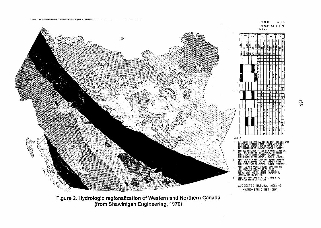
1 r-..J,,"I 1 .1 m:: otta·wt,rt:tyan Ml-flt1t-eenmg L-umpa.ny JAmuea ·--~--~--

Figure 2. Hydrologic regionalization of Western and Northern ~an ad a (from Shawinigan Engineering, 1970)

FIGURE 6. I. 3 REPORT &019-1-70

LEGE NO

SLOP[ 5111 ELD IIUA![II IIAIIIIEII: UUI£11 . . • • • .

w ~ ~ ~ ~

: ~ ~

~ : ~ ~ ~ ~

~ ~

~ . . . . . 0 " 0 0 . ~ ~ ~ ~ ~ ~ ~

A A A

8 B B

c c c

~~ D D

E E

F F

G G H H

I I

J J J

! ! !

L ~ L

I I M M M N N N

0 0 0 p p p

a a a R R R

s s s I r T

:I u u u

I V V V

w w w X X X

I y y y

I I I

* * *

3'2 EXISTING NATURAL REGIME STATIONS ARE SHOT ON MU.60 STATIONS WITH SLIGHT AND KNOWN CHANCES IN STORAGE NOT SHOWN ON MAP MAY BE CONSIDERED AS NATURAL REGIME STATIONS.

GENERAL LOCATION OF 250 NEW NATURAL .REGIME STATIONS SHOWN ON MAP.WHENEVER POSSIBLE THESE NEW STAll OHS SHOULD BE USED AS APPORTIONMENT AND MAJOR STREAM STATIONS.

ABOUT 100 NEW RESEARCH AKD REPRESENTAT lYE STA 11 OHS REaU I RED ARE NOT SHOWN ON MAP. THESE ARE PART OF·NATURAL REGIME STATIONS.

ABOUT 50 HEW MAJOR STREAMS STATIONS ARE NOT SHOWN 011 MAP. OUT OF WHICH AN UNDETERMINED NUMBER COULD BE NATURAL REGIME STATIONS MEASURING INCREMENTAL NATURAL REGIME BASINS.

ABOUT 20 NEW LAXE LEVEL STAll DNS HAVE HOT BEEN SHOWN ON THE MAP.

SUGGESTED NATURAL REGIME HYDROMETRIC NETWORK

-Q') CJ1

166

Figure 3. Mean annual precipitation in Northern and Western Canada I

(from Atlas of World Water Balance, Unesco 1976)

Jl

I

167

Figure 4. Mean annual runoff in Northern and Western Canada (from Atlas of World Water Balance, Unesco 1976)

3 0. l\ u

145°

Figure 5

ESTJMA TED MEAN ANNUAL PRECJPIT A TION (Inches)

AS SUM OF EVAPORATION AND RUNOFF

168

·-.. ;;~ ---~--

VICTORIA -~Holtnan -~::: "~~---

·"!.: ..... ::.;:~ ISLAND

~ \

~-S"o'• .. R .d ~ op,,

~/(. ~

LEGEND

---lsohyeh

(Dashed ove• open water or mountain areas)

17.5---- lnterml!'diole hoh'fel

105°

'-J

' \

(From Burns, 1974)

Figure 6.

ANNUAL MEAN PRECIPITATION (Inches of water)

Based on period 1941-1970

lEGEND

--- lsohyets (Dashed over open water or mounto~n areas)

169

STANDARD DEVIATIONS FOR SELECTED STATIONS

BASED ON ENTIRE PERIOD OF RECORD linJ (See Fig. I. 1)

Kornakuk Buch 1.!>5 Hol .....

Shingt.Poinl 2.12 l..._.'lik A

c.p. P1rry A 1.29 Ntdlobon Pllftina~LI

Fon Good Hop41 2.311 Nonnen Well& A

FDf1 McPherson 3.86 Pon RMiium

Fort PrOYict.nct 1.97 Slchs H.-bour

Fort Reliara 2.28 Tukloyaktuk

FonSimpMJ~"~ 3.15 Wr~•vA

Fon Smith A 1.82 Y .. lowllntft A

Hay AMI" A 3.01 Scale in Statute

100 50 0

3.42

1.67

U59

3.01

2.50

1.22

1.58

2.78

2.511

Miles 100

Figure 6. (From Burns, 197 4)

200

I :

2

' :

6 = . : ' =

L :

.. u.o !10.0 7t;,.O

100.0

l'ZS.O I 50.0 JH,O

100.0 11.S..0 2!nl.O n;.o 300.0

32S..0

lSO.O

li'S.O ~J.Vb.tl

\l,'i,':l.fl

lj.!,O.D

\1.1!>.0

S®-0 ~,~.!3

sso.o 1!1"1'!.0 6QO.O

':i'j..O

111.9.9

li'~t.!l

1,9.9

22Q..'9'

1'49.9

1714.9

299.9

)210-'9

311.9.9

1711.9

39"9.9

1.1.211-9

'1\11.9-~--

11.7·- ~ ' 11.99.9

); ... '='

~ ... .;.~ 51'-.~

!-9'3.9

f!::!'·.'l

~"'!-~

- '" ' 'i;,l'~. ~

70C.G

~::. 0

7~0. G

~i'~ . :; ,,, ' !!.:::. ' s::.C

170

Figure 7

Mean annual precipitation in the Northwest Territories {from Shawinigan, 1982)

+

.\ill!!! IElM lMMUIL !UOOFF

o.o zs.o .... 75.0

100.0

125.0 1119.9

150.0 1714.9

17'5.0 199.9

200.0 2211-.9

zzs.o 211.9.9

250.0 2711-.9

275.0 299 . .9

300.Q 321.1..9

32'5.0 Jl.l9.9 lSO.Q 371.1..9

J7S.o J99.9 u.oo.o 1(.25.0

1150.0

~~>75.0

~00.0

szs.o sso.o 57'5.0 500,()

62'!1.0

no.o

0-.3"

171

Figure 8

Mean annual runoff in the Northwest Territc (from Shawinigan, 1982)

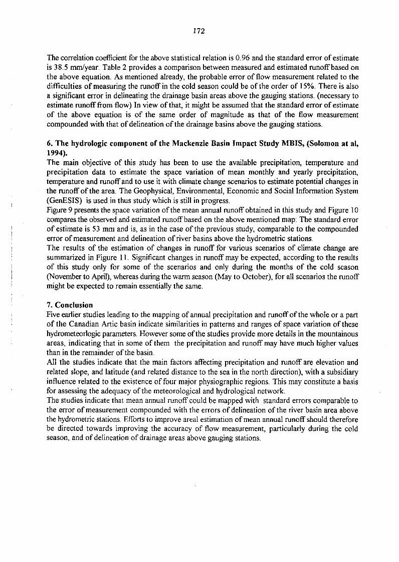
172

The correlation coefficient for the above statistical relation is 0. 96 and the standard error of estimate is 38.5 mm/year. Table 2 provides a comparison between measured and estimated runoffbased on the above equation. As mentioned already, the probable error of flow measurement related to the difficulties of measuring the runoff in the cold season could be of the order of 15%. There is also a significant error in delineating the drainage basin areas above the gauging stations. (necessary to estimate runoff from flow) In view of that, it might be assumed that the standard error of estimate of the above equation is of the same order of magnitude as that of the flow measurement compounded with that of delineation of the drainage basins above the gauging stations.

6. The hydrologic component of the Mackenzie Basin Impact Study MBIS, (Solomon at al, 1994). The main objective of this study has been to use the available precipitation, temperature and precipitation data to estimate the space variation of mean monthly and yearly precipitation, temperature and runoff and to use it with climate change scenarios to estimate potential changes in the runoff of the area. The Geophysical, Environmental, Economic and Social Information System (GenESIS) is used in thus study which is still in progress. Figure 9 presents the space variation of the mean annual runoff obtained in this study and Figure 10 compares the observed and estimated runoff based on the above mentioned map: The.standard error of estimate is 53 mm and is, as in the case of the previous study, comparable to the compounded error of measurement and delineation of river basins above the hydrometric stations. The results of the estimation of changes in runoff for various scenarios of climate change are summarized in Figure 11. Significant changes in runoff may be expected, according to the results of this study only for some of the scenarios and only during the months of the cold season (November to April), whereas during the warm season (May to October), for all scenarios the runoff might be expected to remain essentially the same.

7. Conclusion Five earlier studies leading to the mapping of annual precipitation and runoff of the whole or a part of the Canadian Artic basin indicate similarities in patterns and ranges of space variation of these hydrometeorlogic parameters. However some of the studies provide more details in the mountainous areas, indicating that in some of them the precipitation and runoff may have much higher values than in the remainder of the basin. All the studies indicate that the main factors affecting precipitation and runoff are elevation and related slope, and latitude (and related distance to the sea in the north direction), with a subsidiary influence related to the existence of four major physiographic regions. This may constitute a basis for assessing the adequacy of the meteorological and hydrological network. The studies indicate that mean annual runoff could be mapped with standard errors comparable to the error of measurement compounded with the errors of delineation of the river basin area above the hydro metric stations. Efforts to improve area! estimation of mean annual runoff should therefore be directed towards improving the accuracy of flow measurement, particularly during the cold season, and of delineation of drainage areas above gauging stations.

173

Table 2. Comparison of measured and estimated runoff of gauged river basins in the Northwest Territories (From Shawinigan, 1982)

--R.NFf(tft)-STATI~ rcttJrL PREDICTED (ACT .JPRED.)

ObJB001 153.358 CJS.on 1.564 HANilFI R ABOVE mARE l 07NB001 195.320 158.037 1.236 SLAVE R AT FlllGERALD 01PA001 90.221 65.629 1.375 UFN..O R AT HIGKIAY N5 07QB002 152.565 91.548 1.667 SNOWDRIFT R 0 SILTAZA l 07QC003 107.239 84.277 1.272 OOA R N IN.. H ISLAND l 01QC004 151.706 91.265 1.662 MRTIN R ABOVE llllA R 07QD005 76.511 83.424 0.917 PmlER l WT t Trt.STOO R 07RD001 139.229 114.094 1.220 LOO<HMT R 0 MTILLERY l 010C001 81.069 71.413 1.047 Kt«ISA R CtJTlEl WISA l 10EB001 481.813 435.075 1.107 S NAHANNI R t VIRGINIA F UlEC001 388.742 382.981 1.015 S ~I ~.HT .SPRite 10EC002 349.704 '117 .Z'Jj 1.261 PRAIRIE CREEK CADIUAC K 10£0002 '117.074 'l11.190 0.845 LIARD R tEAR ll£ IOJTH 10ED003 136.305 94.954 1.435 BIRCH R t FT.llARD IIIAY 10FB005 83.590 78.984 1.058 J-MRIE R FT.SI~ I4IY 10GA001 263.935 241.976 1.091 ROOT R tEAR n£ l'DJfH 10GB001 80.673 99.673 0.809 Will~ R t£M twrH 10GB005 106.181 163.498 0.649 lNW£D TRIB.~\l.AKE R 10GC002 54.853 88.380 0.621 iRIS R t£M ll£ twrH 100C003 85.454 114.761 0.745 MRTIN R t£M 1l£ twrH 1CHB003 119.818 141.412 0.847 ~IQ.EY R t£M ll£ twrH 1(8))()3 162."2 96.686 1.680 BIG tOJTH m.ttaaiE.M 10JA002 86.457 116.310 0.743 CMSEU. R OOllET CLUT l 10£003 117.083 109.767 1.067 GT.BEAR R OJT .GT .BEAR l 10JD001 110.691 139.008 0.796 WLDAN R t£M ll£ tOJTH lo.J)()()2 85.293 99.745 0.855 YUTEFISH R t£AR tOJTH 1~001 104.820 141.~ ).740 SLOAN R tEAR ll£ l'DJfH 10KB001 312.688 236.791 1.321 ~ R B UfERirt. R 10KC001 320.821 308.742 1.039 tO.JNTAIN R B CAt1BRIAN CR 10l.A004 71.900 82.260 0.947 WELI£N m.t£AR to.mi 1<l.C003 79.416 90.313 0.879 REtaOO R BLW IfSTR. KN 1<l.C007 93.1(/J 101.~ 0.924 CMIBW CR t llfSlER I4IY 1M002 351.069 243.599 1."1 PEEL R t FOOT tiP\-ERS(Jl

10tm002 135.540 168.193 0.806 BABBAG: R BLW.CMIBOO C. lQt£001 94.181 108.163 0.871 ANDERSON R BLW CR~TH R 10PB001 157.693 139.840 1.128 afPERttlt£ R WT POINT l 10QA001 174.217 148.318 1.175 TREE R t£M THE toJTH 100C001 146.041 148.1" 0.986 BI.RSII£ R tEAR tOJTH 10QC002 171.357 112.582 1.522 GmOON R t£AR Tl£ tOJTH tORMOt ~Lltt 1?7.Qt\7 0.691 Mrl! R m 1'1.1 ~MIV I a~

06£002 97.224 76.374 1.273 ll£l0i R ABOVE BEYER.. Y l 07Q0004 82.625 81.261 1.017 Trt.STOi RAT POOTER L 0 07SA004 81.9XI 112.616 0.781 INDIN R AroJE.OW..CO l 10EA003 351.985 41'5.756 0~847 FLAT R tEAR ll£ t0JTH 10FA002 106.713 1fiJ.914 0.971 TRWT R t FT.Sl~ HWY

·10JB001 81.791 102.889 0.795 ~ lllE R l S. n£RESE 1<l.A002 328.575 198.195 1.658 ARCTIC RED R t£AR IOJTH 1<fC001 150.216 142.~ 1.052 mm..L R ~.OOT DStW.. l 10QD001 120.995 97.134 1.246 B.UCE R l£M ll£ t0JTH 1058001 199.575 121."2 1.643 WtYES R t CHANl'm UUT

Original in color

Figure 9

Mean annual runoff in the Canadian Arctic basin (from Solomon et al, 1994)

Legend (tenths of mm/year)

0 - 200 • 200 - 400 • iOO - 600 • 600 - 800 • 800 -1000 •

1000 -1500 • 1500 -2000 • 2000 -2500 • 2500 -3000 • 3000 -3500 • 3500 -iOOO • iOOO -4500 • i500 -5000 • 5000 -5500 • 5500 a UP •

700 -'-ea 600 (1)

~ E E

500

-t: 400 0 c :::s 300 '-

"C (1) +I 200 ea E ~ (/) 100 UJ

0

0

Figure 10. Measured versus estimated runoff in the Canadian Arctic (From Solomon et al, 1994)

• • •• • I

• •

SE= 53.42

• .. ~ • 97 Stations

, ··' . . ~ ,. •

~:r • . ·~ . •

100 200 300 An(l 500 600

Measured runoff ( mm/year )

--..1 t11

700

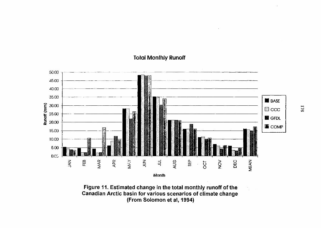
50.00

45.00

40.00

35.00

'E 3o.oo E ;; 25.00 0 c & 20.00

15.00

10.00

5.00

o.c::, z <( I

Tc:>tal Monthly Runoff

CO 0:: 0:: w <( a.. LL

2 <t:

Month

Figure 11. Estimated change in the total monthly runoff of the Canadian Arctic basin for various scenarios of climate change

(From Solomon et al, 1994)

• BASE

lE] ccc

.GFDL

Ill COMP

177

References

Academy of Sciences of the USSR and the State Hydrometeorological Institute (1974), republished in English by UNESO (1976), The Atlas of World Water Balance, Laningrad, Paris

Burns B.M. (1974) The Climate of the Mackenzie Valley- Beaufort SeSl, 2 Volumes, Climatological Studies No 24, Environment Canada, Atmoshperic Environment, Toronto.

Shawinigan (1982), Northwest Territories Water Resources Inventozy Study, Report for Environment Canada, Montreal, Quebec, Canada.

Shawinigan Engineering Co. Ltd; (1970), Hydrological Network Design Study for Western and Northern Canada. Report for Department of Environment, Montreal, Quebec, Canada.

Solomon, S. I (1972), Joint mapping, Section C-2 in Casebook on Hydrological Network Design Practices, W. B. Langbein, Editor, World Meteorological Organization.

Solomon, S.I., J.P. Denouvilliez, E.J. Chart, J.A. Wooley, and C.F. Cadou (1968). The use of a square grid system for computer estimation of precipitation, temperature, and runoff, Water Resources Research. Vol4, No. 5.

Solomon S. 1., E. D. Soulis, N. Kowen, and M. Lee (1994) Two applications ofthe Geophysical, Environmental, Economic and Social Information System (GenESIS) to the solution of water resources assessment problems, Invited paper, Third WMO/UNESCO Workshop on Gridding of Runoff Values. Berne, Switzerland.

Turc, L. (1959) Le bilan d'esu des sots. relations entre les precipitations. l'evaporation at l'ecoulement. Ann Agron No. 5

5

178

THE MEASUREMENT AND MODELING OF ARCTIC HYDROLOGIC PROCESSES

INTRODUCTION

Douglas L. Kane Water Research Center

University of Alaska Fairbanks Fairbanks~ AK USA 99775

Renewed interest in coupled arctic hydrologic and meteorologic processes has surfaced because of potential climate change globally. Unfortunately, hydrologic and meteorologic data in the Arctic is historically very sparse and in many cases ofvery poor quality. The major components of interest in the arctic hydrologic cycle are the input precipitation, the outputs of runoff and evapotranspiration and the processes of subsurface, overland and channel flows within the watershed. These are the same components that are important in watershed studies in other climatic regions; however, phase change plays an important part in arctic hydrology and is manifested in freezing and thawing of soils, development and decay of ice covers, ablation, and evapotranspiration. Many hydrologic processes are subdued or non-existent during all or part of the winter season; but, some such as redistribution of snow by wind are very important.

The measurement of arctic hydrologic processes has been limited by the remoteness and harshness of the environment. Until the advent of solid state electronics, the continuous operation of instrumentation in this region was impossible. For this reason, many data sets only include measurements during the melt season, usually after snowmelt. To understand arctic hydrologic processes, it is necessary to document what happens during the winter months in terms of precipitation and its redistribution by wind. In general, heavy snow years delay the onset of snowmelt, and redistribution by the wind can enhance runoff.

SOLID STATE PRECIPITATION MEASUREMENT IN THE ALASKAN ARCTIC

Each year, snowfall precipitation in the Alaskan Arctic averages about 35% ofthe annual precipitation (Table 1 ). Biologically this water is very important when it melts because it ensures that some recharge of the active layer occurs and water is therefore available for transpiration by the plants that rapidly produce leaves after ablation. Also, the months of March, April and May are the driest months ofthe year (Kane et al., 1989) and ablation generally occurs in May through early June (Kane et al., 1991 ).

In our field studies we utilized data from a Wyoming snow gage to quantify winter precipitation patterns. However, tllis data is of limited use in our hydrologic modeling and simple water balance calculations (Table 1 ). Just prior to ablation, we do detailed snow surveys where we measure depth and water content at a number of sites. Site selection is based on topography and vegetation. Rovansek et al. (1993) showed that double sampling was a useful technique for estimating snowpack water equivalent. Double sampling is a method where snow depth is measured at a large number of points first and then both snow depth and water equivalent are measured at relatively few points Rovansek et al. showed that the optimum ratio for area! estimates was 14 (snow depths) to 1 (water equivalent).

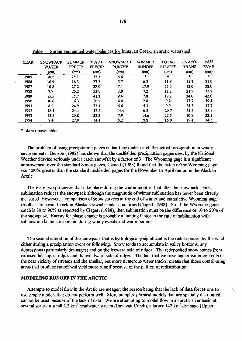
179

Table 1. Spring and annual water balances for Imnavait Creek. an arctic watershed.

YEAR SNOWPACK SUMMER TOTAL SNOWMELT SUMMER TOTAL EVAP().. PAN WATER PRECIP PRECIP RUNOFF RUNOFF RUNOFF TRANS EVAP

~cm} ~cm) ~cm} ~cm~ {cm~ ~cm} ~cml ~cm) 1985 10.2 25.1 35.3 6.6 • • • • 1986 10.9 16.3 27.2 5.7 6.2 11.9 15.3 31.0 1987 10.8 27.2 38.0 7.1 17.9 25.0 13.0 32.0 1988 7.8 25.2 33.0 3.9 7.2 11.1 21.9 33.2 1989 15.5 25.7 41.2 9A 7.8 17.2 24.0 42.0 1990 10.6 16.3 26.9 6.4 2.8 9.2 17.7 39.4 1991 8.2 24.9 33.1 5.6 4.3 9.9 24.2 37.7 1992 18.1 24.1 42.2 14.4 6.3 20.7 21.5 32.8 1993 12.5 20.8 33.3 7.9 14.6 22.5 10.8 32.1 1994 7.4 27.0 34.4 5.2 9.8 15.0 19.4 34.5

* -dat11 unavailable

The problem of using precipitation gages is that they under catch the actual precipitation in windy environments. Benson (1982) has shown that the unshielded precipitation gages used by the National Weather Service seriously under catch snowfall by a factor of3. The Wyoming gage is a significant improvement over the standard 8 inch gages, Clagett (1988) found that the catch of the Wyoming gage was 200% greater than the standard unshielded gages for the November to April period in the Alaskan Arctic.

There are two processes that take place during the winter months that alter the snowpack. First, sublimation reduces the snowpack although the magnitude of winter sublimation has never been directly measured However, a comparison of snow surveys at the end ofwinter and cumulative Wyoming gage results at lmnavait Creek in Alaska showed similar quantities (Clagett, 1988). So, if the Wyoming gage catch is 80 to 90% as reported by Clagett (1988), then sublimation must be the difference or 10 to 20% of the snowpack. Energy for phase change is probably a limiting factor in the rate of sublimation with sublimation being a maximum during windy events and warm periods.

The second alteration of the snowpack that is hydro logically significant is the redistribution by the wind, either during a precipitation event or following. Snow tends to accumulate in valley bottoms, any depressions (particularly drainages) and on the leeward side of ridges. The redeposited snow comes from exposed hillslopes, ridges and the windward side of ridges. The fact that we have higher water contents in the near vicinity of streams and the smaller, but more numerous water tracks, means that those contributing areas that produce runoff will yield more runoff because of the pattern of redistribution.

MODELING RUNOFF IN THE ARCTIC

Attempts to model flow in the Arctic are meager; the reason being that the lack of data forces one to use simple models that do not perform well. More complex physical models that are spatially distributed · cannot be used because of the lack of data. We are attempting to model flow in an arctic river basin at several scales: a small2.2 km2 headwater stream (Imnavait Creek), a larger 142 km2 drainage (Upper

180

Kuparuk River) and an entire drainage basin of8140 km2 (Kuparuk River). A physically based, spatially distributed hydrologic model has been developed for application to these nested watersheds. This model has an added feature that a routine for predicting soil thawing and freezing is included. Hydrologic processes of snowmelt, evapotranspiration, subsurface flow, overland flow and channel flow are all modeled physically. Darcian flow is assumed for the subsurface system and kinematic flow for the surface system. Processes with phase change utilize a surface energy calculation, although simpler algorithms are being developed for snowmelt and evapotranspiration. This model is presently being applied to the smaller Imnavait Creek watershed because it has been studied longer and has more detailed data. In the near. future it will be applied to the Upper Kuparuk River basin and then the entire Kuparuk River basin. Seven meteorologic stations are located in theKuparuk River drainage with one each in Irnnavait Creek and the Upper Kuparuk River.

Validation of spatially distributed models requires substantial data and can only be checked adequately by spatially distributed data sets. Such data sets are very difficult to obtain, particularly for large watersheds. For our model, we are evaluating the spatial performance by comparing simulated soil moisture levels with similar data obtained from synthetic aperture radar (SAR) images. Fo.r Imnavait Creek, the resolution of these two data sets is quite similar. Remotely sensed data is the only way in which such data can be obtained for validation.

Arctic hydrologic models have to be strongly coupled with thermal models. Phase change is present in many hydrologic processes such as snowmelt and evapotranspiration. Also, the soils in the active layer are either thawing or freezing throughout the year. In addition, snowfall occurs from mid-September through mid-May, but can also occur anytime during the summer, only persisting for a short time.

Output from the hydrologic model will include rate and timing of snowmelt, soil moisture distribution, evapotranspiration distribution, channel runoff and active layer thermal regime. Runoff is often used to validate models (especially lumped models) as it is the end result of all of the previously described processes. But, if it does not match the measured flow it is difficult to ascertain where the model is not performing well. This is why it is advantageous to have a spatially distributed data set.

DATA QUALITY

The required quality of data depends upon the use that will be made of that data. The quality of data in the Arctic has always been a concern because of the harsh and remote environment. Much of the research that we are doing now is driven by concerns of climate change. Hinzman and Kane (1992) have estimated what the response of an arctic hydrologic system would be for a range of warming conditions. The modeled changes are not that great for most processes; unfortunately, these changes may be difficult to detect because the error in many of our present measurements are of the same magnitude. This implies that the quality of data that we are collecting has to improve to be useful in climate related studies. When using existing arctic data sets, like precipitation, to predict response to a change in climate the user needs to be aware of the limitations of that data set.

SUMMARY

Existing hydrologic and meteorologic data sets in the Arctic are meager and generally of poor quality. Precipitation measurements, specifically snowfall, are very poor. New instrumentation has improved the quality of data collected, but gages like the Wyoming gage still under catch snowfall by 10 to 20%. Our

181

ability to model hydrologic processes in the Arctic is limited by the quality and amount of data available. For the Kuparuk River basin we are attempting to collect sufficient quality data so that we can utilize a physically based, spatially distributed hydrologic model for a nest of watersheds, ranging from 2.2 km2 to 8140 km2

REFERENCES

Benson, C. S. 1982. Reassessment ofwinter precipitation on Alaska's arctic slope and measurement on flux of wind blown snow. Geophysical Inst., University of Alaska Fairbanks, Res. Rep. UAG R-288, 26 pp.

Clagett, G. P. 1988. The Wyoming windshield--An evaluation after 12 years of use in Alaska. In: Proceedings 56th Annual Western Snow Conference, April 1988, Beaverton, Oregon, pp 113-123.

Hinzman, L. D. and D. L. Kane. 1992. Potential response of an arctic watershed during a period of global warming. Journal of Geophysical Research-Atmos., 97(03):2811-2820. ·

Kane, D. L., L. D. Hinzman, C. S. Benson and K. R. Everett. 1989. Hydrology oflmnavait Creek, an arctic watershed. Holarctic Ecology, 12:262-269.

Kane, D. L., L. D. Hinzman, C. S. Benson and G. E. Liston. 1991. Snow hydrology of a headwater arctic basin 1. Physical measurements and process studies. Water Resources Research, 27(6): 1099-1109.

Rovansek, R. J., D. L. Kane and L. D. Hinzman. 1993. Improving estimates ofsnowpack water equivalents using double sampling. In: Proceedings 50th Annual Eastern Snow Conference, June 1993, Quebec City, Quebec, pp 157-164.

LIST OF PARTICIPANTS

R. Annstrong National Snow & Ice Data Center CIRES, PO Box 449 University of Colorado Boulder, CO 80309, USA tel: 1-303-492-1828 fax: 1-303-492-2468

R. Barry National Snow and Ice Data Center CIRES, Campus Box 449 University of Colorado Boulder, CO 80309, USA tel: 1-303-492-5488 fax: 1-303-492-2468 tlm: rbarry@kryos.colorado.edu

M. Baumgartner Department of Geography University of Berne Hallerstrasse 12 3012 Bern, Switzerland tel: 41-31-631-8020 fax: 41-31-631-8511 tlm: baumgartner@ giub. unibe.ch

S. Bergstrom Swedish Meteorological and Hydrological Institute (SMHI) S-601 76 Norrkoping, Sweden tel: 46-11-158292 fax: 46-11-170207/8 tlm: sbergstrom@smhi.se

C. Bertoia US National Ice Center 4251 Suitland Road FOB4 Washington, DC 20395-5210, USA tel: 301-457-5314, ext. 302 fax: 301-457-5300 tlm: cbertoia@icecen.fb4.noaa.gov

N. N. Briazgin Arctic and Antarctic Research Institute 38 Bering Street St. Petersburg 199397, Russian Federation tel: 7-812-352-0319 fax: 7-812-352-2688

APPENDIX A

APPENDIX A, p. 2

T. Carroll National Operational Hydrological Remote Sensing Centre Office of Hydrology National Weather Service/NOAA 1735 Lake Drive West Chanhassen, Minnesota 55317-8582, USA tel: 1-612-361-6610 fax: 1-612-361-6634 tlm: tc@nohrsc.nws.gov

H. Cattle Hadley Centre for Climate Prediction and Research Meteorological Office London Road Bracknell, Berks RG 12 2SY, UK tel: 44-1344-856209 fax: 44-1344-854898, tlx: 849801 WEAKBC tlm: hcattle@meto.govt. uk

D. Calalieri Laboratory for Hydrospheric Processes, Code 971 NASA Goddard Space Flight Center Greenbelt, MD 20771, USA tel: 1-301-286-2444 fax: 1-301-286-0240 tlm: don@cavalieri.gsfc.nasa.gov

R. Colony International ACSYS Project Office Norwegian Polar Institute Middelthuns gate 29 PO Box 5072, Majorstua N-0301 Oslo, Norway tel: 47-22-959-605 fax: 47-22-959-501 tlm: acsys@npolar.no

T. Fuchs Deutscher Wetterdienst Global Precipitation Climatology Centre Zentralamt, Frankfurter Strasse 135 D-63067 Offenbach-am-Main, Germany tel: 49-69-8062-2978 fax: 49-69-8062-2993 tlm: fuchs@k7 -wzn-za-off enbach.dwd.d400.de

P. Ya. Groisman University of Massachusetts Department of Sciences Amherst, MA 01003, USA tel: 1-413-545-9573 fax: 1-413-545-1200 tlm: pasha@climatel.geo.umass.edu

V. Golubev State Hydrological Institute 23 Second Line St. Petersburg 19905, Russian Federation tel: 7-812-213-3517 fax: 7-812-213-1028 tlm: ishikolom@sovam.com

B. Goodison Climate Processes & Earth Observation Division Atmospheric Environment Service 4905 Dufferin Street Downsview, Ontario M3H 5T 4, Canada tel: 1-416-739-4345 fax: 1-416-739-5700 tlm: goodisonb®aestor .am.doe.ca APPENDIX A, p. 3

A. Gruber NOAA/NESDIS E/RA Washington, DC 20233, USA tel: 1-301-763-8127 fax: 1-301-763-8108 tlm: agruber@orbit.nesdis.noaa.gov

A. Hall Office of Hydrology NOAA/NWS (W /0Hx3) 1325 East-West Highway Silver Spring, MD 20902, USA tel: 1-301-713-1017 fax: 1-301-713-1051 tlm: ahall@smtpgate.ssmc.noaa.gov

D. Hall Laboratory for Hydrospheric Processes NASA Goddard Space Flight Center Code 974 Greenbelt, MD 20771, USA tel: 1-301-286-6892 fax: 1-301-286-1758 tlm: dhall@glacier.gsfc.nasa.gov

APPENDIX A, p. 3

APPENDIX A, p. 4

D. Kane Water Research Center 248 Duckering Building University of Alaska Fairbanks, AK 99775-5860, USA tel: 1-907-474-7808 fax: 1-907-474-6087 tlm: ffdlk@aurora.alaska.edu

V. Kattsov Voeikov Main Geophysical Observatory 7 Karbyshev Street St. Petersburg 194018, Russian Federation tel: 7-812-247-0103 fax: 7-812-247-8661 tlm: kattsov@mgo.spb.su

R. G. Lawford NOAA/Office of Global Programs 1100 Wayne Ave., Suite 1225 Silver Spring, MD 20910, USA tel: 1-301-427-2089, ext. 40 fax: 1-301-427-2222 tlm: lawford@ogp.noaa.gov

G. H. Leavesley US Geological Survey Mail Stop 412 Denver Federal Center Denver, CO 80225, USA tel: 1-303-236-5026 fax: 1-303-236-5034 tlm: george@usgs.gov

D. R. Legates Department of Geography 100 E.Boyd St., Room 684 University of Oklahoma Norman, OK 73019, USA tel: 1-405-325-5325 fax: 1-405-325-3148 tlm: legates@cwarren.ccg.uoknor.edu

D. Lettenmaier Dept. of Civil Engineering Box 352700 University of Washington Seattle, WA 98195, USA tel: 1-206-543-2532 fax: 1-206-695-3036 tlrn: dennisl@u. washington.edu

A. Nolin CIRES, Campus Box 216 University of Colorado Boulder, CO 80309-0216, USA tel: 1-303-492-6508 fax: 1-303-492-1149 tlm: nolin@spectra.colorado.edu

E. Peck Hydex Corporation 2203 Lydia Place Vienna, VA 22181, USA tel: 1-703-281-6284 fax: 1-703-281-6284 tlm: genepeck@lol.com

B. Ramsay Interactive Processing Branch (E/SP22) NOAA Science Centre (Rm 510) 5200 Auth Road, TM. 510, Stop H Camp Springs, MD 207 48, USA tel: 1-301-763-8142, ext. 128 fax: 1-301-763-8131 tlm: bramsay@ssd. wwb.noaa.gov

D. Robinson Department of Geography Rutgers University New Brunswick, NJ 08903, USA tel: 1-908-445-4741 fax: 1-908-445-0006 tlm: drobins@gandalf .rutgers.edu

W. Rouse Geography Department Hamilton College McMaster University 1280 Main St. West Hamilton, Ont L8S 4K1, Canada tel: 1-905-525-9140 ext. 24538 fax: 1-905-546-0463 tlm: rouse@mcmaster .ea

j. Schaake NWS Office of Hydrology, W/0Hx2 1325 East-West Highway Silver Spring, MD 20910, USA tel: 1-302-713-1660 fax: 1-301-713-1051 tlm: jaschaake@smtpgate.ssmc.noaa.gov

APPENDIX A, p. 5

APPENDIX A, p. 6

M. Serreze CIRES, Campus Box 449 University of Colorado Boulder, CO 80309, USA tel: 1-303-492-2963 fax: 1-303-492-2468 tel: serreze@kryos.colorado.edu

S. I. Solomon Department of Civil Engineering University of Waterloo 20 Prince Arthur Avenue, H56 Waterloo, ONT, Canada tel: 1-416-961-2485 fax: 1-416-961-925-8825

P. Twitchell International GEWEX Project Office 409 Third Street SW, Suite 203 Washington, DC 20024, USA tel: 1-202-263-20024 fax: 1-202-488-0012 tlm: gewex@cais.com

Yu. Vinogradov State Hydrological Institute 23 Second Line St. Petersburg 199053, Russian Federation tel: 7-812-213-8921 fax: 7-812-213-1028 tlm: ishiklom@sovam.com

V. Vuglinsky State Hydrological Institute 23 Second Line St. Petersburg 199 053, Russian Federation tel: 7-812-213-3458 fax: 7-812-213-1028 or 3447 tlm: ishiklom@sovam.com

A. Walker Climate Processes and Earth Observation Division Atmopsheric Environment Service 4905 Dufferin St Donwsview, Ont M3H 5T4, Canada tel: 1-416-739-4357 f ax: 1-416-739-5700 tlm: walkera@aestor .am.doe.ca

OR 9 chemin du Couchant Rolle 1180, Switzerland tel: 41-21-825-2768 fax: 41-21-826-0430

J. E. Walsh Dept. of Atmospheric Sciences University of Illinois 105 S. Gregory Avenue Urbana, IL 61801, USA tel: 1-217-333-7521 fax: 1-217-244-4393 tlm: walsh@wx.atmos.uiuc.edu

S. Warren Geophysics and Atmospheric Sciences University of Washington Box 351640 Seattle, WA 98195-1640, USA tel: 1-206-543-7230 fax: 1-206-543-0308 tlm: sgw®atmos. washington.edu

V. Yanuta State Hydrological Institute 23 Second Line St. Petersburg 199053, Russian Federation

V. Savtchenko World Climate Research Programme World Meteorlogical Organization 41 av. Giuseppe Motta Case Postale No. 2300 CH-1211 Geneva 2 Switzerland tel: 41-22-730-8486 fax: 41-22-734-3181 tlm: savtchenko _ v@ gateway. wmo.ch

APPENDIX A, p. 7

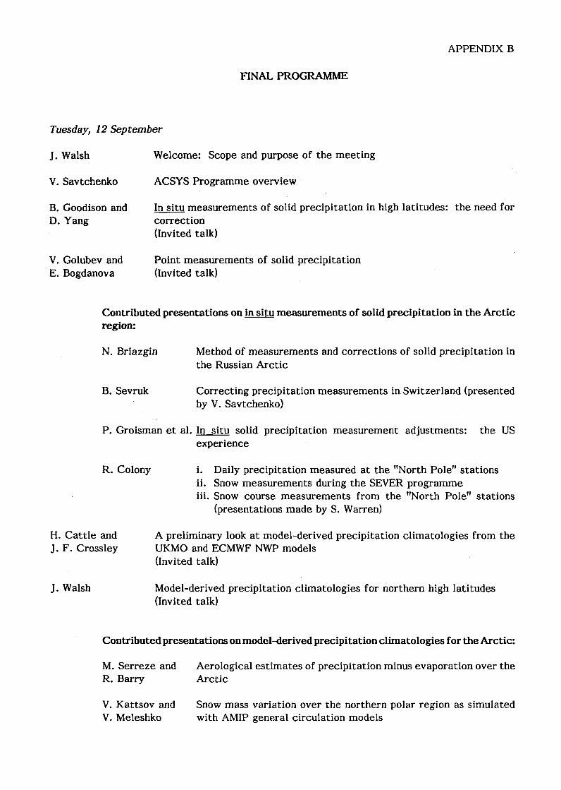
APPENDIX B

FINAL PROGRAMME

Tuesday, 12 September

j. Walsh Welcome: Scope and purpose of the meeting

V. Savtchenko ACSYS Programme overview

B. Goodison and D. Yang

In situ measurements of solid precipitation in high latitudes: the need for correction (Invited talk)

V. Golubev and E. Bogdanova

Point measurements of solid precipitation (Invited talk)

Contributed presentations on in situ measurements of solid precipitation in the Arctic region:

N. Briazgin

B. Sevruk

Method of measurements and corrections of solid precipitation in the Russian Arctic

Correcting precipitation measurements in Switzerland (presented by V. Savtchenko)

P. Groisman et al. In situ solid precipitation measurement adjustments: the US experience

R. Colony i. Daily precipitation measured at the "North Pole" stations ii. Snow measurements during the SEVER programme iii. Snow course measurements from the "North Pole" stations

(presentations made by S. Warren)

H. Cattle and A preliminary look at model-derived precipitation climatologies from the j. F. Crossley UKMO and ECMWF NWP models

(Invited talk)

J. Walsh Model-derived precipitation climatologies for northern high latitudes (Invited talk)

Contributed presentations on model-derived precipitation climatologies for the Arctic:

M. Serreze and R. Barry

V. Kattsov and V. Meleshko

Aerological estimates of precipitation minus evaporation over the Arctic

Snow mass variation over the northern polar region as simulated with AMIP general circulation models

APPENDIX B, p. 2

Wednesday, 13 September

R.G. Barry and D. Hall

Welcome to combined ACSYS/MODIS workshop participants

T. Carroll

D. Hall

Remote sensing of snow in the cold regions (Invited talk)

Satellite snow-cover mapping: a brief review (Invited talk)

Contributed presentations on remote sensing of solid precipitation:

B. Ramsay

C. Bertoia

M. Baumgartner T. Holzer and G.Apfl

A. Nolin

D. Robinson and A. Frei

A. Walker

Interactive multisensor snow and ice mapping system

Use of satellite data for operational sea ice and lake ice monitoring

Monitoring Swiss Alpine snow cover variations using NOAA/ AVHRR data

Mapping fractional snow-covered area and sea ice concentrations

An analysis of the NOAA satellite-derived snow-cover record, 1972-present

Passive microwave snow-cover algorithm development in Canada (presented by B. Goodison)

S. Bergstr6m Hydrological modelling of Arctic river run-off (Invited talk)

Yu. Vinogrodov Hydrological modelling of Arctic river run-off (Invited talk)

Contributed presentations on hydrological modelling of Arctic river run-off:

D. Lettenmaier and B. Nijssen

S. Solomon et al.

D. Kane

Simulation of large continental river run-off using a grid-based land-surface scheme

Some useful experience from past attempts to estimate the precipitation and run-off in the Canadian Arctic basin

The measurement and modelling of Arctic hydrologic processes

APPENDIX B, p. 3

Establishment of working groups:

A. In situ and remotely sensed observations B. Model-derived climatologies C. Hydrological modelling

Thursday, 14 September

Working group sessions followed by working group reports in a plenary session

Friday, 15 September

Working group sessions Plenary session: General discussion on working group reports, conclusions and recommendations of the workshop Closing remarks by the Organizing Committee

APPENDIXC

WORKING GROUP REPORTS

1. Working Group on In Situ and Remotely Sensed Observations of Solid Precipitation

(Chairman: B. Goodison)

A. In situ Measurements

a. Compilation of existing precipitation (rain and snow) ground-based data for the Arctic region

It is essential to identify what precipitation data are available for the ACSYS study region, however that region may finally be defined. Complete records of total precipitation (rain and snow) for the entire period of observation are required for both hydrological and atmospheric modelling. Daily or 6-hourly observations will be required, not just monthly totals, if precipitation data are to be adjusted for known systematic errors.

Data currently available from the Global Precipitation Climatology Centre (GPCC) in Offenbach/Main, Germany include only limited monthly gauge measurement data for the Arctic region. Arctic precipitation estimates in the archive are largely derived from the ECMWF model forecasts. Only rainfall measurements are included in the gauge data base; snowfall measurements are not available. Hence total monthly and annual measured precipitation cannot be determined from the current data base.

The record from Canadian stations in the Arctic region (including the Archipelago) is relatively short (most less than 30 years). However, these synoptic 6-hourly observations are available from the digital archive of the Canadian Atmospheric Environment Service.

Several data rescue efforts to locate, archive and make available data from Russia are in progress. Data from Russian sources that are to be obtained and processed by the National Snow and Ice Data Center (NSIDC) and the World·Data Center A for Glaciology in Boulder, · Colorado (USA) include precipitation at 65 coastal and island stations above 65.8°N and North Pole drifting stations. These data consist of water equivalent measurements and are being provided by the Arctic and Antarctic Research Institute (AARI).

The AARI has also prepared and provided monthly maps of measured and bias-adjusted precipitation. Bias adjustments were made for wetting and evaporation losses, wind effect, and the blowing snow problem associated with the Tretyakov gauge. Wind speed at two metres was used and speeds in excess of 8 ms-1 were truncated to 8 ms for gauge bias adjustment purposes. The methods developed by the Main Geophysical Observatory, Russian Federation prior to 1965 were applied to determine bias adjustments. Water balance maps have not yet been compiled using more recent bias adjustment developments, but these are definitely needed.

APPENDIX C, p. 2

Daily data from 283 Russian stations (with daily maximum and mtmmum air temperature) have also been obtained from Russian sources for the entire former Soviet Union, but few stations are located in the Arctic. These data were screened by the Carbon Dioxide Information and Analysis Center (CDIAC) at Oak Ridge, Tennessee, USA and are available on CD-ROM. Additionally, wind speed data will be required to perform bias adjustments. Dr. Briazgin agreed to provide a list of coastal and Arctic island station locations. R. Colony discussed the precipitation data from the North Pole drifting stations and also the SEVER airborne landings programme for snow depth measurements on the arctic sea ice (see appropriate contributed papers presented at session 1).

Identification of previous field experiments and observing studies ("data rescue") is important. Local and short-term hydrometeorological data obtained from these studies are likely to be available in various university institutional and national expedition archives and could prove invaluable to future research and for validation studies, by eliminating duplication of analyses and measurements. An example is meteorological and radiation data of Severnaya Zemlya during the period 1974-1988 by expeditions of AARI.

b. Required supplemental information and other considerations

Additional information, including metadata and other meteorological observations, will be needed for effective utilization of the daily precipitation data. The archiving of daily precipitation data are critical for proper characterization of gauge bias adjustments. Metadata, including information regarding gauge type and siting characteristics are necessary to make the proper adjustments. Meteorological data, notably air temperature and wind speed, are required for the calculation of gauge bias adjustments. Information on station air pressure and/or station elevation (in addition to location) are further required for some correction procedures. It is imperative that both the measured and the gauge bias adjusted data are archived so that future gauge adjustment procedures can subsequently be applied. In addition to precipitation data, snow course, snow depth, and snowfall measurements are necessary for proper characterization of snowfall in the Arctic region.

Data from both climate and synoptic stations should be used in ACSYS analyses. It is recognized that some countries are automating their manual observational network or expanding the network with new autostations. In most countries, different precipitation gauges will be used at these stations requiring the application of different bias-adjustments of the measured precipitation. Changes in siting, type of gauge and method of observation will cause an artificial change in the measured precipitation time series. Hence, the date of the installation of specialized automatic stations in remote areas should be identified and included in the metadata record.

Blowing snow is a characteristic of Arctic regions, making the measurement of precipitation even more difficult. Maps delineating regions where blowing snow could be a problem (areas where wind speeds exceed a given threshold) would be beneficial in determining areas where gauge measurement biases could be substantial and complicated by the observation and possible measurement of blowing snow.

APPENDIX C, p. 3

Adjustments to measured precipitation for systematic errors (e.g. wind, wetting and evaporation) are a major component in assessing precipitation measurements. There are other considerations. Trace precipitation measurements must be considered as more than a non­event. Canadian scientists use 0.03 mm/6-hour observation in Arctic regions in their precipitation adjustment routine, while Russian scientists assume 0.05 mm/12-hour for each reported trace event. For example, Resolute, Northwest Territories, has more than 800 synoptic (6-hourly) observations of trace precipitation per year. Using a value of 0.03 mm per trace event accounts for about 24 mm of moisture or approximately one-fourth to one-fifth of the current measured precipitation for the year.

In the Arctic, more work is required on quantifying the sublimation of fallen snow. This process can result in relatively large amounts of precipitation not entering the surface water balance (it never crosses the soil/atmosphere interface). This problem is potentially large during drifting and blowing snow events.

In forested areas, consideration must also be made for the interception of fallen snow by trees. This precipitation may also sublimate before entering the surface water balance. Thus, modelling of these two processes, sublimation of snow from the snow pack and from interception by tree limbs, is required for adequate estimation of the water balance of rivers and streams entering the Arctic Ocean. This is particularly important if bias-adjusted precipitation data are used because biases in both directions (gauge undercatch and sublimation effects) must be considered. Research on these issues is being conducted in Canada and there is a limited amount of empirical long-term observational data on this at Russian experimental sites.

c. Recommendations

The Working Group formulated the following recommendations for consideration by the ACSYS Scientific Steering Group:

i. The Global Precipitation Climatology Centre (GPCC) in Offenbach/Main, Germany is the appropriate organization to archive, maintain and provide daily Arctic precipitation (rain, snowfall, and total precipitation) and supplemental (e.g., precipitation type, wind speed, air temperature, air pressure, snowfall duration, siting characteristics, and gauge type) data.

ii. Creation of the ACSYS precipitation archive noted above' will require additional support to the GPCC to be successful. Special consideration with respect to data dissemination and availability of data to research groups must be agreed upon in advance. It is understood that this archive will be kept separate from the other archives maintained by the GPCC and made readily available without cost to ACSYS researchers and ACSYS activities. Quality control and maintenance of the database will be the responsibility of the GPCC.

APPENDIX C, p. 4

111. Bias-adjustments must be implemented using current knowledge and procedures obtained through national and international intercomparisons (e.g. the WMOi CIMO intercomparison). Evaluation of trace precipitation and blowing snow events requires specific attention. Studies specific to the quantification of these effects are recommended.

iv. As most of these intercomparisons are not specific to the Arctic, the results must be evaluated for this region. For example, snow course data, estimates of the regional water balance and specific data from previous field expeditions can be used to validate these gauge bias-adjustment procedures.

v. Additional intercom pari sons and validation of bias-adjustment methods specific to the Arctic region are also recommended.

v 1. It is further recommended that bias-adjustments of the existing Arctic measurements should be implemented by the GPCC although it was recognized that the GPCC would require additional resources to accomplish this. Consultation between the GPCC, WCRP, and Arctic experts in the respective countries is required. An ad-hoc workshop is the recommended forum, which should evaluate the gauge bias-adjustment algorithms and provide assessments of their reliability in providing consistent estimates of precipitation across country boundaries.

vu. The spatial integration of the existing network data and bias-adjusted data requires further investigation. Even given the bias-adjusted precipitation measurements, the sparse station network and the question of station representativeness may not enable the determination of fresh water inputs to the Arctic Ocean from precipitation measurements alone. It may be adequate to determine the net basin input; however, it is likely to be inadequate to produce gridded fields of even monthly precipitation although long-term averages may be possible.

viii. The impact of the conversion from manned to automatic stations must be assessed through overlapping observations for a minimum period of at least one year. For purposes of the ACSYS, 25-year database (1978-2003), the timing of the date of implementation of automation, must be identified as part of the station metadata.

tx. The period chosen for the precipitation analysis (1978 on) should be re-evaluated in light of the availability of more extensive records (ground and satellite data) beginning in approximately 1966. This time period also applies to the runoff data.

x. Data rescue activities are highly encouraged as their use may prove invaluable to ACSYS activities. Specific databases including data from Russian coastal and drifting stations must be incorporated into the ACSYS database. These data are necessary for validation purposes.

APPENDIX C, p. 5

xi. It is recommended that the next generation of global precipitation climatologies be observation-based and incorporate a better representation of the Arctic region. These estimates should incorporate more data from coastal and drifting stations and include precipitation estimates from analyses of snowfall on ice. Global precipitation c1imatologies are widely used to validate global climate models and for large-scale hydrologic analyses, but currently, polar regions are not particularly well-represented in these climatologies. Gridded products are useful for comparison with global climate models.

xii. The efforts to assemble and make available snow depth and snow survey data (water equivalent and depth) at the NSIDC/World Data Center A for Glaciology in Boulder, Colorado (USA) are encouraged and should continue.

xiii. It is recommended that at least a subset of the ACSYS data be made available without charge for research-only (non-commercial) use by researchers in the international community. Data obtained for and used by ACSYS are to conform to the guidelines set forth by the WMO Policy on Data Exchange. Specific exchange agreements between certain countries may have to be made in special circumstances.

x1v For solid precipitation, ACSYS must work closely with GEWEX and EOS programmes to ensure compatibility and prevent duplication of activities.

B. Use of Remotely Sensed Data for Precipitation Measurements

a. Identification of available information

Snow cover extent can presently be estimated using AVHRR imagery (a NOAA/NESDIS product which provides over a 20 year record of weekly snow extent). In Russia, visible satellite imagery has been used to examine changes in snow properties by anthropogenic activities including transportation and urbanization effects. The desired variable for modelling studies, however, is snow water equivalent (snow mass). Passive microwave remote sensing offers the best prospect for deriving snow water equivalent. It is recognized that algorithm development and validation is still progressing and that currently there is no community accepted global algorithm for deriving snow water equivalent from passive microwave imagery. A single global algorithm may never be possible as regional and seasonal dependencies may be substantial.

New capabilities will be available with the launch of the EOS sate11ites carrying the MODIS and AMSR sensors which provide improved spatial resolution and additional channels. In particular, the 1.6um channel will help discriminate between snow and clouds. In addition, the MIMR sensor on METOP (due to be launched in 2000) will collect passive microwave data suitable for studying snow water equivalent on spatial scales of 6-12km. This improved resolution will be of considerable importance to the Arctic region.

APPENDIX C, p. 6

Several groups are investigating the use of remote sensing for determining snow cover, particularly under the auspices of NASA's EOS programme. ACSYS will not need to undertake a separate study as the products developed therein should be sufficient to meet ACSYS' needs. For example, the Canadian CRYSYS investigation within EOS is developing and evaluating algorithms to estimate snow water equivalent from passive microwave sensors within high latitude Arctic areas, including the GEWEX MAGS region. The evaluation of snow cover information from existing SAR sensors is also currently under study by a number of research organizations. The ability of SAR to estimate snow water equivalent is still unresolved.

b. Recommendations

1. Recognizing ACSYS must draw on existing remote sensing archives, especially those with a cryospheric focus, the Working Group strongly endorsed using the NSIDC (Boulder, Colorado, USA) and ASP (Alaska SAR Facility, Fairbanks, Alaska, USA) EOS DAAC's (Distributed Active Archive Center) to meet ACSYS data needs. Remotely-sensed passive microwave data including EASE-Grid (Equal-Area SSM/I Earth Grid) antenna temperatures for each frequency and polarization as well as derived products using community-approved algorithms are being maintained by NSIDC. The NSIDC DAAC also will archive MODIS (Moderate Resolution Imaging Spectro-radiometer) snow and ice products in beginning in 1998. Radar products from the Synthetic Aperture Radar (SAR) are maintained by the ASP DAAC.

11. ACSYS should further assess the usefulness of weather radars for studies of both summer precipitation over land and coastal areas and winter snowfall. For example, radar data from Valdai, Russia (and SMHI, Sweden) are available for evaluation of snowfall precipitation compared with gauge measurements and extensive snow survey data. Gauge measurements and other surface-based observations have been made experimentally over a period of approximately ten years for a 500 km2 area at Valdai.

iii. ACSYS regards the new channel3A (1.6um) on the NOAA AVHRR as of great value to studies of polar snow and ice and strongly endorses the collection and distribution of those data.

1v. Studies evaluating the possibility of merging remotely sensed data with surface observations is highly recommended. Drawing on research outside ACSYS is required. ACSYS should not need to develop its own research programme regarding remotely sensed data but should draw on the results of other programmes, particularly the GEWEX and EOS programmes.

APPENDIX C, p. 7

v. The proposed NOAA NESDIS multi-sensor daily snow and ice maps will have considerable utility for ACSYS research. Existing weekly northern hemisphere snow charts are of limited use for ACSYS research because they have only limited spatial extent and a weekly time resolution. No information is available for snow depth on sea ice or its water equivalent, for example. The NOAA-NESDIS products should be properly archived for rapid retrieval and distribution. Compatibility between these new multi-sensor maps and the old hemispheric charts must be addressed using overlapping periods of observations.

v1. Research on the appropriate strategies and procedures to provide routine snow depth or snow water equivalent on the Arctic sea ice is needed.

11. Working Group on model-derived climatologies

(Chairman: H. Cattle)

a. Potential of models to estimate precipitation fields

Climate simulations by general circulation models have significant biases in their simulation of precipitation. Thus in relation to Arctic precipitation, the AMIP (Atmospheric Model Intercomparison Project) Polar Diagnostic subproject demonstrated that:

(1) The AMIP models appear to produce too much precipitation in the Arctic (if historical climatologies are not grossly in error); however,

(2) Uncertainties in validation data can significantly limit assessments of simulated precipitation and evaporation.

Whilst there remains a need for the identification of the best AMIP simulations and a diagnosis of the reasons why some AMIP models were more successful than others in the Arctic, similar models run in Numerical Weather Prediction (NWP) data assimilation-and-forecast mode have the advantage of having drawn upon the useful available observational input to produce internally consistent fields. The so-called 're-analysis' projects now underway at three centres (the European Centre for Medium Range Weather Forecasting (ECMWF), the U.S. National Meteorological Centre (NMC) and NASA Goddard are following this approach. The results of these efforts have the potential to provide, on a daily basis, useful precipitation fields (and others ofhydrological relevance) for the ACSYS Hydrological Programme.

APPENDIX C, p. 8

b. Available re-analyses and schedule

As already noted, atmospheric re-analysis efforts are now underway at three centres. Each will produce fields of precipitation, evapotranspiration, radiative and sensible heat fluxes, as well as the standard atmospheric variables at various levels. Present timetables call for the completion of all three re-analyses by early 1997. At least one re-analysis product (NMC) will continue to incorporate future years; it is likely that the entire re-analysis cycle will be eventually repeated by NMC, in the lead up to which ACSYS could play an active role in the treatment of the Arctic by drawing upon the lessons learned from its assessment of the present re-analysis efforts. This means that ACSYS needs to develop an active programme for their assessment and use now.

The AMIP experience points to the need in ACSYS for an intercomparison of the Arctic fields from the various re-analysis projects. The re-analysis products have the advantage over the use of similar fields drawn from the archives of the NWP centres themselves in their use of consistent assimilation and forecast schemes throughout the entire periods of re-analysis. However the schemes used are specific to the individual centres running the reanalyses, resulting in different products at each. Further, though broad scale verification programmes are being carried out by these centres, the quality of the outputs over regional areas such as the high Arctic is, as yet, unknown. From an ACSYS perspective there is therefore a need to develop a programme of intercomparison, verification and critical appraisal of these data sets over the region of relevance to the ACSYS programme. This should include an intercomparison of the products of reanalysis from different parts of the assimilation/forecast cycle (e. g . 0-12 hour forecast against 12-24 hour forecast) and, by implication, consideration of issues of spin-up of the forecast precipitation fields. Because ofthe general sparsity of the Arctic precipitation station network, as well as problems of representivity, it is important that verification efforts should draw on all available relevant information (see below).

c. Implementation/co-ordination of examination and assessment of Arctic re-analyses

Initial efforts to assess Arctic re-analyses are being and will be made by individual investigators. Co-ordination of these efforts and interaction with the re-analysis centres would be enhanced by the formation of an ad hoc Working Group consisting of ACSYS participants and representatives ofthe re-analysis centres. We recommend that ACSYS organise such a Working Group in the near future.

Recommended approaches to the verification of the Arctic hydrological fields produced by atmospheric re-analyses include the use of:

( 1) a database of adjusted precipitation measurements from Arctic stations;

(2) remote sensing products depicting snow extent and snow water equivalent;

(3) water vapour budget evaluations based on rawinsonde data.

APPENDIX C, p. 9

Two particular components needed from other parts of the ACSYS Hydrological Programme are, therefore:

(i) a database of adjusted precipitation measurements from observing stations. Data should be at least for the years of the period common to the current reanalysis projects (i.e. 1979 to 1989).

(ii) a database of Arctic-relevant satellite products, in particular snow extent and snow depth/water equivalent accompanied by uncertainty estimates.

It may also be feasible to address the validity of the re-analysed evapotranspiration using historical climatological charts.

d. Strategy for production of fields of precipitation for ACSYS

Three particular strategies may be envisaged for the production of the precipitation fields needed by ACSYS over the Arctic region:

Use of adjusted station data alone, coupled with methods based on precipitation frequency over the data-sparse ocean area;

Use of re-analysis data alone, following verification and possibly ad hoc calibration against station and other data;

A suitably formulated combination of adjusted station and re-analysis data, for example using optimal interpolation of station data against reanalysis data used as background fields.

The first of these approaches has the disadvantage that it requires analysis of data from a sparsely-distributed station network with uncertain representivity, but is the approach which has been traditionally taken in the past (e.g. in a global context by the Jaeger, Legates and Willmott, and Schutz and Gates data sets). The second places too much confidence in the parameterisation schemes ofthe individual re-analysis models and has the disadvantage of placing too little weight on the precipitation network itself The third alternative may need development of new techniques, but is the preferred approach in that it has the potential to make the best use of all available data. It is recommended that this task be undertaken in consultation with the GPCC. It should refer to and build on the assessments of the ad hoc Working Group proposed above.

e. Use of nested models/down scaling techniques and coupled modelling considerations

Application of re-analysis-based fields of precipitation to the forcing of surface hydrological models will need the use of down scaling techniques to be applied to enable the resolution required by these models to be attained. The use of fine resolution regional atmospheric models run from boundary conditions specified from re-analysis atmospheric profile

APPENDIX C, p. 10

data offer one strategy for down scaling. However, the effective use of these models is computationally expensive and their accuracy for forcing of hydrological models has yet to be fully demonstrated. An alternative strategy that merits consideration in ACSYS is the use of circulation down scaling statistics, in which high-resolution topography is used in conjunction with coarse-resolution model output and statistical relationships between variables on the two scales. Note that hydrological models require fields additional to precipitation (see the paper by Bergstrom presented at session 4 of the workshop).

The Group did not see a need for fully coupled (atmosphere-ocean) models as a component of the ACSYS precipitation climatology programme. Land surface and sea ice/ocean models may indeed provide the optimum estimates of evapotranspiration/evaporation when forced by the re-analysis derived products, but, of course, without the opportunity for physical feedback to them.

f Parameterisation of physical processes - atmosphere, land surface and sea ice - in future re-analyses

It is certain that improvements can and will be made in the sea ice and land surface representations used in the models providing future re-analysis programmes. However, the representation of other model elements (e.g. clouds) also needs to be addressed in order to successfully model the Arctic. While the ACSYS Atmospheric Programme will address the formulation of clouds and precipitation processes in climate models, and the ACSYS Hydrological Programme (in collaboration with GEWEX) improved land surface schemes, a particular key ACSYS contribution to future re-analyses is the inclusion of more realistic sea ice boundary conditions. Feasible enhancements over present models are specifications of sea ice concentration and albedo in accordance with observations. Such specifications will require that the atmospheric models used are configured for more than one type of surface within a grid cell.

g. Needs pertaining to assimilated Arctic data

Present re-analyses incorporate all station-based upper air observations from the Arctic and elsewhere. There is a need to ascertain which, if any ice island sounding and Arctic buoy data are in the data input stream and to determine whether unadjusted TOVS soundings from the Arctic are incorporated. Preliminary roles for ACSYS are the identification of (1) systematic errors (e.g. in surface temperature) in the re-analysed Arctic fields, and (2) the provision of corresponding enhanced data sets for future re-analyses for the Arctic. A recommended vehicle for facilitation of these efforts (and of 'f above) is the ad hoc Working Group proposed above.

Recommendations

(i) Intercomparison and critical appraisal of re-analysis products are needed, drawing upon all available information (in particular, station data, remote sensing and water vapour budgets). Such appraisals should aim at feeding back to future re-analysis efforts as well

APPENDIX C, p. 11

as an assessment of the suitability of re-analysis fields over the Arctic for ACSYS purposes. To achieve this, an ad hoc Working Group should be formed with membership from the ACSYS community and, if possible, the re-analysis centres.

(ii) Consideration should be given to developing a strategy to develop Arctic precipitation data sets based on the currently-running atmospheric re-analysis project precipitation products used as background fields against which to analyse corrected observed station precipitation data. In the first instance, development of such a strategy may be carried out by the proposed ad hoc Working Group (or a sub-group) in liaison with the GPCC.

(iii) There is a need to explore strategies for down scaling atmospheric model precipitation for application to more local hydrological models. WCRP/GEWEX should promote this issue, which is not unique to high latitudes.

(iv) Efforts should be made within the ACSYS hydrological programme to ensure that it achieves:

1) a database of adjusted station precipitation for Arctic stations

2) satellite products on snow extent and snow depth water equivalent, accompanied by uncertainty estimates.

m. Working Group on Hydrological Modelling

(Chairman: V. Vuglinsky)

Having discussed the state-of-the-art and prospects of hydrological modelling relative to the objectives of ACSYS, the Group noted that:

1. Freshwater inflow to the Arctic Ocean is a link between the atmosphere and the ocean and, therefore, should be taken into account at the macro-scale modelling of moisture exchange in the Arctic region.

2. Up to 75% of the total mean annual freshwater inflow to the Arctic Ocean is formed in large river basins of the North America and Eurasia which are located within several geographical zones and often have drainage areas exceeding 1·1 06km2 (e.g. the Ob, Yenisei, Lena, Mackenzie rivers). There are hydrometric stations in the lower reaches of these rivers with long-term observations which provide quite reliable assessment of freshwater inflow to the Arctic Ocean (at an accuracy of 5-10% of annual runoff). Therefore, for the development and testing of joint atmosphere-land-ocean models for the Arctic, hydrological modules of the models can be provided with sufficient information for their validation.

APPENDIX C, p. 12

3. However, it is necessary to simulate macro-scale hydrological processes in large river basins discharging to the Arctic Ocean at the modelling of water cycle in the Arctic region for the case of a possible warming of global climate. As the most of the drainage areas of the large northward-flowing rivers are occupied by forests, the Group was convinced that the problem ofhydrological modelling in such basins went beyond the framework of ACSYS and should be implemented under a joint ACSYS/GEWEX project.

4. The assessment of water inflow to the Arctic Ocean from the ungauged areas is the main hydrological problem in the Arctic region. The ungauged part could be filled in by use of hydrological models, or (if input data are missing) simply by interpolation of figures from nearby stations, or similar techniques.

The Group was of the opinion that it was important to distinguish between conventional conceptual models for runoff simulation and more sophisticated physically based ones for modelling of spatially distributed fluxes. These two types of models serve different purposes. The Group agreed that available conceptual models could be adjusted for Arctic river basins. The following Arctic data sets are necessary and need to be assembled for the development of conceptual hydrological models for the Arctic region:

land topography vegetation indices soil cover hydrographic network/lakes/reservoirs daily precipitation daily air temperatures.

It also noted that sophisticated physically based models might be scaled up to Arctic river basins. However, they required more input data and detailed descriptions of the catchments. The Group agreed, that, besides the development of integral models of runoff from ungauged areas of the Arctic region, models of the following processes which were typical ofthe Arctic conditions should be developed:

water exchange in the permafrost zone evolution of mass balance of glaciers snow cover redistribution on glaciers and in tundra snow sublimation ice outflow caused by icebergs freshwater dynamics in the estuaries of large Arctic rivers.

Hydrological models may be used not only for the assessment of river run-off, but for the estimation of other hydrological regime components in the Arctic (e.g. evapotranspiration, soil moisture content, snow storage, water equivalent of snow pack, lake levels, etc.).

The following recommendations were made by the Group:

APPENDIX C, p. 13

1. It would be practical to limit the hydrological modelling in the framework of ACSYS to the Arctic river basins smaller than 1 04 km2

.

n. Discreteness of run-off data required to achieve the ACSYS goal should be determined by the potential users of these data (e.g. coupled climate modellers). The existing conceptual hydrological models provide rather accurate estimation of daily water discharges, as well as of water discharges for longer time intervals.

iii. The ACSYS Runoff Database (ARDB) should also contain runoff data from Alaska and Greenland.

IV. It is reasonable to establish within ACSYS a special panel for developing a strategy and the co-ordination of international activities in hydrological modelling.

WCRP-1

WCRP-2

WCRP-3

WCRP-4

WCRP-5

WCRP-6

WCRP-7

WCRP-8

WCRP-9

WCRP-10

WCRP-11

WCRP-12

WCRP-13

WCRP-14

WCRP-15

WCRP-16

LIST OF REPORTS

VALIDATION OF SATELLITE PRECIPITATION MEASUREMENTS FOR THE GLOBAL PRECIPITATION CLIMATOLOGY PROJECT (Report of an International Workshop, Washington, D.C., 17-21 November 1986) (WMOfTD-No. 203)

WOCE CORE PROJECT 1 PLANNING MEETING ON THE GLOBAL DESCRIPTION (Washington, D.C., 10-14 November 1986) (WMOfTD-No. 205)

INTERNATIONAL SATELLITE CLOUD CLIMATOLOGY PROJECT (ISCCP) WORKING GROUP ON DATA MANAGEMENT (Report of the Sixth Session, Fort Collins, U.S.A., 16-18 June 1987) (WMOfTD-No. 210)

JSC/CCCO TOGA NUMERICAL EXPERIMENTATION GROUP (Report of the First Session, Unesco, Paris, France, 25-26 June 1987) (WMO/TD-No. 204)

CONCEPT OF THE GLOBAL ENERGY AND WATER CYCLE EXPERIMENT (Report of the JSC Study Group on GEWEX, Montreal, Canada, 8-12 June 1987 and Pasadena, U.S.A., 5-9 January 1988) (WMOfTD-No. 215) (out of print)

INTERNATIONAL WORKING GROUP ON DATA MANAGEMENT FOR THE GLOBAL PRECIPITATION CLIMATOLOGY PROJECT (Report of the Second Session, Madison, U.S.A., 9-11 September 1988) (WMO/TD-No. 221) (out of print)

CAS GROUP OF RAPPORTEUR$ ON CLIMATE (Leningrad, U.S.S.R., 28 October-1 November 1985) (WMOfTD-No. 226) (out of print)

JSC WORKING GROUP ON LAND SURFACE PROCESSES AND CLIMATE (Report of the Third Session, Manhattan, U.S.A., 29 June-3 July 1987) (WMO/TD-No. 232)

AEROSOLS, CLOUDS AND OTHER CLIMATICALLY IMPORTANT PARAMETERS: LIDAR APPLICATIONS AND NETWORKS (Report of a Meeting of Experts, Geneva, Switzerland, 1 0-12 December 1985} (WMOfTD-No. 233)

RADIATION AND CLIMATE (Report of the First Session, JSC Working Group on Radiative Fluxes, Greenbelt, U.S.A., 14-17 December 1987) (WMOfTD-No. 235)

WORLD OCEAN CIRCULATION EXPERIMENT - IMPLEMENTATION PLAN - DETAILED REQUIREMENTS (Volume I) (WMOfTD-No. 242)

WORLD OCEAN CIRCULATION EXPERIMENT- IMPLEMENTATION PLAN - SCIENTIFIC BACKGROUND (Volume Ill (WMOfTD-No. 243)

RADIATION AND CLIMATE (Report of the Seventh Session of the International Satellite Cloud Climatology Project (ISCCPl Working Group on Data Management, Banff, Canada, 6-8 July 1988) (WMOfTD-No. 252) (out of print)

AN EXPERIMENTAL CLOUD LIDAR PILOT STUDY (ECLIPS) (Report of the WCRP/CSIRO Workshop on Cloud Base Measurement, CSIRO, Mordialloc, Victoria, Australia, 29 February-3 March 1988) (WMOfTD-No. 251) (out of print)

MODELLING THE SENSITIVITY AND VARIATIONS OF THE OCEAN-ATMOSPHERE SYSTEM (Report of a Workshop at the European Centre for Medium Range Weather Forecasts, 11-13 May 1988) (WMOfTD-No. 254) (out of print)

GLOBAL DATA ASSIMILATION PROGRAMME FOR AIR-SEA FLUXES (Report of the JSC/CCCO Working Group on Air-Sea Fluxes, October 1988) (WMOfTD-No. 257)

WCRP-17

WCRP-18

WCRP-19

WCRP-20

WCRP-21

WCRP-22

WCRP-23

WCRP-24

WCRP-25

WCRP-26

WCRP-27

WCRP-28

WCRP-29

WCRP-30

WCRP-31

WCRP-32

- 2 -

JSC/CCCO TOGA SCIENTIFIC STEERING GROUP (Report of the Seventh Session, Cairns, Queensland, Australia, 11-15 July 1988) (WMO/TD-No. 259)

SEA ICE AND CLIMATE (Report of the Third Session of the Working Group on Sea Ice and Climate, Oslo, 31 May-3 June 1988) (WMO/TD-No. 272) (out of print)

THE GLOBAL PRECIPITATION CLIMATOLOGY PROJECT (Report of the third Session of the International Working Group on Data Management, Darmstadt, FRG, 13-1 5 July 1988) (WMO/TD-No. 274)

RADIATION AND CLIMATE (Report of the Second Session of the WCRP Working Group on Radiative Fluxes, Geneva, Switzerland, 19-21 October 1988) (WMO/TD-No. 291)

INTERNATIONAL WOCE SCIENTIFIC CONFERENCE !Report of the International WOCE Scientific Conference, Unesco, Paris, 28 November-2 December 1988) (WMO/TD-No. 295)

THE GLOBAL WATER RUNOFF DATA PROJECT (Workshop on the Global Runoff Data Set and Grid estimation, Koblenz, FRG, 10-15 November 1988) (WMO/TD-No. 302) (out of print)

WOCE SURFACE FLUX DETERMINATION$- A STRATEGY FOR IN SITU MEASUREMENTS (Report of the Working Group on In Situ Measurements for Fluxes, La Jolla, California, U.S.A., 27 February-3 March 1989) (WMO/TD-No. 304) (out of print)

JSC/CCCO TOGA NUMERICAL EXPERIMENTATION GROUP (Report of the Second Session, Royal Society, London, U.K., 15-16 December 1988) (WMO/TD-No. 307)

GLOBAL ENERGY AND WATER CYCLE EXPERIMENT (GEWEX) (Report of the First Session of the JSC Scientific Steering Group for GEWEX, Pasadena, U.S.A., 7-10 February 1989) (WMO/TD-No. 321) (out of print)

WOCE GLOBAL SURFACE VELOCITY PROGRAMME (SVP) (Workshop Report of WOCE/SVP Planning Committee and TOGA Pan-Pacific Surface Current Study, Miami, Florida, U.S.A., 25-26 April 1988) (WMO/TD-No. 323)

DIAGNOSTICS OF THE GLOBAL ATMOSPHERIC CIRCULATION (Based on ECMWF analyses 1979-1989, Department of Meteorology, University of Reading, Compiled as part of the U.K. Universities Global Atmospheric Modelling Project) (WMO/TO-No. 326)

INVERSION OF OCEAN GENERAL CIRCULATION MODELS (Report of the CCCO/WOCE Workshop, London, 1 0-12 July 1989) (WMO/TD-No. 331) (out of print)

CAS WORKING GROUP ON CLIMATE RESEARCH (Report of Session, Geneva, 22-26 May 1989) (WMO/TD-No. 333)

WOCE- FLOW STATISTICS FROM LONG-TERM CURRENT METER MOORINGS: THE GLOBAL DATA SET IN JANUARY 1989 (Report prepared by Robert R. Dickinson, Eddy Statistics Scientific Panel) IWMO/TD-No. 337)

JSC/CCCO TOGA SCIENTIFIC STEERING GROUP (Report of the Eighth Session, Hamburg, FRG, 18-22 September 1989) (WMO/TD-No. 338)

JSC/CCCO TOGA NUMERICAL EXPERIMENTATION GROUP (Report of the Third Session, Hamburg, FRG, 18-20 September 1989) (WMO/TD-No. 339)

WCRP-33

WCRP-34

WCRP-35

WCRP-36

WCRP-37

WCRP-38

WCRP-39

WCRP-40

WCRP-41

WCRP-42

WCRP-43

WCRP-44

WCRP-45

WCRP-46

WCRP-47

WCRP-48

WCRP-49

- 3 -

TOGA MONSOON CLIMATE RESEARCH (Report of the First Session of the Monsoon Numerical Experimentation Group, Hamburg, FRG, 21-22 September 1989) (WMOfTD-No. 349)

THE GLOBAL PRECIPITATION CLIMATOLOGY PROJECT (Report of the Fourth Session of the International Working Group on Data Management, Bristol, U.K., 26-28 July 1989) (WMOfTD-No. 356)

RADIATION AND CLIMATE (Report of the Third Session of the WCRP Working Group on Radiative Fluxes, Fort Lauderdale, U.S.A., 12-15 December 1989) (WMOfTD-No. 364)

LAND-SURFACE PHYSICAL AND BIOLOGICAL PROCESSES (Report of an ad-hoc Joint Meeting of the IGBP Co-ordinating Panel No. 3 and WCRP Experts, Paris, France, 24-26 October 1989) (WMOfTD-No. 368)

GLOBAL ENERGY AND WATER CYCLE EXPERIMENT (Report of the Workshop to Evaluate the Need for a Rain Radar in Polar Orbit for GEWEX, Greenbelt, U.S.A., 25-26 October 1989) (WMOfTD-No. 369)

GLOBAL ENERGY AND WATER CYCLE EXPERIMENT (Report of the First Session of the WCRP-GEWEX/IGBP-CP3 Joint Working Group on Land-Surface Experiments, Wallingford, U.K., 25-26 January 1990) (WMOfTD-No. 370)

RADIATION AND CLIMATE (lntercomparison of Radiation Codes in Climate Models, Report of Workshop, Paris, France, 15-17 August 1988) (WMOfTD-No. 371)

GLOBAL ENERGY AND WATER CYCLE EXPERIMENT (Scientific Plan), August 1990 (WMOfTD-No. 376) (out of print)

SEA-ICE AND CLIMATE (Report of the Fourth Session of the Working Group, Rome, Italy, 20-23 November 1 989) (WMOfTD-No. 377)

PLANETARY BOUNDARY LAYER (Model Evaluation Workshop, Reading, U.K., 14-15 August 1989) (WMOfTD-No. 378)

INTERNATIONAL TOGA SCIENTIFIC CONFERENCE PROCEEDINGS (Honolulu, U.S.A., 16-20 July 1990) (WMOfTD-No. 379)

GLOBAL ENERGY AND WATER CYCLE EXPERIMENT (Report of the 2nd Session of the JSC Scientific Steering Group, Paris, France, 15-19 January 1990) (WMOfTD-No. 383)

SEA ICE NUMERICAL EXPERIMENTATION GROUP (SINEG) (Report of the First Session, Washington, D.C., 23-25 May 1989) (WMOfTD-No. 384)

EARTH OBSERVING SYSTEM FOR CLIMATE RESEARCH (Report of a WCRP Planning Meeting, Reading, U.K., 2-3 July 1990) (WMOfTD-No. 388)

JSC/CCCO TOGA SCIENTIFIC STEERING GROUP (Report of the Ninth Session, Kona, Hawaii, U.S.A., 23-25 July 1990) (WMOfTD-No. 387)

SPACE OBSERVATIONS OF TROPOSPHERIC AEROSOLS AND COMPLEMENTARY MEASUREMENTS (Report of experts meeting at Science and Technology Corporation, Hampton, Virginia, U.S.A., 15-18 November 1989) (WMOfTD-No. 389) (out of print)

TOGA MONSOON CLIMATE RESEARCH (Report of the Second Session of the Monsoon Numerical Experimentation Group, Kona, Hawaii, U.S.A., 26-27 July 1990) (WMOfTD-No. 392)

WCRP-50

WCRP-51

WCRP-52

WCRP-53

WCRP-54

WCRP-55

WCRP-56

WCRP-57

WCRP-58

WCRP-59

WCRP-60

WCRP-61

WCRP-62

WCRP-63

WCRP-64

WCRP-65

- 4 -

TOGA NUMERICAL EXPERIMENTATION GROUP (Report of the Fourth Session, Palisades, New York, U.S.A., 13-14 June 1990) (WMOITD-No. 393)

RADIATION AND CLIMATE (Report of the First Session, International Working Group on Data Management for WCRP Radiation Projects, New York City, U.S.A., 21-23 May 1990) (WMOITD-No. 398)

THE RADIATIVE EFFECTS OF CLOUDS AND THEIR IMPACT ON CLIMATE (Review prepared by Dr. A. Arking at request of IAMAP Radiation Commission) (WMOITD-No. 399)

CAS/JSC WORKING GROUP ON NUMERICAL EXPERIMENTATION (Report of the Sixth Session, Melbourne, Australia, 24-28 September 1990) (WMOITD-No. 405)

RADIATION AND CLIMATE (Workshop on Implementation of the Baseline Surface Radiation Network, Washington, D.C., 3-5 December 1990) (WMO/TD-No. 406) (out of print)

GLOBAL CLIMATE MODELLING (Report of First Session of WCRP Steering Group on Global Climate Modelling, Geneva, Switzerland, 5-8 November 1990) (WMOITD-No. 411)

THE GLOBAL CLIMATE OBSERVING SYSTEM (Report of a meeting convened by the Chairman of the Joint Scientific Committee for the WCRP, Winchester, U.K., 14-15 January 1991) (WMOITD-No. 412) (out of print)

GLOBAL ENERGY AND WATER CYCLE EXPERIMENT (Report of the 3rd Session of the JSC Scientific Steering Group, Hamilton, Bermuda, 21-25 January 1991) (WMOITD-No. 424) (out of print)

INTERCOMPARISON OF CLIMATES SIMULATED BY 14 ATMOSPHERIC GENERAL CIRCULATION MODELS (CAS/JSC Working Group on Numerical Experimentation, prepared by Dr. G.J. Boer et al) (WMOITD-No. 425)

INTERACTION BETWEEN AEROSOLS AND CLOUDS (Report of Experts Meeting, Hampton, Virginia, U.S.A., 5-7 February 1991) (WMOITD-No. 423)

THE GLOBAL PRECIPITATION CLIMATOLOGY PROJECT (Report of the Fifth Session of the International Working Group on Data Management, Laurel, Maryland, U.S.A., 20-21 May 1991) (WMOITD-No. 436)

GLOBAL ENERGY AND WATER CYCLE EXPERIMENT (Report of the Second Session of the WCRP-GEWEX/IGBP Core Project on BAHC Joint Working Group on Land-Surface Experiments, Greenbelt, Mayland, U.S.A., 3-4 June 1991) (WMO/TD-No. 437)

SEA-ICE AND CLIMATE (Report of a Workshop on Polar Radiation Fluxes and Sea-Ice Modelling, Bremerhaven, Germany, 5-8 November 1990) (WMO/TD-No. 442)

JSC/CCCO TOGA SCIENTIFIC STEERING GROUP (Report of the Tenth Session, Gmunden, Austria, 26-29 August 1991) (WMO/TD-No. 441)

RADIATION AND CLIMATE (Second Workshop on Implementation of the Baseline Surface Radiation Network, Davos, Switzerland, 6-9 August 1991) (WMO/TD-No. 453)

SEA-ICE AND CLIMATE (Report of the Fifth Session of the Working Group, Bremerhaven, Germany, 13-15 June 1991 (WMO/TD-No. 459)

WCRP-66

WCRP-67

WCRP-68

WCRP-69

WCRP-70

WCRP-71

WCRP-72

WCRP-73

WCRP-74

WCRP-75

WCRP-76

WCRP-77

WCRP-78

WCRP-79

WCRP-80

WCRP-81

WCRP-82

- 5 -

GLOBAL ENERGY AND WATER CYCLE EXPERIMENT (Report of the First GEWEX Temperature/Humidity Retrieval Workshop, Greenbelt, U.S.A., 23-26 October 1990) (WMO/TD-No. 460) (out of print)

GEWEX CONTINENTAL SCALE INTERNATIONAL PROJECT (Scientific Plan, December 1991) (WMO/TD-No. 461) (out of print)

SIMULATION OF INTERANNUAL AND INTRASEASONAL MONSOON VARIABILITY (Report of Workshop, Boulder, CO, U.S.A., 21-24 October 1991) (WMO/TD-No. 470)

RADIATION AND CLIMATE (Report of Fourth Session of the WCRP Working Group on Radiative Fluxes, Palm Springs, U.S.A., 24-27 September 1991) (WMO/TD-No. 471)

CAS/JSC WORKING GROUP ON NUMERICAL EXPERIMENTATION (Report of the Seventh Session, Boulder, CO, U.S.A., 24-29 October 1991) (WMO/TD-No. 477)

GLOBAL CLIMATE MODELLING (Report of Second Session of WCRP Steering Group on Global Climate Modelling, Bristol, U.K., 18-20 November 1991) (WMO/TD-No. 482)

SCIENTIFIC CONCEPT OF THE ARCTIC CLIMATE SYSTEM STUDY (ACSYSI (Report of the JSC Study Group on ACSYS, Bremerhaven, Germany, 10-12 June 1991 and London, U.K., 18-19 November 1991) (WMO/TD-No. 486) (out of print)

TOGA NUMERICAL EXPERIMENTATION GROUP (Report of the Fifth Session, San Francisco, California, U.S.A., 9-11 December 1991) (WMO/TD-No. 487)

GLOBAL ENERGY AND WATER CYCLE EXPERIMENT (Report of the Fourth Session of the JSC Scientific Steering Group for GEWEX, Tokyo, Japan, 27-31 January 1992) (WMO/TD-No. 490)

HYDROLOGY AND SURFACE RADIATION IN ATMOSPHERIC MODELS (Report of a GEWEX Workshop, European Centre for Medium-range Weather Forecasts, Reading, U.K., 28 October-1 November 1991) (WMO/TD-No. 492)

REVIEWS OF MODERN CLIMATE DIAGNOSTIC TECHNIQUES -Satellite data in climate diagnostics, (A. Gruber and P.A. Arkin, November 1992) (WMO/TD-No. 519)

INTERNATIONAL SATELLITE CLOUD CLIMATOLOGY PROJECT (Radiance Calibration Report, December 1992) (WMO/TD-No. 520)

GLOBAL OBSERVATIONS, ANALYSES AND SIMULATION OF PRECIPITATION (Report of Workshop, National Meteorological Center, Camp Springs, Maryland, U.S.A., 27-30 October 1992) (WMO/TD-No. 544)

INTERCOMPARISON OF TROPICAL OCEAN GCMS (TOGA Numerical Experimentation Group, prepared by T. Stockdale et al., April 1993) (WMO/TD-No. 545)

SIMULATION AND PREDICTION OF MONSOONS - RECENT RESULTS (TOGA/WGNE Monsoon Numerical Experimentation Group, New Delhi, India, 12-14 January 1993) (WMO/TD-No. 546)

ANALYSIS METHODS OF PRECIPITATION ON A GLOBAL SCALE (Report of a GEWEX Workshop, Koblenz, Germany, 14-17 September 1992) (WMO/TD-No. 558)

INTERCOMPARISON OF SELECTED FEATURES OF THE CONTROL CLIMATES SIMULATED BY COUPLED OCEAN-ATMOSPHERE GENERAL CIRCULATION MODELS (Steering Group on Global Climate Modelling, September 1993) (WMO/TD-No. 574)

WCRP-83

WCRP-84

WCRP-85

WCRP-86

WCRP-87

WCRP-88

WCRP-89

WCRP-90

WCRP-91

WCRP-92

WCRP-93

- 6 -

STRATOSPHERIC PROCESSES AND THEIR ROLE IN CLIMATE (SPARC): INITIAL REVIEW OF OBJECTIVES AND SCIENTIFIC ISSUES (SPARC Scientific Steering Group, December 1993) (WMOfTD-No. 582)

PROCEEDINGS OF THE INTERNATIONAL CONFERENCE ON MONSOON VARIABILITY AND PREDICTION (Trieste, Italy, 9-13 May 1994) (WMOfTD-No. 619) (Out of print)

INITIAL IMPLEMENTATION PLAN FOR THE ARCTIC CLIMATE SYSTEM STUDY (ACSYS) (September 1994) (WMOfTD-No. 627) (out of print)

CLOUD-RADIATION INTERACTIONS AND THEIR PARAMETERIZATION IN CLIMATE MODELS (Report of international workshop, Camp Springs, Maryland, U.S.A., 18-20 October 1993) (WMO!TD-No. 648)

PROCEEDINGS OF THE WORKSHOP ON GLOBAL COUPLED GENERAL CIRCULATION MODELS (La Jolla, California, USA, 1 0-12 October 1994) (WMO!TD-No. 655)

INTRASEASONAL OSCILLATIONS IN 15 ATMOSPHERIC GENERAL CIRCULATION MODELS (Results from an AMIP diagnostic subproject) (WMO!TD-No. 661)

CLIMATE VARIABILITY AND PREDICTABILITY (CLIVAR) Science Plan (August 1995) (WMO!TD-No. 690)

WORKSHOP ON CLOUD MICROPHYSICS PARAMETERIZATIONS IN GLOBAL ATMOSPHERIC CIRCULATION MODELS (Kananaskis, Alberta, Canada, 23-25 May 1995) (WMO!TD-No. 713)

PROCEEDINGS OF THE INTERNATIONAL SCIENTIFIC CONFERENCE ON TOGA (Melbourne, Australia, 2-7 April 1995) (WMO!TD-No. 717)

PROCEEDINGS OF THE FIRST INTERNATIONAL AMIP SCIENTIFIC CONFERENCE (Monterey, California, USA, 15-19 May 1995) (WMOfTD-No. 732)

PROCEEDINGS OF THE WORKSHOP ON ACSYS SOLID PRECIPITATION CLIMATOLOGY PROJECT (Reston, VA, USA, 15-15 September 1995) (WMOfTD-No. 739)

Joint Planning Staff for WCRP c/o World Meteorological Organization Case Postale No. 2300 CH-1211 Geneva 2 Switzerland