For more information, please contact:

World Meteorological Organization

Research Department

Atmospheric Research and Environment Branch

7 bis, avenue de la Paix – P.O. Box 2300 – CH 1211 Geneva 2 – Switzerland

Tel.: +41 (0) 22 730 81 11 – Fax: +41 (0) 22 730 81 81

E-mail: AREP-MAIL@wmo.int – Website: http://www.wmo.int/pages/prog/arep/index_en.html

GAW Report No. 186

14th WMO/IAEA Meeting of Experts on

Carbon Dioxide, Other Greenhouse Gases and

Related Tracers Measurement Techniques

WMO/TD - No. 1487

(Helsinki, Finland, 10-13 September 2007)

© World Meteorological Organization, 2009

The right of publication in print, electronic and any other form and in any language is reserved by WMO. Short extracts from WMO publications may be reproduced without authorization provided that the complete source is clearly indicated. Editorial correspondence and requests to publish, reproduce or translate this publication (articles) in part or in whole should be addressed to:

Chairperson, Publications BoardWorld Meteorological Organization (WMO)7 bis avenue de la Paix Tel.: +41 22 730 8403P.O. Box No. 2300 Fax.: +41 22 730 8040CH-1211 Geneva 2, Switzerland E-mail: publications@wmo.int

NOTE

The designations employed in WMO publications and the presentation of material in this publication do not imply the expression of any opinion whatsoever on the part of the Secretariat of WMO concerning the legal status of any country, territory, city or area or of its authorities, or concerning the delimitation of its frontiers or boundaries.

Opinions expressed in WMO publications are those of the authors and do not necessarily reflect those of WMO. The mention of specific companies or products does not imply that they are endorsed or recommended by WMO in preference to others of a similar nature which are not mentioned or advertised.

This document (or report) is not an official publication of WMO and has not been subjected to its standard editorial procedures. The views expressed herein do not necessarily have the endorsement of the Organization.

WORKSHOP PROCEEDINGS

All oral presentations and national reports given during the workshop are on the enclosed CD and are also available online for download at

http://www.wmo.int/pages/prog/arep/gaw/gaw-reports.html

WORLD METEOROLOGICAL ORGANIZATION GLOBAL ATMOSPHERE WATCH

14th WMO/IAEA Meeting of Experts on Carbon Dioxide, Other Greenhouse Gases

and Related Tracers Measurement Techniques

(Helsinki, Finland, 10-13 September 2007)

Edited by Tuomas Laurila

WMO/TD-No.1487

i

Table of Contents

GROUP PICTURE ................................................................................................................................................................ iii ABBREVIATIONS AND ACRONYMS.................................................................................................................................. iv THE WMO GLOBAL ATMOSPHERE WATCH PROGRAMME .......................................................................................... vii EXPERT GROUP RECOMMENDATIONS

R1. CALIBRATION of GAW MEASUREMENTS - WMO CENTRAL CALIBRATION LABORATORIES...................................... 2 R1.1 Background ............................................................................................................................................................................... 2 R1.2 General requirements for Central Calibration Laboratories ...................................................................................................... 2 R1.3 Maintenance of calibration by GAW measurement laboratories ............................................................................................... 3 R2. SPECIFIC REQUIREMENTS for CO2 CALIBRATION ........................................................................................................... 4 R3. SPECIFIC REQUIREMENTS FOR CO2 STABLE ISOTOPE CALIBRATION ........................................................................ 4 R3.1 Background.............................................................................................................................................................................. 4 R3.2 Current achievements for CO2 stable isotope calibrations....................................................................................................... 4 R3.3 Recommendations for CO2 stable isotope calibrations............................................................................................................ 5

R4. SPECIFIC REQUIREMENTS for RADIOCARBON in CO2 CALIBRATION........................................................................... 6 R4.1 Background.............................................................................................................................................................................. 6 R4.2 14CO2 calibration and intercomparison activities and respective recommendations ................................................................ 6 R5. SPECIFIC REQUIREMENTS FOR O2/N2 CALIBRATION ...................................................................................................... 6 R5.1 Background.............................................................................................................................................................................. 6 R5.2 O2/N2 calibration and intercomparison activities ...................................................................................................................... 7 R5.3 Recommendations ................................................................................................................................................................... 7 R6. SPECIFIC REQUIREMENTS FOR CH4 CALIBRATION......................................................................................................... 7 R7. SPECIFIC REQUIREMENTS FOR N2O CALIBRATION ........................................................................................................ 8 R7.1 Background.............................................................................................................................................................................. 8 R7.2 Recommendations ................................................................................................................................................................... 8 R8. SPECIFIC REQUIREMENTS TO SF6 CALIBRATION............................................................................................................ 8 R8.1 Background.............................................................................................................................................................................. 8 R8.2 Recommendations ................................................................................................................................................................... 9 R9. SPECIFIC REQUIREMENTS FOR CO CALIBRATION.......................................................................................................... 9 R9.1 Background.............................................................................................................................................................................. 9 R9.2 CO intercomparison activities .................................................................................................................................................. 9 R9.3 Specific recommendations for CO calibration at the WMO-GAW CCL and at GAW stations.................................................. 9 R10. SPECIFIC REQUIREMENTS FOR H2 CALIBRATION ........................................................................................................... 10 R10.1 Background.............................................................................................................................................................................. 10 R10.2 Recommendations ................................................................................................................................................................... 11 R11. GENERAL RECOMMENDATIONS FOR QUALITY CONTROL OF ATMOSPHERIC

TRACE GAS MEASUREMENTS ............................................................................................................................................. 11 R11.1 General .................................................................................................................................................................................... 11 R11.2 Flask intercomparison.............................................................................................................................................................. 12 R11.3 Recommendations for in-situ measurements........................................................................................................................... 12 R12. RECOMMENDATIONS FOR DATA MANAGEMENT AND ARCHIVING............................................................................... 13 R12.1 Data management.................................................................................................................................................................... 13 R12.2 Data archiving .......................................................................................................................................................................... 13 R12.3 Co-operative data products...................................................................................................................................................... 13 R13. SUMMARY OF RECENT INTERNATIONAL PLANNING OF ATMOSPHERIC TRACE GAS

MEASUREMENT STRATEGIES ............................................................................................................................................. 14

ii

WORKSHOP PROCEEDINGS

1. CALIBRATIONS AND STANDARDS 1.1 Improvements in the WMO/GAW Nitrous Oxide Mole Fraction Scale (B. Hall) .........................................................................18 1.2 Calibration of atmospheric hydrogen (A. Jordan).......................................................................................................................21 1.3 Preparing and maintaining of CO2 calibration scale in National Institute for Environmental Studies – NIES 95 CO2

scale (T. Machida, K. Katsumata, Y. Tohjima, T. Watai and H. Mukai) ....................................................................................26

2. INTERCOMPARISON ACTIVITIES 2.1 Activities in QA/SAC and WCC in Japan (Yukitomo Tsutsumi) .................................................................................................30 2.2 NOAA Comparison activities: Are we closer to the required measurement accuracy?

(K Masarie, P. Tans, A. Andrews, T. Conway, A. Crotwell, D. Worthy, A. Gomez) ..................................................................33 2.3 Report of The fourth wmo round-robin Reference Gas intercomparison, 2002-2007 (L.X. Zhou, D. Kitzis, P.P. Tans) ............40

3. ISOTOPE CALIBRATION AND ACTIVITIES 3.1 Ten Years of high-precision methane isotope data for Mace Head and London: The Influence of Canadian

and European sources (David Lowry, Euan Nisbet, Rebecca Fisher).......................................................................................44 3.2 Inter-laboratory calibration of CO2 produced from NBS19 calcite, calibration of Narcis-II, and CO2-isotopes

in synthetic air (W. A. Brand, A. Chivulescu, L. Huang, H. Mukai, J. M. Richter, M. Rothe).....................................................48

4. MEASUREMENT TECHNIQUES 4.1. Installation of a new gas chromatograph at Izaña GAW station (Spain) to measure CH4, N2O, and SF6

(A.J. Gomez-Pelaez, R. Ramos) ...............................................................................................................................................55 4. 2 A brief overview of the theory of flow along GC packed columns and some practical consequences for measuring

atmospheric CH4, N2O, and SF6 (A.J. Gomez-Pelaez)..............................................................................................................60 4.3 Measuring selected atmospheric trace gases using gas chromatography and a Valco pulsed discharge ionisation

detector (L.P. Steele, L.W. Porter, M. V. van der Schoot, R.L. Langenfelds) ...........................................................................65 4.4 High precision continuous measurement system of the atmospheric O2/N2 ratio using a fuel cell

oxygen analyzer (S. Morimoto, S. Ishidoya, D. Goto, A. Ogi, S. Aoki, T. Nakazawa) ...............................................................67

5. DATA MANAGEMENT AND QUALITY ASSURANCE 5.1 Report of the WCC-N2O (H.E. Scheel) ......................................................................................................................................71 5.2 Calibration and network monitoring performance of LOFLO continuous CO2 analysers (M. V. van der Schoot

L. P. Steele, D. A. Spencer, P. B. Krummel, R. J. Francey, B. Wastine, M. Ramonet, M. Schmidt) ........................................74 5.3 The Publication of WDCGG Data Submission and Dissemination Guide (Y. Tsutsumi) ...........................................................79 5.4 The Global Analysis Method by the WDCGG using the Archived Data (Y. Tsutsumi)...............................................................83

6. MEASUREMENT NETWORKS 6.1 Quarter Century of Atmospheric CO2 Monitoring and Research in Hungary (L. Haszpra, Z. Barcza) .......................................86 6.2 CO2 isotopic composition in the upper troposphere: the project CARIBIC (S.S. Assonov, C.A.M. Brenninkmeijer,

A. Zahn, C. Koeppel) ................................................................................................................................................................90

7. NATIONAL REPORTS 7.1 Greenhouse gases monitoring in India (S.D. Attri).....................................................................................................................94 7.2 Greenhouse gas and trace gas measurements programme in New Zealand (G. Brailsford) ....................................................97 7.3 Recent changes in trace gas levels at Cape Point, South Africa (E-G. Brunke, C. Labuschagne and H.E. Scheel).................100 7.4 Carbon dioxide and methane concentration and flux measurements at the GAW station of Pallas-Sodankylä

(T. Laurila, J. Hatakka, T. Aalto, M. Aurela, A. Lohila, J,-P, Tuovinen, Y.Viisanen) ..................................................................103 7.5 Set-up of a new continuous greenhouse gas monitoring station for CO2, CH4, N2O, SF6, and CO in Northern Italy

(H.A. Scheeren, P. Bergamaschi, G. Seufert, F. Raes).............................................................................................................108 7. 6 Non-CO2 greenhouse gas mixing ratios at Jungfraujoch, Switzerland (M. Steinbacher, M. K. Vollmer, B. Buchmann, S. Reimann).....................................................................................................111 7.7 Progress on the background greenhouse gases and related tracers measurement programme in China

(L.X. Zhou, X.C. Zhang, F. Zhang, B. Yao, L.X. Liu, M. Wen, L. Xu, S.X. Fang, Y.P. Wen, S. Gu) .........................................116 7.8 Results from the tall tower measurement station for atmospheric greenhouse gases at Bialystok, Poland

(E. Popa, M. Gloor, A. Jordan, U. Schultz, F. Haensel, A. C. Manning, T. Seifert, M. Heimann) ..............................................119 Annex A: List of participants.............................................................................................................................................................127 Annex B: Meeting agenda ................................................................................................................................................................130 Annex C: Previous meetings ............................................................................................................................................................136

iii

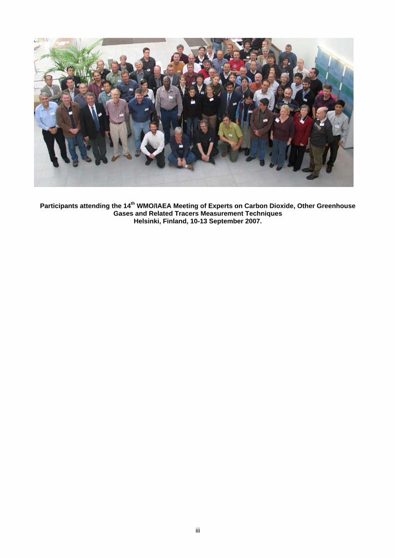
Participants attending the 14th WMO/IAEA Meeting of Experts on Carbon Dioxide, Other Greenhouse

Gases and Related Tracers Measurement Techniques Helsinki, Finland, 10-13 September 2007.

iv

ABBREVIATIONS AND ACRONYMS USED IN THIS REPORT

AGAGE Advanced Global Atmospheric Gases Experiment AVD Absolute Volumetric Determination BIPM International Bureau of Weights and Measures CARBOEUROPE Programme regrouping ecosystem and atmospheric research on the carbon balance of

Europe (EU funded project) CARIBIC Civil Aircraft for Regular Investigation of the atmosphere Based on an Instrument Container CARIBOU An automated NDIR CO2 analyzer used by LSCE cat/GC-FID CO analysis technique with catalytic reduction of CO to CH4, followed GC-FID CCGG Carbon Cycle Greenhouse Gases group of the NOAA/ESRL CCL Central Calibration Laboratory CDIAC Carbon Dioxide Information Analysis Centre CEA-CNRS Commissariat a l'Energie Atomique - Centre National de la Recherche Scientifique (French

Nuclear Energy Agency – National Centre for Scientific Research) CLASSIC Circulation of Laboratory Air Standards for Stable Isotope inter Comparisons CMA China Meteorological Administration CMDL Climate Monitoring and Diagnostics Laboratory, Boulder, CO, U.S.A. (now NOAA ESRL GMD) CSIRO Commonwealth Scientific & Industrial Research Organisation CU University of Colorado, Boulder DBMS Data Base Management Strategy ECD Electron Capture Detector ECMWF European Centre for Medium-range Weather Forecasting EMPA Eidgenössische MaterialPrüfungsAnstalt ENEA Ente per le Nuove Tecnologie, L’Energia e L’Ambiente (Italian National Agency for New

Technology, Energy and the Environment) ESRL Earth System Research Laboratory (NOAA, Boulder, CO U.S.A.) FID Flame Ionisation Detector GAW Global Atmosphere Watch (WMO Programme) GAWTEC GAW Training and Education Centre GCP Global Carbon Project GG or GHG Greenhouse Gases GLOBALVIEW Co-operative Atmospheric Data Integration Project GMD Global Monitoring Division (NOAA ESRL, Boulder, CO, U.S.A.) GOOS Global Ocean Observing System GTOS Global Terrestrial Observing System HITRAN–04 HIgh-resolution TRANsmission molecular absorption database - 2004 version IAEA International Atomic Energy Agency ICOS Integrated Carbon Observation System (EU-funded project) ICP InterComParison (experiment) IGACO Integrated Global Atmospheric Chemistry Observation (system), a WMO programme IGBP International Geosphere-Biosphere Programme IGCO Integrated Global Carbon Observation IHALICE International HALocarbon in Air Comparison Experiment IHDP International Human Dimensions Programme INSTAAR Institute for Arctic and Alpine Research, University of Colorado ISO International Organization for Standardization IUPAC International Union of Pure and Applied Chemistry JMA Japan Meteorological Agency

v

KMA Korean Meteorological Administration KRISS Korea Research Institute of Standards and Science LN2 Liquid Nitrogen (coolant) LOFLO A low volume NDIR CO2 analyzer LSCE Laboratoire des Sciences du Climat et de l’Environnement (Laboratory for Climate and

Environmental Science) (France) MOPITT-TERRA Measurements Of Pollution In The Troposphere MOZAIC Measurement of ozone, water vapour, carbon monoxide and nitrogen oxides aboard Airbus

in-service aircraft MPI-BGC Max-Planck Institut für Biogeochemie, Jena, Germany MSC Meteorological Service of Canada NACP The North American Carbon Programme NCAR C-DAS National Centre for Atmospheric Research Carbon Data-Model Assimilation NIAIST National Institute of Advanced Industrial Science and Technology (formerly National Institute

for Resources and Environment -- NIRE) (Japan) NIES National Institute for Environmental Studies, Tsukuba, Japan NIST National Institute of Standards and Technology NIWA National Institute of Water and Atmospheric Research (New Zealand) NOAA National Oceanic and Atmospheric Administration (USA) OCO Orbital Carbon Observatory OSSE Observing System Simulation Experiment PAN PeroxyAcetylNitrate per mil (per meg) part per thousand (million) deviation from a reference value. Per mil is used in reporting

stable isotope (e.g. δ13C) and per meg for O2/N2 results. Typically used with δ-notation:

3101⎟⎟⎠

⎞⎜⎜⎝

⎛−=

reference

sample

RR

δ per mil (or 106 for per meg)

PI Principal Investigator ppm (ppb, or ppt) parts per million (106) (billion -- 109, or trillion – 1012). When used in reporting mixing ratios

(mole fractions), defined as moles of trace gas per mole of dry air, where, e.g.: 1 ppm CO2 = (10-6 mole CO2)/(mole of dry air)

PTFE Polytetraflouroethylene QA/SAC Quality Assurance/Science Activity Centre RAMCES LSCE atmospheric greenhouse gas network RGD Reduction Gas Detector Rms root mean square (error) SAG Scientific Advisory Group Sccm Standard cubic centimeters per minute (volumetric flowrate normalized to standard

temperature and pressure) SCIAMACHY SCanning Imaging Absorption SpectroMeter for Atmospheric CHartographY SIO Scripps Institution of Oceanography SOPs standard operating procedures SRM Standard Reference Material TACOS Terrestrial and Atmospheric Carbon Observing System -Infrastructure (EU funded project) TCO Terrestrial Carbon Observations TDLAS Tunable Diode Laser Absorption Spectroscopy UEA University of East Anglia UNFCCC United Nations Framework Convention on Climate Change VOCs volatile organic compounds VPDB Vienna Pee Dee Belemnite (Isotope Standard)

vi

VSMOW Vienna Standard Mean Ocean Water (Isotope Standard) VUV Vacuum UltraViolet. Used with reference to a fluorescence technique used to measure

carbon monoxide WCC World Calibration Centre WCRP World Climate Research Programme WDCGG World Data Centre for Greenhouse Gases WMO World Meteorological Organization

vii

THE WMO GLOBAL ATMOSPHERE WATCH (GAW) PROGRAMME

L. A. Barrie Director

Research Department World Meteorological Organization 7 bis, Avenue de la Paix, BP2300,

Geneva, Switzerland

1. INTRODUCTION The Global Atmosphere Watch (GAW) Programme of the World Meteorological

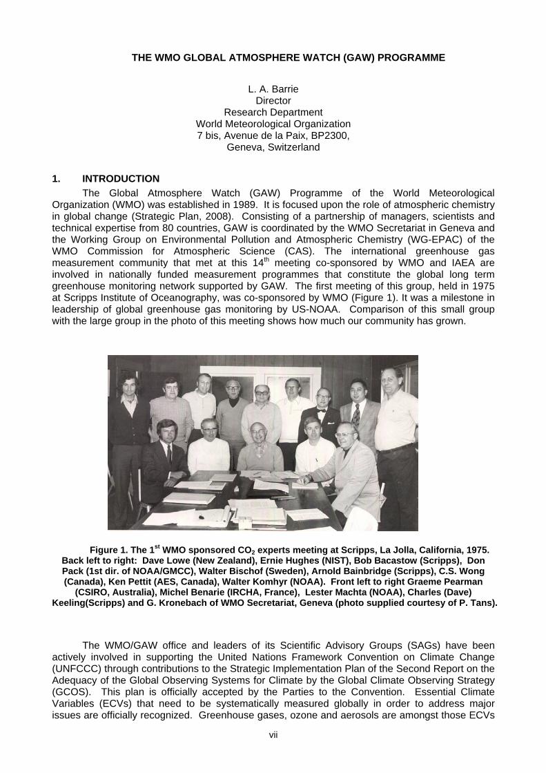
Organization (WMO) was established in 1989. It is focused upon the role of atmospheric chemistry in global change (Strategic Plan, 2008). Consisting of a partnership of managers, scientists and technical expertise from 80 countries, GAW is coordinated by the WMO Secretariat in Geneva and the Working Group on Environmental Pollution and Atmospheric Chemistry (WG-EPAC) of the WMO Commission for Atmospheric Science (CAS). The international greenhouse gas measurement community that met at this 14th meeting co-sponsored by WMO and IAEA are involved in nationally funded measurement programmes that constitute the global long term greenhouse monitoring network supported by GAW. The first meeting of this group, held in 1975 at Scripps Institute of Oceanography, was co-sponsored by WMO (Figure 1). It was a milestone in leadership of global greenhouse gas monitoring by US-NOAA. Comparison of this small group with the large group in the photo of this meeting shows how much our community has grown.

Figure 1. The 1st WMO sponsored CO2 experts meeting at Scripps, La Jolla, California, 1975. Back left to right: Dave Lowe (New Zealand), Ernie Hughes (NIST), Bob Bacastow (Scripps), Don Pack (1st dir. of NOAA/GMCC), Walter Bischof (Sweden), Arnold Bainbridge (Scripps), C.S. Wong (Canada), Ken Pettit (AES, Canada), Walter Komhyr (NOAA). Front left to right Graeme Pearman

(CSIRO, Australia), Michel Benarie (IRCHA, France), Lester Machta (NOAA), Charles (Dave) Keeling(Scripps) and G. Kronebach of WMO Secretariat, Geneva (photo supplied courtesy of P. Tans). The WMO/GAW office and leaders of its Scientific Advisory Groups (SAGs) have been actively involved in supporting the United Nations Framework Convention on Climate Change (UNFCCC) through contributions to the Strategic Implementation Plan of the Second Report on the Adequacy of the Global Observing Systems for Climate by the Global Climate Observing Strategy (GCOS). This plan is officially accepted by the Parties to the Convention. Essential Climate Variables (ECVs) that need to be systematically measured globally in order to address major issues are officially recognized. Greenhouse gases, ozone and aerosols are amongst those ECVs

viii

and GAW is designated as the lead international programme in furthering the observational requirements. In October 2005, the steering committee of the Global Climate Observing System (GCOS) which is co-sponsored by WMO approved the GCOS-GAW Agreement establishing the “WMO-GAW Global Atmospheric CO2 & CH4 Monitoring Network” as a comprehensive network of GCOS. The focus, goals and structure of GAW are outlined in detail in the Strategic Implementation Plan 2008-2015 (GAW Report 172). Recognizing the need to bring scientific data and information to bear in the formulation of national and international policy, the GAW mission is to: a. Reduce environmental risks to society and meet the requirements of environmental

conventions. b. Strengthen capabilities to predict climate, weather and air quality. c. Contribute to scientific assessments in support of environmental policy. Through i. Maintaining and applying global, long-term observations of the chemical composition and

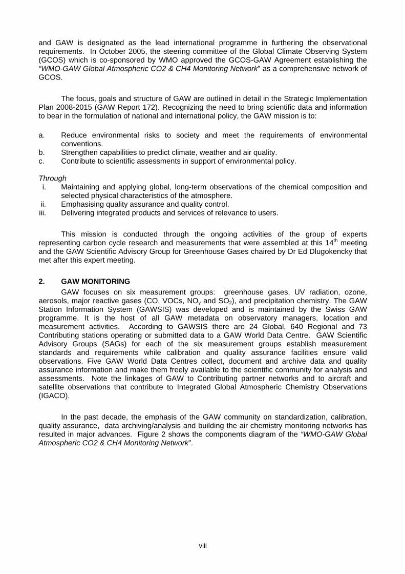
selected physical characteristics of the atmosphere. ii. Emphasising quality assurance and quality control. iii. Delivering integrated products and services of relevance to users. This mission is conducted through the ongoing activities of the group of experts representing carbon cycle research and measurements that were assembled at this 14th meeting and the GAW Scientific Advisory Group for Greenhouse Gases chaired by Dr Ed Dlugokencky that met after this expert meeting. 2. GAW MONITORING GAW focuses on six measurement groups: greenhouse gases, UV radiation, ozone, aerosols, major reactive gases (CO, VOCs, NOy and SO2), and precipitation chemistry. The GAW Station Information System (GAWSIS) was developed and is maintained by the Swiss GAW programme. It is the host of all GAW metadata on observatory managers, location and measurement activities. According to GAWSIS there are 24 Global, 640 Regional and 73 Contributing stations operating or submitted data to a GAW World Data Centre. GAW Scientific Advisory Groups (SAGs) for each of the six measurement groups establish measurement standards and requirements while calibration and quality assurance facilities ensure valid observations. Five GAW World Data Centres collect, document and archive data and quality assurance information and make them freely available to the scientific community for analysis and assessments. Note the linkages of GAW to Contributing partner networks and to aircraft and satellite observations that contribute to Integrated Global Atmospheric Chemistry Observations (IGACO). In the past decade, the emphasis of the GAW community on standardization, calibration, quality assurance, data archiving/analysis and building the air chemistry monitoring networks has resulted in major advances. Figure 2 shows the components diagram of the “WMO-GAW Global Atmospheric CO2 & CH4 Monitoring Network”.

ix

GAW Global CO2 & CH4 Network Components

SCIENTIFIC ADVISORY GROUP(SAG) for GHGs

(Expert C Measurement Community)

QA & CALIBRATION CENTRES:NOAA/CMDL, MeteoSwiss/EMPA,

Japan Met. Agency(JMA)

CENTRAL CALIBRATION. LABORATORY (CCL)

World Reference Standard US- NOAA

GAW STATIONS & GAWSISGlobal Regional

GAW WORLD DATA CENTRE for GREENHOUSE GASES:(WDCGG)

Analysis

TwinningWorkshops

Calibration, Training Site Visits, Comparisons

SynthesisIGACO

ContributingNetworks

Satellite & AircraftObservations

CAS/WG forEnvironmental Pollution

And Atmospheric Chemistry

WMO/GAW Secretariat

AREP

BIPM/CCQM

Figure 2. Components of the WMO-GAW Global Atmospheric CO2 & CH4

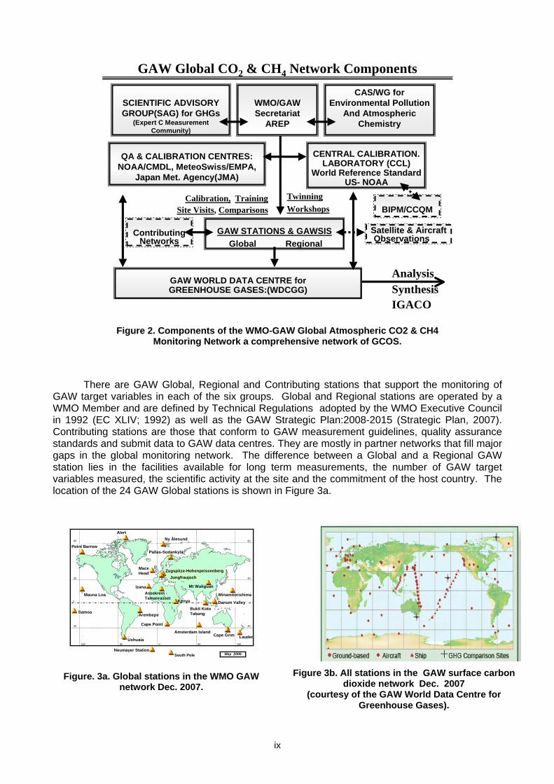
Monitoring Network a comprehensive network of GCOS. There are GAW Global, Regional and Contributing stations that support the monitoring of GAW target variables in each of the six groups. Global and Regional stations are operated by a WMO Member and are defined by Technical Regulations adopted by the WMO Executive Council in 1992 (EC XLIV; 1992) as well as the GAW Strategic Plan:2008-2015 (Strategic Plan, 2007). Contributing stations are those that conform to GAW measurement guidelines, quality assurance standards and submit data to GAW data centres. They are mostly in partner networks that fill major gaps in the global monitoring network. The difference between a Global and a Regional GAW station lies in the facilities available for long term measurements, the number of GAW target variables measured, the scientific activity at the site and the commitment of the host country. The location of the 24 GAW Global stations is shown in Figure 3a.

40

0

South Pole

Point Barrow

Mauna Loa

Alert

Pallas-Sodankylä

MinamitorishimaKenya

Assekrem -Tamanrasset

Arembepe

Ushuaia

Izana

Amsterdam IslandCape Grim

Cape Point

Samoa

Ny Ålesund

Lauder

Mace Head

40

80

40

0

40

80

160 80 0 80 160

May 2006

Zugspitze-Hohenpeissenberg

Mt Waliguan

Neumayer Station

Bukit Koto Tabang

Jungfraujoch

Danum Valley

Figure. 3a. Global stations in the WMO GAW

network Dec. 2007.

Figure 3b. All stations in the GAW surface carbon

dioxide network Dec. 2007 (courtesy of the GAW World Data Centre for

Greenhouse Gases).

x

The GAW global network for surface based carbon dioxide observations is shown in Figure 3b. To monitor global distributions and trends of a particular variable with sufficient resolution to provided quantitative estimates of regional sources and sinks of greenhouse gases requires not only Global but also Regional and Contributing surface-based stations but also aircraft and satellite observations. All stations submitting data to the GAW World Data Centre for Greenhouse Gases provides essential information on how their observations are linked to the WMO world reference scale maintained at NOAA/ESRL in Boulder, USA. In future, many more stations will hopefully be added to fill gaps in Asia, Africa and South America. Also, aircraft and satellite observations will be added as the integrated global atmospheric carbon observation system outlined in the IGACO (2004) report is implemented through the WMO-GAW programme in partnership with national and regional research partners.

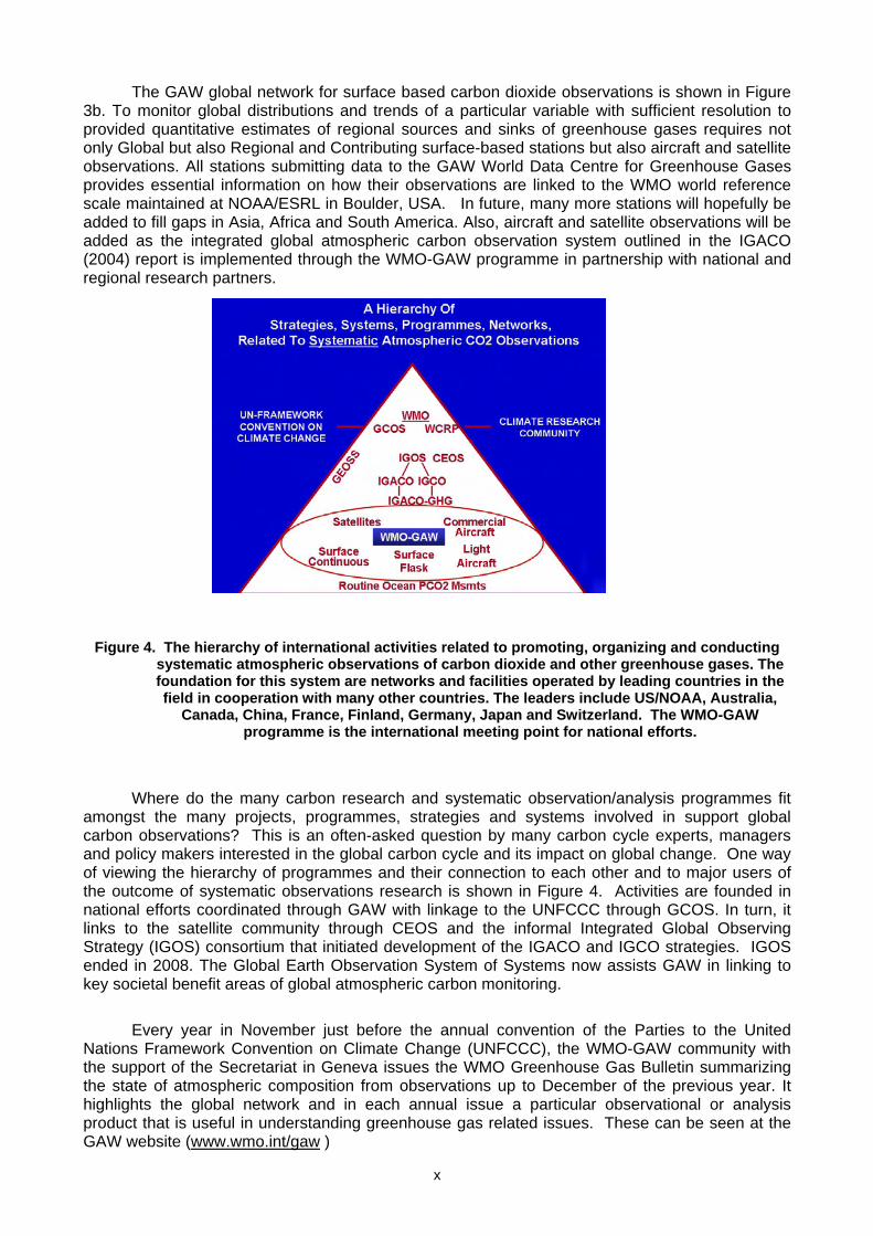
Figure 4. The hierarchy of international activities related to promoting, organizing and conducting

systematic atmospheric observations of carbon dioxide and other greenhouse gases. The foundation for this system are networks and facilities operated by leading countries in the field in cooperation with many other countries. The leaders include US/NOAA, Australia,

Canada, China, France, Finland, Germany, Japan and Switzerland. The WMO-GAW programme is the international meeting point for national efforts.

Where do the many carbon research and systematic observation/analysis programmes fit amongst the many projects, programmes, strategies and systems involved in support global carbon observations? This is an often-asked question by many carbon cycle experts, managers and policy makers interested in the global carbon cycle and its impact on global change. One way of viewing the hierarchy of programmes and their connection to each other and to major users of the outcome of systematic observations research is shown in Figure 4. Activities are founded in national efforts coordinated through GAW with linkage to the UNFCCC through GCOS. In turn, it links to the satellite community through CEOS and the informal Integrated Global Observing Strategy (IGOS) consortium that initiated development of the IGACO and IGCO strategies. IGOS ended in 2008. The Global Earth Observation System of Systems now assists GAW in linking to key societal benefit areas of global atmospheric carbon monitoring. Every year in November just before the annual convention of the Parties to the United Nations Framework Convention on Climate Change (UNFCCC), the WMO-GAW community with the support of the Secretariat in Geneva issues the WMO Greenhouse Gas Bulletin summarizing the state of atmospheric composition from observations up to December of the previous year. It highlights the global network and in each annual issue a particular observational or analysis product that is useful in understanding greenhouse gas related issues. These can be seen at the GAW website (www.wmo.int/gaw )

xi

References 1992 EC XLIV, 1992, Resolution 3, WMO Technical Regulations, 1, Chapter B.2, Global Atmosphere Watch, GAW. 2003 GAW Current activities of the Global Atmosphere Watch Programme (as presented at Cg-XIV, May 2003), Report 152. 2004 GAW: Strategic Plan Addendum for the period 2005-2007 to the Strategy for the implementation of the Global Atmosphere Watch Programme (2001-2007), GAW Report 142. 2004 IGACO: 2004, The Integrated Global Atmospheric Chemistry Observations (IGACO) Report of IGOS-WMO-ESA, GAW Report 159, 53 pp. 2007 WMO/GAW Strategic Plan: 2008-2015 - A Contribution to the Implementation of the WMO Strategic Plan: 2008-2011 (GAW Report # 172, WMO TD No. 1384). http://www.wmo.int/pages/prog/arep/gaw/gaw-reports.html).

Recommendations

1

EXPERT GROUP RECOMMENDATIONS

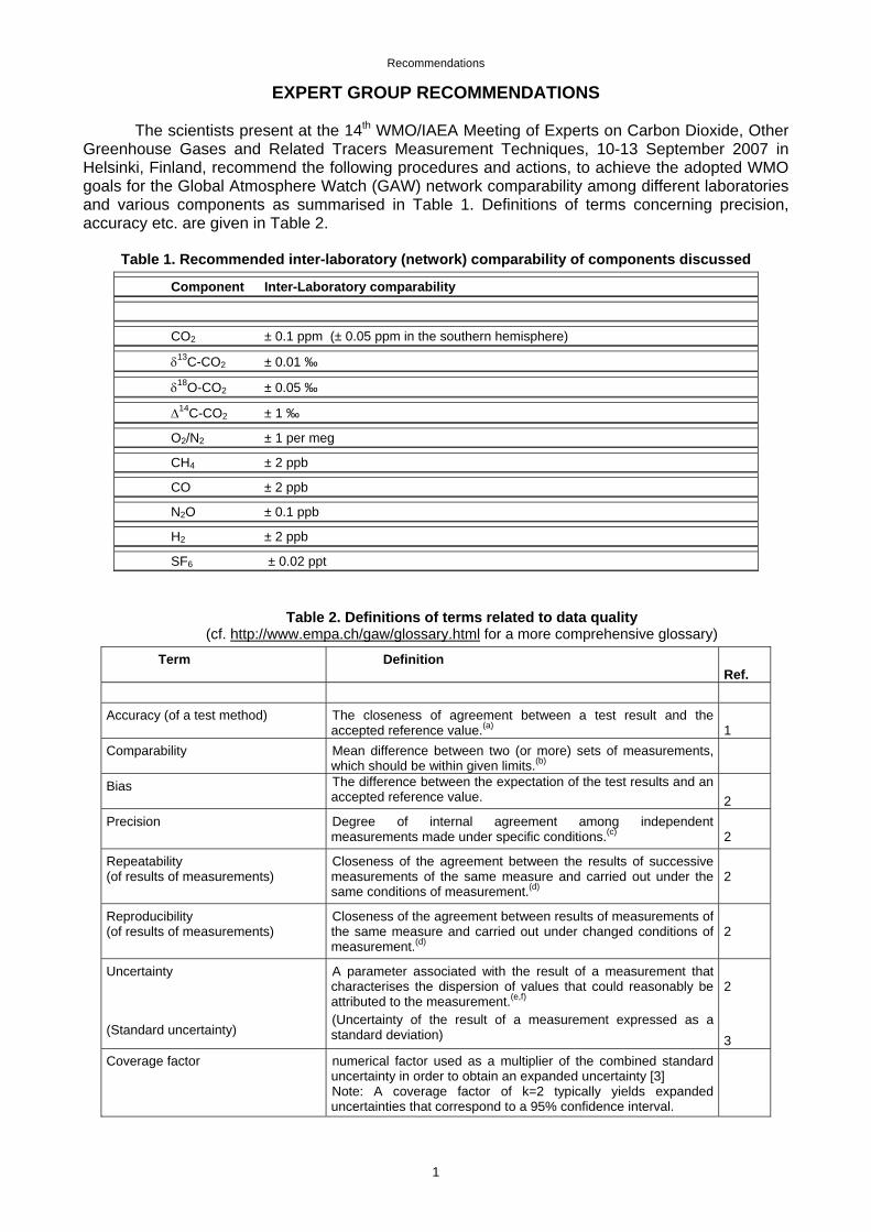
The scientists present at the 14th WMO/IAEA Meeting of Experts on Carbon Dioxide, Other Greenhouse Gases and Related Tracers Measurement Techniques, 10-13 September 2007 in Helsinki, Finland, recommend the following procedures and actions, to achieve the adopted WMO goals for the Global Atmosphere Watch (GAW) network comparability among different laboratories and various components as summarised in Table 1. Definitions of terms concerning precision, accuracy etc. are given in Table 2.

Table 1. Recommended inter-laboratory (network) comparability of components discussed

Component Inter-Laboratory comparability

CO2 ± 0.1 ppm (± 0.05 ppm in the southern hemisphere)

δ13C-CO2 ± 0.01 ‰

δ18O-CO2 ± 0.05 ‰

Δ14C-CO2 ± 1 ‰

O2/N2 ± 1 per meg

CH4 ± 2 ppb

CO ± 2 ppb

N2O ± 0.1 ppb

H2 ± 2 ppb

SF6 ± 0.02 ppt

Table 2. Definitions of terms related to data quality (cf. http://www.empa.ch/gaw/glossary.html for a more comprehensive glossary)

Term Definition Ref.

Accuracy (of a test method) The closeness of agreement between a test result and the

accepted reference value.(a) 1 Comparability Mean difference between two (or more) sets of measurements,

which should be within given limits.(b) Bias The difference between the expectation of the test results and an

accepted reference value. 2 Precision

Degree of internal agreement among independent measurements made under specific conditions.(c) 2

Repeatability (of results of measurements)

Closeness of the agreement between the results of successive measurements of the same measure and carried out under the same conditions of measurement.(d)

2

Reproducibility (of results of measurements)

Closeness of the agreement between results of measurements of the same measure and carried out under changed conditions of measurement.(d)

2

Uncertainty (Standard uncertainty)

A parameter associated with the result of a measurement that characterises the dispersion of values that could reasonably be attributed to the measurement.(e,f)

(Uncertainty of the result of a measurement expressed as a standard deviation)

2

3 Coverage factor numerical factor used as a multiplier of the combined standard

uncertainty in order to obtain an expanded uncertainty [3] Note: A coverage factor of k=2 typically yields expanded uncertainties that correspond to a 95% confidence interval.

Recommendations

2

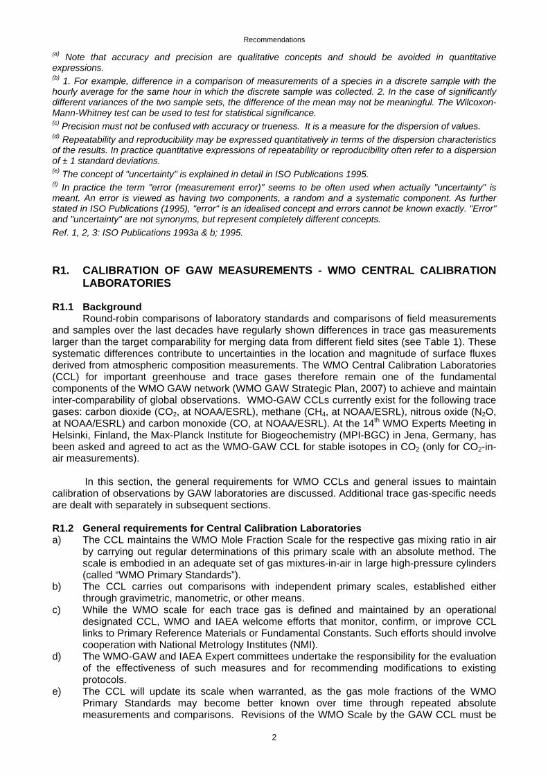
(a) Note that accuracy and precision are qualitative concepts and should be avoided in quantitative expressions. (b) 1. For example, difference in a comparison of measurements of a species in a discrete sample with the hourly average for the same hour in which the discrete sample was collected. 2. In the case of significantly different variances of the two sample sets, the difference of the mean may not be meaningful. The Wilcoxon-Mann-Whitney test can be used to test for statistical significance. (c) Precision must not be confused with accuracy or trueness. It is a measure for the dispersion of values. (d) Repeatability and reproducibility may be expressed quantitatively in terms of the dispersion characteristics of the results. In practice quantitative expressions of repeatability or reproducibility often refer to a dispersion of ± 1 standard deviations. (e) The concept of "uncertainty" is explained in detail in ISO Publications 1995. (f) In practice the term "error (measurement error)" seems to be often used when actually "uncertainty" is meant. An error is viewed as having two components, a random and a systematic component. As further stated in ISO Publications (1995), "error" is an idealised concept and errors cannot be known exactly. "Error" and "uncertainty" are not synonyms, but represent completely different concepts. Ref. 1, 2, 3: ISO Publications 1993a & b; 1995.

R1. CALIBRATION OF GAW MEASUREMENTS - WMO CENTRAL CALIBRATION LABORATORIES

R1.1 Background Round-robin comparisons of laboratory standards and comparisons of field measurements and samples over the last decades have regularly shown differences in trace gas measurements larger than the target comparability for merging data from different field sites (see Table 1). These systematic differences contribute to uncertainties in the location and magnitude of surface fluxes derived from atmospheric composition measurements. The WMO Central Calibration Laboratories (CCL) for important greenhouse and trace gases therefore remain one of the fundamental components of the WMO GAW network (WMO GAW Strategic Plan, 2007) to achieve and maintain inter-comparability of global observations. WMO-GAW CCLs currently exist for the following trace gases: carbon dioxide (CO2, at NOAA/ESRL), methane (CH4, at NOAA/ESRL), nitrous oxide (N2O, at NOAA/ESRL) and carbon monoxide (CO, at NOAA/ESRL). At the 14th WMO Experts Meeting in Helsinki, Finland, the Max-Planck Institute for Biogeochemistry (MPI-BGC) in Jena, Germany, has been asked and agreed to act as the WMO-GAW CCL for stable isotopes in CO2 (only for CO2-in-air measurements). In this section, the general requirements for WMO CCLs and general issues to maintain calibration of observations by GAW laboratories are discussed. Additional trace gas-specific needs are dealt with separately in subsequent sections. R1.2 General requirements for Central Calibration Laboratories a) The CCL maintains the WMO Mole Fraction Scale for the respective gas mixing ratio in air

by carrying out regular determinations of this primary scale with an absolute method. The scale is embodied in an adequate set of gas mixtures-in-air in large high-pressure cylinders (called “WMO Primary Standards”).

b) The CCL carries out comparisons with independent primary scales, established either through gravimetric, manometric, or other means.

c) While the WMO scale for each trace gas is defined and maintained by an operational designated CCL, WMO and IAEA welcome efforts that monitor, confirm, or improve CCL links to Primary Reference Materials or Fundamental Constants. Such efforts should involve cooperation with National Metrology Institutes (NMI).

d) The WMO-GAW and IAEA Expert committees undertake the responsibility for the evaluation of the effectiveness of such measures and for recommending modifications to existing protocols.

e) The CCL will update its scale when warranted, as the gas mole fractions of the WMO Primary Standards may become better known over time through repeated absolute measurements and comparisons. Revisions of the WMO Scale by the GAW CCL must be

Recommendations

3

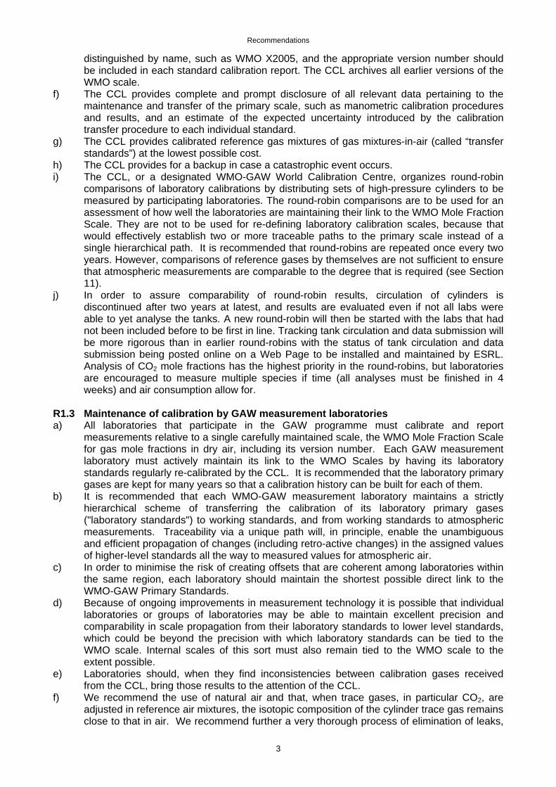
distinguished by name, such as WMO X2005, and the appropriate version number should be included in each standard calibration report. The CCL archives all earlier versions of the WMO scale.

f) The CCL provides complete and prompt disclosure of all relevant data pertaining to the maintenance and transfer of the primary scale, such as manometric calibration procedures and results, and an estimate of the expected uncertainty introduced by the calibration transfer procedure to each individual standard.

g) The CCL provides calibrated reference gas mixtures of gas mixtures-in-air (called “transfer standards”) at the lowest possible cost.

h) The CCL provides for a backup in case a catastrophic event occurs. i) The CCL, or a designated WMO-GAW World Calibration Centre, organizes round-robin

comparisons of laboratory calibrations by distributing sets of high-pressure cylinders to be measured by participating laboratories. The round-robin comparisons are to be used for an assessment of how well the laboratories are maintaining their link to the WMO Mole Fraction Scale. They are not to be used for re-defining laboratory calibration scales, because that would effectively establish two or more traceable paths to the primary scale instead of a single hierarchical path. It is recommended that round-robins are repeated once every two years. However, comparisons of reference gases by themselves are not sufficient to ensure that atmospheric measurements are comparable to the degree that is required (see Section 11).

j) In order to assure comparability of round-robin results, circulation of cylinders is discontinued after two years at latest, and results are evaluated even if not all labs were able to yet analyse the tanks. A new round-robin will then be started with the labs that had not been included before to be first in line. Tracking tank circulation and data submission will be more rigorous than in earlier round-robins with the status of tank circulation and data submission being posted online on a Web Page to be installed and maintained by ESRL. Analysis of CO2 mole fractions has the highest priority in the round-robins, but laboratories are encouraged to measure multiple species if time (all analyses must be finished in 4 weeks) and air consumption allow for.

R1.3 Maintenance of calibration by GAW measurement laboratories a) All laboratories that participate in the GAW programme must calibrate and report

measurements relative to a single carefully maintained scale, the WMO Mole Fraction Scale for gas mole fractions in dry air, including its version number. Each GAW measurement laboratory must actively maintain its link to the WMO Scales by having its laboratory standards regularly re-calibrated by the CCL. It is recommended that the laboratory primary gases are kept for many years so that a calibration history can be built for each of them.

b) It is recommended that each WMO-GAW measurement laboratory maintains a strictly hierarchical scheme of transferring the calibration of its laboratory primary gases ("laboratory standards") to working standards, and from working standards to atmospheric measurements. Traceability via a unique path will, in principle, enable the unambiguous and efficient propagation of changes (including retro-active changes) in the assigned values of higher-level standards all the way to measured values for atmospheric air.

c) In order to minimise the risk of creating offsets that are coherent among laboratories within the same region, each laboratory should maintain the shortest possible direct link to the WMO-GAW Primary Standards.

d) Because of ongoing improvements in measurement technology it is possible that individual laboratories or groups of laboratories may be able to maintain excellent precision and comparability in scale propagation from their laboratory standards to lower level standards, which could be beyond the precision with which laboratory standards can be tied to the WMO scale. Internal scales of this sort must also remain tied to the WMO scale to the extent possible.

e) Laboratories should, when they find inconsistencies between calibration gases received from the CCL, bring those results to the attention of the CCL.

f) We recommend the use of natural air and that, when trace gases, in particular CO2, are adjusted in reference air mixtures, the isotopic composition of the cylinder trace gas remains close to that in air. We recommend further a very thorough process of elimination of leaks,

Recommendations

4

minimization of thermal gradients, and horizontal storage of cylinders in order to minimize the risk of fractionation between the gas components in the cylinder.

R2. SPECIFIC REQUIREMENTS FOR CO2 CALIBRATION a) The primary scale for CO2 shall range from approximately 180 ppm (covering atmospheric

values in ice cores) to over 500 ppm. The scale is currently embodied in a set of 15 CO2-in-air mixtures in large high-pressure cylinders.

b) Since the WMO scale was maintained until 1995 by the Scripps Institution of Oceanography, comparisons with SIO are especially relevant. It is recommended that remaining uncertainties associated with the SIO pre-1995 WMO scale and its transfer to NOAA are resolved.

c) The CCL is encouraged to make available on its web site the calibration results of all GAW laboratory standards based on previous versions of the scale as well as those based on the current scale.

d) In order to make possible a level of consistency of ±0.03 ppm or less among the CO2 calibration scales of laboratories participating in the WMO-GAW programme, the CCL shall aim to provide the calibrated standards for transfer of the CO2 scale to secondary and tertiary standards at that level of consistency.

e) Each WMO-GAW measurement laboratory must actively maintain its link to the WMO Scale by having its laboratory standards for CO2 re-calibrated by the CCL every three years.

R3. SPECIFIC REQUIREMENTS FOR CO2 STABLE ISOTOPE CALIBRATION R3.1 Background Efforts for comparing the stable isotopes of CO2 in air have continued in the last two years and results were reported during the 14th WMO Meeting of CO2 Experts (see contributions in this volume). These intercomparison exercises are indicative of the progress that has been made in CO2 stable isotope ratio measurements in air. Moreover, more fundamental issues have been addressed like release of CO2 from carbonates, 17O and N2O corrections. The results and arguments presented allow a number of conclusions to be drawn on the sources of measured isotopic differences between participating laboratories. The implemented intercomparison programmes (e.g. sausage flasks, high pressure cylinder round-robins, pure CO2 ampoules and whole-air mixtures) are strongly recommended to be continued in the future as a routine surveillance and quality control tool. R3.2 Current achievements for CO2 stable isotope calibrations a) The possible experimental reasons for systematic offsets in measured CO2 isotopic

compositions are different for δ13C and δ18O. In δ13C, scaling errors seem the most prominent issue whereas δ18O suffers from exchange of oxygen with water as well as from different techniques of generating CO2 from carbonate reference material.

b) The possible underlying causes must be addressed separately for clean (pure) CO2 and for CO2 in air. Clean CO2 is developed from carbonates or is available as a calibrated clean gas. In contrast, CO2 in air is always accompanied by N2O. In addition, traces of co-trapped air from the cryogenic separation as well as issues of trapping efficiency and isotopic alterations during trapping can change the measured isotopic ratios.

c) There is only one internationally recognized isotope scale for δ13C: VPDB. This scale has recently been refined by IUPAC and IAEA via adding a second fixed calibration point (L-SVEC Li2CO3 = –46.6‰ versus VPDB). As a result, a number of international secondary reference materials still must be newly evaluated, including reference materials that have been used for CO2-in-air isotopic calibration (see 3.3b)). Intercomparability of δ13C values of air CO2 in the past has mainly suffered from different amounts of cross contamination during mass spectrometric measurement (eta-effect). The new scaling rule should be able to adequately address this problem. In order to implement this rule into CO2-in-air analyses a practical solution (for instance two air standards with 13CO2 isotopic ratios similar to NBS19 and LSVEC) is needed and suggestions are welcome.

Recommendations

5

d) To establish a tie to the VPDB scale kept by the IAEA, standards for CO2-stable isotopes-in-air must be created. MPI-BGC Jena is now able to accurately prepare CO2 from carbonate material and mix this with CO2-free air in a fully automated system. These mixtures can now serve as air reference material (‘J-RAS’, Jena Reference Air Set) and will provide the required firm link of air-CO2 measurements to the VPDB scale (Ghosh et al., 2005, Brand et al., this volume). The long-term integrity of CO2-in-air isotope results should, however, be based on carbonate material. The future production and dissemination of the J-RAS air-CO2 anchor to the VPDB scale has been funded by the European Community under the IMMEC project. Given the progress made in the last two years MPI-BGC is asked to take a leading role for unifying the stable isotope scales across the community and act as a WMO-GAW Central Calibration Lab for isotopes (CCL) for these species by providing the JRAS air-CO2. BGC Jena has agreed to produce this reference material and provide participating laboratories with a new set of gases at a rate of two per year. Propagation of the scale will be performed only via CO2-in-air.

e) Comparability of δ18O data between laboratories remains poor (progress has been made with inter-laboratory precision of close to ±0.2‰, which is still far off the goal of ±0.05‰ (Table 1)). The availability of reference air with assigned isotope values should help to unify reported δ18O data, irrespective of their accuracy.

f) The major cause for the current discrepancies is not scaling (like for δ13C) because air-CO2 is close to VPDB-CO2. Progress evidently cannot be made by having the individual laboratories generate CO2 from NBS19. MSC, NIES and MPI-BGC have reported on progress in our understanding of the underlying causes for the discrepancies. These studies need to be continued and the same partners are asked to further investigate this issue and report on the results during the next meeting. The new findings will enable to establish a more rigorous relation to the VSMOW scale as well.

R3.3 Recommendations for CO2 stable isotope calibrations a) Since δ13C of atmospheric CO2 is close to –8‰ on the VPDB scale, any secondary

reference material used for high-precision isotope work around this value needs to be re-evaluated. The generation of two pure CO2 reference materials (NARCIS 1 and 2) by NIES with a composition of NARCIS 1 close to air CO2 and NARCIS 2 close to NBS 19 has greatly facilitated intercomparison of isotope measurements on pure CO2 from different laboratories. For establishing a set of recommended values from the intercomparison, more data are required for NARCIS 2. MSC, NIES and MPI-BGC have presented new results comparing these materials with CO2 generated form the primary references thereby assigning new delta values with very small error margins.

b) The availability and careful calibration of other CO2 reference materials from NIST (carbon dioxide: RM 8562-8564) has proven to be an independent and reliable resource for tracing offsets between individual laboratory scales. Theses reference materials have already been re-assessed on the 2-point VPDB scale with very small changes to the original values (i.e. RM 8562: δ13C= -3.72‰, RM 8564: δ13C= -10.45‰, RM 8563: δ13C= -41.59‰ (Coplen et al., 2006)). It is recommended to NIST to insure future availability of these materials.

c) Recent findings of the world water pools related fractionation laws for 18O/16O and 17O/16O require a new ruling for high-accuracy calibration of δ13C in air CO2. The recommendation of the 13th WMO experts meeting to exclusively use the ratio assumption set provided by Assonov and Brenninkmeijer (2003a; 2003b) is endorsed. Mass spectrometry evaluation software as well as individual laboratory software packages should be adapted correspondingly.

d) The need of a calcite reference material with carbon and oxygen isotopic compositions close to atmospheric CO2 is re-iterated and emphasized. The material is necessary in order to eliminate ambiguities arising from different mass spectrometric scaling factors and other corrections (17O correction, N2O correction, etc.).

Recommendations

6

R4. SPECIFIC REQUIREMENTS FOR RADIOCARBON IN CO2 CALIBRATION R4.1 Background Standardization of radiocarbon analysis has been well established in the radiocarbon dating community for many years, and the new Oxalic Acid Standard (NIST SRM 4990C) has been agreed upon as the main standard reference material. Other reference materials of various origin and 14C activity are available and distributed by e.g. IAEA. For atmospheric measurements of Δ14C in CO2, two main sampling techniques are used: High-volume CO2 absorption in basic solution or by molecular sieve and whole-air flask sampling (typically 1.5-5 L flasks). Two methods of analysis are used: Conventional radioactive counting and Accelerator Mass Spectrometry (AMS). The current level of measurement uncertainty for Δ14C in CO2 is 2-5‰, with a few laboratories at slightly better than 2‰ uncertainty. As atmospheric gradients in background air are currently very small, a target level of 1‰ for inter-laboratory comparability is recommended (Table 1).

R4.2 14CO2 calibration and intercomparison activities and respective recommendations Calibration with whole-air standards is difficult in the case of large-volume sampling and conventional counting techniques as sample volume is generally larger than 20 cubic meters of air. Therefore, these techniques will still solely rely on the Standard Reference Materials distributed by IAEA. But we recommend that laboratories conducting small-volume flask sampling and AMS analysis should use whole air cylinders as reference material that is similar to the air samples measured. The first intercomparison activity for Δ14C in CO2 was initiated at the 13th WMO/IAEA Meeting of CO2 Experts in Boulder Colorado (WMO GAW Report # 168, 2006) and is currently underway. The intercomparison is being managed by University of Colorado and NOAA/ESRL/GMD with support from WMO. Six laboratories are currently participating by sending flasks to NOAA to be filled with air from two whole-air reference cylinders. This intercomparison exercise should report results by the 15th WMO Meeting of Experts. As the current intercomparison excludes the laboratories using high-volume sampling techniques, we propose the following potential methods for future intercomparison that could include laboratories using either type of sampling technique: a) Splitting and dissemination of high-volume pure CO2 samples to the laboratories. b) Co-located sampling at observation stations.

R5. SPECIFIC REQUIREMENTS FOR O2/N2 CALIBRATION R5.1 Background Measurements of the changes in atmospheric O2/N2 ratio are useful for constraining sources and sinks of CO2 and testing land and ocean biogeochemical models. The relative variations in O2/N2 ratio are very small but can now be observed by at least six techniques. These techniques can be grouped into two categories: (1) those which measure O2/N2 ratios directly (mass spectrometry and gas chromatography), and those which effectively measure changes in the O2 mole fraction in dry air (interferometric, paramagnetic, fuel cell, vacuum ultraviolet photometric). A convention has emerged to convert the raw measurement signals, regardless of technique, into equivalent changes in O2/N2 ratio. For the mole-fraction type measurements, this requires accounting for dilution due to variations in CO2 and possibly other gases. If synthetic air is used as a reference material, corrections may also be needed for differences in Ar/N2 ratio. By convention, O2/N2 ratios are expressed as relative deviations compared to a reference

δ(O2/N2) = (O2/N2)sample/(O2/N2)reference -1

Recommendations

7

where δ(O2/N2) is multiplied by 106 and expressed in “per meg” units. 1 per meg is a dimensionless unit equivalent to 0.001 per mille. The O2/N2 reference is typically tied to natural air delivered from high-pressure gas cylinders. As there is no common source of reference material, each laboratory has employed its own reference, and hence reports on its own scale.

R5.2 O2/N2 calibration and intercomparison activities At the 12th WMO CO2 Experts Meeting in Toronto (WMO GAW Report # 161, 2005) the Global Oxygen Laboratories Link Ultra-precise Measurements (GOLLUM) programme was initiated to provide constraints on the offsets between the different laboratory scales and to clarify the requirements for placing measurements on a common scale. There are two components to this programme, a “sausage flasks” intercomparison programme, and a “round-robin cylinder” intercomparison programme. The sausage flask programme compares the laboratories’ ability to extract and analyse air from a small flask sample, whereas the round-robin cylinder programme compares the laboratories’ calibration scales, and their methods for extracting air from high-pressure gas cylinders. Details of the GOLLUM programme can be found in the WMO Technical Document No. 1275. A document was prepared and distributed to the participating laboratories in the GOLLUM programme outlining the required laboratory protocols. The GOLLUM programme has been coordinated by A. Manning at the University of Each Anglia, with the O2 laboratory of R. Keeling at Scripps Institution of Oceanography (SIO) serving as the point of origin for the round-robin programme and the hub for the sausage-flask programme. The round robin cylinders (2 sets of 3 aluminium cylinders) were prepared in 2004 at SIO and started their worldwide rotations in 2005. At the time of the 14th WMO Experts meeting, two circuits of the round-robin cylinders were completed and three sets of sausage flasks had been distributed. The repeated analyses at SIO, two years after their initial measurement, showed the change in the cylinders was zero to within ±3 per meg, the estimated precision of a trend measurement in the SIO lab. In addition to preparing cylinders for the GOLLUM programme, the O2 lab at SIO has prepared high-pressure cylinders for a number of laboratories. These cylinders have provided another means to assess laboratory scale differences. R5.3 Recommendations a) Continue both, the round-robin cylinder and sausage flask components of the GOLLUM

programme for at least two more years. b) Establish a web page for logistical support and for dissemination of results of the GOLLUM

programme. c) Encourage SIO to continue to provide reference gases to laboratories on request at

reasonable cost. d) Encourage additional efforts, such as overlapping flask sampling from different programmes,

to compare O2/N2 scales and methods between programmes. e) Encourage the standardisation of existing O2/N2 techniques, and particularly to identify and

correct weaknesses in laboratories’ current techniques in sample collection, sample analysis, and in defining and propagating calibration scales.

R6. SPECIFIC REQUIREMENTS FOR CH4 CALIBRATION At the 12th WMO/IAEA Meeting of Experts on Carbon Dioxide Concentration and Related Tracers Measurement Techniques, it was agreed that NOAA would assume the role of the WMO-GAW Central Calibration Laboratory (CCL) for methane. The NOAA04 scale was designated as the official calibration scale consisting of 16 gravimetrically prepared primary standards which cover the nominal range of 300 to 2600 nmol mol-1, so it is suitable to calibrate standards for measurements of air extracted from ice cores and contemporary measurements from GAW sites. This new scale results in CH4 mole fractions that are a factor of 1.0124 greater than the previous scale (now designated CMDL83) (Dlugokencky et al., 2005). The range of secondary transfer

Recommendations

8

standards is the same as the range of the WMO Primary Standards. The CCL will transfer the CH4 scale to calibrated CH4-in-air standards with an uncertainty of <1 nmol mol-1. All laboratories that participate in the GAW programme must calibrate measurements to relative to the WMO CH4-in-air mole fraction scale and report them to the WMO World Data Centre for Greenhouse Gases in Japan. Each GAW measurement laboratory must actively maintain its link to the WMO Scale by having its laboratory standards for CH4 re-calibrated by the CCL every six years. R7. SPECIFIC REQUIREMENTS FOR N2O CALIBRATION

R7.1 Background Measurements of nitrous oxide are made by a number of laboratories around the world in order to better understand the sources and sinks of this greenhouse gas, also in the frame of the global nitrogen cycle. Systematic differences between mole fractions reported by different laboratories are large compared to atmospheric gradients. The mean interhemispheric difference in N2O mole fraction is around 1 ppb and the pole-to-pole difference is 2 ppb. These global differences are 0.3-0.6% of the recent mean mole fraction of N2O in the troposphere. This necessitates not only high measurement precision, but also high consistency among assigned values for standards. Inter-laboratory comparability of 0.1 ppb is needed. R7.2 Recommendations a) NOAA/ESRL/GMD serves as the CCL for nitrous oxide. It maintains a gravimetrically-

prepared N2O-in-air standard scale consisting of 13 WMO Primary Standards covering the range of 260 – 370 nmole mol-1 (Hall et al., 2007). The reproducibility of NOAA N2O calibrations is estimated to be 0.2 ppb at the 95% confidence level. Efforts to improve precision and reproducibility are ongoing.

b) The CCL will include N2O calibration results in the web-based database maintained by the NOAA Carbon Cycle Greenhouse Gases group.

c) Each GAW measurement laboratory must actively maintain its link to the WMO Scale by having its laboratory standards for N2O re-calibrated by the CCL every three years.

d) We encourage the development of new or improved techniques, such as optical techniques, that would lead to improvements in precision and reproducibility.

R8. SPECIFIC REQUIREMENTS TO SF6 CALIBRATION R8.1 Background

Sulfurhexafluoride (SF6) is a long-lived trace gas with strong infrared absorbance properties. Emissions of SF6 are 22800 times more effective than CO2 on a per-mass basis over a 100-year time scale. The tropospheric mixing ratio of SF6 has increased steadily, with a current growth rate of about 0.22 ppt yr-1. The steady growth rate and long lifetime (~3000 years) make it a useful tracer of atmospheric transport, including stratospheric “age-of-air determination”. Because SF6 is almost entirely anthropogenic in origin, used primarily in electrical power distribution, it is a potentially powerful tracer of anthropogenic activity on global and regional scales.

SF6 is typically measured using GC-ECD techniques in a manner similar to that of N2O.

There are currently three scales in use: NOAA, Univ. of Heidelberg, and SIO. Although there have been few formal SF6 comparisons, informal comparisons show that scale comparability is generally good. However, to be optimally useful as a tracer of atmospheric transport, consistency of scale must be exceptionally good (on the order of 0.02 ppt). In this regard, a commonly accepted scale does not exist. The formation of a WMO-GAW CCL for SF6, responsible for maintaining a scale and facilitating the distribution of standards, would benefit the atmospheric (SF6) measurement community.

Recommendations

9

R8.2 Recommendations a) Establish a WMO-GAW CCL for SF6. b) Include SF6 in WMO-GAW round-robin experiments when possible. c) Investigations are encouraged to explore advanced techniques to improve measurement

precision.

R9. SPECIFIC REQUIREMENTS FOR CO CALIBRATION

R9.1 Background CO is an important component in tropospheric chemistry due to its high reactivity with OH. It is the major chemically active trace gas resulting from biomass burning and fossil fuel combustion, and a precursor gas of tropospheric ozone. Most atmospheric measurements are based on collected air samples or in-situ analysis although systematic measurements from satellites, aircraft and surface-based FTIRS are improving (WMO GAW/ACCENT Workshop, 2005). Differences among reference scales and drift of standards have been a serious problem for these in-situ CO measurements in the past. Spectroscopic retrieval of CO provides column abundances; wide geographical coverage of CO with some limited vertical resolution is becoming available from several satellite-based sensors (MOPITT-TERRA, SCIAMACHY-ENVISAT, TESS-AURA). The present recommendations will, however, pertain to the calibration of in-situ observation only; the validation of remote sensing data is a complicated separate issue not treated here.

Experience has shown that the accurate calibration of in-situ CO measurements is far from trivial. Mole fractions between 40 and 250 nmol/mol (and higher) should be determined with an expanded uncertainty of ±2 ppb (k=2). Unlike CO2, for CO there is a low degree of standardization in analytical techniques deployed (WMO/GAW Report No. 168 (2006)). Specific calibration problems for CO are: a) Available measurement techniques can be non-linear and do not have the stability or precision for long-term measurements of low drift rates. b) Gravimetric mixtures must be diluted to environmental levels, and at these levels CO mixing ratios in high-pressure cylinders may not be stable over time periods of several years. c) The preparation of a gravimetric standard does not a priori guarantee that the actual CO mole fraction corresponds to the assumed one. Careful maintenance of the gravimetric scale and/or inter-comparison with diluted gases from high-concentration cylinders (10 ppm) is regularly required. R9.2 CO intercomparison activities NOAA ESRL’s Carbon Cycle Group has on two occasions organized round-robin tests involving 5 to 10 laboratories. This has helped “the international insitu CO measurement community” enormously, but also exposed some drift and inconsistency in the NOAA ESRL calibration scale, as well as the gravimetric technique. WMO through EMPA and its WMO-GAW WCC for CO has endeavoured to improve the international comparability by implementing an audit system for CO measurements at Global GAW stations. Combining all experience gained so far, it is realistic to expect CO data to be expressed on one single scale that is traceable to a single source. For establishing global trends, and to get a sufficiently accurate estimate of the tropospheric burden, it seems that 1% expanded uncertainty (k=2) is now becoming both analytically attainable and scientifically sufficient. R9.3 Specific recommendations for CO calibration at the WMO-GAW CCL and at GAW

stations a) Inter-laboratory comparability for global GAW stations to ±2 ppb (mean bias) and standards

to ±1 ppb or 0.5% (whichever is greater, expanded uncertainty, k=2) are needed. Comparisons of CO measurements among laboratories (through round-robins, and other intercomparison sample exchanges) have documented differences in measurements among laboratories. They have proven useful in identifying inconsistencies and/or drift in CO standards and therefore are strongly encouraged.

b) NOAA ESRL is the CCL for carbon monoxide. In this capacity, they provide calibrated standards to GAW laboratories, and CO calibrations should be traceable to the scale

Recommendations

10

maintained by NOAA ESRL. Based upon several sets of gravimetric standards this scale was revised in 2000. The WMO-2000 scale still underwent some adjustments, and NOAA ESRL is encouraged to ‘freeze’ the current scale prepared in 2006 as WMO-2006 scale. It is this WMO-2006 scale that GAW stations should refer to. The CCL is responsible for documenting the evolution of the WMO CO scale and for communicating all revisions to the stations as well as to WCC-EMPA.

c) The frequency of the preparation of gravimetric Primary Standards should be increased to a biannual interval to determine any long term drift of the scale. Furthermore the CCL should improve its capability of making accurate dilutions as a second means of assuring the stability of the WMO Primary Scale.

d) Standard drift remains a serious issue for CO measurements. Therefore an annual recalibration of at least one of a station's laboratory standards is strongly suggested.

e) In order to be able to use CO as a tracer for fossil fuel CO2 at regional GAW or even moderately polluted sites, the CCL should extend its primary scale towards higher mole fractions (up to 1000 ppb).

f) The WMO SAG Reactive Gases’ Subgroup on Carbon Monoxide should continue to work on resolving issues of the calibration scale, in particular by giving guidance to stations on how to re-process older data. A SAG Guidance Document on CO measurements is being developed.

g) Currently, no laboratory is conducting absolute volumetric measurements of CO. These measurements would be an extremely useful alternative to dynamic dilution of high-concentration gases for confirming the consistency and potential drift in the WMO primary scale.

h) EMPA is the designated World Calibration Centre for Surface Ozone, Carbon Monoxide and Methane (WCC-EMPA) and is in charge of conducting system and performance audits including intercomparisons at global GAW stations. Audit results and other inter-comparison results should be archived along with CO data at the WDCGG or with GAWSIS.

i) Within the GAW programme, regular inter-comparisons or calibrations by designated calibration centres (with global or regional scope) are necessary to ensure traceability of the observations. Furthermore, regular audits by the WCC are needed as an independent check of the measurements on-site.

j) It should be explored if, in this particular case of a trace gas with large danger of drifting standards, regional round robins could help to maintain the link to the CCL.

k) For many stations, a dynamic dilution system may be an additional means of calibrating their instruments, in particular in cases where non-linear instrument response may be an issue. WCC-EMPA should take the lead in establishing the practicality of such an approach and in assessing the resulting uncertainties for the ambient CO measurements.

l) There is a large number of stations (some of which are regional GAW stations) that are equipped with less sophisticated (or calibrated) CO monitoring equipment. These measurements are currently poorly exploited, in part because some of these data (e.g., from environmental agencies) are not easily accessible and the quality of these observations is not well assessed. There is a need for identification, inter-comparison and improved accessibility of these observations.

R10. SPECIFIC REQUIREMENTS FOR H2 CALIBRATION R10.1 Background Molecular hydrogen plays a significant role in global atmospheric chemistry due to its interference in CH4-CO-OH cycling. The balance of hydrogen could change with the implementation of a new H2 energy carrier. Therefore, it is important to establish its global budget and atmospheric trend. There is currently no internationally accepted standard scale available for measurements of atmospheric molecular hydrogen nor is there any institution to distribute such standards.

Recommendations

11

There are different networks of monitoring stations that are linked to independent scales (NOAA, CSIRO-AGAGE, EuroHydros, NIES). These scales have been prepared using different methods, and known biases between these scales exist that have not always been constant in time and include concentration dependencies. Efforts to integrate data from different networks have been undertaken based on results from long-term intercomparison activities (Xiao et al. 2007). While this documents the need to achieve transparent and consistent scales, the reliability of this approach depends on a solid evaluation of these differences. There is a clear need to get consistent data from independent networks and therefore harmonisation of the scale still remains a task of high priority. Molecular hydrogen is recognized as an important target variable to be measured in the WMO-GAW global network and specific tasks are outlined for implementation by the global research community (see the GAW Strategic Plan: 2008-2015; section 7.3.6 referenced in footnote1).

R10.2 Recommendations a) A concerted effort to consolidate the NOAA, CSIRO/AGAGE, EuroHydros and other

calibration activities is urgently needed to enable a collaborative global network for hydrogen measurements. These measurement groups are strongly encouraged to establish a common calibration scale. This scale should cover the range from 350-1000 ppb. As part of this effort the existing scales need to be harmonized and the history of their agreement needs to be documented. Links to the BIPM should be explored.

b) In addition, temporal changes of inter-laboratory biases that have not always been related to scale changes, underline the necessity to continue intercomparison of hydrogen data. These exercises have already been made use of and should be expanded with more high-frequency (i.e. at least monthly) comparisons.

c) A major problem most laboratories that measure hydrogen encompass is to ensure the stability of their standards. It is recommended that every laboratory develops a strategy to account for this. This includes appropriate choice of standard gas containers that have been tested successfully (mostly stainless steel cylinders). A set of standard gases in large low pressure glass flasks has proved to be an easy and useful approach. Aluminium cylinders commonly used for other trace gas standard mixtures often show significant growth of hydrogen. Thus, the long-term use of aluminium cylinders as primary standards is discouraged.

d) Appropriate characterization and regular check of the detector response is required given the strong non-linear response of the commonly used HgO reduction detectors.

e) There is currently no WMO-GAW CCL for atmospheric molecular hydrogen. In the course of the scale harmonisation process institutions that are in the position of taking this role should be identified and proposed to attend WMO Experts meetings. The decision on this future CCL should be based on documentation on internal and external measurement consistency of the respective laboratory, its ability to assure the stability of the H2 primary standards, and its ability to supply standards to the community.

R11. GENERAL RECOMMENDATIONS FOR QUALITY CONTROL OF ATMOSPHERIC

TRACE GAS MEASUREMENTS The Group of WMO Experts nominates Ken Masarie (NOAA/ESRL) to review the recommendations summarized below at least six months before the next meeting, and remind laboratories to prepare summaries of their current ICP activities as they relate to the respective recommendations.

R11.1 General a) Relating standards to the WMO Mole Fraction Scales: Investigators should follow practices

outlined in Section 1.3 of this report for obtaining a sufficient number and range of calibration gases from the respective WMO CCL (laboratory standards) and transferring those calibrations to working and field standards. The data management system in use should allow for easy reprocessing and easy propagation of scale changes from laboratory standards to final measurements.

Recommendations

12

b) Real-air and modern-CO2 (and other trace gas) standards: Working standards must have natural levels of N2, O2, and Ar to avoid biases e.g. due to different pressure-broadening effects between sample and calibration gases. CO2 standards should have CO2 with ambient δ13C ratios.

c) Besides round-robin comparisons, more frequent intercomparison activities between pairs of laboratories which incorporate the analyses of actual air samples, such as flask air intercomparison (ICP) experiments or collocated in-situ instruments are strongly recommended. The tremendous benefit of routine intercomparison has been demonstrated (Masarie et al., 2001) and is reinforced. Mutual exchange of air in glass flasks is encouraged as a means to detect experimental deficiencies at an early stage and identify discrepancies in the results quickly.

d) Flask sampling programmes should be implemented at observational sites making continuous measurements as well as automated data processing for these intercomparison projects. A detailed comparison of collocated continuous and flask measurements will be performed until the next WMO Experts meeting which will form the basis to assess the usefulness of such a programme and to decide if audits also for CO2 need be performed at GAW stations. This would require an instrumental set-up which is easy to ship around.

e) Clear protocols and reports of experience gained in intercomparison projects should be provided. Results should be published and readily accessible. The evaluation of such activities and recommendations for refinement, co-ordination and expansion of such activities has been accepted as a key responsibility of future WMO/IAEA Expert meetings.

f) Defensible uncertainty estimates: Investigators should report uncertainty estimates for their data and provide details of how these estimates are calculated and what activities are used to verify them. ISO nomenclature shall be used for uncertainty estimates and discussions.

g) Deviations from recommendations: We recognize the value of innovation and experimentation with new approaches. However, we stress that deviations from established practices should be fully tested to confirm that the new approach does not introduce bias into the measurements. Furthermore, the results of such experimentation should be reported at future WMO CO2 Experts meetings and similar venues, and published in the peer-reviewed literature whenever possible.

R11.2 Flask intercomparison a) Intercomparison programmes distributing to a larger number of laboratories flasks filled in

series from tank air as a “sausage” as initiated by the European TACOS project (Levin et al., 2003) are able to increase the benefit of mutual flask exchange.

b) Another possibility to link several laboratories in one single intercomparison exercise is the establishment of Trace Gas Comparison Sites which will take on the task to fill a larger number of flasks regularly and simultaneously with ambient air and distribute them to participating laboratories. The Alert, Mauna Loa and Cape Grim stations have been recommended as such sites. At Alert station this activity has already started with 6 laboratories. At Cape Grim there are 9 labs participating in such a programme.

R11.3 Recommendations for in-situ measurements a) Continuous in-situ measurements of CO2 and other trace gases can greatly improve our

understanding of regional-scale fluxes. For this reason, and in response to recent advances in technology, the number of investigators and sites carrying out in-situ trace gas measurements is rapidly increasing. Many sound principles for conducting in-situ CO2 measurements have been described in detail in WMO GAW Report No. 134 (1999). The group recommends that the SAG-GHG initiates a timely update of Report 134 well before the next WMO Experts Meeting in 2009. Preliminary recommendation for CO2 measurements have been summarized in the 13th WMO Experts recommendation (WMO GAW Report No. 168 (2006)).

b) It is recommended that new robust analytical technologies (e.g., laser-based optical analyzers) are tested. The envisaged new European Infrastructure ICOS (Atmospheric Thematic Centre) may be able to support this activity. A forum should be established to distribute the results and generate discussion among “experts”. New techniques should meet the scientific requirements of accuracy and precision as stated in GAW reports.

Recommendations

13

Specific areas that need to be investigated are calibration frequency and ability to correct for water vapour dilution or interference with other trace substances, and other artefacts besides sample drying. Manufacturers are encouraged to offer detailed training, perhaps through GAWTEC. The community should identify species for which new technologies are needed and specify which observables should be available for new instruments.

c) Besides recommendations on the greenhouse and associated trace gases mentioned above the WMO Experts identified a strong need for expert guidance to establish an adequate calibration process and intercomparison activity for atmospheric 222Radon observations. WMO will contact respective specialists to give advice.

R12. RECOMMENDATIONS FOR DATA MANAGEMENT AND ARCHIVING R12.1 Data management All GAW measurement laboratories regardless of programme size are required to manage all new and existing atmospheric trace gas and supporting (meta) data using a database management strategy (DBMS) that meets or exceeds the following criteria:

a) Demonstrate that mole fractions / isotope ratios can be unambiguously and automatically

reproduced from raw data at any time in the future. b) Demonstrate that revisions to a laboratory’s internal calibration scale can be efficiently and

unambiguously propagated throughout the database. c) Support routine and automatic database updates of all measurement and meta data. d) Ensure that all data reside locally, in a single location, and are centrally accessible to

internal users. e) Ensure fast and efficient retrieval of all data. f) Maximise users’ ability to assess data quality. g) Facilitate data exploration. h) Minimise the risk of data loss or corruption due to theft, misuse, or hardware/software

failure. i) Maximise security to primary data (e.g., data from which all processed data is derived). j) Support routine and automatic backup of all data. k) Support complete data recovery in the event of catastrophic data loss.

GAW measurement laboratories are encouraged to use WMO/GAW Report No. 150 as a guideline in developing and implementing an atmospheric data management strategy. Laboratories with demonstrated expertise in data management are encouraged to share their expertise.

R12.2 Data archiving a) Laboratories participating in the WMO-GAW programme must submit their data to the World

Data Centre for Greenhouse Gases (WDCGG) (according to WMO, 2007) A co-ordinated annual submission of data, with clearly identified version number of submitted data and calibration scale, as well as supporting details is strongly recommended. The same recommendation holds to other public-access data archive centres such as the Carbon Dioxide Information Analysis Centre (CDIAC).

b) A new version of the WDCGG Guide that includes new data categories, new data submission formats, data submission procedures, and distribution ways of data and products has been published. The adherence to this WDCGG Guide is requested.

c) The WDCGG distributes data in versions consistent with the annual CD-ROM Report and keeps old versions.

R12.3 Co-operative data products All laboratories making high-quality GHG measurements are strongly encouraged to participate in the Co-operative Atmospheric Data Integration Project which produces the GLOBALVIEW data products. The majority of current participants provide updates in May that include data through December of the preceding year. Data contributed to the GLOBALVIEW project are used to derive the data product. The product includes no actual data.

Recommendations

14

R13. SUMMARY OF RECENT INTERNATIONAL PLANNING OF ATMOSPHERIC TRACE GAS MEASUREMENT STRATEGIES

This report is prepared in the context of widespread governmental acceptance of climate change (United Nations Framework Convention on Climate Change (UNFCCC) and its Kyoto protocol), and leads to new and urgent challenges to the carbon cycle community. Two main objectives justify the deployment of atmospheric observations:

(1) To monitor and assess the effectiveness of emission control and/or reduction activities on

atmospheric levels, including attribution of sources and sinks by region and sector. (2) To quantify the present state of the fluxes of greenhouse gases and better understand the

controlling processes. An overview of the observational needs for validating GHG emissions and reductions is given in this report (Tans et al.). Recently, new GHG measurement data streams from satellites with global coverage have become available based on a variety of instruments (SCIAMACHY, AIRS, IASI,) and are being integrated into global data assimilation systems (e.g. the GEMS project). However, these new observations lack long-term continuity, are subject to various biases and do not cover with sufficient accuracy the full suite of GHG and associated tracers defined by WMO-GAW. Hence a complementary, long-term, high-quality network of surface-based in-situ, tall tower and total column as well as systematic aircraft observations are indispensable, in order to reliably detect and quantify long-term changes in GHG sources and sinks. Furthermore, these measurements allow an independent assessment of regional trends, as needed by local policymakers. In addition to the WMO-GAW global programme and its predecessor BAPMoN operating since 1975 and targeting the coordination of systematic atmospheric greenhouse gases observations, there have been international research efforts on understanding the carbon cycle. One has been co-ordinated by the Global Carbon Project (GCP) (http://www.globalcarbonproject.org/) combining the efforts of International Geosphere-Biosphere Project (IGBP), World Climate Research Project (WCRP) and International Human Dimensions Programme (IHDP). The GCP produced in 2003 a Science Implementation Plan dealing with the patterns and variability of carbon fluxes, the associated processes and feedbacks, and the management of the carbon cycle. GCP identified both systematic observations of concentrations in the atmosphere and oceans and process-oriented carbon cycle observations. In parallel, the former Integrated Global Carbon Observing Strategy Partnership (IGOS-P) produced a Theme Report on Integrated Global Carbon Observations (IGCO). It outlined a strategy to coordinate systematic global carbon observational networks that can form the backbone of an integrated carbon cycle monitoring system. It includes GAW for the atmosphere and builds upon earlier planning by GTOS/TCO (Terrestrial Carbon Observations http://www.fao.org/gtos/TCO.html) and GOOS (Global Ocean Observing System http://ioc.unesco.org/goos/). The main role of the IGCO to establish data requirements, design network configurations, and develop advanced algorithms for carbon observations, which will be the core of a future, sustained observing system by 2015 sees the long term efforts of GAW through this WMO/IAEA Expert team and other components of GAW complementing parallel efforts in terrestrial and marine reservoirs. The GAW greenhouse gas observations were also part of a second IGOS-P strategy on Integrated Global Atmospheric Chemistry Observations (IGACO) which includes not only greenhouse gases, but aerosols and ozone. The IGACO strategy (WMO GAW Report #159, 2004) is being implemented through the WMO-GAW Programme and its Strategic Plan for 2008-2015. In both GCP and IGCO strategies, a strong atmospheric observing component is outlined as indispensable to link land and ocean observing components and to integrate across spatial heterogeneities and temporal variability A modelling strategy for developing Carbon Cycle Data Assimilation schemes that will interpret observations in terms of fluxes is also outlined, based upon a combination of data and models for the different domains: atmosphere, ocean and land, where results from one domain place valuable constraints on the workings of the other two (“multiple constraint”).

Recommendations

15

Two major regional programmes have received funding to increase the density of atmospheric trace gas observations in GAW and terrestrial carbon observations over North America (NACP; http://www.esig.ucar.edu/nacp/), and Europe (CarboEurope-IP http://www. carboeurope.org/; ICOS http://icos-infrastructure.eu). It is important that those regional programmes remain tightly linked to the international WMO-GAW effort and produce regional data sets that can be merged safely into an enhanced global picture of carbon sources and sinks. Lessons from such regional initiatives should be valuable to formulate future atmospheric observing strategies for the remaining under-sampled regions, in particular in the tropics. The strong commitment to build expertise in developing countries by WMO and IAEA, including the establishment of high-quality measurement capabilities, remains a critical issue for achieving adequate spatial coverage of the globe in the coming decade.

The following observational strategies seem to be most promising in this context: a) Expand aircraft flights over vegetated areas not sampled or under-sampled, with priority to

tropical South America, Africa, and South East Asia. Higher altitude flights shall be needed to cope with vigorous convective mixing up to 10 km in the tropics. For that purpose, the use of passenger aircraft such as pioneered in atmospheric chemistry (CARIBIC, MOZAIC programmes) should be promoted.

b) Make the effort to recruit scientists from the under-sampled continents/areas to join the WMO Experts group.

c) Carry out continuous measurements in the boundary layer, in particular on top of high towers, and further pursue the option to use eddy flux towers as a platform for additional precise CO2 mixing ratio observations. These observations will help us to quantify regional sources and sinks by means of inverse modelling.

d) Develop and implement long-term measurements of total column Greenhouse Gases at a number of sites in WMO-GAW and its partner stratospheric network NDAAC recognising the need for satellite calibration/validation and modelling.

e) Carry out in the vicinity of continuous tower-based boundary layer measurement sites frequent vertical profiles if possible under all weather conditions, which will quantify the vertical mixing of surface sources and sink fluxes.

f) Develop high-quality measurements of carbon cycle tracers that can be used to attribute natural fluxes to their controlling processes (13CO2, O2/N2, 18OCO, stable isotopes in CH4 and CO) and separate fossil fuel emissions (14CO2, CO…). Along these lines it is absolutely essential that detailed spatially and temporally resolved fossil fuel CO2 and CO emissions inventories be developed and pursued.

g) Add measurements of characteristic chemical trace substances to the measurement programme or suite of components analysed in flask samples to sort out source contributions of the various GHGs.

h) Develop high-quality measurements of transport tracers (SF6, 222Rn, C2Cl4…) to validate numerical models of atmospheric transport (in particular their vertical mixing) including aircraft sampling.

i) Report actual uncertainties on individual data where available. In particular, pursue the development of data products (e.g. GLOBALVIEW) that can include wherever possible information on representativeness, calibration offsets, etc. Take into account station characteristics and catchment area description.

j) Plan atmospheric measurements jointly with terrestrial and oceanic process communities to optimise the link of atmospheric composition change to surface processes. For example, the development of the “virtual tall tower” concept to use short towers as part of atmospheric networks, and the synergetic use of ocean ΔpCO2 survey programmes to make atmospheric measurements.

k) Encourage and facilitate the development of improved atmospheric tracer transport models. Among the identifiable needs are improving the representation of atmospheric convection, the representation of the surface boundary layer and the need to improve spatial and temporal resolution to better account for sources and sinks variability. Equally as important for assessing the distribution of fluxes is the use of several independently developed models and their frequent intercomparison. Finally, it is important to develop and maintain

Recommendations

16

community models which are numerically efficient, which can run from standard computer platforms with a modest amount of training, and which are made available to the scientific community as a whole.

References Assonov S.S., C.A.M. Brenninkmeijer, On the O-17 Correction for CO2 Mass Spectrometric Isotopic Analysis. Rapid Communications in Mass Spectrometry 17, 1007-1016 (2003a).

Assonov S.S., C.A.M. Brenninkmeijer. A Redetermination of Absolute Values for R-17(VPDB-CO2) and R-17(VSMOW). Rapid Communications in Mass Spectrometry 17, 1017-1029 (2003b).

Coplen, T.B., W. A. Brand, M. Gehre, M. Groening, H. A. J. Meijer, B. Toman, and R. M. Verkouteren. High Accuracy Measurements of Carbon Isotopic Reference Materials and Two-Point Anchoring of the VPDB Scale to Improve δ13C Data. Anal. Chem. 78 (7), 2439 -2441 (2006).

Dlugokencky, E.J., R.C. Myers, P.M. Lang, K.A. Masarie, A.M. Crotwell, K.W. Thoning, B.D. Hall, J.W. Elkins and L.P. Steele. Conversion of NOAA CMDL Atmospheric Dry Air CH4 Mole Fractions to a Gravimetrically Prepared Standard Scale. J. Geophys. Res. 110, D18306, doi:10.1029/2005JD006035 (2005).

Ghosh, P., M. Patecki, M. Rothe and W.A. Brand). Calcite-CO2 Mixed into CO2-Free Air: A New CO2-in-Air Stable Isotope Reference Material for the VPDB Scale. Rapid Comm. Mass Spectrom. 19, 1097-1119 (2005).

Hall, B. D., G. S. Dutton, and J. W. Elkins (2007), The NOAA Nitrous Oxide standard Scale for Atmospheric Observations, J. Geophys. Res., 112, D09305, doi:10.1029/2006JD007954.

ISO Publications, International Vocabulary of Basic and General Terms in Meteorology, International Organization for Standardization (Geneva, Switzerland), (1993a). (The abbreviation of this title is VIM.)

ISO Publications, ISO 3534-1, Statistics - Vocabulary and Symbols - Part1: Probability and General Statistical Terms, International Organization for Standardization (Geneva, Switzerland) (1993b).

ISO Publications, Guide to the Expression of Uncertainty in Measurement, International Organization for Standardization (Geneva, Switzerland), ISBN 92-67-10188-9, 110 p. (1995). (The abbreviation of this title is GUM. Equivalent Guide: American National Standard for Calibration - U.S. Guide to the Expression of Uncertainty in Measurement, ANSI/INCSL Z540-2-1997, NCSL International, Boulder, USA, 101 p. (1997).)

Levin, I. et al., Eurosiberian Carbonflux – CO2 Intercomparison. In Sasaki Toru (Ed.) Report of the 11th WMO/IAEA Meeting of Experts on Carbon Dioxide Concentration and Related Tracer Measurement Techniques, Tokyo, Japan, 25 - 28 September 2001, WMO GAW Report No. 148 (2003).

Masarie, K.A., R.L. Langenfelds, C.E. Allison, T.J. Conway, E.J. Dlugokencky, R.J. Francey, P.C. Novelli, L.P. Steele, P.P. Tans, B. Vaughn and J.W.C. White. NOAA/CSIRO Flask Air Intercomparison Experiment: A Strategy for Directly Assessing Consistency among Atmospheric Measurements Made by Independent Laboratories. J. Geophys. Res. 106, 20445-20464 (2001).

WMO, Global Atmosphere Watch, Guide on Sampling and Analysis Techniques for Chemical Constituents and Physical Properties in Air and Precipitation as Applied at Stations of the Global Atmosphere Watch. Carbon Dioxide, GAW Report No. 134, WMO TD No. 980, (1999), http://www.wmo.int/pages/prog/arep/gaw/gaw-reports.html

WMO, Global Atmosphere Watch, The Integrated Global Atmospheric Chemistry Observations (IGACO) Report of IGOS led by WMO and ESA, (September 2004) GAW Report No.159, WMO TD No. 1235, (2004), http://www.wmo.int/pages/prog/arep/gaw/gaw-reports.html

WMO, Global Atmosphere Watch, 12th WMO/IAEA Meeting of Expert on Carbon Dioxide Concentration and Related Tracers Measurements Techniques (Toronto, Canada, 15-18 September 2003) GAW Report No.161, WMO TD No. 1275 (2005), http://www.wmo.int/pages/prog/arep/gaw/gaw-reports.html

WMO, Global Atmosphere Watch, Joint WMO GAW/ACCENT Workshop on the Global Tropospheric Carbon Monoxide Observations Systems, Quality Assurance and Applications, (EMPA, Dübendorf, Switzerland, 24-26 October 2005). Editor: Jörg Klausen, GAW Report No. 166, WMO TD No. 1335, (2006), http://www.wmo.int/pages/prog/arep/gaw/gaw-reports.html

Recommendations

17

WMO, Global Atmosphere Watch, 13th WMO/IAEA Meeting of Experts on Carbon Dioxide Concentration and Related Tracers Measurement Techniques (Boulder, Colorado, USA, 19-22 September 2005), GAW Report No.168, WMO TD No. 1359 (2006), http://www.wmo.int/pages/prog/arep/gaw/gaw-reports.html

WMO, Global Atmosphere Watch (GAW) Strategic Plan: 2008-2015, GAW Report No. 172, WMO TD NO.1384 (2007), http://www.wmo.int/pages/prog/arep/gaw/gaw-reports.html

Xiao et al., Optimal Estimation of the Soil Uptake Rate of Molecular Hydrogen from the Advanced Global Atmospheric Gases Experiment and other Measurements, J. Geophys. Res., 112, D07303, doi:10.1029/2006JD007241 (2007).

_______

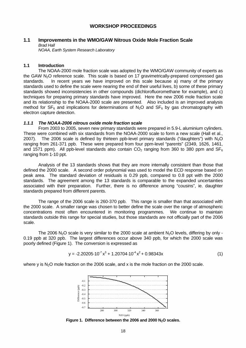
18

WORKSHOP PROCEEDINGS

1.1 Improvements in the WMO/GAW Nitrous Oxide Mole Fraction Scale Brad Hall NOAA, Earth System Research Laboratory

1.1 Introduction

The NOAA-2000 mole fraction scale was adopted by the WMO/GAW community of experts as the GAW N2O reference scale. This scale is based on 17 gravimetrically-prepared compressed gas standards. In recent years we have improved on this scale because a) many of the primary standards used to define the scale were nearing the end of their useful lives, b) some of these primary standards showed inconsistencies in other compounds (dichlorofluoromethane for example), and c) techniques for preparing primary standards have improved. Here the new 2006 mole fraction scale and its relationship to the NOAA-2000 scale are presented. Also included is an improved analysis method for SF6 and implications for determinations of N2O and SF6 by gas chromatography with electron capture detection. 1.1.1 The NOAA-2006 nitrous oxide mole fraction scale

From 2003 to 2005, seven new primary standards were prepared in 5.9-L aluminium cylinders. These were combined with six standards from the NOAA-2000 scale to form a new scale (Hall et al., 2007). The 2006 scale is defined by thirteen ppb-level primary standards (“daughters”) with N2O ranging from 261-371 ppb. These were prepared from four ppm-level “parents” (2349, 1626, 1461, and 1571 ppm). All ppb-level standards also contain CO2 ranging from 360 to 380 ppm and SF6 ranging from 1-10 ppt. Analysis of the 13 standards shows that they are more internally consistent than those that defined the 2000 scale. A second order polynomial was used to model the ECD response based on peak area. The standard deviation of residuals is 0.29 ppb, compared to 0.8 ppt with the 2000 standards. The agreement among the 13 standards is comparable to the expanded uncertainties associated with their preparation. Further, there is no difference among “cousins”, ie. daughter standards prepared from different parents.

The range of the 2006 scale is 260-370 ppb. This range is smaller than that associated with

the 2000 scale. A smaller range was chosen to better define the scale over the range of atmospheric concentrations most often encountered in monitoring programmes. We continue to maintain standards outside this range for special studies, but those standards are not officially part of the 2006 scale.

The 2006 N2O scale is very similar to the 2000 scale at ambient N2O levels, differing by only -

0.19 ppb at 320 ppb. The largest differences occur above 340 ppb, for which the 2000 scale was poorly defined (Figure 1). The conversion is expressed as

y = -2.20205·10-7 x3 + 1.20704·10-4 x2 + 0.98343x (1) where y is N2O mole fraction on the 2006 scale, and x is the mole fraction on the 2000 scale.

-0.7

-0.6

-0.5

-0.4

-0.3

-0.2

-0.1

Diff

eren

ce (p

pb)

360340320300280

N2O (ppb) Figure 1. Difference between the 2006 and 2000 N2O scales.

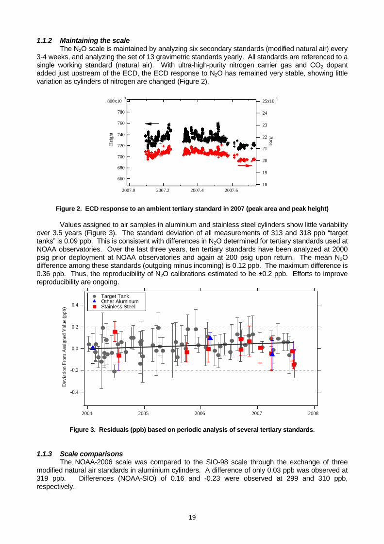
19

1.1.2 Maintaining the scale The N2O scale is maintained by analyzing six secondary standards (modified natural air) every

3-4 weeks, and analyzing the set of 13 gravimetric standards yearly. All standards are referenced to a single working standard (natural air). With ultra-high-purity nitrogen carrier gas and CO2 dopant added just upstream of the ECD, the ECD response to N2O has remained very stable, showing little variation as cylinders of nitrogen are changed (Figure 2).

800x103

780

760

740

720

700

680

660

Hei

ght

2007.62007.42007.22007.0

25x106

24

23

22

21

20

19

18

Area

Figure 2. ECD response to an ambient tertiary standard in 2007 (peak area and peak height)

Values assigned to air samples in aluminium and stainless steel cylinders show little variability

over 3.5 years (Figure 3). The standard deviation of all measurements of 313 and 318 ppb “target tanks” is 0.09 ppb. This is consistent with differences in N2O determined for tertiary standards used at NOAA observatories. Over the last three years, ten tertiary standards have been analyzed at 2000 psig prior deployment at NOAA observatories and again at 200 psig upon return. The mean N2O difference among these standards (outgoing minus incoming) is 0.12 ppb. The maximum difference is 0.36 ppb. Thus, the reproducibility of N2O calibrations estimated to be ±0.2 ppb. Efforts to improve reproducibility are ongoing.

-0.4

-0.2

0.0

0.2

0.4

Dev

iatio

n Fr

om A

ssig

ned

Val

ue (p

pb)

20082007200620052004

Target Tank Other Aluminum Stainless Steel

Figure 3. Residuals (ppb) based on periodic analysis of several tertiary standards.

1.1.3 Scale comparisons

The NOAA-2006 scale was compared to the SIO-98 scale through the exchange of three modified natural air standards in aluminium cylinders. A difference of only 0.03 ppb was observed at 319 ppb. Differences (NOAA-SIO) of 0.16 and -0.23 were observed at 299 and 310 ppb, respectively.

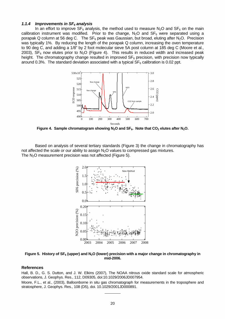
20

1.1.4 Improvements in SF6 analysis In an effort to improve SF6 analysis, the method used to measure N2O and SF6 on the main

calibration instrument was modified. Prior to the change, N2O and SF6 were separated using a porapak Q column at 56 deg C. The SF6 peak was Gaussian, but broad, eluting after N2O. Precision was typically 1%. By reducing the length of the porapak Q column, increasing the oven temperature to 90 deg C, and adding a 1/8” by 2 foot molecular sieve 5A post column at 185 deg C (Moore et al., 2003), SF6 now elutes prior to N2O (Figure 4). This results in reduced width and increased peak height. The chromatography change resulted in improved SF6 precision, with precision now typically around 0.3%. The standard deviation associated with a typical SF6 calibration is 0.02 ppt.

530x103

525

520

515

510

505

500

495

490

ECD

resp

onse

7006005004003002001000

Seconds

3.0

2.8

2.6

2.4

2.2

2.0

CO

2 (ppm)

flow change

CO2 from sample

N2O

SF6flow change

Figure 4. Sample chromatogram showing N2O and SF6. Note that CO2 elutes after N2O.

Based on analysis of several tertiary standards (Figure 3) the change in chromatography has not affected the scale or our ability to assign N2O values to compressed gas mixtures. The N2O measurement precision was not affected (Figure 5).

2.0

1.5

1.0

0.5

0.0

SF6

prec

isio

n (%

)

New Method

0.20

0.15

0.10

0.05

0.00

N2O

pre

cisi

on (%

)

200820072006200520042003

Figure 5. History of SF6 (upper) and N2O (lower) precision with a major change in chromatography in

mid-2006. References Hall, B. D., G. S. Dutton, and J. W. Elkins (2007), The NOAA nitrous oxide standard scale for atmospheric observations, J. Geophys. Res., 112, D09305, doi:10.1029/2006JD007954. Moore, F.L., et al., (2003), Balloonborne in situ gas chromatograph for measurements in the troposphere and stratosphere, J. Geophys. Res., 108 (D5), doi. 10.1029/2001JD000891.

_______

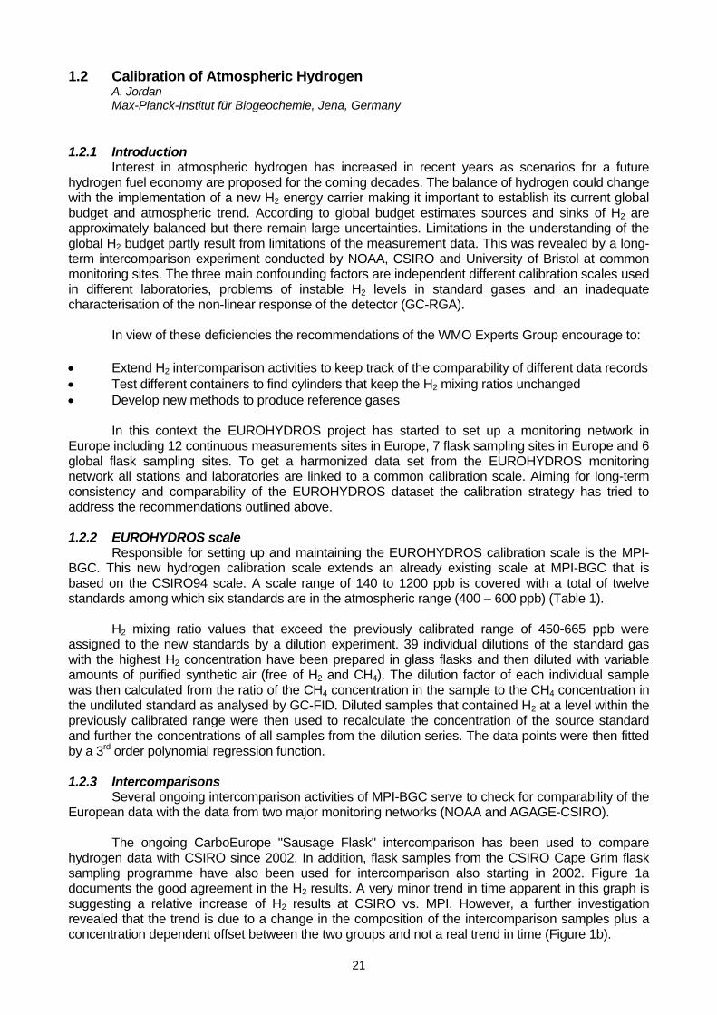
21

1.2 Calibration of Atmospheric Hydrogen A. Jordan Max-Planck-Institut für Biogeochemie, Jena, Germany

1.2.1 Introduction

Interest in atmospheric hydrogen has increased in recent years as scenarios for a future hydrogen fuel economy are proposed for the coming decades. The balance of hydrogen could change with the implementation of a new H2 energy carrier making it important to establish its current global budget and atmospheric trend. According to global budget estimates sources and sinks of H2 are approximately balanced but there remain large uncertainties. Limitations in the understanding of the global H2 budget partly result from limitations of the measurement data. This was revealed by a long-term intercomparison experiment conducted by NOAA, CSIRO and University of Bristol at common monitoring sites. The three main confounding factors are independent different calibration scales used in different laboratories, problems of instable H2 levels in standard gases and an inadequate characterisation of the non-linear response of the detector (GC-RGA).

In view of these deficiencies the recommendations of the WMO Experts Group encourage to:

• Extend H2 intercomparison activities to keep track of the comparability of different data records • Test different containers to find cylinders that keep the H2 mixing ratios unchanged • Develop new methods to produce reference gases

In this context the EUROHYDROS project has started to set up a monitoring network in Europe including 12 continuous measurements sites in Europe, 7 flask sampling sites in Europe and 6 global flask sampling sites. To get a harmonized data set from the EUROHYDROS monitoring network all stations and laboratories are linked to a common calibration scale. Aiming for long-term consistency and comparability of the EUROHYDROS dataset the calibration strategy has tried to address the recommendations outlined above. 1.2.2 EUROHYDROS scale

Responsible for setting up and maintaining the EUROHYDROS calibration scale is the MPI-BGC. This new hydrogen calibration scale extends an already existing scale at MPI-BGC that is based on the CSIRO94 scale. A scale range of 140 to 1200 ppb is covered with a total of twelve standards among which six standards are in the atmospheric range (400 – 600 ppb) (Table 1).

H2 mixing ratio values that exceed the previously calibrated range of 450-665 ppb were

assigned to the new standards by a dilution experiment. 39 individual dilutions of the standard gas with the highest H2 concentration have been prepared in glass flasks and then diluted with variable amounts of purified synthetic air (free of H2 and CH4). The dilution factor of each individual sample was then calculated from the ratio of the CH4 concentration in the sample to the CH4 concentration in the undiluted standard as analysed by GC-FID. Diluted samples that contained H2 at a level within the previously calibrated range were then used to recalculate the concentration of the source standard and further the concentrations of all samples from the dilution series. The data points were then fitted by a 3rd order polynomial regression function. 1.2.3 Intercomparisons

Several ongoing intercomparison activities of MPI-BGC serve to check for comparability of the European data with the data from two major monitoring networks (NOAA and AGAGE-CSIRO).

The ongoing CarboEurope "Sausage Flask" intercomparison has been used to compare

hydrogen data with CSIRO since 2002. In addition, flask samples from the CSIRO Cape Grim flask sampling programme have also been used for intercomparison also starting in 2002. Figure 1a documents the good agreement in the H2 results. A very minor trend in time apparent in this graph is suggesting a relative increase of H2 results at CSIRO vs. MPI. However, a further investigation revealed that the trend is due to a change in the composition of the intercomparison samples plus a concentration dependent offset between the two groups and not a real trend in time (Figure 1b).

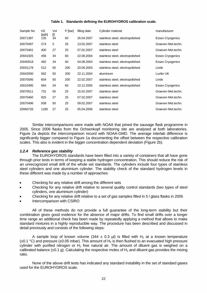
22

Table 1. Standards defining the EUROHYDROS calibration scale. Sample No H2

[ppb] Vol [l]

P [bar] filling date Cylinder material manufacturer

20071387 135 34 60 26.04.2007 stainless steel, electropolished Essex Cryogenics

20070497 274 5 25 13.02.2007 stainless steel Graeven Met.techn.

20070461 400 27 25 07.02.2007 stainless steel Graeven Met.techn.

20041925 456 34 60 22.08.2004 stainless steel, electropolished Essex Cryogenics

20040518 492 34 60 04.08.2004 stainless steel, electropolished Essex Cryogenics

20031178 512 50 200 20.06.2003 stainless steel, electropolished Linde

20042000 562 50 200 22.11.2004 aluminium Luxfer UK

20070595 604 50 200 22.02.2007 stainless steel, electropolished Linde

20010495 664 34 60 10.12.2005 stainless steel, electropolished Essex Cryogenics

20070511 731 50 25 15.02.2007 stainless steel Graeven Met.techn.

20070460 825 27 25 07.02.2007 stainless steel Graeven Met.techn.

20070496 938 50 25 09.02.2007 stainless steel Graeven Met.techn.

20060726 1185 27 25 05.04.2006 stainless steel Graeven Met.techn.

Similar intercomparisons were made with NOAA that joined the sausage flask programme in 2005. Since 2006 flasks from the Ochsenkopf monitoring site are analysed at both laboratories. Figure 2a depicts the intercomparison record with NOAA-GMD. The average interlab difference is significantly bigger compared to Figure 1a documenting the offset between the respective calibration scales. This also is evident in the bigger concentration dependent deviation (Figure 2b). 1.2.4 Reference gas stability

The EUROHYDROS standards have been filled into a variety of containers that all have gone through prior tests in terms of keeping a stable hydrogen concentration. This should reduce the risk of an unrecognized small drift of the whole set standards. The cylinders include four types of stainless steel cylinders and one aluminium cylinder. The stability check of the standard hydrogen levels in these different was made by a number of approaches: • Checking for any relative drift among the different sets • Checking for any relative drift relative to several quality control standards (two types of steel

cylinders, one aluminium cylinder) • Checking for any relative drift relative to a set of gas samples filled in 5 l glass flasks in 2005 • Intercomparison with CSIRO

All of these methods do not provide a full guarantee of the long-term stability but their combination gives good evidence for the absence of major drifts. To find small drifts over a longer time range an additional check has been made by repeatedly applying a method that allows to make standard mixtures in a highly reproducible way. The procedure has been described and discussed in detail previously and consists of the following steps:

A sample loop of known volume (344 ± 0.3 µl) is filled with H2 at a known temperature

(±0.1 °C) and pressure (±0.05 mbar). This amount of H2 is then flushed to an evacuated high pressure cylinder with purified nitrogen or H2 free natural air. The amount of diluent gas is weighed on a calibrated balance (±0.1 g). Calculating the respective moles of H2 and diluent gas provides the mixing ratio.

None of the above drift tests has indicated any standard instability in the set of standard gases

used for the EUROHYDROS scale.

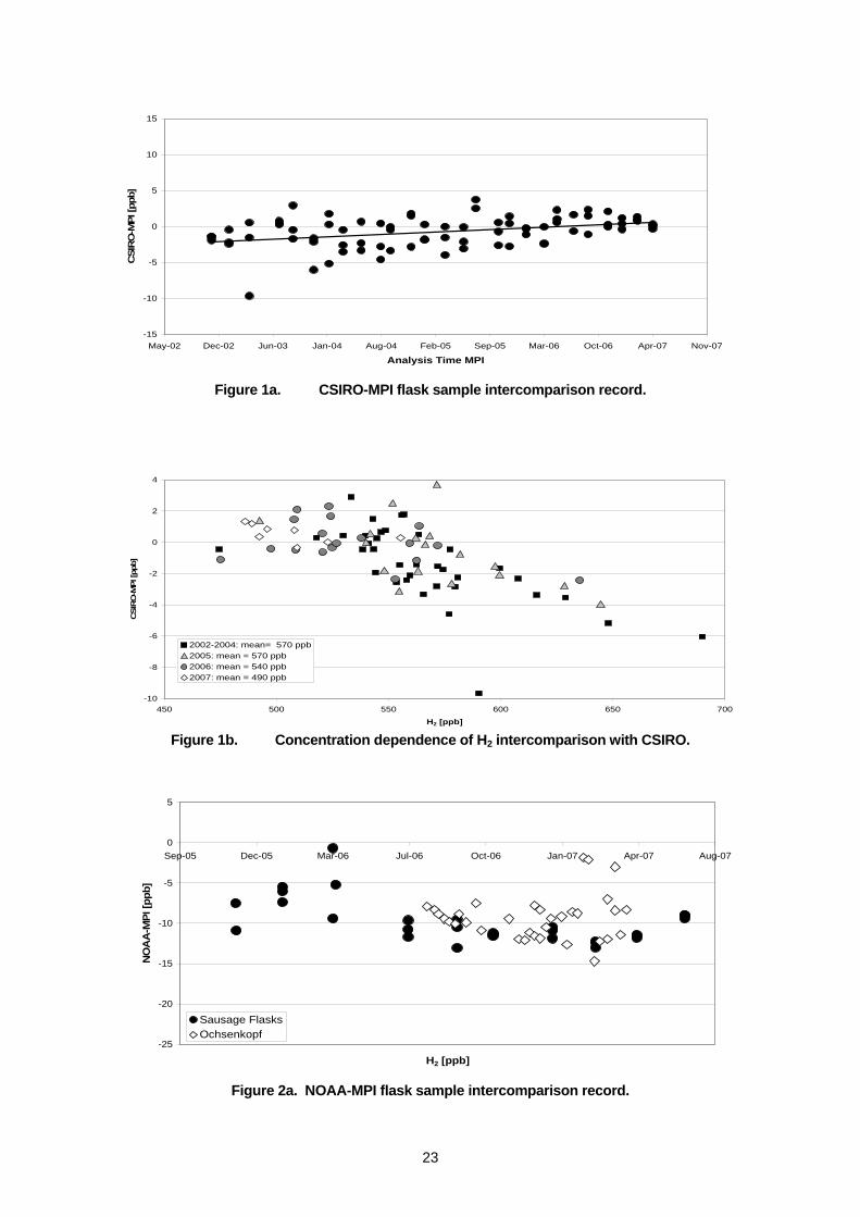
23

-15

-10

-5

0

5

10

15

May-02 Dec-02 Jun-03 Jan-04 Aug-04 Feb-05 Sep-05 Mar-06 Oct-06 Apr-07 Nov-07

Analysis Time MPI

CSI

RO

-MPI

[ppb

]

Figure 1a. CSIRO-MPI flask sample intercomparison record.

-10

-8

-6

-4

-2

0

2

4

450 500 550 600 650 700

H2 [ppb]

CSI

RO

-MPI

[ppb

]

2002-2004: mean= 570 ppb2005: mean = 570 ppb2006: mean = 540 ppb2007: mean = 490 ppb

Figure 1b. Concentration dependence of H2 intercomparison with CSIRO.

-25

-20

-15

-10

-5

0

5

Sep-05 Dec-05 Mar-06 Jul-06 Oct-06 Jan-07 Apr-07 Aug-07

H2 [ppb]

NO

AA

-MPI

[ppb

]

Sausage FlasksOchsenkopf

Figure 2a. NOAA-MPI flask sample intercomparison record.

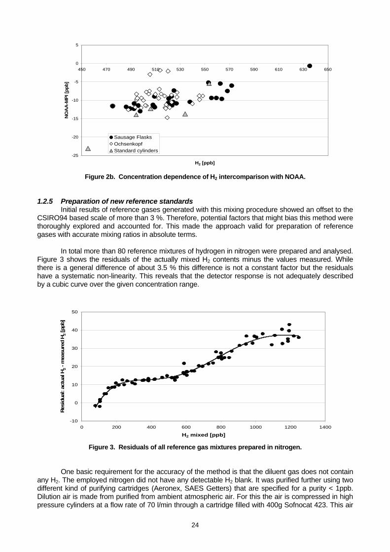
24

-25

-20

-15

-10

-5

0

5

450 470 490 510 530 550 570 590 610 630 650

H2 [ppb]

NO

AA

-MPI

[ppb

]

Sausage FlasksOchsenkopfStandard cylinders

Figure 2b. Concentration dependence of H2 intercomparison with NOAA.

1.2.5 Preparation of new reference standards

Initial results of reference gases generated with this mixing procedure showed an offset to the CSIRO94 based scale of more than 3 %. Therefore, potential factors that might bias this method were thoroughly explored and accounted for. This made the approach valid for preparation of reference gases with accurate mixing ratios in absolute terms.

In total more than 80 reference mixtures of hydrogen in nitrogen were prepared and analysed.

Figure 3 shows the residuals of the actually mixed H2 contents minus the values measured. While there is a general difference of about 3.5 % this difference is not a constant factor but the residuals have a systematic non-linearity. This reveals that the detector response is not adequately described by a cubic curve over the given concentration range.

-10

0

10

20

30

40

50

0 200 400 600 800 1000 1200 1400

H2 mixed [ppb]

Res

idua

l: ac

tual

H2 -

mea

sure

d H

2 [pp

b]

Figure 3. Residuals of all reference gas mixtures prepared in nitrogen.

One basic requirement for the accuracy of the method is that the diluent gas does not contain

any H2. The employed nitrogen did not have any detectable H2 blank. It was purified further using two different kind of purifying cartridges (Aeronex, SAES Getters) that are specified for a purity < 1ppb. Dilution air is made from purified from ambient atmospheric air. For this the air is compressed in high pressure cylinders at a flow rate of 70 l/min through a cartridge filled with 400g Sofnocat 423. This air

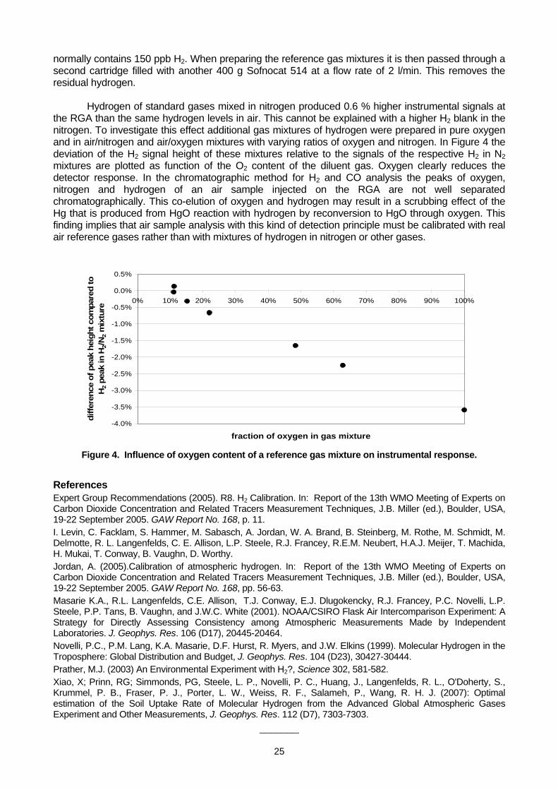
25

normally contains 150 ppb H2. When preparing the reference gas mixtures it is then passed through a second cartridge filled with another 400 g Sofnocat 514 at a flow rate of 2 l/min. This removes the residual hydrogen.

Hydrogen of standard gases mixed in nitrogen produced 0.6 % higher instrumental signals at

the RGA than the same hydrogen levels in air. This cannot be explained with a higher H2 blank in the nitrogen. To investigate this effect additional gas mixtures of hydrogen were prepared in pure oxygen and in air/nitrogen and air/oxygen mixtures with varying ratios of oxygen and nitrogen. In Figure 4 the deviation of the H2 signal height of these mixtures relative to the signals of the respective H2 in N2 mixtures are plotted as function of the O2 content of the diluent gas. Oxygen clearly reduces the detector response. In the chromatographic method for H2 and CO analysis the peaks of oxygen, nitrogen and hydrogen of an air sample injected on the RGA are not well separated chromatographically. This co-elution of oxygen and hydrogen may result in a scrubbing effect of the Hg that is produced from HgO reaction with hydrogen by reconversion to HgO through oxygen. This finding implies that air sample analysis with this kind of detection principle must be calibrated with real air reference gases rather than with mixtures of hydrogen in nitrogen or other gases.

-4.0%

-3.5%

-3.0%

-2.5%

-2.0%

-1.5%

-1.0%

-0.5%

0.0%

0.5%

0% 10% 20% 30% 40% 50% 60% 70% 80% 90% 100%

fraction of oxygen in gas mixture

diffe

renc

e of

pea

k he

ight

com

pare

d to

H2 p

eak

in H

2/N2 m

ixtu

re

Figure 4. Influence of oxygen content of a reference gas mixture on instrumental response.

References Expert Group Recommendations (2005). R8. H2 Calibration. In: Report of the 13th WMO Meeting of Experts on Carbon Dioxide Concentration and Related Tracers Measurement Techniques, J.B. Miller (ed.), Boulder, USA, 19-22 September 2005. GAW Report No. 168, p. 11. I. Levin, C. Facklam, S. Hammer, M. Sabasch, A. Jordan, W. A. Brand, B. Steinberg, M. Rothe, M. Schmidt, M. Delmotte, R. L. Langenfelds, C. E. Allison, L.P. Steele, R.J. Francey, R.E.M. Neubert, H.A.J. Meijer, T. Machida, H. Mukai, T. Conway, B. Vaughn, D. Worthy. Jordan, A. (2005).Calibration of atmospheric hydrogen. In: Report of the 13th WMO Meeting of Experts on Carbon Dioxide Concentration and Related Tracers Measurement Techniques, J.B. Miller (ed.), Boulder, USA, 19-22 September 2005. GAW Report No. 168, pp. 56-63. Masarie K.A., R.L. Langenfelds, C.E. Allison, T.J. Conway, E.J. Dlugokencky, R.J. Francey, P.C. Novelli, L.P. Steele, P.P. Tans, B. Vaughn, and J.W.C. White (2001). NOAA/CSIRO Flask Air Intercomparison Experiment: A Strategy for Directly Assessing Consistency among Atmospheric Measurements Made by Independent Laboratories. J. Geophys. Res. 106 (D17), 20445-20464. Novelli, P.C., P.M. Lang, K.A. Masarie, D.F. Hurst, R. Myers, and J.W. Elkins (1999). Molecular Hydrogen in the Troposphere: Global Distribution and Budget, J. Geophys. Res. 104 (D23), 30427-30444. Prather, M.J. (2003) An Environmental Experiment with H2?, Science 302, 581-582. Xiao, X; Prinn, RG; Simmonds, PG, Steele, L. P., Novelli, P. C., Huang, J., Langenfelds, R. L., O'Doherty, S., Krummel, P. B., Fraser, P. J., Porter, L. W., Weiss, R. F., Salameh, P., Wang, R. H. J. (2007): Optimal estimation of the Soil Uptake Rate of Molecular Hydrogen from the Advanced Global Atmospheric Gases Experiment and Other Measurements, J. Geophys. Res. 112 (D7), 7303-7303.

_______

26

1.3 Preparing and Maintaining of CO2 Calibration Scale in National Institute for Environmental Studies – NIES 95 CO2 Scale T. Machida1, K. Katsumata2, Y. Tohjima1, T. Watai2 and H. Mukai1 1 National Institute for Environmental Studies, Tsukuba, Japan 2 Global Environmental Forum, Tsukuba, Japan

1.3.1 Preparing the primary standard gases

The National Institute for Environmental Studies (NIES) employed the CO2 calibration scale in 1995 based on 10 CO2-in-air standard gases in 10L aluminium cylinders prepared by Nippon Sanso Corp. The pure CO2 gas was diluted with purified air by gravimetric 3-step dilution method. The CO2 mole fractions were determined from measured masses of the pure CO2 and the purified air. The accuracy of the CO2 mole fraction was estimated to be about 0.3ppm [Tanaka et al., 1987]. The relationship between the gravimetric CO2 mole fractions and response of NDIR (XURA-207, Shimadzu, Japan) for the 8 cylinders were fitted by a least square method with a quadratic function and the gravimetric values were adjusted to fit the quadratic function. All of the corrections were less than 0.1ppm (Figure 1). Then we regarded the corrected values of 320.01, 330.03, 340.01, 350.03, 360.16, 369.88, 379.56 and 390.90ppm as NIES 95 CO2 calibration scale for atmospheric air. Remaining two cylinders with their CO2 values of 249.96 and 470.00ppm were also NIES 95 standard gases used for oceanic pCO2 measurement. Mixing ratios and purpose of NIES95 primary cylinders are summarized in Table 1. We used these ten cylinders as primary standard gases for calibrating working standard gases used for CO2 measurements at ground based stations, on the ship, on the aircraft and flask measurements in the laboratory.

Figure 1. Relation between the gravimetric CO2 mole fractions and response of NDIR for eight cylinders (upper panel) and the residuals from the fitting curve (lower panel).

Table 1. Mixing ratios and purpose of NIES95 primary cylinders. Cylinder# CO2[ppm] Purpose

CPB08589 249.96 Ocean pCO2 CPB08595 320.01 Atmosphere CPB08596 330.03 Atmosphere CPB08597 340.01 Atmosphere CPB08598 350.03 Atmosphere CPB08599 360.16 Atmosphere CPB08602 369.88 Atmosphere CPB08603 379.56 Atmosphere CPB08604 390.90 Atmosphere CPB08669 470.00 Ocean pCO2

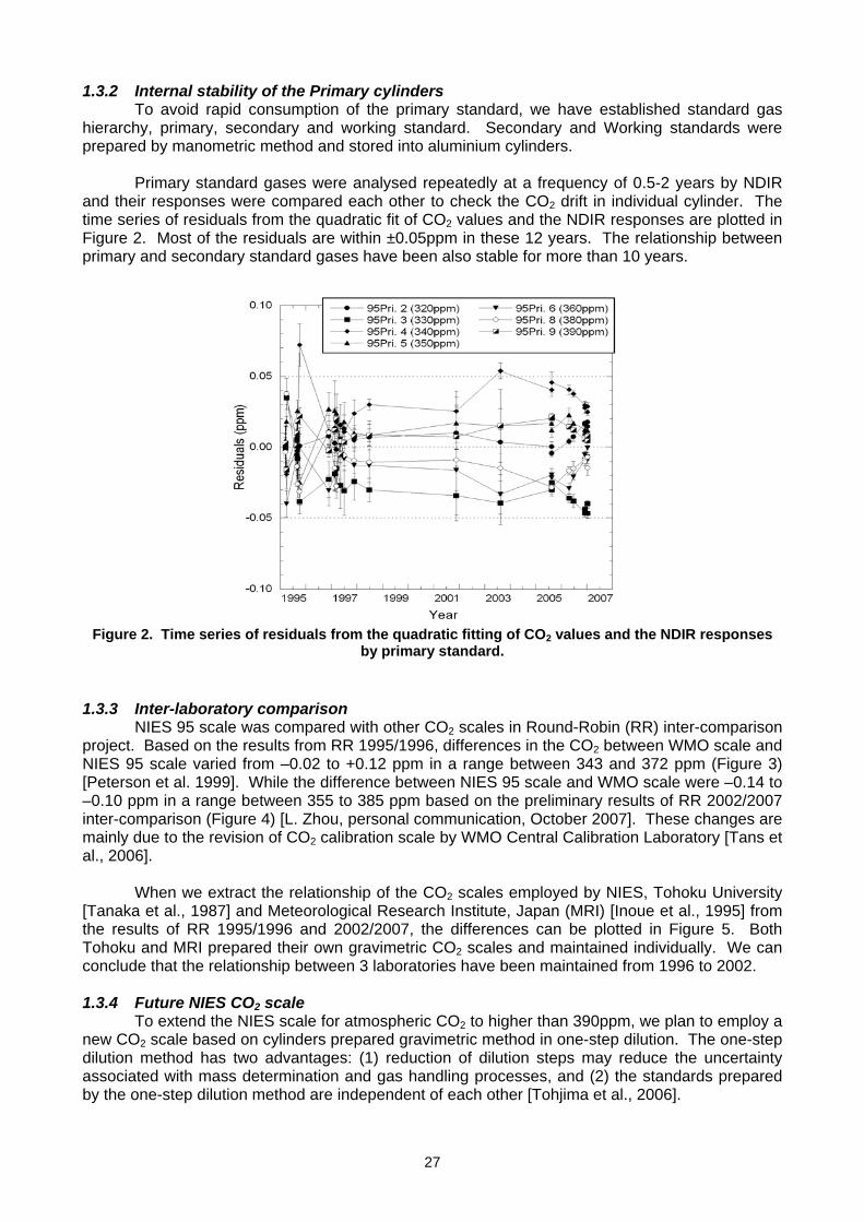
27

1.3.2 Internal stability of the Primary cylinders To avoid rapid consumption of the primary standard, we have established standard gas

hierarchy, primary, secondary and working standard. Secondary and Working standards were prepared by manometric method and stored into aluminium cylinders.

Primary standard gases were analysed repeatedly at a frequency of 0.5-2 years by NDIR

and their responses were compared each other to check the CO2 drift in individual cylinder. The time series of residuals from the quadratic fit of CO2 values and the NDIR responses are plotted in Figure 2. Most of the residuals are within ±0.05ppm in these 12 years. The relationship between primary and secondary standard gases have been also stable for more than 10 years.

Figure 2. Time series of residuals from the quadratic fitting of CO2 values and the NDIR responses

by primary standard. 1.3.3 Inter-laboratory comparison

NIES 95 scale was compared with other CO2 scales in Round-Robin (RR) inter-comparison project. Based on the results from RR 1995/1996, differences in the CO2 between WMO scale and NIES 95 scale varied from –0.02 to +0.12 ppm in a range between 343 and 372 ppm (Figure 3) [Peterson et al. 1999]. While the difference between NIES 95 scale and WMO scale were –0.14 to –0.10 ppm in a range between 355 to 385 ppm based on the preliminary results of RR 2002/2007 inter-comparison (Figure 4) [L. Zhou, personal communication, October 2007]. These changes are mainly due to the revision of CO2 calibration scale by WMO Central Calibration Laboratory [Tans et al., 2006].

When we extract the relationship of the CO2 scales employed by NIES, Tohoku University [Tanaka et al., 1987] and Meteorological Research Institute, Japan (MRI) [Inoue et al., 1995] from the results of RR 1995/1996 and 2002/2007, the differences can be plotted in Figure 5. Both Tohoku and MRI prepared their own gravimetric CO2 scales and maintained individually. We can conclude that the relationship between 3 laboratories have been maintained from 1996 to 2002. 1.3.4 Future NIES CO2 scale

To extend the NIES scale for atmospheric CO2 to higher than 390ppm, we plan to employ a new CO2 scale based on cylinders prepared gravimetric method in one-step dilution. The one-step dilution method has two advantages: (1) reduction of dilution steps may reduce the uncertainty associated with mass determination and gas handling processes, and (2) the standards prepared by the one-step dilution method are independent of each other [Tohjima et al., 2006].

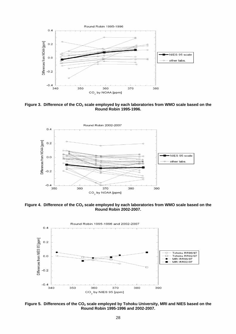
28

Figure 3. Difference of the CO2 scale employed by each laboratories from WMO scale based on the Round Robin 1995-1996.

Figure 4. Difference of the CO2 scale employed by each laboratories from WMO scale based on the Round Robin 2002-2007.

Figure 5. Differences of the CO2 scale employed by Tohoku University, MRI and NIES based on the Round Robin 1995-1996 and 2002-2007.

29

References Inoue, H. Y., H. Matsueda, M. Ishii, K. Fushimi, M. Hirota, I. Asanuma and Y. Takasugi (1995): Long-term Trend of the Partial Pressure of Carbon Dioxide (pCO2) in Surface Waters of the Western North Pacific, 1984-1993. Tellus, 47B, 391-413. Peterson, J., P. Tans, and D. Kitzis (1999), CO2 Round-Robin Reference Gas Intercomparison In R. Francey eds. Report of the Ninth WMO Meeting of Experts on Carbon Dioxide Concentration and Related Tracer Measurement Techniques, Aspendale, Vic. Australia, 1997. Tanaka, M., T. Nakazawa, M. Shiobara, H. Ohshima, S. Aoki, S. Kawaguchi, T. Yamanouchi, Y. Makino, H. Murayama (1987), Variation of Atmospheric Carbon Dioxide Concentration at Syowa Station (69º00´S, 39º35´E), Antarctica., Tellus, 39B, 72-79. Tans, P., C. Zhao and K. Thoning (2006), Revision of the International Calibration Scale for CO2-in-Air: WMO-X2005, In: John B. Miller eds. 13th IAEA/WMO Meeting of CO2 experts, Vol WMO-GAW Report 168. Boulder, 2005, 19-25. Tohjima, Y., T. Machida, H. Mukai, M. Maruyama, T. Nishino, I. Akama, T. Amari, and T. Watai (2006), Preparation of Gravimetric CO2 Standards by One-Step Dilution Method, In: John B. Miller eds. 13th IAEA/WMO Meeting of CO2 Experts, Vol WMO-GAW Report 168. Boulder, 2005, 26-32.

_______

30

2.1 Activities in QA/SAC and WCC in Japan Yukitomo Tsutsumi Atmospheric Environment Division, Japan Meteorological Agency, 1-3-4 Otemachi Chiyodaku Tokyo, Japan

2.1.1 Introduction

The Japan Meteorological Agency (JMA) operates the QA/SAC for Asia and the South-West Pacific in CO2 and CH4 (QA/SAC Japan). The JMA also operates the WCC in Asia and the South-West Pacific for CH4 (WCC Japan). This report focuses on the activities of these centres after the previous meeting. 2.1.2 Activity in the QA/SAC Japan

Some of the roles of QA/SACs are to provide advice and support for the local QA system at individual GAW sites, and to provide training, long-term technical help for station scientists (WMO, 2007).

In 2002, the QA/SAC Japan was asked from the Malaysian Meteorological Department (MMD) for technically support on an establishment of CO2 observation at Danum Valley (in Borneo) in Malaysia. The QA/SAC Japan visited the MMD in Kuala Lumpur and a planned observation site in Borneo in January 2003. During the visit, the QA/SAC Japan made some presentations for general knowledge for CO2 observation and observation environments, and suggested specifications of observation system and operation procedures for CO2 observation at Danum Valley.

Figure 1. Locations of Danum Valley observation station (left) and a tower and laboratory for CO2 observation at Danum Valley.

The MMD started CO2 measurement at Danum Valley using a sampling tower (~100 m) in 2004. As a following up QA/SAC activity of CO2 observations at Danum Valley, the QA/SAC Japan invited an expert of CO2 observation from the MMD. The expert visited the QA/SAC Japan in November 2005, and the centre held the discussions on the Danum Valley CO2 observations. In conclusion, the CO2 observation system is generally well designed with no major faults that could prevent high precision CO2 measurements. The QA/SAC Japan made the QA/SAC report on CO2 observation in Malaysia including some recommendations and sent it to the MMD and the WMO. The CO2 data at Danum Valley from September 2004 through May 2005 are archived in the World Data Centre for Greenhouse Gases in the JMA. However, the CO2 observation system at Danum Valley was damaged by lightning and floods. The system is restored recently with assistance from the manufacturer. However, further checks are necessary for regular operation.

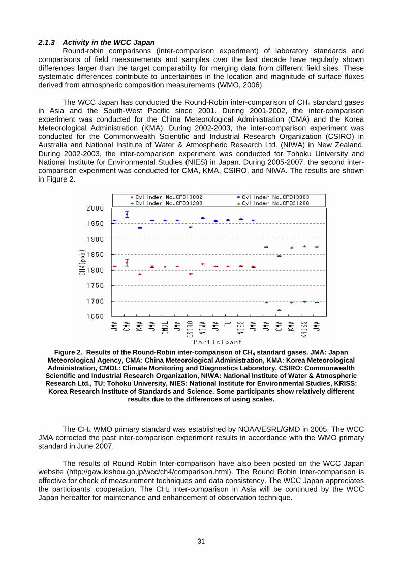
31

2.1.3 Activity in the WCC Japan Round-robin comparisons (inter-comparison experiment) of laboratory standards and

comparisons of field measurements and samples over the last decade have regularly shown differences larger than the target comparability for merging data from different field sites. These systematic differences contribute to uncertainties in the location and magnitude of surface fluxes derived from atmospheric composition measurements (WMO, 2006).

The WCC Japan has conducted the Round-Robin inter-comparison of CH4 standard gases

in Asia and the South-West Pacific since 2001. During 2001-2002, the inter-comparison experiment was conducted for the China Meteorological Administration (CMA) and the Korea Meteorological Administration (KMA). During 2002-2003, the inter-comparison experiment was conducted for the Commonwealth Scientific and Industrial Research Organization (CSIRO) in Australia and National Institute of Water & Atmospheric Research Ltd. (NIWA) in New Zealand. During 2002-2003, the inter-comparison experiment was conducted for Tohoku University and National Institute for Environmental Studies (NIES) in Japan. During 2005-2007, the second inter-comparison experiment was conducted for CMA, KMA, CSIRO, and NIWA. The results are shown in Figure 2.

Figure 2. Results of the Round-Robin inter-comparison of CH4 standard gases. JMA: Japan

Meteorological Agency, CMA: China Meteorological Administration, KMA: Korea Meteorological Administration, CMDL: Climate Monitoring and Diagnostics Laboratory, CSIRO: Commonwealth

Scientific and Industrial Research Organization, NIWA: National Institute of Water & Atmospheric Research Ltd., TU: Tohoku University, NIES: National Institute for Environmental Studies, KRISS: Korea Research Institute of Standards and Science. Some participants show relatively different

results due to the differences of using scales.

The CH4 WMO primary standard was established by NOAA/ESRL/GMD in 2005. The WCC

JMA corrected the past inter-comparison experiment results in accordance with the WMO primary standard in June 2007.

The results of Round Robin Inter-comparison have also been posted on the WCC Japan website (http://gaw.kishou.go.jp/wcc/ch4/comparison.html). The Round Robin Inter-comparison is effective for check of measurement techniques and data consistency. The WCC Japan appreciates the participants’ cooperation. The CH4 inter-comparison in Asia will be continued by the WCC Japan hereafter for maintenance and enhancement of observation technique.

32

References WMO (2006), 13th WMO/IAEA Meeting of Experts on Carbon Dioxide Concentration and Related Tracers Measurement Techniques (Boulder, Colorado, USA, 19-22 September 2005), GAW Report No. 168, (WMO TD No. 1359). WMO (2007), WMO Global Atmosphere Watch (GAW) Strategic Plan: 2008 – 2015, A Contribution to the Implementation of the WMO Strategic Plan: 2008-2011, GAW Report No. 172, (WMO TD No. 1384).

_______

33

2.2 NOAA Comparison Activities: Are We Closer to the Required Measurement Accuracy? Ken Masarie, P. Tans, A. Andrews, T. Conway, A. Crotwell D. Worthy (EC), A. Gomez (AEMET)

Global carbon cycle inverse modelling studies have produced a wide range of estimates of the spatial and temporal distribution of carbon emissions. Debate is ongoing about the percentages of carbon taken up by the ocean and the land biosphere, and where uptake is occurring. Despite their differences, these studies all agree on one point, the need for more observations. However, more observations are only helpful if they can be merged into a cooperative global network of observations with consistency meeting or exceeding target levels as defined by current research topics [WMO TD No. 1359, 2006]. Researchers must now complement their observations with comparison activities designed to determine the level of confidence at which their data can be merged with data from other labs. Several strategies exist within our community and include comparisons of 1) measurements of air from the same high-pressure cylinders; 2) measurements from glass flasks filled from the same high-pressure cylinders; 3) measurements from low-pressure cylinders decanted from high-pressure cylinders; 4) measurements of air from the same ambient samples; and 5) measurements from the same location using different methodologies. What we learn from the different comparison strategies varies greatly and depends on experiment design, comparison frequency, and level of automation. 2.2.1 Introduction

The NOAA ESRL carbon cycle observing programme includes discrete and quasi-continuous sampling from surface sites, aircraft, tall towers, and baseline observatories. While all projects are managed by a single group, sampling and analytical strategies can vary considerably. And while all measurements are traceable to WMO calibration scales, we cannot assume internal consistency with respect to calibration. Thus a critical component of our operation is quality assurance, specifically, procedures designed to assess the level of consistency among measurements made within NOAA. We use the strategies mentioned above to compare measurements made using different methodologies within our lab and also to compare our observations with observations made by other labs. Many of these strategies are fully automated and web-based. But are these efforts producing results? Are NOAA observations internally consistent and comparable with observations made by other labs to the levels required to address current carbon cycle questions?

Here we assess the comparability of NOAA ESRL CO2 measurements. The objective is to achieve and maintain comparability between independent records to within 0.1 ppm. We present comparisons of measurements made solely within NOAA (intra-laboratory) and comparisons between NOAA and other laboratories (inter-laboratory). 2.2.2 Comparison experiments

NOAA participates in several comparison experiments each designed to assess some aspect of the measurement process. The diagram in Figure 1 shows basic components of the measurement process and identifies where several of our comparison activities are located within this process. The WMO/IAEA sponsored Round Robin (RR) experiments, for example, assess the level to which a laboratory scale is tied to the WMO CO2 mole fraction scale. RR experiments are not designed to assess the level of comparability among atmospheric measurements made by different laboratories or using independent methods. Comparisons of measurements from co-located but independent sampling methods perhaps provide the best estimate of the level of consistency between two independent atmospheric records because the experiment incorporates all aspects of the measurement process. However when differences are observed, this comparison, by itself, makes it difficult to identify possible causes. Thus, our comparison activities must complement each other in order to maximize our ability to understand the cause of problems leading to inconsistencies.

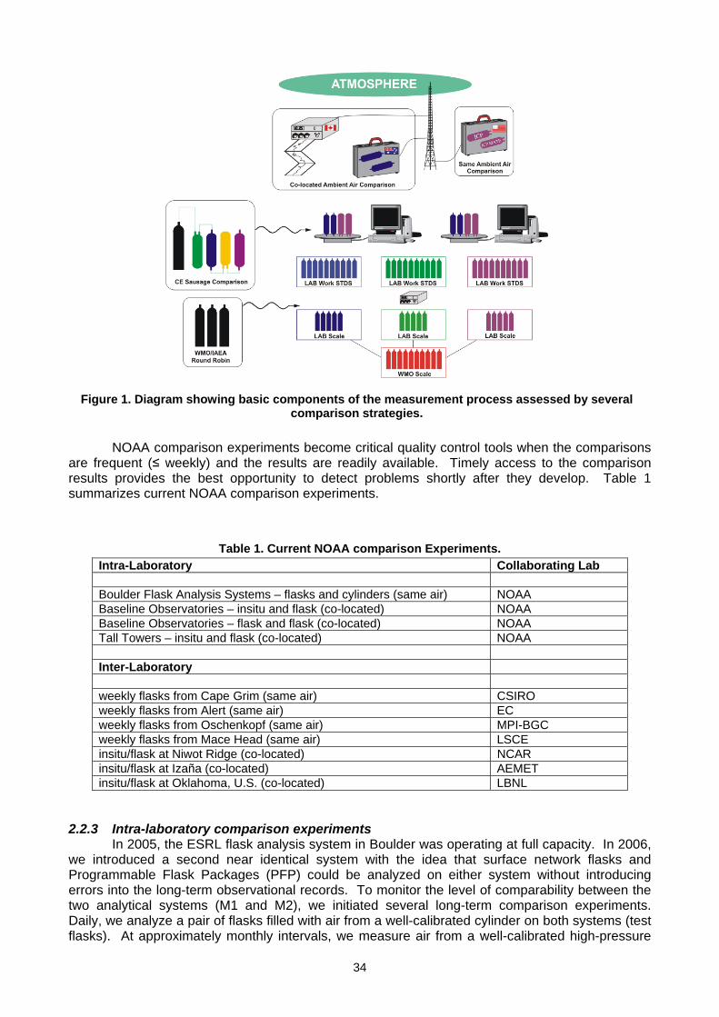
34

NOAA comparison experiments become critical quality control tools when the comparisons are frequent (≤ weekly) and the results are readily available. Timely access to the comparison results provides the best opportunity to detect problems shortly after they develop. Table 1 summarizes current NOAA comparison experiments.

Table 1. Current NOAA comparison Experiments. Intra-Laboratory Collaborating Lab Boulder Flask Analysis Systems – flasks and cylinders (same air) NOAA Baseline Observatories – insitu and flask (co-located) NOAA Baseline Observatories – flask and flask (co-located) NOAA Tall Towers – insitu and flask (co-located) NOAA Inter-Laboratory weekly flasks from Cape Grim (same air) CSIRO weekly flasks from Alert (same air) EC weekly flasks from Oschenkopf (same air) MPI-BGC weekly flasks from Mace Head (same air) LSCE insitu/flask at Niwot Ridge (co-located) NCAR insitu/flask at Izaña (co-located) AEMET insitu/flask at Oklahoma, U.S. (co-located) LBNL

2.2.3 Intra-laboratory comparison experiments

In 2005, the ESRL flask analysis system in Boulder was operating at full capacity. In 2006, we introduced a second near identical system with the idea that surface network flasks and Programmable Flask Packages (PFP) could be analyzed on either system without introducing errors into the long-term observational records. To monitor the level of comparability between the two analytical systems (M1 and M2), we initiated several long-term comparison experiments. Daily, we analyze a pair of flasks filled with air from a well-calibrated cylinder on both systems (test flasks). At approximately monthly intervals, we measure air from a well-calibrated high-pressure

Figure 1. Diagram showing basic components of the measurement process assessed by several comparison strategies.

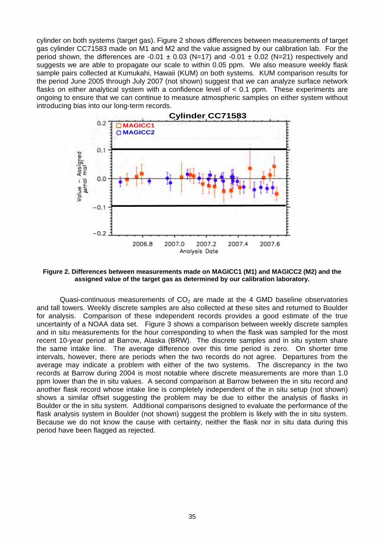
35

cylinder on both systems (target gas). Figure 2 shows differences between measurements of target gas cylinder CC71583 made on M1 and M2 and the value assigned by our calibration lab. For the period shown, the differences are -0.01 ± 0.03 (N=17) and -0.01 ± 0.02 (N=21) respectively and suggests we are able to propagate our scale to within 0.05 ppm. We also measure weekly flask sample pairs collected at Kumukahi, Hawaii (KUM) on both systems. KUM comparison results for the period June 2005 through July 2007 (not shown) suggest that we can analyze surface network flasks on either analytical system with a confidence level of < 0.1 ppm. These experiments are ongoing to ensure that we can continue to measure atmospheric samples on either system without introducing bias into our long-term records.

MAGICC1 MAGICC2

Cylinder CC71583

Figure 2. Differences between measurements made on MAGICC1 (M1) and MAGICC2 (M2) and the

assigned value of the target gas as determined by our calibration laboratory.

Quasi-continuous measurements of CO2 are made at the 4 GMD baseline observatories and tall towers. Weekly discrete samples are also collected at these sites and returned to Boulder for analysis. Comparison of these independent records provides a good estimate of the true uncertainty of a NOAA data set. Figure 3 shows a comparison between weekly discrete samples and in situ measurements for the hour corresponding to when the flask was sampled for the most recent 10-year period at Barrow, Alaska (BRW). The discrete samples and in situ system share the same intake line. The average difference over this time period is zero. On shorter time intervals, however, there are periods when the two records do not agree. Departures from the average may indicate a problem with either of the two systems. The discrepancy in the two records at Barrow during 2004 is most notable where discrete measurements are more than 1.0 ppm lower than the in situ values. A second comparison at Barrow between the in situ record and another flask record whose intake line is completely independent of the in situ setup (not shown) shows a similar offset suggesting the problem may be due to either the analysis of flasks in Boulder or the in situ system. Additional comparisons designed to evaluate the performance of the flask analysis system in Boulder (not shown) suggest the problem is likely with the in situ system. Because we do not know the cause with certainty, neither the flask nor in situ data during this period have been flagged as rejected.

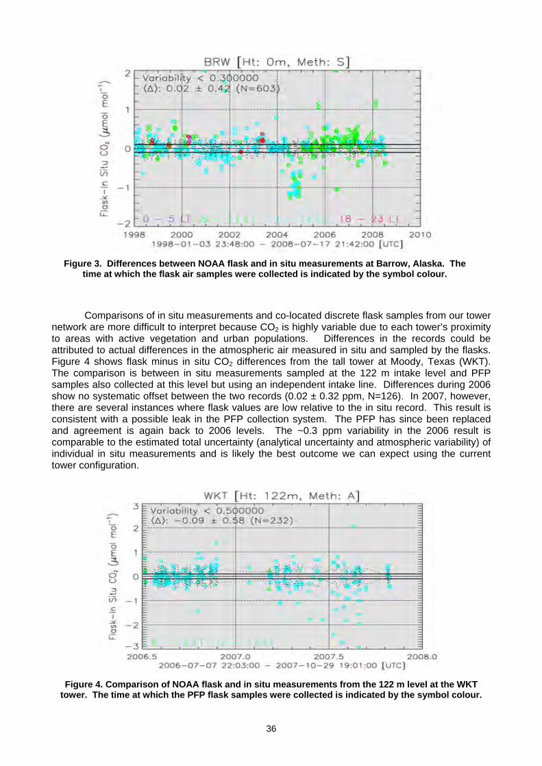
36

Comparisons of in situ measurements and co-located discrete flask samples from our tower

network are more difficult to interpret because CO2 is highly variable due to each tower’s proximity to areas with active vegetation and urban populations. Differences in the records could be attributed to actual differences in the atmospheric air measured in situ and sampled by the flasks. Figure 4 shows flask minus in situ CO2 differences from the tall tower at Moody, Texas (WKT). The comparison is between in situ measurements sampled at the 122 m intake level and PFP samples also collected at this level but using an independent intake line. Differences during 2006 show no systematic offset between the two records (0.02 ± 0.32 ppm, N=126). In 2007, however, there are several instances where flask values are low relative to the in situ record. This result is consistent with a possible leak in the PFP collection system. The PFP has since been replaced and agreement is again back to 2006 levels. The ~0.3 ppm variability in the 2006 result is comparable to the estimated total uncertainty (analytical uncertainty and atmospheric variability) of individual in situ measurements and is likely the best outcome we can expect using the current tower configuration.

Figure 4. Comparison of NOAA flask and in situ measurements from the 122 m level at the WKT

tower. The time at which the PFP flask samples were collected is indicated by the symbol colour.

Figure 3. Differences between NOAA flask and in situ measurements at Barrow, Alaska. The

time at which the flask air samples were collected is indicated by the symbol colour.

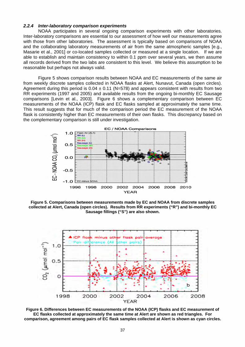
37

2.2.4 Inter-laboratory comparison experiments NOAA participates in several ongoing comparison experiments with other laboratories.

Inter-laboratory comparisons are essential to our assessment of how well our measurements agree with those from other laboratories. The assessment is typically based on comparisons of NOAA and the collaborating laboratory measurements of air from the same atmospheric samples [e.g., Masarie et al., 2001] or co-located samples collected or measured at a single location. If we are able to establish and maintain consistency to within 0.1 ppm over several years, we then assume all records derived from the two labs are consistent to this level. We believe this assumption to be reasonable but perhaps not always valid.

Figure 5 shows comparison results between NOAA and EC measurements of the same air

from weekly discrete samples collected in NOAA flasks at Alert, Nunavut, Canada (open circles). Agreement during this period is 0.04 ± 0.11 (N=578) and appears consistent with results from two RR experiments (1997 and 2005) and available results from the ongoing bi-monthly EC Sausage comparisons [Levin et al., 2003]. Figure 6 shows a complementary comparison between EC measurements of the NOAA (ICP) flask and EC flasks sampled at approximately the same time. This result suggests that for much of the comparison period the EC measurement of the NOAA flask is consistently higher than EC measurements of their own flasks. This discrepancy based on the complementary comparison is still under investigation.

Figure 5. Comparisons between measurements made by EC and NOAA from discrete samples

collected at Alert, Canada (open circles). Results from RR experiments (“R”) and bi-monthly EC Sausage fillings (“S”) are also shown.

Figure 6. Differences between EC measurements of the NOAA (ICP) flasks and EC measurement of

EC flasks collected at approximately the same time at Alert are shown as red triangles. For comparison, agreement among pairs of EC flask samples collected at Alert is shown as cyan circles.

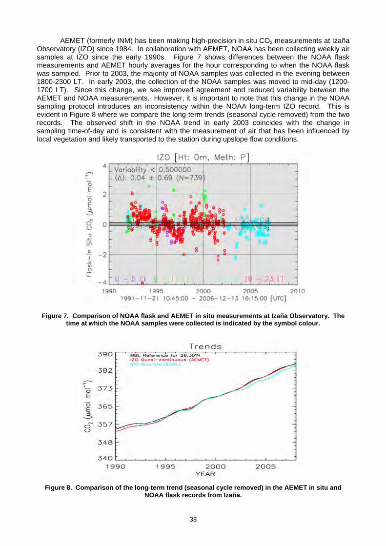
38

AEMET (formerly INM) has been making high-precision in situ CO2 measurements at Izaña Observatory (IZO) since 1984. In collaboration with AEMET, NOAA has been collecting weekly air samples at IZO since the early 1990s. Figure 7 shows differences between the NOAA flask measurements and AEMET hourly averages for the hour corresponding to when the NOAA flask was sampled. Prior to 2003, the majority of NOAA samples was collected in the evening between 1800-2300 LT. In early 2003, the collection of the NOAA samples was moved to mid-day (1200-1700 LT). Since this change, we see improved agreement and reduced variability between the AEMET and NOAA measurements. However, it is important to note that this change in the NOAA sampling protocol introduces an inconsistency within the NOAA long-term IZO record. This is evident in Figure 8 where we compare the long-term trends (seasonal cycle removed) from the two records. The observed shift in the NOAA trend in early 2003 coincides with the change in sampling time-of-day and is consistent with the measurement of air that has been influenced by local vegetation and likely transported to the station during upslope flow conditions.

Figure 7. Comparison of NOAA flask and AEMET in situ measurements at Izaña Observatory. The

time at which the NOAA samples were collected is indicated by the symbol colour.

Figure 8. Comparison of the long-term trend (seasonal cycle removed) in the AEMET in situ and

NOAA flask records from Izaña.

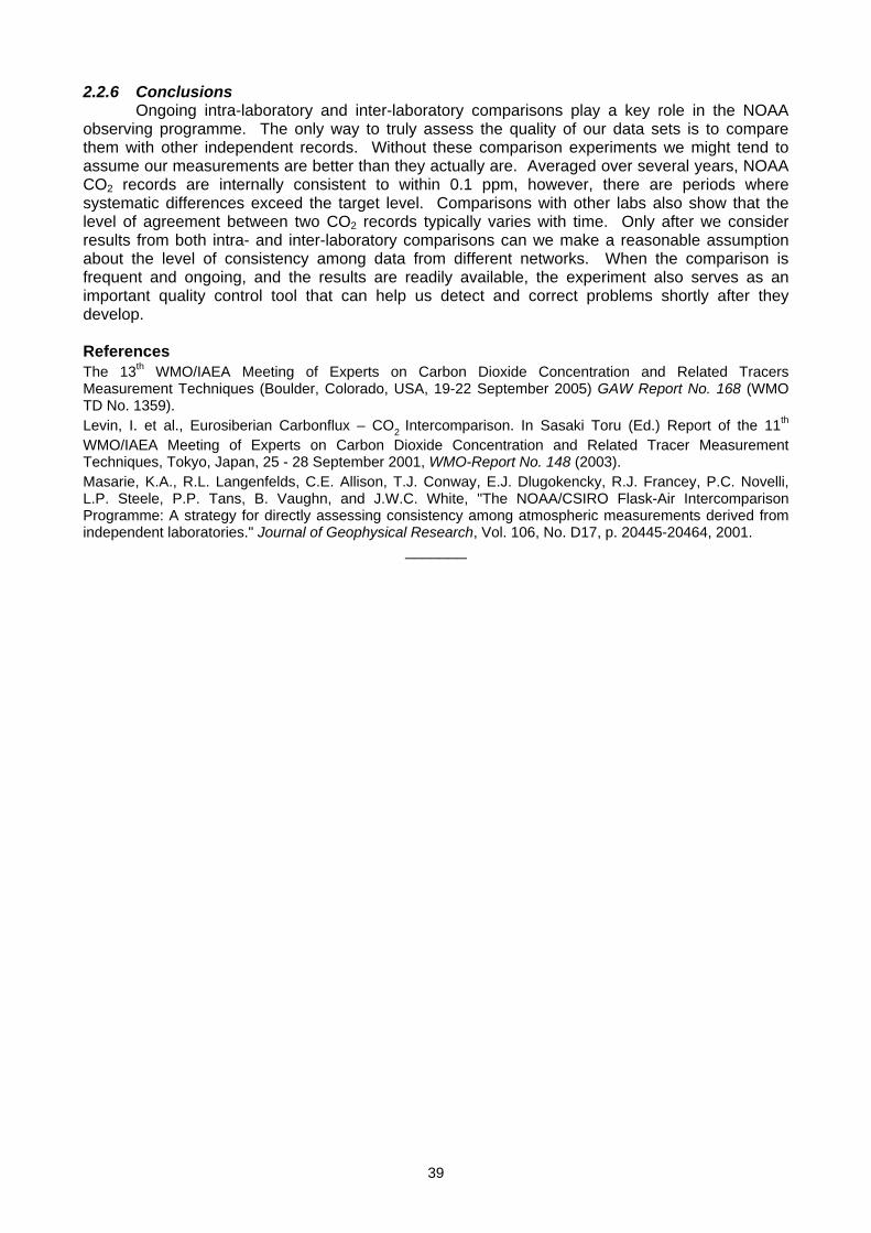
39

2.2.6 Conclusions Ongoing intra-laboratory and inter-laboratory comparisons play a key role in the NOAA

observing programme. The only way to truly assess the quality of our data sets is to compare them with other independent records. Without these comparison experiments we might tend to assume our measurements are better than they actually are. Averaged over several years, NOAA CO2 records are internally consistent to within 0.1 ppm, however, there are periods where systematic differences exceed the target level. Comparisons with other labs also show that the level of agreement between two CO2 records typically varies with time. Only after we consider results from both intra- and inter-laboratory comparisons can we make a reasonable assumption about the level of consistency among data from different networks. When the comparison is frequent and ongoing, and the results are readily available, the experiment also serves as an important quality control tool that can help us detect and correct problems shortly after they develop. References The 13th WMO/IAEA Meeting of Experts on Carbon Dioxide Concentration and Related Tracers Measurement Techniques (Boulder, Colorado, USA, 19-22 September 2005) GAW Report No. 168 (WMO TD No. 1359). Levin, I. et al., Eurosiberian Carbonflux – CO2 Intercomparison. In Sasaki Toru (Ed.) Report of the 11th WMO/IAEA Meeting of Experts on Carbon Dioxide Concentration and Related Tracer Measurement Techniques, Tokyo, Japan, 25 - 28 September 2001, WMO-Report No. 148 (2003). Masarie, K.A., R.L. Langenfelds, C.E. Allison, T.J. Conway, E.J. Dlugokencky, R.J. Francey, P.C. Novelli, L.P. Steele, P.P. Tans, B. Vaughn, and J.W.C. White, "The NOAA/CSIRO Flask-Air Intercomparison Programme: A strategy for directly assessing consistency among atmospheric measurements derived from independent laboratories." Journal of Geophysical Research, Vol. 106, No. D17, p. 20445-20464, 2001.

_______

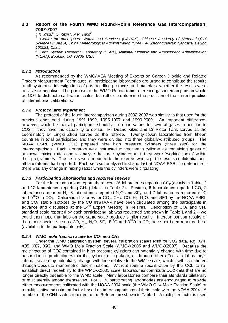
40

2.3 Report of the Fourth WMO Round-Robin Reference Gas Intercomparison, 2002-2007 L.X. Zhou1, D. Kitzis2, P.P. Tans2 1. Centre for Atmosphere Watch and Services (CAWAS), Chinese Academy of Meteorological Sciences (CAMS), China Meteorological Administration (CMA), 46 Zhongguancun Nandajie, Beijing 100081, China 2. Earth System Research Laboratory (ESRL), National Oceanic and Atmospheric Administration (NOAA), Boulder, CO 80305, USA

2.3.1 Introduction

As recommended by the WMO/IAEA Meeting of Experts on Carbon Dioxide and Related Tracers Measurement Techniques, all participating laboratories are urged to contribute the results of all systematic investigations of gas handling protocols and materials, whether the results were positive or negative. The purpose of the WMO Round-robin reference gas intercomparison would be NOT to distribute calibration scales, but rather to determine the precision of the current practice of international calibrations. 2.3.2 Protocol and experiment

The protocol of the fourth intercomparison during 2002-2007 was similar to that used for the previous ones held during 1991-1992, 1995-1997 and 1999-2000. An important difference, however, would be that all participants should also report values for several gases in addition to CO2, if they have the capability to do so. Mr Duane Kitzis and Dr Pieter Tans served as the coordinator; Dr Lingxi Zhou served as the referee. Twenty-seven laboratories from fifteen countries in total participated and they were divided into three globally-distributed groups. The NOAA ESRL (WMO CCL) prepared nine high pressure cylinders (three sets) for the intercomparison. Each laboratory was instructed to treat each cylinder as containing gases of unknown mixing ratios and to analyze the three cylinders as if they were "working tanks" within their programmes. The results were reported to the referee, who kept the results confidential until all laboratories had reported. Each set was analyzed first and last at NOAA ESRL to determine if there was any change in mixing ratios while the cylinders were circulating. 2.3.3 Participating laboratories and reported species

For the intercomparison report, there were 26 laboratories reporting CO2 (details in Table 1) and 12 laboratories reporting CH4 (details in Table 2). Besides, 8 laboratories reported CO, 2 laboratories reported H2, 6 laboratories reported N2O and SF6, and 7 laboratories reported δ13C and δ18O in CO2. Calibration histories for CO2, CH4, CO, H2, N2O, and SF6 by the NOAA ESRL and CO2 stable isotopes by the CU INSTAAR have been circulated among the participants in advance and discussed at the 14th Expert Meeting in Helsinki. Description of CO2 and CH4 standard scale reported by each participating lab was requested and shown in Table 1 and 2 -- we could then hope that labs on the same scale produce similar results. Intercomparison results of the other species such as CO, H2, N2O, SF6, δ13C and δ18O in CO2 have not been reported here (available to the participants only). 2.3.4 WMO mole fraction scale for CO2 and CH4

Under the WMO calibration system, several calibration scales exist for CO2 data, e.g. X74, X85, X87, X93, and WMO Mole Fraction Scale (WMO-X2005 and WMO-X2007). Because the mole fraction of CO2 contained in high-pressure cylinders can potentially change with time due to adsorption or production within the cylinder or regulator, or through other effects, a laboratory's internal scale may potentially change with time relative to the WMO scale, which itself is anchored through absolute manometric determinations. Without routine recalibration by the CCL to re-establish direct traceability to the WMO-X2005 scale, laboratories contribute CO2 data that are no longer directly traceable to the WMO scale. Many laboratories compare their standards bilaterally or multilaterally among themselves. For CH4, participating laboratories are encouraged to provide either measurements calibrated with the NOAA 2004 scale (the WMO CH4 Mole Fraction Scale) or a multiplicative adjustment factor based on intercomparisons of their scale with the NOAA 2004. A number of the CH4 scales reported to the Referee are shown in Table 1. A multiplier factor is used

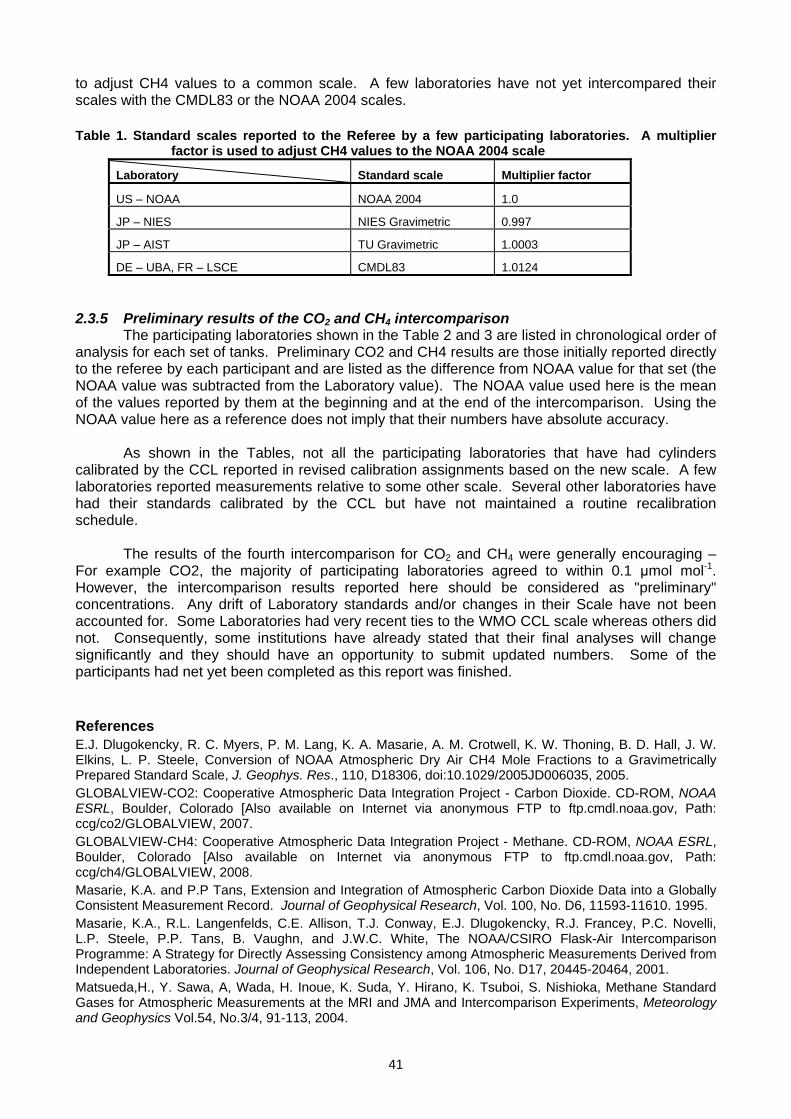
41

to adjust CH4 values to a common scale. A few laboratories have not yet intercompared their scales with the CMDL83 or the NOAA 2004 scales. Table 1. Standard scales reported to the Referee by a few participating laboratories. A multiplier

factor is used to adjust CH4 values to the NOAA 2004 scale

Laboratory Standard scale Multiplier factor

US – NOAA NOAA 2004 1.0

JP – NIES NIES Gravimetric 0.997

JP – AIST TU Gravimetric 1.0003

DE – UBA, FR – LSCE CMDL83 1.0124 2.3.5 Preliminary results of the CO2 and CH4 intercomparison

The participating laboratories shown in the Table 2 and 3 are listed in chronological order of analysis for each set of tanks. Preliminary CO2 and CH4 results are those initially reported directly to the referee by each participant and are listed as the difference from NOAA value for that set (the NOAA value was subtracted from the Laboratory value). The NOAA value used here is the mean of the values reported by them at the beginning and at the end of the intercomparison. Using the NOAA value here as a reference does not imply that their numbers have absolute accuracy.

As shown in the Tables, not all the participating laboratories that have had cylinders

calibrated by the CCL reported in revised calibration assignments based on the new scale. A few laboratories reported measurements relative to some other scale. Several other laboratories have had their standards calibrated by the CCL but have not maintained a routine recalibration schedule.

The results of the fourth intercomparison for CO2 and CH4 were generally encouraging –

For example CO2, the majority of participating laboratories agreed to within 0.1 μmol mol-1. However, the intercomparison results reported here should be considered as "preliminary" concentrations. Any drift of Laboratory standards and/or changes in their Scale have not been accounted for. Some Laboratories had very recent ties to the WMO CCL scale whereas others did not. Consequently, some institutions have already stated that their final analyses will change significantly and they should have an opportunity to submit updated numbers. Some of the participants had net yet been completed as this report was finished.

References E.J. Dlugokencky, R. C. Myers, P. M. Lang, K. A. Masarie, A. M. Crotwell, K. W. Thoning, B. D. Hall, J. W. Elkins, L. P. Steele, Conversion of NOAA Atmospheric Dry Air CH4 Mole Fractions to a Gravimetrically Prepared Standard Scale, J. Geophys. Res., 110, D18306, doi:10.1029/2005JD006035, 2005. GLOBALVIEW-CO2: Cooperative Atmospheric Data Integration Project - Carbon Dioxide. CD-ROM, NOAA ESRL, Boulder, Colorado [Also available on Internet via anonymous FTP to ftp.cmdl.noaa.gov, Path: ccg/co2/GLOBALVIEW, 2007. GLOBALVIEW-CH4: Cooperative Atmospheric Data Integration Project - Methane. CD-ROM, NOAA ESRL, Boulder, Colorado [Also available on Internet via anonymous FTP to ftp.cmdl.noaa.gov, Path: ccg/ch4/GLOBALVIEW, 2008. Masarie, K.A. and P.P Tans, Extension and Integration of Atmospheric Carbon Dioxide Data into a Globally Consistent Measurement Record. Journal of Geophysical Research, Vol. 100, No. D6, 11593-11610. 1995. Masarie, K.A., R.L. Langenfelds, C.E. Allison, T.J. Conway, E.J. Dlugokencky, R.J. Francey, P.C. Novelli, L.P. Steele, P.P. Tans, B. Vaughn, and J.W.C. White, The NOAA/CSIRO Flask-Air Intercomparison Programme: A Strategy for Directly Assessing Consistency among Atmospheric Measurements Derived from Independent Laboratories. Journal of Geophysical Research, Vol. 106, No. D17, 20445-20464, 2001. Matsueda,H., Y. Sawa, A, Wada, H. Inoue, K. Suda, Y. Hirano, K. Tsuboi, S. Nishioka, Methane Standard Gases for Atmospheric Measurements at the MRI and JMA and Intercomparison Experiments, Meteorology and Geophysics Vol.54, No.3/4, 91-113, 2004.

42

Peterson, J., P. Tans, and D. Kitzis, "CO2 Round-Robin Reference Gas Intercomparison" in Report of the Ninth WMO Meeting of Experts on Carbon Dioxide Concentration and Related Tracer Measurement Techniques, Aspendale, Vic. Australia, 1 - 4 September 1997, edited by R. Francey, World Meteorological Organization, Geneva, 1999. TACOS Sausage Flask Intercomparison Exercise: 2002-2005 (Levin, I. et al., Presentation at the 13th WMO / IAEA Meeting of Experts on Carbon Dioxide Concentration and Related Tracer Measurement Techniques Boulder, Colorado, USA; September 19-22, 2005), World Meteorological Organization, GAW Report No. 148. Tans, P., C. Zhao, and K. Masarie, "Maintenance and Propagation of the WMO Mole Fraction Scale for Carbon Dioxide in Air" in Report of the Eleventh WMO Meeting of Experts on Carbon Dioxide Concentration and Related Tracer Measurement Techniques, Tokyo, Japan, 25-28 September 2001, edited by S. Toru, World Meteorological Organization, Geneva, 2003. WMO/GAW, 13th WMO/IAEA Meeting of Experts on Carbon Dioxide Concentration and Related Tracers Measurement Techniques, Boulder, Colorado, USA, 19-22 September 2005. (WMO TD No. 1359). WMO/JMA, Results of Methane Reference Gas Intercomparison Experiment in WCC for Methane, http://gaw.kishou.go.jp/wcc/ch4/comparison.html. Zhao, C.L., P. P Tans, and K. W. Thoning, A High Precision Manometric System for Absolute Calibrations of CO2 in Dry Air, J. Geophys. Res., 102, 5885-5894, 1997. Zhao, C., and P.P. Tans, Estimating Uncertainty of the WMO Mole Fraction Scale for Carbon Dioxide in Air, J. Geophys. Res., 111, D08S09, doi: 10.1029/2005JD006003. 2006.

Table 2. 2002 - 2007 WMO Round-Robin Intercalibration Results Carbon Dioxide Concentrations (Preliminary).

Laboratories Analysis Date

Report Date

TANK # CO2, μmol mol-1

Differences (Lab minus NOAA)

CO2, μmol mol-1 Description of reported

standard scale

GROUP ONE (Tank #4532, #4409, #4584) 4532 4409 4584 4532 4409 4584

US – NOAA average 354.91 368.14 384.81

JP - Tohoku U. Jan.2003 Mar.2004 354.80 367.95 384.52 -0.11 -0.19 -0.29 Gravimetric, Tohoku U. 2003 scale

JP – NIES Apr.2003 Mar.2004 354.81 367.99 384.67 -0.10 -0.15 -0.14 Gravimetric, NIES95 scale

JP – MRI July.2003 Mar.2004 354.75 367.98 384.73 -0.16 -0.16 -0.08 Gravimetric, MRI 1987 scale

JP – AIST Sept./Dec.2003 Mar.2004 354.80 367.92 384.52 -0.11 -0.22 -0.29 Gravimetric, Tohoku U. 2003 scale

JP – JMA Jan.2004 Mar.2004 355.04 368.14 384.79 0.13 0.00 -0.02 WMO X2005 scale

Korea – KMA (KGAWO) Mar./Jun.2004 July.2004 354.47 368.02 384.73 -0.44 -0.12 -0.08 4 tanks NOAA and 2 tanks

KRISS

CN - CMA (WLG) July.2004 Nov.2004 354.86 367.95 384.71 -0.05 -0.19 -0.10 WMO X2007 scale

CN - CMA (BJ) Aug.2004 Nov.2004 354.88 367.94 384.83 -0.03 -0.20 0.02 WMO X2007 scale

US – SCRIPPS (CMM) June.2005 June.2006 355.14 368.31 385.01 0.23 0.17 0.20

Manometric, CMM US - SCRIPPS (ECM II) 355.01 368.16 384.83 0.10 0.02 0.02 Manometric, ECM II

FR – LSCE Oct./Nov.2005 Dec.2005 354.86 368.03 384.72 -0.05 -0.11 -0.09 Calibrated by NOAA between 2001 and 2002

GROUP TWO (Tank #4542, #4509, #4539) 4542 4509 4539 4542 4509 4539

US – NOAA average

355.85 368.35 384.60

IT - Monte Cimone Oct.2002 Oct.2002 355.93 368.37 384.57 0.08 0.02 -0.03

IT - ENEA, Lampedusa Nov.2002

Mar.2003 355.90 368.20 384.34 0.05 -0.15 -0.26

IT – Plateau Rosa,CESI,CNR Dec.2002 Dec.2002 355.83 368.35 384.55 -0.02 0.00 -0.05

HU – HMS Feb.2003 Sept.2003 355.91 368.14 384.54 0.06 -0.21 -0.06 Calibrated by NOAA between 1994 and 2000

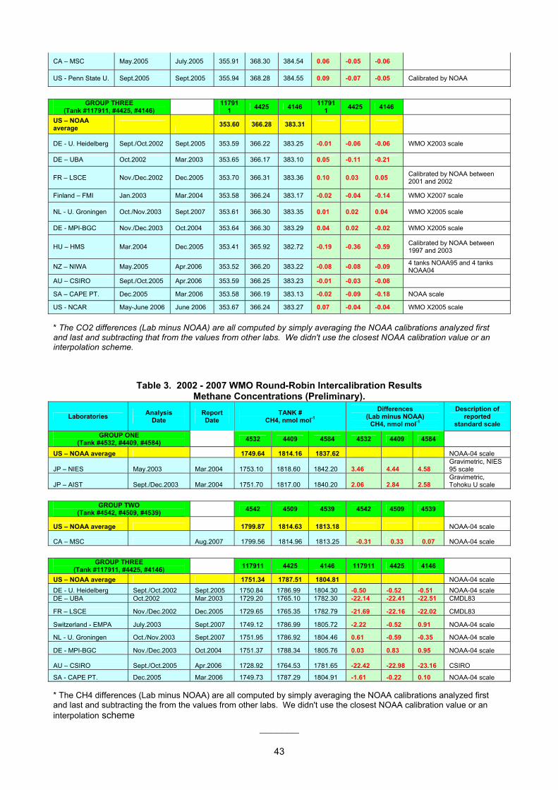
43

CA – MSC May.2005 July.2005 355.91 368.30 384.54 0.06 -0.05 -0.06

US - Penn State U. Sept.2005 Sept.2005 355.94 368.28 384.55 0.09 -0.07 -0.05 Calibrated by NOAA

GROUP THREE

(Tank #117911, #4425, #4146) 11791

1 4425 4146 117911 4425 4146

US – NOAA average

353.60 366.28 383.31

DE - U. Heidelberg Sept./Oct.2002 Sept.2005 353.59 366.22 383.25 -0.01 -0.06 -0.06 WMO X2003 scale

DE – UBA Oct.2002 Mar.2003 353.65 366.17 383.10 0.05 -0.11 -0.21

FR – LSCE Nov./Dec.2002 Dec.2005 353.70 366.31 383.36 0.10 0.03 0.05 Calibrated by NOAA between 2001 and 2002

Finland – FMI Jan.2003 Mar.2004 353.58 366.24 383.17 -0.02 -0.04 -0.14 WMO X2007 scale

NL - U. Groningen Oct./Nov.2003 Sept.2007 353.61 366.30 383.35 0.01 0.02 0.04 WMO X2005 scale

DE - MPI-BGC Nov./Dec.2003 Oct.2004 353.64 366.30 383.29 0.04 0.02 -0.02 WMO X2005 scale

HU – HMS Mar.2004 Dec.2005 353.41 365.92 382.72 -0.19 -0.36 -0.59 Calibrated by NOAA between 1997 and 2003

NZ – NIWA May.2005 Apr.2006 353.52 366.20 383.22 -0.08 -0.08 -0.09 4 tanks NOAA95 and 4 tanks NOAA04

AU – CSIRO Sept./Oct.2005 Apr.2006 353.59 366.25 383.23 -0.01 -0.03 -0.08

SA – CAPE PT. Dec.2005 Mar.2006 353.58 366.19 383.13 -0.02 -0.09 -0.18 NOAA scale

US - NCAR May-June 2006 June 2006 353.67 366.24 383.27 0.07 -0.04 -0.04 WMO X2005 scale

* The CO2 differences (Lab minus NOAA) are all computed by simply averaging the NOAA calibrations analyzed first and last and subtracting that from the values from other labs. We didn't use the closest NOAA calibration value or an interpolation scheme.

Table 3. 2002 - 2007 WMO Round-Robin Intercalibration Results Methane Concentrations (Preliminary).

Laboratories Analysis Date

Report Date

TANK # CH4, nmol mol-1

Differences (Lab minus NOAA)

CH4, nmol mol-1

Description of reported

standard scale GROUP ONE

(Tank #4532, #4409, #4584) 4532 4409 4584 4532 4409 4584

US – NOAA average 1749.64 1814.16 1837.62 NOAA-04 scale

JP – NIES May.2003 Mar.2004 1753.10 1818.60 1842.20 3.46 4.44 4.58 Gravimetric, NIES 95 scale

JP – AIST Sept./Dec.2003 Mar.2004 1751.70 1817.00 1840.20 2.06 2.84 2.58 Gravimetric, Tohoku U scale

GROUP TWO

(Tank #4542, #4509, #4539) 4542 4509 4539 4542 4509 4539

US – NOAA average 1799.87 1814.63 1813.18 NOAA-04 scale

CA – MSC Aug.2007 1799.56 1814.96 1813.25 -0.31 0.33 0.07 NOAA-04 scale

GROUP THREE

(Tank #117911, #4425, #4146) 117911 4425 4146 117911 4425 4146 US – NOAA average 1751.34 1787.51 1804.81 NOAA-04 scale DE - U. Heidelberg Sept./Oct.2002 Sept.2005 1750.84 1786.99 1804.30 -0.50 -0.52 -0.51 NOAA-04 scale DE – UBA Oct.2002 Mar.2003 1729.20 1765.10 1782.30 -22.14 -22.41 -22.51 CMDL83

FR – LSCE Nov./Dec.2002 Dec.2005 1729.65 1765.35 1782.79 -21.69 -22.16 -22.02 CMDL83

Switzerland - EMPA July.2003 Sept.2007 1749.12 1786.99 1805.72 -2.22 -0.52 0.91 NOAA-04 scale

NL - U. Groningen Oct./Nov.2003 Sept.2007 1751.95 1786.92 1804.46 0.61 -0.59 -0.35 NOAA-04 scale

DE - MPI-BGC Nov./Dec.2003 Oct.2004 1751.37 1788.34 1805.76 0.03 0.83 0.95 NOAA-04 scale

AU – CSIRO Sept./Oct.2005 Apr.2006 1728.92 1764.53 1781.65 -22.42 -22.98 -23.16 CSIRO

SA - CAPE PT. Dec.2005 Mar.2006 1749.73 1787.29 1804.91 -1.61 -0.22 0.10 NOAA-04 scale * The CH4 differences (Lab minus NOAA) are all computed by simply averaging the NOAA calibrations analyzed first and last and subtracting the from the values from other labs. We didn't use the closest NOAA calibration value or an interpolation scheme

_______

44

3.1 Ten Years of High-Precision Methane Isotope Data for Mace Head and London: The Influence of Canadian and European Sources David Lowry1, Euan Nisbet1, Rebecca Fisher1, Aodhagan Roddy2, *Phillip O’Brien2 1Depart. of Geology, Royal Holloway, University of London, Egham, Surrey TW20 0EX, UK 2Martin Ryan Marine Science Institute and Department of Physics, National University of Ireland, Galway, Republic of Ireland; * Current Address: EPA Regional Inspectorate, McCumiskey House, Richview, Clonskeagh, Dublin 14 Republic of Ireland

3.1.1 Introduction

Time-series of methane mixing ratio and high-precision carbon isotope ratio (δ13C CH4) have been maintained for air samples collected at the Mace Head site, western Ireland, and at Royal Holloway, University of London, Egham (EGH), UK, for the period 1995-2004. The data have been subdivided using back trajectory analysis and arrival direction of the air masses to assess source contributions. Comparison of the two sites shows that since 2000 there is a very close correlation between the records, particularly in summer. In winter the London site is influenced by the prevailing North Atlantic weather systems and winter methane averages correlate strongly with the winter NAO Index. During summer the SW London site can be a more representative Atlantic background site than Mace Head, on the occasions when the Azores high does not track far enough North to influence Mace Head. Combining background sector data for both sites allows the derivation of an Atlantic background δ13C curve for 45-60°N. 3.1.2 Mace Head and SW London time series

Average mixing ratios have been calculated for each of the 12 months for the period 1995-2004 to compare the bi-weekly Mace Head ‘clean sector’ samples collected for the isotope study with the AGAGE quasi-continuous and NOAA flask sampling records for Mace Head. This confirms that our sampling over the 10-year period was representative (Figure 1a) and identifies a seasonality of 30-35 ppb with minimum mixing ratio in July. The time-series of δ13C for Mace Head shows clear seasonality, but is not synchronous with the mixing ratio cycle. (Figure 1c). The amplitude of the seasonal δ13C cycle when a 10-year average for each month is taken is 0.32‰ with maximum enrichment in April at –47.24‰ and depletion in September at –47.56‰. Taken on an individual year basis the seasonality is larger, between 0.4 and 0.5‰, with the exception of 1995 at 0.8‰ and 2004 at 0.6‰.

The 10-year averaged seasonal cycle for our SW London site is 39 ppb, slightly more than for Mace Head, due largely to the influence of air masses passing over parts of the UK on route to SW London and to incomplete break up of inversions in winter. There is a maximum of 1863 ppb in December and a minimum of 1824 ppb in July. The seasonal cycle in δ13C when a 10-year average for each month is used is 0.34‰, similar to Mace Head, with maximum enrichment in March at –47.11‰ and depletion in September at –47.45‰. Taken on an individual year basis the seasonality is larger, between 0.5 and 0.6‰, with the exception of 1995 at 1.0‰ and 2004 at 0.8‰, slightly larger than for Mace Head, but with the same exceptional years. Since 1999 the tank sampling at RHUL has focussed predominantly on western sectors. Prior to this the sampling was less constrained and seasonality is less clearly defined although local sources within 3 km also hindered ‘clean air’ sampling during the early (1995-1998) period. The mixing ratio annual cycles for individual years since 1999 have been approximately 80 ppb. 3.1.3 Differences between the two records

Comparisons between the two datasets reveal monthly excesses over Mace Head for the Egham site of up to 17 ppb, most significantly in March, April and October (Figure 1b). This excess is associated with enrichment in 13C, for all months except July, of up to 0.2‰ (Figure 1c).

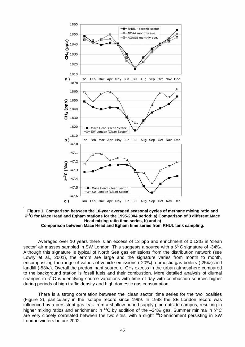
45

.

Figure 1. Comparison between the 10-year averaged seasonal cycles of methane mixing ratio and δ13C for Mace Head and Egham stations for the 1995-2004 period: a) Comparison of 3 different Mace

Head mixing ratio time-series, b) and c) Comparison between Mace Head and Egham time series from RHUL tank sampling.

Averaged over 10 years there is an excess of 13 ppb and enrichment of 0.12‰ in ‘clean sector’ air masses sampled in SW London. This suggests a source with a δ13C signature of -34‰. Although this signature is typical of North Sea gas emissions from the distribution network (see Lowry et al., 2001), the errors are large and the signature varies from month to month, encompassing the range of values of vehicle emissions (-20‰), domestic gas boilers (-25‰) and landfill (-53‰). Overall the predominant source of CH4 excess in the urban atmosphere compared to the background station is fossil fuels and their combustion. More detailed analysis of diurnal changes in δ13C is identifying source variations with time of day with combustion sources higher during periods of high traffic density and high domestic gas consumption.

There is a strong correlation between the ‘clean sector’ time series for the two localities

(Figure 2), particularly in the isotope record since 1999. In 1998 the SE London record was influenced by a persistent gas leak from a shallow buried supply pipe outside campus, resulting in higher mixing ratios and enrichment in 13C by addition of the –34‰ gas. Summer minima in δ13C are very closely correlated between the two sites, with a slight 13C-enrichment persisting in SW London winters before 2002.

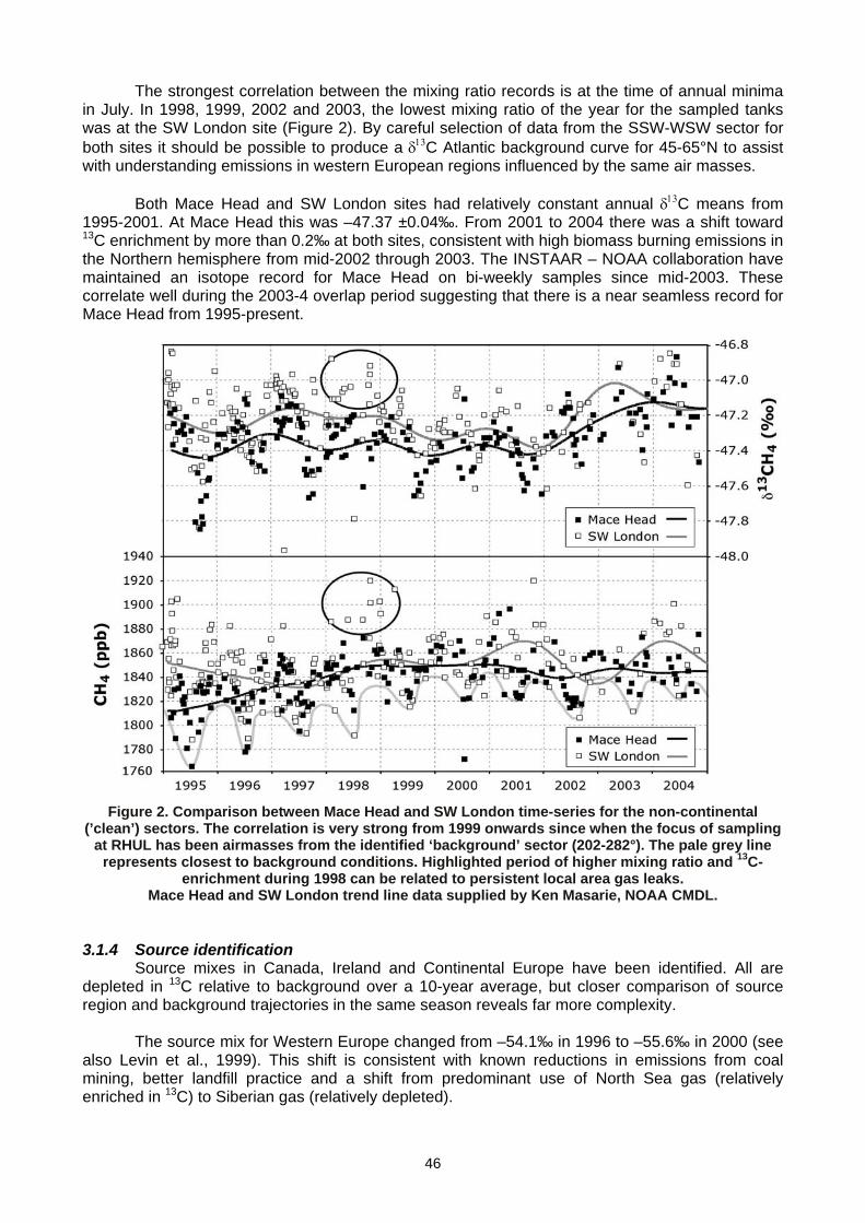
46

The strongest correlation between the mixing ratio records is at the time of annual minima in July. In 1998, 1999, 2002 and 2003, the lowest mixing ratio of the year for the sampled tanks was at the SW London site (Figure 2). By careful selection of data from the SSW-WSW sector for both sites it should be possible to produce a δ13C Atlantic background curve for 45-65°N to assist with understanding emissions in western European regions influenced by the same air masses.

Both Mace Head and SW London sites had relatively constant annual δ13C means from

1995-2001. At Mace Head this was –47.37 ±0.04‰. From 2001 to 2004 there was a shift toward 13C enrichment by more than 0.2‰ at both sites, consistent with high biomass burning emissions in the Northern hemisphere from mid-2002 through 2003. The INSTAAR – NOAA collaboration have maintained an isotope record for Mace Head on bi-weekly samples since mid-2003. These correlate well during the 2003-4 overlap period suggesting that there is a near seamless record for Mace Head from 1995-present.

Figure 2. Comparison between Mace Head and SW London time-series for the non-continental

(’clean’) sectors. The correlation is very strong from 1999 onwards since when the focus of sampling at RHUL has been airmasses from the identified ‘background’ sector (202-282°). The pale grey line

represents closest to background conditions. Highlighted period of higher mixing ratio and 13C-enrichment during 1998 can be related to persistent local area gas leaks.

Mace Head and SW London trend line data supplied by Ken Masarie, NOAA CMDL. 3.1.4 Source identification

Source mixes in Canada, Ireland and Continental Europe have been identified. All are depleted in 13C relative to background over a 10-year average, but closer comparison of source region and background trajectories in the same season reveals far more complexity.

The source mix for Western Europe changed from –54.1‰ in 1996 to –55.6‰ in 2000 (see

also Levin et al., 1999). This shift is consistent with known reductions in emissions from coal mining, better landfill practice and a shift from predominant use of North Sea gas (relatively enriched in 13C) to Siberian gas (relatively depleted).

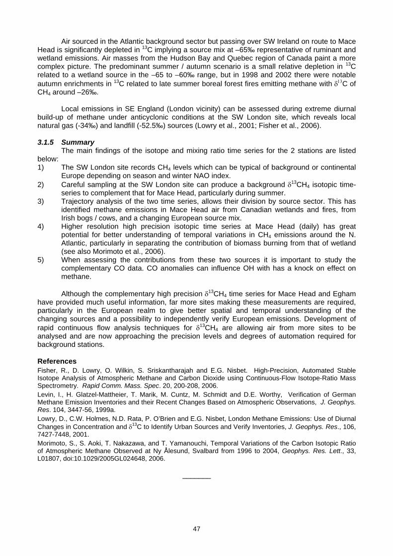
47

Air sourced in the Atlantic background sector but passing over SW Ireland on route to Mace Head is significantly depleted in 13C implying a source mix at –65‰ representative of ruminant and wetland emissions. Air masses from the Hudson Bay and Quebec region of Canada paint a more complex picture. The predominant summer / autumn scenario is a small relative depletion in 13C related to a wetland source in the –65 to –60‰ range, but in 1998 and 2002 there were notable autumn enrichments in 13C related to late summer boreal forest fires emitting methane with δ13C of CH4 around –26‰.

Local emissions in SE England (London vicinity) can be assessed during extreme diurnal

build-up of methane under anticyclonic conditions at the SW London site, which reveals local natural gas (-34‰) and landfill (-52.5‰) sources (Lowry et al., 2001; Fisher et al., 2006). 3.1.5 Summary

The main findings of the isotope and mixing ratio time series for the 2 stations are listed below: 1) The SW London site records CH4 levels which can be typical of background or continental

Europe depending on season and winter NAO index. 2) Careful sampling at the SW London site can produce a background δ13CH4 isotopic time-

series to complement that for Mace Head, particularly during summer. 3) Trajectory analysis of the two time series, allows their division by source sector. This has

identified methane emissions in Mace Head air from Canadian wetlands and fires, from Irish bogs / cows, and a changing European source mix.

4) Higher resolution high precision isotopic time series at Mace Head (daily) has great potential for better understanding of temporal variations in CH4 emissions around the N. Atlantic, particularly in separating the contribution of biomass burning from that of wetland (see also Morimoto et al., 2006).

5) When assessing the contributions from these two sources it is important to study the complementary CO data. CO anomalies can influence OH with has a knock on effect on methane. Although the complementary high precision δ13CH4 time series for Mace Head and Egham

have provided much useful information, far more sites making these measurements are required, particularly in the European realm to give better spatial and temporal understanding of the changing sources and a possibility to independently verify European emissions. Development of rapid continuous flow analysis techniques for δ13CH4 are allowing air from more sites to be analysed and are now approaching the precision levels and degrees of automation required for background stations. References Fisher, R., D. Lowry, O. Wilkin, S. Sriskantharajah and E.G. Nisbet. High-Precision, Automated Stable Isotope Analysis of Atmospheric Methane and Carbon Dioxide using Continuous-Flow Isotope-Ratio Mass Spectrometry. Rapid Comm. Mass. Spec. 20, 200-208, 2006. Levin, I., H. Glatzel-Mattheier, T. Marik, M. Cuntz, M. Schmidt and D.E. Worthy, Verification of German Methane Emission Inventories and their Recent Changes Based on Atmospheric Observations, J. Geophys. Res. 104, 3447-56, 1999a. Lowry, D., C.W. Holmes, N.D. Rata, P. O’Brien and E.G. Nisbet, London Methane Emissions: Use of Diurnal Changes in Concentration and δ13C to Identify Urban Sources and Verify Inventories, J. Geophys. Res., 106, 7427-7448, 2001. Morimoto, S., S. Aoki, T. Nakazawa, and T. Yamanouchi, Temporal Variations of the Carbon Isotopic Ratio of Atmospheric Methane Observed at Ny Ålesund, Svalbard from 1996 to 2004, Geophys. Res. Lett., 33, L01807, doi:10.1029/2005GL024648, 2006.

_______

48

3.2 Inter-Laboratory Calibration of CO2 Produced from NBS19 Calcite, Calibration Of Narcis-II, and CO2-Isotopes in Synthetic Air Willi. A. Brand*,a, Alina Chivulescu†, Lin Huang†, Hitoshi Mukai‡, Juergen M. Richter* and Michael Rothe* * MPI-BGC (Max-Planck-Institut für Biogeochemie), Postfach 10 01 64, D-07701 Jena, Germany † EC (Climate Research Division, Atmospheric Science & Technology Directorate/STB, Environment Canada), 4905 Dufferin St., Toronto, ON, Canada, ‡ NIES (Global Carbon Cycle Research Section, Center for Global Environmental Research, National Institute for Environmental Studies), 16-2 Onogawa, Tsukuba, Ibaraki 305 Japan

Abstract Starting from NBS19 calcite a number of CO2 preparations were made, distributed and

analysed in three laboratories. The results from the different types of preparations were compared to a common reference CO2, Narcis-II, which allowed us to study the isotopic variability of CO2 generated by the calcite acid digestion reaction.

The agreement for δ13C among our laboratories was within a standard error of ±0.003‰. For Narcis-II, a δ13CVPDB value of -1.923‰ was found. For δ18O, with the temperature dependence of the acid digestion reaction for calcites and the associated oxygen exchange with residual water, the agreement was less satisfying, with a maximum δ18O deviation of 0.13‰. In agreement with previous determinations a mean δ18OVPDB-CO2 value of -2.580‰ for Narcis-II was found which, however, requires further studies.

In a second series of experiments, larger amounts of CO2 were prepared from NBS19 at MPI-BGC, analysed for the resulting isotopic composition and then mixed into CO2-free air. The resulting artificial air samples then were analysed by the same three laboratories for the stable isotopic composition of CO2 using locally established extraction lines and protocols. Comparison of the results with the pure CO2 values revealed additional systematic differences in between our laboratories owing to the CO2 extraction process and to local data evaluation and standardization issues. For δ13C the results showed a rather narrow and satisfying range of deviations (±0.012‰). For δ18O, however, cumulative disagreements up to 0.11‰ were observed.

3.2.1 Introduction All carbon stable isotope ratio measurements must be reported on a common scale

formerly defined via a calcite material, PDB (‘Pee Dee Belemnite’)1. The exhaustion of the original material as well as homogeneity issues required a redefinition of the scale which resulted in the VPDB scale. This scale is based on the well characterized calcite material NBS19 which was prepared by Irving Friedman in 19822.

The origin of the VPDB scale has been set by defining a deviation of +1.95‰ (δ13C) and -2.2‰ (δ18O) for NBS193-5. These NBS19 isotope values defining the VPDB scale refer to the isotopic compositions of the elements in the calcite mineral. In order to perform a precise and accurate measurement a conversion step to transfer the isotope ratio information to a gaseous material is required. Usually, CO2 is liberated from the calcite material via reaction with ortho-phosphoric acid under well controlled experimental conditions6-9.

For air-CO2, a (cryogenic) extraction step is necessary to produce pure CO2 (+ N2O) which then is compared with the CO2 from the reference calcite for obtaining δ13CVPDB and δ18OVPDB-CO2. During cryogenic extraction, a number of small experimental effects like trapping efficiency, fractionation upon thawing, co-trapping of traces of air etc. can lead to substantial errors in isotopic determination when comparison is made to a clean CO2 gas as the primary reference10. It has therefore been recognized that for highest precision analysis and consistency in long term records comparison should be made to an air reference gas which goes through the same preparation a Author, to whom correspondence should be addressed: wbrand@bgc-jena.mpg.de

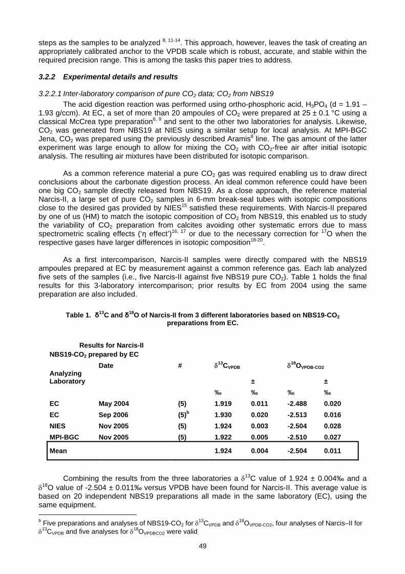
49

steps as the samples to be analyzed 8, 11-14. This approach, however, leaves the task of creating an appropriately calibrated anchor to the VPDB scale which is robust, accurate, and stable within the required precision range. This is among the tasks this paper tries to address.

3.2.2 Experimental details and results

3.2.2.1 Inter-laboratory comparison of pure CO2 data; CO2 from NBS19 The acid digestion reaction was performed using ortho-phosphoric acid, H3PO4 (d = 1.91 –

1.93 g/ccm). At EC, a set of more than 20 ampoules of CO2 were prepared at 25 ± 0.1 °C using a classical McCrea type preparation6, 9 and sent to the other two laboratories for analysis. Likewise, CO2 was generated from NBS19 at NIES using a similar setup for local analysis. At MPI-BGC Jena, CO2 was prepared using the previously described Aramis8 line. The gas amount of the latter experiment was large enough to allow for mixing the CO2 with CO2-free air after initial isotopic analysis. The resulting air mixtures have been distributed for isotopic comparison.

As a common reference material a pure CO2 gas was required enabling us to draw direct conclusions about the carbonate digestion process. An ideal common reference could have been one big CO2 sample directly released from NBS19. As a close approach, the reference material Narcis-II, a large set of pure CO2 samples in 6-mm break-seal tubes with isotopic compositions close to the desired gas provided by NIES15 satisfied these requirements. With Narcis-II prepared by one of us (HM) to match the isotopic composition of CO2 from NBS19, this enabled us to study the variability of CO2 preparation from calcites avoiding other systematic errors due to mass spectrometric scaling effects (‘η effect’)16, 17 or due to the necessary correction for 17O when the respective gases have larger differences in isotopic composition18-20.

As a first intercomparison, Narcis-II samples were directly compared with the NBS19 ampoules prepared at EC by measurement against a common reference gas. Each lab analyzed five sets of the samples (i.e., five Narcis-II against five NBS19 pure CO2). Table 1 holds the final results for this 3-laboratory intercomparison; prior results by EC from 2004 using the same preparation are also included.

Table 1. δ13C and δ18O of Narcis-II from 3 different laboratories based on NBS19-CO2

preparations from EC.

Results for Narcis-II NBS19-CO2 prepared by EC Date # δ13CVPDB δ18OVPDB-CO2 Analyzing Laboratory ± ± ‰ ‰ ‰ ‰ EC May 2004 (5) 1.919 0.011 -2.488 0.020 EC Sep 2006 (5)b 1.930 0.020 -2.513 0.016 NIES Nov 2005 (5) 1.924 0.003 -2.504 0.028 MPI-BGC Nov 2005 (5) 1.922 0.005 -2.510 0.027

Mean 1.924 0.004 -2.504 0.011

Combining the results from the three laboratories a δ13C value of 1.924 ± 0.004‰ and a δ18O value of -2.504 ± 0.011‰ versus VPDB have been found for Narcis-II. This average value is based on 20 independent NBS19 preparations all made in the same laboratory (EC), using the same equipment. b Five preparations and analyses of NBS19-CO2 for δ13CVPDB and δ18OVPDB-CO2, four analyses of Narcis–II for δ13CVPDB and five analyses for δ18OVPDBCO2 were valid.

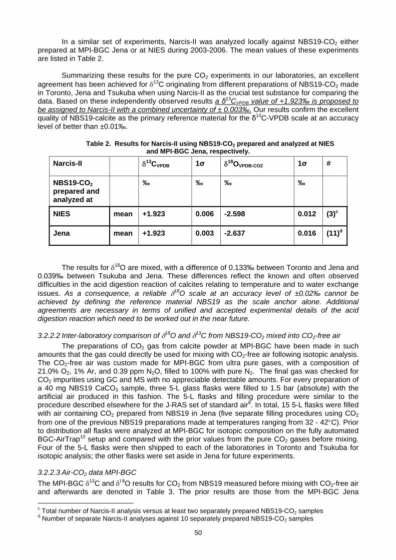
50

In a similar set of experiments, Narcis-II was analyzed locally against NBS19-CO2 either prepared at MPI-BGC Jena or at NIES during 2003-2006. The mean values of these experiments are listed in Table 2.

Summarizing these results for the pure CO2 experiments in our laboratories, an excellent agreement has been achieved for δ13C originating from different preparations of NBS19-CO2 made in Toronto, Jena and Tsukuba when using Narcis-II as the crucial test substance for comparing the data. Based on these independently observed results a δ13CVPDB value of +1.923‰ is proposed to be assigned to Narcis-II with a combined uncertainty of ± 0.003‰. Our results confirm the excellent quality of NBS19-calcite as the primary reference material for the δ13C-VPDB scale at an accuracy level of better than ±0.01‰.

Table 2. Results for Narcis-II using NBS19-CO2 prepared and analyzed at NIES

and MPI-BGC Jena, respectively.

Narcis-II δ13CVPDB 1σ δ18OVPDB-CO2 1σ #

NBS19-CO2 prepared and analyzed at

‰ ‰ ‰ ‰

NIES mean +1.923 0.006 -2.598 0.012 (3)c

Jena mean +1.923 0.003 -2.637 0.016 (11)d

The results for δ18O are mixed, with a difference of 0.133‰ between Toronto and Jena and 0.039‰ between Tsukuba and Jena. These differences reflect the known and often observed difficulties in the acid digestion reaction of calcites relating to temperature and to water exchange issues. As a consequence, a reliable δ18O scale at an accuracy level of ±0.02‰ cannot be achieved by defining the reference material NBS19 as the scale anchor alone. Additional agreements are necessary in terms of unified and accepted experimental details of the acid digestion reaction which need to be worked out in the near future.

3.2.2.2 Inter-laboratory comparison of δ18O and δ13C from NBS19-CO2 mixed into CO2-free air The preparations of CO2 gas from calcite powder at MPI-BGC have been made in such

amounts that the gas could directly be used for mixing with CO2-free air following isotopic analysis. The CO2-free air was custom made for MPI-BGC from ultra pure gases, with a composition of 21.0% O2, 1% Ar, and 0.39 ppm N2O, filled to 100% with pure N2. The final gas was checked for CO2 impurities using GC and MS with no appreciable detectable amounts. For every preparation of a 40 mg NBS19 CaCO3 sample, three 5-L glass flasks were filled to 1.5 bar (absolute) with the artificial air produced in this fashion. The 5-L flasks and filling procedure were similar to the procedure described elsewhere for the J-RAS set of standard air8. In total, 15 5-L flasks were filled with air containing CO2 prepared from NBS19 in Jena (five separate filling procedures using CO2 from one of the previous NBS19 preparations made at temperatures ranging from 32 - 42°C). Prior to distribution all flasks were analyzed at MPI-BGC for isotopic composition on the fully automated BGC-AirTrap10 setup and compared with the prior values from the pure CO2 gases before mixing. Four of the 5-L flasks were then shipped to each of the laboratories in Toronto and Tsukuba for isotopic analysis; the other flasks were set aside in Jena for future experiments.

3.2.2.3 Air-CO2 data MPI-BGC The MPI-BGC δ13C and δ18O results for CO2 from NBS19 measured before mixing with CO2-free air and afterwards are denoted in Table 3. The prior results are those from the MPI-BGC Jena c Total number of Narcis-II analysis versus at least two separately prepared NBS19-CO2 samples d Number of separate Narcis-II analyses against 10 separately prepared NBS19-CO2 samples

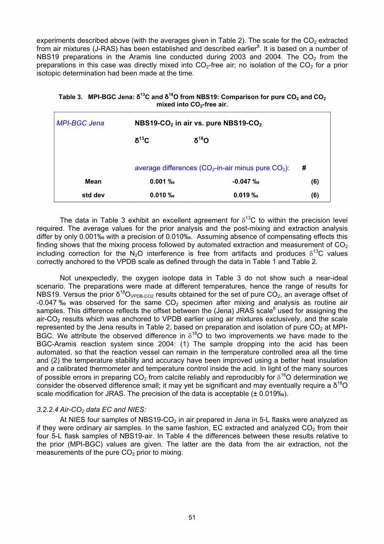
51

experiments described above (with the averages given in Table 2). The scale for the CO2 extracted from air mixtures (J-RAS) has been established and described earlier8. It is based on a number of NBS19 preparations in the Aramis line conducted during 2003 and 2004. The CO2 from the preparations in this case was directly mixed into CO2-free air; no isolation of the CO2 for a prior isotopic determination had been made at the time.

Table 3. MPI-BGC Jena: δ13C and δ18O from NBS19: Comparison for pure CO2 and CO2

mixed into CO2-free air.

MPI-BGC Jena NBS19-CO2 in air vs. pure NBS19-CO2

δ13C δ18O

average differences (CO2-in-air minus pure CO2): #

Mean 0.001 ‰ -0.047 ‰ (6)

std dev 0.010 ‰ 0.019 ‰ (6)

The data in Table 3 exhibit an excellent agreement for δ13C to within the precision level required. The average values for the prior analysis and the post-mixing and extraction analysis differ by only 0.001‰ with a precision of 0.010‰. Assuming absence of compensating effects this finding shows that the mixing process followed by automated extraction and measurement of CO2 including correction for the N2O interference is free from artifacts and produces δ13C values correctly anchored to the VPDB scale as defined through the data in Table 1 and Table 2.

Not unexpectedly, the oxygen isotope data in Table 3 do not show such a near-ideal scenario. The preparations were made at different temperatures, hence the range of results for NBS19. Versus the prior δ18OVPDB-CO2 results obtained for the set of pure CO2, an average offset of -0.047 ‰ was observed for the same CO2 specimen after mixing and analysis as routine air samples. This difference reflects the offset between the (Jena) JRAS scale8 used for assigning the air-CO2 results which was anchored to VPDB earlier using air mixtures exclusively, and the scale represented by the Jena results in Table 2, based on preparation and isolation of pure CO2 at MPI-BGC. We attribute the observed difference in δ18O to two improvements we have made to the BGC-Aramis reaction system since 2004: (1) The sample dropping into the acid has been automated, so that the reaction vessel can remain in the temperature controlled area all the time and (2) the temperature stability and accuracy have been improved using a better heat insulation and a calibrated thermometer and temperature control inside the acid. In light of the many sources of possible errors in preparing CO2 from calcite reliably and reproducibly for δ18O determination we consider the observed difference small; it may yet be significant and may eventually require a δ18O scale modification for JRAS. The precision of the data is acceptable (± 0.019‰).

3.2.2.4 Air-CO2 data EC and NIES: At NIES four samples of NBS19-CO2 in air prepared in Jena in 5-L flasks were analyzed as

if they were ordinary air samples. In the same fashion, EC extracted and analyzed CO2 from their four 5-L flask samples of NBS19-air. In Table 4 the differences between these results relative to the prior (MPI-BGC) values are given. The latter are the data from the air extraction, not the measurements of the pure CO2 prior to mixing.

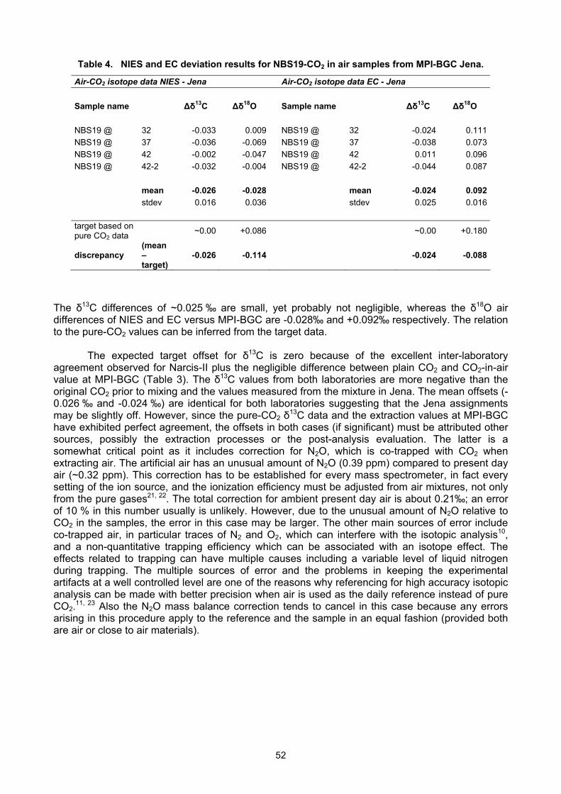
52

Table 4. NIES and EC deviation results for NBS19-CO2 in air samples from MPI-BGC Jena.

Air-CO2 isotope data NIES - Jena Air-CO2 isotope data EC - Jena Sample name Δδ13C Δδ18O Sample name Δδ13C Δδ18O NBS19 @ 32 -0.033 0.009 NBS19 @ 32 -0.024 0.111NBS19 @ 37 -0.036 -0.069 NBS19 @ 37 -0.038 0.073NBS19 @ 42 -0.002 -0.047 NBS19 @ 42 0.011 0.096NBS19 @ 42-2 -0.032 -0.004 NBS19 @ 42-2 -0.044 0.087 mean -0.026 -0.028 mean -0.024 0.092 stdev 0.016 0.036 stdev 0.025 0.016 target based on pure CO2 data ~0.00 +0.086 ~0.00 +0.180

discrepancy (mean –target)

-0.026 -0.114 -0.024 -0.088

The δ13C differences of ~0.025 ‰ are small, yet probably not negligible, whereas the δ18O air differences of NIES and EC versus MPI-BGC are -0.028‰ and +0.092‰ respectively. The relation to the pure-CO2 values can be inferred from the target data.

The expected target offset for δ13C is zero because of the excellent inter-laboratory agreement observed for Narcis-II plus the negligible difference between plain CO2 and CO2-in-air value at MPI-BGC (Table 3). The δ13C values from both laboratories are more negative than the original CO2 prior to mixing and the values measured from the mixture in Jena. The mean offsets (-0.026 ‰ and -0.024 ‰) are identical for both laboratories suggesting that the Jena assignments may be slightly off. However, since the pure-CO2 δ13C data and the extraction values at MPI-BGC have exhibited perfect agreement, the offsets in both cases (if significant) must be attributed other sources, possibly the extraction processes or the post-analysis evaluation. The latter is a somewhat critical point as it includes correction for N2O, which is co-trapped with CO2 when extracting air. The artificial air has an unusual amount of N2O (0.39 ppm) compared to present day air (~0.32 ppm). This correction has to be established for every mass spectrometer, in fact every setting of the ion source, and the ionization efficiency must be adjusted from air mixtures, not only from the pure gases21, 22. The total correction for ambient present day air is about 0.21‰; an error of 10 % in this number usually is unlikely. However, due to the unusual amount of N2O relative to CO2 in the samples, the error in this case may be larger. The other main sources of error include co-trapped air, in particular traces of N2 and O2, which can interfere with the isotopic analysis10, and a non-quantitative trapping efficiency which can be associated with an isotope effect. The effects related to trapping can have multiple causes including a variable level of liquid nitrogen during trapping. The multiple sources of error and the problems in keeping the experimental artifacts at a well controlled level are one of the reasons why referencing for high accuracy isotopic analysis can be made with better precision when air is used as the daily reference instead of pure CO2.11, 23 Also the N2O mass balance correction tends to cancel in this case because any errors arising in this procedure apply to the reference and the sample in an equal fashion (provided both are air or close to air materials).

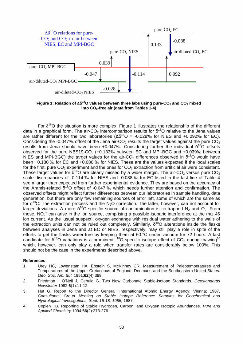
53

For δ18O the situation is more complex. Figure 1 illustrates the relationship of the different

data in a graphical form. The air-CO2 intercomparison results for δ18O relative to the Jena values are rather different for the two laboratories (Δδ18O = -0.028‰ for NIES and +0.092‰ for EC). Considering the -0.047‰ offset of the Jena air-CO2 results the target values against the pure CO2 results from Jena should have been +0.047‰. Considering further the individual δ18O offsets observed for the pure NBS19-CO2 (+0.133‰ between EC and MPI-BGC and +0.039‰ between NIES and MPI-BGC) the target values for the air-CO2 differences observed in δ18O would have been +0.180 ‰ for EC and +0.086 ‰ for NIES. These are the values expected if the local scales for the first, pure CO2 experiment and the ones for CO2 extraction from artificial air were consistent. These target values for δ18O are clearly missed by a wider margin. The air-CO2 versus pure CO2 scale discrepancies of -0.114 ‰ for NIES and -0.088 ‰ for EC listed in the last line of Table 4 seem larger than expected from further experimental evidence. They are based on the accuracy of the Aramis-related δ18O offset of -0.047 ‰ which needs further attention and confirmation. The observed offsets might reflect further differences between our laboratories in sample handling, data generation, but there are only few remaining sources of error left, some of which are the same as for δ13C: The extraction process and the N2O correction. The latter, however, can not account for larger deviations. A more δ18O-specific source of contamination is co-trapped N2 and O2. From these, NO2

+ can arise in the ion source, comprising a possible isobaric interference at the m/z 46 ion current. As the ‘usual suspect’, oxygen exchange with residual water adhering to the walls of the extraction units can not be ruled out completely. Similarly, δ18O alterations inside the flasks between analyses in Jena and at EC or NIES, respectively, may still play a role in spite of the efforts to get the flasks water-free by keeping them at 60 °C under vacuum for 72 hours. A last candidate for δ18O variations is a prominent, 18O-specific isotope effect of CO2 during thawing10 which, however, can only play a role when transfer rates are considerably below 100%. This should not be the case in the experiments described above. References 1. Urey HC, Lowenstam HA, Epstein S, McKinney CR. Measurement of Paleotemperatures and

Temperatures of the Upper Cretaceous of England, Denmark, and the Southeastern United-States. Geo. Soc. Am. Bul. 1951;62(4):399.

2. Friedman I, O'Neil J, Cebula G. Two New Carbonate Stable-Isotope Standards. Geostandards Newsletter 1982;6(1):11-12.

3. Hut G. Report to the Director General; International Atomic Energy Agency: Vienna; 1987. Consultants' Group Meeting on Stable Isotope Reference Samples for Geochemical and Hydrological Investigations, Sept. 16-18, 1985, 1987.

4. Coplen TB. Reporting of Stable Hydrogen, Carbon, and Oxygen Isotopic Abundances. Pure and Applied Chemistry 1994;66(2):273-276.

-0.088 0.133

air-diluted-CO2 MPI-BGC -0.047

air-diluted-CO2 NIES -0.028

pure-CO2 NIES

0.039

-0.114

pure-CO2 EC

air-diluted-CO2 EC

0.092 pure-CO2 MPI-BGC

Figure 1: Relation of Δδ18O values between three labs using pure-CO2 and CO2 mixed into CO2-free air (data from Tables 1-4)

Δδ18O relations for pure-CO2 and CO2-in-air between

NIES, EC and MPI-BGC

54

5. Coplen TB, Kendall C, Hopple J. Comparison of Stable Isotope Reference Samples. Nature 1983;302(5905):236-238.

6. McCrea JM. On the Isotopic Chemistry of Carbonates and a Paleotemperature Scale. Journal of Chemical Physics 1950;18(6):849-857.

7. Swart PK, Burns SJ, Leder JJ. Fractionation of the Stable Isotopes of Oxygen and Carbon in Carbon-Dioxide During the Reaction of Calcite with Phosphoric-Acid as a Function of Temperature and Technique. Chem. Geol. 1991;86(2):89-96.

8. Ghosh P, Patecki M, Rothe M, Brand WA. Calcite-CO2 Mixed intoCO(2)-Free Air: a New CO2-in-Air Stable Isotope Reference Material for the VPDB Scale. Rapid Commun. Mass Spectrom. 2005;19(8):1097-1119.

9. Huang L, Chivulescu A, Ernst D. Traceability Maintenance of High Precision Isotope Measurements in Atmospheric CO2: Uncertainty, Challenges & Recommendations. GAW series 2008; (in this issue).

10. Werner RA, Rothe M, Brand WA. Extraction of CO2 from Air Samples for Isotopic Analysis and Limits to Ultra High Precision Delta O-18 Determination in CO2 Gas. Rapid Commun. Mass Spectrom. 2001;15(22):2152-2167.

11. Allison CE, Francey RJ, White JWC, Vaughn B, Wahlen M, Bollenbacher A, Nakazawa T. What Have we Learnt about Stable Isotope Measurements from IAEA CLASSIC. Proceedings of the 11th WMO/IAEA Meeting of CO2 Experts, Tokyo 2001; WMO/GAW publication series 2003;148:17-30.

12. Francey RJ, Steele LP. Measuring Atmospheric Carbon Dioxide - the Calibration Challenge. Accreditation and Quality Assurance 2003;8(5):200-204.

13. Ghosh P, Brand WA. Isotopic analysis of CO2 in air samples: Requirements for a New CO2 in-Air Standard and Preparation of an Air-CO2 Reference Mixture from Calcite Material. In: Worthy D, Huang L, eds. 12th IAEA/WMO Meeting of CO2 Experts. Vol WMO-GAW Report 161. Toronto, 2003:50-57.

14. Werner RA, Brand WA. Referencing Strategies and Techniques in Stable Isotope Ratio Analysis. Rapid Commun. Mass Spectrom. 2001;15(7):501-519.

15. Mukai H. Intercomparison of Isotope Ratios for CO2 Using Several Reference Materials. In: Worthy D, Huang L, eds. 12th IAEA/WMO Meeting of CO2 Experts. Vol WMO-GAW Report 161. Toronto, 2003: 58-63.

16. Verkouteren RM, Allison CE, Studley SA, Leckrone KJ. Isotopic Metrology of Carbon Dioxide. I. IIterlaboratory Comparison and Empirical Modeling of Inlet Equilibration Time, Inlet Pressure, and Ion Source Conductance. Rapid Commun. Mass Spectrom. 2003;17(8):771-776.

17. Verkouteren RM, Assonov S, Klinedinst DB, Brand WA. Isotopic Metrology of Carbon Dioxide. II. Effects of Ion Source Materials, Conductance, Emission, and Accelerating Voltage on Dual-inlet Cross Contamination. Rapid Commun. Mass Spectrom. 2003;17(8):777-782.

18. Craig H. Isotopic Standards for Carbon and Oxygen and Correction Factors for Mass-Spectrometric Analysis of Carbon Dioxide. Geochim. Cosmochim. Acta 1957;12(1-2):133-149.

19. Assonov SS, Brenninkmeijer CAM. On the O-17 Correction for CO2 Mass Spectrometric Isotopic analysis. Rapid Commun. Mass Spectrom. 2003;17(10):1007-1016.

20. Brand WA, Coplen TB, Assonov SA. Correction for the d17O Interference in d13C Measurements when Analyzing CO2 with Stable Isotope Mass Spectrometry. Pure and Applied Chemistry 2008;xx(yy):zz.

21. Ghosh P, Brand WA. The effect of N2O on the Isotopic Composition of Air-CO2 Samples. Rapid Commun. Mass Spectrom. 2004;18(16):1830-1838.

22. Sirignano C, Neubert REM, Meijer HAJ. N2O Influence on Isotopic Measurements of Atmospheric CO2. Rapid Commun. Mass Spectrom. 2004;18(16):1839-1846.

23. Allison CE, Francey RJ. Verifying Southern Hemisphere trends in Atmospheric Carbon Dioxide Stable Isotopes. J. Geophys. Res.-Atmos. 2007;112(D21).

_______

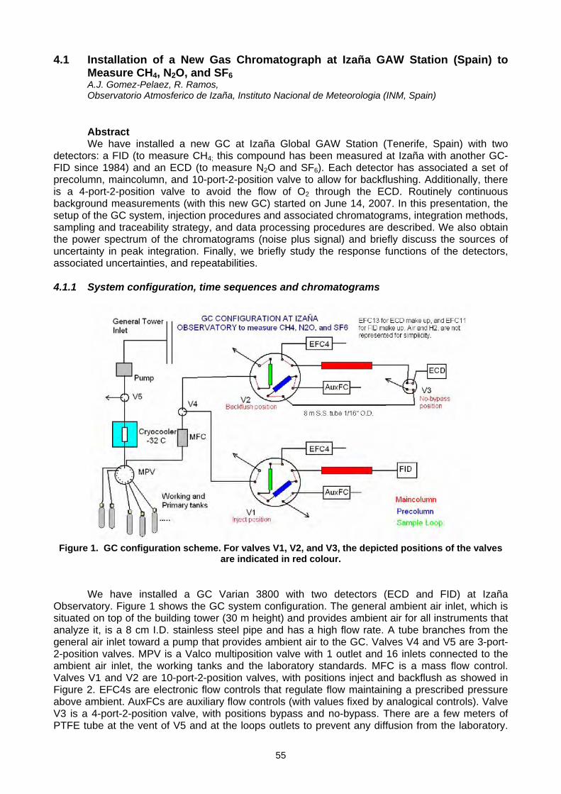
55

4.1 Installation of a New Gas Chromatograph at Izaña GAW Station (Spain) to Measure CH4, N2O, and SF6 A.J. Gomez-Pelaez, R. Ramos, Observatorio Atmosferico de Izaña, Instituto Nacional de Meteorologia (INM, Spain)

Abstract We have installed a new GC at Izaña Global GAW Station (Tenerife, Spain) with two

detectors: a FID (to measure CH4; this compound has been measured at Izaña with another GC-FID since 1984) and an ECD (to measure N2O and SF6). Each detector has associated a set of precolumn, maincolumn, and 10-port-2-position valve to allow for backflushing. Additionally, there is a 4-port-2-position valve to avoid the flow of O2 through the ECD. Routinely continuous background measurements (with this new GC) started on June 14, 2007. In this presentation, the setup of the GC system, injection procedures and associated chromatograms, integration methods, sampling and traceability strategy, and data processing procedures are described. We also obtain the power spectrum of the chromatograms (noise plus signal) and briefly discuss the sources of uncertainty in peak integration. Finally, we briefly study the response functions of the detectors, associated uncertainties, and repeatabilities. 4.1.1 System configuration, time sequences and chromatograms

Figure 1. GC configuration scheme. For valves V1, V2, and V3, the depicted positions of the valves

are indicated in red colour.

We have installed a GC Varian 3800 with two detectors (ECD and FID) at Izaña

Observatory. Figure 1 shows the GC system configuration. The general ambient air inlet, which is situated on top of the building tower (30 m height) and provides ambient air for all instruments that analyze it, is a 8 cm I.D. stainless steel pipe and has a high flow rate. A tube branches from the general air inlet toward a pump that provides ambient air to the GC. Valves V4 and V5 are 3-port-2-position valves. MPV is a Valco multiposition valve with 1 outlet and 16 inlets connected to the ambient air inlet, the working tanks and the laboratory standards. MFC is a mass flow control. Valves V1 and V2 are 10-port-2-position valves, with positions inject and backflush as showed in Figure 2. EFC4s are electronic flow controls that regulate flow maintaining a prescribed pressure above ambient. AuxFCs are auxiliary flow controls (with values fixed by analogical controls). Valve V3 is a 4-port-2-position valve, with positions bypass and no-bypass. There are a few meters of PTFE tube at the vent of V5 and at the loops outlets to prevent any diffusion from the laboratory.

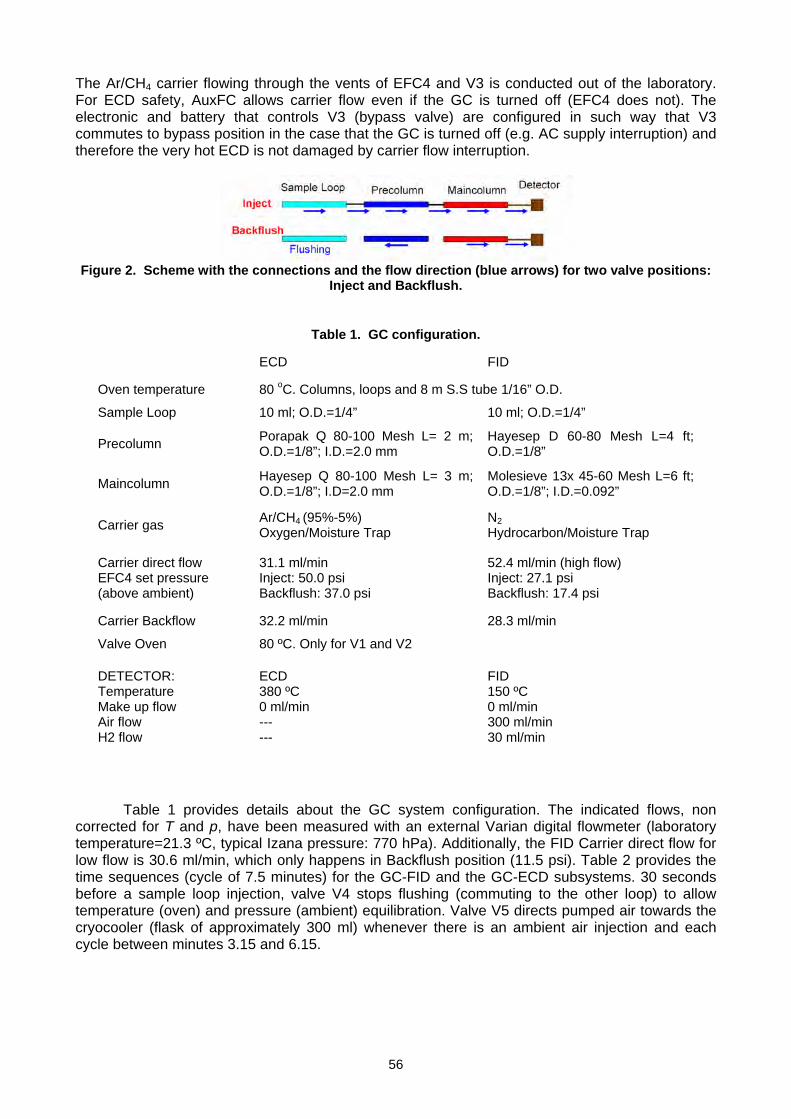
56

The Ar/CH4 carrier flowing through the vents of EFC4 and V3 is conducted out of the laboratory. For ECD safety, AuxFC allows carrier flow even if the GC is turned off (EFC4 does not). The electronic and battery that controls V3 (bypass valve) are configured in such way that V3 commutes to bypass position in the case that the GC is turned off (e.g. AC supply interruption) and therefore the very hot ECD is not damaged by carrier flow interruption.

Figure 2. Scheme with the connections and the flow direction (blue arrows) for two valve positions:

Inject and Backflush.

Table 1. GC configuration.

ECD FID

Oven temperature 80 oC. Columns, loops and 8 m S.S tube 1/16” O.D.

Sample Loop 10 ml; O.D.=1/4” 10 ml; O.D.=1/4”

Precolumn Porapak Q 80-100 Mesh L= 2 m; O.D.=1/8”; I.D.=2.0 mm

Hayesep D 60-80 Mesh L=4 ft; O.D.=1/8”

Maincolumn Hayesep Q 80-100 Mesh L= 3 m; O.D.=1/8”; I.D=2.0 mm

Molesieve 13x 45-60 Mesh L=6 ft; O.D.=1/8”; I.D.=0.092”

Carrier gas Ar/CH4 (95%-5%) Oxygen/Moisture Trap

N2 Hydrocarbon/Moisture Trap

Carrier direct flow EFC4 set pressure (above ambient)

31.1 ml/min Inject: 50.0 psi Backflush: 37.0 psi

52.4 ml/min (high flow) Inject: 27.1 psi Backflush: 17.4 psi

Carrier Backflow 32.2 ml/min 28.3 ml/min

Valve Oven 80 ºC. Only for V1 and V2

DETECTOR: Temperature Make up flow Air flow H2 flow

ECD 380 ºC 0 ml/min --- ---

FID 150 ºC 0 ml/min 300 ml/min 30 ml/min

Table 1 provides details about the GC system configuration. The indicated flows, non corrected for T and p, have been measured with an external Varian digital flowmeter (laboratory temperature=21.3 ºC, typical Izana pressure: 770 hPa). Additionally, the FID Carrier direct flow for low flow is 30.6 ml/min, which only happens in Backflush position (11.5 psi). Table 2 provides the time sequences (cycle of 7.5 minutes) for the GC-FID and the GC-ECD subsystems. 30 seconds before a sample loop injection, valve V4 stops flushing (commuting to the other loop) to allow temperature (oven) and pressure (ambient) equilibration. Valve V5 directs pumped air towards the cryocooler (flask of approximately 300 ml) whenever there is an ambient air injection and each cycle between minutes 3.15 and 6.15.

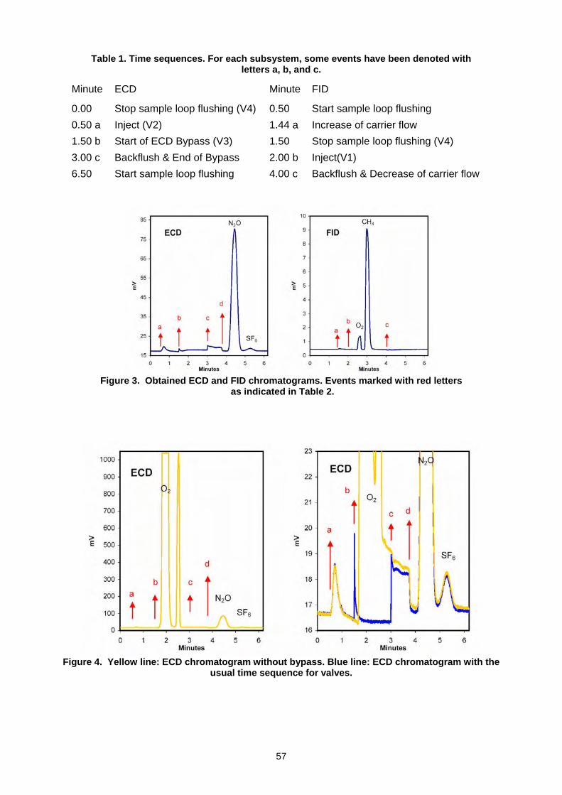
57

Table 1. Time sequences. For each subsystem, some events have been denoted with letters a, b, and c.

Minute ECD Minute FID

0.00 Stop sample loop flushing (V4) 0.50 Start sample loop flushing 0.50 a Inject (V2) 1.44 a Increase of carrier flow 1.50 b Start of ECD Bypass (V3) 1.50 Stop sample loop flushing (V4) 3.00 c Backflush & End of Bypass 2.00 b Inject(V1) 6.50 Start sample loop flushing 4.00 c Backflush & Decrease of carrier flow

Figure 3. Obtained ECD and FID chromatograms. Events marked with red letters

as indicated in Table 2.

Figure 4. Yellow line: ECD chromatogram without bypass. Blue line: ECD chromatogram with the

usual time sequence for valves.

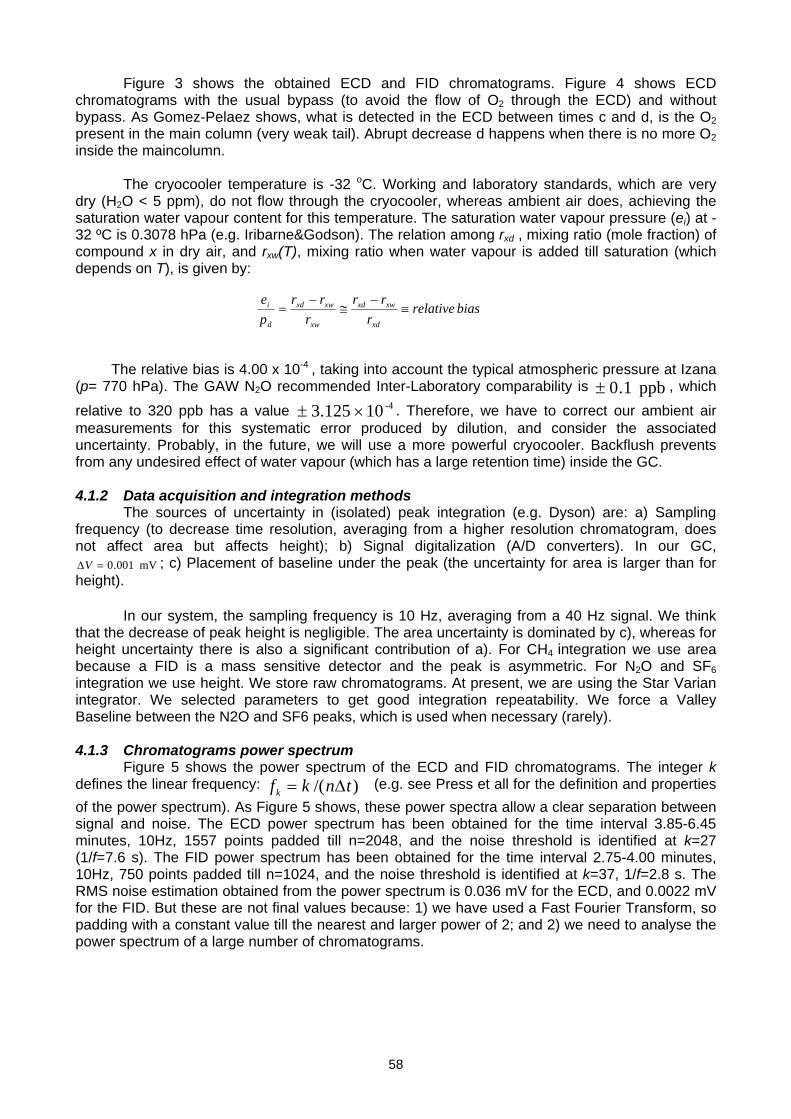
58

Figure 3 shows the obtained ECD and FID chromatograms. Figure 4 shows ECD chromatograms with the usual bypass (to avoid the flow of O2 through the ECD) and without bypass. As Gomez-Pelaez shows, what is detected in the ECD between times c and d, is the O2 present in the main column (very weak tail). Abrupt decrease d happens when there is no more O2 inside the maincolumn.

The cryocooler temperature is -32 oC. Working and laboratory standards, which are very dry (H2O < 5 ppm), do not flow through the cryocooler, whereas ambient air does, achieving the saturation water vapour content for this temperature. The saturation water vapour pressure (ei) at -32 ºC is 0.3078 hPa (e.g. Iribarne&Godson). The relation among rxd , mixing ratio (mole fraction) of compound x in dry air, and rxw(T), mixing ratio when water vapour is added till saturation (which depends on T), is given by:

The relative bias is 4.00 x 10-4 , taking into account the typical atmospheric pressure at Izana

(p= 770 hPa). The GAW N2O recommended Inter-Laboratory comparability is ppb 1.0± , which

relative to 320 ppb has a value -4103.125 ×± . Therefore, we have to correct our ambient air measurements for this systematic error produced by dilution, and consider the associated uncertainty. Probably, in the future, we will use a more powerful cryocooler. Backflush prevents from any undesired effect of water vapour (which has a large retention time) inside the GC. 4.1.2 Data acquisition and integration methods

The sources of uncertainty in (isolated) peak integration (e.g. Dyson) are: a) Sampling frequency (to decrease time resolution, averaging from a higher resolution chromatogram, does not affect area but affects height); b) Signal digitalization (A/D converters). In our GC,

mV 001.0=ΔV ; c) Placement of baseline under the peak (the uncertainty for area is larger than for height).

In our system, the sampling frequency is 10 Hz, averaging from a 40 Hz signal. We think that the decrease of peak height is negligible. The area uncertainty is dominated by c), whereas for height uncertainty there is also a significant contribution of a). For CH4 integration we use area because a FID is a mass sensitive detector and the peak is asymmetric. For N2O and SF6 integration we use height. We store raw chromatograms. At present, we are using the Star Varian integrator. We selected parameters to get good integration repeatability. We force a Valley Baseline between the N2O and SF6 peaks, which is used when necessary (rarely). 4.1.3 Chromatograms power spectrum

Figure 5 shows the power spectrum of the ECD and FID chromatograms. The integer k defines the linear frequency: )/( tnkfk Δ= (e.g. see Press et all for the definition and properties of the power spectrum). As Figure 5 shows, these power spectra allow a clear separation between signal and noise. The ECD power spectrum has been obtained for the time interval 3.85-6.45 minutes, 10Hz, 1557 points padded till n=2048, and the noise threshold is identified at k=27 (1/f=7.6 s). The FID power spectrum has been obtained for the time interval 2.75-4.00 minutes, 10Hz, 750 points padded till n=1024, and the noise threshold is identified at k=37, 1/f=2.8 s. The RMS noise estimation obtained from the power spectrum is 0.036 mV for the ECD, and 0.0022 mV for the FID. But these are not final values because: 1) we have used a Fast Fourier Transform, so padding with a constant value till the nearest and larger power of 2; and 2) we need to analyse the power spectrum of a large number of chromatograms.

biasrelativer

rrr

rrpe

xd

xwxd

xw

xwxd

d

i ≡−

≅−

=

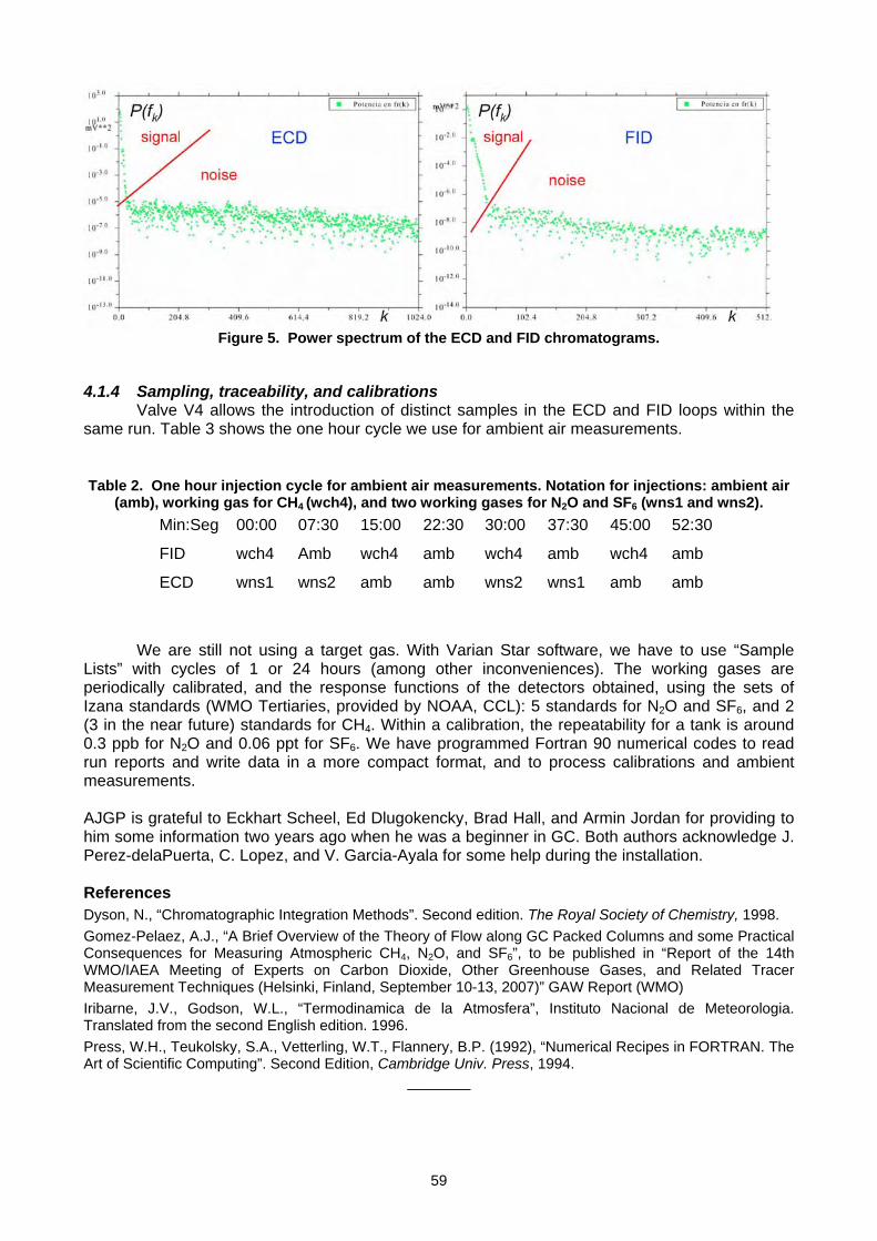
59

Figure 5. Power spectrum of the ECD and FID chromatograms.

4.1.4 Sampling, traceability, and calibrations

Valve V4 allows the introduction of distinct samples in the ECD and FID loops within the same run. Table 3 shows the one hour cycle we use for ambient air measurements. Table 2. One hour injection cycle for ambient air measurements. Notation for injections: ambient air

(amb), working gas for CH4 (wch4), and two working gases for N2O and SF6 (wns1 and wns2). Min:Seg 00:00 07:30 15:00 22:30 30:00 37:30 45:00 52:30

FID wch4 Amb wch4 amb wch4 amb wch4 amb

ECD wns1 wns2 amb amb wns2 wns1 amb amb

We are still not using a target gas. With Varian Star software, we have to use “Sample Lists” with cycles of 1 or 24 hours (among other inconveniences). The working gases are periodically calibrated, and the response functions of the detectors obtained, using the sets of Izana standards (WMO Tertiaries, provided by NOAA, CCL): 5 standards for N2O and SF6, and 2 (3 in the near future) standards for CH4. Within a calibration, the repeatability for a tank is around 0.3 ppb for N2O and 0.06 ppt for SF6. We have programmed Fortran 90 numerical codes to read run reports and write data in a more compact format, and to process calibrations and ambient measurements. AJGP is grateful to Eckhart Scheel, Ed Dlugokencky, Brad Hall, and Armin Jordan for providing to him some information two years ago when he was a beginner in GC. Both authors acknowledge J. Perez-delaPuerta, C. Lopez, and V. Garcia-Ayala for some help during the installation. References Dyson, N., “Chromatographic Integration Methods”. Second edition. The Royal Society of Chemistry, 1998. Gomez-Pelaez, A.J., “A Brief Overview of the Theory of Flow along GC Packed Columns and some Practical Consequences for Measuring Atmospheric CH4, N2O, and SF6”, to be published in “Report of the 14th WMO/IAEA Meeting of Experts on Carbon Dioxide, Other Greenhouse Gases, and Related Tracer Measurement Techniques (Helsinki, Finland, September 10-13, 2007)” GAW Report (WMO) Iribarne, J.V., Godson, W.L., “Termodinamica de la Atmosfera”, Instituto Nacional de Meteorologia. Translated from the second English edition. 1996. Press, W.H., Teukolsky, S.A., Vetterling, W.T., Flannery, B.P. (1992), “Numerical Recipes in FORTRAN. The Art of Scientific Computing”. Second Edition, Cambridge Univ. Press, 1994.

_______

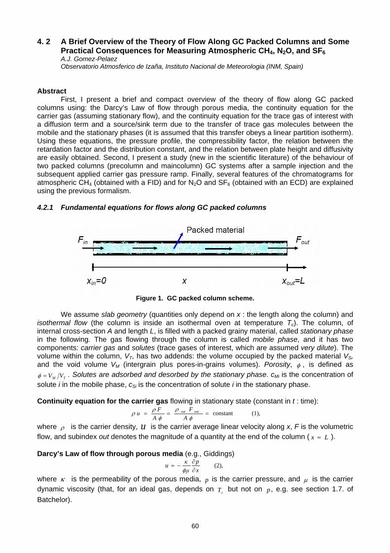
60

4. 2 A Brief Overview of the Theory of Flow Along GC Packed Columns and Some Practical Consequences for Measuring Atmospheric CH4, N2O, and SF6 A.J. Gomez-Pelaez Observatorio Atmosferico de Izaña, Instituto Nacional de Meteorologia (INM, Spain)

Abstract

First, I present a brief and compact overview of the theory of flow along GC packed columns using: the Darcy’s Law of flow through porous media, the continuity equation for the carrier gas (assuming stationary flow), and the continuity equation for the trace gas of interest with a diffusion term and a source/sink term due to the transfer of trace gas molecules between the mobile and the stationary phases (it is assumed that this transfer obeys a linear partition isotherm). Using these equations, the pressure profile, the compressibility factor, the relation between the retardation factor and the distribution constant, and the relation between plate height and diffusivity are easily obtained. Second, I present a study (new in the scientific literature) of the behaviour of two packed columns (precolumn and maincolumn) GC systems after a sample injection and the subsequent applied carrier gas pressure ramp. Finally, several features of the chromatograms for atmospheric CH4 (obtained with a FID) and for N2O and SF6 (obtained with an ECD) are explained using the previous formalism. 4.2.1 Fundamental equations for flows along GC packed columns

Figure 1. GC packed column scheme.

We assume slab geometry (quantities only depend on x : the length along the column) and

isothermal flow (the column is inside an isothermal oven at temperature Tc). The column, of internal cross-section A and length L, is filled with a packed grainy material, called stationary phase in the following. The gas flowing through the column is called mobile phase, and it has two components: carrier gas and solutes (trace gases of interest, which are assumed very dilute). The volume within the column, VT, has two addends: the volume occupied by the packed material VS, and the void volume VM (intergrain plus pores-in-grains volumes). Porosity, φ , is defined as

TM VV=φ . Solutes are adsorbed and desorbed by the stationary phase. cMi is the concentration of solute i in the mobile phase, cSi is the concentration of solute i in the stationary phase. Continuity equation for the carrier gas flowing in stationary state (constant in t : time):

(1), constant ===φ

ρφ

ρρA

FA

Fu outout

where ρ is the carrier density, u is the carrier average linear velocity along x, F is the volumetric flow, and subindex out denotes the magnitude of a quantity at the end of the column ( Lx = ). Darcy’s Law of flow through porous media (e.g., Giddings)

(2), xp

μκu

∂∂

−=φ

where κ is the permeability of the porous media, p is the carrier pressure, and μ is the carrier dynamic viscosity (that, for an ideal gas, depends on cT but not on p , e.g. see section 1.7. of Batchelor).

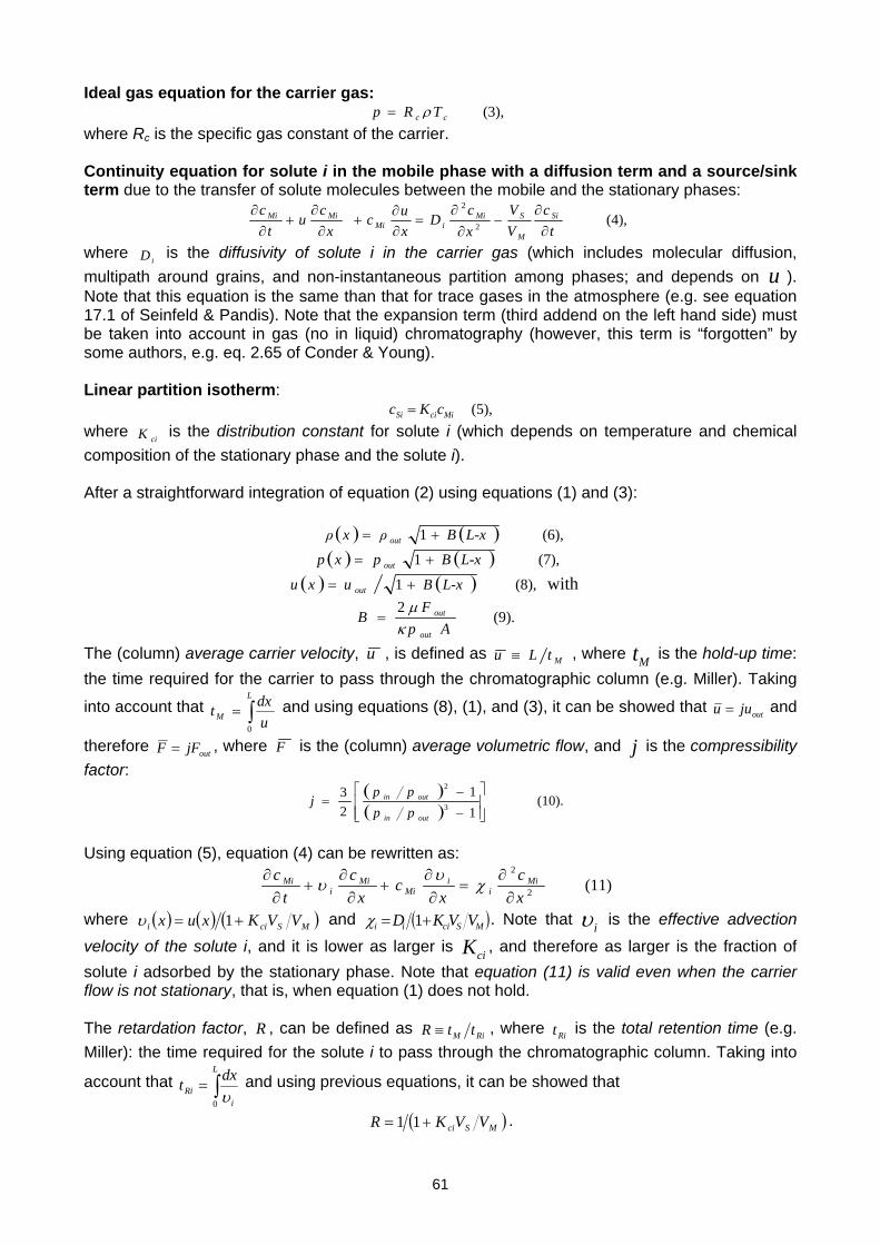
61

Ideal gas equation for the carrier gas: (3), cc TRp ρ=

where Rc is the specific gas constant of the carrier. Continuity equation for solute i in the mobile phase with a diffusion term and a source/sink term due to the transfer of solute molecules between the mobile and the stationary phases:

(4), 2

2

t

cVV

xc

Dxuc

xc

ut

c Si

M

SMiiMi

MiMi

∂∂

−∂

∂=

∂∂

+∂

∂+

∂∂

where iD is the diffusivity of solute i in the carrier gas (which includes molecular diffusion,

multipath around grains, and non-instantaneous partition among phases; and depends on u ). Note that this equation is the same than that for trace gases in the atmosphere (e.g. see equation 17.1 of Seinfeld & Pandis). Note that the expansion term (third addend on the left hand side) must be taken into account in gas (no in liquid) chromatography (however, this term is “forgotten” by some authors, e.g. eq. 2.65 of Conder & Young). Linear partition isotherm:

(5), MiciSi cKc = where ciK is the distribution constant for solute i (which depends on temperature and chemical composition of the stationary phase and the solute i). After a straightforward integration of equation (2) using equations (1) and (3):

( ) ( ) (6), 1 L-xBρxρ out += ( ) ( ) (7), 1 L-xBpxp out +=

( ) ( ) with (8), 1 L-xBuxu out +=

(9). 2

ApF

Bout

out

κμ

=

The (column) average carrier velocity, u , is defined as MtLu ≡ , where Mt is the hold-up time: the time required for the carrier to pass through the chromatographic column (e.g. Miller). Taking

into account that ∫=L

M udxt

0

and using equations (8), (1), and (3), it can be showed that outjuu = and

therefore outjFF = , where F is the (column) average volumetric flow, and j is the compressibility factor:

( )( )

(10). 11

23

3

2

⎥⎥⎦

⎤

⎢⎢⎣

⎡

−

−=

outin

outin

pppp

j

Using equation (5), equation (4) can be rewritten as:

(11) 2

2

xc

xc

xc

tc Mi

ii

MiMi

iMi

∂∂

=∂

∂+

∂∂

+∂

∂ χυυ

where ( ) ( ) ( )MScii VVKxux += 1υ and ( )MSciii VVKD += 1χ . Note that iυ is the effective advection

velocity of the solute i, and it is lower as larger is ciK , and therefore as larger is the fraction of solute i adsorbed by the stationary phase. Note that equation (11) is valid even when the carrier flow is not stationary, that is, when equation (1) does not hold. The retardation factor, R , can be defined as RiM ttR ≡ , where Rit is the total retention time (e.g. Miller): the time required for the solute i to pass through the chromatographic column. Taking into

account that ∫=L

iRi

dxt0 υ

and using previous equations, it can be showed that

( )MSci VVKR += 11 .

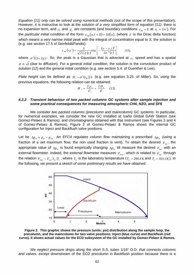
62

Equation (11) only can be solved using numerical methods (out of the scope of this presentation). However, it is instructive to look at the solution of a very simplified form of equation (11): there is no expansion term, and iυ and iχ are constants (and boundary conditions 0=Mic at ±∞=ix ). For the particular initial condition of the form ( ) ( )xStxcMi δ== 0, , (where δ is the Dirac delta function) which means a very narrow initial peak with the integral of concentration equal to S, the solution is (e.g. see section 17.5 of Seinfeld&Pandis):

( )( )

( )( ) (12),

2exp

2 2

2

ttx

tSx,tc i

Mi⎥⎥⎦

⎤

⎢⎢⎣

⎡ −−=

συ

σπ

where ( ) tt iχσ 22 = . So, the peak is a Gaussian that is advected at iυ speed and has a spatial

t∝σ (due to diffusion). For a general initial condition, the solution is the convolution product of solution (12) and the general initial condition (e.g. see section 5.4. of Guenther & Lee). Plate height can be defined as ( ) LtH Rii

2σ= (e.g. see equation 3.25. of Miller). So, using the previous equations, the following relation can be obtained:

(13) 22 uDH i

i

ii ==

υχ

4.2.2 Transient behaviour of two packed columns GC systems after sample injection and

some practical consequences for measuring atmospheric CH4, N2O, and SF6 We consider two packed columns (precolumn and maincolumn) GC systems. In particular,

for numerical examples, we consider the new GC installed at Izaña Global GAW Station (see Gomez-Pelaez & Ramos), and chromatograms obtained with that instrument (see Figures 3 and 4 of Gomez-Pelaez & Ramos). Figure 2 of Gomez-Pelaez & Ramos shows the internal GC configuration for Inject and Backflush valve positions. Let be outinin ppp −≡Δ . An EFC4 regulates column flow maintaining a prescribed inpΔ (using a fraction of a set maximum flow, the non used fraction is vent). To obtain the desired outF , the appropriate value of inpΔ is found empirically changing inpΔ till measure the desired outF with an external flowmeter. Indeed, the external flowmeter measures meaF , which is related to outF through the relation cLoutmea TTFF = , where LT is the laboratory temperature ( K 4.294=LT and K 1.353=cT ). In the following, we present a sketch of some preliminary results we have obtained.

Figure 2. This graphic shows the pressure (units: psi) distribution along the sample loop, the precolumn, and the maincolumn for two valve positions: Inject (blue curve) and Backflush (red

curve). It shows actual values for the ECD subsystem of the GC installed by Gomez-Pelaez & Ramos.

We neglect pressure drops along the short S.S. tubes 1/16” O.D. that connects columns

and valves, except downstream of the ECD precolumn in Backflush position because there is a

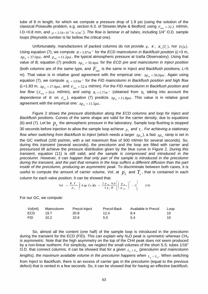
63

tube of 8 m length, for which we compute a pressure drop of 1.9 psi (using the solution of the classical Poiseuille problem, e.g. section 6.3. of Streeter,Wylie & Bedford; using 2.32=meaF ml/min, I.D.=0.8 mm, and 25 msN1054.2 ⋅×= −μ ). The flow is laminar in all tubes, including 1/4” O.D. sample loops (Reynolds number is far bellow the critical one).

Unfortunately, manufacturers of packed columns do not provide φ , κ , ( )cci TK , nor ( )uDi . Using equation (7), we compute 1m87.5 −=B for the ECD maincolumn in Backflush position (L=3 m,

psi0.37=Δ inp , and psi2.11=outp , the typical atmospheric pressure at Izaña Observatory). Using that value of B, equation (7) predicts psi4.50=Δ inp for the ECD pre and maincolumn in Inject position (both columns are of the same type, and outF is the same in Inject and Backflush positions; L=5 m). That value is in relative good agreement with the empirical one: psi0.50=Δ inp . Again using equation (7), we compute 1m03.3 −=hB for the FID maincolumn in Backflush position and high flow (L=1.83 m, psi4.17=Δ inp , and 4.52=meaF ml/min). For the FID maincolumn in Backflush position and low flow ( 6.30=meaF ml/min), and using 1m77.1 −=lB (obtained from hB taking into account the dependence of B on outF ), equation (7) predicts psi8.11=Δ inp . This value is in relative good agreement with the empirical one: psi5.11=Δ inp .

Figure 2 shows the pressure distribution along the ECD columns and loop for Inject and Backflush positions. Curves of the same shape are valid for the carrier density, due to equations (6) and (7). Let be Lp the atmospheric pressure in the laboratory. Sample loop flushing is stopped 30 seconds before injection to allow the sample loop achieve Lp and cT . For achieving a stationary flow when switching from Backflush to Inject (which needs a larger inpΔ ), a fast inpΔ ramp is set in the GC method (100 psi/min, with a set maximum flow of 500 ml/min for several seconds). So, during this transient (several seconds), the precolumn and the loop are filled with carrier and pressurized till achieve the pressure distribution given by the blue curve in Figure 2. During this transient, equation (11) is still valid, and the sample is compressed and introduced in the precolumn. However, it can happen that only part of the sample is introduced in the precolumn during the transient, and the part that remains in the loop suffers a different diffusion than the part inside of the precolumn, producing an asymmetric peak. To discriminate between both cases, it is useful to compute the amount of carrier volume, Vol, at Lp and cT , that is contained in each column for each valve position. It can be showed that:

( ) (14) 1pp

32

3

out

in

⎥⎥⎦

⎤

⎢⎢⎣

⎡−⎟⎟

⎠

⎞⎜⎜⎝

⎛== ∫

L

o L

out

L

cc

BpAp

dxxAp

TRVol

φφρ

For our GC, we compute:

Vol(ml) Maincolumn Precol-Inject Precol-Back Available in Precol Loop ECD 19.7 20.8 12.4 8.4 10 FID 10.2 10.9 5.5 5.4 10

So, almost all the content (one half) of the sample loop is introduced in the precolumn during the transient for the ECD (FID). This can explain why N2O peak is symmetric whereas CH4 is asymmetric. Note that the high asymmetry on the top of the CH4 peak does not seem produced by a non-linear isotherm. For simplicity, we neglect the small volumes of the short S.S. tubes 1/16” O.D. that connect columns. It can be showed that for a given

mp LL + (precolumn and maincolumn lengths), the maximum available volume in the precolumn happens when

mp LL = . When switching from Inject to Backflush, there is an excess of carrier gas in the precolumn (equal to the previous defect) that is vented in a few seconds. So, it can be showed that for having an effective backflush,

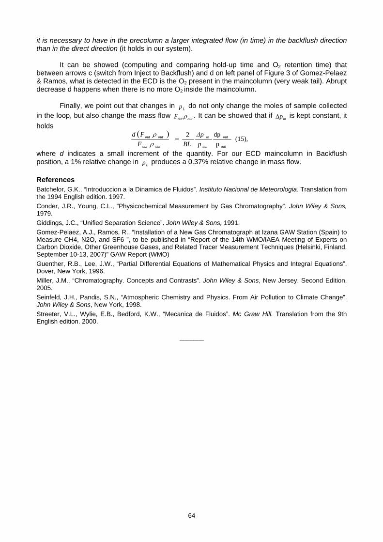
64

it is necessary to have in the precolumn a larger integrated flow (in time) in the backflush direction than in the direct direction (it holds in our system).

It can be showed (computing and comparing hold-up time and O2 retention time) that

between arrows c (switch from Inject to Backflush) and d on left panel of Figure 3 of Gomez-Pelaez & Ramos, what is detected in the ECD is the O2 present in the maincolumn (very weak tail). Abrupt decrease d happens when there is no more O2 inside the maincolumn.

Finally, we point out that changes in Lp do not only change the moles of sample collected in the loop, but also change the mass flow outoutF ρ . It can be showed that if inpΔ is kept constant, it holds

( )(15),

pdp2

out

out

out

in

outout

outout

pΔp

BL

FFd

=ρρ

where d indicates a small increment of the quantity. For our ECD maincolumn in Backflush position, a 1% relative change in Lp produces a 0.37% relative change in mass flow. References Batchelor, G.K., “Introduccion a la Dinamica de Fluidos”. Instituto Nacional de Meteorologia. Translation from the 1994 English edition. 1997. Conder, J.R., Young, C.L., ”Physicochemical Measurement by Gas Chromatography”. John Wiley & Sons, 1979. Giddings, J.C., “Unified Separation Science”. John Wiley & Sons, 1991. Gomez-Pelaez, A.J., Ramos, R., “Installation of a New Gas Chromatograph at Izana GAW Station (Spain) to Measure CH4, N2O, and SF6 ”, to be published in “Report of the 14th WMO/IAEA Meeting of Experts on Carbon Dioxide, Other Greenhouse Gases, and Related Tracer Measurement Techniques (Helsinki, Finland, September 10-13, 2007)” GAW Report (WMO) Guenther, R.B., Lee, J.W., “Partial Differential Equations of Mathematical Physics and Integral Equations”. Dover, New York, 1996. Miller, J.M., “Chromatography. Concepts and Contrasts”. John Wiley & Sons, New Jersey, Second Edition, 2005. Seinfeld, J.H., Pandis, S.N., “Atmospheric Chemistry and Physics. From Air Pollution to Climate Change”. John Wiley & Sons, New York, 1998. Streeter, V.L., Wylie, E.B., Bedford, K.W., “Mecanica de Fluidos”. Mc Graw Hill. Translation from the 9th English edition. 2000.

_______

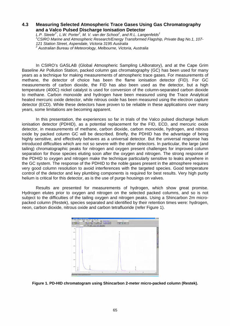
65

4.3 Measuring Selected Atmospheric Trace Gases Using Gas Chromatography and a Valco Pulsed Discharge Ionisation Detector L.P. Steele1*, L.W. Porter2, M. V. van der Schoot1, and R.L. Langenfelds1 1CSIRO Marine and Atmospheric Research/Energy Transformed Flagship, Private Bag No.1, 107-121 Station Street, Aspendale, Victoria 3195 Australia 2 Australian Bureau of Meteorology, Melbourne, Victoria, Australia

In CSIRO’s GASLAB (Global Atmospheric Sampling LABoratory), and at the Cape Grim Baseline Air Pollution Station, packed column gas chromatography (GC) has been used for many years as a technique for making measurements of atmospheric trace gases. For measurements of methane, the detector of choice has been the flame ionisation detector (FID). For GC measurements of carbon dioxide, the FID has also been used as the detector, but a high temperature (400C) nickel catalyst is used for conversion of the column-separated carbon dioxide to methane. Carbon monoxide and hydrogen have been measured using the Trace Analytical heated mercuric oxide detector, while nitrous oxide has been measured using the electron capture detector (ECD). While these detectors have proven to be reliable in these applications over many years, some limitations are becoming apparent.

In this presentation, the experiences so far in trials of the Valco pulsed discharge helium

ionisation detector (PDHID), as a potential replacement for the FID, ECD, and mercuric oxide detector, in measurements of methane, carbon dioxide, carbon monoxide, hydrogen, and nitrous oxide by packed column GC will be described. Briefly, the PDHID has the advantage of being highly sensitive, and effectively behaves as a universal detector. But the universal response has introduced difficulties which are not so severe with the other detectors. In particular, the large (and tailing) chromatographic peaks for nitrogen and oxygen present challenges for improved column separation for those species eluting soon after the oxygen and nitrogen. The strong response of the PDHID to oxygen and nitrogen make the technique particularly sensitive to leaks anywhere in the GC system. The response of the PDHID to the noble gases present in the atmosphere requires very good column resolution to avoid interferences with the targeted species. Good temperature control of the detector and key plumbing components is required for best results. Very high purity helium is critical for this detector, as is the use of purge housings on valves.

Results are presented for measurements of hydrogen, which show great promise.

Hydrogen elutes prior to oxygen and nitrogen on the selected packed columns, and so is not subject to the difficulties of the tailing oxygen and nitrogen peaks. Using a Shincarbon 2m micro-packed column (Restek), species separated and identified by their retention times were: hydrogen, neon, carbon dioxide, nitrous oxide and carbon tetrafluoride (refer Figure 1).

Figure 1. PD-HID chromatogram using Shincarbon 2-meter micro-packed column (Restek).

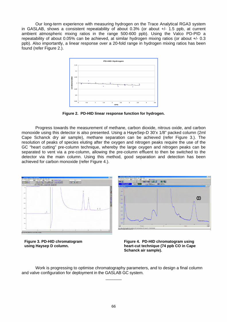
66

Our long-term experience with measuring hydrogen on the Trace Analytical RGA3 system in GASLAB, shows a consistent repeatability of about 0.3% (or about +/- 1.5 ppb, at current ambient atmospheric mixing ratios in the range 500-600 ppb). Using the Valco PD-PID a repeatability of about 0.05% can be achieved, at similar hydrogen mixing ratios (or about +/- 0.3 ppb). Also importantly, a linear response over a 20-fold range in hydrogen mixing ratios has been found (refer Figure 2.).

PD-HID Hydrogen

0.85

0.9

0.95

1

1.05

1.1

1.15

0 0.5 1 1.5 2 2.5 3 3.5 4 4.5

r(Ht)

norm

alised

sen

sitiv

ity

Figure 2. PD-HID linear response function for hydrogen.

Progress towards the measurement of methane, carbon dioxide, nitrous oxide, and carbon

monoxide using this detector is also presented. Using a HayeSep-D 30’x 1/8” packed column (2ml Cape Schanck dry air sample), methane separation can be achieved (refer Figure 3.). The resolution of peaks of species eluting after the oxygen and nitrogen peaks require the use of the GC “heart cutting” pre-column technique, whereby the large oxygen and nitrogen peaks can be separated to vent via a pre-column, allowing the pre-column effluent to then be switched to the detector via the main column. Using this method, good separation and detection has been achieved for carbon monoxide (refer Figure 4.).

Work is progressing to optimise chromatography parameters, and to design a final column

and valve configuration for deployment in the GASLAB GC system. _______

Figure 4. PD-HID chromatogram using heart-cut technique (74 ppb CO in Cape Schanck air sample).

Figure 3. PD-HID chromatogram using Haysep D column.

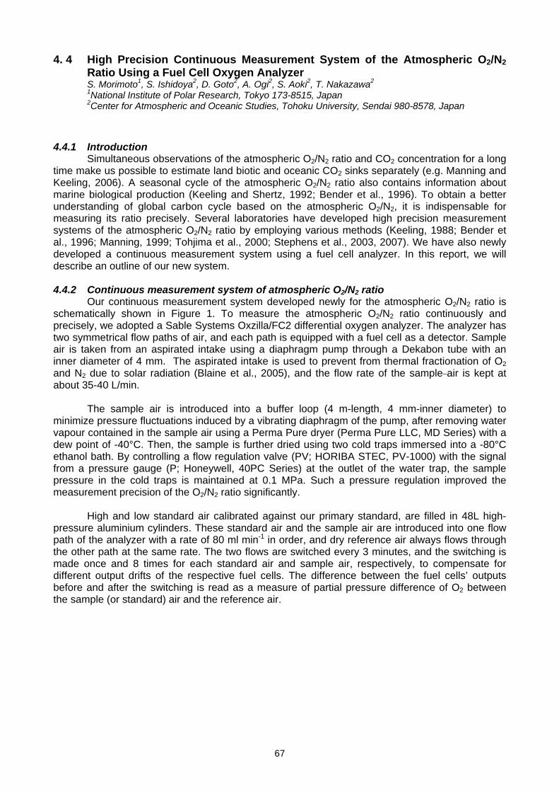
67

4. 4 High Precision Continuous Measurement System of the Atmospheric O2/N2 Ratio Using a Fuel Cell Oxygen Analyzer S. Morimoto1, S. Ishidoya2, D. Goto2, A. Ogi2, S. Aoki2, T. Nakazawa2 1National Institute of Polar Research, Tokyo 173-8515, Japan 2Center for Atmospheric and Oceanic Studies, Tohoku University, Sendai 980-8578, Japan

4.4.1 Introduction

Simultaneous observations of the atmospheric O2/N2 ratio and CO2 concentration for a long time make us possible to estimate land biotic and oceanic CO2 sinks separately (e.g. Manning and Keeling, 2006). A seasonal cycle of the atmospheric O2/N2 ratio also contains information about marine biological production (Keeling and Shertz, 1992; Bender et al., 1996). To obtain a better understanding of global carbon cycle based on the atmospheric O2/N2, it is indispensable for measuring its ratio precisely. Several laboratories have developed high precision measurement systems of the atmospheric O2/N2 ratio by employing various methods (Keeling, 1988; Bender et al., 1996; Manning, 1999; Tohjima et al., 2000; Stephens et al., 2003, 2007). We have also newly developed a continuous measurement system using a fuel cell analyzer. In this report, we will describe an outline of our new system. 4.4.2 Continuous measurement system of atmospheric O2/N2 ratio

Our continuous measurement system developed newly for the atmospheric O2/N2 ratio is schematically shown in Figure 1. To measure the atmospheric O2/N2 ratio continuously and precisely, we adopted a Sable Systems Oxzilla/FC2 differential oxygen analyzer. The analyzer has two symmetrical flow paths of air, and each path is equipped with a fuel cell as a detector. Sample air is taken from an aspirated intake using a diaphragm pump through a Dekabon tube with an inner diameter of 4 mm. The aspirated intake is used to prevent from thermal fractionation of O2 and N2 due to solar radiation (Blaine et al., 2005), and the flow rate of the sample air is kept at about 35-40 L/min.

The sample air is introduced into a buffer loop (4 m-length, 4 mm-inner diameter) to

minimize pressure fluctuations induced by a vibrating diaphragm of the pump, after removing water vapour contained in the sample air using a Perma Pure dryer (Perma Pure LLC, MD Series) with a dew point of -40°C. Then, the sample is further dried using two cold traps immersed into a -80°C ethanol bath. By controlling a flow regulation valve (PV; HORIBA STEC, PV-1000) with the signal from a pressure gauge (P; Honeywell, 40PC Series) at the outlet of the water trap, the sample pressure in the cold traps is maintained at 0.1 MPa. Such a pressure regulation improved the measurement precision of the O2/N2 ratio significantly.

High and low standard air calibrated against our primary standard, are filled in 48L high-

pressure aluminium cylinders. These standard air and the sample air are introduced into one flow path of the analyzer with a rate of 80 ml min-1 in order, and dry reference air always flows through the other path at the same rate. The two flows are switched every 3 minutes, and the switching is made once and 8 times for each standard air and sample air, respectively, to compensate for different output drifts of the respective fuel cells. The difference between the fuel cells’ outputs before and after the switching is read as a measure of partial pressure difference of O2 between the sample (or standard) air and the reference air.

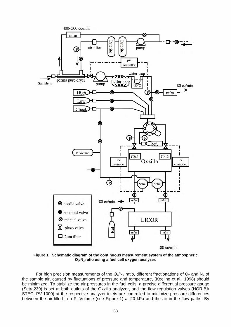
68

Figure 1. Schematic diagram of the continuous measurement system of the atmospheric

O2/N2 ratio using a fuel cell oxygen analyzer.

For high precision measurements of the O2/N2 ratio, different fractionations of O2 and N2 of the sample air, caused by fluctuations of pressure and temperature, (Keeling et al., 1998) should be minimized. To stabilize the air pressures in the fuel cells, a precise differential pressure gauge (Setra239) is set at both outlets of the Oxzilla analyzer, and the flow regulation valves (HORIBA STEC, PV-1000) at the respective analyzer inlets are controlled to minimize pressure differences between the air filled in a P. Volume (see Figure 1) at 20 kPa and the air in the flow paths. By

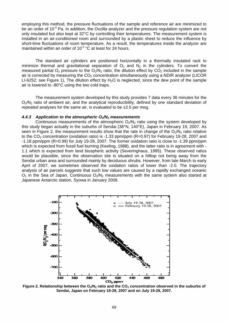
69

employing this method, the pressure fluctuations of the sample and reference air are minimized to be an order of 10-3 Pa. In addition, the Oxzilla analyzer and the pressure regulation system are not only insulated but also kept at 32°C by controlling their temperatures. The measurement system is installed in an air-conditioned room and surrounded by a plastic sheet to reduce the influence by short-time fluctuations of room temperature. As a result, the temperatures inside the analyzer are maintained within an order of 10-3 °C at least for 24 hours.

The standard air cylinders are positioned horizontally in a thermally insulated rack to minimize thermal and gravitational separation of O2 and N2 in the cylinders. To convert the measured partial O2 pressure to the O2/N2 ratio, the dilution effect by CO2 included in the sample air is corrected by measuring the CO2 concentration simultaneously using a NDIR analyzer (LICOR LI-6252; see Figure 1), The dilution effect by H2O is neglected, since the dew point of the sample air is lowered to -80°C using the two cold traps.

The measurement system developed by this study provides 7 data every 36 minutes for the O2/N2 ratio of ambient air, and the analytical reproducibility, defined by one standard deviation of repeated analyses for the same air, is evaluated to be ±2.5 per meg. 4.4.3 Application to the atmospheric O2/N2 measurements

Continuous measurements of the atmospheric O2/N2 ratio using the system developed by this study began actually in the suburbs of Sendai (38°N, 140°E), Japan in February 19, 2007. As seen in Figure 2, the measurement results show that the rate in change of the O2/N2 ratio relative to the CO2 concentration (oxidation ratio) is -1.33 ppm/ppm (R=0.97) for February 19-28, 2007 and -1.18 ppm/ppm (R=0.99) for July 19-28, 2007. The former oxidation ratio is close to -1.39 ppm/ppm which is expected from fossil fuel burning (Keeling, 1988), and the latter ratio is in agreement with -1.1 which is expected from land biospheric activity (Severinghaus, 1995). These observed ratios would be plausible, since the observation site is situated on a hilltop not being away from the Sendai urban area and surrounded mainly by deciduous shrubs. However, from late March to early April of 2007, we sometimes observed the oxidation ratios of lower than -2.0. The trajectory analysis of air parcels suggests that such low values are caused by a rapidly exchanged oceanic O2 in the Sea of Japan. Continuous O2/N2 measurements with the same system also started at Japanese Antarctic station, Syowa in January 2008.

Figure 2. Relationship between the O2/N2 ratio and the CO2 concentration observed in the suburbs of

Sendai, Japan on February 19-28, 2007 and on July 19-28, 2007.

70

References Bender, M., J. T. Ellis, P. Tans, R. Francey, and D. C. Lowe (1996), Variability in the O2/N2 Ratio of Southern Hemisphere Air 1991-1994: Implication for the Carbon Cycle, Global Biogeochem. Cycles, 10, 9-21. Blaine, T. W., R. F. Keeling, and W. J. Paplawsky (2005), An Improved Inlet for Precisely Measuring the Atmospheric Ar/N2 Ratio, Atmos. Chem. And Phys. Discussions, 5, 11899-11910. Keeling, R. F. (1988), Development of an Interferometric Oxygen Analyzer for Precise Measurement of the Atmospheric O2 Mole Fraction, Ph. D. thesis, 178 pp, Harvard University, Cambridge. Keeling, R. F., and S. R. Shertz (1992), Seasonal and Interannual Variations in Atmospheric Oxygen and Implications for the Global Carbon Cycle, Nature, 358, 723-727. Keeling, R. F., A. C. Manning, E. M. McEvoy, and S. R. Shertz (1998), Methods for Measuring Changes in Atmospheric O2 Concentration and their Application in Southern Hemisphere air, J. Geophys. Res., 103, 3381-3397. Manning, A. C., R. F. Keeling, and J. P. Severinghaus (1999), Precise Atmospheric Oxygen Measurements with a Paramagnetic Oxygen Analyzer, Global Biogeochem.Cycles, 13, 1107-1115. Manning, A. C. and R. F. Keeling (2006), Global Oceanic and Land Biotic Carbon Sinks from the Scripps Atmospheric Oxygen Flask Sampling Network, Tellus, 58B, 95-116. Stephens, B. B., R. F. Keeling, and W. J. Paplawsky (2003), Shipboard Measurements of Atmospheric Oxygen using a Vacuum-Ultraviolet Absorption Technique, Tellus, 55B, 857-878. Stephens, B. B., Bakwin, P., Tans, P. P., Teclaw, R. and Baumann, D. (2007), Application of a Differential Fuel-Cell Analyzer for Measuring Atmospheric Oxygen Variations. J. Atmos Oc. Tech. 24. 82-94. Severinghaus, J. P. (1995), Studies of the Terrestrial Molecular Oxygen and Carbon Cycles in Sand Dune Gases and in Biosphere 2, Ph. D. thesis, Columbia University. Tohjima, Y. (2000), Method for Measuring Changes in the Atmospheric O2/N2 Ratio by a Gas Chromatograph Equipped with a Thermal Conductivity, J. Geophys. Res.,105, 14575-14584.

_______

71

5.1 REPORT OF THE WCC-N2O H.E. Scheel

Forschungszentrum Karlsruhe, IMK-IFU, 82467 Garmisch-Partenkirchen, Germany 5.1.1 Introduction

The World Calibration Centre for N2O (WCC-N2O) has been established as a central GAW facility according to requirements of the GAW Strategic Plan 2001–2007 (WMO/GAW Report No. 142). Its overall goal is the improvement of N2O data quality and comparability. The WCC-N2O (http://imk.fzk.de/wcc-n2o/) is hosted by the Forschungszentrum Karlsruhe, IMK-IFU, and its activities are conducted under supervision and through funding by the Quality Assurance/Science Activity Centre (QA/SAC) Germany, operated by the German Environment Agency (UBA). Among the major tasks of the WCC-N2O are the development of quality control procedures, conducting audits at stations and round-robin experiments as well as providing training and technical advice to GAW station personnel. This presentation reports primarily on WCC-N2O activities performed since the 13th Experts Meeting of September 2005. 5.1.2 Activities of the WCC-N2O 5.1.2.1 Contributions to GAW documents Editing work on Measurement Guidelines (MGs) for N2O has been continued in 2007. The MGs for N2O are part of a future WMO/GAW report containing Data Quality Objectives (DQOs) and Measurement Guidelines for both CH4 and N2O (Guidelines for the Measurement of Methane and Nitrous Oxide and their Quality Assurance). Thanks to the input from a number of GAW participants and external experts, the draft of the report is now at an advanced stage and was submitted for approval to the SAG GG prior to the SAG meeting in September 2007. The WCC-N2O has contributed to the WMO/GAW Glossary of QA/QC-Related Termi-nology, which originally started out as a spin-off from a glossary section of the MGs. After further editing and formatting by QA/SAC Switzerland, this document is now available on the web (http://www.empa.ch/gaw/glossary.html). Refinements made to the glossary during the final editing phase were thereafter recirculated to the respective section of the MGs. It is noted that the web version of the glossary is intended as a dynamic process, which will yield enlargement depending on future input by its users, also from outside the greenhouse gas community. Based on the joint input from QA/SAC Switzerland, WCC-Empa and WCC-N2O an Audit Questionnaire (Gases) was compiled. It serves for collecting all relevant information during audits at stations. Moreover, the WCC-N2O has been involved in the editing of an Audit SOP, which was based on an outline by WCC-Empa. Both audit documents have been approved by the SAG GG. 5.1.2.2 Comparisons of standards In the laboratory of the WCC-N2O, extensive comparisons of standards were conducted, several of them as pre- and post-audit checks of the travelling standards involved. The standards of the WCC-N2O are linked to the GAW standard scale maintained by the Central Calibration Laboratory for N2O, operated by NOAA ESRL in Boulder (USA). While the primary and secondary standards of the GAW N2O scale are maintained at the CCL, the standards ranking highest within the WCC-N2O (laboratory standards) are on the tertiary level of the hierarchy. At the beginning of 2007, an intercomparison was conducted between the CCL and the WCC-N2O. It was based on five travelling standards previously used for audits, with N2O mole fractions ranging between 290 and 350 ppb. The intercomparison established an important internal quality check. Analysis results reported by the CCL showed agreement within a range of ± 0.1 ppb for four of the five cylinders (Table 1). The greater deviation (0.37 ppb) found for the lowest mole fraction could be attributed to one of the WCC-N2O laboratory standards, for which the assigned value had already previously been assumed to be possibly too high by 0.3 ppb.

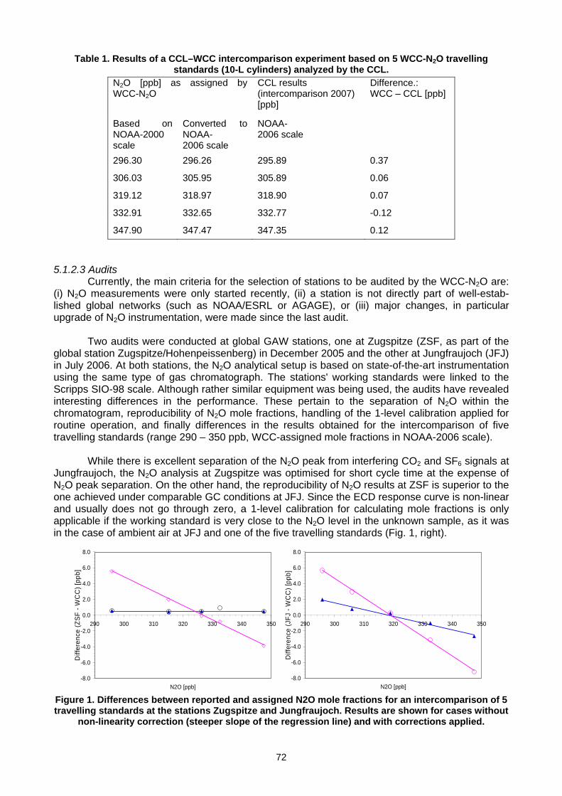
72

Table 1. Results of a CCL–WCC intercomparison experiment based on 5 WCC-N2O travelling standards (10-L cylinders) analyzed by the CCL.

N2O [ppb] as assigned by WCC-N2O

CCL results (intercomparison 2007) [ppb]

Difference.: WCC – CCL [ppb]

Based on NOAA-2000 scale

Converted to NOAA- 2006 scale

NOAA- 2006 scale

296.30 296.26 295.89 0.37

306.03 305.95 305.89 0.06

319.12 318.97 318.90 0.07

332.91 332.65 332.77 -0.12

347.90 347.47 347.35 0.12 5.1.2.3 Audits Currently, the main criteria for the selection of stations to be audited by the WCC-N2O are: (i) N2O measurements were only started recently, (ii) a station is not directly part of well-estab-lished global networks (such as NOAA/ESRL or AGAGE), or (iii) major changes, in particular upgrade of N2O instrumentation, were made since the last audit.

Two audits were conducted at global GAW stations, one at Zugspitze (ZSF, as part of the global station Zugspitze/Hohenpeissenberg) in December 2005 and the other at Jungfraujoch (JFJ) in July 2006. At both stations, the N2O analytical setup is based on state-of-the-art instrumentation using the same type of gas chromatograph. The stations' working standards were linked to the Scripps SIO-98 scale. Although rather similar equipment was being used, the audits have revealed interesting differences in the performance. These pertain to the separation of N2O within the chromatogram, reproducibility of N2O mole fractions, handling of the 1-level calibration applied for routine operation, and finally differences in the results obtained for the intercomparison of five travelling standards (range 290 – 350 ppb, WCC-assigned mole fractions in NOAA-2006 scale).

While there is excellent separation of the N2O peak from interfering CO2 and SF6 signals at

Jungfraujoch, the N2O analysis at Zugspitze was optimised for short cycle time at the expense of N2O peak separation. On the other hand, the reproducibility of N2O results at ZSF is superior to the one achieved under comparable GC conditions at JFJ. Since the ECD response curve is non-linear and usually does not go through zero, a 1-level calibration for calculating mole fractions is only applicable if the working standard is very close to the N2O level in the unknown sample, as it was in the case of ambient air at JFJ and one of the five travelling standards (Fig. 1, right).

Figure 1. Differences between reported and assigned N2O mole fractions for an intercomparison of 5 travelling standards at the stations Zugspitze and Jungfraujoch. Results are shown for cases without

non-linearity correction (steeper slope of the regression line) and with corrections applied.

-8.0

-6.0

-4.0

-2.0

0.0

2.0

4.0

6.0

8.0

290 300 310 320 330 340 350

N2O [ppb]

Diff

eren

ce (Z

SF -

WC

C) [

ppb]

-8.0

-6.0

-4.0

-2.0

0.0

2.0

4.0

6.0

8.0

290 300 310 320 330 340 350

N2O [ppb]

Diff

eren

ce (J

FJ -

WC

C) [

ppb]

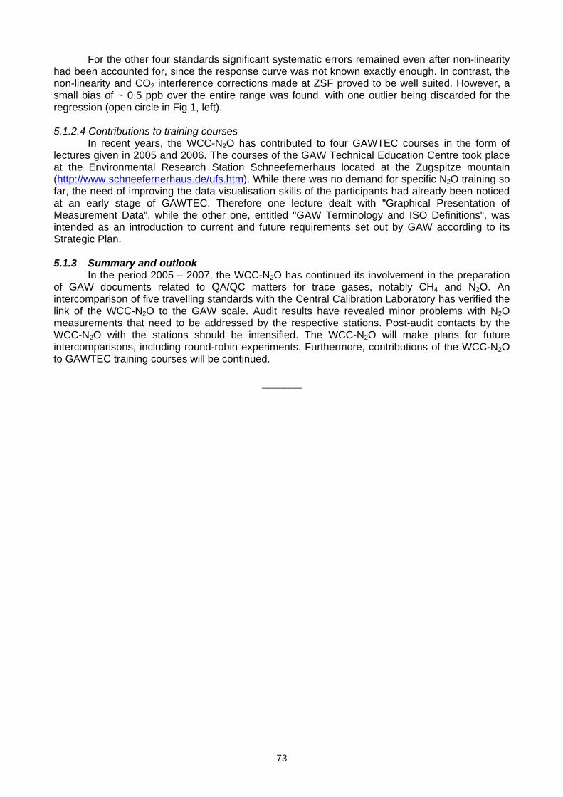
73

For the other four standards significant systematic errors remained even after non-linearity had been accounted for, since the response curve was not known exactly enough. In contrast, the non-linearity and CO2 interference corrections made at ZSF proved to be well suited. However, a small bias of ~ 0.5 ppb over the entire range was found, with one outlier being discarded for the regression (open circle in Fig 1, left). 5.1.2.4 Contributions to training courses In recent years, the WCC-N2O has contributed to four GAWTEC courses in the form of lectures given in 2005 and 2006. The courses of the GAW Technical Education Centre took place at the Environmental Research Station Schneefernerhaus located at the Zugspitze mountain (http://www.schneefernerhaus.de/ufs.htm). While there was no demand for specific N2O training so far, the need of improving the data visualisation skills of the participants had already been noticed at an early stage of GAWTEC. Therefore one lecture dealt with "Graphical Presentation of Measurement Data", while the other one, entitled "GAW Terminology and ISO Definitions", was intended as an introduction to current and future requirements set out by GAW according to its Strategic Plan. 5.1.3 Summary and outlook In the period 2005 – 2007, the WCC-N2O has continued its involvement in the preparation of GAW documents related to QA/QC matters for trace gases, notably CH4 and N2O. An intercomparison of five travelling standards with the Central Calibration Laboratory has verified the link of the WCC-N2O to the GAW scale. Audit results have revealed minor problems with N2O measurements that need to be addressed by the respective stations. Post-audit contacts by the WCC-N2O with the stations should be intensified. The WCC-N2O will make plans for future intercomparisons, including round-robin experiments. Furthermore, contributions of the WCC-N2O to GAWTEC training courses will be continued.

_______

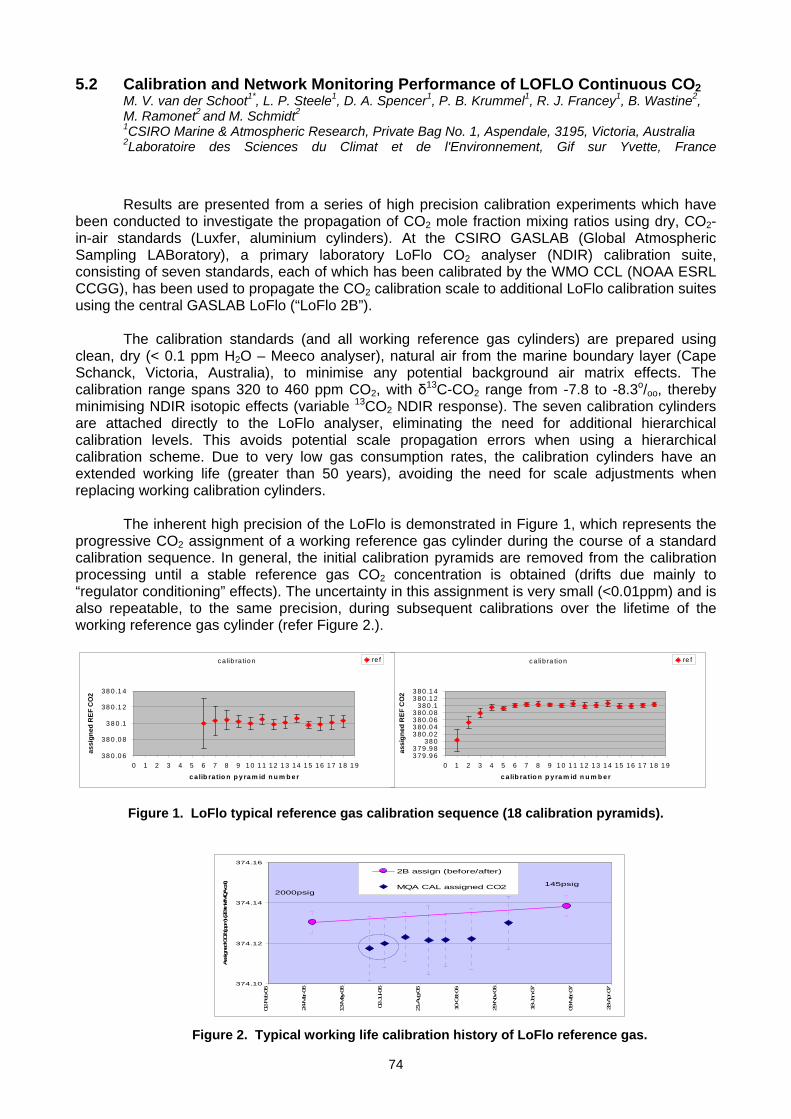
74

5.2 Calibration and Network Monitoring Performance of LOFLO Continuous CO2 M. V. van der Schoot1*, L. P. Steele1, D. A. Spencer1, P. B. Krummel1, R. J. Francey1, B. Wastine2, M. Ramonet2 and M. Schmidt2 1CSIRO Marine & Atmospheric Research, Private Bag No. 1, Aspendale, 3195, Victoria, Australia 2Laboratoire des Sciences du Climat et de l'Environnement, Gif sur Yvette, France

Results are presented from a series of high precision calibration experiments which have

been conducted to investigate the propagation of CO2 mole fraction mixing ratios using dry, CO2-in-air standards (Luxfer, aluminium cylinders). At the CSIRO GASLAB (Global Atmospheric Sampling LABoratory), a primary laboratory LoFlo CO2 analyser (NDIR) calibration suite, consisting of seven standards, each of which has been calibrated by the WMO CCL (NOAA ESRL CCGG), has been used to propagate the CO2 calibration scale to additional LoFlo calibration suites using the central GASLAB LoFlo (“LoFlo 2B”).

The calibration standards (and all working reference gas cylinders) are prepared using

clean, dry (< 0.1 ppm H2O – Meeco analyser), natural air from the marine boundary layer (Cape Schanck, Victoria, Australia), to minimise any potential background air matrix effects. The calibration range spans 320 to 460 ppm CO2, with δ13C-CO2 range from -7.8 to -8.3o/oo, thereby minimising NDIR isotopic effects (variable 13CO2 NDIR response). The seven calibration cylinders are attached directly to the LoFlo analyser, eliminating the need for additional hierarchical calibration levels. This avoids potential scale propagation errors when using a hierarchical calibration scheme. Due to very low gas consumption rates, the calibration cylinders have an extended working life (greater than 50 years), avoiding the need for scale adjustments when replacing working calibration cylinders.

The inherent high precision of the LoFlo is demonstrated in Figure 1, which represents the

progressive CO2 assignment of a working reference gas cylinder during the course of a standard calibration sequence. In general, the initial calibration pyramids are removed from the calibration processing until a stable reference gas CO2 concentration is obtained (drifts due mainly to “regulator conditioning” effects). The uncertainty in this assignment is very small (<0.01ppm) and is also repeatable, to the same precision, during subsequent calibrations over the lifetime of the working reference gas cylinder (refer Figure 2.). ca lib ra tio n

3 79 .9 63 79 .9 8

38 03 80 .0 23 80 .0 43 80 .0 63 80 .0 8

38 0 .13 80 .1 23 80 .1 4

0 1 2 3 4 5 6 7 8 9 1 0 1 1 1 2 1 3 1 4 15 1 6 1 7 18 1 9

c a lib ra tio n p y ra m id n u m b e r

assi

gned

REF

CO

2

re fca lib ra tio n

38 0 .0 6

38 0 .0 8

3 8 0 .1

38 0 .1 2

38 0 .1 4

0 1 2 3 4 5 6 7 8 9 1 0 1 1 1 2 1 3 14 1 5 1 6 17 1 8 1 9

c a lib ra tio n p y ra m id n u m b e r

assi

gned

RE

F C

O2

re f

Figure 1. LoFlo typical reference gas calibration sequence (18 calibration pyramids).

374.10

374.12

374.14

374.16

02-F

eb-06

24-M

ar-06

13-M

ay-06

02-Jul-06

21-A

ug-06

10-O

ct-06

29-N

ov-06

18-Jan

-07

09-M

ar-07

28-A

pr-07

Assign

ed C

O2 (ppm

) (2B

tnk/MQA

cal)

2B assign (before/after)

MQA CAL assigned CO22000psig

145psig

Figure 2. Typical working life calibration history of LoFlo reference gas.

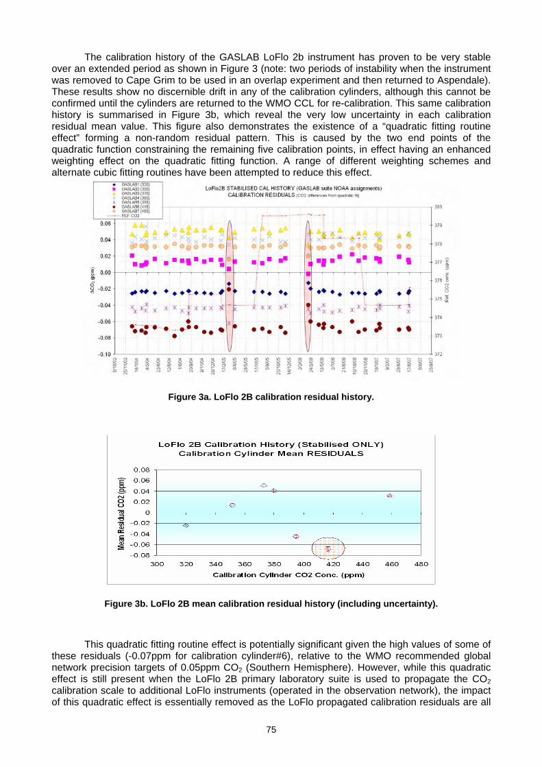
75

The calibration history of the GASLAB LoFlo 2b instrument has proven to be very stable over an extended period as shown in Figure 3 (note: two periods of instability when the instrument was removed to Cape Grim to be used in an overlap experiment and then returned to Aspendale). These results show no discernible drift in any of the calibration cylinders, although this cannot be confirmed until the cylinders are returned to the WMO CCL for re-calibration. This same calibration history is summarised in Figure 3b, which reveal the very low uncertainty in each calibration residual mean value. This figure also demonstrates the existence of a “quadratic fitting routine effect” forming a non-random residual pattern. This is caused by the two end points of the quadratic function constraining the remaining five calibration points, in effect having an enhanced weighting effect on the quadratic fitting function. A range of different weighting schemes and alternate cubic fitting routines have been attempted to reduce this effect.

Figure 3a. LoFlo 2B calibration residual history.

Figure 3b. LoFlo 2B mean calibration residual history (including uncertainty).

This quadratic fitting routine effect is potentially significant given the high values of some of these residuals (-0.07ppm for calibration cylinder#6), relative to the WMO recommended global network precision targets of 0.05ppm CO2 (Southern Hemisphere). However, while this quadratic effect is still present when the LoFlo 2B primary laboratory suite is used to propagate the CO2 calibration scale to additional LoFlo instruments (operated in the observation network), the impact of this quadratic effect is essentially removed as the LoFlo propagated calibration residuals are all

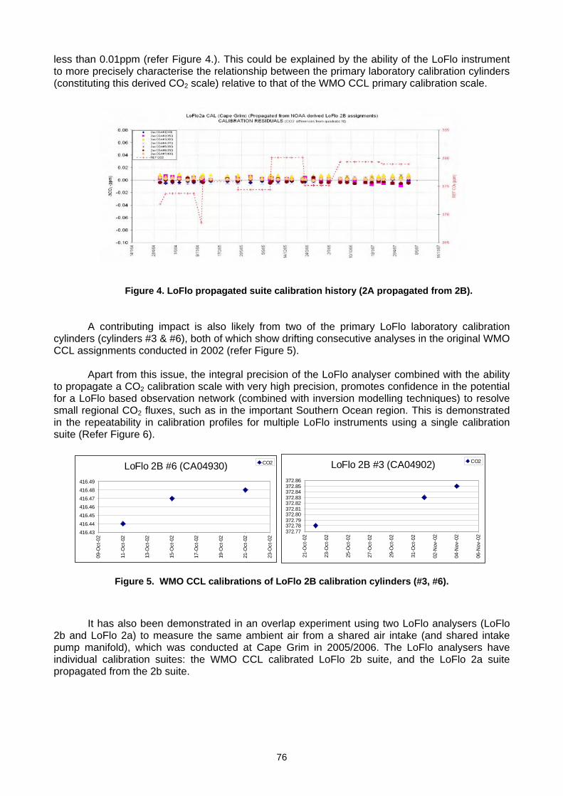
76

less than 0.01ppm (refer Figure 4.). This could be explained by the ability of the LoFlo instrument to more precisely characterise the relationship between the primary laboratory calibration cylinders (constituting this derived CO2 scale) relative to that of the WMO CCL primary calibration scale.

Figure 4. LoFlo propagated suite calibration history (2A propagated from 2B).

A contributing impact is also likely from two of the primary LoFlo laboratory calibration

cylinders (cylinders #3 & #6), both of which show drifting consecutive analyses in the original WMO CCL assignments conducted in 2002 (refer Figure 5).

Apart from this issue, the integral precision of the LoFlo analyser combined with the ability

to propagate a CO2 calibration scale with very high precision, promotes confidence in the potential for a LoFlo based observation network (combined with inversion modelling techniques) to resolve small regional CO2 fluxes, such as in the important Southern Ocean region. This is demonstrated in the repeatability in calibration profiles for multiple LoFlo instruments using a single calibration suite (Refer Figure 6).

LoFlo 2B #3 (CA04902)

372.77372.78372.79372.80372.81372.82372.83372.84372.85372.86

21-O

ct-0

2

23-O

ct-0

2

25-O

ct-0

2

27-O

ct-0

2

29-O

ct-0

2

31-O

ct-0

2

02-N

ov-0

2

04-N

ov-0

2

06-N

ov-0

2

CO2LoFlo 2B #6 (CA04930)

416.43416.44416.45416.46416.47416.48416.49

09-O

ct-0

2

11-O

ct-0

2

13-O

ct-0

2

15-O

ct-0

2

17-O

ct-0

2

19-O

ct-0

2

21-O

ct-0

2

23-O

ct-0

2

CO2

Figure 5. WMO CCL calibrations of LoFlo 2B calibration cylinders (#3, #6).

It has also been demonstrated in an overlap experiment using two LoFlo analysers (LoFlo 2b and LoFlo 2a) to measure the same ambient air from a shared air intake (and shared intake pump manifold), which was conducted at Cape Grim in 2005/2006. The LoFlo analysers have individual calibration suites: the WMO CCL calibrated LoFlo 2b suite, and the LoFlo 2a suite propagated from the 2b suite.

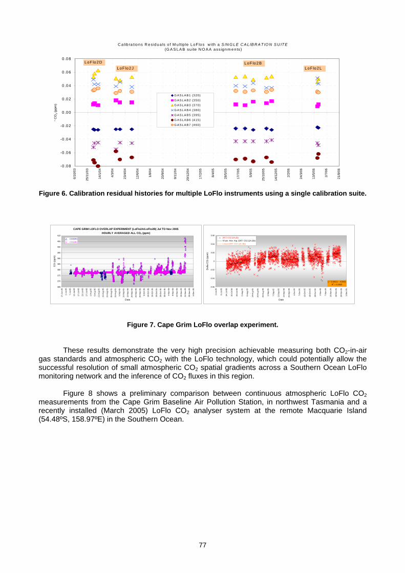
77

C a lib ra tio ns R e sid u a ls o f M u ltip le L oF lo s w ith a S IN G L E C A L IB R A T IO N S U IT E (G A S L A B su ite N O A A a ss ign m e n ts )

-0 .0 8

-0 .0 6

-0 .0 4

-0 .0 2

0 .0 0

0 .0 2

0 .0 4

0 .0 6

0 .0 8

6/10

/03

25/1

1/03

14/1

/04

4/3/

04

23/4

/04

12/6

/04

1/8/

04

20/9

/04

9/11

/04

29/1

2/04

17/2

/05

8/4/

05

28/5

/05

17/7

/05

5/9/

05

25/1

0/05

14/1

2/05

2/2/

06

24/3

/06

13/5

/06

2/7/

06

21/8

/06

°CO

2 (pp

m)

G A S L A B 1 (3 20 )G A S L A B 2 (3 50 )G A S L A B 3 (3 70 )G A S L A B 4 (3 80 )

G A S L A B 5 (3 95 )G A S L A B 6 (4 15 )G A S L A B 7 (4 60 )

L o F lo 2 JL o F lo 2 B

L o F lo 2 LL o F lo 2D

Figure 6. Calibration residual histories for multiple LoFlo instruments using a single calibration suite.

y = 0.0001x - 4.9425R2 = 0.1522

-0.06

-0.04

-0.02

0

0.02

0.04

0.06

2-Ju

l-05

8-Ju

l-05

14-J

ul-0

5

20-J

ul-0

5

26-J

ul-0

5

2-A

ug-0

5

8-A

ug-0

5

14-A

ug-0

5

20-A

ug-0

5

26-A

ug-0

5

1-S

ep-0

5

7-S

ep-0

5

13-S

ep-0

5

19-S

ep-0

5

25-S

ep-0

5

1-O

ct-0

5

7-O

ct-0

5

13-O

ct-0

5

19-O

ct-0

5

25-O

ct-0

5

1-N

ov-0

5

7-N

ov-0

5

13-N

ov-0

5

19-N

ov-0

5

25-N

ov-0

5

1-D

ec-0

5

Date

Del

ta C

O2 (

ppm

)

DIFF CO2 (2A-2B)40 per. Mov. Avg. (DIFF CO2 (2A-2B))Linear (DIFF CO2 (2A-2B))

CAPE GRIM LOFLO OVERLAP EXPERIMENT (LoFlo2A/LoFlo2B) Jul TO Nov 2005HOURLY AVERAGED ALL CO2 (ppm)

365

370

375

380

385

390

395

400

405

410

27-J

un-0

5

2-Ju

l-05

7-Ju

l-05

12-J

ul-0

5

17-J

ul-0

5

22-J

ul-0

5

27-J

ul-0

5

1-A

ug-0

5

6-A

ug-0

5

11-A

ug-0

5

16-A

ug-0

5

21-A

ug-0

5

26-A

ug-0

5

31-A

ug-0

5

5-S

ep-0

5

10-S

ep-0

5

15-S

ep-0

5

20-S

ep-0

5

25-S

ep-0

5

30-S

ep-0

5

5-O

ct-0

5

10-O

ct-0

5

15-O

ct-0

5

20-O

ct-0

5

25-O

ct-0

5

30-O

ct-0

5

4-N

ov-0

5

9-N

ov-0

5

14-N

ov-0

5

19-N

ov-0

5

24-N

ov-0

5

29-N

ov-0

5

4-D

ec-0

5

Date

CO

2 (pp

m)

CO2(2A) CO2(2B)

Figure 7. Cape Grim LoFlo overlap experiment.

These results demonstrate the very high precision achievable measuring both CO2-in-air

gas standards and atmospheric CO2 with the LoFlo technology, which could potentially allow the successful resolution of small atmospheric CO2 spatial gradients across a Southern Ocean LoFlo monitoring network and the inference of CO2 fluxes in this region.

Figure 8 shows a preliminary comparison between continuous atmospheric LoFlo CO2

measurements from the Cape Grim Baseline Air Pollution Station, in northwest Tasmania and a recently installed (March 2005) LoFlo CO2 analyser system at the remote Macquarie Island (54.48ºS, 158.97ºE) in the Southern Ocean.

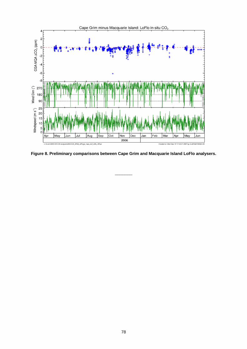
78

Figure 8. Preliminary comparisons between Cape Grim and Macquarie Island LoFlo analysers.

_______

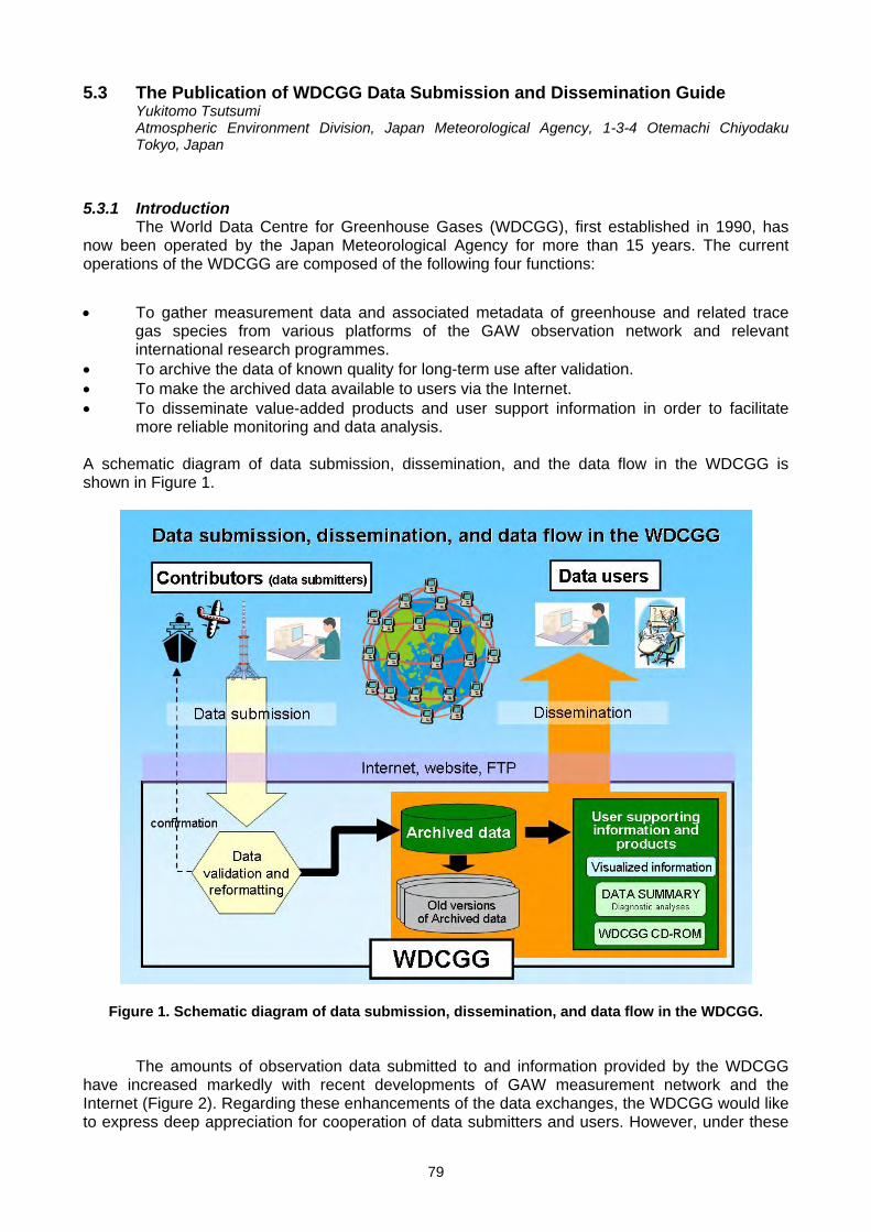
79

5.3 The Publication of WDCGG Data Submission and Dissemination Guide Yukitomo Tsutsumi Atmospheric Environment Division, Japan Meteorological Agency, 1-3-4 Otemachi Chiyodaku Tokyo, Japan

5.3.1 Introduction

The World Data Centre for Greenhouse Gases (WDCGG), first established in 1990, has now been operated by the Japan Meteorological Agency for more than 15 years. The current operations of the WDCGG are composed of the following four functions:

• To gather measurement data and associated metadata of greenhouse and related trace gas species from various platforms of the GAW observation network and relevant international research programmes.

• To archive the data of known quality for long-term use after validation. • To make the archived data available to users via the Internet. • To disseminate value-added products and user support information in order to facilitate

more reliable monitoring and data analysis. A schematic diagram of data submission, dissemination, and the data flow in the WDCGG is shown in Figure 1.

Figure 1. Schematic diagram of data submission, dissemination, and data flow in the WDCGG. The amounts of observation data submitted to and information provided by the WDCGG

have increased markedly with recent developments of GAW measurement network and the Internet (Figure 2). Regarding these enhancements of the data exchanges, the WDCGG would like to express deep appreciation for cooperation of data submitters and users. However, under these

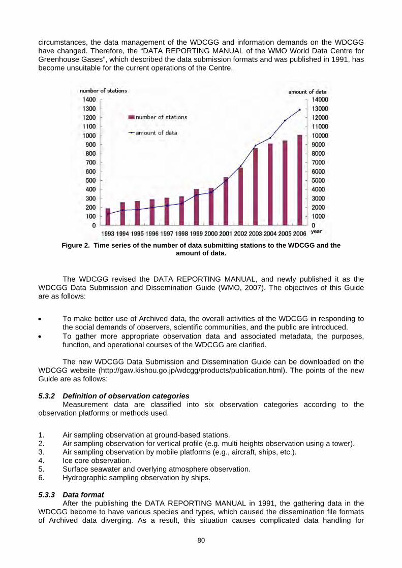
80

circumstances, the data management of the WDCGG and information demands on the WDCGG have changed. Therefore, the “DATA REPORTING MANUAL of the WMO World Data Centre for Greenhouse Gases”, which described the data submission formats and was published in 1991, has become unsuitable for the current operations of the Centre.

Figure 2. Time series of the number of data submitting stations to the WDCGG and the

amount of data.

The WDCGG revised the DATA REPORTING MANUAL, and newly published it as the WDCGG Data Submission and Dissemination Guide (WMO, 2007). The objectives of this Guide are as follows:

• To make better use of Archived data, the overall activities of the WDCGG in responding to the social demands of observers, scientific communities, and the public are introduced.

• To gather more appropriate observation data and associated metadata, the purposes, function, and operational courses of the WDCGG are clarified.

The new WDCGG Data Submission and Dissemination Guide can be downloaded on the

WDCGG website (http://gaw.kishou.go.jp/wdcgg/products/publication.html). The points of the new Guide are as follows: 5.3.2 Definition of observation categories

Measurement data are classified into six observation categories according to the observation platforms or methods used. 1. Air sampling observation at ground-based stations. 2. Air sampling observation for vertical profile (e.g. multi heights observation using a tower). 3. Air sampling observation by mobile platforms (e.g., aircraft, ships, etc.). 4. Ice core observation. 5. Surface seawater and overlying atmosphere observation. 6. Hydrographic sampling observation by ships. 5.3.3 Data format

After the publishing the DATA REPORTING MANUAL in 1991, the gathering data in the WDCGG become to have various species and types, which caused the dissemination file formats of Archived data diverging. As a result, this situation causes complicated data handling for

81

computer, consequently degraded the usability of the WDCGG. To improve this situation, the WDCGG has established new data dissemination file formats aiming at the facilitation of use of Archived data in the WDCGG. The new data dissemination file formats are computer familiar FORTRAN fitting formats.

To simplify the new formats, each file contains mole fraction values of only one parameter;

mole fraction data and ancillary meteorological data are separated; all information to read the data file is included in the header part.

The WDCGG prepared a sample program to read the Archived data file, and this program

is available on the WDCGG website. 5.4.4 Metadata

Accurate metadata of observation is crucial for data users. However, the former WDCGG metadata in the WDCGG was insufficient. The WDCGG arranged the metadata items and established new metadata formats to expand their items to more comprehensive. The WDCGG converted old metadata to new metadata format, but the new metadata formats require additional station and measurement information. The WDCGG is asking Contributors to complete your metadata in the new Metadata Edit Menu on the WDCGG website. Please contact the WDCGG to open the Metadata Edit Menu if you would like to edit your metadata. 5.4.5 Archive of all versions of data

After the publishing the new Guide, a new data version is assigned when existing data are replaced by new data that have different quality. All versions of Archived data are available (only by FTP for the moment) as well as the latest Archived data on the WDCGG website. The version of the Archived data is maintained by the file name. Please refer “WDCGG_filename_format.pdf” on the website. Past WDCGG CD-ROMs data are also available on the WDCGG website.

The WDCGG also has a FTP server on the new website. The users will be able to

download data by accessing the FTP server as an anonymous user. Please refer http://gaw.kishou.go.jp/wdcgg.html. 5.4.6 Submission-data plausible check before acceptance

In the GAW new strategic plan, one of the terms of reference (TOR) of WDC is described as “Ensure that data collected and archived by WMO/GAW WDCs are of known quality, adequate for their intended use and documented comprehensively”. The WDCGG is developing a check method for data plausible check before acceptance. In some cases, the WDCGG performs trail checks, and has begun to communicate with some stations. However, The WDCGG is now accumulating cases to be checked. We need more time for research. In future, the WDCGG would propose check methods to SAG for GG and the measurement community for discussion. 5.4.7 Overall improvement of WDCGG website

In July 2007, The WDCGG improved the website (Figure 3). The new website equips following functions: • User can download the Archive data by FTP. • The new website has easy search system for targeted stations and data “Quick plot” has a

function to produce figures with both PNG and PDF formats. Quick plot is produced in consideration of data quality flag.

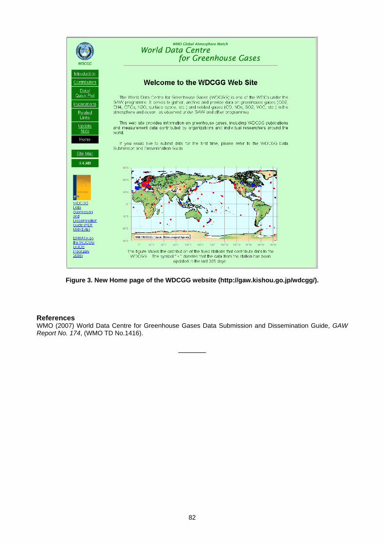
82

Figure 3. New Home page of the WDCGG website (http://gaw.kishou.go.jp/wdcgg/).

References WMO (2007) World Data Centre for Greenhouse Gases Data Submission and Dissemination Guide, GAW Report No. 174, (WMO TD No.1416).

_______

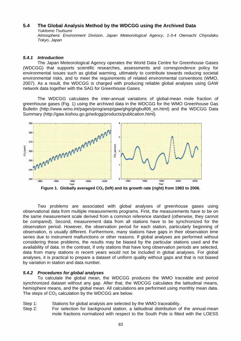
83

5.4 The Global Analysis Method by the WDCGG using the Archived Data Yukitomo Tsutsumi Atmospheric Environment Division, Japan Meteorological Agency, 1-3-4 Otemachi Chiyodaku Tokyo, Japan

5.4.1 Introduction

The Japan Meteorological Agency operates the World Data Centre for Greenhouse Gases (WDCGG) that supports scientific researches, assessments and correspondence policy for environmental issues such as global warming, ultimately to contribute towards reducing societal environmental risks, and to meet the requirements of related environmental conventions (WMO, 2007). As a result, the WDCGG is charged with producing reliable global analyses using GAW network data together with the SAG for Greenhouse Gases.

The WDCGG calculates the inter-annual variations of global-mean mole fraction of

greenhouse gases (Fig. 1) using the archived data in the WDCGG for the WMO Greenhouse Gas Bulletin (http://www.wmo.int/pages/prog/arep/gaw/ghg/ghgbull06_en.html) and the WDCGG Data Summary (http://gaw.kishou.go.jp/wdcgg/products/publication.html).

Figure 1. Globally averaged CO2 (left) and its growth rate (right) from 1983 to 2006.

Two problems are associated with global analyses of greenhouse gases using observational data from multiple measurements programs. First, the measurements have to be on the same measurement scale derived from a common reference standard (otherwise, they cannot be compared). Second, measurement data from all stations have to be synchronized for the observation period. However, the observation period for each station, particularly beginning of observation, is usually different. Furthermore, many stations have gaps in their observation time series due to instrument malfunctions or other reasons. If global analyses are performed without considering these problems, the results may be biased by the particular stations used and the availability of data. In the contrast, if only stations that have long observation periods are selected, data from many stations in recent years would not be included in global analyses. For global analyses, it is practical to prepare a dataset of uniform quality without gaps and that is not biased by variation in station and data number. 5.4.2 Procedures for global analyses

To calculate the global mean, the WDCGG produces the WMO traceable and period synchronized dataset without any gap. After that, the WDCGG calculates the latitudinal means, hemisphere means, and the global mean. All calculations are performed using monthly mean data. The steps of CO2 calculation by the WDCGG are below. Step 1: Stations for global analysis are selected by the WMO traceability. Step 2: For selection for background station, a latitudinal distribution of the annual-mean

mole fractions normalized with respect to the South Pole is fitted with the LOESS

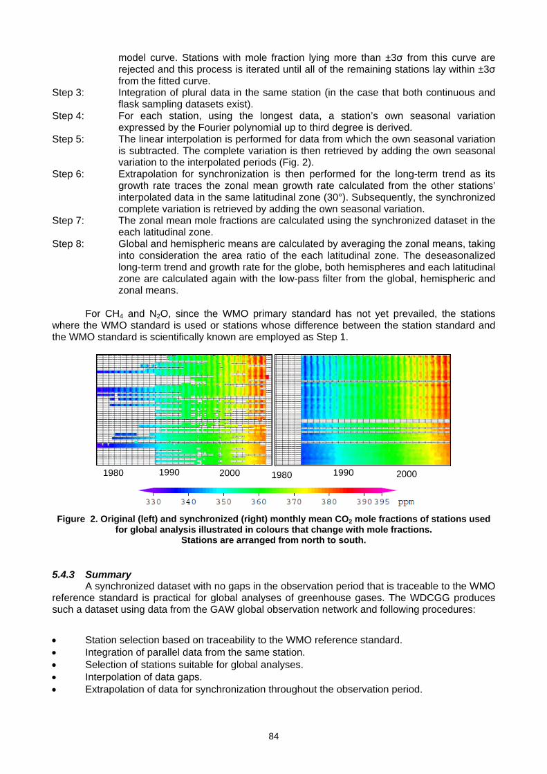
84

model curve. Stations with mole fraction lying more than ±3σ from this curve are rejected and this process is iterated until all of the remaining stations lay within ±3σ from the fitted curve.

Step 3: Integration of plural data in the same station (in the case that both continuous and flask sampling datasets exist).

Step 4: For each station, using the longest data, a station’s own seasonal variation expressed by the Fourier polynomial up to third degree is derived.

Step 5: The linear interpolation is performed for data from which the own seasonal variation is subtracted. The complete variation is then retrieved by adding the own seasonal variation to the interpolated periods (Fig. 2).

Step 6: Extrapolation for synchronization is then performed for the long-term trend as its growth rate traces the zonal mean growth rate calculated from the other stations’ interpolated data in the same latitudinal zone (30°). Subsequently, the synchronized complete variation is retrieved by adding the own seasonal variation.

Step 7: The zonal mean mole fractions are calculated using the synchronized dataset in the each latitudinal zone.

Step 8: Global and hemispheric means are calculated by averaging the zonal means, taking into consideration the area ratio of the each latitudinal zone. The deseasonalized long-term trend and growth rate for the globe, both hemispheres and each latitudinal zone are calculated again with the low-pass filter from the global, hemispheric and zonal means.

For CH4 and N2O, since the WMO primary standard has not yet prevailed, the stations

where the WMO standard is used or stations whose difference between the station standard and the WMO standard is scientifically known are employed as Step 1.

1980 1990 2000 2000 19901980

Figure 2. Original (left) and synchronized (right) monthly mean CO2 mole fractions of stations used

for global analysis illustrated in colours that change with mole fractions. Stations are arranged from north to south.

5.4.3 Summary

A synchronized dataset with no gaps in the observation period that is traceable to the WMO reference standard is practical for global analyses of greenhouse gases. The WDCGG produces such a dataset using data from the GAW global observation network and following procedures:

• Station selection based on traceability to the WMO reference standard. • Integration of parallel data from the same station. • Selection of stations suitable for global analyses. • Interpolation of data gaps. • Extrapolation of data for synchronization throughout the observation period.

85

Using the synchronized dataset, the WDCGG calculates monthly means, long-term trends and the growth rates for each latitudinal band. Subsequently, the global mean and other global statistics are calculated using latitudinal values weighted according to area. References WMO (2007), World Data Centre for Greenhouse Gases Data Submission and Dissemination Guide, GAW Report No. 174, (WMO TD No. 1416).

_______

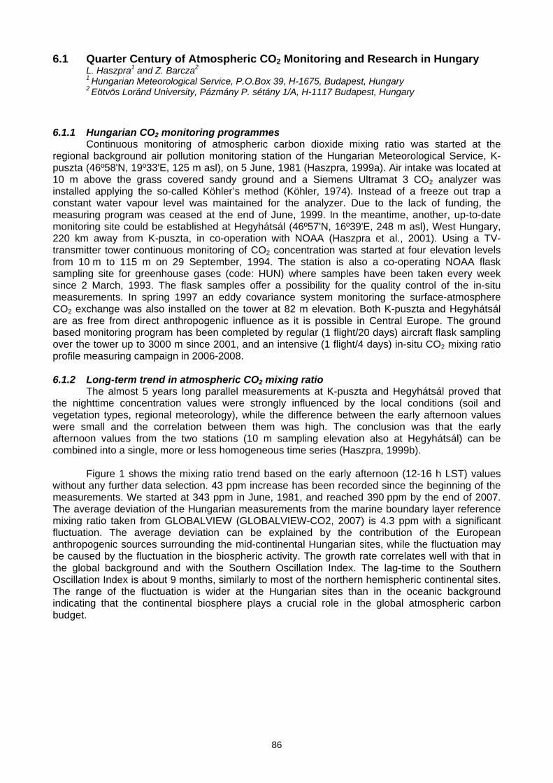
86

6.1 Quarter Century of Atmospheric CO2 Monitoring and Research in Hungary L. Haszpra1 and Z. Barcza2 1 Hungarian Meteorological Service, P.O.Box 39, H-1675, Budapest, Hungary 2 Eötvös Loránd University, Pázmány P. sétány 1/A, H-1117 Budapest, Hungary

6.1.1 Hungarian CO2 monitoring programmes

Continuous monitoring of atmospheric carbon dioxide mixing ratio was started at the regional background air pollution monitoring station of the Hungarian Meteorological Service, K-puszta (46º58'N, 19º33'E, 125 m asl), on 5 June, 1981 (Haszpra, 1999a). Air intake was located at 10 m above the grass covered sandy ground and a Siemens Ultramat 3 CO2 analyzer was installed applying the so-called Köhler’s method (Köhler, 1974). Instead of a freeze out trap a constant water vapour level was maintained for the analyzer. Due to the lack of funding, the measuring program was ceased at the end of June, 1999. In the meantime, another, up-to-date monitoring site could be established at Hegyhátsál (46º57'N, 16º39'E, 248 m asl), West Hungary, 220 km away from K-puszta, in co-operation with NOAA (Haszpra et al., 2001). Using a TV-transmitter tower continuous monitoring of CO2 concentration was started at four elevation levels from 10 m to 115 m on 29 September, 1994. The station is also a co-operating NOAA flask sampling site for greenhouse gases (code: HUN) where samples have been taken every week since 2 March, 1993. The flask samples offer a possibility for the quality control of the in-situ measurements. In spring 1997 an eddy covariance system monitoring the surface-atmosphere CO2 exchange was also installed on the tower at 82 m elevation. Both K-puszta and Hegyhátsál are as free from direct anthropogenic influence as it is possible in Central Europe. The ground based monitoring program has been completed by regular (1 flight/20 days) aircraft flask sampling over the tower up to 3000 m since 2001, and an intensive (1 flight/4 days) in-situ CO2 mixing ratio profile measuring campaign in 2006-2008. 6.1.2 Long-term trend in atmospheric CO2 mixing ratio

The almost 5 years long parallel measurements at K-puszta and Hegyhátsál proved that the nighttime concentration values were strongly influenced by the local conditions (soil and vegetation types, regional meteorology), while the difference between the early afternoon values were small and the correlation between them was high. The conclusion was that the early afternoon values from the two stations (10 m sampling elevation also at Hegyhátsál) can be combined into a single, more or less homogeneous time series (Haszpra, 1999b).

Figure 1 shows the mixing ratio trend based on the early afternoon (12-16 h LST) values

without any further data selection. 43 ppm increase has been recorded since the beginning of the measurements. We started at 343 ppm in June, 1981, and reached 390 ppm by the end of 2007. The average deviation of the Hungarian measurements from the marine boundary layer reference mixing ratio taken from GLOBALVIEW (GLOBALVIEW-CO2, 2007) is 4.3 ppm with a significant fluctuation. The average deviation can be explained by the contribution of the European anthropogenic sources surrounding the mid-continental Hungarian sites, while the fluctuation may be caused by the fluctuation in the biospheric activity. The growth rate correlates well with that in the global background and with the Southern Oscillation Index. The lag-time to the Southern Oscillation Index is about 9 months, similarly to most of the northern hemispheric continental sites. The range of the fluctuation is wider at the Hungarian sites than in the oceanic background indicating that the continental biosphere plays a crucial role in the global atmospheric carbon budget.

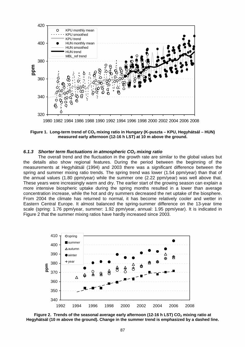
87

320

340

360

380

400

420

1980 1982 1984 1986 1988 1990 1992 1994 1996 1998 2000 2002 2004 2006 2008

ppm

KPU monthly mean KPU smoothed KPU trend HUN monthly mean HUN smoothed HUN trend MBL_ref trend

Figure 1. Long-term trend of CO2 mixing ratio in Hungary (K-puszta – KPU, Hegyhátsál – HUN)

measured early afternoon (12-16 h LST) at 10 m above the ground.

6.1.3 Shorter term fluctuations in atmospheric CO2 mixing ratio

The overall trend and the fluctuation in the growth rate are similar to the global values but the details also show regional features. During the period between the beginning of the measurements at Hegyhátsál (1994) and 2003 there was a significant difference between the spring and summer mixing ratio trends. The spring trend was lower (1.54 ppm/year) than that of the annual values (1.80 ppm/year) while the summer one (2.22 ppm/year) was well above that. These years were increasingly warm and dry. The earlier start of the growing season can explain a more intensive biospheric uptake during the spring months resulted in a lower than average concentration increase, while the hot and dry summers decreased the net uptake of the biosphere. From 2004 the climate has returned to normal, it has become relatively cooler and wetter in Eastern Central Europe. It almost balanced the spring-summer difference on the 13-year time scale (spring: 1.76 ppm/year, summer: 1.92 ppm/year, annual: 1.95 ppm/year). It is indicated in Figure 2 that the summer mixing ratios have hardly increased since 2003.

340

350

360

370

380

390

400

410

1992 1994 1996 1998 2000 2002 2004 2006 2008

ppm

spring

summer

autumn

winter

year

Figure 2. Trends of the seasonal average early afternoon (12-16 h LST) CO2 mixing ratio at

Hegyhátsál (10 m above the ground). Change in the summer trend is emphasized by a dashed line.

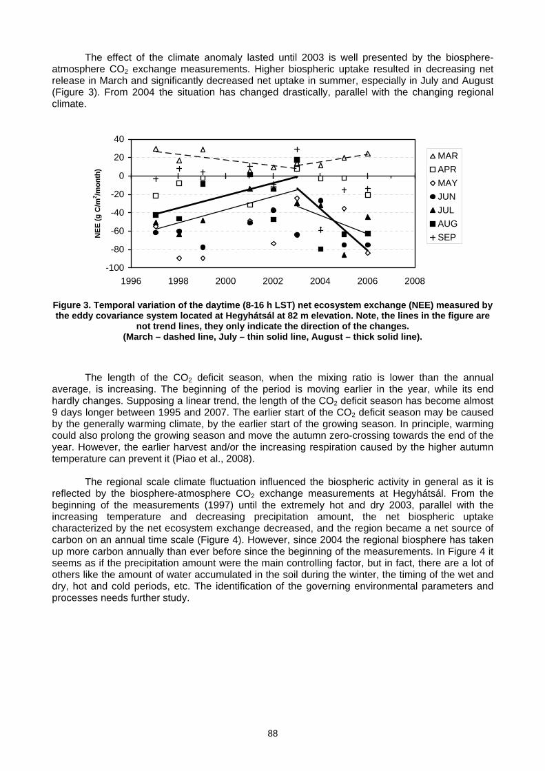
88

The effect of the climate anomaly lasted until 2003 is well presented by the biosphere-atmosphere CO2 exchange measurements. Higher biospheric uptake resulted in decreasing net release in March and significantly decreased net uptake in summer, especially in July and August (Figure 3). From 2004 the situation has changed drastically, parallel with the changing regional climate.

-100

-80

-60

-40

-20

0

20

40

1996 1998 2000 2002 2004 2006 2008

NEE

(g C

/m2 /m

onth

)

MARAPRMAYJUNJULAUGSEP

Figure 3. Temporal variation of the daytime (8-16 h LST) net ecosystem exchange (NEE) measured by the eddy covariance system located at Hegyhátsál at 82 m elevation. Note, the lines in the figure are

not trend lines, they only indicate the direction of the changes. (March – dashed line, July – thin solid line, August – thick solid line).

The length of the CO2 deficit season, when the mixing ratio is lower than the annual average, is increasing. The beginning of the period is moving earlier in the year, while its end hardly changes. Supposing a linear trend, the length of the CO2 deficit season has become almost 9 days longer between 1995 and 2007. The earlier start of the CO2 deficit season may be caused by the generally warming climate, by the earlier start of the growing season. In principle, warming could also prolong the growing season and move the autumn zero-crossing towards the end of the year. However, the earlier harvest and/or the increasing respiration caused by the higher autumn temperature can prevent it (Piao et al., 2008).

The regional scale climate fluctuation influenced the biospheric activity in general as it is

reflected by the biosphere-atmosphere CO2 exchange measurements at Hegyhátsál. From the beginning of the measurements (1997) until the extremely hot and dry 2003, parallel with the increasing temperature and decreasing precipitation amount, the net biospheric uptake characterized by the net ecosystem exchange decreased, and the region became a net source of carbon on an annual time scale (Figure 4). However, since 2004 the regional biosphere has taken up more carbon annually than ever before since the beginning of the measurements. In Figure 4 it seems as if the precipitation amount were the main controlling factor, but in fact, there are a lot of others like the amount of water accumulated in the soil during the winter, the timing of the wet and dry, hot and cold periods, etc. The identification of the governing environmental parameters and processes needs further study.

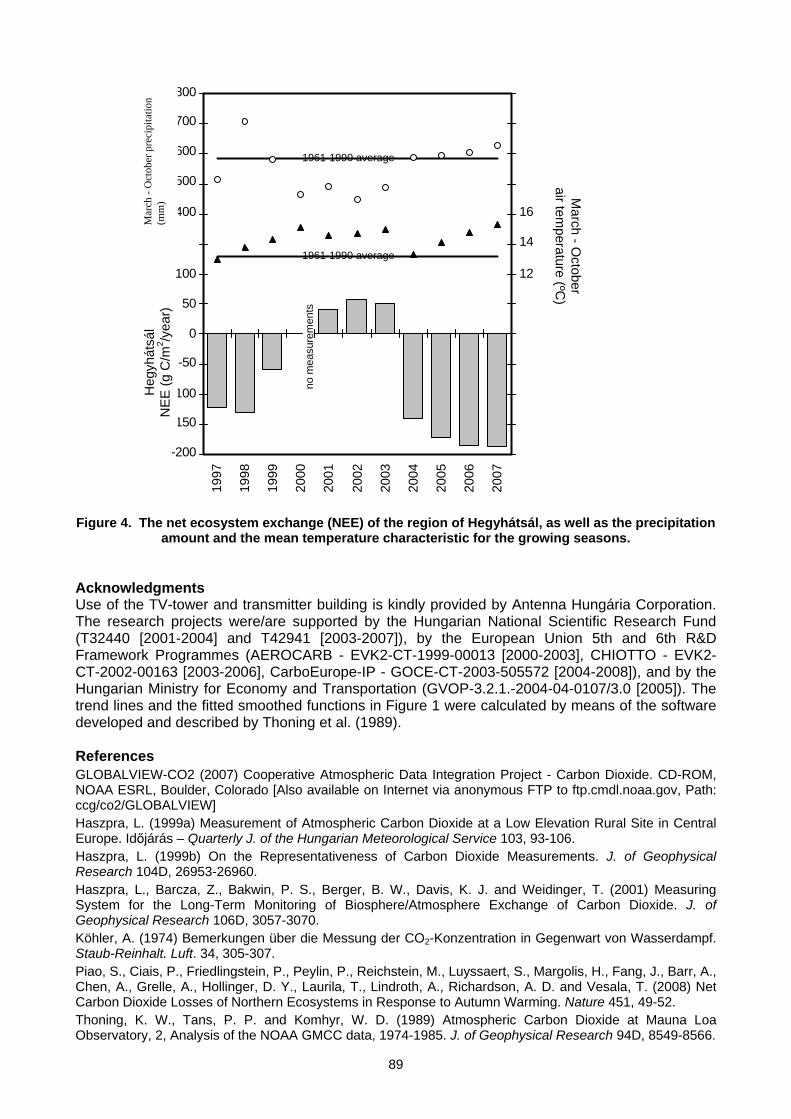
89

1997

1998

1999

2000

2001

2002

2003

2004

2005

2006

2007

800

700

600

500

400

0

50

100

-50

-100

-150

-200

12

14

16

Figure 4. The net ecosystem exchange (NEE) of the region of Hegyhátsál, as well as the precipitation amount and the mean temperature characteristic for the growing seasons.

Acknowledgments Use of the TV-tower and transmitter building is kindly provided by Antenna Hungária Corporation. The research projects were/are supported by the Hungarian National Scientific Research Fund (T32440 [2001-2004] and T42941 [2003-2007]), by the European Union 5th and 6th R&D Framework Programmes (AEROCARB - EVK2-CT-1999-00013 [2000-2003], CHIOTTO - EVK2-CT-2002-00163 [2003-2006], CarboEurope-IP - GOCE-CT-2003-505572 [2004-2008]), and by the Hungarian Ministry for Economy and Transportation (GVOP-3.2.1.-2004-04-0107/3.0 [2005]). The trend lines and the fitted smoothed functions in Figure 1 were calculated by means of the software developed and described by Thoning et al. (1989). References GLOBALVIEW-CO2 (2007) Cooperative Atmospheric Data Integration Project - Carbon Dioxide. CD-ROM, NOAA ESRL, Boulder, Colorado [Also available on Internet via anonymous FTP to ftp.cmdl.noaa.gov, Path: ccg/co2/GLOBALVIEW] Haszpra, L. (1999a) Measurement of Atmospheric Carbon Dioxide at a Low Elevation Rural Site in Central Europe. Időjárás – Quarterly J. of the Hungarian Meteorological Service 103, 93-106. Haszpra, L. (1999b) On the Representativeness of Carbon Dioxide Measurements. J. of Geophysical Research 104D, 26953-26960. Haszpra, L., Barcza, Z., Bakwin, P. S., Berger, B. W., Davis, K. J. and Weidinger, T. (2001) Measuring System for the Long-Term Monitoring of Biosphere/Atmosphere Exchange of Carbon Dioxide. J. of Geophysical Research 106D, 3057-3070. Köhler, A. (1974) Bemerkungen über die Messung der CO2-Konzentration in Gegenwart von Wasserdampf. Staub-Reinhalt. Luft. 34, 305-307. Piao, S., Ciais, P., Friedlingstein, P., Peylin, P., Reichstein, M., Luyssaert, S., Margolis, H., Fang, J., Barr, A., Chen, A., Grelle, A., Hollinger, D. Y., Laurila, T., Lindroth, A., Richardson, A. D. and Vesala, T. (2008) Net Carbon Dioxide Losses of Northern Ecosystems in Response to Autumn Warming. Nature 451, 49-52. Thoning, K. W., Tans, P. P. and Komhyr, W. D. (1989) Atmospheric Carbon Dioxide at Mauna Loa Observatory, 2, Analysis of the NOAA GMCC data, 1974-1985. J. of Geophysical Research 94D, 8549-8566.

Mar

ch -

Oct

ober

pre

cipi

tatio

n

(mm

) H

egyh

átsá

l N

EE

(g C

/m2 /y

ear)

March - O

ctober air tem

perature (ºC)

1961-1990 average

1961-1990 average

no m

easu

rem

ents

90

6.2 CO2 Isotopic Composition in the Upper Troposphere: the Project CARIBIC S.S. Assonov 1,2, C.A.M. Brenninkmeijer2, A. Zahn3, C. Koeppel2

1- Joint Research Centre of European Commission (EC), Institute for Reference Materials and Measurements (IRMM), Geel, Belgium 2- Max Planck Institute for Chemistry, Mainz, Germany 3- Forschungszentrum Karlsruhe, Germany

6.2.1 The approach

Many programmes worldwide aim at greenhouse gas monitoring covering different geographical scales, from very local, via regional to global (background stations). Commonly boundary layer air is assayed this way, close to CO2 sources and sinks, whereas only a few stations are on mountains in the free troposphere. There also are a few programs using ocean ships and vertical profiling by small research aircrafts (NOAA/ESRL). In particular aircraft sampling is relatively expensive. Basically most global networks do cover remote areas (particularly the tropics) only sparsely, and much less information is available at altitude, although satellite observations are filling in some gaps in observation. In view of incomplete global monitoring, the 13th CO2 Expert Meeting recommended [1] to promote programmes using commercial aircraft (altitudes of ~10 km). To provide information about CO2 (including isotopic composition) in background air, in the free tropical troposphere and in the tropopause region, far from CO2 sources and sinks, aircraft-based observational platforms are really important. The project JAL (Japan) studies CO2 concentrations by flights from Japan to Australia, and recently other designations have been added. CO2 isotope measurements by JAL have been started [2]. The project CARIBIC (http://caribic-atmospheric.com) started in 1997 and aims to study atmospheric chemistry and composition by measuring many compounds and species in the upper troposphere around the globe. CARIBIC has two phases, CARIBIC-1 and CARIBIC-2 (CARIBIC-LUFTHANSA).

6.2.2 CARIBIC-1

The instrument container onboard a Boeing 767 operated by LTU (Düsseldorf, Germany) included instruments for on-line analyses of O3 and CO, aerosol measurements as well as air sampling system (twelve SS canisters of 20 l, air pressurised to ~17 bar) for trace gas analyses in lab conditions. Analysed were CO2, CH4, N2O, SF6, NMCH, halogenated organic compounds as well as CO and CO isotopes, including 14CO. The CO extraction by means of CO→CO2 oxidation required a quantitative extraction/stripping of tropospheric CO2 prior to the oxidation step. Isotope analyses presented in this paper were performed on a MAT-252 at the Max Planck Institute for Chemistry (Germany), on the cryogenic extracts obtained from processing ~300 l air. Originally CO2 isotope analysis was not a main focus of CARIBIC-1. Large δ18O(CO2) scatter at the beginning of CARIBIC-1 (Figure 1) indicated CO2-water isotope exchange. For canisters no. 1, 6 and 9 the problem persisted longer than for others. Also the MAT-252 calibration was optimised for CO measurements rather than for CO2 isotope analyses. Despite of these problems and thanks to the high quality extraction, robust IRMS performance, and having extremely large samples, CO2 isotope results are considered to be very reliable (examples are presented below). This success stimulated us to continue CO2 isotope measurements for CARIBIC-LUFTHANSA. 6.2.3 CARIBIC-2

The new instrument container, operating onboard an A360-600 of Lufthansa (Frankfurt, Germany), performs monthly flights from Frankfurt to remote designations such as China, South America and Canada. The container includes an extended range of instrumentation (O3, CO, NOx, H2O and others, adsorption cartridges for NMHC, aerosol measurements etc, see http://caribic-atmospheric.com, [3]). The sampling system consists of two collector boxes (TRACs) each with 14 glass containers (2.7 l volume, pressure ~3 bar) being filled within a minute, giving much better sampling resolution than in CARIBIC-1 (20 minutes, or ~250 km). After a flight, the TRACs are sent to participating institutions. A specially designed CO2 extraction line was installed at IRMM (Geel, Belgium) and measurements started in May 2007. Preliminary CARIBIC-2 data indicate that δ18O(CO2) scatter is small, indicating excellent preservation of δ18O(CO2), due to use of glass containers. We particularly focus on quality δ18O(CO2) data which give information about CO2 exchange with oceans, soils and biosphere [4], being a long-term indicator of global changes in the

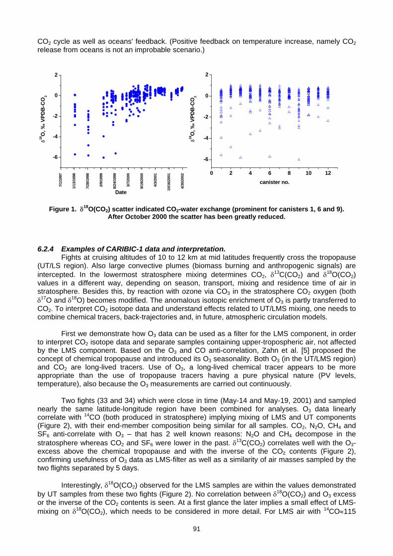
91

CO2 cycle as well as oceans' feedback. (Positive feedback on temperature increase, namely CO2 release from oceans is not an improbable scenario.)

7/1/

1997

1/13

/199

8

7/28

/199

8

2/9/

1999

8/24

/199

9

3/7/

2000

9/19

/200

0

4/3/

2001

10/1

6/20

01

4/30

/200

2

-6

-4

-2

0

2

δ18O

, ‰ V

PDB

-CO

2

Date

0 2 4 6 8 10 12

-6

-4

-2

0

2

δ18O

, ‰ V

PDB

-CO

2

canister no.

Figure 1. δ18O(CO2) scatter indicated CO2-water exchange (prominent for canisters 1, 6 and 9). After October 2000 the scatter has been greatly reduced.

6.2.4 Examples of CARIBIC-1 data and interpretation.

Fights at cruising altitudes of 10 to 12 km at mid latitudes frequently cross the tropopause (UT/LS region). Also large convective plumes (biomass burning and anthropogenic signals) are intercepted. In the lowermost stratosphere mixing determines CO2, δ13C(CO2) and δ18O(CO2) values in a different way, depending on season, transport, mixing and residence time of air in stratosphere. Besides this, by reaction with ozone via CO3 in the stratosphere CO2 oxygen (both δ17O and δ18O) becomes modified. The anomalous isotopic enrichment of O3 is partly transferred to CO2. To interpret CO2 isotope data and understand effects related to UT/LMS mixing, one needs to combine chemical tracers, back-trajectories and, in future, atmospheric circulation models.

First we demonstrate how O3 data can be used as a filter for the LMS component, in order

to interpret CO2 isotope data and separate samples containing upper-tropospheric air, not affected by the LMS component. Based on the O3 and CO anti-correlation, Zahn et al. [5] proposed the concept of chemical tropopause and introduced its O3 seasonality. Both O3 (in the UT/LMS region) and CO2 are long-lived tracers. Use of O3, a long-lived chemical tracer appears to be more appropriate than the use of tropopause tracers having a pure physical nature (PV levels, temperature), also because the O3 measurements are carried out continuously.

Two fights (33 and 34) which were close in time (May-14 and May-19, 2001) and sampled

nearly the same latitude-longitude region have been combined for analyses. O3 data linearly correlate with 14CO (both produced in stratosphere) implying mixing of LMS and UT components (Figure 2), with their end-member composition being similar for all samples. CO2, N2O, CH4 and SF6 anti-correlate with O3 – that has 2 well known reasons: N2O and CH4 decompose in the stratosphere whereas CO2 and SF6 were lower in the past. δ13C(CO2) correlates well with the O3-excess above the chemical tropopause and with the inverse of the CO2 contents (Figure 2), confirming usefulness of O3 data as LMS-filter as well as a similarity of air masses sampled by the two flights separated by 5 days.

Interestingly, δ18O(CO2) observed for the LMS samples are within the values demonstrated

by UT samples from these two fights (Figure 2). No correlation between δ18O(CO2) and O3 excess or the inverse of the CO2 contents is seen. At a first glance the later implies a small effect of LMS-mixing on δ18O(CO2), which needs to be considered in more detail. For LMS air with 14CO≈115

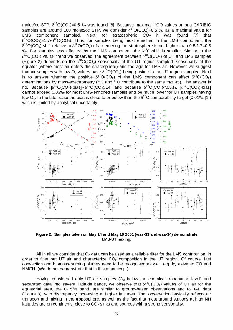
92

molec/cc STP, δ17O(CO2)≈0.5 ‰ was found [6]. Because maximal 14CO values among CARIBIC samples are around 100 molec/cc STP, we consider δ17O(CO2)≈0.5 ‰ as a maximal value for LMS component sampled. Next, for stratospheric CO2 it was found [7] that δ17O(CO2)≈1.7•δ18O(CO2). Thus, for samples being most enriched in the LMS component, the δ18O(CO2) shift relative to δ18O(CO2) of air entering the stratosphere is not higher than 0.5/1.7=0.3 ‰. For samples less affected by the LMS component, the δ18O-shift is smaller. Similar to the δ13C(CO2) vs. O3 trend we observed, the agreement between δ18O(CO2) of UT and LMS samples (Figure 2) depends on the δ18O(CO2) seasonality at the UT region sampled, seasonality at the equator (where most air enters the stratosphere) and the age for LMS air. However we suggest that air samples with low O3 values have δ18O(CO2) being pristine to the UT region sampled. Next is to answer whether the positive δ17O(CO2) of the LMS component can affect δ13C(CO2) determinations by mass-spectrometry (13C and 17O contribute to the same m/z 45). The answer is no. Because [δ13C(CO2)-bias]≈ δ17O(CO2)/14, and because δ17O(CO2)<0.5‰, [δ13C(CO2)-bias] cannot exceed 0.03‰ for most LMS-enriched samples and be much lower for UT samples having low O3. In the later case the bias is close to or below than the δ13C comparability target (0.01‰ [1]) witch is limited by analytical uncertainty.

0 200 400 600

0

20

40

60

80

100

4.3

4.4

4.5

4.6

4.7

4.8

4.9

5.0

0 200 400 600366

368

370

372

374

376

275

280

285

290

295

300

305

310

315

320

-100 0 100 200 300 400 5000.00

0.25

0.50

0.75

1.00

-100 0 100 200 300 400 500

-8.3

-8.2

-8.1

-8.0

0.00268 0.00270 0.00272

-8.3

-8.2

-8.1

-8.0

1600

1650

1700

1750

1800

1850

1900

15 20 25 30 35 40 45 50 55

-8.3

-8.2

-8.1

-8.0

0.00268 0.00270 0.002720.00

0.25

0.50

0.75

1.00

15 20 25 30 35 40 45 50 550.00

0.25

0.50

0.75

1.00

was-33 was-34

14C

O, m

ol/c

c

O3, ppb

SF 6,

ppt

was-33 was-34

CO

2, pp

m

O3, ppb

N2O

, ppb

was-33was-34

δ18O

(CO

2), ‰

excess O3, ppb

was-33 was-34

δ13C

(CO

2), ‰

excess O3, ppb

was-33 was-34

δ13C

(CO

2), ‰

1/CO2, ppm-1

CH

4, pp

b

was-33was-34

δ13C

(CO

2), ‰

Latitude

was-33 was-34

δ13C

(CO

2), ‰

1/CO2, ppm-1

was-33was-34

δ18O

(CO

2), ‰

Latitude

Figure 2. Samples taken on May 14 and May 19 2001 (was-33 and was-34) demonstrate

LMS-UT mixing. All in all we consider that O3 data can be used as a reliable filter for the LMS contribution, in

order to filter out UT air and characterize CO2 composition in the UT region. Of course, fast convection and biomass-burning plumes need to be recognised as well, e.g. by elevated CO and NMCH. (We do not demonstrate that in this manuscript).

Having considered only UT air samples (O3 below the chemical tropopause level) and

separated data into several latitude bands, we observe that δ13C(CO2) values of UT air for the equatorial area, the 0-15oN band, are similar to ground-based observations and to JAL data (Figure 3), with discrepancy increasing at higher latitudes. That observation basically reflects air transport and mixing in the troposphere, as well as the fact that most ground stations at high NH latitudes are on continents, close to CO2 sinks and sources with a strong seasonality.

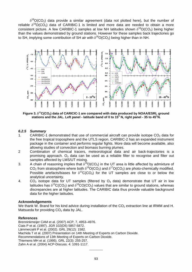
93

δ18O(CO2) data provide a similar agreement (data not plotted here), but the number of reliable δ18O(CO2) data of CARIBIC-1 is limited and more data are needed to obtain a more consistent picture. A few CARIBIC-1 samples at low NH latitudes shown δ18O(CO2) being higher than the values demonstrated by ground stations. However for these samples back trajectories go to SH, implying some contribution of SH air with δ18O(CO2) being higher than in NH.

Figure 3. δ13C(CO2) data of CARICIC-1 are compared with data produced by NOAA/ESRL ground stations and the JAL. Left panel - latitude band of 0 to 15o N, right panel - 35 to 45oN.

6.2.5 Summary 1. CARIBIC-1 demonstrated that use of commercial aircraft can provide isotope CO2 data for

the free tropical troposphere and the UTLS region. CARIBIC-2 has an expanded instrument package in the container and performs regular fights. More data will become available, also allowing studies of convection and biomass burning plumes.

2 Combination of chemical tracers, meteorological data and air back-trajectories is a promising approach. O3 data can be used as a reliable filter to recognise and filter out samples affected by LMS/UT mixing.

3. A chain of reasoning implies that δ18O(CO2) in the UT area is little affected by admixture of CO2 from stratosphere where both δ18O(CO2) and δ17O(CO2) are photo-chemically modified. Possible artefacts/biases for δ13C(CO2) for the UT samples are close to or below the analytical uncertainty.

4. CO2 isotope data for UT samples (filtered by O3 data) demonstrate that UT air in low latitudes has δ13C(CO2) and δ18CO(CO2) values that are similar to ground stations, whereas discrepancies are at higher latitudes. The CARIBIC data thus provide valuable background data for the higher latitudes.

Acknowledgements We thank W. Brand for his kind advice during installation of the CO2 extraction line at IRMM and H. Matsueda for providing CO2 data by JAL. References Brenninkmeijer CAM et al. (2007) ACP, 7, 4953–4976. Ciais P et al. (1997). JGR 102(D5) 5857-5872. Lämmerzahl P et al. (2002). GRL 29(12): 1582. Machida T et al. (2007) Presentation on 14th Meeting of Experts on Carbon Dioxide. Recommendations of 13th Meeting of Experts on Carbon Dioxide. Thiemens MH et al. (1995). GRL 22(3): 255-257. Zahn A et al. (2004) ACP-Discuss. 4: 1091-1117.

_______

-8.4

-8.2

-8.0

-7.8 7/1/

1997

1/1/

1998

7/1/

1998

1/1/

1999

7/1/

1999

1/1/

2000

7/1/

2000

1/1/

2001

7/1/

2001

1/1/

2002

7/1/

2002

δ13C

, ‰ V

PDB

-CO

2

0 - 15oN

7/1/

1997

1/1/

1998

7/1/

1998

1/1/

1999

7/1/

1999

1/1/

2000

7/1/

2000

1/1/

2001

7/1/

2001

1/1/

2002

7/1/

2002

360

365

370

375

RPB GMI CHR

CARIBIC JAL00N05N JAL05N10N JAL10N15N

CO

2, ppm

-8.4

-8.2

-8.0

-7.8

-7.6 7/1/

1997

1/1/

1998

7/1/

1998

1/1/

1999

7/1/

1999

1/1/

2000

7/1/

2000

1/1/

2001

7/1/

2001

1/1/

2002

7/1/

2002

δ13C

, ‰ V

PDB

-CO

2

7/1/

1997

1/1/

1998

7/1/

1998

1/1/

1999

7/1/

1999

1/1/

2000

7/1/

2000

1/1/

2001

7/1/

2001

1/1/

2002

7/1/

2002

360

365

370

375

380

35 - 45oN

AZR KZM NWR UUM WLG CARIBIC

CO

2, pp

m

94

7.1 Greenhouse Gases Monitoring in India S.D. Attri Director, India Meteorological Department, New Delhi-11003, India

7.1.1 Introduction

The quantification of interactions among the atmosphere, biosphere, hydrosphere and lithosphere i.e. bio-geo chemical cycle is necessary to accurately estimate sources and sinks of Greenhouse Gases (GHGs). It requires accurate determination of concentration of these gases and their trends with adequate spatial coverage so as to improve estimates of radiative forcing needed for addressing the climate change issues under UN Framework. About one half of the carbon emitted by combustion remains in the atmosphere, while the other half is taken up by the oceans and terrestrial biosphere. Based on measurements of CO2 abundance, its stable isotopes of carbon and oxygen, and O2/N2 ratios, IPCC 2001 estimated that average uptake was 1.7±0.5 Pg / yr by the oceans and 1.4±0.7 Pg/yr by the land biosphere for the 1990s [Houghton et al., 2001]. These are net fluxes while, gross fluxes between atmosphere and oceans, and atmosphere and terrestrial biosphere (photosynthesis and respiration), are of the order of 100 Pg per yr. Since this partitioning of fossil CO2 between the oceans and biosphere has policy implications, it is important to reduce uncertainties to make better estimates on regional scales (e.g., using inverse modelling to estimate regional fluxes).

Methane is emitted to the atmosphere by natural and anthropogenic sources. Natural

sources include wetlands, vegetation, termites, oceans, and geologic sources (e.g., hydrocarbon seeps, hydrates, mud volcanoes). Anthropogenic sources include fossil fuel exploitation, rice agriculture, landfills, domestic ruminant animals, landfills, municipal waste treatment, and biomass burning. Emission rates from many sources are difficult to quantify from the top-down perspective using atmospheric measurements, because fluxes are small, diffuse, and vary by orders of magnitude, both spatially and temporally.

The major natural sources of N2O to the atmosphere are the ocean and soil processes

while anthropogenic sources are agriculture, through use of nitrogen fertilizers, biomass burning, industrial processes (nylon and nitric acid production), and cattle feedlots. Though the major sources have been identified, but the uncertainties in emissions from each are still large. Two major sink processes are responsible for N2O removal from the atmosphere, both of them in the stratosphere: photolysis and reaction with electronically excited oxygen atoms (WMO GAW 2007).

The Indian sub-continent and surrounding seas with more than 1.1 billion people and

unique natural resources have a significant impact on regional and global environment but lack a comprehensive observational network. India Meteorological Department (IMD) has embarked upon an extensive programme to establish a permanent network of stations in India to monitor atmospheric concentrations of greenhouse gases (CO2, CH4 and N2O) and aerosols in order to quantify source and sink potentials. 7.1.2 Monitoring philosophy

The two main phenomena that affect GHGs variations over the Indian region are the influence of subtropical highs and monsoon wind reversal. The former influences much of the northern parts of the country while the latter would have discernable impacts over the peninsular region. As such, these areas need to be studied in very high temporal resolution (24X365). Hence, the scientific programme of CREM envisages establishment of two baseline stations with continuous monitoring of GHGs at Ranichauri (in the Central Himalayas) and Kodaikanal in the peninsula with having emphasis on long term trends. Both being high altitude stations, are suitable for sampling of free well mixed air over the respective region.

GHGs data from different regions of the country are essential to extrapolate the flux values

obtained from Inverse C – Cycle models for different parts of the country in a broad manner. It requires characterizing the zonal variability of GHGs across east-west India and to bring out characteristic features of contrasting areas viz. arid and non-vegetated areas in the west, sub-

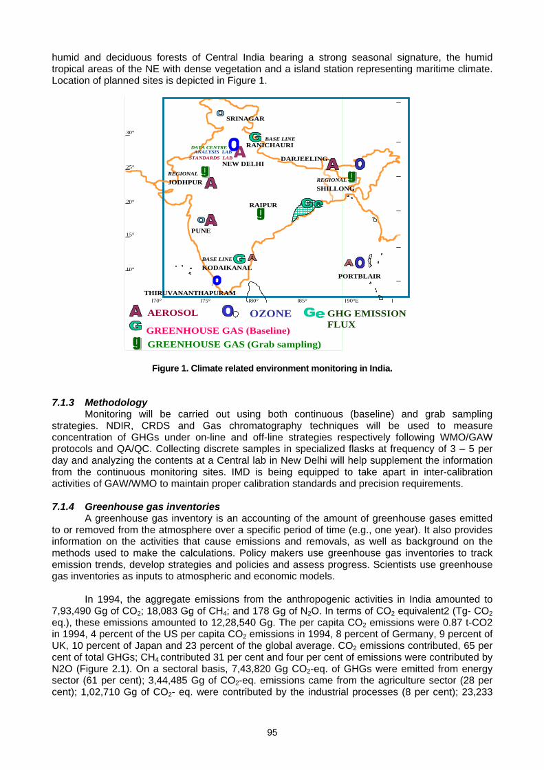
95

humid and deciduous forests of Central India bearing a strong seasonal signature, the humid tropical areas of the NE with dense vegetation and a island station representing maritime climate. Location of planned sites is depicted in Figure 1.

Figure 1. Climate related environment monitoring in India.

7.1.3 Methodology

Monitoring will be carried out using both continuous (baseline) and grab sampling strategies. NDIR, CRDS and Gas chromatography techniques will be used to measure concentration of GHGs under on-line and off-line strategies respectively following WMO/GAW protocols and QA/QC. Collecting discrete samples in specialized flasks at frequency of 3 – 5 per day and analyzing the contents at a Central lab in New Delhi will help supplement the information from the continuous monitoring sites. IMD is being equipped to take apart in inter-calibration activities of GAW/WMO to maintain proper calibration standards and precision requirements. 7.1.4 Greenhouse gas inventories

A greenhouse gas inventory is an accounting of the amount of greenhouse gases emitted to or removed from the atmosphere over a specific period of time (e.g., one year). It also provides information on the activities that cause emissions and removals, as well as background on the methods used to make the calculations. Policy makers use greenhouse gas inventories to track emission trends, develop strategies and policies and assess progress. Scientists use greenhouse gas inventories as inputs to atmospheric and economic models.

In 1994, the aggregate emissions from the anthropogenic activities in India amounted to

7,93,490 Gg of CO2; 18,083 Gg of CH4; and 178 Gg of N2O. In terms of CO2 equivalent2 (Tg- CO2 eq.), these emissions amounted to 12,28,540 Gg. The per capita CO2 emissions were 0.87 t-CO2 in 1994, 4 percent of the US per capita CO2 emissions in 1994, 8 percent of Germany, 9 percent of UK, 10 percent of Japan and 23 percent of the global average. CO2 emissions contributed, 65 per cent of total GHGs; CH4 contributed 31 per cent and four per cent of emissions were contributed by N2O (Figure 2.1). On a sectoral basis, 7,43,820 Gg CO2-eq. of GHGs were emitted from energy sector (61 per cent); 3,44,485 Gg of CO2-eq. emissions came from the agriculture sector (28 per cent); 1,02,710 Gg of CO2- eq. were contributed by the industrial processes (8 per cent); 23,233

AEROSOL OZONEGREENHOUSE GAS (Baseline)

GHG EMISSION FLUX

GREENHOUSE GAS (Grab sampling)

30°

25°

20°

15°

10°

70° 75° 80° 85° 90°E

REGIONAL

SHILLONG

DARJEELING

PORTBLAIR

BASE LINE

KODAIKANAL

2

THIRUVANANTHAPURAM

REGIONAL

JODHPUR

PUNE

SRINAGAR

DATA CENTREANALYSIS LAB

STANDARDS LABNEW DELHI

BASE LINERANICHAURI

RAIPUR

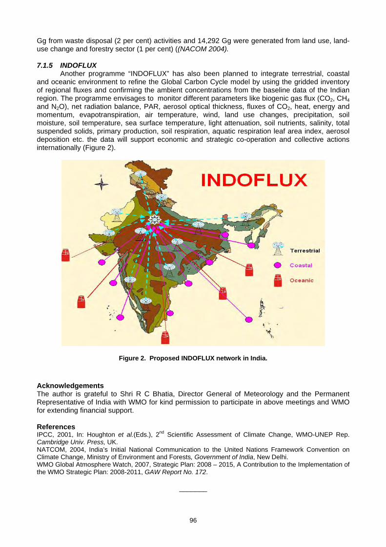
96

Gg from waste disposal (2 per cent) activities and 14,292 Gg were generated from land use, land-use change and forestry sector (1 per cent) ((NACOM 2004). 7.1.5 INDOFLUX Another programme “INDOFLUX” has also been planned to integrate terrestrial, coastal and oceanic environment to refine the Global Carbon Cycle model by using the gridded inventory of regional fluxes and confirming the ambient concentrations from the baseline data of the Indian region. The programme envisages to monitor different parameters like biogenic gas flux (CO2, CH4 and N2O), net radiation balance, PAR, aerosol optical thickness, fluxes of CO2, heat, energy and momentum, evapotranspiration, air temperature, wind, land use changes, precipitation, soil moisture, soil temperature, sea surface temperature, light attenuation, soil nutrients, salinity, total suspended solids, primary production, soil respiration, aquatic respiration leaf area index, aerosol deposition etc. the data will support economic and strategic co-operation and collective actions internationally (Figure 2).

Figure 2. Proposed INDOFLUX network in India.

Acknowledgements The author is grateful to Shri R C Bhatia, Director General of Meteorology and the Permanent Representative of India with WMO for kind permission to participate in above meetings and WMO for extending financial support. References IPCC, 2001, In: Houghton et al.(Eds.), 2nd Scientific Assessment of Climate Change, WMO-UNEP Rep. Cambridge Univ. Press, UK. NATCOM, 2004, India’s Initial National Communication to the United Nations Framework Convention on Climate Change, Ministry of Environment and Forests, Government of India, New Delhi. WMO Global Atmosphere Watch, 2007, Strategic Plan: 2008 – 2015, A Contribution to the Implementation of the WMO Strategic Plan: 2008-2011, GAW Report No. 172.

_______

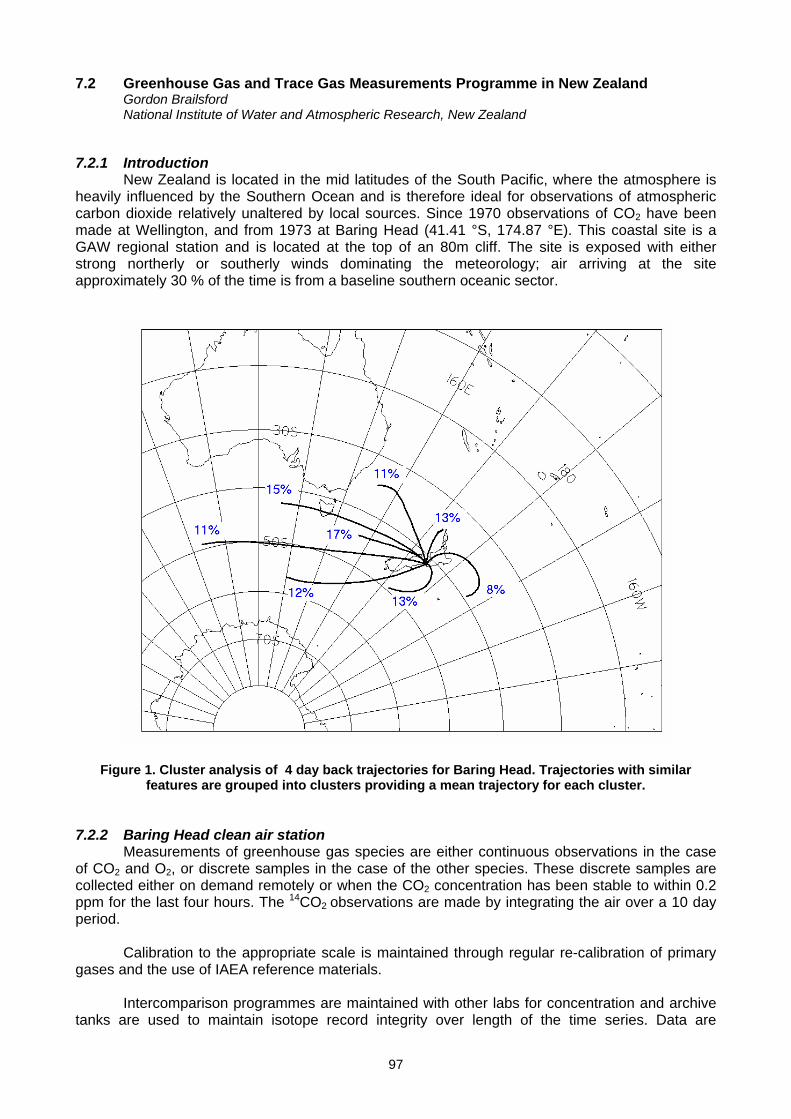
97

7.2 Greenhouse Gas and Trace Gas Measurements Programme in New Zealand Gordon Brailsford National Institute of Water and Atmospheric Research, New Zealand

7.2.1 Introduction

New Zealand is located in the mid latitudes of the South Pacific, where the atmosphere is heavily influenced by the Southern Ocean and is therefore ideal for observations of atmospheric carbon dioxide relatively unaltered by local sources. Since 1970 observations of CO2 have been made at Wellington, and from 1973 at Baring Head (41.41 °S, 174.87 °E). This coastal site is a GAW regional station and is located at the top of an 80m cliff. The site is exposed with either strong northerly or southerly winds dominating the meteorology; air arriving at the site approximately 30 % of the time is from a baseline southern oceanic sector.

Figure 1. Cluster analysis of 4 day back trajectories for Baring Head. Trajectories with similar features are grouped into clusters providing a mean trajectory for each cluster.

7.2.2 Baring Head clean air station

Measurements of greenhouse gas species are either continuous observations in the case of CO2 and O2, or discrete samples in the case of the other species. These discrete samples are collected either on demand remotely or when the CO2 concentration has been stable to within 0.2 ppm for the last four hours. The 14CO2 observations are made by integrating the air over a 10 day period.

Calibration to the appropriate scale is maintained through regular re-calibration of primary

gases and the use of IAEA reference materials. Intercomparison programmes are maintained with other labs for concentration and archive

tanks are used to maintain isotope record integrity over length of the time series. Data are

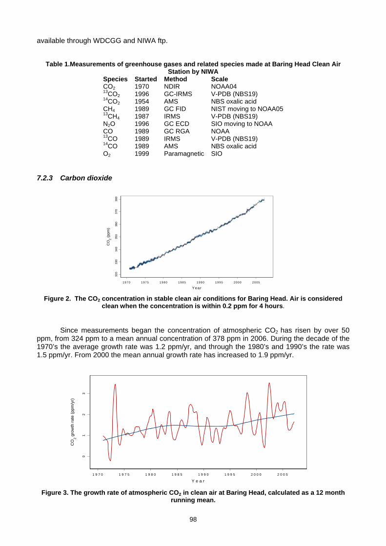
98

available through WDCGG and NIWA ftp.

Table 1.Measurements of greenhouse gases and related species made at Baring Head Clean Air

Station by NIWA Species Started Method Scale CO2 1970 NDIR NOAA04 13CO2 1996 GC-IRMS V-PDB (NBS19) 14CO2 1954 AMS NBS oxalic acid CH4 1989 GC FID NIST moving to NOAA05 13CH4 1987 IRMS V-PDB (NBS19) N2O 1996 GC ECD SIO moving to NOAA CO 1989 GC RGA NOAA 13CO 1989 IRMS V-PDB (NBS19) 14CO 1989 AMS NBS oxalic acid O2 1999 Paramagnetic SIO

7.2.3 Carbon dioxide

1970 1975 1980 1985 1990 1995 2000 2005

Year

320

330

340

350

360

370

380

CO

2 (ppm

)

Figure 2. The CO2 concentration in stable clean air conditions for Baring Head. Air is considered

clean when the concentration is within 0.2 ppm for 4 hours.

Since measurements began the concentration of atmospheric CO2 has risen by over 50 ppm, from 324 ppm to a mean annual concentration of 378 ppm in 2006. During the decade of the 1970’s the average growth rate was 1.2 ppm/yr, and through the 1980’s and 1990’s the rate was 1.5 ppm/yr. From 2000 the mean annual growth rate has increased to 1.9 ppm/yr.

1 9 7 0 1 9 7 5 1 9 8 0 1 9 8 5 1 9 9 0 1 9 9 5 2 0 0 0 2 0 0 5

Y e a r

01

23

CO

2 gro

wth

rate

(ppm

/yr)

Figure 3. The growth rate of atmospheric CO2 in clean air at Baring Head, calculated as a 12 month

running mean.

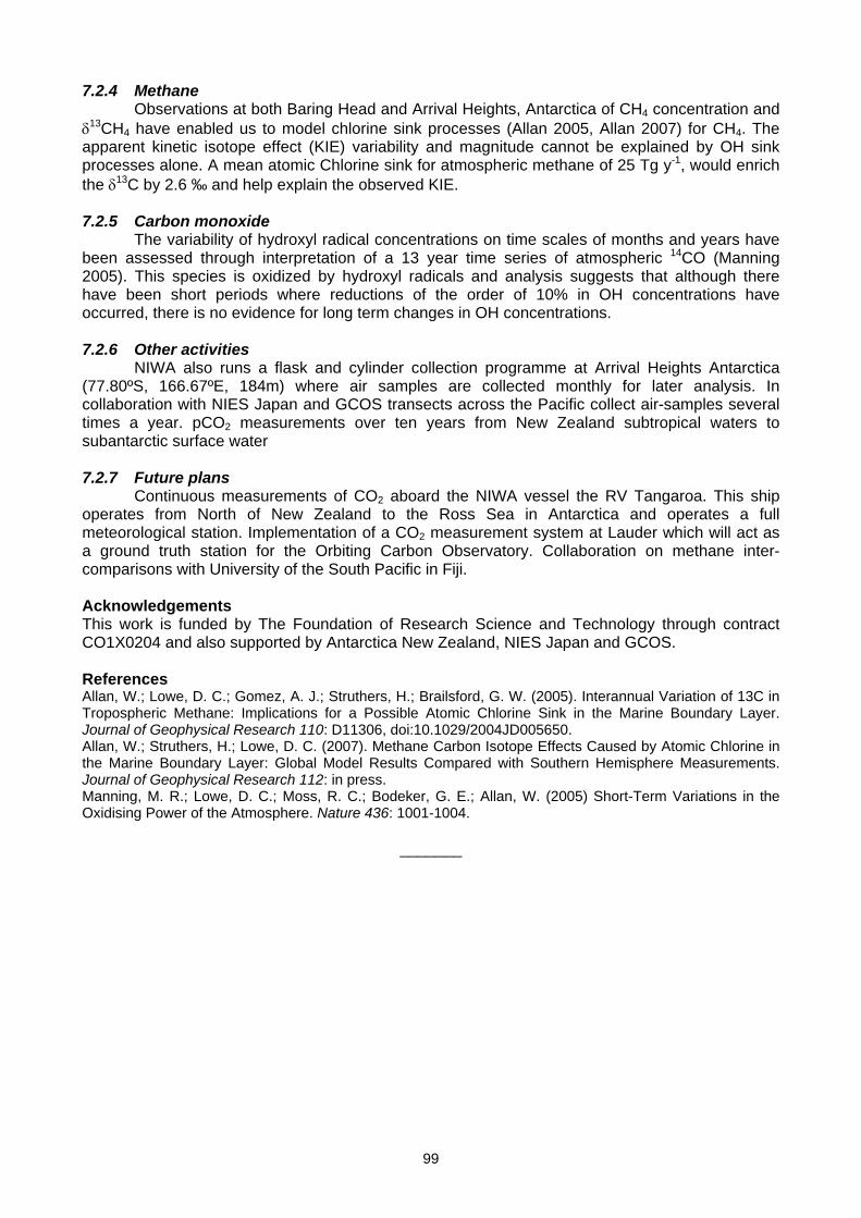
99

7.2.4 Methane Observations at both Baring Head and Arrival Heights, Antarctica of CH4 concentration and

δ13CH4 have enabled us to model chlorine sink processes (Allan 2005, Allan 2007) for CH4. The apparent kinetic isotope effect (KIE) variability and magnitude cannot be explained by OH sink processes alone. A mean atomic Chlorine sink for atmospheric methane of 25 Tg y-1, would enrich the δ13C by 2.6 ‰ and help explain the observed KIE. 7.2.5 Carbon monoxide

The variability of hydroxyl radical concentrations on time scales of months and years have been assessed through interpretation of a 13 year time series of atmospheric 14CO (Manning 2005). This species is oxidized by hydroxyl radicals and analysis suggests that although there have been short periods where reductions of the order of 10% in OH concentrations have occurred, there is no evidence for long term changes in OH concentrations. 7.2.6 Other activities

NIWA also runs a flask and cylinder collection programme at Arrival Heights Antarctica (77.80ºS, 166.67ºE, 184m) where air samples are collected monthly for later analysis. In collaboration with NIES Japan and GCOS transects across the Pacific collect air-samples several times a year. pCO2 measurements over ten years from New Zealand subtropical waters to subantarctic surface water 7.2.7 Future plans

Continuous measurements of CO2 aboard the NIWA vessel the RV Tangaroa. This ship operates from North of New Zealand to the Ross Sea in Antarctica and operates a full meteorological station. Implementation of a CO2 measurement system at Lauder which will act as a ground truth station for the Orbiting Carbon Observatory. Collaboration on methane inter-comparisons with University of the South Pacific in Fiji. Acknowledgements This work is funded by The Foundation of Research Science and Technology through contract CO1X0204 and also supported by Antarctica New Zealand, NIES Japan and GCOS. References Allan, W.; Lowe, D. C.; Gomez, A. J.; Struthers, H.; Brailsford, G. W. (2005). Interannual Variation of 13C in Tropospheric Methane: Implications for a Possible Atomic Chlorine Sink in the Marine Boundary Layer. Journal of Geophysical Research 110: D11306, doi:10.1029/2004JD005650. Allan, W.; Struthers, H.; Lowe, D. C. (2007). Methane Carbon Isotope Effects Caused by Atomic Chlorine in the Marine Boundary Layer: Global Model Results Compared with Southern Hemisphere Measurements. Journal of Geophysical Research 112: in press. Manning, M. R.; Lowe, D. C.; Moss, R. C.; Bodeker, G. E.; Allan, W. (2005) Short-Term Variations in the Oxidising Power of the Atmosphere. Nature 436: 1001-1004.

_______

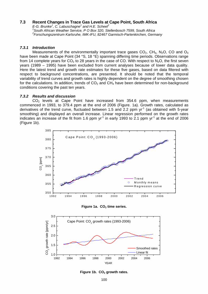
100

7.3 Recent Changes in Trace Gas Levels at Cape Point, South Africa E-G. Brunke1, C. Labuschagne1 and H.E. Scheel2 1South African Weather Service, P O Box 320, Stellenbosch 7599, South Africa

2Forschungszentrum Karlsruhe, IMK-IFU, 82467 Garmisch-Partenkirchen, Germany 7.3.1 Introduction Measurements of the environmentally important trace gases CO2, CH4, N2O, CO and O3 have been made at Cape Point (34 °S, 18 °E) spanning differing time periods. Observations range from 14 complete years for CO2 to 28 years in the case of CO. With respect to N2O, the first seven years (1989 – 1995) have been excluded from current analyses because of lower data quality. Here the latest trend and growth rate estimates for these five gases, based on data filtered with respect to background concentrations, are presented. It should be noted that the temporal variability of trend curves and growth rates is highly dependent on the degree of smoothing chosen for the calculations. In addition, trends of CO2 and CH4 have been determined for non-background conditions covering the past ten years. 7.3.2 Results and discussion CO2 levels at Cape Point have increased from 354.6 ppm, when measurements commenced in 1993, to 379.4 ppm at the end of 2006 (Figure. 1a). Growth rates, calculated as derivatives of the trend curve, fluctuated between 1.5 and 2.2 ppm yr-1 (as obtained with 5-year smoothing) and displayed an overall increase. Linear regression performed on the growth rates indicates an increase of the fit from 1.6 ppm yr-1 in early 1993 to 2.1 ppm yr-1 at the end of 2006 (Figure 1b).

Figure 1a. CO2 time series.

Figure 1b. CO2 growth rates.

1 9 9 2 1 9 9 4 1 9 9 6 1 9 9 8 2 0 0 0 2 0 0 2 2 0 0 4 2 0 0 63 5 0

3 5 5

3 6 0

3 6 5

3 7 0

3 7 5

3 8 0

3 8 5

T re n d M o n th ly m e a n s R e g re s s io n c u rv e

C a p e P o in t: C O 2 (1 9 9 3 -2 0 0 6 )

CO

2 [ppm

]

1992 1994 1996 1998 2000 2002 2004 20061.0

1.5

2.0

2.5

3.0

Smoothed rates Linear fit

Cape Point: CO2 growth rates (1993-2006)

CO

2 gro

wth

rate

[ppm

/yr]

YEAR

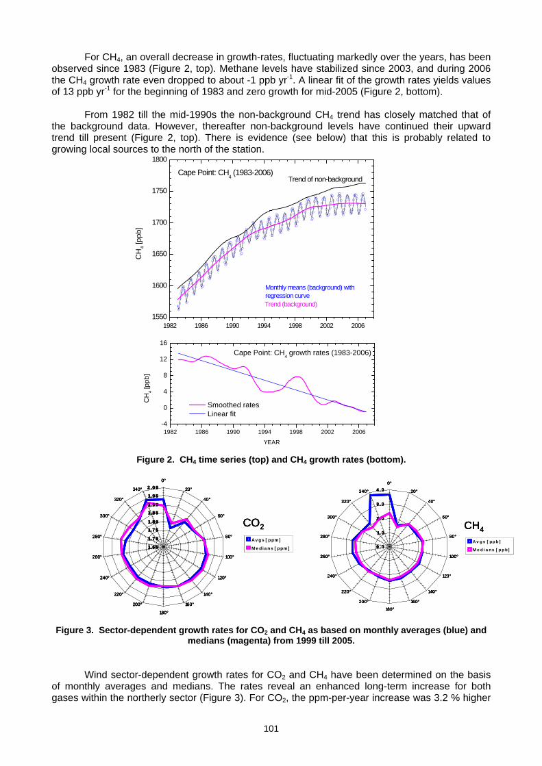
101

For CH4, an overall decrease in growth-rates, fluctuating markedly over the years, has been observed since 1983 (Figure 2, top). Methane levels have stabilized since 2003, and during 2006 the CH4 growth rate even dropped to about -1 ppb yr-1. A linear fit of the growth rates yields values of 13 ppb yr-1 for the beginning of 1983 and zero growth for mid-2005 (Figure 2, bottom). From 1982 till the mid-1990s the non-background CH4 trend has closely matched that of the background data. However, thereafter non-background levels have continued their upward trend till present (Figure 2, top). There is evidence (see below) that this is probably related to growing local sources to the north of the station.

Figure 2. CH4 time series (top) and CH4 growth rates (bottom). Figure 3. Sector-dependent growth rates for CO2 and CH4 as based on monthly averages (blue) and

medians (magenta) from 1999 till 2005. Wind sector-dependent growth rates for CO2 and CH4 have been determined on the basis of monthly averages and medians. The rates reveal an enhanced long-term increase for both gases within the northerly sector (Figure 3). For CO2, the ppm-per-year increase was 3.2 % higher

1982 1986 1990 1994 1998 2002 20061550

1600

1650

1700

1750

1800

Trend (background)

Monthly means (background) withregression curve

Trend of non-backgroundCape Point: CH

4 (1983-2006)

CH

4 [pp

b]

1982 1986 1990 1994 1998 2002 2006-4

0

4

8

12

16

Smoothed rates Linear fit

Cape Point: CH4 growth rates (1983-2006)

CH

4 [ppb

]

YEAR

1.6 5

1.7 0

1.7 5

1.8 0

1.8 5

1.9 0

1.9 5

2 .0 00°

20°

40°

60°

80°

100°

120°

140°

160°

180°

200°

220°

240°

260°

280°

300°

320°

340°

Av gs [ ppm]

Me dia ns [ ppm]

CO2

1.6 5

1.7 0

1.7 5

1.8 0

1.8 5

1.9 0

1.9 5

2 .0 00°

20°

40°

60°

80°

100°

120°

140°

160°

180°

200°

220°

240°

260°

280°

300°

320°

340°

Av gs [ ppm]

Me dia ns [ ppm]

CO2

0 . 0

1. 0

2 . 0

3 . 0

4 . 00°

20°

40°

60°

80°

100°

120°

140°

160°

180°

200°

220°

240°

260°

280°

300°

320°

340°

Av g s [ pp b ]

M e d i a ns [ p p b]

CH4

0 . 0

1. 0

2 . 0

3 . 0

4 . 00°

20°

40°

60°

80°

100°

120°

140°

160°

180°

200°

220°

240°

260°

280°

300°

320°

340°

Av g s [ pp b ]

M e d i a ns [ p p b]

CH4

1.6 5

1.7 0

1.7 5

1.8 0

1.8 5

1.9 0

1.9 5

2 .0 00°

20°

40°

60°

80°

100°

120°

140°

160°

180°

200°

220°

240°

260°

280°

300°

320°

340°

Av gs [ ppm]

Me dia ns [ ppm]

CO2

1.6 5

1.7 0

1.7 5

1.8 0

1.8 5

1.9 0

1.9 5

2 .0 00°

20°

40°

60°

80°

100°

120°

140°

160°

180°

200°

220°

240°

260°

280°

300°

320°

340°

Av gs [ ppm]

Me dia ns [ ppm]

CO2

0 . 0

1. 0

2 . 0

3 . 0

4 . 00°

20°

40°

60°

80°

100°

120°

140°

160°

180°

200°

220°

240°

260°

280°

300°

320°

340°

Av g s [ pp b ]

M e d i a ns [ p p b]

CH4

0 . 0

1. 0

2 . 0

3 . 0

4 . 00°

20°

40°

60°

80°

100°

120°

140°

160°

180°

200°

220°

240°

260°

280°

300°

320°

340°

Av g s [ pp b ]

M e d i a ns [ p p b]

CH4

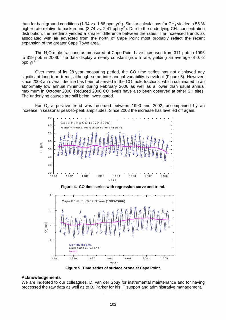
102

than for background conditions (1.94 vs. 1.88 ppm yr-1). Similar calculations for CH4 yielded a 55 % higher rate relative to background (3.74 vs. 2.41 ppb y-1). Due to the underlying CH4 concentration distribution, the medians yielded a smaller difference between the rates. The increased trends as associated with air advected from the north of Cape Point most probably reflect the recent expansion of the greater Cape Town area. The N2O mole fractions as measured at Cape Point have increased from 311 ppb in 1996 to 319 ppb in 2006. The data display a nearly constant growth rate, yielding an average of 0.72 ppb yr-1. Over most of its 28-year measuring period, the CO time series has not displayed any significant long-term trend, although some inter-annual variability is evident (Figure 5). However, since 2003 an overall decline has been observed in the CO mole fractions, which culminated in an abnormally low annual minimum during February 2006 as well as a lower than usual annual maximum in October 2006. Reduced 2006 CO levels have also been observed at other SH sites. The underlying causes are still being investigated.

For O3 a positive trend was recorded between 1990 and 2002, accompanied by an increase in seasonal peak-to-peak amplitudes. Since 2003 the increase has levelled off again.

Figure 4. CO time series with regression curve and trend.

Figure 5. Time series of surface ozone at Cape Point. Acknowledgements We are indebted to our colleagues, D. van der Spuy for instrumental maintenance and for having processed the raw data as well as to B. Parker for his IT support and administrative management.

_______

1982 1986 1990 1994 1998 2002 20060

10

20

30

40

C ap e P oin t: S urface O zone (1983-2006)

O3 [p

pb]

Y E A R

M onth ly m eans,reg ress ion cu rv e andtrend

1 97 8 19 8 2 1 9 86 1 99 0 19 9 4 19 98 2 00 2 2 00 62 0

3 0

4 0

5 0

6 0

7 0

8 0

9 0

M on th ly m e a ns , reg re ss ion cu rv e a n d tre nd

C a p e P o in t: C O (1 9 7 9 -2 0 0 6 )

CO

[ppb

]

Y E A R

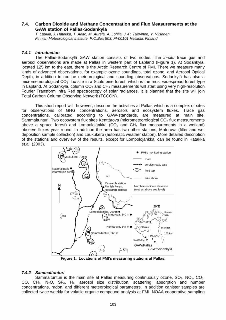
103

7.4. Carbon Dioxide and Methane Concentration and Flux Measurements at the GAW station of Pallas-Sodankylä T. Laurila, J. Hatakka, T. Aalto, M. Aurela, A. Lohila, J,-P, Tuovinen, Y. Viisanen Finnish Meteorological Institute, P.O.Box 503, FI-00101 Helsinki, Finland

7.4.1 Introduction

The Pallas-Sodankylä GAW station consists of two nodes. The in-situ trace gas and aerosol observations are made at Pallas in western part of Lapland (Figure 1). At Sodankylä, located 125 km to the east, there is the Arctic Research Centre of FMI. There we measure many kinds of advanced observations, for example ozone soundings, total ozone, and Aerosol Optical Depth, in addition to routine meteorological and sounding observations. Sodankylä has also a micrometeorological CO2 flux site in a Scots pine forest, which is the most widespread forest type in Lapland. At Sodankylä, column CO2 and CH4 measurements will start using very high-resolution Fourier Transform Infra Red spectroscopy of solar radiances. It is planned that the site will join Total Carbon Column Observing Network (TCCON).

This short report will, however, describe the activities at Pallas which is a complex of sites for observations of GHG concentrations, aerosols and ecosystem fluxes. Trace gas concentrations, calibrated according to GAW-standards, are measured at main site, Sammaltunturi. Two ecosystem flux sites Kenttärova (micrometeorological CO2 flux measurements above a spruce forest) and Lompolojänkkä (CO2 and CH4 flux measurements in a wetland) observe fluxes year round. In addition the area has two other stations, Matorova (filter and wet deposition sample collection) and Laukukero (automatic weather station). More detailed description of the stations and overview of the results, except for Lompolojänkkä, can be found in Hatakka et.al. (2003).

267

N

1 km

lake shore

road

service road, gate

fjeld topNational parkinformation centre

Laukukero, 790 m

Lompolojänkkä, 269 m

Sammaltunturi, 565 m

Matorova, 340 m

Research station,Finnish ForestResearch Institute

646

705

770807

557

554

558

610

332

338

323

325

Numbers indicate elevation(metres above sea level)

FMI's monitoring station

FINLAND

RUSSIANORWAY

100 km

BarentsSea

GAW/PallasSWEDEN

Kenttärova, 347 m

GAW/Sodankylä

29°E

69°30'N

Figure 1. Locations of FMI's measuring stations at Pallas.

7.4.2 Sammaltunturi

Sammaltunturi is the main site at Pallas measuring continuously ozone, SO2, NOx, CO2, CO, CH4, N2O, SF6, H2, aerosol size distribution, scattering, absorption and number concentrations, radon, and different meteorological parameters. In addition canister samples are collected twice weekly for volatile organic compound analysis at FMI. NOAA cooperative sampling

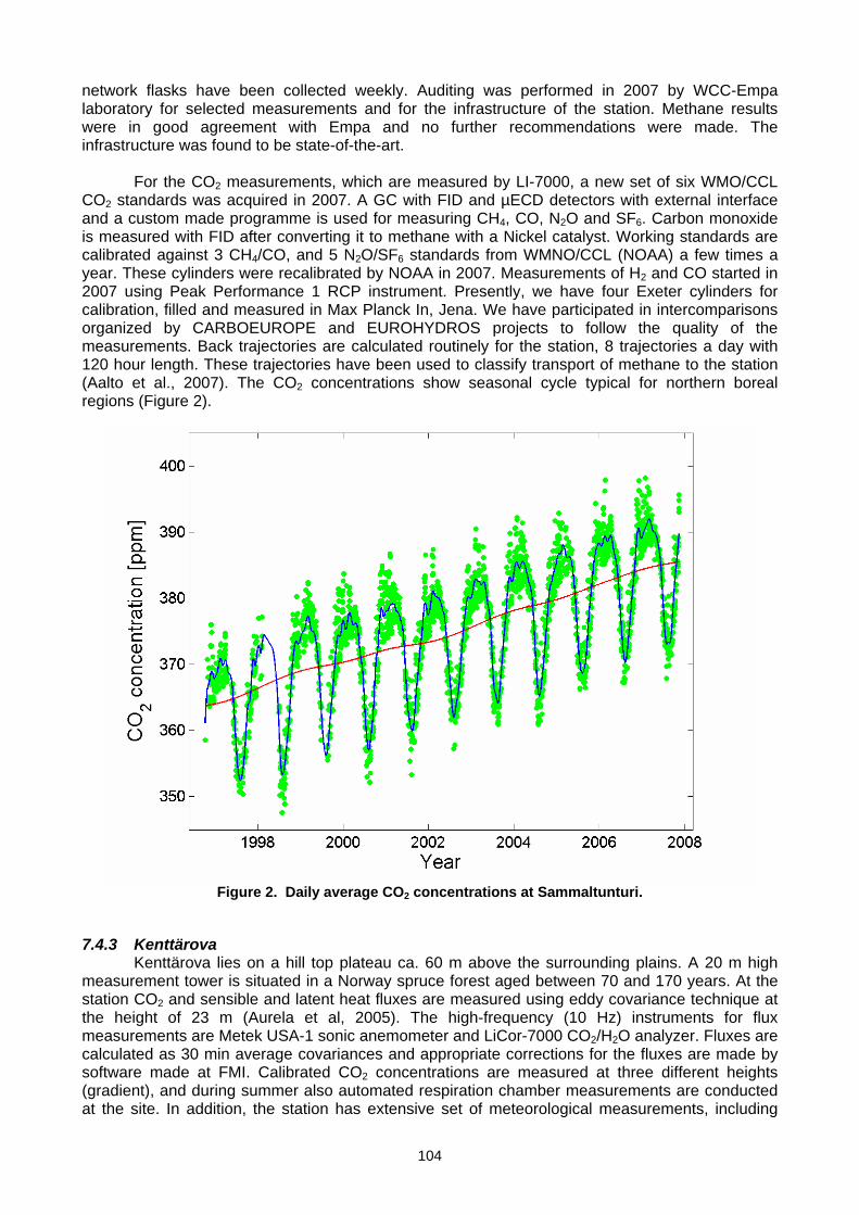
104

network flasks have been collected weekly. Auditing was performed in 2007 by WCC-Empa laboratory for selected measurements and for the infrastructure of the station. Methane results were in good agreement with Empa and no further recommendations were made. The infrastructure was found to be state-of-the-art.

For the CO2 measurements, which are measured by LI-7000, a new set of six WMO/CCL CO2 standards was acquired in 2007. A GC with FID and µECD detectors with external interface and a custom made programme is used for measuring CH4, CO, N2O and SF6. Carbon monoxide is measured with FID after converting it to methane with a Nickel catalyst. Working standards are calibrated against 3 CH4/CO, and 5 N2O/SF6 standards from WMNO/CCL (NOAA) a few times a year. These cylinders were recalibrated by NOAA in 2007. Measurements of H2 and CO started in 2007 using Peak Performance 1 RCP instrument. Presently, we have four Exeter cylinders for calibration, filled and measured in Max Planck In, Jena. We have participated in intercomparisons organized by CARBOEUROPE and EUROHYDROS projects to follow the quality of the measurements. Back trajectories are calculated routinely for the station, 8 trajectories a day with 120 hour length. These trajectories have been used to classify transport of methane to the station (Aalto et al., 2007). The CO2 concentrations show seasonal cycle typical for northern boreal regions (Figure 2).

Figure 2. Daily average CO2 concentrations at Sammaltunturi.

7.4.3 Kenttärova

Kenttärova lies on a hill top plateau ca. 60 m above the surrounding plains. A 20 m high measurement tower is situated in a Norway spruce forest aged between 70 and 170 years. At the station CO2 and sensible and latent heat fluxes are measured using eddy covariance technique at the height of 23 m (Aurela et al, 2005). The high-frequency (10 Hz) instruments for flux measurements are Metek USA-1 sonic anemometer and LiCor-7000 CO2/H2O analyzer. Fluxes are calculated as 30 min average covariances and appropriate corrections for the fluxes are made by software made at FMI. Calibrated CO2 concentrations are measured at three different heights (gradient), and during summer also automated respiration chamber measurements are conducted at the site. In addition, the station has extensive set of meteorological measurements, including

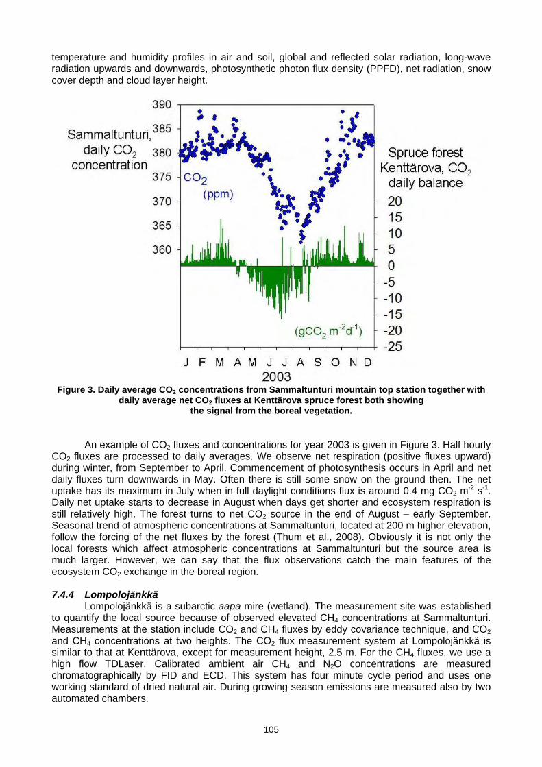
105

temperature and humidity profiles in air and soil, global and reflected solar radiation, long-wave radiation upwards and downwards, photosynthetic photon flux density (PPFD), net radiation, snow cover depth and cloud layer height.

Figure 3. Daily average CO2 concentrations from Sammaltunturi mountain top station together with

daily average net CO2 fluxes at Kenttärova spruce forest both showing the signal from the boreal vegetation.

An example of CO2 fluxes and concentrations for year 2003 is given in Figure 3. Half hourly

CO2 fluxes are processed to daily averages. We observe net respiration (positive fluxes upward) during winter, from September to April. Commencement of photosynthesis occurs in April and net daily fluxes turn downwards in May. Often there is still some snow on the ground then. The net uptake has its maximum in July when in full daylight conditions flux is around 0.4 mg CO2 m-2 s-1. Daily net uptake starts to decrease in August when days get shorter and ecosystem respiration is still relatively high. The forest turns to net CO2 source in the end of August – early September. Seasonal trend of atmospheric concentrations at Sammaltunturi, located at 200 m higher elevation, follow the forcing of the net fluxes by the forest (Thum et al., 2008). Obviously it is not only the local forests which affect atmospheric concentrations at Sammaltunturi but the source area is much larger. However, we can say that the flux observations catch the main features of the ecosystem CO2 exchange in the boreal region. 7.4.4 Lompolojänkkä

Lompolojänkkä is a subarctic aapa mire (wetland). The measurement site was established to quantify the local source because of observed elevated CH4 concentrations at Sammaltunturi. Measurements at the station include CO2 and CH4 fluxes by eddy covariance technique, and CO2 and CH4 concentrations at two heights. The CO2 flux measurement system at Lompolojänkkä is similar to that at Kenttärova, except for measurement height, 2.5 m. For the CH4 fluxes, we use a high flow TDLaser. Calibrated ambient air CH4 and N2O concentrations are measured chromatographically by FID and ECD. This system has four minute cycle period and uses one working standard of dried natural air. During growing season emissions are measured also by two automated chambers.

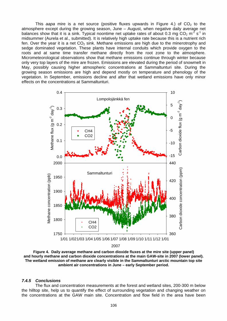
106

Lompolojänkkä fen

X Data

700 750 800 850 900 950 1000

Met

hane

flux

(g m

-2 d

ay-1

)

0.0

0.1

0.2

0.3

0.4

Car

bon

diox

ide

flux

(g m

-2 d

ay-1

)

-15

-10

-5

0

5

10

CH4CO2

Sammaltunturi

2007

1/01 1/02 1/03 1/04 1/05 1/06 1/07 1/08 1/09 1/10 1/11 1/12 1/01

Met

hane

con

cent

ratio

n (p

pb)

1750

1800

1850

1900

1950

2000

Car

bon

diox

ide

conc

entra

tion

(ppm

)

360

380

400

420

440

CH4CO2

This aapa mire is a net source (positive fluxes upwards in Figure 4.) of CO2 to the atmosphere except during the growing season, June – August, when negative daily average net balances show that it is a sink. Typical noontime net uptake rates of about 0.3 mg CO2 m-2 s-1 in midsummer (Aurela et al., submitted). It is relatively high uptake rate because this is a nutrient rich fen. Over the year it is a net CO2 sink. Methane emissions are high due to the minerotrophy and sedge dominated vegetation. These plants have internal conduits which provide oxygen to the roots and at same time transfer methane directly from the root zone to the atmosphere. Micrometeorological observations show that methane emissions continue through winter because only very top layers of the mire are frozen. Emissions are elevated during the period of snowmelt in May, possibly causing higher atmospheric concentrations at Sammaltunturi site. During the growing season emissions are high and depend mostly on temperature and phenology of the vegetation. In September, emissions decline and after that wetland emissions have only minor effects on the concentrations at Sammaltunturi.

Figure 4. Daily average methane and carbon dioxide fluxes at the mire site (upper panel) and hourly methane and carbon dioxide concentrations at the main GAW-site in 2007 (lower panel). The wetland emission of methane are clearly visible in the Sammaltunturi arctic mountain top site

ambient air concentrations in June – early September period.

7.4.5 Conclusions The flux and concentration measurements at the forest and wetland sites, 200-300 m below

the hilltop site, help us to quantify the effect of surrounding vegetation and changing weather on the concentrations at the GAW main site. Concentration and flow field in the area have been

107

simulated using a fluid dynamics model to further understand modifications of the concentrations at the GAW site by the local terrain and natural sources (Aalto et al., 2006). Further developments at Pallas include starting of continuous VOC concentration measurements during 2009 at Sammaltunturi. References Aalto T., J. Hatakka, U. Karstens, M. Aurela, T. Thum and A. Lohila (2006) Modelling Atmospheric CO2 Concentration Profiles and Fluxes above Sloping Terrain at a Boreal Site. Atmospheric Chemistry and Physics 6, pp. 303-314. Aalto T., J. Hatakka and M. Lallo. (2007) Tropospheric Methane in Northern Finland: Seasonal Variations, Transport Patterns and Correlations with other Trace Gases. Tellus 59B, pp. 251-259. Aurela, M. (2005) Carbon Dioxide Exchange in Subarctic Ecosystems Measured by a Micrometeorological Technique. Contributions 51, Finnish Meteorological Institute, Helsinki, ISSN 0782-6117, pp. 132 (T. Vesala; University of Helsinki). Aurela, M., A. Lohila, J.-P. Tuovinen, J. Hatakka, T. Riutta and T. Laurila (2009) Carbon Dioxide Exchange on a Northern Boreal Fen. Submitted to Boreal Environment research. Hatakka J., T. Aalto, V. Aaltonen, M. Aurela, H. Hakola, M. Komppula, T. Laurila, H. Lihavainen, J. Paatero, K. Salminen and Y. Viisanen (2003) Overview of the Atmospheric Research Activities and Results at Pallas GAW station. Boreal Environment Research 8, 365-383. Thum, T., T. Aalto, T. Laurila, M. Aurela, A. Lindroth, and T. Vesala (2008) Assessing Seasonality of Biochemical CO2 Exchange Model Parameters from Micrometeorological Flux Observations at Boreal Coniferous Forest. Biogeosciences 5, 1625-1639.

_______

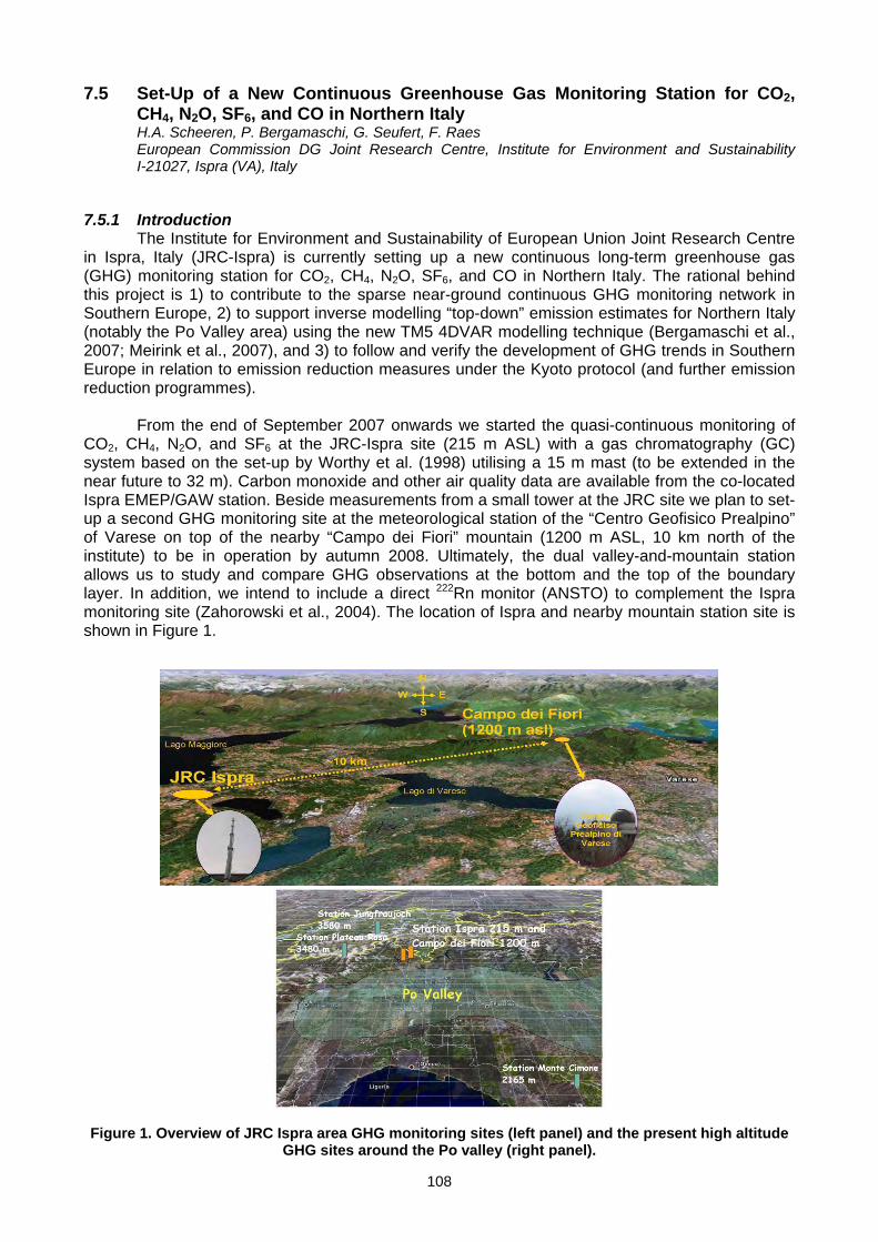
108

7.5 Set-Up of a New Continuous Greenhouse Gas Monitoring Station for CO2, CH4, N2O, SF6, and CO in Northern Italy H.A. Scheeren, P. Bergamaschi, G. Seufert, F. Raes European Commission DG Joint Research Centre, Institute for Environment and Sustainability I-21027, Ispra (VA), Italy

7.5.1 Introduction

The Institute for Environment and Sustainability of European Union Joint Research Centre in Ispra, Italy (JRC-Ispra) is currently setting up a new continuous long-term greenhouse gas (GHG) monitoring station for CO2, CH4, N2O, SF6, and CO in Northern Italy. The rational behind this project is 1) to contribute to the sparse near-ground continuous GHG monitoring network in Southern Europe, 2) to support inverse modelling “top-down” emission estimates for Northern Italy (notably the Po Valley area) using the new TM5 4DVAR modelling technique (Bergamaschi et al., 2007; Meirink et al., 2007), and 3) to follow and verify the development of GHG trends in Southern Europe in relation to emission reduction measures under the Kyoto protocol (and further emission reduction programmes).

From the end of September 2007 onwards we started the quasi-continuous monitoring of

CO2, CH4, N2O, and SF6 at the JRC-Ispra site (215 m ASL) with a gas chromatography (GC) system based on the set-up by Worthy et al. (1998) utilising a 15 m mast (to be extended in the near future to 32 m). Carbon monoxide and other air quality data are available from the co-located Ispra EMEP/GAW station. Beside measurements from a small tower at the JRC site we plan to set-up a second GHG monitoring site at the meteorological station of the “Centro Geofisico Prealpino” of Varese on top of the nearby “Campo dei Fiori” mountain (1200 m ASL, 10 km north of the institute) to be in operation by autumn 2008. Ultimately, the dual valley-and-mountain station allows us to study and compare GHG observations at the bottom and the top of the boundary layer. In addition, we intend to include a direct 222Rn monitor (ANSTO) to complement the Ispra monitoring site (Zahorowski et al., 2004). The location of Ispra and nearby mountain station site is shown in Figure 1.

Figure 1. Overview of JRC Ispra area GHG monitoring sites (left panel) and the present high altitude GHG sites around the Po valley (right panel).

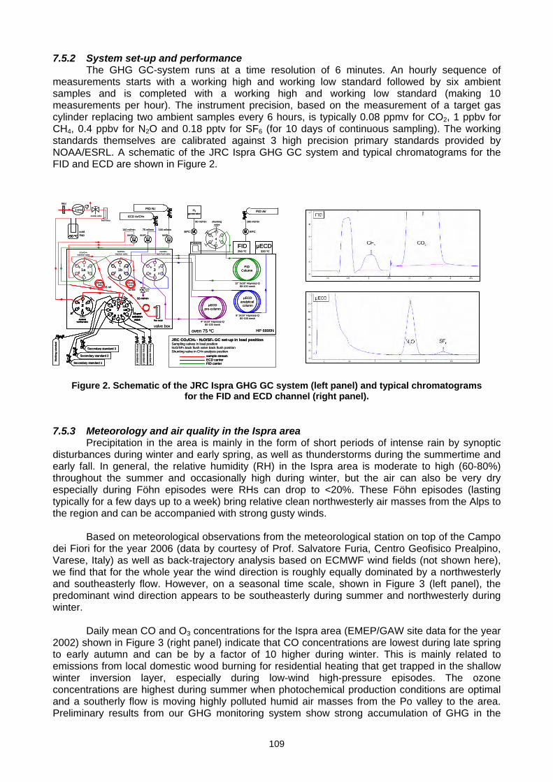
109

7.5.2 System set-up and performance The GHG GC-system runs at a time resolution of 6 minutes. An hourly sequence of

measurements starts with a working high and working low standard followed by six ambient samples and is completed with a working high and working low standard (making 10 measurements per hour). The instrument precision, based on the measurement of a target gas cylinder replacing two ambient samples every 6 hours, is typically 0.08 ppmv for CO2, 1 ppbv for CH4, 0.4 ppbv for N2O and 0.18 pptv for SF6 (for 10 days of continuous sampling). The working standards themselves are calibrated against 3 high precision primary standards provided by NOAA/ESRL. A schematic of the JRC Ispra GHG GC system and typical chromatograms for the FID and ECD are shown in Figure 2.

Figure 2. Schematic of the JRC Ispra GHG GC system (left panel) and typical chromatograms for the FID and ECD channel (right panel).

7.5.3 Meteorology and air quality in the Ispra area

Precipitation in the area is mainly in the form of short periods of intense rain by synoptic disturbances during winter and early spring, as well as thunderstorms during the summertime and early fall. In general, the relative humidity (RH) in the Ispra area is moderate to high (60-80%) throughout the summer and occasionally high during winter, but the air can also be very dry especially during Föhn episodes were RHs can drop to <20%. These Föhn episodes (lasting typically for a few days up to a week) bring relative clean northwesterly air masses from the Alps to the region and can be accompanied with strong gusty winds.

Based on meteorological observations from the meteorological station on top of the Campo

dei Fiori for the year 2006 (data by courtesy of Prof. Salvatore Furia, Centro Geofisico Prealpino, Varese, Italy) as well as back-trajectory analysis based on ECMWF wind fields (not shown here), we find that for the whole year the wind direction is roughly equally dominated by a northwesterly and southeasterly flow. However, on a seasonal time scale, shown in Figure 3 (left panel), the predominant wind direction appears to be southeasterly during summer and northwesterly during winter.

Daily mean CO and O3 concentrations for the Ispra area (EMEP/GAW site data for the year 2002) shown in Figure 3 (right panel) indicate that CO concentrations are lowest during late spring to early autumn and can be by a factor of 10 higher during winter. This is mainly related to emissions from local domestic wood burning for residential heating that get trapped in the shallow winter inversion layer, especially during low-wind high-pressure episodes. The ozone concentrations are highest during summer when photochemical production conditions are optimal and a southerly flow is moving highly polluted humid air masses from the Po valley to the area. Preliminary results from our GHG monitoring system show strong accumulation of GHG in the

Catalyst FID μECD

H2generator

FID Air

N2O/SF6

back flush valve

shuntingvalve

4

oven 75 ºC

FIDColumn

μECDpre-column

μECDanalytical

column

HP 6890N

Prim

ary standard 1

Prim

ary standard 2

Prim

ary standard 3

3

21

6

5 4

CO2/CH4

injection valve

3 1a

N2O/SF6

injection valve

Wor

king

sta

ndar

d

Secondary standard 3

Secondary standard 2

valve box

43

2 16

5

sampleloop

sampleloop

43

21

6

5

15 ml10 ml

1b4

3

2 16

5

JRC CO2/CH4 - N2O/SF6 GC set-up in load position Sampling valves in load positionN2O/SF6 back flush valve back flush positionShunting valve in CH4 analysis position

sample streamECD carrierFID carrier

needlevalve

EPCEPC-50 ºC

4 l/min

needle valve

coldtrap

flow meter

filter

Secondary standard 1

ECD Ar/CH4

FID N2

aux5aux3 aux4

12” 3x16” Hayesep-Q80-100 mesh

6” 3x16” Hayesep-Q80-100 mesh

4” 3x16” Hayesep-Q80-100 mesh

280 ml/min80 ml/min

140 ml/min

320 ºC250 ºC

75 ml/min 100 ml/min

Ambientventing valve

2 1

2

34

5

6

12-port selection

valve

74

6

10

12

8

3

57

9

1112

flow meter

55 ml/min

Catalyst FID μECD

H2generator

FID Air

N2O/SF6

back flush valve

shuntingvalve

4

oven 75 ºC

FIDColumn

μECDpre-column

μECDanalytical

column

HP 6890N

Prim

ary standard 1

Prim

ary standard 2

Prim

ary standard 3

3

21

6

5 4

CO2/CH4

injection valve

3 1a

N2O/SF6

injection valve

Wor

king

sta

ndar

dW

orki

ng s

tand

ard

Secondary standard 3Secondary standard 3

Secondary standard 2Secondary standard 2

valve box

43

2 16

5

sampleloop

sampleloop

sampleloop

43

21

6

5

15 ml10 ml

1b4

3

2 16

5

JRC CO2/CH4 - N2O/SF6 GC set-up in load position Sampling valves in load positionN2O/SF6 back flush valve back flush positionShunting valve in CH4 analysis position

sample streamECD carrierFID carrier

sample streamECD carrierFID carrier

needlevalve

EPCEPC-50 ºC-50 ºC

4 l/min

needle valve

coldtrap

flow meter

filter

Secondary standard 1Secondary standard 1

ECD Ar/CH4

FID N2

aux5aux3 aux4

12” 3x16” Hayesep-Q80-100 mesh

6” 3x16” Hayesep-Q80-100 mesh

4” 3x16” Hayesep-Q80-100 mesh

280 ml/min80 ml/min

140 ml/min

320 ºC250 ºC

75 ml/min 100 ml/min

Ambientventing valve

2 1

2

34

5

6

12-port selection

valve

74

6

10

12

8

3

57

9

1112

flow meter

55 ml/min

Ambientventing valve

2 1

2

34

5

6

12-port selection

valve

74

6

10

12

8

3

57

9

1112

flow meterAmbientventing valve

2 1

2

34

5

6

12-port selection

valve

74

6

10

12

8

3

57

9

1112

Ambientventing valve

2 1

2

34

5

6

12-port selection

valve

74

6

10

12

8

3

57

9

1112

Ambientventing valve

2 1

2

34

5

6

Ambientventing valve

2 1

2

34

5

62 1

2

34

5

6

12-port selection

valve

74

6

10

12

8

3

57

9

1112

12-port selection

valve

74

6

10

12

8

3

57

9

1112

74

6

10

12

8

3

57

9

1112

flow meterflow meter

55 ml/min55 ml/min

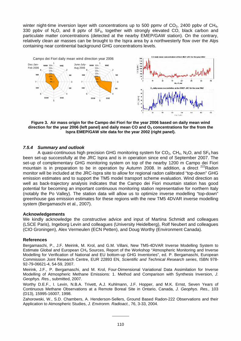
110

winter night-time inversion layer with concentrations up to 500 ppmv of CO2, 2400 ppbv of CH4, 330 ppbv of N2O, and 8 pptv of SF6, together with strongly elevated CO, black carbon and particulate matter concentrations (detected at the nearby EMEP/GAW station). On the contrary, relatively clean air masses can be brought to the Ispra area by a northwesterly flow over the Alps containing near continental background GHG concentrations levels.

Figure 3. Air mass origin for the Campo dei Fiori for the year 2006 based on daily mean wind direction for the year 2006 (left panel) and daily mean CO and O3 concentrations for the from the

Ispra EMEP/GAW site data for the year 2002 (right panel). 7.5.4 Summary and outlook

A quasi-continuous high precision GHG monitoring system for CO2, CH4, N2O, and SF6 has been set-up successfully at the JRC Ispra and is in operation since end of September 2007. The set-up of complementary GHG monitoring system on top of the nearby 1200 m Campo dei Fiori mountain is in preparation to be in operation by Autumn 2008. In addition, a direct 222Radon monitor will be included at the JRC-Ispra site to allow for regional radon calibrated “top-down” GHG emission estimates and to support the TM5 model transport scheme evaluation. Wind direction as well as back-trajectory analysis indicates that the Campo dei Fiori mountain station has good potential for becoming an important continuous monitoring station representative for northern Italy (notably the Po Valley). The station data will allow us to optimize inverse modelling “top-down” greenhouse gas emission estimates for these regions with the new TM5 4DVAR inverse modelling system (Bergamaschi et al., 2007). Acknowledgements We kindly acknowledge the constructive advice and input of Martina Schmidt and colleagues (LSCE Paris), Ingeborg Levin and colleagues (University Heidelberg), Rolf Neubert and colleagues (CIO Groningen), Alex Vermeulen (ECN Petten), and Doug Worthy (Environment Canada). References Bergamaschi, P., J.F. Meirink, M. Krol, and G.M. Villani, New TM5-4DVAR Inverse Modelling System to Estimate Global and European CH4 Sources, Report of the Workshop “Atmospheric Monitoring and Inverse Modelling for Verification of National and EU bottom-up GHG Inventories”, ed. P. Bergamaschi, European Commission Joint Research Centre, EUR 22893 EN, Scientific and Technical Research series, ISBN 978-92-79-06621-4, 54-59, 2007. Meirink, J.F., P. Bergamaschi, and M. Krol, Four-Dimensional Variational Data Assimilation for Inverse Modelling of Atmospheric Methane Emissions: 1. Method and Comparison with Synthesis Inversion, J. Geophys. Res., submitted, 2007. Worthy D.E.F., I. Levin, N.B.A. Trivett, A.J. Kuhlmann, J.F. Hopper, and M.K. Ernst, Seven Years of Continuous Methane Observations at a Remote Boreal Site in Ontario, Canada, J. Geophys. Res., 103 (D13), 15995-16007, 1998. Zahorowski, W., S.D. Chambers, A. Henderson-Sellers, Ground Based Radon-222 Observations and their Application to Atmospheric Studies, J. Environm. Radioact., 76, 3-33, 2004.

_______

SE

0%5%

10%15%20%25%30%

1

2

3

4

5

6

7

8

Dec-Jan-Feb 2006

0%5%

10%15%20%25%30%

1

2

3

4

5

6

7

8

June-July-Aug 2006

NE

SE

SSESSW

SW

NW

NNWNNE

SSESSW

SW

NW

NNW NNE

Campo dei Fiori daily mean wind direction year 2006

NE

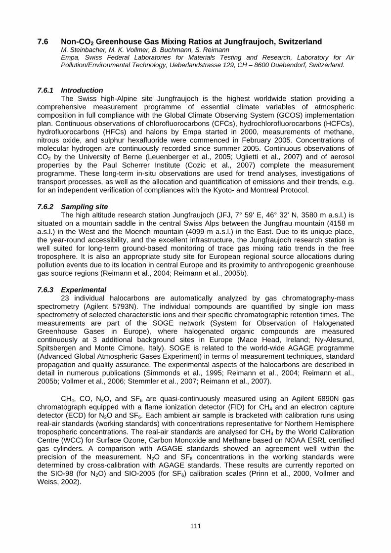
111

7.6 Non-CO2 Greenhouse Gas Mixing Ratios at Jungfraujoch, Switzerland M. Steinbacher, M. K. Vollmer, B. Buchmann, S. Reimann Empa, Swiss Federal Laboratories for Materials Testing and Research, Laboratory for Air Pollution/Environmental Technology, Ueberlandstrasse 129, CH – 8600 Duebendorf, Switzerland.

7.6.1 Introduction

The Swiss high-Alpine site Jungfraujoch is the highest worldwide station providing a comprehensive measurement programme of essential climate variables of atmospheric composition in full compliance with the Global Climate Observing System (GCOS) implementation plan. Continuous observations of chlorofluorocarbons (CFCs), hydrochlorofluorocarbons (HCFCs), hydrofluorocarbons (HFCs) and halons by Empa started in 2000, measurements of methane, nitrous oxide, and sulphur hexafluoride were commenced in February 2005. Concentrations of molecular hydrogen are continuously recorded since summer 2005. Continuous observations of CO2 by the University of Berne (Leuenberger et al., 2005; Uglietti et al., 2007) and of aerosol properties by the Paul Scherrer Institute (Cozic et al., 2007) complete the measurement programme. These long-term in-situ observations are used for trend analyses, investigations of transport processes, as well as the allocation and quantification of emissions and their trends, e.g. for an independent verification of compliances with the Kyoto- and Montreal Protocol. 7.6.2 Sampling site

The high altitude research station Jungfraujoch (JFJ, 7° 59' E, 46° 32' N, 3580 m a.s.l.) is situated on a mountain saddle in the central Swiss Alps between the Jungfrau mountain (4158 m a.s.l.) in the West and the Moench mountain (4099 m a.s.l.) in the East. Due to its unique place, the year-round accessibility, and the excellent infrastructure, the Jungfraujoch research station is well suited for long-term ground-based monitoring of trace gas mixing ratio trends in the free troposphere. It is also an appropriate study site for European regional source allocations during pollution events due to its location in central Europe and its proximity to anthropogenic greenhouse gas source regions (Reimann et al., 2004; Reimann et al., 2005b). 7.6.3 Experimental

23 individual halocarbons are automatically analyzed by gas chromatography-mass spectrometry (Agilent 5793N). The individual compounds are quantified by single ion mass spectrometry of selected characteristic ions and their specific chromatographic retention times. The measurements are part of the SOGE network (System for Observation of Halogenated Greenhouse Gases in Europe), where halogenated organic compounds are measured continuously at 3 additional background sites in Europe (Mace Head, Ireland; Ny-Alesund, Spitsbergen and Monte Cimone, Italy). SOGE is related to the world-wide AGAGE programme (Advanced Global Atmospheric Gases Experiment) in terms of measurement techniques, standard propagation and quality assurance. The experimental aspects of the halocarbons are described in detail in numerous publications (Simmonds et al., 1995; Reimann et al., 2004; Reimann et al., 2005b; Vollmer et al., 2006; Stemmler et al., 2007; Reimann et al., 2007).

CH4, CO, N2O, and SF6 are quasi-continuously measured using an Agilent 6890N gas chromatograph equipped with a flame ionization detector (FID) for CH4 and an electron capture detector (ECD) for N2O and SF6. Each ambient air sample is bracketed with calibration runs using real-air standards (working standards) with concentrations representative for Northern Hemisphere tropospheric concentrations. The real-air standards are analysed for CH4 by the World Calibration Centre (WCC) for Surface Ozone, Carbon Monoxide and Methane based on NOAA ESRL certified gas cylinders. A comparison with AGAGE standards showed an agreement well within the precision of the measurement. N2O and SF6 concentrations in the working standards were determined by cross-calibration with AGAGE standards. These results are currently reported on the SIO-98 (for N2O) and SIO-2005 (for SF6) calibration scales (Prinn et al., 2000, Vollmer and Weiss, 2002).

112

A commercial gas chromatograph (Reduction Gas Analyzer (RGA-3), Trace Analytical, Inc. California, USA) is used to measure H2 and CO via reduction of mercuric oxide and detection of mercury by UV absorption.

Besides the greenhouse gas and related tracer measurements the measurement

programme of Empa at Jungfraujoch also includes continuous in-situ analyses of ozone (O3), carbon monoxide (CO), nitrogen monoxide (NO), nitrogen dioxide (NO2), the sum of nitrogen oxides (NOy), and sulphur dioxide (SO2). Daily samples are taken for the determination of particulate sulphur. The concentrations of PM10 are continuously observed as well as measured as 24-hour bulk samples. 7.6.4 Results

Figure 1 shows the time series of the cooling agent HFC-134a from 2000 to 2007 for the 4 SOGE stations. The observed concentrations at JFJ compare very well with other background stations when sampling unpolluted air masses. In contrast to the more remote sites in Ny-Alesund and Mace Head, JFJ is also occasionally under the influence of polluted air masses due to its location in central Europe and its proximity to anthropogenic source regions. When combining measurements and trajectory statistics such events can be used to allocate source regions in Europe (see Figure 2). Whereas HFC emissions are mainly originated from the highly industrialized Po Basin in Northern Italy only little emissions can be still observed for the Montreal Protocol restricted CFCs and HCFCs. This approach was also already applied for less reactive oxygenated volatile organic compounds at JFJ (Legreid et al., 2007).

Nevertheless, background concentrations that correspond very well with the data from

more remote sites can be determined when extracting conditions using appropriate statistical (see e.g. Reimann et al., 2005b) or meteorological filters (Forrer et al., 2000) when JFJ is under the influence of pristine air masses.

Besides the rather qualitative approach of determination of European source regions,

pollution events are also used for quantitative emission estimates. Figure 3 illustrates estimates of the Swiss emissions of the Kyoto Protocol targeted greenhouse gases CH4 and N2O. The estimates in blue are based on measured trace gas ratios to carbon monoxide during pollution events at JFJ. These ratios allow - under the assumption of known CO emission sources for Switzerland – an independent experimental verification of other reported emissions. Our results for 2005 agree well with the Swiss greenhouse gas inventory based on economic data that is provided by the Swiss Federal Office for the Environment according to UNFCC and IPCC guidelines (see www.climatereporting.ch).

0

50

100

150

200

250

2000 2001 2002 2003 2004 2005 2006

ppt

Monte CimoneJungfraujochMace HeadNy-Alesund

Figure 1. Mixing ratios of the cooling agent HFC-134a at the 4 SOGE stations

(Reimann et al., 2005a, updated).

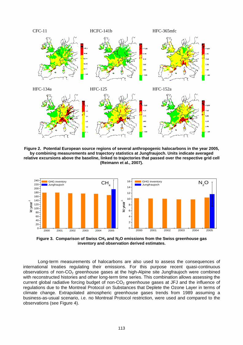
113

2000 2001 2002 2003 2004 20050

2

4

6

8

10

12

14

16 N2O

kt y

ear-1

GHG inventory Jungfraujoch

2000 2001 2002 2003 2004 20050

20406080

100120140160180200220240 CH4

kt y

ear-1

GHG inventory Jungfraujoch

CFC-11 HCFC-141b HFC-365mfc

HFC-134a HFC-125 HFC-152a

Figure 2. Potential European source regions of several anthropogenic halocarbons in the year 2005,

by combining measurements and trajectory statistics at Jungfraujoch. Units indicate averaged relative excursions above the baseline, linked to trajectories that passed over the respective grid cell

(Reimann et al., 2007).

Figure 3. Comparison of Swiss CH4 and N2O emissions from the Swiss greenhouse gas

inventory and observation derived estimates.

Long-term measurements of halocarbons are also used to assess the consequences of international treaties regulating their emissions. For this purpose recent quasi-continuous observations of non-CO2 greenhouse gases at the high-Alpine site Jungfraujoch were combined with reconstructed histories and other long-term time series. This combination allows assessing the current global radiative forcing budget of non-CO2 greenhouse gases at JFJ and the influence of regulations due to the Montreal Protocol on Substances that Deplete the Ozone Layer in terms of climate change. Extrapolated atmospheric greenhouse gases trends from 1989 assuming a business-as-usual scenario, i.e. no Montreal Protocol restriction, were used and compared to the observations (see Figure 4).

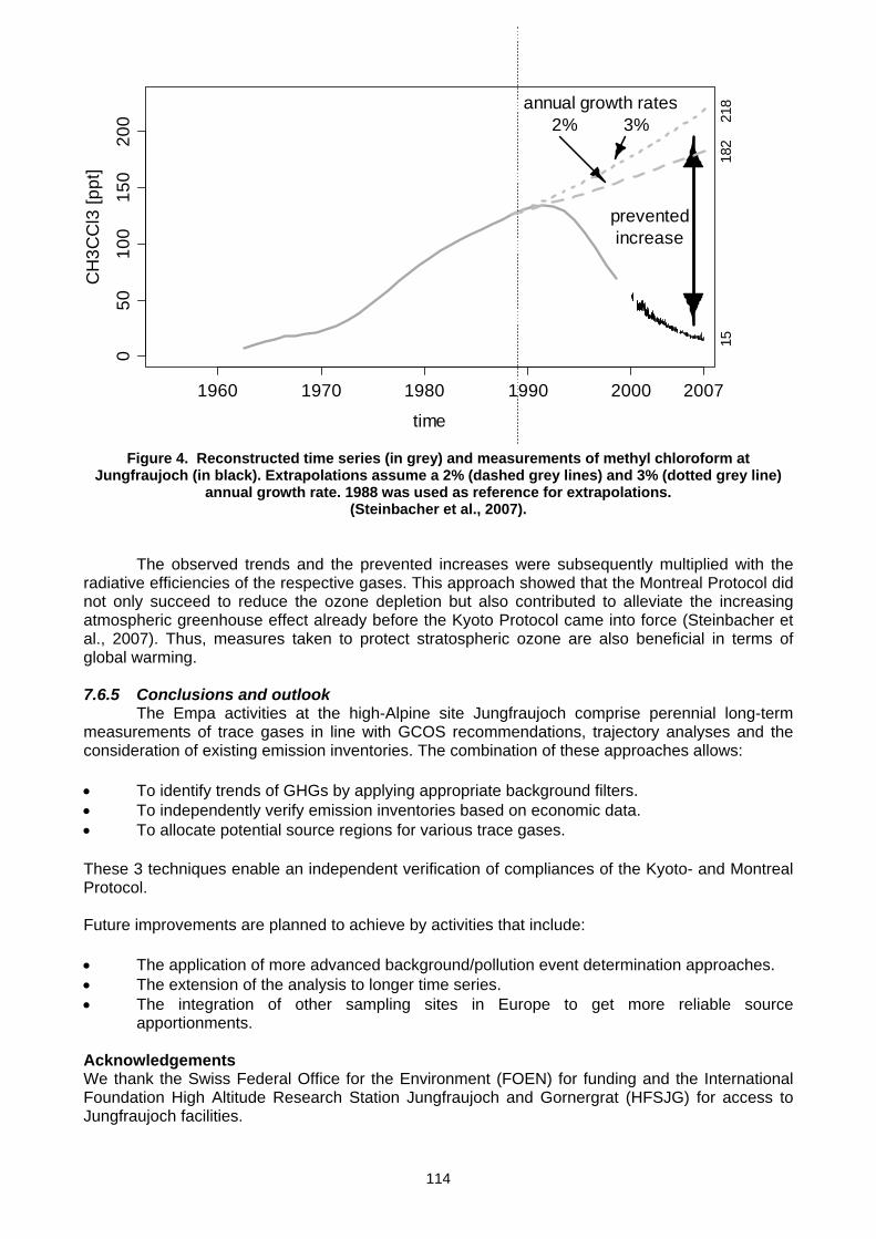
114

050

100

150

200

time

CH

3CC

l3 [p

pt]

1960 1970 1980 1990 2000 2007

preventedincrease

annual growth rates2% 3%

1518

221

8

Figure 4. Reconstructed time series (in grey) and measurements of methyl chloroform at Jungfraujoch (in black). Extrapolations assume a 2% (dashed grey lines) and 3% (dotted grey line)

annual growth rate. 1988 was used as reference for extrapolations. (Steinbacher et al., 2007).

The observed trends and the prevented increases were subsequently multiplied with the

radiative efficiencies of the respective gases. This approach showed that the Montreal Protocol did not only succeed to reduce the ozone depletion but also contributed to alleviate the increasing atmospheric greenhouse effect already before the Kyoto Protocol came into force (Steinbacher et al., 2007). Thus, measures taken to protect stratospheric ozone are also beneficial in terms of global warming. 7.6.5 Conclusions and outlook

The Empa activities at the high-Alpine site Jungfraujoch comprise perennial long-term measurements of trace gases in line with GCOS recommendations, trajectory analyses and the consideration of existing emission inventories. The combination of these approaches allows: • To identify trends of GHGs by applying appropriate background filters. • To independently verify emission inventories based on economic data. • To allocate potential source regions for various trace gases. These 3 techniques enable an independent verification of compliances of the Kyoto- and Montreal Protocol. Future improvements are planned to achieve by activities that include: • The application of more advanced background/pollution event determination approaches. • The extension of the analysis to longer time series. • The integration of other sampling sites in Europe to get more reliable source

apportionments. Acknowledgements We thank the Swiss Federal Office for the Environment (FOEN) for funding and the International Foundation High Altitude Research Station Jungfraujoch and Gornergrat (HFSJG) for access to Jungfraujoch facilities.

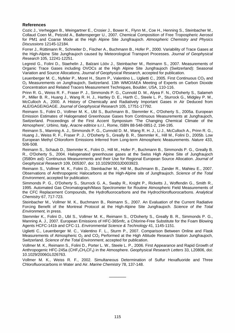
115

References Cozic J., Verheggen B., Weingartner E., Crosier J., Bower K., Flynn M., Coe H., Henning S., Steinbacher M., Collaud Coen M., Petzold A., Baltensperger U., 2007. Chemical Composition of Free Tropospheric Aerosol for PM1 and Coarse Mode at the High Alpine Site Jungfraujoch. Atmospheric Chemistry and Physics Discussions 12145-12184. Forrer J., Rüttimann R., Schneiter D., Fischer A., Buchmann B., Hofer P., 2000. Variability of Trace Gases at the High-Alpine Site Jungfraujoch caused by Meteorological Transport Processes. Journal of Geophysical Research 105, 12241-12251. Legreid G., Folini D., Staehelin J., Balzani Lööv J., Steinbacher M., Reimann S., 2007. Measurements of Organic Trace Gases including OVOCs at the High Alpine Site Jungfraujoch (Switzerland): Seasonal Variation and Source Allocations. Journal of Geophysical Research, accepted for publication. Leuenberger M. C., Nyfeler P., Moret H., Sturm P., Valentino L., Uglietti C., 2005. First Continuous CO2 and O2 Measurements on Jungfraujoch, Switzerland. 13th WMO/IAEA Meeting of Experts on Carbon Dioxide Concentration and Related Tracers Measurement Techniques, Boulder, USA, 110-116. Prinn R. G., Weiss R. F., Fraser P. J., Simmonds P. G., Cunnold D. M., Alyea F. N., O'Doherty S., Salameh P., Miller B. R., Huang J., Wang R. H. J., Hartley D. E., Harth C., Steele L. P., Sturrock G., Midgley P. M., McCulloch A., 2000. A History of Chemically and Radiatively Important Gases in Air Deduced from ALE/GAGE/AGAGE. Journal of Geophysical Research 105, 17751-17792. Reimann S., Folini D., Vollmer M. K., Ubl S., Buchmann B., Stemmler K., O'Doherty S., 2005a. European Emission Estimates of Halogenated Greenhouse Gases from Continuous Measurements at Jungfraujoch, Switzerland. Proceedings of the First Accent Symposium 'The Changing Chemical Climate of the Atmosphere', Urbino, Italy, Aracne editrice s.r.l., Rome, ISBN 88-548-0851-2, 194-195. Reimann S., Manning A. J., Simmonds P. G., Cunnold D. M., Wang R. H. J., Li J., McCulloch A., Prinn R. G., Huang J., Weiss R. F., Fraser P. J., O'Doherty S., Greally B. R., Stemmler K., Hill M., Folini D., 2005b. Low European Methyl Chloroform Emissions Inferred from Long-term Atmospheric Measurements. Nature 433, 506-508. Reimann S., Schaub D., Stemmler K., Folini D., Hill M., Hofer P., Buchmann B., Simmonds P. G., Greally B. R., O'Doherty S., 2004. Halogenated greenhouse gases at the Swiss High Alpine Site of Jungfraujoch (3580m asl): Continuous Measurements and their Use for Regional European Source Allocation. Journal of Geophysical Research 109, D05307, doi: 10.1029/2003JD003923. Reimann S., Vollmer M. K., Folini D., Steinbacher M., Hill M., Buchmann B., Zander R., Mahieu E., 2007. Observations of Anthropogenic Halocarbons at the High-Alpine site of Jungfraujoch. Science of the Total Environment, accepted for publication. Simmonds P. G., O'Doherty S., Sturrock G. A., Swaby R., Knight P., Ricketts J., Woffendin G., Smith R., 1995. Automated Gas Chromatograph/Mass Spectrometer for Routine Atmospheric Field Measurements of the CFC Replacement Compounds, the Hydrofluorocarbons and the Hydrochlorofluorocarbons. Analytical Chemistry 67, 717-723. Steinbacher M., Vollmer M. K., Buchmann B., Reimann S., 2007. An Evaluation of the Current Radiative Forcing Benefit of the Montreal Protocol at the High-Alpine Site Jungfraujoch. Science of the Total Environment, in press. Stemmler K., Folini D., Ubl S., Vollmer M. K., Reimann S., O'Doherty S., Greally B. R., Simmonds P. G., Manning A. J., 2007. European Emissions of HFC-365mfc, a Chlorine-Free Substitute for the Foam Blowing Agents HCFC-141b and CFC-11. Environmental Science & Technology 41, 1145-1151. Uglietti C., Leuenberger M. C., Valentino F. L., Sturm P., 2007. Comparison Between Online and Flask Measurements of Atmospheric O2 and CO2 Performed at the High Altitude Research Station Jungfraujoch, Switzerland. Science of the Total Environment, accepted for publication. Vollmer M. K., Reimann S., Folini D., Porter L. W., Steele L. P., 2006. First Appearance and Rapid Growth of Anthropogenic HFC-245a (CHF2CH2CF3) in the Atmosphere. Geophysical Research Letters 33, L20806, doi: 10.1029/2006GL026763. Vollmer M. K., Weiss R. F., 2002. Simultaneous Determination of Sulfur Hexafluoride and Three Chlorofluorocarbons in Water and Air. Marine Chemistry 78, 137-148.

_______

116

7.7 Progress on the Background Greenhouse Gases and Related Tracers Measurement Programme in China L.X. Zhou, X.C. Zhang, F. Zhang, B. Yao, L.X. Liu, M. Wen, L. Xu, S.X. Fang, Y.P. Wen, S. Gu Centre for Atmosphere Watch and Services (CAWAS) Chinese Academy of Meteorological Sciences (CAMS) China Meteorological Administration (CMA) 46 Zhongguancun Nandajie, Beijing 100081, China

7.7.1 Introduction

Since 1990, CMA has been participating actively in the GAW supporting global networks for greenhouse gases and other atmospheric components. Scientific aim is to obtain observational constraints on the global and regional budget, including global and regional burden, long-term trend, and annual variations in trend, seasonal cycles, and spatial variations, and use the observations to quantify sources and sinks. 7.7.2 Site and in-situ measurement programme

Mt. Waliguan is located in a drought temperate climatic zone surrounded primarily with low grasslands and mountainous regions. Atmospheric CO2 has been measured using a Licor6251 non-dispersive infrared (NDIR) analyzer since 1994. Atmospheric CH4 has been measured quasi-continuously by using a Hewlett Packard (HP) 5890 Series II gas chromatograph (GC) equipped with a flame ionization detector (FID) since 1994. Ambient air is supplied via 3/8 o.d. Dekobon tubing extending 80 m up the tower, approximately 5 m away from the laboratory. 7.7.3 Measurement scale and calibration (traceability)

In-situ atmospheric CO2 and CH4 measurements at Mt. Waliguan are indirectly traceable to the international absolute WMO mole fraction scale maintained by the WMO Central Calibration Laboratory (hosted by NOAA ESRL). Two sets of six secondary tanks are run against each other periodically to check internal consistency. Working standard gases are filled at WLG and calibrated by the secondary standard gases before and after use. The CO2 data from 1994 to 2007 has been adjusted to be consistent with the WMO X2007 scale. The CH4 standard scale at Waliguan is relative to a CH4 measurement scale maintained by the Meteorological Service of Canada (MSC). The MSC CH4 scale has been compared with the NOAA ESRL CH4 scale through several inter-comparison experiments. The CH4 data at Waliguan from 1994 to 2007 has been adjusted to NOAA-2004 CH4 scale. 7.7.4 Data Processing and time series

Hourly averaged CO2 data is computed from valid minute data for one hour measurements. Hourly averaged data are selected using “R” based on an algorithm “robust local regression” to distinguish samples of regionally representative air (background) from samples influenced by local sources and sinks (non-background). Using this statistical method, the acquired rate of the valid data which were categorized as background CO2 values are about 70%. Daily averages are based on those background hourly averages only. Monthly averages are computed from the daily averages. Hourly CH4 data are generated by arithmetic means from the valid raw data (typically 6-7 injections per hour). Valid hourly data are selected using “R” based on an algorithm “robust local regression” to distinguish samples of regionally representative air (background) from samples influenced by local sources and sinks (non-background). About 50% of the data were categorized as selected background CH4 values. The arithmetic means of selected hourly data has been used to generate daily and monthly data. Figure 1 showed atmospheric CO2 and CH4 hourly average data from July 1994 to December 2007 at Mt. Waliguan.

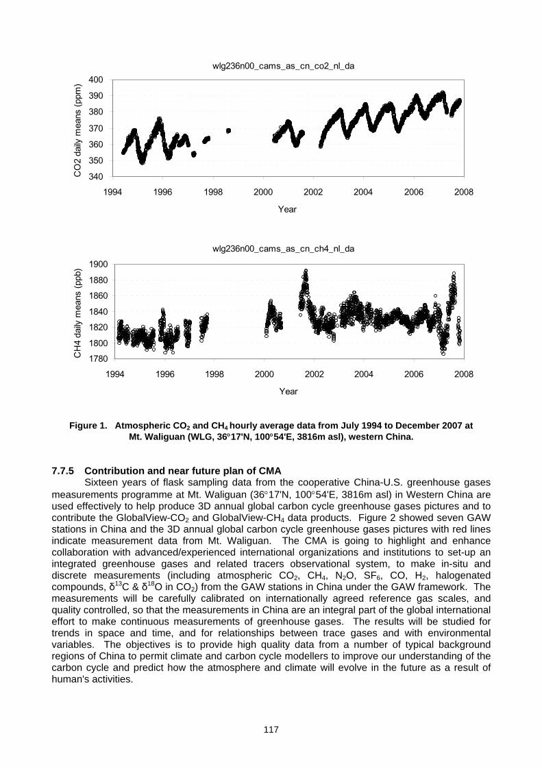
117

wlg236n00_cams_as_cn_co2_nl_da

340

350

360

370

380

390

400

1994 1996 1998 2000 2002 2004 2006 2008

Year

CO

2 da

ily m

eans

(ppm

)

wlg236n00_cams_as_cn_ch4_nl_da

17801800

18201840

18601880

1900

1994 1996 1998 2000 2002 2004 2006 2008

Year

CH

4 da

ily m

eans

(ppb

)

Figure 1. Atmospheric CO2 and CH4 hourly average data from July 1994 to December 2007 at

Mt. Waliguan (WLG, 36°17'N, 100°54'E, 3816m asl), western China. 7.7.5 Contribution and near future plan of CMA

Sixteen years of flask sampling data from the cooperative China-U.S. greenhouse gases measurements programme at Mt. Waliguan (36°17'N, 100°54'E, 3816m asl) in Western China are used effectively to help produce 3D annual global carbon cycle greenhouse gases pictures and to contribute the GlobalView-CO2 and GlobalView-CH4 data products. Figure 2 showed seven GAW stations in China and the 3D annual global carbon cycle greenhouse gases pictures with red lines indicate measurement data from Mt. Waliguan. The CMA is going to highlight and enhance collaboration with advanced/experienced international organizations and institutions to set-up an integrated greenhouse gases and related tracers observational system, to make in-situ and discrete measurements (including atmospheric CO2, CH4, N2O, SF6, CO, H2, halogenated compounds, δ13C & δ18O in CO2) from the GAW stations in China under the GAW framework. The measurements will be carefully calibrated on internationally agreed reference gas scales, and quality controlled, so that the measurements in China are an integral part of the global international effort to make continuous measurements of greenhouse gases. The results will be studied for trends in space and time, and for relationships between trace gases and with environmental variables. The objectives is to provide high quality data from a number of typical background regions of China to permit climate and carbon cycle modellers to improve our understanding of the carbon cycle and predict how the atmosphere and climate will evolve in the future as a result of human's activities.

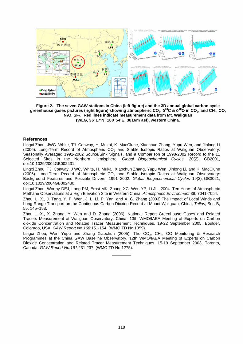
118

References Lingxi Zhou, JWC. White, TJ. Conway, H. Mukai, K. MacClune, Xiaochun Zhang, Yupu Wen, and Jinlong Li (2006). Long-Term Record of Atmospheric CO2 and Stable Isotopic Ratios at Waliguan Observatory: Seasonally Averaged 1991-2002 Source/Sink Signals, and a Comparison of 1998-2002 Record to the 11 Selected Sites in the Northern Hemisphere. Global Biogeochemical Cycles, 20(2), GB2001, doi:10.1029/2004GB002431. Lingxi Zhou, TJ. Conway, J WC. White, H. Mukai, Xiaochun Zhang, Yupu Wen, Jinlong Li, and K. MacClune (2005). Long-Term Record of Atmospheric CO2 and Stable Isotopic Ratios at Waliguan Observatory: Background Features and Possible Drivers, 1991–2002. Global Biogeochemical Cycles 19(3), GB3021, doi:10.1029/2004GB002430. Lingxi Zhou, Worthy DEJ, Lang PM, Ernst MK, Zhang XC, Wen YP, Li JL，2004. Ten Years of Atmospheric Methane Observations at a High Elevation Site in Western China. Atmospheric Environment 38: 7041-7054. Zhou, L. X., J. Tang, Y. P. Wen, J. L. Li, P. Yan, and X. C. Zhang (2003),The Impact of Local Winds and Long-Range Transport on the Continuous Carbon Dioxide Record at Mount Waliguan, China, Tellus, Ser. B, 55, 145–158. Zhou L. X., X. Zhang, Y. Wen and D. Zhang (2006). National Report Greenhouse Gases and Related Tracers Measurement at Waliguan Observatory, China. 13th WMO/IAEA Meeting of Experts on Carbon dioxide Concentration and Related Tracer Measurement Techniques. 19-22 September 2005, Boulder, Colorado, USA. GAW Report No.168:151-154. (WMO TD No.1359). Lingxi Zhou, Wen Yupu and Zhang Xiaochun (2005). The CO2, CH4, CO Monitoring & Research Programmes at the China GAW Baseline Observatory. 12th WMO/IAEA Meeting of Experts on Carbon Dioxide Concentration and Related Tracer Measurement Techniques. 15-19 September 2003, Toronto, Canada. GAW Report No.161:231-237. (WMO TD No.1275).

_______

AKDL

JS

WLG

XGLL

SDZ

LFS

LA

EstablishedExperiment

AKDL

JS

WLG

XGLL

SDZ

LFS

LA

EstablishedExperiment

AKDL

JS

WLG

XGLL

SDZ

LFS

LA

EstablishedExperiment

AKDL

JS

WLG

XGLL

SDZ

LFS

LA

EstablishedExperiment

Figure 2. The seven GAW stations in China (left figure) and the 3D annual global carbon cycle greenhouse gases pictures (right figure) showing atmospheric CO2, δ13C & δ18O in CO2, and CH4, CO,

N2O, SF6. Red lines indicate measurement data from Mt. Waliguan (WLG, 36°17'N, 100°54'E, 3816m asl), western China.

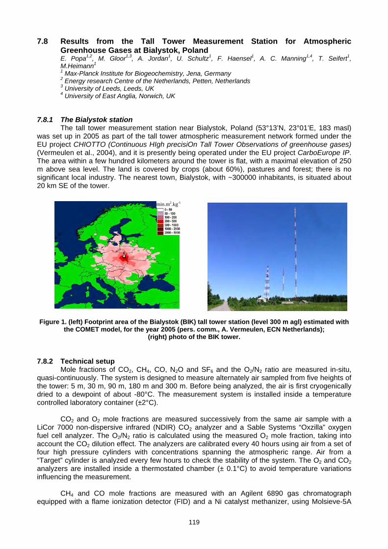
119

min.m2.kg-1

7.8 Results from the Tall Tower Measurement Station for Atmospheric Greenhouse Gases at Bialystok, Poland E. Popa1,2, M. Gloor1,3, A. Jordan1, U. Schultz1, F. Haensel1, A. C. Manning1,4, T. Seifert1, M.Heimann1 1 Max-Planck Institute for Biogeochemistry, Jena, Germany 2 Energy research Centre of the Netherlands, Petten, Netherlands 3 University of Leeds, Leeds, UK 4 University of East Anglia, Norwich, UK

7.8.1 The Bialystok station

The tall tower measurement station near Bialystok, Poland (53°13’N, 23°01’E, 183 masl) was set up in 2005 as part of the tall tower atmospheric measurement network formed under the EU project CHIOTTO (Continuous HIgh precisiOn Tall Tower Observations of greenhouse gases) (Vermeulen et al., 2004), and it is presently being operated under the EU project CarboEurope IP. The area within a few hundred kilometers around the tower is flat, with a maximal elevation of 250 m above sea level. The land is covered by crops (about 60%), pastures and forest; there is no significant local industry. The nearest town, Bialystok, with ~300000 inhabitants, is situated about 20 km SE of the tower. Figure 1. (left) Footprint area of the Bialystok (BIK) tall tower station (level 300 m agl) estimated with

the COMET model, for the year 2005 (pers. comm., A. Vermeulen, ECN Netherlands); (right) photo of the BIK tower.

7.8.2 Technical setup Mole fractions of CO2, CH4, CO, N2O and SF6 and the O2/N2 ratio are measured in-situ,

quasi-continuously. The system is designed to measure alternately air sampled from five heights of the tower: 5 m, 30 m, 90 m, 180 m and 300 m. Before being analyzed, the air is first cryogenically dried to a dewpoint of about -80°C. The measurement system is installed inside a temperature controlled laboratory container (±2°C).

CO2 and O2 mole fractions are measured successively from the same air sample with a

LiCor 7000 non-dispersive infrared (NDIR) CO2 analyzer and a Sable Systems “Oxzilla” oxygen fuel cell analyzer. The O2/N2 ratio is calculated using the measured O2 mole fraction, taking into account the CO2 dilution effect. The analyzers are calibrated every 40 hours using air from a set of four high pressure cylinders with concentrations spanning the atmospheric range. Air from a “Target” cylinder is analyzed every few hours to check the stability of the system. The O2 and CO2 analyzers are installed inside a thermostated chamber (± 0.1°C) to avoid temperature variations influencing the measurement.

CH4 and CO mole fractions are measured with an Agilent 6890 gas chromatograph

equipped with a flame ionization detector (FID) and a Ni catalyst methanizer, using Molsieve-5A

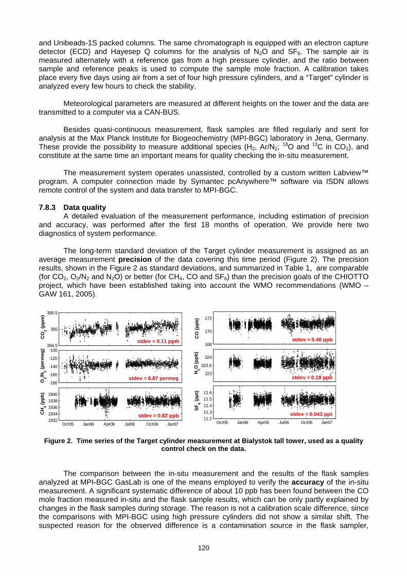
120

394.5

395

395.5

CO

2 (ppm

)

-180

-160

-140

-120

-100

O2/N

2 (per

meg

)

Oct05 Jan06 Apr06 Jul06 Oct06 Jan0719321934193619381940

CH 4 (p

pb)

stdev = 0.11 ppm

stdev = 6.87 permeg

stdev = 0.82 ppb

168

170

172

CO

(ppb

)

323

323.5

324

N2O

(ppb

)

Oct05 Jan06 Apr06 Jul06 Oct06 Jan0711.211.311.411.511.6

SF6 (p

pt)

stdev = 0.40 ppb

stdev = 0.18 ppb

stdev = 0.043 ppt

and Unibeads-1S packed columns. The same chromatograph is equipped with an electron capture detector (ECD) and Hayesep Q columns for the analysis of N2O and SF6. The sample air is measured alternately with a reference gas from a high pressure cylinder, and the ratio between sample and reference peaks is used to compute the sample mole fraction. A calibration takes place every five days using air from a set of four high pressure cylinders, and a “Target” cylinder is analyzed every few hours to check the stability.

Meteorological parameters are measured at different heights on the tower and the data are

transmitted to a computer via a CAN-BUS. Besides quasi-continuous measurement, flask samples are filled regularly and sent for

analysis at the Max Planck Institute for Biogeochemistry (MPI-BGC) laboratory in Jena, Germany. These provide the possibility to measure additional species (H2, Ar/N2; 18O and 13C in CO2), and constitute at the same time an important means for quality checking the in-situ measurement.

The measurement system operates unassisted, controlled by a custom written Labview™

program. A computer connection made by Symantec pcAnywhere™ software via ISDN allows remote control of the system and data transfer to MPI-BGC. 7.8.3 Data quality

A detailed evaluation of the measurement performance, including estimation of precision and accuracy, was performed after the first 18 months of operation. We provide here two diagnostics of system performance.

The long-term standard deviation of the Target cylinder measurement is assigned as an

average measurement precision of the data covering this time period (Figure 2). The precision results, shown in the Figure 2 as standard deviations, and summarized in Table 1, are comparable (for CO2, O2/N2 and N2O) or better (for CH4, CO and SF6) than the precision goals of the CHIOTTO project, which have been established taking into account the WMO recommendations (WMO – GAW 161, 2005).

Figure 2. Time series of the Target cylinder measurement at Bialystok tall tower, used as a quality control check on the data.

The comparison between the in-situ measurement and the results of the flask samples

analyzed at MPI-BGC GasLab is one of the means employed to verify the accuracy of the in-situ measurement. A significant systematic difference of about 10 ppb has been found between the CO mole fraction measured in-situ and the flask sample results, which can be only partly explained by changes in the flask samples during storage. The reason is not a calibration scale difference, since the comparisons with MPI-BGC using high pressure cylinders did not show a similar shift. The suspected reason for the observed difference is a contamination source in the flask sampler,

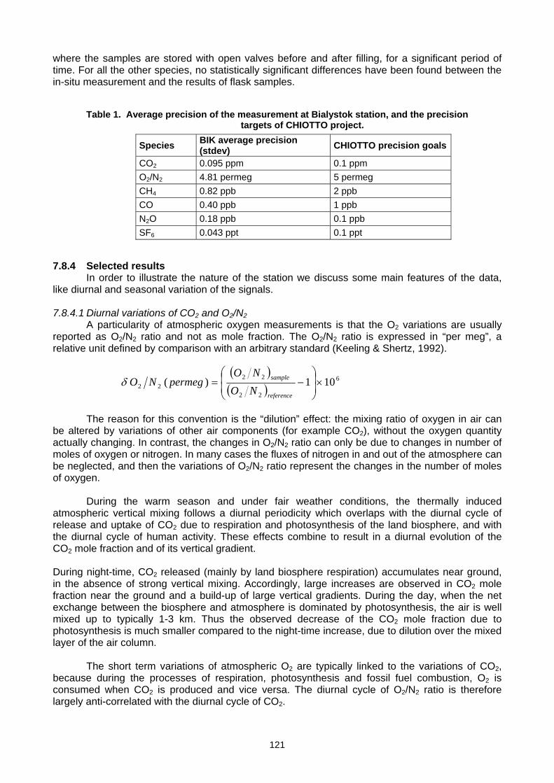
121

( )( )

6

22

2222 101)( ×⎟

⎟⎠

⎞⎜⎜⎝

⎛−=

reference

sample

NONO

permegNOδ

where the samples are stored with open valves before and after filling, for a significant period of time. For all the other species, no statistically significant differences have been found between the in-situ measurement and the results of flask samples.

Table 1. Average precision of the measurement at Bialystok station, and the precision targets of CHIOTTO project.

7.8.4 Selected results

In order to illustrate the nature of the station we discuss some main features of the data, like diurnal and seasonal variation of the signals. 7.8.4.1 Diurnal variations of CO2 and O2/N2

A particularity of atmospheric oxygen measurements is that the O2 variations are usually reported as O2/N2 ratio and not as mole fraction. The O2/N2 ratio is expressed in “per meg”, a relative unit defined by comparison with an arbitrary standard (Keeling & Shertz, 1992).

The reason for this convention is the “dilution” effect: the mixing ratio of oxygen in air can be altered by variations of other air components (for example CO2), without the oxygen quantity actually changing. In contrast, the changes in O2/N2 ratio can only be due to changes in number of moles of oxygen or nitrogen. In many cases the fluxes of nitrogen in and out of the atmosphere can be neglected, and then the variations of O2/N2 ratio represent the changes in the number of moles of oxygen.

During the warm season and under fair weather conditions, the thermally induced

atmospheric vertical mixing follows a diurnal periodicity which overlaps with the diurnal cycle of release and uptake of CO2 due to respiration and photosynthesis of the land biosphere, and with the diurnal cycle of human activity. These effects combine to result in a diurnal evolution of the CO2 mole fraction and of its vertical gradient.

During night-time, CO2 released (mainly by land biosphere respiration) accumulates near ground, in the absence of strong vertical mixing. Accordingly, large increases are observed in CO2 mole fraction near the ground and a build-up of large vertical gradients. During the day, when the net exchange between the biosphere and atmosphere is dominated by photosynthesis, the air is well mixed up to typically 1-3 km. Thus the observed decrease of the CO2 mole fraction due to photosynthesis is much smaller compared to the night-time increase, due to dilution over the mixed layer of the air column.

The short term variations of atmospheric O2 are typically linked to the variations of CO2,

because during the processes of respiration, photosynthesis and fossil fuel combustion, O2 is consumed when CO2 is produced and vice versa. The diurnal cycle of O2/N2 ratio is therefore largely anti-correlated with the diurnal cycle of CO2.

Species BIK average precision (stdev) CHIOTTO precision goals

CO2 0.095 ppm 0.1 ppm O2/N2 4.81 permeg 5 permeg CH4 0.82 ppb 2 ppb CO 0.40 ppb 1 ppb N2O 0.18 ppb 0.1 ppb SF6 0.043 ppt 0.1 ppt

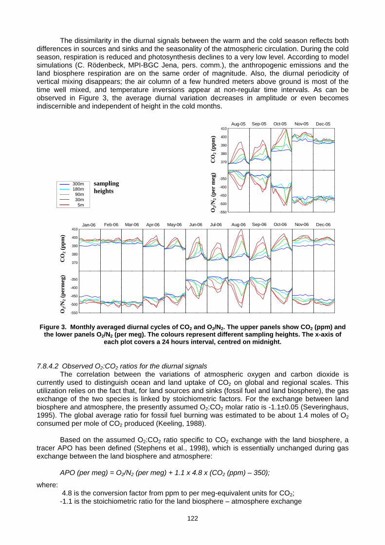
122

CO

2 (pp

m)

370

380

390

400

410

-550

-500

-450

-400

-350

Jan-06 Feb-06 Mar-06 Apr-06 May-06 Jun-06 Jul-06 Aug-06 Sep-06 Oct-06 Nov-06 Dec-06

370

380

390

400

410

-550

-500

-450

-400

-350

Aug-05 Sep-05 Oct-05 Nov-05 Dec-05

O2/N

2 (pe

r m

eg)

CO

2 (pp

m)

O2/N

2 (pe

rmeg

)

sampling heights

300m180m 90m 30m 5m

The dissimilarity in the diurnal signals between the warm and the cold season reflects both differences in sources and sinks and the seasonality of the atmospheric circulation. During the cold season, respiration is reduced and photosynthesis declines to a very low level. According to model simulations (C. Rödenbeck, MPI-BGC Jena, pers. comm.), the anthropogenic emissions and the land biosphere respiration are on the same order of magnitude. Also, the diurnal periodicity of vertical mixing disappears; the air column of a few hundred meters above ground is most of the time well mixed, and temperature inversions appear at non-regular time intervals. As can be observed in Figure 3, the average diurnal variation decreases in amplitude or even becomes indiscernible and independent of height in the cold months.

Figure 3. Monthly averaged diurnal cycles of CO2 and O2/N2. The upper panels show CO2 (ppm) and the lower panels O2/N2 (per meg). The colours represent different sampling heights. The x-axis of

each plot covers a 24 hours interval, centred on midnight.

7.8.4.2 Observed O2:CO2 ratios for the diurnal signals The correlation between the variations of atmospheric oxygen and carbon dioxide is

currently used to distinguish ocean and land uptake of CO2 on global and regional scales. This utilization relies on the fact that, for land sources and sinks (fossil fuel and land biosphere), the gas exchange of the two species is linked by stoichiometric factors. For the exchange between land biosphere and atmosphere, the presently assumed O2:CO2 molar ratio is -1.1±0.05 (Severinghaus, 1995). The global average ratio for fossil fuel burning was estimated to be about 1.4 moles of O2 consumed per mole of CO2 produced (Keeling, 1988).

Based on the assumed O2:CO2 ratio specific to CO2 exchange with the land biosphere, a

tracer APO has been defined (Stephens et al., 1998), which is essentially unchanged during gas exchange between the land biosphere and atmosphere:

APO (per meg) = O2/N2 (per meg) + 1.1 x 4.8 x (CO2 (ppm) – 350);

where: 4.8 is the conversion factor from ppm to per meg-equivalent units for CO2; -1.1 is the stoichiometric ratio for the land biosphere – atmosphere exchange

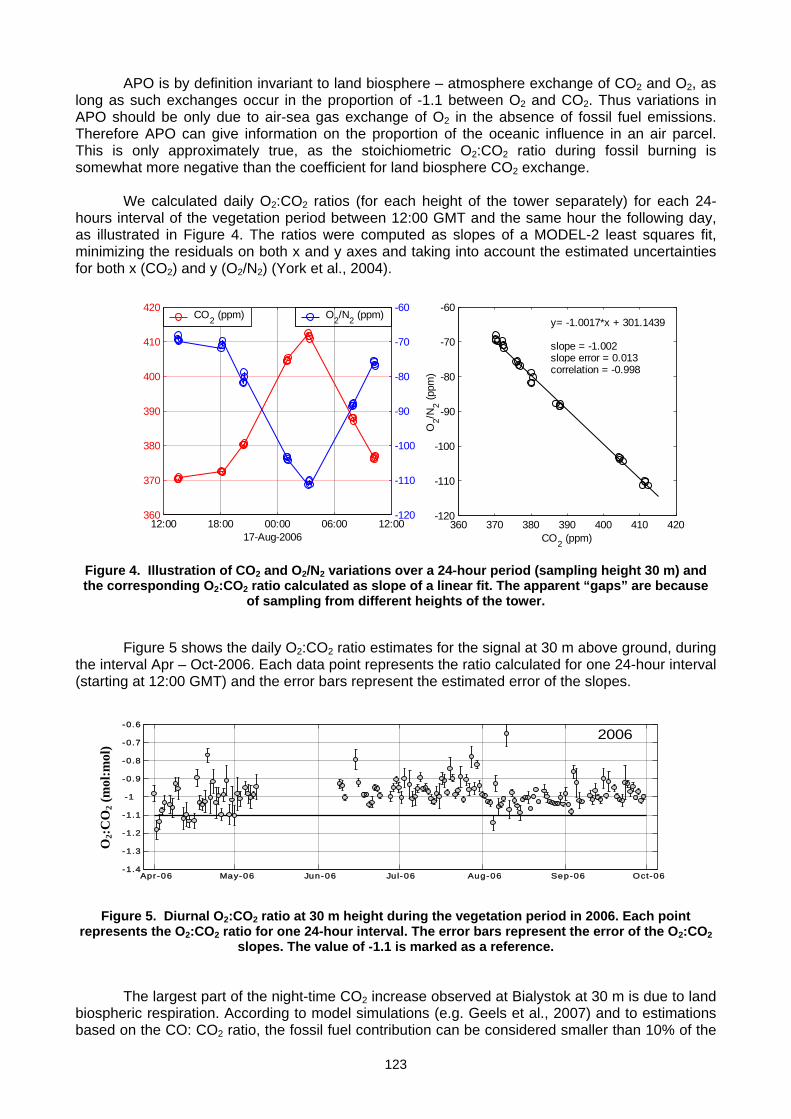
123

12:00 18:00 00:00 06:00 12:00360

370

380

390

400

410

420

17-Aug-2006

CO2 (ppm)

-120

-110

-100

-90

-80

-70

-60O2/N2 (ppm)

360 370 380 390 400 410 420-120

-110

-100

-90

-80

-70

-60y= -1.0017*x + 301.1439 slope = -1.002slope error = 0.013correlation = -0.998

CO2 (ppm)

O2/N

2 (ppm

)

Apr-06 May-06 Jun-06 Jul-06 Aug-06 Sep-06 Oct-06-1.4

-1.3

-1.2

-1.1

-1

-0.9

-0.8

-0.7

-0.6 2006

O2:

CO

2 (m

ol:m

ol)

APO is by definition invariant to land biosphere – atmosphere exchange of CO2 and O2, as long as such exchanges occur in the proportion of -1.1 between O2 and CO2. Thus variations in APO should be only due to air-sea gas exchange of O2 in the absence of fossil fuel emissions. Therefore APO can give information on the proportion of the oceanic influence in an air parcel. This is only approximately true, as the stoichiometric O2:CO2 ratio during fossil burning is somewhat more negative than the coefficient for land biosphere CO2 exchange.

We calculated daily O2:CO2 ratios (for each height of the tower separately) for each 24-

hours interval of the vegetation period between 12:00 GMT and the same hour the following day, as illustrated in Figure 4. The ratios were computed as slopes of a MODEL-2 least squares fit, minimizing the residuals on both x and y axes and taking into account the estimated uncertainties for both x (CO2) and y (O2/N2) (York et al., 2004).

Figure 4. Illustration of CO2 and O2/N2 variations over a 24-hour period (sampling height 30 m) and the corresponding O2:CO2 ratio calculated as slope of a linear fit. The apparent “gaps” are because

of sampling from different heights of the tower.

Figure 5 shows the daily O2:CO2 ratio estimates for the signal at 30 m above ground, during the interval Apr – Oct-2006. Each data point represents the ratio calculated for one 24-hour interval (starting at 12:00 GMT) and the error bars represent the estimated error of the slopes.

Figure 5. Diurnal O2:CO2 ratio at 30 m height during the vegetation period in 2006. Each point represents the O2:CO2 ratio for one 24-hour interval. The error bars represent the error of the O2:CO2

slopes. The value of -1.1 is marked as a reference. The largest part of the night-time CO2 increase observed at Bialystok at 30 m is due to land

biospheric respiration. According to model simulations (e.g. Geels et al., 2007) and to estimations based on the CO: CO2 ratio, the fossil fuel contribution can be considered smaller than 10% of the

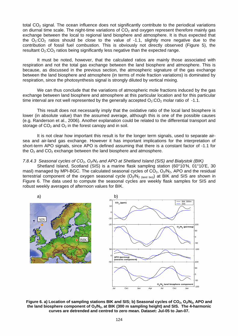
124

SIS

BIK

-100

-50

0

50

100

-50

0

50

-20

-10

0

10

20BIK 300mSIS

Jul Oct Jan Apr Jul Oct Jan-100

-50

0

50

100

CO2 (ppm)

O2/N2 (permeg)

APO (permeg) (oceanic component)

O2/N2 land biosphere component

total CO2 signal. The ocean influence does not significantly contribute to the periodical variations on diurnal time scale. The night-time variations of CO2 and oxygen represent therefore mainly gas exchange between the local to regional land biosphere and atmosphere. It is thus expected that the O2:CO2 ratios should be close to the value of -1.1, slightly more negative due to the contribution of fossil fuel combustion. This is obviously not directly observed (Figure 5), the resultant O2:CO2 ratios being significantly less negative than the expected range.

It must be noted, however, that the calculated ratios are mainly those associated with respiration and not the total gas exchange between the land biosphere and atmosphere. This is because, as discussed in the previous section, the atmospheric signature of the gas exchange between the land biosphere and atmosphere (in terms of mole fraction variations) is dominated by respiration, since the photosynthesis signal is strongly diluted by vertical mixing.

We can thus conclude that the variations of atmospheric mole fractions induced by the gas

exchange between land biosphere and atmosphere at this particular location and for this particular time interval are not well represented by the generally accepted O2:CO2 molar ratio of -1.1.

This result does not necessarily imply that the oxidative ratio of the local land biosphere is

lower (in absolute value) than the assumed average, although this is one of the possible causes (e.g. Randerson et al., 2006). Another explanation could be related to the differential transport and storage of CO2 and O2 in the forest canopy and in soil.

It is not clear how important this result is for the longer term signals, used to separate air-

sea and air-land gas exchange. However it has important implications for the interpretation of short-term APO signals, since APO is defined assuming that there is a constant factor of -1.1 for the O2 and CO2 exchange between the land biosphere and atmosphere. 7.8.4.3 Seasonal cycles of CO2, O2/N2 and APO at Shetland Island (SIS) and Bialystok (BIK)

Shetland Island, Scotland (SIS) is a marine flask sampling station (60°10’N, 01°10’E, 30 masl) managed by MPI-BGC. The calculated seasonal cycles of CO2, O2/N2, APO and the residual terrestrial component of the oxygen seasonal cycle (O2/N2 (land bio)) at BIK and SIS are shown in Figure 6. The data used to compute the seasonal cycles are weekly flask samples for SIS and robust weekly averages of afternoon values for BIK.

a) b)

Figure 6. a) Location of sampling stations BIK and SIS; b) Seasonal cycles of CO2, O2/N2, APO and the land biosphere component of O2/N2, at BIK (300 m sampling height) and SIS. The 4-harmonic

curves are detrended and centred to zero mean. Dataset: Jul-05 to Jan-07.

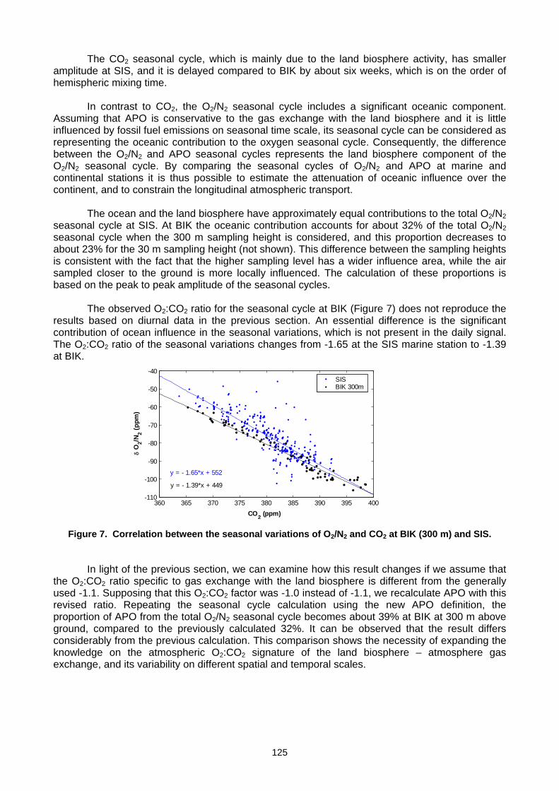
125

360 365 370 375 380 385 390 395 400-110

-100

-90

-80

-70

-60

-50

-40

CO2 (ppm)

δ O

2/N2 (p

pm)

SIS BIK 300m

y = - 1.65*x + 552 y = - 1.39*x + 449

The CO2 seasonal cycle, which is mainly due to the land biosphere activity, has smaller amplitude at SIS, and it is delayed compared to BIK by about six weeks, which is on the order of hemispheric mixing time.

In contrast to CO2, the O2/N2 seasonal cycle includes a significant oceanic component.

Assuming that APO is conservative to the gas exchange with the land biosphere and it is little influenced by fossil fuel emissions on seasonal time scale, its seasonal cycle can be considered as representing the oceanic contribution to the oxygen seasonal cycle. Consequently, the difference between the O2/N2 and APO seasonal cycles represents the land biosphere component of the O2/N2 seasonal cycle. By comparing the seasonal cycles of O2/N2 and APO at marine and continental stations it is thus possible to estimate the attenuation of oceanic influence over the continent, and to constrain the longitudinal atmospheric transport.

The ocean and the land biosphere have approximately equal contributions to the total O2/N2

seasonal cycle at SIS. At BIK the oceanic contribution accounts for about 32% of the total O2/N2 seasonal cycle when the 300 m sampling height is considered, and this proportion decreases to about 23% for the 30 m sampling height (not shown). This difference between the sampling heights is consistent with the fact that the higher sampling level has a wider influence area, while the air sampled closer to the ground is more locally influenced. The calculation of these proportions is based on the peak to peak amplitude of the seasonal cycles.

The observed O2:CO2 ratio for the seasonal cycle at BIK (Figure 7) does not reproduce the

results based on diurnal data in the previous section. An essential difference is the significant contribution of ocean influence in the seasonal variations, which is not present in the daily signal. The O2:CO2 ratio of the seasonal variations changes from -1.65 at the SIS marine station to -1.39 at BIK.

Figure 7. Correlation between the seasonal variations of O2/N2 and CO2 at BIK (300 m) and SIS. In light of the previous section, we can examine how this result changes if we assume that

the O2:CO2 ratio specific to gas exchange with the land biosphere is different from the generally used -1.1. Supposing that this O2:CO2 factor was -1.0 instead of -1.1, we recalculate APO with this revised ratio. Repeating the seasonal cycle calculation using the new APO definition, the proportion of APO from the total O2/N2 seasonal cycle becomes about 39% at BIK at 300 m above ground, compared to the previously calculated 32%. It can be observed that the result differs considerably from the previous calculation. This comparison shows the necessity of expanding the knowledge on the atmospheric O2:CO2 signature of the land biosphere – atmosphere gas exchange, and its variability on different spatial and temporal scales.

126

References Geels C., Gloor M., Ciais P., Bousquet P., Peylin P., Vermeulen A.T., Dargaville R., Aalto T., Brandt J., Christensen J.H., Frohn L.M., Haszpra L., Karstens U., Rödenbeck C., Ramonet M., Carboni G. & Santaguida R. (2007). Comparing Atmospheric Transport Models for Future Regional Inversions over Europe - Part 1: Mapping the Atmospheric CO2 Signals. Atmos. Chem. Phys., 7, 3461-3479. Keeling R.F. & Shertz S.R. (1992). Seasonal and Interannual Variations in Atmospheric Oxygen and Implications for the Global Carbon Cycle. Nature, 358, 723-727. Keeling R. F. (1988). Development of an interferometric oxygen analyzer. Ph.D. thesis, Harvard University, Cambridge, Mass., 178pp. Randerson J.T., Masiello C.A., Still C.J., Rahn T., Poorter H. & Field C.B. (2006). Is Carbon within the Global Terrestrial Biosphere Becoming More Oxidized? Implications for Trends in Atmospheric O2. Global Change Biology, 12, 260-271. Severinghaus J. P. (1995). Studies of the Terrestrial O2 and Carbon Cycles in Sand Dune Gases and in Biosphere 2. Ph.D. thesis, Columbia University, 148 pp. Stephens B.B., Keeling R.F., Heimann M., Six K.D., Murnane R. & Caldeira K. (1998). Testing Global Ocean Carbon Cycle Models using Measurements of Atmospheric O2 and CO2 Concentration. Global Biogeochemical Cycles, 12, 213-230. Vermeulen A.T., Hensen A., Gloor M., Manning A.C., Ciais P., Eisma R., van den Bulk W.C.M., Mols J.J. & Erisman J.W. (2004). CHIOTTO - Continuous High-Precision Tall Tower Observations of Greenhouse Gases. In: Inverse Modelling of National and EU Greenhouse Gas Emission Inventories (eds. P. B, Behrend H & Jol A). JRC Ispra. York D., Evensen N. M., Martinez M. L., and Delgado J. D. (2004). Unified Equations for the Slope, Intercept, and Standard Errors of the Best Straight Line. American Journal of Physics 72(3), 367-375. WMO/GAW Report No. 161 (2005). 12th WMO/IAEA Meeting of Expert on Carbon Dioxide Concentration and Related Tracers Measurements Techniques (Toronto, Canada, 15-18 September 2003).

_______

127

ANNEX A

14th WMO/IAEA Meeting of Experts on Carbon Dioxide, Other Greenhouse Gases and Related Tracer Measurement Techniques

(September 10–13, 2007, Helsinki, Finland)

Tuula Aalto Finnish Meteorological Institute Tuula.Aalto@fmi.fi Shuji Aoki Tohoku University aoki@mail.tains.tohoku.ac.jp Sergey Assonov Institute for Reference Materials and Measurements Sergey.ASSONOV@ec.europa.eu Shiv Dev Attri Government of India sdattri@yahoo.com Mika Aurela Finnish Meteorological Institute mika.aurela@fmi.fi Andrew Ayeni Federal Ministry of Environment, Abudja, Nigeria aiayeni2000@yahoo.com Leonard Barrie World Meteorological Organization Lbarrie@wmo.int Gordon Brailsford National Institute for and Atmospheric Research, NIWA g.brailsford@niwa.co.nz Willi A. Brand Max Planck Institute for Biogeochemistry, Jena wbrand@bgc-jena.mpg.de Ernst-Günther Brunke South African Weather Service ebrunke@weathersa.co.za James Butler NOAA Earth System Research Laboratory james.h.butler@noaa.gov Philippe Ciais CEA philippe.ciais@cea.fr

Eric Crosson Picarro, Inc. eric@picarro.com Edward Dlugokencky NOAA Earth System Research Laboratory (ESRL) ed.dlugokencky@noaa.gov Rebecca Fisher Royal Holloway, University of London r.fisher@gl.rhul.ac.uk Niia Fortelius Finnish Meteorological Institute Niia.Fortelius@fmi.fi Angel J. Gomez-Pelaez Observatorio Atmosferico de Izaña, Instituto Nacional de Meteorologia (INM, Spain) ajgomez@inm.es Heather Graven University of California, San Diego hgraven@ucsd.edu Brad Hall NOAA Earth System Research Lab Bradley.Hall@noaa.gov Samuel Hammer Institut fuer Umweltphysik, University of Heidelberg Samuel.Hammer@iup.uni-heidelberg.de Kathlene Hartnett Picarro, Inc. khartnett@picarro.com László Haszpra Hungarian Meteorological Service haszpra.l@met.hu Juha Hatakka Finnish Meteorological Institute juha.hatakka@fmi.fi Martin Heimann Max Planck Institute for Biogeochemistry, Jena martin.heimann@bgc-jena.mpg.de

128

Lin Huang Environment Canada lin.huang@ec.gc.ca Shigeyuki Ishidoya Tohoku University ishidoya@caos-a.geophys.tohoku.ac.jp Armin Jordan Max Planck Institute for Biogeochemistry, Jena ajordan@bgc-jena.mpg.de Högne Jungner University of Helsinki hogne.jungner@helsinki.fi Keiichi Katsumata Grobal Environmental Forum katsumata.keiichi@nies.go.jp Ralph Keeling University of California, San Diego rkeeling@ucsd.edu Jörg Klausen EMPA joerg.klausen@empa.ch Hannu Koponen University of Kuopio Hannu.Koponen@uku.fi Paul Krummel Commonwealth Scientific and Industrial Research Organisation (CSIRO) paul.krummel@csiro.au Mikko Laakso Vaisala Oyj mikko.laakso@vaisala.com Tuomas Laurila Finnish Meteorological Institute tuomas.laurila@fmi.fi Markus Leuenberger Physics Institute, University of Bern leuenberger@climate.unibe.ch Ingeborg Levin Institut fuer Umweltphysik Ingeborg.Levin@iup.uni-heidelberg.de David Lowry Royal Holloway, University of London d.lowry@gl.rhul.ac.uk Ingrid Luijkx University of Groningen i.t.luijkx@rug.nl

Toshinobu Machida National Institute for Environmental Studies tmachida@nies.go.jp Ivan Mammarella University of Helsinki ivan.mammarella@helsinki.fi Ken Masarie NOAA ESRL kenneth.masarie@noaa.gov Ulla Mattila Vaisala Oyj ulla.mattila@vaisala.com Frank Meinhardt Federal Environmental Agency (Umweltbundesamt) frank.meinhardt@uba.de Hitoshi Mukai National institute for Environmental Studies lnmukaih@nies.go.jp Takakiyo Nakazawa Tohoku University nakazawa@mail.tains.tohoku.ac.jp Rolf Neubert University of Groningen R.E.M.Neubert@rug.nl Nina Paramonova Main Gephysical Observatory reshal@peterlink.ru Mari Pihlatie University of Helsinki mari.pihlatie@helsinki.fi Pekka Plathan Finnish Meteorological Institute Pekka.Plathan@fmi.fi Elena Popa Max-Planck-Institute for Biogeochemistry, Jena epopa@bgc-jena.mpg.de Jukka Pumpanen University of Helsinki jukka.pumpanen@helsinki.fi Michel Ramonet Laboratoire des Sciences du Climat et de l'Environnement (LSCE) michel.ramonet@lsce.ipsl.fr Eckhart Scheel Forschungszentrum Karlsruhe hans-eckhart.scheel@imk.fzk.de

129

Hubertus Scheeren European Commission, Joint Research Centre, Ispra hubertus.scheeren@jrc.it Sebastian Schimmack Vaisala Oyj sebastian.schimmack@vaisala.com Martina Schmidt Laboratoire des Sciences du Climat et de l'Environnement (LSCE) Martina.Schmidt@cea.fr Andrey Sogachev University of Helsinki andrei.sogachev@helsinki.fi Eloni Sonninen University of Helsinki eloni.sonninen@helsinki.fi Srimathy Sriskantharajah Royal Holloway, University of London srimathy@gl.rhul.ac.uk Martin Steinbacher EMPA, Swiss Federal Laboratories for Material Testing and Research martin.steinbacher@empa.ch Atsuko Sunaga National institute for Environmental Studies sunaga.atsuko@nies.go.jp Pieter Tans Earth System Research Laboratory, NOAA Pieter.Tans@noaa.gov Yukio Terao National institute for Environmental Studies yterao@nies.go.jp Rona Thompson Max Planck Institute for Biogeochemistry, Jena rthompson@bgc-jena.mpg.de Tea Thum Finnish Meteorological Institute Tea.Thum@fmi.fi Yasunori Tohjima National Institute for Environmental Studies tohjima@nies.go.jp Yukitomo Tsutsumi Japan Meteorological Agency y-tsutsumi@met.kishou.go.jp Nedialko Valkov National Institute of Meteorology and Hydrology nedialko.valkov@meteo.bg

Sander Van der laan University of Groningen s.van.der.laan@rug.nl Marcel van der Schoot CSIRO Marine & Atmospheric Research marcel.vanderschoot@csiro.au Bruce Vaughn University of Colorado bruce.vaughn@colorado.edu Blagorodka Veleva National Institute of Meteorology and Hydrology blagorodka.veleva@meteo.bg Alex Vermeulen ECN - Energy research Center of the Netherlands a.vermeulen@ecn.nl Timo Vesala University of Helsinki timo.vesala@helsinki.fi Yrjö Viisanen Finnish Meteorological Institute yrjo.viisanen@fmi.fi Benoit Wastine Laboratoire des Sciences du Climat et de l'Environnement (LSCE Benoit.Wastine@cea.fr James White University of Colorado james.white@colorado.edu Douglas Worthy Environment Canada Doug.worthy@ec.gc.ca Hiroaki Yamagishi National Institute for Environmental Studies yamagishi.hiroaki@nies.go.jp Liukang Xu LI-COR Biosciences liukang.xu@licor.com Lingxi Zhou Centre for Atmosphere Watch and Services (CAWAS) Chinese Academy of Meteorological Sciences (CAMS) zhoulx@cams.cma.gov.cn Alexander Zinchenko Main Gephysical Observatory aresh@main.mgo.rssi.ru

130

ANNEX B

14th WMO/IAEA Meeting of Experts on Carbon Dioxide, Other Greenhouse Gases and Related Tracer Measurement Techniques

(September 10–13, 2007, Helsinki, Finland)

Monday, September 10 8:00–9:00 Registration 9:00–9:10 Organizers Information on organization of the meeting 9:10–9:20 P. Plathan Welcome to Helsinki WMO/IAEA 9:20–9:40 L. Barrie The WMO GAW Programme General presentations 9:40–10:00 Y. Viisanen GAW research in the Finnish Meteorological

Institute 10:00–10:20 P. Ciais Autumn warming implies a shorter seasonal carbon uptake 10:20-10:50 Break Standards and calibration (Chair: T. Machida) 10:50–11:10 P. P. Tans The WMO-X2007 mole fraction scale for CO2-in-air 11:10–11:30 B. Hall Improvements in the WMO/GAW nitrous oxide

mole fraction scale 11:30–11:50 A. Jordan The EUROHYDROS calibration scale for hydrogen 11:50–12:10 Y. Tohjima Evaluation of carbon isotope effect on CO2

measurements by NDIR analyzer 12:10–13:10 Lunch 13:10–14:20 Discussion concerning standards and handling of calibration

gases (P. P. Tans) 14:20–14:40 Break 14:40–15:10 Recommendations concerning standards and handling of

calibration gases 15:10–18:00 Poster session with refreshments

131

Tuesday, September 11 Intercomparison activities (Chair: G. Brailsford) 8:30–8:50 R. Neubert A long-term intercomparison experiment of two frequently-

used atmospheric 222Radon monitors 8:50–9:10 I. Levin Five years of international flask intercomparison (SAUSAGE flask ICP) 9:10–9:30 Y. Tsutsumi Activities in QA/SAC and WCC in Japan 9:30–9:50 K. Masarie NOAA comparison activities: Are we closer to the required measurement accuracy? 9:50–10:30 Break 10:30–10:50 L. X. Zhou Report of the fourth WMO round-robin reference gas intercomparison, 2002–2007 10:50–12.00 Discussion and recommendations concerning

intercomparison activities (M. Schmidt) 12:00–13:00 Lunch Isotope calibration and measurements (Chair: S. Aoki) 13:00–13:20 H. D. Graven Measurements of 14CO2 from the Scripps CO2 programme 13:20–13:40 D. Lowry Ten years of high-precision methane isotope data for Mace Head and London: The influence of Canadian and European sources 13:40–14:00 L. Huang Challenges and recommendations of traceability

maintenance of high precision isotope measurements in atmospheric CO2

14:00–14:20 W. A. Brand Variability of δ13C and δ18O in CO2 generated from NBS19 calcite and implications for the VPDB scale in air CO2 records 14:20–14:50 Break 14:50–15:10 B. H. Vaughn High precision calibration instrumentation for δ13C of atmospheric CO2, carbonates, pure CO2, and CO2/H2O equilibration with waters 15:10–15:30 J. W. C. White Stable isotopes of CO2 and CH4 in the NOAA network 15:30–17:00 Discussion and recommendations concerning isotope

calibration and measurements (W. A. Brand, H. D. Graven)

132

Wednesday, September 12 Measurement techniques (Chair: M. Leuenberger) 8:30–8:50 A. J. Gomez-Pelaez Installation of a new gas chromatograph at Izana GAW

station (Spain) to measure CH4, N2O, and SF6 8:50–9:10 E. R. Crosson Ultra-sensitive measurements of methane, carbon dioxide

and water vapor for atmospheric monitoring 9:10–9:30 L. P. Steele (presented by M. van der Schoot) Measuring selected atmospheric trace gases using gas

chromatography and a Valco pulsed discharge ionization detector

9:30–9:50 H. Yamagishi In-situ measurements of atmospheric oxygen/nitrogen ratio at Ochi-Ishi by using GC/TCD technique

9:50–10:10 S. Morimoto (presented by S. Ishidoya) Development of high precision

continuous measurement system of the atmospheric O2/N2 ratio using a fuel cell oxygen analyzer

10:10–10:30 Break 10:30–10:50 P. Ciais ICOS, building a new European research infrastructure to

measure the carbon cycle 10:50–12:00 Discussion and recommendations concerning GHG and

O2/N2 measurement techniques (E. Dlugokencky) 12:00–13:00 Lunch Data management and quality assurance (Chair: D. Worthy) 13:00–13:20 H. E. Scheel Report of the WCC-N2O 13:20–13:40 J. Klausen A screening analysis of ozone, carbon monoxide and methane data at WDCGG 13:40–14:00 M. V. van der Schoot Calibration and network monitoring performance of LoFlo continuous CO2 analysers 14:00–14:20 Y. Tsutsumi The publication of WDCGG data submission and dissemination guide 14:20–14:40 Break 14:40–15:40 Discussion and recommendations concerning data

management and quality assurance (H.-E. Scheel) 15:40–17:00 Draft of recommendations (I. Levin) 19:00 Dinner at the restaurant Uunisaari (http://www.uunisaari.com/, click “kartta” for the

location)

133

Thursday, September 13 Measurement networks (Chair E. Brunke) 9:00–9:20 T. Vesala Absolute CO2 measurements at European flux towers 9:20–9:40 L. Haszpra Quarter century of atmospheric CO2 monitoring and research in Hungary 9:40–10:00 A. Vermeulen The CHIOTTO project: Results and where to go now 10:00–10:20 M. Schmidt Atmospheric greenhouse gas measurements in France 10:20–10:40 Break 10:40–11:00 S. S. Assonov CO2 isotopic composition in the upper troposphere: The project CARIBIC 11:00–11:20 T. Machida Measurements of atmospheric CO2 using commercial airliners 11:20–11:40 P. P. Tans Requirements for global observing systems for carbon dioxide and other greenhouse gases 11:40–12:20 Discussion concerning measurement networks and

strategies (M. Heimann) 12:20–13:20 Lunch 13:20–14:00 Recommendations concerning measurement networks and

strategies 14:00–14:20 Break 14:20–16:00 Discussion and approval of the draft recommendations

(I. Levin) 16:00 End of the meeting

134

Posters Standards and calibration K. Katsumata Development of carbon monoxide standard in background atmospheric level

by dynamic dilution method T. Machida Preparing and maintaining of CO2 calibration scale in National Institute for

Environmental Studies Intercomparison A. M. Crotwell Evaluation of the internal agreement of NOAA/ESRL flask analysis systems Isotopes C. Allison Improved traceability for measurements of the stable isotopic composition of

atmospheric CO2

S. S. Assonov N2O correction used for isotopic analysis of atmospheric CO2 S. Aoki Development of high-precision measurement system for δ13C and δD of

atmospheric methane H. Mukai Preliminary experiment for change in oxygen isotope ratio of CO2 in a glass

bottle Measurement techniques A. J. Gomez-Pelaez A brief overview of the theory of flow along GC packed columns and some

practical consequences for measuring atmospheric CH4, N2O, and SF6 M. Laakso Performance, applications and field experiences for a compact carbon

dioxide measurement probe for outdoor use Data management and QC/QA Y. Tsutsumi The global analysis method by the WDCGG using the archived data B. Wastine CO2 measurement techniques and calibration strategy in the RAMCES

network Observations of greenhouse gases and national programmes S. D. Attri Greenhouse gas monitoring in India G. W. Brailsford Greenhouse gas and trace gas measurements programme in New Zealand E.-G. Brunke Recent changes in trace gas levels at Cape Point, South Africa A. Francesco Greenhouse gas measurements in Italy S. Hammer Lessons from a continuous molecular hydrogen record in Heidelberg on

continental hydrogen sources and sinks N. K. Indira First analysis of the atmospheric CO2 measurements at Hanle Observatory,

Northern India H. T. Koponen Monitoring forest soil respiration using stable isotope techniques S. van der Laan A new set-up for semi-continuous measurements of CO2, CH4, N2O, SF6 and

CO using gas chromatography T. Laurila Carbon dioxide and methane concentrations and flux measurements at the

GAW station of Pallas-Sodankylä M. C. Leuenberger CO2 and O2 trends at three sites in Europe

135

I. T. Luijkx Continuous atmospheric CO2 and O2 measurements on the F3 North Sea gas and oil platform

I. Mammarella On exchange processes of CO2 between vegetation and atmosphere during stable night-time conditions

F. Meinhardt Monitoring of greenhouse gases in the air monitoring network of the Federal Environment Agency (UBA) in Germany

R. Neubert Soil air and soil flux measurements of 222Radon and CO2 – CO2 soil flux parameterization at Lutjewad (NL) E. G. Nisbet Carbon gases in the London air – The 2000-2006 record N. N. Paramonova Greenhouse gas monitoring, performed by Main Geophysical Observatory at

Russian Federation E. Popa Results from the tall tower measurement station for atmospheric greenhouse

gases at Bialystok, Poland J. Pumpanen CO2 budget of Scots pine and silver birch seedlings determined with CO2

exchange measurements and 14C pulse labeling under controlled laboratory conditions

H. Scheeren Set-up of a new continuous greenhouse gas monitoring station for CO2, CH4, N2O, SF6, and CO in Northern Italy

M. Steinbacher In-situ measurements of non-CO2 greenhouse gases at Jungfraujoch, Switzerland

N. Valkov Bulgarian contribution to the WMO WDCGG A. Vermeulen Methane and 222Radon vertical gradient measurements at Cabauw tall tower D. Worthy The Canadian GHG observational programme – summary of progress to

2007 L. X. Zhou Progress on the background greenhouse gases and related tracers

measurements programme in China

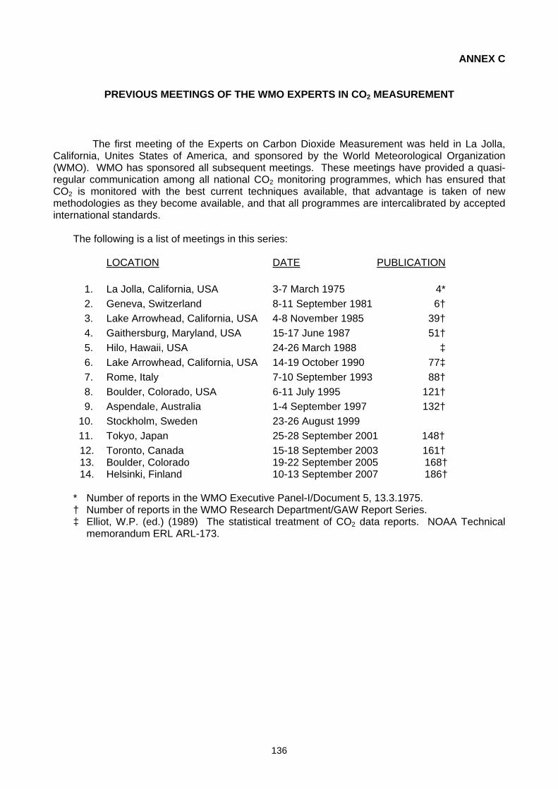
136

ANNEX C

PREVIOUS MEETINGS OF THE WMO EXPERTS IN CO2 MEASUREMENT

The first meeting of the Experts on Carbon Dioxide Measurement was held in La Jolla, California, Unites States of America, and sponsored by the World Meteorological Organization (WMO). WMO has sponsored all subsequent meetings. These meetings have provided a quasi-regular communication among all national CO2 monitoring programmes, which has ensured that CO2 is monitored with the best current techniques available, that advantage is taken of new methodologies as they become available, and that all programmes are intercalibrated by accepted international standards.

The following is a list of meetings in this series:

LOCATION DATE PUBLICATION 1. La Jolla, California, USA 3-7 March 1975 4* 2. Geneva, Switzerland 8-11 September 1981 6† 3. Lake Arrowhead, California, USA 4-8 November 1985 39† 4. Gaithersburg, Maryland, USA 15-17 June 1987 51† 5. Hilo, Hawaii, USA 24-26 March 1988 ‡ 6. Lake Arrowhead, California, USA 14-19 October 1990 77‡ 7. Rome, Italy 7-10 September 1993 88† 8. Boulder, Colorado, USA 6-11 July 1995 121† 9. Aspendale, Australia 1-4 September 1997 132† 10. Stockholm, Sweden 23-26 August 1999 11. Tokyo, Japan 25-28 September 2001 148†

12. Toronto, Canada 15-18 September 2003 161† 13. Boulder, Colorado 19-22 September 2005 168† 14. Helsinki, Finland 10-13 September 2007 186†

* Number of reports in the WMO Executive Panel-I/Document 5, 13.3.1975. † Number of reports in the WMO Research Department/GAW Report Series. ‡ Elliot, W.P. (ed.) (1989) The statistical treatment of CO2 data reports. NOAA Technical

memorandum ERL ARL-173.

137

GLOBAL ATMOSPHERE WATCH REPORT SERIES 1. Final Report of the Expert Meeting on the Operation of Integrated Monitoring Programmes, Geneva, 2 -5 September 1980. 2. Report of the Third Session of the GESAMP Working Group on the Interchange of Pollutants Between the Atmosphere and

the Oceans (INTERPOLL-III), Miami, USA, 27-31 October 1980. 3. Report of the Expert Meeting on the Assessment of the Meteorological Aspects of the First Phase of EMEP, Shinfield Park,

U.K., 30 March - 2 April 1981. 4. Summary Report on the Status of the WMO Background Air Pollution Monitoring Network as at April 1981. 5. Report of the WMO/UNEP/ICSU Meeting on Instruments, Standardization and Measurements Techniques for Atmospheric

CO2, Geneva, 8-11; September 1981. 6. Report of the Meeting of Experts on BAPMoN Station Operation, Geneva, 23–26 November 1981. 7. Fourth Analysis on Reference Precipitation Samples by the Participating World Meteorological Organization Laboratories by

Robert L. Lampe and John C. Puzak, December 1981. 8. Review of the Chemical Composition of Precipitation as Measured by the WMO BAPMoN by Prof. Dr. Hans-Walter Georgii,

February 1982. 9. An Assessment of BAPMoN Data Currently Available on the Concentration of CO2 in the Atmosphere by M.R. Manning,

February 1982. 10. Report of the Meeting of Experts on Meteorological Aspects of Long-range Transport of Pollutants, Toronto, Canada, 30

November - 4 December 1981. 11. Summary Report on the Status of the WMO Background Air Pollution Monitoring Network as at May 1982. 12. Report on the Mount Kenya Baseline Station Feasibility Study edited by Dr. Russell C. Schnell. 13. Report of the Executive Committee Panel of Experts on Environmental Pollution, Fourth Session, Geneva, 27 September - 1

October 1982. 14. Effects of Sulphur Compounds and Other Pollutants on Visibility by Dr. R.F. Pueschel, April 1983. 15. Provisional Daily Atmospheric Carbon Dioxide Concentrations as Measured at BAPMoN Sites for the Year 1981, May 1983. 16. Report of the Expert Meeting on Quality Assurance in BAPMoN, Research Triangle Park, North Carolina, USA, 17-21

January 1983. 17. General Consideration and Examples of Data Evaluation and Quality Assurance Procedures Applicable to BAPMoN

Precipitation Chemistry Observations by Dr. Charles Hakkarinen, July 1983. 18. Summary Report on the Status of the WMO Background Air Pollution Monitoring Network as at May 1983. 19. Forecasting of Air Pollution with Emphasis on Research in the USSR by M.E. Berlyand, August 1983. 20. Extended Abstracts of Papers to be Presented at the WMO Technical Conference on Observation and Measurement of

Atmospheric Contaminants (TECOMAC), Vienna, 17-21 October 1983. 21. Fifth Analysis on Reference Precipitation Samples by the Participating World Meteorological Organization Laboratories by

Robert L. Lampe and William J. Mitchell, November 1983. 22. Report of the Fifth Session of the WMO Executive Council Panel of Experts on Environmental Pollution, Garmisch-

Partenkirchen, Federal Republic of Germany, 30 April - 4 May 1984 (WMO TD No. 10). 23. Provisional Daily Atmospheric Carbon Dioxide Concentrations as Measured at BAPMoN Sites for the Year 1982. November

1984 (WMO TD No. 12).

138

24. Final Report of the Expert Meeting on the Assessment of the Meteorological Aspects of the Second Phase of EMEP, Friedrichshafen, Federal Republic of Germany, 7-10 December 1983. October 1984 (WMO TD No. 11).

25. Summary Report on the Status of the WMO Background Air Pollution Monitoring Network as at May 1984. November 1984

(WMO TD No. 13). 26. Sulphur and Nitrogen in Precipitation: An Attempt to Use BAPMoN and Other Data to Show Regional and Global Distribution

by Dr. C.C. Wallén. April 1986 (WMO TD No. 103). 27. Report on a Study of the Transport of Sahelian Particulate Matter Using Sunphotometer Observations by Dr. Guillaume A.

d'Almeida. July 1985 (WMO TD No. 45). 28. Report of the Meeting of Experts on the Eastern Atlantic and Mediterranean Transport Experiment ("EAMTEX"), Madrid and

Salamanca, Spain, 6-8 November 1984. 29. Recommendations on Sunphotometer Measurements in BAPMoN Based on the Experience of a Dust Transport Study in

Africa by Dr. Guillaume A. d'Almeida. September 1985 (WMO TD No. 67). 30. Report of the Ad-hoc Consultation on Quality Assurance Procedures for Inclusion in the BAPMoN Manual, Geneva, 29-31

May 1985. 31. Implications of Visibility Reduction by Man-Made Aerosols (Annex to No. 14) by R.M. Hoff and L.A. Barrie. October 1985

(WMO TD No. 59). 32. Manual for BAPMoN Station Operators by E. Meszaros and D.M. Whelpdale. October 1985 (WMO TD No. 66). 33. Man and the Composition of the Atmosphere: BAPMoN - An international programme of national needs, responsibility and

benefits by R.F. Pueschel, 1986. 34. Practical Guide for Estimating Atmospheric Pollution Potential by Dr. L.E. Niemeyer. August 1986 (WMO TD No. 134). 35. Provisional Daily Atmospheric CO2 Concentrations as Measured at BAPMoN Sites for the Year 1983. December 1985

(WMO TD No. 77). 36. Global Atmospheric Background Monitoring for Selected Environmental Parameters. BAPMoN Data for 1984. Volume I:

Atmospheric Aerosol Optical Depth. October 1985 (WMO TD No. 96). 37. Air-Sea Interchange of Pollutants by R.A. Duce. September 1986 (WMO TD No. 126). 38. Summary Report on the Status of the WMO Background Air Pollution Monitoring Network as at 31 December 1985.

September 1986 (WMO TD No. 136). 39. Report of the Third WMO Expert Meeting on Atmospheric Carbon Dioxide Measurement Techniques, Lake Arrowhead,

California, USA, 4-8 November 1985. October 1986. 40. Report of the Fourth Session of the CAS Working Group on Atmospheric Chemistry and Air Pollution, Helsinki, Finland, 18-22

November 1985. January 1987. 41. Global Atmospheric Background Monitoring for Selected Environmental Parameters. BAPMoN Data for 1982, Volume II:

Precipitation chemistry, continuous atmospheric carbon dioxide and suspended particulate matter. June 1986 (WMO TD No. 116).

42. Scripps reference gas calibration system for carbon dioxide-in-air standards: revision of 1985 by C.D. Keeling, P.R.

Guenther and D.J. Moss. September 1986 (WMO TD No. 125). 43. Recent progress in sunphotometry (determination of the aerosol optical depth). November 1986. 44. Report of the Sixth Session of the WMO Executive Council Panel of Experts on Environmental Pollution, Geneva, 5-9 May

1986. March 1987. 45. Proceedings of the International Symposium on Integrated Global Monitoring of the State of the Biosphere (Volumes I-IV),

Tashkent, USSR, 14-19 October 1985. December 1986 (WMO TD No. 151).

139

46. Provisional Daily Atmospheric Carbon Dioxide Concentrations as Measured at BAPMoN Sites for the Year 1984. December 1986 (WMO TD No. 158).

47. Procedures and Methods for Integrated Global Background Monitoring of Environmental Pollution by F.Ya. Rovinsky, USSR

and G.B. Wiersma, USA. August 1987 (WMO TD No. 178). 48. Meeting on the Assessment of the Meteorological Aspects of the Third Phase of EMEP IIASA, Laxenburg, Austria, 30 March

- 2 April 1987. February 1988. 49. Proceedings of the WMO Conference on Air Pollution Modelling and its Application (Volumes I-III), Leningrad, USSR, 19-24

May 1986. November 1987 (WMO TD No. 187). 50. Provisional Daily Atmospheric Carbon Dioxide Concentrations as Measured at BAPMoN Sites for the Year 1985. December

1987 (WMO TD No. 198). 51. Report of the NBS/WMO Expert Meeting on Atmospheric CO2 Measurement Techniques, Gaithersburg, USA, 15-17 June

1987. December 1987. 52. Global Atmospheric Background Monitoring for Selected Environmental Parameters. BAPMoN Data for 1985. Volume I:

Atmospheric Aerosol Optical Depth. September 1987. 53. WMO Meeting of Experts on Strategy for the Monitoring of Suspended Particulate Matter in BAPMoN - Reports and papers

presented at the meeting, Xiamen, China, 13-17 October 1986. October 1988. 54. Global Atmospheric Background Monitoring for Selected Environmental Parameters. BAPMoN Data for 1983, Volume II:

Precipitation chemistry, continuous atmospheric carbon dioxide and suspended particulate matter (WMO TD No. 283). 55. Summary Report on the Status of the WMO Background Air Pollution Monitoring Network as at 31 December 1987 (WMO TD

No. 284). 56. Report of the First Session of the Executive Council Panel of Experts/CAS Working Group on Environmental Pollution and

Atmospheric Chemistry, Hilo, Hawaii, 27-31 March 1988. June 1988. 57. Global Atmospheric Background Monitoring for Selected Environmental Parameters. BAPMoN Data for 1986, Volume I:

Atmospheric Aerosol Optical Depth. July 1988. 58. Provisional Daily Atmospheric Carbon Dioxide Concentrations as measured at BAPMoN sites for the years 1986 and 1987

(WMO TD No. 306). 59. Extended Abstracts of Papers Presented at the Third International Conference on Analysis and Evaluation of Atmospheric

CO2 Data - Present and Past, Hinterzarten, Federal Republic of Germany, 16-20 October 1989 (WMO TD No. 340). 60. Global Atmospheric Background Monitoring for Selected Environmental Parameters. BAPMoN Data for 1984 and 1985,

Volume II: Precipitation chemistry, continuous atmospheric carbon dioxide and suspended particulate matter. 61. Global Atmospheric Background Monitoring for Selected Environmental Parameters. BAPMoN Data for 1987 and 1988,

Volume I: Atmospheric Aerosol Optical Depth. 62. Provisional Daily Atmospheric Carbon Dioxide Concentrations as measured at BAPMoN sites for the year 1988 (WMO TD

No. 355). 63. Report of the Informal Session of the Executive Council Panel of Experts/CAS Working Group on Environmental Pollution

and Atmospheric Chemistry, Sofia, Bulgaria, 26 and 28 October 1989. 64. Report of the consultation to consider desirable locations and observational practices for BAPMoN stations of global

importance, Bermuda Research Station, 27-30 November 1989. 65. Report of the Meeting on the Assessment of the Meteorological Aspects of the Fourth Phase of EMEP, Sofia, Bulgaria, 27

and 31 October 1989. 66. Summary Report on the Status of the WMO Global Atmosphere Watch Stations as at 31 December 1990 (WMO TD No.

419).

140

67. Report of the Meeting of Experts on Modelling of Continental, Hemispheric and Global Range Transport, Transformation and Exchange Processes, Geneva, 5-7 November 1990.

68. Global Atmospheric Background Monitoring for Selected Environmental Parameters. BAPMoN Data For 1989, Volume I:

Atmospheric Aerosol Optical Depth. 69. Provisional Daily Atmospheric Carbon Dioxide Concentrations as measured at Global Atmosphere Watch (GAW)-BAPMoN

sites for the year 1989 (WMO TD No. 400). 70. Report of the Second Session of EC Panel of Experts/CAS Working Group on Environmental Pollution and Atmospheric

Chemistry, Santiago, Chile, 9-15 January 1991 (WMO TD No. 633). 71. Report of the Consultation of Experts to Consider Desirable Observational Practices and Distribution of GAW Regional

Stations, Halkidiki, Greece, 9-13 April 1991 (WMO TD No. 433). 72. Integrated Background Monitoring of Environmental Pollution in Mid-Latitude Eurasia by Yu.A. Izrael and F.Ya. Rovinsky,

USSR (WMO TD No. 434). 73. Report of the Experts Meeting on Global Aerosol Data System (GADS), Hampton, Virginia, 11 to 12 September 1990 (WMO

TD No. 438). 74. Report of the Experts Meeting on Aerosol Physics and Chemistry, Hampton, Virginia, 30 to 31 May 1991 (WMO TD No. 439). 75. Provisional Daily Atmospheric Carbon Dioxide Concentrations as measured at Global Atmosphere Watch (GAW)-BAPMoN

sites for the year 1990 (WMO TD No. 447). 76. The International Global Aerosol Programme (IGAP) Plan: Overview (WMO TD No. 445). 77. Report of the WMO Meeting of Experts on Carbon Dioxide Concentration and Isotopic Measurement Techniques, Lake

Arrowhead, California, 14-19 October 1990. 78. Global Atmospheric Background Monitoring for Selected Environmental Parameters BAPMoN Data for 1990, Volume I:

Atmospheric Aerosol Optical Depth (WMO TD No. 446). 79. Report of the Meeting of Experts to Consider the Aerosol Component of GAW, Boulder, 16 to 19 December 1991 (WMO TD

No. 485). 80. Report of the WMO Meeting of Experts on the Quality Assurance Plan for the GAW, Garmisch-Partenkirchen, Germany, 26-

30 March 1992 (WMO TD No. 513). 81. Report of the Second Meeting of Experts to Assess the Response to and Atmospheric Effects of the Kuwait Oil Fires,

Geneva, Switzerland, 25-29 May 1992 (WMO TD No. 512). 82. Global Atmospheric Background Monitoring for Selected Environmental Parameters BAPMoN Data for 1991, Volume I:

Atmospheric Aerosol Optical Depth (WMO TD No. 518). 83. Report on the Global Precipitation Chemistry Programme of BAPMoN (WMO TD No. 526). 84. Provisional Daily Atmospheric Carbon Dioxide Concentrations as measured at GAW-BAPMoN sites for the year 1991 (WMO

TD No. 543). 85. Chemical Analysis of Precipitation for GAW: Laboratory Analytical Methods and Sample Collection Standards by Dr Jaroslav

Santroch (WMO TD No. 550). 86. The Global Atmosphere Watch Guide, 1993 (WMO TD No. 553). 87. Report of the Third Session of EC Panel/CAS Working Group on Environmental Pollution and Atmospheric Chemistry,

Geneva, 8-11 March 1993 (WMO TD No. 555). 88. Report of the Seventh WMO Meeting of Experts on Carbon Dioxide Concentration and Isotopic Measurement Techniques,

Rome, Italy, 7-10 September 1993, (edited by Graeme I. Pearman and James T. Peterson) (WMO TD No. 669). 89. 4th International Conference on CO2 (Carqueiranne, France, 13-17 September 1993) (WMO TD No. 561).

141

90. Global Atmospheric Background Monitoring for Selected Environmental Parameters GAW Data for 1992, Volume I: Atmospheric Aerosol Optical Depth (WMO TD No. 562).

91. Extended Abstracts of Papers Presented at the WMO Region VI Conference on the Measurement and Modelling of

Atmospheric Composition Changes Including Pollution Transport, Sofia, 4 to 8 October 1993 (WMO TD No. 563). 92. Report of the Second WMO Meeting of Experts on the Quality Assurance/Science Activity Centres of the Global Atmosphere

Watch, Garmisch-Partenkirchen, 7-11 December 1992 (WMO TD No. 580). 93. Report of the Third WMO Meeting of Experts on the Quality Assurance/Science Activity Centres of the Global Atmosphere

Watch, Garmisch-Partenkirchen, 5-9 July 1993 (WMO TD No. 581). 94. Report on the Measurements of Atmospheric Turbidity in BAPMoN (WMO TD No. 603). 95. Report of the WMO Meeting of Experts on UV-B Measurements, Data Quality and Standardization of UV Indices, Les

Diablerets, Switzerland, 25-28 July 1994 (WMO TD No. 625). 96. Global Atmospheric Background Monitoring for Selected Environmental Parameters WMO GAW Data for 1993, Volume I:

Atmospheric Aerosol Optical Depth. 97. Quality Assurance Project Plan (QAPjP) for Continuous Ground Based Ozone Measurements (WMO TD No. 634). 98. Report of the WMO Meeting of Experts on Global Carbon Monoxide Measurements, Boulder, USA, 7-11 February 1994

(WMO TD No. 645). 99. Status of the WMO Global Atmosphere Watch Programme as at 31 December 1993 (WMO TD No. 636). 100. Report of the Workshop on UV-B for the Americas, Buenos Aires, Argentina, 22-26 August 1994. 101. Report of the WMO Workshop on the Measurement of Atmospheric Optical Depth and Turbidity, Silver Spring, USA, 6-10

December 1993, (edited by Bruce Hicks) (WMO TD No. 659). 102. Report of the Workshop on Precipitation Chemistry Laboratory Techniques, Hradec Kralove, Czech Republic, 17-21 October

1994 (WMO TD No. 658). 103. Report of the Meeting of Experts on the WMO World Data Centres, Toronto, Canada, 17 - 18 February 1995, (prepared by

Edward Hare) (WMO TD No. 679). 104. Report of the Fourth WMO Meeting of Experts on the Quality Assurance/Science Activity Centres (QA/SACs) of the Global

Atmosphere Watch, jointly held with the First Meeting of the Coordinating Committees of IGAC-GLONET and IGAC-ACE, Garmisch-Partenkirchen, Germany, 13 to 17 March 1995 (WMO TD No. 689).

105. Report of the Fourth Session of the EC Panel of Experts/CAS Working Group on Environmental Pollution and Atmospheric

Chemistry (Garmisch, Germany, 6-11 March 1995) (WMO TD No. 718). 106. Report of the Global Acid Deposition Assessment (edited by D.M. Whelpdale and M-S. Kaiser) (WMO TD No. 777). 107. Extended Abstracts of Papers Presented at the WMO-IGAC Conference on the Measurement and Assessment of

Atmospheric Composition Change (Beijing, China, 9-14 October 1995) (WMO TD No. 710). 108. Report of the Tenth WMO International Comparison of Dobson Spectrophotometers (Arosa, Switzerland, 24 July - 4 August

1995). 109. Report of an Expert Consultation on 85Kr and 222Rn: Measurements, Effects and Applications (Freiburg, Germany, 28-31

March 1995) (WMO TD No. 733). 110. Report of the WMO-NOAA Expert Meeting on GAW Data Acquisition and Archiving (Asheville, NC, USA, 4-8 November

1995) (WMO TD No. 755). 111. Report of the WMO-BMBF Workshop on VOC Establishment of a “World Calibration/Instrument Intercomparison Facility for

VOC” to Serve the WMO Global Atmosphere Watch (GAW) Programme (Garmisch-Partenkirchen, Germany, 17-21 December 1995) (WMO TD No. 756).

142

112. Report of the WMO/STUK Intercomparison of Erythemally-Weighted Solar UV Radiometers, Spring/Summer 1995, Helsinki, Finland (WMO TD No. 781).

112A. Report of the WMO/STUK ’95 Intercomparison of broadband UV radiometers: a small-scale follow-up study in 1999, Helsinki,

2001, Addendum to GAW Report No. 112. 113. The Strategic Plan of the Global Atmosphere Watch (GAW) (WMO TD No. 802). 114. Report of the Fifth WMO Meeting of Experts on the Quality Assurance/Science Activity Centres (QA/SACs) of the Global

Atmosphere Watch, jointly held with the Second Meeting of the Coordinating Committees of IGAC-GLONET and IGAC-ACEEd, Garmisch-Partenkirchen, Germany, 15-19 July 1996 (WMO TD No. 787).

115. Report of the Meeting of Experts on Atmospheric Urban Pollution and the Role of NMSs (Geneva, 7-11 October 1996) (WMO

TD No. 801). 116. Expert Meeting on Chemistry of Aerosols, Clouds and Atmospheric Precipitation in the Former USSR (Saint Petersburg,

Russian Federation, 13-15 November 1995). 117. Report and Proceedings of the Workshop on the Assessment of EMEP Activities Concerning Heavy Metals and Persistent

Organic Pollutants and their Further Development (Moscow, Russian Federation, 24-26 September 1996) (Volumes I and II) (WMO TD No. 806).

118. Report of the International Workshops on Ozone Observation in Asia and the Pacific Region (IWOAP, IWOAP-II), (IWOAP,

27 February-26 March 1996 and IWOAP-II, 20 August-18 September 1996) (WMO TD No. 827). 119. Report on BoM/NOAA/WMO International Comparison of the Dobson Spectrophotometers (Perth Airport, Perth, Australia, 3-

14 February 1997), (prepared by Robert Evans and James Easson) (WMO TD No. 828). 120. WMO-UMAP Workshop on Broad-Band UV Radiometers (Garmisch-Partenkirchen, Germany, 22 to 23 April 1996) (WMO TD

No. 894). 121. Report of the Eighth WMO Meeting of Experts on Carbon Dioxide Concentration and Isotopic Measurement Techniques

(prepared by Thomas Conway) (Boulder, CO, 6-11 July 1995) (WMO TD No. 821). 122. Report of Passive Samplers for Atmospheric Chemistry Measurements and their Role in GAW (prepared by Greg

Carmichael) (WMO TD No. 829). 123. Report of WMO Meeting of Experts on GAW Regional Network in RA VI, Budapest, Hungary, 5 to 9 May 1997. 124. Fifth Session of the EC Panel of Experts/CAS Working Group on Environmental Pollution and Atmospheric Chemistry,

(Geneva, Switzerland, 7-10 April 1997) (WMO TD No. 898) 125. Instruments to Measure Solar Ultraviolet Radiation, Part 1: Spectral Instruments (lead author G. Seckmeyer) (WMO TD No.

1066) 126. Guidelines for Site Quality Control of UV Monitoring (lead author A.R. Webb) (WMO TD No. 884). 127. Report of the WMO-WHO Meeting of Experts on Standardization of UV Indices and their Dissemination to the Public (Les

Diablerets, Switzerland, 21-25 July 1997) (WMO TD No. 921). 128. The Fourth Biennial WMO Consultation on Brewer Ozone and UV Spectrophotometer Operation, Calibration and Data

Reporting, (Rome, Italy, 22-25 September 1996) (WMO TD No. 918). 129. Guidelines for Atmospheric Trace Gas Data Management (Ken Masarie and Pieter Tans), 1998 (WMO TD No. 907). 130. Jülich Ozone Sonde Intercomparison Experiment (JOSIE, 5 February to 8 March 1996), (H.G.J. Smit and D. Kley) (WMO TD

No. 926). 131. WMO Workshop on Regional Transboundary Smoke and Haze in Southeast Asia (Singapore, 2 to 5 June 1998) (Gregory R.

Carmichael). Two volumes. 132. Report of the Ninth WMO Meeting of Experts on Carbon Dioxide Concentration and Related Tracer Measurement Techniques

(Edited by Roger Francey), (Aspendale, Vic., Australia).

143

133. Workshop on Advanced Statistical Methods and their Application to Air Quality Data Sets (Helsinki, 14-18 September 1998) (WMO TD No. 956).

134. Guide on Sampling and Analysis Techniques for Chemical Constituents and Physical Properties in Air and Precipitation as

Applied at Stations of the Global Atmosphere Watch. Carbon Dioxide (WMO TD No. 980). 135. Sixth Session of the EC Panel of Experts/CAS Working Group on Environmental Pollution and Atmospheric Chemistry

(Zurich, Switzerland, 8-11 March 1999) (WMO TD No.1002). 136. WMO/EMEP/UNEP Workshop on Modelling of Atmospheric Transport and Deposition of Persistent Organic Pollutants and

Heavy Metals (Geneva, Switzerland, 16-19 November 1999) (Volumes I and II) (WMO TD No. 1008). 137. Report and Proceedings of the WMO RA II/RA V GAW Workshop on Urban Environment (Beijing, China, 1-4 November 1999)

(WMO-TD. 1014) (Prepared by Greg Carmichael). 138. Reports on WMO International Comparisons of Dobson Spectrophotometers, Parts I – Arosa, Switzerland, 19-31 July 1999,

Part II – Buenos Aires, Argentina (29 Nov. – 12 Dec. 1999 and Part III – Pretoria, South Africa (18 March – 10 April 2000) (WMO TD No. 1016).

139. The Fifth Biennial WMO Consultation on Brewer Ozone and UV Spectrophotometer Operation, Calibration and Data

Reporting (Halkidiki, Greece, September 1998)(WMO TD No. 1019). 140. WMO/CEOS Report on a Strategy for Integrating Satellite and Ground-based Observations of Ozone (WMO TD No. 1046). 141. Report of the LAP/COST/WMO Intercomparison of Erythemal Radiometers Thessaloniki, Greece, 13-23 September 1999)

(WMO TD No. 1051). 142. Strategy for the Implementation of the Global Atmosphere Watch Programme (2001-2007), A Contribution to the

Implementation of the Long-Term Plan (WMO TD No.1077). 143. Global Atmosphere Watch Measurements Guide (WMO TD No. 1073). 144. Report of the Seventh Session of the EC Panel of Experts/CAS Working Group on Environmental Pollution and Atmospheric

Chemistry and the GAW 2001 Workshop (Geneva, Switzerland, 2 to 5 April 2001) (WMO TD No. 1104). 145. WMO GAW International Comparisons of Dobson Spectrophotometers at the Meteorological Observatory Hohenpeissenberg,

Germany (21 May – 10 June 2000, MOHp2000-1), 23 July – 5 August 2000, MOHp2000-2), (10 – 23 June 2001, MOHp2001-1) and (8 to 21 July 2001, MOHp2001-2). Prepared by Ulf Köhler (WMO TD No. 1114).

146. Quality Assurance in monitoring solar ultraviolet radiation: the state of the art. (WMO TD No. 1180). 147. Workshop on GAW in RA VI (Europe), Riga, Latvia, 27-30 May 2002. (WMO TD No. 1206). 148. Report of the Eleventh WMO/IAEA Meeting of Experts on Carbon Dioxide Concentration and Related Tracer Measurement

Techniques (Tokyo, Japan, 25-28 September 2001) (WMO TD No 1138). 149. Comparison of Total Ozone Measurements of Dobson and Brewer Spectrophotometers and Recommended Transfer

Functions (prepared by J. Staehelin, J. Kerr, R. Evans and K. Vanicek) (WMO TD No. 1147). 150. Updated Guidelines for Atmospheric Trace Gas Data Management (Prepared by Ken Maserie and Pieter Tans (WMO TD No.

1149). 151. Report of the First CAS Working Group on Environmental Pollution and Atmospheric Chemistry (Geneva, Switzerland, 18-19

March 2003) (WMO TD No. 1181). 152. Current Activities of the Global Atmosphere Watch Programme (as presented at the 14th World Meteorological Congress, May

2003). (WMO TD No. 1168). 153. WMO/GAW Aerosol Measurement Procedures: Guidelines and Recommendations. (WMO TD No. 1178). 154. WMO/IMEP-15 Trace Elements in Water Laboratory Intercomparison. (WMO TD No. 1195).

144

155. 1st International Expert Meeting on Sources and Measurements of Natural Radionuclides Applied to Climate and Air Quality Studies (Gif sur Yvette, France, 3-5 June 2003) (WMO TD No. 1201).

156. Addendum for the Period 2005-2007 to the Strategy for the Implementation of the Global Atmosphere Watch Programme

(2001-2007), GAW Report No. 142 (WMO TD No. 1209). 157. JOSIE-1998 Performance of EEC Ozone Sondes of SPC-6A and ENSCI-Z Type (Prepared by Herman G.J. Smit and

Wolfgang Straeter) (WMO TD No. 1218). 158. JOSIE-2000 Jülich Ozone Sonde Intercomparison Experiment 2000. The 2000 WMO international intercomparison of

operating procedures for ECC-ozone sondes at the environmental simulation facility at Jülich (Prepared by Herman G.J. Smit and Wolfgang Straeter) (WMO TD No. 1225).

159. IGOS-IGACO Report - September 2004 (WMO TD No. 1235) 160. Manual for the GAW Precipitation Chemistry Programme (Guidelines, Data Quality Objectives and Standard Operating

Procedures) (WMO TD No. 1251). 161 12th WMO/IAEA Meeting of Experts on Carbon Dioxide Concentration and Related Tracers Measurement Techniques

(Toronto, Canada, 15-18 September 2003). 162. WMO/GAW Experts Workshop on a Global Surface-Based Network for Long Term Observations of Column Aerosol Optical

Properties, Davos, Switzerland, 8-10 March 2004 (edited by U. Baltensperger, L. Barrie and C. Wehrli) (WMO TD No. 1287). 163. World Meteorological Organization Activities in Support of the Vienna Convention on Protection of the Ozone Layer (WMO

No. 974). 164. Instruments to Measure Solar Ultraviolet Radiation: Part 2: Broadband Instruments Measuring Erythemally Weighted Solar

Irradiance (WMO TD No. 1289). 165. Report of the CAS Working Group on Environmental Pollution and Atmospheric Chemistry and the GAW 2005 Workshop, 14-

18 March 2005, Geneva, Switzerland (WMO TD No. 1302). 166. Joint WMO-GAW/ACCENT Workshop on The Global Tropospheric Carbon Monoxide Observations System, Quality

Assurance and Applications (EMPA, Dübendorf, Switzerland, 24 – 26 October 2005) (edited by J. Klausen) (WMO TD No. 1335).

167. The German Contribution to the WMO Global Atmosphere Watch Programme upon the 225th Anniversary of GAW

Hohenpeissenberg Observatory (edited by L.A. Barrie, W. Fricke and R. Schleyer (WMO TD No. 1336). 168. 13th WMO/IAEA Meeting of Experts on Carbon Dioxide Concentration and Related Tracers Measurement Techniques

(Boulder, Colorado, USA, 19-22 September 2005) (edited by J.B. Miller) (WMO TD No. 1359). 169. Chemical Data Assimilation for the Observation of the Earth’s Atmosphere – ACCENT/WMO Expert Workshop in support of

IGACO (edited by L.A. Barrie, J.P. Burrows, P. Monks and P. Borrell) (WMO TD No. 1360). 170. WMO/GAW Expert Workshop on the Quality and Applications of European GAW Measurements (Tutzing, Germany, 2-5

November 2004) (WMO TD No. 1367). 171. A WMO/GAW Expert Workshop on Global Long-Term Measurements of Volatile Organic Compounds (VOCs) (Geneva,

Switzerland, 30 January – 1 February 2006) (WMO TD No. 1373). 172. WMO Global Atmosphere Watch (GAW) Strategic Plan: 2008 – 2015 (WMO TD No. 1384) 173. Report of the CAS Joint Scientific Steering Committee on Environmental Pollution and Atmospheric Chemistry (Geneva,

Switzerland, 11-12 April 2007) (WMO TD No.1410). 174. World Data Centre for Greenhouse Gases Data Submission and Dissemination Guide (WMO TD No. 1416). 175. The Ninth Biennial WMO Consultation on Brewer Ozone and UV Spectrophotometer Operation, Calibration and Data

Reporting (Delft, Netherlands, 31-May – 3 June 2005) (WMO TD No. 1419).

145

176. The Tenth Biennial WMO Consultation on Brewer Ozone and UV Spectrophotometer Operation, Calibration and Data Reporting (Northwich, United Kingdom, 4-8 June 2007) (WMO TD No. 1420).

177. Joint Report of COST Action 728 and GURME – Overview of Existing Integrated (off-line and on-line) Mesoscale

Meteorological and Chemical Transport Modelling in Europe (ISBN 978-1-905313-56-3) (WMO TD No. 1427). 178. Plan for the implementation of the GAW Aerosol Lidar Observation Network GALION, (Hamburg, Germany, 27 - 29 March

2007) (WMO TD No. 1443). 179. Intercomparison of Global UV Index from Multiband Radiometers: Harmonization of Global UVI and Spectral Irradiance

(WMO TD No. 1454). 180. Towards a Better Knowledge of Umkehr Measurements: A Detailed Study of Data from Thirteen Dobson Intercomparisons

(WMO TD No. 1456). 181. Joint Report of COST Action 728 and GURME – Overview of Tools and Methods for Meteorological and Air Pollution

Mesoscale Model Evaluation and User Training (WMO TD No. 1457). 182. IGACO-Ozone and UV Radiation Implementation Plan (WMO TD No. 1465). 183. Operations Handbook – Ozone Observations with a Dobson Spectrophotometer (WMO TD No. 1469). 184. Technical Report of Global Analysis Method for Major Greenhouse Gases by the World Data Centre for Greenhouse Gases

(WMO TD No. 1473). 185. Guidelines for the Measurement of Methane and Nitrous Oxide and their Quality Assurance (WMO TD No. 1478).