Meteorological Drought - CiteSeerX

U.S.

* LIBRARY

N .Q. A. A , U.S. Dept. c: Commerce

DEPARTMENT OF COMMERCE JOHN T. CONNOR, Secretcrry

WEATHER BUREAU ROBERT M. WHITE, Chief

RESEARCH PAPER NO. 45

Meteorological Drought

WAYNE C. PALMER Offica of Climatology

U.S. Weather Bureau, Washington, D.C.

WASHINGTON, D.C. FEBRUARY 1965

National Oceanic and Atmospheric Administration

Weather Bureau Research Papers

ERRATA NOTICE

One or more conditions of the original document may affect the quality of the image, such as:

Discolored pages Faded or light ink Binding intrudes into the text

This has been co-operative project between the NOAA Central Library and the Climate Database Modernization Program, National Climate Data Center (NCDC). To view the original document contact the NOAA Central Library in Silver Spring, MD at (301) 713-2607 x 124 or Librarv.Reference @ noaa.gov.

HOV Services Imaging Contractor 12200 Kiln Court Beltsville, MD 20704- 1387 January 22,2008

FOREWORD

Drought has been cited as a scourge of mankind since biblical times. It still is a major menace to world food supplies. Insect plagues, With which it ranks as a crop threat, can be fought by modern means.

It has not even described the phenomenon adequately. This is certainly the first step toward understanding. And then a long road remains ahead toward prediction and, perhaps, limited control. This paper is an important step toward these goals. It presents a numerical approach to the problem and thus permits an objective evaluation of the climatological events.

Although often so classified, drought is not just an agricultural problem. It affects the city dweller, whose water may berationed, and the industrial consumers of water as well. In fact, water is one of the most vital natural resources. Its lack, regionally or temporally, has the most profound effect on economy. In a country as large as the United States drought is likely to affect ody a part of its territory at any one time. However, no section is entirely spared of droughts and occasionally substantial areas are affected. By severity and duration these events can be calamitous not O ~ Y locally but for the whole economic structure. Hence knowledge of the probability of their occurrence and their cowse is an essential element for planning. The thorny problem of a rational land utilization is closely tied in with these considerations.

The pioneering work of the late C . W. Thornthwaite on potential evapotranspiration has underlain all modern attempts to assess the water balance. AS in his work, the aim of the effort reported on in this paper remains primarily on the climatological aspects. The new method presented here is directed at a quantitative assessment of periods of prolonged meterological anomalies. We hope it is a step forward and that it can be followed by similar analyses on a broader geographical basis.

Drought remains an unconquered ill. Meteorologicd science has not yet come to grips with drought.

H. E. LANDSBERG.

ii

CONTENTS Pago

i1 V 1 1 2 2 3 4 4 6 9 9 9

11 13 13 13 14 15 17 18 20 20 20 20 21 23 23 23 24 24 26 26 26 28 28 28 29 30 30 34 34 34 34 34 37 37 37 37 38 39 $3 40 40 41 42 42

iii

13.

14. 15.

LIST OF FIGURES

LIST OF TABLES

Pas0 43 43 44 44 45 47 47 49 50 50 51 51 51 52 52 52 53 53 54 54 54 54 54

55 56 56

20

21

24

40 46 46 56

10 12 12 15 16 17 20 22 25 27 28

31 35 37

39 41 43 44

iv

a a3

B Y 6 A

a AWC

CAFEC d 2 D

C7

C

ET z i j k Kt K K L z E L, L U

P P I*. P,

LIST OF SYMBOLS Page*

11 51 13 13 13 22 51 51 7

22 12 15 18 25 7

11 14 14 29 18 25 18 18 7

13 14

7 7 7

11 14 29

7 11

'Page on whlch sgmbol is introduced.

V

PL PL PL, PL, PR PR PRO PRO Q R B R RO BO

S S‘ S, S: s u

s; t T

Ut0 V X XI

-

kb

ud

X2

X3

2

z 2,

10 13 10 10 9

13 11 13

29 11 13 14 9

13 14 9

10 9 7 9 7

21 10 30 29 29 21 22

32

32

32 18 23 29

‘Page an which symbol is introduoed,

vi

METEOROLOGICAL DROUGHT WAYNE C. PALMER

Office of Climatology, U.S. Weather Bureau, Washington, D.C.

Manuscript received July 23,1962; revised June 16,19641

ABSTRACT

Drought can be considered as a strictly meteorological phenomenon. It can be evaluated as a meteorological anomaly characterized by a prolonged and abnormal moisture deficiency. Not only does this approach avoid many of the complicating biological factors and arbitrary definitions, i t enables one to derive a climatic analysis system in which drought severity is dependent on the duration and magnitude of the abnormal moisture deficiency. Within reasonable limits, time and space comparisons of drought severity are possible. The objective of this paper is to develop a general methodology for evaluating the meteorological anomaly in t e r m of an index which permits time and space comparisons of drought severity.

The underlying concept of the paper is that the amount of precipitation required for the near-normal operation of the established economy of an area during some stated period is dependent on the’average climate of the area and on the prevailing meteorological conditions both during and preceding the month or period in question. A method for computing this required precipitation is demonstrated. The difference between the actual precipitation and the computed precipitation represents a fairly direct measure of the departure of the moisture aspect of the weather from normal. When these departures are properly weighted, the resulting index numbers appear to be of reasonably comparable local significance both in space and time.

Successive monthly index values for past dry periods were combined by a relatively objective procedure to yield an equation for calculating drought severity in four classes- mild, moderate, severe, and extreme. The method of analysis is described and the results of applying the procedure to 76 years of western Kansas weather, 33 years of central Iowa weather, and 32 years of independent data from northwestern North Dakota are presented.

The procedure is tractable for machine data processing by weekly or monthly periods for either points or areas. When this type of climatic analysis has been carried out for a large number of contiguous areas, not only will one obtain drought severity expectancy figures but also other useful items as well. For instance, the analysis will provide wet period expectancies, maps useful in land use capability studies, and material of interest in water resources planning. In addition, some of the derived parameters will very likely prove to be useful in crop yield investigations.

1. INTRODUCTION

Drought means various things to various people, depending on their specific interest. To the farmer drought means a shortage of moisture in the root zone of his crops. To the hydrologist it suggests below average water levels in streams, lakes, reservoirs, and the like. To the economist it means a water shortage which adversely affects the established economy. Each has a concern

which depends on the eyects of a fairly prolonged weather anomaly.

A completely adequate definition of drought is difficult to find. Not only is there disagreement as to the meaning of the word, even its spelling and pronunciation provide room for discussion. It is variously spelled as “drought” and “drouth.” Recommended pronunciation for the’ first spelling

1

is g ( d r o u t , ’ (as in trout) and the second form be- ‘‘drouth’’ (&s in south) [31. These inter-

=ting sidelights are indicative of the Confusion that prevails.

DEFTNITIONS

From previous drought studies one can assemble a number of definitions, such as:

1. A period with precipitation less than some small amount such

2. A period of more than some particular number of days with precipitation less than some specified small amount [161.

3. A period of strong wind, low precipitation, $gh temperature, and unusually low relative humidity (this has been referred to as “atmospheric drought”) 171.

4. A day on which the available soil moisture was depleted to some small percentage of available capacity [68]. 5. A period of time when one or all of the fol-

lowing conditions prevailed: (a) Pasturage becoming scarce, (b) Stock losing condition from fair order, (c) Hand feeding in vogue, (d) Agist- ment of stock [721.

6. Monthly or annual precipitation less than Some particular percentage of normal [30].

7. A condition that may be said to prevail WhtmVer precipitation is insuflicient to meet the needs of established human activities [20].

The list could be extended, but nearly all have in common a certain arbitrariness difficult, in some cases, to defend. A surprising number ignore the protracted dry spell concept given in most dic- tionaries and emphasized by Linsley et al. [28], and only a few, such as the Qlossary of Meteorology [22] and Blair [5] recognize that drought is a relative term.

It appears that the press and the general public Use the term in a more consistent way than do meteorologists, climatologists, hydrologists, and the other scientists who have done work on the subject. It is worthy of note that the term does not ordinarily appear in the public press until an area has endured an unusual moisture deficiency for an extended period of time. Those journalists who use such expressions as “drought of invest- ment capital” and “man-power drought” must msume their share of responsibility for using “drought” as a synonym for “shortage.”

However, most farmers do not call a “dry spell” a drought until matters begin to become rather

2

0.10 in. in 48 hr. [SI.

serious. In spite of the differences which exist, the people in humid climates seem to mean much the same thing when they refer to drought as do the people in a semiarid region; viz, that the moisture shortage has seriously affected the established economy of their region. From consideration of the many facets of the problem, it is possible to formulate a generalized definition that can be used as a starting point. Drought is therefore defined here as a prolonged and abnormal moisture deficiency. This is essentially the definition given by the American Meteorological Society [22]. At the outset this definition may appear to be too generalized for any useful purpose, but examination will show that it established the guidelines necessary for further work. Foley [14] presented an excellent discussion based on a somewhat similar generalized approach.

This may be regarded as a generalized meteorological definition rather than a specific biologic or hydrologic one. In fact, many of the specialized aspects and ramifications of drought can be accommodated by the definition, This generalized definition has been chosen deliberately in order that the phenomenon may be studied in as objective a manner as possible without first having arbitrarily defined “prolonged”, or “abnormal” or “moisture deficiency.”

POINTS OF VIEW

Agricultural drought is probably the most important aspect of drought, but that problem is far more specialized and complicated than some investigators seem to realize. A study of agricultural drought immediately leads one into the realms of soil physics, plant physiology, and agricultural economics. Of all the available possibilities one must choose a particular one, thereby limiting the useful results to particular crops grown under specified conditions of soil and cultural practices.

Hydrologic drought, concerned as it is with reductions in stream flow and in lake and reservoir levels, depletion of soil moisture, a lowering of the ground-water table, and the consequent decrease in ground-water runoff [XI, also poses specialized problems. This is far from being a purely meteorological problem. It is, in fact, more of an engineering problem which involves not only meteorology and hydrology, but geology and other geophysical sciences. as well.

As a matter of fact, both agriculture and hydrology are more concerned with the effects of the moisture shortage than with the purely meteorological aspects. The onset of the effects can be immediate or delayed; likewise, recovery from a recent moisture shortage can be almost immediate or delayed, depending on the particular circumstances of the area and activity affected. For these and other reasons crop yields, pasture conditions, stream flow, lake levels, and the like are not particularly satisfactory measures of the severity of meteorological drought. Probably the severity is most closely related to some local- ized economic measure of the disruption of the established economy. If such a measure exists, it has not come to the author’s attention. In this connection it should be mentioned that man-made drought, a demand, created by economic development, for more water than is normally available in an area, was not considered in this study. How- ever, the procedures developed here will shed Some light on the problems of such over-developed regions.

SPECULATIONS CONCERNING THE DEFINITION

During recent years the US. Government has recognized and provided economic aid to areas which have endured “disaster.” Among the various things that can create a disaster is drought. This is not generally considered to be a moisture deficiency that causes mere inconvenience or even one that creates mild hardship, but rather a shortage of water so unusual that it creates de- struction or ruin, &s of life or property [31]. It is almost impossible for this degree of drought disaster to develop over a short period of time; a t least two or three months of extremely unusual weather are required and ordinarily tho time is much greater, say a year or more [MI.

This relatively substantial fact concerning disastrous drought provides a general framework for speculation concerning the period of time involved in a definition of “prolonged”; it is apparently of the order of months. However, it

seems reasonable to postulate that a mild drought could develop in a single month.

It may at first seem that “moisture deficiency” should be easier to define than “prolonged,” and in some respects it is. However, more is involved than a mere rainfall record. An area may wel- come a period of dry weather if the period immediately preceding was unusually wet. The dry weather provides an opportunity for getting rid of an oversupply of water and allows the area to operate on a more normal basis-a basis which is ordinarily adjusted to the climatic averages, having been arrived at by many years of kial and error. Antecedent conditions must therefore be taken into account when evaluating the ado- quacy of rainfall. One indirect method for accomplishing this is through measurements or estimates of the amount of available soil moisture at the beginning of the period of little or no precipitation. Soil moisture may therefore be regarded as an index of antecedent weather conditions. Deficiency, of course, implies a demand which exceeds supply; however, the “abnormal” aspect must also be considered.

A thing is abnormal that deviates markedly from what has been established as some memure of the middle point between extremes. It is therefore reasonable to state that a period during which moisture need exceeds moisture supply by an unusual amount could be considered as a period of abnormal moisture deficiency. By this postulate of abnormality various climates can be placed on a relatively equal bmis insofar as drought is concerned.

The foregoing discussion may seem to be largely a matter of semantics; however, it has served to develop a basis for a somewhat meaningful approach to the drought problem. A drought period may now be defined as an interval of time, generally of the order of months or years in duration, during which the actual moisture supply a t a given place rather consistently falls short of the climatically expected or climatically appropriate moisture supply. Further, the severity of drought may be considered as being a function of both the duration and magnitude of the moisture deficiency.

757-251-65-2 3

2. THE PROBLEM AND OBJECTIVES T G ~ paper does not deal with the fundamental

causes of &ought. Superficially one can say that drought are associated with periods of anomalous atmospheric circulation patterns, but the basic question concerning the physical reasons for the circulation anomalies remains. As Namias has pointed out [33] there are those who consider the circulation changes as self-evolving, while another school of thought holds that the anomalous states of’the general circulation are due to extraterrestrial causes. Such controversies point out the necessity for fundamental research. Until such questions are answered and real understanding achieved, explanations of the cause of drought as well as attempts at drought prediction will be premature and inadequate.

Stated in the simplest terms the problem here is to develop a method for computing the amount of precipitation that should have occurred in a given area during a given period of time in order for the “weather” during the period to have been normal-normal in the sense that the moisture supply during the period satisfied the average or climatically expected percentage of the absolute moisture requirements during the period. I n other words, the question is how much precipitation should have occurred during a given period to have kept the water resources of the area com- mensurate with their established use? After determining how much precipitation should have occurred, one can readily compare it with the amount that actually did occur and thereby have a measure of the departure of the moisture supply from the “normal” or climatically appropriate

Unfortunately, the derivation of moisture ex- supply.

cesses and deficiencies Over a number of periods of time does not solve the problem because the duration factor must be considered and these moisture departures do not constitute a series drawn from a single statistical population P71. Departures for a series of, say, Mays a t a given place represent a different population from the September departures at the same place, and the departures for another month at a different place represent still another population. In order to develop a drought index which is relatively independent of space and time these various departures must be weighted in such a manner that they can be considered as comparable indices of moisture anomaly. The problem is to develop a weighting factor which transforms the various departures in accordance with their apparent significance in the weather and climate of the area being studied. For instance, if in central Iowa during March the actual moisture SUPP~’ were one inch less than the expected moisture supply, the departure would not be of any great consequence because in their climate the spring- time precipitation generally exceeds the water requirements. On the other hand, a similar shortage in western Kansas in August or Septem- ber would be very important because in this climate any abnormal moistme shortage during the summer months serves to increase the effects of the normally inadequate supply.

The final part of the problem consists of com- bining these derived indices of moisture anomaly into an index of abnormality for extended periods of drought. At the same time systematic procedures must be derived for delineating the abnormal periods.

3. DEVELOPMENTAL DATA USED I n order to develop an index which would

allow space as well as time comparisons of drought statistics, two climatically dissimilar areas were chosen for initial study.

The 31 counties comprising the western one- third of Eansas were formerly grouped by the Wetither Bureau in to one climatological division (now subdivided into three). Therefore the temperature and precipitation data are available

[I31 for the area as a unit on a monthly basis since January 1887. This region possesses a semi-arid to dry subhuniid climate. The winters are rather cold and the summers rather hot with about 13 or 14 in. (70 percent) of the annual precipitation occurring during the freeze-free period of about 595 to 6 months [58]. I n addition tu the availability of the data, the Kansas area was chosen because the author is well acquainted

4

by personal experience with the climate in that region, and it wns expected, or at least hoped, that his agricultural experience in the western Great Plains [36] would enable him to make a better assessment of the implications of moisture deficiencies in that area. The western one-third of Kansas is for some purposes too large an area to be treated as a unit, but for the purposes of this developmental work that is not a particularly serious objection.

The other area studied was made up of the 12 counties of the centra1 climatological division of Iowa. For this area as a whole the monthly temperature and precipitation data were obtained for the period January 1931 through December 1957. These data probably constitute a more homogeneous series than do the Kansas data, but the sparse data coverage in Kansas during the earlier years is not likely to bias this study to any appreciable extent. The climate of central Iowa can be classed as moist subhumid. The winters are colder than those in western Kansas and the summers are not as warm. Approxi- mately 20 in. (65 percent) of the annual precipitation occurs during the freeze-free period of about 5% to 6 months [57]. While both areas have a continental climate, that of central Iowa is decidedly more humid as evidenced by the following facts:

(a) Average precipitation in central Iowa exceeds that of western Kansas by about 10 in. per year.

(b) Iowa has about 40 percent more days with measurable precipitation than does the Eansas area.

(c) The relative humidity in Iowa averages 12 to 15 percent higher than it does in Kansas.

(d) Western Kansas is less cloudy than central Iowa; therefore it receives more solar radiation.

(e) Average wind speeds are somewhat greater in Kansas than in Iowa.

The point in emphasizing these differences is to show that weather which would be considered normal in western Kansas would be considered exceptionally dry were it to occur in central Iowa. Inasmuch as the economy in Iowa is not geared to such dry weather, considerable loss and hardship would result; the local people would most likely consider that they were having a disastrous drought. On the other hand, a smaller

absolute departure toward aridity would create a very serious disruption of the economy in western Kansas because an inch bf rain is so much more important there than it is in Iowa. It is obvious that the effect of a moisture shortage is relative. Therefore these t,wo areas were chosen because their climates are different and the problem is to fit both into a scheme which will produce locnlly meaningful measures of drought.

Some may wonder why areas have been chosen for study rather than points. Of course point data could have been used, but for developmental purposes it was easier to deal with areal averages, thereby avoiding the extreme variability of point weather. The objective here is to deal with drought, which is often prolonged and widespreatf, rather than with dry spells which nre generally considered to be of shorter duration and more or less random in their occurrence a t points. Ac- tually, the method developed has been applied to point data (see Appendix C), but the results have more climatological meaning and may be easier to interpret if they apply to homogeneous climatological areas rather than to points.

This study is based on periods no shorter than one month. This is objectionable in that no account is taken of the distribution of precipitation within the month. Although this produces errors in the timing of computed moisture deficiencies, it is not likely seriously to bias the magnitude of the total moisture deficiency during abnormally dry periods, the item with which this study is primarily concerned. Shorter periods have been studied by machine methods and results seem to justify the preceding statement. Daily and weekly analyses are discussed in Appendix C. A very practical reason for using monthly data was that this is the form in which the data are most readily available, but more important is the fact that the use of daily or weekly data would have incrensed the amount of work almost to the point where this project would have become a career rather than an investigation.

The meteorological data used in this investigation were the monthly areal averages of tempcr- ature and precipitation for each individual month during the period January 1887 through December 1957 for the western one-third of Kansas and similar areal averages for central Iowa for the period January 1931 through December 1957.

5

4. TECHNIQUES USED AND THEIR LIMITATIONS

The water balance or hydrolo& %CCOUnting approach to climatic analysis auOWS one to COm- pute a resonably realistic picture of the time distribution of moisture excesses and deficiencies. The advantages and disadvantages of various methods for computing the water balance have been too often discussed in the literature to require further detailed discussion here. Only a few general remarks seem necessary.

It is well known that evaporation is a very complicated function of the climatic elements; however, close network observational data are not available for some of the elements such as net radiation, vapor pressure deficit, and wind speeds at appropriate levels. This domplication has led a number of investigators to attempt to estimate evaporation on the basis of the more numerous temperature and precipitation data. One of the foremost among these systems is that of Thornthwaite [48].

Thornthwaite’s formula has been widely criti- cized for its empirical nature-but more widely used. It is obvious that Thornthwaite had long been aware of the physical factors involved in the evaporation and transpiration processes [49]. His empirical scheme merely provides a simple usable approximation to the climatic moisture demand. I n spite of its simplicity and obvious limitations, no less an authority than Dr. H. L. Penman regards the Thornthwaite relationship as doing surprisingly well [39]. A rather complete account of the work of Thornthwaite with a long list of pertinent references has been published [50]. Although this drought study is based on this method of estimating potential evapotranspiration, there is no reason why a different method cannot be substituted as the basic working tool in a study such as this-if and when a more useful method is developed. The fact that a large number of such methods appears in the literature shows that the problem is not a t all simple and that no solution so far has been found to be entirely satisfactory.

I n this study potential evapotranspiration was computed from Thornthwaite’s formula by means of the Palmer-Havens Diagram [37, 381 and used 8s 8 measwe of the climatic demand for moisture. In order to carry out a realistic hydrologic

accounting most investigators have found it necessary to derive “actual” evapotranspiration a function of potential evapotranspiration and the dryness of the soil. There are some difficulties involved in this question of the availability of soil moisture. An unresolved argument of considerable proportions is, and has been for many years, underway among soil physicists, Plant physiologists, and others [69]. If a climablo@t may be permitted an opinion in this matter, It seems that West and Perkman [711 may have pointed to the source of the disagreements in their observations concerning the extent to which the roots of plants thoroughly permeate sods under Some circumstances but only partially OCCUPY the soil under other conditions.

AS there does not appear to be a universally acceptable procedure for dealing with the question of the availability of water, rules are required to convert current ignorance into working prac- tice. An empirical procedure which Marlatt [291 tried in 1957 a t this author’s suggestion and found to be fairly satisfactory was adopted here. TGs procedure, which was also tried by Kohler [z41 a t about the same time or a little earlier, consists of dividing the soil into two arbitrary layersm The undefined upper layer, called surface soil and roughly equivalent to the plow layer [521, is assumed to contain 1 in. of available moisture at field capacity. This is the layer onto which the rain falls and from which evaporation takes place* Therefore, in the moisture accounting it is assumed that evapotranspiration takes place at the Potential rate from this’surface layer until all the available moisture in the layer has been removed- only then can moisture be removed from the underlying layer of soil. Likewise, it is assumed that there is no recharge to the underlying portion of the root zone until the surface layer has been brought to field capacity. The available capacity of the soil in the lower layer depends on the depth of the effective root zone and on the soil characteristics in the area under study. It is further assumed that the loss from the underlying layer depends on initial moisture content as well as on the computed potential evapotranspiration (PE) and the available capacity (AWC) of the soil system. Therefore,

6

L.=S: or (PE-P),

whichever is smaller and

where L,=moisture loss from surface layer, Si =available moisture stored in surface

PE=potential evapotranspiration for the layer at start of month,

month, P=precipitation for the month,

L,=loss from underlying levels, Si =available moisture stored in underlying

A WC=combined available capacity of both levels at start of month, and

levels.

Further, it is assumed that no runoff occurs until both layers reach field capacity. This is, of course, not an entirely satisfactory assumption, as Kohler 1241 has pointed out, and this point is further discussed below.

As previously stated, the maximum water requirements of a region are here estimated by Thornthwaite’s potential evapotranspiration term. How realistic is this computed value? PE is an empirically derived quantity which, from the Seabrook data [lo] and other sources [91, is estimated to be in error by as much as 100 percent or more on occasional individual days and to show an average daily absolute error of approximately 35 percent. However, as one increases the period of time considered, the average percent absolute error decreases to approximately 10 to 15 percent for periods of about 2 weeks or longer. This suggests that for the climatological analysis of monthly moisture requirements, the computed pE is not seriously in error in climates of the type being used in this investigation.

The PE concept is, by implication, applicable o d ~ during periods when vegetation is growing actively. This suggests that during the colder months PE may not be a particularly good measwe of the moisture needs of an area. Con- sidering the fact that in most temperate regions precipitation normally exceeds PE during these colder months, the question of moisture requirements becomes a problem concerning expected additions to rather than depletions of the moisture storage within a region. These additions may be viewed as additions to the soil moisture reserve or as the buildup of lake, reservoir, and ground

water storage. In these instances PE values are relatively meaningless, and one could reasonably take the view that the moisture requirement during such periods is related to some factor which we can call “potential recharge.” Just as potential evapotranspiration measures the amount of moisture that could be used provided the supply were not limited, potential recharge would measure the amount of moisture that could be added provided it rained enough. The way in which this potential recharge concept has been used in this study is discussed in the following section.

By this time it is probably fairly obvious to the reader that the supply and demand concept of the economist is being used here; and, though reasoning by analogy is often misleading, this moisture problem bears certain similarities to the supply and demand problems of a manufacturing establishment. During periods of peak demand, production may be exceeded by demand and previously created inventories are relied upon to meet this demand; whether or not the demand is completely met does not, theoretically, decrease it. During periods of minimum demand, production requirements are those necessary to create suitable inventories.

In the case of the moisture problem the supply side of the picture is represented by the moisture supplied directly by precipitation during the period plus the amount of previously stored moisture which is withdrawn to help meet the demand of the period, Inasmuch as the lake, reservoir, and ground water withdrawal cannot be so readily estimated, the degree to which the moisture supply is augmented by previously stored moisture is herein represented by estimates of the amount of the depletion of the available soil moisture. This procedure was used only because it iS a convenient method for converting weather into specisfic numbers of inches of water demand and use.

Depletions of soil moisture must be based on evapotranspiration (ET) estimates. In addition to the problems mentioned previousIy, estimates of ET require that one use a realistic value for the available water capacity (AWC) of the soils in the area under consideration. The A WC varies markedly from soil to soil; however, it is probably no more variable than is microclimate and for the purposes of this study of meteorological drought AWC can be taken as a value which is more or less representative of the area in general. For studies of agricultural drought specifically, AWC must be known [19], or the problem must

7

be solved for a wide range of capacities as was done by pan &vel and Verlinden [68I. A considerable amount of work has been done on the problem of moisture availability in sods, and a rbsume of much of this work on soil water and plant growth has been published MI. There is, however, a dearth of readily available information on even the approximate available water capacities of various soils.

The soils in question in western Kansas are predominantly of Colby series [4] and possess rather good infiltration, retention, and moisture release characteristics. An AWC of 6 in. was assumed for this study (1 in. in the surface layer and 5 in. in the lower layers). It is likely that 6 in. is too small a value; however, some experimenting with the use of a 4-in. AWC and an &in. AWC indicated that all three values would give substantially the same results in this particular study because precipitation in this area is ordinarily insufEcient to provide more than 3 or 4 in. of stored moisture.

Central Iowa consists of a level to gently rolling area of dark and generally permeable soils which are quite productive. Much of the area is copered by deep soils of the Webster, Clarion, 01 Musca- tine series. Though the Webster soils are rather poorly drained, all the soils are capable of holding fairly large amounts of available water [40]. In this study an available water capacity of 10 in. was assumed for the probable root zone in this region, with 1 in. assigned to the surface layer and 9 in. to the lower layers. Obviously, not all points in the region possess soils having an AWC of exactly 10 in., but this seems to be a reasonable figure to use for the area as a whole.

Another dBculty encountered in making estimates of evapotranspiration involves runoff which of course varies a great deal from place to place and depends on soil, topography, and many other factors [25]. It would be possible to incorporate

into this type of study some systematic procedure for handling runoff in a more realistic manner than has been done here. Such a complication has, in fact, been adapted for machine data processing [12]. Perhaps, in time, runoff can be corn- puted as a function of deficiency and precipitation, somewhat along the lines suggested by Kohler and Richards 1261. However, herein it’has been assumed that runoff occurred whenever precipitation fell and the full amount of available water was already stored in the soil. In the western Ihnsas area this procedure produced an average annual computed runoff of 0.29 in. which is about 1.5 percent of the average annual precipitation. This figure agrees rather well with the Geological Survey estimate [27]. In central Iowa, on the other hand, the computed average annual runoff was 5.58 in. which is approximately 1 in. larffer than the Geological Survey estimate for this region [27]. This does not appear to be 8 Par- ticularly serious departure from reality, the discrepancy being only n few days of moisture supply at midsummer use rates. If this were specifically an irrigation study, an error of this size would be too large to tolerate; but for the type of climatological analysis involved here the amount of pro- cipitation which is assigned as runoff appears to be reasonably correct. The most serious objection is that the runoff is not always dowed $0

Occur a t the proper time. These timing errors probably produce some bias in the analysis. It seems likely that in the two climates studied bere the moisture situation sometimes appears slightly more favorable than it really was, particularly in m-mmer. Remember too that this study deals with areas rather than points and inasmuch 8s Precipitation a t excessive rates seldom covers large areas [45], the climatological analysis is Probably not affected as seriously as one might first suppose.

8

5. PROCEDURE AND DISCUSSION

I n brief, the procedure, which is described in some detail in subsequent sections, consists of the following steps:

1. Carry out a hydrologic accounting by months for a long series of years.

2. Summarize the results to obtain certain constants or coefficients which are dependent on the climate of the area being analyzed.

3. Reanalyze the series using the derived coefficients to determine the amount of moisture required for “normal” weather during each month.

4. Convert the departures to indices of moisture anomaly.

5. Analyze the index series to develop:

and ending of drought periods.

severity.

a. Criteria for determining the beginning

b. A formula for determining drought

HYDROLOGIC ACCOUNTING

The hydrologic accounting procedure is illustrated by the central Iowa data for the years 1933-35 in table 1. The previous year, 1932, was relatively wet in central Iowa and both layers of the soil were computed to have been at field capacity a t the end of December 1932. This condition persisted until April 1933 when PE exceeded the precipitation (P) by 0.47 in. Column 5 shows that this 0.47 in. was withdrawn from the surface layer (in accordance with equation (I)), thereby reducing the surface layer storage to 0.53 in. by the end of April as shown in column 7. The loss from the underlying soil was zero (col. 6) and the storage in the underlying soil remained unchanged from the previous month (col. 8). Note also that the total loss, L, from both soil layers is carried in column 13. There was, of course, no net recharge and no runoff so columns 11 and 15 show zero for this month. The 0.47 in., withdrawn from the surface layer a t the potential rate, is added to the precipitation to give a computed evapotranspiration of 1.63 in. (col. 14). Column 9 shows that the available water in both

soil layers was reduced to 9.53 in. by the end of April.

May was rather wet and precipitation exceeded PE by 2.04 in. Only 0.47 in. was required to return the soil to field capacity and the remainder, 1.57 in., was assigned as runoff (col. 15). The 0.47 in. appears as a positive change in storage in the surface layer (col. 5) and since no change occurred in the underlying soils, total recharge in column 11 is also 0.47 in.

June was dry and hot and PE exceeded the rainfall by 5.34 in. After the inch of available moisture in the surface layer was used at the potential rate, the weather still “demanded” 4.34 in. from the soil. By equation (2) the loss from the lower portion of the soil was computed as 3.91 in. (col. 6), thereby reducing the available soil moisture to 5.09 in. (col. 9) all of which was in the lower layer (col. 8). The computed evapotranspiration (P+L) during June (5.94 in. in col. 14) was not far short of the PE for the month, but it was obtained largely a t the expense of the previously stored soil moisture; column 13 shows 4.91 in. of water lost from the soil during June. The remainder of the table further illustrates this two-level moisture accounting method.

POTENTIAL VALUES There are some items in table 1 which, although

not used directly in the water balance compnta- tions, have been tabulated RS part of the accounting procedure because they will be needed later. The potential recharge (PR col. 10) is such an item. Potential recharge can be considered as a measbe somewhat similar to potential evapotranspiration, similar in that it measures some supposedly maximum condition that could exist. Just as the dieerence be tween evapotranspiration and potential evapotranspiration measures one aspect of the moisture deficiency during a period, the difference between recharge and potential recharge is related to another aspect of the moisture deficiency. Potential recharge is defined as the amount of moisture required to bring the soil to field capacity.

9

1 2 3 -- Year T P

(“F.) --

26.1 26.1 34.4 60.1 70.0 78.4 79.3 72.9 61.1 56. 6 41.7 21.0

0.90 .21

3.22 1.16 6. 60 1.03 3.67 1.84 3.67 1. QK

.26

.89

1.34 .6$

1.01 .61 .7t

2 . u 4.81 2.8: 6. 6< 1.11 6.11 .3.

1.6 1 .4 1.41 1.2. 4.1: 8 .6 4.4 1. 6 3.8 3.6 2.8 1.3

NOTE: Values in oolumns 3-16 are lnches of water.

4 1 6 1 6 1 I I I

-I-- 0.01 0 .31

1.63 3.56 6.37 6.22 4.84 4.18 1.62

34 d

0 0 .09

1.82 6.08 6.63 6.82 6.26 3.02 2.26

o w

0 0 .62

1.39 2.70 4.27 6.66 6.26 3.46 1.60 07 d -

I 0 0 0 -. 47

.47 -1. 00 0 0 0 .43 -. 08 .66

0 0 0

-1.00 0 0 0 0 1.00

-1. 00 1.00 0

0 0 0 -. 16

-1.00 0

.43

d l6

0 h7 0 -

- 0 0 0 0 0

-3.91 -1.36 -1.11 -. 16

0 0 .24

, 1.34 .69 .a -. 12

-2.33 -1.37 -. 36 -. 34

1.67 -. 03 3.66 .34

1.63 1. 00 0 0 0 0

-1.11 -2.86

0 1 . 3 2. M 0

PR=AWC-S’, (3)

where S’ is the amount of available moisture in both layers of the soil at the beginning of the month.

Potential loss (PL col. 12) expresses another measure of a maximum condition that could exist. It is defined as the amountof moisture that could be lost from the soil provided the precipitation during the period were zero. It is assumed that PE for the period and the initial soil moisture conditions were as “observed.”

PL=PL,+ PL,, (4)

where PL,=PE or Si, whichever is smaller, and

Potential loss allows one to evolve some measure of a condition such as existed during June 1933 in Iowa. Under the initial condition for that month (see table 1) one would expect no recharge; there-

PL,= (PE- PLJ S)AWC.

(at end of month)

::: 1.00 1 .a 1.00 0 0 0 0

.43

.36 1.00

1.00 1.00 1.00 0 0 0 0 0 1.00 0 1.00 1.00

1.00 1.00 1. 00 .86

1.00 1.00 0 0 .43

1.00 1.00 1.00 -

9.00 9.00 9.00 9.00 9.00 6.09 3.74 2.63 2.47 2.47 2.47 2.71

4.06 4.84 5. w 8.44 3.11 1.74 1 . 3 1.04 2.61 2. M 6. I? 6.4;

8. M 9. M: 9. M 9. M: 9. OI 9. M 7. 8( 5 . 0 6.08 6.4: 9. M 9. M

- 10.00 10.00 10. w 9. E3

10.00 6.09 3.74 2.63 2.47 2.90 2.82 3.71

6.06 6.64 6.56 5.44 3.11 1.74 1. 38 1.04 3.61 2. Ea 7.13 7.47

9.00 10.00 10.00 9.86

10. 00 10. w 7.89 6.04 6.41 7.42

10. M: 10. o(

- pR I :~ d 47

0 0

4.91 6.26 7.37 7. Ea 7.10 7.18

6.29 4.96 4.36 3.44 4.66 6.89 8.26 8.62 8.96 6.38 7.42 2.87

2.63 1.00 0 0 .16

0 0 2.11 4.96 4.63 2.63 0 -

R

- 0 0 0 0

0 0 0 0

0

.47

.43

.89

1.34 .69 82 0’

0 0 0 0 2.67 0 4.66 .a4

1.63 1. w 0 0 .16

0 0 0

.43 1.96 2.68 0 -

12 1 13 ‘ --

- pL I 0.01

.31 1. 67 3.26 6.83 3.17 1.81 1.10 .38 .a4

0

0 0 .09

1.46 2.76 2. 03 1.19 .72

1.33 .16

0

0 0 .62

1.36 2.61 3.94 6.09 4.14 1.74 1.02

07

0 ~

. a i

0’ -

L

0 0 0 .47

0 4.91 1.36 1.11 .16

0 .08

0

0 0 0 1.12 2.33 1.37 .36 .34

0 1.03 0 0

0 0 0 .16

0 0 2.11 2.86 0 0 0 0 -

=== 14

ET

- 0.01 0 .31

1.63 3.66 6.94 4 .H 2.96 3.73 1.62 .34

0

0 0

.OB 1.73 3. OQ 3.47 6.04 3.17 3.02 2.18

6c d

0 0

.62 1.3C 2.n 4. % 6.64 4.4( 3.4( 1.

0’ O’

s 16

RO - .---

0.89 .21

2.91 0 1.67 0 0 0 0 0 0 0

0 0 0 0 0 0 0 0 0 0 0 0

0 * 44 .84

0 1.28 4.38 0 0 0 0

.24 1.31 -

fore the fact that none occurred is not surprising and cannot be used as a measure of the unusual dryness of the month. ET as computed Was 93 Percent of PE, so this small shortage does not adequately express the dry condition. The unusual thing was that nearly 50 percent of th.e available moisture was removed from the SO! during a single month. When we compare this loss with the potential loss, it, is seen that it represents about 84 percent of potential. This is an unusually large percentage, much larger than would normally be expected to occur in central Iowa in June. As will be shown later the actual 108s in Iowa during June averages only 17 percent of the potential loss.

I n hy~ologic accounting one cannot neglect runoff because under some conditions it is the most important thing that is taking place. Hav- ing evolved measures of potential recharge and potential loss as well as potential evapotranspira-

10

tion, there is also a need for some measure of potential runoff, PRO.

Consider the case of April 1935 in table 1. Note that a t the beginning of April the soil was a t field capacity; therefore the potential recharge is zero. The month was somewhat cooler than normal and PE was only 1.39 in. Inasmuch as the 27-yr. mean April rainfall is 2.58 in., it is apparent that one could reasonably expect some runoff to have occurred during that month, even if the rainfall were a good deal below average. It turns out that ET=PE, R=PR, and the loss from the soil was only 0.15 in., 11 percent of PL; the runoff was zero. Agriculturally speaking, there was no moisture shortage, but the fact remains that the month was a good deal drier than normal. This unusual dryness shows up in the stream-flow data. The Des Moines river, which drains the western part of the central division of Iowa, averaged 2.4 ft. below its long-term mean stage [59]. If this scheme is to measure the moisture abnormalities of the weather, it must take account of the fact that in. situations such as this one the runoff was not as large as one might have expected. Having a measure of potential runoff makes it possible to handle this part of the moisture situation in a manner similar to that used for the other aspects.

Developing this turned out to be more difficult than expected. Actually, of course, the maximum runoff that could occur in a given situation (assuming PESO and following the accounting rules which are being used) would be equal to the precipitation minus the amount that could be added to the soil. It turns out that this measure cannot be used in this particular study because the approach being used requires that the actual precipitation should not be introduced a t this stage of the development. After experimenting with at least a dozen measures and estimates of potential runoff , the following simple reasoning was used.

At the outset one can reasonably assume that runoff is most likely to be small when potential recharge is large and to be large when the soil is already at field capacity and recharge can, therefore, be only zero. Returning to equation (3, it is obvious that potential recharge is largest when S’ is smallest and vice versa. For want of a more satisfying relationship one can assume that potential runoff is some function of the amount of soil moisture available and simply write,

(5) This assigns “potential precipitation” as being equal to AWC. While this is not a particularly elegant way of handling this problem, it seemed to be the best that could be done a t the time. It has worked out better than expected.’

The water balance computations were carried out for 27 years of central Iowa data and for 71 years of western Kansas data. The montHy means of the various important items for both areas are shown in tabIe 2. Note that when one processes the data in this manner, one derives a value of average soil moisture recharge as well as a value for average soil moisture loss for most months. For example, in western Hansas many Aprils show a gain in soil moisture and the 71-yr. average gain is 0.55 in. On the other hand many Aprils show a loss for the month and the 71-yr. average loss is 0.26 in. The values of potential evapotranspiration tabulated in table 2 are the averages of all the individual values. This is the reason they do not exactly correspond to the average temperature values.

PRO=A WC- PR= S’

COEFFICIENT OF EVAPOTRANSPIRATION, Q!

In humid climates12 evapotranspiration is usually nearly equal to potential evapotranspiration; but in rather dry climates the usual condition is for the evapotranspiration to fall a good deal short of the potential. This fact can be used to estimate the amount of ET that one can normally expect in any particular climate; i.e., in terms of the PE for that climate. For example, consider June in Kansas in table 2. The average PE is 5.20 in. and the average ET is 3.69 in.; therefore, the average ET is about 71 percent of average PE in western Kansas in June. This 0.71 is here called the coefficient of evapotranspiration, (Y

a = E f P T . (6)

Similarly, CY for June in central Iowa is about

1 A t the time of this writing 80 much machine work has been based on “potential precipitation”-AWC, that it would be diWcult to Justify achange in equation (6). However, if the job wero to be done over, it now appem that the computed potential runoff would generally be closer to reality if one assigned some rather large constant value to “potential precipitation.” For example, one might assume that “potential precipitation” for a month ls equal to 3 times the normal precipitation for the month. If this were done, equation (6) would become PRO=BP-PR.

f “Climnte” 89 used hore refers to timo 89 well 89 place. Each month has a cllmatio average; so central Iowa has 12 climates.

757-251-65-3 11

Weatem Kansas* 1887-1967 71 years AWC.-1.00 Id., AWC.-hO in.

T T

0.07 .08 .07 .OB

0 0 0 0

0 .01

.28

0.02 -03 .21 .26 .63 .86 .86 .44 .16 .04 .03 .02

3.44 -__.

0.06 .14 .64

1.76 3.38 6.20 6.37 6.69 3.67 1.88 .62 .08

28.39

0.34 .61 .44 .65 .ae .OQ .03 .02 .01 .26 .35 .46

3.43 --

Central Iowa: 1931-67, 27 ear8 AWC,-1.00in.,AWC.=9.~In.

1.33 4.67 1.65 4.36 2.12 3.88 2.36 3.66 2.64 3.36 2.52 3.48 1.76 4.26 .93 6.07 .60 6.80 .36 6.66 .56 6.44 .89 6.11 --- ---------- _ _ _ _ _ _ _ _ _

January . . . . . . . . . . . . . . . . . . . . . . . February . . . . . . . . . . . . . . . . . . . . . March .... . . . . . . . . . . . . . . . . . . . . . A r i l . . . . . . . . . . . . . . . . . . . . . . . . . &---- _ _ _ _ _ _ _ _ _ _ _ _ _ _ _ _ _ _ _ _ _ _ June _ _ _ _ _ _ _ _ _ _ _ _ _ _ _ _ _ _ _ _ _ _ _ _ _ _ July _ _ _ _ _ _ _ _ _ _ _ _ _ _ _ _ _ _ _ _ _ _ _ _ _ _ August _._____________________ 6eptember . . . . . . . . . . . . . . . . . . . . October _ _ _ _ _ _ _ _ _ _ _ _ _ _ _ _ _ _ _ _ _ _ _ November . . . . . . . . . . . . . . . . . . . . December . . . . . . . . . . . . . . . . . . . . . E .............................

20.6 0 !?A. 6 .O2 34.6 .26 49.1 1.71 80.6 8.49 70.4 4.89 76.4 6.66 72.8 4.40 64.8 3.08 63.7 1.78 36.9 .XI 24.8 0

_ _ _ _ _ _ _ _ _ _ 26.49 --

0.94. These coefficients have been computed a for each month in both regions and are shown in column 2 of table 3.“

These coefficients in themselves do a fairly good job of measuring the agricultural climate. For example, the fact that ET averages only a little over one-half of PE in July in western Kansas ties in with the fact that this is a very unsatisfactory region for corn production. However, in this study these coefficients are used to estimate the amount of ET that would be normal for a particular place after having taken account of the moisture demand (PE) during that month. In other words, if in western Kansas a particular June was much warmer than normal, say pE=6.00 in., then ET would have to be 0.71X6 or 4.26 in. in order that ET should bear its normal relation to the climatic demand for moisture. This derived evapotranspiration, 4.26 in. in this case,

be called the ‘‘CAFEC’’ (Climatically Ap- propriate For Existing Conditions) evapotranspiration. This derived evapotranspiration can

8 The kfflclents were computed from long-term sums rather than from long-term meam which accounts lor the slight discrepancies noted when one

to compute table 3 from table 2. The coefflcienta in table 3 are shown to decimals to avoid cumuletlveroundln~errors In subsequent calculetlons.

cwhenE-Tand-~bothequaleero, consider a31.0; a-Oonly w h e n r ~ = ~ and =>Os

0 .O2 .28

1.72 3.69 6.19 6.13 6.26 3.62 1.97 .30

0 -- n. m

12

0. M) .49 .46 .!a .26

iOQ

.74

.46 1.36 .73

.41

7.48 2.61 8.07 1.93 8.66 1.44 9.01 .QQ

8.76 1.26 8.13 1.87 6.04 3.96 6.37 4 . 8 6.63 4.47 6.71 4.29 7.04 2.m

Q.06 .96

0.37 .62 .92

1.99 2.83 2.99 2.79 2.47 1.66

.a . b2

19.08

1.25 -

0 .iw 0 .1496 .1835 .1677 .4635 .a418 .3246 .2420 .1160

0

0.68 .64

1.33 .83 .Bo .78

-02

.13

.23

.42

0

0

0.80 1.55 .a8 1.61 36 1.41

:71 1-14 .83 .97 .92 -94

1.10 1.28 1.18 e93 1.12 1.04 1.02 1.28 .88 1.16 .8 1.62

6.76 -

0.2316 .2630 .3129 .2804 .2790

.lo27

.1603

.IO12

.3171

.2463

oo708

- 0 0 0

.23

.57

.71 2.12 1.07 .69 .27 .02

0

0.0776 .0670 .1664 .OQ19 ,0698

.0028

.0244

.0408

.0603

omg7 0

6. 68 -

0.98 6.61 1.00 7.07 1.00 7.m 1.00 8.01 .79 8.26 .65 8.10 .66 7.67 .06 6.69 .18 6.19 .34 6.19 .44 6.27 .84 6.M --

be. compared with the ET as computed in the original hydrologic accounting and thereby one gabs Some measure of the abnormality Of this Particular aspect of the moisture situation. For

TABLE X-airnatic coe.ficients and constant8 --7---=

WESTERN KANBAS

0.0722 .1166 .1136 .1499 .1166 .O2@ . ow1 .mo . o009 .0436 .0652 .o800

0.0023 .0020 .0317 .0369 .0266

0 0 0 0

0 . o m

I I I I

CENTRAL IOWA

1

1

example, PE in Iowa in June 1934 (see table 1) was 6.53 in. Using a=0.9425, from table 3, the CAFEC evapotranspiration is 6.15 in. Note, however, that because of the initial dryness of the soil and the shortage of rainfall during June, the computed ET was only 3.47 in. The difference, 2.68 in,, measures the amount by which the moisture supply failed to provide the amount of ET that, from climatic considerations, one might reasonably expect in central Iowa during such a warm June.

COEFFICIENT OF RECHARGE,

In many places soil moisture recharge is a seasonal affair. Table 2 shows that the main recharge period in central Iowa is November through March. During this period PE is very small, and the moisture need is a need for rebuilding the moisture supply that was depleted by the weather of the past summer. Just as ET cannot exceed PE, the recharge R cannot exceed the potentid recharge PR and is ordinarily a good deal less than the potential except in climates that are humid to superhumid and in areas with small water storage capability.

The ratio of the average recharge to the average potential recharge is called the coefficient of recharge, P --

B=RJPR. (7)

The monthly values of B are shown in table 3. They range from at or near zero during the moisture-depletion seasons of the year to as high as 32 percent during some months of the moisture- recharge season in Iowa. These coefficients, when used in conjunction with the potential recharge for a particular month, enable one to estimate the CAFEC recharge, i.e., the recharge that would have been climatically appropriate for the conditions of the time and place being examined. For example, PR in Iowa at the beginning of June 1934 (see table 1) was 6.89 in. The coefficient of recharge during June in Iowa is 0.0709. CAFEC recharge is therefore 6.89X 0.0709=0.49 in. This is to say that the addition of 0.49 in. of moisture to the soil during June 1934 would have been climatically appropriate in view of the initial dryness of the soil. Actually, the computed recharge was zero, so the 0.49 in, represents an abnormal deficit of soil moisture recharge.

In the preceding section on the coefficient of

evapotranspiration it was shown that the expected evapotranspiration for June 1934 in central Iowa was 6.15 in. To this we can add the 0.49 in. of expected recharge and show, so far, a need for 6.64 in. of moisture. This is not a “maximum moisture need” measurement; it might better be called a “customary or established moisture use” estimate.6

COEFFICIENT OF RUNOFF, y

As pointed out earlier, potential runoff is related to the initial amount of available water in the soil and for simplicity has been set equal to it as shown in equation (5). The coeEcient of runoff y can be obtained in the same manner as were previously discussed coefficients.

(8) r=RO/PRO=ROJS’.

The monthly values of Y for both central Iowa and western Eansas are shown in column 4 of table 3.

Returning to the trusty example of June 1934 in central Iowa, the CAFECrunoff can be calcu- lated by multiplying 0.0897, the June value of y from table 3, by 3.11, the amount of moisture in the soil a t the end of May 1934 (see table 1). This gives 0.28 in. for the CAFECrunoff for this particular month.

Adding this to the CAFEC evapotranspiration and the CAFECrecharge for this month, we have 6.15+0.28+0.49=6.92 in. This represents the amount of moisture that was needed in order to maintain the water resources of the area at a “normal” level. However, this does not represent the amount of precipitation that was “needed”, because there was at the beginning of June some moisture in the soil which could be expected to supply a part of the evapotranspiration, if necessary. The computation of the “expected” loss from the soil is discussed in the following section.

COEFFICIENT OF LOSS, 6

-- --

Following the same reasoning used previously, the Coefficient of Loss 6 can be determined:

-- 6= LIPL. (9)

The monthly values of 6 are shown in table 3.

8 It Is unfortunate that these rather odd expressions need be Introduced, but we nre not wellquippod verbnlly for the tcsk of deallng with some of these wnoepb.

13

Note that during summer in Kansas the average computed moisture loss from the soil is approximately 50 percent of the average potential loss. Although the coefficients are larger in western Kansas than they are in central Iowa, the potential loss averages a good deal larger in Iowa (see table 2) ; therefore, the expected withdrawal of soil moisture is smaller in Kansas-as one would expect.

The example of June 1934 in Iowa can now be completed. The CAFEC loss from the soil=6 XPL=0.1677X2.03=0.34 in. This can be sub- tracted from the previously computed 6.92 in. of moisture needed thereby giving 6.581in. of CAFEC precipitation. This is the amount of precipitation that would have maintained the water resources of the area a t a level appropriate for the established economic activity of the area.

CAFEC PRECIPITATION, f;

Summarizing, we have, for any individual month the CAFEC quantities (denoted by a circumflex) for evapotranspiration, recharge, runoff , loss, and precipitation :

&=&E A

R=BPR A

RO=rPRO (12) A L=GPL

Because of the manner in which each of these components of the CAFEC precipitatiop is corn- puted, each has a mean value equal to the mean value of its counterpart as given in table 2. This is true because,

and rn

Therefore

This is to say, for example, that the 71-yr. mean value of the CAFEC evapotranspiration for July in western Kansas is 3.61 in., the same as the 71-V. mean value of the evapotranspiration as determined from the original hydrologic accounting. The same reasoning holds for the other corn- ponents of the CAFEC precipitation. (Of course, the CAFEC value and the “actual” value seldom agree in a particular month,)

From this it follows that the long-term mean of the CAFEC precipitation is equal to the long-term mean of the actual precipitation. This simply means that the average departure of the actual precipitation from the CAFEC precipitation is zero and no bias has been introduced. The departures in individual months therefore represent departures from the average moisture climate of the area being considered. These departures are correlated with, but are by no means identical to, the monthly departures of the precipitation from its long- term mean; in fact, on occasion the two departures may be of opposite sign. In the case of June 1934 in Iowa, the actual precipitation, 2.10 in., departed from the CAFEC precipitation, 6.58 in., by -4.48 in., while the departure of the actual from its long-term mean was only - 2.96 in. As one Would expect from considerations of the antecedent weather, and as was actually the case, the moisture situation during June 1934 in central Iowa Was a good deal more serious than is represented by the -2.96 in. departure from long-term mean precipitation. As a matter of fact, the Iowa Weekly Weather and Crop Bulletin of July 3, 1934, carried such remarks as: ((. . . more wells failing and water being bought and hauled from long distances . . .”, ‘ I . . . pastures burned up . . . and “. . . livestock fast going down in flesh . m1.

9 1

9 ,

It 5hould be pointed out that on rare occasions turns out to be negative. This occurs o&’

when the weather has been very wet during a season which is normally quite dry. Negative values are interpreted as indicating that the past weather has been so unusually wet that the area w i l l remain abnormally wet for another month even though no precipitation at all occurs during the month. Although the idea of “negative pro-

14

cipitation” is a bit disconcerting, the few instances in which p has been negative have produced reasonable appearing results without introducing any difficulties.

PRECIPITATION EXCESSES AND DEFICIENCIES

A

When the entire series of data had been re- worked and the CAFEC precipitation had been computed for each individual month, the difference between the actual precipitation and the CAFEC precipitation for each month,

A

d=P-p, (15)

provided what appear to be meaningful measures of the departure of the moisture aspect of the weather from normal. Table 4 shows an example of the computations for a selected period from the western Kansas record. This period contaiw

1

the “infamous” year of 1934 when drought forced many of the inhabitants to leave or face starva- tion. This extremeIy long period of drought (July 1932 through October 1940) was characterized by unusually warm weather as well as exceptionally dry weather. July 1934 was the most extreme month. The CAFEC precipitation for this month (col. 10) was computed by equations (10) through (14) as follows:

$=(.5660X7.90) 4- (.0071 X5.86) +(OX0.14)

-(.5151 X0.14)=4.44 in.

This unusually large value is a consequence of the extremely hot weather coupled with the initial dryness created by the hot dry weather which preceded July. Ordinarily almost 25 percent of the evapotranspiration during July comes from previously stored soil moisture, but in this case there was hardly any soil moisture; therefore,

2

P E

1 os1 June _ _ _ _ _______---- July --...- - _ _ _ __---- August. __---_--- --- September- _ _ _----- October _ _ _ _ _ _ _ ----- November. - - _ _ _ _ _ ~

December __-__ - -- - - 109s

January ... _ _ _ _ _ _ - _ _ February- - - - __--_- March. _ _ _ _ _ _ _ _ _ _ _ _ _ April----- _ _ _ _ _ _ _ _ _ _ May- - - - - - - - - - - - - - - Juue _ _ _ _ _ _ _ _ _ _ _ - - _ - July ________-___- - - - August. ______- - - - - - September. ___----- October.--.--.----- November. - _------ December ___._ -----

IOSb January _____---- --- Februery. - ~ - -- - --- March ______-..-- ---- April _ _ _ _ _ _ _ _ _ __---- May ..-...---.------ June.. _____-__ - - --- July ____________- - - - August __________-__ September _ _ _ _ _ _ _ _ _ October _ _ _ _ _ _ _ _ - - __ November. -. - _- -_ - December __-_._----

iBS6

January _ _ _ _ - _ - - - February-- _ _ _ _ - - _ _ March .___ __-___- -_ - April _ _ _ _ _ _ _ _ _ _ _ - - _ _ May ..-.-.....----..

TABLE 4.-Climatic analysis of moisture departures in western Kansas - - 13 -

( t k ) - 3.3!

-2.0: -2 .6 -. 76 -. 8( -. 71 -. 3(

-. 46 -. 51 -. 86 -. 32 . I 3

-6.00 -3.71

4.23 -1.69 -1.45

.G9

.23

-. 36 .51 -. 43

-2.10 -3.49 -2.70 -6.51 -3.70

.14 -1.55 -. 32 -. 46

-. 29 -. 70 -1.19 -2.15

2. 02

G 10

PR

- 4.67 3.91 5. 66 5.93 5.95 5.97 5.97

5.73 5.92 5.74 6.97 6. 52 5.40 5.99 5.99 6.99 6.99 5.99 5.80

6.16 6.26 4.08 4.35 5.23 5.67 5.86 6.99 5.99 5.99 5.99 5.99

5.92 5.82 5.89 5.99 5.99

PRO

- 1.32 2.08 .34 .07 .05 .03 .03

.27

.08

.26

.03

.48 . 60 . 01 . 01 . 01 . 01 .01 .20

.84

.74 1.92 1.05 .77 .33 . I4 . 01 .01 .01 . 01 .01

.08

.18

.ll . 01 . 01

PL aAPE ET+

B p R R f

. y S‘ R%- -

0.0: 0 0 0 0 0 0

0 0

0 O1 . 01 .01 0 0 0 0 0 0

0 0 . 06 .2(1 .02 * 01 0 0 0 0 0 0

0 0 0 0 0

6 p L L= -

0. 4( 1.01 . 1I

o“:

0 lC

0’ 26

0 0

.m

.I7

. 01 . 01

.08

0

0 0

.10

.04

.31

.@I

.21

.14

.07 . 01 0 0 0 0

.03

.04

.04 0 0

P

- 5. 6E 1.78 1.63 1. 28 . 62 .IO .24

.02

.18

.58 2. 17 3.48 .88

1.84 4. 01 1. 33 .50 .97

1.04

. 11

.55

.39 1.24 2.39

* 74 1.44 1.45 . 66 .M .15

I. 30

.31

.25

.61

.25 4.05

d (P-F) -

2.41 -1.u -1.34 -. 3f -. 64 -. 64 -. 30

-. 48 -. 51 -. 60 -. 31 .12

-3.62 -2.11

2.16 -. 78 -. 88 .07 ,23

-. 36 . e1 -. 45 -2 04 -3.12 -2. w -3.70 -1.89

.07 -. 94 -. 20 -. 48

-. 2Q -. 70 -1.24 -2.09

1.80

Q (9

3.10 2.93 2.87 1.66 1.16 .74 .54

.51 . 69 1.48 2.48 3. 36 4.60 3.95 2.75 2.11 1.38 . 90 .81

.47

.75 1.00 2. 43 4.36 4.39 4.44 3.33 1.38 1. GO

* 02 . G 1

. 60

.95 1.85 2.34 2.85

1. Of 2. M .34 .w 01

0’ 0

.21

.23

. O l

.46 . GO . 01 . 01

.01

.19

0

0 0

.21

.18

.82

.95

.59

.33

.14 . 01 . 01 0 0 0

.07

.17 10 0’

0

3.41 3.98 3.03 1. 67 .Bo

0 35

0 2o .91

1.58 288 4.61 8.91 2.74 2.11 1. 12 .51 .37

.20

.I8 .7Q

1.98 3.95 4.37 4.47 3.32 1.37 1.34 .63 .07

.m -31

1.22 1.44 2. 10

0.11 .03 .02 . 01 .2G .39 .M

.41

.69

.65

.Bo

.G4

.14

.04

.02 . 01

.2G

.39

.62

.37 . G 1 .46 .05 .60 .15 .04 .02 . 01 * 26 .39 .54

.43

.08

.67

.Bo . 00

4.80 7. 04 5. 97 3.41 1. 63 .€I3

0

* 21

.94 1.72 3.36 6.50 8. 91 5.41 4.30 2.03 .78 .40

.21

.I8 -82

2.15 4. Bo 0. 18 7.90 6.54 2. 80 2.42 .EO .08

.21

.32 1.28 1.57 2.52

3.15 -1.59 -2.22 -. 71 -. 98 -1.31 -. 08

--I. 26 -1.12 -1.60 -. 48

.17 -4.63 -2.91

3.59 -1.40 -1.60

.14

.62

-. 83 1.34 -. 83

-3.14 -4.31 -2. 66 -6.11 -3.14

.13 -1.71 -. 53 -1.04

-. 75 -1.54 -2. 28 -3.22

2. 48 _ _ ~

Col. I O - C O ~ . GSCOI. 7-fCOl. 8-COl. 9.

15

.46 -. 19

.OK -. 18 -. 21

.39 -. 21 -. 52 .03 -. 25 -. 21 -. 26 -. 45 .03 -. 03 -. 12 .fig -. 49 -. 38 -. 29

-. 37 -. 01 .22 .@ -. 02 -. 1f

1. 3: .7< -. 1: .41 . 01 . 61 -. 2! .3' -. 11

-.4, -. 01 . 0: .l:

-.If * 11 . 31

1.1 -. 31 .21

-. 04 -. ni

I

-1.03 .44 .38 -. 90

1.74 1.33 -. 71 -. 07 -. 52 -. 36

.25 -. 52 -. 02 -. 25 .41 .30 -. 11

-1.10 -. 14 .09 -. 82

-1.03 .e6

-1.43 -1.06

1.28 -. 47 -. 65 .62 -. 00 -. 65 .37 .56 -. 72 -. 85

1.02 -. 41 2.40 -. 88 .27 .65 .39 -. 41 -. 67

1.84 .18 -. 90 -. 45

-1.24 -1.08

.01 -. 36 . 60

.24

.38 -. 38

.06 -. 6f

.3€

1. 6P 1. 11 -. 44 -. ot .0< -. 21 -. -. 71 -. RI

2.1: 2. M . 01 .7. . 3 . 91

. ne

i.ni

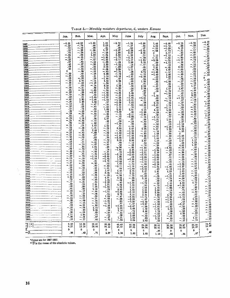
TABLE 5.-Monthly moisture departures, d , western Kansas

2 5 . 0 25. 0. 0 .7 -

- - Feb.

-0.05 -. 74 -. 12 -. 26 -, 34

e64 -. 35 .47 .Bo -. 67 .33 -. 44 -. 08 .41 .a4 -. 18

2.16 -.69 .06 -. 31 -. 39 .36 -. 30 . 01 1. a0 1.40 .31 .03 .76 -. 23 -. 58 . 01

1.18 -. 44 -. 23 .01

-.E€ .61 -. 4€ -. E€ -. 01 .B1 .21 -. 7: .64 -. 3: -. 61 .61 -. 7( -. 6( -. 21 -. 3: .31 -. 11 . 3 .2l -. fi .3: -. 0: -. 2 .z .81 . 31 -. 1 . 11 -. 2 -. 6 -. 6 -. 1 -. 2 -. R . 2 -. 0

1.8 -. 6 -. 2

16.3 16.1 0

. 4

-

-

- - Apr.

1.63 2.03 .35

1.67 -. 28 -. 64 -1.80 -1.33 -. 99

1.33 2.03 -. 88 -. 93 2.93 1.14

-1.44 1.03

1.20 -. 96 -1.80

-1.31 -1.23

.37 -. 35 -. 05 1.58

! 5 3 -. 10 . 09 1.57 .49 .17

1.52 -. 26 -. 11 -. 89 -. 01 .33 -. 63 -. 27 -. 67 .38 .14 -. 31

-2.04 -2. OE -1. 62 -1.7c . 05 -. 94 -.81 1.0; 3. Of -. 4( 4.91 1.31

-2.3! 1.0:

-1.8: . 2:

-1. O! . oi 1. M -. m

-1.9 -. 7 -1.3

.R .a -. 8

.0 -.4 -. 7

-. a4 2. m

-1. m

38.0 38.1 0 1.0 -

-0.74 .87 .68

-2.07 1.39 3.52

-1.74 -2.17 -. 49 -1.32 -. 92

2.86 -1.74 -. 79 -1.16

.67 1. ea .ll

1.60 -. 80 -. 91 -1.31 -. 61 -. 28 -1.24 -1.08 -2.20

1.16 3.52

-1.28 -. 10 -. 13 .OR .MI

-1.29 .51

3.8t -. 3t -1. .E -1.41 -2.3t

2.4t .6( .44

w. 04 -1.81

.1: -3.1:

1.8( 1.21

-2.41 1. 6:

-2.1' .&

1.4. -1. 1 -. 0'

2.43 -. 6' . 41 2. 4' -. 2 2.6

-1.0 2.7 -. 4 -. 8

.8

. 6 -2.0

2.8 1.1 -. 4

.a 1.2

-.E

46. E 47. € 0 1. :

-

-1.24 -. 57 .82

-2.28 3.07 -. 22

-2.14 -1.17

1.83 .14 -. 27

1.11 .28 .52

-1.91 .43 . 90

1.05 .20 .54 .37

1.49 2.40

-1.78 -3.01

2.02 -. 84 .19

2.07

-2.11 -2.88

.87 -. 24

.39 -. 44 2.67

-1.26 -2.59 -1.50

1.38 3.88 -. 13 -. 88 -. 86 2.40

-3.02 -2. w

.03 -2.66

-.RE -. 70 -1.1P

3.7E 2.22 -. 72 -. 3f . 9f

-1.01 1.3 2. l i 4.3:

-2. I! 0.11

-3.21 -3.01

-. 1 -3.4'

3.41 .7:

-1.51 1.61 1.2 3.0

67. 6 67.6 0 1.0

.m

- 1 . ~

-2.3:

-

- - J ~ Y - -0.98

.30

.27 -2.06

.72 -. 39 -1.93

3.50 -. 17 .45 .92

2.72 -. 12 -2.33

.24 1.09 .51

2.09 2.38 .Bo .27 .72

-1.61 -. 21 .98

-2.55 .12

4.25

-1.85 -. 16 .94 -. 39 .30 .23

-. 10 -. 93 -1. oc

.61 2.87 -34 -. 7f

-1.03 -1. It -2.11 -3.7( -2. B( -3.2: -2.21 -. Ot -2.41 -2.3:

3.4: .2:

-1.5: 3. 61 , 1:

-1.71 -91

2. R 3. Ri 3.3

-1.7 -. 6 -2.1 -2.9 -. 9

I. 3 4.4 .1 -. 2 .8

2. e

a. 08

-1. m

2. ne

1. n:

64.0 54. c 0 1. t -

- - Aug. -

1.48 1.33 -. 03 - 98 1.12 -. 21

-2.08 . 09 -. 46 1.31

-.78 -1.66 -1.46

.22 -. 02

.@I

.41 -. 67 * 53 .24

0 -1. MI

.88 . 09 2.75

-2.81 .56

4.56 -. 29 .30

-1.13 -1.31

.77 -. 80 -. 81 1.31 -. 10 1.03

1.66 1.55 -. 62 -. 39 .06

-1.34 2.10

-1.88 -1.60 -2.07 -1.04 -2.28 -1.64

.62 1.61 .81

-.BE .2$ . oc -. 9f -. 7(

1.7( 2.0t 3. Of 1. 9(

-.7f -. 01 -. 61 -1.0: -1.6 -. 0

1.71 -. 2 -1.1'

1.2 .o

38. R 30.6

.o 1.1

0'

-1. n i

-

- - Uept.

-0.08 -1.13 -1.08 -. 73

2.17 -1.12 -. 06 -. 05 -1.12

.18 -. 41 1.97 -. 47 1.60 1.25 .77

-1. M) .lm .08

1.07 -. 29 -1.06

.36 -. 73 -1.15

. 6 6 1.79

-1.11 1.80 -. 94 .42 .77

1.01 . 98 .03

-1.29 1.84 .29 .@ -. 24 .01 -. 2: . 9f .01

-1.65 -. 31 -. 7t . 0; .61 .31 -. 6< .41

-1. Q! -. 1: 1.8: .3'

-1.1: -. 71 . 11 1.11

-1.41 -. 81 -. 1, .l

1. 7' -1.5 -1.5 -1.4

.5 -1.8

1.0 .o

1.0 -. 0 -. R .7

30.3 30.3

E . E

-

-

- - OCt.

-0.13 .38

1. 13 -. 51 .30 -. 57 -. 90

-1.07 -. 26 .64

2.02 -.06 -. 65 -. 90 -. 41

* 78 -. 27 .20 -. 17

1.67 -. 12 .42 -. 21

-1.24 .07 -. 57 -. 76 .08 .71 -. 32 -. 76 .80 .31

1.37 -1.10 -1.26

3.42 -. 25 0

-1.28 -1.10

1.07 .53

4.32 -. 65 -. 54 -. 88 -. 94 -. 08 -. 23 -. 14 -1.3E -1.37 -1.1c

1. G( 1.5E -. fx -. 04 -. 7( 4.6:

-LO( -,K

.72 -. 41 -. O! -1. I! . 0: . 11 -1.2 -. 9

. 3 -. 0 2.3 . 4' -. 1 -. 5

29.9 30.0 0 . 8

-

-

- - Nov.

-0.28 -. 28 .17 -. 17 -. 43 -. 37 -. 38 -. 73 .ll -. 16 -. 37 .02 .92 -. 02 -. 75 -. 58 -. 07 -. 78

1.27 .35 -. 44

1.35 2.83 -. 77

-.OB -. 17 .32 -. 91 -. 31 -. 59 -. 63 -. 17 .pa . oe -. 7t .1t .a

-.of ,3! ,1i -. 7(

1.1: 1.2: 1.2( .4t -. 6' . 0: -. 21 .3l -. 71 -. 6' -. M -. fi .8: -. 0 -. 8, -. 61

-. 7 2.7

. 4

. 8 -. 8 -. 5

. 2 1.2 -. 9 -. 6 -. 4

.1

.3 -. 3

.1 1. z -. 1

.n

20.4 20. t 0 . I -

e Dec. -

-0.13 -. 47 -. 79 - .04 76

-. 01 .18 -. 07 -. 41

* 67 . lo -. 43 -. 22

.22 -. 40 -. 16

.73 -. 37

.eo -. 49 .97

C. 43 2.64 -. 00 -03 -. 16

-. 30 2.68 -. 25 .08 .01 -. 63 .41 .72 -. 37

-. 30

. I 2 -. 29 -. 30 C. 46 -. 38 -.I1 -. 25 -. 62

.10

.52

. 4 1 -. 07 -. 13

.71 C. 20 L. 34 -. 56 -. 27

.71 -. 31 -. 31 -. 09 -. KS -. 06 -. n2

.20

-. 22

14.25

.M

: 11

.03

0,. 43

.07

n8 -: 34

.23

.05

.29

-27

. n i

.13

14.41 -

0

/

16

additional rainfall was required if moisture use was to be “normal.”

For the 35-month period beginning with July 1932 the total computed need for precipitation (col. 10) was 69.09 in. This is 14.84 in. greater than the average precipitation (54.25 in. from table 2) for such 8. period. Actually, the pro- cipitation totaled only 40.66 in. (col. ll), which is 28.43 in. less than the amount that would have been climatologically appropriate for the existing conditions. The point is that although the below- average precipitation, in itself, accounts for 13.59 in. of the computed abnormal moisture deficiency,, the procedure outlined here brings to light an additional abnormality of - 14.84 in. which is by no means insignificant. This is the result of having taken account of temperature and the other aspects of the water balance.

THE CLIMATlC CHARACTERISTIC, K

Column 12 of table 4 shows a sample of the derived monthly moisture departures. Such values were computed for the 852 months of western Kansas data and the 324 months of central Iowa data, These values are shown in tables 5 and 6.

-2.14 2.80 .w - .90

1. 61 .63

3.83 -2.17

1.87 -2.41 -1.79

4.35 1.65 1. OB - .07 1.05 1.99

-3.02 -2.42

.09 -1. E4

* 42 -2.07

.49 - .56 -1.73 - .80

1.11 .44 .86

5.24 - .76

-2.9s

--

From practical as well as statistical considerations it is apparent that a given departure means different things at different places and at different times. We can compare a series of such departures for, say, September in western Kansas; but we cannot compare September departures with, say, February departures, or with departures computed for a different area unless we determine beforehand that the sets of data are truly comparable. This suggests that the importance or significance of each departure somehow depends on the normal moisture climate for the month and place being considered.

In order to evaluate this importance, it was assumed that the economic consequences of the driest year in central Iowa were approximately as serious for the inhabitants of centra1 Iowa as were the consequences of the driest year in western Kansas for the inhabitants of western Kansas. It turned out that the driest period of approximately 1-yr. duration in central Iowa began with June 1933 and continued through August 1934, a period of 15 months. The computed total moisture departure for the entire 15-month period was -30.67 in. or an average of -2.045 in. per

-0.20 .07 . 01 - .15

-1.31 1.76 - .lm - .ll

-1.48 - .70 - .26

4.03 .61 - .a? - -95

-1.56 2.03 1.77 - .46 - .14

-1. 28 1.64

-1.04 -2.69

2. 66 -1. B -1.07

.81 -1.25

.44 .MI

1.40 -66 --

TABLE 6.-Monthly moisture departures, d , central Iowa - Aug.

- MlU.

- Apr. Dee. Feb. June

-0.40 -2.10 - .02 - .46 -1.00

.59

.47

.39 - .75 1.42

-.lm - .21 .41 .19 .31 .98 - .w - .30

1.10 .29 .50 .91 - .I1 .77 - .45 * 56

-1.45 -1.47 - .41

.36

.43 1.29 1. 12

-1.00 -1.51 - .33

1.36 -1.32 - .71 - .72

.14 - .47 - .39 - .61 - .78

.03

.G9

.86

.89 1.68 - .07 1.04 .62

-1.05 2.40 2.25 .93 - .48 - .69

-1.87 -1.15 -1.07

2.00 .04

2.37 - .02

0.18 -1.65 -1.07 -1.15 -2.54 - .87 - .79

1.28 1.84 - .67 .83

-1. 34 -1.88

1.07 2.66 2.35

-1.90 3.15 - .29

-1.23 .31

3.05 - .90 1.46 .78 .10

-1.41 -1.00 - .60

.80 . 90

.50 - .33

-0.2: -2.2

.1f 1. BE

-5.48 .94

-1.78 .71

2.59 -2.85 -1.15 -2.53

.86 1. 10 4.76 3.46 1.02 1.65

-1.79 -2.41

2.28 .56 .22

-1. I6 .99 - .80

-1.94 1. 10

-2.02 2.64 2.91

-1.86 .74

0. MI -2.62

* 18 -4.89 -4.48

4.39 -1.04 -1.06 - .22

* 76 -2.37

1.78 1.67 .84 .80 - . l o

2.57 7.87

-1.92 - .60 1.35 1. 40 .36 - .12

1.60 -2.59 -3.72

.08

.83 -1.46 -1.38 -1.36 -1.93

-2.04 - .89 .04 - .64 - .97

3.14 -3.97 - .95

1.23 - .60 1.60 - .85 2.28 3.00 1.81 - .40 .40

-1.89 .74 - .99 - .26

1.60 .86 - .16

-1. 99 .19 - ,69 .14

6.25 - .54 - . ll 3.38 2.63

-2. 6t -1. BE

3.97 -2.23 - 2 . a -1.67 -2.44

.23 - .81

.87 3.65

-1.36 1.28 I. 95 3.21 .70 - .24

-3.39 -1.47 -2.44 - .88

2. 80 1.13

-2.49 ‘6.66

-2.67 -1.00 - .39

.28 - .76 2.38 - .33 - .47

-1.32

.76 -1.04 - .79

.71

.63 - .a - .03 -1.05

.56 1.70 .e9 .I8 .68 .w - .18 .10 .49 - .QQ

-1.12 .36 - .01 - .Q4 - .05

-1.49 -1.40

.07 - .77

.42 - .40 .92

-1.05

2 a i 0.2f -1.44

1.26 . ll - .41 .30 .86

1.03 - .36 .02 - .83

1.04 29

.59 - .23 1.35 .76

-1.06 1.68 - .22

-1.07 .51 - .19

-1.56 - .03 -1.33 -1.18 - .21 - .33

1. 00 - .88 - .49

0

-1.42 .86

1.38 -2.42

2.11 1.71 - .&3

-1.36 1.11

-2.01 1. 17 1.05

* 67 .27 - .33 - .69 .44 - .20 .56

-2.17 -1.74

.OO

.64 -1.77 - .84 -2.26 -1.25

1.02 - .10 1.02

-1.05 1.64

-1.63

12.19 12.15

.90 0

18.78 18.76 0 1.39

24.19 24.25 0 1.79

25.61 26.62 0 1.90

15. 08 15.15 0 1.12 -

28.85 28.84 0 I. 69 -

22.47 15 09 17.89 22.45 1

$10 1 17.91 0 0

10.02 10.00

8.89 8.00 0 .e6

0 ,74 1 . m j 1.121 1.33

17

month. Considering the same 27 years as wore considered in Iowa, the driest period of similar length in western Kansas was a 14-month period from March 1934 through April 1935. The total moisture departure for this period (see column 12, table 4) was -19.11 in. or an average of -1.365 in. per month.

On the assumption that these dry periods were of approximately equal significance locally, we can multiply each by some factor, K, and write

I - K r o m X & o t m = Z r a n X & a n (16)

Z i o c w l K K a n - -8 Kan Id’ row=- 1.365/-2.045 = 0.67. ( 17)

and

The p s represent averages for some, as yet, undefined characteristics of the climates of these two areas during the 14- and 15-month periods; i.e., they apply to the periods as a whole rather than to each month individually. However, for the moment they can be treated as constants to be evaluated from some measured aspects of the local climate.

From equation (17) it is apparent that I? for western Eansas must be about 1% times as large as R for central Iowa. Now, the average moisture demand in the two areas is roughly the same but the average moisture supply in Iowa is roughly 1% times larger than in Kansas. This suggests that the values of the constants may depend on the average moisture shortage in the two places. This seems reasonable inasmuch as the less the supply, in relation to the demand, the greater the significance of a given shortage.

How can one best measure average moisture demand? In some months it can be reasonably estimated by m, and in some months it can be estimated by the average amount of recharge that occurs. However, in some spring and fall months PE and fi are roughly equal and both are important. Therefore average moisture demand for any period can be estimated by m+E.

The average moisture supply is not always dependent entirely on the precipitation. In some cases the precipitation alone does not truly represent all of the moisture supply because previously shred moisture is used also. Therefore, average moisture supply for a month or period can be measured by p+E.

The normal moisture demand for the 14-month dry period in Kansas can be found from table 2 as:

-

14 - 14

n-1 n=l c P E + c &!=36.21 in.

The normal moisture supply for the same period can also be found from table 2 as:

14 - 14

n = l n=l P + C 2=25.90 in.

If we take the ratio of demand to supplY, We

get 36.21/25.90=1.398, which we can call K for this 14-month period in Kansas.

Turning to the 15-month period in Iowa and following the same procedure,

n=l n=1 n - 1 n = l

=50.88/53.23=0.95%

which can be considered 8s E for this 15-month period in Iowa.

If this ratio of moisture demand and supply Can be used as a measure of the importance of mois-

departures, then according to equation (17), K r o w a / Z a . should be about 0.67. It turns out that 0.956/1.398=0.68, which is in surprisingly good agreement.

From the above it appears that K, the climatic characteristic, can be reasonably estimated for each of the 12 calendar months as:

k= (PE+Z)/(F+E) where k is a first approximation of K.

The k-values in column 6 of table 3 were corn- puted by this equation. These numbers are in- tended as measures of the local significance of the moisture departures which have been derived. However, it later turned out that equation (18) did not work very well in some other climates and 8 different equation for K had to be derived. Since the work on the final K was dependent on this first approximation, k, the following few pages describe the development based on k and are followed by the “back tracking” which evolved the final equation for K.

THE MOISTURE ANOMALY INDEX, a

These monthly constants, the k-values, Were used as weighting factors for each of the monthly moisture departures during the two dry periods

18

being considered. Beginning with March 1934 the departures listed in column 12 of table 4 were multiplied by the corresponding factors in column 6 of table 3 to obtain the index values shown in column 13 of table 4. When the index values, z, were algebraically addod for the 14-month Kansas dry period which ended with April 1935, the sum was -25.51. This represents an average index of -1.82 per month. ’ When the same procedure was followed for the 15-month dry period in Iowa, the 15-month index sum was -27.06 or -1.80 per month. This agrees very well with the average index for the driest Kansas period and suggests that the derived index values do, in fact, provide comparable measures of relative climatic abnormalities. The monthly “moisture anomaly index, z,” is therefore defined as:

z=dk. (19)

What are these z ~ d n e s and what do they mean? They cannot be regarded as inches of departure of the moisture supply €rom normal as are the values in column 12 of table 4. Those departures have now been weighted and must be regarded only as index numbers. Each number expresses on a monthly basis and from a moisture standpoint the departure of the weather of the month from the average moisture climate of the month. Each has, presumably, been adjusted or weighted in such a way that the same scale-the ordinate, if you wish to think of it graphically-is applicable to all values in both areas.

Small abnormalities of moisture can occur a t any time in any place. Of course, this is hardly surprising. Equally to be expected is the fact that in these climates large abnormalities very rarely occur during the cold season from Novem- ber through February. The largest cold-season anomalies are positive and occur ’ mostly in November as would be expected from the fact

that large monthly amounts of precipitation can and sometimes do occur in November. On the other hand, even a complete failure of the moisture supply during any cold month will not result in any very great departure of the moisture supply from normal because in these particular climates the cold season moisture demand or CAFEc precipitation is always rather small.

In Kansas and Iowa the really important negative moisture anomalies occur during the warm season. This, again, is as one would expect because the moisture requirement during summer can be rather large and, on occasion, the moisture supply can fail almost completely. Note the very large negative anomalies during July in the 1930’s in western Eansas. The -6.51 in 1934 is the largest negative anomaly that has thus far been computed. This large value is a direct consequence of the extremely warm and dry weather which preceded July, coupled with the hot dry weather of July itself. The mean temperature over the area during July 1934 was an all-time record 85.6’ E’. and the area rainfan averaged only 0.74 in.

While central Iowa has not produced such an extremely dry single month, a number of negative anomalies of the order of -4 have occurred. Also the Iowa data show a greater tendency for long uninterrupted runs of abnormally dry months. The 15-month period which began in June 1933 and the 21-month period beginning with August 1955 were both uninterrupted by even a :single wet month.

Some of the unusually wet months in both Kansas and Iowa produce some really outstanding positive anomalies. For example, it rained 12.26 in. over central Iowa in June 1947 and the anomaly index, z, was f7.24. Likewise, western Kansas had an index of +8.49 for June 1951 owing to 7.89 in. of rainfall which was 267 percent of normal and produced much floodicg.

757-281-66-4 19

6. THE DURATION FACTOR

THE EFFECT OF TIME TABLE 7.-The driest intervals

As m d r e t h and Thomas have pointed out [18] in most cases it is not the first year of low rainfall that is disastrous to farming and ranching, but the prolonged periods which extend for 2, 3, or 4 years in a row. The same reasoning applies if one is concerned about the hydrologic aspects of drought. A relatively short period of abnormally dry weather will lower lake and reservoir levels, but matters do not become really serious until a prolonged drought period has brought the water supply to a critically low level. Therefore, if one wishes to make a distinction between, say, mild drought and extreme or disastrous drought, the duration of the abnormally dry period must be taken into account.

DROUGHT CATEGORIES

It is reasonable, and it certainly would be convenient, to have names assigned to the various categories of drought seventy just as arbitrary names and definitions have been assigned to such things as dense fog, moderate rain, and other phenomena. It appears that drought seventy could be adequately expressed by four classes, mild, moderate, severe, and extreme-terms which are frequently used by the U.S. Department of Agriculture as well as by the Weather Bureau. Unfortunately, no satisfactory definitions exit for these expressions. There doesn’t seem to be much hope for making even a semi-objective approach to specific definitions of “mild,” “moderate,” or “severe” drought; but if we assume that “extreme” drought occurred in the two areas being studied during some of the driest periods of record, we can describe extreme drought in terms of the accumulation of the monthly index values.

THE DRIEST INTERVALS

Table 7 shows some accumulated moisture anomaly index values in both central Iowa and western Kansas. These periods were selected as

L_

ZZ - -13.40 -13.62 -14.88 -16.46 -14.14 -18.66 -23.39 -27.06 -28.71 -31.28 -31.69 -46.82 -62.66 -

representing the maximum rate at which the M a - tive values of the monthly index have accumulated during various time intervals. These data are shown in figure 1. The straight solid line thereon was drawn by eye. This line itself does not show rate of accumulation of the index values; it merely indicates the approximate maximum rates which have been observed during extremeb’

0

d

+

c

- -60 - -

- 7 0 ‘ 1 ’ 1 1 1 1 1 1 0 48 12 24 36

LENGTH OF DRY PERIOD (MONTHS)

FIGURE 1 .-Accumulated index during the driest periods of various lengths.

20

dry periods of various lengths. For instance, z-values have been known to accumulate a t the rate of about -3.0 per month for 6 months, but a t the average rate of only -1.5 per month over a 42-month period. Therefore, this line can represent extreme drought; i.e., an extremely dry and very unusual condition exists if z= -12.00 for one month as well as if Xz= -70.1 in 4 years. This is one of a family of lines that can be drawn. Since the horizontal line at the top of this chart represents “normal,” the ordinate from normal to extreme was divided into four equal lengths and the body of the graph was correspondingly divided by the dashed lines arbitrarily labeled “mild,” “moderate,” and “severe” drought. It is convenient to assign a numerical drought severity value of -4.0 to the line for extreme drought, 73.0 to severe drought, -2.0 to moderate drought, and -1.0 to mild drought. The solid line drawn is therefore the -4.0 line and the equation can be determined by noting that from t (duration) = 1 month and 2=-12.0 to t=48 months and Xz= -70.1, the drought severity= -4.0. Drought severity is therefore approximated by

x , = z ~,/(0.3092+2.691). i

t=1

0

-10

t A 0 2 4 6 8 1 0 1 2

MONTHS

DETERMINING MONTHLY INCREMENTS OF DROUGHT SEVERITY

Equation (20) is only a first approximation to the relationship sought because it is based on algebraic sums of the index, 2, over various periods of time. This is not the best way to handle the problem because this cumulative procedure causes the effect of a single month-say, a very wet month in a long series of dry months-to be directly reflected in Zz even years later. Obviously, this is unrealistic because a single wet month during a given dry summer should not, by the following summer, have any great influence on the severity of a drought which had continued during the intervening period. For instance, August 1933 was a very wet month in Kansas (see table 4) and i t grently reduced the severity of the drought that was underway. However, the drought continued and by the end of May 1934 the situation was very, very serious. But, this seriousness is not completely apparent when the z-values are accumulated and plotted on a diagram such as figure 1. In fact this procedure will create a misleading picture.

Figure 2 demonstrates how misleading the cumulative procedure can be. Figure 2A was constructed by assuming that z= - 1.0 each

0 2 4 6 8 1 0 1 2 MONTHS

(A) Six relatively dry months followed by four very dry FIQTJRE 2.-An illustration of the cumulative procedure. months; (B) The four very dry months by themselves.

21

month for 6 months and then Z= -4.0 during each of the following 4 months. The total accumulated value is therefore -22.0 in 10 months. Note that the 10th month does not quite reach the extreme drought h e .

Now assume that the first 6 months were each very wet and that the remaining 4 months each had z=-4.0 as before. I n this case the dry period begins with the first month in which 2=-4.0 and these 4 dry months give the curve in figure 2B. Note that the value for the last month now falls below the extreme drought l i e .

We are now confronted with a result which indicates that four very dry months following six wet months produce a more serious drought than is produced by the same four very dry months following six months of relatively dry weather. Obviously, this is a fallacy. The cumulative procedure is misleading and cannot be used as a method of taking account of the duration of the dry period.

The problem must, therefore, be handled on an increment basis such that each successive month is evaluated in terms of its contribution to the severity of drought. In effect, this will eliminate direct consideration of the duration factor and bring duration in indirectly as a consequence of the accumulation of successive monthly contributions to drought severity.

In order to evaluate the contribution of each month, we can set i= 1 and t= 1 in equation (20) and we have,

x1=2,/3. (21)

Since this is an initial month,

1-1 t-1 ------__c

2 -1.0 -3.0 0 -1.0 -3.309 10 -1.0 -6.472 0 -1.0 -6.181 2 -3.0 -9.0 0 -3.0 -9.927 10 -3.0 -16.416 0 -3.0 -17.343

However, this is not the whole story because in successive months a certain amount of abnormal dryness (z <0) will be required merely to maintain the severity of the existing dry spell. For instance, one knows intuitively that an extreme drought will not continue in the extreme category if subsequent months are normal or only very slightly drier than normal. The question is, how much dryness is required to maintain a drought of given severity; i.e., for AX=O?

From equation (20) or from figure 1, it is appaent that Zz must increase as t increases in

z i

-0.309

-.g2’ --.927

TABLE %-The amount of abnormal dryness required to maintain a given drought severity

order to maintain a given value of X. The rate of increase of t is constant; i.e., t increases by 1 each month, thereby increasing the denominator by steps of 0.309. Therefore, the rate at which the index, z, must increase in order to maintain a constant value of X (AX=O) depends on the value of X that is to be maintained. This reasoning suggests that for all months following an initial dry month an additional term must be added to equation (22), and that the equation is of the form,

where

The problem is to determine c. Returning to equation (20), we can compute the value of 21

which will maintain a given value of X from month to month. Table 8 shows the computed values of z in the i th month for two arbitrary values of x f - l = X , and two arbitrary valuos of t*

If we place these values of z,, Xtw1 and AX into equation (23), we have,

and

a z o = ( -0.927/3) -3 .0~ .

C is therefore -0.103 and the final equation is:

This equation can be used to compute the monthly contributions to drought severity. Of course, the sum of the increments gives the severity itself, i.e.,

x , = x , ~ , + ~ - 0 . 1 0 3 x 1 ~ , . (25)

22

7. RE-EVALUATION OF THE WEIGHTING FACTOR

EVIDENCE OF UNSATISFACTORY K VALUES

Originally, this study was carried through to completion on the basis of the equations shown above. Results for western Kansas and central Iowa appeared reasonable and realistic. How- ever, when the entire method was subsequently applied to other areas with rather different types of climate, some of the results were definitely peculiar and unrealistic. For example, in Kansas and Iowa the most extreme drought periods produced maximum drought index values around -5.0 to -6.0. These seemed reasonable inasmuch as the system is designed to indicate extreme drought whenever the index exceeds -4.0. How- ever, an analysis for the southern climatological division of Texas produced index values ranging as large as -10.23. Such values were obviously rather far from the expected maximum around -6.0. On inspection it was found that some of the monthly weighting factors were inflating the departures, the d values, in an unrealistic fashion.

The other analysis that showed peculiar results was done for western Tennessee by Mr. M. H. Bailey, then State Climatologist for Tennessee. The worst flood in the history of the area (January 1937) produced an index, X , only slightly larger than zero. Again, the k values were at fault. They were so small that even huge moisture departures were rendered quite insignificant when multiplied by the weighting factor, k. In this particular January in western Tennessee, rainfall

averaged 19.35 in. over the mea and P-P was a huge f12.26 in. As will be shown later on, this system should measure unusually wet periods as well as unusually dry periods. Obviously, the index, X, should receive a large positive increment during this extremely wet month. From equation (22)a one can see that this will occur only if K for January (see eq. (19)) is of the order of 0.5 to 0.7, say, 0.6. Actually, k had been computed (by eq. (18)) as 0.051 for January.

. A

~~ - ~

0 From hore on z becomes Znnd k becomes Kln equations 18 through 26, as these are the final estlmnten of these Indices.

PROCEDURE FOR ESTIMATING MEAN VALUES OF K

It seemed the simplest procedure for re- evaluating the weighting factor was to use equation (20) to determine what Z Z should be for extreme drought over a 12-month period. It turned out that for X=-4.0 and t=12 months, the sum of the weighted departures should be -25.60. If we again assume that the driest 12- month period represents extreme drought in any area, we can obtain a new 12-month mean weighting factor, z, by dividing -25.60 by the 12-month sum of d for the driest periods of record.

Referring to table 5, it will be noted that the driest 12-month period in western Kansas began with May 1934 and continued through April 1925. The sum of the d values for this period is -16.62. A period almost as dry began with March 1956 and extended through February 1957. This 12- month sum of d was -15.60. Averaging these two, to eliminate a little of the sampling variability, gives a mean 12-month sum of d of -16.11. Dividing -25.60 (12-month Z Z for extreme drought) by -16.11 gives 1.59. This is E for western Kansas. It is a mean weighting factor- the mean of the 12 monthly weighting factors.

In central Iowa the driest 12-month periods were June 1933 through May 1934 and August 1955 through July 1956 (see table 6) when the 12-month sums of d were -23.02 and -20.56. The mean is -21.79. When we divide -25.60 by -21.79 we get 1.17 for z i s central Iowa.

By this time analyses and a monthly table of d values mere available for nine different areas, viz, the climatological divisions of northwestern North Dakota, western Kansas, central Iowa, Texas High Plains, Edwards Plateau of Texas, southern Texas, western Tennessee, west central Ohio, and a point analysis for Scranton, Pa. The values computed for ranged from 1.06 in western Tennessee to 1.73 in northwestern North Dakota. In addition, there is the previously mentioned estimate that K for January in western Tennessee should be around 0.6 if the 1937 case is to look at all reasonable.

23

1.8

1.7

1.6

1.5

1.4 -0

5%- 1.3

1.2 (\I

I 1.1 II

IY 1.0

0.9

0.8

0.7

0.6

0.5

* I . 0

- Northwestern N. Dakota - - - A@ - . - -

e

t Southern Texas

High Plains, Texaz 0 0

/ f 0.50 a Western Kansas

PE+H+HO + Z . B O ( P t i - D

Western- Tennessee (Jan. 1937 estimate) - 0 -

FIQURE 3.-Mean annual weighting factor as related to average moisture demand, average moisture supply, and twerage absolute moisture departure.

K AS A FUNCTION OF OTHER ASPECTS OF CLIMATE

From an inspection of the failures of the original k values it was apparent that K should depend on average water supply, H+Z, as originally used. It was also apparent that the average runoff , m, should be considered as a part of the moisture “demand” in addition - to the average potential evapotranspiration, PE, and the average recharge, fi. Also, it was apparent that K varies inversely with n, the mean of the absolute values of d.

After some experimenting with various empirical relationships, the semi-logarithmic plot shown in figwe 3 was evolved. NO doubt, greater scatter would result if more stations or areas were

24

added. This relationship may be fortuitous, but it Seems reasonable. The problem is also cOmPli- cated by sampling variability.

The K values in figure 3 were based on the driest 12-month periods in these various places and the abscissa is made up of mean values for the entire period of record analyzed, the 30 years 1931-1960 in most cases. For example, f‘E is average annual PE divided by 12, and the other mean values were computed in the same fashion.

MONTHLY WEIGHTING FACTORS

The next step was to apply this empirical relationship to each of the 12 calends months in each of the various places and thereby derive the 12 K values for each place. These results are

- - - K' = 1.5 l o g 1 0 [YE? R,f '4- 2. SO)/B]+ 0.50.

shown in table 9. In this table ll is the monthly mean of the absolute values of d, and K' is the weighting factor computed for each month by the equation developed from figure 3; Viz,

Pi-Z

(26)

0.86 0.70 0.81 1.47 1.80 1.61 1.26 1.12 1.22 1.46 1.68 t 4 8

- D K' DK'

K

0.96 1.30 1.36 2.27 1.60 1.43 1.29 1.27 0.85 _ _ _ _ _ _ _ _ _ _ 1.40 1.20 1.18 . . 8 6 1.09 1.18 1.21 1.21 1.40 _ _ _ _ _ _ _ _ _ _ 1.34 1.66 1.61 1.95 1.74 1.69 1.66 1.64 1.83 17.92 1.38 1.18 1.17 .86 1.07 1.16 1.18 1.19 1.38 _ _ _ _ _ _ _ _ _ _

25

1.16 0.86 0.96 1.40 1.81 1.90 1.68 1.213 1.48 1.42 1.18 1.09 1.06 1.27 1.48 1.26 1.36 1.66 1.76 2-01 2-02 1.14 1.31 1.26 1.06 .96 .@4 1.13

- D K'

K EK'

1.14 2.08 1.61 0.77 1.10 _ _ _ _ _ _ _ _ _ _ 1.58 1.01 1.13 1.66 1.32 _ _ _ _ _ _ _ _ _ _ 1.80 2.10 1.82 1.20 1.46 19.88 1.40 .BO 1.00 1.39 1.17 _ _ _ _ _ _ _ _ _ _

- 0.97 0.80 0.63 1.38 1.33 1.66 1.23 1.41 1 . m 1.76 1.29 1.28 1.28 1.67 D 1.37 1.n 1.11 1.79 1.72 2.00 1.93

K' 1.28 1.38 1.60 1.17 1.17 1.17 1.43 iTK'

K

1.49 1.73 1 8 6 0.66 0.80 _ _ _ _ _ _ _ _ _ _ 1.41 1.16 1.30 1.73 1.47 _ _ _ _ _ _ _ _ _ _ 2.10 1.89 1.77 1.14 1.321 19.46 1.28 1.04 1.18 1.67 1.33 _ _ _ _ _ _ _ _ _ _

- 0.28 o . 4 a I 0.71 1.07 1.34 1.82 1.66 1.10 2.26 1.82 1.80 1.34 1.20 1.12 1.20 1.46

1.14 1.43 1.61 1.81 1.87 1.80 1.38 1.64 1.28 1.38 1.66

D K'

SK' K

.68 2.68

0.86 0.84 0.67 0.40 _ _ _ _ _ _ _ _ _ _ 1.63 1.69 1.78 1.97 _ _ _ _ _ _ _ _ _ _ 1.40 1.34 1.01 ,78 16.41 1.87 1.82 2.04 2.26 ___.______

0.61 0.42 0.63 0.86 1.M) 1.48 1.40 0.89 1.28 1.22 1.81 1.84 1.70 1.64 1.16 1.23 1.33 1.66 1.37 1.32 D

K' 1.07 1.32 1.72 1.82 1.86 1.48 1.76 1.81 .QZ i7K' 1.83 1.66 1.24 1.32 1.43 1.79 1.48 1.42

1.86 2.08 K

- 0.62 0.66 ___.______ 1.86 1.66 __-_______ .98 1.08 16.40

1.99 1.78 ___.______

0.20 0.23 0.33 0.67 1.04 1.48 0,88 0.81 0.91 0.69 2.42 2.93 2.08 1.84 1.37 1.14 1.48 1.66 1.69 1.81

1.10 1.42 1.69 1.46 1.34 1.46 1.07 EKI 2.33 1.94 1.02 2.10 2.36 2.25 2.67 3.43 a 3 0 2.95

- D K'

K .a ~4

0.38 0.19 _ _ _ _ _ _ _ _ _ _ 2.00 2.46 _ _ _ _ _ _ _ _ _ _ .78 .47 12.46

2.84 3.47 __-_______

As mentioned previously, the mean values used in the development of this equation were average annual values divided by 12. I n applying equation (26) to compute monthly weighting factors the mean values used are means for one of the 12 calendar months.

FINAL ADJUSTMENT OF THE MONTHLY K VALUES

If equation (26) is producing reasonably ‘(correct” values for use in equation (19), then the average annual sum of the weighted average departures should be about the same for all places analyzed. Table 9 shows these weighted average departures, DK’ for each month and their sum for the 12 months. These sums agree fairly well, but not well enough. The disagreement indicates that the departures are being given more weight in some places than in others. For example, the Tennessee weighting factors must be too large while the North Dakota weighting factors must be too small. This discrepancy was demonstrated by using the K’ values to compute drought seventy (using equation (19) and (25)) for some of the driest periods of record in each of these places. As an example, drought index values computed on the basis of K‘ indicated that drought in western Tennessee becomes more extreme than does drought in northwestern North Dakota or western Kansas. This did not seem reasonable and suggested that the weighting factors needed further adjustment.

The annual sums of EK’ in table 9 range from 12.46 to 20.97. The mean sum for the nine areas is 17.67. If all weighting factors are adjusted SO

that all the annual sums of EK=17.67, drought analysis results should be more comparable. The K values shown in table 9 were computed on this basis. For example, for January in west Tennessee, 0.51=(17.67/20.97)0.60. This can be expressed as,

(27)

This completes the derivation of the weighting factors. They apparently establish reasonable comparab.bility between areas, but there seems no way of assuring that they establish more than fair to good comparability between months. NO doubt it would have been better to base the con-

stant, 17.67, on analyses from many more places, but quite a range of climates is represented by these nine areas and the value 17.67 seems to work fairly well.

STANDARD DEVIATION OF d AS A WEIGHTING FACTOR

Some surely wonder why the standard deviation of d was not used as a weighting factor, thereby Permitting one to deal with a standardized variable. This, of course, was tried, but results were definitely unrealistic partly because some of the distributions of d are rather skewed. Another likely factor is that the local significance of a &en moisture departure is not solely dependent on its place in the distribution of departures. For example, the standard deviation of d is 1.64 in. in October in western Tennessee and it is also 1.64 in. in July in southern Texas. In c - the Ten- - nessee case average moisture demand, PE+n+ 5 0 0 ) i S 3.27 in. and average moisture SUPP~YJ P+J% is 2.99 in. On the other hand, southern Texas has an average July moisture demand of 7.57 in., but an average moisture supply of only 2.13 in. Here demand is about 334 times suPPlY, while in Tennessee they are roughly equal. It Seems obvious that a given moisture shortage would not be equally significant in both places. w e would be assuming equality if we used the standard deviation as a weighting factor.

AN EXAMPLE OF THE DROUGHT SEVERITY COMPUTATIONS

At this point it is probably time to stop and take stock of the relationships which have beon developed. It seems likely that a short example will best illustrate some of the more important steps. The year 1947 was a rather unusual one for central Iowa. April, May, and June Were Very wet and July, August, and September were VerY dry. The data for the 3 dry months are shown in table 10.

Inasmuch as June had been very wet, the CAFEC precipitation computed by equation (14) was only 2.81 in. for July. However, the actual Precipitation was so small that the departure (by equation (15)) was -1.89 in. The final climatic characteristic, K, for July in central Iowa is (table 3) 1.28, therefore, the July anomaly Was (by equation (19)) -2.42. The next three COl- umns in table 10 show the parts of equation (24). Since this was the first dry month, the drought

26

Actual Cornp. Moisture Beverity for precip. precip. C l h . char. anomaly month

Month P B K z z/3

-_.___I_-p-,

0.82 2.81 I. m -2.42 -0.81 1.36 4.76 .03 -3.15 -1.05 July - _ _ _ _ - _______--

September. - _-_._-- -- 1.28 4.30 1. 04 -3.14 -1.05 August - __________-- -

index for the previous month was, of course, zero. The change in drought severity due to the dryness in July was therefore -0.81. We have previously defined mild drought as beginning when the severity index reaches - 1.0; therefore the index value of -0.81 indicates that the drought was still not serious a t the end of July. For convenience we can call this “incipient” drought, a condition which we will now arbitrarily define by a severity index value between -0.50 and -1.0. Inasmuch as the drought index is only 81 percent as large as is required to establish mild drought, we can state that there is an 81 percent probability that this July marks the beginning of a drought period. Not until the severity index reaches -1.0 can we say with certainty that (by definition) a drought began in July. This provides a very convenient method for methodically determining the beginning of drought periods. In addition, it provides a basis for preparhlg statements expressing the probability that a drought has begun. The tendency for persistence during drought makes such probability statements worth- while from a practical standpoint.

Table 10 shows that the dry August intensified the drought (equation (25)) and matters were beginning to get a little serious by the end of the month. The drought reached a severity of - 1.78, which is classed as mild, but it was approaching moderate severity. By the end of September a moderate drought existed. The comments published in the Iowa Weekly Weather and Crop Bulletins [62] agree reasonably well with this analysis, Early in August there seems to have been a good deal of concern about the fact that the area was rapidly running out of moisture and that crop damage might become serious unless rains came in the next week or 10 days. By the

Index to Change In Drought ma1ntaIn sevtulty index severity

--.103x1-1 Ax X

0.0 -0.81 -0.81 .08 -. 87 -1. 78 .18 -. 87 -2.65

end of August it was apparent that the dry weather had produced serious damage to Some crops and that pastures were no longer Supplying adequate forage for livestock. By the end of September there were general complaints of dry soil, delayed seeding, and poor pastures, but the growing season had essentially ended and the agricultural remarks cease to be particularly useful in estimating drought severity. However, as far as one can tell, moderate drought appears to be a reasonable classification for the September weather. It is difficult to estimate the severity of meteorological drought from remarks concerning agricultural conditions because fortuitous rains sometimes produce very satisfactory yields of some crops during seasons which were, as a whole, much drier than normal. Also there seems to be a tendency for exaggeration in crop condition reports. A week of hot, dry weather seems to foster reports that the crops are practically ruined, while rain of less than 1 in. the following week may lead to forecasts of a bumper crop. This is one of the reasons it was necessary to start this drought analysis development with selected cases in which it was so dry that there could be no disagreement as to the fact that the drought was very serious from all standpoints-agricultural as well as hydrologic.

By way of comparison it is interesting to see what happens to the examples of figure 2 when one analyzes these data by equation (25). At the end of the sixth month in figure 2A the drought severity is - 1.54; at the end of the 10th month it is -5.55. The four very dry months increase the severity by 4.01 and produce an extreme drought condition. On the other hand, the four very dry months in figure 2B give a drought severity of -4.53 at the end of the fourth month. ,

27

8. APPLICATION OF THE DROUGHT FORMULAS TO WET PERIODS

It Seems reasonable to assume that the abnormal moisture deficiencies which could create, say, a moderate drought would have created a moderately wet period had they been positive rather than negative moisture departures. In other words,

not the drought equations be applied to wet periods merely by changing the signs where necessary? For example, equation (15) yields positive departures as well as negative. Also by equation (19) the monthly moisture anomaly 2, may be positive as well as negative. Likewise, equation (25) will give positive values when the monthly index is positive. Inasmuch as the equations will provide a measure of wetness the following categories were more or less arbitrarily set up, and are given in table 11.

Originally the objective of this study was to deal only with abnormally dry periods, but this proved to be not entirely feasible. It is difficult t o determine the beginnings and endings of dry

TABLE II.--C2asses for wet and d r y periods

X

1 4.00 8.00 to a.09 2.00 to 2.09 1.00 to 1.89 .mto .@a .4QtO -.49

--.soto -.w -1.00 to -1.90 -2.00 to -2.89 -am to -am

$ -4.00

Class

Extremely wet. Ver wet Mo&mteiy wet. Slightly wet. Incipient wet spell. Near normal. Incl lent drought. Miladrought. Moderate drought. Severe drought. Extreme drought.

periods unless one also recognizes a J takes account of the wet periods. For example, a relatively dry month such as August 1935 in central Iowa (see table 6 ) will appear as a separate drought period unless one recognizes that this month constituted only a slight and probably beneficia1 interruption in a fairly long period of unusualb' wet weather.

9. END OF DROUGHT (OR WET SPELL) Generally speaking, the beginning of drought

closely follows the onset of an extended period of unusually dry weather. It follows, therefore, that the end of meteorological drought should coincide with the time when some rather major and fairly abrupt readjustment in the large-scale circulation pattern begins to produce weather which is normal or wetter and continues so for a significant length of time. This return to normal weather terminates the meteorological drought, but it does not ordinarily end the effects of the bought. The effects may linger for weeks or months or even years depending on which effects are considered [7O]. These persistent effects constitute a separate problem which is outside the scope of this study.

CHANGES IN THE SEVERITY INDEX

If a drought has been going on and the weather turns consistently normal or wetter, the severity index d, by equation (25) eventually reach zero. However, it does not seem reasonable to require that the index drop all the way to zero before concluding that a drought has definitely ended. From examination of a number of cases this seems to be too stringent a requirement. For example, a &ought that was just barely established, say

x=--l.lO, would, by equation (25), require z=+2.97 in order to reduce the index to Zero

in a single month. This seems like an excessive requirement, but it is plainly so if one computes the number of months of exactly normal weather G = O ) required to bring X to zero. This can also be done from equation (25). We find that X reduces from -1.10 to -0.99 in 1 month, to -0.52in 7 months, and approaches zero in about 3 years. Obviously, one would consider the drought over long before the end of 1 year Of

normal weather, let alone 3 years. On the other hand, if one ends drought 89 soon as the index is numerically less than -1.0, normal weather wodd end the -1.10 drought in a single month- This is a little extreme in the other direction! because it would certainly not be a definite fact that a drought had ended merely because one month had been normal.

B'rom the speculations above it would appear reasonable to assume that drought ends when the

d severity index reaches some value between 0 an -1.0. In order to have some consistency and at the same time not risk breaking long drought periods into a number of short but barely separate drought periods, the lower limit of incipient drought, -0.50, was chosen as the value of

28

which will be considered to definitely end a drought. In other words, as soon as the severity index reaches the “near normal” category, which lies between -0.50 and +0.50, no drought exists.

DETERMINING THE END OF A DROUGHT I n the previous section it was assumed that

drought can be considered as definitely terminated as soon as the drought index reaches the “near- normal” category. The question, then, is, how much moisture would be required to reduce the severity of a given drought to -0.501 This can be solved by substituting the appropriate values into equation (25).

and

Let &=-0.50, then

-0.50=X~-1$-Z/3-0.103X~,~

Z=-2.691Xi,1-1.50.

Therefore, the Z-value that will end a drought in a single month is :

Z,=-2.691X1-1-1.50. (2%

By saying that drought has definitely ended when X= -0.50, we are also saying that there is some algebraically smallest value of 2 which could occur month after month and eventually produce X=-O.50 for month after month. When this occurs AX-0 and X,-,=-0.50, so by equation (24) one finds that 2=-0.15. This indicates, and quite reasonably so, that a drought period can end even though the weather is consistently just slightly drier than normal. Therefore, any value of 22 -0.15 will tend to end a drought, and the “effective wetness” is:

U, = Z + 0.15 (29)

(After a drought has definitely begun (x5 -1.00)~ equation (29) applies to the first. “wet)’ month; i.e., the first month having 21-0.15. U, should then be computed for each successive month until the computations show either a 0 percent or a 100 percent likelihood that the drought has ended.)

If the amount of wetness required to end a drought in the first wet month (2, from equation (28)) is greater than the effective wetness (U, from equation (29)) for that month, the drought severity will decrease, but the drought has not definitely ended. However, since the drought severity will have been diminished by the first wet month, it will not require as much wetness to end it the second month; i.e., 2, will be smaller

the next month and the total amount of wetness required to end the drought will be the new 2, computed for the ith month plus the previously accumulated wetness, viz,

where

U=U,, i refers to the ith month; i.e., the month being considered, j indicates the number of months of lag; e.g., UL-, at j=1 refers to the value of U, in the preceding month, and j= j * , the upper limit of the summation, indicates that U, is to be summed back in time to and including the value a t the j * month, where the j * month is the first month of the current wet spell. If ZU,<O, zU=O. Otherwise, one comes out with negative probabilities.

The percentage probability that a drought has ended is therefore:

(See table 12, column 5.)

Now it frequently happens that a drought period is temporarily interrupted by a month or so of abnormally wet weather. Such occurrences nearly always give rise to speculations that the drought has ended. From the strictly soil moisture standpoint of agricultural drought, the drought has ended, a t least temporarily; but from the meteorological standpoint or even from an economic standpoint the short wet spell may turn out to be of little consequence, The wet August of 1933 in western Kansas is a good example of a temporary interruption of a serious drought. The drought had begun in July 1932 and by the end of July 1933 the drought index stood at -4.07, which is extreme drought for the area as a whole. August 1933 was cool and wet over the area. The average precipitation was 4.91 in. and the index for the month was Z=+3.59. This was, however, far from enough moisture really to end the drought. From equation (28) one can compute that Z, , the amount needed to end the drought in August, was f9.45. From equation (29), the effective wetness, U,= +3.74, and from

P , actually expresses moisture recoived 8s a percantage of the amount ol moisture required definitely to terminate a drought. Of course, the probability that a particular drought has ended is either zero or 1.0, but it is convenient to think of P. 8s the prohabllity that a drought has ended.

29

equation (30) the probability that the drought had ended turns out to be 40 percent. The drought index stood a t -2.45 at the end of August. However, the dry weather was resumed in Sep- tember and October (see table 5), and the probability that the drought had ended had dropped to 12 percent by the end of October. Subsequent dry weather reduced the probability to zero in the spring of 1934. If, however, the wet August had been followed by continued wet weather, the probability that the drought had ended would have reached 100 percent and the last month of drought would have been the last month in which the probability was not greater than zero; i.e., July 1933.

DETERMINING THE END OF A WET SPELL

I n order to treat wet periods methodically in the same fashion as dry periods, some sign changes are required in the equations for computing the probability that a dry spell has ended. To determine the index, Z,, which will end a wet spell in a single month, an equation similar to equation (28) must be developed. In this case one can substitute X=+0.50 in equation (25) and get:

Z=-2.691X~-lf1.50. (31)

This gives a measure of the amount of abnormal dryness (-a required to reduce the severity Of

a wet spell to +O.ciO in a single month. Just as a drought period can end even though

the weather is consistently just slightly drier than normal, a wet period can also end with the weather continuing verg slighty wetter than normal. By substituting AXSO and X1-1=+0.50 in equation (24) one gets the value of Z which Wift tend to end a wet spell. The '(effective dryness becomes :

Ua=Z-0.15. (32)

Equation (30) for determining the probability that a drought has ended can be used to compute the probability that a wet spell has ended.'

The following section describes the procedure for using these equations to make a comPlete Clkatologkal analysis of the moisture aspects of the weather. The term, seventy, which is ordinarily applied to drought rather than $0 wet periods, is here applied to both. This may not be a very accurate use of the term, but it is "OF'

venient, and there does not seem to be a sat1s- factory word to use in place of it.

Spe l l la being Considered. ' In eWatl0Il (a), u- Ud for the aam In which the termination of wet

10. PROCEDURE FOR COMPUTING SEVERITY OF DROUGHT AND WET SPELLS

In order to carry out the computations for determining monthly drought severity, X, from a long series of monthly values of the index, 2, one must keep track of the wet spells as well as the dry spells. Therefore, a number of things must be computed for each month. For example, when there is no drought or wet spell going on, one must each month compute the "probability" that a wet spell or a dry spell has begun. After this probability has reached 100 percent and a drought or a wet spell is actually underway, one must examine each month in turn to determine the probability that the spell has ended and a t the same time determine the probability that a spell of the opposite sign has begun.

The computations are really quite simple. Were they being made by hand, simultaneous computations of various items would not be

necessary because one could easily go back :nd pick UP anything that later turned out to be lm- portant, but for machine data processing the simultaneous computations save time in the long run. The computational routine will be explained by describing an example.

Table 12 shows a &&month period from the western Kansas record. It was necessary to turn so far back into history for the example, because it was diflFicult to locate a short period that would illustrate most of the points that can come UP.

There are four sub-routines illustrated. GO1- umns 3 to 8 show the routine for computing probability that a drought or a wet spell has ended. Columns i o to 12 show the routine for computing the probability that a wet spell has begun. Columns 13 to 15 show the routine for computing the probability that a drought bas

30

TABLE 12.-An example of the computational procedure for determining the beginning and ending of wet pe twds and dry periods and the monthly severity index of each (western Kansas data)

-.lo3 X2.t-1

X -

L28 L55 L 15 1.17 1.79 -. 70 -. 40 -. 55 -. 84

.62

.47

.65

.77

.95 1.10 1.11 -. 02 -. 70 .@a .74 -. 60

-. 45 -. 59 -L 12

.81 -.95

-1.79 -2.83 -3. os -3.22 -3.20 -2.99 -3.16

.62

.31 1.35 1.07 1. Bo 2.75 4 2 1

-- Axl I XI

Xtd-1

1.04 .40 -. 24 .14 .74 -. 70 .23 -. 19 -. 35

0 0 33 26 0

68 54 80

100

0 0 0 0 0 0 0

13 100

0 0 0

0 0 0

1 W

0 0 C C c c c

a

2l 2: 81 71

1M ( I

1.28 0 0 0 0 0

0

.23

.02

.62 ~ 47 .65 .TI .95

1.10 0 0 0 .69 .74 .06

.14 0 0

0 0 0 0 0 0 0

0

.62

.31 1.35 1.07 1.60 0 0

O I 0 -. 24 -. os 0 -. 70 -. 40 -. 55 -. 84

-. 13 -. 21 0 0 0 0 0 -. 02 -. 70 0 0 -. 60

-. 45 -. 59 -L 12

0 -. 95 -1.79

0 0 0 0 0 0

0 -. 25 0 -. 14 0 0 0

1.28 L55 1.15 1.17 L 79 .91

1.05 -75

0

0 0 0 0 0 1.10 1.11 .Qa

0 0 0 0

0 0

-1.1: 0 0

-1.71 -2. g -3. !n -3.2: -3.21 -2. g! -3.11

-2.2 -2.2 -. 9 -. g

1.6 2.7 4 2

0 ______.__. __._____.. 0 _.._..._._ ___...__.. -.85 -2.67 -2 .6i -.63 -1.53 -2.47 0 _.__..__._ .__..-.---

-2.26 -3.33 -3.32 -1.72 -.95 -3.21 -2.44 -1.33 -3.05 -3.65 -,52 -2.96

April--- _.__ .. . May--- -._____._ June _______.__.. July__ ____. . .. August- - _ _ - - - _. September-. _.. . October _____.__ - November- - _ _ _. December _____. -

1889

_---__--- -.21 -. 35 I

.62 -. 09

.23

.19

.26

.35

. I2 -. 02 -. 68

.69

.12 -. 60 .---___--_

.06 -. 68

.08 -. 20 .26 - 57

.09 -. 19 -. 59

.81 -. 95 -. 94 -1.22 -. 54 -. 46 -. 31 -. 12 -. 48 1.45 _ _ _ _ _ _ _ _ _ _ _____.___. - I I I

.62 -. 25 1.07 -. 14 .64

1.31 1.74

1.86 -. 75

-. 43 1.92 3.93 --. 4.22 -_.

3. m

begun. Columns 16 to 18 show the computations for determining the severity of any Wet Spell Or any drought that has been established.

prior to the period shown in table 12, the weather had been slightly dry and “near normal.” The index value, z, for March 1888 was +0.81 and had produced a seventy index value of f0.27. This value of Xl (which would have appeared in col. 12) indicated a 27 percent chance that a , wet spell had begun with March. April was rather wet with 2=3.13 (see col. 2 of table 12) so no “probability of end” computations are necessary. April was the second wet month in this spell and the next step is to determine the probability that a wet spell has begun. This is done by equation (25) and turns out to be 1.28 as shown in column 12. Without, at this point, going into the details, column 15 shows that there is a 0 percent probability that a drought has begun. However, a wet spell has been definitely established; therefore X,=X,, and subsequent computations for this spell are transferred to columns 16-18. (Remember that X 3 is re- served for indicating the severity of any wet spell or any drought which has become definitely established; i.e., X,21.00 or X21 -1.00). Col- umn 19 will be discussed later. So, at the end of April we have a wet spell underway.

BY the end of May the wet spell has continued and intensified as shown by the fact that, X3=1.55.

June was drier than normal; z=-0.73. The first operation is to determine the probability that this dry month has ended the wet spell. From equation (31) Z,=-2.67. By equation (32) one finds that Ud=-0.88, as shown in column 4. This is the first dry month, so V= Ud, and by equation (30) we get a 33 percent chance that the wet spell has ended. The computations for this particular wet spell have been shifted from column 12 to column 18, so X,=O. Inas- much as this was a dry month, it may turn out to be the beginning of a drought period, provided that this wet spell ends. The drought severity index, X, in column 15, turns out to be -0.24 (from equation (25)). This shows a 24 percent chance that a drought has begun. We must continue to compute X3 until this particular wet spell ends. Column 18 shows that the dry month has reduced the wet spell index to 1.15.

July, being a little wetter than normal, reduces the probability that the wet spell has ended to 26 percent. It also reduces the probability that

a drought has begun to 8 percent (col. 15). Even though there is only a 26 percent chance that this wet spell has ended, we must compute the probability that July marks the beginning of another wet spell, because under certain rare circumstances a value of X, for this month will be needed later on. For example, this or any wet spell will have ended if the weather is near normal month after month. When this happens, it turns out that the best measure of the weather (X in C O ~ . 19) must be obtained from the computed values of XI and X2. Therefore, both must be computed a t every opportunity.

August ends all questions about a drought beginning or a near-normal period being underwaY 9

because it was so wet that P, dropped to 0 percent. Since the probability of ending dropped to Zero, we must wait for a subsequent dry period to end the existing wet spell. Note also that when Pe=O, XI and X 2 also equal zero.

w e do not have to wait long for another dry period. September 1888 was rather dry and starts a new “ending period.” Looking ahead We note that by the end of December P, has reached 100 percent. Actually P,>lOO percent, SO it is entered as 100. Therefore a wet spell has been delineated as beginning with March and extending though August 1888. April, May, June, July, and August qualify as “slightly wet” (refer to table 11). Having defined the beginning tnd ending of the wet speU, we can now determine the proper d u e s for X (~01. 19). During the early portion of the wet spell, before XI reached 1.00 (not shown), X=Xl ; thereafter x=x3 until August, the last wet month.

Inasmuch as the period September through December 1888 was essentially dry and finally Produced P,= 100 percent, the X3 values entered for September, October, and November are of interest only in that they enable one to compute the values in column 6. By December there is no more interest in X, (p,=100 percent) for this past wet spell; SO X,=o.

September began a %month period in which neither a drought nor a wet spell became established. XI and X, were computed at every opportunity, of course, and during most months we have two severity index values, one indicating slightly wetter than normal, the other indicating slightly drier than normal. Which one best represents the weather for each month?

If one accumulates the 2 values from Septenlber

32

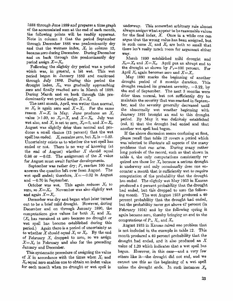
1888 through June 1889 and prepares a time graph of the accumulated sum a t the end of each month, the following points will be readil3 apparent. Note in column . 2 that the period September through December 1888 was predominantly dry and that the wetness index, XI in column 12, became zero d u h g December. During December and on back through this predominantly dry period assign X=Xz.

Following the slightly dry period was a period which was, in general, a bit wet. This wet period began in January lS89 and continued through July 1889. During this period the drought index, Xz, was gradually approaching zero and finally reached zero in March of 1889. During March and on back through this predominantly wet period assign X=Xl.

The next month, April, was wetter than normal, SO X2 is again zero and X=X,. For the same reason X=X, in May. June produces an X I value >1.00, so X,=X, and X=X,. July was wet also, and XI is set to zero, Xz=O, and X=X3. August was slightly drier than normal and produces a small chance (13 percent) that the wet spell has ended. XI remains zero, but X z is -0.02. Uncertainty exists as to whether the wet spell has ended or not. There is no way of knowing (at the end of August) whether X should equal 0.98 or -0.02. The assignment of the X value for August must await further developments.

September was rather dry; P, reaches 100 and answers the question left over from August. The wet s p d ended; therefore, X=-0.02 in August and -0.70 in September.

October was wet. This again reduces x2 to zero, so X=X,. November was also slightly wet and again X=Xl.

December was dry and began what later turned out to be a brief mild drought. However, during December and on through January 1890, the computations give values for both X I and Xz. (X3 has remained at zero because no drought or wet spell has become established during this period.) Again there is a period of uncertainty as to whether X should equal X, or Xa. By the end of February X, dropped to zero, so we assign X=X2 in February and also for the preceding January ‘and December.

This systematic procedure of assigning the value of X in accordance with the times when X, and x2 equal zero enables one to obtain an index value for each month when no drought or wet speU is

underway. This somewhat arbitrary rule almost. always assigns what appear to be reasonable values for the final index, X . Once in a while one can argue that the wrong value has been assigned, but in such cases X , and X2 are both so small that there isn’t really much room for argument either way.

March 1890 established mild drought and x3=x2 and X=X3. April put an abrupt end to the drought as shown by P,=100 percent. For April X, again becomes zero and X=X,.

May 1890 marks the beginning of another drought period of 8 months duration. This drought reached its greatest severity, -3.22, by the end of September. The next 3 months were drier than normal, but not suffciently dry to maintain the severity that was reached in Septem- ber, and the severity generally decreased until the abnormally wet weather beginning with January 1891 brought an end to this drought period. By May it was definitely established (col. 8) that the drought had ended and that another wet spell had begun.

If the above discussion seems confusing at first, please recall that table 12 covers a period which was ‘selected to illustrate all aspects of the many problems that can arise. During many rather long periods of the record, such as that shown in table 4, the only computations consistently required are those for X3 because a serious drought is underway and only occasionally does one en- counter a month that is sufficiently wet to require computation of the probability that the drought has ended. The slightly wet May 1933 in Kansas produced a 6 percent probability that the drought had ended, but this dropped to zero the following month. The wet August 1933 produced a 40 percent probability that the drought had ended, but the probability never got above 47 percent (in February 1934) and by the following spring it again became zero, thereby bringing an end to the computations of P,, X,, and &.

August 1933 in Kansas raised one problem that is not included in the example in table 12. This month produced a 40 percent probability that the drought had ended, and it also produced an X value of 1.20 which indicates that a wet spell has begun. However, in this case-and a very few others like i G t h e drought did not end, and we cannot use this as the beginning of a wet spell unless the drought ends. Jn such instances Xs

33

does not equal XI and the XI computations must be continued in column 12 until P e reaches zero or 100 percent or until X I returns to zero.

It might be well to point out that tables 1, 4, and 12 make up the work sheet that one uses to make these computations.

11. RESULTS FOR WESTERN KANSAS DROUGHTS

The monthly index computations were carried out for western Eansas for the 71-yr. base period, 1887-1957, and later for the years 1958-1962. The values of X are listed in table 13. Let us examine the index values for some of the individual months to see what one might conclude as to their reasonableness or representativeness.

As has been pointed out previously, there is hardly any satisfactory means for checking the validity of index values which indicate “mad” or “moderate” drought. However, “extreme” drought produces conditions which can be recognized and more or less agreed upon.

THE DROUGHT OF 1894

It is dfficult to locate any very concrete information concerning the drought of 1894 in western Kansas, but the following statements are indicative of the situation. Tannehill [43] mote, “. . . the great drought of 1894 brought complete crop failure and disaster [to the Great Plains]. As many as 90 percent of the settlers abandoned their farms in some areas.” In the Department of Agriculture Yearbook for 1894 [ll] we find, “During the prevalence of this hot period [in late July 18941 the prospects for crops [over portions of Kansas and Nebraska], already un- favorable on account of prolonged drought, were grestly reduced. Much corn was completely dried up and cut for fodder.”

From other sources [13] it is apparent that western Kansas was included. in these rather general statements. At any rate 1894 has gone down in history as a year of disastrous drought and it seems reasonable to assume that the drought was “extreme” during a t least the latter part of the summer. I n table 13 the index indicates extreme drought (> -4.00) from July through December 1894.

THE DROUGHT OF 1913

The next serious dry period in western Kan- sas reached its peak of severity in August 1913.

Fortunately, the drought months during 1913 did not follow directly on the heels of the very dry period of 1910 and 1911; the intervening year of 1912 was abnormally wet. Even so, 1913 produced Some memorable corn- ments in the Monthly Weather Rewiew of August 1913 [17]. For example, “The month [of August] will long be remembered 8s one of the most disastrous from an agricultural standpoint ever experienced.” Also, “The drought of the summer of 1913 was one of the most damaging droughts that Kansas has experienced since authentic weather records were begun in the State.” And,

. . with the possible exception of the summer of 1874, the summer of 1913 stands alone as the driest the State [as a whole] has experienced since the early fifties. . . .” The index shows moderate drought in July and extreme drought in August.

THE DROUGHT OF THE 1930’s

( I

Agricultural Aspects.-The drought during the 1930’s was the longest and most serious of record in western Eansas. Between August 1932 and October 1940 the index indicates 38 months of extreme drought. There is a great deal of information about this drought period and its effects. Many books and innumerable articles have been mitten. One useful source of information of 8

a@cultural nature is the Weekly Weather and GOp Bulletin [65]. From the Kansas reports representative remarks pertinent to the wester* thisd of the State are listed below.

July 25, 1933-----_ Corn needing rain badly and Some greatly damaged.

Aug. 1, 1933------ Pastures poor or dried UP, Cattle being shipped out in some local1- ties. Stock water scarce in many places.

June 26, 1934----- Needing rain badly in all parts. July 3, 1934------ Hot and dry. All crops need rain

badly. Corn condition critica1, crop badly stunted. Pastures insufficient to support livestock in much of west.

July 17, 1934.. - _ _ Corn stunted and burned until

34

TABLE^ l3.-Dtought (and wet spell) index, X , western Kansas

-0.11 -. b .6: -. 41 .6: 3.4'

-1.H -2. w -3.M -. 1;

* 03 .I 0 .32

-1.18 -1.29 -. 51 -1.17

.47 1.71 -. 07 .21 -. 34 2.20

-3.05 .45 -. 75 -. 20 . 09 6. 66

-1.81 -2.20 2.10 2.13 1.98

-1.30 -2.09 4.75 -. 50

-1.13 -2.40 -1.50 3.84 -. 26 2.54 .63

-2.07 -2.24 -4. 5tl -3.12 -3.71 -4.32 -3.10 -4.11

1. 13 4. 56 -. 14 1.32 3. 77 -. 93 4.30 2. 10 1.34 -. 88 1.67 4.02

-2.48 -1.32 -3.18 -3.16 -5.26 2. 52 3. 40 2. Go 1.39 1.92

1 Jan. - -

June

-0.8 1.1 1. 11

-1. 7! 2.71 3.9'

-3.41 -3.71 . 71 -. 51 .E 1.81 .1: -. 1(

-1.2f .4f 2.51 .4( 1.85 1.55 .I6 .64 1.05

-2.05 -4.03 2.09

-1.90 .60 4. OB -. 35

-2. Ea -2.34 3.11 .85 .17 -. 19 2.69 -. 73

-3.00 -2.34

.59 2. 92 2.25

-1.24 -. 38 1.05

-3.46 -4.20 -3.64 -3.81 -4.31 -2.48 -3.16 -3.12 3.49 4.71

- =

Feb.

-0. : -1. (

-. 1 3.1

-1. I -2.3 -2.7 -.e

. 2 -. 3 -. 0 . 6 .o

-1.2 1.6

-1.5 .4 1.3 -. 3 .4 -. 5

1. g: -1. 71 1. 4' -. 4( -. 11 .fi -. 1:

-2.01 -1.91 2.81 1. 51 -. li .O1

-2.3( 4.0: -. 7>

-1.44 -2. It

.4f 3.5s -. 7f 2.6E .34

-2.23 -1. 6C

-3.17 -3.64 -4.11 -2.50 -3.83 1.24 4.20 -. 55 1. 42 3.3G -. 98 4.03 2.47 1.42 -. 91 1. 67 3.40

-2.64 -1.69 -2 05 -2.98 -6.22 2.41 2.99 3. 74 .88 1.52

' . I

-4.0a

-0. !

-1.; * I

1. * 4. I

-1. I -2. I -2. i -. i

. 2 -. t -. (

.3

.2 -. 9 1.3

-2. 1 .3 1.6 -. 8 -. 6 -. 0 -. 8

-2.2 2.1 -. 6 -. 6 . 9 -. 5

-2.11 -1. 6, 2. 81 . 9' -. 6' .61

-2.3, 6. M

-1.2. -1.1: -1. 5' . GZ 2.9:

-LO( 3.5: .41

-2.6f -1. a -4.8f -3.5c -3.17 -3. 9c -1.94 -3.29 1.16 4.08 -. 71 1.85 2.46 -. 67 4.23 3. I8 2.00

-1. 08 1. 36 3.47

-2.50 -1.73

-3.16 1. 31 3.74 3. 10 3.80 1.02 1.91

-3. oa

-

- .__

, Apr.

-0. E 1.2

. 7

1.0 3.2

-2.3 -2.9 -2.9 -. 0 1.3 -. 9 -. 5 1.8. .a,

-1. 6: 1. 7<

-2. 01 I. 4: 2.01

-1.2: -1. 41 -. 6L -1. 41 -2 4L 2. M -. 7f -. 61 1.6t -. 24

-2.01 -1.32 3.38 1. 14 -. 51 1. 36

-2.20 -.OB -1.57 -1.31 -1.21

.30 2.52

-1.32 3.37 .44

-2.45 -2.56 -5.46 -3.98 -3.71 -3.49 -2.22 -3.37 1.59 6.24 -. 80 4. 18 2. QO

-1.81 4.31 1.92 1.91

-1.52 1. 25 3.07

-2.28 -2.54 -3.15 -3.55 1.53 3.52 2.34 3.43 .67 1.30

.a

- almost ruined. Pastures too poor to support livestock.

Aug. 7, 1934- - - - - - Conditions worst ever known in many places. Corn not sufficient growth even for fodder in many western counties.

Distressed animals being shipped out in increasing numbers.

Aug. 14, 1934- _ _ _ _ Pastures generally bare.

-0. t 1. t

. f -. 6 1. E 4. E

-2. a -3.6 -2.9 -. 6

.8 1.3

-1.2 -. 3 -. 5 .3 2.4 . o

1. 91 1 . 4

-1.51 -1. 9, -. 81 -1.43 -2.71 1.3;

-1.7: .6: 3.11 -. 81

-1.8i -1.24 3.0[ 1. Of

-1. ot 1.44 1.75 -. 21

-2.11 -1.88 -2.17

1. 40 2.58 -. 98 -. 02 -. 85

-2.14 -3.74 -4.07 -2.99 -4.48 -2.43 -2. 96 -2.77 2. 10 4.19

-1.29 4.87 2.33

-1.44 5.02 1.62 2.86

-1.82 2.40 -. 22

-2.45 -1.91 -2.57 -4.40 2.67 3.68 1.91 3. 12 1. 16 .79 -

-1.41 4.21 2. 51

-1.72 5. 17 2.38 4.40

-2.55 4. 77

-1.58 -3.52 -2.69 -2.38 -5.43 3.87 3.61 1. 04 3.51 1.56 2.03

- - July

-1. 1. 1.

-2. t 4. : 3. 1

-4.1 2. i

-

-3.;

-. i 1: ; 1.3 -. I

-2.2 .6 2.8

.6 3.0 2.4 .4 .6 1.2

-2.5 -3.7 2.3

-2.8 .51 5. 5

-1. I1 -3. 11 -2.1' 3.2:

.M

.3: -. M 3.3: -.7( -3.1: -2.5L

.81 3.94 2. 11

-1. 4f -. 81 -. 52 -4.07 -5.47 -4.66 -4. Qc -4. Qc -2.67 -3.9s -3.87 4.73 4.32

-1.90 5. 42 2.31

-2.33 5. 05 2. GO 5. 17 1.78 5.82

-2.22 -3.47 -3.42 -3.50 -5.31 4.07 6.28 .98 3.04 1.78 3.12

- - Aug - 0. 1.

-.I

3. 4.

-3. I -4. I

1. ' 1. : -. E

-1. E . 4 3. c .E 2.3 2.6 .6 . e -. 8

-1.9 -3.2 3. 6

-4. 1 .8 7.5

-1. 2 -2.61 -2.6' 2. 1' .9 -. 4. -. 51 3. 71 -. 7!

-2. z -2.81 1. 61 4.31 1.6:

-1. K -. 7( -1.2: -2.4: -5. 9f -6.11 -5.55 -5. 45 -3.86 -4.4t -3.13 5.13 4.33

-2.14 5. 02 2. 12

-2.62 4.09 3.27 6. 11 3.80 G. 27

-2.02 -3.14 -3.45 -4.21 -5. 66 3. 64 6. 71 .76 2.11 2.27 2.83

-3. !

2. ! . ( -

-.

- - Bept.

-0. ( -. 5 -. 7 -3.2 4.7 -. 7

-2.8 -4.4 -. 7 -. 6 1.0 2.9

-1. 1 . 9, -. 9 .a -. 6 1.1 2. I1 2.9: -. II -. 61 .2:

-2 II -3. e4 3. (Ir 1.1: -. 6< 7. ai

-1. @ -2.13

.4E 2. BE 1.4c -. 37

-1.26 4.64 -. 47

-1.38 -2.72 . 01 3. 78 2.05 . 01

-1.64 -1.33 -2.89 -5.31 -4.26 -4.79 -5.34 -2.89 -5.26 -2.89 5.74 4.07

-2. 82 4. 03 2.01 . 89 2.74 2.39 5.39 3.48 6. 74

-2.65 -3.78 -3. QB -3.42 -6.20 3.91 5. 18 1.35 I. 88 1.61 2.08

- - I_

Oct.

-0. I -. 4 . f

-3. i 4.4 -. f

-8. c -4. e -. 7 -. 0 2.1 2.1

-1.3 -. 6 -1.0 1.2 -. 7 1.1 1.8 3.6 -. 2 .2 .n

-2.7 -3.22 -. 31

.58 -. 6' 7. 41

-1. 71 -2.3;

.9: 2.84 2. 14

-1. o( -1. af

G. 14 -. 57 -1.24 -3.22 -. 67 4.40 2.18 2w

-1.80 -1.52 -2.94 -5.33 -4.23 -4.44 -4.87 -3.52 -5.65 -3.31 6.12 4. GI

-2.73 3.69 -. 42 3.43 1.82 1.81 5. 28 2.84 6.02

-3.08 -3.37 -3.44 -3.84 4 . 1 4 3.74 4.00 2. 64 1.69 1. 38 -. 35

- ~

Nov.

-0.3 -. 6 .7

-2.9 3.6

-1. 1 -2. B -4.71 -. B. -. 11 -. 2, 1. 81 .a -. 9'

-1.4: -. 31 -. 7( -. 6: 2. 5: 3.5[ -. 61 1.14 I. BE

-2.91 -2.95 -. 43

.7G -1.13 6.61

-1.92 -2.49

.71 3.09 1. 90

-1.41 -1.59 5.52 -. B6 -. 87

-2.77 -1.08 4.71 2.78 3.18 .30

-1.80 -2.59 -4.96 -3.52 -4.50 -4.76 -3.50 -5.44

.63 5. 46 3. BO

3. 49 -. 91 4.94 1.95 1.18 -. 55 2.20 5. 41

-2.62 -2.14 -3.70 -3.79 -6. 78 I 3.45

-a. 88

-. 41

- Dee. - -0.38. -. 84 -. 60. -3.16 3.87 -. 93

-3.12 -4. 08 -. 62 -. 48

.02 2.20 .05

-1.16 -1.49 -. 35 -. 95 .17 1.96 -. 11 .65 -. 28 2.23

-3.02 .73 -. 71 2.62

-1. os 6.86

-1.84 -2.60 2.58 2.68 1.83

-1.25 -1. 83 6.25 -. 32

-1. OB -2.43 -1.24 4. 25 -. 26 2.94 .05

-1.84 -2.15 -4.80 -3.45 -4.12 -4.46 -3.53 -4.80

.61 5. 10 3.89

3 20 3.44 -. 87 4.33 2.28 .91 -. 75 1. 56 4. 66

-2.34 -1.39 -3.66 -3.63 -5. 70 2.65 3. 44 1.91 1.89 1. 95

-. 54

Sept. 4, 1934----,- Russian thistles being put up as fodder.

Oct. 9, 1934- - - - ~ - Winter wheat sowing delayed by dryness and crop making little growth.

Nov. 27, 1934..--,- Wheat fields bare in nearly all of western third.

Feb. 27, 1935 _ _ _ _ _ _ Severe duststorms. Apr. 16, 1935- _ _ _ _ Severe duststorms; practically nu

pastures in western half.

35

May 7, 1935- - - - - - Duststorms [continue] frequent in western half; wheat crop very poor t o poor in western half and deteriorating.

May 28, 1935----- Rain. July 2, 1935------ Moderate rains in northwest, south-

western counties are needing moisture.

Much [of corn crop] damaged beyond recovery. Pastures deteriorating rapidly in west.

Aug. 27, 1935----- Corn in southwest counties not worth

Pastures greening.

July 30, 1935----- Dry.

Oct. 29, 1935-----

Nov. 19, 1935-----

Mar. 17, 1936----- Apr. 21, 1936 --_--- May 26, 1936----- June 23, 1936----- July 28, 1936------

Sept. 1,1936 - -_- - - Nov. 24, 1936 _ _ - - e

Dec. 1, 1936 ___- -_

Mar. 2, 1937 _ _ _ _ _ _

Apr. 27, 1937----- May 25, 1937-----

June 22, 1937-----

cutting. Grain sorghums badly stunted. Pastures deteriorating.

Wheat very poor to poor in extreme west.

Forage scarce in most of western half where wheat pastures poor.

Duststorms again reported. Many [wheat] fields bare. Pastures much improved. Wheat badly damaged. Little [corn] in the western half will

Pastures brown and scanty. Wheat needs moisture rather badly;

some soil blowing. Pastures scanty. Wheat deteriorating. Moderate dusb

storms. Considerable damage from previous

duststorms. Substantial moisture badly needed.

be fit for forage.

Duststorms frequent. Wheat deteriorated in most of west

and greatly damaged in southwest. Pastures weedy in west [from pre-

vious rains]. July 20, 1937----- Corn stunted and not tasseling, Aug. 31, 1937----- Soil moisture very deficient. Pas-

Sept. 28, 1937----- Duststorms in southwest. NOV. 16, 1937-,--- Duststorms. Dec. 7, 1937------ Wheat deteriorating in southwest. Apr. 26, 1938 _ _ _ _ _ Duststorms. June 28, 1938- - - - - Corn making satisfactory growth.

Aug. 30, 1938----- Soil very dry; corn badly burned. Sept. 20, 1938----- Soil moisture sufficient for early

growth [of wheat]. Nov. 15, 1938----- Many wheat fields bare, some showing

drill rows and, in favored localities, covers ground; root system there poor.

tures dried badly.

Wheat deteriorating.

Pastures improving.

Dec. 6, 1938--- _ _ - Wheat deteriorated. Jan. 10, 1939 _ _ _ _ _ Heavy duststorms. Feb. 21, 1939- _ - _ - [More] duststorms. Mar. 14, 1939--- - - Sufficient topsoil moisture for present

needs and outlook is improved. Apr. 11, 1939----- soil moisture now ample except in

some western counties. Winter wheat improved; rank growth in southwest.

May 2, 1939------ Winter wheat deteriorated. May 23, 1939----- Lack of rain being felt in west,

especially in southwest where condition serious. Wheat deteriorated.

Aug. 1, 1939- - - -_ - Corn deteriorated; bulk in West damaged beyond recovery.

Sept. 5, 1939------ Record-breaking heat, soil moisture badly depleted. Condition of all crops declined. Wheat seeding halted account dry soil.

Oct. 17, 1939- - - - - Severe duststorms. Pastures very poor.

Oct. 31, 1939----- [Still] waiting for rain [before seeding winter wheat]. Sowing so far has been done in dust.

NOV. 28, 1939----- Much [wheat] not germinated, seeding still underway.

Dec. 19, 1939----- Winter wheat condition generally lowest on record. Duststorms.

Mar. 5, 1940------ Moisture ample for current needs. Apr. 30, 1940- - -_- Moisture deficient in western third,

especially in southwest where duststorms [occurred]. Wheat fair in west.

May 28, 1940----- Wheat crop poor and weedy. Pas- tures growing well.

July 2, N40- - - --- Hot winds shriveled [wheat]. July 30,1940------ Severe damage to corn; half to three-

fourths tassels burned white. Grain sorghums deteriorating. Pastures not sufficient to support livestock.

Aug. 13, 1940----- Rain adequate for current needs. More than half of corn [Statewidel past help. Pastures poor, but will revive.

Aug. 27, 1940----- Soil mostly too dry [for wheat seeding]. Pastures poor.

Oct. 1, 1940------ Topsoil moisture sufficient to abun- dant. Bulk of wheat up to excellent stands.

Oct. 29, 1940- - - - - Moisture badly needed. Wheat growth slowed. Pastures dry.

Dec. 3, 1940 _ _ _ _ _ _ soil moisture penetrated to 1 to 2 feet or more. Wheat good $0 excellent condition with sufficient moisture to carry i t through the winter.

Deo. 24, 1940----- [Wheat] prospects better than for a considerable number of years.

When one compares these remarks with the index values for the corresponding months in table 13, it becomes apparent that the index numbers are fairly representative of the severity of the agricultural drought. Consider, for instance, the fall of 1939. Many accounts of this great drought of the 1930’s fail to point out that this was the worst fall season that occurred. The index indicates extreme drought, and the published remarks ‘during October, November, and December substantiate it: pastures were very

36

Poor; it was too dry to plant wheat; and dust storms raged nearly every week.

Vegetative Cover Measurements.-Weaver and Albertson [70] have presented so many observations and interesting details of the effects of drought on the plant communities of the Great Plains that it is difficult to select an illustrative example. However, the basal cover measurements which they made annually (apparently in the fall) for over two decades in an ungrazed area near Hays, Kans. are indicative of the seriousness of the drought that prevailed in the 1930’s and again in the 1950’s. (Hays lies just to the east of the western Kansas area studied here.)

The most interesting feature of the figures in table 14 is the fact that they show that the drought in the 1930’s was essentially continuous until ye- viva1 of the vegetation began in 1941. The data (not shown) from the moderately grazed and overgrazed plots at Hays show a much more rapid deterioration of basal cover during the initial drought years. The overgrazed plot was reduced from 80 percent cover in 1932 to 30 percent cover in 1934. The minimum of 3 percent was reached in 1936. Some slight increase in cover took place in 1937, 1938, and 1939, but by 1940 the cover was only 14 percent. Incidentally, recovery in 1941 was slightly more rapid than on the ungrazed area.

The Duststorms.-Other aspects of the drought picture in western Kansas during the early 1930’s have been pieced together by Johnson I231. He paints 8 fairly vivid picture of the trials and tribulations of those people who were Strug- gling to eke out a living from the land during those dry years, From Johnson as well as from the numerous publications of Albertson and co- workers at Kansas State College, Fort Hays, it is very clear that much of the notoriety associated with the years of 1934-1930, is a direct result Of

year percent Year Percent yew Percent cover ___- ____ --

1932.. ~g 1038.-.. a0 1944 .... 05

1934------- 85 1040.-.. x) 1 9 4 ~ . 89 19a5 - - _ _ _ _ _ 65 1041---- 1947 _ _ _ _ 88 1936------- 68 io42.-.. 94 1948---. 83

cover COVer

“33--::::: 86 lQ30---. 22 1946.-.. 83

lQ37------- 20 1043 _ _ _ _ 90 1848--.. 82

the unusually strong winds which created the terrible duststorms during those years. The wind combined with the drought to produce the disastrous conditions and the publicity. Other years have been about as dry and nearIy as warm, but they lacked the strong winds, and the droughts were therefore less spectacular as well as less damaging.

.Disaster Declaration.-On June 19, 1934 Congress passed an emergency appropriation bill providing funds for the purchase of drought- stricken livestock. This program got underway at approximat,ely the same time that the index indicates the existence of an extreme drought condition. Apparently a t that time there was recognition that an extreme and disastrous condition had developed. On this basis one could postulate that extreme drought may well have coincided with the conditions which led to an official designation of “drought disaster area. J J

yew Percent In September of 1954 the moisture shortage _-. was apparently more pronounced; but, the iwo -.-- 91 published Crop Bulletins for that period are m 2 - - - - !; unfortunately rather vague. The comments are 1063 -_ -_ 196*---- so general that it is &&cult to tell very nluch

cover

1051---- 90

THE 1950’s DROUGHT

The drought which began in Icansas in 1952 was a very serious matter by the summer of 1953. A t the end of June the drought index indicates a severe drought. On the last day of June the Disaster Designation Committee of the U.S. De- partment of Agriculture, on the basis of first-hand reports from the drought area, declared all 31 counties of western Ihnsas a disaster wea. Although the index does not show extreme drought it is interesting to note that the index value is very close to the value it had when drought disaster was recognized in 1934.

By the end of September 1953 the drought situation was even more critical. The index is -3.78 and the agricultural reports [66] indicate a serious shortage of feed with farmers faced with the choice of selling part of their breeding herds or buying high-priced feed. Table 14 shows the astonishing decrease in measured basal cover that had occurred during 1953. Also the streamflow

37

Kansas. From reading all the reports one is aware that the area was very dry with delayed wheat seeding, feed shortages, and poor prospects in general.

The streamflow data for September 1954 show very slightly more runoff than during September 1953, but apparently this was the result of fairly heavy rains between the eastern border of the area and the gaging station at Beloit. The basal cover data in table 14 give a specific bit of infomation which reinforces the idea that very serious drought conditions existed in September 1954.

In 1955 the spring rains again produced some temporary alleviation of the drought, but during July the situation became critical and the Kansas Weekly Weather and Crop Reports 1631 of August 2 indicate that the crop, pasture, and hay prospects were fading rapidly, with supplemental livestock feeding on the increase. By the end of August (report of Aug. 30) it was apparent that many grain sorghum fields would not head, corn would not produce grain, and the pastures were supplyirlg practically no feed a t all. Further evidence of the extreme drought during August is the fact that the runoff for the month established a record low for August (see table 15).

The moisture situation was dismal all during 1956. The spring was dry and the summer and fall were drier. The total runoff for the year, computed by the method described in the next section, was the lowest of record. The following remarks [67] illustrate the extreme seriousness of the drought in western Kansas.

May 28, 1956----- Pastures furnishing little or no grazing.

July 2, 1956------ Dry soil delayed planting [of grain sorghums] and stands poor. Rain urgently needed. Supplemental feeding of livestock still necessary. Drought intensified.

July 30, 1956- - _ _ - Grain sorghums at a standstill; plants firing. Corn tassels turned white and stalks firing.

stands, but plants beginning t o die. Herds being liquidated.

Much damage to seedbeds [by severe duststorms]. Wheat plants dying. Kansas River last three days lowest stage of record,

Oct. 8, 1956------ All major streams at near-record low flows.

Oct. 22, 1956----- Fields [for wheat] powder dry and seeding awaiting rains.

006. 29, 1956----- Strong winds and dust severely damaged newly emerged [wheat] seedlings. Winter roughage supplies critically low.

Nw. 12, 1956----- [Wheat] seeding continues in southwest and west central where soil powder dry.

When one compares the above remarks with the appropriate index values in table 13, it becomes apparent that the index values are relatively representative of the general agricultural situation. An index value of -4.00 seems to correspond reasonably well with “extreme” drought.

Sept. 24, 1956----- Seeding being delayed.

DROUGHT AND STREAMFLOW

‘Records of rates of streamflow can also be 3xamined to determine whether or not such data show a useful relationship to drought severity. However, the available data pertinent to the western third of Kansas are far from satisfactory inasmuch as the stream-gaging stations are SO

located that the measured flow is not by m y means dependent on only this area.

Four drainage basins are represented in the western third of Kansas [42]. An area in the northwestern corner, the equivalent of four or five counties, lies in the Upper Republican River basin and the drainage is toward the northeast. There are no long-record gaging stations which could be used to represent the runoff from this relatively small area. A similar situation exists in the southwestern part of the State where the Cimarron River carries the runoff from seven or

27, 1g56----- Droughty conditions steadily in- eight counties. Here too no records are available for the period of concern in this study.

At Garden City, Kans., there is a long record of ~uwAE on the Arkansas River [54]. This

-

creasing. Crop5 continue to de- teriorate. Many sorghum fields beyond help. No available soil moisture to 4 f t . at Garden City.

[of wheat] emerged to- uneven one that can be used for this portion of the State.

38

With the exception of the previously mentioned counties in the northwest, the northern half of the western third of Kansas is drained by the Smoky Hill, the Saline, and the Solomon Rivers. Good runoff records exist for all three rivers [55]. The long-record stations are all a little too far east of :u area, but the data may be at least partially Indicative of the runoff from the area of concern.

The stations used were at Ellsworth, on the Smoky Hill River, Tescott on the Saline River, and Beloit on the Solomon River., The records of monthly runoff in thousands of .acre feet were tabulated for these three stations and for Garden city for the period May 1929-August 1950 and the period October 1952-September 1957. No effort was expended in weighting or adjusting these records because even at best one could hardly expect to get more than a rough indication of the runoff from the study &rea. Therefore the runoff from the four stations was merely added to obtain a single value for each month. From these records table 15 was prepared. The three lowest index values for each month from table 13 have also been entered on table 15 for convenience.

From this table a number of things are apparent. pkst, the record low runoff for the 1-5-month Period ending with April occurred in 1935. One can see also that the most serious April drought, as indicated by the index, also occurred in 1935.

The lowest I-month and %month runoff values for the other months appear to coincide reasonably well with the lowest index values. For instance,

6

the least April and May runoff (11,600 acre feet) occurred in 1937. The index, -4.48, also indicates the most serious May drought occurred that same year. Also, the least May and June runoff occurred in 1933 with 1956 not far behind (see footnote, table 15). The driest June according to the index was 1956 which was also the year with the least %month total runoff.

The remaining months in the table show much the same sort of thing. Considering the crude method of handling the only partially represenb ative runoff informa tion, the correspondence between years of very low index numbers and years of very small runoff is rather encouraging, but not unexpected. Both are a consequence of about the same climatic elements.

The reader wil l no doubt have noticed that the largest negative index value occurred in 1956 rather than in 1934 or 1936 as might have been expected. The runoff data for the periods ending with September seem to confirm that this dryness in 1956 was at least as extreme as that during &e drought in 1934. As previously mentioned, some eflects were worse in 1934 than in 1956 because of the wind and dust in 1934.

Yoar and amount of tho 3 lowest Index vlrluos lor tlio month

PASTURE FEED CONDITIONS

At the beginning of each month during the period April 1 to November 1 the United States Department of Agriculture receives numerous reports on pasture feed conditions in each State.

- Ant.

6.2

11.6

a43.1

26.6

16.6

18.4

2.7 3.6

TABLFI 15.-Droughl i n d a value6 and the least amount Of runoff (thowands Of acre-feet) during periods of various leiiglhs ending with the month and year shown, western Kansas ...- -

I

Yr. Amt. Yr. Amt. ----- 1936 ao 1936 10.2

1937 22.8 1934 ~38.9

I966 66.4 1940 66.3

1933 63.4 1933 88.4

88.9 1056 122.6

1934 45.3 1966 110.6

1966 20.1 1934 47.9

Ig66 6.6’ 1958 23.3

1940

-- Amt. --

2.9

6.9

6.3

D.8

6.0

1.0

1.6 2.1

Yr.

1936

1937

1833

1938

1934

19.56

1966

1939

Yr. Amt. --- 1935 12.6

1966 45.8

1940 68.2

1933 95.6

1966 128.7

I956 123.6

1966 112.2

1934 50.4

-5.46 1935

-4.48 1937

-5.49 1966

-5.47 1934

-5.98 1934

-6.20 1 95Li

-6.14 1956

-5.78 1956

- -3.08

19.36 -4.40

195ti -4.31

1937 -5. a1 1058

-5.65 lD5Li

-5.34 lD39

-5.55 1039

-5.44 1939 -

-3.71 1037

-4.07 193.5

-4.20 1934

-4. DO 11936 -5.55

-6.31 1934

-6.33 1934

-6. e8 1934

1938

__

39

a W > a

‘ Z 9-0 k g g s

:% E k

01: k I =?i

k

W

I-

a u) z z

0

;q==l 4: I I I I , I

t- 2 40

30 -6 -5 -4 -3 -2 -1 0 1 2 3 4 5 6

Ti. MEAN INDEX, MAY-OCTOBER

FIQURE 4.-Mean pasture condition, western Kansas for

(Data for period 1932-57.) June 1 to November 1, versus the average index the same growing season.

150

140

130

120

((0

100

90

80

7 0 t 0 46 .43

32 54

-52

53 055

0 33

036-= YEAR, 1936

.40

These subjective reports are expressed in terms of percent of normal condition, where “normal” indicates not the average but the expected condition under very favorable weather.

These monthly data for the western third of Kansas for 1932 through 1957 were obtained from the United States Department of Agriculture Crop Reporting Board by personal communica- tion. Each monthly value represents approximately 200 individual reports. These data apparently contain some month-to-month and season-to-season fluctuations and trends which are in part dependent on the outlook and state of mind of the observers. It is suspected that

the reports tend to show an exaggerated response to month-to-month weather changes. For example, from other accounts, such as table 14, there is evidence that. pastures became gradually poorer and poorer during the drought in the 1930’s. However, these condition reports show a very abrupt drop to a minimum of 11 percent of normal during 1934 followed by an improvement to 30 to 50 percent of normal during 1939.

I n addition there are month-to-month trends in the data which indicate that a given percentage does not mean the same thing from month to month. For example, the average reported conditions for 25 years were as follows:

Percent Percent Apr. 1 _ _ _ _ _ _ _ _ _ _ _ _ _ _ 64 Aug. 1 _ _ _ _ _ _ _ _ _ _ _ _ _ _ _ 62 May 1 _ - _ _ - - - - _ _ _ _ _ _ 64 Sept. 1 _ _ _ _ _ _ _ _ _ _ _ _ _ _ 60 June 1 _ _ _ _ _ - - - _ _ L _ _ _ 68 Oct. 1 _ _ _ _ _ _ _ _ _ _ _ _ _ _ _ 59 July 1 _ _ _ _ _ _ - _ - _ _ _ _ _ _ 69 Nov. 1 _ _ _ _ _ _ _ _ _ _ _ _ _ _ 62

In order to remove this variability all the monthly values were recomputed in terms of mean reported condition. For example, a report of 34 percent of normal on June 1 becomes 50 percent of mean reported condition.

From these monthly values of mean reported condition it was possible to obtain a mean value for the period June 1 to November 1 for each year. Figure 4 shows the relation between this measure of pasture condition and the average April to October index (from table 13). The poorer condition in the 1930’s as compared to the 1950’s may be related to the amount of wind. The relatively poor condition in 1957 is the result of the poor condition (55 percent) that existed in the spring of this wet year. All in all, the index appears to be relatively representative of pasture conditions in western Kansas. No effort was made to investigate similar relationships in other areas.

12. DROUGHT CONDITIONS IN CENTRAL IOWA

The monthly index values for central Iowa for the period 1930-1962* are shown in table 16. Only in 1931, 1934, 1936, 1956, and early 1957 does the index indicate really serious drought. Crops were rather poor in 1931, especially in the northern part of the area and average corn yield for the entire area was only 38.9 bushels per acre.

1930 and the years sinw 1957 were analyzed Wing the coefncients from the bga period, 1931-57.

40

THE DROUGHT OF 1934

The severity of the drought in 1934 is evidenced by the following remarks [61] concerning the agricultural situation in central Iowa. May 15, 1934----- Intense duststorms; meadows poor;

hay and oats practtcally ruined; farm crop outlook poorest in mem- ory; water scarce on great many farms.

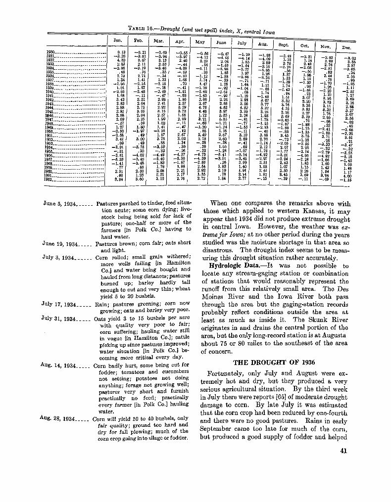
TABLE 16.-Drought (and wet spell) indez, X. central Iowa

June

-0.47 -4.45

2.04 -1.63 -5.98

1.66 -1.33 -.33 1.25 --.=

-2.61 -.92 2.24 2.65 4.52 3.97 2.35 5.35

-1.21 -1.24

1.18 2.87 2.60

-.38 1.05

-1.28 -b.41 -3.91

.26 1.82 2.19 .78

1.84

I Jan. July -- -1.2 -4.1

1.8. -1.6, -5.7:

1.9: -2.85 -.71 1. 64

-1.04 .6E

-1.18 2.9€ 3.56 4.82 3.39 2.28

-.81 -.77

-1.53 -.11 3.10 2.69

-.41 .OB

-1.07 -5.14 -3.45

2.90 1.40 1.91 2.14 2.17

0. 13 -3.26

4.10 2.63

-2.95 .49

2.73 1.34

-1.06 1.01

-2.69 1.68 3.43 2.83 2.88 2.81 2.58 2.69 -. 57 1.27

-2.50 -2.58

3.41 . 09

-, 31 -3.61 -5.23 -1.41

.77 2.31 .60

3.34

-a. 91

NoV.

-2.62 2.99 2.76

-2.81 .82

2.44 .7c

-1.70 1.26

-2.20 1. 10 3-16 3.13

3.32 1.76 2.95

- a 0 8 I22

-2.41 -1.88

3.71 .26

-3.33 -*32

-2.79 -4.92 -1.66 1.60 1.42 1.84 3.94

--.e9

3.11

-- Feb* I Mar. Dec. -- -3.02

3.86 2.87

-3.06 .34

2.55 .90

-1.95 1.11

-2.52 1.27 3.6% 3.16

3.27 2.07 2.56 -.02

.45 -2.88 -2.26

3.61 .21

-3.47 -.32

-3.25 -5.15 -1.45

1.05 1.48 1.17 4.69

-1.16

2.88

-0.21 -3.81

3.67 2. 11

-3.19 .76

2.71 1.41

-2.16 1.67

-2.45 -.11 3.31 2.64 2.75 3.05 2.04 2.25 .59

1.30 -1.97

.49 3.00 .49

-3.76 .30

-4.02 -5.48 -1.48

.88 2.36 1.23 3.60

I

-0.6( -3.9<

3.1: 2.6:

-3.4E .31

-.34 1.33

-2.16 -.18

-2.40 -.47 2.98 2.41 2.92 3. 15 2.57 1.99 1.02 1.41

-2.26 1.57 3.75 .88

-3.69 -.32

-4.49 -5.46 -1.83

1.76 2.08 2.21 3.22

- - Apr.

-0.56 -3.97

2.40 -. 44 -4.09 -. 63 -. 60

1.68 .70 -. 41

-1.91 -. 93 1. 95 2.57 3.69 3.72 1.55 2.99 -. 11 -. 47 .12

2.57 3.02 1.34 .30 -. 26

-4.57 -5.30 -1.87

1.88 2.21 2.17 2.76

- -1.88 -4.09

-5.86

-. 71 1.21 -. 66

-2.16 2.89

-3.34 1.28

-1.49 1.74

3.07 3.77 6.32 3.26

-1.78 1.98

-1.15 -2.13 -. 40

3.68 -1.14 2.76

-4.92 -2.97

2. 51 1.03 2.46 1.82 -. 15

-1.76 2.12

June 5, 1934- - _ _ - - Pastures parched to tinder, feed situation acute; some corn dying; livestock being being sold for lack Of pasture; one-half or more of the farmers [in Polk CO.] having to haul water.

June 19, 1934----- Pastures brown; corn fair; oats short and light.

July 3, 1934- - - - _ _ Corn rolled; small grain withered; more wells failing [in Hamilton co.] and water being bought and hauled from long distances; pastures burned up; barley hardly tall enough to cut and very thin; wheat yield 5 to 20 bushels.

17, 1934----- Rain; pastures greening; corn now growing; oats and barley very poor.

31, 1934----- Oats yield 3 t o 15 bushels per acre with quality very poor $0 fair; corn suffering; hauling water still in vogue [in Hamilton c0.1; cattle picking up since pastures improved; water situation [in Polk CO.] becoming more critical every day.

14, 1934----- Corn badly hurt, some being cut for fodder; tomatoes and cucumbers not setting; potatoes not doing anything; forage not growing well; pastures very short and furnish practically no feed; practically every farmer [in Polk Co.] hauling water.

28, 1934----- Corn will yield 10 t o 40 bushels, only fair quality; ground too hard and dry for fall plowing; much of the corn crop going into silage or fodder.

-2.48 1.13 2.76

-2.26 .56

1.37 1.33

-1.39 1.74

-1.43 .94

1.51 3.32 3.76 4.76 3.28 2.48

-2.65 -1.87 -1.88 -.89 3.45 -. 72

-2.05 2.07

-1.77 -5.01 -2.94

2.63 1.07 2.50 3.45 -. 39

- - May

-0.5t -4, l i

2.21 .54

-5.11 ‘30

-1.12 1.74 1.47

-1.29 -2.09

-

-1.65 2.06 2.67 4.76 4.46 1.72 3.21 -. 68

-1.20 .85

2.49 2.78 -. 38 . 69 -. 52

-4.73 -4.39 -2.33

2.64 2.92 I. 36 2.72 -

-2 3 1.1 2. 4,

-2.01

1.9: 1. 11

- 1 . 3 .9:

-1.N .7:

3. O i 3.2( 3.3E 3.a 2.27 3.10

.76 -1.88 -1.75 -1.35

3.75 -1.35 -2.95

2.95 -2.14 -4.95 -2.28

1.83 1.15 2. 28 3.69 -. 11

-. 51

When one compares the remarks above with those which applied to western Kansas, it may appear that 1934 did not produce extreme drought in centra1 Iowa. However, the weather was ez- trme for Iowa; at no other period during the years studied was the moisture shortage in that area so disastrous. The drought index seems to be measuring this drought situation rather accurately.

Hydrologic Data.-It was not possible to locate any stream-gaging station or combination of stations that would reasonably represent the runoff from this relatively small area. The Des Moines River and the Iowa River both pass through the area but the gaging-station records probably reflect conditions outside the area at least as much as inside it. The Skunk River originates in and drains the central portion of the area, but the only long-record station is a t Augusta about 75 or 80 miles to the southeast of the area of concern.

THE DROUGHT OF 1936 Fortunately, only July and August were ex-

tremely hot and dry, but they produced a very serious agricultural situation. By the third week in July there were reports [65] of moderate drought damage to corn. By late July it was estimated that the corn crop had been reduced by one-fourth and there were no good pastures. Rains in early September came too late for much of the corn, but produced a good supply of fodder and helped

41

pastures. &an expected. value, -3.34, in August.

Corn yields turned out to be better The index reached its largest

THE DROUGHT OF 1947

In September of 1947 there were complaints 1621 of pastures dry and short, corn and soybean crops being injured by drought, and soil too dry for fall plowing and seeding. But the situation did not approach the seriousness of the extreme drought of 1934. The index, -2.65, at the close of September also indicates a much less serious drought than in 1934.

THE DROUGHT DURING THE 1950’s

During most of the first half of tho summer of 1953 growing conditions were ideal [62]. (Note that the index indicates this as a period of mostly near-normal weather.) The moisture shortage began to develop about the middle of the growing season, and “. . . by the end of the season it was quite dry over the entire State, with some areas in critical condition.” In October “Reports of dry wells are common over the State.” “The fire hazard has increased, . . . communities have banned all outdoor fires.”

The really serious dryness occurred so late in the year that the agricultural reports are very meager, but from the quoted reports above one can estimate that the drought was quite serious. Apparently it lasted all winter because the first Iowa Weekly Weather and Orop Bulletin of the spring of 1954 (April 5) reported, “water is still being hauled for livestock.”

Noteworthy dryness returned in late 1955, and 1956 brought the most serious drought since the 1930’s. The following selected excerpts from the Crop Bulletins [67] are more or less indicative of the agricultural situation in central Iowa during the 1956 growing season. Most of the reports were worded in such general terms that one cannot tell what area of the State they apply to; only a few contain remarks specscally pertinent to the problem being considered here. May 28, 1956,---- Some late corn and soybeans no6

germinating because of a lack of moisture. Pastures and meadows need rain.

June 4, 1956------ Poor yields on first cutting of alfalfa; oats heading only 6 to 8 in. tall. Only 1.4 in. of available moisture in 5-ft. root zone of aka fescue at Amea.

June 11, 1956----- Corn and soybeans look good; pastures very dry and furnishing little forage.

June 18, 1956----- Oat crop light; pastures very dry;

June25,1956-----

July 16, 1956 _ _ _ _ _ _

July 23, 1956 _ _ _ _ _ _

July 30, 1956 _ - - _ _ _

Aug. 6, 1956 _ _ _ _ _ _

Aug. 20, 1956 _-_-_

Aug. 27, 1956 _ _ _ _ _

Sept. 24, 1950-----

Oct. 8, 1956 _ _ _ _ _ _ _

yields of first cutting of alfalfa generally poor; some stands of red clover did not survive the dry fall and winter; corn generally not showing drought damage yet.

Oats being harvested as hay or pasture.

Corn in excellent condition; second cutting of alfalfa short with poor yields.

corn and soybeans developing un- evenly; excellent prospects where rains received, but prospects de- clining in drier spots.

Hay fields damaged by lack of moisture, some too far gone to recover if rains came now. Soybeans hurt- ing for rain. Many meadows too dry to furnish forage. Rains badly needed in most of State.

Corn prospects deteriorated in drier spots. Many clover seedlings de- stroyed by drought. Only 0.9 in. of available soil moisture in top 5 ft. a t Ames.

Corn crop uneven with best prospect in years in some areas, while other areas need rain to avoid further deterioration. Fall plowing re- tarded by dry soil.

Crop prospects very uneven; some areas damaged beyond help by drought. Only 1.5 in. of available soil moisture (to 5 ft.) a t Ames on August 31.

Fall plowing and wheat seeding a t a standstill because of dry soil.

NO available moisture to 6 f t . under alta fescue at Ames. Wheat only 50 percent planted, latest in 10 yr.

As they stand these remarks are not very in- formative; however, 1956 produced the least rainfall recorded for central Iowa during any year from 1930-60. It therefore seems likely that such remarks as “in the drier areas” included central Iowa. Insofar as the soil moisture measurements at Ames are representative, they certainly indicate an unusually dry condition at every sampling date.

As further evidence of the drou, oht in central Iowa all rivers draining the area reached or almost reached record low stages during the latter half of 1956 [60]. As measured a t Augusta the Skunk River equaled its 41-yr. record low in October, November, and December. The Iowa River a t

42

wapello was near its 42-yr. record low stage in The combined evidence indicates very unusual both October and November. At Des Moines dryness in central Iowa during 1956. The index the Des Moines River equaled its 60-yr. record values show extreme drought from February 1956 ]OW in October and very nearly equaled it in through May 1957. This classification seems July, September, and November. reasonable.

13. S U m A R Y OF DROUGHT PERIODS AND FREQUENCY OF DROUGHT CLASSES

Tables 17 and 18 were prepared from tables 13 and 16. These t,ables show the month in which each of the various drought periods became established in western Kansas and central Iowa and the last dry month in each drought period. Also, the maximum value of the drought index has been tabulated for each period, as well as the number of months of mad, moderate, severe, and extreme drought as defined in table 11. The total duration of each drought period does not in every instance agree with the ,cjum of the number of months in each class because on occasion a month or so in the incipient class occurred in the middle

of a long drought period. Iowa (see table 16) is an example of this.

July 1948 in central

WESTERN KANSAS

In western Kansas the median duration of drought is about 4 months, but the distribution is very skewed and the mean is about 12 months. A total of 339 months of drought occurred in the 76 years. This is 37 percent of the time. From table 13 one can also determine that a wet spell was underway in 37 percent of the months and $hat. near-normal conditions existed in 12 percent of the months. It may at first seem unrealistic to have

TABLB 17.-Drought periods, western Kansas, 188Y-1962

- Year

1867 1888 1880 1890 1892 1899 1899

1004 1807

1913 1914 1916 1921 1921 1922 1925 1927 1930 1931 1932 1943 1948 1954 1962 1

- E?

%

start I Year

1887 1888 1890 1880 1896 1899 1899 1901 1802 1904 1807 leoB 1911 1913 1914 1918 1921 1922 1923 1927 1928 1930 1931 1940 1943 1946 1960 1957

- End Number of months

Mild Moderate Severe Extreme Total ~ - - - _ _ _ - I I 1 I - Maximum

severity Month

-1.19 -1.02 -1.12 -a. 22 -4.97 -1.28 -1.39 -1.18 -2.23 -2.11 -1.66 -1.94 4.03 -4.12 -1.13 -3.16 -1.05 -1.41 -2.31 -3.22 -1. KO -1.63 -1.80 -5.88 -2.88 -2.62 -2.65 -6.20

43

TABLE 18.-Drought periods, central Iowa, 1930-1968

Jan.

0 1

First month- _ _ _ - ~ __.--------- Last month _____________-- ----

- Year

1930 1933 1936 1937 1939 1941 1947 1948 1949 1950 1952 1953 1955 1882

Feb. Mar. APT. May June July Aug. 1 Bept. oet. NOV. Dec. ------- -.---- 1 2 0 1

2 0 0 0 4 3 1 0 1 1 0

0 0 0 3

End Maximum

severity start

I Month Month

Number of months

three-fourths of the time devoted to either a drought or abnormally wet weather; but it is a well-known fact that normal or average weather does not occur very frequently, even on a monthly basis. This, coupled with the tendency for persistence, helps to explain the high percentage of abnormal conditions.

Table 17 also shows that western Eansas has mild drought during 11 percent of the months, moderate drought in 11 percent, severe drought in 8 percent, and extreme drought in 6 percent of the months.

At the bottom of table 17 is an auxiliary tabu- lation showing the number of times (out of the 28 drought periods) that each of the calendar months established a drought period. Spring and early summer account for about half of the drought beginnings, but apparently there is no really preferred time of beginning, so the information is neither startling nor particularly useful.

On the other hand it was a little surprising to find that almost one-third of the drought periods ended with April or May. This may be useful information in that it’suggests that if a drought continues through May there is a good chance that June and July wil l also be drought months. There Seems to be a slight tendency for the change to normal or wetter weather to occur during Sep- tember, but the evidence is rather meager.

44

CENTRAL IOWA

The shorter record from central Iowa produced only the 14 drought periods shown in table 18. From this table and table 16 the following facts are evident.

Mild drought occurred 11 percent of the time, moderate drought 9 percent, severe drought 5 percent, and extreme drought 6 percent of the time. Drought was underway in 32 percent of the months, and a wet spell was underway in 50 percent of the months. In 11 percent of the months the weather was near-normal. (The remainder were “incipient. ’,>

The average duration of drought was about 9.6 months, but the median was about 7 months. Half the droughts became established in May or June and all but three started between May and September. With the possible exceptions of March and August no month seems to have been a particularly preferred final drought month.

From these facts it is apparent that drought is almost as frequent in central Iowa as in western Eansas, but it is a little dangerous to make comparisons between the two areas because the analyses cover unequal periods of record.

MEANING OF THE DROUGHT CLASSES

On the basis of available evidence it appears

that the drought index values are reasonably comparable in their local significance both in space and time. It seems reasonable to postulate that a drought index of -4.0 spells economic disaster in any region in which the established economy is significantly dependent on the vagaries of weather for its moisture supply.

As a point of departure the following descriptions of the consequence of each of the four classes of drought are proposed. These descriptions are more or less ecological and are probably not as close to being universally applicable as is the drought index itself. However, they may be useful for certain purposes.

Mild drought: Some of the native vegetation almost ceases to grow.

Moderate drought: The least drought-resistant members of the native plant c0mmunit.y begin to die and the more xerophytic varieties start to take their place.

Severe drought: Only the most xerophytic varieties of native vegetation continue to grow. And vegetal cover decreases.

Extreme drought : Drough t-resistan t varieties gradually give way to open cover. More and more bare soil is exposed.

14. PROGNOSTIC VALUE OF THE INDEX

This index apparently measures something that might be of value in forecasting. Inasmuch as it provides a single number which is a function of many aspects of the current and recent weather, it seems likely that the index could, under certain circumstances, be useful in predicting the precipitation for the following month.

Figure 5 shows that not only does precipitation average much less during drought periods than during wet periods, but also that the two regimes show some remarkable departures from the average precipitation climate of central Iowa. For example, the fact that February produces near normal precipitation, on the average, during wet Periods warrants some investigation. Can one use the previous index value as an indicator that February precipitation is not likely to exceed the normal by any substantial amount?

Monthly .precipitation forecasts are ordinarily issued in terms of “light,” “near-normal” or

These classes are defined in such a way that each contains 1/3 of the total number of occurrences. For central Iowa the February limit for “light” for this 33-yr. period is about 0.58 in. and ‘(heavy” includes all amounts in excess of about 1.25 in.

There were 13 years during this period when the index was >+1.50 at the end of January. These 13 cases Were followed by 5 Februaries which had “light” precipitation, 6 with “near- normal” precipitation, and 2 with “heavy” Precipitation. This suggests only a 15 percent Probability of heavy February precipitation when the index is greater than +1.50 at the end of January.

heavy.” 4 (

Table 19 shows the relationship between May precipitation and the index value at the end of April. The class limits for May are shown in the table. Of particular interest is the fact that the index at the end of April was positive in 16 of the 33 years, and in only 2 of those 16 years did “light” precipitation occur during the following May. Even more surprising is the fact that in 13 of the 16 cases (81 percent) the May precipitation was greater than the long-term mean with 8 of the 16 falling into the “heavy” category. Equally surprising is the fact that in 12 of the 17 Mays which followed Aprils having a negative index value the precipitation was less than the long-term mean. “Light” precipitation was observed in about half of these cases and only 3 years produced “heavy.”

This relationship seems too good to be true and very likely it is to some extent fortuitous, but the chance of its breaking down completely on subsequent data seems a bit remote.

This relationship suggests a number of things.

TABLE 19.-Contingency table showing May precipitation in central Iowa a8 a function of the index value at the end of April, 1980-61

I May precipitation

Near normal Index value at end of April

l- l-l-

45

far as drought is concerned there does not appear to be much chance of April being the last of a. drought period. As a matter of fact one can deternine from table 16 that 12 of the 15 Aprils having a negative index were followed by Mays which added to the droughtiness.

Of course, the factor that is being reflected in these relationship is persistence. It may be that this index is a more useful parameter for studying certain types of persistence relationships than is precipitation by itself.

Another subject for speculation arises here. Perhaps the persistence in the moisture aspect of this continental climate is related to the sources of the precipitation. It may well be that a good deal of the precipitation in continental climates represents moisture re-evaporated from land areas. This portion may be more substantial than some authorities have surmised. If it is, it would afford a partial explanation of the persistence of'wet and dry periods. Begemann and Libby [2], from studies of the tritium content of rainfall, estimated that about one-third of the rain in the upper Mississippi Valley is ocean water and about two-thirds represents re-evaporated surface water.

As can be seen from figure 5 , the July precipitation during drought periods in central Iowa does not average as much as it does during wet periods. Also, the difference between June and July is much less during drought periods than in the mean or during wet periods. This is an interesting difference which bears looking into.

The most striking thing that one finds on examination of the data is that there were 7 years when the June precipitation was less than the July normal with a drought underway a t the end of June; and in all of these cases the July precipitation exceeded the June precipitation with the average difference being 1.98 in. Further, the July rainfall was normal or above in all but one of these 7 years.

Figure 5 also shows a large percentage difference in November precipitation between wet periods and drought periods. Apparently drought is rather persistent during the fall months because there were 12 years when drought was underway a t the end of October and 9 of these were followed by Novembers in which the precipitation was below normal, the average departure being about 1 in.

Figure 6 shows a decrease in the average rainfall

46

'CI I I I I I I 1 I I d ;i= W I 0 5 3 - 2 4 e a G 2 a

I

z 3 - W

a

J F M A M J J A S O N D

MONTH

FIGURE 5.-Mean monthly precipitation in central Iowa.

- a E2L

i

0 J F M A M J J A S O N O

MONTH

FIQURE 6.-Mean monthly precipitation in western Kansas.

from May to June in western Kansas during drought. This is in contrast to both the average change and the change during wet periods. On examination of the data it turns out that the drought index at the end of May was negative in 42 of the 76 years. In 30 of the 42 years the subsequent rainfall during June was less than the 76-yr. mean. There were 30 years when the May index was <--1.00 and 77 percent were followed by drier than average Junes.

The unusual dryness of October during drought periods in Kansas led to further examination of those years. There were 28 years when drought was underway at the end of September and 26 (93 percent) were followed by below average rainfall during October. In 24 of the years the Octo-

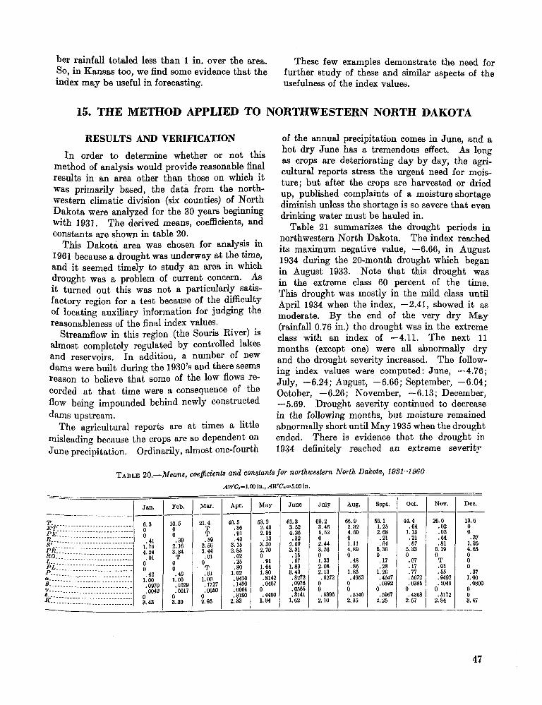
ber rainfall totaled less than 1 in. over the area. So, in Kansas too, we find some evidence that the index may be useful in forecasting.

These few examples demonstrate the need for further study of these and similar aspects of the usefulness of the index values.

Aug. Sept.

66.9 56.1

--- 2.32 1.26 4.60 2.68

.21 0 1.11 .64 4.80 5.36 0 0 .48 .17 .86 .28 1.85 1.26 .4053 .4647

0 .NO2 0 0 .5646 .5W7 2.35 2.25

15. THE METHOD APPLIED TO NORTHWESTERN NORTH DAKOTA

Oct.

44.4 .64 1.13 .21 .67 5.33 0 .07 .17 .77 .E72 .N85

.43@ 0

2.57

RESULTS AND VERIFICATION

In order to determine whether or not this method of analysis would provide reasonable final resulk in an area other than those on which it was primarily based, the data from the northwestern climatic division (si. counties) of North Dakota were analyzed for the 30 years beginning with 1931. The derived means, coefficienk, and constants are shown in table 20.

This Dakota area was chosen for analysis in 1961 because a drought was underway at the time, and it seemed timely to study an area in which drought was a problem of current concern. As it turned out this was not a particularly satisfactory region for a test because of the d s c u l t y of locating auxiliary information for judging the reasonableness of the final index d u e s .

Streamflow in this region (the Souris River) is almost completely regulated by controlled lakes and reservoirs. In addition, a number of new dams were built during the 1930’s and there seems reason to believe that some of the low flows recorded at that time were a consequence of the flow being impounded behind newly constructed darns upstream.

The agricultural reports are a t times a little misleading because the crops are so dependent on June precipitation. Ordinarily, almost one-fourth

Mar.

21.4 T T .hO 2.66 3.44 . 01 0 T .61 1.00 .1727 .00m 0 2.06

of the annual precipitation comes in June, and a hot dry June has a tremendous effect. As long as crops are deteriorating day by day, the agricultural reports stress the urgent need for moisture; but after the crops are harvested or dried up, published complaints of a moisture shortage diminish unless the shortage is so severe that even drinking water must be hauled in.

Table 21 summarizes the drought periods in northwestern North Dakota. The index reached its maximum negative value, -6.66, in August 1934 during the 20-month drought which began in August 1933. Note that this drought was in the extreme class 60 percent of the time. This drought was mostly in the mild class until April 1934 when the index, -2.41, showed it as moderate. By the end of the very dry May (rainfall 0.76 in.) the drought was in the extreme class with an index of -4.11. The next 11 months (except one) were all abnormally dry and the drought severity increased. The following index values were computed: June, -4.76; July, -6.24; August, -6.66; September, -6.04; October, -6.26; November, -6.13; December, -5.69. Drought severity continued to decrease in the following months, but moisture remained abnormally short until May 1935 when the drought ended. There is evidence that the drought in 1934 definitely reached an extreme severity

Apr.

40.5 --

.86

.01

.40 3.15 2.85 .02 .25 .80

1.02 .0410 .1m .OOM .3180 2.33

TABLE 20.-Means, coeficients and constants for northwestern North Dakota, 1951-1960 AWC.=1 .00In.,AWC...B.M)ln.

======= Fob.

10.6 0 0 .30 2.16 3.84 T 0 0

. 4 G 1.00 .lo20 .0017 0 3.30

-

-

- - May

53.2

- 2.40 2.05

* 13 3.30 2.70 0 .01

1.80 .a142 .0467 0 .44m 1.04

1. 64

-

- - June - 61.3 3.62 4.26 .32

2.60 3.31 .15 .57 1.83 3.43 .a272 .0076 .0565 . ai41 1. G2 __

- - July - 60.2 3.46 5.52 0 2.44 3.56 0 1.83 2.08 2.n

0 0

2. 10

.0272

.6306

-

Nov.

26.0 .02 .02 .64 .81

6.19 0 T . 01 .55 ,0402 ,1040

,5172 0

2.84

Doc.

13.6 0 0 .37 1.35 4.65 0 0 0 .37 1.00 .OB00 0 0 3.47

47

Bavendick [l] leaves no doubt of this. He wrote: It was not until June [1934] that any semblance of

normal precipitation occurred and even that month showed a deficiency [59 percent of 30-yr. mean]. To further aggravate the situation, duststorms of unprece- dented severity occurred during April and May. Much of the livestock was shipped out of the State due to lack of feed. Drought was so severe that plans for the evacua- tion of farmers from western North Dakota were seriously discussed, . . . Many cattle died from lack of feed and water and from dust which accumulated in their lungs and stomach. Some persons died from “dust pneumonia” caused by an accumulation of dust in their lungs.

As was the case in Kansas the effects of the abnormal moisture deficiency were greatly increased by the windstorms and dust, but the driest spring and summer on record certainly seems a likely candidate for the classification of extreme drought.

Turning to the drought in 1961, we find serious complaints of drought as the hottest and driest June on record reduced the wheat crop to about one-fourth of average. There were a few local showers in July and those areas enjoyed some temporary relief, but this was followed by the driest and hottest August on record. The following selected comments from the North Dakota Weekly Weather and &op Report of August 29, 1961 [64] illustrate the seriousness of the drought a t this time.

“Stock water situation is serious with many hauling water to livestock [in Burke Co.]. [The same was true in Mountrail Co.] Wheat yields averaged 4 to 7 bushels with a variation of 1.5 to

17 bushels. [Much of this was summer-fallowed wheat.] Very little barley and oats was harvested. Wells and dugouts are being constructed. Ma- jority of [Renville] County remains extremely dry. Fall tillage delayed because of dry weather. Everything is at a standstill.”

By way of comparison, the computed drought index values during 1961 were as follows: May, -1.16; June, -3.11; July, -4.14; August, -5.67. The peak seventy during this drought was the -5.67 at the end of August. Severity decreased during subsequent months until the drought ended with April 1962.

This drought does not appear to have been as devastating as the drought of 1934, and from a crop yield standpoint the drought of 1936 (X= -3.28 a t the end of July) was apparently more serious [I] than this one in 1961. There are many reasons why the effects were not as serious in 1961. In the first place there is a good deal more know- how these days for coping with the problems of dryland agriculture. There is evidence here that the Great Plains Conservation Program [53] has already met with some success in its objective- “to assist farmers and ranchers to develop for themselves a land use program which will help them avert many of the hazards that come with the recurring droughts common to the region.” In addition, the availability of livestock feed on soil-bank acreages greatly alleviated the stock- men’s problems in 1961. This feed was made available for haying and grazing by an official

4s

US. Department of Agriculture action in late June declaring this a drought disaster area.

This action-possibly necessitated by the word- ing of the soil-bank law-led to much confusion concerning the seriousness of the drought during June and July. Some noted this disaster designation and visualized conditions similar to those in the dustbowl days of the 1930’s in the southern Plains.

Conditions in July 1961 were by no means as serious as those which prevailed at the peak of the droughts in the southern Plains in the 1930’s and in the 1950’s. Descriptions such as [56] bear this out. The index also reflects this fact. At the end of July 1961 the index showed -4.14 in northwestern North Dakota. This value compares with the western Kansas values of -5.96 in August 1934 and -6.20 in September 1956.

It is also interesting to note that in the Kansas cases the index was around -3.5 to -4.0 when disaster was declared, but in the case of northwestern North Dakota the index was only about -3.00. There seems to be some evidence that the index provides a better estimate of the severity Of this drought than does the disaster declaration. However, one must always bear in mind that this index is a function of the anomalous weather rather than of the eflects of the weather. Agri- culturally, one might be justified in considering the June weather as a calamity, but from a meteorological standpoint the drought a t the end of June could not reasonably be placed in the same category with the drought of 1934.

AN EXAMPLE OF CURRENT DROUGHT ANALYSIS

During the summer of 1961 there was a considerable amount of public interest in the drought in the northern Great Plains and the Prairie Provinces of Canada. A period of showery Weather began early in July and immediately there were reports that the drought had ended. On the basis of this analysis an article was pre- Pared [35] pointing out that the weather of June had already used nearly nJ1 the antecedent moisture so that above normal July rainfall was required if the evapotranspiration was to be normal. It was further demonstrated that July had increased rather than ended the water shortage in this area. Early in August another article Was released [34] pointing out the strong climatological likelihood for the drought gradually

becoming worse during August. This article was based, in large part, on equation (14) which estimates the amount of precipitation needed for “normal” weather. It turned out that August had provided this much rain only eight times during the last 30 years, with most of the eight occurring during years in which most months were wetter than normal. From this it was concluded that the drought was more likely to become worse than to end during August. Actually, this turned out to be the driest and hottest August in 30 years and the drought became more extreme by September 1.

During September it rained 2.79 in. over the area. This was, by equations (29) and (30), far from being enough moisture definitely to establish an end to the long period of drought, but it did produce a 27 percent probability that the drought had ended. At that time there was no way of being certain that September was not just an interruption in the long drought. I n fact, October and November were among the driest of record and both reduced the probability that the drought had ended. By the first of December the probability had been reduced to 9 percent with no prospect of its reaching 100 percent before the following spring. The unhappy truth is that under the existing circumstances there was no way of making a reasonable estimate as to whether this very serious drought period had ended or if the area was destined to suffer through another hot dry summer. This is in marked contrast to the situation in July and early August when there existed relatively high probabilities that the drought would get worse before it got better.

Actually, the change from prevailingly dry weather to unusually wet weather did not take place until May of 1962. It turned out, therefore, that the wet weather of September 1961 was only a brief interruption in the dry weather. That this would be the case was suspected in early winter, but there was no certainty until the following spring. This demonstrates that the need for reliable seasonal weather forecasts remains. How- ever, under certain circumstances this method does provide a useful substitute.

In general this method of analysis seems to have provided fairly good results in North Dakota. There seems no way of measuring exactly how well the index is describing the moisture variable. The best one can say is that the results seem reasonable both in time and in comparison with the results obtained in Kansas and Iowa.

49

16. CONCLUDING REMARKS

To a large extent this drought analysis method requires strict adherence to the procedures which have been described. Any radical departure from these procedures will produce values of 2 which are incompatible with the equations for determining drought severity. However, there is no reason why one could not use a different method for computing potential evapotranspiration. Any metihod of monthly hydrologic accounting which is more refined and realistic than the method used here would likely produce as good or better results, but a cruder method might introduce bias or inconsistencies.

The method was specifically designed to treat

the drought problem in semiarid and dry subhumid regions. Extrapolation beyond the circumstances for which it was designed may lead to unrealistic results. Some regions are so near to being a desert that there is really little point in attempting drought analysis. At the other extreme are the very humid regions where, again, “abnormal dryness” has very little meaning.

In conclusion, this method of climatic analysis must be regarded as only a step in measuring and describing meteorological drought. Real understanding can only follow measurement and de- scription. Prediction and control await understanding.

ACKNOWLEDGMENTS

The author is pleased to thank Dr. H. Lands- berg, Director of Climatology, for providing time and facilities for carrying out this Work. I n addition, his unfailing words of encouragement are greatly appreciated. Mr. Milton L. Blanc proved to be a most patient listener who could always be counted on for helpful suggestions,

pertinent questions, and stimulating discussion. Without his interest and advice this work might never have been completed. To these two men the writer is particularly grateful, though it is not to be implied that they are in any way responsible for whatever errors, fallacies, and similar detrac- tions may still exist.

50

APPENDIX A .-AUXI LIARY CLIMATIC INFORMATION

71 71 71 71 71 71 71 71 71 71 0 0 0 0 0 0 0 0 0 0

E-- ---.... _ _ _ _ _ _ _ _ _ _ 71 71 0

* ( d ) . _ _ _ _ _ _ _ _ _ _ _ _ _ _ _ .36 -87 1.38 1.05 2.06 1.03 1.44 1.21 1.20 .77 a 3 ( d ) _ _ _ _ _ _ _ _ _ _ _ _ _ _ ~ 1.321 1.234 .721 .780 .447 .435 .320 .e43 .203 1.814 1.650 2.353 a(d) _ _ _ _ _ _ _ _ _ _ _ _ _ _ _ ,763 ,767 .E21 ,778 .813 .a02 .788 .7G7 .a15 .704 .740 .a72

.GO d - - - - - - - - -__________ 0

GEOGRAPHICAL DISTRIBUTION OF THE CLIMATIC CONSTANTS

The analytical technique described in this paper is rather long and tedious. The large amount of work required stems largely from the necessity for carrying out the hydrologic accounting for a long series of years in order to compute the five constants that are required for each calendar month. However, once the constants have been determined, a current drought analysis can be carried out without reference to a long historical recqrd. If present plans can be carried out, the historical record will be analyzed for a network covering the United States. From these machine analyses 60 maps will be prepared showing each of the five constants for each calendar month.

Maps of CY, the coefficient of evapotranspiration, should provide a reasonably good delineation of the agricultural capabilities of various “systems,” where a system represents a particular combination of precipitation, temperature, and soil.

Likewise, from a study of maps of 6, the CoefE- cient of soil moisture loss, one could, with some additional work, mathematically demonstrate the advantages of cultural practices which increase the available water capacity of some soils.

71 0 6.54 .e24 .784

DISTRIBUTION OF THE MOISTURE DEPARTURES

Table 22 shows the moments of the distributions of the moisture departures for each calendar month for the three areas studied. As one would expect, the standard deviation, u, shows that the greatest dispersion occurs during the summer months. Note the secondary minimum during July in central Iowa.

In order to test the distributions for normality, two statistics, a3 and a, which are measures of skewness and flatness have been computed. ct3 is the standardized third moment and a =z]d(/na is a measure which is highly correlated with the fourth moment [46]. On comparison of these values with Geary and Pearson’s table [15] it is seen that the number of a values which fall outside the 5 percent limit is approximately the same as the number which would be expected by chance or if there were no departure from normality.

However, these distributions show a rather large amount of skewness. This is indicated by the disproportionately large number of a3 values which exceed the 5 percent limit. This skewness is partly a result of the fact t,hat the moisture

30 30 30 30 30 30 30 30 30 30 0 0 0 0 0 0 0 0

?! -----.-_____ _ _ _ _ _ _ 30

u(d) _ _ _ _ _ _ _ _ ~ _ _ _ _ _ _ _ -26 .3o . 4 2 .87 1.34 2.06 1.21 1.04 1.30 . 7 2 .47 Q s ( d ) . - - - - _ _ _ _ _ _ _ _ _ _ .173 .640 -. 430 -. 115 1.172 .170 ,269 1.573 .688 .823 d - ...------- _ _ _ _ _ _ _ _ 0 0 0

a(d) _ _ _ _ _ _ _ _ _ _ _ _ _ _ _ _ ,759 .7913 .773 .779 .720 .779 ,782 ,701 .813 .SO9

30 30 0 0

.26 4.67 ,992 .204 .747 .758

51

!? -------- - - _ _ _ _ _ _ _ _ 27 27 27 27 27 27 d ----..- ---- ~ _ _ _ _ _ _ _ 0 0 0 0 0 w----------* _ _ _ _ _ ,01

0 .84 1.11 1.03 2.23 2.07

add’::::: ::---- _ _ _ _ --.040 _. 017 .4oo .473 -. 104 .671 a( 1 _ _ _ _ .805 .784 .812 .a53 .808 .711

27 27 27 27 27 27 27 0 0 0 0 0 0 0 1.47 2.40 2.03 1.50 1.G5

--.282 .807 .318 .740 .a30 .a02 .3z5 -94 6.09

.702 -808 .820 .745 .804 ,780 .8GO

departure distribution has the precipitation distribution a component. Precipitation is rather skewed because it has a lower bound of zero. The skewness in the moisture departures results in a few Occurrences of large departures, especially large positive departures.

Since the addition of non-normal distributions produces a distribution which approaches normality, the “summer months,” May through August, have been combined to produce a single climatological series for each of the three areas. The moments for these three distributions of total moisture departure for the 4-month period are shown in the last column of table 22. On referring to Geary and Pearson’s table one finds the values of both a and are reasonably close to their expected value in a normal distribution. From these tests it was concluded that the normal distribution could be used to represent the 4-month moisture departures.

The mean and the standard deviation contain all the information needed to estimate the noma1 distribution in the population from a normal sample. In the samples with which we are dealing here the mean is zero. This is very convenient inasmuch as one must determine only the standard

deviation in order to estimate the probability that any particular moisture departure will be exceeded during this 4-month period. It therefore seems likely that a map of the standard deviation could be prepared as soon as a sufficient number of areas have been analyzed and that the map would be all that is required in order to pre- pare probability statements concerning the “summer” moisture departures. Such information might be very useful for the planning of hydrologic structures.

It may well be that for crop yield investigations the moisture departure, d,-for the appropriate phenological periods-is the most useful variable in this study. For instance, the moisture departure in June 1961 in northwestern North Dakota was -3.69 in. This very abnormal moisture deficiency during a critical month was the most important variable responsible for the much below normal wheat yields in that area. Of course the moisture variable is only one of the factors affecting crop yields, but in the drier regions it is one of the most significant. In the wetter areas, such as central Iowa, yield reductions may often be related to the positive moisture departures a t planting and harvesting times.

APPENDIX Be-EFFECT OF THE AVAILABLE WATER CAPACITY TERM

PURPOSE OF THE AWC VALUE

As mentioned earlier in this paper, the computed soil moisture is used primarily as a device for taking account of antecedent weather. It allows one to derive a number which is regarded as an index of the amount of previously stored water available for future use. If the assigned available water capacity is too small, we tend to under- estimate the amount of water in storage. On the other hand, too large an available capacity will, in humid climates where runoff is large, lead to an overestimation of the supply of water available. That is, the computations will show water in storage for some time after the actual supply has diminished to the point where the local economy is beginning to suffer. In semiarid regions the AWC value is not so critical, and little difficulty is introduced by assuming too large a value for AWC in such areas of little runoff.

EXPERIMENTS AT DOVER, DELAWARE

While it has been known all along that reasonable final results required the use of a fairly realistic value for AWC, it was not entirely clear as to the effect on the drought index of using an unrealistic AWC value. Therefore, we analyzed a 44-yr. period of Dover data, with assumed values of AWC of 2.0 in., 4.0 in., and 8.0 in. That is, the complete analysis from water balance book- keeping through the final drought index values was carried out three times, the only difference being the assigned value of AWC. Apparently, somewhere around 4.0 to 6.0 in., could be considered as realistic for that area.

The analysis using AWC =2.0 in. produced a maximum drought severity index of - 3.45, thereby indicating that extreme drought never occurred during this 44-yr. period. The analysis using AWC ~ 4 . 0

Results were somewhat unexpected.

52

k. gave a maximum drought severity index of -4.51, and AWC =8.0 in. gave a maximum CAPABILITY index of - 6.17. When one recalls that the driest year in 30 years was to be used to define extreme drought, it is apparent that either this 44-yr. period was a very biased sample or the assigned AWC value of 2.0 in. was somehow limiting the method.

AREAS WITH SMALL STORAGE

What sort of results can we expect in an area- Particularly a humid area-which actually has a rather small capability for storing water? In the first place, the analysis indicates that, as far as water is concerned, cumulative weather has little significance. This lack of an adequate moisture carryover capability makes it impossible to fully utilize the humid climate. Such an area has a water use expectation characteristic of a more arid climate which does have an adequate

Why should an AWC value that is too small capability for the carryover of water. During tend to limit the method’s capability for showing periods of high moisture demand the small amount large departures from normal? If, for the momenti in storage is soon exhausted, and, even though we assume a ridiculously small value for AWC, the area is very dry, there is no expectation that a 0.10 in., it is apparent that the main effect is &loss large moisture recharge will take place-in spite of the capability for taking account of antw~dent of the fact that the humid climate is capable of weather. One dry day or one ComPIetelY dry producing such a recharge. The outcome is that year will produce the same result, viz, no water the f1dI extent of the abnormal wetness or dryness in storage. Likewise, a wet day 01 8 wet Year will of the climate cannot be completely utilized or produce full storage. In either h&nce the taken into account; therefore, there is no oppor- system is no longer capable of taking adequate tunity for cumulative weather to build up to a account of past weather. As the assigned storage point where the index indicates either extreme becomes smaller and smaller, we begin to lose a wetness or extreme drought. part of the basis for estimating the tmount of rain In view of the “droughty soil” concept, this is a needed. Finally, all estimates will tend to lie rather surprising development. However, if one very close to the normal precipitation itself, recognizes that expectations are actually dimin- irrespective of the dryness or wetness of the Past. ished by the lack of an adequate water storage Large values of the moisture departure (the facility, the reasonableness of the result is quite d values) are therefore ruled Out, which also rules apparent. On a relative basis, an area which out large drought index values. lacks an adequate capability for storing water is

If, in humid climates, the assigned storage not as affected by prolonged dry weather as is an capability is too large, rather than too small, it adjoining area which has this capability. This, will allow insufficient runoff during wet periods, too, may at first Seem illogical; however, on a

introduce fictitious water supplies and over- relative basis, it is true because the favored area optimistic during dry periods, and is accustomed to and expects an adequate

of water at all times. If the supply cannot meet the demand, a serious disruption of the economy thereby tend to make the area appear more humid takes place. On the other hand, the less-favored than it actually is. As a consequence, drought area is accustomed to frequent water shortages; severity will tend to be somewhat inflated.

It does not appear, now, that the the demands and operations are geared to the from the use of $00 large 8 storage capacity are as fact that water shortages are to be expected. misleading as those stemming from the Use of too Therefore, while drought may become apparent small a storage capacity. Actually, the system sooner in the area of little moisture carryover is not as sensitive to this factor as this dissertation capability, it will never reach the peak severity might suggest. In general, the Dover results for that will, in time, occur in the more favored area. AWCE4.0 in. and AWC=8.0 in. were very This interpretation seems to conform to reality, similar. It was only the results from using AWC and this is the sort of result the drought ‘index ~ 2 . 0 in. that seemed to be markedly different. will show.

EFFECT OF UNREPRESENTATIVE VALUES

53

APPENDIX C.-ANALYSIS OVER OTHER TIME OR SPACE UNITS

WEEKLY ANALYSES

The foregoing discussion applies entirely to the use of monthly temperature and precipitation data as input. Inasmuch as monthly hydrologic accounting is a rather crude way of es t imahg the water balance [51] some experiments were conducted using weekly, and even daily, data as input.

It turned out that the daily accounting followed by weekly summarimtion and weekly drought seventy computations introduced some difficulties, much unnecessary detail, and considerable expense without producing results which were appreciably different from those obtained from the use of weekly input data, This “daily-weekly” approach was soon abandoned.

As far as procedure is concerned, the weekly analysis was carried out by the same steps that were used in the monthly analysis. The main difference was that the long-term means of P, PE, etc. were computed for each of the 52 standard climatological weeks, whereas the monthly program requires such means only for the 12 months.

Results.-Weekly analyses were compared with monthly analyses a t two stations, Gothenburg, Nebr. and Ames, Iowa. The weekly system gave more detail; it came closer to pinpointing the time when events such as the beginning of a drought happen; and it allows one to keep up with a currently developing situation. But, over- all results were, from a climatological standpoint, very similar to those obtained from monthly data with only a fraction of the work and expense.

Briefly, the weekly results and the monthly results were in agreement over 90 percent of the time; i.e., when one system indicated drought underway, the other system generally agreed. Also, the systems seldom disagreed by as much 8s 2 percent as to the percentage of time each class of drought (mild, moderate, etc.) existed. The two indications of maximum drought severity (62 cases) never differed bv more than 0.7 of a drought class and the mean absolute difference

was about 0.2 of a drought class. The average difference between the two indications of the time of occurrence of the most severe point in each of the 62 drought periods was about 11 days. In general, when the two sets of drought index values were plotted against time, the agreement looked very good, both at Ames and a t Go thenburg.

Conc]usions.-On the basis of the records analyzed from both weekly and monthly input data, it appears that results are not very much different. The weekly data provide more detail and apparently get just a .little closer to a realistic measure, but for climatological purposes the differences are slight. The monthly analysis can be done manually without spending too much time. On the other hand, weekly analysis requires much more than four times as much work. Either could be done by machine, but of course it costs more to do the job by weeks. Also, weekly data are not readily available either in published form or on punch cards. On0 main advantage of Nireekly analysis is that it enables one to keep uprwith a current drought .

POINT VERSUS AREA ANALYSIS

Although this method of drought analysis is based on areal data, it is of interest to determine its applicability to single station data within the area. Studies have been made for a few points, but at this writing there is only one area-single point comparison which is available.

Since only one case (in Iowa) has been analyzed, it must be realized that the results are tentative. The conclusions are that the analysis a t a point tells one a good deal about the weather and climate of a sizable surrounding area. This is, of course, not so true in more rugged terrain. Like- wise, areal analysis gives a fairly good picture of the dry and wet periods at points within the area. For climatological purposes areal analyses are probably adequate, and it is likely that future work will be concentrated on areal analyses.

54

APPENDIX D.-RELATIVE INSTABILITY OF THE CLIMATE OF WESTERN KANSAS SINCE THE EARLY 19303

If one accumulates the monthly values of d or 2 for western Kansas and plots them against time, the curve shows rather a large amplitude since the early 1930's as compared to the preponderance of relatively small oscillations in the previous years. Of course, the index values in table 13 show the same sort of thing. Prior to 1932 a fairly sizable number of months show an index value indicating near normal or only an incipient wet or dry condition. However, since 1932 small index values are rather rare.

This can be demonstrated in a crude fashion by counting the number of months with 1x1 < 1.0 each year and plotting the cumulative total against time.

This figure shows that the period 1887 through 1932 was not marked by numerous large anomalies. At the end of this 46-yr. period, 223 months, about 5 per year, had had small index values. In other words the weather was definitely abnormal only 60 percent of the time.

However, since 1932 the climate has been noteworthy for the absence of near-normal weather. In fact, more than 11 months per year have produced either drought or unusually wet conditions. It is easy to see how the area gained its "feast or famine" reputation in recent years.

Unfortunately, there is no handy explanation for this apparent shift in the frequency of abnormal weather. It may continue and it may not. The warming trend in mean annual temperatures

Such a plot appears in figure 7.

in the latitude zone 40" to 70" N. seems to have come to an end a t about this time [32]. Also, an apparent increase in the frequency of tropical storms in the north Atlantic began in the early 1930's [8]. Are these various events coincidental? Probably not, but we simply do not yet know enough about the fundamentals of atmospheric actions and interactions really to explain what, if anything, has taken place. Only when such things can be adequately explained will there be hope for prediction on a time scale measured in years or decades.

I 2 0 .

0 I I I I I I I I I I I I ( ( I I I I J I 1 I 1 ' I I I I I I I I I I I I I ism so e4 on ($02 06 IO 14 In 22 26 PO 34 sn 42 46 so sa sn 62

YE4RS

FIQURE 7.-Cumulative annual number of months with 1x1 <1.0, western Kansas.

55

AppENDIX E.-RECURRENCE OF SERIOUS DROUGHT IN WESTERN KANSAS

Although no effort was made to discover llcycles of drought,” the relative regularity of the occurrence of severe and extreme drought in western Kansas is rather striking. From table 13 one can see that the index indicated extreme drought in 1894, 1913, 1934 (and following years) , and in 1954 (and following years). These four fairly regularly spaced occurrences of extreme drought may be accidental. However, when one recalls that the discussion of the drought of 1913 [17] mentioned damaging drought in 1874 and in the early 1850Js, there appears to be sufEcient evidence to lead one to speculate concerning the possibility that an extreme drought will #again occur in western Kansas sometime between 1972 and 1975. We have no basis or method for estimating the probability of such an occurrence, but

one could reasonably think it may be greater than the 6 percent probability of extreme drought shown in table 17.

It is interesting to note that Tannehill reached a similar conclusion in 1954 [44]. In a study of the long-range prospects for rainfall in the United States he concluded that ‘ I . . . another dry cycle in this country should begin near the middle of the 1970’s, probably in 1975.” Tannehill, too, was concerned with the occurrence of widespread, disastrous drought, the sort of thing that produces dustbowls and dry reservoirs.

The only thing that seems to be certain is that future years will sooner or later bring a recurrence of extreme drought in the area. The question is, when? On the basis of past history the early 1970’s may be years one might well anticipate.

REFERENCES

1. F. J. Bavendick, Climate and weather in North Dakota, Water Conservation Commission, Bismarck, N. Dak., 1952, pp. 14-15.

2. F. Begemann and W. F. Libby, “Continental Water Balance, Ground Water Inventory and Storage Times, Surface Ocean Mixing Rates and World-Wide Water Circulation Patterns from Cosmic Ray and Bomb Tritium,” Geochimica et Cosmochimica Acta,

3. J. F. Bender, compiler, N B C Handbook of Pronuncia- tion, Thomas Y. Crowell Co., New York, 1943, 289 pp.

4. 0. W. Bidwell, “Major soils of Kansas,” circular 336, Kansas Agricultural Experiment Station, Manhattan, Kans., July 1956, 13 pp.

5. T. A, Blair, Climatology, Prentice-Hall, New York, 1942, p. 37.

6. G. Blumenstock, Jr., “Drought in the United States Analyzed by Means of the Theory of Probability,” TechnicaZ Bulletin No. 819, U.S. Department of Agriculture, April 1942, p. 5.

7. G. E. Condra, “Drought, Its Effects and Measures of Control in Nebraska,” Nebraska Conservation Bulletin No. 25, University of Nebraska, Conserva- tion and Survey Div., April 1944, p. 1.

8. G. w. Cry, W. H. Haggard and H. S. White, “North Atlantic Tropical Cyclones,” Technical Paper No. 36, U.S. Weather Bureau, 1959, 214 pp. (see p. 6).

V O ~ . 12, 1957, pp. 277-96.

9. W. L. Decker and J. F. Gerber, “Comparison of Estimated Values of Evapotranspiration,” Final Report on Contract CWB-8807, University of Missouri, Columbia, Mo., 1957, 51 pp.

10. Drexel Institute of Technology, “Summary of Climatic Observations, 1956,” Publications in Climatology, vol. X, No. 2, Laboratory of Climatology, Centerton. N.J., 1957. Also vol. V, No. 7; vol. VI, No. 6; vol. VIII, No. 2; and vol. IX, No. 4.

11. H. H. C. Dunwoody, “Weather Conditions of the Crop of 1894,” Yearbook of the u.8. Department of Agriculture, 1894, U.S. Department of Agriculture, Washington, D.C., 1895, p. 532.

12. D. J. Fieldhouse and H. H. Englebrecht, “Calculating the Need for Irrigation in Delaware,” paper presented a t Second National Conference on Agricultural Meteorology, New Haven, Conn., Oct. 1958.

13. S. D. Flora, The Climate of Kansas, Report of the Kansas State Board ,of Agriculture, vol. LXVII, No. 285, June 1948, pp. 29 and 183.

14. J. C. Foley, “Droughts in Australia,” Commonwealth of Australia, Bureau of Meteorology, Bulletin No. 43, Sept. 1957, 281 pp.

15. R. c. Geary and E. S. Pearson, Tests of Normality, Biometrika Office, London, 1958, p. 8, tables 3 and 4.

16. Great Britain Meteorological Office, The Meleoro- logical Glossary, Published by the authority of the

56

Meteorological Committee, Chemical Publishing CO., New York, 1951, 253 pp.

17. M. W. Hayes, “Climatological Data for August 1913, District NO. 6, Missouri Valley,” Monthly Weather Review, vol. 41, NO. 8, Aug. 1913, pp. 1192-1193.

18. R. J. Hildreth and G. W. Thomas, “Farming and Ranching Risk as Influenced by Rainfall. 1. High and Rolling Plains,” MP-154, Texas Agricultural Experiment Station, College Station, Tex., Jan. 1956,

19. J. L. Holcombe and F. H. Wiegmann, “Drought In- tensity and Irrigation Needs for Cotton in the St. Joseph Area,” D.A.E. Circular No. 185, Louisiana State University and A. and M. College, Department of Agricultural Economics, Dec. 1955, 47 PP.

20. J. C. Hoyt, “Drought of 1936, with Discussion of the Significance of Drought in Relation to Climate,” U.S. Geological Survey, Water Suppb Paper No.

p. 4.

Vole I X in .Physics-of the Earth, National Research Council, MoGraw-Hill Book Co., New York, 1942,

22* R* E. Huschke, editor, Glossary of Meteorology, Amer- ican Meteorological Society, Boston, Mass., 1959, 638 pp.

23* v. Johnson, Heaven’s Tableland, The Dustbowl Story, Farrar, Straus and Co., New York, 1947, 288 pp.

24. A. Kohler, “Meteorological Aspects of Evapora- tion Phenomena,” International Union of Geodesy and Geophysics, Association of Scientific Hydrology, Publication No. 45, General Assembly of Toronto,

25. M. A. Kohler and R. K. Linsley, “Predicting the Runoff from Storm Rainfall,” Research Paper No. 34, U.S. Weather Bureau, Sept. 1951, 10 pp.

26. M. A. Kohler and M. M. Richards, “Multi-Capacity Basin Accounting for Predicting Runoff from Storm Precipitation,” Journal of Geophysical Research, vol. 67, No. 13, Deo. 1962, pp. 5187-5197.

27. W. B. Langbein and others, “Annual Runoff in the United States,” U.S. Geological Survey, Circular 52, June 1949, 14 pp.

28. R. K. Linsley, Jr., M. A. Kohler, and J. L. H. Paulhus, Applied Hydrology, McGraw-Hill Book CO., Inc., New York, 1959, 689 pp. (see p. 581).

29. W. E. Marlatt, A. V. Havens, N. A. Willets, and G. D. Brill, “A Comparison of Computed and Measured Soil Moisture under Snap Beans,” Journal of Geo- physical Research, vol. 66, No. 2, Feb. 1961, pp.

30. J. K. McGuire and W. C. Palmer, “The 1957 Drought in the Eastern United States,” Monthly Weather Review, vol. 85, No. 9, Sept. 1957, pp. 305-314.

31. G. and C. Merriam Co., Webster’s Dictionary Of SYn- onym, Springfield, Mass,, 1942.

32. J. M. Mitchell, Jr., “Recent Secular Changes of Global Temperature,” Annals of the New York Academy of Sciences, vol. 95, Art. 1, New York, Oct. 5, 1961, p. 240.

PP. 579-591.

1957, vol. 3, pp. 421-436.

535-541.

33. J. Namias, “Some Meteorological Aspects of Drought,” Monthly Weather Review, vol. 83, No. 9, Sept. 1955, pp. 199-205.

34. W. c. Palmer, “Drought and Climatology,” Weekly Weather and Crop Bulletin, National Summary, vol. XLVIII, No. 32, Aug. 7, 1961.

35. W. c. Palmer, “End of Drought?”, Weekly Weather and Crop Bulletin, National Summary, vol. XLVIII, No. 30, July 24, 1961.

36. W. C. Palmer, “Weather Service to Agriculture in the Western Great Plains,” Bulletin of the American Meteorological Society, vol. 37, No. 9, Nov. 1956,

37. W. C. Palmer and A. V. Havens, “A Graphical Technique for Determining Evapotranspiration by the Thornthwaite Method,” Monthly Weather Review, vol. 86, No. 4, Apr. 1958, pp. 123-128.

38. W. C. Palmer and A. V. Havens, “Palmer-Havens Diagram for Computing Potential Evapotranspiration by the Thornthwaite Method,” U.S. Department of of Agriculture, Soil Conservation Service, Portland, Oreg., 1960.

39. H. L. Penman, “Evaporation: An Introductory Survey, Netherlands Journal of Agricultural Science, V O ~ . 4, 1956, PP. 9-29.

40. w. H. Pierre and F. F. Riecken, “The Midland Feed Region,” Yearbook Of Agriculture, 1967, soil, U.S. DeDartment of Agriculture, Washington, D.C., 1958,

pp. 458-461.

pp.- 535-546.. 41. L. A. Richards and C. H. Wadleigh, “Soil Water and

Plant Growth,” Chapt. 3 in Soil Physical Conditions and Plant Growth, B. T. Shaw, editor, American Society of Agronomy, Monograph 11, Academic Press, New York, 1952, pp. 73-251.

42. Subcommittee on Hydrology of the Inter-AgencY Committee on Water Resources, “River Basin Maps Showing Hydrologic Stations,” Hydrologic Activities Bulletin No. 11, Washington, D.C., April 1961, 79 pp.

43. I. E. Tannchill, Drought: Its Cause and Eflects, Prince- ton University Press, Princeton, N.J., 1946, p. 46.

44. I. R. Tannehill, “More Dry Years Ahead,,’ Country Gentleman, Curtis Publishing Co., Philadelphia, Pa., vol. 124, No. 9, Sept. 1954.

45. H. C. S. Thom, “The Analytical Foundations of Climatology,” U.S. Weather Bureau manuscript, Jan. 1954, pp. 24-25.

46. H. C. S. Thom, “Seasonal Degree-Day Statistics for the United States,” Monthly Weather Review, vol. 80, No. 9, Sept. 1952, pp. 143-147 (see p. 144).

47. H. C. S. Thom, with the assistance of the Working Group on Statistical Requirements and Methods in Climatology, WMO-CCI, “Three Chapters on Clima- tological Analysis,” U.S. Weather Bureau manuscript, Aug. 1960, 62 pp.

48. C. W. Thornthwaite, “An Approach toward a Rational Classification of Climate, ” Geographical Review,

49. C. W. Thornthwaite and B. Holzman, “Measurement of Evaporation from Land and Water Surfaces,” Technical Bulletin NO. 817, U.S. Department of

V O ~ . 38, 1948, p. 55-94.

57

Agriculture, soil Conservation Service, May 19421

50. c. w. Thornthwaite and J. R. Mather, “The Water ~ ~ l ~ ~ ~ ~ , ” publications in Climatology, vol. 8, NO. 1, Drexel Institute of Technology, Laboratory Of

Climatology, Centerton, N.J., 1955, 104 PP. 51. C. W. Thornthwaite, J. R. Mather, and D. €3. Carter,

Three Water Balance Maps of Eastern North America, Resources for the Future, Washington, D.C., Nov. 1958, 47 PP. + 3 maps.

52. U.S. Agricultural Research Administration, “Soil Survey Manual,” U.S. Department of Agriculture

53. U.S. Department of Agriculture, “Program for the Great Plains,” developed by the U.S. Department of Agriculture with the cooperation of the Great Plains Agricultural Council, U.S. Department of Agriculture, Miscellaneous Publication No. 709, Jan. 1956, P. IV.

54. U.S. Geological Survey, “Compilation of Records of Surface Waters of the United States through Septem- ber 1950,” Geological Survey Water-Supply Paper 1311, 1955, Also Papers 1280, 1340, 1391, 1441 and 1511.

55. U.S. Geological Survey, “Compilation of Records of Surface Waters of the United States through Sep- tember 1950,” Geological Survey Waler-Supply Paper 1310, 1958. Also Water-Supply Papers 1280, 1340, 1390, 1440 and 1510.

56. u.8. News and world Report, “Parched Plains: First Hand Report,” United States News Publishing COT., Washington, D.C., vol. LI, No. 6, Aug. 7, 1961,

57. U.S. Weather Bureau, “Climates of the States, Iowa,” Climatography of the United States, No. 60-13, May 1959.

68. U.S. Wzather Bureau, “Climates of the States, Kansas,” Climatography of the United States, No. 60-14, Nov. 1959.

59. U.S. Weather Bureau, Climatological Data, Iowa Section, U.S. Department of Agriculture-U.S. Weather Bureau, Des Moines, Iowa, April 1935.

60. U.S. Weather Bureau, Daily River Stages, vol. 52, 1956, Washington, D.C.

61. U.S. Weather Bureau, Iowa Weather and Crop Bulletin, published weekly in cooperation with Iowa Depart- ment of Agriculture, Des Moines, Iowa, 1934.

143 PP.

Handbook NO. 18, Aug. 1951, p. 185.

pp. 71-73.

62. U.S. Weather Bureau, Iowa Weekly Weather and Crop Bulletin, published weekly in cooperation with U.S. Department of Agriculture, Bureau of Agricultural Economics, and Iowa Department of Agriculture, Des Moines, Iowa. Issues: Aug. 1947, Sept. 1947, Sept. 1948, Aug. 1949, Sept. 1949, Oct. 1953, Nov. 1953.

63. U.S. Weather Bureau, Kansas Weekly weather and Crop Reports, published weekly in cooperation with U.S. Department of Agruculture, Marketing Service; Kansas State Board of Agriculture, and Agriculture Extens:ion Service of Kansas State College, Topeka, Kans., Aug. 1955.

64. U.S. Weather Bureau, North Dakota Weekly weather and Crop Report, published weekly in cooperation with U.S. Department of Agriculture, Statistical Reporting Service and North Dakota State University Extension Service, Fargo, N. Dak., Aug. 29, 1961.

65. U.S. Weather Bureau, Weekly Weather and Crop Bulletin, No. 30, 1933 through No. 52, 1940, Wash- ington, D.C.

66. U.S. Weather Bureau, Weekly Weather and CTQP Bulletin National Summary, vol. XL, No. 41, Oct. 12, 1953.

67. U.S. Weather Bureau, Weekly Weather and Crop Bulletin, National Summary, vol. XLIII, Nos. 22-46,

68. C. H. M. van Bavel and F. J. Verlinden, “Agricultural Drought in North Carolina,” North Carolina Agri- cultural Experiment Station, Technical Bulletin No. 122, 1956, 60 pp.

69. F. J. Veihmeyer and A. H. Hendrickson, “Does Transpiration Decrease as Soil Moisture Decreases?” Transactions of the American Geophysical Union, V O ~ . 36, June 1955, pp. 425-448.

70. J. E. Weaver and F. W. Albertson, Grasslands of the Great Plains, Johnsen Publishing Co., Lincoln, Nebr., 1957, pp. 139 and 153.

71. E. S. West and 0. Perkman, “Effects of Soil Moisture on Transpiration,” Australian Journal of Agricultural Research, vol. 4, NO. 3, 1953, pp. 326-332.

72. R. C. L. White, “Drought and Effective Rainfall Frequency in Pastoral New South Wales, West of the Wheat Belt,” Meteorological Study No. 5, Bureau 0‘ Meteorology, Melbourne, Australia, 1955, p. 2.

May 28-Nov. 12, 1956.

it U. S . GOVERNMENT PRINTING OFFICE : 1972-481-334/269

58

Meteorological Drought - CiteSeerX

Documents

Transcript of Meteorological Drought - CiteSeerX