DROUGHT ANALYSIS IN BURUNDI A THESIS SUBMITTED AND PRESENTED To ARBA MINCH UNIVERSITY SCHOOL OF GRADUATE STUDIES BY CELEUS NGOWENUBUSA IN PARTIAL FULFILLMENT OF REQUIREMENTS FOR THE DEGREE OF MASTER OF SCIENCE IN HYDROLOGY AND WATER RESOURCES MANAGEMENT

September 2008

i

CERTIFICATION

The undersigned certify that they have read and hereby recommend for the

acceptance by the University of Arba Minch the dissertation entitled “DROUGHT ANALYSIS IN BURUNDI” in partial fulfillment of the requirements for the degree

of Master of Science in Hydrology and Water Resources Management.

……………………………………………………………………………. Dr. Semu Ayalew Moges Advisor Date: … …………… ………………………………………………………………………………. Dr.P.Deka Co-Advisor

ii

DECLARATION AND COPYRIGHT

I, CELEUS NGOWENUBUSA, declare that this dissertation is my original work

and that it has not been presented and will not be presented to any other

University for similar or any other degree award.

Signature: Date……………………… This dissertation is a copy righted material protected under the Berne

Convention, the Copy Right Act 1999 and other International and National

enactments in the behalf, on the intellectual property. It may not be reproduced

by any means in full or in parts, except for short extracts in fair dealing, for

research or private study, critical scholarly review or disclosure with an

acknowledgement, without written permission of the school of Graduate studies,

on behalf of the author and the Arba Minch University.

iii

ACKNOWLEGMENT I would like to express my sincere gratitude to the Nile Basin Initiative through

ATP for providing me financial support in order to undertake this research work.

Very special thanks to my primary supervisor Dr. Semu Ayalew Moges for his

all-round support, excellent guidance and encouragement during my studies. His

critical comments and valuable advices helped me to take this research in the

right direction. I really appreciate his keen interest and deep knowledge in the

subject matter.I am greatly indebted to my second supervisor Dr P. Deka for his

help whenever I am in need of it. I appreciate his constructive comments and

invaluable tips to improve my research work.

It is also my immense pleasure to express my deep gratitude to all who helped

me, in one or the other, in carrying out this study and the following are some of

them:

National hydro meteorological service: IGEBU (Institut Géographique du

Burundi) for providing me relevant data

Every staff in school of Graduate studies program and the Arba minch

University

All my classmates for their wonderful social atmosphere and lending hand

for each other

Last but not least, I wish to express my deep gratitude to all my family and

my friends for their continuous moral support and encouragement in times

of stress.

iv

DEDICATION

As a memorial to

My Lovely Grand Mother Sofia Ntakabaronga

And

My Dear Father Michael Bayanda

v

Abstract

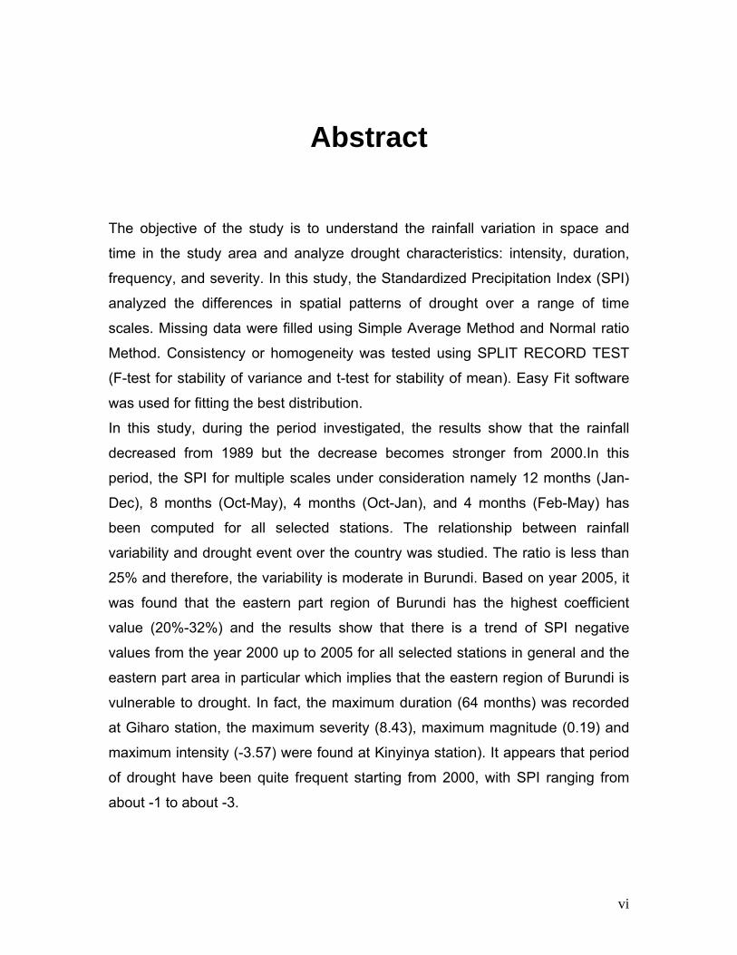
The objective of the study is to understand the rainfall variation in space and

time in the study area and analyze drought characteristics: intensity, duration,

frequency, and severity. In this study, the Standardized Precipitation Index (SPI)

analyzed the differences in spatial patterns of drought over a range of time

scales. Missing data were filled using Simple Average Method and Normal ratio

Method. Consistency or homogeneity was tested using SPLIT RECORD TEST

(F-test for stability of variance and t-test for stability of mean). Easy Fit software

was used for fitting the best distribution.

In this study, during the period investigated, the results show that the rainfall

decreased from 1989 but the decrease becomes stronger from 2000.In this

period, the SPI for multiple scales under consideration namely 12 months (Jan-

Dec), 8 months (Oct-May), 4 months (Oct-Jan), and 4 months (Feb-May) has

been computed for all selected stations. The relationship between rainfall

variability and drought event over the country was studied. The ratio is less than

25% and therefore, the variability is moderate in Burundi. Based on year 2005, it

was found that the eastern part region of Burundi has the highest coefficient

value (20%-32%) and the results show that there is a trend of SPI negative

values from the year 2000 up to 2005 for all selected stations in general and the

eastern part area in particular which implies that the eastern region of Burundi is

vulnerable to drought. In fact, the maximum duration (64 months) was recorded

at Giharo station, the maximum severity (8.43), maximum magnitude (0.19) and

maximum intensity (-3.57) were found at Kinyinya station). It appears that period

of drought have been quite frequent starting from 2000, with SPI ranging from

about -1 to about -3.

vi

TABLE OF CONTENT

TABLE OF CONTENT ................................................................................................ VII

LIST OF TABLES ........................................................................................................... X

LIST OF APPENDICES ................................................................................................XI

LIST OF ABBREVIATIONS ....................................................................................... XII

CHAPITER ONE .............................................................................................................. 1

1.1.INTRODUCTION ......................................................................................................... 1

1.2.BACKGROUND AND LOCATION .................................................................................. 3

1.3. CLIMATE AND RAINFALL PATTERN ........................................................................... 4

I. 4. PROBLEM OF STATEMENT AND OBJECTIVE OF THE STUDY ..................................... 6

CHAPTER TWO............................................................................................................... 7

2. LITERATURE REVIEW ............................................................................................. 7

2. 1. THE CONCEPT OF DROUGHT........................................................................... 7

2. 2. TYPES OF DROUGHT ............................................................................................... 9

2. 2. B. Meteorological Drought ............................................................................. 9

2. 2. C. Hydrological Drought ............................................................................... 10

2. 2. D. Socioeconomic Drought .......................................................................... 10

2. 3. IMPACT OF DROUGHT............................................................................................ 11

2. 4.1. Standardized Precipitation index (SPI)................................................... 12

2. 4.2. Palmer Drought Severity Index (The Palmer; PDSI)............................ 14

2. 4.3. Percent of Normal ...................................................................................... 16

2. 4.4. Surface Water Supply Index (SWSI; pronounced “swazee”).............. 16

2. 4.5. Reclamation Drought Index...................................................................... 18

2. 4.6. Deciles ......................................................................................................... 18

2.4.7. Crop Moisture Index (CMI) ........................................................................ 19

vii

2. 4.8. National Rainfall Index (NRI).................................................................... 20

2. 4.9. Dependable Rain (DR) .............................................................................. 20

2.5. SELECTION OF DROUGHT INDEX............................................................................ 21

CHAPITER THREE ....................................................................................................... 23

3. METHODOLOGY ...................................................................................................... 23

3. 1. GENERAL .............................................................................................................. 23

3. 2. DATA AVAILABLE AND SOURCE ............................................................................. 25

3. 3.FILLING MISSING DATA AND SCREENING DATA ..................................................... 26

3.4. SPI COMPUTATION............................................................................................... 26

3. 4. SPI INTERPRETATION .................................................................................... 29

CHAPTER FOUR........................................................................................................... 33

4. DATA ANALYSIS AND RESULTS ........................................................................ 33

4.1.RAINFALL VARIABILITY ........................................................................................... 33

4. 2 .DROUGHT CHARACTERISTICS............................................................................... 36

5.CONCLUSIONS AND RECOMMENDATIONS ..................................................... 49

5. 1. CONCLUSIONS................................................................................................. 49

5. 2. RECOMMENDATIONS............................................................................................. 50

5. 2.a. Information evaluation and needs ........................................................... 50

5.2. b. Early warning system ................................................................................ 51

5.2. C. Drought management and prevention ................................................... 51

5. 2. d. Predicting Drought .................................................................................... 52

REFERENCES ................................................................................................................ 53

APPENDIX A.………………………………………………………………………….57 APPENDIX B…………………………………………………………………………..67 APPENDIX C………………………………………………………………………….69 APPENDIX D………………………………………………………………………….71 APPENDIX F…………………………………………………………………………..77

viii

LIST OF FIGURES

Figure 1.1.Graphical representation of Cankuzo station-1993..............................4

Figure 2.1.Types of drought................................................................................12

Figure 3.2 Probability density Function ...............................................................30

Figure 4.1 Coefficient of Variation (percentage) based on year 2005.................35

Figure 4.2 show case of SPI-12 rain season 2005..............................................39

Figure 4.3 show case of SPI-12 rain season 1978..............................................40

Figure 4.4 SPI-8 Rainy Season 2005..................................................................41

Figure 4.5 SPI-8 Rainy Season 1978..................................................................42

Figure 4.6SPI-4 (oct-jan) rain season 2005 ........................................................43

Figure 4.7 SPI-4 (oct-jan) rainy season 1978 .....................................................44

Figure 4.8 SPI-4 (Feb-May) Rainy season 2005.................................................45

Figure4.9 SPI-4 (Feb-May) rainy season 1978 ...................................................46

ix

LIST OF TABLES

Table 2.1: SPI Values

Table 2.2: Palmer classifications

Table 2.3: RDI classifications

Table 2.4: Decile classifications

Table 2.5: Characteristics of drought indices

Table 3.1: Total station in Burundi is 169

Table 3.1: Total station in Burundi is 169 (Cont’)

Table 3.2: Stations selected for study

Table 3.3: T-test and F-test: case of Bugarama station (SPI-8, Oct-May)

Table 3.4: SPI-8 (Oct-May) case of Bugarama station

Table 3.5: Results for SPI-8 (Oct-May) case of Bugarama Station

Table 3.6: SPI Values Category Table 4.1: % of Coefficient of variation for different time scale

Table 4.2: Drought characteristics based on SPI-8 (Oct-May)

x

LIST OF ANNEXES

APPENDIX A: SPI Values for different time scale and for selected stations APPENDIX B: Statistical parameters (CV in %) APPENDIX C: Table of total stations in Burundi APPENDIX D: Drought Intensity and Trend (SPI-8) for selected stations APPENDIX E: Drought duration, severity, magnitude, and frequency (SPI-8) APPENDIX F: Drought category based on SPI-8

xi

LIST OF ABBREVIATIONS

AMU Arba Minch University

AWC Available Water Content

C Century

CMI Crop Moisture Index

CSDI Crop Specific Drought Index

CV Coefficient of Variation

Dec December

DR Dependable Rain

ED Extreme Drought

%ED Percentage of Extreme Drought

Feb February

Jan January

IDWA Inverse Distance Weight Average

IGEBU Institut géographique du Burundi

m Month

MD Mild Drought

%MD Percentage of mild Drought

MoD Moderate Drought

%MoD Percentage of Moderate Drought

NDI National Rainfall Index

NDVI Normalized differences of vegetation

P Precipitation

PDSI Palmer Drought Severity Index

PN Percent of Normal

RAI Rainfall Anomaly Index

RDI Reclamation Drought index

S.d Standard deviation

xii

%SD Percentage of Severe Drought

SMDI Soil Moisture Drought Index

SPI Standardized precipitation Index

SPI-4 Accumulation Precipitation of 4 months

SPI-8 Accumulation Precipitation of 8 months

SPI-12 (annual) Accumulation Precipitation of Jan to Dec

SWSI Surface Water Supply Index

xiii

CHAPTER ONE

1. Introduction and Background

1.1.Introduction

BURUNDI is a country prone to extreme climate events such as drought.

Successive years of low precipitation have left large areas in drought that result

in crop failure, water shortage and raising serious food security concerns.

Drought is one of the environmental disasters in BURUNDI, generally

characterized by a deficiency of precipitation over an extended period of time.

Impacts are cumulative and the effects magnify when events continue from one

season to the next. The economical impact occurs in agriculture and related

sectors, which depend on the surface and groundwater supplies. In addition to

obvious losses in yields in crop and livestock production, drought is associated

with the increase in insect infestations, plant disease and wind erosion. The

social impact is present in periods of extreme, persistent drought. The severity of

drought depends upon the degree of precipitation deficiency, the duration and

the size of the affected area. As there is no precise and universally accepted

definition of drought, there exists uncertainty in the occurrence of drought and its

severity. This uncertainty often affects decisions on whether to take the remedial

measure at the right time and place. Drought impacts may vary from region to

region based upon the differences in social, economical and environmental

characteristics at all levels. Drought risk is based on a combination of the

frequency, severity, and spatial extent of drought (the physical nature of drought)

and the degree to which a population or activity is vulnerable to the effects of

drought.

1

Although drought is a natural hazard, society can reduce its vulnerability .The

impacts of drought, like those of other natural hazards; can be reduced through

mitigation and preparedness (risk management). Planning for drought is

essential (early warning, drought management, disaster prevention), but it may

not come easily because one of the major impediments to drought planning is its

cost and there are many constraints to planning:

Decision makers, policy makers, and the general public may lack an

understanding of drought.

In areas where drought occurs frequently, governments and the public

may ignore drought planning, or give it low priority. Governments and the

public may have inadequate financial ressources.

Most countries lack a unified philosophy for managing natural resources,

including water

2

1.2.Background and location

In Burundi, some meteorological services are existing from 1962 and this paper

used data available in meteorological services in order to carry out Drought

Analysis. As the famine due to drought is nowadays a big concern, it is expected

that such study should help through enhancing or improvement of actual

conditions about degradation of environment, which may be one of the causes of

drought. Burundi is a small country with a geographical area 27,834 km2 and its

location is 3°3’ under equator in Central Africa (Figure 1.1.)

Figure.1.1.Study area

3

1.3. Climate and rainfall pattern

In Burundi, the general climate is defined as tropical highland, but differences in

altitude from region to region cause temperature variations with an average of 23

degrees Celsius and annual precipitation of about 800mm. There are two main

seasons: the dry season (June - September); the wet season (October- May).

The water catchments of Burundi fall within 2 great African watersheds: the Nile

basin and the Congo basin.

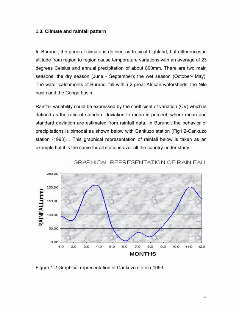
Rainfall variability could be expressed by the coefficient of variation (CV) which is

defined as the ratio of standard deviation to mean in percent, where mean and

standard deviation are estimated from rainfall data. In Burundi, the behavior of

precipitations is bimodal as shown below with Cankuzo station (Fig1.2-Cankuzo

station -1993). . This graphical representation of rainfall below is taken as an

example but it is the same for all stations over all the country under study.

Figure 1.2.Graphical representation of Cankuzo station-1993

4

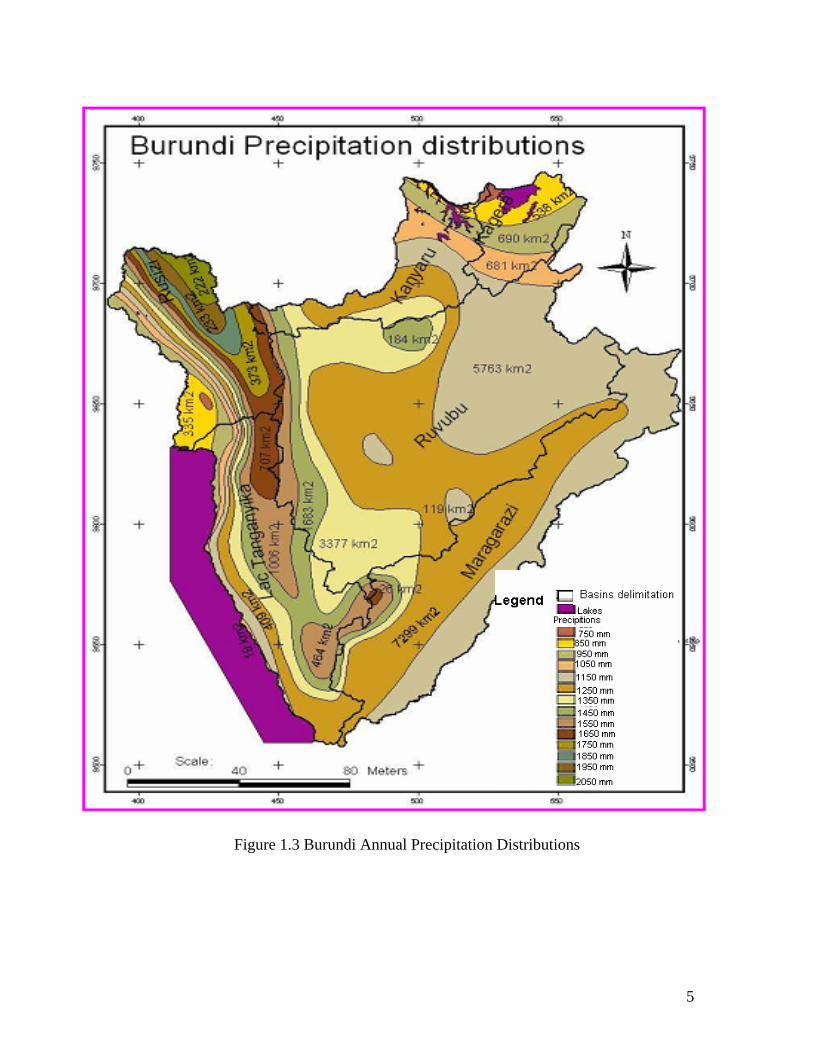
Figure 1.3 Burundi Annual Precipitation Distributions

5

I. 4. Statement of the problem and Objective of the study

Drought is natural disasters, which originates from the lack of precipitation

and brings significant economic losses. It is not possible to avoid it but

drought preparedness can be developed and droughts impacts can be

managed. In Burundi, drought and desertification are taking place step by

step, and there is a spatial variability between different locations because

some receive insufficient rainfall in a year while in others locations it is more

than 2000mm (Figure 1.3). Therefore, it is important to analyze the variations

of precipitations in time and space.

The objective of the study is to understand the rainfall variation in space and

time in the study area and analyze drought characteristics: intensity, duration,

frequency, severity in order to solve the fundamental problem which is to

protect people from repetitive drought impacts. This study may highlight

recommendations about identifying appropriate mitigation action for future

drought event and minimizing its impacts on water management and

agriculture, economic sector, social sector, water resources and drinking

water supply, health problems, environmental problems…etc.

6

CHAPTER TWO

2. LITERATURE REVIEW

2. 1. The concept of drought

A shortage of water is not the same as drought. Drought is an insidious hazard of

nature. Although it has scores of definitions, it originates from a deficiency of

precipitation over an extended period of time, usually a season or more. This

deficiency results in a water shortage for some activity, group, or environmental

sector. Drought should be considered relative to some long-term average

condition of balance between precipitation and evapotranspiration (i.e.,

evaporation + transpiration) in a particular area, a condition often perceived as

“normal”. It is also related to the timing (i.e., principal season of occurrence,

delays in the start of the rainy season, occurrence of rains in relation to principal

crop growth stages) and the effectiveness (i.e., rainfall intensity, number of

rainfall events) of the rains.

The term “drought “has different connotation in various part of the world: in

Egypt, any year the Nile river doesn’t flood is drought, regardless of rainfall; in

Libya when annual rain fall is less than 180 mm, so, drought can be neither

accurately define in term of mm of rainfall or by number of days without rains.

Drought occurs in almost all climatic regimes. It occurs in high as well as low

rainfall areas. It is a temporary anomaly and as such it differs from aridity, which

is a permanent feature of climate in low rainfall areas (Wilhite 2000).

Drought is considered by many to be the most complex but least understood of

all natural hazards, making it hard to predict and monitor. Scientists are trying to

develop mathematical models to help predicting drought a month or more in

advance for most parts of the world.

7

Geraldine Wong of the University of Adelaide has used global climatic indices

such as the Southern Oscillation Index (SOI) in conjunction with rainfall statistics

to develop the copulas models that predict future droughts with a high degree of

accuracy (The Economic Times,posted on Google –Alert drought by Willen Van

Cotthem,june 2008).If you are a farmer, drought means that you do not have

enough water in the soil for crops to grow normally or for pastures to produce

enough grass for livestock. For farmers who rely on irrigation to produce their

crops, drought may be a shortage of water in reservoirs, streams, or

groundwater, and irrigation may be restricted. If you live in a city, drought may

result in a shortage of water for watering grass, trees, and other plants. Often

during drought, people in cities are asked to conserve water used inside the

home and outside.

There are many definitions of drought because its characteristics and impacts

differ from one location to another. Drought is more relative than absolute

concept in water resources An operational definition for agriculture might

compare daily precipitation values to evapotranspiration rates to determine the

rate of soil moisture depletion, then express these relationships in terms of

drought effects on plant behavior (i.e., growth and yield) at various stages of crop

development. A definition such as this one could be used in an operational

assessment of drought severity and impacts by tracking meteorological variables,

soil moisture, and crop conditions during the growing season, continually

reevaluating the potential impact of these conditions on final yield. Operational

definitions can also be used to analyze drought frequency, severity, and duration

for a given historical period. Such definitions, however, require weather data on

hourly, daily, monthly, or other time scales and, possibly, impact data (e.g., crop

yield), depending on the nature of the definition being applied. Developing

climatology of drought for a region provides a greater understanding of its

characteristics and the probability of recurrence at various levels of severity.

Information of this type is extremely beneficial in the development of response

and mitigation strategies and preparedness plans.

8

2. 2. Types of drought

According to World Meteorological Organizations, drought has been categorized

as, Agricultural drought, Meteorological drought, Hydrological drought and Socio-

economic drought (figure 2.1). The definitions of each drought term are given

subsequently.

2. 2. A. Agricultural Drought An agricultural drought refers to a situation when the amount of moisture in the soil no longer meets the needs of a particular crop. Agricultural drought occurs when the yield drops below the average crop

production. This happens due to non-availability of desired level of natural soil

moisture and the periods may not necessarily coincide with the period of

meteorological and hydrological drought A good definition of agricultural drought

should be able to account for the variable susceptibility of crops during different

stages of crop development, from emergence to maturity. It occurs when yield

drops much below the average crop production. Agricultural drought links various

characteristics of meteorological (or hydrological) drought to agricultural impacts,

focusing on precipitation shortages, differences between actual and potential

evapotranspiration, soil water deficits, reduced ground water or reservoir levels,

and so forth.

2. 2. B. Meteorological Drought

Period of meteorological drought is characterized by a situation when the rainfall

is substantially below its climatologically expectations. In common language,

large water shortage due to lack of precipitation implies meteorological drought. It

is a measure of departure of precipitation from the normal and defined usually on

the basis of the degree of dryness (in comparison to some “normal” or average

amount) and the duration of the dry period. Its period may last a few days up to

several weeks or even years.

9

2. 2. C. Hydrological Drought

Hydrological drought occurs when river flows or stored water in reservoir, lake

and aquifers fall below some critical levels. It is associated with the effects of

periods of precipitation (including snowfall) shortfalls on surface or subsurface

water supply (i.e., stream flow, reservoir and lake levels, ground water).A fall of

20% or more in groundwater level with respect to normal mean positions is

considered to be a drought year. The frequency and severity of hydrological

drought is often defined on a watershed or river basin scale. Although all

droughts originate with a deficiency of precipitation, hydrologists are more

concerned with how this deficiency represents the temporal hydrologic system.

Hydrological droughts are usually out of phase with or lag the occurrence of

meteorological and agricultural droughts. It takes longer for precipitation

deficiencies to show up in components of the hydrological system such as soil

moisture, stream flow, and ground water and reservoir levels. As a result, these

impacts are out of phase with impacts in other economic sectors. For example, a

precipitation deficiency may result in a rapid depletion of soil moisture that is

almost immediately discernible to agriculturalists, but the impact of this deficiency

on reservoir levels may not affect hydroelectric power production or recreational

uses for many months.

2. 2. D. Socioeconomic Drought

It refers to the situation that occurs when physical water shortage begins to affect

people. It expresses features of the socio – economic effects of drought and can

also incorporate features of meteorological, agricultural, and hydrological

drought. They are usually associated with the supply and demand of some

economic grounds.

Socioeconomic definitions of drought associate the supply and demand of some

economic good with elements of meteorological, hydrological, and agricultural

drought. It differs from the other types of drought because its occurrence

depends on the time and space processes of supply and demand to identify or

classify droughts.

10

The supply of many economic goods, such as water, forage, food grains, fish,

and hydroelectric power, depends on weather. Because of the natural variability

of climate, water supply is ample in some years but unable to meet human and

environmental needs in other years. Socioeconomic drought occurs when the

demand for an economic good exceeds supply as a result of a weather-related

shortfall in water supply.

2. 3. Impact of drought

When drought begins, the agricultural sector is usually the first to be affected because of

its heavy dependence on stored soil water. Soil water can be rapidly depleted during

extended dry periods. If precipitation deficiencies continue, then people dependent on

other sources of water will begin to feel the effects of the shortage. Those who rely on

surface water (i.e., reservoirs and lakes) and subsurface water (i.e., ground water), for

example, are usually the last to be affected. When precipitation returns to normal and

meteorological drought conditions have abated, the sequence is repeated for the

recovery of surface and subsurface water supplies. Soil water reserves are replenished

first, followed by stream flow, reservoirs and lakes, and ground water. Ground water

users, often the last to be affected by drought during its onset, may be last to experience

a return to normal water levels. The length of the recovery period is a function of the

intensity of the drought and its duration.

11

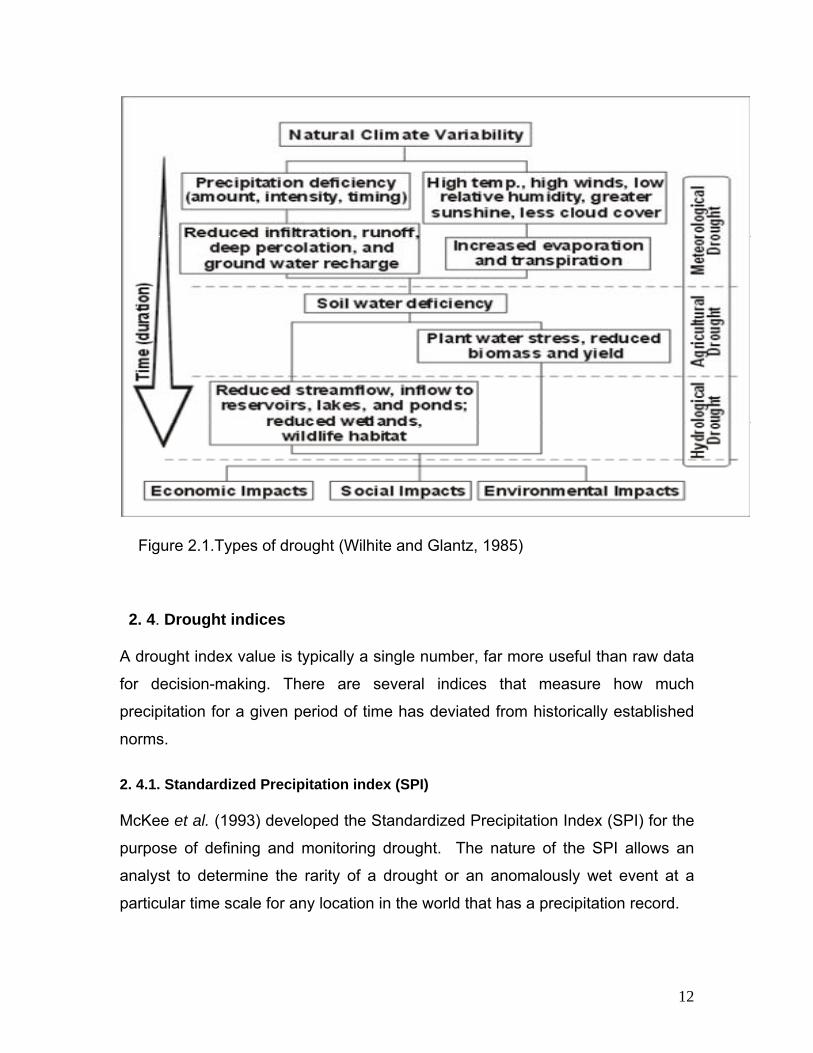
Figure 2.1.Types of drought (Wilhite and Glantz, 1985)

2. 4. Drought indices

A drought index value is typically a single number, far more useful than raw data

for decision-making. There are several indices that measure how much

precipitation for a given period of time has deviated from historically established

norms.

2. 4.1. Standardized Precipitation index (SPI)

McKee et al. (1993) developed the Standardized Precipitation Index (SPI) for the

purpose of defining and monitoring drought. The nature of the SPI allows an

analyst to determine the rarity of a drought or an anomalously wet event at a

particular time scale for any location in the world that has a precipitation record.

12

The SPI is an index based on the probability of precipitation for any time scale.

Many drought planners appreciate the SPI versatility. The SPI can be computed

for different time scales, can provide early warning of drought and help assess

drought severity, and is less complex than the Palmer. The SPI calculation for

any location is based on the long-term precipitation record for a desired period.

This long-term record is fitted to a probability distribution, which is then

transformed into a normal distribution so that the mean SPI for the location and

desired period is zero (Edwards and McKee, 1997). Positive SPI values indicate

greater than median precipitation, and negative values indicate less than median

precipitation.

Because the SPI is normalized, wetter and drier climates can be represented in

the same way, and wet periods can also be monitored using the SPI. McKee et

al. (1993) also defined the criteria for a drought event for any of the time scales.

A drought event occurs any time the SPI is continuously negative and reaches

intensity of -1.0 or less. The event ends when the SPI becomes positive. Each

drought event, therefore, has a duration defined by its beginning and end, and

intensity for each month that the event continues. The positive sum of the SPI for

all the months within a drought event can be termed the drought’s magnitude.

13

Table 2.1: SPI Values

SPI values

2.0+ Extremely wet

1.5 to 1.99 Very wet

1.0 to 1.49 Moderately wet

-.99 to .99 Near normal

-1.0 to -1.49 Moderately dry

-1.5 to -1.99 Severely dry

-2 and less Extremely dry

2. 4.2. Palmer Drought Severity Index (The Palmer; PDSI)

Palmer has developed the PDSI in 1965. It is calculated based on precipitation

and temperature data, as well as the local Available Water Content (AWC) of the

soil. From the inputs, all the basic terms of the water balance equation can be

determined, including evapotranspiration, soil recharge, runoff, and moisture loss

from the surface layer. Human impacts on the water balance, such as irrigation,

are not considered. The Palmer is a soil moisture algorithm calibrated for

relatively homogeneous regions.

14

Table 2.2: Palmer classifications

Palmer Classifications 4.0 or more Extremely wet 3.0 to 3.99 Very wet 2.0 to 2.99 Moderately wet 1.0 to 1.99 Slightly wet 0.5 to 0.99 Incipient wet spell 0.49 to -0.49 Near normal -0.5 to -0.99 Incipient dry spell -1.0 to -1.99 Mild drought -2.0 to -2.99 Moderate drought -3.0 to -3.99 Severe drought -4.0 or less Extreme drought

There are considerable limitations when using the Palmer Index, and these are

described in detail by Alley (1984) and Karl and Knight (1985). Drawbacks of the

Palmer Index include:

The Palmer Index is sensitive to the AWC of a soil type. Thus, applying

the index for a climate division may be too general.

The two soil layers within the water balance computations are simplified

and may not be accurately representative of a location.

Snowfall, snow cover, and frozen ground are not included in the index. All

precipitation is treated as rain, so that the timing of PDSI or PHDI values

may be inaccurate in the winter and spring months in regions where snow

occurs. The natural lag between when precipitation falls and the resulting runoff is

not considered. In addition, no runoff is allowed to take place in the model

until the water capacity of the surface and subsurface soil layers is full,

leading to an underestimation of runoff. Several other researchers have

presented additional limitations of the Palmer Index. McKee et al. (1995) and suggested that the PDSI is designed for

agriculture but does not accurately represent the hydrological impacts

resulting from longer droughts.

15

2. 4.3. Percent of Normal

Percent of normal is easily misunderstood and gives different indications of

conditions depending on the location and season. It is one of the simplest

measurements of rainfall for a location. Analyses using the percent of normal are

very effective when used for a single region or a single season. It is calculated by

dividing actual precipitation by normal precipitation typically considered to be a

30-year mean and multiplying by 100%. This can be calculated for a variety of

time scales. Usually these time scales range from a single month to a group of

months representing a particular season, to an annual or water year. Normal

precipitation for a specific location is considered to be 100%. One of the

disadvantages of using the percent of normal precipitation is that the mean, or

average, precipitation is often not the same as the median precipitation, which is

the value exceeded by 50% of the precipitation occurrences in a long-term

climate record. The reason for this is that precipitation on monthly or seasonal

scales does not have a normal distribution.

2. 4.4. Surface Water Supply Index (SWSI; pronounced “swazee”)

Surface Water Supply Index (SWSI) was developed by Shafer and Dezman

(1982) to complement the Palmer Index for moisture conditions. The procedure

to determine the SWSI for a particular basin is as follows: monthly data are

collected and summed for all the precipitation stations, reservoirs, and stream

flow measuring stations over the basin. Each summed component is normalized

using a frequency analysis gathered from a long-term data set. The probability of

non-exceedence—the probability that subsequent sums of that component will

not be greater than the current sum—is determined for each component based

on the frequency analysis.

16

This allows comparisons of the probabilities to be made between the

components. Each component has a weight assigned to it depending on its

typical contribution to the surface water within that basin, and these weighted

components are summed to determine a SWSI value representing the entire

basin. Like the Palmer Index, the SWSI is centered on zero and has a range

between -4.2 and +4.2.

Several characteristics of the SWSI limit its application. Because the SWSI

calculation is unique to each basin or region, it is difficult to compare SWSI

values between basins or regions. Within a particular basin or region,

discontinuing any station means that new stations need to be added to the

system and new frequency distributions need to be determined for that

component.

Additional changes in the water management within a basin, such as flow

diversions or new reservoirs, mean that the entire SWSI algorithm for that basin

needs to be redeveloped to account for changes in the weight of each

component. Thus, it is difficult to maintain a homogeneous time series of the

index. Extreme events also cause a problem if he events are beyond the

historical time series, and the index will need to be reevaluated to include these

events within the frequency distribution of a basin component.

17

2. 4.5. Reclamation Drought Index

The Reclamation Drought Index (RDI) was recently developed as a tool for

defining drought severity and duration, and for predicting the onset and end of

periods of drought. The RDI differs from the SWSI in that it builds a temperature-

based demand component and duration into the index. The RDI is adaptable to

each particular region and its main strength is its ability to account for both

climate and water supply factors. Like the SWSI, the RDI is calculated at a river

basin level, and it incorporates the supply components of precipitation, snow

pack, stream flow, and reservoir levels. The RDI values and severity

designations are similar to the SPI, PDSI, and SWSI.

Table 2.3: RDI classifications

RDI Classifications

4.0 or more Extremely wet

1.5 to 4.0 Moderately wet

1 to 1.5 Normal to mild wetness

0 to -1.5 Normal to mild drought

-1.5 to -4.0 Moderate drought

-4.0 or less Extreme drought

2. 4.6. Deciles

The deciles method was selected as the meteorological measurement of drought

because it is relatively simple to calculate and requires less data and fewer

assumptions than the Palmer Drought Severity Index. Arranging monthly

precipitation data into deciles is another drought-monitoring technique.

18

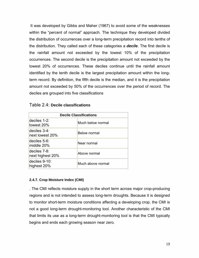
It was developed by Gibbs and Maher (1967) to avoid some of the weaknesses

within the “percent of normal” approach. The technique they developed divided

the distribution of occurrences over a long-term precipitation record into tenths of

the distribution. They called each of these categories a decile. The first decile is

the rainfall amount not exceeded by the lowest 10% of the precipitation

occurrences. The second decile is the precipitation amount not exceeded by the

lowest 20% of occurrences. These deciles continue until the rainfall amount

identified by the tenth decile is the largest precipitation amount within the long-

term record. By definition, the fifth decile is the median, and it is the precipitation

amount not exceeded by 50% of the occurrences over the period of record. The

deciles are grouped into five classifications

Table 2.4: Decile classifications

Decile Classifications deciles 1-2: lowest 20% Much below normal

deciles 3-4: next lowest 20% Below normal

deciles 5-6: middle 20% Near normal

deciles 7-8: next highest 20% Above normal

deciles 9-10: highest 20% Much above normal

2.4.7. Crop Moisture Index (CMI)

. The CMI reflects moisture supply in the short term across major crop-producing

regions and is not intended to assess long-term droughts. Because it is designed

to monitor short-term moisture conditions affecting a developing crop, the CMI is

not a good long-term drought-monitoring tool. Another characteristic of the CMI

that limits its use as a long-term drought-monitoring tool is that the CMI typically

begins and ends each growing season near zero.

19

This limitation prevents the CMI from being used to monitor moisture conditions

outside the general growing season, especially in droughts that extend over

several years.

The CMI also may not be applicable during seed germination at the beginning of

a specific crop’s growing season.

Palmer (1968) developed the Crop Moisture Index (CMI) from procedures within

the calculation of the PDSI. Whereas the PDSI monitors long-term

meteorological wet and dry spells, the CMI was designed to evaluate short-term

moisture conditions across major crop-producing regions. It uses a

meteorological approach to monitor week-to-week crop conditions based on the

mean temperature and total precipitation for each week within a climate division.

2. 4.8. National Rainfall Index (NRI)

It is used to compare precipitation patterns and anomalies on a continental

scale.NRI were developed by Gommes and Petrassi stated in Hayes (2003) to

characterize recent precipitation patterns across Africa. It is calculated for each

country by taking a national annual precipitation average weighted according to

the long – term precipitation averages off all the individual stations. The NRI

allows comparisons to be made between years and between countries.

2. 4.9. Dependable Rain (DR)

Dependable Rain is another rainfall monitoring tool which has been applied to the

African continent by Le Houerou(1993) stated in Hayes (2003).It is defined as the

amount of rainfall that occurs in four of every five years(statistically, not

consecutively).In Africa, the relationship of the DR to the mean is not straight

forward and reflects the characteristics of annual precipitation across the

continent.

20

Table 2.5: Characteristics of drought indices

N° Name Factors used Time scale Main concept

1 PDSI P, T, ET, SM, RO m Based on moisture ,inflow, outflow and storage

2 SWSI PDSI, SN m Like the PDSI but consider SN

3 PN P m Dividing actual P by the normal value

4 Deciles P m Dividing distribution of occurrences over along term p record

into sections each representing ten percent

5 SPI P 3m Difference of P from the mean for a particular time and

6m dividing it by the standard deviation 12m 24m 48m

6 RDI P m, y Percent departure of P from the long-term mean

in top 5 feet of soil profile

7 DR P y, c Patterns and abnormalities of P on a continental scale

8 NRI P M ,y P compared to arbitrary value of +3 and -3,which assigned

9 RDI P m, y Percent departure of P from the long-term mean

2.5. Selection of drought index

Although none of the major indices is inherently superior to the rest in all

circumstances, some indices are better suited than others for certain uses.

Depending upon the data already available and collected, a suitable index can be

chosen. The selection of method of analysis is governed by the availability of

data and accuracy of the result required.

21

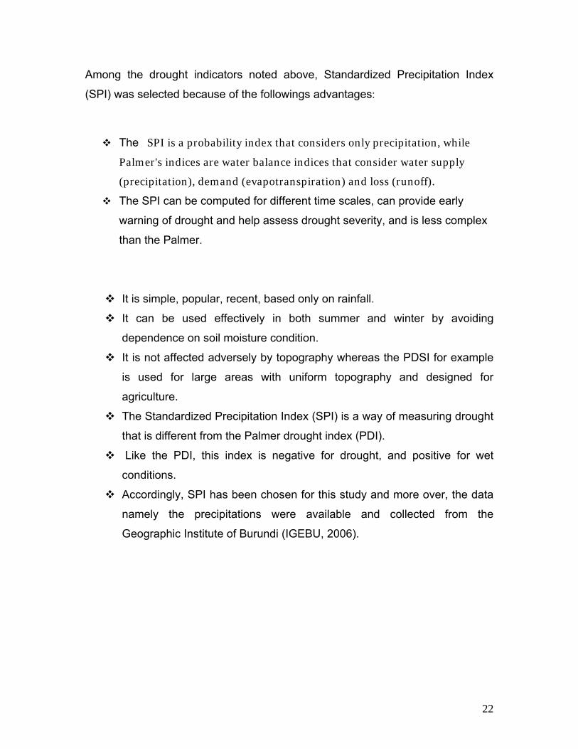
Among the drought indicators noted above, Standardized Precipitation Index

(SPI) was selected because of the followings advantages:

The SPI is a probability index that considers only precipitation, while

Palmer's indices are water balance indices that consider water supply

(precipitation), demand (evapotranspiration) and loss (runoff).

The SPI can be computed for different time scales, can provide early

warning of drought and help assess drought severity, and is less complex

than the Palmer.

It is simple, popular, recent, based only on rainfall. It can be used effectively in both summer and winter by avoiding

dependence on soil moisture condition. It is not affected adversely by topography whereas the PDSI for example

is used for large areas with uniform topography and designed for

agriculture.

The Standardized Precipitation Index (SPI) is a way of measuring drought

that is different from the Palmer drought index (PDI).

Like the PDI, this index is negative for drought, and positive for wet

conditions. Accordingly, SPI has been chosen for this study and more over, the data

namely the precipitations were available and collected from the

Geographic Institute of Burundi (IGEBU, 2006).

22

CHAPITER THREE

3. METHODOLOGY

3. 1. General

The variation of rainfall and drought can be analyzed by Statistical analysis and

using several indices (Table2.5). There are some Index: e.g. Percent of Normal

(PN), Standardized Precipitation Index (SPI), Palmer Drought Severity Index

(PDSI), Crop Moisture Index (CMI), Surface water supply Index (SWSI),

Reclamation Drought Index (RDC), Deciles, etc. Dry or wet period is determined

from the numerical value of the index. A drought index value is typically a single

number and measures how much precipitation for a given period of time has

deviated from historically established norms. To analyze the drought condition in

Burundi, 26 meteorological stations among 169 stations scattered all over the

country were selected based on a minimum of 25 years recording of data. The

objective was achieved by using one of the most popular index: the Standardized

Precipitation Index. It is a tool, which was developed primarily for defining and

monitoring drought. It allows an analyst to determine the rarity of a drought at a

given time scale of interest for any rainfall station with historic data. It can also be

used to determine periods of anomalously wet events. The SPI is not a drought

prediction tool. It is based on the cumulative probability of a given rainfall event

occurring at a station. The historic data of the station is fitted to a gamma

distribution, as gamma distribution has been found to fit the precipitation

distribution quite well. This is done trough gamma distribution parameters, alpha

and beta. A drought event occurs any time the SPI is continuously negative and

reaches intensity of -1.0 or less. The event ends when the SPI becomes positive

(Table2.1, SPI values).

23

Many researchers agree that, two characteristics are enough to identify the

drought since they can derive the third and for each negative value.

Duration is defined as the time difference between the onset and the end

of the drought event (cumulative of mild, moderate, severe and extreme).

Severity is defined as the cumulative water deficiency (degree of deficit),

expressed based on SPI value (in table2.1)

Drought intensity, as categorized( in table 2.1)

Drought magnitude, defined as the ratio of severity to duration

Drought duration is the number of successive months during which SPI

value in table 2.1.is mild, moderate, severe or extreme.

24

3. 2. Data availability and source

Monthly data of rainfall has been acquired from the Geographic institute of

Burundi (IGEBU). The appendix C shows the total of rainfall stations (169)

over the country among which only 26 stations were selected for the study.

The criteria for selection of these stations was subjective but an attempt was

made to get stations scattered all over the country with a minimum recording

data of 25 years in West, East, Centre, South and North of Burundi (table3.1).

Table 3. 1. Stations selected for study

Location N° Longitude Latitude Altitude Starting End Total Year Year Years West 1. Bugarama-Aéro 29.55 -3.3 2240 1971 2005 34West 2. Bujumbura-Aéro 29.32 -3.3 783 1961 2005 44East 3. Cankuzo 29.17 -2.7 1307 1973 2005 32East 4. Giharo 30.23 -2.78 1250 1962 2005 43Centre 5. Giheta 29.85 -3.4 1624 1971 2005 34Centre 6. Gisozi 29.68 -3.6 2097 1961 2005 44Centre 7. Gitega-Aéro 29.92 -3.4 1645 1971 2005 34Centre 8. Karusi 30.17 -3.1 1600 1961 2005 44South 9. Kayogoro ( Maka) 29.93 -4.1 1550 1974 2005 31East 10. Kinyinya 30.33 -3.65 1308 1967 2005 38North 11. Kirundo 30.12 -2.58 1449 1971 2005 34West 12. Mabayi 29.23 -2.7 1509 1958 2002 44South 13. Makamba 29.82 -4.1 1450 1971 2005 34West 14. Mparambo 29.08 -2.8 887 1961 1996 35Centre 15. Mpota-Tora 29.57 -3.7 2160 1965 2005 40Centre 16. Mugera - paroisse 29.97 -3.32 1757 1960 2005 45East 17. Musasa 30.1 -4 1260 1961 2005 44East 18. Musongati 30.07 -3.7 1770 1976 2005 29Centre 19. Mutumba(Nyab) 29.35 -3.6 971 1971 2000 29North 20. Muyaga 30.55 -3.2 1750 1931 2005 74North 21. Muyinga 30.35 -2.85 1756 1961 2005 45North 22. Nyamuswaga 30.03 -2.88 1720 1980 2005 25South 23. Nyanza-Lac 29.6 -4.4 792 1980 2005 25Centre 24. Ruvyironza 30.25 -3.5 1610 1961 2005 44North 25. Rwegura 29.52 -2.9 2302 1961 2005 44South 26. Rweza-vyanda 29.6 -4.1 1851 1980 2005 25

25

3. 3.Filling missing data and Screening Data

Different methods can be used when filling missing data like Arithmetic Mean

Method, Normal Ratio Method, used when the normal annual precipitation of the

index stations differ by more than 10% of the missing station, Regression

Method, Inverse Distance Method, Weight Average using Loc Clim Software

…etc. For this study, there were almost no missing data and when it was

missing, Arithmetic Mean Method was used because stations in the study area

were closed and the normal annual rainfall of the missing station say x was within

10% of the normal annual rainfall of the surrounding stations.

Screening data was also important to avoid erroneous recorded data and double

mass curve technique was used to check the relative spatial consistency and

homogeneity of the data. Using the tests for stability of variance (F-test)and

mean (T-test), the data were suitable for further use according to the

methodology in : Screening of Hydrological data (Tests for Stationary and

Relative Consistency, by E.R. Dahmen & M.J.Hall, 1989).

3.4. SPI Computation

Mathematically, the SPI is based on the cumulative probability of a given rainfall

event occurring at a station. The is computed by fitting a probability density

function to the frequency distribution of precipitation summed over the time scale

of interest. This is performed separately for each month and for each location in

space. Each probability density function is then transformed into the standardized

normal distribution. Thus, the SPI is said to be normalized in location and time

scale.

Once standardized, the strength of values is classified as shown in table2.1.and

the process of SPI calculation can be resumed as follows:

26

1. Calculation of accumulated precipitation for time scale interest.

2. Adjustment accumulated precipitation to the distribution functions, it may

be Gamma, Lognormal, Logistic and so forth, but according to Edwards

and McKee, Gamma distribution is fitting well precipitation data.

3. Select the distribution function that fit accumulated precipitation value

4. Transform the select distribution function obtained into SPI values.

Using Gamma distribution SPI is calculated as follows:

For 0<H(x) ≤0.5 For 0.5< H(x) <1 For 0<H(x) ≤0.5 And For 0.5< H(x) <1 q=the probability of zero precipitation, gamma distribution is undefined for X=0 and q=p(x=0)>0 , G(x) = Cumulative probability

27

( )

( )

( )

( ) dtetr

xGx

1

0

11)( −−∫= α

α

dxexxdxxqxG

xGqqobabliityCumulativexH

dddCCC

xHt

xHIntWhere

tdtdtdtCtCCtSPIZ

tdtdtdtCtCCtSPIZ

B

xx

n

00

3

2

1

2

1

0

2

2

33

221

2210

33

221

2210

)(1)(

)()1(Pr)(

001308.0189269.0432788.10100328.0

802853.0515517.2

)(11ln

)(1:

1

1

∫∫−

Γ==

−+==

======

⎟⎟⎠

⎞⎜⎜⎝

⎛

−=

⎟⎟⎠

⎞⎜⎜⎝

⎛=

⎥⎦

⎤⎢⎣

⎡+++

++−+==

⎥⎦

⎤⎢⎣

⎡+++

++−−==

α

αβα

Substituting t for x/β

( )βα

α αβ

x

exxg−

−

Γ= 11)( , for x>0

Where: α>0, α is a shape

β >0, β is a scale parameter

X>0, X is precipitation amount

( ) ∫∞

−−=Γ0

1 dyey yαα , Γ (α) is the gamma function

Fitting the distribution to the request α and β to be estimated using the

approximation of Thom for maximum likelihood as stated in Edwards (2000) as

follows:

For n observations

( )

n

nxnxnA

AA

x−

−

=

Σ−⎟⎠⎞

⎜⎝⎛=

⎟⎟⎠

⎞⎜⎜⎝

⎛++=

β

α

ll

3411

41

28

3. 4. SPI INTERPRETATION

The process described allows the rainfall distribution at the station to be

effectively represented by a mathematical cumulative probability function.

Based on the historic rainfall data, an analyst can then see what is the

probability being less than or equal to a certain amount. Therefore, if a

particular rainfall event gives a low probability of the cumulative probability

function, then this is indicates a drought event. Alternatively, a rainfall event,

which gives a high probability on the cumulative probability function, is a wet

event. Thus, medium SPI value is approximately zero (0), high SPI value

closer to three (+3) is a heavy precipitation event while low SPI value closer

to minus three (-3) is a drought event over time period specified. McKee et al.

(1993) has also developed the SPI for the purpose of interpretation (table2.1)

that shows clearly how the interpretation has to be for a wet or dry event.

Therefore, the SPI can effectively represent the amount of rainfall over a

given time scale, with the advantage that it provides not only information on

the amount of rainfall, but that it also provides an indication of what this

amount is in relation to the normal, thus leading to the definition of whether a

station is experiencing drought or not and the longer the period used to

calculate the distribution parameters, the more likely one gets better results

(e.g. 50 years better than 20 years). Likely, for selected stations in this study,

the minimum of recorded data up to 2005 is 25 years. Below is a show case

of Bugarama station based on SPI-8 (Oct-May).

29

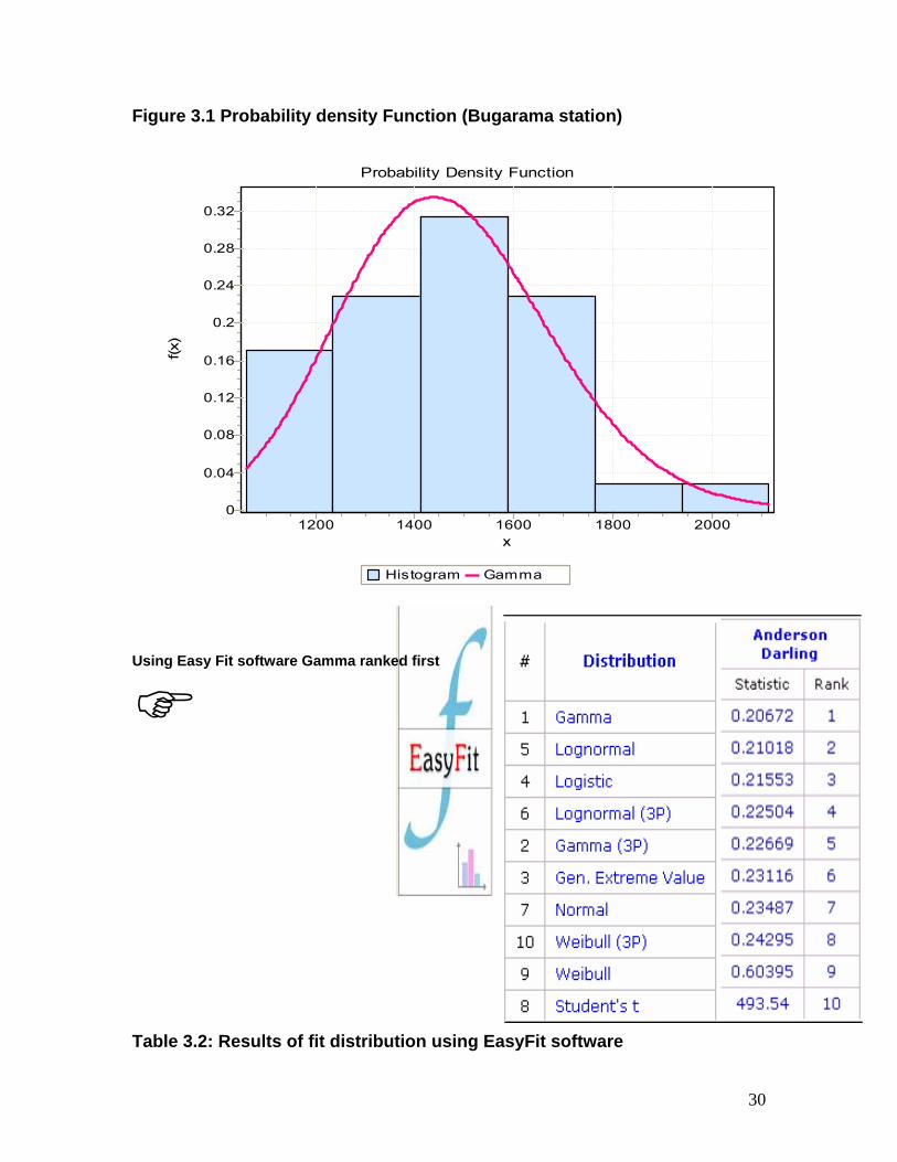
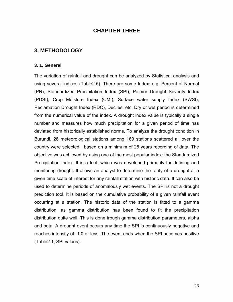
Figure 3.1 Probability density Function (Bugarama station)

Probability Density Function

Histogram Gamma

x20001800160014001200

f(x)

0.32

0.28

0.24

0.2

0.16

0.12

0.08

0.04

0

Using Easy Fit software Gamma ranked first

Table 3.2: Results of fit distribution using EasyFit software

30

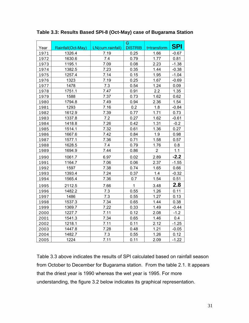
Table 3.3: Results Based SPI-8 (Oct-May) case of Bugarama Station

Year Rainfall(Oct-May) LN(cum.rainfall)G DISTRIB t=transform SPI

1971 1326.4 7.19 0.25 1.66 -0.67 1972 1630.6 7.4 0.79 1.77 0.81 1973 1195.1 7.09 0.08 2.23 -1.38 1974 1382.5 7.23 0.35 1.44 -0.38 1975 1257.4 7.14 0.15 1.95 -1.04 1976 1323 7.19 0.25 1.67 -0.69 1977 1478 7.3 0.54 1.24 0.09 1978 1751.1 7.47 0.91 2.2 1.35 1979 1588 7.37 0.73 1.62 0.62 1980 1794.8 7.49 0.94 2.36 1.54 1981 1293 7.16 0.2 1.8 -0.84 1982 1612.9 7.39 0.77 1.71 0.73 1983 1337.8 7.2 0.27 1.62 -0.61 1984 1418.8 7.26 0.42 1.31 -0.2 1985 1514.1 7.32 0.61 1.36 0.27 1986 1667.6 7.42 0.84 1.9 0.98 1987 1577.1 7.36 0.71 1.58 0.57 1988 1628.5 7.4 0.79 1.76 0.8 1989 1694.9 7.44 0.86 2 1.1 1990 1061.7 6.97 0.02 2.89 -2.2 1991 1164.7 7.06 0.06 2.37 -1.55 1992 1597 7.38 0.74 1.65 0.66 1993 1393.4 7.24 0.37 1.4 -0.32 1994 1565.4 7.36 0.7 1.54 0.51

1995 2112.5 7.66 1 3.48 2.8 1996 1482.2 7.3 0.55 1.26 0.11 1997 1486 7.3 0.55 1.27 0.13 1998 1537.3 7.34 0.65 1.44 0.38 1999 1369.7 7.22 0.33 1.49 -0.44 2000 1227.7 7.11 0.12 2.08 -1.2 2001 1541.3 7.34 0.65 1.46 0.4 2002 1218.1 7.11 0.11 2.12 -1.25 2003 1447.8 7.28 0.48 1.21 -0.05 2004 1482.7 7.3 0.55 1.26 0.12 2005 1224 7.11 0.11 2.09 -1.22

Table 3.3 above indicates the results of SPI calculated based on rainfall season

from October to December for Bugarama station. From the table 2.1. It appears

that the driest year is 1990 whereas the wet year is 1995. For more

understanding, the figure 3.2 below indicates its graphical representation.

31

Figure 3.2: Graphical representation of the intensity of Bugarama station

3. 5. Time scale

The identification of drought characteristics requires the choice of the minimum

discrete time interval to be used in the analysis of the time-series. Thus, drought

will be identified as a negative departure from the truncation level assigned for

the corresponding season. The different time scale (season) for which the SPI is

computed address the various type of droughts: the shorter season for

Meteorological and Agricultural drought (soil moisture deficit during 2-4months),

the longer for Hydrological drought.

In BURUNDI, the wet season is from October to May and within this season

there are 2 distinct periods: small precipitations from October to January and

heavy precipitations from February to May. Therefore, in this study, 4 series of

SPI time scales were considered:

1. SPI-4 (From October to January, for small precipitations)

2. SPI–4 (From February to May, for heavy precipitations)

3. SPI-8 (From October to May, for all the rainfall season)

4. SPI-12(From January to December, full year, wet and dry season)

32

CHAPTER FOUR

4. RESULTS AND DISCUSSION

The SPI values were computed for the time scale of 12 months (Jan-Dec),

8months (Oct-May) and 4months (Oct-Jan), and (Feb-May) for 26 stations

(Appendix A). The statistical parameters namely coefficient of variation (CV),

the standard deviation (SD) and the mean were also computed (Appendix B).

The objective behind was to extract the maximum information and get

somewhat a general overview of SPI values over the study area.

4.1.Rainfall Variability

Rainfall variability is expressed by the coefficient variation (CV) and is defined

as the ratio of standard deviation to mean in percent, where mean and

standard deviation are estimated from rainfall data. A high ratio indicates an

erratic behavior. If the variability ratio is less than 15%, the precipitation is

generally reliable. If it is between 20% and 25%, prolonged droughts may

occur and when it is more than 40%, typical deserts are indicated (Rajit

Kumar Ghosh, Forecasting Drought in Ethiopia, 30th May 2001). As a general

rule, it is noted that variability is low where the average amounts are high, and

vice-versa.

In this study, the monthly rainfall data for about 25 to 45 years (1961 up to

2005) were selected for 26 stations and the statistical parameters were

computed. The CV has been computed separately for each of the 26 rain

gauge stations (Table 4.1). It varies from 9.7 to 31.2 over the study area for

the 26 stations selected. Table 4.1. Shows clearly that in Burundi, there is no

high variability. In fact, for all time scale under study, more than 90% values in

the table are less than 25% of CV. Based on year 2005 (from October to

May), it has been interpolated into aerial data in Arc View GIS to demarcate

its spatial variability (Figure 4.1).

33

Table 4.1: % of Coefficient of variation for different time scale

Station name CV-SPI 8 CV-SPI 12 CV-SPI 4 CV-SPI 4 (Oct-May) (Jan-Dec) (Oct-Jan) (Feb-May)

1. Bugarama-Aéro 14.32 13.22 21.58 20.652. Bujumbura-Aéro 18.02658 16.90418 28.37561 22.687113. Cankuzo 17.78974 17.6266 21.54482 21.918664. Giharo 14.98 15.1 17.34 21.265. Giheta 18.68047 15.31107 24.79347 26.851196. Gisozi 14.69554 13.54124 20.897 17.689387. Gitega-Aéro 16.67106 15.86279 22.30511 24.39897 8. Karusi 22.9122 21.4354 26.29392 31.204319. Kayogoro ( Makamba) 9.715283 8.553122 15.66593 11.8392210. Kinyinya 25.68299 24.56811 31.81134 26.2871211. Kirundo 13.50682 11.98293 20.87309 17.6662712. Mabayi 16.45892 17.24511 20.57431 21.1504213. Makamba 15.97177 15.50498 22.85751 19.3946714. Mparambo 17.45579 15.43497 28.8287 22.6749 15. Mpota-Tora 11.99273 11.11694 16.67814 17.8782416. Mugera - paroisse 17.37835 16.82925 26.17509 25.4890617. Musasa 17.70392 17.33305 23.56575 21.0229718. Musongati 13.54929 12.69768 17.49697 23.8834419. Mutumba 19.32855 18.3621 15.73464 27.8191120. Muyaga 18.00139 17.42797 26.01215 21.389221. Muyinga 17.09303 15.65317 25.73465 20.9015622. Nyamuswaga 17.16499 16.05588 21.47181 23.1569723. Nyanza-Lac 12.7275 12.33084 23.99412 22.4676224. Ruvyironza 13.03857 12.57614 20.53482 16.1753925. Rwegura 15.21221 14.5211 24.315 18.181126. Rweza-vyanda 17.74367 16.85485 22.17989 18.08673

34

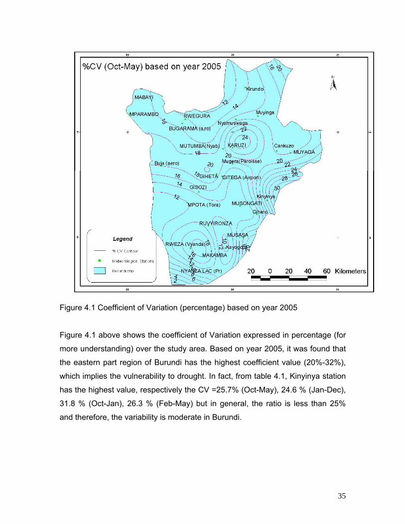
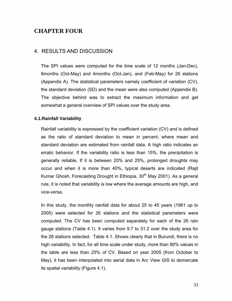
Figure 4.1 Coefficient of Variation (percentage) based on year 2005

Figure 4.1 above shows the coefficient of Variation expressed in percentage (for

more understanding) over the study area. Based on year 2005, it was found that

the eastern part region of Burundi has the highest coefficient value (20%-32%),

which implies the vulnerability to drought. In fact, from table 4.1, Kinyinya station

has the highest value, respectively the CV =25.7% (Oct-May), 24.6 % (Jan-Dec),

31.8 % (Oct-Jan), 26.3 % (Feb-May) but in general, the ratio is less than 25%

and therefore, the variability is moderate in Burundi.

35

4.2 .Drought characteristics

In this study, based on SPI-8 (Oct-May), the table 4.2.below summarizes the

results of the maximum and minimum values for drought characteristics namely:

duration, severity, magnitude and intensity.

Table 4.2: Drought characteristics based on SPI-8 (Oct-May)

Station Name Duration Severity Magnitude Intensity

N° Max Min Max Min Max Min Max Min 1 Cankuzo 32 8 5.15 0.20 0.19 0.03 -2.21 -0.10 2 Kinyinya 48 8 8.43 0.07 0.19 0.01 -3.57 -0.06 3 Giharo 64 8 7.25 0.33 0.16 0.02 -1.53 -0.20

4 MUSONGATI 24 8 3.70 0.38 0.38 0.19 -2.12 -0.48 5 MUSASA 24 8 4.22 0.40 0.27 0.22 -2.44 -0.26 6 Muyinga 32 8 3.66 0.16 0.21 0.02 -1.78 -0.01 7 MUYAGA 56 8 4.55 0.01 0.20 0.00 -2.23 -0.05 8 Nyamuswaga 56 8 6.16 0.62 0.15 0.08 -1.97 -0.31 9 Kirundo 32 8 5.08 0.51 0.21 0.06 -2.06 -0.51

10 GITEGA (Airport) 56 8 4.94 0.29 0.26 0.04 -2.09 -0.05 11 RUVYIRONZA 40 8 3.26 0.36 0.16 0.02 -2.08 -0.04 12 Mugera(Paroisse) 56 8 5.51 0.50 0.19 0.04 -2.47 -0.06 13 GIHETA 32 8 3.70 0.22 0.19 0.03 -2.80 -0.16 14 Buja (aero) 48 8 8.29 0.18 0.35 0.02 -1.95 -0.16 15 GISOZI 40 8 5.24 0.09 0.19 0.03 -1.90 -0.06

16 MPOTA (Tora) 40 8 6.46 0.06 0.21 0.01 -2.03 -0.16 17 KARUZI 32 8 4.64 0.37 0.29 0.03 -2.55 -0.09

18 MUTUMBA(Nyab) 56 8 3.96 0.13 0.11 0.02 -1.50 -0.06 19 Kayogoro 32 8 3.48 0.60 0.11 0.05 -1.42 -0.21 20 MAKAMBA 48 8 4.67 0.23 0.15 0.03 -2.17 -0.05 21 NYANZA LAC 24 8 4.02 0.11 0.17 0.01 -1.86 -0.05 22 MABAYI 40 8 5.46 0.77 0.23 0.08 -1.62 -0.08 23 MPARAMBO 32 8 4.37 0.25 0.18 0.00 -2.18 -0.07

24 RWEZA (Vyanda) 40 8 2.80 0.21 0.35 0.03 -2.80 -0.21 25 RWEGURA 32 8 3.58 0.32 0.22 0.02 -2.65 -0.08 26 Bugarama-aéro 32 8 3.48 0.32 0.23 0.04 -2.16 -0.05

From Table. 4.2. above, since two characteristics are enough to identify the drought, based on SPI-8 (Oct-May), Table 4.3 below summarizes for each station under study the different worst years of drought, their duration and their severity.

36

Table 4.3: Worst years drought based on SPI-8, their duration & severity

SPI-8 (Oct-May) Duration Severity Duration Severity Duration Severity 1.Mparambo station

2.Kirundo station 3.Ruvyironza station

Start End Start End Start End 1964 1967 24 2 1972 1976 32 3.1 1963 1966 24 0.4 1973 1976 24 4.4 1998 2001 24 5.1 1972 1976 32 5 1982 1986 32 2.8 1978 1981 24 1.8 1994 1996 32 2.3 1989 1994 40 3

2002 2005 24 3.3 4.Nyanza Lac station 5.Cankuzo station 6.Bujumbura station Start End Start End Start End

1998 2001 24 4 1997 2000 24 2.5 1972 1978 48 3.8 2002 2005 24 1.7 2001 2005 32 5.2 1989 2001 24 8.3

7.Giharo Station 8.Giheta STATION

9.Gisozi STATION

Start End Start End Start End 1989 1997 64 7.2 1972 1976 32 3.7 1972 1976 32 5.2 1998 2001 24 3.9 1986 1987 24 0.8 1991 1996 40 3.3 2002 2005 24 1.9 1989 1990 8 0.2 2000 2005 40 4.2

1991 1995 32 1.1 1999 2001 24 1.1 2002 2005 24 2.1

10.Gitega aero Station 11.Karusi Station 12.Kayogoro Station

Start End Start End Start End 1989 1996 56 4.9 1963 1966 24 0.7 1973 1976 24 2.7

1972 1976 32 3.1 1989 1993 32 3.5 1987 1990 24 1.4 13.Kinyinya station

14.Mabayi Station 15.Makamba station

Start End Start End Start End 1973 1977 32 3 1957 1960 24 2.9 1970 1976 48 4.7 1999 2005 48 8.4 1965 1972 56 3.9 1982 1985 24 3.7

1974 1979 40 3.8 2002 2005 24 3.4 1995 2002 24 5.5

16.Mpota-tora Station 17.Mugera-paroisse Station 18.Musasa Station

Start End Start End Start End 1972 1977 40 4.7 1972 1976 32 4.5 1982 1985 24 2.1 2000 2005 40 6.5 1989 1996 56 5.5 1998 2001 24 1.8

19.Musongati Station 20.Mutumba Station 21.Muyaga Station

Start End Start End 1951 1958 56 7.3 1998 2001 24 3.7 1978 1985 56 4 1968 1971 24 1.6

1992 1996 32 2.2 1997 2001 32 4.6 2002 2005 24 3.1 22.Muyinga Station 23.Nyamuswaga Station 24.Rwegura Station Start End Start End Start End

1973 1976 24 2.3 1991 1994 24 3.6 1963 1966 24 3.2 1997 2000 24 3.7 1998 2005 56 6.2 1968 1971 24 1.4

1977 1981 32 2.7 1982 1985 24 2 25.Rweza Station 26.Bugarama Station Start End Start End

1997 2002 40 2.2 1972 1976 32 3.5

37

Based on SPI-8 (from October up to May), Table 4.3.above shows that the worst

droughts in Burundi have occurred in:

Years 1972 up to 1976 for almost all stations existing at that time namely:

Mparambo, Kirundo, Ruvyironza, Bujumbura, Gisozi, Giheta, Karuzi,

Kayogoro, Kinyinya, Mabayi, Makamba, Mpota, Muyinga, Mugera and

Bugarama.

Years 2000 up to 2005 for almost all stations in use (because of the civilian

war from 1993, some stations cut off) namely : Kirundo, Ruvyironza, Nyanza

lac, Cankuzo, Bujumbura, Giharo, Giheta, Kinyinya, Mabayi, Makamba,

Musongati, Muyaga, Muyinga, Nyamuswaga and Rweza.

Once again, as for the coefficient of variation, the results (from Tables 4.2 & 4.3)

show that the eastern part area of Burundi is vulnerable to drought .In fact, the

maximum duration (64 months) was recorded at Giharo station, the maximum

severity(8.43) , maximum magnitude (0.19) and maximum intensity(-3.57) were

found at Kinyinya station.

The analyses in which worst droughts have occurred indicates clearly that

drought is becoming a real problem in Burundi be. In fact, it is known that the

Burundian government has established an inter-ministerial committee to help

boost aid to the people affected by food shortages.

Therefore, as the drought and the famine look like twins, and since historically

the government of Burundi has decided to help the people affected by the famine

in 2005 because of drought, that year was considered in this study as the worst

year drought to be compared with the year 1978 which was the mild year drought

according to its smallest negative values (Appendix A). Hence, below is the

comparison of the years 2005 and 1978 through which the different contour

maps were made based on SPI-12 (Jan-Dec), SPI-8 (Oct-May), SPI-4 (Oct-Jan)

and SPI (Feb-May), using Arc View GIS.

38

Figure 4.2 show case of SPI-12 rain season 2005

As categorized in Table 3.6 (SPI values), Figure 4.2 above shows that based on

the year 2005 and SPI-12 (Jan-Dec), Burundi was affected by severe drought in

general, and it was increasing from moderate to extreme drought in the north-

west to the centre, south & eastern regions (SPI values from -0.5 up to -4.5).

39

Figure 4.3 show case of SPI-12 rain season 1978

In contrast to Figure 4.2, Figure 4.3 above is different from figure 4.2 in that

based on the year 1978 and SPI-12 (Jan-Dec), Burundi was affected only by

moderate drought in the southern and northern regions.

40

Figure 4.4 SPI-8 Rainy Season 2005

Figure 4.4 above shows from Table 3.6 (SPI values) that, based on the year

2005 and SPI-8 (Oct-May), Burundi was affected by severe drought in general,

and by extreme drought in the southern east regions in particular.

41

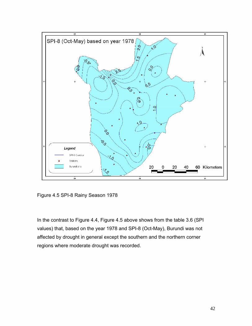
Figure 4.5 SPI-8 Rainy Season 1978

In the contrast to Figure 4.4, Figure 4.5 above shows from the table 3.6 (SPI

values) that, based on the year 1978 and SPI-8 (Oct-May), Burundi was not

affected by drought in general except the southern and the northern corner

regions where moderate drought was recorded.

42

Figure 4.6 SPI-4 (Oct-Jan) rain season 2005

Figure 4.6 above shows from Table 3.6 (SPI values) that, based on the year

2005 and SPI-4 (Oct-Jan), Burundi was affected by drought in general and by

extreme drought in the southern east regions in particular.

43

Figure 4.7 SPI-4 (oct-jan) rainy season 1978

In contrast to Figure 4.6, Figure 4.7 above shows from Table 3.6 (SPI values)

that, based on the year 1978 and SPI-4 (Oct-Jan), Burundi was almost not

affected by drought except in the northern west corner region where moderate

drought is recorded.

44

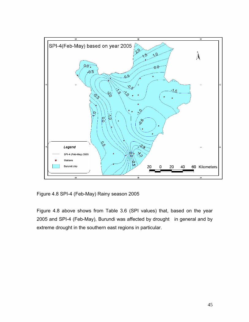
Figure 4.8 SPI-4 (Feb-May) Rainy season 2005

Figure 4.8 above shows from Table 3.6 (SPI values) that, based on the year

2005 and SPI-4 (Feb-May), Burundi was affected by drought in general and by

extreme drought in the southern east regions in particular.

45

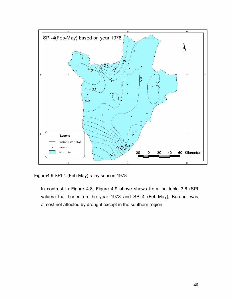
Figure4.9 SPI-4 (Feb-May) rainy season 1978

In contrast to Figure 4.8, Figure 4.9 above shows from the table 3.6 (SPI

values) that based on the year 1978 and SPI-4 (Feb-May), Burundi was

almost not affected by drought except in the southern region.

46

4.3. The trend of SPI over the study area

In this study, during the period investigated, the results show that the

rainfall decreased from 1989 but the decrease becomes stronger from 2000

(Appendix D). In this period, the SPI for multiple scale under consideration

namely 12 months (Jan-Dec), 8 months (Oct-May), 4 months (Oct-Jan), 4

months (Feb-May) has been computed for all selected stations. It appears

that period of drought have been quite frequent starting from 2000, with SPI

ranging from about -1 to about -3. Below is the trend case of Musasa station,

located in the eastern region already mentioned as one region vulnerable to

drought in Burundi.

Musasa station: SPI-4(feb-may)

-3

-2

-1

0

1

2

3

1961

1963

1965

1967

1969

1971

1973

1975

1977

1979

1981

1983

1985

1987

1989

1991

1993

1995

1997

1999

2001

2003

2005

Year

Inte

nsity

SPI-4(feb-may) 5 per. Mov. Avg. (SPI-4(feb-may))

Figure 4.10. Drought Intensity and trend based on SPI-4 (show case of Musasa

station

47

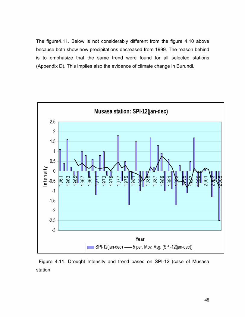
The figure4.11. Below is not considerably different from the figure 4.10 above

because both show how precipitations decreased from 1999. The reason behind

is to emphasize that the same trend were found for all selected stations

(Appendix D). This implies also the evidence of climate change in Burundi.

Musasa station: SPI-12(jan-dec)

-3

-2.5

-2

-1.5

-1

-0.5

0

0.5

1

1.5

2

2.5

1961

1963

1965

1967

1969

1971

1973

1975

1977

1979

1981

1983

1985

1987

1989

1991

1993

1995

1997

1999

2001

2003

2005

Year

Inte

nsity

SPI-12(jan-dec) 5 per. Mov. Avg. (SPI-12(jan-dec))

Figure 4.11. Drought Intensity and trend based on SPI-12 (case of Musasa

station

48

CHAPTER 5

5.Conclusions and Recommendations

5. 1. CONCLUSIONS

In this study, during the period investigated, the results show that the rainfall

decreased from 1989 but the decrease becomes stronger from 2000 (Appendix

D). In this period, the SPI for multiple scale under consideration namely 12

months (Jan-Dec), 8 months (Oct-May), 4 months (Oct-Jan), 4 months (Feb-

May) has been computed for all selected stations. It appears that period of

drought have been quite frequent starting from 2000, with SPI ranging from about

-1 to about -3. The North Eastern regions of Burundi is vulnerable to drought .In

fact, the maximum duration (64 months) was recorded at Giharo station, the

maximum severity (8.43), maximum magnitude (0.19) and maximum intensity (-

3.57) were found at Kinyinya station and since historically the government of

Burundi has decided to help the people affected by the famine in 2005 because

of drought, that year was considered in this study as the worst year drought to be

compared of the year 1978 which was the mild year drought according to its

smallest negative values(Appendix A) using Arc View GIS . As categorized in the

table 2.1 (SPI values), based on the years 2005 and 1978, for all time scale of

SPI under study, Burundi was affected by severe drought in general in 2005, and

it was increasing from moderate to extreme drought in the north-west to the

centre, south & eastern regions (SPI values from -0.5 up to -4.5) whereas in

contrast to the year 1978 for the same time scale, Burundi was in general not

affected by drought except in very few northern east regions where moderate

drought was recorded. Therefore, from the results of this study, drought is

becoming a real problem in Burundi with the time. As drought and famine look

like twins, even drought is a natural hazard, society can reduce its vulnerability

like other natural hazards through mitigation, planning and preparedness (risk

management) and recommendations are suggested.

49

5. 2. RECOMMENDATIONS

Drought is natural disasters, which originates from the lack of precipitation and

brings significant economic losses. It is not possible to avoid it but drought

preparedness can be developed and droughts impacts can be managed.

Therefore, in Burundi, a national drought policy is strongly needed to coordinate

or to take actions regarding above suggestions and recommendations:

5. 2.a. Information evaluation and needs

Analysis of all available information would lead to decision-making in the

following areas: Food security and distribution, Water management and

Agriculture, Water supply management, seeds, livestock survival and Health

problems (Ruben Barakiza -2006). In water management and Agriculture, priority should be given to the following

actions: ensure water supply to the population and livestock affected, put in place

local scale irrigation, campaign for technical water management supply

necessary funds for repairing/install water pumps, strengthen continuous

coordination among agricultural engineers, meteorologists, hydraulics engineers,

agricultural monitors to inform and help farmers to adapt their farming practices

to the drought situation

During drought it is important to conserve reserves of seeds and as

a measure of precaution, government should: set up conservation of seeds in

seed bank, regional cooperation (external aid in seeds, fertilizers and pesticides

from countries of similar soils and climate conditions), International aid

organization such as FAO can mobilize seed assistance during emergency

situation and research is needed with a view to develop varieties that are

drought-resistant and early maturing varieties. •When drought is limited to only

certain regions, livestock can migrate to others regions which are not

experiencing drought

50

5.2. b. Early warning system

An efficient system of agricultural data in collaboration with Meteorological

service should be able to supply to the government, at any time, information on:

meteorological conditions and the characteristics of seasonal rainfall, the state of

crops and variations outlook compared to previous seasons, infestations of

insects and parasites, production outlook, situation of water supply for human,

health problems and livestock consumption and those information should be

supported by the Use of satellite data ( Normalized differences of vegetation

index-NDVI)

5.2. C. Drought management and prevention When preventive measures are integrated in long-term economical planning they

have a considerable effect in reducing drought related impacts. The mitigate programs implemented by the country government during recent

droughts can be characterized as emergency actions taken to alleviate the

ongoing crisis and preparedness is the logical solution where a national drought

policy and plan might be set up .A national drought commission should be set up

and the commission should include meteorological service, agriculture, water

resources management, planning, public water supply, natural resources,

environmental protection, health, finance, rural development, emergency

management, and tourism. The objectives that should be considered include the

following:

To provide timely and systematic data collection, analysis and dissemination

of drought-related information;

To establish proper criteria to identify and designate drought-affected areas

and to trigger response activities by government and NGOs;

To provide an organization a structure that assures information between and

within levels of government and define the duties and responsibilities of all

agencies with respect to drought;

To develop a set of appropriate emergency programs;

51

To provide a mechanism to ensure the timely and accurate assessment of

drought impact on agriculture, industry, municipalities, wildlife, health, and

other areas as appropriate;

To provide accurate and timely information in order to keep the public

informed;

To establish and pursue a strategy to make equitable supply of water during

shortage and encourage water conservation;

To establish a set of procedures to evaluate and revise the plan

5. 2. d. Predicting Drought Predicting drought is extremely important. It allows policy makers and others to take appropriate measures to combat drought’s effects. It saves lives and reduces property damage. However, no perfect method exists to reliably predict the occurrence, persistence, cessation or recurrence of drought. There are mathematical models to help predict drought. SYDNEY are Models developed to take the uncertainty out of predicting droughts and say exactly where and for how long they are expected to occur. The models, named copulas, can help assist farmers determine the viability of different crops and the drought mitigation steps they need to take under varying climatic conditions.

Actually, it is known that most of countries all over the world and especially in

Africa, that prediction of drought is an alluring problem. It is not yet possible to

foretell the exact onset and intensity of droughts with the current available

knowledge. Therefore, since the objective of the present work is to analyze the

past drought in Burundi and to develop some techniques for prevention and

management, my expectations is that the government of Burundi will encourage

for future studies in the sense of drought prediction.

52

References

1 - Alley, W.M. 1984. The Palmer Drought Severity Index: Limitations and assumptions. Journal of Climate and Applied Meteorology 23:1100–1109.

2 - Edwards, D.C.; and T. B. McKee. 1997. Characteristics of 20th century

drought in the United States at multiple time scales. Climatology Report Number

3 - E.R. Dahmen & M.J.Hall,Publication N°49,London May 1989 :

Screening of Hydrological data :Tests for Stationarity and Relative Consistency

Gibbs and Maher - The deciles method (1967)

4 - Gommes, R.; and F. Petrassi. 1994. Rainfall variability and drought in Sub-

Saharan Africa since 1960. Agrometeorology Series Working Paper No. 9, Food

and Agriculture Organization, Rome, Italy.

5 - IGEBU(Institut géographique du Burundi) : Evolution climatique actuelle et

développement des scénarios de changements climatiques à l-horizon 2050

,Gitega-Burundi(2001)

6 -Karl, T.R.; and R.W. Knight. 1985. Atlas of Monthly Palmer Hydrological

7 - Le Houerou(1993)- Dependable Rain - stated in Hayes (2003).

8 -McKee, T.B.; N.J. Doesken; and J. Kleist. 1993. The relationship of drought

frequency and duration to time scales. Preprints, 8th Conference on Applied

Climatology, pp. 179–184. January 17–22, Anaheim, California.

9 -McKee, T.B.; N.J. Doesken; and J. Kleist. 1995. Drought monitoring with

multiple time scales.

53

10 -Palmer, W.C. 1965. Meteorological drought. Research Paper No. 45, U.S.

Department of Commerce Weather Bureau, Washington, D.C.

11 - Ranjit KUMAR (30th May, 2001), Forecasting Drought in Ethiopia

12 - Ruben Barakiza - Recent drought impact management in Burundi:

Presentation in the 7th forum Maputo (16-20 October 2006)

13 -Shafer and Dezman (1982) -Surface Water Supply Index (SWSI) 14 - Wilhite, D.A.; and M.H. Glantz, (1985). Understanding the drought phenomenon: The role of definitions. Water International 10(3): 111–120. 15 -Willen Van Cotthem, The Economic Times,posted on Google –Alert drought ,june 2008

54

Appendix A: SPI Values for different time scale and for selected stations

55

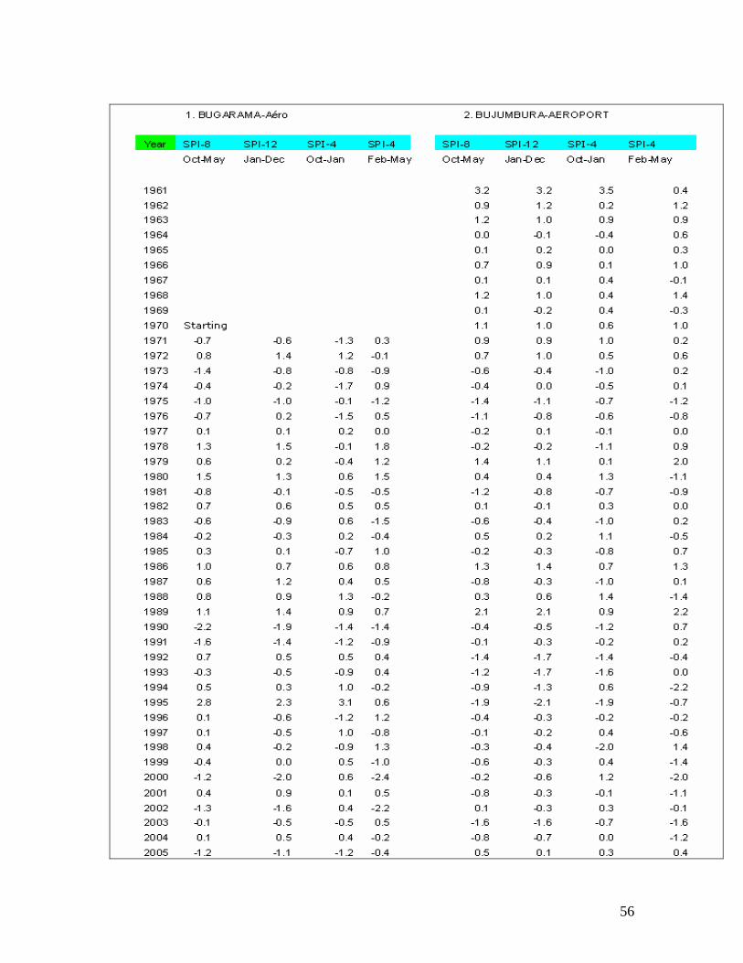
56

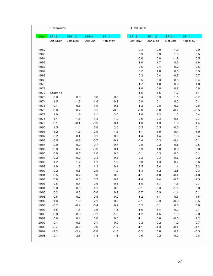
57

58

59

60

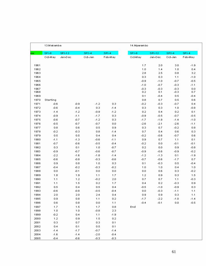
61

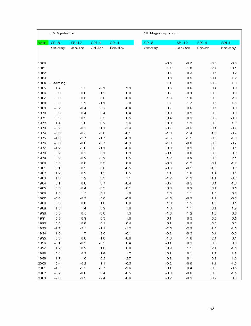
62

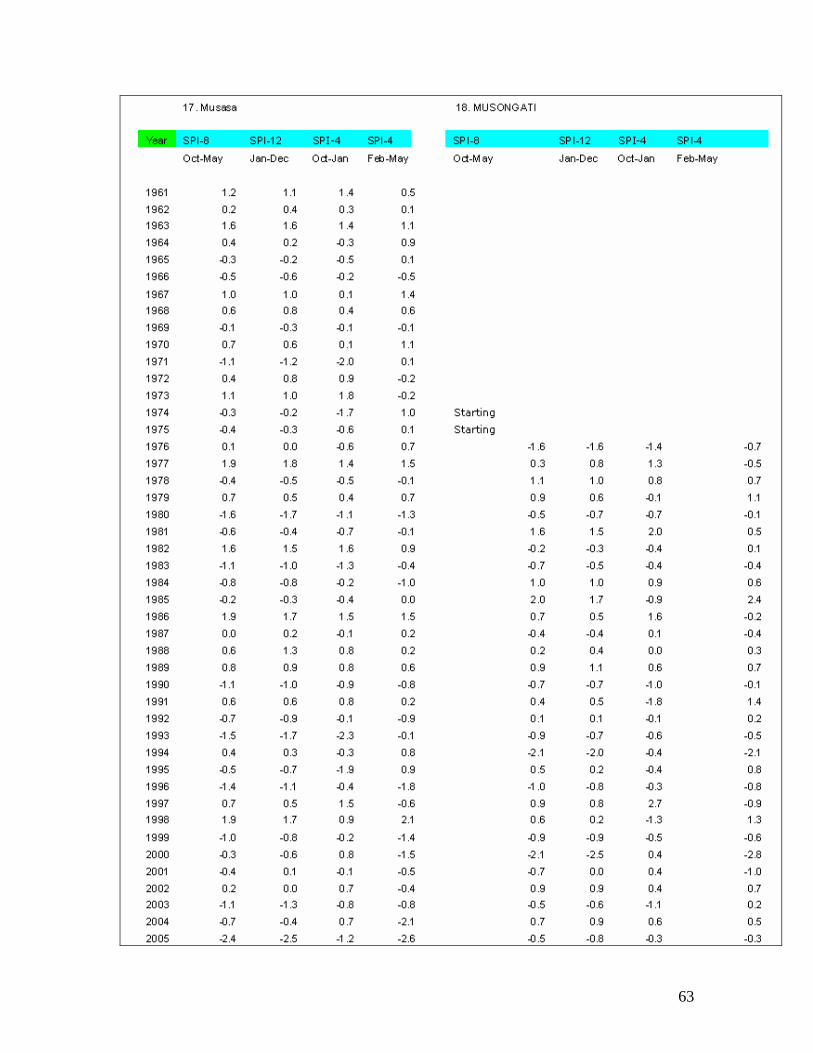
63

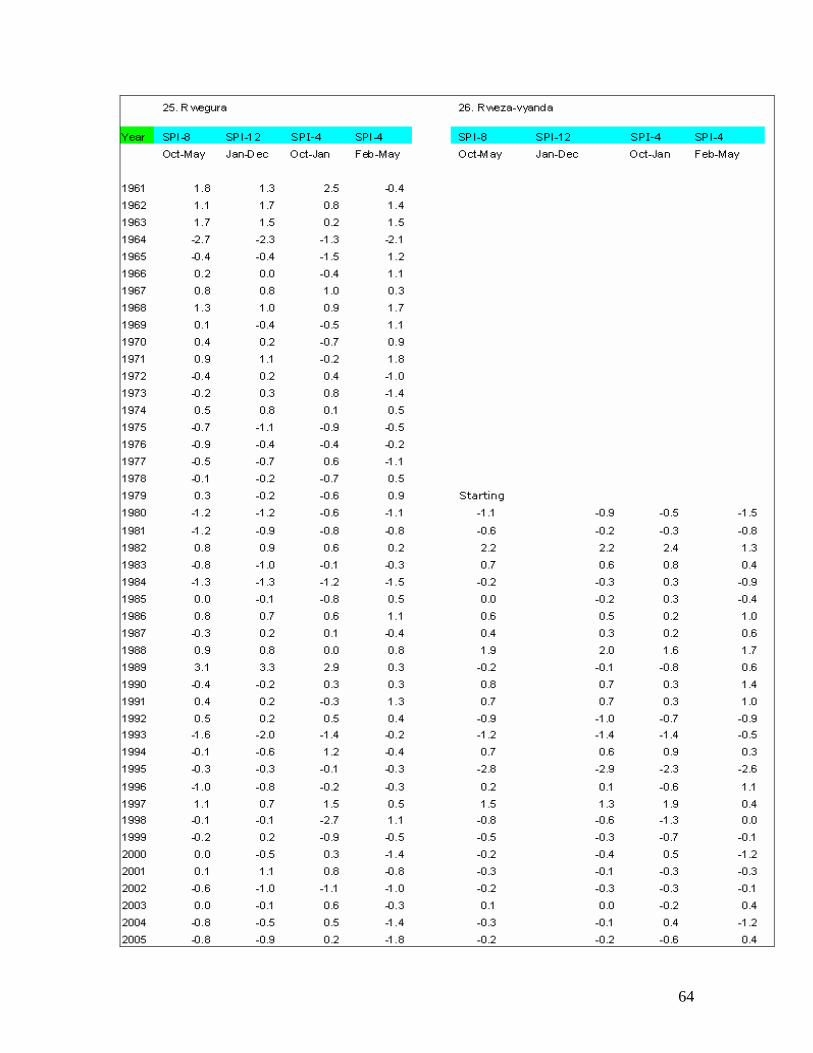
64

Appendix B: STATISTICAL PARAMETERS (CV in %)

65

Legend – CV(%) = coefficient of variation

- SD = Standard deviation

66

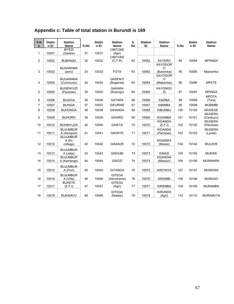
Appendix c: Table of total station in Burundi is 169

S.No

Station ID

Station Name S.No

Station ID

Station Name

S.No

Station ID

Station Name S.No

Station ID

Station Name

1 10001 BITEZI

(Gasibe) 31 10031 CIBITOKE

(Agri)

2 10002 BUBANZA 32 10032 CIBITOKE

(C.F.R) 62 10062 KAYERO 94 10094 MPANDA

3 10003 BUGARAMA

(aero) 33 10033 FOTA 63 10063

KAYOGORO

(Bukemba) 95 10095 Mparambo

4 10004 BUGARAMA (Commune) 34 10034

GASENYI (Buganda) 64 10064

KAYOGORO

(Makamba) 96 10096 MPETE

5 10005 BUGENYUZI

(Paroisse) 35 10035 GAKARA (Rutongo) 65 10065

KAYONGOZI 97 10097 MPINGA

6 10006 BUGIGA 36 10036 GATARA 66 10066 KAZIBA 98 10098 MPOTA (Tora)

7 10007 BUHIGA 37 10037 GIFURWE 67 10067 KIBIMBA 99 10099 MUBIMBI 8 10008 BUHONGA 38 10038 GIHANGA 68 10068 KIBUMBU 100 10100 MUGEGE

9 10009 BUHORO 39 10039 GIHARO 69 10069 KIGAMBA 101 10101 MUGERA (Cankuzo)

10 10010 BUHINYUZA 40 10040 GIHETA 70 10070 KIGANDA

(E.F.I) 102 10102 MUGERA (Paroisse)

11 10011 BUJUMBURA (Aeroport) 41 10041 GIKWIYE 71 10071

KIGANDA (Paroisse) 103 10103

MUGERA (Lycee)

12 10012

BUJUMBURA (Ex

college) 42 10042 GISANZE 72 10072 KIGARIKA

(Mosso) 104 10104 MULEHE

13 10013 BUJUMBUR

A (Jabe) 43 10043 GISHUBI 73 10073 KINAZI 105 10105 MUKIKE

14 10014 BUJUMBURA (Kamenge) 44 10044 GISOZI 74 10074

KIGWENA (Mission) 106 10106 MUNANIRA

15 10015 BUJUMBUR

A (Port) 45 10045 GITANGA 75 10075 KINYINYA 107 10107 MUNGWA

16 10016 BUJUMBUR

A (Ville) 46 10046 GITEGA

(Aerodrome) 76 10076 KIRAMBI 108 10108 MURAGO

17 10017 BUKEYE

(E.F.I) 47 10047 GITEGA

(Agri) 77 10077 KIREMBA 109 10109 MURAMBA

18 10018 BUKWAVU 48 10048 GITEGA (Ndebe) 78 10078

KIRUNDO (Agri) 110 10110 MURAMVYA

67

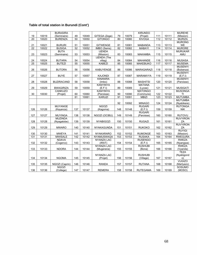
Table of total station in Burundi (Cont’)

19 10019 BURASIRA (Seminaire) 49 10049 GITEGA (Zege) 79 10079

KIRUNDO (Projet) 111 10111

MUREHE (Mission)

20 10020 BURENZA 50 10050 GITONGO 80 10080 KIVOGA 112 10112 MURIZA

21 10021 BURURI 51 10051 GITWENGE 81 10081 MABANDA 113 10113 MURONG

WE 22 10022 BUSIGA 52 10052 IMBO (Sems) 82 10082 MABAYI 114 10114 MURORE

23 10023 BUTA

(Seminaire) 53 10053 IJENDA (Mission) 83 10083 MAKAMBA 115 10115

MURUKARAMU

24 10024 BUTARA 54 10054 IJENDA (The

villag) 84 10084 MAHANDE 116 10116 MUSASA 25 10025 BUTEZI 55 10055 KABEZI 85 10085 MAKEBUKO 117 10117 MUSEMA

26 10026 BUTORA 56 10056 KABUYENGE 86 10086 MARAGARAZI 118 10118 MUSENYI (Bubanza)

27 10027 BUYE 57 10057 KAJONDI 87 10087 MARAMVYA 119 10119 MUSENYI

(E.F.I)

28 10028 BUZIRACAND 58 10058 KINANIRA

(Imbo) 88 10088 MASHITSI 120 10120 MUSENYI (Paroisse)

29 10029 BWAGIRIZA 59 10059 KANYINYA

(E.F.I) 89 10089 MATANA (Lycee) 121 10121 MUSIGATI

30 10030 CANKUZO

(Projet) 60 10060 KANYINYA (Paroisse) 90 10090

MATONGO (Commune) 122 10122

MUSONGATI

61 10061 KARUZI 91 10091 MBIZI 123 10123 MUTUMBA

92 10092 MINAGO 124 10124 MUTUMBA (Nyabikere)

126 10126 MUYANGE (Kayanza) 137 10137

NGOZI (Kagoma) 148 10148

RUGARI (E.F.I) 159 10159

RUTONGANIK

127 10127 MUYINGA 138 10138 NGOZI (OCIBU) 149 10149 RUGARI

(Paroisse) 160 10160 RUTOVU

128 10128 MUZINDA

(Nyagatobe) 139 10139 NYABIGOZI 150 10150 RUGAZI 161 10161 RUVYIRON

ZA

129 10129 MWARO 140 10140 NYAKAGUNDA 151 10151 RUKOKO 162 10162 RUVYIRON

ZA

130 10130 MWEYA 141 10141 NYAKARARO 152 10152 RUMONGE 163 10163 RUYIGI

(Mission) 131 10131 MWISALE 142 10142 NYAMUSWAGA 153 10153 RUSAKA 164 10164 RWEGURA

132 10132 NDAVA

(Cogerco) 143 10143 NYANZA LAC

(IRAT) 154 10154 RUSENGO

(E.F.I) 165 10165 RWEZA

(Nyangwa)

133 10133 NDORA 144 10144 NYANZA LAC

(Mugerana) 155 10155 RUSHUBI

(Bona) 166 10166 RWEZA (Vyanda)

134 10134 NGOMA 145 10145 NYANZA LAC

(Projet) 156 10156 RUSHUBI (Village) 167 10167

TEZA (Nyabigond

o)

135 10135 NGOZI (Caprin) 146 10146 RANDA 157 10157 RUTANA 168 10168 VUGIZO

(Martyazo)

136 10136 NGOZI

(College) 147 10147 REMERA 158 10158 RUTEGAMA 169 10169 SOSUMO (MOSO)

68

69

-Appendix D: Drought Intensity and Trend (SPI-8) for selected stations

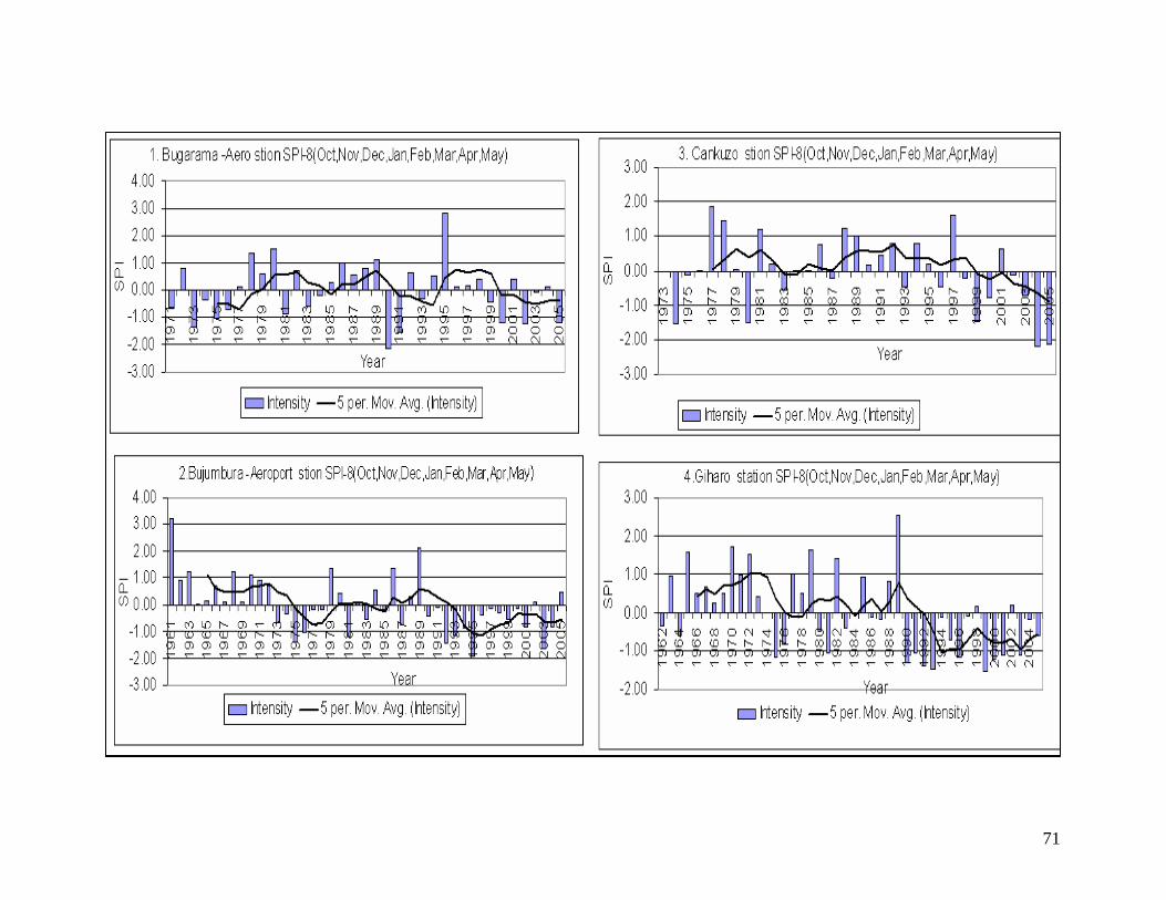
71

72

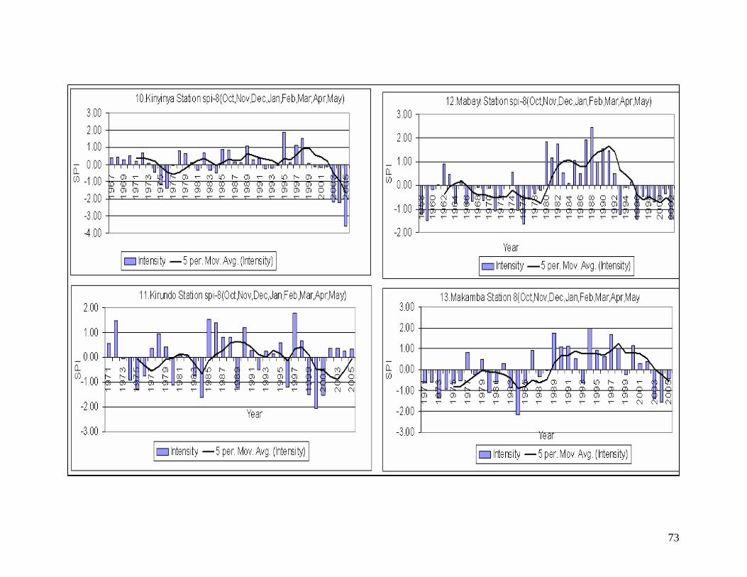
73

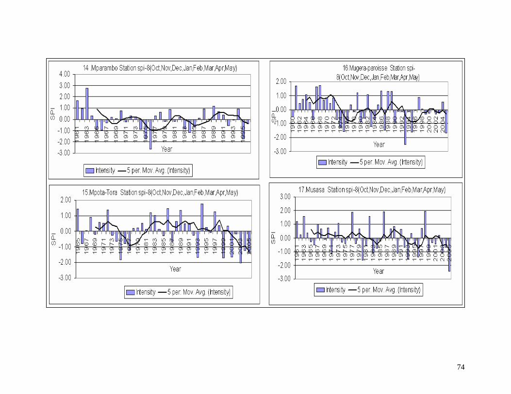
74

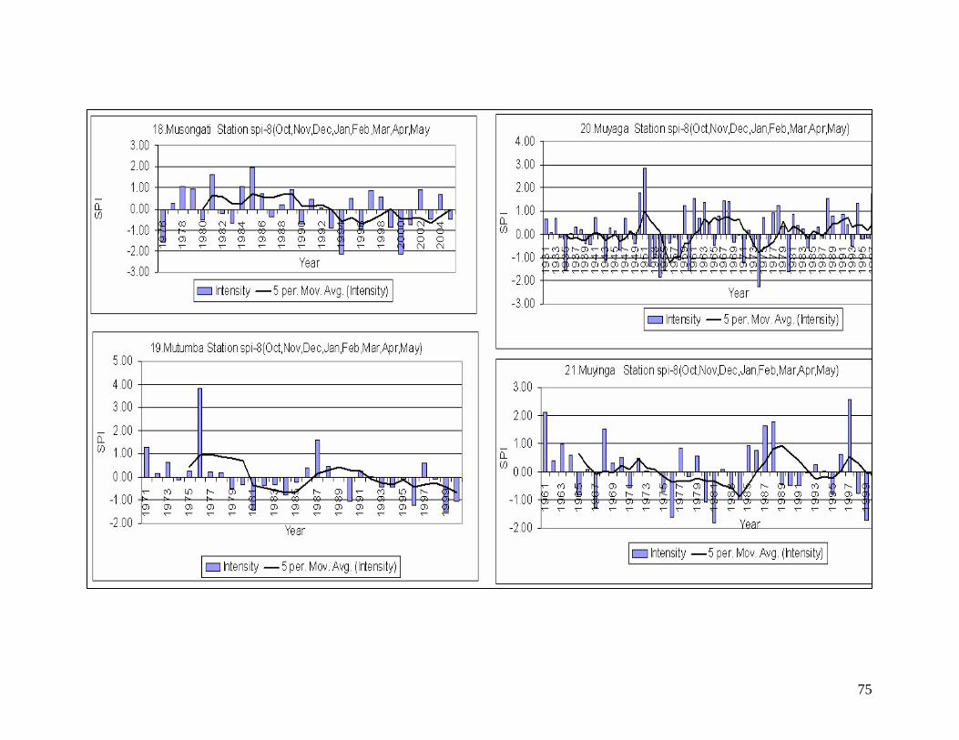
75

76

Appendix E: Drought duration, severity, magnitude, frequency based on SPI-8

77

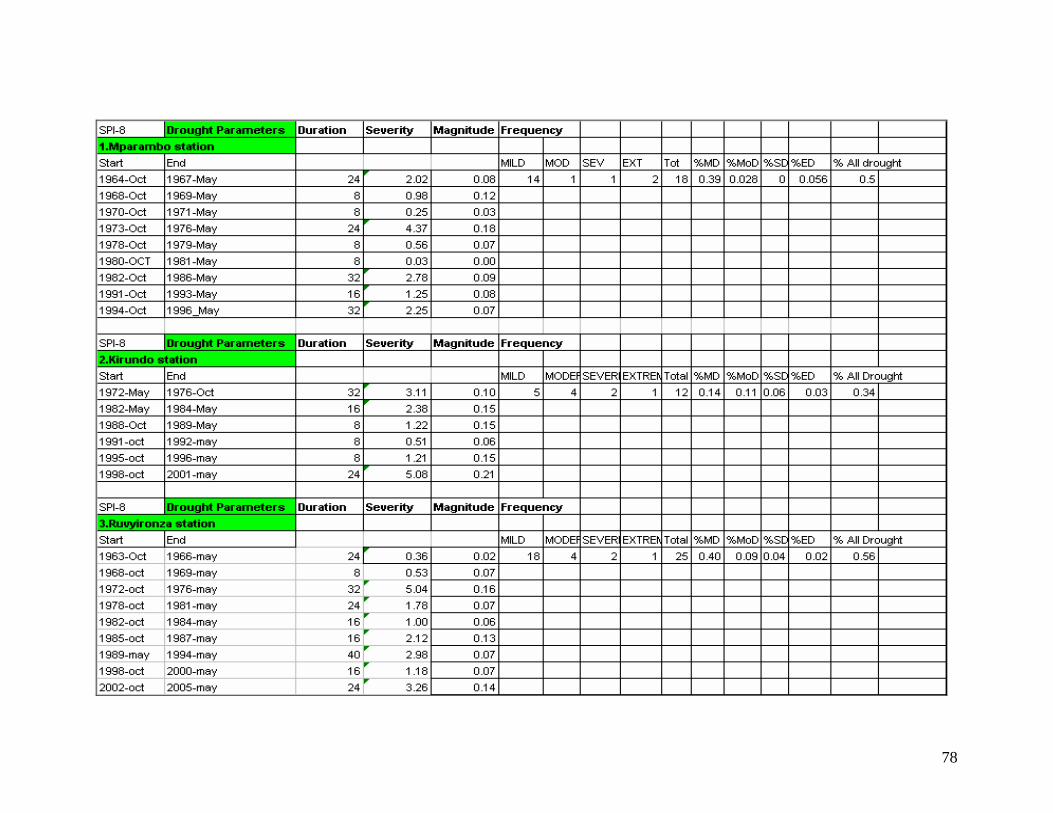
78

79

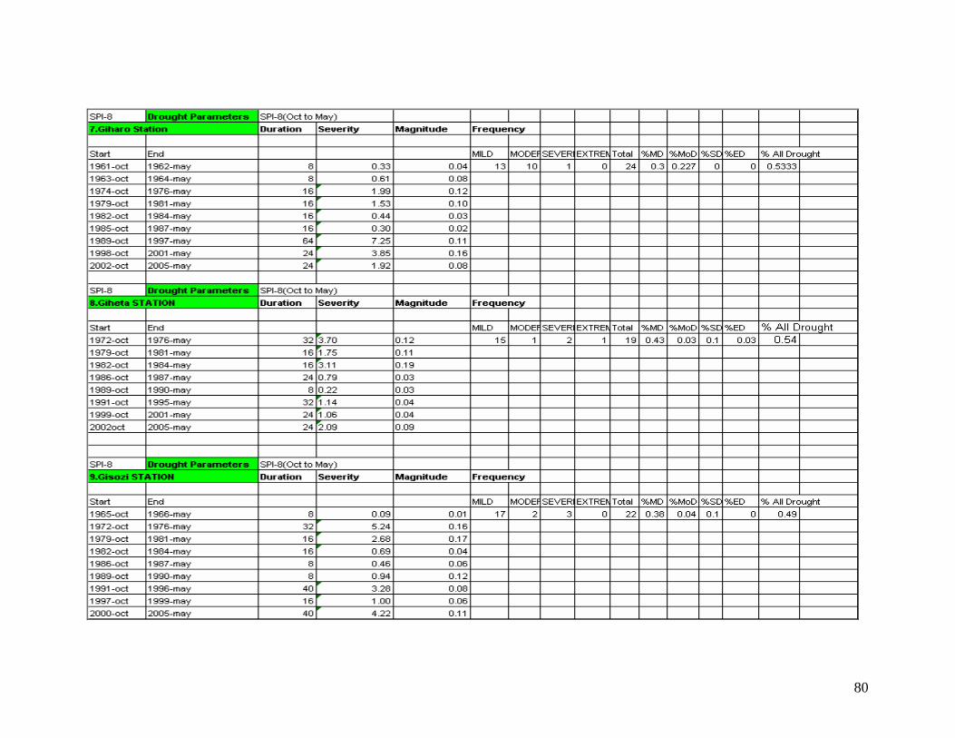
80

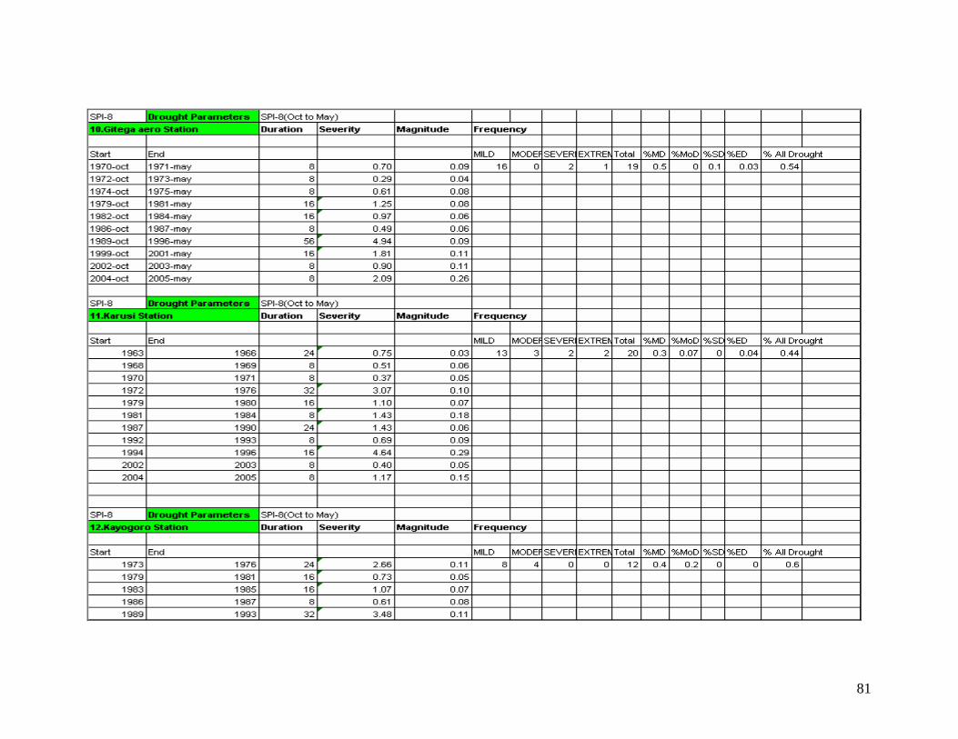
81

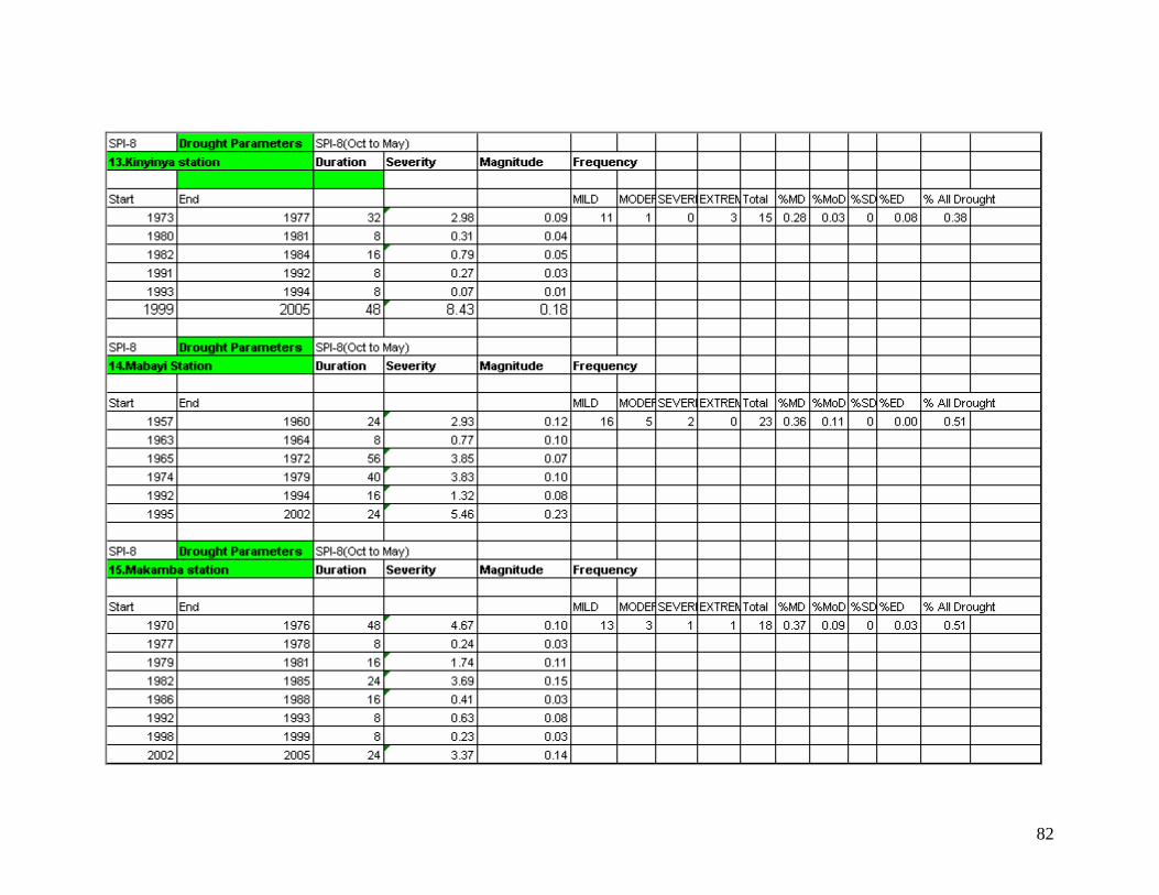
82

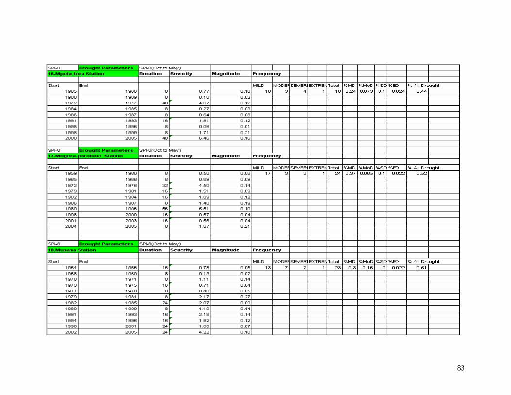
83

84

85

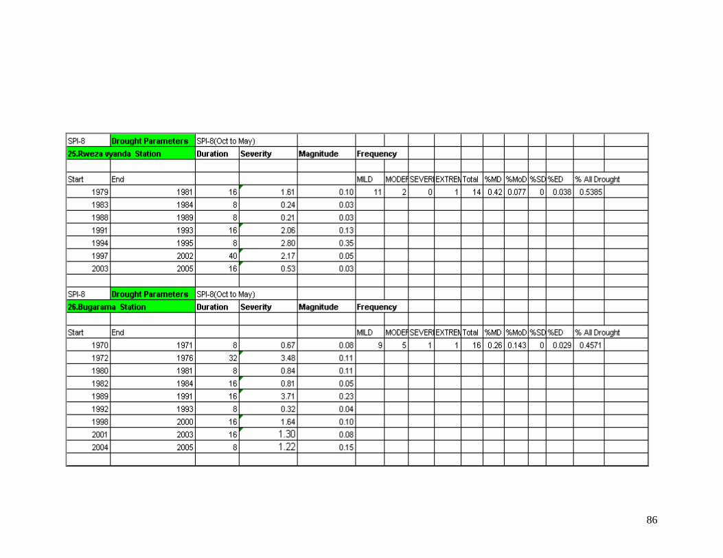
86

Appendix F: Drought category based on SPI-8

87

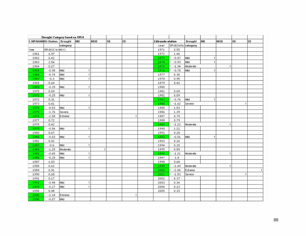
88

89

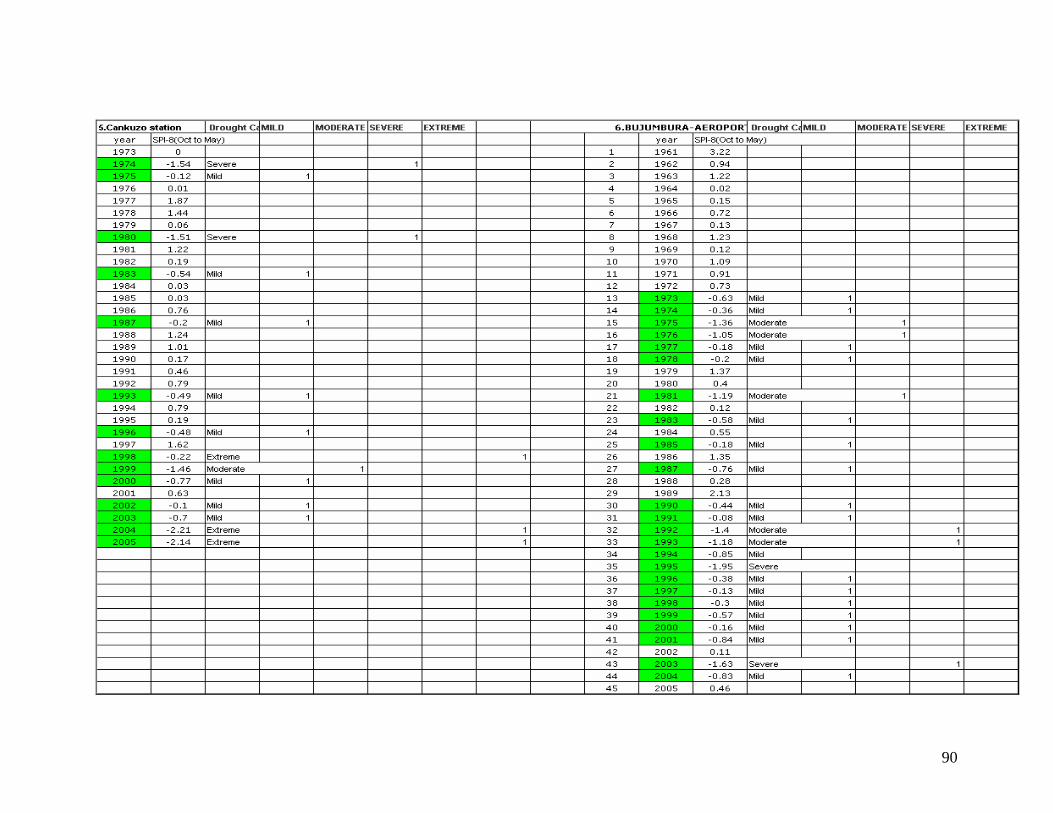
90

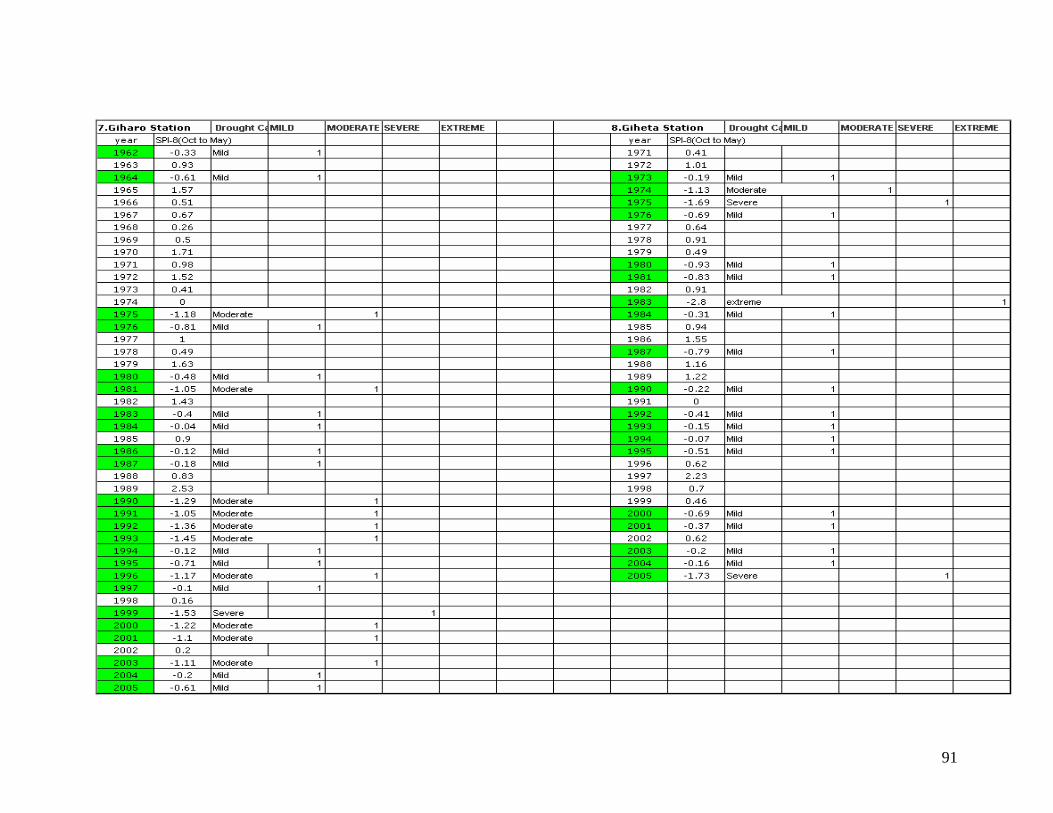
91

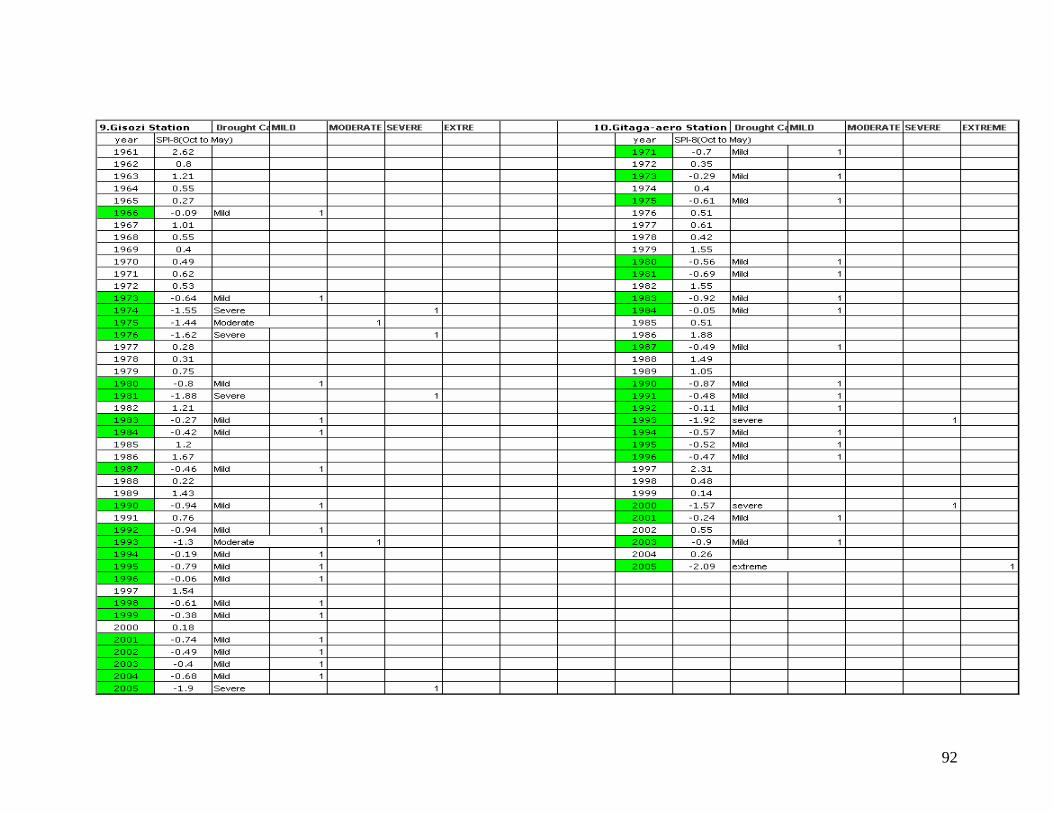
92

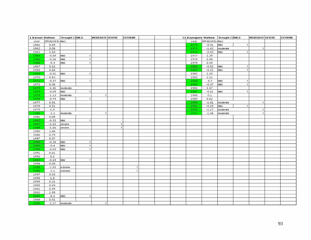
93

94

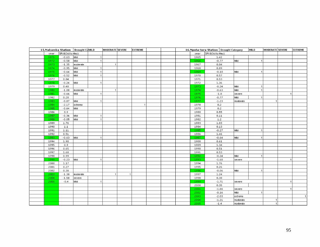
95

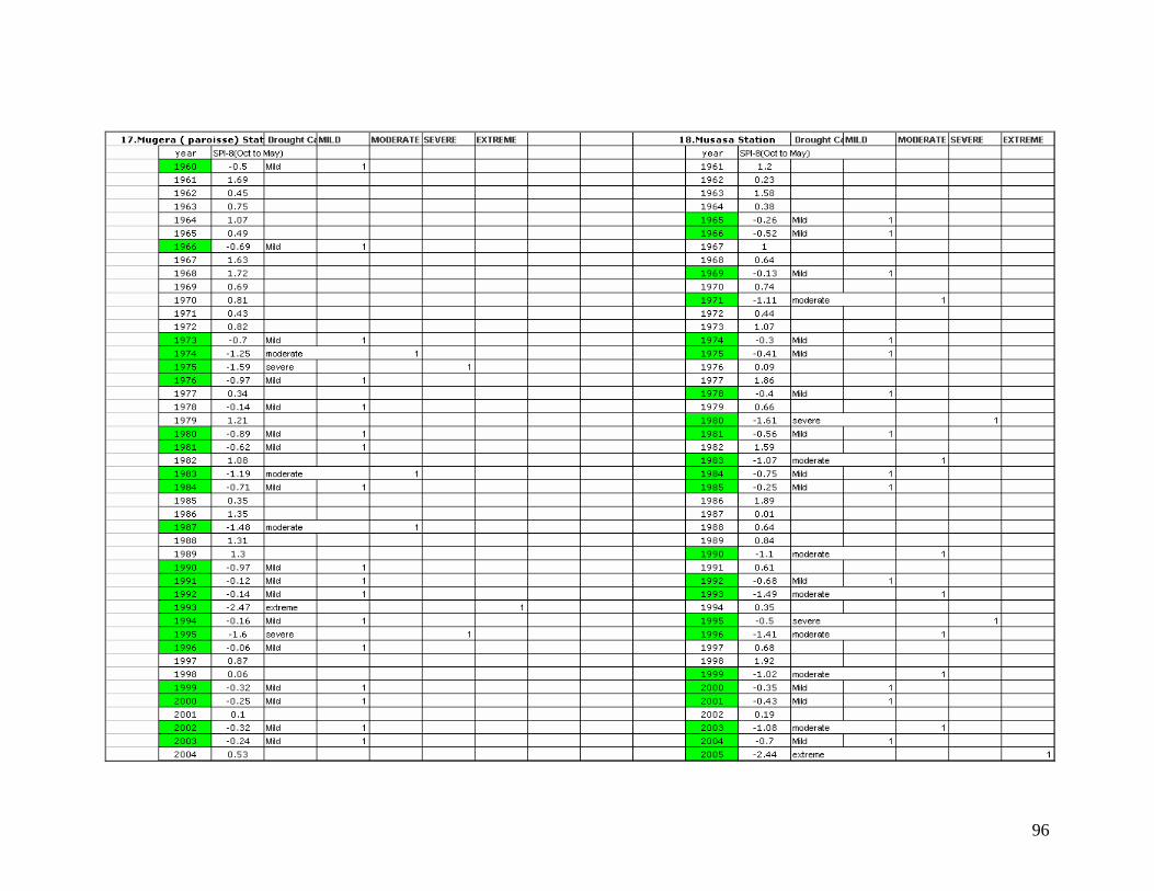
96

97

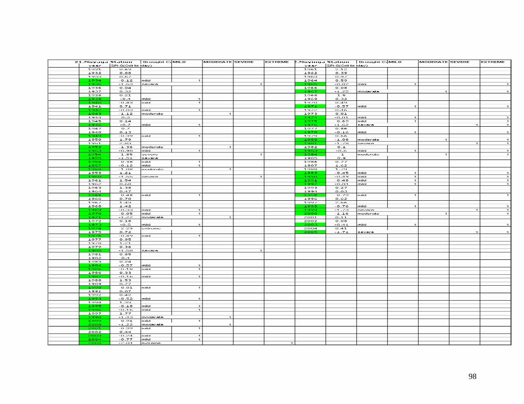
98

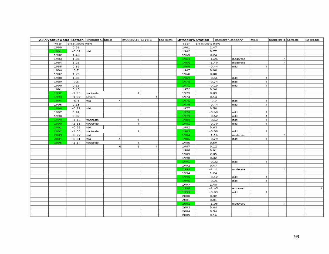
99

100