
Volume 19, Number 4, July - August 2021 - ThaiJO
92
Volume 19, Number 4, July - August 2021
-
Upload
khangminh22 -
Category
Documents
-
view
0 -
download
0
Transcript of Volume 19, Number 4, July - August 2021 - ThaiJO

Volume 19, Number 4, July - August 2021

Environment and Natural Resources Journal (EnNRJ) Volume 19, Number 4, July - August 2021 ISSN: 1686-5456 (Print)
ISSN: 2408-2384 (Online)
AIMS AND SCOPE
The Environment and Natural Resources Journal is a peer-reviewed journal, which provides insight scientific
knowledge into the diverse dimensions of integrated environmental and natural resource management. The journal aims to
provide a platform for exchange and distribution of the knowledge and cutting-edge research in the fields of environmental
science and natural resource management to academicians, scientists and researchers. The journal accepts a varied array of
manuscripts on all aspects of environmental science and natural resource management. The journal scope covers the
integration of multidisciplinary sciences for prevention, control, treatment, environmental clean-up and restoration. The
study of the existing or emerging problems of environment and natural resources in the region of Southeast Asia and the
creation of novel knowledge and/or recommendations of mitigation measures for sustainable development policies are
emphasized.
The subject areas are diverse, but specific topics of interest include:
- Biodiversity
- Climate change
- Detection and monitoring of polluted sources e.g., industry, mining
- Disaster e.g., forest fire, flooding, earthquake, tsunami, or tidal wave
- Ecological/Environmental modelling
- Emerging contaminants/hazardous wastes investigation and remediation
- Environmental dynamics e.g., coastal erosion, sea level rise
- Environmental assessment tools, policy and management e.g., GIS, remote sensing, Environmental
Management System (EMS)
- Environmental pollution and other novel solutions to pollution
- Remediation technology of contaminated environments
- Transboundary pollution
- Waste and wastewater treatments and disposal technology
Schedule
Environment and Natural Resources Journal (EnNRJ) is published 6 issues per year in January-February, March-April,
May-June, July-August, September-October, and November-December.
Publication Fees
There is no cost of the article-processing and publication.
Ethics in publishing
EnNRJ follows closely a set of guidelines and recommendations published by Committee on Publication Ethics (COPE).

Environment and Natural Resources Journal (EnNRJ) Volume 19, Number 4, July - August 2021 ISSN: 1686-5456 (Print)
ISSN: 2408-2384 (Online)
EXECUTIVE CONSULTANT TO EDITOR
Associate Professor Dr. Kampanad Bhaktikul
(Mahidol University, Thailand)
Associate Professor Dr. Sura Pattanakiat
(Mahidol University, Thailand)
EDITOR
Associate Professor Dr. Benjaphorn Prapagdee
(Mahidol University, Thailand)
ASSOCIATE EDITOR
Dr. Witchaya Rongsayamanont
(Mahidol University, Thailand)
Dr. Piangjai Peerakiatkhajohn
(Mahidol University, Thailand)
EDITORIAL BOARD
Professor Dr. Anthony SF Chiu
(De La Salle University, Philippines)
Professor Dr. Chongrak Polprasert
(Thammasat University, Thailand)
Professor Dr. Gerhard Wiegleb
(Brandenburgische Technische Universitat Cottbus, Germany)
Professor Dr. Hermann Knoflacher
(University of Technology Vienna, Austria)
Professor Dr. Jurgen P. Kropp
(University of Potsdam, Germany)
Professor Dr. Manish Mehta
(Wadia Institute of Himalayan Geology, India)
Professor Dr. Mark G. Robson
(Rutgers University, USA)
Professor Dr. Nipon Tangtham
(Kasetsart University, Thailand)
Professor Dr. Pranom Chantaranothai
(Khon Kaen University, Thailand)
Professor Dr. Shuzo Tanaka
(Meisei University, Japan)
Professor Dr. Sompon Wanwimolruk
(Mahidol University, Thailand)

Professor Dr. Tamao Kasahara
(Kyushu University, Japan)
Professor Dr. Warren Y. Brockelman
(Mahidol University, Thailand)
Professor Dr. Yeong Hee Ahn
(Dong-A University, South Korea)
Associate Professor Dr. Kathleen R Johnson
(Department of Earth System Science, USA)
Associate Professor Dr. Marzuki Ismail
(University Malaysia Terengganu, Malaysia)
Associate Professor Dr. Sate Sampattagul
(Chiang Mai University, Thailand)
Associate Professor Dr. Takehiko Kenzaka
(Osaka Ohtani University, Japan)
Associate Professor Dr. Uwe Strotmann
(University of Applied Sciences, Germany)
Assistant Professor Dr. Devi N. Choesin
(Institut Teknologi Bandung, Indonesia)
Assistant Professor Dr. Said Munir
(Umm Al-Qura University, Saudi Arabia)
Dr. Mohamed Fassy Yassin
(University of Kuwait, Kuwait)
Dr. Norberto Asensio
(University of Basque Country, Spain)
Dr. Thomas Neal Stewart
(Mahidol University, Thailand)
ASSISTANT TO EDITOR
Associate Professor Dr. Kanchana Nakhapakorn
Dr. Kamalaporn Kanongdate
Dr. Paramita Punwong
JOURNAL MANAGER
Isaree Apinya
JOURNAL EDITORIAL OFFICER
Nattakarn Ratchakun
Parynya Chowwiwattanaporn
Editorial Office Address
Research Management and Administration Section,
Faculty of Environment and Resource Studies, Mahidol University
999, Phutthamonthon Sai 4 Road, Salaya, Phutthamonthon, Nakhon Pathom, Thailand, 73170
Phone +662 441 5000 ext. 2108 Fax. +662 441 9509-10
Website: https://ph02.tci-thaijo.org/index.php/ennrj/index
E-mail: [email protected]

Environment and Natural Resources Journal (EnNRJ) Volume 19, Number 4, July - August 2021 ISSN: 1686-5456 (Print)
ISSN: 2408-2384 (Online)
CONTENT
Effectivity of Indonesian Rice Husk as an Adsorbent for Removing Congo
Red from Aqueous Solutions Neza Rahayu Palapa, Normah, Tarmizi Taher, Risfidian Mohadi, Addy Rachmat, and
Aldes Lesbani*
255
Impact of Climate Change on Reservoir Reliability: A Case of Bhumibol
Dam in Ping River Basin, Thailand
Allan Sriratana Tabucanon, Areeya Rittima*, Detchasit Raveephinit, Yutthana
Phankamolsil, Wudhichart Sawangphol, Jidapa Kraisangka, Yutthana Talaluxmana,
Varawoot Vudhivanich, and Wenchao Xue
266
Bioaccumulation of Lead by Pepper Elder (Peperomia pellucida (L.)
Kunth) in a Lead-Contaminated Hydroponic System Jessica O. Tablang, Florenda B. Temanel, Ron Patrick C. Campos*, and Helen C. Ramos
282
Effects of Campaign-Based Soil and Water Conservation Practice on Soil
Properties: The Case of Workamba Watershed, Debark District, North
Ethiopia Muluneh Bogale*, Getnet Wondie, and Abdrahman Shafi
292
In Vitro Removal of Electronic and Electrical Wastes by Fungi Isolated
from Soil at Annaba Area in Northeast of Algeria
Ghania Bourzama*, Nadjet Iratni, Nadjet Ennaghra, Houria Ouled-Haddar, Boudjema
Soumati, Khouloud Amour, and Khouloud Bechiri
302
Environmental and Microbial Influences on Corrosion of Selected Types
of Petroleum Industry Steel Anwuli U. Osadebe*, Dorcas C. Olorondu, and Gideon C. Okpokwasili
310
Characterization and Application of Mangosteen Peel Activated Carbon
for Ammonia Gas Removal Zarah Arwieny Hanami* and Puji Lestari
320
Removal of Iron from Groundwater by Ozonation: The Response Surface
Methodology for Parameter Optimization Apiradee Sukmilin and Ratsamee Sangsirimongkolying*
330
Environment and Natural Resources Journal 2021; 19(4): 255-265
Effectivity of Indonesian Rice Husk as an Adsorbent for Removing
Congo Red from Aqueous Solutions
Neza Rahayu Palapa1, Normah2, Tarmizi Taher3, Risfidian Mohadi1,2, Addy Rachmat1,2,
and Aldes Lesbani1,4*
1Graduate School of Mathematics and Natural Sciences, Univesitas Sriwijaya, Palembang, South Sumatera 30139, Indonesia 2Department of Chemistry, Faculty of Mathematics and Natural Sciences, Universitas Sriwijaya, Ogan Ilir,
South Sumatera 30662, Indonesia
3Department of Environmental Engineering, Institut Teknologi Sumatera, Kecamatan Jati Agung, Lampung Selatan 35365, Indonesian 4Reseach Center of Inorganic Materials and Complexes, Universitas Sriwijaya, Ogan Ilir, South Sumatera 30662, Indonesia
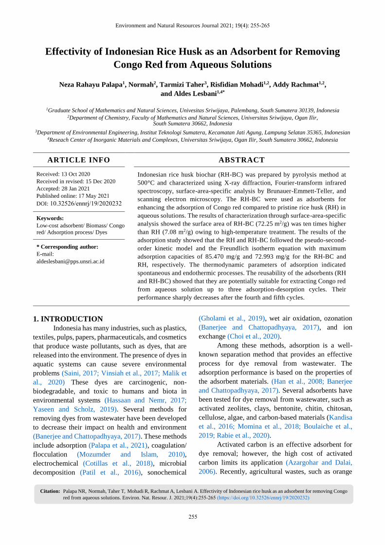
ARTICLE INFO ABSTRACT
Received: 13 Oct 2020
Received in revised: 15 Dec 2020
Accepted: 28 Jan 2021
Published online: 17 May 2021DOI: 10.32526/ennrj/19/2020232
Indonesian rice husk biochar (RH-BC) was prepared by pyrolysis method at
500°C and characterized using X-ray diffraction, Fourier-transform infrared
spectroscopy, surface-area-specific analysis by Brunauer-Emmett-Teller, and
scanning electron microscopy. The RH-BC were used as adsorbents for
enhancing the adsorption of Congo red compared to pristine rice husk (RH) in
aqueous solutions. The results of characterization through surface-area-specific
analysis showed the surface area of RH-BC (72.25 m2/g) was ten times higher
than RH (7.08 m2/g) owing to high-temperature treatment. The results of the
adsorption study showed that the RH and RH-BC followed the pseudo-second-
order kinetic model and the Freundlich isotherm equation with maximum
adsorption capacities of 85.470 mg/g and 72.993 mg/g for the RH-BC and
RH, respectively. The thermodynamic parameters of adsorption indicated
spontaneous and endothermic processes. The reusability of the adsorbents (RH
and RH-BC) showed that they are potentially suitable for extracting Congo red
from aqueous solution up to three adsorption-desorption cycles. Their
performance sharply decreases after the fourth and fifth cycles.
Keywords:
Low-cost adsorbent/ Biomass/ Congo
red/ Adsorption process/ Dyes
* Corresponding author:
E-mail:
1. INTRODUCTION
Indonesia has many industries, such as plastics,
textiles, pulps, papers, pharmaceuticals, and cosmetics
that produce waste pollutants, such as dyes, that are
released into the environment. The presence of dyes in
aquatic systems can cause severe environmental
problems (Saini, 2017; Vinsiah et al., 2017; Malik et
al., 2020) These dyes are carcinogenic, non-
biodegradable, and toxic to humans and biota in
environmental systems (Hassaan and Nemr, 2017;
Yaseen and Scholz, 2019). Several methods for
removing dyes from wastewater have been developed
to decrease their impact on health and environment
(Banerjee and Chattopadhyaya, 2017). These methods
include adsorption (Palapa et al., 2021), coagulation/
flocculation (Mozumder and Islam, 2010),
electrochemical (Cotillas et al., 2018), microbial
decomposition (Patil et al., 2016), sonochemical
(Gholami et al., 2019), wet air oxidation, ozonation
(Banerjee and Chattopadhyaya, 2017), and ion
exchange (Choi et al., 2020).
Among these methods, adsorption is a well-
known separation method that provides an effective
process for dye removal from wastewater. The
adsorption performance is based on the properties of
the adsorbent materials. (Han et al., 2008; Banerjee
and Chattopadhyaya, 2017). Several adsorbents have
been tested for dye removal from wastewater, such as
activated zeolites, clays, bentonite, chitin, chitosan,
cellulose, algae, and carbon-based materials (Kandisa
et al., 2016; Momina et al., 2018; Boulaiche et al.,
2019; Rabie et al., 2020).
Activated carbon is an effective adsorbent for
dye removal; however, the high cost of activated
carbon limits its application (Azargohar and Dalai,
2006). Recently, agricultural wastes, such as orange
Citation: Palapa NR, Normah, Taher T, Mohadi R, Rachmat A, Lesbani A. Effectivity of Indonesian rice husk as an adsorbent for removing Congo
red from aqueous solutions. Environ. Nat. Resour. J. 2021;19(4):255-265 (https://doi.org/10.32526/ennrj/19/2020232)
255
Palapa NR et al. / Environment and Natural Resources Journal 2021; 19(4): 255-265
peel (Annadurai et al., 2002), longan peel (Wang et al.,
2016), limetta peel (Shakoor and Nasar, 2016), and
rice husk (RH) (Liu and Zhang, 2009), have been used
as feedstock for adsorbents. RH is agricultural waste
feedstock produced from the rice milling industry, and
it contains chemical compounds, such as lignin,
cellulose, and hemicellulose, which can be used as
active-site adsorbents for dye removal (Connor et al.,
2018). However, the RH has a low adsorption
capacity. Thus, to increase this adsorption capacity,
they should be activated by carbonization
(Bamroongwongdee et al., 2019; Milla et al., 2013).
Malik et al. (2020) also reported comparative
comparison of RH, RH char, and chemically modified
RH used as adsorbents for the removal of the Congo
red dye. This study reported that the adsorption
capacities of the RH, RH char, and chemically
modified RH char (CMRHC) are 1.58 mg/g, 1.28
mg/g, and 2.04 mg/g, respectively, for Congo red dye
removal. This comparative study indicated that the
adsorption efficiency of the CMRHC was higher than
that of the RH and RH char. Herlina and Masri (2017)
reported that the adsorption of Congo red using the RH
occurred in an optimum contact time of 30 min, with
an adsorption percentage of 91.99%. The adsorption
capacity was 7.19 mg/g. Gad et al. (2016) also used
the RH as an adsorbent of metal ion Co(II) from
wastewater, which resulted in a maximum adsorption
capacity of 75.70 mg/g, and it followed the Langmuir
isotherm model.
In this study, the RH and RH-BC-based local
Indonesian feedstock were used as adsorbents of
Congo red from aqueous solutions. The factors
influencing the adsorption process, such as adsorption
time, concentration of Congo red, and temperature
adsorption, were studied in detail. The kinetics of
adsorption, isotherm, and thermodynamics of the
adsorption process of Congo red onto the RH and RH-
BC are discussed in this article.
2. METHODOLOGY
2.1 Chemical and instrumentation
Analytical grade (p.a.) chemicals such as
sodium hydroxide, ethanol, hydrochloric acid, and
congo red (>75%) were purchased from Merck
(Darmstadt, Germany). Water was supplied by the
Research Center of Inorganic Materials and
Complexes, FMIPA Universitas Sriwijaya. Destilled
water was obtained after purify using a Pureit, which
removed undesirable ionic, organic, and bacterial
contaminants from the water. Further, this water was
prepared for washing the RH from rice mills in
Bukataorganics, Indonesia. The RH was washed with
distilled water and dried at 60°C in an oven for 8 h.
Production of the RH-BC by pyrolysis method was
done by placing RH in the reactor and then heating at
600°C for 1 h. The RH and RH-BC was characterized
using X-ray diffraction (XRD; Rigaku miniflex-6000).
The RH and RH-BC were scanned from 5° to 80° at a
scan rate of 1 min-1. The functional groups were
analyzed using Fourier-transform infrared (FT-IR)
spectroscopy (Shimadzu Prestige-21) at 400-4,000
cm-1 and a KBr pellet. The adsorption-desorption of N2
was performed using a Quantachrome Micrometic
ASAP adsorption analyzer. Morphology analysis was
performed using a scanning electron microscopy
(SEM; Quanta-650 Oxford). The concentration of
Congo red was determined through an ultraviolet-
visible (UV-Vis) spectrophotometer (Biobase BK-UV
1800 PC) at 501 nm.
2.2 Adsorption process
The adsorption process was studied in a batch
system by varying the adsorption time, Congo red
concentration, and temperature for three replication
measurements. The initial pH of Congo red is 5.3, and
the adsorbents were sieved through 80 mesh. The
variation in the adsorption times was performed with
50 mg/L of Congo red dye. Further, 25 mL of the
Congo red dye was placed in a glass beaker, 0.025 g
of the adsorbent was added to it, and the mixture was
stirred by a horizontal shaker for 5-180 min at 250
rpm. The mixing solution was centrifuged at 1,000
rpm before scanning at 501 nm using a UV-Vis
spectrophotometer. The kinetic adsorption was
calculated using the kinetic adsorption models, such as
pseudo-first-order (PFO) and pseudo-second-order
(PSO) kinetic models, as presented in equations
1 and 2.
log (qe-qt) = log qe – (k1
2,303) t (1)
t
qt=
1
k2qe2 + 1
qet (2)
Where; qe is the adsorption capacity at
equilibrium (mg/g); qt is the adsorption capacity
(mg/g) at t, which is the adsorption time (min); k1 and
k2 denote the adsorption kinetic rates at PFO kinetics
(min-1) and PSO kinetics (g/mg·min), respectively.
The Congo red concentration was determined at
dye concentrations of 50, 75, 100, 125, and 150 mg/L
using 0.025 g of the adsorbents and 25 mL of Congo
256
Palapa NR et al. / Environment and Natural Resources Journal 2021; 19(4): 255-265
red. Moreover, the mixture was stirred by a horizontal
shaker for 100 min at 250 rpm at different adsorption
temperatures of 303, 313, 323, and 333 K. The
concentration of the Congo red was analyzed using the
UV-Vis spectrophotometer at a maximum wavelength
of 501 nm. Thereafter, the thermodynamic parameters
were obtained from the Langmuir and Freundlich
equations. The Langmuir adsorption model is assumed
to be the chemical and monolayer adsorption
processes, while the Freundlich adsorption model is
assumed to be the physical and multilayer adsorption
processes. Equations 3, 4, and 5 represent the
Langmuir adsorption model, Freundlich adsorption
model, and thermodynamic equations, respectively.
C
m=
1
bKML+
C
b(3)
Where; C is the saturated concentration of the
adsorbate, m is the amount of adsorbate, b is the
maximum adsorption capacity (mg/g), and KML is the
Langmuir constant (L/mg).
Log qe = log KF + 1/n log Ce (4)
Where; qe is the adsorption capacity at
equilibrium (mg/g), Ce is the concentration of
adsorbate at equilibrium (mg/L), and KF is the
Freundlich constant.
ln Kd = ∆S
R−
∆H
RT(5)
Where; R is the rate gas constant, T is the
temperature of the adsorption process (K), Kd is the
thermodynamic equilibrium constant, H is the
enthalpy (kJ/mol), and S is the entropy (J/mol·K).
2.3 Desorption and reusability process
Based on the amount of adsorbed dye, the
amount of desorbed dye can be calculated using the
following equation.
% D =Cads
Cdsp × 100% (6)
Where; Cads is the concentration of adsorbed
Congo red (mg/L), Cdsp is the concentration of
desorbed Congo red (mg/L), and %D is the percentage
of the desorption process.
The regeneration efficiency is determined using
the equation:
% regeneration =Qr
Q0
× 100% (7)
Where; Qr is the adsorption capacity of
reusability (mg/g) and Qo is the adsorption capacity of
the initial reusability (mg/g).
The desorption process was used to test each
adsorbent using 1 g of RH and RH-BC, followed by
the addition of 50 mL of the Congo red solution. Then,
the mixture was stirred for 2 h. The used adsorbent was
desorbed by taking 0.01 g of RH and RH-BC,
respectively, and adding 10 mL of solvent (sodium
hydroxide (0.01 M), hydrochloric acid (0.01 M),
absolute ethanol, and distilled water) and stirring the
mixture for 2 h for each conical flask. The reusability
process was performed with the desorbed adsorbent
reused to adsorb 100 mg/L of Congo red. The
adsorption was performed for 2 h using a batch system
and analyzed by UV-Vis spectrophotometry. The
reusability of the adsorbent was evaluated in three
cycles of the adsorption process.
3. RESULTS AND DISCUSSION
3.1 Adsorbent characterization
Figure 1 shows the XRD powder patterns of the
RH and RH-BC characterization at 2θ diffraction
peaks shown in the range of 16°-29°. A previous study
(Suyanta and Kuncaka, 2011) reported that there were
no diffraction peaks, except one of approximately 23°
with reflection (002) at 2θ diffraction. These
diffractions indicate the presence of silica in an
amorphous state from the RH and RH-BC (Milla et al.,
2013). The XRD powder pattern of the RH exhibited
diffraction at 23°. Another 2 peak (101) at 18°
disappeared after heating the RH at a high temperature
(600C) due to decomposition of cellulose (Rosa et al.,
2012). As reported by De Bhowmick et al. (2018), the
change in the peak occurred due to the destruction of
the biomass structure by pyrolysis.
The FT-IR spectra of the RH and RH-BC are
shown in Figure 2. The vibration peak at 3,448 cm-1
corresponds to the -OH group. The peak at 1,620 cm-1
indicates the presence of C-O bonds in the carboxylate
group. The peak at wavenumber 794 cm-1 corresponds
to the presence of Si-O bond (Bamroongwongdee et
al., 2019). The vibration at 1,103 cm-1 refers to C-H
stretching of lignin in the RH and RH-BC (Gad et al.,
2016). Furthermore, the intensity of the water
molecule (OH vibration) and carboxylate group (CO
vibration) in the RH decreased after heating at 600C
to form the RH-BC.
257

Palapa NR et al. / Environment and Natural Resources Journal 2021; 19(4): 255-265
Figure 1. XRD powder patterns of (a) RH-BC and (b) RH
Figure 2. FT-IR spectra of (a) RH-BC and (b) RH
Table 1 shows the Brunauer-Emmett-Teller
(BET) surface analyses of the RH and RH-BC. The
RH-BC has a larger surface area than that of the RH
because of the use of high temperatures during RH-BC
pyrolysis. These temperatures can open the pore
channels of the RH during thermal process to form the
RH-BC (Fernandes et al., 2016). As shown in Table 1,
the larger pore size can affect the higher adsorption
capacity due to the increasing pore volume. This was
also reported by Mangun et al. (1998). They also
reported that the pore size and volume size can affect
the adsorption capacity.
Table 1. Surface properties of RH and RH-BC
Adsorbent Surface area Pore size Pore volume
(m2/g) (nm) (cm3/g)
RH-BC 72.25 3.33 0.060
RH 7.08 3.14 0.011
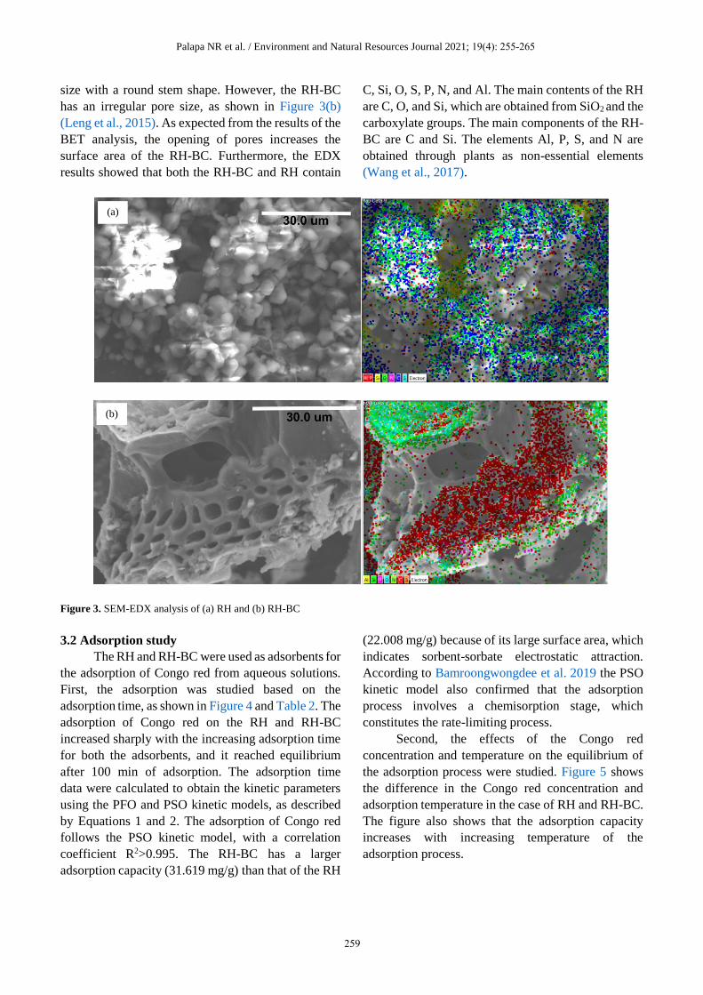
SEM-energy-dispersive X-ray (EDX) analysis
revealed the elemental composition of the RH and RH-
BC. The SEM-EDX analyses of the RH and RH-BC
are shown in Figure 3(a) and 3(b), respectively. The
morphology of the RH (Figure 3(a)) shows a uniform
10 20 30 40 50 60 70 80
Inte
nsi
ty (
a,u
)
2θ (deg)
#002
#101
*002
(b)
(a)
400 900 1,400 1,900 2,400 2,900 3,400 3,900
Tra
nsm
itta
nce
(%
)
Wavenumber (cm-1)
(b)*3,448
#3,448
#2,924#1,620
*1,620
#1,103
*1,103
#794
*794
*470
#470
(a)
258
Palapa NR et al. / Environment and Natural Resources Journal 2021; 19(4): 255-265
size with a round stem shape. However, the RH-BC
has an irregular pore size, as shown in Figure 3(b)
(Leng et al., 2015). As expected from the results of the
BET analysis, the opening of pores increases the
surface area of the RH-BC. Furthermore, the EDX
results showed that both the RH-BC and RH contain
C, Si, O, S, P, N, and Al. The main contents of the RH
are C, O, and Si, which are obtained from SiO2 and the
carboxylate groups. The main components of the RH-
BC are C and Si. The elements Al, P, S, and N are
obtained through plants as non-essential elements
(Wang et al., 2017).
Figure 3. SEM-EDX analysis of (a) RH and (b) RH-BC
3.2 Adsorption study
The RH and RH-BC were used as adsorbents for
the adsorption of Congo red from aqueous solutions.
First, the adsorption was studied based on the
adsorption time, as shown in Figure 4 and Table 2. The
adsorption of Congo red on the RH and RH-BC
increased sharply with the increasing adsorption time
for both the adsorbents, and it reached equilibrium
after 100 min of adsorption. The adsorption time
data were calculated to obtain the kinetic parameters
using the PFO and PSO kinetic models, as described
by Equations 1 and 2. The adsorption of Congo red
follows the PSO kinetic model, with a correlation
coefficient R2>0.995. The RH-BC has a larger
adsorption capacity (31.619 mg/g) than that of the RH
(22.008 mg/g) because of its large surface area, which
indicates sorbent-sorbate electrostatic attraction.
According to Bamroongwongdee et al. 2019 the PSO
kinetic model also confirmed that the adsorption
process involves a chemisorption stage, which
constitutes the rate-limiting process.
Second, the effects of the Congo red
concentration and temperature on the equilibrium of
the adsorption process were studied. Figure 5 shows
the difference in the Congo red concentration and
adsorption temperature in the case of RH and RH-BC.
The figure also shows that the adsorption capacity
increases with increasing temperature of the
adsorption process.
(a)
(b)
259

Palapa NR et al. / Environment and Natural Resources Journal 2021; 19(4): 255-265
Figure 4. The plot of the fitted kinetics model against the experimental data
Table 2. Kinetic adsorption of Congo red on the RH and RH-BC
Adsorbent Initial concentration
(mg/L)
Qeexperiment
(mg/g)
PFO PSO
QeCalc
(mg/g)
R2 k1 QeCalc
(mg/g)
R2 k2
RH-BC 51.492 31.619 29.573 0.995 0.032 36.231 0.997 0.023
RH 51.492 22.008 19.037 0.979 0.029 25.062 0.994 0.021
Figure 5. Effects of Congo red dye concentration on the adsorption capacities of (a) RH and (b) RH-BC
0
5
10
15
20
25
30
0 20 40 60 80 100 120 140 160 180
qt
(mg/g
)
Contact time (minutes)
RH-BC
RH
PFO
PSO
0
10
20
30
40
50
60
70
80
90
40 60 80 100 120 140 160
Ad
sorp
tio
n c
apac
ity (
mg/g
)
Initial concentration (mg/L)
303 K
313 K
323 K
333 K
(a)
260

Palapa NR et al. / Environment and Natural Resources Journal 2021; 19(4): 255-265
Figure 5. Effects of Congo red dye concentration on the adsorption capacities of (a) RH and (b) RH-BC (cont.)
Table 3 presents the Langmuir and Freundlich
data, which were obtained from the data provided in
Figure 5. According to the data in Table 3, the
adsorption on the RH and RH-BC is appropriate with
the Freundlich isotherm model with R2>0.99, which
suggests that the adsorption process is physisorption
and occurs through multilayer (Wijayanti et al., 2018).
However, this is in contrast to the PSO equation,
which indicated that the adsorption process involves
chemisorption. This finding suggests that physico-
chemical adsorption occurred in the adsorption
process. This conforms with the enthalpy results listed
in Table 4, which indicate that the adsorption of Congo
red has low enthalpy. Further, according to IUPAC,
physisorption with the enthalpy in the range of 4-40
kJ/mol and >40 kJ/mol corresponds to chemisorption
(Thommes et al., 2015; Oktriyanti et al., 2019). The
increasing dye uptake with the increasing temperature
decreased the viscosity of the solution, increased the
porosity, or interlayer, resulting in the enhancement of
active sites form (Zhu et al., 2005). According to the
results summarized in Table 4, the adsorption capacity
of Congo red removal using the RH-BC is slightly
higher than that for other adsorbents.
Table 3. Isotherm models of Congo red adsorption on RH and RH-BC
Isotherm Parameters 303 K 313 K 323 K 333 K
RH-BC Langmuir Qmax 77.519 79.365 83.333 85.470
kL 0.058 0.112 0.219 0.480
R2 0.971 0.992 0.999 0.998
Freundlich n 1.909 4.361 1.448 1.444
kF 7.034 1.328 3.631 3.928
R2 0.999 0.996 0.993 0.999
RH Langmuir Qmax 60.606 72.993 74.627 75.188
kL 0.067 0.088 0.039 0.058
R2 0.997 0.976 0.956 0.969
Freundlich N 1.071 10.953 5.688 9.497
kF 1.295 1.455 1.386 1.441
R2 0.999 0.979 0.983 0.994
0
10
20
30
40
50
60
70
80
90
40 60 80 100 120 140 160
Ad
sorp
tio
n c
apac
ity (
mg/g
)
Initial concentration (mg/L)
303 K
313 K
323 K
333 K
(b)
261

Palapa NR et al. / Environment and Natural Resources Journal 2021; 19(4): 255-265
Table 4. Comparison of Congo red adsorption using different adsorbents.
Adsorbent Qe (mg/g) Refs
Na-bentonite 35.84 (Vimonses et al., 2009)
Bagasse fly ash 11.88 (Mall et al., 2005)
Spirulinna algae 3.11 (Mohadi et al., 2017)
m-cell/Fe3O4/ACCs 66.09 (Zhu et al., 2011)
Magnetic Fe3O4@graphene 33.66 (Inyang et al., 2012)
Funalia trogii 83.70 (Bayramoglu and Arica, 2018)
RH-BC 85.47 This research
RH 75.188 This research
The thermodynamic parameters of the Congo
red adsorption on the RH and RH-BC adsorbents, such
as ∆H (enthalpy), ∆G (Gibbs free energy), and ∆S
(entropy), are shown in Table 5. The positive values of
∆S indicate an increase in the degree of irregularity
between the adsorbate and adsorbent. The positive
value of ∆H indicates that the Congo red adsorption on
the RH and RH-BC is endothermic. The negative
value of ∆G indicates that the Congo red adsorption is
spontaneous (Naushad et al., 2019).
Table 5. Thermodynamic parameters of Congo red adsorption on RH and RH-BC
Concentration T (K) Qe (mg/g) ∆H (kJ/mol) ∆S (kJ/mol) ∆G (kJ/mol)
48.524 mg/L 303 31.270 9.544 3.200 -0.070
313 37.063 -0.387
323 43.889 -0.704
333 47.698 -1.022
48.524 mg/L 303 24.841 19.565 6.500 -0.132
313 27.778 -0.782
323 30.714 -1.432
333 32.857 -2.082
Desorption of the adsorbent was studied using
several solvents on the RH and RH-BC after the
adsorption of Congo red, and the results are shown in
Figure 6, which indicate that hydrochloric acid as a
solvent can give higher results in the desorption
process of Congo red. This is because the H+ ion from
the hydrochloric acid releases the Congo red dye anion
by interacting with the adsorbent. Congo red prefers
Figure 6. Desorption of Congo red on the RH and RH-BC
0
20
40
60
80
100
Water Hydrochloric Acid Sodium Hydroxide Ethanol
% D
eso
rpti
on
RH RH-BC
262

Palapa NR et al. / Environment and Natural Resources Journal 2021; 19(4): 255-265
lower number of H+ ions than those present in
hydrochloric acid because of greater electrostatic
interactions than adsorbents (Palapa et al., 2020). The
reusability of the adsorbent was evaluated using
hydrochloric acid as a desorption reagent to release
Congo red after the adsorption process.
The reusability study was conducted for five
adsorption cycles, as demonstrated in Figure 7. The
adsorption capacity of Congo red on both the
adsorbents decreased sharply after three cycles, i.e.,
during the fourth and fifth adsorption processes. The
first reusabilities of the RH and RH-BC were 58.88%
and 54.32%, and the second reusabilities were 53.44%
and 47.33% for the RH and RH-BC, respectively. The
third reusability was more stable with reusability
values of 47.91% for RH and 44.24% for RH-BC.
However, the adsorption capacity decreased
significantly in the fourth and fifth adsorption
processes. Thus, the RH and RH-BC are suitable
adsorbents for the Congo red adsorption in three
adsorption cycles. Furthermore, these adsorbents can
be reused, although their adsorption capacity is
slightly reduced.
Figure 7. Reusability of the RH and RH-BC for Congo red adsorption
4. CONCLUSION
In this study, characterization of RH and RH-
BC using XRD indicated the presence of silica
molecules at a diffraction peak of 23°. The FT-IR
spectra of the RH and RH-BC showed Si-O vibrations
at 794 cm-1, and the peak at 1,103 cm-1 corresponded
to the C-H strain, which indicated the presence of
lignin on the RH and RH-BC. The BET analysis
showed that the surface areas of the RH and RH-BC
were 72.25 m2/g and 7.08 m2/g, respectively. The
adsorption of Congo red on the RH and RH-BC
followed the PSO kinetics model with optimum
adsorption after 100 min and the Freundlich equation
model with a maximum adsorption capacity of 85.470
mg/L. The RH-BC was more effective at Congo red
dye removal than the RH. The thermodynamic
parameters indicated that the Congo red was adsorbed
spontaneously on the RH and RH-BC, and this
adsorption was an endothermic process. The
reusability of the adsorbents indicated that the RH and
RH-BC had a decreasing adsorption capacity after
three cycles of adsorption. Furthermore, these
experimental results are useful to increase the use of
biomass as a potential adsorbent for wastewater
treatment. The studied adsorbents are suitable to
remove Congo red in an aqueous solution. In addition,
the use of agricultural wastes as one source of
adsorbents has the potential to further help to reduce
agricultural waste in the environment.
ACKNOWLEDGEMENTS
This study was supported by “Hibah Profesi”
Universitas Sriwijaya in fiscal year 2020-2021 by the
financial support program for research with contact
number 0687/UN9/SK.BUK.KP/2020. Special thanks
for Research Center of Inorganic Materials and
Complexes, Faculty of Mathematic and Natural
0
10
20
30
40
50
60
70
1 2 3 4 5
% A
dso
rpti
on
RH RH-BC
263

Palapa NR et al. / Environment and Natural Resources Journal 2021; 19(4): 255-265
Science, Universitas Sriwijaya for analysis and
instrumental measurement.
REFERENCES Annadurai G, Juang RS, Lee DJ. Use of cellulose-based wastes for
adsorption of dyes from aqueous solutions. Journal of
Hazardous Materials 2002;92(3):263-74.
Azargohar R, Dalai AK. Biochar as a precursor of activated
carbon. Applied Biochemistry and Biotechnology 2006;129-
132:762-73.
Bamroongwongdee C, Suwannee S, Kongsomsaksiri M.
Adsorption of Congo red from aqueous solution by surfactant-
modified rice husk: Kinetic, isotherm and thermodynamic
analysis. Songklanakarin Journal of Science and Technology
2019;41(5):1076-83.
Banerjee S, Chattopadhyaya MC. Adsorption characteristics for
the removal of a toxic dye, tartrazine from aqueous solutions
by a low cost agricultural by-product. Arabian Journal of
Chemistry 2017;10:S1629-38.
Bayramoglu G, Arica MY. Adsorption of Congo red dye by native
amine and carboxyl modified biomass of Funalia trogii:
Isotherms, kinetics and thermodynamics mechanisms. Korean
Journal of Chemical Engineering 2018;35:1303-11.
De Bhowmick G, Sarmah AK, Sen R. Production and
characterization of a value added biochar mix using seaweed,
rice husk and pine sawdust: A parametric study. Journal of
Cleaner Production 2018;200:641-56.
Boulaiche W, Hamdi B, Trari M. Removal of heavy metals by
chitin: Equilibrium, kinetic and thermodynamic studies.
Applied Water Science 2019;9:39.
Choi Y, Gurav R, Kim HJ, Yang Y, Bhatia SK. Evaluation for
simultaneous removal of anionic and cationic dyes onto maple
leaf-derived biochar using response surface methodology.
Applied Sciences 2020;10:2982.
Connor DO, Peng T, Li G, Wang S, Duan L, Mulder J, et al. Sulfur-
modified rice husk biochar: A green method for the
remediation of mercury contaminated soil. Science of the
Total Environment 2018;621:819-26.
Cotillas S, Llanos J, Cañizares P, Clematis D, Cerisola G, Rodrigo
MA, et al. Removal of Procion red MX-5B dye from
wastewater by conductive-diamond electrochemical
oxidation. Electrochimica Acta 2018;263:1-7.
Fernandes IJ, Calheiro D, Kieling AG, Moraes CAM, Rocha
TLAC, Brehm FA, et al. Characterization of rice husk ash
produced using different biomass combustion techniques for
energy. Fuel 2016;165:351-9.
Gad HM, Omar H, Aziz A, Hassan M, Khalil M. Treatment of rice
husk ash to improve adsorption capacity of cobalt from aqueous
solution. Asian Journal of Chemistry 2016;28(2):385-94.
Gholami P, Dinpazhoh L, Khataee A, Hassani A, Bhatnagar A.
Facile hydrothermal synthesis of novel Fe-Cu layered double
hydroxide/biochar nanocomposite with enhanced
sonocatalytic activity for degradation of cefazolin sodium.
Journal of Hazardous Materials 2019;381:120742.
Han R, Ding D, Xu Y, Zou W, Wang Y, Li Y, et al. Use of rice
husk for the adsorption of congo red from aqueous solution in
column mode. Bioresource Technology 2008;99(8):2938-46.
Hassaan MA, Nemr A El. Health and environmental impacts of
dyes: Mini review. American Journal of Environmental
Science and Engineering 2017;1(3):64-7.
Herlina R, Masri MS. Adsorption study of rice bran against Congo
red dyes in Wajo. Journal Chemical 2017;18(1):16-25.
Inyang M, Gao B, Yao Y, Xue Y, Zimmerman AR,
Pullammanappallil P, et al. Removal of heavy metals from
aqueous solution by biochars derived from anaerobically
digested biomass. Bioresource Technology 2012;110:50-6.
Kandisa RV, Kv NS, Shaik KB, Gopinath R. Dye removal by
adsorption: A review. Journal of Bioremediation and
Biodegradation 2016;7(6):371.
Leng L, Yuan X, Zeng G, Shao J, Chen X, Wu Z, et al. Surface
characterization of rice husk bio-char produced by liquefaction
and application for cationic dye (Malachite green) adsorption.
Fuel 2015;155:77-85.
Liu Z, Zhang FS. Removal of lead from water using biochars
prepared from hydrothermal liquefaction of biomass. Journal
of Hazardous Materials 2009;167(1-3):933-9.
Malik A, Khan A, Natasha A, Naeem M. A comparative study of
the adsorption of Congo red dye on rice husk, rice husk char
and chemically modified rice husk char from aqueous media.
Bulletin of the Chemical Society of Ethiopia 2020;
34(1):41-54.
Mall ID, Srivastava VC, Agarwal NK, Mishra IM. Adsorptive
removal of malachite green dye from aqueous solution by
bagasse fly ash and activated carbon-kinetic study and
equilibrium isotherm analyses. Colloids and Surfaces A:
Physicochemical and Engineering Aspects 2005;264(1-3):
17-28.
Mangun CL, Daley MA, Braatz RD, Economy J. Effect of pore
size on adsorption of hydrocarbons in phenolic-based
activated carbon fibers. Carbon 1998;36(1-2):123-9.
Milla OV, Rivera EB, Huang W, Chien C, Wang Y. Agronomic
properties and characterization of rice husk and wood
biochars and their effect on the growth of water spinach in a
field test. Journal of Soil Science and Plant Nutrition
2013;13(2):251-66.
Mohadi R, Hanafiah Z, Hermansyah H, Zulkifli H. Adsorption of
procion red and congo red dyes using microalgae Spirulina sp.
Science and Technology Indonesia 2017;2(4):102-4.
Momina, Shahadat M, Isamil S. Regeneration performance of
clay-based adsorbents for the removal of industrial dyes: A
review. RSC Advances 2018;8:24571-87.
Mozumder MSI, Islam MA. Development of treatment technology
for dye containing industrial wastewater. Journal of Scientific
Research 2010;2(3):567-76.
Naushad M, Abdullah A, Abdullah Z, Hotan I, Saad M,
Mohammed A. Adsorption kinetics, isotherm and reusability
studies for the removal of cationic dye from aqueous medium
using arginine modified activated carbon. Journal of
Molecular Liquids 2019;293:111442.
Oktriyanti M, Palapa NR, Mohadi R, Lesbani A. Modification of
Zn-Cr layered double hydroxide with keggin ion. Indonesian
Journal of Environmental Management and Sustainability
2019;3(3):93-9.
Palapa NR, Taher T, Rahayu BR, Mohadi R, Rachmat A, Lesbani
A. CuAl LDH/rice husk biochar composite for enhanced
adsorptive removal of cationic dye from aqueous solution.
Bulletin of Chemical Reaction Engineering and Catalysis
2020;15(2):525-37.
Palapa NR, Taher T, Mohadi R, Rachmat A, Lesbani A.
Preparation of copper aluminum-biochar composite as
adsorbent of malachite green in aqueous solution. Journal of
Engineering Science and Technology 2021;16(1):259-74.
264

Palapa NR et al. / Environment and Natural Resources Journal 2021; 19(4): 255-265
Patil NP, Bholay AD, Kapadnis BP, Gaikwad VB. Biodegradation
of model azo dye methyl red and other textile dyes by isolate
Bacillus circulans npp1. Journal of Pure and Applied
Microbiology 2016;10(4):2793-800.
Rabie AM, Abukhadra MR, Rady AM, Ahmed SA, Labena A,
Mohamed HSH, et al. Instantaneous photocatalytic
degradation of malachite green dye under visible light using
novel green Co-ZnO/algae composites. Research on Chemical
Intermediates 2020;46:1955-73.
Rosa SML, Rehman N, De Miranda MIG, Nachtigall SMB, Bica
CID. Chlorine-free extraction of cellulose from rice husk and
whisker isolation. Carbohydrate Polymers 2012;87(2):1131-8.
Saini RD. Textile organic dyes: Polluting effects and elimination
methods from textile waste water. International Journal of
Chemistry Engineering Research 2017;9(1):121-36.
Shakoor S, Nasar A. Removal of methylene blue dye from
artificially contaminated water using citrus limetta peel waste
as a very low cost adsorbent. Journal of the Taiwan Institute of
Chemical Engineers 2016;66:154-63.
Suyanta, Kuncaka A. Utilization of rice husk as raw material in
synthesis of mesoporous silicates mcm-41. Indonesian Journal
of Chemistry 2011;11(3):279-84.
Thommes M, Kaneko K, Neimark AV, Olivier JP, Rodriguez-
Reinoso F, Rouquerol J, et al. Physisorption of gases, with
special reference to the evaluation of surface area and pore size
distribution (IUPAC technical report). Pure and Applied
Chemistry 2015;87(9-10):1051-69.
Vimonses V, Lei S, Jin B, Chow CWK, Saint C. Kinetic study and
equilibrium isotherm analysis of Congo red adsorption by
clay materials. Chemical Engineering Journal 2009;148
(2-3):354-64.
Vinsiah R, Mohadi R, Lesbani A. Performance of graphite for
Congo red and direct orange adsorption. Indonesian Journal
of Environmental Management and Sustainability 2020;4:
125-32.
Wang F, Pan Y, Cai P, Guo T, Xiao H. Single and binary
adsorption of heavy metal ions from aqueous solutions using
sugarcane cellulose-based adsorbent. Bioresource Technology
2017;241:482-90.
Wang Y, Zhu L, Jiang H, Hu F, Shen X. Application of longan
shell as non-conventional low-cost adsorbent for the removal
of cationic dye from aqueous solution. Spectrochimica Acta
Part A: Molecular and Biomolecular Spectroscopy 2016;
159:254-61.
Wijayanti A, Susatyo EB, Kurniawan C. Adsorpsi logam Cr(VI)
dan Cu(II) pada tanah dan pengaruh penambahan pupuk
organik. Indonesian Journal of Chemical Science
2018;7(3):242-8 (in Indonesian).
Yaseen DA, Scholz M. Textile dye wastewater characteristics and
constituents of synthetic effluents: A critical review.
International Journal of Environmental Science and
Technology 2019;16:1193-226.
Zhu J, He J, Du X, Lu R, Huang L, Ge X. A facile and flexible
process of β-cyclodextrin grafted on Fe3O4 magnetic
nanoparticles and host-guest inclusion studies. Applied
Surface Science 2011;257(21):9056-62.
Zhu MX, Li YP, Xie M, Xin HZ. Sorption of an anionic dye by
uncalcined and calcined layered double hydroxides: A case
study. Journal of Hazardous Materials 2005;120(1-3):163-71.
265

Environment and Natural Resources Journal 2021; 19(4): 266-281
Impact of Climate Change on Reservoir Reliability:
A Case of Bhumibol Dam in Ping River Basin, Thailand
Allan Sriratana Tabucanon1, Areeya Rittima2*, Detchasit Raveephinit2, Yutthana Phankamolsil3,
Wudhichart Sawangphol4, Jidapa Kraisangka4, Yutthana Talaluxmana5,
Varawoot Vudhivanich6, and Wenchao Xue7
1Faculty of Environment and Resource Studies, Mahidol University, Nakhon Pathom 73170, Thailand 2Faculty of Engineering, Mahidol University, Nakhon Pathom 73170, Thailand
3Environmental Engineering and Disaster Management Program, Mahidol University, Nakhon Pathom 73170, Thailand 4Faculty of Information and Communication Technology, Mahidol University, Nakhon Pathom 73170, Thailand
5Faculty of Engineering, Kasetsart University, Bangkok 10900, Thailand 6Faculty of Engineering at Kamphaeng Saen, Kasetsart University, Nakhon Pathom 73140, Thailand
7Department of Energy, Environment and Climate Change, School of Environment, Resources and Development, Asian Institute of Technology, Pathum Thani 12120, Thailand
ARTICLE INFO ABSTRACT
Received: 21 Jan 2021
Received in revised: 18 Mar 2021
Accepted: 16 Apr 2021
Published online: 18 May 2021DOI: 10.32526/ennrj/19/2021012
Bhumibol Dam is the largest dam in the central region of Thailand and it serves
as an important water resource. The dam’s operation relies on reservoir
operating rules that were developed on the basis of the relationships among
rainfall-inflow, water balance, and downstream water demand. However, due
to climate change, changing rainfall variability is expected to render the
reliability of the rule curves insecure. Therefore, this study investigated the
impact of climate change on the reliability of the current reservoir operation
rules of Bhumibol Dam. The future scenarios from 2000 to 2099 are based on
EC-EARTH under RCP4.5 and RCP8.5 scenarios downscaled by RegCM4.
MIKE11 HD was developed for the inflow simulation. The model generates the
inflow well (R2=0.70). Generally, the trend of increasing inflow amounts is
expected to continue in the dry seasons from 2000-2099, while large
fluctuations of inflow are expected to be found in the wet seasons, reflecting
high uncertainties. In the case of standard deviations, a larger deviation is
predicted under the RCP8.5 scenario. For the reservoir’s operation in a climate
change study, standard operating procedures were applied using historical
release records to estimate daily reservoir release needed to serve downstream
water demand in the future. It can be concluded that there is high risk of current
reservoir operating rules towards the operation reliability under RCP4.5 (80%
reliability), but the risk is lower under RCP8.5 (87% reliability) due to
increased inflow amounts. The unmanageability occurs in the wet season,
cautioning the need to redesign the rules.
Keywords:
Bhumibol Dam/ Climate change/
Hydrological model/ Ping River
Basin/ Reservoir reliability
* Corresponding author:
E-mail: [email protected]
1. INTRODUCTION
Anthropogenic greenhouse gas emissions have
been regarded as the cause for 1.0oC of global
warming above pre-industrial levels. The global
warming phenomenon has been scientifically related
to changing rainfall variability patterns (IPCC, 2018).
The IPCC (2012) concluded that climate change is
causing the emergence of statistically significant
trends in the number of heavy rainfall events, as well
as more intense and longer droughts. These findings
are also consistent with statistical long-term records of
Thailand, including increasing extreme temperature
indices (Limsakul, 2020), as well as less frequent but
more intense rainfall events (Limsakul and Singhruck,
2016). Raneesh (2014) proposed a variety of factors
arising from the challenges in water resources
planning and management. The major factor will be
the impact of climate change through the alteration of
Citation: Tabucanon AS, Rittima A, Raveephinit D, Phankamolsil Y, Sawangphol W, Kraisangka J, Talaluxmana Y, Vudhivanich V, Xue W.
Impact of climate change on reservoir reliability: A case of Bhumibol Dam in Ping River Basin, Thailand. Environ. Nat. Resour. J. 2021;19(4):266-281. (https://doi.org/10.32526/ennrj/19/2021012)
266

Tabucanon AS et al. / Environment and Natural Resources Journal 2020; 19(4): 266-281
the hydrological cycle, which affects quantity and
quality of regional water resources, especially in Asia.
These consequences will be further exacerbated by
population growth, economic factors, and land use
changes (including urbanization). Shiferaw et al.
(2014) and Miyan (2015) found that these changes
impact the vulnerable and poor, especially those
related to agricultural activities. A major reason for the
impact is the uncertainty of the capability of reservoir
operating rules for dams influenced by the impacts of
climate change (Kang et al., 2007; Kim et al., 2009;
Ehsani et al., 2017). Reservoir operating rules are
generally developed based on the relationship between
rainfall-inflow, water balance, and downstream water
demand. The rules are applied to ensure appropriate
management of flood in the wet season and water
scarcity in the dry season. Therefore, understanding
future changes of inflow into the dam is important for
adaptive management of the rules (Raneesh, 2014;
Koontanakulvong et al., 2020).
The objective of this study was to investigate
the impact of climate change on the reliability of the
current reservoir operating rules of Bhumibol Dam,
the largest dam in Thailand, which is an important
water resource for agriculture in the central region,
especially in the dry season (Kitpaisalsakul, 2018;
Koontanakulvong et al., 2020). This is one of two
major dams regulating the Chao Phraya River, the
major river in Thailand. From a historical perspective,
floods frequently occur in Thailand and the 2011 flood
was the largest experienced by the country, which was
triggered by successive storms that forced the dam to
fully release its stored water. The 2011 flood was
responsible for economic losses totaling 45.5 billion
USD (World Bank, 2012). In contrast, due to
inadequate rainfall, there was a severe drought in
2020. It was anticipated that production of sugarcane,
off-season rice and cassava were decreased by 27%,
21% and 7%, respectively. This resulted in an
extensive decline of the farmers’ overall income. The
most seriously impacted region was in the central part
of the country and was influenced by critically low
water level in the dams (Siam Commercial Bank,
2020). The start of the problems in 2020 can be traced
to November 2019, when the total reservoir storage of
Bhumibol Dam was at a critical level of only 22%
(Thana-dachophol et al., 2020).
Kitpaisalsakul (2018), and Sharma and Babel
(2013) conducted a climate change impact study on the
inflow and water storage of the dam. However, their
study lacked consideration of a number of updated
climate change scenarios to sufficiently address future
uncertainties and reliability of the current reservoir
operating rule curves under climate change scenarios.
Furthermore, Kure et al. (2013) applied MIKE11 to
estimate annual inflow to the Bhumibol Dam, in which
a significant increase was detected. Moreover,
according to our extensive literature reviews, the
research of reservoir operating reliability under recently
developed climate change scenarios in the South East
Asia (SEA) region is still very limited. In this study, we
used MIKE11 rainfall-runoff (RR) and MIKE11
Hydrodynamic (HD) for inflow simulation of the
current situation and we incorporated the climate
change scenarios that were developed by
Ramkhamhaeng University Center of Regional Climate
Change and Renewable Energy (RU-CORE). The
prediction was based on the simulation of EC-EARTH
under RCP4.5 and RCP8.5 scenarios for future inflow
simulation. The reliability of the future inflows was
then examined, based on the standard operating
procedure (SOP) of reservoir operating rules.
The additional information derived from this
study can inform water management-related agencies
to redesign reservoir operating rules under climate
change scenarios to minimize future flood and drought
risks. The current incidents and damage impacts
triggered by unsatisfactory operation of major dams
are evidence of the importance and necessity of
redesigning reservoir operation rules with adaptive
management strategies under climate change to
minimize these disaster risks.
2. METHODOLOGY
2.1 Study area
Bhumibol Dam is located at 17°14′33″N
Latitude and 98°58′20″E Longitude in Sam Ngao
District in Tak Province in the northern region of
Thailand, as shown in Figure 1. It is a concrete arch
gravity dam, with a storage capacity of 13,462 million
m3 (MCM) to receive inflow from the Ping River
Basin with an area of 25,370 km2. The dam is
designed for a hydroelectric power plant with a total
installed capacity of 779.2 MW. According to
Koontanakulvong et al. (2020), the long-term annual
inflow over the period between 1969 and 2019
averaged 5,637 MCM. Nevertheless, their study
indicated a trend of decreasing inflow after the 2011
flood, with an average annual inflow of only 3,960
MCM between 2012-2019. This highlights the
challenge of reservoir management of the Bhumibol
Dam, both currently and in the future. A flowchart of
267

Tabucanon AS et al. / Environment and Natural Resources Journal 2020; 19(4): 266-281
Figure 1. The Greater Chao Phraya River Basin (a) and land use of Ping River Basin in 2013 (b)
the methodology used in this study is given in Figure 2.
The methods and tools that were used are described in
detail in the following sections.
2.2 Development of hydrological models
The platform of MIKE11 Zero Version 2016,
developed by the Danish Hydraulic Institute (DHI),
was adopted for simulation of inflow into Bhumibol
Dam. The package consists of a variety of
hydrological-hydraulic models for use, depending
upon the nature of the problem and solution objective.
In this study, we selected MIKE11 (Rainfall-runoff)
RR NAM model and MIKE11 Hydrodynamics (HD)
for inflow simulation. The MIKE11 RR NAM model,
the lumped model, was applied for rainfall-runoff
simulation in the Ping River Basin. As shown in
Figure 3(a), 30 sub-basins were delineated in
accordance with the recommendation of the Royal
Irrigation Department (RID), as well as Thiessen
polygons of 22 daily rainfall stations, namely 070731
and 170181 derived from RID, and 20 stations, namely
300201, 300202, 303201, 303301, 310201, 327301,
327501, 328201, 328202, 328301, 32920,1 373201,
373301, 376201, 376202, 376203, 376301, 376401,
380201, and 400201 derived from the Thailand
Meteorological Department (TMD). In addition, daily
evaporation data in the study area was obtained from
TMD station 48376. The simulated runoff was
compared with the observed runoff at RID discharge
stations, namely P.4A (Mat Taeng station), P.20
(Chiang Dao station), P.21 (Mae Rim station), P.24A
(Mae Klang station), and P.26A (Klong Suan Mak
station), as shown in Figure 3(b) for the model setup.
The list and adjustment methods of rainfall-runoff
parameters can be found in DHI (2017). The adjusted
parameters include maximum water content in surface
storage (Umax), maximum water content in root zone
storage (Lmax), overland flow runoff coefficient
(CQOF), time constant for interflow (CKIF), time
constants for routing overland flow (CK1,2), root zone
threshold value for overland flow (TOF), root zone
threshold value for interflow (TIF), time constant for
routing baseflow (CKBF), and root zone threshold
value for ground water recharge (TG). In this study,
the period for model calibration was between 2000 and
2010, in which the auto-calibration function of
MIKE11 RR was first applied and followed by manual
adjustment to find the best fit with the observations,
while the verification period was independently
simulated between 2010 and 2018.
The developed MIKE11 RR model was then
incorporated with MIKE11 HD. The data input for
MIKE11 HD includes MIKE11 RR runoffs and 128
river cross-sections along Ping River, obtained from
(a) (b)
268

Tabucanon AS et al. / Environment and Natural Resources Journal 2020; 19(4): 266-281
RID and Hydro-Informatics Institute (HAII) for
hydrodynamic simulation of the inflow into Bhumibol
Dam. The model calculation is based on one- dimension
flow Saint Venant equation. Furthermore, the river
discharge record at P.20 station and water level at P.17
derived from RID were set as upstream and
downstream boundaries, respectively. The record of
reservoir storage of the dam on 1 January 2000
(9,508.49 MCM) was set as an initial storage condition.
As for MIKE11 HD, Manning’s coefficients of river
channels and flood plains were adjusted to improve the
fitness of inflow between simulation and observation.
To evaluate the model’s performance, the
coefficient of determination (R2) was applied. In
addition, the Q-Q plots of wet season (May-October)
and dry season (November-April) were also used to
evaluate the simulated inflow performance.
Figure 2. Flowchart of the methodology used in this study
269

Tabucanon AS et al. / Environment and Natural Resources Journal 2020; 19(4): 266-281
Figure 3. 30-subbasins delineated, selected rainfall (a) and selected discharge stations (b)
2.3 Climate change scenarios
Prediction of rainfall and evaporation under
climate change scenarios was extracted from RU-
CORE. The prediction was based on the simulation of
EC-EARTH under RCP4.5 and RCP8.5 scenarios
regionally downscaled by RegCM4 with 25 km ×
25 km grid size over the study area (Ngo-Duc et al.,
2017; Cruz et al., 2017; Tangang et al., 2019).
According to the IPCC glossary, RCP stands for
representative concentration pathways, providing
possible future scenarios regarding long-term
concentrations of greenhouse gases (Moss et al.,
2010). RCP4.5 indicates that radiative forcing is
stabilized at approximately 4.5 W/m2 (intermediate
intensity level of global warming), while RCP8.5
shows radiative forcing greater than 8.5 W/m2 by 2100
and continues to rise afterwards (highest possible
intensity level of global warming). Rainfall and
evaporation data at the stations described in Section
2.2 were extracted in reference to the average values
of four grids neighboring the targeted station grid.
Murphy (1999) indicated that this method provided
more precise rainfall data than the grid over the
targeted station. In addition, bilinear interpolation was
applied to correct the predicted values, as shown in the
following equation:
Pcorrected i = PRU−CORE i ×μpobserved i
μPRU−CORE i
Where; Pcorrected i is the corrected daily
prediction data in month i, PRU−CORE i is the average
value of four grids neighboring the targeted
meteorological station grid in month i, μpobserved i is
the monthly average of observed value over the
targeted period between 2000 and 2018 in month I,
and μPRU−CORE i is the monthly average of predicted
value over the targeted period between 2000 and 2018
in month i. In this study, predictions were temporally
separated into five periods-namely 2000-2020
(baseline), 2021-2040, 2041-2060, 2061-2080, and
2081-2099 to investigate the changes in comparison
with the baseline value. The statistical parameters for
the analysis include average, standard deviation and
the storage at the end of wet season, representing water
security in the dry season.
2.4 The reservoir operating policy used in this
study
The reservoir operating rules of Bhumibol Dam,
developed in 2012, were obtained from the Electricity
Generating Authority of Thailand (EGAT). The
previous rules were redesigned after the 2011 flood
event in Thailand. The procedure to evaluate the
reliability of the current rules under climate change
scenarios is described as follows.
1) Daily reservoir release was based on the
record between 2000-2018. Annual inflow into the
(a) Rainfall Stations in Ping River Basin (b) Discharge Stations in Ping River Basin
270

Tabucanon AS et al. / Environment and Natural Resources Journal 2020; 19(4): 266-281
dam was fitted with Gumbel Distribution (Rittima,
2018). The behavior of daily reservoir release was set
to be constant across a respective month. The record
of annual inflow over 2000-2018 was first categorized
into three groups, namely low inflow year (<20th
percentile), normal inflow year (20th-80th percentile)
and high inflow year (>80th percentile). Each group
had its own constant daily release behavior in the
respective month, dependent upon inflow year groups,
as shown in Table 1. This was done to represent the
daily release behavior based on expected amount of
river inflow in the following year.
Table 1. Daily release of Bhumibol Dam based on the respective
months and inflow year groups
Daily reservoir release (MCM)
Low
inflow year
Normal
inflow year
High
inflow year
Jan 15.77 24.85 19.75
Feb 19.17 27.40 21.58
Mar 17.46 24.26 19.21
Apr 16.22 20.59 16.40
May 24.20 13.59 11.61
Jun 21.08 9.24 9.57
Jul 10.16 9.98 8.67
Aug 7.35 7.57 11.82
Sep 3.54 4.95 9.30
Oct 3.70 3.52 24.30
Nov 10.04 8.11 20.69
Dec 10.70 18.48 25.87
Annual 4832.41 5223.55 6041.38
2) The concept of standard operating procedure
(SOP) of reservoir operating rule curves was applied
with the following four conditions:
2.1) When storage of the previous day (St-1)
is lower than the value specified by the lower rule
curve, the release is regulated to a rate of 5 MCM/day,
this value is set to maintain the vitality of downstream
ecosystems.
2.2) When St-1 is in the range between the
value of lower and upper rule curves, the release is
regulated based on daily reservoir release behaviors
that was previously described.
2.3) When St-1 is higher than the value
specified by the upper rule curve, the release is
regulated to a rate of 69.76 MCM/day, which is the
maximum release capacity of the dam.
2.4) When St-1 is higher than the normal
high-water level value of the dam, which is 13,462
MCM, the exceedance value above 13,462 MCM is
regarded as spilled water and the storage of the
following day will remain at 13,462 MCM.
The reliability of reservoir operation was
calculated by the following equation (Rittima, 2018);
Rl = 1.00 −FL
n
Where; Rl is the reservoir reliability, FL is the
failure of reservoir storage to maintain in the range
between lower and upper rule curves, and n is the total
number operation days.
3. RESULTS AND DISCUSSION
3.1 Performance of the developed hydrological
models
The results of MIKE11 RR calibration and
verification are, respectively, shown in Figure 4 and
Figure 5. For calibration, R2 ranged between 0.29 and
0.55. It was apparent that there is an overestimation of
runoff at P.21 at low runoff periods and an
underestimation at high runoff periods. These may be
due to a limited number of rainfall stations
representing the sub-basin. Other factors may include
unknown hydraulic structures in the P.21 sub-basin
that can decelerate runoff and also correction of sub-
basin delineation size by the governments. Therefore,
an additional field survey is required for improvement.
In addition, MIKE11 RR can capture the observed
runoff patterns at other stations well. Considering the
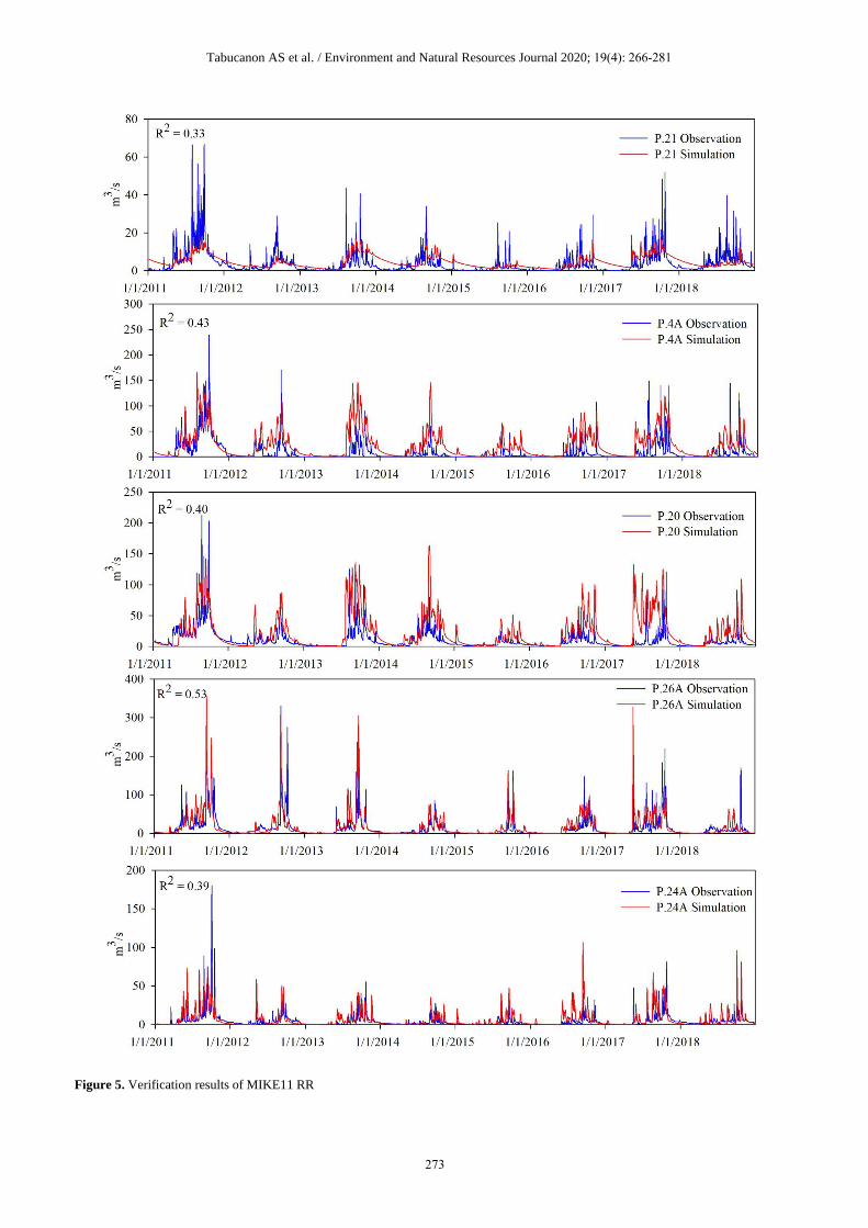
verification period, R2 ranged between 0.39 and 0.53.
To be consistent with calibration results, the runoff
simulation at P.21 was still problematic. Furthermore,
runoff simulation at P.4A and P.20 was overestimated
while simulated runoff at P.26A and P.24A can
capture the observed runoff patterns well. Additional
information regarding a number of rainfall stations
and operations of weirs and small-to-middle sized
reservoirs can improve the results in this section.
Concerning MIKE11 HD, adjusted Manning’s
coefficients of channel flow ranged between 0.040 in
downstream and 0.066 in upstream areas, which are
consistent with the study of Sriwongsitanon (1997). In
the case of flood plain flows, the values were between
0.060 in downstream and 0.100 in upstream areas.
271

Tabucanon AS et al. / Environment and Natural Resources Journal 2020; 19(4): 266-281
Figure 4. Calibration results of MIKE11 RR
1/1/2000 1/1/2001 1/1/2002 1/1/2003 1/1/2004 1/1/2005 1/1/2006 1/1/2007 1/1/2008 1/1/2009 1/1/2010
m3
/s
0
20
40
60
80
P.21 Observation
P.21 Simulation
1/1/2000 1/1/2001 1/1/2002 1/1/2003 1/1/2004 1/1/2005 1/1/2006 1/1/2007 1/1/2008 1/1/2009 1/1/2010
m3
/s
0
50
100
150
200
250
300
350
P.4A Observation
P.4A Simulation
1/1/2000 1/1/2001 1/1/2002 1/1/2003 1/1/2004 1/1/2005 1/1/2006 1/1/2007 1/1/2008 1/1/2009 1/1/2010
m3
/s
0
100
200
300
400
500
600
P.20 Observation
P.20 Simulation
1/1/2000 1/1/2001 1/1/2002 1/1/2003 1/1/2004 1/1/2005 1/1/2006 1/1/2007 1/1/2008 1/1/2009 1/1/2010
m3
/s
0
100
200
300
400
500
P.26A Observation
P.26A Simulation
1/1/2000 1/1/2001 1/1/2002 1/1/2003 1/1/2004 1/1/2005 1/1/2006 1/1/2007 1/1/2008 1/1/2009 1/1/2010
m3
/s
0
20
40
60
80
100
120
140
160
P.24A Observation
P.24A Simulation
R2 = 0.29
R2 = 0.55
R2 = 0.50
R2 = 0.49
R2 = 0.32
272
Tabucanon AS et al. / Environment and Natural Resources Journal 2020; 19(4): 266-281
Figure 5. Verification results of MIKE11 RR
273

Tabucanon AS et al. / Environment and Natural Resources Journal 2020; 19(4): 266-281
According to our land use data collection in Ping River
Basin between 1989 and 2016 as shown in Figure 6,
we found gradual changes in land uses. Therefore,
Manning’s coefficients were not different from
Sriwongsitanon (1997). According to the results of the
simulated daily inflow into Bhumibol Dam as shown
in Figure 7, the predicted inflow matched the actual
inflow well over the period between 2000 and 2018
(R2=0.70). Nevertheless, the simulation was not
capable of capturing high inflow rate periods, which
are typical limitations for hydrological modelling,
especially for daily rainfall input. To simulate extreme
events, hourly rainfall data is necessary. The results
of seasonal inflow Q-Q plot are shown in Figure 8. It
was found that the model can calculate monthly
inflows in the wet season well, and the model only
underestimated the values in extreme events.
However, in the dry season, the simulated inflow was
overestimated. This was due to the unknown
characteristics of the operated weirs and small-to-
middle sized reservoirs in the study area, which can
decelerate the river flow rate.
Figure 6. Proportion of land use change between 1989 and 2016. Blue, red, yellow, orange and green denote percentage proportion of
water, urban, paddy land, upland agriculture and forest, respectively. (Source: Land Use Development Department, Thailand)
Figure 7. Comparison of simulated and observed inflows into Bhumibol Dam between 2000 and 2018 based on MIKE 11 HD
274

Tabucanon AS et al. / Environment and Natural Resources Journal 2020; 19(4): 266-281
Figure 8. Q-Q plot of monthly inflow into Bhumibol Dam in wet (upper) and dry seasons (lower) between 2000 and 2018
3.2 Changes in monthly and seasonal inflow
The prediction of inflow into Bhumibol Dam
under RCP4.5 and RCP8.5 is summarized in Tables 2
and 3, respectively. In comparison with the baseline
period (2000-2020), RCP4.5 scenarios indicate
increases in inflow in dry season by +0.07%,
+10.00%, +15.42%, and +6.25% in 2021-2040, 2041-
2060, 2061-2080, and 2081-2099, respectively.
However, the results are generally converse in the wet
season because the changes are expected to be
-10.44%, +9.60%, -13.01%, and -2.63%, respectively.
In the RCP8.5 scenario, the results in dry season are
generally consistent with RCP4.5 in which the
changes compared with the baseline period are
expected to be -5.03%, +8.14%, +8.15%, and
+22.71% in 2021-2040, 2041-2060, 2061-2080, and
2081-2099, respectively. In contrast to RCP4.5,
RCP8.5 in the wet season also shows fluctuating
results which are projected to be -4.68%, +20.17%,
-10.13%, and +18.04%, respectively. The findings in
this study do not correspond with Kitpaisalsakul
(2018), who applied bias corrected MRI-GCM climate
data and concluded a slightly decreasing trend of
annual inflow into Bhumibol Dam in both seasons
through the near future (2015-2039) at the slope rate
of -5.744 MCM/year and the far future (2075-2099) at
275

Tab
uca
no
n A
S e
t al
. /
En
vir
on
men
t an
d N
atu
ral
Res
ou
rces
Jo
urn
al 2
020
; 1
9(X
): x
x-x
x
Tab
le 2
. S
um
mar
y o
f p
erce
nta
ge
chan
ge
in s
tati
stic
al i
nd
icat
ors
com
par
ed w
ith
th
e b
asel
ine
per
iod
(2
000
-202
0)
und
er R
CP
4.5
Aver
age
Yea
r Ja
n
Feb
M
ar
Ap
r M
ay
Jun
Jul
Au
g
Sep
O
ct
No
v
Dec
A
nn
ual
W
et
Dry
20
21
-204
0
-0.6
4%
-1.8
9%
-8.6
7%
45
.44
%
44
.21
%
-32
.29
%-1
1.4
8%
-19
.49
%-1
2.3
4%
-5.3
5%
-1.3
0%
-6.6
1%
-8.7
4%
-10
.44
%0
.07
%
20
41
-206
0
7.0
9%
5
.44
%
8.2
9%
2
8.2
2%
7
7.1
9%
5
4.5
3%
-3
.22
%-2
.53
%5
.08
%
-1.5
5%
12
.83
%
3.6
5%
9
.67
%
9.6
0%
1
0.0
0%
20
61
-208
0
9.0
4%
1
.56
%
13
3.7
6%
3
5.2
6%
2
3.8
3%
-1
6.3
2%
-19
.88
%-7
.40
%-2
1.5
1%
-10
.33
%1
.87
%
6.6
4%
-8
.40
%-1
3.0
1%
15
.42
%
20
81
-209
9
10
.97
%
2.7
9%
-7
.63
%1
7.2
0%
1
6.4
2%
9
.42
%
0.1
5%
-1
0.3
1%
-0.7
1%
-8.7
1%
9.1
6%
0
.60
%
-1.1
9%
-2.6
3%
6.2
5%
Sta
nd
ard d
evia
tion
Jan
F
eb
Mar
A
pr
May
Ju
n
Jul
Au
g
Sep
O
ct
No
v
Dec
A
nn
ual
W
et
Dry
20
21
-204
0
12
.58
%
12
.55
%
-18
.63
%5
8.5
6%
8
2.6
7%
-9
.40
%4
5.4
7%
-3
5.7
6%
38
.98
%
23
.64
%
-4.8
5%
3.5
9%
-2
.53
%1
2.7
5%
8
.49
%
20
41
-206
0
6.7
8%
3
.49
%
-3.5
5%
39
.79
%
13
4.1
9%
7
7.7
3%
-1
1.1
0%
-42
.74
%3
7.3
7%
2
.79
%
41
.81
%
-11
.05
%6
.18
%
14
.43
%
19
.38
%
20
61
-208
0
54
.55
%
36
.45
%
91
1.7
8%
4
5.8
6%
3
4.7
7%
1
3.6
9%
-2
3.5
0%
-44
.10
%2
3.9
3%
3
.18
%
73
.54
%
96
.97
%
-2.1
0%
-5.7
1%
14
6.9
3%
20
81
-209
9
15
.78
%
-11
.28
%-4
4.4
4%
74
.93
%
71
.72
%
88
.84
%
29
.47
%
-41
.97
%3
4.0
0%
-1
8.9
7%
-14
.19
%-3
6.4
2%
-9.6
1%
9.6
3%
-4
.19
%
Sto
rage
at t
he
end
of
wet
sea
son
20
21
-204
0
-10
.44
%
20
41
-206
0
9.6
0%
20
61
-208
0
-13
.01
%
20
81
-209
9
-2.6
3%
Tabucanon AS et al. / Environment and Natural Resources Journal 2021; 19(4): 266-281
276

Tab
uca
no
n A
S e
t al
. /
En
vir
on
men
t an
d N
atu
ral
Res
ou
rces
Jo
urn
al 2
020
; 1
9(X
): x
x-x
x
Tab
le 3
. S
um
mar
y o
f p
erce
nta
ge
chan
ge
in s
tati
stic
al i
nd
icat
ors
com
par
ed w
ith
th
e b
asel
ine
per
iod
(2
000
-202
0)
und
er R
CP
8.5
Aver
age
Yea
r Ja
n
Feb
M
ar
Ap
r M
ay
Jun
Jul
Au
g
Sep
O
ct
No
v
Dec
A
nn
ual
W
et
Dry
20
21
-204
0
-4.9
1%
-2.8
0%
-9.0
6%
-28
.34
%-1
.47
%-1
1.8
3%
-36
.68
%2
.28
%
-14
.92
%1
6.1
8%
-3
.66
%0
.80
%
-4.7
4%
-4.6
8%
-5.0
3%
20
41
-206
0
11
.93
%
13
.35
%
7.0
3%
-1
6.3
7%
8.4
2%
6
.59
%
3.3
0%
1
31.0
9%
3
.00
%
2.7
3%
1
0.6
5%
8
.04
%
18
.20
%
20
.17
%
8.1
4%
20
61
-208
0
15
.73
%
8.9
0%
0
.77
%
-26
.91
%-5
6.4
7%
-37
.78
%-3
1.9
9%
17
.52
%
-12
.32
%5
.13
%
15
.08
%
4.9
0%
-7
.15
%-1
0.1
3%
8.1
5%
20
81
-209
9
13
.11
%
15
.64
%
9.0
8%
6
1.4
7%
3
9.3
1%
1
0.1
9%
2
4.5
9%
7
6.4
5%
1
.42
%
6.9
5%
2
1.7
2%
2
3.8
8%
1
8.8
0%
1
8.0
4%
2
2.7
1%
Sta
nd
ard d
evia
tion
Jan
F
eb
Mar
A
pr
May
Ju
n
Jul
Au
g
Sep
O
ct
No
v
Dec
A
nn
ual
W
et
Dry
20
21
-204
0
5.8
6%
1
2.8
9%
-1
5.6
9%
-76
.78
%1
7.9
3%
-2
5.3
0%
-23
.38
%4
9.1
5%
1
8.7
3%
6
5.6
7%
-1
1.4
4%
28
.26
%
44
.32
%
16
.79
%
-18
.71
%
20
41
-206
0
20
.02
%
23
.62
%
-6.7
5%
-70
.15
%8
.48
%
-1.5
0%
-6.7
7%
34
6.4
7%
3
5.5
6%
2
7.1
0%
8
.94
%
29
.00
%
62
.78
%
53
.03
%
-6.8
1%
20
61
-208
0
77
.98
%
43
.98
%
2.3
6%
-8
0.0
3%
-62
.32
%-1
9.7
5%
-15
.07
%9
5.6
0%
5
.49
%
80
.80
%
85
.01
%
38
.75
%
34
.32
%
14
.94
%
27
.48
%
20
81
-209
9
30
.26
%
37
.67
%
3.6
9%
8
2.1
3%
1
13.5
4%
2
5.8
3%
6
9.4
8%
1
84.6
6%
1
0.9
2%
3
5.7
6%
4
9.5
5%
7
6.3
8%
7
3.5
8%
5
7.7
7%
5
5.4
0%
Sto
rage
at t
he
end
of
wet
sea
son
20
21
-204
0
-4.6
8%
20
41
-206
0
20
.17
%
20
61
-208
0
-10
.13
%
20
81
-209
9
18
.04
%
Tabucanon AS et al. / Environment and Natural Resources Journal 2021; 19(4): 266-281
277

Tabucanon AS et al. / Environment and Natural Resources Journal 2020; 19(4): 266-281
the slope rate of -23.03 MCM/year. The results closely
relate with predicted decreasing rainfall in those
periods. Similarly, the results are dependent upon the
studied location. For example, Harraki et al. (2020)
indicated a decrease in the total average supply
between 9% and 12% for mid-term scenario (2046-
2065) and 20% to 27% for the long-term scenario
(2081-2100) for the Sebou Basin in Morocco. Our
results correspond with the work of Sharma and Babel
(2013), especially in the dry season. The work applied
bias corrected and downscaled ECHAM4/OPYC and
indicated continuous decreases in inflow rate in the
wet season by -29.0% in the period between 2023-
2027 and -27.0% in 2093-2097 under A2, as well as
-23.0% and -27.0% under B2. As for dry season,
insistent increases in inflow rate were detected by
+10.0% and +6.0% under A2, as well as +19.0% and
+24.0% under B2. In addition, our study also had the
same finding that the peak flows in the future would
be shifted from September to October, which was
more apparent in RCP8.5. Giesen et al. (2010) also
found a shift of ending rainy season to later periods
under climate change in the Volta Basin, West Africa.
In terms of inflow variation, a large change in
standard deviation indicates increasing difficulty for
reservoir managers to estimate and regulate
appropriate release to control the storage within the
range between lower and upper rule curves. Under
RCP4.5, in comparison with the baseline period, the
deviation will be less at the annual change rate of
-2.53%, +6.18%, -2.10%, and -9.61% in 2020-2040,
2041-2060, 2061-2080, and 2081-2099, respectively.
This implies more stability of water inflow into the
dam, leading to better estimation for the appropriate
release. In contrast, RCP8.5 is challenging due to a
large increase in the deviation rate at +44.32%,
+62.78%, +34.32%, and +73.58%, respectively.
Regarding the results of storage at the end of
wet season (May-October), this indicates water
security for utilization in the dry season, especially for
agricultural activities. The results show high
uncertainties in which RCP4.5 provides change rates
of -10.44%, +9.60%, -13.01%, and -2.36% in 2020-
2040, 2041-2060, 2061-2080, and 2081-2099,
respectively. While for RCP8.5, the changes are
expected to be -4.68%, +20.17%, -10.13%, and
+18.04%, respectively. Therefore, with an
understanding of climate change impacts, the adaptive
or flexible management of the reservoir operating rule
curves should be considered to be able to be
proactively redesigned under uncertain conditions
(Adeloye and Dau, 2019; Fletcher et al., 2019).
3.3 Reliability of current reservoir operating rules
Daily reservoir storage of Bhumibol Dam based
on the standard operating rules under RCP4.5 and
RCP8.5 is illustrated in Figure 9. Under RCP4.5, the
reliability of reservoir operation throughout 2000-
2099 will be 80%. This indicates high failure risk
(20%) in reservoir operation reliability quality, in
which the acceptable percentage is 80% (Rittima,
2018). Interestingly, RCP8.5 indicates higher
reliability with the rate of 87%. The results are
consistent with the findings of Park and Kim (2014),
who suggested that under the new climatic conditions,
the reliability of water and hydropower supply from
the Chungju Multipurpose Dam in South Korea would
be generally improved as a consequence of increased
dam inflow. In addition, the study of Zolghadr-Asli et
al. (2019) found similar results in which the dam
reliability for power generation will be generally
improved through 2010-2099 due to climate change
because of the increased inflow from four hydropower
projects in the Karkheh River Basin in Iran.
Considering reservoir operation reliability, the
dominant cases will be the storage below the lower
rule curve accountable for 92% for RCP4.5 and 86%
for RCP8.5. The monthly failure ratios are
summarized in Table 4. Under RCP4.5, the apparent
failure rates above 10% would occur in January
(11.87%), August (10.72%), September (11.50%),
October (13.09%), November (14.20%), and
December (13.93%). In case of failure of upper rule
curve, the frequent flood risks would occur in June
(20.80%), July (35.88%), August (12.65%), and
October (10.75%). Under RCP8.5, the failure to be
below the lower rule curve would apparently occur
in July (11.01%), August (12.66%), September
(12.01%), October (12.78%), November (15.25%),
and December (12.31%), while the failure of upper
rule curve management would be in June (14.88%),
July (23.07%), August (22.77%), September
(18.45%), and October (15.63%). The major cause of
these failures would be due to high fluctuation of
average and deviation rates of monthly rainfall
between April and September through 2021 to 2099,
in which the monthly rainfall pattern is relatively
different from the current situation (2000-2020); as
can be seen in Tables 2 and 3. The results indicate that
the failure of lower and upper rule curves generally
278
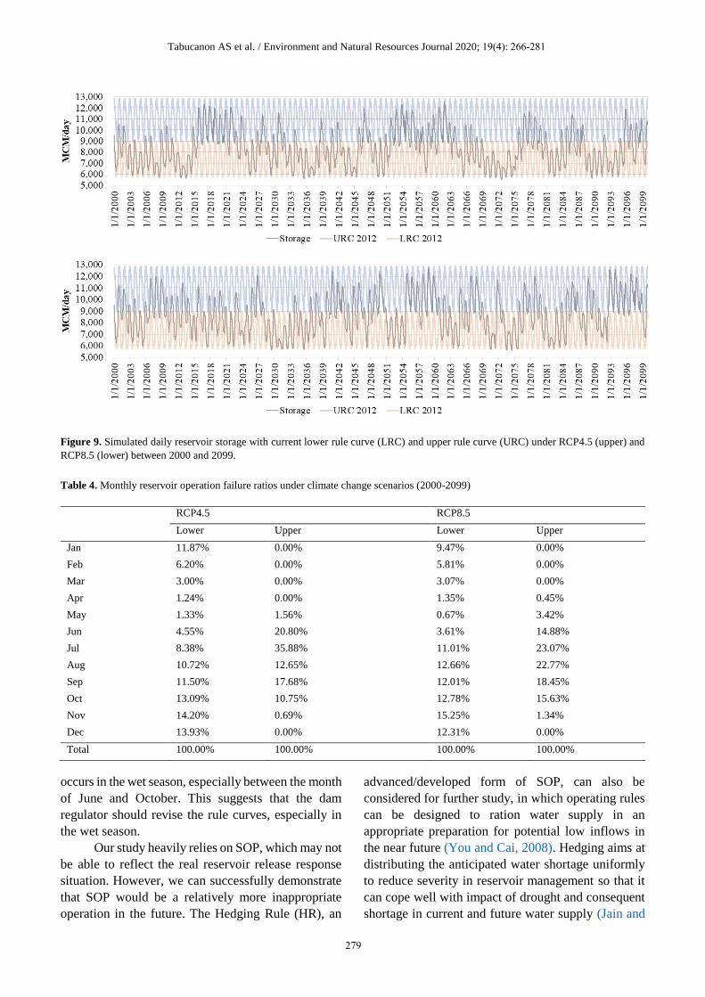
Tabucanon AS et al. / Environment and Natural Resources Journal 2020; 19(4): 266-281
Figure 9. Simulated daily reservoir storage with current lower rule curve (LRC) and upper rule curve (URC) under RCP4.5 (upper) and
RCP8.5 (lower) between 2000 and 2099.
Table 4. Monthly reservoir operation failure ratios under climate change scenarios (2000-2099)
RCP4.5 RCP8.5
Lower Upper Lower Upper
Jan 11.87% 0.00% 9.47% 0.00%
Feb 6.20% 0.00% 5.81% 0.00%
Mar 3.00% 0.00% 3.07% 0.00%
Apr 1.24% 0.00% 1.35% 0.45%
May 1.33% 1.56% 0.67% 3.42%
Jun 4.55% 20.80% 3.61% 14.88%
Jul 8.38% 35.88% 11.01% 23.07%
Aug 10.72% 12.65% 12.66% 22.77%
Sep 11.50% 17.68% 12.01% 18.45%
Oct 13.09% 10.75% 12.78% 15.63%
Nov 14.20% 0.69% 15.25% 1.34%
Dec 13.93% 0.00% 12.31% 0.00%
Total 100.00% 100.00% 100.00% 100.00%
occurs in the wet season, especially between the month
of June and October. This suggests that the dam
regulator should revise the rule curves, especially in
the wet season.
Our study heavily relies on SOP, which may not
be able to reflect the real reservoir release response
situation. However, we can successfully demonstrate
that SOP would be a relatively more inappropriate
operation in the future. The Hedging Rule (HR), an
advanced/developed form of SOP, can also be
considered for further study, in which operating rules
can be designed to ration water supply in an
appropriate preparation for potential low inflows in
the near future (You and Cai, 2008). Hedging aims at
distributing the anticipated water shortage uniformly
to reduce severity in reservoir management so that it
can cope well with impact of drought and consequent
shortage in current and future water supply (Jain and
279

Tabucanon AS et al. / Environment and Natural Resources Journal 2020; 19(4): 266-281
Singh, 2003). Advanced research and technology,
including further climate change impact studies with
various future scenarios and application of artificial
intelligence (AI), could support improvement of water
regulation through adaptive management of rule
curves, which are highly recommended for further
study. For example, Kompor et al. (2020) found that
changing the reservoir operation plan with seasonal
prediction adopted from Centre for Medium-Range
Weather Forecasts could decrease the peak river
discharge in the Chao Phraya River by 20% under the
2011 flood rainfall scenario. Therefore, integration of
climate change scenarios should be further included in
future studies to understand and minimize climate
change uncertainties, which would be useful
information for decision-makers in the development of
appropriate rule curves.
4. CONCLUSION
According to the results of this study, it can be
concluded that there is high risk of current reservoir
operating rules moving towards reliability failure
under RCP4.5, but the risk will be lower under RCP8.5
due to increased inflow amounts. The failures
obviously occur in the wet season, due to a large
fluctuation of the rainfall amount and standard
deviation, which cautions the need to redesign the
rules. Therefore, it is necessary to revisit the rule
curves, especially in the wet season, to maximize
reliability. A limitation of this study is the assumption
of SOP representing reservoir release behaviors,
which is fixed and inflexible. In addition, unknown
future water demand in the downstream area was not
considered. For future study, adaptive management of
rule curves through application of artificial
intelligence (AI), such as fuzzy logic model or neuro
fuzzy optimization model, is a promising alternative to
cope with high uncertainties under climate change.
ACKNOWLEDGEMENTS
This work is financially supported by the
Thailand Science Research and Innovation and
National Research Council of Thailand, under Grant
No. SIP6230022. The authors would like to express
their sincere gratitude to Thailand government
agencies, including Electricity Generating Authority
of Thailand, Royal Irrigation Department, Hydro-
informatics Institute and Thai Meteorological
Department, for their kind support and sharing of data
input for analysis in this study.
REFERENCES Adeloye AJ, Dau QV. Hedging as an adaptive measure for climate
change induced water shortage at the Pong Reservoir in the
Indus Basin Beas River, India. Science of The Total
Environment 2019;687:554-66.
Cruz FT, Narisma GT, Dado JB, Singhruck P, Tangang F, Linarka
UA, et al. Sensitivity of temperature to physical
parameterization schemes of RegCM4 over the CORDEX-
Southeast Asia region. International Journal of Climatology
2017;37:5139-53.
Danish Hydraulic Institute (DHI.) MIKE 11 User Guide [Internet].
2017 [cited 2021 Jan 12]. Available from: https://manuals.
mikepoweredbydhi.help/2017/Water_Resources/MIKE11_Us
erManual.pdf.
Ehsani N, Vörösmarty CJ, Fekete BM, Stakhiv EZ. Reservoir
operations under climate change: Storage capacity options to
mitigate risk. Journal of Hydrology 2017;555:435-46.
Fletcher S, Lickley M, Strzepek K. Learning about climate change
uncertainty enables flexible water infrastructure planning.
Nature Communications 2019;10:1782.
Giesen NVD, Liebe J, Jung G. Adapting to climate change in the
Volta Basin, West Africa. Current Science 2010;98(8):1033-7.
Harraki WEL, OUAZAR D, Bouziane A, Hasnaoui D. Climate
change observations and trends overview: Focus on Morocco
with a case-study of a future reservoir’s response to climate
change. E3S Web Conference 2020;150.
Intergovernmental Panel on Climate Change (IPCC). Global
Warming of 1.5oC: An IPCC Special Report on the Impacts of
Global Warming of 1.5oC Above Preindustrial Levels and
Related Global Greenhouse Gas Emission Pathways, in the
Context of Strengthening the Global Response to the Threat of
Climate Change, Sustainable Development, and Efforts to
Eradicate Poverty. In Press; 2018.
Intergovernmental Panel on Climate Change (IPCC). Managing
the Risks of Extreme Events and Disasters to Advance Climate
Change Adaptation. A Special Report of Working Groups I
and II of the Intergovernmental Panel on Climate Change.
Cambridge, England: Cambridge University Press; 2012.
Jain SK, Singh, VP. Water Resources Systems Planning and
Management. New York, USA: Springer; 2003.
Kang B, Lee SJ, Kang DH, Kim YO. A flood risk projection for
Yongdam Dam against future climate change. Journal of
Hydro-environment Research 2007;1:118-25.
Kim S, Tachikawa Y, Nakakita E, Takara K. Reconsideration of
reservoir operations under climate change: case study with
Yagisawa Dam, Japan. Annual Journal of Hydraulics
Engineering 2009;53:115-20.
Kitpaisalsakul T. Impact of climate change on irrigation water
management by the Bhumibol Dam in Thailand. Journal of
Thai Interdisciplinary Research 2018;13:49-54.
Koontanakulvong S, Vudhivanich V, Rittima A, Phankamolsil Y,
Tabucanon AS, Sawangphol W, et al. Lesson learnt from past
to present and water storage potential in future for Bhumibol
and Sirikit Dams. Proceedings of the 13th THAICID National
E-Symposium; 2020 Jul 31; Studio of Irrigation Development
Institute, Bangkok: Thailand; 2020.
Kompor W, Yoshikawa S, Kanae S. Use of seasonal streamflow
forecasts for flood mitigation with adaptive reservoir
operation: A case study of the Chao Phraya River Basin,
Thailand, in 2011. Water 2020;12(3210):1-19.
Kure S, Tenakari T, Okabe M. Spatial and seasonal differences in
the response of flow to climate change in the Chao Phraya
280

Tabucanon AS et al. / Environment and Natural Resources Journal 2020; 19(4): 266-281
River Basin, Thailand. Journal of Japan Society of Civil
Engineers, Ser.B1 (Hydraulic Engineering) 2013;69(4):55-60.
Limsakul A, Singhruck P. Long-term trends and variability of total
and extreme precipitation in Thailand. Atmospheric Research
2016;169:301-17.
Limsakul A. Trends in Thailand’ s extreme temperature indices
during 1955-2018 and their relationship with global mean
temperature change. Applied Environmental Research 2020;
42:94-107.
Miyan MA. Droughts in Asian least developed countries:
Vulnerability and sustainability. Weather and Climate
Extremes 2015;7:8-23.
Moss R, Edmonds J, Hibbard K, Manning M, Rose S, Vuuren D,
et al. The next generation of scenarios for climate change
research and assessment. Nature 2010;463:747-56.
Murphy J. An evaluation of statistical and dynamical techniques
for downscaling local climate. Journal of Climate
1999;12:2256-84.
Ngo‐Duc T, Tangang FT, Santisirisomboon J, Cruz F, Trinh‐Tuan
L, Nguyen‐Xuan T, et al. Performance evaluation of RegCM4
in simulating extreme rainfall and temperature indices over the
CORDEX‐ Southeast Asia region. International Journal of
Climatology 2017;37:1634-47.
Park JY, Kim SJ. Potential impacts of climate change on the
reliability of water and hydropower supply from a
multipurpose dam in South Korea. Journal of the American
Water Resources Association 2014;50:1273-88.
Raneesh J. Impact of climate change on water resources. Earth
Science and Climatic Change 2014;5(3):1-5.
Rittima A. Reservoir Systems and Operation Planning. Bangkok,
Thailand: Mittrapopkarnpim; 2018.
Sharma D, Babel MS. Application of downscaled precipitation for
hydrological climate-change impact assessment in the upper
Ping River Basin of Thailand. Climate Dynamics 2013;
41:2589-602.
Shiferaw B, Tesfaye K, Kassie M, Abate T, Prasanna BM, Menkir
A. Managing vulnerability to drought and enhancing
livelihood resilience in sub- Saharan Africa: Technological,
institutional and policy options. Weather and Climate
Extremes 2014;3:67-79.
Siam Commercial Bank. EIC evaluates that the 2020 drought
could extend to June with severe impacts on sugarcane, off-
season rice, and cassava [Internet]. 2020 [cited 2021 Jan 12].
Available from: https://www.scbeic.com/en/detail/file/product
/6660/fl65yywwln/EIC-Note_drought_EN_20200302 .pdf.
Sriwongsitanon N. The study of the flood conditions of the Upper
Ping River Basin by an application of MIKE 1 1 model (part
1). Kasetsart Engineering Journal 1997;11:74-87 (in Thai).
Tangang F, Santisirisomboon J, Juneng L, Salimun E, Chung J,
Supari S, et al. Projected future changes in mean precipitation
over Thailand based on multi-model regional climate
simulations of CORDEX Southeast Asia. International Journal
of Climatology 2019;39:5413-36.
Thana-dachophol T, Teamsuwan V, Udomsap L, Wongsamut W,
Chamnankaew U. An analysis of water management in 2020
drought conditions. Proceedings of the 13th THAICID national
esymposium; 2020 Jul 31; Studio of Irrigation Development
Institute, Bangkok: Thailand; 2020.
The World Bank. Thai flood 2011, Rapid Assessment for Resilient
Recovery and Reconstruction Planning. The World Bank; 2012.
You JY, Cai X. Hedging rule for reservoir operations: 1. A
theoretical analysis. Water Researches Research 2008:
44:W01415.
Zolghadr-Asli B, Bozorg-Haddad O, Chu X. Effects of the
uncertainties of climate change on the performance of
hydropower systems. Journal of Water and Climate Change
2019;10.3:591-609.
281

Environment and Natural Resources Journal 2021; 19(4): 282-291
Bioaccumulation of Lead by Pepper Elder (Peperomia pellucida (L.)
Kunth) in a Lead-Contaminated Hydroponic System
Jessica O. Tablang, Florenda B. Temanel, Ron Patrick C. Campos*, and Helen C. Ramos
College of Arts and Sciences, Isabela State University-Echague, 3309 Isabela, Philippines
ARTICLE INFO ABSTRACT
Received: 28 Jan 2021Received in revised: 21 Mar 2021Accepted: 21 Apr 2021Published online: 25 May 2021DOI: 10.32526/ennrj/19/2021010
Lead (Pb) has become one of the most common heavy metal contaminants,
demanding research on economical remediation approaches with minimal
ecological impacts. Pepper elder (Peperomia pellucida) is a fast-growing plant
that can be a candidate for bioaccumulation and phytoremediation. In this study,
the lead bioaccumulation of P. pellucida was assessed by determining the growth
response and absorptive capacity of the plant. Plants were grown in hydroponic
solution spiked with 500 mg/L of Pb for 28 days. Growth response, absorptive
capacity and tolerance of plants grown in contaminated nutrient solution were
determined in comparison with control plants. After 28 days of exposure, lead
phytotoxicity symptoms such as wilting, chlorosis and necrosis were observed on
some plants. The control plants recorded 3.08 g total dry weight (DW) compared
to the 1.35 g in Pb-contaminated plants. The tolerance index (TI) of P. pellucida
was at 43.40%. The plants were able to absorb lead, with the concentration of
lead in the roots (158.6 µg/g) being greater than the concentration of the metal
in the shoots (43.2 µg/g). Meanwhile, bioconcentration factor (BCF) and
translocation factor (TF) values were recorded at 0.40 and 0.27, respectively.
BCF criterion indicates that the plant is not suitable for phytoextraction, but TF
value shows that the plant can be a potential excluder. The findings of the study
show that P. pellucida accumulated considerable amount of lead within its
tissues, indicating that the plants may be further exploited for their capacity to
absorb heavy metals by tweaking several factors that may affect its
bioaccumulation ability.
Keywords:
Pepper elder/ Peperomia
pellucida/ Phytoremediation/
Heavy metal/ Lead
* Corresponding author:
E-mail:
1. INTRODUCTION
Global industrialization and human activity
have caused the widespread contamination of
persistent pollutants that resulted in the degradation of
the environment (Lado et al., 2008). This is caused by
contamination of inorganic and organic pollutants
from various sources such as direct discharge of
industrial effluents to soil, accidental spillage of
chemicals, application of agrochemicals to soils and
the percolation of contaminated surface water to
subsurface stratum, or improper disposal of wastes
(Mirsal, 2004). Many heavy metals can be considered
essential to the life cycles of both flora and fauna, but
may reach toxic levels when the number of pollutants
exceeds the demand of the inherent biological systems
(Mandkini et al., 2016). Furthermore, the non-
biodegradability of heavy metal pollutants creates a
hazard when discharged in soils and bodies of water
(Thayaparan et al., 2013).
Lead (Pb) has become one of the most common
heavy metal contaminants in the soil (Thayaparan et
al., 2013; Solidum et al., 2010). Lead contamination
has become prevalent due to existing mining and
smelting activities (Liu et al., 2010) and the disposal
of sewage sludge and industrial wastes (Ona et al.,
2006), as well as being a component of common
products such as paints, gasoline and explosives.
Phytoremediation is a cheap and reliable
technology that is utilized for the cleansing of polluted
environments that can potentially address the
problems of contaminated areas affected by urban and
industrial activities (Mojiri, 2011). It is based on
exploiting plant’s natural mechanisms to detoxify and
accumulate heavy metals within soil or from aquatic
Citation: Tablang JO, Temanel FB, Campos RPC, Ramos HC. Bioaccumulation of lead by pepper elder (Peperomia pellucida (L.) Kunth) in a lead-contaminated hydroponic system. Environ. Nat. Resour. J. 2021;19(4):282-291. (https://doi.org/10.32526/ennrj/19/2021010)
282

Tablang JO et al. / Environment and Natural Resources Journal 2021; 19(4): 282-291
environments (Mandkini et al., 2016). Plants can be
used to either partially or substantially remediate
different media including sludge, soil, groundwater,
sediment and waste water contaminated with
pollutants (Salt et al., 1998).
Owing to its physiological and morphological
characteristics, Peperomia pellucida can be a
candidate for bioaccumulation and phytoremediation.
This plant, commonly referred to as shiny bush, clear
weed or pepper elder, belongs to the family
Piperaceae. It is an herbaceous plant found in many
South American and Asian countries (Arquion et al.,
2015) and is distinguished by its heart-shaped and
fleshy leaves with lush and succulent stems, shallow
roots and small flowers, which eventually develop into
numerous tiny seeds attached on cord-like spikes
(Tablang et al., 2020). In the Philippines, the plant has
been listed as one of the clinically tested and approved
alternative herbal medicines endorsed by the
Department of Health (Tolentino et al., 2019).
Traditionally, the plant is used in the treatment of
different ailments such as convulsions, conjunctivitis,
headache, fever, gout, skin diseases, and rheumatic
pains (Tolentino et al., 2019; Mosango, 2008;
Raghavendra and Kekuda, 2018).
Pepper elder possesses a number of remarkable
qualities which makes it a candidate for
phytoremediation. It is (1) a plant with fast growth
rates (McIntyre, 2003); (2) produces large biomass
above and below ground (Mosango et al., 2008); (3)
establishes a vast niche for the development of
rhizosphere microorganisms (Kirk et al., 2002); and
(4) is widely distributed, well adapting to different
climatic conditions. In a study by Anoliefo et al.
(2006), P. pellucida was labelled as the plant species
with the most engine oil-tolerant phytoremediation
capacity in Benin City, Nigeria because it was found
in every heavy metal contaminated site in the city. P.
pellucida grown on lead, copper and manganese
contaminated soils also showed accumulation of up to
1,769 ppm of copper, 2,478 ppm of lead and 621 ppm
of manganese (Calawagan et al., 2012). Belonias
(2009) further supported the capacity of the plant to
bioaccumulate lead, concluding that P. pellucida can
tolerate Pb levels as high as 400 ppm without affecting
its growth. Moreover, it was reported that P. pellucida
can contain high amount of toxic metals like lead (Pb)
and cadmium (Cd) surpassing the limits allowed by
the World Health Organization (De Guzman, 1999).
The deterioration of the environment due to
lead contamination demands technology involving
economical approaches with minimal ecological
impacts. Phytoremediation through bioaccumulation
can be one of these approaches. With the objective of
determining the lead-absorptive capacity and heavy
metal tolerance of P. pellucida, this study was
conducted to evaluate the potential of P. pellucida in
the bioaccumulation of lead ex situ and determine the
growth response of the plant upon exposure to Pb
contamination in a hydroponic setting.
2. METHODOLOGY
2.1 Plant collection and acclimatization
Plant samples of P. pellucida were obtained
from uncontaminated sites in Isabela State University,
Echague, Isabela (16.7212° N, 121.6887° E). Young
and healthy plants in uniform height were selected,
and tested for initial heavy metal content to ensure
absence of heavy metals prior to experimentation.
Collected plants were transplanted individually in a
sowing bed containing 50.8 mm-deep coconut coir
dust. The plants were watered regularly for three (3)
days. After which, each plant was transferred to
individual growing pots and introduced to the nutrient
solution for ten (10) days to allow the plants to adapt
to the experimental conditions and to obtain
substantial biomass prior to contamination.
2.2 Hydroponic system set-up and experimental
set-up
This study employed the Simple Nutrient
Addition Program (SNAP) hydroponics system, a
non-circulating, passive aeration hydroponics system
(Santos and Ocampo, 2005).
A treatment series of 0 mg/L (control) and 500
mg/L Pb (Pb-contaminated) was prepared on par with
the regulatory standards for environmental levels of
the heavy metal (USEPA, 1992). Lead stock solution
was prepared using analytical grade Pb (NO3)2. After
the 10-day acclimatization period, the nutrient
solution was spiked with 500 mg/L of lead by
dissolving 8.789 g of Pb (NO3)2 in every 11 litre-
capacity culture boxes. Control plants were grown
exclusively on nutrient solution.
In each treatment, four hydroponic culture
boxes were set up, each containing eight (8) individual
plants of P. pellucida. The schematic diagram of the
hydroponic set up is presented in Figure 1. The
experiment was conducted for 28 days and toxicity
symptoms of plants were observed throughout the
experiment.
283

Tablang JO et al. / Environment and Natural Resources Journal 2021; 19(4): 282-291
Figure 1. Schematic diagram of SNAP hydroponic system; (A) top view of the hydroponic culture box; (B) growing pots; (C) cross-
section view of the hydroponic system
2.3 Monitoring of growth response
Growth response to lead contamination was
determined by measuring the observable physical
changes in the test plants, such as height, leaf area and
number of leaves. Measurement was done periodically
before and after Pb contamination. These factors are
the indications that the tested plant species had
undergone lead bioaccumulation in terms of physical
changes. Dry weight of the plants was calculated using
the formula:
Dry Weight (g) =Total dry weight of plants in treatment (g)
Total number of plants in treatment
2.4. Plant harvesting
At the end of the 28-day growth period, the P.
pellucida plants were gently removed from each
growing pot while carefully separating the coconut
coir dust from roots. After which, they were rinsed
with distilled water to remove adherent debris, taking
extra caution to preserve as much root as possible. The
roots of the plant were then gently separated from
shoots (stems and leaves). Separately, the above
ground and below ground parts were cut into smaller
pieces and blot-dried. Root and shoot samples were
separately placed in microwavable containers, labelled
and subjected to oven-drying at 80oC for 72 h. After
which, the dried plant samples were weighed and acid-
digested.
2.5 Sample preparation and analysis
The USEPA (2007) Method 7000B as modified
by Atayese et al. (2009) was used in the preparation of
plant tissues for lead-content analysis. Once the drying
process is completed, the tissue was removed from the
containers and ground using a mortar and pestle.
Approximately, 0.5 g of homogenized powder (shoot
or root) was transferred into a 100 mL conical flask
and 5 mL of concentrated H2SO4 was added, followed
by the addition of 25 mL of concentrated HNO3. Then,
the contents of the conical flask were heated on a
heating plate at 100°C until a clear solution is
obtained. After cooling, distilled water was added to
the falcon tube to obtain a final volume of 25 mL. The
filtered and rinsed solution was collected in a sterile,
25 mL capacity graduated falcon tube. Finally, the
falcon tube was left to settle down for 24 h. Each tube
was labelled and prepared for Flame Atomic
Absorption Spectroscopy (Flame AAS) analysis.
284

Tablang JO et al. / Environment and Natural Resources Journal 2021; 19(4): 282-291
2.6 Computation of absorptive capacity and
tolerance parameters
In response to Pb exposure, the following heavy
metal absorptive capacity and tolerance parameters
were determined: survival rate (SR), tolerance index
(TI), bioconcentration factor (BCF), translocation
factor (TF) and lead metal uptake. These were
calculated following the equations of Meeinkuirt et al.
(2012), Zhivotovsky et al. (2011), Yaowakhan et al.
(2005), Tanhan et al. (2007), Niu et al. (2007), and
Vamerali et al. (2010):
1) Survival rate (SR): This is percentage of
plants still alive after the experimentation period
computed as:
SR =Final number of plants
Initial number of plants × 100
2) Tolerance index (TI): This is the ratio of dry
weight in plants grown on contaminated solution and
control plants grown on uncontaminated solution, and
is expressed as a percentage using the formula:
TI (%) =Dry weight of plant in Pb treatment (g)
Dry weight of plant in control treatment (g) × 100
3) Bioconcentration factor (BCF): This was
determined by the ratio of lead concentration in plant
tissues to the total metal initial concentration
expressed in mg/kg. This was obtained using the
following equation (Wilson and Pyatt, 2007):
BCF = Pb concentration in whole plant (mg/kg)
Initial Pb concentration in solution(mg/L)
4) Translocation factor: This was used to
evaluate the efficiency of P. pellucida in translocating
the accumulated metal from its roots to shoots. The
value was obtained by measuring the ratio in
concentration in the aerial tissues and that in the roots,
respectively, with the heavy metal content expressed
as mg/kg. The following formula was used
(Padmavathiamma and Li, 2007):
TF = Heavy metal concentration in shoot (mg/kg)
Pb concentration in root (mg/kg)
5) Pb concentration: This is the ratio of the
product of AAS reading and dilution factor to the
weight of sample used for acid digestion. This was
calculated using the formula:
Pb accumulation
= AAS Reading (µg/mL) × Dilution Factor (mL/g)
Weight of sample (g)
6) Pb uptake: It is the ratio of the lead
concentration in the tissues of P. pellucida and the
dry biomass of the plant after experimentation. This is
determined by the following formula:
Pb uptake (µg/plant) = Pb accumulation (µg/g) ×
dry weight (g/plant)
2.7 Statistical analysis
Paired Student’s t-test was used to evaluate the
growth response of the plant on Pb exposure. The dry
weight was also compared using the said test. For
heavy metal absorptive capacity and tolerance
parameters, the values were computed based on given
formula.
3. RESULTS AND DISCUSSION
3.1 Growth response of P. pellucida on lead
(Pb) contamination
The growth response and performance of P.
pellucida in the presence of Pb can determine its
viability as a phytoremediator. The physiological
parameters and growth response of P. pellucida upon
lead-exposure is presented in Figure 2-4.
Throughout the experimental growth period, P.
pellucida plants grown exclusively on nutrient
solution were constantly growing, as noticed in the
gradual and continuous increase in plant height, leaf
number and leaf area (Figure 2-4). On the other hand,
P. pellucida plants exposed to 500 mg/L of Pb were
growing relatively at the same rate as the unexposed
plants during the first two weeks of experimentation;
however, manifestation of lead phytotoxicity appeared
during the third week, where biomass production was
affected as implied in the reduction of plant height,
leaf number and leaf area of lead-exposed plants.
Relative growth of uncontaminated and
contaminated plants became divergent during the third
week of experimentation. Plants grown solely on
nutrient solution depicted an upward slope of relative
growth, exhibiting constant linear increment in height,
and leaf number and area; whereas lead-contaminated
plants showed a curb in the figures of plant height, leaf
number and leaf area during the third week of
exposure (Figure 2-4), mainly due to the slowed
285

Tablang JO et al. / Environment and Natural Resources Journal 2021; 19(4): 282-291
growth and death of some plants. Symptoms of lead
phytotoxicity such as drooping, necrosis and leaf
bleaching also started to manifest as early as the
second week, while the indications became more
apparent during the third and fourth week where lead-
exposed plants started to wilt, lose turgidity and die.
Figure 2. Effect of 500 mg/L Pb on the plant height of P. pellucida.
Figure 3. Effect of 500 mg/L Pb on the leaf number of P. pellucida.
Figure 4. Effect of 500 mg/L Pb on the leaf area of P. pellucida.
0
50
100
150
200
250
300
350
Week 0 Week 1 Week 2 Week 3 Week 4
Pla
nt
hei
gh
t (m
m)
Exposure time
Control
Pb-contaminated
0
10
20
30
40
50
60
Week 0 Week 1 Week 2 Week 3 Week 4
Lea
f n
um
ber
Exposure time
Control
Pb-contaminated
0
200
400
600
800
1000
1200
Week 0 Week 1 Week 2 Week 3 Week 4
Lea
f ar
ea (
mm
2)
Exposure time
Control
Pb-contaminated
286

Tablang JO et al. / Environment and Natural Resources Journal 2021; 19(4): 282-291
Throughout the first two weeks of
experimentation, the plant height, leaf number and leaf
area of the plants were not significantly affected
(p>0.05) by the presence of 500 mg/L of Pb
concentration. This is because of the consistent
increment of biomass produced in both treatments
during the first two weeks. However, at the conclusion
of the experimental period, final mean values for
plant height, leaf number and leaf area were
determined to be significantly different from each
other (p>0.05) with respect to the presence or absence
of 500 mg/L of Pb.
As plants grow in a contaminated environment,
they tend to continue to absorb Pb and sequester the
metal within their tissues, causing the toxicity
symptoms in the plant to increase. In hydroponics
experiment, P. pellucida grew well without the
presence of Pb concentrations, and little to no
morphological symptoms such as chlorosis and
necrosis were observed. However, lead-exposed
plants had reduced total biomass which is a result of
decreased number of leaves, fresh and dry weight, and
length of root and shoot. According to Belonias
(2009), P. pellucida can tolerate lead levels of up to
400 ppm, with Pb-treated plants and the control
showing comparably uniform vigorous growth during
a 3-week experimental period. However, in this study,
the 500 mg/L concentration had significant effect on
the growth response of the plant. Same results were
obtained by some other studies at the calculated lead
concentration on different plants; root, shoot and leaf
growth, fresh and dry biomass were critically reduced
in Pisum sativum, Zea mays, Paspalum distichum,
Cynodon dactylon, Lycopersicon esculentum,
Ipomoea aquatica, Phaseolus vulgaris, and Lens
culinaris (Nas and Ali, 2018; Jaja and Odoemena,
2004; Gothberg et al., 2004).
The result of the study shows that manifestation
of Pb effect on plant is evident after two to three
weeks. Manifestations of toxicity became apparent as
the plants were increasingly exposed to the Pb. Visual
examination of the plants exposed to Pb also shows
signs of toxicity such as necrosis of leaf tip and
darkened shoot base, pale-colored leaves, drooped and
shrunken shoots and short and dark roots, with heavily
shrunken shoot base (Figure 5).
Figure 5. Lead-phytotoxicity symptoms during the four-week exposure period; (A) second week plants showing necrosis of leaf tip and
darkened shoot base; (B) third week plants with pale-colored leaves and drooped and shrunken shoots; (C) final week plants showing
short and dark roots, with heavily shrunken shoots base (top) and deceased plant (bottom).
(B)
leaf tip necrosis
blackened shoot base
dark roots
shrunken shoot
withered leaves
(A) (C)
287

Tablang JO et al. / Environment and Natural Resources Journal 2021; 19(4): 282-291
These results and observations corroborate with
the findings of by Sharma and Dubey (2005) and Nas
and Ali (2018). According to them, the visual non-
specific symptoms of Pb toxicity are rapid inhibition
of root growth, stunted growth of the plant and
chlorosis. This claim is also supported. They stated
that Pb toxicity is manifested outwardly in the plant
such as stunted growth, chlorosis and blackening of
the root system. In addition, Pb inhibits
photosynthesis, upsets mineral nutrition and balance,
changes hormonal status and affects membrane
structure and permeability. These disorders upset
normal physiological activities of the plants (Nas and
Ali, 2018).
It can also be noted in the result that symptoms
of Pb toxicity were manifested by the plants in the later
part of the experimental period. This may mean that
the amount of Pb absorbed in the earlier part of the
experiment is not yet considerable. According to Putra
et al. (2016), the amount of Pb accumulation must be
in considerable amount to inhibit plant metabolism
before showing a visible phytotoxic and oxidative
damage effect.
3.2 Lead tolerance of P. pellucida
Tolerance is an organism’s ability to cope with
heavy metals that are excessively accumulated within
its body. The effect of lead on biomass production and
the parameters for lead tolerance are presented in
Table 1.
Results showed that plants exposed to Pb have
a lower biomass compared to those plants that were
not contaminated by Pb. The DW of P. pellucida was
significantly affected (p>0.05) by 500 mg/L of lead.
The low biomass may be attributed to the relatively
lower plant height, number of leaves and leaf area. In
addition, the dry weight reduction relates to high Pb
concentration, since plants may have to use energy to
cope with the high Pb concentration in their tissues
(Karimi et al., 2012).
Table 1. Lead tolerance of P. pellucida after 28 days of exposure.
Note: Each value is mean of four replications ± standard deviation. Mean of each column indexed with different small letters denote a significant difference
of relative leaf number between absence and presence of Pb concentration (500 mg/L) as determined by paired t-test at p≤0.05.
Higher survival rate was also observed in the
control group with 93.70%, while only 71.80%
survival rate was observed in Pb contaminated plants.
Result also shows that plants exposed to 500 mg/L Pb
had a tolerance index (TI) of 43.40% which is
relatively low. Herlina et al. (2020) suggested that
plants with TI values greater than 100% reflect a net
increase in biomass and tolerance-acquisition of
the plant, whereas, TI values lower than 100% indicate
a net decrease in biomass and a stressed plant
condition. However, it was suggested by Zhivotovsky
et al. (2011) and Wang et al. (2014) that a 60% TI
criterion value indicates ability of plants to tolerate
heavy metals. The recorded TI value for P. pellucida
(43.40%) was far below 100%, indicating that the
plants have become stressed throughout the
experiment as evident in the retardation of growth of
the plants.
Different plant species develop different
mechanisms to tolerate excess levels of metals (Aini
Syuhaida et al., 2014). The earliest mechanism is a
synthesis of polysaccharide such as callose (β-1, 3
glucan) deposited on the outside of the cell membrane,
thereby reducing the diffusion of heavy metal ions into
the plant cell. In in situ applications and in soil
experiments, plant roots secrete exudates into the soil
matrix to chelate metals and to prevent their uptake
inside the cells (Furini, 2012; Małachowska-Jutsz and
Gnida, 2015). However, in a hydroponics experiment,
this mechanism is hardly employed due to the roots
being suspended in a liquid environment, thus
preventing the roots from releasing the exudates and
thereby reducing the resistance from lead uptake.
3.3 Lead accumulation and lead absorptive
capacity of P. pellucida
Table 2 presents the accumulation and
absorptive capacity of P. pellucida after 28 days of
exposure to 500 mg/L to Pb. This lead absorptive
capacity was measured in terms of Pb uptake
(µg/plant), bio-accumulation factor (BCF) and
translocation factor (TF).
Treatments Dry weight (g) Lead tolerance parameters
Roots Shoots Total Survival rate (%) Tolerance index (%)
Control (0 mg/L) 0.43±0.20a 2.65±0.95a 3.08±1.08a 93.70 -
Pb-contaminated
(500 mg/L)
0.21±0.10b 1.15±0.37b 1.35±0.46b 71.80 43.40
288

Tablang JO et al. / Environment and Natural Resources Journal 2021; 19(4): 282-291
Table 2. Lead absorptive capacity of P. pellucida after 28 days of exposure.
Results showed that there is an accumulation of
Pb in the tissues of P. pellucida plants. The amount of
Pb accumulated in the roots (158.6 µg/g) is greater
than the amount accumulated in the shoots (43.2 µg/g).
This result implies that the roots system of the P.
pellucida has the ability to absorb Pb; however,
translocation into the shoot system might have been
restricted. According to Mleczek et al. (2019),
mechanisms of metal uptake and accumulation in
plants have demonstrated that plants have the ability
to translocate selected elements in its tissues, with the
roots being the most capable organ in taking up
significant quantities of Pb whilst simultaneously
restricting translocation to hypogeal parts.
The Pb concentrations (158.6 µg/kg in shoots,
and 43.2 µg/kg in roots) from this study were lower
than Pb concentrations reported in shrubs; for
example, Chromolaena odorata (L.) with Pb in shoots
1,721 mg/kg, and in roots 51,493 mg/kg (Niu et al.,
2007). The results follow a similar trend as some other
studies. The other common phenomenon is Pb
accumulation in roots more than that in shoots and
several previous studies, including this study, show
the same pattern. Zhivotovsky et al. (2011) found that
at the highest Pb concentration of 241 μM, Salix
lucida, Salix nigra, and Salix serissima had higher Pb
concentration in roots than in aerial tissue, such as
wood, in shoot and in leaves. Liu et al. (2015) found
that Phyllostachys pubescens grown in nutrient
solution supplemented with 200 μM Pb contained
higher Pb in the root (1,221 mg/kg) as compared to
that in the stem (351 mg/kg) and in leaf (165 mg/kg).
The Pb uptake of P. pellucida plants was
calculated to be 272.43 µg/plant. Meanwhile, BCF and
TF values were recorded at 0.40 and 0.27,
respectively. Ramana et al. (2021) stated that (BCF)
and Translocation Factor (TF) are the defining
parameter in phytoremediation by providing insight on
metal uptake, mobilization and storage. Since, BCF
and TF values are used to evaluate a plant’s ability to
accumulate and translocate heavy metals, and identify
the suitability of plants for phytoextraction and
phytostabilization (Niu et al., 2007; Wang et al.,
2014), values >1 indicate that the plant has the
potential for phytoextraction (Ali et al., 2013). With
BCF criterion, P. pellucida shows relatively low
potential for bioaccumulation.
According to Napoli et al. (2020), a high value
of TF (TF>1) signifies promising ability of a plant to
translocate heavy metals from roots to aerial tissues.
On the other hand, a low value (TF<1) indicates a
limited capacity of a plant to translocate the metal to
aerial tissues. In this study, P. pelludica recorded TF
value <1. This is indicative of P. pellucida’s low
capacity to uptake high quantity of Pb, potentially
classifying the plant as an excluder of Pb.
The uptake and translocation of a pollutant in
plants depends on many factors: (1) the pollutant’s
concentration in the solution, (2) its efficiency to enter
the root system, and (3) the rate of transpiration in the
plants (Glime, 2017). Pepper elder plants are very
reliant to the turgor pressure within their systems, and
any disruption in this system might compromise the
integrity of their structures and the plant in general.
In this study, P. pellucida was determined to
have the capacity to accumulate and uptake lead in its
tissues. On the other hand, the results showed values
of phytoremediation parameters (SR, TI, BCF, TF)
that are below the criterion for each respective
parameter. This implies that, the plants were affected
by the spiking of 500 mg/L of Pb. Despite this, the
plants showed the capacity to uptake lead and still
survive, which is promising considering that the
concentration of lead used to spike the nutrient
solution was relatively high. Nevertheless, it must still
be taken into account that the experiment was
conducted ex situ in a hydroponic setting with a single
treatment. The present conditions might have affected
the capacity of P. pellucida to survive, uptake and
accumulate lead in its tissues, and different results may
be obtained in a pot experiment.
4. CONCLUSION
Manifestations of toxicity became apparent as
the plants were exposed longer to Pb. Prolonged
exposure to Pb induced phytotoxicity symptoms and
reduced biomass production, affecting plant height,
leaf number and leaf area as implied in the curb of the
respective growth parameters during the third week of
exposure, which consequently caused retardation of
Pb-accumulation (µg/g) Lead absorptive capacity parameters
Roots Shoots Lead uptake (µg/plant) BCF TF
Pb-contaminated (500 mg/L) 158.60 43.20 272.43 0.40 0.27
289

Tablang JO et al. / Environment and Natural Resources Journal 2021; 19(4): 282-291
growth. Lead-absorptive capacity parameters imply
that the plant may be classified as a heavy metal
excluder. Despite the manifestations of phytotoxicity,
P. pellucida absorbed considerable amounts of lead
within its tissues, especially its roots. This indicates
that the plant may be further exploited for their
capacity to absorb heavy metals. Only a limited
number of studies and reports on bioaccumulation,
phytoremediation potential and heavy metal uptake
capacity of P. pellucida are available. Hence, this
study may establish a framework for future studies to
improve efficiency and ability of the plant in heavy
metal accumulation.
ACKNOWLEDGEMENTS
The author would like to give special thanks to
the faculty of the Department of Biological Sciences
of Isabela State University for their assistance in
carrying out this study.
REFERENCES Aini Syuhaida AW, Norkhadijah SIS, Praveena SM, Suriyani A.
The comparison of phytoremediation abilities of water
mimosa and water hyacinth. ARPN Journal of Science and
Technology 2014;4:722-31.
Ali H, Naseer M, Sajad MA. Phytoremediation of heavy metals
by Trifolium alexandrinum. International Journal of
Environmental Science 2013;2:1459-69.
Anoliefo G, Ikhajiagbe B, Okonofhua B, Diafe F. Eco-taxonomic
distribution of plant species around motor mechanic
workshops in Asaba and Benin City, Nigeria: Identification of
oil tolerant plant species. African Journal Of Biotechnology
2006;5(19):1757-62.
Arquion RD, Galanida CC, Villamor B, Aguilar HT.
Ethnobotanical study of indigenous plants used by local people
of Agusan del Sur, Philippines. Asian Pacific Higher
Education Journal 2015;2(2):1-11.
Atayese MO, Eigbadon AI, Oluwa KA, Adesodun JK. Heavy
metal contamination of amaranthus grown along major
highways in Lagos, Nigeria. African Crop Science Journal
2009;6:135-225.
Belonias BS. Bioaccumulation of lead in the medicinal plant
Peperomia pellucida (L.) Kunth. Philippine Journal of Crop
Science 2009;34(1):115.
Calawagan KM, Japitana JJ, Lapada JA, Alvior HB.
Phytoremediation potentials of carabao grass (Paspalum
conjugatum), talahib (Saccharum spontaneum), and ulasimang
bato (Peperomia pellucida) in removing copper (Cu), lead
(Pb), and manganese (Mn) in soils. Proceedings of the PSSN
13th National Scientific Meeting; 2013 May 21-25; Cebu
Business Hotel, Cebu City: Philippines; 2013.
De Guzman CC. Hydroponic culture of pansit-pansitan
(Peperomia pellucida). Proceedings of the 1998 Regional
Research and Development Symposia, Philippine Council for
Agriculture, Forestry and Natural Resources Research and
Development; University of the Philippines Los Baños, Los
Baños, Laguna: Philippines; 1999. p. 120.
Furini A. Plants and Heavy Metals. Dordrecht, Netherlands:
Springer; 2012.
Glime JM. Water relations: Conducting structures. In: Glime JM,
editor. Bryophyte Ecology (Volume 1). USA: Michigan
Technological University and the International Association of
Bryologists; 2017. p. 1-26.
Gothberg A, Greger M, Holm K, Bengtsson BE. Influence of
nutrient levels on uptake and effects of mercury, cadmium, and
lead in water spinach. Journal of Environmental Quality
2004;33(4):1247-55.
Herlina L, Widianarko B, Sunoko HR. Phytoremediation potential
of Cordyline fruticose for lead contaminated soil. Jurnal
Pendidikan IPA Indonesia 2020;9(1):42-9.
Jaja ET, Odoemena CSI. Effect of Pb, Cu, and Fe compounds on
the germination and early seedling growth of tomato varieties.
Journal of Applied Sciences and Environmental Management
2004;8(2):51-3.
Karimi R, Fitzgerald TP, Fisher NS. A quantitative synthesis of
mercury in commercial seafood and implications for exposure
in the United States. Environmental Health Perspective
2012;120:1512-9.
Kirk JL, Klirnomos JN, Lee H, Trevors JT. Phytotoxicity assay to
assess plant species for phytoremediation of petroleum-
contaminated soil. Bioremediation Journal 2002;6:57-63.
Lado LR, Hengl T, Reuter HI. Heavy metals in European soils: A
geostatistical analysis of the FOREGS Geochemical database.
Geoderma 2008;148:189-99.
Liu S, Xia X, Shen M, Liu R. Polycyclic aromatic hydrocarbons
in urban soils of different land uses in Beijing, China:
Distribution, sources and their correlation with the city’s
urbanization history. Journal of Hazardous Materials
2010;177:1085-92.
Liu D, Li S, Islam E, Chen JR, Wu JS, Ye ZQ, et al. Lead
accumulation and tolerance of Moso bamboo (Phyllostachys
pubescens) seedlings: Applications of phytoremediation.
Journal of Zhejiang University Science B 2015;16(2):123-30.
Małachowska-Jutsz A, Gnida A. Mechanisms of stress avoidance
and tolerance by plants used in phytoremediation of heavy
metals. Archives of Environmental Protection 2015;41(4):96-
103.
Mandkini LL, Bandara NG, Gunawardana D. A Study on the
phytoremediation potential of Azolla pinnata under laboratory
conditions. Journal of Tropical Forestry and Environment
2016;6(1):36-49.
McIntyre T. Phytoremediation of heavy metals from soils.
Advances in Biochemical Engineering/Biotechnology
2003;78:97-123.
Meeinkuirt W, Pokethitiyook P, Kruatrachue M, Tanhan P,
Chaiyarat R. Phytostabilization of a Pb-contaminated mine
tailing by various tree species in pot and field trial
experiments. International Journal of Phytoremediation
2012;14:925-38.
Mirsal IA. Soil Pollution, Origin, Monitoring and Remediation.
Berlin, Heidelberg, Germany: Springer; 2004.
Mleczek M, Rutkowski P, Kaniuczak J, Szostek M, Budka A,
Magdziak Z, et al. The significance of selected tree species age
in their efficiency in elements phytoextraction from wastes
mixture. International Journal of Environmental Science and
Technology 2019;16:3579-94.
Mojiri A. The potential of corn (Zea mays) for phytoremediation
of soil contaminated with cadmium and lead. Journal of
Biological and Environmental Science 2011;5(13):17-22.
290

Tablang JO et al. / Environment and Natural Resources Journal 2021; 19(4): 282-291
Mosango DM. Peperomia pellucida (L.) Kunth. In: Schmelzer
GH, Gurib-Fakim A, editors. Prota 11(1): Medicinal
Plants/Plantes médicinales 1. Wageningen, Netherlands:
PROTA; 2008.
Napoli M, Cecchi S, Grassi C, Baldi A, Zanchi CA, Orlandini S.
Phytoextraction of copper from a contaminated soil using
arable and vegetable crops. Chemosphere 2020;219:122-9.
Nas FS, Ali M. The effect of lead on plants in terms of growing
and biochemical parameters: A review. MOJ Ecology and
Environmental Sciences 2018;3(4):265-8.
Niu ZX, Sun LN, Sun TH, Li YS, Hong W. Evaluation of
phytoextracting cadmium and lead by sunflower, ricinus,
alfalfa, and mustard in hydroponic culture. Journal of
Environmental Science 2007;19:961-7.
Ona LF, Alberto AP, Prudente JA, Sigua GC. Levels of lead in
urban soils from selected cities in the rice-based region of the
Philippines. Environmental Science and Pollution Research
2006;13(3):177-83.
Padmavathiamma PK, Li LY. Phytoremediation technology:
Hyperaccumulation metals in plants. Water, Air and Soil
Pollution 2007;184:105-26.
Putra RS, Novarita D, Cahyana F. Remediation of lead (Pb) and
copper (Cu) using water hyacinth (Eichornia crassipes (Mart.)
Solms) with electro-assisted phytoremediation (EAPR). AIP
Conference Proceedings 2016;1744:020052.
Raghavendra HL, Kekuda TRP. Ethnobotanical uses,
phytochemistry and pharmacological activities of Peperomia
pellucida (L.) Kunth (Piperaceae): A review. International
Journal of Pharmacy and Pharmaceutical Sciences 2018;
10(2):1-8.
Ramana S, Tripathi AK, Kumar A, Dey P, Saha JK, Patra AK.
Phytoremediation of soils contaminated with cadmium by
Agave americana. Journal of Natural Fibers 2021;In press:1-9.
Salt DE, Smith RD, Raskin I. Phytomediaion. Annual Review of
Plant Physiology and Plant Molecular Biology 1998;49:643-
68.
Santos PJA, Ocampo ETM. SNAP hydroponics: Development and
potential for urban vegetable production. Philippine Journal of
Crop Science 2005;30(2):3-11.
Sharma P, Dubey RS. Lead toxicity in plants. Brazilian Journal of
Plant Physiology 2005;17:1-19.
Solidum JN, Dahilig VRA, Omran A. Lead levels of water sources
in Manila, Philippines. Annals of Faculty Engineering
Hunedoara - International Journal of Engineering 2010;8:111-8.
Tablang JO, Campos RC, Jacob JS. Phytochemical screening and
antibacterial properties of silverbush (Peperomia pellucida)
against selected cultured bacteria. Global Journal of Medicinal
Plant Research 2020;8(1):1-6.
Tanhan P, Kruatrachue M, Pokethitiyook P, Chaiyarat R. Uptake
and accumulation of cadmium, lead and zinc by Siam weed
(Chromolaena odorata (L.) King and Robinson).
Chemosphere 2007;68:323-9.
Thayaparan M, Iqbal SS, Chathuranga PK, Iqbal MC.
Rhizofiltration of Pb by Azolla pinnata. International Journal
of Environmental Sciences 2013;3(6):1811-21.
Tolentino RD, Tomas VCB, Travezonda JC, Magnaye BP. Herbal
medicine utilization among Batangueños. Asian Pacific
Journal of Education, Arts and Sciences 2019;6(1):9-22.
United States of America Environmental Protection Agency
(USEPA). Selection of Control Technologies for Remediation
of Lead Battery Recycling Sites: EPA/540/S-92/011.
Washington, DC: Office of Emergency and Remedial
Response; 1992.
United States of America Environmental Protection Agency
(USEPA). Method 7000B Flame Atomic Absorption
Spectrophotometry, United States of America Environmental
Protection Agency. Washington, DC: Office of Emergency
and Remedial Response; 2007.
Vamerali T, Bandiera M, Mosca G. Field crops for
phytoremediation of metal-contaminated land: A review.
Environmental Chemistry Letters 2010;8:1-17.
Wang Y, Yang X, Zhang X, Dong L, Zhang J, Wei Y, et al.
Improved plant growth and Zn accumulation in grains of rice
(Oryza sativa L.) by inoculation of endophytic microbes
isolated from a Zn Hyperaccumulator, Sedum alfredii H.
Journal of Agricultural Food Chemistry 2014;62:1783-91.
Wilson B, Pyatt FN. Heavy metal bioaccumulation by the important
food plant, Olea europaea L., in an ancient metalliferous
polluted area of Cyprus. Bulletin of Environmental
Contamination and Toxicology 2007;78:390-4.
Yaowakhan P, Kruatrachue M, Pokethitiyook P,
Soonthornsarathool V. Removal of lead using some aquatic
macrophytes. Bulletin of Environmental Contamination and
Toxicology 2005;75:723-30.
Zhivotovsky O, Kuzovkina Y, Schulthess C, Morris CT, Pettinelli
D. Lead uptake and translocation by willows in pot and field
experiments. International Journal of Phytoremediation 2011;
13:731-49.
291

Environment and Natural Resources Journal 2021; 19(4): 292-301
Effects of Campaign-Based Soil and Water Conservation Practice on
Soil Properties: The Case of Workamba Watershed, Debark District,
North Ethiopia
Muluneh Bogale1*, Getnet Wondie1, and Abdrahman Shafi2
1Department of Natural Resource Management, Debark University, College of Agriculture and Environmental Science (DKU CAES),
P.O Box 90, Debark, Ethiopia2Department of Natural Resource Management, Wolkite University, College of Agriculture and Natural Resource Management,
P.O Box 70, Wolkite, Ethiopia
ARTICLE INFO ABSTRACT
Received: 6 Dec 2020
Received in revised: 5 Apr 2021
Accepted: 21 Apr 2021
Published online: 27 May 2021DOI: 10.32526/ennrj/19/2020256
Land degradation is a serious environmental problem in Ethiopia. To address
the problem, soil and water conservation practices were implemented through
campaign. This study was conducted at Workamba watershed Debark district,
North Ethiopia to assess the effect of campaign soil and water conservation
(SWC) practice on selected soil properties. Composite soil samples from 1.5
meters above the soil bunds, at the center and 1.5 meters below the soil bunds
between the two consecutive structures were collected. The soil samples were
analyzed following standard laboratory procedures. Results showed bulk
density (BD), electrical conductivity (EC), calcium (Ca2+), and sodium (Na+)
were not significantly affected by slope gradient and terrace position and their
interaction. But pH was significantly influenced by the interaction effect.
Cation exchange capacity (CEC), exchangeable potassium (K+), and clay
content were significantly changed with both slope gradient and terrace
position. Whereas, total nitrogen (TN), available phosphorus (Av-P), and
magnesium (Mg2+), and soil organic carbon (SOC) were significantly affected
with terrace position and slope gradient, respectively. Because of the
conservation barrier, most soil properties were better at the bottom terrace
position and gentle slope gradient.
Keywords:
Campaign soil and water
conservation work/ Workamba
watershed/ Land degradation/ Soil
erosion/ Soil and water
conservation
* Corresponding author:
E-mail:
1. INTRODUCTION
Land degradation is a loss of natural capital, the
value to society of land, water, plant and animal
resources and the direct detriment to primary
production in the agricultural system and related
industries (Hurni et al., 2010; Tesfa and Mekuriaw,
2014). Farming populations have experienced decline
in real income due to demographic, economic, social
and environmental changes (Esser et al., 2002). Land
degradation has also become apparent in many
different angles: vegetation becomes increasingly
scarce; footpaths grow into gullies and soils become
thin and stony. All of these manifestations have
negative impacts on the environment (Berry, 2003;
Temesgen et al., 2014).
Soil erosion is one of the main causes of land
degradation and environmental change that affect the
physical and chemical properties of the soil and its
productive potential (Esser et al., 2002). It is the
primary and the most generalized problem in nearly all
tropical mountain regions including Ethiopia (Nyssen
et al., 2009; Demelash and Stahr, 2010). About 350
million (M) hectares or 20 to 25 percent of the total
land area of sub-Saharan Africa is estimated to be
severely damaged with about 100 million (M) hectares
damaged from agricultural use (Zingore et al., 2015).
In Ethiopia, loss of arable land is most common
everywhere; the top-soil and even part of the sub-soil
in some areas has been removed (Esser et al., 2002).
In locations with the most intense population density,
the area of greatest livestock density and the area of
greatest land degradation, recorded measurements of
soil loss range from 3.4 to 84.5 tons/ha/year with a
mean of 32.0 tons/ha/year (Berry, 2003). Similarly,
Citation: Bogale M, Wondie G, Shafi A. Effects of campaign-based soil and water conservation practice on soil properties: The case of Workamba Watershed, Debark District, North Ethiopia. Environ. Nat. Resour. J. 2021;19(4):292-301. (https://doi.org/10.32526/ennrj/19/2020256)
292
Bogale M et al. / Environment and Natural Resources Journal 2021; 19(4): 292-301
Dagnew et al. (2015) reported that soil erosion affects
half of the agricultural land and results in an annual
soil loss rate of 1.5 to 2 billion tons. (Amdemariam et
al., 2011; Mekonnen and Michael, 2014) also
explained that the extent and scale of the problem has
dramatically increased. The issue is also critical in the
highlands (greater than 1,500 m.a.s.l.) (Gebremedhin
and Swinton, 2003; Demelash and Stahr, 2010).
However, considerable efforts have been made
by the government of Ethiopia in collaboration with
donor organizations since the 1980s. Rehabilitation of
degraded environment, minimizing and stopping
further degradation and enhancing soil fertility works
were done to arrest the problem (Bewket, 2007;
Nyssen et al., 2009; Amdihun et al., 2014; Temesgen
et al., 2014; Dagnew et al., 2015). Additionally,
afforestation and conservation practices; which
include physical soil and water conservation structures
like stone bund, hill-side terraces, soil bund, fanya
juu, and other biological measures have been
introduced at massive scale (Amsalu and Graaff,
2007). Despite these efforts, sustainable utilizations
were not expected and the success has been uncertain
and limited in addressing the problem (Bishaw, 2001;
Amsalu and Graaff, 2007; Amdihun et al., 2014;
Dagnew et al., 2015), because the emphasis has been
on more of construction of mechanical soil and water
conservation (SWC) structures and the conservation
activities were applied through blanket
recommendation, fundamental truth, and top-down
approach (Bewket, 2001; Bewket and Sterk, 2002;
Bewket, 2007; Mushir and Kedru, 2012; Amare et al.,
2014). Blanket approach to conservation intervention
could make the measures inconvenient to local
conditions and eventually less accepted by technology
users (Amsalu and Graaff, 2007). The practice also
largely remained delivery oriented in which the
farmers were forced to implement conservation
measures designed for them by technical experts
(Bewket, 2007). Similarly, it is highly claimed that the
local farmers were eventually highly ignorant of land
management and were not welcomed to judge on the
introduced conservation options (Esser et al., 2002;
Bewket 2007; Amdihun et al., 2014).
As shown by experiences of the previous works,
these blanket and top-down conservation interventions
cannot be expected to be effective (Bewket, 2007). In
recognition of the truth on the ground, some efforts
towards participatory and community-based
watershed management approaches (public campaign)
have been made since 2012 (Haregeweyn et al., 2012;
Dagnew et al., 2015). Increasing agricultural
productivity with double digit trough maintaining the
environment and improving natural resource
conservation efforts was the main objective of the
program (MoFED, 2010). Following the launch of the
program the regional bureaus of agriculture, district
agricultural offices, including Debark District and
other local administrative bodies, mobilized the
farmers to help with the construction of soil and water
conservation (SWC) measures. Farmers massively and
voluntarily implemented soil and water conservation
measures on the farm lands at different watershed
within an average of 40 to 50 working days (MoFED,
2013). Within a year, greater than 3,000 community
watersheds were treated with mechanical and
biological conservation techniques. Except food
insecure areas, over 15 million peoples participated
without any incentives and over 40,000 hectares of
land were covered by different soil and water
conservation (SWC) measures (Dagnew et al., 2015).
However, beyond presenting a monitoring and
evaluation report in terms of area coverage, no more
meaningful study was conducted on the effect on
selected soil properties. Since the practice is
campaign-based, evaluating its effect on selected soil
physical and chemical properties would be vital for
enhancing and improving the conservation effort.
Therefore, the objective of this study is intended to
evaluate the effects of soil and water conservation
(SWC) practice implemented through mass
community mobilization on selected soil physico-
chemical properties.
2. METHODOLOGY
2.1 Study area description
The study was carried out in Workamba
watershed at Debark District North Gondar zone,
Amhara national regional state Ethiopia. The study
area is located at about 830 km North of Addis Ababa
which is the capital city of Ethiopia (Figure 1). The
district is geographically situated at 2,712 m to 3,122
m above sea level (m.a.s.l.) and located between
latitude of 13°03' to 13.133°N and longitude of 37°54'
to 37.900°E. The mean annual maximum and
minimum temperatures are 20.7°C and 6.2°C,
respectively and the mean annual rainfall varies
between 900 and 1,400 mm.
293

Bogale M et al. / Environment and Natural Resources Journal 2020; 19(4): 292-301
Figure 1. Study area map
The area is mostly mountainous and degraded.
Most commonly shallow soil is predominant. The
major soils types of the area are Andosols,
Cambisols, Vertisols, Luvisols and Lithosols (FAO,
1986; Hurni, 1988). The natural vegetation is almost
removed, but in some areas and around the Orthodox
Church Juniperus procera is sparsely populated.
Proportionally, the vegetation coverage of the area
dominated by manmade plantation with eucalyptus.
The total human population of the district was
estimated to be about 159,193, out of which 80,274 are
male and 78,919 are female (CSA, 2007). The major
farming systems of the people are subsistence farming
practicing mixed crop and livestock agriculture.
Among the annual crops, barley (Hordeum vulgare),
wheat (Triticum spp.), fava bean (Vicia faba), pea
(Pisum sativum) and flax (Linum usitatissimum) are
the most common in the area (Tefera et al., 2014).
2.2 Methods of data collection
Before sampling, a visual field survey of the
study area was made to identify appropriate sampling
site. Based on the slope gradient, the study watershed
was divided in to three slope classes (steep, moderate,
and gentle). Composite soil samples were collected
from crop lands found in each slope gradient (steep,
moderate, and gentle) treated with campaign soil and
water conservation practices at nine separate fields up
to 20 cm depth using auger. Soil samples from the
bottom spot (1.5 meter from the lower soil bunds or
above the bunds), center spot (midpoints between the
two successive bunds), and upper spot (1.5 meter from
the upper soil bunds or below the soil bunds) between
the two consecutive soil and water conservation
(SWC) structures were collected following
Vancampenhout et al. (2006). A total of 27 composite
soil samples 3 (slope class: gentle, moderate and steep)
*3(terrace position: bottom spot, center spot or
midpoint and upper spot) *3(replications) were
collected for laboratory analysis. Additionally,
undisturbed soils were collected using core sampler
for soil bulk density determination.
2.2.1 Soil laboratory analysis
Soil physical and chemical properties analysis
were conducted in the soil laboratory at the Srinka
Regional Agricultural Research Institute (SRARI).
Soil samples were air-dried, ground and passed
through 2 mm sieve for analysis. The particle size
distributions (texture) were determined using standard
hydrometer methods. The soil bulk density also
estimated by using a core sample method, after the soil
dried in an oven at 105°C for 24 h.
The pH (pH-H2O) of the suspension was read
using a pH meter. The Total nitrogen (TN) was
determined by macro-Kjeldahl digestion-distillation
and titration procedures, available phosphorus (Av-P)
by using Bray-II extraction method, and exchangeable
bases (Ca2+, Mg2+, K+, and Na+) determined by
ammonium acetate (NH4OAc) at pH 7.0.
Exchangeable Ca2+ and Mg2+ in the extracts were
analyzed using atomic absorption spectrophotometer,
Outlate
Debark-District
Ethiopa
Workamba-Watershed
294

Bogale M et al. / Environment and Natural Resources Journal 2021; 19(4): 292-301
while Na+ and K+ were analyzed by flame photometer.
The cation exchange capacity (CEC) was determined
by extraction with ammonium acetate. Electrical
conductivity (EC) was determined by EC-meter.
Additionally, the soil organic carbon (SOC) was
determined by the Walkley-Black oxidation wet
digestion and titration method.
2.3 Methods of statistical analysis
The data were subjected to analysis using
statistical package for social science (SPSS v.22)
software. In order to evaluate the effect of campaign-
based soil and water conservation (SWC) practices on
selected soil properties, soil physical and chemical
properties were subjected to two-way factorial
analysis of variance (ANOVA) through the general
linear model (GLM). Slope categories and terrace
position/sampling spot considered as factor variables
and the selected soil properties were dependent
variables. Additionally, mean values were compared
using Tukey’s Honest Significant Difference test
(Tukey-Kramer test) at (p<0.05).
3. RESULTS AND DISCUSSION
3.1 Effects of soil and water conservation (SWC)
practice on properties of soil
3.1.1 Soil texture
Based on the two-way factorial ANOVA test
result (Table 1), the particle size distribution of the soil
was not significantly (p>0.05) influenced by the
interaction effect of slope gradient by terrace position.
However, it was significantly (p<0.05) affected by the
slope gradient and terrace position.
The highest percentages of clay (49.770% and
53.611%) (Significance p<0.05) were observed in
samples when the slope and terrace position were
gentle and at bottom spot, respectively (Table 2).
While, the slope and terrace position were steep and
upper position, greater (32.278% and 34.639%)
percentage of sand content were recorded
respectively. The clay content showed an increasing
trend as slope gradient decrease while sand content
showed a decreasing trend (Aytenew, 2015).
Similarly, Guadie et al. (2020) the overall mean of
sand fraction was found to be higher in the upper slope
and low in the lower slope positions.
Table 1. Interaction effect of slope gradient by terrace position on some physical properties of soil
Sources of variation SS Df MS F-value
Clay (%)
Slope 439.014 2 219.507 4.761*
Terrace position 1444.264 2 722.132 15.662*
Slope*Terrace position 303.306 4 75.826 1.645Ns
Silt (%)
Slope 304.222 2 152.111 4.047*
Terrace position 550.125 2 275.062 7.317*
Slope*Terrace position 129.069 4 32.267 0.858Ns
Sand (%)
Slope 204.292 2 102.146 4.751*
Terrace position 527.764 2 263.882 12.274*
Slope*Terrace position 129.736 4 32.434 1.509Ns
Bulk density (g/cm3)
Slope 0.083 2 0.041 0.522Ns
Terrace position 0.258 2 0.129 1.624Ns
Slope*Terrace position 0.087 4 0.022 0.273Ns
Ns=not-significant at p>0.05; (*)=Significant at p<0.05; Slope*Terrace=interaction effect
3.1.2 Soil bulk density (BD)
As shown in (Table 1), soil bulk density
analysis was not significantly (p>0.05) varied with
either the change in slope gradient and terrace position
or their interaction effect. Dagnachew et al. (2020)
also determined that bulk density of the soil did not
show any significant variations with slope gradient
and positions within the terraces as well as their
interaction effects. Nevertheless, the significant
different results of this study revealed that higher bulk
density (1.663 g/cm3 and 1.729 g/cm3) values were
295

Bogale M et al. / Environment and Natural Resources Journal 2020; 19(4): 292-301
observed in the steep slope gradient and upper terrace
position, respectively (Table 2).
The lower bulk density (1.539 g/cm3) from
gentle slope gradient and (1.491 g/cm3) bottom spot
position is due to the presence of organic materials
transported from the steeper slope. As the land slope
gradient decreases, the runoff speed also decreases,
causing sediments and organic matter to settle. At the
position of lower slope gradient, the presence of
significantly greater organic matter evidently reduced
the bulk density of the soil (Demelash and Stahr,
2010). Hailu et al. (2012) also reported that soil bulk
density has a direct relationship with slope gradient.
Table 2. Some physical properties of soil in relation to slope gradient and terrace position
Soil properties Slope gradient Terraced position/sampling spot
Steep Moderate Gentle F-value Upper Center Bottom F-value
Clay (%) 40.972a 41.500a 49.770b 4.760* 35.833a 42.806a 53.611b 15.662*
Silt (%) 26.750a 31.972ab 23.861b 4.048* 29.528a 31.778a 21.278b 7.317*
Sand (%) 32.278a 26.528b 26.361b 4.751* 34.639a 25.417b 25.111b 12.274*
Bulk density (g/cm3) 1.663a 1.649a 1.539a 0.522Ns 1.729a 1.631a 1.491a 1.624Ns
Ns=not-significant at p>0.05; (*)=Significant at p<0.05; Rows having the same letters are not statistically significant at 0.05 significance level (Tukey-
Kramer)
3.1.3 Soil reaction (pH)
Soil reaction was significantly (p<0.05)
affected with slope gradient, terrace position and their
interaction effect (Table 3). The result of this study is
in-contrast with other findings. Vancampenhou et al.
(2006) stated that pH values did not vary with respect
to terrace position. Amare et al. (2014) also found a
non-significant difference in soil pH value between
the loss and depositional zone of the two consecutive
soil and water conservation structures. Similarly,
Challa et al. (2016) reported there was no significant
difference in soil pH value between slope gradient.
However, the result of this study is in line with a
previous study done by Alemayehu and Fisseha
(2018) who reported the soil pH significantly varied
between slope gradient.
The highest pH (5.902 and 5.959) values were
observed at gentle slope and bottom terrace position
and the lowest (5.139 and 4.923) at steep and upper
spot of the terrace position, respectively (Table 4). In
line with this finding, Aytenew (2015) reported the
highest pH (6.8) value was obtained on gently sloping
gradient soils. Based on the rating of Landon (1991),
the overall mean pH value of the study soil was from
4 to 6, which is categorized as moderately acidic.
3.1.4 Soil electrical conductivity (EC)
According to Brady and Weil (2002), the
electrical conductivity (EC) of a soil solution is an
indirect measurement of salt content. The overall
means of electrical conductivity of the sampled soils
were not significantly (p>0.05) influenced by slope
gradient and terrace position, and their interaction
effect (Table 3).
Even though, the statistical test showed no
significant (p>0.05) difference, the mean value was
slightly changed with slope gradient. Relatively
higher electrical conductivity values (0.077 dS/m and
0.072 dS/m) were found at gentle and bottom terrace
position. Whereas lower values (0.021 dS/m and 0.022
dS/m) were recorded at steep slope gradient and upper
terrace position, respectively (Table 4). The results of
this study are somewhat inconsistent with the study of
Hailu et al. (2012), that found the electrical
conductivity variations of the soil was significant with
respect to the slope gradient. Based on Landon (1991)
salinity range classification, the soil in the study area
could be regarded as salt free.
3.1.5 Soil organic carbon (SOC)
The soil organic carbon contents in Table 3
were significantly (p<0.05) affected by the conserved
land slope gradient. However, it was not significantly
(p>0.05) influenced by terrace position and their
interaction effect. The organic carbon content under
steep slope gradient (1.554%) was significantly lower
(p<0.05) than gentle (2.957%) and moderate (2.802%)
slopes (Table 4). This might be due to accumulation
of organic materials that are transported from the
higher sloping due to the speed of running water.
The results of this study contradicted with the
study conducted by Gadisa and Hailu (2020) who
reported there was no significant difference between
slope gradient in soil organic carbon content.
296

Bogale M et al. / Environment and Natural Resources Journal 2021; 19(4): 292-301
However, the result agreed with the finding of Hailu
et al. (2012) who observed soil organic carbon content
significantly varied with slope gradient. The results of
this study are again consistent with Aytenew (2015)
who found that the minimum soil organic carbon was
recorded under soils of the strongly sloping area,
whereas the maximum was recorded in soils of the
gently sloping area.
Table 3. Interaction effect of slope gradient and terrace position on some chemical properties of soil
Sources of variation SS Df MS F-value
pH (H2O)
Slope 2.728 2 1.364 8.523*
Terrace position 4.893 2 2.446 15.286*
Slope*Terrace position 1.821 4 0.450 2.844*
Electrical conductivity (EC Ds/m)
Slope 0.015 2 0.077 2.398Ns
Terrace position 0.011 2 0.006 1.865Ns
Slope*Terrace position 0.77 4 0.002 0.680Ns
Soil organic carbon (SOC %)
Slope 10.637 2 5.318 13.913*
Terrace position 1.434 2 0.717 1.876Ns
Slope*Terrace position 0.784 4 0.196 0.513Ns
Total nitrogen (TN %)
Slope 0.380 2 0.190 2.775Ns
Terrace position 1.5799 2 0.789 11.5838*
Slope*Terrace position 0.172 4 0.043 0.628Ns
Available phosphorus (Av-P mg/kg)
Slope 2.915 2 1.457 0.268Ns
Terrace position 2.915 2 37.589 6.915*
Slope*Terrace position 75.17 4 5.497 1.011Ns
Cation exchange capacity (CEC cmol/kg)
Slope 113.790 2 56.895 4.171*
Terrace position 284.451 2 142.226 10.427*
Slope*Terrace position 24.707 4 6.177 0.453Ns
Ns=not-significant at p>0.05; (*)=Significant at p<0.05; Slope*Terrace=interaction effect
3.1.6 Total nitrogen (TN)
Total nitrogen analysis Table 3 revealed that
there was a significant (p<0.05) differance between
the three terrace positions. On the other hand, there
was no significant variation (p>0.05) related with the
topographic slope of the area. Similar trends were also
observed in the interaction effect of slope gradient by
terrace position. The result of this study is inconsistent
with the result of Dagnachew et al. (2020) who
reported total nitrogen was not significantly varied
with terrace position, but statistically significant
different with slope and the interactions effects.
Significantly (p<0.05) higher value (1.097%) of
total nitrogen at the bottom spot position and slightly
greater mean value (0.890%) at gentle slope gradient
were recorded (Table 4). This indicated total nitrogen
content of the study soil showed decreasing trend
towards the steep slope and upper terrace position.
According to Aytenew (2015), an increasing trend in
the total nitrogen content of the soil of the study site
from moderately steep to gently sloping gradient was
observed. Similarly, Guadie et al. (2020) reported the
highest total nitrogen was recorded in the lower slope
gradient than in the higher slope gradients.
The reason might be due to the transportation of
organic material and clay particles that hold some
easily transportable plant nutrient inside the inter-
structural terrace area. According to Amdemariam et
al. (2011), terraced land where soils are actively
eroded and deposited to the soil accumulation zone,
forming spatial variability in nutrient availability
within the inter-terrace space.
297

Bogale M et al. / Environment and Natural Resources Journal 2020; 19(4): 292-301
3.1.7. Available phosphorus (Av-P)
The available phosphorus of the sampled soils
was not significantly varied (p>0.05) with respect to
slope gradient and interaction effect. However,
available phosphorus was significantly influenced
(p<0.05) by terrace position (Table 3). Significantly
greater value (10.321 mg/kg) was observed at the
bottom terrace position as compared to upper and
midpoint (Table 4). Alemayehu and Fisseha (2018)
and Gadisa and Hailu (2020) also stated there were
statistically significant differences in available
phosphorus with respected to terrace position.
Significant accumulation of phosphorus at the
bottom terrace position might be the inherent capacity
of phosphorus to adhere with other soil materials and
easily transported by erosion effect and accumulate
due to structural barriers of conservation practice.
Vancampenhout et al. (2006) also reported higher
values of available phosphorus in the accumulation
zone was observed due to tillage and water erosion and
formation of slow forming terraces.
In terms of slope gradient, slightly greater mean
available phosphorus was found at the gentle slope
gradient (8.4251 mg/kg) than the steep (7.703 mg/kg)
and moderate slope (7.7561 mg/kg). According to the
ratings following Olsen (1965), the overall means of
available phosphorus was (5-9 mg/kg) which is low
concentration in the study soils. This might be due to
low availability of phosphorus in the low pH soil.
Table 4. Some chemical properties of soil in relation to slope gradient and terrace position
Soil properties Slope gradient Terraced position/sampling spot
Steep Moderate Gentle F-value Upper Center Bottom F-value
pH (H2O) 5.139a 5.388a 5.902b 8.523* 4.923a 5.547b 5.959b 15.286*
EC (Ds/m) 0.021a 0.036a 0.077a 2.398Ns 0.022a 0.041a 0.072a 1.865Ns
SOC (%) 1.554a 2.802b 2.957b 13.913* 2.191a 2.376a 2.746a 1.876Ns
TN (%) 0.605a 0.798a 0.890a 2.775Ns 0.529a 0.666a 1.097b 11.533*
Av-P (mg/kg) 7.703a 7.756a 8.425a 0.268Ns 6.759a 6.802a 10.321b 6.915*
CEC (cmol/kg) 41.896a 43.828ab 46.882b 4.171* 41.600a 42.228a 48.778b 10.427*
Ns=not-significant at p>0.05; (*)=Significant at p<0.05; Rows having the same letters are not statistically significant at 0.05 significant level (Tukey-
Kramer); EC=Electrical conductivity; TN=Total nitrogen; Av-P=Available phosphorus; CEC=Cation Exchange Capacity
3.1.8 Cation exchange capacity of soil (CEC)
According to Table 3, the cation exchange
capacity (CEC) of the study soil was significantly
(p<0.05) affected by both slope gradient and terrace
position; but the interaction of the two factors was not
statistically significant (p>0.05).
Significantly (p<0.05) lower CEC values were
measured at steep slope (41.896 cmol/kg) and upper
terrace position (41.600 cmol/kg) and significantly
(p<0.05) higher values were measured at gentle slope
(46.882 cmol/kg) and bottom terrace position (48.778
cmol/kg) were observed (Table 4). This might be due
to the fact that the high rainfall, coupled with a steep
slope gradient, accelerates leaching of cations. The
same holds true for Aytenew (2015), which reported
an increasing trend of exchangeable basic cations
available from moderately steep to gently sloping
gradient. This might be due to their loss through runoff
erosivity and erosion in the high sloping areas and
concentration in areas having lower slope gradient.
3.1.9 Exchangeable bases (K+, Na+, Ca2+, and
Mg2+)
The interaction of slope gradient by the terrace
position were not significantly (p>0.05) affected the
K+, Na+, Ca2+, and Mg2+ values of the sampled soil
properties. On the other hand, the exchangeable
potassium (K+) significantly (p<0.05) altered with
both the slope gradient and the terrace position (Table
5). Likewise, exchangeable Mg2+ was significantly
(p<0.05) influenced by terrace position. The results of
this study are somewhat consistent with Amare et al.
(2014). Regardless of soil depositional variation, the
value of exchangeable bases i.e., Na+, K+, Ca2+, and
Mg2+ did not show significant change.
The highest mean values of exchangeable
potassium (K+) were measured at the gentle slope land
(6.371 cmol/kg) and bottom terrace position (5.662
cmol/kg), and the lowest means were recorded at
the steep slope gradient (3.455 cmol/kg) and upper
terrace position (4.027 cmol/kg) (Table 6). Similarly,
298

Bogale M et al. / Environment and Natural Resources Journal 2021; 19(4): 292-301
exchangeable Na+ was also slightly higher under
gentle slope gradient (4.342 cmol/kg) and bottom
terrace position (4.299 cmol/kg) and moderately lower
under steep slope (2.378 cmol/kg) and upper terrace
position (2.651 cmol/kg).
Considering Table 6, statistically slightly
different increments in the mean value of
exchangeable magnesium at the gentle slope gradient
(2.305 cmol/kg) was observed as compared to steep
(1.559 cmol/kg) and moderate slope (1.132 cmol/kg).
Similarly, slightly higher mean values of
exchangeable calcium were observed at the gentle
slope gradient (7.526 cmol/kg) and bottom terrace
position (7.788 coml/kg) as compared to at the
moderate slope (6.4267cmol/kg) and upper terrace
position (6.148 cmol/kg).
Table 5. Interaction effect of slope gradient and terrace position on exchangeable bases
Sources of variation SS Df MS F-value
Ca2+ (cmol/kg)
Slope 5.528 2 2.764 0.951Ns
Terrace position 12.163 2 6.082 2.092Ns
Slope*Terrace position 7.316 4 1.829 0.629Ns
Mg2+ (cmol/kg)
Slope 6.349 2 3.175 2.569Ns
Terrace position 12.626 2 6.313 5.108*
Slope*Terrace position 1.758 4 0.440 0.356Ns
K+ (cmol/kg)
Slope 38.355 2 19.178 10.866*
Terrace position 12.704 2 6.352 3.599*
Slope*Terrace position 1.717 4 0.429 0.243Ns
Na+ (cmol/kg)
Slope 17.420 2 8.710 2.246Ns
Terrace position 12.562 2 6.281 1.620Ns
Slope*Terrace position 17.638 4 4.409 1.137Ns
Ns=not-significant at p>0.05; (*)=Significant at p<0.05; Slope*Terrace=interaction effect
In general, regardless of the significant
difference all the exchangeable bases showed
increasing trend when the slope and terrace position
go towards gentle and bottom (Table 6). The results of
this study coincide with Ademe et al. (2017) who
found average exchangeable K+ values of 5.70, 5.50
and 4.53 ppm from the bottom, middle and upper
position of the field, respectively. The overall relative
mean concentration of basic cations of the sampled
soil was in the order of Ca2+>K+>Na+>Mg2+, which is
different from the finding of (Miheretu and Yimer,
2018).
Table 6. Exchangeable bases of soil in relation to slope gradient and terrace position
Soil properties Slope gradient Terraced position/sampling spot
Steep Moderate Gentle F-value Upper Center Bottom F-value
Ca2+ (cmol/kg) 6.851a 6.4267a 7.526a 0.951Ns 6.148a 6.868a 7.788 2.092Ns
Mg2+ (cmol/kg) 1.559a 1.132a 2.305a 2.569Ns 0.931a 1.488ab 2.578b 5.108*
K+ (cmol/kg) 3.455a 5.041b 6.371b 10.866* 4.027a 5.179ab 5.662b 3.599*
Na+(cmol/kg) 2.378a 3.466a 4.342a 2.246Ns 2.651a 3.236a 4.299a 1.620Ns
Ns=not-significant at p>0.05; (*)=Significant at p<0.05; Rows having the same letters are not statistically significant at 0.05 significance level (Tukey-
Kramer)
4. CONCLUSION
Land degradation is one of the major
environmental problems that limit the productive
capacity of agriculture lands in Ethiopia. Some efforts
towards a campaign for soil and water conservation
practice were made to reduce the problem. Since the
practices is a campaign, evaluation of its effect on
selected soil properties were critical.
299

Bogale M et al. / Environment and Natural Resources Journal 2020; 19(4): 292-301
Soils analyzed in the study area indicated
moderately acidic condition. The soil pH, texture,
cation exchange capacity (CEC), and exchangeable
potassium (K+) were changed with both slope gradient
and terrace position, whereas, total nitrogen, available
phosphorus, magnesium, and calcium were changed
with terrace position. Soil organic carbon significantly
varied only with slope gradient. Soil properties were
significantly higher at gentle slope gradient and
bottom terrace position than the steep and the upper
terrace position between the two consecutive soil and
water conservation structures. The observed soil
property gradient is due to the effect of past soil
erosion and inappropriate tillage implementation and
conservation barrier. Integration of biological
conservation practice, proper maintenance and
appropriately following the contour line during tillage
practice are important for soil property improvement.
ACKNOWLEDGEMENTS
The authors would like to thank Debark
University for covering the research cost. We also
would like to acknowledged Debark District
agriculture office (Milligebssa kebele agriculture
office) and Srinka Regional Agricultural Research
Institute (SRARI) for their helps and assistances,
during field data collection and soil laboratory
analysis respectively. Lastly, our gratitude extends to
the anonymous reviewers and editorial for their
valuable comments which helps to improve the
manuscript.
REFERENCES Ademe Y, Kebede T, Mullatu A, Shafi T. Evaluation of the
effectiveness of soil and water conservation practices on
improving selected soil properties in Wonago District,
Southern Ethiopia. Journal of Soil Science and Environmental
Management 2017;8(3):70-9.
Alemayehu T, Fisseha G. Effects of soil and water conservation
practices on selected soil physicochemical properties in Debre
Yakob Micro-watershed, Northwest Ethiopia. Ethiopian
Journal of Science and Technology 2018;11(1):29-38.
Amare T, Zegeye AD, Yitaferu B, Steenhuis TS, Hurni H, Zeleke
G. Combined effect of soil bund with biological soil and water
conservation measures in the Northwestern Ethiopian
highlands. Ecohydrology and Hydrobiology 2014;14(3):192-
9.
Amdemariam T, Selassie YG, Haile M, Yamoh C. Effect of soil
and water conservation measures on selected soil physical and
chemical properties and barley (Hordeum spp.) yield. Journal
of Environmental Science and Engineering 2011;5(11).
Amdihun A, Gebremariam E, Rebelo LM, Zeleke G. Suitability
and scenario modeling to support soil and water conservation
interventions in the Blue Nile Basin, Ethiopia. Environmental
Systems Research 2014;3(1):23.
Amsalu A, De Graaff J. Determinants of adoption and continued
use of stone terraces for soil and water conservation in an
Ethiopian highland watershed. Ecological Economics
2007;61(2-3):294-302.
Aytenew M. Effect of slope gradient on selected soil
physicochemical properties of in Dawja watershed in Enebse
Sar Midir District, Amhara National Regional State. American
Journal of Scientific and Industrial Research 2015;6(4):74-81.
Berry L. Land Degradation in Ethiopia: Its Extent and Impact.
World Bank; 2003. p. 2-7.
Bewket W, Sterk G. Farmers' participation in soil and water
conservation activities in the Chemoga watershed, Blue Nile
basin, Ethiopia. Land Degradation and Development
2002;13(3):189-200.
Bewket W. Soil and water conservation intervention with
conventional technologies in northwestern highlands of
Ethiopia: Acceptance and adoption by farmers. Land Use
Policy 2007;24(2):404-16.
Bewket W. The need for a participatory approach to soil and water
conservation (SWC) in the Ethiopian highlands: A case study
in Chemoga watershed, East Gojjam. Eastern Africa Social
Science Research Review 2001;17(2):43-68.
Bishaw B. Deforestation and land degradation in the Ethiopian
highlands: A strategy for physical recovery. Northeast African
Studies 2001;1:7-25.
Brady NC, Weil RR. The Nature and Properties of Soils. 13th ed.
New Jersey, USA: Prentice Hall; 2002. p. 249.
Central Statistical Agency (CSA). Statistical Reports of the Census
for Amhara Region Population Size and Characteristics. Addis
Ababa, Ethiopia: Central Statistical Agency of Ethiopia; 2007.
Challa A, Abdelkadir A, Mengistu T. Effects of graded stone
bunds on selected soil properties in the central highlands of
Ethiopia. International Journal of Natural Resource Ecology
and Management 2016;1(2):42-50.
Dagnachew M, Moges A, Kebede A, Abebe A. Effects of soil and
water conservation measures on soil quality indicators: The
case of Geshy sub-catchment, Gojeb river catchment,
Ethiopia. Applied and Environmental Soil Science 2020;
2020:e1868792.
Dagnew DC, Guzman CD, Zegeye AD, Tibebu TY, Getaneh M,
Abate S, et al. Impact of conservation practices on runoff and
soil loss in the sub-humid Ethiopian highlands: The Debre
Mawi watershed. Journal of Hydrology and Hydromechanics
2015;63(3):210-9.
Demelash M, Stahr K. Assessment of integrated soil and water
conservation measures on key soil properties in South Gonder,
North-Western Highlands of Ethiopia. Journal of Soil Science
and Environmental Management 2010;1(7):164-76.
Esser K, Magen T, Tilahun Y, Haile M. Soil conservation in
Tigray, Ethiopia. Noragric Report No. 5. Oslo, Norway:
Agricultural University of Norway; 2002.
Food and Agriculture Organization of the United Nations (FAO).
Ethiopian Funds in Trust: Ethiopian Highland Reclamation
Study: Volume 1. FAO; 1986.
Gadisa S, Hailu L. Effect of level soil bund and fayna juu on soil
physico-chemical properties, and farmers adoption towards
the practice at Dale Wabera District, Western Ethiopia.
American Journal of Environmental Protection 2020;9(5):
107-20.
Gebremedhin B, Swinton SM. Investment in soil conservation in
Northern Ethiopia: The role of land tenure security and public
programs. Agricultural Economics 2003;29(1):69-84.
300

Bogale M et al. / Environment and Natural Resources Journal 2021; 19(4): 292-301
Guadie M, Molla E, Mekonnen M, Cerdà A. Effects of soil bund
and stone-faced soil bund on soil physico-chemical properties
and crop yield under rain-fed conditions of Northwest
Ethiopia. Land 2020;9(1):13.
Hailu W, Moges A, Yimer F. The effects of ‘fanya juu’soil
conservation structure on selected soil physical and chemical
properties: The case of Goromti watershed, Western Ethiopia.
Resources and Environment 2012;2(4):132-40.
Haregeweyn N, Berhe A, Tsunekawa A, Tsubo M, Meshesha DT.
Integrated watershed management as an effective approach to
curb land degradation: A case study of the Enabered watershed
in Northern Ethiopia. Environmental Management 2012;
50(6):1219-33.
Hurni H, Abate S, Bantider A, Debele B, Ludi E, Portner B, et al.
Land degradation and sustainable land management in the
highlands of Ethiopia. Global Change and Sustainable
Development 2010;187-207.
Hurni H. Degradation and conservation of the resources in the
Ethiopian highlands: International mountain society.
Mountain Reseasrch and Develelopment 1988;8(2):123-30.
Landon JR. A Handbook for Soil Survey and Agricultural Land
Evaluation in the Tropics and Subtropics. Hong Kong:
Longman Scientific and Technical Group Ltd; 1991.
Mekonnen GT, Michael AG. Review on overall status of soil and
water conservation system and its constraints in different agro-
ecology of Southern Ethiopia. Journal of Natural Sciences
Research 2014;4(7):59-69.
Miheretu BA, Yimer AA. Spatial variability of selected soil
properties in relation to land use and slope position in Gelana
sub-watershed, Northern highlands of Ethiopia. Physical
Geography 2018;39(3):230-45.
Ministry of Finance and Economic Development (MoFED).
Federal Democratic Republic of Ethiopia (FDRE): Growth
and transformation plan of Ethiopia (GTP): Annual Progress
Report for F.Y. MoFED; 2013.
Ministry of Finance and Economic Development (MoFED). The
Federal Democratic Republic of Ethiopia (FDRE): Growth
and Transformation Plan of Ethiopia (GTP). MoFED; 2010.
Mushir A, Kedru S. Soil and water conservation management
through indigenous and traditional practices in Ethiopia: A
case study. Ethiopian Journal of Environmental Studies and
Management 2012;5(4):343-55.
Nyssen J, Poesen J, Deckers J. Land degradation and soil and water
conservation in tropical highlands. Soil and Tillage Research
2009;103(2):197-202.
Olsen SR. Test of an ascorbic acid method for determining
phosphorus in water and NaHCO3 extracts from soil. Soil
Science Society of America Journal 1965;29(6):677-8.
Tefera B, Ruelle ML, Asfaw Z, Tsegay BA. Woody plant diversity
in an Afromontane agricultural landscape (Debark District,
Northern Ethiopia). Forests Trees and Livelihoods 2014;
23(4):261-79.
Temesgen G, Amare B, Silassie HG. Land degradation in
Ethiopia: Causes, impacts and rehabilitation techniques.
Journal of Environment and Earth Science 2014;4(9):98-104.
Tesfa A, Mekuriaw S. The effect of land degradation on farm size
dynamics and crop-livestock farming system in Ethiopia: A
Review. Open Journal of Soil Science 2014;4(1):1-5.
Vancampenhout K, Nyssen J, Gebremichael D, Deckers J, Poesen
J, Haile M, et al. Stone bunds for soil conservation in the
Northern Ethiopian highlands: Impacts on soil fertility and
crop yield. Soil and Tillage Research 2006;90(1-2):1-5.
Zingore S, Mutegi J, Agesa B, Tamene L, Kihara J. Soil
degradation in sub-Saharan Africa and crop production
options for soil rehabilitation. Better Crops 2015;99(1):24-6.
301

Environment and Natural Resources Journal 2021; 19(4): 302-309
In Vitro Removal of Electronic and Electrical Wastes by Fungi Isolated
from Soil at Annaba Area in Northeast of Algeria
Ghania Bourzama1*, Nadjet Iratni2, Nadjet Ennaghra3, Houria Ouled-Haddar4,
Boudjema Soumati1, Khouloud Amour1, and Khouloud Bechiri1
1Laboratory of Biochemistry and Environmental Toxicology, Department of Biochemistry, Faculty of Sciences, University of Badji Mokhtar, Annaba 23000, Algeria
2Faculty of Sciences, University of Bordj Bou Arreridj, Bordj Bou Arreridj 3400, Algeria 3Deparement de SNV, Faculty of Sciences, 20 August University, Skikda 21000, Algeria
4University of Mohamed Seddik Benyahia, Laboratory of Molecular Toxicology, Jijel 18000, Algeria
ARTICLE INFO ABSTRACT
Received: 28 Dec 2020
Received in revised: 17 Mar 2021
Accepted: 21 Apr 2021
Published online: 28 May 2021DOI: 10.32526/ennrj/19/2020294
Electronic and electrical wastes (EEW) have increased exponentially in recent
years due to technological progress. The uncontrolled incineration of these
wastes causes pollution of air, soil, and water that has dangerous effects on
health of human beings and other living organisms. This work isolated fungi
that are capable of degrading some of these electronic wastes. In this study,
fungi isolated from soil polluted by EEW were grown on potatoes dextrose
agar (PDA) medium. The estimation of the biodegradation was achieved by
inoculation of both rechargeable batteries and printed circuit boards on a
minimum solid and liquid medium with selected fungal strains. During the
process of biodegradation on solid medium, microscopic observation was done,
and on liquid medium the production of keratinolytic enzymes was evaluated
using a colorimetric method after incubation with keratine powder. After 30
days, the obtained results showed that Geotrichum candidum is capable of
degrading battery and circuit boards with rates of 23% and 71%, respectively,
while Rhizopus stolonifer reduced battery weight by 7% and printed circuit
boards by 60%. Microscopic observations showed no morphological
modification in Geotrichum candidum, while there was sporocyst formation in
Rhizopus stolonifer. The detection of enzymatic production indicated that there
is a relation between the biodegradation process of electronic wastes and
keratinolytic enzymes in Geotrichum candidum.
Keywords:
Bioremediation/ Keratinolytic
enzyme/ Fungi/ Electrical and
electronic waste
* Corresponding author:
E-mail: [email protected]
1. INTRODUCTION
The use of electrical and electronic equipment
(EEE) is nowadays increasing rapidly and significantly
in all fields, which has led to the accumulation of
their wastes in the environment (Gavilán-García et al.,
2009; Hall and Williams, 2007). EEW are rich in highly
toxic metals such as Cd, Hg, Pb, As, Cr, Cu, Ni,
and Zn (Huang et al., 2009; Sodhi and Reimer, 2001;
Sum, 1991). These wastes are toxic due to their
complexed primary substance, and their effect on the
environment. The composition fully justifies the
specific management of the wastes resulting from these
equipments once used. Moreover, these wastes
represent an interesting and a respectable source of raw
materials (Cui and Zhang, 2008). Faced with this
situation, chemical processes have been used for the
bioremediation and recovery of metals from EEW, but
the residues from these processes are highly polluting
and corrosive and also consume large amounts of
energy (Cui and Zhang, 2008; Weidenhamer and
Clement, 2007).
Recently, microorganisms provide new
pathways for eliminating the accumulated electronic
wastes. In view of the environmental problems caused
by these metal extraction processes, a very limited
amount of research have been realized about the
microorganisms, including filamentous fungi, for the
biodegradation of EEW and the recovery of metals
from these wastes by several methods. This limited
research focuses on species of the genera of Aspergillus,
Citation: Bourzama G, Iratni N, Ennaghra N, Ouled-Haddar H, Soumati B, Amour K, Bechiri K. In Vitro removal of electronic and electrical wastes by fungi isolated from soil at Annaba Area in Northeast of Algeria. Environ. Nat. Resour. J. 2021;19(4):302-309. (https://doi.org/10.32526/ennrj/19/2020294)
302
Bourzama G et al. / Environment and Natural Resources Journal 2021; 19(4): 302-309
Penicillium and Rhizopus and their ability to recover
metals from these wastes. These fungal strains are able
to perform several mechanisms to biodegrade and
remove these wastes. Hydrolysis as the first stage is
defined as the reaction with water where the water
molecules lead to cleavage of chemical bonds within a
material followed by the esterification, dehydro-
genation, hydroxylation, and dioxygenation in order to
obtain simple molecules that are easy to use by fungal
cells and other cells (Brandl et al., 2001).
In absence of sufficient research on this subject,
the objective of this work is to isolate potential
filamentous fungi from polluted soil that are able to
biologically degrade EEW without any risk to the
environment, and to estimate the production of certain
enzymes during this process, since filamentous fungi
are the preferred source of industrial enzymes due to
their excellent capacity to produce extracellular
proteins (Kubicek et al., 2009; Schaffner and Toledo,
1991). Because of their consistent morphology and
versatile metabolic ability, fungi play crucial roles as
degraders and symbionts in the environment as a whole,
including soil and aquatic habitats (Tomer et al., 2020).
The use of fungi isolated from natural sources that are
able to remediate these wastes is more effective and
safer as they do not harm the environment, and the
research can be expanded and applied in all areas to
eliminate these wastes which are harmful to humans in
short and long term.
2. METHODOLOGY
2.1 Isolation and identification of fungal strains
The fungal strains were isolated and screened
from a soil rich in electronic and electrical wastes
located at the Wilaya of Annaba in Algeria, in this site,
EEW have accumulated for more than 20 years. After,
5 cm of the surface layer of the soil is removed using
a sterile spatula, 100-150 g of soil were collected in a
sterile flask and transported to the laboratory at 4°C
(Pochon and Tardieux, 1962).
A 10 g aliquot of soil was diluted in 90 mL of
sterile normal saline, then decimal dilutions were
prepared until 10-6 (Clark et al., 1983). The isolation
was carried out on PDA with gentamicin antibiotic in
order to inhibit the growth of bacteria (Botton et al.,
1990). PDA was prepared using extracts of 200 g of
Potatoes, 20 g of Dextrose and 15 g of Agar in 1 L of
distilled water then autoclaved at 120°C for 20 min.
Surfacely, 1 mL of each dilution was inoculated onto
the PDA medium, plates were incubated at 25°C for 7
days (Botton et al., 1990).
For purifaction of the isolated fungi, a small
piece of agar was taken where the hyphal end is
located and transfer to another agar plate.
Fungi were identified by their morphology in
culture and their mycelium and spores under the
optical microscope with magnification of 40X and 60X.
2.2 Screening of the isolated fungal strains
The isolated and identified fungi were
transferred to PDA meduim with electronic and
electrical wastes. The diameter of the isolated fungal
mycelium were measured in order to screen the fungal
strain for the biodegradation test.
2.3 Preservation of the screened strains
The most common method for preserving
fungal strains consists of seeding the strains into PDA
slants agar, these cultures were kept for one week at
25°C, then they are stored at 4°C to promote their
viability and limit the possibility of variations (Botton
et al., 1990).
2.4 Preparation of EEW
EEW namely, rechargeable batteries (Sony) and
printed circuit boards (Sony) have been cut into small
pieces with a known weight (0.3 g); they were then
disinfected separately with ethanol (Figure 1).
2.5 Test of biodegradation
2.5.1 In liquid medium
In this method, a piece of EEW was placed in a
1 L flask containing 800 mL of the basal medium
which consists of (g/mL): K2HPO4 (6.4), KH2PO4
(0.8), (NH4)2SO4 (0.4), MgSO4 (0.16), NaCl (0.08),
FeSO4·7H2O (0.016), CuSO4 (0.0004), ZnSO4, CaCO3
(0.4) with pH=7 (Nakajima-Kambe et al., 1999). EEW
pieces were added to an erlenmeyer flask (250 mL)
containing 100 mL of the basal medium described
above. Agar disks with fungal mycelium (7 mm
diameter) were then used to inoculate each fungal
strain, a control was also prepared which was free of
EEW pieces, after inoculation, the media were
incubated in a shaker incubator (100 rpm) at 27°C for
1 month. The weight of EEW was measured before
and after to evaluate the weight variation.
2.5.2 On solid medium
The pieces of EEW with equal weights were put
on the surface of Petri plates, then the basal solid
medium supplmented with Tween 80 (0.6 mL/L) was
303
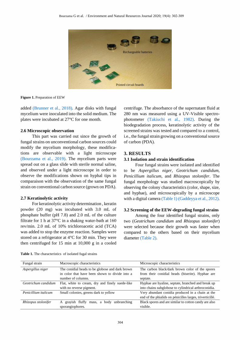
Bourzama G et al. / Environment and Natural Resources Journal 2020; 19(4): 302-309
Figure 1. Preparation of EEW
added (Brunner et al., 2018). Agar disks with fungal
mycelium were inoculated into the solid medium. The
plates were incubated at 27°C for one month.
2.6 Microscopic observation
This part was carried out since the growth of
fungal strains on unconventional carbon sources could
modify the mycelium morphology, these modifica-
tions are observable with a light microscope
(Bourzama et al., 2019). The mycelium parts were
spread out on a glass slide with sterile normal saline,
and observed under a light microscope in order to
observe the modifications shown on hyphal tips in
comparaison with the observation of the same fungal
strain on conventional carbon source (grown on PDA).
2.7 Keratinolytic activity
For keratinolytic activity determination , keratin
powder (20 mg) was incubated with 3.0 mL of
phosphate buffer (pH 7.8) and 2.0 mL of the culture
filtrate for 1 h at 37°C in a shaking water‐bath at 160
rev/min. 2.0 mL of 10% trichloroacetic acid (TCA)
was added to stop the enzyme reaction. Samples were
stored on a refrigerator at 4°C for 30 min. They were
then centrifuged for 15 min at 10,000 g in a cooled
centrifuge. The absorbance of the supernatant fluid at
280 nm was measured using a UV-Visible spectro-
photometer (Takiuchi et al., 1982). During the
biodegradation process, keratinolytic activity of the
screened strains was tested and compared to a control,
i.e., the fungal strain growing on a conventional source
of carbon (PDA).
3. RESULTS
3.1 Isolation and strain identification
Four fungal strains were isolated and identified
to be Aspergillus niger, Geotrichum candidum,
Penicillium italicum, and Rhizopus stolonifer. The
fungal morphology was studied macroscopically by
observing the colony characteristics (color, shape, size,
and hyphae), and microscopically by a microscope
with a digital camera (Table 1) (Gaddeyya et al., 2012).
3.2 Screening of the EEW-degrading fungal strains
Among the four identified fungal strains, only
two (Geotrichum candidum and Rhizopus stolonifer)
were selected because their growth was faster when
compared to the others based on their mycelium
diameter (Table 2).
Table 1. The characteristics of isolated fugal strains
Fungal strain Macroscopic characteristics Microscopic characteristics
Aspergillus niger The conidial heads to be globose and dark brown
in color that have been shown to divide into a
number of columns.
The carbon black/dark brown color of the spores
from their conidial heads (biserite). Hyphae are
septate.
Geotrichum candidum Flat, white to cream, dry and finely suede-like
with no reverse pigment.
Hyphae are hyaline, septate, branched and break up
into chains subglobose to cylindrical arthroconidia.
Penicillium italicum Small colonies, greens dark to yellow Very abundant conidia produced in a chain at the
end of the phialids on pénicilles larges, triverticillé.
Rhizopus stolonifer A grayish fluffy mass, a body unbranching
sporangiophores.
Black spores and are similar to cotton candy are also
visible.
Rechargeable batteries
Printed circuit boards
304
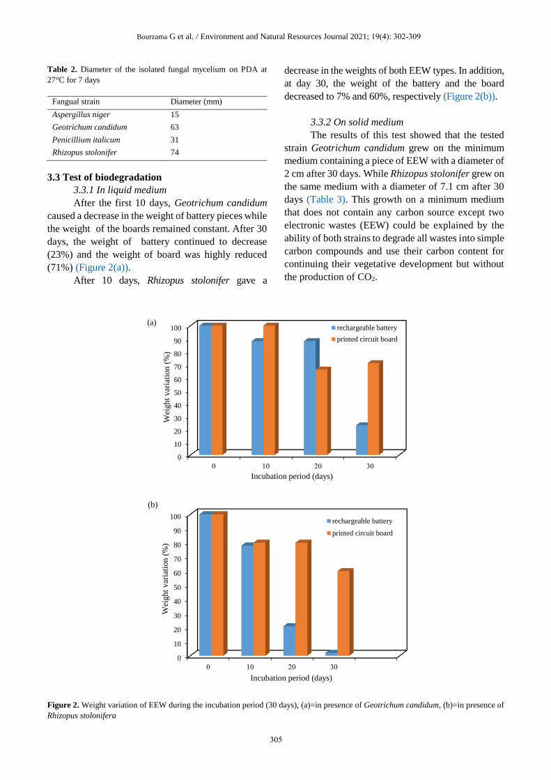
Bourzama G et al. / Environment and Natural Resources Journal 2021; 19(4): 302-309
Table 2. Diameter of the isolated fungal mycelium on PDA at
27°C for 7 days
Fangual strain Diameter (mm)
Aspergillus niger 15
Geotrichum candidum 63
Penicillium italicum 31
Rhizopus stolonifer 74
3.3 Test of biodegradation
3.3.1 In liquid medium
After the first 10 days, Geotrichum candidum
caused a decrease in the weight of battery pieces while
the weight of the boards remained constant. After 30
days, the weight of battery continued to decrease
(23%) and the weight of board was highly reduced
(71%) (Figure 2(a)).
After 10 days, Rhizopus stolonifer gave a
decrease in the weights of both EEW types. In addition,
at day 30, the weight of the battery and the board
decreased to 7% and 60%, respectively (Figure 2(b)).
3.3.2 On solid medium
The results of this test showed that the tested
strain Geotrichum candidum grew on the minimum
medium containing a piece of EEW with a diameter of
2 cm after 30 days. While Rhizopus stolonifer grew on
the same medium with a diameter of 7.1 cm after 30
days (Table 3). This growth on a minimum medium
that does not contain any carbon source except two
electronic wastes (EEW) could be explained by the
ability of both strains to degrade all wastes into simple
carbon compounds and use their carbon content for
continuing their vegetative development but without
the production of CO2.
Figure 2. Weight variation of EEW during the incubation period (30 days), (a)=in presence of Geotrichum candidum, (b)=in presence of
Rhizopus stolonifera
0
10
20
30
40
50
60
70
80
90
100
0 10 20 30
Incubation period (days)
rechargeable battery
printed circuit board
0
10
20
30
40
50
60
70
80
90
100
0 10 20 30
rechargeable battery
printed circuit board
Incubation period (days)
Wei
gh
t v
aria
tion
(%
) W
eig
ht
var
iati
on
(%
)
(a)
(b)
305

Bourzama G et al. / Environment and Natural Resources Journal 2020; 19(4): 302-309
Table 3. Growth of Geotrichum candidum and Rhizopus stolonifer
on a minimum solid medium with the parts of EEW after 30 days
Fungal strain Diameter with
rechargeable
batteries (mm)
Diameter with
printed circuit
boards (mm)
Geotrichum candidum 20 19
Rhizopus stolonifer 68 71
3.4 Micrscopic observation
The following Figure 3(a) showed that there is
no difference in microscopic observation between the
fungal strain Geotrichum candidum after 30 days
incubation on a minimum medium, and that on the
conventional carbon source (PDA). While in Rhizopus
stolonifer with EEW parts, sporocyst formation was
observed at the tip which gives the black color which
is darker than the normal and bursts to release a higher
number of spores, also the formation of spherical
vesicles (Figure 3(a) and (b)) compared to the control
on a conventional carbon source (on PDA) was noticed.
3.5 Keratinolytic activity
As shown in Figure 4(a), the highest values of
enzyme secretion were obtained after 10 days of
incubation and it decreased following the same pattern
of the control. This may be explained by the presence
of a relation between this enzyme secretion and the
biodegradation process.
The same note was observed with Rhizopus
stolonifer (Figure 4(b)) but after 20 days, keratinolytic
activity was not detected. This means that there no
relation between this enzyme and EEW
biodegradation.
Figure 3. Microscopic observation of the screened strains, (a) Geotrichum candidum, (b) Rhizopus stolonifer after 30 days of incubation
on a basal medium solid with EEW (60X).
Figure 4. Relation between the keratinolytic activity (U/mg) and the degradation of EEW during the incubation period (days) in
comparison with the control grown on a conventional source of carbon (PDA) for each screened strain, (a)=Geotrichum candidum,
(b)=Rhizopus stolonifer.
8
6
0
5
10
15
20
25
30
0 10 20 30
strain on the basal medium
control on PDA
(a)
sporocyst
formation
(b)
Ker
atin
oly
tic
acti
vit
y (
U/m
g)
Incubation period (days)
(a)
306

Bourzama G et al. / Environment and Natural Resources Journal 2021; 19(4): 302-309
Figure 4. Relation between the keratinolytic activity (U/mg) and the degradation of EEW during the incubation period (days) in
comparison with the control grown on a conventional source of carbon (PDA) for each screened strain, (a)=Geotrichum candidum,
(b)=Rhizopus stolonifera. (cont.)
4. DISCUSSION
Recent chemical research aiming to recycle
some components of EEW have been carried out to
eliminate these dangerous wastes (Mozos et al., 2020).
Thus, the aim of the current study is to safely remove
some types of EEW using microrganisms. Tomer et al.
(2020) exposed several mecanisms for biodegradation
in fungi. Microrganisms achieve this process direcly
by the cells or indirectly by the extracellular enzymes
(Muthu, 2014). Fungi have a large exo-enzymatic
arsenal capable of degrading organic macromolecules
that are unable to bio-assimilate due to their high
molecular weight (Internship report IUT, 2013), like
in Geotrichum candidum in our study. Many fungi
excrete enzymes into the environment and can be used
as producers of keratinolytic enzymes. A specific class
of proteolytic enzymes includes the keratinases which
catalyse the hydrolysis of keratins. The microorga-
nisms responsible for biodegradation are different
from each other and they have their own optimal
growth conditions. The biodegradation is generally
considered to be enzyme-catalyzed hydrolysis and
non-enzymatic hydrolysis (Wackett and Hershberger,
2001).
EEW are rich mainly in metals and heavy
metals: Cu, Fe, Cd, Cr, Pb, etc., and with lower rate,
plastic substances (Huang et al., 2009; Sodhi and
Reimer, 2001; Sum, 1991). In our study, we used
printed circuit boards (PCBs) which are flat bases
generally made of phenolic resin reinforced with glass
fibre that functions as an electrical insulator. These
boards are made up mainly of metallic and non-
metallic parts and organic compounds (Szałatkiewicz
et al., 2014). The metallic parts include 13% Cu, 5%
Fe, and 2% Al (Hall and Williams, 2007).
Rechargeable lithium-ion batteries have also been
used, consisting of lithium, Mn, Ni, Cd, Zn, and Cu.
This leads us to the fact that Geotrichum candidum and
Rhizopus stolonifer are also able to absorb/adsorb
heavy metals from rechargeable batteries.
However, only few studies have been carried on
the use of fungi in the biodegradation of EEW. Some
studies focused on the biodegradation of EEW by two
species of fungi, Aspergillus niger and Penicillium sp.
to extract lithium and cobalt from spent batteries by
the production of organic acids (oxalic acid and citric
acid). These acids have the effect of leaching and
extracting up to 85% of lithium and 48% of cobalt
from the cathodes of the batteries (Cunningham and
Harwood, 2016). Similarly, Navaneethakrishnan et al.
(2020) used fungi, namely, Ustilago trichophora and
Aspergillus niger, for recycling lithium ion batteries.
The acids change the status of several metals such as
copper in EEW (Brandl et al., 2001). Citric acid
produced by A. niger is the main leaching agent for
PCB heavy metals (Aung and Ting, 2005). Because of
the lack of reports on other species of fungi, we have
chosen to extrapolate our study on other species which
are Rhizopus sp. and Geotrichum sp.
The fungi are non-chlorophyllous, therefore
they are incapable of performing photosynthesis. They
need to find their carbon in organic compounds. In
spite of the use of a minimum medium that is free of
organic matter for biodegrading EEW with our fungal
0
0.5
1
1.5
2
2.5
3
3.5
0 10 20 30
strain on the basal medium
control on PDA
Ker
atin
oly
tic
acti
vit
y (
U/m
g)
Incubation period (days)
(b)
307

Bourzama G et al. / Environment and Natural Resources Journal 2020; 19(4): 302-309
strains, they were still alive. This suggests that they
have used some of the components of the EEW as a
source of carbon.
The growth of the fungal strains supplemented
with the EEW was very fast because the tested fungi
already contained the biodegradation enzymes, as they
were isolated from a soil rich with these class of wastes.
Rhizopus sp. produces several organic acids (De
Reu et al., 1995). However, in PCB biodegradation,
the produced acids facilitate the eliminantion of the
metallic components of PCBs via solubilization (Dave
et al., 2018). The acids induce leaching of metals from
PCB wastes through acidolysis and complexolysis
mechanisms (Ceci et al., 2015). After extensive
research, only a few studies were found on the ability
of Geotrichum candidum to biodegrade the EEW.
Therefore, the current study will be a first step in this
field. This work is only a preliminary step and further
studies are intended regarding the application of these
fungal strains in EEW removal and the role of
keratinolytic enzymes in the biodegradation process as
well as to understand the nature of sporocyst formation
in Rhizopus stolonifer. This application can be by
insertion of nonspecific extracellular enzymes such as
keratinolytic enzymes directly in the natural
environments for providing degradation of EEW, or
by formation of fungal biofilm mainly in the aquatic
media.
5. CONCLUSION
The results of this research are very
encouraging, considering that the isolated fungal
strains Geotrichum candidum and Rhizopus stolonifer
showed a significant capacity to biodegrade EEW,
which was more remarkable with Geotrichum
candidum. This study also affirmed a role of the
keratinolytic enzymes in Geotrichum candidum and
sporocyst formation in Rhizopus stolonifer during the
biodegradation process of electronic wastes.
ACKNOWLEDGEMENTS
This study was funded by Department of
Biochemistry, Faculty of Sciences, University of
Annaba, Badji Mokhtar. The authors would like to
thank the head of the Department of Biochemistry;
Branes Zidane for all facilities provided.
REFERENCES Aung KMM, Ting YP. Bioleaching of spent fluid catalytic
cracking catalyst using Aspergillus niger. Journal of
Biotechnology 2005;116(2):159-70.
Botton B, Breton A, Fevre M, Gauthier S, Guy P, Larpent JP.
Useful and Harmful Mold: Importance Industrial (Moisissure
Utiles et Nuisibles: Importance industrielle). Paris, France:
Elsevier Masson; 1990. p. 11-190.
Bourzama G, Ennaghra N, Soumati B, Benoune S, Atriche N.
Effect of zinc metal at high concenetration on secondary
metabolic pathways in Penicillium chrysogenum strain.
Journal of Microbiology, Biotechnology and Food Sciences
2019;9(2):307-13.
Brandl H, Bosshard R, Wegmann M. Computer-munching
microbes: Metal leaching from electronic scrap by bacteria and
fungi. Hydrometallurgy 2001;59:319-26.
Brunner I, Fischer M, Ruthi J, Stierli B, Frey B. Ability of fungi
isolated from plastic debris floating in the shoreline of a lake
to degrade plastics. PLOS ONE 2018;13(8):e0202047.
Ceci A, Kierans M, Hillier S, Persiani AM, Gadd GM. Fungal
bioweathering of mimetite and a general geomycological
model for lead apatite mineral biotransformations. Applied
and Environmental Microbiology 2015;81:4955-64.
Clark EM, White JF, Patterson RM. Improved histochemical
techniques for the detection of Acremonium coenophialum in
tall fescue and methods of in vitro culture of the fungus.
Journal of Microbiology Methods 1983;1:149-55.
Cui J, Zhang L. Metallurgical recovery of metals from electronic
waste: A review. Journal of Hazardous Materials 2008;58:
228-56.
Cunningham JA, Harwood V. Fungi recycle rechargeable lithium-
ion batteries. American Chemical Society [Internet]. 2016
[cited 2020 Aug 21]. Available from: https://
www.sciencedaily.com/releases/2016/08/160821093037.htm.
Dave SR, Sodha AB, Tipre DR. Microbial technology for metal
recovery from e-waste printed circuit boards. Journal of
Bacteriology and Mycology 2018;6(4):241-7.
De Reu JC, Rombouts FM, Nout MJR. Influence of acidity and
initial substrate temperature on germination of Rhizopus
oligosporus sporangiospores in tempe fermentation. Journal of
Applied Bacteriolology 1995;78:200-8.
Gaddeyya G, Niharika PS, Bharathi P, Kumar PKR. Isolation and
identification of soil mycoflora in different crop fields at Salur
Mandal. Advances in Applied Science Research 2012;3:2020-6.
Gavilán-García A, Román-Moguel A, Almada-Calvo F, Aburto-
Mejía S. Electronic waste generation and technology for an
appropriate management in México. Boletín de la Sociedad
Química de México 2009;3(2):85-92.
Hall WJ, Williams PT. Processing waste printed circuit boards for
material recovery. Circuit World 2007;33:43-50.
Huang K, Guo J, Xu Z. Recycling of waste printed circuit boards:
A review of current technologies and treatment status in China.
Journal of Hazardous Materials 2009;164:399-408.
Kubicek CP, Mikus M, Schuster A, Schmoll M, Seiboth B.
Metabolic engineering strategies for the improvement of
cellulose production by Hypocrea jecorina. Biotechnology
Biofuels 2009;2:19.
Mozos EA, Bilbao AR, Díaz-Martín F. WEEE Recycling and
circular economy assisted by collaborative robots. Applied
Science 2020;10(14):4800.
Muthu SS. Roadmapto Sustainable Textiles and Clothing:
Environmental and Social Aspects of Textiles and Clothing
Supply Chain. New York, USA: Springer Singapore; 2014.
Nakajima-Kambe T, Shigeno-Akutsu Y, Nomura N, Onuma F,
Nakahara T. Microbial degradation of polyurethane, polyester
308

Bourzama G et al. / Environment and Natural Resources Journal 2021; 19(4): 302-309
polyurethanes and polyether polyurethanes. Applied
Microbiology and Biotechnology 1999;51(2):134-40.
Navaneethakrishnan V, Pavithra K, Vanitha V. Recycling of
lithium ion batteries using fungi based organic acids.
Materials Science and Engineering 2020;872:12-3.
Internship report IUT. Nîmes on Study of the biodegradation of
biodegradable polymers (Etude de la biodégradation de
polymères biodégradables). Paris, France: Ecole des Mines
d’Alès; 2013.
Pochon J, Tardieux P. Soil microbiology analysis technique
(Technique d’analyse en microbiologie du sol). Edition of
Tourtourelle. France: Saint-Mandé; 1962.
Schaffner DW, Toledo RT. Cellulase production by Trichoderma
reesei when cultured on xylose-based media supplemented
with sorbose. Biotechnology and Bioengineering 1991;37:12-6.
Sodhi MS, Reimer B. Models for recycling electronics end-of-life
products. OR Spektrum 2001;23:97-115.
Sum E. The recovery of metals from electronic scrap. Journal of
Metallurgy 1991;43:53-61.
Szałatkiewicz J, Szewczyk R, Budny E, Missala T, Winiarski W.
Measurement and control system of the Plasmatron Plasma
reactor for recovery of metals from printed circuit board waste.
Advanced Intelligent 2014;267:687-95.
Takiuchi I, Higuchi D, Sei Y, Koga M. Isolation of an extracellular
proteinase (keratinase) from Microsporum canis. Sabouraudia
1982;20:281-8.
Tomer A, Singh R, Singh SK, Dwivedi SA, Reddy CU, Keloth
MRA, et al. Role of Fungi in Bioremediation and
Environmental Sustainability. Switzerland: Springer Nature;
2020. p.1-20.
Wackett LP, Hershberger CD. Biocatalysis and Biodegradation:
the Microbial Transformation of Organic Compounds.
Washington, USA: ASM Press; 2001.
Weidenhamer JD, Clement ML. Leaded electronic waste is a
possible source material for lead-contaminated jewelry.
Chemosphere 2007;7:1111-5.
309
Environment and Natural Resources Journal 2021; 19(4): 310-319
Environmental and Microbial Influences on Corrosion of Selected
Types of Petroleum Industry Steel
Anwuli U. Osadebe*, Dorcas C. Olorondu, and Gideon C. Okpokwasili
Department of Microbiology, Faculty of Science, University of Port Harcourt, P.M.B. 5323, Choba, Nigeria
ARTICLE INFO ABSTRACT
Received: 22 Jan 2021
Received in revised: 13 Apr 2021
Accepted: 23 Apr 2021
Published online: 1 Jun 2021DOI: 10.32526/ennrj/19/2021004
This study explored the influence of brackish water sediment, mangrove swamp
sediment, clayey/lateritic soil, and river water (freshwater) sediment on the
corrosion rates of carbon, mild, and stainless steels and the species of sulphate
reducing bacteria (SRB) and iron bacteria associated with the process. The
material loss following burial of the steel samples for a 9-month period was
assessed. Standard and specialised microbiological techniques were employed
in the characterisation of the bacterial species. Qualitative assessment for
corrosion was done via optical microscopy and macroscopy. Corrosion was
highest on steel buried in brackish water sediment and lowest in that from river
water sediment. Carbon steel was the most susceptible to corrosion while
stainless steel was the most resistant. Sulphite, sulphide, nitrate and phosphate
concentrations had a strong impact on corrosion rates. Thiobacillus, Leptothrix
and Gallionella dominated amongst the iron bacteria while Desulfobacter and
Desulfovibrio dominated amongst the SRB. There were significant differences
in corrosion rates and bacterial abundance from one environment to the other.
Iron bacteria showed greater abundance than SRB across the different
environments and steel types. Iron bacteria counts, however, did not correlate
positively with corrosion rates. The findings suggest that oil industry facilities
in brackish water environments are more liable to corrosion than those located
in fresh water ecosystems.
Keywords:
Corrosion/ Environment/ Iron
bacteria/ Steel/ Sulphate reducing
bacteria/ Petroleum industry
* Corresponding author:
E-mail: [email protected]
1. INTRODUCTION
Corrosion is a naturally occurring electro-
chemical process driven by physical, chemical or
biological processes working in synergy.
Environmental stimuli around the metal are the most
common triggers of physicochemical corrosion.
Properties like characteristics of the metal, chloride
and SO2 deposition rates, temperature, humidity, pH,
salinity and length of exposure are key initiators of
physical and chemical corrosion in steel installations
(Yan et al., 2020). Biological corrosion, more
commonly tagged microbially influenced corrosion
(MIC), is the irreversible deterioration of metal by the
activities of microorganisms. It is also termed
biocorrosion. MIC results from the combined action of
microbial cells, their cellular metabolites, the metal
surface and environmental factors (Maluckov, 2012).
Groups of microorganisms will often adhere to
surfaces via biofilms; MIC then ensues beneath these
biofilms via mechanisms like direct electron transfer,
cathodic depolarization, build-up of a concentration
gradient or galvanic cell formation (Akpan and
Iliyasu, 2015; Da Silva et al., 2019). Microbial
involvement has been reported to speed up corrosion
rates by up to ten times (Liu and Cheng, 2018).
Steel is the material of choice for oil and gas and
marine installations. It is used for the construction of
platforms and transportation infrastructure for the
conveyance of petroleum and water amongst other
uses. Most pipelines are constructed with carbon steel.
Although highly prone to corrosion and attack by
microbes, carbon steel is preferred as it succumbs
easily to welding, endures bending well and is less
liable to cracking under stress. Furthermore, it is
considered durable and of relatively low cost. Mild
steel and stainless steel, though not as popular as
carbon steel, are also used. Stainless steel is
considered expensive and less malleable. The
Citation: Osadebe AU, Olorondu DC, Okpokwasili GC. Environmental and microbial influences on corrosion of selected types of petroleum
industry steel. Environ. Nat. Resour. J. 2021;19(4):310-319. (https://doi.org/ 10.32526/ennrj/19/2021004)
310

Osadebe AU et al. / Environment and Natural Resources Journal 2021; 19(4): 310-319
susceptibility of steel to corrosion is a chief concern in
oil and gas plants as the maintenance of failed
pipelines and fittings is often not only expensive but
challenging. This is especially true of sub-surface
instalments. Mechanical failure with regards to
pipelines is usually corrosion-related in form of
rupture from loss of wall thickness or fracturing (Hou
et al., 2016; Valencia-Cantero and Peña-Cabriales,
2014). Corrosion of carbon steel was reported to be
about 6 times greater when SRB are involved with
the corrosion pit depth 7.7 times deeper than without
SRB (Liu et al., 2019).
Research establishes a 4% and 20% reduction in
national Gross Domestic Product (GDP) in developing
and developed countries respectively due to corrosion
in industry (Kruger, 2011; Hou et al., 2017; Fayomi et
al., 2019). Arena-Ortiz et al. (2019) place the global
corrosion cost including management measures at $4
trillion. In 2011, corrosion accounted for $13.4 billion
in annual expenses in the US petroleum industry with
biocorrosion consuming $2 billion of the sum
(Bermont-Bouis et al., 2007). Corrosion has been
implicated in most cases of pipeline failure in the Gulf
of Mexico (Arena-Ortiz et al., 2019). In the global oil
and gas sector it is estimated that for 50% of buried
installations and about 40% of internal pipelines, MIC
accounts for the observed corrosion. For anaerobic
environments, the total value for both is lower at about
20% (Bano and Qazi, 2011; Rasheed et al., 2019).
Sulphate Reducing Bacteria (SRB), Sulphate
Oxidising Bacteria (SOB), Iron Oxidising Bacteria
(IOB), Iron Reducing Bacteria (IRB), manganese-
oxidisers and acid-producing bacteria are the main
microbial groups involved in MIC (Beech and
Gaylarde, 1999; Bano and Qazi, 2011; Akpan and
Iliyasu, 2015). Khouzani et al. (2019) opine that SRB
are the main culprits in severe biodeterioration and
rupture of buried pipelines. SRB are anaerobic and so
where oxygen is present, they tend to occur underneath
deposits of soil, sediment or rust on the pipeline or
even beneath an already formed biofilm creating the
oxygen-deficient microenvironment they require (Liu
et al., 2019). Iron bacteria are a group of aerobic
bacteria that generate energy by oxidation of ferrous
ions as a key part of their metabolism (Bryce et al.,
2018). They are the main culprits of rust deposits on
metals and are known to cause corrosion by creating
an oxygen gradient which splits the metal surface to
which the biofilm is attached into small anodic sites
surrounded by larger cathodic areas. They are more
commonly associated with the crevice type of
corrosion (Beimeng et al., 2015). SRB and iron
bacteria often co-exist on buried metal infrastructure
and tend to exert a more aggressive corrosive effect as
a team than as individual colonisers of the metal
surface (Valencia-Cantero and Peña-Cabriales, 2014).
An understanding of the varying influences on
the rate of corrosion of steel is essential to predicting
its longevity and suitability for purpose. In this study,
corrosion of three types of steel used in the petroleum
industry was analysed using microscopic assessment
and weight loss to establish corrosion rates relative to
environmental conditions. Furthermore, the species of
autochthonous SRB and iron bacteria associated with
the observed corrosion were determined.
2. METHODOLOGY
2.1 Sample sites
The sediment/ soil for this study were mangrove
swamp sediment, brackish water sediment, fresh
(river) water sediment and clayey/lateritic soil. All the
mangrove swamp and brackish water sediment
samples were collected from Eagle Island in Nkpolu
area of Port Harcourt, Rivers State. The freshwater
sediment samples were obtained from the New
Calabar River, Choba, Nigeria. The sampling site for
the ochre-coloured clayey/lateritic soil was the
Postgraduate Hall of Abuja campus, University of Port
Harcourt.
2.2 Study design
The study was field based. The steel samples
were placed in fabricated wide-mesh plastic baskets
before being buried to a depth of 1 m, similar to the
minimum depth for pipelines, for a period of 9 months.
The baskets were for ease of location and retrieval
while allowing the bars to be in complete contact with
the environment on all sides. Sediment or soil samples
from the area around the metal bars were taken before
and during retrieval for physicochemical and
microbiological analysis. Sampling was done in
triplicates.
2.3 Sample collection
2.3.1 Steel samples
Three types of structural grade customised steel
bars were used to monitor the rate of corrosion in the
environment-carbon steel ASTM A36, mild steel
ASTM A283 and stainless steel ASTM A316L. The
samples were supplied by Sirpi AluSteel Construction
311

Osadebe AU et al. / Environment and Natural Resources Journal 2021; 19(4): 310-319
Ltd., Trans-Amadi Industrial layout, Port Harcourt,
Nigeria. The bars measured 80 mm × 25 mm × 6 mm.
The minimum recommended pipeline thickness is
6.35 mm (0.25 in). The mechanical properties of the
steel bars used are described in Table 1.
Table 1. Mechanical Properties of the Metal Samples
Sample CS ASTM A36 MS ASTM A283 SS ASTM A316L
Type Structural quality carbon Structural quality carbon Austenite
Condition of steel AS Rolled AS Rolled Annealed
Tensile strength (KSI) 58-80 55-60 75 minimum
Yield strength (KSI) 36 minimum 30 minimum 30
% Elongation in “2” 23 25 60 minimum
% Elongation in “8” 20 22 65
Approx. Brinell hardness 137 133 180
Carbon content (%) 0.26-0.29 0.24 0.03
CS=Carbon steel; MS=Mild steel; SS=Stainless steel
The steel bars of known weight were first
degreased using analytical grade acetone and then
rinsed with distilled water. This was followed by
sterilisation by immersion in ethanol for 30 sec. They
were then dried and kept desiccated (Rasheed et al.,
2019). The final weights of the steel bars in the
desiccator were determined prior to burial.
2.3.2 Soil/sediment sample collection
Samples of soil and sediment were collected for
analyses prior to burial of the steel bars and after their
retrieval. The soil samples were collected for analyses
using a hand trowel and put in heat resistant plastic
bottles. Sediment samples were obtained using a
sediment grab. Water samples were collected using a
1 L clean plastic container. All the samples were
appropriately labelled with date, time and place of
collection.
2.4 Determination of physicochemical parameters
The physicochemical parameters were
measured in the environments before burial and at
retrieval. Salinity was determined using a digital
salinometer (Hanna Instruments), while for pH, a pH
meter (Wintab digital pH meter, Germany) was used.
The sulphate (SO42-), sulphite (SO3
2-) and sulphide
(S2-) concentrations were determined using the method
of Fogg and Wilkinson (1952). The ferric ion (Fe3+)
concentration was measured using the ferrozine assay.
Electrical conductivity was determined using a
benchtop combination meter. The nitrite (NO2-) and
nitrate ion (NO3-) content was measured using the
spectrophotometric method described by Narayana
and Sunil (2009). The combined modified methods of
spectroscopy and molybdenum blue phosphorus
method of Kharat and Pagar (2019) was used for
analysis of phosphate ion (PO43-) content.
2.5 Determination of loss in material and corrosion
analysis
The outer debris on the steel bars was carefully
rinsed off with distilled water. Following removal of
any attached biological material via probe sonication
and drying in an oven (ThermoFisher Scientific
PR305225M, USA) at 70°C for 15 min, the
dimensions of the bars were determined using calipers
and a ruler. The weights of the steel bars were
measured as well using an analytical balance (Mettler
Toledo New Classic ML204T, Switzerland). The Area
was calculated. The volume of the bars was
determined using the modified water displacement
technique of Hargens et al. (2014).
Corrosion analysis was via the weight loss
technique. Assuming uniform corrosion over the
entire surface of the bars, the corrosion rate in
millimetre per year was determined using the formula
from Daille et al. (2020):
CR = KW
ATD
Where; CR=corrosion Rate, K is a constant
(8.76 × 10⁴), W=weight loss in grams, A=area in cm2,
T=time of exposure in hours, and D=density in g/cm3.
2.6 Qualitative analysis of steel bars
The cleaned corroded surfaces of the retrieved
bars were observed under the x400 magnification of
the optical microscope. Visible (non-microscopic)
changes were also recorded.
312

Osadebe AU et al. / Environment and Natural Resources Journal 2021; 19(4): 310-319
2.7 Enumeration and characterisation of micro-
organisms from biofilms
The biofilms formed on the retrieved metal
samples were scrapped off using sterile surgical blade.
Any possible remaining biological material was
extracted by sonification. The scrapings were
collected in sterile bottles containing about 5 mL
phosphate buffered saline at pH 7. Following four-
fold serial dilution, 1 mL aliquots were plated out on
specialised media in triplicates using the pour plate
technique. Discrete colonies were purified by
streaking unto fresh media. Pure cultures were
preserved on relevant media slants for further
investigation.
The iron bacteria medium described by APHA
(2012) at pH 5.0 was used for the isolation of iron
bacteria. Incubation was at room temperature for 7-14
days. Postgate B medium was used for the isolation of
the sulphate reducing bacteria, SRB. Inoculation was
done via the tube method. After inoculation, the tubes
were rapidly cooled with screw caps to seal the tubes
to prevent aeration and dehydration of the medium.
The cultures were incubated at room temperature in an
anaerobic jar containing Gas Pak for about 4 weeks
with regular observation for the black colonies
representative of sulphate reducing bacteria (SRB).
The abundance of the SRB and iron bacteria
isolates was determined in colony forming units per
gram (CFU/g) using an automated colony counter.
Identification of the isolates was on the basis of
cell morphology and cultural and biochemical
characteristics. Apart from the microscopic
observation of the cells and observation of colony
characteristics, several standard biochemical tests
were employed in the characterisation of the isolates;
some of the tests include Gram’s staining, urease
production, lysine utilisation, nitrate reduction,
hydrogen sulphide production, citrate utilisation,
motility, methyl red, Voges Proskauer reaction,
ornithine utilisation, gelatine liquefaction, triple
sugar iron test, phenylamine deamination, indole
production, starch utilisation, catalase reaction,
oxidase production, ONPG and utilisation of 10
simple and complex sugars.
2.8 Statistical analysis
The relationship between corrosion rates and
SRB and iron bacteria counts and physicochemical
parameters from one environment to the other was
assessed using Microsoft Excel 2016.
3. RESULTS AND DISCUSSION
3.1 Physicochemical influences
The changes in the physicochemical properties
of the different environments studied before burial of
the bars and at retrieval are shown in Table 2.
Table 2. Observed variation physicochemical characteristics during the study
Parameters Brackish water sediment Mangrove swamp Clayey/lateritic soil River water sediment
At burial At retrievala At burial At retrievala At burial At retrievala At burial At retrievala
pH 7.65 7.10 3.72 6.88 6.27 6.84 6.14 6.05
Salinity (ppt) 15.303 13.000 13.100 10.327 0.011 0.010 0.002 0.001
Conductivity
(μS/m)
738 1011 1724 814 212 484 388 548
PO43- (mg/kg) 0.149 1.40 0.0002 0.05 0.0121 0.50 0.0086 0.70
NO3- (mg/kg) 1.00 93.60 1.10 112.20 1.20 835.70 1.40 54.90
S2- (mg/kg) 30.40 41.20 29.30 53.60 17.00 32.28 13.30 5.59
SO42- (mg/kg) 0.10 8.29 0.25 3.39 0.25 0.077 0.15 0.219
SO32- (mg/kg) 0.10 7.50 0.25 12.50 0.25 11.00 0.15 11.00
Fe3+ (mg/kg) 0.07 7.97 0.02 5.37 0.03 5.54 0.06 34.94
NO2- (mg/kg) 0.00 2.20 0.20 0.16 0.20 0.70 0.30 0.59
a=month 9-peak of wet season
A study on biocorrosion by SRB in the Yucatan
Peninsula concluded that physicochemical properties
have a strong influence on corrosion rates (Arena-
Ortiz et al., 2019). In the same vein, Obuekwe et al.
(1987) demonstrated extensive pitting of mild steel
when ferrous and sulphide ions were being formed
concurrently. When only sulphide was produced,
corrosion rates first increased and then declined due to
the formation of a protective iron sulphide (FeS) film.
Gubner and Andersson (2007) and Agarry et al. (2015)
both linked corrosion rates to pH levels. It has been
found that pH exerts a stronger impact on corrosion
313
Osadebe AU et al. / Environment and Natural Resources Journal 2021; 19(4): 310-319
rates than salinity or nitrate concentration with the
more acidic pH levels encouraging faster corrosion
rates. The observed pH in this current study generally
revolved around neutral except in the mangrove
swamp sediment where more acidic values were
originally observed.
3.2 Observed corrosion, corrosion rates, and
environmental influences
The steel samples from brackish water sediment
and Mangrove swamp sediment demonstrated the
greatest loss in material and the highest corrosion
rates. Stainless steel samples fared best having the
lowest material loss while carbon steel showed
relatively high material loss. Table 3 outlines the mean
percentage material loss in thickness, area, volume
and weight observed.
Table 4 highlights the physical changes
observed in the different steel samples following
retrieval while Figure 1 provides a comparison of
corrosion rates across the four environments studied.
Carbon steel showed the greatest corrosion rates
across the board followed by mild steel. Corrosion
rates ranged from 0.07214-0.76505 mm/year, 0.0668-
0.55143 mm/year, 0.00991-0.23851 mm/year and
0.00762-0.23038 mm/year for brackish water
sediment, mangrove swamp sediment, lateritic soil,
and river water sediment, respectively, from stainless
steel (lowest observed values) to carbon steel (highest
values).
Table 3. Mean percentage material loss in the steel samples
Sample % Loss in area % Loss in thickness % Loss in volume % Loss in weight
CS E1 5.63 6.86 12.10 2.66
CS E2 5.60 20.59 25.04 2.35
CS E3 1.15 6.13 7.20 1.32
CS E4 0.72 4.68 5.37 0.82
MS E1 1.71 1.12 2.81 1.41
MS E2 2.53 3.66 6.10 0.86
MS E3 0.58 2.84 3.40 0.48
MS E4 0.69 2.22 4.57 0.27
SS E1 0.39 0.004 0.78 0.41
SS E2 0.69 1.69 2.38 0.34
SS E3 1.80 0.00 0.00 0.05
SS E4 0.002 0.20 0.20 0.005
CS=Carbon steel; MS= Mild steel SS=Stainless steel
E1= Brackish water sediment E2=Mangrove swamp bottom sediment; E3=Clayey/lateritic soil; E4=River Water sediment
Table 4. Qualitative assessment of the retrieved steel bars
Sample Corrosion-related observations after retrieval
Carbon Steel ASTM A36
CS E1 Generalised corrosion (iron oxide). Very heavy pitting on most of the surfaces. Presence of crevices. Severe edge
corrosion. Presence of sulphide coatings
CS E2 Extensive corrosion. Crevice corrosion and surface corrosion. Deposition of iron oxide as well as sulphide coatings.
Pitting significantly present.
CS E3 Generalised surface corrosion. Sulphide coating on one side of the slab surface. Scanty blister formations. Localised
deep pitting on one side of the slab surface. Scaling effect along the edges.
CS E4 Generalised surface corrosion with deposition of iron oxide. No pitting or sulphide coating seen. Scaling effect not too
severe.
Mild Steel ASTM A283
MS E1 Generalised corrosion (iron oxide). Deep pitting, sulphide coating, scaling along the edges.
MS E2 Extensive corrosion. Heavy pitting and skinning effects concentrated around the edges. Presence of sulphide cover.
MS E3 Generalised corrosion. Less pitting and skinning effect. Sulphide cover on one side of the slab. No crevices observed
MS E4 Generalised corrosion, no pitting or skinning
CS=Carbon steel; MS= Mild steel SS=Stainless steel
E1= Brackish water sediment E2=Mangrove swamp bottom sediment; E3=Clayey/lateritic soil; E4=River Water sediment
314

Osadebe AU et al. / Environment and Natural Resources Journal 2021; 19(4): 310-319
Table 4. Qualitative assessment of the retrieved steel bars
Sample Corrosion-related observations after retrieval
Stainless Steel ASTM A316L
SS E1 Only slight corrosion observed on both surfaces of the slab, localised pitting observed.
SS E2 Localised pitting and blackening on both surfaces of the slab and along edges. Concentrated deposition of iron oxide
along the edges where blackening was observed.
SS E3 Localised fine pitting on a small area of only one surface
SS E4 Two separate pitting portions with formation of iron oxide on only one surface. Fine localised pitting observed.
CS=Carbon steel; MS= Mild steel SS=Stainless steel
E1= Brackish water sediment E2=Mangrove swamp bottom sediment; E3=Clayey/lateritic soil; E4=River Water sediment
Figure 1. Mean corrosion rates of the different steel types
Pure iron is innately reactive and so naturally
corrodes quite rapidly. The addition of carbon makes
iron more stable; this stability is informed by both the
concentrations of incorporated carbon and the
presence of other alloying elements. The greatest
mean material loss and highest corrosion rate was seen
with the carbon steel bars most likely because it is the
steel with the highest percentage of incorporated
carbon (0.26-0.29%) in the absence of other alloying
metals. The mild steel bars (0.24% carbon) from the
results come next in mean material loss and corrosion
rates. Stainless steel (0.03% carbon) demonstrated a
stronger resistance to MIC than the other steel types
having the lowest mean material loss and corrosion
rate. Apart from its low carbon content, this resistance
could be further attributed to the presence of certain
alloying elements like chromium and nickel. Its
chromium content (10.5-11.0%) particularly, results
in the formation of an oxidation-inhibiting chromium
oxide layer in oxygenated systems.
Average percentage weight loss (APWL) values
under microbial influence, in one study, were found to
be 2.8% and 5.4% for MS in sandy soil and water-
logged soil, respectively, and 3.6% and 4.5% for CS
in sandy soil and water- logged soil, respectively. For
the SS, APWL was 0.12% and 0.08% for the water-
logged soil and the sandy soil, respectively (Oparaodu
and Okpokwasili, 2014). While this corroborates the
finding in this study that MIC proceeds at faster rates
in anaerobic or low oxygen environments, the APWL
values in the present study are lower than those
recorded.
The higher corrosion rates observed in the
mangrove swamp and brackish water sediment
corresponds with conclusions from a study on the
biocorrosion of stainless steel in varying tidal cycles
in a coastal region that high salinity tends to be
associated with increased corrosion rates (Daille et al.,
2020). Several studies report similar microorganism-
induced corrosion rates as recorded in the current
study. An assessment of microbial biofilms on carbon
steel found comparable corrosion rates of 0.45±0.01-
0.12±0.01 mm/year dependent on environmental
conditions (De Melo et al., 2011). Pratikno and Titah
(2016) observed corrosion rates of 0.5797-0.6173
mm/year in steel during a ten-day study in saline and
0
0.1
0.2
0.3
0.4
0.5
0.6
0.7
0.8
0.9
Carbon Steel ASTM A36 Stainless Steel ASTM A316L Mild Steel ASTM A283
Mea
n C
orr
osi
on
Rat
e (m
m/y
ear)
Brackish Water Sediment
Mangrove Swamp Bottom Sediment
Clayey/ Lateritic Soil
River Water Sediment
315
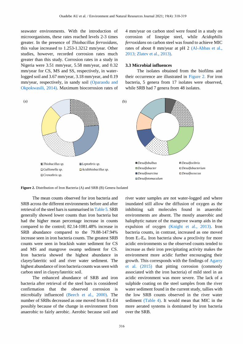
Osadebe AU et al. / Environment and Natural Resources Journal 2021; 19(4): 310-319
seawater environments. With the introduction of
microorganisms, these rates reached levels 2-3 times
greater. In the presence of Thiobacillus ferroxidans,
this value increased to 1.253-1.3212 mm/year. Other
studies, however, recorded corrosion rates much
greater than this study. Corrosion rates in a study in
Nigeria were 3.51 mm/year, 5.58 mm/year, and 0.32
mm/year for CS, MS and SS, respectively, in water-
logged soil and 3.67 mm/year, 3.18 mm/year, and 0.19
mm/year, respectively, in sandy soil (Oparaodu and
Okpokwasili, 2014). Maximum biocorrosion rates of
4 mm/year on carbon steel were found in a study on
corrosion of linepipe steel, while Acidophilis
ferroxidans on carbon steel was found to achieve MIC
rates of about 8 mm/year at pH 2 (Al-Abbas et al.,
2013; Zlatev et al., 2013).
3.3 Microbial influences
The isolates obtained from the biofilms and
their occurrence are illustrated in Figure 2. For iron
bacteria, 5 genera from 17 isolates were observed,
while SRB had 7 genera from 48 isolates.
Figure 2. Distribution of Iron Bacteria (A) and SRB (B) Genera Isolated
The mean counts observed for iron bacteria and
SRB across the different environments before and after
retrieval of the steel bars is summarised in Table 5. SRB
generally showed lower counts than iron bacteria but
had the higher mean percentage increase in counts
compared to the control; 82.14-1081.48% increase in
SRB abundance compared to the 79.88-147.94%
increase seen in iron bacteria counts. The greatest SRB
counts were seen in brackish water sediment for CS
and MS and mangrove swamp sediment for CS.
Iron bacteria showed the highest abundance in
clayey/lateritic soil and river water sediment. The
highest abundance of iron bacteria counts was seen with
carbon steel in clayey/lateritic soil.
The enhanced abundance of SRB and iron
bacteria after retrieval of the steel bars is considered
confirmation that the observed corrosion is
microbially influenced (Beech et al., 2000). The
number of SRBs decreased as one moved from E1-E4
possibly because of the change in environment from
anaerobic to fairly aerobic. Aerobic because soil and
river water samples are not water-logged and where
inundated still allow the diffusion of oxygen as the
inhibiting salt molecules found in anaerobic
environments are absent. The mostly anaerobic and
halophytic nature of the mangrove swamp aids in the
expulsion of oxygen (Knight et al., 2013). Iron
bacteria counts, in contrast, increased as one moved
from E1-E4. Iron bacteria show a proclivity for more
acidic environments so the observed counts tended to
increase as their iron precipitating activity makes the
environment more acidic further encouraging their
growth. This corresponds with the findings of Agarry
et al. (2015) that pitting corrosion (commonly
associated with the iron bacteria) of mild steel in an
acidic environment was more severe. The lack of a
sulphide coating on the steel samples from the river
water sediment found in the current study, tallies with
the low SRB counts observed in the river water
sediment (Table 4). It would mean that MIC in the
more aerated systems is dominated by iron bacteria
over the SRB.
Thiobacillus sp. Leptothrix sp.
Gallionella sp. Acidithiobacillus sp.
Crenothrix sp.
Desulfobulbus Desulfovibrio
Desulfobacter Desulfobacterium
Desulfosarcina Desulfococcus
Desulfotomaculum
(b) (a)
316
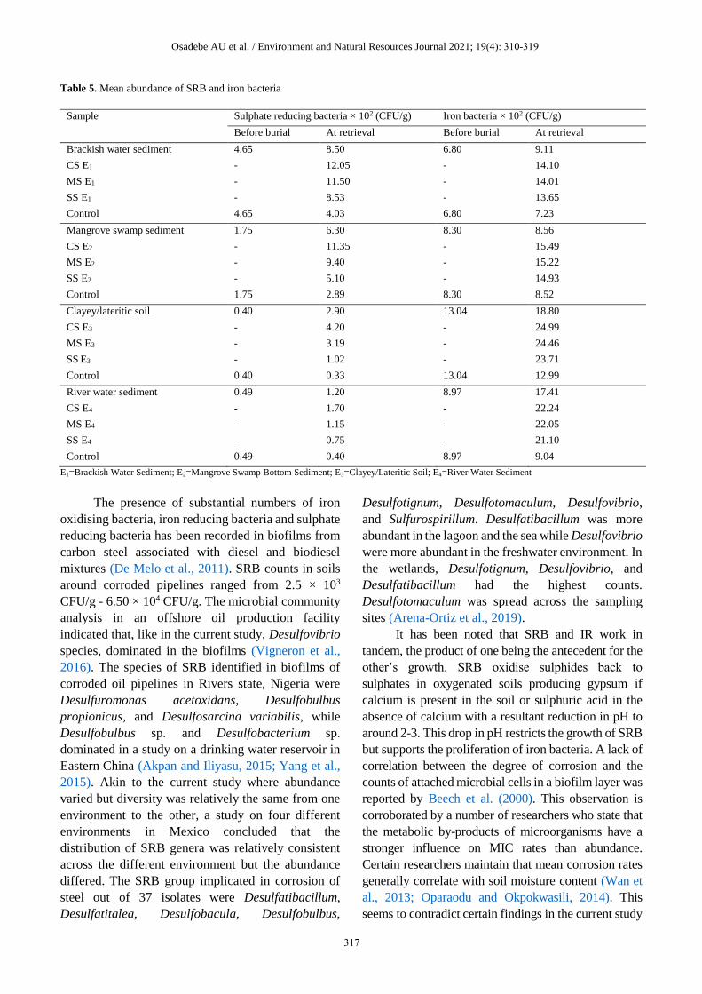
Osadebe AU et al. / Environment and Natural Resources Journal 2021; 19(4): 310-319
Table 5. Mean abundance of SRB and iron bacteria
Sample Sulphate reducing bacteria × 102 (CFU/g) Iron bacteria × 102 (CFU/g)
Before burial At retrieval Before burial At retrieval
Brackish water sediment 4.65 8.50 6.80 9.11
CS E1 - 12.05 - 14.10
MS E1 - 11.50 - 14.01
SS E1 - 8.53 - 13.65
Control 4.65 4.03 6.80 7.23
Mangrove swamp sediment 1.75 6.30 8.30 8.56
CS E2 - 11.35 - 15.49
MS E2 - 9.40 - 15.22
SS E2 - 5.10 - 14.93
Control 1.75 2.89 8.30 8.52
Clayey/lateritic soil 0.40 2.90 13.04 18.80
CS E3 - 4.20 - 24.99
MS E3 - 3.19 - 24.46
SS E3 - 1.02 - 23.71
Control 0.40 0.33 13.04 12.99
River water sediment 0.49 1.20 8.97 17.41
CS E4 - 1.70 - 22.24
MS E4 - 1.15 - 22.05
SS E4 - 0.75 - 21.10
Control 0.49 0.40 8.97 9.04
E1=Brackish Water Sediment; E2=Mangrove Swamp Bottom Sediment; E3=Clayey/Lateritic Soil; E4=River Water Sediment
The presence of substantial numbers of iron
oxidising bacteria, iron reducing bacteria and sulphate
reducing bacteria has been recorded in biofilms from
carbon steel associated with diesel and biodiesel
mixtures (De Melo et al., 2011). SRB counts in soils
around corroded pipelines ranged from 2.5 × 10³
CFU/g - 6.50 × 10⁴ CFU/g. The microbial community
analysis in an offshore oil production facility
indicated that, like in the current study, Desulfovibrio
species, dominated in the biofilms (Vigneron et al.,
2016). The species of SRB identified in biofilms of
corroded oil pipelines in Rivers state, Nigeria were
Desulfuromonas acetoxidans, Desulfobulbus
propionicus, and Desulfosarcina variabilis, while
Desulfobulbus sp. and Desulfobacterium sp.
dominated in a study on a drinking water reservoir in
Eastern China (Akpan and Iliyasu, 2015; Yang et al.,
2015). Akin to the current study where abundance
varied but diversity was relatively the same from one
environment to the other, a study on four different
environments in Mexico concluded that the
distribution of SRB genera was relatively consistent
across the different environment but the abundance
differed. The SRB group implicated in corrosion of
steel out of 37 isolates were Desulfatibacillum,
Desulfatitalea, Desulfobacula, Desulfobulbus,
Desulfotignum, Desulfotomaculum, Desulfovibrio,
and Sulfurospirillum. Desulfatibacillum was more
abundant in the lagoon and the sea while Desulfovibrio
were more abundant in the freshwater environment. In
the wetlands, Desulfotignum, Desulfovibrio, and
Desulfatibacillum had the highest counts.
Desulfotomaculum was spread across the sampling
sites (Arena-Ortiz et al., 2019).
It has been noted that SRB and IR work in
tandem, the product of one being the antecedent for the
other’s growth. SRB oxidise sulphides back to
sulphates in oxygenated soils producing gypsum if
calcium is present in the soil or sulphuric acid in the
absence of calcium with a resultant reduction in pH to
around 2-3. This drop in pH restricts the growth of SRB
but supports the proliferation of iron bacteria. A lack of
correlation between the degree of corrosion and the
counts of attached microbial cells in a biofilm layer was
reported by Beech et al. (2000). This observation is
corroborated by a number of researchers who state that
the metabolic by-products of microorganisms have a
stronger influence on MIC rates than abundance.
Certain researchers maintain that mean corrosion rates
generally correlate with soil moisture content (Wan et
al., 2013; Oparaodu and Okpokwasili, 2014). This
seems to contradict certain findings in the current study
317

Osadebe AU et al. / Environment and Natural Resources Journal 2021; 19(4): 310-319
as corrosion rates in clayey/lateritic soil were greater
than in river water sediment.
3.4 Statistical analyses
There were statistically significant differences
in corrosion rates of MS, CS, and SS from one
environment to the other and within each different
environment. While iron bacteria counts differed from
one environment to the other, SRB counts did not.
SRB counts differed significantly from iron bacteria
counts across board. A strong positive correlation was
observed between corrosion rates for the three types of
steel and SO32- (r=0.850, mean value) and S2- (r=0.876,
mean value) concentrations, but a weak positive
correlation between corrosion rates and SO42-
concentration (r=0.266, mean value) and SRB counts
(r=0.147, mean value) was seen for CS and SS. For
MS, a strong positive correlation (r=0.710) was
recorded with regards to SO42- concentration. This
relationship is confirmed by Carbini et al. (2018) who
confirmed that sulphite ions increase the corrosion rate
of steel. Generally, sulphide formation drives
corrosion rates by promoting the establishment of pits
in the metal. These pits provide microenvironments
for SRB where their activities eventually lead to stress
corrosion cracking or hydrogen blistering. Iron
bacteria counts, however, did not correlate positively
with corrosion rates. A weak negative correlation
(r=-0.181, mean value) was observed.
The increase in ferric ion (Fe3+) concentration is
indicative of the oxidation of iron, an occurrence
fundamental to the corrosion process. Some
researchers also maintain that it points to the activities
of iron bacteria. Iron bacteria are known to precipitate
Fe3+ which impedes corrosion unlike Fe2+ or Fe(SO4)3
that fuels the corrosion process. Iron bacteria hardly
instigate corrosion but often facilitate the process
using the by-products formed. An alternative
influence of Fe2+ ions on corrosion rates lies in their
proven capacity for enzyme regulation. Cheung and
Beech (1996) established the regulatory action of
ferrous ion (Fe2+) on hydrogenase enzyme activity in
Desulfovibrio vulgaris. The presence of Fe3+ ion did
not have the same effect. A strong negative correlation
(r=-0.598, mean value) was observed between NO3-
concentrations and corrosion rates. This could be due
to the ability of some SRB species to metabolise NO3-
under low SO42- concentrations. There was a greater
build-up of nitrate ions (NO3-) than nitrites (NO2
-) as
corrosion proceeded. No relationship was observed
between nitrite (NO2-) concentrations and corrosion
rate. The results for phosphate (PO43-) indicated that
an increase in phosphate concentration would
precipitate a resultant increase in corrosion rates as a
strong positive correlation was found between
phosphate concentration and corrosion rates.
4. CONCLUSION
The study suggests that environmental
conditions and the presence of SRB and iron bacteria
play a significant role in the corrosion rate of steel. The
findings showed that the more saline environments of
the mangrove swamp and brackish water sediment had
a stronger influence on corrosion rates. Sulphite,
sulphide, nitrate and phosphate concentrations had a
strong impact on observed corrosion rates. SRB
showed greater influence in the more anaerobic
mangrove swamp sediment and brackish water
sediment, while iron bacteria had greater impact in the
relatively aerobic lateritic soil and river water
sediment. The different metals in order of resistance to
corrosion and microbial attack were Stainless
steel>Mild steel>Carbon steel. Stainless steel is,
therefore, recommended for oil and gas installations
where feasible.
CONFLICT OF INTEREST STATEMENT
The authors declare that there are no conflicts of
interest regarding the publication of this manuscript.
REFERENCES Agarry SE, Salam KK, Arinkoola AO, Soremekun IO.
Microbiologically influenced corrosion of mild steel in crude
oil environment. European Journal of Engineering and
Technology 2015;3(6):40-52.
Akpan GU, Iliyasu M. Biocidal effects of ozone, sodium
hypochlorite and formaldehyde, on sulphate reducing bacteria
isolated from biofilms of corroded oil pipelines in the Niger
Delta, Nigeria. Donnish Journal of Microbiology and
Biotechnology Research 2015;2(2):8-14.
Al-Abbas FM, Bhola SM, Spear JR, Olson DL, Mishra B. The
shielding effect of wild type iron reducing bacterial flora on
the corrosion of linepipe steel. Engineering Failure Analysis
2013;33:222-35.
American Public Health Association (APHA). Standard Methods
for the Examination of Water and Wastewater. 22nd ed,
Washington D.C., USA: APHA; 2012.
Arena-Ortiz LM, Muhilan M, Reyes-Sosa M, Ortiz-Alcantara J.
Bio-corrosion, sulfate-reducing bacteria in the Yucatan
Peninsula. Journal of Marine Biology and Oceanography
2019;8(1):1000202.
Bano AS, Qazi JI. Soil buried mild steel corrosion by Bacillus
cereus-SNB4 and its inhibition by Bacillus thuringiensis-SN8.
Pakistan Journal of Zoology 2011;43(3):555-62.
Beech IB, Gaylarde CC. Recent advances in the study of
biocorrosion: An overview. Revista de Microbiologia
1999;30(3):177-90.
318

Osadebe AU et al. / Environment and Natural Resources Journal 2021; 19(4): 310-319
Beech I, Bergel A, Mollica A, Flemming H, Scotto V, Sand, W.
Simple methods for the investigation of the role of biofilms in
corrosion. In: Microbially Influenced Corrosion of Industrial
Materials. Brite-Euram III Thematic Network No. ERB
BRRT-CT98-5084. Biocorrosion Network; 2000.
Beimeng QI, Chongwei C, Yixing Y. Effects of Iron bacteria on
cast iron pipe corrosion and water quality in water distribution
systems. International Journal of Electrochemical Science
2015;10:545-58.
Bermont-Bouis D, Janvier M, Grimont PAD, Dupont I, Vallaeys
T. Both SRB and Enterobateriaceae take part in marine
biocorrosion of carbon steel. Journal of Applied Microbiology
2007;102:161-8.
Bryce C, Blackwell N, Schmidt C, Otte J, Huang Y, Kleindienst S,
et al. Microbial anaerobic Fe(II) oxidation-ecology,
mechanisms and environmental implications. Environmental
Microbiology 2018;20(10):3462-83.
Carbini M, Lorenzi S, Pastore T. Effects of thiosulphates and
sulphite ions on steel corrosion. Corrosion Science 2018;
135:158-66.
Cheung CWS, Beech IB. The use of biocides to control sulphate
reducing bacteria in biofilms on mild steel surfaces.
Biofouling 1996;9:231-49.
Daille LK, Aguirre J, Fischer D, Galarce C, Armijo F, Pizzarro
GE, et al. Effect of tidal cycles on bacterial biofilm formation
and biocorrosion of stainless steel AISI 316L. Journal of
Marine Science and Engineering 2020;8:124.
Da Silva PS, de Senna FL, Goncalves MMM, do Lago DCB.
Microbiologically-influenced corrosion of 1020 carbon steel
in artificial seawater using garlic oil as natural biocide.
Materials Research 2019;22(4):e20180401.
De Melo IR, Filho SLU, Oliveira FJS, de França FP. Formation of
biofilms and biocorrosion on AISI-1020 carbon steel exposed
to aqueous systems containing different concentrations of a
diesel/biodiesel mixture. International Journal of Corrosion
2011;2011:415920.
Fayomi OSI, Akande IG, Odigie S. Economic impact of corrosion
in oil sectors and prevention: An overview. Journal of Physics:
Conference Series 2019;1378:022037.
Fogg DN, Wilkinson NT. The determination of sulphur, sulphide,
thiosulphate, sulphite and sulphate in commercial calcium
chloride. Journal of Applied Chemistry 1952;2(7):357-67.
Gubner R, Andersson U. Corrosion Resistance of Copper Canister
Weld Material. Technical Report TR-07-07. Stockholm,
Sweden: Swedish Nuclear Fuel and Waste Management Co;
2007.
Hargens AR, Kim JM, Cao P. Accuracy of water displacement
hand volumetry using ethanol and water mixture. Aviation,
Space and Environmental Medicine 2014;85(2):187-90.
Hou Y, Lei D, Li S, Yang W, Li C. Experimental investigation on
corrosion effect on mechanical properties of buried metal
pipes. International Journal of Corrosion 2016;5808372.
Hou B, Li X, Ma X, Du C, Zhang D. The cost of corrosion in
China. Npj Materials Degradation 2017;1:1-10.
Kharat SJ, Pagar SD. Determination of phosphate in water samples
of Nashik District (Maharashtra State, India) rivers by UV-
Spectroscopy. Journal of Chemistry 2019;6(1):515-21.
Khouzani MK, Bahrami A, Hosseini-Abari A, Khandouzi M,
Taheri P. Microbiologically influenced corrosion of a pipeline
in a petrochemical plant. Metals 2019;9:459.
Kruger J. Cost of Metallic Corrosion: Uhlig’s Corrosion
Handbook. 3rd ed. Hoboken, NJ, USA: Wiley; 2011.
Knight JM, Griffin L, Dale PER, Sheaves M. Short-term dissolved
oxygen patterns in sub-tropical mangroves. Estuarine, Coastal
and Shelf Science 2013;131:290-6.
Liu H, Cheng YF. Microbial corrosion of X52 pipeline steel under
soil with varied thicknesses soaked with a simulated soil
solution containing sulfate-reducing bacteria and the
associated galvanic coupling. Electrochimica Acta 2018;
266:312-25.
Liu H, Meng G, Li W, Gu T, Liu H. Microbially influenced
corrosion of carbon steel beneath a deposit of CO2-saturated
formation water containing Desulfotomaculum nigrificans.
Frontiers in Microbiology 2019;10:1298.
Maluckov BS. Corrosion of steels induced by microorganisms.
Metallurgical and Materials Engineering 2012;18:223-31.
Narayana B, Sunil K. A Spectrophotometric method for the
determination of nitrite and nitrate. Eurasian Journal of
Analytical Chemistry 2009;4(2):204-14.
Obuekwe CO, Westlake JA, Plamebek JA. Bacterial corrosion of
mild steel under the condition of simultaneous formation of
ferrous and sulphide ions. Applied Microbiology Technology
1987;26(3):294-8.
Oparaodu KO, Okpokwasili GC. Comparison of percentage
weight loss and corrosion rate trends in different metal
coupons from two soil environments. International Journal of
Environmental Bioremediation and Biodegradation 2014;
2(5):243-9.
Pratikno H, Titah HS. Biocorrosion of steel structure (ASTM
A106 and A53) in marine environment. Asian Journal of
Applied Sciences 2016;9:120-5.
Rasheed PA, Jabar KA, Rasool K, Panday RP, Sliem MH, Helal
M, et al. Controlling the biocorrosion of sulfate-reducing
bacteria (SRB) on carbon steel using ZnO/chitosan
nanocomposite as an eco-friendly biocide. Corrosion Science
2019;148:397-406.
Valencia-Cantero E, Peña-Cabriales JJ. Effects of iron reducing
bacteria on carbon steel corrosion induced by thermophilic
sulphate reducing consortia. Journal of Microbiology and
Biotechnology 2014;24(2):280-6.
Vigneron A, Alsop EB, Chambers B, Lomans BP, Head IM,
Tsesmetzis N. Complementary microorganisms in highly
corrosive biofilms from an offshore oil production facility.
Applied Environmental Microbiology 2016;82:2545-54.
Wan Y, Ding L, Wang X, Li Y, Sun H, Wang Q. Corrosion
behaviours of Q235 steel in indoor soil. International Journal
of Electrochemical Science 2013;8:12531-42.
Yan L, Diao Y, Laang Z, Gao K. Corrosion rate prediction and
influencing factors evaluation of low-alloy steels in marine
atmosphere using machine learning approach. Journal of
Science and Technology of Advanced Materials 2020;
21(1):359-70.
Yang X, Huang TL, Guo L, Xia C, Zhang HH, Zhou SL.
Abundance and diversity of sulfate-reducing bacteria in the
sediment of the Zhou Cun drinking water reservoir in Eastern
China. Genetics and Molecular Research 2015;14(2):5830-44.
Zlatev R, Stoycheva M, Kiyota S, Ovalle M, Valdez B, Ramos R.
Microbially induced corrosion rate determination applying
clark amperometric sensor. International Journal of
Electrochemical Science 2013;8:1079-94.
319

Environment and Natural Resources Journal 2021; 19(4): 320-329
Characterization and Application of Mangosteen Peel Activated Carbon
for Ammonia Gas Removal
Zarah Arwieny Hanami* and Puji Lestari
Faculty of Civil and Environmental Engineering, Bandung Institute of Technology, Bandung 40132, Indonesia
ARTICLE INFO ABSTRACT
Received: 9 Jan 2021
Received in revised: 3 May 2021
Accepted: 21 May 2021
Published online: 10 Jun 2021DOI:10.32526/ennrj/19/2020298
Mangosteen peel can be used as an activated carbon precursor because of its
high lignin content and hardness. In this study, mangosteen peel activated
carbon (MP-AC) was prepared by a physical activation method using CO2 at
850°C. The Brunauer-Emmett-Teller (BET) analysis was used to assess the
optimal activation time to identify the largest surface area. The properties of
MP-AC were characterized by the SEM-EDS and FTIR analyses. The results
showed that MP-AC obtained from the 120-minute activation time had the
largest BET specific surface area of 588.41 m2/g and was selected as an
adsorbent in the dynamic adsorption of ammonia gas. The values of moisture
content, ash content, and iodine number of MP-AC were 6.07%, 9.8%, and
1153.69 mg/g, respectively. Breakthrough curve indicated that with lower inlet
concentration and higher adsorbent mass, longer breakthrough time is reached.
Equilibrium data was best fitted to the Langmuir isotherm, while the pseudo-
first order kinetic model favorably described the adsorption kinetics. The
results revealed a potential to utilize MP-AC as an adsorbent for ammonia gas
removal with average NH3 adsorption capacity of 0.41 mg/g.
Keywords:
Activated carbon/ Adsorption/
Ammonia/ Mangosteen peel
* Corresponding author:
E-mail:
1. INTRODUCTION
Ammonia (NH3) is a colorless gas with pungent
odor which is emitted from agriculture, fertilizer
industry, fossil fuel combustion, and some chemical
industries (Vohra, 2020). The typical NH3
concentrations emitted from the industrial process can
range from 5 to 60 ppm (Chung et al., 2001) and
ammonia from agricultural activities comprises
approximately 80%-90% of total anthropogenic
ammonia emissions (Xu et al., 2019). Ammonia is a
threat to the environment due to its contribution to
aerosol (PM2.5) formation that could adversely affect
respiratory and cardiovascular systems, and its
deposition leads to eutrophication, acidification, and
loss of biodiversity (Xu et al., 2019).
Adsorption using activated carbon is a simple
and low-cost method (Guo et al., 2005) to purify NH3.
Many reports have described the adsorption of
ammonia gas by activated carbon (Domingo-Garcia et
al., 2002; Ro et al., 2015; Vohra, 2020). This
adsorption process depends on some factors such as
the pore size, area, and surface chemistry (Bernal et
al., 2018). Lignocellulosic agricultural wastes with
their abundant availability, biodegradability, and non-
toxic nature (Crini and Lichtfouse, 2018) can be used
as an ideal precursor to produce activated carbon due
to its high carbon content from the lignin composition
(Nor et al., 2013). Several studies that used fruit peels
for activated carbon productions such as durian peel
(Chandra et al., 2009), rambutan peel (Ahmad and
Alrozi, 2011), orange peel (Fernandez et al., 2014),
and mangosteen peel (Nasrullah et al., 2019) have
been conducted, and mangosteen peel has the highest
lignin content of 48.63% (Devi et al., 2012).
Mangosteen (Garcinia mangostana L.) is a fruit
largely found in Indonesia. The production in 2018
reached 228,155 tons which increased 41.05% from
the previous year (Statistics Indonesia, 2019). This
mass production leads to the peel waste increase
(Rattanapan et al., 2014) where, according to Foo and
Hameed (2012) and this study, about 60-70% of 1 kg
of mangosteen fruit is the peel. Mangosteen peel can
be used as an activated carbon precursor because it
hardens when exposed to air thus making it suitable
for granular activated carbon productions, has high
lignin content (Devi et al., 2012) and low volatile
Citation: Hanami ZA, Lestari P. Characterization and application of mangosteen peel activated carbon for ammonia gas removal. Environ. Nat.
Resour. J. 2021;19(4):320-329. (https://doi.org/ 10.32526/ennrj/19/2020298)
320

Hanami ZA and Lestari P / Environment and Natural Resources Journal 2021; 19(4): 320-329
substances, and it has porous properties comparable to
commercial activated carbon (Chen et al., 2011).
Physical activation using carbon dioxide (CO2)
has advantages such as creating narrower pores, being
easy to control, inexpensive, and environmentally
safe (Ahmad et al., 2013; Rangabhashiyam and
Balasubramanian, 2019). However, the use of CO2
activation for mangosteen peel activated carbon (MP-
AC) is rarely reported. Mukti et al. (2015) was using
steam activation, while other studies were using
chemical activation (Rattanapan et al., 2014;
Nasrullah et al., 2019). Although the effectiveness of
mangosteen peel as an adsorbent in CO2 and ethylene
gas adsorption (Giraldo and Moreno-Piraján, 2017;
Mukti et al., 2015) is accepted, none has assessed the
MP-AC for the NH3 adsorption. This study aims to
characterize MP-AC prepared by CO2 activation for
NH3 gas removal. Dynamic adsorption was used to
illustrate the real conditions in the environment
(Meneghetti et al., 2010; Patel, 2019) where emitted
gas moves continuously through the bed. The
adsorption capacities, kinetics, and isotherm were also
investigated in this study. The results may provide
necessary theoretical guidance of this material using
physical activation method and implementation in the
gas-phase dynamic adsorption.
2. METHODOLOGY
2.1 Adsorbent preparation
Mangosteen peels collected from the market
were washed with distilled water and then dried at
105°C for 24 h (Li et al., 2018) before they were
crushed using roll crushing machine and mortar
grinder RM 200, and sieved into 10-20 mesh size. The
carbonization was conducted in a tube furnace,
Carbolite Gero HST 12/600 + 301 Controller, with a
temperature of 700°C for 3 h under the flow of
nitrogen (N2) gas. The process continued with CO2
activation under N2 atmosphere at 850°C for 15, 120,
and 180 min. The ramping rate for carbonization and
activation process was 10°C/min. The purity of CO2
and N2 gases used in this study was industrial grade
≥99% from PT. Aneka Gas Industri.
2.2 Activated carbon characterization
The Brunauer-Emmett-Teller (BET) analysis
(Quantachrome Nova Ver 11.0) carried out to
determine the surface area through nitrogen adsorption
experiment at the temperature of 77 K (-196.15°C).
Scanning Electron Microscope-Energy Dispersive
Spectroscopy (SEM-EDS, Analytical SEM JEOL
JSM-6510A) was used to determine the morphological
and elemental composition of MP-AC. The surface
functional group was also determined using FTIR
spectroscopy (IRPrestige-21 Shimadzu) at the wave
interval of 4,000 and 340 cm-1.
Moisture content, ash content, and iodine
adsorption were determined according to the
Indonesian standard, SNI 06-3730-1995 (Hastuti et
al., 2015). The moisture content test was done by
drying 1 g of the MP-AC at 105ºC until the constant
mass. The MP-AC was heated in the furnace at 600ºC
for 4 h to determine the ash content. Meanwhile, the
iodine number test was performed by mixing 0.5 g of
MP-AC with 50 mL of 0.1 N of iodine solution for 15
min. The filtrate (10 mL) was then titrated with 0.1 N
of sodium thiosulfate solution and starch as an
indicator. The equations used were as follows:
%Moisture content =a−b
a× 100% (1)
%Ash content =b
a× 100% (2)
Iodine number (mg
g) =
(V1N1−V2N2)×126.93 ×fp
W (3)
Where; a and b are initial and final mass of
activated carbon (g) respectively; V1 is the analyzed
iodine volume (mL); V2 is the volume of Na2S2O3 used
(mL); W is activated carbon weight (g); N1 and N2 are
the iodine and Na2S2O3 normality (N) respectively; fp
is the dilution factor; and 126.93 is the iodine amount
corresponding to 1 mL of Na2S2O3 solution.
2.2 Adsorbate preparation
An analytical grade stock solution of ammonia
(NH4OH) was prepared in this study to make artificial
gas by aerating dilute ammonia solution (Yani et al.,
2013) with an air flow of 880 mL/min for 30 min. The
NH3 gas was produced and collected in a polyethylene
bag with a volume capacity of 120 L.
2.3 Adsorption experiment
Dynamic adsorption experiments were
conducted in the laboratory using the Duran glass
column (diameter=1.2 cm, height=40 cm). The NH3
gas was injected into the column at a flow rate of
1.1 L/min. The outlet gas was measured by a gas
sensor SKY2000-M2 at intervals of one reading per
minute. The test was carried out continuously until
the adsorbent reached saturated condition. The
schematic diagram for the adsorption test is presented
in Figure 1.
321

Hanami ZA and Lestari P / Environment and Natural Resources Journal 2021; 19(4): 320-329
Figure 1. Illustration of the adsorption system test
The variations used in NH3 adsorption process
were adsorbent mass (1, 3, and 5 g) and initial NH3
concentrations (10±1, 20±1, and 40±1ppm). Data were
collected twice for each variation and the adsorption
capacity was calculated using equation 4 (Choo et al.,
2013):
q (mg
g) =
(C0−Ct) mg/L ×Flowrate (L/min)×t (min )
Adsorbent mass (g) (4)
Where; t is the equilibrium time, C0 and Ct are
the gas inlet and outlet concentrations.
Activated carbon used in this study were
disposed to the waste management and treatment
facility by following applicable rules or can be
regenerated using thermal, steam, and chemical
processes (Reza et al., 2020).
3. RESULTS AND DISCUSSION
3.1 BET analysis and activation time selection
Microporosities and surface area are important
properties that characterize carbon adsorbents
(Saputro et al., 2020). The results of BET analysis at
various activation times are shown in Figure 2.
Figure 2 shows that the surface area increased
from 39.06 m2/g to 588.41 m2/g with activation times
of 15 and 120 min, respectively, and then decreased to
535.62 m2/g with longer activation time (180 min). In
the activation process, superheated CO2 diffuses into
the inner precursor which burns the blockage of the
byproducts, expands the pore, and increases the
surface area (Lan et al., 2019; Yuliusman et al., 2017).
The activation reaction can be seen below
(Cheremisinoff dan Ellerbusch, 1978).
CO2 + Cx → 2CO + Cx−1 (5)
Figure 2. MP-AC surface area at various activation times.
According to Yang and Lua (2003), the increase
in activation time increases the BET surface area.
However, it can also result in the excessive carbon-
CO2 reaction, thus causing the expansion of the pores
and some pore walls to collapse. Therefore, the surface
area decreases in 180 min, and 120 min was chosen as
the optimum activation time used in this study. The
surface area obtained is smaller compared to the
previous MP-AC studies using steam and chemical
activation (Mukti et al., 2015; Nasrullah et al., 2019),
probably due to the temperature and activating agent
being used (Gebreegziabher et al., 2019). However,
the surface area of activated carbon usually ranges
300-2,000 m2/g (Saputro et al., 2020), meaning that
the result is still in the suitable range.
The isotherm graph obtained (Figure 3) showed
the BET type 1 according to IUPAC classification,
which usually indicates that the material is micro-
shaped (Ambroz et al., 2018) with a relatively broad
range of pore size distributions including wider and
39.06
588.41
535.62
0
100
200
300
400
500
600
700
0 60 120 180
Su
rfac
e ar
ea (
m2/g
)
Activation time (min)
322

Hanami ZA and Lestari P / Environment and Natural Resources Journal 2021; 19(4): 320-329
narrower micropores (<~2.5 nm) (Giraldo and
Moreno-Pirajan, 2018).
Figure 3. BET isotherm graph
3.2 Characterization of mangosteen peel activated
carbon
The results of moisture, ash content, and iodine
number compared to other studies are shown in Table 1.
Based on Table 1, the moisture content (6.07%)
is higher than other studies’ which use chemical
activation, and lower than that of using
physicochemical activation. This content indicates
the hygroscopic nature which can affect the
adsorption capacity (Hastuti et al., 2015). Meanwhile,
the ash content which indicates the mineral content in
activated carbon (Hastuti et al., 2015) has the highest
value (9.8%) of all. According to Rangabhashiyam
and Balasubramanian (2019), it can be influenced by
the pyrolysis temperature and the activation method.
The physical activation has a lower efficiency in
reducing the mineral content than chemical activation,
so the ash content becomes relatively higher.
Table 1. Characterization of MP-AC
Activation/temperature (oC) Moisture content
(%)
Ash content
(%)
Iodine number
(mg/g)
References
Physical CO2/850 6.07 9.8 1153.69 This research
Chemical ZnCl2 600 4.8 1.45 N/A Nasrullah et al. (2019)
Chemical ZnCl2 1.07 5.68 820 Rattanapan et al. (2014)
Physicochemical KOH-CO2/828 9.08 1.63 N/A Ahmad and Alrozi (2010)
The iodine number obtained is 1153.69 mg/g,
higher than that of Rattanapan et al. (2014). This
iodine number shows adsorption ability, illustrates the
porosity of activated carbon, and its higher value
attributed to the presence of micropores as already
proven in the BET isotherm graph. The result is also
included in the range of suitable activated carbon
(500-1,200 mg/g) (Saka, 2012).
3.3 FTIR and SEM-EDS analyses
The surface functional group of MP-AC is
characterized using FTIR as seen in Figure 4.
Figure 4. FTIR characterization spectrum of MP-AC
160
170
180
190
200
210
0 0.1 0.2 0.3 0.4
Vo
lum
e @
ST
P (
cc/g
)
Relative pressure P/Po
323

Hanami ZA and Lestari P / Environment and Natural Resources Journal 2021; 19(4): 320-329
The FTIR result (Figure 4) shows many peaks
which representing the complex nature of MP-AC
(Nasrullah et al., 2019). The broad peak in 3,600-3,200
cm-1 indicates the presence of hydroxyl (O-H) group
influenced by CO2 as an activating agent, and the peak
in 2,400-2,300 cm-1 shows a formation of nitrile
(C≡N) (Ahmad et al., 2013). The small peak that
occurs in 1,267.23 cm-1 and 1,120.64 cm-1 indicates the
MP-AC contains a lack of C-O stretching as oxygen
functional group in lactonic groups, alcoholic groups,
and carboxylate moieties (Chen et al., 2011; Nasrullah
et al., 2019). Moreover, the peaks in range of 1,620-
1,400 cm-1, 1,760-1,690 cm-1, 3,100-2,850 cm-1, and
<900 cm-1, indicates C=C stretching, carbonyl group
C=O, hydrocarbons C-H, and aromatic bond C-H,
respectively (Ahmad et al., 2013).
The results of SEM analysis before and after the
adsorption process can be seen in Figure 5 as follows
Figure 5. SEM image (a) before; (b) after NH3 adsorption
Before adsorption (Figure 5(a)), morphology
shows presence of circular pores in different size and
crevices after the carbonization and CO2 activation. It
is shown that the MP-AC has porous nature that might
affect the adsorption process (Nasrullah et al., 2019).
After the adsorption (Figure 5(b)) there is an increase
of impurities on MP-AC surface compared to the
initial sample. This is because the adsorbate moves
into the carbon pores during adsorption and results in
the pore blockage (Basrur and Bhat, 2018). The
surface elements of MP-AC determined using EDS is
presented in Table 2.
Table 2. EDS analysis result of MP-AC before and after NH3
adsorption
Sample % mass
C N O Other
compounds
Before adsorption 71.84 16.07 8.77 3.32
After adsorption 70.62 16.94 9.43 3.01
Based on Table 2, the major compounds of MP-
AC surface are carbon (71.84%), nitrogen (16.07%),
and oxygen (8.77%). The N value of activated carbon
is higher than dried mangosteen peel (1-2.67%) (Devi
et al., 2014; Giraldo and Moreno-Pirajan, 2018;
Nasrullah et al., 2019), probably due to the use of N2
as the inert atmosphere during the pyrolysis and
cooling processes (Ahmad et al., 2013). Meanwhile,
after the adsorption, there is no significant difference
to these three major compounds.
3.4 Adsorption of NH3
3.4.1 Effect of adsorbent mass and adsorbate
concentration
The breakthrough curves of NH3 adsorption at
different adsorbent mass and adsorbate inlet
concentration are presented in Figure 6.
Based on Figure 6, initially, NH3 is fully
adsorbed and adsorption process decreases with
approaching equilibrium and gradually becomes
constant. Figure 6(a) shows that for adsorbent mass of
1, 3, and 5 g, the equilibrium time was 16, 23, and 25
minutes respectively, indicating that saturation time
becomes longer with the addition of adsorbent mass.
This is due to the increasing surface area and available
adsorption sites (Patel, 2019). Meanwhile, shown in
Figure 6(b), smaller inlet concentrations produce the
(a) (b)
324

Hanami ZA and Lestari P / Environment and Natural Resources Journal 2021; 19(4): 320-329
longer breakthrough curves. According to Ding and
Liu (2020) the decreasing inlet concentration
decreases the amount of gas molecule passing the
adsorbent, so the active sites are exhausted slowly.
Figure 6. NH3 breakthrough curve at different (a) adsorbent mass (10 ppm inlet concentration), and (b) different inlet concentration
(adsorbent dosage 1 g/27.5 L)
3.4.2 Adsorption capacity
The adsorption capacity value is obtained from
the breakthrough graph (Figure 6) which is calculated
using Equation 4. The average NH3 adsorption
capacity on MP-AC is 0.41 mg/g. The value is lower
compared to commercial activated carbon which
ranges from 0.6 to 4.7 mg/g (Ro et al., 2015). This
result correlates with the EDS result that the N
compounds after and before adsorption do not show
significant differences. The NH3 adsorption may be
affected by several factors such as surface functional
group, pore size and structure, and surface area (Kang
et al., 2020; Yeom and Kim, 2017). Suspected in this
study, acidic oxygen functional groups such as –OH,
–NH, –C=O, –COOH, and metal ions is the main
factor affecting adsorption capacity (Ro et al., 2015;
Kang et al., 2020). According to the FTIR result, some
of acidic surface oxygen groups are present such as
–OH and –C=O. However, the nitrile group is also
found, thus increasing the basic nature of the activated
carbon, as supported from the EDS result that the
%mass of nitrogen can increase the basicity of the
activated carbon (Ahmad et al., 2013). This finding
might indicate that the surface of MP-AC is less acidic
in nature due to the use of physical activation method
(Nowicki et al., 2015) thus affecting the adsorption
capacity. Additionally, further research is needed to
enhance the NH3 adsorption capacity and the use in
numerous environmental applications.
3.4.3 Adsorption kinetics
Lagergren pseudo-first and pseudo-second
order kinetic models are evaluated to describe the
mechanism of NH3 adsorption due to their good
applicability in most cases (Ghasemi et al., 2014). The
equations of pseudo-first order and pseudo-second
order can be expressed as follows (Lagergren, 1898;
Ho and McKay, 1999);
qt = qe[1 − e(−kt)] (6)
qt =k2qe2t
1+ k2qe2t (7)
Where; qe and qt (mg/g) are the adsorption
capacity at equilibrium and time t, respectively; k and
k2 is the pseudo first and second order rate constant,
respectively.
The results of kinetic parameters for each
kinetic model are presented in Table 3.
For determining the appropriate kinetic model,
calculated qe and R2 values should be taken into
account (Unugul and Nigiz, 2020). According to the
results in Table 3 and Figure 7, both pseudo-first order
and pseudo-second order kinetic models show high
and good R2 values. However, from the calculated qe
value, the pseudo-first order kinetic model is close to
the experiment data. This indicates that the pseudo-
first order kinetic model is more suitable to describe
the adsorption mechanism where NH3 adsorption is
0.00
0.10
0.20
0.30
0.40
0.50
0.60
0.70
0.80
0.90
1.00
0 5 10 15 20 25
C/C
o
t (min)
1 gram
3 gram
5 gram
0.00
0.10
0.20
0.30
0.40
0.50
0.60
0.70
0.80
0.90
1.00
0 5 10 15 20 25
C/C
ot (min)
10 ppm
20 ppm
40 ppm
(a) (b)
325

Hanami ZA and Lestari P / Environment and Natural Resources Journal 2021; 19(4): 320-329
physically controlled. The physisorption occurs due to
the Van der Waals forces (Guo et al., 2005) and in the
pore surfaces which contain hydroxyl group as a
preferred site to bind NH3 (Yeom and Kim, 2017).
Table 3. Kinetics parameter of NH3 adsorption on MP-AC
Mass
(g)
Co
(ppm)
qe exp
(mg/g)
Pseudo-first order Pseudo-second order
k1 (min-1) qe1 (mg/g) R2 k2 (g/min.mg-1) qe2 (mg/g) R2
1 10 0.413 0.205 0.404 0.971 0.394 0.516 0.986
20 0.303 0.565 0.290 0.991 1.909 0.347 0.999
40 0.316 0.793 0.309 0.996 2.507 0.370 1.000
3 10 0.363 0.231 0.345 0.988 0.619 0.417 0.992
20 0.450 0.201 0.475 0.996 0.259 0.650 0.992
40 0.448 0.306 0.474 0.993 0.415 0.637 0.987
5 10 0.427 0.134 0.441 0.994 0.204 0.586 0.986
20 0.493 0.124 0.581 0.989 0.106 0.857 0.983
40 0.515 0.169 0.612 0.989 0.135 0.908 0.984
Figure 7. Adsorption kinetics of NH3 on MP-AC at 20 ppm inlet concentration and adsorbent mass of (a) 1 g, (b) 3 g, and (c) 5 g
3.4.4 Adsorption isotherm
In this study, to describe the interaction between
adsorbate and adsorbent at the equilibrium, the
Freundlich and Langmuir isotherm were investigated.
The linear equation of Freundlich and Langmuir
isotherm model is shown in Equation 8 and 9
respectively as follows (Freundlich, 1906; Langmuir,
1917):
log qe = logKF +1
nlogCe (8)
Ce
qe=
Ce
q+
1
qKL (9)
0.00
0.05
0.10
0.15
0.20
0.25
0.30
0.35
0 1 2 3 4 5 6 7 8 9
qt
(mg/g
)
t (min)
Exp
Pseudo 1
Pseudo 2
0.00
0.05
0.10
0.15
0.20
0.25
0.30
0.35
0.40
0.45
0.50
0 1 2 3 4 5 6 7 8 9 10 11 12 13 14
qt
(mg/g
)
t (min)
Exp
Pseudo 1
Pseudo 2
0.00
0.10
0.20
0.30
0.40
0.50
0.60
0 1 2 3 4 5 6 7 8 9 10 11 12 13 14 15 16 17
qt
(mg/g
)
t (min)
Exp
Pseudo 1
Pseudo 2
(a) (b)
(c)
326

Hanami ZA and Lestari P / Environment and Natural Resources Journal 2021; 19(4): 320-329
RL = 1
1+KL.Co (10)
Where; qe is the adsorption capacity at
equilibrium (mg/g adsorbent), KF is the Freundlich
constant, KL is the Langmuir constant (L/mg), n is the
constant related to the adsorption energy of
heterogeneity adsorbent site, Ce is the concentration
of contaminants in equilibrium (mg/L), and RL is
equilibrium parameter.
The values of isotherm parameters for both
Freundlich and Langmuir isotherm models are
presented in Table 4.
Table 4. Isotherm parameters of NH3 adsorption on MP-AC
Mass Freundlich Langmuir
1/n N Kf (mg/g)(L/mg)1/n R2 q (mg/g) KL (L/mg) RL R2
1 g 0.195 5.1 0.15 0.615 0.297 820.63 0.09 0.992
3 g 0.153 6.5 1.22 0.644 0.481 611.00 0.12 0.994
5 g 0.146 6.8 1.10 0.877 0.557 544.21 0.13 0.999
Based on determination coefficient (R2) from
Table 4, the Langmuir isotherm is more suitable to
describe the NH3 adsorption process with the R2 of
0.999. The similar result has also been reported in
previous studies for Methylene Blue adsorption (Foo
and Hameed, 2012; Nasrullah et al., 2019), and in the
NH3 adsorption on corncob activated carbon
(Gebreegziabher et al., 2019). Langmuir isotherms
indicates the monolayer adsorption where there is no
interaction in adsorbate molecules (El maguana et al.,
2020), and the carbon surfaces have homogeneous
structures and identical active sites (Kutluay et al.,
2019). Moreover, the equilibrium parameter (RL)
value is in the range of 0<RL<1, suggesting that the
NH3 adsorption using MP-AC is favorable (Hamzaoui
et al., 2018).
4. CONCLUSION
MP-AC prepared from physical activation using
CO2 at 850oC for 120 min shows good porosity with
surface area of 588.41 m2/g, 6.07% moisture content,
9.8% ash content, and iodine number of 1153.69 mg/g.
MP-AC can be used as an adsorbent material to
remove NH3 with adsorption capacity of 0.41 mg/g
which is lower than commercial activated carbon (0.6-
4.7 mg/g). The pseudo-first order kinetic and the
Langmuir isotherm are best fitted to the experimental
data. Consequently, mangosteen peel may be
potentially used as an activated carbon precursor with
further modification for NH3 adsorption and various
environmental applications.
ACKNOWLEDGEMENTS
The authors would like to acknowledge
Research Center for Nanoscience and Nano-
technology ITB for providing facilities in this
research.
REFERENCES Ahmad F, Daud WMAW, Ahmad MA, Radzi R, Azmi AA. The
effects of CO2 activation, on porosity and surface functional
group of cocoa (Theobroma cacao): Shell based activation
carbon. Journal of Environmental Chemical Engineering
2013;1:378-88.
Ahmad MA, Alrozi R. Optimization of preparation conditions for
mangosteen peel-based activated carbons for the removal of
Remazol Brilliant Blue R using response surface methodology.
Chemical Engineering Journal 2010;165:883-90.
Ahmad MA, Alrozi R. Removal of malachite green dye from
aqueous solution using rambutan peel-based activated carbon:
Equilibrium, kinetic, and thermodynamic studies. Chemical
Engineering Journal 2011;171:510-6.
Ambroz F, Macdonald TJ, Martis V, Parkin IP. Evaluation of the
BET theory for the characterization of meso and microporous
MOFs. Small Methods 2018;2:1800173.
Basrur D, Bhat J. Preparation of activated carbon from mustard
seed and its adsorption efficiency towards dye and acid.
Journal of Urban and Environmental Engineering 2018;
12:266-76.
Bernal V, Giraldo L, Moreno-Piraján J. Physicochemical
properties of activated carbon: Their effect on the adsorption
of pharmaceutical compounds and adsorbate-adsorbent
interactions. Journal of Carbon Research 2018;4:62.
Chandra TC, Mirna MM, Sunarso J, Sudaryanto Y, Ismadji S.
Activated carbon from durian shell: Preparation and
charavterization. Journal of the Taiwan Institute of Chemical
Engineering 2009;40:457-62.
Chen Y, Huang B, Huang M, Cai B. On the preparation and
characterization of activated carbon from mangosteen shell.
Journal of the Taiwan Institute of Chemical Engineers
2011;42:837-42.
Cheremisinoff PN, Ellerbusch F. Carbon Adsorption Handbook.
Michigan, USA: Ann Arbor Science Publishers; 1978.
Choo HS, Lau LC, Mohamed AR, Lee KT. Hydrogen sulfide
adsorption by alkaline impregnated coconut shell ativated
carbon. Journal of Engineering Science and Technology
2013;8:741-53.
327

Hanami ZA and Lestari P / Environment and Natural Resources Journal 2021; 19(4): 320-329
Chung Y, Huang C, Liu CH, Bai H. Biotreatment of hydrogen
sulfide- and ammonia-containing waste gases by fluidized bed
bioreactor. Journal of the Air and Waste Management
Association 2001;51:163-72.
Crini G, Lichtfouse E. Green adsorbents for Pollutant Removal:
Innovative material. Heidelberg, Germany: Springer; 2018.
Devi AS, Latif PA, Tham YJ, Taufiq-Yap YH. Physical
characterization of activated carbon derived from mangosteen
peel. Asian Journal of Chemistry 2012;24:579-83.
Ding S, Liu Y. Adsorption of CO2 from flue gas by novel seaweed-
based KOH-activated porous biochars. Fuel 2020;260:116382.
Domingo-Garcia M, Groszek AJ, Lopez-Garzon FJ, Perez-
Mendora M. Dynamic adsorption of ammonia on activated
carbons measured by flow microcalorimetry. Applied
Catalysis A: General 2002;233:141-50.
El maguana Y, Elhadiri N, Benchanaa M, Chikri R. Adsorption
thermodynamic and kinetic studies of methyl orange onto
sugar scum powder as a low-cost inorganic adsorbent. Journal
of Chemistry 2020;2020:1-10.
Foo KY, Hameed BH. Factors affecting the carbon yield and
adsorption capability of the mangosteen peel activated carbon
prepared by microwave assisted K2CO3 activation. Chemical
Engineering Journal 2012;180:66-74.
Fernandez ME, Nunell GV, Bonelli PR, Cukierman AL. Activated
carbon developed from orange peels: Batch and dynamic
competitive adsorption of basic dyes. Industrial Crops and
Products 2014;62:437-45.
Freundlich H. Over the adsorption in solution. Journal of Physics
Chemistry 1906;57:385-470.
Gebreegziabher TB, Wang S, Nam H. Adsorption of H2S, NH3,
and TMA from indoor air using porous corncob activated
carbon: Isotherm and kinetic study. Journal of Environmental
Chemical Engineering 2019;7:103234.
Ghasemi M, Ghasemi N, Zahedi G, Alwi SRW, Goodarzi M,
Javadian H. Kinetic and equilibrium study of Ni(II) sorption
from aqueous solutions onto Peganum harmala-L.
International Journal of Environmental Science and
Technology 2014;11:1835-44.
Giraldo L, Moreno-Piraján JC. CO2 adsorption on activated carbon
prepared from mangosteen peel. Journal of Thermal Analysis
and Calorimetry 2017;133:337-54.
Guo J, Xu WS, Chen YL, Lua AC. Adsorption of NH3 onto
activated carbon prepared from palm shells impregnated with
H2SO4. Journal of Colloid and Interface Science 2005;
281:285-90.
Hamzaoui M, Bestani B, Benderdouche N. The use of linear and
nonlinear methods for adsorption isotherm optimization of
basic green 4-dye onto sawdust-based activated carbon.
Journal of Materials and Environmental Sciences 2018;
9:1110-8.
Hastuti N, Pari G, Setiawan D, Mahpudin M, Godang DM. Acidity
and alkalinity level of Mayan bamboo activated charcoal
(MBAC) on saturated vapor of acid chloride and natrium
hydroxide. Widyariset 2015;1:41-50.
Ho YS, McKay G. Pseudo-second order model for sorption
processes. Process Biochemistry 1999;34:451-65.
Kang DW, Ju SE, Kim DW, Kang M, Kim H, Hong CS. Emerging
porous materials and their composites for NH3 gas removal.
Advanced Science 2020;7:2002142.
Kutluay S, Baytar O, Şahin Ö. Equilibrium, kinetic and
thermodynamic studies for dynamic adsorption of benzene in
gas phase onto activated carbon produced from Elaeagnus
angustifolia seeds. Journal of Environmental Chemical
Engineering 2019;7:102947.
Lagergren S. About the theory of so-called adsorption of soluble
substances. Kungliga Svenska Vetenskapsakademiens
Handlingar 1898;24:1-39.
Lan X, Jiang X, Song Y, Jing X, Xing X. The effect of activation
temperature on structure and properties of blue coke-based
activated carbon by CO2 activation. Green Processing and
Synthesis 2019;8:837-45.
Langmuir I. The constitution and fundamental properties of solids
and liquids. II. Liquids. Journal of the American Chemical
Society 1917;3:1848-906.
Li Y, Wang X, Cao M. Three-dimensional porous carbon
frameworks derived from mangosteen peel waste as promising
materials for CO2 capture and supercapacitors. Journal of CO2
Utilization 2018;27:204-16.
Meneghetti E, Baroni P, Vieira RS, Da Silva MGC, Beppu MM.
Dynamic adsorption of chromium ions onto natural and
crosslinked chitosan membranes for wastewater treatment.
Material Research 2010;13:89-94.
Mukti NIF, Prasetyo I, Mindaryani A. Preparation of ethylene
adsorbent by pyrolysis of mangosteen peels. Proceeding of
Indonesian National Seminar on Chemical Engineering 2015
Sustainable Energy and Mineral Processing for National
Competitiveness; 2015 Oct 12-13; Gadjah Mada University
Club Hotel, Yogyakarta: Indonesia; 2015.
Nasrullah A, Saad B, Bhat AH, Khan AS, Danish M, Isa MH, et
al. Mangosteen peel waste as a sustainable precursor for high
surface area mesoporous activated carbon: Characterization
and application for methylene blue removal. Journal of
Cleaner Production 2019;211:1190-200.
Nor NM, Lau LC, Lee KT, Mohamed AR. Synthesis of activated
carbon from lignocellulosic biomass and its applications in air
pollution control: A review. Journal of Environmental
Chemical Engineering 2013;1:658-66.
Nowicki P, Kazmierczak J, Pietrzak R. Comparison of
physicochemical and sorption properties of activated carbons
prepared by physical and chemical activation of cherry stones.
Powder Technology 2015;269:312-9.
Patel H. Fixed bed column adsorption study: A comperehensive
review. Applied Water Science 2019;9:1-17.
Rangabhashiyam S, Balasubramanian P. The potential of
lignocellulosic biomas precursors for biochar production:
Performance, mechanism, and wastewater application.
Industrial Crops and Products 2019;128:405-23.
Rattanapan S, Pengjam P, Kongsune P. Preparation and
characterization of mangosteen peel activated carbon. Thaksin
University Journal 2014;17:13-21.
Reza MS, Yun CS, Afroze S, Radenahmad N, Bakar MSA, Saidur
R, et al. Preparation of activated carbon from biomass and its’
applications in water and gas purification: A review. Arab
Journal of Basic and Applied Sciences 2020;27:208-38.
Ro KS, Lima IM, Reddy GB, Jackson MA, Gao B. Removing
gaseous NH3 using biochar as an adsorbent. Agriculture
2015;5:991-1002.
Saka C. BET, TG-DTG, FT-IR, SEM, iodine number analysis and
preparation of activated carbon from acorn shell by chemical
activation with ZnCl2. Journal of Analytical and Applied
Pyrolysis 2012;95:21-4.
Saputro EA, Wulan VDR, Winata BY, Yogaswara RR, Erliyanti
NK. The process of activated carbon from coconut shells
328

Hanami ZA and Lestari P / Environment and Natural Resources Journal 2021; 19(4): 320-329
through chemical activation. Journal of Science and
Technology 2020;9:23-9.
Statistics Indonesia (BPS). Statistics of Annual Fruit and
Vegetable Plants Indonesia 2018. Jakarta, Indonesia: BPS-
Statistics Indonesia; 2019.
Unugul T, Nigiz FU. Preparation and characterization an active
carbon adsorbent from waste mandarin peel and determination
of adsorption behavior on removal of synthetic dye solutions.
Water, Air and Soil Pollution 2020;231:538.
Xu R, Tian H, Pan S, Prior SA, Feng Y, Batchelor WD, et al.
Global ammonia emissions from synthetic nitrogen fertilizer
applications in agricultural systems: Empirical and process-
based estimates and uncertainty. Global Change Biology
2019;25:314-26.
Vohra M. Treatment of gaseous ammonia emissions using date
palm pits based granular activated carbon. International
Journal of Environmental Research and Public Health
2020;17:1519.
Yang T, Lua AC. Characteristics of activated carbons prepared
from pistachio-nut shells by physical activation. Journal of
Colloid and Interface Science 2003;267:408-17.
Yani M, Nurcahyani PR, Rahayuningsih M. Ammonia removal by
biofilter technique packed with coral and granulated activated
carbon (GAC) inoculated with enriched nitrifying bacteria.
Journal of Agroindustrial Technology 2013;23:22-9.
Yeom C, Kim Y. Adsorption of ammonia using mesoporous
alumina prepared by a templating method. Environmental
Engineering Research 2017;22:401-6.
Yuliusman, Nasruddin, Afdhol MK, Haris F, Amiliana RA, Hanafi
A, et al. Production of activated carbon from coffee grounds
using chemical and physical activation method. Advanced
Science Letters 2017;23:5751-5.
329

Environment and Natural Resources Journal 2021; 19(4): 330-336
Removal of Iron from Groundwater by Ozonation: The Response
Surface Methodology for Parameter Optimization
Apiradee Sukmilin1 and Ratsamee Sangsirimongkolying2*
1Environmental Science and Technology Program, Faculty of Science and Technology, Phranakhon Rajabhat University, Bangkok 10220, Thailand
2Chemistry Program, Faculty of Science and Technology, Phranakhon Rajabhat University, Bangkok 10220, Thailand
ARTICLE INFO ABSTRACT
Received: 11 Jan 2021
Received in revised: 21 Apr 2021
Accepted: 24 Apr 2021
Published online: 14 Jun 2021DOI: 10.32526/ennrj/19/2020286
This research studied the possibility of using ozone to remove iron from
groundwater. The optimum conditions were investigated using a Box-Behnken
experiment design with statistical analysis by response surface technique. The
three parameters investigated, pH (6.0-8.0), hardness (300-500 mg/L as CaCO3)
and removal time (10 to 60 min) were independent parameters of iron removal.
Data was examined for optimal conditions and included main effects and their
interactions. Analysis of variance indicated that the proposed quadratic model
successfully interpreted the experimental data with a coefficient of determination
(R2) of 98.83% and adjusted R2 of 96.72%. Through this model, it could predict
the iron removal efficiency under variable conditions. Furthermore, the optimum
conditions were pH 6.99, hardness of 300 mg/L as CaCO3, and 10 min of reaction
time. The predicted iron removal efficiency obtained from the model under the
optimum conditions was 99.00%. The experiment confirmed that the optimum
condition which validated the model’s accuracy of iron removal efficiency was
98.45%. The results showed that ozone can remove iron from groundwater.
Keywords:
Box-Behnken experiment design/
Groundwater/ Iron/ Ozonation/
Response surface methodology
* Corresponding author:
E-mail: [email protected]
1. INTRODUCTION
Iron, the fifth most abundant element of the
Earth’s crust, easily contaminates groundwater (Das et
al., 2007). Iron is an essential mineral for humans;
however, its presence in groundwater above a certain
level makes water unusable, mainly for aesthetic
considerations such as giving reddish color, metallic
taste, odor, and turbidity. Iron oxides which are formed
in reservoirs upon aerial oxidation of dissolved iron can
promote the growth of micro-organisms in water.
Therefore, the World Health Organization (WHO) has
set a guideline value of 0.3 ppm of iron in drinking
water (WHO, 1984; Chaturvedi and Dave, 2012).
There are many conventional methods for the
detection and removal of iron from water such as
adsorption, complexation, ion exchange, water
softening, and electrocoagulation (Das and Nandi,
2019; Thaweechai and Kaewvilai, 2019). These
methods are expensive for domestic applications
(Choothong et al., 2013; Das and Nandi, 2019).
Another effective water treatment is the oxidation
method, which involves the transfer of electrons from
iron(II) to iron(III). The most common chemical
oxidants in water treatment are chlorine and potassium
permanganate. Chlorination is widely used for
oxidation of divalent iron. However, the formation of
trihalomethane (THMs) in highly colored water can
create a problem (Ellis et al., 2000). In contrast,
potassium permanganate is normally more expensive
than chlorine and must be carefully controlled.
Furthermore, the former can form precipitates that
cause mudball formations on filters that are difficult
to remove and compromise filter performance.
Alternatively, a low-cost method of providing
oxidation by adding oxygen and reducing the use of
chemicals and operating attention is often used.
However, this method is not effective for iron in water
with complex humic materials or other large organic
molecules due to its inability to break strong
complexes formed between iron and large organic
molecules (Chaturvedi and Dave, 2012).
Citation: Sukmilin A, Sangsirimongkolying R. Removal of iron from groundwater by ozonation: The response surface methodology for parameter
optimization. Environ. Nat. Resour. J. 2021;19(4):330-336. (https://doi.org/ 10.32526/ennrj/19/2020286)
330

Sukmilin A and Sangsirimongkolying R / Environment and Natural Resources Journal 2021; 19(4): 330-336
Ozone may provide a suitable catalyst for iron
oxidation and leaves no environmentally harmful
residues. The parameters that affect iron removal by
ozone are time, pH, and hardness. Iron(II) can be
easily oxidized by ozone, which is shown in Equation1
(Araby et al., 2009).
2Fe2+ + Q3(aq) + 5H2O 2Fe(OH)3(s) + O2(aq) + 4H+ (1)
In many studies, the optimization parameters
are still based on trial and error, such as changing one
factor at a time. This is an experimental technique
based on varying a single factor while fixing the
remaining parameters at a certain set of conditions.
However, the single-dimensional factor of the
experiment is a time-consuming technique and the
attained optimum conditions are not accurate due to
the neglect of the interaction between the operating
variables (Tayeb et al., 2018). To solve this problem,
the response surface methodology (RSM) has been
suggested to define the effects of individual
parameters.
RSM is an assortment of statistical and
mathematical tools that have proven valuable for
multifactor optimization of various processes.
(Aljundi, 2011) Box Behnken design (BBD) is a
widely exploited form of RSM, particularly tailored
for three levels (-1, 0, and +1). BBD is more efficient
than other factorial designs including Central
Composite Design (CCD) and requires fewer
experiments (Kumar et al., 2016). Recently, RSM has
been extensively used in the optimization of operating
parameters in combined systems (Qiu et al., 2014).
For this reason, the objective of this study was
to investigate the optimum condition of iron removal
from groundwater with ozonation by using RSM.
Factors affecting ozonation including pH, time and
hardness were studied. The results from this research,
which exhibit achievements of the utilization of
ozonation, can be applied to the oxidation of iron
present in groundwater.
2. METHODOLOGY
2.1 Materials
All reagents used in this experiment, including
sodium hydroxide (NaOH), sodium thiosulfate
(Na2S2O3), potassium iodide (KI), nitric acid (HNO3)
and sulfuric acid (H2SO4) were analytical grades.
Sodium thiosulfate (Na2S2O3) was used to quench
residual ozone. Potassium iodide (KI) was used to
determine ozone concentration and to trap unreacted
ozone. Groundwater was derived from a groundwater
well with a depth of approximately 80 meters. The
groundwater had a reddish color, an odor, and an
initial pH of 7.5. The groundwater sample was
preserved by adding 6 M of nitric acid until the pH
was 2 in order to stabilize the metal in solution form
and prevent precipitation (Rice et al., 2017).
2.2 Groundwater characterization, ozonation, and
analysis
Iron concentration in groundwater was analyzed
by inductively coupled plasma optical emission
spectrophotometer (ICP-OES, Perkin model optima
2100 DV). Hardness was analyzed by following
standard methods for water and wastewater treatment
(Rice et al., 2017). The ozone generation rate
measured by iodometric method was 0.57 mg/min.
Ozonation experiments were carried out in batch mode
using a cylindrical reactor. Ozone was generated by a
laboratory ozone generator (ZON027) using oxygen
from an air pump (CS-51). The ozone flow was
introduced into the reactor via air diffusers. Aliquot
samples of 50 mL were collected at the specified time.
Ozone concentration was measured by standard
iodometry (Rice et al., 2017). A few drops of sodium
thiosulfate solution were added to quench the residual
ozone. All experiments were performed in triplicates.
Ozone generation rate was measured with the
iodometric method using 2% KI solution in the
absorption of ozone gas, then subsequently titrated
against sodium thiosulfate titrant. The total iron
concentration and pH of groundwater before and after
ozonation was analyzed by ICP-OES (Perkin model
optima 2100 DV) and pH meter (Eutech Model
CyberScan pH1100). The detection limit of ICP-OES
was 0.1 µg/L. The instrument was calibrated by
standard solutions for obtaining a curve with
regression coefficient R2=0.9999. Deionized water
was used as a blank. The efficiency of iron removal
was calculated and analyzed by using BBD and
statistical analysis.
2.3 Box-Behnken design and statistical analysis
To analyse the problem and to achieve a model,
the researcher used BBD, a RSM which is a collection
of mathematical and statistical techniques. To
investigate the optimum of the response, this study
focused on three significant independent variables: (1)
Time; (2) pH; and (3) Hardness as shown in Table1.
331

Sukmilin A and Sangsirimongkolying R / Environment and Natural Resources Journal 2021; 19(4): 330-336
Table 1. Levels of each factor for Box-Behnken design
Parameters Code levels
-1 0 1
Time (min) 10 30 60
pH 6 7 8
Hardness
(mg/L as CaCO3)
300 400 500
Each variable was manipulated independently
over three levels between -1 and +1, at the determined
ranges, based on a set of preliminary experiments. To
reduced possible bias, experimental order was
randomized. Considering that there are only three levels
for each factor, the appropriate model was identified as
the quadratic model as shown in Equation 2.
y = β0 + ∑ βjxjkj= 1 + ∑ βjjxj
2kj=1 + (2)
∑ xi ∑ βijxixj + eik<j=2
Where; y is the response; xi and xj are the
variables; β is the regression coefficient; k is the
number of factors studied and optimized in the
experiment; and e is the random error. The optimum
condition for iron removal was analyzed by RSM with
different variable combinations according to the BBD.
3. RESULTS AND DISCUSSION
3.1 Groundwater characterization, ozonation, and
analysis
The groundwater sample had a reddish color
and odor. The chemical properties of groundwater
were examined as shown in Table 2.
Iron found in the groundwater was 109 mg/L,
which was higher than the permissible concentration
standard for iron in drinking water (0.3 mg/L) (Araby
et al., 2009). The groundwater sample was considered
very hard water with a hardness of 304 mg/L as
CaCO3. The most common sources of iron in
groundwater occur naturally from weathering of iron-
bearing minerals and rocks. Water hardness in natural
water can be up to 100 mg/L as CaCO3, depending on
the associated sources. The concentration of iron and
hardness in the groundwater was high due to minerals
leached from surrounding soil releasing their
constituents, including iron, calcium or magnesium
carbonate into the source well (Pentamwa et al., 2011).
The high iron and hardness of the groundwater sample
not only effects health but also contributed to
inefficient and costly operation resulting from scale
deposition in the distribution system.
Table 2. Chemical properties of groundwater
Chemical properties
Iron (mg/L) 109
pH 7.5
Hardness (mg/L as CaCO3) 304
3.2 Box-Behnken design and statistical analysis
A model suitability analysis was performed to
explain the change in the efficiency of iron removal,
resulting from ozonation at different lengths of time
(min). The initial pH and hardness of the groundwater
were analyzed using four models: (1) Linear model;
(2) Linear + square model; (3) Linear + interaction
model; and (4) Quadratic model as shown in Table 3.
Table 3. Statistical summary for each model
Model S R2 (%) R2 (adj) (%)
Linear 2.04572 85.49 81.54
Linear + square 1.07718 97.07 94.88
Linear + interaction 2.24922 87.25 77.68
Full quadratic 0.86253 98.83 96.72
Note: S is standard deviation; R2 is coefficient of determination; R2 (adj) is adjusted coefficient of determination
According to Table 3, the quadratic model had
the lowest standard error (0.8625) and the highest
adjusted decision coefficient R2 (adj) (96.72 %). This
shows that the Quadratic model is the most suitable to
explain the results when it is compared to all the
others. It might be indicated that the quadratic model
was fit to data which explained that some parameters
are twice as effective for iron removal with ozone. On
the other hand, the linear models did not provide
suitable data of iron removal (high standard error with
low R2) with ozone due to results that showed the y
parameter did not change equally to the x parameter in
the equation.
332

Sukmilin A and Sangsirimongkolying R / Environment and Natural Resources Journal 2021; 19(4): 330-336
Table 4. Estimated coefficients and analysis of variance with coded units suggesting a quadratic model for removal of iron by ozone
Term Coef SE Coef t p
Constant 33.3286 26.9029 1.239 0.270
pH 29.6853 6.5518 4.531 0.006
Hardness -0.2046 0.0474 -4.316 0.008
Time -0.3900 0.1484 -2.628 0.057
pH × pH -1.8513 0.4489 -4.124 0.009
Hardness× hardness 0.0002 0.0000 5.171 0.004
Time × time 0.0011 0.0007 1.512 0.191
pH × hardness -0.0049 0.0043 -1.148 0.303
pH × time 0.0401 0.0173 2.325 0.068
Hardness × time 0.0002 0.0002 0.870 0.424
Note: Coef is coefficients; SE Coef is the standard error of the coefficients; t is t-value; p is p-value
According to Table 4, regression coefficient,
initial pH and hardness showed t significant factors in
the removal of iron. The efficiency of iron removal
at 95% confidence level with the p-value was less
than the significance level (p<0.05). The p-value of
time was not significant because it was greater than the
p-value (p>0.05), indicating that the initial pH,
groundwater and hardness significantly influenced
iron removal efficiency at 95% confidence level.
Considering the second influence (square terms) in
Table 4, which was pH × pH (pH2), hardness ×
hardness (hardness2) and time × time (time2), the
possibility of the square terms was p=0.005. It can be
interpreated that at least one independent variable
influenced the efficiency of iron removal. The p-value
of pH2 and hardness2 was less than 95%. This implied
that these factors had a significant effect on iron
removal efficiency at 95% confidence level.
However, the fact that the p-value of time2 was
significantly greater than the p-value >0.05 indicates
that time2 had no effect on the removal efficiency.
When examining the interaction terms in Table 4, it
was found that pH × hardness had a p-value of 0.303
and pH × time had a p-value of 0.068, which were
greater than the significance level (p>0.05).
Meanwhile hardness × time had a p-value of 0.424,
which was greater than the significance level (p>0.05).
In other words, the change in time has no influence on
iron removal in the groundwater.
The equations for predicting the iron removal
efficiency in groundwater obtained from statistical
analysis using RSM from the Quadratic model,
showed the relationships among the independent
variables (pH, hardness, and removal time) with iron
removal efficiency, which can be shown as Equation 3.
Remove efficiency (%) (3)
= 33.3286 + 29.6853 – 0.2046 hardness – 0.3900 time –
1.8513 pH × pH + 0.0002 hardness × hardness + 0.0011
time × time – 0.0049 pH × hardness + 0.0401 pH × time
+ 0.0002 hardness × time
According to Equation 3, iron removal efficiency
could be predicted by inserting values of hardness, pH
and time. However, the range of each factor was limited
(pH 6-8, hardness 300-500 mg/L, time 5-60 min). For
this reason, Equation 3 may provide unexpected results
for data outside these ranges.
3.3 Response surface optimization of iron ozonation
The determination of the optimum condition for
iron removal was performed according to the BBD
featuring different variable combinations. To
determine the optimum level of independent variables,
three- dimensional surface plots were constructed as
shown in Figure 1.
The effect of time and pH on iron removal at a
fixed hardness at 300 mg/L as CaCO3 clearly showed
that iron removal favored high pH. According to
previous studies, under alkaline pH conditions,
iron(II) oxidized to iron(III) and subsequent formation
of ferric hydroxide (Abraham et al., 2020). In the
ozonation process, high pH is attributed to the
decomposition of ozone and consequently the
generation of the hydroxyl radicals (OH•), which was
a very powerful radical and reacted with iron
(Sukmilin et al., 2019). For these reasons, at pH 8 with
ozone applied to oxidized iron from the groundwater,
the removal efficiency of iron was almost 100 %.
333

Sukmilin A and Sangsirimongkolying R / Environment and Natural Resources Journal 2021; 19(4): 330-336
Figure 1. Contour plot of iron removal on variable affected (a) pH vs time; (b) time vs hardness; and (c) pH vs hardness (Experimental
conditions: O3 generation=0.57 mg/min, iron concentration=109 mg/L).
The effect of time and pH on iron removal at a
fixed hardness at 300 mg/L as CaCO3 clearly showed
that iron removal favored high pH. According to
previous studies, under alkaline pH conditions,
iron(II) oxidized to iron(III) and subsequent formation
of ferric hydroxide (Abraham et al., 2020). In the
ozonation process, high pH is attributed to the
decomposition of ozone and consequently the
generation of the hydroxyl radicals (OH•), which was
a very powerful radical and reacted with iron
(Sukmilin et al., 2019). For these reasons, at pH 8 with
ozone applied to oxidized iron from the groundwater,
the removal efficiency of iron was almost 100 %.
The reaction time did not affect iron removal by
ozonation due to ozone acting as a strong oxidant.
Ozone could rapidly oxidize iron(II) to iron(III). For
this reason, reaction time had no effect on iron
removal by ozonation.
When the hardness in the groundwater was
increased, the oxidation of iron decreased. The results
showed that at 60 minutes, as the hardness as CaCO3
increased from 300 to 500 mg/L, the removal
efficiency of iron decreased. According to a previous
study Araby et al. (2009), carbonate and bicarbonate
can act as ozone radical scavengers as shown in
Equation 4 and Equation 5.
HCO3− + OH∙ → HCO3
∙ + OH− (4)
CO32− + OH∙ → CO3
∙ + OH− (5)
From Equation 4 and Equation 5, bicarbonate
and carbonate are strong scavengers for hydroxyl
radicals (Hachemi et al., 2013). Therefore, the
ozonation process with high hardness could slow
down decomposition of ozone in the groundwater. For
this reason, at hardness 300 mg/L as CaCO3, the
removal efficiency of iron was nearly 100%. It might
suggest, when the hardness increased, the oxidation of
iron decreased. Conversely, when pH increased, iron
removal increased. The results showed that high
efficiency of removing iron occurred at high pH and
(a) (b)
(c)
334

Sukmilin A and Sangsirimongkolying R / Environment and Natural Resources Journal 2021; 19(4): 330-336
low hardness. In other words, high pH and low
hardness could remove iron almost 100%.
3.4 Condition optimization and confirmation test
The compared results between experimental
data and the predicted data, calculated using Equation
3, is shown in Table 5.
Table 5 showed the maximum predicting iron
removal percentage was about 99% at an initial iron
concentration of 109 mg/L, initial solution pH of
6.99, contact time 10 min, hardness 300 mg/L as
CaCO3 and ozone concentration 0.57 mg/min. The
optimum conditions were calculated from Equation 3.
The optimum conditions were 10 min, pH 6.99 and
hardness 300 mg/L. The optimum iron removal
efficiency of the experiment was 98.45%, which was
close to the target iron removal efficiency (99%). The
percentage of error was 0.558%. Therefore, the
Quadratic model was accurate. According to a
previous study, the optimum condition to remove iron
from simulated groundwater was a pH between 9-10.
The percentage of removal iron was 96% (Araby et al.,
2009) which was close to the test results. This
showed that the RSM model could be effectively used
to predict the optimal conditions for iron removal in
real groundwater. Therefore, the ozonation process
was efficient for removal of iron from groundwater as
a pre-treatment process before continuing to other
processes such as filtration and ion-exchange in the
water treatment.
Table 5. Experimental design matrix and iron removal from the experimental data compared to the predicted values.
Order Time
(min)
pH Hardness
(mg/L)
Iron removal efficiency (%) % Error
Experiment Predict
1 10 6.00 400 86.95 87.450 0.575
2 10 7.00 300 99.95 99.011 0.939
3 10 7.00 500 88.65 88.976 0.367
4 10 8.00 400 91.35 91.827 0.522
5 35 6.00 300 92.65 93.088 0.472
6 35 6.00 500 84.89 84.428 0.544
7 35 7.00 400 91.35 91.48 0.142
8 35 7.00 400 91.26 91.48 0.241
9 35 7.00 400 91.83 91.48 0.381
10 35 8.00 300 100.00 100.46 0.46
11 35 8.00 500 90.26 89.821 0.486
12 60 6.00 400 87.26 86.782 0.547
13 60 7.00 300 99.56 99.598 0.038
14 60 7.00 500 89.76 90.689 1.034
15 60 8.00 400 95.67 95.17 0.522
Optimum condition 10 6.99 300 98.45 99.0 0.558
4. CONCLUSION
The ozonation process, of which the optimum
condition was identified by the BBD with the RSM,
was successfully applied to remove iron from the
groundwater. Furthermore, the quadratic model was
proven suitable to describe the relationship between
pH and hardness. The model fitted the experimental
data well, with a coefficient of determination (R2) of
98.83 % and an Adj-R2 of 96.72%. In addition, the p-
value of this model was less than 0.05, which indicates
that the model was statistically significant. At the
optimum condition of pH 8 and hardness of 300 mg/L,
removal efficiency of iron reached 99.00%. Moreover,
the experiment revealed that iron removal was
98.45% . It can be concluded that ozonation was able
to effectively oxidize iron in the groundwater as
predicted by the model constructed according to the
BBD. Future research is required to investigate more
effective pilot-scale treating. In addition, the
efficiency of disinfection and economic aspects such
as operation cost and investment cost should be
investigated.
ACKNOWLEDGEMENTS
The research was supported by Pranakhon
Rajabhat University.
335

Sukmilin A and Sangsirimongkolying R / Environment and Natural Resources Journal 2021; 19(4): 330-336
REFERENCES Abraham N, James J, Banerji T, Menon R. Development of a novel
groundwater iron removal system using adsorptive Fe(II)
process. Groundwater for Sustainable Development 2020;
10:1-7.
Aljundi IH. Bromate formation during ozonation of drinking
water: A response surface methodology study. Desalination
2011;277:24-8.
Araby R El, Hawash S, Diwani G El. Treatment of iron and
manganese in simulated groundwater via ozone technology.
Desalination 2009;249:1345-9.
Chaturvedi S, Dave PN. Removal of iron for safe drinking water.
Desalination 2012;303:1-11.
Choothong N, Kaewvilai A, Laobuthee A, Lertworasirikul A. A
novel colorimetric sensing material, poly(γ-glutamic acid)-
graft-3, 4-dihydro-3-(2′-ethyl hydroxyl)-6-ethyl-1,3,2H-
benzoxazine (γ-PGA-graft-ethyl-Bx), for iron(III) ions. Sains
Malaysiana 2013;42(2):223-9.
Das B, Hazarika P, Saikia G, Kalita H, Goswami DC, Das HB, et
al. Removal of iron from groundwater by ash: A systematic
study of a traditional method. Journal of Hazardous Materials
2007;141:834-41.
Das B, Nandi BK. Removal of Fe (II) ions from drinking water
using Electrocoagulation (EC) process: Parametric
optimization and kinetic study. Journal of Environmental
Chemical Engineering 2019;7:1-9.
Ellis D, Bouchard C, Lantagne G. Removal of iron and manganese
from groundwater by oxidation and microfiltration.
Desalination 2000;130:255-64.
Hachemi MEE, Naffrechoux E, Suptil J, Hausler R. Bicarbonate
effect in the ozone-UV process in the presence of nitrate.
Ozone: Science and Engineering 2013;35:3-7.
Kumar SS, Malyan SK, Kumar A, Bishnoi NR. Optimization of
fenton’s oxidation by box Behnken design of response surface
methodology for landfill leachate. Journal of Material and
Environmental Science 2016;12:4456-66.
Pentamwa P, Thipthara W, Nuangon S. Removal of hardness from
groundwater by synthetic resin from waste plastics.
International Journal of Environmental Science and
Development 2011;2(6):479-83.
Qiu P, Cui M, Kang K, Park B, Son Y, et al. Application of Box
Behnken design with response surface methodology for
modelling and optimizing ultrasonic oxidation of arsenite
with H2O2. Central European Journal of Chemistry
2014;12(2):164-72.
Rice EW, Baird RB, Eaton AD. Standard Methods for the
Examination of Water and Wastewater. 23rd ed. American
Public Health Association, American Water Works
Association, Water Environment Federation; 2017.
Sukmilin A, Boonchom B, Jarusuttirak C. Catalytic ozonation
using iron-doped water treatment sludge as a catalyst for
treatment of phenol in synthetic wastewater. Environment and
Natural Resources Journal 2019;17(2):87-95.
Tayeb A, Tony MA, Mansour SA. Application of Box Behnken
factorial design for parameters optimization of basic dye
removal using nano hematile photo fenton. Applied Water
Science 2018;8(138):1-9.
Thaweechai T, Kaewvilai A. Benzoxazine grafted poly(γ-glutamic
acid) functional material: Synthesis, characterization and
photophysical properties. Materials Chemistry and Physics
2019;227:117-22.
World Health Organization (WHO). World Health Organization
Guidelines for Drinking Water Quality, Recommendations.
Geneva, Switzerland: WHO; 1984. p. 79.
336

INSTRUCTION FOR AUTHORS
Publication and Peer-reviewing processes of Environment and Natural Resources Journal
Environment and Natural Resources Journal is a peer reviewed and open access journal that is published twice a year
(January-June and July-December). Manuscripts should be submitted online at https://ph02.tci-thaijo.org/
index.php/ennrj/about/submissions by registering and logging into this website. Submitted manuscripts should not have
been published previously, nor be under consideration for publication elsewhere (except conference proceedings papers).
A guide for authors and relevant information for the submission of manuscripts are provided in this section and also online
at: https://ph02.tci-thaijo.org/index.php/ennrj/author. All manuscripts are refereed through a double-blind peer-review
process.
Submitted manuscripts are reviewed by outside experts or editorial board members of Environment and Natural
Resources Journal. This journal uses double-blind review, which means that both the reviewer and author identities are
concealed from the reviewers, and vice versa, throughout the review process. Steps in the process are as follows:
Accepted
Peer-review process (Selection the reviewer/ Review/Report)
(1-3 months)
Manuscript submitted online
Prescreening by editor (Scope/ Format/
Academic Value/ Plagiarism) (5 days)
Author informed by editor
Rejected
Author informed by editor
Rejected
Manuscript considered
after Minor Revision
Revised manuscript (3 weeks)
Manuscript considered after
Major Revision
Revised manuscript (≥4 weeks)
Revision
Consideration by editor and/or reviewers
(2nd
round reviewing) (1 month)
Author informed by editor
Rejected
Copyright, artwork & manuscript preparation
by journal editorial office (1 week)
Gallery proof and copyright returned to
journal editorial office by author (2 weeks)
Final corrections, proof read, and publication
on the website by journal editorial office (1-2 weeks)
Accepted Acceptance letter
for publication
Revision and resubmission

The Environment and Natural Resources Journal (EnNRJ) accepts 2 types of articles for consideration of publication
as follows:
Original Research Article: Manuscripts should not exceed 3,500 words (excluding references).
Review Article (by invitation): This type of article focuses on the in-depth critical review of a special aspect in the
environment and also provides a synthesis and critical evaluation of the state of the knowledge of the subject.
Manuscripts should not exceed 6,000 words (excluding references).
Submission of Manuscript
Cover letter: Key points to include:
Statement that your paper has not been previously published and is not currently under consideration by another
journal
Brief description of the research you are reporting in your paper, why it is important, and why you think the
readers of the journal would be interested in it
Contact information for you and any co-authors
Confirmation that you have no competing interests to disclose
Manuscript-full: Manuscript (A4) must be submitted in Microsoft Word Files (.doc or .docx). Please make any identifying
information of name(s) of the author(s), affiliation(s) of the author(s). Each affiliation should be indicated with
superscripted Arabic numerals immediately after an author’s name and before the appropriate address. Specify the
Department/School/Faculty, University, Province/State, and Country of each affiliation.
Manuscript-anonymized: Manuscript (A4) must be submitted in Microsoft Word Files (.doc or .docx). Please remove any
identifying information, such as authors' names or affiliations, from your manuscript before submission and give all
information about authors at title page section.
Reviewers suggestion (mandatory): Please provide the names of 3 potential reviewers with the information about their
affiliations and email addresses. The recommended reviewers should not have any conflict of interest with the authors.
Each of the reviewers must come from a different affiliation and must not have the same nationality as the authors. Please
note that the editorial board retains the sole right to decide whether or not the recommended potential reviewers will be
selected.
Preparation of Manuscript Manuscript should be prepared strictly as per guidelines given below. The manuscript (A4 size page) must be
submitted in Microsoft Word (.doc or .docx) with Times New Roman 12 point font and a line spacing of 1.5. The manuscript
that is not in the correct format will be returned and the corresponding author may have to resubmit. The submitted
manuscript must have the following parts:
Title should be concise and no longer than necessary. Capitalize first letters of all important words, in Times New
Roman 12 point bold.
Author(s) name and affiliation must be given, especially the first and last names of all authors, in Times New
Roman 11 point bold.
Affiliation of all author(s) must be given in Times New Roman 11 point italic.
Abstract should indicate the significant findings with data. A good abstract should have only one paragraph and
be limited to 250 words. Do not include a table, figure or reference.
Keywords should adequately index the subject matter and up to six keywords are allowed.
Text body normally includes the following sections: 1. Introduction 2. Methodology 3. Results and Discussion 4.
Conclusions 5. Acknowledgements 6. References
Reference style must be given in Vancouver style. Please follow the format of the sample references and citations
as shown in this Guide below.
Unit: The use of abbreviation must be in accordance with the SI Unit.
Format and Style
Paper Margins must be 2.54 cm on the left and the right. The bottom and the top margin of each page must be 1.9 cm.
Introduction is critically important. It should include precisely the aims of the study. It should be as concise as possible
with no sub headings. The significance of problem and the essential background should be given.
Methodology should be sufficiently detailed to enable the experiments to be reproduced. The techniques and methodology
adopted should be supported with standard references.

Headings in Methodology section and Results and Discussion section, no more than three levels of headings should be
used. Main headings should be typed (in bold letters) and secondary headings (in bold and italic letters). Third level
headings should be typed in normal and no bold, for example;
2. Methodology
2.1 Sub-heading
2.1.1 Sub-sub-heading
Results and Discussion can be either combined or separated. This section is simply to present the key points of your
findings in figures and tables, and explain additional findings in the text; no interpretation of findings is required. The
results section is purely descriptive.
Tables Tables look best if all the cells are not bordered; place horizontal borders only under the legend, the column headings
and the bottom.
Figures should be submitted in color; make sure that they are clear and understandable. Please adjust the font size to 9-10,
no bold letters needed, and the border width of the graphs must be 0.75 pt. (Do not directly cut and paste them from MS
Excel.) Regardless of the application used, when your electronic artwork is finalized, please 'save as' or convert the images
to TIFF (or JPG) and separately send them to EnNRJ. The images require a resolution of at least 300 dpi (dots per inch). If
a label needed in a figure, its font must be “Times New Roman” and its size needs to be adjusted to fit the figure without
borderlines.
All Figure(s) and Table(s) should be embedded in the text file.
Conclusions should include the summary of the key findings, and key take-home message. This should not be too long or
repetitive, but is worth having so that your argument is not left unfinished. Importantly, don’t start any new thoughts in
your conclusion.
Acknowledgements should include the names of those who contributed substantially to the work described in the
manuscript but do not fulfill the requirements for authorship. It should also include any sponsor or funding agency that
supported the work.
References should be cited in the text by the surname of the author(s), and the year. This journal uses the author-date
method of citation: the last name of the author and date of publication are inserted in the text in the appropriate place. If
there are more than two authors, “et al.” after the first author’ name must be added. Examples: (Frits, 1976; Pandey and
Shukla, 2003; Kungsuwas et al., 1996). If the author’s name is part of the sentence, only the date is placed in parentheses:
“Frits (1976) argued that . . .”
Please be ensured that every reference cited in the text is also present in the reference list (and vice versa).
In the list of references at the end of the manuscript, full and complete references must be given in the following style and
punctuation, arranged alphabetically by first author’s surname. Examples of references as listed in the References section
are given below.
Book
Tyree MT, Zimmermann MH. Xylem Structure and the Ascent of Sap. Heidelberg, Germany: Springer; 2002.
Chapter in a book
Kungsuwan A, Ittipong B, Chandrkrachang S. Preservative effect of chitosan on fish products. In: Steven WF, Rao MS,
Chandrkachang S, editors. Chitin and Chitosan: Environmental and Friendly and Versatile Biomaterials. Bangkok:
Asian Institute of Technology; 1996. p. 193-9.
Journal article
Muenmee S, Chiemchaisri W, Chiemchaisri C. Microbial consortium involving biological methane oxidation in relation to
the biodegradation of waste plastics in a solid waste disposal open dump site. International Biodeterioration and
Biodegradation 2015;102:172-81.
Published in conference proceedings
Wiwattanakantang P, To-im J. Tourist satisfaction on sustainable tourism development, amphawa floating marketSamut
songkhram, Thailand. Proceedings of the 1st Environment and Natural Resources International Conference; 2014 Nov
6-7; The Sukosol hotel, Bangkok: Thailand; 2014.

Ph.D./Master thesis
Shrestha MK. Relative Ungulate Abundance in a Fragmented Landscape: Implications for Tiger Conservation
[dissertation]. Saint Paul, University of Minnesota; 2004.
Website
Orzel C. Wind and temperature: why doesn’t windy equal hot? [Internet]. 2010 [cited 2016 Jun 20]. Available from:
http://scienceblogs.com/principles/2010/08/17/wind-and-temperature-why-doesn/.
Report organization:
Intergovernmental Panel on Climate Change (IPCC). IPCC Guidelines for National Greenhouse Gas Inventories: Volume
1-5. Hayama, Japan: Institute for Global Environmental Strategies; 2006.
Remark
* Please be note that manuscripts should usually contain at least 15 references and some of them must be up-to-date
research articles.
* Please strictly check all references cited in text, they should be added in the list of references. Our Journal does not
publish papers with incomplete citations.
Copyright transfer
The copyright to the published article is transferred to Environment and Natural Resources Journal (EnNRJ) which is
organized by Faculty of Environment and Resource Studies, Mahidol University. The accepted article cannot be published
until the Journal Editorial Officer has received the appropriate signed copyright transfer.
Online First Articles
The article will be published online after receipt of the corrected proofs. This is the official first publication citable with
the Digital Object Identifier (DOI). After release of the printed version, the paper can also be cited by issue and page
numbers. DOI may be used to cite and link to electronic documents. The DOI consists of a unique alpha-numeric character
string which is assigned to a document by the publisher upon the initial electronic publication. The assigned DOI never
changes.
Environment and Natural Resources Journal (EnNRJ) is licensed under a Attribution-NonCommercial 4.0 International
(CC BY-NC 4.0)