
Ultrafast charge dynamics in CuInS2 nanocrystal quantum dots
Upload
khangminh22Category
view
4download
0
Ultrafast Dynamics of Adenine Derivatives Studied by Time-ResolvedPhotoelectron Spectroscopy in Water Microjets
by
Holly Lynn Williams
A dissertation submitted in partial satisfaction of the
requirements for the degree of
Doctor of Philosophy
in
Chemistry
in the
Graduate Division
of the
University of California, Berkeley
Committee in charge:
Professor Daniel M. Neumark, ChairProfessor Richard J. SaykallyProfessor Roger W. Falcone
Fall 2017

Ultrafast Dynamics of Adenine Derivatives Studied by Time-ResolvedPhotoelectron Spectroscopy in Water Microjets
Copyright 2017
by
Holly Lynn Williams

1
Abstract
Ultrafast Dynamics of Adenine Derivatives Studied by Time-Resolved PhotoelectronSpectroscopy in Water Microjets
by
Holly Lynn Williams
Doctor of Philosophy in Chemistry
University of California, Berkeley
Professor Daniel M. Neumark, Chair
Femtosecond time-resolved photoelectron spectroscopy (TRPES) in liquid microjets is apowerful tool for elucidating the ultrafast photoinduced dynamics of species in the condensedphase. A pump pulse first excites the molecule of interest and is then followed by a probepulse, which detaches the nascent electron distribution to vacuum at varying time-delays.The transient lifetimes, solvation timescales, and binding energies of the molecule can then beelucidated by tracking the time-evolving photoelectron distribution with a magnetic bottletime-of-flight spectrometer.
Of particular interest to many fields of chemistry and biology is the process by whichDNA and its nucleic acid (NA) constituents shed excess energy imparted by UV radiation.Beyond their intrinsic interest, study of UV-photoexcited NA constituents can also providefundamental insights into the non-adiabatic processes of organic molecules generally. DNAcomponents are known to undergo rapid de-excitation through a slew of conical intersectionsthat involve ring-puckering modes of the nitrogenous base. Importantly, the local environ-ment and small structural changes in the NA constituent are known to drastically affectthese dynamics. For this reason, a bottom-up approach to DNA photophysics is necessary.
This dissertation explores the photodeactivation of the NA constituents adenosine andadenosine monophosphate in aqueous solution. In a series of pseudo-degenerate experiments,4.69-4.97eV and 6.20eV photons were used as both the pump and probe pulses. The lowestππ* excited state was populated by photons ranging in energy from 4.69-4.97eV, and thisstate was found to decay via internal conversion to vibrationally hot ground state on a sub-ps

2
timescale. Another non-adiabatic channel was seen at an excitation energy of 6.20eV, andwas tentatively assigned to the decay of a higher-lying ππ* excited state.
These experiments mark the first reported use of a 6.20eV pulse to study the photoin-duced dynamics in NA constituents with TRPES in liquid microjets. As a probe pulse,the 6.20eV pulse provides a fuller picture of the excited state relaxation dynamics. Whenused as a pump, this pulse is posited to interrogate different excited states than previouslystudied by others. Regardless, in both cases, information about the ground electronic stateis energetically inaccessible.
The lack of information regarding the ground state dynamics of NA constituents, and, infact, many solvated species, remains an outstanding issue for TRPES in liquid microjets. Thesecond half of this dissertation focuses on remedying this through the implementation of anew XUV source. High harmonic generation in a semi-infinite gas cell will be used to producea femtosecond probe pulse ranging in energy from 20-100eV. With a more energetic probe,new regimes of fundamental physical chemistry in the condensed phase will be accessible.

i
To Eugene and Katarzyna

ii
Contents
Contents ii
List of Figures v
List of Tables vii
I Introduction and Methods 1
1 Introduction 21.1 Overview . . . . . . . . . . . . . . . . . . . . . . . . . . . . . . . . . . . . . . 21.2 Photochemistry of DNA Subunits . . . . . . . . . . . . . . . . . . . . . . . . 3
1.2.1 Absorption of UV Radiation . . . . . . . . . . . . . . . . . . . . . . . 41.2.2 Photoinduced Dynamics . . . . . . . . . . . . . . . . . . . . . . . . . 51.2.3 Open Problems . . . . . . . . . . . . . . . . . . . . . . . . . . . . . . 7
1.3 Principles of Photoelectron Spectroscopy . . . . . . . . . . . . . . . . . . . . 71.3.1 Selection Rules . . . . . . . . . . . . . . . . . . . . . . . . . . . . . . 8
1.4 Time-Resolved Photoelectron Spectroscopy . . . . . . . . . . . . . . . . . . . 91.5 Non-Adiabatic Molecular Dynamics . . . . . . . . . . . . . . . . . . . . . . . 12
1.5.1 Conical Intersections . . . . . . . . . . . . . . . . . . . . . . . . . . . 121.6 Dynamics in the Condensed Phase . . . . . . . . . . . . . . . . . . . . . . . 13
1.6.1 Vibrational Cooling and Solvation Dynamics . . . . . . . . . . . . . . 151.7 Summary of Systems Studied and Outlook . . . . . . . . . . . . . . . . . . . 171.8 References . . . . . . . . . . . . . . . . . . . . . . . . . . . . . . . . . . . . . 18
2 Experimental Methods 212.1 Overview . . . . . . . . . . . . . . . . . . . . . . . . . . . . . . . . . . . . . . 212.2 Liquid Microjet Technique . . . . . . . . . . . . . . . . . . . . . . . . . . . . 21
2.2.1 Microjet Design and Implementation . . . . . . . . . . . . . . . . . . 222.2.2 Probe Depth Considerations . . . . . . . . . . . . . . . . . . . . . . . 23
2.3 Photoelectron Spectrometer . . . . . . . . . . . . . . . . . . . . . . . . . . . 242.3.1 Microjet Trap . . . . . . . . . . . . . . . . . . . . . . . . . . . . . . . 25

iii
2.3.1.1 Laser Power and Microjets . . . . . . . . . . . . . . . . . . . 262.3.2 Detector Chamber . . . . . . . . . . . . . . . . . . . . . . . . . . . . 26
2.3.2.1 Magnetic Bottle Spectrometer . . . . . . . . . . . . . . . . . 272.3.2.2 Microchannel Plate Detector and Phosphor Screen . . . . . 29
2.4 Data Acquisition . . . . . . . . . . . . . . . . . . . . . . . . . . . . . . . . . 312.4.1 Post-Processing . . . . . . . . . . . . . . . . . . . . . . . . . . . . . . 322.4.2 Time-of-Flight and Energy Resolution . . . . . . . . . . . . . . . . . 332.4.3 Obtaining Accurate Electron Binding Energies . . . . . . . . . . . . . 34
2.5 Analysis of Time-Resolved Data . . . . . . . . . . . . . . . . . . . . . . . . . 352.5.1 Global Lifetime Analysis . . . . . . . . . . . . . . . . . . . . . . . . . 37
2.6 New Ultrafast Laser System . . . . . . . . . . . . . . . . . . . . . . . . . . . 392.6.1 Fourth Harmonic Generation . . . . . . . . . . . . . . . . . . . . . . 402.6.2 White-Light TOPAS with NiRUVis Extension . . . . . . . . . . . . . 42
2.7 References . . . . . . . . . . . . . . . . . . . . . . . . . . . . . . . . . . . . . 43
II Ultrafast Photophysics of DNA Components 45
3 Ultrafast Excited State Relaxation of Adenosine and Adenosine Monophos-phate Studied with Time-Resolved Photoelectron Spectroscopy in Liq-uid Microjets 463.1 Introduction . . . . . . . . . . . . . . . . . . . . . . . . . . . . . . . . . . . . 463.2 Methods . . . . . . . . . . . . . . . . . . . . . . . . . . . . . . . . . . . . . . 503.3 Results . . . . . . . . . . . . . . . . . . . . . . . . . . . . . . . . . . . . . . . 523.4 Analysis . . . . . . . . . . . . . . . . . . . . . . . . . . . . . . . . . . . . . . 543.5 Discussion . . . . . . . . . . . . . . . . . . . . . . . . . . . . . . . . . . . . . 563.6 Conclusion . . . . . . . . . . . . . . . . . . . . . . . . . . . . . . . . . . . . . 603.7 Acknowledgements . . . . . . . . . . . . . . . . . . . . . . . . . . . . . . . . 603.8 References . . . . . . . . . . . . . . . . . . . . . . . . . . . . . . . . . . . . . 60
III High Harmonic Generation for Future Experiments 65
4 Principles of High Harmonic Generation 664.1 Overview . . . . . . . . . . . . . . . . . . . . . . . . . . . . . . . . . . . . . . 664.2 Three Step Model . . . . . . . . . . . . . . . . . . . . . . . . . . . . . . . . . 66
4.2.1 Cut-Off Energy . . . . . . . . . . . . . . . . . . . . . . . . . . . . . . 684.2.2 Propagation Effects . . . . . . . . . . . . . . . . . . . . . . . . . . . . 69
4.3 HHG Methods . . . . . . . . . . . . . . . . . . . . . . . . . . . . . . . . . . . 714.4 References . . . . . . . . . . . . . . . . . . . . . . . . . . . . . . . . . . . . . 71
5 Design of a New XUV Source 73

iv
5.1 Overview . . . . . . . . . . . . . . . . . . . . . . . . . . . . . . . . . . . . . . 735.2 Semi-Infinite Gas Cell . . . . . . . . . . . . . . . . . . . . . . . . . . . . . . 745.3 XUV Analyzer . . . . . . . . . . . . . . . . . . . . . . . . . . . . . . . . . . 765.4 Harmonic Selection and Pump-Probe Recombination . . . . . . . . . . . . . 785.5 References . . . . . . . . . . . . . . . . . . . . . . . . . . . . . . . . . . . . . 80
IVAppendices 82
A Principles of Ultrafast Lasers 83A.0.1 Light Amplification by Stimulated Emission of Radiation . . . . . . . 83
A.1 Ultrafast Lasers . . . . . . . . . . . . . . . . . . . . . . . . . . . . . . . . . . 84A.2 Alignment Notes for New Ultrafast Laser System . . . . . . . . . . . . . . . 88
A.2.1 Astrella . . . . . . . . . . . . . . . . . . . . . . . . . . . . . . . . . . 88A.2.2 White-Light TOPAS-Prime with NiRUVis Extension . . . . . . . . . 89
A.2.2.1 Alignment Notes for a Quick Tune-Up . . . . . . . . . . . . 90A.2.2.2 Full Alignment Notes . . . . . . . . . . . . . . . . . . . . . . 90
A.3 Pulse Characterization . . . . . . . . . . . . . . . . . . . . . . . . . . . . . . 91A.3.1 Autocorrelation, Cross-Correlation and FROG . . . . . . . . . . . . . 91A.3.2 Finding Time Zero . . . . . . . . . . . . . . . . . . . . . . . . . . . . 93A.3.3 Instrument Response Function . . . . . . . . . . . . . . . . . . . . . . 94
A.4 References . . . . . . . . . . . . . . . . . . . . . . . . . . . . . . . . . . . . . 94
B Updated Code for Executable Computer Programs 95B.1 Automated Background Scans . . . . . . . . . . . . . . . . . . . . . . . . . . 95B.2 Arduino Servo Motors . . . . . . . . . . . . . . . . . . . . . . . . . . . . . . 95
C Machine Drawings for New XUV Liquid Microject Photoelectron Spec-troscopy Project 99
D Publications from Graduate Work 108
E Acronyms 109

v
List of Figures
1.1 DNA double strand featuring the nucleobases adenine, thymine, guanine, andcytosine. . . . . . . . . . . . . . . . . . . . . . . . . . . . . . . . . . . . . . . . . 3
1.2 Timescales for DNA dynamics subsequent to photoexcitation at 4.7eV. . . . . . 41.3 UV absorption spectra for nucleobases and DNA. . . . . . . . . . . . . . . . . . 51.4 Schematic of time-resolved photoelectron spectroscopy, where the relevant po-
tential energy surfaces are shown. The resulting photoelectron spectra at twopump-probe delays are shown in the inset to the right. . . . . . . . . . . . . . . 10
1.5 Example of solvation dynamics as manifested in the photoelectron spectra of e−aqgenerated via charge-transfer-to-solvent from KI in water. . . . . . . . . . . . . 16
2.1 The universal curve and measured electron effective attenuation length measuredfor liquid water. . . . . . . . . . . . . . . . . . . . . . . . . . . . . . . . . . . . . 24
2.2 Photoelectron spectrometer: microjet assembly in vacuum and top view of mi-crojet and detector chambers with laser and time of flight axes indicated. . . . . 25
2.3 Schematic of the magnetic bottle assembly. . . . . . . . . . . . . . . . . . . . . . 282.4 Photographs of the microchannel plate assembly. . . . . . . . . . . . . . . . . . 302.5 The phosphor image when the magnetic bottle is well-aligned. . . . . . . . . . . 312.6 Picture of the servo motors with beam blocks attached and the Arduino UNO
circuit diagram. . . . . . . . . . . . . . . . . . . . . . . . . . . . . . . . . . . . . 322.7 Sequence diagram for MATLAB script PostProcessor.m. . . . . . . . . . . . . . 332.8 Example of Global Lifetime Analysis results and interpretation: Case 1. . . . . . 382.9 Example of Global Lifetime Analysis results and interpretation: Case 2. . . . . . 392.10 Beam path for quadrupler setup. . . . . . . . . . . . . . . . . . . . . . . . . . . 42
3.1 Structures of the 9H tautomer of adenine, adenosine, and adenosine monophosphate. 473.2 Schematic of the potential energy surface of adenine. . . . . . . . . . . . . . . . 493.3 Time-resolved adenosine data with spectral lineouts at select delays. . . . . . . . 523.4 Time-resolved adenosine monophosphate data with spectral lineouts at select
delays. . . . . . . . . . . . . . . . . . . . . . . . . . . . . . . . . . . . . . . . . . 533.5 Global lifetime analysis results for adenosine photoexcited at 4.78eV and pho-
todetached at 6.20eV. . . . . . . . . . . . . . . . . . . . . . . . . . . . . . . . . 55

vi
3.6 Global lifetime analysis results for adenosine monophosphate photoexcited at4.88eV and photodetached at 6.20eV, for positive pump-probe delays. . . . . . . 55
4.1 Schematic of the three step model of high harmonic generation, with both thedriving laser pulse and distorted Coulomb potential of the nonlinear medium shown. 67
4.2 Different nonlinear effects generated in various laser intensity regimes. . . . . . . 69
5.1 Schematic of the new XUV source. . . . . . . . . . . . . . . . . . . . . . . . . . 745.2 Schematic of the semi-infinite gas cell and picture of the Teflon cap and custom
entrance window. . . . . . . . . . . . . . . . . . . . . . . . . . . . . . . . . . . . 755.3 Schematic of the XUV analyzer, with the beam path indicated. . . . . . . . . . 775.4 Picture of the transmission nanograting and top view schematic with the scanning
electron micrograph of the silicon nitride grating. . . . . . . . . . . . . . . . . . 785.5 Schematic of a multilayer mirror. . . . . . . . . . . . . . . . . . . . . . . . . . . 80
A.1 Ti:Sapph absorption and emission curves, with relevant states shown in a energylevel diagram. . . . . . . . . . . . . . . . . . . . . . . . . . . . . . . . . . . . . . 85
A.2 Principles of Kerr lens mode-locking. . . . . . . . . . . . . . . . . . . . . . . . . 86A.3 Schematic of how a stretcher assembly introduces negative chirp. . . . . . . . . . 87A.4 Example design of a regenerative amplifier. . . . . . . . . . . . . . . . . . . . . . 87
B.1 LabVIEW code flow for automated background scans. . . . . . . . . . . . . . . . 96
C.1 Semi-infinite gas cell machine drawing (1/3): Vacuum chamber. . . . . . . . . . 100C.2 Semi-infinite gas cell machine drawing (2/3): Gas cell. . . . . . . . . . . . . . . 101C.3 Semi-infinite gas cell machine drawing (3/3): End cap. . . . . . . . . . . . . . . 102C.4 XUV beam analyzer machine drawing (1/4): Nanograting holster. . . . . . . . . 103C.5 XUV beam analyzer machine drawing (2/4): Microchannel plate assembly holster.104C.6 XUV beam analyzer machine drawing (3/4): Microchannel plate retaining ring. 105C.7 XUV beam analyzer machine drawing (4/4): Aluminum utility mirror holster. . 106C.8 Microjet catcher machine drawing. . . . . . . . . . . . . . . . . . . . . . . . . . 107
vii
List of Tables
1.1 Excited state lifetimes for DNA nucleobases in aqueous solution following excita-tion at 250nm, as measured by femtosecond transient absorption. . . . . . . . . 6
3.1 Lifetimes and peak intensities for the excited state of adenosine for various pho-toexcitation energies. . . . . . . . . . . . . . . . . . . . . . . . . . . . . . . . . . 56
3.2 Lifetimes and peak intensities for the excited states of adenosine monophosphatefor various pump-probe schemes. . . . . . . . . . . . . . . . . . . . . . . . . . . 57
4.1 Ionization potentials of the noble gases. . . . . . . . . . . . . . . . . . . . . . . . 684.2 Comparison of different high harmonic generation methods. . . . . . . . . . . . 71
5.1 Approximate transmission ranges for select 0.2µm thick thin metal foils. . . . . 78

viii
Acknowledgments
I am fortunate to be surrounded by a great many people who have helped me throughoutthis endeavor. Their knowledge, support, and guidance have profoundly impacted me.
Dan has been a tremendous adviser, and I am humbled to have worked in his group for thepast five years. His keen eye, expansive knowledge, and standards of excellence served asthe crucible by which my scientific mind was refined. He also tolerated my penchant for
snark, which in and of itself was a Herculean task.
I am forever indebted to our administrative assistant, Michelle Haskins, who fearlesslymarched me through seemingly endless bureaucratic red tape and provided me with a
steady supply of sweets. Eric Granlund, Emanuel Druga, Mark Thompson, Doug Kressefrom Coherent, and the rest of the shop and facilities personnel were life-savers during “The
Dark Ages.” With their expertise and patience, all the broken equipment was revived.
I was incredibly lucky to work alongside Dr. Madeline Elkins and Blake Erickson on theliquid microjet project. Madeline was hugely influential and taught me all the skills that Ineeded in order to survive after she graduated. She is one of the best scientists I know, and
I still miss her presence in lab terribly. Blake is supremely sharp and sarcastic, and haskept me on my toes since joining lab. He is an incredibly capable scientist, and I know a
luminous graduate experience—one filled with XUV light—lies ahead of him.
Alice Kunin and Dr. Weili Li were also my effective femtosecond labmates, and I owe agreat debt of gratitude to them. Although they were all the way at the opposite end of the
hall, not a day went by that we didn’t lean on each other for support, both moral andtechnical. Thank you for feeding me and making me laugh.
My gratitude to the Neumark group is beyond measure. In my time with the group, I havebeen privileged to work with outstanding scientists who I am also proud to call dear
friends. In particular, Dr. Marissa Weichman has been a close friend, one who is destinedfor academic glory. One day I will tell my grandchildren about her, I’m sure. Dr. Neil
Cole-Filipiak, Mark Shapero, and Erin Sullivan were all stalwart companions who madegraduate school more bearable.
Thank you to my family and to my friends outside of the Latimer sub-basement. Dr. TomOliver was my friend and neighbor at the beginning of my time here at UC Berkeley, and
his confidence in me always buoyed my spirits. To Kasia and my pets, thank you forkeeping me sane.
Finally, thank you to my husband-to-be, Eugene. Without him, none of this would havebeen possible. я тебя люблю.

1
Part I
Introduction and Methods

2
Chapter 1
Introduction
1.1 Overview
The interaction of ionizing radiation with cellular material is known to produce many reactivephotoproducts, and can ultimately result in genetic damage. DNA can undergo a richvariety of photoinduced processes that span multiple energy regimes and timescales.[1–3]The photostability of this macromolecule is attributed, in part, to its ability to rapidlyfunnel away excess energy. Acquiring a better understanding of the fundamental chemicalunderpinnings of this phenomenon is the central task of this dissertation.
Due to the complexity of the cellular environment, a bottom-up approach has been widelyadopted to study DNA photodeactivation. Nucleic acid constituents—namely nucleobases,nucleosides, and nucleotides—have been the subject of intense scrutiny in both the gas andsolution phases.[4–7] The surrounding aqueous environment has been shown to profoundlyimpact these systems; thus, a complete accounting of the various intra- and intermoleculareffects that drive photodeactivation demands the presence of water.
This dissertation is focused on exploring the photoinduced dynamics of nucleic acid con-stituents using time-resolved photoelectron spectroscopy in liquid microjets. First, the the-oretical foundations used in tracking non-adiabatic dynamics in the condensed phase arepresented in Chapter 1. Chapter 2 details the experimental apparatus and liquid microjetengineering considerations. Then, the photodeactivation of adenosine and adenosine mono-hosphate in water are investigated in Chapter 3. Finally, Chapters 4 and 5 detail the designand implementation of a new table-top source of femtosecond XUV pulses for future exper-iments.

CHAPTER 1. INTRODUCTION 3
Figure 1.1: DNA double strand featuring adenine (green), thymine (orange), guanine (blue),and cytosine (red). Hydrogen bonds are indicated by dashed, highlighted bonds. The ribosemoiety is shaded in grey.
1.2 Photochemistry of DNA Subunits
The building blocks of nucleic acids (NAs) are nucleotide monomers. Nucleotides comprise anucleobase (NB)—adenine, cytosine, thymine, guanine, or uracil—that is bound to a riboseand a phosphate moiety through a glycosidic linkage. Nucleobases are aromatic heterocycliccompounds that form two distinct groups: six-membered rings called pyrimidines and fusedrings called purines. To form a single stranded NA, the phosphate of one monomer connectsto the ribose group of an adjacent monomer; to form a double helix, NBs of one strandhydrogen bond with their base pair on the opposite strand. Pyrimidines specifically basepair to a purine partner. The basic structure of NAs shown in Figure 1.1.
Monomers, single base pairs, stacked NBs, and NA oligomers all absorb ultraviolet (UV)light and undergo various de-excitation processes, many of which can lead to the formationof undesirable photoproducts.[8] Excess energy is removed in these systems across severaltimescale regimes. This is illustrated in Figure 1.2. In monomers, de-excitation occurs on asub-ps timescale; in polynucleotides, this process occurs on a pico- to nano-second timescale.For the purposes of this dissertation, discussion of these dynamics will be restricted tomonomers.

CHAPTER 1. INTRODUCTION 4
timescale (s)
10-15 10-13 10-1110-12 10-10 10-910-14
*
ISC
n*
eximer/exiplexexiton
Figure 1.2: Timescales for DNA dynamics subsequent to photoexcitation at 4.7eV. Exitons,eximers, and exiplexes are excited states of stacked NAs. Monomers show both singletexcited state decay (ππ* and nπ*) and intersystem crossing (ISC) to triplet states, whichpersist for microseconds.
1.2.1 Absorption of UV Radiation
Nucleic acid constituents are good UV chromophores, and exhibit strong absorption crosssections in this spectral region.[1, 9] Two absorption peaks—one centered ∼200nm and theother centered ∼260nm—are seen in all NA constituents. The absorption spectra for severalNBs are shown in Figure 1.3. Nucleosides and -tides show similar absorption spectra as theirNB counterparts. In NAs, a single absorption band peaks near 260nm.
Advances in quantum chemistry calculations have enabled the study of the excited statepotential energy surfaces of NA constituents in both gas and solution phases with goodaccuracy.[6, 7] Energy ordering of these excited states depends strongly on the environment,and thus our discussion will be constrained to the condensed phase results relevant to theliquid microjet technique described in Chapter 2. Although the relative ordering of excitedstates changes between gas and solution phase, the shape of the potential energy surfaces isgenerally invariant to environment.
Both UV absorption bands are attributed to excitation of the π system of the NB.Discussion of the electronic structure will thus be limited to NBs—these are well studiedand demonstrate several characteristics common across NA constituents. Several close-lyingexcited states are energetically accessible near 4.7eV (260nm) and are singlet states of ππ*or nπ* character.
Transitions to the ππ* states dominate the optical absorption spectra at 260nm, but thereturn of the electron population to the ground state has been found to involve an interplaybetween the ππ* and nπ* states, and possibly other triplet states. The nπ* excited statesare found to lie higher in energy than the ππ* states in both pyrimidine and purine NAconstituents in water. The destabilization of the nπ* state in water can be explained by a

CHAPTER 1. INTRODUCTION 5
adenine
cytosine
thymine
guanine
wavelength (nm)
ε (1
03 M
-1cm
-1)
220 240 260 280 300 320
5
10
20
15
200180
25
Figure 1.3: Absorption spectra for NBs and DNA. Adapted from References [1] and [5].
decrease in the solute-solvent hydrogen bond strength. Because this excitation involves thetransfer of an electron from the oxygen lone pair into a π* molecular orbital, one potentialhydrogen bond donor is removed.
Nucleic acid constituents have low fluorescence yield, on the order of 10−4.[1] This im-plies that excess energy is dissipated primarily through non-radiative means (i.e. bonddissociation, internal conversion). As we will see in Section 1.2.2, although the deactivationpathways of NA constituents show dependencies on the constituent composition, these sys-tems are generally found to return to their ground states within a few picoseconds throughvarious conical intersections (CI)—crossings between the potential energy surfaces of theinitial and final states—that involve distortions of the NB ring.
1.2.2 Photoinduced Dynamics
Time-resolved pump-probe spectroscopies opened a new window into the photophysics ofNA constituents, and have since been widely used in conjunction with theoretical calcu-lations to study the dynamic behavior of these systems.[4, 5] Excited state deactivationof monomers has been found to be extremely efficient.1 Purines and pyrimidines exhibit
1Extended polymer NA systems return to their ground states on a much longer timescale than NAconstituents.

CHAPTER 1. INTRODUCTION 6
nucleobase lifetimes (ps) pathwaythymine 0.72 ππ∗ → S0
30 ππ∗ → nπ∗ → S0
cytosine 0.2 ππ∗ → S0
1.3 ππ∗ → nπ∗ → S0
adenine (9H) 0.18 ππ∗ → S0
guanine (gas phase) 0.46 ππ∗ → S0
Table 1.1: Excited state lifetimes for DNA NBs in aqueous solution following excitationat 250nm, as measured by femtosecond transient absorption. Guanine is not sufficientlysoluble at neutral pH for study, and instead, the gas phase lifetime is provided. Adaptedfrom References [1] and [10].
slightly different decay dynamics when photoexcited at 4.7eV, but all decay within a fewpicosecond timescale. Furthermore, higher photoexcitation energies have been correlated toshorter excited state decay lifetimes. This potentially indicates competitive decay channels.The measured lifetimes for NB in aqueous solution are organized in Table 1.1.
In uracil and thymine, two relaxation pathways to the ground state, S0, have been iden-tified following excitation at 4.7eV.[11, 12] The first directly transfers ππ∗ → S0. Thesecond pathway first traps population into another excited state of nπ*character and followsππ∗ → nπ∗ → S0. Characterization of cytosine photodeactivation pathways is somewhatmore contentious because the nπ* excited state is calculated to lie significantly above theππ* excited state in solution. However, transient absorption studies have found that thedecay pathway is likely in agreement with uracil and thymine.[10, 13]
Quantum calculations paint a somewhat simpler picture for purines.[14] In both adenineand guanine, a ring-puckering CI returns the excited state to S0 via ππ∗ → S0. The nπ*excited state lies sufficiently high in energy above S0 such that it cannot be accessed near4.7eV and has not been seen to be populated through a CI with ππ*. In adenine, a disso-ciative πσ* state is also postulated to play a role at higher excitation energies, but has yetto be experimentally observed in water.[15, 16]
Although NA constituent photodeactivation mechanisms display many similarities, smallstructural changes have been shown to greatly impact dynamics. For example, adenine isknown to have two tautomers—7H and 9H—at neutral pH which have dramatically differentdecay lifetimes. The biologically relevant tautomer, 9H, decays with a sub-ps lifetime whilethe 7H tautomer exhibits a several picosecond lifetime.[17] Clearly, experimental study ofNB derivatives is critical to understanding the subtle effects that can impact the excitedstate dynamics of NA systems.

CHAPTER 1. INTRODUCTION 7
1.2.3 Open Problems
A detailed map of the photoactivated processes in NA constituents has been the subject ofan extensive body of research, yet many outstanding questions remain.[1] In particular, therole of long-lived triplet excited states—which have been implicated as precursors to manyphotoproducts, including pyrimidine dimers—is somewhat opaque given the low intersystemcrossing yields and the ultrafast decay timescale of the singlet excited states. The involve-ment of higher-lying excited states, including the nπ* excited state in purines and the πσ*state in adenine, are also the subject of debate. Theoretical calculations of the excited statesof nucleosides and nucleotides are somewhat limited, and study of extended NAs is yet ayoung area of research. Finally, the states giving rise to the 200nm absorption band, andtheir subsequent relaxation mechanism, are ill-studied across NA constituents. This rich va-riety of complex questions thus requires continued attention in order to construct a holisticunderstanding of DNA photochemistry and photophysics.
Several time-resolved spectroscopic techniques—including transient absorption, fluores-cence upconversion, and photoelectron spectroscopy—have been employed to study NBs.Time-resolved photoelectron spectroscopy is a powerful technique for monitoring radiation-less transitions with state specificity. When coupled to a liquid microjet, dynamics of solutesin an aqueous environment can also be explored. This dissertation focuses on the implemen-tation of this technique to shed light on new facets of the dynamics of NA constituents inwater. To this end, the remainder of this chapter will focus on providing a foundationalunderstanding of the technique and its application to the study of non-adiabatic dynamicsin the condensed phase.
1.3 Principles of Photoelectron Spectroscopy
A photon can eject an electron from a parent molecule provided the photon has more energythan the electron binding energy (eBE). If this is indeed the case, then the bound electroncan be projected onto an appropriate unbound continuum state, and any energy in excessof the eBE manifests as electron kinetic energy (eKE). The relationship between the photonenergy (hν), eBE, and eKE is then related by Equation 1.1.
eBE = hν − eKE (1.1)
Experimentally, this is realized by intersecting a species of interest with a laser beam andrecording the kinetic energy of the nascent photoelectrons—this technique is photoelectronspectroscopy (PES).[8] Ionization selection rules are somewhat relaxed because the outgoing

CHAPTER 1. INTRODUCTION 8
photoelectron can carry the necessary symmetry for any given transition. In principle, anystate can be photoionized and, consequently, there are no dark states in PES like there arein other optical spectroscopies. Furthermore, charged particles can be easily steered andfocused and detection of electrons is extremely sensitive.
1.3.1 Selection Rules
Electron photodetachment is a vertical process and is therefore governed by the Born-Oppenheimer approximation (BOA).[18, 19] Under this paradigm, electrons of a moleculemove much faster than the nucleus. The electronic coordinates are thus parametrized by thenuclear coordinates and the molecular wavefunction is separable. This is shown in Equation1.2, where Ψ is the total molecular wavefunction and ψe and ψv correspond to the electronicand vibrational wavefunctions, respectively.
|Ψ〉 = |ψe〉 |ψv〉 (1.2)
To calculate the optical transition rate from some initial state, Ψi, to some final state,Ψf , we first define the Hamiltonian with first order perturbation theory.[18] This is shownin Equation 1.3, where ω is the angular frequency of the electromagnetic field.
H = H0 + V (t)
= H0 + V0sin(ωt)(1.3)
Invoking the electric dipole approximation allows us to re-express V (t) in terms of thepolarization vector, ~ε, and dipole operator, ~µµµ, of the perturbing field. This is given byEquation 1.4.
〈Ψf |V (t)|Ψi〉 ∝ 〈Ψf |~ε · ~µµµ|Ψi〉 (1.4)
Fermi’s Golden Rule (FGR) can then be used to approximate the transition rate, Γf←i.[18]It is described by Equation 1.5, where ρ(Ef ) is the density of final states. Note that Ψf ispart of a near continuum of states in this treatment.
Γf←i ∝ | 〈Ψf |~ε · ~µµµ|Ψi〉 |2ρ(Ef ) (1.5)

CHAPTER 1. INTRODUCTION 9
Here we can see that Γf←i depends on the strength of the coupling between the initial andfinal wavefunctions through ~µµµ. Under the BOA, ~µµµ is also separable into electronic, ~µµµe, andnuclear, ~µµµn, components. After substituting the separable forms of Ψ (Equation 1.2) and ~µµµinto Equation 1.5, Γf←i can be simplified as shown in Equation 1.6. Note that 〈ψfe |ψie〉 = δif ;~µµµ is of odd parity, so ψfe and ψie must necessarily have opposite parity to each other.
Γf←i ∝ | 〈ψfeψfv |~µµµe + ~µµµn|ψieψiv〉 |2| 〈ψfn|ψin〉 |2
∝ | 〈ψfe |~µµµe|ψie〉 〈ψfv |ψiv〉+ 〈ψfe |ψie〉 〈ψfv |~µµµn|ψiv〉 |2
∝ | 〈ψfe |~µµµe|ψie〉 |2| 〈ψfv |ψiv〉 |2(1.6)
Finally, because the photoelectron is ionized from the molecule, |ψfe 〉 can be rewrittenin terms of the photoelectron, |k〉, and bound core electrons, |φfe 〉. Thus, Γf←i can be re-expressed according to Equation 1.7.
Γf←i ∝ | 〈k, φfe |~µµµe|ψie〉 |2| 〈ψfv |ψiv〉 |2 (1.7)
Hence, we arrive at the selection rules for PES—both terms in Equation 1.7 must benon-zero for a transition to be allowed.2 The first term contains the electronic symme-try condition; because the photoelectron is ejected from the molecule, it can leave withwhatever wavefunction is required to fulfill the condition. The second term is the so-called“Franck-Condon (FC) factor” (| 〈ψfv |ψiv〉 |2).[20] Good overlap of the initial and final nuclearwavefunctions is needed to appreciably access a transition; transitions with zero FC overlapare forbidden, even if the detachment photon energy is sufficient.
1.4 Time-Resolved Photoelectron Spectroscopy
The rise in reliable3 commercial ultrafast lasers has enabled real-time monitoring of moleculardynamics by numerous pump-probe spectroscopies.[21] Dynamics subsequent to electronicexcitation involve the coupled flow of energy between electronic and nuclear configurations.In general, PES has the capacity to disentangle these configurations, which—when carriedout in a time-resolved manner—greatly aids in understanding deactivation mechanisms.
2Chapter 1 of M. L. Weichman’s dissertation provides an excellent treatment of PES selection rules.3somewhat

CHAPTER 1. INTRODUCTION 10
Energy
A
A-*
A-
hνpump
hνprobeΔt
Δt
eKE
Intensity
Figure 1.4: Schematic of TRPES, where the relevant potential energy surfaces are shown.The anion ground state is indicated by A−, the anion excited state is indicated by A−∗, andthe neutral is indicated by A. The resulting photoelectron spectra at two pump-probe delaysare shown in the inset to the right.
In time-resolved photoelectron spectroscopy (TRPES), a pump pulse first prepares thestate of interest and a subsequent probe pulse generates photoelectrons by coupling the pre-pared state to the ionization continuum (i.e. photodetachment or photoionization). Thetime delay between the pump and probe is varied to follow the nascent photoelectron dis-tribution as it evolves. Provided sufficient probe energy, the ensuing wavepacket can, inprinciple, be tracked directly throughout the entire relaxation process.[8, 22–25] With itsfemtosecond laser pulse capabilities, our apparatus can readily monitor short-lived excitedstates, radiationless decay pathways, and vibrational relaxation processes along the groundstate surface.
TRPES is schematically shown in Figure 1.4. Spectra are typically plotted in eBE becauseit is photon-invariant. Feature intensity depends on the absorption and detachment cross-sections. The vertical binding energy (VBE), or the peak of the feature, is fundamental tothe spectrum—it corresponds to the transition with maximum FC overlap.
As an introductory exercise to the theoretical treatment of TRPES, consider a simplesystem comprising three states: the ground state, |Ψi〉, excited state, |Ψm〉, and ionizedstate, |Ψf〉. This system is defined by Equation 1.8, where k is the sum over all three states.The eigenfunctions of the time-independent Schrodinger equation are given by |ψk〉 and ck(t)= 〈ψk|Ψ(t)〉.

CHAPTER 1. INTRODUCTION 11
|Ψ(t)〉 =∑k
ck(t) |ψk〉
=∑k
ck(0)e
−iEkt~ |ψk〉
(1.8)
The excited and ionized states are assumed to be populated through single photon pro-cesses and the |Ψm〉 to |Ψf〉 transition is considered irreversible. The coefficient cf (t) canthen be calculated using second-order time-dependent perturbation theory.[18] Assumingthat t0 = 0, we can write cf (t) according to the interaction representation, as shown inEquation 1.9. Note that the notation ωab is shorthand for ωa − ωb, where ωa = Ea/~.
cf (t) = δfi −i
~
∫ t
0
dt′ 〈Ψf |V (t
′)|Ψi〉 eiωfit
′
− 1
~2
∫ t
0
∫ t′
0
dt′dt′′ 〈Ψf |V (t
′)|Ψm〉 〈Ψm|V (t
′′)|Ψi〉 eiωfmt
′
eiωmit′′
(1.9)
Both the first and second terms in Equation 1.9 are zero, leaving only the third term.4 Wecan further simplify this expression by applying the BOA and electric dipole approximations.The wavefunctions |Ψn〉 are given by Equation 1.10, and cf (t) is given by Equation 1.11,
where Hprobe is the nuclear Hamiltonian for the detached potential energy surface. Recall |k〉is the wavefunction for the photoelectron and |φfe 〉 is the wavefunction for the core electrons.
|Ψi〉 = |ψie〉 |ψiv〉 |Ψm〉 = |ψme 〉 |ψmv 〉 |Ψf〉 = |k〉 |φfe 〉 |ψfv 〉 (1.10)
cf (t) ∝∫ t
0
∫ t′
0
dt′dt′′ 〈k, φfe |~µµµe · ~εprobe(t
′)|ψme 〉 〈ψme |~µµµe · ~εpump(t
′′)|ψie〉
× e− i(ωf t′− ωit
′′)/~ 〈ψfv |eiHprobe(t
′− t
′′)/~|ψmv 〉 (1.11)
Calculation of the photoelectron spectrum, S(∆t), at some pump-probe delay ∆t isstraightforward, as S(∆t) ∝ |cf (t)|2. Notably, this depends on time-evolving FC factors.
4The second cancels because the pump photon is assumed to be insufficiently energetic to detach thephotoelectron from |Ψi〉.

CHAPTER 1. INTRODUCTION 12
1.5 Non-Adiabatic Molecular Dynamics
The BOA breaks down when the nuclear and electronic motions of a molecule couple.5
Dynamics resulting from this behavior are called “non-adiabatic” and many ultrafast re-laxation processes, including those important to photochemistry, involve strong and rapidnon-adiabatic couplings.[24] This section will focus in particular on “internal conversion”—aradiationless transition between two different electronic states. Prerequisite to internal con-version are an initial electronic state and equivalently energetic vibrational levels of a lowerlying electronic state which can effectively couple.6 These vibrational levels are generally adense manifold in polyatomic molecules.
The coupling between an initial electronic state, |ψie〉, and final electronic state, |ψfe 〉,is accounted for by the non-adiabatic coupling operator contained in the electronic Hamil-tonian. It is a vector differential operator, and depends on the derivative coupling vector,FFF f←i, described by Equation 1.12 for i 6= f .
FFF f←i = 〈ψfe |∇∇∇ψie〉
=〈ψfe |∇∇∇He|ψie〉Ei − Ef
(1.12)
We see that the non-adiabatic coupling depends inversely on the energy difference betweenthe two adiabatic states. This is the so-called “energy gap law”—the coupling between twostates is stronger the smaller the energy gap between them.[26, 27]
1.5.1 Conical Intersections
The unique case in which the potential energy surfaces of the adiabatic states |Ψf〉 and |Ψi〉are degenerate is called a “conical intersection” (CI).[27–29] This occurs in the strong cou-pling limit, where the coupling is infinite. CIs provide a path for rapid electronic relaxationon a femtosecond timescale7 and are nearly ubiquitous in polyatomic systems. Computa-tional methods to simulate the dynamics of polyatomic molecules are often ill-equipped to
5This is often called “vibronic” coupling.6IC occurs in states with the same spin, if the states have different spin this process is called an inter-
system crossing.7Hence the slang “photochemical funnel.”

CHAPTER 1. INTRODUCTION 13
perform fully quantum mechanical calculations, particularly for systems in the condensedphase. Direct study of the potential energy surfaces through femtosecond pump-probe tech-niques is thus invaluable to the study of non-adiabatic processes.
To better understand the existence of CIs, consider a two-state system given by Equa-tion 1.13 and the corresponding Hamiltonian, where Hnm = 〈φm|H|φn〉, given by Equation1.14.[18, 19] The wavefunctions for each adiabatic state, Ψn, are assumed to be a linearcombination of diabatic states φn with coefficients cnm.
[Ψ1
Ψ2
]=
[c11 c12
c21 c22
] [φ1
φ2
](1.13)
H =
[H11 H12
H21 H22
](1.14)
The eigenvalues for this problem are shown in Equation 1.15.
E1,2 =H11 +H22
2±√
(H11 −H22)2
4+H2
12 (1.15)
Because the adiabatic states must be degenerate, E1 = E2. Thus we arrive at theconditions for a CI, given by Equations 1.16 and 1.17.
H11 −H22 = 0 (1.16)
H12 = H21 = 0 (1.17)
These conditions can be satisfied in an N − 2 dimensional subspace, where N is thenumber of degrees of freedom. Notably, CIs are not single points, but rather an N − 2dimensional seam.8
1.6 Dynamics in the Condensed Phase
The unique properties of water and their effects on chemical dynamics cannot be under-stated.[30] Solvation can dramatically affect potential energy surfaces, so much so that the
8When the potential energy surfaces are plotted in two dimensions, they form a cone at the intersection.

CHAPTER 1. INTRODUCTION 14
course of a chemical reaction can be changed. Photoisomerization, proton and electrontransfer, and excess energy dissipation are all enabled by strong coupling between water andsolute molecules.
Solvation can be described simply if water is treated as a structureless dielectric con-tinuum.[31–33] The so-called “Born model” for the free energy of solvation of a single,monatomic ion treats the change in energy between gas and solution phases as a changein the energy content of the environment surrounding the solute.
We begin by recalling that the molar Gibbs free energy can be generally expressed byEquation 1.18, where N is the number of components, ni is moles, and µi is the chemicalpotential.
G =N∑i=1
ni · µi (1.18)
The electrostatic potential energy of an ion of radius R and charge q in a medium witha dielectric constant ε can be expressed by Equation 1.19.
µi(ε) =∂U
∂Ni
=1
2
q2
4πεR
(1.19)
Substituting Equation 1.19 in for µi, ∆Gsolv is then the difference in energy between thevacuum and solution. This is given by Equation 1.20, where NA is Avogadro’s number. Thedielectric constant in vacuum is given by ε0; the relative dielectric constant is then given byεr = ε/ε0.
∆Gsolv = NA[µ(ε)− µ(ε0)]
=1
2
NAq2
4πε0R
( 1
εr− 1) (1.20)
This can be used to determine the energetic and entropic cost of solvation.9 Notably, thistreatment considers solvation as an equilibrium effect. With the advent of ultrafast laser
9Recall, ∆G = ∆H − T∆S, where ∆H is the heat of the process, and ∆S the entropy.

CHAPTER 1. INTRODUCTION 15
spectroscopies, the dynamics of solvation can be interrogated in real time. Considering wateras a dielectric continuum is typically not appropriate for computational studies of chemicaldynamics in the condensed phase. The low mass of hydrogen gives rise to nuclear quantumeffects, such as nuclear tunneling and zero-point energy. Cooperative hydrogen bonding inliquid water further complicates accurate accounting of solvation effects.[34]
1.6.1 Vibrational Cooling and Solvation Dynamics
When a solute undergoes a vertical transition, such as one in TRPES, the orientation of thelocal solvent molecules immediately after the excitation is still in the thermalized configu-ration for the initial state. The solvent molecules will subsequently reorient to adapt theirconfiguration to the excited state in a series of steps. An initial sub-picosecond “inertialresponse” involves rotations and subsequent librations of the first solvent shell. This is fol-lowed by collective motions which are diffusive in nature and happen on pico- to nanosecondtimescales.[35, 36]
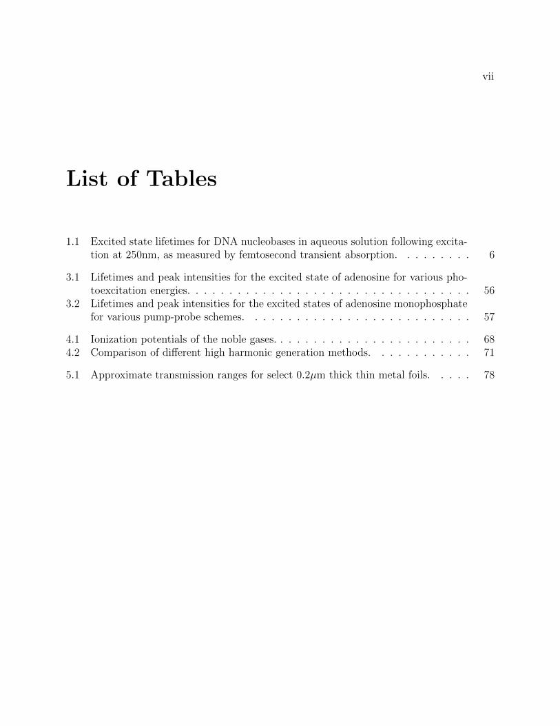
This behavior has a number of effects on the photoelectron spectra. First, vibrational androtational detail are typically smeared out by the high density of solvent shell configurationssampled. Second, the eBE of a species is often increased in solution if solvation is favorable.Finally, solvation shifts with lifetimes of ∼1ps are common in water. These are characterizedby spectral shifts to tighter binding energies and spectral narrowing as the equilibriumconfiguration is approached. An illustrative example of typical solvation dynamics seenin TRPES photoelectron spectra is shown in Figure 1.5.
Large polyatomic molecules in the gas phase can provide their own heat bath—energyin a high-lying vibrational mode is redistributed to lower lying modes without changing thetotal energy of the molecule. This is called intramolecular vibrational energy redistribution.In the condensed phase, the solvent can expedite vibrational relaxation of the solute throughboth solvent-assisted intramolecular vibrational energy redistribution10 and intermolecularvibrational relaxation. This discussion will focus on the latter.
Energy from a solute can be irreversibly transfered to the surrounding solvent by cou-pling of the solute and solvent modes—this is intermolecular vibrational relaxation.[38, 39]This typically takes place on a picosecond timescale and is sometimes referred to as “vibra-tional cooling”. Strictly speaking, vibrational cooling refers only to intermolecular processes;intramolecular processes are generally assumed to be fully complete before cooling.
Intermolecular vibrational relaxation can be described by a simple collision model, similar
10Whereby the solute-solvent modes couple.
CHAPTER 1. INTRODUCTION 16
eKE (eV)
0.5 1 1.5 2 2.5 3 3.5 4
Inte
nsi
ty (
arb
)
0
0.1
0.2
0.3
0.4
t0
0.1ps
0.33ps
0.5ps
1ps
Figure 1.5: Photoelectron spectra of e−aq generated via charge-transfer-to-solvent from KI inwater. At early times, spectra are broad and electrons are less tightly bound; as pump-probedelay increases, the spectra are seen to shift to tighter binding energies and narrow in widthas the solvent undergoes reorganization. See Reference [37] for more details.
to the one used in the gas phase.[31] Notably, however, the collisional relaxation rate insolution is not bimolecular, as in the gas phase, but unimolecular. This is a consequenceof the high molecule density in the condensed phase. The collision relaxation rate law canthen be defined by Equation 1.21, where [C∗] is concentration of vibrationally excited solutemolecules, and k is the unimolecular rate coefficient.11
d[C∗]
dt= −k[C∗] (1.21)
Fermi’s Golden Rule can be used to approximate the vibrational relaxation rate if thesolute is assumed to be a diatomic harmonic oscillator and the solvent is treated as a bathof harmonic oscillators. The system must also be constrained to obey energy conservation.The Hamiltonian can then be expressed by Equation 1.22, where HB is the Hamiltonian fora harmonic bath, HD for the diatomic harmonic oscillator solute, and V is the operator thatdescribes solute-bath coupling.
H = HB + HD + V (1.22)
11Recall, k = 1/τ where τ is the relaxation time.

CHAPTER 1. INTRODUCTION 17
We will now consider the transition between states |i〉 and |f〉 of the diatomic solute,which are eigenstates of HD. The initial and final eigenstates of the bath Hamiltonian aregiven by |α〉 and |α′〉, respectively. The FGR expression for the transition, Γf←i, is thengiven by Equation 1.23, where the thermal distribution of states in the manifold have beenaveraged over and all final states have been summed. The bath partition function is givenby Q, β = 1/kBT where kB is Boltzmann’s constant and T is temperature, and the densityof states is given by the sum of δ(Ei + εα − Ef − εα′ ).
Γf←i ∝∑α
e−β(Ei+εα)
Qα
∑α′
| 〈α′ , f |V |i, α〉 |2δ(Ei + εα − Ef − εα′ ) (1.23)
This can then be rewritten in time correlation form to give Equation 1.24.
Γf←i ∝∑α
e−β(Ei+εα)
Qα
∑α′
〈α|Vif |α′〉 〈α′|Vfi|α〉
∫ +∞
−∞dte
it(Ei + εα − Ef − εα′ )/~
∝∫ +∞
−∞dte
it(Ei − Ef )/~ 〈Vif (t)Vfi(0)〉T
(1.24)
As we learned previously, the key parameters that govern the rate of energy transfer arethe coupling strength between the solute-bath modes and the energy gap between initial andfinal states.
1.7 Summary of Systems Studied and Outlook
Chapter 3 of this dissertation focuses on a recently finished study of the excited state deac-tivation dynamics of the DNA components adenosine (Ado) and adenosine monophosphate(AMP). Femtosecond TRPES in a water microjet was used with photon energies rangingfrom 4.69-6.20eV. Two absorption bands were studied; the lowest-lying ππ* excited state waspopulated by 4.69-4.97eV photons while 6.20eV photons were proposed to excite a higher-lying ππ* transition.
The ππ* excited state was found to decay on a timescale ranging from ∼210-270fs in Adoand ∼240-290fs in AMP. These lifetimes were assigned to the internal conversion of the S1
ππ* excited state to vibrationally hot ground state, S0, and were found to inversely dependon the photoexcitation energy. Photoexcitation at 6.20eV produced a transient signal boundby ∼4eV in both Ado and AMP. A lifetime was only recoverable in AMP and found to be

CHAPTER 1. INTRODUCTION 18
∼300fs. Spectral analysis suggests that a high-lying ππ* excited state is initially populatedand subsequently relaxes to the S1 ππ* excited state before internal conversion to hot S0.
Notably, the probe photon energies used in these experiments were insufficient to photode-tach electrons from the ground state—bound by ∼7.5eV—and observe dynamics along thissurface. This belies a common short-coming of TRPES studies that employ conventionalfemtosecond table-top lasers: photons in excess of 6.2eV are unavailable with solid-statefrequency-mixing techniques.
Chapter 4 addresses this concern by introducing a technique known as “high-harmonicgeneration,” which up-converts the output of a commercial femtosecond laser into the ex-treme ultraviolet to soft X-ray regime. Efforts are currently underway to experimentallyrealize this on the liquid microjet project, and these plans are described in detail in Chapter5. We hope to open new frontiers in the investigation of chemical dynamics in the condensedphase with this new setup.
1.8 References
1. Photoinduced phenomena in nucleic acids I: Nucleobases in the gas phase and in sol-vents (eds Barbatti, M., Borin, A. C. & Ullrich, S.) (Springer International Publishing,Cham, 2015).
2. Cadet, J., Mouret, S., Ravanat, J.-L. & Douki, T. Photoinduced damage to cellularDNA: Direct and photosensitized reactions. Photochem. Photobiol. 88, 1048 (2012).
3. Alizadeh, E. & Sanche, L. Precursors of solvated electrons in radiobiological physicsand chemistry. Chem. Rev. 112, 5578 (2012).
4. Crespo-Hernandez, C. E., Cohen, B., Hare, P. M. & Kohler, B. Ultrafast excited-statedynamics in nucleic acids. Chem. Rev. 104, 1977 (2004).
5. Middleton, C. T. et al. DNA excited-state dynamics: From single bases to the doublehelix. Annu. Rev. Phys. Chem. 60, 217 (2009).
6. Improta, R., Santoro, F. & Blancafort, L. Quantum mechanical studies on the pho-tophysics and the photochemistry of nucleic acids and nucleobases. Chem. Rev. 116,3540 (2016).
7. Shukla, M. K. & Leszczynski, J. Electronic spectra, excited state structures and inter-actions of nucleic acid bases and base assemblies: A review. J. Biomol. Struct. Dyn.25, 93 (2007).
8. Neumark, D. M. Time-resolved photoelectron spectroscopy of molecules and clusters.Annu. Rev. Phys. Chem. 52, 255 (2001).

CHAPTER 1. INTRODUCTION 19
9. Voet, D., Gratzer, W. B., Cox, R. A. & Doty, P. Absorption spectra of nucleotides,polynucleotides, and nucleic acids in the far ultraviolet. Biopolymers 1, 193 (1963).
10. Hare, P. M., Crespo-Hernandez, C. E. & Kohler, B. Internal conversion to the electronicground state occurs via two distinct pathways for pyrimidine bases in aqueous solution.Proc. Natl. Acad. Sci. U.S.A. 104, 435 (2007).
11. Gustavsson, T. et al. Singlet excited-state behavior of uracil and thymine in aqueoussolution: A combined experimental and computational study of 11 uracil derivatives.J. Am. Chem. Soc. 128, 607 (2006).
12. Buchner, F., Nakayama, A., Yamazaki, S., Ritze, H.-H. & Lubcke, A. Excited-staterelaxation of hydrated thymine and thymidine measured by liquid-jet photoelectronspectroscopy: Experiment and simulation. J. Am. Chem. Soc. 137, 2931 (2015).
13. Sharonov, A., Gustavsson, T., Carre, V., Renault, E. & Markovitsi, D. Cytosine ex-cited state dynamics studied by femtosecond fluorescence upconversion and transientabsorption spectroscopy. Chem. Phys. Lett. 380, 173 (2003).
14. Improta, R., Santoro, F. & Blancafort, L. Quantum mechanical studies on the pho-tophysics and the photochemistry of nucleic acids and nucleobases. Chem. Rev. 116,3540 (2016).
15. Roberts, G. M., Marroux, H. J. B., Grubb, M. P., Ashfold, M. N. R. & Orr-Ewing,A. J. On the participation of photoinduced N-H bond fission in aqueous adenine at266 and 220nm: A combined ultrafast transient electronic and vibrational absorptionspectroscopy study. J. Phys. Chem. A 118, 11211 (2014).
16. Perun, S., Sobolewski, A. L. & Domcke, W. Photostability of 9H-adenine: Mechanismsof the radiationless deactivation of the lowest excited singlet states. Chem. Phys. 313,107 (2005).
17. Cohen, B., Hare, P. M. & Kohler, B. Ultrafast excited-state dynamics of adenine andmonomethylated adenines in solution: Implications for the nonradiative decay mecha-nism. J. Am. Chem. Soc. 125, 13594 (2003).
18. Schatz, G. C. & Ratner, M. A. Quantum mechanics in chemistry (Dover Publications,Inc., 2002).
19. Voorhis, T. V. 5.73 Introductory Quantum Mechanics I <https://ocw.mit.edu>(Massachusetts Institute of Technology: MIT OpenCourseWare, Fall 2005).
20. Tokmakoff, A. 5.74 Introductory Quantum Mechanics II <https://ocw.mit.edu>(Massachusetts Institute of Technology: MIT OpenCourseWare, Spring 2009).
21. Pedersen, S. & Zewail, A. H. Femtosecond real time probing of reactions XXII. Kineticdescription of probe absorption, fluorescence, depletion and mass spectrometry. Mol.Phys. 89, 1455 (1996).
22. Stolow, A. Femtosecond time-resolved photoelectron spectroscopy of polyatomic molecules.Annu. Rev. Phys. Chem. 54, 89 (2003).

CHAPTER 1. INTRODUCTION 20
23. Stolow, A., Bragg, A. E. & Neumark, D. M. Femtosecond time-resolved photoelectronspectroscopy. Chem. Rev. 104, 1719 (2004).
24. Stolow, A. & Underwood, J. G. Time-resolved photoelectron spectroscopy of nonadia-batic dynamics in polyatomic molecules 497 (John Wiley & Sons, Inc., 2008).
25. Suzuki, T. Time-resolved photoelectron spectroscopy of non-adiabatic electronic dy-namics in gas and liquid phases. Int. Rev. Phys. Chem. 31, 265 (2012).
26. Englman, R. & Jortner, J. The energy gap law for radiationless transitions in largemolecules. Mol. Phys. 18, 145 (1970).
27. Worth, G. A. & Cederbaum, L. S. Beyond Born-Oppenheimer: Molecular dynamicsthrough a conical intersection. Annu. Rev. Phys. Chem. 55, 127 (2004).
28. Matsika, S. & Krause, P. Nonadiabatic events and conical intersections. Annu. Rev.Phys. Chem. 62, 621 (2011).
29. Domcke, W. & Yarkony, D. R. Role of conical intersections in molecular spectroscopyand photoinduced chemical dynamics. Annu. Rev. Phys. Chem. 63, 325 (2012).
30. Chandler, D. Introduction to modern statistical mechanics (Oxford University Press,1987).
31. Nitzan, A. Chemical dynamics in the condensed phases: Relaxation, transfer, and re-actions in condensed molecular systems (Oxford University Press, Oxford, New York,2006).
32. Levine, R. D. Molecular reaction dynamics (Cambridge University Press, 2005).
33. Atkins, P. W. & MacDermott, A. J. The Born equation and ionic solvation. J. Chem.Ed. 59, 359 (1982).
34. Bakker, H. J. & Skinner, J. L. Vibrational spectroscopy as a probe of structure anddynamics in liquid water. Chem. Rev. 110, 1498 (2010).
35. Aherne, D., Tran, V. & Schwartz, B. J. Nonlinear, nonpolar solvation dynamics inwater: The roles of electrostriction and solvent translation in the breakdown of linearresponse. J. Phys. Chem. B 104, 5382 (2000).
36. Rosspeintner, A., Lang, B. & Vauthey, E. Ultrafast photochemistry in liquids. Annu.Rev. Phys. Chem. 64, 247 (2013).
37. Elkins, M. H., Williams, H. L. & Neumark, D. M. Dynamics of electron solvationin methanol: Excited state relaxation and generation by charge-transfer-to-solvent. J.Chem. Phys. 142, 234501 (2015).
38. Elles, C. G. & Crim, F. F. Connecting chemical dynamics in gases and liquids. Annu.Rev. Phys. Chem. 57, 273 (2006).
39. Owrutsky, J. C., Raftery, D. & Hochstrasser, R. M. Vibrational relaxation dynamics insolutions. Annu. Rev. Phys. Chem. 45, 519 (1994).
21
Chapter 2
Experimental Methods
2.1 Overview
The current experimental setup comprises a commercial ultrafast laser, liquid microjet, andphotoelectron spectrometer. Data analysis is performed in MATLAB with home-brewedcode. The design of a new XUV source is described in Section III and will be implementedin short order by Blake A. Erickson.
2.2 Liquid Microjet Technique
Photoelectron spectroscopy necessitates that experiments be performed in vacuum; inelasticscattering events alter the observed kinetic energies of the photoejected electrons. Practicallyspeaking, this means that the mean free path—the average distance traveled by a particlebetween collisions—of the electron must be greater than the electron flight length. Mean freepath, λ, is described below by Equation 2.1, where σ is the molecular collision cross-section,ρ is the number density of the vapor, kB is the Boltzmann constant, T is the temperature,P is the vapor pressure, and c is the ratio of the particle and gas velocities.1[1–4]
λ =1
cσρ
=kBT
cσP
(2.1)
1This ratio is difficult to calculate, but typically ranges from ∼0.75-1.5.

CHAPTER 2. EXPERIMENTAL METHODS 22
Liquids with high vapor pressures have been historically difficult to study because theequilibrium vapor density renders λ prohibitively short. In water, σ is generally ∼30A2, andλ ≈ 10µm in water at its equilibrium vapor pressure at 277K. We employ a cylindrical liquidmicrojet to overcome this obstacle.
First described by Manfred Faubel and coworkers, the microjet enables the introductionof high vapor pressure liquids into vacuum.[5, 6] Microjets are thin, fast-flowing liquid jetsthat satisfy the Knudsen condition, which is to say the diameter of the jet is the same asor smaller than λ in equilibrium vapor. Under this paradigm, evaporation is effectivelycollision-free. Thus, the gas density at the surface of the liquid jet is greatly reduced, and λof electrons photoejected from the jet is increased. A skimmer can also be used to cut intothe vapor jacket around the liquid core, further reducing the number of collisions an outgoingparticle might undergo in the vapor. For example, a 5µm diameter water microjet (at 252K)skimmed 1mm away from the surface will have λ = 250µm.[4] The low vapor density alsoreduces the gas load such that a modest turbomolecular pump may be used to evacuate thesample chamber into the sub-mTorr regime. Moreover, the microjet affords a sample whichis continually renewed, impervious to laser burn, and has a high target density.
2.2.1 Microjet Design and Implementation
Our microjet design mirrors that of the Saykally group[7] at UC Berkeley and is describedin detail in the dissertation of Alexander T. Shreve.[8] The microjet principally comprisesan inline sub-micron filter, a Swagelok union, and a jet aperture (see Figure 2.2a). Theaperture is constructed by securing a fused-silica capillary in a jacket of polyether etherketone (PEEK) tubing with a Swagelok ferrule. PEEK tubing is resistant to corrosion by avariety of chemicals. A diamond wheel cutter is used to evenly score the capillary to ensurestraight flow of the microjet. This design affords a laminar flow regime of several millimetersand a turbulent flow regime of several centimeters.
The diameter of these microjets can range from 5-100µm; our lab uses 20µm ID capillaries.Empirically, we have found that a constant flow rate of 0.2-0.3mL/min and backing pressureof 80atm produces the most stable water microjets. The temperature of the microjet can becalculated through an evaporative cooling model,[9] and is found to be ∼280K at the laserinteraction region, 1mm down from the exit of the capillary.2 Because DNA components areexpensive, we have begun the practice of recycling solutions. Recycled solution was analyzedand found not to differ significantly in concentration from fresh solution. Used solutions aresub-micron filtered before reuse and can be recycled in this way ∼3 times before the solute
2The code for this model is written in Igor Pro and maintained by the Saykally group. It is also describedin the dissertation of Alexander T. Shreve.
CHAPTER 2. EXPERIMENTAL METHODS 23
concentration drops appreciably.
Conveniently, alignment of the laser beams onto the microjet is made obvious by aFraunhofer diffraction pattern that is present when the laser and microjet are spatiallyoverlapped. The microjet acts as a single slit for most wavelengths currently used (200-800nm). Average laser powers must be kept under 200µW; beyond this limit space chargeeffects result in plasma generation.[10, 11]
The original Faubel microjets (Microliquids, GmbH) are formed from pulled capillaries.Because the Saykally design loads pressure onto a smaller surface area than the Faubelmicrojets, a higher backing pressure is used for a comparable flow rate. However, thesemicrojets are more inexpensive to implement and we have found no considerable differencein stability.
Our pump is a 500mL capacity syringe pump (Teledyne Isco, Model 500D), but a peri-staltic pump would work equally well and could afford easy switching between solvents. Thesyringe pump valve manufacturer was changed to Vindum Engineering (MV-210-HC) in 2016at the suggestion of Royce K. Lam.3 Vindum valves have been found to be more robust and,as of the time of this writing, only one valve has needed to be serviced. Finally, solutionsof DNA components, which have modest water solubilities, were found to clog the microjetassembly somewhat more frequently. This was remedied by flushing the syringe pump andPEEK tubing with a 1M solution of HCl as needed.
2.2.2 Probe Depth Considerations
Of considerable interest to the liquid-phase community is determining whether or not spec-tral interrogation of the microjet occurs at the surface or in the liquid core for a givenexperiment.[11, 12] In condensed-phase matter, the emission intensity of electrons attenu-ates exponentially as a function of depth from the surface at which they were born. Tounderstand the type of solvation environment that surrounds the solute of interest, it ishelpful to know the effective electron attenuation length—the shortest distance between twopoints through which the electron intensity is reduced by 1/e—as a function of eKE.[13] Mostcondensed phase materials qualitatively obey the same curve, the so-called “universal curve”as shown in Figure 2.1.
The universal curve does show some material dependence, and there is still some out-standing debate regarding the exact shape of the curve for liquid water.[13–15] However, itis generally accepted that the minimum attenuation length is on the order of 10A, or four
3A Saykally group doctoral student (Ph.D. Fall 2017).

CHAPTER 2. EXPERIMENTAL METHODS 24
electron kinetic energy (eV)
elec
tron
eff
ecti
ve
atte
nuat
ion
leng
th (
Å)
100 101 102 103
100
101
102
103
Universalcurve H2O
Figure 2.1: The universal curve (solid red line) and measured electron effective attenuationlength measured for liquid water (blue dashed line). Adapted from References [13] and [14].
water monolayers, at 50-100eV electron kinetic energy.
Recently, the implementation of so-called “flat jets” has garnered much attention.[3, 16]These can be generated by orthogonally crossing two traditional cylindrical jets to form a flatliquid sheet.4 A flat jet generated from two 10µm cylindrical jets is approximately 750µm x500µm x 1µm. The shorter path length through flat jets as compared to cylindrical jets isone key advantage to this design. Additionally, higher pulse energies can be used on the jetwithout introducing space charge or multiphoton effects, and the larger surface area of flatjets may be more compatible with the diameter of the focused laser beam.
2.3 Photoelectron Spectrometer
The photoelectron spectrometer comprises two main regions, as shown in Figure 2.2: 1)the microjet trap and 2) the detector chamber. Our current apparatus was designed byAlexander T. Shreve, and an extensive discussion of the apparatus can be found in his dis-sertation.[8] Changes made to the Shreve design are discussed in the dissertation of MadelineH. Elkins.[17]
Briefly, the sample of interest is injected into vacuum via a liquid microjet, which isthen crossed by femtosecond pump and probe laser pulses and subsequently cryotrapped.Photoejected electrons are sampled through a skimmer, steered down the time-of-flight (ToF)
4Assemblies can be purchased from Microliquids, GmbH.

CHAPTER 2. EXPERIMENTAL METHODS 25
(a) Microjet (b) Trap and detector chambers
Figure 2.2: Photoelectron spectrometer: (a) Microjet assembly in vacuum with optionalcatcher installed, (b) Top view of trap and detector chambers with laser and time of flightaxes indicated. The microjet axis is into the plane of the page.
tube by a magnetic bottle, and collected by a microchannel plate chevron stack with aphosphor screen. This is pictured in Figure 2.2b and detailed below.
2.3.1 Microjet Trap
The assembled microjet is introduced into vacuum by a three-axis micrometer holster onformed bellows. This allows the microjet to be readily positioned inside of the chamber.When acquiring data, the microjet is centered 1mm from the skimmer orifice, and the capil-lary tip is moved above the orifice. Laser pulses are orthogonally crossed with the jet in frontof the skimmer. A 900µm diameter skimmer is currently used to cut into the vapor jacketand limit the travel of photoelectrons through the vapor. Skimmer diameters of 300-500µmhave also been used successfully.
The rare earth magnet component of the magnetic bottle is also located in this chamber,and is described fully in Section 2.3.2.1. For bottle alignment purposes, the magnet ismounted on a three-axis translation setup which can be moved in vacuo by picomotor piezolinear actuators (Newport, 8302).
A 150L/s turbomolecular pump (Leybold, Turbovac 151) is used to evacuate the chamber.This is backed by a rotary vane mechanical pump (Edwards, E2M8). The jet is cryotrappedwith liquid nitrogen at the bottom of the chamber to assist the pumps, and a 7L dewarlocated in a secondary chamber (a four-way 10” ConFlat (CF) cross mounted to the left ofthe trap chamber in Figure 2.2, but not shown) is used to further enable a quick pump-down.Typical operating pressures are on the order of ∼10−4Torr.

CHAPTER 2. EXPERIMENTAL METHODS 26
Many researchers in the liquid microjet community utilize a “catcher” to cryotrap themicrojet as soon as possible. This helps to lower the chamber pressure and prevents icenucleation, which results in frozen microjets. A new catcher has been designed and willlikely be installed in tandem with the new XUV source (see Appendix C for drawings). Themicrojet trap chamber, with optional catcher, is shown in Figure 2.2a.
2.3.1.1 Laser Power and Microjets
Excessively high laser power incident on the microjet can cause a number of undesirableeffects: namely, space-charge, ponderomotive, and AC stark shift effects.[10, 11] Averagepowers, per beam, in excess of 200µW are to be avoided.
• Electron-electron repulsion results in a space charge effect which homogeneously broad-ens the photoelectron spectral features. This effect is often seen at the onset of themultiphoton laser power regime (peak laser intensity of ∼ 1010W/cm2).
• A ponderomotive force by the laser pulse on the photoelectrons will often occur whenentering the tunnel ionization laser power regime (peak laser intensity of > 1014W/cm2).Here, observed VBEs are typically offset.
• When the incident laser power exceeds ∼10mW, an AC Stark effect has been seen.This induces an instantaneous energy shift which can either increase or totally closeresonant multiphoton transitions to certain ionization channels. For this reason, whencalibrating the instrument and calculating streaming potentials, as described below,the incident power is kept below 5mW.
Laser-driven plasma formation is also possible in the tunnel ionization laser power regime(aka the strong field regime). This interaction results in the accumulation of quasi-freeelectrons in the microjet at the focus of the laser. For peak laser intensities above∼ 1017W/cm2
collective electron motions can be resonantly excited by the laser field; generated plasmaoscillates in resonance with the laser frequency.
2.3.2 Detector Chamber
The detector chamber comprises a solenoid and microchannel plate detector with a phosphorscreen, described in the sections below. It is designed such that the solenoid is not undervacuum so it can be easily removed and serviced if necessary, and to prevent a virtual leak.A gate valve cannot be added to isolate the chamber because the solenoid must abut the

CHAPTER 2. EXPERIMENTAL METHODS 27
back of the skimmer for the magnetic bottle to operate properly; thus, the detector chamberis not under vacuum when the trap chamber is vented.5
Operating pressures in this region are ∼10−6Torr. The chamber is pumped by threeturbomolecular pumps with a total pumping speed of 1400L/s (Leybold, Turbovac 150, 151,and 1000C), backed by a rotary vane mechanical pump (Edwards, E2M12).
2.3.2.1 Magnetic Bottle Spectrometer
A magnetic bottle is used in the spectrometer because it greatly increases the collectionefficiency of photoelectrons—theoretically to 2π steradians.[18, 19] Without this bottle, thelow signal levels would require greatly increasing the number of shots taken at each delay,rendering the required data acquisition period for time-resolved experiments prohibitivelylong. The magnetic bottle utilizes an inhomogeneous magnetic field and the Lorentz force,described by Equation 2.2, where ~F is the Lorentz force, q is the charge of the photoelectron,~v is the photoelectron velocity, and ~B is the magnetic field.
~F = q~v × ~B
= qvBsinθ(2.2)
As shown in Figure 2.3, a strong, diverging magnetic field first causes photoelectronsemitted with velocity components off-axis to the desired flight path to spiral axially aroundthe field lines. These helically traveling photoelectrons then encounter a weak, homogeneousmagnetic field, with field lines parallel to the ToF axis, and are guided along the flight pathfor collection. As the photoelectrons travel in this region, their spiral trajectories unraveland become collinear to the ToF axis. Assuming the total velocity is conserved, the cyclotronenergy of the photoelectrons is converted into axial energy. The 3D cloud of photoelectronsemitted from the microjet is thus bent so that the trajectories of the photoelectrons arenearly parallel to the ToF axis.
Additionally, the photoelectron distribution is spatially magnified according to Equation2.3, where M is the magnification factor, Bi is the magnitude of the initial magnetic field,and Bf is the the magnitude of the final magnetic field. Clearly, larger initial fields andsmaller final fields result in greater magnification.
5We have not found this to significantly accelerate MCP degradation.

CHAPTER 2. EXPERIMENTAL METHODS 28
Bi Bf
e-rare earth
MCP stack
solenoid
magnet
Figure 2.3: Schematic of the magnetic bottle assembly. Magnetic field lines are shown inbright green, and photoelectron trajectories are indicated in white.
M =
√Bi
Bf
(2.3)
To experimentally realize the magnetic bottle, we employ rare-earth permanent magnetsand a solenoid.[18] A stack of Nickel-coated, high-pull Samarium-cobalt (McMaster-Carr,57325K93) and Neodymium (McMaster-Carr, 58605K85) disk magnets provide the stronginitial magnetic field.6 A magnetically soft iron cone (Ed Fagan Inc., Hiperco 50A) sitson the end of this stack to shape the magnetic field lines. Initial magnetic fields typicallyrange from 5,000-10,000G in magnetic bottles7; our initial field strength is ∼10,000G. Thesolenoid is 26” long, and is made of 14 gauge copper wire coiled at ten turns per inch. Thetotal length of copper wire used is 4200”. From Ampere’s Law, the field within a solenoidis defined according to Equation 2.4, where B is the magnitude of the magnetic field, µ/µ0is the relative magnetic permeability8, n is the number of turns per unit length, and I thecurrent applied to the wire.
B =µ
µ0
nI (2.4)
6Notably, the permanent magnets, as with everything in the trap chamber, are subject to consider-able corrosion despite their Nickel-based anti-corrosion casings. Bead-blasting only exacerbates this issue.However, even when pitted and corroded, the magnetic bottle operation was found to be largely unaffected.
7Measured as surface field strength.8For copper, µ/µ0 is 0.999994.
CHAPTER 2. EXPERIMENTAL METHODS 29
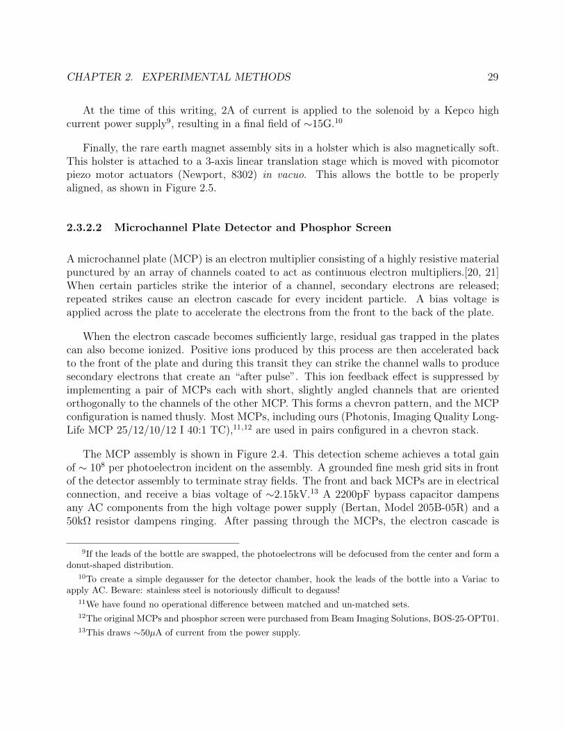
At the time of this writing, 2A of current is applied to the solenoid by a Kepco highcurrent power supply9, resulting in a final field of ∼15G.10
Finally, the rare earth magnet assembly sits in a holster which is also magnetically soft.This holster is attached to a 3-axis linear translation stage which is moved with picomotorpiezo motor actuators (Newport, 8302) in vacuo. This allows the bottle to be properlyaligned, as shown in Figure 2.5.
2.3.2.2 Microchannel Plate Detector and Phosphor Screen
A microchannel plate (MCP) is an electron multiplier consisting of a highly resistive materialpunctured by an array of channels coated to act as continuous electron multipliers.[20, 21]When certain particles strike the interior of a channel, secondary electrons are released;repeated strikes cause an electron cascade for every incident particle. A bias voltage isapplied across the plate to accelerate the electrons from the front to the back of the plate.
When the electron cascade becomes sufficiently large, residual gas trapped in the platescan also become ionized. Positive ions produced by this process are then accelerated backto the front of the plate and during this transit they can strike the channel walls to producesecondary electrons that create an “after pulse”. This ion feedback effect is suppressed byimplementing a pair of MCPs each with short, slightly angled channels that are orientedorthogonally to the channels of the other MCP. This forms a chevron pattern, and the MCPconfiguration is named thusly. Most MCPs, including ours (Photonis, Imaging Quality Long-Life MCP 25/12/10/12 I 40:1 TC),11,12 are used in pairs configured in a chevron stack.
The MCP assembly is shown in Figure 2.4. This detection scheme achieves a total gainof ∼ 108 per photoelectron incident on the assembly. A grounded fine mesh grid sits in frontof the detector assembly to terminate stray fields. The front and back MCPs are in electricalconnection, and receive a bias voltage of ∼2.15kV.13 A 2200pF bypass capacitor dampensany AC components from the high voltage power supply (Bertan, Model 205B-05R) and a50kΩ resistor dampens ringing. After passing through the MCPs, the electron cascade is
9If the leads of the bottle are swapped, the photoelectrons will be defocused from the center and form adonut-shaped distribution.
10To create a simple degausser for the detector chamber, hook the leads of the bottle into a Variac toapply AC. Beware: stainless steel is notoriously difficult to degauss!
11We have found no operational difference between matched and un-matched sets.12The original MCPs and phosphor screen were purchased from Beam Imaging Solutions, BOS-25-OPT01.13This draws ∼50µA of current from the power supply.

CHAPTER 2. EXPERIMENTAL METHODS 30
(a) Top view (b) Side view
Figure 2.4: The MCP assembly: (a) A fine mesh grid is grounded and placed in front of theMCPs to terminate stray field lines, (b) The MCP chevron and phosphor screen are housedin a white Teflon puck and wired to BNC-type pinouts on a 2-3/4” Conflat flange.
accelerated to a phosphor screen, which receives ∼3.25kV.14 The impinging cascade causesthe phosphor to emit photons which are imaged by a charge-coupled device (a camera) forthe sole purpose of aligning the magnetic bottle. Figure 2.5 shows the phosphor screen fora good magnetic bottle alignment—the photoelectron cloud should be round and tightlyfocused. Signal is capacitively coupled off of the back MCP by a 1000pF capacitor.15 Tomitigate impedance mismatch, each of the MCPs and the phosphor are connected to 1MΩresistors.16 The voltage in the circuit is regulated by a 50V Zener diode. The detector circuitdiagram can be found in the dissertations of Shreve and Elkins.[8, 17]
Microchannel plates are so sensitive that, even in the absence of photoelectrons, strayions or high-energy photons can cause an electron cascade. These “dark counts” originatefrom several sources, including thermionic emission from ion gauges and cosmic radiation.Typical dark count intensities in our apparatus are quite low, ∼5-10mV.17 Often, ringing ispresent in the dark count signal and is principally due to cross-talk between the layers of
14This draws 0µA.15Signal could also be coupled off of the phosphor—we have found no considerable difference as compared
to coupling off of the back MCP.16These typically are the first to overheat and mushroom in the circuit.17To measure dark counts, the signal off of the high-voltage applied MCP is measured on the oscilloscope
in the absence of light and photoelectrons. The signal is self-triggered at ∼1mV.

CHAPTER 2. EXPERIMENTAL METHODS 31
Figure 2.5: The phosphor image when the magnetic bottle is well-aligned.
the detector.18 The period of the ringing from the MCPs is ∼8ns—this corresponds to anenergy spread (between the peaks in the ringing signal) that is much smaller than typicalbandwidth of solution-phase spectra, and is thus not accounted for in analysis of TRPESdata.
2.4 Data Acquisition
The capacitively coupled signal from the MCPs is sent to an oscilloscope (Textronix, DPO3034), which acts in part as a digital-to-analog converter. The oscilloscope is triggered by aTTL pulse sent from the Astrella system synchronization and delay generator. The pulse isdelayed such that the laser spike is 16ns before the oscilloscope trigger.19 Data is recordedby the oscilloscope for 2000ns after the trigger in 2ns bins. This is then averaged over 512shots, and the averaged waveform is sent to the data acquisition computer to be written tofile by the data acquisition software.
The LabVIEW data acquisition software was largely written by Alexander T. Shreve,but has since been modified to accommodate automated background scans.[8] It is describedbriefly herein; a fuller discussion of the main body of the code can be found in AppendixC of the Shreve dissertation; updates to the code can be found in Appendix B.1 of thisdissertation. Currently, 1,024 shots are taken at each sequential delay, followed by 1,024shots of each background. The laser pulses produce a static, two-photon, one-color signal,and these are collected at a pump-probe delay of zero. When this sequence is completed,the motorized stage is instructed to loop back to the first delay and start the process overagain until the specified number of shots per stage delay are acquired. The delays and shots
18The characteristic period of electronic ring is on the order of tens of nanoseconds. If the source of thering is due to signal reflection or impedance mismatch in the BNC cables, this can be confirmed by changingthe cable length.
19This is for historical reasons and is largely arbitrary.

CHAPTER 2. EXPERIMENTAL METHODS 32
(a) Beam block
IOREF
RESET
3.3V
5V
GND
GND
Vin
A1
A2
A3
A4
A5
A0
RX←0
TX→0
~6
~5
4
~3
2
7
12
~11
~10
~9
8
13
AREF
GND
PO
WE
RA
NA
LO
G IN
DIG
ITA
L (P
WM
~)
ARDUINO
UNO
SERVO #1 SERVO #2 SERVO #3
EXTERNAL POWER
5V DC
- + - + - +
(b) Circuit diagram
Figure 2.6: Arduino-controlled servo motors for automated background scans: (a) Eachbeam block comprises an aluminum flag mounted to the horn of a servo which is in turnmounted to an optical post, (b) The circuit diagram for the Arduino UNO and servo motors;digital pins 9, 10, and 11 are used to communicate with the servos, and the UNO and servosare powered by a standard 5V plug.
to be acquired are specified in the configuration table CSV file, which is called by the dataacquisition software. As data packets are sent to the computer, they are 1) appended to theappropriate delay-specific CSV file and 2) summed along with the previous waveforms togenerate a new total intensity for that delay. These combined sums are saved in a new CSVfile—this is the useful output of the program.
The background scans have been automated through implementation of servo motors(AdaFruit Industries, TowerPro SG-5010) and an Arduino UNO microcontroller. Black alu-minum flags were mounted to each servo horn to block the individual laser beams. SimpleASCII characters sent to the UNO control the flag positions, making integration into theexisting acquisition software straightforward. The Arduino UNO code can be found in Ap-pendix B.2, along with a brief explanatory text. The circuit diagram and a picture of thedevice are presented in Figures 2.6a and 2.6b.
2.4.1 Post-Processing
Before fitting TRPES data, it first undergoes a post-processing procedure in MATLAB. TheMATLAB script used for this is described in detail in the Elkins dissertation.[17] The scriptis summarized by the code flow diagram pictured in Figure 2.7. Briefly, this script convertsToF data into eKE-space, subtracts the one-color, two-photon backgrounds, and accountsfor the intentionally low discrimination by correcting the baseline level.

CHAPTER 2. EXPERIMENTAL METHODS 33
Import data
Convert ToF into eKE
Convert stage position
into time delay
Subtract backgrounds
sub’d data matrix
Load constants
User prompt
Setup fit function
Select data for
baseline correction
Fit baseline
bs data matrix
Subtract bs from
sub’d data
Rebin final dataset
Write matfile
Figure 2.7: Sequence diagram for MATLAB script PostProcessor.m.
2.4.2 Time-of-Flight and Energy Resolution
The conversion between arrival time and eKE of a photoelectron is straightforward if theflight length is known. Electron kinetic energy is defined by Equation 2.5, where me is theelectron mass, v is the photoelectron velocity, l is the flight length, and t is the time-of-arrival.
eKE =mev
2
2
=mel
2
2t2
(2.5)
Note that the center-of-mass velocity does not need to be accounted for because the flowof the microjet is orders of magnitude slower than the photoelectron flight time.
The conversion between the waveform in ToF and eKE space is a non-linear transforma-tion, and thus the appropriate Jacobian must be invoked. This is given by Equation 2.6,where IeKE is the intensity in eKE space, IToF is the intensity in time-of-flight space, andeKE is the electron kinetic energy at the point of interest.
IeKE =IToF
eKE3/2
(2.6)
Taken together, Equations 2.5 and 2.6 reveal several important features of eKE spectra.

CHAPTER 2. EXPERIMENTAL METHODS 34
First, and perhaps most obviously, eKE goes as t−2, so early time photoelectrons have greatereKE than those that arrive later. Second, because eKE does not scale linearly with arrivaltime, there is greater point density at lower eKE than at higher eKE, in eKE space, for ourdetection scheme. Third, we notice that the feature widths in eKE spectra depend on theirToF. If we assume that a Gaussian feature has a FWHM of 2ns, we can see that in energyspace, the feature will be sharper at lower eKE than at higher eKE.20
Instrumental resolution depends on the flight length and width of time bins on the detec-tor. The energy resolution of a typical femtosecond laser pulse is ∼30meV, and thus rarelyaffects the peak widths observed in our spectra. It is also worth noting that the magneticbottle will slightly spread the arrival times of photoelectrons. An off-axis photoelectronwith equivalent kinetic energy as one fully on axis will arrive slightly later in time if itscyclotron energy is not fully converted into axial energy. However, this has never noticeablyaffected the data, particularly given that features typically have a full width at half maxi-mum (FWHM) of ∼1eV. Finally, data below eKE 0.3eV is not analyzed; photons scatteringoff of water arrive at early times and generate considerable noise at low eKE because theMCPs are not gated.
2.4.3 Obtaining Accurate Electron Binding Energies
To obtain eBEs, observed ToF data must be calibrated and consistent. This necessitates:1) regular spectrometer calibration and 2) measurement of the microjet streaming potential.Procedures for these are detailed in the dissertations of Elkins and Shreve, and the principlesare described briefly below.[8, 17]
Rather conveniently, xenon can be multiphoton ionized to its cationic 2P3/2 and 2P1/2 statesby readily available UV photons.21,22 The flight tube length and time zero can be backed outby measuring the ToF of these photoelectrons at several photoionization wavelengths nearresonance. These parameters are related by Equation 2.7, where t is the time-of-arrival, qeis the charge of the electron, me is the mass of the electron, n is the number of photonsinvolved in the multiphoton ionization, hν is the photon energy, l is the flight length, and t0is time zero.
20Hence, cryo-SEVI.21This is a 3-photon process; Xe has a 12.13eV IP.22Argon, with a 4-photon ionization (15.76eV IP) can also be used.

CHAPTER 2. EXPERIMENTAL METHODS 35
t =l√
2qeme
(nhν − eBE)+ t0
=l√qemem
1
v+ t0
(2.7)
When the Xe data is then plotted as t as a function of 1/v it can be fit by Equation 2.7. Togenerate a reconstruction error, the recovered values for l and t0 are used to back-calculatethe eBEs of the Xe 2P3/2 and 2P1/2 peaks and these are compared to their known values.Reconstruction errors should be on the order of 10meV. The known flight length and timezero23 can also be compared to the values obtained from the fit as a secondary check. If thecalibration is significantly off, the gas load or the laser power may be too high; if these arereasonable, the alignment of the magnetic bottle may be poor.
A charge separation is present at the solution-capillary interface. In conjunction with theflow velocity profile of the solution—which goes to zero at the walls of the capillary—this givesrise to a static microjet streaming potential, φ.[6, 22, 23] This must also be measured to reportan accurate eKE. Fortunately, φ is effectively constant for any given microjet on any givenday. To correct for it, we must simply measure φ (as described in the Elkins dissertation[17])and offset the observed eKE by the appropriate amount, as shown by Equation 2.8.24
eBE = hνprobe − eKE − φ (2.8)
Typical φ are a few hundred meV and can vary in sign.25 Usually, NaCl (100mM) isadded to solutions which do not already contain ions to offset φ somewhat.
2.5 Analysis of Time-Resolved Data
Extracting dynamic information from TRPES data is often frustrated by the complexity ofcondensed phase systems. To this end, we have adopted several fitting routines. M. H. Elkins
23We obtain t0 from the time-of-arrival of laser photons which hit the noble gas jet and are scattered tothe detector.
24Conveniently, a calibration can also be done at the end of a φ measurement if necessary.25Although with our recent DNA work, we have seen |φ| as large as 900meV!

CHAPTER 2. EXPERIMENTAL METHODS 36
provides a comprehensive discussion of these in her dissertation; however, a brief descriptionis given here.[17]
In systems where features are clearly separated or isolated, lane integration is generallyused to analyze time-evolving photoelectron spectra. Here, the total integrated intensity ofa single feature is calculated over some narrow energy range at each delay, and the resultingintensity is plotted as a function of delay. This can then be fit by a sum of exponentials con-volved with the Gaussian instrument response function (IRF).26 A convolution is describedby Equation 2.9, where (f ∗ g)(t) is the convolution and f and g are the functions which areto be convolved.
(f ∗ g)(t) =
∫ +∞
−∞dTf(T )g(t− T ) =
∫ +∞
−∞dTf(t− T )g(T ) (2.9)
Let us consider an excited state feature which decays with some monoexponential lifetime.An exponential must be multiplied by a Heaviside step function to describe the time-resolvedbehavior of the feature (see Equation 2.10). This is consequent to the vertical excitation tran-sition, which instantaneously populates the excited state; before the pump pulse is present,it is assumed that the excited state is unpopulated. This population function, I(t) is givenby Equation 2.10, where I0 is the initial intensity, t0 is time zero, τ is the monoexponentiallifetime, and θ the Heaviside function.
I(t) = I0e−t/τθ(t− t0) (2.10)
To arrive at the fitting function, I(t) must be convolved with the Gaussian temporalprofile of the IRF. This is given by Equation 2.11, and can ultimately be expressed byEquation 2.12. A complete derivation of f(t− t0) can be found in the dissertation of G. B.Griffin.[24]
f(t− t0) =I0
σ√
2
∫ +∞
−∞dTe−
T/2σ2
I(t− t0 − T ) (2.11)
f(t− t0) =I0
2e(σ2/2τ2−t− t0/τ)
[erf(t− t0σ√
2− σ
τ√
2
)+ 1]
(2.12)
As previously stated, lane integration is only appropriate for TRPES data containingeither a single feature or multiple well-separated features. Great care must be taken to
26Recall, our experiment is currently limited by the pump-probe cross correlation—this is our IRF.
CHAPTER 2. EXPERIMENTAL METHODS 37
choose an appropriate energy lane when features have considerable spectral overlap. If thelane of interest is significantly contaminated by other features, the fit will not accuratelyreport the lifetime of the feature represented by the chosen lane. Due to the high number ofpossible local environmental configurations, features in the condensed phase are quite broad(i.e. FWHM of 0.5-1.0eV) and different features often overlap. Consequently, we turn to asecond technique that is capable of disentangling highly congested spectra—Global LifetimeAnalysis.
2.5.1 Global Lifetime Analysis
Global Lifetime Analysis (GLA) is a nonlinear Levenberg-Marquardt fitting routine.[25–30]It is an iterative procedure which simultaneously fits the spectral and temporal componentsof TRPES data. Importantly, this algorithm is dependent on several assumptions:
1. Data can be decomposed into two parts, one that depends only on time si(t) andanother that depends only on energy si(λ).
2. The energy features are assumed to change only in intensity; they do not changeposition or lineshape.
3. Kinetics are exponential, and the time-dependence of the data can be described by asum of exponentials convolved with the IRF.
We begin by writing an expression for TRPES data, given by Equation 2.13, where S(t, λ)is the full data set and n is the minimum number of components necessary to accuratelydescribe the data.
S(t, λ) =n∑i=1
si(t)si(λ) (2.13)
The third assumption of GLA allows us to rewrite S(t, λ) so that it is defined according toEquation 2.12. The time-dependent component, si(t), is now represented as an exponentialdecay convolved with the IRF (Equation 2.10). Each decay lifetime τj has an associated pre-factor, DASτj , which depends on energy. This coefficient is the so-called “decay associatedspectrum” (DAS). Notably, and despite its name, the DAS is not inherently a photoelectronspectrum. Rather, it is the part of the time-resolved photoelectron spectra that changeswith the associated τj.

CHAPTER 2. EXPERIMENTAL METHODS 38
(a) Raw data (b) Decay associated spectra (c) Kinetic components
Figure 2.8: Case 1: (a) Filled contour plot of the two spectral features as they evolve intime, (b) DAS retrieved from GLA clearly show significant overlap, (c) The total integratedintensity plotted alongside each kinetic component.
S(t, λ) =m∑j=1
DASτj(λ)[e− t/τj · IRF ] (2.14)
To obtain a global fit, an initial guess for τj is first made and then the temporal andspectral components of S(t, λ) are iterated upon until the algorithm converges. Lifetimesand DAS are the outputs. To better understand the advantages and limitations of GLA, letus consider the following two cases.
Case 1 Consider two features that spectrally overlap, but decay with different mono-exponential lifetimes. These are shown in Figure 2.8. Here, lane integration would proveinsufficient to disentangle these features and qualitative assessment of the data cannot deter-mine whether the time-resolved data show a single shifting feature or two separate features.However, if we perform GLA on this dataset, we see that the procedure readily disentanglesthis congested spectra. GLA gives two DAS and two lifetimes, each corresponding to onespectral feature.
Case 2 Now, let us consider two features which are spectrally-well separated and ex-change populations. These are shown in Figure 2.9. If we performed lane integration analysison this spectrum, we would quickly see that the high eKE feature decays to populate the loweKE feature. On the other hand, GLA will only return one DAS and one lifetime for thesetwo features because they share a lifetime. Remember, DAS are not inherently spectra. Inthis fortuitous case, the low eKE feature persists well beyond the observation window. Toaccurately fit the data, an additional lifetime can be added to the GLA to account for this(essentially) static feature. Because the DAS for this second lifetime corresponds only toone feature, the spectra of each feature are readily recoverable if a kinetic model is applied

CHAPTER 2. EXPERIMENTAL METHODS 39
(a) Raw data (b) Decay associated spectra (c) Kinetic components
Figure 2.9: Case 2: (a) Filled contour plot of the two spectral features as they evolve in time;(b) DAS retrieved from GLA; (c) Total integrated intensity plotted alongside each kineticcomponent. Note that τ2 is much larger than the observation window and is thus a stand-infor a non-evolving feature.
to the TRPES data.
One critical shortcoming of a GLA-based approach lies in the assumption that spectralfeatures do not evolve. Consequently, GLA is unable to handle solvation shifts, which areubiquitous to condensed phase dynamics, and characterized by features that narrow and shiftto tighter eBE as they evolve. The algorithm typically interprets these shifts as spectrally-overlapping features which exchange, resulting in DAS that look like DAS1 in Figure 2.9b.M. H. Elkins devised a work-around for this challenge, as described in her dissertation.[17]Additionally, Elkins discusses error analysis for GLA fits.
2.6 New Ultrafast Laser System
All of the ultrafast publications from our lab up until October 2016 resulted from work doneusing a commercially available titanium sapphire (Ti:Sapph) femtosecond system (SpectraPhysics, Tsunami oscillator and Spitfire amplifier). This setup is described in Chapter 2 ofthe dissertation of Madeline H. Elkins.[17]
To generate higher order harmonics for the new XUV setup, described in Chapter 4, morepower and shorter pulses than the extant Spectra Physics system could provide were needed.In October 2016, a new closed one-box Ti:Sapph laser—the Astrella—was purchased fromCoherent, Inc. and installed in the laboratory to replace the old system. A brief overview ofthe setup, and its particular quirks, is detailed below for LPES students. Details concerningthe principles and operation of ultrafast lasers can be found in Appendix A of this work and

CHAPTER 2. EXPERIMENTAL METHODS 40
in the Elkins dissertation.[17]
The Astrella gives ∼7.1W at 1kHz repetition rate and a pulse duration of 32fs (measuredas standard deviation, σ). It comprises the Verdi-G oscillator pump laser, Vitara oscillator,Revolution amplifier pump laser, and amplifier itself. The Vitara suffers ∼ 60% loss in thestretcher and ultimately seeds the amplifier with ∼100mW. The amplifier cavity is a so-called “Z-scheme” design and is pumped by ∼38W of 527nm light from the Revolution. Anafterburner mirror behind the amplifier cavity reflects a small amount of fresh 527nm pumpback through the Ti:Sapph crystal to give ∼1W additional gain. Two Pockels cells act inconcert; the first rotates the polarization of the oscillator seed to trap it in the cavity andthe second rotates the polarization of the amplified light to let the pulse out. The Ti:Sapphgain medium is a slab cut at Brewster’s angle and cooled with water. Finally, the compressorhas an efficiency of ∼ 75%.
The output of the Astrella is split between two arms: (1) the quadrupler, which generates200nm pulses and (2) the 1mJ White-Light TOPAS-Prime with NiRUVis Extension (LightConversion) which generates tunable UV pulses. Currently, 1W is sent to each arm andthe remaining 5W is dumped. Because the pulses are re-compressed before exiting theAstrella, the compression of each arm cannot be independently tuned. Different amounts ofchirp—temporal separation in the red and blue edges of a pulse due to their different indicesof refraction—are added to each arm because the beam paths are not identical. Consequently,an optimal compression for one arm may not be ideal for the other. Adding chirped mirrorsto the quadrupler line could mitigate this issue.
2.6.1 Fourth Harmonic Generation
The fourth harmonic of the Astrella fundamental is generated through a series of sum fre-quency generation (SFG) processes carried out in β-barium borate (BBO) crystals (THAT-SHIGH Photoelectric Technology Co., Ltd.; Type 1, 10mm × 10mm clear aperture, p-coating, mounted). SFG is a second order nonlinear optical process, and thus can only occurin noncentrosymmetric materials with very high light intensities, such as those produced byultrafast pulsed lasers.[31] The optical response of a non-linear material can be described bya power series expansion of the linear polarization. This is given by Equation 2.15, whereP (t) is the polarization, ε0 is the permittivity of free space, χ(n) is the nth order opticalsusceptibility, and E(t) is the optical field strength.
P (t) = ε0[χ(1)E(t) + χ(2)E2(t) + χ(3)E3(t) + ...] (2.15)
The above assumes that the material is lossless and dispersionless, and that P (t) and

CHAPTER 2. EXPERIMENTAL METHODS 41
E(t) are scalar. To describe SFG, we start with Equation 2.16, which describes an opticalfield with two frequency components, ω1 and ω2. The complex conjugate is denoted by “c.c”.
E(t) = E1e−iω1t + E2e
−iω2t + c.c. (2.16)
Substituting this in for the second-order term of Equation 2.15, we arrive at the simplifiedexpression given by Equation 2.17.
P (2)(t) =∑n
P (ωn)e−iωnt (2.17)
The term P (ω1 + ω2) described SFG, and is enumerated below in Equation 2.18, whereε0 is the permitivitty of free space. In the special case where ω1 = ω2, SFG is preferablycalled second harmonic generation (SHG).27
P (ω1 + ω2) = 2ε0χ(2)E1E2 (2.18)
In SFG, ω1 and ω2 will interact with the non-linear medium to produce an outgoing fieldof frequency ω3, where ω3 = ω1 + ω2. Notably, the above treatment ignores the positiondependence of the optical field. To achieve wave-mixing, the proper phase relationship mustalso be maintained between the two input fields. This is the so-called “phase-matchingcondition”, and is described by Equation 2.19, where ~kn is the wavevector for frequency ωn.
~k3 = ~k1 + ~k2 (2.19)
As stated above, this is practically realized through a series of BBO crystals, arrangedas shown in Figure 2.10. Each crystal is 90-200µm thick and type I.28 Typical efficienciesare ∼ 40% for SHG, ∼ 20% for third harmonic generation, and ∼ 4% for fourth harmonicgeneration. Thin crystals are used to minimize the extent to which the pulses are stretchedin time. Because the mixed frequencies have different indices of refraction through the BBO,thicker crystals tend to introduce chirp. However, the intensity of the generated harmonicincreases with the thickness of the crystal.
27Difference frequency generation (DFG) is described by P (ω1 − ω2).28Type I and Type II refer to the relative polarizations of the incident beams. For a Type I process, the
input beams have the same polarization axis as the crystal (ordinary axis) and the generated output hasorthogonal polarization (extraordinary axis).

CHAPTER 2. EXPERIMENTAL METHODS 42
BBO
(29.2o)
BBO
(45o)
BBO
(65o)
delay
stage
delay
stage
λ/2
λ/2
2ω
3ω
4ω
ω
Figure 2.10: Beam path for quadrupler setup. BBO thicknesses range from 90-200µm andthe phase matching angles are in parentheses. All optics are dielectric high reflectors, or longwave pass dielectric beamsplitters (BS) with minimum thickness. Half-wave plates (λ/2) are90µm thick.
2.6.2 White-Light TOPAS with NiRUVis Extension
The TOPAS-Prime is an optical parametric amplifier (OPA) that is nearly ubiquitous inmodern fs-laser systems. Optical parametric amplifiers are non-linear optical devices whichutilize the χ(3) optical susceptibility. Here, a pump photon generates white light continuum(WLC) in a non-linear medium. The pump photon (ω1) is split into two photons, thesignal (ω2) and idler (ω3), which obey energy conservation, described by Equation 2.20.Conventionally, the idler is the longest wavelength.
ω1 = ω2 + ω3 (2.20)
Because any ω2 < ω1 can satisfy Equation 2.20, OPAs are tunable. The TOPAS-Primecan produce wavelengths ranging from ∼235nm to ∼2600nm through a variety of non-linearmixing processes. It is designed as a two-stage system; the first stage generates the WLCseed and the second amplifies the seed. The components for the various additional mixingprocesses are housed in the NiRUVis Extension. A portion of the pump is used as a freshpump for sum-frequency processes for more efficient conversion. Operation has been confinedlargely to 240-265nm, which affords ∼5-7mW of UV measured at the TOPAS-Prime output.Alignment notes can be found in Appendix A.2.2.

CHAPTER 2. EXPERIMENTAL METHODS 43
2.7 References
1. McQuarrie, D. A. & Simon, J. D. Physical chemistry: A molecular approach (UniversityScience Books, 1997).
2. Faubel, M., Schlemmer, S. & Toennies, J. P. A molecular beam study of the evaporationof water from a liquid jet. Z. Phys. D: At., Mol. Clusters 10, 269 (1988).
3. Faust, J. A. & Nathanson, G. M. Microjets and coated wheels: Versatile tools forexploring collisions and reactions at gas-liquid interfaces. Chem. Soc. Rev. 45, 3609(2016).
4. Wilson, K. R. et al. Investigation of volatile liquid surfaces by synchrotron X-ray spec-troscopy of liquid microjets. Rev. Sci. Instrum. 75, 725 (2004).
5. Faubel, M., Schlemmer, S. & Toennies, J. P. A molecular beam study of the evaporationof water from a liquid jet. Z. Phys. D: At., Mol. Clusters 10, 269 (1988).
6. Faubel, M., Steiner, B. & Toennies, J. P. Photoelectron spectroscopy of liquid water,some alcohols, and pure nonane in free micro jets. J. Chem. Phys. 106, 9013 (1997).
7. Wilson, K. R. et al. Investigation of volatile liquid surfaces by synchrotron x-ray spec-troscopy of liquid microjets. Rev. Sci. Instrum. 75, 725 (2004).
8. Shreve, A. T. Photoelectron spectroscopy of solvated electrons in liquid microjets PhDdissertation (UC Berkeley, 2012).
9. Smith, J. D., Cappa, C. D., Drisdell, W. S., Cohen, R. C. & Saykally, R. J. Ramanthermometry measurements of free evaporation from liquid water droplets. J. Am.Chem. Soc. 128, 12892 (2006).
10. Faubel, M., Siefermann, K. R., Liu, Y. & Abel, B. Ultrafast soft X-ray photoelectronspectroscopy at liquid water microjets. Acc. Chem. Res. 45, 120 (2012).
11. Link, O. et al. Ultrafast electronic spectroscopy for chemical analysis near liquid waterinterfaces: Concepts and applications. Appl. Phys. A 96, 117 (2009).
12. Jungwirth, P. & Tobias, D. J. Ions at the air/water interface. J. Phys. Chem. B 106,6361 (2002).
13. Ottosson, N., Faubel, M., Bradforth, S. E., Jungwirth, P. & Winter, B. Photoelectronspectroscopy of liquid water and aqueous solution: Electron effective attenuation lengthsand emission-angle anisotropy. J. Electron. Spectrosc. Relat. Phenom. 177, 60 (2010).
14. Suzuki, Y.-I., Nishizawa, K., Kurahashi, N. & Suzuki, T. Effective attenuation lengthof an electron in liquid water between 10 and 600eV. Phys. Rev. E 90, 010302 (2014).
15. Seidel, R., Winter, B. & Bradforth, S. E. Valence electronic structure of aqueous so-lutions: Insights from photoelectron spectroscopy. Annu. Rev. Phys. Chem. 67, 283(2016).
CHAPTER 2. EXPERIMENTAL METHODS 44
16. Bush, J. W. M. & Hasha, A. E. On the collision of laminar jets: Fluid chains andfishbones. J. Fluid Mech. 511, 285 (2004).
17. Elkins, M. H. Dynamics of electron relaxation studied using time-resolved photoelectronspectroscopy in liquid microjets PhD dissertation (UC Berkeley, 2015).
18. Kruit, P. & Read, F. H. Magnetic field paralleliser for 2π electron-spectrometer andelectron-image magnifier. J. Phys. E: Sci. Instrum. 16, 313 (1983).
19. Rijs, A. M., Backus, E. H. G., de Lange, C. A., Westwood, N. P. C. & Janssen, M. H. M.‘Magnetic bottle’ spectrometer as a versatile tool for laser photoelectron spectroscopy.J. Electron. Spectrosc. Relat. Phenom. 112, 151 (2000).
20. Gys, T. Micro-channel plates and vacuum detectors. Nuclear Inst. and Methods inPhysics Research, A 787, 254 (2015).
21. Ladislas Wiza, J. Microchannel plate detectors. Nucl. Instr. Meth. Phys. Res. 162, 587(1979).
22. Faubel, M. & Steiner, B. Strong bipolar electrokinetic charging of thin liquid jets emerg-ing from 10µm PtIr nozzles. Ber. Bunsenges. Phys. Chem. 96, 1167 (1992).
23. Kelly, D. N., Lam, R. K., Duffin, A. M. & Saykally, R. J. Exploring solid/aqueousinterfaces with ultradilute electrokinetic analysis of liquid microjets. J. Phys. Chem. C117, 12702 (2013).
24. Griffin, G. B. Time resolved photoelectron imaging of electronic relaxation dynamics inanionic clusters PhD dissertation (UC Berkeley, 2009).
25. Knutson, J. R., Walbridge, D. G. & Brand, L. Decay-associated fluorescence spectra andthe heterogeneous emission of alcohol dehydrogenase. Biochemistry 21, 4671 (1982).
26. Van Stokkum, I. H. M., Larsen, D. S. & van Grondelle, R. Global and target analysisof time-resolved spectra. Biochim. Biophys. Acta 1657, 82 (2004).
27. Elkins, M. H., Williams, H. L. & Neumark, D. M. Dynamics of electron solvationin methanol: Excited state relaxation and generation by charge-transfer-to-solvent. J.Chem. Phys. 142, 234501 (2015).
28. Hendler, R. W. & Shrager, R. I. Deconvolutions based on singular value decompositionand the pseudoinverse: A guide for beginners. J. Biochem. Bioph. Methods 28, 1 (1994).
29. Marciniak, H. & Lochbrunner, S. On the interpretation of decay associated spectra inthe presence of time dependent spectral shifts. Chem. Phys. Lett. 609, 184 (2014).
30. Shlens, J. A Tutorial on Principal Component Analysis. CoRR. arXiv: 1404.1100
(2014).
31. Boyd, R. W. Nonlinear optics 3rd ed. (Academic Press, Burlington, 2008).

45
Part II
Ultrafast Photophysics of DNAComponents

46
Chapter 3
Ultrafast Excited State Relaxation ofAdenosine and AdenosineMonophosphate Studied withTime-Resolved PhotoelectronSpectroscopy in Liquid Microjets
H. L. Williams, B. A. Erickson, & D. M. Neumark. In preparation.
The excited state relaxation dynamics of adenosine and adenosine monophosphate werestudied at multiple excitation energies using femtosecond time-resolved photoelectron spec-troscopy in a water microjet. Photoexcitation wavelengths of 4.69-4.97eV and 6.20eV wereobserved to access the lowest ππ* excited state, S1, and a higher-lying excited state of pos-sible ππ* character, respectively. Electrons were photodetached from S1 at 6.20eV and fromthe higher-lying excited state at 4.69-4.97eV. The S1 ππ* excited state was found to decaywith a lifetime ranging from 220-270fs in adenosine and 240-290fs in adenosine monophos-phate. This lifetime depends inversely on the pump photon energy. The higher-lying excitedstate decayed on a timescale ranging from 290-350fs, and was only measurable in adenosinemonophosphate.
3.1 Introduction
DNA and its constituent components are the fundamental building blocks of life and arecapable of a rich variety of photoinduced processes.[1, 2] Despite strong absorption bands inthe UV regime—known to be genotoxic—DNA is remarkably photostable.[3–7] Consequently,

CHAPTER 3. PHOTODEACTIVATION OF ADENINE DERIVATIVES 47
9H-Adenine AdenosineAdenosine
monophosphate
Figure 3.1: Structures of the 9H tautomer of Ade, Ado, and AMP.
there is considerable interest in developing a fundamental, molecular-level understanding ofphotodeactivation in DNA. In particular, the mechanisms by which excess energy is funneledaway from nucleic acid (NA) constituents, and the relationship between these dynamics andthe composition of the NA constituent and surrounding environment, is a primary focus ofresearch efforts. One of the most extensively studied DNA components is isolated adenine(Ade).[8, 9] Gas phase studies provide important insights into the fundamental chemistryof Ade, however, study of the isolated Ade nucleoside and nucleotide, adenosine (Ado) andadenosine monophosphate (AMP), respectively, has been hampered by experimental chal-lenges.[10, 11] These systems are of particular interest because even modest structural alter-ations to nucleobases have been shown to dramatically impact dynamics.[12] Furthermore, itis important to understand the role that the aqueous environment surrounding cellular DNAplays in the spectroscopy and dynamics of NA constituents, as water both significantly altersthe potential energy landscape of these molecules and acts as a major radiation dump.[6,13, 14] Here, we investigate the ultrafast deactivation dynamics of photoexcited Ado andAMP in water microjets at several energies, ranging from 4.69-6.20eV, using time-resolvedphotoelectron spectroscopy.
Adenine and its derivatives (Figure 3.1) have strong UV absorption bands with maximaat ∼260 and ∼200nm (4.77 and 6.20eV).[15] These correspond to excitations of the systemon the aromatic ring of the nitrogenous base. The electronic structure of isolated Adehas been extensively studied by transient absorption (TA), fluorescence upconversion (FU),time-resolved photoelectron spectroscopy (TRPES) and by theoretical techniques.[12, 13,16–29] More recent efforts have also interrogated Ade in aqueous solution by employingthe same experimental techniques.[6, 12, 16–18, 30–41] It is generally understood that UVlight near 4.77eV photoexcites a ππ* transition; transitions to low lying nπ* excited stateshave weak oscillator strengths.[29] Theoretical modeling results for the electronic structureare confounded regarding the energy ordering of the nπ* and ππ* excited states becausethis depends heavily on the chosen ground state geometry in an aqueous environment. Itis generally accepted, however, that nπ* states of Ade and its derivatives are destabilizedrelative to the ππ* states in water.[6]

CHAPTER 3. PHOTODEACTIVATION OF ADENINE DERIVATIVES 48
A small fluorescence quantum yield (on the order of 10−4) across DNA components sug-gests that quenching through non-radiative processes, such as bond dissociation or internalconversion, dominates the photoinduced dynamics.[3, 5] Multiple low-lying excited states inthe Franck-Condon (FC) region and competitive relaxation processes render interpretationof photodeactivation mechanisms complex, but Ade and its derivatives are generally foundto decay through internal conversion when photoexcited near the absorption band max-ima. Recent theoretical work[30–32, 41, 42] on Ade-based NA constituents suggests thatnon-radiative relaxation occurs from the lowest ππ* excited states—which can be furthersubdivided into La and Lb states1—to the ground state, S0, via a multi-step process. First,any population in the Lb excited state undergoes a sub-100fs internal conversion to La. Then,La undergoes barrierless internal conversion to vibrationally hot S0 on a sub-ps timescale.Relaxation to S0 is remarkably efficient, and is typically attributed to a conical intersection(CI) between La and S0 involving an out-of-plane deformation of the purine ring.[3, 6] Thenπ* excited state is typically not found to contribute significantly to de-excitation[33, 34],although this interpretation has been a matter of some debate.[35, 36] Following a return toS0, excess vibrational energy is deposited into the surrounding aqueous environment on apicosecond timescale.[34]
The excited state dynamics of Ado and AMP in water have also been experimentallyinvestigated, predominately using ultrafast time-resolved TA[12, 33, 34, 44], FU[17, 18, 37–40], and TRPES[16] techniques. The electronic character of both Ado and AMP has his-torically been considered to be similar to Ade because the sugar and phosphate moietiesdo not have absorptions in the UV regime.[3, 5] However, small structural modifications tonucleobases are known to have profound effects.[12, 22] Qualitative agreement of the excitedstate decay lifetimes suggests that all techniques track the internal conversion of the lowestππ* excited state, S1, to S0. This process is measured to occur on a timescale of 250-500fsfor both Ado and AMP, and is interpreted in the same manner as Ade, explained above.Generally, nucleotides have been found to have longer S1 lifetimes than those of their corre-sponding nucleosides, however, Ade derivatives show no such trend.[37] This suggests thatthe phosphorous moiety may have a limited effect on S1 for this particular nucleobase series.Furthermore, Pecourt and coworkers[33, 34] observed full recovery of S0 within picoseconds,precluding the assignment of any component of the relaxation mechanism to long-lived low-lying nπ* states or possible triplet states.
The dynamics pursuant to excitation of the 200nm (6.20eV) absorption band in thecondensed phase remain poorly understood in many DNA constituents, including in thefamily of Ade-based components. Circular dichroism (CD), magnetic CD, and linear CDstudies suggest that two electronic transitions are responsible for the band, and tentativelyassign at least one to a high-lying ππ* excited state.[45–47] This has been corroborated by
1This labeling convention follows the Platt formalism.[43]

CHAPTER 3. PHOTODEACTIVATION OF ADENINE DERIVATIVES 49
Energy
S1(ππ*)
S0
Sn(ππ*)
Figure 3.2: Schematic of the potential energy surface of Ade, where possible higher-lyingππ* excited states are indicated by the blue dashed line. The shape of S1 is adapted fromReference [6]
recent resonance Raman measurements with time-dependent density functional theory (TD-DFT) calculations,[48] which see different modes activated when Ade is excited at 200nmversus 260nm, indicating that the ππ* transitions excited by 200nm and 260nm are indeeddistinct. Although the existence of ππ* excited states accessible near 6.20eV have beenfound with theoretical methods, nπ* excited states with reasonable oscillator strength havealso been found for hydrated Ade in this region.[7, 49, 50] Furthermore, Sobolewski andDomcke[24, 51] have proposed a repulsive πσ* state in the 9H Ade tautomer, which can beaccessed above 5.5eV. However, it is unclear that this pathway exists in Ado and AMP, asit is attributed to N9 hydrogen abstraction; this hydrogen is replaced with a sugar in bothAdo and AMP and presumably the β-glycosidic linkage cannot be as readily ruptured. Toour knowledge, no dynamic studies of Ado and AMP in water subsequent to photoexcitationat 6.20eV have been reported until now.
The development of the liquid microjet has enabled the study of high vapor pressureliquids in vacuum.[52–54] Femtosecond time-resolved photoelectron spectroscopy in thesemicrojets has been shown in recent years to be a powerful technique for the interrogationof species in the condensed phase.[14, 55–58] In these types of experiments, the system iselectronically excited by a femtosecond pump pulse and the resulting distribution is pho-todetached by a femtosecond probe pulse at varying pump-probe delays. Provided sufficientprobe energy, TRPES can, in theory, track electrons throughout an entire relaxation processand give the binding energies of all states involved. In this way, excited state lifetimes canbe directly measured. Recent work by Buchner and coworkers[16] used this approach tomeasure the excited state lifetimes of Ade and Ado in water at variable pump and probeenergies. They observed lifetimes that agreed well with previous TA and FU studies[4, 5],and suggested that above 5.0eV, the probe energy was sufficiently energetic to observe thefull relaxation of the excited state.

CHAPTER 3. PHOTODEACTIVATION OF ADENINE DERIVATIVES 50
In this paper, we characterize the ultrafast deactivation of Ado and AMP in aqueoussolution subsequent to excitation by UV photons using TRPES in water microjets. This workextends the range of photon energies used to study the excited state relaxation mechanismsof Ade-based DNA components with a pseudo-degenerate pump-probe scheme. At positivepump-probe delays, Ado and AMP are photoexcited at 4.67-4.97eV and photodetached at6.20eV; this pump-probe scheme is reversed for negative delays. This work marks the firstuse of a 6.20eV probe for TRPES experiments on NA constituents in order to provide a morecomplete perspective of the photodeactivation dynamics. Pump energies ranging from 4.69-4.97eV excite the ππ* state corresponding to the 260nm absorption band, while a 6.20eVpump used to promote electrons into a high-lying excited state corresponding to the 200nmabsorption band, which has been previously unexplored by time-resolved experiments (Figure3.2). Moreover, AMP is investigated by TRPES in water for the first time. We report S1
lifetimes of 250fs in both Ado and AMP for pump photon energies <5eV, and observe aninverse dependence of the magnitude of the lifetime on the pump photon energy. Excitedstate dynamics consequent to a 6.20eV pump provide possible evidence for the emergence ofa new decay channel involving a higher-lying ππ* excited state. This is more pronounced inAMP, suggesting that the phosphate moiety may have a nontrivial effect on the electronicstructure of higher-lying excited states in NA constituents.
3.2 Methods
Our experimental apparatus has been described in detail previously[57, 58], and is summa-rized briefly here. To collect PE spectra, a liquid microjet[52–54] was crossed by two fem-tosecond laser pulses and the resulting photoelectrons were measured via magnetic bottletime-of-flight (ToF).[59] Time-resolved photoelectron spectroscopy experiments were con-ducted according to the scheme outlined in Equation 3.1, where a variable-energy femtosec-ond UV pump pulse (4.69-4.97eV), hν1, first excited Ado or AMP and a 6.20eV femtosecondprobe pulse, hν2, then photodetached the nascent electron distribution. The delay betweenthe pump and probe pulses, ∆t, was varied to obtain time-resolved data. This scheme ap-plies to positive pump-probe delays only. Because Ado and AMP are strong absorbers of allenergies used, this experiment is pseudo-degenerate. For negative delays, the pump-probescheme is reversed, such that hν2 acts as the pump pulse and hν1 acts as the probe pulse.
Ahν1−−→ A∗
∆t,hν2−−−−→ A·+ + e− (3.1)
Solutions of Ado (5mM, Sigma Aldrich), and AMP (5mM, Sigma Aldrich) were intro-duced into vacuum by applying high backing pressure behind a fused silica capillary witha 20µm inner diameter. The flow rate for all experiments was held at 0.25mL/min. All

CHAPTER 3. PHOTODEACTIVATION OF ADENINE DERIVATIVES 51
solutions were buffered at pH8 with Trizma HCl (2mM, Sigma Aldrich) and NaCl (100mM,Sigma Aldrich) was added as a counterion to mitigate streaming potentials. These showedno time-resolved photoelectron spectra.
A commercial femtosecond titanium:sapphire laser (Coherent Astrella) generated 1kHz,35fs pulses centered at 800nm with 7mJ per pulse. Part of this output was then split anddirected to a Light Conversion TOPAS-Prime optical parametric amplifier, which generatedthe tunable-UV pump (4.69-4.97eV), and a BBO-based sum frequency generation system,which generated the fourth harmonic probe (6.20eV). The power of each pulse was main-tained between 40-60W, as measured at the liquid microjet chamber. The cross correlation(measured as σ) of the pump and probe was between 160-170fs. This is the experimentalinstrumental response function (IRF). Note that because the pulses are compressed beforesplitting into the pump and probe arms, the cross correlations are necessarily wavelengthdependent. To obtain time-resolved data, the fourth harmonic was routed onto a motorizedstage so the pump and probe pulses could be variably delayed between -2ps and +2ps. Statictwo-photon, one-color background spectra were taken for the pump and the probe.
Once ejected into vacuum, electrons were sampled through a 900µm skimmer located1mm away from the jet along the ToF axis. The ToF spectrometer comprises a magneticbottle and microchannel plate (MCP) chevron stack detector; the magnetic bottle comprisesa 1.1T rare earth magnet stack and 10G solenoid. A phosphor screen is coupled to theMCPs, but is used for alignment purposes only. Resulting arrival time distributions wererecorded by measuring the capacitively coupled current off the back MCP as a function oftime.
Background scans were subtracted from spectra at each delay, and the resulting ToFdata were converted to electron kinetic energy (eKE) using the appropriate Jacobian trans-formation. Spectra and lifetimes were extracted through a Global Lifetime Analysis (GLA)fitting routine using a minimum number of kinetic components.[60, 61] This routine hasbeen described extensively in our previous work.[57] Briefly, GLA can decompose spectrallycongested, time-evolving features by simultaneously fitting the entire time-resolved data set.Two assumptions are made. First, the spectral components are assumed to change only inintensity. Each spectral component is then separable into the spectrum of the component,Sj(eKE), which depends only on kinetic energy and the kinetics of the component, Si(∆t),which depends only on pump-probe delay. Second, it is assumed that the kinetics can beexpressed as a sum of monoexponentials. To reconstruct a TRPES data set, the spectralcomponents are scaled by their relative photodetachment cross-sections (σr) and summed.This is expressed in Equation 3.2 below. Under this paradigm, data can also be representedas a sum of exponentials, convolved with the IRF L(z−∆t) and scaled by a constant whichdepends on energy—the decay associated spectrum (DASτi)—and indexed by the kinetictime constants (τi = 1/ki), as expressed in Equation 3.3. Notably, DAS are not inherentlyspectra; a kinetic scheme must first be assumed and the σr known before a spectrum can be

CHAPTER 3. PHOTODEACTIVATION OF ADENINE DERIVATIVES 52
(a) Time-resolved data (b) Spectral lineouts
Figure 3.3: Ado data photoexcited at 4.78eV and photodetached at 6.20eV: (a) filled contourplot of the background-subtracted time resolved photoelectron spectra, (b) spectral lineoutsat pump-probe delays of -300, -100, 0, and 100fs. Feature B is found only to contribute tospectra within the IRF at negative delays.
recovered from the DAS.
S(eKE,∆t) =n∑j=1
σr,j · Sj(eKE) · Si(∆t) (3.2)
S(eKE,∆t) =m∑i=1
DASτi ·[e− z/τi · L(z −∆t)
](∆t) (3.3)
3.3 Results
The background-subtracted time-resolved photoelectron spectra of Ado at 4.78eV pump and6.20eV probe photon energies and AMP at 4.88eV pump and 6.20eV probe photon energiesare presented in Figures 3.3a and 3.4a, respectively. These data are representative of allpump-probe configurations. In both, a single feature is peaked above eKE 1.5eV and spansseveral eV of eKE. Its intensity decays with increasing positive delay until it is fully depletedwithin the observation window of 2ps. In AMP, a lower eKE feature is seen to evolveover negative pump-probe delays as well. Spectral lineouts taken at several delays facilitatefurther inspection of the time-evolving behavior of photoexcited Ado and AMP. These areshown in Figures 3.3b and 3.4b. Here, the pump is always 4.69-4.97eV for positive delaysand 6.20eV for negative delays.

CHAPTER 3. PHOTODEACTIVATION OF ADENINE DERIVATIVES 53
(a) Time-resolved data (b) Spectral lineouts
Figure 3.4: AMP data photoexcited at 4.88eV and photodetached at 6.20eV for positivepump-probe delays: (a) filled contour plot of the background-subtracted time resolved pho-toelectron spectra, (b) spectral lineouts at pump-probe delays of -300, -100, 0, and 100fs.Feature B, located eKE 1.4eV, grows in with the IRF and decays over positive delays. Fea-ture C, peaked at eKE 0.6eV, also grows in with the IRF and decays over negative delays.The pump-probe scheme is reversed for negative delays.
Adenosine and AMP lineouts both show two overlapping singly-peaked features, wherethe feature at higher eKE dominates at positive pump-probe delays, while the feature atlower eKE dominates at negative delays. In Ado, feature A is peaked at eKE ∼1.7eV andfeature B is peaked at ∼0.8eV; in AMP, feature C is peaked at ∼1.6eV and feature D ispeaked ∼0.7eV. Evolution of the spectral shape is not evident for any feature.
The eKE of features A and C are consistent with detachment from the S1 ππ* excitedstate of Ado as observed in previous TRPES studies[16], and we assign these features assuch. Assignment of features B and D is somewhat more elusive. In AMP, the 6.20eVphoton pulse excites an electronic transition that decays on a measureable timescale. InAdo, however, feature B shows no evolution on the timescale of the experiment, suggestingthat whatever state is accessed at 6.20eV relaxes within the IRF. Near time zero, t0, allfeatures are present and, thus, considerable spectral contamination is likely present acrossthe entire breadth of the spectra. Because of this complexity, we reserve assignment offeatures B and D until after analysis of the data by GLA, which is the preferred approachfor evaluation of congested spectra. In the next section, it will be used to examine thepresented time-resolved photoelectron spectra.
CHAPTER 3. PHOTODEACTIVATION OF ADENINE DERIVATIVES 54
3.4 Analysis
Adenosine data were fit using the standard GLA routine described in Section 3.2 with onekinetic component. A minimum of two kinetic components were needed to adequately fitthe AMP data by GLA. Figures 3.5a and 3.6a show the total integrated intensity of Adoand AMP, respectively, taken across the entire spectrum at each delay and plotted as afunction of delay, with the corresponding GLA kinetic components. Fitted lifetimes for allpump-probe combinations are presented in Tables 3.1 and 3.2. The functional form of anindividual kinetic component is a single exponential decay convolved with the Gaussian IRFand a Heaviside function, and is described by Equation 3.4. Normalized DAS for Ado andAMP are presented in Figures 3.5b and 3.6b, respectively. Spectral lineouts at ±300fs arepresented alongside the DAS for comparison and are scaled accordingly. These delays werechosen because they lie outside of the Gaussian IRF centered at t0 and the features in one arethus reasonably uncontaminated by features in the other. Finally, a comparison of DASAand DASC across pump photon energies of 4.69-4.97 are shown in Figures 3.5c and 3.6c.
f(t− t0) =I0
2e(σ2/2τ2−t− t0/τ)
[erf(t− t0σ√
2− σ
τ√
2
)+ 1]
(3.4)
Global lifetime analysis recovers a lifetime of <300fs for the decay of the S1 ππ* excitedstate in Ado and AMP (DASA and DASC , respectively) for all pump-probe combinations.As the pump photon energy increases, the S1 lifetime is seen to decrease. This effect issomewhat less pronounced in AMP. Furthermore, the S1 lifetime in AMP for a given pumpphoton is slightly longer than in Ado. Spectral evolution reflecting relaxation along theelectronic excited state is expected to be seen prior to internal conversion if the decay doesindeed correspond to passage of S1 through the conical intersection into vibrationally hot S0.Typically, this is evidenced by a photoelectron feature which shifts to lower eKE and narrowsas the pump-probe delay increases. As indicated in Section 3.3, evidence for this behaviorin the photoelectron spectra at positive delays is sparse. Furthermore, features which shifton a timescale equivalent to or greater than the IRF are expected to be evidenced by asingle DAS with positive components at higher eKE and negative components at lower eKE,corresponding to a population exchange between these regions.[57] Clearly, the DAS forfeatures A and C do not show this lineshape and instead overlap well with spectral lineoutstaken at positive delays. Thus GLA is considered to accurately report the lifetime of thesefeatures.
Notably, however, the DAS peaks are spaced by somewhat less than the difference inpump photon energy (see Tables 3.1 and 3.2), although this difference is challenging to reportwith a high degree of accuracy given our experimental resolution (∼0.1eV). If the measuredsignal results only from internal conversion, the peak of the DAS would be expected to be

CHAPTER 3. PHOTODEACTIVATION OF ADENINE DERIVATIVES 55
(a) Total integral (b) DASA (c) DAS comparison
Figure 3.5: GLA results for Ado photoexcited at 4.78eV and photodetached at 6.20eV: (a)kinetic component and total integrated intensity; (b) normalized DASA and spectrum at+300fs; (c) comparison of normalized DASA recovered for all pump photon energies.
(a) Total integral (b) DASC and DASD (c) DASC comparison
Figure 3.6: GLA results for AMP photoexcited at 4.88eV and photodetached at 6.20eV,for positive delays: (a) kinetic components and total integrated intensity; (b) normalizedDASC , DASD, and spectrum at ±300fs; (c) comparison of normalized DASC recovered forall pump photon energies.
invariant to the energy of the pump photon. Additionally, the photoelectron distributionextends ∼2eV above the peak, and the maximum eKE agrees well with the eKE of anelectron vertically detached from S0 at t0. This suggests that some portion of the electronpopulation in the excited state still has energy in excess of the lowest energy configuration ofS1. These observations both suggest that features A and C have not completely relaxed alongthe excited state. Consequently, the dynamics at positive delays are interpreted as follows.Within the IRF, the initially populated ππ* excited state evolves. Then, this distributionundergoes internal conversion to S0 on a timescale that is longer than the IRF.
When the system is pumped at 6.20eV, GLA only recovers a lifetime for DASD in AMP.DASB fully decays within the IRF and a lifetime cannot be accurately reported for thenegative delays of Ado. Because the peak eKE of features B and D are similar (see Figures3.3b and 3.4b), we posit that they arise from the same transition; however, the lack ofmeasurable dynamics precludes a meaningful discussion of feature B. In contrast, DASD is

CHAPTER 3. PHOTODEACTIVATION OF ADENINE DERIVATIVES 56
pump (eV) probe (eV) τ (fs) peak intensity DASA (eV)6.20 4.69 ... 4.97 <170.0 n/a4.97 6.20 218.0 ± 26.3 1.8 ± 0.14.88 6.20 228.8 ± 30.1 1.7 ± 0.14.78 6.20 241.5 ± 28.1 1.7 ± 0.14.69 6.20 271.0 ± 71.0 1.6 ± 0.1
Table 3.1: Lifetimes and the location of the peak intensity in for DASA in Ado photoexcitedand photodetached at UV photons ranging in energy from 4.69-6.20eV. The IRF is ∼170fs.
seen to decay with a lifetime ranging from 290-350fs, as shown in Table 3.2. This is longerthan that for all other pump photon energies, even though the probe photon at negativedelays is considerably less energetic than at positive delays. Interpretation of DASD is notstraightforward; DASD agrees with feature D below ∼1.5eV but shows a markedly differentintensity profile than that of feature D at higher eKEs. The intensity of DASD is positiveabove ∼2.5eV, negative from ∼1.3-2.5eV, and then positive again below ∼1.3eV. FeatureD, conversely, peaks near 1.7eV eKE, and its intensity extends nearly eKE 3eV above itspeak. Remarkably, the peaks of features C and D agree to within error when the differencein detachment energy are taken into account (∼4.4eV).
The shape of DASD in the high-eKE region is consistent with a population exchangebetween the >2.5 and 1.3-2.5eV regions. We note that this second kinetic component isnecessary to obtain a reasonable GLA fit and that, strictly speaking, GLA cannot distinguishbetween a population transfer caused by the relaxation of a vibrationally hot electronic stateor the internal conversion of one state to another.[57] However, the population exchange inDASD is between a higher- and lower-eKE region, which is characteristic of a shifting feature.This suggests a complex non-adiabatic relaxation process can be attributed to this portion ofthe photoelectron spectrum. The underpinnings of this finding will be discussed in Section3.5.
3.5 Discussion
The photon energies used in this series of experiments access both the 260 and 200nm (4.77eVand 6.20eV) absorption bands observed in Ado and AMP. It is generally understood thata ππ* transition is responsible for the 260nm (4.77eV) band[3, 6, 15, 62], while the 200nm(6.20eV) absorption band is believed to arise from higher-lying excited states also of ππ*character.[49, 50] Here, pump energies ranging from 4.69-4.97eV are only able to excite thelowest ππ* excited state, while the 6.20eV pump is also able to promote electrons into higher-
CHAPTER 3. PHOTODEACTIVATION OF ADENINE DERIVATIVES 57
pump (eV) probe (eV) τC (fs) peak intensity DASC (eV)4.97 6.2 220.8 ± 30.3 1.9 ± 0.24.88 6.2 287.8 ± 67.5 1.9 ± 0.24.78 6.2 291.8 ± 43.4 1.7 ± 0.24.69 6.2 260.3 ± 30.0 1.8 ± 0.2
pump (eV) probe (eV) τD (fs) peak intensity DASD (eV)6.2 4.97 348.8 ± 52.8 0.8 ± 0.26.2 4.88 303.0 ± 82.8 0.7 ± 0.16.2 4.78 305.3 ± 119.9 0.6 ± 0.16.2 4.69 287.3 ± 108.9 0.7 ± 0.1
Table 3.2: Lifetimes and the location of the peak intensity in for DASC and DASD in AMPphotoexcited and photodetached with photons ranging in energy from 4.69-6.20eV. The IRFis ∼170fs.
lying excited states. Previous studies have found a sub-500fs lifetime for the S1 ππ* excitedstate subsequent to photoexcitation near the band maximum.[12, 16–18, 33, 34, 37, 38, 40,44] However, little is known about the photodeactivation dynamics of Ado and AMP excitedat 6.20eV. We will now discuss the TRPES data presented in this paper in the context ofthis energetic picture (see Figure 3.2).
The lifetimes of Ado and AMP photoexcited at 4.69-4.97eV and photodetached at 6.20eVare found to decay with a sub-ps lifetime. General agreement between TRPES findings withthose of both TA and FU measurements suggest that all observe the decay of the lowestlying ππ*, or fluorescent, excited state.[5] DASA and DASC peak near eKE 1.6eV, extendup to 3.6eV, and are not seen to shift. Taken as a whole, these results suggest the followingmechanistic picture. First, the pump pulse initially populates S1 with some excess energy.This nascent distribution then undergoes rapid relaxation to the energetic minimum witha lifetime that is somewhat faster than that of internal conversion to S0. Once here, thepopulation undergoes internal conversion to hot S0 with a lifetime ranging from 220-270fs.Theoretical studies suggest that this CI is a nearly barrierless.[6]
To accurately report the excited state lifetime, the accessibility of the FC window shouldnot be limited by the probe photon energy. A 5.21eV probe has been previously reportedto be sufficiently energetic to access the FC window of S1.[16] The 6.20eV probe used in thecurrent experiments is then expected to access the photoionization FC window, regardlessof pump energy, and not affect the measured lifetime. Both Ado and AMP exhibited S1
relaxation dynamics that were consistent with previous TA, FU, and TRPES studies.[12,16–18, 33, 34, 37–40, 44] Notably, however, the excited state lifetimes in this work are longerthan those reported by Buchner and coworkers, who also studied Ado with TRPES on watermicrojets.[16] The lifetime of Ado photoexcited at 4.69eV and photodetached at 6.2eV in this

CHAPTER 3. PHOTODEACTIVATION OF ADENINE DERIVATIVES 58
study was found to agree to within error with the lifetime reported for a photoexcitationenergy of 4.66eV and photodetachment energy of 5.0-5.21eV; although we note that thelifetime reported here is slightly longer and in better agreement with the lifetime reported byTA and FU studies. In contrast, when Ado was photoexcited at 5.0eV and photodetachedat 4.66eV, the authors reported a lifetime of ∼143fs, which is significantly shorter thanthe lifetime of ∼218fs reported in this study subsequent to photoexcitation at 4.97eV andphotodetachment at 6.20eV. This suggests that probe energies below 5.0eV are insufficientto access the FC window for the entire S1 decay process.
The S1 lifetime was also found to depend inversely on the pump photon energy. This trendwas also observed by others[16, 18] and is explained simply as follows: if more excess energy isdeposited into the excited state by the pump photon, then the wave packet motion to the S1-S0 CI will be faster. No contributions from other excited states were seen. In particular, therewas no evidence for relaxation contributions from the nπ* state, which has been implicatedto play a role in the deactivation dynamics of other nucleosides and nucleotides.[3, 5] Thiscorroborates other TA findings[34, 44], which did not see any long-lived spectral contributionsin Ado or AMP. Both Ado and AMP generally agree with the lifetime of S1 in the biologically-relevant 9H Ade tautomer. This supports the findings of quantum chemistry calculations[5],which indicate that the aromatic ring of the nucleobase is principally responsible for theelectronic structure and dynamics in NA constituents. Interestingly, the lifetime of S1 inAMP was found to be slightly longer than in Ado. This has been reported by others[34, 44]as well but is a relatively small difference in lifetime as compared to differences seen in othernucleoside/tide pairs[37].
Finally, no evidence corresponding to vibrationally hot S0 was found in the data. Pre-sumably hot S0 will lie energetically close to S1 until it relaxes away, and it would not bewholly unreasonable to expect to see a signature of this at low eKE provided sufficient FCintensity. Pecourt and coworkers[34] observed thermal broadening of the S0 absorption bandat early times following photoexcitation of Ado at ∼4.77eV. This was attributed to vibra-tional cooling along S0 and a lifetime of <2ps was ascribed to this process. Although the6.20eV probe used in these experiments is quite energetic as compared to previous TRPESstudies, it is obvious that a more energetic probe which can access the fully thermalizedS0 population (bound in excess of 7.5eV[13]) is required for a complete description of thephotodeactivation of Ado and AMP by TRPES.
Markedly different dynamic behavior is observed for negative delays. The lifetime cor-responding to DASD does not fit into the trend seen for the S1 excited states at positivedelays; given the high pump photon energy, the lifetime is expected to be shorter than thoseacquired at pump photon energies of 4.69-4.97eV if the 260nm absorption band was excited,but it is in fact longer. This suggests that different states are involved in the relaxationmechanism for AMP photoexcited at 6.20eV. This is reasonable, as the 6.20eV pump pulseis considerably more energetic than the center of the S1 ππ* absorption band and can ac-

CHAPTER 3. PHOTODEACTIVATION OF ADENINE DERIVATIVES 59
cess the ∼200nm absorption band known to exist in Ade-based DNA components. We thenlook to the transition responsible for the absorption band near ∼200nm (6.20eV). Study ofthis band is sparse, but it has been suggested that it is caused by one or more high-lyingππ* states[7, 49], and we tentatively assign the observed negative-time dynamics to the de-excitation of this state. However, a close inspection of the data suggests that several statesmay be involved in the relaxation pathway giving rise to the 290-350fs lifetime. This isexplored below.
Because only one kinetic component is required to fit the negative time data, and becausethe DAS shape indicates a shifting feature, the measured lifetime is thought to contain con-tributions from both relaxation and depletion processes. Given the relative differences in in-tensity of the different regions of the DAS, we suspect that most of the population—althoughsomewhat less than seen in positive delays—has fully relaxed to the final excited state beforeit decays by internal conversion to hot S0. Relating the intensity of DAS to population is notstraightforward and the relative cross sections have not been accounted for, however, thispicture is supported by the time-resolved spectra and is described herein. These data also aidin feature assignment in DASD. First, we note that the maximum eKE of feature D, whichlies 3eV above the peak, is a reasonable difference in energy for two electronic states. Thedifference between the peak and maximum eKE of feature D is also larger in magnitude thanthe difference seen in either feature A or C, and further supports the notion that the pumppulse prepares an initial excited state that does not correspond to the 260nm absorptionband. Second, we observe that, when the differences in detachment energy are accountedfor, the peaks of features C and D agree. This suggests that population in this energy regionof DASD could arise from the same electronic excited state as feature C, namely the S1
excited state. This is supported by the observation that the lifetime of DASD increases asthe variable probe photon energy increases. As discussed above for positive delays, the FCwindow of S1 is only accessible for probe energies above 5.0eV. Probe photon energies fornegative delays are 4.69-4.97eV.
Taken as a whole, we postulate the following deactivation pathway. First, the 6.20eVpump photon excites electrons into a high-lying ππ* state, which is responsible for themodest intensity above eKE 2.5eV in DASD. This state then undergoes considerable non-adiabatic relaxation and shifts to a lower eKE region, indicated by the negative DASDintensity between ∼1.3-2.5eV. Finally, the electron population arrives at the S1 ππ* excitedstate, situated below ∼1.3eV in DASD, and is depleted by internal conversion to S0. Mondaland Puranik[48] studied photoexcited Ade in solution at 200nm with resonance Raman andTD-DFT methods, and, although the ring distortions are somewhat different between theS1 and higher-lying ππ* state, posit that mode-specific coupling of the higher-lying ππ*excited state to nearby states is possible. In particular, vibronic contributions from otherelectronic states to the absorption profile of Ade near 210-230nm were observed. Ultimately,however, more work is needed to fully understand the photodeactivation mechanism of AMPsubsequent to excitation of the 200nm absorption band.

CHAPTER 3. PHOTODEACTIVATION OF ADENINE DERIVATIVES 60
3.6 Conclusion
Femtosecond time-resolved photoelectron spectroscopy on water microjets has been usedto interrogate the de-excitation dynamics of adenosine (Ado) and adenosine monophosphate(AMP) subsequent to photoexcitation at energies ranging from 4.69-6.20eV. This work looksat two absorption bands; 4.69-4.97eV photons populate the lowest ππ* excited state, S1,while 6.20eV photons excite a higher-lying ππ* transition. In Ado, the excited state wasfound to decay with a lifetime of ∼220-270fs that inversely depends on the pump photonenergy. Similarly, when AMP was photoexcited by photons in this energy regime, the excitedstate population was found to decay with a lifetime of ∼240-290fs. These lifetimes wereassigned to the internal conversion of the S1 ππ* excited state to vibrationally hot S0, andagree well with previous experiments. Upon photoexcitation at 6.20eV, a transient signalat low eKE was evident in both Ado and AMP. Notably, a lifetime for this signal was onlymeasureable in AMP, and was found to be 290-350fs. Spectral analysis suggests that a high-lying ππ* excited state is initially populated, but ultimately relaxes to the S1 ππ* excitedstate before internal conversion to hot S0. Further study is required for a comprehensiveunderstanding of the dynamics of Ado and AMP subsequent to photoexcitation at 6.20eV.
3.7 Acknowledgements
This work was funded by the National Science Foundation under the grant CHE-1663832and by the Air Force Office of Scientific Research under the Multidisciplinary UniversityInitiative, grant number 24086151-01. The data presented here are available on request sentto [email protected].
3.8 References
1. Ravanat, J.-L., Douki, T. & Cadet, J. Direct and indirect effects of UV radiation onDNA and its components. J. Photochem. Photobiol. B: Biol. 63, 88 (2001).
2. Cadet, J., Mouret, S., Ravanat, J.-L. & Douki, T. Photoinduced damage to cellularDNA: Direct and photosensitized reactions. Photochem. Photobiol. 88, 1048 (2012).
3. Photoinduced phenomena in nucleic acids I: Nucleobases in the gas phase and in sol-vents (eds Barbatti, M., Borin, A. C. & Ullrich, S.) (Springer International Publishing,Cham, 2015).

CHAPTER 3. PHOTODEACTIVATION OF ADENINE DERIVATIVES 61
4. Middleton, C. T. et al. DNA excited-state dynamics: From single bases to the doublehelix. Annu. Rev. Phys. Chem. 60, 217 (2009).
5. Crespo-Hernandez, C. E., Cohen, B., Hare, P. M. & Kohler, B. Ultrafast excited-statedynamics in nucleic acids. Chem. Rev. 104, 1977 (2004).
6. Improta, R., Santoro, F. & Blancafort, L. Quantum mechanical studies on the pho-tophysics and the photochemistry of nucleic acids and nucleobases. Chem. Rev. 116,3540 (2016).
7. Shukla, M. K. & Leszczynski, J. Electronic spectra, excited state structures and inter-actions of nucleic acid bases and base assemblies: A review. J. Biomol. Struct. Dyn.25, 93 (2007).
8. Saigusa, H. Excited-state dynamics of isolated nucleic acid bases and their clusters. J.Photochem. Photobiol. C: Photochem. Rev. 7, 197 (2006).
9. De Vries, M. S. & Hobza, P. Gas-phase spectroscopy of biomolecular building blocks.Annu. Rev. Phys. Chem. 58, 585 (2007).
10. Chatterley, A. S., West, C. W., Roberts, G. M., Stavros, V. G. & Verlet, J. R. R.Mapping the ultrafast dynamics of adenine onto its nucleotide and oligonucleotides bytime-resolved photoelectron imaging. J. Phys. Chem. Lett. 5, 843 (2014).
11. De Camillis, S. et al. Ultrafast non-radiative decay of gas-phase nucleosides. Phys.Chem. Chem. Phys. 17, 23643 (2015).
12. Cohen, B., Hare, P. M. & Kohler, B. Ultrafast excited-state dynamics of adenine andmonomethylated adenines in solution: Implications for the nonradiative decay mecha-nism. J. Am. Chem. Soc. 125, 13594 (2003).
13. Pluharova, E., Jungwirth, P., Bradforth, S. E. & Slavıcek, P. Ionization of purine tau-tomers in nucleobases, nucleosides, and nucleotides: From the gas phase to the aqueousenvironment. J. Phys. Chem. B 115, 1294 (2011).
14. Seidel, R., Winter, B. & Bradforth, S. E. Valence electronic structure of aqueous so-lutions: Insights from photoelectron spectroscopy. Annu. Rev. Phys. Chem. 67, 283(2016).
15. Voet, D., Gratzer, W. B., Cox, R. A. & Doty, P. Absorption spectra of nucleotides,polynucleotides, and nucleic acids in the far ultraviolet. Biopolymers 1, 193 (1963).
16. Buchner, F., Ritze, H.-H., Lahl, J. & Lubcke, A. Time-resolved photoelectron spec-troscopy of adenine and adenosine in aqueous solution. Phys. Chem. Chem. Phys. 15,11402 (2013).
17. Gustavsson, T., Sharonov, A., Onidas, D. & Markovitsi, D. Adenine, deoxyadenosineand deoxyadenosine 5’-monophosphate studied by femtosecond fluorescence upconver-sion spectroscopy. Chem. Phys. Lett. 356, 49 (2002).

CHAPTER 3. PHOTODEACTIVATION OF ADENINE DERIVATIVES 62
18. Pancur, T., Schwalb, N. K., Renth, F. & Temps, F. Femtosecond fluorescence up-conversion spectroscopy of adenine and adenosine: Experimental evidence for the πσ*state? Chem. Phys. 313, 199 (2005).
19. Evans, N. L. & Ullrich, S. Wavelength dependence of electronic relaxation in iso-lated adenine using UV femtosecond time-resolved photoelectron spectroscopy. J. Phys.Chem. A 114, 11225 (2010).
20. Ullrich, S., Schultz, T., Zgierski, M. Z. & Stolow, A. Electronic relaxation dynamicsin DNA and RNA bases studied by time-resolved photoelectron spectroscopy. Phys.Chem. Chem. Phys. 6, 2796 (2004).
21. Canuel, C. et al. Excited states dynamics of DNA and RNA bases: Characterization ofa stepwise deactivation pathway in the gas phase. J. Chem. Phys. 122, 074316 (2005).
22. Barbatti, M. et al. Relaxation mechanisms of UV-photoexcited DNA and RNA nucle-obases. Proc. Natl. Acad. Sci. U. S. A. 107, 21453 (2010).
23. Barbatti, M., Aquino, A. J. A. & Lischka, H. The UV absorption of nucleobases: Semi-classical ab initio spectra simulations. Phys. Chem. Chem. Phys. 12, 4959 (2010).
24. Perun, S., Sobolewski, A. L. & Domcke, W. Ab initio studies on the radiationless decaymechanisms of the lowest excited singlet states of 9H-adenine. J. Am. Chem. Soc. 127,6257 (2005).
25. Barbatti, M. & Ullrich, S. Ionization potentials of adenine along the internal conversionpathways. Phys. Chem. Chem. Phys. 13, 15492 (2011).
26. Serrano-Andres, L., Merchan, M. & Borin, A. C. Adenine and 2-aminopurine: Paradigmsof modern theoretical photochemistry. Proc. Natl. Acad. Sci. U.S.A. 103, 8691 (2006).
27. Serrano-Andres, L., Merchan, M. & Borin, A. C. A three-state model for the photo-physics of adenine. Chem. Eur. J 12, 6559 (2006).
28. Blancafort, L. Excited-state potential energy surface for the photophysics of adenine.J. Am. Chem. Soc. 128, 210 (2006).
29. Conti, I., Garavelli, M. & Orlandi, G. Deciphering low energy deactivation channels inadenine. J. Am. Chem. Soc. 131, 16108 (2009).
30. Mennucci, B., Toniolo, A. & Tomasi, J. Theoretical study of the photophysics of ade-nine in solution: Tautomerism, deactivation mechanisms, and comparison with the 2-aminopurine fluorescent isomer. J. Phys. Chem. A 105, 4749 (2001).
31. Yamazaki, S. & Kato, S. Solvent effect on conical intersections in excited-state 9H-adenine: Radiationless decay mechanism in polar solvent. J. Am. Chem. Soc. 129,2901 (2007).
32. Santoro, F. et al. Relative stability of the La and Lb excited states in adenine andguanine: Direct evidence from TD-DFT calculations of MCD spectra. J. Phys. Chem.Lett. 5, 1806 (2014).

CHAPTER 3. PHOTODEACTIVATION OF ADENINE DERIVATIVES 63
33. Pecourt, J.-M. L., Peon, J. & Kohler, B. Ultrafast internal conversion of electronicallyexcited RNA and DNA nucleosides in water. J. Am. Chem. Soc. 122, 9348 (2000).
34. Pecourt, J.-M. L., Peon, J. & Kohler, B. DNA excited-state dynamics: Ultrafast internalconversion and vibrational cooling in a series of nucleosides. J. Am. Chem. Soc. 123,10370 (2001).
35. Lan, Z., Lu, Y., Fabiano, E. & Thiel, W. QM/MM nonadiabatic decay dynamics of9H-adenine in aqueous solution. Chemphyschem 12, 1989 (2011).
36. Ludwig, V. et al. Photophysics and photostability of adenine in aqueous solution: Atheoretical study. Chem. Phys. Lett. 492, 164 (2010).
37. Peon, J. & Zewail, A. H. DNA/RNA nucleotides and nucleosides: Direct measurementof excited-state lifetimes by femtosecond fluorescence up-conversion. Chem. Phys. Lett.348, 255 (2001).
38. Onidas, D., Markovitsi, D., Marguet, S., Sharonov, A. & Gustavsson, T. Fluorescenceproperties of DNA nucleosides and nucleotides: A refined steady-state and femtosecondinvestigation. J. Phys. Chem. B 106, 11367 (2002).
39. Stuhldreier, M. C. & Temps, F. Ultrafast photo-initiated molecular quantum dynamicsin the DNA dinucleotide d(ApG) revealed by broadband transient absorption spec-troscopy. Faraday Discuss. 163, 173 (2013).
40. Kwok, W.-M., Ma, C. & Phillips, D. L. Femtosecond time- and wavelength-resolvedfluorescence and absorption spectroscopic study of the excited states of adenosine andan adenine oligomer. J. Am. Chem. Soc. 128, 11894 (2006).
41. Gustavsson, T. et al. A joint experimental/theoretical study of the ultrafast excitedstate deactivation of deoxyadenosine and 9-methyladenine in water and acetonitrile.Photochem. Photobiol. Sci. 12, 1375 (2013).
42. Improta, R. & Barone, V. The excited states of adenine and thymine nucleoside and nu-cleotide in aqueous solution: A comparative study by time-dependent DFT calculations.Theor. Chem. Acc. 120, 491 (2008).
43. Platt, J. R. Classification of spectra of cata-condensed hydrocarbons. J. Chem. Phys.17, 484 (1949).
44. Crespo-Hernandez, C. E., Cohen, B. & Kohler, B. Base stacking controls excited-statedynamics in A·T DNA. Nature 436, 1141 (2005).
45. Sprecher, C. A. & Johnson, W. C. Circular dichroism of the nucleic acid monomers.Biopolymers 16, 2243 (1977).
46. Holmen, A., Broo, A., Albinsson, B. & Norden, B. Assignment of electronic transitionmoment directions of adenine from linear dichroism measurements. J. Am. Chem. Soc.119, 12240 (1997).

CHAPTER 3. PHOTODEACTIVATION OF ADENINE DERIVATIVES 64
47. Voelter, W., Records, R., Bunnenberg, E. & Djerassi, C. Magnetic circular dichroismstudies. VI. Investigation of some purines, pyrimidines, and nucleosides. J. Am. Chem.Soc. 90, 6163 (1968).
48. Mondal, S. & Puranik, M. Ultrafast structural dynamics of photoexcited adenine. Phys.Chem. Chem. Phys. 19, 20224 (2017).
49. Fulscher, M. P., Serrano-Andres, L. & Roos, B. O. A theoretical study of the electronicspectra of adenine and guanine. J. Am. Chem. Soc. 119, 6168 (1997).
50. Clark, L. B. Transition moments of 2’-deoxyadenosine. J. Phys. Chem. 99, 4466 (1965).
51. Perun, S., Sobolewski, A. L. & Domcke, W. Photostability of 9H-adenine: Mechanismsof the radiationless deactivation of the lowest excited singlet states. Chem. Phys. 313,107 (2005).
52. Faubel, M., Schlemmer, S. & Toennies, J. P. A molecular beam study of the evaporationof water from a liquid jet. Z. Phys. D: At., Mol. Clusters 10, 269 (1988).
53. Smith, J. D., Cappa, C. D., Drisdell, W. S., Cohen, R. C. & Saykally, R. J. Ramanthermometry measurements of free evaporation from liquid water droplets. J. Am.Chem. Soc. 128, 12892 (2006).
54. Wilson, K. R. et al. Investigation of volatile liquid surfaces by synchrotron X-ray spec-troscopy of liquid microjets. Rev. Sci. Instrum. 75, 725 (2004).
55. Shreve, A. T., Elkins, M. H. & Neumark, D. M. Photoelectron spectroscopy of solvatedelectrons in alcohol and acetonitrile microjets. Chem. Sci. 4, 1633 (2013).
56. Shreve, A. T., Yen, T. A. & Neumark, D. M. Photoelectron spectroscopy of hydratedelectrons. Chem. Phys. Lett. 493, 216 (2010).
57. Elkins, M. H., Williams, H. L. & Neumark, D. M. Dynamics of electron solvationin methanol: Excited state relaxation and generation by charge-transfer-to-solvent. J.Chem. Phys. 142, 234501 (2015).
58. Elkins, M. H., Williams, H. L. & Neumark, D. M. Isotope effect on hydrated electronrelaxation dynamics studied with time-resolved liquid jet photoelectron spectroscopy.J. Chem. Phys. 144, 184503 (2016).
59. Kruit, P. & Read, F. H. Magnetic field paralleliser for 2π electron-spectrometer andelectron-image magnifier. J. Phys. E: Sci. Instrum. 16, 313 (1983).
60. Van Stokkum, I. H. M., Larsen, D. S. & van Grondelle, R. Global and target analysisof time-resolved spectra. Biochim. Biophys. Acta 1657, 82 (2004).
61. Knutson, J. R., Davenport, L. & Brand, L. Anisotropy decay associated fluorescencespectra and analysis of rotational heterogeneity. 1. Theory and applications. Biochem-istry 25, 1805 (1986).
62. Callis, P. R. Electronic states and luminescence of nucleic acid systems. Annu. Rev.Phys. Chem. 34, 329 (1983).

65
Part III
High Harmonic Generation for FutureExperiments

66
Chapter 4
Principles of High HarmonicGeneration
4.1 Overview
The electronic ground state of most solvated species is bound in excess of the fourth harmonicof our laser (6.2eV).[1] To photodetach these states, a more energetic probe pulse is neededthan can be generated by a traditional solid state non-linear crystal. Instead, a noble gaswill be used as the non-linear medium to upconvert the fundamental to energies on the orderof 10eV—this technique is called high harmonic generation (HHG).
High harmonic generation has enabled table-top extreme ultraviolet (XUV) and soft X-ray femtosecond and attosecond science.[2–9] Previously, only large synchrotron light sourcesand free-electron lasers could access this energy regime, generally with nano- to picosecondcapabilities.[10] We will implement a widely-used technique—HHG by a semi-infinite gas cell(SIGC)—and aim to generate harmonics ranging from 20-100eV with our new setup, “XUVfemtosecond time-resolved photoelectron spectroscopy in liquid microjets (XUV LPES).” Asof this writing, the apparatus has been largely designed and is being built, but harmonicshave yet to be generated. Herein, the principles of HHG will be discussed; Chapter 5 willfocus on instrumental design.
4.2 Three Step Model
Under the influence of an intense laser field, the Coulomb potential of an atom can besignificantly distorted such that a valence electron readily tunnel ionizes.[2, 3] The interactionof such a laser with a single atom was first described (semi-classically) by Paul Corkum with

CHAPTER 4. PRINCIPLES OF HIGH HARMONIC GENERATION 67
Figure 4.1: The Three Step Model of HHG. The driving laser pulse is pictured on top,with the locations of the three steps indicated, for one cycle, by open circles. The dis-torted Coulomb potential and electron motion corresponding to each step are shown below.Adapted from Reference [10].
his so-called “three step model”.[5, 11] This is summarized in Figure 4.1. First, the electrontunnel ionizes near the peak of the laser field, when the distortion of the Coulomb potentialis greatest. Once unbound, the electron is influenced wholly by the field of the laser. Theelectron is accelerated away from the parent atom until the laser field changes sign. Then,it is accelerated back to the atom core, picking up kinetic energy along the way. Finally, theelectron and core radiatively recombine.
This process repeats for the duration of the driving field, such that an XUV burst isemitted every half cycle of the laser. The energy of the XUV photons correspond to odd,integer multiples of the driving fundamental. Because the non-linear medium must possessinversion symmetry, even harmonics are forbidden.[10]
The energy of the emitted photon is given by Equation 4.1, where IP is the ionizationpotential of the atom and T is the average kinetic energy the electron gains in the continuum.
EXUV = IP + T (4.1)
We can readily see from Equation 4.1 that different energy regimes can be accessed by

CHAPTER 4. PRINCIPLES OF HIGH HARMONIC GENERATION 68
element Xe Kr Ar Ne HeIp (eV) 12.13 13.99 15.76 21.56 24.58
Table 4.1: Ionization potentials of the noble gases.
tunnel ionizing target gases with different ionization potentials.[12] The ionization potentialsof the noble gases typically used in HHG are presented in Table 4.1.
Notably, two different electron trajectories can result the same kinetic energy at the timeof the electron-core recombination. These are referred to as the “short” and “long” trajecto-ries, in accordance with their respective travel times of 1/2 and one optical period.[4, 13] Theinterference of these two electron quantum paths depends on their different dipole phases,and control of this effect can be used to modify the properties of the emitted harmonics.[10]
Because this ionization process is synchronized to the sub-cycles of the laser pulse, thephotons are inherently emitted in ultrashort bursts of radiation.1 In attosecond science, thedriving pulses are few-cycle to facilitate the generation of an attosecond train of XUV pulses.Future XUV LPES experiments will only use one selected harmonic and will have a drivingfield that has a FWHM of 35fs.2
4.2.1 Cut-Off Energy
High harmonic generation is a strong field phenomenon and is thus non-perturbative. Thishas a number of consequences, including the fact that high order harmonics are equallyintense up to a “cut-off energy”.[10] This is distinct from the BBO-based SFG processes(see Section 2.6.1) by which lower order harmonics are typically generated. These low orderharmonics are generated in the weak field, or perturbative, regime where the probability ofa n-photon excitation process decreases exponentially with n.3
The strong and weak field regimes are distinguished by the Keldysh parameter (see Figure4.2).[10] This is defined in Equation 4.2, where γ is the Keldysh parameter and Up is theponderomotive energy. If γ 1, tunnel ionization occurs; if γ 1, multiphoton ionizationoccurs because the tunneling time is longer than the laser period.
1This is a consequence of the energy-time uncertainty principle—shorter pulses have broader spectralbandwidth and vice versa.
2So, the time duration of the XUV pulse will be on the order of tens of femtoseconds.3This is because only a single photon can be emitted for n photons absorbed.

CHAPTER 4. PRINCIPLES OF HIGH HARMONIC GENERATION 69
Perturbative regime
χ(2) processes
χ(3) processes
Non-perturbative regime
HHG
Multiphoton
above-
threshold
ionization
1010 1011 1012 1013 1014 1015 1016 1017 1018
Laser intensity (W/cm2)
Figure 4.2: Different nonlinear effects generated in various laser intensity regimes. Adaptedfrom Reference [6].
γ =
√Ip
2Up(4.2)
The maximum XUV photon energy—or cut-off energy—is determined by the maximumkinetic energy of the photoionized electron and Ip of the parent atom. This is defined inEquation 4.3, where Ecutoff is the cut-off energy. The maximum kinetic energy is ∼ 3.17Up.
4
Ecutoff = 3.17Up + Ip (4.3)
The ponderomotive energy is defined in Equation 4.4, where q is the charge of an electron,E0 is the amplitude of the laser field, me is the electron mass, and ω0 is the driving laserfrequency. Physically, this is the kinetic energy the ionized electron gains in the continuum.
Up =q2E0
2
4meω02
(4.4)
4.2.2 Propagation Effects
High harmonic generation involves many atoms which are coherently excited by the drivinglaser pulse; however, the three step model only considers the microscopic case of a singleatom. To adequately describe the phase matching conditions—that is to say, the phase
4This is numerically calculated by determining the kinetic energy of the electrons when they recombinewith the core at various phases of the laser field. Maximum kinetic energy in imparted when the electron isionized at a phase of 18, near the peak of the laser field!

CHAPTER 4. PRINCIPLES OF HIGH HARMONIC GENERATION 70
relationship that must be maintained during propagation of the fundamental and XUVbeams for coherent radiative emission—we must consider the macroscopic limit (i.e. themany atom case).[10, 14, 15] The wavevector mismatch between the driving pulse and the
XUV in a collinear geometry can be described by Equation 4.5, where ~k is the phase vectorand m is the mth harmonic of ω0.
∆k = m~kωf − ~kmωf (4.5)
To achieve proper phase matching, ∆k must tend to zero in the macroscopic limit.[16]Dispersion off the neutral gas, off the laser-generated plasma, and that arising from thegeometry of the HHG apparatus itself will all affect the phase matching conditions.
Finally, it is important to note the additional constraints imposed on HHG in the macro-scopic regime. In the single atom limit, the cut-off energy can be extended by increasingthe laser intensity and decreasing the laser frequency (see Equation 4.4); however, in themacroscopic limit this tunability is hampered.[17] Effects from plasma generation at highlaser intensities and decreased recombination efficiencies at longer driving wavelengths ul-timately limit the ability to shift the cut-off energy.[6] Reabsorption of harmonics by theparent atoms also poses a considerable problem at high laser intensity.
Photoabsorption cross sections of HHG by the generation gas medium are generally high,owing in part to the large photon energy.[10] The absorption length, La, is the distance lightcan propagate before its intensity drops by 1/e, and is described by Equation 4.6, where ρ isthe gas density and σ is the absorption cross section of the gas.
La = ρσ (4.6)
The intensity of the generated harmonics would increase as the square of the length ofthe gas medium, L, sans these absorption effects. Under ideal phase-matching conditions,the coherence length, Lc, of the harmonics—defined as π/∆k—is much greater than La. Prac-tically, in order to produce roughly half the maximum HHG intensity for long coherence andpropagation lengths, the conditions in Equation 4.7 must be met.[10]
L > 3La
Lc > 5La(4.7)

CHAPTER 4. PRINCIPLES OF HIGH HARMONIC GENERATION 71
technique length pressure (Torr)PV 1 - 2mm 10
FGC O(confocal parameter) <50SIGC N × confocal parameter 100
Table 4.2: Comparison of different HHG methods. Adapted from Reference [18].
4.3 HHG Methods
High harmonic generation can be practically implemented by tightly focusing the drivinglaser pulse into a rare gas target. Pulsed valves (PVs), finite gas cells (FGCs), and semi-infinite gas cells (SIGCs) are all common approaches to gas-based HHG.[18] These are brieflycompared in Table 4.2.
As we have seen in the sections above, the efficiency of HHG depends on several pa-rameters, chief among them the 1) number density of the gas, 2) length of the interactionregion, 3) reabsorption by the gas, and 4) quasi-phase matching. We can see that SIGCs arefavorable due to their long interaction length and high gas density. Additionally, with itswith a simple geometry and loose focus, implementation of this configuration is relativelystraightforward.
In a SIGC, the driving laser beam is focused at the pinhole exit of cell filled with someamount of noble gas. The gas cell is “semi-infinite” because the propagation length is severaltimes the confocal parameter. As a result of this design, the harmonic flux is typically greaterfrom a SIGC as compared to other HHG techniques—conversion efficiencies are in excessof 10−6.[18] Conversely, these parameters also favor re-absorption of the harmonics by themedium. The implementation of a SIGC will be discussed at length in Section 5.2.
4.4 References
1. Seidel, R., Winter, B. & Bradforth, S. E. Valence electronic structure of aqueous so-lutions: Insights from photoelectron spectroscopy. Annu. Rev. Phys. Chem. 67, 283(2016).
2. Ferray, M. et al. Multiple-harmonic conversion of 1064 nm radiation in rare gases. J.Phys. B At. Mol. Opt. Phys. 21, L31 (1988).
3. McPherson, A. et al. Studies of multiphoton production of vacuum-ultraviolet radiationin the rare gases. J. Opt. Soc. Am. B 4, 595 (1987).
CHAPTER 4. PRINCIPLES OF HIGH HARMONIC GENERATION 72
4. Lewenstein, M., Balcou, P., Ivanov, M. Y., L’Huillier, A. & Corkum, P. B. Theory ofhigh-harmonic generation by low-frequency laser fields. Phys. Rev. A 49, 2117 (1994).
5. Corkum, P. B. Plasma perspective on strong field multiphoton ionization. Phys. Rev.Lett. 71, 1994 (1993).
6. Brabec, T. & Krausz, F. Intense few-cycle laser fields: Frontiers of nonlinear optics.Rev. Mod. Phys. 72, 545 (2000).
7. Popmintchev, T., Chen, M.-C., Arpin, P., Murnane, M. M. & Kapteyn, H. C. Theattosecond nonlinear optics of bright coherent X-ray generation. Nature Photonics, 822(2010).
8. Ramasesha, K., Leone, S. R. & Neumark, D. M. Real-time probing of electron dynamicsusing attosecond time-resolved spectroscopy. Annu. Rev. Phys. Chem. 67, 41 (2016).
9. Chang, Z., Corkum, P. B. & Leone, S. R. Attosecond optics and technology: Progressto date and future prospects. J. Opt. Soc. Am. B 33, 1081 (2016).
10. Pfeifer, T., Spielmann, C. & Gerber, G. Femtosecond X-ray science. Rep. Prog. Phys.69, 443 (2006).
11. Corkum, P. B. & Krausz, F. Attosecond science. Nature Physics 3, 381 (2007).
12. Chang, Z. Fundamentals of attosecond optics (CRC Press, Boca Raton, 2011).
13. Lewenstein, M., Salieres, P. & L’Huillier, A. Phase of the atomic polarization in high-order harmonic generation. Phys. Rev. A 52, 4747 (1995).
14. Mette, B. G., Jennifer, L. T. & Kenneth, J. S. Macroscopic aspects of attosecond pulsegeneration. J. Phys. B At. Mol. Opt. Phys. 41, 132001 (2008).
15. Salieres, P. & Christov, I. Strong field laser physics (Springer New York, New York,NY, 2009).
16. Rundquist, A. et al. Phase-matched generation of coherent soft X-rays. Science 280,1412 (1998).
17. Shiner, A. D. et al. Wavelength scaling of high harmonic generation efficiency. Phys.Rev. Lett. 103, 073902 (2009).
18. Brichta, J.-P. et al. Comparison and real-time monitoring of high-order harmonic gen-eration in different sources. Phys. Rev. A 79, 033404 (2009).

73
Chapter 5
Design of a New XUV Source
5.1 Overview
The XUV LPES apparatus will comprise three distinct regions under vacuum: (1) the SIGC,(2) the XUV analyzer, and (3) the harmonic selection and pump-probe collinear recombi-nation regions. The output of the Astrella will be split between this new XUV probe armand the TOPAS-Prime, which will generate the tunable UV pump pulse. No changes to theliquid microjet trap and magnetic bottle chambers are expected at this time. An overviewof the new XUV source can be seen in Figure 5.1 and machine drawings are in Appendix C.
All of the vacuum chambers in these regions will be secured to a new laser table system(Newport, RS2000 series) that has been recently installed. Our narrow room necessitates asomewhat strange table geometry. One 4’ × 10’ × 12” table is monolithically joined in aside-by-side configuration to another 4’ × 12’ × 12” table. The tables are offset length-wise1
by 4’ and are each supported by four rigid legs 23.5” in height. The Astrella and TOPAS-Prime sit on the 10’ long table and the XUV source will sit on the 12’ long table. Thesetables are not floating because they must be precisely coupled to the rigid liquid microjetand magnetic bottle chambers which are externally supported.
The microjet and magnetic bottle chambers are mounted on a new frame designed byEric Granlund. This frame is made of T-slotted aluminum framing (80/20 Inc.). Two inchesof travel across both the x- and y-planes of the frame are afforded by a home-built manuallyadjustable two-axis rail system. This is critical to the proper alignment of the apparatus—themicrojet and XUV beam line positions are fixed, necessitating another degree of freedom toalign the XUV beam onto the microjet.
1Like a left snake tetromino

CHAPTER 5. DESIGN OF A NEW XUV SOURCE 74
1. Semi-infinite gas cell 2. XUV analyzer
3. Harmonic selection
and recombination
IR driving
laser
UV pump
pulse
to CCD
to microjet
a. b. d.c.
e.
f.
h.
g.
LPES apparatus
a. thin metal filter
b. slit and nanograting
c. MCPs and phosphor
d. aluminim mirror
e. linear translation stage
f. multilayer mirror
g. toroidal mirror
h. annular mirror
Figure 5.1: Schematic of the new XUV source (top view). Dashed circles indicate where tur-bomolecular pumps are located, and dashed rectangles indicate gate valves. A key identifyinginternal components can be found in the upper left corner of the figure.
The chambers are differentially pumped by three turbomolecular pumps (Leybold, TUR-BOVAC 1000C and TURBOVAC 450i) with a combined pumping speed of 1900L/s.[1] Eachturbomolecular pump is backed by a rotary vane roughing pump (Pfeiffer, DUO 11 M). Be-cause of space constraints, the turbomolecular pumps are mounted on top of the chambers.Other femtosecond HHG-based experiments in the Leone group at UC Berkeley employ asimilar design and have not found considerable issues with vibrational stability. Several gatevalves joined to small segments of formed bellows allow for easy venting of select regions ofthe XUV source. These will also need to be routed into an interlock system to protect thecustom optical components from ice fragments that can fly off of frozen microjets. Additionaluninterruptible power supplies will also need to be installed to protect the turbomolecularpumps in the event of a power outage.
5.2 Semi-Infinite Gas Cell
The SIGC configuration chosen was originally designed by Eric R. Hosler and Andrew R.Attar.[2, 3] The designs were updated with the help of Eric Granlund.

CHAPTER 5. DESIGN OF A NEW XUV SOURCE 75
(a) Schematic of the SIGC (b) SIGC top view
Figure 5.2: The semi-infinite gas cell (a) The IR driving laser pulse is focused into the SIGCwhich is filled with the noble gas; (b) The Teflon cap, Viton gasket, and custom entrancewindow.
The cell comprises an anti-reflective coated window mounted to a 1-1/3” mini-CF teethat is mated to a capped 1” diameter tube.2 This is shown in Figure 5.2. The window is3/4” ø × 1mm and was custom-made by CVI Laser Optics (W1-PW1-0704-UV-800-0). Itsits inside a Teflon flange, and a Viton CF gasket with a flat cross-section is used to matethe seal with the mini-CF tee (see Figure 5.2b). The cap at the opposite end of the gastube holds a Viton O-ring (Sealing Devices Inc., 2-032) and a replaceable thin Teflon disk3
(0.5”ø × 0.03”), which is drilled through by the focused fundamental laser beam. The totaldistance between the mini-CF tee input and the Teflon disk output is 14”. A 2-3/4” CFflange sits midway along the tube to mount the cell to a vacuum chamber for differentialpumping.
The cell is filled with gas through the mini-CF tee and the positive pressure in the SIGCis monitored with a Baratron gauge (MKS Instruments, 622C13TBE). The harmonics exitthe cell through the hole in the Teflon disk, which sits in the center of a 10” to 8” CFreducing tee vacuum chamber. An 8” acrylic flange serves as a viewport. The 10” tube isequipped with three 2-3/4” ports: two are perpendicular to the 8” half nipple and serve asthe input and output for the SIGC, while the third is welded across from the 8” half nippleand serves as a port for a thermocouple gauge to measure pressure in the chamber. The1000L/s turbomolecular pump should afford chamber pressures of a few milliTorr.
2Plate nuts are used in lieu of standard hex nuts because of the limited clearance between the flangeand the tubing.
3The Teflon disk is punched using a hammer-driven steel hole punch (McMaster-Carr, 3427A15), but ashim punch could also be used if a cleaner cut is needed (Precision Brand, 40105).

CHAPTER 5. DESIGN OF A NEW XUV SOURCE 76
A short length of formed bellows and a gate valve (VAT Incorporated) are mated tothe 2-3/4” output arm to allow this region to be readily isolated from the high-vacuumchambers downstream. Based on discussions with members of the Leone group, we expectto change the thin Teflon disk every week. A ∼65cm-long stainless steel tube then connectsthe gate valve to the XUV analyzer region. At least 1m of defocussing length is required toprevent the residual fundamental from burning through the thin metal filters positioned atthe entrance of the XUV analyzer.
Finally, instead of using standard copper gaskets, copper plates with holes drilled in thecenterline are used to facilitate differential pumping between the SIGC and SUV analyzer andto block any scattered light. Based on discussions with members of the helium nanodropletcollaboration with Oliver Gessner at Lawrence Berkeley Laboratory, three plates will beimplemented between the SIGC and the beam analyzer. These connect the formed bellowsto the SIGC vacuum chamber, the gate valve to the defocussing tube, and the defocussingtube to the analyzer. The diameters of the drilled holes are 10, 8, and 6mm, respectively.
5.3 XUV Analyzer
In order to recover the eBE of the photoelectron spectral features, and to optimize SIGCparameters, the XUV probe pulse must be characterized. To this end, an XUV analyzer willbe used. It is heavily inspired by the device used by the Gessner group.[4, 5] It comprises anXUV spectrometer and beam profiler. Because the analyzer is of considerable size and hasseveral vacuum feedthroughs, a 6-way, 10” CF cross from the liquid microjet apparatus wasre-purposed. This was originally used to house the 7L liquid nitrogen dewar and has beensince replaced by a 4-way, 10” CF cross. Figure 5.3 shows the analyzer in detail.
The XUV beam first passes through a beam enclosure tube to a 50µm wide and 3mmlong precision laser-drilled slit (Lenox Laser, mounted A-SLIT-3/8-DISC). Then, it passesthrough a transmission nanograting with an 100nm period (LumArray Inc.) at 0 incidence.Harmonics are horizontally separated in space by the nanograting; the slit is used to ensurethat different harmonics do not significantly overlap as this would complicate analysis con-siderably. The diffraction angle, ϕ, for this geometry is given by Equation 5.1, where η isthe diffraction order, λ is the XUV wavelength, and d is the grating period.
sinϕ =ηλ
d(5.1)
The nanograting is made of free-standing silicon nitride developed from a silicon frameby achromatic lithography.[6, 7] Three “windows” each expose an area of the nanograting

CHAPTER 5. DESIGN OF A NEW XUV SOURCE 77
slitnanograting
MCP assembly
(not shown)
Al utility
mirror
to CCD
XUV
Figure 5.3: Schematic of the XUV analyzer, with the beam path indicated. Note that onlythe MCP assembly holster is pictured.
to be used in the spectrometer. These windows are 0.5mm × 4.5mm and are spaced by2mm. The support has a period of 1.5µm and bars that are ∼0.17µm wide; these runapproximately perpendicular to the nanograting.4 The small period of the grating affordsa sub-nm resolution at wavelengths of tens of nanometers.[6, 7] Notably, the incident XUVlight will diffract off of the support grating, resulting in crescent shaped diffraction patterns.These are described in detail in Reference [5] The nanograting is pictured in Figure 5.4.
The diffracted XUV beam is then collected on a 2” ø MCP matched-set chevron with aP-43 phosphor screen detector (Beam Imaging Solutions, BOS-40-IDA-CH-MS). The MCPpore size is 25µm in diameter. The detector is angled by 30 relative to the nanograting andsupported by custom aluminum holsters (see Appendix C). XUV photons are sufficientlyenergetic to cause an electron cascade in the MCP. Light emitted by the phosphor screen isthen sent out of vacuum by an enhanced aluminum utility mirror and onto a digital camerafor analysis. The analysis procedure is described in the dissertation of Camila Bacellar C.Silveira.[4] The mirror was purchased from Newport (75J00ER.3) and cut to size (2” × 4”)with a diamond blade in the College of Chemistry machine shop.
By interchanging a series of thin metal foils (Lebow Company)5 before the nanograting,the harmonics can be identified. These foils act as filters, blocking the residual driving laserlight, and are only transmissive to a certain range of XUV energies. A selection of filters andtheir transmission regions can be found in Table 5.1. A 2-3/4” CF half nipple welded to the
4The bars block ∼11% of the signal.5Foils are mounted on LS-Lebow standard UHV sandwich rings.
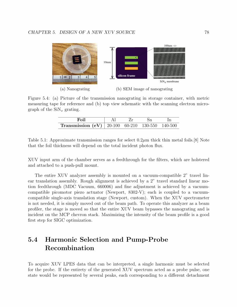
CHAPTER 5. DESIGN OF A NEW XUV SOURCE 78
(a) Nanograting
10mm
silicon frame
SiNx membrane
100nm
(b) SEM image of nanograting
Figure 5.4: (a) Picture of the transmission nanograting in storage container, with metricmeasuring tape for reference and (b) top view schematic with the scanning electron micro-graph of the SiNx grating.
Foil Al Zr Sn InTransmission (eV) 20-100 60-210 130-550 140-500
Table 5.1: Approximate transmission ranges for select 0.2µm thick thin metal foils.[8] Notethat the foil thickness will depend on the total incident photon flux.
XUV input arm of the chamber serves as a feedthrough for the filters, which are holsteredand attached to a push-pull mount.
The entire XUV analyzer assembly is mounted on a vacuum-compatible 2” travel lin-ear translation assembly. Rough alignment is achieved by a 2” travel standard linear mo-tion feedthrough (MDC Vacuum, 660006) and fine adjustment is achieved by a vacuum-compatible picomotor piezo actuator (Newport, 8302-V); each is coupled to a vacuum-compatible single-axis translation stage (Newport, custom). When the XUV spectrometeris not needed, it is simply moved out of the beam path. To operate this analyzer as a beamprofiler, the stage is moved so that the entire XUV beam bypasses the nanograting and isincident on the MCP chevron stack. Maximizing the intensity of the beam profile is a goodfirst step for SIGC optimization.
5.4 Harmonic Selection and Pump-Probe
Recombination
To acquire XUV LPES data that can be interpreted, a single harmonic must be selectedfor the probe. If the entirety of the generated XUV spectrum acted as a probe pulse, onestate would be represented by several peaks, each corresponding to a different detachment

CHAPTER 5. DESIGN OF A NEW XUV SOURCE 79
harmonic. This can be experimentally accomplished by several means—including by imple-mentation of a transmission grating monochromator[9] or multilayer mirrors (MLMs). Wehave opted to implement a MLM because of its simple geometry and ease of alignment.
Multilayer mirrors comprise nanolayers of alternating materials with high and low refrac-tive indices and atomic numbers.[10] As such, MLMs act as interference reflectors, where thelayer thicknesses and angle of incidence are optimized to fulfill the Bragg equation for somepeak wavelength, λmax. This is given by Equation 5.2, where m is the order of the reflection,n is the refractive index, θ is the angle of incidence, and d = dA + dB is the structure periodfor materials A and B of thicknesses dA and dB, respectively. A schematic of a MLM is alsoshown in Figure 5.5.
mλmax ≈ 2ndcosθ (5.2)
Modern MLMs consist of tens to hundreds of alternating layers, and are commonly madeof molybdenum and silicon (Mo/Si). An ideal Mo/Si multilayer with 100 layers will havea reflectivity near 70% for 80-120eV photons at a 90 angle of incidence.[11] This is thetheoretical upper limit for the reflectivity of current Mo/Si MLMs.
Of chief interest to the XUV LPES application is the spectral bandwidth (λ/∆λ)—or selec-tivity—of the MLM. Although the reflectivity of MLMs is generally good, the selectivity canbe problematic.[12] The bandwidth may include multiple harmonics, and if the reflectivityof the undesirable harmonic is too large, the MLM cannot fulfill its primary function. Twoidentical MLMs near normal incidence have been used by others to increase the selectivity(< 10% contribution from neighboring harmonics), but the reflectivity drastically drops,often to under 10%.[13]
An active line of communication has been opened with Eric Gullikson at the Center forX-ray Optics at Lawrence Berkeley Laboratory.6 He has suggested that, for our initial targetregime of 20-100eV, a 45 angle of incidence MLM be selected. Consequently, we will firsttest if the selectivity of one MLM of this type is sufficient for the purposes of XUV LPES.This preliminary geometry is reflected in the apparatus scheme shown above in Figure 5.1.
After the harmonic is selected, it will be focused onto the liquid microjet with a toroidalmirror (ARW Optical Corporation) on a motorized, vacuum-compatible mount. Ratherconveniently, the fundamental laser beam travels a roughly equivalent path as the XUVharmonics, and can be used for alignment purposes before pump down. To collinearlyrecombine the pump and probe arms, the OPA-generated UV pump will be sent into vacuumand reflect off of an annular mirror with a dielectric UV high-reflectance coating. The beam
6CXRO is a world leader in multilayer coating research and their databases are extraordinarily useful.

CHAPTER 5. DESIGN OF A NEW XUV SOURCE 80
Incident beam Reflected beams
dA
dB
d
φ
Substrate
A
B
Figure 5.5: Schematic of a MLM, labeled in accordance with Equation 5.2. Adapted fromReference [10].
diameter of the XUV probe is significantly smaller than that of the UV pump, and will besent through the hole in the center of the mirror. To protect the optics from frozen microjetdebris, a gate valve will be implemented and a beamline skimmer is recommended.
5.5 References
1. Moore, J. H., Davis, C. C. & Coplan, M. A. Building scientific apparatus 4th ed.(Cambridge University Press, 2009).
2. Hosler, E. R. Ultrafast strong-field vibrational dynamics dtudied by femtosecond extreme-ultraviolet transient absorption spectroscopy PhD dissertation (UC Berkeley, 2013).
3. Attar, A. R. Photochemical reaction dynamics studied by femtosecond soft X-ray tran-sient absorption spectroscopy PhD dissertation (UC Berkeley, 2016).
4. Bacellar C. Silveira, C. Ultrafast dynamics in helium nanodroplets probed by XUV spec-troscopy and X-ray imaging PhD dissertation (UC Berkeley, 2017).
5. Kornilov, O., Wilcox, R. & Gessner, O. Nanograting-based compact vacuum ultravioletspectrometer and beam profiler for in situ characterization of high-order harmonicgeneration light sources. Rev. Sci. Instrum. 81, 063109 (2010).
6. Savas, T. A., Shah, S. N., Schattenburg, M. L., Carter, J. M. & Smith, H. I. Achromaticinterferometric lithography for 100-nm-period gratings and grids. J. Vac. Sci. Technol.B Microelectron. Nanometer Struct. Process. Meas. Phenom. 13, 2732 (1995).

CHAPTER 5. DESIGN OF A NEW XUV SOURCE 81
7. Savas, T. A., Schattenburg, M. L., Carter, J. M. & Smith, H. I. Large-area achromaticinterferometric lithography for 100 nm period gratings and grids. J. Vac. Sci. Technol.B Microelectron. Nanometer Struct. Process. Meas. Phenom. 14, 4167 (1996).
8. Center for X-ray Optics filter transmission engine http://henke.lbl.gov/optical_
constants/filter2.html (accessed November 22, 2017).
9. Von Conta, A., Huppert, M. & Worner, H. J. A table-top monochromator for tun-able femtosecond XUV pulses generated in a semi-infinite gas cell: Experiment andsimulations. Rev. Sci. Instrum. 87, 073102 (2016).
10. X-ray data booklet http://xdb.lbl.gov (accessed November 22, 2017).
11. Multilayer coatings: A mini-tutorial http://henke.lbl.gov/multilayer/mltutor.
html (accessed November 22, 2017).
12. Gullikson, E. M. et al. Molybdenum/silicon multilayer components for high harmonicgeneration sources. Appl. Opt. 54, 4280 (2015).
13. Zurch, M. et al. Real-time and sub-wavelength ultrafast coherent diffraction imagingin the extreme ultraviolet. Sci. Rep. 4, 7356 (2014).

82
Part IV
Appendices

83
Appendix A
Principles of Ultrafast Lasers
A.0.1 Light Amplification by Stimulated Emission of Radiation
A laser is an optical device that amplifies light through stimulated emission to produce ahighly directional, coherent source of radiation.1[1, 2] Lasers can be operated in several differ-ent configurations, but this discussion will focus on continuous-wave (cw) and mode-lockedlasers. Continuous-wave lasers are continuously pumped, and continuously lase. Mode-lockedlasers emit a train of ultrafast laser pulses at some repetition rate.
Lasers can be simply constructed out of a gain medium, sandwiched between two mirrors,that is optically pumped to excite the medium. Initially, light is spontaneously emitted fromthe medium subsequent to excitation. Light propagating along the length of the cavitydefined by the two mirrors is captured and used to stimulate emission in the medium. Witheach pass, successively more photons stimulate emission. If one mirror is ∼1% transmissive,the laser light can be extracted for experiments.
Spontaneous and stimulated emission can be described by Einstein coefficients.[3] If weassume that the ground state is given by |1〉 and the excited state by |2〉, these coefficientsare given by Equations A.1 and A.2, where gi is the degeneracy of state i, hν is the photonenergy, and c is the speed of light. B12 is absorption (|1〉 + hν → |2〉), B21 is stimulatedemission (|2〉+ hν → |1〉+ 2hν), and A21 is spontaneous emission (|2〉 → |1〉+ hν).
B12 =g2
g1
B21 (A.1)
1“L.A.S.E.R.” is an acronym for light amplification by stimulated emission of radiation.
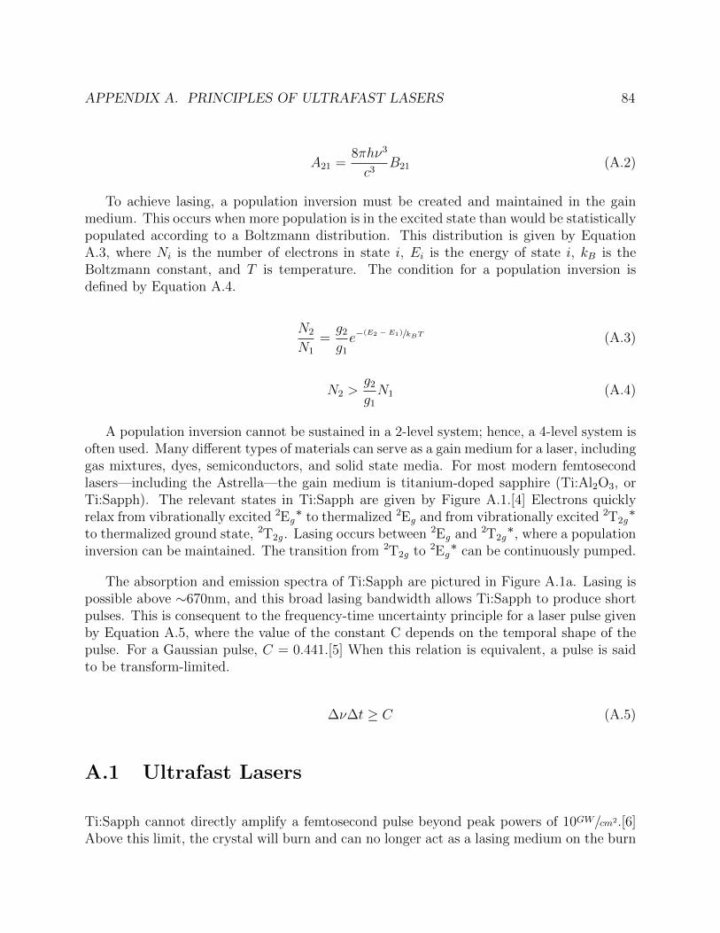
APPENDIX A. PRINCIPLES OF ULTRAFAST LASERS 84
A21 =8πhν3
c3B21 (A.2)
To achieve lasing, a population inversion must be created and maintained in the gainmedium. This occurs when more population is in the excited state than would be statisticallypopulated according to a Boltzmann distribution. This distribution is given by EquationA.3, where Ni is the number of electrons in state i, Ei is the energy of state i, kB is theBoltzmann constant, and T is temperature. The condition for a population inversion isdefined by Equation A.4.
N2
N1
=g2
g1
e−(E2 − E1)/kBT (A.3)
N2 >g2
g1
N1 (A.4)
A population inversion cannot be sustained in a 2-level system; hence, a 4-level system isoften used. Many different types of materials can serve as a gain medium for a laser, includinggas mixtures, dyes, semiconductors, and solid state media. For most modern femtosecondlasers—including the Astrella—the gain medium is titanium-doped sapphire (Ti:Al2O3, orTi:Sapph). The relevant states in Ti:Sapph are given by Figure A.1.[4] Electrons quicklyrelax from vibrationally excited 2Eg* to thermalized 2Eg and from vibrationally excited 2T2g*
to thermalized ground state, 2T2g . Lasing occurs between 2Eg and 2T2g*, where a populationinversion can be maintained. The transition from 2T2g to 2Eg* can be continuously pumped.
The absorption and emission spectra of Ti:Sapph are pictured in Figure A.1a. Lasing ispossible above ∼670nm, and this broad lasing bandwidth allows Ti:Sapph to produce shortpulses. This is consequent to the frequency-time uncertainty principle for a laser pulse givenby Equation A.5, where the value of the constant C depends on the temporal shape of thepulse. For a Gaussian pulse, C = 0.441.[5] When this relation is equivalent, a pulse is saidto be transform-limited.
∆ν∆t ≥ C (A.5)
A.1 Ultrafast Lasers
Ti:Sapph cannot directly amplify a femtosecond pulse beyond peak powers of 10GW/cm2.[6]Above this limit, the crystal will burn and can no longer act as a lasing medium on the burn

APPENDIX A. PRINCIPLES OF ULTRAFAST LASERS 85
400 500 600 700 800 900 1000
Wavelength (nm)
1.0
0.5
Inte
nsi
ty (
arb)
EmissionAbsorption
(a) Absorption and emission spectra
2Eg
2T2g
Energy
hνlasinghνpump
(b) Energy level diagram
Figure A.1: (a) Ti:Sapph absorption and emission spectra, where lasing can only occur atemission wavelengths that do not overlap with the absorption region, and (b) the energylevels relevant to the lasing transition in Ti:Sapph. Adapted from [1] and [4].
spot. The Kerr lens effect—the non-linear effect whereby intense coherent light will modifythe refractive index of a material and consequently self-focuses in the material—furtheraggravates this condition.[1] To circumvent damage while still amplifying the peak powerbeyond the damage threshold of Ti:Sapph, chirped pulse amplification (CPA) is used. Thiscomprises three steps: 1) the “seed” pulse is stretched in time to reduce the peak power, 2)the seed is amplified, 3) the amplified pulse is re-compressed to its original pulse duration.[7]The seed pulse dictates the amplified laser pulse properties.
To generate the seed pulse, an oscillator is used. This is a laser which generates pulsesthrough so-called “Kerr lens mode-locking.”[1] Then, CPA is used to amplify the power ofthis pulse by orders of magnitude for use in experiments. Mode-locking occurs when thestanding laser modes inside the oscillator cavity are forced into equal phase. This results ina wave interference pattern that generates an intense, short burst of light. If the oscillatoris not properly mode-locked, the laser will be cw. Kerr lens mode-locking uses the Kerr lensself-focusing phenomenon to suppress cw operation and establish stable mode-locking.2 Kerrlens mode-locking is illustrated in Figure A.2 and the repetition rate, τ , is given by EquationA.6, where L is the cavity length.
2Generally, oscillators are either passively or actively mode-locked. In active mode-locking an acousto-optical modulator or electro-optical modulator is used to sustain mode-locking.

APPENDIX A. PRINCIPLES OF ULTRAFAST LASERS 86
Inte
nsi
ty
Frequency
Laser output
Cavity modes
Gain bandwidth
Figure A.2: Principles of Kerr lens mode-locking. The gain bandwidth is the frequencyregion that the cavity can mode-lock, the cavity modes are all possible modes, and the laseroutput is the modes which are selected through Kerr lens mode-locking. Adapted fromReference [1].
τ =c
2L(A.6)
Pulses are stretched and re-compressed with the aptly named stretcher and compressorcomponents, which are typically gratings. These can be single gratings or pairs of gratings,and can be reflective or transmissive. Regardless, the stretcher and compressor are matchedso that the compressor can undo the work of the stretcher once the pulse is fully amplified.The gratings change the pulse duration by introducing group velocity dispersion (GVD)—or“chirp”—into the pulse. Group velocity dispersion is the spectral separation of a pulsein time and the grating accomplishes GVD through spectral dispersion. When a pulse is“negatively chirped,” the red edge leads the blue edge (see Figure A.3).
Once the seed passes through the stretcher, it will be sent to the amplifier. Amplifiercavities come in many designs, but can generally be either classified as regenerative or multi-pass.[1, 5] This discussion will focus on regenerative amplifiers (regens), like the Spitfire and

APPENDIX A. PRINCIPLES OF ULTRAFAST LASERS 87
Figure A.3: Schematic of how a stretcher assembly introduces negative chirp.
seed
pump
Pockels cell
(input)
Pockels cell
(output)
λ/4
thin film
polarizer
to compressor
Ti:Sapph
Figure A.4: Example regen design. The first Pockels cell picks the input pulse by flippingthe polarization of the seed so the pulse is trapped in the cavity. After some time, the secondPockels cell flips the polarization of the amplified light so that it will reflect off of the thethin film polarizer and be sent to the compressor. The cavity beam path, and the inputlocations of the pump and seed beams, are indicated. Adapted from Reference [4]
Astrella.3 A simple regen design is given in Figure A.4.
Pulses are trapped in a cavity by their polarization, which can be rotated by a Pockelscell—an electro-optic device that acts as a 1/4-waveplate when a high voltage is applied.[1, 5]A thin film polarizer and one or more Pockels cell can be used both to let a seed pulse in foramplification, and subsequently kick the amplified pulse out to be re-compressed. Pockelscells do not perfectly pick pulses—a small fraction of the previous and subsequent pulse inthe pulse train often leak out. The Pockels cells are birefringent, and this ultimately limitsthe contrast ratio of the main pulse to the pre- and post-pulses. A contrast ratio of 1000:1and 100:1 are expected for the main pulse to the pre- and post-pulses, respectively.
Pulses are picked-off and sent to the compressor after they have made enough round trips
3The KM Labs Dragon used in the gas-phase TRPES project is a multi-pass amplifier.

APPENDIX A. PRINCIPLES OF ULTRAFAST LASERS 88
to reach maximum gain. After this point, each successive pass in the cavity results in lossesthat reduce the total gain. Generally the pulse with the highest intensity gives the bestpower, but the pulse after this in the cavity pulse train gives the most stable output withminimal power losses. A well aligned cavity will have the smallest possible build up time(i.e. require the fewest number of passes to reach gain saturation).
A.2 Alignment Notes for New Ultrafast Laser System
A.2.1 Astrella
Much of the Astrella is closed-box,4 and, as such, the Verdi-G, Revolution, Vitara, andstretcher/compressor components cannot be self-serviced. However, the Vitara output, Revooutput, and Astrella cavity can be aligned and characterized. The diagnostic and alignmentprocedures for the Verdi, Revolution, and Astrella amplifier cavity are provided below.
The Verdi-G is a 5W pump laser, that is set to 3W. Pumped at 3W, the Vitara oscillatorshould give ∼200mW of seed into the stretcher unit. The Astrella can be seeded with aslittle as 10mW, but an order of magnitude more power is typical. The alignment of the seedinto the stretcher and cavity regions is straightforward. Two mirrors before the stretchermodule can be used to align the seed onto an iris into the stretcher and a cross hatch at theopposite side of the module. This cross hatch catches a higher-order dispersion off of thestretcher grating. To align into the cavity, the two steering mirrors at the stretcher moduleexit are aligned onto preset irises.
A beamsplitter before the stretcher diverts some of the Vitara beam to an output portwhich can be uncovered so the seed can be analyzed when necessary. Notably, the Vitaraspecrum is normally double-bumped. Part of the 800nm is blocked so it does not dominatethe spectrum and a wider bandwidth (∼85nm) can be achieved. Finally, the Vitara is themaster trigger for the entire experiment, and runs at 80MHz. The fast photodiode insidethe oscillator is hooked into the back of the synchronization and delay generator (SDG) box.If this is hooked into an oscilloscope, the amplitude of the peaks should be above 500mV,otherwise the bandwidth detector interlock will be triggered and the rest of the system willturn off.
The Revolution threshold is ∼10.5A; lasing in the Astrella cavity begins around 12-15A.An internal power meter provides a constant power readout on the Revolution software, but,
4i.e. void warranty if opened

APPENDIX A. PRINCIPLES OF ULTRAFAST LASERS 89
because this includes the afterburner, the reported value is ∼2W higher than the actualpower. To measure the power out, a frosted mirror has been provided and is bolted next tothe Revolution. This can be moved into the beamline at the Revolution output and act asa pick-off mirror so the power can be accurately measured. The Revolution is a slave to theVitara, and is triggered off of channel D4 on the SDG. Finally, the Revolution cavity has atransit time of 9ns, while the Astrella amplifier cavity has a transit time of 12ns. About 14round trips, or about 132ns of build-up time, are required in the amplifier.
Below is a brief summary of some important notes on the Astrella’s amplifier cavity.
• The amplified spontaneous emission (ASE) and burn-in reduction time should alwaysbe checked when the amplifier cavity is re-aligned or the power out is low but the seedalignment looks good. To measure these, block the seed after the stretcher and openup the timing on the second Pockels cell until the power of the ASE is equivalent tothe seeded power, when both are measured into the compressor. The burn-in reductiontime on a good cavity alignment should be ∼35ns. Slight ridging in the ASE spectrumis normal, and is caused by the Pockels cells.
• Whenever the amplifier cavity has been realigned from scratch, the delay on the secondPockels cell should be closed down to ∼30ns to keep the power low when realigning thecompressor. This protects the gratings in the compressor unit from accidental burns.The Astrella output just barely passes through the compressor unclipped. If the veryedges image the grating, the alignment is acceptable.
• The pre-pulse contrast is 1000:1 for this system. The post-pulse contrast is 100:1.
• Before the output of the Astrella is sent through a beamsplitter, it must be expandedand collimated. Any passage through transmissive optics for such short-duration, high-energy pulses can cause self-phase modulation and GVD that can considerably distortthe pulses. These effects can be mitigated by expanding the beam diameter withreflective telescope optics.
• To align the amplifier cavity, first align the seed with the irises, then tweak on thecavity end mirrors for the most efficient buildup in the cavity. This can be measuredby hooking the amplifier photodiode into an oscilliscope. Then, the Revolution pumpand afterburner can be aligned for the best power. The power should be ∼9.3W asmeasured before the iris into the compressor.
A.2.2 White-Light TOPAS-Prime with NiRUVis Extension
The purpose of this section is to elaborate on alignment procedures for the TOPAS-Prime.The beam layout and a description of the operation of the TOPAS-Prime can be found in

APPENDIX A. PRINCIPLES OF ULTRAFAST LASERS 90
its user’s manual (p.p. 19-29), and is not reproduced herein. This discussion will adhere tothe labeling convention for various optics that is established in the manual.
A.2.2.1 Alignment Notes for a Quick Tune-Up
1. Align the pump onto the removable pinhole after NC2 with the first telescope lens(labeled T3) into the TOPAS-Prime.
2. Align the white light continuum (WLC) onto the same pinhole with the turning mirrorinto the unit (labeled WL).
3. Tweak the alignment for power and far-field alignment with M5. If needed, tweak DM3to improve the fresh pump alignment.
A.2.2.2 Full Alignment Notes
1. Check the rough alignment into the TOPAS-Prime and adjust it with the two telescopelenses (T3 and T4) and WL directly before the unit. Keep the flag down, and dialdown the power out of the Astrella if the alignment is potentially dramatically off. Thebeam diameter should be 11mm into the TOPAS-Prime.
2. Align the first pass: Block the first pass pump before L5, and verify that the WLC iscentered onto A2. The WLC should be focused in NC1. Then, unblock the first passpump and verify that it is focused after NC1. L5 can be moved to adjust the focus.Tweak M3 and M4 as needed to align the pump onto the WLC. Finally, move the flagin front of M5 as needed. Only the signal should pass the flag, if the pump passes itcould damage M5. Check the alignment at 1300nm and 1500nm, as the position of thesignal onto M5 will be slightly different for each.
a) Note that the pump and the WLC are non-collinear.
b) The first stage amplification generates the WLC and impacts the output powergreatly. If the output power drops significantly when the signal is tuned between1300 and 1500nm, the alignment of the first pass is not good.
c) After M5, there should be 2-3mW of seed at 1300nm, and ∼1mW at 1500nm.
3. Use M5 to align the seed onto NC2, and use DM1 for power after NC2. At 1300nm,there should be∼2mW of signal. The seed should be uniformly bright and pass throughNC2 without significantly clipping.
4. Align the second pass: Use M8 to align the second pass pump onto the removablepinhole after NC2. To align the second pass pump onto the seed signal in the far field,

APPENDIX A. PRINCIPLES OF ULTRAFAST LASERS 91
use DM2. The manual delay of M8 will need to be tweaked for the best temporaloverlap by looking at the intensity of the far field output.
a) At 1300nm, there should be ∼320mW after the second stage amplification; at1500nm, the power should not change by more than 30mW.
5. Align the fresh pump: Remove the external set screw to access M15. Use M15 to alignthe fresh pump to the TOPAS-Prime output at the entrance of the NiRUVis Extensionunit. Then, use DM3 to align the pump and TOPAS-Prime output at the exit of theNiRUVis Extension. When the two beams are spatially overlapped, move the freshpump delay (M16/M17 retroreflector) to optimize power. The Astrella compression orthe mixing crystal angle may also need to be tweaked.
a) To filter out the sum frequency signal, the 400nm high-reflector can be put intothe NiRUVis Extension.
A.3 Pulse Characterization
Characterization of laser pulses is critical to time-resolved experiments. To meaningfullyreport a lifetime, τ , the pump-probe cross-correlation, σ, must be shorter than τ . Moreover,the temporal profile of the pulse can act as a diagnostic tool for the laser system. Thereare a number of techniques we employ to characterize our pulses, including cross-correlationand frequency-resolved optical gating (FROG) measurements.
A.3.1 Autocorrelation, Cross-Correlation and FROG
To measure the pulse duration of ultrafast lasers, the pulses are typically used to measurethemselves.[8] The simplest device used to perform such a measurement is an intensity auto-correlator.[9] Here, the input pulse is split into the two arms of a Michelson interferometerby a beamsplitter. The arms are delayed relative to each other by the interferometer andthen non-collinearly recombined inside a non-linear crystal to frequency-double the pulses bysecond-harmonic generation (SHG). The intensity of SHG depends on the temporal overlapof the two pulses, according to Equation A.7, where I(auto) is the time-dependent intensityof the frequency-doubled light, I(t) is the time-dependent intensity of the input light, and t
′
is the relative time delay.
I(auto)(t, t′) ∝ I(t)I(t− t′) (A.7)

APPENDIX A. PRINCIPLES OF ULTRAFAST LASERS 92
However, the diode array detectors inside most autocorrelators are too slow to record thisin real-time, and instead they measure the intensity convolution, A(t
′), given by Equation
A.8. This is the intensity “autocorrelation”.
A(auto)(t′) =
∫ ∞−∞
dtI(t)I(t− t′) (A.8)
This is called a “cross-correlation” if the pulses are not identical (e.g. not the samewavelength). A(t
′) is now described by Equation A.9, where subscripts a and b denote the
different pulses.
A(cross)(t′) =
∫ ∞−∞
dtIa(t)Ib(t− t′) (A.9)
Importantly, if we assume that the pulses have a Gaussian temporal profile, then theconvolution will return a Gaussian whose width5 (variance, σ) is described by EquationA.10, where σcross is the width of the cross-correlation and σa and σb are the widths of pulsesa and b, respectively.
σ2cross = σ2
a + σ2b (A.10)
As we have seen, in order to return meaningful information about the pulse width, wemust assume a pulse shape (e.g. Gaussian, sech). This is a major shortcoming of theautocorrelation technique. Furthermore, this approach cannot provide insight into pulsedistortions; we employ FROG to obtain this information.
FROG is an autocorrelation measurement that is spectrally resolved—the time and fre-quency domain measurements are made simultaneously.[10] The intensity of a FROG traceis given by Equation A.9, where E(t) is the time-dependent laser field of frequency ω.
I(ω, t′) =
∣∣∣ ∫ +∞
−∞dtE(t)|E(t− t′)|2e−iωt
∣∣∣2 (A.11)
When the spectral and temporal profiles of the input pulse are measured in this way,the temporal pulse shape, the pulse width, the spectral bandwidth, and any chirp in thepulse can be recorded. Recovery of the intensity and phase information requires solving a
5Note, pulses are often reported by full width at half maximum (FWHM), where FWHM = 2√
2ln(2)σor as the average single pulse duration, FWHM/
√2.

APPENDIX A. PRINCIPLES OF ULTRAFAST LASERS 93
2D phase-retrieval problem. A functional form is imposed on the pulse, typically by SHG,allowing for this problem to be uniquely solved.
Our project uses a GRating-Eliminated No-nonsense Observation of Ultrafast IncidentLaser Light E-fields, or GRENOUILLE, in lieu of a traditional FROG. This design uses aFresnel biprism and a thick SHG crystal instead of an interferometer and a spectrometer,respectively, but recovers the same information as a FROG in a much more compact andinexpensive design.
A.3.2 Finding Time Zero
For all TRPES experiments, two time-stamps must be measured: the time when the pumppulse first hits the microjet and the time when the pump and the probe pulses are maxi-mally overlapped (time zero, or t0). Determining when the laser hits the microjet is fairlystraightforward. Light scatters off of the microjet and is energetic enough to cause an elec-tron cascade on the MCP. Because this light travels faster than any electron, and becausethe scope only bins 2ns, we assume this electron cascade is a good estimate for the timewhen the laser pulse hits the microjet. We set the trigger for the scope (which is sent fromthe Astrella’s SDG box) to be 16ns after this laser spike; this time delay must be re-addedback when converting data from ToF to eKE.
To find time-overlap of the pump and probe pulses, the path length of each arm is firstmeasured and adjusted to be roughly equivalent. Overlap can then be found in one of twoways. Conventionally, the UV pump and probe pulses are independently difference-frequencymixed with residual 800nm that is on a delay line at the entrance of the liquid microjetchamber. A thin window is set before the mixing BBO crystal (90µm, 45) to account forthe additional delay added from the entrance window of the liquid microjet chamber. Thetransmitted light is then spatially separated by wavelength with a Pellin Broca prism so theDFG signal can be readily seen. A thicker BBO can be initially used because it generates abrighter DFG signal. Because the TOPAS-Prime line is fixed, it is first mixed with 800nm.Once overlap is established between the two, the 800nm stage position is fixed and thenmixed with the quadrupler or tripler arm, which is also on a delay line. Alternatively, time-overlap of the pump and probe can be found on the microjet itself. Solvated electrons arereadily generated in aqueous solutions of 100mM potassium iodide and give strong signalnear ToF 800ns when the pump and probe pulses are overlapped in space and time. This isoften the preferred approach to finding t0 because of its simplicity.

APPENDIX A. PRINCIPLES OF ULTRAFAST LASERS 94
A.3.3 Instrument Response Function
The cross-correlation of the pump and probe pulses is the instrumental response function(IRF) in our experiment. Traditionally, we have directly measured this by independentlydifference-frequency mixing residual fundamental with the pump and probe pulses beforethe microjet trap chamber entrance window, as described above. By varying the delay timebetween one pulse relative to the other and measuring the intensity of the DFG light on aphotodiode, we can recover the cross-correlation of two pulses. From these cross-correlations,we can back out the cross-correlation of the pump and probe together.6 This process is oftenlabor-intensive, particularly for the fourth harmonic. We can also fit our data, as describedin Section 2.5, to return the IRF.
A.4 References
1. Femtosecond laser pulses: Principles and experiments 2nd ed. (ed Rulliere, C.) (Springer,2005).
2. Paschotta, R. Field guide to: Lasers (SPIE Press, 2008).
3. Hilborn, R. C. Einstein coefficients, cross sections, f values, dipole moments, and allthat. Am. J. Phys. 50, 982 (1982).
4. Spitfire: Ti:Sapphire regenerative amplifier systems user’s manual (Spectra Physics,2004).
5. Paschotta, R. Field guide to: Laser pulse generation (SPIE Press, 2008).
6. Francois Salin, J. S. & Piche, M. Mode locking of Ti:Al2O3 lasers and self-focusing: aGaussian approximation. Opt. Lett. 16, 1674 (1991).
7. Elkins, M. H. Dynamics of electron relaxation studied using time-resolved photoelectronspectroscopy in liquid microjets PhD dissertation (UC Berkeley, 2015).
8. Swamp Optics: Tutorials http://www.swampoptics.com/tutorials.html (accessedNovember 25, 2017).
9. Swamp Optics tutorial: Intensity autocorrelation http://www.swampoptics.com/
assets/tutorials_autocorrelation-2015.pdf (accessed November 25, 2017).
10. Swamp Optics tutorial: FROG http://www.swampoptics.com/assets/tutorials-
frog-2015.pdf (accessed November 25, 2017).
6Mixing the pump and probe directly in a BBO would require a non-physical angle.

95
Appendix B
Updated Code for ExecutableComputer Programs
B.1 Automated Background Scans
The original LabVIEW code (termed a virtual instrument, or VI) was written by AlexanderT. Shreve, and is detailed in his dissertation. This code was then modified in early 2014to enable automated background scans. A code flow diagram for the new block diagramcomponents is presented in Figure B.1, and described herein.
To acquire data for each delay, the VI first compares the number of scans taken at a delayto the target number of scans. These values are located in the configuration table CSV file,which is updated by the VI after data is taken at each delay position. The vectors for theacquired and target number of scans are compared and the result is fed into a case structure.If the two vectors are not equal, the first stage position with the least number of scans isselected and the stage is instructed to move accordingly. If the stage position correspondsto the ASCII character “a”, “b”, or “c,” the background character is read and written tothe Arduino UNO so the appropriate beam can be blocked. For all other stage positions,the code writes “0” to the Arduino UNO to instruct all servo motors to move to unblockedpositions. For more details regarding the Arduino UNO and servo motors, see Section 2.4.
B.2 Arduino Servo Motors
Arduino Software is an open-source integrated development environment that allows theuser to write programs (called sketches) and upload them to a microcontroller board. The

APPENDIX B. UPDATED CODE 96
Query: are acquired and
target vectors equal?
Query: does the stage
need to be moved to
acquire a bacground scan?
Read ASCII characterQuery: is the smallest
value of the acquired scans
less than the largest value?
Write ASCII character
to Arduino UNO
Write “0” to
Arduino UNO
TRUE
TRUE
TRUE
CONTINUE
CONTINUE
Figure B.1: LabVIEW code flow for automated background scans.
beam blocks are controlled by an Arduino UNO board.1 This device has digital and analogI/O ports, a USB interface, and a 5V power pin. Three high-torque standard servo motorsequipped with home-built flags are used to block laser pulses. The flags are rotated into andout of position by the drive shaft of a servo. The rotation of the shaft is determined by pulsewidth modulation signals sent from the UNO and can vary between 0 and ±90. Servosrun on 5V DC. Beam block positions are set to 45 because the mechanical stop mechanismat 90 introduces a slight jitter.
Below is the sketch that was written to the UNO to control these motors. Digital pinouts9, 10, and 11 are attached to the servo objects and the motion of the motors is controlledthrough a switch statement. The LabVIEW data acquisition code will send an ASCII charac-ter to the UNO, and the servo motors will rotate to different positions based on the characterreceived. Character “a” blocks beam 1, “b” blocks beam 2, and “c” blocks beam 3. Whenone beam is blocked, the other two servos are set to unblock their beams. All other characterswill command all three beams to be unblocked.
1This device is commonly used by hobbyists interested in robotics and is inexpensive (∼30USD).

APPENDIX B. UPDATED CODE 97
#include <Servo.h> // call the servo library
Servo beam1; // create a servo object to control each servo
Servo beam2;
Servo beam3;
void setup()
beam1.attach(9); // attach servos on pins to servo object
beam2.attach(10);
beam3.attach(11);
Serial.begin(9600); //connect to USB port
// Initialize the servos to the baseline
beam1.write(45);
beam2.write(45);
beam3.write(45);
// block and unblock beams one at a time with a switch statement
void loop()
// get the number of bytes available to read from the serial port
if (Serial.available() > 0)
int inByte = Serial.read(); //read incoming byte
// choose between several discrete options
switch (inByte)
case 'a' : // beam1 blocked
beam1.write(135);
beam2.write(45);
beam3.write(45);
break;
case 'b' : // beam2 blocked
beam1.write(45);
beam2.write(135);
beam3.write(45);
break;
case 'c' : // beam3 blocked
beam1.write(45);

APPENDIX B. UPDATED CODE 98
beam2.write(45);
beam3.write(135);
break;
default: // if nothing matches, unblock all
beam1.write(45);
beam2.write(45);
beam3.write(45);
delay(15);
Serial.write(inByte);

99
Appendix C
Machine Drawings for New XUVLiquid Microject PhotoelectronSpectroscopy Project

APPENDIX C. MACHINE DRAWINGS FOR XUV LPES 100
Figure C.1: SIGC vacuum chamber machine drawing. The 10” to 8” CF reducing tee waspurchased with flanges, and the 2-3/4” CG half nipples were installed by the College ofChemistry machine shop. The bottom 10” CF flange is rotatable; all other flanges are fixed.All components are made from stainless steel (304 SS).

APPENDIX C. MACHINE DRAWINGS FOR XUV LPES 101
Figure C.2: SIGC machine drawing. The 1-1/3” mini-CF tee was purchased and used as is,and the 2-3/4” CF flange is rotatable. The end cap is pictured in Figure C.3. The cap ismade from stainless steel (304 SS).

APPENDIX C. MACHINE DRAWINGS FOR XUV LPES 102
Figure C.3: SIGC end cap machine drawing, and is made from stainless steel (304 SS).

APPENDIX C. MACHINE DRAWINGS FOR XUV LPES 103
Figure C.4: Nanograting holster machine drawing. Tabs are drilled into the corners of the0.4” × 0.4” shelf to house dabs of epoxy, which will be used to affix the nanograting to theholster. These are not shown in the drawing. The holster is made from aluminum.

APPENDIX C. MACHINE DRAWINGS FOR XUV LPES 104
Figure C.5: MCP and phosphor holster machine drawing. Toe clamps will be used to fastenthe holster to the breadboard of the stage. The holster is made from aluminum.

APPENDIX C. MACHINE DRAWINGS FOR XUV LPES 105
Figure C.6: MCP retaining ring, made of aluminum.

APPENDIX C. MACHINE DRAWINGS FOR XUV LPES 106
Figure C.7: The holster for the aluminum utility mirror. Two strips of Teflon sit over the8-32 bolt holes to hold the mirror in place. Toe clamps will be used to fasten the holster tothe stage breadboard. The holster is made of aluminum.

APPENDIX C. MACHINE DRAWINGS FOR XUV LPES 107
Figure C.8: A microjet catcher made of stainless steel. When placed a few millimeters underthe microjet to the catcher can reduce the pressure in the microjet chamber.

108
Appendix D
Publications from Graduate Work
1. Elkins, M. H., Williams, H. L., Shreve, A. T. & Neumark, D. M. Relaxation mech-anism of the hydrated electron. Science 342, 1496 (2013).
2. Elkins, M. H., Williams, H. L. & Neumark, D. M. Dynamics of electron solvationin methanol: Excited state relaxation and generation by charge-transfer-to-solvent. J.Chem. Phys. 142, 234501 (2015).
3. Elkins, M. H., Williams, H. L. & Neumark, D. M. Isotope effect on hydrated electronrelaxation dynamics studied with time-resolved liquid jet photoelectron spectroscopy.J. Chem. Phys. 144, 184503 (2016).
4. Williams, H. L., Erickson, B. A. & Neumark, D. M. Time-resolved photoelectronspectroscopy of adenosine and adenosine monophosphate photodeactivation dynamicsin water microjets. In Preparation (2017).

109
Appendix E
Acronyms
Ade Adenine. 47
Ado Adenosine. 17, 47
AMP Adenosine Monophosphate. 17, 47
ASE Amplified Spontaneous Emission. 89
BBO β-Barium-Borate. 40, 68, 93
BOA Born-Oppenheimer Approximation. 8
CD Circular Dichroism. 48
CF ConFlat. 25, 75
CI Conical Intersection. 5, 12, 48
CPA Chirped Pulse Amplification. 85
cw Continuous-wave. 83
DAS Decay Associated Spectrum. 37
DFG Difference-Frequency Generation. 41, 93, 94
DNA Deoxyribonucleic Acid. 2, 17, 46
eBE Electron Binding Energy. 7
eKE Electron Kinetic Energy. 7

ACRONYMS 110
FC Franck-Condon. 9, 48
FGR Fermi’s Golden Rule. 8
FROG Frequency-Resolved Optical Gating. 91
FU Fluorescence Upconversion. 47
FWHM Full Width at Half Maximum. 34, 92
GLA Global Lifetime Analysis. 37
GVD Group Velocity Dispersion. 86
HHG High Harmonic Generation. 66
IRF Instrument Response Function. 36, 51, 94
ISC Intersystem Crossing. 4
MCP Microchannel Plate. 29, 77
MLM Multilayer Mirror. 79
NA Nucleic Acid. 3, 47
NB Nucleobase. 3
OPA Optical Parametric Amplifier. 42, 79
PEEK Polyether Ether Ketone. 22
PES Photoelectron Spectroscopy. 7
regen Regenerative Amplifier. 86
SDG Synchronization and Delay Generator. 88, 93
SFG Sum Frequency Generation. 40, 68
SHG Second Harmonic Generation. 41, 91
SIGC Semi-Infinite Gas Cell. 66, 71
TA Transient Absorption. 47

ACRONYMS 111
TD-DFT Time-Dependent Density Functional Theory. 49
Ti:Sapph Titanium-doped Sapphire. 84
ToF Time-of-Flight. 24
TRPES Time-Resolved Photoelectron Spectroscopy. 10, 47
UV Ultraviolet. 3
VBE Vertical Binding Energy. 10
VI Virtual Instrument. 95
WLC White Light Continuum. 42, 90
XUV Extreme Ultraviolet. 66
XUV LPES XUV Time-Resolved Photoelectron Spectroscopy on Microjets. 66, 73
Copyright © 2022 FDOKUMEN