ORI GIN AL PA PER

Predicting species distributions in poorly-studiedlandscapes

P. A. Hernandez Æ I. Franke Æ S. K. Herzog Æ V. Pacheco ÆL. Paniagua Æ H. L. Quintana Æ A. Soto Æ J. J. Swenson ÆC. Tovar Æ T. H. Valqui Æ J. Vargas Æ B. E. Young

Received: 1 June 2007 / Accepted: 25 October 2007 / Published online: 17 May 2008� Springer Science+Business Media B.V. 2008

Abstract Conservationists are increasingly relying on distribution models to predict

where species are likely to occur, especially in poorly-surveyed but biodiverse areas.

Modeling is challenging in these cases because locality data necessary for model formation

are often scarce and spatially imprecise. To identify methods best suited to modeling in

these conditions, we compared the success of three algorithms (Maxent, Mahalanobis

Typicalities and Random Forests) at predicting distributions of eight bird and eight

mammal species endemic to the eastern slopes of the central Andes. We selected study

species to have a range of locality sample sizes representative of the data available for

endemic species of this region and also that vary in their distribution characteristics. We

found that for species that are known from moderate numbers (N = 38–94) of localities, the

three methods performed similarly for species with restricted distributions but Maxent and

Electronic supplementary material The online version of this article (doi:10.1007/s10531-007-9314-z)contains supplementary material, which is available to authorized users.

P. A. Hernandez (&)2 Parr Street, Toronto, ON, Canada M6J 2E3e-mail: pilar_hernandez@natureserve.org

P. A. Hernandez � L. Paniagua � J. J. Swenson � B. E. YoungNatureServe, Arlington, VA, USA

I. Franke � V. Pacheco � H. L. QuintanaMuseo de Historia Natural, Universidad Nacional Mayor de San Marcos, Lima, Peru

S. K. HerzogAsociacion Armonıa – BirdLife International, Santa Cruz de la Sierra, Bolivia

A. Soto � C. TovarCentro de Datos para la Conservacion, Universidad Nacional Agraria La Molina, Lima, Peru

T. H. ValquiMuseum of Natural Science, Louisiana State University, Baton Rouge, LA, USA

J. VargasColeccion Boliviana de Fauna, Museo Nacional de Historia Natural, La Paz, Bolivia

123

Biodivers Conserv (2008) 17:1353–1366DOI 10.1007/s10531-007-9314-z

Random Forests yielded better results for species with wider distributions. For species with

small numbers of sample localities (N = 5–21), Maxent produced the most consistently

successful results, followed by Random Forests and then Mahalanobis Typicalities.

Because evaluation statistics for models derived from few localities can be suspect due to

the poor spatial representation of the evaluation data, we corroborated these results with

review by scientists familiar with the species in the field. Overall, Maxent appears to be the

most capable method for modeling distributions of Andean bird and mammal species

because of the consistency of results in varying conditions, although the other methods

have strengths in certain situations.

Keywords Maxent � Mahalanobis Typicalities � Model evaluation �Species distribution models � Random Forests

Introduction

Species distribution models (SDMs) are a useful tool for estimating the potential for

species to occur in areas not previously surveyed (Guisan and Thuiller 2005). Models have

utility for conservation (Rodrıguez et al. 2007) because they can (1) direct biological

surveys towards places where species are likely to be found (Raxworthy et al. 2003; Engler

et al. 2004; Bourg et al. 2005), (2) provide a baseline for predicting a species’ response to

landscape alterations and/or climate change (Thuiller 2003; Araujo et al. 2006), and (3)

identify high-priority sites for conservation (Araujo and Williams 2000; Ferrier et al. 2002;

Loiselle et al. 2003; Wilson et al. 2005). Constructing a SDM relies on a description of the

species’ relationship with its environment to depict areas within a region of interest where

the species is likely to occur. The species-environment relationship can either be defined

by a biologist familiar with the species or by analyzing the environmental conditions at

points of known occurrence in a statistical analysis to construct a definition of the species’

relationship with its environment. The analytical approach can be used to model species

whose habitat requirements are poorly understood and can be developed at any spatial

scale. They are limited only by the availability of environmental data and species locality

data. The challenge of using SDMs in poorly-studied landscapes is that the condition of

species locality data available is usually less than ideal for modeling. Data are often not

collected by systematic surveys but instead gathered in an ad hoc fashion from many

different sources, including museum collections, the literature, and unpublished observa-

tions. Collection dates can span many years and often were obtained before the widespread

use of global positioning systems (GPS) and therefore cannot be geo-referenced with high

levels of spatial precision. Finally, the number of records available for any given species is

usually limited because of the lack of survey effort and because species of conservation

concern generally have relatively limited spatial distributions and are therefore infre-

quently observed. Modeling with small numbers of spatially imprecise localities is

challenging but not impossible (Pearson et al. 2007). Numerous species distribution

modeling methods are available (Guisan and Thuiller 2005) and some methods have

proven to be more effective under certain modeling conditions than others (Elith et al.

2006; Hernandez et al. 2006). Our goal here is to test several promising methods for

developing SDMs to determine which yields the best results for a variety of species

occurring in the poorly-surveyed but highly biodiverse region of the eastern slope of the

Andes in Peru and Bolivia.

1354 Biodivers Conserv (2008) 17:1353–1366

123

Recently several comparative analyses have investigated the efficacy of different

methods for modeling species’ distributions (Segurado and Araujo 2004; Elith et al. 2006;

Hernandez et al. 2006; Tsoar et al. 2007). While some methods are more effective at

predicting species’ distributions than others, no one modeling method has proven to be the

best in all situations. Many interacting factors can influence model performance, such as

the quantity and quality of the species occurrence data, the accuracy and completeness (i.e.

inclusion of all relevant factors contributing to the processes driving the species’ distri-

bution pattern) of the environmental data, the spatial scale (extent and size of analysis

unit), and the ecological characteristics of the species being modeled (Segurado and Araujo

2004; Elith et al. 2006; Hernandez et al. 2006; McPherson and Jetz 2007).

When modeling species inhabiting regions that are poorly-surveyed, the purpose may be

to generate potential distribution maps for many species with as much confidence as

possible, thereby providing baseline biological diversity information previously unavail-

able. We have designed our comparative research to identify a modeling method that

would be most effective for achieving these objectives. Previous comparative studies

demonstrated that Maxent, a statistical mechanics approach, performs very well (Elith

et al. 2006; Phillips et al. 2006) even with small samples (Hernandez et al. 2006), thus

making it an obvious candidate. Two new promising methods that use very different

approaches to developing an SDM we also chose for comparison. They are Mahalanobis

Typicalities, a method adopted from remote sensing analyses (IDRISI 2006), and Random

Forests, a model averaging approach to the non-parametric procedure classification and

regression tree (CART) (Breiman 2001). Researchers have demonstrated that both methods

can produce useful results although neither has been formally compared to each other or

Maxent. Here we compare the ability of these three very different methods to predict the

spatial distributions of a sample of 16 montane bird and mammal species on the eastern

slope of the Andes in Peru and Bolivia. The results should provide useful guidance to

practitioners about the best approaches for modeling multiple species’ distributions in

poorly-studied landscapes.

Materials and methods

Species locality data

We modeled the distributions of eight bird and eight mammal species endemic to forested

habitats on the eastern slope of the Andes in Peru and Bolivia (Table 1). The species were

selected to have a range of sample sizes representative of the data available for the 170 bird

and mammal species endemic to the region. Twelve of the selected species have small

samples (5–21 unique records) while the other four have larger samples (38–94 records).

The species selected ranged from having relatively restricted to widespread geographic

distributions throughout the Andes of Peru and Bolivia.

We obtained locality records for each endemic bird and mammal species from natural

history museums, published literature and reliable observational data (see Acknowledge-

ments for list of contributors). When specific geographic coordinates were not provided for

a locality, we used maps and gazetteers to assign geographical coordinates to these records.

Then scientists with expertise in the species’ distribution reviewed the data to correct any

errors in geo-referencing or taxonomic status as reported by the data provider. These

specialists included IF, SKH, THV, VP, JVM, and the scientists listed in the

Biodivers Conserv (2008) 17:1353–1366 1355

123

Acknowledgments. The species locality data were developed as part of a larger study

designed to model hundreds of endemic species of this region (Young 2007).

Environmental data

We used 11 environmental variable layers that described the climatic, topographic and

vegetation cover conditions (Table 2). Each layer was converted to the study’s geographic

projection (a customized Lambert Azimuthal Equal Area), resampled to 1 km resolution (if

provided at a finer resolution) and clipped to the general area where the 16 focal species

occur and buffered by 100 km. Elevation, slope and topographic exposure layers were

derived from the Shuttle Radar Topographic Mission dataset (SRTM; available at

srtm.csi.cgiar.org). Climate data were obtained from the Worldclim bioclimatic database,

which houses 19 summary variables of precipitation and temperature for the 1950–2000

time period (Hijmans 2005; available at http://www.worldclim.org). We performed a

correlation analysis to identify a subset of climatic variables that were not correlated with

each other and also not correlated with elevation. We used Moderate Resolution Imaging

Spectroradiometer (MODIS) data to derive three layers that represent estimates of vege-

tation cover. We obtained one MODIS layer, percent tree cover from the global vegetation

continuous fields (Hansen et al. 2003) and derived the other two by entering the Enhanced

Vegetation Index (EVI) layers of the 16-day vegetation indices for the years 2001–2003

into a standardized principle components analysis (PCA). This is a commonly used data

reduction technique of multi-temporal remotely sensed imagery (Hirosawa et al. 1996).

The first two axes of the PCA represent vegetation structure and temporal dynamics

Table 1 Endemic bird and mammal species modeled and the number of unique localities available for eachspecies. Nomenclature follows Wilson and Reeder (2005) and Remsen et al. (2006)

Order Family Species English common name Uniquelocalities

Chiroptera Phyllostomidae Carollia manu Manu Short-tailed Bat 7

Didelphimorphia Didelphidae Gracilinanusaceramarcae

Aceramarca GracileOpossum

12

Primates Pitheciidae Callicebus oenanthe Rio Mayo Titi 8

Rodentia Echimyidae Dactylomys peruanus Montane Bamboo Rat 5

Rodentia Cricetidae Akodon aerosus Yungas Akodont 70

Rodentia Cricetidae Akodon surdus Slate-bellied Akodont 5

Rodentia Cricetidae Akodon torques Cloud Forest Akodont 38

Rodentia Cricetidae Lenoxus apicalis White-tailed Akodont 11

Apodiformes Trochilidae Aglaeactis castelnaudii White-tufted Sunbeam 18

Apodiformes Trochilidae Loddigesia mirabilis Marvelous Spatuletail 6

Passeriformes Formicariidae Grallaria capitalis Bay Antpitta 8

Passeriformes Formicariidae Grallaria blakei Chestnut Antpitta 7

Passeriformes Tyrannidae Phyllomyias sp. nov. A newly-describedTyrannulet

9

Passeriformes Turdidae Entomodestes leucotis White-eared Solitaire 73

Passeriformes Emberizidae Atlapetes rufinucha Rufous-naped Brush-Finch 94

Passeriformes Emberizidae Atlapetes melanolaemus Black-faced Brush-Finch 21

1356 Biodivers Conserv (2008) 17:1353–1366

123

respectively. Data for the three layers were summarized within a 5 km moving window in

an attempt to resolve the spatial mismatch between the low spatial precision of the species

locality data and relatively high spatial precision of the MODIS satellite data. Specialist

review of trial runs with a larger set of bird and mammal species from this region dem-

onstrated that summarizing the MODIS data in this manner yielded superior models than

unsummarized MODIS data or MODIS data summarized for different-sized moving

windows (Young 2007).

Modeling methods

Species locality data were prepared for input into the three modeling methods. First we

filtered the data so that there was only one record per analysis cell for each species and then

Table 2 Environmental predictors and their data sources

Variable Data source

Mean Temperature diurnal range Worldclim (http://www.worldclim.org)

Isothermality Worldclim

Precipitation of wettest month Worldclim

Precipitation of driest month Worldclim

Precipitation seasonality Worldclim

Elevation SRTM digital elevation data provided by CGIAR(http://www.srtm.csi.cgiar.org/)

Slope Degree of slope (maximum rate of change inelevation from each pixel to its neighbors)derived from the SRTM digital elevation data

Topographic exposure Expresses the relative position of each pixel on ahillslope (e.g. ridge, valley, toe slope). It iscalculated by determining the differencebetween the mean elevation within aneighborhood of pixels and the center pixel.The difference is determined over a number ofneighborhood windows and averaged in ahierarchical fashion (more weight given to thesmallest window) to produce a standardizedmeasure of topographic exposure.We calculated topographic exposure usingan ArcInfo application by Zimmermann (2000)on the SRTM digital elevation data usingthree neighborhood windows of 3 9 3, 6 9 6and 9 9 9.

Percent tree cover summarized within5 km moving window

MODIS Global Vegetation Continuous Fieldssourced from http://www.glcf.umiacs.umd.edu/data/modis/vcf/data.shtml (Hansen et al. 2003)

Principal component axis 1of temporal MODIS EVIdata summarized within 5 kmmoving window

MODIS Vegetation Indices 16-day data productsourced from the NASA EOS data gateway

Principal component axis 2of temporal MODIS EVIdata summarized within 5 kmmoving window

MODIS Vegetation Indices 16-day data productsourced from the NASA EOS data gateway

Biodivers Conserv (2008) 17:1353–1366 1357

123

partitioned the data into records used for training the model and those set aside for model

evaluation. Data partitioning methods and subsequent evaluation differed by species

depending on the number of localities available. Details are discussed in the evaluation

section.

(1) Maxent. Maxent utilizes a statistical mechanics approach called maximum entropy

to make predictions from incomplete information. It estimates the most uniform distri-

bution (maximum entropy) across the study area given the constraint that the expected

value of each environmental predictor variable under this estimated distribution matches its

empirical average (average values for the set of presence-only occurrence data). Detailed

descriptions of the Maxent’s methods can be found in Phillips et al. (2004, 2006). Max-

ent’s predictions are ‘cumulative values’, representing, as a percentage, the probability

value for the current analysis pixel and all other pixels with equal or lower probability

values. The algorithm is implemented in a stand-alone, freely available application. In this

study we considered each environmental variable (linear features) and its square (quadratic

features). Because both Maxent and Random Forests utilize pseudo-absence (i.e. back-

ground) data, we generated the background data independently of both applications in an

effort to standardize the input. Here pseudo-absence data were generated by randomly

selecting 10,000 analysis pixels for each species that were not within 5 km of any known

locality of the species.

(2) Mahalanobis Typicalities. The Mahalanobis Typicalities function is traditionally

used as a method for classifying remotely sensed imagery (Foody et al. 1992) and has only

recently been applied to the task of species distribution modeling by members of Clark

Labs (R. Eastman, personal communication, 2006). Mahalanobis Typicalities calculates a

similarity metric based on the Mahalanobis distance measure, the distance computed using

the mean conditions at known localities described by environmental predictors and the co-

variance between these predictors (Farber and Kadmon 2003). Mahalanobis Typicalities

predictions (labeled typicality probabilities) are derived by rescaling Mahalanobis dis-

tances to values ranging from 0 to 1.0, where pixels with a value of 1.0 would have

conditions identical to the multivariate mean, and values close to zero are at the edge of the

distribution (IDRISI 2006). The Mahalanobis Typicalities application is available in the

Andes edition of IDRISI (2006). See software documentation for more details on its

methods.

Given that Mahalanobis Typicalities equally weights each environmental predictor

variable, it does not perform well when the ratio of the number of species localities to

environmental predictors is small. We therefore created a second Mahalanobis Typicalities

model (‘Mahalanobis Typicalities 2’) for the 12 species with 25 or fewer localities by using

only three or four predictors to formulate the model. The variable set for each species was

selected based on a jackknife test performed by Maxent. The Maxent test for determining

variable importance creates several models using the same occurrence data but varies the

predictor variable set. A model is generated using each predictor alone, or created leaving

out just one predictor at a time. The loss in modeling performance is compared to the

model generated with all predictors. The variables selected for the Mahalanobis Typical-

ities 2 run either had the two highest model gains when used on their own or, when

excluded from a model, produced the two greatest losses in model performance. Only runs

generated using all occurrence data available for a given species were used to select these

variables. Often the same variable would be in both categories, therefore the selected

variable set usually contained only three predictors.

(3) Random Forests. Random Forests is a machine-learning version of the CART

procedure (Breiman 2001). CART is a non-parametric, data-driven algorithm that

1358 Biodivers Conserv (2008) 17:1353–1366

123

constructs a dichotomous tree using environmental predictors to describe the conditions at

suitable and unsuitable locations for a species occurrence (Breiman et al. 1984). Random

Forests builds multiple trees (in this study 1000) using randomly selected (with replace-

ment) subsets of both the environmental predictor variables and species occurrence data. A

final tree is constructed based on an average of all trees (Breiman 2001; Lawler et al. 2006;

Prasad et al. 2006). We implemented this modeling method using the randomForestpackage in the R statistical software (R 2.1.1 2005). The parameter for the number of

predictor variables to be randomly selected at each split was set to three as suggested by

developers based on the total number of predictors considered. The trees constructed were

classification (instead of regression), so the outputs are predictions of the probability of an

analysis pixel being classified as suitable for occupancy. The same pseudo-absence data

used in the Maxent model were also used in the Random Forests implementation.

Model evaluation

Partitioning methods and evaluation differed by species depending on the number of

localities available. Data for the four species with over 25 locality records were randomly

sampled to obtain a dataset of roughly 75% of the localities for training and the remaining

25% for model evaluation. The data were divided this way 10 times to produce 10 replicate

datasets for each of the four species. The presence locality data set aside for evaluation

were merged with 10,000 randomly selected background pixels and the subsequent data

entered into a receiver operating characteristic (ROC) plot analysis to derive the evaluation

metric AUC (Fielding and Bell 1997; Phillips et al. 2006). The ROC is a plot of the true-

positive fraction against one minus the specificity (equivalent to the false-positive fraction)

for all possible thresholds (prediction value above which model predictions are to be

considered a positive). The area under the ROC curve (AUC) is a measure of model

success because a curve that maximizes true-positive predictions and minimizes false-

positive predictions will have AUC values approaching 1.0 and could be considered a good

model. A model with an AUC close to 0.5 is considered to be no better than random. The

advantage of AUC over the traditional confusion matrix-derived evaluation metrics is that

it is threshold independent and therefore not affected by the arbitrary selection of a model

threshold, which can bias model evaluations. The background pixels for this analysis were

selected using the same method as for the training pseudo-absence pixels for Maxent and

Random Forests such that selected pixels for a species could not be within 5 km of any

locality record of the species.

We used a ‘leave-one-out’ method to evaluate models for the 12 species with fewer than

25 localities (Fielding and Bell 1997; Pearson et al. 2007). The number of models gen-

erated for a species was equal to the number of localities available for that species. Each

model was created with a unique training dataset consisting of the entire dataset minus one

locality. Models were evaluated for their ability to predict a positive occurrence at the

locality left out of the model formulation. Data were summed by species to derive an

estimate of prediction success rate. Again, because the arbitrary selection of a model

threshold can bias model evaluations we calculated prediction success rate at a number of

possible thresholds. For Maxent and Mahalanobis Typicalities, thresholds started at and

increased by equal interval of 5 and 0.05 respectively. Given that most of Random Forests’

prediction values tended to be smaller than 0.1, the majority of the thresholds used are

smaller than this value and intervals between thresholds could not be of equal size. Total

predicted spatial area was also determined at each threshold for all models generated. The

Biodivers Conserv (2008) 17:1353–1366 1359

123

total area predicted is used as an estimate of the probability of success under randomness to

derive a P-value estimate of significance for the prediction success rate (Pearson et al.

2007). A model that predicts a large spatial area has a higher probability of predicting the

left out locality by chance alone, but the utility of this model would be low because it

would likely have high rates of commission error. By controlling for the total predicted

area, the P-value estimate provides a balanced metric of model success.

Results

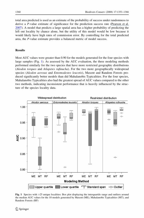
Most AUC values were greater than 0.90 for the models generated for the four species with

large samples (Fig. 1). As assessed by the AUC evaluation, the three modeling methods

performed similarly for the two species that have more restricted geographic distributions

(Akodon torques and Atlapetes rufinucha). For the two more geographically widespread

species (Akodon aerosus and Entomodestes leucotis), Maxent and Random Forests pro-

duced significantly better models than did Mahalanobis Typicalities. For the four species,

Mahalanobis Typicalities also had the greatest spread of AUC values compared to the other

two methods, indicating inconsistent performance that is heavily influenced by the struc-

ture of the species locality data.

Fig. 1 Species with [25 unique localities: Box plot displaying the interquartile range and outliers aroundthe median AUC values for the 10 models generated by Maxent (ME), Mahalanobis Typicalities (MT), andRandom Forests (RF)

1360 Biodivers Conserv (2008) 17:1353–1366

123

The proportion of localities correctly predicted as present (i.e. prediction success rate)

for models generated by the four modeling methods (including the two versions of Ma-

halanobis Typicalities) for species with small samples are displayed for a number of

thresholds in Fig. 2. As one would expect, the rate of prediction success decreases with

increasing threshold. Maxent models at threshold 5 had prediction success rates between

0.8 and 1.0 and decreased to 0 for most species at the largest thresholds. This was generally

the case for most models generated by Random Forests except for two species (Carolliamanu, and Dactylomys peruanus) whose models never reached 50% prediction success for

even the lowest threshold level. These two species had very few localities (N = 7 and 5,

respectively) scattered over a large area in southern Peru and Bolivia. Mahalanobis Typ-

icalities models generated with all 11 predictor variables performed poorly and had success

rates of zero for every threshold in all but two species. Prediction success rate for those two

Fig. 2 Species with \25 localities: Prediction success rate (proportion of localities correctly predicted aspresent) at different thresholds of models generated by Maxent, Mahalanobis Typicalities, Random Forests,and Mahalanobis Typicalities 2 for each species (number of unique localities available are in parentheses)

Biodivers Conserv (2008) 17:1353–1366 1361

123

species (Aglaeactis castelnaudii and Atlapetes melanolaemus) never reached 0.5. The

Mahalanobis Typicalities 2 models generated with the reduced predictor variable set

indicated by Maxent performed much better than the standard Mahalanobis Typicalities

models, but they still performed poorly for species with fewer than 10 localities. The

prediction success rate measured at the lowest threshold for these species ranged from 0.14

to 0.75.

The P-value test of significance revealed that all prediction success rate values above

0.5 were significant (P \ 0.05) except for Maxent models for Carollia manu at thresholds

of 5, 10 and 15 and Dactylomys peruanus at thresholds from 5 to 20. Prediction success

values (above 0.5) at other thresholds for these species’ Maxent models were deemed

significant.

Discussion

Our results demonstrated consistent differences among models in their performance at

predicting species distributions. Statistical evaluation of the modeled distributions revealed

that Maxent and Random Forests performed similarly except that Maxent worked better for

two species with very small samples that have relatively widespread geographic distri-

butions. Maxent performed well for all species tested regardless of the number of records

or the extent of occurrence. Mahalanobis Typicalities yielded mixed results. Models

generated with the same 11 predictors used for Maxent and Random Forests performed

poorly for virtually all species with fewer than 25 localities. Mahalanobis Typicalities

models formulated with fewer variables (Mahalanobis Typicalities 2) were significant

improvements, but in most cases even these models did not perform as well as the other

two methods according to statistical evaluations. The addition of an internal variable

selection procedure to maximize performance when modeling species with few records

would improve the usability of Mahalanobis Typicalities considerably. For species with

moderate numbers (N = 38–94) of localities Mahalanobis Typicalities performed as well

as other methods for species with relatively restricted geographic distributions but was

outperformed for the two species with widespread geographic distributions. All three

methods produced lower evaluation scores for the two species with widespread distribu-

tions compared to those with relatively restricted distributions, an observation that has been

made previously (Segurado and Araujo 2004; Elith et al. 2006; McPherson and Jetz 2007).

Overall our findings support previous comparative research showing variable model per-

formance related to factors including species’ ecological characteristics and the condition

of model data (Segurado and Araujo 2004; Elith et al. 2006; Hernandez et al. 2006; Tsoar

et al. 2007).

Differences in the spatial predictions of the three modeling methods can be interpreted

by visual inspection of the models (examples in Appendix). Typically Maxent predicted a

larger extent of area with high prediction values than Mahalanobis Typicalities and

especially Random Forests. In two cases, Mahalanobis Typicalities excluded records

located far from the core distribution of a species (e.g. Akodon aerosus (Appendix) and

Entomodestes leucotis (Appendix)). We argue that this characteristic of Maxent is useful

particularly in under-studied regions for identifying unknown sites (Pearson et al. 2007)

and for the purposes of selecting a threshold to convert continuous predictions to binary

values of presence/absence. Maxent’s continuous predictions (Phillips et al. 2006) usually

represent a gradual gradient thereby allowing the flexibility to selecting a threshold that

realistically matches the species’ expected distribution. The more restrictive and overly

1362 Biodivers Conserv (2008) 17:1353–1366

123

fragmented spatial predictions generated by Random Forests and Mahalanobis Typicalities

are in many cases unrealistic and therefore cause threshold selection to be more difficult.

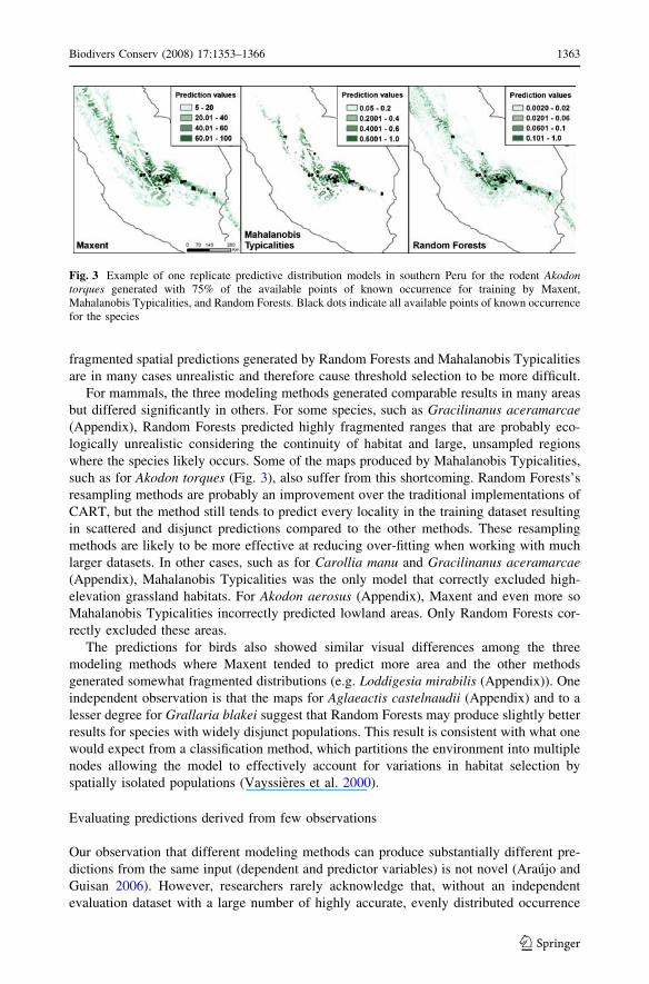
For mammals, the three modeling methods generated comparable results in many areas

but differed significantly in others. For some species, such as Gracilinanus aceramarcae(Appendix), Random Forests predicted highly fragmented ranges that are probably eco-

logically unrealistic considering the continuity of habitat and large, unsampled regions

where the species likely occurs. Some of the maps produced by Mahalanobis Typicalities,

such as for Akodon torques (Fig. 3), also suffer from this shortcoming. Random Forests’s

resampling methods are probably an improvement over the traditional implementations of

CART, but the method still tends to predict every locality in the training dataset resulting

in scattered and disjunct predictions compared to the other methods. These resampling

methods are likely to be more effective at reducing over-fitting when working with much

larger datasets. In other cases, such as for Carollia manu and Gracilinanus aceramarcae(Appendix), Mahalanobis Typicalities was the only model that correctly excluded high-

elevation grassland habitats. For Akodon aerosus (Appendix), Maxent and even more so

Mahalanobis Typicalities incorrectly predicted lowland areas. Only Random Forests cor-

rectly excluded these areas.

The predictions for birds also showed similar visual differences among the three

modeling methods where Maxent tended to predict more area and the other methods

generated somewhat fragmented distributions (e.g. Loddigesia mirabilis (Appendix)). One

independent observation is that the maps for Aglaeactis castelnaudii (Appendix) and to a

lesser degree for Grallaria blakei suggest that Random Forests may produce slightly better

results for species with widely disjunct populations. This result is consistent with what one

would expect from a classification method, which partitions the environment into multiple

nodes allowing the model to effectively account for variations in habitat selection by

spatially isolated populations (Vayssieres et al. 2000).

Evaluating predictions derived from few observations

Our observation that different modeling methods can produce substantially different pre-

dictions from the same input (dependent and predictor variables) is not novel (Araujo and

Guisan 2006). However, researchers rarely acknowledge that, without an independent

evaluation dataset with a large number of highly accurate, evenly distributed occurrence

Fig. 3 Example of one replicate predictive distribution models in southern Peru for the rodent Akodontorques generated with 75% of the available points of known occurrence for training by Maxent,Mahalanobis Typicalities, and Random Forests. Black dots indicate all available points of known occurrencefor the species

Biodivers Conserv (2008) 17:1353–1366 1363

123

records, two very different distribution predictions can have similar accuracy values. The

prediction maps for Akodon torques displayed in Fig. 3 each have high AUC values of 0.99

but have very different geographic predictions. Had there been observations of the state of

occurrence (positive or truly negative) of this species in regions where these discrepancies

exist, estimates of prediction accuracy would also differ. Vaughan and Ormerod (2005)

suggest that 200 or more observations and at least 100 of the less common state of

occurrence (present/absent) are needed for rigorous evaluations. The ideal number will

vary somewhat by study because the spatial extent and resolution influences the required

number of samples (Dungan et al. 2002). One must also consider the spatial distribution of

these samples as they should be distributed so that they adequately represent the study area

in both geographic and environmental space (Vaughan and Ormerod 2003). Even in cases

with seemingly large numbers of samples, statistical evaluations can yield results at odds

with visual assessments of predictions. For a number of species modeled by Elith et al.

(2006, Appendix Fig. S1), the prediction maps for two or more methods have the same

AUC yet differ in their geographic distributions. These differences likely result from some

regions of the study area being under-represented in the samples used to evaluate the

models.

Although many modeling methods make use of limited observational data to produce

what appear to be useful predictions, probably no model evaluation metric can compensate

for evaluation data with poor spatial representation. There is no substitute for sufficient

field survey data to obtain reliable evaluations of predictive models. Nevertheless, in many

regions, the locality information available is largely presence-only data sourced mainly

from natural history collections. These kinds of data are not ideal for model evaluations

(Guisan et al. 2006; Pearce and Boyce 2006), but better alternatives are unlikely to be

available soon (Graham et al. 2004). Moreover, evaluations of predictive models are

sometimes not conceptually possible when species ranges are actively expanding or con-

tracting (Araujo and Guisan 2006). Araujo and Guisan (2006) advocate tailoring

evaluations to the purpose of the modeling exercise. Researchers should design evaluations

to maximize the usefulness of the resulting models. Here we employed the strongest

evaluation technique known for such limited samples of locality data. We recognize that

different models sometimes produce different geographic predictions even though statis-

tical evaluations do not acknowledge them. In these situations it may be best for scientists

familiar with the species to examine the predictions in light of our knowledge of the

species’ natural history and pattern of habitat occupation. Although specialist review is

controversial (Pearce et al. 2001; Seoane et al. 2005; McPherson et al. 2006), it may be the

only option for evaluating models derived from few observations or in cases in which

dispersal barriers or competition pressures from similarly-niched species are important

(Anderson et al. 2003).

Conclusion

This study can provide guidance to other researchers attempting to predict species’ dis-

tributions in under-studied landscapes. Although one approach might be to employ

multiple methods and identify consensus areas (Burgman et al. 2005; Araujo et al. 2006),

time and resource constraints may require reliance on a single model. Both Maxent and

Random Forests performed well for the species examined here. Maxent’s more continuous

predictions provide several advantages that Random Forests do not, but Random Forests

may be better for species with widely disjunct populations. Mahalanobis Typicalities also

1364 Biodivers Conserv (2008) 17:1353–1366

123

showed some promise for locally-distributed species, but generally seems better suited to

cases with large sets of locality data.

Acknowledgments We are indebted to the Gordon and Betty Moore Foundation for their generousfinancial support and to J. Cavelier for inspiring this study. We thank the curators at the following naturalhistory museums for providing locality records for bird and mammal species: AMNH, ANSP, CBF, CBG,CM, DMNH, FMNH, KU, LSUMZ, MUSM, MNK, MSB, MVZ, UMMZ. J. Fjeldsa, D. Lane, and J. O’Neillkindly made unpublished locality data available to us. We are also grateful to D. Lane and J. O’Neill, fortheir careful review of the locality data.

References

Anderson RP, Lew D, Peterson AT (2003) Evaluating predictive models of species’ distributions: criteria forselecting optimal models. Ecol Model 162:211–232

Araujo MB, Thuiller W, Pearson RG (2006) Climate warming and the decline of amphibians and reptiles inEurope. J Biogeogr 33:1712–1728

Araujo MB, Guisan A (2006) Five (or so) challenges for species distribution modeling. J Biogeogr 33:1677–1688

Araujo MB, Williams PH (2000) Selecting areas for species persistence using occurrence data. Biol Conserv96:331–345

Bourg NA, McShea WJ, Gill DE (2005) Putting a CART before the search: successful habitat prediction fora rare forest herb. Ecology 86:2793–2804

Breiman L, Friedman JH, Olshen RA, Stone CJ (1984) Classification and regression trees. WadsworthInternational Group, Belmont, California, USA

Breiman L (2001) Random forests. Mach Learn 45:5–32Burgman MA, Lindenmayer DB, Elith J (2005) Managing landscapes for conservation under uncertainty.

Ecology 86:2007–2017Dungan JL, Citron-Pousty S, Dale M, Fortin M-J, Jakomulska A, Legendre P, Miriti M, Rosenberg M (2002)

A balanced view of scaling in spatial statistical analysis. Ecography 25:626–640Elith J, Graham CH, Anderson RP, Dudık M, Ferrier S, Guisan A, Hijmans RJ, Huettmann F, Leathwick JR,

Lehmann A, Li J, Lohmann LG, Loiselle BA, Manion G, Moritz C, Nakamura M, Nakazawa Y,Overton JM, Peterson AT, Phillips SJ, Richardson K, Scachetti-Pereira RE, Schapire RE, Soberon J,Williams S, Wisz MS, Zimmermann NE (2006) Novel methods improve prediction of species’ dis-tributions from occurrence data. Ecography 29:129–151

Engler R, Guisan A, Rechsteiner L (2004) An improved approach for predicting the distribution of rare andendangered species from occurrence and pseudo-absence data. J Appl Ecol 41:263–274

Farber O, Kadmon R (2003) Assessment of alternative approaches for bioclimatic modeling with specialemphasis on the Mahalanobis distance. Ecol Model 160:115–130

Fielding AH, Bell JF (1997) A review of methods for the assessment of prediction errors in conservationpresence/absence models. Environ Conserv 24:38–49

Ferrier S, Watson G, Pearce J, Drielsma M (2002) Extended statistical approaches to modelling spatialpattern in biodiversity in northeast New South Wales. I. Species - level modelling. Biodivers Conserv11:2275–2307

Foody GM, Campbell NA, Trodd NM, Wood TF (1992) Derivation and applications of probabilisticmeasures of class membership from the maximum-likelihood classification. Photogramm Eng RemoteSens 58:1335–1341

Guisan A, Lehmann A, Ferrier S, Austin M, Overton JM, Aspinall R, Hastie T (2006) Making betterbiogeographical predictions of species’ distributions. J Appl Ecol 43:386–392

Guisan A, Thuiller W (2005) Predicting species distribution: offering more than simple habitat models. EcolLett 8:993–1009

Graham CH, Ferrier S, Huettman F, Moritz C, Peterson AT (2004) New developments in museum-basedinformatics and application in biodiversity analysis. Trends Ecol Evol 19:497–503

Hansen M, DeFries R, Townshend JR, Carroll M, Dimiceli C, Sohlberg R (2003) Vegetation continuousfields MOD44B, 2001 percent tree cover, collection 3, University of Maryland, College Park, Mary-land, 2001

Hernandez PA, Graham CH, Master LL, Albert DL (2006) The effect of sample size and species charac-teristics on performance of different species distribution modeling methods. Ecography 29:773–785

Biodivers Conserv (2008) 17:1353–1366 1365

123

Hirosawa Y, March SE, Kliman DH (1996) Application of standardized principal component analysis toland-cover characterization using multitemporal AVHRR data. Remote Sens Environ 58:267–281

Hijmans RJ, Cameron SE, Parra JL, Jones PG, Jarvis A (2005) Very high resolution interpolated climatesurfaces for global land areas. Int J Climatol 25:1965–1978

IDRISI (2006) The Andes edition. Clark Labs, Clark University, Worcester, MALawler JJ, White D, Neilson RP, Blaustein AR (2006) Predicting climate-induced range shifts: model

differences and model reliability. Global Change Biol 12:1568–1584Loiselle BA, Howell CA, Graham CH, Goerck JM, Brooks T, Smith KG, Williams PH (2003) Avoiding

pitfalls of using species distribution models in conservation planning. Conserv Biol 17:1591–1600McPherson JM, Jetz W (2007) Effects of species’ ecology on the accuracy of distribution models. Eco-

graphy 30:135–151McPherson JM, Jetz W, Rogers DJ (2006) Using coarse-grained occurrence data to predict species distri-

butions at finer spatial resolutions—possibilities and limitations. Ecol Model 192:499–522Pearce J, Boyce MS (2006) Modeling distribution and abundance with presence-only data. J Appl Ecol

43:405–412Pearce JL, Cherry K, Drielsma M, Ferrier S, Whish G (2001) Incorporating expert opinion and fine - scale

vegetation mapping into statistical models of faunal distribution. J Appl Ecol 38:412–424Pearson RG, Raxworthy CJ, Nakamura M, Peterson AT (2007) Predicting species’ distributions from small

numbers of occurrence records: a test case using cryptic geckos in Madagascar. J Biogeogr 34:102–117Phillips SJ, Dudik M, Schapire RE (2004) A maximum entropy approach to species distribution modeling.

Proceedings of the Twenty-first Century International Conference on Machine Learning, Banff,Canada, 2004

Phillips SJ, Anderson RP, Schapire RE (2006) Maximum entropy modeling of species geographic distri-butions. Ecol Model 190:231–259

Prasad AM, Iverson LR, Liaw A (2006) Newer classification and regression tree techniques: bagging andrandom forests for ecological prediction. Ecosystems 9:181–199

R 2.1.1 (2005) The R development core team. URL: http://www.r-project.org/Raxworthy CJ, Martinez-Meyer E, Horning N, Nussbaum RA, Schneider GE, Ortega-Huerta MA, Peterson

AT (2003) Predicting distributions of known and unknown reptile species in Madagascar. Nature426:837–841

Remsen JV Jr, Cadena CD, Jaramillo A, Nores M, Pacheco JF, Robbins MB, Schulenberg TS, Stiles FG,Stotz DF, Zimmer KJ (2006) A classification of the bird species of South America. American Orni-thologists’ Union. Version 4. http://www.museum.lsu.edu/*Remsen/SACCBaseline.html

Rodrıguez JP, Brotons L, Bustamante J, Seoane J (2007) The application of predictive modeling of speciesdistribution to biodiversity conservation. Divers Distrib. doi:10.1111/j.1472-4642.2007.00356.x

Seoane J, Bustamante J, Dıaz-Delgado R (2005) Effect of expert opinion on the predictive ability ofenvironmental models of bird distribution. Conserv Biol 19:512–522

Segurado P, Araujo MB (2004) An evaluation of methods for modelling species distributions. J Biogeogr31:1555–1568

Tsoar A, Allouche O, Steinitz O, Rotem D, Kadmon R (2007) A comparative evaluation of presence-onlymethods for modeling species distribution. Divers Distrib. doi:10.1111/j.1472-4642.2007.00346.x

Thuiller W (2003) BIOMOD – optimizing predictions of species distributions and projecting potential futureshifts under global change. Global Change Biol 9:1353–1362

Vaughan IP, Ormerod SJ (2003) Improving the quality of distribution models for conservation by addressingshortcomings in the field-collection of training data. Conserv Biol 17:1601–1611

Vaughan IP, Osmerod SJ (2005) The continuing challenges of testing species distribution models. J ApplEcol 42:720–730

Vayssieres MP, Plant RE, Allen-Diaz BH (2000) Classification trees: an alternative non-paramentricapproach for predicting species distribution. J Veg Sci 11:679–694

Wilson DE, Reeder DM (2005) Mammal species of the world, 3rd edn. Johns Hopkins University Press,Baltimore, USA

Wilson KA, Westphal MI, Possingham HP, Elith J (2005) Sensitivity of conservation planning to differentapproaches to using predicted species distribution data. Biol Conserv 122:99–112

Young BE (2007) Endemic species distributions on the east slope of the Andes in Peru and Bolivia.NatureServe, Arlington, Virginia, USA

Zimmermann N (2000) Tools for analyzing, summarizing, and mapping of biophysical variables. Accessed:8/5/2005. URL: http://www.wsl.ch/staff/niklaus.zimmermann/progs.html

1366 Biodivers Conserv (2008) 17:1353–1366

123