RNA Folding and Combinatory LandscapesByWalter Fontanac;d, Peter F. Stadlera;b;c, Erich G. Bornberg{Bauera,Thomas Griesmachera, Ivo L. Hofackera, Manfred Tackera,Pedro Tarazonaa;f, Edward D. Weinbergerb,and Peter Schustera;c;e;�a Institut f�ur Theoretische Chemie, Universit�at Wienb Max-Planck-Institut f�ur Biophysikalische Chemie, G�ottingenc Santa Fe Institute, Santa Fed Theoretical Division, Los Alamos National Laboratorye Institut f�ur Molekulare Biotechnologie, Jenaf Dept. de Fisica de la Materia Condensada, Univ. Autonoma de Madrid� Correspondence to:Peter Schuster, Institut f�ur Theoretische Chemie, Universit�at WienW�ahringerstra�e 17, A-1090 Vienna, AustriaPhone: [431] 40 480 / 678Fax: [431] 40 28 525Email: pks@itc.univie.ac.at

Fontana et al.: Combinatory LandscapesAbstractIn this paper we view the folding of polynucleotide (RNA) sequences asa map that assigns to each sequence a minimum free energy pattern of basepairings, known as secondary structure. Considering only the free energyleads to an energy landscape over the sequence space. Taking into accountstructure generates a less visualizable non-scalar \landscape", where a se-quence space is mapped into a space of discrete \shapes". We investigate thestatistical features of both types of landscapes by computing autocorrelationfunctions, as well as distributions of energy and structure distances, as afunction of distance in sequence space. RNA folding is characterized by veryshort structure correlation lengths compared to the diameter of the sequencespace. The correlation lengths depend strongly on the size and the pairingrules of the underlying nucleotide alphabet. Our data suggest that almostevery minimum free energy structure is found within a small neighborhoodof any random sequence.The interest in such landscape results from the fact that they governnatural and arti�cial processes of optimization by mutation and selection.Simple statistical model landscapes, like Kau�man's n-k model, are oftenused as a proxy for understanding realistic landscapes, like those inducedby RNA folding. We make a detailed comparison between the energy land-scapes derived from RNA folding and those obtained from the n-k model.We derive autocorrelation functions for several variants of the n-k model,and brie y summarize work on its �ne structure. The comparison leads toan estimate for k = 7 to 8, independent of n, where n is the chain length.While the scaling behaviors agree, the �ne structure is considerably di�erentin the two cases. The reason is seen to be the extremely high frequency ofneutral neighbors, that is: neighbors with identical energy (and structure),in the RNA case. { 1 {

Fontana et al.: Combinatory LandscapesI Combinatory MapsProcesses like combinatorial optimization and evolutionary adaptationtake place on landscapes that result from mapping microcon�gurations to en-ergies or non-scalar entities like structures. A classic example from physicsis a Hamiltonian that assigns an energy value to a spin con�guration. An-other instance, taken from operations research, is a geography that mapstours through a set of cities into transport costs. Many properties of thoseprocesses re ect the local and global statistical features of the landscape onwhich they occur. This leads to the problem of understanding what thesefeatures are, and how to study them. In this paper we make an attempt byderiving new results and integrating them with established ones.As an example we study the biologically important landscape inducedby the folding of polynucleotides (RNA). Here the microcon�gurations aresequences over an alphabet of nucleotides, and scalar properties are freeenergies of secondary or tertiary structure formation. Another scalar couldbe the rate constant of a reaction involving that structure (e.g. replicationof viral RNA). Non-scalar properties like the secondary structure or the 3Dstructure are of particular interest. Here we consider both the energy as wellas the structure landscapes induced by RNA folding, and compare the formerwith a simple parametrized model landscape, known as the n-k model [1].Common to all these examples is a function whose domain is a set ofcombinatorial complexity | where the elements represent combinations orvariations of some kind | and whose range is either IR, or another set ofcombinatorial complexity (suitably discretized structures, for example). Thismotivates the following de�nition of a combinatory map (CM).De�nition. A CM is a quintuple (X ; dX ;Y; dY ; f) where X and Y are setsendowed with metrics dX and dY , respectively, and f is a map X �! Y. If{ 2 {

Fontana et al.: Combinatory LandscapesY = IR and dY(a; b) = ja � bj, we refer to the quintuple as a combinatorylandscape (CL).(X ; dX ) is known as con�guration space. The natural metric is inducedby some physically meaningful set of operations that interconvert con�gu-rations. In the present case of RNAs a con�guration (or sequence) spaceconsists of all sequences of �xed length n over an alphabet of size � (typ-ically � = 4), the interconversion operations are point mutations, and theHamming metric provides a distance measure between sequences.The basic problem we are concerned with here is how to investigate themajor statistical features of CMs. One approach studies CMs from the pointof view of a randomwalker [2,3]. This essentially converts spatial informationinto time series that can be characterized, for example, by autocorrelationfunctions. Another approach attempts to devise tools that re ect the statis-tical features of CMs as a whole. Some of these features cannot be accessedwith random walks alone.In section 2 we generalize the autocorrelation function to the case ofcombinatory maps, and de�ne density surfaces as an instance for the sec-ond approach above. Section 3 gives a brief classi�cation of landscapes byautocorrelation, section 4 presents a study of the RNA case, section 5 intro-duces Kau�man's n-k model, derives landscape autocorrelation functions,and brie y reviews analytic results on gradient and adaptive walks. Sec-tion 6 compares the RNA energy landscape with the n-k model. Section 7concludes the paper. { 3 {

Fontana et al.: Combinatory LandscapesII Autocorrelation and Density SurfacesIn the case of landscapes a random walk fx1; x2; : : :g on a con�gurationspace generates a real valued time series ff(x1); f(x2); : : :g whose autocor-relation function is given byr(s) = hf(xt)f(xt+s)it � hfi2�2 ; (1)with variance �2 = hf2i � hfi2. A landscape autocorrelation function, how-ever, should yield information about the average changes of f(xt+s) as thecon�guration space distance d of xt+s to some reference point xt is varied.This leads to the de�nition:�(d) = hf(x)f(y)id(x;y)=d � hfi2�2 ; (2)where h : id(x;y)=d denotes an average over all pairs of con�gurations (x; y) atdistance d from each other.The autocorrelation of the landscape and the autocorrelation along awalk on the landscape are related to each other viar(s) =Xd 'sd�(d) (3)where 'sd denotes the probability that a walk of s steps ends at a distance dfrom the starting point. Equation (3) establishes a complete correspondencebetween the random walk and the landscape autocorrelations, provided the'sd are independent of the initial conditions of the walk. For this to bethe case a su�cient regularity of the con�guration space is required. Such aregularity is missing, for example, on spaces of sequences with variable lengththat result from insertion and deletion operations. On sequence spaces with�xed length we obtain [4]'sd = 's�1;d�1� � d+ 1� + 's�1;d d� �� 2�� 1 + 's�1;d+1d+ 1� 1�� 1 (4){ 4 {

Fontana et al.: Combinatory LandscapesIn the generic case of CMs, where the range of f could be a non-scalarobject - for example a structure - we must generalize the de�nition of �(d)with the help of the distance measure on Y. We propose the followingDe�nition. �(d) = 1� hdY [f(x); f(y)]2id(x;y)=dhd2Yi : (5)It is readily seen that for landscapes, dY(a; b) = ja � bj, we recover theusual autocorrelation:hd2Y i � hdY [f(x); f(y)]2id(x;y)=d == h(f(p) � f(q))2i � h(f(x) � f(y))2id(x;y)=d == 2hf2i � 2hfi2 � 2hf2i+ 2hf(x)f(y)id(x;y)=d == 2hf(x)f(y)id(x;y)=d � 2hfi2 (6)Here h(f(p) � f(q))2i = 2(hf2i � hfi2) denotes the average over pairs ofrandomly chosen con�gurations p; q.Further insight into the statistical properties of CMs is provided by den-sity surfaces [5]. A density surface P (tjs) is the conditional probability thatthe images f(x) and f(y) have distance dY [f(x); f(y)] = t, given that thecon�gurations x and y are at distance dX [x; y] = s from each other. The den-sity surface shows how, and how fast, the distribution of image di�erenceschanges as the con�gurations become uncorrelated. This approach providesmore information than can be obtained by random walks alone. The auto-correlation �(d), equation (5), is extracted from the density surface with thefollowing correspondences:hdY [f(x); f(y)]2 id(x;y)=s =Xt t2P (t; j s)hd2Yi =Xt Xd t2P (tjs)p(s): (7){ 5 {

Fontana et al.: Combinatory Landscapesp(s) is the frequency of con�guration pairs with distance dX = s. For se-quence spaces this amounts top(s) = 1�n � (�� 1)s�ns�: (8)From the density surface the number of neighbors with identical imageis retrieved as P (0j1)(� � 1)n.III Classi�cation by AutocorrelationIt has been suggested [6] to characterize CMs by the behavior of theautocorrelation function at small distances dX . Landscapes with known au-tocorrelation function are listed in Tab.1.Let the scaled distance be � = dX=max(dX ). Many combinatorial op-timization problems exhibit landscape autocorrelation functions that can beapproximated for small � by the �rst terms in the expansion of the exponen-tial, �(�) = 1� 1� � � + : : : (9)The examples of table 1 all induce random walks with exponential autocorre-lation functions r(s). This need not be generally the case, as exempli�ed bysuperpositions of independent landscapes with di�erent characteristic lengthsthat obviously result in landscapes with no unique �. Even if a walk on alandscape does not exhibit exactly a decaying exponential as autocorrela-tion function, a rough correlation indicator is given by the nearest-neighborcorrelation: � = n� � hd2Y ihdY [f(x); f(y)]2id(x;y)=1 (10)Another class of landscapes is characterized by discontinous autocorre-lation functions, as for example, the random energy model [7], or the asym-metric TSP [8], see table 1.Smooth landscapes have �(�) = 1� �2+ : : :, and nontrivial fractal land-scapes are characterized by �(�) = 1� j�j� + : : :, with � 6= 0; 1; 2.{ 6 {

Fontana et al.: Combinatory LandscapesTable 1: Combinatorial optimization problems and their autocorrelationfunctions.Name Metric �(d) r(s) ` diam� Ref.REM any �0;d �0;s 0 n [7]s.TSP Tr. ? �e�4s=n n=4 n�1 [8]2opt ? �e�2s=n n=2 n=2:::n�1 [8]c.Tr. ? �e�2s=n n=2 n(n�1)2 [6]a.TSP Tr. ? �e�4s=n n=4 n�1 [8]2opt ? � 12 (�0;s+e�2s=n) � � [8]c.Tr. ? �e�3s=n n=3 n(n�1)2 [6]GM Tr. ? �e�4s=n n=4 n�1 [9]GBP Ex. 1�n�1n�2 [8 dn�16( dn )2] (1� 8n+ 8n2 )s (n�3)=8 n=2 [10]LAS Ham. ? �e�10s=n n=10 n [9]rnd.Nk Ham. (1� dn )(1� kn�1 )d �(1� k+1n )s n=(k+1) n [11;y]p.r.Nk Ham. (1� k+1n )d �(1� k+1n )s n=(k+1) n [y]adj.Nk Ham. equ.(24c) �(1� k+1n )s n=(k+1) n [11;y]p-Spin Ham. 1� 2(np)P0 (dj)(n�dp�j) �e�2ps=n n=(2p) n [6]SK Ham. 1� nn�1 [4 dn�4( dn )2] (1� 4n )s n=4 n [6]y) This paper.Remark. P0 for the p-spin model denotes the sum over all odd j subject to the restric-tion j>min(d;p).REM is Derrida's random energy model; s.TSP and a.TSP denote symmetric and asym-metric travelling salesman problems [12], GM is the graph matching problem [13]. (M�ezardand Parisi 1986 The correspondingmetrics are transpositions (Tr.), 2opt moves and canon-ical transpositions (c.Tr). GBP is the graph bipartitioning problem [14], its metric (Exc)is derived from exchanging a pair of objects. LAS stands for the low autocorrelated stringproblem [15]. The Sherrington-Kirkpatrick spinglass [16] is the special case p=2 of thep-Spin model introduced in [17] as a model for a rugged landscape in evolutionary op-timization. The abbreviations rnd.Nk, p.r.Nk, and adj.Nk refer to random neighbour,purely random and adjecent neighbour N-k-model, resp. Here the canonical metric is theHamming metric. { 7 {

Fontana et al.: Combinatory LandscapesIV RNA LandscapesIV.1 RNA FoldingAn RNA sequence of length n is represented as a string I = [s1s2 : : : sn],with the si taken from an alphabetA. Here we consider the natural four letteralphabet A = fA;U;G;Cg, the binary alphabets A = fG;Cg and A =fA;Ug, as well as arti�cial four and six letter alphabets, A = fA;B;C;DgandA = fA;B;C;D;E;Fg, respectively, where complementarity is assumedbetween A and B, C andD, E and F (with energy parameters as in the GCcase).RNA structure can be broken down conceptually into a secondary struc-ture, and a tertiary structure. The secondary structure is a pattern of com-plementary base pairings (�gure 1). The tertiary structure is the three-dimensional con�guration of the molecule. As opposed to the protein case,the secondary structure of RNA sequences is well de�ned; it provides themajor set of distance constraints that guide the formation of tertiary struc-ture, and covers the dominant energy contribution to the 3D structure. Inthis paper we will be concerned only with secondary structures.The de�nition of secondary structure used in most computational ap-proaches assumes planarity. Planarity means that unpaired nucleotides in-side a loop cannot pair with unpaired nucleotides outside a loop. It is known,however, that unpaired bases from di�erent loop regions may pair with eachother, forming so-called pseudo-knots. While the computational problem forstrictly planar secondary structures has been essentially solved in the early80s [18 { 21], the problem involving long-range pseudo-knots is still unsolved.A secondary structure S(I) 2 S is formally de�ned as the set of all basepairs (si; sj) with (i < j) ful�lling two requirements [19]:1) each base is involved in at most one base pair,{ 8 {

Fontana et al.: Combinatory Landscapes2) there are no knots or pseudo-knots, i.e. if (si; sj ) and (sk; sl) are basepairs then i < k < l < j or k < i < j < l.The basic elements of secondary structures are shown in �gure 1. Forthe free energies of these building blocks experimental data are available.The elements are assumed to contribute additively to the overall free energyof the complete secondary structure. The data set used here has been takenfrom the literature [22 { 24]Under thermodynamically reasonable assumptions the folding problemfor planar RNA secondary structure consists in �nding a minimum free en-ergy structure, and can be attacked by the technique of dynamic program-ming. Our implementation of the folding algorithm follows the reasoninggiven by Zuker and Stiegler [20]. The combinatory map from the space ofsequences, An, into the space of minimum free energy structures, S,S : An ! S; I ! S(I); (11)is the quintuple (An; dH ;S; dS ; S) with dH denoting the Hamming distance,and dS being a suitably de�ned distance between secondary structures (seebelow). If we view the folding procedure as a map from a sequence to thefree energy of the corresponding structure,�G : An ! IR; I ! �G(I) (12)we obtain the combinatory landscape (An; dH ; IR; j : j;�G).{ 9 {

Fontana et al.: Combinatory Landscapes5

hairpin loop

G A

UC

G

G

5

3

interior base pair

closing base pair

interior loop

G

CA U

CA

A5

3

interior base pair

closing base pair

bulge

stacking pair

G

C A

U

interior base pair

closing base pair

G

C

closing base pair

A

U

C

3

5

3

G

C

A

U

C G

A A

5

3

interior base pairs

closing base pair

multiple loopFigure 1: Top: Example of a secondary structure. Below: Basic structure elements.Every secondary structure can be decomposed into such basic elements. Thefree energy of a secondary structure is the sum over all contributions of theseelements. Their energy contributions have been experimentally determined as afunction of the nucleotide sequence [22{24].{ 10 {

Fontana et al.: Combinatory LandscapesIV.2 Distribution of EnergiesHere we focus on global features relating to the distribution of free energyvalues over the RNA landscape. Table 2 shows the mean free energy valuesh�Gi and variances �2 for a variety of alphabets. We have also computedthe skewness (third moment scaled by �3) and the kurtosis (fourth momentscaled by �4) of the distribution (not shown).The main observations are that h�Gi scales linearly with chain lengthn for all alphabets, and so does the variance �2 for n > 50 (see table 4below). The distribution sharpens considerably for longer chains. A Gaus-sian distribution is characterized by vanishing skewness and a value of 3 forthe kurtosis. This seems to be mostly the case for the biophysical GCAUalphabet and long chains. The other alphabets show deviations from theGaussian case in skewness and/or kurtosis. The available data do not allowa de�nite statement about the limiting behavior for very large n to be made.We did not pursue this issue in depth because of doubts about the validityof a thermodynamic (rather than kinetic) folding algorithm in that limit.IV.3 Free Energy AutocorrelationFigure 4a shows an example of the landscape autocorrelation function�(d). Complementary sequences have similar structures and energies. Foreach reference sequence on binary alphabets there is only one complement,and, therefore, this approximate symmetry shows up as a U-shaped correla-tion. Table 3 lists the characteristic lengths of the landscape, equation (10),for various alphabets as a function of n. The characteristic length has beencalculated by both random walks and density surfaces. The agreement isremarkable, indicating that the landscapes are indeed su�ciently regular forthe random walk approach to be meaningful.{ 11 {

Fontana et al.: Combinatory LandscapesTable 2: Averages of free energies, �G, and their variances, �2, for 1) GC,2) AU, 3) GCAU, 4) GCXK and 5) ABCDEF. For 3) thebiophysical parameter set is used, for 4) and 5) theGC parameterset is used for all base pairs. Energy unit: 0.1 kcal�mol�1 Energydata set taken from [23].��G �n 1) 2) 3) 4) 5) 1) 2) 3) 4) 5)20 74:40 2:22 10:29 19:06 6:59 28:80 5:12 14:63 19:95 12:3525 108:85 5:68 17:56 31:50 16:05 31:86 8:78 18:56 23:88 16:0528 39:38 25:7930 144:23 9:59 25:58 44:46 16:91 34:55 11:24 21:81 26:96 18:89?30 25:68 22:0035 180:27 14:09 33:61 58:24 22:71 36:96 13:18 24:35 29:22 21:3240 217:00 18:83 42:33 72:60 29:30 39:17 14:64 26:88 31:54 23:5945 253:73 23:53 50:58 86:98 35:67 40:87 15:81 28:83 33:25 25:3850 290:61 28:54 60:12 101:89 42:36 42:66 16:89 31:03 35:32 27:24?50 60:16 31:1355 327:59 33:54 68:84 116:47 48:89 44:23 17:81 32:82 36:89 28:7060 365:50 38:61 77:48 131:28 55:81 45:51 18:79 34:63 38:19 30:1070 440:73 48:46 95:64 161:63 69:59 47:95 20:25 37:64 40:99 32:6680 516:83 59:32 113:77 192:19 83:57 50:76 21:78 40:46 43:37 34:87100 669:35 80:12 150:78 254:56 111:46 54:21 24:17 45:96 48:04 38:90120 824:41 58:42150 1054:77 133:45 244:57 62:12 28:79 57:06200 1445:62 188:21 339:16 68:63 32:58 66:28250 1838:36 243:62 434:93 74:08 36:04 73:79300 2233:63 299:62 531:34 79:80 39:70 81:14350 2629:50 355:88 628:59 84:40 42:72 87:96400 3026:54 412:50 726:02 88:44 45:50 94:41450 3423:91 469:30 823:52 92:98 47:70 99:92500 3822:34 526:24 921:46 95:74 49:69 105:2?) Specially stable tetraloops taken into account.{ 12 {

Fontana et al.: Combinatory LandscapesTable 3: Correlation lengths for various types of RNA free energy land-scapes. R and D denote calculations via random walks and withdensity surfaces via equation (7), respectively. Energy parametersare taken from [23].n GC AU GCAU GCXK ABCDEFR D R D R D R D R D20 1:96 1:97 1:13 3:64 3:62 2:62 2:48 2:70 2:501:2725 2:44 2:41 1:50 4:83 4:76 3:21 3:17 3:46 3:161:4428 3:4930 2:95 2:96 1:85 1:93 5:97 6:01 3:84 3:75 4:02 3:922:90 ?6:082:8235 3:49 3:23 2:23 7:29 7:79 4:35 4:39 4:59 4:6640 4:00 3:97 2:49 2:56 8:67 8:16 4:88 4:85 5:464:04 8:1245 4:47 4:15 2:75 10:05 9:60 5:38 5:22 5:96 5:9750 4:57 4:51 3:07 11:49 11:11 6:08 5:95 6:68 6:323:15 10:83 5:61?11:7455 5:43 3:24 12:10 6:68 7:0560 5:50 6:17 3:72 14:88 13:20 7:05 7:03 7:97 7:5570 6:68 4:45 16:22 16:40 7:68 9:06 8:716:56 4:19 15:05 8:097:0380 7:82 4:88 19:03 8:84 9:98 9:894:8990 5:14 11:45100 8:41 8:52 6:11 24:73 25:18 12:20 10:57 12:31 11:55120 10:55?) With specially stable tetra-loops. { 13 {

Fontana et al.: Combinatory LandscapesThe characteristic length scales linearly with n. This is understoodby observing that the absolute free energy di�erence between two neigh-bors (one-digit mutants) is bounded from above by twice the largest possiblestacking energy plus the strain of an internal loop of size two (approximately10 kcal�mol�1). This is seen by considering that in the worst case a mutationdisables a base pair, thus interrupting a stack by creating an internal loop. Ifthis leads to a complete refold of the sequence, then the new structure musthave a smaller absolute energy di�erence than the worst case. The expecta-tion value of the squared energy di�erence between nearest neighbors will,therefore, level o� to a constant at su�ciently large n. At the same time thedata of the previous section show a variance linear in n, and hence we have� � n (see table 4 below).Figure 2 shows the free energy density surfaceP (zjd) = P (j�G(I1)��G(I2)j = z �� dH(I1; I2) = d): (13)It reveals a very rugged landscape. Cuts along constant Hamming distanceshow roughly the positive half of a Gaussian, except for a pronounced peak atP (0j1) corresponding to neighbors with identical energy. If the free energieswere sums of independently distributed random variables one would expectfor the density surface:P (zjd) = 1p�(1� �(d)) � ��exp�� z24�2(1� �(d))�� �0;z� (14)Figure 2b shows P (zjd) as in equation (14) with �(d) taken from the datain table 3. The overall shape is in agreement. For comparison we also plotthe corresponding exact density surface for the Sherrington-Krikpatrick spinglass. (�(d) from table 1, and references therein.)From the density surface we can read o� the frequency of neutral neigh-bors (see section 2). This is shown in �gure 3. The fraction of neutral neigh-bors tends to a positive constant for long chains. From statistics of structural{ 14 {

Fontana et al.: Combinatory LandscapesTable 4: Scaling with sequence length of average free energy, variance andcorrelation length of free energies for di�erent alphabets. Energyparameters from [23].GC AU GCAU GCXK ABCDEF�h�Gislope 7:8120 1:0948 1:9006 2:9495 1:3044intercp �101:21 �26:14 �32:25 �43:97 �21:40corr. 0:99996 0:9998 0:99992 0:9996 0:998�2slope 17:33 5:06 22:61 23:56 17:07intercp 959:8 22:2 �180:4 16:1 �143:3corr. 0:996 0:997 0:99996 0:997 0:998�slope 0:0857 0:0600 0:2627 0:1078 0:1182intercp 0:43 0:06 �1:93 0:50 0:47corr. 0:992 0:997 0:997 0:993 0:997elements [5,25] we know that for long chains the average loop size becomesconstant, while the average number of loops per structure scales linearly withn. The sequence positions that can be changed without a�ecting the struc-ture and its energy must be located within loops (or external elements). Thisexplains the linear scaling of the number of neutral neighbors.IV.4 Structure AutocorrelationAs detailed in section 2, computing the autocorrelation of the struc-tures themselves requires a distance measure on the space of structures. The{ 15 {

Fontana et al.: Combinatory Landscapes

Figure 2: a) Sampled denisty surface P (zjd) for energy di�erences of minimumfree energystructures on GC-sequences of length n=100. b) Gaussian approximation withthe statistically determined autocorrelation function �(d)). c) Exact densitysurface for the Sherrington Kirkpatrick spin-glass. d) Exact density surface fora RN n-k model with k=7.{ 16 {

Fontana et al.: Combinatory LandscapesFigure 3: Frequency of neutral neighbors (0j1) on the free energy landscape as a functionof chain length. The upper two of curves belongs to the GCAU alphabet, thelower two curves belong to theGC alphabet. The upper curve in each pair refersto the older parameter set taken from [22], the lower curve in each pair refers tothe updated set taken from [23].de�nition is essentially based on converting one-to-one secondary structuregraphs into rooted ordered trees [5,26 { 28] The distance between two trees isobtained as a generalization of sequence alignment procedures, and involvesminimizing the cost of transforming one tree into the other with elemen-tary editing operations, like deletion, insertion, and relabeling of nodes. Fordetails see [5].Fig. 4b shows the structure autocorrelation function �(d). The U-shapedform for the binary alphabet arises for the same reason given in sect. IV.3.The structure density surfaces of sequences with n = 100 for the GCand GCAU alphabet are shown in �gure 5. First we note that nearestneighbors in con�guration space can exhibit already substantially di�erentstructures with signi�cant probability. Furthermore, it is extremely unlikelythat two randomly chosen sequences fold into identical structures. This is in{ 17 {

Fontana et al.: Combinatory Landscapes0.0 20.0 40.0 60.0 80.0 100.0

Hamming distance

-0.2

0.0

0.2

0.4

0.6

0.8

1.0

Cor

rela

tion

b

a

c

0.0 20.0 40.0 60.0 80.0 100.0Hamming distance

-0.2

0.0

0.2

0.4

0.6

0.8

1.0

Cor

rela

tion a

b

cFigure 4: Autocorrelation functions for sequences of length n=100 for free energy land-scapes (left) and (right) secondary structure landscape with alphabets GCAU(a), GCXK (b), and GC (c).sharp contrast to the energy landscape. Stated di�erently: there are manymore structures than energies. Nonetheless, the distribution of structure dis-tances approaches already at fairly short Hamming distances the distributionexpected for random sequences. In contrast to the free energy there is nosize independent upper bound to the distance between secondary structuresof two neighboring sequences. This suggests that in a small ball around arandom sequence one may �nd the vast majority of all minimum free energystructures S [5]. The phenomenon is known as \shape space covering" [29]We will report elsewhere on the veri�cation of this conjecture with additionalmethods. Although there are many fewer di�erent energy values than min-imum energy structures, the energies are not scattered randomly across thesequence space.The characteristic lengths of the structure autocorrelation (table 5) areshorter by a factor between 2 and 3 compared to their free energy coun-terparts. They roughly correspond to the Hamming distance at which the{ 18 {

Fontana et al.: Combinatory Landscapes

Figure 5: Density surface for secondary structure di�erences as determined by tree edit-ing. Parameters are as in �gure 2. n=100, upper part: GC, lower part: GCAU{ 19 {

Fontana et al.: Combinatory LandscapesTable 5: Characteristic lengths of RNA secondary structure landscapes forvarious alphabets and chain lengths. Energy parameters are takenfrom [23].n GC AU GCAU GCXK ABCDEF20 1:51 1:22 2:84 2:43 2:5025 1:69 1:61 3:68 2:88 3:2830 1:87 1:85 3:99 3:25 3:9235 2:02 2:12 4:49 3:57 4:5140 2:15 2:24 4:85 3:7445 2:33 2:33 4:97 4:10 5:4950 2:35 2:50 5:46 4:33 5:8455 2:62 2:64 6:2060 2:68 2:83 6:01 4:84 6:6070 2:87 2:91 6:25 5:24 7:1480 3:13 3:32 5:67 7:9390 3:60100 3:36 3:77 7:63 6:45 8:94120 3:72dominant peak resulting from identical or very similar structures has dis-solved. Randomization of structure for GCAU sequences of length n = 100occurs already at a distance of about dH = 16 from a random reference point(�gure 5). From table 5 we see that this corresponds to a ball of radiusdH � 2�. The characteristic length data are roughly consistent with linearscaling in n.The ordering of characteristic lengths of the structure autocorrelationfor long sequences is summarized by:AU � GC� GCXK < GCAU < ABCDEF (15)Binary alphabets generally form more structures because the probability fortwo randomly chosen position along the sequence to pair is highest. Changing{ 20 {

Fontana et al.: Combinatory Landscapesone position, therefore, is more likely to alter the minimum energy structure.In contrast, the characteristic lengths of the free energy autocorrelation doesnot follow the same ordering:AU < GC < GCXK < ABCDEF� GCAU (16)IV.5 Biased Walks and Local OptimaAdditional information about the local structure of landscapes is pro-vided by biased walks. These are random walks aimed at reaching localextrema of the landscape. The data provided by this technique will be com-pared with a statistical model in the next sections.We de�ne a local minimum y in con�guration space byf(y) � f(x) for all neighbors x of y: (17)Local maxima are de�ned analogously. The term local optimummeans eitherminimum or maximum according to context.We consider here two types of biased walks, adaptive walks and gradientwalks. In an adaptive walk a starting point x0 is chosen at random. The walkthen proceeds to a randomly chosen neighbor x0 such that f(x0) < f(x0), andit stops if no neighbor satis�es this condition, at which point the walk hasreached a local minimum. A gradient walk, in contrast, proceeds to theneighbor x0 for which f(x0) is minimal.Table 6 compiles the average lengths of adaptive and gradient walkson the free energy landscape, as well the the average free energy (and thecorresponding variances) of start and end points. These quantities werecalculated for an energy parameter set available in the late 70s [22] andfor a recently updated parameter set [23,24]. While the absolute valuesdi�er, the scaling behavior is not a�ected. The average free energy of local{ 21 {

Fontana et al.: Combinatory LandscapesTable 6: Adaptive and gradient walks on RNA free energy landscapes. �Fdenotes the free energy of random sequences. Average free ener-gies of local optima are denoted by �Fopt, �F ?opt, and �F ??opt, dependingon whether they are generated randomly, as end points of adap-tive walks, or as end points of gradient walks, respectively. Thestandard deviations of their distributions are denoted by �F , �opt,�?opt, and �??opt. The lengths of adaptive and gradient walks aredenoted by Ladap and Lgrad, respectively. The rightmost columncompiles the probability pl.o. for �nding a local optimum at ran-dom.n �F �F �Fopt �opt �F?opt �?opt �F??opt �??opt � Ladap Lgrad pl.o.GCEnergy parameters from [22]20 118:9 43:0 179:7 32:0 204:5 29:1 211:5 31:2 2:10 2:42 1:72 0:113825 178:9 47:3 257:6 44:1 300:4 37:8 305:2 42:0 2:70 3:30 2:29 0:053030 239:7 50:8 329:3 50:6 398:5 48:7 402:9 53:7 3:09 4:44 3:12 0:022035 303:1 54:0 390:3 43:6 493:1 60:5 496:5 67:4 3:57 5:49 3:88 0:010840 368:6 57:6 465:5 48:8 584:7 74:5 585:3 79:1 3:98 6:42 4:48 0:008450 500:1 62:3 633:4 48:9 759:8 90:7 755:5 92:4 4:67 8:06 5:50 0:002560 632:2 66:7 768:0 � 934:4 97:4 930:9 94:9 5:65 9:61 6:42 0:0008Energy parameters from [23]20 74:4 28:8 127:9 24:9 148:3 21:6 152:0 22:2 1:96 3:55 2:51 0:023030 144:2 34:6 213:1 28:1 262:6 36:6 265:1 37:3 2:93 5:32 3:70 0:005040 217:0 39:2 315:0 29:5 369:2 44:4 372:4 44:7 4:00 6:78 4:69 0:001150 290:6 42:7 415:0 � 478:0 48:9 481:9 49:3 4:51 8:27 5:68 0:000260 365:5 45:5 � � 587:6 56:6 589:4 55:1 6:17 9:62 6:64 �GCAUEnergy parameters from [22]30 34:2 31:0 94:6 45:4 208:5 72:3 228:5 78:4 6:73 8:01 5:12 0:000940 59:8 37:9 � � 307:3 93:5 339:8 103:7 9:85 11:62 7:57 �50 90:6 43:8 � � 404:1 105:1 441:8 112:0 13:76 14:77 9:31 �60 128:1 48:1 � � 504:6 118:0 � � 18:38 17:99 � �70 162:7 50:6 � � 604:2 125:3 644:1 132:9 20:80 21:22 13:32 �80 201:9 55:3 � � 704:2 139:2 � � 23:81 24:17 � �Energy parameters from [23]30 25:7 22:0 � � 172:9 43:9 181:1 47:4 6:08 11:84 7:17 �40 42:3 26:9 � � 253:0 50:4 272:0 54:8 8:14 16:26 9:95 �50 60:2 31:1 � � 325:8 59:6 352:3 65:1 11:74 20:73 12:53 �60 77:5 34:6 � � 401:8 68:3 428:0 71:9 13:20 25:30 14:92 �70 95:6 37:6 � � 478:4 73:1 508:0 80:1 16:20 29:13 17:44 �{ 22 {

Fontana et al.: Combinatory Landscapesoptima reached by adaptive and gradient walks is roughly the same and scaleslinearly with n. The rightmost column in table 6 summarizes the frequencypl.o. with which the initially chosen sequence was already a local optimum.We refer to such a sequence as a \random optimum". The frequency pl.o.decreases exponentially with chain lenght n (see sect. IV.5). This frequencywas, however, too low to yield meaningful quantities for GCAU sequencesin both parameter sets. We note that the energy of local optima reachedat the end of the biased walks is substantially lower than the average freeenergy of random optima.Figure 6: Distribution of per-step energy di�erences along a random walk. (a) GCsequences of length n=100. (b) GCAU sequences of length n=100.The distribution of free energy increments per step along a random walkis shown in Figure 6. The local deviations from a Gaussian distribution areagain most pronounced at 0, resulting from the substantial fraction of neutralneighbors. In the case of binary sequences (�gure 6a) particular free energychanges are favored. As a biased walk proceeds the distribution of energy{ 23 {

Fontana et al.: Combinatory Landscapesincrements is obviously altered. After some �ve steps the distribution isdominated by a few quanta (�gure 7) that identify the most likely structuralchanges.Figure 7: Distribution of energy increments after more than 4 steps along a gradientwalk. (a) GC-landscape and (b) GCAU-landscape.In �gure 8 we plot the average change in free energy for landscapes ofdi�erent length along biased walks. The number of walk steps is scaled bythe corresponding characteristic length �. The �gure demonstrates that fora �xed alphabet the properly scaled statistical features of walks are indepen-dent of the system size.V Kau�man's n-k ModelBecause of the important role of landscapes in problems of optimizationand evolutionary adaptation [30] there has been considerable interest in de-vising simple statistical models. The hope being that these models re ect{ 24 {

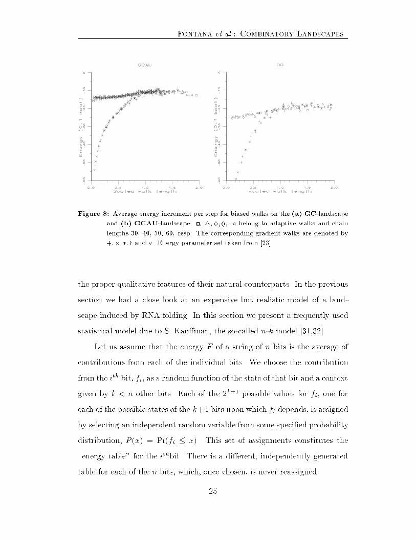
Fontana et al.: Combinatory LandscapesFigure 8: Average energy increment per step for biased walks on the (a) GC-landscapeand (b) GCAU-landscape. , 4;}; (), ./ belong to adaptive walks and chainlengths 30, 40, 50, 60, resp. The corresponding gradient walks are denoted by+;�;�; y and _. Energy parameter set taken from [23].the proper qualitative features of their natural counterparts. In the previoussection we had a close look at an expensive but realistic model of a land-scape induced by RNA folding. In this section we present a frequently usedstatistical model due to S. Kau�man, the so-called n-k model [31,32].Let us assume that the energy F of a string of n bits is the average ofcontributions from each of the individual bits. We choose the contributionfrom the ith bit, fi, as a random function of the state of that bit and a contextgiven by k < n other bits. Each of the 2k+1 possible values for fi, one foreach of the possible states of the k+1 bits upon which fi depends, is assignedby selecting an independent random variable from some speci�ed probabilitydistribution, P (x) = Pr(fi � x). This set of assignments constitutes the\energy table" for the ithbit. There is a di�erent, independently generatedtable for each of the n bits, which, once chosen, is never reassigned.{ 25 {

Fontana et al.: Combinatory LandscapesIt remains to specify the k sites which in uence a given position. Thesimplest choice is to imagine that the neighborhoods consist of the k=2 bitsthat are the nearest neighbors on each side of the bit in question and toassume that the bits are arranged in a circle (periodic boundary conditions).The other extreme is to pick the k sites at random. In a variant of thismodel it is not required that fi depends on i, but all k + 1 relevant sites arechosen randomly. These three versions of the n-k model will be referred to asAN (adjacent neighborhood), RN (random neighborhood) and PR (purelyrandom) model, respectively. These two extremes correspond to two impor-tant types of spin glasses: the adjacent neighborhoods correspond to a onedimensional, short range spin glass; the random neighborhoods correspondto a dilute, long range spin glass.If the underlying probability distribution of the site energies, fi, has a�nite variance, the distribution of the �tness of the entire string,F = 1nXi fi; (18)will tend to a Gaussian with mean � and variance �2=n, where � and �2 are,respectively, the mean and variance of the fi's as n!1.V.1. CorrelationWeinberger [3] shows that the autocorrelation function of a random walkon the n-k model landscape is a single decaying exponential to within anerror of O(1=n). All isotropic landscapes of this kind can be generated by anappropriate choice of the mean and variance of the site energy distribution,P (x), and an appropriate choice of k.The ruggedness of the landscape varies dramatically as k varies from 0through n � 1. For k = 0, each site is independent of all other sites. Theautocorrelation function in this special case reads�(d) = 1� d=n (19){ 26 {

Fontana et al.: Combinatory LandscapesAfter some algebra one shows that a randomwalk on this landscape generatesan AR(1) process with autocorrelation functionr(s) = sXd=0'(s; d)�(d) = �1� 1n ��� 1�s : (20)In contrast, the k = n � 1 landscape is the random energy model: theenergy contribution of each site then depends on all of the other sites becausethe context for each of the n� 1 other bits is changed when even a single bitis ipped. In this case, therefore, the energy of each n bit string is assigneda energy that is statistically independent of its neighbors.The autocorrelation functions for the various types of n-k models areobtained from[F (x)�F (y)]2 = NXi=1[fi(x)�fi(y)]2+2Xi<j [fi(x)�fi(y)][fj (x)�fj (y)]: (21)The average over the second sum vanishes because of the independence ofthe fi's and the contributions of the terms (fi(x) � fi(y))2 are zero if x andy have the same digit at all positions which are in the neighborhood of sitei. Otherwise the contributions are random with mean value �2. Thus weobtain h(F (x) � F (y))2)i = 1n2�2nh(d); (22)where h(d) is the probability for a site to appear at least once in the list ofthe d sites which are changed by moving from x to y. For the n-k model itis evident that complementary strings are uncorrelated because they do nothave any contribution to site �tnesses in common, therefore the variance ofF is �2 and �(d) = 1� h(d): (23){ 27 {

Fontana et al.: Combinatory LandscapesFor the three variants of the n-k model the functions h(d) are derivedin the appendix.hRN (d) = 1� (1� dn )(1� kn� 1)dhPR(d) = 1� (1� k + 1n )dhAN (d) = k + 1n d� 1�nd� min(k;n+1�d)Xj=1 (k � j + 1)�n� j � 1d� 2 � ford � 2(24)Evidently, h(d) is independent of the number of letters in the alphabet. Forall three types of n-k models the correlation length can be estimated fromthe nearest-neighbor correlations, equation (10),�(1) = (1� 1n )(1 � kn� 1) = 1� k + 1n (25)since all h(1) are identical. This yields the estimate� = �1= ln(1 � k + 1n ) = nk + 1 � 12 +O(k + 1n ): (26)V.2. Biased Walks and Local OptimaIn the case k = 0 there is, with probability one, a unique optimal digitfor each site; hence, a single speci�c sequence comprised of the optimal digitvalues in each position is almost surely the single, global optimum in theenergy landscape. Any other string is suboptimal, and lies on a connectedwalk via nearest neighbor better variants to the global optimum. The lengthof the walk is just the Hamming distance from the initial string to the globaloptimum. For a randomly chosen initial string, (��1)=� of the digits will bein a energetically less favourable state (� is the size of the alphabet), hencethe expected walk length is just ��1� n.For the random energy model it has been shown [1,33 { 35] that the land-scapes have many local optima, that the walks to optima are short (O(lnn)),{ 28 {

Fontana et al.: Combinatory Landscapesand that only a small fraction of local optima are accessible from any initialstring.Weinberger [36] derived expressions for the expected number of localoptima and the probability distribution of their energies. In the Gaussiancase, the expected number of local optima, Nl.o., is given bylog(Nl.o.) � c0 + n � �log�� log[(�� 1)(k + 1)]k + 1 � (27)where c0 is some small constant. The distribution of energies of local optimais Gaussian with mean hFl:o:i = �� ��, where� =r2 log[(�� 1)(k + 1)]k + 1 (28)and variance �2l.o. = �2 � 1n 11 + 4(�� 1)(k + 2) log(k+1)k+1 : (29)Estimates for the average lengths of biased walks have been derivedrecently [36]. The average length of gradient walks can be estimated fromthe average distance of two local optima asLGrad = n ���� 1� � log[(�� 1)(k + 1)](k + 1) log � : (30)As an estimate for the length of adaptive walks one obtainsLAdap = n � log[(�� 1)(k + 1)](k + 1) : (31)The lengths of adaptive walks and gradient walks di�er, therefore, by a con-stant factor LAdapLGrad = � log��� 1 (32)The chance to �nd a local optimum at random is given bylog pl.o. = logNl.o. � n log� = c0 � n � log[(�� 1)(k + 1)]k + 1 : (33){ 29 {

Fontana et al.: Combinatory LandscapesVI Comparison of the RNA Landscape with the n-k modelIn order to compare the n-k model and the RNA landscape we need ahypothetical k-value. From equation (26) we obtaink = n�1� e�1=��� 1: (34)Since the characteristic length of the RNA landscape scales linearly withn, � � � � n+ a0, we �nd asymptoticallyk = 1� � 1 +O(n�1): (35)Table 7 compares the statistics of local optima in the n-k landscape with thestatistics of local optima in the RNA free energy landscape. The ensembles oflocal optima in the RNA case have been obtained with gradient and adaptivewalks as detailed in sect IV.5. The comparisons use the scaled quantitiesfl.o. = hF i � hFl.o.i� : (36)Table 7 shows that average free energies of local optima for the RNAlandscapes, sampled with both gradient (f??l.o.) and adaptive walks (f?l.o.), dif-fer signi�cantly from those predicted by the n-k model. Due to the samplingmethod the local optima in the RNA case are obviously not a true randomsample, but are biased towards those optima that have large basins of attrac-tions. These optima usually have more extreme values than purely randomlysampled local optima. The comparison, therefore, is only limited. On theother hand, the n-k model predicts a distribution of average energies of localoptima that sharpens like �2l.o.=�2 � 1=n, equation (29). If this were the casefor the RNA landscape we should observe no di�erence between our biasedsample and a random sample. This is clearly not the case. In fact, the vari-ances �2l.o. (table 7), scale linearly with chain length. In the GC case we{ 30 {

Fontana et al.: Combinatory LandscapesTable 7: Hypothetical k-values and a comparison between the n-k modeland the computed RNA data from table 6. Small numbers referto the older data set from [22].kpred is the predicted valued of k for the RNA landscape as ob-tained from equation (34), fpred is the predicted average scaledenergy of a local optimum according to equation (28). fl.o., f?l.o.,and f??l.o. are the numerical average scaled energies for random localoptima and for local optima obtained from adaptive and gradientwalks, respectively.n kpred fl.o. f?l.o. f??l.o. fpred = �GC20 6:58 6:99 1:41 1:85 1:99 2:57 2:15 2:69 0:73 0:7225 6:74 � 1:66 � 2:57 � 2:68 � 0:73 �30 7:29 7:64 1:76 1:99 3:13 3:42 3:21 3:49 0:71 0:7135 7:55 � 1:62 � 3:52 � 3:58 � 0:71 �40 7:89 7:85 1:68 2:50 3:75 3:88 3:75 3:96 0:70 0:7050 8:64 8:94 2:14 2:91 4:17 4:41 4:10 4:48 0:69 0:7060 8:73 7:98 2:04 � 4:53 4:88 4:48 4:92 0:68 0:68GCAU30 3:14 3:55 1:95 � 5:62 6:69 6:27 7:38 1:10 1:0740 2:86 3:62 � � 6:53 7:83 � 8:54 1:13 1:0750 2:51 3:08 � � 7:17 8:54 8:02 9:39 1:16 1:1160 2:17 3:38 � � 7:83 9:37 � 10:13 1:19 1:0870 2:29 2:29 � � 8:73 10:18 9:51 10:97 1:18 1:1280 2:29 � � � 9:19 � � � 1:18 �could accumulate a representative random sample of local optima (referredto as random optima in sect. IV.5). This allows a direct comparison with theprediction from the model as seen from table 7, fl.o. is still in disagreementwith fpred. { 31 {

Fontana et al.: Combinatory LandscapesWe �nd that some scaling properties are in common. In particular, thelinear dependence of the walk length on n and the exponential decrease ofthe probability for �nding a local optimum pl.o. as a function of n. Estimatesfor the latter can already be derived by assuming that in highly correlatedlandscapes there should be O(1) local optima in a patch of radius � [8] whichafter some calculations leads tolog pl.o. = c0 � n � [log 2 + log(�� 1)�� 2(�� 1=2)2] (37)Table 8: Scaling of the number of local optima and walk length for forGC and GCAU landscapes. Shown are the slopes of linear �ts tothe calculated data (table 7). n-k model refers to the predictionfrom section V. Also shown are the rough estimates obtained fromequations (37) and (38). Small letters refer to the older parameterset from Salser [22]. log pl.o.=n LAdap=n LGrad=nGCGC landscape �0:15 �0:12 0:15 0:18 0:10 0:12n� k model �0:25 �0:25 0:25 0:25 0:18 0:18equ.(37,38) �0:35 �0:34 � � 0:09 0:08GCAUGCAU landscape < �0:3 ��0:2 0:44 0:32 0:26 0:20n � k modelhfil �0:60 �0:67 0:60 0:67 0:32 0:36equ.(37,38) �0:87 �0:94 � � 0:26 0:30By the same reasoning the length of a gradient walk should be roughlyLgrad � � � � � n: (38){ 32 {

Fontana et al.: Combinatory LandscapesTable 8 lists the scaled lengths of adaptive and gradient walks, as well as thelogarithm of the probability of randomly hitting an optimum. The measuredquantities are compared with the predictions from the n-k model and thecrude estimates based on equations (37) and (38). The latter agree fairlywell in the case of gradient walks with the observed data. The n-k model isat best in the ball-park. The ratios Ladap=Lgrad, equation (32), are prettyclose to the predictions. For the GC alphabet we �nd 1:45 and for GCAUwe �nd 1:57, versus a prediction of 1:45 and 1:85, respectively.VII ConclusionsAmong the most important steps in understanding evolutionary adapta-tion is the construction of a model landscape based on the proper abstractionsof the adapting entities. In this paper we explored in detail the statistics of arealistic and biologically motivated landscape induced by RNA folding. Wecompare its features with a widely used simple statistical model for ruggedlandscapes, known as the n-k model.RNA energy as well as structure landscapes were explored by numeri-cally computing landscape autocorrelation functions, randomwalk autocorre-lation functions and density surfaces as a function of the nucleotide alphabetand the sequence length. The main results can be summarized as follows:RNA Landscapes1. The energy as well as the structure autocorrelation function is char-acterized to a reasonable approximation by one characteristic lengthscale.2. The characteristic length of the energy and of the structure landscapescale linearly with sequence length.3. The characteristic length for structures strongly depends on the nu-cleotide alphabet. { 33 {

Fontana et al.: Combinatory Landscapes(i) Binary sequences, AU orGC, have very short correlation lengths,indicating that they are very likely to change their structure withfew changes in the underlying sequences.(ii) GCXK sequences, with XK denoting two arti�cial nucleotideswith the same pairing strength asGC, are less sensitive to changesthan binary sequences.(iii) Natural GCAU sequences are even less sensitive than GCXK.We have checked the in uence of the non-Watson-Crick pair GU.Disabling GU pairs in GCAU sequences strongly in uenced theenergy autocorrelation (shorter correlation length), but had no orlittle e�ect on the structure autocorrelation. We conclude that thesensitivity di�erence between GCAU and GCXK is due to theunequal base stacking and pairing energies associated with GCand AU pairs.(iv) ABCDEF sequences (GC pairing strength) have a very low sen-sitivity.This suggests that a natural four letter GCAU alphabet is a goodcompromise between (a) enough structural variety to support biologicalfunction, and (b) su�cient, but not excessive, stability towards changesin the sequence.4. Exploration of the structure density surface suggests that there is asmall region (compared to the diameter of the sequence space) aroundany random sequence, such that the sequences within that region foldinto almost all minimum free energy structures.{ 34 {

Fontana et al.: Combinatory LandscapesComparison with the n-k ModelThe n-k model is a powerful and exible, yet simple, tool for generatingscalar landscapes with prescribed correlation structure. Although both RNAand n-k landscapes share some simple scaling behavior, they do not agreein important details concerning the statistics of local optima and the lengthof adaptive and gradient walks. We trace the disagreement between the �nestructure of the two landscapes back to one basic di�erence. As detailedin section IV.5 the distribution of energy increments upon changes in oneposition are not properly described by a Gaussian in both binary alphabetsand the natural alphabet. This is mainly due to a very high degree of neu-trality, that is: neighboring sequences with identical minimum free energyand possibly, but not necessarily identical structure. With respect to ener-gies there are only a few thousand di�erent values [30]. In the n-k modelall values are pairwise distinct with probability one. Even a discretization ofthe n-k model (e.g. cutting o� all decimal places) would still remain Gaus-sian, without yielding a neutral neighbor peak of the kind observed in RNAfolding. The physical process of polynucleotide folding | as far as it is prop-erly abstracted by the presently used algorithm | is not in the class de�nedby the n-k model. The neutrality issue has profound e�ects on the numberand the distribution of local optima as well as biased walks on both land-scapes. These are the features in which the disagreement is most apparent.At the same time these are also the features that are the most relevant toevolutionary optimization.The RNA energy landscape agrees to a good approximation with the n-kmodel in the basic functional form of the autocorrelation function (roughlya single decaying exponential). This is the basis for extracting a k � 7 to 8as the number of context sites in uencing the energetic contribution of eachposition, independently of sequence length. This coincides roughly with thetypical size of secondary structure elements [5], and one may speculate aboutthe nature of this coincidence. { 35 {

Fontana et al.: Combinatory LandscapesAcknowledgementsThis work was partly supported by the Austrian Fonds zur F�orderungder Wissenschaftlichen Forschung, project nos. S5305-PHY and P8526-MOB.The Santa Fe Institute is sponsored by core funding from the U.S. Depart-ment of Energy (ER-FG05-88ER25054) and the National Science Foundation(PHY-8714918). Pedro Tarazona acknowledges support from the DireccionCentral de Investigacion Cienti�ca y Tecnica, project no. PB91-090.AppendixDerivation of the autocorrelation function for the n-k modelIn case of the PR version the chance that a site energy remains un-changed when a single digit is ipped equals 1� k+1n , independent of whetherother bits have been ipped before. Therefore,1� hPR(d) = (1� k + 1n )d: (A:1)The RN version is only slightly more involved. A site energy fi is un-changed if it is not one of the d positions that have been changed previously,and if it is not one of the k neighbors of any of the ipped sites. These eventsare statistically independent, and thus1� hRN (d) = (1� dn ) � (1 � kn� 1)d: (A:2)For the AN model, however, the situation is more complicated. Firstnote that h(1) = k+1n since for a single bit ip it does not matter wether theassignment of neighbours is random or not, because the contributions to thesite energies are pairwise independent. Now suppose that the d � 2 changesare labelled si such thats1 = 1 < s2 < s3 < : : : < sd: (A:3){ 36 {

Fontana et al.: Combinatory LandscapesEvidently there are �n�1d�1� such ipping patterns. Let us now calculate theprobability that a particular pair of ips occured ` sites apart, i.e. si+1�si =`. Suppose s1 and s2 are chosen this way. The remaining d � 2 ips havetherefore to be arranged within the remaining n�`�1 sites; there are �n�`�1d�2 �such arrangements. Therefore we obtain the probability that two ips areseparated by ` digits along the chain by�d(`) = (�n�`�1d�2 �=�n�1d�1� 1 < ` < n� 1 and 2 � d � n� `+ 10 otherwiseIf ` � k then ` site energies are changed as a result of changing the corre-sponding position. Otherwise all k+1 sites are changed. Thus the probabilitythat a given site energy is changed by moving to Hamming distance d ishAN (d) = dn ( kX=1 �d(`) � `+ (k + 1)"1� kX=1 �d(`)#)References[1] Kau�man, S.A. and S. Levin. Towards a General Theory of AdaptiveWalks on Rugged Landscapes. J. theor. Biol. 128, 11-45 (1987).[2] Eigen M., J. McCaskill and P. Schuster. The Molecular Quasispecies.Adv. Chem. Phys. 75, 149-263 (1989).[3] Weinberger E.D. Correlated and Uncorrelated Landscapes and Howto Tell the Di�erence. Biol. Cybern. 63,3 25-336 (1990).[4] Fontana W., T. Griesmacher, W. Schnabl, P.F. Stadler and P. Schus-ter. Statistics of Landscapes Based on Free Energies, Replicationand Degradation Rate Constants of RNA Secondary Structures. Mh.Chem. 122, 795-819 (1991).[5] Fontana W., D.A.M. Konings, P.F. Stadler and P. Schuster. Statisticsof RNA Secondary Structures. Submitted to Biopolymers (1992).{ 37 {

Fontana et al.: Combinatory Landscapes[6] Weinberger E.D. and P.F. Stadler. Why Some Fitness Landscapes areFractal. Submitted to J. Theor. Biol. 1992.[7] Derrida, B. Random Energy Model: An exactly solvable model ofdisordered system. Phys. Rev. B 24 2613-2626 (1981).[8] Stadler P.F. and W. Schnabl. The Landscape of the Travelling Sales-man Problem. Phys. Lett. A 161, 337-344 (1992).[9] Stadler P.F. Corrlation of Landscapes of Combinatorial OptimizationProblems Submitted to Europhys. Lett. (1992).[10] Stadler P.F. and R. Happel. Correlation Structure of the Graph Bi-partition Problem. J. Phys. A: Math. Gen. 25, 3103-3110 (1992).[11] Weinberger, E.D. NP Completeness of Kau�man's N-k Model, aTuneably Rugged Fitness Landscape. Submitted to Acta Appl. Math.(1991).[12] Lawler E.L., J.K. Lenstra A.H.G. Rinnoy Kan and D.B. Shmoys. TheTraveling Salesman Problem. A Guided Tour of Combinatorial Opti-mization. John Wiley & Sons, New York, 1985.[13] M�ezard M. and G. Parisi. Mean-Field Equations for the Matchingand Travelling Salesman Problems. Europhys. Lett. 2, 913-918 (1986).[14] Fu Y. and P.W. Anderson. Application of Statistical Mechanics toNP-complete problems in combinatorial optimization. J. Phys. A19, 1605-1620 (1986).[15] Bernasconi J. Low autocorrelation binary sequences: Statistical Me-chanics and con�guration space analysis. J. Physique 48, 559-567(1987)[16] Sherrington D. and S. Kirkpatrick. Solvable Model of a Spin Glass.Phys. Rev. Lett. 35 1792-1796 (1975).[17] Amitrano C., L. Peliti and M. Saber. Population Dynamics in a SpinGlass Model of Chemical Evolution. J. Mol. Evol. 29, 513-525 (1989).{ 38 {

Fontana et al.: Combinatory Landscapes[18] Nussinov R., G. Pieczenik, J.R. Griggs, and D.J. Kleitman. Algo-rithms for Loop Matchings. SIAM J. Appl. Math. 35 (1978) 68-82.[19] Waterman M.S. and T.F. Smith. RNA Secondary Structure. A Com-plete Mathematical Analysis. Math. Biosc. 42 (1978) 257-266.[20] Zuker M. and P. Stiegler. Optimal computer folding of large RNA se-quences using thermodynamics and auxiliary information. Nucl. AcidRes. 9,133-148.[21] Zuker M. and D. Sanko�. RNA secondary structures and their pre-diction. Bull. Math. Biol. 46, 591-621 (1984).[22] Salser W. Globin Messenger Sequences | Analysis of Base-Pairingand Evolutionary Implications. Cold Spring Harbor Symp. Quant.Biol. 42, 985-1002 (1977).[23] Freier S.M., R. Kierzek, J.A. Jaeger, N. Sugimoto, M.H. Caruthers, T.Neilson and D.H. Turner. Improved free-energy parameters for pre-dictions of RNA duplex stability. Biochemistry 83, 9373-9377 (1986).[24] Jaeger J.A., D.H. Turner and M. Zuker. Improved predictions of sec-ondary structures for RNA. Proc. Natl. Acad. Sci. USA 86, 7706-7710(1989).[25] Hofacker I., P. Schuster and P.F. Stadler. Combinatorics of RNASecondary Structures Submitted to J. Comb. Theory.[26] Konings D.A.M. and P. Hogeweg. Pattern Analysis of RNA Struc-tures. J. Mol. Biol. 207, 597-614 (1989)[27] Hogeweg P. and P. Hesper. Energy directed folding of RNA sequences.Nucl. Acid Res. 12, 67-74 (1984).[28] Shapiro B.A. An algorithm for comparing multiple RNA secondarystructures. CABIOS, 4, 381-393 (1988).[29] Perelson A.S. and G.F. Oster. Theoretical studies of clonal selection:minimal antibody repertoire size and reliability of self{nonself discrim-ination. J. Theor. Biol. 81 645-670 (1979).{ 39 {

Fontana et al.: Combinatory Landscapes[30] Fontana W., W. Schnabl and P. Schuster. Physical aspects of evo-lutionary optimization and adaptation. Phys. Rev. A 40, 3301-3321(1989).[31] Kau�man, S.A. and E.D. Weinberger. The N-k Model of RuggedFitness Landscapes and Its Application to Maturation of the ImmuneResponse. J. Theor. Biol. 141, 211-245 (1989).[32] Kau�man, S.A., E.D. Weinberger, and A.S. Perelson. Maturation ofthe Immune Response Via Adaptive Walks On A�nity Landscapes.In: Theoretical Immunology, Part I Santa Fe Institute Studies in theSciences of Complexity, A.S. Perelson (ed.), Addison-Wesley, Reading,Ma. 1988.[33] Weinberger, E.D. A More Rigorous Derivation of Some Properties ofUncorrelated Fitness Landscapes. J. Theor. Biol. 134, 125-129 (1988).[34] Macken, C.A. and A.S. Perelson. Protein Evolution on Rugged Land-scapes. Proc. Natl. Acad. Sc. 86, 6191-6195 (1989).[35] Macken C.A., P.S. Hagan and A.S. Perelson. Evolutionary Walks onRugged Landscapes. SIAM J. Appl. Math. 51, 799-827 (1991).[36] Weinberger E.D. Local Properties of theNk Model, a Tunably RuggedLandscape Phys. Rev. A 44, 6399-6413 (1991).{ 40 {