Quantifying visual prominence in social landscapes

This article appeared in a journal published by Elsevier. The attachedcopy is furnished to the author for internal non-commercial researchand education use, including for instruction at the authors institution

and sharing with colleagues.

Other uses, including reproduction and distribution, or selling orlicensing copies, or posting to personal, institutional or third party

websites are prohibited.

In most cases authors are permitted to post their version of thearticle (e.g. in Word or Tex form) to their personal website orinstitutional repository. Authors requiring further information

regarding Elsevier’s archiving and manuscript policies areencouraged to visit:

http://www.elsevier.com/authorsrights

http://www.elsevier.com/authorsrights

Author's personal copy

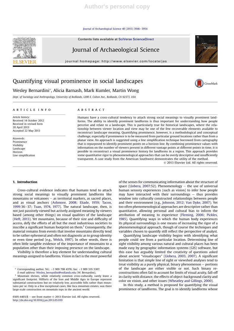
Quantifying visual prominence in social landscapes

Wesley Bernardini*, Alicia Barnash, Mark Kumler, Martin WongDept. of Sociology and Anthropology, University of Redlands, 1200 E. Colton Ave., Redlands, CA 92373, USA

a r t i c l e i n f o

Article history:Received 14 October 2012Received in revised form26 April 2013Accepted 22 May 2013

Keywords:ProminenceVisibilityLandscapeHorizonLine simplification

a b s t r a c t

Humans have a cross-cultural tendency to attach strong social meanings to visually prominent land-forms. The ability to identify prominent landforms is thus important for understanding how peopleperceive and relate to a landscape. This is particularly true for historical landscapes, where the rela-tionship between viewer location and view may be one of the few recoverable elements available toreconstruct landscape meaning. Quantifying prominence, however, is a methodological and conceptualchallenge, especially if prominence is to be measured from particular ground locations rather than from aplanar view. An approach is suggested using a line simplification technique borrowed from cartographythat is repurposed to identify prominent points on a horizon line. By combining prominence values withinformation on the number of viewers present in different vantage points at different points in time, it ispossible to reconstruct a visual prominence history for landforms in a region. This approach providessome quantitative rigor to phenomenological approaches that can be overly descriptive and insufficientlytransparent. A case study from the American Southwest demonstrates the utility of the method.

� 2013 Elsevier Ltd. All rights reserved.

1. Introduction

Cross-cultural evidence indicates that humans tend to attachstrong social meanings to visually prominent landforms likemountains or volcanoes e as territorial markers, as sacred places,and as visual anchors (Ashmore, 2008; Eliade, 1959; Tacon,1999:36e37; Tuan, 1974, 1977). The natural landscape, then, isnot just passively viewed but actively assigned meaning by viewersbased (among other things) on visual qualities of the landscape(Heft, 2013). Yet mountains, because of their size and difficulty ofaccess, defy the efforts of all but the most industrious societies toinscribe a significant human footprint on them.1 Consequently, thematerial remains from events that involve mountains directly tendto be rather ephemeral and often not diagnostic as to group identityor even time period (e.g., Welch, 1997). In other words, there isoften little tangible evidence of the importance of mountains to apopulation other than their imposing presence on the landscape.

Visibility is therefore a key element for understanding culturalmeanings assigned to landforms. Vision in fact is the most powerful

of the senses for communicating information about the structure ofspace (Llobera, 2007:52). Phenomenology e the use of universalhuman sensory experiences (such as vision) to infer how peoplemay have interacted with their surroundings e thus provideswindow into culturally constructed relationships between peopleand their environment (e.g., Johnson, 2012; Van Dyke, 2007). Yettoo often phenomenological approaches are descriptive rather thanquantitative, allowing personal and cultural bias to inform theattribution of meaning to experience (Fleming, 2006; Pickles,1985). Quantifying ways in which the human body experiencesits physical surroundings is one means of increasing the rigor of aphenomenological approach, though of course the techniques andvariables chosen to quantify still reflect the perspective of analyst.

Quantifying landscape visibility begins with identifying whatpeople could see from a particular location. Determining line ofsight visibility among various natural and cultural places has beenmade easy by geographic information systems (GIS) software, butthis ease has arguably limited the creativity of questions askedabout ancient “visualscapes” (Llobera, 2003, 2007). A significantlimitation is that simple line of sight or viewshed analyses tend totreat visibility as a purely physical, binary phenomenon e portionsof the landscape are either visible or not. Such binary re-constructions often fail to account for limits of visual acuity, fall-offin clarity with distance, the effects of object-background clarity andcolor on vision, and other issues (Wheatley and Gillings, 2000).

In this study, a method is proposed for quantifying the visualprominence of landforms. The goal is to identify landforms whose

* Corresponding author. Tel.: þ1 909 798 4376; fax: þ1 909 335 5307.E-mail address: [email protected] (W. Bernardini).

1 Mountain shrines, while relatively common cross-culturally, rarely leave asignificant footprint. Hillforts of the Iron and Middle Ages in Europe representsubstantial constructions but on relatively low, accessible hills rather than moun-tains per se. Only in a few exceptional cases, like Inca mountain estates, was therelarge-scale construction on mountain tops in the ancient world.

Contents lists available at SciVerse ScienceDirect

Journal of Archaeological Science

journal homepage: http: / /www.elsevier .com/locate/ jas

0305-4403/$ e see front matter � 2013 Elsevier Ltd. All rights reserved.http://dx.doi.org/10.1016/j.jas.2013.05.019

Journal of Archaeological Science 40 (2013) 3946e3954


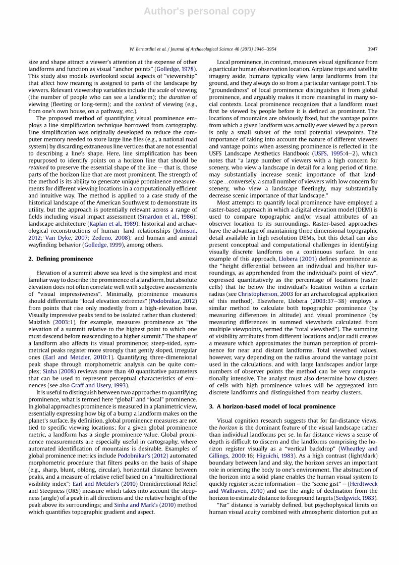
size and shape attract a viewer’s attention at the expense of otherlandforms and function as visual “anchor points” (Golledge, 1978).This study also models overlooked social aspects of “viewership”that affect how meaning is assigned to parts of the landscape byviewers. Relevant viewership variables include the scale of viewing(the number of people who can see a landform); the duration ofviewing (fleeting or long-term); and the context of viewing (e.g.,from one’s own house, on a pathway, etc.).

The proposed method of quantifying visual prominence em-ploys a line simplification technique borrowed from cartography.Line simplification was originally developed to reduce the com-puter memory needed to store large line files (e.g., a national roadsystem) by discarding extraneous line vertices that are not essentialto describing a line’s shape. Here, line simplification has beenrepurposed to identify points on a horizon line that should beretained to preserve the essential shape of the line e that is, thoseparts of the horizon line that are most prominent. The strength ofthe method is its ability to generate unique prominence measure-ments for different viewing locations in a computationally efficientand intuitive way. The method is applied to a case study of thehistorical landscape of the American Southwest to demonstrate itsutility, but the approach is potentially relevant across a range offields including visual impact assessment (Smardon et al., 1986);landscape architecture (Kaplan et al., 1989); historical and archae-ological reconstructions of humaneland relationships (Johnson,2012; Van Dyke, 2007; Zedeno, 2008); and human and animalwayfinding behavior (Golledge, 1999), among others.

2. Defining prominence

Elevation of a summit above sea level is the simplest and mostfamiliar way to describe the prominence of a landform, but absoluteelevation does not often correlate well with subjective assessmentsof “visual impressiveness”. Minimally, prominence measuresshould differentiate “local elevation extremes” (Podobnikar, 2012)from points that rise only modestly from a high-elevation base.Visually impressive peaks tend to be isolated rather than clustered;Maizlish (2003:1), for example, measures prominence as “theelevation of a summit relative to the highest point to which onemust descend before reascending to a higher summit.” The shape ofa landform also affects its visual prominence; steep-sided, sym-metrical peaks register more strongly than gently sloped, irregularones (Earl and Metzler, 2010:1). Quantifying three-dimensionalpeak shape through morphometric analysis can be quite com-plex; Sinha (2008) reviews more than 40 quantitative parametersthat can be used to represent perceptual characteristics of emi-nences (see also Graff and Usery, 1993).

It is useful to distinguish between two approaches to quantifyingprominence, what is termed here “global” and “local” prominence.In global approaches prominence ismeasured in a planimetric view,essentially expressing how big of a bump a landform makes on theplanet’s surface. By definition, global prominence measures are nottied to specific viewing locations; for a given global prominencemetric, a landform has a single prominence value. Global promi-nence measurements are especially useful in cartography, whereautomated identification of mountains is desirable. Examples ofglobal prominence metrics include Podobnikar’s (2012) automatedmorphometric procedure that filters peaks on the basis of shape(e.g., sharp, blunt, oblong, circular), horizontal distance betweenpeaks, and a measure of relative relief based on a “multidirectionalvisibility index”; Earl and Metzler’s (2010) Omnidirectional Reliefand Steepness (ORS) measure which takes into account the steep-ness (angle) of a peak in all directions and the relative height of thepeak above its surroundings; and Sinha and Mark’s (2010) methodwhich quantifies topographic gradient and aspect.

Local prominence, in contrast, measures visual significance froma particular human observation location. Airplane trips and satelliteimagery aside, humans typically view large landforms from theground, and they always do so from a particular vantage point. This“groundedness” of local prominence distinguishes it from globalprominence, and arguably makes it more meaningful in many so-cial contexts. Local prominence recognizes that a landform mustfirst be viewed by people before it is defined as prominent. Thelocations of mountains are obviously fixed, but the vantage pointsfromwhich a given landformwas actually ever viewed by a personis only a small subset of the total potential viewpoints. Theimportance of taking into account the nature of different viewersand vantage points when assessing prominence is reflected in theUSFS Landscape Aesthetics Handbook (USFS, 1995:4e2), whichnotes that “a large number of viewers with a high concern forscenery, who view a landscape in detail for a long period of time,may substantially increase scenic importance of that land-scape.conversely, a small number of viewers with low concern forscenery, who view a landscape fleetingly, may substantiallydecrease scenic importance of that landscape.”

Most attempts to quantify local prominence have employed araster-based approach in which a digital elevation model (DEM) isused to compare topographic and/or visual attributes of anobserver location to its surroundings. Raster-based approacheshave the advantage of maintaining three dimensional topographicdetail available in high resolution DEMs, but this detail can alsopresent conceptual and computational challenges in identifyingvisually discrete landforms on a continuous surface. In oneexample of this approach, Llobera (2001) defines prominence asthe “height differential between an individual and his/her sur-roundings, as apprehended from the individual’s point of view”,expressed quantitatively as the percentage of locations (rastercells) that lie below the individual’s location within a certainradius (see Christopherson, 2003 for an archaeological applicationof this method). Elsewhere, Llobera (2003:37e38) employs asimilar method to calculate both topographic prominence (bymeasuring differences in altitude) and visual prominence (bymeasuring differences in summed viewsheds calculated frommultiple viewpoints, termed the “total viewshed”). The summingof visibility attributes from different locations and/or radii createsa measure which approximates the human perception of promi-nence for near and distant landforms. Total viewshed values,however, vary depending on the radius around the vantage pointused in the calculations, and with large landscapes and/or largenumbers of observer points the method can be very computa-tionally intensive. The analyst must also determine how clustersof cells with high prominence values will be aggregated intodiscrete landforms and distinguished from nearby clusters.

3. A horizon-based model of local prominence

Visual cognition research suggests that for far-distance views,the horizon is the dominant feature of the visual landscape ratherthan individual landforms per se. In far distance views a sense ofdepth is difficult to discern and the landforms comprising the ho-rizon register visually as a “vertical backdrop” (Wheatley andGillings, 2000:16; Higuichi, 1983). As a high contrast (light/dark)boundary between land and sky, the horizon serves an importantrole in orienting the body to one’s environment. The abstraction ofthe horizon into a solid plane enables the human visual system toquickly register scene information e the “scene gist” e (Herdtweckand Wallraven, 2010) and use the angle of declination from thehorizon to estimate distance to foreground targets (Sedgwick,1983).

“Far” distance is variably defined, but psychophysical limits onhuman visual acuity combined with atmospheric distortion put an

W. Bernardini et al. / Journal of Archaeological Science 40 (2013) 3946e3954 3947


upper limit on visual range at around 55e150 km in most areas oftheworld (230� 40 km in optimal conditions),2 with notable drop-offs in detail over that distance (Ogburn, 2006). Higuichi (1983) setfar distance views as the point at which a forested area is visible as“wooded” but little more than texture and color can be perceived, adistance of about 12 km. Ogburn (2006) applied a fuzzy viewshedmethod of modeling visual distortionwith distance for size-specifictargets; results suggest the kind of blurred landscape described byHiguichi in the neighborhood of 15e30 km, depending on targetsize and atmospheric conditions.

Because the horizon bounds the viewer inside a wall-like ver-tical visual barrier, it commonly takes on deep cultural significance.As the point at which the land breaks visual contact with moredistant places, in traditional societies the horizon often symbolizesthe boundary between known and unknown, safe and dangerous,familiar and foreign (Ortiz, 1972; Tuan, 1974). The interaction of thesolid plane of the horizon with astronomical objects also results inthe horizon’s common use as a solar calendar (McCluskey, 1977;Zelik, 1985; Zuidema, 1982) and a compass (Ortiz, 1972).

The horizon, then, registers visually as a linear boundary sepa-rating land from sky. If this is the case, then perhaps vector-basedmethods of analysis may be a productive alternative to raster-based techniques. If we conceptualize the horizon as a line, theemphasis shifts from cells to vertices: which vertices, in whatconfiguration, mark visually prominent landforms? Beyond theadvantage of corresponding to the human visual perception of thehorizon as a line, vector analyses are also computationally lessdemanding than raster analyses. Defining the boundary of the baseof a mountain, or the saddle separating one mountain from thenext, for example, is much more difficult in a raster environmentthan a vector one, where simple changes in slope and Euclideandistance may suffice. With the insight that horizons may be pro-ductively modeled as lines, we now turn our attention to vectorprocessing tools that help to identify prominent vertices on a ho-rizon line.

3.1. Mapping the horizon

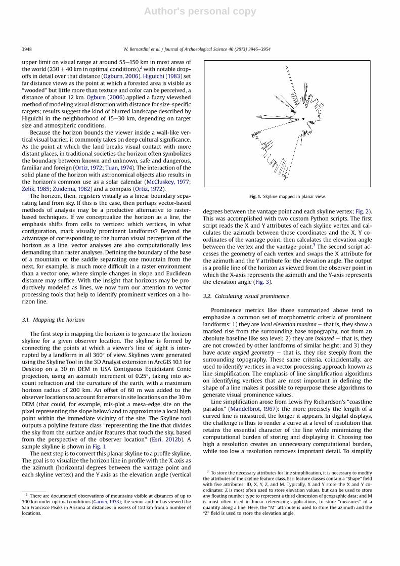
The first step in mapping the horizon is to generate the horizonskyline for a given observer location. The skyline is formed byconnecting the points at which a viewer’s line of sight is inter-rupted by a landform in all 360� of view. Skylines were generatedusing the Skyline Tool in the 3DAnalyst extension in ArcGIS 10.1 forDesktop on a 30 m DEM in USA Contiguous Equidistant Conicprojection, using an azimuth increment of 0.25�, taking into ac-count refraction and the curvature of the earth, with a maximumhorizon radius of 200 km. An offset of 60 m was added to theobserver locations to account for errors in site locations on the 30mDEM (that could, for example, mis-plot a mesa-edge site on thepixel representing the slope below) and to approximate a local highpoint within the immediate vicinity of the site. The Skyline tooloutputs a polyline feature class “representing the line that dividesthe sky from the surface and/or features that touch the sky, basedfrom the perspective of the observer location” (Esri, 2012b). Asample skyline is shown in Fig. 1.

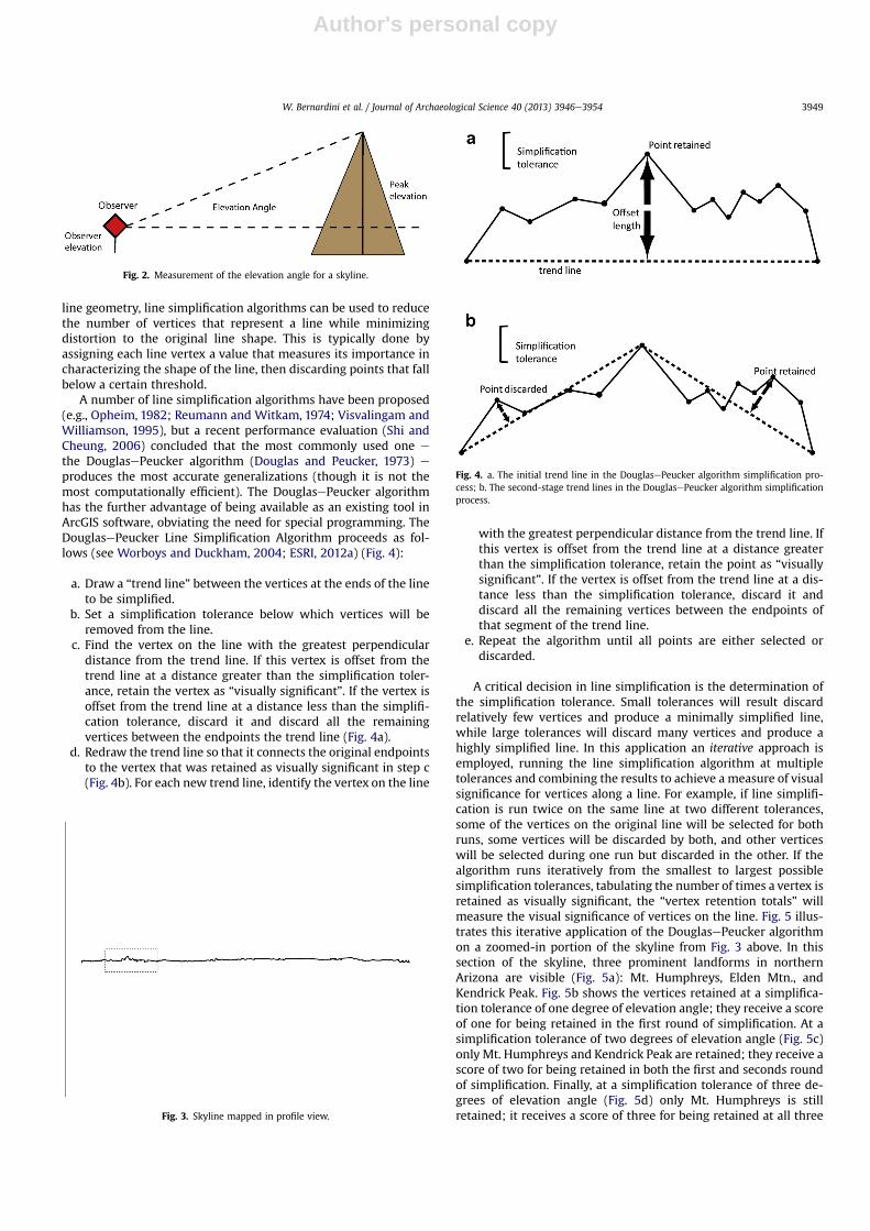
The next step is to convert this planar skyline to a profile skyline.The goal is to visualize the horizon line in profile with the X axis asthe azimuth (horizontal degrees between the vantage point andeach skyline vertex) and the Y axis as the elevation angle (vertical

degrees between the vantage point and each skyline vertex; Fig. 2).This was accomplished with two custom Python scripts. The firstscript reads the X and Y attributes of each skyline vertex and cal-culates the azimuth between those coordinates and the X, Y co-ordinates of the vantage point, then calculates the elevation anglebetween the vertex and the vantage point.3 The second script ac-cesses the geometry of each vertex and swaps the X attribute forthe azimuth and the Y attribute for the elevation angle. The outputis a profile line of the horizon as viewed from the observer point inwhich the X-axis represents the azimuth and the Y-axis representsthe elevation angle (Fig. 3).

3.2. Calculating visual prominence

Prominence metrics like those summarized above tend toemphasize a common set of morphometric criteria of prominentlandforms: 1) they are local elevation maxima e that is, they show amarked rise from the surrounding base topography, not from anabsolute baseline like sea level; 2) they are isolated e that is, theyare not crowded by other landforms of similar height; and 3) theyhave acute angled geometry e that is, they rise steeply from thesurrounding topography. These same criteria, coincidentally, areused to identify vertices in a vector processing approach known asline simplification. The emphasis of line simplification algorithmson identifying vertices that are most important in defining theshape of a line makes it possible to repurpose these algorithms togenerate visual prominence values.

Line simplification arose from Lewis Fry Richardson’s “coastlineparadox” (Mandelbrot, 1967): the more precisely the length of acurved line is measured, the longer it appears. In digital displays,the challenge is thus to render a curve at a level of resolution thatretains the essential character of the line while minimizing thecomputational burden of storing and displaying it. Choosing toohigh a resolution creates an unnecessary computational burden,while too low a resolution removes important detail. To simplify

Fig. 1. Skyline mapped in planar view.

2 There are documented observations of mountains visible at distances of up to300 km under optimal conditions (Garner, 1933); the senior author has viewed theSan Francisco Peaks in Arizona at distances in excess of 150 km from a number oflocations.

3 To store the necessary attributes for line simplification, it is necessary to modifythe attributes of the skyline feature class. Esri feature classes contain a “Shape” fieldwith five attributes: ID, X, Y, Z, and M. Typically, X and Y store the X and Y co-ordinates; Z is most often used to store elevation values, but can be used to storeany floating number type to represent a third dimension of geographic data; and Mis most often used in linear referencing applications, to store “measures” of aquantity along a line. Here, the “M” attribute is used to store the azimuth and the“Z” field is used to store the elevation angle.

W. Bernardini et al. / Journal of Archaeological Science 40 (2013) 3946e39543948


line geometry, line simplification algorithms can be used to reducethe number of vertices that represent a line while minimizingdistortion to the original line shape. This is typically done byassigning each line vertex a value that measures its importance incharacterizing the shape of the line, then discarding points that fallbelow a certain threshold.

A number of line simplification algorithms have been proposed(e.g., Opheim, 1982; Reumann and Witkam, 1974; Visvalingam andWilliamson, 1995), but a recent performance evaluation (Shi andCheung, 2006) concluded that the most commonly used one e

the DouglasePeucker algorithm (Douglas and Peucker, 1973) e

produces the most accurate generalizations (though it is not themost computationally efficient). The DouglasePeucker algorithmhas the further advantage of being available as an existing tool inArcGIS software, obviating the need for special programming. TheDouglasePeucker Line Simplification Algorithm proceeds as fol-lows (see Worboys and Duckham, 2004; ESRI, 2012a) (Fig. 4):

a. Draw a “trend line” between the vertices at the ends of the lineto be simplified.

b. Set a simplification tolerance below which vertices will beremoved from the line.

c. Find the vertex on the line with the greatest perpendiculardistance from the trend line. If this vertex is offset from thetrend line at a distance greater than the simplification toler-ance, retain the vertex as “visually significant”. If the vertex isoffset from the trend line at a distance less than the simplifi-cation tolerance, discard it and discard all the remainingvertices between the endpoints the trend line (Fig. 4a).

d. Redraw the trend line so that it connects the original endpointsto the vertex that was retained as visually significant in step c(Fig. 4b). For each new trend line, identify the vertex on the line

with the greatest perpendicular distance from the trend line. Ifthis vertex is offset from the trend line at a distance greaterthan the simplification tolerance, retain the point as “visuallysignificant”. If the vertex is offset from the trend line at a dis-tance less than the simplification tolerance, discard it anddiscard all the remaining vertices between the endpoints ofthat segment of the trend line.

e. Repeat the algorithm until all points are either selected ordiscarded.

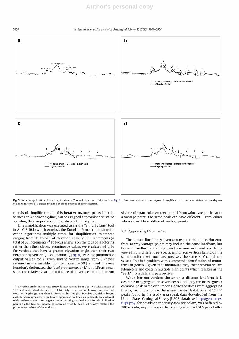
A critical decision in line simplification is the determination ofthe simplification tolerance. Small tolerances will result discardrelatively few vertices and produce a minimally simplified line,while large tolerances will discard many vertices and produce ahighly simplified line. In this application an iterative approach isemployed, running the line simplification algorithm at multipletolerances and combining the results to achieve a measure of visualsignificance for vertices along a line. For example, if line simplifi-cation is run twice on the same line at two different tolerances,some of the vertices on the original line will be selected for bothruns, some vertices will be discarded by both, and other verticeswill be selected during one run but discarded in the other. If thealgorithm runs iteratively from the smallest to largest possiblesimplification tolerances, tabulating the number of times a vertex isretained as visually significant, the “vertex retention totals” willmeasure the visual significance of vertices on the line. Fig. 5 illus-trates this iterative application of the DouglasePeucker algorithmon a zoomed-in portion of the skyline from Fig. 3 above. In thissection of the skyline, three prominent landforms in northernArizona are visible (Fig. 5a): Mt. Humphreys, Elden Mtn., andKendrick Peak. Fig. 5b shows the vertices retained at a simplifica-tion tolerance of one degree of elevation angle; they receive a scoreof one for being retained in the first round of simplification. At asimplification tolerance of two degrees of elevation angle (Fig. 5c)only Mt. Humphreys and Kendrick Peak are retained; they receive ascore of two for being retained in both the first and seconds roundof simplification. Finally, at a simplification tolerance of three de-grees of elevation angle (Fig. 5d) only Mt. Humphreys is stillretained; it receives a score of three for being retained at all threeFig. 3. Skyline mapped in profile view.

Fig. 4. a. The initial trend line in the DouglasePeucker algorithm simplification pro-cess; b. The second-stage trend lines in the DouglasePeucker algorithm simplificationprocess.

Fig. 2. Measurement of the elevation angle for a skyline.



rounds of simplification. In this iterative manner, peaks (that is,vertices on a horizon skyline) can be assigned a “prominence” valuesignaling their importance to the shape of the skyline.

Line simplification was executed using the “Simplify Line” toolin ArcGIS 10.1 (which employs the DouglasePeucker line simplifi-cation algorithm) multiple times for simplification tolerancesranging from 0.1 to 5.0� of elevation angle in 0.1� increments (atotal of 50 increments).4 To focus analysis on the tops of landformsrather than their slopes, prominence values were calculated onlyfor vertices that have a greater elevation angle than their twoneighboring vertices (“local maxima”) (Fig. 6). Possible prominenceoutput values for a given skyline vertex range from 0 (neverretained in the simplification iterations) to 50 (retained in everyiteration), designated the local prominence, or LProm. LProm mea-sures the relative visual prominence of all vertices on the horizon

skyline of a particular vantage point. LProm values are particular toa vantage point; the same peak can have different LProm valueswhen viewed from different vantage points.

3.3. Aggregating LProm values

The horizon line for any given vantage point is unique. Horizonsfrom nearby vantage points may include the same landform, butbecause landforms are large and asymmetrical and are beingviewed from different perspectives, horizon vertices falling on thesame landform will not have precisely the same X, Y coordinatevalues. This is a problem with automated identification of moun-tains in general, given that mountains may cover several squarekilometers and contain multiple high points which register as the“peak” from different perspectives.

When horizon vertices cluster on a discrete landform it isdesirable to aggregate those vertices so that they can be assigned acommon peak name or number. Horizon vertices were aggregatedfirst by searching for nearby named peaks. A database of 12,750peaks found in the study area (peak data downloaded from theUnited States Geological Survey [USGS] database, http://geonames.usgs.gov/; for details on the study area see below) was buffered by300 m radii; any horizon vertices falling inside a USGS peak buffer

Fig. 5. Iterative application of line simplification. a. Zoomed in portion of skyline from Fig. 3; b. Vertices retained at one degree of simplification; c. Vertices retained at two degreesof simplification; d. Vertices retained at three degrees of simplification.

4 Elevation angles in the case study dataset ranged from 0 to 19.4 with a mean of1.75 and a standard deviation of 1.44. Only 3 percent of horizon vertices hadelevation angles greater than 5. Because the DouglasePeucker algorithm beginseach iteration by selecting the two endpoints of the line as significant, the endpointwith the lowest elevation angle is set as zero degrees and the azimuth of all otherpoints on the line are rotated counterclockwise to avoid artificially inflating theprominence values of the endpoints.



were assigned the name of the USGS peak. The 300 m buffer radiusrepresents the high end of the smallest mode in distances betweenpeaks measured in the study area, suggesting that in most caseshorizon vertices separated by less than this distance thresholdshould be considered part of the same landform (99.7% of peaks inthe study area were separated by greater than 300 m; mean2618 m, std. deviation 2285 m). Horizon vertices that could not belinked to USGS peaks were then buffered at 150 m and the buffersdissolved. Points within each discrete dissolved buffer were thenassigned the same arbitrary peak identification number.

4. Modeling viewership

As discussed above, the “viewership” of a landform is affected bymore than just the visual prominence of the landform. A number ofsocial variables also influence meanings attributed by viewers,including the scale of viewing (the number of people who can see alandform); the duration of viewing (fleeting or long-term); and thecontext of viewing (e.g., from one’s own house, from a pathway,etc.). Not all vantage points, in other words, are created equal.Arguably one of the most important contexts of viewing is from theviewer’s place of residence; this the most frequent view, andtypically the most heavily loaded with meaning (Tuan, 1977). Theduration of a residential view is bracketed by the beginning and endof occupation of a given settlement. The scale of viewing from aplace of residence is relatively straightforward to estimate (espe-cially compared to vantage points along transportation routes),requiring only a population estimate for a given human settlementat a given point in time.5

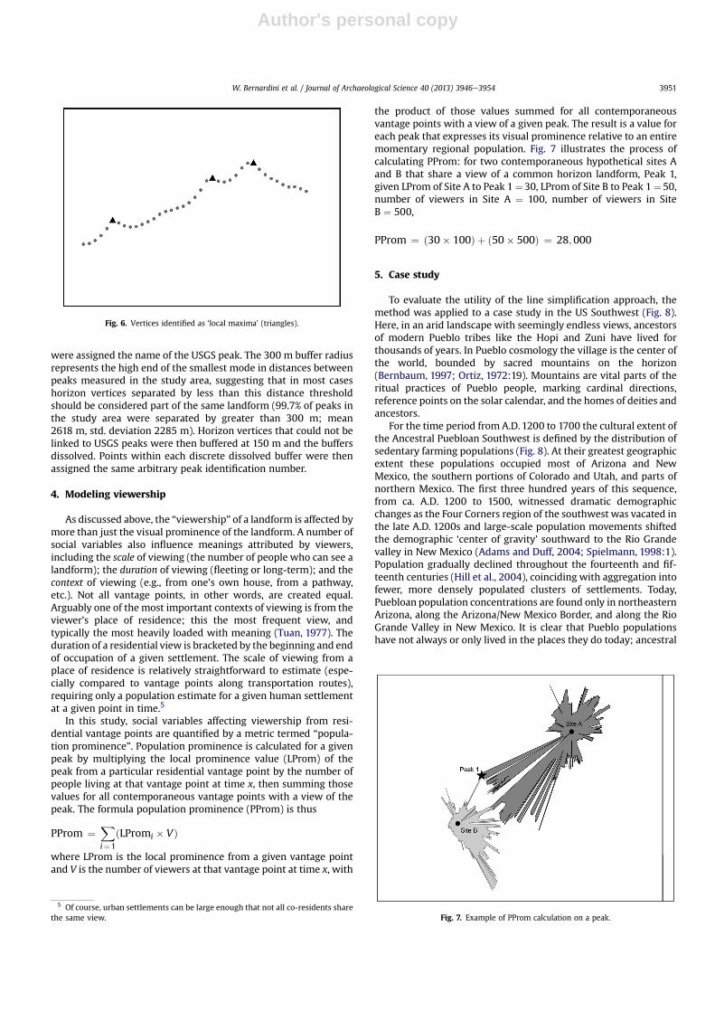
In this study, social variables affecting viewership from resi-dential vantage points are quantified by a metric termed “popula-tion prominence”. Population prominence is calculated for a givenpeak by multiplying the local prominence value (LProm) of thepeak from a particular residential vantage point by the number ofpeople living at that vantage point at time x, then summing thosevalues for all contemporaneous vantage points with a view of thepeak. The formula population prominence (PProm) is thus

PProm ¼X

i¼1

ðLPromi � VÞ

where LProm is the local prominence from a given vantage pointand V is the number of viewers at that vantage point at time x, with

the product of those values summed for all contemporaneousvantage points with a view of a given peak. The result is a value foreach peak that expresses its visual prominence relative to an entiremomentary regional population. Fig. 7 illustrates the process ofcalculating PProm: for two contemporaneous hypothetical sites Aand B that share a view of a common horizon landform, Peak 1,given LProm of Site A to Peak 1 ¼30, LProm of Site B to Peak 1¼50,number of viewers in Site A ¼ 100, number of viewers in SiteB ¼ 500,

PProm ¼ ð30� 100Þ þ ð50� 500Þ ¼ 28;000

5. Case study

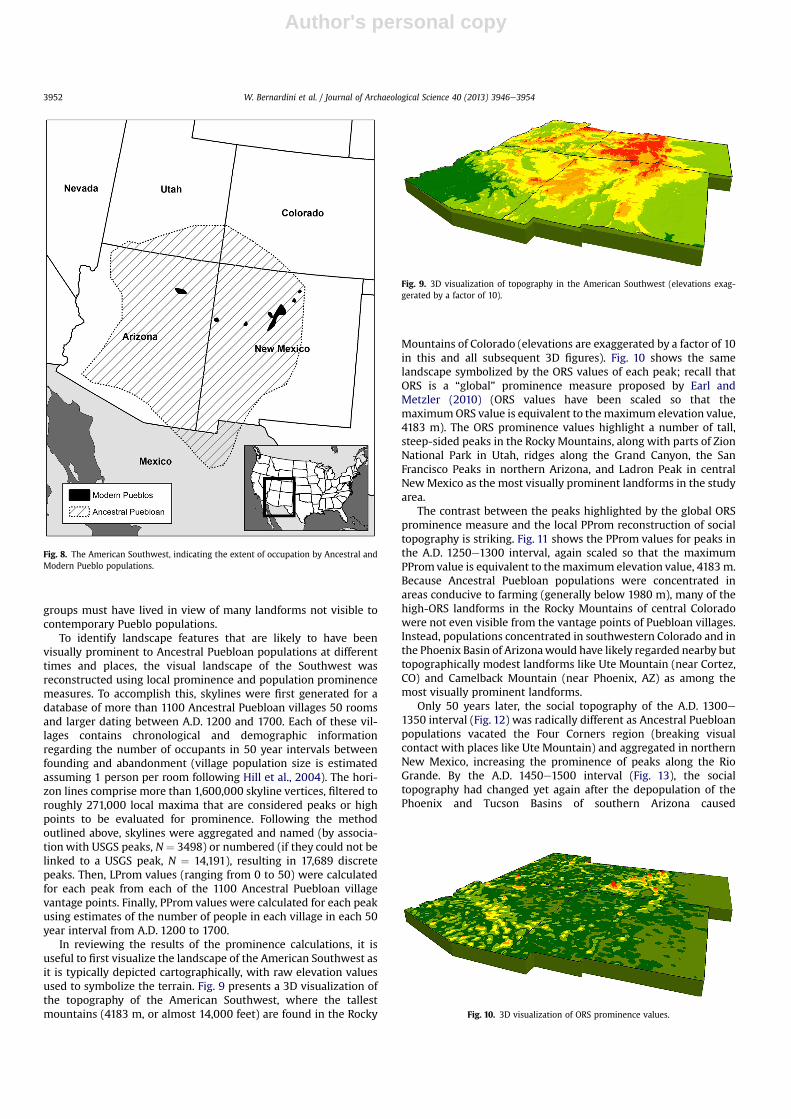
To evaluate the utility of the line simplification approach, themethod was applied to a case study in the US Southwest (Fig. 8).Here, in an arid landscape with seemingly endless views, ancestorsof modern Pueblo tribes like the Hopi and Zuni have lived forthousands of years. In Pueblo cosmology the village is the center ofthe world, bounded by sacred mountains on the horizon(Bernbaum, 1997; Ortiz, 1972:19). Mountains are vital parts of theritual practices of Pueblo people, marking cardinal directions,reference points on the solar calendar, and the homes of deities andancestors.

For the time period from A.D. 1200 to 1700 the cultural extent ofthe Ancestral Puebloan Southwest is defined by the distribution ofsedentary farming populations (Fig. 8). At their greatest geographicextent these populations occupied most of Arizona and NewMexico, the southern portions of Colorado and Utah, and parts ofnorthern Mexico. The first three hundred years of this sequence,from ca. A.D. 1200 to 1500, witnessed dramatic demographicchanges as the Four Corners region of the southwest was vacated inthe late A.D. 1200s and large-scale population movements shiftedthe demographic ‘center of gravity’ southward to the Rio Grandevalley in New Mexico (Adams and Duff, 2004; Spielmann, 1998:1).Population gradually declined throughout the fourteenth and fif-teenth centuries (Hill et al., 2004), coinciding with aggregation intofewer, more densely populated clusters of settlements. Today,Puebloan population concentrations are found only in northeasternArizona, along the Arizona/New Mexico Border, and along the RioGrande Valley in New Mexico. It is clear that Pueblo populationshave not always or only lived in the places they do today; ancestral

Fig. 6. Vertices identified as ‘local maxima’ (triangles).

Fig. 7. Example of PProm calculation on a peak.

5 Of course, urban settlements can be large enough that not all co-residents sharethe same view.



groups must have lived in view of many landforms not visible tocontemporary Pueblo populations.

To identify landscape features that are likely to have beenvisually prominent to Ancestral Puebloan populations at differenttimes and places, the visual landscape of the Southwest wasreconstructed using local prominence and population prominencemeasures. To accomplish this, skylines were first generated for adatabase of more than 1100 Ancestral Puebloan villages 50 roomsand larger dating between A.D. 1200 and 1700. Each of these vil-lages contains chronological and demographic informationregarding the number of occupants in 50 year intervals betweenfounding and abandonment (village population size is estimatedassuming 1 person per room following Hill et al., 2004). The hori-zon lines comprise more than 1,600,000 skyline vertices, filtered toroughly 271,000 local maxima that are considered peaks or highpoints to be evaluated for prominence. Following the methodoutlined above, skylines were aggregated and named (by associa-tion with USGS peaks, N ¼ 3498) or numbered (if they could not belinked to a USGS peak, N ¼ 14,191), resulting in 17,689 discretepeaks. Then, LProm values (ranging from 0 to 50) were calculatedfor each peak from each of the 1100 Ancestral Puebloan villagevantage points. Finally, PProm values were calculated for each peakusing estimates of the number of people in each village in each 50year interval from A.D. 1200 to 1700.

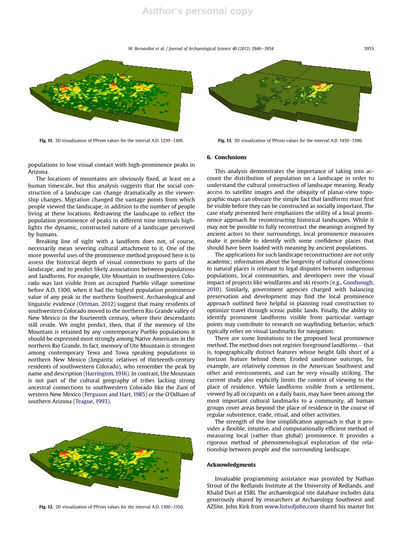
In reviewing the results of the prominence calculations, it isuseful to first visualize the landscape of the American Southwest asit is typically depicted cartographically, with raw elevation valuesused to symbolize the terrain. Fig. 9 presents a 3D visualization ofthe topography of the American Southwest, where the tallestmountains (4183 m, or almost 14,000 feet) are found in the Rocky

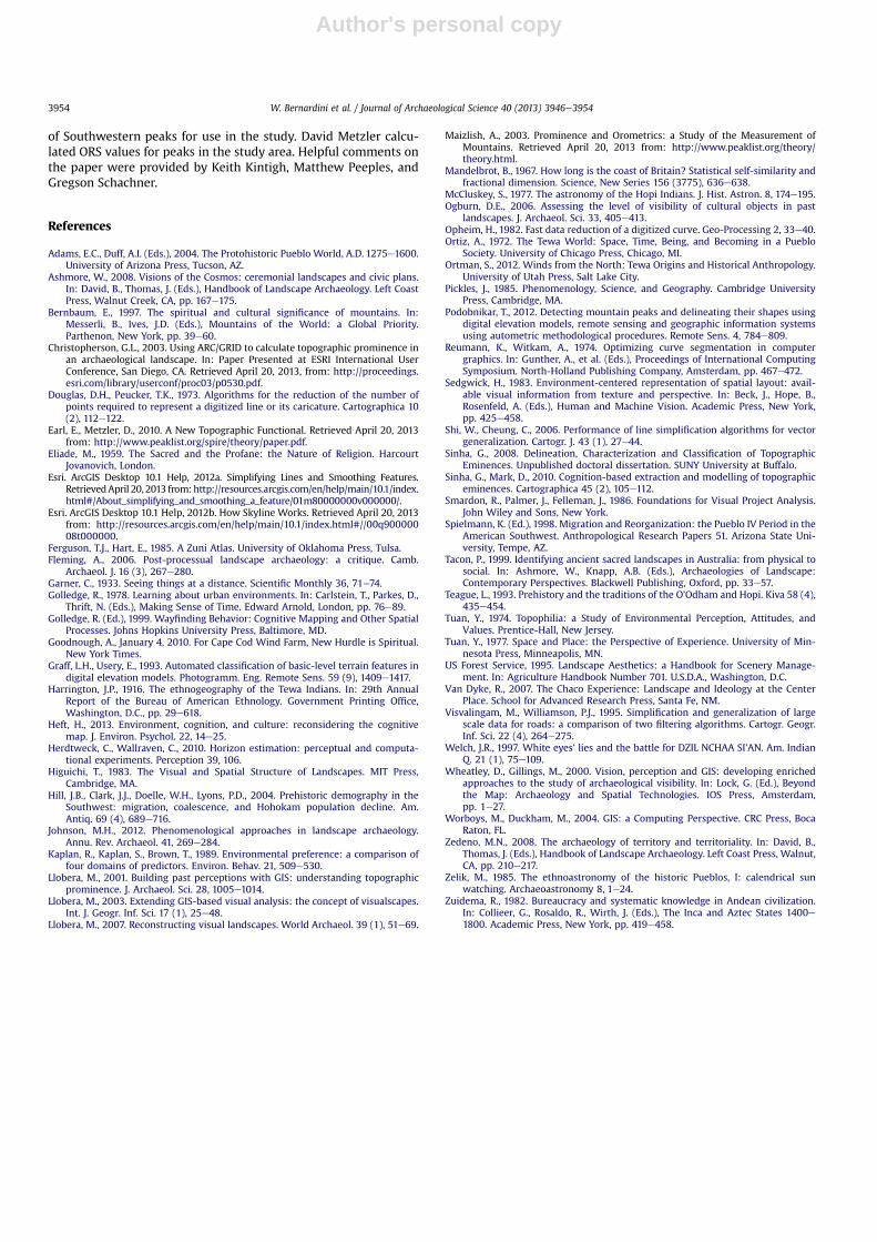
Mountains of Colorado (elevations are exaggerated by a factor of 10in this and all subsequent 3D figures). Fig. 10 shows the samelandscape symbolized by the ORS values of each peak; recall thatORS is a “global” prominence measure proposed by Earl andMetzler (2010) (ORS values have been scaled so that themaximumORS value is equivalent to the maximum elevation value,4183 m). The ORS prominence values highlight a number of tall,steep-sided peaks in the Rocky Mountains, along with parts of ZionNational Park in Utah, ridges along the Grand Canyon, the SanFrancisco Peaks in northern Arizona, and Ladron Peak in centralNewMexico as the most visually prominent landforms in the studyarea.

The contrast between the peaks highlighted by the global ORSprominence measure and the local PProm reconstruction of socialtopography is striking. Fig. 11 shows the PProm values for peaks inthe A.D. 1250e1300 interval, again scaled so that the maximumPPromvalue is equivalent to the maximum elevation value, 4183m.Because Ancestral Puebloan populations were concentrated inareas conducive to farming (generally below 1980 m), many of thehigh-ORS landforms in the Rocky Mountains of central Coloradowere not even visible from the vantage points of Puebloan villages.Instead, populations concentrated in southwestern Colorado and inthe Phoenix Basin of Arizonawould have likely regarded nearby buttopographically modest landforms like Ute Mountain (near Cortez,CO) and Camelback Mountain (near Phoenix, AZ) as among themost visually prominent landforms.

Only 50 years later, the social topography of the A.D. 1300e1350 interval (Fig. 12) was radically different as Ancestral Puebloanpopulations vacated the Four Corners region (breaking visualcontact with places like Ute Mountain) and aggregated in northernNew Mexico, increasing the prominence of peaks along the RioGrande. By the A.D. 1450e1500 interval (Fig. 13), the socialtopography had changed yet again after the depopulation of thePhoenix and Tucson Basins of southern Arizona caused

Fig. 8. The American Southwest, indicating the extent of occupation by Ancestral andModern Pueblo populations.

Fig. 9. 3D visualization of topography in the American Southwest (elevations exag-gerated by a factor of 10).

Fig. 10. 3D visualization of ORS prominence values.



populations to lose visual contact with high-prominence peaks inArizona.

The locations of mountains are obviously fixed, at least on ahuman timescale, but this analysis suggests that the social con-struction of a landscape can change dramatically as the viewer-ship changes. Migration changed the vantage points from whichpeople viewed the landscape, in addition to the number of peopleliving at these locations. Redrawing the landscape to reflect thepopulation prominence of peaks in different time intervals high-lights the dynamic, constructed nature of a landscape perceivedby humans.

Breaking line of sight with a landform does not, of course,necessarily mean severing cultural attachment to it. One of themore powerful uses of the prominence method proposed here is toassess the historical depth of visual connections to parts of thelandscape, and to predict likely associations between populationsand landforms. For example, Ute Mountain in southwestern Colo-rado was last visible from an occupied Pueblo village sometimebefore A.D. 1300, when it had the highest population prominencevalue of any peak in the northern Southwest. Archaeological andlinguistic evidence (Ortman, 2012) suggest that many residents ofsouthwestern Colorado moved to the northern Rio Grande valley ofNew Mexico in the fourteenth century, where their descendantsstill reside. We might predict, then, that if the memory of UteMountain is retained by any contemporary Pueblo populations itshould be expressed most strongly among Native Americans in thenorthern Rio Grande. In fact, memory of Ute Mountain is strongestamong contemporary Tewa and Towa speaking populations innorthern New Mexico (linguistic relatives of thirteenth-centuryresidents of southwestern Colorado), who remember the peak byname and description (Harrington, 1916). In contrast, UteMountainis not part of the cultural geography of tribes lacking strongancestral connections to southwestern Colorado like the Zuni ofwestern New Mexico (Ferguson and Hart, 1985) or the O’Odham ofsouthern Arizona (Teague, 1993).

6. Conclusions

This analysis demonstrates the importance of taking into ac-count the distribution of population on a landscape in order tounderstand the cultural construction of landscape meaning. Readyaccess to satellite images and the ubiquity of planar-view topo-graphic maps can obscure the simple fact that landforms must firstbe visible before they can be constructed as socially important. Thecase study presented here emphasizes the utility of a local promi-nence approach for reconstructing historical landscapes. While itmay not be possible to fully reconstruct the meanings assigned byancient actors to their surroundings, local prominence measuresmake it possible to identify with some confidence places thatshould have been loaded with meaning by ancient populations.

The applications for such landscape reconstructions are not onlyacademic; information about the longevity of cultural connectionsto natural places is relevant to legal disputes between indigenouspopulations, local communities, and developers over the visualimpact of projects like windfarms and ski resorts (e.g., Goodnough,2010). Similarly, government agencies charged with balancingpreservation and development may find the local prominenceapproach outlined here helpful in planning road construction tooptimize travel through scenic public lands. Finally, the ability toidentify prominent landforms visible from particular vantagepoints may contribute to research on wayfinding behavior, whichtypically relies on visual landmarks for navigation.

There are some limitations to the proposed local prominencemethod. Themethod does not register foreground landformse thatis, topographically distinct features whose height falls short of ahorizon feature behind them. Eroded sandstone outcrops, forexample, are relatively common in the American Southwest andother arid environments, and can be very visually striking. Thecurrent study also explicitly limits the context of viewing to theplace of residence. While landforms visible from a settlement,viewed by all occupants on a daily basis, may have been among themost important cultural landmarks to a community, all humangroups cover areas beyond the place of residence in the course ofregular subsistence, trade, ritual, and other activities.

The strength of the line simplification approach is that it pro-vides a flexible, intuitive, and computationally efficient method ofmeasuring local (rather than global) prominence. It provides arigorous method of phenomenological exploration of the rela-tionship between people and the surrounding landscape.

Acknowledgments

Invaluable programming assistance was provided by NathanStrout of the Redlands Institute at the University of Redlands, andKhalid Duri at ESRI. The archaeological site database includes datagenerously shared by researchers at Archaeology Southwest andAZSite. John Kirk from www.listsofjohn.com shared his master list

Fig. 11. 3D visualization of PProm values for the interval A.D. 1250e1300.





of Southwestern peaks for use in the study. David Metzler calcu-lated ORS values for peaks in the study area. Helpful comments onthe paper were provided by Keith Kintigh, Matthew Peeples, andGregson Schachner.

References

Adams, E.C., Duff, A.I. (Eds.), 2004. The Protohistoric Pueblo World, A.D. 1275e1600.University of Arizona Press, Tucson, AZ.

Ashmore, W., 2008. Visions of the Cosmos: ceremonial landscapes and civic plans.In: David, B., Thomas, J. (Eds.), Handbook of Landscape Archaeology. Left CoastPress, Walnut Creek, CA, pp. 167e175.

Bernbaum, E., 1997. The spiritual and cultural significance of mountains. In:Messerli, B., Ives, J.D. (Eds.), Mountains of the World: a Global Priority.Parthenon, New York, pp. 39e60.

Christopherson, G.L., 2003. Using ARC/GRID to calculate topographic prominence inan archaeological landscape. In: Paper Presented at ESRI International UserConference, San Diego, CA. Retrieved April 20, 2013, from: http://proceedings.esri.com/library/userconf/proc03/p0530.pdf.

Douglas, D.H., Peucker, T.K., 1973. Algorithms for the reduction of the number ofpoints required to represent a digitized line or its caricature. Cartographica 10(2), 112e122.

Earl, E., Metzler, D., 2010. A New Topographic Functional. Retrieved April 20, 2013from: http://www.peaklist.org/spire/theory/paper.pdf.

Eliade, M., 1959. The Sacred and the Profane: the Nature of Religion. HarcourtJovanovich, London.

Esri. ArcGIS Desktop 10.1 Help, 2012a. Simplifying Lines and Smoothing Features.RetrievedApril 20, 2013 from:http://resources.arcgis.com/en/help/main/10.1/index.html#/About_simplifying_and_smoothing_a_feature/01m80000000v000000/.

Esri. ArcGIS Desktop 10.1 Help, 2012b. How Skyline Works. Retrieved April 20, 2013from: http://resources.arcgis.com/en/help/main/10.1/index.html#//00q90000008t000000.

Ferguson, T.J., Hart, E., 1985. A Zuni Atlas. University of Oklahoma Press, Tulsa.Fleming, A., 2006. Post-processual landscape archaeology: a critique. Camb.

Archaeol. J. 16 (3), 267e280.Garner, C., 1933. Seeing things at a distance. Scientific Monthly 36, 71e74.Golledge, R., 1978. Learning about urban environments. In: Carlstein, T., Parkes, D.,

Thrift, N. (Eds.), Making Sense of Time. Edward Arnold, London, pp. 76e89.Golledge, R. (Ed.), 1999. Wayfinding Behavior: Cognitive Mapping and Other Spatial

Processes. Johns Hopkins University Press, Baltimore, MD.Goodnough, A., January 4, 2010. For Cape Cod Wind Farm, New Hurdle is Spiritual.

New York Times.Graff, L.H., Usery, E., 1993. Automated classification of basic-level terrain features in

digital elevation models. Photogramm. Eng. Remote Sens. 59 (9), 1409e1417.Harrington, J.P., 1916. The ethnogeography of the Tewa Indians. In: 29th Annual

Report of the Bureau of American Ethnology. Government Printing Office,Washington, D.C., pp. 29e618.

Heft, H., 2013. Environment, cognition, and culture: reconsidering the cognitivemap. J. Environ. Psychol. 22, 14e25.

Herdtweck, C., Wallraven, C., 2010. Horizon estimation: perceptual and computa-tional experiments. Perception 39, 106.

Higuichi, T., 1983. The Visual and Spatial Structure of Landscapes. MIT Press,Cambridge, MA.

Hill, J.B., Clark, J.J., Doelle, W.H., Lyons, P.D., 2004. Prehistoric demography in theSouthwest: migration, coalescence, and Hohokam population decline. Am.Antiq. 69 (4), 689e716.

Johnson, M.H., 2012. Phenomenological approaches in landscape archaeology.Annu. Rev. Archaeol. 41, 269e284.

Kaplan, R., Kaplan, S., Brown, T., 1989. Environmental preference: a comparison offour domains of predictors. Environ. Behav. 21, 509e530.

Llobera, M., 2001. Building past perceptions with GIS: understanding topographicprominence. J. Archaeol. Sci. 28, 1005e1014.

Llobera, M., 2003. Extending GIS-based visual analysis: the concept of visualscapes.Int. J. Geogr. Inf. Sci. 17 (1), 25e48.

Llobera, M., 2007. Reconstructing visual landscapes. World Archaeol. 39 (1), 51e69.

Maizlish, A., 2003. Prominence and Orometrics: a Study of the Measurement ofMountains. Retrieved April 20, 2013 from: http://www.peaklist.org/theory/theory.html.

Mandelbrot, B., 1967. How long is the coast of Britain? Statistical self-similarity andfractional dimension. Science, New Series 156 (3775), 636e638.

McCluskey, S., 1977. The astronomy of the Hopi Indians. J. Hist. Astron. 8, 174e195.Ogburn, D.E., 2006. Assessing the level of visibility of cultural objects in past

landscapes. J. Archaeol. Sci. 33, 405e413.Opheim, H., 1982. Fast data reduction of a digitized curve. Geo-Processing 2, 33e40.Ortiz, A., 1972. The Tewa World: Space, Time, Being, and Becoming in a Pueblo

Society. University of Chicago Press, Chicago, MI.Ortman, S., 2012. Winds from the North: Tewa Origins and Historical Anthropology.

University of Utah Press, Salt Lake City.Pickles, J., 1985. Phenomenology, Science, and Geography. Cambridge University

Press, Cambridge, MA.Podobnikar, T., 2012. Detecting mountain peaks and delineating their shapes using

digital elevation models, remote sensing and geographic information systemsusing autometric methodological procedures. Remote Sens. 4, 784e809.

Reumann, K., Witkam, A., 1974. Optimizing curve segmentation in computergraphics. In: Gunther, A., et al. (Eds.), Proceedings of International ComputingSymposium. North-Holland Publishing Company, Amsterdam, pp. 467e472.

Sedgwick, H., 1983. Environment-centered representation of spatial layout: avail-able visual information from texture and perspective. In: Beck, J., Hope, B.,Rosenfeld, A. (Eds.), Human and Machine Vision. Academic Press, New York,pp. 425e458.

Shi, W., Cheung, C., 2006. Performance of line simplification algorithms for vectorgeneralization. Cartogr. J. 43 (1), 27e44.

Sinha, G., 2008. Delineation, Characterization and Classification of TopographicEminences. Unpublished doctoral dissertation. SUNY University at Buffalo.

Sinha, G., Mark, D., 2010. Cognition-based extraction and modelling of topographiceminences. Cartographica 45 (2), 105e112.

Smardon, R., Palmer, J., Felleman, J., 1986. Foundations for Visual Project Analysis.John Wiley and Sons, New York.

Spielmann, K. (Ed.), 1998. Migration and Reorganization: the Pueblo IV Period in theAmerican Southwest. Anthropological Research Papers 51. Arizona State Uni-versity, Tempe, AZ.

Tacon, P., 1999. Identifying ancient sacred landscapes in Australia: from physical tosocial. In: Ashmore, W., Knapp, A.B. (Eds.), Archaeologies of Landscape:Contemporary Perspectives. Blackwell Publishing, Oxford, pp. 33e57.

Teague, L., 1993. Prehistory and the traditions of the O’Odham and Hopi. Kiva 58 (4),435e454.

Tuan, Y., 1974. Topophilia: a Study of Environmental Perception, Attitudes, andValues. Prentice-Hall, New Jersey.

Tuan, Y., 1977. Space and Place: the Perspective of Experience. University of Min-nesota Press, Minneapolis, MN.

US Forest Service, 1995. Landscape Aesthetics: a Handbook for Scenery Manage-ment. In: Agriculture Handbook Number 701. U.S.D.A., Washington, D.C.

Van Dyke, R., 2007. The Chaco Experience: Landscape and Ideology at the CenterPlace. School for Advanced Research Press, Santa Fe, NM.

Visvalingam, M., Williamson, P.J., 1995. Simplification and generalization of largescale data for roads: a comparison of two filtering algorithms. Cartogr. Geogr.Inf. Sci. 22 (4), 264e275.

Welch, J.R., 1997. White eyes’ lies and the battle for DZIL NCHAA SI’AN. Am. IndianQ. 21 (1), 75e109.

Wheatley, D., Gillings, M., 2000. Vision, perception and GIS: developing enrichedapproaches to the study of archaeological visibility. In: Lock, G. (Ed.), Beyondthe Map: Archaeology and Spatial Technologies. IOS Press, Amsterdam,pp. 1e27.

Worboys, M., Duckham, M., 2004. GIS: a Computing Perspective. CRC Press, BocaRaton, FL.

Zedeno, M.N., 2008. The archaeology of territory and territoriality. In: David, B.,Thomas, J. (Eds.), Handbook of Landscape Archaeology. Left Coast Press, Walnut,CA, pp. 210e217.

Zelik, M., 1985. The ethnoastronomy of the historic Pueblos, I: calendrical sunwatching. Archaeoastronomy 8, 1e24.

Zuidema, R., 1982. Bureaucracy and systematic knowledge in Andean civilization.In: Collieer, G., Rosaldo, R., Wirth, J. (Eds.), The Inca and Aztec States 1400e1800. Academic Press, New York, pp. 419e458.


Quantifying visual prominence in social landscapes

Documents

Transcript of Quantifying visual prominence in social landscapes