Turkish Economic Review - KSP Journals

Turkish Economic Review www.kspjournals.org

Volume 5 September 2018 Issue 3

An empirical analysis of the impact of floating exchange

rate on balance of payment in Nigeria (1986 - 2016)

By N. M. GATAWAaa Sunday ELIJAHab†

& Mohammed UMARac†

Abstract. This paper empirically investigates the impact of floating exchange rate on balance of payment in Nigeria during 1986 – 2016. Unit root test, cointegration test, VEC Granger causality/Exogeneity Wald test and Vector Error Correction Model (VECM) were econometric tools used to establish the relationship between exchange rate and balance of payment. The results showed a positive and statistically significant relationship in both short-run and long-run between balance of payment and exchange rate of the Nigerian Economy during the period under review. The VEC Granger Causality/Block Exogeneity further revealed that the major determinants of exchange rate are real GDP and money supply. It further reveals that the nexus among the variables runs from government expenditure to real GDP and money supply to exchange rate, and then to Balance of Payment. Therefore it was recommended amongst other things that the policy of exchange rate depreciation should be maintained but with government intervention guide. Government through Central Bank of Nigeria (CBN) should apply expenditure reducing monetary policies through money supply and domestic credit to promote favourable BOT which invariably stabilizes BOP. Keywords. Floating exchange rate, Balance of payments, VECM. JEL. F10, F30, F31.

1. Introduction ost of the developing countries are facing serious economic crises over the past five decades in various forms such as balance of payments deficits, low growth rates, and high foreign debt. The causes of this poor

economic performance include currency appreciation, high interest rates, fiscal expansion, expansionary monetary policies, deterioration in terms of trade, price distortion, high debt servicing, protectionism, the devaluation of the British pound sterling in 1067, the French franc in 1969, the US dollar in 1971 and 1973, the global economic and financial meltdown in 2008 and the two oil price hikes in 1973 and 1974 and in 1979 and 1980, or combination of these factors (Ahmed & Mohammed, 2001). Variation in exchange rate, in particular, is a vital endogenous factor that affects economic performance, due to its impact on macroeconomic variables like, interest rate, inflation rate, outputs, imports prices, export prices, investment, employment as well as distribution of income and wealth. A sound exchange rate policy and an appropriate exchange rate are important conditions for improving economic performance (Chang & Tan, 2008; Oladipupo & a Department of Economics, Usmanu Danfodiyo University, Sokoto, Nigeria.

. [email protected] b† Department of Economics, Federal University, Gusau, Nigeria.

. +2348066929820 . [email protected]

b Department of Economics, Usmanu Danfodiyo University, Sokoto, Nigeria. . [email protected]

M

Turkish Economic Review

TER, 5(3), N.M. Gatawa, S. Elijah, & M. Umar, p.285-307.

286

Onotaniyohuwo, 2011). This is one of the main reasons why research related to exchange rates has been a topical issue among economist, academics and policy makers for a very long time especially in developing countries, despites a relatively enormous body of literature in the area. This is also owing to the fact that there is barely any country that lives in absolute autarchy in this globalized world. The economics of all the countries of the world are linked directly or indirectly through asset and goods markets. This linkage is made possible through trade and foreign exchange. The exchange rate in whatever conceptualization, is not only an important relative price, which connects domestic and world markets for goods and assets, but it also signals the competitiveness of a country’s exchange power vis-à-vis the rest of the world in a pure market in order to sustain the internal and external macroeconomic balances over the medium-to-long term (Ademola & David, 2011).

Following the failure of the fixed exchange rate to yield favorable balance of payment, Nigerian adopted structural adjustment programme (SAP) in September 1986. The major element of which was the pursuant of a realistic exchange rate through liberalization of exchange rate as proposed by the International Monetary Fund (IMF) and the World Bank in 1986. Almost throughout the 1970s, there was persistent appreciation of the nominal exchange rate of the naira occasioned by increases in the price of oil in the international market. These appreciations in the nominal exchange rate gave rise to over-reliance on imports leading to increase in the marginal propensity to import with its accompanying capital flight, discouraging non-oil exports which ultimately led to Balance of Payment problems and depletion of external reserves (Eze & Okpala, 2014).

Despite all the programmes that followed the end of the oil boom period when the Nigerian economy benefited from a steady balance of payment surplus, her balance of payments has been fluctuating between positions of surplus and deficit. Nigeria has recorded well over fifteen deficits in her balance of payments account between 1970 and 2015. These deficits were recorded in 1976, 1977, 1981, 1982, 1983, 1988, 1995, 1998, 1999, 2002, 2003, 2009, 2010, 2013, 2014, 2015 and 2016 (CBN, 2006; NBS, 2011).

Structural Adjustment Programme (SAPs) has come and gone but the national economic ailment remains. Despite the efforts of the Nigerian government to maintain a relatively stable rate of exchange, the naira has continued to depreciate after the introduction of SAP leading to a large number of balance of payment deficits. The general view is that depreciation enhances export competitiveness, encourages export diversification, protects domestic industries from imports, improves trade balance and ultimately improve balance of payments. But statistics shows that depreciation of the national currency has not really translated into balance of payments improvement in Nigeria. It was then felt that a depreciation of the naira would relieve pressures on the balance of payments. But the irony of this policy instrument is that the new exchange rate policy did not satisfy the condition for a successful balance of payment policy.

Even though, a far reaching effort has been made by several authors to investigate the impact of exchange rate on macro-economic variables in Nigeria, the study of the impact of exchange rate on balance of payment (which is measured by net reserve) is limited. In actual fact, it has been observed that the empirical investigation of the impact of floating exchange rate (which commenced in 1986) on balance of payments in Nigeria which satisfies the Central Limit Theorem (CLT) of minimum requirement of 30 observations for robust and reliable result is rare in the previous literature. According to CLT, if there is population with mean and standard deviation, the mean of a sample data will be closer to the mean of the overall population in question as sample size increases with replacement, notwithstanding the actual distribution of the data. As a general rule, sample size equal to or greater than 30 are considered sufficient for the CLT to hold, meaning the distribution of the sample is fairly normally distributed (Gujarati, 2007). In this regard, previous related study in Nigeria like Anthony (2015) did not satisfy the



287

requirement of 30 observations and did not carry out descriptive statistics to even check whether the population is normal or not. For this reason, his findings seem to be spurious and inconclusive. Hence, this necessitates the need to fill this lacuna.

Against this background, increased international trade, global interdependence, exchange rate and capital account liberalization and perpetual balance of payment deficit in Nigeria prompt the need to investigate the effects of floating exchange rate on balance of payment in Nigeria. Therefore, this research seeks to empirically examine the impact of floating exchange rate on balance of payment, determine the long run relationship between exchange rate and balance of payment in Nigeria, determine the direction of causality among floating exchange rate, balance of payments and other associated macro-economic variables, investigate the major determinants of exchange rate which in turn influence balance of payment and examine the nexus between exchange rate and balance of payment in Nigeria over a period of 31 years (1986-2016), with a view to suggesting policy implications and recommendations. The study will be significant and contribute to knowledge as no study has been carried on the empirical analysis of the impact of floating exchange rate on balance of payment in Nigeria with largely required sample size.

Following the introduction, the rest of the paper is arranged in sections, namely: overview of exchange rate policy in Nigeria, conceptual clarification, theoretical framework, empirical review of related literature, research methodology, data presentation and analysis, summary of findings, and recommendations.

2. Overview of exchange rate policies in Nigeria Given the significance of foreign exchange in international economic

transactions especially in developing country like Nigeria, the management of scarce foreign exchange has, over the years been a significant component of national economic management. Nigeria has undergone various changes since the enactment of exchange control act of 1962 but spanning between the two regimes (the fixed and floating exchange rate regimes) with a view to achieve the following major objectives: To preserve the value of the domestic currency, the naira; to maintain a favourable external reserves position; and to ensure price stability. The fixed exchange rate was in place before 1986 while the flexible exchange rate regime remains in use from 1986 till date with series of modification.

2.1. Exchange rate management in Nigeria before and after 1986 Before the enactment of Exchange Control Act of 1962, foreign exchange was

earned by private sector operators. These were hold in their banks overseas which then acted as agents for local exporters. These were mainly foreigners doing business in Nigeria. During this period, Agricultural exports contributed the buck of foreign exchange receipts. By then, the currency, Nigeria Pound was tied to the British Pound with ease of convertibility. But this caused delay in the development of active exchange market. However, with the establishment of the Central Bank of Nigeria (CBN) in 1958, there was centralization of foreign exchange authorities in the CBN. Then there came a need to develop a local foreign exchange market (Umeora, 2013).

Before 1986, the prevailing exchange rate policies encouraged over-valuation of the naira. Almost throughout the 1970s there was persistent appreciation of the nominal exchange rate of the naira occasioned by increased in the price of oil in the international market. These appreciations in the nominal exchange rates gave rise to over-reliance on imports leading to an increase in the marginal propensity to import with its accompanying capital flight, collapse of the agricultural sector, discouragement of non-oil exports which ultimately led to Balance of Payments problems and depletion of external reserves. However, all the various exchange rate policies could not lead to the realization of the stated objectives. As a result, a flexible exchange rate was adopted in 1986 (Eze & Okpala, 2014).

The naira was deregulated in September 1986 under the structural Adjustment Programme Package. Following the oil glut of early 80s, it became glaring that



288

Nigerian economy which depends on oil was not able to sustain the fixed exchange regime because national currency was over-valued and its foreign reserves not only depleted but foreign debt also mounted. This was the second phase of exchange rate history in Nigeria. As an integral part of the Structural Adjustment Programme introduced in 1986, the country adopted a flexible exchange arte through the Second tier Foreign Exchange Market (SFEM). SFEM was expected to usher in a mechanism for exchange rates determination and allocation in order to ensure short term stability and long term Balance of Payments equilibrium. As stated by Mordi (2006) the essential objectives of SFEM include to achieve a realistic naira exchange rate through the market forces of demand and supply, ensure more efficient allocation of resources, stimulate non-oil efforts, encourage foreign exchange in flow and discourage outflow, eliminate currency trafficking y wiping out unofficial parallel foreign exchange market, and lead to improvements on the Balance of Payments (Eze & Okpala, 2014). Several modifications were made in order to achieve the objectives of SFEM, from Foreign Exchange Market (FEM) on July 2, 1987 to Autonomous Foreign Exchange Market (AFEM) in 1995, to Dutch Action System in October 25, 1999 and, to the wholesale Dutch Auction System on February 20, 2006.

Under IFEM, the exchange rate was determined through one or more of the following; marginal rate pricing, in the same year, the bureau de change was introduced to accord increased access to small users of foreign exchange in a less formal manner and encourage the integration of the informal market to the officially recognized market, Bureau de change was introduced in 1989 with a view to enlarging the scope of FEM. In spite of various modifications such as introduction of Dutch Auction System (DAS) in December 1990, foreign exchange continues to increase. In 1992, IFEM was depreciated by the adoption of completely regulated exchange rate regime. CBN was unable to meet all the demands of authorized dealers.

In order to further liberalize the market, narrow the arbitrage premium between the official interbank, ensure bureau de change segments of the markets and achieve convergence, the CBN introduced the Wholesale Dutch Auction System (WDAS) on February 20, 2006. This was meant to consolidate the gains of the retail Dutch Auction System as well as deepen the foreign exchange market in order to evolve a realistic exchange rate of the naira. Under this arrangement, the authorized dealers were permitted to deal in foreign exchange on their own accounts for onward sale to their customers (Umeora, 2013).

The important point to not about all these changes since SAP to date is that the authorities, as much as they can, have tried to determine the exchange rate by the operation of market forces of demand and supply. The overall idea is to remove what people have argued, which is over valuation of the Naira and improve balance of payments.

3. Trend analysis of floating exchange rates and balance of

payments in Nigeria (1986-2016) Economic theory postulates that if nominal devaluation translates into real

devaluation, it likely improves balance of payments of a nation through its effects on import and export. That is, economic theory hypothesizes that real exchange rates are measures of international competitiveness. It is argued that reduction in real value of a currency improves global competitiveness of the nation’s trade by making exports relatively cheaper. It is believed that the gain in international competitiveness shifts production from non-tradable to tradable, trade from illegal to legal. It is also argued that devaluation makes import expensive and hence discourages it. The combined effect of increased competitiveness and discouraged imports is expected to improve trade balance and consequently balance of payments.



289

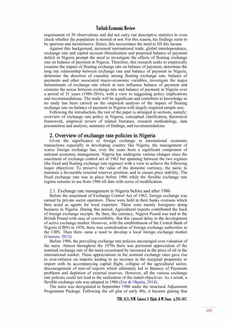
Figure 1. Average (AFEM/DAS) Exchange rate or Effective Central Exchange Rate of the

Naira viz-a-viz the United States’ Dollar (=₦=/$1.00). Source: CBN (2016) and NBS (2011).

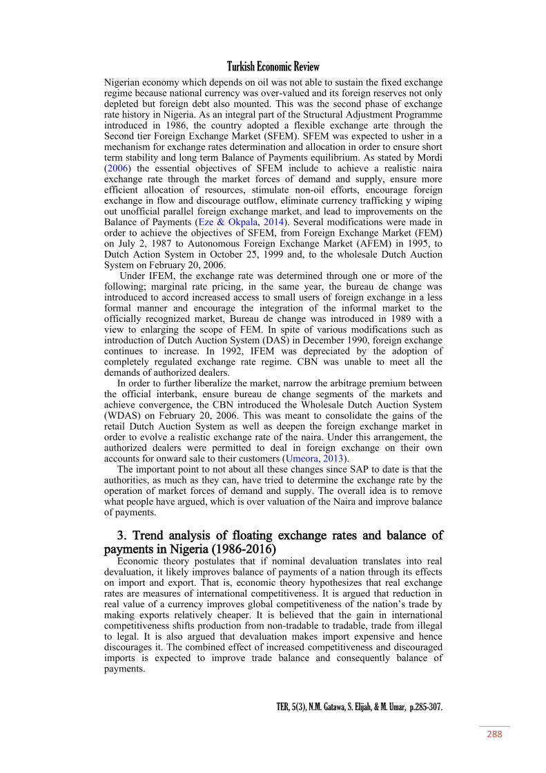
Figure 2. Annual Balance of Payments (in billion Naira)

Source: CBN (2016) and NBS (2011). Figures (1 and 2) show the trend analyses of the naira exchange rate and balance

of payments movements in Nigeria from 1986 to 2016. In both figures, years are measured on the horizontal axis, while Nigeria naira exchange rates movement with USD are measured on the vertical axis of figure (1), balance of payments (in billion) are measured in the vertical axis of figure (2).

Observation of the trend of effective central exchange rate index from 1986 to 2016 reveals about twenty four distinctive periods of depreciations with few exception. Contrary to the theory, for most of the periods under consideration, balance of payment did not improve following the steady growth of naira depreciation, showing the indecisive relationship between changes in exchange rate and balance of payment. It is also observed that import was not discouraged by depreciation of RCER.

0

50

100

150

200

250

300

1986 1988 1990 1992 1994 1996 1998 2000 2002 2004 2006 2008 2010 2012 2014 2016

EXR

EXR

-2000

-1500

-1000

-500

0

500

1000

1500

2000

1986 1988 1990 1992 1994 1996 1998 2000 2002 2004 2006 2008 2010 2012 2014 2016

BOP

BOP



290

4. Conceptual clarification 4.1. Concept balance of payments CBN (2016) and NBS (2013) defined balance of payments as a systematic

record of economic and financial transactions for a given period between residents of an economy and non-residents (the rest of the world). These transactions involve the provision and receipts of real resources and changes in claims on, and liabilities to, the rest of the world. Specifically, it records transactions in goods, services and incomes, as well as changes in ownership and other holdings of financial instruments, including monetary gold, special Drawing Rights (SDRs) and claims on, and liabilities to, the rest of the world. The BOP also records current transfers-the provision or receipt of an economic value without the acceptance or relinquishing of something of equal value (or quid pro quo). Jhingan (2006) defined balance of payments of a country as a systematic record of all its economic transactions with the outside world in a given year. Basically, following the BPM5, the BOP table is usually divided into two main sections, namely the Current Account, and the Capital and Financial Account; and the Net Errors and Omissions, which is a balancing item.

4.2. Concept of Exchange Rate Jhingan (2003) defined foreign exchange rate or exchange rate as the rate at

which one currency is exchanged for another. It is the price of one currency in terms of another currency. Exchange rate is the price of one currency in relation to another. In a slightly different perspective, it expresses the national currency’s quotation in respect to foreign ones. Thus, exchange rate is a conversion factor, a multiplier or a ratio, depending on the direction of conversion (Benedict, 2013).

5. Theoretical literature The theoretical basis for this study is provided by those theories, which deal

with the instruments for correcting balance of payments deficits. Such theories include the neoclassical theory of elasticity approach, the Keynesian theory of absorption approach and monetarists theory.

5.1. Elasticity approach One of the most important neoclassical theories that are applied in

determination of balance of payment (BOP) is the elasticity approach. The elasticity approach to BOP is associated with the Marshal-Lerner (ML) condition (Marshall, 1923, Lerner, 1994) which was worked out independently by these two economists (Jhingan, 2003). The elasticity’s approach emphasizes the role of the relative prices (or exchange rate) in balance of payments adjustments by considering imports and exports as being dependent on relative prices (through the exchange rate) (Adamu & Osi, 2011).

According to this theory, when a country devalues its currency, the domestic prices of its imports are raised and the foreign prices of its exports are reduced. The devaluation helps to improve BOP deficit of a country by increasing its exports and reducing its exports. But the extent to which it will succeed depends on the country’s price elasticity of domestic demand for imports and foreign demand for exports. The Marshal-Lerner condition states that when the sum of price elasticity of demand for exports and imports in absolute terms is greater than unity, devaluation will improve the country’s BOP (Jhingan, 2003). This condition can be expressed mathematically as follow:

𝑒𝑥 + 𝑒𝑚> 1

where 𝑒𝑥 is the demand for elasticity of exports and 𝑒𝑚 is the demand elasticity

for imports.



291

On the contrary, if the sum of price elasticity of demand for exports and imports, in absolute terms, is less than unity, 𝑒𝑥 + 𝑒𝑚< 1, devaluation will worsen the BOP. If the sum of these elasticities in absolute terms is equal to unity, 𝑒𝑥 + 𝑒𝑚 = 1-------- (5.1), devaluation has no effect on the BOP situation which will remain unchanged. In contrast, Oladipupo & Onotaniyohuwo, (2011) are of the view that most less developed countries, who are exporters of raw materials or primary products, and importers of necessities may not successfully apply devaluation as a means of correcting balance of payments disequilibrium, because of the low values for the elasticity of demand.

5.2. The absorption or Keynesian approach Another Neoclassical theory in international trade is the absorption approach.

The absorption approach to balance of payments is a general equilibrium in nature. It dwells on the national income relationship developed by Keynes and it tries to find out its implication on balance of payments. It is, therefore, also known as the Keynesian approach (Jhingan, 2003). It runs through the income effect of devaluation as against the price effect to the elasticity approach. The theory states that if a country has a deficit in its balance of payments, it means that people are ‘absorbing, more than they produce. Domestic expenditure on consumption and investment is greater than national income. If they have surplus in the balance of payments, they are absorbing less. Expenditure in consumption and investment is less than national income.

The Absorption approach was first presented by Alexander (1952). In an open economy, the national income accounting framework shows income (Y) as the sum of consumption expenditure (C), total domestic investment ( 𝐼𝑑 ) autonomous government expenditure (G) and exports less imports (X - M). Thus the analysis can be explained in the following form:

Y = C 𝐼𝑑 + G + X - M (1)

The sum of (C + 𝐼𝑑 + G) is the total absorption designated as A, and the balance of payments (X – M) is designated as B. Thus equation (1) becomes

Y = A + B (2) or B = Y - A (3)

Which means that BOP on current account is the difference between national

income (Y) and total absorption (A). BOP can be improved by either increasing domestic income or reducing the absorption. Equation (3) implies that, if total absorption (expenditure) exceeds income (production), then imports will exceed exports, resulting in a balance of payments deficit. If the opposite occurs, i.e. where income exceeds absorption, then the balance of payments will be in surplus. A balance of payments deficit can, therefore, only be corrected if the level of absorption changes relative to the level of income (Adamu & Osi, 2011).

5.3. Monetarists approach The monetary approach focuses on both the current and capital accounts of the

balance of payments. This is quite different from the elasticity and absorption approaches, which focus on the current account only. As pointed out by Melvin (1992), the general view of monetary approach makes it possible to examine the balance of payments not only in terms of the demand for goods and services, but also in terms of the demand for and the supply of money. This approach also provides a simplistic explanation to the long run devaluation as a means of improving the balance of payments, since devaluation represents an unnecessary and potentially distorting intervention in the process of equilibrating financial



292

flows. Jhingan (2003) emphasizes that the relationship between the foreign sector and the domestic sector of an economy through the working of the monetary sector can be traced by Humes David’s price flow mechanism. The emphasis here is that balance of payments disequilibrium is associated with the disequilibrium between the demand for and supply of money, which are determined by variables such as income, interest rate, price level (both domestic and foreign) and exchange rate. The approach also sees balance of payments as regards international reserve to be associated with imbalances prevailing in the money market. This is because in a fixed exchange rate system, an increase in money supply would lead to an increase in expenditure in the forms of increased purchases of foreign goods and services by domestic residents. To finance such purchases, much of the foreign reserves would be used up, thereby worsening the balance of payments. As the foreign reserve flows out, money supply would continue to diminish until it equals money demand, at which point, monetary equilibrium is restored and outflow of foreign exchange reserve is stopped. Conversely, excess demand for money would cause foreign exchange reserve inflows, domestic monetary expansion and eventually balance of payment equilibrium position is restored. The monetary approach is specifically geared towards an explanation of the overall settlement of a balance of payments deficit or surplus. If the supply of money increases through an expansion of domestic credit, it will cause a deficit in the balance of payments, an increase in the demand for goods and various assets and decrease in the aggregate in the economy.

5.4. The Purchasing Power Parity Theory A variant of the elasticity approach is the purchasing power parity (PPP)

hypothesis. This is one of the leading hypotheses about the forces that determine exchange rate. The Purchasing Power Parity (PPP) theory propounded by a Swedish economist, named Gustav Cassel in 1920, gives us a basic and fundamental relationship between the exchange rate and the price level. PPP also known as the ‚Law of one price‛, is based on the premise that prices of comparable goods should not be different in two different locations. The general idea behind purchasing power parity is that a unit of currency should be able to buy the same basket of goods in one country as the equivalent amount of foreign currency, at the going exchange rate, can buy in a foreign country, so that there is parity in the purchasing power of the unit of currency across the two economies (Bonface, 2013). The hypothesis stresses that countries that experience high depreciation also have high inflation. The PPP postulates that if the inflation rate in a given country accelerates relative to other countries, the country’s currency would tend to depreciate relative to the other countries. This means that a relatively high internal price level will tend to bring about a depreciation of the currency on the foreign exchange market, just as a fall in price internally would tend to cause it to appreciate. The implication is that with every change in the price level, the exchange rate also changes (Ndiomu, 1993). Jhingan (2003) pointed out that, if there is inflation in the country, prices of exports increase. As a result, exports fall. At the same time, the demand for imports increases. Thus increase in exports prices leading to decline in exports and rise in imports results in adverse BOP.

The relative form of the PPP or ‚Law of one price‛ affirms that starting from a base of an equilibrium exchange rate between two currencies, the future of the exchange rate between the two currencies will be determined by the relative movements in the price level in the two countries. The hypothesis thrives in an economy that has floating exchange rates (Blessing, 2014).

6. Empirical literature A vast amount of empirical studies has been conducted within and across the

countries to reveal whether exchange rate causes movements in macro-economic variables, particularly, balance of payment. Prominent scholar Ibrahim (2008) tested the monetary approach to balance of payments to explain the Sudan’s balance of payments deficit during the period 1970-2005. He examined whether



293

money supply played a role in explaining the behaviour of balance of payments using cointegrating and error-correction modelling. The empirical results suggest that money did not play a significant role in explaining the behaviour of Sudan balance of payments. The long-run restriction and unrestricted test indicated that monetary variables (money supply and net foreign assets) could not explain the behaviour of the balance of payments. The estimated short-run dynamics showed that to some extent monetary variables play role in explaining the behaviour of balance of payments. But the main variables that play a significant role are real variables (GDP and aggregate expenditure).

Bonface (2013) examined the relationship between exchange rate volatility and BOP in Kenya. Qualitative comparative design and simple linear regression model was employed to determine the relationship between the two variables. Monthly data on the exchange rates and BOP for the period between the years 2001 and 2012 were used. He found that there is a direct relationship between foreign exchange rate volatility and balance of payments. As the Kenya currency depreciates, the balance of payments for Kenya worsens. The study concluded that apart from the exchange rates, there are other factors having greater influence on the levels of BOP. Agu (2002) examined the real exchange rate distortions and external Balance Position of Nigeria from 1960 to 1990, using the single equation procedure. He found that over the sample period, real exchange rate misalignment (measured as the deviation of the actual from the estimated equilibrium path) was irregular but persistent. After generating the misalignment and volatility of the real exchange rate, he proceeded to ascertain the influence of these distortions on the balance of payment – a gauge of the external balance position of the country. It was then observed that real exchange rate distortions (misalignment and volatility) hurt both the trade balance and the capital account. However, while RER misalignment is critical to the two external sector variables, volatility matters more to the flow of capital.

Oladipupo & Onotaniyohuwo (2011) empirically investigated the impact of exchange rate on the Nigeria External sector (the balance of payments position) using the Ordinary Least Square (OLS) method of estimation for data covering the period between 1970 and 20087. He found that exchange rate has a significant impact of the balance of payments position. He found out that improper allocation and misuse of domestic credit, fiscal indiscipline, and lack of appropriate expenditure control policies due to centralization of power in government were some of the causes of persistent balance of payments deficits in Nigeria.

Umoru & Odjegba (2013) analyzed the relationship between exchange rate misalignment and balance of payments (BOP) mal-adjustment in Nigeria over the sample period of 1973 to 2012, using the vector error correction econometric modelling technique and Granger Causality Tests. They found that exchange rate misalignment exhibited a positive impact on the Nigeria’s balance of payments position. The Granger pair-wise causality test result indicated a unidirectional causality running from exchange rate misalignment to balance of payments adjustment in Nigeria. In the year that followed, Okwuchukwu (2014) examined the impact of exchange rate on balance of payment in Nigeria, using annual data from 1971 to 2012. The empirical methodology employed were autoregressive distributed lag (ARDL) and co-integration estimation technique to detect possible long-run and short-run dynamic relationship between the variables used in the model. He also tested the Marshall-Lerner (ML) condition to see if it is satisfied for Nigeria. He found evidence in favour of a positive and statistically significant relationship in the long-run and also a positive but not statistically significant relationship in the short-run between balance of payment and that Marshall-Lerner (ML) condition subsists for Nigeria. In the following year, Anthony (2015) examined exchange rate variations and balance of payments position in Nigeria over the period of 1960 to 2013. The econometric techniques of ordinary least squares, co-integration and error correction mechanism were used to analyzed the sourced data. He fund that exchange rate had more impact on the balance of



294

payments position during the deregulated period than the regulated period in Nigeria.

Martins & Olarinde (2014) investigated the impact of exchange rate on the balance of payments (BOP) in Nigeria over the period 1961-2012. The analysis is based on a multivariate vector error correction framework. A long-term equilibrium relationship was found between BOP, exchange rate and other associated variables. The empirical results are in favour of bidirectional causality between BOP and other variables employed. Results of the generalized impulse response functions suggest that one standard deviation innovation on exchange rate reduces positive BOP in the medium and long term, while results of the variance decomposition indicate that a significant variation in Nigeria’s BOP is not due to changes in exchange rate movements.

Ahmed t al., (2014) investigated the impact of exchange rate on Balance of Payments in Pakistan. Annual time series data for the period between the years 2007 and 2013 were used. In order to achieve the purpose various tests such as unit root, ARDL and Granger causality tests were employed. They found that a significant and positive relationship existed between exchange rate and BOP. Therefore, they concluded that stability of exchange rates may create a positive environment by encouraging the investment, and this can improves balance of payment.

7. Methodology 7.1. Type, source of data, sample size and sampling technique The study utilized annual time series secondary data sourced from the Central

Bank of Nigeria’s statistical bulletin (2016) and the National Bureau of Statistics (NBS) (2011). The sample size employed for the study covered a period of 31 years (1986 - 2016). The justification for the choice of this period is that it corresponds to the period when Nigeria economy was deregulated and exchange rate was liberalized and consistent data on the relevant variables are available. The selection of this period also conforms to time series research requirement of a minimum of thirty (30) observations (Gujarati, 2007).

7.2. Model specification Model specification involves the representation of the hypotheses in a

mathematical sense to achieve the objective of a quantitative study. In the present investigation, a multivariate Vector Error Correction Model (VECM) was adopted. The choice of VEC model is its efficiency, reliability, adequacy and its ability to capture the long run behavioural pattern of variables under co-integration situation, to permits short-run dynamic adjustment following an innovation or shock as all variables return to their long-run values and to avoid error specification. VEC does not require explicit a priori functional form of the variables employed. The model takes care of the problem of the so-called ‚Spurious‛ regression associated with non-stationary data. In trying to investigate the impact of floating exchange rate on balance of payments in Nigeria, the following model was adopted and modified from the works of Martins & Olarinde (2014); Umoru & Odjegba (2013); and Akinlo & Lawal (2015) and it is expressed in linear econometric equation. This is presented thus:

BOP = f (EXR, RGDP, GEXP, MS, INF, CPS) (4) 𝐵𝑂𝑃𝑡= f (𝐸𝑋𝑅𝑡−𝑗 + 𝑅𝐺𝐷𝑃𝑡−𝑗 + 𝐺𝐸𝑋𝑃𝑡−𝑗 + 𝑀𝑆𝑡−𝑗 + 𝐼𝑁𝐹𝑡−𝑗 + 𝐶𝑃𝑆𝑡−𝑗 ) (5)

Where BOP = Balance of Payment RGDP = real Gross Domestic Product GEXP = Government Expenditure MS = Money Supply



295

INF = Inflation Rate INT = Credit to Private Sector 𝑒𝑡 = Error Term t-j = Time adjusted with lag of the endogenous variables f = Mapping rule which indicates that the LHS is a function of the RHS The econometric function is specified as follows:

BOP = 𝛼0 + 𝛼1 EXR + 𝛼2 RGDP + 𝛼3 GEXP + 𝛼4 MS + 𝛼5 INF + 𝛼6 CPS + 𝛼1𝑡 (6)

8. Techniques of estimation To estimate this model, Vector Error Correction Model was used. Engle &

Granger (1987) stated that there is an existence of both short-run and long-run equilibrium in VECM once the variables are cointegrated of order I(1). The VECM specifications employed in this study are compactly presented in seven labeled equations:

∆ ( 𝐵𝑂𝑃)𝑡 = 𝛼0 + 𝜎𝐵𝑂𝑃∅𝑡−1 𝜎1𝑗𝑡=1 ∆(𝐵𝑂𝑃)𝑡−1 + 𝛽1

𝑗𝑡=1 ∆(𝐸𝑋𝑅)𝑡−1 +

𝛾1𝑗𝑡=1 ∆(𝑅𝐺𝐷𝑃)𝑡−1 + 𝛿1

𝑗𝑡=1 ∆(𝐺𝐸𝑋𝑃)𝑡−1 + ∈1

𝑗𝑡=1 ∆(𝑀𝑆)𝑡−1 +

𝜌1𝑗𝑡=1 ∆(𝐼𝑁𝐹)𝑡−1+ 𝜑

𝑗𝑡=1 ∆(𝐶𝑃𝑆)𝑡−1+휀8 (7)

∆ ( 𝐸𝑋𝑅)𝑡 = 𝛼0 + 𝛽𝐸𝑋𝑅∅𝑡−1 𝜎1𝑗𝑡=1 ∆(𝐵𝑂𝑃)𝑡−1 + 𝛽1

𝑗𝑡=1 ∆(𝐸𝑋𝑅)𝑡−1 +


𝑗𝑡=1 ∆(𝐺𝐸𝑋𝑃)𝑡−1 + ∈1

𝑗𝑡=1 ∆(𝑀𝑆)𝑡−1 +


𝑗𝑡=1 ∆(𝐶𝑃𝑆)𝑡−1+휀8 (8)

∆ ( 𝑅𝐺𝐷𝑃)𝑡 = 𝛼0 + 𝛾𝑅𝐺𝐷𝑃∅𝑡−1 𝜎1𝑗𝑡=1 ∆(𝐵𝑂𝑃)𝑡−1 + 𝛽1

𝑗𝑡=1 ∆(𝐸𝑋𝑅)𝑡−1 +


𝑗𝑡=1 ∆(𝐺𝐸𝑋𝑃)𝑡−1 + ∈1

𝑗𝑡=1 ∆(𝑀𝑆)𝑡−1 +


𝑗𝑡=1 ∆(𝐶𝑃𝑆)𝑡−1+휀8 (9)

∆ ( 𝐺𝐸𝑋𝑃)𝑡 = 𝛼0 + 𝛿𝐺𝐸𝑋𝑃∅𝑡−1 𝜎1𝑗𝑡=1 ∆(𝐵𝑂𝑃)𝑡−1 + 𝛽1

𝑗𝑡=1 ∆(𝐸𝑋𝑅)𝑡−1 +


𝑗𝑡=1 ∆(𝐺𝐸𝑋𝑃)𝑡−1 + ∈1

𝑗𝑡=1 ∆(𝑀𝑆)𝑡−1 +


𝑗𝑡=1 ∆(𝐶𝑃𝑆)𝑡−1+휀8 (10)

∆ ( 𝑀𝑆)𝑡 = 𝛼0 + ∈

𝑀𝑆∅𝑡−1 𝜎1𝑗𝑡=1 ∆(𝐵𝑂𝑃)𝑡−1 + 𝛽1

𝑗𝑡=1 ∆(𝐸𝑋𝑅)𝑡−1 + 𝛾1

𝑗𝑡=1 ∆(𝑅𝐺𝐷𝑃)𝑡−1 +

𝛿1𝑗𝑡=1 ∆(𝐺𝐸𝑋𝑃)𝑡−1+ ∈1

𝑗𝑡=1 ∆(𝑀𝑆)𝑡−1+ 𝜌1

𝑗𝑡=1 ∆(𝐼𝑁𝐹)𝑡−1+ 𝜑

𝑗𝑡=1 ∆(𝐶𝑃𝑆)𝑡−1

+휀8 (11)

∆ ( 𝐼𝑁𝐹)𝑡 = 𝛼0 + 𝜌𝐼𝑁𝐹∅𝑡−1 𝜎1𝑗𝑡=1 ∆(𝐵𝑂𝑃)𝑡−1 + 𝛽1

𝑗𝑡=1 ∆(𝐸𝑋𝑅)𝑡−1 +


𝑗𝑡=1 ∆(𝐺𝐸𝑋𝑃)𝑡−1 + ∈1

𝑗𝑡=1 ∆(𝑀𝑆)𝑡−1 +


𝑗𝑡=1 ∆(𝐶𝑃𝑆)𝑡−1+휀8 (12)

∆ ( 𝐼𝑁𝑇)𝑡 = 𝛼0 + 𝜑𝐼𝑁𝑇∅𝑡−1 𝜎1𝑗𝑡=1 ∆(𝐵𝑂𝑃)𝑡−1 + 𝛽1

𝑗𝑡=1 ∆(𝐸𝑋𝑅)𝑡−1 +


𝑗𝑡=1 ∆(𝐺𝐸𝑋𝑃)𝑡−1 + ∈1

𝑗𝑡=1 ∆(𝑀𝑆)𝑡−1 +


𝑗𝑡=1 ∆(𝐶𝑃𝑆)𝑡−1+휀8 (13)

Where 𝛼0 … … 𝛼7 are constant terms 𝜎,𝛽, 𝛾, 𝛿, 𝜖,𝜌,𝜑are slope parameters independent variables



296

𝑌𝑡 Dependent variable at time t ∑ Vector of coefficient variables in the model 휀1 휀8 are innovations or error, stochastic or random terms in VEC language

representing all the variables that are captured in the model. 9. Methods of data analysis The study utilized secondary data in the form of time series spanning the period

of thirty one (31) years as earlier mentioned. As widely known time series macro-economic data are notably not stationary due to change in their trend. Thus the desire to have models which combine both short run and long run features and maintain stationarity in all the variables is a process this study cherish and tend not to discard. Since the study used time series secondary data, it began its empirical analysis by testing the statistical properties of the variables to ascertain its statistical adequacy. Our diagnostic tests involved: (i) Descriptive statistics (ii) Checking the temporal properties of the variables in the model via unit root tests to determine the stationarity of the variables in order not to obtain spurious result using Augmented Dickey-Fuller (ADF, 1979) test and Philip Perron test; (iii) Determination of a meaningful long-run equilibrium relationship among the variables, that is, to determine if the variables in the equation are co-integrated using Johansen’s Maximum Likelihood co-integrated test; (iv) optimal lag selection; (v) Vector Error Correction Model was estimated to model the short-run dynamics; (vii) the VEC Granger Causality Block/Exogeneity Wald tests was conducted to determine the causality relationships among variables; (viii) and lastly, in addition to the VECM estimates, impulse response function, variance decomposition post-diagnostic and parameter stability tests were also employed to test the adequacy, reliability, stability and validity of the data and model. All these models were used in order to avoid a number of challenges in econometric studies. Some of these challenges include the issue of subjectivity and spurious and bias of result.

10. Data presentation, analysis and discussion of findings The section presents and analyses all the available results which have been

estimated using E-views version 9.5. 10.1. Data Presentation and Analysis of Results Table 1 indicates the descriptive statistics result of the data covering the period

under study using thirty one observations in each of the variables to estimate the impact of floating exchange rate on balance of payment in Nigeria from 1986 to 2016. The variables BOP, EXR, RGDP, GEXP, MS, INF and CPS with skewness of 0.170614, 0.046544, 0.819178, 1.18922, 1.235275, 1.574415 and 1.311135 respectively are positively skewed or are rightward skewed, indicating that the distribution of the data is symmetrical and have a long tail toward large value within the study period. The fact that the values of skewness fall between the range -1.96 and +1.96, shows that the data are normally distributed.

Table 1. Descriptive Statistics Variables Obs. Mean Std. Dev. Skewness Kurtosis Jarque-Bera BOP 31 71.66613 806.2000 0.170614 3.514560 0.492394 EXR 31 95.99774 64.99030 0.046544 2.428607 0.432909 RGDP 31 32827.58 17304.81 0.819177 2.262126 4.170356 GEXP 31 3045.306 3727.469 1.189922 2.871797 7.336793 MS 31 4842.210 6626.222 1.235275 3.133361 7.906806 INF 31 20.70452 19.45031 1.574415 4.249124 14.82244 CPS 31 4476.244 6594.423 1.311135 43.243367 8.958396

The kurtosis of 3.514560 for BOP, 2.428607 for EXR, 2.262128 for RGDP, 2.871797 for GEXP, 3.133355 for MS, with the exception of 4.249124 for INF and



297

4.466333 for CPS suggested that the data used for the study are normally distributed.

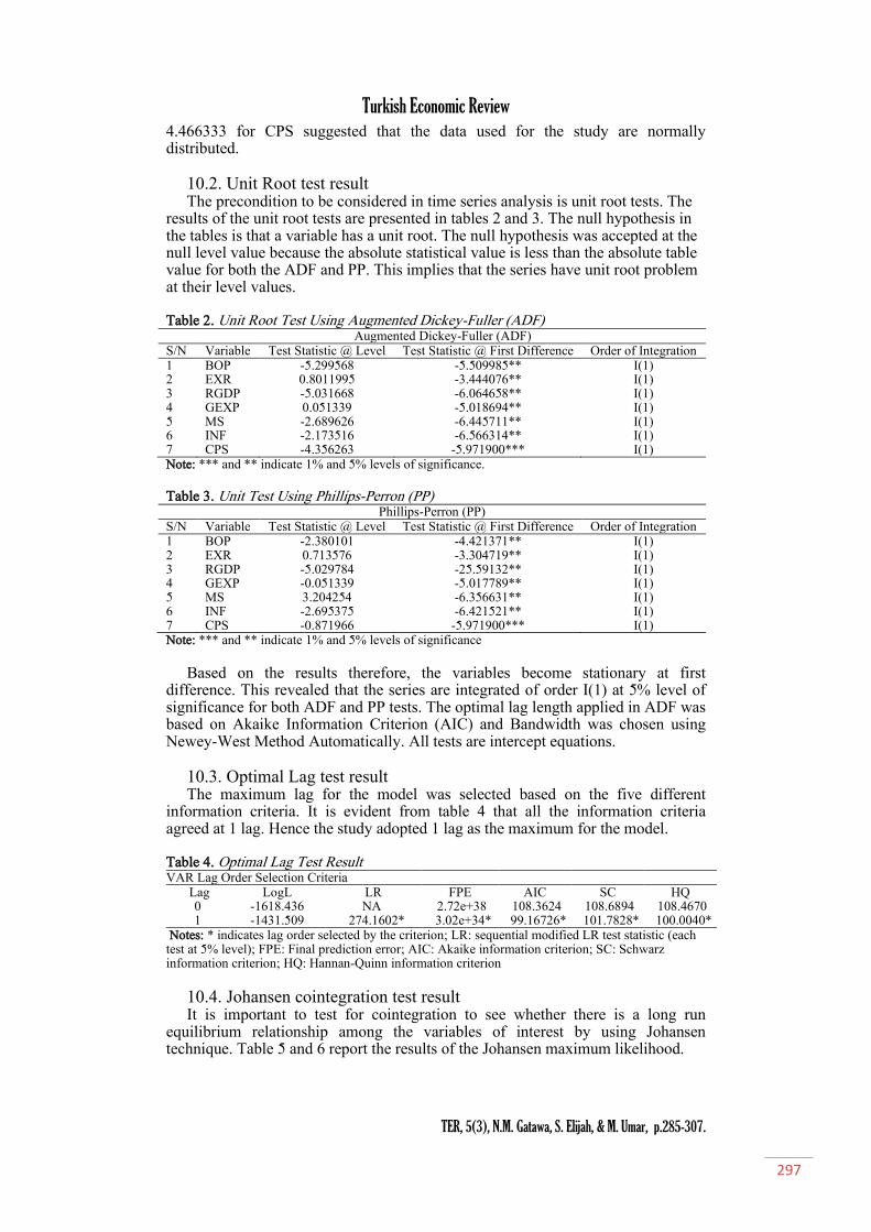
10.2. Unit Root test result The precondition to be considered in time series analysis is unit root tests. The

results of the unit root tests are presented in tables 2 and 3. The null hypothesis in the tables is that a variable has a unit root. The null hypothesis was accepted at the null level value because the absolute statistical value is less than the absolute table value for both the ADF and PP. This implies that the series have unit root problem at their level values.

Table 2. Unit Root Test Using Augmented Dickey-Fuller (ADF) Augmented Dickey-Fuller (ADF) S/N Variable Test Statistic @ Level Test Statistic @ First Difference Order of Integration 1 BOP -5.299568 -5.509985** I(1) 2 EXR 0.8011995 -3.444076** I(1) 3 RGDP -5.031668 -6.064658** I(1) 4 GEXP 0.051339 -5.018694** I(1) 5 MS -2.689626 -6.445711** I(1) 6 INF -2.173516 -6.566314** I(1) 7 CPS -4.356263 -5.971900*** I(1) Note: *** and ** indicate 1% and 5% levels of significance. Table 3. Unit Test Using Phillips-Perron (PP)

Phillips-Perron (PP) S/N Variable Test Statistic @ Level Test Statistic @ First Difference Order of Integration 1 BOP -2.380101 -4.421371** I(1) 2 EXR 0.713576 -3.304719** I(1) 3 RGDP -5.029784 -25.59132** I(1) 4 GEXP -0.051339 -5.017789** I(1) 5 MS 3.204254 -6.356631** I(1) 6 INF -2.695375 -6.421521** I(1) 7 CPS -0.871966 -5.971900*** I(1) Note: *** and ** indicate 1% and 5% levels of significance

Based on the results therefore, the variables become stationary at first difference. This revealed that the series are integrated of order I(1) at 5% level of significance for both ADF and PP tests. The optimal lag length applied in ADF was based on Akaike Information Criterion (AIC) and Bandwidth was chosen using Newey-West Method Automatically. All tests are intercept equations.

10.3. Optimal Lag test result The maximum lag for the model was selected based on the five different

information criteria. It is evident from table 4 that all the information criteria agreed at 1 lag. Hence the study adopted 1 lag as the maximum for the model.

Table 4. Optimal Lag Test Result VAR Lag Order Selection Criteria

Lag LogL LR FPE AIC SC HQ 0 -1618.436 NA 2.72e+38 108.3624 108.6894 108.4670 1 -1431.509 274.1602* 3.02e+34* 99.16726* 101.7828* 100.0040*

Notes: * indicates lag order selected by the criterion; LR: sequential modified LR test statistic (each test at 5% level); FPE: Final prediction error; AIC: Akaike information criterion; SC: Schwarz information criterion; HQ: Hannan-Quinn information criterion

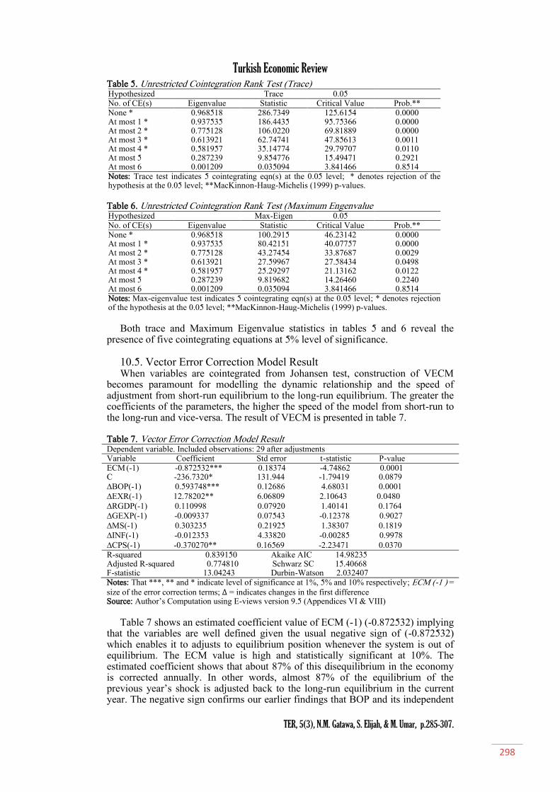
10.4. Johansen cointegration test result It is important to test for cointegration to see whether there is a long run

equilibrium relationship among the variables of interest by using Johansen technique. Table 5 and 6 report the results of the Johansen maximum likelihood.



298

Table 5. Unrestricted Cointegration Rank Test (Trace) Hypothesized Trace 0.05 No. of CE(s) Eigenvalue Statistic Critical Value Prob.** None * 0.968518 286.7349 125.6154 0.0000 At most 1 * 0.937535 186.4435 95.75366 0.0000 At most 2 * 0.775128 106.0220 69.81889 0.0000 At most 3 * 0.613921 62.74741 47.85613 0.0011 At most 4 * 0.581957 35.14774 29.79707 0.0110 At most 5 0.287239 9.854776 15.49471 0.2921 At most 6 0.001209 0.035094 3.841466 0.8514 Notes: Trace test indicates 5 cointegrating eqn(s) at the 0.05 level; * denotes rejection of the hypothesis at the 0.05 level; **MacKinnon-Haug-Michelis (1999) p-values. Table 6. Unrestricted Cointegration Rank Test (Maximum Engenvalue Hypothesized Max-Eigen 0.05 No. of CE(s) Eigenvalue Statistic Critical Value Prob.** None * 0.968518 100.2915 46.23142 0.0000 At most 1 * 0.937535 80.42151 40.07757 0.0000 At most 2 * 0.775128 43.27454 33.87687 0.0029 At most 3 * 0.613921 27.59967 27.58434 0.0498 At most 4 * 0.581957 25.29297 21.13162 0.0122 At most 5 0.287239 9.819682 14.26460 0.2240 At most 6 0.001209 0.035094 3.841466 0.8514 Notes: Max-eigenvalue test indicates 5 cointegrating eqn(s) at the 0.05 level; * denotes rejection of the hypothesis at the 0.05 level; **MacKinnon-Haug-Michelis (1999) p-values.

Both trace and Maximum Eigenvalue statistics in tables 5 and 6 reveal the

presence of five cointegrating equations at 5% level of significance. 10.5. Vector Error Correction Model Result When variables are cointegrated from Johansen test, construction of VECM

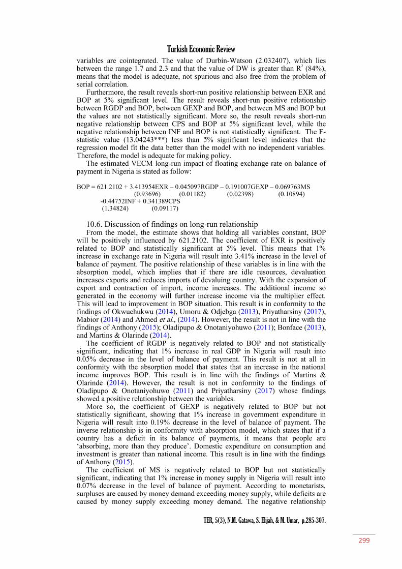
becomes paramount for modelling the dynamic relationship and the speed of adjustment from short-run equilibrium to the long-run equilibrium. The greater the coefficients of the parameters, the higher the speed of the model from short-run to the long-run and vice-versa. The result of VECM is presented in table 7.

Table 7. Vector Error Correction Model Result Dependent variable. Included observations: 29 after adjustments Variable Coefficient Std error t-statistic P-value ECM (-1) -0.872532*** 0.18374 -4.74862 0.0001 C -236.7320* 131.944 -1.79419 0.0879 ∆BOP(-1) 0.593748*** 0.12686 4.68031 0.0001 ∆EXR(-1) 12.78202** 6.06809 2.10643 0.0480 ∆RGDP(-1) 0.110998 0.07920 1.40141 0.1764 ∆GEXP(-1) -0.009337 0.07543 -0.12378 0.9027 ∆MS(-1) 0.303235 0.21925 1.38307 0.1819 ∆INF(-1) -0.012353 4.33820 -0.00285 0.9978 ∆CPS(-1) -0.370270** 0.16569 -2.23471 0.0370 R-squared 0.839150 Akaike AIC 14.98235 Adjusted R-squared 0.774810 Schwarz SC 15.40668 F-statistic 13.04243 Durbin-Watson 2.032407 Notes: That ***, ** and * indicate level of significance at 1%, 5% and 10% respectively; ECM (-1 ) = size of the error correction terms; ∆ = indicates changes in the first difference Source: Author’s Computation using E-views version 9.5 (Appendices VI & VIII)

Table 7 shows an estimated coefficient value of ECM (-1) (-0.872532) implying

that the variables are well defined given the usual negative sign of (-0.872532) which enables it to adjusts to equilibrium position whenever the system is out of equilibrium. The ECM value is high and statistically significant at 10%. The estimated coefficient shows that about 87% of this disequilibrium in the economy is corrected annually. In other words, almost 87% of the equilibrium of the previous year’s shock is adjusted back to the long-run equilibrium in the current year. The negative sign confirms our earlier findings that BOP and its independent



299

variables are cointegrated. The value of Durbin-Watson (2.032407), which lies between the range 1.7 and 2.3 and that the value of DW is greater than R2 (84%), means that the model is adequate, not spurious and also free from the problem of serial correlation.

Furthermore, the result reveals short-run positive relationship between EXR and BOP at 5% significant level. The result reveals short-run positive relationship between RGDP and BOP, between GEXP and BOP, and between MS and BOP but the values are not statistically significant. More so, the result reveals short-run negative relationship between CPS and BOP at 5% significant level, while the negative relationship between INF and BOP is not statistically significant. The F-statistic value (13.04243***) less than 5% significant level indicates that the regression model fit the data better than the model with no independent variables. Therefore, the model is adequate for making policy.

The estimated VECM long-run impact of floating exchange rate on balance of payment in Nigeria is stated as follow:

BOP = 621.2102 + 3.413954EXR – 0.045097RGDP – 0.191007GEXP – 0.069763MS (0.93696) (0.01182) (0.02398) (0.10894) -0.44752INF + 0.341389CPS (1.34824) (0.09117)

10.6. Discussion of findings on long-run relationship From the model, the estimate shows that holding all variables constant, BOP

will be positively influenced by 621.2102. The coefficient of EXR is positively related to BOP and statistically significant at 5% level. This means that 1% increase in exchange rate in Nigeria will result into 3.41% increase in the level of balance of payment. The positive relationship of these variables is in line with the absorption model, which implies that if there are idle resources, devaluation increases exports and reduces imports of devaluing country. With the expansion of export and contraction of import, income increases. The additional income so generated in the economy will further increase income via the multiplier effect. This will lead to improvement in BOP situation. This result is in conformity to the findings of Okwuchukwu (2014), Umoru & Odjebga (2013), Priyatharsiny (2017), Mabior (2014) and Ahmed et al., (2014). However, the result is not in line with the findings of Anthony (2015); Oladipupo & Onotaniyohuwo (2011); Bonface (2013), and Martins & Olarinde (2014).

The coefficient of RGDP is negatively related to BOP and not statistically significant, indicating that 1% increase in real GDP in Nigeria will result into 0.05% decrease in the level of balance of payment. This result is not at all in conformity with the absorption model that states that an increase in the national income improves BOP. This result is in line with the findings of Martins & Olarinde (2014). However, the result is not in conformity to the findings of Oladipupo & Onotaniyohuwo (2011) and Priyatharsiny (2017) whose findings showed a positive relationship between the variables.

More so, the coefficient of GEXP is negatively related to BOP but not statistically significant, showing that 1% increase in government expenditure in Nigeria will result into 0.19% decrease in the level of balance of payment. The inverse relationship is in conformity with absorption model, which states that if a country has a deficit in its balance of payments, it means that people are ‘absorbing, more than they produce’. Domestic expenditure on consumption and investment is greater than national income. This result is in line with the findings of Anthony (2015).

The coefficient of MS is negatively related to BOP but not statistically significant, indicating that 1% increase in money supply in Nigeria will result into 0.07% decrease in the level of balance of payment. According to monetarists, surpluses are caused by money demand exceeding money supply, while deficits are caused by money supply exceeding money demand. The negative relationship



300

between the two variables is attributed to the later theoretical preposition of monetarists which states that an increase in money supply over money demand would lead to an increase in expenditure in the forms of increased purchases of foreign goods and services by domestic residents. To finance such purchases, much of the foreign reserves would be used up, thereby worsening the balance of payments. Although, the insignificant relationship between the two variables during the study period is not surprising in Nigeria, because money supply tended to support growth in the real sector of the economy and induced lower interest rates which are expected to attract firms in sourcing for investment funds from the financial sector. Investment increases production, which consequently improve a country’s net export and thus the BOP position. This result is in line with the findings of Anthony (2015) and Martins & Olarinde (2014) and Mabior (2014). However, the result is not in line with the findings of Oladipupo & Onotaniyohuwo (2011).

The coefficient of INF is negatively related to BOP but not statistically significant, showing that 1% increase in inflation rate in Nigeria will result into 0.45% decrease in the level of balance of payment. The result is in conformity with the purchasing power parity as pointed out by Jhingan (2003) if there is inflation in the country, prices of exports increase. As a result, exports fall. At the same time, the demand for imports increases. Thus increase in exports leading to decline in exports and rise in imports results in adverse BOP. This result is in line with the findings of Oladipupo & Onotaniyohuwo (2011).

For the credit to private sector, on the other hand, the coefficient revealed significant positive relationship with BOP at 5% level. This implies that as credit to private sector increases, BOP also increases with high implication. The positive relationship is in conformity with the joint contribution of monetarists and Mundell-Flemming which stress that an increasing level of money demand coupled with an increase in credit creation raises money supply and income and consequently reduces the level of interest rates. A fall in the level of interest rate improves the investment level and thus employment and production which can consequently improve a country’s net export and thus the BOP position. This result is not in conformity with the findings of FN (2005).

The coefficient of determination R2 is 0.839150 indicating that about 84% of the variation of BOP was explained by the variables controlled in the model between the year 1986 and 2016 while the remaining 16% were explained by other variables not captured by the model, which is represented by the error term. In addition, the result shows that the F-statistic is 13.04243 showing statistical significance at 5% level.

10.7. VEC Granger causality block/exogeneity Wald test result

In order to analyze the short-run relationship among the variables in the VECM, a VEC Granger Causality Block/Exogeneity Wald Test Result is shown in Table 8.



301

Table 8. Short-Run Granger Causality Test Short-run Causality

Dep

ende

nt

Var

iabl

es

Independent Variables

Join

t BO

P∅

t-

1

∆(E

XR

) t-

1

∆(R

GD

P)

t-1

∆(G

EX

P)

t-1

∆(M

S)

t-1

∆(I

NF

) t-

1

𝐶𝑃

S)

t-1

∆BOP - 4.44** [0.0251]

1.96 [0.1611]

0.02 [0.9015]

1.91 [0.1666]

8.11 [0.9977]

4.94** [0.0254]

10.31 [0.1120]

∆EXR 1.37 [0.2417]

- 4.18** [0.0409]

2.08 [0.1419]

4.16** [0.0415]

0.23 [0.6298]

8.48 [0.9927]

11.06* [0.0865]

∆RGDP 1.09 [0.2965]

4.12** [0.0423]

- 0.91 [0.3398]

0.90 [0.3424]

0.06 [0.8130]

0.04 [0.8386]

7.09 [0.3125]

∆GEXP 6.9*** [0.0083]

0.41 [0.5219]

1.64 [0.1998]

- 0.04 [0.8458]

0.04 [0.8370]

0.40 [0.2372]

12.97** [0.04]

∆MS 6.9*** [0.0083]

1.38** [0.0364]

4.32*** [0.0377]

7.06*** [0.0079]

- 0.56 [0.4550]

1.64 [0.2000]

15.62** [0.0159]

∆INF 0.01 [0.9389]

1.99 [0.1584]

0.22 [0.6353]

0.03 [0.8669]

0.02 [0.9020]

- 1.20 [0.6563]

2.09 [0.9113]

∆CPS 0.37 [0.5412]

2.27 [0.1319]

0.00 [0.9853]

16.4*** [0.0001]

13.3*** [0.0003]

4.10** [0.7485]

- 38.4*** [0.0000]

Note: that ***, ** and * indicate level of significance at 1%, 5% and 10% respectively

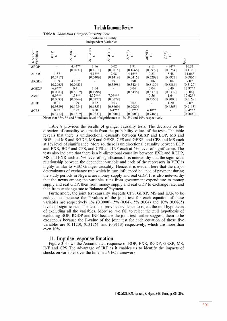
Table 8 provides the results of granger causality tests. The decision on the direction of causality was made from the probability values of the tests. The table reveals that there is unidirectional causality between GEXP and BOP, MS and BOP, and MS and RGDP, MS and GEXP, CPS and GEXP, and CPS and MS each at 1% level of significance. More so, there is unidirectional causality between BOP and EXR, BOP and CPS, and CPS and INF each at 5% level of significance. The tests also indicate that there is a bi-directional causality between EXR and RGDP, MS and EXR each at 5% level of significance. It is noteworthy that the significant relationship between the dependent variable and each of the repressors in VEC is highly similar to VEC Granger causality. Hence, it is evident here that the major determinants of exchange rate which in turn influenced balance of payment during the study periods in Nigeria are money supply and real GDP. It is also noteworthy that the nexus among the variables runs from government expenditure to money supply and real GDP, then from money supply and real GDP to exchange rate, and then from exchange rate to Balance of Payment.

Furthermore, the joint test causality suggests CPS, GEXP, MS and EXR to be endogenous because the P-values of the joint test for each equation of these variables are respectively 1% (0.0000), 5% (0.04), 5% (0.04) and 10% (0.0865) levels of significance. The test also provides evidence to reject the null hypothesis of excluding all the variables. More so, we fail to reject the null hypothesis of excluding BOP, RGDP and INF because the joint test further suggests them to be exogenous because the P-value of the joint test for each equation of those five variables are (0.1120), (0.3125) and (0.9113) respectively, which are more than even 10%.

11. Impulse response function Figure 3 shows the Accumulated response of BOP, EXR, RGDP, GEXP, MS,

INF and CPS The advantage of IRF as it enables us to identify the impacts of shocks on variables over the time in a VEC framework.



302

-800,000

-400,000

0

400,000

800,000

2 4 6 8 10

Response of BOP to BOP

Response to Cholesky One S.D. Innovations

-800,000

-400,000

0

400,000

800,000

2 4 6 8 10

Response of BOP to EXR


-800,000

-400,000

0

400,000

800,000

2 4 6 8 10

Response of BOP to RGDP


-800,000

-400,000

0

400,000

800,000

2 4 6 8 10

Response of BOP to GEXP


-40,000

-20,000

0

20,000

40,000

2 4 6 8 10

Response of EXR to MS


-800,000

-400,000

0

400,000

800,000

2 4 6 8 10

Response of BOP to INF


-800,000

-400,000

0

400,000

800,000

2 4 6 8 10

Response of BOP to CPS


The blue line is the reaction of balance of payment. The first two figures show

that a positive standard deviation shock to BOP and exchange rate will make balance of payment to be static and steady in the first five periods and then begin to fall (decline) steadily and gradually from fifth period to tenth period. The third figure shows that a positive standard deviation shock to real GDP will make balance of payment to be static and steady in the first five periods and then begin to rise steadily and gradually from fifth period to tenth period.

The fourth figure shows that a positive standard deviation shock to government expenditure will make balance of payment to be static and steady throughout the next ten years. The fifth figure shows that a positive standard deviation shock to money supply will make balance of payment to be static and steady in the first seven periods and then begin to fall (decline) steadily and gradually from seventh period to tenth period.

The sixth figure shows that a positive standard deviation shock to money inflation rate will make balance of payment to be static and steady in the first seven periods and then begin to fall (decline) steadily and gradually from seventh period to tenth period. The seventh figure shows that a positive standard deviation shock to credit to private sector will make balance of payment to be static and steady throughout the next ten periods.

12. Variance decomposition Variance decomposition analysis provides a means of determining the relative

importance of various shocks in explaining variations in the variable of interest.



303

Table 9. Variance Decomposition VD of BOP Period S.E. BOP EXR RGDP GEXP MS INF CPS

1 382.8614 100.0000 0.000000 0.000000 0.000000 0.000000 0.000000 0.000000 2 1574.562 17.60158 26.79666 50.74947 2.157487 1.549195 0.197723 0.947893 3 6619.378 29.81317 36.51981 32.77761 0.204163 0.600824 0.011498 0.072930 4 16456.82 31.01565 41.46224 26.83766 0.053268 0.513741 0.088939 0.028503 5 34597.54 30.02582 43.36012 25.84436 0.017724 0.526058 0.182126 0.043797 6 69888.79 29.35964 43.68830 26.12359 0.013398 0.564403 0.210237 0.040430 7 142190.0 29.37430 43.40995 26.38969 0.011207 0.573062 0.206025 0.035774 8 289064.8 29.53454 43.35864 26.28577 0.009899 0.570448 0.204807 0.035886 9 583970.4 29.58776 43.41765 26.17110 0.008608 0.567635 0.209235 0.038012

10 1173729. 29.56744 43.47432 26.12951 0.008233 0.568400 0.212994 0.039105

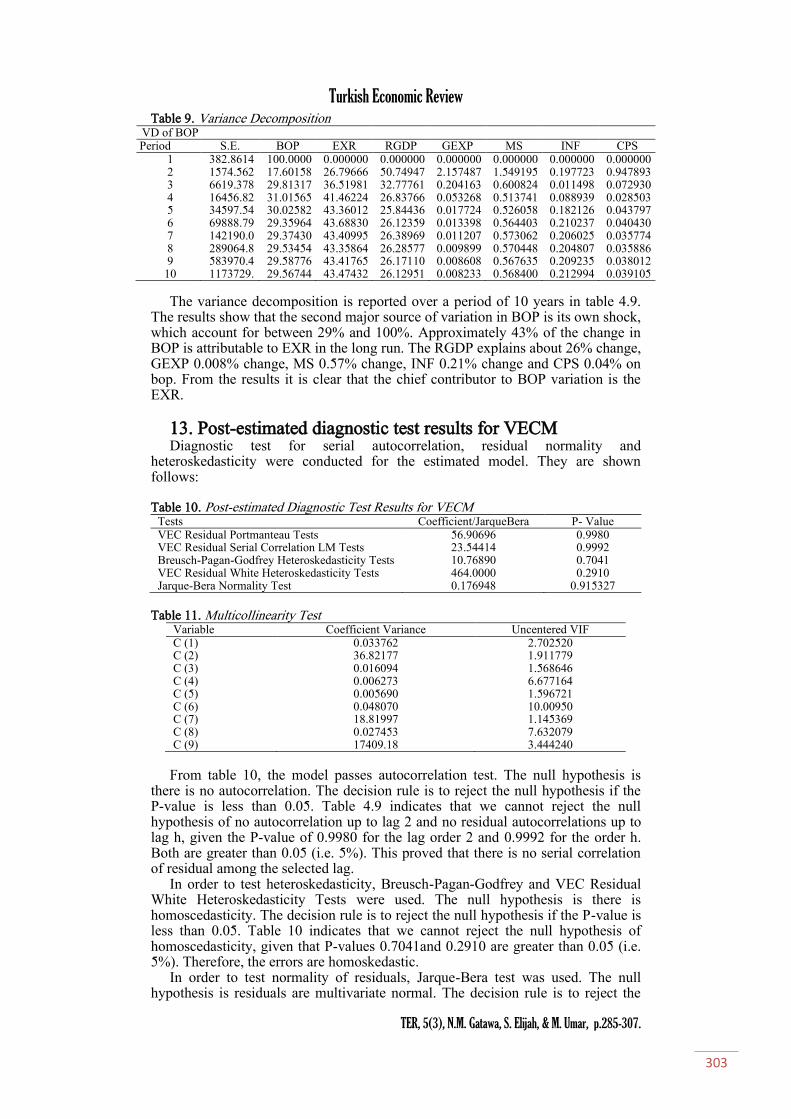
The variance decomposition is reported over a period of 10 years in table 4.9. The results show that the second major source of variation in BOP is its own shock, which account for between 29% and 100%. Approximately 43% of the change in BOP is attributable to EXR in the long run. The RGDP explains about 26% change, GEXP 0.008% change, MS 0.57% change, INF 0.21% change and CPS 0.04% on bop. From the results it is clear that the chief contributor to BOP variation is the EXR.

13. Post-estimated diagnostic test results for VECM Diagnostic test for serial autocorrelation, residual normality and

heteroskedasticity were conducted for the estimated model. They are shown follows: Table 10. Post-estimated Diagnostic Test Results for VECM

Tests Coefficient/JarqueBera P- Value VEC Residual Portmanteau Tests VEC Residual Serial Correlation LM Tests

56.90696 23.54414

0.9980 0.9992

Breusch-Pagan-Godfrey Heteroskedasticity Tests VEC Residual White Heteroskedasticity Tests

10.76890 464.0000

0.7041 0.2910

Jarque-Bera Normality Test 0.176948 0.915327 Table 11. Multicollinearity Test

Variable Coefficient Variance Uncentered VIF C (1) 0.033762 2.702520 C (2) 36.82177 1.911779 C (3) 0.016094 1.568646 C (4) 0.006273 6.677164 C (5) 0.005690 1.596721 C (6) 0.048070 10.00950 C (7) 18.81997 1.145369 C (8) 0.027453 7.632079 C (9) 17409.18 3.444240

From table 10, the model passes autocorrelation test. The null hypothesis is

there is no autocorrelation. The decision rule is to reject the null hypothesis if the P-value is less than 0.05. Table 4.9 indicates that we cannot reject the null hypothesis of no autocorrelation up to lag 2 and no residual autocorrelations up to lag h, given the P-value of 0.9980 for the lag order 2 and 0.9992 for the order h. Both are greater than 0.05 (i.e. 5%). This proved that there is no serial correlation of residual among the selected lag.

In order to test heteroskedasticity, Breusch-Pagan-Godfrey and VEC Residual White Heteroskedasticity Tests were used. The null hypothesis is there is homoscedasticity. The decision rule is to reject the null hypothesis if the P-value is less than 0.05. Table 10 indicates that we cannot reject the null hypothesis of homoscedasticity, given that P-values 0.7041and 0.2910 are greater than 0.05 (i.e. 5%). Therefore, the errors are homoskedastic.

In order to test normality of residuals, Jarque-Bera test was used. The null hypothesis is residuals are multivariate normal. The decision rule is to reject the



304

null hypothesis if the P-value is less than 0.05. Table 10 indicates that the P-value of each variable is greater than 0.05 (i.e. 5%). The VEC residual normality test confirmed the acceptance of the null hypothesis of normality properties given the P-value 0.915327, which is greater than 5% level of significance. This provides a support that the residuals from our VEC model have a normal distribution.

From table 11, the model passes multicollinearity test. VIF has a minimum value of 1, but once it is below 10, there is no ground to suspect severity of multicollinearity; when it is above 10, it is a cause of worry. The table indicates that there is no ground to suspect severity of multicollinearity. The reason being that, each coefficient of the variables has a VIF value which lies between the range 1 and 10.

14. Parameter stability test results for VECM Inverse Roots of AR Characteristics Polynomial: Figure 3 indicates that almost

all the eigen values of the system obtainable in modulus lie within the unit circle. Hence from the analysis VEC model satisfies the stability condition.

Figure 3. Inverse Roots of AR Characteristics Polynomial

15. Discussion of findings in relation to objectives and

hypotheses This study empirically analyzed the impact of floating exchange rate on balance

of payment in Nigeria using VECM. The discussion of the findings is categorized into its various objectives. This is as follows:

i. In order to empirically examine the impact of floating exchange rate on

balance of payment in Nigeria. The findings of the study based on the result of VECM established that exchange rate impacted on BOP and the relationship is positive and statistically significant at 5% level. It is also clear from the variance composition result that the chief contributor to BOP variation both in the short run and long run is the EXR. The result is in conformity to the findings of Okwuchukwu (2014) and Ahmed et al., (2014). However, the result is not in line with the findings of Anthony (2015); Oladipupo & Onotaniyohuwo (2011); Bonface (2013), and Martins & David (2014). It is therefore reasonable to reject the hypothesis that there is no significant impact of floating exchange rate on balance of payment in Nigeria is rejected.

ii. To determine the long run relationship between exchange rate and balance of payment in Nigeria as the second objective of the study. The findings of the study based on the result of Johansen cointegration test revealed that there is a long run relationship between exchange rate and balance of payment. Hence,



305

VECM established that the relationship between the two variables is positive and statistically significant at 5% level. The result is in conformity to the findings of Okwuchukwu (2014) and Ahmed et al., (2014). However, the result is not in line with the findings of Anthony (2015); Oladipupo & Onotaniyohuwo (2011); Bonface (2013), and Martins & David (2014). Therefore it is reasonable to reject the null hypothesis that there is no long run relationship between exchange rate and balance of payments in Nigeria is rejected.

iii. To determine the direction of causality among floating exchange rate, balance of payments and other estimated key macro-economic variables in Nigeria. The granger causality results revealed that there is unidirectional causality between GEXP and BOP, MS and BOP, and MS and RGDP, MS and GEXP, CPS and GEXP, and CPS and MS each at 1% level of significance. More so, there is unidirectional causality between BOP and EXR, BOP and CPS, and CPS and INF each at 5% level of significance. The tests also indicate that there is a bi-directional causality between EXR and RGDP, MS and EXR each at 5% level of significance. Hence, the third null hypothesis that there is no causality direction among exchange rate, balance of payment and other key macro-economic variables is rejected. The direction of causality between EXR and BOP is in conformity with the findings of Ahmed et al., (2014), Mabior (2014) and Martins & Olarinde (2014).

iv. To investigate the major determinants of exchange rate which in turn influence balance of payment in Nigeria. The granger causality results revealed unidirectional causal relationship between exchange rate and balance of payment at 5% level of significant. More so, exchange rate has unidirectional causal relationship with money supply and bi-directional causal relationship with real GDP both at level of significance. Hence, it is evident here that the major determinants of exchange rate which in turn influenced balance of payment during the study periods in Nigeria are money supply and real GDP. Hence, null hypothesis that there are no major determinants of exchange rate which in turn influenced balance of payment in Nigeria is rejected.

v. To examine the nexus between exchange rate and balance of payment in Nigeria. The granger causality results revealed that the nexus among the variables runs from government expenditure to money supply and real GDP, then from money supply and real GDP to exchange rate, and then from exchange rate to Balance of Payment. Hence, the null hypothesis that there is no nexus among the studied variables in Nigeria is rejected.

16. Conclusion and recommendation The main topic of discussion was not only to empirically investigate the impact

of floating exchange rate on balance of payment, but also to relate the findings of this study to the theoretical propositions related to this study as well as the related previous studies. However, based on the findings of this study, we conclude that floating exchange rate contributed positively to balance of payment in both short-run and long-run. For causality relationship, balance of payment has unidirectional causality relationship with exchange rate and real GDP. More also, exchange rate has unidirectional causal relationship with money supply and bi-directional causal relationship with real GDP. Hence, the major determinants of exchange rate are money supply and real GDP which in turn influenced balance of payment during the study periods in Nigeria. We also conclude that the nexus among the variables runs from government expenditure to real GDP and money supply, then from real GDP and money supply to exchange rate, and then from exchange rate to Balance of Payment. It is noteworthy that real GDP granger cause money supply and exchange rate.

Noteworthy is the fact that the policy implication of this is that exchange rate depreciation which has been preponderant in Nigeria especially since 1986 has not been very useful in promoting the country’s positive BOP due to internal forces,



306

evident from the insignificant relationship between most of the regressors and the dependent variable (BOP). It is important to stress that the results of the study are based on the proxies employed and that the findings may be country-specific.

Therefore it was recommended amongst other things that the policy of exchange rate depreciation should be maintained but with government intervention guide. Government through Central Bank of Nigeria (CBN) should apply expenditure reducing monetary policies through money supply and domestic credit to promote favourable BOT which invariably stabilizes BOP.

References Adamu, P.A., & Osi, C.I. (2011). Balance of payments adjustment: The West African monetary zone

experience. West African Institute for Financial and Economic Management. 10(2), 100-116. Ademola, O., & David, O.W. (2011). Exchange rate volatility: an analysis of the relationship between

the Nigerian Naira, oil prices, and US dollar. Department of Business Administration, Gotland University. [Retrieved from].

Agbola, F.W. (2004). Does devaluation improve trade balance of Ghana? The International Conference on Ghana’s Economy at Half Century, M-Plaza Hotel, Accra, Ghana.

Agu, C. (2002). Real exchange rate distortions and external balance of position o Nigeria: Issues and policy options. Journal of African Finance and Economic Development, 5(2), 1-27.

Ahmad, N., Ahmed, R.R., Khoso, I., Palwishah, R.I., Raza, U. (2014). Impact of exchange rate on balance of payment: An investigation from Pakistan. Research Journal of Finance and Accounting. 5(13), 32-42.

Ahmed, A.I., & Yusoff, M.B. (2001). The effects of exchange rate change on imports and exports: The Sudanese case. Semiar 13. [Retrieved from].

Alexander, S. (1952). Effects of a devaluation on a trade balance. IMF Staff Papers 2(2), 263-278. doi. 10.2307/3866218

Anthony, I.I. (2015). Exchange rate and balance of payments position in Nigeria. JORIND, 13(2), 1-10.

Azeez, B.A., Kolapo, Funso T. & Ajayi, L.B. (2012). Effect of exchange rate volatility on macroeconomic performance in Nigeria. Interdisciplinary Journal of Contemporary Research in Business. 4(1), 1149-155. doi. 10.26458/1814

Bonface, W. & Barasa, B. (2013). The relationship between exchange rate volatility and balance of payments in Kenya. Department of Finance and Accounting University of Nairobi. [Retrieved from].

Central Bank of Nigeria, (2006). Statistical Bulletin, Abuja, Nigeria. Central Bank of Nigeria, (2016). Second Quarterly Statistical Bulletin, Abuja, Nigeria. Central Bank of Nigeria, (2016). Statistical Bulletin, Abuja, Nigeria Chang, L.L., & Tan, H.B. (2008). Exchange rate risk and macroeconomics fundamental, evidence

from our neighbouring South East Asian economic. International Research Journal of Finance and Economics, 16(1), 88-99.

Ehinomen, C. & Oladipo, T.I. (2012). Exchange rate management and the manufacturing sector performance in the Nigerian economy. IOSR Journal of Humanities and Social Science, 5(5), 1-12.

Eze, T.C. & Okpala, C.S. (2014). Quantitative analysis of the impact of exchange rate policies on Nigeria’s economic growth: A test of stability of parameter estimates. International Journal of Humanities and Social Science, 4(7), 265-272.

Fleermys, F.N. (2005). The Balance of Payment as a Monetary Phenomenon: An Econometric Study of Namibia. Directorate of Environmental Affairs. [Retrieved from].

Gujarati, D. (2007). Basic Econometrics, 3rd Edition, McGraw. Hill, New York. Hume, D. (1752). Of the Balance of Trade, in R. Cooper (ed.) International Finance. IMF, (2006). Balance of Payment, Manual, 4th edition. [Retrieved from]. Ibrahim, M.A.A. (2008). Behaviour of Sudan balance of payments: An application of a monetary

approach. Department of Economics, faculty of Economic and Social Studies, University of Khartoum. [Retrieved from].

Isard, P. (1999). Exchange Rate Economics, Cambridge University press: Cambridge. Jhingan, M.L. (2003). Macro-economic Theory. Vrinda Publications. Jhingan, M.L. (2006). International Economics. Vrinda Publications. Mabior, A.G. (2014). Determinants of balance of payments performance in Kenya. Economic Policy

Management of the University of Nairobi, Kenya. [Retrieved from]. Iyoboyi, B., Muftau, O.,. & McMillan, D. (2014). Impact of exchange rate depreciation on the

balance of payments: Empirical evidence from Nigeria. Cogent Economics and Finance, 2(1), 923323. doi. 10.1080/23322039.2014.923323

Melvin, M. (1992). International Monetary and Finance. Third Edition, New Work: Jarper Collins Publishers Inc.

National Bureau of Statistics, (2011). Annual Abstract of Statistics, Federal Republic of Nigeria.

http://www.diva-portal.org/smash/get/diva2:420652/FULLTEXT01.pdf

https://www.researchgate.net/profile/Mohamed_Elgali/publication/228435006_THE_IMPACT_OF_EXCHANGE_RATE_POLICY_ON_THE_SUDANESE_AGRICULTURE/links/0912f50dc3f5088443000000/THE-IMPACT-OF-EXCHANGE-RATE-POLICY-ON-THE-SUDANESE-AGRICULTURE.pdf

https://doi.org/10.2307/3866218

https://doi.org/10.26458/1814

http://chss.uonbi.ac.ke/sites/default/files/chss/BONFACE%20W.BARASA%20-D61-60463-2011.pdf



http://www.the-eis.com/data/RDPs/RDP72.pdf

https://www.imf.org/external/pubs/ft/bop/archives/BPM4.pdf

http://khartoumspace.uofk.edu/bitstream/handle/123456789/13609/Behavior%20of%20Sudan%20Balance%20Of%20Payments%20An%20Application%20of%20a%20Monetary%20Approach.pdf?sequence=1&isAllowed=y

http://erepository.uonbi.ac.ke/bitstream/handle/11295/76538/Mabior%20_The%20determinants%20of%20balance%20of%20payments%20performance%20in%20Kenya.pdf?sequence=3&isAllowed=y

https://doi.org/10.1080/23322039.2014.923323



307

Okwuchukwu, O. (2014). Exchange rate and balance of payment: An autoregressive distributed Lag (ARDL) econometric investigation on Nigeria. IOSR Journal of Economics and Finance. 4(6), 21-30.

Oladipupo, A.O., & Onotaniyohuwo, F.O. (2011). Impact of exchange rate on balance of payment in Nigeria. An International Multidisciplinary Journal, Ethiopia. 5(4), 73-88.

Priyatharsiny. P. (2017). Impact of exchange rate on balance of payment In Sri Lanka. Preceeding of 7th International Symposium, SEUL. pp 580-592. [Retrieved from].

Umeora, C.E. (2013). Accumulation of external reserves and effects on exchange rates and inflation in Nigeria. International Business and Management. 6(2), 105-114.

Umoru, D., & Odegba, O.P. (2013). Exchange rate misalignment and balance of payment adjustment in Nigeria. European Scientific Journal, 9(13), 260-273.

Copyrights Copyright for this article is retained by the author(s), with first publication rights granted to the journal. This is an open-access article distributed under the terms and conditions of the Creative Commons Attribution license (http://creativecommons.org/licenses/by-nc/4.0).

http://www.seu.ac.lk/researchandpublications/symposium/7th/Inaternational%20Symposium%202017%20-%20SEUSL%20(61).pdf

Turkish Economic Review - KSP Journals

Documents

Transcript of Turkish Economic Review - KSP Journals