Quintessenz Journals

International Journal of Computerized Dentistry 2018;21(3):201–214 201

SCIENCE

Prof. Dr. Albert Mehl, Division of Computerized Restorative Dentistry, Clinic of Preventive Dentistry, Periodontology and Cariology, University of Zurich, Zurich, Switzerland

Abstract

Different concepts are used for the analysis and transfer of mandibular movements to virtual or conventional articulating systems. Some common procedures and analyses include the determination of the terminal hinge axis. However, despite the widespread use of different methods for hinge axis determina-tion, very little information on the applicability and quality of these methods is currently available in the literature. The aim of this study was to provide an overview of the methods already being applied and to search for novel algorithmic methods, comparing them with respect to achievable accuracy and indication. This comparison was based on new extensive computer simulations, where the influence of measurement noise on the result of the hinge axis position could be investi-gated. The assumptions used for the simulations were set so that the conditions allowed for the most accurate hinge axis determination: this comprised a pure rotation during mouth opening, within an incisal pathway of 15 mm, a measurement accuracy of 50 μm, and an optimal positioning of the entire measurement setup. The results of the computer calculations show that the best accuracy can be guaranteed by the novel least squares method, introduced in this article for temporo-mandibular joint (TMJ) measurements. Additionally, only methods tracking two and more (iterative or parallel) inde-pendent markers or equivalent jaw position measurements provide enough information for reliable accuracy. Using actual

A. Mehl

The determination of the terminal hinge axis: a fundamental review and comparison of known and novel methods

Albert Mehl

technical equipment, the highest accuracies can be achieved in a TMJ-near measurement setup. However, even in that best-possible setup, the error of hinge axis determination can-not be expected to be less than ±1 mm. For a better charac-terization of actual electronic recording systems, manufactur-ers need to provide more insight into the evaluation processes.

Keywords: terminal hinge axis, jaw tracking, temporoman-dibular joint, accuracy, computer simulation

Introduction

Dynamic mandibular movement can be fully described and reconstructed for various purposes by an unconstrained 6DoF (six degrees of freedom) time-dense acquisition of mandible positions in relation to the maxilla. These tasks can theoretically be fulfilled by electronic measurement devices such as SICAT JMT, Zebris JMA, etc.1 By transferring these mandible positions and rotations into a software-based virtu-al articulating system, an exact replay of the patient’s man-dibular movements can be visualized and used for checking the interpenetrations with restorations or for functional diag-nosis.2 It is important to emphasize that while, in general, this process does not need any anatomical reference points, in the literature the determination of some anatomical and constructional points or planes is demanded for various diag-

Dear Reader,

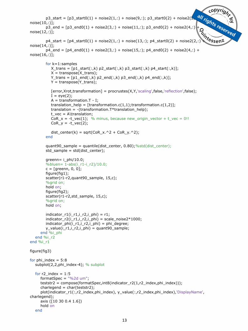
all program codes and further information about the processes applied can be found at the end of the article.

International Journal of Computerized Dentistry 2018;21(3):201–214202

SCIENCE

nostic or therapeutic concepts. Reference points are also needed, for instance, by physical articulators to position the plaster replicas in the correct individual position.

As one of such reference parameters of mandibular movement, the determination of the hinge axis – also called the terminal hinge axis or transverse horizontal axis – is claimed to be important for various diagnostic and therapeu-tic indications for certain clinical rehabilitation procedures in the fields of prosthodontics, orthodontics, and temporoman-dibular joint (TMJ) surgery.3 In this theory, the early phase of opening and the terminal phase of closing, respectively, are seen as a pure rotation, where the mandible rotates around the intercondylar axis.4-7 Despite the widespread use of this concept, several other studies have suggested that a pure rotary movement does not occur, and that there is no fixed axis of rotation during mandibular movement.8-11 Other concepts introduced to describe mandibular movement have been the concept of the kinematic axis,12,13 and the concept of the instantaneous center of rotation (ICR) or helicoidal axis.14-16 These concepts have been scientifically investigat-ed in a number of studies, with results that have shown dis-crepancies and a lack of consistency.4 It must be emphasized that it has not yet been proven whether there is pure rotation in the early stage of opening, or whether it occurs with a combined translational movement.

Due to its widespread acceptance (and perhaps due to its simplicity), the theory of terminal hinge axis is mostly applied in cases of prosthetic rehabilitation and temporomandibular. joint (TMJ) diagnostics. The critical point in the clinical work-flow is the determination of the exact location of the hinge axis or hinge axis points, respectively. In the past, the mechan-ical strategy used to detect the hinge axis points was mainly based on processes described by McCollum6,17 and Lau-ritzen.18-20 A good overview of different mechanical approaches to detect the hinge axis can be found in Bosman.21 In more recent times, electronic recording devices have increasingly been applied to detect the exact hinge axis posi-tion. With these devices, the axis points are calculated by the software after the execution of some specific jaw movements. However, there is almost nothing in the literature about the algorithms that perform these calculations, and only rare sci-entifically profound studies about the accuracy of this detec-tion can be found. Additionally, there is no hint as to which kind of strategy or measurement protocol provides the best and most reproducible results.

As hinge axis determination in several clinical diagnostic and rehabilitation processes is so important, evidence about the accuracy, including the reproducibility one can expect

from the different approaches, is crucial. In particular, nothing is known as yet about the fundamental limits, which can only be analyzed using theoretical considerations, independently of measurement devices or particular systems used. The aim of this study was first to review possible methods and second to systematically evaluate and simulate the various approaches and to give a range for their intrinsic inaccuracies in the case of hinge axis determination. Apart from commonly used approaches, new modern algorithms are also introduced and are ranked and discussed for their applicability. The following systematic review and overview of known and new methods, including their simulations with error propagation, should provide answers to the following questions:1. Which different fundamental strategies and measure-

ment protocols can be applied for hinge axis determina-tion?

2. How can these strategies be logically grouped according to their underlying principles?

3. What are the theoretical limits for the accuracy of hinge axis determination, taking into consideration that all measurements are subject to inaccuracy due to noise (ie, there is never an exact measurement in real situations)?

4. Which concept allows for the best hinge axis determina-tion?

Methods and strategies for hinge axis determination

Applying the terminal hinge axis concept, an important assumption has to be made when exploring the answers to the above questions: The early phase of mouth opening move-ment or the late phase of mouth closing movement is a pure rotation around an axis. That means that for a certain phase, the axis remains stable and does not move. This important assumption is inherent to the hinge axis concept and is funda-mental for all the other methods described in this study.

During a pure rotational movement, each point on the rotating object will move in a circle-like path around the hinge axis, which can be used to determine the rotation axis according to standard geometric and trigonometric calcula-tions. Without loss of generality, it is possible to focus only on two-dimensional (2D) calculations. Some special three-di-mensional (3D) aspects are discussed later. Additionally, to achieve the most exact determination of the rotation axis, the largest possible opening rotation is chosen. The literature describes values of 7 to 18 mm mouth opening, according to which a nearly pure rotation is performed before the start of


SCIENCE

pose a hypothetical measurement accuracy of ±20 μm, the range of radius error will be around ±6 mm. Additionally, it should be mentioned that only the error of radius is discussed here; an additional error of locating the position of the rotation center may also arise and therefore increase the inaccuracy of determining the hinge axis position. Additionally, it seems doubtful that a physiological movement by an individual can be performed with a repeated precision of less than 50 μm.

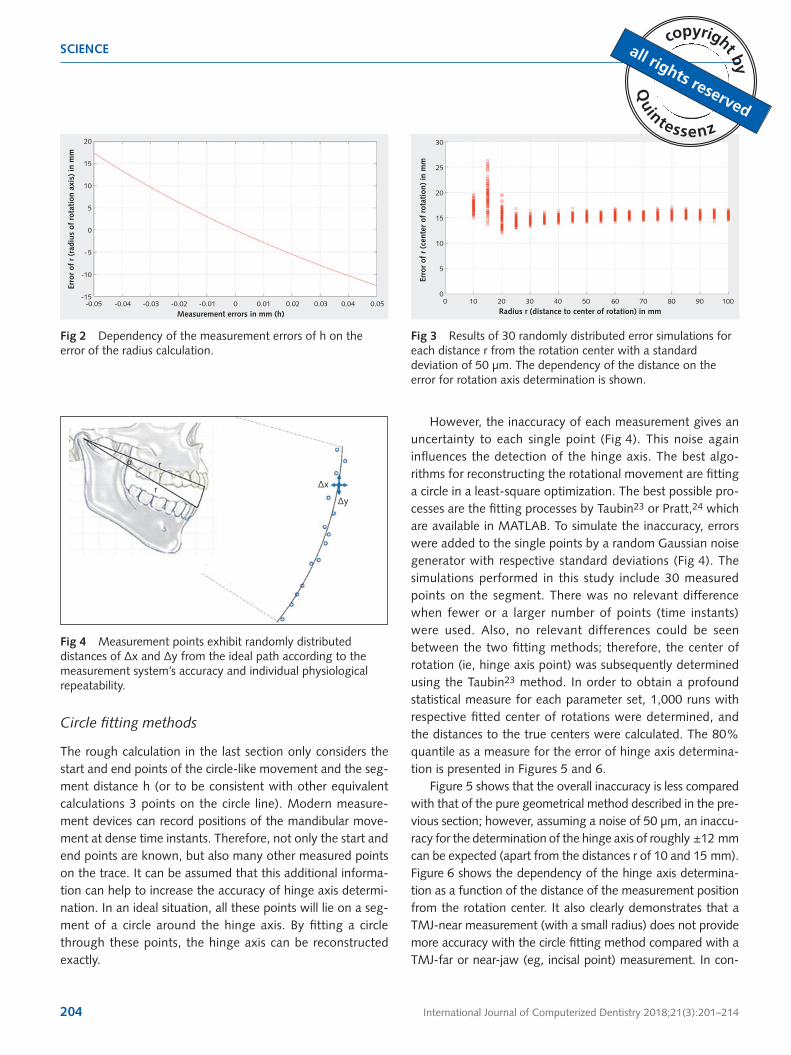
Figure 2 shows the results for a measurement at a dis-tance of 90.7 mm from the rotation axis. If the measurement changes from near jaw position to near condyle position, the errors may change accordingly. Therefore, in a further step, equation (1) undergoes a simulation, where for different val-ues of r, the parameters s and h were subjected to additive noise of 50 μm and 1,000 randomly independent runs to determine rcalc. From those runs, the 80% quantile of the respective differences of rcalc to the true r were determined. This process was repeated 30 times for each parameter set in order to obtain the high safety shown in Figure 3. This figure reveals the dependency of the measurement distance r on the error in locating the rotation center. The noise was set to 50 μm, and the same opening angle of 9.5 degrees, as men-tioned above, was used. There is no significant difference of error, which is around 15 mm, from a distance r of 100 mm down to around 25 mm. TMJ-near measurements with dis-tances lower or equal to 20 mm become more and more unstable. This simple estimation gives a clue as to the magni-fied influence of small errors with measurement devices or movement deviations in determining the true hinge axis.

an additional translational movement.1 Although it is ques-tionable whether a 15-mm opening really exhibits a pure rotation, this value can be seen as the upper limit for the best possible hinge axis detection. The radius of the movement, especially of the incisal point, can be calculated from the average Bonwill triangle (with arms of 103.5 mm and a base of 99.6 mm22), and equals 90.7 mm. With this radius and 15-mm opening, the angle of opening corresponds to 9.5 degrees. These parameters are the basis for the further calculations in this study. The simulations and calculations were performed with MATLAB (Version R2018a, Math-Works, USA).

Single trace recording processes

Any opening movement recorded by any adequate measure-ment device will exhibit a path lying on an arc segment of a circle. The task is to find the corresponding radius of the movement from this information, or more exactly, the posi-tion of the rotation center.

Rough estimation of errors

Theoretically, the radius can be recalculated from the cir-cle-like opening movement from the chord s and the sagitta (height) h (Fig 1):

rcalc = (4h + s2)/8h (1)

where h and s can be determined from the measured path.

However, considering that an exact measurement is never possible, especially when dealing with real physical objects, the question is therefore: to what extent does the calculated rcalc deviate from the true radius r, if h and s are subjected to some inaccuracies? With the average parameters given above, s and h are around 14.9 mm and 0.31 mm, respect-ively. If measurement inaccuracies are taken into account, s and especially h will change accordingly, and rcalc will have different values after using formula (1). Figure 2 shows the dependency of the error of r from the inaccuracy introduced by determining h (inaccuracies of the same amount in s can be neglected here, because s >> h).

This rough estimation shows that with actual measure-ment systems and their best possible accuracies of around ±50 μm, the exactness of recalculating the true radius of rotation can only be done in a range from -13 mm to 17 mm (total of around 3 cm [!] inaccuracy). Even if we sup-

Fig 1 The first phase of opening is assumed to be a pure rotation. Each point on the mandible (eg, incisal point) describes a segment of a circle. With h and s, the radius r and therefore the center of rotation can be reconstructed. Opening angle α of 9.8 degrees was assumed for all further simulations (which corresponds to an incisal path of 15 mm).

s

rα

r

b

h


SCIENCE

However, the inaccuracy of each measurement gives an uncertainty to each single point (Fig 4). This noise again influences the detection of the hinge axis. The best algo-rithms for reconstructing the rotational movement are fitting a circle in a least-square optimization. The best possible pro-cesses are the fitting processes by Taubin23 or Pratt,24 which are available in MATLAB. To simulate the inaccuracy, errors were added to the single points by a random Gaussian noise generator with respective standard deviations (Fig 4). The simulations performed in this study include 30 measured points on the segment. There was no relevant difference when fewer or a larger number of points (time instants) were used. Also, no relevant differences could be seen between the two fitting methods; therefore, the center of rotation (ie, hinge axis point) was subsequently determined using the Taubin23 method. In order to obtain a profound statistical measure for each parameter set, 1,000 runs with respective fitted center of rotations were determined, and the distances to the true centers were calculated. The 80% quantile as a measure for the error of hinge axis determina-tion is presented in Figures 5 and 6.

Figure 5 shows that the overall inaccuracy is less compared with that of the pure geometrical method described in the pre-vious section; however, assuming a noise of 50 μm, an inaccu-racy for the determination of the hinge axis of roughly ±12 mm can be expected (apart from the distances r of 10 and 15 mm). Figure 6 shows the dependency of the hinge axis determina-tion as a function of the distance of the measurement position from the rotation center. It also clearly demonstrates that a TMJ-near measurement (with a small radius) does not provide more accuracy with the circle fitting method compared with a TMJ-far or near-jaw (eg, incisal point) measurement. In con-

Erro

r of

r (

radi

us o

f ro

tati

on a

xis)

in m

m

Measurement errors in mm (h)

20

15

10

5

0

- 5

-10

-15-0.05 -0.04 -0.03 -0.02 -0.01 0 0.01 0.02 0.03 0.04 0.05

Fig 2 Dependency of the measurement errors of h on the error of the radius calculation.

Fig 3 Results of 30 randomly distributed error simulations for each distance r from the rotation center with a standard deviation of 50 μm. The dependency of the distance on the error for rotation axis determination is shown.

Radius r (distance to center of rotation) in mm0 10 20 30 40 50 60 70 80 90 100

Erro

r of

r (

cent

er o

f ro

tati

on)

in m

m

30

25

20

15

10

5

0

Fig 4 Measurement points exhibit randomly distributed distances of Δx and Δy from the ideal path according to the measurement system’s accuracy and individual physiological repeatability.

Δx

Δy

rα

r

Circle fitting methods

The rough calculation in the last section only considers the start and end points of the circle-like movement and the seg-ment distance h (or to be consistent with other equivalent calculations 3 points on the circle line). Modern measure-ment devices can record positions of the mandibular move-ment at dense time instants. Therefore, not only the start and end points are known, but also many other measured points on the trace. It can be assumed that this additional informa-tion can help to increase the accuracy of hinge axis determi-nation. In an ideal situation, all these points will lie on a seg-ment of a circle around the hinge axis. By fitting a circle through these points, the hinge axis can be reconstructed exactly.


SCIENCE

trast, radius values lower than 20 mm do substantially increase the inaccuracy of hinge axis determination.

It can be concluded that, theoretically, methods using cir-cle fitting approaches are not suitable for hinge axis determi-nation, independently of whether the marker or the position is traced close to or far away from the TMJ.

The single trace iterative method

A very common method, especially used in former times, was first described by McCollum,6,17 and then successively improved upon in later decades.18-20 The basic principle of this method is that a pin fixed to a device, which is connected to the mandibular teeth, traces the movements on a frame, which itself is fixed to the head as a reference system. In case of a rotational movement, the pin traces circular segments whose sizes depend on the distance to the center of rotation (Fig 7).20 The closer the position of the pin to the center of

rotation, the shorter the circular segment. The hinge axis can be determined by iteratively changing the position of the pin until the point is detected at which movement can no longer be observed.20 This method is also known as the panto-graphic kinematic method.21

The advantage of this method compared to the methods described above is that the only information used for the evaluation is the length of the segment or respective chord, ie, the straight connection of the start and end points of the segment. This measure is less susceptible to noise. Figure 8 shows the theoretical dependency of the length of the chord as a function of the distance from the rotation axis. If chord lengths can be measured with an accuracy of around 0.2 mm, the rotation axis can be determined within ±1.5 mm, and in case of a 0.15-mm accuracy (3 × 50 μm, accuracy start and end point [2x] plus segment length 50 μm), even down to an uncertainty of ±1.0 mm. However, with conventional mechanical recording and in a clinical environment, it is

Erro

r of

cen

ter

of r

otat

ion

in m

m

Measurement inaccuracy (noise) in mm

40

35

30

25

20

15

10

5

00.01 0.02 0.03 0.04 0.05 0.06 0.07 0.08 0.09 0.1

5 mm10 mm15 mm20 mm25 mm30 mm35 mm40 mm45 mm50 mm55 mm60 mm65 mm70 mm75 mm80 mm85 mm90 mm95 mm

100 mm

Erro

r of

cen

ter

of r

otat

ion

in m

m

Radius r (distance to center of rotation) in mm

40

35

30

25

20

15

10

5

00 10 20 30 40 50 60 70 80 90 100

10 μm20 μm30 μm40 μm50 μm60 μm70 μm80 μm90 μm

100 μm

Fig 5 Circle fitting methods: Error of the axis center determi-nation in dependency of the measurement accuracy and the distance (see legend in figure) of the measurement from the real rotation center.

Fig 6 Circle fitting methods: Error of the axis center determi-nation in dependency of the distance of the measurement from the real rotation center and the measurement accuracy (see legend in figure).

Fig 7 Mechanical approach for the single trace iterative method:20 a pin, fixed directly to the mandible via a rigid device, tracks the early phase of opening movement. The length and orientation of the circular segments are dependent on the distance from, and position in relation to, the real rotation center – the nearer the pin to this center, the shorter the tracked pathways. By iteratively adjusting the pin position, the point at which no movement is present can be located.


SCIENCE

unfeasible to assume selectivity below 0.5 mm for visually differentiating between a point and a small segment. There-fore, the resulting accuracy of hinge axis determination prob-ably lies around ±3.5 mm. This value accords well with the accuracy found in an elaborate study by Bosman.21 The dis-advantage of this method is the time-consuming iterative approach that must be employed until the point of no or negligible movement is reached. However, instead of a mechanical system, an electronic recording system may record pin or marker movement in a parallel manner using more than one marker, therefore reducing the time needed for the iterative adjustment. This may also potentially result in higher accuracy down to ±1 mm (with 50 μm measure-ment accuracy). It is important to mention that this proce-dure is only viable in a TMJ-near measurement setup.

Two and more trace recordings

In contrast to single position or marker measurements, meth-ods using two and more independent markers and/or two and more independent jaw position measurements may pro-vide more safety and accuracy for hinge axis determination. A common method used for that application is the Reuleaux principle.25,26

Reuleaux principle

Originally, this method uses two markers for tracking the start and end positions of a rotational movement (Fig 9). First, the chords of the two segments are constructed by con-necting the respective start and end points. The center of the rotational movement must lie on a line perpendicular to the chords, going through the midpoint of the chord (ie, halfway between the start and end points). The center of rotation can

then be determined as the intersection point between the two perpendiculars.

To simulate the accuracy as a function of distances of the tracking positions to the rotation center r1, r2 and the angle between the positions ϕ of the two markers, the same pre-sumptions as before were used: an incisal opening of 15 mm (ie, an opening angle of 9.5 degrees). Measurement inaccu-racy was set to 50 μm for capturing the marker positions, and 1,000 statistically independent runs were simulated for each parameter combination of r1, r2, and ϕ. The distances of the 1,000 perturbed centers from the real center were determined, and the 80% quantile was calculated as a meas-ure for the error of the rotation center determination.

The result is shown in Figure 10. This figure clearly demonstrates three facts: 1) The angle ϕ between the two markers crucially influences the accuracy. Small angles result in significantly higher inaccuracy, whereas from 50 degrees on, the accuracy increases slowly up to a value of around 0.9 mm for 90 degrees. 2) Whether one marker is positioned near to the rotation axis or far away from it has no influence. 3) The distance position of the second marker is independent of the position of the first marker: the relative distances from the axis center for both markers have a negligible influence on the accuracy.

However, for markers in a near-jaw position, an angle dif-ference of 40 degrees and more can only be achieved if the markers have a distance of at least ±60 mm, measured in the sagittal plane. It is difficult to apply these marker settings in a clinical setting. Additionally, a larger measurement field is required if both markers must be measured in parallel, which leads to decreased accuracy. Therefore, a practicable and economical process with high measurement accuracy leads to a setup where the two markers are located near to the condyle, so that in case of distances of 10 to 20 mm, angles between the markers of 60 degrees and more can be achieved in a relatively small measurement field. It is impor-tant to mention that, a priori, an angle of 90 degrees cannot be ensured, because the real position of the axis center is not known. Therefore, in a realistic process, the angles will lie somewhere between 60 and 90 degrees. From this it follows that a possible accuracy for the described process will be around ±0.9 mm for hinge axis determination.

Least squares method

In general, the Reuleaux method has three drawbacks: 1) It is a purely geometrical approach and it is not obvious that it gives the best solution in case of noisy measurements,

Fig 8 Single trace iterative method: Length of the recorded segment trace as a function of the distance of the pin (or marker position) from the rotation axis.

1.51.41.31.21.11.00.90.80.70.60.50.40.30.20.1

0

Segm

ent

leng

th in

mm

Distance from rotation axis in mm0 1 2 3 4 5 6 7 8 9 10


SCIENCE

Fig 9 Reuleaux principle (left image) and a schematic illustration for the parameter values used in the computer simulation (right image). P1_start and P2_start are the marker positions at the start of the move-ment, and P1_end and P2_end are the respective marker positions at the end of the movement. r1 and r2 are the distances of both markers from the rotation center, and ϕ is the angle between the marker positions.

P1_start

P1_start

P2_startP2_start

P1_endP1_end

P2_endP2_end

r1

r2

ϕ

Fig 10 Results of the simulation for the Releaux method: Error of the axis determination (y-axis, in mm) in dependency with the marker position, which is defined as a function of the distance r1 of the first marker from the rotation axis (x-axis, in mm), of the distance r2 of the second marker from the rotation axis (see legend, in mm) and the angle ϕ between them (see Fig 9). Measure-ment accuracy was set to 50 μm for all simulations.

which is the realistic situation. 2) Although the Reuleaux method can be extended for more than two markers, it is not clear how to combine the intersections between the dif-ferent perpendicular lines in order to get the best proposal for the rotation center. 3) Extending to general 3D meas-

urements, it is difficult to deal with non-intersecting lines to define the best-located center. These problems can better be solved if fundamental algebraic approaches are applied. The advantage is that, independent of the position of the markers, the number of markers, and the time intervals

Position r1 in mm

Erro

r fo

r ce

nter

of

rota

tion

in m

m

Angle 10 degrees Angle 20 degrees Angle 30 degrees

Angle 60 degreesAngle 40 degrees


Angle 50 degrees


SCIENCE

(when each start and end point are measured), all the solu-tions can be calculated with the same process, and it guar-antees the best solution. In a more general sense, the pro-cess implies optimization and the use of the least squares method.

Each rigid transformation in space can be described as:

pend_i = R * pstart_i + t (2)

where pend_i and pstart_i are the respective end and start posi-tions of the i-th marker, R is the rotation matrix defining the rotation axis direction and the rotation angle, and t is the translation.

The task is to find the optimal R̂ and t̂, when n start and end points are measured (n ≥ 2). The assumption is that the measurement errors are normally distributed. Then, the sum of the quadratic errors between calculated and measured

coordinates should be minimal (according to the Gauss-Markow theorem):

Σi([pend_i – R̂ * pstart_i –]2) = min

The best R̂ and t̂ can be determined by mathematical optimi-zation, applying singular value decomposition (SVD) or eigenvalue methods. The exact processes are described in more detail in, for example, Mehl27 and Eggert et al.28 (It is important to mention that both described algorithms also give the best solution in the total least square sense, ie, that both pend_i and pstart_i are subjected to noise, and not only pend_i). In a first step, R̂ is determined. It is important to men-tion that, independent of the coordinate system used to measure the marker positions, the direction of the rota-tion axis (rotation vector) and the rotation angle are invar-iant and always the same. In a next step, t̂ can be calculated by t̂ = pend – R̂ * pstart, where pend and pstart are the mean

Fig 11 Results of the simulation for the least squares method with two markers: Error of the axis determination (y-axis, in mm) in dependency with the marker position, which is defined as a function of the distance r1 of the first marker from the rotation axis (x-axis, in mm), of the distance r2 of the second marker from the rotation axis (see legend, in mm) and the angle ϕ between them (see Fig 9). Measurement accuracy was set to 50 μm for all simulations.

Position r1 in mm

Erro

r fo

r ce

nter

of

rota

tion

in m

m




Angle 50 degrees


SCIENCE

values (centroid) of the n start and end points. Then, the position of the rotation axis has to be extracted from t̂. In case of a pure rotation, the origin of the reference coordinate system lies on the rotation axis, ie, the translation in this coordinate system vanishes. This condition allows for the cal-culation of a point on the rotation axis by:

posrotaxis = (R̂ – I)-1 * t̂

where I is the identity matrix.

This process was implemented in MATLAB first with the same two marker points and positions used for the calculation with the Reuleaux method. Also, the other parameters used were the same: mouth opening 1,000 runs, noise 50 μm, 80% quantile. Therefore, the results in Figure 11 with the least squares method can be directly compared with the results in Figure 10. From these figures it is obvious that the least squares method allows for a more accurate and stable hinge axis determination, especially in the case of smaller angles between the markers. The other behaviors relating to the posi-tion of the marker (r1, r2) and the angle (ϕ) are mostly similar to the Reuleaux method. These findings are in accordance with other studies also comparing the Reuleaux method with slightly other algorithmic approaches, as presented here.26,29,30 Additionally, it should be mentioned that under the assump-tions of the Gauss-Markow theorem the least square solution is the best solution in a mathematical exact sense. Those assumptions can be made with a very good approximation for the specific measurement tasks in case of TMJs.

The result when using four markers is shown in Figure 12. The additional markers were distributed between the two markers described before at angles of 1/3 and 2/3 of the angle ϕ of the second marker, and at distances of 1/3 and 2/3 intervals between the r1 and r2 positions. An improve-ment in accuracy can be seen compared with the two-marker situation; however, the gain is not very substantial. While using more markers does slightly improve the accuracy, the expenditure may not compensate for the benefit. A similar conclusion was also reported by Challis.30 Setups involving two to four markers therefore seem to be suitable. It should be mentioned that at small angles ϕ there are combinations of marker positions that allow for a fairly accurate determina-tion of the rotation center (Figs 11 and 12). However, the more accurate values are only achieved if the markers are placed at small and large radius positions. Again, this implies a distance between the markers of at least 60 mm, and it is doubtful whether devices with such a measuring field are

able to capture these movements with the desired accuracy. Overall, with the least squares method, hinge axis determi-nation with an accuracy of around 0.7 mm seems to be pos-sible (for angles of ϕ from 60 degrees and higher).

Time intervals and repetitive measurements

In equation (2), the presented least squares method assumes a unique opening angle α. A repetitive opening (ie, the patient opens the mouth two or more times) does not guar-antee the exact same end position, nor, therefore, the exact same angle α. Under such conditions, the least squares meth-od described above cannot be applied. In a clinical situation, therefore, an important precondition using the least squares method is that all n marker positions pstart_i have to be meas-ured at the same time Tstart, and all n marker positions pend_i

at the same time Tend= Tstart + ΔT (parallel measurement!).With the Reuleaux method in general, the two markers

can be tracked at different opening angles, ie, at different time intervals, which allows for a sequential recording of the two markers. However, performing more than two time steps or using more than two markers means that the method for constructing or calculating the center from the intersections in a least squares sense is again not obvious. For that kind of problem, algorithms have been developed that are able to handle different time steps or sequential marker or position measurements. They also apply fundamental optimization of object functions with least squares method. Such solutions are, for example, generalizations of the Reuleaux method (Halvorsen et al31), generalizations of the circle fit methods (Gamage and Lasenby32), and generalizations of the least squares method described above by combining various time-frames (Ehrig et al,33,34 Schwartz and Rozumalski35). In case of the generalizations of the Reuleaux and circle fit methods, it can be shown that they are equivalent, if the same combi-nations of timeframes are used.36 Additionally, some studies also report that the least squares method (and its generaliza-tion) is less error prone to some special kind of noise than other methods.33,34 Own simulations of the generalized Reuleaux method,31 the results of which are not presented here, show no benefit for clinically relevant marker positions and measurement protocols compared to the least squares method. A further issue is that the Reuleaux and circle fit methods are often discussed advantageously, if the markers undergo additional skin or soft tissue movements,31,32 which is not the case for TMJ measurements, if the markers are fixed to the teeth or jaw, respectively. In that case, it can be assumed that the marker positions relative to each other are


SCIENCE

rigid. It is also important to emphasize that the results of the behaviors discussed above concerning marker positions, rela-tive marker positions, and marker numbers remain valid with the generalized methods, eg, if one marker is used and the jaw movement is tracked repeatedly, the position of this marker has to be changed after each single movement and cannot remain in the same position for two consecutive measurements.

In general, it may be argued that repetitive measurements of a marker in the same position or more general repetitive measurements of all the methods described above may enhance accuracy. In a pure statistical sense, with a Gaussian normal distribution of noise or errors, this would be correct. In such cases, the standard error of the mean value (eg, the mean center of rotation) will decrease by the inverse factor of the square root of the number of repetitions. However, this does not apply in a clinical situation with real measure-ment devices because not only statistical errors but also a

high percentage of systematic errors are present. The sys-tematic errors themselves do not decrease if repetitive meas-urements are performed. Therefore, the only way to enhance the information is to perform independent measurements such as with different marker positions or time intervals, etc. For simulating the accuracy of a single measurement process, as has been done in this study, the Gaussian distribution of noise can be applied as an approximation, according to the central limit theorem, but this cannot be applied in a second step for repeated measurements.

Additional sources of error

Reference coordinate system

For all the calculations in this study, it was assumed that the movement of the mandible was carried out against a fixed global reference system. In general, this reference system is

Fig 12 Results of the simulation for the least squares method with four markers: Error of the axis determination (y-axis, in mm) in dependency with the marker position, which is defined as a function of the distance r1 of the first marker from the rotation axis (x-axis, in mm), of the distance r2 of the fourth marker from the rotation axis (see legend, in mm) and the angle ϕ between them (see Fig 9). Markers two and three were equally distributed with respect to the difference of r1 and r2 and the angle ϕ. Measure-ment accuracy was set to 50 μm for all simulations.

Position r1 in mm

Erro

r fo

r ce

nter

of

rota

tion

in m

m




Angle 50 degrees


SCIENCE

the maxilla or the head itself. In a clinical situation, the maxilla or the head cannot be fixed, and slight movements also have to be tracked. Only with this additional information can the mandibular movement be measured relative to the maxilla or the head position. This maxilla or head tracking involves fur-ther inaccuracies that add to the mandibular movement meas-urement errors. These tracking errors also originate, for exam-ple, from the position measurement of the markers of the maxilla or from head mounting devices that are affected by small deformations of the skin or other soft tissue. Figure 13 shows the result of a simulation where the reference system underwent some inaccuracies according to the separate track-ing. For this figure, the most realistic and promising parameter combinations from Figure 12 were selected. The inaccuracy of the reference system determination was set from 0 μm (no noise) up to 100 μm inaccuracy. The results of the 0 μm calcu-lation show no difference compared with the results in Fig-ure 12, as it was the assumption for that simulation. If the

inaccuracy of the reference system determination increases, the errors increasingly add to the pure mandibular movement errors, resulting in a more error-prone hinge axis determina-tion. It should be emphasized that noise does not add linearly due to the statistical behavior and the calculation process for hinge axis determination. In a realistic situation using actual best tracking systems, the inaccuracy can also be estimated at 50 μm. Therefore, according to Figure 13, a hinge axis deter-mination better than ±1 mm seems unrealistic, even when the best measurement devices are used under ideal conditions.

3D measurements

All methods described above were applied in a 2D environ-ment. In general, this is not a relevant restriction for hinge axis determination because if there are 3D measured points, they can be transformed into the sagittal plane. Also, some methods do per definitionem use the sagittal plane (eg, for

Fig 13 Influence of additional measurement errors originating from reference system determination, ie, the position of the maxilla: For some specific marker combinations from Figure 12, the consequences of different measurement errors determining the position of the head or maxilla are shown (see legend in the figure). Distance of all four markers to the rotation center was equal and is represented on the x-axis (in mm). The error of rotation center is shown on the y-axis (in mm).

Position r1 in mm

Erro

r fo

r ce

nter

of

rota

tion

in m

m

Angle 70 degrees

Angle 50 degrees Angle 60 degrees

Angle 80 degrees

0 μm25 μm50 μm75 μm

100 μm

0 μm25 μm50 μm75 μm

100 μm


SCIENCE

recording the movement of the pin on a sheet), with the sag-ittal plane or parallel planes having to be determined or defined beforehand. This involves an additional inaccuracy and therefore increases the potential for the errors that are described for all the methods in this article. However, it is easy to show that the error using a plane, which deviates with an angle β from the real sagittal plane, is proportional to the cos(β). In case of a deviation angle of only a few degrees, the error is very small and therefore negligible.

It is important to mention that a further advantage of the least squares method described here is that it can be used directly in three dimensions without any further adaptation.

Discussion

Different methods and concepts for hinge axis determination were presented in this article. Some methods have already been implemented in a variety of different instruments. Two of the methods propose a new algorithmic approach based on fundamental modern mathematical pathways. Despite the discussion about the importance of hinge axis determina-tion and whether or not it is necessary for clinical applica-tions, there is virtually nothing in the literature about the accuracy of such a process, even when new electronic recording systems are used. This lack of information is sur-prising because many rehabilitation concepts are based on accurate hinge axis determination and its transfer to articula-tor systems and diagnostic tools.

This study aimed to find a theoretical limit in order to estimate the errors and from that the possible indications for a costly hinge axis determination. A literature review was performed to research all possible hinge axis determi-nation methods and to systematically group them accord-ing to their basic principles. A further extensive survey was undertaken to extract modern mathematical approaches for solving such tasks. To the author’s best knowledge, the methods presented here cover all relevant possibilities for a reasonable hinge axis determination; however, no guaran-tees are given that better strategies for doing this are not available.

Simulations of sophisticated processes are increasingly becoming standard (eg, to fundamentally investigate differ-ent influencing parameters and to rank methods according to different input conditions). Mandibular movement can be seen as a pure rigid body movement within clinically rel-evant conditions. Rigid body movements can be fully described by geometrical or linear algebraic formulae;

therefore, simulations are able to describe the real situation. In a second step, measurement errors have to be consid-ered. These errors may influence the accuracy of hinge axis determination by varying amounts, depending on the method used. In general, these errors can be simulated by adding the noise of a Gaussian normal distribution with respective mean and standard deviation. In the simulation code, the randomly generated noise values were added to the ideal calculated/measured points, and these perturbat-ed points were used as input for the processes. To have a reliable statistical statement of the error on the axis accura-cy, the random value generation was repeated 1,000 times for each parameter setting of each method. For each of those 1,000 calculated rotation centers, the distances to the real rotation center were determined, and the 80% quantile of this distribution was taken as a measure for the accuracy of hinge axis determination. The reason for taking an 80% quantile is that the distance measurements used here did not provide negative values or any normal distribution; therefore, a measure such as standard deviation is not applicable. On the other hand, to be comparable with such a measure, the plus/minus of the 80% quantile enclose the percentage of the values represented by the plus/minus standard deviation, with some additional buffer. All accura-cy measures in this study, therefore, include hinge axis determinations with an 80% probability lying within the range, while 20% of these determinations lie outside the range.

An accuracy of 50 μm for the measurement of single point positions or the position of the mandible as the most reliable best performance of actual systems or devices was assumed in this study. This value seems to be a lower limit for the following reasons: 1) The repeatability of finding the habitual occlusion was shown to be around 50 μm.37 There-fore, it might be concluded that individual physiological movements cannot be performed with a better repeatability than 50 μm. 2) The best optical intraoral measurement devic-es that scan larger areas of the jaw also show measurement inaccuracies of around 50 μm, which can be extrapolated to other applications. 3) In a few studies, electronic recording devices have been reported to be mostly around 100 μm in the best cases, and worse in others. These three points together affirm the postulation that, even in a best-case sce-nario, the accuracy for a position measurement cannot be higher than 50 μm. In contrast, it should be borne in mind that actual realistic measurement processes will exhibit high-er errors and result in a more inaccurate hinge axis determi-nation than has been discussed here.


SCIENCE

Conclusion

The possible accuracy of hinge axis determination by apply-ing different available methods under the best possible input conditions was investigated. Under the important hinge axis assumption that a pure rotation is present, the results can be summarized as follows:1. The highest accuracy can be guaranteed by the novel

least squares method as described in this article.2. Only methods tracking two and more (iterative or paral-

lel) independent markers provide enough information for a reliable accuracy.

3. The two or more markers should be positioned around the rotation center, as far as possible from each other. Importantly, the angle between the markers should at least exceed 45 degrees.

4. With the actual state of technical equipment, the highest accuracies can only be achieved in a TMJ-near measure-ment setup.

5. In an actual best-available setup, the errors for hinge axis determination cannot be lower than ±1 mm.

References

1. Hugger A, Kordaß B. Handbuch Instrumentelle Funktionsanalyse und funktionelle Okklusion Wissenschaftliche Evidenz und klinisches Vorge-hen. 1. Auflage. Berlin: Quintessenz, 2017.

2. Mehl A. A new concept for the integration of dynamic occlusion in the digital construction process. Int J Comput Dent 2012;15:109–123.

3. Lindauer SJ, Sabol G, Isaacson RJ, Davidovitch M. Condylar movement and mandibular rotation during jaw opening. Am J Orthod Dentofacial Orthop 1995;107:573–577.

4. Ahn SJ, Tsou L, Antonio Sánchez C, Fels S, Kwon HB. Analyzing center of rotation during opening and closing movements of the mandible using computer simulations. J Biomech 2015;48:666–671.

5. Lucia VO. Centric relation – theory and practice. J Prosthet Dent 1960;10:849–856.

6. McCollum BB. The mandibular hinge axis and a method of locating it. J Prosthet Dent 1960;10:428–435.

7. Posselt U. Terminal hinge movement of the mandible. J Prosthet Dent 1957;7:787–797.

8. Ferrario VF, Sforza C, Miani A Jr, Serrao G, Tartaglia G. Open-close move-ments in the human temporomandibular joint: does a pure rotation around the intercondylar hinge axis exist? J Oral Rehabil 1996;23:401–408.

9. Hellsing G, Hellsing E, Eliasson S. The hinge axis concept: a radiograph-ic study of its relevance. J Prosthet Dent 1995;73:60–64.

10. Koski K. Axis of the opening movement of the mandible. J Prosthet Dent 1962;12:888–893.

11. Torii K. Analysis of rotation centers of various mandibular closures. J Prosthet Dent 1989;61:285–291.

12. Pröschel P, Feng H, Ohkawa S, Ott R, Hofmann M. Untersuchung zur Interpretation des Bewegungsverhaltens kondylärer Punkte. Dtsch Zahnärztl Z 1993;48:323.

13. Naeije M, Hofman N. Biomechanics of the human temporomandibular joint during chewing. J Dent Res 2003;82:528–531.

14. Grant PG. Biomechanical significance of the instantaneous center of rota-tion: the human temporomandibular joint. J Biomech 1973;6:109–113.

15. Spoor CW, Veldpaus FE. Rigid body motion calculated from spatial co-ordinates of markers. J Biomech 1980;13:391–393.

16. Gallo LM, Airoldi GB, Airoldi RL, Palla S. Description of mandibular finite helical axis pathways in asymptomatic subjects. J Dent Res 1997;76:704–713.

17. McCollum BB. Fundamentals Involved in Prescribing Restorative Dental Remedies. Dent Items Interest 1939; 61:522–535,641–648,724–736,852,863,942–950.

18. Lauritzen AG, Wolford LW. Hinge axis location on an experimental basis. J Prosthet Dent 1961;11:1059–1067.

19. Lauritzen AG. Arbeitsanleitung für die Lauritzen Technik. Manual 6, Post Graduate Course 1970. (According to Bosman).

20. Lauritzen AG. Atlas of occlusal analysis. Colorado Springs: HAH Publi-cations, 1974:95–105.

21. Bosman AE. Hinge axis determination of the mandible. Leiden: Stafleu & Tholen, 1974.

22. Maggetti I, Bindl A, Mehl A. A three-dimensional morphometric study on the position of temporomandibular joints. Int J Comput Dent 2015;18:319–331.

23. Taubin G. Estimation of Planar Curves, Surfaces and Nonplanar Space Curves defined by Implicit Equations, with Applications to Edge and Range Image Segmentation. IEEE Trans 1991. PAMI;13:1115–1138.

24. Pratt V. Direct least-squares fitting of algebraic surfaces. Computer Graphics 1987;21:145–152.

25. Panjabi MM. Centers and angles or rotation of body joints: a study of errors and optimization. J Biomech 1979;12:911–920.

26. Spiegelman JJ, Woo SL. A rigid-body method for finding centers of rotation and angular displacements of planar joint motion. J Biomech 1987;20:715–721.

27. Mehl A. Der “biogenerische Zahn”– ein neuartiges Verfahren zur hochpräzisen biologisch funktionellen Gestaltung von Zahnrestaura-tionen. Dissertationsschrift, München, 2003.

28. Eggert DW, Lorusso A, Fisher RB. Estimating 3-D rigid body transfor-mations: a comparison of four major algorithms. Machine Vision and Appl 1997;9:272–290.

29. Crisco JJ 3rd, Chen X, Panjabi MM, Wolfe SW. Optimal marker place-ment for calculating the instantaneous center of rotation. J Biomech 1994;27:1183–1187.

30. Challis JH. Estimation of the finite center of rotation in planar move-ments. Med Eng Phys 2001;23:227–233.

31. Halvorsen K, Lesser M, Lundberg A. A new method for estimating the axis of rotation and the center of rotation. J Biomech 1999;32:1221–1227.


SCIENCE

32. Gamage SS, Lasenby J. New least squares solutions for estimating the average centre of rotation and the axis of rotation. J Biomech 2002;35:87–93.

33. Ehrig RM, Taylor WR, Duda GN, Heller MO. A survey of formal meth-ods for determining the centre of rotation of ball joints. J Biomech 2006;39:2798–2809.

34. Ehrig RM, Taylor WR, Duda GN, Heller MO. A survey of formal meth-ods for determining functional joint axes. J Biomech 2007;40: 2150–2157.

35. Schwartz MH, Rozumalski A. A new method for estimating joint par-ameters from motion data. J Biomech 2005;38:107–116.

36. Cereatti A, Camomilla V, Cappozzo A. Estimation of the centre of rota-tion: a methodological contribution. J Biomech 2004;37:413–416.

37. Jaschouz S, Mehl A. Reproducibility of habitual intercuspation in vivo. J Dent 2014;42:210–218.

Address

Prof. Dr. A. Mehl, Division of Computerized Restorative Dentistry, Clinic of

Preventive Dentistry, Periodontology and Cariology, University of Zurich

Plattenstr. 11, 8032 Zurich, Switzerland

e-mail: [email protected]

Bestimmung der terminalen ScharnierachseReview der verfahrenstechnischen Grundlagen und Vergleich bekannter und neuer Methoden

Schlüsselwörter: terminale Scharnierachse, Bewegungsanalyse, Kiefergelenk, Genauigkeit, Computersimulation

Zusammenfassung

Die Analyse und Übertragung der Unterkieferbewegungen auf einen virtuellen oder konventionellen Artikulator erfolgt nach unterschiedlichen Konzepten. Einige verbreitete Techniken und Analysemethoden erfordern eine Bestimmung der terminalen Scharnierachse. Doch trotz vielfacher Anwendung diverser Verfahren der Scharnierachsenbestimmung sind in der Fachliteratur nur wenige Informationen zu ihrer Eignung und Qualität greifbar. Zielsetzung: Das Ziel dieser Studie war es, einen Überblick über bereits verwendete Methoden zu erstellen, eine Suche nach neueren Methoden mit modernen Algorithmen durchzuführen, und beide bezüglich der erreichbaren Genauigkeit und ihrer Indikation miteinander zu vergleichen. Material und Methode: Dieser Vergleich wurde auf Grundlage umfangreicher neuer Computersimulationen durchge-führt, mit deren Hilfe der Einfluss des Messrauschens auf die ermittelte Scharnierachse untersucht werden konnte. Die Grundannahmen für diese Simulationen wurden so gewählt, dass sie eine möglichst genaue Scharnierachsenbestimmung ermöglichten. Dazu zählten: eine reine Kreisbewegung während der Mundöffnung über einen inzisalen Öffnungsweg von 15 mm, eine Messgenauigkeit von 50 μm und eine möglichst optimale Positionierung der gesamten Messanord-nung. Ergebnisse: Die Ergebnisse dieser Computersimulation zeigen, dass die höchste Genauigkeit durch moderne Least-Squa-re-Verfahren erreicht wird, die in dieser Übersicht zugleich für Kiefergelenkmessungen erstmals eingeführt wurden. Zudem erfassen nur Methoden, die zwei oder mehr voneinander unabhängige Marker (iterativ oder parallel) verfolgen, oder vergleichbar dazu, zwei oder mehr unabhängige Kieferpositionsmessungen durchführen, genug Informationen für zuverlässige und genaue Ergebnisse. Schlussfolgerung: Auf dem gegenwärtigen Stand der Messtechnik lassen sich die höchsten Genauigkeiten nur in einer kiefergelenknahen Messanordnung erreichen. Allerdings muss selbst in der besten verfügbaren Anordnung mit einem Fehler von ± 1 mm bei der Scharnierachsenbestimmung gerechnet werden. Um ein besseres Verständnis für die aktuellen elektronischen Aufzeichnungssysteme zu bekommen, sollten die Hersteller mehr Einblick in deren Auswertungsmetho-den gewähren.

/////////////////////////////////////////////////////////////////////////////////////////////////////////// %Hinge Axis - Single Trace Recordings %Rough Geometrical Estimation of Errors % Author: Albert Mehl % Corresponding Paper: % July 2018; Last revision: 07-2018 %Values for Model: % Radius(in mm): r = 90.7; % Length of Arc (Opening) (in mm): b = 15; % Center of Circle (Rotation): center = [0; 0]; % angle in rad: alpha = b/r; % angle in degree: fprintf('Winkel: %i deg\n', rad2deg(alpha)); %Calculate start and end point %r_var = linspace(5, 100, 20); % units in mm for run = 1:100 const_var = 0; %linspace(0,0,20); for r_var = 10:5:100 p_start = [r_var;const_var]; p_end = [r_var.*cos(alpha); r_var.*sin(alpha)]; s_ref = sqrt((p_end(1)-p_start(1)).^2 + (p_end(2)-p_start(2)).^2); h_ref = s_ref/2 .* tan(alpha/4);

scale_noise = 0.05; % in mm samples = 1000; %number of Gaussian samples noise = scale_noise .* randn(5,samples); % add noise: pn_start = [p_start(1) + noise(1,:); p_start(2) + noise(2,:)]; pn_end = [p_end(1) + noise(3,:); p_end(2) + noise(4,:)]; %length of the chord (s) and sagitta (height) (h_noise) s = sqrt((pn_end(1,:)-pn_start(1,:)).^2 + (pn_end(2,:)-pn_start(2,:)).^2); %from these values r can be recalculated %r_calc = (4*h.*h + s.*s) ./ (8*h); h_noise = h_ref + noise(5,:); r_noise = (4*h_noise.*h_noise + s.*s) ./ (8*h_noise); delta_r_noise = abs(r_noise - r_var); %plot results scatter(r_var, quantile(delta_r_noise, 0.72), 'r'); grid on; hold on; %axis equal; end end ///////////////////////////////////////////////////////////////////////////////////////////////////////////

/////////////////////////////////////////////////////////////////////////////////////////////////////////// %Hinge Axis - Single Trace Recordings %Circle Fitting Methods % Author: Albert Mehl % Corresponding Paper: The determination of the terminal hinge axis: % a fundamental review and comparison of known and novel methods % July 2018; Last revision: 07-2018 %Values for Model: %Radius (in mm): run_radius = 0; f1 = figure('Name', 'Center Error versus Noise'); f2 = figure('Name', 'Center Error versus Radius'); for r = 5:5:100 % Length of Arc (Opening) (in mm): %b = 15; % Number of Distinct Measured Points on the circle segment: samples = 30; % Center of Circle (Rotation): center = [0; 0]; % angle in rad:: alpha = 0.15; %b/r=15/100 = constant opening angle % angle in degree: fprintf('Angle: %i deg\n', rad2deg(alpha));

% generate point steps on circle segment: t = linspace(0, alpha, samples); runmax = 500; for run = 1:runmax indicator_noisevalue=0; for i = 0.01:0.01:0.10 %scale noise (in mm) indicator_noisevalue= indicator_noisevalue +1; noise_value(indicator_noisevalue) = i; for j=1:500 %make n-dimensional statistical event vectors % create random noise (normal distribution, [-1, 1]); noise = i .* randn(2,samples); % create x and y coordinates on circle: circsx = r.*cos(t) + center(1) + noise(1,:); circsy = r.*sin(t) + center(2) + noise(2,:); % show circle segment: %plot(circsx, circsy , '*b'); %hold on; %plot center: %plot(center(1), center(2), '+'); %plot entire circle: %t_full = linspace(0,2*pi, 100); %plot(r.*cos(t_full) + center(1), r.*sin(t_full) + center(2), 'r'); % fitting the circle throuhg points: %result = CircleFitByPratt([circsx; circsy]'); result = CircleFitByTaubin([circsx; circsy]'); xc = result(1); yc = result(2); r_fit = result(3); distcenter_single = sqrt(((xc-center(1)).^2 + (yc-center(2)).^2)); %centerx_res(1,counter) = xc; %centery_res(1,counter) = yc; radius_diffvalue(indicator_noisevalue,j) = r_fit-r; distcenter_vector(indicator_noisevalue, j) = distcenter_single; % visualize calculated circle: %plot(r_fit.*cos(t_full) + xc, r_fit.*sin(t_full) + yc, 'r'); %plot(xc, yc, '.r'); %axis ([-1.1*r 1.1*r -1.1*r 1.1*r]); %pbaspect([1 1 1]); %axis equal; %hold off; %fprintf('Calculated Radius: %i\n', r_fit); %fprintf('Calculated Center: (%i,%i)\n', xc, yc); end end for ti = 1:indicator_noisevalue test1 = radius_diffvalue(ti,:)'; test2 = distcenter_vector(ti,:)';

stdnoisestep(run,ti) = std(test1); %minmax(run,ti) = range(test1); minmax(run,ti) = quantile(test1,0.9)- quantile(test1,0.1); stdnoisestep_center(run,ti) = std(test2); %minmax_center(run,ti) = range(test2); minmax_center(run,ti) = quantile(test2,0.75); end end run_radius = run_radius+1; for ri = 1:indicator_noisevalue test3 = stdnoisestep(:,ri); test4 = minmax(:,ri); test5 = stdnoisestep_center(:,ri); test6 = minmax_center(:,ri); stdnoisestep_radius(run_radius,ri) = mean(test3); minmax_radius(run_radius,ri) = mean(test4); stdnoisestep_center_radius(run_radius,ri) = mean(test5); minmax_center_radius(run_radius,ri) = mean(test6); radius_indicator(run_radius,ri) = r; noise_value_radius(run_radius,ri) = noise_value(ri); end formatSpec = "%d mm"; teststr = compose(formatSpec,r); charlegend = char(teststr); figure(f1) plot(noise_value_radius(run_radius,:), minmax_center_radius(run_radius,:),'DisplayName', charlegend); hold on end legend figure(f2) for ri = 1:indicator_noisevalue formatSpec = "%3d um"; teststr2 = compose(formatSpec,int8(noise_value(ri).*1000)); charlegend2 = char(teststr2); plot(radius_indicator(:,ri).', minmax_center_radius(:,ri).','DisplayName', charlegend2); hold on end legend %{ sz = [indicator_noisevalue * run_radius 6]; varTypes = {'single','single','single','single','single','single'}; varNames = {'Radius','Noise','STD_Radius','Range_Radius','STD_Center','Range_Center'}; T = table('Size', sz,'VariableTypes',varTypes,'VariableNames',varNames); %T=table(run_indicator(1,:)', noise_value(1,:)', stdnoisestep(1,:)', stdnoisestep_center(1,:)') for runradius=1:run_radius T((runradius-1)*indicator_noisevalue+1:runradius*indicator_noisevalue,:)=table(radius_indicator(runradius,:)', noise_value_radius(runradius,:)', stdnoisestep_radius(runradius,:)', minmax_radius(runradius,:)',stdnoisestep_center_radius(runradius,:)', minmax_center_radius(runradius,:)'); end

T writetable(T,'SimulationCircleFitWithNoise_RadiusDependent3_quantile.txt'); summary(T) %} ///////////////////////////////////////////////////////////////////////////////////////////////////////////

///////////////////////////////////////////////////////////////////////////////////////////////////////////

% Hinge Axis - Single Trace Iterative Method % TMJ near approach % Author: Albert Mehl % Corresponding Paper: The determination of the terminal hinge axis: % a fundamental review and comparison of known and novel methods % July 2018; Last revision: 07-2018 %Define model values % Radius (in mm): r = 100; % center of rotation: center = [0; 0]; %arc length of mouth opening %b=15; % in mm f1 = figure; f2 = figure; for b=1:2:15 %arc length of mouth opening, in mm %max. opening angle alpha = b/r; %fprintf('Angle: %i deg\n', rad2deg(alpha)); %linear spacing of rotation angles: samples = 30; %number of intervals t = linspace(0, alpha, samples); %indicator for the single runs (will be increased during the for-loop) run = 1; %Length of pantograph arm ( s in mm): for s = 90:1:110 % in mm, adjust to a desired range %Angle deviation of pantograph arm from the ideal position: for epsilon = -3:0.5:3 % in degree, adjust to a desired range p = sqrt(s^2 + r^2 - (2*s*r*cos(deg2rad(epsilon)))); py = s*sin(deg2rad(epsilon)); %take sign of px into account (due to cos) if s<r px = sqrt(p^2 - py^2); else

px = -sqrt(p^2 - py^2); end % apply rotation: px_rot = px.*cos(t) - py.*sin(t); py_rot = px.*sin(t) + py.*cos(t); % show circle segment: figure(f1); plot(px_rot, py_rot); hold on; plot(center(1), center(2), '+'); hold on; maxdist = -1.0; %set maxdist for index=1:(samples-1) px_at_index = px_rot(1,index); py_at_index = py_rot(1,index); for indj=index+1:samples px_at_indj = px_rot(1,indj); py_at_indj = py_rot(1,indj); distsquare = (px_at_indj-px_at_index)^2 + (py_at_indj-py_at_index)^2; if distsquare > maxdist maxdist = distsquare; end end end s_value(1,run) = s; epsilon_value(1,run) = epsilon; distance_center(1,run) = p; range_center(1, run) = sqrt(maxdist); run=run+1; %increase run indicator variable end end figure(f2); formatSpec = "%2.1f° "; teststr2 = compose(formatSpec,rad2deg(alpha)); charlegend = char(teststr2); plot(distance_center(1,:), range_center(1, :),'DisplayName', charlegend); legend; hold on; end ///////////////////////////////////////////////////////////////////////////////////////////////////////////

/////////////////////////////////////////////////////////////////////////////////////////////////////////// %Hinge Axis - Multiple Trace Recordings %Reuleaux Methods

% Author: Albert Mehl % Corresponding Paper: The determination of the terminal hinge axis: % a fundamental review and comparison of known and novel methods % Aug 2018; Last revision: 08-2018 %Values for Model: % Radius(in mm): r = 90.7; % Length of Arc (Opening) (in mm): b = -15; % Center of Circle (Rotation): center = [0; 0]; % angle in rad: alpha = b/r; % angle in degree: fprintf('Winkel: %i deg\n', rad2deg(alpha)); f1 = figure('Name', 'Center Error versus Radius'); %f2 = figure('Name', 'Center Error versus Radius'); for i_r1 = 1:9 %Calculate start and end point of p1 r1 = i_r1 * 10; %units in mm p1_start0 = [r1;0]; p1_end0 = [r1*cos(alpha); r1*sin(alpha)]; for i_r2 = 1:9 %Calculate start and end point of p2 %i_r2 = i_r1; r2 = i_r2 *10; %units in mm for i_phi = 1:9 phi_degree = i_phi * 10; %units in degree phi = deg2rad(phi_degree); p2_start0 = [r2*cos(phi); r2*sin(phi)]; p2_end0 = [r2*cos(phi + alpha); r2*sin(phi + alpha)]; %create Gaussian noise [-1,1] ; 8xtimes for 4 points with 2 coordinates scale_noise = 0.05; % in mm samples = 1000; %number of Gaussian samples noise = scale_noise .* randn(8,samples); % add noise: p1_start = [p1_start0(1) + noise(1,:); p1_start0(2) + noise(2,:)]; p1_end = [p1_end0(1) + noise(3,:); p1_end0(2) + noise(4,:)]; p2_start = [p2_start0(1) + noise(5,:); p2_start0(2) + noise(6,:)]; p2_end = [p2_end0(1) + noise(7,:); p2_end0(2) + noise(8,:)]; %middle point of p1_end and p1_start p1_middle = 0.5.*(p1_start + p1_end); %diff vector of p1_end - p1_start diffp1 = p1_end - p1_start; %perpendicular line normal1_x = -diffp1(2,:)./diffp1(1,:); normal1_length = sqrt(normal1_x.^2 + 1); norm1 = [normal1_x./normal1_length; 1./normal1_length]; %middle point of p2_end and p2_start p2_middle = 0.5*(p2_start + p2_end); %diff vector of p2_end - p2_start diffp2 = p2_end - p2_start; %perpendicular line

normal2_x = -diffp2(2,:)./diffp2(1,:); normal2_length = sqrt(normal2_x.^2 + 1); norm2 = [normal2_x./normal2_length; 1./normal2_length]; a = norm1(1,:).*(p1_middle(2,:) - p2_middle(2,:)) + norm1(2,:).*(p2_middle(1,:) - p1_middle(1,:)); b = norm1(1,:).*norm2(2,:) - norm2(1,:).*norm1(2,:); lambda2 = a./b; %point of intersection CoR_x = p2_middle(1,:) + lambda2.*norm2(1,:); CoR_y = p2_middle(2,:) + lambda2.*norm2(2,:); dist_center = sqrt(CoR_x.^2 + CoR_y.^2); %quant90_sample = quantile(dist_center, 0.9); quant90_sample = quantile(dist_center, 0.80); %greenn= i_phi/10.0; %bluen= 1-abs(i_r1-i_r2)/10.0; %c = [greenn, 0, 0]; %plot(r1-r2,quant90_sample, 15,c); %grid on; %hold on; %Indicators for later use indicator_r1(i_r1,i_r2,i_phi) = r1; indicator_r2(i_r1,i_r2,i_phi) = r2; indicator_phi(i_r1,i_r2,i_phi) = phi_degree; y_value(i_r1,i_r2,i_phi) = quant90_sample; end %i_phi end %i_r2 end %i_r1 figure(f1) for phi_index = 1:9 subplot(3,3,phi_index); % subplot for r2_index = 1:9 formatSpec = "%2d mm"; teststr2 = compose(formatSpec,int8(indicator_r2(1,r2_index,phi_index))); charlegend = char(teststr2); plot(indicator_r1(:,r2_index,phi_index), y_value(:,r2_index,phi_index),'DisplayName', charlegend); axis ([10 90 0.4 1.6]) hold on end grid on if phi_index == 3 | phi_index == 6 | phi_index == 9 legend end formatSpec = "Angle %2d°"; teststr = compose(formatSpec,int8(indicator_phi(1,1,phi_index))); chartitel = char(teststr); title(chartitel); hold off; end ///////////////////////////////////////////////////////////////////////////////////////////////////////////

///////////////////////////////////////////////////////////////////////////////////////////////////////////

%Hinge Axis - Multiple Trace Recordings %Least Squares Methods (SVD / Procrustes) % Author: Albert Mehl % Corresponding Paper: The determination of the terminal hinge axis: % a fundamental review and comparison of known and novel methods % Aug 2018; Last revision: 08-2018 %Values for Model: % Radius(in mm): r = 90.7; % Length of Arc (Opening) (in mm): b = -15; % Center of Circle (Rotation): center = [0; 0]; % angle in rad: alpha = b/r; % angle in degree: fprintf('Winkel: %i deg\n', rad2deg(alpha)); %set figures fig1 = figure; fig2 = figure; fig3 = figure; for i_r1 = 1:9 %Calculate start and end point of p1 r1 = i_r1 * 10; %units in mm p1_start0 = [r1;0]; p1_end0 = [r1*cos(alpha); r1*sin(alpha)]; for i_r2 = 1:9 %Calculate start and end point of p2 r2 = i_r2 *10; %units in mm for i_phi = 1:9 phi_degree = i_phi * 10; %units in degree phi = deg2rad(phi_degree); p2_start0 = [r2*cos(phi); r2*sin(phi)]; p2_end0 = [r2*cos(phi + alpha); r2*sin(phi + alpha)]; r3 = (2*r1 + r2)/3; phi3 = phi/3; p3_start0 = [r3*cos(phi3); r3*sin(phi3)]; p3_end0 = [r3*cos(phi3 + alpha); r3*sin(phi3 + alpha)];

r4 = (r1 + (2*r2))/3; phi4 = 2*phi/3; p4_start0 = [r4*cos(phi4); r4*sin(phi4)]; p4_end0 = [r4*cos(phi4 + alpha); r4*sin(phi4 + alpha)]; %create Gaussian noise [-1,1] ; 16xtimes for 4 points (start and end) with 2 coordinates scale_noise = 0.05; % in mm samples = 500; %number of Gaussian samples %noise = scale_noise .* randn(8,samples); noise = normrnd(0,scale_noise,[16,samples]); % add noise: p1_start = [p1_start0(1) + noise(1,:); p1_start0(2) + noise(2,:)]; p1_end = [p1_end0(1) + noise(3,:); p1_end0(2) + noise(4,:)]; p2_start = [p2_start0(1) + noise(5,:); p2_start0(2) + noise(6,:)]; p2_end = [p2_end0(1) + noise(7,:); p2_end0(2) + noise(8,:)]; p3_start = [p3_start0(1) + noise(9,:); p3_start0(2) + noise(10,:)]; p3_end = [p3_end0(1) + noise(11,:); p3_end0(2) + noise(12,:)]; p4_start = [p4_start0(1) + noise(13,:); p4_start0(2) + noise(14,:)]; p4_end = [p4_end0(1) + noise(15,:); p4_end0(2) + noise(16,:)]; for k=1:samples X_trans = [p1_start(:,k) p2_start(:,k) p3_start(:,k) p4_start(:,k)]; X = transpose(X_trans); Y_trans = [p1_end(:,k) p2_end(:,k) p3_end(:,k) p4_end(:,k)]; Y = transpose(Y_trans); [error,Xrot,transformation] = procrustes(X,Y,'scaling',false,'reflection',false); I = eye(2); A = transformation.T - I; translation_help = [transformation.c(1,1);transformation.c(1,2)]; translation = -(transformation.T*translation_help); t_vec = A\translation; CoR_x = -t_vec(1); % minus, because new_origin_vector + t_vec = 0!! CoR_y = -t_vec(2); dist_center(k) = sqrt(CoR_x.^2 + CoR_y.^2); end quant90_sample = quantile(dist_center, 0.80);%std(dist_center); std_sample = std(dist_center); %temporary(i_r1,i_r2,i_phi) = quant90_sample; greenn= i_phi/10.0; %bluen= 1-abs(i_r1-i_r2)/10.0; c = [greenn, 0, 0]; figure(fig1); scatter(r1-r2,quant90_sample, 15,c); %grid on; hold on; figure(fig2); scatter(r1-r2,std_sample, 15,c); %grid on; hold on; indicator_r1(i_r1,i_r2,i_phi) = r1; indicator_r2(i_r1,i_r2,i_phi) = r2; indicator_phi(i_r1,i_r2,i_phi) = phi_degree; y_value(i_r1,i_r2,i_phi) = quant90_sample; end %i_phi end %i_r2 end %i_r1

figure(fig3) for phi_index = 1:9 subplot(3,3,phi_index); % subplot for r2_index = 1:9 formatSpec = "%2d mm"; teststr2 = compose(formatSpec,int8(indicator_r2(1,r2_index,phi_index))); charlegend = char(teststr2); plot(indicator_r1(:,r2_index,phi_index), y_value(:,r2_index,phi_index),'DisplayName', charlegend); axis ([10 90 0.4 1.6]) hold on end grid on if phi_index == 3 | phi_index == 6 | phi_index == 9 legend end formatSpec = "Angle %2d°"; teststr = compose(formatSpec,int8(indicator_phi(1,1,phi_index))); chartitel = char(teststr); title(chartitel); hold off; end

///////////////////////////////////////////////////////////////////////////////////////////////////////////

/////////////////////////////////////////////////////////////////////////////////////////////////////////// %Hinge Axis - Multiple Trace Recordings %Additional Inaccuracies According to the determination of the reference coordinate system % -> Least Squares Methods (SVD / Procrustes) % Author: Albert Mehl % Corresponding Paper: The determination of the terminal hinge axis: % a fundamental review and comparison of known and novel methods % Aug 2018; Last revision: 08-2018 %Values for Model: % Radius(in mm): r = 90.7; % Length of Arc (Opening) (in mm): b = -15; % Center of Circle (Rotation): center = [0; 0]; % angle in rad: alpha = b/r; % angle in degree: fprintf('Winkel: %i deg\n', rad2deg(alpha));

%set figures fig1 = figure; fig2 = figure; fig3 = figure; for i_r1 = 1:6 %Calculate start and end point of p1 r1 = i_r1/2 * 10; %units in mm p1_start0 = [r1;0]; p1_end0 = [r1*cos(alpha); r1*sin(alpha)]; for i_r2 = 1:5 %Calculate start and end point of p2 %i_r2 = i_r1; r2 = mod((i_r1 *10 +10),40); %units in mm if (r1 == 25 || r1 == 30) r2 = 10; end for i_phi = 5:8 phi_degree = i_phi * 10; %units in degree phi = deg2rad(phi_degree); p2_start0 = [r2*cos(phi); r2*sin(phi)]; p2_end0 = [r2*cos(phi + alpha); r2*sin(phi + alpha)]; r3 = (2*r1 + r2)/3; phi3 = phi/3; p3_start0 = [r3*cos(phi3); r3*sin(phi3)]; p3_end0 = [r3*cos(phi3 + alpha); r3*sin(phi3 + alpha)]; r4 = (r1 + (2*r2))/3; phi4 = 2*phi/3; p4_start0 = [r4*cos(phi4); r4*sin(phi4)]; p4_end0 = [r4*cos(phi4 + alpha); r4*sin(phi4 + alpha)]; %create Gaussian noise [-1,1] ; 16xtimes for 4 points with 2 coordinates scale_noise = 0.05; % in mm samples = 500; %number of Gaussian samples noise = normrnd(0,scale_noise,[16,samples]); %additional noise due to inaccuracies of determining the actual %reference system (= upper jaw) scale_noise2 = (i_r2-1) * 0.025; % in mm %samples = 500; %number of Gaussian samples noise2 = normrnd(0,scale_noise2,[4,samples]); if i_r2 == 1 noise2(1,:) = 0; noise2(2,:) = 0; noise2(3,:) = 0; noise2(4,:) = 0; end % add noise: p1_start = [p1_start0(1) + noise2(1,:) + noise(1,:); p1_start0(2) + noise2(2,:) + noise(2,:)]; p1_end = [p1_end0(1) + noise2(3,:) + noise(3,:); p1_end0(2) + noise2(4,:) + noise(4,:)]; p2_start = [p2_start0(1) + noise2(1,:) + noise(5,:); p2_start0(2) + noise2(2,:) + noise(6,:)]; p2_end = [p2_end0(1) + noise2(3,:) + noise(7,:); p2_end0(2) + noise2(4,:) + noise(8,:)];

p3_start = [p3_start0(1) + noise2(1,:) + noise(9,:); p3_start0(2) + noise2(2,:) + noise(10,:)]; p3_end = [p3_end0(1) + noise2(3,:) + noise(11,:); p3_end0(2) + noise2(4,:) + noise(12,:)]; p4_start = [p4_start0(1) + noise2(1,:) + noise(13,:); p4_start0(2) + noise2(2,:) + noise(14,:)]; p4_end = [p4_end0(1) + noise2(3,:) + noise(15,:); p4_end0(2) + noise2(4,:) + noise(16,:)]; for k=1:samples X_trans = [p1_start(:,k) p2_start(:,k) p3_start(:,k) p4_start(:,k)]; X = transpose(X_trans); Y_trans = [p1_end(:,k) p2_end(:,k) p3_end(:,k) p4_end(:,k)]; Y = transpose(Y_trans); [error,Xrot,transformation] = procrustes(X,Y,'scaling',false,'reflection',false); I = eye(2); A = transformation.T - I; translation_help = [transformation.c(1,1);transformation.c(1,2)]; translation = -(transformation.T*translation_help); t_vec = A\translation; CoR_x = -t_vec(1); % minus, because new_origin_vector + t_vec = 0!! CoR_y = -t_vec(2); dist_center(k) = sqrt(CoR_x.^2 + CoR_y.^2); end quant90_sample = quantile(dist_center, 0.80);%std(dist_center); std_sample = std(dist_center); greenn= i_phi/10.0; %bluen= 1-abs(i_r1-i_r2)/10.0; c = [greenn, 0, 0]; figure(fig1); scatter(r1-r2,quant90_sample, 15,c); %grid on; hold on; figure(fig2); scatter(r1-r2,std_sample, 15,c); %grid on; hold on; indicator_r1(i_r1,i_r2,i_phi) = r1; indicator_r2(i_r1,i_r2,i_phi) = scale_noise2*1000; indicator_phi(i_r1,i_r2,i_phi) = phi_degree; y_value(i_r1,i_r2,i_phi) = quant90_sample; end %i_phi end %i_r2 end %i_r1 figure(fig3) for phi_index = 5:8 subplot(2,2,phi_index-4); % subplot for r2_index = 1:5 formatSpec = "%2d um"; teststr2 = compose(formatSpec,int8(indicator_r2(1,r2_index,phi_index))); charlegend = char(teststr2); plot(indicator_r1(:,r2_index,phi_index), y_value(:,r2_index,phi_index),'DisplayName', charlegend); axis ([10 30 0.4 1.6]) hold on end

grid on if phi_index-4 == 2 || phi_index-4 == 4 %|| phi_index == 9 legend end formatSpec = "Angle %2d°"; teststr = compose(formatSpec,int8(indicator_phi(1,1,phi_index))); chartitel = char(teststr); title(chartitel); hold off; end ///////////////////////////////////////////////////////////////////////////////////////////////////////////

Quintessenz Journals

Documents

Transcript of Quintessenz Journals