sysmea_v9_n34_2016_paged.pdf - IARIA Journals

The International Journal on Advances in Systems and Measurements is published by IARIA.

ISSN: 1942-261x

journals site: http://www.iariajournals.org

contact: [email protected]

Responsibility for the contents rests upon the authors and not upon IARIA, nor on IARIA volunteers,

staff, or contractors.

IARIA is the owner of the publication and of editorial aspects. IARIA reserves the right to update the

content for quality improvements.

Abstracting is permitted with credit to the source. Libraries are permitted to photocopy or print,

providing the reference is mentioned and that the resulting material is made available at no cost.

Reference should mention:

International Journal on Advances in Systems and Measurements, issn 1942-261x

vol. 9, no. 3 & 4, year 2016, http://www.iariajournals.org/systems_and_measurements/

The copyright for each included paper belongs to the authors. Republishing of same material, by authors

or persons or organizations, is not allowed. Reprint rights can be granted by IARIA or by the authors, and

must include proper reference.

Reference to an article in the journal is as follows:

<Author list>, “<Article title>”

International Journal on Advances in Systems and Measurements, issn 1942-261x

vol. 9, no. 3 & 4, year 2016, http://www.iariajournals.org/systems_and_measurements/

IARIA journals are made available for free, proving the appropriate references are made when their

content is used.

Sponsored by IARIA

www.iaria.org

Copyright © 2016 IARIA

International Journal on Advances in Systems and Measurements

Volume 9, Number 3 & 4, 2016

Editors-in-Chief

Constantin Paleologu, University "Politehnica" of Bucharest, RomaniaSergey Y. Yurish, IFSA, Spain

Editorial Advisory Board

Vladimir Privman, Clarkson University - Potsdam, USAWinston Seah, Victoria University of Wellington, New ZealandMohammed Rajabali Nejad, Universiteit Twente, the NetherlandsNageswara Rao, Oak Ridge National Laboratory, USARoberto Sebastian Legaspi, Transdisciplinary Research Integration Center | Research Organization ofInformation and System, JapanVictor Ovchinnikov, Aalto University, FinlandClaus-Peter Rückemann, Westfälische Wilhelms-Universität Münster / Leibniz Universität Hannover /North-German Supercomputing Alliance, GermanyTeresa Restivo, University of Porto, PortugalStefan Rass, Universität Klagenfurt, AustriaCandid Reig, University of Valencia, SpainQingsong Xu, University of Macau, Macau, ChinaPaulo Estevao Cruvinel, Embrapa Instrumentation Centre - São Carlos, BrazilJavad Foroughi, University of Wollongong, AustraliaAndrea Baruzzo, University of Udine / Interaction Design Solution (IDS), ItalyCristina Seceleanu, Mälardalen University, SwedenWolfgang Leister, Norsk Regnesentral (Norwegian Computing Center), Norway

Indexing Liaison Chair

Teresa Restivo, University of Porto, Portugal

Editorial Board

Jemal Abawajy, Deakin University, Australia

Ermeson Andrade, Universidade Federal de Pernambuco (UFPE), Brazil

Francisco Arcega, Universidad Zaragoza, Spain

Tulin Atmaca, Telecom SudParis, France

Lubomír Bakule, Institute of Information Theory and Automation of the ASCR, Czech Republic

Andrea Baruzzo, University of Udine / Interaction Design Solution (IDS), Italy

Nicolas Belanger, Eurocopter Group, France

Lotfi Bendaouia, ETIS-ENSEA, France

Partha Bhattacharyya, Bengal Engineering and Science University, India

Karabi Biswas, Indian Institute of Technology - Kharagpur, India

Jonathan Blackledge, Dublin Institute of Technology, UK

Dario Bottazzi, Laboratori Guglielmo Marconi, Italy

Diletta Romana Cacciagrano, University of Camerino, Italy

Javier Calpe, Analog Devices and University of Valencia, Spain

Jaime Calvo-Gallego, University of Salamanca, Spain

Maria-Dolores Cano Baños, Universidad Politécnica de Cartagena,Spain

Juan-Vicente Capella-Hernández, Universitat Politècnica de València, Spain

Vítor Carvalho, Minho University & IPCA, Portugal

Irinela Chilibon, National Institute of Research and Development for Optoelectronics, Romania

Soolyeon Cho, North Carolina State University, USA

Hugo Coll Ferri, Polytechnic University of Valencia, Spain

Denis Collange, Orange Labs, France

Noelia Correia, Universidade do Algarve, Portugal

Pierre-Jean Cottinet, INSA de Lyon - LGEF, France

Paulo Estevao Cruvinel, Embrapa Instrumentation Centre - São Carlos, Brazil

Marc Daumas, University of Perpignan, France

Jianguo Ding, University of Luxembourg, Luxembourg

António Dourado, University of Coimbra, Portugal

Daniela Dragomirescu, LAAS-CNRS / University of Toulouse, France

Matthew Dunlop, Virginia Tech, USA

Mohamed Eltoweissy, Pacific Northwest National Laboratory / Virginia Tech, USA

Paulo Felisberto, LARSyS, University of Algarve, Portugal

Javad Foroughi, University of Wollongong, Australia

Miguel Franklin de Castro, Federal University of Ceará, Brazil

Mounir Gaidi, Centre de Recherches et des Technologies de l'Energie (CRTEn), Tunisie

Eva Gescheidtova, Brno University of Technology, Czech Republic

Tejas R. Gandhi, Virtua Health-Marlton, USA

Teodor Ghetiu, University of York, UK

Franca Giannini, IMATI - Consiglio Nazionale delle Ricerche - Genova, Italy

Gonçalo Gomes, Nokia Siemens Networks, Portugal

Luis Gomes, Universidade Nova Lisboa, Portugal

Antonio Luis Gomes Valente, University of Trás-os-Montes and Alto Douro, Portugal

Diego Gonzalez Aguilera, University of Salamanca - Avila, Spain

Genady Grabarnik,CUNY - New York, USA

Craig Grimes, Nanjing University of Technology, PR China

Stefanos Gritzalis, University of the Aegean, Greece

Richard Gunstone, Bournemouth University, UK

Jianlin Guo, Mitsubishi Electric Research Laboratories, USA

Mohammad Hammoudeh, Manchester Metropolitan University, UK

Petr Hanáček, Brno University of Technology, Czech Republic

Go Hasegawa, Osaka University, Japan

Henning Heuer, Fraunhofer Institut Zerstörungsfreie Prüfverfahren (FhG-IZFP-D), Germany

Paloma R. Horche, Universidad Politécnica de Madrid, Spain

Vincent Huang, Ericsson Research, Sweden

Friedrich Hülsmann, Gottfried Wilhelm Leibniz Bibliothek - Hannover, Germany

Travis Humble, Oak Ridge National Laboratory, USA

Florentin Ipate, University of Pitesti, Romania

Imad Jawhar, United Arab Emirates University, UAE

Terje Jensen, Telenor Group Industrial Development, Norway

Liudi Jiang, University of Southampton, UK

Kenneth B. Kent, University of New Brunswick, Canada

Fotis Kerasiotis, University of Patras, Greece

Andrei Khrennikov, Linnaeus University, Sweden

Alexander Klaus, Fraunhofer Institute for Experimental Software Engineering (IESE), Germany

Andrew Kusiak, The University of Iowa, USA

Vladimir Laukhin, Institució Catalana de Recerca i Estudis Avançats (ICREA) / Institut de Ciencia de Materials de

Barcelona (ICMAB-CSIC), Spain

Kevin Lee, Murdoch University, Australia

Wolfgang Leister, Norsk Regnesentral (Norwegian Computing Center), Norway

Andreas Löf, University of Waikato, New Zealand

Jerzy P. Lukaszewicz, Nicholas Copernicus University - Torun, Poland

Zoubir Mammeri, IRIT - Paul Sabatier University - Toulouse, France

Sathiamoorthy Manoharan, University of Auckland, New Zealand

Stefano Mariani, Politecnico di Milano, Italy

Paulo Martins Pedro, Chaminade University, USA / Unicamp, Brazil

Don McNickle, University of Canterbury, New Zealand

Mahmoud Meribout, The Petroleum Institute - Abu Dhabi, UAE

Luca Mesin, Politecnico di Torino, Italy

Marco Mevius, HTWG Konstanz, Germany

Marek Miskowicz, AGH University of Science and Technology, Poland

Jean-Henry Morin, University of Geneva, Switzerland

Fabrice Mourlin, Paris 12th University, France

Adrian Muscat, University of Malta, Malta

Mahmuda Naznin, Bangladesh University of Engineering and Technology, Bangladesh

George Oikonomou, University of Bristol, UK

Arnaldo S. R. Oliveira, Universidade de Aveiro-DETI / Instituto de Telecomunicações, Portugal

Aida Omerovic, SINTEF ICT, Norway

Victor Ovchinnikov, Aalto University, Finland

Telhat Özdoğan, Recep Tayyip Erdogan University, Turkey

Gurkan Ozhan, Middle East Technical University, Turkey

Constantin Paleologu, University Politehnica of Bucharest, Romania

Matteo G A Paris, Universita` degli Studi di Milano,Italy

Vittorio M.N. Passaro, Politecnico di Bari, Italy

Giuseppe Patanè, CNR-IMATI, Italy

Marek Penhaker, VSB- Technical University of Ostrava, Czech Republic

Juho Perälä, Bitfactor Oy, Finland

Florian Pinel, T.J.Watson Research Center, IBM, USA

Ana-Catalina Plesa, German Aerospace Center, Germany

Miodrag Potkonjak, University of California - Los Angeles, USA

Alessandro Pozzebon, University of Siena, Italy

Vladimir Privman, Clarkson University, USA

Mohammed Rajabali Nejad, Universiteit Twente, the Netherlands

Konandur Rajanna, Indian Institute of Science, India

Nageswara Rao, Oak Ridge National Laboratory, USA

Stefan Rass, Universität Klagenfurt, Austria

Candid Reig, University of Valencia, Spain

Teresa Restivo, University of Porto, Portugal

Leon Reznik, Rochester Institute of Technology, USA

Gerasimos Rigatos, Harper-Adams University College, UK

Luis Roa Oppliger, Universidad de Concepción, Chile

Ivan Rodero, Rutgers University - Piscataway, USA

Lorenzo Rubio Arjona, Universitat Politècnica de València, Spain

Claus-Peter Rückemann, Leibniz Universität Hannover / Westfälische Wilhelms-Universität Münster / North-

German Supercomputing Alliance, Germany

Subhash Saini, NASA, USA

Mikko Sallinen, University of Oulu, Finland

Christian Schanes, Vienna University of Technology, Austria

Rainer Schönbein, Fraunhofer Institute of Optronics, System Technologies and Image Exploitation (IOSB), Germany

Cristina Seceleanu, Mälardalen University, Sweden

Guodong Shao, National Institute of Standards and Technology (NIST), USA

Dongwan Shin, New Mexico Tech, USA

Larisa Shwartz, T.J. Watson Research Center, IBM, USA

Simone Silvestri, University of Rome "La Sapienza", Italy

Diglio A. Simoni, RTI International, USA

Radosveta Sokullu, Ege University, Turkey

Junho Song, Sunnybrook Health Science Centre - Toronto, Canada

Leonel Sousa, INESC-ID/IST, TU-Lisbon, Portugal

Arvind K. Srivastav, NanoSonix Inc., USA

Grigore Stamatescu, University Politehnica of Bucharest, Romania

Raluca-Ioana Stefan-van Staden, National Institute of Research for Electrochemistry and Condensed Matter,

Romania

Pavel Šteffan, Brno University of Technology, Czech Republic

Chelakara S. Subramanian, Florida Institute of Technology, USA

Sofiene Tahar, Concordia University, Canada

Muhammad Tariq, Waseda University, Japan

Roald Taymanov, D.I.Mendeleyev Institute for Metrology, St.Petersburg, Russia

Francesco Tiezzi, IMT Institute for Advanced Studies Lucca, Italy

Wilfried Uhring, University of Strasbourg // CNRS, France

Guillaume Valadon, French Network and Information and Security Agency, France

Eloisa Vargiu, Barcelona Digital - Barcelona, Spain

Miroslav Velev, Aries Design Automation, USA

Dario Vieira, EFREI, France

Stephen White, University of Huddersfield, UK

Shengnan Wu, American Airlines, USA

Qingsong Xu, University of Macau, Macau, China

Xiaodong Xu, Beijing University of Posts & Telecommunications, China

Ravi M. Yadahalli, PES Institute of Technology and Management, India

Yanyan (Linda) Yang, University of Portsmouth, UK

Shigeru Yamashita, Ritsumeikan University, Japan

Patrick Meumeu Yomsi, INRIA Nancy-Grand Est, France

Alberto Yúfera, Centro Nacional de Microelectronica (CNM-CSIC) - Sevilla, Spain

Sergey Y. Yurish, IFSA, Spain

David Zammit-Mangion, University of Malta, Malta

Guigen Zhang, Clemson University, USA

Weiping Zhang, Shanghai Jiao Tong University, P. R. China

International Journal on Advances in Systems and Measurements

Volume 9, Numbers 3 & 4, 2016

CONTENTS

pages: 132 - 141Butterfly-like Algorithms for GASPI Split Phase AllreduceVanessa End, Gesellschaft für wissenschaftliche Datenverarbeitung mbH Göttingen, GermanyRamin Yahyapour, Gesellschaft für wissenschaftliche Datenverarbeitung mbH Göttingen, GermanyChristian Simmendinger, T-Systems Solutions for Research GmbH, GermanyThomas Alrutz, T-Systems Solutions for Research GmbH, Germany

pages: 142 - 153Influences of Meshing and High-Performance Computing towards Advancing the Numerical Analysis ofHigh-Velocity ImpactsArash Ramezani, University of the Federal Armed Forces Hamburg, GermanyHendrik Rothe, University of the Federal Armed Forces Hamburg, Germany

pages: 154 - 166A Complete Automatic Test Set Generator for Embedded Reactive Systems: From AUTSEG V1 to AUTSEGV2Mariem Abdelmoula, LEAT, University of Nice-Sophia Antipolis, CNRS, FranceDaniel Gaffé, LEAT, University of Nice-Sophia Antipolis, CNRS, FranceMichel Auguin, LEAT, University of Nice-Sophia Antipolis, CNRS, France

pages: 167 - 176Engineering a Generic Modular Mapping FrameworkPhilipp Helle, Airbus Group Innovations, GermanyWladimir Schamai, Airbus Group Innovations, Germany

pages: 177 - 187Falsification of Java Assertions Using Automatic Test-Case GeneratorsRafael Caballero, Universidad Complutense, SpainManuel Montenegro, Universidad Complutense, SpainHerbert Kuchen, University of Münster, GermanyVincent von Hof, University of Münster, Germany

pages: 188 - 198Evaluation of Some Validation Measures for Gaussian Process Emulation: a Case Study with an Agent-BasedModelWim De Mulder, KU Leuven, BelgiumBernhard Rengs, VID/ÖAW, AustriaGeert Molenberghs, UHasselt, BelgiumThomas Fent, VID/ÖAW, AustriaGeert Verbeke, KU Leuven, Belgium

pages: 199 - 209Combining spectral and spatial information for heavy equipment detection in airborne imagesKatia Stankov, Synodon Inc., CanadaBoyd Tolton, Synodon Inc., Canada

pages: 210 - 219Management Control System for Business Rules Management

Koen Smit, Research Chair Digital Smart Services, the NetherlandsMartijn Zoet, Research Chair Optimizing Knowledge-Intensive Business Processes, the Netherlands

pages: 220 - 229Big Data for Personalized HealthcareLiseth Siemons, Centre for eHealth and Well-being Research; Department of Psychology, Health, and Technology;University of Twente, the NetherlandsFloor Sieverink, Centre for eHealth and Well-being Research; Department of Psychology, Health, and Technology;University of Twente, the NetherlandsWouter Vollenbroek, Department of Media, Communication & Organisation; University of Twente, the NetherlandsLidwien van de Wijngaert, Department of Communication and Information Studies; Radboud University, theNetherlandsAnnemarie Braakman-Jansen, Centre for eHealth and Well-being Research; Department of Psychology, Health, andTechnology; University of Twente, the NetherlandsLisette van Gemert-Pijnen, Centre for eHealth and Well-being Research; Department of Psychology, Health, andTechnology; University of Twente, the Netherlands

pages: 230 - 241E-business Adoption in Nigerian Small Business EnterprisesOlakunle Olayinka, University of Gloucestershire, United KingdomMartin George Wynn, University of Gloucestershire, United KingdomKamal Bechkoum, University of Gloucestershire, United Kingdom

pages: 242 - 252The State of Peer Assessment: Dimensions and Future ChallengesUsman Wahid, Learning Technologies Research Group (Informatik 9), RWTH Aachen University, GermanyMohamed Amine Chatti, Learning Technologies Research Group (Informatik 9), RWTH Aachen University,GermanyUlrik Schroeder, Learning Technologies Research Group (Informatik 9), RWTH Aachen University, Germany

pages: 253 - 265Knowledge Processing and Advanced Application Scenarios With the Content Factor MethodClaus-Peter Rückemann, Westfälische Wilhelms-Universität Münster and Leibniz Universität Hannover and HLRN,Germany

pages: 266 - 275Open Source Software and Some Licensing Implications to ConsiderIryna Lishchuk, Institut für Rechtsinformatik Leibniz Universität Hannover, Germany

132

International Journal on Advances in Systems and Measurements, vol 9 no 3 & 4, year 2016, http://www.iariajournals.org/systems_and_measurements/

2016, © Copyright by authors, Published under agreement with IARIA - www.iaria.org

Butterfly-like Algorithms for GASPI Split PhaseAllreduce

Vanessa Endand Ramin Yahyapour

Gesellschaft fur wissenschaftlicheDatenverarbeitung mbH Gottingen

Gottingen, GermanyEmail: <vanessa.end>,

<ramin.yahyapour>@gwdg.de

Christian Simmendingerand Thomas Alrutz

T-Systems Solutions for Research GmbHStuttgart/Gottingen, Germany

Email: <christian.simmendinger>,<thomas.alrutz>@t-systems-sfr.com

Abstract—Collective communication routines pose a significantbottleneck of highly parallel programs. Research on differentalgorithms for disseminating information among all participat-ing processes in a collective communication has brought forthmany different algorithms, some of which have a butterfly-like communication scheme. While these algorithms have beenabandoned from usage in collective communication routineswith larger messages, due to the congestion that arises fromtheir use, these algorithms have ideal properties for split-phaseallreduce routines: all processes are involved in the computationof the result in each communication round and they have fewcommunication rounds. This article will present several differentalgorithms with a butterfly-like communication scheme andexamine their usability for a GASPI allreduce library routine.The library routines will be compared to state-of-the-art MPIimplementations and also to a tree-based allreduce algorithm.

Keywords–GASPI; Allreduce; Partitioned Global Address Space(PGAS); Collective Communication; Algorithms.

I. INTRODUCTION

In high performance computing (HPC), one of the mainbottlenecks is always communication. As we are lookinginto the exascale age, this bottleneck becomes even moreimportant than before: with more processes participating inthe computation of a problem, also more communicationbetween these processes is necessary. But already in the past,this bottleneck has been observed - especially when usingcollective communication routines, e.g., barrier or allreduceroutines, where all processes (of a given group) are active inthe communication. Therefore, many different algorithms havebeen developed in the course of time to reduce the runtimeof collective routines and thus, the overall communicationoverhead. Key to this reduction of runtime is the underlyingcommunication algorithm.

In this paper, we extend our work from [1], where wehave introduced an adaption of the n-way dissemination al-gorithm, such that it is usable for split-phase allreduce oper-ations, as they are defined in, e.g., the Global Address SpaceProgramming Interface (GASPI) specification [2]. GASPI isbased on one-sided communication semantics, distinguishing itfrom message-passing paradigms, libraries and application pro-gramming interfaces (API) like the Message-Passing Interface

(MPI) standard [3]. In the spirit of hybrid programming (e.g.,combined MPI and OpenMP communication) for improvedperformance, GASPI’s communication routines are designedfor inter-node communication and leaves it to the programmerto include another communication interface for intra-node, i.e.,shared-memory communication. Thus, one GASPI process isstarted per node or cache coherent non-uniform memory access(ccNUMA) socket.

To enable the programmer to design a fault-tolerant appli-cation and to achieve perfect overlap of communication andcomputation, GASPI’s non-local operations are equipped witha timeout mechanism. By either using one of the predefinedconstants GASPI_BLOCK or GASPI_TEST or by giving auser-defined timeout value, non-local routines can either becalled in a blocking or a non-blocking manner. In the sameway, GASPI also defines split-phase collective communicationroutines, namely gaspi_barrier, gaspi_allreduceand gaspi_allreduce_user, for which the user candefine a personal reduce routine. The goal of our researchis to find a fast algorithm for the allreduce operation, whichhas a small number of communication rounds and, wheneverpossible, uses all available resources for the computation ofthe partial results computed in each communication round.

Collective communication is an important issue in high per-formance computing and thus, research on algorithms for thedifferent collective communication routines has been pursuedin the last decades. In the area of the allreduce operation,influences from all other communication algorithms can beused, e.g., tree algorithms like the binomial spanning tree(BST) [4] or the tree algorithm of Mellor-Crummey and Scott[5]. These are then used to first reduce and then broadcast thedata. Also, more barrier related algorithms like the butterflybarrier of Brooks [6] or the tournament algorithm described byDebra Hensgen et al. in the same paper as the disseminationalgorithm [7] influence allreduce algorithms.

Yet, none of these algorithms seems fit for the challengesof split-phase remote direct memory access (RDMA) allre-duce, with potentially computation-intense user-defined reduceoperations over an InfiniBand network. The tree algorithmshave a tree depth of dlog2(P )e and have to be run throughtwice, leading to a total of 2dlog2(P )e communication rounds.

133



In each of these rounds, a large part of the participatingranks remain idling, while the n-way dissemination algorithmand Bruck’s algorithm only need dlogn+1(P )e communicationrounds and involve all ranks in every round. Also, the butterflybarrier has k = dlog2(P )e communication rounds to traverse,but it is also only fit for 2k participants.

There are two key features which make (n-way) dissemina-tion based allreduce operations very interesting for both split-phase implementations as well as user-defined reductions, likethey are both defined in the GASPI specification [2].

1) Split-phase collectives either require an external ac-tive progress component or, alternatively, progresshas to be achieved through suitable calls from thecalling processes. Since the underlying algorithm forthe split-phase collectives is unknown to the enduser,all participating processes have to repeatedly call thecollective several times. Algorithms for split-phasecollectives hence ideally both involve all processesin every communication step and moreover ideallyrequire a minimum number of steps (and thus aminimum number of calls). The n-way disseminationalgorithm exactly matches these requirements. It re-quires a very small number of communication roundsof order dlogn+1(P )e and additionally involves everyprocess in all communication rounds.

2) User-defined collectives share some of the aboverequirements in the sense that CPU-expensive localreductions ideally should leverage every calling CPUin each round and ideally would require a minimumnumber of communication rounds (and hence a min-imum number of expensive local reductions).

In the following section, we will describe related work. InSection III, we will shortly introduce the algorithms chosenfor the experiments, elaborating on the adaption of the n-way dissemination algorithm. In addition to the adapted n-way dissemination algorithm, this paper will also presentBruck’s algorithm [8] and the butterfly algorithm [6] with twoadaptions for P 6= 2k in more detail. While we have onlyshown experimental results of the allreduce function with thesum operation in the former paper, we will now also showresults using the minimum and the maximum operation inallreduce. The experimental setup and experimental results arepresented in Section IV, where we also evaluate the results ofthe experiments. Section V will then give a conclusion of thework and an outlook on future work.

II. RELATED WORK

Some related work, especially in terms of developed al-gorithms, has already been presented in the introduction. Stillto mention is the group around Jehoshua Bruck, which hasdone much research on multi-port algorithms, hereby devel-oping a k-port algorithm with a very similar communicationscheme as that of the n-way dissemination algorithm [8], [9].These works were found relatively late in the implementationphase of the adapted n-way dissemination algorithm, why anextensive comparison of the two has been postponed to thispaper.

In the past years, more and more emphasis has been put onRDMA techniques and algorithms [10][11] due to hardwaredevelopment, e.g., InfiniBandTM[12] or RDMA over Con-verged Ethernet (RoCE) [13]. While Panda et al. [10] exploit

0 1 2 3 4 0 1 2

0 1 2 3 4 0 1 2

0 1 2 3 4 0 1 2

0 1 2 3 4 0 1 20 1 2 3 4

0 1 2 3 4

0 1 2 3 4

4

0 1 2 3 4

Figure 1. Comparison of the Butterfly Algorithm for P = 5 with virtualprocesses (left) to the Pairwise Exchange Algorithm for the same number of

processes (right).

the multicast feature of InfiniBandTM, this is not an option forus because the multicast is a so called unreliable operation andin addition an optional feature of the InfiniBandTMarchitecture[12]. Congestion in fat tree configured networks is still atopic in research, where for example Zahavi is an activeresearcher [14]. While a change of the routing tables or routingalgorithm is often not an option for application programmers,the adaption of node orders within the API is a possible option.

III. ALGORITHMS

Since communication is one of the most important bottle-necks in parallel computing, many different algorithms havebeen developed for the numerous different collective commu-nication routines. In this section, several algorithms, usablefor collective communication routines, will be presented. Ourfocus lies on algorithms with butterfly-like communicationschemes, as these are at the moment not used for communi-cation with large messages, but our initial research shows thatin modern architecture, the congestion does not arise in theway expected. In addition to this, the algorithms are not usedfor allreduce operations at all, because they potentially deliverwrong results for some numbers of participating processes, ifimplemented in their original design. With some adaptions, thisis no longer true for these algorithms. We start the presentationof algorithms with the name-giving algorithm, the butterflyalgorithm.

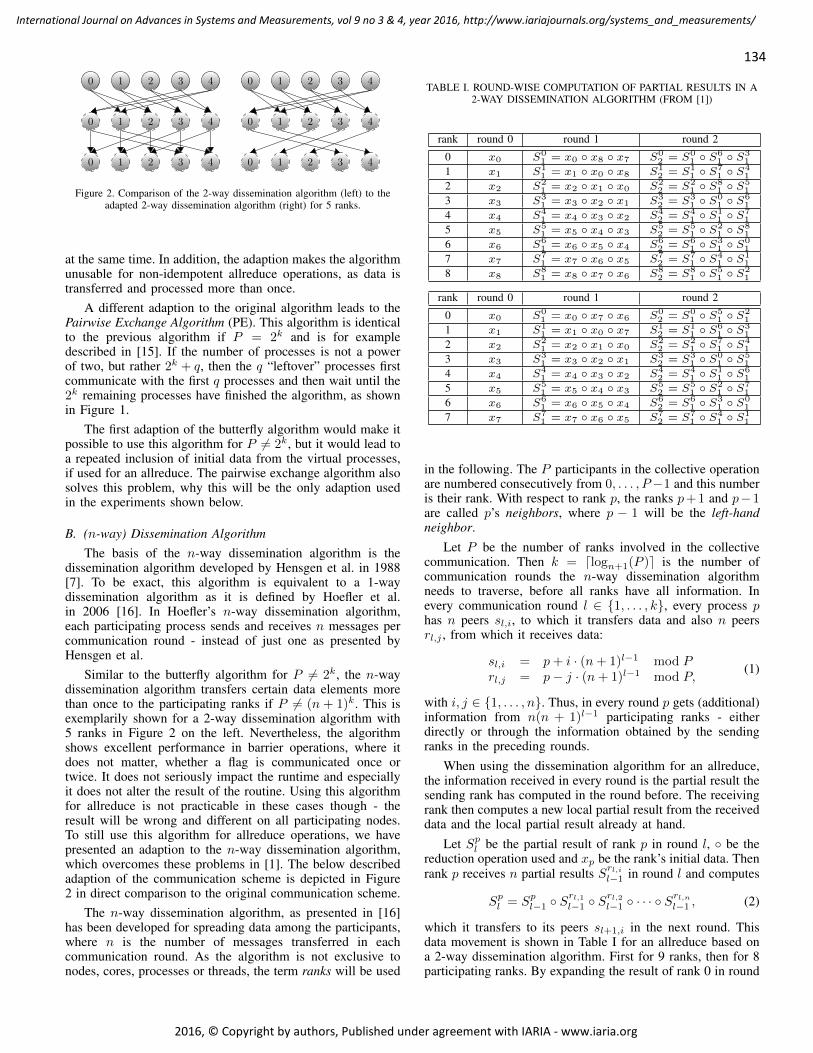
A. Butterfly Algorithm and Pairwise Exchange AlgorithmEugene D. Brooks introduced the butterfly algorithm in

the Butterfly Barrier in 1986 [6]. It has been designed foroperations with P = 2k participants. It then has k = dlog2 P ecommunication rounds, where in each round l, rank p commu-nicates with p ± 2l−1. Since this algorithm was not intendedfor the use with P = 2k−1+q < 2k processes, a first adaptionwas made: virtual processes were introduced to virtually haveP ′ = 2k processes to use the algorithm on. Existing processesadopted the role of these virtual processes as depicted in Figure1. Processes 0 to 2 act as if they were additional processes 5,6 and 7 to comply to the communication scheme for P = 8.This introduces unnecessary additional communication andoverhead. While this is not too dramatic in the case of abarrier, this becomes very interesting when the message sizesincrease. Even when P = 2k, the symmetric communicationscheme of the butterfly algorithm quickly leads to congestionin network topologies where there is exactly one link from oneprocessor to another, as this link will be used in both directions

134



0 1 2 3 4

0 1 2 3 4

0 1 2 3 4

0 1 2 3 4

0 1 2 3 4

0 1 2 3 4

Figure 2. Comparison of the 2-way dissemination algorithm (left) to theadapted 2-way dissemination algorithm (right) for 5 ranks.

at the same time. In addition, the adaption makes the algorithmunusable for non-idempotent allreduce operations, as data istransferred and processed more than once.

A different adaption to the original algorithm leads to thePairwise Exchange Algorithm (PE). This algorithm is identicalto the previous algorithm if P = 2k and is for exampledescribed in [15]. If the number of processes is not a powerof two, but rather 2k + q, then the q “leftover” processes firstcommunicate with the first q processes and then wait until the2k remaining processes have finished the algorithm, as shownin Figure 1.

The first adaption of the butterfly algorithm would make itpossible to use this algorithm for P 6= 2k, but it would lead toa repeated inclusion of initial data from the virtual processes,if used for an allreduce. The pairwise exchange algorithm alsosolves this problem, why this will be the only adaption usedin the experiments shown below.

B. (n-way) Dissemination AlgorithmThe basis of the n-way dissemination algorithm is the

dissemination algorithm developed by Hensgen et al. in 1988[7]. To be exact, this algorithm is equivalent to a 1-waydissemination algorithm as it is defined by Hoefler et al.in 2006 [16]. In Hoefler’s n-way dissemination algorithm,each participating process sends and receives n messages percommunication round - instead of just one as presented byHensgen et al.

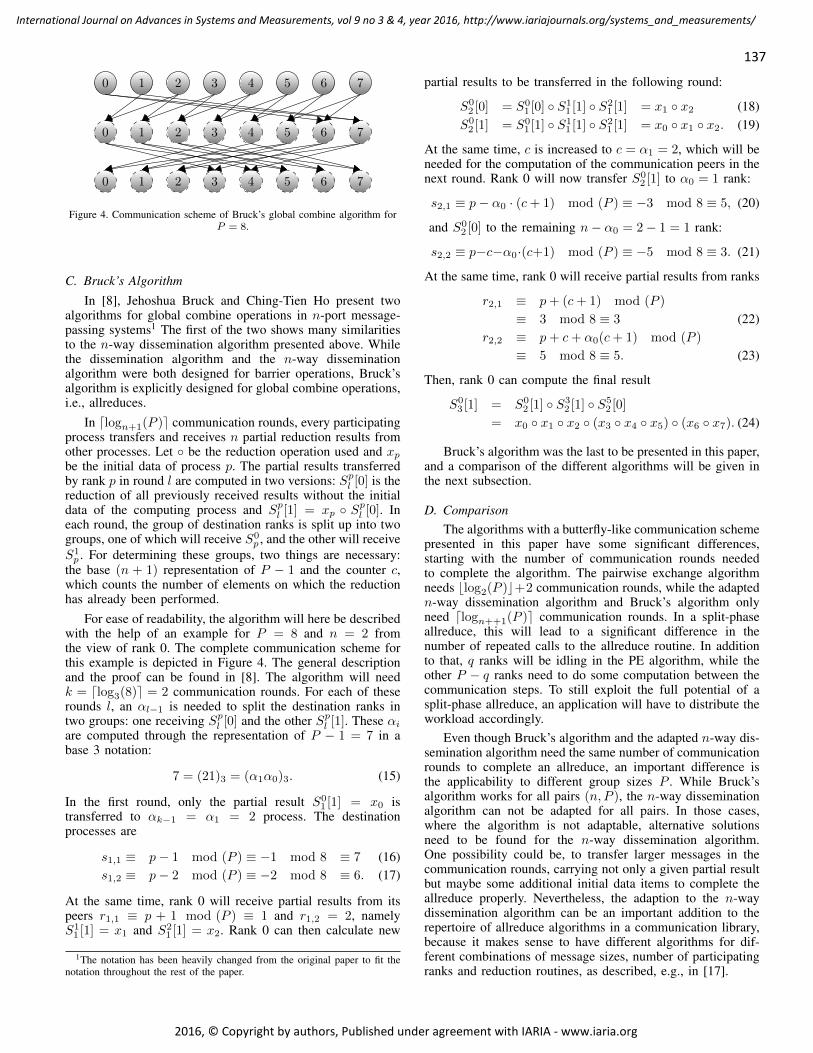
Similar to the butterfly algorithm for P 6= 2k, the n-waydissemination algorithm transfers certain data elements morethan once to the participating ranks if P 6= (n + 1)k. This isexemplarily shown for a 2-way dissemination algorithm with5 ranks in Figure 2 on the left. Nevertheless, the algorithmshows excellent performance in barrier operations, where itdoes not matter, whether a flag is communicated once ortwice. It does not seriously impact the runtime and especiallyit does not alter the result of the routine. Using this algorithmfor allreduce is not practicable in these cases though - theresult will be wrong and different on all participating nodes.To still use this algorithm for allreduce operations, we havepresented an adaption to the n-way dissemination algorithm,which overcomes these problems in [1]. The below describedadaption of the communication scheme is depicted in Figure2 in direct comparison to the original communication scheme.

The n-way dissemination algorithm, as presented in [16]has been developed for spreading data among the participants,where n is the number of messages transferred in eachcommunication round. As the algorithm is not exclusive tonodes, cores, processes or threads, the term ranks will be used

TABLE I. ROUND-WISE COMPUTATION OF PARTIAL RESULTS IN A2-WAY DISSEMINATION ALGORITHM (FROM [1])

rank round 0 round 1 round 2

0 x0 S01 = x0 ◦ x8 ◦ x7 S0

2 = S01 ◦ S

61 ◦ S

31

1 x1 S11 = x1 ◦ x0 ◦ x8 S1

2 = S11 ◦ S

71 ◦ S

41

2 x2 S21 = x2 ◦ x1 ◦ x0 S2

2 = S21 ◦ S

81 ◦ S

51

3 x3 S31 = x3 ◦ x2 ◦ x1 S3

2 = S31 ◦ S

01 ◦ S

61

4 x4 S41 = x4 ◦ x3 ◦ x2 S4

2 = S41 ◦ S

11 ◦ S

71

5 x5 S51 = x5 ◦ x4 ◦ x3 S5

2 = S51 ◦ S

21 ◦ S

81

6 x6 S61 = x6 ◦ x5 ◦ x4 S6

2 = S61 ◦ S

31 ◦ S

01

7 x7 S71 = x7 ◦ x6 ◦ x5 S7

2 = S71 ◦ S

41 ◦ S

11

8 x8 S81 = x8 ◦ x7 ◦ x6 S8

2 = S81 ◦ S

51 ◦ S

21

rank round 0 round 1 round 2

0 x0 S01 = x0 ◦ x7 ◦ x6 S0

2 = S01 ◦ S

51 ◦ S

21

1 x1 S11 = x1 ◦ x0 ◦ x7 S1

2 = S11 ◦ S

61 ◦ S

31

2 x2 S21 = x2 ◦ x1 ◦ x0 S2

2 = S21 ◦ S

71 ◦ S

41

3 x3 S31 = x3 ◦ x2 ◦ x1 S3

2 = S31 ◦ S

01 ◦ S

51

4 x4 S41 = x4 ◦ x3 ◦ x2 S4

2 = S41 ◦ S

11 ◦ S

61

5 x5 S51 = x5 ◦ x4 ◦ x3 S5

2 = S51 ◦ S

21 ◦ S

71

6 x6 S61 = x6 ◦ x5 ◦ x4 S6

2 = S61 ◦ S

31 ◦ S

01

7 x7 S71 = x7 ◦ x6 ◦ x5 S7

2 = S71 ◦ S

41 ◦ S

11

in the following. The P participants in the collective operationare numbered consecutively from 0, . . . , P−1 and this numberis their rank. With respect to rank p, the ranks p+1 and p−1are called p’s neighbors, where p − 1 will be the left-handneighbor.

Let P be the number of ranks involved in the collectivecommunication. Then k = dlogn+1(P )e is the number ofcommunication rounds the n-way dissemination algorithmneeds to traverse, before all ranks have all information. Inevery communication round l ∈ {1, . . . , k}, every process phas n peers sl,i, to which it transfers data and also n peersrl,j , from which it receives data:

sl,i = p+ i · (n+ 1)l−1 mod Prl,j = p− j · (n+ 1)l−1 mod P,

(1)

with i, j ∈ {1, . . . , n}. Thus, in every round p gets (additional)information from n(n + 1)l−1 participating ranks - eitherdirectly or through the information obtained by the sendingranks in the preceding rounds.

When using the dissemination algorithm for an allreduce,the information received in every round is the partial result thesending rank has computed in the round before. The receivingrank then computes a new local partial result from the receiveddata and the local partial result already at hand.

Let Spl be the partial result of rank p in round l, ◦ be the

reduction operation used and xp be the rank’s initial data. Thenrank p receives n partial results Srl,i

l−1 in round l and computes

Spl = Sp

l−1 ◦ Srl,1l−1 ◦ S

rl,2l−1 ◦ · · · ◦ S

rl,nl−1 , (2)

which it transfers to its peers sl+1,i in the next round. Thisdata movement is shown in Table I for an allreduce based ona 2-way dissemination algorithm. First for 9 ranks, then for 8participating ranks. By expanding the result of rank 0 in round

135



S00 S7

0S60S5

1S21

S10S0

0 S20

0 1 2 3 4 5 6 7

0 1 2 3 4 5 6 7

g1[1]g1[2]g2[1]g0 gB

g21 [1]g21 [2] g20

Figure 3. The data boundaries g and received partial results Srl,ji of ranks 0

and 2 (from [1]).

2 from the second table, it becomes visible, that the reductionoperation has been applied twice to x0:

S02 = (x0 ◦ x7 ◦ x6) ◦ (x5 ◦ x4 ◦ x3) ◦ (x2 ◦ x1 ◦ x0). (3)

In general, if P 6= (n+1)k, the final result will include data ofat least one rank twice: In every communication round l, eachrank receives n partial results each of which is the reduction ofthe initial data of its (n+1)l−1 left-hand neighbors. Thus, thenumber of included initial data elements is described through

l∑i=1

n(n+ 1)i−1 + 1 = (n+ 1)l (4)

for every round l.

In the cases of the maximum or minimum operation to beperformed in the allreduce, this does not matter. In the caseof a summation though, this dilemma will result into differentfinal sums on the participating ranks. In general, the adaptionis needed for all operations, where the repeated application ofthe function to the same element changes the final result, socalled non-idempotent functions.

The adaption of the n-way dissemination algorithm ismainly based on these two properties: (1) in every roundl, p receives n new partial results. (2) These partial resultsare the result of the combination of the data of the next∑l−1

i=0 n(n+1)i−1 +1 left-hand neighbors of the sender. Thisis depicted in Figure 3 through boxes. Highlighted in green arethose ranks, whose data view is represented, that is rank 0’s inthe first row and rank 2’s in the second row. Each box enclosesthose ranks, whose initial data is included in the partial resultthe right most rank in the box has transferred in a given round.This means for rank 0, it has its own data, received S6

0 andS70 in the first round (gray boxes) and will receive S5

1 and S21

from ranks 2 and 5 in round 2 (white boxes).

As each of the boxes describes one of the partial resultsreceived, the included initial data items can not be retrieved bythe destination rank. The change from one box to the next isthus defined as a data boundary. The main idea of the adaptionis to find data boundaries in the data of the source ranks inthe last round, which coincide with data boundaries in thedestination rank’s data. When such a correspondence is found,the data sent in the last round is reduced accordingly. To beable to do so, it is necessary to describe these boundaries in amathematical manner. Considering the data elements included

in each partial result received, the data boundaries of thereceiver p can be described as:

glrcv [jrcv] =

p− nlrcv−2∑i=0

(n+ 1)i − jrcv(n+ 1)lrcv−1 mod P, (5)

where jrcv(n+1)lrcv−1 describes the boundary created throughthe data transferred by rank rlrcv,jrcv in round lrcv.

Also, the sending ranks have received partial results in thepreceding rounds, which are marked through correspondingboundaries. From the view of rank p in the last round k, theseboundaries are then described through

gslsnd [jsnd] =

p− s(n+ 1)k−1 − nlsnd−2∑i=0

(n+ 1)i

− jsnd(n+ 1)lsnd−1 mod P, (6)

with s ∈ {1, . . . , n} distinguishing the n senders and jsnd, lsndcorresponding to the above jrcv, lrcv for the sending rank. Toalso consider those cases, where only the initial data of thesending or the receiving rank is included more than once inthe final result, we let lsnd, lrcv ∈ {0, . . . , k−1} and introducean additional base border gB in the destination rank’s data.

These boundaries are also depicted in Figure 3 for thepreviously given example of a 2-way dissemination algorithmwith 8 ranks. The figure depicts the data present on ranks 0and 2 after the first communication round in the gray boxeswith according boundaries gB , g0, g1[1] and g1[2] on rank 0and g20 , g21 [1] and g21 [2] on rank 2. Since the boundaries gBand g21 [1] coincide, the first sender in the last round, that isrank 5, transfers its partial result but rank 2 only transfers areduction S′ = x2 ◦ x1 instead of x2 ◦ x1 ◦ x0.

More generally speaking, the algorithm is adaptable, ifthere are boundaries on the source rank that coincide withboundaries on the destination rank, i.e.,

gslsnd [jsnd] = glrcv [jrcv] (7)

or gslsnd [jsnd] = gB . Then the last source rank, defined throughs, transfers only the data up to the given boundary and thereceiving rank takes the partial result up to its given boundaryout of the final result. Taking out the partial result in thiscontext means: if the given operation has an inverse ◦−1,apply this to the final result and the partial result definedthrough glrcv [jrcv]. If the operation does not have an inverse,recalculate the final result, hereby omitting the partial resultdefined through glrcv [jrcv]. Since this boundary is known fromthe very beginning, it is possible to store this partial result inthe round it is created, thus saving additional computation timeat the end.

From this, one can directly deduce the number of partici-pating ranks P , for which the n-way dissemination algorithm

136



is adaptable in this manner:

P = gslsnd[jsnd]− glrcv [jrcv]

= s(n+ 1)k−1 + n

lsnd−2∑i=0

(n+ 1)i + jsnd(n+ 1)lsnd−1

− nlrcv−2∑i=0

(n+ 1)i − jrcv(n+ 1)lrcv−1 . (8)

For given P , a 5-tuple (s, lsnd, lrcv, jsnd, jrcv) can be precal-culated for different n. Then this 5-tuple also describes theadaption of the algorithm:

Theorem 1: Given the 5-tuple (s, lsnd, lrcv, jsnd, jrcv), thelast round of the n-way dissemination algorithm is adaptedthrough one of the following cases:

1) lrcv, lsnd > 0The sender p − s(n + 1)k−1 sends its partial resultup to gslsnd

[jsnd] and the receiver takes out its partialresult up to the boundary glrcv [jrcv].

2) lrcv > 0, lsnd = 0The sender p−s(n+1)k−1 sends its own data and thereceiver takes out its partial result up to the boundaryglrcv [jrcv].

3) lrcv = 0, lsnd = 0The sender p − (s − 1)(n + 1)k−1 sends its lastcalculated partial result. If s = 1 the algorithm endsafter k − 1 rounds.

4) lrcv = 0, lsnd = 1The sender p−s(n+1)k−1 sends its partial result upto gslsnd

[jsnd − 1]. If jsnd = 1, the sender only sendsits initial data.

5) lrcv = 0, lsnd > 1The sender p − s(n + 1)k−1 sends its partial resultup to gslsnd

[jsnd] and the receiver takes out its initialdata from the final result.

Proof: We show the correctness of the above theoremby using that at the end each process will have to calculatethe final result from P different data elements. We thereforelook at (8) and how the given 5-tuple changes the termsof relevance. We will again need the fact, that the receivedpartial results are always a composition of the initial data ofneighboring elements.

1) lrcv, lsnd > 0:

P = s (n+ 1)k−1

+ n

lsnd−2∑i=0

(n+ 1)i+ jsnd (n+ 1)

lsnd−1

−nlrcv−2∑i=0

(n+ 1)i − jrcv (n+ 1)

lrcv−1

= gslsnd[jsnd]− glrcv [jrcv] . (9)

In order to have the result of P elements, the sendermust thus transfer the partial result including the data upto gslsnd

[jsnd] and the receiver takes out the elements up toglrcv [jrcv].

2) lrcv > 0, lsnd = 0:

P = s (n+ 1)k−1 − n

lrcv−2∑i=0

(n+ 1)i − jrcv (n+ 1)

lrcv−1

= s (n+ 1)k−1 − glrcv [jrcv] (10)

and thus we see that the sender must send only its own data,while the receiver takes out data up to glrcv [jrcv].

3) lrcv = 0, lsnd = 0:

P = s (n+ 1)k−1

. (11)

In the first k − 1 rounds, the receiving rank will alreadyhave the partial result of n

∑k−1i=1 (n+ 1)

i= (n+ 1)

k−1 − 1elements. In the last round it then receives the partial sumsof (s− 1) (n+ 1)

k−1 further elements by the first s − 1senders and can thus compute the partial result from a totalof (s− 1) (n+ 1)

k−1+ (n+ 1)

k−1= s (n+ 1)

k−1 − 1elements. Including its own data makes the final result ofs (n+ 1)

k−1= P elements. If s = 1 the algorithm is done

after k − 1 rounds.

4) lrcv = 0, lsnd = 1:

P = s (n+ 1)k−1

+ jsnd (12)

Following the same argumentation as above, the receivingrank will have the partial result of s (n+ 1)

k−1− 1 elements.It thus still needs

P −(s (n+ 1)

k−1 − 1)

= s (n+ 1)k−1

+ jsnd − s (n+ 1)k−1

+ 1

= jsnd + 1 (13)

elements. Now, taking into account its own data it still needsjsnd data elements. The data boundary g1 [jsnd] of the senderincludes jsnd elements plus its own data, i.e., jsnd+1 elements.The jthsnd element will then be the receiving rank’s data, thusit suffices to send up to g1 [jsnd − 1].

5) lrcv = 0, lsnd > 1:

P = s (n+ 1)k−1

+ n

lsnd−2∑i=0

(n+ 1)i+ jsnd (n+ 1)

lsnd−1 (14)

In this case, the sender sends a partial result which nec-essarily includes the initial data of the receiving rank. Thismeans that the receiving rank has to take out its own initialdata from the final result. Due to lsnd > 1 the sender will notbe able to take a single initial data element out of the partialresult to be transferred.

Note that the case where a data boundary on the sendingside corresponds to the base border on the receiving side, i.e.,gslsnd

[jsnd] = gB , has not been covered above. In this case,there is no 5-tuple like above, but rather P − 1 = gslsnd

[jsnd]and the adaption and reasoning complies to case 4 in the abovetheorem.

137



0 1 2 3 4 5 6 7

0 1 2 3 4 5 6 7

0 1 2 3 4 5 6 7

Figure 4. Communication scheme of Bruck’s global combine algorithm forP = 8.

C. Bruck’s AlgorithmIn [8], Jehoshua Bruck and Ching-Tien Ho present two

algorithms for global combine operations in n-port message-passing systems1 The first of the two shows many similaritiesto the n-way dissemination algorithm presented above. Whilethe dissemination algorithm and the n-way disseminationalgorithm were both designed for barrier operations, Bruck’salgorithm is explicitly designed for global combine operations,i.e., allreduces.

In dlogn+1(P )e communication rounds, every participatingprocess transfers and receives n partial reduction results fromother processes. Let ◦ be the reduction operation used and xpbe the initial data of process p. The partial results transferredby rank p in round l are computed in two versions: Sp

l [0] is thereduction of all previously received results without the initialdata of the computing process and Sp

l [1] = xp ◦ Spl [0]. In

each round, the group of destination ranks is split up into twogroups, one of which will receive S0

p , and the other will receiveS1p . For determining these groups, two things are necessary:

the base (n + 1) representation of P − 1 and the counter c,which counts the number of elements on which the reductionhas already been performed.

For ease of readability, the algorithm will here be describedwith the help of an example for P = 8 and n = 2 fromthe view of rank 0. The complete communication scheme forthis example is depicted in Figure 4. The general descriptionand the proof can be found in [8]. The algorithm will needk = dlog3(8)e = 2 communication rounds. For each of theserounds l, an αl−1 is needed to split the destination ranks intwo groups: one receiving Sp

l [0] and the other Spl [1]. These αi

are computed through the representation of P − 1 = 7 in abase 3 notation:

7 = (21)3 = (α1α0)3. (15)

In the first round, only the partial result S01 [1] = x0 is

transferred to αk−1 = α1 = 2 process. The destinationprocesses are

s1,1 ≡ p− 1 mod (P ) ≡ −1 mod 8 ≡ 7 (16)s1,2 ≡ p− 2 mod (P ) ≡ −2 mod 8 ≡ 6. (17)

At the same time, rank 0 will receive partial results from itspeers r1,1 ≡ p + 1 mod (P ) ≡ 1 and r1,2 = 2, namelyS11 [1] = x1 and S2

1 [1] = x2. Rank 0 can then calculate new

1The notation has been heavily changed from the original paper to fit thenotation throughout the rest of the paper.

partial results to be transferred in the following round:

S02 [0] = S0

1 [0] ◦ S11 [1] ◦ S2

1 [1] = x1 ◦ x2 (18)S02 [1] = S0

1 [1] ◦ S11 [1] ◦ S2

1 [1] = x0 ◦ x1 ◦ x2. (19)

At the same time, c is increased to c = α1 = 2, which will beneeded for the computation of the communication peers in thenext round. Rank 0 will now transfer S0

2 [1] to α0 = 1 rank:

s2,1 ≡ p− α0 · (c+ 1) mod (P ) ≡ −3 mod 8 ≡ 5, (20)

and S02 [0] to the remaining n− α0 = 2− 1 = 1 rank:

s2,2 ≡ p−c−α0·(c+1) mod (P ) ≡ −5 mod 8 ≡ 3. (21)

At the same time, rank 0 will receive partial results from ranks

r2,1 ≡ p+ (c+ 1) mod (P )

≡ 3 mod 8 ≡ 3 (22)r2,2 ≡ p+ c+ α0(c+ 1) mod (P )

≡ 5 mod 8 ≡ 5. (23)

Then, rank 0 can compute the final result

S03 [1] = S0

2 [1] ◦ S32 [1] ◦ S5

2 [0]

= x0 ◦ x1 ◦ x2 ◦ (x3 ◦ x4 ◦ x5) ◦ (x6 ◦ x7). (24)

Bruck’s algorithm was the last to be presented in this paper,and a comparison of the different algorithms will be given inthe next subsection.

D. ComparisonThe algorithms with a butterfly-like communication scheme

presented in this paper have some significant differences,starting with the number of communication rounds neededto complete the algorithm. The pairwise exchange algorithmneeds blog2(P )c+2 communication rounds, while the adaptedn-way dissemination algorithm and Bruck’s algorithm onlyneed dlogn++1(P )e communication rounds. In a split-phaseallreduce, this will lead to a significant difference in thenumber of repeated calls to the allreduce routine. In additionto that, q ranks will be idling in the PE algorithm, while theother P − q ranks need to do some computation between thecommunication steps. To still exploit the full potential of asplit-phase allreduce, an application will have to distribute theworkload accordingly.

Even though Bruck’s algorithm and the adapted n-way dis-semination algorithm need the same number of communicationrounds to complete an allreduce, an important difference isthe applicability to different group sizes P . While Bruck’salgorithm works for all pairs (n, P ), the n-way disseminationalgorithm can not be adapted for all pairs. In those cases,where the algorithm is not adaptable, alternative solutionsneed to be found for the n-way dissemination algorithm.One possibility could be, to transfer larger messages in thecommunication rounds, carrying not only a given partial resultbut maybe some additional initial data items to complete theallreduce properly. Nevertheless, the adaption to the n-waydissemination algorithm can be an important addition to therepertoire of allreduce algorithms in a communication library,because it makes sense to have different algorithms for dif-ferent combinations of message sizes, number of participatingranks and reduction routines, as described, e.g., in [17].

138



0

5

10

15

20

24 8 12 16 24 32 48 64 80 96

tim

e in

µs

number of nodes

Comparison of Averaged Runtimes of the Allreduce with 1 element 2 x 12 core Ivy Bridge E5-2695 v2 2.40GHz, InfiniBand ConnectX FDR

n-way allreduceIntel 4.1.3

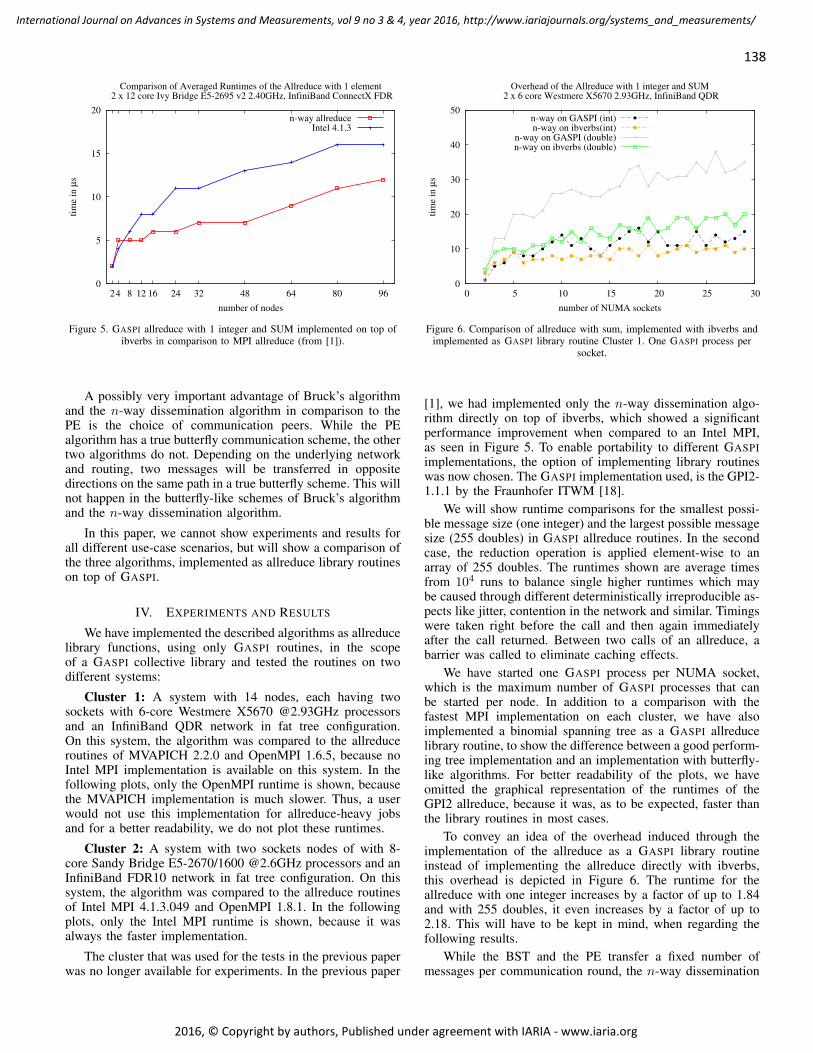
Figure 5. GASPI allreduce with 1 integer and SUM implemented on top ofibverbs in comparison to MPI allreduce (from [1]).

A possibly very important advantage of Bruck’s algorithmand the n-way dissemination algorithm in comparison to thePE is the choice of communication peers. While the PEalgorithm has a true butterfly communication scheme, the othertwo algorithms do not. Depending on the underlying networkand routing, two messages will be transferred in oppositedirections on the same path in a true butterfly scheme. This willnot happen in the butterfly-like schemes of Bruck’s algorithmand the n-way dissemination algorithm.

In this paper, we cannot show experiments and results forall different use-case scenarios, but will show a comparison ofthe three algorithms, implemented as allreduce library routineson top of GASPI.

IV. EXPERIMENTS AND RESULTS

We have implemented the described algorithms as allreducelibrary functions, using only GASPI routines, in the scopeof a GASPI collective library and tested the routines on twodifferent systems:

Cluster 1: A system with 14 nodes, each having twosockets with 6-core Westmere X5670 @2.93GHz processorsand an InfiniBand QDR network in fat tree configuration.On this system, the algorithm was compared to the allreduceroutines of MVAPICH 2.2.0 and OpenMPI 1.6.5, because noIntel MPI implementation is available on this system. In thefollowing plots, only the OpenMPI runtime is shown, becausethe MVAPICH implementation is much slower. Thus, a userwould not use this implementation for allreduce-heavy jobsand for a better readability, we do not plot these runtimes.

Cluster 2: A system with two sockets nodes of with 8-core Sandy Bridge E5-2670/1600 @2.6GHz processors and anInfiniBand FDR10 network in fat tree configuration. On thissystem, the algorithm was compared to the allreduce routinesof Intel MPI 4.1.3.049 and OpenMPI 1.8.1. In the followingplots, only the Intel MPI runtime is shown, because it wasalways the faster implementation.

The cluster that was used for the tests in the previous paperwas no longer available for experiments. In the previous paper

0

10

20

30

40

50

0 5 10 15 20 25 30

tim

e in

µs

number of NUMA sockets

Overhead of the Allreduce with 1 integer and SUM 2 x 6 core Westmere X5670 2.93GHz, InfiniBand QDR

n-way on GASPI (int)n-way on ibverbs(int)

n-way on GASPI (double)n-way on ibverbs (double)

Figure 6. Comparison of allreduce with sum, implemented with ibverbs andimplemented as GASPI library routine Cluster 1. One GASPI process per

socket.

[1], we had implemented only the n-way dissemination algo-rithm directly on top of ibverbs, which showed a significantperformance improvement when compared to an Intel MPI,as seen in Figure 5. To enable portability to different GASPIimplementations, the option of implementing library routineswas now chosen. The GASPI implementation used, is the GPI2-1.1.1 by the Fraunhofer ITWM [18].

We will show runtime comparisons for the smallest possi-ble message size (one integer) and the largest possible messagesize (255 doubles) in GASPI allreduce routines. In the secondcase, the reduction operation is applied element-wise to anarray of 255 doubles. The runtimes shown are average timesfrom 104 runs to balance single higher runtimes which maybe caused through different deterministically irreproducible as-pects like jitter, contention in the network and similar. Timingswere taken right before the call and then again immediatelyafter the call returned. Between two calls of an allreduce, abarrier was called to eliminate caching effects.

We have started one GASPI process per NUMA socket,which is the maximum number of GASPI processes that canbe started per node. In addition to a comparison with thefastest MPI implementation on each cluster, we have alsoimplemented a binomial spanning tree as a GASPI allreducelibrary routine, to show the difference between a good perform-ing tree implementation and an implementation with butterfly-like algorithms. For better readability of the plots, we haveomitted the graphical representation of the runtimes of theGPI2 allreduce, because it was, as to be expected, faster thanthe library routines in most cases.

To convey an idea of the overhead induced through theimplementation of the allreduce as a GASPI library routineinstead of implementing the allreduce directly with ibverbs,this overhead is depicted in Figure 6. The runtime for theallreduce with one integer increases by a factor of up to 1.84and with 255 doubles, it even increases by a factor of up to2.18. This will have to be kept in mind, when regarding thefollowing results.

While the BST and the PE transfer a fixed number ofmessages per communication round, the n-way dissemination

139



0

5

10

15

20

25

0 5 10 15 20 25 30

tim

e in

µs


Average Runtimes of the Allreduce with 1 integer and SUM 2 x 6 core Westmere X5670 2.93GHz, InfiniBand QDR

BinomialPairwiseBruck’s

n-wayOpenMPI

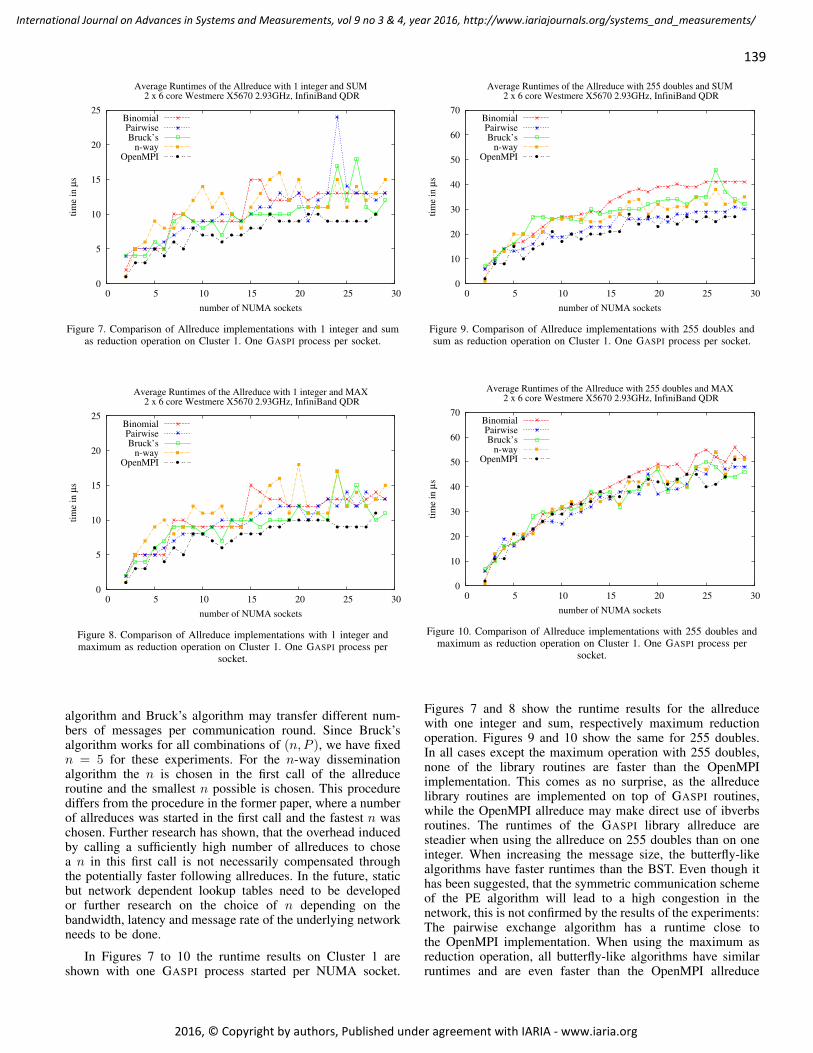
Figure 7. Comparison of Allreduce implementations with 1 integer and sumas reduction operation on Cluster 1. One GASPI process per socket.

0

5

10

15

20

25

0 5 10 15 20 25 30

tim

e in

µs


Average Runtimes of the Allreduce with 1 integer and MAX 2 x 6 core Westmere X5670 2.93GHz, InfiniBand QDR


n-wayOpenMPI

Figure 8. Comparison of Allreduce implementations with 1 integer andmaximum as reduction operation on Cluster 1. One GASPI process per

socket.

algorithm and Bruck’s algorithm may transfer different num-bers of messages per communication round. Since Bruck’salgorithm works for all combinations of (n, P ), we have fixedn = 5 for these experiments. For the n-way disseminationalgorithm the n is chosen in the first call of the allreduceroutine and the smallest n possible is chosen. This procedurediffers from the procedure in the former paper, where a numberof allreduces was started in the first call and the fastest n waschosen. Further research has shown, that the overhead inducedby calling a sufficiently high number of allreduces to chosea n in this first call is not necessarily compensated throughthe potentially faster following allreduces. In the future, staticbut network dependent lookup tables need to be developedor further research on the choice of n depending on thebandwidth, latency and message rate of the underlying networkneeds to be done.

In Figures 7 to 10 the runtime results on Cluster 1 areshown with one GASPI process started per NUMA socket.

0

10

20

30

40

50

60

70

0 5 10 15 20 25 30

tim

e in

µs


Average Runtimes of the Allreduce with 255 doubles and SUM 2 x 6 core Westmere X5670 2.93GHz, InfiniBand QDR


n-wayOpenMPI

Figure 9. Comparison of Allreduce implementations with 255 doubles andsum as reduction operation on Cluster 1. One GASPI process per socket.

0

10

20

30

40

50

60

70

0 5 10 15 20 25 30

tim

e in

µs


Average Runtimes of the Allreduce with 255 doubles and MAX 2 x 6 core Westmere X5670 2.93GHz, InfiniBand QDR


n-wayOpenMPI

Figure 10. Comparison of Allreduce implementations with 255 doubles andmaximum as reduction operation on Cluster 1. One GASPI process per

socket.

Figures 7 and 8 show the runtime results for the allreducewith one integer and sum, respectively maximum reductionoperation. Figures 9 and 10 show the same for 255 doubles.In all cases except the maximum operation with 255 doubles,none of the library routines are faster than the OpenMPIimplementation. This comes as no surprise, as the allreducelibrary routines are implemented on top of GASPI routines,while the OpenMPI allreduce may make direct use of ibverbsroutines. The runtimes of the GASPI library allreduce aresteadier when using the allreduce on 255 doubles than on oneinteger. When increasing the message size, the butterfly-likealgorithms have faster runtimes than the BST. Even though ithas been suggested, that the symmetric communication schemeof the PE algorithm will lead to a high congestion in thenetwork, this is not confirmed by the results of the experiments:The pairwise exchange algorithm has a runtime close tothe OpenMPI implementation. When using the maximum asreduction operation, all butterfly-like algorithms have similarruntimes and are even faster than the OpenMPI allreduce

140



0

10

20

30

40

50

2 4 8 12 16 24 32 48 64 72 96

tim

e in

µs


Average Runtimes of the Allreduce with 1 integer and SUM 2 x 8-core Sandy Bridge - E5-2670/1600 2.6 GHz, InfiniBand FDR10


n-wayIntelMPI

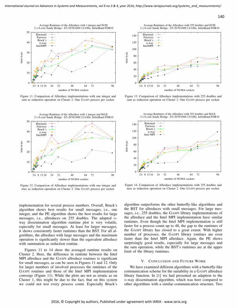
Figure 11. Comparison of Allreduce implementations with one integer andsum as reduction operation on Cluster 2. One GASPI process per socket.

0

10

20

30

40

50

2 4 8 12 16 24 32 48 64 72 96

tim

e in

µs


Average Runtimes of the Allreduce with 1 integer and MAX 2 x 8-core Sandy Bridge - E5-2670/1600 2.6 GHz, InfiniBand FDR10


n-wayIntelMPI

Figure 12. Comparison of Allreduce implementations with one integer andmax as reduction operation on Cluster 2. One GASPI process per socket.

implementation for several process numbers. Overall, Bruck’salgorithm shows best results for small messages, i.e., oneinteger, and the PE algorithm shows the best results for largemessages, i.e., allreduces on 255 doubles. The adapted n-way dissemination algorithm runtime plot is very volatile,especially for small messages. At least for larger messages,it shows consistently faster runtimes than the BST. For all al-gorithms, the allreduce with large messages and the maximumoperation is significantly slower than the equivalent allreducewith summation as reduction routine.

Figures 11 to 14 show the averaged runtime results onCluster 2. Here, the difference in runtime between the IntelMPI allreduce and the GASPI allreduce routines is significantfor small messages, as can be seen in Figures 11 and 12. Onlyfor larger numbers of involved processes the runtimes of theGASPI routines and those of the Intel MPI implementationconverge (Figure 11). While the plots are not as erratic as onCluster 1, this might be due to the fact, that on this systemwe could not test every process count. Especially Bruck’s

0

20

40

60

80

100

120

140

2 4 8 12 16 24 32 48 64 72 96

tim

e in

µs


Average Runtimes of the Allreduce with 255 doubles and SUM 2 x 8-core Sandy Bridge - E5-2670/1600 2.6 GHz, InfiniBand FDR10


n-wayIntelMPI

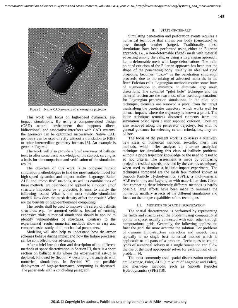
Figure 13. Comparison of Allreduce implementations with 255 doubles andsum as reduction operation on Cluster 2. One GASPI process per socket.

0

20

40

60

80

100

120

140

2 4 8 12 16 24 32 48 64 72 96

tim

e in

µs


Average Runtimes of the Allreduce with 255 doubles and MAX 2 x 8-core Sandy Bridge - E5-2670/1600 2.6 GHz, InfiniBand FDR10


n-wayIntel MPI

Figure 14. Comparison of Allreduce implementations with 255 doubles andmax as reduction operation on Cluster 2. One GASPI process per socket.

algorithm outperforms the other butterfly-like algorithms andthe BST for allreduces with small messages. For large mes-sages, i.e., 255 doubles, the GASPI library implementations ofthe allreduce and the Intel MPI implementation have similarruntimes. Even though the Intel MPI implementation is stillfaster for a process count up to 48, the gap to the runtimes ofthe GASPI library has closed to a great extent. With highernumber of processes, the GASPI library routines are evenfaster than the Intel MPI allreduce. Again, the PE showssurprisingly good results, especially for large messages andthe sum operation, while the BST’s runtimes are at the upperlimit of the library runtimes.

V. CONCLUSION AND FUTURE WORK

We have examined different algorithms with a butterfly-likecommunication scheme for the suitability in a GASPI allreducelibrary function. In [1] we had presented an adaption to then-way dissemination algorithm, which was here compared toother algorithms with a similar communication structure. Two

141



important properties of these algorithms are their low numberof communication rounds while at the same time involvingall processes in each computation step of the algorithm. Thismakes them ideal candidates for a split-phase allreduce routineas defined in the GASPI specification.

We have seen in the experiments, that algorithms with abutterfly-like communication scheme are often significantlyfaster than, e.g., the BST and sometimes even reach theperformance of existing MPI implementations. This is espe-cially important to note, because the results presented in thisarticle are results obtained from library implementations, i.e.,not directly implemented on ibverbs but rather with GASPIroutines. As shown in Figure 6, the overhead induced throughthis additional layer of indirection can slow a routine downby a factor of 2. Considering this, an implementation of theallreduce routine with ibverbs should accelerate the routine toapproximately the level of the MPI implementations shown forsmall messages and even faster in the case of large messages.This is a relevant starting point for future research.

Another important comparison to make is the influence ofthe different network interconnects on the algorithm. While inthe former paper, the FDR network had an immense influenceon the runtime of the n-way dissemination algorithm. In thiscase, we are comparing a QDR network to a FDR-10 networkand do not see the same performance increase. Instead, wepartially even see a decrease in speed. While Bruck’s algorithmdoes not need more than 10 µs for small messages Cluster 1, itneeds 16 µs on Cluster 2. For large messages we see a speedupfrom 32 µs to 30 µs for the global maximum and from 30 µs to27 µs for the global sum. This again highlights the importanceof adjusting the used algorithms to the underlying networkand will be investigated further in the scope of a library withcollective routines for GASPI implementations.

All in all, algorithms with a butterfly-like communicationscheme should not be ignored for new communication routinesand libraries. The increasing message rates and network topol-ogy developments might make the use of these algorithms veryfeasible again.

REFERENCES[1] V. End, R. Yahyapour, C. Simmendinger, and T. Alrutz, “Adapting the

n-way Dissemination Algorithm for GASPI Split-Phase Allreduce,” inINFOCOMP 2015, The Fifth International Conference on AdvancedCommunications and Computation, June 2015, pp. 13 – 19.

[2] GASPI Consortium, “GASPI: Global Address Space ProgrammingInterface, Specification of a PGAS API for communication Version16.1,” https://raw.githubusercontent.com/GASPI-Forum/GASPI-Forum.github.io/master/standards/GASPI-16.1.pdf, February 2016, retrieved2016.11.29 at 13:07.

[3] Message-Passing Interface Forum, MPI: A Message Passing InterfaceStandard, Version 3.0. High-Performance Computing Center Stuttgart,09 2012.

[4] N.-F. Tzeng and H.-L. Chen, “Fast compaction in hypercubes,” IEEETransactions on Parallel and Distributed Systems, vol. 9, 1998, pp. 50–55.

[5] J. M. Mellor-Crummey and M. L. Scott, “Algorithms for scalable syn-chronization on shared-memory multiprocessors,” ACM Transactionson Computer Systems, vol. 9, no. 1, Feb. 1991, pp. 21–65.

[6] E. D. Brooks, “The Butterfly Barrier,” International Journal of ParallelProgramming, vol. 15, no. 4, 1986, pp. 295–307.

[7] D. Hensgen, R. Finkel, and U. Manber, “Two algorithms for barrier syn-chronization,” International Journal of Parallel Programming, vol. 17,no. 1, Feb. 1988, pp. 1–17.

[8] J. Bruck and C.-T. Ho, “Efficient global combine operations in multi-port message-passing systems,” Parallel Processing Letters, vol. 3,no. 04, 1993, pp. 335–346.

[9] J. Bruck, C.-T. Ho, S. Kipnis, E. Upfal, and D. Weathersby, “Efficientalgorithms for all-to-all communications in multi-port message-passingsystems,” in IEEE Transactions on Parallel and Distributed Systems,1997, pp. 298–309.

[10] S. P. Kini, J. Liu, J. Wu, P. Wyckoff, and D. K. Panda, “Fast and ScalableBarrier using RDMA and Multicast Mechanisms for InfiniBand-basedClusters,” in Recent Advances in Parallel Virtual Machine and MessagePassing Interface. Springer, 2003, pp. 369–378.

[11] V. Tipparaju, J. Nieplocha, and D. Panda, “Fast collective operationsusing shared and remote memory access protocols on clusters,” inProceedings of the 17th International Symposium on Parallel andDistributed Processing, ser. IPDPS ’03. Washington, DC, USA: IEEEComputer Society, 2003, pp. 84.1–.

[12] InfiniBand Trade Association, “Infiniband architecture specificationvolume 1, release 1.3,” https://cw.infinibandta.org/document/dl/7859,March 2015, retrieved 2016.11.29 at 13:09.

[13] ——, “Infiniband architecture specification volume 1, release 1.2.1, an-nex a16,” https://cw.infinibandta.org/document/dl/7148, 2010, retrieved2016.11.29 at 13:08.

[14] E. Zahavi, “Fat-tree Routing and Node Ordering Providing ContentionFree Traffic for MPI Global Collectives,” J. Parallel Distrib. Comput.,vol. 72, no. 11, Nov. 2012, pp. 1423–1432.

[15] R. Gupta, V. Tipparaju, J. Nieplocha, and D. Panda, “Efficient Barrierusing Remote Memory Operations on VIA-Based Clusters,” in IEEECluster Computing. IEEE Computer Society, 2002, p. 83ff.

[16] T. Hoefler, T. Mehlan, F. Mietke, and W. Rehm, “Fast Barrier Syn-chronization for InfiniBand,” in Proceedings of the 20th InternationalConference on Parallel and Distributed Processing, ser. IPDPS’06.Washington, DC, USA: IEEE Computer Society, 2006, pp. 272–272.

[17] R. Thakur, R. Rabenseifner, and W. Gropp, “Optimization of CollectiveCommunication Operations in MPICH,” International Journal of HighPerformance Computing Applications, vol. 19, 2005, pp. 49–66.

[18] Fraunhofer ITWM, “GPI2 homepage,” www.gpi-site.com/gpi2, re-trieved 2016.11.29 at 13:11.

142



Influences of Meshing and High-Performance Computing towards Advancing the

Numerical Analysis of High-Velocity Impacts

Arash Ramezani and Hendrik Rothe

University of the Federal Armed Forces

Hamburg, Germany

Email: [email protected], [email protected]

Abstract—By now, computers and software have spread into

all fields of industry. The use of finite-difference and finite-

element computer codes to solve problems involving fast,

transient loading is commonplace. A large number of

commercial codes exist and are applied to problems ranging

from fairly low to extremely high damage levels. Therefore,

extensive efforts are currently made in order to improve the

safety by applying certain numerical solutions. For many

engineering problems involving shock and impact, there is no

single ideal numerical method that can reproduce the various

aspects of a problem. An approach which combines different

techniques in a single numerical analysis can provide the

“best” solution in terms of accuracy and efficiency. But, what

happens if code predictions do not correspond with reality?

This paper discusses various factors related to the

computational mesh that can lead to disagreement between

computations and experience. Furthermore, the influence of

high-performance computing is a main subject of this work.

The goal is to find an appropriate technique for simulating

composite materials and thereby improve modern armor to

meet current challenges. Given the complexity of penetration

processes, it is not surprising that the bulk of work in this area

is experimental in nature. Terminal ballistic test techniques,

aside from routine proof tests, vary mainly in the degree of

instrumentation provided and hence the amount of data

retrieved. Here, both the ballistic trials as well as the analytical

methods will be discussed.

Keywords-solver methologies; simulation models; meshing;

high-performance computing; high-velocity impact; armor

systems.

I. INTRODUCTION

In the security sector, failing industrial components are ongoing problems that cause great concern as they can endanger people and equipment. Therefore, extensive efforts are currently made in order to improve the safety of industrial components by applying certain computer-based solutions. To deal with problems involving the release of a large amount of energy over a very short period of time, e.g., explosions and impacts, there are three approaches, which are discussed in detail in [1].

As the problems are highly non-linear and require information regarding material behavior at ultra-high loading rates, which are generally not available, most of the work is experimental and may cause tremendous expenses. Analytical approaches are possible if the geometries

involved are relatively simple and if the loading can be described through boundary conditions, initial conditions, or a combination of the two. Numerical solutions are far more general in scope and remove any difficulties associated with geometry [2].

For structures under shock and impact loading, numerical simulations have proven to be extremely useful. They provide a rapid and less expensive way to evaluate new design ideas. Numerical simulations can supply quantitative and accurate details of stress, strain, and deformation fields that would be very costly or difficult to reproduce experimentally. In these numerical simulations, the partial differential equations governing the basic physics principles of conservation of mass, momentum, and energy are employed. The equations to be solved are time-dependent and nonlinear in nature. These equations, together with constitutive models describing material behavior and a set of initial and boundary conditions, define the complete system for shock and impact simulations.

The governing partial differential equations need to be solved in both time and space domains (see Figure 1). The solution for the time domain can be achieved by an explicit method. In the explicit method, the solution at a given point in time is expressed as a function of the system variables and parameters, with no requirements for stiffness and mass matrices. Thus, the computing time at each time step is low but may require numerous time steps for a complete solution.

The solution for the space domain can be obtained utilizing different spatial discretization techniques, such as Lagrange [3], Euler [4], Arbitrary Lagrange Euler (ALE) [5], or “mesh free” methods [6]. Each of these techniques has its unique capabilities, but also limitations. Usually, there is not a single technique that can cope with all the regimes of a problem [7].

Figure 1. Discretization of time and space is required.

143



Figure 2. Native CAD geometry of an exemplary projectile.

This work will focus on high-speed dynamics, esp. impact simulations. By using a computer-aided design (CAD) neutral environment that supports direct, bidirectional, and associative interfaces with CAD systems, the geometry can be optimized successively. Native CAD geometry can be used directly without a translation to IGES or other intermediate geometry formats [8]. An example is given in Figure 2.

The work will also provide a brief overview of ballistic tests to offer some basic knowledge of the subject, serving as a basis for the comparison and verification of the simulation results.

The objective of this work is to compare current simulation methodologies to find the most suitable model for high-speed dynamics and impact studies. Lagrange, Euler, ALE, and “mesh free” methods, as well as combinations of these methods, are described and applied to a modern amor structure impacted by a projectile. It aims to clarify the following issues: What is the most suitable simulation model? How does the mesh density affect the results? What are the benefits of high-performance computing?

The results shall be used to improve the safety of ballistic structures, esp. for armored vehicles. Instead of running expensive trials, numerical simulations should be applied to identify vulnerabilities of structures. Contrary to the experimental results, numerical methods allow an easy and comprehensive study of all mechanical parameters.

Modeling will also help to understand how the armor schemes behave during impact and how the failure processes can be controlled to our advantage.

After a brief introduction and description of the different methods of space discretization in Section III, there is a short section on ballistic trials where the experimental set-up is depicted, followed by Section V describing the analysis with numerical simulations. In Section VI, the possible deployment of high-performance computing is discussed. The paper ends with a concluding paragraph.

II. STATE-OF-THE-ART

Simulating penetration and perforation events requires a numerical technique that allows one body (penetrator) to pass through another (target). Traditionally, these simulations have been performed using either an Eulerian approach, i.e., a non-deformable (fixed) mesh with material advecting among the cells, or using a Lagrangian approach, i.e., a deformable mesh with large deformations. The main point of criticism of the Eulerian approach has been that the shape of the penetrating body, usually an idealized rigid projectile, becomes “fuzzy” as the penetration simulation proceeds, due to the mixing of advected materials in the fixed Eulerian cells. Lagrangian methods require some form of augmentation to minimize or eliminate large mesh distortions. The so-called “pilot hole” technique and the material erosion are the two most often used augmentations for Lagrangian penetration simulations. In the pilot hole technique, elements are removed a priori from the target mesh along the penetrator trajectory, which works well for normal impacts where the trajectory is known a priori. The latter technique removes distorted elements from the simulation based upon a user supplied criterion. They are also removed along the penetrator trajectory, but with no general guidance for selecting certain criteria, i.e., they are ad hoc.

The focus of the present work is to assess a relatively new class of numerical methods, so-called mesh free methods, which offer analysts an alternate analytical technique for simulating this class of ballistic problems without a priori trajectory knowledge or the need to resort to ad hoc criteria. The assessment is made by comparing projectile residual speeds provided by the various techniques, when used to simulate a ballistic impact experiment. The techniques compared are the mesh free method known as Smooth Particle Hydrodynamics (SPH), a multi-material ALE technique, and Lagrangian with material erosion. Given that comparing these inherently different methods is hardly possible, large efforts have been made to minimize the numerous ancillary aspects of the different simulations and focus on the unique capabilities of the techniques.

III. METHODS OF SPACE DISCRETIZATION

The spatial discretization is performed by representing the fields and structures of the problem using computational points in space, usually connected with each other through computational grids. Generally, the following applies: the finer the grid, the more accurate the solution. For problems of dynamic fluid-structure interaction and impact, there typically is no single best numerical method which is applicable to all parts of a problem. Techniques to couple types of numerical solvers in a single simulation can allow the use of the most appropriate solver for each domain of the problem [9].

The most commonly used spatial discretization methods are Lagrange, Euler, ALE (a mixture of Lagrange and Euler), and mesh-free methods, such as Smooth Particles Hydrodynamics (SPH) [10].

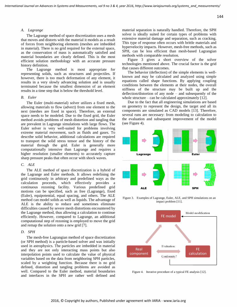
144



A. Lagrange

The Lagrange method of space discretization uses a mesh that moves and distorts with the material it models as a result of forces from neighboring elements (meshes are imbedded in material). There is no grid required for the external space, as the conservation of mass is automatically satisfied and material boundaries are clearly defined. This is the most efficient solution methodology with an accurate pressure history definition.

The Lagrange method is most appropriate for representing solids, such as structures and projectiles. If however, there is too much deformation of any element, it results in a very slowly advancing solution and is usually terminated because the smallest dimension of an element results in a time step that is below the threshold level.

B. Euler

The Euler (multi-material) solver utilizes a fixed mesh, allowing materials to flow (advect) from one element to the next (meshes are fixed in space). Therefore, an external space needs to be modeled. Due to the fixed grid, the Euler method avoids problems of mesh distortion and tangling that are prevalent in Lagrange simulations with large flows. The Euler solver is very well-suited for problems involving extreme material movement, such as fluids and gases. To describe solid behavior, additional calculations are required to transport the solid stress tensor and the history of the material through the grid. Euler is generally more computationally intensive than Lagrange and requires a higher resolution (smaller elements) to accurately capture sharp pressure peaks that often occur with shock waves.

C. ALE

The ALE method of space discretization is a hybrid of the Lagrange and Euler methods. It allows redefining the grid continuously in arbitrary and predefined ways as the calculation proceeds, which effectively provides a continuous rezoning facility. Various predefined grid motions can be specified, such as free (Lagrange), fixed (Euler), equipotential, equal spacing, and others. The ALE method can model solids as well as liquids. The advantage of ALE is the ability to reduce and sometimes eliminate difficulties caused by severe mesh distortions encountered by the Lagrange method, thus allowing a calculation to continue efficiently. However, compared to Lagrange, an additional computational step of rezoning is employed to move the grid and remap the solution onto a new grid [7].

D. SPH

The mesh-free Lagrangian method of space discretization (or SPH method) is a particle-based solver and was initially used in astrophysics. The particles are imbedded in material and they are not only interacting mass points but also interpolation points used to calculate the value of physical variables based on the data from neighboring SPH particles, scaled by a weighting function. Because there is no grid defined, distortion and tangling problems are avoided as well. Compared to the Euler method, material boundaries and interfaces in the SPH are rather well defined and

material separation is naturally handled. Therefore, the SPH solver is ideally suited for certain types of problems with extensive material damage and separation, such as cracking. This type of response often occurs with brittle materials and hypervelocity impacts. However, mesh-free methods, such as SPH, can be less efficient than mesh-based Lagrangian methods with comparable resolution.

Figure 3 gives a short overview of the solver technologies mentioned above. The crucial factor is the grid that causes different outcomes.

The behavior (deflection) of the simple elements is well-known and may be calculated and analyzed using simple equations called shape functions. By applying coupling conditions between the elements at their nodes, the overall stiffness of the structure may be built up and the deflection/distortion of any node – and subsequently of the whole structure – can be calculated approximately [12].

Due to the fact that all engineering simulations are based on geometry to represent the design, the target and all its components are simulated as CAD models [13]. Therefore, several runs are necessary: from modeling to calculation to the evaluation and subsequent improvement of the model (see Figure 4).

Figure 3. Examples of Lagrange, Euler, ALE, and SPH simulations on an

impact problem [11].

Figure 4. Iterative procedure of a typical FE analysis [12].

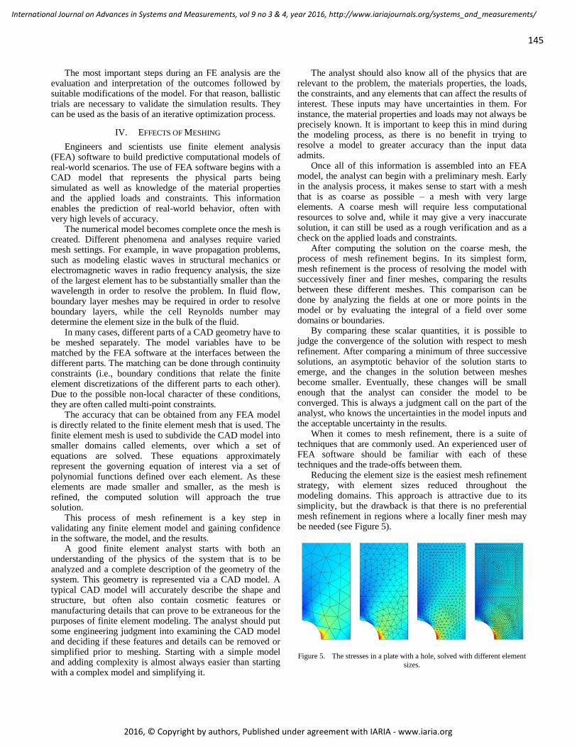
145



The most important steps during an FE analysis are the evaluation and interpretation of the outcomes followed by suitable modifications of the model. For that reason, ballistic trials are necessary to validate the simulation results. They can be used as the basis of an iterative optimization process.

IV. EFFECTS OF MESHING

Engineers and scientists use finite element analysis (FEA) software to build predictive computational models of real-world scenarios. The use of FEA software begins with a CAD model that represents the physical parts being simulated as well as knowledge of the material properties and the applied loads and constraints. This information enables the prediction of real-world behavior, often with very high levels of accuracy.

The numerical model becomes complete once the mesh is created. Different phenomena and analyses require varied mesh settings. For example, in wave propagation problems, such as modeling elastic waves in structural mechanics or electromagnetic waves in radio frequency analysis, the size of the largest element has to be substantially smaller than the wavelength in order to resolve the problem. In fluid flow, boundary layer meshes may be required in order to resolve boundary layers, while the cell Reynolds number may determine the element size in the bulk of the fluid.

In many cases, different parts of a CAD geometry have to be meshed separately. The model variables have to be matched by the FEA software at the interfaces between the different parts. The matching can be done through continuity constraints (i.e., boundary conditions that relate the finite element discretizations of the different parts to each other). Due to the possible non-local character of these conditions, they are often called multi-point constraints.

The accuracy that can be obtained from any FEA model is directly related to the finite element mesh that is used. The finite element mesh is used to subdivide the CAD model into smaller domains called elements, over which a set of equations are solved. These equations approximately represent the governing equation of interest via a set of polynomial functions defined over each element. As these elements are made smaller and smaller, as the mesh is refined, the computed solution will approach the true solution.

This process of mesh refinement is a key step in validating any finite element model and gaining confidence in the software, the model, and the results.

A good finite element analyst starts with both an understanding of the physics of the system that is to be analyzed and a complete description of the geometry of the system. This geometry is represented via a CAD model. A typical CAD model will accurately describe the shape and structure, but often also contain cosmetic features or manufacturing details that can prove to be extraneous for the purposes of finite element modeling. The analyst should put some engineering judgment into examining the CAD model and deciding if these features and details can be removed or simplified prior to meshing. Starting with a simple model and adding complexity is almost always easier than starting with a complex model and simplifying it.

The analyst should also know all of the physics that are relevant to the problem, the materials properties, the loads, the constraints, and any elements that can affect the results of interest. These inputs may have uncertainties in them. For instance, the material properties and loads may not always be precisely known. It is important to keep this in mind during the modeling process, as there is no benefit in trying to resolve a model to greater accuracy than the input data admits.

Once all of this information is assembled into an FEA model, the analyst can begin with a preliminary mesh. Early in the analysis process, it makes sense to start with a mesh that is as coarse as possible – a mesh with very large elements. A coarse mesh will require less computational resources to solve and, while it may give a very inaccurate solution, it can still be used as a rough verification and as a check on the applied loads and constraints.

After computing the solution on the coarse mesh, the process of mesh refinement begins. In its simplest form, mesh refinement is the process of resolving the model with successively finer and finer meshes, comparing the results between these different meshes. This comparison can be done by analyzing the fields at one or more points in the model or by evaluating the integral of a field over some domains or boundaries.

By comparing these scalar quantities, it is possible to judge the convergence of the solution with respect to mesh refinement. After comparing a minimum of three successive solutions, an asymptotic behavior of the solution starts to emerge, and the changes in the solution between meshes become smaller. Eventually, these changes will be small enough that the analyst can consider the model to be converged. This is always a judgment call on the part of the analyst, who knows the uncertainties in the model inputs and the acceptable uncertainty in the results.

When it comes to mesh refinement, there is a suite of techniques that are commonly used. An experienced user of FEA software should be familiar with each of these techniques and the trade-offs between them.

Reducing the element size is the easiest mesh refinement strategy, with element sizes reduced throughout the modeling domains. This approach is attractive due to its simplicity, but the drawback is that there is no preferential mesh refinement in regions where a locally finer mesh may be needed (see Figure 5).

Figure 5. The stresses in a plate with a hole, solved with different element

sizes.

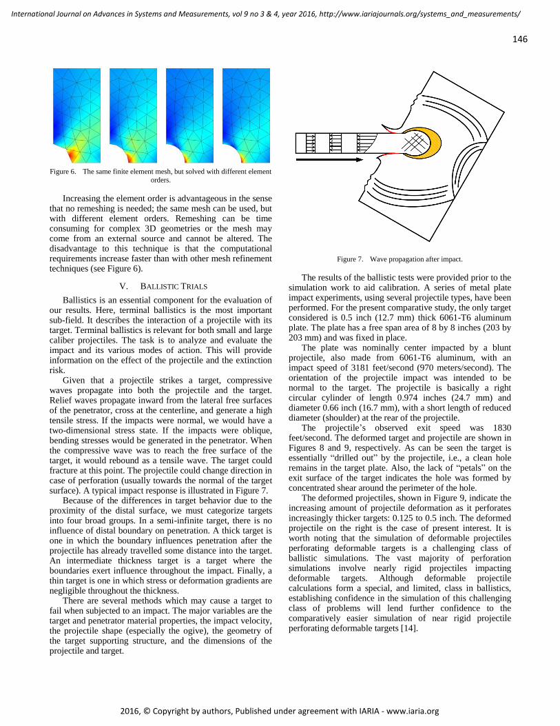
146



Figure 6. The same finite element mesh, but solved with different element

orders.

Increasing the element order is advantageous in the sense that no remeshing is needed; the same mesh can be used, but with different element orders. Remeshing can be time consuming for complex 3D geometries or the mesh may come from an external source and cannot be altered. The disadvantage to this technique is that the computational requirements increase faster than with other mesh refinement techniques (see Figure 6).

V. BALLISTIC TRIALS

Ballistics is an essential component for the evaluation of our results. Here, terminal ballistics is the most important sub-field. It describes the interaction of a projectile with its target. Terminal ballistics is relevant for both small and large caliber projectiles. The task is to analyze and evaluate the impact and its various modes of action. This will provide information on the effect of the projectile and the extinction risk.

Given that a projectile strikes a target, compressive waves propagate into both the projectile and the target. Relief waves propagate inward from the lateral free surfaces of the penetrator, cross at the centerline, and generate a high tensile stress. If the impacts were normal, we would have a two-dimensional stress state. If the impacts were oblique, bending stresses would be generated in the penetrator. When the compressive wave was to reach the free surface of the target, it would rebound as a tensile wave. The target could fracture at this point. The projectile could change direction in case of perforation (usually towards the normal of the target surface). A typical impact response is illustrated in Figure 7.

Because of the differences in target behavior due to the proximity of the distal surface, we must categorize targets into four broad groups. In a semi-infinite target, there is no influence of distal boundary on penetration. A thick target is one in which the boundary influences penetration after the projectile has already travelled some distance into the target. An intermediate thickness target is a target where the boundaries exert influence throughout the impact. Finally, a thin target is one in which stress or deformation gradients are negligible throughout the thickness.

There are several methods which may cause a target to fail when subjected to an impact. The major variables are the target and penetrator material properties, the impact velocity, the projectile shape (especially the ogive), the geometry of the target supporting structure, and the dimensions of the projectile and target.

Figure 7. Wave propagation after impact.

The results of the ballistic tests were provided prior to the simulation work to aid calibration. A series of metal plate impact experiments, using several projectile types, have been performed. For the present comparative study, the only target considered is 0.5 inch (12.7 mm) thick 6061-T6 aluminum plate. The plate has a free span area of 8 by 8 inches (203 by 203 mm) and was fixed in place.

The plate was nominally center impacted by a blunt projectile, also made from 6061-T6 aluminum, with an impact speed of 3181 feet/second (970 meters/second). The orientation of the projectile impact was intended to be normal to the target. The projectile is basically a right circular cylinder of length 0.974 inches (24.7 mm) and diameter 0.66 inch (16.7 mm), with a short length of reduced diameter (shoulder) at the rear of the projectile.

The projectile’s observed exit speed was 1830 feet/second. The deformed target and projectile are shown in Figures 8 and 9, respectively. As can be seen the target is essentially “drilled out” by the projectile, i.e., a clean hole remains in the target plate. Also, the lack of “petals” on the exit surface of the target indicates the hole was formed by concentrated shear around the perimeter of the hole.

The deformed projectiles, shown in Figure 9, indicate the increasing amount of projectile deformation as it perforates increasingly thicker targets: 0.125 to 0.5 inch. The deformed projectile on the right is the case of present interest. It is worth noting that the simulation of deformable projectiles perforating deformable targets is a challenging class of ballistic simulations. The vast majority of perforation simulations involve nearly rigid projectiles impacting deformable targets. Although deformable projectile calculations form a special, and limited, class in ballistics, establishing confidence in the simulation of this challenging class of problems will lend further confidence to the comparatively easier simulation of near rigid projectile perforating deformable targets [14].

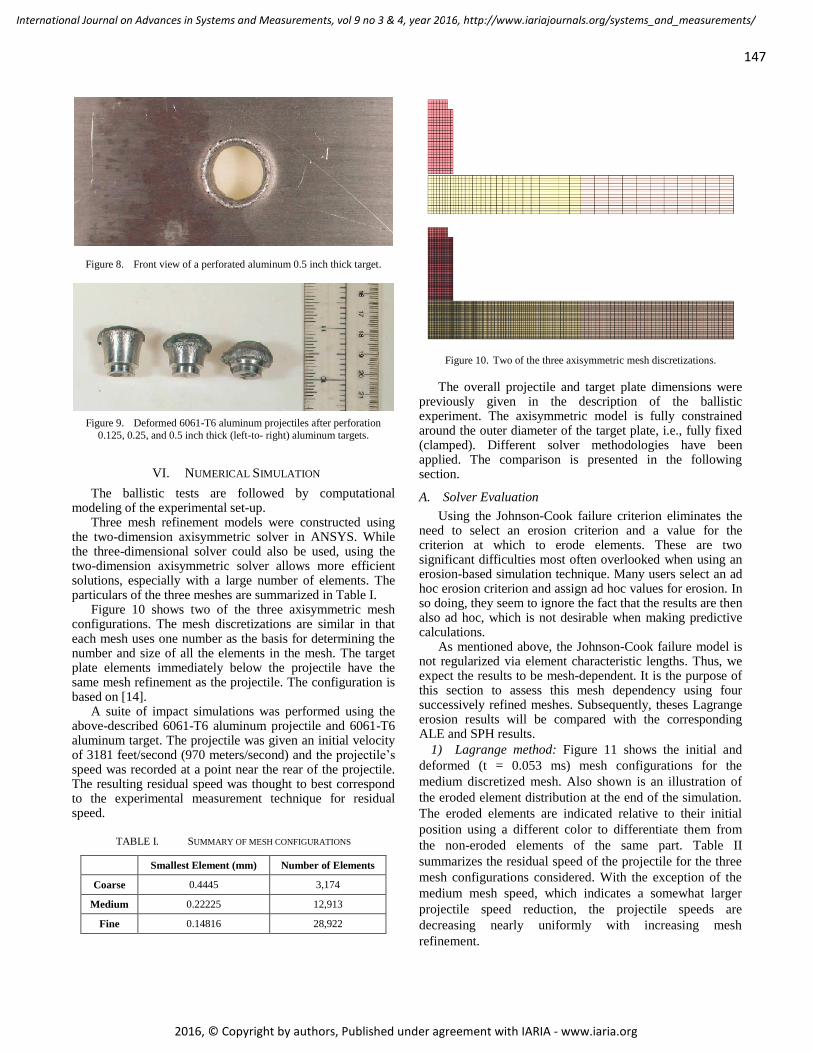
147



Figure 8. Front view of a perforated aluminum 0.5 inch thick target.

Figure 9. Deformed 6061-T6 aluminum projectiles after perforation

0.125, 0.25, and 0.5 inch thick (left-to- right) aluminum targets.

VI. NUMERICAL SIMULATION

The ballistic tests are followed by computational modeling of the experimental set-up.

Three mesh refinement models were constructed using the two-dimension axisymmetric solver in ANSYS. While the three-dimensional solver could also be used, using the two-dimension axisymmetric solver allows more efficient solutions, especially with a large number of elements. The particulars of the three meshes are summarized in Table I.

Figure 10 shows two of the three axisymmetric mesh configurations. The mesh discretizations are similar in that each mesh uses one number as the basis for determining the number and size of all the elements in the mesh. The target plate elements immediately below the projectile have the same mesh refinement as the projectile. The configuration is based on [14].

A suite of impact simulations was performed using the above-described 6061-T6 aluminum projectile and 6061-T6 aluminum target. The projectile was given an initial velocity of 3181 feet/second (970 meters/second) and the projectile’s speed was recorded at a point near the rear of the projectile. The resulting residual speed was thought to best correspond to the experimental measurement technique for residual speed.

TABLE I. SUMMARY OF MESH CONFIGURATIONS

Smallest Element (mm) Number of Elements

Coarse 0.4445 3,174

Medium 0.22225 12,913

Fine 0.14816 28,922

Figure 10. Two of the three axisymmetric mesh discretizations.

The overall projectile and target plate dimensions were previously given in the description of the ballistic experiment. The axisymmetric model is fully constrained around the outer diameter of the target plate, i.e., fully fixed (clamped). Different solver methodologies have been applied. The comparison is presented in the following section.

A. Solver Evaluation

Using the Johnson-Cook failure criterion eliminates the need to select an erosion criterion and a value for the criterion at which to erode elements. These are two significant difficulties most often overlooked when using an erosion-based simulation technique. Many users select an ad hoc erosion criterion and assign ad hoc values for erosion. In so doing, they seem to ignore the fact that the results are then also ad hoc, which is not desirable when making predictive calculations.

As mentioned above, the Johnson-Cook failure model is not regularized via element characteristic lengths. Thus, we expect the results to be mesh-dependent. It is the purpose of this section to assess this mesh dependency using four successively refined meshes. Subsequently, theses Lagrange erosion results will be compared with the corresponding ALE and SPH results.

1) Lagrange method: Figure 11 shows the initial and

deformed (t = 0.053 ms) mesh configurations for the

medium discretized mesh. Also shown is an illustration of

the eroded element distribution at the end of the simulation.

The eroded elements are indicated relative to their initial

position using a different color to differentiate them from

the non-eroded elements of the same part. Table II

summarizes the residual speed of the projectile for the three

mesh configurations considered. With the exception of the

medium mesh speed, which indicates a somewhat larger

projectile speed reduction, the projectile speeds are

decreasing nearly uniformly with increasing mesh

refinement.

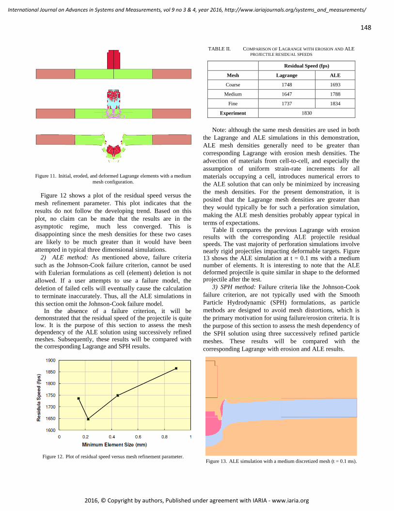
148



Figure 11. Initial, eroded, and deformed Lagrange elements with a medium

mesh configuration.

Figure 12 shows a plot of the residual speed versus the

mesh refinement parameter. This plot indicates that the

results do not follow the developing trend. Based on this

plot, no claim can be made that the results are in the

asymptotic regime, much less converged. This is

disappointing since the mesh densities for these two cases

are likely to be much greater than it would have been

attempted in typical three dimensional simulations.

2) ALE method: As mentioned above, failure criteria

such as the Johnson-Cook failure criterion, cannot be used

with Eulerian formulations as cell (element) deletion is not

allowed. If a user attempts to use a failure model, the

deletion of failed cells will eventually cause the calculation

to terminate inaccurately. Thus, all the ALE simulations in

this section omit the Johnson-Cook failure model. In the absence of a failure criterion, it will be

demonstrated that the residual speed of the projectile is quite low. It is the purpose of this section to assess the mesh dependency of the ALE solution using successively refined meshes. Subsequently, these results will be compared with the corresponding Lagrange and SPH results.

Figure 12. Plot of residual speed versus mesh refinement parameter.

TABLE II. COMPARISON OF LAGRANGE WITH EROSION AND ALE

PROJECTILE RESIDUAL SPEEDS

Residual Speed (fps)

Mesh Lagrange ALE

Coarse 1748 1693

Medium 1647 1788

Fine 1737 1834

Experiment 1830

Note: although the same mesh densities are used in both

the Lagrange and ALE simulations in this demonstration,

ALE mesh densities generally need to be greater than

corresponding Lagrange with erosion mesh densities. The

advection of materials from cell-to-cell, and especially the

assumption of uniform strain-rate increments for all

materials occupying a cell, introduces numerical errors to

the ALE solution that can only be minimized by increasing

the mesh densities. For the present demonstration, it is

posited that the Lagrange mesh densities are greater than

they would typically be for such a perforation simulation,

making the ALE mesh densities probably appear typical in

terms of expectations. Table II compares the previous Lagrange with erosion

results with the corresponding ALE projectile residual speeds. The vast majority of perforation simulations involve nearly rigid projectiles impacting deformable targets. Figure 13 shows the ALE simulation at t = 0.1 ms with a medium number of elements. It is interesting to note that the ALE deformed projectile is quite similar in shape to the deformed projectile after the test.

3) SPH method: Failure criteria like the Johnson-Cook

failure criterion, are not typically used with the Smooth

Particle Hydrodynamic (SPH) formulations, as particle

methods are designed to avoid mesh distortions, which is

the primary motivation for using failure/erosion criteria. It is

the purpose of this section to assess the mesh dependency of

the SPH solution using three successively refined particle

meshes. These results will be compared with the

corresponding Lagrange with erosion and ALE results.

Figure 13. ALE simulation with a medium discretized mesh (t = 0.1 ms).

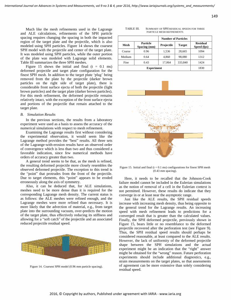
149



Much like the mesh refinements used in the Lagrange and ALE calculations, refinements of the SPH particle spacing requires changing the spacing in both the impacted region of the target plate and the projectile, which is also modeled using SPH particles. Figure 14 shows the coarsest SPH model with the projectile and center of the target plate. It was modeled using SPH particles, while the outer portion of the plate was modeled with Lagrange solid elements. Table III summarizes the three SPH meshes.

Figure 15 shows the initial and final (t = 0.1 ms) deformed projectile and target plate configuration for the finest SPH mesh. In addition to the target plate ‘plug’ being removed from the plate by the projectile (darker brown particles on the right side of target plate), there is considerable front surface ejecta of both the projectile (light brown particles) and the target plate (darker brown particles). For this mesh refinement, the deformed projectile remains relatively intact, with the exception of the front surface ejecta and portions of the projectile that remain attached to the target plate.

B. Simulation Results

In the previous sections, the results from a laboratory experiment were used as a basis to assess the accuracy of the numerical simulations with respect to mesh refinement.

Examining the Lagrange results first without considering the experimental observation, it would seem like the Lagrange method provides the “best” results. All three sets of the Lagrange-with-erosion results have an observed order of convergence which is less than two and thus considered a favorable indication, since few numerical methods have orders of accuracy greater than two.

A general trend seems to be that, as the mesh is refined, the resulting deformed projectile more closely resembles the observed deformed projectile. The exception to this trend is the “point” that protrudes from the front of the projectile. Due to target elements, this “point” appears to be eroded erroneously along the axis of symmetry.

Also, it can be deduced that, for ALE simulations, meshes need to be more dense than it is required for the corresponding Lagrange mesh density. The current status is as follows: the ALE meshes were refined enough, and the Lagrange meshes were more refined than necessary. It is more likely that the advection of material, e.g., from target plate into the surrounding vacuum, over-predicts the motion of the target plate, thus effectively reducing its stiffness and allowing for a “soft catch” of the projectile and an associated reduced projectile residual speed.

Figure 14. Coarsest SPH model (0.96 mm particle spacing).

TABLE III. SUMMARY OF SPH RESIDUAL SPEEDS FOR THREE

PARTICLE MESH REFINEMENTS

Number of Particles

Mesh Particle

Spacing (mm) Projectile Target

Residual

Speed (fps)

Coarse 0.96 1,536 28,665 1094

Medium 0.64 4,860 98,080 1312

Fine 0.43 17,064 333,840 1424

Experiment 1830

Figure 15. Initial and final (t = 0.1 ms) configurations for finest SPH mesh

(0.43 mm spacing).

Here, it needs to be recalled that the Johnson-Cook failure model cannot be included in the Eulerian simulations as the notion of removal of a cell in the Eulerian context is not permitted. However, these results do indicate that they converge in or at least near the asymptotic range.

Just like the ALE results, the SPH residual speeds increase with increasing mesh density, thus being opposite to the general trend for the Lagrange results. An increasing speed with mesh refinement leads to predictions for a converged result that is greater than the calculated values. Finally, the SPH deformed projectile, previously shown in Figure 15, bears little or no resemblance to the deformed projectile recovered after the perforation test (see Figure 9). Thus, the SPH residual speed results should perhaps be considered reasonable, at least compared to the ALE results. However, the lack of uniformity of the deformed projectile shape between the SPH simulations and the actual experiment might be an indication that the “right” answer might be obtained for the “wrong” reason. Future perforation experiments should include additional diagnostics, e.g., strain measurements on the target plates, so that assessments of agreement can be more extensive than solely considering residual speed.

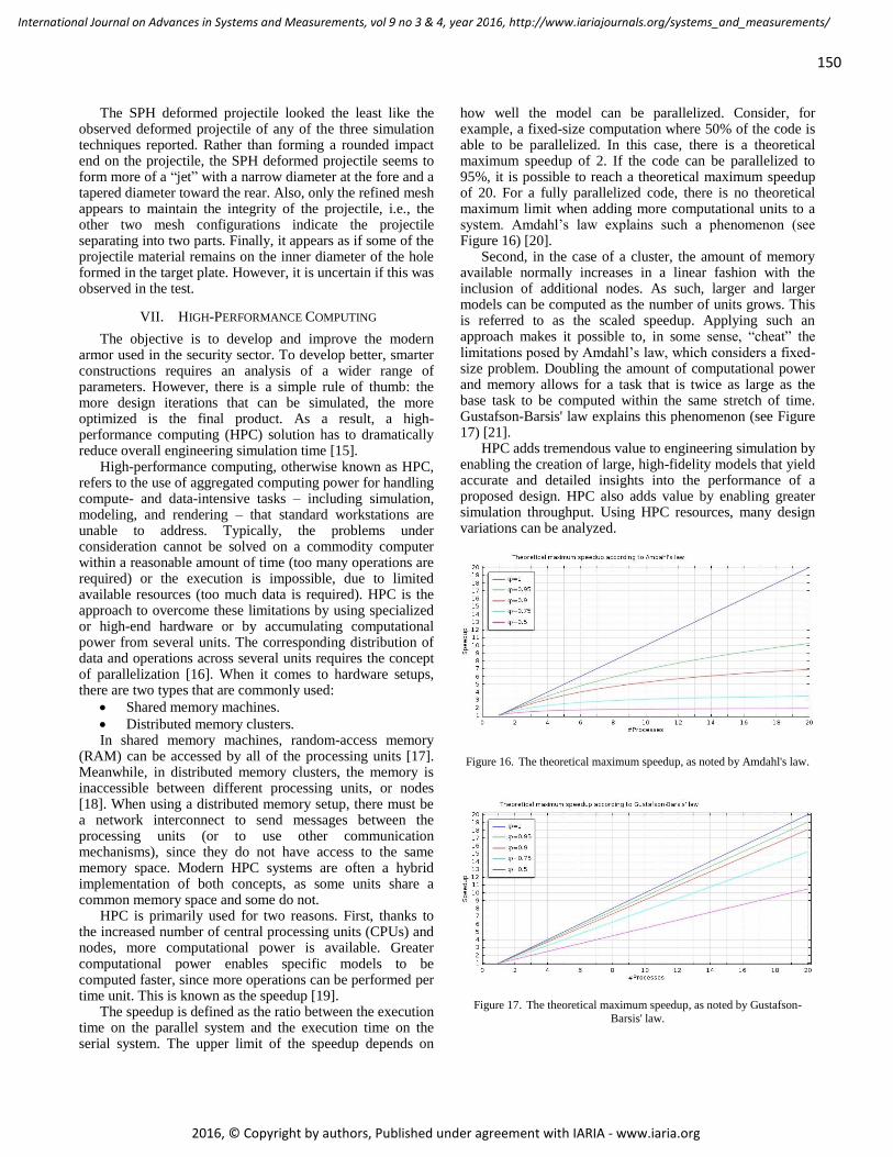
150



The SPH deformed projectile looked the least like the observed deformed projectile of any of the three simulation techniques reported. Rather than forming a rounded impact end on the projectile, the SPH deformed projectile seems to form more of a “jet” with a narrow diameter at the fore and a tapered diameter toward the rear. Also, only the refined mesh appears to maintain the integrity of the projectile, i.e., the other two mesh configurations indicate the projectile separating into two parts. Finally, it appears as if some of the projectile material remains on the inner diameter of the hole formed in the target plate. However, it is uncertain if this was observed in the test.

VII. HIGH-PERFORMANCE COMPUTING

The objective is to develop and improve the modern armor used in the security sector. To develop better, smarter constructions requires an analysis of a wider range of parameters. However, there is a simple rule of thumb: the more design iterations that can be simulated, the more optimized is the final product. As a result, a high-performance computing (HPC) solution has to dramatically reduce overall engineering simulation time [15].

High-performance computing, otherwise known as HPC, refers to the use of aggregated computing power for handling compute- and data-intensive tasks – including simulation, modeling, and rendering – that standard workstations are unable to address. Typically, the problems under consideration cannot be solved on a commodity computer within a reasonable amount of time (too many operations are required) or the execution is impossible, due to limited available resources (too much data is required). HPC is the approach to overcome these limitations by using specialized or high-end hardware or by accumulating computational power from several units. The corresponding distribution of data and operations across several units requires the concept of parallelization [16]. When it comes to hardware setups, there are two types that are commonly used:

Shared memory machines.

Distributed memory clusters. In shared memory machines, random-access memory

(RAM) can be accessed by all of the processing units [17]. Meanwhile, in distributed memory clusters, the memory is inaccessible between different processing units, or nodes [18]. When using a distributed memory setup, there must be a network interconnect to send messages between the processing units (or to use other communication mechanisms), since they do not have access to the same memory space. Modern HPC systems are often a hybrid implementation of both concepts, as some units share a common memory space and some do not.

HPC is primarily used for two reasons. First, thanks to the increased number of central processing units (CPUs) and nodes, more computational power is available. Greater computational power enables specific models to be computed faster, since more operations can be performed per time unit. This is known as the speedup [19].

The speedup is defined as the ratio between the execution time on the parallel system and the execution time on the serial system. The upper limit of the speedup depends on

how well the model can be parallelized. Consider, for example, a fixed-size computation where 50% of the code is able to be parallelized. In this case, there is a theoretical maximum speedup of 2. If the code can be parallelized to 95%, it is possible to reach a theoretical maximum speedup of 20. For a fully parallelized code, there is no theoretical maximum limit when adding more computational units to a system. Amdahl’s law explains such a phenomenon (see Figure 16) [20].

Second, in the case of a cluster, the amount of memory available normally increases in a linear fashion with the inclusion of additional nodes. As such, larger and larger models can be computed as the number of units grows. This is referred to as the scaled speedup. Applying such an approach makes it possible to, in some sense, “cheat” the limitations posed by Amdahl’s law, which considers a fixed-size problem. Doubling the amount of computational power and memory allows for a task that is twice as large as the base task to be computed within the same stretch of time. Gustafson-Barsis' law explains this phenomenon (see Figure 17) [21].

HPC adds tremendous value to engineering simulation by enabling the creation of large, high-fidelity models that yield accurate and detailed insights into the performance of a proposed design. HPC also adds value by enabling greater simulation throughput. Using HPC resources, many design variations can be analyzed.

Figure 16. The theoretical maximum speedup, as noted by Amdahl's law.

Figure 17. The theoretical maximum speedup, as noted by Gustafson-

Barsis' law.

151



In 1965, Gordon Moore made a prediction that would set the pace for our modern digital revolution. From careful observation of an emerging trend, Moore extrapolated that computing would dramatically increase in power, and decrease in relative cost, at an exponential pace [22]. Moore’s Law predicts that the number of transistors that can be economically placed on an integrated circuit will double about every two years. The insight, known as Moore’s Law, became the golden rule for the electronics industry, and a springboard for innovation.

Moore’s observation transformed computing from a rare and expensive venture into a pervasive and affordable necessity. All of the modern computing technology we know and enjoy sprang from the foundation laid by Moore’s Law. From the Internet itself, to social media and modern data analytics, all these innovations stem directly from Moore and his findings.

Performance and cost are two key drivers of technological development. As more transistors fit into smaller spaces, processing power increased and energy efficiency improved, all at a lower cost for the end user. This development not only enhanced existing industries and increased productivity, but it has spawned whole new industries empowered by cheap and powerful computing.

This research will evaluate the performance of the following server generations: HP ProLiant SL390s G7, HP ProLiant DL580 G7, and HP ProLiant DL380p G8.

Taking the influence of the software into account, different versions of ANSYS will be applied here. Regarding the Lagrange solver in a complex 3D multi-material simulation model (modern composite armor structure instead of 6061-T6 aluminum target), the following benchmark is obtained for the different simulations (see Table IV below).

The results indicate the importance of high-performance computing in combination with competitive simulation software to solve current problems of the computer-aided engineering sector.

VIII. CONCLUSION

This work focuses on the comparison of current simulation methodologies to find the most suitable model for high-speed dynamics and impact studies. The influence of meshing on the simulation results is pointed out based on an example. The benefits of high-performance computing are discussed in detail.

The reader is reminded that the ballistic simulation attempted in this work is among the most difficult as both the projectile and target experience significant deformation. The deformation of the projectile as it interacts with the target affects the deformation of the target, and vice versa.

TABLE IV. BENCHMARK TO ILLUSTRATE THE INFLUENCE OF

DIFFERENT SERVER AND SOFTWARE GENERATIONS

ANSYS 14.5 ANSYS 15.0

SL390s G7 27m31s 24m47s

DL580 G7 21m44s 19m51s

DL380p G8 19m16s 14m32s

The introduction of a failure criterion, such as the Johnson-Cook failure criterion, is clearly necessary for Lagrange models, and appears to also be necessary for SPH models. A better overall approach than on-off failure models, like the Johnson-Cook failure model, would be the use of continuum damage models. These models allow for the gradual reduction in strength of highly deformed materials and can be used in all three solution techniques.

Many modern computer-aided modeling, analysis, and manufacturing systems provide both interactive and automatic finite element mesh generation of surface and solid entities that describe the parts or products being virtually engineered as new designs. Unfortunately, for complex products, the interactive approach is too time consuming to factor into the design process and the quality of automatically created meshes often does not meet engineers’ criteria for element shape and density. Though commercial finite element analysis packages have some ability to control and direct the automatic mesh generation process, determining a correlation between these user controlled mesh parameters and acceptable quality of the generated mesh is difficult if not impossible. Since the validity of analysis results is heavily dependent upon mesh quality, obtaining better meshes in the shortest amount of time is essential for the integration of FEA into the automated design process.

The importance of mesh refinement has been emphasized in this work. This relatively simple to perform assessment of how the key results change with mesh density is all too often overlooked in computational solid mechanics. Further, establishing that the results are in the asymptotic regime provides some confidence that the mesh density is adequate.

When predictions are required, analysts want as many checks and assurances as possible that their results are credible. Mesh refinement studies provide the analyst some confidence the results are at a minimum not being affected by ad hoc choices of discretization.

A technique that is frequently employed in industry is that of modifying existing nodes and elements. Mesh smoothing routines have likewise long been an effective method of improving mesh quality in a pre-existing mesh. Many techniques are available for performing mesh smoothing. Some of the more advanced ones use gradient-based optimization techniques to quickly determine the optimal distribution of existing nodes. Others iterate using brute-force methods, such as Laplacian smoothing, to improve mesh distribution and corresponding element quality. Beyond this geometrical optimization of element shape, some schemes have been developed to modify and optimize the topology of the mesh by editing the node-adjacency structure of the mesh. Routines and optimizers include methods and operators such as edge swapping, vertex removing, edge collapsing, etc. to edit and improve the mesh topology. Special operators are required for maintaining a valid mesh in the case of quadrilateral and hexahedral meshes. Still other mesh improvement methods involve generating a new mesh based on information learned from previous attempts. Several algorithms use a posteriori

152



techniques to improve the mesh once regions of inaccuracy are located.

Although the above techniques have undoubtedly improved the quality of meshes available to the mesh researcher, the accessibility to such techniques within commercial FEA is still limited. It is a well-accepted fact that it takes software companies years to adopt and dispense new methods and techniques. Often the effectiveness of their implementation is called into question: smoothing algorithms, for example, are restricted by the node/element configuration of the starting mesh and may not be able to improve a mesh to meet the desired criteria. This paper proposes a strategy for generating an optimal mesh within the framework of existing FEA software. Rather than optimizing initial node placement or operations to be performed on existing elements, the mesh control parameters available in a commercial FEA package can be optimized to yield a high-quality mesh [23].

Meshing is considered to be one of the most difficult tasks of preprocessing in traditional FEA. In modern FEA packages, an initial mesh may be automatically altered, during the solution process in order to minimize or reduce the error in the numerical solution. This is referred to as adaptive meshing.

If creating the mesh is considered a difficult task, then selecting and setting the solvers and obtaining a solution to the equations (which constitute the numerical model) in a reasonable computational time is an even more difficult task. The difficulty is associated with a variety of challenges.

This work demonstrates how a small number of well-defined experiments can be used to develop, calibrate, and validate solver technologies used for simulating the impact of projectiles on armor systems.

New concepts and models can be developed and easily tested with the help of modern hydrocodes. The initial design approach of the units and systems has to be as safe and optimal as possible. Therefore, most design concepts are analyzed on the computer.

The gained experience is of prime importance for the development of modern armor. By applying the numerical model, a large number of potential armor schemes can be evaluated and the understanding of the interaction between different materials under ballistic impact can be improved.

The most important steps during an FE analysis are the evaluation and interpretation of the outcomes followed by suitable modifications of the model. For that reason, ballistic trials are necessary to validate the simulation results.

They are designed to obtain information about

the velocity and trajectory of the projectile prior to the impact,

changes in configuration of the projectile and target due to the impact,

masses, velocities, and trajectories of fragments generated by the impact process.

The combined use of computations, experiments and high-strain-rate material characterization has, in many cases, supplemented the data achievable by experiments alone at considerable savings in both cost and engineering manhours.

REFERENCES

[1] A. Ramezani and H. Rothe, “Simulation Methodologies for the Numerical Analysis of High-Speed Dynamics,” The Seventh International Conference on Advances in System Simulation (SIMUL 2015) IARIA, Nov. 2015, pp. 59-66, ISBN 978-1-61208-442-8

[2] J. Zukas, “Introduction to Hydrocodes,” Elsevier Science, February 2004.

[3] A. M. S. Hamouda and M. S. J. Hashmi, “Modelling the impact and penetration events of modern engineering materials: Characteristics of computer codes and material models,” Journal of Materials Processing Technology, vol. 56, Jan. 1996, pp. 847–862.

[4] D. J. Benson, “Computational methods in Lagrangian and Eulerian hydrocodes,” Computer Methods in Applied Mechanics and Engineering, vol. 99, Sep. 1992, pp. 235–394, doi: 10.1016/0045-7825(92)90042-I.

[5] M. Oevermann, S. Gerber, and F. Behrendt, “Euler-Lagrange/DEM simulation of wood gasification in a bubbling fluidized bed reactor,” Particuology, vol. 7, Aug. 2009, pp. 307-316, doi: 10.1016/j.partic.2009.04.004.

[6] D. L. Hicks and L. M. Liebrock, “SPH hydrocodes can be stabilized with shape-shifting,” Computers & Mathematics with Applications, vol. 38, Sep. 1999, pp. 1-16, doi: 10.1016/S0898-1221(99)00210-2.

[7] X. Quan, N. K. Birnbaum, M. S. Cowler, and B. I. Gerber, “Numerical Simulations of Structural Deformation under Shock and Impact Loads using a Coupled Multi-Solver Approach,” 5th Asia-Pacific Conference on Shock and Impact Loads on Structures, Hunan, China, Nov. 2003, pp. 152-161.

[8] N. V. Bermeo, M. G. Mendoza, and A. G. Castro, “Semantic Representation of CAD Models Based on the IGES Standard,” Computer Science, vol. 8265, Dec. 2001, pp. 157-168, doi: 10.1007/ 978-3-642-45114-0_13.

[9] G. S. Collins, “An Introduction to Hydrocode Modeling,” Applied Modelling and Computation Group, Imperial College London, August 2002, unpublished.

[10] R. F. Stellingwerf and C. A. Wingate, “Impact Modeling with Smooth Particle Hydrodynamics,” International Journal of Impact Engineering, vol. 14, Sep. 1993, pp. 707–718.

[11] ANSYS Inc. Available Solution Methods. [Online]. Available from: http://www.ansys.com/Products/Simulation+Technology/Structural+Analysis/Explicit+Dynamics/Features/Available+Solution+Methods [retrieved: August, 2015]

[12] P. Fröhlich, “FEM Application Basics,” Vieweg Verlag, September 2005.

[13] H. B. Woyand, “FEM with CATIA V5,” J. Schlembach Fachverlag, April 2007.

[14] L. E. Schwer, “Aluminum Plate Perforation: A Comparative Case Study using Lagrange with Erosion, Multi-Material ALE, and Smooth Particle Hydrodynamics,” 7th European LS-DYNA Conference, Salzburg, Austria, May. 2009.

[15] ANSYS Inc. “The Value of High-Performance Computing for Simulation,” [Online]. Available from: http://investors.ansys.com/~/media/Files/A/Ansys-IR/annual-reports/whitepapers/the-value-of-high-performance-computing-for-simulation.pdf [retrieved: November, 2016]

[16] G. S. Almasi, and G. Allan. “Highly parallel computing,” Benjamin-Cummings Publishing Co., Inc., 1988.

[17] H. El-Rewini, and A. Mostafa, “Advanced computer architecture and parallel processing,” Vol. 42, John Wiley & Sons, 2005.

[18] J. E. Savage, “Models of computation,” Exploring the Power of Computing, 1998.

153



[19] J. L. Hennessy, and D. A. Patterson, “Computer architecture: a quantitative approach,” Elsevier, 2011.

[20] G. M. Amdahl, “Validity of the single processor approach to achieving large scale computing capabilities,” Proceedings of the April 18-20, 1967, spring joint computer conference. ACM, 1967.

[21] J. L. Gustafson, “Reevaluating Amdahl's law,” Communications of the ACM 31.5: 532-533, 1988.

[22] G. E. Moore, “Cramming more components onto integrated circuits, Reprinted from Electronics, volume 38, number 8, April 19, 1965, pp. 114 ff.” IEEE Solid-State Circuits Newsletter 3.20:33-35, 2006.

[23] J. P. Dittmer, C. G. Jensen, M. Gottschalk, and T. Almy, “Mesh Optimization Using a Genetic Algorithm to Control Mesh Creation Parameters,” Computer-Aided Design & Applications, vol. 3, May 2006, pp. 731–740.

154



A Complete Automatic Test Set Generator for Embedded Reactive Systems: From

AUTSEG V1 to AUTSEG V2

Mariem Abdelmoula, Daniel Gaffe, and Michel Auguin

LEAT, University of Nice-Sophia Antipolis, CNRSEmail: [email protected]

Email: [email protected]: [email protected]

Abstract—One of the biggest challenges in hardware and softwaredesign is to ensure that a system is error-free. Small defectsin reactive embedded systems can have disastrous and costlyconsequences for a project. Preventing such errors by identifyingthe most probable cases of erratic system behavior is quite chal-lenging. Indeed, tests performed in industry are non-exhaustive,while state space analysis using formal verification in scientificresearch is inappropriate for large complex systems. We presentin this context a new approach for generating exhaustive testsets that combines the underlying principles of the industrialtesting technique with the academic-based formal verification.Our method consists in building a generic model of the systemunder test according to the synchronous approach. The goal is toidentify the optimal preconditions for restricting the state space ofthe model such that test generation can take place on significantsubspaces only. So, all the possible test sets are generated fromthe extracted subspace preconditions. Our approach exhibits asimpler and efficient quasi-flattening algorithm compared withexisting techniques, and a useful compiled internal descriptionto check security properties while minimizing the state spacecombinatorial explosion problem. It also provides a symbolicprocessing technique for numeric data that provides an expressiveand concrete test of the system, while improving system verifica-tion (Determinism, Death sequences) and identifying all possibletest cases. We have implemented our approach on a tool calledAUTSEG V2. This testing tool is an extension of the first versionAUTSEG V1 to integrate data manipulations. We present in thispaper a complete description of our automatic testing approachincluding all features presented in AUTSEG V1 and AUTSEGV2.

Keywords–AUTSEG; Quasi-flattening; SupLDD; Backtrack;Test Sets Generation.

I. INTRODUCTION

System verification generates great interest today, espe-cially for embedded reactive systems which have complex be-haviors over time and which require long test sequences. Thiskind of system is increasingly dominating safety-critical do-mains, such as the nuclear industry, health insurance, banking,the chemical industry, mining, avionics and online payment,where failure could be disastrous. Preventing such failure byidentifying the most probable cases of erratic system behavioris quite challenging. A practical solution in industry usesintensive test patterns in order to discover bugs, and increaseconfidence in the system, while researchers concentrate theirefforts instead on formal verification. However, testing is obvi-ously non-exhaustive and formal verification is impracticable

on real systems because of the combinatorial explosion natureof the state space.

AUTSEG V1 [2] combines these two approaches to providean automatic test set generator, where formal verificationensures automation in all phases of design, execution andtest evaluation and fosters confidence in the consistency andrelevance of the tests. In a first version of AUTSEG, onlyBoolean inputs and outputs were supported, while most ofactual systems handle numerical data. Numerical data ma-nipulation represents a big challenge for most of existingtest generation tools due to the difficulty to express formalproperties on those data using a concise representation. In ourapproach, we consider symbolic test sets which are therebymore expressive, safer and less complex than the concrete ones.

Therefore, we have developed a second version AUTSEGV2 [1] to take into account numerical data manipulation inaddition to Boolean data manipulation. This was achievedby developing a new library for data manipulation calledSupLDD. Prior automatic test set generation methods havebeen consequently extended and adapted to this new numer-ical context. Symbolic data manipulations in AUTSEG V2allow not only symbolic data calculations, but also systemverification (Determinism, Death sequences), and identificationof all possible test cases without requiring coverage of allsystem states and transitions. Hence, our approach bypassesin numerous cases the state space explosion problem.

We present in this paper a complete description of our auto-matic testing approach that includes all operations introducedin AUTSEG V1 and AUTSEG V2. In the remainder of thispaper, we give an overview of related work in Section II. Wepresent in Section III our global approach to test generation. Acase study is presented in Section IV. We show in Section Vexperimental results. Finally, we conclude the paper in SectionVI with some directions for future works.

II. RELATED WORK

Lutess V2 [3] is a test environment, written in Lustre, forsynchronous reactive systems. It automatically generates teststhat dynamically feed the program under test from the formaldescription of the program environment and properties. Thisversion of Lutess deals with numeric inputs and outputs unlikethe first version [4]. Lutess V2 is based on Constraint LogicProgramming (CLP) and allows the introduction of hypotheses

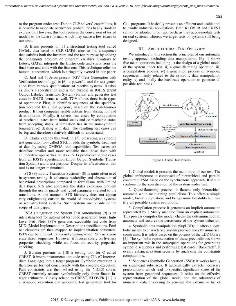
155



to the program under test. Due to CLP solvers’ capabilities, itis possible to associate occurrence probabilities to any Booleanexpression. However, this tool requires the conversion of testedmodels to the Lustre format, which may cause a few issues inour tests.

B. Blanc presents in [5] a structural testing tool calledGATeL, also based on CLP. GATeL aims to find a sequencethat satisfies both the invariant and the test purpose by solvingthe constraints problem on program variables. Contrary toLutess, GATeL interprets the Lustre code and starts from thefinal state and ends with the first one. This technique relies onhuman intervention, which is stringently averted in our paper.

C. Jard and T. Jeron present TGV (Test Generation withVerification technology) in [6], a powerful tool for test gener-ation from various specifications of reactive systems. It takesas inputs a specification and a test purpose in IOLTS (InputOutput Labeled Transition System) format and generates testcases in IOLTS format as well. TGV allows three basic typesof operations: First, it identifies sequences of the specifica-tion accepted by a test purpose, based on the synchronousproduct. It then computes visible actions from abstraction anddetermination. Finally, it selects test cases by computationof reachable states from initial states and co-reachable statesfrom accepting states. A limitation lies in the non-symbolic(enumerative) dealing with data. The resulting test cases canbe big and therefore relatively difficult to understand.

D. Clarke extends this work in [7], presenting a symbolictest generation tool called STG. It adds the symbolic treatmentof data by using OMEGA tool capabilities. Test cases aretherefore smaller and more readable than those done withenumerative approaches in TGV. STG produces the test casesfrom an IOSTS specification (Input Output Symbolic Transi-tion System) and a test purpose. Despite its effectiveness, thistool is no longer maintained.

STS (Symbolic Transition Systems) [8] is quite often usedin systems testing. It enhances readability and abstraction ofbehavioral descriptions compared to formalisms with limiteddata types. STS also addresses the states explosion problemthrough the use of guards and typed parameters related to thetransitions. At the moment, STS hierarchy does not appearvery enlightening outside the world of timed/hybrid systemsor well-structured systems. Such systems are outside of thescope of this paper.

ISTA (Integration and System Test Automation) [9] is aninteresting tool for automated test code generation from High-Level Petri Nets. ISTA generates executable test code fromMID (Model Implementation Description) specifications. Petrinet elements are then mapped to implementation constructs.ISTA can be efficient for security testing when Petri nets gen-erate threat sequences. However, it focuses solely on livenessproperties checking, while we focus on security propertieschecking.

J. Burnim presents in [10] a testing tool for C calledCREST. It inserts instrumentation code using CIL (C Interme-diate Language) into a target program. Symbolic execution istherefore performed concurrently with the concrete execution.Path constraints are then solved using the YICES solver.CREST currently reasons symbolically only about linear, in-teger arithmetic. Closely related to CREST, KLOVER [11] isa symbolic execution and automatic test generation tool for

C++ programs. It basically presents an efficient and usable toolto handle industrial applications. Both KLOVER and CRESTcannot be adopted in our approach, as they accommodate testson real systems, whereas we target tests on systems still beingdesigned.

III. ARCHITECTURAL TEST OVERVIEW

We introduce in this section the principles of our automatictesting approach including data manipulation. Fig. 1 showsfive main operations including: i) the design of a global modelof the system under test, ii) a quasi-flattening operation, iii)a compilation process, iv) a generation process of symbolicsequences mainly related to the symbolic data manipulationentity, v) and finally the backtrack operation to generate allpossible test cases.

Figure 1. Global Test Process.

1. Global model: it presents the main input of our test. Theglobal architecture is composed of hierarchical and parallelconcurrent FSM based on the synchronous approach. It shouldconform to the specification of the system under test.

2. Quasi-flattening process: it flattens only hierarchicalautomata while maintaining parallelism. This offers a simplemodel, faster compilation, and brings more flexibility to iden-tify all possible system evolutions.

3. Compilation process: it generates an implicit automatonrepresented by a Mealy machine from an explicit automaton.This process compiles the model, checks the determinism of allautomata and ensures the persistence of the system behavior.

4. Symbolic data manipulation (SupLDD): it offers a sym-bolic means to characterize system preconditions by numericalconstraints. It is solely based on the potency of the LDD library[4]. The symbolic representation of these preconditions showsan important role in the subsequent operations for generatingsymbolic sequences and performing test cases ”Backtrack”. Itevenly enhances system security by analyzing the constraintscomputations.

5. Sequences Symbolic Generation (SSG): it works locallyon significant subspaces. It automatically extracts necessarypreconditions which lead to specific, significant states of thesystem from generated sequences. It relies on the effectiverepresentation of the global model and the robustness ofnumerical data processing to generate the exhaustive list of

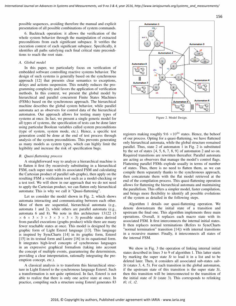
156



possible sequences, avoiding therefore the manual and explicitpresentation of all possible combinations of system commands.

6. Backtrack operation: it allows the verification of thewhole system behavior through the manipulation of extractedpreconditions from each significant subspace. It verifies theexecution context of each significant subspace. Specifically, itidentifies all paths satisfying each final critical state precondi-tions to reach the root state.

A. Global modelIn this paper, we particularly focus on verification of

embedded software controlling reactive systems behavior. Thedesign of such systems is generally based on the synchronousapproach [12] that presents clear semantics to exceptions,delays and actions suspension. This notably reduces the pro-gramming complexity and favors the application of verificationmethods. In this context, we present the global model byhierarchical and parallel concurrent Finite States Machines(FSMs) based on the synchronous approach. The hierarchicalmachine describes the global system behavior, while parallelautomata act as observers for control data of the hierarchicalautomaton. Our approach allows for testing many types ofsystems at once. In fact, we present a single generic model forall types of systems, the specification of tests can be done laterusing particular Boolean variables called system preconditions(type of system, system mode, etc.). Hence, a specific testgeneration could be done at the end of test process throughanalysis of the system preconditions. This prevents generatingas many models as system types, which can highly limit thelegibility and increase the risk of specification bugs.

B. Quasi-flattening processA straightforward way to analyze a hierarchical machine is

to flatten it first (by recursively substituting in a hierarchicalFSM, each super state with its associated FSM and calculatingthe Cartesian product of parallel sub-graphs), then apply on theresulting FSM a verification tool such as a model-checking ora test tool. We will show in our approach that we do not needto apply the Cartesian product, we can flatten only hierarchicalautomata: This is why we call it ”Quasi-flattening”.

Let us consider the model shown in Fig. 2, which showsautomata interacting and communicating between each other.Most of them are sequential, hierarchical automata (e.g.,automata 1 and 2), while others are parallel automata (e.g.,automata 6 and 8). We note in this architecture 13122 (3× 6 × 3 × 3 × 3 × 3 × 3 × 3) possible states derivedfrom parallel executions (graphs product) while there are manyfewer reachable states at once. This model is designed by thegraphic form of Light Esterel language [13]. This languageis inspired by SyncCharts [14] in its graphic form, Esterel[15] in its textual form and Lustre [16] in its equational form.It integrates high-level concepts of synchronous languagesin an expressive graphical formalism (taking into accountthe concept of multiple events, guaranteeing the determinism,providing a clear interpretation, rationally integrating the pre-emption concept, etc.).

A classical analysis is to transform this hierarchical struc-ture in Light Esterel to the synchronous language Esterel. Sucha transformation is not quite optimized. In fact, Esterel is notable to realize that there is only one active state at once. Inpractice, compiling such a structure using Esterel generates 83

Figure 2. Model Design.

registers making roughly 9.6 ×1024 states. Hence, the behoofof our process. Opting for a quasi-flattening, we have flattenedonly hierarchical automata, while the global structure remainedparallel. Thus, state 2 of automaton 1 in Fig. 2 is substitutedby the set of states {4, 5, 6, 7, 8, 9} of automaton 2 and so on.Required transitions are rewritten thereafter. Parallel automataare acting as observers that manage the model’s control flags.Flattening parallel FSMs explode usually in terms of numberof states. Thus, there is no need to flatten them, as we cancompile them separately thanks to the synchronous approach,then concatenate them with the flat model retrieved at theend of the compilation process. This quasi-flattening operationallows for flattening the hierarchical automata and maintainingthe parallelism. This offers a simpler model, faster compilation,and brings more flexibility to identify all possible evolutionsof the system as detailed in the following steps.

Algorithm 1 details our quasi-flattening operation. Wedenote downstream the initial state of a transition andupstream the final one. This algorithm implements three mainoperations. Overall, it replaces each macro state with itsassociated FSM. It first interconnects the internal initial states.It then replaces normal terminations (Refers to SyncCharts”normal termination” transition [14]) with internal transitionsin a recursive manner. Finally, it interconnects all states ofthe internal FSM.

We show in Fig. 3 the operation of linking internal initialstates described in lines 3 to 9 of algorithm 1. This latter startsby marking the super state St to load it in a list and to bedeleted later. Then, it considers all associated sub-states sub-St (states 3, 4, 5). For each transition in the global automaton,if the upstream state of this transition is the super state St,then this transition will be interconnected to the transition ofthe initial state of St (state 3). This corresponds to relinkingt0, t1, t2.

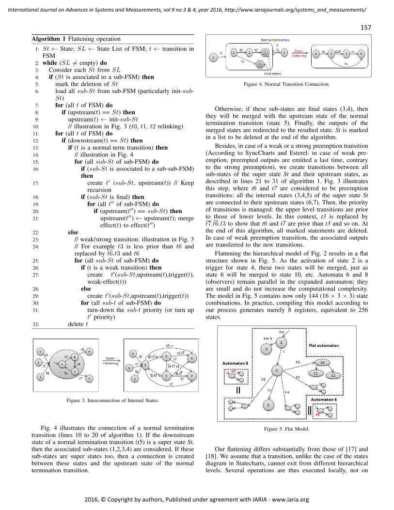
157



Algorithm 1 Flattening operation

1: St ← State; SL ← State List of FSM; t ← transition inFSM

2: while (SL 6= empty) do3: Consider each St from SL4: if (St is associated to a sub-FSM) then5: mark the deletion of St6: load all sub-St from sub-FSM (particularly init-sub-

St)7: for (all t of FSM) do8: if (upstream(t) == St) then9: upstream(t) ← init-sub-St

10: // illustration in Fig. 3 (t0, t1, t2 relinking)11: for (all t of FSM) do12: if (downstream(t) == St) then13: if (t is a normal-term transition) then14: // illustration in Fig. 415: for (all sub-St of sub-FSM) do16: if (sub-St is associated to a sub-sub-FSM)

then17: create t′ (sub-St, upstream(t)) // Keep

recursion18: if (sub-St is final) then19: for (all t′′ of sub-FSM) do20: if (upstream(t′′) == sub-St) then21: upstream(t′′) ← upstream(t); merge

effect(t) to effect(t′′)22: else23: // weak/strong transition: illustration in Fig. 324: // For example t3 is less prior than t6 and

replaced by t6.t3 and t625: for (all sub-St of sub-FSM) do26: if (t is a weak transition) then27: create t′(sub-St,upstream(t),trigger(t),

weak-effect(t))28: else29: create t′(sub-St,upstream(t),trigger(t))30: for (all sub-t of sub-FSM) do31: turn-down the sub-t priority (or turn up

t′ priority)32: delete t

Figure 3. Interconnection of Internal States.

Fig. 4 illustrates the connection of a normal terminationtransition (lines 10 to 20 of algorithm 1). If the downstreamstate of a normal termination transition (t5) is a super state St,then the associated sub-states (1,2,3,4) are considered. If thesesub-states are super states too, then a connection is createdbetween these states and the upstream state of the normaltermination transition.

Figure 4. Normal Transition Connection.

Otherwise, if these sub-states are final states (3,4), thenthey will be merged with the upstream state of the normaltermination transition (state 5). Finally, the outputs of themerged states are redirected to the resulted state. St is markedin a list to be deleted at the end of the algorithm.

Besides, in case of a weak or a strong preemption transition(According to SyncCharts and Esterel: in case of weak pre-emption, preempted outputs are emitted a last time, contraryto the strong preemption), we create transitions between allsub-states of the super state St and their upstream states, asdescribed in lines 21 to 31 of algorithm 1. Fig. 3 illustratesthis step, where t6 and t7 are considered to be preemptiontransitions: all the internal states (3,4,5) of the super state Stare connected to their upstream states (6,7). Then, the priorityof transitions is managed: the upper level transitions are priorto those of lower levels. In this context, t3 is replaced byt7.t6.t3 to show that t6 and t7 are prior than t3 and so on. Atthe end of this algorithm, all marked statements are deleted.In case of weak preemption transition, the associated outputsare transferred to the new transitions.

Flattening the hierarchical model of Fig. 2 results in a flatstructure shown in Fig. 5. As the activation of state 2 is atrigger for state 4, these two states will be merged, just asstate 6 will be merged to state 10, etc. Automata 6 and 8(observers) remain parallel in the expanded automaton; theyare small and do not increase the computational complexity.The model in Fig. 5 contains now only 144 (16 × 3 × 3) statecombinations. In practice, compiling this model according toour process generates merely 8 registers, equivalent to 256states.

Figure 5. Flat Model.

Our flattening differs substantially from those of [17] and[18]. We assume that a transition, unlike the case of the statesdiagram in Statecharts, cannot exit from different hierarchicallevels. Several operations are thus executed locally, not on

158



the global system. This yields a simpler algorithm and fastercompilation. To this end, we have integrated the followingassumptions in our algorithm:-Normal termination. Fig. 4 shows an example of normaltermination carried when a final internal state is reached. Itallows a unique possible interpretation and facilitates codegeneration.-Strong preemption. Unlike the weak preemption, internaloutputs of the preempted state are lost during the transition.

C. Compilation process

We proceed in our approach to a symbolic compilation ofthe global model into Mealy machines, implicitly representedby a set of Boolean equations (circuit of logic gates andregisters presenting the state of the system). In fact, the flatautomata and concurrent automata are compiled separately.Compilation results of these automata are concatenated atthe end of this process. They are represented by a union ofsorted equations rather than a Cartesian product of graphs tosupport the synchronous parallel operation and instantaneousdiffusion of signals as required by the synchronous approach.Accordingly, the system model is substantially reduced. Ourcompilation requires only log2(nbstates) registers, while clas-sical works uses one register per state [19]. It also allowschecking the determinism of all automata, which ensures thepersistence of the system behavior.

Algorithm 2 describes the compilation process in details.First, it counts the number of states in the automaton anddeduces the size of the states vector. Then, it develops thefunction of the next state for a given state variable. Finally,the generated vector is characterized by a set of Booleanexpressions. It is represented by a set of BDDs.

Let us consider an automaton with 16 states as an exam-ple. The vector characterizing the next state is created by 4(log2(16)) expressions derived from inputs data and the currentstate. For each transition from state ”k” to state ”l”, two typesof vectors encoded by n (n = 4 bits in this example) bitsare created: Vk vector specifying the characteristic function oftransition BDDcond, and Vl vector characterizing the functionof the future state BDD−NextState. If Vk(i) is valued to 1,then the state variable yi is considered positively. Otherwise,yi is reversed (lines 18-22). In this context, the BDD charac-terizing the transition condition is deduced by the combinationof ”yi” and the condition ”cond” on transition. For instance,BDDcond = y0 × y1 × y2 × y3 × cond for Vk = (1, 0, 0, 1).

We show in lines (23-27) the construction of the NextState function BDD − NextState(i) = BDDy(i)+ ×notBDDy(i)′+ . BDDy(i)+ characterizes all transitions thatturns y+i to 1 (Set registers to 1). Conversely, BDDy(i)′+

characterizes all transitions that turns y+i to 0 (Reset registersto 0). So, each function satisfying y+ and not (y

′+) isa possible solution. In this case, parsing all states of thesystem is not necessary. Fig. 6 shows an example restrictedto only 2 states variables where it is possible to find anappropriate function ”BDD+

y1 respect = y0.x + y0.x” fory+1 and ”BDD+

y0 respect = y0.x + y1.y0.x” for y+0 evenif the system state is not specified for ”y1y0 = 11”.Thus,BDD − NextState (BDDy(i)+) is specified by the twoBDDrespect looking for the simplest expressions to check

on one hand y+0 and not(y′+0 ) and on the other hand y+1 and

not(y′+1 ).

Algorithm 2 Compilation process

1: R ← Vector of states2: R-I ← Initial vector of states (initial value of registers)3: Next-State ← Vector of transitions4: N ← Size of R and Next-State5: f,f’ ← Vectors of Boolean functions6: N ← log2 (Statesnumber − 1)+ 17: Define N registers encapsulated in R.8: for (i=0 to N − 1) do9: BDDf(i) ← BDD-0 // BDD initialisation

10: BDDf ′(i) ← BDD-011: for (j=0 to Noutputs− 1) do12: OutputO(j) ← BDD-013: R-I ← binary coding of initial state14: for (transition tkl=k to l) do15: Vk ← Binary coding of k16: Vl ← Binary coding of l17: BDDcond ← cond (tkl);18: for (i=0 to N − 1) do19: if Vk(i)==1 then20: BDDcond ← BDDand(R(i), BDDcond ) //

BDDcond: tkl BDD characteristics21: else22: BDDcond ← BDDand(BDDnot (R(i)),

BDDcond)23: if (Vl(i)==1) then24: BDDf(i) ← BDDor(BDDf(i), BDDcond )//

BDDf(i): set of register25: else26: BDDf ′(i) ← BDDor(BDDf ′(i), BDDcond))//

BDDf ′(i): reset of register27: outputO(output(tkl))← BDDor

(outputO(output(tkl)), BDDcond)28: for (i=0 to N − 1) do29: BDD-NextState(i)← BDDrespect (BDDf , BDD′

f )30: // respect: every BDDh such us BDDf → BDDh

AND BDDh → not(BDD′f )

Figure 6. Next State Function.

As we handle automata with numerical and Boolean vari-ables, each data inequation was first replaced by a Booleanvariable (abstraction). Then at the end of the compilationprocess, data were re-injected to be processed by SupLDDlater.

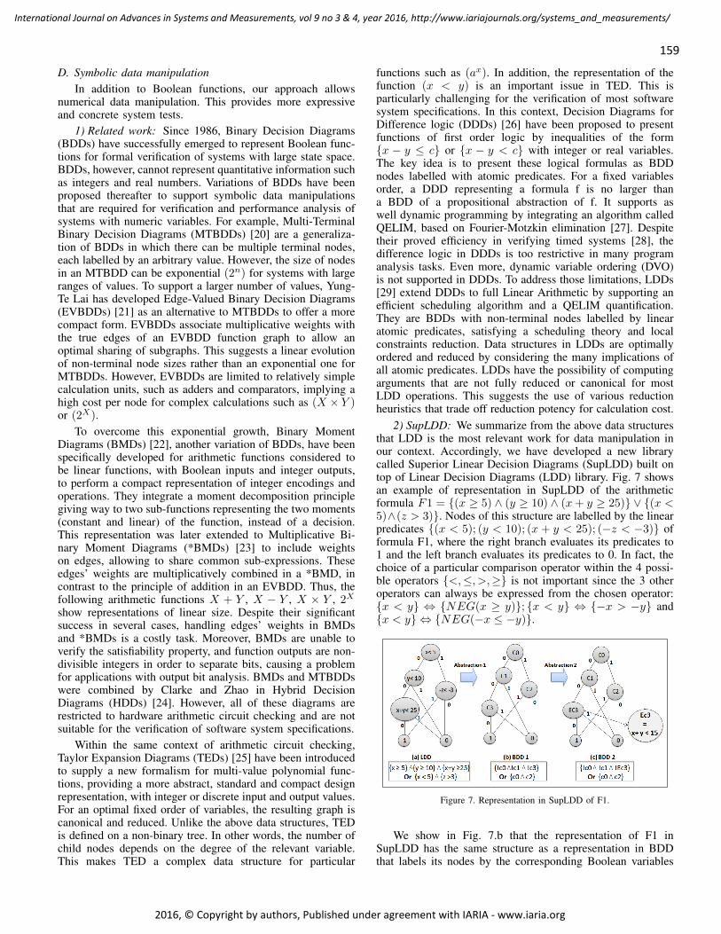
159



D. Symbolic data manipulationIn addition to Boolean functions, our approach allows

numerical data manipulation. This provides more expressiveand concrete system tests.

1) Related work: Since 1986, Binary Decision Diagrams(BDDs) have successfully emerged to represent Boolean func-tions for formal verification of systems with large state space.BDDs, however, cannot represent quantitative information suchas integers and real numbers. Variations of BDDs have beenproposed thereafter to support symbolic data manipulationsthat are required for verification and performance analysis ofsystems with numeric variables. For example, Multi-TerminalBinary Decision Diagrams (MTBDDs) [20] are a generaliza-tion of BDDs in which there can be multiple terminal nodes,each labelled by an arbitrary value. However, the size of nodesin an MTBDD can be exponential (2n) for systems with largeranges of values. To support a larger number of values, Yung-Te Lai has developed Edge-Valued Binary Decision Diagrams(EVBDDs) [21] as an alternative to MTBDDs to offer a morecompact form. EVBDDs associate multiplicative weights withthe true edges of an EVBDD function graph to allow anoptimal sharing of subgraphs. This suggests a linear evolutionof non-terminal node sizes rather than an exponential one forMTBDDs. However, EVBDDs are limited to relatively simplecalculation units, such as adders and comparators, implying ahigh cost per node for complex calculations such as (X × Y )or (2X).

To overcome this exponential growth, Binary MomentDiagrams (BMDs) [22], another variation of BDDs, have beenspecifically developed for arithmetic functions considered tobe linear functions, with Boolean inputs and integer outputs,to perform a compact representation of integer encodings andoperations. They integrate a moment decomposition principlegiving way to two sub-functions representing the two moments(constant and linear) of the function, instead of a decision.This representation was later extended to Multiplicative Bi-nary Moment Diagrams (*BMDs) [23] to include weightson edges, allowing to share common sub-expressions. Theseedges’ weights are multiplicatively combined in a *BMD, incontrast to the principle of addition in an EVBDD. Thus, thefollowing arithmetic functions X + Y , X − Y , X × Y , 2X

show representations of linear size. Despite their significantsuccess in several cases, handling edges’ weights in BMDsand *BMDs is a costly task. Moreover, BMDs are unable toverify the satisfiability property, and function outputs are non-divisible integers in order to separate bits, causing a problemfor applications with output bit analysis. BMDs and MTBDDswere combined by Clarke and Zhao in Hybrid DecisionDiagrams (HDDs) [24]. However, all of these diagrams arerestricted to hardware arithmetic circuit checking and are notsuitable for the verification of software system specifications.

Within the same context of arithmetic circuit checking,Taylor Expansion Diagrams (TEDs) [25] have been introducedto supply a new formalism for multi-value polynomial func-tions, providing a more abstract, standard and compact designrepresentation, with integer or discrete input and output values.For an optimal fixed order of variables, the resulting graph iscanonical and reduced. Unlike the above data structures, TEDis defined on a non-binary tree. In other words, the number ofchild nodes depends on the degree of the relevant variable.This makes TED a complex data structure for particular

functions such as (ax). In addition, the representation of thefunction (x < y) is an important issue in TED. This isparticularly challenging for the verification of most softwaresystem specifications. In this context, Decision Diagrams forDifference logic (DDDs) [26] have been proposed to presentfunctions of first order logic by inequalities of the form{x − y ≤ c} or {x − y < c} with integer or real variables.The key idea is to present these logical formulas as BDDnodes labelled with atomic predicates. For a fixed variablesorder, a DDD representing a formula f is no larger thana BDD of a propositional abstraction of f. It supports aswell dynamic programming by integrating an algorithm calledQELIM, based on Fourier-Motzkin elimination [27]. Despitetheir proved efficiency in verifying timed systems [28], thedifference logic in DDDs is too restrictive in many programanalysis tasks. Even more, dynamic variable ordering (DVO)is not supported in DDDs. To address those limitations, LDDs[29] extend DDDs to full Linear Arithmetic by supporting anefficient scheduling algorithm and a QELIM quantification.They are BDDs with non-terminal nodes labelled by linearatomic predicates, satisfying a scheduling theory and localconstraints reduction. Data structures in LDDs are optimallyordered and reduced by considering the many implications ofall atomic predicates. LDDs have the possibility of computingarguments that are not fully reduced or canonical for mostLDD operations. This suggests the use of various reductionheuristics that trade off reduction potency for calculation cost.

2) SupLDD: We summarize from the above data structuresthat LDD is the most relevant work for data manipulation inour context. Accordingly, we have developed a new librarycalled Superior Linear Decision Diagrams (SupLDD) built ontop of Linear Decision Diagrams (LDD) library. Fig. 7 showsan example of representation in SupLDD of the arithmeticformula F1 = {(x ≥ 5) ∧ (y ≥ 10) ∧ (x + y ≥ 25)} ∨ {(x <5)∧(z > 3)}. Nodes of this structure are labelled by the linearpredicates {(x < 5); (y < 10); (x + y < 25); (−z < −3)} offormula F1, where the right branch evaluates its predicates to1 and the left branch evaluates its predicates to 0. In fact, thechoice of a particular comparison operator within the 4 possi-ble operators {<,≤, >,≥} is not important since the 3 otheroperators can always be expressed from the chosen operator:{x < y} ⇔ {NEG(x ≥ y)}; {x < y} ⇔ {−x > −y} and{x < y} ⇔ {NEG(−x ≤ −y)}.

Figure 7. Representation in SupLDD of F1.

We show in Fig. 7.b that the representation of F1 inSupLDD has the same structure as a representation in BDDthat labels its nodes by the corresponding Boolean variables

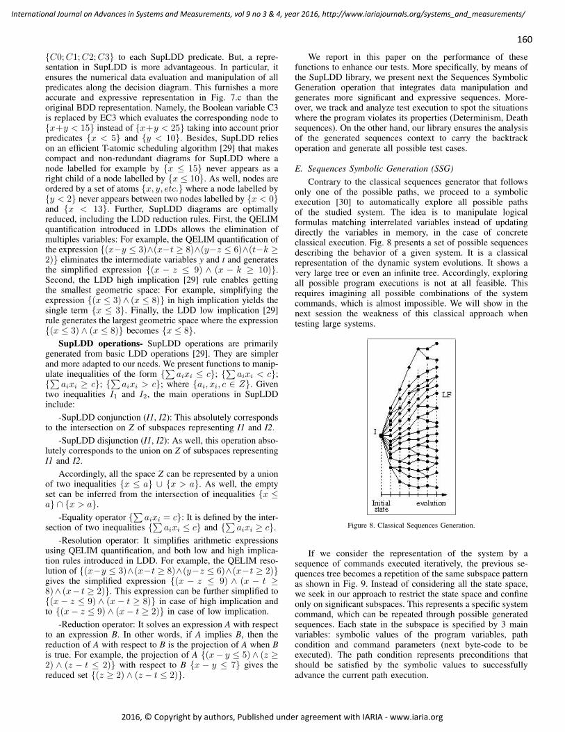
160



{C0;C1;C2;C3} to each SupLDD predicate. But, a repre-sentation in SupLDD is more advantageous. In particular, itensures the numerical data evaluation and manipulation of allpredicates along the decision diagram. This furnishes a moreaccurate and expressive representation in Fig. 7.c than theoriginal BDD representation. Namely, the Boolean variable C3is replaced by EC3 which evaluates the corresponding node to{x+y < 15} instead of {x+y < 25} taking into account priorpredicates {x < 5} and {y < 10}. Besides, SupLDD relieson an efficient T-atomic scheduling algorithm [29] that makescompact and non-redundant diagrams for SupLDD where anode labelled for example by {x ≤ 15} never appears as aright child of a node labelled by {x ≤ 10}. As well, nodes areordered by a set of atoms {x, y, etc.} where a node labelled by{y < 2} never appears between two nodes labelled by {x < 0}and {x < 13}. Further, SupLDD diagrams are optimallyreduced, including the LDD reduction rules. First, the QELIMquantification introduced in LDDs allows the elimination ofmultiples variables: For example, the QELIM quantification ofthe expression {(x−y ≤ 3)∧(x−t ≥ 8)∧(y−z ≤ 6)∧(t−k ≥2)} eliminates the intermediate variables y and t and generatesthe simplified expression {(x − z ≤ 9) ∧ (x − k ≥ 10)}.Second, the LDD high implication [29] rule enables gettingthe smallest geometric space: For example, simplifying theexpression {(x ≤ 3)∧ (x ≤ 8)} in high implication yields thesingle term {x ≤ 3}. Finally, the LDD low implication [29]rule generates the largest geometric space where the expression{(x ≤ 3) ∧ (x ≤ 8)} becomes {x ≤ 8}.

SupLDD operations- SupLDD operations are primarilygenerated from basic LDD operations [29]. They are simplerand more adapted to our needs. We present functions to manip-ulate inequalities of the form {

∑aixi ≤ c}; {

∑aixi < c};

{∑

aixi ≥ c}; {∑

aixi > c}; where {ai, xi, c ∈ Z}. Giventwo inequalities I1 and I2, the main operations in SupLDDinclude:

-SupLDD conjunction (I1, I2): This absolutely correspondsto the intersection on Z of subspaces representing I1 and I2.

-SupLDD disjunction (I1, I2): As well, this operation abso-lutely corresponds to the union on Z of subspaces representingI1 and I2.

Accordingly, all the space Z can be represented by a unionof two inequalities {x ≤ a} ∪ {x > a}. As well, the emptyset can be inferred from the intersection of inequalities {x ≤a} ∩ {x > a}.

-Equality operator {∑

aixi = c}: It is defined by the inter-section of two inequalities {

∑aixi ≤ c} and {

∑aixi ≥ c}.

-Resolution operator: It simplifies arithmetic expressionsusing QELIM quantification, and both low and high implica-tion rules introduced in LDD. For example, the QELIM reso-lution of {(x−y ≤ 3)∧(x−t ≥ 8)∧(y−z ≤ 6)∧(x−t ≥ 2)}gives the simplified expression {(x − z ≤ 9) ∧ (x − t ≥8)∧ (x− t ≥ 2)}. This expression can be further simplified to{(x − z ≤ 9) ∧ (x − t ≥ 8)} in case of high implication andto {(x− z ≤ 9) ∧ (x− t ≥ 2)} in case of low implication.

-Reduction operator: It solves an expression A with respectto an expression B. In other words, if A implies B, then thereduction of A with respect to B is the projection of A when Bis true. For example, the projection of A {(x− y ≤ 5) ∧ (z ≥2) ∧ (z − t ≤ 2)} with respect to B {x − y ≤ 7} gives thereduced set {(z ≥ 2) ∧ (z − t ≤ 2)}.

We report in this paper on the performance of thesefunctions to enhance our tests. More specifically, by means ofthe SupLDD library, we present next the Sequences SymbolicGeneration operation that integrates data manipulation andgenerates more significant and expressive sequences. More-over, we track and analyze test execution to spot the situationswhere the program violates its properties (Determinism, Deathsequences). On the other hand, our library ensures the analysisof the generated sequences context to carry the backtrackoperation and generate all possible test cases.

E. Sequences Symbolic Generation (SSG)Contrary to the classical sequences generator that follows

only one of the possible paths, we proceed to a symbolicexecution [30] to automatically explore all possible pathsof the studied system. The idea is to manipulate logicalformulas matching interrelated variables instead of updatingdirectly the variables in memory, in the case of concreteclassical execution. Fig. 8 presents a set of possible sequencesdescribing the behavior of a given system. It is a classicalrepresentation of the dynamic system evolutions. It shows avery large tree or even an infinite tree. Accordingly, exploringall possible program executions is not at all feasible. Thisrequires imagining all possible combinations of the systemcommands, which is almost impossible. We will show in thenext session the weakness of this classical approach whentesting large systems.

Figure 8. Classical Sequences Generation.

If we consider the representation of the system by asequence of commands executed iteratively, the previous se-quences tree becomes a repetition of the same subspace patternas shown in Fig. 9. Instead of considering all the state space,we seek in our approach to restrict the state space and confineonly on significant subspaces. This represents a specific systemcommand, which can be repeated through possible generatedsequences. Each state in the subspace is specified by 3 mainvariables: symbolic values of the program variables, pathcondition and command parameters (next byte-code to beexecuted). The path condition represents preconditions thatshould be satisfied by the symbolic values to successfullyadvance the current path execution.

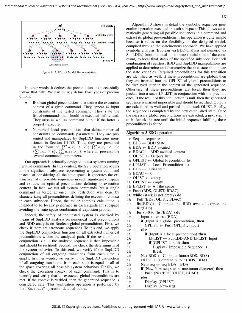
161



Figure 9. AUTSEG Model Representation.

In other words, it defines the preconditions to successfullyfollow that path. We particularly define two types of precon-ditions:

• Boolean global preconditions that define the executioncontext of a given command. They appear as inputconstraints of the tested command. They state thelist of commands that should be executed beforehand.They arise as well as command output if the latter isproperly executed.

• Numerical local preconditions that define numericalconstraints on commands parameters. They are pre-sented and manipulated by SupLDD functions men-tioned in Section III-D2. Thus, they are presentedin the form of {

∑aixi ≤ c}; {

∑aixi < c};

{∑

aixi ≥ c}; {∑

aixi > c}; where xi presents theseveral commands parameters.

Our approach is primarily designed to test systems runningiterative commands. In this context, the SSG operation occursin the significant subspace representing a system commandinstead of considering all the state space. It generates the ex-haustive list of possible sequences in each significant subspaceand extracts the optimal preconditions defining its executioncontext. In fact, we test all system commands, but a singlecommand is tested at once. The restriction was done bycharacterizing all preconditions defining the execution contextin each subspace. Hence, the major complex calculation isintended to be locally performed in each significant subspaceavoiding the state space combinatorial explosion problem.

Indeed, the safety of the tested system is checked bymeans of SupLDD analysis on numerical local preconditionsand BDD analysis on Boolean global preconditions. First, wecheck if there are erroneous sequences. To this end, we applythe SupLDD conjunction function on all extracted numericalpreconditions within the analyzed path. If the result of thisconjunction is null, the analyzed sequence is then impossibleand should be rectified! Second, we check the determinism ofthe system behavior. To this end, we verify if the SupLDDconjunction of all outgoing transitions from each state isempty. In other words, we verify if the SupLDD disjunctionof all outgoing transitions from each state is equal to all ofthe space covering all possible system behaviors. Finally, wecheck the execution context of each command. This is toidentify and verify that all extracted global preconditions aremet. If the context is verified, then the generated sequence isconsidered safe. This verification operation is performed bythe ”Backtrack” operation detailed below.

Algorithm 3 shows in detail the symbolic sequences gen-eration operation executed in each subspace. This allows auto-matically generating all possible sequences in a command andextract its global pre-conditions. This operation is quite simplebecause it relies on the flexibility of the designed model,compiled through the synchronous approach. We have appliedsymbolic analysis (Boolean via BDD-analysis and numeric viaSupLDDs) from the local initial state (initial state of the com-mand) to local final states of the specified subspace. For eachcombination of registers, BDD and SupLDD manipulations areapplied to determine and characterize the next state and updatethe state variables. Required preconditions for this transitionare identified as well. If these preconditions are global, thenthey are inserted into the GPLIST of global preconditions tobe displayed later in the context of the generated sequence.Otherwise, if these preconditions are local, then they arepushed into a stack LPLIST, in conjunction with the previousones. If the result of this conjunction is null, then the generatedsequence is marked impossible and should be rectified. Outputsare calculated as well and pushed into a stack OLIST. Finally,the sequence is completed by the new established state. Oncethe necessary global preconditions are extracted, a next step isto backtrack the tree until the initial sequence fulfilling thesepreconditions is found.

Algorithm 3 SSG operation

1: Seq ← sequence2: BDS ← BDD State3: BDA ← BDD awaited4: BDAC ← BDD awaited context5: OLIST ← Outputs list6: GPLIST ← Global Precondition list7: LPLIST ← Local Precondition list8: BDS ← Initial state9: BDAC ← 0

10: OLIST ← empty11: GPLIST ← empty12: LPLIST ← All the space13: Push (BDS, OLIST, BDAC)14: while (stack is not empty) do15: Pull (BDS, OLIST, BDAC)16: list(BDA)← Compute the BDD awaited expressions

list(BDS)17: for (i=0 to |list(BDA)|) do18: Input ← extract(BDA)19: if (Input is a global precondition) then20: GPLIST ← Push(GPLIST, Input)21: else22: if (Input is a local precondition) then23: LPLIST ← SupLDD-AND(LPLIST, Input)24: if (GPLIST is null) then25: Display ( Impossible Sequence !)26: Break27: NextBDS ← Compute future(BDS, BDA)28: OLIST ← Compute output (BDS, BDA)29: New-seq ← seq BDA | BDA30: if (New New-seq size < maximum diameter) then31: Push (NextBDS, OLIST, BDAC)32: else33: Display (GPLIST)34: Display (New-seq)

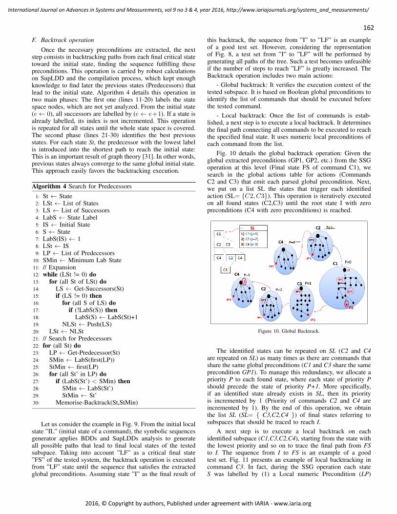
162



F. Backtrack operation

Once the necessary preconditions are extracted, the nextstep consists in backtracking paths from each final critical statetoward the initial state, finding the sequence fulfilling thesepreconditions. This operation is carried by robust calculationson SupLDD and the compilation process, which kept enoughknowledge to find later the previous states (Predecessors) thatlead to the initial state. Algorithm 4 details this operation intwo main phases: The first one (lines 11-20) labels the statespace nodes, which are not yet analyzed. From the initial state(e← 0), all successors are labelled by (e← e+1). If a state isalready labelled, its index is not incremented. This operationis repeated for all states until the whole state space is covered.The second phase (lines 21-30) identifies the best previousstates. For each state St, the predecessor with the lowest labelis introduced into the shortest path to reach the initial state:This is an important result of graph theory [31]. In other words,previous states always converge to the same global initial state.This approach easily favors the backtracking execution.

Algorithm 4 Search for Predecessors

1: St ← State2: LSt ← List of States3: LS ← List of Successors4: LabS ← State Label5: IS ← Initial State6: S ← State7: LabS(IS) ← 18: LSt ← IS9: LP ← List of Predecessors

10: SMin ← Minimum Lab State11: // Expansion12: while (LSt != 0) do13: for (all St of LSt) do14: LS ← Get-Successors(St)15: if (LS != 0) then16: for (all S of LS) do17: if (!LabS(S)) then18: LabS(S) ← LabS(St)+119: NLSt ← Push(LS)20: LSt ← NLSt21: // Search for Predecessors22: for (all St) do23: LP ← Get-Predecessor(St)24: SMin ← LabS(first(LP))25: StMin ← first(LP)26: for (all St’ in LP) do27: if (LabS(St’) < SMin) then28: SMin ← LabS(St’)29: StMin ← St’30: Memorise-Backtrack(St,StMin)

Let us consider the example in Fig. 9. From the initial localstate ”IL” (initial state of a command), the symbolic sequencesgenerator applies BDDs and SupLDDs analysis to generateall possible paths that lead to final local states of the testedsubspace. Taking into account ”LF” as a critical final state”FS” of the tested system, the backtrack operation is executedfrom ”LF” state until the sequence that satisfies the extractedglobal preconditions. Assuming state ”I” as the final result of

this backtrack, the sequence from ”I” to ”LF” is an exampleof a good test set. However, considering the representationof Fig. 8, a test set from ”I” to ”LF” will be performed bygenerating all paths of the tree. Such a test becomes unfeasibleif the number of steps to reach ”LF” is greatly increased. TheBacktrack operation includes two main actions:

- Global backtrack: It verifies the execution context of thetested subspace. It is based on Boolean global preconditions toidentify the list of commands that should be executed beforethe tested command.

- Local backtrack: Once the list of commands is estab-lished, a next step is to execute a local backtrack. It determinesthe final path connecting all commands to be executed to reachthe specified final state. It uses numeric local preconditions ofeach command from the list.

Fig. 10 details the global backtrack operation: Given theglobal extracted preconditions (GP1, GP2, etc.) from the SSGoperation at this level (Final state FS of command C1), wesearch in the global actions table for actions (CommandsC2 and C3) that emit each parsed global precondition. Next,we put on a list SL the states that trigger each identifiedaction (SL= {C2, C3}). This operation is iteratively executedon all found states (C2,C3) until the root state I with zeropreconditions (C4 with zero preconditions) is reached.

Figure 10. Global Backtrack.

The identified states can be repeated on SL (C2 and C4are repeated on SL) as many times as there are commands thatshare the same global preconditions (C1 and C3 share the sameprecondition GP1). To manage this redundancy, we allocate apriority P to each found state, where each state of priority Pshould precede the state of priority P+1. More specifically,if an identified state already exists in SL, then its priorityis incremented by 1 (Priority of commands C2 and C4 areincremented by 1). By the end of this operation, we obtainthe list SL (SL= { C3,C2,C4 }) of final states referring tosubspaces that should be traced to reach I.

A next step is to execute a local backtrack on eachidentified subspace (C1,C3,C2,C4), starting from the state withthe lowest priority and so on to trace the final path from FSto I. The sequence from I to FS is an example of a goodtest set. Fig. 11 presents an example of local backtracking incommand C3. In fact, during the SSG operation each stateS was labelled by (1) a Local numeric Precondition (LP)

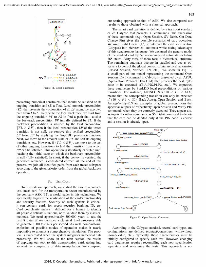
163



Figure 11. Local Backtrack.

presenting numerical constraints that should be satisfied on itsongoing transition and (2) a Total Local numeric precondition(TL) that presents the conjunction of all LP along the executedpath from I to S. To execute the local backtrack, we start fromthe ongoing transition PT to FS to find a path that satisfiesthe backtrack precondition BP initially defined by TL. If thebacktrack precondition is satisfied by the total precondition{TL ≥ BP}, then if the local precondition LP of the testedtransition is not null, we remove this verified preconditionLP from BP by applying the SupLDD projection function.Next, we move to the amount state of PT and test its ongoingtransitions, etc. However, if {TL < BP}, we move to the testof other ongoing transitions to find the transition from whichBP can be satisfied. This operation is iteratively executed untilreaching the initial state on which the backtrack preconditionis null (fully satisfied). In short, if the context is verified, thegenerated sequence is considered correct. At the end of thisprocess, we join all identified paths from each traced subspaceaccording to the given priority order from the global backtrackoperation.

IV. USE CASE

To illustrate our approach, we studied the case of a contact-less smart card for the transportation sector manufactured bythe company ASK [32], a world leader in this technology. Wespecifically targeted the verification of the card’s functionalityand security features. Security of such systems is critical:it can concern cards for access security, banking, ID, etc.Card complexity makes it difficult for a human to identifyall possible delicate situations, or to validate them by classicalmethods. We need approximately 500,000 years to test thefirst 8 bytes if we consider a classical Intel processor ableto generate 1000 test sets per second. As well, combinatorialexplosion of possible modes of operation makes it nearlyimpossible to attempt a comprehensive simulation. The prob-lem is exacerbated when the system integrates numerical dataprocessing. We will show in the next session the resultsof applying our tool to this transportation card, taking intoaccount the complexity of data manipulation. We compared

our testing approach to that of ASK. We also compared ourresults to those obtained with a classical approach.

The smart card operation is defined by a transport standardcalled Calypso that presents 33 commands. The successionof these commands (e.g., Open Session, SV Debit, Get Data,Change Pin) gives the possible scenarios of card operation.We used Light Esterel [13] to interpret the card specification(Calypso) into hierarchical automata while taking advantagesof this synchronous language. We designed the generic modelof the studied card by 52 interconnected automata including765 states. Forty-three of them form a hierarchical structure.The remaining automata operate in parallel and act as ob-servers to control the global context of hierarchical automaton(Closed Session, Verified PIN, etc.). We show in Fig. 12a small part of our model representing the command OpenSession. Each command in Calypso is presented by an APDU(Application Protocol Data Unit) that presents the next byte-code to be executed (CLA,INS,P1,P2, etc.). We expressedthese parameters by SupLDD local preconditions on varioustransitions. For instance, AUTSEGINT(h10 < P1 < h1E)means that the corresponding transition can only be executedif (10 < P1 < 30). Back-Autseg-Open-Session and Back-Autseg-Verify-PIN are examples of global preconditions thatappear as outputs of respectively Open Session and Verify PINcommands when they are correctly executed. They appear alsoas inputs for other commands as SV Debit command to denotethat the card can be debited only if the PIN code is correctand a session is already open.

Figure 12. Open Session Command.

According to the Calypso standard, several card types andconfigurations are defined (contact/contactless, with/withoutStored-Value, etc.). Typically, these characteristics must beinitially configured to specify each test. However, changingcard parameters requires recompiling each new specificationseparately and re-running the tests. This approach is un-

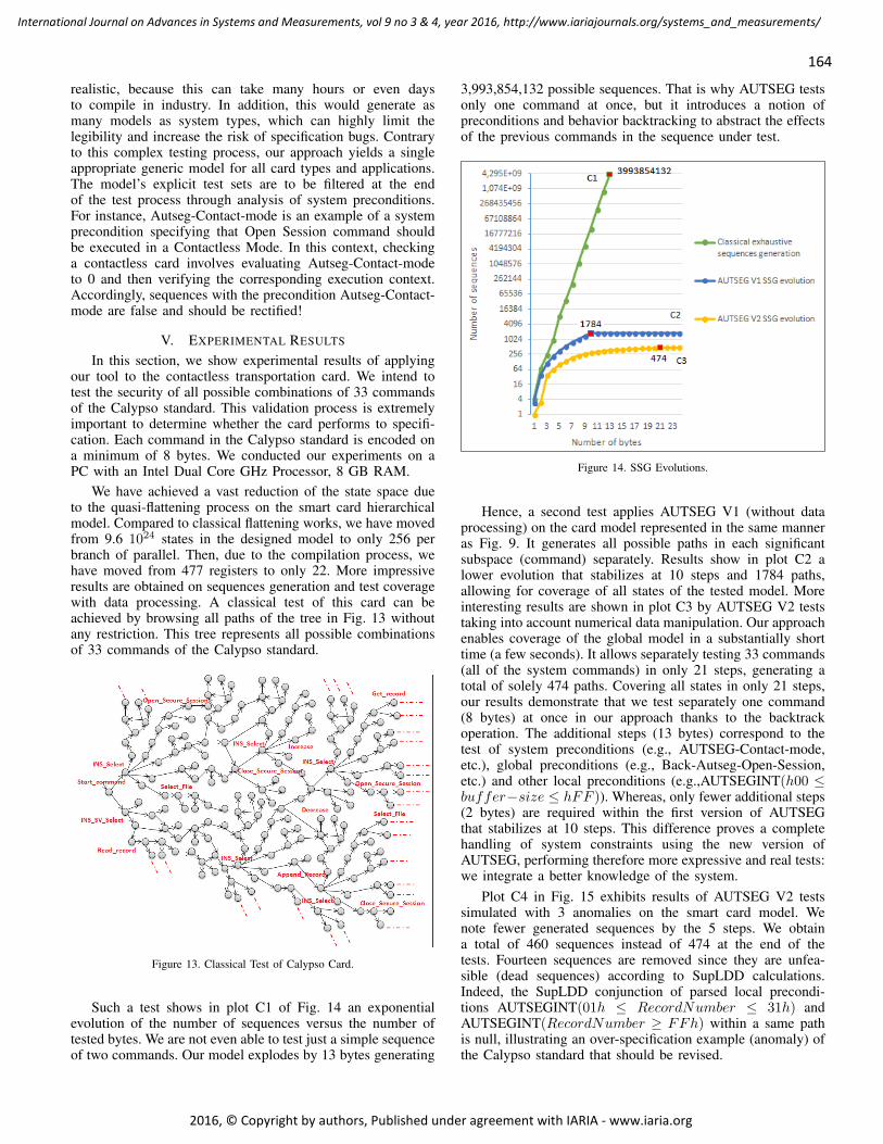
164



realistic, because this can take many hours or even daysto compile in industry. In addition, this would generate asmany models as system types, which can highly limit thelegibility and increase the risk of specification bugs. Contraryto this complex testing process, our approach yields a singleappropriate generic model for all card types and applications.The model’s explicit test sets are to be filtered at the endof the test process through analysis of system preconditions.For instance, Autseg-Contact-mode is an example of a systemprecondition specifying that Open Session command shouldbe executed in a Contactless Mode. In this context, checkinga contactless card involves evaluating Autseg-Contact-modeto 0 and then verifying the corresponding execution context.Accordingly, sequences with the precondition Autseg-Contact-mode are false and should be rectified!

V. EXPERIMENTAL RESULTS

In this section, we show experimental results of applyingour tool to the contactless transportation card. We intend totest the security of all possible combinations of 33 commandsof the Calypso standard. This validation process is extremelyimportant to determine whether the card performs to specifi-cation. Each command in the Calypso standard is encoded ona minimum of 8 bytes. We conducted our experiments on aPC with an Intel Dual Core GHz Processor, 8 GB RAM.

We have achieved a vast reduction of the state space dueto the quasi-flattening process on the smart card hierarchicalmodel. Compared to classical flattening works, we have movedfrom 9.6 1024 states in the designed model to only 256 perbranch of parallel. Then, due to the compilation process, wehave moved from 477 registers to only 22. More impressiveresults are obtained on sequences generation and test coveragewith data processing. A classical test of this card can beachieved by browsing all paths of the tree in Fig. 13 withoutany restriction. This tree represents all possible combinationsof 33 commands of the Calypso standard.

Figure 13. Classical Test of Calypso Card.

Such a test shows in plot C1 of Fig. 14 an exponentialevolution of the number of sequences versus the number oftested bytes. We are not even able to test just a simple sequenceof two commands. Our model explodes by 13 bytes generating

3,993,854,132 possible sequences. That is why AUTSEG testsonly one command at once, but it introduces a notion ofpreconditions and behavior backtracking to abstract the effectsof the previous commands in the sequence under test.

Figure 14. SSG Evolutions.

Hence, a second test applies AUTSEG V1 (without dataprocessing) on the card model represented in the same manneras Fig. 9. It generates all possible paths in each significantsubspace (command) separately. Results show in plot C2 alower evolution that stabilizes at 10 steps and 1784 paths,allowing for coverage of all states of the tested model. Moreinteresting results are shown in plot C3 by AUTSEG V2 teststaking into account numerical data manipulation. Our approachenables coverage of the global model in a substantially shorttime (a few seconds). It allows separately testing 33 commands(all of the system commands) in only 21 steps, generating atotal of solely 474 paths. Covering all states in only 21 steps,our results demonstrate that we test separately one command(8 bytes) at once in our approach thanks to the backtrackoperation. The additional steps (13 bytes) correspond to thetest of system preconditions (e.g., AUTSEG-Contact-mode,etc.), global preconditions (e.g., Back-Autseg-Open-Session,etc.) and other local preconditions (e.g.,AUTSEGINT(h00 ≤buffer−size ≤ hFF )). Whereas, only fewer additional steps(2 bytes) are required within the first version of AUTSEGthat stabilizes at 10 steps. This difference proves a completehandling of system constraints using the new version ofAUTSEG, performing therefore more expressive and real tests:we integrate a better knowledge of the system.

Plot C4 in Fig. 15 exhibits results of AUTSEG V2 testssimulated with 3 anomalies on the smart card model. Wenote fewer generated sequences by the 5 steps. We obtaina total of 460 sequences instead of 474 at the end of thetests. Fourteen sequences are removed since they are unfea-sible (dead sequences) according to SupLDD calculations.Indeed, the SupLDD conjunction of parsed local precondi-tions AUTSEGINT(01h ≤ RecordNumber ≤ 31h) andAUTSEGINT(RecordNumber ≥ FFh) within a same pathis null, illustrating an over-specification example (anomaly) ofthe Calypso standard that should be revised.

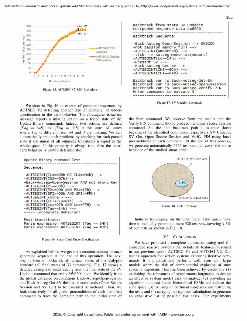
165



Figure 15. AUTSEG V2 SSG Evolutions.

We show in Fig. 16 an excerpt of generated sequences byAUTSEG V2 detecting another type of anomaly: an under-specification in the card behavior. The Incomplete Behaviormessage reports a missing action on a tested state of theUpdate-Binary command. Indeed, two actions are defined(Tag = 54h) and (Tag = 03h) at this state. All stateswhere Tag is different from 84 and 3 are missing. We canautomatically spot such problems by checking for each parsedstate if the union of all outgoing transitions is equal to thewhole space. If this property is always true, then the smartcard behavior is proved deterministic.

Figure 16. Smart Card Under-Specification.

As explained before, we get the execution context of eachgenerated sequence at the end of this operation. The nextstep is then to backtrack all critical states of the Calypsostandard (all final states of 33 commands). Fig. 17 shows adetailed example of backtracking from the final state of the SVUndebit command that emits SW6200 code. We identify fromthe global extracted preconditions Back-Autseg-Open-Sessionand Back-Autseg-Get-SV the list of commands (Open SecureSession and SV Get) to be executed beforehand. Then, welook recursively for all global preconditions of each identifiedcommand to trace the complete path to the initial state of

Figure 17. SV Undebit Backtrack.

the Start command. We observe from the results that theVerify PIN command should proceed the Open Secure Sessioncommand. So, the final backtrack path is to trace (localbacktrack) the identified commands respectively SV Undebit,SV Get, Open Secure Session and Verify PIN using localpreconditions of each command. At the end of this process,we generate automatically 5456 test sets that cover the entirebehavior of the studied smart card.

Figure 18. Tests Coverage.

Industry techniques, on the other hand, take much moretime to manually generate a mere 520 test sets, covering 9.5%of our tests as shown in Fig. 18.

VI. CONCLUSION

We have proposed a complete automatic testing tool forembedded reactive systems that details all features presentedin our previous works AUTSEG V1 and AUTSEG V2. Ourtesting approach focused on systems executing iterative com-mands. It is practical and performs well, even with largemodels where the risk of combinatorial explosion of statespace is important. This has been achieved by essentially (1)exploiting the robustness of synchronous languages to designan effective system model easy to analyze, (2) providing analgorithm to quasi-flatten hierarchical FSMs and reduce thestate space, (3) focusing on pertinent subspaces and restrictingthe tests, and (4) carrying out rigorous calculations to generatean exhaustive list of possible test cases. Our experiments

166



confirm that our tool provides expressive and significant tests,covering all possible system evolutions in a short time. Moregenerally, our tool including the SupLDD calculations can beapplied to many numerical systems as they could be modelledby FSMs handling integer variables. Since SupLDD is imple-mented on top of a simple BDD package, we aim in a futurework to rebuild SupLDD on top of an efficient implementationof BDDs with complement edges [33] to achieve a betterlibrary optimization. More generally, new algorithms can beintegrated to enhance the LDD library. We aim as well tointegrate SupLDD in data abstraction of CLEM [13]. Moredetails about these future works are presented in [34]. Anotherinteresting contribution would be to generate penetration teststo determine whether a system is vulnerable to an attack.

REFERENCES

[1] M. Abdelmoula, D. Gaffe, and M. Auguin, “Automatic Test Set Gen-erator with Numeric Constraints Abstraction for Embedded ReactiveSystems: AUTSEG V2,” in VALID 2015: The Seventh InternationalConference on Advances in System Testing and Validation Lifecycle,Barcelone, Spain, Nov. 2015, pp. 23–30.

[2] M. Abdelmoula, D. Gaffe, and M. Auguin, “Autseg: Automatic testset generator for embedded reactive systems,” in Testing Software andSystems, 26th IFIP International Conference,ICTSS, ser. Lecture Notesin Computer Science. Madrid, Spain: springer, September 2014, pp.97–112.

[3] B. Seljimi and I. Parissis, “Automatic generation of test data generatorsfor synchronous programs: Lutess v2,” in Workshop on Domain specificapproaches to software test automation: in conjunction with the 6thESEC/FSE joint meeting, ser. DOSTA ’07. New York, NY, USA:ACM, 2007, pp. 8–12.

[4] L. DuBousquet and N. Zuanon, “An overview of lutess: A specification-based tool for testing synchronous software,” in ASE, 1999, pp. 208–215.

[5] B. Blanc, C. Junke, B. Marre, P. Le Gall, and O. Andrieu, “Handlingstate-machines specifications with gatel,” Electron. Notes Theor.Comput. Sci., vol. 264, no. 3, 2010, pp. 3–17. [Online]. Available:http://dx.doi.org/10.1016/j.entcs.2010.12.011 [Accessed 15 November2016]

[6] J. R. Calam, “Specification-Based Test Generation With TGV,” CWI,CWI Technical Report SEN-R 0508, 2005. [Online]. Available:http://oai.cwi.nl/oai/asset/10948/10948D.pdf [Accessed 15 November2016]

[7] D. Clarke, T. Jeron, V. Rusu, and E. Zinovieva, “Stg: A symbolic testgeneration tool,” in TACAS, 2002, pp. 470–475.

[8] L. Bentakouk, P. Poizat, and F. Zaıdi, “A formal framework for serviceorchestration testing based on symbolic transition systems,” Testing ofSoftware and Communication Systems, 2009.

[9] D. Xu, “A tool for automated test code generation from high-levelpetri nets,” in Proceedings of the 32nd international conference onApplications and theory of Petri Nets, ser. PETRI NETS’11. Berlin,Heidelberg: Springer-Verlag, 2011, pp. 308–317.

[10] J. Burnim and K. Sen, “Heuristics for scalable dynamic test generation,”in Proceedings of the 2008 23rd IEEE/ACM International Conferenceon Automated Software Engineering, ser. ASE ’08. Washington, DC,USA: IEEE Computer Society, 2008, pp. 443–446.

[11] G. Li, I. Ghosh, and S. P. Rajan, “Klover: a symbolic execution andautomatic test generation tool for c++ programs,” in Proceedings ofthe 23rd international conference on Computer aided verification, ser.CAV’11. Berlin, Heidelberg: Springer-Verlag, 2011, pp. 609–615.

[12] C. Andre, “A synchronous approach to reactive system design,” in 12thEAEEIE Annual Conf., Nancy (F), May 2001, pp. 349–353.

[13] A. Ressouche, D. Gaffe, and V. Roy, “Modular compilation of asynchronous language,” in Soft. Eng. Research, Management and Ap-plications, best 17 paper selection of the SERA’08 conference, R. Lee,Ed., vol. 150. Prague: Springer-Verlag, August 2008, pp. 157–171.

[14] C. Andre, “Representation and analysis of reactive behaviors: A syn-chronous approach,” in Computational Engineering in Systems Appli-cations (CESA). Lille (F): IEEE-SMC, July 1996, pp. 19–29.

[15] G. Berry and G. Gonthier, “The esterel synchronous programminglanguage: Design, semantics, implementation,” Sci. Comput.Program., vol. 19, no. 2, Nov. 1992, pp. 87–152. [Online].Available: http://dx.doi.org/10.1016/0167-6423(92)90005-V [Accessed15 November 2016]

[16] N. Halbwachs, P. Caspi, P. Raymond, and D. Pilaud, “The synchronousdataflow programming language lustre,” in Proceedings of the IEEE,1991, pp. 1305–1320.

[17] A. C. R. Paiva, N. Tillmann, J. C. P. Faria, and R. F. A. M. Vidal,“Modeling and testing hierarchical guis,” in Proc.ASM05. Universitede Paris 12, 2005, pp. 8–11.

[18] A. Wasowski, “Flattening statecharts without explosions,” SIGPLANNot., vol. 39, no. 7, Jun 2004, pp. 257–266. [Online]. Available:http://doi.acm.org/10.1145/998300.997200 [Accessed 15 November2016]

[19] I. Chiuchisan, A. D. Potorac, and A. Garaur, “Finite state machinedesign and vhdl coding techniques,” in 10th International Conferenceon development and application systems. Suceava, Romania: Facultyof Electrical Engineering and Computer Science, 2010, pp. 273–278.

[20] M. Fujita, P. C. McGeer, and J. C.-Y. Yang, “Multi-terminal binarydecision diagrams: An efficient datastructure for matrix representation,”Form. Methods Syst. Des., vol. 10, no. 2-3, Apr. 1997, pp. 149–169.

[21] Y.-T. Lai and S. Sastry, “Edge-valued binary decision diagramsfor multi-level hierarchical verification,” in Proceedings of the 29thACM/IEEE Design Automation Conference, ser. DAC’92. Los Alami-tos, CA, USA: IEEE Computer Society Press, 1992, pp. 608–613.

[22] R. E. Bryant and Y.-A. Chen, “Verification of arithmetic circuitswith binary moment diagrams,” in Proceedings of the 32Nd AnnualACM/IEEE Design Automation Conference, ser. DAC ’95. New York,NY, USA: ACM, 1995, pp. 535–541.

[23] L. Arditi, “A bit-vector algebra for binary moment diagrams,” I3S,Sophia-Antipolis, France, Tech. Rep. RR 95–68, 1995.

[24] E. Clarke and X. Zhao, “Word level symbolic model checking: A newapproach for verifying arithmetic circuits,” Pittsburgh, PA, USA, Tech.Rep., 1995.

[25] M. Ciesielski, P. Kalla, and S. Askar, “Taylor expansion diagrams: Acanonical representation for verification of data flow designs,” IEEETransactions on Computers, vol. 55, no. 9, 2006, pp. 1188–1201.

[26] J. Møller and J. Lichtenberg, “Difference decision diagrams,” Master’sthesis, Department of Information Technology, Technical University ofDenmark, Building 344, DK-2800 Lyngby, Denmark, Aug. 1998.

[27] A. J. C. Bik and H. A. G. Wijshoff, Implementation of Fourier-MotzkinElimination. Rijksuniversiteit Leiden. Valgroep Informatica, 1994.

[28] P. Bouyer, S. Haddad, and P.-A. Reynier, “Timed petri nets andtimed automata: On the discriminating power of zeno sequences,” Inf.Comput., vol. 206, no. 1, Jan. 2008, pp. 73–107.

[29] S. Chaki, A. Gurfinkel, and O. Strichman, “Decision diagrams for lineararithmetic.” in FMCAD. IEEE, 2009, pp. 53–60.

[30] R. S. Boyer, B. Elspas, and K. N. Levitt, “Select a formal system fortesting and debugging programs by symbolic execution,” SIGPLANNot., vol. 10, no. 6, Apr. 1975, pp. 234–245. [Online]. Available:http://doi.acm.org/10.1145/390016.808445 [Accessed 15 November2016]

[31] D. B. Johnson, “A note on dijkstra’s shortest path algorithm,” J.ACM, vol. 20, no. 3, Jul. 1973, pp. 385–388. [Online]. Available:http://doi.acm.org/10.1145/321765.321768 [Accessed 15 November2016]

[32] “Ask.” [Online]. Available: http://www.ask-rfid.com/ [Accessed 15November 2016]

[33] K. Brace, R. Rudell, and R. Bryant, “Efficient implementation of a bddpackage,” in Design Automation Conference, 1990. Proceedings., 27thACM/IEEE, June 1990, pp. 40–45.

[34] M. Abdelmoula, “Automatic test set generator with numeric constraintsabstraction for embedded reactive systems,” Ph.D. dissertation, Pub-lished in ”Generation automatique de jeux de tests avec analyse sym-bolique des donnees pour les systemes embarques”, Sophia AntipolisUniversity, France, 2014.

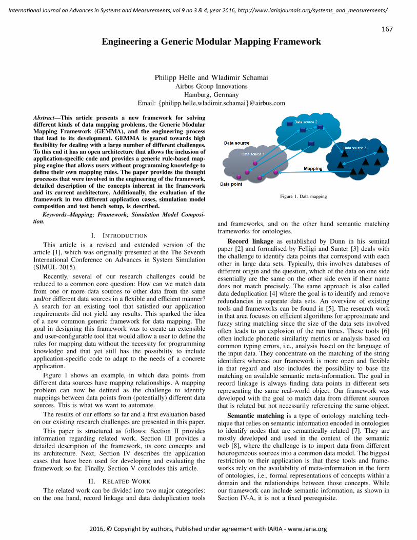
167



Engineering a Generic Modular Mapping Framework

Philipp Helle and Wladimir SchamaiAirbus Group Innovations

Hamburg, GermanyEmail: {philipp.helle,wladimir.schamai}@airbus.com

Abstract—This article presents a new framework for solvingdifferent kinds of data mapping problems, the Generic ModularMapping Framework (GEMMA), and the engineering processthat lead to its development. GEMMA is geared towards highflexibility for dealing with a large number of different challenges.To this end it has an open architecture that allows the inclusion ofapplication-specific code and provides a generic rule-based map-ping engine that allows users without programming knowledge todefine their own mapping rules. The paper provides the thoughtprocesses that were involved in the engineering of the framework,detailed description of the concepts inherent in the frameworkand its current architecture. Additionally, the evaluation of theframework in two different application cases, simulation modelcomposition and test bench setup, is described.

Keywords–Mapping; Framework; Simulation Model Composi-tion.

I. INTRODUCTION

This article is a revised and extended version of thearticle [1], which was originally presented at the The SeventhInternational Conference on Advances in System Simulation(SIMUL 2015).

Recently, several of our research challenges could bereduced to a common core question: How can we match datafrom one or more data sources to other data from the sameand/or different data sources in a flexible and efficient manner?A search for an existing tool that satisfied our applicationrequirements did not yield any results. This sparked the ideaof a new common generic framework for data mapping. Thegoal in designing this framework was to create an extensibleand user-configurable tool that would allow a user to define therules for mapping data without the necessity for programmingknowledge and that yet still has the possibility to includeapplication-specific code to adapt to the needs of a concreteapplication.

Figure 1 shows an example, in which data points fromdifferent data sources have mapping relationships. A mappingproblem can now be defined as the challenge to identifymappings between data points from (potentially) different datasources. This is what we want to automate.

The results of our efforts so far and a first evaluation basedon our existing research challenges are presented in this paper.

This paper is structured as follows: Section II providesinformation regarding related work. Section III provides adetailed description of the framework, its core concepts andits architecture. Next, Section IV describes the applicationcases that have been used for developing and evaluating theframework so far. Finally, Section V concludes this article.

II. RELATED WORK

The related work can be divided into two major categories:on the one hand, record linkage and data deduplication tools

Figure 1. Data mapping

and frameworks, and on the other hand semantic matchingframeworks for ontologies.

Record linkage as established by Dunn in his seminalpaper [2] and formalised by Felligi and Sunter [3] deals withthe challenge to identify data points that correspond with eachother in large data sets. Typically, this involves databases ofdifferent origin and the question, which of the data on one sideessentially are the same on the other side even if their namedoes not match precisely. The same approach is also calleddata deduplication [4] where the goal is to identify and removeredundancies in separate data sets. An overview of existingtools and frameworks can be found in [5]. The research workin that area focuses on efficient algorithms for approximate andfuzzy string matching since the size of the data sets involvedoften leads to an explosion of the run times. These tools [6]often include phonetic similarity metrics or analysis based oncommon typing errors, i.e., analysis based on the language ofthe input data. They concentrate on the matching of the stringidentifiers whereas our framework is more open and flexiblein that regard and also includes the possibility to base thematching on available semantic meta-information. The goal inrecord linkage is always finding data points in different setsrepresenting the same real-world object. Our framework wasdeveloped with the goal to match data from different sourcesthat is related but not necessarily referencing the same object.

Semantic matching is a type of ontology matching tech-nique that relies on semantic information encoded in ontologiesto identify nodes that are semantically related [7]. They aremostly developed and used in the context of the semanticweb [8], where the challenge is to import data from differentheterogeneous sources into a common data model. The biggestrestriction to their application is that these tools and frame-works rely on the availability of meta-information in the formof ontologies, i.e., formal representations of concepts within adomain and the relationships between those concepts. Whileour framework can include semantic information, as shown inSection IV-A, it is not a fixed prerequisite.

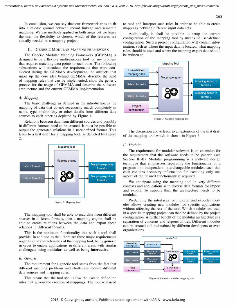
168



In conclusion, we can say that our framework tries to fitinto a middle ground between record linkage and semanticmatching. We use methods applied in both areas but we leavethe user the flexibility to choose, which of the features areactually needed in a mapping project.

III. GENERIC MODULAR MAPPING FRAMEWORK

The Generic Modular Mapping Framework (GEMMA) isdesigned to be a flexible multi-purpose tool for any problemthat requires matching data points to each other. The followingsubsections will introduce the requirements that were con-sidered during the GEMMA development, the artifacts thatmake up the core idea behind GEMMA, describe the kindof mapping rules that can be implemented, show the genericprocess for the usage of GEMMA and describe the softwarearchitecture and the current GEMMA implementation.

A. MappingThe basic challenge as defined in the introduction is the

mapping of data that do not necessarily match completely inname, type, multiplicity or other details from different datasources to each other as depicted by Figure 1.

Relations between data from different sources and possiblyin different formats need to be created. It must be possible tooutput the generated relations in a user-defined format. Thisleads to a first draft for a mapping tool, as depicted by Figure2.

Figure 2. Mapping tool

The mapping tool shall be able to read data from differentsources in different formats, then a mapping engine shall beable to create relations between the data and export theserelations in different formats.

This is the minimum functionality that such a tool shallprovide. In addition to that, there are three major requirementsregarding the characteristics of the mapping tool, being genericin order to enable applications in different areas with similarchallenges; being modular, as well as being interactive.

B. GenericThe requirement for a generic tool stems from the fact that

different mapping problems and challenges require differentdata sources and mapping rules.

This means that the tool shall allow the user to define therules that govern the creation of mappings. The tool will need

to read and interpret such rules in order to be able to createmappings between different input data sets.

Additionally, it shall be possible to setup the currentconfiguration of the mapping tool by means of user-definedconfiguration. Such a project configuration will contain infor-mation, such as where the input data is located, what mappingrules should be used and where the mapping export data shouldbe written to.

Figure 3. Generic mapping tool

The discussion above leads to an extension of the first draftof the mapping tool which is shown in Figure 3.

C. ModularThe requirement for modular software is an extension for

the requirement that the software needs to be generic (seeSection III-B). Modular programming is a software designtechnique that emphasizes separating the functionality of aprogram into independent, interchangeable modules, such thateach contains necessary information for executing only oneaspect of the desired functionality if required.

We anticipate using the mapping tool in very differentcontexts and applications with diverse data formats for importand export. To support this, the architecture needs to bemodular.

Predefining the interfaces for importer and exporter mod-ules allows creating new modules for specific applicationswithout affecting the rest of the tool. Which modules are usedin a specific mapping project can then be defined by the projectconfiguration. A further benefit of the modular architecture is aseparation of concerns and responsibilities. Different modulescan be created and maintained by different developers or evenorganizations.

Figure 4. Generic modular mapping tool

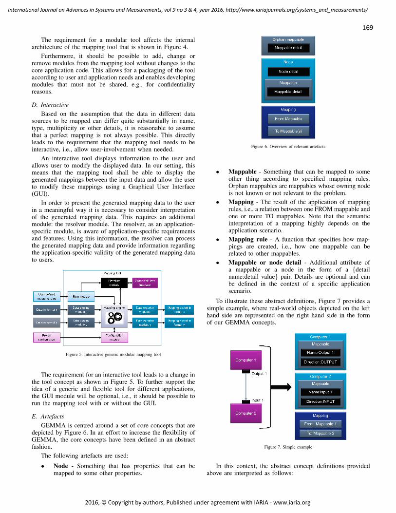
169



The requirement for a modular tool affects the internalarchitecture of the mapping tool that is shown in Figure 4.

Furthermore, it should be possible to add, change orremove modules from the mapping tool without changes to thecore application code. This allows for a packaging of the toolaccording to user and application needs and enables developingmodules that must not be shared, e.g., for confidentialityreasons.

D. InteractiveBased on the assumption that the data in different data

sources to be mapped can differ quite substantially in name,type, multiplicity or other details, it is reasonable to assumethat a perfect mapping is not always possible. This directlyleads to the requirement that the mapping tool needs to beinteractive, i.e., allow user-involvement when needed.

An interactive tool displays information to the user andallows user to modify the displayed data. In our setting, thismeans that the mapping tool shall be able to display thegenerated mappings between the input data and allow the userto modify these mappings using a Graphical User Interface(GUI).

In order to present the generated mapping data to the userin a meaningful way it is necessary to consider interpretationof the generated mapping data. This requires an additionalmodule: the resolver module. The resolver, as an application-specific module, is aware of application-specific requirementsand features. Using this information, the resolver can processthe generated mapping data and provide information regardingthe application-specific validity of the generated mapping datato users.

Figure 5. Interactive generic modular mapping tool

The requirement for an interactive tool leads to a change inthe tool concept as shown in Figure 5. To further support theidea of a generic and flexible tool for different applications,the GUI module will be optional, i.e., it should be possible torun the mapping tool with or without the GUI.

E. ArtefactsGEMMA is centred around a set of core concepts that are

depicted by Figure 6. In an effort to increase the flexibility ofGEMMA, the core concepts have been defined in an abstractfashion.

The following artefacts are used:

• Node - Something that has properties that can bemapped to some other properties.

Figure 6. Overview of relevant artefacts

• Mappable - Something that can be mapped to someother thing according to specified mapping rules.Orphan mappables are mappables whose owning nodeis not known or not relevant to the problem.

• Mapping - The result of the application of mappingrules, i.e., a relation between one FROM mappable andone or more TO mappables. Note that the semanticinterpretation of a mapping highly depends on theapplication scenario.

• Mapping rule - A function that specifies how map-pings are created, i.e., how one mappable can berelated to other mappables.

• Mappable or node detail - Additional attribute ofa mappable or a node in the form of a {detailname:detail value} pair. Details are optional and canbe defined in the context of a specific applicationscenario.

To illustrate these abstract definitions, Figure 7 provides asimple example, where real-world objects depicted on the lefthand side are represented on the right hand side in the formof our GEMMA concepts.

Figure 7. Simple example

In this context, the abstract concept definitions providedabove are interpreted as follows:

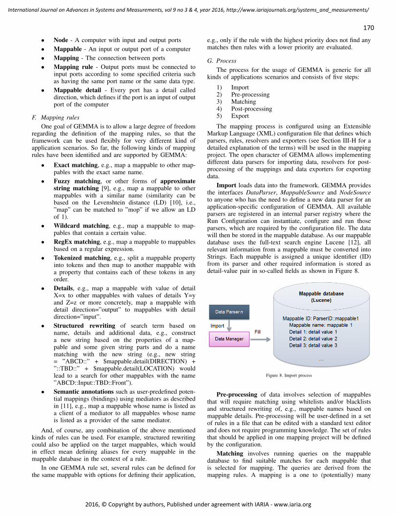
170



• Node - A computer with input and output ports• Mappable - An input or output port of a computer• Mapping - The connection between ports• Mapping rule - Output ports must be connected to

input ports according to some specified criteria suchas having the same port name or the same data type.

• Mappable detail - Every port has a detail calleddirection, which defines if the port is an input of outputport of the computer

F. Mapping rulesOne goal of GEMMA is to allow a large degree of freedom

regarding the definition of the mapping rules, so that theframework can be used flexibly for very different kind ofapplication scenarios. So far, the following kinds of mappingrules have been identified and are supported by GEMMA:

• Exact matching, e.g., map a mappable to other map-pables with the exact same name.

• Fuzzy matching, or other forms of approximatestring matching [9], e.g., map a mappable to othermappables with a similar name (similarity can bebased on the Levenshtein distance (LD) [10], i.e.,”map” can be matched to ”mop” if we allow an LDof 1).

• Wildcard matching, e.g., map a mappable to map-pables that contain a certain value.

• RegEx matching, e.g., map a mappable to mappablesbased on a regular expression.

• Tokenized matching, e.g., split a mappable propertyinto tokens and then map to another mappable witha property that contains each of these tokens in anyorder.

• Details, e.g., map a mappable with value of detailX=x to other mappables with values of details Y=yand Z=z or more concretely, map a mappable withdetail direction=”output” to mappables with detaildirection=”input”.

• Structured rewriting of search term based onname, details and additional data, e.g., constructa new string based on the properties of a map-pable and some given string parts and do a namematching with the new string (e.g., new string= ”ABCD::” + $mappable.detail(DIRECTION) +”::TBD::” + $mappable.detail(LOCATION) wouldlead to a search for other mappables with the name”ABCD::Input::TBD::Front”).

• Semantic annotations such as user-predefined poten-tial mappings (bindings) using mediators as describedin [11], e.g., map a mappable whose name is listed asa client of a mediator to all mappables whose nameis listed as a provider of the same mediator.

And, of course, any combination of the above mentionedkinds of rules can be used. For example, structured rewritingcould also be applied on the target mappables, which wouldin effect mean defining aliases for every mappable in themappable database in the context of a rule.

In one GEMMA rule set, several rules can be defined forthe same mappable with options for defining their application,

e.g., only if the rule with the highest priority does not find anymatches then rules with a lower priority are evaluated.

G. ProcessThe process for the usage of GEMMA is generic for all

kinds of applications scenarios and consists of five steps:

1) Import2) Pre-processing3) Matching4) Post-processing5) Export

The mapping process is configured using an ExtensibleMarkup Language (XML) configuration file that defines whichparsers, rules, resolvers and exporters (see Section III-H for adetailed explanation of the terms) will be used in the mappingproject. The open character of GEMMA allows implementingdifferent data parsers for importing data, resolvers for post-processing of the mappings and data exporters for exportingdata.

Import loads data into the framework. GEMMA providesthe interfaces DataParser, MappableSource and NodeSourceto anyone who has the need to define a new data parser for anapplication-specific configuration of GEMMA. All availableparsers are registered in an internal parser registry where theRun Configuration can instantiate, configure and run thoseparsers, which are required by the configuration file. The datawill then be stored in the mappable database. As our mappabledatabase uses the full-text search engine Lucene [12], allrelevant information from a mappable must be converted intoStrings. Each mappable is assigned a unique identifier (ID)from its parser and other required information is stored asdetail-value pair in so-called fields as shown in Figure 8.

Figure 8. Import process

Pre-processing of data involves selection of mappablesthat will require matching using whitelists and/or blacklistsand structured rewriting of, e.g., mappable names based onmappable details. Pre-processing will be user-defined in a setof rules in a file that can be edited with a standard text editorand does not require programming knowledge. The set of rulesthat should be applied in one mapping project will be definedby the configuration.

Matching involves running queries on the mappabledatabase to find suitable matches for each mappable thatis selected for mapping. The queries are derived from themapping rules. A mapping is a one to (potentially) many

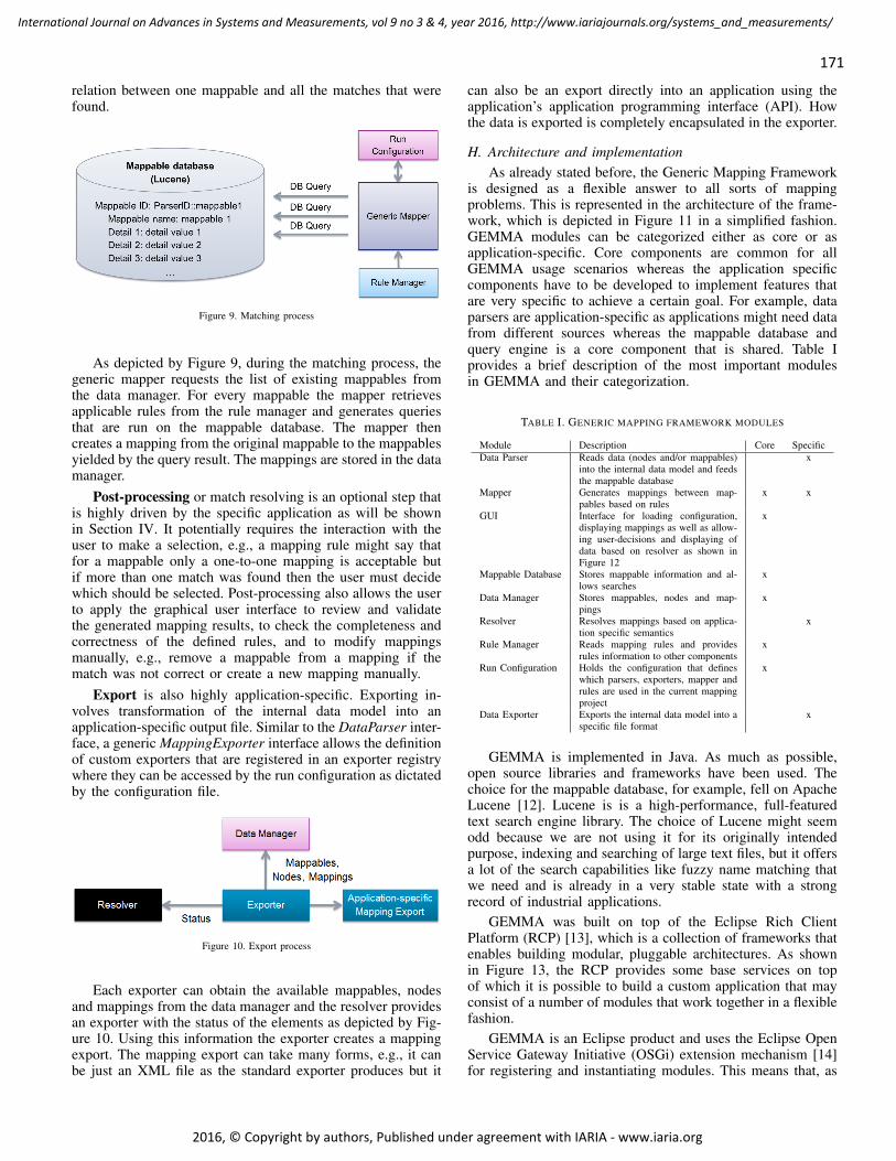
171



relation between one mappable and all the matches that werefound.

Figure 9. Matching process

As depicted by Figure 9, during the matching process, thegeneric mapper requests the list of existing mappables fromthe data manager. For every mappable the mapper retrievesapplicable rules from the rule manager and generates queriesthat are run on the mappable database. The mapper thencreates a mapping from the original mappable to the mappablesyielded by the query result. The mappings are stored in the datamanager.

Post-processing or match resolving is an optional step thatis highly driven by the specific application as will be shownin Section IV. It potentially requires the interaction with theuser to make a selection, e.g., a mapping rule might say thatfor a mappable only a one-to-one mapping is acceptable butif more than one match was found then the user must decidewhich should be selected. Post-processing also allows the userto apply the graphical user interface to review and validatethe generated mapping results, to check the completeness andcorrectness of the defined rules, and to modify mappingsmanually, e.g., remove a mappable from a mapping if thematch was not correct or create a new mapping manually.

Export is also highly application-specific. Exporting in-volves transformation of the internal data model into anapplication-specific output file. Similar to the DataParser inter-face, a generic MappingExporter interface allows the definitionof custom exporters that are registered in an exporter registrywhere they can be accessed by the run configuration as dictatedby the configuration file.

Figure 10. Export process

Each exporter can obtain the available mappables, nodesand mappings from the data manager and the resolver providesan exporter with the status of the elements as depicted by Fig-ure 10. Using this information the exporter creates a mappingexport. The mapping export can take many forms, e.g., it canbe just an XML file as the standard exporter produces but it

can also be an export directly into an application using theapplication’s application programming interface (API). Howthe data is exported is completely encapsulated in the exporter.

H. Architecture and implementationAs already stated before, the Generic Mapping Framework

is designed as a flexible answer to all sorts of mappingproblems. This is represented in the architecture of the frame-work, which is depicted in Figure 11 in a simplified fashion.GEMMA modules can be categorized either as core or asapplication-specific. Core components are common for allGEMMA usage scenarios whereas the application specificcomponents have to be developed to implement features thatare very specific to achieve a certain goal. For example, dataparsers are application-specific as applications might need datafrom different sources whereas the mappable database andquery engine is a core component that is shared. Table Iprovides a brief description of the most important modulesin GEMMA and their categorization.

TABLE I. GENERIC MAPPING FRAMEWORK MODULES

Module Description Core SpecificData Parser Reads data (nodes and/or mappables)

into the internal data model and feedsthe mappable database

x

Mapper Generates mappings between map-pables based on rules

x x

GUI Interface for loading configuration,displaying mappings as well as allow-ing user-decisions and displaying ofdata based on resolver as shown inFigure 12

x

Mappable Database Stores mappable information and al-lows searches

x

Data Manager Stores mappables, nodes and map-pings

x

Resolver Resolves mappings based on applica-tion specific semantics

x

Rule Manager Reads mapping rules and providesrules information to other components

x

Run Configuration Holds the configuration that defineswhich parsers, exporters, mapper andrules are used in the current mappingproject

x

Data Exporter Exports the internal data model into aspecific file format

x

GEMMA is implemented in Java. As much as possible,open source libraries and frameworks have been used. Thechoice for the mappable database, for example, fell on ApacheLucene [12]. Lucene is is a high-performance, full-featuredtext search engine library. The choice of Lucene might seemodd because we are not using it for its originally intendedpurpose, indexing and searching of large text files, but it offersa lot of the search capabilities like fuzzy name matching thatwe need and is already in a very stable state with a strongrecord of industrial applications.

GEMMA was built on top of the Eclipse Rich ClientPlatform (RCP) [13], which is a collection of frameworks thatenables building modular, pluggable architectures. As shownin Figure 13, the RCP provides some base services on topof which it is possible to build a custom application that mayconsist of a number of modules that work together in a flexiblefashion.

GEMMA is an Eclipse product and uses the Eclipse OpenService Gateway Initiative (OSGi) extension mechanism [14]for registering and instantiating modules. This means that, as

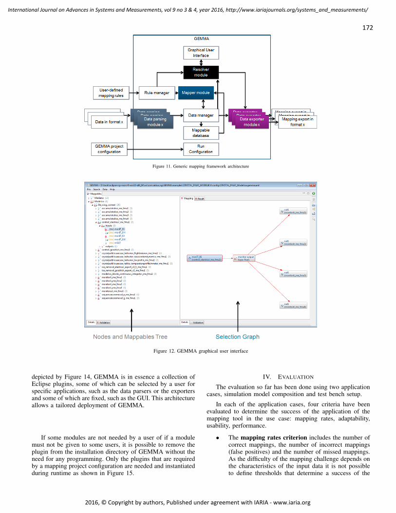
172



Figure 11. Generic mapping framework architecture

Figure 12. GEMMA graphical user interface

depicted by Figure 14, GEMMA is in essence a collection ofEclipse plugins, some of which can be selected by a user forspecific applications, such as the data parsers or the exportersand some of which are fixed, such as the GUI. This architectureallows a tailored deployment of GEMMA.

If some modules are not needed by a user of if a modulemust not be given to some users, it is possible to remove theplugin from the installation directory of GEMMA without theneed for any programming. Only the plugins that are requiredby a mapping project configuration are needed and instantiatedduring runtime as shown in Figure 15.

IV. EVALUATION

The evaluation so far has been done using two applicationcases, simulation model composition and test bench setup.

In each of the application cases, four criteria have beenevaluated to determine the success of the application of themapping tool in the use case: mapping rates, adaptability,usability, performance.

• The mapping rates criterion includes the number ofcorrect mappings, the number of incorrect mappings(false positives) and the number of missed mappings.As the difficulty of the mapping challenge depends onthe characteristics of the input data it is not possibleto define thresholds that determine a success of the

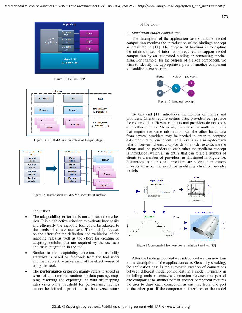
173



Figure 13. Eclipse RCP

Figure 14. GEMMA as a collection of Eclipse plugins

Figure 15. Instantiation of GEMMA modules at runtime

application.• The adaptability criterion is not a measurable crite-

rion. It is a subjective criterion to evaluate how easilyand efficiently the mapping tool could be adapted tothe needs of a new use case. This mainly focuseson the effort for the definition and validation of themapping rules as well as the effort for creating oradapting modules that are required by the use caseand their integration in the tool.

• Similar to the adaptability criterion, the usabilitycriterion is based on feedback from the tool usersand their subjective assessment of the effectiveness ofusing the tool.

• The performance criterion mainly refers to speed interms of tool runtime: runtime for data parsing, map-ping, resolving and exporting. As with the mappingrates criterion, a threshold for performance metricscannot be defined a priori due to the diverse nature

of the tool.

A. Simulation model compositionThe description of the application case simulation model

composition requires the introduction of the bindings conceptas presented in [11]. The purpose of bindings is to capturethe minimum set of information required to support modelcomposition by an automated binding or connecting mecha-nism. For example, for the outputs of a given component, wewish to identify the appropriate inputs of another componentto establish a connection.

Figure 16. Bindings concept

To this end [11] introduces the notions of clients andproviders. Clients require certain data; providers can providethe required data. However, clients and providers do not knoweach other a priori. Moreover, there may be multiple clientsthat require the same information. On the other hand, datafrom several providers may be needed in order to computedata required by one client. This results in a many-to-manyrelation between clients and providers. In order to associate theclients and the providers to each other the mediator conceptis introduced, which is an entity that can relate a number ofclients to a number of providers, as illustrated in Figure 16.References to clients and providers are stored in mediatorsin order to avoid the need for modifying client or providermodels.

Figure 17. Assembled ice-accretion simulation based on [15]

After the bindings concept was introduced we can now turnto the description of the application case. Generally speaking,the application case is the automatic creation of connectionsbetween different model components in a model. Typically inmodelling tools, to create a connection between one port ofone component to another port of another component requiresthe user to draw each connection as one line from one portto the other port. If the components’ interfaces or the model

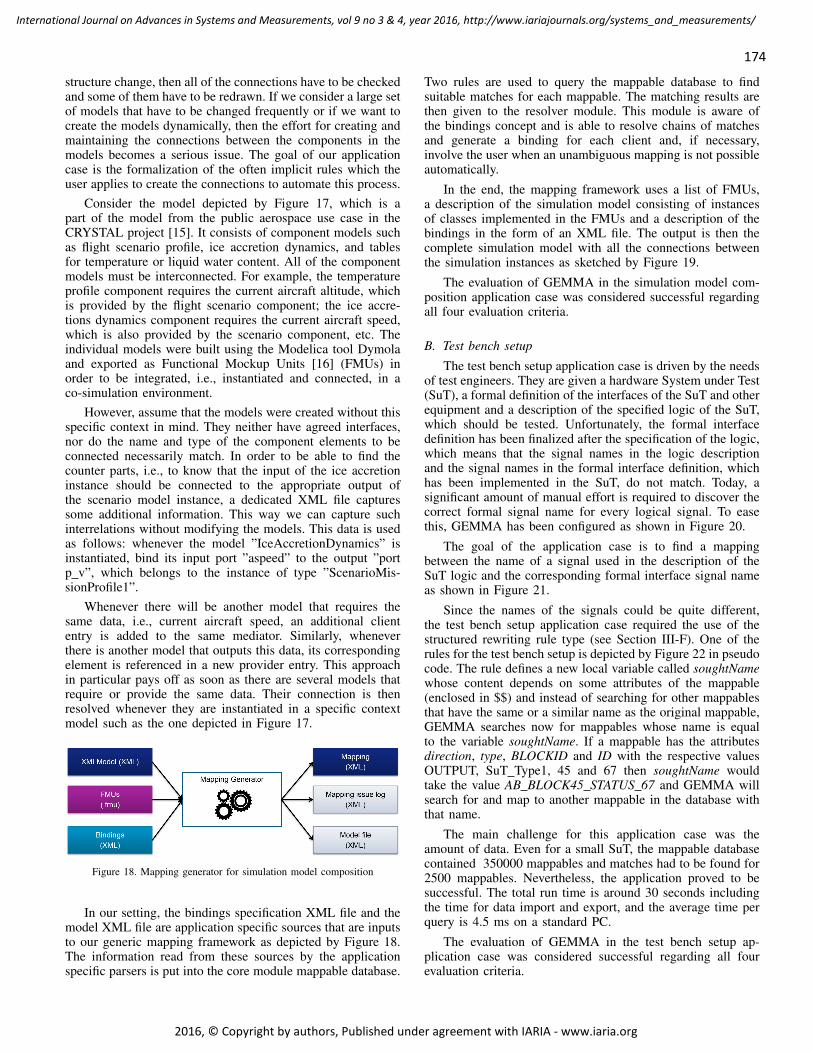
174



structure change, then all of the connections have to be checkedand some of them have to be redrawn. If we consider a large setof models that have to be changed frequently or if we want tocreate the models dynamically, then the effort for creating andmaintaining the connections between the components in themodels becomes a serious issue. The goal of our applicationcase is the formalization of the often implicit rules which theuser applies to create the connections to automate this process.

Consider the model depicted by Figure 17, which is apart of the model from the public aerospace use case in theCRYSTAL project [15]. It consists of component models suchas flight scenario profile, ice accretion dynamics, and tablesfor temperature or liquid water content. All of the componentmodels must be interconnected. For example, the temperatureprofile component requires the current aircraft altitude, whichis provided by the flight scenario component; the ice accre-tions dynamics component requires the current aircraft speed,which is also provided by the scenario component, etc. Theindividual models were built using the Modelica tool Dymolaand exported as Functional Mockup Units [16] (FMUs) inorder to be integrated, i.e., instantiated and connected, in aco-simulation environment.

However, assume that the models were created without thisspecific context in mind. They neither have agreed interfaces,nor do the name and type of the component elements to beconnected necessarily match. In order to be able to find thecounter parts, i.e., to know that the input of the ice accretioninstance should be connected to the appropriate output ofthe scenario model instance, a dedicated XML file capturessome additional information. This way we can capture suchinterrelations without modifying the models. This data is usedas follows: whenever the model ”IceAccretionDynamics” isinstantiated, bind its input port ”aspeed” to the output ”portp v”, which belongs to the instance of type ”ScenarioMis-sionProfile1”.

Whenever there will be another model that requires thesame data, i.e., current aircraft speed, an additional cliententry is added to the same mediator. Similarly, wheneverthere is another model that outputs this data, its correspondingelement is referenced in a new provider entry. This approachin particular pays off as soon as there are several models thatrequire or provide the same data. Their connection is thenresolved whenever they are instantiated in a specific contextmodel such as the one depicted in Figure 17.

Figure 18. Mapping generator for simulation model composition

In our setting, the bindings specification XML file and themodel XML file are application specific sources that are inputsto our generic mapping framework as depicted by Figure 18.The information read from these sources by the applicationspecific parsers is put into the core module mappable database.

Two rules are used to query the mappable database to findsuitable matches for each mappable. The matching results arethen given to the resolver module. This module is aware ofthe bindings concept and is able to resolve chains of matchesand generate a binding for each client and, if necessary,involve the user when an unambiguous mapping is not possibleautomatically.

In the end, the mapping framework uses a list of FMUs,a description of the simulation model consisting of instancesof classes implemented in the FMUs and a description of thebindings in the form of an XML file. The output is then thecomplete simulation model with all the connections betweenthe simulation instances as sketched by Figure 19.

The evaluation of GEMMA in the simulation model com-position application case was considered successful regardingall four evaluation criteria.

B. Test bench setup

The test bench setup application case is driven by the needsof test engineers. They are given a hardware System under Test(SuT), a formal definition of the interfaces of the SuT and otherequipment and a description of the specified logic of the SuT,which should be tested. Unfortunately, the formal interfacedefinition has been finalized after the specification of the logic,which means that the signal names in the logic descriptionand the signal names in the formal interface definition, whichhas been implemented in the SuT, do not match. Today, asignificant amount of manual effort is required to discover thecorrect formal signal name for every logical signal. To easethis, GEMMA has been configured as shown in Figure 20.

The goal of the application case is to find a mappingbetween the name of a signal used in the description of theSuT logic and the corresponding formal interface signal nameas shown in Figure 21.

Since the names of the signals could be quite different,the test bench setup application case required the use of thestructured rewriting rule type (see Section III-F). One of therules for the test bench setup is depicted by Figure 22 in pseudocode. The rule defines a new local variable called soughtNamewhose content depends on some attributes of the mappable(enclosed in $$) and instead of searching for other mappablesthat have the same or a similar name as the original mappable,GEMMA searches now for mappables whose name is equalto the variable soughtName. If a mappable has the attributesdirection, type, BLOCKID and ID with the respective valuesOUTPUT, SuT Type1, 45 and 67 then soughtName wouldtake the value AB BLOCK45 STATUS 67 and GEMMA willsearch for and map to another mappable in the database withthat name.

The main challenge for this application case was theamount of data. Even for a small SuT, the mappable databasecontained 350000 mappables and matches had to be found for2500 mappables. Nevertheless, the application proved to besuccessful. The total run time is around 30 seconds includingthe time for data import and export, and the average time perquery is 4.5 ms on a standard PC.

The evaluation of GEMMA in the test bench setup ap-plication case was considered successful regarding all fourevaluation criteria.

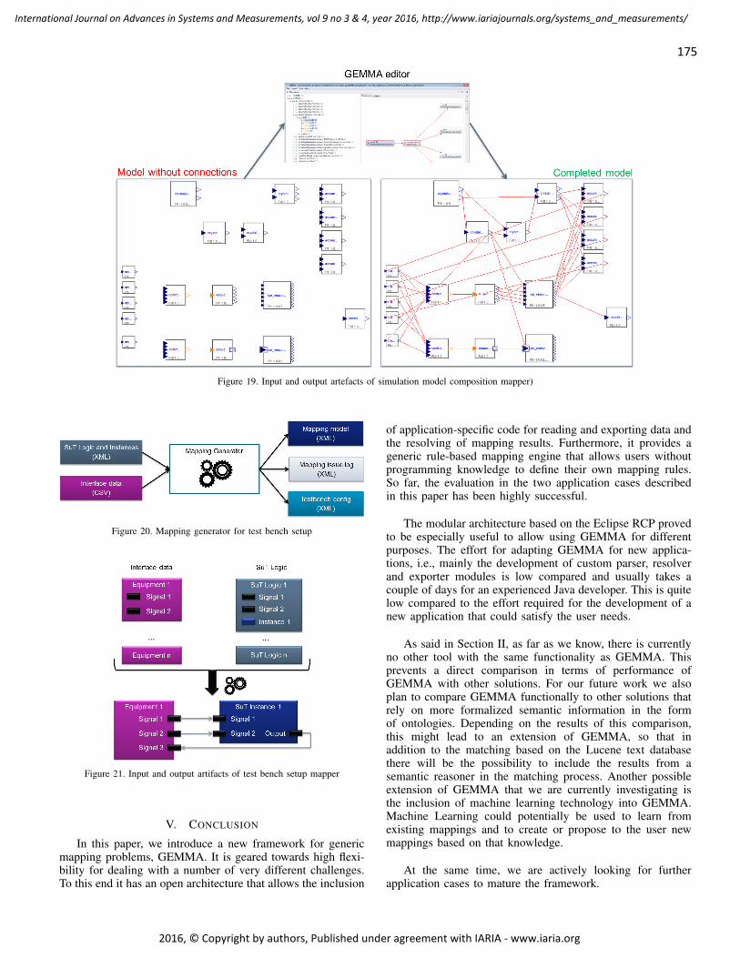
175



Figure 19. Input and output artefacts of simulation model composition mapper)

Figure 20. Mapping generator for test bench setup

Figure 21. Input and output artifacts of test bench setup mapper

V. CONCLUSION

In this paper, we introduce a new framework for genericmapping problems, GEMMA. It is geared towards high flexi-bility for dealing with a number of very different challenges.To this end it has an open architecture that allows the inclusion

of application-specific code for reading and exporting data andthe resolving of mapping results. Furthermore, it provides ageneric rule-based mapping engine that allows users withoutprogramming knowledge to define their own mapping rules.So far, the evaluation in the two application cases describedin this paper has been highly successful.

The modular architecture based on the Eclipse RCP provedto be especially useful to allow using GEMMA for differentpurposes. The effort for adapting GEMMA for new applica-tions, i.e., mainly the development of custom parser, resolverand exporter modules is low compared and usually takes acouple of days for an experienced Java developer. This is quitelow compared to the effort required for the development of anew application that could satisfy the user needs.

As said in Section II, as far as we know, there is currentlyno other tool with the same functionality as GEMMA. Thisprevents a direct comparison in terms of performance ofGEMMA with other solutions. For our future work we alsoplan to compare GEMMA functionally to other solutions thatrely on more formalized semantic information in the formof ontologies. Depending on the results of this comparison,this might lead to an extension of GEMMA, so that inaddition to the matching based on the Lucene text databasethere will be the possibility to include the results from asemantic reasoner in the matching process. Another possibleextension of GEMMA that we are currently investigating isthe inclusion of machine learning technology into GEMMA.Machine Learning could potentially be used to learn fromexisting mappings and to create or propose to the user newmappings based on that knowledge.

At the same time, we are actively looking for furtherapplication cases to mature the framework.

176



Figure 22. One implemented rule for test bench setup (in pseudo code)

REFERENCES[1] P. Helle and W. Schamai, “Using a generic modular mapping framework

for simulation model composition,” in SIMUL 2015, The SeventhInternational Conference on Advances in System Simulation, 2015, pp.72–78.

[2] H. L. Dunn, “Record linkage*,” American Journal of Public Health andthe Nations Health, vol. 36, no. 12, 1946, pp. 1412–1416.

[3] I. P. Fellegi and A. B. Sunter, “A theory for record linkage,” Journalof the American Statistical Association, vol. 64, no. 328, 1969, pp.1183–1210.

[4] Q. He, Z. Li, and X. Zhang, “Data deduplication techniques,” in FutureInformation Technology and Management Engineering (FITME), 2010International Conference on, vol. 1. IEEE, 2010, pp. 430–433.

[5] H. Koepcke and E. Rahm, “Frameworks for entity matching: A com-parison,” Data & Knowledge Engineering, vol. 69, no. 2, 2010, pp. 197– 210.

[6] A. K. Elmagarmid, P. G. Ipeirotis, and V. S. Verykios, “Duplicaterecord detection: A survey,” Knowledge and Data Engineering, IEEETransactions on, vol. 19, no. 1, 2007, pp. 1–16.

[7] F. Giunchiglia, A. Autayeu, and J. Pane, “S-match: An open sourceframework for matching lightweight ontologies,” Semantic Web, vol. 3,no. 3, 2012, pp. 307–317.

[8] Y. Hooi, M. Hassan, and A. Shariff, “A survey on ontology mappingtechniques,” in Advances in Computer Science and its Applications, ser.Lecture Notes in Electrical Engineering, H. Y. Jeong, M. S. Obaidat,N. Y. Yen, and J. J. J. H. Park, Eds. Springer Berlin Heidelberg, 2014,vol. 279, pp. 829–836.

[9] P. A. Hall and G. R. Dowling, “Approximate string matching,” ACMcomputing surveys (CSUR), vol. 12, no. 4, 1980, pp. 381–402.

[10] V. I. Levenshtein, “Binary codes capable of correcting deletions, inser-tions, and reversals,” in Soviet physics doklady, vol. 10, no. 8, 1966,pp. 707–710.

[11] W. Schamai, P. Fritzson, C. J. Paredis, and P. Helle, “ModelicaML valuebindings for automated model composition,” in Proceedings of the 2012Symposium on Theory of Modeling and Simulation-DEVS IntegrativeM&S Symposium. Society for Computer Simulation International,2012, p. 31.

[12] M. McCandless, E. Hatcher, and O. Gospodnetic, Lucene in Action.Manning Publications Co., 2010.

[13] J. McAffer, J.-M. Lemieux, and C. Aniszczyk, Eclipse Rich ClientPlatform. Addison-Wesley Professional, 2010.

[14] R. Hall, K. Pauls, S. McCulloch, and D. Savage, OSGi in action:Creating modular applications in Java. Manning Publications Co.,2011.

[15] A. Mitschke et al., “CRYSTAL public aerospace use case DevelopmentReport - V2,” ARTEMIS EU CRYSTAL project, Tech. Rep. D208.902,2015.

[16] T. Blochwitz et al., “The functional mockup interface for tool inde-pendent exchange of simulation models,” in 8th International ModelicaConference, Dresden, 2011, pp. 20–22.

177



Falsification of Java Assertions Using Automatic Test-Case Generators

Rafael Caballero Manuel MontenegroUniversidad Complutense, Facultad de Informatica

Madrid, Spainemail: {rafacr,mmontene}@ucm.es

Herbert Kuchen Vincent von HofUniversity of Munster, ERCIS, Munster, Germany

email: {kuchen,vincent.von.hof}@wi.uni-muenster.de

Abstract—We present a technique for the static generation of test-cases falsifying Java assertions. Our framework receives as inputa Java program including assertions and instruments the code inorder to detect whether the assertion conditions are met by everydirect and indirect method call within a certain depth level. Then,any automated test-case generator can be used to look for inputexamples that falsify the conditions. The transformation ensuresthat the value obtained for the test-case inputs represents a pathof method calls that ends with a violation of some assertion. Ourtechnique deals with Java features such as object encapsulationand inheritance, and can be seen has a compromise between theusual but too late detection of an assertion violation at runtimeand an often too expensive complete analysis based on a modelchecker.

Keywords–assertion; automatic test-case generation; programtransformation; inheritance.

I. INTRODUCTION

The goal of this paper is to present a source-to-sourceprogram transformation useful for the static generation oftest-cases falsifying Java assertions. In a previous paper [1],we addressed the same goal with a simpler approach which,however, could lead to a combinatorial explosion in the gen-erated program. In this paper, we overcome this problem byintroducing a data type containing the aforementioned path ofmethod calls in case of assertion violation.

Using assertions is nowadays a common programmingpractice and especially in the case of what is known as’programming by contract’ [2], [3], where they can be used,e.g., to formulate pre- and postconditions of methods as well asinvariants of loops. Assertions in Java [4] are used for findingerrors in an implementation at run-time during the test-phaseof the development phase. If the condition in an assertstatement is evaluated to false during program execution, anAssertionException is thrown.

During the same phase, testers often use automated test-case generators to obtain test suites that help to find errors inthe program. The goal of our work is to use these same au-tomated test-case generators for detecting assertion violations.However, finding an input for a method m() that falsifies someassertion in the body of m() is not enough. For instance, inthe case of preconditions it is important to observe whether themethods calling m() ensure that the call arguments satisfy the

precondition, which is the source of the assertion falsificationcan be an indirect call (if in the body of method m1 there is acall to m2, then we say that m1 calls m2 directly. When m2

calls m3 directly and m1 calls m2 directly or indirectly, we saythat m1 calls m3 indirectly). Our technique considers indirectcalls up to a fixed level of indirection, allowing checking theassertions in the context of the whole program.

In order to fulfill these goals we propose a techniquebased on a source-to-source transformation that converts theassertions into if statements and changes the return typeof methods to represent the path of calls leading to anassertion violation as well as the normal results of the originalprogram. Converting the assertions into a program control-flowstatement is very useful for white-box, path-oriented test-casegenerators, which determine the program paths leading to someselected statement and then generate input data to traverse sucha path (see [5] for a recent survey on the different types oftest-case generators). Thus, our transformation allows this kindof generators to include the assertion conditions into the setsof paths to be covered.

The next section discusses related approaches. SectionIII presents a running example and introduces some basicconcepts. Section IV presents the program transformation,while Section V sketches a possible solution to the problemof inheritance. Section VI shows by means of experimentshow two existing white-box, path-oriented test-case generatorsbenefit from this transformation. Finally, Section VII presentsour conclusions.

II. RELATED WORK

The most common technique for checking program asser-tions is model-checking [6]. It is worth observing that, incontrast to model checking, automated test-case generators arenot complete and thus our proposal may miss possible assertionviolations. However, our experiments show that the techniquedescribed in this paper performs quite well in practice andis helpful either in situations where model checking cannot beapplied, or as a first approach during program development be-fore using model checking [7]. The overhead of an automatedtest-case generator is smaller than for full model checking,since data and/or control coverage criteria known from testingare used as a heuristic to reduce the search space.

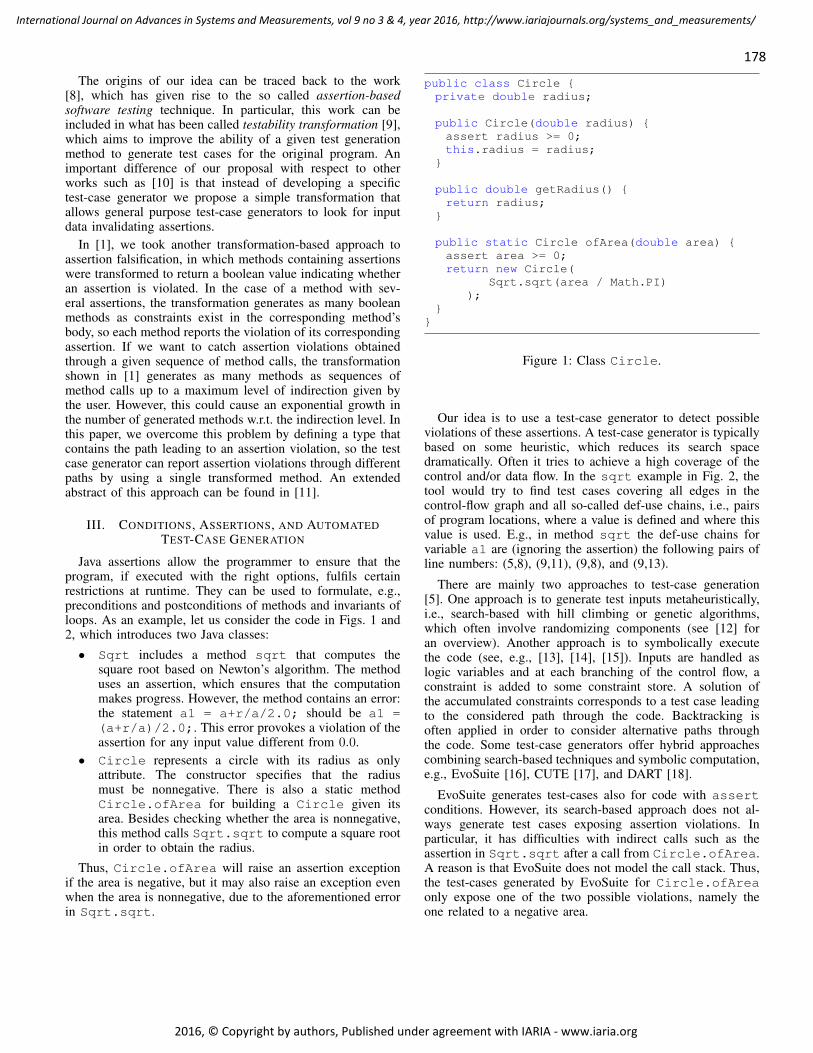
178



The origins of our idea can be traced back to the work[8], which has given rise to the so called assertion-basedsoftware testing technique. In particular, this work can beincluded in what has been called testability transformation [9],which aims to improve the ability of a given test generationmethod to generate test cases for the original program. Animportant difference of our proposal with respect to otherworks such as [10] is that instead of developing a specifictest-case generator we propose a simple transformation thatallows general purpose test-case generators to look for inputdata invalidating assertions.

In [1], we took another transformation-based approach toassertion falsification, in which methods containing assertionswere transformed to return a boolean value indicating whetheran assertion is violated. In the case of a method with sev-eral assertions, the transformation generates as many booleanmethods as constraints exist in the corresponding method’sbody, so each method reports the violation of its correspondingassertion. If we want to catch assertion violations obtainedthrough a given sequence of method calls, the transformationshown in [1] generates as many methods as sequences ofmethod calls up to a maximum level of indirection given bythe user. However, this could cause an exponential growth inthe number of generated methods w.r.t. the indirection level. Inthis paper, we overcome this problem by defining a type thatcontains the path leading to an assertion violation, so the testcase generator can report assertion violations through differentpaths by using a single transformed method. An extendedabstract of this approach can be found in [11].

III. CONDITIONS, ASSERTIONS, AND AUTOMATEDTEST-CASE GENERATION

Java assertions allow the programmer to ensure that theprogram, if executed with the right options, fulfils certainrestrictions at runtime. They can be used to formulate, e.g.,preconditions and postconditions of methods and invariants ofloops. As an example, let us consider the code in Figs. 1 and2, which introduces two Java classes:

• Sqrt includes a method sqrt that computes thesquare root based on Newton’s algorithm. The methoduses an assertion, which ensures that the computationmakes progress. However, the method contains an error:the statement a1 = a+r/a/2.0; should be a1 =(a+r/a)/2.0;. This error provokes a violation of theassertion for any input value different from 0.0.

• Circle represents a circle with its radius as onlyattribute. The constructor specifies that the radiusmust be nonnegative. There is also a static methodCircle.ofArea for building a Circle given itsarea. Besides checking whether the area is nonnegative,this method calls Sqrt.sqrt to compute a square rootin order to obtain the radius.

Thus, Circle.ofArea will raise an assertion exceptionif the area is negative, but it may also raise an exception evenwhen the area is nonnegative, due to the aforementioned errorin Sqrt.sqrt.

public class Circle {private double radius;

public Circle(double radius) {assert radius >= 0;this.radius = radius;

}

public double getRadius() {return radius;

}

public static Circle ofArea(double area) {assert area >= 0;return new Circle(

Sqrt.sqrt(area / Math.PI));

}}

Figure 1: Class Circle.

Our idea is to use a test-case generator to detect possibleviolations of these assertions. A test-case generator is typicallybased on some heuristic, which reduces its search spacedramatically. Often it tries to achieve a high coverage of thecontrol and/or data flow. In the sqrt example in Fig. 2, thetool would try to find test cases covering all edges in thecontrol-flow graph and all so-called def-use chains, i.e., pairsof program locations, where a value is defined and where thisvalue is used. E.g., in method sqrt the def-use chains forvariable a1 are (ignoring the assertion) the following pairs ofline numbers: (5,8), (9,11), (9,8), and (9,13).

There are mainly two approaches to test-case generation[5]. One approach is to generate test inputs metaheuristically,i.e., search-based with hill climbing or genetic algorithms,which often involve randomizing components (see [12] foran overview). Another approach is to symbolically executethe code (see, e.g., [13], [14], [15]). Inputs are handled aslogic variables and at each branching of the control flow, aconstraint is added to some constraint store. A solution ofthe accumulated constraints corresponds to a test case leadingto the considered path through the code. Backtracking isoften applied in order to consider alternative paths throughthe code. Some test-case generators offer hybrid approachescombining search-based techniques and symbolic computation,e.g., EvoSuite [16], CUTE [17], and DART [18].

EvoSuite generates test-cases also for code with assertconditions. However, its search-based approach does not al-ways generate test cases exposing assertion violations. Inparticular, it has difficulties with indirect calls such as theassertion in Sqrt.sqrt after a call from Circle.ofArea.A reason is that EvoSuite does not model the call stack. Thus,the test-cases generated by EvoSuite for Circle.ofAreaonly expose one of the two possible violations, namely theone related to a negative area.

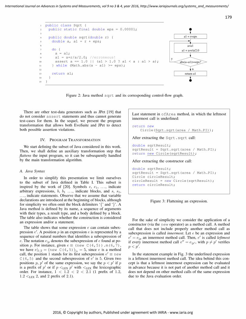
179



1 public class Sqrt {2 public static final double eps = 0.00001;3

4 public double sqrt(double r) {5 double a, a1 = r + eps;6

7 do {8 a = a1;9 a1 = a+r/a/2.0; //erroneous!

10 assert a == 1.0 || (a1 > 1.0 ? a1 < a : a1 > a);11 } while (Math.abs(a - a1) >= eps);12

13 return a1;14 }15 }

a1 = a+r/a/2.0

a1 = r+eps

a=a1

abs(a−a1)>=eps?y

n

return a1

Figure 2: Java method sqrt and its corresponding control-flow graph.

There are other test-data generators such as JPet [19] thatdo not consider assert statements and thus cannot generatetest-cases for them. In the sequel, we present the programtransformation that allows both EvoSuite and JPet to detectboth possible assertion violations.

IV. PROGRAM TRANSFORMATION

We start defining the subset of Java considered in this work.Then, we shall define an auxiliary transformation step thatflattens the input program, so it can be subsequently handledby the main transformation algorithm.

A. Java Syntax

In order to simplify this presentation we limit ourselvesto the subset of Java defined in Table I. This subset isinspired by the work of [20]. Symbols e, e1, . . . , indicatearbitrary expressions, b, b1 . . . , indicate blocks, and s, s1,. . . , indicate statements. Observe that we assume that variabledeclarations are introduced at the beginning of blocks, althoughfor simplicity we often omit the block delimiters ‘{’ and ‘}’. AJava method is defined by its name, a sequence of argumentswith their types, a result type, and a body defined by a block.The table also indicates whether the construction is consideredan expression and/or a statement.

The table shows that some expression e can contain subex-pression e′. A position p in an expression e is represented by asequence of natural numbers that identifies a subexpression ofe. The notation e|p denotes the subexpression of e found at po-sition p. For instance, given e ≡ (new C(4,5)).m(6,7),we have e|1.2 = (new C(4,5))|2 = 5, since e is a methodcall, the position 1 stands for its first subexpression e′ ≡ newC(4,5) and the second subexpression of e′ is 5. Given twopositions p, p′ of the same expression, we say the p < p′ if pis a prefix of p′ or if p <LEX p′ with <LEX the lexicographicorder. For instance, 1 < 1.2 < 2 < 2.1 (1 prefix of 1.2,1.2 <LEX 2, and 2 prefix of 2.1).

Last statement in ofArea method, in which the leftmostinnermost call is underlined:

return newCircle(Sqrt.sqrt(area / Math.PI));

After extracting the Sqrt.sqrt call:

double sqrtResult;sqrtResult = Sqrt.sqrt(area / Math.PI);return new Circle(sqrtResult);

After extracting the constructor call:

double sqrtResult;sqrtResult = Sqrt.sqrt(area / Math.PI);Circle circleResult;circleResult = new Circle(sqrtResult);return circleResult;

Figure 3: Flattening an expression.

For the sake of simplicity we consider the application of aconstructor (via the new operator) as a method call. A methodcall that does not include properly another method call assubexpression is called innermost. Let e be an expression ande′ = e|p an innermost method call. Then, e′ is called leftmostif every innermost method call e′′ = e|p′ , with p 6= p′ verifiesp < p′.

In the statement example in Fig. 3 the underlined expressionis a leftmost innermost method call. The idea behind this con-cept is that a leftmost innermost expression can be evaluatedin advance because it is not part of another method call and itdoes not depend on other method calls of the same expressiondue to the Java evaluation order.

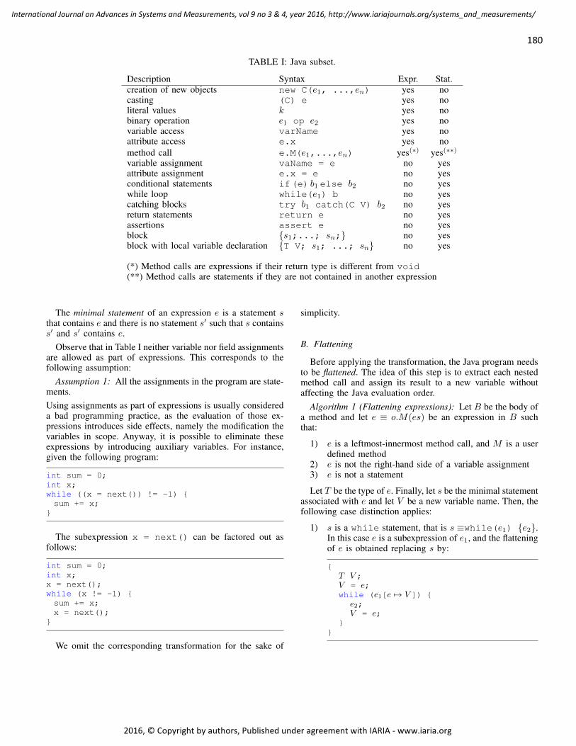
180



TABLE I: Java subset.

Description Syntax Expr. Stat.creation of new objects new C(e1, ...,en) yes nocasting (C) e yes noliteral values k yes nobinary operation e1 op e2 yes novariable access varName yes noattribute access e.x yes nomethod call e.M(e1,...,en) yes(∗) yes(∗∗)variable assignment vaName = e no yesattribute assignment e.x = e no yesconditional statements if(e) b1 else b2 no yeswhile loop while(e1) b no yescatching blocks try b1 catch(C V) b2 no yesreturn statements return e no yesassertions assert e no yesblock {s1;...; sn;} no yesblock with local variable declaration {T V; s1; ...; sn} no yes

(*) Method calls are expressions if their return type is different from void(**) Method calls are statements if they are not contained in another expression

The minimal statement of an expression e is a statement sthat contains e and there is no statement s′ such that s containss′ and s′ contains e.

Observe that in Table I neither variable nor field assignmentsare allowed as part of expressions. This corresponds to thefollowing assumption:

Assumption 1: All the assignments in the program are state-ments.Using assignments as part of expressions is usually considereda bad programming practice, as the evaluation of those ex-pressions introduces side effects, namely the modification thevariables in scope. Anyway, it is possible to eliminate theseexpressions by introducing auxiliary variables. For instance,given the following program:

int sum = 0;int x;while ((x = next()) != -1) {sum += x;

}

The subexpression x = next() can be factored out asfollows:

int sum = 0;int x;x = next();while (x != -1) {sum += x;x = next();

}

We omit the corresponding transformation for the sake of

simplicity.

B. Flattening

Before applying the transformation, the Java program needsto be flattened. The idea of this step is to extract each nestedmethod call and assign its result to a new variable withoutaffecting the Java evaluation order.

Algorithm 1 (Flattening expressions): Let B be the body ofa method and let e ≡ o.M(es) be an expression in B suchthat:

1) e is a leftmost-innermost method call, and M is a userdefined method

2) e is not the right-hand side of a variable assignment3) e is not a statement

Let T be the type of e. Finally, let s be the minimal statementassociated with e and let V be a new variable name. Then, thefollowing case distinction applies:

1) s is a while statement, that is s ≡while(e1) {e2}.In this case e is a subexpression of e1, and the flatteningof e is obtained replacing s by:

{T V ;V = e;while (e1[e 7→ V ]) {

e2;V = e;

}}

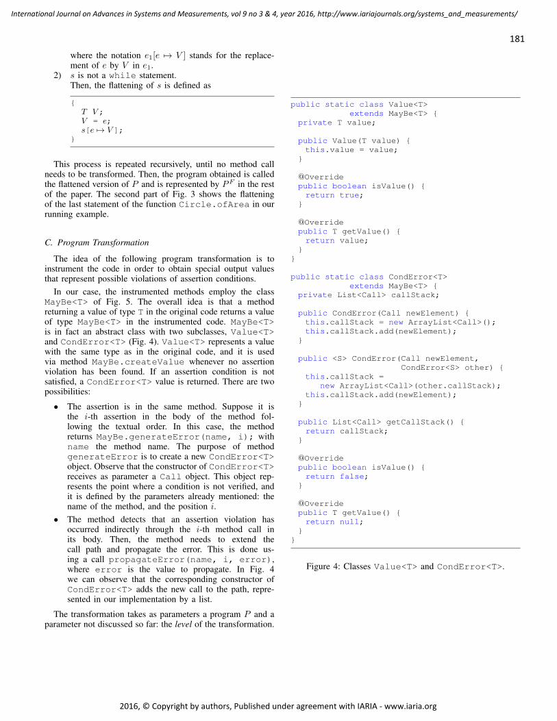
181



where the notation e1[e 7→ V ] stands for the replace-ment of e by V in e1.

2) s is not a while statement.Then, the flattening of s is defined as

{T V ;V = e;s[e 7→ V ];

}

This process is repeated recursively, until no method callneeds to be transformed. Then, the program obtained is calledthe flattened version of P and is represented by PF in the restof the paper. The second part of Fig. 3 shows the flatteningof the last statement of the function Circle.ofArea in ourrunning example.

C. Program Transformation

The idea of the following program transformation is toinstrument the code in order to obtain special output valuesthat represent possible violations of assertion conditions.

In our case, the instrumented methods employ the classMayBe<T> of Fig. 5. The overall idea is that a methodreturning a value of type T in the original code returns a valueof type MayBe<T> in the instrumented code. MayBe<T>is in fact an abstract class with two subclasses, Value<T>and CondError<T> (Fig. 4). Value<T> represents a valuewith the same type as in the original code, and it is usedvia method MayBe.createValue whenever no assertionviolation has been found. If an assertion condition is notsatisfied, a CondError<T> value is returned. There are twopossibilities:

• The assertion is in the same method. Suppose it isthe i-th assertion in the body of the method fol-lowing the textual order. In this case, the methodreturns MayBe.generateError(name, i); withname the method name. The purpose of methodgenerateError is to create a new CondError<T>object. Observe that the constructor of CondError<T>receives as parameter a Call object. This object rep-resents the point where a condition is not verified, andit is defined by the parameters already mentioned: thename of the method, and the position i.

• The method detects that an assertion violation hasoccurred indirectly through the i-th method call inits body. Then, the method needs to extend thecall path and propagate the error. This is done us-ing a call propagateError(name, i, error),where error is the value to propagate. In Fig. 4we can observe that the corresponding constructor ofCondError<T> adds the new call to the path, repre-sented in our implementation by a list.

The transformation takes as parameters a program P and aparameter not discussed so far: the level of the transformation.

public static class Value<T>extends MayBe<T> {

private T value;

public Value(T value) {this.value = value;

}

@Overridepublic boolean isValue() {return true;

}

@Overridepublic T getValue() {return value;

}}

public static class CondError<T>extends MayBe<T> {

private List<Call> callStack;

public CondError(Call newElement) {this.callStack = new ArrayList<Call>();this.callStack.add(newElement);

}

public <S> CondError(Call newElement,CondError<S> other) {

this.callStack =new ArrayList<Call>(other.callStack);

this.callStack.add(newElement);}

public List<Call> getCallStack() {return callStack;

}

@Overridepublic boolean isValue() {return false;

}

@Overridepublic T getValue() {return null;

}}

Figure 4: Classes Value<T> and CondError<T>.

182



public abstract class MayBe<T> {

public static class Value<T> extends MayBe<T> {//→ Fig. 4}

public static class CondError<T> extends MayBe<T> {//→ Fig. 4}

// did the method return a normal value (no violation)?abstract public boolean isValue();

// value returned by the method.abstract public T getValue();

// called if no condition violation detected. Return same value as before the instrumentation.public static <K> MayBe<K> createValue(K value) {return new Value<K>(value);

}

// called if an assert condition is not verified.public static <T> MayBe<T> generateError(String method, int position) {return new CondError<T>(new Call(method, position));

}

// calls another method whose assertion is not satisfied.public static <T,S> MayBe<T> propagateError(String method, int position, MayBe<S> error){return new CondError<T>(new Call(method, position), (CondError<S>) error);

}}

Figure 5: Class MayBe<T>: New result type for instrumented methods.

This parameter is determined by the user and indicates themaximum depth of the instrumentation. If level = 0 then onlythe methods including assertions are instrumented. This meansthat the tests will be obtained independently of the method callsperformed in the rest of the program. If level = 1, then all themethods that include a call to a method with assertions arealso instrumented, checking if there is an indirect conditionviolation and thus a propagation of the error is required.Greater values for level enable more levels of indirection, andthus allow to find errors occurring in a more specific programcontext.

The algorithm can be summarized as follows:Algorithm 2:

Input: P , a Java Program verifying Assumption 1 (all theassignments in the program are statements), and an integerlevel ≥ 0.Output: a transformed program PT

1) Flatten P delivering PF as explained in Section IV-B.2) Make a copy of each of the methods to instrument by

replacing the result type by MayBe, as described inAlgorithm 3. Call the new program PC .

3) Replace assertions in PC by new code that generates anerror if the assertion condition is not met, as explainedin Algorithm 4. This produces a new program P0 anda list of methods L0.

4) For k = 1 to level : apply Algorithm 5 to P , Pk−1,

and Lk−1. Call the resulting program Pk and list Lk,respectively.

5) Apply your favourite automatic test-data generator toobtain test cases for the methods in Llevel with re-spect to Plevel . Look for the test cases that produceCondError values. Executing the test case with re-spect to the original program P produces an assertionviolation and thus the associated exception displays thetrace of method calls that lead to the error, which cor-reponds to the path contained within the CondErrorobject.

Now we need to introduce algorithms 3, 4, and 5.We assume as convention that it is possible to generate a

new method name M ′ and a new attribute name MA givena method name M . Moreover, we assume that the mappingbetween ‘old’ and ‘new’ names is one-to-one, which allows toextract name M both from M ′ and from MA.

Algorithm 3:Input: flat Java program PF verifying Assumption 1.Output: transformed program PCopy with copies of the methods.

1) Let PCopy := PF .2) For each method (not constructor) C.M in PF with

result type T :a) Include in class C of PCopy a new method C.M ′

with the same body and arguments as C.M , butwith return type MayBe<T>

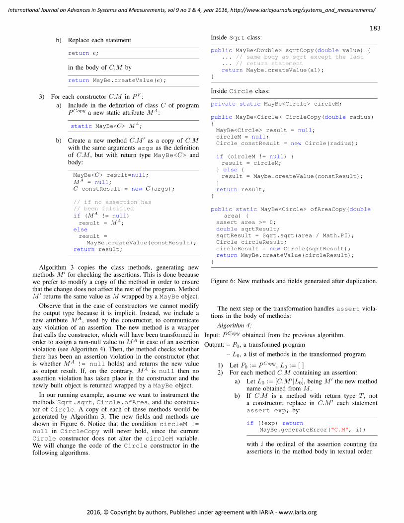
183



b) Replace each statement

return e;

in the body of C.M by

return MayBe.createValue(e);

3) For each constructor C.M in PF :a) Include in the definition of class C of program

PCopy a new static attribute MA:

static MayBe<C> MA;

b) Create a new method C.M ′ as a copy of C.Mwith the same arguments args as the definitionof C.M , but with return type MayBe<C> andbody:

MayBe<C> result=null;MA = null;C constResult = new C(args);

// if no assertion has// been falsifiedif (MA != null)result = MA;

elseresult =

MayBe.createValue(constResult);return result;

Algorithm 3 copies the class methods, generating newmethods M ′ for checking the assertions. This is done becausewe prefer to modify a copy of the method in order to ensurethat the change does not affect the rest of the program. MethodM ′ returns the same value as M wrapped by a MayBe object.

Observe that in the case of constructors we cannot modifythe output type because it is implicit. Instead, we include anew attribute MA, used by the constructor, to communicateany violation of an assertion. The new method is a wrapperthat calls the constructor, which will have been transformed inorder to assign a non-null value to MA in case of an assertionviolation (see Algorithm 4). Then, the method checks whetherthere has been an assertion violation in the constructor (thatis whether MA != null holds) and returns the new valueas output result. If, on the contrary, MA is null then noassertion violation has taken place in the constructor and thenewly built object is returned wrapped by a MayBe object.

In our running example, assume we want to instrument themethods Sqrt.sqrt, Circle.ofArea, and the construc-tor of Circle. A copy of each of these methods would begenerated by Algorithm 3. The new fields and methods areshown in Figure 6. Notice that the condition circleM !=null in CircleCopy will never hold, since the currentCircle constructor does not alter the circleM variable.We will change the code of the Circle constructor in thefollowing algorithms.

Inside Sqrt class:

public MayBe<Double> sqrtCopy(double value) {... // same body as sqrt except the last... // return statementreturn Maybe.createValue(a1);

}

Inside Circle class:

private static MayBe<Circle> circleM;

public MayBe<Circle> CircleCopy(double radius){MayBe<Circle> result = null;circleM = null;Circle constResult = new Circle(radius);

if (circleM != null) {result = circleM;

} else {result = Maybe.createValue(constResult);

}return result;

}

public static MayBe<Circle> ofAreaCopy(doublearea) {

assert area >= 0;double sqrtResult;sqrtResult = Sqrt.sqrt(area / Math.PI);Circle circleResult;circleResult = new Circle(sqrtResult);return MayBe.createValue(circleResult);

}

Figure 6: New methods and fields generated after duplication.

The next step or the transformation handles assert viola-tions in the body of methods:

Algorithm 4:Input: PCopy obtained from the previous algorithm.Output: – P0, a transformed program

– L0, a list of methods in the transformed program

1) Let P0 := PCopy , L0 := [ ]2) For each method C.M containing an assertion:

a) Let L0 := [C.M ′|L0], being M ′ the new methodname obtained from M .

b) If C.M is a method with return type T , nota constructor, replace in C.M ′ each statementassert exp; by:

if (!exp) returnMayBe.generateError("C.M", i);

with i the ordinal of the assertion counting theassertions in the method body in textual order.

184



c) If C.M is a constructor, replace in C.M eachstatement assert exp; by:

if (!exp) MA =MayBe.generateError("C.M", i);

with i as in the case of a non-constructor.

In our running example, we get L0 = [Sqrt.sqrtCopy,Circle.CircleCopy, Circle.ofAreaCopy], whichare the new names introduced by our transformation for themethods with assertions. In Sqrt.sqrtCopy the assertstatement would be replaced by the following,

...if (!(a == 1.0 ||

(a1 > 1.0 ? a1 < a : a1 > a)))return MayBe.generateError("sqrt", 1);

...

whereas in Circle the transformation would affect the con-structor and the ofAreaCopy method:

public Circle(double radius) {if (!(radius >= 0)) {

circleM = MayBe.generateError("Circle", 1);return;

}this.radius = radius;

}

public static MayBe<Circle> ofAreaCopy(doublearea) {

if (!(area >= 0))return MayBe.generateError("ofArea", 1);

...}

Finally, the last transformation focuses on indirect calls. Theinput list L contains the names of all the new methods alreadyincluded in the program. If L contains a method call C.M ′,then the algorithm looks for methods D.L that include callsof the form C.M(args). The call is replaced by a call toC.M ′ and the new value is returned. A technical detail is thatin the new iteration we keep the input methods that have nomore calls, although they do not reach the level of indirectionrequired. The level must be understood as a maximum.

Algorithm 5:Input: – P , a Java flat Program verifying Assumption 1

– Pk−1, the program obtained in the previous phase– A list Lk−1 of method names in Pk−1

Output: – Pk, a transformed program– Lk, a list of methods in the Pk

1) Let Pk := Pk−1, Lk := Lk−12) For each method D.L in P including a call x = C.M

with C.M such that C.M ′ is in Lk−1:a) Let i be the ordinal of the method call in the

method body and y a new variable name’

public class Sqrt {public static final double eps = 0.000001;

public static double sqrt(double r) { ... }

public static MayBe<Double> sqrtCopy(doubler) {

double a, a1 = 1.0;a = a1;a1 = a+r/a/2.0;double aux = Math.abs(a-a1);while (aux >= eps) {a = a1;a1 = a+r/a/2.0;if (!(a == 1.0 ||

(a1 > 1.0 ? a1 < a : a1 > a)))return MayBe.generateError("sqrt", 1);

aux = Math.abs(a - a1);}return MayBe.createValue(a1);

}}

Figure 7: Sqrt class after transformation.

b) If C.M ′ is in Lk, then remove it from Lk.c) Let Lk := [D.L′|Lk]d) If D.L is a method of type T , not a constructor

then replace in D.M ′ the selected call to x =C.M by:

MayBe<T> y = C.M ′;if (!y.isValue()) return

MayBe.propagateError("D.L", i, y);x = y.getValue();

e) If D.L is a constructor, then let x′ be a newvariable name. Replace in the constructor D.Lthe selected call to x = C.M by:

MayBe<T> y = C.M ′;if (!y.isValue()) MA =

MayBe.propagateError("D.L", i, y);x = y.getValue();

where MA is the static variable associated to theconstructor and introduced in Algorithm 3.

In our example, we have L1 = L0 since the only indirect callto a method in L0 is by means of Circle.ofAreaCopy,but the latter is already in the list. In fact, Lk = L0 for everyk > 0.

The transformation of our running example can be found inFigs. 7 and 8. It can be observed that in practice the methodsnot related directly nor indirectly to an assertion do not needto be modified. This is the case of the getRadius method.

185



public class Circle {private double radius;private static MayBe<Circle> circleM;

public Circle(double radius) {if (!(radius >= 0)) {circleM =MayBe.generateError("Circle", 1);

return;}this.radius = radius;

}

public MayBe<Circle> CircleCopy(doubleradius)

{MayBe<Circle> result = null;circleM = null;Circle constResult = new Circle(radius);

if (circleM != null) {result = circleM;

} else {result = Maybe.createValue(constResult);

}return result;

}

public double getRadius() {return radius;

}

public static Circle ofArea(double area) {...

}

public static MayBe<Circle>ofAreaCopy(double area) {

if (!(area >= 0))return MayBe.generateError("ofArea", 1);

MayBe<Double> sqrtResultM;sqrtResultM = Sqrt.sqrtCopy(area /

Math.PI);if (!sqrtResultM.isValue())return MayBe.propagateError("ofArea", 2,

sqrtResultM);double sqrtResult = sqrtResultM.getValue();

MayBe<Circle> circleResultM;circleResultM = CircleCopy(sqrtResult);if (!circleResultM.isValue()) {return MayBe.propagateError("ofArea", 3,

circleResultM);}Circle circleResult =

circleResultM.getValue();return MayBe.createValue(circleResult);

}}

Figure 8: Circle class after transformation.

Class Aint m()

Class B@Override int m()

Class C@Override int m()

Class D

Class E Class F@Override int m()

Figure 9: Inheritance example.

V. INHERITANCE

Inheritance poses a new interesting challenge to our pro-posal. Consider the hierarchy shown in Fig. 9, in which weassume that the implementation of m() in B contains anassertion, and hence, it is transformed according to Algorithm4. If there are neither assertions nor calls to B.m() in theremaining classes of the hierarchy, it seems that there isno further transformations to apply. However, assume thefollowing method:

public int foo(A a) {return a.m();

}

If we have the call foo(new B(..)) then it becomesapparent that foo() can raise an assertion due to dynamicdispatching, because the call a.m() corresponds in thiscontext to a call to B.m(). Thus, in order to detect thispossible assertion violation, foo() needs to be transformedby introducing a fooCopy() method containing a call toa.mCopy() in its body. In turn, this implies that class A mustcontain a method mCopy() as well. Therefore, we create amethod mCopy() in A with the following implementation:

public MayBe<Integer> mCopy() {return MayBe.createValue(m());

}

which wraps the result of m() into a MayBe value. Thiswrapper implementation must be replicated in classes C and Fas well, since they also override m().

In general, whenever we create a copy of a method C.M , wehave to create a copy method with the wrapper implementationin the class where M is defined for the first time in the classhierarchy, and in each descendant C ′ of C overriding M unlessthere is another class between C and C ′ in the hierarchy which

186



TABLE II: Detecting assertion violations.

EvoSuite JPetMethod Total P PT P PT

Circle.ofArea 2 1 2 0 2BloodDonor.canGiveBlood 2 0 2 0 2TestTree.insertAndFind 2 0 2 0 2Kruskal 1 1 1 0 1Numeric.foo 2 1 2 0 2TestLibrary.test* 5 0 5 0 5MergeSort.TestMergeSort 2 0 1 0 1java.util.logging.* 5 0 2 - -

also overrides M , or C ′ already has a copy M ′ of the methodM (e.g., because C ′.M contains another assertion). In theexample of Fig. 9, this means that we need to create additionalmCopy() methods in classes A, C, and F.

An obvious limitation is when we introduce an assertionin methods defined in a library class such as Object (forinstance, when overriding method toString), since wecannot introduce new methods in these classes. Fortunately,introducing assertions when overriding library methods is quiteunusual. A possible improvement, still under development, isto look in advance for polymorphic calls. For instance, maybemethod foo() is never called with arguments of type C inthe program and there is no need of transforming this class.

VI. EXPERIMENTS

We observed the effects of the transformation by meansof experiments, including the running example shown above,the implementation of the binary tree data structure, Kruskal’salgorithm, the computation of the mergesort method, a con-structed example with nested if-statements called Numeric, anexample representing a blood donation scenario BloodDonorand two bigger examples, namely a self devised Library sys-tem, which allows customers to lend and return books and the6500 lines of code of the package java.util.logging of the JavaDevelopment Kit 6 (JDK). In all the cases, the transformationhas been applied with level infinite, i.e., application of thetransformation until a fixed point is reached. In the next step,we have evaluated the examples with different test-case genera-tors with and without our level=1 program transformation.We have developed a prototype that performs this transfor-mation automatically. It can be found at https://github.com/wwu-ucm/assert-transformer, whereas the aforementioned ex-amples can be found at https://github.com/wwu-ucm/examples.

We have used two test-case generators, JPet and EvoSuite,for exposing possible assertion violations. First of all, we cannote that our approach works. In our experiments, all but onepossible assertion violation could be detected. Moreover, wecan note that our program transformation typically improvesthe detection rate, as can be seen in Table II. In this table,column Total displays for each example the number of pos-sible assertion violations that can be raised for the method.Column P shows the number of detected assertion viola-tions using the test-case generator and the original program,while column PT displays the number of detected assertion

violations after applying the transformation. For instance, inour running example, Circle.getRadius can raise thetwo assertion violations explained in Section III. Withoutthe transformation, only one assertion violation is found byEvoSuite. With the transformation, EvoSuite correctly detectsboth assertion violations. For JPet no test cases are created forjava.util.logging, since JPet does not support librarymethod calls. Notice that JPet cannot find any assertion vi-olation without our transformation, since it does not supportassertions. Thus, our transformation is essential for tools, thatdo not support assertions, such as jPet. An improvement in theassertion violation detection rate is observed for all examples.

Additionally, tools that already support assertions to somedegree benefit from our program transformation, since it makesthe control flow more explicit than the usual assertion-violationexceptions. This helps the test-case generators to reach ahigher coverage, as can be seen in Table III. The dashes inthe JPet row indicate that JPet does not support assertionsand hence cannot be used to detect assertion violations inthe untransformed program. Our program transformation oftenonly requires a few seconds and even for larger programs suchas the JDK 6 logging package the transformation finishes in18.2 seconds. The runtime of our analysis depends on theemployed test-case generator and the considered example. Itcan range from a few seconds to several minutes.

VII. CONCLUSIONS

We have presented an approach to use test-case generatorsfor exposing possible assertion violations in Java programs.Our approach is a compromise between the usual detectionof assertion violations at runtime and the use of a full modelchecker. Since test-case generators are guided by heuristicssuch as control- and data-flow coverage, they have to considera much smaller search space than a model checker and canhence deliver results much more quickly. If the coverage ishigh, the analysis is nevertheless quite accurate and useful inpractice; in particular, in situations where a model checkerwould require too much time. We tried to use the modelchecker Java Pathfinder [21] to our examples, but we had togive up, since this tool was too time consuming or stoppedbecause of a lack of memory.

Additionally, we have developed a program transformationthat replaces assertions by computations, which explicitlypropagate violation information through an ordinary computa-tion involving nested method calls. The result of a computationis encapsulated in an object. The type of this object indicateswhether the computation was successful or whether it causedan assertion violation. In case of a violation, our transformationmakes the control flow more explicit than the usual assertion-violation exceptions. This helps the test-case generators toreach a higher coverage of the code and enables more asser-tion violations to be exposed and detected. Additionally, thetransformation allows to use test-case generators such as JPet,which do not support assertions.

We have presented some experimental results demonstratingthat our approach helps indeed to expose assertion violations

187



TABLE III: Control and data-flow coverage in percent.

Binary Blood Kruskal Library MergeSort Numeric StdDev CircleTree Donor

P PT P PT P PT P PT P PT P PT P PT P PT

EvoSuite 90 95 83 91 95 100 63 92 82 82 76 82 71 71 80 100JPet – 89 – 99 – 49 – 20 – 87 – 82 – 74 – 100

and that our program transformation improves the detectionrate.

Although our approach accounts for the call path that leadsto an assertion violation, this path is represented as a chainof object references, so some test case generators might notbe able to recreate it in their generated tests. We are studyingan alternative transformation that represents the call path interms of basic Java data types. Another subject of future workis to use the information provided by a dependency graph ofmethod calls in order to determine the maximum call depthlevel where the transformation can be applied.

ACKNOWLEDGMENT

This work has been supported by the German Aca-demic Exchange Service (DAAD, 2014 Competitive callRef. 57049954), the Spanish MINECO project CAVI-ART (TIN2013-44742-C4-3-R), Madrid regional project N-GREENS Software-CM (S2013/ICE-2731) and UCM grantGR3/14-910502.

REFERENCES

[1] R. Caballero, M. Montenegro, H. Kuchen, and V. von Hof, “Automaticfalsification of Java assertions,” in Proceedings of the 7th InternationalConference in Advances in System Testing and Validation Lifecycle(VALID 2015), T. Kanstren and B. Gersbeck-Schierholz, Eds. IARIA,2015, pp. 36–41.

[2] B. Meyer, Object-oriented Software Construction (2Nd Ed.), 2nd ed.Upper Saddle River, NJ, USA: Prentice-Hall, Inc., 1997.

[3] R. Mitchell, J. McKim, and B. Meyer, Design by Contract, by Example.Redwood City, CA, USA: Addison Wesley Longman Publishing Co.,Inc., 2002.

[4] Oracle, “Programming With Assertions,”http://docs.oracle.com/javase/7/docs/technotes/guides/language/assert.html, Retrieved: 8 January 2017.

[5] S. Anand, E. Burke, T. Y. Chen, J. Clark, M. B. Cohen, W. Grieskamp,M. Harman, M. J. Harrold, and P. McMinn, “An orchestrated surveyon automated software test case generation,” Journal of Systems andSoftware, vol. 86, no. 8, August 2013, pp. 1978–2001.

[6] W. Visser, K. Havelund, G. Brat, S. Park, and F. Lerda, “Model checkingprograms,” Automated Software Engineering, vol. 10, no. 2, 2003, pp.203–232.

[7] M. Utting, A. Pretschner, and B. Legeard, “A taxonomy of model-basedtesting approaches,” Softw. Test. Verif. Reliab., vol. 22, no. 5, Aug.2012, pp. 297–312. [Online]. Available: http://dx.doi.org/10.1002/stvr.456

[8] B. Korel and A. M. Al-Yami, “Assertion-oriented automated test datageneration,” in Proceedings of the 18th International Conference onSoftware Engineering, ser. ICSE ’96. Washington, DC, USA: IEEEComputer Society, 1996, pp. 71–80.

[9] M. Harman, A. Baresel, D. Binkley, R. Hierons, L. Hu, B. Korel,P. McMinn, and M. Roper, “Testability transformation program trans-formation to improve testability,” in Formal Methods and Testing,ser. Lecture Notes in Computer Science, R. Hierons, J. Bowen, andM. Harman, Eds. Springer Berlin Heidelberg, 2008, vol. 4949, pp.320–344.

[10] C. Boyapati, S. Khurshid, and D. Marinov, “Korat: Automated testingbased on Java predicates,” SIGSOFT Softw. Eng. Notes, vol. 27, no. 4,Jul. 2002, pp. 123–133.

[11] R. Caballero, M. Montenegro, H. Kuchen, and V. von Hof, “Checkingjava assertions using automated test-case generation,” in Proceedings ofthe 25th International Symposium on Logic-Based Program Synthesisand Transformation (LOPSTR), ser. Lecture Notes in Computer Sci-ence, M. Falaschi, Ed., vol. 9527. Springer International Publishing,2015, pp. 221–226.

[12] P. McQuinn, “Search-based software test data generation: A survey,”Software Testing, Verification and Reliability, vol. 14, no. 2, 2004, pp.105–156.

[13] J. C. King, “Symbolic execution and program testing,” Commun.ACM, vol. 19, no. 7, 1976, pp. 385–394. [Online]. Available:http://doi.acm.org/10.1145/360248.360252

[14] M. Gomez-Zamalloa, E. Albert, and G. Puebla, “Test case generationfor object-oriented imperative languages in CLP,” TPLP, vol. 10, no.4-6, 2010, pp. 659–674. [Online]. Available: http://dx.doi.org/10.1017/S1471068410000347

[15] M. Ernsting, T. A. Majchrzak, and H. Kuchen, “Dynamic solutionof linear constraints for test case generation,” in Sixth InternationalSymposium on Theoretical Aspects of Software Engineering, TASE2012, Beijing, China, 2012, pp. 271–274. [Online]. Available:http://dx.doi.org/10.1109/TASE.2012.39

[16] J. P. Galeotti, G. Fraser, and A. Arcuri, “Improving search-based testsuite generation with dynamic symbolic execution,” in IEEE Interna-tional Symposium on Software Reliability Engineering (ISSRE). IEEE,2013, pp. 360–369.

[17] K. Sen, D. Marinov, and G. Agha, “CUTE: A concolic unittesting engine for C,” in Proceedings of the 10th EuropeanSoftware Engineering Conference, ser. ESEC/FSE-13. New York,NY, USA: ACM, 2005, pp. 263–272. [Online]. Available: http://doi.acm.org/10.1145/1081706.1081750

[18] P. Godefroid, N. Klarlund, and K. Sen, “DART: directed automatedrandom testing,” in Proceedings of the ACM SIGPLAN 2005Conference on Programming Language Design and Implementation,Chicago, IL, USA, June 12-15, 2005, 2005, pp. 213–223. [Online].Available: http://doi.acm.org/10.1145/1065010.1065036

[19] E. Albert, I. Cabanas, A. Flores-Montoya, M. Gomez-Zamalloa, andS. Gutierrez, “jPET: An automatic test-case generator for Java,” in 18thWorking Conference on Reverse Engineering, WCRE 2011, Limerick,Ireland, October 17-20, 2011, 2011, pp. 441–442.

[20] G. Klein and T. Nipkow, “A machine-checked model for a Java-likelanguage, virtual machine and compiler,” vol. 28, no. 4, 2006, pp. 619–695.

[21] W. Visser, K. Havelund, G. P. Brat, S. Park, and F. Lerda, “Modelchecking programs,” Autom. Softw. Eng., vol. 10, no. 2, 2003, pp. 203–232. [Online]. Available: http://dx.doi.org/10.1023/A:1022920129859

188



Evaluation of Some Validation Measures for Gaussian Process Emulation:a Case Study with an Agent-Based Model

Wim De Mulderand Geert Molenberghs

and Geert Verbeke

Leuven Biostatistics andStatistical Bioinformatics Centre

KU Leuven and Hasselt University, BelgiumEmail: [email protected],

[email protected],[email protected]

Bernhard Rengsand Thomas Fent

Wittgenstein Centre (IIASA, VID/OAW, WU)VID/OAW

Vienna, AustriaEmail: [email protected],

[email protected]

Abstract—A common way to evaluate surrogate models is byusing validation measures. This amounts to applying a chosenvalidation measure to a test data set that was not used to trainthe surrogate model. The selection of a validation measure istypically motivated by diverse guidelines, such as simplicity ofthe measure, ease of implementation, popularity of the measure,etc., which are often not related to characteristics of the measureitself. However, it should be recognized that the validity of amodel is not only dependent on the model, as desired, but alsoon the behavior of the chosen validation measure. Some, althoughvery limited, research has been devoted to the evaluation ofvalidation measures, by applying them to a given model thatis trained on a data set with some known properties, and thenevaluating whether the considered measures validate the model inan expected way. In this paper, we perform an evaluation of somestatistical and non statistical validation measures from anotherpoint of view. We consider a test data set generated by an agent-based model and we successively remove those elements from itfor which our previously developed Gaussian process emulator, asurrogate model, produces the worst approximation to the trueoutput value, according to a selected validation measure. Allconsidered validation measures are then applied to the sequenceof increasingly smaller test data sets. It is desired that a validationmeasure shows improvement of a model when test data points onwhich the model poorly performs are removed, irrespective of thevalidation measure that is used to detect such data points. Ourexperiments show that only the considered statistical validationmeasures have this desired behavior.

Keywords–Gaussian process emulation; Agent-based models;Validation.

I. INTRODUCTION AND OUTLINE OF THE PAPER

In previous work we applied Gaussian process emulation,a surrogate model, to a training data set generated by anagent-based model that we had developed before [1]. Severalalternative implementations of the Gaussian process emulationtechnique were considered and each of these was evaluatedaccording to two different validation measures. Evaluation ofthe emulators was performed with respect to a test data set ofsize 500.

In this paper, we consider a research question that is notgiven proper attention in the literature, namely the evaluation

of validation measures themselves. Although some researchershave examined certain characteristics of validation measures,their research is typically limited to the application of severalselected validation measures to a given model that is trainedon a data set with some known properties, and then evaluatingwhether these measures are able to validate these properties,see, e.g., [2], [3], [4]. Although such research is, of course,useful, we take here another perspective on the evaluation ofvalidation measures. We consider the influence on validationmeasures when elements from the test data set are removedin the order proposed by a fixed validation measure. Thatis, we select a validation measure and we use that measureto find the element in the test data set for which a givensurrogate model produces the worst approximation. We willsimply refer to the element of a given test data set in whicha given surrogate model produces the worst approximationaccording to a given validation measure as the worst testdata point, and we will use the more vague term bad testdata point to denote a test data point in which the surrogatemodel produces a bad approximation according to the givenvalidation measure. It is then clear that the selected validationmeasure will show improvement when applied with respect tothe reduced test data set, i.e., the elements of the test data setthat remain after removing the worst test data point. However,an interesting and important research question is how the othervalidation measures will perform on the same reduced test dataset. Will they also consider the selected test data point as themost problematic and thus have improved values when theyevaluate the surrogate model on the reduced test data set? Orwill they have another view on the test data point that is tobe considered as the one where the surrogate model performsworst and, therefore, maybe even show deterioration of thesurrogate model on the reduced data set?

The operation of removing the worst test data point isthen repeatedly performed on the remaining test data set suchthat a graph of the considered validation measures results.This graph shows the evolution of the validation measures onincreasingly smaller test data sets, where each test data setin this sequence does not contain the worst test data pointof its predecessor. The whole procedure is then repeated by

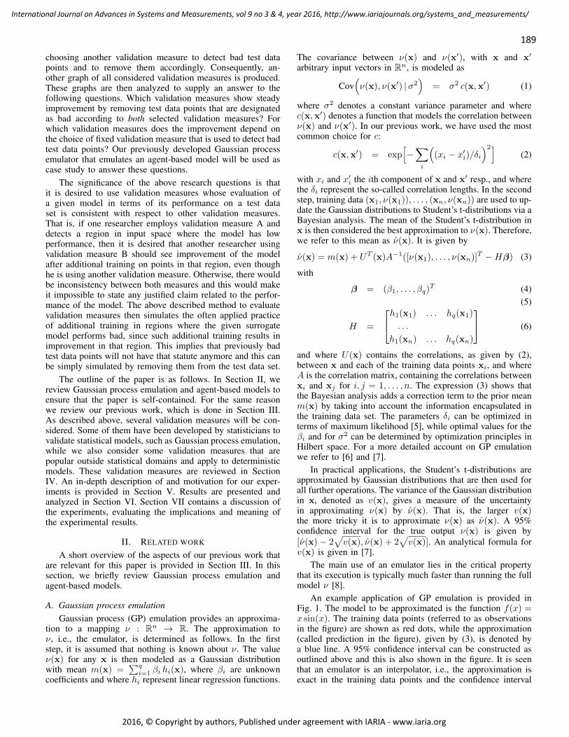
189



choosing another validation measure to detect bad test datapoints and to remove them accordingly. Consequently, an-other graph of all considered validation measures is produced.These graphs are then analyzed to supply an answer to thefollowing questions. Which validation measures show steadyimprovement by removing test data points that are designatedas bad according to both selected validation measures? Forwhich validation measures does the improvement depend onthe choice of fixed validation measure that is used to detect badtest data points? Our previously developed Gaussian processemulator that emulates an agent-based model will be used ascase study to answer these questions.

The significance of the above research questions is thatit is desired to use validation measures whose evaluation ofa given model in terms of its performance on a test dataset is consistent with respect to other validation measures.That is, if one researcher employs validation measure A anddetects a region in input space where the model has lowperformance, then it is desired that another researcher usingvalidation measure B should see improvement of the modelafter additional training on points in that region, even thoughhe is using another validation measure. Otherwise, there wouldbe inconsistency between both measures and this would makeit impossible to state any justified claim related to the perfor-mance of the model. The above described method to evaluatevalidation measures then simulates the often applied practiceof additional training in regions where the given surrogatemodel performs bad, since such additional training results inimprovement in that region. This implies that previously badtest data points will not have that statute anymore and this canbe simply simulated by removing them from the test data set.

The outline of the paper is as follows. In Section II, wereview Gaussian process emulation and agent-based models toensure that the paper is self-contained. For the same reasonwe review our previous work, which is done in Section III.As described above, several validation measures will be con-sidered. Some of them have been developed by statisticians tovalidate statistical models, such as Gaussian process emulation,while we also consider some validation measures that arepopular outside statistical domains and apply to deterministicmodels. These validation measures are reviewed in SectionIV. An in-depth description of and motivation for our exper-iments is provided in Section V. Results are presented andanalyzed in Section VI. Section VII contains a discussion ofthe experiments, evaluating the implications and meaning ofthe experimental results.

II. RELATED WORK

A short overview of the aspects of our previous work thatare relevant for this paper is provided in Section III. In thissection, we briefly review Gaussian process emulation andagent-based models.

A. Gaussian process emulationGaussian process (GP) emulation provides an approxima-

tion to a mapping ν : Rn → R. The approximation toν, i.e., the emulator, is determined as follows. In the firststep, it is assumed that nothing is known about ν. The valueν(x) for any x is then modeled as a Gaussian distributionwith mean m(x) =

∑qi=1 βi hi(x), where βi are unknown

coefficients and where hi represent linear regression functions.

The covariance between ν(x) and ν(x′), with x and x′

arbitrary input vectors in Rn, is modeled as

Cov(ν(x), ν(x′) |σ2

)= σ2 c(x,x′) (1)

where σ2 denotes a constant variance parameter and wherec(x,x′) denotes a function that models the correlation betweenν(x) and ν(x′). In our previous work, we have used the mostcommon choice for c:

c(x,x′) = exp[−∑i

((xi − x′i)/δi

)2](2)

with xi and x′i the ith component of x and x′ resp., and wherethe δi represent the so-called correlation lengths. In the secondstep, training data (x1, ν(x1)), . . . , (xn, ν(xn)) are used to up-date the Gaussian distributions to Student’s t-distributions via aBayesian analysis. The mean of the Student’s t-distribution inx is then considered the best approximation to ν(x). Therefore,we refer to this mean as ν(x). It is given by

ν(x) = m(x) + UT (x)A−1([ν(x1), . . . , ν(xn)]T −Hβ) (3)

with

β = (β1, . . . , βq)T (4)

(5)

H =

h1(x1) . . . hq(x1)

. . .

h1(xn) . . . hq(xn)

(6)

and where U(x) contains the correlations, as given by (2),between x and each of the training data points xi, and whereA is the correlation matrix, containing the correlations betweenxi and xj for i, j = 1, . . . , n. The expression (3) shows thatthe Bayesian analysis adds a correction term to the prior meanm(x) by taking into account the information encapsulated inthe training data set. The parameters δi can be optimized interms of maximum likelihood [5], while optimal values for theβi and for σ2 can be determined by optimization principles inHilbert space. For a more detailed account on GP emulationwe refer to [6] and [7].

In practical applications, the Student’s t-distributions areapproximated by Gaussian distributions that are then used forall further operations. The variance of the Gaussian distributionin x, denoted as v(x), gives a measure of the uncertaintyin approximating ν(x) by ν(x). That is, the larger v(x)the more tricky it is to approximate ν(x) as ν(x). A 95%confidence interval for the true output ν(x) is given by[ν(x)− 2

√v(x), ν(x) + 2

√v(x)]. An analytical formula for

v(x) is given in [7].The main use of an emulator lies in the critical property

that its execution is typically much faster than running the fullmodel ν [8].

An example application of GP emulation is provided inFig. 1. The model to be approximated is the function f(x) =x sin(x). The training data points (referred to as observationsin the figure) are shown as red dots, while the approximation(called prediction in the figure), given by (3), is denoted bya blue line. A 95% confidence interval can be constructed asoutlined above and this is also shown in the figure. It is seenthat an emulator is an interpolator, i.e., the approximation isexact in the training data points and the confidence interval

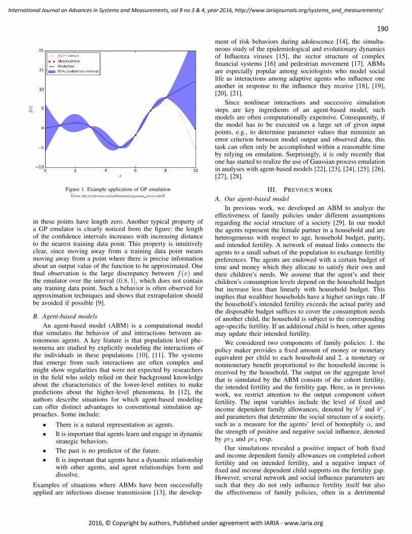
190



Figure 1. Example application of GP emulation(From http://scikit-learn.org/stable/modules/gaussian process.html)

in these points have length zero. Another typical property ofa GP emulator is clearly noticed from the figure: the lengthof the confidence intervals increases with increasing distanceto the nearest training data point. This property is intuitivelyclear, since moving away from a training data point meansmoving away from a point where there is precise informationabout an output value of the function to be approximated. Onefinal observation is the large discrepancy between f(x) andthe emulator over the interval (0.8, 1], which does not containany training data point. Such a behavior is often observed forapproximation techniques and shows that extrapolation shouldbe avoided if possible [9].

B. Agent-based modelsAn agent-based model (ABM) is a computational model

that simulates the behavior of and interactions between au-tonomous agents. A key feature is that population level phe-nomena are studied by explicitly modeling the interactions ofthe individuals in these populations [10], [11]. The systemsthat emerge from such interactions are often complex andmight show regularities that were not expected by researchersin the field who solely relied on their background knowledgeabout the characteristics of the lower-level entities to makepredictions about the higher-level phenomena. In [12], theauthors describe situations for which agent-based modelingcan offer distinct advantages to conventional simulation ap-proaches. Some include:

• There is a natural representation as agents.• It is important that agents learn and engage in dynamic

strategic behaviors.• The past is no predictor of the future.• It is important that agents have a dynamic relationship

with other agents, and agent relationships form anddissolve.

Examples of situations where ABMs have been successfullyapplied are infectious disease transmission [13], the develop-

ment of risk behaviors during adolescence [14], the simulta-neous study of the epidemiological and evolutionary dynamicsof Influenza viruses [15], the sector structure of complexfinancial systems [16] and pedestrian movement [17]. ABMsare especially popular among sociologists who model sociallife as interactions among adaptive agents who influence oneanother in response to the influence they receive [18], [19],[20], [21].

Since nonlinear interactions and successive simulationsteps are key ingredients of an agent-based model, suchmodels are often computationally expensive. Consequently, ifthe model has to be executed on a large set of given inputpoints, e.g., to determine parameter values that minimize anerror criterion between model output and observed data, thistask can often only be accomplished within a reasonable timeby relying on emulation. Surprisingly, it is only recently thatone has started to realize the use of Gaussian process emulationin analyses with agent-based models [22], [23], [24], [25], [26],[27], [28].

III. PREVIOUS WORK

A. Our agent-based modelIn previous work, we developed an ABM to analyze the

effectiveness of family policies under different assumptionsregarding the social structure of a society [29]. In our modelthe agents represent the female partner in a household and areheterogeneous with respect to age, household budget, parity,and intended fertility. A network of mutual links connects theagents to a small subset of the population to exchange fertilitypreferences. The agents are endowed with a certain budget oftime and money which they allocate to satisfy their own andtheir children’s needs. We assume that the agent’s and theirchildren’s consumption levels depend on the household budgetbut increase less than linearly with household budget. Thisimplies that wealthier households have a higher savings rate. Ifthe household’s intended fertility exceeds the actual parity andthe disposable budget suffices to cover the consumption needsof another child, the household is subject to the correspondingage-specific fertility. If an additional child is born, other agentsmay update their intended fertility.

We considered two components of family policies: 1. thepolicy maker provides a fixed amount of money or monetaryequivalent per child to each household and 2. a monetary ornonmonetary benefit proportional to the household income isreceived by the household. The output on the aggregate levelthat is simulated by the ABM consists of the cohort fertility,the intended fertility and the fertility gap. Here, as in previouswork, we restrict attention to the output component cohortfertility. The input variables include the level of fixed andincome dependent family allowances, denoted by bf and bv ,and parameters that determine the social structure of a society,such as a measure for the agents’ level of homophily α, andthe strength of positive and negative social influence, denotedby pr3 and pr4 resp.

Our simulations revealed a positive impact of both fixedand income dependent family allowances on completed cohortfertility and on intended fertility, and a negative impact offixed and income dependent child supports on the fertility gap.However, several network and social influence parameters aresuch that they do not only influence fertility itself but alsothe effectiveness of family policies, often in a detrimental

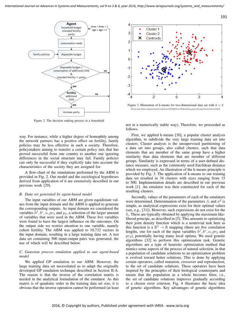
191



consumption needs

Agenthousehold budgetintended fertility

parity

disposable budget ≥ consumption of additional child

&intended fertility > parity

disposable budgetfamiliy policies

fertilityadditional

child

increase parity

yes

yes

time = time + 1age = age + 1

no

no

Figure 2. The decision making process in a household

way. For instance, while a higher degree of homophily amongthe network partners has a positive effect on fertility, familypolicies may be less effective in such a society. Therefore,policymakers aiming to transfer a certain policy mix that hasproved successful from one country to another one ignoringdifferences in the social structure may fail. Family policiescan only be successful if they explicitly take into account thecharacteristics of the society they are assigned for.

A flow-chart of the simulations performed by the ABM isprovided in Fig. 2. Our model and the sociological hypothesesderived from application of it are extensively described in ourprevious work [29].

B. Data set generated by agent-based modelThe input variables of our ABM are given equidistant val-

ues from the input domain and the ABM is applied to generatethe corresponding outputs. As input domain we considered thevariables bf , bv, α, pr3 and p4, a selection of the larger amountof variables that were used in the ABM. These five variableswere found to have the largest influence on the outcomes. Onthe output side we restrict attention to one variable, namelycohort fertility. The ABM was applied to 10,732 vectors inthe input domain, resulting in a large training data set. A testdata set containing 500 input-output pairs was generated, theuse of which will be described below.

C. Gaussian process emulation applied to our agent-basedmodel

We applied GP emulation to our ABM. However, thelarge training data set necessitated us to adapt the originallydeveloped GP emulation technique described in Section II-A.The reason is that the inverse of the correlation matrix isneeded in the analytical formulation of the emulator. As thismatrix is of quadratic order in the training data set size, it isobvious that the inverse operation cannot be performed (at least

Figure 3. Illustration of k-means for two-dimensional data set with k = 2(From http://mines.humanoriented.com/classes/2010/fall/csci568/portfolio exports/mvoget/cluster/cluster.html)

not in a numerically stable way). Therefore, we proceeded asfollows.

First, we applied k-means [30], a popular cluster analysisalgorithm, to subdivide the very large training data set intoclusters. Cluster analysis is the unsupervised partitioning ofa data set into groups, also called clusters, such that dataelements that are member of the same group have a highersimilarity than data elements that are member of differentgroups. Similarity is expressed in terms of a user-defined dis-tance measure, such as the commonly used Euclidean distancewhich we employed. An illustration of the k-means principle isprovided by Fig. 3. The application of k-means to our trainingdata set resulted in 34 clusters with sizes ranging from 15to 500. Implementation details are described in our previouswork [1]. An emulator was then constructed for each of theresulting clusters.

Secondly, values of the parameters of each of the emulatorswere determined. Determination of the parameters βi and σ2 issimple, as analytical expressions exist for their optimal values(see, e.g., [31]). However, such expressions do not exist for theδi. These are typically obtained by applying the maximum like-lihood principe, as described in [5]. This amounts to optimizingtheir joint density function which is a nontrivial task here asthis function is a R5 → R mapping (there are five correlationlengths, one for each of the input variables bf , bv, α, pr3 andpr4), potentially having many local optima. We used geneticalgorithms [32] to perform this optimization task. Geneticalgorithms are a type of heuristic optimization method thatmimics some aspects of the process of natural selection, in thata population of candidate solutions to an optimization problemis evolved toward better solutions. This is done by applyingcertain operators, called mutation, crossover and reproduction,to the set of candidate solutions. These operators have beeninspired by the principles of their biological counterparts andensure that the population as a whole becomes fitter, i.e.,the set of candidate solutions improves gradually accordingto a chosen error criterion. Fig. 4 illustrates the basic ideaof genetic algorithms. Key advantages of genetic algorithms

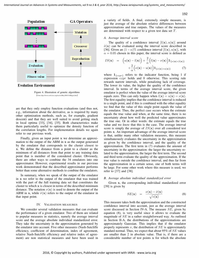
192



Figure 4. Illustration of genetic algorithms(From http://www.ewh.ieee.org/soc/es/May2001/14/Begin.htm)

are that they only employ function evaluations (and thus not,e.g., information about the derivative, as is required by manyother optimization methods, such as, for example, gradientdescent) and that they are well suited to avoid getting stuckin local optima [33], [34], [35]. Both characteristics makethem particularly useful to optimize the density function ofthe correlation lengths. For implementation details we againrefer to our previous work.

Finally, given an input point x we determine an approxi-mation to the output of the ABM in x as the output generatedby the emulator that corresponds to the cluster closest tox. We define the distance from a point to a cluster as theminimum of all distances from that point to any training datapoint that is member of the considered cluster. Obviously,there are other ways to combine the 34 emulators into oneapproximator. However, experimental results in our previouswork demonstrated that the described approximator performsbetter than some alternative methods to combine the emulators.

In summary, when we speak of the output of the emulatorin x we refer to the output of the emulator that was trainedwith the part of the full training data set that constitutes thecluster to which x is closest in terms of the described minimumdistance. The notation ν(x) is used to denote the output of theABM in x, while ν(x) refers to the output of the emulator inthat input point.

IV. VALIDATION MEASURES

We consider several validation measures that can evaluatethe performance of a given emulator. Two of them are relatedto popular measures in statistics, namely the average intervalscore and the average absolute individual standardized error.They take the uncertainty in the approximation generated bythe emulator into account. Five other measures (Nash-Sutcliffeefficiency, coefficient of determination, index of agreement,relative Nash-Sutcliffe efficiency and relative index of agree-ment) are non statistical measures and have been used in

a variety of fields. A final, extremely simple measure, isjust the average of the absolute relative differences betweenapproximations and true outputs. The values of the measuresare determined with respect to a given test data set T .

A. Average interval scoreThe quality of a confidence interval [l(x), u(x)] around

ν(x) can be evaluated using the interval score described in[36]. Given an (1−α)% confidence interval [l(x), u(x)], withα = 0.05 chosen in this paper, the interval score is defined as

IS(x) =(u(x)− l(x)

)+

2

α

(l(x)− ν(x)

)1{ν(x)<l(x)}

+2

α

(ν(x)− u(x)

)1{ν(x)>u(x)} (7)

where 1{expr} refers to the indicator function, being 1 ifexpression expr holds and 0 otherwise. This scoring rulerewards narrow intervals, while penalizing lack of coverage.The lower its value, the higher the quality of the confidenceinterval. In terms of the average interval score, the givenemulator is perfect when the value of the average interval scoreequals zero. This can only happen when l(x) = u(x) = ν(x).The first equality implies that the confidence interval is reducedto a single point, and if this is combined with the other equalitywe find that the value of this single point equals the value ofthe emulator. Thus, the perfect case occurs when the estimateequals the true value and when, at the same time, there is nouncertainty about how well the predicted value approximatesthe true one. Or in other words: the estimate equals the truevalue and we know that this is the case. The average intervalscore is simply the average of IS(x) over all considered testpoints x. An important advantage of the average interval scoreis that, unlike many other validation measures, this measuresimultaneously evaluates the uncertainty in the approximationas given by the confidence interval, and the quality of theapproximation. The first term in (7) evaluates the amount ofuncertainty in the approximation: the larger the uncertainty re-lated to the approximation, the larger the first term. The secondand third term evaluate the quality of the approximation. If thetrue value is outside the confidence interval, and thus far fromthe approximation in a certain sense, one of both terms willbe large. For some other work where this measure is used, werefer to [37] and [38].

B. Average absolute individual standardized errorGiven x, the corresponding individual standardized error

[39] is given by

SE(x) =ν(x)− ν(x)√

v(x)(8)

This measure takes both the approximation and the constructedconfidence interval into account, just as the average intervalscore discussed in Section IV-A. The measure SE, given byequation (8), is very useful since it allows to evaluate themagnitude of SE in a rather straightforward way. As outlinedin Section II-A, the distributions of the approximations areapproximately Gaussian. This implies that if the emulatorproperly represents ν, the distribution of SE is approximatelystandard normal. Thus, we expect that about 95% of SE valuesare smaller than 2 in absolute value. That is, if there are aconsiderable number of test points x for which the absolute

193



value of SE(x) is larger than 2, then this is a clear warningthat the emulator might not perform well. This convenientevaluation of a given emulator is an important advantageover the average interval score, where we do not have suchreference values. The average interval score is only usefulwhen at least two different emulators are to be compared toeach other, while SE can be used to evaluate a single emulator.On the other hand, the average interval score has the benefitof not making any assumption about the distribution of theapproximations. Taking absolute values and averaging over allconsidered test data points, we obtain our average absoluteindividual standardized error.

C. Nash-Sutcliffe efficiency

The Nash-Sutcliffe efficiency (NSE), proposed in [40], isdetermined as

NSE = 1−

∑x∈T

(ν(x)− ν(x)

)2∑

x∈T

(ν(x)− ν

)2 (9)

with ν the average of ν(x) over all elements of T . Therange of NSE lies between 1.0 (perfect fit) and -∞. AnNSE of lower than zero indicates that ν would have beena better predictor than the calculated approximations ν(x).The fact that the Nash-Sutcliffe efficiency squares differencesbetween true and estimated values implies that large valueshave large influence while small values are almost neglected,which might or might not be desired for the application athand [4]. Furthermore, while the NSE is a convenient andnormalized measure of model performance, it does not providea reliable basis for comparing the results of different casestudies [41]. Nevertheless, NSE is a popular measure for theevaluation of models, especially of hydrological models [42].

D. Coefficient of determination

The coefficient of determination r2 is the square of thePearson correlation coefficient:

r2 =

∑x∈T

(ν(x)− ν)(ν(x)− ν)√∑x∈T

(ν(x)− ν)2√∑

x∈T(ν(x)− ν)2

2

(10)

where ν refers to the averages of ν(x) over the test data points.The measure is widely applied by statisticians [43].

The values of r2 are between 0 and 1. The measuredescribes how much of the observed dispersion is explainedby the estimation. A value of zero means no correlationat all, whereas a value of 1 means that the dispersion ofthe estimations is equal to that of the true values. Althoughmany authors consider the coefficient of determination a usefulmeasure of success of predicting the dependent variable fromthe independent variables [44], the fact that only the dispersionis quantified is a major drawback of r2. A surrogate model thatsystematically over- or underestimates all the time can stillresult in good r2 values close to 1.0 even if all estimations arecritically wrong [45], [46].

E. Index of agreementThe index of agreement d was proposed in [47] to over-

come the insensitivity of NSE and r2 to differences in thetrue and estimated means and variances. It is defined as:

d = 1−

∑x∈T

(ν(x)− ν(x)

)2∑

x∈T

(|ν(x)− ν|+ |ν(x)− ν|

)2 (11)

Due to the mean square error in the numerator, d is alsovery sensitive to large values and rather insensitive to smallvalues, as is the case for NSE. The range of d is [0, 1] with 1denoting perfect fit.

Practical applications of d show that it has some disad-vantages [45]. First, relatively high values, say more than0.65, may be obtained even for poor surrogate model fits.Secondly, systematic over- or underestimation can, as withthe coefficient of determination, be masked by high valuesof d. There exist several variations on the above definition ofthe index of agreement, for example, by considering absolutedifferences instead of squared differences [48] or by removingthe approximations ν(x) from the denominator [49].

F. Relative Nash-Sutcliffe efficiencyThe NSE described above quantifies the difference between

the original model and the surrogate model in terms of absolutevalues. As a result, an over- or underestimation of highervalues has, in general, a greater influence than those of lowervalues. Therefore, one has introduced the following relativeNSE [45]:

NSErel = 1−

∑x∈T

(ν(x)− ν(x)

ν(x)

)2

∑x∈T

(ν(x)− ν

ν

)2 (12)

Some recent research where the relative NSE is used include[50] and [51].

G. Relative index of agreementThe same idea can be applied to the index of agreement,

resulting in the relative index of agreement [45]:

drel = 1−

∑x∈T

(ν(x)− ν(x)

ν(x)

)2

∑x∈T

(|ν(x)− ν|+ |ν(x)− ν|

ν

)2 (13)

H. Average absolute relative differenceGiven a test data point x, we can evaluate the quality of

the approximation as the absolute relative difference betweenν(x) and ν(x) as follows:

RD(x) =∣∣∣ ν(x)− ν(x)1/2(ν(x) + ν(x))

∣∣∣ (14)

The average absolute relative difference, denoted ARD, is thenthe average of RD(x) over all considered test data points.

194



This measure has the disadvantage of being unbounded, whichmakes it difficult to evaluate whether the obtained value is, e.g.,large or very large. However, the fact that this measure is verysimple makes it easy to interpret.

V. DESCRIPTION OF THE EXPERIMENTS

We experimentally evaluate how the described validationmeasures evolve when we successively remove elements fromthe test data set. Three methods are considered to removeelements. First, removal in terms of the absolute individualstandardized error. That is, we calculate all validation measuresfor the full test data set T consisting of 500 test points. Thenwe remove the element with the largest absolute individualstandardized error and calculate the validation measures againwith respect to this reduced test data set. This procedure isrepeated until only two elements remain (we do not calculatethe measures for a test data set consisting of one elementsince this makes some measures, such as r2, undefined due todivision by zero). Secondly, removal in terms of the absoluterelative difference, where the element with the largest absoluterelative difference is removed first, then the element withthe second largest absolute relative difference, etc. The thirdremoval method discards elements in a purely random way.

Our experiments are related to the well established practiceof evaluating a model with respect to some test data setand enlarging the training data set if the evaluation indicatespoor performance. Preferably, the training data set is extendedwith bad points, i.e., points for which a chosen validationmeasure indicates large discrepancy between the true outputvalue and the generated approximation, since it is intuitiveto consider such points as lying in regions of input spacewhere training was not performed properly. The points withwhich the training data set is extended should then be removedfrom the test data set. However, our purpose here is not toconsider the influence of the extension of the training dataset on the performance of the model, since it is clear thatoverall performance will, in general, be improved by extendinglearning to regions that were not given proper attention ina previous learning step. Rather, our goal is to assess theinfluence of removing bad data points from the test data set onour validation measures. Of course, it is obvious that removingthe element with the largest absolute individual standardizederror will result in an improvement of the average absoluteindividual standardized error. What is less obvious, however,is how this will affect the other validation measures. Thus,a first research question is to what extent the values of thedescribed validation measures are sensitive to the choice ofcriterion that is used to describe a test data point as bad. Fromanother perspective, this research question asks if the validationmeasures are compatible. That is, if a test point is regarded asbad by a certain measure, do all the other measures agree withthis, in the sense that removing such an element improves theirvalue? This research question is of the utmost importance, as itis desired that our evaluation of the goodness-of-fit of a modelis only, or at least mainly, dependent on the model and not onthe choice of validation measure. Furthermore, even when itwould hold that all validation measures improve by removingtest points that are bad according to a certain measure, theymight not improve to the same extent. Some measures mightimprove very significantly when one bad point is removed,while other measures might encounter only a marginal benefit.

It is also important to detect such differences, if they exist,between validation measures, since an overly optimism in theimprovement of a model after having extended training mightnot be justified if the improvement according to other measureswould only show incremental improvement. Indeed, such acase would point to an artifact of the chosen validation measurerather than to inherent characteristics of the improved model.

The random removal of elements serves as a benchmarkcase: validation measures should improve much more in re-sponse to the removal of bad points according to a wellchosen validation measure than according to a removal thatis completely random.

VI. RESULTS

The results are shown in Figs. 5-12. Each figure displaysthe evolution of one of the eight considered validation mea-sures, described in Section IV, as elements are progressivelydiscarded from the test data set, and this for each of the threeremoval methods (i.e., according to the absolute individualstandardized error, according to the absolute relative differenceand via random removal).

It is seen that, at first sight, the average interval score,the average absolute individual standardized error, the Nash-Sutcliffe efficiency, the coefficient of determination, and the in-dex of agreement behave as desired: they all gradually improveas the worst element of the current test data set is removed.However, a closer look at Figs. 7-9 reveals that the Nash-Sutcliffe efficiency, the coefficient of determination and theindex of agreement evaluate the emulator as becoming worsefor the removal of, approximately, the first 20 elements whenremoval is done according to the absolute relative difference.

Although the relative versions of the Nash-Sutcliffe effi-ciency and of the index of agreement have been developed tocompensate certain deficiencies of these measures, we observethat these extensions do not result in unequivocally betterbehavior in our experiments. Their behavior with respect tothe removal of elements according to the absolute individualstandardized error is quite erratic, almost indiscernible fromtheir behavior when removal is random. On the other hand,these relative measures show more consistent behavior interms of removal according to the absolute relative difference.Whereas the non relative Nash-Sutcliffe efficiency and thenon relative index of agreement become worse by removingthe approx. first 20 elements and only steadily increase afterhaving reduced the test data set by these 20 elements, therelative counterparts increase steadily from the removal of thefirst element on.

Our simplest validation measure, the average absoluterelative difference, decreases steadily if removal is with respectto the absolute relative difference. But this is of course atrivial observation, as it is obvious that a measure improvesif elements are discarded that are bad according to that samemeasure. Much more relevant is that the average absoluterelative difference shows undesired behavior when elementsare removed according to their absolute individual standardizederror. Although its global trend is decreasing until about 350elements are deleted, it suddenly starts to increase after thatturning point.

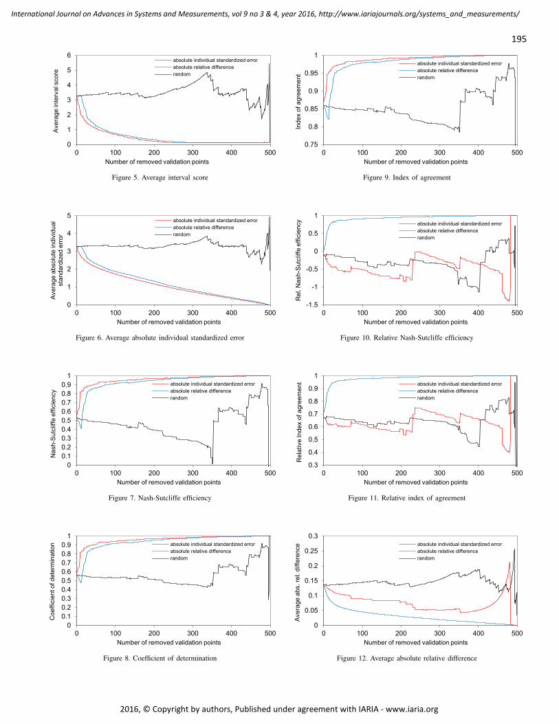
195



0

1

2

3

4

5

6

0 100 200 300 400 500

Ave

rage

inte

rval

sco

re

Number of removed validation points

absolute individual standardized errorabsolute relative differencerandom

Figure 5. Average interval score

0

1

2

3

4

5

0 100 200 300 400 500

Ave

rage

abs

olut

e in

divi

dual

st

anda

rdiz

ed e

rror



Figure 6. Average absolute individual standardized error

00.10.20.30.40.50.60.70.80.9

1

0 100 200 300 400 500

Nas

h-S

utcl

iffe

effic

ienc

y



Figure 7. Nash-Sutcliffe efficiency

00.10.20.30.40.50.60.70.80.9

1

0 100 200 300 400 500

Coe

ffici

ent o

f det

erm

inat

ion



Figure 8. Coefficient of determination

0.75

0.8

0.85

0.9

0.95

1

0 100 200 300 400 500

Inde

x of

agr

eem

ent



Figure 9. Index of agreement

-1.5

-1

-0.5

0

0.5

1

0 100 200 300 400 500

Rel

. Nas

h-S

utcl

iffe

effic

ienc

y



Figure 10. Relative Nash-Sutcliffe efficiency

0.3

0.4

0.5

0.6

0.7

0.8

0.9

1

0 100 200 300 400 500

Rel

ativ

e In

dex

of a

gree

men

t



Figure 11. Relative index of agreement

0

0.05

0.1

0.15

0.2

0.25

0.3

0 100 200 300 400 500

Ave

rage

abs

. rel

. diff

eren

ce



Figure 12. Average absolute relative difference

196



VII. DISCUSSION

The experiments indicate that the average interval scoreand the average absolute individual standardized error havethe most desired behavior. Whether a point is labeled ’bad’according to its absolute individual standardized error oraccording to its absolute relative difference, removing theworst element from the test data set results in better valuesof both measures. We remind that only these two measurestake the uncertainty in the approximation into account (seeSection IV). Thus, our experiments suggest that statisticalsurrogate models, such as Gaussian process emulation, havecertain benefits over deterministic surrogate models, such aspolynomial approximation, in particular that the uncertainty inthe approximation is also modeled. This uncertainty measureshould then be taken into account in validating the model.

Comparing Fig. 5 and Fig. 6, the main difference betweenthe average interval score and the average absolute individualstandardized error is that the first one reacts much morepronounced to the removal of elements, at least concerning theremoval of about the first half of all elements. The decreaseof the average interval score appears to be of exponentialorder, while the average absolute individual standardized errorseems to improve only linearly except for the first dozen or soelements. This indicates that one should be careful to report animprovement in a model as very significant when the averageinterval score is used as validation measure, since part of theimprovement might be solely due to characteristics inherentin that validation measure. It is advised to validate the modelin terms of both the average interval score and the averageabsolute individual standardized error.

The other measures do not show steady improvement withrespect to either the average interval score or the averageabsolute individual standardized error. Remarkably, each ofthese other measures do improve steadily in terms of one ofthese measures. The Nash-Sutcliffe efficiency, the coefficientof determination and the index of agreement improve con-sistently when removal of elements is performed accordingto the absolute individual standardized error, as is seen fromFigs. 7, 8, and 9. On the other hand, the relative Nash-Sutcliffe efficiency, the relative index of agreement and, ofcourse, the average absolute relative difference show steadyimprovement in terms of the absolute relative difference. Thisimplies that these measures are sensitive to the criterion that isused to measure the quality of the approximation in a certainpoint. A point that is designated as bad, i.e., low qualityof approximation in that point, according to the absoluteindividual standardized error might not be recognized as suchby the aforementioned six non statistical validation measures.The same applies to measuring the quality of approximationin a point by the absolute relative difference.

VIII. CONCLUSION AND FUTURE WORK

In this paper, we have evaluated eight validation measuresfor surrogate models: the average interval score, the averageabsolute individual standardized error, the Nash-Sutcliffe ef-ficiency, the coefficient of determination, the index of agree-ment, the relative Nash-Sutcliffe efficiency, the relative indexof agreement and the average absolute relative difference. Thefirst two measures are statistical in nature, taking into accountthe uncertainty of the approximation generated by the surrogatemodel. The other measures are solely based on the generated

approximation values. The evaluation was performed usinga Gaussian process emulator that was applied to an agent-based model. We developed both Gaussian process emulatorand agent-based model in previous work.

Our method of evaluating validation measures has, as far aswe are aware of, not been applied yet. We consider a test dataset and successively remove those elements from it for whichour emulator produces the worst approximation to the trueoutput value, in terms of the absolute individual standardizederror. The considered validation measures are then applied tothe sequence of increasingly smaller test data sets. The sameprocedure is applied with removal of test data points in termsof the absolute relative difference. It is desired that a validationmeasure shows improvement of a model when test data pointson which the model poorly performs are removed, irrespectiveof the measure that is used to detect such data points. Ourexperiments indicate that only the average interval score andthe average absolute individual standardized error have thisdesired behavior.

Our work has some practical implications:

• Statistical surrogate models, which not only producean approximation to or estimation of the output in agiven input point but also a measure for the uncertaintyin the approximation, are preferred over deterministicmodels. Evaluation of such a model should then bedone by a statistical validation measure that takes thisuncertainty measure into account, such as the averageinterval score and the average absolute individualstandardized error.

• It is bad practice to evaluate a given model in termsof a single validation measure, as the value of thismeasure might not only reflect the performance of themodel but also certain inherent artifacts of the measureitself. Evaluating a model using several measuresensures different perspectives on the performance ofthe model, and thus avoids an overly optimistic orpessimistic view on its performance that might not bejustified.

As future research, it would be interesting to evaluate othervalidation measures according to our evaluation procedure.Especially recently developed validation measures that aremeant to extend or improve previously developed measuresshould be evaluated. Examples include:

• A relatively recent alternative to the index of agree-ment that is dimensionless, bounded by -1.0 and1.0 and for which the authors claim that it is morerationally related to model accuracy than are otherexisting indices [52].

• Another alternative to the index of agreement thatis also dimensionless and bounded [53]. The authorsdemonstrate the use and value of their index onsynthetic and real data sets, but an evaluation in linewith our procedure would increase justification of theirclaims.

• A bounded version of the Nash-Sutcliffe efficiency[54].

Our experiments show that such an additional evaluation isnot superfluous, as modifications to existing measures that interms of analytical formulation seemingly compensate some

197



clear drawbacks of the existing measure might not show asconsistent behavior in practice as one is inclined to anticipate.

ACKNOWLEDGMENT

The authors acknowledge funding from the KU Leuvenfunded Geconcerteerde Onderzoeksacties (GOA) project Newapproaches to the social dynamics of long-term fertility change[grant 20142018;GOA/14/001].

REFERENCES[1] W. De Mulder, B. Rengs, G. Molenberghs, T. Fent, and G. Verbeke,

“Statistical emulation applied to a very large data set generated by anagent-based model,” in Proceedings of the 7th International Conferenceon Advances in System Simulation, SIMUL, 2015, pp. 43–48.

[2] Y. Liu, Z. Li, H. Xiong, X. Gao, and J. Wu, “Understanding ofinternal clustering validation measures,” in Proceedings of the IEEEInternational Conference on Data Mining. IEEE, 2010.

[3] M. Brun, C. Sima, J. Hua, J. Lowey, B. Carroll, E. Suh, andE. Dougherty, “Model-based evaluation of clustering validation mea-sures,” Pattern Recognition, vol. 40, 2007, pp. 807–824.

[4] D. R. Legates and G. J. McCabe Jr., “Evaluating the use of goodness-of-fit measures in hydrologic and hydroclimatic model validation,” WaterResources Research, vol. 35, 1999, pp. 233–241.

[5] I. Andrianakis and P. G. Challenor, “The effect of the nugget on Gaus-sian process emulators of computer models,” Computational Statisticsand Data Analysis, vol. 56, 2012, pp. 4215–4228.

[6] A. O’Hagan, “Bayesian analysis of computer code outputs: A tutorial,”Reliability Engineering & System Safety, vol. 91, 2006, pp. 1290–1300.

[7] J. Oakley and A. O’Hagan, “Bayesian inference for the uncertaintydistribution of computer model outputs,” Biometrika, vol. 89, 2002, pp.769–784.

[8] J. Gomez-Dans, P. Lewis, and M. Disney, “Efficient emulation ofradiative transfer codes using Gaussian processes and application toland surface parameter inferences,” Remote Sensing, vol. 8, 2016,doi:10.3390/rs8020119.

[9] D. Larose and C. Larose, Eds., Data mining and predictive analytics.Wiley, 2015.

[10] N. Gilbert, Ed., Agent-based models: quantitative applications in thesocial sciences. SAGE Publications, Inc, 2007.

[11] F. C. Billari, T. Fent, A. Prskawetz, and J. Scheffran, Eds., Agent–BasedCompuational Modelling: Applications in Demography, Social, Eco-nomic, and Environmental Sciences, ser. Contributions to Economics.Springer, 2006.

[12] C. Macal and M. North, “Agent-based modeling and simulation: Abmsexamples,” in Proceedings of the 2008 Winter Simulation Conference,2008, pp. 101–112.

[13] L. Willem, Agent-based models for infectious disease transmission:exploration, estimation & computational efficiency. PhD thesis, 2015.

[14] N. Schuhmacher, L. Ballato, and P. van Geert, “Using an agent-based model to simulate the development of risk behaviors duringadolescence,” Journal of Artificial Societies and Social Simulation,vol. 17, no. 3, 2014.

[15] B. Roche, J. M. Drake, and P. Rohani, “An agent-based model to studythe epidemiological and evolutionary dynamics of influenza viruses,”BMC Bioinformatics, vol. 12, no. 87, 2011.

[16] J.-J. Chen, L. Tan, and B. Zheng, “Agent-based model with multi-levelherding for complex financial systems,” Scientific Reports, vol. 5, 2015.

[17] A. Crooks, A. C. X. Lu, S. Wise, J. Irvine, and A. Stefanidis, “Walk thisway: improving pedestrian agent-based models through scene activityanalysis,” ISPRS International Journal of Geo-Information, vol. 4, no. 3,2015, pp. 1627–1656.

[18] M. Macy and R. Willer, “From factors to factors: computationalsociology and agent-based modeling,” Annual Review of Sociology,vol. 28, 2002, pp. 143–166.

[19] F. Bianchi and F. Squazzoni, “Agent-based models in sociology,” WileyInterdisciplinary Reviews: Computational Statistics, vol. 7, 2015, pp.284–306.

[20] F. Squazzoni, Ed., Agent-based computational sociology. Wiley, 2012.

[21] A. El-Sayed, P. Scarborough, L. Seemann, and S. Galea, “Social net-work analysis and agent-based modeling in social epidemiology,” Epi-demiologic Perspectives & Innovations, vol. 9, 2012, doi: 10.1186/1742-5573-9-1.

[22] G. Dancik, D. Jones, and K. Dorman, “Parameter estimation andsensitivity analysis in an agent-based model of Leishmania majorinfection,” Journal of Theoretical Biology, vol. 262, 2010, pp. 398–412.

[23] J.-S. Lee, T. Filatova, A. Ligmann-Zielinska, B. Hassani-Mahmooei,F. Stonedahl, and I. e. a. Lorscheid, “The complexities of agent-basedmodeling output analysis,” Journal of Artificial Societies and SocialSimulation, vol. 18, 2015, doi: 10.18564/jasss.2897.

[24] J. Sexton and Y. Everingham, “Global sensitivity analysis of key param-eters in a process-based sugarcane growth model: a Bayesian approach,” in Proceedings of the 7th International Congress on EnvironmentalModelling and Software, 2014.

[25] A. Heppenstall, A. Crooks, L. See, and M. Batty, Eds., Agent-basedmodels of geographical systems. Springer, 2011.

[26] D. Heard, G. Dent, T. Schifeling, and D. Banks, “Agent-Based modelsand microsimulation,” Annual Review of Statistics and Its Application,vol. 2, 2015, pp. 259–272.

[27] J. Bijak, J. Hilton, and E. Silverman, “From agent-based modelsto statistical emulators,” in Joint Eurostat/UNECE Work Session onDemographic Projections, 2013.

[28] J. Castilla-Rho, G. Mariethoz, M. Rojas, R. Andersen, and B. Kelly,“An agent-based platform for simulating complex human-aquifer inter-actions in managed groundwater systems,” Environmental Modelling &Software, vol. 73, 2015, pp. 305–323.

[29] T. Fent, B. Aparicio Diaz, and A. Prskawetz, “Family policies in thecontext of low fertility and social structure,” Demographic Research,vol. 29, 2013, pp. 963–998.

[30] A. Jain and R. Dubes, Eds., Algorithms for clustering data. PrenticeHall College Div, 1988.

[31] J. Oakley and A. O’Hagan, “Bayesian inference for the uncertaintydistribution of computer model outputs,” Biometrika, vol. 89, 2002, pp.769–784.

[32] M. Mitchell, Ed., An introduction to genetic algorithms. MIT Press,1998.

[33] P. Fleming and A. Zalzala, Eds., Genetic algorithms in engineeringsystems. The Institution of Engineering and Technology, 1997.

[34] E. Sanchez, Ed., Genetic algorithms and fuzzy logic systems: softcomputing perspectives. Wspc, 1997.

[35] L. Chambers, Ed., The practical handbook of genetic algorithms: newfrontiers. CRC Press, 1995.

[36] T. Gneiting and A. Raftery, “Strictly proper scoring rules, prediction,and estimation,” Journal of the American Statistical Association, vol.102, 2007, pp. 359–378.

[37] N. Cahill, A. Kemp, B. Horton, and A. Parnell, “Modeling sea-levelchange using errors-in-variables integrated Gaussian processes,” TheAnnals of Applied Statistics, vol. 9, 2015, pp. 547–571.

[38] C. Lian, C. Chen, Z. Zeng, W. Yao, and H. Tang, “Prediction intervalsfor landslide displacement based on switched neural networks,” IEEETransactions on Reliability, vol. 65, 2016, pp. 1483–1495.

[39] L. Bastos and A. O’Hagan, “Diagnostics for Gaussian process emula-tors,” Technometrics, vol. 51, 2009, pp. 425–438.

[40] J. Nash and J. Sutcliffe, “River flow forecasting through conceptualmodels, Part I - A discussion of principles,” Journal of Hydrology,vol. 10, 1970, pp. 282–290.

[41] B. Schaefli and H. Gupta, “Do Nash values have value?” HydrologicalProcesses, vol. 21, 2007, pp. 2075–2080.

[42] H. Gupta, H. Kling, K. Yilmaz, and G. Martinez, “Decomposition ofthe mean squared error and NSE performance criteria: Implicationsfor improving hydrological modelling,” Journal of Hydrology, vol. 377,2009, pp. 80–91.

[43] N. Soren Blomquist, “A note on the use of the coefficient of deter-mination,” The Scandinavian Journal of Economics, vol. 82, 980, pp.409–412.

[44] N. Nagelkerke, “A note on a general definition of the coefficient ofdetermination,” Biometrika, vol. 78, 1991, pp. 691–692.

198



[45] P. Krause, D. Boyle, and F. Base, “Comparison of different efficiencycriteria for hydrological model assessment,” Advances in Geosciences,vol. 5, 2005, pp. 89–97.

[46] J. Liao and D. McGee, “Adjusted coefficients of determination forlogistic regression,” The American Statistician, vol. 57, 2003, pp. 161–165.

[47] C. Willmot, “On the validation of models,” Physical Geography, vol. 2,1981, pp. 184–194.

[48] C. Willmott, S. Ackleson, R. Davis, Feddema, K. Klink, D. Legates,J. O’Donnell, and C. Rowe, “Statistics for the evaluation and compar-ison of models,” Journal of Geophysical Research, vol. 90, 1985, pp.8995–9005.

[49] C. Willmott, S. Robeson, and K. Matsuura, “A refined index of modelperformance,” International Journal of Climatology, vol. 32, 2012, pp.2088–2094.

[50] M. Barbouchi, R. Abdelfattah, K. Chokmani, N. B. Aissa, R. Lhissou,and A. E. Harti, “Soil salinity characterization using polarimetric InSARcoherence: Case studies in Tunisia and Morocco,” IEEE Journal ofSelected Topics in Applied Earth Observations and Remote Sensing,vol. 8, 2015, pp. 3823–3832.

[51] D. M. M. Ahouansou, S. K. Agodzo, S. Kralisch, L. O. Sintondji, andC. Furst, “Analysis of the hydrological budget using the J2000 modelin the Pendjari River Basin, West Africa,” Journal of Environment andEarth Science, vol. 5, 2015, pp. 24–37.

[52] C. Willmott, S. Robeson, and K. Matsuura, “A refined index of modelperformance,” International Journal of Climatology, vol. 32, 2011, pp.2088–2094.

[53] G. Duveiller, D. Fasbender, and M. Meroni, “Revisiting the conceptof a symmetric index of agreement for continuous datasets,” ScientificReports, vol. 6, 2016, doi:10.1038/srep19401.

[54] T. Mathevet, C. Michel, V. Andreassian, and C. Perrin, “A boundedversion of the Nash-Sutcliffe criterion for better model assessment onlarge sets of basins,” in IAHS Red Books Series no. 307. IAHS, 2006.

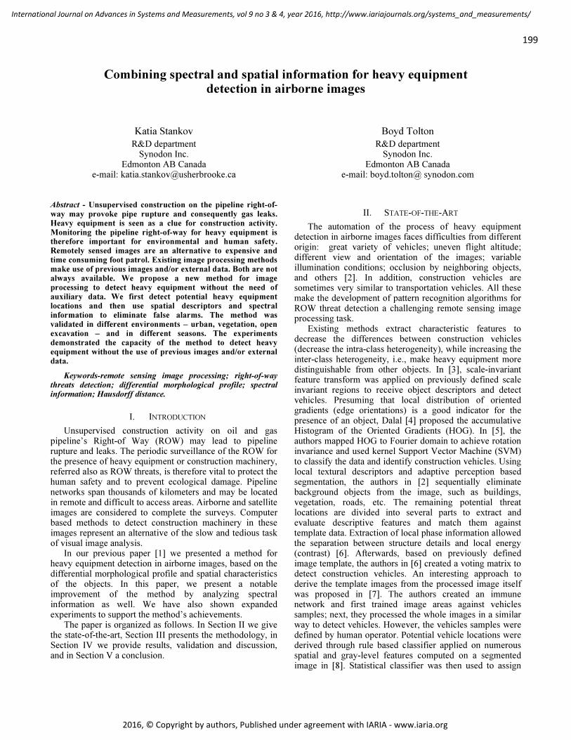
199



Combining spectral and spatial information for heavy equipment detection in airborne images

Katia Stankov

R&D department Synodon Inc.

Edmonton AB Canada e-mail: [email protected]

Boyd Tolton

R&D department Synodon Inc.

Edmonton AB Canada e-mail: boyd.tolton@ synodon.com

Abstract - Unsupervised construction on the pipeline right-of-way may provoke pipe rupture and consequently gas leaks. Heavy equipment is seen as a clue for construction activity. Monitoring the pipeline right-of-way for heavy equipment is therefore important for environmental and human safety. Remotely sensed images are an alternative to expensive and time consuming foot patrol. Existing image processing methods make use of previous images and/or external data. Both are not always available. We propose a new method for image processing to detect heavy equipment without the need of auxiliary data. We first detect potential heavy equipment locations and then use spatial descriptors and spectral information to eliminate false alarms. The method was validated in different environments – urban, vegetation, open excavation – and in different seasons. The experiments demonstrated the capacity of the method to detect heavy equipment without the use of previous images and/or external data.

Keywords-remote sensing image processing; right-of-way threats detection; differential morphological profile; spectral information; Hausdorff distance.

I. INTRODUCTION

Unsupervised construction activity on oil and gas pipeline’s Right-of Way (ROW) may lead to pipeline rupture and leaks. The periodic surveillance of the ROW for the presence of heavy equipment or construction machinery, referred also as ROW threats, is therefore vital to protect the human safety and to prevent ecological damage. Pipeline networks span thousands of kilometers and may be located in remote and difficult to access areas. Airborne and satellite images are considered to complete the surveys. Computer based methods to detect construction machinery in these images represent an alternative of the slow and tedious task of visual image analysis.

In our previous paper [1] we presented a method for heavy equipment detection in airborne images, based on the differential morphological profile and spatial characteristics of the objects. In this paper, we present a notable improvement of the method by analyzing spectral information as well. We have also shown expanded experiments to support the method’s achievements.

The paper is organized as follows. In Section II we give the state-of-the-art, Section III presents the methodology, in Section IV we provide results, validation and discussion, and in Section V a conclusion.

II. STATE-OF-THE-ART

The automation of the process of heavy equipment detection in airborne images faces difficulties from different origin: great variety of vehicles; uneven flight altitude; different view and orientation of the images; variable illumination conditions; occlusion by neighboring objects, and others [2]. In addition, construction vehicles are sometimes very similar to transportation vehicles. All these make the development of pattern recognition algorithms for ROW threat detection a challenging remote sensing image processing task.

Existing methods extract characteristic features to decrease the differences between construction vehicles (decrease the intra-class heterogeneity), while increasing the inter-class heterogeneity, i.e., make heavy equipment more distinguishable from other objects. In [3], scale-invariant feature transform was applied on previously defined scale invariant regions to receive object descriptors and detect vehicles. Presuming that local distribution of oriented gradients (edge orientations) is a good indicator for the presence of an object, Dalal [4] proposed the accumulative Histogram of the Oriented Gradients (HOG). In [5], the authors mapped HOG to Fourier domain to achieve rotation invariance and used kernel Support Vector Machine (SVM) to classify the data and identify construction vehicles. Using local textural descriptors and adaptive perception based segmentation, the authors in [2] sequentially eliminate background objects from the image, such as buildings, vegetation, roads, etc. The remaining potential threat locations are divided into several parts to extract and evaluate descriptive features and match them against template data. Extraction of local phase information allowed the separation between structure details and local energy (contrast) [6]. Afterwards, based on previously defined image template, the authors in [6] created a voting matrix to detect construction vehicles. An interesting approach to derive the template images from the processed image itself was proposed in [7]. The authors created an immune network and first trained image areas against vehicles samples; next, they processed the whole images in a similar way to detect vehicles. However, the vehicles samples were defined by human operator. Potential vehicle locations were derived through rule based classifier applied on numerous spatial and gray-level features computed on a segmented image in [8]. Statistical classifier was then used to assign

200



objects to the vehicle class. Though this method avoids the definition of template images, it involved manual image analysis to design training samples.

Exploiting the fact that heavy equipment has a larger number of right corners than natural objects, the authors in [9] defined target and background templates from the images. They used Harris corner detector to perform a first fast processing of UAV images and to reject background. In the second stage of the method the authors compared the performance of four classifiers (k Nearest Neighbors, Support Vector Machine, Decision Trees and Random Tress) and two feature extraction algorithms (HOG and Gabor coefficients). Best results were achieved with Gabor coefficients and Random Trees classifier. However, the results were more consistent while using a set of indoor images of model vehicles, taken in a sand box, than with the set defined from the images.

To decrease the large sets of templates needed to train and test the classifier, the authors in [10] developed a novel system based on the AdaBoost classifier. They applied it on SAR images to detect three types of vehicles and achieved recognition rates above 95% with a very limited training set. Gabor wavelet of SAR images was used to extract descriptive feature parameters in [11] to identify several types of vehicles.

Synthetic aperture radar images provide all weather coverage and are not restricted to the presence of daylight illumination. This property proved very efficient for change detection and potential threat localization [12]. Additional high spatial resolution optical images are to be analyzed to identify positive alarms.

To fully avoid the need of image template, potential threats locations are assessed with the aid of change detection in [13], next auxiliary data is used to decide upon the presence of a threat.

A common trait of existing methods is that the successful recognition of heavy equipment is impossible without complete set of image templates, previous images, and/or auxiliary data. These are not always available in practice. Airborne images of the pipeline ROW are taken only when a customer orders a survey. Previous images are not available when it comes to a new customer. Acquiring auxiliary data or building complete set of templates for the large variety of heavy equipment vehicles will significantly increase the cost of the survey. All of the above made existing methods not applicable in our case, thus we opted for a method that involves the interpretation of individual images.

The new methodology for heavy equipment detection we present in this paper avoids both the need of template images, and the need of auxiliary data or previously acquired images. In addition to increased flexibility, it also makes the performance of the method independent of the quality of the external data. As in our previous method [1], we first localize potential threats by detecting areas of high frequency of the image that correspond to the size of construction machinery and compute spatial descriptors. Unlike the previous method, where we used all the descriptors at once to discriminate between threats and other

objects, here we consecutively eliminate non threats locations. The significant improvement of the recognition came from the inclusion of spectral information. We analyze spectral information on the inner parts of the potential locations retained in the previous steps to refine the results. In the following section we give a step by step description of the method.

III. DESCRIPTION OF THE METHOD

The method may be roughly divided in three parts. First, we find potential threat locations. In the next step these locations are treated as objects, and spatial indices are derived to eliminate the ones that are certainly no threats. Finally, we introduce spectral information to further tune the results. A detailed description is given in Fig. 4.

A. Finding potential threat locations

To build our method we take advantage of the fact that construction vehicles have non-flatten surfaces, which creates inequality in the intensity of surface pixels and together with their outer edges make that they appear as areas of high frequency in the image. Therefore, potential threat locations may be found by identifying areas of high frequencies that are in the range of heavy equipment size. We apply the differential morphological profile on the gradient of the image to find areas of high frequency.

1) Differential Morphological Profile (DMP): DMP is an iterative algorithm that performs opening/closing by reconstruction with a structuring element (SE) to find structures that are brighter/darker than their surroundings. The size of the SE is increased in the consecutive iteration and the result is extracted from the result of the previous iteration. As we are searching for structures that are brighter than their surroundings, we used only the opening by reconstruction to compute the DMP, as follows [14]. Let the vector )(xγΠ be the opening profile at the point x of image

I defined by:

[ ]{ }nxx ,...,0),(:)(*

∈∀=ΠΠ=Π λγγγγλλλ

(1)

where )(* xλ

γ is the morphological opening by

reconstruction operator and the size of the SE = λ.

The DMP )(xγ∆ is a vector that stores a measure of the

slope between consecutive iterations of the opening profile corresponding to the increased size of the SE:

[ ]{ }nx ,...,1,:)(1

∈∀Π−Π=∆∆=∆−

λγγγγγλλλλ

(2)

When the SE size exceeds the object size, the background intensity values are assigned to the object. Thus, by extracting two consecutive results, bright objects that correspond or are bigger than the size of the corresponding SE are retained. The object is eliminated in the consecutive iteration if it is smaller than the SE. Thus by knowing when,

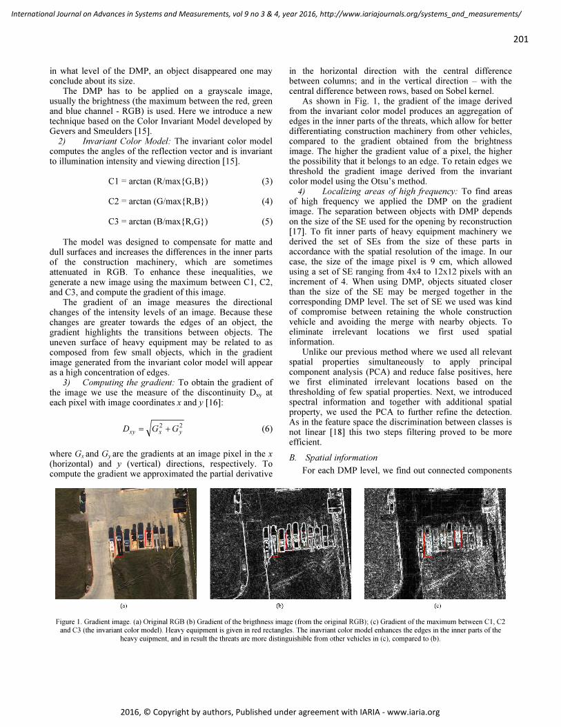
201



in what level of the DMP, an object disappeared one may conclude about its size.

The DMP has to be applied on a grayscale image, usually the brightness (the maximum between the red, green and blue channel - RGB) is used. Here we introduce a new technique based on the Color Invariant Model developed by Gevers and Smeulders [15].

2) Invariant Color Model: The invariant color model computes the angles of the reflection vector and is invariant to illumination intensity and viewing direction [15].

C1 = arctan (R/max{G,B}) (3)

C2 = arctan (G/max{R,B}) (4)

C3 = arctan (B/max{R,G}) (5)

The model was designed to compensate for matte and

dull surfaces and increases the differences in the inner parts of the construction machinery, which are sometimes attenuated in RGB. To enhance these inequalities, we generate a new image using the maximum between C1, C2, and C3, and compute the gradient of this image.

The gradient of an image measures the directional changes of the intensity levels of an image. Because these changes are greater towards the edges of an object, the gradient highlights the transitions between objects. The uneven surface of heavy equipment may be related to as composed from few small objects, which in the gradient image generated from the invariant color model will appear as a high concentration of edges.

3) Computing the gradient: To obtain the gradient of the image we use the measure of the discontinuity Dxy at each pixel with image coordinates x and y [16]:

22

yxxyGGD += (6)

where Gx and Gy are the gradients at an image pixel in the x (horizontal) and y (vertical) directions, respectively. To compute the gradient we approximated the partial derivative

in the horizontal direction with the central difference between columns; and in the vertical direction – with the central difference between rows, based on Sobel kernel.

As shown in Fig. 1, the gradient of the image derived from the invariant color model produces an aggregation of edges in the inner parts of the threats, which allow for better differentiating construction machinery from other vehicles, compared to the gradient obtained from the brightness image. The higher the gradient value of a pixel, the higher the possibility that it belongs to an edge. To retain edges we threshold the gradient image derived from the invariant color model using the Otsu’s method.

4) Localizing areas of high frequency: To find areas of high frequency we applied the DMP on the gradient image. The separation between objects with DMP depends on the size of the SE used for the opening by reconstruction [17]. To fit inner parts of heavy equipment machinery we derived the set of SEs from the size of these parts in accordance with the spatial resolution of the image. In our case, the size of the image pixel is 9 cm, which allowed using a set of SE ranging from 4x4 to 12x12 pixels with an increment of 4. When using DMP, objects situated closer than the size of the SE may be merged together in the corresponding DMP level. The set of SE we used was kind of compromise between retaining the whole construction vehicle and avoiding the merge with nearby objects. To eliminate irrelevant locations we first used spatial information.

Unlike our previous method where we used all relevant spatial properties simultaneously to apply principal component analysis (PCA) and reduce false positives, here we first eliminated irrelevant locations based on the thresholding of few spatial properties. Next, we introduced spectral information and together with additional spatial property, we used the PCA to further refine the detection. As in the feature space the discrimination between classes is not linear [18] this two steps filtering proved to be more efficient.

B. Spatial information

For each DMP level, we find out connected components

Figure 1. Gradient image. (a) Original RGB (b) Gradient of the brigthness image (from the original RGB); (c) Gradient of the maximum between C1, C2

and C3 (the invariant color model). Heavy equipment is given in red rectangles. The inavriant color model enhances the edges in the inner parts of the

heavy euipment, and in result the threats are more distinguishible from other vehicles in (c), compared to (b).

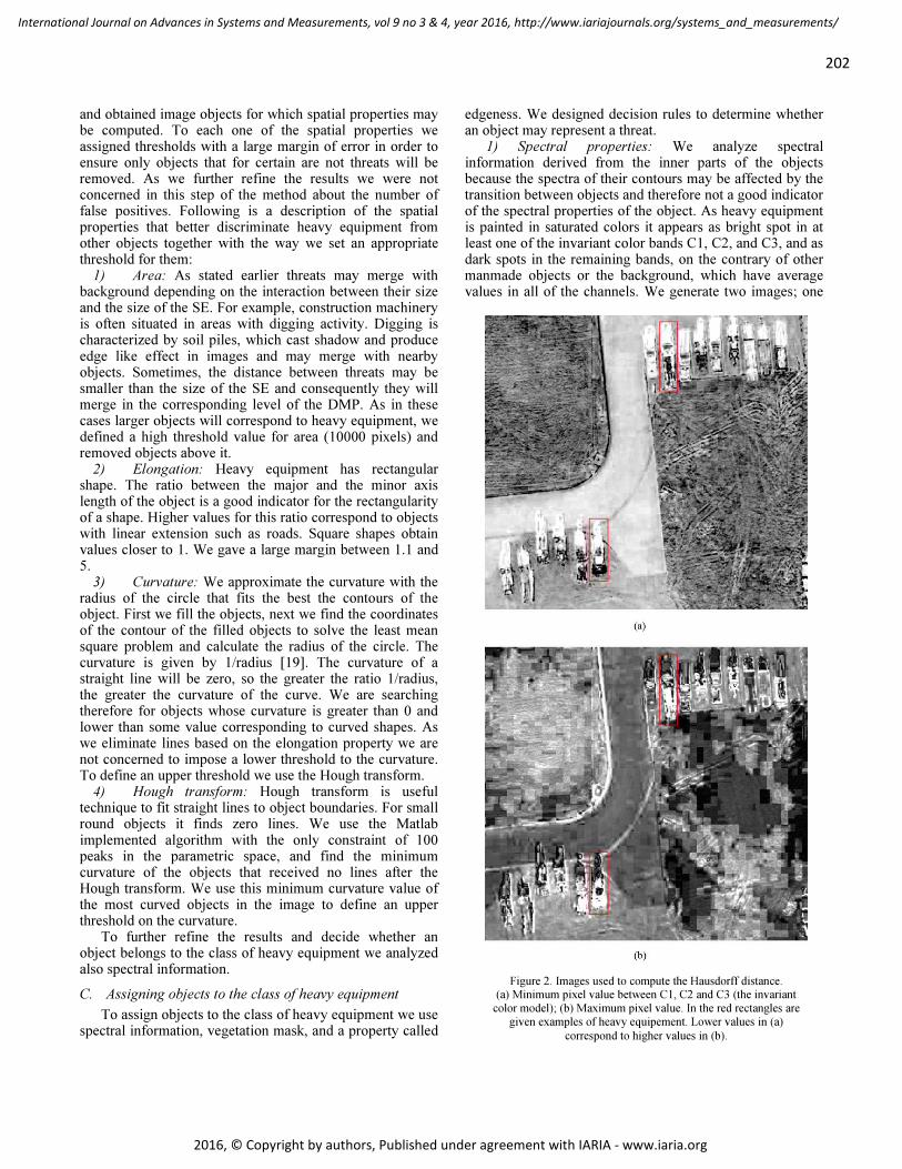
202



and obtained image objects for which spatial properties may be computed. To each one of the spatial properties we assigned thresholds with a large margin of error in order to ensure only objects that for certain are not threats will be removed. As we further refine the results we were not concerned in this step of the method about the number of false positives. Following is a description of the spatial properties that better discriminate heavy equipment from other objects together with the way we set an appropriate threshold for them:

1) Area: As stated earlier threats may merge with background depending on the interaction between their size and the size of the SE. For example, construction machinery is often situated in areas with digging activity. Digging is characterized by soil piles, which cast shadow and produce edge like effect in images and may merge with nearby objects. Sometimes, the distance between threats may be smaller than the size of the SE and consequently they will merge in the corresponding level of the DMP. As in these cases larger objects will correspond to heavy equipment, we defined a high threshold value for area (10000 pixels) and removed objects above it.

2) Elongation: Heavy equipment has rectangular shape. The ratio between the major and the minor axis length of the object is a good indicator for the rectangularity of a shape. Higher values for this ratio correspond to objects with linear extension such as roads. Square shapes obtain values closer to 1. We gave a large margin between 1.1 and 5.

3) Curvature: We approximate the curvature with the radius of the circle that fits the best the contours of the object. First we fill the objects, next we find the coordinates of the contour of the filled objects to solve the least mean square problem and calculate the radius of the circle. The curvature is given by 1/radius [19]. The curvature of a straight line will be zero, so the greater the ratio 1/radius, the greater the curvature of the curve. We are searching therefore for objects whose curvature is greater than 0 and lower than some value corresponding to curved shapes. As we eliminate lines based on the elongation property we are not concerned to impose a lower threshold to the curvature. To define an upper threshold we use the Hough transform.

4) Hough transform: Hough transform is useful technique to fit straight lines to object boundaries. For small round objects it finds zero lines. We use the Matlab implemented algorithm with the only constraint of 100 peaks in the parametric space, and find the minimum curvature of the objects that received no lines after the Hough transform. We use this minimum curvature value of the most curved objects in the image to define an upper threshold on the curvature.

To further refine the results and decide whether an object belongs to the class of heavy equipment we analyzed also spectral information.

C. Assigning objects to the class of heavy equipment

To assign objects to the class of heavy equipment we use spectral information, vegetation mask, and a property called

edgeness. We designed decision rules to determine whether an object may represent a threat.

1) Spectral properties: We analyze spectral information derived from the inner parts of the objects because the spectra of their contours may be affected by the transition between objects and therefore not a good indicator of the spectral properties of the object. As heavy equipment is painted in saturated colors it appears as bright spot in at least one of the invariant color bands C1, C2, and C3, and as dark spots in the remaining bands, on the contrary of other manmade objects or the background, which have average values in all of the channels. We generate two images; one

Figure 2. Images used to compute the Hausdorff distance.

(a) Minimum pixel value between C1, C2 and C3 (the invariant

color model); (b) Maximum pixel value. In the red rectangles are

given examples of heavy equipement. Lower values in (a)

correspond to higher values in (b).

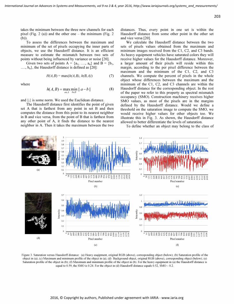
203



takes the minimum between the three new channels for each pixel (Fig. 2 (a)) and the other one – the minimum (Fig. 2 (b)).

To assess the differences between the maximum and minimum of the set of pixels occupying the inner parts of objects, we use the Hausdorff distance. It is an efficient measure to estimate the mismatch between two sets of points without being influenced by variance or noise [20].

Given two sets of points A = {a1, …., an} and B = {b1, …., bn}, the Hausdorff distance is defined as [20]:

H(A,B) = max(h(A,B), h(B,A)) (7)

where

||||minmax),( baBAhBbAa

−=

∈∈

(8)

and ||.|| is some norm. We used the Euclidean distance.

The Hausdorff distance first identifies the point of given set A that is farthest from any point in set B and then computes the distance from this point to its nearest neighbor in B and vice versa, from the point of B that is farthest from any other point of A, it finds the distance to the nearest neighbor in A. Then it takes the maximum between the two

distances. Thus, every point in one set is within the Hausdorff distance from some other point in the other set and vice versa [20].

We calculate the Hausdorff distance between the two sets of pixels values obtained from the maximum and minimum images received from the C1, C2, and C3 bands. As heavy equipment vehicles have saturated colors they will receive higher values for the Hausdorff distance. Moreover, a larger amount of their pixels will reside within this margin, according to the per pixel difference between the maximum and the minimum of the C1, C2, and C3 channels. We compute the percent of pixels in the whole object whose differences between the maximum and the minimum of the C1, C2, and C3 channels are within the Hausdorff distance for the corresponding object. In the rest of the paper we refer to this property as spectral mismatch occupancy (SMO). Construction machinery receives higher SMO values, as most of the pixels are in the margins defined by the Hausdorff distance. Would we define a threshold on the saturation image to compute the SMO, we would receive higher values for other objects too. We illustrate this in Fig. 3. As shown, the Hausdorff distance allowed to better differentiate the levels of saturation.

To define whether an object may belong to the class of

Figure 3. Saturation versus Hausdorff distance: (a) Heavy euqipment, original RGB (above), corresponding object (below); (b) Saturation profile of the object in (a); (c) Maximum and minimum profile of the object in (a); (d) Background object, original RGB (above), corresponding object (below); (e)

Saturation profile of the object in (b); (f) Maximum and minimum profile of the object in (b). For the heavy equipment in (a) the Hausdorff distance is

equal to 0.59, the SMO is 0.24. For the object in (d) Hausdorff distance equals 0.52, SMO – 0.2.

204



heavy equipment we compare the SMO to the vegetation occupancy.

2) Compare SMO to vegetation occupancy and apply decision rules: First, we compute the vegetation index from the RGB bands, because the airborne images we work with have only these three bands:

Vegetation Index = (Green – Red)/(Green + Red) (9) Using the Otsu’s threshold method, we generate a

vegetation mask. The vegetation occupancy of an object is obtained as the percent of masked pixels in the object area.

The difference between SMO and vegetation occupancy varies according to the scene. To adapt our method we apply the following rules to retain ROW threats.

In scenes occupied mostly by green vegetation, a single threat will have definitely higher SMO than vegetation occupancy, compared to other objects. Thus, if less than 10 percent of the objects have higher SMO than vegetation occupancy, we assume that this is the case and retain these objects (Fig. 6 (a)). However, when the scene is occupied by buildings, excavations, or the image is taken in winter season when no green vegetation is present, but only leafless trees and shrubs, the vegetation mask may also cover part of the heavy equipment and the predominance of SMO over vegetation occupancy is not so evident.

In cases where there is a lack of strict distinction between vegetation and other objects (the SMO is less than the vegetation occupancy for all of the objects or more than 10 percent of the objects have higher SMO than vegetation occupancy), we use the property called edgeness. It is obtained by dividing the area of the object by the number of edge pixels of the object. To receive the area of the object we fill the boundary of the object. As stated earlier, because of the surface inequalities of construction vehicles, they will receive higher edgeness than vegetation areas, or other transport vehicles as shown in Fig. 1 (c).

We concatenate the two properties: 1) the difference between SMO and vegetation occupancy; 2) the edgeness value. Then we computed the principal component analysis and divided the objects according to their first principal score, setting the median of the scores as a threshold. To decide which group to retain we used the ratio between the eigenvalues of the covariance matrix of each group. Threats have higher intra-class heterogeneity compared to other objects. The ratio between the eigenvalues is a good indicator for heterogeneity [21], thus we used the ratio of the eigenvalues of the covariance matrix. Greater values correspond to greater heterogeneity, thus we retained the group that produced higher value for the eigenvalue’s ratio.

Step by step results together with a flow chart of the method are given in Fig. 4.

D. Post-processing

As the images may not contain threats at all, we included a step of automate post-processing to refine the results. We used a vector composed from the Hausdorff distance and the SMO. We then sorted the magnitude of the vector and computed the slope of the tangent at each point. A point

Figure 4. Flow chart of the proposed method.

From (a) to (h) - the consecutive steps.

205



represents the sorted magnitude value for each object. An empirically derived threshold was set to retain objects whose slope was less than the threshold. The rationale here is that if the objects belong to the class of threat their magnitude will be similar and therefore the slope of the tangent will be less than this ratio. If no threat were retained the values for the magnitude will be quite different and the slope will be higher than the threshold. As shown in Fig. 5 this step was efficient to further refine the results.

IV. RESULTS AND VALIDATION

We present some results in Figs. 6, 7 and 8. We indicated true detections – heavy equipment that are present in the image and were identified by the method – with rectangles with yellow contours; false alarms, or false positives – objects that were identified by the method as threats, but are actually not threats – with rectangles with red contours, and missed detection – heavy equipment that is present in the image but was not identified as such by the method – with rectangles with green contours.

As may be seen from Fig. 6 the method performs well in different scenes – forest (a), urban scene (c), abandoned site (e), and ongoing excavations (g). These different backgrounds provide low (abandoned site – (e)) to high contrast (ongoing excavations – (g)). Despite that, the method successfully detected ROW threats. We explain this with the improved spectral contrast obtained with the invariant color model. In Fig. 6 (c) many transportation vehicles were present, which are usually a source of confusion with heavy equipment. The edgeness property allowed for better separation between them. Similar results are shown in Fig. 7 ((a) and (e)).

Fig. 7 (c) shows a typical case of missing a threat. Although both vehicles are very similar, only one was detected. The other one was merged with the nearby fence and treated as a linear object. Fig. 7 (g) demonstrates the capacity of the method to detect threats when there is an accumulation of objects with size similar to this of heavy equipment, that appear as areas of high frequency. However, in this case, many false alarms were also detected as threats.

In Fig. 8 we demonstrate the limitation of the method. When a single threat is present in the image, other objects may be misinterpreted as threats and the real threat omitted. In our opinion, the main reason for this is that while

performing the PCA we assume the presence of only two classes. This may be improved by using cluster analysis, applied on the objects principal component scores. In Fig. 8 (c, e and g) we demonstrate typical cases of false alarms. We believe that more rigorous post- processing step would decrease their number.

To validate the accuracy of the method we compared the results to manually detected threats. We refer to the latter as ground truth data. A set of 300 images taken from different surveys was processed. The image size is 1200x800 pixels with average pixel resolution of 9 cm. The detection rate was 83.9% - heavy equipment machines that are present in the ground truth data and were detected by the algorithm. This is a slight improvement compared to our previous method, where the detection rate was 82.6%. However, in the current experiment the images are more heterogeneous, taken from different seasons, as opposite to the previous test where we used images of the same flight day. Also, visual comparison reveals that the number of false positive was significantly reduced.

To place our method among other algorithms for threat detection we compare its achievement to the results reported in [9]. The authors compared several classifiers. Our method, with the detection rate of 83.9% performs slightly better than the kNN classifier (83.3%) and less than the regression trees and SVM classifiers – 85.7% and 93.3%, respectively. However, these classifiers were applied on rural scene only and used template models. As we demonstrated above, our method performs well in different scenes, without using templates or auxiliary data. We may say therefore that it has a potential and we focus our further developments to improve the detection rate and reduce the false detections.

At this stage of the development of the algorithm we are less concerned with the rate of false recognition, as the results are reviewed by an operator. We consider including additional descriptors to reduce the number of false positives events while increasing the detection rate.

The limitation of the method is related to the spatial resolution of the image. In our opinion, the method performance may decrease when applied on images with much lower spatial resolution, more than 1 meter for example, as it relies explicitly on information taken from an increasing neighborhood.

Figure 5. Post-processsing. (a) Original RGB; (b) Processed image; (c) Results after post-processing.

206



Figure 6. Results. Left column original RGB image. Righ column – detection. Rectangles with yellow contours indicate true detections;

rectangles with red contours - false alarms; rectangles with green contours - missed detections.

207



Figure 7. Results. Left column original RGB image. Righ column – detection. Rectangles with yellow contours indicate true detections; rectangles

with red contours - false alarms; rectangles with green contours - missed detections.

208



Figure 8. Results. Left column original RGB image. Righ column – detection. Rectangles with yellow contours indicate true detections; rectangles

with red contours - false alarms; rectangles with green contours - missed detections.

209



V. CONCLUSION

In this paper, we presented a novel methodology for heavy equipment detection. The method first detects high frequency areas in the image that may represent potential heavy equipment locations, and then compute spatial descriptors and explore spectral information to eliminate false detections. It does not involve the use of external data, or previously acquired images, which makes it more flexible, compared to already existing algorithms. An improvement compared to our previous method [1] is due to the exploration of spectral information all along the spatial descriptors. Our method compares favorably to other methods for threat detection. On the contrary of other studies, we tested it in different scenes – urban, forest, excavation areas. The experiments proved its efficiency for surveillance of the pipeline ROW, which is important for human safety and ecological damage prevention. The results are promising and we believe that the method has the potential to replace the manual processing of the images.

ACKNOWLEDGMENT

This research was funded by Alberta Innovates Technology Future. The authors would like to express their gratitude for the support provided by the Industry Associate Program of the institution.

REFERENCES

[1] K. Stankov and B. Tolton, “Differential morphological profile for threat detection on pipeline right-of-way. Heavy equipment detection,” The Eighth International Conference on Advanced Geographic Information Systems, Applications, and Services (Geoprocessing 2016), IARIA, Apr 2016, pp. 76-77, ISSN: 2308-393X , ISBN: 978-1-61208-469-5.

[2] V. Asari, Vijayan, P. Sidike, C. Cui, and V. Santhaseelan. "New wide-area surveillance techniques for protection of pipeline infrastructure,” SPIE Newsroom, 30 January 2015, DOI: 10.1117/2.1201501.005760

[3] G. Dorko and C. Schmid, “Selection of scale-invariant parts for object class recognition,” IProceedings of the 9th International Conference on Computer Vision, Nice, France, pp. 634–640, 2003.

[4] N. Dalal and B. Triggs, ”Histograms of oriented gradients for human detection,” IEEE Conference on Computer Vision and Pattern Recognition, pp. 886-893, 2005

[5] A. Mathew and V. K. Asari, ”Rotation-invariant Histogram Features for Threat Object Detection on Pipeline Right-of-Way,” in Video Surveillance and Transportation Imaging Applications 2014, edited by Robert P. Loce, Eli Saber, Proc. of SPIE-IS&T Electronic Imaging, SPIE vol. 9026, pp. 902604-1-902604-1, 2014 SPIE-IS&T doi: 10.1117/12.2039663

[6] B. Nair, V. Santhaseelan, C. Cui, and V. K. Asari, “Intrusion detection on oil pipeline right of way using monogenic signal representation,” Proc. SPIE 8745, 2013, p. 87451U, doi:10.1117/12.2015640

[7] H. Zheng and L. Li, “An artificial immune approach for vehicle detection from high resolution space imagery,” IJCSNS International Journal of Computer Science and Network Security, vol.7 no.2, pp. 67-72, February 2007.

[8] L. Eikvil, L. Aurdal, and H. Koren, “Classification-based vehicle detection in high resolution satellite images,” ISPRS Journal of Photogrammetry and Remote Sensing, vol. 64, issue 1, pp. 65-72, January 2009. doi.org/10.1016/j.isprsjprs.2008.09.005

[9] J. Gleason, A. Nefian, X. Bouyssounousse, T. Fong, and G. Bebis, “Vehicle detection from aerial imagery,” 2011 IEEE International Conference on Robotics and Automation, pp. 2065-2070, May 2011.

[10] Y. Sun, Z. Liu, S. Todorovic, and J. Li, “Synthetic aperture radar automatic target recognition using adaptive boosting,” Proceedings of the SPIE, Algorithms for Synthetic Aperture Radar Imagery XII, 5808, pp. 282-293, May 2005.

[11] P. Vasuki and S. M. M. Roomi, “Man-made object classification in SAR images using Gabor wavelet and neural network classifier,” Proc. IEEE. Devices, Circuits and Systems Int. Conf., India, pp. 537–539, IEEE 2012.

[12] Roper, W. E. and Dutta, S. "Oil Spill and Pipeline Condition Assessment Using Remote Sensing and Data Visualization Management Systems,” George Mason University, 4400 University Drive, 2006.

[13] M. Zarea, G. Pognonec, C. Schmidt, T. Schnur, J. Lana, C. Boehm, M. Buschmann, C. Mazri, and E. Rigaud, “First steps in developing an automated aerial surveillance approach,” Journal of Risk Research, vol.13(3–4): pp. 407–420, 2013 doi:10.1080/13669877.2012.729520.

[14] J. A. Benediktsson, M. Pesaresi, and K. Arnason, “Classification and feature extraction from remote sensing images from urban areas based on morphological transformations,” IEEE Transactions on Geoscience and Remote Sensing, vol. 41(9), pp. 1940–1949, 2003.

[15] T. Gevers and A. W. M. Smeulders, “Color based object recognition,” Pattern Recognit., vol. 32, pp. 453–465, Mar. 1999.

[16] H. Wang and D. Suter, “Color image segmentation using global information and local homogeneity,” in: Proc. VIIth Digital Image Computing: Techniques and Applications, Sun C., Talbot H., Ourselin S. and Adriaansen T., Eds., Sydney, pp. 89-98, Dec. 2003.

[17] G.K. Ouzounis, M. Pesaresi, and P. Soille, "Differential area profiles: decomposition properties and efficient computation,” IEEE Transactions on Pattern Analysis and Machine Intelligence, vol. 34, no. 8, pp. 1533-1548, Aug. 2012.

[18] X. Chen, T. Fang, H. Huo, and D. Li, “Graph-based feature selection for object-oriented classification in VHR airborne imagery,” IEEE Transactions on Geoscience and Remote Sensing, vol. 49 (1), pp. 353–365, 2011.

[19] https://www.mathworks.com/matlabcentral/newsreader/view_thread/152405

[20] D. P. Huttenlocher, G. Klanderman, and W. J. Rucklidge,. “Comparing images using the Hausdorff distance,” IEEE Trans. Pattern Anal. Mach. Intell. 15, 9, pp. 850–863, 1993.

[21] F. O’Sullivan, S. Roy, and J. Eary, “A statistical measure of tissue heterogeneity with application to 3D PET sarcoma data,” Biostatistics vol. 4, pp. 433–448, 2003.

210



Management Control System for Business Rules Management

Koen Smit

Digital Smart Services

HU University of Applied Sciences Utrecht

Utrecht, the Netherlands

[email protected]

Martijn Zoet

Optimizing Knowledge-Intensive Business Processes

Zuyd University of Applied Sciences

Sittard, the Netherlands

[email protected]

Abstract — With increasing investments in business rules

management (BRM), organizations are searching for ways to

value and benchmark their processes to elicitate, design, specify,

verify, validate, deploy, execute and govern business rules. To

realize valuation and benchmarking of previously mentioned

processes, organizations must be aware that performance

measurement is essential, and of equal importance, which

performance indicators to apply as part of performance

measurement processes. However, scientific research on BRM, in

general, is limited and research that focuses on BRM in

combination with performance indicators is nascent. The

purpose of this paper is to define performance indicators for

previously mentioned BRM processes. We conducted a three

round focus group and three round Delphi Study, which led to

the identification of 14 performance indicators. In this paper, we

re-address and - present our earlier work [33], yet we extended

the previous research with more detailed descriptions of the

related literature, findings, and results, which provide a

grounded basis from which further, empirical, research on

performance indicators for BRM can be explored.

Keywords-Business Rules Management; Business Rules;

Performance Measurement; Performance Indicator.

I. INTRODUCTION

Business rules are an important part of an organization’s

daily activities. Many business services nowadays rely heavily

on business rules to express assessments, predictions and

decisions [7][27]. A business rule is [23] “a statement that

defines or constrains some aspect of the business intending to

assert business structure or to control the behavior of the

business.” Most organizations experience three challenges

when dealing with business rules management: 1) consistency

challenges, 2) impact analysis challenges, and 3) transparency

of business rule execution [4]. A consistent interpretation of

business rules ensures that different actors apply the same

business rules, and apply them consistently. This is a

challenge since business rules are often not centralized, but

they are embedded in various elements of an organization's

information system instead. For example, business rules are

embedded in minds of employees, part of textual procedures,

manuals, tables, schemes, business process models, and hard-

coded as software applications. Impact assessment determines

the impact of changes made to business rules and the effect on

an existing implementation. Currently, impact assessments can

take significant time, which results in situations where the

business rules already have changed again while the impact

assessment is still ongoing [2]. Transparency, or business rules

transparency, indicates that organizations should establish a

system to prove what business rules are applied at a specific

moment in time. To tackle the previously mentioned

challenges and to improve grip on business rules,

organizations search for a systematic and controlled approach

to support the discovery, design, validation and deployment of

business rules [7][32]. To be able to manage or even address

these challenges, insight has to be created concerning business

rule management processes at organizations. This can be

achieved using performance management, which can provide

insight into an organization’s current situation, but can also

point towards where and how to improve. However, research

on performance management concerning BRM is nascent.

The measurement of performance has always been

important in the field of enterprise management and, therefore,

has been of interest for both practitioners and researchers [9].

Performance measurement systems are applied to provide

useful information to manage, control and improve business

processes. One of the most important tasks of performance

management is to identify (and properly) evaluate suitable

Performance Indicators (PI’s) [13]. The increase of interest

and research towards identifying the right set of indicators has

led to ‘standard’ frameworks and PI’s tailored to a specific

industry or purpose. Examples of such frameworks are the

balanced scorecard, the total quality management framework,

and the seven-S model [19][31]. Moreover, research on

standard indicators is increasingly performed for sales and

manufacturing processes. To the knowledge of the authors,

research, which focuses on performance measures for BRM is

absent. This article extends the understanding of performance

measurement with regard to the BRM processes. To be able to

do so, the following research question is addressed: “Which

performance indicators are useful to measure the BRM

processes?” This paper is organized as follows: In section two we provide insights into performance management and performance measurement. This is followed by the exploration of performance measurement Systems in section three. In section four, we provide an overview of the BRM capabilities and their goals. In section five, we report upon the research method utilized to construct our set of PI’s. Next, the data collection and analysis of our study is described in section six. In section seven, our results, which led to our PI’s for BRM are

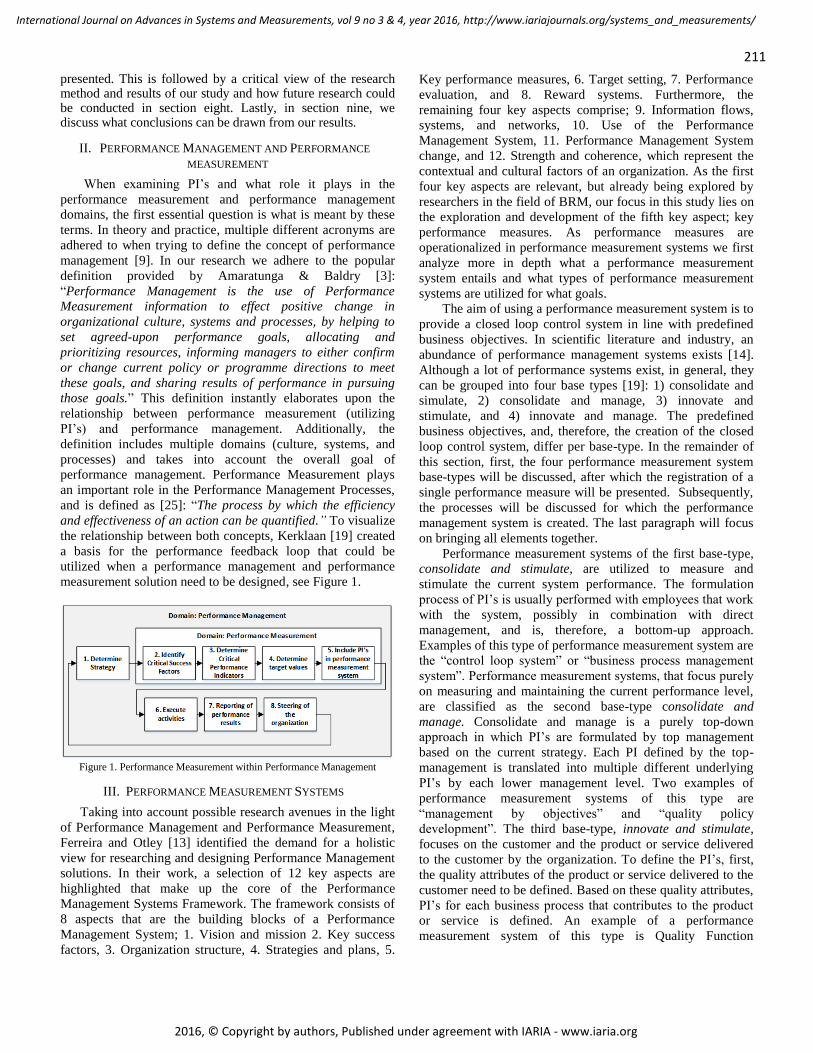
211



presented. This is followed by a critical view of the research method and results of our study and how future research could be conducted in section eight. Lastly, in section nine, we discuss what conclusions can be drawn from our results.

II. PERFORMANCE MANAGEMENT AND PERFORMANCE

MEASUREMENT

When examining PI’s and what role it plays in the

performance measurement and performance management

domains, the first essential question is what is meant by these

terms. In theory and practice, multiple different acronyms are

adhered to when trying to define the concept of performance

management [9]. In our research we adhere to the popular

definition provided by Amaratunga & Baldry [3]:

“Performance Management is the use of Performance

Measurement information to effect positive change in

organizational culture, systems and processes, by helping to

set agreed-upon performance goals, allocating and

prioritizing resources, informing managers to either confirm

or change current policy or programme directions to meet

these goals, and sharing results of performance in pursuing

those goals.” This definition instantly elaborates upon the

relationship between performance measurement (utilizing

PI’s) and performance management. Additionally, the

definition includes multiple domains (culture, systems, and

processes) and takes into account the overall goal of

performance management. Performance Measurement plays

an important role in the Performance Management Processes,

and is defined as [25]: “The process by which the efficiency

and effectiveness of an action can be quantified.” To visualize

the relationship between both concepts, Kerklaan [19] created

a basis for the performance feedback loop that could be

utilized when a performance management and performance

measurement solution need to be designed, see Figure 1.

Figure 1. Performance Measurement within Performance Management

III. PERFORMANCE MEASUREMENT SYSTEMS

Taking into account possible research avenues in the light

of Performance Management and Performance Measurement,

Ferreira and Otley [13] identified the demand for a holistic

view for researching and designing Performance Management

solutions. In their work, a selection of 12 key aspects are

highlighted that make up the core of the Performance

Management Systems Framework. The framework consists of

8 aspects that are the building blocks of a Performance

Management System; 1. Vision and mission 2. Key success

factors, 3. Organization structure, 4. Strategies and plans, 5.

Key performance measures, 6. Target setting, 7. Performance

evaluation, and 8. Reward systems. Furthermore, the

remaining four key aspects comprise; 9. Information flows,

systems, and networks, 10. Use of the Performance

Management System, 11. Performance Management System

change, and 12. Strength and coherence, which represent the

contextual and cultural factors of an organization. As the first

four key aspects are relevant, but already being explored by

researchers in the field of BRM, our focus in this study lies on

the exploration and development of the fifth key aspect; key

performance measures. As performance measures are

operationalized in performance measurement systems we first

analyze more in depth what a performance measurement

system entails and what types of performance measurement

systems are utilized for what goals.

The aim of using a performance measurement system is to

provide a closed loop control system in line with predefined

business objectives. In scientific literature and industry, an

abundance of performance management systems exists [14].

Although a lot of performance systems exist, in general, they

can be grouped into four base types [19]: 1) consolidate and

simulate, 2) consolidate and manage, 3) innovate and

stimulate, and 4) innovate and manage. The predefined

business objectives, and, therefore, the creation of the closed

loop control system, differ per base-type. In the remainder of

this section, first, the four performance measurement system

base-types will be discussed, after which the registration of a

single performance measure will be presented. Subsequently,

the processes will be discussed for which the performance

management system is created. The last paragraph will focus

on bringing all elements together.

Performance measurement systems of the first base-type,

consolidate and stimulate, are utilized to measure and

stimulate the current system performance. The formulation

process of PI’s is usually performed with employees that work

with the system, possibly in combination with direct

management, and is, therefore, a bottom-up approach.

Examples of this type of performance measurement system are

the “control loop system” or “business process management

system”. Performance measurement systems, that focus purely

on measuring and maintaining the current performance level,

are classified as the second base-type consolidate and

manage. Consolidate and manage is a purely top-down

approach in which PI’s are formulated by top management

based on the current strategy. Each PI defined by the top-

management is translated into multiple different underlying

PI’s by each lower management level. Two examples of

performance measurement systems of this type are

“management by objectives” and “quality policy

development”. The third base-type, innovate and stimulate,

focuses on the customer and the product or service delivered

to the customer by the organization. To define the PI’s, first,

the quality attributes of the product or service delivered to the

customer need to be defined. Based on these quality attributes,

PI’s for each business process that contributes to the product

or service is defined. An example of a performance

measurement system of this type is Quality Function

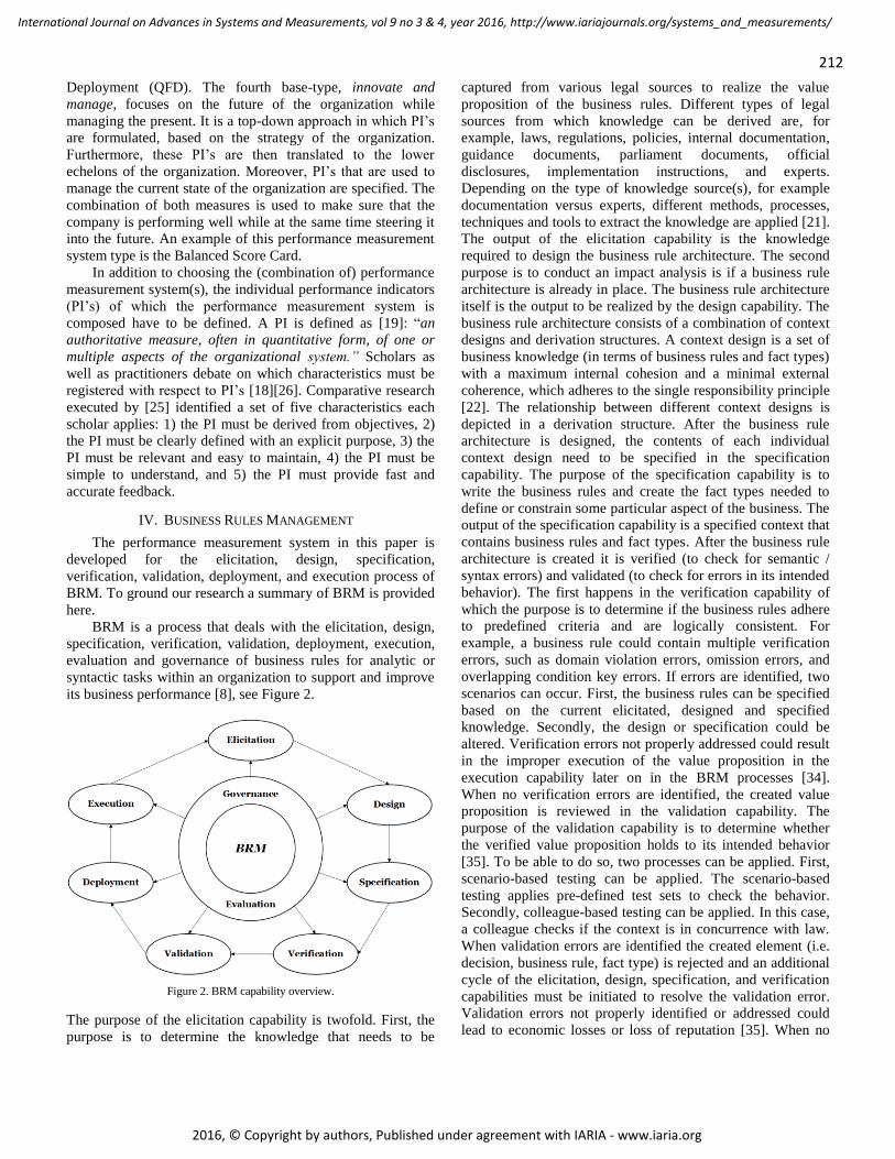
212



Deployment (QFD). The fourth base-type, innovate and

manage, focuses on the future of the organization while

managing the present. It is a top-down approach in which PI’s

are formulated, based on the strategy of the organization.

Furthermore, these PI’s are then translated to the lower

echelons of the organization. Moreover, PI’s that are used to

manage the current state of the organization are specified. The

combination of both measures is used to make sure that the

company is performing well while at the same time steering it

into the future. An example of this performance measurement

system type is the Balanced Score Card.

In addition to choosing the (combination of) performance

measurement system(s), the individual performance indicators

(PI’s) of which the performance measurement system is

composed have to be defined. A PI is defined as [19]: “an

authoritative measure, often in quantitative form, of one or

multiple aspects of the organizational system.” Scholars as

well as practitioners debate on which characteristics must be

registered with respect to PI’s [18][26]. Comparative research

executed by [25] identified a set of five characteristics each

scholar applies: 1) the PI must be derived from objectives, 2)

the PI must be clearly defined with an explicit purpose, 3) the

PI must be relevant and easy to maintain, 4) the PI must be

simple to understand, and 5) the PI must provide fast and

accurate feedback.

IV. BUSINESS RULES MANAGEMENT

The performance measurement system in this paper is

developed for the elicitation, design, specification,

verification, validation, deployment, and execution process of

BRM. To ground our research a summary of BRM is provided

here.

BRM is a process that deals with the elicitation, design,

specification, verification, validation, deployment, execution,

evaluation and governance of business rules for analytic or

syntactic tasks within an organization to support and improve

its business performance [8], see Figure 2.

Figure 2. BRM capability overview.

The purpose of the elicitation capability is twofold. First, the

purpose is to determine the knowledge that needs to be

captured from various legal sources to realize the value

proposition of the business rules. Different types of legal

sources from which knowledge can be derived are, for

example, laws, regulations, policies, internal documentation,

guidance documents, parliament documents, official

disclosures, implementation instructions, and experts.

Depending on the type of knowledge source(s), for example

documentation versus experts, different methods, processes,

techniques and tools to extract the knowledge are applied [21].

The output of the elicitation capability is the knowledge

required to design the business rule architecture. The second

purpose is to conduct an impact analysis is if a business rule

architecture is already in place. The business rule architecture

itself is the output to be realized by the design capability. The

business rule architecture consists of a combination of context

designs and derivation structures. A context design is a set of

business knowledge (in terms of business rules and fact types)

with a maximum internal cohesion and a minimal external

coherence, which adheres to the single responsibility principle

[22]. The relationship between different context designs is

depicted in a derivation structure. After the business rule

architecture is designed, the contents of each individual

context design need to be specified in the specification

capability. The purpose of the specification capability is to

write the business rules and create the fact types needed to

define or constrain some particular aspect of the business. The

output of the specification capability is a specified context that

contains business rules and fact types. After the business rule

architecture is created it is verified (to check for semantic /

syntax errors) and validated (to check for errors in its intended

behavior). The first happens in the verification capability of

which the purpose is to determine if the business rules adhere

to predefined criteria and are logically consistent. For

example, a business rule could contain multiple verification

errors, such as domain violation errors, omission errors, and

overlapping condition key errors. If errors are identified, two

scenarios can occur. First, the business rules can be specified

based on the current elicitated, designed and specified

knowledge. Secondly, the design or specification could be

altered. Verification errors not properly addressed could result

in the improper execution of the value proposition in the

execution capability later on in the BRM processes [34].

When no verification errors are identified, the created value

proposition is reviewed in the validation capability. The

purpose of the validation capability is to determine whether

the verified value proposition holds to its intended behavior

[35]. To be able to do so, two processes can be applied. First,

scenario-based testing can be applied. The scenario-based

testing applies pre-defined test sets to check the behavior.

Secondly, colleague-based testing can be applied. In this case,

a colleague checks if the context is in concurrence with law.

When validation errors are identified the created element (i.e.

decision, business rule, fact type) is rejected and an additional

cycle of the elicitation, design, specification, and verification

capabilities must be initiated to resolve the validation error.

Validation errors not properly identified or addressed could

lead to economic losses or loss of reputation [35]. When no

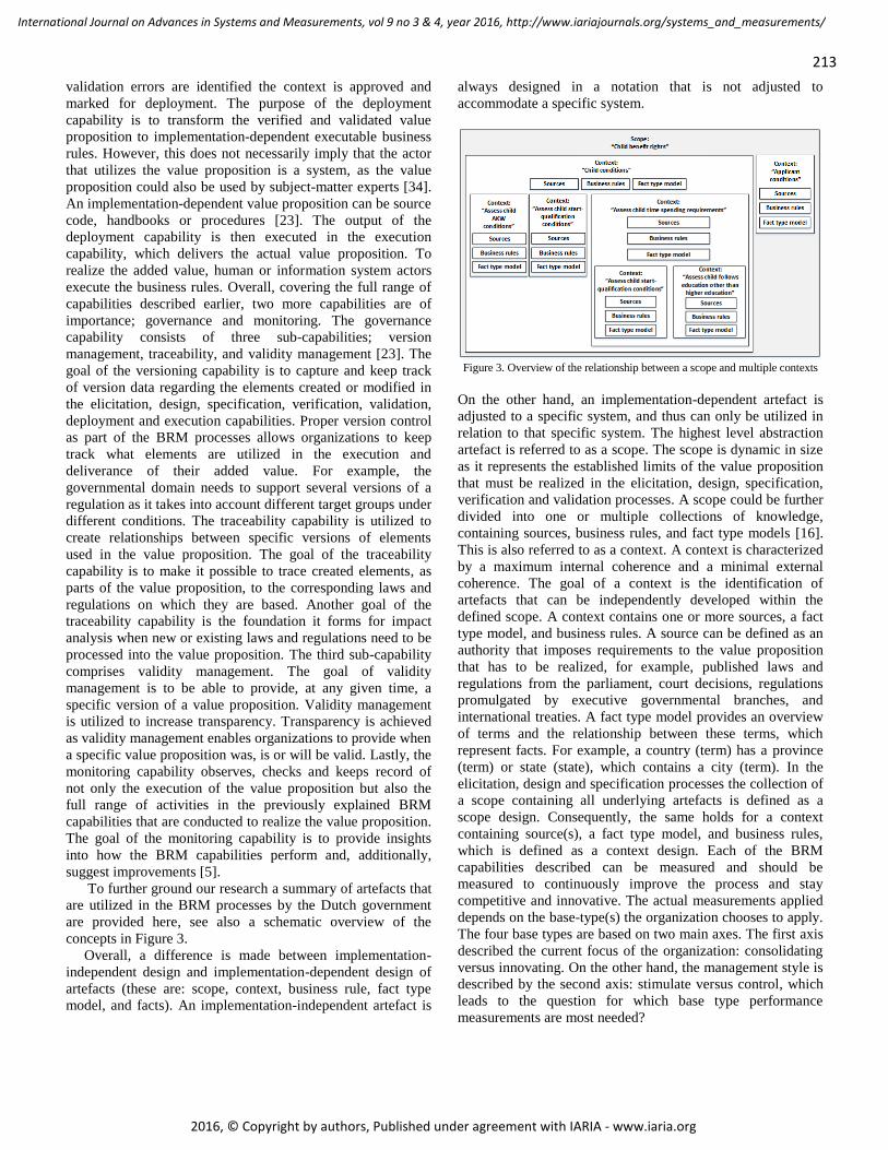
213



validation errors are identified the context is approved and

marked for deployment. The purpose of the deployment

capability is to transform the verified and validated value

proposition to implementation-dependent executable business

rules. However, this does not necessarily imply that the actor

that utilizes the value proposition is a system, as the value

proposition could also be used by subject-matter experts [34].

An implementation-dependent value proposition can be source

code, handbooks or procedures [23]. The output of the

deployment capability is then executed in the execution

capability, which delivers the actual value proposition. To

realize the added value, human or information system actors

execute the business rules. Overall, covering the full range of

capabilities described earlier, two more capabilities are of

importance; governance and monitoring. The governance

capability consists of three sub-capabilities; version

management, traceability, and validity management [23]. The

goal of the versioning capability is to capture and keep track

of version data regarding the elements created or modified in

the elicitation, design, specification, verification, validation,

deployment and execution capabilities. Proper version control

as part of the BRM processes allows organizations to keep

track what elements are utilized in the execution and

deliverance of their added value. For example, the

governmental domain needs to support several versions of a

regulation as it takes into account different target groups under

different conditions. The traceability capability is utilized to

create relationships between specific versions of elements

used in the value proposition. The goal of the traceability

capability is to make it possible to trace created elements, as

parts of the value proposition, to the corresponding laws and

regulations on which they are based. Another goal of the

traceability capability is the foundation it forms for impact

analysis when new or existing laws and regulations need to be

processed into the value proposition. The third sub-capability

comprises validity management. The goal of validity

management is to be able to provide, at any given time, a

specific version of a value proposition. Validity management

is utilized to increase transparency. Transparency is achieved

as validity management enables organizations to provide when

a specific value proposition was, is or will be valid. Lastly, the

monitoring capability observes, checks and keeps record of

not only the execution of the value proposition but also the

full range of activities in the previously explained BRM

capabilities that are conducted to realize the value proposition.

The goal of the monitoring capability is to provide insights

into how the BRM capabilities perform and, additionally,

suggest improvements [5].

To further ground our research a summary of artefacts that

are utilized in the BRM processes by the Dutch government

are provided here, see also a schematic overview of the

concepts in Figure 3.

Overall, a difference is made between implementation-

independent design and implementation-dependent design of

artefacts (these are: scope, context, business rule, fact type

model, and facts). An implementation-independent artefact is

always designed in a notation that is not adjusted to

accommodate a specific system.

Figure 3. Overview of the relationship between a scope and multiple contexts

On the other hand, an implementation-dependent artefact is

adjusted to a specific system, and thus can only be utilized in

relation to that specific system. The highest level abstraction

artefact is referred to as a scope. The scope is dynamic in size

as it represents the established limits of the value proposition

that must be realized in the elicitation, design, specification,

verification and validation processes. A scope could be further

divided into one or multiple collections of knowledge,

containing sources, business rules, and fact type models [16].

This is also referred to as a context. A context is characterized

by a maximum internal coherence and a minimal external

coherence. The goal of a context is the identification of

artefacts that can be independently developed within the

defined scope. A context contains one or more sources, a fact

type model, and business rules. A source can be defined as an

authority that imposes requirements to the value proposition

that has to be realized, for example, published laws and

regulations from the parliament, court decisions, regulations

promulgated by executive governmental branches, and

international treaties. A fact type model provides an overview

of terms and the relationship between these terms, which

represent facts. For example, a country (term) has a province

(term) or state (state), which contains a city (term). In the

elicitation, design and specification processes the collection of

a scope containing all underlying artefacts is defined as a

scope design. Consequently, the same holds for a context

containing source(s), a fact type model, and business rules,

which is defined as a context design. Each of the BRM

capabilities described can be measured and should be

measured to continuously improve the process and stay

competitive and innovative. The actual measurements applied

depends on the base-type(s) the organization chooses to apply.

The four base types are based on two main axes. The first axis

described the current focus of the organization: consolidating

versus innovating. On the other hand, the management style is

described by the second axis: stimulate versus control, which

leads to the question for which base type performance

measurements are most needed?

214



The current trend in business rules management is a shift

from an information technology perspective towards a broader

information systems perspective. Therefore, researchers and

scientist are interested in measuring the current state of

business rules management implementations and capabilities

[20][28][34]. An important question when measuring the

current state is that organizations want to compare and

benchmark their implementations, processes, and capabilities.

For this purpose, multiple initiatives are started, for example,

expert group BRM [17], the blue chamber [6]. This trend of

comparing different parts of a BRM implementation also

concerns the comparison of different rule sets built for the

same solutions. An example of this are the challenges released

by the decision management community [10]. Every month

they release a problem for which different vendors provide

their solutions such that they can be compared to each other.

To manage and improve the different BRM

capabilities/processes insight has to be created regarding the

current situation of these processes. Thus, on the current focus

of the organization axis we adopt the consolidating

perspective over the innovating perspective for this study.

The selection of the participants should be based on the

group of individuals, organizations, information technology,

or community that best represents the phenomenon studied

[33]. In this study, we want to measure the current practice of

the work of the employees that perform the capabilities. This

implies that we will apply a bottom-up approach and will

involve employees working on business rules and their direct

management. Therefore, on the second axis we focus on the

stimulating over controlling, thereby adopting the perspective

of the first base-type, consolidate and stimulate, as described

in detail in section three.

Our focus per PI will be on the characteristics as defined

by [18]: 1) derived from objectives, 2) clearly defined with an

explicit purpose, 3) relevant and easy to maintain, 4) simple to

understand, and 5) provide fast and accurate feedback. These

PI’s form the basis to build a framework that organizations

can utilize to design their BRM evaluation process focused on

evaluating and improving its business performance.

V. RESEARCH METHOD

The goal of this research is to identify performance

measurements that provide relevant insight into the

performance of the elicitation, design, specification,

verification, validation, deployment, execution, and

governance processes of BRM. In addition to the goal of the

research, also, the maturity of the research field is a factor in

determining the appropriate research method and technique.

The maturity of the BRM research field, with regard to non-

technological research, is nascent [20][27][34]. Focus of

research in nascent research fields should lie on identifying

new constructs and establishing relationships between

identified constructs [12]. Summarized, to accomplish our

research goal, a research approach is needed in which a broad

range of possible performance measurements are explored and

combined into one view in order to contribute to an

incomplete state of knowledge.

Adequate research methods to explore a broad range of possible ideas / solutions to a complex issue and combine them into one view when a lack of empirical evidence exists consist of group-based research techniques [11][24][29][30]. Examples of group based techniques are Focus Groups, Delphi Studies, Brainstorming and the Nominal Group Technique. The main characteristic that differentiates these types of group-based research techniques from each other is the use of face-to-face versus non-face-to-face approaches. Both approaches have advantages and disadvantages, for example, in face-to-face meetings, provision of immediate feedback is possible. However, face-to-face meetings have restrictions with regard to the number of participants and the possible existence of group or peer pressure. To eliminate the disadvantages, we combined the face-to-face and non-face-to-face technique by means of applying the following two group based research approaches: the Focus Group and Delphi Study.

VI. DATA COLLECTION AND ANALYSIS

Data for this study is collected over a period of six months, through three rounds of focus groups (rounds 1, 2 and 3: experts focus group) and a three-round Delphi study (rounds 4, 5 and 6 Delphi study), see Figure 4. Between each individual round of focus group and Delphi Study, the researchers consolidated the results (rounds 1, 2, 3, 4, 5, 6 and 7: research team). Both methods of data collection and analysis are further discussed in the remainder of this section.

A. Focus Groups

Before a focus group is conducted, a number of key issues

need to be considered: 1) the goal of the focus group, 2) the

selection of participants, 3) the number of participants, 4) the

selection of the facilitator, 5) the information recording

facilities, and 6) the protocol of the focus group. The goal of

the focus group was to identify performance measurements for

the performance of the elicitation, design, specification,

verification, validation, deployment, execution, and

governance capabilities of BRM. The selection of the

participants should be based on the group of individuals,

organizations, information technology, or community that best

represents the phenomenon studied [33]. In this study,

organizations and individuals that deal with a large amount of

business rules represent the phenomenon studied. Such

organizations are often financial and government institutions.

During this research, which was conducted from September

2014 to December 2014, five large Dutch government

institutions participated. Based on the written description of

the goal and consultation with employees of each government

institution, participants were selected to take part in the three

focus group meetings. In total, ten participants took part,

which fulfilled the following positions: two enterprise

architects, two business rules architects, three business rules

analysts, one project manager, and two policy advisors. Each

of the participants had, at least, five years of experience with

business rules. Delbecq and van de Ven [11] and Glaser [15]

state that the facilitator should be an expert on the topic and

familiar with group meeting processes. The selected facilitator

has a Ph.D. in BRM, has conducted 7 years of research on the

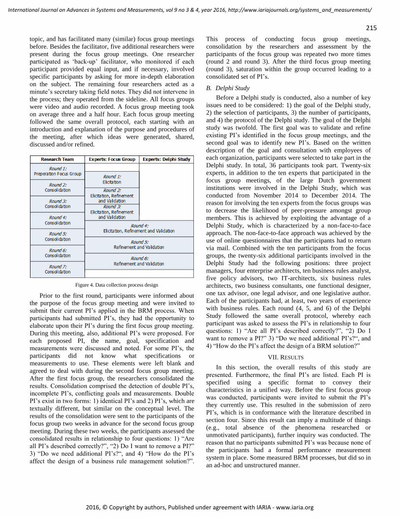
215



topic, and has facilitated many (similar) focus group meetings

before. Besides the facilitator, five additional researchers were

present during the focus group meetings. One researcher

participated as ‘back-up’ facilitator, who monitored if each

participant provided equal input, and if necessary, involved

specific participants by asking for more in-depth elaboration

on the subject. The remaining four researchers acted as a

minute’s secretary taking field notes. They did not intervene in

the process; they operated from the sideline. All focus groups

were video and audio recorded. A focus group meeting took

on average three and a half hour. Each focus group meeting

followed the same overall protocol, each starting with an

introduction and explanation of the purpose and procedures of

the meeting, after which ideas were generated, shared,

discussed and/or refined.

Figure 4. Data collection process design

Prior to the first round, participants were informed about

the purpose of the focus group meeting and were invited to

submit their current PI’s applied in the BRM process. When

participants had submitted PI’s, they had the opportunity to

elaborate upon their PI’s during the first focus group meeting.

During this meeting, also, additional PI’s were proposed. For

each proposed PI, the name, goal, specification and

measurements were discussed and noted. For some PI’s, the

participants did not know what specifications or

measurements to use. These elements were left blank and

agreed to deal with during the second focus group meeting.

After the first focus group, the researchers consolidated the

results. Consolidation comprised the detection of double PI’s,

incomplete PI’s, conflicting goals and measurements. Double

PI’s exist in two forms: 1) identical PI’s and 2) PI’s, which are

textually different, but similar on the conceptual level. The

results of the consolidation were sent to the participants of the

focus group two weeks in advance for the second focus group

meeting. During these two weeks, the participants assessed the

consolidated results in relationship to four questions: 1) “Are

all PI’s described correctly?”, “2) Do I want to remove a PI?”

3) “Do we need additional PI’s?“, and 4) “How do the PI’s

affect the design of a business rule management solution?”.

This process of conducting focus group meetings,

consolidation by the researchers and assessment by the

participants of the focus group was repeated two more times

(round 2 and round 3). After the third focus group meeting

(round 3), saturation within the group occurred leading to a

consolidated set of PI’s.

B. Delphi Study

Before a Delphi study is conducted, also a number of key

issues need to be considered: 1) the goal of the Delphi study,

2) the selection of participants, 3) the number of participants,

and 4) the protocol of the Delphi study. The goal of the Delphi

study was twofold. The first goal was to validate and refine

existing PI’s identified in the focus group meetings, and the

second goal was to identify new PI’s. Based on the written

description of the goal and consultation with employees of

each organization, participants were selected to take part in the

Delphi study. In total, 36 participants took part. Twenty-six

experts, in addition to the ten experts that participated in the

focus group meetings, of the large Dutch government

institutions were involved in the Delphi Study, which was

conducted from November 2014 to December 2014. The

reason for involving the ten experts from the focus groups was

to decrease the likelihood of peer-pressure amongst group

members. This is achieved by exploiting the advantage of a

Delphi Study, which is characterized by a non-face-to-face

approach. The non-face-to-face approach was achieved by the

use of online questionnaires that the participants had to return

via mail. Combined with the ten participants from the focus

groups, the twenty-six additional participants involved in the

Delphi Study had the following positions: three project

managers, four enterprise architects, ten business rules analyst,

five policy advisors, two IT-architects, six business rules

architects, two business consultants, one functional designer,

one tax advisor, one legal advisor, and one legislative author.

Each of the participants had, at least, two years of experience

with business rules. Each round (4, 5, and 6) of the Delphi

Study followed the same overall protocol, whereby each

participant was asked to assess the PI’s in relationship to four

questions: 1) “Are all PI’s described correctly?”, “2) Do I

want to remove a PI?” 3) “Do we need additional PI’s?“, and

4) “How do the PI’s affect the design of a BRM solution?”

VII. RESULTS

In this section, the overall results of this study are

presented. Furthermore, the final PI’s are listed. Each PI is

specified using a specific format to convey their

characteristics in a unified way. Before the first focus group

was conducted, participants were invited to submit the PI’s

they currently use. This resulted in the submission of zero

PI’s, which is in conformance with the literature described in

section four. Since this result can imply a multitude of things

(e.g., total absence of the phenomena researched or

unmotivated participants), further inquiry was conducted. The

reason that no participants submitted PI’s was because none of

the participants had a formal performance measurement

system in place. Some measured BRM processes, but did so in

an ad-hoc and unstructured manner.

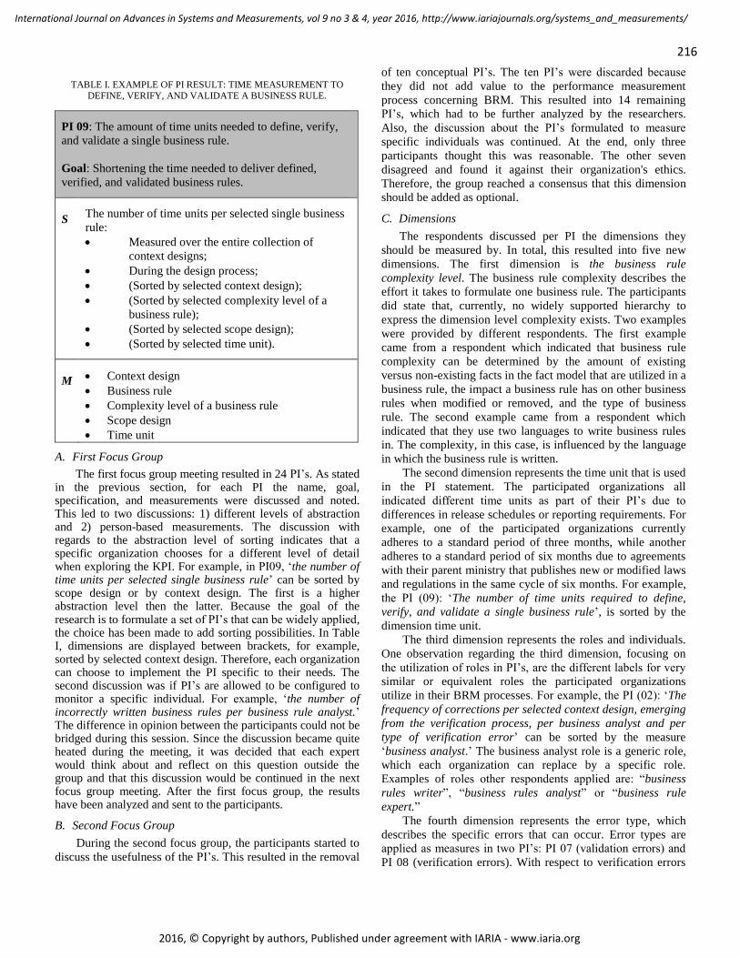
216



TABLE I. EXAMPLE OF PI RESULT: TIME MEASUREMENT TO

DEFINE, VERIFY, AND VALIDATE A BUSINESS RULE.

PI 09: The amount of time units needed to define, verify,

and validate a single business rule.

Goal: Shortening the time needed to deliver defined,

verified, and validated business rules.

S

The number of time units per selected single business

rule:

Measured over the entire collection of

context designs;

During the design process;

(Sorted by selected context design);

(Sorted by selected complexity level of a

business rule);

(Sorted by selected scope design);

(Sorted by selected time unit).

M

Context design

Business rule

Complexity level of a business rule

Scope design

Time unit

A. First Focus Group

The first focus group meeting resulted in 24 PI’s. As stated in the previous section, for each PI the name, goal, specification, and measurements were discussed and noted. This led to two discussions: 1) different levels of abstraction and 2) person-based measurements. The discussion with regards to the abstraction level of sorting indicates that a specific organization chooses for a different level of detail when exploring the KPI. For example, in PI09, ‘the number of time units per selected single business rule’ can be sorted by scope design or by context design. The first is a higher abstraction level then the latter. Because the goal of the research is to formulate a set of PI’s that can be widely applied, the choice has been made to add sorting possibilities. In Table I, dimensions are displayed between brackets, for example, sorted by selected context design. Therefore, each organization can choose to implement the PI specific to their needs. The second discussion was if PI’s are allowed to be configured to monitor a specific individual. For example, ‘the number of incorrectly written business rules per business rule analyst.’ The difference in opinion between the participants could not be bridged during this session. Since the discussion became quite heated during the meeting, it was decided that each expert would think about and reflect on this question outside the group and that this discussion would be continued in the next focus group meeting. After the first focus group, the results have been analyzed and sent to the participants.

B. Second Focus Group

During the second focus group, the participants started to

discuss the usefulness of the PI’s. This resulted in the removal

of ten conceptual PI’s. The ten PI’s were discarded because

they did not add value to the performance measurement

process concerning BRM. This resulted into 14 remaining

PI’s, which had to be further analyzed by the researchers.

Also, the discussion about the PI’s formulated to measure

specific individuals was continued. At the end, only three

participants thought this was reasonable. The other seven

disagreed and found it against their organization's ethics.

Therefore, the group reached a consensus that this dimension

should be added as optional.

C. Dimensions

The respondents discussed per PI the dimensions they

should be measured by. In total, this resulted into five new

dimensions. The first dimension is the business rule

complexity level. The business rule complexity describes the

effort it takes to formulate one business rule. The participants

did state that, currently, no widely supported hierarchy to

express the dimension level complexity exists. Two examples

were provided by different respondents. The first example

came from a respondent which indicated that business rule

complexity can be determined by the amount of existing

versus non-existing facts in the fact model that are utilized in a

business rule, the impact a business rule has on other business

rules when modified or removed, and the type of business

rule. The second example came from a respondent which

indicated that they use two languages to write business rules

in. The complexity, in this case, is influenced by the language

in which the business rule is written.

The second dimension represents the time unit that is used

in the PI statement. The participated organizations all

indicated different time units as part of their PI’s due to

differences in release schedules or reporting requirements. For

example, one of the participated organizations currently

adheres to a standard period of three months, while another

adheres to a standard period of six months due to agreements

with their parent ministry that publishes new or modified laws

and regulations in the same cycle of six months. For example,

the PI (09): ‘The number of time units required to define,

verify, and validate a single business rule’, is sorted by the

dimension time unit.

The third dimension represents the roles and individuals.

One observation regarding the third dimension, focusing on

the utilization of roles in PI’s, are the different labels for very

similar or equivalent roles the participated organizations

utilize in their BRM processes. For example, the PI (02): ‘The

frequency of corrections per selected context design, emerging

from the verification process, per business analyst and per

type of verification error’ can be sorted by the measure

‘business analyst.’ The business analyst role is a generic role,

which each organization can replace by a specific role.

Examples of roles other respondents applied are: “business

rules writer”, “business rules analyst” or “business rule

expert.”

The fourth dimension represents the error type, which

describes the specific errors that can occur. Error types are

applied as measures in two PI’s: PI 07 (validation errors) and

PI 08 (verification errors). With respect to verification errors

217



three types can be recognized: 1) context error types, 2)

business rules errors, and 3) fact type errors. Examples of

specific errors are: circularity error, consequent error,

unnecessary condition fact type error, interdeterminism error,

overlapping condition key coverage error, unused fact type

error and domain violation error. Not every organization can

measure every error type, as this depends on the language and

tool they apply. Therefore, the dimension can vary per

organization.

The fifth dimension represents the implementation of the

business rules: implementation-independent versus

implementation-dependent. In this first case, an organization

elicits, designs, specifies, verifies and validates the business

rules in an implementation-independent way. Therefore, the PI

also focuses on the implementation-independent part.

However, one of the participated organizations already

designs, specifies, verifies and validates the business rules in

an implementation-dependent environment. In this case the

PI’s focus on the implementation-dependent part.

D. The Third Focus Group

During the third focus group, the participants discussed

the remaining 14 final PI’s, which led to the further

refinement of goals, specifications, and measurements.

Additionally, the subject-matter experts expressed a certain

need to categorize PI’s into well-known phases within the

development process of business rules at the case

organizations. From the 14 remaining PI’s, nine PI’s were

categorized as business rule design PI’s, two PI’s were

categorized as business rule deployment PI’s, and three PI’s

were categorized as business rules execution PI’s.

E. Delphi Study

After the third focus group, the 14 PI’s were subjected to

the Delphi Study participants. In each of the three rounds, no

additional PI’s were formulated by the 26 experts. However,

during the first two rounds, the specification and measurement

elements of multiple PI’s were refined. During the third round,

which was also the last round, no further refinements were

proposed and participants all agreed to the 14 formulated PI’s,

which are presented in Table II.

TABLE II. PI'S for BRM

PI 01: The frequency of corrections per selected context

design emerging from the verification process.

Goal: Improve upon the design process of

business rules.


design, emerging from the verification process, per business

analyst and per type of verification error.

Goal: Improving the context design.


design emerging from the validation process per complexity

level of a business rule.

Goal: Improve upon the design process of

business rules.


design emerging from the validation process per type of

validation error.

Goal: Improve upon the validation process for the

benefit of improving the context design.


architecture emerging from the design process per scope

design.

Goal: Improve upon the design process for the

benefit of improving the context architecture.

PI 06: The frequency of instantiations per selected context

design

Goal: Provide insight into the possible instances of

a context design.

PI 07: The frequency per selected type of validation error.



PI 08: The frequency per selected type of verification error



PI 09: The number of time units required to define, verify,

and validate a single business rule.

Goal: Shortening the lead time of a business rule

with regard to the design process.

PI 10: The frequency of deviations between an

implementation dependent context design and an

implementation independent context design.

Goal: Improve upon the deployment process.

PI 11: The frequency of executions of an implementation

dependent business rule.

Goal: Gaining insight into what business rules are

executed.

PI 12: The frequency of execution variants of a scope

design.

Goal: Gaining insight into what decision paths are

traversed to establish different decisions.

PI 13: The number of time units required for the execution

per execution variant.

Goal: Shortening the lead time of an execution

process with regard to enhancing an execution

variant.

PI 14: The amount of business rules that cannot be

automated.

Goal: Provide insight into what business rules

cannot be automated.

Analyzing the defined PI’s showed that three out of fourteen (PI 11, 12, and 14) are PI’s that can be classified as ‘innovate and manage’ PI’s. PI number eleven and twelve focus on the number of times a business rule is executed, thereby providing insight on which business rules are most applied. PI twelve goes beyond that and shows which variants of business rules are executed. In other words, it shows the characteristics of the decision based on which citizens or organizations get services. This insight can be used to determine how many and which citizens or organizations are affected by changing specific laws (and, therefore, business rules). In other words, this can be used to further support the

218



development of law. PI fourteen indicated the amount of business rules that cannot be automated, in other words, that need to be executed manually. This can also provide an indication of the amount of workload that organizations encounter due to the manual execution of these specific business rules. This PI can be used to decide if these business rules should be executed manually or that they should be reformulated in such a manner that they can be executed mechanically.

VIII. DISCUSSION AND FUTURE WORK

From a research perspective, our study provides a

fundament for PI measurement and benchmarking of the

elicitation, design, specification, verification, validation,

deployment, execution, and governance capabilities of BRM.

In addition to the PI’s, one of the biggest discussion has been

the question whether a PI should be measured per individual

person. Regarding this discussion most respondents in our

research agreed that PI’s should not measure the performance

of an individual person. This could be related to the fact that

the sample group didn’t contain respondents from a

commercial organization where it might be more accepted that

the performance of an individual person is measured. From the

perspective of performance management systems we focused

on the base type 1) consolidate and simulate. When BRM

implementations become more mature, innovation should be

encouraged and PI’s for the base types 3) innovate and

stimulate, and 4) innovate and manage should be measured.

From an economic perspective, our research results contribute

to the design of a proper performance measurement design for

the BRM capabilities in order to provide insights about how

organizational resources are utilized and how they could be

utilized more effectively.

Another discussion focused on the terminology applied to

formulate the PI’s. The discussion started because the

organizations that employ the participants applied different

terms and definitions to describe the same elements. This is

mainly caused by the different business rule management

methods used, business rule management systems applied,

business rule language(s) used or business rule engines

implemented by the participating organizations. Most of the

proprietary systems apply their own language, thereby

decreasing interoperability. For example, one organization has

implemented Be Informed, which applies the Declarative

Process Modeling Notation while another organization

implemented The Annotation Environment, which applies

Structured Dutch. Therefore, the terminology chosen to

formulate the PI’s is neutral. However, the terms of the PI’s

can be adapted to the specific organization.

Several limitations may affect our results. The first

limitation is the sampling and sample size. The sample group

of participants is solely drawn from government institutions in

the Netherlands. While we believe that government

institutions are representative for organizations implementing

business rules, further generalization towards non-

governmental organizations, amongst others, is a

recommended direction for future research. Taken the sample

size of 36 participants into account, this number needs to be

increased in future research as well. Another observation is the

lack of PI’s regarding some BRM capabilities described in

section four. This could have been caused due to participants

focusing on a specific BRM capability in practice, limiting the

input of PI’s regarding other BRM capabilities. Future

research should focus on including participants, which are

responsible for one capability (taking into account to cover all

capabilities) a combination of BRM capabilities, or all BRM

capabilities (higher level management).

This research focused on identifying new constructs and

establishing relationships given the current maturity of the

BRM research field. Although the research approach chosen

for this research type is appropriate given the present maturity

of the research field, research focusing on further

generalization should apply different research methods such as

qualitative research methods, which also allow incorporating a

larger sample size in future research regarding PI’s for BRM.

IX. CONCLUSION

This research investigated PI’s for the elicitation, design,

acceptance, deployment and execution of business rules with

the purpose of answering the following research question:

“Which performance measurements are useful to measure the

BRM processes?” To accomplish this goal, we conducted a

study combining a three round focus group and three round

Delphi Study. Both were applied to retrieve PI’s from

participants, 36 in total, employed by five governmental

institutions. This analysis revealed fourteen PI’s. We believe

that this work represents a further step in research on PI’s for

BRM and maturing the BRM field as a whole.

REFERENCES

[1] M. M. Zoet, K. Smit, and E. Y. de Haan, “Performance Indicators for Business Rule Management,” Proceedings of the Eighth International Conference on Information, Process, and Knowledge Management - EKNOW, Venice, 2016.

[2] M. Alles, G. Brennan, A. Kogan, and M. Vasarhelyi, “Continuous monitoring of business process controls: A pilot implementation of a continuous auditing system at Siemens,” International Journal of Accounting Information Systems, 7, 2006, pp. 137-161. doi: 10.1016/j.accinf.2005.10.004

[3] D. Amaratunga and D. Baldry, “Moving from performance measurement to performance management,” Facilities, 20(5/6), 2002, pp. 217-223.

[4] D. Arnot and G. Pervan, “A critical analysis of decision support systems research,” Journal of information technology, 20(2), 2005, pp. 67-87.

[5] M. Baject and M. Krisper, “A methodology and tool support for managing business rules in organisations,” Information Systems, 30, 2005, pp. 423-443.

[6] Blue Chamber, “Legislation to services: an approach for agile execution of legislation,” 2013.

[7] J. Boyer and H. Mili, “Agile Business Rules Development: Process, Architecture and JRules Examples,” Heidelberg: Springer, 2011.

[8] J. Breuker and W. Van De Velde, “CommonKADS Library for Expertise Modelling: reusable problem-solving components,” Amsterdam: IOS Press/Ohmsha, 1994.

[9] G. Cokins, “Performance Management: Integrating Strategy Execution, Methodologies, Risk, and Analytics,” Hoboken: John Wiley & Sons, Inc., ISBN13: 9780470449981, 2009.

219



[10] Decision Management Community, “DMcommunity” Retrieved November, 2016, from https://www.dmcommunity.org.

[11] A. L. Delbecq and A. H. Van de Ven, “A group process model for problem identification and program planning,” The Journal of Applied Behavioral Science, 7(4), 1971, pp. 466-492.

[12] A. Edmondson and S. McManus, “Methodological Fit in Management Field Research,” Academy of Management Review, 32(4), 2007, pp. 1155-1179.

[13] A. Ferreira and D. Otley, “The design and use of performance management systems: An extended framework for analysis,” Management accounting research, 20(4), 2009, pp. 263-282.

[14] M. Franco-Santos, L. Lucianetti, and M. Bourne, “Contemporary performance measurement systems: A review of their consequences and a framework for research,” Management Accounting Research, 23(2), 2012, pp. 79-119.

[15] B. Glaser, “Theoretical Sensitivity: Advances in the Methodology of Grounded Theory,” Mill Valley, CA: Sociology Press, 1978.

[16] I. Graham, “Business Rules Management and Service Oriented Architecture,” New York: Wiley, 2006.

[17] Handvestgroep Publiek Verantwoorden, “Together means more,” HPV, Den Haag, 2013, pp. 22-23.

[18] M. Hudson, A. Smart, and M. Bourne, “Theory and practice in SME performance measurement systems,” International Journal of Operations & Production Management, 21(8), 2001, pp. 1096-1115.

[19] L. Kerklaan, “The cockpit of the organization: performance management with scorecards,” Deventer: Kluwer, 2007.

[20] A. Kovacic, “Business renovation: business rules (still) the missing link,” Business Process Management Journal, 10(2), 2004, pp. 158-170.

[21] S. H. Liao, “Expert System Methodologies and Applications - A Decade Review from 1995 to 2004,” Expert Systems with Applications, 28(1), 2004, pp. 93-103

[22] R. Martin, “Agile Software Development: Principles, Patterns and Practices,” New York, 2003.

[23] T. Morgan, “Business rules and information systems: aligning IT with business goals,” London: Addison-Wesley, 2002.

[24] M. K. Murphy, N. Black, D. L. Lamping, C. M. McKee, C. F. B. Sanderson, and J. Askham, “Consensus development methods and their use in clinical guideline development,” Health Technology Assessment, 2(3), 1998, pp. 31-38.

[25] A. Neely, H. Richards, H. Mills, K. Platts, and M. Bourne, “Designing performance measures: a structured approach,” International Journal of Operations and Production, 17(11), 1997, pp. 1131-1152.

[26] A. Neely, “The evolution of performance measurement research: developments in the last decade and a research agenda for the next,” International Journal of Operations & Production Management, 25(12), 2005, pp. 1264-1277.

[27] M. L. Nelson, J. Peterson, R. L. Rariden, and R. Sen, “Transitioning to a business rule management service model: Case studies from the property and casualty insurance industry,” Information & Management, 47(1), 2010, pp. 30-41.

[28] M. L. Nelson, R. L. Rariden, and R. Sen, “A Lifecycle Approach towards Business Rules Management,” Proceedings of the 41st Hawaii International Conference on System Sciences, Hawaii, 2008.

[29] C. Okoli and S. D. Pawlowski, “The Delphi method as a research tool: an example, design considerations and applications,” Information & Management, 42(1), 2004, pp. 15-29.

[30] R. Ono and D. J. Wedemeyer, “Assessing the validity of the Delphi technique,” Futures, 26(3), 1994, pp. 289-304.

[31] V. Owhoso and S. Vasudevan, “A balanced scorecard based framework for assessing the strategic impacts of ERP systems,” Computers in Industry, 56, 2005, pp. 558-572.

[32] R. Ross, “Business Rule Concepts,” Houston: Business Rule Solutions, LLC, 2009.

[33] A. Strauss and J. Corbin, “Basics of qualitative research: Grounded theory procedures and techniques,” Newbury Park: Sage Publication, INC, 1990.

[34] M. M. Zoet, “Methods and Concepts for Business Rules Management,” Utrecht: Hogeschool Utrecht, 2014.

[35] M. M. Zoet and J. Versendaal, “Business Rules Management Solutions Problem Space: Situational Factors,” Proceedings of the 2013 Pacific Asia Conference on Information Systems, Jeju, 2013.

220



Big Data for Personalized Healthcare

Liseth Siemons, Floor Sieverink, Annemarie Braakman-Jansen, Lisette van Gemert-Pijnen

Centre for eHealth and Well-being Research Department of Psychology, Health, and Technology

University of Twente Enschede, the Netherlands

(l.siemons, f.sieverink, l.m.a.braakman-jansen, j.vangemert-pijnen)@utwente.nl

Wouter Vollenbroek Department of Media, Communication & Organisation

University of Twente Enschede, the Netherlands [email protected]

Lidwien van de Wijngaert Department of Communication and Information Studies

Radboud University Nijmegen, the Netherlands [email protected]

Abstract - Big Data, often defined according to the 5V model (volume, velocity, variety, veracity and value), is seen as the key towards personalized healthcare. However, it also confronts us with new technological and ethical challenges that require more sophisticated data management tools and data analysis techniques. This vision paper aims to better understand the technological and ethical challenges we face when using and managing Big Data in healthcare as well as the way in which it impacts our way of working, our health, and our wellbeing. A mixed-methods approach (including a focus group, interviews, and an analysis of social media) was used to gain a broader picture about the pros and cons of using Big Data for personalized healthcare from three different perspectives: Big Data experts, healthcare workers, and the online public. All groups acknowledge the positive aspects of applying Big Data in healthcare, touching upon a wide array of issues, both scientifically and socially. By sharing health data, value can be created that goes beyond the individual patient. The Big Data revolution in healthcare is seen as a promising and innovative development. Yet potential facilitators and barriers need to be faced first to reach its full potential. Concerns were raised about privacy, trust, reliability, safety, purpose limitation, liability, profiling, data ownership, and loss of autonomy. Also, the importance of adding the people-centered view to the rather data-centered 5V model is stressed, in order to get a grip on the opportunities for using Big Data in personalized healthcare. People should be aware that the development of Big Data advancements is not self-evident.

Keywords - Big Data; personalized healthcare; eHealth.

I. INTRODUCTION The “Big Data” revolution is a promising development

that can significantly advance our healthcare system, promoting personalized healthcare [1]. Imagine a system that analyzes large amounts of real-time data from premature babies to detect minimal changes in the condition of these babies that might point to a starting infection. Science fiction? No, IBM and the Institute of Technology of the University of Ontario developed a system that enables physicians to respond much sooner to a changing condition

of the baby, saving lives, and leading to a significantly improved quality of care for premature babies [2].

We are standing at the beginning of the “Big Data” revolution. Many different definitions exist for “Big Data”. Where Mayer-Schönberger and Cukier [2] focus on the new insights and economic value that can be obtained from Big Data in contrast to traditional smeller settings, Wang & Krishnan [3] refer to Big Data as complex and large data sets that can no longer be processed using the traditional processing tools and methods. Yet another definition comes from Laney [4], who defines Big Data according to 3 assets (often referred to as the 3V-model) that require new, cost-effective forms of information processing to promote insight and decision making, including: 1) high-volume (i.e., the quantity of data), 2) high-velocity (i.e., the speed of data generation and processing), and 3) high-variety (i.e., the amount of different data types). Marr [5] expanded this 3V model to the 5V model by adding 2 additional Vs: veracity (i.e., the accuracy or trustworthiness of the data) and maybe the most important asset: value (i.e., the ability to turn the data into value).

Though this is just a grasp out of all the definitions available, there is one thing they have in common: The use of Big Data for analysis and decision making requires a change of thought from knowing “why” to knowing “what”. Where we focused on small, exact datasets and causal connections in the past (i.e., knowing “why”), we now focus on gathering or linking large amounts of (noisy) data, with which we can demonstrate the presence of (unexpected) correlational connections (i.e., knowing “what”) [2]. As a result, we will obtain (and apply) new insights that we did not have before. Insights that can not only be lifesaving, as demonstrated by the example of IBM and the University of Ontario, but that also opens the door towards more personalized medicine [6-8]; i.e., where medical decisions, medications, and/or products are tailored to the individual’s personal profile instead of to the whole patient group. For example, when genetic biomarkers in pharmacogenetics are used to determine the best medical treatment for a patient [6] or when data from thousands of patients that have been

221



treated in the past is being analyzed to determine what treatment best fits the individual patient that is under treatment now (e.g., in terms of expected treatment effects and the risk for severe side-effects given the patient’s personal characteristics like age, gender, genetic features, etc.).

This shift towards more personalized healthcare is reflected in the change of focus within healthcare from a disease-centered approach towards a patient-centered approach, empowering patients to take an active role in the decisions about their own health [8]. As a result, an increasing number of technologies (e.g., Personal Health Records) are being launched by companies to support chronically ill people in the development of self-management skills [9].

The past decades have also shown a rapid growth in the amount of (personal) data that is digitally collected by individuals via wearable technologies that may or may not be stored on online platforms for remote control [2, 6-8, 10], or shared via other online sources like social media. Social media have become socially accepted and used by a growing group of people [11]. They use it, for example, to share data collected by activity, mood, nutrition and sleep trackers on a variety of online platforms (such as Facebook, Twitter, blogs or forums). These data provide new opportunities for healthcare to personalize and improve care even further [12-14]. Furthermore, the data and messages shared via these tools provide insight in vast amounts of valuable information for scientific purposes. For example, [14] used the data from Twitter to predict flu trends and [15] used social media as a measurement tool for the identification of depression. The information gleaned from social media has the potential to complement traditional survey techniques in its ability to provide a more fine-grained measurement over time while radically expanding population sample sizes [15].

By combining clinical data with personal data on, for instance, eating and sleeping patterns, life style, or physical activity level, treatment and coaching purposes can be tailored to the needs of patients even better than before and are, therefore, seen as the key towards a future with optimal medical help [6]. However, it also confronts us with new technological and ethical challenges that require more sophisticated data management tools and data analysis techniques. This vision paper aims to better understand the technological and ethical challenges we face when using and managing Big Data in healthcare as well as the way in which it impacts our way of working, our health, and our wellbeing.

This paper builds on first insights obtained from Big Data experts as already described in [1] and adds the perspectives of healthcare workers (HCWs) and the online public. Section I describes the background of Big Data in literature. Section II describes the procedure of the meetings with experts (focus group; individual meetings) and HCWs (interviews), and describes how the online public’s associations with Big Data in a health context were assessed. Section III presents the results, which are discussed more into depth in Section IV. Finally, Section V concludes this paper, describing a number of implications for research using Big Data in healthcare and addressing some future work.

II. METHODS The impact and challenges of Big Data will be examined

from three different perspectives: 1) from the perspective of Big Data experts [1], 2) from the perspective of HCWs, and 3) from the perspective of the online public. Different methods were used to gather information from each group. Where a focus group was planned with the Big Data experts, this turned out to unfeasible with HCWs because of their busy schedule. That is why individual interviews were scheduled with them. Finally, to evaluate the perspective of the online public, social media posts were scraped and analyzed.

A. Focus group with experts Many potential issues regarding the use of Big Data have

already been mentioned in the literature, newspapers, social media, or debates, and panel discussion websites. However, many of these media sources do not specifically address the healthcare setting and only focus on a limited set of issues at a time (e.g., the privacy and security issues).

To gain more in depth insights into the pros and cons of using Big Data in personalized healthcare, a focus group was organized [16]. The aim was to gain a variety of opinions regarding the scientific and societal issues that play a role in using and managing Big Data to support the growing needs for personalized (and cost-effective) healthcare.

Purposeful sampling was used in the formation of the focus group, meaning that the selection of participants was based on the purpose of the study [16]; i.e., to map the experts’ variety and range of attitudes and beliefs on the use of Big Data for (personalized) healthcare purposes. To gather a broad perspective of viewpoints, multiple disciplines were invited to join the expert meeting, resulting in a panel of 6 experts in Big Data research and quantified self-monitoring from different scientific disciplines: psychology, philosophy, computer science, business administration, law, and data science. Participants were recruited at the University of Twente (the Netherlands), based on their societal impact, expertise, and experiences with conducting Big Data research. Individual face to face meetings were conducted to validate the focus group results.

The focus group took 2 hours in total and was facilitated by LS and FS (authors). All participants signed an informed consent for audiotaping the focus group and for the anonymous usage of the results in publications. LVGP and ABJ took additional notes during the discussion. Group discussion was encouraged and participants were repeatedly asked to share their concerns and thoughts.

In preparation of the focus group discussion, literature and multiple sources of (social) media were searched for information on potential Big Data issues that might play a role. During the discussion itself, experts were asked to write down as many issues as they could think of that might become relevant using Big Data for healthcare. Flip-overs were used to express the issues and experts had to categorize these issues into overall concepts that covered the issues. They named these overall concepts themselves by thinking aloud. These concepts are presented in this vision paper. The focus group was audio taped and transcripts were made by

222



authors of this paper. Loose comments without any further specification were excluded to ensure the results are not a representation of the authors’ interpretation. Ethical approval for the scientific expert meeting and the consent procedure was obtained by the ethics committee of the University of Twente.

B. Interviews with healthcare workers Based on the results of the focus group, an interview

scheme was constructed to assess how HCWs perceive and experience the issues that were identified. Questions were formulated open-ended to encourage HCWs to elaborate on their perceptions of and experiences with Big Data (or eHealth applications) in healthcare. For each question, HCWs were asked to think aloud and to elaborate on their thoughts. Interviews were transcribed verbatim afterwards and a coding scheme was developed.

A total of 6 physicians with experience in Big Data were interviewed. Participants received a first description of the aim of the interviews by e-mail and, in addition, each interview started with a 1.5 minute long movie presenting the interview’s subject: Big Data eHealth applications in healthcare. All participants were interviewed in their work setting. Interviews were semi-structured and continued until the interviewer felt that all questions were answered and no new information could be expected. This took about 60 minutes on average. Participants gave informed consent for audiotaping the interviews and for the anonymous usage of the results in publications. The study was approved by the ethics committee of the University of Twente. No additional ethical approval was necessary from the medical ethical committee.

C. Online public’s associations with Big Data in a health context Though Big Data receives a lot of attention nowadays,

little is known about the publics’ associations with the term Big Data in health contexts. With the digitalization of society, the online public that uses social media channels encloses a large proportion of the potential users of Big Data-driven technological applications in healthcare. Furthermore, the content within the social media provides new opportunities to identify the associations made by the online public in relation to Big Data in a healthcare setting. These associations provide a better understanding of the concerns, opportunities, and considerations that the health sector must take into account.

As such, Coosto, a social media monitoring tool (www.coosto.com), was used as a first explorative analysis to analyze these associations among social media users, using multiple data sources (social networks, microblogs, blogosphere, forums) in both Dutch and English.

The identification of the online public’s perceptions regarding the terms they use when discussing about Big Data in relation to healthcare was completed by following three phases. In the first phase, social media posts were scraped, based on 6 search queries in the Dutch social media monitoring tool Coosto (Table I). To avoid issues caused by word variations (for example: healthcare, health-care, health

TABLE I. SEARCH QUERIES

Search query 1. "big data" "e-health" OR "ehealth" OR "e health" 2. "big data" "healthcare" OR "health care" OR "health-care" 3. "big data" "care" 4. "big data" "sensors" OR "health" OR "e-health" OR "e health" OR

"ehealth" OR "care" OR "healthcare" OR "health care" OR "health-care" OR "wellness" OR “wellbeing” OR “well-being”

5. "big data" "wearables" OR "health" OR "e-health" OR "e health" OR "ehealth" OR OR "care" OR "healthcare" OR "health care" OR "health-care" OR OR "wellness" OR “wellbeing” OR “well-being”

6. "big data" "domotica"

care) and synonyms, an extensive list of different spellings was used in each search query. The terms selected for the search query were derived from a systematic analysis of synonyms in academic literature, popular literature, and websites and Google search results. To treat (longer) blog posts and (shorter) tweets equally, each sentence of all posts was analyzed separately in the second phase. More citations and shares means that more online users are interested in that particular topic.

The second phase was aimed at extracting the most commonly used (combinations of) terms in the collected social media posts and measuring the proximity (the relative distance (similarity)) of these terms. The more frequently two terms are mentioned simultaneously in the whole dataset the higher the proximity between these two (combinations of) terms. Based on a codebook (Appendix 1) consisting of terms that are related to and associated with Big Data and/or healthcare, the most frequently mentioned terms in the social media posts were identified. The codebook terms were selected based on a systematic analysis of scientific and popular literature (including references) and websites (including links to other websites), news articles, social media posts (e.g., Twitter), and Google search results. In our design, the sentences of analysis were considered as the cases, and the terms in these messages – after properly filtering for example the stop words, hyperlinks and @mentions – as the variables. The next step in our analysis was to find the terms (e.g., privacy) or phrases (e.g., Internet of Things) from the codebook in the sentences (cases). The sentences without any of the terms were omitted from further analysis. Thus, a matrix was operated that contained terms as the variables in the columns and sentences as cases in the rows. The cells in the matrix consisted of binary data (whether or not a particular term occurs in the sentences). A proximity measurement [17] indicates what combinations of terms are most prevalent.

In the third phase, the main objective was to determine what terms are mostly associated with Big Data in the context of healthcare within the social media. To do so, the open-source network analysis and visualization software package Gephi (http://gephi.github.io/) was used to visualize the interrelationships between (groups of) terms in a semantic network [18]. The binary matrix formed the basis for the semantic network graph. Due to the reasonably large dataset and the minimum agreement between the terms, the correlations have been relatively low. Therefore, all correlations higher than 0.02 were included in the actual

223



analysis. The terms which served as the basis for the search queries were then removed from the semantic network analysis, since the preservation of these terms in the search results would produce biased results because they will occur significantly more than in reality may be assumed.

III. RESULTS Results are presented separately for each group: 1) Big

Data experts, 2) HCWs, and 3) the online public.

A. Focus group meeting with experts The results can be subdivided in 3 categories: 1)

empowerment, 2) trust, and 3) data wisdom.

1) Empowerment What does it mean when you monitor your activities,

food intake, or stress 24 hours a day using technologies like smart wearables? What drives people to use these 24 hour monitoring devices and what do they need to understand the data generated by these systems? Do they understand the algorithms that are used to capture our behaviors and moods in pictures and graphs? Who owns the data and how to control the maintenance of that data? How to avoid a filtered scope on our lives ignoring others that are out of our affinity groups? The concept of empowerment captures topics as autonomy, freedom, and having control.

Big data evokes a discussion about freedom and autonomy. Autonomy concerns our critical view on how to use technology, while freedom is more about our way of living and thinking. It might, therefore, be more important to focus on freedom instead of autonomy: understanding how you are being influenced and taking a stance against that instead of trying to keep everything away. The focus group made a distinction between positive freedom and negative freedom; two common concepts within the field of philosophy. Positive freedom is the freedom to do something yourself (e.g., to decide for yourself that you want to share your data), whilst negative freedom is the freedom to keep things away, protecting yourself (e.g., when you do not give permission to companies to link your data with other sources). Not losing control, being able to use, share and understand your data is one of the topics when discussing freedom, self-efficacy using self-monitoring technologies.

Empowerment forces us to think about having control, who has the power through the use of Big Data? There might be just a small elite that understands the algorithms and with the increasing complexity, this elite will become even smaller in the future. This can create a division between people who can access and understand the algorithms and people who do not.

Empowering by personalization is one of the aims of the participatory society. Big data can be a leverage to realize this by creating a personal profile, providing the right information, at right moments to enable just in time coaching. Though it can be useful to put people in a profile, the danger of profiling is that you can never leave the assigned group again; once assigned to a group means always assigned to that group. Profiling might be suffocating to people because it creates uncertainty about what people

know about you, what data are being collected, and for what purposes. Also, it is often unclear how to determine the norm to which people are compared when assigning them to a group (i.e., standardization, losing freedom). Furthermore, being assigned to a profile might lead to discrimination and certain prejudices/biases. Questions that arise are: How can profiling be used in a sensible/sound way? And who is responsible when mistakes are being made based on a certain profile?

2) Trust Trust will become a key concept in a data driven society.

This concept captures more than privacy and security issues. Trust refers to topics as how to create faith in data management and data maintenance, and how to make sense of these data for humans.

Privacy issues become particularly relevant when the linkage of anonymous datasets leads to re-identification. Encryption of the data might prevent identification of individuals, but transparency is not always possible (e.g., when analyzing query logs with search terms). In the end it is all about creating trust to overcome uncertainty or anxiety for a digital world.

People often give consent to institutions to use their data for certain purposes in return for the (free) use of the product or service. However, data can be (re)used for other purposes as well or can be sold to other interested parties, even though that is not always allowed. This leads to great concerns: e.g., healthcare insurance companies who use treatment data for other purposes on a more personal level (for instance, for determining a personalized health insurance premium based on your personal data about your health and lifestyle). It is not that people do not want to share data, they already do this using Facebook or Google services, but they want to understand what happens with the data, in particularly when it concerns the health domain.

Self-monitoring technologies, with no doctors or nurses involved in the caring process, are provided more and more by institutions. Smart algorithms can be applied to personalize data in such a way so you can manage your health and wellbeing yourself. However, these algorithms decide what information you get to see, based on information about you as a user (e.g., search history, Facebook friends, location). This will influence trust in the healthcare system, using data from your device compared to personal advices given by your doctor or nurse.

3) Data Wisdom There is a rapid growth of self-monitoring technologies,

but little is known about the reliability and validity of these systems. The lack of evidence for causality can lead to unreliability as well. Furthermore, how can you tell what you are actually measuring? How can the correlations that are found be validated? Does it really say what we think it says or are it just assumptions?

Data wisdom is the concept that captures scientific and societal topics. Scientific refers to how to create data wisdom, in several ways. Those who generate data are not the ones that have the knowledge to analyze, those who analyze lack domain insight (technologies, behaviors). Different kinds of expertise will be needed in the future to

224



deal with Big Data. For instance, expertise to analyze Big Data, expertise to develop and understand the working of algorithms, or expertise in data interpretation and visualizations. The use of data to personalize healthcare demands for new knowledge to support critical and creative thinking to understand data driven decisions and to watch the impact on science, health and society. We all know the disaster with google flu trends, but we have to learn from these failures to set the agenda for future research in using several sources of data (geospatial data, medical data, technology device data) to develop predictive models about health and wellbeing. We have to search for new models, methods to deal with huge datasets, search for patterns rather than testing hypotheses based on small data. Results are not causal-driven but correlational-driven. This requires a change in thought. The golden rule for Randomized Clinical Trials will no longer be the ultimate format for health sciences. New methods are needed to get a grip on “big”, how many data (critical mass) is needed and how rich and mature should data be to make meaningful decisions? How to add qualitative experiences and expertise to Big data? Numbers do not tell the whole story, and a clinical eye is important to interpret data in the context of individual health and wellbeing.

Societal refers to the implications for healthcare, addressing topics as ethics, values for a meaningful life. How to avoid a division between people who can access and understand the data and analytics that rule the decisions about treatments and lifestyle advices, and people that cannot? Knowledge and skills are needed to empower people and people should participate in debates about the values of data for self-regulations on the level of individuals, communities and society. Transparency and trust are the key-topics in that debate. Digging into data starts with a scientific and societal debate on the vales of data for a smart and healthy society.

B. Interviews with healthcare workers Again, the results can be subdivided in the 3 categories:

1) empowerment, 2) trust, and 3) data wisdom.

1) Empowerment Physicians recognize the advantages of data sharing. For

instance, it provides them easy insight in treatment outcomes, which is an important instrument for quality of care. Yet though the large majority of people probably do not have any problems with sharing their data, patients cannot be forced to share their data and should give informed consent first. Nevertheless, patients often do not understand where they give permission for. What if they change their minds, is it possible to undo their data sharing? What if the data is already shared with different disciplines, will they all be refused access after withdrawing the data sharing approval? Possibly, an independent supervisor should be appointed the task to safeguard the proper handling of patient data (at least till data encryption).

There was no consensus among the physicians about data ownership. Some argue the data is primarily of the patient, but the hospital or healthcare practitioner should be able to

gain access to it as well when they have to give account for their actions. On the other hand, it is the physician who writes most of the medical data down in the patient’s personal health record, so it can be argued that he owns (that part of) the data (as well).

Next, the physicians argued that profiling as a concept is nothing new. Current practice is already to gather as much information as possible from a patient and to “go through a checklist” of characteristics, symptoms, or complaints before deciding which treatment might be best. Yet profiling based on Big Data might make this process more accurate, improving treatment outcomes. Especially in complex cases, profiling based on Big Data might be of significant value. It promotes personalized healthcare. Concerns about profiling mainly involve drawing conclusions with far-reaching consequences based on incomplete/imprecise data and the unauthorized misuse of data by third parties, like insurance companies. Also professionals might lose professional skills when they do not have to think for themselves anymore.

When using Big Data for predictive modeling proposes (e.g., to predict the chance you might get lung cancer in the next 5 years), people have the “right not to know”. Within a certain boundary that is. If national health is in danger, personal rights do not weigh up to national security. Patients should be informed at an early stage about their rights and about who is liable when something goes wrong. In case of treatment decisions, the physician is most of the time liable if something goes wrong. In the Netherlands, physicians are guilty until proven innocent in case of an accusation. When using Big Data algorithms in treatment decisions, physicians should still think for themselves whether the provided advice by a system appears to be reasonable, because they make the final judgment about the best possible treatment for their patient. That is not different from the current process in which a physician also has to deal with information from, for instance, radiology, long-term research, laboratory results, etc. It does not matter whether choices are based on Big Data or not, the physician needs to keep thinking as a doctor. Yet liability is not always clear. For instance, what if a patient wears a smart watch that registers his blood pressure, but the device has a defect. Who is liable? The manufacturer or supplier of the device? But how to deal with liability when the patient uses the device in an ignorant way? Who is liable then? Who has to prove what and how is it regulated? It will be a long juridical procedure because rules are not clear and straightforward in cases like this.

2) Trust Physicians definitely recognize the importance of secure

data management. Data management might be outsourced to a third party, on condition that the liability in case of data leaks is properly arranged. Yet physicians might also play an important role in data management, since they are needed for data interpretation. Furthermore, there should be restricted access to sensitive patient data. For instance, when implementing a patient portal, it can be decided to only grant the patient and his own physician access to the portal. In addition, it is of utmost importance that the portal’s communication and data transport mechanisms between the

225



patient and the physician are thoroughly thought through, to minimize the risk on data leaks and cyber-attacks.

Opinions on the need to understand the underlying algorithms of the system were divided. Yet most physicians do want to know the basic reasoning behind the algorithms. They fear to lose their professional clinical skills when blindly following the system, without thinking for themselves anymore. They also argue that the standards and guidelines in the medical field exist because the reasoning behind them are clear. They would never trust a computer without at least some insight into the underlying principles, the reliability of the results, and the parameters that were taken into account. Others, however, express no need to understand the algorithms, but they do argue that the algorithms should be checked by a group of experts.

3) Data Wisdom When asking about their (future) profession, physicians

acknowledge the added value of Big Data systems. The medical field encompasses an enormous amount of data that has been collected over the years. It would be helpful if the data from all the existing different platforms could be combined into one overall system to make it surveyable for both clinical and scientific purposes. When the Big Data revolution offers new opportunities for combining this data using innovative data management tools, many new medical and scientific research questions can be explored. When the right algorithms are being developed, Big Data systems might be more accurate than the patient and physician together could ever be, improving quality of care. For instance, when monitoring a patient’s condition at home, the data is send to the physician via an interactive application right away (i.e., real-time, 24/7), changes can be detected at an early stage, and (remote) treatment can be provided timely. Also, certain risk factors can be detected and controlled at an early stage. Such applications can improve treatment outcomes and significantly reduce healthcare costs.

A certain expertise is needed to translate the enormous amount of data into clinically relevant pieces of information. These Big Data specialists might be appointed from outside the hospital, although the hospital might not have the financial means to do this. Nevertheless, when implemented, Big Data applications can serve as medical decision aids that help the physicians to combine and process all the available data real quick or it could be used for e-consults, where the patient can login onto the system to see lab results, to make appointments, or to ask questions. As a result, patients need to visit the physician less often. An important note that was made, is the need for guidance to the patients. For instance, if a patient suddenly notices a drop in his blood pressure from 120 to 90, he might think: “oh, I am dying”. However, it is still within the norm and this should be explained to the patient to reassure him.

The physicians also recognize the challenges that come with the application of Big Data systems in healthcare. First of all, not all patients will be able to use such systems. For instance, elderly or cognitively impaired patients might not understand the working mechanisms and do not know how to interpret the results. Furthermore, the physicians already always base their decisions on data and it does not really

matter where that data comes from (and, as such, whether it is called “Big Data”). What really matters is that the data is reliable. When you start digging into the data without any clinical expertise, chances are that you will find a significant result. However, it might have no clinical meaning and relevance at all. Data collection and data interpretation cost time (and money) as do the development and testing of the underlying algorithms. People (and insurance companies) should be aware of the imperfections of the system and should not blindly follow it as if it is the golden rule. The system does not replace the physician. The physician still makes the decisions and they will only use a Big Data system if it is proven to be more effective than current practice.

C. Online public’s associations with Big Data in a health context For the social media analysis, a total of 5.852 social

media posts (blogs, forums, microblogs, and social networks) were crawled and scraped, with a total of 59.281 sentences from a time period of five years, with a focus on Big Data in the context of healthcare. In Appendix 1, the frequencies of emerging words are given. Fig. 1 shows the semantic graph consisting of 49 nodes (interrelationships) and 174 edges (collections of terms). The larger the node, the higher the frequency with which the term is mentioned in relation to Big Data in the context of healthcare. The weight of the edges is determined by the proximity between the terms.

With the modularity algorithm [19], ten clusters of terms were established that are often used together. The modularity metric is a well-known exploration concept to identify a network that is more densely connected internally than with the rest of the network [20]. Five of the major ten clusters are (Fig. 1): concerns (red), opportunities (violet), personalized healthcare (green), infrastructure (yellow), and applications (blue). These clusters cover 92 percent of the associations. The remaining clusters (8 percent) are solitary nodes or dyads and have a lack of power.

When evaluated per cluster, the cluster concerns shows the most frequent associations with the terms: 1) privacy, 2) regulations, 3) reliability, 4) algorithms, 5) transparency, and 6) legislations. The terms that are mentioned the most in the cluster involving the opportunities of Big Data in the context of healthcare are 1) innovation, 2) future, 3) development, 4) technology, 5) challenges, 6) start-up and 7) revolution; whereas the personalized healthcare cluster shows the most frequent associations with the terms 1) quantified self, 2) medicine, and 3) personalization. In the infrastructure cluster, the most associated terms with Big Data and healthcare are 1) cloud, 2) service, 3) platform, and 4) software. And finally, the majority of social media posts related to applications focus on 1) S-Health app, 2) Healthkit, and 3) Healthtap.

On average, the vast majority of terms are related to more than one other term (average degree: 7.102). The average degree is a numerical measure of the size for the neighborhood of an individual node [21]. The terms most associated with Big Data in the context of healthcare that

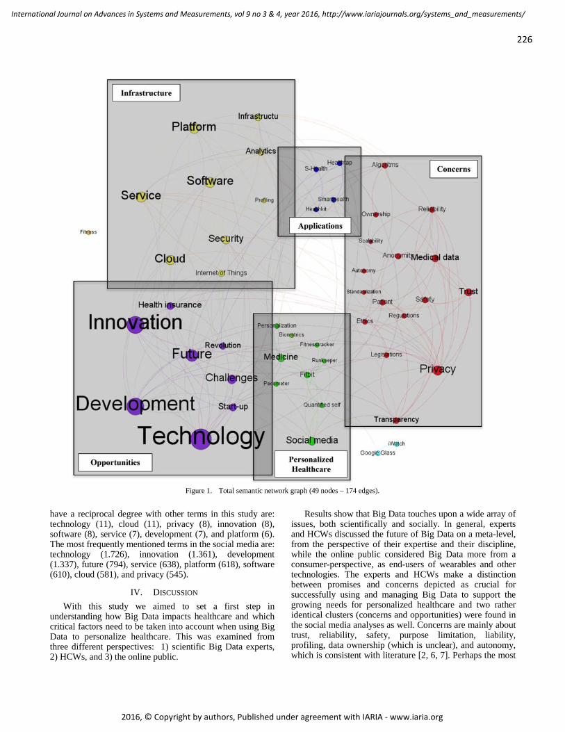
226



Figure 1. Total semantic network graph (49 nodes – 174 edges).

have a reciprocal degree with other terms in this study are: technology (11), cloud (11), privacy (8), innovation (8), software (8), service (7), development (7), and platform (6). The most frequently mentioned terms in the social media are: technology (1.726), innovation (1.361), development (1.337), future (794), service (638), platform (618), software (610), cloud (581), and privacy (545).

IV. DISCUSSION With this study we aimed to set a first step in

understanding how Big Data impacts healthcare and which critical factors need to be taken into account when using Big Data to personalize healthcare. This was examined from three different perspectives: 1) scientific Big Data experts, 2) HCWs, and 3) the online public.

Results show that Big Data touches upon a wide array of issues, both scientifically and socially. In general, experts and HCWs discussed the future of Big Data on a meta-level, from the perspective of their expertise and their discipline, while the online public considered Big Data more from a consumer-perspective, as end-users of wearables and other technologies. The experts and HCWs make a distinction between promises and concerns depicted as crucial for successfully using and managing Big Data to support the growing needs for personalized healthcare and two rather identical clusters (concerns and opportunities) were found in the social media analyses as well. Concerns are mainly about trust, reliability, safety, purpose limitation, liability, profiling, data ownership (which is unclear), and autonomy, which is consistent with literature [2, 6, 7]. Perhaps the most

227



well-known concern bears upon our privacy [6, 7]. For a great deal, these privacy concerns are associated with potential misuse of data by, for instance, insurance companies [6, 10]. If these privacy concerns are not dealt with appropriately, the public’s trust in technological applications might diminish severely [10]. According to the HCWs, patients are often unaware of what is being collected, who is able to view it, and what decisions are being made based on that information. Transparency is needed, people should know what they give informed consent for when they decide to share their data and what happens if they change their mind after some time.

Both experts and HCWs acknowledge the need for a new sort of expertise to be able to understand the algorithms (or at least the basic reasoning behind them) and to interpret the data that is being generated by the technology. At the end, the technology does not replace the physician but they supplement each other. Quality of care can be improved and personalized healthcare becomes the future. Personalized healthcare received a lot of attention in the expert group and among the HCWs. Telemonitoring is seen as a promising development, enabling the physician to react quickly on changes in the clinical status of a patient 24/7, improving the patient’s prognosis. In social media personalized healthcare showed clear associations with the Quantified Self movement, medicine, and personalization. Though the semantic network graph (Fig. 1) only visualized the interrelationships between the (groups of) terms without providing it with an interpretation, this result does demonstrate that the emergence of personalized healthcare and the Quantified Self movement receives a lot of attention in science as well as in society. Yet the main themes discussed by the online public did not include personalized healthcare that much, but rather focused on the technological innovation brought by Big Data, the infrastructure that is needed to make this happen, and privacy issues. The need for a good infrastructure was something the experts also stressed, whereas HCWs focused less on this technological aspect of Big Data.

Some other differences between the groups could be identified as well. An aspect specifically addressed by the HCWs is a concern about a potential loss of their autonomy, control, and professional skills if they “ blindly” follow an algorithm and do not have to think for themselves anymore. The technology has to respect and keep into account their medical autonomy. Furthermore, experts were rather concerned about the misuse of profiling, whereas HCWs stated that profiling in itself is nothing new. According to the experts, the danger of profiling is that you can never leave the assigned group again. Also, profiling might be suffocating to people because it creates uncertainty about what people know about you, what data is being collected, and for what purpose. Profiling might lead to discrimination and certain prejudices/biases and people might experience the feeling that they lose control. On the other hand, HCWs claim that “profiling is something we have always done, otherwise you cannot start any treatment”. HCWs believe that Big Data has the potential to increase its accuracy even further. One concern they do have, in correspondence with

the experts, is about the potential misuse of profiling by third parties like insurance companies.

Though these results provide a broad overview of promises as well as barriers that need to be taken into account when using Big Data in healthcare, a few important limitations should be taken into consideration when interpreting the results. At first, we only performed one focus group. This provided us with diverse insights, but we are not able to determine if saturation has been reached [16]. Still, we do expect that we covered a rather broad area, given the multidisciplinary composition of the group and the large variety of expertise they brought into the discussion. To ensure the accuracy of the results and to prevent that the results represent the interpretation of the researchers, clarification and follow-up questions were asked in case of ambiguity to ensure the validity of the results. As such, we believe that the findings provide an accurate exploration of issues that play a role when using Big Data for personalization purposes in healthcare, from a scientific perspective as well as from a societal perspective.

Secondly, only 6 physicians were interviewed, potentially providing a rather limited view on how HCWs in general think about Big Data. However, that was also not the intent of this study. The aim was to gain a better understanding of technological and ethical challenges that need to be faced when using and managing Big Data in healthcare, as well as to gain insight into its impact on our way of working, our health, and our wellbeing. The interviews with the physicians provide some important first insights for this that can be studied further. All physicians had knowledge of and/or experience with Big Data in some way, to ensure they were able to discuss the topics that were addressed. The interview scheme was constructed based on the input from experts to make sure the same themes were addressed, allowing us to compare the results. At the same time the interview scheme was semi-structured and questions were formulated open-ended to allow the physicians to raise other thoughts as well, enriching the data.

Another limitation is that the results from the perspective of the online public might be colored, as the data are restricted to those who use social media. Therefore, a completely reliable reflection of how the general (online) public thinks or speaks about Big Data in the context of healthcare cannot be given at this moment.

Finally, none of the experts or healthcare workers turned out to be a strong adversary of Big Data in healthcare, even though they did provide some critical comments. As such, it would be interesting to extent the results with the opinions of strong adversaries. After all, for sake of implementation, it is important to take their concerns into consideration as well.

V. CONCLUSION AND FUTURE WORK Big Data is seen as the key towards personalized

healthcare. However, it also confronts us with new technological and ethical challenges that require more sophisticated data management tools and data analysis techniques. This vision paper aimed to better understand the technological and ethical challenges we face when using and managing Big Data in healthcare as well as the way in which

228



it impacts our way of working, our health, and our wellbeing. A mixed-methods approach (including a focus group, interviews, and an analysis of social media) was used to gain a broader picture about the pros and cons of using Big Data for personalized healthcare from three different perspectives: Big Data experts, HCWs, and the online public. All groups acknowledge the positive aspects of applying Big Data in healthcare, touching upon a wide array of issues, both scientifically and socially. By sharing health data, value can be created that goes beyond the individual patient. The Big Data revolution in healthcare is seen as a promising and innovative development.

Yet the development of these advancements is not self-evident and potential facilitators and barriers need to be addressed first. Concerns were raised, mainly about privacy, trust, reliability, safety, purpose limitation, liability, profiling, data ownership, and loss of autonomy. Also, trust in the technological applications is essential to overcome uncertainty or anxiety for a digital world. To achieve this, a first condition is that privacy and security issues are dealt with appropriately. People should be able to decide for themselves whether or not to share their data and with whom. Also, algorithms should be transparent (at least to a certain degree) to the users (e.g., physicians) to make them meaningful. Reliability should be assured and different kinds of expertise need to evolve. Expertise to analyze Big Data, to develop and understand the working of algorithms, and to interpret and visualize the data in a meaningful way. Moreover, technology should be embedded in our way of working and living. As such, technology should supplement the work of physicians, not replace it, respecting the medical autonomy. The digitalization of society is an ongoing process and the “Big Data” revolution is already changing science, healthcare, and society.

In general, Big Data is described according to the 5V model (Volume, Velocity, Variety, Veracity and Value) [5]. Yet this paper stresses the importance of adding the people-centered view to this rather data-centered 5V model, in order to get a grip on the opportunities for using Big Data in personalized healthcare. Following this view, this vision paper aimed to discuss Big Data topics for personalized healthcare that need to be investigated further to 1) develop new methods and models to better measure, aggregate, and make sense of previously hard-to-obtain or non-existent behavioral, psychosocial, and biometric data, and 2) to develop an agenda for Big Data research to transform and improve healthcare. Topics include: Health analytics: Advanced methods (machine learning)

and models to analyze Big Data. Predictive modelling: To set up smart models to predict

behaviors, to prevent diseases, and to personalize healthcare.

Visualization of data: How to present data meaningful (to the patient as well as the HCW) to support decision making?

Integration of (mobile) technology with data-platforms to enable automated services and to tailor feedback.

Disruptive models (new actors, role-players in data driven systems).

ACKNOWLEDGMENT The authors thank the participants of the focus group as

well as the healthcare workers that were interviewed for their valuable input in this study.

REFERENCES [1] J. E. W. C. van Gemert-Pijnen, F. Sieverink, L. Siemons, and

L. M. A. Braakman-Jansen, "Big data for personalized and persuasive coaching via self-monitoring technology," The Eigth International Conference on eHealth, Telemedicine, and Social Medicine (eTELEMED 2016), IARIA, 2016, pp. 127-130, ISBN: 978-1-61208-470-1.

[2] V. Mayer-Schonberger and K. Cukier, Big data: a revolution that will transform how we live, work, and think. New York, NY: Houghton Mifflin Harcourt, 2013.

[3] W. Wang and E. Krishnan, "Big data and clinicians: a review on the state of the science," JMIR Med Inform, vol. 2, pp. e1, 2014, doi:10.2196/medinform.2913.

[4] D. Laney, 3D Data management: Controlling data volume, velocity, and variety. Stamford, CT: META Group Inc., 2001.

[5] B. Marr, Big Data: Using SMART big data, analytics and metrics to make better decisions and improve performance. West Sussex, United Kingdom: John Wiley & Sons, 2015.

[6] S. Klous and N. Wielaard, We are big data. The future of the information society [Wij zijn big data. De toekomst van de informatiesamenleving]. Amsterdam: Business Contact, 2014.

[7] T. B. Murdoch and A. S. Detsky, "The inevitable application of big data to health care," JAMA, vol. 309, pp. 1351-1352, 2013, doi:10.1001/jama.2013.393.

[8] N. V. Chawla and D. A. Davis, "Bringing big data to personalized healthcare: a patient-centered framework," J Gen Intern Med, vol. 28, pp. S660-665, 2013, doi:10.1007/s11606-013-2455-8.

[9] F. Sieverink, L. M. A. Braakman-Jansen, Y. Roelofsen, S. H. Hendriks, R. Sanderman, H. J. G. Bilo, et al., "The diffusion of a personal health record for patients with type 2 diabetes mellitus in primary care," International Journal on Advances in Life Sciences, Vol. 6, pp. 177-183, 2014.

[10] P. Kamakshi, "Survey on big data and related privacy issues," International Journal of Research in Engineering and Technology, vol. 3, pp. 68-70, 2014.

[11] A. M. Kaplan and M. Haenlein, "Users of the world, unite! The challenges and opportunities of Social Media," Business Horizons, vol. 53, pp. 59-68, 2010.

[12] R. Batool, W. A. Khan, M. Hussain, J. Maqbool, M. Afzal, and S. Lee, "Towards personalized health profiling in social network," Information Science and Service Science and Data Mining (ISSDM), 2012 6th International Conference on New Trends in (IEEE, 2013), 2012 pp. 760-765, ISBN: 978-89-94364-20-9.

[13] F. Greaves, D. Ramirez-Cano, C. Millett, A. Darzi, and L. Donaldson, "Harnessing the cloud of patient experience: using social media to detect poor quality healthcare," BMJ quality & safety, vol. 22, pp. 251-255, 2013, doi: 10.1136/bmjqs-2012-001527.

[14] R. Nagar, Q. Yuan, C. C. Freifeld, M. Santillana, A. Nojima, R. Chunara, et al., "A case study of the New York city 2012-2013 influenza season with daily geocoded Twitter data from temporal and spatiotemporal perspectives," J Med Internet Res, vol. 16, pp. e236, 2014, doi: 10.2196/jmir.3416.

[15] M. De Choudhury, S. Counts, and E. Horvitz, "Social media as a measurement tool of depression in populations,"

229



Proceedings of the 5th Annual ACM Web Science Conference (ACM 2013), 2013, pp. 47-56, ISBN: 978-1-4503-1889-1.

[16] R. A. Krueger and M. A. Casey, Focus groups - a practical guide for applied research. Thousand Oaks, CA: Sage, 2015.

[17] D. Wishart, CLUSTAN user manual, 3rd ed., Edinburgh: Program Library Unit, Edinburgh University, Inter-university research councils series, 1978.

[18] M. Bastian, S. Heymann, and M. Jacomy, "Gephi: an open source software for exploring and manipulating networks," Proceedings Third International ICWSM Conference, 2009, pp. 361-362.

[19] V. D. Blondel, J.-L. Guillaume, R. Lambiotte, and E. Lefebvre, "Fast unfolding of communities in large networks," Journal of Statistical Mechanics: Theory and Experiment, vol. 10, pp. P10008, 2008, doi: 10.1088/1742-5468/2008/10/P10008.

[20] M. E. Newman, "Modularity and community structure in networks," Proceedings of the National Academy of Sciences, 2006, vol. 103, pp. 8577-8582, doi: 10.1073/pnas.0601602103.

[21] J. Scott, Social network analysis. London: Sage, 2012.

SUPPORTING INFORMATION - APPENDIX 1

WORD FREQUENCY TERMS “BIG DATA” – “HEALTHCARE.

Term* Word frequency Term Word frequency

Care 7469 Safety 167 Health 4196 Anonymity 163

Technology 1726 Patients 153 Innovation 1361 Algorithms 142

Development 1337 Reliability 139 Healthcare 1320 Legislations 91

Future 794 Ethics 90 eHealth 668 Healthtap 90 Service 638 S Health 89

Platform 618 Ownership 83 Software 610 Smarthealth 81

Cloud 581 Personalization 81 Privacy 545 Wellbeing 80

Challenges 484 Regulations 74 Security 400 Google Glass 69

Wearable 374 Domotica 55 Social media 374 Quantified self 53

Big Data 337 iWatch 44 Start-up 324 Healthkit 42

Medical data 311 Autonomy 37 Health insurance 310 Profiling 36

Trust 310 Pedometer 34 Medicine 309 Wellness 31

Infrastructure 291 Biometrics 19 Analytics 249 Scalability 13

Revolution 242 Runkeeper 12 Sensors 229 Fitnesstracker 11

Transparency 196 Health condition 4 Fitbit 185 Fitness 2

Internet of Things 185 Standardization 1

* Bold: Not included in the data-analysis, since they were also present in the search query. Not bold: Included in the data-analysis.

230



E-business Adoption in Nigerian Small Business Enterprises

Olakunle Olayinka, Martin George Wynn, Kamal Bechkoum

School of Computing and Technology

University of Gloucestershire

Cheltenham, United Kingdom

e-mail: [email protected], [email protected], [email protected]

Abstract— Within the last decade, there has been a global

increase in the use of e-business by both large and small

companies. Today, it is generally acknowledged that e-

business provides a range of opportunities for small

businesses to operate and compete effectively; however, in

developing countries such as Nigeria, there is very limited

research on e-business adoption in the small business sector.

This paper reviews existing literature on e-business adoption

in developing countries, identifies key issues impacting upon

e-business adoption and examines the use of e-business in four

Nigerian small businesses using existing analytical models.

The results indicate that Small Business Enterprises in

Nigeria are indeed benefitting from e-business deployment,

and key influencing factors affecting e-business adoption are

identified. The study also concludes that different processes

in different companies are affected by e-business, but that it

is the customer facing processes in the main that have gained

most from the adoption of e-business.

Keywords- e-business; Nigeria; Small Business

Enterprises; SBEs; process mapping; e-business models;

critical influencing factors.

I. INTRODUCTION

Within the last decade, there has been a general increase in the use of e-business by both large and small corporations across the globe, and recent research suggests there has been an increase in the use of e-business technologies in Nigerian businesses [1]. In developing countries such as Nigeria, as a result of the increased use of the internet [2], and mobile networks penetration [3], current and potential customers of both large and small companies are not only equipped with desktop computers and laptops, but also with mobile devices such as iPads, smart phones and tablets. The demand for e-business capabilities in developing countries is on the increase, but very little research has explored the impact on smaller companies.

In developed countries, research has shown that both large enterprises and small businesses have successfully adopted e-business technologies and processes to gain competitive advantage [4], transform business models [5], and improve relationships with customers and suppliers [6] [7]. Various researchers have also pointed out that the motivation for e-business adoption varies from organization to organization, though it often encompasses reducing transaction costs [8], improved access to national or global markets [9], or increasing bottom-line profit performance [10].

Research conducted by the Organization for Economic Cooperation and Development (OECD) found that over 95% of companies in two thirds of OECD countries use the internet for various business activities [11]. The commercialization of the internet has brought about an increased use of information technology in businesses [12] and today, an increasing number of multinationals and large companies have automated all their business processes; even simple activities such as leave booking and room reservation have now been moved to online portals [13]. Empirical evidence has also shown that e-business adoption could be regarded as a strategy for organizations to compete and outperform competition [4] [5]. However, since developing countries often suffer from infrastructure and internet penetration issues [14], understanding the extent of e-business usage in smaller companies in developing countries has not been of research interest up until now. For the purposes of this research, we use the term Small Business Enterprises (SBEs), being defined as enterprises which employ fewer than 50 persons, while Small to Medium Enterprises (SMEs) are defined as enterprises which employ fewer than 250 persons [15] [16]. The significance of SBEs in many economies of the world is considerable. In Nigeria, SMEs contribute about 46.5% to Nigeria’s GDP with SBEs making up 99% of these SMEs.

Using case studies of four Nigerian SBEs, this research investigates e-business adoption in a developing country context. The research utilizes process mapping and other existing frameworks to analyze the current situation in these companies. Following this introduction, Section II reviews relevant literature on e-business in developing countries and e-business frameworks, and positions two research questions for the study. Section III then describes the methodology employed in this study and Section IV presents and discusses the findings to date. Section V provides an analysis of these findings, and Section VI summarises results to date and addresses the two research questions. The final concluding section briefly outlines some future research directions.

II. LITERATURE REVIEW

In 1997, IBM first used the term “e-business” to mean “the transformation of key business processes through the use of internet technologies” [17]. E-business can be viewed as the integration of web technologies with business processes and management practices to increase efficiency and lower costs [18]. The adoption of e-business has been of interest to researchers for several years. In developed

231



countries, numerous researchers [5] [7] [19]–[23] have explored various aspects of e-business, including factors affecting e-business adoption, challenges of adopting e-business, the development of e-business models, and critical factors in successful e-business adoption.

SMEs can contribute in various ways to a nation’s economy, offering flexible employment opportunities [9], poverty alleviation [24], and supply chain flexibility [25]. Overall, their contribution to a country’s overall GDP growth is significant [26], and e-business adoption in SMEs has been the focus of a number of studies in developed countries, including the UK [10] [27], the USA [28], Australia [19] and in Canada [29]. However, there is still considerable debate in the existing literature on the value and productivity gain e-business has to offer to SBEs [11] [13].

The following two sub-sections critically review, first, relevant literature regarding e-business adoption in developing countries, and, second, existing e-business models and frameworks.

A. E-business Adoption in Developing Countries

Research conducted on e-business in developing countries has identified factors responsible for adoption [30] [31], challenges and barriers to e-commerce adoption [32] [33] [34], the benefits of e-business and consumer attitudes to e-business adoption [35]. While several studies have been carried out in developed countries to investigate some of these topics, when results of such studies are compared with studies in developing countries, it becomes evident that the different environmental, infrastructural and cultural issues predominant in developing countries do not allow for all-encompassing generalizations, hence the need for country specific studies.

Kapurubandara and Lawson [34] investigated the barriers to ICT and e-commerce adoption in Sri-Lanka. Their research indicated that SMEs lag behind and are often skeptical about the uptake of e-business technologies. Their study also suggests that SMEs face unique and significant challenges in the uptake of e-commerce and these challenges could be broadly classified as internal and external barriers. Using data from exploratory pilot studies, surveys and existing literature, they identified nine barriers to the adoption of ICT and e-commerce in Sri-Lanka which include lack of skills, security, cultural and political barriers. Their research also proposed relevant support measures needed by SMEs in developing countries to overcome such barriers.

Quite similarly, Janita and Chong [33] also researched the barriers to B2B e-business adoption in SMEs in Indonesia, a country with the largest proportion of SMEs in South East Asia. Their research identified poor infrastructure, lack of owner or manager motivation, lack of power to influence partners and lack of online policies, as some of the key barriers to e-business adoption by SMEs. They proposed a conceptual framework which consists of six key indicators (Individual, Organisational, Technology, Market & Industry, External Support and Government

Support) for analyzing the barriers of B2B e-business adoption in Indonesian SMEs.

More recently, Rahayua and Day [31] conducted a study on Indonesian SMEs to determine factors that affect e-commerce adoption. Their research, which was based on the Technological, Organisational and Environmental theoretical framework (TOE), surveyed 292 Indonesian SMEs and identified 11 variables as important factors that influence adoption of e-commerce in SMEs. These variables are further grouped into four, - technological factors, organizational factors, environmental factors and individual factors.

Hitherto, most relevant studies on Nigerian small businesses have focused primarily on e-commerce, i.e., the buying and selling of good and services online, neglecting the potential of e-business in transforming business processes and core operations in the more traditional “bricks and mortar” companies [8] [24]. In 2011, Olatokun and Bankole [36] investigated the factors influencing e-business technology adoption by SMEs in Ibadan, a city in south western Nigeria. Data was collected by structured questionnaires administered to key personnel in 60 SMEs (30 adopters and 30 non-adopters of e-business), and the results revealed that the age of SMEs was a significant influencing factor on whether e-business was used or not, while company size was of very little significance. It was the younger companies that constituted the majority of e-business users.

Agwu [30] also conducted an investigative analysis of factors affecting e-business adoption and website maintenance of commercial organisations in Nigeria. This case study research gathered information from six organisations based in three geopolitical zones of the country – North, West and East. Overall, 9 managers were interviewed and the results of the study indicated that consumer readiness, IT Skills shortage and internet connectivity are vital to e-business adoption and website maintenance in Nigerian businesses.

As a follow on to previous research, in 2015, Agwu and Murray [37] also researched the barriers to e-commerce adoption by SMEs in Nigeria. The research which was conducted in three states in Nigeria – Lagos, Abuja and Enugu - made use of interviews to gather information from SME owners, and their findings indicated that lack of an e-commerce regulatory security framework, technical skills and basic infrastructures are some of the main factors that hamper e-commerce adoption in Nigeria.

Recently, Erumi-Esin and Heeks [38] researched e-business adoption and use among African Women-Owned SMEs. Their study, which made use of both qualitative and quantitate methods of research, surveyed 140 SMEs in Warri - a commercial city in southern Nigeria. Using questions informed by the Unified Theory of Acceptance and Use of Technology Model (UTAUT), they examined factors that influence adoption in women-owned SMEs in sub-Sharan Africa. Their results indicated that perceived usefulness plays an important role in e-business adoption, market forces serve as drivers, while lack of infrastructure and resources serve as impediments to adoption.

232



These research initiatives indicate both the current use and potential that e-business has in developing countries such as Nigeria, but no study has focused on Nigerian SBEs. This study aims to fill this research gap and provide insights into the key issues impacting upon e-business adoption in Nigerian SBEs. Rather than look at barriers, success factors or indicators, the research at this stage will attempt to identify the key influencing factors that are impacting the take-up and deployment of e-business in the Nigerian SBE sector.

B. E-business Models and Frameworks

To understand and extend the deployment of e-business in companies, researchers, governments and e-business consultants have developed several analytical and operational frameworks [39] [40]. Analytical tools such as process mapping and systems profiling have also been used in previous studies [10] [41].

The DTI Adoption Ladder constitutes one of the earliest e-business frameworks. It breaks down e-business adoption into five stages and suggests that organisations move through these stages in a sequential order [9] [42]. Levy and Powell [43] proposed the “transporter model” as an alternative non-linear e-business adoption model for SMEs. This model suggests that different types of SMEs will view e-business adoption in different ways and identifies four dimensions of e-business deployment in an SME - brochureware, business opportunity, business network and business support.

In order to determine e-business adoption at individual process level – rather than at overall company level - the Connect, Publish, Interact, Transform (CPIT) model was developed by the UK Department of Trade and Industry [44]. This model offers a 2-dimensional matrix to evaluate the impact of e-business technologies across an organisation’s main business processes. When compared with the Adoption Ladder, the CPIT model offers a more in-depth assessment of the impact of e-business on SME operations [9]. The Stages of Growth for e-business (SOG-e) model [45] is the combination of a six stage IT maturity model with a six stage Internet Commerce maturity model. However, somewhat akin to the CPIT model, the SOG-e model recognises that it is possible for an organisation to have different levels of e-business maturity in different areas of a business. A related model is that of Willcocks and Sauer [46], who identified 4 main stages through which organisations will pass as they develop and apply the skills needed for successful e-business deployment. The organization gains increased business value from e-business as it attains the new capabilities required to advance to the next stage.

Research studies in developed countries have applied some of these methods and frameworks to evaluate e-business technology and process adoption in SMEs. However, in the context of Nigeria, no study has to date applied similar methods in the analysis of e-business adoption in SBEs. This research will attempt to apply some of these models to Nigerian SBEs, using, as a starting point,

a simple top level process mapping technique that has been applied in similar studies [10] [47]. More specifically, it will address the following research questions (RQs):

RQ1. Can these mapping techniques and models of e-business adoption be usefully applied to SBEs in a developing world context?

RQ2. What are the critical influencing factors impacting upon e-business adoption in Nigerian SBEs?

III. RESEARCH METHODOLOGY

Research projects usually adopt a particular philosophical stance based on a research paradigm, for example post-positivism, pragmatism, interpretivism or constructivism [48]. This philosophical stance has a major influence on the choice of research methods and approaches to be used in order to obtain relevant findings [49]. For the purposes of this research, an interpretivist paradigm is adopted, and the research approach is qualitative, using multiple case studies.

The case study method of research has been selected because it is well suited for observations where the researcher aims to probe deeply and analyse with a view to making generalisations about the wider population in which the unit being studied belongs [50] [51]. Furthermore, the use of e-business is quite complex and will often vary from one company to another. According to Yin [52], the case study method of research is well suited for exploratory studies that aim to understand a phenomenon which will often result in the use and review of multiple evidences.

The four case studies (Table I) were selected from a cross-section of SBE industry sectors in Lagos – Nigeria’s most populous city and its economic capital. The use of multiple case studies adds greater weight to the research and makes research findings more convincing [52]. Qualitative data was gathered through questionnaires and semi-structured interviews with key personnel in the company case studies. The case studies were identified through existing contacts with company owners and IT managers, and all organisations selected for the study had already attempted to apply e-business within their organisations.

The interview data was used to build a process map of each company, employing a simple technique used in similar studies [41]. Interviewees were also questioned

Company Date Founded

No. of Staff

Turnover 2014/15

ABC Laundries 2010 7 £14,000

GPY Properties 2012 23 £76,000

KDE Energy 2012 10 £235,000

LTE Consulting 2007 7 £24,000

TABLE I. THE FOUR CASE STUDY COMPANIES

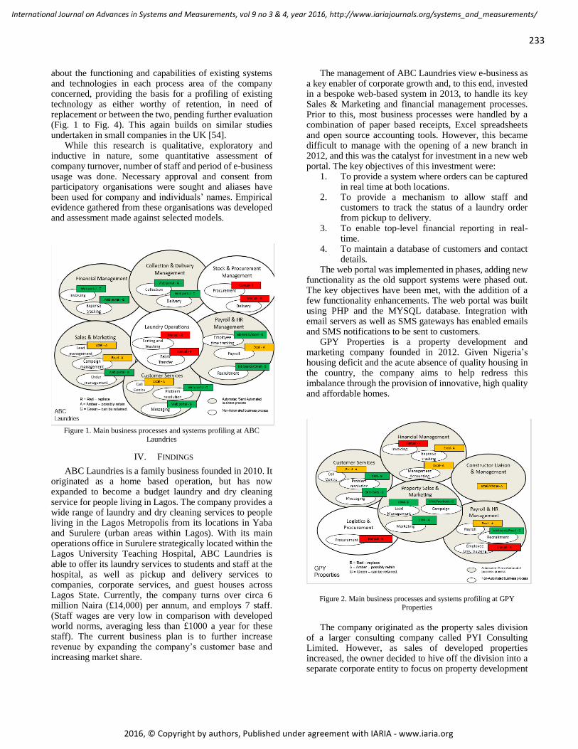
233



about the functioning and capabilities of existing systems and technologies in each process area of the company concerned, providing the basis for a profiling of existing technology as either worthy of retention, in need of replacement or between the two, pending further evaluation (Fig. 1 to Fig. 4). This again builds on similar studies undertaken in small companies in the UK [54].

While this research is qualitative, exploratory and inductive in nature, some quantitative assessment of company turnover, number of staff and period of e-business usage was done. Necessary approval and consent from participatory organisations were sought and aliases have been used for company and individuals’ names. Empirical evidence gathered from these organisations was developed and assessment made against selected models.

Figure 1. Main business processes and systems profiling at ABC

Laundries

IV. FINDINGS

ABC Laundries is a family business founded in 2010. It originated as a home based operation, but has now expanded to become a budget laundry and dry cleaning service for people living in Lagos. The company provides a wide range of laundry and dry cleaning services to people living in the Lagos Metropolis from its locations in Yaba and Surulere (urban areas within Lagos). With its main operations office in Surulere strategically located within the Lagos University Teaching Hospital, ABC Laundries is able to offer its laundry services to students and staff at the hospital, as well as pickup and delivery services to companies, corporate services, and guest houses across Lagos State. Currently, the company turns over circa 6 million Naira (£14,000) per annum, and employs 7 staff. (Staff wages are very low in comparison with developed world norms, averaging less than £1000 a year for these staff). The current business plan is to further increase revenue by expanding the company’s customer base and increasing market share.

The management of ABC Laundries view e-business as a key enabler of corporate growth and, to this end, invested in a bespoke web-based system in 2013, to handle its key Sales & Marketing and financial management processes. Prior to this, most business processes were handled by a combination of paper based receipts, Excel spreadsheets and open source accounting tools. However, this became difficult to manage with the opening of a new branch in 2012, and this was the catalyst for investment in a new web portal. The key objectives of this investment were:

1. To provide a system where orders can be captured in real time at both locations.

2. To provide a mechanism to allow staff and customers to track the status of a laundry order from pickup to delivery.

3. To enable top-level financial reporting in real-time.

4. To maintain a database of customers and contact details.

The web portal was implemented in phases, adding new functionality as the old support systems were phased out. The key objectives have been met, with the addition of a few functionality enhancements. The web portal was built using PHP and the MYSQL database. Integration with email servers as well as SMS gateways has enabled emails and SMS notifications to be sent to customers.

GPY Properties is a property development and marketing company founded in 2012. Given Nigeria’s housing deficit and the acute absence of quality housing in the country, the company aims to help redress this imbalance through the provision of innovative, high quality and affordable homes.

Figure 2. Main business processes and systems profiling at GPY Properties

The company originated as the property sales division

of a larger consulting company called PYI Consulting Limited. However, as sales of developed properties increased, the owner decided to hive off the division into a separate corporate entity to focus on property development

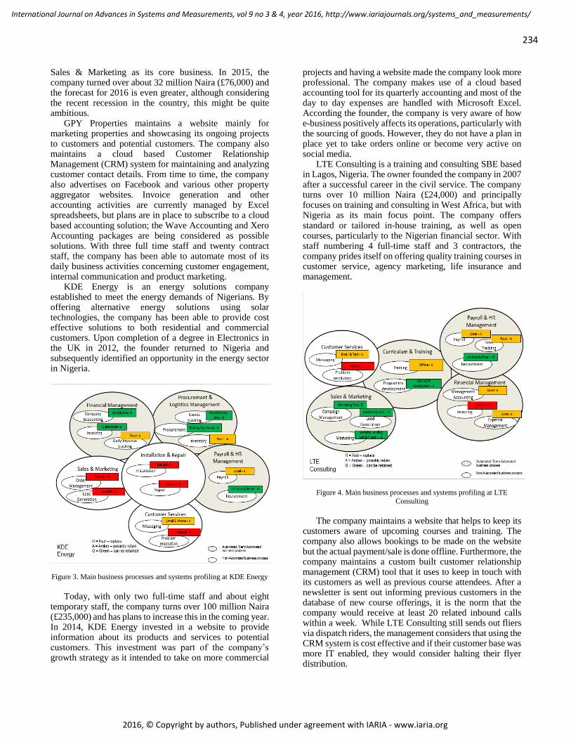
234



Sales & Marketing as its core business. In 2015, the company turned over about 32 million Naira (£76,000) and the forecast for 2016 is even greater, although considering the recent recession in the country, this might be quite ambitious.

GPY Properties maintains a website mainly for marketing properties and showcasing its ongoing projects to customers and potential customers. The company also maintains a cloud based Customer Relationship Management (CRM) system for maintaining and analyzing customer contact details. From time to time, the company also advertises on Facebook and various other property aggregator websites. Invoice generation and other accounting activities are currently managed by Excel spreadsheets, but plans are in place to subscribe to a cloud based accounting solution; the Wave Accounting and Xero Accounting packages are being considered as possible solutions. With three full time staff and twenty contract staff, the company has been able to automate most of its daily business activities concerning customer engagement, internal communication and product marketing.

KDE Energy is an energy solutions company established to meet the energy demands of Nigerians. By offering alternative energy solutions using solar technologies, the company has been able to provide cost effective solutions to both residential and commercial customers. Upon completion of a degree in Electronics in the UK in 2012, the founder returned to Nigeria and subsequently identified an opportunity in the energy sector in Nigeria.

Figure 3. Main business processes and systems profiling at KDE Energy

Today, with only two full-time staff and about eight

temporary staff, the company turns over 100 million Naira (£235,000) and has plans to increase this in the coming year. In 2014, KDE Energy invested in a website to provide information about its products and services to potential customers. This investment was part of the company’s growth strategy as it intended to take on more commercial

projects and having a website made the company look more professional. The company makes use of a cloud based accounting tool for its quarterly accounting and most of the day to day expenses are handled with Microsoft Excel. According the founder, the company is very aware of how e-business positively affects its operations, particularly with the sourcing of goods. However, they do not have a plan in place yet to take orders online or become very active on social media.

LTE Consulting is a training and consulting SBE based in Lagos, Nigeria. The owner founded the company in 2007 after a successful career in the civil service. The company turns over 10 million Naira (£24,000) and principally focuses on training and consulting in West Africa, but with Nigeria as its main focus point. The company offers standard or tailored in-house training, as well as open courses, particularly to the Nigerian financial sector. With staff numbering 4 full-time staff and 3 contractors, the company prides itself on offering quality training courses in customer service, agency marketing, life insurance and management.

Figure 4. Main business processes and systems profiling at LTE

Consulting

The company maintains a website that helps to keep its

customers aware of upcoming courses and training. The company also allows bookings to be made on the website but the actual payment/sale is done offline. Furthermore, the company maintains a custom built customer relationship management (CRM) tool that it uses to keep in touch with its customers as well as previous course attendees. After a newsletter is sent out informing previous customers in the database of new course offerings, it is the norm that the company would receive at least 20 related inbound calls within a week. While LTE Consulting still sends out fliers via dispatch riders, the management considers that using the CRM system is cost effective and if their customer base was more IT enabled, they would consider halting their flyer distribution.

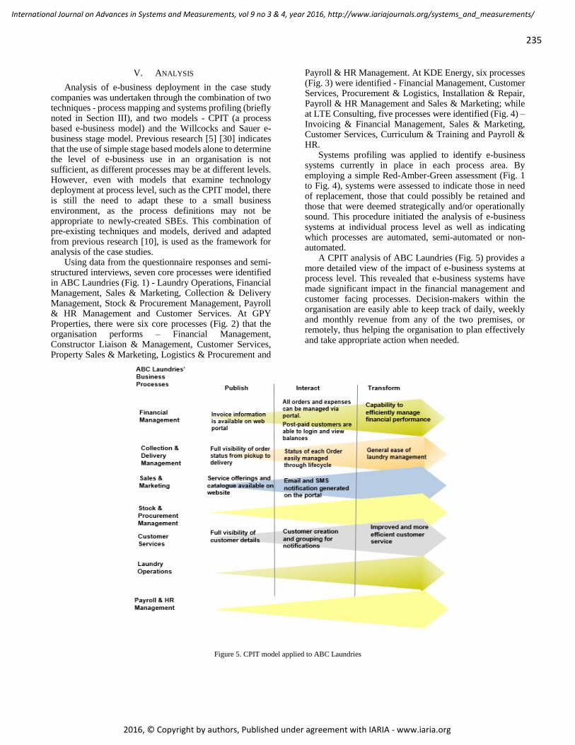
235



V. ANALYSIS

Analysis of e-business deployment in the case study companies was undertaken through the combination of two techniques - process mapping and systems profiling (briefly noted in Section III), and two models - CPIT (a process based e-business model) and the Willcocks and Sauer e-business stage model. Previous research [5] [30] indicates that the use of simple stage based models alone to determine the level of e-business use in an organisation is not sufficient, as different processes may be at different levels. However, even with models that examine technology deployment at process level, such as the CPIT model, there is still the need to adapt these to a small business environment, as the process definitions may not be appropriate to newly-created SBEs. This combination of pre-existing techniques and models, derived and adapted from previous research [10], is used as the framework for analysis of the case studies.

Using data from the questionnaire responses and semi- structured interviews, seven core processes were identified in ABC Laundries (Fig. 1) - Laundry Operations, Financial Management, Sales & Marketing, Collection & Delivery Management, Stock & Procurement Management, Payroll & HR Management and Customer Services. At GPY Properties, there were six core processes (Fig. 2) that the organisation performs – Financial Management, Constructor Liaison & Management, Customer Services, Property Sales & Marketing, Logistics & Procurement and

Payroll & HR Management. At KDE Energy, six processes (Fig. 3) were identified - Financial Management, Customer Services, Procurement & Logistics, Installation & Repair, Payroll & HR Management and Sales & Marketing; while at LTE Consulting, five processes were identified (Fig. 4) – Invoicing & Financial Management, Sales & Marketing, Customer Services, Curriculum & Training and Payroll & HR.

Systems profiling was applied to identify e-business systems currently in place in each process area. By employing a simple Red-Amber-Green assessment (Fig. 1 to Fig. 4), systems were assessed to indicate those in need of replacement, those that could possibly be retained and those that were deemed strategically and/or operationally sound. This procedure initiated the analysis of e-business systems at individual process level as well as indicating which processes are automated, semi-automated or non-automated.

A CPIT analysis of ABC Laundries (Fig. 5) provides a more detailed view of the impact of e-business systems at process level. This revealed that e-business systems have made significant impact in the financial management and customer facing processes. Decision-makers within the organisation are easily able to keep track of daily, weekly and monthly revenue from any of the two premises, or remotely, thus helping the organisation to plan effectively and take appropriate action when needed.

Figure 5. CPIT model applied to ABC Laundries

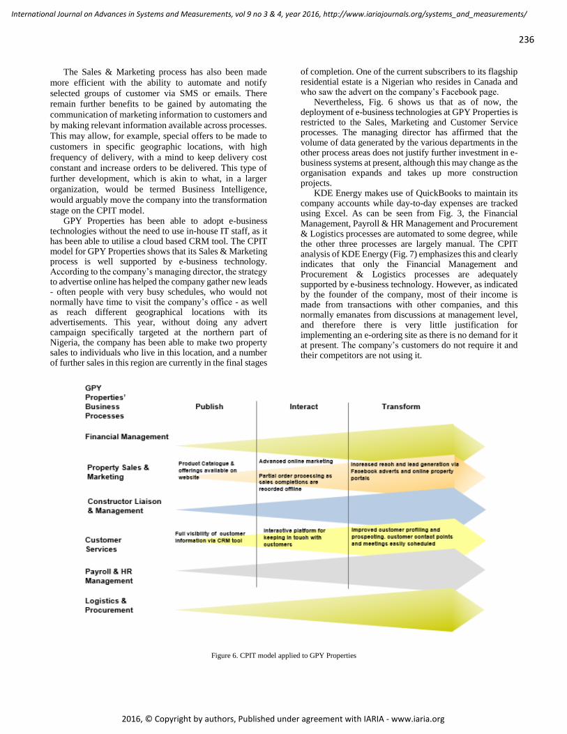
236



The Sales & Marketing process has also been made

more efficient with the ability to automate and notify

selected groups of customer via SMS or emails. There

remain further benefits to be gained by automating the

communication of marketing information to customers and

by making relevant information available across processes.

This may allow, for example, special offers to be made to

customers in specific geographic locations, with high

frequency of delivery, with a mind to keep delivery cost

constant and increase orders to be delivered. This type of

further development, which is akin to what, in a larger

organization, would be termed Business Intelligence,

would arguably move the company into the transformation

stage on the CPIT model. GPY Properties has been able to adopt e-business

technologies without the need to use in-house IT staff, as it has been able to utilise a cloud based CRM tool. The CPIT model for GPY Properties shows that its Sales & Marketing process is well supported by e-business technology. According to the company’s managing director, the strategy to advertise online has helped the company gather new leads - often people with very busy schedules, who would not normally have time to visit the company’s office - as well as reach different geographical locations with its advertisements. This year, without doing any advert campaign specifically targeted at the northern part of Nigeria, the company has been able to make two property sales to individuals who live in this location, and a number of further sales in this region are currently in the final stages

of completion. One of the current subscribers to its flagship residential estate is a Nigerian who resides in Canada and who saw the advert on the company’s Facebook page.

Nevertheless, Fig. 6 shows us that as of now, the deployment of e-business technologies at GPY Properties is restricted to the Sales, Marketing and Customer Service processes. The managing director has affirmed that the volume of data generated by the various departments in the other process areas does not justify further investment in e-business systems at present, although this may change as the organisation expands and takes up more construction projects.

KDE Energy makes use of QuickBooks to maintain its company accounts while day-to-day expenses are tracked using Excel. As can be seen from Fig. 3, the Financial Management, Payroll & HR Management and Procurement & Logistics processes are automated to some degree, while the other three processes are largely manual. The CPIT analysis of KDE Energy (Fig. 7) emphasizes this and clearly indicates that only the Financial Management and Procurement & Logistics processes are adequately supported by e-business technology. However, as indicated by the founder of the company, most of their income is made from transactions with other companies, and this normally emanates from discussions at management level, and therefore there is very little justification for implementing an e-ordering site as there is no demand for it at present. The company’s customers do not require it and their competitors are not using it.

Figure 6. CPIT model applied to GPY Properties

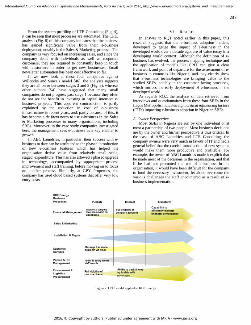
237



From the system profiling of LTE Consulting (Fig. 4), it can be seen that most processes are automated. The CPIT analysis (Fig. 8) of this company indicates that the business has gained significant value from their e-business deployment, notably in the Sales & Marketing process. The company is very focused on increasing sales, and since the company deals with individuals as well as corporate customers, they are required to constantly keep in touch with customers in order to get new businesses. Email newsletter automation has been cost effective so far.

If we now look at these four companies against Willcocks and Sauer’s model [46], the analysis suggests they are all on or between stages 2 and 3 (Fig. 9), whereas other authors [54] have suggested that many small companies do not progress past stage 1 because they often do not see the benefit in investing in capital intensive e-business projects. This apparent contradiction is partly explained by the reduction in cost of e-business infrastructure in recent years, and, partly because of this, it has become a de facto norm to use e-business in the Sales & Marketing processes in many organisations, including SBEs. Moreover, in the case study companies investigated here, the management sees e-business as a key enabler to growth.

In ABC Laundries, in particular, their success with e-business to date can be attributed to the phased introduction of new e-business features which has helped the organisation derive value from relatively small scale, staged, expenditure. This has also allowed a phased upgrade in technology, accompanied by appropriate process improvement and staff training, before moving on to focus on another process. Similarly, at GPY Properties, the company has used cloud based systems that offer very low entry costs.

VI. RESULTS

In answer to RQ1 noted earlier in this paper, this research suggests that the e-business adoption models, developed to gauge the impact of e-business in the developed world over a decade ago, are of value today in a developing world context. Although the definition of e-business has evolved, the process mapping technique and the application of models like CPIT can give a clear framework and point of departure for the assessment of e-business in countries like Nigeria; and they clearly show that e-business technologies are bringing value to the studied SBEs, notably in the customer facing processes, which mirrors the early deployment of e-business in the developed world.

As regards RQ2, the analysis of data retrieved from interviews and questionnaires from these four SBEs in the Lagos Metropolis indicates eight critical influencing factors (CIFs) impacting e-business adoption in Nigerian SBEs.

A. Owner Perspective

Most SBEs in Nigeria are run by one individual or at most a partnership of two people. Most business decisions are by the owner and his/her perspective is thus critical. In the case of ABC Laundries and LTE Consulting, the company owners were very much in favour of IT and had a general belief that the careful introduction of new systems would make them more productive and profitable. For example, the owner of ABC Laundries made it explicit that he made most of the decisions in the organisation, and that if he had not promoted the use of e-business in his organisation, it would have been difficult for the company to fund the necessary investment, let alone overcome the various challenges the staff encountered as a result of e-business implementation.

Figure 7. CPIT model applied to KDE Energy

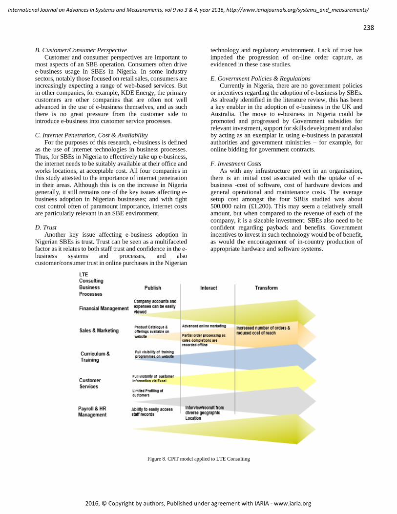
238



B. Customer/Consumer Perspective Customer and consumer perspectives are important to

most aspects of an SBE operation. Consumers often drive e-business usage in SBEs in Nigeria. In some industry sectors, notably those focused on retail sales, consumers are increasingly expecting a range of web-based services. But in other companies, for example, KDE Energy, the primary customers are other companies that are often not well advanced in the use of e-business themselves, and as such there is no great pressure from the customer side to introduce e-business into customer service processes. C. Internet Penetration, Cost & Availability

For the purposes of this research, e-business is defined as the use of internet technologies in business processes. Thus, for SBEs in Nigeria to effectively take up e-business, the internet needs to be suitably available at their office and works locations, at acceptable cost. All four companies in this study attested to the importance of internet penetration in their areas. Although this is on the increase in Nigeria generally, it still remains one of the key issues affecting e-business adoption in Nigerian businesses; and with tight cost control often of paramount importance, internet costs are particularly relevant in an SBE environment. D. Trust

Another key issue affecting e-business adoption in Nigerian SBEs is trust. Trust can be seen as a multifaceted factor as it relates to both staff trust and confidence in the e-business systems and processes, and also customer/consumer trust in online purchases in the Nigerian

technology and regulatory environment. Lack of trust has impeded the progression of on-line order capture, as evidenced in these case studies.

E. Government Policies & Regulations

Currently in Nigeria, there are no government policies or incentives regarding the adoption of e-business by SBEs. As already identified in the literature review, this has been a key enabler in the adoption of e-business in the UK and Australia. The move to e-business in Nigeria could be promoted and progressed by Government subsidies for relevant investment, support for skills development and also by acting as an exemplar in using e-business in parastatal authorities and government ministries – for example, for online bidding for government contracts.

F. Investment Costs

As with any infrastructure project in an organisation, there is an initial cost associated with the uptake of e-business -cost of software, cost of hardware devices and general operational and maintenance costs. The average setup cost amongst the four SBEs studied was about 500,000 naira (£1,200). This may seem a relatively small amount, but when compared to the revenue of each of the company, it is a sizeable investment. SBEs also need to be confident regarding payback and benefits. Government incentives to invest in such technology would be of benefit, as would the encouragement of in-country production of appropriate hardware and software systems.

Figure 8. CPIT model applied to LTE Consulting

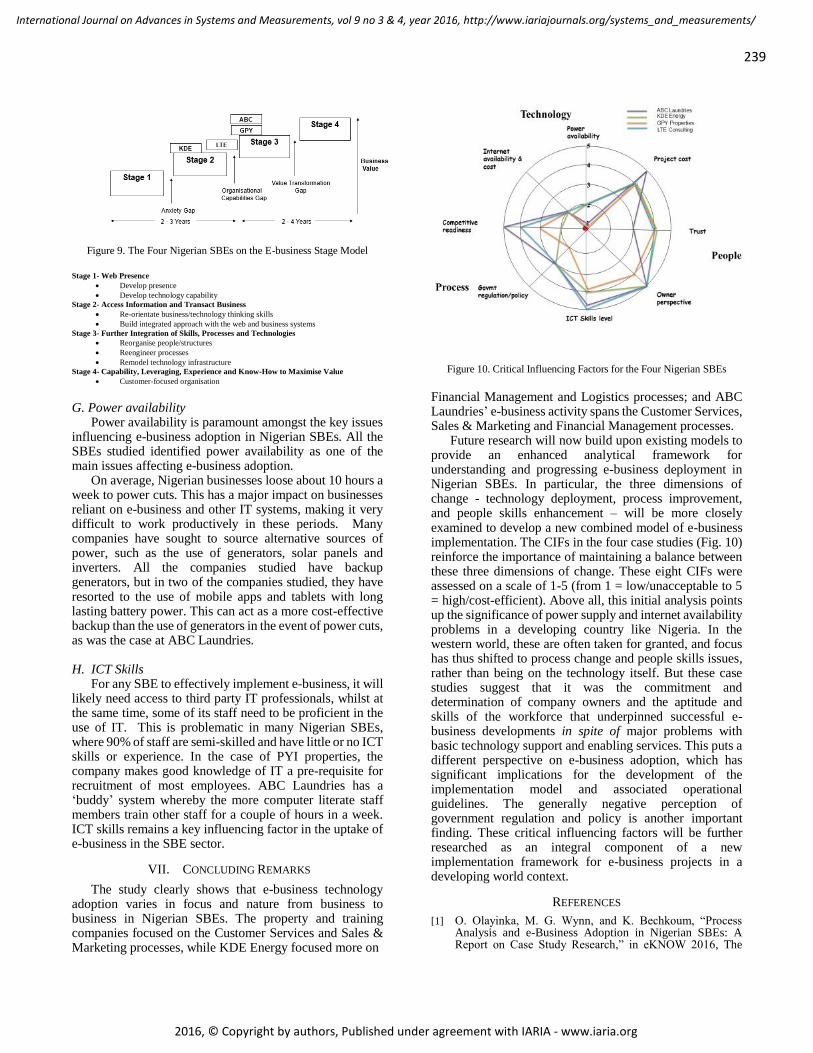
239



Figure 9. The Four Nigerian SBEs on the E-business Stage Model

Stage 1- Web Presence

Develop presence

Develop technology capability

Stage 2- Access Information and Transact Business

Re-orientate business/technology thinking skills

Build integrated approach with the web and business systems

Stage 3- Further Integration of Skills, Processes and Technologies

Reorganise people/structures

Reengineer processes

Remodel technology infrastructure

Stage 4- Capability, Leveraging, Experience and Know-How to Maximise Value

Customer-focused organisation

G. Power availability

Power availability is paramount amongst the key issues influencing e-business adoption in Nigerian SBEs. All the SBEs studied identified power availability as one of the main issues affecting e-business adoption.

On average, Nigerian businesses loose about 10 hours a week to power cuts. This has a major impact on businesses reliant on e-business and other IT systems, making it very difficult to work productively in these periods. Many companies have sought to source alternative sources of power, such as the use of generators, solar panels and inverters. All the companies studied have backup generators, but in two of the companies studied, they have resorted to the use of mobile apps and tablets with long lasting battery power. This can act as a more cost-effective backup than the use of generators in the event of power cuts, as was the case at ABC Laundries.

H. ICT Skills

For any SBE to effectively implement e-business, it will likely need access to third party IT professionals, whilst at the same time, some of its staff need to be proficient in the use of IT. This is problematic in many Nigerian SBEs, where 90% of staff are semi-skilled and have little or no ICT skills or experience. In the case of PYI properties, the company makes good knowledge of IT a pre-requisite for recruitment of most employees. ABC Laundries has a ‘buddy’ system whereby the more computer literate staff members train other staff for a couple of hours in a week. ICT skills remains a key influencing factor in the uptake of e-business in the SBE sector.

VII. CONCLUDING REMARKS

The study clearly shows that e-business technology adoption varies in focus and nature from business to business in Nigerian SBEs. The property and training companies focused on the Customer Services and Sales & Marketing processes, while KDE Energy focused more on

Figure 10. Critical Influencing Factors for the Four Nigerian SBEs Financial Management and Logistics processes; and ABC Laundries’ e-business activity spans the Customer Services, Sales & Marketing and Financial Management processes.

Future research will now build upon existing models to provide an enhanced analytical framework for understanding and progressing e-business deployment in Nigerian SBEs. In particular, the three dimensions of change - technology deployment, process improvement, and people skills enhancement – will be more closely examined to develop a new combined model of e-business implementation. The CIFs in the four case studies (Fig. 10) reinforce the importance of maintaining a balance between these three dimensions of change. These eight CIFs were assessed on a scale of 1-5 (from 1 = low/unacceptable to 5 = high/cost-efficient). Above all, this initial analysis points up the significance of power supply and internet availability problems in a developing country like Nigeria. In the western world, these are often taken for granted, and focus has thus shifted to process change and people skills issues, rather than being on the technology itself. But these case studies suggest that it was the commitment and determination of company owners and the aptitude and skills of the workforce that underpinned successful e-business developments in spite of major problems with basic technology support and enabling services. This puts a different perspective on e-business adoption, which has significant implications for the development of the implementation model and associated operational guidelines. The generally negative perception of government regulation and policy is another important finding. These critical influencing factors will be further researched as an integral component of a new implementation framework for e-business projects in a developing world context.

REFERENCES

[1] O. Olayinka, M. G. Wynn, and K. Bechkoum, “Process Analysis and e-Business Adoption in Nigerian SBEs: A Report on Case Study Research,” in eKNOW 2016, The

240



Eighth International Conference on Information, Process, and Knowledge Management, pp. 57–63, 2016.

[2] Vanguard Nigeria, “Nigeria has 48m active internet users – NITDA,” 2014. [Online]. Available: http://www.vanguardngr.com/2014/10/nigeria-48m-active-internet-users-nitda/. [Accessed: 24-Nov-2016].

[3] Paul Budde Communication Pty Ltd, “Nigeria - Mobile Market - Insights, Statistics and Forecasts,” Paul Budde Communication Pty Ltd, 2015.

[4] B. A. Wagner, I. Fillis, and U. Johansson, “E-business and e-supply strategy in small and medium sized businesses (SMEs),” Supply Chain Manag. An Int. J., vol. 8, no. 4, pp. 343–354, 2003.

[5] T. Oliveira and M. F. Martins, “Understanding e-business adoption across industries in European countries,” Ind. Manag. Data Syst., vol. 110, no. 9, pp. 1337–1354, 2010.

[6] D. Sharma and M. Ranga, “Mobile customer relationship management - A competitive tool,” Excel Int. J. Multidiscip. Manag. Stud., vol. 4, no. 7, pp. 37–42, 2014.

[7] T. Oliveira and M. F. Martins, “Firms Patterns of e-Business Adoption: Evidence for the European Union-27,” Electron. J. Inf. Syst., vol. 13, no. 1, pp. 47–56, 2010.

[8] W. Olatokun and B. Bankole, “Factors influencing electronic business technologies adoption and use by small and medium scale enterprises (SMEs) in a Nigerian municipality,” J. Internet Bank. Commer., vol. 16, no. 3, 2011.

[9] M. Taylor and A. Murphy, “SMEs and e-business,” J. Small Bus. Enterp. Dev., vol. 11, no. 3, pp. 280–289, 2004.

[10] M. G. Wynn, P. Turner, and E. Lau, “E-business and process change: two case studies (towards an assessment framework),” Journal of Small Business and Enterprise Development, vol. 20, no. 4, pp. 913–933, 2013.

[11] OECD, “Internet adoption and use: Businesses,” OECD Internet Econ. Outlook 2012, 2012.

[12] L. Chen and C. W. Holsapple, “E-Business Adoption Research: State of the Art,” J. Electron. Commer. Res., vol. 14, no. 3, pp. 261–286, 2013.

[13] P. Taylor, “The Importance of Information and Communication Technologies (ICTs): An Integration of the Extant Literature on ICT Adoption in Small and Medium Enterprises,” Int. J. Econ. Commer. Manag., vol. 3, no. 5, 2015.

[14] M. Kapurubandara, “A model to etransform SMEs in developing countries,” Proc. 2008 4th Int. Conf. Inf. Autom. Sustain. ICIAFS 2008, pp. 401–406, 2008.

[15] European Commission, The new SME definition: user guide and model declaration. Office for Official Publications of the European Communities, 2005.

[16] Small and Medium Enterprises Development Agency of Nigeria, “National Policy on Micro, Small and Medium Enterprises,” 2014.

[17] D. Chaffey, E-business and E-commerce Management: Strategy, Implementation and Practice. Financial Times Prentice Hall, 2007.

[18] V. Bordonaba-Juste, L. Lucia-Palacios, and Y. Polo-Redondo, “Antecedents and consequences of e-business adoption for European retailers,” Internet Res., vol. 22, no. 5, pp. 532–550, 2012.

[19] A. Prananto, J. McKay, and P. Marshall, “Lessons learned from analysing e-business progression using a stage model in Australian Small Medium Enterprises (SMEs),” ACIS 2004 Proc., no. 1969, pp. 75-86, 2004.

[20] D. Chaffey, E-Business and E-Commerce Management - Strategy, Implementation and Practice. 2009.

[21] A. Prananto, J. McKay, and P. Marshall, “A study of the progression of e-business maturity in Australian SMEs: some evidence of the applicability of the stages of growth for e-business model,” Proc. PACIS, Adelaide, July, pp. 68–80, 2003.

[22] A. Basu and S. Muylle, “How to plan e-business initiatives in established companies,” MIT Sloan Manag. Rev., vol. 49, no. 1, pp. 28-36, 2007.

[23] F. Wu, V. Mahajan, and S. Balasubramanian, “An Analysis of E-Business Adoption and its Impact on Business Performance,” J. Acad. Mark. Sci., vol. 31, April, pp. 425–447, 2003.

[24] D. O. Faloye, “The adoption of e-commerce in small businesses: an empirical evidence from retail sector in Nigeria.,” J. Bus. Retail Manag. Res., vol. 8, no. 2, 2014.

[25] A. Afolayan, E. Plant, G. R. T. White, P. Jones, and P. Beynon-Davies, “Information Technology Usage in SMEs in a Developing Economy,” Strateg. Chang., vol. 24, no. 5, pp. 483–498, 2015.

[26] Bloomberg Business, “Nigerian Economy Overtakes South Africa’s on Rebased GDP,” Bloomberg Business, 2014. [Online]. Available: http://www.bloomberg.com/news/articles/2014-04-06/nigerian-economy-overtakes-south-africa-s-on-rebased-gdp. [Accessed: 24-Nov-2016].

[27] C. Parker and T. Castleman, “New directions for research on SME-eBusiness: insights from an analysis of journal articles from 2003-2006,” J. Inf. Syst. Small Bus., vol. 1, no. 1, pp. 21–40, 2007.

[28] H. D. Kim, I. Lee, and C. K. Lee, “Building Web 2.0 enterprises: A study of small and medium enterprises in the United States,” Int. Small Bus. J., vol. 31, no. 2, pp. 156–174, 2013.

[29] P. Ifinedo, “Internet/e-business technologies acceptance in Canada’s SMEs: an exploratory investigation,” Internet Res., vol. 21, no. 3, pp. 255–281, 2011.

[30] E. M. Agwu, “An investigative analysis of factors influencing E-business adoption and maintenance of commercial websites in Nigeria,” Basic Res. J. Bus. Manag. Accounts ISSN 2315-6899 vol. 3, pp. 5–16, 2014.

[31] R. Rahayu and J. Day, “Determinant Factors of E-commerce Adoption by SMEs in Developing Country: Evidence from Indonesia,” Procedia - Soc. Behav. Sci., vol. 195, pp. 142–150, 2015.

[32] D. K. Agboh, “Drivers and challenges of ICT adoption by SMES in Accra metropolis , Ghana,” J. Technol. Res., vol. 6, pp. 1–16, 2015.

[33] I. Janita and W. K. Chong, “Barriers of b2b e-business adoption in Indonesian SMEs: A Literature Analysis,” Procedia Comput. Sci., vol. 17, pp. 571–578, 2013.

[34] M. Kapurubandara and R. Lawson, “Barriers to Adopting ICT and e-commerce with SMEs in Developing Countries : An Exploratory study in Sri Lanka,” Univ. West. Sydney, Aust., May, pp. 1–12, 2006.

[35] C. I. Emeti and O. Onyeaghala, “E-Business Adoption and Consumer Attitude in Nigeria,” Eur. J. Bus. Manag., vol. 7, no. 21, pp. 76–87, 2015.

[36] W. Olatokun and B. Bankole, “Factors Influencing Electronic Business Technologies Adoption and Use by Small and Medium Scale Enterprises (SMEs) in a Nigerian Municipality,” J. Internet Bank. Commer., vol. 16, no. 3, pp. 1–26, 2011.

[37] E. M. Agwu and P. J. Murray, “Empirical Study of Barriers to Electronic Commerce Adoption by Small and Medium Scale Businesses in Nigeria,” Int. J. Innov. Digit. Econ., vol. 6, no. 2, pp. 1–19, 2015.

241



[38] R. Erumi-Esin and R. Heeks, “e-Business Adoption and Use Among African Women-Owned SMEs: An Analytical Study in Nigeria,” ICTD 2015 Proc. Seventh Int. Conf. Inf. Commun. Technol. Dev., pp. 11-21, 2015.

[39] P. Jones, E. Muir, and P. B. Davies, “The proposal of a comparative framework to evaluate e-business stages of growth models,” Int. J. Inf. Technol. Manag., vol. 5, no. 4, pp. 249-267, 2006.

[40] R. Gatautis and E. Vitkauskaite, “eBusiness Policy Support Framework,” no. 5, pp. 35–48, 2009.

[41] M. Wynn, P. Turner, A. Banik, and A. G. Duckworth, “The impact of customer relationship management systems in small businesses,” Strategic Change, vol. 25, Issue 6, pp. 655–670, 2016. Published online in Wiley Online Library (wileyonlinelibrary.com) DOI: 10.1002/jsc.2100.

[42] A. Gunasekaran, Modelling and Analysis of Enterprise Information Systems. IGI Pub., 2007.

[43] M. Levy and P. Powell, “Exploring SME internet adoption: towards a contingent model,” Electron. Mark., vol. 13, no. 2, pp. 173–181, 2003.

[44] Department of Trade and Industry, Business in the Information Age: International Benchmarking Study 2003. Booz Allen Hamilton, London, 2003.

[45] J. McKay, A. Prananto, and P. Marshall, “E-business maturity: The SOG-e model,” in Proceedings of the 11th Australasian Conference on Information Systems (ACIS), pp. 6–8, 2000.

[46] C. Sauer and L. P. Willcocks, Moving to e-business. Random House Business Books, 2000.

[47] M. Wynn and O. Olubanjo, “Demand-supply chain management: systems implications in an SME packaging business in the UK,” Int. J. Manuf. Res., vol. 7, no. 2, pp. 198–212, 2012.

[48] J. W. Creswell, Research Design: Qualitative, Quantitative, and Mixed Methods Approaches, Fourth edi. SAGE Publications, 2013.

[49] M. B. Davies, Doing a Successful Research Project: Using Qualitative or Quantitative Methods. Palgrave Macmillan, 2007.

[50] R. B. Burns, Introduction to Research Methods. SAGE Publications, 2000.

[51] D. Silverman, Interpreting Qualitative Data. SAGE Publications, 2015.

[52] R. K. Yin, Case Study Research: Design and Methods. SAGE Publications, 2003.

[53] M. Wynn, P. Turner, H. Abbas, and R. Shen, "Employing Knowledge Transfer to support IS implementation in SMEs," Journal of Industry and Higher Education, vol. 23, no. 2, April, pp. 111-125, 2009.

[54] M. Levy, P. Powell, and P. Yetton, “SMEs: aligning IS and the strategic context,” J. Inf. Technol., vol. 16, no. 3, pp. 133–144, 2001.

242



The State of Peer Assessment: Dimensions and Future Challenges

Usman Wahid, Mohamed Amine Chatti, Ulrik Schroeder

Learning Technologies Research Group (Informatik 9), RWTH Aachen University

Aachen, Germany

{Wahid; Schroeder}@cil.rwth-aachen.de; [email protected]

Abstract— Modern day education and learning has moved on

from brick and mortar institutions to open learning

environments. Massive Online Open Courses (MOOCs) are a

perfect example of these learning environments. MOOCs

provide a cost and time effective choice for learners across the

globe. This has led to new challenges for teachers such as

providing valuable and quality assessment and feedback on such

a large scale. Recent studies have found peer assessment where

learners assess the work of their peers to be a viable and cost

effective alternative to teacher/staff evaluation. This study

systematically analyzes the current research on peer assessment

published in the context of MOOCs and the online tools that are

being used in MOOCs for peer assessment. 48 peer reviewed

papers and 17 peer assessment tools were selected for the

comparison in this study and were assessed on three main

dimensions, namely, system design, efficiency and effectiveness.

Apart from these dimensions, the study highlights the main

challenges of peer assessment. In the light of the comparison and

discussion of current research in terms of the identified

dimensions, we present future visions and research perspectives

to improve the peer assessment process in MOOCs.

Keywords-Open Assessment; Peer Assessment; Open

Learning Environments; MOOC; Blended Learning; Peer

Reviews; Peer Feedback; Online Assessment.

I. INTRODUCTION

This paper presents an extended and more detailed version of our paper presented at the eighth international conference on mobile, hybrid, and online learning (eLmL 2016), where we reviewed the existing tools and research directions for peer assessment [1]. The field of education has transformed in recent year, with a growing interest in learner-centered, open, and networked learning models. These include Personalized Learning Environments (PLEs), Open Educational Resources (OER) and Massive Open Online Courses (MOOCs).

Massive Online Open Courses (MOOCs) have revolutionized the field of technology-enhanced learning (TEL). MOOCs enable a massive number of learners from all over the world to attend online courses irrespective of their social and academic backgrounds [2]. MOOCs have been classified in different forms by researchers, e.g., Siemens [3] classifies MOOCs into cMOOCs and xMOOCs. In his opinion cMOOCs allow the learners to build their own learning networks by using blogs, wikis, Twitter, Facebook and other social networking tools outside the confines of the learning platform and without any restriction and interference from the teachers [4]. Whereas, xMOOCs follow a more institutional model, having pre-defined learning objectives, e.g., Coursera, edX and Udacity. Apart from these sMOOCs

and bMOOCs have also been introduced as variations of the MOOC platform with sMOOCs catering to a relatively smaller number of participants and bMOOCs combining the in-class and online learning activities to form a hybrid learning environment [3].

Irrespective of the classification, MOOCs require their stakeholders to address a number of challenges including and not limited to the role of university/teacher, plagiarism, certification, completion rates, innovating the learning model beyond traditional approaches and last but not the least assessment [5].

Assessment and Feedback are an integral part of the learning process and MOOCs are no different in this regard. Researchers acknowledge that the Teach-Learn-Access cycle in education cannot function in the absence of quality assessment [6]. However, in the case of MOOCs assessment presents a bottleneck issue due to the massiveness of the course participants and requires increased resources (time, money, manpower etc.) on part of the teachers to provide useful feedback to all the learners for a satisfying academic experience. This limitation causes many MOOCs to use automated assessments, e.g., quizzes with closed questions like multiple choice and fill in the blanks. These questions largely focus on the cognitive aspects of learning, and they are unable to capture the semantic meaning of learners’ answers; in particular, in open ended questions [7]. Some other methods used in this scenario make use of crowd sourcing techniques to provide assessment and feedback to students. These methods include portfolios and self-assessment, group feedback and last but not the least peer assessment [8].

Peer assessment offers a scalable and cost effective way of providing assessment and feedback to a massive amount of learners where learners can be actively involved in the assessment processes [9]. A significant amount of research is directed towards exploring peer assessment in MOOCs. While this research discusses many issues such as the effective integration of peer assessment in various MOOC platforms and the improvement of the peer assessment process, it does not cover what has been done in this field for the past years from an analysis point of view.

Since, it is evident that peer assessment is a very viable assessment method in MOOCs, hence, the need for scouting all the available systems and studies becomes paramount in importance as it could be beneficial for future developments as well as provide a good comparison of available tools. In this study, we look at the peer assessment in general and the state of art of peer assessment in the MOOC era along with perceived benefits and challenges of peer assessment. We also look at different tools for peer assessment and the way they

243



try to address the challenges and drawbacks of peer assessment.

The remainder of this paper is structured as follows: Section II introduces peer assessment and its pros and cons. Section III is a review of the related work. Section IV describes the research methodology and how we collected the research data. In Section V, we review and discuss the current research based on several dimensions. Section VI summarises the results of our findings. Section VII presents challenges and future perspectives in peer assessment. Finally, Section VIII gives a conclusion of the main findings of this paper.

II. PEER ASSESSMENT

In recent years, student assessments have shifted from the

traditional testing of knowledge to a culture of learning

assessments [10]. This culture of assessment encourages

students to take an active part in the learning and assessment

processes [11]. Peer assessment is one of the flag bearers in

this new assessment culture. Peer assessment also known as

Peer grading, is defined by Topping as “an arrangement in

which individuals consider the amount, level, value, worth,

quality or success of the products or outcomes of learning of

peers of similar status” [12].

Peer assessment has been leveraged in a wide range of

subject domains over the years including natural sciences,

social sciences, business, medicine and engineering [13].

According to Somervell [14], at one end of the spectrum peer

assessment may involve feedback of a qualitative nature or,

at the other, may involve students in the actual marking

process. This exercise may or may not entail previous

discussion or agreements over criterion. It may involve the

use of rating instruments or checklists, which may have been

designed by others before the exercise, or designed by the

user group to meet its particular needs [15]. The use of peer

assessment not only reduces the teacher workload; it also

brings many potential benefits to student learning. These

benefits include a sense of ownership and autonomy,

increased motivation, better learning and high level cognitive

and discursive processing [13], [16].

Despite these potential benefits, peer assessment still has

not been able to have strong backing from either teachers or

students [17]. Both parties have pre-conceived notions of low

reliability and validity on their minds when discussing peer

assessment [18], [19]. A number of possible factors have

been identified for the lack of effectiveness of peer

assessment in MOOCs. These factors include the scalability

issue, diversity of reviewers, perceived lack of expertise, lack

of transparency and fixed grading rubrics [8].

There have been many studies on the effectiveness and

usefulness of peer assessment but these studies focus on a

certain context and tool, which covers the aspects related to

the context of the study. The aim of this paper is to examine

the available literature and tools for peer assessment, provide

a systematic analysis by reviewing them according to

different aspects critical to their usage in the MOOC

platform, and provide a bigger picture of the research domain.

We will try to highlight the challenges of peer assessment and

then provide some viable solutions to overcome these

challenges.

III. RELATED WORK

Peer assessment in MOOCs is still an emerging field, hence, we did not find any research directly related to our work. Luxton-Reily [20] made a systematic comparison of a number of online peer assessment tools in 2009, but the study was conducted with limited dimensions for comparing the tools. The study examined tools including legacy systems, and divided the tools in different categories; namely generic, domain specific and context specific. The study identifies the problem that majority of online tools have been used in computer science courses, and most of the tools could not be used outside the context in which they were developed. The context limitations of the tools are the biggest hindrance preventing them from being widely adopted, which gives rise to the need for more general-purpose tools. Luxton-Reily also stressed the need to investigate the quality of the feedback provided by students [20].

Apart from this, another study identifies a number of approaches taken by different peer assessment tools to address the concerns of the involved stakeholders [21]. These approaches include connectivist MOOCs where the onus is on getting superior results through collaboration and not focusing on correctness. Rather, the course is designed in a way to encourage and welcome diverse perspectives from participants. Another approach is the use of calibration like in Calibrated Peer Reviews (CPR), where raters have to evaluate a number of training submissions before they get to evaluate submissions from their peers [22]–[24]. Other approaches highlighted in the study involve making use of a Bayesian post hoc statistical correction method [25]–[27] and to create a credibility index by modifying and refining the CPR method [21].

In comparison to the above-mentioned studies, our study adds a wide range of latest tools and analyzes them over several dimensions based on cognitive mapping approach. The study further provides critical discussion according to each dimension and suggests new areas for future work.

IV. METHODOLOGY

The research methodology used for this study is divided

in two parts; namely, identification of eligible studies

followed by a cognitive mapping approach to find certain

criterion for categorizing and analyzing peer assessment

tools.

A. Identification of Eligible Studies

We applied the significant research method of identifying papers from internet resources in our study [28]. This method was carried out in two rounds.

Firstly, we conducted a search in 7 major refereed academic databases. These include Education Resources Information Center (ERIC), JSTOR, ALT Open Access Repository, Google Scholar, PsychInfo, ACM publication,

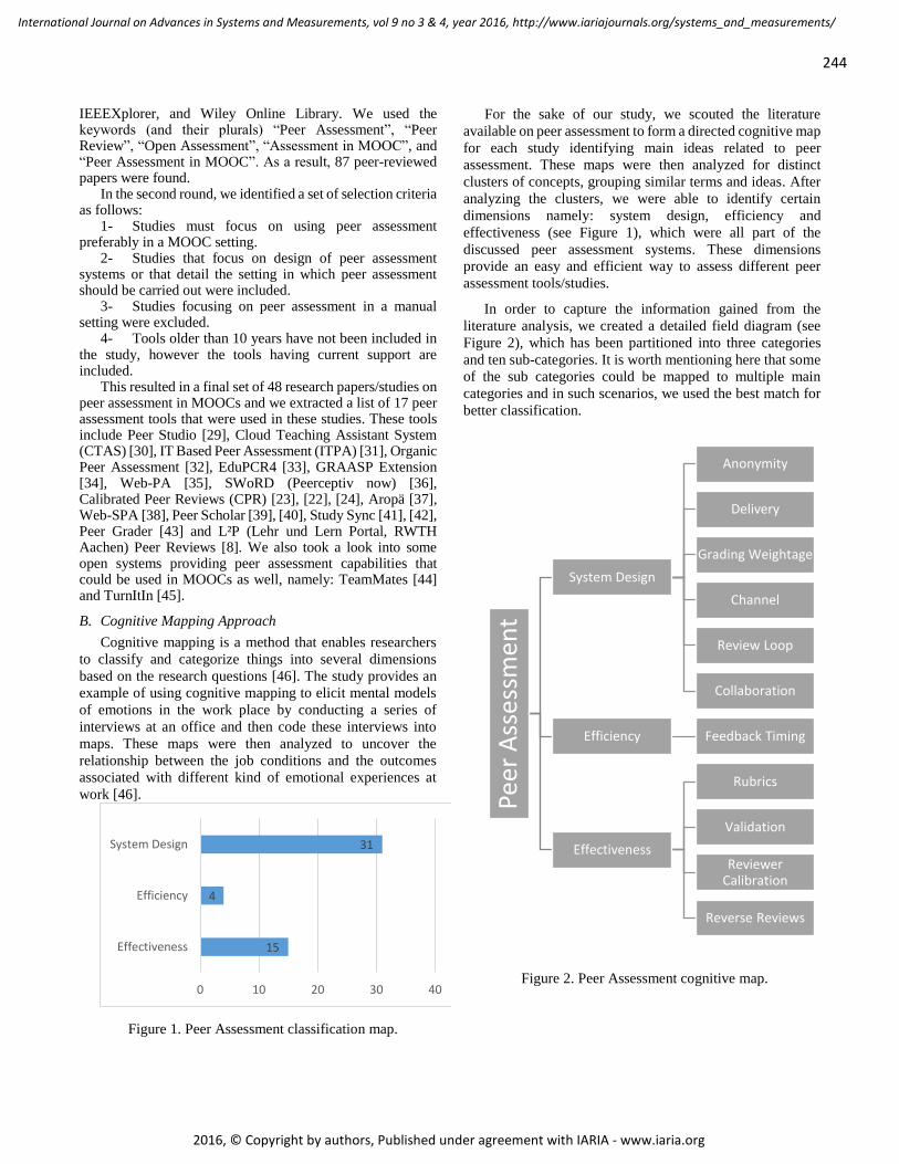
244



IEEEXplorer, and Wiley Online Library. We used the keywords (and their plurals) “Peer Assessment”, “Peer Review”, “Open Assessment”, “Assessment in MOOC”, and “Peer Assessment in MOOC”. As a result, 87 peer-reviewed papers were found.

In the second round, we identified a set of selection criteria as follows:

1- Studies must focus on using peer assessment preferably in a MOOC setting.

2- Studies that focus on design of peer assessment systems or that detail the setting in which peer assessment should be carried out were included.

3- Studies focusing on peer assessment in a manual setting were excluded.

4- Tools older than 10 years have not been included in the study, however the tools having current support are included.

This resulted in a final set of 48 research papers/studies on peer assessment in MOOCs and we extracted a list of 17 peer assessment tools that were used in these studies. These tools include Peer Studio [29], Cloud Teaching Assistant System (CTAS) [30], IT Based Peer Assessment (ITPA) [31], Organic Peer Assessment [32], EduPCR4 [33], GRAASP Extension [34], Web-PA [35], SWoRD (Peerceptiv now) [36], Calibrated Peer Reviews (CPR) [23], [22], [24], Aropä [37], Web-SPA [38], Peer Scholar [39], [40], Study Sync [41], [42], Peer Grader [43] and L²P (Lehr und Lern Portal, RWTH Aachen) Peer Reviews [8]. We also took a look into some open systems providing peer assessment capabilities that could be used in MOOCs as well, namely: TeamMates [44] and TurnItIn [45].

B. Cognitive Mapping Approach

Cognitive mapping is a method that enables researchers

to classify and categorize things into several dimensions

based on the research questions [46]. The study provides an

example of using cognitive mapping to elicit mental models

of emotions in the work place by conducting a series of

interviews at an office and then code these interviews into

maps. These maps were then analyzed to uncover the

relationship between the job conditions and the outcomes

associated with different kind of emotional experiences at

work [46].

For the sake of our study, we scouted the literature

available on peer assessment to form a directed cognitive map

for each study identifying main ideas related to peer

assessment. These maps were then analyzed for distinct

clusters of concepts, grouping similar terms and ideas. After

analyzing the clusters, we were able to identify certain

dimensions namely: system design, efficiency and

effectiveness (see Figure 1), which were all part of the

discussed peer assessment systems. These dimensions

provide an easy and efficient way to assess different peer

assessment tools/studies.

In order to capture the information gained from the

literature analysis, we created a detailed field diagram (see

Figure 2), which has been partitioned into three categories

and ten sub-categories. It is worth mentioning here that some

of the sub categories could be mapped to multiple main

categories and in such scenarios, we used the best match for

better classification.

15

4

31

0 10 20 30 40

Effectiveness

Efficiency

System Design

Pee

r A

sse

ssm

ent

System Design

Anonymity

Delivery

Grading Weightage

Channel

Review Loop

Collaboration

Efficiency Feedback Timing

Effectiveness

Rubrics

Validation

Reviewer Calibration

Reverse Reviews

Figure 1. Peer Assessment classification map.

Figure 2. Peer Assessment cognitive map.

245



Apart from these dimensions, we identified a number of

challenges as well for peer assessment from the literature

review. The list of challenges of peer assessment includes

transparency, credibility, accuracy, reliability, validity,

diversity, scalability, and efficiency. Transparency refers to

the fact that the assessee is aware of how the review process

works and has confidence in it. The credibility refers to the

issue, whether the reviewing person has sufficient knowledge

in the subject area and is capable enough of providing

credible feedback. Accuracy is closely linked to credibility in

the sense that if the reviewer has a good mastery of the subject

then his/her reviews would tend to be more accurate.

Reliability is the consistency of grades that different peers

would assign to the same assessment, or in other words as

inter-rater reliability. Whereas, validity is calculated as a

correlation coefficient between peer and instructor grades,

assuming that the instructor grade is considered a trustworthy

benchmark [30]. Diversity refers to the different educational

backgrounds of the assessors. Scalability is inherent to open

learning environments with a large number of participants.

And last but not the least, efficiency related to feedback

timing. Studies have shown that the earlier the learners get

feedback to their work, the more time they have to improve

the final product. Reducing the time, it takes to get feedback

to a draft submission automatically allows for a better final

product.

The peer assessment dimensions identified earlier try to

address some of the challenges presented here in a number of

ways, which will be discussed later with the discussion of

each peer assessment dimension in the following sections.

V. DISCUSSION

This section deals with the critical analysis of the peer assessment literature based on the cognitive mapping dimensions derived in the previous section. For the critical discussion part, we look at the identified dimensions and then discuss the way in which certain tools cater to that dimension (if at all).

A. System Design

A lot of effort has been put into the design of peer assessment systems, design of certain features provided by the system and the manner in which they are implemented. Nearly 70% of the studies deal in one way or the other with system or a feature design in peer assessment.

In the following sections, we discuss some key features of peer assessment systems and the way they are realized by different tools.

1) Anonymity: Anonymity is a key feature that is to be

kept in mind while designing any peer assessment system, as

it safeguards the system against any type of bias (gender,

nationlity, friendship etc.) to play a factor in the assessment

from peers. There are three levels of anonymity namely,

single blind: assessor knows the assessee but the assessee has

no idea of the assessor, double blind: both assessor and

assessee are unaware of each other and finally no anonymity

in which the identity of both the assessor and assessee is

known to each other. Most of the systems reviewed in this

study follow the principle of double blind reviews for the sake

of bias free reviews, however, TurnItIn [45] and Study Sync

[41] only implement the single blind reviews.Whereas,

organic peer assessment [32] has no mention of the feature at

all.

Anonymity in peer assessment is also important as it helps

increase the reliability of reviews to some extent by removing

bias from the system.

2) Delivery: This feature entails the delivery mode of the

review, whether it is delivered indirectly (as is the case in

most of the MOOC courses), or directly face to face (could

be a situation in a bMOOC). All the reviewed systems only

support indirect feedback at the moment. Moreover, a study

[8] conducted in a bMOOC platform found that students feel

more free to voice their evaluations in an indirect way rather

than delivering it directly to the assessee. This helps them to

give their honest feedback and enables them to be more fair

in their assessment.

The in-direct delivery of reviews also serves the purpose

of addressing the challenge of accuracy of reviews, as

students do not have to worry about giving their feedback

face to face to their peers and they can provide honest

assessment of peer’s work.

3) Grading Weightage: Almost two third of the reviewed

systems assign a pre-defined weightage to the review from

the peers in the overall grade. This means that the final grade

is calculated by combining the grade from the peers and the

instructor and assigning certain weightages to each of them.

L2P Peer Reviews [8] implements a novel way of assigning

weightage to the reviews from peers, by allowing the teacher

to define the weightage per peer review task. This also

enables the system to bypass reviews from peers, as the

teacher could assign a zero weightage to student reviews.

Moreover, the systems that do not give any weightage to

student reviews still use these reviews in order to help the

teacher in giving their assessment of the task. The teacher

could use the student review as an input to write their own

review for the submission.

4) Channel: It is a general principle, the more the

merrier/better. Researchers believe that the same holds true

for the assessment reviews, as more reviews help the assessee

to have multiple inisghts about their work and learn from

them instead of a single point of view being forced upon them

[8]. However, this also means that every reviewer/reviewing

group has to review a greater number of submissions from

their peers, which puts extra burdern on the students.

The peer assessment system could handle the channel

requirement in two ways, namely single channel: where every

submission is reviewed by exacly one peer or peer group, or

multi-channel: where the number of reviewers varies and is

grater than one. All the reviewed systems provide multi-

246



channel feedback support for the reviews, except the L²P Peer

Reviews module, which only offers single channel reviews at

the moment [8].

A study conducted at Stanford and University of

California, proposed a process of selecting an appropriate

number of reviewers needed for each submission by making

use of an automated system. Initially the student grade is

predicted by a machine learning algorithm, which then

estimates the confidence value. This value is used to

determine the required number of peer graders. These graders

then identify the attributes of the answer with the help of a

rubric. Finally, other peer graders then verify whether these

attributes actually exist or not. If the results of these peer

graders are similar then final score will be generated and if it

is not the case then re-identification of attributes takes place

by one more peer grader [47]. This automated process aims

at putting manageable load on peers by trying to reduce the

number of peers required for each submission.

The multi-channel review also paves the way for the peer

assessment system to calculate inter-rater reliability from the

difference between peer reviews for any submission.

5) Review Loop: The purpose of this feature is to allow

the students to work on their assignments in multiple

iterations in order to improve the final product and have a

better learning outcome. Although, researchers claim it to be

a very important feature for any peer assessment tool, only a

handful of the reviewed tools actually implement more than

one review loops. These systems include PeerStudio [29],

EduPCR4 [33], Peerceptiv [36], Aropä [37], Web-SPA [38]

and Peer Grader [43].

Peer grader is unique in this respect as it allows for a

communication channel between the author and the reviewer

to help the authors improve their submissions. The assessor

can provide their review that is directly available to the

assessee, and then assessee can then in turn improve their

original submission untill the deadline. Essentially, it makes

use of the single review loop in an efficient way to

accommodate multiple loops [43].

6) Collaboration: Collaboration means the ability of the

tool to allow students to form and work in small groups. This

leads to sharing of ideas inside the group and promotes a

healthy learning enviroment. Although many MOOC

platforms make use of discussion forums and wikis for

enabling collaboration and idea sharing between the students,

but we found that only a few systems actually allow the

students to form groups and submit their work in groups.

Team mates [44] is an open source tool that allows the

students to form smaller groups/teams and submit their work.

Also L2P Peer reviews [8], makes use of a separate module

Group Workspace in their learning management system to

manage student groups. This separate module allows students

to work collaboratively in their own workspace online with

document sharing and chat functionalities. The peer reviews

tool communicates with this module to get the group

information for the students and allows group submissions

and reviews of the assignments. The L²P Peer reviews tool,

also offers the option of individual submissions and feedback,

which are available in the individual assignment settings, so

the teacher could decide whether to have individual or group

work possibilities per assignment.

B. Efficiency

In this section, we list the features that contribute to the

overall efficiency of the system. These features allow the

system to be more efficient for its users and help them get the

most value out of the system. The dimensions discussed here

directly relate to the challenge of efficiency of peer

assessment systems.

1) Feedback Timing: Research has shown that the

optimal timing of a feedback is early in the assessment

process, as it gives the learners more time to react and

improve their work. Peer Studio, a tool used in Coursera

MOOC platfrom proposes an effective way to reduce the

review response time. The learners are required to review

work from two peers to get an early feedback to their

submission. Also, the learners can submit their work any

number of times for a peer review and get the review by

reviewing others. The system assigns the reviews to

reviewers based on certain criteria that includes the users who

have submitted their work for review, currently online users

etc. A study conducted on the usefulnes of the system

concludes that the students in the Fast Feedback condition did

better than the No Early Feedback condition group. It also

states that on average students scored higher by 4.4% of the

assignment’s total grade, hence proving the usefulnes of early

feedback. The study also claims to have average feedback

times of 20 minutes and 1 hour in MOOC and in person

classes respectively [29].

C. Effectiveness

Several researchers in TEL have explored how to design effective peer assessment modules with a higher level of user satisfaction. We identified certain features that contribute to the effectiveness of the reviews being provided by the peers, which are discussed in the following sections.

1) Rubrics: Rubrics provide a way to define flexible task

specific questions that could include descriptions of each

assessment item to achieve fair and consistent feedback for

all course participants.

Their have been certain studies that focus on establishing

methods to enhance the effectiveness of peer assessment by

asking direct questions for the peer to answer, in order to

assess the quality of someone’s work [8]. This eables the

reviewer to easily reflect on the quality of submitted work in

a goal oriented manner. Hence, a flexible rubric system

becomes a must have feature for any good peer assessment

system.

In our study, we found that majority of the reviewed

systems offer this feature in one way or the other with a

247



notable exception of Peer Grader. While many tools allow the

teachers to define rubrics for tasks, Peerceptiv offers a shared

rubric library that allows for templating the rubrics for re-use

and editing [36].

Another variation of the use of rubrics in the systems is

the way they are handled in peer studio tool. The tool allows

the teachers to define rubrics and then enforces the students

to answer these questions in a better way by using a technique

they call scaffolding comments [29]. The system does this

scaffolding by making use of short tips for writing comment

below the comments box. The tool provides helpful tips to

the reviewers like “Is your feedback actionable?” or it may

ask reviewers to “Say more…” when they write “great job!”

etc. to enforce the reviewers to write more meaningful

comments.

Rubrics are an efficient and effective way of introducing

transparency to the peer assessment process, as all the course

participants could see the criteria/questions for the evaluation

of their submissions. The rubrics also address the challenge

of diversity in course participants to some extent. The

participants are provided with the same rubrics, which lays a

benchmark for them to evaluate the peer submissions in a

similar manner.

2) Validation: A number of studies have been carried out

on the validation aspect of the reviews provided by peers, i.e.,

on methods to make sure that the feedback provided the peers

is valid and of a certain value. Luo et al. [13] conducted a

study, specifically on Coursera platform to evaluate the

validity of the reviews from peers. In their study they propose

that increasing the number of reviewers and giving prior

training to the reviewers on how to review the work of others

are some techniques used to bolster the validity of the

reviews.

Similar studies focus on other ways to achieve validiy of

the reviews, like Peerceptiv measures the validation of

reviews to a submission by simply calculating the agreement

rate between different reviewers. It takes score difference,

consitency and the spread of scores into consideration for

evaluating the validity of reviews. Although, this is a

minimalistic approach but it still provides a good starting

point for other measures to be carried out, to judge the

validity of reviews in detail [36].

The validation dimension identified here is linked to

several challenges of peer assessment including reliability,

accuracy, validity and credibility. By validating the

assessment provided by the peers, the peer assessment tool

could address these challenges and ensure quality feedback

for all course participants.

3) Reviewer Calibration: Calibrated peer reviews [24]

along with some other studies carried out in MOOCs [48]

propose a different method to achieve system effectivness,

namely, reviewer calibration. In this method, the reviewers

are required to grade some sample solutions that have been

pre-graded by the instructor to train them in the process of

providing reviews. The reviewers are not allowed to review

the work of their peers, unles they achieve a certain threshold

in the review of the sample submission and only then can they

review the work of their peers. In the end, the system takes

into account the calibration accuracy of the reviewer by

assigning weightage to each submitted review.

The calibration of reviewers before the actual review

phase increases the level of accuracy of their reviews and also

makes it easier to identify credible reviewers from all course

participants.

4) Reverse Reviews: Another interesting method to verify

the effectiveness of the reviews is to use the reverse review

method. Peer Grader [43] and EduPCR4 [33] tools make use

of this method to allow the original authors of the reviewed

submissions to rate the reviews they received from their

peers. The students can specify, whether the review helped

them in improving their submission, or was of a certain

quality, or helped them understand the topic clearly. This

review is then taken into consideration at the time of

calculation of the final grade, so the peers who provided

better reviews have a chance to better their assignment score.

Aropä varies from other tools in this aspect, as it manages

the reverse reviews by giving this option to teachers instead

of students [37]. This way teachers could judge the credibility

of the review and take it into consideration before providing

their own review.

The reverse reviews, also provide an easy and efficient way

of creating a credibility index for the course participants,

which could be used in later assignments to help the teachers

in the grading process.

VI. SUMMARY

Table 1 shows a summary of evaluation of different tools

against the dimensions identified in Section IV. The table

shows that nearly all the tools reviewed in our study follow a

similar system design varying slightly based on the context

in which they are used. The only major discrepancy in most

tools is their inability to allow students to work in groups (for

assignment submission and reviews). Another pattern

emerging from studying the table is that more and more tools

are giving weightage to the student reviews in the overall

grade of the students. This means that the teachers must be

sure about the validity and quality of the student reviews, and

the system must provide features for its insurance.

Another useful observation is the usage of assessment

rubrics by the tools to help students in the process of

reviewing their peers. As identified by Yousef et al. [8],

rubrics are an easy way to provide learners with task specific

questions, allowing the achievement of fair and consistent

feedback for all course participants.

In the comparison for the validation, we mention all the

tools for whom a study has been conducted for the validation

of peer reviews. It does not specify that the tool has some in-

built validation mechanism for the reviews provided by peers.

248



Efficien

cy

Too

lsA

no

nym

ityD

elive

ryG

radin

g We

ightage

Ch

ann

el

Re

view

Loo

pC

ollab

oratio

nTim

e/R

apid

Fee

db

ackR

ub

ricsV

alidatio

nR

evie

we

r Calib

ration

Re

verse

Re

view

s

Pe

er Stu

dio

[29]D

ou

ble

InD

irect

Yes

Mu

ltiple

Mu

ltiple

No

Yes

Yes

Yes

No

No

CTA

S [30]D

ou

ble

InD

irect

Yes

Mu

ltiple

Single

-N

oYe

sYe

sN

oN

o

ITPA

[31]Ye

sIn

Dire

ctN

oM

ultip

leSin

gle-

No

Yes

No

t me

asure

dN

oN

o

Organ

ic PA

[32]N

oIn

Dire

ctN

oM

ultip

leSin

gle-

No

No

Yes

No

No

Edu

PC

R4 [33]

Do

ub

leIn

Dire

ctYe

sM

ultip

leD

ou

ble

-N

oYe

sN

ot m

easu

red

No

Yes

GR

AA

SP e

xten

sion

[34]N

oIn

Dire

ctYe

sM

ultip

leSin

gle-

No

Yes

Yes

No

No

We

b-P

A [35]

Yes

InD

irect

Yes

Mu

ltiple

Single

Yes

No

Yes

No

t me

asure

dN

oN

o

SWo

RD

/Pe

erce

ptiv [36]

Do

ub

leIn

Dire

ctYe

sM

ultip

leD

ou

ble

Yes

No

Yes

Yes

No

No

CP

R [22]-[24]

Do

ub

leIn

Dire

ctYe

sM

ultip

leSin

gleN

oN

oYe

sYe

sYe

sN

o

Aro

pä [37]

Yes

InD

irect

Yes

Mu

ltiple

Do

ub

le-

No

Yes

Yes

No

Yes

We

b-SP

A [38]

Yes

InD

irect

No

Mu

ltiple

Do

ub

leYe

sN

oYe

sYe

sN

oN

o

Pe

er Sch

olar [39][40]

Do

ub

leIn

Dire

ctYe

sM

ultip

leSin

gleN

oN

oYe

sYe

sN

oN

o

Stud

y Sync [41][42]

Single

InD

irect

No

Mu

ltiple

Single

No

No

Yes

Yes

No

No

Pe

er G

rade

r [43]D

ou

ble

InD

irect

Yes

Mu

ltiple

Do

ub

leN

oN

oN

oYe

sN

oYe

s

L²P P

ee

r Re

view

s [8]D

ou

ble

InD

irect

Yes

Mu

ltiple

Single

Yes

No

Yes

Yes

No

No

Team

Mate

s [44]D

ou

ble

InD

irect

No

Mu

ltiple

Single

Yes

No

Yes

No

t me

asure

dN

oN

o

Turn

ItIn [45]

Single

InD

irect

No

Mu

ltiple

Single

No

No

Yes

Yes

No

No

System

De

signEffe

ctiven

ess

Tab

le 1. A

system

atic com

pariso

n o

f peer assessm

ent to

ols

249



Table I also highlights an important trend in the field of

peer assessment for MOOCs. It shows that most systems are

moving on from the basic system design and looking for ways

to improve the efficiency and effectiveness of the system.

This leads to the use of more innovative ways to ensure the

quality of reviews provided by peers, and a focus to find ways

on improving the overall user experience and learning. The

main reason behind this trend is to decrease the workload on

the teachers while addressing the challenges of peer

assessment making sure that students get the most out of the

course.

VII. CHALLENGES AND FUTURE VISION

MOOCs with their large number of participants pose a

challenge when it comes to assessment and feedback, and

peer assessment offers a viable solution to the problem.

However, peer assessment itself faces many challenges

including scalability, reliability, quality and validation.

Several studies have focused on overcoming these

limitations, as outlined in the previous sections but there is

still a lot of room for improvement.

The challenges faced by peer assessment are inherent from

the challenges of open assessment in general [49], and the

field of learning analytics offers a number of techniques to

overcome these challenges. In this section, we try to offer

some solutions from the field of learning analytics, which

could be used to overcome certain peer assessment

challenges.

1) Scalability: The massive number of participants in the

MOOC courses requires the feedback provided to students to

be scalable as well. This requires the use of certain measures

to decrease the time required by the teacher to provide useful

feedback to the student submissions. Although, peer

assessment tries to lessen the teacher’s burden but still the

teacher has to be in the loop to ensure quality feedback. To

overcome this issue of scalability, we could make use of

clustering techniques in a number of ways. We could cluster

similar submissions together and in case of peer assessment,

the similar reviews (including rubric answers) could also be

clustered together to form a single unit. The teacher could

easily grade the clusters, in turn, saving valuable time. A

similar approach has been used in scaling short answer

questions grading with satisfactory results . The study in [50],

found out that using clustering to scale feedback not only

saves time but it also helps teachers to develop a high-level

view of students‘ understanding and misconceptions.

Another solution to the problem of scalability could be the

use of word clouds by extracting important parameters from

the submitted work of students. This could help the teacher

by providing an overview of the submission and giving a fair

idea about the contents. Hence, a teacher could decide if the

submission requires in depth review or they could grade

based on the provided information.

Further, it can be helpful to leverage statistical methods and

visualization techniques (e.g., dashboards) to support

teachers in getting a good overview on the provided feedback

in a visual manner.

2) Reviewer Credibility/Reliability: There have been

cases identified in peer assessment studies, where students do

not take the process of reviewing others work seriously. This

leads to invalid reviews and casts a doubt over the credibility

of the reviews being provided to students. In this scenario, the

teacher must be in the loop to ensure valid reviews. One

solution to this could be to rate the reviewers using the

reverse reviews method and maintain a ranking of reviewers

based on these reverse reviews. This way, we could identify

possible bad reviewers and they could be screened out for

further reviews or they could be urged to provide better

reviews. This could lead to the use of predictive analytics

methods to predict the accuracy of reviewers based on

knowledge in the subject area, received ratings and feedback

history etc.

Another approach, could be to use the peer rank method,

similar to the page rank method for ranking online search

results [51]. The peers are rated based on the ratings they

received for their own submissions. The idea behind this

approach is that in a usual scenario, the student getting a

better grade should have a better grasp of the concept and

hence, it is safer to predict that he/she is able to provide better

feedback on the topic.

3) Validity: We have already seen the usage of calibration

to improve the validity of the reviews. Raman and Joachims

make use of a statistical method in their study to ensure the

validity of the reviews. They use Bayesian ordinal peer

grading to form an aggregated ordering for all the

submissions in a course room. The difference in ranking from

different peers is also taken into account to ensure the

effectiveness and validity of reviews [25].

Another approach could be the usage of semi-automated

assessment, as is the case in automatic essay grading systems.

The system considers the grade from one human reviewer and

the automated assessment grade. If the difference in grades

from both sources is greater than a certain threshold, then the

system asks for an additional review from a human grader

[52]. This technique can be applied to the peer assessment,

and if the disagreement between the review from peer and the

automated assessment is significant, the system could mark

the submission for grading by the teacher or ask for a review

from some other peer as well.

4) Quality: Rubrics provide an easy way of improving the

quality of the reviews by providing certain questions that a

student has to answer in the review process [8]. The peer

assessment system could further enhance this by providing a

way for the teacher to specify common mistakes that students

make, so that the reviewer could look for them in the

submission and in turn, improve the quality of the review.

5) System Configuration: Another improvement to the

peer assessment tools could be to allow the user to configure

different settings from a central location rather than making

250



it a part of system design that could not be altered. Majority

of peer assessment systems in use today have pre-defined

configuration in features like anonymity, review loops,

grading weightage, collaboration etc. These pre-configured

settings make it difficult for the tool to be used in a more

generic way and in different contexts. Also, a large number

of these tools are only used in computer science courses as

the teachers could tailor make a tool for their specific needs

and use it in their course. These domain specific tools make

it impossible for the peer assessment to be used in different

disciplines of study uniformly. Hence, a tool that allows its

users to configure all these settings could be a lot more useful

across different domains and have a higher acceptance rate

from users all over the world.

VIII. CONCLUSION

Peer assessment is a rich and powerful assessment method

used in technology-enhanced learning (TEL) to improve

learning outcomes as well as learner satisfaction. In this

paper, we analysed the research on peer assessment published

in the MOOC era, and the tools that could be used to provide

peer assessment capabilities in a MOOC. A cognitive

mapping approach was used to map the selected studies on

peer assessment into three main dimensions namely: system

design, efficiency and effectiveness. Furthermore, we

identified the challenges of peer assessment and linked them

to the system dimensions, which try to overcome these

challenges.

The following is a summary of the main findings in our

study as well as aspects of peer assessment that need further

research, according to each dimension.

A. System Design

The analysis of the peer assessment research showed that

majority of the systems are designed on similar lines to each

other, differing in only a small number of features or the way

these features are implemented. Despite these possible

differences in implementation, the general idea for different

system features remains the same across different tools.

However, several features concerning system design need a

better acceptance across these tools: (1) Collaboration: The

tools should allow the students to work in a collaborative

environment and submit their assignments and even review

in groups. This could help ease the burden on individual

students and the sharing of knowledge would in turn help

them achieve better learning objectives. (2) Review Loops:

In our opinion, all peer assessment tools should provide at

least double review loops, to give students more chances of

improvement and in doing so we leverage the peer

assessment model in an effective way to achieve better

overall results.

B. Efficiency

Studies have established the positive effect of timely

feedback on student performance but the assessment tools are

lagging far behind in this regard. In our opinion, more tools

should focus on efficient ways to decrease the feedback time,

and focus on more innovations to make the process more

efficient.

C. Effectiveness

Several methods are being used in peer assessment to

increase effectiveness of the reviews and in turn the learners’

satisfaction with peer assessment. Although, rubrics,

reviewer calibration and reverse reviews are good ideas to

improve the effectiveness of the reviews; more and more

research must be put into measuring the validity of the

reviews provided by peers. Future research needs to find out

new ways to record validity of reviews and improvements to

this validity.

The systematic comparison of peer assessment tools also

reveals certain patterns and trends across the analysed tools.

It points out the fact that most tools are quite similar in system

design, and the way they carry out the peer assessment

process. The difference arises in the way they apply

validation and effectiveness techniques to the peer reviews.

The study also highlights the shift in focus from basic system

design to innovative ways of improving the quality and

effectiveness of the reviews provided by peers. It also lists a

few techniques that are being used in different peer

assessment tools to ensure quality and effectiveness.

The study concludes with providing a list of open

challenges in the peer assessment process/systems and

proposes certain techniques that could be applied to address

these challenges. The proposed solutions include a number of

techniques from the field of learning analytics including

statistics, prediction, visualizations, and data mining

techniques that could prove useful in improving the peer

assessment process/tools.

REFERENCES

[1] U. Wahid, M. A. Chatti, and U. Schroeder, “A Systematic

Analysis of Peer Assessment in the MOOC Era and Future

Perspectives,” in Proceedings of the Eighth International

Conference on Mobile, Hybrid, and On-line Learning, elml

2016, pp 64-69.

[2] T. Liyanagunawardena, S. Williams, and A. Adams, “The

Impact and reach of MOOCs: A developing countries’

perspective,” eLearning Pap., no. 33, 2013.

[3] G. Siemens, “MOOCs are really a Platform. Elearnspace

(2012).”.

[4] G. Siemens, “Connectivism: A learning theory for the

digital age,” 2014.

[5] A. M. F. Yousef, M. A. Chatti, U. Schroeder, M. Wosnitza,

and H. Jakobs, “MOOCs-A Review of the State-of-the-

Art,” in Proc. CSEDU 2014 conference, vol. 3, pp. 9–20.

[6] J. R. Frederiksen and A. Collins, “A systems approach to

educational testing,” Educ. Res., vol. 18, no. 9, pp. 27–32,

1989.

[7] C. Kulkarni, K. P. Wei, H. Le, D. Chia, K. Papadopoulos,

J. Cheng, D. Koller, and S. R. Klemmer, “Peer and self

assessment in massive online classes,” in Design Thinking

Research, Springer, 2015, pp. 131–168.

[8] A. M. F. Yousef, U. Wahid, M. A. Chatti, U. Schroeder,

251



and M. Wosnitza, “The Effect of Peer Assessment Rubrics

on Learners’ Satisfaction and Performance within a

Blended MOOC Environment,” in Proc. CSEDU 2015

conference, vol. 2, pp. 148–159.

[9] R. O’Toole, “Pedagogical strategies and technologies for

peer assessment in Massively Open Online Courses

(MOOCs),” 2013.

[10] A. Planas Lladó, L. F. Soley, R. M. Fraguell Sansbelló, G.

A. Pujolras, J. P. Planella, N. Roura-Pascual, J. J. Suñol

Martínez, and L. M. Moreno, “Student perceptions of peer

assessment: an interdisciplinary study,” Assess. Eval. High.

Educ., vol. 39, no. 5, pp. 592–610, 2014.

[11] S. Lindblom-ylänne, H. Pihlajamäki, and T. Kotkas, “Self-

, peer-and teacher-assessment of student essays,” Act.

Learn. High. Educ., vol. 7, no. 1, pp. 51–62, 2006.

[12] K. Topping, “Peer assessment between students in colleges

and universities,” Rev. Educ. Res., vol. 68, no. 3, pp. 249–

276, 1998.

[13] H. Luo, A. C. Robinson, and J.-Y. Park, “Peer grading in a

mooc: Reliability, validity, and perceived effects,” Online

Learn. Off. J. Online Learn. Consort., vol. 18, no. 2, 2014.

[14] H. Somervell, “Issues in assessment, enterprise and higher

education: The case for self-peer and collaborative

assessment,” Assess. Eval. High. Educ., vol. 18, no. 3, pp.

221–233, 1993.

[15] N. Falchikov, “Peer feedback marking: developing peer

assessment,” Program. Learn., vol. 32, no. 2, pp. 175–187,

1995.

[16] T. Papinczak, L. Young, and M. Groves, “Peer assessment

in problem-based learning: A qualitative study,” Adv. Heal.

Sci. Educ., vol. 12, no. 2, pp. 169–186, 2007.

[17] W. Cheng and M. Warren, “Peer and teacher assessment of

the oral and written tasks of a group project,” Assess. Eval.

High. Educ., vol. 24, no. 3, pp. 301–314, 1999.

[18] N. Falchikov and J. Goldfinch, “Student peer assessment in

higher education: A meta-analysis comparing peer and

teacher marks,” Rev. Educ. Res., vol. 70, no. 3, pp. 287–

322, 2000.

[19] O. McGarr and A. M. Clifford, “‘Just enough to make you

take it seriously’: exploring students’ attitudes towards

peer assessment,” High. Educ., vol. 65, no. 6, pp. 677–693,

2013.

[20] A. Luxton-Reilly, “A systematic review of tools that

support peer assessment,” Comput. Sci. Educ., vol. 19, no.

4, pp. 209–232, 2009.

[21] H. Suen, “Peer assessment for massive open online courses

(MOOCs),” Int. Rev. Res. Open Distrib. Learn., vol. 15, no.

3, 2014.

[22] M. E. Walvoord, M. H. Hoefnagels, D. D. Gaffin, M. M.

Chumchal, and D. A. Long, “An analysis of calibrated peer

review (CPR) in a science lecture classroom,” J. Coll. Sci.

Teach., vol. 37, no. 4, p. 66, 2008.

[23] A. Russell, O. Chapman, and P. Wegner, “Molecular

science: Network-deliverable curricula,” J. Chem. Educ.,

vol. 75, no. 5, p. 578, 1998.

[24] P. A. Carlson and F. C. Berry, “Calibrated peer review/sup

TM/and assessing learning outcomes,” in fie, 2003, pp.

F3E1–6.

[25] K. Raman and T. Joachims, “Bayesian Ordinal Peer

Grading,” in Proceedings of the Second (2015) ACM

Conference on Learning @ Scale, pp. 149–156.

[26] C. Piech, J. Huang, Z. Chen, C. Do, A. Ng, and D. Koller,

“Tuned models of peer assessment in MOOCs,” arXiv

Prepr. arXiv1307.2579, 2013.

[27] I. M. Goldin, “Accounting for peer reviewer bias with

bayesian models,” in Proceedings of the Workshop on

Intelligent Support for Learning Groups at the 11th

International Conference on Intelligent Tutoring Systems,

2012.

[28] A. Fink, Conducting research literature reviews: from the

Internet to paper. Sage Publications, 2013.

[29] C. Kulkarni, M. S. Bernstein, and S. Klemmer,

“PeerStudio: Rapid Peer Feedback Emphasizes Revision

and Improves Performance,” in Proceedings from The

Second (2015) ACM Conference on Learning@ Scale, pp.

75–84.

[30] T. Vogelsang and L. Ruppertz, “On the validity of peer

grading and a cloud teaching assistant system,” in

Proceedings of the Fifth International Conference on

Learning Analytics And Knowledge, 2015, pp. 41–50.

[31] K. Lehmann and J.-M. Leimeister, “Assessment to Assess

High Cognitive Levels of Educational Objectives in Large-

scale Learning Services,” 2015.

[32] S. Komarov and K. Z. Gajos, “Organic Peer Assessment,”

in Proceedings of the CHI 2014 Learning Innovation at

Scale workshop.

[33] Y. Wang, Y. Liang, L. Liu, and Y. Liu, “A Motivation

Model of Peer Assessment in Programming Language

Learning,” arXiv Prepr. arXiv1401.6113, 2014.

[34] A. Vozniuk, A. Holzer, and D. Gillet, “Peer assessment

based on ratings in a social media course,” in Proceedings

of the Fourth International Conference on Learning

Analytics And Knowledge, 2014, pp. 133–137.

[35] P. Willmot and K. Pond, “Multi-disciplinary Peer-mark

Moderation of Group Work,” Int. J. High. Educ., vol. 1, no.

1, p. p2, 2012.

[36] J. H. Kaufman and C. D. Schunn, “Students’ perceptions

about peer assessment for writing: their origin and impact

on revision work,” Instr. Sci., vol. 39, no. 3, pp. 387–406,

2011.

[37] J. Hamer, C. Kell, and F. Spence, “Peer assessment using

arop{ä},” in Proceedings of the ninth Australasian

conference on Computing education-Volume 66, 2007, pp.

43–54.

[38] Y.-T. Sung, K.-E. Chang, S.-K. Chiou, and H.-T. Hou,

“The design and application of a web-based self-and peer-

assessment system,” Comput. Educ., vol. 45, no. 2, pp.

187–202, 2005.

[39] D. E. Paré and S. Joordens, “Peering into large lectures:

examining peer and expert mark agreement using

peerScholar, an online peer assessment tool,” J. Comput.

Assist. Learn., vol. 24, no. 6, pp. 526–540, 2008.

[40] S. Joordens, S. Desa, and D. Paré, “The pedagogical

anatomy of peer-assessment: Dissecting a peerScholar

assignment,” J. Syst. Cybern. Informatics, vol. 7, no. 5,

2009.

[41] B. McCrea and M. Weil, “On Cloud Nine: Cloud-Based

Tools Are Giving K-12 Collaboration Efforts a Boost,” J.

(Technological Horizons Educ., vol. 38, no. 6, p. 46, 2011.

[42] D. L. White, “Gatekeepers to Millennial Careers: Adoption

of Technology in Education by Teachers,” Handb. Mob.

Teach. Learn., p. 351, 2015.

[43] E. F. Gehringer, “Electronic peer review and peer grading

in computer-science courses,” ACM SIGCSE Bull., vol. 33,

252



no. 1, pp. 139–143, 2001.

[44] G. Goh, X. Lai, and D. C. Rajapakse, “Teammates: A

cloud-based peer evaluation tool for student team projects,”

2011.

[45] S. Draaijer and P. van Boxel, “Summative peer assessment

using ‘Turnitin’ and a large cohort of students: A case

study,” 2006.

[46] S. McDonald, K. Daniels, and C. Harris, “Cognitive

mapping in organizational research In C. Casssell & G.

Symon (Eds.), Essential guide to qualitative methods in

organizational research (pp. 73-85).” London: Sage, 2004.

[47] C. E. Kulkarni, R. Socher, M. S. Bernstein, and S. R.

Klemmer, “Scaling short-answer grading by combining

peer assessment with algorithmic scoring,” in Proceedings

of the first ACM conference on Learning@ scale

conference, 2014, pp. 99–108.

[48] J. Wilkowski, D. M. Russell, and A. Deutsch, “Self-

evaluation in advanced power searching and mapping with

google moocs,” in Proceedings of the first ACM conference

on Learning@ scale conference, 2014, pp. 109–116.

[49] A. M. Chatti, V. Lukarov, H. Thüs, A. Muslim, F. A. M.

Yousef, U. Wahid, C. Greven, A. Chakrabarti, and U.

Schroeder, “Learning Analytics: Challenges and Future

Research Directions,” eleed, vol. 10, no. 1, 2014.

[50] M. Brooks, S. Basu, C. Jacobs, and L. Vanderwende,

“Divide and Correct: Using Clusters to Grade Short

Answers at Scale,” in Proceedings of the First ACM

Conference on Learning @ Scale Conference, 2014, pp.

89–98.

[51] T. Walsh, “The peerrank method for peer assessment,”

arXiv Prepr. arXiv1405.7192, 2014.

[52] H. Chen and B. He, “Automated Essay Scoring by

Maximizing Human-Machine Agreement.,” in EMNLP,

2013, pp. 1741–1752.

253



Knowledge Processing and Advanced Application ScenariosWith the Content Factor Method

Claus-Peter RuckemannWestfalische Wilhelms-Universitat Munster (WWU),

Leibniz Universitat Hannover,North-German Supercomputing Alliance (HLRN), Germany

Email: [email protected]

Abstract—This paper presents the developments and resultson knowledge processing for advanced application scenarios.The processing and discovery is based on the new ContentFactor (CONTFACT) methodology used for data description andanalysis. The Content Factor method can be applied to arbitrarydata and content and it can be adopted for many purposes.Normed factors and variants can also support data analysisand knowledge discovery. This paper presents the algorithm,introduces into the norming of Content Factors, and discussesadvanced examples, practical case studies, and implementationsbased on long-term knowledge resources, which are continuouslyin development. The Content Factor can be used with hugestructured and even unstructured data resources, allows anautomation, and can therefore also be used for long-term multi-disciplinary knowledge. The methodology is used for advancedprocessing and also enables methods like data rhythm analysisand characterisation. It can be integrated with complementarymethodology, e.g., classification and allows the application ofadvanced computing methods. The goal of this research is tocreate new practical processing algorithms based on the generaland flexible Content Factor methodology and develop advancedprocessing components.

Keywords–Data-centric Knowledge Processing; Content Factor(CONTFACT) method; Data Rhythm Analysis; Universal DecimalClassification; Advanced Computing.

I. INTRODUCTION

The application of the Content Factor method has cre-ated new flexible means for the enhancement of knowledgeresources and for knowledge discovery processes. This ex-tended research is based on the results from multi-disciplinaryprojects enhancement of knowledge resources and discoveryby computation of Content Factors. The fundaments of thenew Content Factor method were presented at the INFOCOMP2016 conference in Valencia, Spain [1].

This research presents complex use cases for knowledgeprocessing and advanced application scenarios in context withthe computation of Content Factors and discusses the results.Information systems handling unstructured as well as struc-tured information are lacking means for data description andanalysis, which is data-centric and can be applied in flexibleways. In the late nineteen nineties, the concept of in-text doc-umentation balancing has been introduced with the knowledgeresources in the LX Project. Creating knowledge resourcesmeans creating, collecting, documenting, and analysing dataand information. This can include digital objects, e.g., factual

data, process information, and executable programs, as well asrealia objects. Long-term means decades because knowledgeis not isolated, neither in space nor time. All the more,knowledge does have a multi-disciplinary context. Data [2]and data specialists [3] are becoming increasingly important.Data repositories are core means [4] for long-term knowledgeand are discussed to be a core field of activities [5].

Therefore, after integration knowledge should not disinte-grate, instead it should be documented, preserved, and analysedin context. The extent increases with growing collections,which requires advanced processing and computing. Especiallythe complexity is a driving force, e.g., in depth, in width,and considering that parts of the content and context may becontinuously in development. Therefore, the applied methodscannot be limited to certain algorithms and tools. Instead thereare complementary sets of methods.

The methodology of computing factors [6] and patterns [7]being representative for a certain part of content was consid-ered significant for knowledge resources and referred material.Fundamentally, a knowledge representation is surrogate. Itenables an entity to determine consequences without forcingan action. For the development of these resources a definition-supported, sortable documentation-code balancing was createdand implemented.

The Content Factor (CONTFACT) method advancesthis concept and integrates a definition-supported sortabledocumentation-code balancing and a universal applicability.The Content Factor method is focussing on documentation andanalysis. The Content Factor can contain a digital ‘constructionplan’ or a significant part of digital objects, like sequencedDeoxyriboNucleic Acid (DNA) does for biological objects [8].Here, a construction plan is what is decided to be a significantsequence of elements, which may, e.g., be sorted or unsorted.Furthermore, high level methods, e.g., “rhythm matching”, canbe based on methods like the Content Factor.

This paper is organised as follows. Section II summarises thestate-of-the-art and motivation, Sections III and IV introducethe Content Factor method and an example for the applicationprinciple. Section V shows basic Content Factor examples,explains flags, definition sets, and norming. Sections VI andVII introduce the background and provide the results from8 application scenarios and implementations. Section VIIIdiscusses aspects of processing and computation. Sections XIand X present and evaluation and main results, summarise thelessons learned, conclusions and future work.

254



II. STATE-OF-THE-ART AND MOTIVATION

Most content and context documentation and knowledgediscovery efforts are based on data and knowledge entities.Knowledge is created from a subjective combination of differ-ent attainments, which are selected, compared and balancedagainst each other, which are transformed, interpreted, andused in reasoning, also to infer further knowledge. Therefore,not all the knowledge can be explicitly formalised.

Classification has proven to be a valuable tool for long-term and complex information management, e.g., for envi-ronmental information systems [9]. Conceptual knowledge isalso a complement for data and content missing conceptualdocumentation, e.g., for data based on ontologies used withdynamical and autonomous systems [10].

Growing content resources means huge amounts of data,requirements for creating and further developing advancedservices, and increasing the quality of data and services. Withgrowing content resources content balancing and valuation isgetting more and more important.

Knowledge and content are multi- and inter-disciplinarylong-term targets and values [11]. In practice, powerful andsecure information technology can support knowledge-basedworks and values. Computing goes along with methodologies,technological means, and devices applicable for universal au-tomatic manipulation and processing of data and information.Computing is a practical tool and has well defined purposesand goals.

Most measures, e.g., similarity, distance and vector mea-sures, are only secondary means [12], which cannot cope withcomplex knowledge. Evaluation metrics are very limited, andso are the connections resulting from co-occurences in giventexts, e.g., even with Natural Language Processing (NLP), orclustering results in granular text segments [13].

Evaluation can be based on word semantic relatedness,datasets and evaluation measures, e.g., the WordSimilarity 353dataset (EN-WS353) for English texts [14]. The developmentof Big Data amounts and complexity up to this point show thatprocessing power is not the sole solution [15]. Advanced long-term knowledge management and analytics are on the rise.

Value of data is an increasingly important issue, especiallywhen long-term knowledge creation is required, e.g., knowl-edge loss due to departing personnel [16]. Current informationmodels are not able to really quantify the value of information.Due to this fact one of the most important assets [17], theinformation, is often left out [18]. Today a full understandingof the value of information is lacking. For example, free OpenAccess contributions can bear much higher information valuesthan contributions from commercial publishers or providers.

For countless application scenarios the entities have to bedocumented, described, selected, analysed, and interpreted.Standard means like statistics and regular expression searchmethods are basic tools used for these purposes.

Anyhow, these means are not data-centric, they are volatilemethods, delivering non-persistent attributes with minimaldescriptive features. The basic methods only count, the resultis a number. Numbers can be easily handled but in theirsolelity such means are quite limited in their descriptivenessand expressiveness.

Therefore, many data and information handling systemscreate numbers of individual tools, e.g., for creating abstracts,generating keywords, and computing statistics based on thedata. Such means and their implementations are either verybasic or they are very individual. Open Access data representsvalue, which must not be underestimated for the developmentof knowledge resources and Open Access can provide newfacilities [19] but it also provides challenges [20].

The pool of tools requires new and additional methods ofmore universal and data-centric character – for structured andunstructured data.

New methods should not be restricted to certain types ofdata objects or content and they should be flexibly usable incombination and integration with existing methods and gener-ally applicable to existing knowledge resources and referenceddata. New methods should allow an abstraction, e.g., for thechoice of definitions as well as for defined items.

III. THE CONTENT FACTOR

The fundamental method of the Basic Content Factor (BCF),κB – “Kappa-B” –, and the Normed Basic Content Factor(NBCF), κB, can be described by simple mathematical no-tations. For any elements oi in an object o, holds

oi ∈ o . (1)

The organisation of an object is not limited, e.g., a referencecan be defined an element. For κB of an object o, with elementsoi and the count function c, holds

κB(oi) = c(oi) . (2)

For κB of an object o, for all elements n, with the countfunction c, holds

κB(oi) =c(oi)n∑

i=1

c(oi)

. (3)

All normed κ for the elements oi of an object o sum up to1 for each object:

n∑i=1

κB(oi) = 1 . (4)

For a mathematical representation counting can be describedby a set o and finding a result n, establishing a one toone correspondence of the set with the set of ‘numbers’1, 2, 3, . . . , n. It can be shown by mathematical induction thatno bijection can exist between 1, 2, 3, . . . , n and 1, 2, 3, . . . ,munless n = m. A set can consist of subsets. The method can,e.g., be applied to disjoint subsets, too. It should be noted thatcounting can also be done using fuzzy sets [21].

IV. ABSTRACT APPLICATION EXAMPLE

The methodology can be used with any object, independentif realia objects or digital objects. Nevertheless, for ease ofunderstanding the examples presented here are mostly consid-ering text and data processing. Elements can be any part ofthe content, e.g., equations, images, text strings, and words.

255



In the following example, “letters” are used for demonstratingthe application. Given is an object with the sample content of10 elements:

A T A H C T O A R Z (5)

For this example it is suggested that A and Z are relevantfor documentation and analysis. The relevant elements, AAAZ,in an object of these 10 elements for element A means 3/10normed so the full notation is

AAAZ/10 with κB(A) = 3/10 and κB(Z) = 1/10 . (6)

In consequence, the summed value for AAAZ/10 is

κB(A,Z) = 4/10 . (7)

AAAZ in an object of 20 elements, for element A means3/20 normed, which shows that it is relatively less often inthis object. 3/22 for element A for this object would mean thisobject or an instance in a different development stage, e.g., ata different time or in a different element context. The notation

{i1}, {i2}, {i3}, . . . , {in}/n (8)

of available elements holds the respective selection where{i1}, {i2}, {i3}, . . . , {in} refers to the definitions of elementgroups. Elements can have the same labels respectively values.From this example it is easy to see that the method can beapplied independent from a content structure.

V. PRACTICAL CONTENT FACTOR EXAMPLES

The following examples (Figures 1, 2, 4, 3, 5) show validnotations of the Normed Basic Content Factor κB, which weretaken from the LX Foundation Scientific Resources [22]. TheLX Project is a long-term multi-disciplinary project to createuniversal knowledge resources. Application components canbe efficiently created to use the resources, e.g., from the GeoExploration and Information (GEXI) project. Any kind ofdata can be integrated. Data is collected in original, authenticform, structure, and content but data can also be integratedin modified form. Creation and development are driven bymultifold activities, e.g., by workgroups and campaigns. Amajor goal is to create data that can be used by workgroupsfor their required purposes without limiting long-term data toapplications cases for a specific scenario. The usage includes atargeted documentation and analysis. For the workgroups, theContent Factor has shown to be beneficial with documentationand analysis. There are countless fields to use the method,which certainly depend on the requirements of the workgroups.For the majority of use cases, especially, selecting objectsand comparing content have been focus applications. Withthese knowledge resources multi-disciplinary knowledgeis documented over long time intervals. The resourcesare currently already developed for more than 25 years. Ageneral and portable structure was used for the representation.

1 CONTFACT:20150101:MS:{A}{A}{G}{G}{G}/29002 CONTFACT:20150101:M:{A}:=Archaeology|Archeology3 CONTFACT:20150101:M:{G}:=Geophysics

Figure 1. NBCF κB for an object, core notation including the normedCONTFACT and definitions, braced style.

The Content Factor can hold the core, the definitions, andadditional information. The core is the specification of κBor κB. Definitions are assignments used for the elements ofobjects, specified for use in the core.

Here, the core entry shows an International StandardsOrganisation (ISO) date or optional date-time code field,a flag, and the CONTFACT core. The definitions hold adate-time code field, flag, and CONTFACT definitions ordefinitions sets as shown here. Definition sets are groupsof definitions for a certain Content Factor. The followingexamples show how the definition sets work.

1 CONTFACT:20150101:MS:AAG/892 CONTFACT:20150101:M:A:=Archaeology|Archeology3 CONTFACT:20150101:M:G:=Geophysics

Figure 2. NBCF κB for an object, core notation including the normedCONTFACT and definitions, non-braced style.

1 CONTFACT:20150101:MU:A{Geophysics}{Geology}/892 CONTFACT:20150101:M:A:=Archaeology|Archeology3 CONTFACT:20150101:M:{Geophysics}:=Geophysics|

Seismology|Volcanology4 CONTFACT:20150101:M:{Geology}:=Geology|

Palaeontology

Figure 3. NBCF κB for an object, core notation including the normedCONTFACT and definitions, mixed style.

1 CONTFACT:20150101:MU:{Archaeology}{Geophysics}/1202 CONTFACT:20150101:M:Archaeology:=Archaeology|

Archeology3 CONTFACT:20150101:M:Geophysics:=Geophysics

Figure 4. NBCF κB for an object, core notation including the normedCONTFACT and definitions, multi-character non-braced style.

1 CONTFACT:20150101:MU:vvvvaSsC/702 CONTFACT:20150101:M:v:=volcano3 CONTFACT:20150101:M:a:=archaeology4 CONTFACT:20150101:M:S:=Solfatara5 CONTFACT:20150101:M:s:=supervolcano6 CONTFACT:20150101:M:C:=Flegrei

Figure 5. NBCF κB for an object from a natural sciences collection,multi-case non-braced style.

Definitions can, e.g., be valid in braced, non-braced, andmixed style. Left values can have different labels, e.g.,uppercase, lowercase, and mixed style can be valid. Figure 6shows an example using Universal Decimal Classification(UDC) notation definitions.

1 CONTFACT:20150101:MS:{UDC:55}{UDC:55}/2102 CONTFACT:20150101:M:{UDC:55}:=Earth Sciences. Geological

sciences

Figure 6. NBCF κB for an object from a natural sciences collection,UDC notation definitions, braced style.

Conceptual knowledge like UDC can be considered in manyways, e.g., via classification and via description.

256



A. Flags

Content Factors can be associated with certain qualities.Sample flags, which are used with core, definition, and ad-ditional entries are given in Table I.

TABLE I. SAMPLE FLAGS USED WITH CONTFACT ENTRIES.

Purpose Flag Meaning

Content Factor quality U UnsortedS Sorted

Content Factor source M ManualA AutomatedH Hybrid

The CONTFACT core entries can have various qualities,e.g., unsorted (U) or sorted (S). Unsorted means in the orderin which they appear in the respective object. Sorted means in adifferent sort order, which may also be specified. CONTFACTentries can result from various workflows and procedures, e.g.,they can be created on manual base (M) or on automated base(A). If nothing else is specified the flag refers to the way objectentries were created. Content Factor quality refers to coreentries, source also refers to the definitions and information.

The Content Factor method provides the specified instruc-tions. The required features with an implementation can, e.g.,implicitly require large numbers of comparisons, resulting inhighly computationally intensive workflows on certain archi-tectures. It is the choice of the user to weighten betweenthe benefits and the computational efforts, and potentially toprovide suitable environments.

B. Definition sets

Definition sets for object elements can be created and usedvery flexibly, e.g., word or string definitions. Therefore, areasonable set of elements can be defined for the respectivepurpose, especially:• Definition sets can contain appropriate material, e.g., text

or classification.• Groups of elements can be created.• Contributing elements can be subsummarised.• Definition sets can be kept persistent and volatile.• Definition set elements can be weighted, e.g., by param-

eterisation of context-sensitive code growth.• Context sensitive definition sets can be referenced with

data objects.• Content can be described with multiple, complementary

definition sets.• Any part of the content can be defined as elements.

The Content Factors can be computed for any object, e.g.,for text and other parts of content. Nevertheless, the abovedefinition sets for normed factors are intended to be used withone type of elements.

C. Normed application

κB is a normed quantity. Norming is a mathematical proce-dure, by which the interesting quantity (e.g., vector, operator,function) is modified by multiplication in a way that after thenorming the application of respective functionals delivers 1.The respective κB Content Factor can be used to create aweighting on objects, e.g., multiplying the number of elementswith the respective factor value.

VI. VALUE AND APPRECIATION

The value of objects and collections, e.g., regarding libraries[23], is matter of discussion [24]. Nevertheless, bibliometricsis a very disputable practice with highly questionable resultsfrom content point of view and relevance.

Whereas some data is of high scientific value it maycurrently have less or no economic value [25]. Studies on datagenomics has delivered a lot of information [26] on the relatedaspects.

It is interesting to see that on the other hand the form of thecontent is associated with resulting citations, e.g., more figuresmay lead to more citations [27]. However, visual informationin scientific literature [28] is only one small aspect, it may alsohave some value.

The demand for better information and reference servicesis obvious for scientific knowledge, however in rare cases thequestion if separate services [29] may be required is still asked[30]. A large implementation, which cannot recognise the valueof data and knowledge in huge heterogeneous data sources issurely neither a viable solution nor a desirable state. Basicdefinitions for “data-centric” and “Big Data” in this contextare emphasizing the value:

“The term data-centric refers to a focus, in which data ismost relevant in context with a purpose. Data structuring, datashaping, and long-term aspects are important concerns. Data-centricity concentrates on data-based content and is beneficialfor information and knowledge and for emphasizing theirvalue. Technical implementations need to consider distributeddata, non-distributed data, and data locality and enable ad-vanced data handling and analysis. Implementations shouldsupport separating data from technical implementations as faras possible.” [31].

“The term Big Data refers to data of size and/or complexityat the upper limit of what is currently feasible to be handledwith storage and computing installations. Big Data can bestructured and unstructured. Data use with associated applica-tion scenarios can be categorised by volume, velocity, variabil-ity, vitality, veracity, value, etc. Driving forces in context withBig Data are advanced data analysis and insight. Disciplineshave to define their ‘currency’ when advancing from Big Datato Value Data.” [31].

The long-term creation and development of knowledge val-ues as well as next generation services require additional andimproved features and new algorithms for taking advantage ofhigh quality knowledge resources and increasing the qualityof results.

257



VII. APPLICATION SCENARIOS AND IMPLEMENTATIONS

The implementation has been created for the primary usewith knowledge resources’ objects (lxcontfact). This meanshandling of any related content, e.g., documentation, keywords,classification, transliterations, and references. The respectiveobjects were addressed as Content Factor Object (CFO) (stan-dard file extension .cfo) and the definition sets as ContentFactor Definition (CFD) (standard file extension .cfd).

A. Case study: Computing complementation and propertiesThe following case, consisting of a sequence of short

examples shows a knowledge resources object (Figure 7),and three pairs of complementary CONTFACT definition setsand the according κB computed for the knowledge resourcesobject and respective definition sets (Figures 8 and 9; 10 and11; 12 and 13).

1 object A %-GP%-XX%---: object A [A, B, C, D, O]:2 %-GP%-EN%---: A B C D O3 %-GP%-EN%---: A B C D O4 %-GP%-EN%---: A B C D O5 %-GP%-EN%---: A B C D O6 %-GP%-EN%---: A B C D O

Figure 7. Artificial knowledge resources object (LX Resources, excerpt).

Here, the algorithm can count in object entry name (right“object A”) and label, keywords (in brackets), and objectdocumentation (lower right block).

1 % (c) LX-Project, 2015, 20162 {A}:=\bA\b3 {O}:=\bO\b

Figure 8. CONTFACT definition set 1 of 3 (LX Resources, excerpt).

The definition set defines {A} and {O}. The definitions are casesensitive for this discovery. We can compute κB (Figure 9)according to the knowledge resources object and definition set.

1 CONTFACT:BEGIN2 CONTFACT:20160117-175904:AU:{A}{A}{O}{A}{O}{A}{O}{A}{O}{A}{O}{A}{O}/323 CONTFACT:20160117-175904:AS:{A}{A}{A}{A}{A}{A}{A}{O}{O}{O}{O}{O}{O}/324 CONTFACT:20160117-175904:M:{A}:=\bA\b5 CONTFACT:20160117-175904:M:{O}:=\bO\b6 CONTFACT:20160117-175904:M:STAT:OBJECTELEMENTSDEF=27 CONTFACT:20160117-175904:M:STAT:OBJECTELEMENTSALL=328 CONTFACT:20160117-175904:M:STAT:OBJECTELEMENTSMAT=139 CONTFACT:20160117-175904:M:STAT:OBJECTELEMENTSCFO=.40625000

10 CONTFACT:20160117-175904:M:STAT:OBJECTELEMENTSKWO=211 CONTFACT:20160117-175904:M:STAT:OBJECTELEMENTSLAN=112 CONTFACT:20160117-175904:M:INFO:OBJECTELEMENTSOBJ=object A13 CONTFACT:20160117-175904:M:INFO:OBJECTELEMENTSDCM=(c) LX-Project, 2015, 201614 CONTFACT:20160117-175904:M:INFO:OBJECTELEMENTSMTX=LX Foundation Scientific

Resources; Object Collection15 CONTFACT:20160117-175904:M:INFO:OBJECTELEMENTSAUT=Claus-Peter R\"uckemann16 CONTFACT:END

Figure 9. NBCF κB computed for knowledge resources object anddefinition set 1 (LX Resources, excerpt).

The result is shown in a line-oriented representation, each linecarrying the respective date-time code for all the core, statis-tics, and additional information. The second complementaryset (Figure 10) defines {B} and {D} with its κB (Figure 11).

1 % (c) LX-Project, 2015, 20162 {B}:=\bB\b3 {D}:=\bD\b


1 CONTFACT:BEGIN2 CONTFACT:20160117-175904:AU:{B}{D}{B}{D}{B}{D}{B}{D}{B}{D}{B}{D}/323 CONTFACT:20160117-175904:AS:{B}{B}{B}{B}{B}{B}{D}{D}{D}{D}{D}{D}/324 CONTFACT:20160117-175904:M:{B}:=\bB\b5 CONTFACT:20160117-175904:M:{D}:=\bD\b6 CONTFACT:20160117-175904:M:STAT:OBJECTELEMENTSDEF=27 CONTFACT:20160117-175904:M:STAT:OBJECTELEMENTSALL=328 CONTFACT:20160117-175904:M:STAT:OBJECTELEMENTSMAT=129 CONTFACT:20160117-175904:M:STAT:OBJECTELEMENTSCFO=.37500000

10 ...


The third complementary set (Figure 12) defines {C}.

1 % (c) LX-Project, 2015, 20162 {C}:=\bC\b


The resulting κB is shown in the excerpt (Figure 13).1 CONTFACT:BEGIN2 CONTFACT:20160117-175905:AU:{C}{C}{C}{C}{C}{C}/323 CONTFACT:20160117-175905:AS:{C}{C}{C}{C}{C}{C}/324 CONTFACT:20160117-175905:M:{C}:=\bC\b5 CONTFACT:20160117-175905:M:STAT:OBJECTELEMENTSDEF=16 CONTFACT:20160117-175905:M:STAT:OBJECTELEMENTSALL=327 CONTFACT:20160117-175905:M:STAT:OBJECTELEMENTSMAT=68 CONTFACT:20160117-175905:M:STAT:OBJECTELEMENTSCFO=.187500009 ...


The sum of all elements considered for κB by the respectiveCONTFACT algorithm in an object is 100 percent. Here, theoverall number of• definitions is 2 + 2 + 1 = 5,• elements is 32 (25, 5 keywords, 2 name and label),• matches is 13 + 12 + 6 = 31.

The sum of the aggregated κB values for complementarydefinitions and all relevant elements results in

0.40625000 + 0.37500000 + 0.18750000 + 1/32 = 1

This also means the used definitions completely cover theelements in an object with their description.

B. Case study: Complex resources and discovery scenarioThe data used here is based on the content and context from

the knowledge resources, provided by the LX Foundation Sci-entific Resources [22]. The LX knowledge resources’ structureand the classification references [32] based on UDC [33] areessential means for the processing workflows and evaluationof the knowledge objects and containers.

Both provide strong multi-disciplinary and multi-lingualsupport. For this part of the research all small unsorted excerptsof the knowledge resources objects only refer to main UDC-based classes, which for this part of the publication aretaken from the Multilingual Universal Decimal ClassificationSummary (UDCC Publication No. 088) [34] released by theUDC Consortium under the Creative Commons AttributionShare Alike 3.0 license [35] (first release 2009, subsequentupdate 2012).

The excerpts (Figures 14, 15, 16), show a CFO from theknowledge resources a CFD and the computed CONTFACT.

258



1 Vesuvius [Volcanology, Geology, Archaeology]:2 (lat.) Mons Vesuvius.3 (ital.) Vesuvio.4 Volcano, Gulf of Naples, Italy.5 Complex volcano (compound volcano). Stratovolcano, large cone (Gran

Cono).6 ...7 The most well known antique settlements at the Vesuvius are \lxidx{

Pompeji}, \lxidx{Herculaneum}, and \lxidx{Stabiae}.8 s. also seismology, phlegra, Solfatara9 %%IML: keyword: volcano, Vesuvius, Campi Flegrei, phlegra, scene of

fire, Pompeji, Herculaneum, volcanic ash, lapilli, catastrophe,climatology, eruption, lava, gas ejection, Carbon Dioxide

10 %%IML: UDC:[911.2+55]:[57+930.85]:[902]"63"(4+37+23+24)=12=1411 ...12 Object: Volcanic material.13 Object-Type: Realia object.14 Object-Location: Vesuvius, Italy.15 Object-FindDate: 2013-10-0016 Object-Discoverer: Birgit Gersbeck-Schierholz, Hannover, Germany.17 Object-Photo: Claus-Peter Ruckemann, Minden, Germany.18 %%IML: media: YES 20131000 {LXC:DETAIL--M-} {UDC:(0.034)(044)770}

LXDATASTORAGE://...img_3824.jpg19 %%IML: UDC-Object:[551.21+55]:[911.2](37+4+23)=1220 %%IML: UDC: 551.21 :: Vulcanicity. Vulcanism. Volcanoes. Eruptive

phenomena. Eruptions21 %%IML: UDC: 55 :: Earth Sciences. Geological sciences22 %%IML: UDC: 911.2 :: Physical geography

Figure 14. Knowledge resources object (geosciences collection, LX,excerpt).

Labels, language fields, and spaces were stripped. Aknowledge object can contain any items required, e.g.,including storing data, documentation, classification,keywords, algorithms, references, implementations, inany languages and representations, allowing support tablesand algorithms. An object can also include subobjects andreferences [36] as shown here. Examples of applicationscenarios for the Content Factor method range from libraries,natural sciences and archaeology, statics, architecture, riskcoverage, technology to material sciences [37].

1 % (c) LX-Project, 2009, 20152 {Ve}:=Vesuvius3 {Vo}:=\b[Vv]olcano4 {Po}:=Pompe[ji]i5 {UDC:55}:=Geology6 {UDC:volcano}:=UDC.*\b911\b.*\b55\b

Figure 15. CONTFACT definition set (geosciences collection, LX,excerpt).

The definition sets can contain anything required for thedefinitions and additional information for the respectiveContent Factor implementation, e.g., definitions of elementsand groups as well as comments. The left side defines theelement used in the Content Factor and the right side statesthe matching element components. Left value and right valueare separated by “:=” for an active definition.

1 CONTFACT:BEGIN2 CONTFACT:20160130-235804:AU:{Ve}{Vo}{UDC:55:geology}{Ve}{Ve}{Vo}{Vo}{Vo}{Vo}{Vo

}{Vo}{Vo}{Ve}{Ve}{Po}{Ve}{Po}{Ve}{Ve}{Ve}{Vo}{Vo}{Vo}{Vo}{Vo}{UDC:volcano}{Vo}{Vo}/319

3 CONTFACT:20160130-235804:AS:{Po}{Po}{UDC:55:geology}{UDC:volcano}{Ve}{Ve}{Ve}{Ve}{Ve}{Ve}{Ve}{Ve}{Ve}{Vo}{Vo}{Vo}{Vo}{Vo}{Vo}{Vo}{Vo}{Vo}{Vo}{Vo}{Vo}{Vo}{Vo}{Vo}/319

4 CONTFACT:20160130-235804:M:{Ve}:=Vesuvius5 CONTFACT:20160130-235804:M:{Vo}:=\b[Vv]olcano6 CONTFACT:20160130-235804:M:{Po}:=Pompe[ji]i7 CONTFACT:20160130-235804:M:{UDC:55:geology}:=Geology8 CONTFACT:20160130-235804:M:{UDC:volcano}:=UDC.*\b911\b.*\b55\b9 CONTFACT:20160130-235804:M:STAT:OBJECTELEMENTSDEF=5

10 CONTFACT:20160130-235804:M:STAT:OBJECTELEMENTSALL=31911 CONTFACT:20160130-235804:M:STAT:OBJECTELEMENTSMAT=2812 CONTFACT:20160130-235804:M:STAT:OBJECTELEMENTSCFO=.0918030413 CONTFACT:20160130-235804:M:INFO:OBJECTELEMENTSDCM=(c) LX-Project, 2009, 201514 ...15 CONTFACT:END

Figure 16. NBCF κB computed for knowledge resources object anddefinition set (geosciences collection, LX Resources, excerpt).

The left value can include braces (e.g., curly brackets) inorder to support the specification and identification of the leftvalue. The right value can include common representations ofpattern specification. The result of which can be seen from thecomputed CONTFACT.

The example patterns follow the widely used Perl (PracticalExtraction and Report Language) regular expressions [38], e.g.,\b for word boundaries and [. . .] and multiple choices ofcharacters at a certain position.

C. Definitions

Definitions link the elements used in an Content Factorwith a certain content. The following figures show examplesfor a collection object (Figure 17), a related definition set(Figure 18), and a computed CONTFACT (Figure 19).1 object A %-GP%-XX%---: object A [A, B, C, D, O]:2 %-GP%-EN%---: A B C D O3 %-GP%-EN%---: A B C D O4 %-GP%-EN%---: A B C D O5 %-GP%-EN%---: A B C D O6 %-GP%-EN%---: A B C D O

Figure 17. Example of single LX collection object, used withCONTFACT (LX Resources, excerpt).

1 % (c) LX-Project, 2015, 20162 {A}:=\bA\b3 {Letter_B}:=\bB\b4 {charC}:=\bC\b5 {004}:=\bD\b6 {Omega}:=\bO\b

Figure 18. Example of CONTFACT definitions (LX Resources, excerpt).

The definitions (braced) define single letters in this case.In this representation, the CONTFACT computation sees theright side of the object entry (right of the language flags ‘EN’and ‘XX’).

The computed CONTFACT (Figure 19) uses the braceddefinitions for building the CONTFACT core.1 CONTFACT:BEGIN2 CONTFACT:20160829-094358:AU:{A}{A}{Letter_B}{charC}{004}{Omega}{A}{Letter_B}{

charC}{004}{Omega}{A}{Letter_B}{charC}{004}{Omega}{A}{Letter_B}{charC}{004}{Omega}{A}{Letter_B}{charC}{004}{Omega}{A}{Letter_B}{charC}{004}{Omega}/32

3 CONTFACT:20160829-094358:AS:{004}{004}{004}{004}{004}{004}{A}{A}{A}{A}{A}{A}{A}{charC}{charC}{charC}{charC}{charC}{charC}{Letter_B}{Letter_B}{Letter_B}{Letter_B}{Letter_B}{Letter_B}{Omega}{Omega}{Omega}{Omega}{Omega}{Omega}/32

4 CONTFACT:20160829-094358:M:{A}:=\bA\b5 CONTFACT:20160829-094358:M:{Letter_B}:=\bB\b6 CONTFACT:20160829-094358:M:{charC}:=\bC\b7 CONTFACT:20160829-094358:M:{004}:=\bD\b8 CONTFACT:20160829-094358:M:{Omega}:=\bO\b9 CONTFACT:20160829-094358:M:STAT:OBJECTELEMENTSDEF=5

10 CONTFACT:20160829-094358:M:STAT:OBJECTELEMENTSALL=3211 CONTFACT:20160829-094358:M:STAT:OBJECTELEMENTSMAT=3112 CONTFACT:20160829-094358:M:STAT:OBJECTELEMENTSCFO=.9687500013 CONTFACT:20160829-094358:M:STAT:OBJECTELEMENTSKWO=214 CONTFACT:20160829-094358:M:STAT:OBJECTELEMENTSLAN=115 CONTFACT:20160829-094358:M:INFO:OBJECTELEMENTSOBJ=object A16 CONTFACT:20160829-094358:M:INFO:OBJECTELEMENTSDCM=(c) LX-Project, 2015, 201617 CONTFACT:20160829-094358:M:INFO:OBJECTELEMENTSMTX=LX Foundation Scientific


Figure 19. Example of CONTFACT output (LX Resources, excerpt).

The left side values can be used in the core. For applicationpurposes these values can internally be mapped or referencedto other unique values or representations like meta-levels andnumbering schemes, e.g., if this practice may provide benefitsfor a certain implementation.

259



D. Case study: Rhythm matching and core sequencesAs soon as Content Factors have been computed for an

object the patterns can be compared with pattern of otherobjects. The Content Factor method allows to compareoccurrences of relevant elements in objects in many ways.The following example shows the “rhythm matching” methodon the basis of an object and a definition set (Figure 20),for two computed unsorted CONTFACT core sequences(Figures 21, 22).

1 % (c) LX-Project, 2009, 2015, 20162 {Am}:=\b[Aa]mphora3 {Ce}:=[Cc]eramic4 {Gr}:=\b[Gg]reek\b5 {Pi}:=[Pp]itho[is]6 {Ro}:=\b[Rr]oman\b7 {Tr}:=[Tt]ransport8 {Va}:=[Vv]ases

Figure 20. Example of CONTFACT definition set, geoscientific andarchaeological resources (LX Resources, excerpt).

1 CONTFACT:20160828-215751:AU:{Am}{Gr}{Ce}{Gr}{Gr}{Ro}{Am}{Gr}{Am}{Am}{Va}{Am}{Ce}{Am}{Am}{Pi}{Pi}{Tr}{Tr}{Gr}{Ro}{Am}{Am}{Tr}{Am}{Gr}{Ro}{Am}{Tr}{Am}{Tr}{Am}{Am}{Am}{Am}{Tr}{Am}{Am}{Am}{Am}{Gr}{Ce}{Ce}{Tr}/474

Figure 21. CONTFACT rhythm matching: Computed core for sameobject (before modification) and definition set (LX Resources, excerpt).

1 CONTFACT:20160828-231806:AU:{Am}{Gr}{Ce}{Gr}{Gr}{Ro}{Am}{Gr}{Am}{Am}{Va}{Am}{Ce}{Am}{Am}{Pi}{Pi}{Tr}{Tr}{Gr}{Ro}{Am}{Am}{Tr}{Am}{Gr}{Ro}{Am}{Tr}{Am}{Tr}{Am}{Am}{Am}{Am}{Tr}{Am}{Am}{Am}{Am}{Gr}{Ce}{Ce}{Tr}{Ce}{Ce}{Tr}{Ce}{Ce}{Tr}{Ce}{Ce}{Ce}{Ce}{Pi}{Pi}{Am}/589

Figure 22. CONTFACT rhythm matching: Computed core for sameobject (after modification) and definition set (LX Resources, excerpt).

The comparison shows that relevant passages were appendedto the object (italics font). Relevant regarding the rhythmmatching means relevant from the object and definition set.Even short sequences like {Am}{Gr}{Ce} and even whensorted like {Am}{Ce}{Gr} can be relevant and significant inorder to compute factors and identify and compare objects.The Content Factor method does not have built-in or intrinsiclimitations specifying certain ways of further use, e.g., withcomparisons and analysis.

Unsorted CONTFACT are more likely to describe objectsand quality, including their internal organisation. Sorted CON-TFACT tend to describe objects by their quantities, withreduced focus on their internal organisation.

Objects with larger amount of documentation maybe can-didates for unsorted CONTFACT. Objects, e.g., with factual,formalised content maybe candidates for sorted CONTFACT.Combining several methods in a workflow is possible.

Anyhow, the further use of the CONTFACT core, e.g.,sorting the core data for a certain comparison, is a matter ofapplication and purpose with respective data.

E. Object ComparisonThe Content Factor can be used with arbitrary data, e.g.,

with knowledge resources, for all objects, referenced dataand information, collections, and containers. The example(Figure 23) shows an excerpt of a collection object in an ar-bitrary stage of creation. The excerpt contains some elements,

which can be relevant regarding Content Factor and respectivedefinitions sets.1 Amphora [Archaeology, Etymology]:2 (greek) amphoreus = ceramic container with two handles.3 (greek) amphı = on both sides.4 (greek) pherein = carry.5 The Greco-Roman term amphora is of ancient Greek origin and has been

developed during the Bronze Age.6 Container of a characteristic shape and size and two handles.7 Amphoras are a subgroup of antique \lxidx{vases}.8 Most amphoras are made from ceramic material, often clay.9 There are rare amphoras made from stone and metal, like bronze, silver

or gold.10 Amphoras typically have a volume of 5--50\UD{l}, in some cases 100 or

more litres.11 Larger containers mostly had the purpose of storage only,12 named pithos and pithoi (pl.).13 ...14 Object: Amphora, transport.15 Object-Type: Realia object.16 Object-Relocation: Museu d’Arqueologia de Catalunya, Barcelona, Spain.17 %%IML: media: YES 20111027 {LXC:DETAIL----} {UDC:(0.034)(460)770}

LXDATASTORAGE://.../img_5831.jpg18 %%IML: media: YES 20111027 {LXC:DOC-------} {UDC:(0.034)(460)770}

LXDATASTORAGE://.../img_5831.jpg19 %%IML: UDC-Object:[902+903.2+904]+738+738.8+656+(37)+(4)20 %%IML: UDC-Relocation:069.51+(4)+(460)+(23)21 %%IML: label: {MUSEUM-Material: Ceramica}

Figure 23. Example of LX collection object, matter of change, used withCONTFACT (LX Resources, excerpt).

Figure 24 shows a definition set as used with objects aswith the example (Figure 23), instances of which are to becompared.1 % (c) LX-Project, 2009, 2015, 20162 {Am}:=\b[Aa]mphora3 {Ce}:=[Cc]eramic4 {Gr}:=\b[Gg]reek\b5 {Pi}:=[Pp]itho[is]6 {Ro}:=\b[Rr]oman\b7 {Tr}:=[Tt]ransport8 {Va}:=[Vv]ases

Figure 24. Example of CONTFACT definitions, geoscientific andarchaeological resources (LX Resources, excerpt).

Definition sets are used when the Content Factor is applied toobjects. This definition set is used for comparing an instanceof an object with an instance of the same object, which hasbeen modified later.

Figure 25 presents the resulting Content Factor of thisimplementation, including κB for this context, the core lines(lines 2–3), unsorted (U) and sorted (S), definition set lines(lines 4–10) resolving the used elements, and integratedadditional information and statistics (lines 11-20).

1 CONTFACT:BEGIN2 CONTFACT:20160829-123531:AU:{Am}{Gr}{Ce}{Gr}{Gr}{Ro}{Am}{Gr}{Am}{Am}{Va}{Am}{Ce

}{Am}{Am}{Pi}{Pi}{Tr}{Tr}{Gr}{Ro}{Am}{Am}{Tr}{Am}{Gr}{Ro}{Am}{Tr}{Am}{Tr}{Am}{Am}{Am}{Am}{Tr}{Am}{Am}{Am}{Am}{Gr}{Ce}{Ce}{Tr}/496

3 CONTFACT:20160829-123531:AS:{Am}{Am}{Am}{Am}{Am}{Am}{Am}{Am}{Am}{Am}{Am}{Am}{Am}{Am}{Am}{Am}{Am}{Am}{Am}{Am}{Ce}{Ce}{Ce}{Ce}{Gr}{Gr}{Gr}{Gr}{Gr}{Gr}{Gr}{Pi}{Pi}{Ro}{Ro}{Ro}{Tr}{Tr}{Tr}{Tr}{Tr}{Tr}{Tr}{Va}/496

4 CONTFACT:20160829-123531:M:{Am}:=\b[Aa]mphora5 CONTFACT:20160829-123531:M:{Ce}:=[Cc]eramic6 CONTFACT:20160829-123531:M:{Gr}:=\b[Gg]reek\b7 CONTFACT:20160829-123531:M:{Pi}:=[Pp]itho[is]8 CONTFACT:20160829-123531:M:{Ro}:=\b[Rr]oman\b9 CONTFACT:20160829-123531:M:{Tr}:=[Tt]ransport

10 CONTFACT:20160829-123531:M:{Va}:=[Vv]ases11 CONTFACT:20160829-123531:M:STAT:OBJECTELEMENTSDEF=712 CONTFACT:20160829-123531:M:STAT:OBJECTELEMENTSALL=49613 CONTFACT:20160829-123531:M:STAT:OBJECTELEMENTSMAT=4414 CONTFACT:20160829-123531:M:STAT:OBJECTELEMENTSCFO=.0928268015 CONTFACT:20160829-123531:M:STAT:OBJECTELEMENTSKWO=216 CONTFACT:20160829-123531:M:STAT:OBJECTELEMENTSLAN=217 CONTFACT:20160829-123531:M:INFO:OBJECTELEMENTSOBJ=Amphora18 CONTFACT:20160829-123531:M:INFO:OBJECTELEMENTSDCM=(c) LX-Project, 2009, 2015,

201619 CONTFACT:20160829-123531:M:INFO:OBJECTELEMENTSMTX=LX Foundation Scientific


Figure 25. Computed CONTFACT, geoscientific and archaeologicalresources (LX Resources, excerpt).

260



Additional information maybe required for supporting an inte-gration with an application scenario and practical implemen-tation can be added very flexibly.

Figure 26 presents the resulting core lines after changes tothe object.

1 CONTFACT:20160829-123532:AU:{Am}{Gr}{Ce}{Gr}{Gr}{Ro}{Am}{Gr}{Am}{Am}{Va}{Am}{Ce}{Am}{Am}{Pi}{Pi}{Tr}{Tr}{Gr}{Ro}{Am}{Am}{Tr}{Am}{Gr}{Ro}{Am}{Tr}{Am}{Tr}{Am}{Am}{Am}{Am}{Tr}{Am}{Am}{Am}{Am}{Gr}{Ce}{Ce}{Tr}{Ce}{Ce}{Tr}{Ce}{Ce}{Tr}{Ce}{Ce}{Ce}{Ce}{Pi}{Pi}{Am}/510

2 CONTFACT:20160829-123532:AS:{Am}{Am}{Am}{Am}{Am}{Am}{Am}{Am}{Am}{Am}{Am}{Am}{Am}{Am}{Am}{Am}{Am}{Am}{Am}{Am}{Am}{Ce}{Ce}{Ce}{Ce}{Ce}{Ce}{Ce}{Ce}{Ce}{Ce}{Ce}{Ce}{Gr}{Gr}{Gr}{Gr}{Gr}{Gr}{Gr}{Pi}{Pi}{Pi}{Pi}{Ro}{Ro}{Ro}{Tr}{Tr}{Tr}{Tr}{Tr}{Tr}{Tr}{Tr}{Tr}{Va}/510

Figure 26. Computed CONTFACT core after changes, geoscientific andarchaeological resources (LX Resources, excerpt).

This method can be used to document and analyse the devel-opment of objects over time. It is possible to compare differentobjects or instances as well as comparing sequences andmovements of sequences inside an object. In principle thereis no limitation for changes, which can be considered whencomparing results. Comparing results with arbitary changescan be reasonable for an application scenario.

Anyway, if one parameter changes at a time then theinterpretation from a comparison is most unambiguousness.

F. Multi-lingual Discovery and Concordances

The Content Factor method can also be used for discoveryprocedures based on multi-lingual definitions (Figures 27, 28,29). Figure 27 excerpts complementary relevant parts of thecollection object (Figure 23).

The parts are relevant for this application regarding ContentFactor and respective definitions sets.

1 Amphora %-GP%-XX%---: Amphora [Archaeology, Etymology]:2 %-GP%-EN%---: (greek) amphoreus = ceramic

container with two handles.3 %-GP%-EN%---: (greek) amphı = on both sides.4 %-GP%-EN%---: (greek) pherein = carry.5 %-GP%-DE%---: (altgriech.) amphoreus =

zweihenkliges Tongefaß.6 %-GP%-DE%---: (griech.) amphı = auf beiden

Seiten.7 %-GP%-DE%---: (griech.) pherein = tragen.8 ...9 %-GP%-XX%---: catalan: \lxidxlangeins{

amphora}10 %-GP%-XX%---: english: \lxidxlangeins{

amphore, amphorae / amphoras (pl.)}11 %-GP%-XX%---: french: \lxidxlangeins{

amphora}12 %-GP%-XX%---: german: \lxidxlangeins{

Amphore}13 %-GP%-XX%---: greek: \lxidxlangzwei{

amphora, amphoreas}{$\alpha\mu\varphi o\rho\epsilon\alpha\varsigma$}

14 %-GP%-XX%---: italian: \lxidxlangeins{anfora, anfore}

15 %-GP%-XX%---: latin: \lxidxlangeins{amphora}

16 %-GP%-XX%---: spanish: \lxidxlangeins{amfora}

Figure 27. Example LX collection object, multi-lingual elements, usedwith CONTFACT (LX Resources, excerpt).

Regarding this case study, the excerpt contains multi-lingualentries (EN, DE) in an object as well as multi-lingual ele-ments in the multi-lingual entries, including translations andtranscriptions. Figure 28 excerpts a CONTFACT definition set,which has been generated from concordance references.

1 % (c) LX-Project, 2009, 2015, 20162 {Am}:=[Aa]mphora3 {AA}:=[Aa]mphora4 {Ae}:=[Aa]mphore5 {An}:=[Aa]nfor[ae]6 {Af}:=[Aa]mfora

Figure 28. Example of CONTFACT definitions, generated fromconcordance references (LX Resources, excerpt).

In this case different representations of the same term are de-fined. The resulting core will contain the different distinctableoccurences and supports a complex analysis. Figure 29 ex-cerpts the resulting Content Factor core lines.1 CONTFACT:20160101-220551:AU:{Am}{Ae}{Ae}{Am}{Am}{Ae}{Am}{Am}{Am}{Ae}{Am}{Ae}{Ae

}{Am}{Am}{Ae}{Am}{Ae}{Am}{Ae}{Ae}{Am}{Am}{Am}{Am}{Am}{Am}{Am}{AA}{Ae}{Am}{Am}{Am}{Ae}{Am}{Ae}{An}{An}{Am}{Af}{Ae}{Am}/488

Figure 29. Computed CONTFACT core only containingmulti-lingual/concordances information (LX Resources, excerpt).

The resulting Content Factor allows to document and analysemulti-lingual entries as well as concordances in many ways,e.g., all the data, dedicated entries or translations. The methodalso allows to create relations from the context and deductrelevances.

G. Concordances Discovery

Knowledge processing can benefit from creating concor-dances with the conceptual knowledge [39] as well as con-cordances can be used with advanced association processing[40].

The Content Factor works with classification references thesame way as with patterns and definitions. The applicationof concordances for the use with Content Factors is thereforecomparable but introduces additional complexity at the levelof evaluating concordances.

The differences in classification and concordances are re-sulting from the different level of detail in the collectionsand containers as well as in different potential of the variousclassification schemes to describe certain knowledge as can beseen from the different depth of classification. In integration,together the concordances can create valuable references indepth and width to complementary classification schemes andknowledge classified with different classification.

The term concordance is not only used in the simpletraditional meaning. Instead, the organisation is that of a meta-concordances concept. That results from the use of universalmeta-classification, which in turn is used to classify and inte-grate classifications. The samples include simple classificationsfrom UDC, Mathematics Subject Classification (MSC) [41],Library of Congress Classification (LCC) [42], and Physicsand Astronomy Classification Scheme (PACS) [43].

The Universal Classified Classification (UCC) entries con-tain several classifications. The UCC blocks provide concor-dances across the classification schemes. The object classifi-cation is associated with the items associated with the objectwhereas the container classification is associated with thecontainer, which means it refers to all objects in the containers.

Figure 30 excerpts a definition set based on UCC entries.

261



1 % (c) LX-Project, 2009, 2015, 20162 {UCC:}:=3 {UCC:UDC2012:}:=UDC2012:551.214 {UCC:UDC2012:}:=UDC2012:5515 {UCC:UDC2012:}:=UDC2012:902/9086 {UCC:MSC2010:}:=MSC2010:86,86A17,86A607 {UCC:LCC:}:=LCC:QE521-5458 {UCC:LCC:}:=LCC:QE1-996.59 {UCC:LCC:}:=LCC:QC801-809

10 {UCC:LCC:}:=LCC:CC1-960,CB3-48211 {UCC:PACS2010:}:=PACS2010:91.40.-k12 {UCC:PACS2010:}:=PACS2010:91.65.-n,91.

Figure 30. Concordances information: UCC (LX Resources, excerpt).

In general, the typification for taking advantage of concor-dances can consider all the according levels spanned by theclassification trees. In practice, organising concordances dis-covery means to care for the individual typecasting, mapping,and referencing with the implementation.

H. Element GroupsThe algorithm can be used with discovery procedures using

definitions based on element groups (Figures 31, 32, 33).

1 object or %-GP%-EN%---: object or [Alternatives]:2 %-GP%-EN%---: Archaeology, Archeology.3 %-GP%-DE%---: Archaologie.4 %-GP%-EN%---: Underwaterarchaeology,

Underwaterarcheology.5 %-GP%-DE%---: Unterwasserarchaologie.6 %-GP%-EN%---: archaeology, archeology.7 %-GP%-DE%---: ...archaologie.

Figure 31. Example LX collection object for computing Content Factorsincluding element groups (LX Resources, excerpt).

This example (Figure 31) defines a collection object withseveral main lines. The lines contain terms composed in twolanguages, with and without umlauts, and using upper caseand lower case. A definition set containing an element groupdelivering several hits is given in Figure 32.

1 % (c) LX-Project, 2009, 2015, 20162 {Boundary_A}:=\b[Aa]rchaeology\b|\b[Aa]rcheology\b|\b[Aa]rchaologie\b

Figure 32. Example definition set for computing Content Factorsincluding element groups (LX Resources, excerpt).

The definition set defines an element group of terms with andwithout umlauts, all choosing lower case and upper case termswith word boundaries.1 CONTFACT:BEGIN2 CONTFACT:20160829-220828:AU:{Boundary_A}{Boundary_A}{Boundary_A}{Boundary_A}{

Boundary_A}{Boundary_A}/123 CONTFACT:20160829-220828:AS:{Boundary_A}{Boundary_A}{Boundary_A}{Boundary_A}{

Boundary_A}{Boundary_A}/124 CONTFACT:20160829-220828:M:{Boundary_A}:=\b[Aa]rchaeology\b|\b[Aa]rcheology\b|\b

[Aa]rchaologie\b5 CONTFACT:20160829-220828:M:STAT:OBJECTELEMENTSDEF=16 CONTFACT:20160829-220828:M:STAT:OBJECTELEMENTSALL=127 CONTFACT:20160829-220828:M:STAT:OBJECTELEMENTSMAT=68 CONTFACT:20160829-220828:M:STAT:OBJECTELEMENTSCFO=.500000009 CONTFACT:20160829-220828:M:STAT:OBJECTELEMENTSKWO=1

10 CONTFACT:20160829-220828:M:STAT:OBJECTELEMENTSLAN=211 CONTFACT:20160829-220828:M:INFO:OBJECTELEMENTSOBJ=object or12 CONTFACT:20160829-220828:M:INFO:OBJECTELEMENTSDCM=(c) LX-Project, 2009, 2015,

201613 CONTFACT:20160829-220828:M:INFO:OBJECTELEMENTSMTX=LX Foundation Scientific


Figure 33. Example CONTFACT output including element groups (LXResources, excerpt).

This results in one definition and six matches from twelveelements for the CONTFACT: The definitions define groupsof alternative element representation subsummarised in the

same element group. The subsummarisation may be createdfor specific purposes, e.g., for different writing for a certainterm.

In a Perl notation alternatives are separated with pipesymbols (|). The right side value is used accordingly forcounting. The two commented examples in the definition setshow using lower and upper case specification for letter anddefining word boundaries.

In principle, the definitions are subject of the respectiveapplication scenario and creator. Anyhow, it is a good practiceto think about the sort order, e.g., to consider more special/-conditions first. In a Content Factor implementation this canmean to use a sort key, a priority or simply place the respectivegroups on top.

Here, the definitions can include substring alternatives,boundary delimited first-letter case insensitive alternatives, andfirst-letter case insensitive substring alternatives.

With element groups the alternatives are counted for therespective element group. The implementation of the ContentFactor has to make sure to handle the alternatives and thecounting appropriately.

VIII. PROCESSING AND COMPUTATION

It is advantageous if algorithms used with arbitrary contentcan be adopted for different infrastructure and data-locality,e.g., with different computing, network, and storage resources.This is especially helpful when data quantities are large.Therefore, scalability, modularisation, and dynamical use aswell as parallelisation and persistence of individual stages ofcomputation should be handled in flexible ways.

A. Scalability, modularisation, and dynamical use

The algorithms can be used for single objects as well asfor large collections and containers, containing millions ofentries each. Not only simulations but more and more Big Dataanalysis is conducted using High Performance Computing.Therefore, data-centric models are implemented expanding thetraditional compute-centric model for an integrated approach[44]. In addition to the data-centric knowledge resources, theContent Factor computation routines allow a modularised anddynamical use.

The parts required for an implementation computing aContent Factor can be modularised, which means that not onlya Content Factor computation can be implemented as a modulebut even core, definitions, and additional parts can be computedby separate modules.

Sequences of routine calls can be used in order to mod-ularise complex workflows. The sequence of routine callsused for examples in this case study shows the principle andmodular application of respective functions (Figure 34). Themodules create an entity for the implemented Content Factor(contfactbegin to contfactend). They include labels,date, unsorted elements and so on as well as statistics andadditional information.

The possibility to modularise the routine calls even withinthe Content Factor provides the features increased flexibility

262



and scalability, which can be used for individual implementa-tions optimised for distributed and non-distributed Big Data.

1 contfactbegin23 contfact4 contfactdate5 contfacttype6 contfactelementsu7 contfactref8 contfactsum9

10 contfact11 contfactdate12 contfacttypes13 contfactelementss14 contfactref15 contfactsum1617 contfactdef1819 contfact20 contfactdate21 contfacttypestat22 contfact_stat_def_lab23 contfact_stat_def2425 contfact26 contfactdate27 contfacttypestat28 contfact_stat_all_lab29 contfact_stat_all3031 contfact32 contfactdate33 contfacttypestat34 contfact_stat_mat_u_lab35 contfact_stat_mat_u3637 contfact38 contfactdate39 contfacttypestat40 contfact_stat_cfo_lab41 contfact_stat_cfo

4243 contfact44 contfactdate45 contfacttypestat46 contfact_stat_kwo_lab47 contfact_stat_kwo4849 contfact50 contfactdate51 contfacttypestat52 contfact_stat_lan_lab53 contfact_stat_lan5455 contfact56 contfactdate57 contfacttypeinfo58 contfact_info_obj_lab59 contfact_info_obj6061 contfact62 contfactdate63 contfacttypeinfo64 contfact_info_dcm_lab65 contfact_info_dcm6667 contfact68 contfactdate69 contfacttypeinfo70 contfact_info_mtx_lab71 contfact_info_mtx7273 contfact74 contfactdate75 contfacttypeinfo76 contfact_info_aut_lab77 contfact_info_aut7879 contfactend808182 ...

Figure 34. Sequence of modular high-level CONTFACT routines forlxcontfact implementation (LX Resources, excerpt).

In this case atomised modules are used to create entries.The module calls are grouped by their purpose for creatingcertain entries. In the example one single Content Factorwith additional information is created. For example, afterthe contfactbegin, the contfact, contfactdate up tocontfactsum create an entry with date / timestamp, typespecification, specification of unsorted elements, referencespecification (/), and sum. The next block adds a sorted entryto the Content Factor. The contfactdef calculates and adds thedefinitions used with the above entries. The following blocksadd additional information and statistics, e.g., statistics on thenumber of elements or information on the referred object inthe knowledge resources. This means any core entries, statisticsand so on can be computed with individual implementationsif required.

Application scenarios may allow to compute Content Factorsfor many objects in parallel. Content Factors can be computeddynamically as well as in batch mode or “pre-computed”.Content Factors can be kept volatile as well as persistent.Everything can be considered a set, e.g., an object, a collection,and a container. Content Factors can be computed for arbitrarydata, e.g., objects, collections, and containers. A consistent im-plementation delivers a Content Factor for a collection, whichis the sum of the Content Factors computed for the objectscontained in the collection. Therefore, an implementation canscale from single on the fly objects to millions of objects,which may also associated with pre-computed Content Factors.

B. Parallelisation and persistence

There is a number of modules supporting computation basedon persistent data, e.g., in collections and containers. Thearchitecture allows task parallel implementations for multipleinstances as well as highly parallel implementations for coreroutines.

Applications are decollators, which extract objects fromcollection and containers and compute object based ContentFactors. Other applications are slicers and atomisers, which cutdata, e.g., objects, into slices or atoms, e.g., lines or strings,for which Content Factors can be computed. Examples incontext with the above application scenarios are collectiondecollators, container decollators, collection slicers, containerslicers, collection atomisers, container atomisers, formattingmodules, computing modules for (intermediate) result matrixrequests.

Content Factor data can easily be kept and handled onpersistent as well as on dynamical base. The algorithms andworkflows allow the flexible organisation of data locality, e.g.,central locations and with compute units, e.g., in groups orcontainers.

IX. EVALUATION

The presented application scenarios and according imple-mentations have shown that many different cases targeting onknowledge processing can benefit from data description andanalysis with the Content Factor method.

The case studies showed that the formal description canbe implemented very flexibly and successful (lxcontfact).Content Factors can be computed for any type of data. TheContent Factor is not limited to text processing or even NLP,term-frequencies, and statistics. It has been successfully usedwith long term knowledge resources and with unstructuredand dynamical data. The Content Factor method can describearbitrary data in a unique form and supports data analysisand knowledge discovery in many ways, e.g., complex datacomparison and tracking of relevant changes.

Definition sets can support various use cases. Exampleswere given from handling single characters to string elements.Definitions can be kept with the Content Factor, together withadditional Content Factor data, e.g., statistics and documenta-tion. Any of this Content Factor information has been success-fully used to analyse data objects from different sources. Thecomputation of Content Factors is non invasive, the results canbe created dynamically and persistent. Content Factors can beautomatically computed for elements and groups of large dataresources. The integration with data and knowledge resourcescan be kept non invasive to least invasive, depending on thedesired purposes. Knowledge objects, e.g., in collections andcontainers, can carry and refer to complementary informationand knowledge, especially Content Factor information, whichcan be integrated with workflows, e.g., for discovery processes.

The implementation is as far data-centric as possible. Dataand technical implementations can be separated and the createdknowledge resources and technical components comply to theabove criteria.

263



The benefits and usability may depend on the field of ap-plication and the individual goals. The evaluation refers to thecase context presented, which allows a wide range of freedomand flexibility. The benefits for the knowledge resources areadditional means for documentation of objects. In detail, thebenefits for the example workflows were improved data-miningpipelines, due to additional features for comparisons of objects,integrating developing knowledge resources, and creating anddeveloping knowledge resources.

In practice, the computation of Content Factors has re-vealed significant benefits for the creation and analysis oflarge numbers of objects and for the flexibility and availablefeatures for building workflows, e.g., when based on long-termknowledge objects. In addition, creators, authors, and users ofknowledge and content have additional means to express theirviews and valuation of objects and groups of objects. Fromthe computational point of view, the computation of ContentFactors can help minimise the recurrent computing demandsfor data.

X. CONCLUSION

This paper introduced a methodology for data descriptionand analysis, the Content Factor (CONTFACT) method andpresented the developments and results on knowledge pro-cessing algorithms and discovery for advanced applicationscenarios.

The paper presents the formal description and examples, asuccessful implementation, and a practical case study. It hasbeen shown that the Content Factor is data-centric and candescribe and analyse arbitrary data and content, structured andunstructured. Data-centricity is even emphasized due to thefact that the Content Factor can be seamlessly integrated withthe data. The data locality is most flexible and allows an effi-cient use of different computing, storage, and communicationarchitectures.

The method can be adopted for many purposes. The ContentFactor method has been successfully applied for knowledgeprocessing and analysis with long-term knowledge resources,for knowledge discovery, and with variable data for systemoperation analysis. It enables to specify a wide range of pre-cision and fuzziness for data description and analysis and alsoenables methods like data rhythm analysis and characterisation,can be integrated with complementary methodologies, e.g.,classifications, concordances, and references.

Therefore, the method allows weighting data regardingsignificance, promoting the value of data. The method supportsthe use of advanced computing methods for computationand analysis with the implementation. The computation andprocessing can be automated and used with huge and evenunstructured data resources. The methodology allows an in-tegrated use with complementary methodologies, e.g., withconceptual knowledge like UDC.

It will be interesting to see further various Content Factorimplementations for individual applications, e.g., dynamicalclassification and concordances. Future work concentrates onhigh level applications and implementations for advancedanalysis and automation.

ACKNOWLEDGEMENTS

We are grateful to the “Knowledge in Motion” (KiM)long-term project, Unabhangiges Deutsches Institut fur Multi-disziplinare Forschung (DIMF), for partially funding thisimplementation, case study, and publication under grantsD2014F1P04518 and D2014F2P04518 and to its senior scien-tific members, especially to Dr. Friedrich Hulsmann, GottfriedWilhelm Leibniz Bibliothek (GWLB) Hannover, to Dipl.-Biol.Birgit Gersbeck-Schierholz, Leibniz Universitat Hannover, andto Dipl.-Ing. Martin Hofmeister, Hannover, for fruitful discus-sion, inspiration, practical multi-disciplinary case studies, andthe analysis of advanced concepts. We are grateful to Dipl.-Ing.Hans-Gunther Muller, Cray, for his work on flexible practicalsolutions to architectural challenges and excellent technicalsupport. We are grateful to all national and internationalpartners in the Geo Exploration and Information cooperationsfor their constructive and trans-disciplinary support. We thankthe Science and High Performance Supercomputing Centre(SHPSC) for long-term support of collaborative research since1997, including the GEXI developments and case studies.

REFERENCES

[1] C.-P. Ruckemann, “Enhancement of Knowledge Resources andDiscovery by Computation of Content Factors,” in Proceedings ofThe Sixth International Conference on Advanced Communications andComputation (INFOCOMP 2016), May 22–26, 2016, Valencia, Spain.XPS Press, 2016, Ruckemann, C.-P., Pankowska, M. (eds.), pages 24–31, ISSN: 2308-3484, ISBN-13: 978-1-61208-478-7, ISBN-13: 978-1-61208-061-1 (CDROM), TMDL: infocomp 2016 2 30 60047, URL:http://www.thinkmind.org/download.php?articleid=infocomp 20162 30 60047 [accessed: 2016-06-18], URL: http://www.thinkmind.org/index.php?view=article&articleid=infocomp 2016 2 30 60047[accessed: 2016-06-18].

[2] T. Koltay, “Data literacy for researchers and data librarians,” Journal ofLibrarianship and Information Science, 2015, pp. 1–12, Preprint, DOI:10.1177/0961000615616450.

[3] E. Konig, “From Information Specialist to Data Specialist, (German:Vom Informationsspezialisten zum Datenspezialisten),” library essenti-als, LE Informationsdienst, March 2016, 2016, pp. 8–11, ISSN: 2194-0126, URL: http://www.libess.de [accessed: 2016-03-20].

[4] R. Uzwyshyn, “Research Data Repositories: The What, When, Why, andHow,” Computers in Libraries, vol. 36, no. 3, Apr. 2016, pp. 11–14,ISSN: 2194-0126, URL: http://www.libess.de [accessed: 2016-03-20].

[5] E. Konig, “Research Data Repositories - A new Field of Activities, (inGerman: Forschungsdaten-Repositorien als ein neues Betatigungsfeld),”library essentials, LE Informationsdienst, Jun. 2016, 2016, pp. 11–14,ISSN: 2194-0126, URL: http://www.libess.de [accessed: 2016-03-20].

[6] C.-P. Ruckemann, “Advanced Content Balancing and Valuation:The Content Factor (CONTFACT),” Knowledge in Motion Long-term Project, Unabhangiges Deutsches Institut fur MultidisziplinareForschung (DIMF), Germany; Westfalische Wilhelms-UniversitatMunster, Munster, 2009, Project Technical Report.

[7] C.-P. Ruckemann, “CONTCODE – A Code for Balancing Content,”Knowledge in Motion Long-term Project, Unabhangiges DeutschesInstitut fur Multidisziplinare Forschung (DIMF), Germany; Westfalis-che Wilhelms-Universitat Munster, Munster, 2009, Project TechnicalReport.

[8] F. Hulsmann and C.-P. Ruckemann, “Content and Factor in Practice:Revealing the Content-DNA,” KiM Summit, October 26, 2015, Knowl-edge in Motion, Hannover, Germany, 2015, Project Meeting Report.

264



[9] C.-P. Ruckemann, “Integrated Computational and Conceptual Solutionsfor Complex Environmental Information Management,” in The FifthSymposium on Advanced Computation and Information in Natural andApplied Sciences, Proceedings of The 13th International Conference ofNumerical Analysis and Applied Mathematics (ICNAAM), September23–29, 2015, Rhodes, Greece, Proceedings of the American Institute ofPhysics (AIP), vol. 1738. AIP Press, 2016, Simos, T. E., Tsitouras,C. (eds.), ISBN-13: 978-0-7354-1392-4, ISSN: 0094-243X (AmericanInstitute of Physics Conference Proceedings, print), ISSN: 1551-7616(online) (eISSN), DOI: 10.1063/1.4951833.

[10] D. T. Meridou, U. Inden, C.-P. Ruckemann, C. Z. Patrikakis, D.-T. I.Kaklamani, and I. S. Venieris, “Ontology-based, Multi-agent Supportof Production Management,” in The Fifth Symposium on AdvancedComputation and Information in Natural and Applied Sciences, Pro-ceedings of The 13th International Conference of Numerical Analysisand Applied Mathematics (ICNAAM), September 23–29, 2015, Rhodes,Greece, Proceedings of the American Institute of Physics (AIP), vol.1738. AIP Press, 2016, Simos, T. E., Tsitouras, C. (eds.), ISBN-13:978-0-7354-1392-4, ISSN: 0094-243X (American Institute of PhysicsConference Proceedings, print), ISSN: 1551-7616 (online) (eISSN),DOI: 10.1063/1.4951834.

[11] C.-P. Ruckemann, F. Hulsmann, B. Gersbeck-Schierholz, P. Skurowski,and M. Staniszewski, Knowledge and Computing. Post-SummitResults, Delegates’ Summit: Best Practice and Definitions of Knowl-edge and Computing, September 23, 2015, The Fifth Symposiumon Advanced Computation and Information in Natural and AppliedSciences, The 13th International Conference of Numerical Analysisand Applied Mathematics (ICNAAM), September 23–29, 2015, Rhodes,Greece, 2015.

[12] O. Lipsky and E. Porat, “Approximated Pattern Matching with theL1, L2 and L∞ Metrics,” in 15th International Symposium on StringProcessing and Information Retrieval (SPIRE 2008), November 10–12,2008, Melbourne, Australia, ser. Lecture Notes in Computer Science(LNCS), vol. 5280. Springer, Berlin, Heidelberg, 2008, pp. 212–223,Amir, A. and Turpin, A. and Moffat, A. (eds.), ISSN: 0302-9743, ISBN:978-3-540-89096-6, LCCN: 2008938187.

[13] G. Ercan and I. Cicekli, “Lexical Cohesion Based Topic Modeling forSummarization,” in Proceedings of The 9th International Conferenceon Computational Linguistics and Intelligent Text Processing (CICLing2008), February 17–23, 2008, Haifa, Israel, ser. Lecture Notes in Com-puter Science (LNCS), vol. 4919. Springer, Berlin, Heidelberg, 2008,pp. 582–592, Gelbukh, A. (ed.), ISSN: 0302-9743, ISBN: 978-3-540-78134-9, LCCN: 2008920439, URL: http://link.springer.com/chapter/10.1007/978-3-540-78135-6 50 [accessed: 2016-01-10].

[14] G. Szarvas, T. Zesch, and I. Gurevych, “Combining HeterogeneousKnowledge Resources,” in Proceedings of The 12th InternationalConference on Computational Linguistics and Intelligent Text Pro-cessing (CICLing 2011), February 20–26, 2011, Tokyo, Japan, ser.Lecture Notes in Computer Science (LNCS), vol. 6608 and 6609.Springer, Berlin, Heidelberg, 2011, pp. 289–303, Gelbukh, A. (ed.),ISSN: 0302-9743, ISBN: 978-3-642-19399-6, DOI: 10.1007/978-3-642-19400-9, LCCN: 2011921814, URL: http://link.springer.com/chapter/10.1007/978-3-642-19400-9 23 [accessed: 2016-01-10].

[15] A. Woodie, “Is 2016 the Beginning of the End for Big Data?” Datanami,2016, January 5, 2016, URL: http://www.datanami.com/2016/01/05/is-2016-the-beginning-of-the-end-for-big-data/ [accessed: 2016-01-10].

[16] M. E. Jennex, “A Proposed Method for Assessing Knowledge LossRisk with Departing Personnel,” VINE: The Journal of Information andKnowledge Management Systems, vol. 44, no. 2, 2014, pp. 185–209,ISSN: 0305-5728.

[17] R. Leming, “Why is information the elephant asset? An answer to thisquestion and a strategy for information asset management,” Business In-formation Review, vol. 32, no. 4, 2015, pp. 212–219, ISSN: 0266-3821(print), ISSN: 1741-6450 (online), DOI: 10.1177/0266382115616301.

[18] E. Konig, “The (Unknown) Value of Information (in Ger-man: Der (unbekannte) Wert von Information),” library essentials,

LE Informationsdienst, Dez. 2015 / Jan. 2016, 2015, pp. 10–14, ISSN:2194-0126, URL: http://www.libess.de [accessed: 2016-08-27].

[19] E. Konig, “Effects of Open Access on Remote Loan and Other Informa-tion Resources, (in German: Die Auswirkungen von Open Access aufdie Fernleihe und andere Informationsressourcen),” library essentials,LE Informationsdienst, Jun. 2015, 2015, pp. 11–14, ISSN: 2194-0126,URL: http://www.libess.de [accessed: 2016-03-20].

[20] T. Baich, “Open access: help or hindrance to resource sharing?”Interlending & Document Supply, vol. 43, no. 2, 2015, pp. 68–75, DOI:10.1108/ILDS-01-2015-0003.

[21] B. Kosko, “Counting with Fuzzy Sets,” IEEE Transactions on PatternAnalysis and Machine Intelligence, vol. PAMI-8, no. 4, Jul. 1986, pp.556–557, ISSN: 0162-8828, DOI: 10.1109/TPAMI.1986.4767822.

[22] “LX-Project,” 2016, URL: http://www.user.uni-hannover.de/cpr/x/rprojs/en/#LX [accessed: 2016-06-18].

[23] C. W. Belter and N. K. Kaske, “Using Bibliometrics to Demonstrate theValue of Library Journal Collections,” College & Research Libraries,vol. 77, no. 4, Jul. 2016, pp. 410–422, DOI: 10.5860/crl.77.4.410,URL: http://crl.acrl.org/content/77/4/410.full.pdf+html [accessed: 2016-08-20].

[24] E. Konig, “Demonstrate the Value of Libraries Using BibliometricAnalyses (German: Den Wert von Bibliotheken mittels bibliometrischerAnalysen nachweisen),” library essentials, LE Informationsdienst, Aug.2016, 2016, pp. 11–16, ISSN: 2194-0126, URL: http://www.libess.de[accessed: 2016-08-20].

[25] E. Konig, “Most Stored Data is of no Economic Value (German: Diemeisten gespeicherten Daten sind ohne wirtschaftlichen Wert),” libraryessentials, LE Informationsdienst, Aug. 2016, 2016, pp. 30–32, ISSN:2194-0126, URL: http://www.libess.de [accessed: 2016-08-20].

[26] “Data Genomics Index 2016,” 2016, URL: http://datagenomicsproject.org/Data Genomics Index 2016.pdf [accessed: 2016-08-20].

[27] E. Konig, “More Figures = More Citations (German: Mehr Bilder= mehr Zitierungen),” library essentials, LE Informationsdienst, Aug.2016, 2016, pp. 34–35, ISSN: 2194-0126, URL: http://www.libess.de[accessed: 2016-08-20].

[28] P. Lee, J. D. West, and B. Howe, “Viziometrics: Analyzing VisualInformation in the Scientific Literature,” 2016, URL: http://arxiv.org/abs/1605.04951 [accessed: 2016-08-20].

[29] E. Konig, “Are Reference Services Still Needed in the Age of Googleand Co.? (German: Werden Auskunftsdienste im Zeitalter von Googleund Co. noch benotigt?),” library essentials, LE Informationsdienst,Aug. 2016, 2016, pp. 11–14, ISSN: 2194-0126, URL: http://www.libess.de [accessed: 2016-08-20].

[30] S. P. Buss, “Do We Still Need Reference Services in the Age of Googleand Wikipedia?” The Reference Librarian, vol. 57, no. 4, 2016, pp. 265–271, DOI: 10.1080/02763877.2015.1134377, URL: http://dx.doi.org/10.1080/02763877.2015.1134377 [accessed: 2016-08-20].

[31] C.-P. Ruckemann, Z. Kovacheva, L. Schubert, I. Lishchuk, B. Gersbeck-Schierholz, and F. Hulsmann, Best Practice and Definitions of Data-centric and Big Data – Science, Society, Law, Industry, and Engineering.Post-Summit Results, Delegates’ Summit: Best Practice and Definitionsof Data-centric and Big Data – Science, Society, Law, Industry, andEngineering, September 19, 2016, The Sixth Symposium on AdvancedComputation and Information in Natural and Applied Sciences(SACINAS), The 14th International Conference of Numerical Analysisand Applied Mathematics (ICNAAM), September 19–25, 2016, Rhodes,Greece, 2016, URL: http://www.user.uni-hannover.de/cpr/x/publ/2016/delegatessummit2016/rueckemann icnaam2016 summit summary.pdf[accessed: 2016-11-06].

[32] C.-P. Ruckemann, “Enabling Dynamical Use of Integrated Sys-tems and Scientific Supercomputing Resources for ArchaeologicalInformation Systems,” in Proceedings INFOCOMP 2012, Oct. 21–26, 2012, Venice, Italy, 2012, pp. 36–41, ISBN: 978-1-61208-226-4, URL: http://www.thinkmind.org/download.php?articleid=infocomp2012 3 10 10012 [accessed: 2016-08-28].

265



[33] “UDC Online,” 2015, URL: http://www.udc-hub.com/ [accessed: 2016-01-01].

[34] “Multilingual Universal Decimal Classification Summary,” 2012, UDCConsortium, 2012, Web resource, v. 1.1. The Hague: UDC Consortium(UDCC Publication No. 088), URL: http://www.udcc.org/udcsummary/php/index.php [accessed: 2016-01-01].

[35] “Creative Commons Attribution Share Alike 3.0 license,” 2012, URL:http://creativecommons.org/licenses/by-sa/3.0/ [accessed: 2016-01-01].

[36] B. F. S. Gersbeck-Schierholz, “Testimonies of Nature and History inthe Napoli and Vesuvius Region, Italy,” Media Presentation, January2014, Hannover, Germany, 2014, URL: http://www.user.uni-hannover.de/zzzzgers/bgs volcano.html [accessed: 2016-08-27].

[37] F. Hulsmann, C.-P. Ruckemann, M. Hofmeister, M. Lorenzen, O. Lau,and M. Tasche, “Application Scenarios for the Content Factor Method inLibraries, Natural Sciences and Archaeology, Statics, Architecture, RiskCoverage, Technology, and Material Sciences,” KiM Strategy Summit,March 17, 2016, Knowledge in Motion, Hannover, Germany, 2016.

[38] “The Perl Programming Language,” 2016, URL: https://www.perl.org/[accessed: 2016-01-10].

[39] C.-P. Ruckemann, “Creation of Objects and Concordances for Knowl-edge Processing and Advanced Computing,” in Proceedings of The FifthInternational Conference on Advanced Communications and Computa-tion (INFOCOMP 2015), June 21–26, 2015, Brussels, Belgium. XPSPress, 2015, pp. 91–98, ISSN: 2308-3484, ISBN-13: 978-1-61208-416-9, URL: http://www.thinkmind.org/download.php?articleid=infocomp2015 4 30 60038 [accessed: 2016-08-28].

[40] C.-P. Ruckemann, “Advanced Association Processing and ComputationFacilities for Geoscientific and Archaeological Knowledge ResourcesComponents,” in Proceedings of The Eighth International Conferenceon Advanced Geographic Information Systems, Applications, andServices (GEOProcessing 2016), April 24–28, 2016, Venice,Italy. XPS Press, 2016, Ruckemann, C.-P. and Doytsher,Y. (eds.), pages 69–75, ISSN: 2308-393X, ISBN-13: 978-1-61208-469-5, ISBN-13: 978-1-61208-060-4 (CDROM), TMDL:geoprocessing 2016 4 20 30144, URL: http://www.thinkmind.org/download.php?articleid=geoprocessing 2016 4 20 30144 [accessed:2016-06-05], URL: http://www.thinkmind.org/index.php?view=article&articleid=geoprocessing 2016 4 10 30144 [accessed: 2016-06-05].

[41] “Mathematics Subject Classification (MSC2010),” 2010, URL: http://msc2010.org [accessed: 2015-02-01].

[42] Fundamentals of Library of Congress Classification, Developed by theALCTS/CCS-PCC Task Force on Library of Congress ClassificationTraining, 2007, Robare, L., Arakawa, S., Frank, P., and Trumble, B.(eds.), ISBN: 0-8444-1186-8 (Instructor Manual), ISBN: 0-8444-1191-4 (Trainee Manual), URL: http://www.loc.gov/catworkshop/courses/fundamentalslcc/pdf/classify-trnee-manual.pdf [accessed: 2015-02-01].

[43] “Physics and Astronomy Classification Scheme, PACS 2010 RegularEdition,” 2010, American Institute of Physics (AIP), URL: http://www.aip.org/pacs [accessed: 2015-02-01].

[44] IBM, ““Data-Centric” approach feeds cognitive computing; How todeploy a data-centric methodology for your organization,” 2016, ISSN:2194-0126, URL: http://www-01.ibm.com/common/ssi/cgi-bin/ssialias?htmlfid=DCG12426USEN [accessed: 2016-06-25].

266



Open Source Software and Some Licensing Implications to Consider

Iryna Lishchuk

Institut für Rechtsinformatik

Leibniz Universität Hannover

Hannover, Germany

e-mail: [email protected]

Abstract — As more and more areas of science make use of

open source software, legal research seeks to reconcile various

open source licenses (OSS) (which may be used in a single

research project) and explores solutions to allow exploitation of

software outcomes in a license-compliant way. In this paper,

we consider some licensing implications of open source licenses

along with solutions on how to distribute software

developments in a license compatible way. The steps

undertaken in course of defining a license and checking license

compatibility are demonstrated by a case study.

Keywords - open source software; free software; open source

licensing; copyleft.

I. INTRODUCTION

As previously discussed in the paper “Licensing Implications of the Use of Open Source Software in Research Projects”, presented at INFOCOMP 2016 [1], the use of open source software in IT-projects may produce licensing implications. Such implications may in turn interfere with the plans of the developer on the potential exploitation of newly developed software. However, as we found out and describe below, some potentially risky legal issues can be avoided a priori by applying the basic knowledge of license terms and managing the use of dependencies in a legally and technically skillful way. We describe in simple terms the basic ideas and principles of free and open source software (FOSS) and suggest some guidelines, which should help a developer to make such uses of OSS, which would go in line with the exploitation plans of the developer and the license terms.

Some key areas of computing, such as Apple/Linux/GNU, Google/Android/Linux, rely on open source software. There are numerous platforms and players in the market of OSS, which offer their tools “open source”, but dictate their own rules for using their developments. Well-known examples are the Apache Software Foundation (ASF) and the Apache http server; the Mozilla Foundation, whose browser Firefox makes strong competition to Google Chrome and Microsoft Internet Explorer; the Free Software Foundation with its benchmarking GNU project. The bringing of such innovative products to the market enriches the software development community and helps solving various technical problems. On the other hand, binding the use of such products within the rules of the platforms may also cause legal challenges for the developers, who try to combine products of several platforms in one project.

Many research projects use the potential of OSS and contribute to the open source movement as well. One

example is the EU FP7 CHIC project in the area of health informatics (full title “Computational Horizons In Cancer (CHIC): Developing Meta- and Hyper-Multiscale Models and Repositories for In Silico Oncology” [2]). CHIC is engaged in “the development of clinical trial driven tools, services and infrastructures that will support the creation of multiscale cancer hypermodels (integrative models)” [2]. In the course of this, it makes use of OSS. For example, the hypermodelling framework VPH-HF relies on an open source domain-independent workflow management system Taverna [3], while an open source finite element solver, FEBio, is used in biomechanical and diffusion modeling [4].

CHIC also explores the possibility of releasing the project outcomes “open source” as well. This is part of a wider trend in all areas of scientific research, in which OSS is becoming increasingly popular. However, while the use of OSS may benefit the conduct of the project and promote its outcomes, it may at times limit the exploitation options.

In this paper, we look into the licensing implications associated with the use of OSS and open sourcing the project outcomes. Also, we seek to suggest solutions on how licensing implications (and incompatibility risks) may best be managed. The rest of this paper is organized as follows. Section II describes the notion of FOSS and elaborates on the license requirements for software distribution. Section III addresses peculiarities of the set of GNU General Public Licenses (GPL) and points up some specific aspects stemming from the use of GPL software. In Section IV, we consider some instruments for solving license incompatibility issues. The article concludes by way of a case study in Section V, showing how the use of OSS may impact on future licensing of software outcomes.

II. FREE AND OPEN SOURCE SOFTWARE

Open source software is not simply a popular term, but it

has its own definition and criteria, which we describe below.

A. Open Source Software

According to the Open Source Initiative (OSI), “Open

source doesn't just mean access to the source code. The

distribution terms of open-source software must comply

with the following criteria…” [5]. These requirements

normally dictate distribution of a program: either in source

form (a script written in one or another programming

language, such as C++

, Java, Python, etc.) or as a compiled

executable, i.e., object code (“a binary code, simply a

concatenation of “0”‘s and “1”‘s.” [6]).

The basic requirements of OSS are as follows:

267



1. Free Redistribution. The license may not restrict distributing a program as part of an aggregate software distribution and/or may not require license fees.

2. Source Code. The license must allow distribution of the program both in source code and in compiled form. By distribution in object code, the source code should also be accessible at a charge not exceeding the cost of copying (download from Internet at no charge).

3. Derived Works. The license must allow modifications and creation of derivative works and distribution of such works under the same license terms.

4. Integrity of The Author's Source Code. The license may require derivative works and modification to be distinguishable from original, such as by a version number or by name.

5. No Discrimination Against Persons or Groups. 6. No Discrimination Against Fields of Endeavor. 7. Distribution of License. The license terms apply to

all subsequent users without the need to conclude individual license agreements.

8. License Must Not Be Specific to a Product. The license may not be dependent on any software distribution.

9. License Must Not Restrict Other Software. The license must not place restrictions on other programs distributed with the open source program (e.g., on the same medium).

10. License Must Be Technology-Neutral. The license may not be pre-defined for a specific technology [5].

There are currently more than 70 open source licenses, which can be categorized according to the license terms.

B. Free Software

One category is free software, which also has its own

criteria. As defined by the Free Software Foundation (FSF),

a program is free software, if the user (referred to as “you”)

has the four essential freedoms: 1. “The freedom to run the program as you wish, for

any purpose (freedom 0). 2. The freedom to study how the program works, and

change it so it does your computing as you wish (freedom 1). Access to the source code is a precondition for this.

3. The freedom to redistribute copies so you can help your neighbor (freedom 2).

4. The freedom to distribute copies of your modified versions to others (freedom 3). By doing this you can give the whole community a chance to benefit from your changes. Access to the source code is a precondition for this.” [7].

The GPL, in its different versions, is a true carrier of

these freedoms and GPL software (when distributed in a

GPL compliant way) is normally free. The licenses, which

qualify as free software licenses are defined by the FSF [8].

C. Free Software and Copyleft

The mission of free software is to provide users with

these essential freedoms. This mission is achieved in a way

that not only the original author, who licenses his program

under a free license first, but also the subsequent developers,

who make modifications to such free program, are bound to

release their modified versions in the same “free” way.

Maintaining and passing on these freedoms for

subsequent software distributions are usually achieved by

the so called copyleft. “Copyleft is a general method for

making a program (or other work) free, and requiring all

modified and extended versions of the program to be free as

well.” [9]. A copyleft license usually requires that modified

versions be distributed under the same terms. This

distinguishes copyleft from non-copyleft licenses: copyleft

licenses pass identical license terms on to derivative works,

while non-copyleft licenses govern the distribution of the

original code only.

D. Licensing Implications on Software Distribution

From the whole spectrum of FOSS licenses, mostly the free licenses with copyleft may produce licensing implications on software exploitation. The other free licenses without copyleft are, in contrast, rather flexible, providing for a wider variety of exploitation options, subject to rather simple terms: acknowledgement of the original developer and replication of a license notice and disclaimer of warranties.

Such more relaxed non-copyleft licenses usually allow the code to be run, modified, distributed as standalone and/or as part of another software distribution, either in source form and/or as a binary executable, under condition that the license terms for distribution of the original code are met. Among the popular non-copyleft licenses are: the Apache License [10], the MIT License [11], the BSD 3-Clause License [12], to name but a few. “Code, created under these licenses, or derived from such code, may “go “closed” and developments can be made under that proprietary license, which are lost to the open source community.” [13].

The conditions for distributing the original code under these non-copyleft licenses are rather simple. The basic rationale is to keep the originally licensed code under the original license (irrespective whether it is distributed as standalone or as part of software package) and to inform subsequent users that the code is used and the use of that code is governed by its license. The basic principle, which, generally, not only these, but all open source licenses follow, is that the use of the original code and its authors should be acknowledged. For instance, the MIT license requires that “copyright notice and this permission notice shall be included in all copies or substantial portions of the Software” [11]. The easiest way to fulfill this license requirement is to keep all copyright and license notices found in the original code intact. By this, the copyright notice, the program license with disclaimer stay replicated (maintained) throughout the whole re-distribution chain.

Failure to do so may, on the one hand, compromise the ability of the developer to enforce his own copyright in parts of the code, which he wrote himself, and, on the other hand, put him at risk of becoming an object of cease and desist action or a lawsuit [13].

268



E. Copyleft Licenses

At the same time though, the free licenses with copyleft,

in promoting the four essential freedoms to the users, may

take away the developer´s freedom to decide on licensing of

his own software, by pre-determining a license choice for

him. While supporters of free software speak about copyleft

as protecting the rights, some developers, affected by the

copyleft against their will, tend to refer “to the risk of

“viral” license terms that reach out to infect their own,

separately developed software and of improper market

leverage and misuse of copyright to control the works of

other people.” [14].

The GPL Version 2 (GPL v2) [15] and Version 3 (GPL

v3) [16] are examples of free licenses with strong copyleft.

GPL copyleft looks as follows. GPL v2, in Section 1, allows

the user “to copy and distribute verbatim copies of the

Program's source code… in any medium” under the terms

of GPL, requiring replication of the copyright and license

notice with disclaimer and supply of the license text. In

Section 2, the GPL license allows modifying the program,

“thus forming a work based on the Program, and copy and

distribute such modifications or work under the terms of

Section 1 above”, i.e., under GPL itself. In doing so, it

implies that a developer may distribute his own

developments, only if he licenses under GPL. In some cases,

this binding rule may place the developer in a dilemma:

either to license under GPL or not to license at all. A more positive aspect of GPL is that at times it may be

rather flexible. In particular, not all modes of using a GPL program create a modified version and not all models of software distribution are necessarily affected by GPL.

III. GPL AND GPL COPYLEFT

Among the decisive factors whether software is affected

by GPL copyleft are: the mode, in which software uses a

GPL program, the version and wording of the applicable

GPL license, and the method of how software will be

distributed.

A. Mode of Use

The mode of use essentially determines whether a

development qualifies as “a work based on a GPL

program” or not. If because of using a GPL program,

software qualifies as a derivative work, i.e., a“work based

on the Program”, then according to the terms of GPL it

shall go under GPL [15]. Otherwise, if a program is not a

modified version of GPL, then there is no binding reason for

it to go under GPL.

In this regard, not all uses of a GPL program will

automatically produce a derivative work. For example,

developing a software using the Linux operating system, or

creating a piece of software designed to run on Java or

Linux (licensed under GPL v2 [17]) does not affect

licensing of this software (unless it is intended to be

included into the Linux distribution as a Linux kernel

module). Also, calculating algorithms by means of a GPL

licensed R (a free software environment for statistical

computing and graphics [18]) in the course of developing a

software model does not affect licensing of a model, since

the model is not running against the GPL code.

Even so, a distinctive feature of GPL is that, in contrast

to the majority of other open source licenses, which do not

regard linking as creating a modified version (e.g., Mozilla

Public License [19], Apache License [10]), the GPL license

considers linking, both static and dynamic, as making a

derivative work. Following the FSF interpretation criteria,

“Linking a GPL covered work statically or dynamically with

other modules is making a combined work based on the

GPL covered work. Thus, the terms and conditions of the

GNU General Public License cover the whole combination”

[20]. This is interpretation of GPL license by the FSF and

this position is arguable. When testing whether linking

programs produces a GPL-derivative, the technical aspects

of modification, dependency, interaction, distribution

medium and location (allocation) must be taken into account

[21].

The controversy Android v Linux [22] illustrates how

Google avoided licensing of Android under GPL because

the mode, in which it used Linux stayed beyond the scope of

Linux GPL license. This case concerned the Android

operating system, which relies on the GPL licensed Linux

kernel and which was ultimately licensed under the Apache

License. Android is an operating system, primarily used by

mobile phones. It was developed by Google and consists of

the Linux kernel, some non-free libraries, a Java platform

and some applications. Despite the fact that Android uses

the Linux kernel, licensed under GPL v2, Android itself was

licensed under Apache License 2.0. “To combine Linux with

code under the Apache 2.0 license would be a copyright

infringement, since GPL version 2 and Apache 2.0 are

incompatible” [22]. However, the fact that the Linux kernel

remains a separate program within Android, with its source

code under GPL v2, and the Android programs

communicate with the kernel via system calls clarified the

licensing issue. Software communicating with Linux via

system calls is expressly removed from the scope of

derivative works, affected by GPL copyleft. A note, added

to the GPL license terms of Linux by Linus Torvalds, makes

this explicit:

“NOTE! This copyright does *not* cover user programs

that use kernel services by normal system calls - this is

merely considered normal use of the kernel, and does *not*

fall under the heading of "derived work". Also note that the

GPL below is copyrighted by the Free Software Foundation,

but the instance of code that it refers to (the linux kernel) is

copyrighted by me and others who actually wrote it.” [17].

Examples of normal system calls are: fork(), exec(),

wait(), open(), socket(), etc. [22]. Such system calls operate

within the kernel space and interact with the user programs

in the user space [23]. Taking into consideration these

technical details, “Google has complied with the

269



requirements of the GNU General Public License for Linux,

but the Apache license on the rest of Android does not

require source release.” [22]. In fact, the source code for

Android was ultimately released. However, in the view of

the FSF, even the use of Linux kernel and release of the

Android source code do not make Android free software. As

commented by Richard Stallman [22], Android comes up

with some non-free libraries, proprietary Google

applications, proprietary firmware and drivers. Android

deprives the users of the freedom to modify apps, install and

run their own modified software and leaves the users with

no choice except to accept versions approved by Google.

What is most interesting, that the Android code, which has

been made available, is insufficient to run the device. All in

all, in opinion of Richard Stallman, these “faults”

undermine the philosophy of free software [22].

B. GPL Weak Copyleft and Linking Exceptions

Another factor that determines whether a development is

subject to GPL copyleft is the form of GPL license used.

Some GPL licenses have so-called weak copyleft.

Examples are the GNU Library or "Lesser" General Public

License, Version 2.1 (LGPL-2.1) [24] and Version 3.0

(LGPL-3.0) [25].

By the use of these licenses, a program or an application,

which merely links to a LGPL program or library (without

modifying it), does not necessarily have to be licensed under

LGPL. As LGPL-2.1 explains, “A program that contains no

derivative of any portion of the Library, but is designed to

work with the Library by being compiled or linked with it, is

called a "work that uses the Library". Such a work, in

isolation, is not a derivative work of the Library, and

therefore falls outside the scope of this License.” [24].

LGPL allows combining external programs with a LGPL

licensed library and distributing combined works under the

terms at the choice of the developer. What LGPL requires is

that the LGPL licensed library stay under LGPL and license

of the combined work allow “modification of the work for

the customer's own use and reverse engineering for

debugging such modifications” [24].

Some practical consequences of how a switch from

LGPL to GPL in one software product may affect

exploitation and usability of another software product are

demonstrated by the dispute that arose between MySQL and

PHP [21].

PHP is a popular general-purpose scripting language that

is especially suited to web development [26]. PHP was

developed by the Zend company and licensed under the

PHP license, which is not compatible with GPL [27]. PHP is

widely used and distributed with MySQL in web

applications, such as in the LAMP system (standing for:

Linux, Apache, MySQL and PHP), which is used for

building dynamic web sites and web applications [28].

MySQL is the world's most popular open source database,

originally developed by MySQL AB, then acquired by Sun

Microsystems in 2008, and finally by Oracle in 2010 [29].

In 2004, MySQL AB decided to switch the MySQL

libraries from LGPL to GPL v2. That is when the

controversy arose. The PHP developers responded by

disabling an extension in PHP 5 to MySQL. If PHP was

thus unable to operate with MySQL, the consequences for

the open source community, which widely relied on PHP for

building web applications with MySQL, would be serious

[21]. To resolve the conflict, MySQL AB came up with a

FOSS license exception (initially called the FLOSS License

Exception). The FOSS license exception allowed developers

of FOSS applications to include MySQL Client Libraries

(also referred to as "MySQL Drivers" or "MySQL

Connectors") within their FOSS applications and distribute

such applications together with GPL licensed MySQL

Drivers under the terms of a FOSS license, even if such

other FOSS license were incompatible with the GPL [30].

A similar exception may be found in GPL license text of

the programming language Java. Java is licensed under GPL

v2 with ClassPath Exception [31]. ClassPath is a classic

GPL linking exception based on permission of the copyright

holder. The goal was to allow free software implementations

of the standard class library for the programming language

Java [21]. It consists of the following statement attached to

the Java GPL license text: “As a special exception, the

copyright holders of this library give you permission to link

this library with independent modules to produce an

executable, regardless of the license terms of these

independent modules, and to copy and distribute the

resulting executable under terms of your choice, provided

that you also meet, for each linked independent module, the

terms and conditions of the license of that module. An

independent module is a module which is not derived from

or based on this library.” [31].

As we explore further in Section IV, a developer may be

motivated to add such linking exceptions to solve GPL-

incompatibility issues, which can arise if a GPL program is

supposed to run against GPL incompatible programs or

libraries. Such linking exception may also allow certain uses

of GPL software in software developments, which are not

necessarily licensed in a GPL compatible way.

C. Mode of Distribution

Thirdly, the mode of distribution, namely: whether a

component is distributed packaged with a GPL dependency

or without it, may matter for the application of GPL.

According to the first criterion of OSS, which says that a

license must permit distribution of a program either as

standalone or as part of “an aggregate software distribution

containing programs from several different sources” [5], the

GPL license allows distributing GPL software “as a

component of an aggregate software”. As interpreted by the

FSF, “mere aggregation of another work not based on the

Program with the Program (or with a work based on the

Program) on a volume of a storage or distribution medium

does not bring the other work under the scope of this

License” [33]. Such an “aggregate” may be composed of a

270



number of separate programs, placed and distributed

together on the same medium, e.g., USB. [33].

The core legal issue here is of differentiating an

“aggregate” from other “modified versions” based on GPL

software. “Where's the line between two separate programs,

and one program with two parts? This is a legal question,

which ultimately judges will decide.” [33]. In the view of

the FSF, the deciding factor is the mechanism of

communication (exec, pipes, rpc, function calls within a

shared address space, etc.) and the semantics of the

communication (what kinds of information are exchanged).

So, including the modules into one executable file or

running modules “linked together in a shared address

space” would most likely mean “combining them into one

program”. By contrast, when “pipes, sockets and command-

line arguments” are used for communication, “the modules

normally are separate programs” [33].

These observations bring us to the following

conclusions. Distributing an independent program together

with a GPL program on one medium, so that the programs

do not communicate with each other, does not spread the

GPL of one program to the other programs. Equally,

distributing a program, which has a GPL dependency,

separately and instructing the user to download that GPL

dependency for himself would release a program from the

requirement to go under GPL. However, distributing a

program packaged with a GPL dependency would require

licensing the whole software package under GPL, unless

exceptions apply.

D. Commercial Distribution

In contrast to the open source licenses, which allow the

code to go “closed” (as proprietary software “lost to the

open source community” [13]), GPL is aimed to preserve

software developments open for the development

community. For this reason, GPL does not allow “burying”

GPL code in proprietary software products. Against this

principle, licensing GPL software in a proprietary way and

charging royalties is not admissible.

Alternative exploitation options for GPL components,

though, remain. One of these may be to charge fees for

distribution of copies, running from the network server as

“Software as a Service” or providing a warranty for a fee.

For instance, when a GPL program is distributed from the

site, fees for distributing copies can be charged. However,

“the fee to download source may not be greater than the fee

to download the binary” [34].

Offering warranty protection and additional liabilities

would be another exploitation option. In this regard, GPL

allows providing warranties, but requires that such provision

must be evidenced in writing, i.e., by signing an agreement.

A negative aspect here is that by providing warranties a

developer accepts additional liability for the bugs, caused by

his predecessors, and assumes “the cost of all necessary

servicing, repair and correction” [16] for the whole

program, including modules provided by other developers.

Nonetheless, the business model of servicing GPL software

has proven to be quite successful, as the Ubuntu [35] and

other similar projects, which distribute and provide services

for Linux/GNU software, demonstrate.

At the same time, the open source requirement and

royalty free licensing of GPL software are not very

convenient for some business models. In this regard,

businesses, which are not comfortable with GPL (or, to be

more exact, with licensing their software developments

under GPL), may on occasion be tempted to test the

boundaries of what uses of GPL software are still controlled

under the GPL license [36]. This has given rise to a number

of lawsuits, involving allegations of improper

circumvention of GPL license requirements, one of which

we consider in more detail below.

E. GPL and Copyright Relevant Actions

The case in question is Oracle America, Inc. v. Google Inc., C 10-03561 WHA [37]. The case dealt with a question in how far Google´s use of Java´s API violated Oracle´ copyright in Java.

Java is a powerful object oriented programming language, developed by Sun Microsystems, first released in 1996, and acquired by Oracle in 2010. Java is a popular programming language and makes an integral part of many contemporary software. Between 2006 and 2007 Java migrated to GPL v2 and continued under GPL v2, when it was acquired by Oracle in 2010. Java was designed to run on different operating systems and makes use of Java virtual machine for that. “Programs written in Java are compiled into machine language, but it is a machine language for a computer that doesn’t really exist. This so-called “virtual” computer is known as the Java virtual machine” [38].

Java created a number of pre-written programs, called “methods”, which invoke different functions, such as retrieving the cosine of an angle. These methods are grouped into “classes” and organised into “packages”. Software developers can access and make use of those classes through the Java APIs [37]. In 2008 Java APIs had 166 “packages”, split into more than six hundred “classes”, all divided into six thousand “methods”.

A very popular Java project is the Open JDK project [39]. Open JDK was released under GPL v2 license with the ClassPath exception. However, the package, which was involved in the dispute, was Java ME phone platform development (known as PhoneMe [40]). The package

PhoneMe) did not contain the ClassPath exception. Google

built its Android platform for the smartphones using the Java language. The GPL v2 license was inconvenient for Android's business model. So, apparently, Google used the syntax of the relevant Java APIs and the Java virtual machine techniques, but with its own virtual machine called the Dalvik [41] and with its own implementations of class libraries [21]. According to Oracle, Google “utilized the same 37 sets of functionalities in the new Android system callable by the same names as used in Java” [37].

By doing that, Google wrote its own implementations of the methods and classes, which it needed. The only one

271



substantial element, which Google copied from Java into Android was the names and headers of 37 API packages in question. Such copying of the headers amounted to replication of the structure, sequence and organization of Java APIs. Oracle claimed copyright infringement, and Google defended with fair use, arguing that Java is an open solution (which Oracle did not dispute) and there was no literal copying of the Java code.

In fact, 9 lines of Java code were copied verbatim into Android, but those 9 lines related to a Java function of 3179 lines called Range Check [37]. The judge assessed such copying as accidental and not substantial enough to qualify for copyright violation.

As regards the structure of Java APIs, the district court qualified the headers and method names in Java APIs as non-copyrightable, referring to the interpretation criteria of the US Copyright Office: “Even if a name, title, or short phrase is novel or distinctive or lends itself to a play on words, it cannot be protected by copyright.” [42].

In terms of the copying of the declarations and duplicating the command structure of Java APIs, the court found that the command structure of Java APIs amounts to a method of operation – a material not subject to copyright in the US [42]. In Java programming, the specific declarations in the Java APIs designate a method. A method can be implemented in different ways, but is invoked by that specific declaration only. The command format, used to call the methods in Java, reads:

“java.package.Class.method().” Here, a formula “a = java.package.Class.method()” sets

the field “a”, which is equal to the return of the method called. For example, the following call would call the method from Java:

“int a = java.lang.Math.max (2, 3)” This command line would instruct the computer to fetch

“the max method under the Math class in the java.lang package, input “2” and “3” as arguments, and then return a “3,” which would then be set as the value of “a.” [37].

As interpreted by the district court judge, in Java, each symbol in a command structure is more than a simple name - each symbol carries a task to invoke a pre-assigned function.

Considering that for using Java class methods software developers need to replicate the Java declarations, the judge qualified the command structure of Java APIs as a method of operation – a functional element essential for interoperability, not subject to the US Copyright Act. This position was based on the merger doctrine and non-copyrightability of structures dictated by efficiency: “... When there is only one way to express an idea or function, then everyone is free to do so and no one can monopolize that expression.” [37].

However, on appeal, the Federal Circuit Court reversed that ruling [43]. The appellate court found the declaring code and the structure, sequence and organization of packages in Java APIs were entitled to be protected by copyright.

The appellate court supported its decision by the argument that Java programmers were not limited in the

way they could arrange the 37 Java API packages at issue and had a choice to organize these API packages in other ways. For instance, instead of using the command format “java.package.Class.method()”: language – package – class – method, the same method could be called by the format: method – class – package – language. By making a decision to arrange the declarations in Java in this way and by having also other choices, the programmers were not prevented by the factor of efficiency, which would preclude copyright. Rather, the programmers had a scope to exercise their creation, which they, in view of the court, exercised, indeed. This creation, realized in sequencing the Java APIs, amounted to a copyrightable expression. Against these considerations, the court concluded that, “the structure, sequence, and organization of the 37 Java API packages at issue are entitled to copyright protection.” [43].

Google argued fair use and petitioned the US Supreme Court to hear the case. The US Supreme Court, referring to the opinion of the US Solicitor General, denied the petition. In the result, a new district court trial began. On 26 of May 2016 the district court jury found that Google´s Android did not infringe Oracle copyrights, because Google´s re-implementation of 37 Java APIs in question amounted to and was protected by fair use. According to a Google spokesperson, "Today's verdict that Android makes fair use of Java APIs represents a win for the Android ecosystem, for the Java programming community, and for software developers who rely on open and free programming languages to build innovative consumer products." [44].

This lawsuit, although not concerning the GPL license directly, sheds some light on very important questions of software copyright: free use of Java APIs, copyrightability of interfaces and an attempt “to control APIs with copyright law” and counter-balance between copyrights and "fair use" [44]. As established in this case, the APIs, although elements responsible for interoperability, can be protected by copyrights (at least in the opinion of one court of appeals); the APIs, although protected by copyright, may be reused in other software systems, if such re-use is covered by fair use of open and free programming languages, like Java.

Another conclusion, which may be drawn from this litigation, is that copying structure, sequence and organization of someone else’s GPL program or APIs, and in the process making a GPL program and a newly developed program compatible with each other, may be not the best solution to avoid GPL copyleft. Such copying may, under some circumstances and unless exempted by “fair use” doctrine, infringe third party copyright and lead to litigation and associated financial costs, which might be spared if compliance with GPL had been observed.

Also, as may be observed, although the programming languages, which comprise ideas and principles, may not be subject of copyright, at least not in the EU [45], Java is an object oriented programming language, which tested this assumption under the US law and has passed the copyrightability test [21].

272



IV. MANAGING LICENSE INCOMPATIBILITY

In this section, we consider some examples and practices

of managing license incompatibility issues.

A. Exceptions and Permissions

There are about 70 open source licenses and some of

them are incompatible with each other in some respect [46].

The FSF made an attempt to analyze open source licenses

on compatibility with GPL and published the list of GPL-

compatible and GPL-incompatible licenses on the FSF

website [8]. Also, compatibility checks and the lists of

compatible and non-compatible licenses have been

identified by the Apache Software Foundation [47], the

Mozilla Foundation [48], etc.

The FSF developments are powerful software and are

very popular with the software development community. By

that, the specifics of GPL license often causes license

incompatibility issues. The reason for this is the position of

FSF to consider linking as creating a derivative work:

“Linking a GPL covered work statically or dynamically with

other modules is making a combined work based on the

GPL covered work. Thus, the terms and conditions of the

GNU General Public License cover the whole combination”

[20]. In contrast, in terms of Apache License, Version 2.0,

“Derivative Works shall not include works that remain

separable from, or merely link (or bind by name) to the

interfaces of, the Work and Derivative Works thereof” [10].

Also, Mozilla Public License, Version 2.0 (MPL 2.0), which

has a weak copyleft, allows “programs using MPL-licensed

code to be statically linked to and distributed as part of a

larger proprietary piece of software, which would not

generally be possible under the terms of stronger copyleft

licenses.” [48].

However, what approach should a developer adopt, who

intends to release his program under GPL, but uses GPL-

incompatible dependencies, modules or libraries linking to

his code? In this situation, the FSF recommends the

developers to provide a permission to do so. The appropriate

examples are: systems call exception added by Linus

Torvalds to the GPL license terms for Linux [17] or GNU

ClassPath exception, aimed at allowing free software

implementations of the standard class libraries for Java [31].

For GPL v3, the FSF advises adding the linking

permission by making use of Section 7 GPL v3 “Additional

permissions”. Section 7 GPL v3 allows adding terms that

supplement the terms of GPL license by making exceptions

from one or more of its conditions [16]. For adding a linking

permission to the GPL v3 license text, the FSF advises

developers to insert the following text after the GPL license

notice:

“Additional permission under GNU GPL version 3

section 7. If you modify this Program, or any covered work,

by linking or combining it with [name of library] (or a

modified version of that library), containing parts covered

by the terms of [name of library's license], the licensors of

this Program grant you additional permission to convey the

resulting work. {Corresponding Source for a non-source

form of such a combination shall include the source code

for the parts of [name of library] used as well as that of the

covered work.}” [32]. If a developer does not want

everybody to distribute source for the GPL-incompatible

libraries, he should remove the text in brackets or otherwise

remove the brackets.

In GPL v2, a developer may add his own exception to

the license terms. The FSF recommends the following

notice for that:

“In addition, as a special exception, the copyright

holders of [name of your program] give you permission to

combine [name of your program] with free software

programs or libraries that are released under the GNU

LGPL and with code included in the standard release of

[name of library] under the [name of library's license] (or

modified versions of such code, with unchanged license).

You may copy and distribute such a system following the

terms of the GNU GPL for [name of your program] and the

licenses of the other code concerned{, provided that you

include the source code of that other code when and as the

GNU GPL requires distribution of source code}.” [32].

By this, the FSF notes that people who make modified

versions of a program, licensed with a linking exception, are

not obliged to grant this special exception for their modified

versions. GPL v2 allows licensing a modified version

without this exception. However, when such exception is

added to the GPL license text, it allows the release of a

modified version, which carries forward this exception [32].

However, only an original developer, who creates a

program from scratch and owns copyrights in it, may add

such permission. This would be the case when a developer

does programming as a hobby or in his spare time. At the

same time, when a developer writes a program in the

employment relation, then, according to the work-for-hire

doctrine, a developer is the author and owns moral rights in

the program (such as a right to be named as the author),

however, economic or exploitation rights in the program

(such as to distribute or license) pass to the employer [45].

This principle may, however, be derogated from by the

contract. On the other hand, when a developer writes a

program as a freelance, then, unless the contract foresees

otherwise, software copyright would pass to the developer.

In case of doubt, it is advisable to check the contractual

basis or consult a lawyer.

It may also be said that although such a linking

exception may be added and would be valid for a program,

which a programmer creates by himself, it would not apply

to the parts of other GPL-covered programs. If a developer

intends to use parts of other GPL licensed programs in his

code, a developer cannot authorize this exception for them

and needs to get the approval of the copyright holders of

those programs [32].

B. License Upgrade

License upgrade may be considered and suggested as

273



another option for dealing with license incompatibility. It

may be considered, if such upgrade is provided for by the

license. This may be explained by the fact that in the

process of open source movement, some licenses, issued in

initial versions, underwent changes, were adapted and

became more flexible and compatible with the other open

source licenses.

Examples of license upgrades, which provided for a

better license compatibility, include: upgrade of MPL 1.1 to

MPL 2.0, Apache 1.1 to Apache 2.0, GPL v2 to GPL v3,

BSD original to BSD 3-Clause, etc.

Thus, for instance, whereas the original Mozilla Public

License was incompatible with GPL, MPL 2.0 provides an

indirect compatibility with GNU GPL version 2.0, the GNU

LGPL version 2.1, the GNU AGPL version 3, and all later

versions of those licenses. Section 3.3 MPL 2.0 gives a

permission to combine software, covered by these GPL

licenses, with MPL software and distribute a combined

work under a GPL license, but requires to leave the MPL

code under MPL [8]. In any case, it is advisable to check the

MPL license notices, before making a GPL-MPL-combined

work. This is also important, given that developers, who

release their software under MPL, may opt out of the GPL-

compatibility by listing GPL licenses in Exhibit B

“Incompatible With Secondary Licenses”, declaring in this

way that MPL code is not compatible with the GPL or

AGPL. Although software originally released under earlier

versions of MPL may be brought to compatibility with GPL

by upgrade or dual licensing under MPL 2.0, the software,

which is only available under the previous MPL versions,

will remain GPL-incompatible. Also, whereas the original

BSD license because of its advertising clause was

recognized as GPL-incompatible, a modified BSD 3-Clause

License complies with GPL [8].

Although GNU GPL accepts BSD 3-Clause License as a

lax permissive license, the FSF rather supports Apache v2.

Apache v2 has been recognized by the FSF as free software

license and compatible with GPL v3. Therefore, Apache v2

programs may be included into GPL v3 projects. However,

this compatibility works in one direction only: Apache

v2→GPL v3 and does not work vice versa [50]. Thus,

software under GNU GPL licenses, including: GPL, LGPL,

GPL with exceptions may not be used in Apache products.

In opinion of the Apache software foundation, “the licenses

are incompatible in one direction only, and it is a result of

ASF's licensing philosophy and the GPL v3 authors'

interpretation of copyright law” [50].

V. CASE STUDY

In this paper, we have considered some licensing

implications, which may arise by the use of open source

software. We conclude by way of a case study, showing

how the use of OSS may affect licensing of a project

component.

In this example, let us consider licensing of a repository

for computational models. The repository links, by calling

the object code, to the database architecture MySQL,

licensed under GPL v2 [51], and a web application Django,

licensed under BSD 3-Clause License [52].

We may identify the future (downstream) licensing

options for the repository in the following way. GPL v2

considers, “linking a GPL covered work statically or

dynamically with other modules making a combined work

based on the GPL covered work. Thus, GNU GPL will cover

the whole combination” [20]. In terms of GPL, a repository,

which links to GPL MySQL, qualifies as a work based on a

GPL program.

Assuming the repository is distributed packaged with

MySQL, then, in order to be compliant with GPL license,

the repository must go under GPL as well. BSD 3-Clause

License is a lax software license, compatible with GPL [8].

GPL permits BSD programs in GPL software. Hence, no

incompatibility issues with the BSD licensed Django arise.

Section 9 GPL v2, applicable to MySQL, allows a work to

be licensed under GPL v2 or any later version. This means,

a repository, as a work based on GPL v2 MySQL, may go

under GPL v3. Hence, GPL v3 has been identified as a

license for this repository. The license requirements for

distribution are considered next.

A repository may be distributed in source code and/or in

object code. Distribution in object code must be supported

by either: (a) source code; (b) an offer to provide source

code (valid for 3 years); (c) an offer to access source code

free of charge; or (d) by peer-to-peer transmission –

information where to obtain the source code. If the

repository is provided as “Software as a service”, so that the

users can interact with it via a network without having a

possibility to download the code, release of the source code

is not required.

In distributing this repository under GPL v3, the

developer must include into each source file, or (in case of

distribution in an object code) attach to each copy: a

copyright notice, a GPL v3 license notice with the

disclaimer of warranty and include the GPL v3 license text.

If the repository has interactive user interfaces, each must

display a copyright and license notice, disclaimer of

warranty and instructions on how to view the license.

Django and MySQL, as incorporated into software

distribution, remain under BSD and GPL v2, respectively.

Here the BSD and GPL v2 license terms for distribution

must be observed. This means, all copyright and license

notices in the Django and MySQL code files must be

reserved. For Django, a copyright notice, the license notice

and disclaimer shall be retained in the source files or

reproduced, if Django is re-distributed in object code [12].

Distribution of MySQL should be accompanied by a

copyright notice, license notices and disclaimer of warranty;

recipients should receive a copy of the GPL v2 license. For

MySQL, distributed in object code, the source code should

be accessible, either directly, or through instructions on how

to get it.

At the same time, as we described above, MySQL GPL

274



v2 will spread its copyleft effect upon the repository only, if

the repository is distributed packaged with GPL-covered

MySQL. On the other hand, if the repository is distributed

separately from MySQL with clear instructions to the user

to download and install MySQL on the user´s machine

separately, licensing of the repository will not be affected

and the repository may go under its own license. A user,

who runs GPL covered MySQL when using the repository,

will not be affected by GPL either, because GPL v2 does

not consider running a GPL program as producing a license

relevant action. According to GPL v2, “Activities other than

copying, distribution and modification are not covered by

this License; they are outside its scope. The act of running

the Program is not restricted, and the output from the

Program is covered only if its contents constitute a work

based on the Program (independent of having been made by

running the Program). Whether that is true depends on what

the Program does.” [15]. As this case study suggests, licensing software under

copyleft licenses, such as GPL, may be a preferred option for keeping the project components open for the software development community. By contrast, the use of dependencies under copyleft licenses will not be suitable for business models, pursuing commercial purposes. If commercial distribution is intended, use of dependencies under lax permissive licenses, such as BSD 3-Clause License, Apache v2 or MIT License would suit these interests better.

VI. CONCLUSIONS

In this paper, we considered the spectrum of FOSS

licenses, identified essential criteria of different categories

of open source licenses, such as free software and copyleft,

and tested different uses of software against license terms.

The three categories of licenses were distinguished:

a) Non-copyleft licenses, examples: Apache and BSD.

The use of non-copyleft licenses, in principle, does not

cause serious licensing implications, except that the license

terms for the distribution of the original code must be

observed. The best mode to come to terms with this is to

keep all license notices in the original code files intact. The

modification and distribution of such software as part of

other software and under different license terms is generally

allowed, as long as the original code stays under its license.

b) Licenses with weak copyleft, examples: LGPL and

MPL. These licenses require that modifications should go

under the same license, but programs, which merely link to

the code with weak copyleft are released from this

obligation. Therefore, linking an application to a program

with weak copyleft does not bring an application under the

same license terms and, in general, should not limit the

licensing options for an application. Distribution of the

original code is governed by the original license.

c) Copyleft licenses, example: GPL. GPL requires that

modified versions should go under the same license terms

and also spreads this requirement to the programs, which

merely link to a GPL-program. When testing whether

linking programs produces a modified version of GPL-

software, the technical aspects of modification, dependency,

interaction, distribution medium and location (allocation)

must be taken into account. The distribution of programs,

developed with the use of or from GPL-software should

normally follow the GPL license terms and pass on the same

rights and obligations to subsequent licensees. Commercial

uses of GPL software are restricted.

ACKNOWLEDGMENT

The research leading to these results has received funding from the European Union Seventh Framework Programme FP7/2007-2013 under grant agreement No 600841. Particular credit is given to Luis Enriquez A. for his insightful Master Thesis “Dynamic Linked Libraries: Paradigms of the GPL license in contemporary software”, which was of great help in doing the research.

REFERENCES

[1] I. Lishchuk, “Licensing Implications of the Use of Open Source Software in Research Projects,” in Proc. INFOCOMP 2016, The Sixth International Conference on Advanced Communications and Computation, Valencia, Spain, 22-26 May, 2016, ISBN: 978-1-61208-478-7, pp. 18-23.

[2] CHIC, Project, <http://chic-vph.eu/project/> [retrieved: 23 November 2016].

[3] D. Tartarini et al., “The VPH Hypermodelling Framework for Cancer Multiscale Models in the Clinical Practice”, In G. Stamatakos and D. Dionysiou (Eds): Proc. 2014 6th Int. Adv. Res. Workshop on In Silico Oncology and Cancer Investigation – The CHIC Project Workshop (IARWISOCI), Athens, Greece, Nov.3-4, 2014 (www.6thiarwisoci.iccs.ntua.gr), pp.61-64. (open-access version), ISBN: 978-618-80348-1-5.

[4] F. Rikhtegar, E. Kolokotroni, G. Stamatakos, and P. Büchler, “A Model of Tumor Growth Coupling a Cellular Biomodel with Biomechanical Simulations”, In G. Stamatakos and D. Dionysiou (Eds): Proc. 2014 6th Int. Adv. Res. Workshop on In Silico Oncology and Cancer Investigation – The CHIC Project Workshop (IARWISOCI), Athens, Greece, Nov.3-4, 2014 (www.6thiarwisoci.iccs.ntua.gr), pp.43-46. (open-access version), ISBN: 978-618-80348-1-5.

[5] Open Source Initiative, Open Source Definition, <http://opensource.org/osd> [retrieved: 23 November 2016].

[6] Whelan Associates Inc. v. Jaslow Dental Laboratory, Inc., et al, U.S. Court of Appeals, Third Circuit, November 4, 1986, 797 F.2d 1222, 230 USPQ 481.

[7] GNU Operating System, The Free Software Definition, <http://www.gnu.org/philosophy/free-sw.en.html> [retrieved: 23 November 2016].

[8] GNU Operating System, Various Licenses and Comments about Them, <http://www.gnu.org/licenses/license-list.en.html> [retrieved: 23 November 2016].

[9] GNU Operating System, What is Copyleft?, <http://www.gnu.org/licenses/copyleft.en.html> [retrieved: 23 November 2016].

[10] OSI, Licenses by Name, Apache License, Version 2.0, <http://opensource.org/licenses/Apache-2.0> [retrieved: 6 April, 2016].

[11] OSI, Licenses by Name, The MIT License (MIT), <http://opensource.org/licenses/MIT> [retrieved: 23 November 2016].

275



[12] OSI, Licenses by Name, The BSD 3-Clause License, <http://opensource.org/licenses/BSD-3-Clause> [retrieved: 23 November 2016].

[13] A. St. Laurent, “Understanding Open Source and Free Software Licensing,” O´Reilly, 1 Edition, 2004.

[14] R. Nimmer, “Legal Issues in Open Source and Free Software Distribution,” adapted from Chapter 11 in Raymond T. Nimmer, The Law of Computer Technology, 1997, 2005 Supp.

[15] GNU General Public License, Version 2 (GPL-2.0), <http://opensource.org/licenses/GPL-2.0> [retrieved: 23 November 2016].

[16] GNU General Public License, Version 3 (GPL-3.0), <http://opensource.org/licenses/GPL-3.0> [retrieved: 23 November 2016].

[17] The Linux Kernel Archives, <https://www.kernel.org/pub/linux/kernel/COPYING> [retrieved: 23 November 2016].

[18] The R Project for Statistical Computing, R Licenses, <https://www.r-project.org/Licenses/> [retrieved: 23 November 2016].

[19] Mozilla, MPL 2.0 FAQ, <https://www.mozilla.org/en-US/MPL/2.0/FAQ/> [retrieved: 26 November 2016].

[20] GNU Operating System, Frequently Asked Questions about the GNU Licenses, <http://www.gnu.org/licenses/gpl-faq#GPLStaticVsDynamic> [retrieved: 26 November 2016].

[21] L. Enriquez, “Dynamic Linked Libraries: Paradigms of the GPL license in contemporary software,” EULISP Master Thesis, 2013.

[22] R. Stallman, “Android and Users' Freedom,” first published in The Guardian, <http://www.gnu.org/philosophy/android-and-users-freedom.en.html> [retrieved: 26 November 2016].

[23] H. Kroat, “Linux kernel in a nutshell,” O’Reilly, United States, 2007.

[24] Open Source Initiative, Licenses by Name, The GNU Lesser General Public License, version 2.1 (LGPL-2.1), <http://opensource.org/licenses/LGPL-2.1> [retrieved: 26 November 2016].

[25] Open Source Initiative, Licenses by Name, The GNU Lesser General Public License, version 3.0 (LGPL-3.0), <http://opensource.org/licenses/LGPL-3.0> [retrieved: 26 November 2016].

[26] The PHP Group, <http://php.net/> [retrieved: 26 November 2016].

[27] OSI, Licenses by Name, The PHP License 3.0 (PHP-3.0), <https://opensource.org/licenses/PHP-3.0> [retrieved: 26 November 2016].

[28] Building a LAMP Server, <http://www.lamphowto.com/> [retrieved: 26 November 2016].

[29] Oracle, Products and Services, MySQL, Overview, <http://www.oracle.com/us/products/mysql/overview/index.html> [retrieved: 26 November 2016].

[30] MySQL, FOSS License Exception, <https://www.mysql.de/about/legal/licensing/foss-exception//> [retrieved: 26 November 2016].

[31] GNU Operating System, GNU Classpath, <http://www.gnu.org/software/classpath/license.html> [retrieved: 26 November 2016].

[32] GNU Operating System, Frequently Asked Questions about the GNU Licenses, <http://www.gnu.org/licenses/gpl-faq#GPLIncompatibleLibs> [retrieved: 26 November 2016].

[33] GNU Operating System, Frequently Asked Questions about the GNU Licenses, <http://www.gnu.org/licenses/gpl-faq#MereAggregation> [retrieved: 26 November 2016].

[34] GNU Operating System, Frequently Asked Questions about the GNU Licenses, <https://www.gnu.org/licenses/gpl-faq.html#DoesTheGPLAllowDownloadFee> [retrieved: 26 November 2016].

[35] Ubuntu, <http://www.ubuntu.com/> [retrieved: 26 November 2016].

[36] Software Freedom Conservancy, Conservancy Announces Funding for GPL Compliance Lawsuit, VMware sued in Hamburg, Germany court for failure to comply with the GPL on Linux <https://sfconservancy.org/news/2015/mar/05/vmware-lawsuit/> [retrieved: 26 November 2016].

[37] U.S. District Court for the Northern District of California, Ruling of 31 May 2012, Case C 10-03561 WHA, Oracle America, Inc., v. Google Inc.

[38] E. David, “Introduction to Programming using Java,” Hobart and William Smith Colleges, 1996.

[39] Java.net, JDK Project, <https://jdk7.java.net/> [retrieved: 26 November 2016].

[40] Java ME phone platform development, <http://java.net/projects/phoneme> [retrieved: 26 November 2016].

[41] B. Cheng and B. Buzbee, “A JIT Compiler for Android's Dalvik VM,” May 2010, pp.5-14, <www.android-app-developer.co.uk> [retrieved: 26 November 2016]

[42] U.S. Copyright Office, Circular 34; “Copyright Protection ‘Not Available for Names, Titles or Short Phrases”, rev. January 2012.

[43] U.S. Court of Appeals for the Federal Circuit, Ruling of 09 May 2014, Oracle America, Inc., v. Google Inc., Appeals from the United States District Court for the Northern District of California in No. 10-CV-3561.

[44] J. Mullin, “Google beats Oracle—Android makes “fair use” of Java APIs,” Ars Technica, 26 May 2016, <http://arstechnica.com/tech-policy/2016/05/google-wins-trial-against-oracle-as-jury-finds-android-is-fair-use/> [retrieved: 26 November 2016].

[45] Directive 2009/24/EC of the European Parliament and of the Council of 23 April 2009 on the legal protection of computer programs, Official Journal of the European Union (OJEU), L 111/16 – 111/22, 5 May 2009.

[46] D.Rowland, U.Kohl, A.Charlesworth, “Information Technology Law”, 4th edition, Routledge, TaylorFrancis Group, 2012, p. 412 et seq.

[47] The Apache Software Foundation, ASF Legal Previously Asked Questions, <http://www.apache.org/legal/resolved.html> [retrieved: 26 November 2016].

[48] Mozilla, MPL 2.0 FAQ, <https://www.mozilla.org/en-US/MPL/2.0/FAQ/> [retrieved: 26 November 2016].

[49] GNU Operating System, Various Licenses and Comments about Them, BSD original license

[50] The Apache Software Foundation, GPL-Compatibility, <http://www.apache.org/licenses/GPL-compatibility.html> [retrieved: 26 November 2016].

[51] MySQL, MySQL Workbench, <http://www.mysql.com/products/workbench/> [retrieved: 26 November 2016].

[52] Django, Documentation, <https://docs.djangoproject.com/en/1.9/> [retrieved: 26 November 2016].

www.iariajournals.org

International Journal On Advances in Intelligent Systems

issn: 1942-2679

International Journal On Advances in Internet Technology

issn: 1942-2652

International Journal On Advances in Life Sciences

issn: 1942-2660

International Journal On Advances in Networks and Services

issn: 1942-2644

International Journal On Advances in Security

issn: 1942-2636

International Journal On Advances in Software

issn: 1942-2628

International Journal On Advances in Systems and Measurements

issn: 1942-261x

International Journal On Advances in Telecommunications

issn: 1942-2601

sysmea_v9_n34_2016_paged.pdf - IARIA Journals

Documents

Transcript of sysmea_v9_n34_2016_paged.pdf - IARIA Journals