Travel Time Variability and Airport Accessibility

Transportation Research Part B 45 (2011) 1545–1559

Contents lists available at ScienceDirect

Transportation Research Part B

journal homepage: www.elsevier .com/ locate/ t rb

Travel time variability and airport accessibility

Paul Koster a,⇑, Eric Kroes a,b, Erik Verhoef a

a Department of Spatial Economics, VU University Amsterdam, The Netherlandsb Significance BV, The Hague, The Netherlands

a r t i c l e i n f o

Article history:Received 23 June 2010Received in revised form 25 May 2011Accepted 25 May 2011

Keywords:Value of timeValue of reliabilityTrip schedulingAirport accessibility

0191-2615/$ - see front matter � 2011 Elsevier Ltddoi:10.1016/j.trb.2011.05.027

⇑ Corresponding author. Address: Faculty of EconE-mail address: [email protected] (P. Koster).

a b s t r a c t

We analyze the cost of access travel time variability for air travelers. Reliable access to air-ports is important since the cost of missing a flight is likely to be high. First, the determi-nants of the preferred arrival times at airports are analyzed. Second, the willingness to pay(WTP) for reductions in access travel time, early and late arrival time at the airport, and theprobability to miss a flight are estimated, using a stated choice experiment. The resultsindicate that the WTPs are relatively high. Third, a model is developed to calculate the costof variable travel times for representative air travelers going by car, taking into account tra-vel time cost, scheduling cost and the cost of missing a flight using empirical travel timedata. In this model, the value of reliability for air travelers is derived taking ‘‘anticipatingdeparture time choice’’ into account, meaning that travelers determine their departuretime from home optimally. Results of the numerical exercise show that the cost of accesstravel time variability for business travelers are between 0% and 30% of total access travelcost, and for non-business travelers between 0% and 25%. These numbers depend stronglyon the time of the day.

� 2011 Elsevier Ltd. All rights reserved.

1. Introduction

The accessibility of airports has been researched since several decades as it is an interesting topic for researchers, govern-ments, airlines and airports. The work of Skinner (1976) and Harvey (1986) showed that the accessibility of airports in termsof travel time is of vital importance for the choice of an airport by air travelers. Increasing the accessibility of an airport cantherefore be one of the possible strategic actions of airports to improve their market position.

As discussed by Kouwenhoven (2008), airport choice models can use generalized access cost as an accessibility indicator.In that case, all monetary cost for going to the airport such as parking cost and airport specific taxes are taken into account,while non-monetary cost such as travel time can be multiplied by the willingness to pay (WTP) values and then added toother monetary cost. Usually, such WTP values are estimated using stated choice experiments.

The WTP for a reduction in airport access travel time, or the value of access time (VOAT), has been frequently estimated inthe literature. It has been found that the VOAT is considerably higher than the value of time for commuters. For example,Furuichi and Koppelman (1993) use RP data and find a value of 70 $/h for business travelers and 41 $/h for leisure travelers,although they add that there may be possible collinearity between travel time and travel cost so that the estimations may bebiased. Pels et al. (2003) find even higher values of 118 $/h for non-business and 174 $/h for business travelers. Hess et al.(2007) find similar values as Furuichi and Koppelman for business and non-business travelers using data from a stated pref-erence study. Furthermore, Hess and Polak (2005) suggest that a possible reason for the high estimates of the VOAT could be

. All rights reserved.

omics and Business Administration, De Boelelaan 1105, 1081HV Amsterdam, The Netherlands.

http://dx.doi.org/10.1016/j.trb.2011.05.027

mailto:[email protected]

http://dx.doi.org/10.1016/j.trb.2011.05.027

http://www.sciencedirect.com/science/journal/01912615

http://www.elsevier.com/locate/trb

1546 P. Koster et al. / Transportation Research Part B 45 (2011) 1545–1559

that travelers see increasing travel times as an increase in risk to miss their flight. Hess and Polak (2005, 2006), Dresner(2006) and Ishii et al. (2009) also show that there is significant heterogeneity in the VOAT.

The main contribution of this paper is that we include the cost of airport access travel time variability, using a schedulingmodel. Earlier models take into account schedule delay at the destination (Lijesen, 2006; Hess et al., 2007), but ignore accesstravel time variability. The only study that incorporates the effects of access travel time variability that we are aware of is arevealed preference study by Tam et al. (2008). They estimate the disutility of a safety margin that travelers apply when trav-eling to the airport. The safety margin in their study is defined as the difference between the preferred arrival time and theexpected arrival time, and can be interpreted as the buffer that travelers take into account to cope with access travel timevariability. They find that both business and non-business travelers are willing to pay money to decrease the safety marginby amounts between 1 and 1.3 times the WTP for reductions in travel time. We extend the paper of Tam et al. (2008) byexplicitly explaining the determinants of the safety margin, using a scheduling model. In transport economics, the schedul-ing model has been frequently estimated for commuters (for overviews of empirical research see for example: Bates et al.,2001; Brownstone and Small, 2005; Tseng, 2008; Li et al., 2010). It is an intuitive model, where travelers make a trade-offbetween monetary costs, travel time costs and the expected cost of being early and/or late when determining the optimaldeparture time from home. In this paper, the WTP values for reductions in access travel time, schedule delay early, scheduledelay late, and the probability to miss a flight, are estimated using stated choice data.

After that, a model is developed, to analyze the cost of access travel time variability for car travelers using empirical traveltime distributions and taking into account ‘‘anticipating departure time choice’’, meaning that in order to cope with accesstravel time variability, travelers may depart earlier from home. This final step is needed to connect the estimated WTP valuesto real travel time data. The resulting generalized cost can be implemented in accessibility models that analyze airportchoice behavior of travelers (see, for example, Kouwenhoven, 2008).

The main motivation to develop a separate model for air travelers is that the variability of travel time is important, be-cause the cost of missing a flight is expected to be high. Therefore, air travelers can be expected to apply large buffers, to besure that they are on time. Using our departure time choice model it is possible to test the hypothesis of Hess and Polak(2005, 2006) that the high VOAT is the result of an increase in risk of missing a flight, because the risk to miss a flight isnow included explicitly in the model and in the stated preference survey.

The setup of the paper is as follows. In Section 2 the scheduling model for air travelers is introduced. This model differsfrom the standard models used for commuters, in that air travelers have a large cost penalty if they arrive at the airport laterthan their final check-in time. Section 3 analyzes the determinants of the preferred arrival time at the airport. In Section 4binary mixed logit models are estimated to derive the WTP values for reductions in travel time and travel time variability,using data from a stated choice experiment. In Section 5 a model is developed to derive the generalized access cost for cartravelers taking into account access travel time and access travel time variability. Section 5 establishes the connection be-tween the estimated WTPs and the observed travel time data and also models the behavioral response of travelers to accesstravel time variability. We use a real world travel time dataset to apply the model, and show how to calculate the cost ofaccess travel time variability. Section 6 concludes and discusses the results.

2. The scheduling model for air travelers

2.1. The basic model

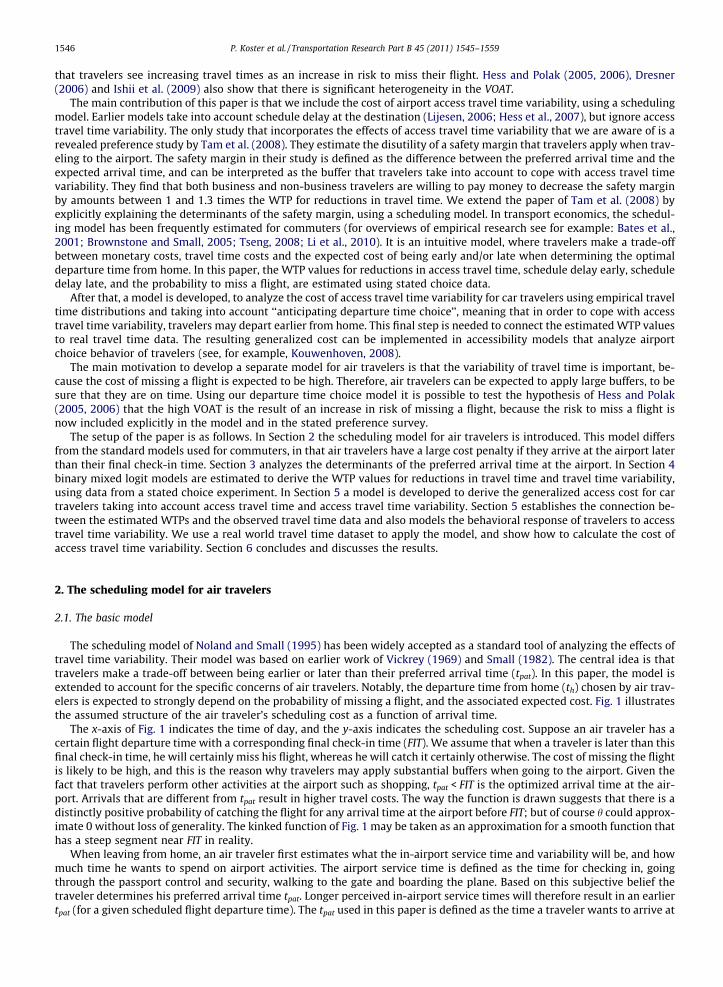
The scheduling model of Noland and Small (1995) has been widely accepted as a standard tool of analyzing the effects oftravel time variability. Their model was based on earlier work of Vickrey (1969) and Small (1982). The central idea is thattravelers make a trade-off between being earlier or later than their preferred arrival time (tpat). In this paper, the model isextended to account for the specific concerns of air travelers. Notably, the departure time from home (th) chosen by air trav-elers is expected to strongly depend on the probability of missing a flight, and the associated expected cost. Fig. 1 illustratesthe assumed structure of the air traveler’s scheduling cost as a function of arrival time.

The x-axis of Fig. 1 indicates the time of day, and the y-axis indicates the scheduling cost. Suppose an air traveler has acertain flight departure time with a corresponding final check-in time (FIT). We assume that when a traveler is later than thisfinal check-in time, he will certainly miss his flight, whereas he will catch it certainly otherwise. The cost of missing the flightis likely to be high, and this is the reason why travelers may apply substantial buffers when going to the airport. Given thefact that travelers perform other activities at the airport such as shopping, tpat < FIT is the optimized arrival time at the air-port. Arrivals that are different from tpat result in higher travel costs. The way the function is drawn suggests that there is adistinctly positive probability of catching the flight for any arrival time at the airport before FIT; but of course h could approx-imate 0 without loss of generality. The kinked function of Fig. 1 may be taken as an approximation for a smooth function thathas a steep segment near FIT in reality.

When leaving from home, an air traveler first estimates what the in-airport service time and variability will be, and howmuch time he wants to spend on airport activities. The airport service time is defined as the time for checking in, goingthrough the passport control and security, walking to the gate and boarding the plane. Based on this subjective belief thetraveler determines his preferred arrival time tpat. Longer perceived in-airport service times will therefore result in an earliertpat (for a given scheduled flight departure time). The tpat used in this paper is defined as the time a traveler wants to arrive at

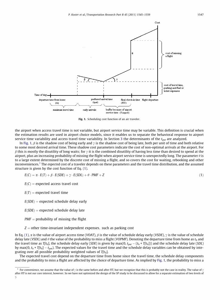
Fig. 1. Scheduling cost function of an air traveler.

P. Koster et al. / Transportation Research Part B 45 (2011) 1545–1559 1547

the airport when access travel time is not variable, but airport service time may be variable. This definition is crucial whenthe estimation results are used in airport choice models, since it enables us to separate the behavioral response to airportservice time variability and access travel time variability. In Section 3 the determinants of the tpat are analyzed.

In Fig. 1, b is the shadow cost of being early and c is the shadow cost of being late, both per unit of time and both relativeto some most desired arrival time. These shadow cost parameters indicate the cost of non-optimal arrivals at the airport. Forb this is mostly the disutility of long waits; for c it is the combined disutility of having less time than desired to spend at theairport, plus an increasing probability of missing the flight when airport service time is unexpectedly long. The parameter h isto a large extent determined by the discrete cost of missing a flight, and so covers the cost for waiting, rebooking and otherinconveniences.1 The expected cost of a traveler depends on these parameters and the travel time distribution, and the assumedstructure is given by the cost function of Eq. (1).

1 Forafter FITc.

EðCÞ ¼ a � EðTÞ þ b � EðSDEÞ þ c � EðSDLÞ þ h � PMF þ Z ð1Þ

EðCÞ ¼ expected access travel cost

EðTÞ ¼ expected travel time

EðSDEÞ ¼ expected schedule delay early

EðSDEÞ ¼ expected schedule delay late

PMF ¼ probability of missing the flight

Z ¼ other time-invariant independent expenses; such as parking cost

In Eq. (1), a is the value of airport access time (VOAT), b is the value of schedule delay early (VSDE), c is the value of scheduledelay late (VSDL) and h the value of the probability to miss a flight (VOPMF). Denoting the departure time from home as th andthe travel time as T[th], the schedule delay early (SDE) is given by max(0, tpat � (th + T[th])) and the schedule delay late (SDL)by max(0, th + T[th] � tpat). The expected values for the travel time and the schedule delay variables can be obtained by inte-grating over all possible probability weighted values of T[th].

The expected travel cost depend on the departure time from home since the travel time, the schedule delay componentsand the probability to miss a flight are affected by the choice of departure time. As implied by Fig. 1, the probability to miss a

convenience, we assume that the value of c is the same before and after FIT, but we recognize that this is probably not the case in reality. The value of cis not our core interest, however. So we have not optimized the design of the SP study to be discussed to allow for a separate estimation of two levels of

Table 1Summary statistics of the survey.

Access mode Non-business Business

Car driver 39.6% 38.6%Car passengera 25.4% 21.4%Taxi 8.9% 7.0%Train 20.1% 30.1%Other 5.9% 2.9%

Total 100.0% 100.0%

Characteristics of the last tripAverage travel time (min) 82 79Average # of flights per year 2.66 5.84Average duration of the trip 12 days 7 days

Airport chosenSchiphol Airport 73.5% 79.7%Small Dutch airports 8.8% 5.5%Belgian Airports 5.8% 7.0%German Airports 11.3% 6.1%Other 0.8% 1.7%

Total 100.0% 100.0%

a If travelers do not travel alone, on average there are three people in the car.


flight depends indirectly on the preferred arrival time, because this in turn affects the departure time from home. A laterpreferred arrival time will result in a later departure time from home and therefore in a larger probability to miss the flight.In the next section, we will analyze the determinants of the preferred arrival time.

3. Determinants of the preferred arrival time

3.1. Descriptive statistics of the survey

An internet survey was held among Dutch air travelers, to collect the data that are necessary for the analysis of the accesscost function. Only travelers who made a trip in the last 3 months were invited. A total of 971 completed surveys were collectedwith 345 reporting about a business trip and 626 reporting about a non-business trip. In the survey, information was askedabout the latest trip to the airport. This information was used to customize the stated choice experiment. It was found that1.5% of the air travelers (0.52% of all flights) had actually missed a flight during the last year, due to delays during their accesstrip. The other summary statistics are given in Table 1. It is noteworthy that the modal share is quite similar for business andnon-business travelers, except that business travelers take more often the train. This high share of train as an access mode ismainly caused by the fact that Schiphol Airport is very well connected by train, and most travelers in the survey use SchipholAirport as their departure airport. The high share of taxi users of non-business travelers is also surprising, and may be due to thefact that Schiphol airport offers his own airport-taxi service, which has lower monetary travel cost than a standard taxi.

The mean average travel time, defined as the average travel time from the location of departure to the check in counter atthe airport, is somewhat longer for non-business trips than for business travelers. The average number of flights per year forbusiness travelers is more than twice that for non-business travelers. Finally, one can see that non-business travelers aretraveling less often via Schiphol Airport and more often from German airports. Table 2 shows the yearly household incomedistribution of our sample, compared to the income distribution of all travelers who made a flight in the last 3 months priorto the survey. The sample is well-balanced, but there is a slight under-sampling of low income travelers.

Fig. 2 depicts the spatial distribution of the departure place of the respondents, based on 4-digit zipcode levels. There aremore departures in the western part of The Netherlands, not in the least place because more people live and work there. For86% of the business travelers the departure place is their home location. For non-business travelers this is true in 92% of thecases. This information is relevant for the analysis of airport choice, since residential locations are usually available in stan-dard statistics while the work location of these travelers is often unknown.

3.2. Determinants of the preferred arrival time

In this section we analyze the preferred arrival (tpat) time at the airport using a basic regression analysis. We define Tairport

as the dependent variable in the regression. It is defined as the scheduled flight departure time minus the preferred arrivaltime at the airport, and gives the number of minutes before the flight departure that a travelers prefers to arrive at the air-port if there would be a guarantee of no access travel time delays.2 As implied by Fig. 1, the Tairport may be an important

2 The exact phrasing of the question to obtain the tpat is: ‘‘Suppose that you know for sure that there are no delays for your trip to the airport. What would beyour preferred arrival time at the airport?’’

Table 2Sampling distribution of incomes.

Yearly household income % Sample % Total

<23,000 5.50 8.1323,000–34,000 10.17 12.6334,000–45,000 15.49 14.5945,000–56,000 13.47 12.6956,000–68,000 13.38 11.3668,000–91,000 13.75 12.01>91,000 10.91 10.41Unknown 17.32 18.19

Total 100.00 100.00

Fig. 2. Spatial distribution of the departure place for business and non-business (personal) trips.


determinant of the cost of variable airport access time, as a larger value implies an earlier tpat, and the resulting earlier departuretime from home would reduce the probability to miss a flight.

There are 926 observations included in the analysis. Travelers that arrive the previous day at the airport and sleep in ahotel are excluded from the analysis. Furthermore, travelers with a dependent variable lower or equal than 0, or with veryextreme values, are excluded from the analysis because they most likely made a mistake when filling in the questionnaire.

In Table 3 the regression results are shown. The log of Tairport is the dependent variable, ln[E(T)] is the log of expectedtravel time and ln[FTT] is the log of the flight duration, both in minutes. Furthermore, variables for type of traveler (business),type of check-in and time of the day are included. Also type of access mode was included, but this variable appears to be non-significant and was dropped from the final model.

The results show that longer expected travel times and longer flight travel times result in a larger Tairport. Furthermore,business travelers prefer to arrive later than non-business travelers. Travelers who are retired prefer to arrive earlier, likelybecause of less pressing scheduling constraints and possibly because they move less quickly in the airport.

Experience plays an important role. Travelers who fly between 5 and 10 times per year prefer to arrive on average 10 minlater than travelers with less experience, and travelers who fly more than 10 times per year prefer to arrive on average20 min later. This result indicates for example that uncertainty about in airport service times decreases, or risk avoiding re-duces, when a traveler is more experienced. An experienced traveler has probably a better perception of the real in-airportservice time than a non-experienced traveler, and possibly has more knowledge about the possibilities to limit consequences

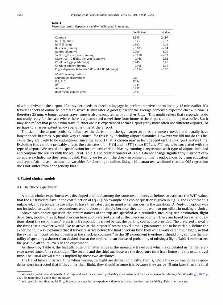
Table 3Regression results, dependent variable: ln(Tairport) in minutes.

Coefficient t-Value

Constant 3.363 24.97ln[E(T)] (min) 0.053 2.32ln[FTT] (min) 0.162 9.26Business (dummy) �0.103 �2.94Retired (dummy) 0.090 1.705–10 Flights per year (dummy) �0.110 �2.12More than 10 flights per year (dummy) �0.168 �2.52Check in luggage (dummy) 0.245 5.26Check in online (dummy) �0.108 �3.39Flight departure between 0:00 and 7:00 (dummy) �0.154 �3.16

Model summary statisticsNumber of observations 926F(9, 916) 32.84R2 0.244Adjusted R2 0.237Root mean squared error 0.461


of a late arrival at the airport. If a traveler needs to check in luggage he prefers to arrive approximately 15 min earlier. If atraveler checks in online he prefers to arrive 10 min later. A good guess for the average perceived expected check-in time istherefore 25 min. A longer access travel time is also associated with a higher Tairport. This might reflect that respondents donot really reply for the case where there is a guaranteed travel time from home to the airport, and building in a buffer. But itmay also reflect that people who travel further are less experienced at that airport (they more often use different airports), orperhaps to a larger extent enjoy spending time at the airport.

The size of the airport probably influences the decision on the tpat. Larger airports are more crowded and usually havelonger check-in times. A possible way to control for this is by including airport dummies. However we did not do this be-cause they are likely to be endogenous, since the airport that is chosen may in turn depend on the in-airport service time.Excluding this variable probably affects the estimates of ln[E(T)] and ln[FTT] since E(T) and FTT might be correlated with thetype of airport. We tested the specification for omitted variable bias by running a regression with type of airport includedand compare the results with the results of Table 3. The point estimates of Table 3 do not change significantly if airport vari-ables are excluded, so they remain valid. Finally we tested if the check-in online dummy is endogenous by using educationand type of airline as instrumental variables for checking in online. Using a Hausman test we found that the OLS regressiondoes not suffer from endogeneity bias.3

4. Stated choice models

4.1. The choice experiment

A stated choice experiment was developed and held among the same respondents as before, to estimate the WTP valuesthat the air travelers have in the cost function of Eq. (1). An example of a choice question is given in Fig. 3. The experiment isunlabeled, and respondents are asked to have their latest trip in mind when answering the questions. An ‘opt-out’ option wasnot included to avoid that respondents would choose it simply because they do not want to put effort in making a choice.

Above each choice question the circumstances of the trip are specified as a reminder, including trip destination, flightdeparture, mode of travel, final check-in time and preferred arrival at the check-in counter. These are based on earlier ques-tions about the respondents’ latest trip. If respondents travel by car, the parking cost is also provided. The preferred arrival isthe time that a traveler would like to arrive at the airport if access travel time is guaranteed not to be variable. Before theexperiment, it was explained that if travelers arrive before the final check-in time they will always catch their flight, so thatthe experiment controls for queuing at the check-in counters.4 In this SP experiment therefore c should only capture the dis-utility of spending a shorter than desired time at the airport, not an increased probability of missing a flight. Table 4 summarizesthe possible attribute levels in the experiment.

As shown by Table 4, the first attribute of an alternative is the monetary travel cost which is calculated using the refer-ence travel time of the respondent. The second and the third attribute are the departure time from home and the usual traveltime. The usual arrival time is implied by these two attributes.

The travel time and arrival time when missing the flight are defined implicitly. That is, before the experiment, the respon-dents were instructed that if they miss their flight, they should assume it is because they arrive 15 min later than the final

3 We used a probit estimation in the first stage and used the estimated probability as an instrument for the check-in online dummy. See Wooldridge (2002, p.632), for more details about this procedure.

4 We tested for our final model if tpat is too early, since in the experiment there is no airport service time variability. This is not the case.

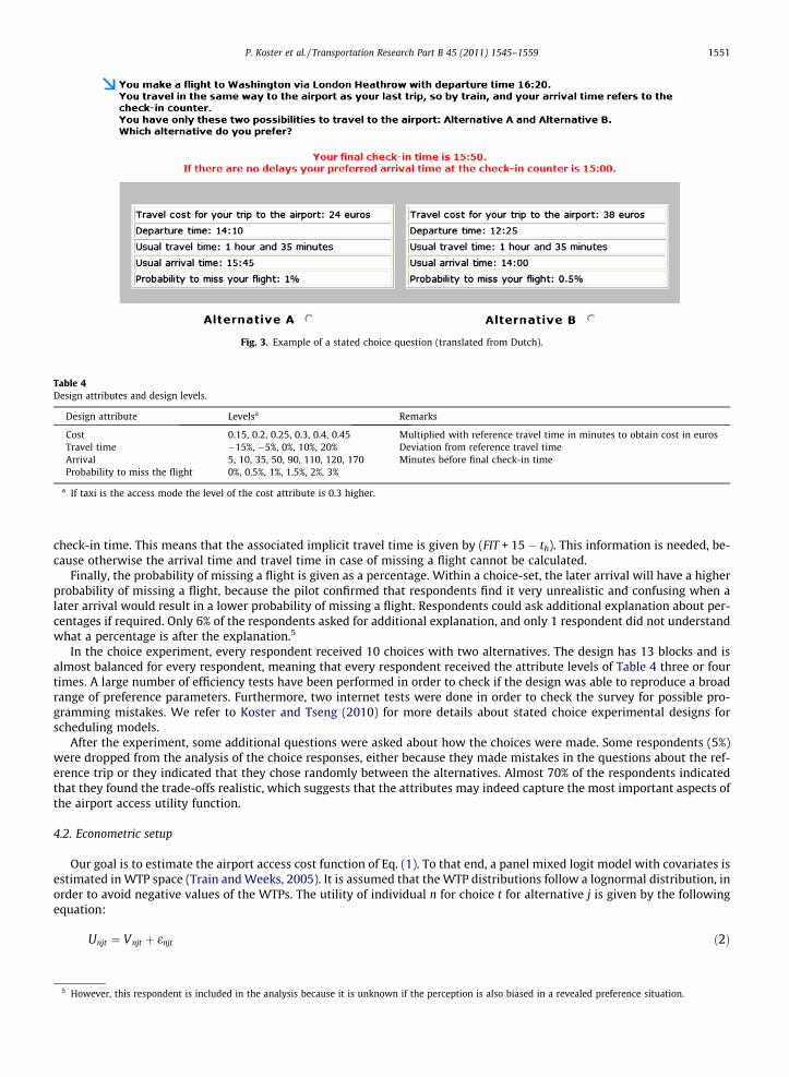
Fig. 3. Example of a stated choice question (translated from Dutch).

Table 4Design attributes and design levels.

Design attribute Levelsa Remarks

Cost 0.15, 0.2, 0.25, 0.3, 0.4, 0.45 Multiplied with reference travel time in minutes to obtain cost in eurosTravel time �15%, �5%, 0%, 10%, 20% Deviation from reference travel timeArrival 5, 10, 35, 50, 90, 110, 120, 170 Minutes before final check-in timeProbability to miss the flight 0%, 0.5%, 1%, 1.5%, 2%, 3%

a If taxi is the access mode the level of the cost attribute is 0.3 higher.


check-in time. This means that the associated implicit travel time is given by (FIT + 15 � th). This information is needed, be-cause otherwise the arrival time and travel time in case of missing a flight cannot be calculated.

Finally, the probability of missing a flight is given as a percentage. Within a choice-set, the later arrival will have a higherprobability of missing a flight, because the pilot confirmed that respondents find it very unrealistic and confusing when alater arrival would result in a lower probability of missing a flight. Respondents could ask additional explanation about per-centages if required. Only 6% of the respondents asked for additional explanation, and only 1 respondent did not understandwhat a percentage is after the explanation.5

In the choice experiment, every respondent received 10 choices with two alternatives. The design has 13 blocks and isalmost balanced for every respondent, meaning that every respondent received the attribute levels of Table 4 three or fourtimes. A large number of efficiency tests have been performed in order to check if the design was able to reproduce a broadrange of preference parameters. Furthermore, two internet tests were done in order to check the survey for possible pro-gramming mistakes. We refer to Koster and Tseng (2010) for more details about stated choice experimental designs forscheduling models.

After the experiment, some additional questions were asked about how the choices were made. Some respondents (5%)were dropped from the analysis of the choice responses, either because they made mistakes in the questions about the ref-erence trip or they indicated that they chose randomly between the alternatives. Almost 70% of the respondents indicatedthat they found the trade-offs realistic, which suggests that the attributes may indeed capture the most important aspects ofthe airport access utility function.

4.2. Econometric setup

Our goal is to estimate the airport access cost function of Eq. (1). To that end, a panel mixed logit model with covariates isestimated in WTP space (Train and Weeks, 2005). It is assumed that the WTP distributions follow a lognormal distribution, inorder to avoid negative values of the WTPs. The utility of individual n for choice t for alternative j is given by the followingequation:

5 How

Unjt ¼ Vnjt þ enjt ð2Þ

ever, this respondent is included in the analysis because it is unknown if the perception is also biased in a revealed preference situation.


Total utility is an additive function of the deterministic utility and an error term, which is independently and identically ex-treme value distributed over choices, people and alternatives.6 The systematic part of the utility is given by the followingequation:

6 A m7 We

used wdecomp

Vnjt ¼ �k � ðcostnjt þ eZn � YnjtÞ ð3Þ

In this equation costnjt are the monetary cost for the trip. Zn captures the individual specific covariates, including a dummy forthe type of traveler (business or non-business) and the log of yearly income. The e-power is used because of the fact that wewill use lognormal distributions for the WTPs.

Zn ¼ sbus � DBUSn þ sINC � logðincomeÞn ð4Þ

In this equation DBUSn is a dummy indicating if a traveler is a business traveler and log(income)n is the log of the householdsyearly income. sbus and sINC are the parameters to be estimated. Next we define Yntj, which is the product of the WTP valuesand the independent variables.

Ynjt ¼ an � EðTÞnjt þ bn � EðSDEÞnjt þ cn � EðSDLÞnjt þ hn � PMFnjt ð5Þ

In order to capture unobserved heterogeneity, we apply lognormal distributions with mean l and standard deviation r,which vary over WTPs. These distributions have mean exp(l + r2/2) and median exp(l). For a given type of traveler and in-come level, the mean and median WTP are then given by the following equation:

WTP mean ¼ eZn � elþr22 ¼ eZnþlþr2

2 ð6aÞ

WTP median ¼ eZn � el ¼ eZnþl ð6bÞ

The explanatory variable PMFnjt is the probability to miss a flight, and is directly visible on the choice screen. For the othervariables some additional calculation is needed. Define UTTnjt as the usual travel time, FITn as the final check-in time for indi-vidual n, and thnjt

as the departure time from home. In order to show the relationship with the choice screen of Fig. 3, theindependent variables of Eq. (4) are given by the following equation:

EðTÞnjt ¼ ð1� PMFnjtÞ � UTTnjt þ PMFnjt � ðFITn þ 15� thnjtÞ ð7aÞ

EðSDEÞnjt ¼ ð1� PMFnjtÞ �max½0; PATn � thnjt� UTTnjtÞ ð7bÞ

EðSDLÞnjt ¼ ð1� PMFnjtÞ �max½0; thnjtþ UTTnjt � PATnÞ þ PMFnjt � ðFITn þ 15� PATnÞ ð7cÞ

All variables are in minutes. As explained before, the second arrival time is implicitly given in the choice question and is al-ways set 15 min later than the FIT.

We estimate a panel mixed logit model, so we account for repeated observations of one individual. Conditional on theWTP values, the probability that an individual makes a sequence of choices i = {i1, . . . , iT} is given by the product of the logitprobabilities (Train, 2003).

Lni½WTP� ¼YT

t¼1

eVnitt½WTPn �P

jeVnjt½WTPn �

ð8aÞ

The unconditional probability is then given by the integral over all values of the WTPs. We use a multivariate lognormal dis-tribution g[WTP], where the marginal distributions may be correlated. The choice probability is then given by the followingequation (Train, 2003).

Pni ¼Z

Lni½WTP�g½WTP�dWTP ð8bÞ

For the approximation of the integral 25,000 Modified Latin Hypercube draws per individual are used (Hess et al., 2006). Allmodels are estimated in Biogeme using maximum simulated likelihood (Bierlaire, 2003, 2008; Train, 2003).7

4.3. Estimation results

The estimation results for the binary panel mixed logit models are given in Table 5. Model 1 is the model with uncorre-lated distributions. In model 2 we allow for correlated distributions. In model 1 all the estimated parameters are significantat the 5% level, except sINC. There is significant unobserved heterogeneity, and especially for the VOPMF the estimated

ultiplicative formulation as proposed by Fosgerau and Bierlaire (2009) was tested but resulted in a worse model fit.use FASTBIOGEME to estimate the models because it has the advantage of parallel computing possibilities. Therefore a high number of draws can be

hile the running times stay reasonable. For more details about simulated likelihood and generating draws for correlated distributions using Choleskyosition, we refer to Train (2003), and Bierlaire (2003, 2008).

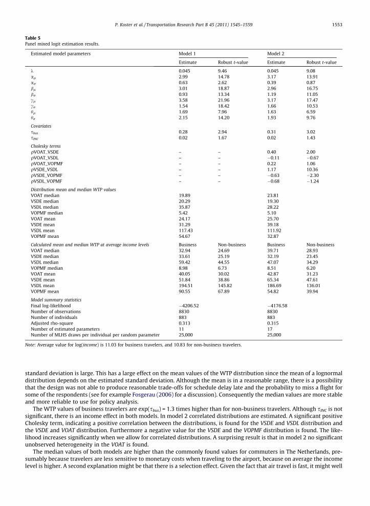
Table 5Panel mixed logit estimation results.

Estimated model parameters Model 1 Model 2

Estimate Robust t-value Estimate Robust t-value

k 0.045 9.46 0.045 9.08al 2.99 14.78 3.17 13.91ar 0.63 2.62 0.39 0.87bl 3.01 18.87 2.96 16.75br 0.93 13.34 1.19 11.05cl 3.58 21.96 3.17 17.47cr 1.54 18.42 1.66 10.53hl 1.69 7.96 1.63 6.59hr 2.15 14.20 1.93 9.76

Covariatessbus 0.28 2.94 0.31 3.02sINC 0.02 1.67 0.02 1.43

Cholesky termsqVOAT_VSDE – – 0.40 2.00qVOAT_VSDL – – �0.11 �0.67qVOAT_VOPMF – – 0.22 1.06qVSDE_VSDL – – 1.17 10.36qVSDE_VOPMF – – �0.63 �2.30qVSDL_VOPMF – – �0.68 �1.24

Distribution mean and median WTP valuesVOAT median 19.89 23.81VSDE median 20.29 19.30VSDL median 35.87 28.22VOPMF median 5.42 5.10VOAT mean 24.17 25.70VSDE mean 31.29 39.18VSDL mean 117.43 111.92VOPMF mean 54.67 32.87

Calculated mean and median WTP at average income levels Business Non-business Business Non-businessVOAT median 32.94 24.69 39.71 28.93VSDE median 33.61 25.19 32.19 23.45VSDL median 59.42 44.55 47.07 34.29VOPMF median 8.98 6.73 8.51 6.20VOAT mean 40.05 30.02 42.87 31.23VSDE mean 51.84 38.86 65.34 47.61VSDL mean 194.51 145.82 186.69 136.01VOPMF mean 90.55 67.89 54.82 39.94

Model summary statisticsFinal log-likelihood �4206.52 �4176.58Number of observations 8830 8830Number of individuals 883 883Adjusted rho-square 0.313 0.315Number of estimated parameters 11 17Number of MLHS draws per individual per random parameter 25,000 25,000

Note: Average value for log(income) is 11.03 for business travelers, and 10.83 for non-business travelers.


standard deviation is large. This has a large effect on the mean values of the WTP distribution since the mean of a lognormaldistribution depends on the estimated standard deviation. Although the mean is in a reasonable range, there is a possibilitythat the design was not able to produce reasonable trade-offs for schedule delay late and the probability to miss a flight forsome of the respondents (see for example Fosgerau (2006) for a discussion). Consequently the median values are more stableand more reliable to use for policy analysis.

The WTP values of business travelers are exp(sbus) = 1.3 times higher than for non-business travelers. Although sINC is notsignificant, there is an income effect in both models. In model 2 correlated distributions are estimated. A significant positiveCholesky term, indicating a positive correlation between the distributions, is found for the VSDE and VSDL distribution andthe VSDE and VOAT distribution. Furthermore a negative value for the VSDE and the VOPMF distribution is found. The like-lihood increases significantly when we allow for correlated distributions. A surprising result is that in model 2 no significantunobserved heterogeneity in the VOAT is found.

The median values of both models are higher than the commonly found values for commuters in The Netherlands, pre-sumably because travelers are less sensitive to monetary costs when traveling to the airport, because on average the incomelevel is higher. A second explanation might be that there is a selection effect. Given the fact that air travel is fast, it might well

Table 6Basic assumptions for the two representative travelers.

Variable Business traveler Non-business traveler

DBUS 1 0log(income) 11.03 10.83a 39.71 28.93b 32.19 23.45c 47.07 34.29h 8.51 6.20tpat 60 min before final check-in time 90 min before final check-in time


be that this is the reason that travelers with a high disutility of time use this travel mode. The median VOAT is slightly lowerthan earlier findings in the literature (Furuichi and Koppelman, 1993; Hess and Polak, 2006). In the next section the medianWTP values of model 2 will be used to illustrate the anticipating departure time choice model for a typical business and non-business traveler.

5. Empirical illustration

5.1. Introduction

In this section the model is developed to calculate the cost of airport access travel time variability for car travelers usingreal-world travel data. This is a crucial step in the analysis, because the connection is made between the estimated WTP val-ues of the previous section, and the empirical travel time distribution. We take into account anticipating behavior, meaningthat travelers are assumed to optimize their departure time from home given their knowledge about the empirical traveltime distribution (see for example: Noland and Small, 1995; Fosgerau and Karlström, 2010; Fosgerau and Engelson,2010). In order to keep the illustration as simple as possible, two representative travelers will be considered. Both travel

Fig. 4. Time of day dependent mean and standard deviation of travel time.

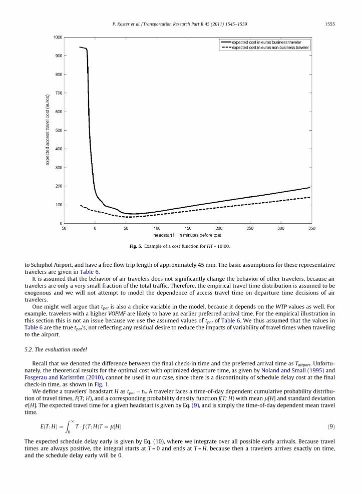
Fig. 5. Example of a cost function for FIT = 10:00.


to Schiphol Airport, and have a free flow trip length of approximately 45 min. The basic assumptions for these representativetravelers are given in Table 6.

It is assumed that the behavior of air travelers does not significantly change the behavior of other travelers, because airtravelers are only a very small fraction of the total traffic. Therefore, the empirical travel time distribution is assumed to beexogenous and we will not attempt to model the dependence of access travel time on departure time decisions of airtravelers.

One might well argue that tpat is also a choice variable in the model, because it depends on the WTP values as well. Forexample, travelers with a higher VOPMF are likely to have an earlier preferred arrival time. For the empirical illustration inthis section this is not an issue because we use the assumed values of tpat of Table 6. We thus assumed that the values inTable 6 are the true tpat’s, not reflecting any residual desire to reduce the impacts of variability of travel times when travelingto the airport.

5.2. The evaluation model

Recall that we denoted the difference between the final check-in time and the preferred arrival time as Tairport. Unfortu-nately, the theoretical results for the optimal cost with optimized departure time, as given by Noland and Small (1995) andFosgerau and Karlström (2010), cannot be used in our case, since there is a discontinuity of schedule delay cost at the finalcheck-in time, as shown in Fig. 1.

We define a travelers’ headstart H as tpat � th. A traveler faces a time-of-day dependent cumulative probability distribu-tion of travel times, F(T; H), and a corresponding probability density function f(T; H) with mean l[H] and standard deviationr[H]. The expected travel time for a given headstart is given by Eq. (9), and is simply the time-of-day dependent mean traveltime.

EðT; HÞ ¼Z 1

0T � f ðT; HÞT ¼ l½H� ð9Þ

The expected schedule delay early is given by Eq. (10), where we integrate over all possible early arrivals. Because traveltimes are always positive, the integral starts at T = 0 and ends at T = H, because then a travelers arrives exactly on time,and the schedule delay early will be 0.

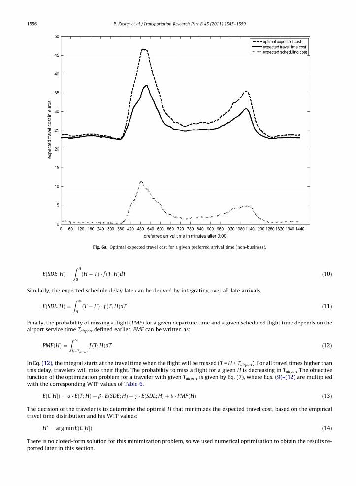
Fig. 6a. Optimal expected travel cost for a given preferred arrival time (non-business).


EðSDE; HÞ ¼Z H

0ðH � TÞ � f ðT; HÞdT ð10Þ

Similarly, the expected schedule delay late can be derived by integrating over all late arrivals.

EðSDL; HÞ ¼Z 1

HðT � HÞ � f ðT; HÞdT ð11Þ

Finally, the probability of missing a flight (PMF) for a given departure time and a given scheduled flight time depends on theairport service time Tairport defined earlier. PMF can be written as:

PMFðHÞ ¼Z 1

HþTairport

f ðT; HÞdT ð12Þ

In Eq. (12), the integral starts at the travel time when the flight will be missed (T = H + Tairport). For all travel times higher thanthis delay, travelers will miss their flight. The probability to miss a flight for a given H is decreasing in Tairport The objectivefunction of the optimization problem for a traveler with given Tairport is given by Eq. (7), where Eqs. (9)–(12) are multipliedwith the corresponding WTP values of Table 6.

EðC½H�Þ ¼ a � EðT; HÞ þ b � EðSDE; HÞ þ c � EðSDL; HÞ þ h � PMFðHÞ ð13Þ

The decision of the traveler is to determine the optimal H that minimizes the expected travel cost, based on the empiricaltravel time distribution and his WTP values:

H� ¼ argminEðC½H�Þ ð14Þ

There is no closed-form solution for this minimization problem, so we used numerical optimization to obtain the results re-ported later in this section.

Fig. 6b. Optimal expected travel cost for a given preferred arrival time (business).


5.3. The travel time data

Travel time data are obtained using loop-detector measurements on a highway road stretch for every 15 min of the day.The data are interpolated to obtain 1-min interval data. We use a trip from Rotterdam to Schiphol Airport with a free flowtravel time of around 45 min as an example. The mean and the standard deviation are plotted in Fig. 4, where a time-of-daypattern with a morning and an evening peak is clearly visible.

Fig. 4 shows that there is a clear positive relationship between the mean and the standard deviation of travel time. Thisphenomenon is analyzed theoretically by Fosgerau (2010) and empirically by Peer (2010), and is caused by the fact that thereis bottleneck congestion on this road. Van Lint et al. (2008) found that the shape of the empirical travel time distribution isvarying over time of day, and therefore no particular parametric form of the empirical travel time distribution is appropriate.Therefore we use nonparametric Kernel smooth density estimation to fit a time-of-day dependent travel time distribution.8

5.4. Empirical results

An example of an expected cost function for a given final check-in time 10:00 is given in Fig. 5. Note that the costs aregiven as a function of H in minutes before tpat. Because tpat is not observed, we use the plausible values of Table 6.

The expected cost for both travelers is optimal for a headstart of around 60 min. The expected cost for the business trav-eler is higher than for the non-business traveler, because of the smaller buffer at the airport and the higher WTP values. Thenext step is to repeat this same optimization procedure for every time of the day. We have done this with a resolution of1 min, so in total we considered 1440 tpat’s over the day. This results in Fig. 6a (business) and Fig. 6b (non-business), withoptimal expected cost as a function of time-of-day. These costs are strongly dependent on the time of day and follow thebimodal pattern of the mean travel time. Furthermore, the expected scheduling costs are strongly related to the expectedmean travel time cost because the mean and the standard deviation are closely related. During night hours the expected

8 The densities are estimated using the ksdensity function in Matlab with 500 equally spaced points. This function uses an optimal bandwidth for Normaldensities. More detailed information about this bandwidth selection procedure can be found in Bowman and Azzalini (1997). Results are available uponrequest.


scheduling cost are close to 0. During day time the cost is in between 5% and 15% of total expected travel cost. In the morningand evening peak the expected scheduling cost is in between 10% and 30% of total expected travel cost. For business travelersthe share is slightly higher (up to 30%) than for non-business travelers (up to 25%).

Cost estimates like these could subsequently be used in, for example, airport choice models. If the impact of certain pol-icies or investments on travel time distribution are known, the same approach could be used for cost-benefit analysis. How-ever, such exercises are beyond the scope of this paper.

6. Conclusions and discussion

We analyzed the effect of airport access travel time variability on access travel cost. The mixed logit estimations showthat, as expected, scheduling plays an important role in departure time decisions of travelers going to the airport. For bothbusiness and non-business travelers there is heterogeneity in the scheduling parameters. A connection was made betweenthe estimated shadow cost of scheduling and equilibrium cost taking into account anticipating departure time choice of airtravelers. Using a dataset of Dutch travel times we show that for business travelers the cost of variability are in between 0%and 30% of expected access travel cost depending on the time of day. For non-business travelers this number is in between0% and 25%. These numbers are somewhat higher than the values of Fosgerau and Karlström (2010) who analyzed the cost oftravel time variability for commuters.

The model that is developed in Section 5 has of course some limitations. One is that it is assumed that air travelers have aperfect perception of the empirical travel time distribution. For commuters, perfect perception may be a realistic assump-tion, because these travelers are usually experienced. But for air travelers it may well be that travelers do not know theempirical travel time distribution, and therefore make larger perception errors. This may result in non-optimal behavior,and therefore the cost of variable travel times may be higher than estimated in Section 5 (Koster and Verhoef, 2012).

Role of the funding source

The project ‘‘Reliable Accessibility of Airports’’ has been made possible with support of TRANSUMO (TRANsition SUstain-able MObility). TRANSUMO is a Dutch platform for companies, governments and knowledge institutes that cooperate in thedevelopment of knowledge with regard to sustainable mobility.

Acknowledgements

The authors like to thank two referees for very helpful comments. We also like to thank Chris Jacobs of the SPINLAB (VUUniversity Amsterdam) for GIS assistance. Furthermore, we like to thank Peter Schout of DVS (Directorate General for PublicWorks and Water Management) for provision of the travel time data, and Sander Duijm and Matthijs de Gier of TNS NIPO forcollection of the survey data. The usual disclaimer applies.

References

Bates, J., Polak, J., Jones, P., Cook, A.J., 2001. The valuation of reliability for personal travel. Transportation Research Part E 37 (2–3), 191–229.Bierlaire, M., 2003. BIOGEME: a free package for the estimation of discrete choice models. In: Proceedings of the 3rd Swiss Transportation Research

Conference, Ascona, Switzerland.Bierlaire, M., 2008. An Introduction to BIOGEME Version 1.7. <biogeme.epfl.ch>.Bowman, A.W., Azzalini, A., 1997. Applied Smoothing Techniques for Data Analysis. Oxford University Press.Brownstone, D., Small, K.S., 2005. Valuing time and reliability: assessing the evidence from road pricing demonstrations. Transportation Research Part A 39

(4), 279–293.Dresner, M., 2006. Leisure versus business passengers: similarities, differences, and implications. Journal of Air Transport Management 12 (1), 28–32.Fosgerau, M., 2006. Investigating the distribution of the value of travel time savings. Transportation Research Part B 40 (8), 688–707.Fosgerau, M., 2010. On the relation of mean and variance of delay in dynamic queues with random capacity and demand. Journal of Economic Dynamics and

Control 34 (4), 598–603.Fosgerau, M., Bierlaire, M., 2009. Discrete choice models with multiplicative error terms. Transportation Research Part B 43 (5), 494–505.Fosgerau, M., Engelson, L., 2010. The value of travel time variance. Transportation Research Part B 45 (1), 1–8.Fosgerau, M., Karlström, A., 2010. The value of reliability. Transportation Research Part B 44 (1), 38–49.Furuichi, M., Koppelman, F.S., 1993. An analysis of air travelers’ departure airport and destination choice behavior. Transportation Research Part A 28 (3),

187–195.Harvey, G., 1986. Study of airport access mode choice. Journal of Transportation Engineering 112 (5), 525–545.Hess, S., Polak, J.W., 2005. Mixed logit modeling of airport choice in multi-airport regions. Journal of Air Transport Management 11 (2), 59–68.Hess, S., Polak, J.W., 2006. Airport, airline and access mode choice in the San Fransisco Bay area. Papers in Regional Science 85 (4), 543–567.Hess, S., Train, K., Polak, J., 2006. On the use of a modified latin hypercube sampling (MLHS) method in the estimation of a mixed logit model for vehicle

choice. Transportation Research Part B 40 (2), 147–163.Hess, S., Adler, T., Polak, J.W., 2007. Modelling airport and airline choice behavior with the use of stated preference survey data. Transportation Research Part

E 43 (3), 221–233.Ishii, J., Jun, S., van Dender, K., 2009. Air travel choices in multi-airport markets. Journal of Urban Economics 65 (2), 216–227.Koster, P.R., Tseng, Y.-Y., 2010. Sated choice experimental designs for scheduling models. Choice modeling: the state-of-the-art and the state-of-practice. In:

Hess, S., Daly, A. (Eds.), Proceedings of the Inaugural Choice Modeling Conference.Koster, P.R., Verhoef, E.T., 2012. A rank dependent scheduling model. Journal of Transport Economics and Policy, in press.Kouwenhoven, M., 2008. The Role of Accessibility in Passengers’ Choice of Airports, OECD Discussion Paper No. 2008-14, Paris.

http://biogeme.epfl.ch


Li, Z., Hensher, D.A., Rose, J., 2010. Willingness to pay for travel time reliability in passenger transport: a review and some new empirical evidence.Transportation Research Part E 46 (3), 384–403.

Lijesen, M., 2006. A mixed logit based valuation of frequency in civil aviation from SP-data. Transportation Research Part E 42 (2), 82–94.Noland, R.B., Small, K.A., 1995. Travel-time uncertainty, departure time choice, and the cost of morning commutes. Transportation Research Record 1493,

150–158.Peer, S., Koopmans, C., Verhoef, E.T., 2010. Predicting Travel Time Variability for Cost-Benefit Analysis, Tinbergen Institute Discussion Paper, TI 2010-071/3.Pels, E., Nijkamp, P., Rietveld, P., 2003. Access to and competition between airports: a case study for the San Francisco Bay area. Regional Studies 35 (1), 1–9.Skinner, R.E., 1976. Airport choice: an empirical study. Transportation Engineering Journal 102 (4), 871–882.Small, K.A., 1982. The scheduling of consumer activities: work trips. American Economic Review 72 (3), 469–479.Tam, M.L., Lam, H.K., Lo, H.P., 2008. Modeling air passenger travel behavior on airport ground access mode choices. Transportmetrica 4 (2), 135–153.Train, K., 2003. Discrete Choice Methods with Simulation. Cambridge University Press, Cambridge, MA.Train, K., Weeks, M., 2005. Discrete choice models in preference space and willingness-to-pay space. In: Alberini, A., Scarpa, R. (Eds.), Applications of

Simulation Methods in Environmental Resource Economics. Springer, Dordrecht, The Netherlands, pp. 1–17 (Chapter 1).Tseng, Y.-Y., 2008. Valuation of Travel Time Reliability in Passenger Transport. PhD Thesis, VU University Amsterdam, Tinbergen Research Series No. 439.Van Lint, J., Van Zuylen, H., Tu, H., 2008. Travel time unreliability on freeways: why measures based on variance tell only half the story. Transportation

Research Part A 42 (1), 258–277.Vickrey, W.S., 1969. Congestion theory and transport investment. American Economic Review 59 (2), 251–261.Wooldridge, J.M., 2002. Econometric Analysis of Cross Section and Panel Data. MIT Press, Cambridge, MA.

Travel Time Variability and Airport Accessibility

Documents

Transcript of Travel Time Variability and Airport Accessibility