Transmitter Based Techniques for ISI andMAI Mitigation in CDMA-TDD Downlink

Stamatis L. GeorgoulisT

HE

U N I V E R S

I TY

OF

ED I N B U

RG

H

A thesis submitted for the degree of Doctor of Philosophy.The University of Edinburgh.

January 2003

Abstract

The third-generation (3G) of mobile communications systems aim to provide enhanced voice,

text and data services to the user. These demands give rise to the complexity and power con-

sumption of the user equipment (UE) while the objective is smaller, lighter and power efficient

mobiles. This thesis aims to examine ways of reducing the UE receiver’s computational cost

while maintaining a good performance.

One prominent multiple access scheme selected for 3G is code division multiple access. Re-

ceiver based multiuser detection techniques that utilise the knowledge of the downlink channel

by the mobile have been extensively studied in the literature, in order to deal with multiple

access and intersymbol interference. However, these techniques result in high mobile receiver

complexity.

Recently, work has been done on algorithms that transfer the complexity from the UE to the

base station by exploiting the fact that in time division duplex mode the downlink channel can

be known to the transmitter. By linear precoding of the transmitted signal the user equipment

can be simplified to a filter matched to the user’s spreading code. In this thesis the problem

of generic linear precoding is analysed theoretically and a method for analytical calculation

of BER is developed. The most representative of the developed precoding techniques are de-

scribed under a common framework, compared and classified as bitwise or blockwise. Bitwise

demonstrate particular advantages in terms of complexity and implementation but lack in per-

formance. Two novel bitwise algorithms are presented and analysed. They outperform signifi-

cantly the existing ones, while maintain a reduced computational cost and realisation simplicity.

The first, named inverse filters, is the Wiener solution of the problem after applying a minimum

mean squared error criterion with power constraints. The second recruits multichannel adap-

tive algorithms to achieve the same goal. The base station emulates the actual system in a cell

to converge iteratively to the pre-filters that precode the transmitted signals before transmis-

sion. The advantages and the performance of the proposed techniques, along with a variety of

characteristics are demonstrated by means of Monte Carlo simulations.

ii

Declaration of originality

I hereby declare that the research recorded in this thesis and the thesis itself was composed and

originated entirely by myself in the Department of Electronics and Electrical Engineering at the

University of Edinburgh.

The software used to perform the simulations was written by myself with the following excep-

tions:

• The routines used to generate uniform and Gaussian distributed pseudo-random samples

were obtained from Numerical recipes in C[1].

Stamatis Georgoulis

iii

to my parents Leandros and Margarita.

στoυς γoνεις µoυ Λεανδρo και Mαργαριτα.

Acknowledgements

First and foremost, I wish to thank my supervisor Dr. Dave Cruickshank whose continuous and

patient guidance as well as his timely advice contributed greatly to the completion of this thesis.

Also, my second supervisor Prof. Stephen McLaughlin for his advice and guidance when Dr.

Cruickshank was away, and for reviewing the manuscript.

I would like to thank the Faculty of Science and Engineering at Edinburgh University for pro-

viding the financial support without which I would not have been in the position to commence

and complete this Ph.D. project.

Special thanks to my colleagues and friends in the Signals and Systems Group for sharing their

knowledge and a pleasant time in our office.

I express my sincere gratitude to my grandfather Apostolos and my uncle Antonis for their

small financial help that added quality in my life during the three years in Edinburgh.

Last but not least, I wish to thank my parents Leandros and Margarita for their relentless sup-

port, priceless guidance and boundless love.

v

Contents

Abstract . . . . . . . . . . . . . . . . . . . . . . . . . . . . . . . . . . . . . . iiDeclaration of originality . . . . . . . . . . . . . . . . . . . . . . . . . . . . . iiiAcknowledgements . . . . . . . . . . . . . . . . . . . . . . . . . . . . . . . . vContents . . . . . . . . . . . . . . . . . . . . . . . . . . . . . . . . . . . . . . viList of figures . . . . . . . . . . . . . . . . . . . . . . . . . . . . . . . . . . . ixList of tables . . . . . . . . . . . . . . . . . . . . . . . . . . . . . . . . . . . xiiAcronyms and abbreviations . . . . . . . . . . . . . . . . . . . . . . . . . . . xiiiNomenclature . . . . . . . . . . . . . . . . . . . . . . . . . . . . . . . . . . . xvi

1 Introduction 11.1 Cellular fundamentals . . . . . . . . . . . . . . . . . . . . . . . . . . . . . . . 2

1.1.1 Channel characteristics . . . . . . . . . . . . . . . . . . . . . . . . . . 31.1.2 Multiple access scheme . . . . . . . . . . . . . . . . . . . . . . . . . . 61.1.3 Channel reuse . . . . . . . . . . . . . . . . . . . . . . . . . . . . . . . 8

1.2 Third-Generation systems . . . . . . . . . . . . . . . . . . . . . . . . . . . . . 91.3 Open problems-Motivation of the thesis . . . . . . . . . . . . . . . . . . . . . 101.4 Thesis layout . . . . . . . . . . . . . . . . . . . . . . . . . . . . . . . . . . . 12

2 System model - Multiuser detection 142.1 System model . . . . . . . . . . . . . . . . . . . . . . . . . . . . . . . . . . . 14

2.1.1 Continuous-time model . . . . . . . . . . . . . . . . . . . . . . . . . . 142.1.2 Discrete-time downlink transmission model . . . . . . . . . . . . . . . 182.1.3 Matrix-vector notation for the discrete-time transmission model . . . . 20

2.2 Air interface structure . . . . . . . . . . . . . . . . . . . . . . . . . . . . . . . 232.2.1 Frame length design . . . . . . . . . . . . . . . . . . . . . . . . . . . 242.2.2 Pilot signals . . . . . . . . . . . . . . . . . . . . . . . . . . . . . . . . 242.2.3 Spreading code design . . . . . . . . . . . . . . . . . . . . . . . . . . 252.2.4 Scrambling . . . . . . . . . . . . . . . . . . . . . . . . . . . . . . . . 272.2.5 Modulation . . . . . . . . . . . . . . . . . . . . . . . . . . . . . . . . 272.2.6 Error control schemes . . . . . . . . . . . . . . . . . . . . . . . . . . 292.2.7 Power control . . . . . . . . . . . . . . . . . . . . . . . . . . . . . . . 292.2.8 Handover . . . . . . . . . . . . . . . . . . . . . . . . . . . . . . . . . 302.2.9 Discussion . . . . . . . . . . . . . . . . . . . . . . . . . . . . . . . . 31

2.3 RAKE receiver . . . . . . . . . . . . . . . . . . . . . . . . . . . . . . . . . . 312.4 Multiuser detection . . . . . . . . . . . . . . . . . . . . . . . . . . . . . . . . 35

2.4.1 Zero-Forcing algorithm . . . . . . . . . . . . . . . . . . . . . . . . . . 382.4.2 Minimum mean square error algorithm . . . . . . . . . . . . . . . . . 392.4.3 Discussion . . . . . . . . . . . . . . . . . . . . . . . . . . . . . . . . 402.4.4 Complexity . . . . . . . . . . . . . . . . . . . . . . . . . . . . . . . . 41

2.5 Simulation results . . . . . . . . . . . . . . . . . . . . . . . . . . . . . . . . . 422.5.1 General assumptions . . . . . . . . . . . . . . . . . . . . . . . . . . . 422.5.2 Receiver based JD performance . . . . . . . . . . . . . . . . . . . . . 44

2.6 Summary . . . . . . . . . . . . . . . . . . . . . . . . . . . . . . . . . . . . . 45

vi

Contents

3 Linear precoding - A general approach 463.1 Motivation . . . . . . . . . . . . . . . . . . . . . . . . . . . . . . . . . . . . . 463.2 WCDMA-TDD . . . . . . . . . . . . . . . . . . . . . . . . . . . . . . . . . . 483.3 Performance analysis of linear precoding . . . . . . . . . . . . . . . . . . . . . 503.4 Precoding techniques-Classification . . . . . . . . . . . . . . . . . . . . . . . 53

3.4.1 Blockwise techniques . . . . . . . . . . . . . . . . . . . . . . . . . . . 533.4.2 Bitwise techniques . . . . . . . . . . . . . . . . . . . . . . . . . . . . 54

3.5 Power scaling factor . . . . . . . . . . . . . . . . . . . . . . . . . . . . . . . . 573.6 Summary . . . . . . . . . . . . . . . . . . . . . . . . . . . . . . . . . . . . . 59

4 Linear precoding - State of the art 604.1 Joint transmission . . . . . . . . . . . . . . . . . . . . . . . . . . . . . . . . . 604.2 Transmitter precoding . . . . . . . . . . . . . . . . . . . . . . . . . . . . . . . 63

4.2.1 Unconstrained optimisation . . . . . . . . . . . . . . . . . . . . . . . 634.2.2 Constrained optimisation . . . . . . . . . . . . . . . . . . . . . . . . . 65

4.3 Decorrelating prefilters-Jointly optimized sequences . . . . . . . . . . . . . . . 664.3.1 Decorrelating prefilters . . . . . . . . . . . . . . . . . . . . . . . . . . 664.3.2 Jointly optimised sequences . . . . . . . . . . . . . . . . . . . . . . . 68

4.4 Pre-RAKE diversity . . . . . . . . . . . . . . . . . . . . . . . . . . . . . . . . 694.5 Complexity . . . . . . . . . . . . . . . . . . . . . . . . . . . . . . . . . . . . 744.6 Other techniques . . . . . . . . . . . . . . . . . . . . . . . . . . . . . . . . . 764.7 Simulation results . . . . . . . . . . . . . . . . . . . . . . . . . . . . . . . . . 764.8 Summary . . . . . . . . . . . . . . . . . . . . . . . . . . . . . . . . . . . . . 79

5 Inverse filters - Wiener solution 805.1 INVF in stereophonic sound reproduction system . . . . . . . . . . . . . . . . 805.2 Least squares power constrained algorithm . . . . . . . . . . . . . . . . . . . . 825.3 Generalisation . . . . . . . . . . . . . . . . . . . . . . . . . . . . . . . . . . . 865.4 Wiener solution . . . . . . . . . . . . . . . . . . . . . . . . . . . . . . . . . . 875.5 λ - In depth . . . . . . . . . . . . . . . . . . . . . . . . . . . . . . . . . . . . 90

5.5.1 Numerical solution . . . . . . . . . . . . . . . . . . . . . . . . . . . . 905.5.2 Performance results . . . . . . . . . . . . . . . . . . . . . . . . . . . . 93

5.6 Observations on λ parameter . . . . . . . . . . . . . . . . . . . . . . . . . . . 955.6.1 BER vs λ & filter length . . . . . . . . . . . . . . . . . . . . . . . . . 955.6.2 BER vs λ & Eb/No . . . . . . . . . . . . . . . . . . . . . . . . . . . . 985.6.3 Performance spread vs λ . . . . . . . . . . . . . . . . . . . . . . . . . 995.6.4 Discussion . . . . . . . . . . . . . . . . . . . . . . . . . . . . . . . . 103

5.7 Simulation results-Comparison . . . . . . . . . . . . . . . . . . . . . . . . . . 1045.8 Summary . . . . . . . . . . . . . . . . . . . . . . . . . . . . . . . . . . . . . 111

6 Multichannel adaptive algorithms 1136.1 Motivation . . . . . . . . . . . . . . . . . . . . . . . . . . . . . . . . . . . . . 1136.2 Filtered-X LMS . . . . . . . . . . . . . . . . . . . . . . . . . . . . . . . . . . 1156.3 Multichannel algorithms . . . . . . . . . . . . . . . . . . . . . . . . . . . . . 118

6.3.1 Multichannel LMS . . . . . . . . . . . . . . . . . . . . . . . . . . . . 1186.3.2 Multichannel LMS with power constraints . . . . . . . . . . . . . . . . 1206.3.3 Multichannel RLS . . . . . . . . . . . . . . . . . . . . . . . . . . . . 123

vii

Contents

6.3.4 Alternative MC adaptive techniques . . . . . . . . . . . . . . . . . . . 1256.4 Convergence speed . . . . . . . . . . . . . . . . . . . . . . . . . . . . . . . . 126

6.4.1 MC-LMS, leakage MC-LMS, rescaling MC-LMS . . . . . . . . . . . . 1266.4.2 MC-RLS . . . . . . . . . . . . . . . . . . . . . . . . . . . . . . . . . 1296.4.3 UMTS-TDD block sizes . . . . . . . . . . . . . . . . . . . . . . . . . 132

6.5 BER performance-Simulation results . . . . . . . . . . . . . . . . . . . . . . . 1326.5.1 MC-LMS, leakage MC-LMS, rescaling MC-LMS . . . . . . . . . . . . 1336.5.2 MC-RLS . . . . . . . . . . . . . . . . . . . . . . . . . . . . . . . . . 1346.5.3 Comparison-Discussion . . . . . . . . . . . . . . . . . . . . . . . . . 136

6.6 Summary . . . . . . . . . . . . . . . . . . . . . . . . . . . . . . . . . . . . . 137

7 Summary - Conclusions 1397.1 Summary and thesis contributions . . . . . . . . . . . . . . . . . . . . . . . . 1397.2 Limitations of the work and scope for further research . . . . . . . . . . . . . . 142

7.2.1 Time varying channels . . . . . . . . . . . . . . . . . . . . . . . . . . 1427.2.2 Channel estimation . . . . . . . . . . . . . . . . . . . . . . . . . . . . 1437.2.3 Space-time techniques . . . . . . . . . . . . . . . . . . . . . . . . . . 143

References 144

A Wiener solution for unequal powers 153

B Publications 155

viii

List of figures

1.1 A typical cellular system setup . . . . . . . . . . . . . . . . . . . . . . . . . . 31.2 A mobile multipath environment . . . . . . . . . . . . . . . . . . . . . . . . . 41.3 Call allocation in the spectrum with different multiple access schemes . . . . . 61.4 (a) A cluster of three cells (b) Channels reuse concept using a three cell cluster 9

2.1 Transmitter-receiver DS-CDMA block diagram . . . . . . . . . . . . . . . . . 152.2 Continuous-time downlink model for multiple access . . . . . . . . . . . . . . 152.3 Generation of a SS signal . . . . . . . . . . . . . . . . . . . . . . . . . . . . . 182.4 Discrete-time CDMA channel model . . . . . . . . . . . . . . . . . . . . . . . 202.5 Layer structure of CDMA air interface . . . . . . . . . . . . . . . . . . . . . . 242.6 Two-tap linear binary shift register . . . . . . . . . . . . . . . . . . . . . . . . 262.7 The autocorrelation function of an 31-chips long M-sequence and the crosscor-

relation function of two randomly selected M-sequences with the same length. . 262.8 Beginning of the channelisation code tree. . . . . . . . . . . . . . . . . . . . . 272.9 Spreading circuits . . . . . . . . . . . . . . . . . . . . . . . . . . . . . . . . . 282.10 Constellation diagrams of linear modulation methods . . . . . . . . . . . . . . 292.11 Transmitter block diagram . . . . . . . . . . . . . . . . . . . . . . . . . . . . 312.12 Intersymbol interference (ISI): how bit d−1’s multipath replicas affect the next

bit d0. Interchip interference (ICI) : within one symbol by delayed replicas ofitself. . . . . . . . . . . . . . . . . . . . . . . . . . . . . . . . . . . . . . . . 33

2.13 RAKE receiver configuration . . . . . . . . . . . . . . . . . . . . . . . . . . . 342.14 RAKE receiver’s fingers . . . . . . . . . . . . . . . . . . . . . . . . . . . . . 352.15 Problem of data detection . . . . . . . . . . . . . . . . . . . . . . . . . . . . . 362.16 Multiuser detection classification . . . . . . . . . . . . . . . . . . . . . . . . . 372.17 Block diagram of linear receiver based multiuser detection scheme . . . . . . . 402.18 Receiver-based MUD algorithms performance in AWGN channels. K = 5 users. 442.19 Receiver-based MUD algorithms performance in frequency selective channels

(Table: 2.3) when K = 5 users. Single user performance in AWGN channel. . . 45

3.1 Linearity of CDMA downlink . . . . . . . . . . . . . . . . . . . . . . . . . . 463.2 Linear Precoding . . . . . . . . . . . . . . . . . . . . . . . . . . . . . . . . . 473.3 TDD and FDD principles . . . . . . . . . . . . . . . . . . . . . . . . . . . . . 483.4 TDD frames and bursts structure [2] . . . . . . . . . . . . . . . . . . . . . . . 503.5 Blockwise precoding diagram . . . . . . . . . . . . . . . . . . . . . . . . . . 533.6 Bitwise precoding diagram . . . . . . . . . . . . . . . . . . . . . . . . . . . . 55

4.1 Pre-RAKE combination process . . . . . . . . . . . . . . . . . . . . . . . . . 704.2 RAKE combiner . . . . . . . . . . . . . . . . . . . . . . . . . . . . . . . . . 714.3 Pre-RAKE combiner . . . . . . . . . . . . . . . . . . . . . . . . . . . . . . . 714.4 Single user noiseless output of a RAKE receiver . . . . . . . . . . . . . . . . . 734.5 Single user noiseless matched filter output after pre-RAKE processing . . . . . 734.6 Block-length effect on JT performance . . . . . . . . . . . . . . . . . . . . . . 77

ix

List of figures

4.7 Block-length effect on Transmitted Energy Eg . . . . . . . . . . . . . . . . . . 774.8 Transmitter based precoding techniques and MMSE-JD vs Eb/No . . . . . . . 78

5.1 A stereophonic sound reproduction system . . . . . . . . . . . . . . . . . . . . 805.2 Block diagram of sound reproduction system with inverse filters . . . . . . . . 815.3 Modified diagram to comply with a single antenna CDMA model . . . . . . . . 825.4 Two users block diagram of an inverse filters system . . . . . . . . . . . . . . 835.5 Two users block diagram of a simplified inverse filters system . . . . . . . . . 835.6 Rearranged inverse filters block-diagram for two users . . . . . . . . . . . . . 845.7 Generalised block diagram of an inverse filters system . . . . . . . . . . . . . . 875.8 Generalised rearranged block diagram for µ user. . . . . . . . . . . . . . . . . 875.9 Transmitted energy and BER vs λ for INVF. . . . . . . . . . . . . . . . . . . . 945.10 BER vs λ for scaled and non-scaled sp. K=5, Q=16, Eb/No=15dB. . . . . . . 945.11 BER vs λ & P . K=5, Q=16, Eb/No = 10dB. . . . . . . . . . . . . . . . . . . 955.12 BER vs λ & P . K = 12, Q = 16, Eb/No = 10dB. . . . . . . . . . . . . . . . 965.13 BER vs λ. K = 5, Q = 16, Eb/No = 10dB. . . . . . . . . . . . . . . . . . . . 975.14 BER vs Eb/No & λ. K = 5, Q = 16, P = 32. . . . . . . . . . . . . . . . . . 975.15 BER vs λ. P = 32, K = 5, Q = 16. . . . . . . . . . . . . . . . . . . . . . . . 985.16 BER vs λ. P = 32, K = 12, Q = 16. . . . . . . . . . . . . . . . . . . . . . . 995.17 Individual users and average BER, K=7, Q=16, λ = 0.05. . . . . . . . . . . . 1005.18 Individual users and average BER, K=7, Q=16, λ = 0.15. . . . . . . . . . . . 1005.19 SNIR spread vs λ. K = 5, Q = 16, L = 11, Eb/No = 10dB. . . . . . . . . . . 1015.20 SNIR spread vs λ & P . K = 5, Q = 16, Eb/No = 8dB. . . . . . . . . . . . . 1025.21 Φs vs λ & Eb/No . . . . . . . . . . . . . . . . . . . . . . . . . . . . . . . . . 1035.22 BER vs P . K = 5, Eb/No = 10dB, Q = 16. λ = 0.05 for INVF. . . . . . . . 1055.23 BER vs Eb/No. K = 5, Q = 16, L = 11. . . . . . . . . . . . . . . . . . . . . 1065.24 BER vs Eb/No. K = 14, Q = 16. . . . . . . . . . . . . . . . . . . . . . . . . 1065.25 BER vs K . Eb/No = 10dB, Q = 16. P = 32 for INVF and DPF. λ = 0.05

for INVF. . . . . . . . . . . . . . . . . . . . . . . . . . . . . . . . . . . . . . 1075.26 Channel’s effect for spreading codes set 1. . . . . . . . . . . . . . . . . . . . . 1085.27 Channel’s effect for spreading codes set 2. . . . . . . . . . . . . . . . . . . . . 1095.28 BER vs Eb/No. K = 3, Q = 16. . . . . . . . . . . . . . . . . . . . . . . . . . 1105.29 BER vs Eb/No. K = 3, Q = 16 for complex channels. . . . . . . . . . . . . . 110

6.1 Block diagram of emulation in the BS . . . . . . . . . . . . . . . . . . . . . . 1146.2 Adaptive inverse modeling of a noisy plant . . . . . . . . . . . . . . . . . . . . 1166.3 Development of filtered-X algorithm . . . . . . . . . . . . . . . . . . . . . . . 1176.4 Detailed MC-LMS algorithm for two users . . . . . . . . . . . . . . . . . . . . 1206.5 Alternative MC techniques . . . . . . . . . . . . . . . . . . . . . . . . . . . . 1256.6 Convergence speed with different µ parameter. Ensemble of 100 trials. Q =

16, K = 3, P = 16. . . . . . . . . . . . . . . . . . . . . . . . . . . . . . . . . 1276.7 Convergence speed comparison for µ = 0.02. Ensemble of 100 trials. Q = 16,

K = 3, P = 16, µ = 0.02. . . . . . . . . . . . . . . . . . . . . . . . . . . . . 1276.8 Mean-squared error among all users. MC-LMS. K = 3, P = 32 . . . . . . . . 1286.9 Mean-squared error among all users. Leakage MC-LMS. K = 3, P = 32 . . . 1296.10 Convergence speed. . . . . . . . . . . . . . . . . . . . . . . . . . . . . . . . . 1306.11 MC-RLS. K = 3, P = 16 . . . . . . . . . . . . . . . . . . . . . . . . . . . . 131

x

List of figures

6.12 MC-RLS. K = 3, P = 16 . . . . . . . . . . . . . . . . . . . . . . . . . . . . 1326.13 BER versus Eb/No. K = 3, P = 16, µ = 0.02, 400 iterations. . . . . . . . . . 1336.14 BER versus Eb/No. K = 5, P = 32, µ = 0.005, 1500 iterations. . . . . . . . . 1346.15 BER vs Eb/No for MC-RLS. K = 3, P = 16. θ = 1.0, λ = 0.05 for INVF. . . 1356.16 BER vs Eb/No for MC-RLS. K = 5, P = 32. θ = 1.0, λ = 0.05 for INVF. . . 1356.17 BER versus Filter Length for Eb/No = 10dB, K = 5 users . . . . . . . . . . . 1366.18 BER versus Eb/No, K = 5 users . . . . . . . . . . . . . . . . . . . . . . . . . 137

7.1 Space-time INVF extension . . . . . . . . . . . . . . . . . . . . . . . . . . . . 143

A.1 Two users with unequal powers block diagram . . . . . . . . . . . . . . . . . . 153

xi

List of tables

2.1 Air design procedure for CDMA . . . . . . . . . . . . . . . . . . . . . . . . . 242.2 Important contributions to multiuser detection algorithms . . . . . . . . . . . . 372.3 Severe multipath channels’ profile . . . . . . . . . . . . . . . . . . . . . . . . 43

4.1 Precoding algorithms computational complexity . . . . . . . . . . . . . . . . . 75

5.1 INVF vs JT computational cost comparison . . . . . . . . . . . . . . . . . . . 1075.2 Mild multipath channel’s profile . . . . . . . . . . . . . . . . . . . . . . . . . 1095.3 Complex multipath channel’s profile . . . . . . . . . . . . . . . . . . . . . . . 111

xii

Acronyms and abbreviations

3G Third-Generaration

3GPP Third-Generaration Partnership Project

AMPS Advanced Mobile Phone Services

ARQ Automatic Repeat Request

AWGN Additive White Gaussian Noise

BER Bit Error Ratio

BPSK Binary Phase Shift Key

BS Base Station

CDMA Code Division Multiple Access

DPF Decorrelating Prefilters

DS Direct Sequence

ETACS European Total Access Communication System

ETSI European Telecommunications Standards Institute

FDD Frequency Division Duplex

FDMA Frequency Division Multiple Access

FEC Forward Error Control

FH Frequency Hopping

FIR Finite Impulse Response

FPLMTS Future Public Land Mobile Telecommunications Service

FTF Fast Transerval Filter

GSM Global System for Mobile communications

IMT International Mobile Telecommunications

INVF Inverse Filters

IS Interim Standard

ISI Intersymbol Interference

ITU International Telecommunications Union

JD Joint Detection

JOS Jointly Optimised Sequences

JT Joint Transmission

xiii

Acronyms and abbreviations

JTACS Japanese Total Access Communication System

KKT Karush-Kuhn-Tucker

LAN Local Area Network

LMS Least Mean Squares

MAI Multiple Access Interference

MC Multichannel

MC-LMS Multichannel-Least Mean Squares

MC-RLS Multichannel-Recursive Least Squares

MLSE Maximum-likelihood Sequence Estimation

MMSE Minimum Mean Squared Error

MS Mobile Station

MSC Mobile Switching Center

MUD Multiuser Detection

NMT Nordic Mobile Telephone

NTT Nippon Telephone and Telegraph

PDC Personal Digital Cellular

PIC Parallel Interference Cancellation

PN Pseudo-Noise

QPSK Quadrature Phase Shift Keying

SD Single Detection

SIC Serial Interference Cancellation

SNIR Signal to Noise plus Interference Ratio

SNR Signal to Noise Ratio

SS Spread Spectrum

TACS Total Access Communication System

TDD Time Division Duplex

TDMA Time Division Multiple Access

TH Time Hopping

TP Transmitter Precoding

UE User Equipment

UMTS Universal Mobile Telecommunications System

UTRA UMTS Terestial Radio Access

W-CDMA Wideband-Code Division Multiple Access

xiv

Acronyms and abbreviations

XOR EXclusive OR

ZF Zero Forcing

rms Root Mean Square

xv

Nomenclature

Ak general matrix for the description of the detected data at the receiver’s output

Av general matrix that describes the noise after being filtered by the receiver

Ak matrix that consists of γkj(n) for j = 1 . . . K

B block-diagonal matrix of Bk

Bk matrix whose columns are the spreading code of kth user plus zeros

B matrix that consists of zk(n) samples for k = 1 . . . K

C block-diagonal matrix of Ck

Ck matrix whose columns are the spreading code of kth user

Dk all-zero vector except for a unity entry at position k

E[·] expectation of ·Eg transmission power per user per symbol of a conventional CDMA (no precoding)

Eg transmission power per user per symbol of a CDMA with precoding√F scaling factor to normalise the transmission power of the precoding techniques

G length of the expanded symbol at the k-user pre-filter output

Gγ length of expanded symbol of filtered reference outputs

G arrangement of K matrices Gk

Gk matrix whose columns are the vector gk

H Hk matrices arranged in a column

Hk matrix whose columns are the channel impulse response hk of kth user

I identity matrix

J cost function

Jc cost function with power constraint

K total users active in a cell

K(T ns ) auxiliary matrix used in the MC-RLS

L chip-rate sampled length of the channel impulse response

Ls length of optimally designed signature sequence ζk

M number of bits responsible for intersymbol interference

M(T ns ) matrix used in the MC-RLS

N block of data addressed to one user

xvi

Nomenclature

No power spectral density

P pre-filter length

Pe(dmk ) error probability of detected symbol dmk

Pe(dm) K users system average theoretical error probability

Q spreading gain

Rd covariance matrix of data vector d

Rv covariance matrix of noise vector v

R matrix that contains all filtered reference signals in an INVF system

Re denotes the real part of a complex number

Tc chip period

Ts symbol period

Tss sampling time on the receiver

T ns sampling time sequence on the receiver

T general transformation matrix for precoding

T TP transformation matrix for TP

T JT transformation matrix for JT

Uk matrix whose columns vectors are the ck, used for power calculation

V(n) filtered reference matrix used in MC-RLS algorithm

U block-diagonal matrix of K Uk

W block-diagonal matrix of Wk

Wk diagonal matrix with diagonal elements the kth user’s transmission amplitude

Z length of a FIR filter which results by cascaded channel and matched filter receiver

ck k-user’s spreading code in a vector form of length Q

cqk rectangular chip waveform, cqk = ±1

ck(n) spreading code in discrete time, 0 ≤ n ≤ Q

ck(t) spreading code in continuous time, 0 ≤ t ≤ Ts

dmk the mth bit transmitted for kth user

dmk soft decision on the receiver of the mth bit transmitted for kth user

d0 vector of K data-bits d0k

d0 estimated received vector of K data-bits d0k

d vector of a block of KN data-bits assigned to all users

dk vector of a block of N data-bits assigned to user k

xvii

Nomenclature

d vector of a block of KN receiver estimated data-bits assigned to all users

dk vector of a block of N receiver estimated data-bits assigned to user k

ek(n) discrete time received signal on k-user’s receiver

ek(t) continuous time received signal on k-user’s receiver

e arrangement in a vector of K ek

ek received signal on k-receiver in vector form of length Q+ L− 1

fo carrier frequency

gk vector of the expanded symbol at the k-user pre-filter output

gc(t) the chip waveform

hk channel impulse response in a vector form, of length L

hk(n) chip-rate sampling of channel impulse response

hk(t, τ) time-varying linear channel impulse response for downlink with k-user

hk(τ) time-invarying linear channel impulse response for downlink with k-user

k denotes a particular user index

m index for transmitted bit

n discrete time index n = 1, 2, 3, ...., chip rate sampling

p arrangement of K vectors pk in a vector of length KP

pk k-user pre-filter FIR in vector form of length P

pk(n) continuous time k-user’s pre-filter impulse response

pk(t) discrete time k-user’s pre-filter impulse response

q index for the chips in a spreading sequence, q = 0 . . . Q− 1

rij(n) filtered reference signal

rij vector of P length associated with filtered reference signal rij(n)

s transmitted vector of length NQ with no precoding

sp transmitted vector of length NQ with precoding

s(n) discrete time transmitted signal with no precoding from the BS

s(t) continuous time transmitted signal with no precoding from the BS

sp(n) discrete time transmitted signal with precoding from the BS

s(t) continuous time transmitted signal with precoding from the BS

s(t) bandpass transmitted signal with no precoding from the BS

t continuous time index

v(n) additive Gaussian noise at the receiver

v(n) noise at the receiver’s output

xviii

Nomenclature

v additive Gaussian noise vector on the receiver

xmk (n) spread symbol dmk

Y complex symbol alphabet set

Yi complex symbols from data alphabet i = 1 . . . `

wmk transmission amplitude of kth user’s mth data-bit

zk(n) convolution of kth user channel impulse response and its matched filter receiver

Γ expectation of RTR

Γij matrix whith columns the vector γ ij

∆ delay in sampling

Φxs SNIR spread

Ωbitwise computational cost of bitwise precoding techniques

Ωblockwise computational cost of blockwise precoding techniques

β roll-off factor for the raised cosine pulse shaping

γ expectation of RTd0

γij expanded symbol that corresponds to the filtered reference signal rij(n)

γij(n) convolution of ith user spread. code with jth user channel and matched filter FIR

γij vector of P length with elements [Γij ]p,(M+1), where p = 1 . . . P

δ small positive constant for MC-RLS

ζk optimally designed signature sequence of length Ls

θ forgetting factor for MC-RLS algorithm

ϑ/ϑ first order gradient

λ Lagrange multiplier

λ(T ns ) time variant Lagrange multiplier

λ diagonal matrix of Lagrange multipliers

µ step-size parameter for MC-LMS algorithm

ρij crosscorrelation of spreading codes ci(t) and cj(t)

σ2 AWGN variance

τ time delay in propagation time

τmax maximum time delay in propagation time, delay spread

τr half the chip-period, used for the raised cosine pulse shaping

φ(dmk ) SNIR associated with data-bit dmk

xix

Nomenclature

ψ(·) minimum eigenvalue of a matrix

ψ(·) maximum eigenvalue of a matrix

∗ convolution operator

·T transpose operator

·∗ conjugate operator

‖x‖ norm:√

xTx

‖X‖s spectral norm: sq. root of maximum eigenvalue of XTX

[·]i,j element in the ith row and jth column of a matrix

[·]i ith element of a vector

xx

Chapter 1Introduction

The radio age began just over 100 years ago with the invention of the radio telegraph by

Gulielmo Marconi. This event gave birth to a large number of deployments, many of which

operate widely even today (representative examples include the transmission of speech, music

and/or images by radio and TV stations). The development of wireless communication systems

continued through the years and their design and implementation was both aided and influenced

initially by the invention of the triode cathode tube, and later by the advent of the semiconductor

technology in the form of the transistor. Continuous advances in this technology have greatly

benefited wireless communications systems, which have been increasingly capable of handling

such demanding tasks as video, multimedia transmission and teleconferencing among individ-

uals who are physically thousands of kilometers apart. A modern and very interesting aspect of

wireless communications is that of mobile communications or cellular communications.

The cellular concept was invented by Bell Laboratories and the first commercial analog voice

system was introduced in Chicago in October 1983 [3, 4]. The first generation analog cordless

phone and cellular systems became popular using the design based on a standard known as Ad-

vanced Mobile Phone Services (AMPS). Similar standards were developed around the world

including Total Access Communication System (TACS), Nordic Mobile Telephone (NMT) 450,

and NMT 900 in Europe; European Total Access Communication System (ETACS) in the

United Kingdom; C-450 in Germany; and Nippon Telephone and Telegraph (NTT), JTACS

and NTACS in Japan [5].

In contrast to the first generation analog systems, second generation systems are designed to

use digital transmission. These systems include the Pan-European Global System for Mobile

Communications (GSM) and DCS 1800 systems, North American dual-mode cellular system

Interim Standard (IS)-54, North American IS-95 system, and Japanese personal digital cellular

(PDC) system [3, 6].

The third-generation (3G) mobile communications systems are being studied worldwide, under

the names of Universal Mobile Telecommunications System (UMTS) and International Mobile

1

Introduction

Telecommunications (IMT)-2000 [7]. The aim of these systems is to provide users advanced

communication services, having wideband capabilities, using a single standard. In 3G commu-

nications systems, satellites are going to play a major role providing a global coverage. Further-

more, future generation systems promise even more reliable and higher speed communication,

which is expected to enable additional services like mobile multimedia, real-time mobile video

transmission, mobile access to Internet resources and even shopping, making these systems

increasingly indispensable.

The remaining of this Chapter is organised in the following sections: Section 1.1 presents a gen-

eral overview of the cellular fundamentals and section 1.2 a brief history of the third-generation

wireless systems. In section 1.3 the open problems are given along with the motivation and the

goal of this thesis. Finally, the layout of this thesis is given in section 1.4.

1.1 Cellular fundamentals

Nowadays wireless communications are used widely in many communication systems: mobile

telephony, satellite networks, digital radio/television broadcasting, fixed wireless local loops,

etc. The success of mobile communications lies in the ability to provide instant connectivity

anytime and anywhere and the ability to provide high speed data services to the mobile users.

The quality and speeds available in the mobile environment must match the fixed networks

if the convergence of the mobile wireless and fixed communication networks is to happen in

the real sense. So, the challenges for the mobile networks lie in making the movement from

one network to the another as transparent to the user as possible and the availability of high

speed reliable data services along with high quality voice. A range of successful technologies

exists today in various parts of the world and every technology must evolve to fulfill all these

requirements. In this work we are particularly interested in the cellular mobile environment,

therefore, our attention will be primarily focused on this research area.

The area served by mobile phone systems is divided into small areas known as cells. Each

cell contains a base station (BS) that communicates with mobiles in the cell by transmitting and

receiving signals on radio links. The transmission from the base station to a mobile station (MS)

is typically referred to as downstream, forward-link or downlink. The corresponding terms for

the transmission from a mobile to a base station are upstream, reverse-link and uplink. Each

base station is associated with a Radio Network Controller (RNC) and each RNC is connected

2

Introduction

with a mobile switching center (MSC) that connects calls to and from the base stations to

mobiles in other cells and the public switched telephone network. A typical setup depicting a

group of base stations and a MSC is shown in Figure 1.1.

Mobile

Switching

Center

Base StationBase Station

Base StationBase Station

LinkLink

Link

RNC

Link

Networks

Telephone

Switched

Public

RNC

Figure 1.1: A typical cellular system setup

A base station communicates with mobiles using two types of radio channels, control channels

to carry control information and traffic channels to carry messages. Each base station contin-

uously transmits control information on its control channels. When a mobile is switched on,

it scans the control channels and tunes to a channel with the strongest signal. This normally

would come from the BS located in the cell in which the mobile is also located. The mobile

exchanges identification information with the BS and establishes the authorization to use the

network. At this stage the mobile is ready to initiate and receive a call. Important elements that

describe a cellular mobile system are the channel characteristics, the multiple access scheme

and the channel reuse.

1.1.1 Channel characteristics

In the study of communication systems the classical (ideal) additive Gaussian noise channel,

with statistically independent Gaussian noise samples corrupting data samples, is the usual

starting point for understanding basic performance relationships. The primary source of per-

3

Introduction

formance degradation is thermal noise generated in the receiver. However, for most practical

channels, where signal propagation takes place in the atmosphere and near the ground, the free

space propagation model is inadequate to describe the channel and predict the system perfor-

mance. In the following a brief description of the channel characteristics is given. More details

about channel characterization and interference mitigation can be found in [8–10].

1.1.1.1 Fading channels

The propagation of radio signals on both the forward (BS to mobile) and reverse (mobile to

BS) links is affected by the physical channel in several ways. The signal arriving at the receiver

is a combination of many components arriving from various directions as a result of multipath

propagation. These paths arise from scattering, reflection, refraction or diffraction of radiated

energy off the objects that lie in the environment as it is illustrated in Figure 1.2. The terrain

conditions and local buildings and structures cause the received signal power to fluctuate ran-

domly as a function of distance. Fluctuations of the order of 20dB are common within the

distance of one wavelength. This phenomenon is called fading. One may think this signal as a

product of two variables. The first component, also referred to as the short-term fading com-

Far out region

Highrise

Antenna

Mountain

Local scatterers

Figure 1.2: A mobile multipath environment

ponent, changes faster than the second one and can be modeled with a Rayleigh distribution.

The second component is a long term or slow-varying quantity modeled with a log-normal dis-

tribution. In other words, the local mean varies slowly with lognormal distribution and the fast

4

Introduction

variation around the local mean has a Rayleigh distribution.

1.1.1.2 Doppler spread

The movement of a mobile causes the received frequency to differ from the transmitted fre-

quency because of the Doppler shift resulting from its relative motion. As the received signals

arrive along many paths, the relative velocity of the mobile with respect to various components

of the signal differs, causing the different components to have different Doppler shifts. This can

be viewed as Doppler spreading of the transmitted frequency and is referred to as the Doppler

effect. The width of the Doppler spread in the frequency domain is closely related to the rate of

fluctuations in the observed signal. Fast fading results in Doppler spread and is often referred to

as time-selective fading, since signal amplitude varies with time. Time-selective fading can be

characterised by the coherence time of the channel. Coherence time represents the maximum

time separation for which the channel impulse responses at two time instants remain strongly

correlated. The coherence time is inversely proportional to the Doppler spread [11, 12].

1.1.1.3 Delay spread

In a multipath propagation environment, several time-shifted and scaled versions of the trans-

mitted signal arrive at the receiver. That results in spreading of the signal in time. A double-

negative exponential model is typically observed: the delay separation between paths increases

exponentially with the path delay and the path amplitudes also fall exponentially with delay

[12]. This spread of path delays is called delay spread. Delay spread causes frequency-selective

fading, which implies that fading now depends on the frequency. It can be characterized in

terms of coherence bandwidth, which represents the maximum frequency separation for which

the frequency domain channel responses at two frequency shifts remain strongly correlated.

The coherence bandwidth is inversely proportional to the delay spread [11]. This is the band-

width over which the channel is flat; that is; it has a constant gain and linear phase. For a

signal bandwidth above the coherence bandwidth the channel loses its constant gain and linear

phase characteristic and becomes frequency-selective. Roughly speaking, a channel becomes

frequency selective when the root mean square (rms) delay spread is smaller than the sym-

bol duration and causes intersymbol interference (ISI) in digital communications. Frequency-

selective channels are also known as dispersive channels whereas the nondispersive channels

are referred to as flat-fading channels.

5

Introduction

1.1.1.4 Link budget and path loss

Link Budget is a name given to the process of estimating the power at the receiver site for a mi-

crowave link taking into account the attenuation caused by the distance between the transmitter

and the receiver. This reduction is referred to as the path loss. In free space the path loss is pro-

portional to the second power of the distance. In other words, by doubling the distance between

the transmitter and the receiver, the received power at the receiver reduces to one fourth of the

original amount. In a non-free space the attenuation can be higher or lower than that.

1.1.2 Multiple access scheme

The available spectrum bandwidth is shared in a number of ways by various wireless radio

links. The ways in which this is done are referred to as multiple access schemes. There are

basically three principle schemes. These are frequency division multiple access (FDMA), time

division multiple access (TDMA) and code division multiple access (CDMA) [5]. Figure 1.3

shows how the calls are distributed into the spectrum according to the multiple access scheme

used.

Call1 Call 2 Call 3 Call 1

Call 1

Call 2

Call 3

time time time

freq

uenc

y

freq

uenc

y

TDMA FDMA CDMA

Call 2...Call 3...

Call 1...fr

eque

ncy

Figure 1.3: Call allocation in the spectrum with different multiple access schemes

1.1.2.1 FDMA

In a FDMA scheme the available spectrum is divided into a number of frequency channels of

certain bandwidth and individual calls use different frequency channels. All first-generation

cellular systems use this scheme.

6

Introduction

1.1.2.2 TDMA

In a TDMA scheme several calls share a frequency channel. The scheme is useful for digitized

speech or other digital data. Each call is allocated a number of time slots based on its data

rate within a frame for uplink as well as downlink. Apart from the user data, each time slot

also carries other data for synchronisation, equalisation, guard times and control information.

The traffic in two directions is separated either by using two separate frequency channels or by

alternating in time. The two schemes are named as frequency division duplex (FDD) and time

division duplex (TDD), respectively.

1.1.2.3 CDMA

CDMA is a spread spectrum (SS) method [13]. The main characteristic of any spread spectrum

system is that the transmitted signal has a bandwidth much larger than the bandwidth of the

baseband representation of the original signal. CDMA is classified depending on the modula-

tion method used to obtain a wideband signal. This division leads to three types of CDMA:

direct sequence (DS), frequency hopping (FH), and time hopping (TH). In DS-CDMA, spec-

trum is spread by multiplying the information signal with a pseudo-noise sequence, resulting

in a wideband signal. In FH-CDMA a pseudo noise sequence defines the instantaneous trans-

mission frequency. The bandwidth at each moment is small but the total bandwidth over, for

example, a symbol period is large. In TH-CDMA a pseudo noise sequence defines the transmis-

sion moment. Furthermore, combinations of these techniques are possible. In the current thesis

we focus on DS-CDMA because it is the technique used for the third-generation wideband

CDMA (W-CDMA) proposals. Wideband CDMA is defined as direct sequence spread spec-

trum multiple access scheme where the information is spread over a bandwidth significantly

more than the coherence bandwidth of the channel.

DS-CDMA uses linear modulation with wideband pseudonoise (PN) sequences to generate sig-

nals. These sequences, also known as codes, spread the spectrum of the modulating signal over

a large bandwidth, simultaneously reducing the spectral density of the signal. Various CDMA

signals occupy the same bandwidth and appear as noise to each other. Each user is assigned

an individual code at the time of call initiation. This code is used both for spreading the sig-

nal at the time of transmission and despreading it at the time of reception. Cellular systems

using CDMA [14–16] schemes can utilise FDD or TDD for the forward and reverse link sep-

aration. The principle of DS-CDMA is that the codes are orthogonal between each other to

7

Introduction

allow for decoupling at the receiver. On downlink the BS transmits to all users synchronously

and this preserves the orthogonality of various codes assigned to different users. The orthogo-

nality, however, is not preserved between different components arriving from different paths in

multipath propagation or when the users transmit asynchronously, in the uplink, for instance.

Hence, although the spreading codes are designed to be orthogonal with each other, there are

scenarios under which the orthogonality cannot be controlled. This results in interference from

user to user. This type of interference is called multiple access interference (MAI) and imposes

a limitation to CDMA systems. The reason for selecting CDMA over TDMA is that in a high

number of users scheme the transmission on time slots, that TDMA provides, is a limitation

factor for the development of high rate data transmission. The full bandwidth should be utilised

in this scenario, which is feasible with CDMA.

1.1.3 Channel reuse

The generic term channel is normally used to denote a frequency in FDMA system, a time slot

in TDMA system and a code in CDMA or a combination of these in a mixed system. Two

channels are different if they use different combinations of these at the same place. For an

allocated spectrum and a given performance aim the number of channels in a system is limited.

This limits the capacity of a system to sustain simultaneous calls and may only be increased by

using each traffic channel to carry many calls simultaneously. Using the same channel again

and again is one way of doing it and this is the concept of channel reuse.

The concept of channel reuse can be understood from Figure 1.4(a). It shows a cluster of three

cells. These cells use three separate sets of channels. Each set is indicated by a letter. In Figure

1.4(b) this cluster of three cells is repeated to indicate that three sets of channels are being

reused in different cells.

Let F channels be available over a given geographical area and there be N cells in a cluster to

use the available channels. In the absence of the channel reuse this cluster covers the whole area

and the system can sustain simultaneously F calls. If the cluster on N cells is repeated M times

over the same area, then the system capacity increases to MF as each channel is used M times.

Of course the re-use factor would be chosen to ensure that the level of co-channel interference

is low enough that the system can operate satisfactorily. The co-channel interference results

from neighboring cells and it is referred to as intercell interference and it is another factor that

8

Introduction

A

B C

A

B C

A

B C

A

B C

(a)

(b)

Figure 1.4: (a) A cluster of three cells (b) Channels reuse concept using a three cell cluster

limits the cellular system’s performance.

1.2 Third-Generation systems

The emphasis and the contribution of this thesis is on techniques to be applied on WCDMA-

TDD which is one of the air interface selected for the third-generation mobile telecommuni-

cations system. Thus, a brief reference on the development of these systems is given in this

section.

The third-generation systems aim to provide a network that can provide user voice, data, mul-

timedia and video services regardless of their location on the network: fixed, cordless, cellular,

satellite and so on. These networks support global roaming while providing high-speed data

and multimedia applications of up to 144Kbps on the move and up to 2Mbps in a local area[17].

WCDMA, in FDD mode, can achieve up to 3.84 Mcps in contrast with IS-95 than cannot ex-

ceed the chip rate of 1.2288 Mcps. In TDD mode WCDMA can achieve chip rates up to 1.28

Mcps. Some type reference channels are refered in the 3GPP Technical Specifications 25.xxx

9

Introduction

series [18–21]. Third-generation systems are currently being defined by both the International

Telecommunications Union (ITU) and regional standardization bodies. Globally, the ITU has

been defining third-generation systems since the late 1980s through work on the IMT-2000 sys-

tem, formerly called the Future Public Land Mobile Telecommunications Service (FPLMTS)

[5]. The ITU sought and evaluated candidate technologies in accordance with agreed guide-

lines. The European proposal for IMT-2000 is known as the UMTS and is being defined by

the European Telecommunications Standards Institute (ETSI), which has been responsible for

UMTS standardization since the 1980s. UMTS will provide significant changes for customers

and technologies and it will be fully deployed within a short time frame.

IMT-2000 defines systems capable of providing continuous mobile telecommunications cover-

age for any point on the earth’s surface. Access to IMT-2000 is via either a fixed terminal or

a small, light, portable mobile terminal. More details and informations about UMTS can be

found in [22–24].

1.3 Open problems-Motivation of the thesis

A third-generation wireless system designer is faced with a number of challenges. These in-

clude a complex multipath time-varying propagation environment; limited availability of ra-

dio spectrum; limited energy-storage capability of batteries in portable units; user demand for

higher data rates, better voice quality, fewer dropped calls, enhanced in-building penetration

and longer talk times, and operator demand for greater area coverage by base stations, increased

subscriber capacity and lower infrastructure and operating costs. A number of different tech-

nologies have been used to meet such diverse requirements, including advanced multiple access

schemes, bandwidth-efficient source coding, and sophisticated signal-processing techniques.

Cellular-radio signal processing includes modulation and demodulation, channel coding and

decoding, equalization, and diversity combining.

In a CDMA scheme the major problems encountered are already mentioned in this Chapter

and are the MAI, due to simultaneous usage of the bandwidth by many users and ISI due to

multipath channels. MAI and ISI are often added to the background thermal noise modeled

as additive white Gaussian noise (AWGN). Thus, the system’s utility is limited by the amount

of total interference instead of the background noise exclusively as in other cases. In other

words, the signal to noise plus interference ratio (SNIR) is the limiting factor for a mobile

10

Introduction

communications system instead of the signal to noise ratio (SNR).

Therefore, in systems applying CDMA the two problems of equalisation and signal separation

have to be solved simultaneously to increase the SNIR and achieve a good performance. In the

state of the art for CDMA systems this is addressed by multiuser detection (MUD) techniques.

MUD has been studied extensively and a number of solutions have been proposed. These

techniques are all receiver based, they usually require channel estimation, knowledge of all

the active users spreading codes and they have considerable computational cost. While this is

feasible for the base station (for the uplink scheme), it contrasts with the desire to keep portable

units (for the downlink scheme), like mobile phones, simple and power efficient. This will be

shown in Chapter 2. An alternative to multiuser detection is to precode the transmitted signal

such that the ISI and MAI effects are minimised before transmission in the downlink. The extra

computational cost is transfered to the base station where power and computational resources

are more readily available. This is the motivation and the goal of this thesis.

Recently, work has been done on algorithms that move towards that goal. They all exploit

the fact that in a TDD scheme the downlink channel is known to the transmitter. This is true

because in TDD mode the same channel impulse response is valid for both the uplink and

the downlink, if the time elapsing between uplink and downlink transmissions is sufficiently

small compared to the coherence time of the mobile radio channel1 . In these algorithms, the

multiuser detection and channel equalisation can be carried out at the transmitter. This can

be achieved with linear precoding of the transmitted signal. The receiver structure at the user

equipment is then simplified when compared to a multiuser detection receiver, and can be a

conventional matched filter (which only requires knowledge of the desired user’s spreading

code). Thus no channel estimation or adaptive equaliser is required at the mobile receiver.

Techniques which only require a matched filter receiver also enhance the downlink system

capacity since no system resources have to be allocated for the transmission of training signals

on the downlink.

In this thesis the problem of linear precoding in a CDMA scheme is generally examined. An

analytical framework for the theoretical calculation of the performance of any precoding algo-

rithm is presented. A basic assumption to apply these algorithms is that the downlink channels

remain constant during transmission and perfect knowledge of them is assumed at the BS. The

1Channel reciprocity also pressumes that the same antenna configuration is used in both uplink and downlinkdirections and the temporar changes are negligible.

11

Introduction

state of the art precoding algorithms are thoroughly examined under this common framework

and they are compared in terms of bit error ratio performance (BER) and computational cost.

They are also compared with their receiver based counterparts and the results are discussed.

This work classifies the precoding techniques into blockwise and bitwise. It is shown that the

existing blockwise techniques demonstrate a superior performance compared to the existing

bitwise techniques at the cost of increased complexity. It emerges then the need for a new

bitwise technique that combines low complexity with a good performance.

Thus, we propose and analyse a new bitwise technique, called inverse filters (INVF) that

achieves a BER performance equivalent to or better than the blockwise techniques. The im-

plementation of this method can be described as applying an individual linear finite impulse

response (FIR) filter to each user signal after the spreading process and before transmission.

The advantage of low complexity now is combined with a very good BER performance. Fur-

thermore, adaptive multichannel feed-forward algorithms are examined for the first time in the

mitigation of MAI and ISI in a CDMA system. Three different algorithms are appropriately

modified and applied to wireless telecommunications.

1.4 Thesis layout

This thesis is organised as follows:

In Chapter 2 we derive the discrete time vector-matrix description of a CDMA downlink system.

The major air interface components of a CDMA system are briefly described. The receiver

based conventional reception technique is given along with the multiuser detection schemes

and the reasons why they are difficult to be applied at the MS for the downlink are explicitly

explained. Complexity and performance issues are also addressed in Chapter 2.

Chapter 3 presents the problem of linear precoding in a CDMA system from a general and theo-

retical point of view. The assumptions and the scenarios under which linear precoding can give

the desired results are discussed. A classification, in terms of realisation and implementation,

of the linear precoding algorithms is given and the advantages and disadvantages of each are

also presented. Furthermore, a theoretical analysis results in a general analytical expression

that calculates the BER performance of any precoding method.

The state of the art major linear precoding techniques are described in Chapter 4. The different

12

Introduction

criteria applied by different algorithms are written under a common framework and notation.

They are classified as blockwise or bitwise while their performance and computational cost is

analysed. A comparison by means of Monte Carlo simulations follows along with a discussion.

The discussion leads to the conclusion that there is space for the development of a new bitwise

technique that applies more efficient criteria and that should give better performance.

A new bitwise technique is developed in Chapter 5. It is called inverse filters and it is proved

that the mitigation of MAI and ISI is more efficient compared with the other bitwise techniques.

The criteria applied are minimum mean squared error (MMSE) plus power constraint and the

theoretical analysis is fully presented in Chapter 5. The derivation of the Wiener solution is

also given in a closed form, while a detailed discussion on the power constraint term follows.

Finally, the performance of the INVF algorithm is demonstrated and compared to the state of

the art precoding techniques and the receiver based MUD ones.

In Chapter 6 adaptive feed-forward algorithms are appropriately modified and applied for the

first time on the CDMA downlink. The idea and the motivation for investigating such tech-

niques is given along with the area that they derived from. Metrics such as convergence speed

and BER performance are demonstrated by means of Monte Carlo simulations. The results are

presented and a discussion on them is following.

Chapter 7 summarises the work and the results of this thesis. Furthermore, future extensions

and fields to be further investigated are presented.

13

Chapter 2System model - Multiuser detection

In this Chapter a CDMA system model is described in section 2.1 and some of CDMA’s fun-

damental functions are presented in section 2.2. Section 2.3 gives an overview of the RAKE

receiver and section 2.4 presents the receiver based multiuser detection techniques. It is also

explained why receiver based MUD algorithms are not appropriate to be applied on the user

equipment for the downlink transmission due to high complexity cost, capacity and hardware

requirements. Section 2.5 describes the assumptions made for the simulations of this thesis and

the simulation results of the receiver based MUD techniques BER performance are displayed.

2.1 System model

In this section, a discrete-time model to describe the transmission in a CDMA system is de-

rived from the continuous-time model under certain assumptions. The emphasis is given to the

DS-CDMA downlink scheme. The model is a further development of the models presented in

[25, 26] associated with a flat-fading channel and [27] extended to multipath propagation. Fur-

thermore, the matrix-vector description of the system is deduced from the discrete-time model.

2.1.1 Continuous-time model

As mentioned in Chapter 1 in DS-CDMA communication systems the information-bearing

signal is multiplied directly by a spreading code (also known and as signature waveform or

spreading sequence) with a much larger bandwidth than the data. The general transmitter-

receiver block diagram of such a system is given in Figure 2.1. After transmission of the signal,

the receiver despreads the SS-signal using a locally generated code sequence. To be able to

perform the despreading operation, the receiver must not only know the code sequence used to

spread the signal, but the code of the received signal and the locally generated code must also

be synchronised. This synchronisation must be accomplished at the beginning of the reception

and maintained until the whole signal has been received [2]. This operation is performed by the

14

System model - Multiuser detection

synchronisation/tracking block. In this work perfect code synchronisation/tracking is assumed

and thus the corresponding block in Figure 2.1 is omitted. We will get into more details about

the transmitter and receiver operations in sections 2.1 and 2.3. In this section, we will restrict

our description to the data spreading and transmission over a radio channel.

Code

Binary dataWidebandModulator

Carriergenerator generator

Code Carriergenerator

DatademodulatorDespreading

Code

trackingsynchronisation/

Data

generator

Figure 2.1: Transmitter-receiver DS-CDMA block diagram

For the derivation of the continuous time model of a CDMA system we start from the general

block diagram as presented in Figure 2.2. In every cell of a modern mobile communications

system there areK active users. Values and functions related to user k, where k takes the values

1 . . . K are marked with subscript k. In this model the base station has one omnidirectional

antenna element. The bandpass signal s(t) transmitted from the BS to K mobile stations is

h (t)K

1e (t)

ke (t)

Ke (t)

d

d

d

1

k

K

m

m

m

h (t)

c (t)1

c (t)k

c (t)K

1

k

h (t)

v (t)

v (t)1

v (t)K

ks (t)

s (t)

s (t)

s (t)

1

k

K

Spreading circuit

Figure 2.2: Continuous-time downlink model for multiple access

given by eq.(2.1). In eq.(2.1) Re denotes the real part of a complex number and fo is the carrier

frequency.

s(t) = Res(t)ej2πf0t

(2.1)

The analysis throughout this thesis will be simplified by representing all signals with their com-

plex lowpass equivalents. Thus, s(t) is transmitted over K time-varying linear radio channels

15

System model - Multiuser detection

with impulse response hk(τ, t), where τ denotes the delay time and t denotes the absolute time

[8, 9, 11, 28]. The delay time τ is the delay in excess of the minimum propagation time between

transmitter and receiver and characterises the time spread introduced by multipath propagation

when an impulse is transmitted over the channel. The delays arise from scattering, reflection,

refraction or diffraction of radiated energy off the objects that lie in the environment, as ex-

plained in Chapter 1. The minimum delay time is zero and the maximum delay time is denoted

as τmax. The maximum delay time is also known as the delay spread. At site k the received

signal ek(t) is the result of the convolution of s(t) with the channel impulse response h(τ, t).

The convolution product is:

ek(t) =

∫ τmax

0s(t− τ)hk(τ, t)dτ + v(t) (2.2)

In Figure 2.2 the received signal is disturbed by an additive noise signal v(t). The additive noise

signal v(t) is mainly determined by intercell interference as the same frequency band is reused

in adjacent cells according to a CDMA cellular system. Adjacent channel intracell interference

and thermal noise is also present in v(t) as in the case of CDMA the K signals are neither

disjoint in frequency domain, as in FDMA, nor in the time domain, as in TDMA, but are only

separable by means of different spreading sequences. An essential assumption that simplifies

our notation is that the time duration of the signal s(t) is short enough that the channel impulse

response hk(τ, t) may be considered time-invariant during the transmission of s(t), i.e.

hk(τ, t) = hk(τ) (2.3)

The case of time-invariant channels hk(τ) is relevant for the CDMA-TDD system concept and

is valid for low mobility users as will be explained in Chapter 3.

In order to describe the continuous model of the transmitted downlink lowpass signal s(t) for

multiple access, as depicted in Figure 2.2, the spread signals sk(t) addressed to each user should

be:

sk(t) =

M∑

m=−Mwmk d

mk ck(t−mTs) (2.4)

The data symbols transmitted are denoted as dmk , m = −M . . .M . The block of transmitted

data has a length of N = 2M + 1 data. They are taken from a complex symbol alphabet

Y = Y1 . . .Y` of length `. Each one of the K users transmits data symbols scaled by the

amplitude wmk determined by power control algorithms. The data symbols are spread before

16

System model - Multiuser detection

transmission with specific signature waveforms. The symbol duration is Ts and the signature

waveform designated for kth user is denoted as ck(t):

ck(t) =

∑Q−1q=0 c

(q)k gc(t− qTc), t ε [0, Ts]

0, otherwise(2.5)

The chips c(q)k , of duration Tc are taken from the alphabet −1,+1 and gc(t) is the chip

waveform which is assumed to be the same for each of the K users. An example of a direct-

sequence chip waveform is a rectangular pulse:

gc(t) =

1, if 0 ≤ t ≤ Tc

0, otherwise(2.6)

The magnitude of the Fourier transform of the rectangular pulse waveform displays consider-

able frequency content beyond the spectral null 1/Tc. For the sake of spectral efficiency some

CDMA systems choose a smooth chip waveform with very little energy beyond the chip rate.

Such typical chip waveforms can be the raised cosine pulse shaping [11] with a roll off factor

β = 0.22 and τr = Tc/2.

gc(t) =sin(πt

τr) · cos(πβt

τr)

(πtτr

) · (1 − 4(βtτr

)2)(2.7)

For every symbol of duration Ts, there is a corresponding number Q of weighted chip impulses

gc(t) with the weighting factors c(q)k forming the kth user’s specific spreading sequence. The

ratio

Q =TsTc

(2.8)

by which the chip rate 1/Tc is increased over the symbol rate 1/Ts is the spreading factor or

processing gain related to a data symbol [13]. In frequency domain this means that the spectrum

of the source signal is increased by a factor of Q times. An example of a direct sequence spread

spectrum (DS-SS) signal sk(t) is shown in Figure 2.3. In this example 14 code chips per

information symbol are transmited (the chip rate is 14 times the data rate).

Returning to Figure 2.2 the resulting transmitted signal from the BS to the K mobile active

17

System model - Multiuser detection

time

signal

spreading sequence

signal spreading sequence

Tc

sT

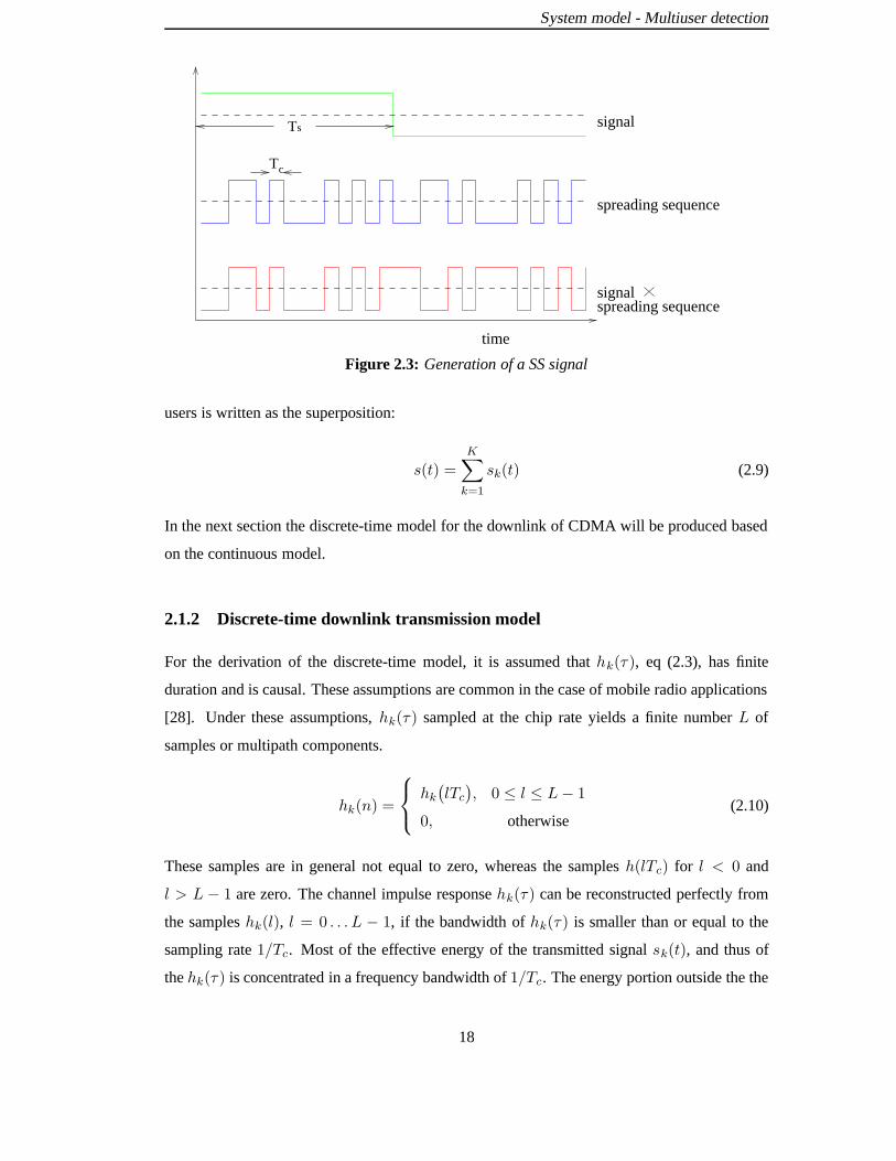
Figure 2.3: Generation of a SS signal

users is written as the superposition:

s(t) =K∑

k=1

sk(t) (2.9)

In the next section the discrete-time model for the downlink of CDMA will be produced based

on the continuous model.

2.1.2 Discrete-time downlink transmission model

For the derivation of the discrete-time model, it is assumed that hk(τ), eq (2.3), has finite

duration and is causal. These assumptions are common in the case of mobile radio applications

[28]. Under these assumptions, hk(τ) sampled at the chip rate yields a finite number L of

samples or multipath components.

hk(n) =

hk(lTc), 0 ≤ l ≤ L− 1

0, otherwise(2.10)

These samples are in general not equal to zero, whereas the samples h(lTc) for l < 0 and

l > L − 1 are zero. The channel impulse response hk(τ) can be reconstructed perfectly from

the samples hk(l), l = 0 . . . L − 1, if the bandwidth of hk(τ) is smaller than or equal to the

sampling rate 1/Tc. Most of the effective energy of the transmitted signal sk(t), and thus of

the hk(τ) is concentrated in a frequency bandwidth of 1/Tc. The energy portion outside the the

18

System model - Multiuser detection

bandwidth 1/Tc is assumed to be negligible.

In the same way, the spreading sequence, as described in eq. (2.5), sampled at the chip rate is:

ck(n) =

ck(qTc), 0 ≤ q ≤ Q− 1

0, otherwise(2.11)

In this work the rectangular pulse chip waveform is adopted and therefore it turns out regarding

eq. (2.5) that:

ck(qTc)

= c(q+1)k , q = 0 . . . Q− 1 (2.12)

The number Q of chips per bit and the chip waveform are common to all users in a direct-

sequence spread-spectrum CDMA system. The difference among the signature waveforms is

the assignment of binary “sequence” or “code” c0k . . . cQ−1k , which is different for each user.

As mentioned in Chapter 1 multiple access capability in CDMA requires low crosscorrelations

of different spreading sequences. In subsection 2.2.3 a brief introduction to spreading codes

design and classification is given. Throughout this research the period of the pseudonoise

waveform is equal to the symbol period, although in some practical CDMA systems it can

be larger (Q ≥ Ts/Tc).

The total transmitted downlink signal s(n) for the conventional CDMA downlink scenario in

discrete-time mode is derived directly from equations (2.4) and (2.9) and can be:

s(n) =M∑

m=−M

K∑

k=1

wmk dmk ck(n−mQ) (2.13)

Similarly, the received signal ek(t), eq. (2.2), on kth mobile terminal takes the following

discrete-time description:

ek(n) =L−1∑

l=0

s(n− l)h(l) + v(n) (2.14)

The discrete-time transmission model of eq. (2.14), which describes the transmission in a

CDMA system, is illustrated in Figure 2.4. In this representation the channel has been replaced

by a tapped delay line transversal filter or finite impulse response filter with delays equal to the

chip duration Tc and tap-coefficients equal to hk(n), n = 0 . . . L − 1 [11]. A representative

model of the channel profile (tap delays and statistical properties) can be provided by the UMTS

19

System model - Multiuser detection

specifications [29].

Tc Tc Tc

ke (n)

h (0) h (1)k k k kh (L−1)

s (n)

h (2)

v (n)

Σ

Figure 2.4: Discrete-time CDMA channel model

2.1.3 Matrix-vector notation for the discrete-time transmission model

Based on the aforementioned assumptions and notations of the discrete-time transmission model,

the matrix-vector notation is introduced in this section. For the sake of clarity we state, at this

point, that for any vector x, ‖x‖2 denotes the inner product xTx and [x]j the jth element of

the x vector. For any matrix X, [X]i,j denotes the element in the ith row and jth column. Fur-

thermore, vectors are represented by boldface lower case letters and matrices by boldface upper

case letters while symbols x∗/X∗ and xT /XT indicate complex conjugation and transposition

of vector/matrix x/X respectively.

The spreading code consists of Q chips and it is described by the vector:

ck = [ck(0) · · · ck(Q− 1)]T (2.15)

The channel vector hk consists of the tap-coefficients of the FIR filter that represents the chan-

nel:

hk = [hk(0) · · · hk(L− 1)]T (2.16)

Let dk be a vector sequence of N = 2M + 1 transmitted bits for user k

dk = [d−Mk · · · d0k · · · dMk ]T (2.17)

20

System model - Multiuser detection

The column vector d of length KN is a block of data that contains the bits of all the users and

is defined as :

d =[dT1 · · ·dTk · · ·dTK

]T(2.18)

By defining now the NQ×N matrix Ck :

Ck = [Ck]i,j ; i = 1...NQ, j = 1...N

[Ck]i,j =

ck(i−Q(j − 1) − 1), for 0 ≤ i−Q(j − 1) − 1 ≤ Q− 1

0, otherwise(2.19)

and the NQ×NK matrix C:

C =[C1 · · ·Ck · · ·CK

](2.20)

the NQ-length vector form for signal s, in eq. (2.13), for a conventional CDMA system is:

s = CWd (2.21)

where W is a NK × NK diagonal matrix with the diagonal elements the amplitude of each

transmitted symbol dmk . W is defined as:

W = blockdiag(W1 . . .Wk . . .WK

)(2.22)

and N ×N matrix Wk as:

Wk = [Wk]i+M+1,j+M+1 ; i = −M...M, j = −M...M

[Wk]i+M+1,j+M+1 =

wik, i = j

0, i 6= j(2.23)

The received signal ek(n) at the kth MS is the result of the convolution s(n)∗hk(n) or in vector

form the vector ek of length NQ+ L− 1 :

ek = Hks + v = HkCWd + v (2.24)

21

System model - Multiuser detection

where channel matrix Hk is of size (NQ+ L− 1) × (NQ)

Hk = [Hk]i,j ; i = 1 . . . NQ+ L− 1, j = 1 . . . NQ

[Hk]i,j =

hk(i− j), for 0 ≤ i− j ≤ L− 1

0, otherwise(2.25)

and v is a noise vector of length (NQ + L − 1) . The components [v]i are assumed to be

statistically independent from the data symbols dmk . The noise vector v, in eq. (2.26), has a

covariance matrix Rv . The matrix Rv is Hermitian and in the case of stationary noise it has a

Toeplitz structure. In eq. (2.26) E[·] denotes expectation or mean.

Rv = E[vv∗T ]

= (2.26)

E[[v]1[v]1

∗]

E[[v]1[v]2

∗]

· · · E[[v]1[v](NQ+L−1)∗

]

E[[v]2[v]1

∗]

E[[v]2[v]2

∗]

· · · E[[v]2[v](NQ+L−1)∗

]

......

. . ....

E[[v](NQ+L−1)[v]1

∗]

E[[v](NQ+L−1)[v]2

∗]

· · · E[[v](NQ+L−1)[v](NQ+L−1)∗

]

Data symbols dmk , k = 1 . . . K,m = −M . . .M , have also zero mean and the covariance

matrix of the vector d is Rd.

Rd = E[ddT

](2.27)

For instance, in the case of Q = 3, L = 2, N = 3,K = 2,M = 1 eq. (2.21) takes the form:

s =

c1(0) 0 0 c2(0) 0 0

c1(1) 0 0 c2(1) 0 0

c1(2) 0 0 c2(2) 0 0

0 c1(0) 0 0 c2(0) 0

0 c1(1) 0 0 c2(1) 0

0 c1(2) 0 0 c2(2) 0

0 0 c1(0) 0 0 c2(0)

0 0 c1(1) 0 0 c2(1)

0 0 c1(2) 0 0 c2(2)

︸ ︷︷ ︸

C

w−11 0 0 0 0 0

0 w01 0 0 0 0

0 0 w11 0 0 0

0 0 0 w−12 0 0

0 0 0 0 w02 0

0 0 0 0 0 w11

︸ ︷︷ ︸

W

d−11

d01

d11

d−12

d02

d12

︸ ︷︷ ︸

d

(2.28)

22

System model - Multiuser detection

and Hk of eq. (2.24) is :

Hk =

hk(0) 0 0 0 0 0 0 0 0

hk(1) hk(0) 0 0 0 0 0 0 0

0 hk(1) hk(0) 0 0 0 0 0 0

0 0 hk(1) hk(0) 0 0 0 0 0

0 0 0 hk(1) hk(0) 0 0 0 0

0 0 0 0 hk(1) hk(0) 0 0 0

0 0 0 0 0 hk(1) hk(0) 0 0

0 0 0 0 0 0 hk(1) hk(0) 0

0 0 0 0 0 0 0 hk(1) hk(0)

0 0 0 0 0 0 0 0 hk(1)

(2.29)

2.2 Air interface structure

The design of an air interface presupposes good understanding of the system’s requirements.

Target data rates, bit error rate, delays along with the channel models define the radio environ-

ment. The radio environment sets the constraints on the system design and therefore it has to be

carefully modeled. More issues that have to be taken into account when designing an air inter-

face are the spectrum availability, the synchronisation constraints, signaling requirements and

complexity restrictions. The IMT-2000 system requirements have been specified in [30] and

described in more detail in [31]. Corresponding ETSI documents for UMTS are [32, 33]. The

CDMA radio interface involves several areas, as shown in table 2.1, that sometimes contradict

with each other. The desire, for example, for minimisation of equipment and complexity cost

leads in general to poorer performance since the later demands more advanced and complex

receivers. Figure 2.5 shows that the air interface functions are divided into protocol layers [34].

The physical layer performs error control, modulation, spreading, interleaving, transmitting and

receiving data for the physical channels. The medium access layer coordinates the resources

provided by the physical layer and the link access layer sets up, maintains and releases the log-

ical link connection. The network layer includes call control, mobility manager and the radio

resource management, part of which are the handover and power control. A brief description

of some of the above functions that depend on the underlying multiple access method (CDMA)

follows next. Data detection and recovery at the receiver will be examined in details in the next

sections.

23

System model - Multiuser detection

System requirements Radio interface design

data rates physical channelsBER, delay spreading codes designradio environment modulationbandwidth availability error control schemessynchronisation need packet data transmissioncomplexity aspects transceiver

handoverpower controlchannel estimation

Table 2.1: Air design procedure for CDMA

Link access layer

Medium access control

Physical Layer Layer 1

Network layer Layer 3

Layer 2

Figure 2.5: Layer structure of CDMA air interface

2.2.1 Frame length design

The service requirements and desired radio performance determine the frame length of the

data transmitted, e.g. in a fading channel the frame length has to be long enough to support

a reasonable interleaving depth but it cannot exceed the transmission delay requirement of

service. For third generation wireless systems the delay requirement for speech is specified to

be 30−40ms and hence, a frame length of 10ms is short enough if interleaving is spanning only

one frame. On the other hand, for data services a longer interleaving period is often tolerable.

2.2.2 Pilot signals

A pilot channel is useful in order to obtain a phase reference for the coherent detection of the

data modulated signal. User dedicated pilot symbols can be used as a reference for channel

estimation and initialisation of the RAKE receiver fingers.

24

System model - Multiuser detection

2.2.3 Spreading code design

In a DS-CDMA transmitter the information signal is modulated by a spreading code and in the

receiver it is correlated with a replica of the same code. Thus, low crosscorrelation between the

desired and the interfering users is important to reduce the multiple access interference. More-

over, adequate autocorrelation properties are required for reliable initial synchronisation. Large

sidelobes of the autocorrelation function can easily lead to erroneous code synchronisation de-

cisions. Good autocorrelation properties of the spreading code result in a better resolution of

the multipath components of a spread spectrum signal. Crosscorrelation and autocorrelation

properties are connected in such a way that both cannot be adequate simultaneously [2]. For

example, random codes exhibit good autocorrelation properties but worse crosscorrelation than

the deterministic ones. Spreading codes can be divided into pseudo-noise codes and orthogonal

codes.

Pseudo-noise sequences are generated with a linear feedback shift register generator. The out-

puts of the shift register cells are connected through a linear function formed by exclusive-or

(XOR) logic gates into the input of the shift register. A two-tap linear binary shift register is

displayed in Figure 2.6. Three of the basic classes of pseudo-noise sequences are:

• Maximum length sequences (M-sequences)

• Gold sequences

• Kasami sequences

Figure 2.7 displays the autocorrelation function of an M-sequence and the crosscorrelation

function of two randomly selected M-sequences. The autocorrelation properties of M-sequences

are very good, in contrast with their crosscorrelation properties. Orthogonal sequences are

completely orthogonal for zero delay but for other delays they have very bad crosscorrelation

properties and thus they are suitable only for synchronous applications.

In any case the correlation properties and the number of codes needed are two important selec-

tion criteria in order to design and select the most appropriate code family for a particular air

interface design. For a more detailed description of spreading codes design, analysis and usage

readers can refer to [13, 35–40].

The spreading codes for UTRA are called channelisation codes. Channelisation codes are used

25

System model - Multiuser detection

01234

Figure 2.6: Two-tap linear binary shift register

0 5 10 15 20 25 30−10

−5

0

5

10

15

20

25

30

35

Shift Delay

31 chipsautocorrelation

31 chipscrosscorrelation

Figure 2.7: The autocorrelation function of an 31-chips long M-sequence and the crosscorre-lation function of two randomly selected M-sequences with the same length.

from a single source to seperate transmissions, i.e. downlink connections within one sector and

the dedicated physical channel in the uplink from one terminal. The spreading/channelisation

codes of UTRA are based on the Orthogonal Variable Spreading Factor (OVSF) technique,

which was originally proposed in [41]. The use of OVSF codes allows the spreading factor

to be changed and orthogonality between different spreading codes of different lengths to be

maintained. The codes are picked from the code tree, which is illustrated in Figure 2.8. In

case the connection uses a variable spreading factor, the proper use of the code tree also allows

despreading according to the smallest spreading factor. This requires only that channelisation

codes are used from the branch indicated by the code used for the smallest spreading factor. In

downlink the only impairment of channelisation codes is their limited number which reduces

the number of active users. For examble for channelisation of length Q = 16, only 16 users can

be active simultaneously. The problem is solved with random codes at the cost of orthogonality.

26

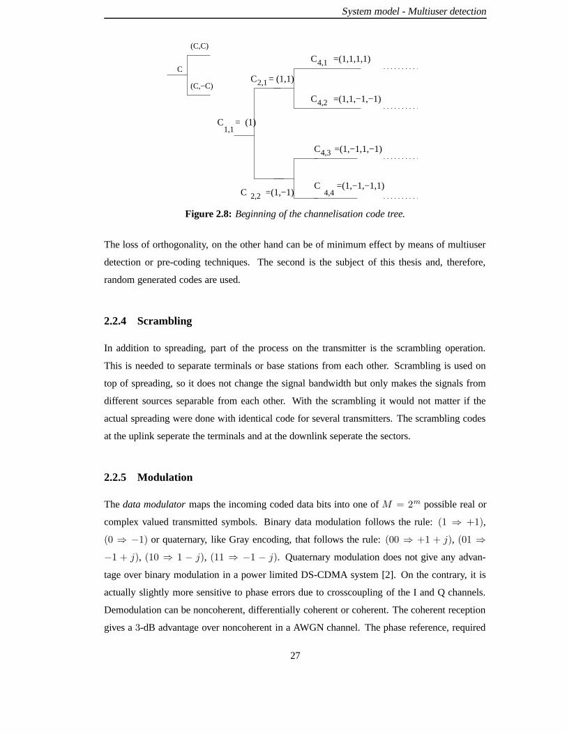
System model - Multiuser detection

C = (1)

C = (1,1)

C =(1,1,−1,−1)

1,1

2,1

C =(1,−1)2,2

C =(1,1,1,1)4,1

4,2

4,3C =(1,−1,1,−1)

C =(1,−1,−1,1)4,4

(C,−C)

(C,C)

C

Figure 2.8: Beginning of the channelisation code tree.

The loss of orthogonality, on the other hand can be of minimum effect by means of multiuser

detection or pre-coding techniques. The second is the subject of this thesis and, therefore,

random generated codes are used.

2.2.4 Scrambling

In addition to spreading, part of the process on the transmitter is the scrambling operation.

This is needed to separate terminals or base stations from each other. Scrambling is used on

top of spreading, so it does not change the signal bandwidth but only makes the signals from

different sources separable from each other. With the scrambling it would not matter if the

actual spreading were done with identical code for several transmitters. The scrambling codes

at the uplink seperate the terminals and at the downlink seperate the sectors.

2.2.5 Modulation

The data modulator maps the incoming coded data bits into one of M = 2m possible real or

complex valued transmitted symbols. Binary data modulation follows the rule: (1 ⇒ +1),

(0 ⇒ −1) or quaternary, like Gray encoding, that follows the rule: (00 ⇒ +1 + j), (01 ⇒−1 + j), (10 ⇒ 1 − j), (11 ⇒ −1 − j). Quaternary modulation does not give any advan-

tage over binary modulation in a power limited DS-CDMA system [2]. On the contrary, it is

actually slightly more sensitive to phase errors due to crosscoupling of the I and Q channels.

Demodulation can be noncoherent, differentially coherent or coherent. The coherent reception

gives a 3-dB advantage over noncoherent in a AWGN channel. The phase reference, required

27

System model - Multiuser detection

for coherent demodulation, can be provided by a data bearing signal or an auxiliary source such

as a pilot symbol.

The modulated data are transmitted with binary, quaternary or complex spreading via spreading

circuits. The binary DS-spreading circuit has a simple transmitter structure, as in Figure 2.2,

with only one PN sequence per symbol. Its drawback is that it is more sensitive to MAI than the

balanced and the dual-channel quaternary transmitter. The balanced quaternary DS-spreading

spreads the same data signal onto I and Q channels using two spreading sequences, while

in the dual-channel QPSK spreading circuit the symbol streams on the I and Q channels are

independent of each other. Both spreading circuits are depicted in Figure 2.9.

πsin(2 f t)0

πcos(2 f t)0

Σ

πsin(2 f t)0

πcos(2 f t)0

Σ

c

c Qk

Ik c

c Qk

Ik

spreading modulator

(a)Balanced spreading circuit (b)Dual−channel spreading circuit

Data

Data I

Data Q

Figure 2.9: Spreading circuits

The spreading circuit is followed by the spreading modulator. Linear modulation methods

(BPSK, QPSK, and offset QPSK) have been proposed for WCMDA on the grounds that they

offer good modulation efficiency. The modulated signal should be able to tolerate as much as

possible the fact that nonlinear power amplifiers (preferred over linear) on the transmitter result

in spectrum leakage to adjacent carriers. Thus, in practice, after the modulation is fixed, pulse

shaping, eq. (2.7), determines the final spectrum properties of the modulation scheme. The

BPSK, QPSK and O-QPSK constellation diagrams are illustrated in the Figure 2.10.

28

System model - Multiuser detection

x x

Q

I

BPSK QPSK O−QPSK

I

Q Q

I

Figure 2.10: Constellation diagrams of linear modulation methods

2.2.6 Error control schemes

Error control schemes, used in wireless telecommunications, are divided in two major cate-

gories: the forward error control (FEC) and automatic repeat request (ARQ) [42]. A hybrid

scheme is a combination of these two. In FEC, the error correcting code, sometimes referred to

as the channel code, is used to combat transmission errors in a fading radio channel, while in

ARQ the error detecting is used together with a retransmission protocol. Among the different

error control schemes the right choice is a function of the required quality of service (data rate,

delay and BER) and the radio channel. Error ratios without any error correcting algorithms in a

fading channel are of the order of 10−1 to 10−2. After using convolutional codes [11] (standard

coding for all cellular systems) the resulting error ratio drops down to the order of 10−2 to

10−3 which is sufficient for speech transmission. However, this performance is not sufficient

for data transmission, where the required BER is 10−6 or better. This can be achieved with a

concatenated coding scheme using a convolutional and a block code, typically a Reed-Solomon

code [43]. A recently developed FEC coding scheme is turbo coding [44–47]. Turbo codes

are parallel or serial concatenated recursive convolutional codes, whose decoding is carried out

iteratively [47] and they demonstrate performance close to the Shannon capacity limit on both

AWGN and Rayleigh fading channels. Another scheme used for controlling errors is interleav-

ing that is mostly effective against burst errors. The interleaving scheme can either be block or

convolutional interleaving [11].

2.2.7 Power control

The power control problem arises particularly in the uplink of a DS-CDMA system and it is

due to multiple access interference. The signal received by the BS from a user terminal close to

29

System model - Multiuser detection

the BS will be stronger than the signal received from another terminal located further. [2, 48].

Therefore, the remote users will be dominated by the close users. This is called the near-far

effect. To overcome this problem the signals should arrive at the BS with the same mean power.

The power control mechanism achieves a near constant received mean power for each user. In

addition to these, this mechanism may improve the overall performance of a DS-CDMA system

against fading channels by compensating for the fading dips.

In the downlink, in contrast to the uplink all signals are transmitted through the same channel

and they are received by a given MS with equal powers. Thus, power control is not required

to eliminate the near-far problem. However, the power control is still needed to minimise the

interference to other cells and to compensate for the interference of other cells. The worst-case

scenario occurs when the MS is located at the cell’s edge, equidistant from more than one BS.

There are two types of power control: open loop and closed loop [49]. In the open loop power

control, the receiver measures the interference conditions from the channel and consecutively

adjusts the transmission power to meet the desired error rate. This method presumes that the

uplink and the downlink channels are correlated, otherwise a closed loop algorithm is necessary.

In closed loop power control, the receiver measures the signal to interference ratio and sends

the information to the transmitter.

2.2.8 Handover

In a CDMA system the neighboring cell frequency bands are arranged as mentioned in Chapter

1. With this type of approach a mobile performs a hard handover, when the signal strength of

a neighboring cell exceeds the signal strength of the current cell by a given threshold. In order

to avoid this kind of interference, an instantaneous handover from the current cell to the new

cell would be required but this is not feasible in practice. The solution that allows the MS to be

connected into a cell from which it receives the highest power is soft handover. In accordance

with that the mobile terminal is connected simultaneously to two or more base stations thereby

its transmission power can be controlled according to the cell whose signal arrives with the

strongest power. A mobile station enters the soft handover state when the signal strength of a

neighboring cell exceeds a certain threshold but is still below the current base station’s signal

strength. We should mention here that, typically, soft handover is only applied in FDD systems

while it is more difficult to be applied in TDD systems.

30

System model - Multiuser detection

2.2.9 Discussion

From the above we conclude that a CDMA system is more complex than the simple version

presented in Figure 2.1. A more elaborate version of the transmitter, for instance, is illustrated

in Figure 2.11. The data before transmission are passing through the blocks for framing, chan-

nel coding, interleaving and multiplexing with other services if necessary. Parameters like the

spreading factor, the data rate and the power factor by which the transmitted data are scaled are

determined by the control block. In this section only a general idea was given of the variety of

operations that take place in a CDMA air interface. In reality, the system is much more com-

plicated and depend on the actual CDMA (WCDMA, cdma2000,...) specifications. For more

details on the 3G partnership project (3GPP) wideband CDMA physical layer, for instance, the

TS25 series of 3GPP specifications should be studied.

Frame designFEC algorithmsInterleaving

.........Multiplexing

RF parts

D/A parts

IF parts

−processing gain−channel coding−transmission rate−power control.........

Parameters forSet

Data sourcePowerAmplifier

Spreading Filters Antenna

Figure 2.11: Transmitter block diagram

2.3 RAKE receiver

If a synchronous AWGN channel is assumed in conjuction with orthogonal codes it is adequate

for the receiver to correlate the received signal with the spreading code of the user of interest.

The correlator can be replaced by a filter matched to the spreading code [11]. Setting ‖ck‖ = 1

the output of the correlator will be:

yk =

∫ Ts

0ek(t)ck(t)dt = dk +

K∑

i=1i6=k

ρikdi +

∫ Ts

0ck(t)v(t), 1 ≤ k ≤ K (2.30)

31

System model - Multiuser detection

where by ρik we denote the crosscorrelation between the spreading codes ci(t), ck(t)

ρik =

∫ Ts

0ci(t)ck(t)dt, ρik = cTi ck (2.31)

Thus, if ρik = 0, i 6= k, then the output of the matched filter consists of the decoupled desired

symbol perturbated by the filtered noise. However, in Chapter 1 it was mentioned that radio

channels usually include multipath propagation where, several time-shifted and scaled versions

of the transmitted signal arrive at the receiver, reflected by mountains, buildings and other ob-

stacles. The presence of multipath fading environment or even random time offsets between

signals destroy the orthogonality among the spreading sequences of the received user signals.

Lack of orthogonality leads to cross interference or multiple access interference between the

signals of different users while the multipath imposes intersymbol interference to the transmit-

ted signal. In Figure 2.12 the multipath effect is illustrated. Equation (2.30) is extended to

(2.32) for the multiple access in multipath.

yk =

∫ Ts

0ek(t)ck(t)dt = dk + MAI + ISI +

∫ Ts

0ck(t)v(t) (2.32)

Correlation with the kth user gives rise to the recovered data term, a correlation term from all

the other users (MAI), and correlation with the thermal noise v(t) yields the noise term. The

signal to noise-plus-interference ratio was defined in Chapter 1 as the the desired signal energy

over the sum of the power of all kinds of interferences. For data detection in systems applying

CDMA, the two problems of channel equalisation and of signal separation have to be solved

simultaneously. A simple correlator or a matched filter is not adequate any more as it detects

only one user while the signals of the other users are treated as noise and it can’t cope with

the intersymbol interference. We will examine next the single-user scenario of a DS-CDMA

system in a frequency selective channel.

As shown in section 2.1 a multipath channel can be modeled as a tapped delay line with statis-

tically independent tap weights that provides us with L replicas of the same transmitted signal

at the receiver. Hence, a receiver that processes the received signal in an optimum manner

will achieve the performance of an equivalent Lth-order diversity communications system. The

signals are resolvable when they arrive more than one chip apart in time from each other. In

frequency domain, it means that the bandwidth of the transmitted signal should be larger than

the coherence bandwidth of the channel. This is the case when a spread spectrum signal is as-

sumed, as in a DS-CDMA system. In DS-CDMA, multipath has both a positive and a negative

32

System model - Multiuser detection

1 chip delay

3 chips delay

multipath signals

d−1

d0

symbol of 6 chips

chips affected by intersymbol interference (ISI)

chips affected by interchip interference (ICI)

d1

Figure 2.12: Intersymbol interference (ISI): how bit d−1’s multipath replicas affect the next bitd0. Interchip interference (ICI) : within one symbol by delayed replicas of itself.

effect. On one hand, the independent paths can be a valuable source of diversity and on the

other hand impose intersymbol interference.

A popular single-user receiver in the presence of multipath is the RAKE combiner proposed by

Price and Green in 1958 [50, 51]. The RAKE receiver uses multiple correlators, one for each

path, and the outputs of the correlators are combined into a single output to maximise the signal

to noise ratio. The combination method is usually maximal ratio combining in accordance

to which each of the replicas of the signal is weighted by its own complex conjugated path

gain (attenuation factor). In Figure 2.13 the configuration for a RAKE receiver is given. It

is a tapped delay line whose tap-coefficients correspond to the multipath channel illustrated

in Figure 2.4. In effect, the tapped delay line receiver structure attempts to collect the signal

energy from all the received signal paths that fall within the span of the delay line and carry the

same information. In the configuration of Figure 2.13 the correlators can be replaced by filters

matched to the k-user’s spreading code ck. The outputs are sampled at bit times, which yields

“soft” estimates of the transmitted data. The final ±1 “hard” data decisions are made according

to the signs of the soft estimates.

While the RAKE receiver gives good results and increases the signal to interference ratio for

the single-user case it doesn’t do the same in the multiuser DS-CDMA scenario. Orthogonal

codes lose their properties when passed through different multipath channels. It is clear that the

conventional RAKE receiver follows a single-user detector strategy; it detects one user without

regard to the existence of other users, which are treated as noise. Thus, there is no sharing of

multiuser information or joint signal processing. The success of this detector depends on the

33

System model - Multiuser detection

Tc cTe (n)k

h (L−1) h (0)k k k* * *h (L−2)

ky (n)

c (n)k*

T

Figure 2.13: RAKE receiver configuration

properties of the correlation between codes. Thus eq. (2.32) is also valid for the RAKE receiver.

As the number of interfering users increases, the MAI increases and consequently the signal

to (MAI+ISI+noise) reduces. Therefore, the overall performance of the system is dramatically

decreased. On the top of that, the conventional detector is very sensitive to the near-far problem

as weaker users may be overwhelmed by stronger users. All of these give rise to the multiuser

detection problem which will be discussed in the next section.

The matrix description of the conventional detector will be described. The output of the kth

user’s matched filter is:

dk = BTk ek (2.33)

where the (NQ+ L− 1) ×N matrix Bk is defined as

Bk =[CTk O

]T

and O is aN× (L−1) zero matrix. For a AWGN channel, when L = 0, Bk = Ck. The output

of a RAKE receiver is written as:

dk =(HkCk

)Tek (2.34)

34

System model - Multiuser detection

Amplitude & Phaseestimation

Code generation Code tracking

Pilot

I&D

RAKE receiver’s fingers

maximalratiocombine

Impulse response measurement

Figure 2.14: RAKE receiver’s fingers

The RAKE receiver involves several more functions that become even more complicated when

it comes to actual implementation. Figure 2.14 illustrates some of the functions that take place

in each finger of the RAKE-receiver in addition to the despreading correlator and the maximal

ratio combining. The impulse response measurement correlates the received signal with dif-

ferent phases of the pilot code to find the multipath components. Whenever the delays of the

impulse response change, the impulse response measurement block allocates new code phases

for the code tracking block that tracks the small changes. The RAKE receiver’s weights must

be updated, whenever the channel changes, with the complex conjugated channel coefficients.

Therefore, the amplitude and phase estimation block is necessary. The channel estimate can

be implemented using pilot symbols or adaptively with training sequences. More details about

RAKE receiver implementation and extended bibliography can be found in [2].

2.4 Multiuser detection

The goal of the data detection in every mobile user k is to determine an estimate of the trans-

mitted symbols addressed to the particular user. In other words, an estimate dk of the source

data vector d has to be determined from the received vector ek, which is disturbed by the noise

vector v, eq. (2.24).

dk =(d−mk . . . d0

k . . . dmk

)T= dk (2.35)

The detection problem results from the fact that a number of signals, only distinguished by

different codes arrive at the receiver at the same time in the same frequency band and the

35

System model - Multiuser detection

orthogonality properties cannot be controlled in a multipath environment. As discussed in

section 2.3, RAKE receivers fail to recover the data when MAI is present because there is no

sharing of multiuser information or joint signal processing. Therefore, a more sophisticated

receiver should be implemented. In Figure 2.15 the detection problem is illustrated for the

uplink and the downlink. In the uplink the BS knows the codes of all users and the channels

that link it with them, while in the downlink the MS should have an estimate of the channel

and knowledge of all the spreading codes active in a cell. Vector e in Figure 2.15 denotes a

superposition of all signals ek arriving at the BS.

1c ,..., c K R v 1c ,..., c K R vh ,..., h1 Kh k

ke kd dedata detectiondownlink

data detectionuplink

BSMS

Figure 2.15: Problem of data detection

The optimum solution to the equalisation problem, under the assumption that all possible trans-

mitted sequences are equally probable, is nonlinear maximum-likelihood sequence estimation

(MLSE) implemented, for instance, by the Viterbi algorithm [26]. The detector which yields the

most likely transmitted sequence, d, chooses d to maximise the probability that d was transmit-

ted given that e was received . This probability is reffered to as a joint a posteriority probability

P (d|e)[11]. The problem with the MLSE approach is that the complexity of the Viterby al-

gorithm increases exponentially with the size of the symbol alphabet and the number of active

users K . Actually, there are 2NK possible d vectors that results in an exhaustive search for

typical message sizes and number of users. Another disadvantage of the MLSE detector is that

it requires knowledge of the received amplitudes and phases. These values, however, are not

known a priori, and must be estimated. Despite the huge performance and capacity gains over

conventional detection, the MLSE detector is not practical. A realistic direct-sequence system

has a relatively large number of active users; thus an exponential complexity in the number of

users makes the computational cost of this detector too high.

Therefore, several suboptimum algorithms for the multiuser detection problem have been devel-

oped. Figure 2.16 shows their classification. The proposed detectors can be classified in one of

36

System model - Multiuser detection

Multiuserdetection

SuboptimalOptimalMLSE

Linear

MMSEMAIwhitening

PIC SICDecision

Decorrelator

Interferencecancellation

Neural networks

feedback

partial trellis search

Figure 2.16: Multiuser detection classification

two categories: linear multiuser detectors and subtractive interference cancellation detectors.

Representative and popular linear multiuser detection are the zero-forcing (ZF) and MMSE.

In subtractive interference cancellation detection, estimates of the interference are generated

and subtracted out. Successive interference cancellation can take place in serially (SIC) or in

parallel stages (PIC). In extension to that, some interference cancellation algorithms that use

decision feedback for improved performance create a new family of algorithms. An overview

of the multiuser detection algorithms can be found in [28, 52–54]. Table 2.2 is a list of impor-

tant contributions where various multiuser detection algorithms are derscibed in detail. In the

“remarks” column we state if the algorithm is developed for a synchronous or asynchronous

CDMA system, in a multipath Rayleigh or flat-fading radio-channel.

References Remarks[55–57] synchronous, flat channel

[25, 58, 59] asynchronous, flat-fadingLinear [60–63] synchronous, frequency-selective, Rayleigh

[64] asynchronous, frequency-selective, Rayleigh[65] asynchronous, frequency-selective, Rayleigh fading,

antenna diversity[26] maximum likelihood, Gaussian, asynchronous

Non-linear [66, 67] subtractive interferencecancellation, multipath

Table 2.2: Important contributions to multiuser detection algorithms

A comparison by means of Monte-Carlo simulations of the above methods can be found in [68].

In addition to the algorithms named above, in the bibliography adaptive multiuser detection

algorithms [69–75] or blind algorithms [55] can be found. Two linear multiuser detection

algorithms applied for a frequency selective channel, will be presented in detail in this section.

37

System model - Multiuser detection

The reason for selecting linear ones is to compare them with linear transmitter based precoding

techniques, which is the main topic of this thesis. The synchronous case scheme is considered

for simplicity and since in this thesis we are interested in the downlink of a CDMA system the

algorithms are the ones that can be applied on the mobile receiver.

2.4.1 Zero-Forcing algorithm

The zero forcing block linear equalization is described for the uplink case in [28]. A mod-

ification applicable for the downlink is presented here. The estimate of the data vector dk

determined by the ZF algorithm is defined as:

d = arg mind

((ek −HkCd)HR−1

v (ek −HkCd))

(2.36)

Note that all the transmitted data d are detected here and not only the desired ones dk. Thus,

this is a joint detection zero forcing algorithm (ZF-JD). ZF minimises the quadratic form((ek−

HkCd)HR−1v (ek − HkCd)

)with respect to d. If Rv = σ2I this minimisation is equivalent

to minimising the squared Euclidean distance ‖ek − HkCd‖2. The function to be minimised

is the same for MLSE. However, while the minimisation in the case of MLSE is performed

under the constrained that d is taken from the data vector alphabet, in the case of the ZF d may

take any value. The ZF can be interpreted as an MLSE for unknown data vector alphabet. The

solution of this criterion is

d =((HkC)HR−1

v (HkC))−1

(HkC)HR−1v ek (2.37)

By assuming that Rv = σ2I the above equation is simplified to:

d =((HkC)H(HkC)

)−1(HkC)Hek (2.38)

As a presupposition for the ZF algorithm the matrix((HkC)H(HkC)

)has to be non-singular.

When considering real world time-variant channel impulse responses hk and when choosing

the user specific CDMA codes ck properly the matrix is singular with probability equal to zero

if K ≤ Q [28]. The requirement K ≤ Q is deduced from the fact that the number NQ+L− 1

of samples of the received vector ek (number of scalar equations forming the system of linear

equations given in eq. (2.38) ) has to be larger than the number KN of data symbols combined

in d, which have to be estimated. Independently of the number L of multipath components

38

System model - Multiuser detection

of hk this is fulfilled if K 6= Q. The JD-ZF algorithm is particularly useful in the downlink

when non-orthogonal, e.g. pseudo-random spreading sequences, are used as it exploits fully

the known crosscorrelation of all users. In case of orthogonal codes a single-detection ZF

(ZF-SD) algorithm can be used as described in [28] where the mobile detector knowledge is

restricted to its own spreading code and the channel link. The received signal is filtered by

a channel equalizer(HHk Hk

)−1HHk and the codes’ orthogonal properties are recovered. The

performance of ZF-SD is worse than ZF-JD as shown in [28]. On the top of that, the number

of users for a spreading gain Q that can be active is restricted to Q for orthogonal codes, while

it increases up to 2Q for non-orthogonal codes. The modified algorithm for ZF-SD is:

dk =(CTkCk

)−1CTk

(HHk Hk

)−1HHk ek (2.39)

If we replace ek with the right-hand side of eq. (2.24) in equations (2.39) and (2.38) it be-

comes obvious that ZF algorithms eliminate the ISI and MAI perturbation term. The re-

sult output contains only the desired symbols and a noise term with enhanced covariance((HkC)H(HkC)

)−1σ2 (for ZF-JD), which is further reflected in the BER performance.

2.4.2 Minimum mean square error algorithm

The linear data detector based on MMSE block linear equaliser is presented here. The MMSE

multiuser detection algorithm has been well analysed in [55] for a single path Gaussian channel

and extended for multipath in [59, 61]. Again two versions can be employed. The joint detec-

tion (MMSE-JD) where the full construction of the downlink transmitted signal is taken into

account and the single detection (MMSE-JD) that presupposes orthogonal spreading codes for

sufficient performance. We note here that for the uplink only a joint detection can be applied as

the different channels over which the mobiles transmit destroy the orthogonality. The criterion

to be optimised is the following:

d = argmind′E[‖d′ − d‖2

](2.40)

The MMSE minimises the mean squared norm of the estimation error vector d′−d with respect

to d′. With Rd , as in eq. (2.27), the solution is:

d =((HkC)HR−1

v (HkC) + R−1d

)−1(HkC)HR−1

v ek (2.41)

39

System model - Multiuser detection

By adopting the assumptions that Rd = I and Rv = σ2I eq. (2.41) is further simplified to:

d =((HkC)H(HkC) + σ2I

)−1(HkC)Hek (2.42)

While MMSE-JD depends on full knowledge of the spreading codes of all users MMSE-SD

describes a single detection form of this algorithm where each mobile knows only its own

signature waveform [28].

dk =(CHk Ck

)−1CTk

(HHk Hk + σ2R−1

s

)−1HHk ek (2.43)

where Rs = E[ss], s as in eq. (2.21). As before the single detection algorithm can give

sufficient performance only under the condition that the signature waveforms of the users are

orthogonal and even under this assumption it is outperformed by its joint detection counterpart.

2.4.3 Discussion

The NK × NQ+ L− 1 dimension matrix (HkC)H in equations (2.38) and (2.42) implies a

bank of RAKE receivers. The NK outputs of those receivers is transformed by the appropriate

decorrelating matrices (ZF or MMSE) to yield the estimate transmitted data as shown in Figure

2.17. Another approach could be that each multipath component is used as an additional user

and then a number ofKNL of samples has to be taken at the chip rate at the outputs of matched

filters. The later approach is described in [27].

RAKE 1

RAKE 2

RAKE K

e (n)k

Linear MUD

ZF/MMSEd k

H CkH

Figure 2.17: Block diagram of linear receiver based multiuser detection scheme

40

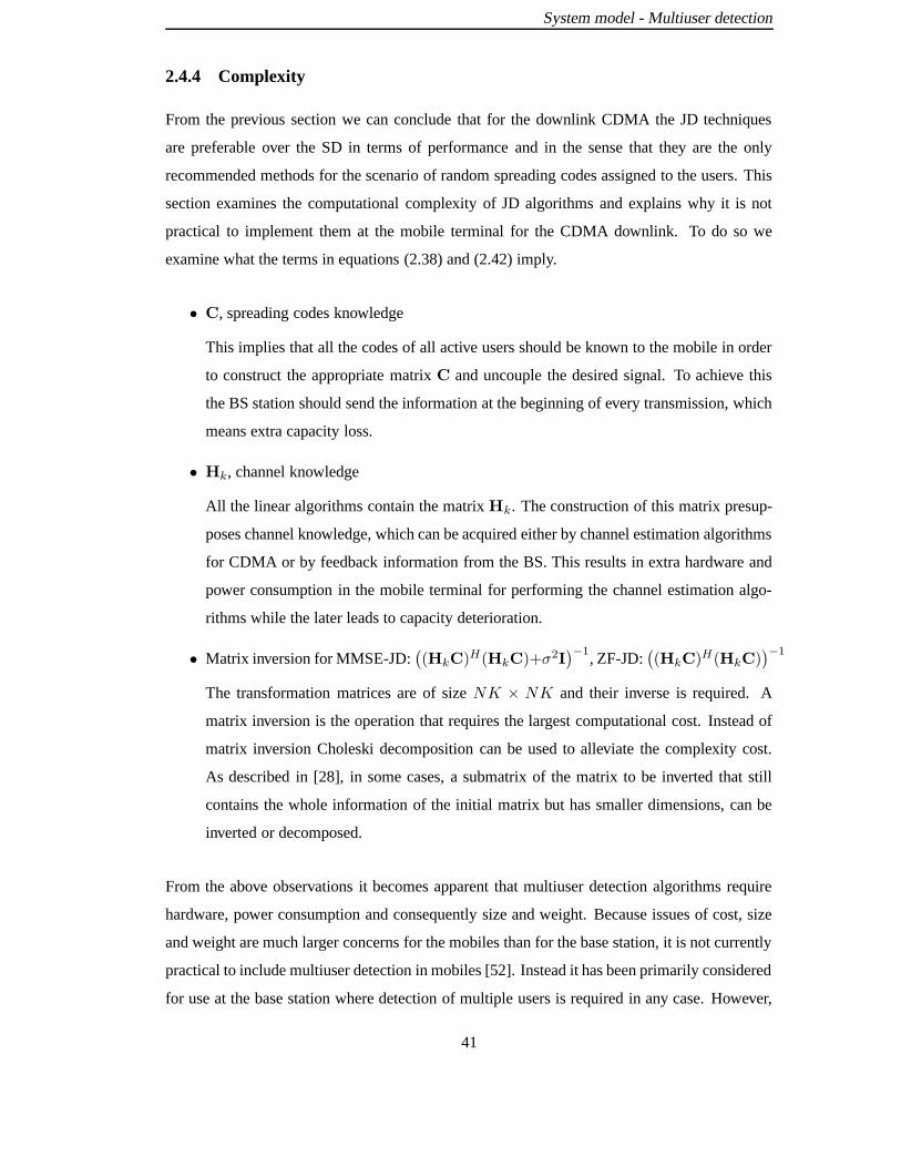
System model - Multiuser detection

2.4.4 Complexity

From the previous section we can conclude that for the downlink CDMA the JD techniques

are preferable over the SD in terms of performance and in the sense that they are the only

recommended methods for the scenario of random spreading codes assigned to the users. This

section examines the computational complexity of JD algorithms and explains why it is not

practical to implement them at the mobile terminal for the CDMA downlink. To do so we

examine what the terms in equations (2.38) and (2.42) imply.

• C, spreading codes knowledge

This implies that all the codes of all active users should be known to the mobile in order

to construct the appropriate matrix C and uncouple the desired signal. To achieve this

the BS station should send the information at the beginning of every transmission, which

means extra capacity loss.

• Hk, channel knowledge

All the linear algorithms contain the matrix Hk. The construction of this matrix presup-

poses channel knowledge, which can be acquired either by channel estimation algorithms

for CDMA or by feedback information from the BS. This results in extra hardware and

power consumption in the mobile terminal for performing the channel estimation algo-

rithms while the later leads to capacity deterioration.

• Matrix inversion for MMSE-JD:((HkC)H(HkC)+σ2I

)−1, ZF-JD:

((HkC)H(HkC)

)−1

The transformation matrices are of size NK × NK and their inverse is required. A

matrix inversion is the operation that requires the largest computational cost. Instead of

matrix inversion Choleski decomposition can be used to alleviate the complexity cost.

As described in [28], in some cases, a submatrix of the matrix to be inverted that still

contains the whole information of the initial matrix but has smaller dimensions, can be

inverted or decomposed.

From the above observations it becomes apparent that multiuser detection algorithms require

hardware, power consumption and consequently size and weight. Because issues of cost, size

and weight are much larger concerns for the mobiles than for the base station, it is not currently

practical to include multiuser detection in mobiles [52]. Instead it has been primarily considered

for use at the base station where detection of multiple users is required in any case. However,

41

System model - Multiuser detection

improving the capacity of the uplink past that of the downlink does not improve the overall

capacity of the system [54]. For these reasons in the next Chapters we will examine under a

common framework techniques that simplify the mobile terminal and transfer the complexity

to the BS.

2.5 Simulation results

2.5.1 General assumptions

The basic assumptions for the Monte Carlo simulations that are carried out in this thesis are

listed in this section. The simulated systems are simplified in such a way that the objective of

this research remains unaffected.

• The data symbols dmk , m = −M . . .M , are BPSK modulated thus dmk = ±1. They are

uncorrelated and thus, Rd = I. In this work the data transmission is continual.

• For the implementation of receiver-based multiuser detection techniques for comparison

purposes, perfect knowledge of the downlink channels is assumed at the MS. The BS has

also perfect knowledge of the downlink channel that can be extracted from the uplink

reception under certain conditions. Those conditions will be examined in Chapter 3.

Thus, no pilot symbols or training sequences are required for channel estimation.

• The additive noise at the receiver is white Gaussian and uncorrelated. Hence, Rv = σ2I.

• The spreading codes for the users are random generated binary codes to allow for the

worst case. The spreading gain selected is Q = 16.

• Throughout our research we focus on the downlink system and we consider only one cell.

The intercell interference is modeled as AWGN.

• The channels are also assumed to have slow fading characteristics and are constant during

the data-block transmission. The channels have a multipath profile that follows the delays

of the vehicular environment A [29], shifted to be the nearer integer multiplier of the chip

period Tc = 0.26µsec. The profiles of 5 of the channels used in this work, characterised

as severe multipath, are given in table 2.3. For the scenario of more than five users,

wherever examined in this thesis, the rest of the channels follow a similar pattern. The

delay spead is L = 11 chip spaces taps. The tap coefficients are real and so is the

42

System model - Multiuser detection

Delay in µsec Tap coefficients

User 1 User 2 User 3 User 4 User 5

0.00 0.714206 -0.711388 0.712718 -0.742424 -0.7009680.26 -0.614927 0.598559 -0.650006 0.596557 0.5567990.52 0.000000 0.000000 0.000000 0.000000 0.0000000.78 0.233789 -0.283209 -0.200871 -0.240244 0.3513161.04 -0.201291 0.200496 0.142206 0.153339 -0.2268291.30 0.000000 0.000000 0.000000 0.000000 0.0000001.56 0.000000 0.000000 0.000000 0.000000 0.0000001.82 0.100884 -0.112747 0.089726 -0.093466 -0.1398622.08 0.000000 0.000000 0.000000 0.000000 0.0000002.34 0.000000 0.000000 0.000000 0.000000 0.0000002.60 -0.080135 0.050362 -0.030055 -0.054407 -0.064669

Table 2.3: Severe multipath channels’ profile

Gaussian noise added at the receive point. In section 5.7 we also examine the scheme

under which the tap-coefficients are complex and their power distribution follows random

pattern (normalised). Another multipath delay profile used throughout this thesis is the

mild one with L = 3 chips delay spread as presented in table 5.2. For both multipath

schemes the channel length is less than one symbol period (L ≤ Q) and thus ISI is

extended only into the next transmitted symbol.

• The BS transmits all users signals with equal power normalised to (wmk )2 = 1. Therefore,

W in equations (2.21) and (2.23) is replaced by the NK×NK identity matrix I. This is

done mainly for simplicity reasons and for examining the spread in performance that the

users may demonstrate even if transmitted with equal power depending on the precoding

method used on the transmitter. The case of unequal powers and how this affects the

system will also be addressed. The transmission of the users is synchronous.

• Error control coding is beyond the scope of this thesis.

• For simplicity reasons synchrononisation, tracking and coherent reception are considered

to be perfect.

• In this work the issue of handover will not considered as we consider only one cell.

43

System model - Multiuser detection

2.5.2 Receiver based JD performance

Following the assumptions described above, Monte Carlo simulations were implemented to

examine the performance of the linear receiver based multiuser detection algorithms ZF-JD

and MMSE-JD. Figure 2.18 shows the BER performance graphs versus Eb/No for a system of

K = 5 users in a flat-fading channel. Eb is the transmitted energy per bit per user and No/2

the power spectral density of the noise. The corresponding graph for the conventional RAKE

receiver is also illustrated. It is obvious that both multiuser detection schemes outperform the

RAKE receiver. The MMSE-JD is slightly better than the ZF-JD which is expected as the

MMSE algorithm takes into account the noise variance in conjunction with the MAI. Figure

2.19 shows the BER performance graphs versus Eb/No for a system of K = 5 users in a

frequency selective propagation scheme. In both graphs the BER performance of the single

user refers to the AWGN channel. The conclusions are similar to the ones drawn from Figure

2.18.

0 5 10 15 2010

−5

10−4

10−3

10−2

10−1

100

Eb/N

o

BE

R

RAKEZF−JDMMSE−JDsingle−user

Figure 2.18: Receiver-based MUD algorithms performance in AWGN channels. K = 5 users.

44

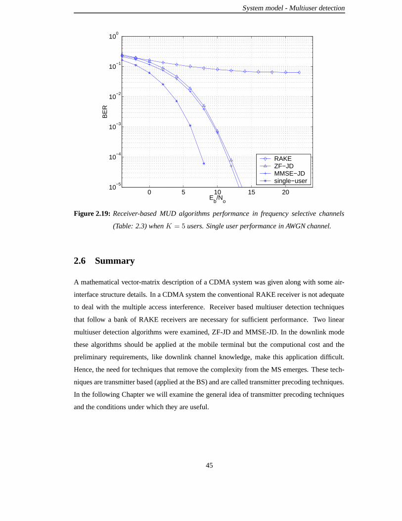
System model - Multiuser detection

0 5 10 15 2010

−5

10−4

10−3

10−2

10−1

100

Eb/N

o

BE

R

RAKEZF−JDMMSE−JDsingle−user

Figure 2.19: Receiver-based MUD algorithms performance in frequency selective channels

(Table: 2.3) when K = 5 users. Single user performance in AWGN channel.

2.6 Summary

A mathematical vector-matrix description of a CDMA system was given along with some air-

interface structure details. In a CDMA system the conventional RAKE receiver is not adequate

to deal with the multiple access interference. Receiver based multiuser detection techniques

that follow a bank of RAKE receivers are necessary for sufficient performance. Two linear

multiuser detection algorithms were examined, ZF-JD and MMSE-JD. In the downlink mode

these algorithms should be applied at the mobile terminal but the computional cost and the

preliminary requirements, like downlink channel knowledge, make this application difficult.

Hence, the need for techniques that remove the complexity from the MS emerges. These tech-

niques are transmitter based (applied at the BS) and are called transmitter precoding techniques.

In the following Chapter we will examine the general idea of transmitter precoding techniques

and the conditions under which they are useful.

45

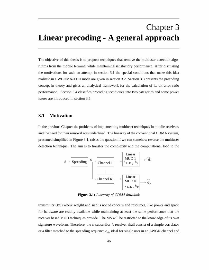
Chapter 3Linear precoding - A general approach

The objective of this thesis is to propose techniques that remove the multiuser detection algo-

rithms from the mobile terminal while maintaining satisfactory performance. After discussing

the motivations for such an attempt in section 3.1 the special conditions that make this idea

realistic in a WCDMA-TDD mode are given in section 3.2. Section 3.3 presents the precoding

concept in theory and gives an analytical framework for the calculation of its bit error ratio

performance . Section 3.4 classifies precoding techniques into two categories and some power

issues are introduced in section 3.5.

3.1 Motivation

In the previous Chapter the problems of implementing multiuser techniques in mobile receivers

and the need for their removal was underlined. The linearity of the conventional CDMA system,

presented simplified in Figure 3.1, raises the question if we can somehow reverse the multiuser

detection technique. The aim is to transfer the complexity and the computational load to the

c 1...K

c 1...K h1

Kh

d1

dK

Spreading Channel 1

Channel K

d

MUD KLinear

LinearMUD 1

,

,

s

Figure 3.1: Linearity of CDMA downlink

transmitter (BS) where weight and size is not of concern and resources, like power and space

for hardware are readily available while maintaining at least the same performance that the

receiver based MUD techniques provide. The MS will be restricted to the knowledge of its own

signature waveform. Therefore, the k-subscriber ’s receiver shall consist of a simple correlator

or a filter matched to the spreading sequence ck, ideal for single user in an AWGN channel and

46

Linear precoding - A general approach

no channel estimation, adaptive equaliser or feedback from the BS is required. In addition to

that the overall capacity of the downlink in system is increased as no training sequences need

be transmitted.

precoding

spreading&

dK

d1

sp

c c1 K

h hK1

Channel 1

Channel K

c (Q−n)

c (Q−n)

1

K

d

Figure 3.2: Linear Precoding

An answer to the question posed is to apply a linear transformation matrix, T , on the transmit-

ted vector d (the data spreading is included in the T matrix) in order to eliminate ISI and MAI,

the major impairements of a CDMA system, before transmission. Under this scheme, the actual

transmitted signal is distorted before transmission, in a way that after passing through the radio

channel and the mobile receiver yields the desired data. In Chapter 2 we showed that each MS

needs knowledge of the downlink channel impulse response hk(n) and the spreading codes of

every user to apply a joint multiuser detection. If we take into account all mobile receivers,

then the total information required is all K downlink channels and signature waveforms (hk,

ck, k = 1 . . . K). The transformation matrix T should be a function of the same knowledge

in linear precoding. In other words, to achieve good performance the transmitted signals in

the downlink must be jointly optimised based on the spreading code and the downlink channel

impulse response of every user. The BS station obviously knows the spreading codes of all the

active users in a cell and all it needs is the downlink channels impulse responses. The uplink

channels can be estimated by the BS but this knowledge cannot be used for the downlink unless

the principle of reciprocity is valid. Under certain conditions the downlink and uplink channels

of a radio link are reciprocal. This can be assumed for the 3GPP WCDMA-TDD mode pro-

vided the time taken to switch between uplink and downlink is smaller than the coherence time

of the channel [76].

47

Linear precoding - A general approach

3.2 WCDMA-TDD

The WCDMA [2] air interface, also referred as UMTS terrestrial radio access (UTRA), was

developed by the 3GPP. WCDMA has two modes characterised by the duplex method used:

frequency division duplex and time division duplex, for operating with paired and unpaired

bands respectively. In FDD mode the uplink and the downlink are allocated different frequency

bands separated by a significant gap in frequency, the guard frequency. In contrast in TDD

mode, the uplink and downlink are time multiplexed into the same carrier. For IMT-2000 there

exist two types of frequency band, paired and unpaired, and this means that both FDD and TDD

modes are required to fully utilise the IMT-2000 spectrum. The principles of TDD and FDD

are illustrated in the Figure 3.3.

a)FDD

b)TDD

Guard Time

Time

Forward Link

Reverse LinkGuard Freq.

BW

BW1

BW2

TimeDLUL UL DL DLUL

UL = Uplink

DL = Downlink

time

freq

uenc

y

Figure 3.3: TDD and FDD principles

The fast fading due to multipath propagation depends on the frequency and so is uncorrelated

between the uplink and the downlink in a FDD system. Therefore, the FDD transmitter cannot

predict the fast fading that will affect its transmission. In TDD, where both uplink and downlink

use the same frequency, the transmitter based on the uplink received signal is able to know the

fast fading of the multipath channel, from the uplink and use this knowledge for precoding on

the downlink. This presumes that the TDD frame length is shorter than the coherence time

of the channel, as defined in Chapter 1. According to [77], Doppler frequencies up to 80Hz

48

Linear precoding - A general approach

(43km/h at 2-GHz carrier frequency) can be supported with a very small degradation if the

uplink part of the TDD frame is 1.5ms. If the TDD system is intended only for slowly moving

terminals then longer TDD frames could also be used. A possible scenario in which the above

assumptions are satisfied would be a personal communication system with low mobility users

such as pedestrians in an outdoor environment. Indoor and microcell environments are the most

probable application areas for TDD communications. A second scenario could be a wireless

local area network (LAN). In such a case the indoor RF channel has a small delay spread and

a computer workstation environment has essentially stationary channels [78]. A slow variation

of the channels could be addressed with a periodical update of the channel profile estimates in

the BS.

The air interface structure specifications of a WCDMA-TDD system follow the general princi-

ples described in section 2.2. A brief description can be found in [2] and for a detailed explana-

tion the 3GPP specification documents should be studied. The physical layer of WCDMA-TDD

is a combination of TDMA and CDMA. Each TDD frame is of length 10ms and is divided into

15 time slots. The physical content of time slots are the bursts of corresponding length. There

are two types of bursts: type 1 suitable for the uplink and type 2 for the downlink. They consist

of two data symbol fields, a midamble and a guard period. In Figure 3.4(a) the structure of

the burst type 2 is displayed. The TDD time slots can be allocated to either the uplink or the

downlink. At least one time slot has to be allocated for the downlink and the same is valid for

the uplink. In Figure 3.4(b) a multiple-switching-point configuration is illustrated. Downlink

physical channels are using a spreading factor of 16, while multiple parallel physical channels

transmitted using different channelisation codes can be used to support higher data rates. For

the uplink physical channels the spreading factor can range from 16 down to 1.

In WCDMA-TDD mode power control is applied to limit the interference level within the

system, thereby reducing the intercell interference level and the power consumption in the

mobile station. Power control is performed on a frame basis (i.e. every 10ms). Based on the

SNIR of the received signal, the transmitter is able to track the fast fading of the multipath

channel. This assumption holds only if the frame length of 10ms is shorter than the coherence

time of the channel. For the downlink a closed loop power control is used so that the mobile

station can compare the estimated received SNIR with the target SNIR. This information can

then be transferred to the BS, which accordingly adapts its transmitted power for that particular

mobile station. We will not focus on power control issues in this work, as we assumed in

49

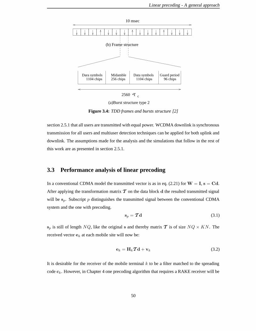
Linear precoding - A general approach

10 msec

(b) Frame structure

Dara symbols Midamble Data symbols 1104 chips 256 chips 1104 chips

(a)Burst structure type 2

96 chipsGuard period

c2560 T*

Figure 3.4: TDD frames and bursts structure [2]

section 2.5.1 that all users are transmitted with equal power. WCDMA downlink is synchronous

transmission for all users and multiuser detection techniques can be applied for both uplink and

downlink. The assumptions made for the analysis and the simulations that follow in the rest of

this work are as presented in section 2.5.1.

3.3 Performance analysis of linear precoding

In a conventional CDMA model the transmitted vector is as in eq. (2.21) for W = I, s = Cd.

After applying the transformation matrix T on the data block d the resulted transmitted signal

will be sp. Subscript p distinguishes the transmitted signal between the conventional CDMA

system and the one with precoding.

sp = T d (3.1)

sp is still of length NQ, like the original s and thereby matrix T is of size NQ ×KN . The

received vector ek at each mobile site will now be:

ek = HkT d + vk (3.2)

It is desirable for the receiver of the mobile terminal k to be a filter matched to the spreading

code ck. However, in Chapter 4 one precoding algorithm that requires a RAKE receiver will be

50

Linear precoding - A general approach

examined. Thus, in eq. (3.3) the output of the receiver is given for both cases:

dk =

BTkHkT d + BT

k vk , matched filter

CTkH

TkHkT d + CT

kHTk vk , RAKE receiver

(3.3)

From eq. (3.3) we can conclude that the detected signal at the output of the receiver has the

general form:

dk = Akd + Avvk, k = 1 . . . K (3.4)

where Ak is a N ×KN matrix with elements [Ak]i+M+1,j, i = −M . . .M, j = 1 . . . KN

and Av is also of dimensions N ×KN .

Based on eq. (3.4) we follow a general approach to calculate the theoretical BER performance

of the precoding systems. The technique is similar to the one followed in [28] for receiver based

linear multiuser detection techniques. Each component dmk ,m = −M . . .M , in dk consists of

three contributions, the first determined by the desired symbol dmk , the second determined by

ISI and MAI and the third determined by noise.

dk = diag(Ak)d︸ ︷︷ ︸

desired symbol

+ diag(Ak)d︸ ︷︷ ︸

ISI andMAI

+ATv vk

︸ ︷︷ ︸

noise

(3.5)

In eq. (3.5), diag(Ak) represents a diagonal matrix containing only the diagonal elements of the

matrix Ak and diag(Ak) = Ak − diag(Ak) represents a matrix with zero diagonal elements

containing all but the diagonal elements of Ak. The covariance matrix of the noise term, in

eq. (3.5), is equal to

ATv RvAv (3.6)

A performance measure is the SNIR φ(dmk ) of dmk at the receiver’s output. The SNIR φ(dmk ) is:

φ(dmk ) =E∣∣symbol energy in dmk

∣∣2

E∣∣ISI and MAI in dmk

∣∣2

+E∣∣noise in dmk

∣∣2 (3.7)

The SNIR defined in eq. (3.7) takes into account the perturbation due to noise, ISI and MAI.

51

Linear precoding - A general approach

We can substitute the components from eq. (3.5) to obtain:

φ(dmk ) =

desired symbol︷ ︸︸ ︷

E|[diag(Ak)d]m|2

E‖[diag(Ak)d]m‖2

︸ ︷︷ ︸

ISI and MAI

+E|[Avv]m|2

︸ ︷︷ ︸

noise

(3.8)

Proceeding further to determine the desired and perturbation coefficients we write φ(dmk ) =

desired symbol︷ ︸︸ ︷∣∣∣[Ak]

m′,j′∣∣∣

2E

|dj′k |2

[AkRdATk ]m

′,j′ − 2Re

[AkRd]m′,j′ [AT

k ]m′,j′

+ |[Ak]m′,j′|2E

|dm′

k |2

︸ ︷︷ ︸

ISI and MAI

+ [AvRvATv ]m

′,j′

︸ ︷︷ ︸

noise

(3.9)

In eq. (3.9) and eq. (3.10) it is m′ = m+M + 1 and j ′ = M + 1 +N(k − 1). For a matched

filter receiver and after taking into account the assumptions previously made that Rd = I and

Rv = σ2I the expression in eq. (3.8) is simplified to:

φ(dmk ) =

(

[Ak]m′,j′

)2

∑KNj=1

j 6=j′([Ak]m

′,j)2+ σ2

(3.10)

The SNIR as given by eq. (3.10) can be used for calculating the error probability Pe for the

detected BPSK bit d0k. For K → ∞ we can consider that ISI and MAI follow a Gaussian

distribution as dictated by the central limit theorem. Therefore, the error probability Pe(d0k) is

given by applying the Q function:

Pe(dmk ) = Q

(√

φ(dmk )

)

(3.11)

For a system of K users the average theoretical error probability is

Pe(dm) =

∑Kk=1 Pe(d

mk )

K(3.12)

A critical issue in CDMA systems is to provide all users with equivalent performance assuming

that signals of equal power are addressed to them. That means that the SNIR φk must be

52

Linear precoding - A general approach

approximately the same for every user. By defining the SNIR spread Φxs as:

Φxs =

maxφiminφj

i, jε1 · · ·K for Eb/No = x(dB) (3.13)

we have a measure of the variety among the K individual performances for Eb/No = xdB.

Ideal values for Φxs are close to unity. SNIR spread behavior varies according to the precoding

algorithm used and it will be considered in the following Chapters.

3.4 Precoding techniques-Classification

As shown in eq. (3.1) the precoded transmitted signal can be described in general with a linear

transformation matrix T applied on the data. In this section we will classify the realisation of

this linear algorithm as either blockwise or bitwise. Although they can both be described by an

appropriate matrix T there are important differences.

3.4.1 Blockwise techniques

In blockwise algorithms, as will be explained in Chapter 4, the data is precoded and transmitted

in blocks of N data bits for each of the K users in a cell. This means that transformation

matrix T is applied to a block of NK data bits. Furthermore, it is desirable for the resulting

signal sp to retain the same length NQ as produced by the conventional CDMA system. Thus,

dimensions of the T matrix shall be NK ×NQ. The block diagram of a blockwise precoding

technique is shown in Figure 3.5.

NQ 1d

d0

d

d−M

d0

d

1

1

1

K

K

K

M

−M

M

d = s p

KN 1

T : NQ KN

T d

N=2M+1

Figure 3.5: Blockwise precoding diagram

53

Linear precoding - A general approach

Matrix T can be chosen according to different optimisation criteria and the complexity for

determining it varies from algorithm to algorithm. Ignoring this complexity the multiplications

required per bit per user for transmission of any blockwise technique results from sp = T d, it

is denoted as Ωblockwise and is:

Ωblockwise =(KN)(NQ)(KN)

KN= N2QK (3.14)

Eq. (3.14) shows that the multiplications required for one symbol transmission are proportional

to the square of a block length N 2 which for a real WCDMA-TDD can be excessively high.

A not so apparent problem with the blockwise algorithms is the fact that in a multipath envi-

ronment the end bits of each block are not correctly precoded and this deteriorates the overall

performance. Each block is treated independently and the ISI, between the symbols of the block

itself, is canceled. However, under the scenario of continual block transmission each block is

extended in duration due to multipath and therefore it overlaps with the next one. The degree

of damage (the number of symbols affected) depends on the channel’s delay spread L. One

solution to mitigate this problem is to increase the block length, but this results in increased

complexity. A second solution is to neglect the number of affected symbols resulting in loss of

capacity.

3.4.2 Bitwise techniques

In the bitwise techniques, the precoding realisation does not include blocks of data to be pro-

cessed. The data of user k after being spread is pre-filtered by an FIR filter of length P with

a discrete time impulse response pk(n) as shown in Figure 3.6. The resulting modified signals

are summed to form the final transmitted signal sp. The filter is applied on the transmitted

waveform, rather than the data symbols as in the blockwise techniques. Thus the multipath res-

olution afforded by the CDMA spreading is exploited. Moreover, since the filters are applied at

the chip level and the derivation of the algorithms are restricted to consider only a few symbols

(even one), the higher computation required for data-block solutions is eliminated. Pre-filters

have also the advantage of not modifying the original CDMA structure directly as it is a simple

addition of an array of FIR filters to the existing BS transmission system. Furthermore, the bit-

wise nature of the algorithms removes the undesirable effect of the end bock-bits as described

in the previous section. The taps of the pre-filters are determined by the adopted technique. Ig-

noring the complexity of the algorithm used to determine the taps, the multiplications required

54

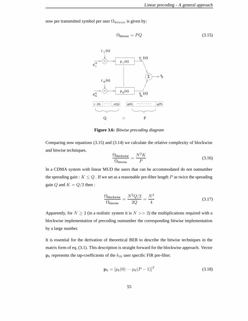
Linear precoding - A general approach

now per transmitted symbol per user Ωbitwise is given by:

Ωbitwise = PQ (3.15)

Σ

1

d K

d 1

p (n)

p (n)m

m

spK

K

c (n)

1c (n)

Q P

c (0) c(Q) p(P)p(0)

y (n)

y (n)K

1

Figure 3.6: Bitwise precoding diagram

Comparing now equations (3.15) and (3.14) we calculate the relative complexity of blockwise

and bitwise techniques.Ωblockwise

Ωbitwise=N2K

P(3.16)

In a CDMA system with linear MUD the users that can be accommodated do not outnumber

the spreading gain : K ≤ Q . If we set as a reasonable pre-filter length P as twice the spreading

gain Q and K = Q/2 then :

Ωblockwise

Ωbitwise=N2Q/2

2Q=N2

4(3.17)

Apparently, for N ≥ 2 (in a realistic system it is N >> 2) the multiplications required with a

blockwise implementation of precoding outnumber the corresponding bitwise implementation

by a large number.

It is essential for the derivation of theoretical BER to describe the bitwise techniques in the

matrix form of eq. (3.1). This description is straight forward for the blockwise approach. Vector

pk represents the tap-coefficients of the kth user specific FIR pre-filter.

pk = [pk(0) · · · pk(P − 1)]T (3.18)

55

Linear precoding - A general approach

The transmitted symbol is now expanded to dmk ck(n) ∗ pk(n) = dmk gk(n), where ∗ denotes the

convolution effect. The length of the pre-filter output symbol gk in vector form is of length

G = Q+ P − 1 chips.

gk = [gk(0) · · · gk(G− 1)]T (3.19)

The pre-filters impose intersymbol interference on the system. This interference is caused by

the symbols transmitted before and after the symbol under consideration. Without affecting the

generality, for the bitwise techniques let us assume that the transmitted symbol under consider-

ation is d0k. Let yk(n) be the signal at the output of the kth pre-filter as shown in Figure 3.6. In

order to describe this signal in matrix form we must take into account M transmitted bits before

and after. The right choice for M is M =⟨(G − Q)/Q

⟩where 〈x〉 denotes that x is rounded

up to the nearest integer. Thus, the G-length transmitted vector for user k, yk, is written as:

yk = Gkdk (3.20)

where the G×N matrix Gk is:

Gk = [Gk]i,(j+M+1) ; i = 1...G, j = −M...M

[Gk]i,(j+M+1) =

gk(i− jQ− 1), for 0 ≤ i− jQ− 1 ≤ G− 1

0, otherwise(3.21)

The summation of yk for all the users gives the transmitted signal sp which can be written as

the G-length column vector:

sp =K=1∑

k=1

yk = Gd (3.22)

where the G×NK matrix G is defined as:

G =[G1 · · ·Gk · · ·GK

](3.23)

From eq. (3.1) and eq. (3.22), it is obvious that matrix G corresponds to the T for the bitwise

algorithm matrix description. Matrix G is associated with the pre-filters taps and it is based on

the optimisation method chosen to define the taps. Now we can apply G directly in the analysis

of section 3.3 to calculate the theoretical BER of a bitwise precoding system.

56

Linear precoding - A general approach

3.5 Power scaling factor

All the precoding techniques, examined in the following Chapters, aim to mitigate the ISI and

MAI impairements of a CDMA system before the transmission. In Figure 3.2, ignoring noise

and assuming a unit gain channel, it is aparrent that the objective goal is dmk = dmk . Depending

on the method employed into the “precoding and spreading procedure” box , a certain transmit

power is required for interference elimination which is usually greater than the one required for

conventional spreading. In real systems however power is limited. Thus, the transmitted signal

sp must be scaled to maintain the total (for K users) average transmitted energy per bit interval

to the desired level. The transmitted power may vary from user to user individually, according

to the precoding algorithm employed, but the overall average energy per bit interval is constant.

The reference power used is the one for the corresponding conventional CDMA system. The

unscaled total transmission power per symbol produced by any algorithm is denoted as Eg.

For a precoding system that handles block of data the transmited energy per symbol [79] is

given by the eq. (3.24).

Eg =traceT T

T N

(3.24)

The average total transmitted energy Eg per symbol for a system using pre-filters is:

Eg =

K∑

k=1

‖ck ∗ pk‖2 (3.25)

The conventional CDMA system model is described in section 2.1.3 in eq. (2.21). For that sys-

tem the energy per transmitted symbol per user is denoted as Eg and for W = I it is equivalent

to:

Eg = traceCTC (3.26)

The matrix CTC is the crosscorelation matrix of the spreading codes and in the case of sig-

nature waveforms normalised to ‖ck‖ = 1, Eg is equal to the number of users active in the

system:

Eg = K (3.27)

At this point the vectors pk, k = 1 . . . K , (3.18), will be arranged in a KP -length vector p as

in eq. (3.28). The reasons for doing that will become apparent when describing the derivation

57

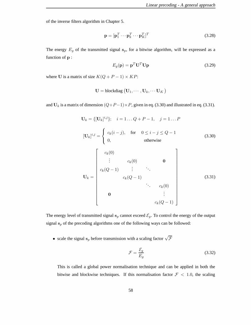
Linear precoding - A general approach

of the inverse filters algorithm in Chapter 5.

p = [pT1 · · ·pTk · · ·pTK ]T (3.28)

The energy Eg of the transmitted signal sp, for a bitwise algorithm, will be expressed as a

function of p :

Eg(p) = pTUTUp (3.29)

where U is a matrix of size K(Q+ P − 1) ×KP :

U = blockdiag(U1, · · · ,Uk, · · ·UK

)

and Uk is a matrix of dimension (Q+P−1)×P , given in eq. (3.30) and illustrated in eq. (3.31).

Uk = [Uk]i,j; i = 1 . . . Q+ P − 1, j = 1 . . . P

[Uk]i,j =

ck(i− j), for 0 ≤ i− j ≤ Q− 1

0, otherwise(3.30)

Uk =

ck(0)... ck(0) 0

ck(Q− 1)...

. . .

ck(Q− 1)

. . . ck(0)

0...

ck(Q− 1)

(3.31)

The energy level of transmitted signal sp cannot exceed Eg. To control the energy of the output

signal sp of the precoding algorithms one of the following ways can be followed:

• scale the signal sp before transmission with a scaling factor√F

F =EgEg

(3.32)

This is called a global power normalisation technique and can be applied in both the

bitwise and blockwise techniques. If this normalisation factor F < 1.0, the scaling

58

Linear precoding - A general approach

results in a decrease in the SNR at the receiver decision point. With this in mind, the

optimum precoding technique is one that minimises the MAI and ISI and maximises F .

• In [78] the author applies a different power scaling technique for the bitwise algorithm,

called decorrelating pre-filters. Each user is individually normalised to achieve a spec-

ified received SNR in contrast with the global normalisation derived in eq. (3.32). The

data bit dmk is scaled before spreading with the factor 1‖ck∗pk‖ . Thus, after being filtered

by pk pre-filter its power is normalised to one.

• Power constraint optimisation criteria should be imposed on the algorithms that give the

precoding solution. In this case the resulted power may not be exactly the intended Eg and

a extra scaling step should take place, but the scaling step should be a small adjustment.

3.6 Summary

The linearity of a CDMA system with linear MUD gave birth to the idea of transfering the

MUD complexity to the BS. Knowledge of the downlink channels is necessary for this idea

and this problem is solved by assuming a WCDMA-TDD system where the reciprocity of

the downlink and uplink channel is valid. The theoretical BER of a precoding system can be

calculated assuming that ISI and MAI have Gaussian distribution and a new metric, called SNIR

spread was introduced for testing if all the MSs are undergoing the same performance, given

that signals of equal energies are transmitted to them. Precoding techniques can be classified in

blockwise and bitwise with the later displaying particular advantages over the former, in terms

of complexity and implementation. Linear transformation of transmitted data usually leads to

an increased transmitted power and a scaling factor applied before transmission is necessary.

An important conclusion is that the optimum precoding technique is one that minimises the

MAI and ISI and maximises F . In the next Chapter the state of the art of linear precoding

techniques is presented.

59

Chapter 4Linear precoding - State of the art

In the previous Chapter the idea of linear precoding in a TDD system for slow fading channels

(where the rapidity of fading is slow relative to signaling rate) was supported. Such condi-

tions can be encountered in indoor, microcellular and some satellite communications scenarios.

By means of precoding, the multiuser detection problem is reduced to decoupled single user

detection problems. In what follows we will describe recently developed linear precoding tech-

niques. For all methods downlink channel knowledge is assumed at the BS. In the previous

Chapter the precoding techniques were classified in blockwise and bitwise in accordance to

their realisation and block diagram. Blockwise techniques like joint transmission (JT) and

transmitter-precoding (TP) are given in sections 4.1 and 4.2, respectively. The bitwise ones as

decorrelating pre-filters (DPF) and pre-RAKE are presented in sections 4.3 and 4.4. Section 4.5

deals with the complexity encountered by each technique while section 4.6 is a reference to a

number of alternative algorithms. A discussion on the performance and a number of issues as-

sociated with precoding techniques is raised in section 4.7 and the conclusions are summarised

in section 4.8.

4.1 Joint transmission

In joint transmission [80, 81] the algorithm seeks for a common signal sp, of length NQ, which

gives the desired data at the output of every user’s receiver. The received signal ek at user site

k is as described in eq. (2.24). The noiseless version of ek is written as:

ek = Hksp (4.1)

After arranging all K matrices Hk into the K(NQ+W − 1) ×NQ matrix H

H =[HT

1 · · ·HTk · · ·HT

K

]T (4.2)

60

Linear precoding - State of the art

and all ek, k = 1 . . . K , vectors to a total received vector e:

eT =[eT1 · · · eTk · · · eTK

]T(4.3)

it can be written:

e = Hsp (4.4)

The total received signal e of eq. (4.4) cannot be observed by a single MS. A MS can only

observe ek as described by eq. (2.24). The outputs dk, k = 1 . . . K , at the decision variable of

the K users are combined to form the vector d:

dT =[dT1 · · · dTk · · · dTK

]T(4.5)

Recalling that the k-user’s receiver is a filter matched to the user’s spreading code as in eq. (2.33),

d can be written as in eq. (4.6).

d = BTe = BTHsp (4.6)

In eq. (4.6) the K(NQ+W − 1) ×KN block diagonal matrix B is defined as:

B = blockdiag(B1, · · · ,Bk, · · · ,BK

)(4.7)

The objective of any precoding algorithm is that the output of the mobile receiver yields the

transmitted data :

d = d (4.8)

By substitution of eq. (4.8) into eq. (4.6) the problem of JT takes the form:

BTHsp = d (4.9)

Matrices B, H and vector d in eq. (4.9) are known at the BS and sp is an unknown vector with

length NQ . The condition

KN ≤ NQ (4.10)

is a basic assumption for TD-CDMA [28], and hence eq. (4.9) constitutes an optimisation

problem [82], where the number of restrictions contained in the vector d of length KN , is

smaller than the number NQ of degrees of freedom, expressed by the vector sp. Therefore, the

validility of eq. (4.10) implies that eq. (4.9) has infinitely many solutions for sp. A constraint

61

Linear precoding - State of the art

criterion is necessary to be imposed to the system. It is desirable for the transmitted vector sp

to be of minimum energy and the approach to achieve that is by following standard Lagrange

techniques [83]. The minimisation of the power sTp sp using the constraints as expressed in

eq. (4.9) is described with the following Lagrange function:

F (sp) = sTp sp − λT (BTHsp − d) (4.11)

where λ is the KN × 1 vector of Lagrange multipliers. The minimisation of eq. (4.11) can be

achieved by taking the gradient of F (sp):

ϑF (sp)

ϑsp= 2sp −HTBλ = 0 (4.12)

The solution is straightforward:

sp = HTBλ (4.13)

The factor 2 in eq. (4.12) has been absorbed by λ. By replacing sp in eq. (4.9) with the right-

hand part of eq. (4.13) the Lagrange multipliers can be calculated:

λ =(BTHHTB

)−1d (4.14)

Hence, returning back and manipulating eq. (4.13) the final solution for signal sp is proved to

be:

sp = HTB(BTHHTB

)−1d (4.15)

Recalling the general linear precoding eq. (3.1) it is obvious that the joint precoding matrix T

for JT can be written as:

T JT = HTB(BTHHTB

)−1(4.16)

Equation (4.13) shows that joint transmission can be considered as a set of independent pre-

RAKEs (HTB) applied on the modified information signal given by λ, which is a linear trans-

formation of the data vector d [84]. The same equation for linear transformation of the trans-

mitted signal has been derived through different methods in [85, 86]. The conclusions reached

for a system with a conventional receiver apply also when a RAKE receiver is employed, in

which case the channel matrix H in eq. (4.15) should be substituted by the matrix H ′ that rep-

resents the cascaded channel and RAKE receiver H′ = HTH. In case the K channels are

62

Linear precoding - State of the art

AWGN channels H = I and B is equal to C. Consequently T JT becomes:

T JT = C(CTC

)−1(4.17)

4.2 Transmitter precoding

Transmitter precoding is presented in [79]. It represents a linear transformation technique of

transmitted data, such that the mean squared errors at all receivers are minimised. The author

describes both a power unconstrained and constrained optimisation. However, the case of power

constrained precoding is given only for a flat fading channel. In the unconstrained algorithm the

transmitted signal is scaled with an appropriate factor in order to maintain the transmit power

the same as in the case without precoding. The author in [79] considers transmitter precoding

with either a conventional matched filter receiver or a RAKE receiver.

4.2.1 Unconstrained optimisation

In the scheme of a conventional CDMA system the matched filter outputs of all mobile receivers

can be jointly expressed by defining the following NK ×NK matrix U:

d =

BT1 H1C

...

BTkHkC

...

BTKHKC

︸ ︷︷ ︸

U

d +

BT1...

BTk

...

BTK

v

︸ ︷︷ ︸

v

(4.18)

where v is a zero-mean Gaussian noise vector with covariance matrix equal to diagσ2, if

‖c2k‖ = 1. To reduce the effect of MAI and ISI the author in [79] applies a linear transforma-

tion matrix T, of dimension NK × NK on the block of data, before the spreading process.

Therefore, after precoding and spreading, the vector at the outputs of the MS receivers will be:

d = UTd + v (4.19)

In order to calculate T the MMSE criterion is employed. The cost function J that has to be

63

Linear precoding - State of the art

minimised is defined as:

J = Ed,v

[‖d − d‖2

]

= Ed,v

[‖d − (UTd + v)‖2

](4.20)

Ed,v[·] represents the expectation with respect to the data block vector d and noise vector v.

The matrix T, that minimises J is given in eq. (4.21). The derivation is given in [79].

T = U−1 (4.21)

Hence, eq. (4.19) becomes:

d = d + v (4.22)

The multiuser detection problem that normally should have taken place in the receiver has

been decoupled into NK separate single user detection problems, by means of precoding.

An additional advantage is that the noise is not enhanced at the receiver, due to the lack of a

receiver based decorrelating process. The cost is an increase in the transmitted energy which

may neutralise the benefit described before.

The author of [79] gives the precoding matrix solution when a RAKE receiver is employed.

Under this scenario T is still equal to U−1 but now U is defined as:

U =

CT1 HT

1 H1C

...

CTkH

TkHkC

...

CTKHT

KHKC

(4.23)

Hereafter, we will denote the TP with matched filter receiver as TP-MAT to distinguish it from

the TP with RAKE receiver, which in turn will be denoted as TP-RAKE.

From both definitions of U in eq. (4.18) and eq. (4.23) C can be taken out to write U = U ′C.

C spreads the data after precoding and U′ corresponds to the cascaded channel and receiver.

Observing eq. (4.19) and after replacing U with U′C it is easy to write sp as:

sp = CTd (4.24)

64

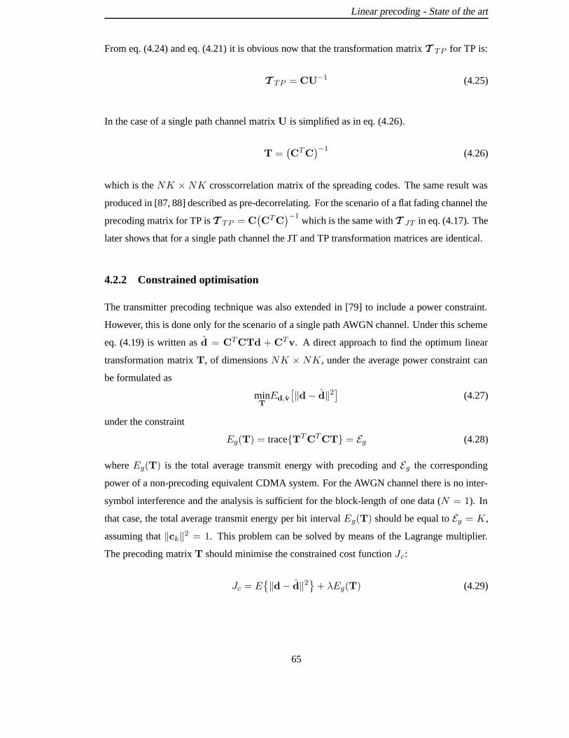
Linear precoding - State of the art

From eq. (4.24) and eq. (4.21) it is obvious now that the transformation matrix T TP for TP is:

T TP = CU−1 (4.25)

In the case of a single path channel matrix U is simplified as in eq. (4.26).

T =(CTC

)−1(4.26)

which is the NK ×NK crosscorrelation matrix of the spreading codes. The same result was

produced in [87, 88] described as pre-decorrelating. For the scenario of a flat fading channel the

precoding matrix for TP is T TP = C(CTC

)−1which is the same with T JT in eq. (4.17). The

later shows that for a single path channel the JT and TP transformation matrices are identical.

4.2.2 Constrained optimisation

The transmitter precoding technique was also extended in [79] to include a power constraint.

However, this is done only for the scenario of a single path AWGN channel. Under this scheme

eq. (4.19) is written as d = CTCTd + CTv. A direct approach to find the optimum linear

transformation matrix T, of dimensions NK × NK , under the average power constraint can

be formulated as

minTEd,v

[‖d − d‖2

](4.27)

under the constraint

Eg(T) = traceTTCTCT = Eg (4.28)

where Eg(T) is the total average transmit energy with precoding and Eg the corresponding

power of a non-precoding equivalent CDMA system. For the AWGN channel there is no inter-

symbol interference and the analysis is sufficient for the block-length of one data (N = 1). In

that case, the total average transmit energy per bit interval Eg(T) should be equal to Eg = K ,

assuming that ‖ck‖2 = 1. This problem can be solved by means of the Lagrange multiplier.

The precoding matrix T should minimise the constrained cost function Jc:

Jc = E‖d− d‖2

+ λEg(T) (4.29)

65

Linear precoding - State of the art

The solution is given in [79]:

T = (CTC + λI)−1 (4.30)

where I is the identity matrix and λ can be found from (4.29) and (4.30). It is shown in [79] that

a unique λ ≥ 0 exists as the desired solution where CTC, is a positive defined matrix (property

of cross correlation matrix [89]). The constrained transmitter precoding optimisation results in

a worse performance than the unconstrained one with power scaling, as demonstrated in [79].

This fact in conjunction with the lack of an extension for the multipath environment will lead

us into not examining this algorithm any further.

4.3 Decorrelating prefilters-Jointly optimized sequences

In [78] channel and multiple access effects are mitigated by jointly designing user transmit

waveforms. It is an alternative approach to the one given in [79], but the implementation is

different. Rather than relying on transmit data filtering and receiver RAKE or matched filter

processing, the transmit waveforms themselves are modified. The methods described in [78] are

named as decorrelating pre-filters (DPF) and jointly optimized sequences (JOS). They attempt

to precompensate for the channel multipath and minimise the crosscorrelation of other users at

the individual receivers simultaneously. The system is analogous to a system using a multiuser

detector, specifically the decorrelator [28], at the receiver except that the processing is now at

the transmitter.

4.3.1 Decorrelating prefilters

The block diagram of the DPF follows the bitwise precoding one as illustrated in Figure 3.6.

The algorithm is similar to TP-MAT which calculates the best pre-filter to apply to the data

symbols, filtering the data by blocks. DPF are applied to the transmit signal (instead of the

data symbols directly, as in [79]), so that the filter can be applied externally and the multipath

component resolution available from spread spectrum coding can be exploited.

Under the assumption of a synchronous CDMA system the received signal at mobile user j is

written as:

ej(n) =

K∑

k=1

dkck(n) ∗ pk(n) ∗ hj(n) + vj(n) (4.31)

66

Linear precoding - State of the art

The pre-filters pk(n), k = 1 . . . K are designed such that the signal meant for interfering users

is orthogonal to the matched filter response for the desired user, irrespective of the received

signals powers. Each user’s pre-filter must be designed jointly taking into account the channel

information and the transmit codes of all users. The approach taken in [78] is to design the

pre-filters that maximise the signal to noise ratio at the receiver while reducing the MAI inter-

ference. This method is not a strict error probability minimizing scheme, but rather a zero forc-

ing simultaneous multiuser interference rejecting and channel pre-equalization method. The

problem formulation is stated as follows. The matched filter output at the receiver of user j is:

dj =

K∑

k=1

dkck(n) ∗ pk(n) ∗ hj(n) ∗ cj(Q− n) + vj(n) (4.32)

vj(n) is the noise contribution to sample n of the receiver’s output. To simplify the notation,

let:

γij(n) = ci(n) ∗ hj(n) ∗ cj(Q− n); i, j = 1, . . . ,K (4.33)

Then eq. (4.32) becomes:

dj =

K∑

k=1

dkpk(n) ∗ γkj(n) + vj(n) (4.34)

Now the pre-filter optimisation problem is written mathematically as:

maxpj

(pj(n) ∗ γjj(n)

)|n=Tss

subject to constraints:

(pk(n) ∗ γkj

)|n=Tss = 0 ∀ j 6= k

‖pk ∗ ck‖ = 1 (4.35)

where Tss is the decision sample. The second constraint in eq. (4.35) allows for proper normal-

isation. Each user is individually normalised to achieve a specified received SNIR in contrast

with the global normalisation in eq. (3.32). Therefore the signal addressed to user k must be

scaled by 1/‖ck ∗ pk‖. The solution is found by solving for the minimum two-norm vector pk

67

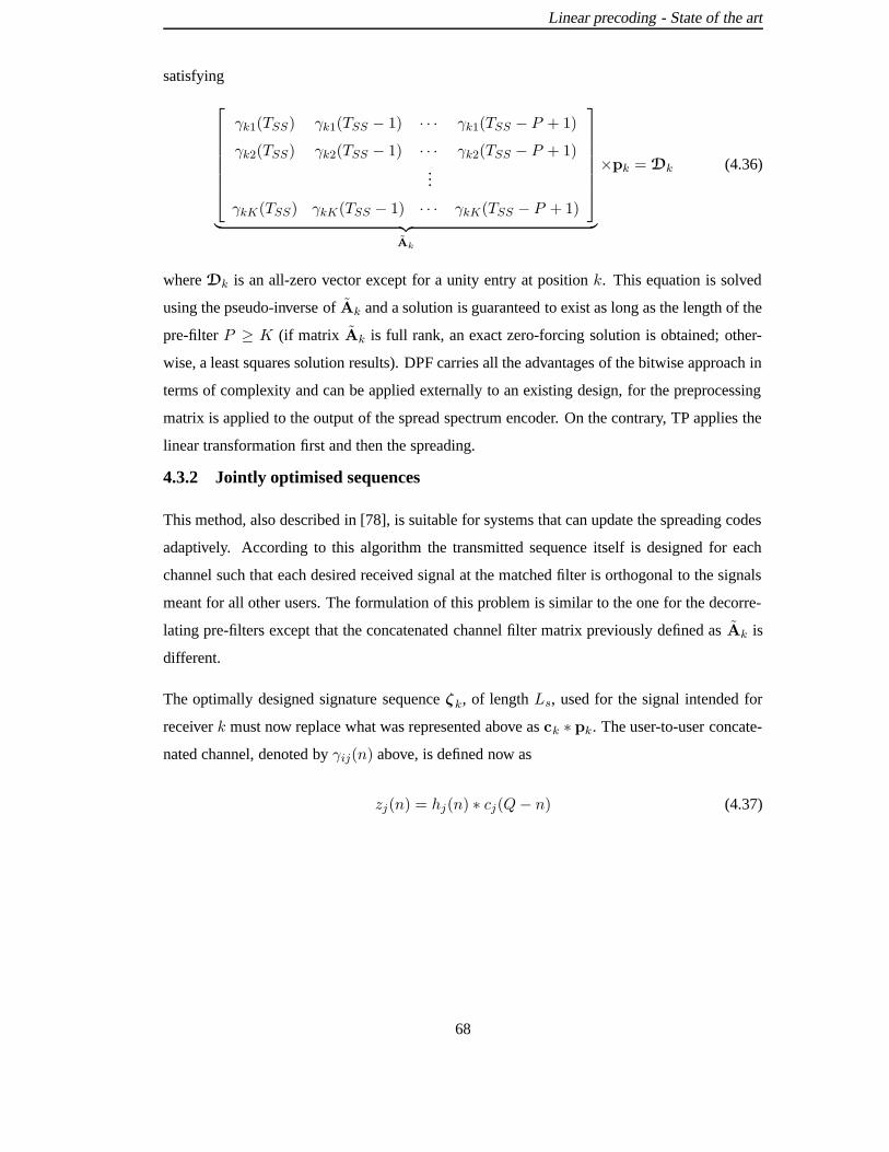
Linear precoding - State of the art

satisfying

γk1(TSS) γk1(TSS − 1) · · · γk1(TSS − P + 1)

γk2(TSS) γk2(TSS − 1) · · · γk2(TSS − P + 1)...

γkK(TSS) γkK(TSS − 1) · · · γkK(TSS − P + 1)

︸ ︷︷ ︸

Ak

×pk = Dk (4.36)

where Dk is an all-zero vector except for a unity entry at position k. This equation is solved

using the pseudo-inverse of Ak and a solution is guaranteed to exist as long as the length of the

pre-filter P ≥ K (if matrix Ak is full rank, an exact zero-forcing solution is obtained; other-

wise, a least squares solution results). DPF carries all the advantages of the bitwise approach in

terms of complexity and can be applied externally to an existing design, for the preprocessing

matrix is applied to the output of the spread spectrum encoder. On the contrary, TP applies the

linear transformation first and then the spreading.

4.3.2 Jointly optimised sequences

This method, also described in [78], is suitable for systems that can update the spreading codes

adaptively. According to this algorithm the transmitted sequence itself is designed for each

channel such that each desired received signal at the matched filter is orthogonal to the signals

meant for all other users. The formulation of this problem is similar to the one for the decorre-

lating pre-filters except that the concatenated channel filter matrix previously defined as Ak is

different.

The optimally designed signature sequence ζk, of length Ls, used for the signal intended for

receiver k must now replace what was represented above as ck ∗ pk. The user-to-user concate-

nated channel, denoted by γij(n) above, is defined now as

zj(n) = hj(n) ∗ cj(Q− n) (4.37)

68

Linear precoding - State of the art

The channel filter matrix equation becomes

z1(TSS) z1(TSS − 1) · · · z1(TSS − Ls + 1)

z2(TSS) z2(TSS − 1) · · · z2(TSS − Ls + 1)...

zK(TSS) zK(TSS − 1) · · · zK(TSS − Ls + 1)

︸ ︷︷ ︸

B

×ζk = Dk (4.38)

The length Ls of the signature sequence must be at least K and B must be a full rank matrix,

or the system will not have a direct solution. Again the minimum norm solution ζ k is found

using the pseudoinverse of B and the unit-norm signature sequence for user k is ζk/‖ζk‖. The

normalisation guarantees that the transmit power will be equal to a conventional CDMA system.

Jointly optimised sequences could also be derived for a block of symbols in a manner similar

to the derivation of TP in [79]. The solution for the best jointly optimised sequence would be

found by modifying eq. (4.38) to include the transmitted symbols for the block data. Block

processing has the advantage that the residual ISI is eliminated between symbols of the same

block. However, the disadvantage is that the channel must remain stationary for the duration of

the block and the end bits of the block are not correctly precoded.

4.4 Pre-RAKE diversity

This technique was initially described in [90] for DS-Spread spectrum systems and then ex-

tended in [76] for CDMA-TDD mobile communications. The algorithm for pre-RAKE origins

from the diversity theory in frequency selective channels. In a mobile environment the com-

bination of the received signals from diverse independent paths or mediums can improve the

system performance. According to the central limit theorem as the number of independent

paths increase, the combination of their signals will have less of a Rayleigh fading characteris-

tic and more of a Gaussian one [89]. Hence in the radio mobile communications it is desirable

to receive a signal from diverse independent paths and then combine their powers. This is what

a RAKE receiver does as described in section 2.3.

The pre-RAKE technique is straight forward and takes direct advantage of the fact that in TDD

the channel impulse response can be assumed the same for the uplink and the downlink. The

idea is to transmit a number of signals that when received after the multipath channel merge to

69

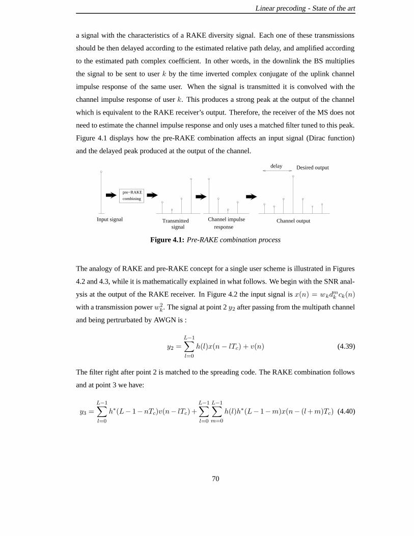
Linear precoding - State of the art

a signal with the characteristics of a RAKE diversity signal. Each one of these transmissions

should be then delayed according to the estimated relative path delay, and amplified according

to the estimated path complex coefficient. In other words, in the downlink the BS multiplies

the signal to be sent to user k by the time inverted complex conjugate of the uplink channel

impulse response of the same user. When the signal is transmitted it is convolved with the

channel impulse response of user k. This produces a strong peak at the output of the channel

which is equivalent to the RAKE receiver’s output. Therefore, the receiver of the MS does not

need to estimate the channel impulse response and only uses a matched filter tuned to this peak.

Figure 4.1 displays how the pre-RAKE combination affects an input signal (Dirac function)

and the delayed peak produced at the output of the channel.

Channel impulseresponse

Channel output

Desired outputdelay

Input signal Transmitted signal

combining

pre−RAKE

Figure 4.1: Pre-RAKE combination process

The analogy of RAKE and pre-RAKE concept for a single user scheme is illustrated in Figures

4.2 and 4.3, while it is mathematically explained in what follows. We begin with the SNR anal-

ysis at the output of the RAKE receiver. In Figure 4.2 the input signal is x(n) = wkdmk ck(n)

with a transmission power w2k. The signal at point 2 y2 after passing from the multipath channel

and being pertrurbated by AWGN is :

y2 =

L−1∑

l=0

h(l)x(n− lTc) + v(n) (4.39)

The filter right after point 2 is matched to the spreading code. The RAKE combination follows

and at point 3 we have:

y3 =L−1∑

l=0

h∗(L− 1−nTc)v(n− lTc)+L−1∑

l=0

L−1∑

m=0

h(l)h∗(L− 1−m)x(n− (l+m)Tc) (4.40)

70

Linear precoding - State of the art

Tc

Tc

Tc

2

(L−1) h L−1

h 1

h 2

h 0

Tc

Tc

Tc

spreading

filtermatched

*

*

*

*

2

(L−1) h

h

h

h L−1

0

L−2

2

3

multipath channelRAKE combiner

decisionoutput

+

noise v(n)

x(n)

L−3

1

Figure 4.2: RAKE combiner

multipath channelpre−RAKE Combiner

Tc

Tc

Tc

Tc

Tc

Tc

spreading

x(n)

*

*

*

*

2

(L−1) h

h

h

h L−1

0

L−2

L−3

filtermatched

+

noise v(n)2

(L−1) h L−1

h 1

h 2

h 0

4 5 6

Figure 4.3: Pre-RAKE combiner

The desired output of the RAKE system is∑L−1

l=0 h(l)h∗(l)x(n−(L−1)Tc) and occurs at time

n = (L− 1)Tc (l +m = L− 1). This has a signal strength of

(L−1∑

l=0

h(l)h∗(l)

)2

w2k (4.41)

Noise adds up incoherently and its power is:

(L−1∑

l=0

h(l)h∗(l)

)

σ2 (4.42)

From equations (4.41) and (4.42) the SNR at the output of the RAKE receiver is equal to:

SNRRAKE =w2k

σ2

(L−1∑

l=0

h(l)h∗(l)

)

(4.43)

In Figure 4.3 the block diagram of a pre-RAKE is illustrated. In order to make sure that the

power of the signal at the output of the pre-RAKE transmitter is equal to w2k, a power scaling

71

Linear precoding - State of the art

factor should be chosen to compensate for the gains produced by h(l)∗. In [90] the scaling

factor is:

F =1

√∑L−1

l=0 h(l)h∗(l)(4.44)

In Figure 4.3 after pre-RAKE combining the signal at point 4 y4 is :

y4 = FL−1∑

l=0

h∗(n− lTc)x(n− lTc) (4.45)

After transmission, convolution with the multipath channel and addition of AWGN the signal

at point 6 of Figure 4.3 becomes:

y6 = F2

(L−1∑

l=0

L−1∑

m=0

h∗(l)h(L− 1 −m)x(n− (l +m)Tc)

)

+ v(n) (4.46)

The desired signal occurs again at time n = (L− 1)Tc and has a power equal to

w2kF(L−1∑

l=0

h(l)h∗(l)

)2

(4.47)

The noise at the output of the matched filter has a power equal to σ2. We replace F with the

right-hand part of eq. (4.44) and thus the SNR is written as:

SNRpre−RAKE = F2w2k

σ2

(L−1∑

l=0

h(l)h∗(l)

)2

=w2k

σ2

(L−1∑

l=0

h(l)h∗(l)

)

(4.48)

From equations (4.43) and (4.48) the SNR for the Pre-RAKE system is equal to that of the

RAKE system, for a single user. This analysis holds only under the assumption that the chan-

nels parameters are estimated ideally [90] on the transmitter. The two systems have similar

performance. In Figure 4.4 the noiseless RAKE receiver’s output is illustrated and this corre-

sponds to point 3 of Figure 4.2. The graph in Figure 4.5 shows the matched filter’s output and

corresponds to the noiseless pre-RAKE block diagram graph of Figure 4.3. In both Figures we

mark the delay after which the peak is detected. The multipath channel has a length of L = 11

chips. The data has been spread with a signature waveform of Q = 16 chips. The similarities

between a single user pre-RAKE and RAKE system are obvious and will be verified in the next

section by means of a BER performance comparison.

72

Linear precoding - State of the art

0 20 40 60 80 100−1.5

−1

−0.5

0

0.5

1

1.5

chips

datareceiver output

∆Delay in detection

Figure 4.4: Single user noiseless output of a RAKE receiver

0 20 40 60 80 100−1.5

−1

−0.5

0

0.5

1

1.5

chips

datareceiver ouput∆Delay in detection

Figure 4.5: Single user noiseless matched filter output after pre-RAKE processing

In [76] the concept of pre-RAKE was extended to a multiuser CDMA-TDD system. The signal

for user k after spreading is filtered by the time inverse complex conjugate impulse response

of the k-user’s channel and this process is repeated for every user before transmission. The

73

Linear precoding - State of the art

produced signals are appropriately scaled to maintain the power at the desired levels and then

superimposed at the antenna element. The block diagram of the pre-RAKE technique applied

in a CDMA-TDD is identical with the general description of a bitwise precoding technique

as illustrated in Figure 3.6. Therefore, pre-RAKE has the advantages of a bitwise approach

in terms of complexity and simplicity in implementation. Furthermore, the calculation of the

pre-filter’s tap coefficients don’t require any complicated algorithm. Each pre-filter’s impulse

response is the time inverse conjugated of the corresponding uplink channel. The transmitted

signal sp(n), under the multiuser scheme is:

sp(n) =K∑

k=1

FkL−1∑

l=0

h∗(n− lTc)xk(n− lTc) (4.49)

The principle applied is that in the downlink the desired user’s signal is maximal ratio combined

by the channel itself while other user signals are not. In the analysis presented in [76] at the

sampling time the matched filter output consists of the desired part of the transmitted bit, the

intersymbol and multiple access interference and the noise. The mean and the variance of each

one of these terms is calculated. Under the multiuser scenario the pre-RAKE is proved to be an

insufficient technique unable to compensate for the multipath interference and MAI as shown

in [76, 91].

4.5 Complexity

The precoding techniques described in this Chapter require excessive computational cost com-

pared to the usual conventional spreading. The complexity is similar or exceeds the one demon-

strated by the receiver based multiuser techniques as described in [28, 60, 62]. However, it is

shifted to the BS, where the resources are more readily available and thus it is less critical. Ta-

ble 4.1 summarises the computational cost for JT, TP-MAT, DPF, Pre-RAKE. The criteria used

are the dimension of the matrix that needs to be inverted and the number of multiplications per

transmitted symbol. The number of multiplications are calculated after the final transformation

matrix T , for the blockwise techniques, as defined in Chapter 3, has been formulated. As ex-

pected the blockwise techniques JT and TP-MAT are more demanding in terms of complexity

compared to the bitwise DPF and pre-RAKE.

It will be shown in the next section that JT outperforms in terms of performance the other tech-

niques. Therefore, it is useful to emphasize on this technique. JT algorithm can be optimized

74

Linear precoding - State of the art

Precoding-algorithm Dimension of matrix to be Number of multiplicationsinverted per symbol

JT KN ×KN N 2QK

TP-MAT KN ×KN N 2QK

DPF K(P × P ) PQ

Pre-RAKE none LQ

Table 4.1: Precoding algorithms computational complexity

by taking advantage of two properties of matrix(BTHHTB

)[86]:

•(BTHHTB

)is Hermitian

• It consists of non-vanishing blocks of coefficients located near the diagonal which are

repeated along the diagonal.

Property 1 allows for decomposing the matrix triangularly (Cholesky decomposition), which

in turn allows efficient calculation of(BTHHTB

)−1d by back-substitution. On the other

hand property 2 allows for decomposing(BTHHTB

)more efficiently than by the usual full

Cholesky decomposition. The complexity of JT can be compared with the receiver based ZF-

JD, described in 2.4.1. We reproduce here, for convenience, the basic equation of ZF-JD.

d =((HkC)H(HkC)

)−1(HkC)Hek (4.50)

The matrices to be inverted for both receiver and transmitter based techniques are of dimension

KN × KN . Both have exactly the same structure with exactly the same non-vanishing ele-

ments. Both matrices can be inverted efficiently by taking into account properties 1 and 2. So

inverting the matrices for ZF-JD and JT requires the same computational power. The only com-

plexity difference between JT and ZF-JT arises from matrix multiplications HTB and (HkC)H

respectively. The complexity of the joint predistortion techniques can be further reduced by ex-

ploiting the structure of the matrices as explained in [92]. However, the multiplications required

per symbol after the matrix inversion outnumber the ones required by a bitwise technique, in a

realistic system.

75

Linear precoding - State of the art

4.6 Other techniques

The precoding techniques described in this Chapter are only representative and most commonly

used as a reference. In the recent bibliography there are alternative techniques for reducing the

mobile complexity that may utilise smart antennas or even the frequency domain of a system.

A comparison and review among different linear precoding techniques can be found in [91, 93].

The usage of antenna arrays can result in space-time (ST) algorithms that, when applied at the

downlink, minimise the MAI and ISI. Such a ST precoding downlink transmission is described

in [94, 95]. In [96–98] the authors develop a space-time zero-forcing pre-equalisation technique

for interference cancellation in the TDD downlink, by transferring the analysis to the frequency

domain. Moreover, an alternative blockwise precoding technique that incorporates a power

constraint (JT with power constraint) is described in [84], named joint signal precoding. An

extension of the pre-RAKE named post-RAKE is presented in [99]. The idea of post-RAKE is

to maximise the signal to noise ratio at the MS by replacing the matched filter in the pre-RAKE

block diagram with a receiver which is matched to the combination of the pre-RAKE filter and

the channel. Finally, joint transmitter-receiver optimisation is also investigated in [100, 101].

The impairment of the post-RAKE and the transmitter-receiver optimisation algorithms is that

the idea of the simplest possible receiver is not valid any more. The precoding techniques

described so far induce distortion in the signal’s spectral properties. A power constrained algo-

rithm that acts on the amplitude of the transmitted signals by a simple scaling is demonstrated

in [102]. This method is called optimising precoder and maintains the spectral properties of

the initial designed signals. However, this method is developed only for a single path Gaussian

channel and, on top of that, the determination of each user’s power needs to be readjusted at

each bit interval, which in turn results in excessive computational cost.

4.7 Simulation results

In Chapter 3 it was asserted that one of drawbacks of the blockwise techniques is that they do

not allow for correct precoding of the end data, when a multipath channel occurs. Therefore,

the overlapping of the signal’s replicas affect the first and last transmitted bit(s). This results

in a performance degradation which is more intense when the length of the transmitted block

is small. This conclusion is illustrated in the Figure 4.6. The performance of JT versus the

number of users is shown for block lengths 1, 3 and 20 data. Spreading gain is set to the default

76

Linear precoding - State of the art

for this thesis Q = 16 chips. The simulation corresponds to a system where the channels

follow a severe multipath profile (L = 11 chips) and Eb/No = 10dB. Each curve represents

an average over 60 different sets of random codes to smooth out the effect of codes with low or

high crosscorrelation. As shown the performance is better for N = 20.

2 4 6 8 10 12 14 1610

−5

10−4

10−3

10−2

10−1

100

Number of users

BE

R

JT−block 1JT−block 3JT−block 20

Figure 4.6: Block-length effect on JT performance

0 5 10 15 200.4

0.45

0.5

0.55

0.6

0.65

0.7

0.75

Block Length N

√ F

JTTP−MATTP−RAKE

Figure 4.7: Block-length effect on Transmitted Energy Eg

77

Linear precoding - State of the art

In Figure 4.7 we investigate how the block length affects the scaling factor needed to maintain

the total transmitted energy per symbol Eg equal to Eg . The blockwise algorithms displayed are

TP-MAT, TP-RAKE and JT. The same system is simulated for each curve and thus a conclusion

of how the different methods affect the transmitted energy can be drawn. The system adopted

is one of K = 5 users in a multipath environment. For each algorithm the scaling factor√F is

almost flat versus N . For smallN there is some differentiation but it can be assumed negligible.

We recall here from Chapter 3 that ideally the scaling factor should be√F ≥ 1.0, otherwise it

deteriorates the SNR at the receiver point. Comparing the three algorithms it is obvious that TP-

MAT results in the highest increase of transmitted energy (it corresponds to the smallest√F ),

while JT is the most modest and displays the least energy increase. TP-RAKE lies in between.

The excess energy is the penalty paid for the cancellation of MAI and ISI before transmission.

It is expected from these observations that JT will demonstrate the best BER performance and

TP-MAT the worst. This will be verified by the simulations that are following.

0 5 10 15 2010

−5

10−4

10−3

10−2

10−1

100

Eb/N

o(dB)

BE

R

Pre−RAKEDPFTP−MATTP−RAKEJTMMSE−JD

Figure 4.8: Transmitter based precoding techniques and MMSE-JD vs Eb/No

In Figure 4.8 the BER performance is shown versus Eb/No. The system is one of K = 5 users

in a severe multipath environment. The best performance is displayed by JT and the worst by the

pre-RAKE. In the blockwise techniques the end bits have been discarded from the calculation

of BER. This is because the theoretical BER, as calculated from eq. (3.12) pressumes transmis-

sion of a single block of data without taking into account the end-bits interference. Thus, the

78

Linear precoding - State of the art

analytical and the simulation results can be in agreement. This can be justified from the fact that

for large blocks the effect of the end bits is negligible. We examine first the region where BER

is equal to 10−3. TP-MAT is worse than TP-RAKE. This is because TP-MAT over-increases

the required transmitted energy Eg , compared with TP-RAKE. The RAKE receiver utilised by

TP-RAKE exploits the diversity principles and increases the SNR at the receiver output. In the

same Figure the performance of the MMSE-JD receiver based multiuser detection is illustrated.

We observe that MMSE-JD outperforms all the transmitter based precoding techniques except

JT. JT completely eliminates the ISI and MAI within a block of data and selects the transmis-

sion vector with the minimum energy. This, in conjuction with the lack of any receiver based

decorrelation that may increase the noise justifies the superiority of JT. This simulation does

not include any channel coding such as convolutional or turbo coding techniques. Utilisation

of such techniques would further reduce the BER, e.g. 10−1 would have been reduced down

to 10−3. By setting as minimum target BER=10−3, with channel coding implemented, it is

interesting to discuss the BER at the region of 10−1. JT and receiver-based MMSE-JD clearly

outperform the others, however the performance gap is not so large anymore. Pre-RAKE not

only performs sufficiently but outperforms methods as TP-MAT and DPF.

4.8 Summary

In Chapter 4 recent developed transmitter based tecnhniques were described. Their algorithms

were briefly described pointing out the different criteria that lead to different performance.

It was shown that the blockwise techniques outperform the bitwise and that among them JT

demonstrates a very good BER performance. It’s even a better solution than the receiver based

MMSE-JD. On the other hand, in Chapter 3 specific advantages of bitwise techniques were

addressed. These advantages are summarised as the low computational cost and flexibility in

implementation. Hence, it makes it essential to investigate and develop bitwise techniques

that outperform the current ones and achieve a BER performance competitive with the one

demonstrated by blockwise techniques. In the next two Chapters our research is towards this

goal and two new bitwise algorithms are proposed.

79

Chapter 5Inverse filters - Wiener solution

In this Chapter a new bitwise algorithm, named inverse filters (INVF) is proposed. Part of this

work has been published in [103] In section 5.1 the origin of this technique is discussed. The

adaptation to a CDMA system, the criteria and an analysis of the algorithm is presented in

sections 5.2 and 5.3. Sections 5.4, 5.5 and 5.6 deal with the Wiener solution and the parameters

associated with it. At last, section 5.7 presents some simulation results and compares INVF

with other techniques in terms of performance and complexity.

5.1 INVF in stereophonic sound reproduction system

It’s useful to present briefly the origins of the inverse filtering before describing their appli-

cation and appropriate modification in a CDMA-TDD system. In [104–110] the problem of

producing better approximations to the perfect reproduction of prerecorded acoustic signals

was addressed. Let two channel stereophonic signals be recorded at two points Γ, ∆ in an

existing sound field. When these signals are replayed via two loudspeakers in a listening room,

h11

h12h21

h22

1 1

2 2

x

x

d

d

Α

Β∆

Γ

: Microphone

: Loudspeaker

Figure 5.1: A stereophonic sound reproduction system

at points A and B as shown in Figure 5.1, the original signals are imperfectly reproduced at the

ears of a listener. The imperfections in the reproduction arise from the following main causes:

• The signal played via the right channel is reproduced at both the right and the left ears of

the listener. It is the same for the signal played via the left channel.

• The acoustic response of the listening room provides a reverberant field which is in addi-

tion to the reverberant field of the space in which the existing recordings were made.

80

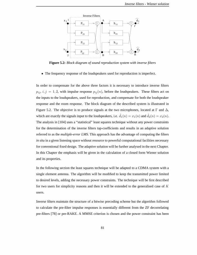
Inverse filters - Wiener solution

h11

h21

h12

h22

A

B2

1

Γ

∆

11

p21

p12

22p

px

d

d

x

1

2

1

2

Inverse Filters

Figure 5.2: Block diagram of sound reproduction system with inverse filters

• The frequency response of the loudspeakers used for reproduction is imperfect.

In order to compensate for the above three factors it is necessary to introduce inverse filters

pij , i, j = 1, 2, with impulse response pij(n), before the loudspeakers. These filters act on

the inputs to the loudspeakers, used for reproduction, and compensate for both the loudspeaker

response and the room response. The block diagram of the described system is illustrated in

Figure 5.2. The objective is to produce signals at the two microphones, located at Γ and ∆,

which are exactly the signals input to the loudspeakers, i.e. d1(n) = x1(n) and d2(n) = x2(n).

The analysis in [104] uses a “statistical” least squares technique without any power constraints

for the determination of the inverse filters tap-coefficients and results in an adaptive solution

referred to as the multiple-error LMS. This approach has the advantage of computing the filters

in situ in a given listening space without resource to powerful computational facilities necessary

for conventional fixed design. The adaptive solution will be further analysed in the next Chapter.

In this Chapter the emphasis will be given in the calculation of a closed form Wiener solution

and its properties.

In the following section the least squares technique will be adapted to a CDMA system with a

single element antenna. The algorithm will be modified to keep the transmitted power limited

to desired levels, adding the necessary power constraints. The technique will be first described

for two users for simplicity reasons and then it will be extended to the generalised case of K

users.

Inverse filters maintain the structure of a bitwise precoding scheme but the algorithm followed

to calculate the pre-filter impulse responses is essentially different from the ZF decorrelating

pre-filters [78] or pre-RAKE. A MMSE criterion is chosen and the power constraint has been

81

Inverse filters - Wiener solution

included in the algorithm so as to minimise the resulting transmitted power.

5.2 Least squares power constrained algorithm

In Figure 5.2 the sound is produced by two loudspeakers at points A and B in the space and

received by two microphones at points Γ and ∆. In a CDMA system it is equivalent to having

two antennas at the transmission point (BS for the downlink scheme) and two mobile units at

different sites. The model of Figure 5.2 has to be modified for a single element antenna. Thus

the channels hj1, j = 1, 2, linking antenna A with receiver j and hj2, j = 1, 2, linking antenna

B with receiver j have to be reduced down to the channels h1 and h2 between the antenna and

the mobile terminals. The resulted modified model is then as displayed in Figure 5.3 where

the analogy with the bitwise general model of Figure 3.6 is obvious. Filters pi correspond to

the transmission pre-filters for bitwise transmission precoding as described in section 3.4.2. To

x2

x11

p

Inverse Filters

2

p1

A B

d2

d11h

2h

1 Γ

∆

Σ

Figure 5.3: Modified diagram to comply with a single antenna CDMA model

make the model suitable for a two user CDMA system with transmitter precoding we must

further replace the input signals x1 and x2 by the corresponding spread data dm1 c1(n) and

dm2 c2(n), respectively. By including the matched filter receivers ck(Q − n), k = 1, 2, instead

of the microphones, in the diagram a complete CDMA downlink model with bitwise precoding

results. The new block diagram is as shown in Figure 5.4 where the power scaling factor√F

has been also included. In Figure 5.4 the cascaded filters hk(n) and ck(Q− n) are substituted

by an FIR filter of length Z = Q+ L− 1 and impulse response zk(n) = hk(n) ∗ ck(Q− n),

also defined in eq. (4.37). Now the block diagram can be redrawn as illustrated in Figure 5.5.

The noise vawgn, included in Figure 5.4, is not included in Figure 5.5 because the noise is not

pre-filtered by pk(n) and thus it cannot affect the solution for the tap-coefficients. The scaling

factor√F has also been omitted and temporarily excluded from our analysis. The objective is

to calculate the inverse filters impulse response in a MMSE sense.

82

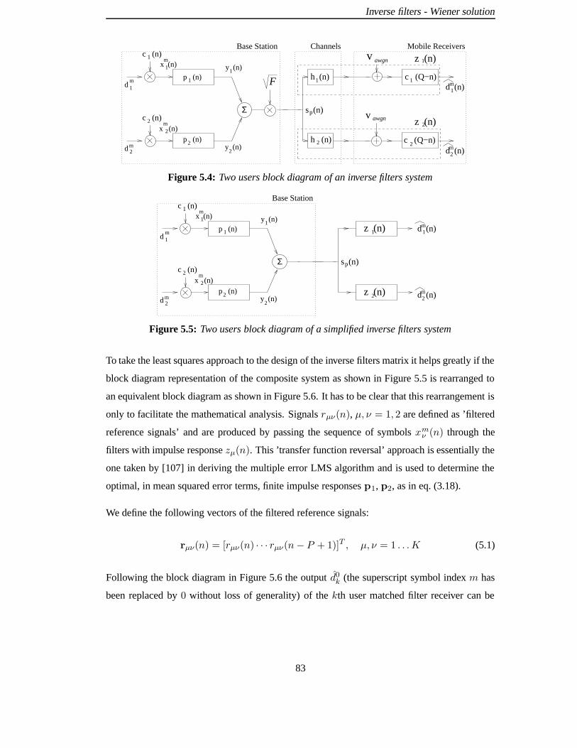
Inverse filters - Wiener solution

y (n)1

F

Σ

1

d 2

d 1

p (n)m

m

1x (n)m

m

d (n)

1md (n)1

m

h (n)1

h (n)

s (n)

y (n)2

p (n)

x (n)z (n)

z (n)1

2

c (Q−n)

c (Q−n)

awgn

awgn

v

v2

2

1c (n)Base Station

2

Channels Mobile Receivers

2 2

c (n)

2

p

Figure 5.4: Two users block diagram of an inverse filters system

y (n)1 md (n)1

d (n)m

Σ

1

d 2

d 1

p (n)m

m

1x (n)m

m

s (n)

y (n)2

p (n)

x (n)

z (n)

z (n)

1

2 2

2

2

1c (n)Base Station

2

c (n)p

Figure 5.5: Two users block diagram of a simplified inverse filters system

To take the least squares approach to the design of the inverse filters matrix it helps greatly if the

block diagram representation of the composite system as shown in Figure 5.5 is rearranged to

an equivalent block diagram as shown in Figure 5.6. It has to be clear that this rearrangement is

only to facilitate the mathematical analysis. Signals rµν(n), µ, ν = 1, 2 are defined as ’filtered

reference signals’ and are produced by passing the sequence of symbols xmν (n) through the

filters with impulse response zµ(n). This ’transfer function reversal’ approach is essentially the

one taken by [107] in deriving the multiple error LMS algorithm and is used to determine the

optimal, in mean squared error terms, finite impulse responses p1, p2, as in eq. (3.18).

We define the following vectors of the filtered reference signals:

rµν(n) = [rµν(n) · · · rµν(n− P + 1)]T , µ, ν = 1 . . . K (5.1)

Following the block diagram in Figure 5.6 the output d0k (the superscript symbol index m has

been replaced by 0 without loss of generality) of the kth user matched filter receiver can be

83

Inverse filters - Wiener solution

Σ m1

Σ

21

11m

1m

d

x (n)

2

22

222m

m

d

x (n)

11

11m

1m

d

x (n)

1

12

212m

m

d

x (n)

m2

d (n)

r (n)p (n)

1c (n)

z (n)

p (n)r (n)2

c (n)2

r (n)p (n)

1c (n)

z (n)

p (n)r (n)

z (n)2

c (n)2

z (n)

d (n)

Figure 5.6: Rearranged inverse filters block-diagram for two users

expressed in a matrix-vector notation form:

d0k = [rT11r

T12]p (5.2)

where p is a column arrangement of both inverse filters tap coefficients.

p = [pT1 pT2 ]T (5.3)

By arranging both estimate outputs in one vector d0 the system illustrated in Figure 5.6 is

described as:

d0(n) = R(n)p (5.4)

where the vector d0(n) and the matrix R(n) are denoted as:

d0(n) =

d01(n)

d02(n)

,R(n) =

rT11(n) rT12(n)

rT21(n) rT22(n)

(5.5)

84

Inverse filters - Wiener solution

We now seek the optimal filter vector p to minimise the time averaged squared error between the

actual and desired outputs. The desired outputs are sampled every symbol period T ns = nQ+∆,

n = 1, 2, . . ., where ∆ is an imposed delay in the system which assists the equalisation of the

multipath channels [111]. The cost function to be minimised is:

J = E[(d0 − d0(Tns ))T (d0 − d0(T

ns ))] (5.6)

where d0 is the vector of desired data defined as d0 = [d01d

02]T .

The problem now is that the resulted Wiener solution po for the inverse filters may increase

to undesired levels the transmitted power compared with the unprecoding CDMA scheme. As

explained in section 3.5 the usage of the power scaling factor√F < 1 afterwards will cause a

degradation in the SNR at the receiver point. Thus, it is wise to impose to the cost function the

necessary power constraint term by means of Lagrange multipliers.

The average total transmitted power for the bitwise techniques has been calculated in section

3.5 as a function of the vector p that contains the tap-coefficients of all inverse filters. We

reproduce here the equation.

Eg(p) = pTUT · Up (5.7)

with U as defined in eq. (3.30). The Eg(p) should not exceed the power that corresponds to

the conventional CDMA scheme Eg. Thus:

Eg(p) ≤ Eg (5.8)

The complete power constrained cost function to be minimised then takes the form:

Jc = E[(d0 − d0(Tns ))T (d0 − d0(T

ns ))] + λ

(Eg(p) − Eg

)(5.9)

Recalling eq. (5.4) Jc can be written as:

Jc = E[(d0 −R(T ns )p)T (d0 −R(T ns )p)] + λ(Eg(p) − Eg

)(5.10)

After expansion and use of the expectation operator, eq. (5.10) reduces to the quadratic form:

Jc = E[dT0 d0] − 2E[dT0 R(T ns )]p + pTE[RT (T ns )R(T ns )]p + λ(Eg(p) − Eg

)(5.11)

85

Inverse filters - Wiener solution

Taking the gradient ϑ/ϑp of the power constraint term we have:

ϑ(Eg(p) − Eg

)

ϑp=ϑ(pTUTUp

)

ϑp= 2UTUp (5.12)

The gradient ϑ/ϑp of the cost function Jc is:

ϑJcϑp

= −2E[RT (T ns )d0] + 2E[RT (T ns )R(T ns )]p + 2λUTUp (5.13)

The Wiener solution for the tap-coefficients of the pre-filters po is obtained by setting:

ϑJcϑp

∣∣∣∣po

= 0 (5.14)

Thus, from eq. (5.13) and eq. (5.14) we can write:

−2E[RT (T ns )d0] + 2E[RT (T ns )R(T ns )]po + 2λUTUpo = 0 (5.15)

−E[RT (T ns )d0] +(E[RT (T ns )R(T ns )] + λUTU

)po = 0 (5.16)

Finally, the Wiener solution po is calculated as:

po =[E[RT (T ns )R(T ns )] + λUTU

]−1E[RT (T ns )d0] (5.17)

The Wiener solution as shown in eq. (5.17) is valid even if users are transmitted with unequal

powers. In that case, the desired output vector is Wd0 (W is the power matrix) and it is shown

in Appendix A that the final solution po is not affected.

5.3 Generalisation

The least squares approach can easily be extended to deal with the case of multiple channels

and multiple users as in Figure 5.7. Figure 5.8 shows how the rearranged block diagram of

Figure 5.6 is extended in the general case for receiver µ. Eq. (5.4) is still valid but now the

terms are redefined as follows:

d0(n) =

d01(n)

...

d0K(n)

,R(n) =

rT1 (n)...

rTK(n)

, (5.18)

86

Inverse filters - Wiener solution

y (n)1

F

z K(n)n awgn

n awgn

Σ

1

d K

d 1

p (n)

p (n)m

m

1x (n)m

m

d (n)

1c (Q−n)md (n)1

m

h (n)1

h (n)

s (n)

y (n)K

x (n)

c (Q−n)

K

K

K

c (n)

1c (n)Base Station

K

KK

Channels Mobile Receivers

p

Figure 5.7: Generalised block diagram of an inverse filters system

µ ν

µνΣ m

µ

µ1

1µ1m

1m

d

x (n)

m

m

dν

ν

µΚ

ΚµKm

m

d

x (n)

x (n)

p (n)r (n)

z (n) d (n)

r (n)p (n)z (n)

1c (n)

c (n)ν

p (n)r (n)

z (n)

Kc (n)

K

Figure 5.8: Generalised rearranged block diagram for µ user.

with rTk (n), k = 1 . . . K , given as:

rk(n) = [rTk1(n), · · · , rTkK(n)]T (5.19)

rµν(n) is as in eq. (5.1) and p is as in eq. (3.28). The power constrained mean minimum

squared error cost function Jc is as in eq. (5.9) and following the analysis presented in the

previous section we get to the Wiener solution as described in eq. (5.17). An attempt to find a

closed form solution for the Wiener solution takes place in the next section.

5.4 Wiener solution

In order to find the analytical Wiener solution po, the expectation terms E[RT (n)R(n)] and

E[RT (n)d0] in eq. (5.17) must be calculated. As stated before rµν(n) = dmν cν(n) ∗ hµ(n) ∗

87

Inverse filters - Wiener solution

cµ(Q − n). Let γµν(n) = cν(n) ∗ hµ(n) ∗ cµ(Q − n) as also defined in eq. (4.33). The

corresponding symbol in vector form is denoted as γµν of length Gγ = 2Q+ L− 2 due to the

convolution effect.

γµν = [γµν(0) · · · γµν(Gγ − 1)]T (5.20)

Vector rµν(n) of length P , defined as in eq. (5.1), is given next as a function of theN = 2M+1

vector dν accounting for the ISI effect that is introduced due to the pre-filters. M symbols

transmitted before and after symbol d0ν are taken into account. We recall here that the sampling

time is T ns = nQ + ∆, n = 1, 2, . . . and we further assume that ∆ + Q ≤ Gγ , ∆ + Q ≥ P

(these assumptions are only to assist the illustration of the Wiener solution as both P and ∆

can be arbitrarily chosen). Then:

rµν = Γµνdν (5.21)

where the P ×N matrix Γµν is:

Γµν = [Γµν ]i,(j+M+1) ; i = 1...P, j = −M...M

[Γµν ]i,(j+M+1) =

γµν(∆ +Q− i− jQ), for 0 ≤ ∆ +Q− i− jQ ≤ Gγ − 1

0, otherwise(5.22)

For instance, in the case of Q = 4, P = 5,∆ = 2, L = 3,M = 1 eq. (5.21) takes the form:

rµν(Tns )

...

rµν(Tns − P + 1)

=

0 γµν(5) γµν(1)

γµν(8) γµν(4) γµν(0)

γµν(7) γµν(3) 0

γµν(6) γµν(2) 0

γµν(5) γµν(1) 0

d−1ν

d0ν

d1ν

(5.23)

By combining now eq. (5.18) and eq. (5.21) we obtain:

R(T ns ) =

dT1 ΓT11 · · · dTKΓT1K...

. . ....

dT1 ΓTK1 · · · dTKΓTKK

(5.24)

We will consider again the simple case of two users to calculate the mean terms of the Wiener

88

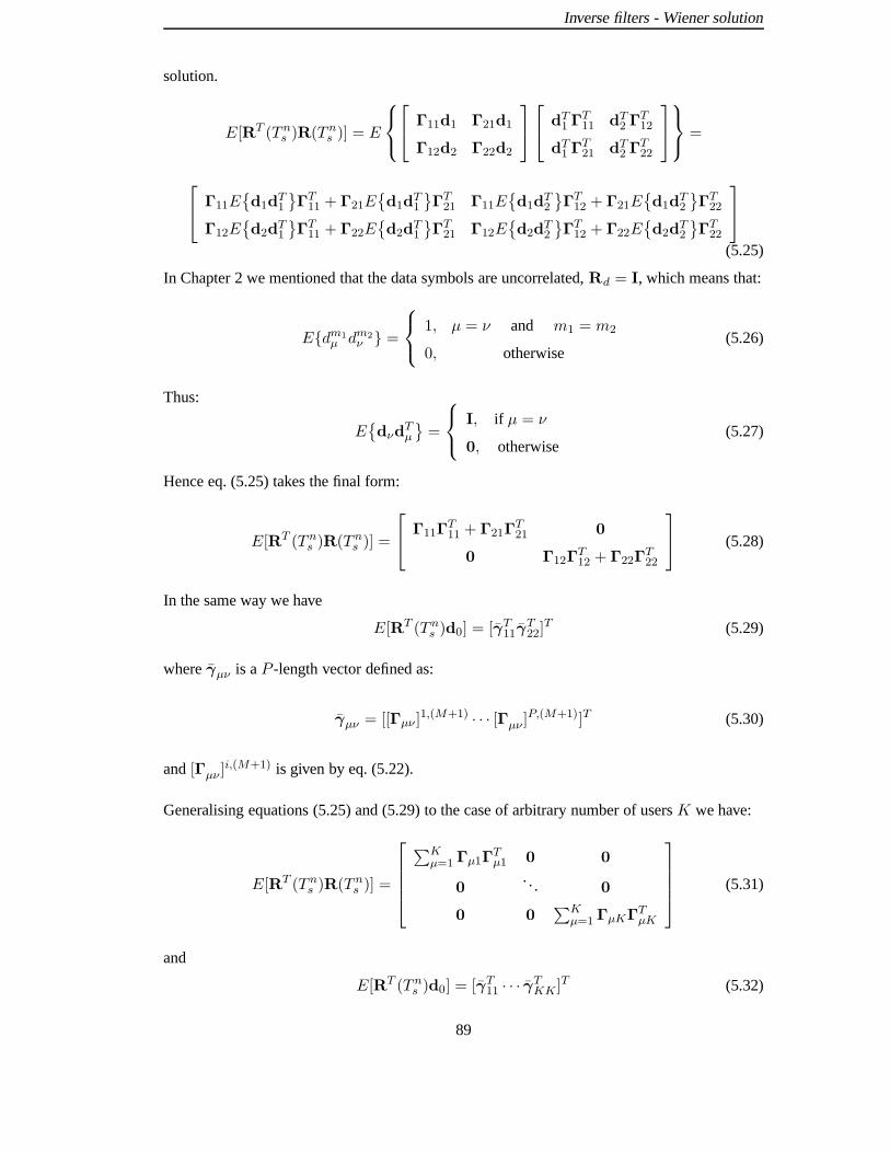
Inverse filters - Wiener solution

solution.

E[RT (T ns )R(T ns )] = E

Γ11d1 Γ21d1

Γ12d2 Γ22d2

dT1 ΓT11 dT2 ΓT12

dT1 ΓT21 dT2 ΓT22

=

Γ11E

d1d

T1

ΓT11 + Γ21E

d1d

T1

ΓT21 Γ11E

d1d

T2

ΓT12 + Γ21E

d1d

T2

ΓT22

Γ12Ed2d

T1

ΓT11 + Γ22E

d2d

T1

ΓT21 Γ12E

d2d

T2

ΓT12 + Γ22E

d2d

T2

ΓT22

(5.25)

In Chapter 2 we mentioned that the data symbols are uncorrelated, Rd = I, which means that:

Edm1

µ dm2

ν =

1, µ = ν and m1 = m2

0, otherwise(5.26)

Thus:

Edνd

Tµ

=

I, if µ = ν

0, otherwise(5.27)

Hence eq. (5.25) takes the final form:

E[RT (T ns )R(T ns )] =

Γ11Γ

T11 + Γ21Γ

T21 0

0 Γ12ΓT12 + Γ22Γ

T22

(5.28)

In the same way we have

E[RT (T ns )d0] = [γT11γT22]

T (5.29)

where γµν is a P -length vector defined as:

γµν = [[Γµν ]1,(M+1) · · · [Γµν ]P,(M+1)]T (5.30)

and [Γµν ]i,(M+1) is given by eq. (5.22).

Generalising equations (5.25) and (5.29) to the case of arbitrary number of users K we have:

E[RT (T ns )R(T ns )] =

∑Kµ=1 Γµ1Γ

Tµ1 0 0

0. . . 0

0 0∑K

µ=1 ΓµKΓTµK

(5.31)

and

E[RT (T ns )d0] = [γT11 · · · γTKK]T (5.32)

89

Inverse filters - Wiener solution

By replacing now the expectation terms in eq. (5.17) with the right-hand side of eq. (5.31)

and eq. (5.32) the Wiener solution is almost determined in a closed form. What remains to be

investigated is the right value for the parameter λ. This is the objective of the following two

sections.

5.5 λ - In depth

The question raised is as to what is the best choice for the parameter λ in eq. (5.17). A numerical

solution with reference to [102] is given and the performance of this solution is discussed. The

performance graphs, in terms of system’s average BER, given in this section are mostly based

on the analytical eq. (3.12). The consistency between theory and simulation results will be

shown in section 5.7.

5.5.1 Numerical solution

The problem described in section 5.2 can be restated in the following form:

minimize : E[‖d0 −R(T ns )p‖2

]

subject to : ‖Up‖2 ≤ Eg (5.33)

The objective function to be minimised is:

E[dT0 d0] − 2E[dT0 R(T ns )]p + pTE[RT (T ns )R(T ns )]p (5.34)

After deletion of the constant term E[dT0 d0] and the following substitutions

E[dT0 R(T ns )] = −γ

E[RT (T ns )R(T ns )] = Γ (5.35)

eq. (5.33) is rewritten as:

minimize : 2γp + pTΓp

subject to : ‖Up‖2 ≤ Eg (5.36)

90

Inverse filters - Wiener solution

This problem specifies minimisation of a convex quadratic function (Γ is positive semi-definite

as a correlation matrix) over an ellipsoid whose surface is the set of signal vectors which have

a transmitted power level Eg. This is a trust-region-subproblem as occurs in nonlinear opti-

misation theory and the solution is determined with reference to the numerical optimisation

techniques in [112, 113]. The gradient of the objective function is given by 2γ + 2Γp while

the gradient to the constraint is, as shown in eq. (5.12), 2UTUp. If the Karush-Kuhn-Tucker

(KKT) conditions for the local optimum po are satisfied with Lagrange multiplier λ then the

following holds:

(Γ + λUTU)po + γ = 0 (5.37)√

Eg − ‖Upo‖ ≥ 0 (5.38)

λ ≥ 0 (5.39)

λ(√

Eg − ‖Upo‖) = 0 (5.40)

To establish that po is a minimum, the second order sufficient condition requires positive cur-

vature of the objective function at po. This is described with the following equation:

xT(Γ + λUTU

)x > 0, ∀x ∈

w|wTpo = 0,w 6= 0

(5.41)

The matrix Γ is positive semi-definite and so is UTU (both are correlation matrices). Therefore

the quantity(Γ + λUTU

)is positive definite for λ > 0. Eq. (5.41) will then be satisfied for

any point on the constraint surface. When λ = 0, we obtain the unconstrained minimum of

the objective function which must be a minimum based on the convexity implied by a positive

semi-definite Γ. These observations coupled with a non-zero constraint gradient at all points

other than the origin result in the conclusion that the KKT conditions are satisfied with a unique

λ and that the associated point po is a global optimum.

The optimum value for λ can be found with numerical optimization techniques. The lower

bound for λ is zero. Before calculating an upper bound some notations are necessary to precede.

For any matrix X, ψ(X) and ψ(X) denote a minimum and maximum eigenvalue of matrix X,

respectively. The upper bound for λ can now be calculated by rearranging and taking the norm

of each side of eq. (5.37) as shown in [113]. The calculations following are not intented to be a

vigorous proof for the upper bound of λ. The norm used is the spectral norm ‖X‖s defined in

[89] as the square root of the largest eigenvalue of the matrix product XTX. For a vector x it

91

Inverse filters - Wiener solution

is ‖x‖s = ‖x‖ =√

xTx.

‖(Γ + λUTU

)−1γ‖s = ‖p‖s (5.42)

which implies,1

ψ(Γ) + λψ(UTU)‖γ‖s ≥ ‖p‖s (5.43)

which further implies,

ψ(Γ) + λψ(UTU) ≤ ‖γ‖s‖p‖s

(5.44)

Hence,

λ ≤ 1

ψ(UTU)

(‖γ‖s‖p‖s

− ψ(Γ)

)

(5.45)

If a non-zero λ satisfies the KKT conditions, then the corresponding po must have ‖Upo‖s =√

Eg. Then, if we write

‖Upo‖s ≤ ‖U‖s‖po‖s =√

Eg (5.46)

and further proceed to (using ‖po‖s = ‖po‖) :

‖po‖ =

√Eg

√

ψ(UTU)(5.47)

In case the eigenvalues of the correlation matrix Γ cannot be calculated the term ψ(Γ) may be

dropped out from eq. (5.45) which relaxes the upper bound. The new simplified upper bound

for the parameter λ is then:

λ ≤ ‖γ‖√Eg

√

ψ(UTU)

ψ(UTU)(5.48)

The above analysis provides a range of possible values for λ parameter. The search for the

right choice of λ starts from λ = 0. If the norm ‖Upo‖ ≤√Eg then the solution is inside

the constraint. Otherwise, an arbitrary λ can be tested for optimality by solving eq. (5.37) and

then checking the power constraint. If ‖Upo‖ =√Eg, then po is the solution we are looking

for. This procedure suggests a bisection algorithm for solving eq. (5.36). For such an algorithm

a converge precision has to be determined and it is denoted as ε. The bisection algorithm

92

Inverse filters - Wiener solution

proceeds as follows [113]:

1. set λlow = 0 and λhigh = ‖γ‖√Eg

√ψ(UT U)

ψ(UT U)

2. set λ = 12 (λlow + λhigh)

3. if (λhigh − λlow) ≤ ε exit procedure, otherwise go to 4.

4. solve (Γ + λUTU)po + γ = 0 for p

5. if ‖Up‖ ≥√Eg, then set λlow = λ, otherwise set λhigh = λ

6. go to step 2

(5.49)

The complexity of this algorithm is determined by the desired accuracy and the cost of the

linear system solution in step 4. At least log2‖γ‖√Eg

√ψ(UT U)

ψ(UT U)− log2ε iterations are required

to converge to the desired precision [102]. If the eigenvalues of Γ are known the number of

iterations can be reduced. The structure of the linear system in step 4 is more helpful. As

λ > 0 in each iteration, (Γ + λUTU) must be symmetric positive definite which suggests the

Cholesky factorization to solve the system quickly.

5.5.2 Performance results

In graph 5.9(a) the average total energy transmitted per symbol Eg versus λ if no power scaling

takes place is shown. The system under consideration is one of 5 users with spreading gain

of 16 in a multipath environment with Eb/No = 10dB. We observe that Eg is very high for

λ ∼ 0 and is radically reduced as λ increases. When ‖ck‖ = 1 then the energy transmitted

of a corresponding conventional CDMA system is Eg = 5. In the inverse filters scheme, for

the particular scenario, Eg = 5 is achieved for λ = 0.1077, as shown in the graph. This

result is in agreement with the convergence of the bisection algorithm in (5.49). In Figure

5.9(b) the performance in terms of the system’s average BER versus λ is illustrated. The solid

line shows the BER when the resulted signal sp after pre-filtering is transmitted without any

scaling. For λ very small, where the transmitted power is nearly uncontrolled, the performance

is very good but gets very poor as λ increases, due to over-reduction of the power as shown

in Figure 5.9(a). The dashed line shows how the BER evolves versus λ for the same system

when the power is scaled with scaling factor√F . Now the energy is kept constant at Eg = 5.

The crossing point with the unscaled graph is at λ = 0.1077 as expected. The interesting

thing is that the performance is getting better for a λ ∼ 0.05 which is other than the one the

numerical solution suggests. This does not create a contradiction as no power scaling was

93

Inverse filters - Wiener solution

0 0.1 0.2 0.3 0.4 0.52

3

4

5

6

7

8

9

λ

Eg

0.1077

(a) Unscaled transmitted signal vs λ. K=5,Q=16, Eb/No=10dB.

0 0.1 0.2 0.3 0.4 0.510

−6

10−5

10−4

10−3

10−2

10−1

λ

BE

R

no scalingscaling

λ=0.1077, numerical solution

(b) BER vs λ for scaled and non-scaled transmittedsignal. K=5, Q=16, Eb/No=10dB.

Figure 5.9: Transmitted energy and BER vs λ for INVF.

imposed in the numerical solution. It means that by letting the pre-filters to achieve Eg > Egand then scaling the resulted signal back to the desired power we can have a better average BER.

This observation is becoming more intense if we repeat the experiment for Eb/No = 15dB as

shown in Figure 5.10. In the next section we investigate how λ affects a variety of the system’s

characteristics and we try to determine some criteria for choosing it.

0 0.1 0.2 0.3 0.4 0.5

10−15

10−10

10−5

100

λ

BE

R

no scalingscaling

Figure 5.10: BER vs λ for scaled and non-scaled sp. K=5, Q=16, Eb/No=15dB.

94

Inverse filters - Wiener solution

5.6 Observations on λ parameter

Last section gave a numerical solution for λ but it also showed that the converged value is not

necessary the optimum. By setting λ to zero the Wiener solution is unconstrained, as given in

[104] but the power of the produced signal is prohibitive. λ selection determines the trade off

between reducing the mean squared error and the transmitted energy that the Wiener solution

achieves. In the following the effect of λ on the performance, the performance spread and

the transmitted energy will be examined. In all the graphs in this section the total energy

transmitted per symbol is ensured to be the reference power of a corresponding conventional

CDMA system. This is achieved, as already have been explained, by multiplying the precoded

signal with a scaling factor√F .

0

0.05

0.1

1020

3040

5060

−4

−3

−2

−1

0

λFilter length

log1

0−B

ER

(a) Multipath channel

0

0.05

0.1

1020

3040

5060

−4

−3

−2

−1

0

λFilter length

log1

0−B

ER

(b) AWGN channel

Figure 5.11: BER vs λ & P . K=5, Q=16, Eb/No = 10dB.

5.6.1 BER vs λ & filter length

In Figure 5.11(a) the BER performance versus λ and filter length P is displayed for a system of

K = 5 users and Q = 16 when Eb/No is set to 10dB. The channel is set to be multipath, while

in Figure 5.11(b) is AWGN. In both graphs for a constant λ the performance is getting better

as the filter length is increased. For the Gaussian channel the performance versus filter length

reaches a lower bound (levels off) for a smaller number of taps compared to the multipath

environment with channel length L = 11 chips. This is expected as more taps are needed

to achieve the channel equalisation. In these graphs the initial value for λ is 0.0001. We

95

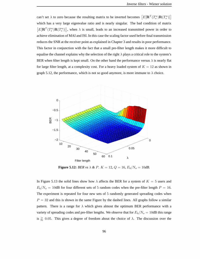
Inverse filters - Wiener solution

can’t set λ to zero because the resulting matrix to be inverted becomes[E[RT (T ns )R(T ns )]

]

which has a very large eigenvalue ratio and is nearly singular. The bad condition of matrix[E[RT (T ns )R(T ns )]

], when λ is small, leads to an increased transmitted power in order to

achieve elimination of MAI and ISI. In this case the scaling factor used before final transmission

reduces the SNR at the receiver point as explained in Chapter 3 and results in poor performance.

This factor in conjunction with the fact that a small pre-filter length makes it more difficult to

equalise the channel explains why the selection of the right λ plays a critical role to the system’s

BER when filter length is kept small. On the other hand the performance versus λ is nearly flat

for large filter length, at a complexity cost. For a heavy loaded system of K = 12 as shown in

graph 5.12, the performance, which is not so good anymore, is more immune to λ choice.

0

0.05

0.1

1020

3040

5060

−2

−1.5

−1

−0.5

0

λFilter length

BE

R

Figure 5.12: BER vs λ & P . K = 12, Q = 16, Eb/No = 10dB.

In Figure 5.13 the solid lines show how λ affects the BER for a system of K = 5 users and

Eb/No = 10dB for four different sets of 5 random codes when the pre-filter length P = 16.

The experiment is repeated for four new sets of 5 randomly generated spreading codes when

P = 32 and this is shown in the same Figure by the dashed lines. All graphs follow a similar

pattern. There is a range for λ which gives almost the optimum BER performance with a

variety of spreading codes and pre-filter lengths. We observe that for Eb/No = 10dB this range

is ' 0.05. This gives a degree of freedom about the choice of λ. The discussion over the

96

Inverse filters - Wiener solution

relationship between BER, λ and Eb/No is in the next section.

0 0.05 0.1 0.15 0.2 0.25 0.3

10−4

10−3

10−2

10−1

100

λ

BE

R

16 taps32 taps

Figure 5.13: BER vs λ. K = 5, Q = 16, Eb/No = 10dB.

0

0.05

0.1

468101214

−10

−8

−6

−4

−2

0

Eb/N

oλ

log1

0−B

ER

Figure 5.14: BER vs Eb/No & λ. K = 5, Q = 16, P = 32.

97

Inverse filters - Wiener solution

5.6.2 BER vs λ & Eb/No

Since λ is the power control term it is expected that the best value for it is a function of Eb/No.

In Figure 5.14 the performance in terms of BER versus different choices of λ and Eb/No is

shown. The CDMA system is one of 5 users with random selected codes and pre-filter length

set to 32 taps. Channels are always multipath with the profile given in table 2.3. From the

contour diagram in the xy plane we can draw the conclusion that for low Eb/No there is a

wide range where the BER versus λ is nearly flat. The flat range begins around the value of

0.04−0.05 for λ. In contrast, for Eb/No higher than 12dB the BER is a more sensitive function

of λ and the best performance is shifted to smaller λ values (' 0.025). We assume here that

for a telecommunication system the average Eb/No encountered is 10dB and, therefore, our

conclusions are drawn relied on the 10dB line. In the next two figures these remarks are more

clear.

0 0.05 0.1 0.15 0.210

−7

10−6

10−5

10−4

10−3

10−2

10−1

100

λ

BE

R

Eb/N

o=3−15dB

Figure 5.15: BER vs λ. P = 32, K = 5, Q = 16.

From Figure 5.15 we observe the relationship between the BER of a 5 users system and λ for

Eb/No that varies from 3 to 15dB. The channels used follow the profile that is presented in

table 2.3. Again it is shown that the higher the Eb/No the closer to zero the best value for λ

is shifted. On the other hand, for Eb/No / 12dB the graphs are almost flat. Similar results

are drawn for the case that the system under consideration is loaded up to 12 users while the

spreading gain remains to Q = 16, as shown in Figure 5.16. These results hold on even for

98

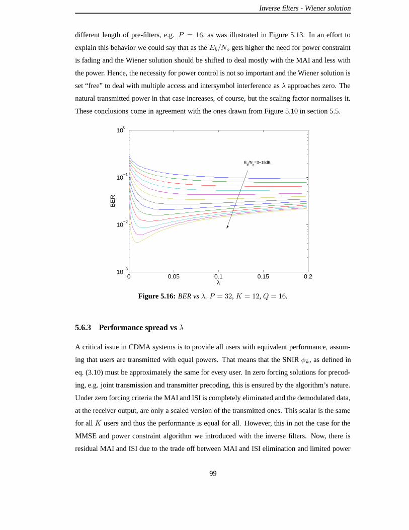
Inverse filters - Wiener solution

different length of pre-filters, e.g. P = 16, as was illustrated in Figure 5.13. In an effort to

explain this behavior we could say that as the Eb/No gets higher the need for power constraint

is fading and the Wiener solution should be shifted to deal mostly with the MAI and less with

the power. Hence, the necessity for power control is not so important and the Wiener solution is

set “free” to deal with multiple access and intersymbol interference as λ approaches zero. The

natural transmitted power in that case increases, of course, but the scaling factor normalises it.

These conclusions come in agreement with the ones drawn from Figure 5.10 in section 5.5.

0 0.05 0.1 0.15 0.210

−3

10−2

10−1

100

λ

BE

R

Eb/N

o=3−15dB

Figure 5.16: BER vs λ. P = 32, K = 12, Q = 16.

5.6.3 Performance spread vs λ

A critical issue in CDMA systems is to provide all users with equivalent performance, assum-

ing that users are transmitted with equal powers. That means that the SNIR φk, as defined in

eq. (3.10) must be approximately the same for every user. In zero forcing solutions for precod-

ing, e.g. joint transmission and transmitter precoding, this is ensured by the algorithm’s nature.

Under zero forcing criteria the MAI and ISI is completely eliminated and the demodulated data,

at the receiver output, are only a scaled version of the transmitted ones. This scalar is the same

for all K users and thus the performance is equal for all. However, this in not the case for the

MMSE and power constraint algorithm we introduced with the inverse filters. Now, there is

residual MAI and ISI due to the trade off between MAI and ISI elimination and limited power

99

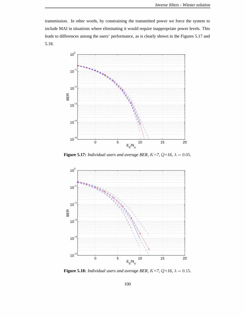
Inverse filters - Wiener solution

transmission. In other words, by constraining the transmitted power we force the system to

include MAI in situations where eliminating it would require inappropriate power levels. This

leads to differences among the users’ performance, as is clearly shown in the Figures 5.17 and

5.18.

0 5 10 15 2010

−5

10−4

10−3

10−2

10−1

100

Eb/N

o

BE

R

Figure 5.17: Individual users and average BER, K=7, Q=16, λ = 0.05.

0 5 10 15 2010

−5

10−4

10−3

10−2

10−1

100

Eb/N

o

BE

R

Figure 5.18: Individual users and average BER, K=7, Q=16, λ = 0.15.

100

Inverse filters - Wiener solution

In Figure 5.17 the BER versus Eb/No is illustrated for a system ofK = 7 users, when λ = 0.05

and P = 32. This time, the graphs are produced by means of Monte-Carlo simulations. The

solid line corresponds to the average BER of the system while the dashed lines are the individual

performances for each one of the seven users. The same system is depicted in Figure 5.18, but

now the Wiener solution is calculated with λ set to 0.15. It is obvious that in the first case the

users are almost equivalent in performance while in the later there is a ’performance spread’

among the users, which becomes more significant for higher Eb/No.

0 0.05 0.1 0.15 0.2 0.25 0.31

1.5

2

2.5

3

3.5

4

λ

Φs

16 taps32 taps

Figure 5.19: SNIR spread vs λ. K = 5, Q = 16, L = 11, Eb/No = 10dB.

To achieve a deeper insight of how λ affects the system we recall the performance spread Φxs

as defined in eq. (3.13). This gives a good idea of the “gap” between the best and the worst

performance in a system of K users, when equal powers are considered. In Figure 5.19 the

performance spread versus λ value is shown for a system of 5 users and Eb/No = 10dB when

filter length is set to 16 or 32 taps. The solid lines represent analytical results for 4 sets of 5

different random spreading codes when P = 16. The dashed lines represent analytical results

for 4 new sets of 5 randomly generated codes when P = 32. In both cases the results are

similar. An important conclusion that can be drawn from these graphs is that large values of λ

result in significant differences in the users’ performance while small values result in similar

performance.

Φ8s is illustrated as a function of two variables, λ & filter length P for K = 5 in the Figure

101

Inverse filters - Wiener solution

5.20. It is apparent that across any filter length, inequalities among users’ performance are more

intense as λ increases. The Φ8s is larger for small filter lengths due to insufficient precoding/pre-

equalisation. In figures 5.21(a) and 5.21(b) Φs versus Eb/No & λ is shown for P = 16 and

P = 32 respectively. The graphic representation in the two Figures has nearly the same pattern.

For any yz plane the performance spread increases with the Eb/No. This is consistent with the

remarks from Figures 5.17 and 5.18 and it is explained as follows.

AWGN is assumed to be the same for all users in a cell and thus the differences among users

performance is due to MAI and ISI. Therefore, for low Eb/No, the overwhelming interference

is the noise and the system is more likely to have a performance spread close to unity. On the

other hand, for high Eb/No MAI and ISI (mostly MAI) are the dominant disturbances and these

result in larger Φs. The solution is a small λ under the restriction of not increasing too much

the power.

The graphs of this section proved that there is more to say than the numerical solution given for

the parameter λ in section 5.5. These remarks are given in a summary next.

0

0.1

0.2

10

20

30

40

1

1.2

1.4

1.6

1.8

2

λFilter length

Per

form

ance

spr

ead

Φs8

Figure 5.20: SNIR spread vs λ & P . K = 5, Q = 16, Eb/No = 8dB.

102

Inverse filters - Wiener solution

0

0.1

0.2

05

1015

20

1

1.5

2

2.5

3

3.5

Eb/N

oλ

Per

form

ance

spr

ead

Φs

(a) K=5, Q=16, P = 16

0

0.1

0.2

05

1015

20

1

1.5

2

2.5

3

3.5

Eb/N

oλ

Per

form

ance

spr

ead

Φs

(b) K=5, Q=16, P = 32.

Figure 5.21: Φs vs λ & Eb/No

5.6.4 Discussion

The bisection algorithm given in eq. (5.49) converges to the λ that satisfies two criteria simulta-

neously. It minimises the mean squared error and ensures that the averaged transmitted power

per symbol is the desired one. But analytical and simulated results show that by relaxing the

criteria better results can be achieved. By letting the power of sp to exceed the desired level and

then scaling it to Eg the BER performance can be significantly improved. Depending on the

conditions (e.g. Eb/No) the Wiener solution trades off between power constraint and ISI-MAI

cancellation. High Eb/No ' 12dB requires small λ (e.g.. λ / 0.025) to allow the suppression

of the dominant MAI and ISI and keep the unscaled power to reasonable limits. For these range

of Eb/No the BER is sensitive to λ choice. Things are more clear when Eb/No / 12dB for

a variety of scenarios. Now the BER performance is almost flattened versus λ for λ ≥ 0.05.

This gives a degree of freedom, which is restricted by the need to keep the performance among

different users in the same levels. The performance spread is increased proportionally with

λ. Consequently, of the available range of λ values we choose the smallest (λ ' 0.05). In

addition, it is shown that the longer the tap-vector of the pre-filters (P ), the less sensitive is the

system’s characteristics to λ parameter. However, it is desirable to keep P small for complexity

reasons. In conclusion, a rough empirical rule could be proposed for the choice of λ based on

103

Inverse filters - Wiener solution

the knowledge of Eb/No:

Eb/No

/ 12dB then λ ' 0.05

' 12dB then λ / 0.025(5.50)

5.7 Simulation results-Comparison

In this section the results are produced by means of Monte Carlo simulations. We compare

the INVF with the methods described in Chapter 4. Complexity comparison takes place and

it is also shown how the analytical performance calculated in Chapter 3 is consistent with the

simulation results. The basic assumptions for the simulations are the same as presented in

section 2.5, which we repeat briefly here.

BPSK data symbols dmk are spread by random binary spreading codes ck of length Q = 16

and transmitted synchronously over the mobile channel. Variations of the received power due

to path loss and log-normal fading are assumed to be eliminated by power control. Each of

the users is assumed to be transmitted with equal energy which is normalised to have unit

amplitude. The codes are also normalised to have unit power. The scheme of unequal powers

will also be addressed. The mobile radio channels are different for each user and the tap weights

are normalised to ‖hk‖ = 1. The delay profile adopted is the one of the channel A case in

[114], which is line with the UMTS European system and has a delay spread of L = 11 chips.

Their impulse response is given in table 2.3 of section 2.5.1. The channels are assumed to be

stationary with no Doppler effects. Perfect knowledge of the downlink channel is presumed in

the BS. For the DPF and INVF methods the delay, ∆, in sampling the output at the receiver is

set to half the pre-filter length [111].

In Figure 5.22 the BER performance versus the length of the pre-filters for the DPF and INVF

is displayed for a CDMA system of 5 users and Eb/No = 10dB. The parameter λ in INVF is

set to 0.05 as derived from the previous section. Analytical curves are displayed along with

the simulation results. It is obvious that the performance of INVF dramatically exceeds the

performance of DPF. For a filter length close to the number of users, DPF encounters near rank

deficiency of the matrices to be inverted [78]. This is mirrored in the graph by the mismatch of

the analytical and the simulated results for small filter lengths. Furthermore, according to the

algorithm presented in [78] the pre-filter length for DPF is restricted to P ≤ ∆ + Q whereas

the length for the INVF can be arbitrarily chosen. It is worth noting how closely the analytical

104

Inverse filters - Wiener solution

0 5 10 15 20 25 30 35 4010

−4

10−3

10−2

10−1

100

Filter length

BE

R

Simulated DPFSimulated INVFAnalytical DPFAnalytical INVF

Figure 5.22: BER vs P . K = 5, Eb/No = 10dB, Q = 16. λ = 0.05 for INVF.

graphs correspond to the simulation results. The improved performance of INVF over the DPF

is expected due to the power constraint incorporated in the algorithm and the MMSE approach

adopted in comparison with the ZF one of DPF.

In the next two figures the BER versusEb/No of INVF is shown and compared with pre-RAKE,

TP, JT and DPF in a severe multipath propagation environment. A system of K = 5 and one

of K = 14 is considered in Figure 5.23 and Figure 5.24 respectively. In Figure 5.23 TP is

illustrated for both a matched filter (TP-MAT) and a RAKE (TP-RAKE) receiver versions. TP-

RAKE is omitted in Figure 5.24 to ease the congestion of the graph. In these simulations the

end-bits of the block transmitting techniques are being discarded for the sake of consistency

with the analytical results in chapter 3. Their contribution to the performance deterioration

is negligible. For K = 5, JT and INVF have the same performance and by far outperform

the other techniques. For K = 14 INVF is the best technique for reasonable Eb/No with

a significant error floor in performance when P = 32. By increasing the number of taps to

P = 90 taps and selecting λ = 0.003, ideal for Eb/No = 20dB, INVF performance is further

improved and becomes consistently better than JT. However, the penalty is a degradation in the

low Eb/No ratio region, when compared with the (P = 32, λ = 0.05)-graph and it results in

a crossing point at about 12dB. This is due to the fact that λ = 0.003, selected for the case of

P = 90, is not the best choice for Eb/No = 10dB, according to our conclusions in expression

105

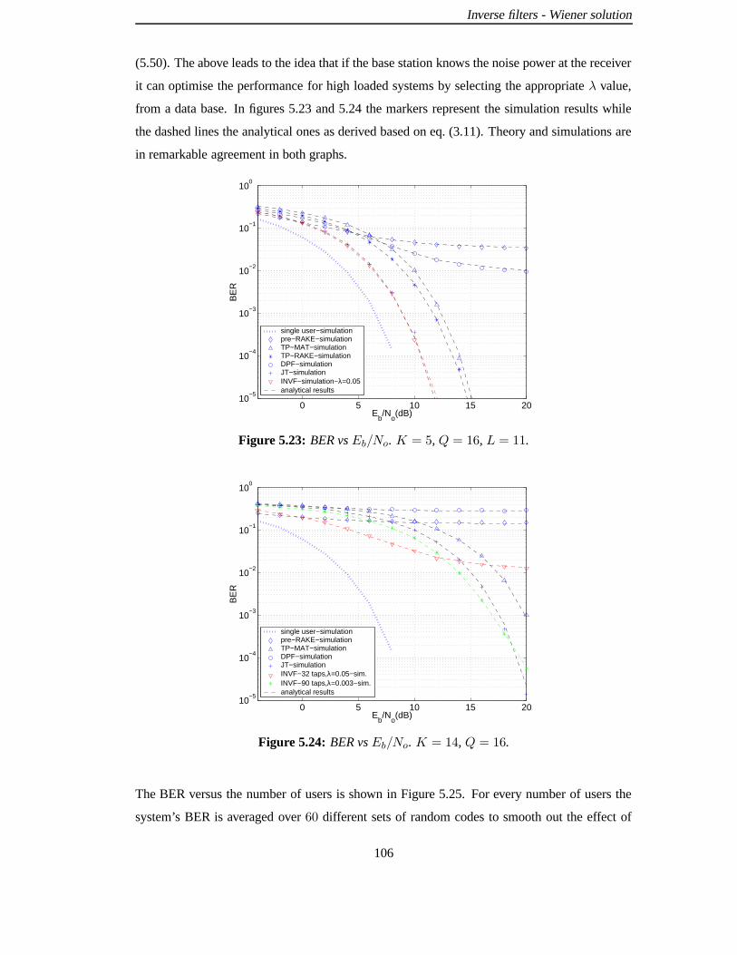
Inverse filters - Wiener solution

(5.50). The above leads to the idea that if the base station knows the noise power at the receiver

it can optimise the performance for high loaded systems by selecting the appropriate λ value,

from a data base. In figures 5.23 and 5.24 the markers represent the simulation results while

the dashed lines the analytical ones as derived based on eq. (3.11). Theory and simulations are

in remarkable agreement in both graphs.

0 5 10 15 2010

−5

10−4

10−3

10−2

10−1

100

Eb/N

o(dB)

BE

R

single user−simulationpre−RAKE−simulationTP−MAT−simulationTP−RAKE−simulationDPF−simulationJT−simulationINVF−simulation−λ=0.05analytical results

Figure 5.23: BER vs Eb/No. K = 5, Q = 16, L = 11.

0 5 10 15 2010

−5

10−4

10−3

10−2

10−1

100

Eb/N

o(dB)

BE

R

single user−simulationpre−RAKE−simulationTP−MAT−simulationDPF−simulationJT−simulationINVF−32 taps,λ=0.05−sim.INVF−90 taps,λ=0.003−sim.analytical results

Figure 5.24: BER vs Eb/No. K = 14, Q = 16.

The BER versus the number of users is shown in Figure 5.25. For every number of users the

system’s BER is averaged over 60 different sets of random codes to smooth out the effect of

106

Inverse filters - Wiener solution

2 4 6 8 10 12 14 1610

−5

10−4

10−3

10−2

10−1

100

Number of users

BE

R

pre−RAKETP−MATDPFJT−block 32INVF−λ=0.05

Figure 5.25: BER vs K . Eb/No = 10dB, Q = 16. P = 32 for INVF and DPF. λ = 0.05 forINVF.

codes with low or high crosscorrelation. Eb/No is set to 10dB and for INVF and DPF the pre-

filters have a length of P = 32 taps. It is clear that INVF outperform TP, Pre-RAKE and DPF.

INVF exhibits better performance than JT for a heavily loaded CDMA system. For a system

loaded to a number of users less than half the spreading gain INVF and JT are competitive in

terms of performance but it worths examining the computational cost of the two methods. The

block length for JT is set to N = 32 bits. The matrices that need to be inverted for both JT and

INVF algorithms have the same dimensions. Thus, we examine the multiplications needed per

symbol per user after any matrix inversion has been completed. Recalling the computational

cost as issued for blockwise and bitwise techniques in Chapter 3, table 5.1 is obtained. INVF

Algorithm Size of matrix to be inverted Number of Multiplicationswhen channel changes per symbol

(excluding inversions)

JT NK ×NK = 160 × 160 N 2KQ = 81920INVF PK × PK = 160 × 160 PQ = 512

The numerical examples correspond to the case of N = 32, K = 5, Q = 16, P = 32.

Table 5.1: INVF vs JT computational cost comparison

requires a lot less computational cost than JT. The block length of JT can by reduced at the

107

Inverse filters - Wiener solution

cost of capacity loss if N is too small, due to incorrect precoding of the end-bits of the block.

Moreover, the blocks to be transmitted in a real CDMA system are much longer than the 32

length used in Figure 5.25.

The degree of deterioration in performance due to severity in multipath channels is shown

in Figures 5.26 and 5.27. Only JT and INVF are shown as they both outperform the other

0 5 10 15 2010

−5

10−4

10−3

10−2

10−1

100

Eb/N

o(dB)

BE

R

INVF AWGNJT AWGNINVF mild multipathJT mild multipathINVF severe multipathJT severe multipath

Figure 5.26: Channel’s effect for spreading codes set 1.

techniques and compete in performance terms. For each algorithm the BER is shown for a

AWGN channel along with the BER for a mild and a severe multipath channels. The system

chosen is one of K = 6 users and the filters length is set to P = 40 taps. For JT the end

bits are discarded. The difference between the two graphs is the set of spreading codes used

(denoted as spreading codes set 1 and 2). The severe multipath channels follow the same

pattern as shown in table 2.3, while for the mild channel is as in table 5.2. As observed from

both graphs, deterioration in performance occurs to the same extent for both algorithms and as

expected is more significant and apparent when a severe multipath environment is considered.

The difference in performance among the two Figures reflects the effect that different random

codes can have on a system.

108

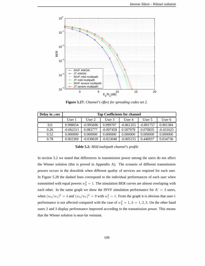
Inverse filters - Wiener solution

0 5 10 15 2010

−5

10−4

10−3

10−2

10−1

100

Eb/N

o(dB)

BE

R

INVF AWGNJT AWGNINVF mild multipathJT mild multipathINVF severe multipathJT severe multipath

Figure 5.27: Channel’s effect for spreading codes set 2.

Delay in µsec Tap Coefficients for channel

User 1 User 2 User 3 User 4 User 5 User 6

0.0 0.998054 -0.995696 0.999707 -0.861355 -0.891757 0.9013840.26 -0.062311 0.083777 -0.007458 0.507978 0.070835 -0.4316250.52 0.000000 0.000000 0.000000 0.000000 0.000000 0.0000000.78 0.002369 -0.039639 -0.023048 -0.005155 0.446937 0.034736

Table 5.2: Mild multipath channel’s profile

In section 5.2 we stated that differences in transmission power among the users do not affect

the Wiener solution (this is proved in Appendix A). The scenario of different transmission

powers occurs in the downlink when different quality of services are required for each user.

In Figure 5.28 the dashed lines correspond to the individual performances of each user when

transmitted with equal powers w2k = 1. The simulation BER curves are almost overlaping with

each other. In the same graph we show the INVF simulation performance for K = 3 users,

when (w2/w1)2 = 4 and (w3/w1)

2 = 9 with w21 = 1. From the graph it is obvious that user-1

performance is not affected compared with the case of w2k = 1, k = 1, 2, 3. On the other hand

users 2 and 3 display performance improved according to the transmission power. This means

that the Wiener solution is near-far resistant.

109

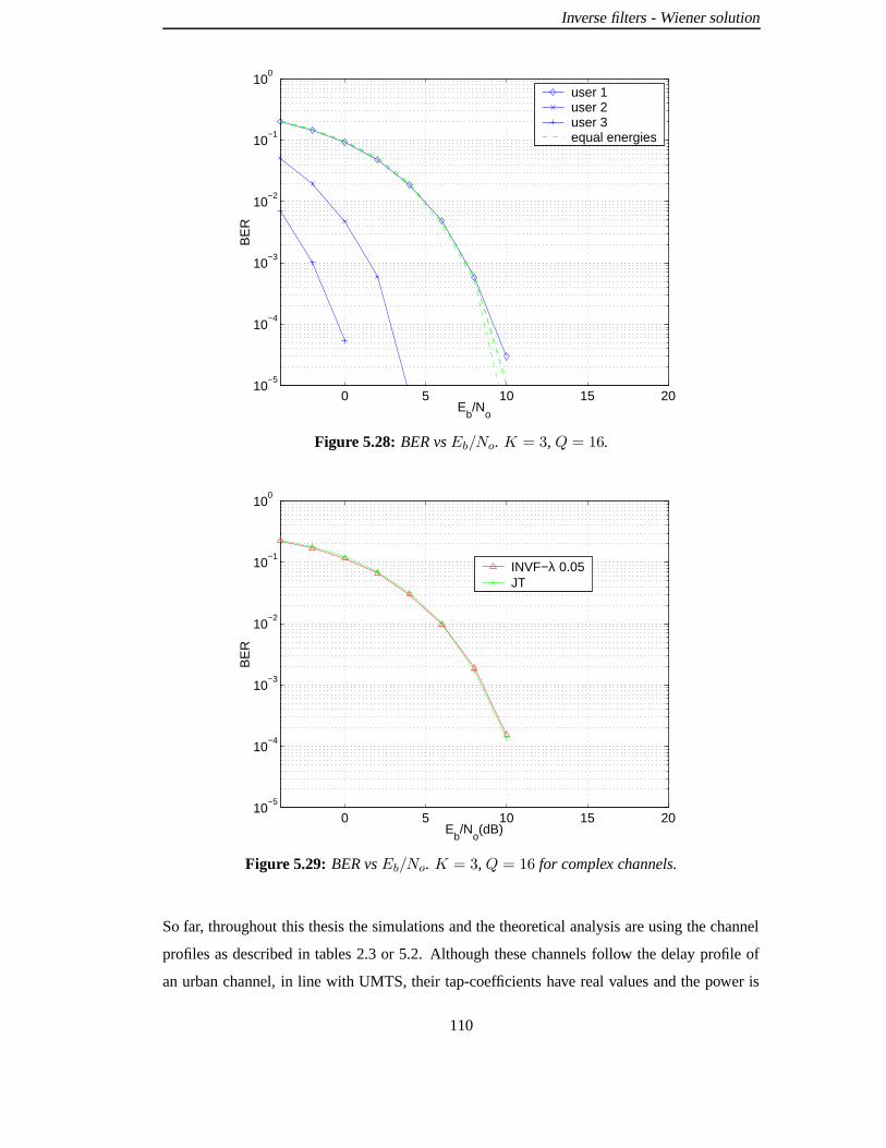
Inverse filters - Wiener solution

0 5 10 15 2010

−5

10−4

10−3

10−2

10−1

100

Eb/N

o

BE

R

user 1user 2user 3equal energies

Figure 5.28: BER vs Eb/No. K = 3, Q = 16.

0 5 10 15 2010

−5

10−4

10−3

10−2

10−1

100

Eb/N

o(dB)

BE

R

INVF−λ 0.05JT

Figure 5.29: BER vs Eb/No. K = 3, Q = 16 for complex channels.

So far, throughout this thesis the simulations and the theoretical analysis are using the channel

profiles as described in tables 2.3 or 5.2. Although these channels follow the delay profile of

an urban channel, in line with UMTS, their tap-coefficients have real values and the power is

110

Inverse filters - Wiener solution

equivantly distributed among them, which is not very realistic. The channel tap-coefficients in

a real system are complex numbers and they can follow a Rayleigh distribution, time varying

with a Doppler frequency. Figure 5.29 displays the average BER of three users. The techniques

compared are the INVF and JT. Each tap-coefficient is time varying and complex. The real and

imaginary part are simulated independently as sum of sinus [115, 116] with a selected Doppler

frequency. The power of tap-coefficient has a Rayleigh distribution. Each one of the three

channels is initialised with different phases to achieve uncorrelated results. We let the channels

run for 20 seconds, with Doppler frequencies of 30-90 Hz. We lock them and then run the BER

simulation for INVF and JT. The set of channels was for both graphs the same for the sake of

fair comparison and they are demonstrated in table 5.3.

Delay in µsec Tap Coefficients for channel

User 1 User 2 User 3

0.00 -0.242974-j0.303296 0.220272-j0.342193 -0.612400+j0.7304950.26 -0.125466-j0.063417 -0.099331-j0.277136 -0.444251-j0.6694370.52 0.000000-j0.000000 0.000000-j0.000000 0.000000-j0.0000000.78 0.010125+j0.036019 -0.066840+j0.004550 -0.048003+j0.2645311.04 0.174803+j0.117559 -0.071114+j0.103831 -0.238124-j0.1233691.30 0.000000-j0.000000 0.000000-j0.000000 0.000000-j0.0000001.56 0.000000-j0.000000 0.000000-j0.000000 0.000000-j0.0000001.82 0.027070+j0.011528 -0.107521-j0.036790 -0.089175-j0.0840122.08 0.000000-j0.000000 0.000000-j0.000000 0.000000-j0.0000002.34 0.000000-j0.000000 0.000000-j0.000000 0.000000-j0.0000002.60 0.074906+j0.012934 -0.006503-j0.048724 0.052034-j0.031326

Table 5.3: Complex multipath channel’s profile

5.8 Summary

In this Chapter a new technique was proposed called inverse filters originating from the stereo-

phonic sound reproduction systems. The algorithm was appropriately modified and the power

constraint was added to it. The Wiener solution was calculated and given in a closed form,

while the power constraint parameter λ was thoroughly investigated. The technique is bitwise

and outperforms DPF, TP-MAT and TP-RAKE. INVF also outperforms JT for heavily loaded

systems, while the methods are competitive when K ≤ Q/2 for sufficiently large data-block

length. However, INVF requires significantly less computational cost than JT. The simulation

BER curves for a variety of precoding techniques, produced in this Chapter, were in ultimate

111

Inverse filters - Wiener solution

agreement with the analytical ones as derived from the analysis in Chapter 3. INVF can be

easily adjusted to any existing CDMA-TDD system with slowly varying propagation channels.

112

Chapter 6Multichannel adaptive algorithms

In this Chapter we will examine adaptive transmitter based techniques that reduce MAI and

ISI in a TDD system. Part of this work has been published in [117]. Section 6.1 presents the

motivation that inspired the study of adaptive techniques and the link with the Wiener solution

for INVF, as given in Chapter 5. Section 6.2 introduces filtered-X. The adaptive multichannel

techniques are described in section 6.3. In sections 6.4 and 6.5 there is a discussion about

convergence speed and BER performance.

6.1 Motivation

The fundamental basis that precoding techniques rely on is that the base station (transmitter)

has knowledge of all the downlink channels plus the receiver structure (filters matched to the

spreading codes) of the mobile stations. In Chapter 4 and Chapter 5 the methods presented

use this knowledge to implement algorithms that calculate directly a precoded signal which

is ISI and MAI resistant prior to transmission. These algorithms include inversion of one or

more matrices, which contributes to the complexity and computational cost. Pre-RAKE doesn’t

involve any matrix inversion but its performance for a multiuser scheme is rather poor. A matrix

inversion free technique is then sought.

In conventional receiver based equalisation or multiuser detection systems adaptive techniques

[11, 69–74, 89] are commonly used to converge to the tap-coefficients that remove the inter-

ference and increase the signal to noise ratio. Therefore the matrix inversion needed for the

receiver based ZF, eq. (2.38), or MMSE, eq. (2.42), is avoided. The objective is to find such

an approach which is feasible for the transmitter based techniques. This idea implies that the

adaptive filters are placed before the channels, within the BS. In active control of sound and

vibration technology an adaptive feedforward technique, named filtered-X, is extensively used

to pre-equalise the sound produced by a loudspeaker and compensate for any distortion caused

by the channel between the microphone and the loudspeaker. Obviously, such an approach

113

Multichannel adaptive algorithms

presumes that the controller, which adaptively sets the pre-filter taps, is provided with the er-

ror sensed at the microphone with a feedback link. An adaptation of this method to a CDMA

system implies that the mobile terminal should receive a training sequence and provide the BS

with the error at its output. However, in wireless telecommunications the feedback from the

receiver to the transmitter in conjunction with the necessary training sequences result in band-

width usage and waste of capacity. Hence, this is not the solution that designers are in favor of.

It would have been ideal if there was no need for the mobile to feed back any error to the BS ,

but yet the error was known to the BS.

Σ

Σ

Σ

Z−∆

Z−∆

d 1

h (n)1

h (n)k

d kdesired

sc (T −n)k

s

1

K

z (n)

Kx (n)

p (n)K

x (n)1

1

d (n)

d (n)

antenna

Base station

K

1

s

to mobiles

n

+

h (n)K c (T −n)K

d K

1d

d K

eK

e1

ee1

K

Adaptive Algorithm

1c (T −n)

p (n)

z (n)

s (n)c (n)K

c (n)1

p

Figure 6.1: Block diagram of emulation in the BS

This is feasible under the TDD scenario according to which the BS along with the knowledge of

the receivers structure is feasible to have an estimate hk(n), k = 1 . . . K , of kth user’s channel

hk(n), from the last uplink burst. There is nothing to prevent then the BS from emulating

the actual system, in a cell, in an internal block. The block diagram of the emulation that

takes place in the BS is shown in Figure 6.1. It is similar to the block diagram suggested for

the INVF with the addition of the adaptive algorithm block and the error feedback lines. The

BS station initialises the tap-coefficients of the pre-filters and then starts transmission. The

resulting sp(n) signal is sent to the BS antenna element and an internal block that emulates the

real receivers and their corresponding channels. By emulating the system, the BS can estimate

the output dk(n) sampled from the mobile. The errors ek = dk − dk, k = 1 . . . K , are fed back

114

Multichannel adaptive algorithms

to the adaptive algorithm and after a number of transmissions the algorithm converges to the

coefficients that minimise the sum of the squares of K error signals. If the same cost function

is used the converged solution should be, ideally, the Wiener solution for INVF. Instead of a

single error as in the conventional adaptation process, a vector of errors

e = [e1 . . . eK ]T (6.1)

is sent now back to the adaptive block. Therefore, an independent adaptive algorithm for each

user’s pre-filter is not effective. A joint adaptive approach should be followed for the simulta-

neous convergence of all the filters pk. This is achieved with the multichannel (MC) adaptive

algorithms for feedforward control as will be explained in a later section.

These algorithms were originally used and investigated for active noise control and sound repro-

duction systems. These systems consist generally by a number of I source signals, a number

of J actuators (typically loudspeakers) and a number of K “error” sensors (typically micro-

phones). In the CDMA systems we examine in the current thesis the source signals are the

K spread spectrum signals addressed to each user, the actuator is one single element antenna

(although this could be generalised for a multiple antenna array) and the the “error” sensors the

K matched filter receivers.

6.2 Filtered-X LMS

It is considered as essential to present a short introduction to the origin and principles of the

monochannel filtered-X algorithm as introduced in [111]. The classic problem of the adaptive

inverse modeling of a noisy plant is illustrated in Figure 6.2(a). The plant noise can be rep-

resented as additive noise at the plant output. This noise is an additive input to the adaptive

filter and is not correlated with the desired-response input to the system. The result of the plant

noise is therefore to cause the adaptive solution to be generally different from that of a close

approximation to the delayed inverse.

The problem of plant noise led to the development of the filtered-X algorithm, which allows

adaptation of the inverse filter placed forward of the plant in the cascade sequence. This ap-

proach is partially illustrated in Figure 6.2(b), where plant noise doesn’t appear in the adaptive

filter input. Consequently, this noise will have no effect on the converged solution for the in-

verse filter provided that the adapting input can be derived properly. Assuming an FIR model,

115

Multichannel adaptive algorithms

Plant

PlantAdaptive

inverse filter

−∆zDelay Line

noise

+−

e

(a)

(b)

e

noise

Adaptive

inverse filter

++ −

?

x y

d

Σ Σ

ΣΣ

+

Figure 6.2: Adaptive inverse modeling of a noisy plant

the mean square of error e in Figure 6.2(b) is a quadratic function of the adaptive filter weights

and the adaptation has the potential for smooth convergence with a unimodal performance sur-

face. The classic least mean squares (LMS) algorithm cannot be used unless an appropriate

“desired” signal is derived to be compared with the adaptive filter output y. The signals d and e

are not sufficient because e is the error at the plant output, not at the adaptive filter output. If e

is used directly with the LMS algorithm to adapt the inverse filter, the adaptive process is very

likely to be unstable or, if not, to converge to an irrelevant solution [111].

The correct approach of the problem as shown in Figure 6.2(b) is shown in Figures 6.3(a)-(c).

In Figure 6.3(a) the noise plant is neglected for the moment and the plant is commuted with

the LMS filter , whereupon the LMS algorithm can be directly applied. Adjusting the weights

to minimise the mean square error e will yield the correct set of weights to minimise the e

in Figure 6.2(b) with plant noise neglected. Next the system diagrammed in Figure 6.3(b) is

regarded. Here the adaptive filter and the plant are cascaded as originally in Figure 6.2(b). The

objective is that the adaptive process shown in Figure 6.3(c) produce the same set of weights

as the systems illustrated in Figure 6.3(a) and (b). Then, the filtered-X algorithm is a viable

solution to the adaptation problem of Figure 6.2(b). Comparing the systems of Figure 6.3(a)

and (b) it is clear that the input signal vectors available to the LMS algorithms in both systems

are identical at all times. However, the errors e are not necessarily identical to each other at

all times. They would be identical if the adaptive FIR filter weight vectors were identical to

each other at all times and if the plant and the adaptive filter were commutable. For the same

116

Multichannel adaptive algorithms

Σ

x

ed+

Plantinverse filter

Adaptive

algorithmLMS

−

inverse filter

Adaptive

algorithmLMS

Plant

Plant

xy

e

Σ+

+g

Σ−

d+

(c)

(a)

inverse filter

Adaptive

algorithmLMS

Plant

Plant Σ

xy

e−

d+

g

g

filtered x

(b) noise

Figure 6.3: Development of filtered-X algorithm

input, the same output results when the positions of two cascaded filters are commutable. They

would be commutable if the plant were linear and if the time variations of the impulse responses

of both the plant and the adaptive filter took place with time constants long compared to the

combined memory times or time constants of the adaptive filter and the plant. Thus assuming

slow adaptation plant and that the adaptive filters are commutable, the weight vectors of the

systems in Figures 6.3(a) and (b) undergo the same changes if the are identically initialised.

Hence, the adaptive process in Figure 6.3(b) is suitable for the problem in Figure 6.2(b). In

Figure 6.3(c) the noise plant is added again to the system. The expected value of the adaptive

weight vector will be the same with the noiseless system in Figure 6.3(b). However it will of

course cause some misadjustment to the weight vector.

117

Multichannel adaptive algorithms

6.3 Multichannel algorithms

The filtered-X technique refers to a single input single output feedforward adaptive system.

Multichannel/multiuser feedforward adaptive algorithms have also been developed. The most

popular of them are the multichannel least mean squares (MC-LMS)1 and multichannel re-

cursive least squares (MC-RLS). Originally in the derivation of these algorithms the power

constraint term was omitted. However, in recent publications control output constraints have

been incorporated into MC-LMS method. The cost function for the derivation of the adaptive

algorithms can be taken directly from Chapter 5 with or without the power constraint term, de-

noted as Jc and J respectively. These techniques adapted to a CDMA system will be described

along with a reference to some alternative versions.

6.3.1 Multichannel LMS

The multichannel LMS algorithm [107] provides a multichannel generalisation of Widrow’s

filtered-X LMS algorithm [111]. It is widely used and it is the benchmark to which most adap-

tive filtering algorithms are compared. In this algorithm, the gradient of the instantaneous sum

of squared error signals is computed as a function of each coefficient in the adaptive filters.

Thus, the method of steepest descent can be used to descend toward the minimum on the per-

formance surface of the quadratic form in eq. (5.11). The values of the pre-filter taps weight

vector are iteratively updated by an amount proportional to the negative of the gradient of the

quadratic performance surface.

The complete cost function to be minimised is as in eq. (5.11) without the power constraint

term:

J = E[dT0 d0] − 2E[dT0 R(T ns )]p + pTE[RT (T ns )R(T ns )]p (6.2)

The gradient ϑJ/ϑp of eq. (6.2) is:

ϑJ

ϑp= −2E[RT (T ns )d0] + 2E[RT (T ns )R(T ns )]p

= −2E[RT (T ns )

(d0 −R(T ns )p

)]

= −2E[

RT (T ns )(d0 − d0(T

ns ))]

(6.3)

1Multichannel LMS can also be found in the bibliography as Multiple error LMS emphasising in the vector errorfeedback

118

Multichannel adaptive algorithms

By defining the instantaneous error vector e(T ns ) between the desired data and the estimated

data as:

e(T ns ) = d0 − d0(Tns ) (6.4)

and substituting in eq. (6.3) the gradient is expressed as:

ϑJ

ϑp= −2E[RT (T ns )e(T ns )] (6.5)

If each pre-filter taps vector is now adjusted at every sample time (T ns ) by an amount propor-

tional to the negative instantaneous value of the gradient, a modified form of the well-known

LMS algorithm is produced:

p(T ns ) = p(T n−1s ) + µRT (T ns )e(T ns ) (6.6)

where µ is the step-size parameter of the algorithm. The error vector e is known to the BS due

to the emulation of the real system as explained in section 6.1.

Recalling equations (5.18) and (5.19) we can ’break’ eq. (6.6) down to the corresponding update

step for the specific pre-filter of each user:

pk(Tns ) = pk(T

n−1s ) + µ

[r1k(T

ns ) · · · rKk(T ns )

]e(T ns ) (6.7)

where rµν(n) as in eq. (5.1).

The representation of eq. (6.7) for individual pre-filters can be realised as shown in Figure

6.4. The block diagram corresponds to the 2-users case. Both in Figures 6.1 and 6.4 zk(n) =

hk ∗ck(Q−n) means that an estimate hk(n) of the downlink channel hk(n) is available. Under

ideal conditions perfect knowledge of the channels is available and thus the internal emulation

reflects the actual system. The detailed block diagram of the MC-LMS algorithm in Figure

6.4 is given for simplicity reasons only for user 2. The analogy with the filtered-X, which is

the monochannel version of MC-LMS, is obvious. Spread signal d2c2(n) is passing in parallel

through the corresponding pre-filter p2(n) and z1, z2 to produce the ’reference signals’ r12(n),

r22(n). Each sample, taken in chip rate, is stored in a corresponding P -length buffer. Estimated

errors e1, e2 multiply the contents of the r12, r22 signal buffers, respectively. The MC-LMS

algorithm is applied then, every Q chips, to update the coefficients of the adaptive pre-filters.

The algorithm is very simple and doesn’t require excessive computational cost. A drawback of

119

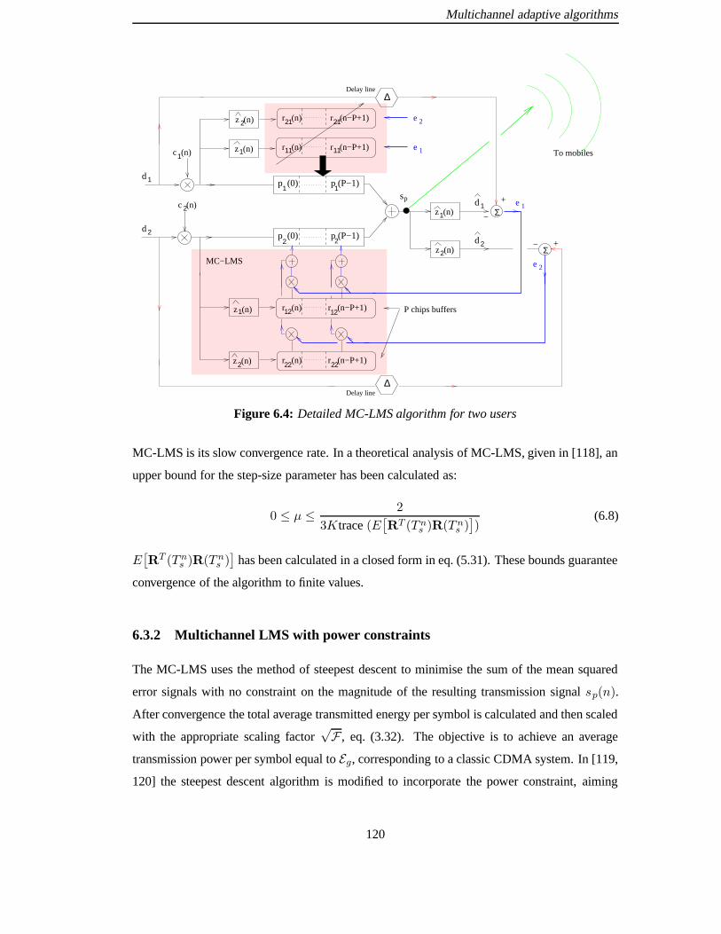
Multichannel adaptive algorithms

e

e

1

2

∆

∆Delay line

Delay line

e 1

e 2

Σ

Σ

11 11

2121

22 22

12 12

1

2

r (n) r (n−P+1)

r (n) r (n−P+1)

r (n) r (n−P+1)

1

2

p (0) p (P−1)

p (0) p (P−1)

r (n) r (n−P+1)

d

1

2

MC−LMS

d

d

1

2

+

−

+

To mobiles

−

P chips buffers

d

z (n)

z (n)

z (n)

z (n)

z (n)

z (n)

2

1

1

2

1

2

c (n)1

c (n)2

sp

Figure 6.4: Detailed MC-LMS algorithm for two users

MC-LMS is its slow convergence rate. In a theoretical analysis of MC-LMS, given in [118], an

upper bound for the step-size parameter has been calculated as:

0 ≤ µ ≤ 2

3Ktrace (E[RT (T ns )R(T ns )

])

(6.8)

E[RT (T ns )R(T ns )

]has been calculated in a closed form in eq. (5.31). These bounds guarantee

convergence of the algorithm to finite values.

6.3.2 Multichannel LMS with power constraints

The MC-LMS uses the method of steepest descent to minimise the sum of the mean squared

error signals with no constraint on the magnitude of the resulting transmission signal sp(n).

After convergence the total average transmitted energy per symbol is calculated and then scaled

with the appropriate scaling factor√F , eq. (3.32). The objective is to achieve an average

transmission power per symbol equal to Eg, corresponding to a classic CDMA system. In [119,

120] the steepest descent algorithm is modified to incorporate the power constraint, aiming

120

Multichannel adaptive algorithms

to render the scaling factor unnecessary. The developed techniques are named leakage and

rescaled MC-LMS algorithms.

6.3.2.1 Leakage algorithm

The leakage algorithm [119], tries to minimise the square moduli of the error signals eTe

subject to the constraint that uTu is less than some upper limit Wmax, with u the control

signals. The cost function is:

E[eTe

]+ λ(uTu−Wmax) (6.9)

This cost function is not in accordance with the block diagram given in Figure 6.1 and certain

modifications need to be done. In our system the control signals u are replaced by the pre-

filtered spread signals ck ∗ pk, k = 1 . . . K . The total average power per symbol ‖Up‖2 =(pTUTUp

)replaces uTu, while the error vector e(T ns ) is as defined in eq. (6.4). Furthermore

Wmax is replaced by Eg and the power constrained cost function is

Jc = J + λ(pTUTUp− Eg

)(6.10)

with J as in eq. (6.2). By usage of equations (5.12) and (6.5) the derivative ϑJc/ϑp is given

by:

ϑJcϑp

= −2E[RT (T ns )e(T ns )] + 2λUTUp = −2(E[RT (T ns )e(T ns )] − λUTUp

)(6.11)

Equation (6.11) can now be used as the basis for an adaptive algorithm using the method of

steepest descent such that the vector of pre-filter taps at the n iteration, denoted as p(T ns ), is

given by:

p(T ns ) = p(T n−1s ) + µ

(RT (T ns )e(T ns ) − λUTUp(T n−1

s ))

(6.12)

After manipulating the right-hand part of (6.12) the following update equation2 is derived

p(T ns ) =(I− λµUTU

)p(T n−1

s ) + µ(RT (T ns )

)(6.13)

2In [119] the update equation given is :

p(T ns ) =

(1 − λµ

)p(T n−1

s ) + µ(R

T (T ns ))

121

Multichannel adaptive algorithms

which is a form of the MC-LMS with leakage [121]. µ is the step-size parameter of the algo-

rithm. The addition of leakage keeps the output power under control by continual removal, or

leakage, of a small value of the weights, which represents a compromise between biasing the

pre-filters weights from the original optimum solution (when cost function is J ) and bounding

the output power [120]. Therefore the final performance of the control algorithm significantly

depends on the value of the leakage coefficient and it is not guaranteed that the final solution

will be within the constraint.

It is possible to increase the performance of the leakage algorithm by applying a time-varying

leakage coefficient λ(T ns ). The value of λ(T ns ) is changed during adaptation and made depen-

dent on the value of ‖Up(T ns )‖2, which is calculated in every updating step. A method of

scheduling λ(T ns ) on ‖Up(T ns )‖2 is proposed in [119] and is given in eq. (6.14). According

to that λ(T ns ) is set to zero if ‖Up(T ns )‖2 is less than 90% of Eg and then it is increased in

proportion to the value of ‖Up(T ns )‖2 above this value.

λ(T ns ) =

0 ‖Up(T ns )‖2 ≤ 0.9Eg‖Up(Tn

s )‖2−0.9Eg

Eg‖Up(T ns )‖2 ≥ 0.9Eg

(6.14)

6.3.2.2 Rescaling algorithm

An alternative way to solve this problem is to use the idea of the active set method (a gradient

projection method focused on the solution of the Kuhn-Tucker equations), which is widely used

in the field of constrained optimisation to solve the nonlinear programming problem. The active

set method is an iterative procedure that involves two phases: the first phase calculates a feasible

point (a weight vector satisfies the constraint); the second phase generates an iterative sequence

of feasible points that converge to the solution. The search direction for generating the sequence

of feasible points is calculated by projecting the gradient along the constraint boundary if the

constraint is violated. Depending on the quadratic nature of the objective function and the

strictly convex property of the constraint set, the algorithm should converge to the minimum

under the constraints. The algorithm so obtained is called the rescaling algorithm and is given

in [120] for a single-input single-output problem, which corresponds to the filtered-X. Here,

we generalise this method to the multichannel/multiuser case. According to this algorithm the

weight vector p and output signal sp(n) are rescaled after updating as follows:

p(T ns ) = p(T n−1s ) + µRT (T ns )e(T ns ) (6.15)

122

Multichannel adaptive algorithms

if Eg(T ns ) = p(T ns )UTUp(T ns ) ≥ Eg, then

p(T ns ) = p(T ns )√

Eg/Eg(T ns ) (6.16)

sp(Tns ) = sp(T

ns )√

Eg/Eg(T ns ) (6.17)

The original MC-LMS algorithm uses the estimated gradient RT (T ns )e(T ns ) as the weight up-

date vector, which, however, sometimes makes the output power per symbol greater than the

desired Eg after convergence. The rescaling algorithm remedies the problem by projecting the

estimated gradient into the constraint set to obtain the new updated vector, which is simply ob-

tained in eq. (6.17) by rescaling the control weight vector and control output after the updating.

6.3.3 Multichannel RLS

For the learning of FIR filters using linear adaptive filtering algorithms, it is well known that

classic recursive-least-squares algorithms [89] produce a faster convergence speed than stochas-

tic gradient descent techniques, such as the basic least mean squares algorithm [111]. This con-

clusion remains valid for the feedforward control systems like active noise control. The filtered-

X monochannel RLS algorithm for active noise control has been introduced in [122, 123]. In

[106] the filtered-X RLS is upgraded to deal with a multichannel/multiuser scheme. To update

the coefficients of the adaptive filters, the multichannel RLS algorithm uses an approach similar

to the multichannel LMS algorithm, in the update eq. (6.6), but a gain matrix is used to mul-

tiply the error signals, instead of directly using the rµν(n), µ, ν = 1 . . . K filtered-reference

signals. MC-RLS algorithm combines a decorrelation of the filtered-reference signals (reduc-

ing the effect of the eigenvalue spread in the filtered-reference signals correlation matrix) and a

minimisation of a weighted sum of the past squarred errors.

Each input sample in the input vector of the classical RLS algorithm is replaced by a P ×K

matrix, to produce the MC-RLS filtered-reference matrix V(n), whose dimensions are KP ×K:

V(n) =

r11(n) · · · rK1(n)...

. . ....

r1K(n) · · · rKK(n)

(6.18)

123

Multichannel adaptive algorithms

The number of rows in V(n) 3reflects the total number of coefficients in all the adaptive filters

(degrees of freedom in the system), while the number of columns reflects the number of error

signals to be minimised by the adaptive filters. The P -length weight vector (adaptive filter) in

the classical RLS algorithm is replaced by KP vector p, eq. (3.28), that contains the weights

of all filter-taps. Error vector e, defined in eq. (6.1), replaces the scalar error of the classic RLS.

Then the multichannel RLS algorithm is:

M(0) = δ−1I, I : K ×K identity matrix (6.19)

p(0) = 0 (6.20)

K(T ns ) = θ−1M(T n−1s )V(T ns )

[I + θ−1VT (T ns )M(T n−1

s )V(T ns )]−1

(6.21)

e(T ns ) = d(T ns ) −R(T ns )p(T n−1s ) (6.22)

p(T ns ) = p(T n−1s ) + K(T ns )e(T ns ) (6.23)

M(T ns ) = θ−1M(T n−1s ) − θ−1K(T ns )VT (T ns )M(T n−1

s ) (6.24)

The factor θ in equations (6.20) and (6.24) is a “forgetting factor” (typically 0.9 ≤ θ ≤ 1.0)

that enables RLS-type algorithms to track the statistics of the input signals (filtered-reference

signals in this case) if they are time varying. δ is a small positive constant [89].

In the MC-RLS presented there was no power constraint incorporated. Therefore after setting

the filter coefficients we must scale the transmitted signal sp(n) with a factor√F to achieve the

desired average total transmitted energy per symbol. An effort to use the rescaling MC-LMS

principles in the MC-RLS by means of simulations resulted in an unstable algorithm.

Both the unconstrained MC-LMS and MC-RLS algorithms are derived from the unconstrained

cost function J , presented in eq. (6.2). They try to converge adaptively to the unconstrained

Wiener solution, as in eq. (5.17) for λ = 0. In other words, both algorithms compute recur-

sively the value of the inverse of a time-averaged correlation matrix [RT (T ns )R(T ns )]. However

instability can occur if the correlation matrix is ill-conditioned. In multichannel systems, the

ill-conditioning may be caused by some coupling between the different “channels” or between

the difference reference signals, or simply by the finite numerical resolution. In MC-RLS this

3In [106] vector p is defined as p = [p1(0) . . . pK(0) . . . pK(P − 1) . . . pK(P − 1)] and thus matrix V(n)has a different representation. The matrix content remains the same but the arrangement of the rows is different toconform with the V(n) definition.

124

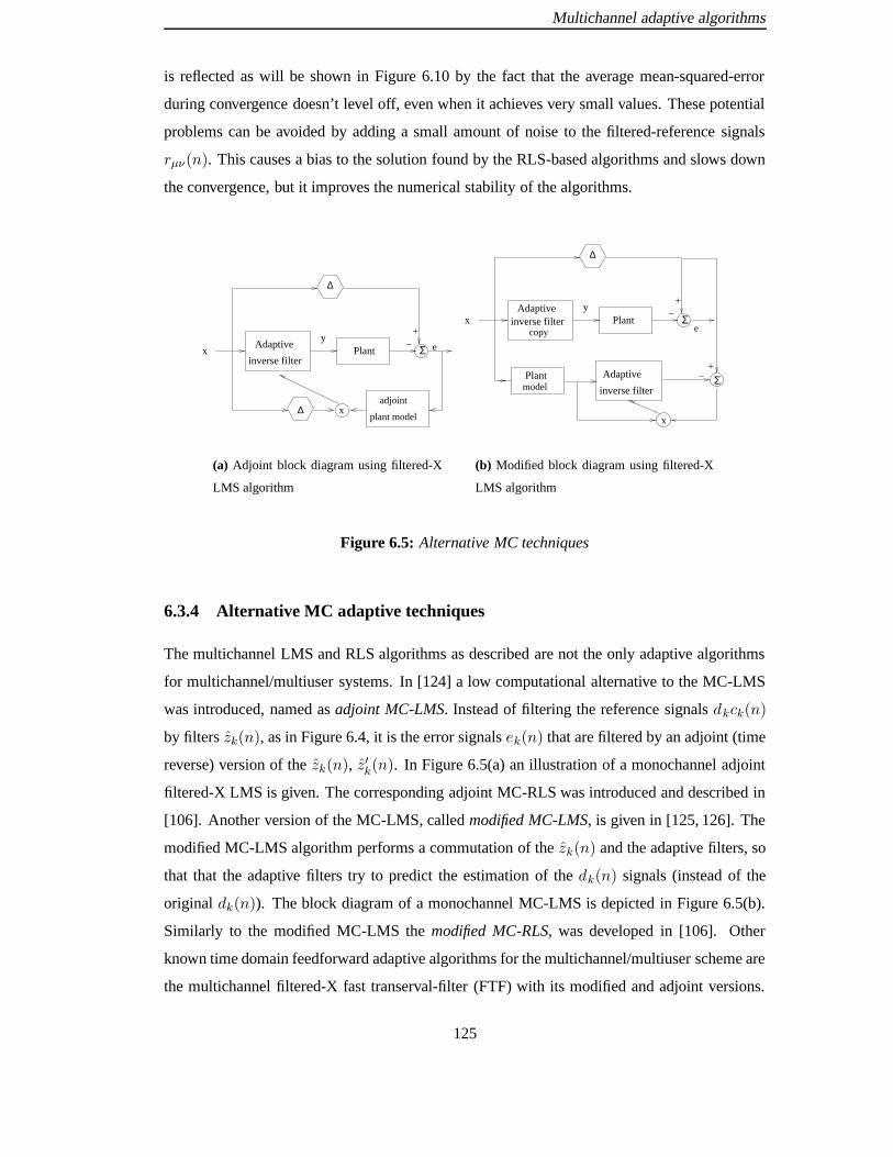
Multichannel adaptive algorithms

is reflected as will be shown in Figure 6.10 by the fact that the average mean-squared-error

during convergence doesn’t level off, even when it achieves very small values. These potential

problems can be avoided by adding a small amount of noise to the filtered-reference signals

rµν(n). This causes a bias to the solution found by the RLS-based algorithms and slows down

the convergence, but it improves the numerical stability of the algorithms.

inverse filter

AdaptivePlant Σ

+−

plant model

adjoint∆

∆

xy

x

e

(a) Adjoint block diagram using filtered-X

LMS algorithm

Σ

+−

∆

xyAdaptive

inverse filtercopy

Adaptive

inverse filter

Plant

Plantmodel

Σ+

−

e

x

(b) Modified block diagram using filtered-X

LMS algorithm

Figure 6.5: Alternative MC techniques

6.3.4 Alternative MC adaptive techniques

The multichannel LMS and RLS algorithms as described are not the only adaptive algorithms

for multichannel/multiuser systems. In [124] a low computational alternative to the MC-LMS

was introduced, named as adjoint MC-LMS. Instead of filtering the reference signals dkck(n)

by filters zk(n), as in Figure 6.4, it is the error signals ek(n) that are filtered by an adjoint (time

reverse) version of the zk(n), z′k(n). In Figure 6.5(a) an illustration of a monochannel adjoint

filtered-X LMS is given. The corresponding adjoint MC-RLS was introduced and described in

[106]. Another version of the MC-LMS, called modified MC-LMS, is given in [125, 126]. The

modified MC-LMS algorithm performs a commutation of the zk(n) and the adaptive filters, so

that that the adaptive filters try to predict the estimation of the dk(n) signals (instead of the

original dk(n)). The block diagram of a monochannel MC-LMS is depicted in Figure 6.5(b).

Similarly to the modified MC-LMS the modified MC-RLS, was developed in [106]. Other

known time domain feedforward adaptive algorithms for the multichannel/multiuser scheme are

the multichannel filtered-X fast transerval-filter (FTF) with its modified and adjoint versions.

125

Multichannel adaptive algorithms

An elaborate explanation of these methods can be found in [106]. The reader can find more

information, including theoretical analysis, about multichannel algorithms as applied in the

stereophonic sound reproduction area in [105, 107–110, 118, 127]. In this thesis we apply MC-

LMS, power constrained MC-LMS and MC-RLS in the scenario of CDMA-TDD to control the

MAI and ISI, adaptively and before transmission. In the next sections the performance and the

efficiency of these techniques is discussed.

6.4 Convergence speed

An important and essential characteristic of the adaptive algorithms is the convergence speed.

The leakage MC-LMS algorithm used in the following simulations is the one with the time

varying leakage coefficient λ(T ns ) as shown in eq. (6.14). The reason is that a constant leakage

coefficient doesn’t guarantee that after convergence the power will be consistent with the initial

constraint. The propagation channels used in the following simulations correspond to the severe

multipath profile channels given in table 2.3.

6.4.1 MC-LMS, leakage MC-LMS, rescaling MC-LMS

In Figure 6.6 we present the convergence of one user within a system of K = 3 users when the

pre-filter length is P = 16. The mean-squared error versus iterations displayed is an ensemble

averaging of 100 independent trials of the experiment. Two different step-size parameters µ

have been chosen, and the algorithm applied is the MC-LMS. The same user is represented

in both curves. As expected µ = 0.02 results to a smaller mean-squared error compared to

the case of µ = 0.1 at the cost of slower convergence. The fact that no power constraint is

included in MC-LMS leads to an increase in transmit power. In both schemes the scaling factor

needed to normalise the power to Eg (power corresponds to classic CDMA transmission) after

convergence is√F ' 0.6, which negatively affects the BER performance at the receiver’s

output as we will see.

126

Multichannel adaptive algorithms

0 500 1000 1500 2000 2500 300010

−3

10−2

10−1

100

Iterations

Mea

n−S

quar

ed E

rror

MC−LMS, µ=0.02MC−LMS, µ=0.1

Figure 6.6: Convergence speed with different µ parameter. Ensemble of 100 trials. Q = 16,

K = 3, P = 16.

0 500 1000 1500 2000 2500 300010

−2

10−1

100

Iterations

Mea

n−S

quar

ed E

rror

MC−LMSRescaling MC−LMSLeakage MC−LMS

Figure 6.7: Convergence speed comparison for µ = 0.02. Ensemble of 100 trials. Q = 16,

K = 3, P = 16, µ = 0.02.

127

Multichannel adaptive algorithms

In Figure 6.7 the convergence speed of the MC-LMS, leakage MC-LMS and rescaling MC-

LMS is compared. Again a system of K = 3 users with P = 16 taps is under consideration.

The same step-size parameter µ = 0.02 is used for all algorithms and the same user is picked

up for our analysis. For leakage MC-LMS and rescaling MC-LMS the average total power

per symbol Eg , after convergence, is as desired (Eg = 3, for 3 users with ‖ck‖2 = 1), which

makes the scaling factor necessary (√F = 1.0). A scaling factor of

√F ' 0.6 is required for

the MC-LMS. From the curves we observe that the least mean-squared error achieved by the

unconstrained MC-LMS which is expected as the tap coefficients can take any value in order to

reduce MAI and ISI, due to the lack of restrictions. The rescaling MC-LMS achieves the fastest

convergence of all but the worst mean-squared error. From a simple observation on the qcurves

it is easy to be misled to the conclusion that MC-LMS may display the best performance due to

the smallest mean-squared error. However, it will be shown later that this is not true, under the

requirement that all methods are normalised to transmit the same average power per symbol.

0 200 400 600 800 100010

−3

10−2

10−1

100

Iterations

Mea

n−S

quar

ed E

rror

user 1user 2user 3

Figure 6.8: Mean-squared error among all users. MC-LMS. K = 3, P = 32

In Figures 6.8 and 6.9 the mean-squared error versus iterations is given for all 3 users for

MC-LMS and leakage MC-LMS algorithms respectively. An ensemble averaging of 100 in-

dependent trials is shown by the graphs. The same spreading codes are used for both graphs,

a filter length P = 32 has been chosen and the step-size parameter is set to µ = 0.02. We

128

Multichannel adaptive algorithms

0 200 400 600 800 100010

−2

10−1

100

Iterations

Mea

n−S

quar

ed E

rror

user 1user 2user 3

Figure 6.9: Mean-squared error among all users. Leakage MC-LMS. K = 3, P = 32

note that MC-LMS results in intensified differences among user’s converged mean-squared er-

ror compared with the leakage MC-LMS. The MC-LMS converges to tap-weights that increase

the transmitted power to a level that a scaling factor of√F ' 0.7 is needed to normalise it.

We compare now the curves that corresponds to MC-LMS-µ = 0.02-P = 16 in Figure 6.6 and

the ones of 6.8 for MC-LMS-µ = 0.02-P = 32. In these two graphs the same set of spreading

codes has been used and the same µ = 0.02. For P = 32 we have a faster convergence at

the cost of deteriorated mean-squared error, which is often true for adaptive filters which are

unable to keep up.

6.4.2 MC-RLS

The parameters to be selected in the MC-RLS algorithm, described in equations (6.19) to (6.24),

are the forgetting factor θ and δ, which initialise matrix M(0). In what follows the forgetting

factor is consistently set to θ = 1.

In Figure 6.10 we examine the mean-squared error versus the number of iterations for a various

values of δ for one of the system’s user. The curve shown is an ensemble averaging of 50

independent examples. The system considered is one of K = 3 users and pre-filter length

129

Multichannel adaptive algorithms

0 50 100 150 200 250 30010

−6

10−5

10−4

10−3

10−2

10−1

100

Iterations

Mea

n−S

quar

ed E

rror

(lo

g)

δ=0.001

δ=0.01

δ=0.1

δ=1.0

δ=1.5

Figure 6.10: Convergence speed.

P = 16. For a small δ ∼ 10−2 the mean-squared error reaches values of 10−4 order within

a few iterations (less than 50). As δ increases (up to 1.5) convergence is slowing down and

after 50 iterations the mean-squared error reaches an order 10−2. The same pattern of curves

is followed by the other two users. For all schemes, convergence speed outperforms by far

the MC-LMS with or without power constraints which is expected. This occurs at the cost of

excess computational cost compared with the MC-LMS. In Figure 6.10 it is also shown that

despite the very low average values that the mean-squared error can reach, it doesn’t level off

but carries on reducing. This is due to the very high eigenvalue ratio (nearly singular) of matrix

RT (T ns )R(T ns ) as explained in section 6.3.3.

MC-RLS, as presented in section 6.3.3, doesn’t incorporate any power constraints. Therefore

it is important to investigate the evolution of the average total energy per symbol Eg as the

convergence proceeds. In Figure 6.11 Eg is displayed versus iterations as MC-RLS is proceed-

ing for a variety of δ values. The same training sequence is used for all curves. The system

considered is the same with the one given for Figure 6.10. Given that ‖ck‖2 = 1, the desired

energy of a conventional CDMA system is Eg = 3. The graph shows that for small values of

δ after only a few iterations Eg exceeds the desired levels and stabilises there. As δ increases

the unscaled transmitted power Eg starts from levels close to Eg and slowly increases with the

iterations. It is clear that in every case a scaling factor√F ≤ 1.0 is needed before final trans-

130

Multichannel adaptive algorithms

0 50 100 150 200 250 3002

3

4

5

6

7

8

9

10

11

12

13

Iterations

Eg

δ=0.001δ=0.01δ=0.1δ=1.0δ=1.5δ=2.0

Figure 6.11: MC-RLS. K = 3, P = 16

mission to the users. The value of√F is critical as it results in a decrease of the SNR at the

receivers outputs and it is obvious by Figure 6.11 that it is affected by two factors. These factors

are the δ parameter and the time the convergence process is ceased and the pre-filter weights

are locked. The question raises as to what value is the best choice. On one hand small δ may

raise excessively the transmitted power but it achieves a very small mean-squared error after

only a few iterations and on the other higher values of δ do not give an unreasonable boost to

the transmitted power at the cost of increasing the mean-squared error, as shown in Figure 6.10.

To answer the question the following experiment was realised. For a particular δ value MC-

RLS algorithm was run for 300 iterations and every 10 iterations the tap-weights were locked.

The average total transmitted energy Eg per symbol is calculated and the appropriate scaling

factor is used to normalise the power to Eg. Then, transmission to the users for the scenario

of Eb/No = 10dB occurred by means of Monte Carlo simulations. Hence, the system’s BER

could be evaluated. The same experiment was repeated for different values of δ and the same

training sequence was always used for fair comparison. The results are illustrated in Figure

6.12. It is shown that for a δ ' 1.0 the best BER is achieved after 50 iterations. For more than

50 iterations the BER is deteriorated as the transmitted energy is increased and√F plays a

critical role. However, the deterioration is not severe (we can consider the performance versus

iterations flat) and this gives a flexibility to the number of iterations selected. It is important,

131

Multichannel adaptive algorithms

0 50 100 150 200 250 30010

−3

10−2

10−1

Iterations

BE

R

δ=0.001δ=0.01δ=0.1δ=1.0δ=1.5δ=2.0

Figure 6.12: MC-RLS. K = 3, P = 16

though to let an initial minimum number of iterations to allow for the algorithm to converge to

a sufficient mean-squared error as shown in Figure 6.10.

After 50 iterations, when the best BER performance occurred for δ = 1.0 the mean-squared

error for our 3-users system, with P = 16, was of order 10−2. The same conclusions were

drawn for a system of K = 5 users and P = 32. Therefore, we define as sufficient mean-

squared error value for MC-RLS the 10−2 and as minimum number of iterations the number of

iterations required to achieve this level of mean-squared error.

6.4.3 UMTS-TDD block sizes

In a UMTS TDD system downlink with spreading code Q = 8 each slot can be a vector of 320

symbols per slot (0.66msec). That gives sufficient time for the MC-RLS algorithm to converge

to the desired tap-coeffiecients.

6.5 BER performance-Simulation results

In this section the BER versus Eb/No after the tap-weights of the pre-filters have been adap-

tively determined is discussed. The results are produced by means of Monte Carlo simulations.

132

Multichannel adaptive algorithms

The effect of the choice of parameters used in the algorithms is also examined. The basic as-

sumptions for the simulations are the ones presented in section 2.5.1. All users are transmitted

through the severe multipath profile channels as given in table 2.3.

6.5.1 MC-LMS, leakage MC-LMS, rescaling MC-LMS

In Figure 6.13 the system’s average BER is shown against Eb/No. The simulated system is one

of K = 3 users with pre-filter length set to P = 16. For all the adaptive algorithms the same

step-size parameter µ = 0.02 has been selected and the same training sequence. Convergence

is stopped after 400 iterations. For the leakage MC-LMS algorithm the time varying leakage

coefficient λ(T ns ) is used. It is shown that the leakage MC-LMS outperforms the rescaling

and the unconstrained MC-LMS. This is in contrast with Figure 6.7 where the leakage LMS

converges to a larger mean-squared error than the unconstrained MC-LMS. The explanation

is that the leakage MC-LMS converges to tap weights that do not increase the transmitted

power above the allowed level. Thus, no scaling factor is required afterwards. On the other

hand, MC-LMS increases the Eg in order to achieve better cancellation of MAI and ISI and

consequently a scaling factor√F ≤ 1.0 is necessary. Hence, the final BER performance is

deteriorated. Equivalent observations can be made for a system of 5 users and pre-filters length

set to P = 32, as illustrated in Figure 6.14.

0 5 10 15 2010

−5

10−4

10−3

10−2

10−1

100

Eb/N

o(dB)

BE

R

LMS−No ConstraintRescaling LMSLeakage LMSWiener

Figure 6.13: BER versus Eb/No. K = 3, P = 16, µ = 0.02, 400 iterations.

133

Multichannel adaptive algorithms

0 5 10 15 2010

−5

10−4

10−3

10−2

10−1

100

Eb/N

o(dB)

BE

R

LMS−No ConstraintRescaling LMSLeakage LMSWiener−λ=0.05

Figure 6.14: BER versus Eb/No. K = 5, P = 32, µ = 0.005, 1500 iterations.

6.5.2 MC-RLS

The next two figures illustrate the BER versusEb/No when the multichannel adaptive algorithm

implemented is the MC-RLS. The results are shown for different values of the δ parameter,

while the forgeting factor is consistently set to θ = 1.0. The curves are in consistency with

the results in Figure 6.12. Figure 6.15 shows a system of K = 3 users and P = 16. For

δ ' 1.0 the BER curve is very close to the Wiener solution as given for the INVF in section

5.4. Parameter λ for Wiener solution is set to 0.05. As δ gets smaller the performance is getting

worse. The same observations are valid for Figure 6.16, where the system chosen is one of

K = 5 users and P = 32 pre-filters length. The MC-RLS doesn’t reach the Wiener solution

as the initial cost function from which the two techniques are derived is essentially different.

Wiener solution incorporates a power constraint term while MC-RLS does not. The scaling

factor is used instead. MC-RLS algorithm was let to run for 50 and 70 iterations for the system

of 3 and 5 users respectively.

134

Multichannel adaptive algorithms

0 5 10 15 2010

−5

10−4

10−3

10−2

10−1

100

Eb/N

o(dB)

BE

R

δ=0.001δ=0.01δ=0.1δ=1.0δ=1.5δ=2.0Wiener

Figure 6.15: BER vs Eb/No for MC-RLS. K = 3, P = 16. θ = 1.0, λ = 0.05 for INVF.

0 5 10 15 2010

−5

10−4

10−3

10−2

10−1

100

Eb/N

o(dB)

BE

R

δ=0.001δ=0.01δ=0.1δ=1.0δ=2.0Wiener

Figure 6.16: BER vs Eb/No for MC-RLS. K = 5, P = 32. θ = 1.0, λ = 0.05 for INVF.

135

Multichannel adaptive algorithms

6.5.3 Comparison-Discussion

In Figure 6.17 the bit error rate performance of a K = 5 users system is displayed versus

the length of the pre-filters for DPF, INVF, leakage MC-LMS and MC-RLS techniques. The

Eb/No is set to 10dB and ∆ = P/2. Step-size parameter for leakage MC-LMS is set as

µ = 0.005 and for MC-RLS θ = 1.0 and δ = 1.0. Tap-coefficients for the adaptive algorithms

are locked after 1500 iterations for MC-LMS and 50 for MC-RLS. The MC-RLS, for θ = 1.0,

and leakage MC-LMS, for µ = 0.005 display far better performance than the DPF, whose taps

are determined according to [78]. Wiener solution, leakage MC-LMS and MC-RLS display

similar performance for small P . However, as the pre-filter length is increased the difference

in performance becomes distinguished with MC-RLS outperforming constistently the leakage

MC-LMC. As expected the best performance is associated with the Wiener solution. We recall,

at this point that MC-RLS doesn’t overlap with the Wiener solution because they originate from

different cost functions. Furthermore, INVF and adaptive algorithms allow for an arbitrary

selection of P while DPF restricts the pre filters to a length of P ≤ ∆ +Q .

0 5 10 15 20 25 30 35 4010

−5

10−4

10−3

10−2

10−1

100

Filter Length

BE

R

Leakage MC−LMS, µ=0.005MC−RLS, δ=1.0, θ=1.0Wiener (INVF), λ=0.05DPF

Figure 6.17: BER versus Filter Length for Eb/No = 10dB, K = 5 users

In Figure 6.18 the BER performance versus Eb/No is displayed for K = 5 users CDMA

system with DPF, Pre-RAKE, JT, INVF and feedforward adaptive precoding techniques. The

set of spreading codes is different from the one used in the previous figures. The pre-filter

136

Multichannel adaptive algorithms

0 5 10 15 2010

−5

10−4

10−3

10−2

10−1

100

Eb/N

o(dB)

BE

R

Pre−RAKEDPFLeakage MC−LMSMC−RLSINVFJT

Figure 6.18: BER versus Eb/No, K = 5 users

taps have a length of P = 32 chips and the delay ∆ imposed in the system is 16 chips. Both

MC-RLS and leakage MC-LMS outperform pre-RAKE, DPF techniques. Leakage MC-LMS

outperforms MC-RLS for low Eb/No because the noise is the dominant interference and the

power constraint is very critical. On the contrary, when Eb/No is high the major interference is

MAI and ISI and MC-RLS copes better as it converges fast to a very low mean-squared error.

The INVF and the JT have almost the same performance and outperform all the others.

6.6 Summary

In this Chapter adaptive techniques were proposed for the determination of the pre-filters in the

bitwise precoding approach. The crucial idea was that the BS can emulate the actual system

in a cell, due to knowledge of downlink channels and the receivers structure, in an internal

block. The errors at the output of the receivers are used by the adaptive algorithms in order

to calculate the pre-filters tap-weights. Multichannel LMS and RLS feedforward adaptive al-

gorithms were studied from the sound and stereo-phonics reproduction systems. They are an

extension of the monochannel filtered-X LMS technique for active noise control introduced in

[111]. Certain modifications to versions of the power constraint filtered-X LMS had to be done

to apply them to our multiuser/multichannel CDMA system. The algorithms derived were the

137

Multichannel adaptive algorithms

adaptive leakage and the rescaling MC-LMS. The leakage MC-LMS appears to display the best

performance, in terms of BER, among the LMS algorithms as shown by means of Monte Carlo

simulations. MC-RLS is the one that approaches the Wiener solution and outperforms any other

MC adaptive technique. MC-LMS exhibits a slow convergence speed compared with MC-RLS

but the computational cost is significantly reduced. MC-RLS only needs a few iterations to

converge to a sufficient mean-squared error, e.g. 50 iterations for P = 32. Adaptive techniques

have the advantage of excluding completely matrix inversion (MC-LMS with or without power

constraint) or reducing the dimension of the matrices needed to be inverted (MC-RLS).

138

Chapter 7Summary - Conclusions

The aim of the work presented in this thesis was to simplify the user equipment in a DS-

CDMA system by removing the MUD techniques and implementing linear precoding of the

signal prior transmission. This final Chapter summarises in section 7.1 the main topics and

conclusions contained within this thesis. Finally, section 7.2 presents the limitations of this

work and proposes areas that this work can be extended to.

7.1 Summary and thesis contributions

The lack of orthogonality among the users’ spreading codes in a DS-CDMA poses limitations

on the system due to the presence of multiple access interference. However, in 3G cellular

systems limitations should be minimised as much as possible due to the requirement for high

quality and demanding services. Numerous multiuser detection techniques have been proposed

and applied that mitigate the MAI and ISI and restore sufficiently the transmitted signal, de-

coupling the multiplexed users. MUD algorithms often have high computational cost, require

channel estimation and presume that the spreading codes of all active users are known to the

receiver. All these requirements are easy to satisfy at the BS where the resources are readily

available but not at the mobile terminal, where size, power consumption, weight, and hardware

are of great concern and are often limited. Hence, MUD techniques are very successful when

applied on the BS for the reverse link, but they can’t be implemented on the mobile terminals

for the forward link so easily. This gave birth to the idea of precoding (pre-distorting) the signal

to be transmitted in such a way that the MAI and ISI are reduced if not completely cancelled

prior to transmission. The receiver structure at the user equipment is then simplified when

compared to a multiuser detection receiver, and can be a conventional matched filter (which

only requires knowledge of the desired user’s spreading code). Thus no channel estimation or

adaptive equaliser is required at the mobile receiver. Techniques which only require a matched

filter receiver also enhance the downlink system capacity since no system resources have to

be allocated for the transmission of training signals on the downlink. The basic assumption

139

Summary - Conclusions

for achieving a correct precoding is base station knowledge of the downlink channel. This is

feasible in a TDD scheme if the time elapsing between uplink and downlink transmissions is

small compared to the coherence time of the mobile radio channel. Then, the downlink channel

is highly correlated with the uplink one and it can be estimated by the uplink burst. These

conditions may be valid for the WCDMA-TDD mode (air interface for the 3G) in a personal

communication system with low mobility users such as pedestrians in an outdoor environment

or in a wireless local area network. Throughout this work the channels are assumed to be

stationary during transmission without variations.

In Chapter 2 the discrete-time model and the vector-matrix description of a CDMA downlink

system was derived. A few air interface structure characteristics were briefly described to give

an idea of the complexity that a modern cellular communications system has. The conventional

RAKE receiver was described and it was explained that its inability to use multiuser information

is responsible for its poor performance. Algorithms that perform a joint detection and utilise

the cross-correlation of the spreading codes should be employed instead. Such algorithms

are called multiuser detection algorithms and can be linear, non-linear, optimal or suboptimal.

The ZF-JD and MMSE-JD linear multiuser detection techniques are described along with a

discussion on their complexity and requirements. It is shown that they are too demanding

to be applied on a mobile terminal for many applications and hence, the need for precoding

techniques emerges.

The motivation and the scheme under which a linear precoding technique can give the desired

results are given in Chapter 3. The theoretical BER performance of any linear precoding tech-

nique that assumes a simple matched filter or a RAKE receiver is analytically calculated. The

SNIR spread is introduced as a metric to measure the differences in performance among dif-

ferent users under the condition that signals of equal power are addressed to each one of them.

Ideal values for the SNIR spread are close to unity. The linear precoding techniques are clas-

sified, according to their realisation, to bitwise and blockwise. The former’s implementation

is by individually filtering the spread data before transmission and the later is by applying a

transformation matrix on a block of data prior to transmission. Bitwise techniques display a

lighter computational cost than the blockwise ones in addition to the fact that they are easier to

apply to an existing system. Furthermore the end block-bits in the blockwise schemes are not

correctly precoded in the case of a multipath environment. An important conclusion of Chapter

3 was that the optimum precoding technique is one that minimises the MAI and ISI and max-

140

Summary - Conclusions

imises the scaling factor√F , which is used to scale and normalise the transmitted power. That

conclusion implies the use of a power constraint.

In Chapter 4 the state of the art for the linear precoding techniques is given. The most represen-

tative and popular blockwise and bitwise techniques are used as reference. Bitwise pre-RAKE

method includes pre-RAKE diversity combining at the transmitter. Although the pre-RAKE

method reduces the multipath channel effects, it unfortunately doesn’t reduce the multiuser

interference. One alternative transmitter based multiuser detection is TP. Nevertheless this

technique does not adequately deal with the issue of constrained transmission power resulting

in poor noise performance and requires a RAKE receiver for reasonable performance. An-

other recently published transmitter precoding technique is JT, according to which a common

transmit signal for all users is determined in the base station. DPF is a bitwise algorithm and

the tap-coefficients of the pre-filters are calculated using zero forcing without power constraint

which tends to increase the transmitted power. In the BER performance comparison that fol-

lows it is shown that the blockwise JT and TP outperform the bitwise DPF and pre-RAKE at

the cost of complexity. That conclusion triggers the idea of further research on the bitwise

techniques.

A new bitwise technique that uses an MMSE approach with the necessary power constraint

incorporated is introduced in Chapter 5. The method originates from the unconstrained inverse

filters applied for active noise control in stereophonic sound reproduction. It is appropriately

modified for application in a CDMA system. The Wiener solution for the filter-taps is calcu-

lated in a closed form. The power constraint is included using the Lagrange multiplier λ. Small

values for λ result in sufficient cancellation of MAI and ISI but over-increase the transmitted

power. On the other hand, large values do control the power but increase the SNIR spread. A

numerical solution along with an empirical solution is proposed for the value of the parameter

λ. The performance of INVF, in terms of BER, is demonstrated and compared with the state of

the art techniques from the previous Chapter. The simulation results are in remarkable agree-

ment with the analytical ones as developed in Chapter 3. INVF outperforms DPF, TP-MAT

and TP-RAKE. INVF also outperforms JT for heavily loaded systems, while the methods are

competitive when K ≤ Q/2 for sufficiently large data-block length. However, INVF requires

significantly less computational cost than JT.

All the techniques, apart from the pre-RAKE, that were mentioned till now require the inver-

sion of matrices for the tap-coefficients calculation, which implies large complexity. In Chapter

141

Summary - Conclusions

6 adaptive multichannel feed-forward algorithms are applied at the transmitter of a CDMA sys-

tem. The algorithms are an extension of the well known single-channel filtered-X method for

noise control. MC-LMS, MC-RLS are implemented and the results are discussed. Certain mod-

ifications to versions of power constrained filtered-X LMS had to be made to apply them to our

multiuser/multichannel CDMA system. The algorithms derived were the adaptive leakage and

rescaling MC-LMS. MC-RLS is the one that approaches the Wiener solution and outperforms

any other MC adaptive techniques. MC-LMS exhibits a slow convergence speed compared with

MC-RLS but the computational cost is significantly reduced. Adaptive techniques have the ad-

vantage of excluding completely matrix inversion (MC-LMS with or without power constraint)

or reducing the dimensions of the matrices that need to be inverted (MC-RLS).

7.2 Limitations of the work and scope for further research

7.2.1 Time varying channels

Throughout this thesis we assumed that the transmitter (BS) has a perfect knowledge of the

downlink channel due to reciprocity. In the reciprocity method we use the fact that the transmit

and receiver channels are at the same frequency and at the same time are identical according to

the principle of reciprocity [128]. In TDD systems receive and transmit are separated in time

but not in frequency. In principle we can then rely on the reciprocity and use the estimates of

the uplink channel as estimates of the downlink channel. However, for time varying channels

the reciprocity will only be valid if the duplexing time is much shorter than the coherence

time. The accuracy of the transmit channel estimation depends on the channel characteristics.

Doppler spread induced by the motion of subscribers or scatterers has a strong influence on time

processing algorithms. The Doppler spread is large in macro-cells which serve high mobility

subscribers and it increases with higher operating frequencies. Doppler spread is also present

in low mobility (microcell) or fixed wireless networks due to mobility of scatterers.

Thus, in real systems perfect knowledge of the downlink channel is realistic under certain

conditions only. It is important to examine the precoding algorithms for time varying channels

and investigate for what Doppler frequencies they can still give sufficient results and when do

they collapse.

142

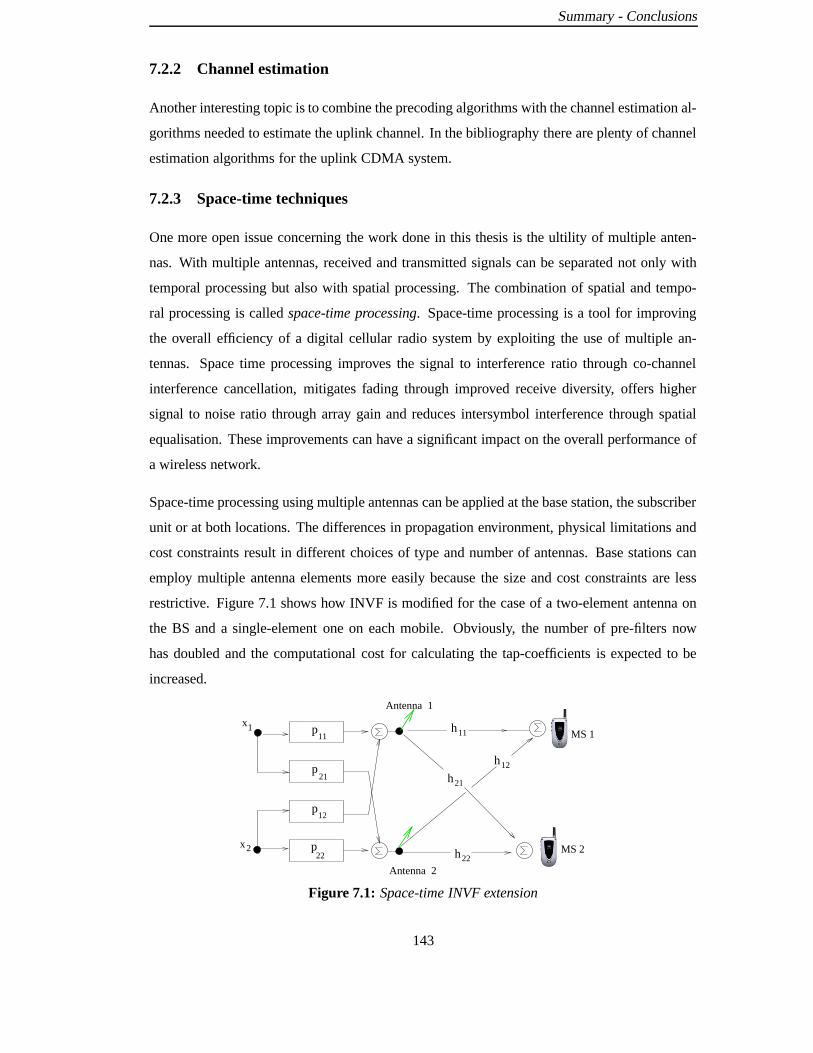
Summary - Conclusions

7.2.2 Channel estimation

Another interesting topic is to combine the precoding algorithms with the channel estimation al-

gorithms needed to estimate the uplink channel. In the bibliography there are plenty of channel

estimation algorithms for the uplink CDMA system.

7.2.3 Space-time techniques

One more open issue concerning the work done in this thesis is the ultility of multiple anten-

nas. With multiple antennas, received and transmitted signals can be separated not only with

temporal processing but also with spatial processing. The combination of spatial and tempo-

ral processing is called space-time processing. Space-time processing is a tool for improving

the overall efficiency of a digital cellular radio system by exploiting the use of multiple an-

tennas. Space time processing improves the signal to interference ratio through co-channel

interference cancellation, mitigates fading through improved receive diversity, offers higher

signal to noise ratio through array gain and reduces intersymbol interference through spatial

equalisation. These improvements can have a significant impact on the overall performance of

a wireless network.

Space-time processing using multiple antennas can be applied at the base station, the subscriber

unit or at both locations. The differences in propagation environment, physical limitations and

cost constraints result in different choices of type and number of antennas. Base stations can

employ multiple antenna elements more easily because the size and cost constraints are less

restrictive. Figure 7.1 shows how INVF is modified for the case of a two-element antenna on

the BS and a single-element one on each mobile. Obviously, the number of pre-filters now

has doubled and the computational cost for calculating the tap-coefficients is expected to be

increased.

h11

h21

h12

h22

11

p21

p12

22p

p

Antenna 1

Antenna 2

x

x

1

2

MS 1

MS 2

Figure 7.1: Space-time INVF extension

143

References

[1] W.H. Press, S.A. Teukolsky, W.T. Vetterling, and B.P. Flannery, Numerical Recipes inC, The Art of Scientific Computing, Cambridge University Press, second edition, 1992.

[2] T. Ojanpera and R. Prasad, WCDMA, Towards IP Mobility and Mobile Internet, PersonalCommunications Series. Artech House Publishers, 2001.

[3] W.W. Erdman, “A decade of progress,” IEEE Commun. Mag., vol. 31, pp. 48–51, Dec.1993.

[4] J.E. Padgett, C.G. Gunther, and T. Hattori, “Overview of wireless personal communica-tions,” IEEE Commun. Mag., vol. 33, pp. 28–41, Jan. 1995.

[5] Lal Chand Godara, Handbook of Antennas in Wireless Communications, CRC Press,2002.

[6] D.J. Goodman, “Second generation wireless information networks,” IEEE Trans. onVeh. Technol., vol. 40, pp. 366–374, 1991.

[7] L.C. Godara, M.J. Ryan, and N. Padovan, “Third generation mobile communicationsystems: overview and modelling considerations,” Annals of Telecommunications, vol.54, no. 1-2, pp. 114–136, 1999.

[8] B. Sklar, “Rayleigh fading channels in mobile digital communication systems partI:characterization,” IEEE Commun. Mag., pp. 90–100, Jul. 1997.

[9] B. Sklar, “Rayleigh fading channels in mobile digital communication systems part II:Mitigation,” IEEE Commun. Mag., pp. 102–109, Jul. 1997.

[10] R. Ertel, P. Cardiery, K.W. Sowerby, T.S. Rappaport, and J.H. Reed, “Overview of spatialchannel models for antenna array communication systems,” IEEE Personal Communi-cations, pp. 114–136, Feb. 1998.

[11] John G. Proakis, Digital Communications, Electrical Engineering. McGraw-Hill, 3rdedition, 1995.

[12] A. Paulraj and C.B. Papadias, “Space-time processing for wireless communications,”IEEE Signal Processing Mag., pp. 49–83, Nov. 1997.

[13] R.C. Dixon, Spread Spectrum, John Wiley & Sons, 1976.

[14] W.C.Y. Lee, “Overview of cellular CDMA,” IEEE Trans. on Veh. Technol., vol. 40, no.2, pp. 291–301, May 1991.

[15] K.S. Gilhousen, I.M. Jacobs, L.A. Weaver R Padovani, A. Viterbi, and C.E. Wheatley,“On the capacity of a cellular CDMA system,” IEEE Trans. on Veh. Technol., vol. 40,no. 2, pp. 303– 312, May 1991.

144

References

[16] A.J. Viterbi, CDMA: principles of spread spectrum communication, Addison-Wesley,1995.

[17] E. Nikula, A.Toskala, E. Dahlman, Girald L., and A. Klein, “FRAMES multiple accessfor umts and imt-2000,” IEEE Personal Communications, pp. 16–24, Apr. 1998.

[18] “Multiplexing and Channel Coding (FDD),” 3GPP Technical Specifications 25.212.

[19] “Spreading and Modulation (FDD),” 3GPP Technical Specifications 25.213.

[20] “Physical Layer Procedures (FDD),” 3GPP Technical Specifications 25.214.

[21] “Physical Layer Measurements (FDD),” 3GPP Technical Specifications 25.215.

[22] T. Ojanpera and R. Prasad, WCDMA: Towards IP Mobility and Mobile Internet, ArtechHouse, 2000.

[23] J. Laiho, A. Wacker, and T. Novosad, Radio Network Planning and Optimization forUMTS, John Wiley and Sons Ltd, 2001.

[24] Harri Holma and Antti Toskala, WCDMA for UMTS: Radio Access for Third GenerationMobile Communications, John Wiley and Sons Ltd, 2002.

[25] Z. Zvonar and D. Brady, “On multiuser detection in asynchronous CDMA flat Rayleighfading channels,” Personal, Indoor and Mobile Radio Communications 1992, PIMRC’92, pp. 123–127, 1992.

[26] S. Verdu, “Minimum probabilty of error for asynchronous gaussian multiple accesschannels,” IEEE Trans. on Inform. Theory, vol. IT-32, no. 1, pp. 85–96, Jan. 1986.

[27] Z. Zvoran and D. Brady, “Suboptimum multiuser detector for synchronous CDMAfrequency-selective Rayleigh fading channels,” Proc. Global Telecommunications Con-ference, Communication Theory Mini-Conference, pp. 82–86, Dec. 1992.

[28] A. Klein, Multi-user detection of CDMA signals-algorithms and their application tocellular mobile radio, Fortschritt-Berichte VDI, 1996.

[29] “Selection procedures for the choice of radio transmission technologies of the UMTS(UMTS 30.03 version 3.2.0),” .

[30] Recommendation ITU-R M.687, Future Public Land Mobile Telecommunication Sys-tems (FPLMST), 1998.

[31] Recommendation ITU-R M.1034, Requirements for the radio interface(s) for FuturePublic Land Mobile Telecommunication Systems (FPLMTS), 1998.

[32] ETSI ETR 291, “Systems requirements for the UMTS,” Tech. Rep., ETSI, May 1996.

[33] ETSI UMTS 21.01, “Requirements for the UMTS terrestial radio access system(UTRA),” Tech. Rep., ETSI, May 1997.

[34] Recommendation ITU-R M.1035, Framework for the radio interface(s) and radiosub-system functionality for Future Public Land Mobile Telecommunication Systems(FPLMTS), 1998.

145

References

[35] K.G. Beauchamp, Walsh Functions and their Applications, London: Academic Press,1975.

[36] R.L. Pickholtz, D.L. Schilling, and L.B. Milstein, “Theory of Spread-SpectrumCommunications—A Tutorial”,” IEEE Trans. Commun., vol. 30, no. 5, pp. 855–884,May 1982.

[37] R.L. Pickholtz, L.B. Milstein, and D.L. Schilling, “Spread spectrum for mobile commu-nications,” IEEE Trans. on Veh. Technol., vol. 40, no. 2, pp. 313–321, May 1991.

[38] M.K. Simon, J.K. Omura, R.A. Scholtz, and B.K. Levitt, Spread Spectrum Communica-tions Handbook, New York: McGraw-Hill, revised edition, 1994.

[39] R.L. Peterson, R.E. Ziemer, and D.E. Borth, Introduction to Spread Spectrum Commu-nications, Englewood Cliffs, NJ: Prentice Hall, 1995.

[40] K. Karkkainen, Code Families and their Performance Measures for CDMA and MilitarySpread-Spectrum Systems, Ph.D. thesis, Ph.D. Dissertation, University of Oulu, Finland,1996.

[41] F. Adachi, M. Sawahashi, and K. Okawa, ,” .

[42] S. Lin and J. Costello, Error Control Coding: Fundamentals and Applications, Engle-wood Cliffs, NJ: Prentice Hall, 1983.

[43] R.D. Cideciyan, E. Eleftheriou, and M. Rupf, “Concatenated Reed-Solomon/convolutional coding for data transmission in CDMA-based cellular systems,”IEEE Trans. Commun., vol. 45, no. 10, pp. 1291–1303, Oct. 1997.

[44] S. Benedetto, D. Divsalar, and J. Hagenauer, “Concatenated coding techniques anditerative decoding: Sailing toward channel capacity,” IEEE J. Select. Areas Commun.,vol. 16, no. 2, Feb. 1998.

[45] ,” Proc. of International Symbosium on Turbo Codes and Related Topics, Brest, France,Sep. 1997.

[46] P. Jung, J. Plechinger, M. Doetsch, and F. Berens, “Pragmatic approach to rate com-patible punctured turbo-codes for mobile radio applications,” Proc. in 6th InternationalConference on Advances in Communications and Control: Telecommunications/SignalProcessing,Corfu, pp. 23–27, Jun. 1997.

[47] C. Berrou, A. Glavieux, and P. Thitimajshima, “Near shannon limit error-correcting cod-ing and decoding: Turbo codes,” IEEE International Conference on Communications,ICC’93, Geneva, vol. 1, pp. 1064–1070, May 1993.

[48] J.M. Holtzman, CDMA Power Control for Wireless Networks, Norwell, MA:Kluwer,1992.

[49] V.K. Garg, K. Smolic, and J.E. Wilkes, Applications of Code-Division Multiple Access(CDMA) in Wireless/Personal Communications, NJ:Prentice Hall, 1996.

[50] R. Price and P.E. Green, “A communication technique for the multipath channels,” Pro-ceedings of the IRE, vol. 46, pp. 555–569, Mar. 1958.

146

References

[51] G.L. Turin, “Introduction to spread-spectrum antimultipath techniques and their appli-cation to urban digital radio,” Proc. IEEE, vol. 68, no. 3, pp. 328–353, Mar. 1980.

[52] S. Moshavi and Bellcore, “Multi-user detection for ds-CDMA communications,” IEEECommunications Magazine, pp. 124–136, Oct. 1996.

[53] Z. Xie, R.T. Short, and C.K. Rushforth, “A family of suboptimum detectors for coherentmultiuser communications,” IEEE J. Select. Areas Commun., vol. 8, no. 4, pp. 683–690,May 1990.

[54] A. Duel-Hallen, J.H., and Z. Zvonar, “Multiuser detection for CDMA systems,” IEEEPersonal Communications, vol. 2, no. 2, pp. 46–58, Apr. 1995.

[55] Sergio Verdu, Multiuser Detection, Cambridge University Press, 1 edition, 1998.

[56] H.V. Poor and S. Verdu, “Probability of error in MMSE multiuser detection,” IEEETrans. on Inform. Theory, vol. 43, no. 3, pp. 858–871, May 1997.

[57] R. Lupas and S. Verdu, “Linear multiuser detectors for synchronous code division mul-tiple access channels,” IEEE Trans. on Inform. Theory, vol. 35, no. 1, pp. 123–136, Jan.1989.

[58] Z. Zvoran and D. Brady, “Multiuser detection in single-path fading channels,” IEEETrans. Commun., vol. 42, no. 3, pp. 1729–1739, Mar. 1994.

[59] U. Madhow and M.L. Honig, “MMSE interference suppression for direct-sequencespread-spectrum CDMA,” IEEE Trans. Commun., vol. 42, no. 12, pp. 3178–3188, Dec.1994.

[60] Z. Zvoran and D. Brady, “Suboptimal multiuser detector for frequency-selectiveRayleigh fading synchronous CDMA channels,” IEEE Trans. Commun., vol. 43, no.3, pp. 154–157, Mar. 1995.

[61] A. Klein, G.K. Kaleh, and P.W. Baier, “Zero forcing and minimum mean-square-errorequalization for multiuser detection in code-division multiple-access channels,” IEEETrans. on Veh. Technol., vol. 45, no. 2, pp. 276–286, May 1996.

[62] A. Klein and P.W. Baier, “Linear unbiased data estimation in mobile radio systemsapplying CDMA,” IEEE J. Select. Areas Commun., vol. 11, no. 7, pp. 1058–1066, Sep1993.

[63] H.C. Huang and S.C. Schwartz, “A comparative analysis of linear multiuser detectorsfor fading multipath channels,” Proc. of the IEEE GLOBECOM Conf., pp. 11–15, 1994.

[64] Z. Zvonar and D. Brady, “Linear multipath-decorrelating receivers for CDMAfrequency-selective fading channels,” IEEE Trans. Commun., vol. 44, no. 6, pp. 650–653, Jun. 1996.

[65] Z. Zvoran, “Combined multiuser detection and diversity reception for wireless CDMAsystems,” IEEE Trans. on Veh. Technol., vol. 45, no. 1, pp. 205–211, Feb. 1996.

147

References

[66] M.K. Varanasi and B. Aazhang, “Multistage detection in asynchronous code-divisionmultiple-access communications,” IEEE Trans. Commun., vol. 38, no. 4, pp. 509–519,Apr. 1990.

[67] J.M. Holtzman, “DS/CDMA successive interference cancellation,” Spread SpectrumTechniques and Applications,IEEE ISSSTA ’94, vol. 1, pp. 69–78, 1994.

[68] R.M. Buehrer, N.S. Correal-Mendoza, and B.D. Woerner, “A simulation comparison ofmultiuser receivers for cellular CDMA,” IEEE Trans. on Veh. Technol., vol. 49, no. 4,pp. 1065–1085, Jul. 2000.

[69] P. B. Rapajic and D.K. Borah, “Performance study of the adaptive MMSE maximumlikelihood CDMA receiver,” Personal, Indoor and Mobile Radio Communications 1998,PIMRC ’98, vol. 3, pp. 1285–1289, 1998.

[70] D. K. Borah and P. B. Rapajic, “Adaptive weighted least squares CDMA multiuserdetection,” IEEE Vehicular Technology Conference Spring Tokyo2000, vol. 1, pp. 92–96, 2000.

[71] H. Elders-Boll, M. Herper, and A. Busboom, “Adaptive receivers for mobile DS-CDMAcommunication systems,” IEEE Vehicular Technology Conference 1997, vol. 3, pp.2128–2132, 1997.

[72] P. B. Rapajic and D.K. Borah, “Adaptive receiver structures for asynchronous CDMAsystems,” IEEE J. Select. Areas Commun., vol. 17, no. 12, pp. 2110–2122, Dec. 1994.

[73] P. B. Rapajic and B.S. Vucetic, “Adaptive receiver structures for asynchronous CDMAsystems,” IEEE J. Select. Areas Commun., vol. 12, no. 4, pp. 685–697, May 1994.

[74] S. Verdu, “Adaptive Multiuser Detection,” Spread Spectrum Techniques and Applica-tions,IEEE ISSSTA ’94, vol. 1, pp. 43–50, 1994.

[75] D.G.M. Cruickshank, “Optimal and adaptive FIR filter receivers for DS-CDMA,” IEEEPIMRC ’94, pp. 1339–1343, Sep. 1994.

[76] R. Esmailzadeh, E. Sourour, and M. Nakagawa, “Pre-rake diversity combining in timedivision duplex CDMA mobile communications,” IEEE Trans. on Veh. Technol., vol. 48,no. 3, pp. 795–801, May 1999.

[77] R. Esmailzadeh, M. Nakagawa, and E.A. Sourour, “Time-division duplex CDMA,” IEEEPersonal Communications, vol. 4, pp. 51–56, Apr. 1997.

[78] M. Brandt-Pearce and A. Dharap, “Transmitter-based multiuser interference rejectionfor the down-link of a wireless CDMA system in a multipath environment,” IEEE J.Select. Areas Commun., vol. 18, no. 3, pp. 407–417, Mar. 2000.

[79] B. R. Vojcic and W. M. Jang, “Transmitter precoding in synchronous multiuser commu-nications,” IEEE Trans. Commun., vol. 46, no. 10, pp. 1346–1355, Oct. 1998.

[80] M. Meurer, P.W. Baier, T. Weber, Y. Lu, and A. Papathanasiou, “Joint transmis-sion:advantageous downlink concept for CDMA mobile radio systems using time di-vision duplexing,” IEE Electronics Letters, vol. 36, pp. 900–901, May 2000.

148

References

[81] A. Papathanasiou, M. Meurer, T. Weber, and P.W. Baier, “A novel multiuser transmissionscheme requiring no channel estimation and no equalization at the mobile stations forthe downlink of TD-CDMA operating in the TDD mode,” IEEE Vehicular TechnologyConference Fall 2000, pp. 203–210, 2000.

[82] G.R. Walsh, Methods of optimization, John Wiley & Sons Inc., 1975.

[83] L. Scharf, Statistical signal processing : detection, estimation, and time series analysis,Addison-Wesley series in electrical and computer engineering. Addison-Wesley Pub. Co,1991.

[84] A.N. Barreto and G. Fettweis, “Capacity increase in the downlink of spread spectrumsystems through joint signal precoding,” in Proc. ICC, vol. 4, pp. 1142–1146, 2001.

[85] M. Joham and W. Utschick, “Downlink processing for mitigation of intracell interferencein DS-CDMA systems,” IEEE 6th Int. Symp. on Spread-Spectrum Tech. & Applic.,NewJersey,USA, pp. 15–19, Sep. 2000.

[86] F. Kowalewski, “Joint predistortion and transmit diversity,” IEEE Global Telecommuni-cations Conference ’00, vol. 1, pp. 245–249.

[87] Z. Tang and S. Cheng, “Pre-decorrelating single user detection for CDMA systems,”IEEE Vehicular Technology Conference ’94,IEEE 44th, vol. 2, pp. 767–769, 1994.

[88] Z. Tang and S. Cheng, “Interference cancellation for DS-CDMA systems over flat fadingchannels through pre-decorrelating,” PIMRC’94, pp. 435–438, 1994.

[89] S. Haykin, Adaptive Filter Theory, Prentice Hall, 1991.

[90] R. Esmailzadeh and M. Nakagawa, “Pre-RAKE diversity combination for direct se-quence spread spectrum communications systems,” International Conference on Com-munications, vol. 1, pp. 463–467, Geneva 1993.

[91] S. Georgoulis and D.G.M. Cruickshank, “Pre-equalization, transmitter precoding andjoint transmission techniques for time division duplex CDMA,” IEE 3G 2001 Conferenceon Mobile Telecommunications Technologies, pp. 257–261, Mar. 2001.

[92] R. Irmer F. Wathan and G. Fettweis, “On transmitter-based interference mitigationin TDD-downlink with frequency selective fading channel environment,” Proc. Asia-Pacific Conference on Communications (APCC), Bandung, Indonesia, Sep. 2002.

[93] R. Irmer A.N. Barreto and G.Fettweis, “Transmitter precoding forSpread-Spectrum sig-nals in frequency-selective fading channels,” Proc. 3G Wireless 2001, pp. 939–944, Jun.2001.

[94] W. Wang, X. Wu, and Q. Yin, “A novel space-time pre-multiuser downlink transmissionscheme suitable for TDD-CDMA systems,” IEEE Vehicular Technology Conference2001-Spring, vol. 2, pp. 185–189, 2001.

[95] U. Ringel, R. Irmer, and G. Fettweis, “Transmit diversity for frequency selective chan-nels in UMTS-TDD,” Spread Spectrum Techniques and Applications, IEEE ISSSTA ’02,vol. 3, pp. 802–806, 2002.

149

References

[96] A. Morgado, A. Gameiro, and J. Fernandes, “Constrained space-time zero-forcing pre-equalizer for the downlink channel of UMTS-TDD,” Personal, Indoor and Mobile RadioCommunications 2002, PIMRC ’02, vol. 3, pp. 1122–1126, 2002.

[97] A. Gameiro, A. Morgado, and J. Fernandes, “Space-time pre-equaliser for the down-link channel of UMTS-TDD,” IEE 3G 2001 Conference on Mobile TelecommunicationsTechnologies, pp. 99–103, 2001.

[98] A. Morgado, P.Pinho, A. Gameiro, and J. Fernandes, “Pre-equalisation technique forthe interference cancellation in the UMTS-TDD downlink channel,” IEEE VehicularTechnology Conference 2001-Fall, vol. 2, pp. 878–881, 2001.

[99] A.N. Barreto and G. Fettweis, “Performance improvement in DS-spread spectrumCDMA systems using a pre- and a post-RAKE,” Proc. of 2000 International ZurichSeminar on Broadband Communications, pp. 39–46, 2000.

[100] W.M. Jang, B.R. Vojcic, and R.L. Pickholtz, “Joint transmitter-receiver optimization insynchronous multiuser communications over multipath channels,” IEEE Trans. Com-mun., vol. 46, no. 2, pp. 269–278, Feb. 1998.

[101] R. Irmer and G.Fettweis, “Combined transmitter and receiver optimization for multipleantenna frequency-selective channels,” Proc. WPMC’02, Honolulu, Hawaii, Oct. 2002.

[102] E.S. Hons, A.K. Khandani, and W. Tong, “An optimized transmitter precoding scfhemefor synchronouds DS-CDMA,” in Proc. ICC, , no. 3, pp. 1818–1822, 2002.

[103] S. Georgoulis and D.G.M. Cruickshank, “Transmitter based inverse filters for MAI andISI mitigation in a TDD/CDMA downlink,” IEEE Vehicular Technology Conference2002-Fall, vol. 2, pp. 618–622, Sep. 2002.

[104] P.A. Nelson, H. Hamada, and S. Elliott, “Adaptive inverse filters for stereophonic soundreproduction,” IEEE Trans. Signal Processing, vol. 40, no. 7, pp. 1621–1632, Jul. 1992.

[105] F. Yu and M. Bouchard, “Multichannel active noise control algorithms using inversefilters,” in Proc. ICASSP’00, vol. 2, pp. 825–828, 2000.

[106] M. Bouchard and S. Quednau, “Multichannel recursive-least-squares algorithms andfast-transversal-filter algorithms for active noise control and sound reproduction sys-tems,” IEEE Trans. Speech Audio Processing, vol. 8, no. 5, pp. 606–618, Sep. 2000.

[107] S.J. Elliott, I.M. Stothers, and P.A. Nelson, “A multiple error LMS algorithm and itsapplication to the active control of sound and vibration,” IEEE Trans. on Acoust., Speech,Signal Processing, vol. 35, no. 10, pp. 1423–1434, Oct. 1987.

[108] P.A. Nelson, F. Orduna-Bustamante, and H. Hamada, “Inverse filters design and equal-ization zones in multichannel sound reproduction,” IEEE Trans. Speech Audio Process-ing, vol. 3, no. 3, pp. 185–192, May 1995.

[109] S.J. Elliott and P.A. Nelson, “Algorithm for multichannel LMS adaptive filtering,” Elec-tronics Letters, vol. 21, no. 21, pp. 979–981, Oct. 1985.

150

References

[110] M. Miyoshi and Y. Kaneda, “Inverse filtering of room acoustics,” IEEE Trans. onAcoust., Speech, Signal Processing, vol. 36, no. 2, pp. 145–152, Feb. 1988.

[111] Bernard Widrow, Adaptive Signal Processing, Prentice-Hall, 1985.

[112] J. Nocedal and S.J. Wright, Numerical Optimization, Springer Series in Operationsresearch, Springer-Verlag, New York, 1999.

[113] Y. Ye, “On affine scaling algorithms for nonconvex quadratic programming,” Mathe-matical Programming, vol. 56, pp. 285–300, 1992.

[114] Simon R.Saunders, Antennas and Propagation for Wireless Communication Systems,Wiley, 1999.

[115] M. Patzold, U. Killat, F. Laue, and Y. Li, “On the statistical properties of deterministicsimulation models for mobile fading channels,” IEEE Trans. on Veh. Technol., vol. 47,no. 1, pp. 254–269, Feb. 1998.

[116] M. Patzold, U. Killat, Y. Shi, and F. Laue, “A deterministic method for the derivation ofa discrete WSSUS multipath fading channel model,” Telecommunication Systems, vol.7, no. 2, pp. 165–175, Mar.-Apr. 1996.

[117] S. Georgoulis and D.G.M. Cruickshank, “Multichannel LMS and RLS algorithms forcancelling MAI and ISI before transmission in TDD/CDMA downlink,” Spread Spec-trum Techniques and Applications, IEEE ISSSTA ’02, vol. 2, pp. 681–685, Sep. 2002.

[118] S. C. Douglas, “Analysis of the multiple-error and block least-mean-square adaptivealgorithms,” IEEE Trans. Circuits and Syst., vol. 42, no. 2, pp. 92–101, Feb. 1995.

[119] S. Elliott and K.H. Baek, “Effort constraints in adaptive feedforward control,” IEEESignal Processing Lett., vol. 3, no. 1, pp. 7–9, Jan. 1996.

[120] X. Qiu and C.H. Hansen, “A study of time-domain FXLMS algorithms with controloutput constraint,” The Journal of the Acoustical Society of America, pp. 2815–2823,Jun. 2001.

[121] S.J. Elliott, C.C. Boucher, and P.A. Nelson, “The behavior of a multiple channel activecontrol system,” IEEE Trans. Signal Processing, vol. 40, pp. 1041–1052, 1991.

[122] S.M. Kuo and D.R. Morgan, Active Noise Control Systems: Algorithms and DSP Imple-mentations, New York, Wiley, 1996.

[123] T. Auspitzer, D. Guicking, and S.J. Elliott, “Using a fast-recursive-least-squares algo-rithm in a feedback-controller,” IEEE ASSP Workshop Applications Signal ProcessingAudio Acoustics, pp. 61–64, 1995.

[124] E. A. Wan, “Adjoint LMS:An efficient alternative to the filtered-X LMS and multipleerror LMS algorithms,” in Proc. ICASSP’96, pp. 1842–1845.

[125] S.C. Douglas, “Fast exact filtered-x LMS and LMS algorithms for multichannel ac-tive noise control,” Proc. Int. Conf. Acoustics Speech, Signal Processing ’97, Munich,Germany, pp. 399–402, 1997.

151

References

[126] E. Bjarnarson, “Active noise cancellation using a modified form of the filtered-x LMSand multiple error LMS algorithms,” Proc. 6th Eur. Signal Processing Conf., Munich,Germany, vol. 2, pp. 1053–1056, 1992.

[127] S. C. Douglas and W. Pan, “Exact expectation analysis of the lms adaptive filter,” IEEETrans. Signal Processing, vol. 43, no. 12, pp. 2863–2871, Dec. 1995.

[128] R.K. Wangsness, Electromagnetic fields, John Wiley & Sons Inc., 1986.

152

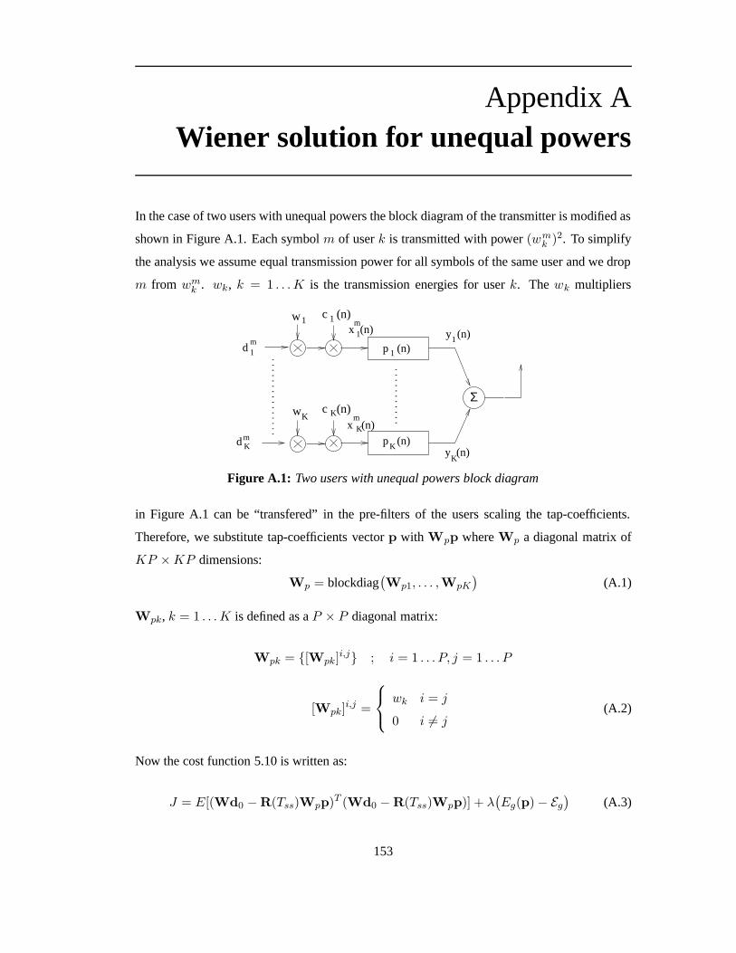
Appendix AWiener solution for unequal powers

In the case of two users with unequal powers the block diagram of the transmitter is modified as

shown in Figure A.1. Each symbol m of user k is transmitted with power (wmk )2. To simplify

the analysis we assume equal transmission power for all symbols of the same user and we drop

m from wmk . wk, k = 1 . . . K is the transmission energies for user k. The wk multipliers

y (n)1d 1

m

Σ

1p (n) 1x (n)m

m

y (n)K

p (n)d Km

x (n)K

1c (n)

K

w

w c (n)K

1

K

Figure A.1: Two users with unequal powers block diagram

in Figure A.1 can be “transfered” in the pre-filters of the users scaling the tap-coefficients.

Therefore, we substitute tap-coefficients vector p with Wpp where Wp a diagonal matrix of

KP ×KP dimensions:

Wp = blockdiag(Wp1, . . . ,WpK

)(A.1)

Wpk, k = 1 . . . K is defined as a P × P diagonal matrix:

Wpk = [Wpk]i,j ; i = 1 . . . P, j = 1 . . . P

[Wpk]i,j =

wk i = j

0 i 6= j(A.2)

Now the cost function 5.10 is written as:

J = E[(Wd0 −R(Tss)Wpp)T (Wd0 −R(Tss)Wpp)] + λ(Eg(p) − Eg

)(A.3)

153

Wiener solution for unequal powers

where W is a diagonal K ×K matrix with diagonal elements [W]i,i = wi, i = 1 . . . K . The

average total transmission power per symbol is:

Eg =(UWpp

)TUWpp (A.4)

and its gradient:

ϑ(Eg(p) − Eg

)

ϑp=ϑ(pTWT

p UTUWpp)

ϑp= 2WT

p UTUWpp (A.5)

The gradient ϑ/ϑp of the new cost function Jc is:

ϑJcϑp

= −2WTp E[RT (Tss)Wd0] + 2WpE[RT (Tss)R(Tss)]Wpp + 2λWT

p UTUWpp

(A.6)

It is easy to prove that:

E[RT (Tss)Wd0] = E[RT (Tss)d0]Wp (A.7)

Hence A.6 is rewritten :

−WTpE[RT (Tss)d0]Wp +

(WT

p E[RT (Tss)R(Tss)]Wp + λWTpUTUWp

)p = 0

−WTp E[RT (Tss)d0]Wp + WT

p

(E[RT (Tss)R(Tss)] + λUTU

)Wpp = 0

(A.8)

Eventually, the equation is reduced to eq. (5.13) and the solution is:

po =[E[RT (Tss)R(Tss)] + λUTU

]−1E[RT (Tss)d0] (A.9)

which proves that differen transmission power per user doesn’t affect the Wiener solution.

154

Appendix BPublications

• S.Georgoulis and D.G.M. Cruickshank, “Pre-equalization, transmitter precoding and

joint transmission techniques for time division duplex CDMA,” 3G 2001 Conference,

London, pp. 257–261, Mar. 2001.

• S.Georgoulis and D.G.M. Cruickshank, “ Multichannel LMS and RLS Algorithms for

Cancelling MAI and ISI before Transmission in TDD/CDMA Downlink,” ISSSTA 2002,

Prague, Sep. 2002.

• S.Georgoulis and D.G.M. Cruickshank, “Transmitter Based Inverse Filters for MAI and

ISI Mitigation in a TDD/CDMA Downlink ,” IEEE VTC 2002-Fall, Vancouver, vol.: 2,

pp. 681-685, Sep. 2002.

• S.Georgoulis and D.G.M. Cruickshank, “Inverse Filters for Transmitter based Interfer-

ence Mitigation in TDD/CDMA,” accepted for publication in IEEE Transactions on

Wireless Communications.

• S.Georgoulis and D.G.M. Cruickshank, “Adaptive Techniques for Transmission in TDD

Downlink ,” submitted to AEI European Transactions on Telecommunications

• Contributing author in textbook entitled “Next Generation Mobile Access Technologies:

Implementing TDD”, Dr. Harald Haas & Professor Stephen McLaughlin. Due to be

published in 2003.

155

Publications

!"#$% '&()$*+ ),'-(".)/102 3$4%56$%7 86"$

9;:=<?>@BADCE@EFHGJILK?MON;P)Q:R<:TSU:;VWADFHILXYHK[Z;MONHY\ NHI^]_>AK[I^`[a@ObcWPdIJNdeHFHADCEZ

Q>f;MOAD`Dgh>Nd`i@Obc+GJ>OXj`DAD@ENHIkX5KlMON;P)c+G^>OX `DADILXMOG=cNHCEI^NH>>ADI^NHC>gMOI^Gnm-K[Cdo>>_: >pPq:rMEXE: FsY=tdPdCEg%XOo?>>_: >OP=:TMEXE: FHY

uHvkwLxTy^z[LxT|~n = Od;-[ 5 pH H lDjTDD d[ L+Jj'nnlr +n T? W[jO [ =j1OD rOW[ W ¡O[ LD¢ E£+n n O[ Or #¤r njn 7D[O ¢DW[ ¥ D# 5in5¦? = ¥7D¢ l¤r WOD[ ¦¥?5+D¢r l HDD dR =[Oj =§=¨-©¦ª)DHJD¢l[ [ +ROr[ O qª- _nWn n ;DlD¥ O=¥Ol- = DOis¥-[ OO=n-n n «= - ¬DT ?pOnW«;T¨ j#¨-O D­^«=¨¬¨-®ljO¥l¯°1±-©¦«=²7 1Wn[jOD_ ¬k nOD++O=njl; O TO- WOD TO+ W[ WODT^ ³¥O rO?+n5?l B«= D WD+n5l;D ; DD[ k DD¢ # r+ODD[ DO ¢5D+ nE[ Dn+ WDD =[ Ll [ DD´

µ¶i·¸¦¹Wº?»¼½7¾W¹i·»¸¿-ÀTÁÂ[Ã[ÄLÅkÆÂÇÈOÂ[ÉOÃÂÊÃ[ËÌOÂnÅLÌOÀTÍÀrÆÀrË ÉÅLÎÈOÏrÄÀrÐOÏTÂUÑÃ[Ã[Â[ÆÆÊÒJ¿+Ó Å

Ô ¿ÕÖ+×lÀrÆÂØÐEÂ[Ã[ÄÂ[Ì)ÄËÚÙÑÀrÉÑÆÀTÙjÉOÀ ÛEÃDÑÉÄÆÜEÑÁÂËÝ+ÄÜOÂÃ[Â[ÏrÏTÈOÏÑÁ+ΦÑÁÞ Â[ÄßlàÜOÀrÆiÄÂ[ÃnÜOÉOÀrÇÈO á;ÑÏrÁÂÑÌOâ7ãEÂÀTÉOÙÈOÆÂ[ÌÚÀTÉÃ[ÈOÁÁÂ[ÉÄHäÓ Åå æ=Æâ5ÆÄÂÎ?ÆDáÀTÆHÑÏrÆËÙ Ë ÀrÉOÙÄËãEÂ=Â[Î?ÐpÏTËâ Â̬ÀrÉ+ÄÜOÂÉOÂ[ØÄWÙ Â[ÉOÂÁnÑÄÀTË ÉÚËÝÎ?Ë ãOÀrÏrÂÃË Î?ÎÈOÉOÀrÃDÑÄÀrË ÉÆâÆÄÂ[ÎÆiÃÈOÁkÅÁÂ[É5ÄÏTâ¡ÈOÉOÌOÂ[ÁÆÄ¥ÑÉOÌEÑÁÌOÀrÆnÑÄÀTËjÉdßÖ-ÉOË ÄÜOÂÁ?ÄÂÃnÜOÉOÀrÇÈOÂ7ÄÜEÑÄÜEÑÆãEÂ[Â[ÉÀTÉOÃÁÂDÑÆÀTÉpÙ ÏTâÐEË ÐOÈOÏÑÁÀTÆ=àÀTÎÂ+¿¬ÀrÍÀrÆÀTËjÉ?¿-ÈOÐOÏrÂ[Ø ÅÀTÉOÙÒRà-¿+¿+×[çrènédÀTÉêÜOÀTÃnÜÄÜOÂWÆ¥ÑÎ?Â-ÃDÑÁÁÀrÂ[ÁÀTÆÈOÆÂ[Ì?Ý^Ë ÁãEË ÄÜÈOÐÅÑÉO̦ÌOËêÉOÏrÀTÉOÞÀrɦÌOÀ ë_Â[ÁÂÉĬÄÀTÎÂ+ÆÏrË ÄÆDß;àÜOÀrƬÄÂ[ÃnÜOÉOÀrÇÈOÂÀTÆHÂ[ÎÐOÏrËâ Â[ÌWÀTÉÄÜpÂìHÈOÁË ÐEÂDÑÉÃ[Ë ÁÌOÏTÂÆÆ=ÆâÆÄÂ[Î1¿+ì Ô àÑÉOÌêÀTÏrÏ_ãEÂiÈOÆÂ[ÌÀrÉÐEÑÁÄ-ËÝ;ÄÜOÂ+Ý^ÁÂ[ÇÈOÂÉOÃ[âÁnÑÉOÙ ÂÑÏrÏTËÃÑÄÂ[ÌÄËÄÜOÀrÁÌÙ Â[ÉOÂ[Á¥ÑÄÀrË ÉÆâÆÄÂ[ÎÆDßäLÉÑ Ô ¿+ÕÖíÆÃnÜpÂ[Î?ÂWÄÜOÂWÎÑîË Á=ÂÉOÃ[Ë ÈOÉÄÂ[ÁÂÌ#ÐOÁËjãOÏTÂ[ÎÆ

ÑÁÂ-ÄÜOÂ-ÎÈOÏTÄÀTÐOÏrÂ=ÑÃ[ÃÂ[ÆÆ-ÀTÉ5ÄÂ[ÁLÝJÂ[ÁÂ[ÉOÃ[ÂÒJÕÖ-ä×;ÌOÈOÂ-ÄËÆÀrÎÈOÏ ÅÄnÑÉOÂË ÈOÆ+ÈOÆnÑÙ ÂËÝÄÜOÂãEÑÉOÌOêÀrÌOÄÜãâÑÏrÏdÈOÆÂÁÆÑÉOÌÀrÉÄÂÁkÅÆâÎãEË ÏOÀrÉÄÂ[ÁLÝJÂÁÂ[ÉOæÒäÓä×=ÌOÈOÂ+ÄËÎÈOÏTÄÀTÐEÑÄÜiÝLÑÌOÀrÉOÙlÃ¥ÜEÑÉÅÉOÂ[ÏrÆDßHÕ¦ÈOÏrÄÀrÐEÑÄÜ-ÝLÑÌOÀTÉOÙ=ËÝ^ÄÂÉiÃÑÈOÆÂ[Æ=Ñ=ÎÑîË ÁEÏrÀTÎÀrÄnÑÄÀrË ÉÄËÔ ¿ÕÖ)ÆâÆÄÂ[γÐBÂ[ÁkÝ^Ë ÁÎÑÉOÃ[Â+ÆÀrÉOÃ[ÂWÀTÄÌOÂÆÄÁËâÆ-ÄÜOÂWË ÁÄÜOËÅÙ Ë ÉEÑÏrÀTÄLâiÑÎ?Ë ÉOÙ+ÄÜO¬ÆÐOÁÂDÑÌOÀTÉOÙWÆÂÇÈOÂ[ÉOÃ[ÂÆDßäkÉÄÜOÂ+ÑãOÆÂ[ÉOÃ[ÂËÝÕ¦Ö-ä+ÄÜOÂÃ[Ë ÉÍjÂ[ÉÄÀrË ÉEÑÏ;ÑÐOÐOÁËÑÃnÜÚÄËÌEÑÄnÑÌOÂ[ÄÂ[Ã[ÄÀrË É¡ÀTÆÄËWÂ[ÎÐOÏTËâWÑÉÀTÉpÌOÂ[ÐEÂ[ÉOÌOÂÉÄDáOÆÀrÉOÙ ÏrÂÈOÆÂ[ÁïÖ-ðiìÁÂ[ÃÂ[ÀTÍjÂ[ÁDç ñDéêÜOÀTÃnÜWÂ[Ç5ÈEÑÏTÀrÆÂ[ÆHÄÜOÂÃnÜEÑÉOÉOÂÏkßdäkÉÄÜOÂÑãpÆÂ[ÉOìËÝBÎÈOÏrÄÀrÐEÑÄÜÒRÀLß Â ßdÑÌpÌOÀTÄÀTÍ ÂHêÜOÀrÄÂ;òiÑÈOÆÆÀÑÉWÉOË ÀrÆÂHÃnÜEÑÉOÉpÂ[ÏR×_ÄÜOÂ=ÏTÀrÉOÂDÑÁ;ç óDéÑÉOÌÉOË ÉOÏTÀrÉOÂDÑÁç ôéBÎÈOÏrÄÀrÈOÆÂ[Á;ÌOÂÄÂ[ÃÄÀTËjɦÄÂÃnÜOÉOÀrÇÈOÂ[Æ+ÑÁÂ-ê=Â[ÏrÏÆÄÈpÌOÀTÂ[ÌÑÉOÌÑÉEÑÏrâÆÂÌdßdõ¬ËêqÂÍ Â[ÁdÝ^Ë ÁdÌEÑÄnÑÌOÂ[ÄÂ[Ã[ÄÀTË ÉÀTÉWÆâÆkÅÄÂ[ÎÆ-ÑÐOÐOÏrâÀTÉOÙ Ô ¿ÕÖ'ÄÜOÂiÄLê=ËÐOÁË ãOÏTÂÎ?ÆËÝ;Â[ÇÈBÑÏTÀrÆnÑÄÀTË ÉÑÉOÌÆÀTÙjÉEÑÏ_ÆÂ[ÐBÑÁnÑÄÀTË ÉÜEÑDÍ Â+ÄËãEÂWÆË ÏrÍ Â[ÌÆÀrÎÈOÏrÄnÑÉOÂË ÈOÆÏrâßö_ÀrÉOÂDÑÁ+ÆÈOãEË ÐpÄÀTÎÑÏ_ÎÈOÏTÄÀTÈOÆÂ[Á-ÌOÂ[ÄÂÃ[ÄËjÁÆ+ÝJË Á-ÝJÁÂ[ÇÈOÂÉOÃ[â Å

ÆÂ[ÏrÂ[Ã[ÄÀTÍj¬ï-ÑDâÏrÂ[ÀrÙ ÜWÝkÑÌOÀrÉOÙ-ÃnÜEÑÉOÉOÂÏTÆ=ÀTÉpÃ[ÏTÈOÌpÂÄÜOÂÎÈOÏrÄÀrÐEÑÄÜÌOÂ[Ã[ËjÁÁÂÏRÑÄÀTÉOÙ-ÌOÂ[ÄÂ[Ã[ÄË ÁHÌOÂ[Í Â[ÏrË ÐEÂ[ÌWÀrÉdç æDé5ÑÉOÌ+ÄÜOÂïÖ¬ðWìÌOÂnÅÃ[Ë ÁÁÂ[ÏÑÄÀrÉOÙWÌOÂ[ÄÂÃ[ÄË Áç ÷Déß;àÜp¬ÏÑÄÄÂ[Á=ÄÂ[Ã¥ÜOÉOÀTÇ5ÈO á ÑÏTÆËÞÉOËêÉÑÆ#ÏrÀTÉOÂÑÁÈOÉãpÀRÑÆÂ[Ì1ÌEÑÄ¥Ñ)Â[ÆÄÀTÎÑÄÀrË É'Ý^Ë ÁÌOÀrÆÃ[ÁÂ[ÄÂ/ÄÀrÎ?ÂÔ ¿ÕÖ~ÆâÆÄÂ[ÎÆDá;ÁÂÌOÈOÃ[Â[ÆÀTÉ5ÄÂ[ÁÆâÎãEË ÏÑÉOÌÎÈOÏTÄÀTÐOÏrÂÑÃnÅÃ[Â[ÆÆHÀTÉÄÂ[ÁkÝ^Â[ÁÂÉOÃ[Â-ãEÑÆÂÌiË ÉWø[ÂÁËÅ^ÝJË ÁÃ[ÀTÉpÙÒ^ù_úH×kË ÁHÎÂDÑÉ+Î?ÀrÉÅÀTÎÈOÎûÆÇÈEÑÁÂÂÁÁËjÁ#ÒJÕÕ7ÓOì;×ÑÏTÙjË ÁÀrÄÜOÎÆDß'àÜOÀTÆÆÃ¥ÜOÂ[Πá

êÜOÀrÃnܦüý þÿ Ò à-×lÑÏrÏ=ÄÜOÂÈOÆÂÁÆDá;Ù ÀrÍ Â[ÆWÀTÎÐOÁËÍ Â[ÌÁÂ[ÆÈpÏTÄÆËÍ ÂÁ?ÄÜOÂ7ÆÄ¥ÑÉOÌEÑÁÌ)ïÖ¬ðWìUÁÂ[Ã[Â[ÀrÍ Â[Áá¬ãOÈpÄ?ÄÜpÂ7ÁÂ¥ÅÃÂ[ÀrÍ Â[Á-ÁÂ[Ç5ÈOÀTÁÂÆ-ÞÉOËêÏTÂÌOÙ Â-ËÝ=ÑÏTÏEÄÜOÂiÈpÆÂ[ÁÆ Ô ¿+Õ¦Ö'ÃËÌOÂ[ÆáÄÜOÂ#Ã¥ÜEÑÉOÉOÂ[Ï ÆÀTÎÐOÈOÏrÆÂÁÂ[ÆÐEË ÉOÆÂhÑÉOÌÄÜO¡ÑÏrÙ Ë ÁÀrÄÜOÎ ÀrÉÅÃÏTÈOÌOÂƬÀrÉÍ ÂÁÆÀrË É¦ËÝ=ÑiÝLÑÀTÁÏTâÏRÑÁÙ Â+ΦÑÄÁÀrØ_ßHàÜOÀrÆÁÂ[ÆÈOÏTÄÆÀrÉÜpÀTÙ ÜÎ?Ë ãpÀTÏr¬ÁÂ[Ã[ÂÀTÍ Â[Á+Ã[ËjÎ?ÐOÏrÂ[ØÀrÄkâË É7ÄÜOÂlÌpËêÉOÏTÀrÉOÞ?êÜOÀrÃnÜÀrÆÜOÀTÙjÜOÏTâÈOÉOÌOÂ[ÆÀTÁ¥ÑãOÏTÂjß

ïÂ[Ã[Â[É5ÄÏTâ5áOêqËjÁÞ¦ÜBÑƬãBÂ[Â[ÉÌOË ÉOÂWË ÉÑÏrÙ Ë ÁÀTÄÜOÎÆ;ÄÜEÑĬÂØ ÅÐpÏTË ÀrÄ;ÄÜOÂÝkÑÃÄ=ÄÜEÑÄ=ÀrɦÑ+à-¿¿%ÆÃnÜOÂÎ?Â-ÄÜOÂ+ÌOËêÉOÏrÀTÉOÞWÃnÜEÑÉÅÉpÂ[Ï_ÀTÆ;ÞÉOËêÉÄËWÄÜOÂ+ÄÁnÑÉOÆÎ?ÀrÄÄÂÁDßdäkÉÄÜOÂ-ÃDÑÆÂËÝdି+¿ÄÜOÂÆ¥ÑÎÂÃnÜBÑÉOÉOÂ[Ï=ÀrÎ?ÐOÈOÏrÆÂÁÂ[ÆÐEË ÉOÆÂƦÑÁÂ?ÍjÑÏTÀrÌ7Ý^Ë ÁiãBË ÄÜÄÜOÂÈpÐOÏTÀrÉOÞÑÉOÌÄÜOÂÌOËêÉOÏrÀTÉOÞ_áEÀ Ý=ÅÑÉOÌÄÜOÀrÆiÑÆÆÈOÎÂ[ÌÀTÉêÜBÑÄÝ^Ë ÏrÏTËêÆLÅsÄÜOÂWÄÀTÎÂ-Â[ÏÑÐOÆÀrÉOÙlãEÂÄkê=Â[ÂÉÈOÐOÏrÀTÉOÞÑÉOÌÌOËêÉOÏTÀrÉOÞÄÁnÑÉOÆÎ?ÀrÆÆÀTË ÉOÆWÀrÆlÆÈ?ÃÀTÂ[ÉÄÏTâÚÆÎÑÏTÏ;Ã[ËjÎ?ÐEÑÁÂ[ÌÄËÄÜOÂ?ÃËÅÜpÂ[ÁÂ[ÉpÃ[¦ÄÀTÎÂlËÝÄÜOÂ?ÎË ãOÀrÏTÂWÁnÑÌpÀTËÃnÜEÑÉOÉOÂÏkßäkÉ#ÄÜOÂ[ÆÂÑÏ ÅÙjË ÁÀrÄÜOÎÆDáEÄÜOÂÎÈOÏTÄÀTÈOÆÂÁ-ÌOÂ[ÄÂÃ[ÄÀrË ÉÑÉOÌÚÂ[ÇÈEÑÏTÀrÆnÑÄÀrË ÉÃDÑÉãBÂÃÑÁÁÀrÂ[ÌË ÈOÄ;ÑÄHÄÜpÂÄÁnÑÉOÆÎ?ÀrÄÄÂÁDßdàÜOÂ=ÁÂ[ÃÂ[ÀTÍjÂ[Á=ÆÄÁÈOÃ[ÄÈpÁÂÑÄqÄÜOÂ-ÈOÆÂ[Á=ÂÇÈOÀTÐOÎÂ[ÉÄ;ÀrÆ;ÄÜOÂ[ÉÆÀrÎ?ÐOÏrÀ ÛEÂÌlêÜOÂÉ?Ã[ËjÎ?ÐEÑÁÂ[ÌêÀrÄÜ'Ñ¡ÎÈOÏrÄÀrÈOÆÂÁÁÂÃ[Â[ÀrÍ Â[ÁálÑÉOÌ/ÃDÑÉ)ãE¡Ñ#Ã[ËjÉÍ Â[ÉÄÀTË ÉEÑÏÎÑÄÃnÜOÂ[ÌÛEÏTÄÂ[Á-ÒRêÜOÀrÃnÜË ÉOÏTâÁÂÇÈOÀTÁÂ[Æ=ÞÉOËêÏrÂ[ÌOÙ ÂËÝ_ÄÜp¬ÌOÂ¥ÅÆÀTÁÂ[ÌÈOÆÂ[ÁÆÃ[ËÌOÂ×Ë ÁÑ#ïÖ-ðWìíÁÂ[ÃÂ[ÀTÍjÂ[Á#ÒêÜOÀTÃnÜhÁÂ[Ç5ÈOÀTÁÂ[ÆÞ5ÉOËêÏTÂ[ÌpÙ Â?ËÝ+ÄÜOÂ7ÌOÂ[ÆÀTÁÂ[ÌÈOÆÂ[ÁÆÃ[ËÌOÂÑÉOÌ¡ÄÜO¦ÐpÁË ÐEÑÙÑÅÄÀTËjÉÃnÜBÑÉOÉOÂ[Ï×[ßHàHÂ[ÃnÜOÉOÀrÇÈOÂ[Æ=êÜOÀrÃnÜË ÉOÏTâWÁÂÇÈOÀTÁÂ+ÑÎÑÄÃ¥ÜOÂ[ÌÛBÏTÄÂÁÁÂ[Ã[ÂÀTÍ ÂÁÑÏTÆËÂ[ÉOÜBÑÉOÃ[ÂWÄÜOÂ+ÆâÆÄÂ[Î~ÃÑÐEÑÃ[ÀrÄkâÆÀrÉOÃ[ÂWÉOËÆâÆÄÂ[ÎÊÁÂÆË ÈOÁÃ[Â[ÆÜEÑDÍ ÂWÄËãEÂlÑÏTÏrËÃDÑÄÂ[̦Ý^Ë Á-ÄÜOÂÄÁ¥ÑÉOÆÎÀTÆLÅÆÀTËjɦËÝHÄÁnÑÀrÉOÀTÉOÙÆÀrÙ ÉEÑÏrÆ=Ë É¦ÄÜOÂÌOËêÉpÏTÀrÉOÞ_ß

ÉO ÆÈOÃnÜÄÁ¥ÑÉOÆÎÀTÄÄÂ[ÁdÄÂ[ÃnÜOÉOÀrÇÈOÂ=ÀTÆ! "#rþ$%"Jþý ÿ?ç &Déáç 'DéEêÜOÀrÃnÜÀTÉOÃ[ÏrÈOÌOÂ[Æ;ÐOÁÂnÅïÖ-ðWì#ÌOÀrÍ Â[ÁÆÀTÄLâÃË ÎãOÀrÉOÀrÉOÙÑÄ ÄÜOÂÄÁnÑÉOÆÎ?ÀrÄÄÂ[ÁDßÚäkÉÄÜO¦ÌOËêÉOÏrÀTÉOÞÄÜOÂÌOÂ[ÆÀTÁÂÌÈOÆÂ[Á! ÆÆÀTÙ ÉEÑÏÀrÆ=ΦÑØÀTÎÑÏ ÁnÑÄÀrËiÃ[ËjÎãOÀrÉOÂ[ÌêÜOÀTÏrÂË ÄÜOÂ[Á=ÈOÆÂ[Á! ÆÆÀrÙ ÉEÑÏTÆ=ÑÁÂÉpË ÄDß)(-ÉOÌOÂ[Á=ÄÜOÀrÆ;ÆÃ[ÂÉEÑÁÀrËlÄÜOÂ-ÁÂ[ÃÂ[ÀTÍjÂ[ÁÀTÆBîÈpÆÄ=ѬÛBØÂ[ÌÛEÏTÄÂÁÎÑÄÃnÜOÂ[ÌÚÄËÄÜOÂ?ÌpÂ[ÆÀrÁÂ[ÌhÈOÆÂ[Á ÆÃ[ËÌOÂÑÉOÌÄÜOÂ?ÁÂ[Ã[ÂÀTÍ ÂÁ?ÀrÆÉpË Ä¦ÁÂ[ÇÈOÀrÁÂ[Ì'ÄËÀrÎ?ÐOÏrÂ[ÎÂ[ÉÄÑÉâÃ¥ÜEÑÉOÉOÂ[ÏWÂ[ÆÄÀrΦÑÄÀTË ÉhË ÁÑÌEÑÐOÄÀrÍ Â+Â[ÇÈEÑÏrÀTÆÂ[ÁDßÖ-ÉOË ÄÜOÂÁ?ÄÁ¥ÑÉOÆÎÀTÄÄÂ[ÁãEÑÆÂ[ÌÄÂ[ÃnÜOÉOÀrÇÈOÂÀTÆ+*," ÿ%-lþ.!

/ ¥ý! þÿ07ÑÆ-ÐOÁËjÐEË ÆÂ[ÌÚÀTÉÚç åéßäkÉÄÜOÀrƬÄÂ[ÃnÜOÉOÀrÇÈO á_ÄÜOÂlËjãÅînÂ[ÃÄÀTÍjÂÀrÆÄ˦ÃÑÁÁâË ÈOÄWÎÈOÏrÄÀrÐOÏTÂWÑÃÃ[Â[ÆÆlÀrÉÄÂ[ÁLÝJÂÁÂ[ÉOÃÂ?ÃDÑÉÅÃÂ[ÏrÏRÑÄÀTË ÉÑÄÄÜOÂWÄÁ¥ÑÉOÆÎÀTÄÄÂ[ÁÁnÑÄÜOÂ[Á-ÄÜBÑɦÄÜOÂÁÂ[Ã[ÂÀTÍ ÂÁDß=äkÉÄÜOÀTÆ=ÃÑÆ áEÑWïÖ-ðiìÚÁÂ[ÃÂ[ÀTÍ ÂÁ-ÀTÆ;ÁÂÇÈOÀTÁÂ[Ì?Ý^Ë Á;ÆÈÃ[ÀrÂ[ÉÄÐEÂ[ÁLÅÝ^Ë ÁÎÑÉOìÈOÉOÌpÂ[Á-ÆÂ[Í ÂÁÂWÎÈOÏrÄÀrÐEÑÄÜdß

Ö-ÉÑÏrÄÂ[ÁÉEÑÄÀrÍ ÂWÄÁnÑÉOÆÎÀTÄÄÂ[Á-ãEÑÆÂÌÎÈOÏTÄÀTÈOÆÂ[ÁÌOÂ[ÄÂÃ[ÄÀrË ÉÆÃnÜOÂÎ?ÂÀTÆ21ý þÿ3" ÿ4-þ$ þRý ÿOá_ÐOÁË ÐEË ÆÂÌ#ÀrÉçrè!5DéßWäkÉÄÜOÀrÆÑÐOÐOÁËÑÃ¥Ü#ÑÃ[Ë ÎÎ?Ë ÉÄÁ¥ÑÉOÆÎÀTÄ-ÆÀTÙ ÉEÑÏdÝ^Ë Á+ÑÏTÏHÈOÆÂ[ÁÆÀrÆÌOÂ¥ÅÄÂ[ÁÎÀrÉOÂ[Ì?ÀrÉÄÜOÂ+ãEÑÆÂ+ÆÄ¥ÑÄÀrË É7ÑÉOÌ?ÂÑÃnÜÆÀTÙjÉEÑÏEÀTÆ-ÑÆÆÈOÎÂ[ÌÄËÐEÑÆƦÄÜOÁË ÈOÙjÜ'Ñ#ÌOÀ ë_Â[ÁÂÉĦÎÈOÏrÄÀTÐEÑÄÜÃ¥ÜEÑÉOÉOÂ[ÏLßUÖÝJÄÂÁÜBÑDÍÀTÉOÙ+ÐEÑÆÆÂ[ÌÄÜOÁË ÈOÙ ÜÄÜOÂÎË ãOÀTÏrÂHÁnÑÌOÀrË+ÃnÜEÑÉOÉOÂÏOÄÜOÀrÆ;ÆÀTÙÅÉBÑÏÀrÆ?ÛBÏTÄÂÁÂ[Ì/ãâÑ#ÛEÏrÄÂÁ¦ÎÑÄÃ¥ÜOÂ[ÌÄËÄÜOÂÈOÆÂ[Á ÆÃ[ËÌOÂjáâ5ÀTÂ[ÏrÌOÀrÉOÙlÄÜOÂÌOÂÆÀrÁÂ[ÌÌEÑÄnÑpßäkÉWÄÜOÀrÆdÐEÑÐEÂ[ÁHê=Â;ÌOÂ[ÁÀTÍ ÂÑÉ+ÀrÎ?ÐOÏrÂ[ÎÂ[ÉÄnÑÄÀTËjɬÑÉOÌiÆÀTÎÈOÏRÑÅ

ÄÀTËjɦËÝ;ÄÜpÂlÑãEËÍ Â+ÄÁnÑÉOÆÎ?ÀrÄÄÂ[ÁkÅLãEÑÆÂ̦ÎÈOÏTÄÀTÈOÆÂ[Á=ÌOÂ[ÄÂÃ[ÄÀrË É

156

Publications

!"$#% &'("() +*-,/.02133&45768 +("9)" :"&;=< ":>?2((" &'$@A +B /"+@A +? " C"? ">?D((" &FE G& H' ? I5J D;+( "K" F2'@$ LM:"C"N &" OO"C"& -@A P(;@H?"B5$.$O &?O -QR"-QR"S " ?T <"UQR?" ?5.$OV+PWX>'" QC" @%Q:O" ? ?"=<>? & -" ? YY5T.$"&;+ ">? & -"Z?[(\; + +? YYY?5]YU Y=^_ `! -"A;"("2;`Z a7"@$ L(" ? + &??9"- +("b5ccBde7fKehgOijkjml`niZopOq9rsBt?uRvBwyxzv?tB| ~7uR!*"W "% ?" >F&; )E J 0I@$ +-??C"&' C &");"QR" ?D? +ZB &?OK> -B< +ER,20IO BM 8'/&; =5K.$@$ LW"QR"@$"K L2@$ K : -("?M 25T35X.$ "?&<U $"+ z+' T " >KTQR;@A5

user 1

channel 1

user k

user Kchannel k

channel K

base station

;B`7?RTR! P$& ¡$R¢U&£ .$$>$& "&;+ h>' L:QP¤>T¥¦HQ"O§¨©X"Bª « ¬ ­®P¯ ER¥ ¦ °:±B±± ¥ ¦² IR³´ E3BI

.$2`>¥¦8" J$µ 0¶·__"D("B;_>_("B ` ?`¸ ¬ ­® Q:D¹%@$ &2??Z a7?"$ ? ZQ:¹m & ('Bª¸ ¬ ­® ¯ Eº ¦ ° ±B±B± º ¦» I ³ ER¼I

.$9`>) ")7 $½7¾O & ( "P½7¿Bª½7¿ ¯ ½ ¾¹ ERÀI

.$Z§)¨R©O &? C &;"& " ?/>+ +(C"(@$ &+ A('CO & (/")ªÁ ¬ ­® ¯ ER ¦ ° ±B±B±  ¦Ã I ³ E\ÄI@$"KÅÆ O+)8;QZ U52# /+Ç\¨©`>)];QA(;@C"XÈ]É Ê O"+ ?/QR)"z`"Ë ¨©ÌO7@$ L 7 A? " >?8ªÍÎ

É;Ï ° ¸ ¬ Ð®Ñ È]É ÊB¥É Ê ERÒI

.$?"&Q"C) ??:" ? ) )P§¨©-,20O@A >Z("( +Q7?":"?`>O§¨© &?Á ¬ ­® ªÓ ¬ ­®Ô ¯ ÍÎ

É;Ï ° ¸ ¬ Ю Ñ È É Ê ¥ É Ê:Õ Á ¬ ­® EÖI.$$" + ?"CÓ ¬ ­®Ô QR":Ç!¨R©-"+ Z`>) :QPKER¹W×DÅVØW3BI:$9"'CQ7'Z ? X ?75Ö5:Y= A(("-7O )$"z"& /@$ ?-(@C"ÙÈ¦Ê +" ?MBK ++(< 5Ú ""&;+ )/QC> L/Q$¤+<=X>' -'`BQ"<+ 'O" ? ?`? )"] $§¨R©,K0zÓ ¬ ­®Ô T[?`- "$Ó ­ QTDE¤2¹×ÛÅØÛ3BI$+-!?" [("??_ F75C3BÜKBQR"OQR" ? )" « ;Q)8E2¤KIª « ¯ E « ¬\Ý?®Þ ±B±B± « ¬ßC®Þ IUàZ´ EáIO/" [â QT ã?E¹z¤KICä8ERK¤2I-ªâ ¯ ERå Êæ É I7ç Ç ¯ 3èèè ¤2¹´ Ë ¯ 3èèè 2¤å » ¬ éê ° ®!ë7ì æ ² ¬ ¦ ê ° ®!ëé ¯îíï ð º ¬ ¦ ®ì ñò;óõô ¯ 3:èBèBèU¹`´ö ¯ 3:èèBè=¤´§ ¯ 3:èBèè=Ü ò÷ Âø ó ÈÇùBø ERúI;/9" [û ¬ ­® Q: ãER¹O¤ü×_Å·Øý3BICäDE¹z¤KIªû ¬ ­® ¯þUÿ ¦Êæ É çîÇ ¯ 3:èBèBèU¤2¹Û×Å Ø3´ Ë ¯ 3NèèBè=¹O¤

ÿ ¦Êæ É ¯  ¦Ê ê É ë ° ñòó 3ýÇØ Ë ×Ù3ÙÅÜ ò÷ Âø ó ÈÇRùBø EI.$?Mª

Ó ­ ¯ û ­ â « × ¯ « × E3ÜI@$?"-û ­ â ¯ :`E¹z¤×2Å ØK3BIT ":QPã?"+BW +([/#P6ü@$`"B$W "+(";"- ?(B5C.A'9 ?" ! -" [ ¯ þ ö ö ¯ E3)3BI5 .$X) ??O BQ¹ü:ÀÌTÅ TK¼ÌP¤?P¼2V?7+¼$>KK +75P3B¼'ª !" # $ % &¯'(((((()* * ! * * ! * * ! * * !

+ ,,,,,,-'((()/. . ! . ! . !!. " . !". . ! . ! . !!. " . !"

+ ,,,- ')10 0 !0 ! 0 !!+-

E3¼IY=C N +("&;PQR":QU "CX'"-C+'"$ ?"& "&;+ T7(@C"5 Ú ":U<S? " >W>9"& ??"+ H) ª÷&ó32 ºø54â ± â 6 E3ÀI

157

Publications

"!$#&%('*)+,- ./0,1,) 2 4365 789#:%';'0<>=#&?+@BA#:';CED#&%'FC@G?4!'0HIH9A#-A$J'0F#&CLK*M ?4<H'#:'K&@?4!'0HNG/O#&%'QP'K:C$D1CK&F0?4!R#&'0F%!?+S/T'UAE!HBH'-V9!'HNGWOXM Y[Z/\0]_^`ab cde fhg i M j&k:lmBnpoq de fhg i M j>r d:st j

u FFCK:H?4!Rv#&Cw#&%''<&#:?4@vA#&?+C!B#:%'CK:OxA!Hzy?4#:%|m q A<Q?4!'S~ ss #&%'Q'<:#&?+@BA#:';G9'0FC@'<XM Y c g k&l ig r npo ig k&l ie d:s ju <[AK&'0<&T9C<:?4#:?4C!D1CK#&%(?4<[AE4RCK:?4#:%@v#&%'@vA#&K:?4g k l ig %9AE<;#:C$G9'!C!/="<&?+!RTAKy%?+F%w?4<!C#QA+yAO/<#&%'FA<:';Cy'0J'KQy%'!NF0C!<&?+H'K&'0HxK:'AyCK&+HB#:?4@'=>JLAK&?A!/#F%9A!!'0?4@T4<:'*K:'<&9CL!<&'< LA!(Hy%'!F%C/C<:?4!Rv#&%'T<&'K"=><:9'F? V9FxQ u F0C/H'<v #&%(?4<@BA#:K&?+x?+<U<:?4!RTAKy?4#&%AQK&CG9AEG?4+?4#"O*'0S/T9A9#&CP'0K&C9~?4!'AKT!/G?,AE<&'H'<&#:?4@=A#&?+C!FA!G9'F0C!<&?+H'K&'0HNA<AQG9A!CD u* K&'F0'?4J'0K&<DC+4CEy'0H$G/OAH'FCK:K&'A#:CK5 s 8&0 ¡*m gI¢w£p¤¦¥ ¡¡§;m©¨ gB£ §ª©¡§«¬ ¢B¥­® § £¯K:C@©'S~ s ?+#$?+<CG/J/?4CLT<$#:%9A#$#:%'NK:'F'0?4J'0KIK&'0S/T?4K:'</!Cy4'0HR'CDA4#:%'$T<:'KFC/H'<A!HA!'0<&#&?+@vA#&'CD#&%'F%9A!!'0?4@T+<&'K&'0<&9C!<:';#:C;9'0K>D1CK&@#:%';ADCK:'@I'0!/#&?+C!'HA4RLCK&?+#&%@[?+!$AEHH?4#:?4C!#&CQ#&%('!'0'HDCKp?+!/J'K:<&?4CL!UCDpAD"A?4K:4O,AK:R'Q@BA#:K&?+~°%?+<<&F%'0@I'%9A<QA!w?4!FK:'A<:'HxF0C@I+'/?+#>O?4!vFC!/#:KA<:#y?+#&%v#&%'?4!FK:'A<:'HH'0@BA!(HID1CK+'<:<F0C@I+'9CK&#-AG4'QT!?+#&<±°%'0K&'D1CK&'F0TK&K&'0!/#QK&'<:'AK&F-%N%9A<G9'0'!BD1C=FT<&'0HNC!vA+RCK&?+#&%@<#&%9A##AE'Q,AF0'C!v#&%'QG9A<:'*<:#A#:?4C!'/+C?4#:?4!R#&%'QD"AF##&%9A#?+!NA°²<&F%'0@I'#&%'HCy!+?4!F%9A!!'0p?4</!Cy!v#&C#&%'#&K-A!<&@?4#:#&'K³ I´9 &L/,1 µ &0¶&·L,2 "!¸5 ¹8?4#?4<Q<&%(Cy!N#&%9AE#y%'0!xA u K&'0F'?+J'K?4<Q'@=4CEO'HpG9C#&%º@$T+#&?+4'AFF0'<&<wA!H¸?+!/#&'0K&<&OW@$G9C?+!/#&'0K>D'0K>='!F'QFAE!IG9'Q'+?4@?4!9AE#&'HG/O@I'AE!<CDA<:T?4#-AG4'#:KA!<&@?+#>=#&'KK&'0FC/H?+!R<:F%'@' u 4?+!'AK#&KAE!<>D1CK&@vA#&?+C!@vA#&K:?4¡ CD#&%'H9A#-A$M #&CG9'U#:KA!<:@I?+#&#&'0HB?+<T(<&'HA!HB#:%/T<#&%'K&'F0'?4JL'HN<:?4R!»A~?4<R?+J'!wA<¼

e Y[¬ « c ¡ M r½¾ Y g c ¡ M r½|¾ d:s 7j°%'CLT#&T#J'F0#&CK¿ CDAG9AE!UCEDÀ u K&'0F'?+J'K:<D1CKA*G+C/FCDÁ#&K-A!<&@?4#:#&'HH9A#-AU?+<R?4J'0!BG/O¿ Y g k l g c ¡ M r½|¾  d:sà j°%'@'A!/="<&S/T9AEK&'H'K&K:CKFK&?+#&'0K&?4CL!ÄH('V9!'HzA<¼

ÄBYÆÅ;Ç:È ÉËÊUÌM f c dg k l g j id ¡ M j ½|¾ Â r ÌÍÎ d:sÏ j°%'UC(#&?4@T@6K:'FC/H?+!RB#:KA!<"DCK:@BA#:?4CL!N¡ ~y%?+F%z@I?+!/=?4@?4<:'<Ä?+<¡ Y c&g k l g r npo d:s ¹j >!CK&H'0K#&CQ@BA?+!/#AE?4!#&%'#&K-A!<&@?4#:#&'H'!'0K&RO'S/T9AE#&CQ#&%'FA<:'$CD!C="K&'0FC/H?+!RA<R?+J'!GWO'S~ sÐ y'$@C/H? DO#&%'K&'F0C/H?4!(R$#:KA!<>D1CK&@vA#:?4C!A<¼

¡ Y[Ñ Ò c"g k l g r npo d1Ó j

y%'0K&'#&%'QD>AF0#&CK Ñ ÒÒY Ô \Z/Õ0Ö/Ê/« k:× « Î

Ô \ZWÕÖ Ê d « ¡ j k × « ¡ Î d(s j°%'<:F%'@vA#:?4FQH?,AERKA@CDK:'="FC/H?+!R$<:F%'@'Q?4<R?+J'!?+!V9R9 °%'QK:'S/T?+K&'H u K:'F'?+J'KHC/'0<;!CL#;AF-%?4'0J'#:%'<&?+@I+'<&#@CG?+4'T!?+#y%?+F%?4<AV9+#&'K@vA#&F%'0H$#:C*#:%'T(<&'KØ <<&K:'AH?+!R$F0C/H'°%'A#:#&'KQA?+@?4<AF-%?4'JL'HB?+!B#:%'D1C+4Cy?+!R*AE4RCK:?4#:%@

data of user 1

data of user K

data of user k +

nk

F

C

C

C1

k

K

precoding

matrix

for channel

k channel k +RAKE RECEIVER

USER k

T

Ù/Ú ÛÜÝÜ$Þ9ß àáâãÚ äÛ-å>äæàçèå>äéLê,æÚ è1èë"åìå>ë"í,á:àãÚ éÛî/Q´9 &/+°%'@vA?+!$?+H'ACD#&%?+<AK&C/AEF%NAE<K:C9C<:'HN?+!x5 sÓ 8p?+<#:%9A##&%'ïðBH'0#&'K:@I?+!'<QA$F0C@I@C!<&?+R!9Añ DCKQA+pNð/<°%?+<<&?+R!9AAD1#&'K%9AJ/?4!R9A<:<&'H#&%K:CTR%#&%'@CG?4+'KAH?+CF-%9A!!'+<O/?+'4H(<$#&%('H9A#-Ax<&'0!/#$D1CKI'AF%ÆNð¸G/Oº<&?+@I+'V»4#&'0K&?+!R9ï+C/FW<òCEDÁI="H9A#AQ<&O/@G9C+<AEK&'#&KAE!<&@?4#:#&'HA!H#:%'V94#:'K&<A#p'AF%NðAK&'@vA#&F-%'HQ#&CQA<&9'F0? V9F<&K:'AH?+!RF0C/H'QCDp4'0!R#&%vó$ "#?4<A<&<:T@I'0HI#:%9A##&%'FC@@ICL!*<:?4R!9AEñ ?+<CED4'!RL#&%wÁNóôu 4#&%'wAF#:?4J'F%9A!(!'4<?+!¸ANF0'4A!(H|#&%'vJ'F0#&CK&<K&'-=F0'?+J'H|AE#;'0J'K&ONðw@$T<:#G9'$#-A'!w?4!/#:CBAF0FCT!/#U°%/T<Ahõ d Áwó ½ö f÷s j>øùNÁwó¦@vA#&K&?+¬ ?4<H'V9!'0Hp¼

¬ Y c ¬ o l iii ¬ L l iii ¬ +ú l rû dL jy%'0K&'¬ ?4<A<?+!$'0S~/¹p°%'K:'F'0?4J'0HB<&?+R!9A+< e L CED'0S~ sÓ AK&'AK&K-A!R'Hv?4!vA d Áwó ½÷ö fºs jJ'F#:CK e A<¼

e Y c e o l iiie l iiie +ú lpr û dLÐ j°%'#&CL#A~K&'0F'?+J'HwJ'F#:CK e ?+<FC!F?+<&'04O'/K:'<&<:'H|A<¼e Y[¬ ñ dEt j°%'*K:'S/T?+K&'@'!/##&%»A#?4!v'J'K:ONwðB#&%('V9+#&'K:'HzÁNó ½ö fzs J'F#:CK e O/?4'04H<#&%(';H9AE#AQJ'F#:CKM $A<H'-V9!'H?+!v'S~ s ?4<Ëü0C?+!/#&+O'/K&'0<&<&'0HND1CKA4~T<:'K&<A<¼ý k l e Y[M dL jý ?4<#:%'UQ u FC/H'@BAE#&K&?+B¼

ý Y÷þÿppM õ ý o iii ý iii ý +ú ø d 7j

ý pY ý È `pY s ÁNó ½ö f¸s Y s Áwý È Y Õ n n "! \ s$# ` f ó dQfºs j # óÓ ! Ô&% Ö\('`)Ö dLÃ j

158

Publications

! "#

$%'&)(+*+,-./0001324 56.78.9;:=<?>@:AB.C7 1 D%E 5. D2F) G0HI0C. 52KJLM NO"P780;2QIHP0CJR)1.C)J30+PST7 )O 5U0CJR)1.C)JV)W 5XQ)0;.7 FJ JLM24)212Y 53 5DHZ Z+[T\ -]T7^_7`)0aJb.C)212cd.C7 e0 530 -.78.a.C7 e.D_3024.b8J]- 5DT)0-2F)2F 0 a f gh ijakl ! X#

ST7 d^J242FJ08R )0T0^lR) PmIHFnLo^5.CJDMp qQq sr_tuwv5xIyIz z |ZM Z [ !~ *#

.J` 5I18R0 -.7 T.D02F).C. 5 5 DH;LhJD.C7 -0HI0.C 52F0e1 5D^5J2Fb8D0J;/.C7)0eb8b8 D+ST7 0C^_7 52Q.C)^-D_2JL.7 bD _Eo^5JI0^_7 24 `)0T 5F)88 ~

nk

n1

nK

+

+channel 1

channel k

channel K

matched filter 1

matched filter k

matched filter K+

Common

signal for all

the users

S

I +8 +T+ _%G_Oh_ 8%_OT _-h%MST70Y0^_7 24 0?bbDJObD. ?LhJODb8J)w..JK21R. Eb8J)w.R)3 I0^JI.D0.`]T).C7.C7 n.CD_0C24.. Db3D _Eo^5JI8¡MJ]- 5 5Dl¢+LhJD-M024bR eJ -b8.C7£a¤¦¥`§c^78 5R8.C7 ©¨JI..D_02F)0C0)JOnRJDC).C72 D 531^5 50eJ]T.JM.D02F).C. 5DabDC _E^5JI8Mª3 5D`.702F 5.73JIP.C7 «@¬DC 5I1D 50; IJ]TR 5 JRHJL­J -10 5D0CbD +3)`^5JI -]T7^_7^_7 5 502F)212^5J2FbR) ®I).oHI¯e°±T²³´hµT¶+·³£ ¸ 5D I.bbDJI^_7BJLT.C7 4bDCJmR) 2¹JLTD 51^)W.7 ^5J2FbR) ®I).oH4JLT.C7 «@¬PDC 5^5 5 5D)0`bDC 50 I. 5º)º& "+,C/ST7 0^_73 52.)^TD_2»LhJD-.C7)0-0^7 52F 0-bD 50C 5I.C 5P­88ST7 /¼T¬@8R). D0.7 08R.JQm8 0 5I..JQ10 D½@].7W.7

pre-rakefilter

pre-rakefilter

nk

n1

nK

pre-rakefilter

+

++

1

k

K

data of user 1

data of user k

data of user K

channel 1

channel k

channel K

matched filter 1

matched filter k

matched filter K

C

C

C1

k

K

+I +¾8 +l 5%_6_I¿o%ÀÁaÂaÃÄho.24 M)w 5D.C 5@^5J2FbR) 5®F^5Jl¨_1I.C dJLÅ.C7 ;1bIE%R) F^_783 5R)2Fb1R0 `D 50Cb8J0 FJLT.7 0_2F 10 5Dl/ST7 5V)W.7 J]TIER) .7 ; 50D 10 D+Æ 00C)­R)0-2Q®I)2QRID.J/^J2m 5mIH.C7 ^78 5R-.0C 5R L-]T7R) J.7 Dn10C 5D+Æ 0;0)O8R)0;DC /JO.+ST7 DC 501R.;)040C.DJ3Pb8 + G.`.7 FJ1.b31.dJLT.C7 4^78IE 5R]T7)^7P0d I1)OR) I.T.J4.C7 FÇ£MÈ;cD ^5 5 5DlÆ 0;J1.b13.+ST7 5D LhJDC .C7 MD 5^5 ) D-JL.7 M«P¬JI 0É3J.e 5 5.J; 50.C)2E. ;.7 ^_78 5R)2Fb1R0 `D 50Cb8J0 F@^+Wm8 ^5JIO 5IE.J8R82Q.^_73 58R. D.CJ/.C7 ;10 5DlÆ 0M0bDC +^JI Ê Ë ÌÍ

SJU2Q)w._U 5I18R.CD_0C2400C)J6b8J]- 5DF04 ( ~ ]- 0C^+R n.C7 `8._JLe½ÎÏn10C 5DM].7Q.7 MLo^5.JDl(Ð Ñ ÒÓÔaÕ ZlÖ8×Ó Z [

!h~ (+#ØÙQÚ/ÛaÜÝßÞà-á`â;Ü+ãäæåFç`ÛaÞàâÛ

$%W.70n0C 5^5.C)JV.7 .D_02F)..C 5D;m80 G. ^_7I1 50l¢N E0C^5Dm8 5m8J ¢;D V^5J2Fb8D ß]T).C7 .7 6D 5^ 5) DGm80C 5¨_JI. 5.C 5^5.J ! R) +D?1Im0 A 50.C)2Q. ?. ^_7I1 +#ÇM3J2?m)8DHP0CbD +)@^5JI 0Ê Ë ÌÍ JLTR) .7V9 ~ (D c21R.)bR 5 mIH».C7 c¼Tèe¬IÈé8._¦0CHI2m8JR)0 Ë ÌÍ .CD_0C24..C 5PPmRJI^_ w0dJLT: s~ 0HI^7DJJO10RHPJ Dd.C7 2FJmR) -^_7­ 5RoNê-D.)JO0eJL.7 `D 5^ 5 5Qb8J]- 5DT1 `.Jb­.7QR)J0C0RJJDC2RILo/D 00C124 5F.Jm8 ; 5R)2E8.C 5UmIHWb8J]- 5D`^5Jw.DJRoe^7GJLT.C7 10C 5D0)0;0C012F 5.CJGm8 Q.D02F).C. 56].76 5I18RT 5 DHº]7^_76)0JD2QR E0 U.JF78+ 1.`24bR).C1 TST7 /^7)bW)I.C 5DORa)0` 5I18R.CJëì *í îï x+v FLhJDT.7 ;^5JODD 0b8J I.d^JI.I1J10oE.C)2F -0HI0C. 52MD_)0 ^J0 Mb1R)0C 0C78b8& +,3)010 4]T.7;Lo^5.JODð *í ;Pñ ëì \ 0 !+ò Îó #ô5^5J0 ! ò+õ Îó #! ò Îó #ô ! (ÅöW ! õ Îó # [ #

!h~ #÷M1 V.J¦b1R0 6078b¦I. D^_7bßI. 5DoLh 5DC 5^5 º780Pm­ 5 5. 5Q)w.J^5^5J13I.+£c2FJm)R D_J`^_78 R)0 5mIH;).C0^_78 R8)2Fb1R)0C DC 50b­J0 Wø Ë ÌÍ ¢Å]T7^_7c03 5D 5BLDJ2æ.C7 UùTú`¬ISMû¥;¬«2FJI R)0+'S7 @ 5R+Hcb8J]Å D4bDCJ8R) @JL;.7 @ 57^51RD4 IEw)DJO24 I.n£LDJ2ü&((_,-0JOb. 56]73 5D @.7 FR) 53.7BJL.C7 4^78 5R-04ý ((^_7b0+ST7 F._bV^5JI _þF^5 5I.C0/ ®Eb­ 5D 5^5 @) b8 5 I.4ÇM+HIR 57PLo)3P]T).C7G.73 ù-R00^÷MJbb3R) 5DT0b­ 5^5.DC12U

0 5 10 15 2010

−4

10−3

10−2

10−1

100

Eb/No(db)

BE

R(d

b)

receiver−based transm. precoding joint transmission

20 users

10 users

1 user

w ÿ+MÄ8Á%%aÁ)8ÂhO_o CÃ Áa_la$%.)0F00C124 BLJDm8J.C7c.C7 PD ^5 5 5D@c.CD_0C24.. Dm­0 5bDJw^5 500C)O0.78.a.73 Å^78 5R0)2Fb1R0 aD 0b8J0C DC ^J0.I.T1D.7 ;:4Eo8._;mR)Jw^_ .CD_0C2400C)Jaèa 5DoLh ^5. wJ]TR) 53 nJLÉ.C7 ;^_78 R)Q.7 ;24R) MJLe.C7 ! :T9n#E^7)b@0 I1 5^5 0bDC 5012F 5QLhJDT.C7 nDC 5^5 ) 5D`m80C 5W 50.C)2E. e$%Q^5Jw.D_0C.+¢.73 d^78 5Ra24b1R0 MD 0b8J0C /.C78.T78

159

Publications

!"#$! %'&( ! ) *)"' +""' ,-&(./'021! 3!4256 8759:<;)2,="0>?) @",BA?CED!?F'G:D

,-"@!HI,-"!)'" +>JKL? M>N!O",QPQRTS:G>)Q?;)L Q5MU?H#;?,="VWXNY8 [ZY>)!"( !;\N&# Q5]PM/';>) ^ ;2,="+1>:<! _,-"MBO>NI5`U?O;J12a#H!>K'_" ! :!>MQ@! "80/'3!":>"+",b>"!) $>4@;:!;")8c?>:">"!!'Mc?!]0PQRTS:G*>4d5

0 5 10 15 2010

−5

10−4

10−3

10−2

10−1

100

Eb/No(db)

BE

R(d

b)

receiver−based transm. precoding joint transmissionone user

e'f ghihTjBkl(mn2odp\qp_rIsQl@h'tEu_vJwx'lQyz|T~!|Nnp@_uQNvIx']u_v)vNx_| ndoBeNo2n!qndz~uQw_Q

6 ]75O>N!8",E! M''b3; >Q>)" ) ] +XIY5Q"'Q!!!";;N@"N?\QN'"bc?!M"'_ )>)",="@"c^F'G:Dc?Vb"c?? 7>N'b;!" '_,="b)?#"0"!J"5U?+J !O;)>"' )>K' ";)2,=" L&"!]!V,=" ?" N5

0 5 10 15 2010

−5

10−4

10−3

10−2

10−1

100

Eb/No(db)

BE

R(d

b)

receiver−based transm. precoding pre rake joint transmissionone user

e'f gh'NhTjBkl(mn2odp\qp_rIsQl@h'tEu_Jwx'lQyz|T~!|Nnp@_uQNvIx']u_v)vNx_| ndoBeNo2n!qndz~uQ)wwQQ

6 T>N",O75b%$! ]#'+>)c?* "#;;)Q,-)K'>&",QY#Y<M?@)3!+\

L3)_",B!b+?>)@)3>!N) !"8Z#Y5_"+"?>" "_;J12aM>K'M"!;2,=" b!+ >)! %!>K'IWQc<O,="#3F'G:D:#)<;"L"?!I5@U<?b/L;>! $?;!12JaOI ?")>))'8",M+!;>>)+'!2,=)>5(U< ;d1,="0>)<,="?O")M!"' b,-""c<b!H!M!cb)O>"> . :,=" @;;Q56 !b",_>)";/'2&O"'@!!"+!"'

!K'++>$ "!3! >" ;!"#_!">)!>)bb]>Q!QQ!@!`", !"+ (-.3 ¢¡ XN£¤:[M¥!5E"_2&';>N_",Q¦TZY§¨§TX§ ©XX«ª ",bKB5ZZ+"?!"+]=ZYY+¤[¬#£0!/­5

®0¯8°±+²[°O³b´[µQ¶N±+²6 :B;;_b!')c$",!)E!!!B) H !'1

"L !3! >)["!·L!&'+"M ·+!;>>!')2,=)>[8)·;!"' Q5P!+\!"#[>" ;d1"#c?!]cb 1da'"c?+>)#M .)>K':c<<!;!') %c? <"'MJ "[ !"' [!"cb #& "'"' 0!!<,="@,-!K')>&]!>!DMN&')+>'1I5_PVB: "' @)/';"bM,2>b@,="b:U !>"]>4@! ."48!8J:,-"#V!;a8 8!? "c?aB5BU?b/'J>)";/'2&:8! ",>" ;!"4"L H >JL!0"!QB!" !"3!OA<F c?O)"!>O>N0:'¸ >'N5bF';>)12! !!! >JK']"c¹ +'!'I1!"#Q5

ºM»¼'»½B»¾Q¿»ÀÁ v¦Ãbh ÄNh l@hÅ|mn!h.Æyy~df Ç8|JÈ@y3~!n2 q yobÇf Mn:Nf m)f pf |JzNqÉ n!Ê

Æ_Ë:ÌÍp=Np-)n2Oh%Î=ÏÏ·ÐBÑ2ÒdÓ2ÔMÕ Ö%×BÒØbØbÙNÖÔ x@vÚNvIÛ\ÜÝdÞ IÜvßN)ÜÜNxàQ~!ÇhvJááÚh

Á ¦ÄJ|âz:ÃbhÅod|yãNf ph'ä@Õ åÕ æ\ç)è×BÒØbØbÙNÖÕÓ-çæÕÒÖé2hk n~!Ç\o=f ~!yNkzgJf zên!n2o=f zghË:~ÃQo2yJëê\Bf xodMnNf Ç\f |zxvJááNÜIhÁ Âl@hì#qypQyJz8r#hín2odNqh_ìf znyoQbq Ç\f qp=n2oQn!Ç-n~!Ç-|odpÈ|Jo@p-zê~=âo2|Jz|qp~|NnNf m)f pf |z_bq Ç\f n'y~!~np=p~-â#yzznd p!hÎ-ÏÏÏ.îÑ=çÖédÔÒ!ÖÎdÖ!ïÒÑ2Ø?çæÕ\Ò!Öîðñ-ÒÑdòxIÜNÛ\v)Ý2Þ vßvixÄyzhNváó)áh

Á ÚÂËh tbhQíyo2yJzypf_yz j_hôÌQy)2âyJzghsQn!yo-ê|Çf bqÍnÇ=n~Çf |zf zOp-z#~-âod|z|q#p~|Nn2ê\If mf p\f |zbbq Ç\f nQy~~!np-pBp=Np=Ç-n2Mp!hBÎ-ÏÏÏîÑ-çÖédÔBÒÖ ×BÒØbØbÙNÖÕÓ-çJæÕÒÖédxáÛÜÝ2Þ )ÜßJixË:yMvá)áNvNhÁ ܦõhõ#m|odyz[yJz[bh_jodyhörqÉ'|#Ç\f VyJQ`q Çf q#p-n2oMn!Ç-n~!Ç-|JoÈ|o@È o2n!qn2z#~êp-n- n~!Çf mn@lQy) ndf gâ:ÈyNf zg:p-z#~-âod|z|qp_ÆË:Ì~=âyzzn2 phQÎ-Ï4ÏÏ·îÑ=çÖé2Ô_Ò!Ö]×BÒ!Ø`ØbÙIÖÕÓ=çæÕ\ÒÖé2x'ÚÛNÝdÞ v)ÜÚßvJÜNxË:yoJhvá)áNÜNhÁ iÂÌ@hIt÷ n2f z?yz?Åh [h)jByf n2ohì#f zn!yoqzIÉf y)p-n@yÇ-y@np=Ç\f MyÇ\f |z_f zM|JÉf no2y)Nf |_p=Np=Ç-n2Mp'yJ f z#g_ÆË:Ì@hÎ=ÏÏÏ]øÒ!ÙNÑ2Ö#çè'ÒÖMù'ñ=úè ñÓ2æ-ñûbüQÑ2ñçé@Õ Ö+×BÒØbØbÙNÖÕÓ-çJæÕÒÖédxvvNÛÝ2Þ vwIÜóßNvJwiixrNn2MvJááh

Á Âl@hJkp\Myf !yndâ_yz@ËhsQyãy)gyëyhÅo2ndê\lQÌQt_kONf mn2odp\f Ç\Q~|J?êÉf zy)Ç\f |z È|oONf o2n!~ÇMp-n!qn2z#~nOp\odny0p\Ln~Ço-qý~|?bqzf ~yêÇf |Jzpp=Np-Ç=n2Mph!Î2Öæ=ñ-ÑdÖçæÕ\ÒÖ#çè×BÒÖ2ï)ñ-Ñdñ-ÖÓdñ_ÒÖO×BÒØbØbÙNÖÕÓ-çJæÕÒÖédxvIÞ Ú)ißNÚ)iNNxJÃndznmJybvááhÁ óÂl@hBkpMyf y)n2âLx­kôh÷rI|qod|qoxyJz Ë8hBsQyã)ygyJëyhÅodn2êo2yãInIf m)n2o2pf Ç:~|bÉf zf zg?f z Ç\f MnVIf mf p\f |z+Nq n!ÊHÆ_Ë:ÌTM|Éf n~!|?bqzf ~yÇf |!zph¹Î=ÏÏÏîÑ=çÖédÔ8Ò!ÖÍþñ-ð)ÕÓdÙè çÑ%î'ñÓ2ðÖLÒè Ò\åòJxÚ)óÛIÝ2Þ áNÜ!ßNówNvIxË:yMváá)áhÁ áÂj_hIl@hí|Jÿ~2f~Qyz?[hIË8hÄJyzgh#o2yz#p\?f Ç=Ç-ndo'o2n!~|NIf zgBf z:p-zê~=âo2|Jz|qpbq Çf qp=n2oB~!|?`qzf ~!yÇf |zphBÎ=ÏÏÏ%îÑ=çÖédÔ_ÒÖ0×ôÒ!ØbúØbÙIÖÕÓ=çæÕ\ÒÖé2xÚiÛ\vwIÝ2Þ vÚ)ißv)ÜÜNxJà÷~!ÇhvJááóh

Á vwJÂVËhË:n2qo2n2oJxÅh [hJjByf n2ox_hHndÉ'n2oJxbhìqxyzbÌ@hÅyJyÇ\â#yzyêpf |Jqh?Ä|f zÇQÇo2yzp?f p=p\f |zÞ ymJyzÇ=ygn!|qpB|Jëz f zã:~|Jz~ndÇÈ|JoÆ_Ë:Ì$M|JÉf nQo2y)Nf |?p=Np-Ç=n2MpBqp\f zg?Çf Mn@Nf mf pf |JzHIq nÊf zghÎ=ÏÏ]ÏQè ñÓ2æÑdÒÖÕÓ2éñ=ææ=ñ-Ñdé2xiÞ áw)wßNá)wNvNxË:yMJwwwh

Á vv!ÂrIn2 n~Çf |JzQo2|N~!nNqo2npIÈ|oÇ\ân~=â|f ~n|ÈIo2yIf |BÇo2yz#p\?f p=p\f |z_Ç=n~-âêz#| |gf np|ÈÇânQËQr8Û QËQrV)wh w)@mn2odp\f |zMh Nh wNÝ2h

Á v!ÂV@h ÆQhBqyJzgByz@rh ÆQhrI~-âëyJo2Ç-)hÌ+~|?yJo2yÇf mJnyzyJ Npf p#|È f zên!yoBbq Ç\f qp-ndoBnÇ=n~!Ç-|odpÈ|JoQÈyIf zg_bq Ç\f yÇâ?~-âyJzzn2 phÐBÑdÒ2ÓdÔÒ ïEæðñ÷Î=ÏÏÏBÏ@××BÒ!Ö!ï!Ô xy)gnpBv)vßvÜIxNvá)áÚh

160

Publications

Multichannel LMS and RLS Algorithms for Cancelling MAI and ISIbefore Transmission in TDD/CDMA Downlink

S.L. Georgoulis and D.G.M. CruickshankDepartment of Electronics and Electrical Engineering, The University of Edinburgh

The King’s Buildings, Mayfield Rd., Edinburgh, EH9 3JL, UKemails: sg@ee.ed.ac.uk, dgmc@ee.ed.ac.uk

Abstract—In this paper a novel transmitter based multiuser detec-tion scheme for the TDD/CDMA downlink is presented. The methodassumes knowledge of the channel at the transmitter. This is feasibleunder the Time Division Duplex (TDD) mode where the channel isassumed to be the same on uplink and downlink and can be estim-ated from the uplink at the base station. The portable unit’s struc-ture is significantly simplified since no channel estimation, equalisa-tion or multiuser detection is required. The novelty is that the basestation performs an emulation of the mobile receiver and adaptivelysets the filters that pre-equalise the transmitted signals, reducing mul-tiple access and multipath intersymbol interference. The theoreticalanalysis is supported with simulation results which show that the pro-posed technique increases the system’s capacity, compared with otherrecently published methods and maintains low computational cost.

Keywords— code division multiple access, TDD, interference can-cellation, transmitter based, multiuser detection, multichannel RLS,multichannel LMS

I. INTRODUCTION

Direct sequence code division multiple access (DS-CDMA) is now gaining a significant share of the cellularmarket. Another technique that has been increasingly pop-ular is Time Division Duplex (TDD) in which the same car-rier is used for both up-and downlink in different time slots.This technique is employed in the European cordless sys-tem DECT and will be used in part of the frequency rangeallocated to third generation mobile systems in Europe.

In a CDMA scheme the major problems encounteredare the multiple access interference (MAI) due to simul-taneous usage of the bandwidth by many users and inter-symbol interference (ISI) due to multipath fading channels.Multipath fading is a major limitation on CDMA systemperformance since it destroys the orthogonality among thespreading sequences. Therefore for sufficient data detectionin systems applying CDMA the two problems of equalisa-tion and signal separation have to be solved simultaneouslyfor good performance.

Linear suboptimal multiuser detectors for frequency-selective Rayleigh fading channels have been extensivelystudied in literature [1],[2]. These techniques, reduce in-tersymbol and multiple access interference but the receiverrequires knowledge of the CDMA spreading code and thechannel impulse response of every user and the algorithmsinclude inversion of fairly large matrices. This results inhigh mobile receiver complexity on the downlink which ishighly undesirable.

Recently, work has been done on algorithms that exploitthe fact that in a TDD scheme the downlink channel isknown to the transmitter. In the case of TDD the samechannel impulse responses are valid for both the uplink andthe downlink, if – and this is assumed in what follows –the time elapsing between uplink and downlink transmis-sions is sufficiently small compared to the coherence timeof the mobile radio channel. In these algorithms, the mul-tiuser detection and channel equalisation can be carried out

at the transmitter. This is achieved with linear precodingof the transmitted signal. The receiver structure at the userequipment is then simplified when compared to a multiuserdetection receiver, and can be a conventional matched fil-ter (which only requires knowledge of the desired user’sspreading code). Thus no channel estimation or adaptiveequaliser implementation is required at the mobile receiver.Techniques which only require a matched filter receiveralso enhance the system capacity since no system resourceshave to be allocated for the transmission of training signalson the downlink.

One previously developed transmitter technique is Pre-equalisation [3] which includes pre-RAKE diversity com-bining at the transmitter. In the downlink the desired user’ssignal is maximal ratio combined while other user’s sig-nals are not. Under this scenario the receiver is just a fixedfilter matched to the desired user’s code. Although the pre-RAKE method reduces the multipath channel effects, it un-fortunately doesn’t reduce the multiuser interference evenif used in conjunction with orthogonal sequences as shownin [3], [4].

To achieve a sufficient performance the transmitted sig-nals in the downlink must be jointly optimised based on thespreading code and the channel impulse response of everyuser. Such transmitter based multiuser detection schemesare Transmitter precoding (TP), described in [5] and Jointtransmission (JT), proposed in [6]. Both JT and TP jointlyprecode blocks of data and require a matched filter receiver.For a large block-length the computational cost is increasedsince these algorithms include inversion of matrices whosedimensions are proportional to the number of users and theblock length and as it will be shown the complexity persymbol transmitted is extensive. Furthermore, in the case ofmultipath channel and presuming that the data is transmit-ted continually, the first and last bits are not correctly pre-coded which leads to a capacity loss. Thus, a bitwise tech-nique that overcomes these drawbacks should be sought.

Such a bitwise technique was first introduced in [7] as de-correlating pre-filters (DPF). A conventional matched filteris assumed in the mobile station. According to this tech-nique the spread data is pre-filtered before transmission inan effort to orthogonalise them with respect to each other.The tap coefficients of the pre-filters are calculated with azero-forcing (ZF) algorithm.

In this work we propose inverse filters (INVF) for theequalisation of the response of multichannel/multiuser sys-tems and the structure is the same as [7]. The mobile re-ceiver is a conventional matched filter. The intention is toequalise the multipath channels and minimise the crosscor-relation of the users. The key is that the whole system ina cell is emulated by the base station as the channels ofthe active users and their receivers structure are assumed

161

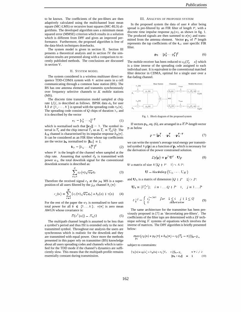
Publications

to be known. The coefficients of the pre-filters are thenadaptively calculated using the multichannel least meansquare (MC-LMS) or recursive least squares (MC-RLS) al-gorithms. The developed algorithm uses a minimum meansquared error (MMSE) criterion which results in a solutionwhich is different from DPF and gives an improved per-formance. Furthermore, the proposed algorithm is free ofthe data-block techniques drawbacks.

The system model is given in section II. Section IIIpresents a theoretical analysis and in section IV the sim-ulation results are presented along with a comparison to re-cently published methods. The conclusions are discussedin section V.

II. SYSTEM MODEL

The system considered is a wireless multiuser direct se-quence TDD-CDMA system with active users in a cellcommunicating through a common base station (BS). TheBS has one antenna element and transmits synchronouslyover frequency selective channels to mobile stations(MS).

The discrete time transmission model sampled at chiprate is described as follows. BPSK data for user

, is spread with the spreading code .

The spreading code consists of chips of duration andit is described by the vector ! #" $ %'&)(+* (1)

which is normalised such that , ,- . . The symbol in-terval is / and the chip interval so as 0/1 . The243

channel is characterised by its impulse response 5 .It can be considered as an FIR filter whose tap coefficientsare the vector 67 normalised to ,167,8 # .69: #" 5$ %5<; (=* (2)

where > is the length of the channel when sampled at thechip rate. Assuming that symbol ? is transmitted withpower @ , the total downlink signal for the conventionaldownlink scenario is described as:ABC $ 4ED @ (3)

Therefore the received signal FHG at the I 243 MS is a super-position of all users filtered by the I 23 channel 5G :FJG?47 ABC $ K 'ED @8L8MN5OG?4PRQ4 (4)

For the rest of the paper the @: is normalised to have unittotal power for all

ST 9UUUV . Q4 is zero meanAWGN whose covariance is:W K QX4%L: ZY\[] (5)

The multipath channel length is assumed to be less thana symbol’s period and thus ISI is extended only to the nexttransmitted symbol. Throughout our analysis the users aresynchronous which is realistic for the downlink and theyare transmitted with equal power. Once more the methodspresented in this paper rely on transmitter (BS) knowledgeabout all users spreading codes and channels which is satis-fied for the TDD mode if the channel’s dynamics are suffi-ciently slow. This means that the multipath profile remainsessentially constant during transmission.

III. ANALYSIS OF PROPOSED SYSTEM

In the proposed system the data of user

after beingspread is pre-filtered by an FIR filter of length ^ , with adiscrete time impulse response _ , as shown in fig. 1.The produced signals are then summed to `O and trans-mitted from the antenna element. Vector a of ^ lengthrepresents the tap coefficients of the

243user specific FIR

filter. a9b c" _d$ e_gf (+* (6)

The mobile receiver has been reduced to e/9hi whichis a time inverse of the spreading code assigned to eachindividual user. It is equivalent to the conventional matchedfilter detector in CDMA, optimal for a single user over aflat-fading channel.

v awgn

vawgn

s

s

s(n)

d (n)h (n)

h (n)d

d

d (n)p (n)

Σ

c (T −n)

1 1c (T −n)

1

p (n) 1

K

1

K

K

Base Station

K K

1

Channelsc (n)

c (n)K

Mobile Receivers

Fig. 1. Block diagram of the proposed system

If vectors a , eq. (6), are arranged in a j^ -length vectora as below a #" a * $ Va * a * A (=* (7)

we can write the system’s average total energy per transmit-ted symbol

W:k ea7 as a function of a , which is necessary forthe derivation of the power constrained solution.W:k la99 ma *on-* n a (8)n a matrix of size pqPr^rhsNtuj^ :n 0vwxy z4 k K n $ < n A Land n is a matrix of dimension rPq^rhmNt|^ :n ~: G z 9UUUVrPr^shrI 9UUU%^

~ 4 G Gy $ x!rzhI8PZ:m x1H5<F@:z`F (9)

The same architecture for the transmitter has been pre-viously proposed in [7] as ’decorrelating pre-filters’. Thecoefficients of the filter taps are determined with a ZF tech-nique solving systems of equations which involves theinverse of matrices. The DPF algorithm is briefly presentedbelow: K 1Md_4M5<?MN1e / hp L C *4subject to constraints:e%4= ¡<¢yl+ ¡£¤+ ¡%¤O=¥¦§¨ 4©1ª «¬­ 4¯®±°9²¨³´®jµ¶· ¤¡¸¤ ¶ ®º¹ (10)

162

Publications

where is the decision sample. The second constraintallows for the desired power normalisation. Each user is in-dividually normalised to achieve a specified received SNRin contrast with the global normalisation derived in eq. (27).

In the current work an emulation of all channels and re-ceivers is performed in the BS exploiting the fact that thechannels have been estimated in the BS during the last up-link burst and thus the whole downlink system is known.The BS uses the MC-LMS or MC-RLS algorithms [8] toadaptively converge to the optimal, in MMSE terms, tapsof the inverse filters. The Wiener solution that includesthe necessary power constraint is also stated. Inverse fil-ters consist of a simple addition of an array of FIR filters tothe existing BS system. The analysis that follows is similarto the analysis in [9] for stereophonic sound reproduction.

A. MMSE power constrained solution

The block diagram of the emulation that takes place inthe BS is shown in fig. 2. After pre-filtering the spread sig-

Σ

Z−∆

Z−∆

h (n)k

d kdesired

sc (T −n)k

MC RLS

LMS/e1

eK

antenna

Base station

11

1

e

Σs(n) s

to mobiles+

d

Kd

1d

ΣK

p (n)

p (n)

e1

K

dd (n)

d (n)1

11

KKK

Kc (T −n)sh (n)

c (T −n)h (n)

z (n)

z (n)

K

v(n)

MC :MultiChannel

c (n)1

2c (n)

Fig. 2. Block diagram of emulation in the BS

nal of user becomes and the transmittedsignal is the superposition of all the users :

!" #" (11)

This signal is sent to the BS antenna element and an internalblock that emulates the real receivers and their correspond-ing channels. The BS has an estimation $% of the down-link channels

% and the remote receivers '& are also known to the BS. By emulating the system, the BScan estimate the output $ sampled from the mobile:

$ ()* $% + & (12)

The error in estimation ,-./ & $ is fed back to theadaptive multichannel algorithm to determine the pre-filtertaps. For simplicity we substitute the cascaded filters $% and " & with an FIR filter of length 01325476 &58and impulse response 9 : $% ; & . Eq. (12)becomes:

$ 3)<=9 (13)

After rearrangement, the system can be equivalently il-lustrated as in fig. 3 for the > receiver. It has to be clear

Σ

1 1

Κ Κ

µ

µ

Κµ

1

µ1

µΚp (n)

r (n)

r (n)p (n)

d c (n)

z (n)

z (n)

d c (n)

d (n)

Fig. 3. Rearranged diagram of ?)@BA receiver

that this approximation is only to facilitate the mathemat-ical analysis. Signals C-D E , >FHG7IKJ 8LLLNMPO , are definedas filtered reference signals and are produced by passingthe signal E E through the filters with impulse response9 D .

CD E :( E E =9 D (14)

This ’transfer function reversal’ approach is essentially theone taken by [10] in deriving the multiple error LMS al-gorithm. This block diagram arrangement can now be usedto determine the optimal, in minimum mean squared errorterms, finite impulse response filters, Q . The fact that noiseR is not included in the rearranged diagram doesn’t af-fect the solution because the noise is not filtered by the in-verse filters.

We define the following vectors of the filtered referencesignals:SD-E *UT CD E VVV CD E &.W 4 8 XBYZF[>FHG\ 8LLLNM

(15)

Following then the block diagram in fig. 3 the filtered refer-ence signals are passing from the pre-filters Q , as in eq. (7),to yield the estimate desired data. The outputs $] can bewritten in matrix form as:

$] 3^5 Q (16)

where the vector $] and the matrix ^7 are denoted as:

$] <_`a $

...$ b cd FH^5*

_`aSY e fVVV

SY

.... . .

...SY gVVV

SY Z

b cd

(17)

We now seek the optimal filter vector Q to minimise thetime averaged squared error between the actual and desiredoutputs. The desired outputs are sampled at the symbolperiod ih j 41k , l 8 FHm"F LLL , where k is an im-posed delay to the system which assists the equalisationof the multipath channels [11]. In the final cost functionwe must include, using Lagrange multipliers, that the aver-age transmitted power per symbol should not exceed npoZqHr .Thus the cost function to be minimised is:s n TB ] & $] h Y ] & $] h Xt4vuw n'x Q &KnioZqer)y

(18)

where n denotes the expectation and]

is the vector of de-sired data, defined as

] zT VVV X Y . The vector $] is re-placed by the right part of eq. (16) and by using the expect-ation operator eq. (18) is expanded to the quadratic form:

|~Z ;-ei ;"'B* +""Z i*; '* Z; *) **) (19)

163

Publications

From vector gradient theory and eq. (8) we find that . Therefore the Wiener solution

for the taps of the inverse filters

is given by ! " #$% " '&(*) +-,/.0 ! " 1&(20)

B. Adaptive solution

An alternative technique to the direct solution of eq. (20),without any matrix inversion is to use the MC-LMS al-gorithm [10] which provides a multichannel generalisa-tion of Widrow’s filtered-x LMS algorithm [11]. Thus themethod of steepest descent can be used to descend towardthe minimum on the performance surface of the quadraticform in eq. (19). The values of the pre-filter taps weightvector are iteratively updated by an amount proportional tothe negative of the gradient of the quadratic performancesurface. The gradient of eq. (19) without the power con-straint term becomes:2 43 0 " 1&5(6 0 " 7 " '& (21)

By defining the instantaneous error vector as:8 " 413:91 " 41;3<7 " = (22)

and substituting in eq. (21) the gradient is expressed as:2 >3?@0 % " 8 ! " A& (23)

If each pre-filter taps vector is now adjusted at every sampletime by an amount proportional to the negative instantan-eous value of the gradient, a modified form of the well-known LMS algorithm is produced:!! " B!! ,/." /(DC/ ! " 8 % " (24)

whereC

is the step-size parameter of the algorithm.A second adaptive algorithm to calculate the taps

FEfor

the pre-filters is the MC-RLS described in [8]. Let G$HJI?Gmatrix K 'L be:

K ALMNOBP .Q.

'LSR-RTRPVU .

AL...

. . ....

P . UALWR-RTR

PXU%UAL

Y Z[ (25)

Then the multichannel RLS algorithm is:\^]`_TacbedgfhQiQjkilmon?mIdentity matrixp ]`_Taqberst]`uvw acbexgfhy\z]uvVfhw a|]`uvw a~ ix fh |t]`u vw aA\z]u vVfhw a|]u vw a` fh ]`u vw acbS]u vw a]`u vw a p ]`u vVfhw ap ]`u vw acb p ]u vVfhw a@st]`u vw a ]u vw a\^]`u vw acbex fh \z]u vVfhw ax fh st]`u vw a|]u vw a'\^]`u vVfhw a

(26)

where , < , is the forgetting factor and asmall positive constant.

After setting the filter coefficients we must scale thetransmitted signal 'L with a factor to achieve the de-sired average total transmitted energy per symbol and this

is done for all the techniques in the following section for thesake of fair comparison. As the reference power

0we use the one of a corresponding CDMA system withoutany precoding.

U ET ./- E?E - (27)

where the denominator is the total transmitted power persymbol for the proposed system.

IV. SIMULATION RESULTS

In this section the performance of the adaptive inversefilters is shown and compared to the pre-RAKE, JT, TP andDPF. BPSK data symbols E are spread by random bin-ary spreading codes E of length T¡ and transmittedsynchronously over the mobile channel. Variations of thereceived power due to path loss and log-normal fading areassumed to be eliminated by power control. Each of theusers is assumed to be transmitted with equal energy whichis normalised to have unit amplitude. The codes are alsonormalised to have unit power. A normalised mobile radiochannel is given by its channel impulse response ¢ E , whichis derived from the UMTS models. The delay profile, ad-opted, is the one of the vehicular environment A describedin [12], with channel length £ . In the current paperthe channels are assumed to be stationary with no Dopplereffects. Perfect knowledge of the channels is presumed forthe receiver based estimate. Thus the emulation in the BSunder this ideal scenario reflects the real system. Equal av-erage transmitted energies per symbol for all the comparedsystems has been forced for a fair comparison.

0 5 10 15 20 25 30 35 4010

−4

10−3

10−2

10−1

100

Filter Length

BE

R

DPFMC LMS−µ=0.015, 200 iter.MC LMS−µ=0.005, 500 iter.MC RLS−θ=1.0, 50 iter.Wiener, λ=0.05

Fig. 4. BER versus Filter Length for ¤¥¦=§¨ bª©T«Q¬ ,mBb®­

users

In fig. 4 the bit error rate performance of a G °¯users

system is displayed versus the length of the pre-filters forDPF and adaptive INVF. The

?±T²tis set to ³ 5´ andµ H . The MC-RLS, for , and MC-LMS, forC7 ¯ display by far better performance than the filters

whose taps are determined according to [7]. ForC® ¯

the convergence is faster as shown in the next figure but theperformance is not as good as with

C¶ ¯ . Further-more, DPF restricts the pre filters to a length H¶ µ ( .

In fig. 5 the convergence speed of one user for thevarious adaptive algorithms is presented. The system has

164

Publications

0 200 400 600 800 1000

10−4

10−3

10−2

10−1

100

← MC LMS,µ=0.005 MC LMS,µ=0.015 ↓

MC RLS, θ=1.0 ↓

Number of Iterarions

Mea

n S

quar

ed E

rror

Fig. 5. Mean squared error of user vs iterations for taps filters

users, pre-filters length is set to , delay to

and an ensemble of 50 experiments is given forevery algorithm. By choosing a large step-size parameter MC-LMS achieves a faster convergence at thecost of deteriorated performance while smaller cancels sufficiently MAI and ISI at the cost of slower con-vergence. It is shown that after 50 transmitted bits MC-RLS reaches a very small mean squared error at a cost ofincreased complexity per iteration. The MC-RLS does notexactly reach the Wiener solution as shown in fig. 4 becauseit increases the transmitted power and by using normalisa-tion factor

we decrease the signal to noise ratio.

0 5 10 15 20

10−4

10−3

10−2

10−1

100

Eb/N

o(dB)

BE

R

pre−RAKETPDPFJTWiener, λ=0.05MC LMS µ=0.005MC RLS θ=1.0

Fig. 6. BER vs ! , "$#% , &'#(*) , +,#$- users

In fig. 6 the BER performance versus .0/21354 is displayedfor a CDMA system of

67users. The pre-filter taps

have a length of 89 chips and the delay

imposed inthe system is

chips. For TP and JT the length 3 of data

block is set to

. The performance of the Wiener solu-tion along with the one after convergence of the adaptivealgorithms is shown in the same figure. Both multichannelRLS and LMS outperform pre-RAKE, DPF and TP tech-niques. The Wiener solution and the joint transmissionhave almost the same performance. The advantage of theproposed technique is that the calculation takes place onlyonce at the beginning of the transmission since it doesn’thandle blocks of data and thus it is characterised as bitwise.

Ignoring the inversion of matrices required for data blocktechniques, and the adaptation process required for conver-ging to the Wiener solution of INVF it can be proven thatfor JT and a block of length 3 data the multiplicationsrequired per symbol transmission are 3(:<; 3(=*>1 3whereas for the INVF is 5: . For instance, a system of3 ? : 7?*@? requires 32000 multi-plications under JT and only 512 under INVF. Furthermore,with JT, assuming that blocks are transmitted continually, adecrease of the block length results in a capacity loss asdata block techniques do not precode correctly the end bits.

V. CONCLUSIONS

A novel technique, called inverse filters, that exploits theknowledge of the downlink channel in TDD was presented.The technique takes the structure presented in [7] and de-velops the MMSE solution for individually pre-filtering thespread data before transmission. An emulation of the sys-tem is performed in the BS and the necessary pre-filters tapsare calculated adaptively. The process takes place once be-fore transmission instead of being repeated for every blockof data and no matrix inversion is required. The perform-ance exceeds that of pre-RAKE, DPF and TP, while it isequivalent to JT for large data blocks, which suffers fromextensive computational cost and complexity. Space timetechniques and efforts to make the adaptation process fasterare under investigation.

REFERENCES

[1] Sergio Verdu, Multiuser Detection, Cambridge University Press, 1edition, 1998.

[2] A. Duel-Hallen, J.H., and Z. Zvonar, “Multiuser detection forCDMA systems,” IEEE Personal Communications, vol. 2, no. 2,pp. 46–58, Apr. 1995.

[3] R. Esmailzadeh, E. Sourour, and M. Nakagawa, “Pre-rake diversitycombining in time division duplex CDMA mobile communications,”IEEE Trans. on Vehicular Technology, vol. 48, no. 3, pp. 795–801,May 1999.

[4] S. Georgoulis and D.G.M. Cruickshank, “Pre-equalization, trans-mitter precoding and joint transmission techniques for time divisionduplex CDMA,” IEE 3G 2001 Conference on Mobile Telecommu-nications Technologies, pp. 257–261, Mar. 2001.

[5] B. R. Vojcic and W. M. Jang, “Transmitter precoding in synchronousmultiuser communications,” IEEE Trans. on Communications, vol.46, no. 10, pp. 1346–1355, Oct. 1998.

[6] M. Meurer, P.W. Baier, T. Weber, Y. Lu, and A. Papathanasiou,“Joint transmission:advantageousdownlink concept for CDMA mo-bile radio systems using time division duplexing,” IEE ElectronicsLetters, vol. 36, pp. 900–901, May 2000.

[7] M. Brandt-Pearce and A. Dharap, “Transmitter-based multiuser in-terference rejection for the down-link of a wireless CDMA systemin a multipath environment,” IEEE Journal on Selected Areas inCommunications, vol. 18, no. 3, pp. 407–417, Mar. 2000.

[8] M. Bouchard and S. Quednau, “Multichannel recursive-least-squares algorithms and fast-transversal-filter algorithms for activenoise control and sound reproduction systems,” IEEE Trans. onSpeech and Audio Processing, vol. 8, no. 5, pp. 606–618, Sep. 2000.

[9] P.A. Nelson, H. Hamada, and S. Elliott, “Adaptive inverse filtersfor stereophonic sound reproduction,” IEEE Trans. on Signal Pro-cessing, vol. 40, no. 7, pp. 1621–1632, Jul. 1992.

[10] S.J. Elliott, I.M. Stothers, and P.A. Nelson, “A multiple error LMSalgorithm and its application to the active control of sound and vi-bration,” IEEE Trans. on Acoustics, Speech and Signal Processing,vol. 35, no. 10, pp. 1423–1434, Oct. 1987.

[11] Bernard Widrow, Adaptive Signal Processing, Prentice-Hall, 1985.[12] “Selection procedures for the choice of radio transmission technolo-

gies of the UMTS (UMTS 30.03 version 3.2.0),” .

165

Publications

Transmitter Based Inverse Filters for MAI and ISIMitigation in a TDD/CDMA Downlink

S.L. Georgoulis and D.G.M. CruickshankDepartment of Electronics and Electrical Engineering, The University of Edinburgh

email: sg@ee.ed.ac.uk, dgmc@ee.ed.ac.uk

Abstract— Recently research has been focused on techniques that sim-plify the mobile receiver structure in a CDMA system by means of signalprecoding. These methods assume knowledge of the channel at the trans-mitter which is feasible in a time division duplex (TDD) system where thechannel is assumed to be the same on uplink and downlink. In this paper anovel algorithm based on pre-filtering the spread signal in the base stationis described. The pre-filter taps are determined with a MMSE criterion andthe necessary power constraint. We shall show that this technique increasesthe system capacity with a low computational cost compared with existingschemes. The portable unit’s structure is reduced to the conventional re-ceiver for a single user in an AWGN channel, a matched filter. Thus nochannel estimation, equalisation or multiuser detection is required at themobile. The theoretical analysis is supported with simulation results wherethe performance is compared to other recently published methods.

I. INTRODUCTION

In a CDMA scheme the major impairements are the mul-tiple access interference (MAI) due to simultaneous usage of thebandwidth by many users and intersymbol interference (ISI) dueto multipath fading channels. In the state of the art for CDMAsystems the multiuser detection problem in multipath environ-ment has been studied extensively and a number of solutionshave been proposed in [1], [2], [3]. These techniques are allreceiver based, they usually require channel estimation, know-ledge of all the active user spreading codes and they have con-siderable computational cost. This contrasts with the desire tokeep portable units simple and power efficient.

An alternative to multiuser detection is to precode the trans-mitted signal such that the ISI and MAI effects are minimisedbefore transmission. The extra computational cost is transferedto the base station where power and computational resourcesare more readily available. Recently, work has been done on al-gorithms that exploit the fact that in a TDD scheme the downlinkchannel is known to the transmitter if the time elapsing betweenuplink and downlink transmissions is sufficiently small com-pared to the coherence time of the mobile radio channel. Thereceiver structure is then simplified when compared to a multi-user detection receiver and can be a conventional filter matchedto the desired user’s spreading code. Such techniques also en-hance the system capacity since no system resources have to beallocated for the transmission of training signals on the down-link.

To achieve a sufficient performance the transmitted signalsin the downlink must be jointly optimised based on the spread-ing code and the channel impulse response of every user. Suchtransmitter based multiuser detection schemes are transmitterprecoding (TP), described in [4] and joint transmission (JT),proposed in [5]. TP was described in [4] for both the case ofa RAKE and a matched filter receiver but in this paper we con-sider only techniques that require a matched filter. Both JT and

TP jointly precode blocks of data. For a large block-length thecomputational cost is increased since these methods require in-version of matrices whose dimensions are proportional to thenumber of users and the block length and as will be shown, thecomplexity per symbol transmitted is extensive. Furthermore,in the case of multipath channels and presuming that the datais transmitted continually, the first and last bits in a block arenot correctly precoded which leads to a capacity loss. Thus,a bitwise technique that overcomes these drawbacks should besought.

One straightforward bitwise transmitter technique is pre-RAKE [6] which includes pre-RAKE diversity combining at thetransmitter. Although the pre-RAKE method reduces the mul-tipath channel effects, it unfortunately doesn’t reduce the mul-tiuser interference as shown in [6], [7]. A second bitwise tech-nique is introduced in [8] as decorrelating pre-filters (DPF). Ac-cording to this technique the spread data is pre-filtered beforetransmission in an effort to orthogonalise users with respect toeach other. The taps of the pre-filters are calculated with theZF algorithm and this tends to increase unacceptably the trans-mitted power. In this work we propose inverse filters (INVF)for multichannel/multiuser systems and the structure is the sameas in [8]. This time, the tap-coefficients have been determinedusing an MMSE approach with the necessary power constraintincluded. The solution is different from DPF and gives an im-proved performance and as a bitwise technique it eliminates thedata-block techniques drawbacks.

The system model is given in section II. In section III a briefdescription of transmitter based techniques is given and in sec-tion IV the theoretical analysis of the inverse filters is developed.The simulation results are presented in section V along with acomparison to recently published methods. The conclusions arediscussed in section VI.

II. SYSTEM MODEL

The system considered is a wireless multiuser direct sequenceTDD-CDMA system with active users in a cell communicat-ing through a common base station (BS). The BS has one an-tenna element and transmits synchronously (which is realisticfor the downlink) over frequency selective channels to mobilestations (MS). The discrete time transmission model sampled atthe chip rate is described as follows.

The symbol for user , , is the BPSK mod-ulated data spread with the spreading code ! , " # ! .The spreading code consists of $ chips and it is described bythe vector % '&)( *" + $-,. /10 which is normalisedsuch that 23% 2 & . The symbol interval is 4 so & !4$ .

166

Publications

The channel is characterised by its impulse response .It can be considered as an FIR filter whose chip spaced tap-coefficients are the vector "! , where is the delay spread of the channel when sampled at the chiprate. Assuming that the #$ symbol of power %'& is transmit-ted for the user, the total transmitted downlink signal for theconventional CDMA downlink scenario is described as:

( ) *+,.- / % &10 & 32 4 (1)

In this work all the users are transmitted with equal power andthus %'& is normalised to one.

Let 56 be a vector sequence of 78:9;<= transmitted bitsfor user

56>? 0@A 0B 0 A ! (2)

The vector 5 of length CD7 is a block of data that contains thebits of all the users and is defined as :

5DFE"5 ! - 5 ! 5 ! *3G ! (3)

By defining now the 7DH?IJ7 matrix KLKMNOQPRS TVUXWZY [\"\]\ 7^H`_ba3\]\"\ 7

ced]f ghjilkm hn"opLqrn s.pLtvupLtvuxwyz8|~$opNqrn s6pLtvup`t)$q^pt| yQz.o(4)

and the 7^HIl7^C matrix K as Kj E KL-6KMrK * G the7DH -length vector form for signal , in eq. (1), for a conventionalCDMA downlink system is rKN5 . The received signal 4at the MS in a vector form is of length 7DH<V and iswritten as $Qr< , where matrix J is of size 7^H<=~Il 7DHN :

JOQRS T UXWY )\\\b7^HV<==_ba[)\\\7DH R S T Y laZQN Y DaL: vQ% Y ( (5)

and is a 7DH<:x vector of zero mean AWGN and cov-ariance matrix ¢¡`:£¤N!6¥>§¦¨© .

The receiver is restricted to be a conventional filter matchedto the spreading code of the desired user. Its impulse responseis 2 H[ and its output vector is ª56l8«! , where the7DH<x~I^7 matrix «L is defined as «¬E­K3! ® G !and ® is a 7¬I¯b= zero matrix.

The multipath channel length is assumed to be less than onesymbol period and thus ISI is extended only to the next transmit-ted symbol. Once more the methods presented in this paper relyon transmitter (BS) knowledge about all users spreading codesand channels which is satisfied for the BS using a TDD modeif the channel’s dynamics are sufficiently slow. This means thatthe multipath profile remains essentially constant during trans-mission.

III. TRANSMITTER BASED TECHNIQUES

A. Data-block and bitwise techniques

Transmitter precoding is introduced in [4]. The author seeksa linear transformation matrix ° to apply to the block of trans-mitted data 5 in order to minimise MAI and ISI. By applyinga MMSE criterion over the noise and the transmitted bits theresulting CD7ICD7 -size ° matrix is given by:

°± ° ! - b° ! b° ! * !3² @ -where °N is a 78I¢C^7 matrix given by °M1§« ! K . Afterbeing precoded the data is spread and the transmitted signal becomes:

rKN°M5³V´ !µ 5 (6)

In joint transmission [9] a common signal , which gives thedesired data at the output of every user’s receiver is sought fortransmission. As shown in [9], is:

3 ! « ¤ « ! : ! « ¥ @ - 5D=´l¶ ! 5 (7)

The C·7^H[<[ZNI7DH matrix is defined as an ar-

rangement of J matrices, ¸ E ! - ! ! * G ! andthe C¯7^Hj<8jJICD7 block diagonal matrix « is«:¹º 2 0 Y »Q¼ ¤b«`-Q_4_«½__« * ¥ .

In the bitwise techniques, including our new algorithm, thedata of each user after being spread is pre-filtered by an FIRfilter of length ¾ with a discrete time impulse response ¿ as shown in fig. 1. The produced signals are then summed andtransmitted from the antenna element. The taps of the pre-filtersare determined by the adopted technique. Vector À~ representsthe tap-coefficients of the ½ user specific FIR pre-filter.

À) ¿¿Á ¾V ! (8)

Pre-RAKE [6] is a straight forward algorithm where the BSfilters the user’s signal with the time inverted uplink channelimpulse response of the same user. In the downlink the desireduser’s signal is maximal ratio combined by the channel itselfwhile other user’s signals are not. The result is a strong peakat the output of the channel which is equivalent to the RAKEreceiver’s output.

DPF, as presented in [8], calculates the pre-filter tap-coefficients with a zero forcing algorithm as presented below.

# »ÂÃÄ ¤ 2 .ÅÆ¿Á½6Å~6Å 2 ½H ¥Ç ¡, !ÈÈsubject to constraints:

¤ 2ÊÉ 6Å.¿ É .Å~ 6Å 2 H= ¥ Ç ¡, ! ÈÈ MË^º~Ì:Í À)rÅ~Î Í (9)

where ÏÐÐ is the decision sample. The second constraint allowsfor the desired power normalisation. Each user is individuallynormalised to achieve a specified received SNR in contrast withthe global normalisation derived in eq. (11).

167

Publications

The average total transmitted energy per symbol for a pre-coding algorithm is given by:

block techniques "!# %$'&' !(bitwise techniques

(10)

where ) is )+*-, or )/.* in accordance with the algorithm used.For a flat fading AWGN channel )0*-, and )1.* are the samematrices.

B. Power scaling factor

In the above methods, ignoring noise and assuming a unitgain channel the aim is 2354 354

. Depending on the methodemployed, a certain transmit power is required for interferenceelimination which is usually greater than the one required fora conventional spreading. Thus, the transmitted signal 6 mustbe scaled with the appropriate factor 7 8 to maintain the aver-age transmitted power per symbol to the same level for all thetechniques. The reference power used is the one for the cor-responding conventional CDMA system, 9: . If 8<;>=5? @ , thescaling results in a decrease in the SNR at the receiver decisionpoint. With this in mind, the optimum precoding technique isone that minimises the MAI and ISI and maximises 8 . If theunscaled total transmission power per symbol produced by anyalgorithm is denoted as , eq. (10), then 8 is given by8AB9CED5% (11)

y (n)1

F

z K(n)Σ

d K

d 1

p (n)

p (n)m

md (n)

1c (T −n)

c (T −n)

s

s

md (n)1

m

1

s(n)

y (n)

h (n)

v(n)

v(n)

h (n)K

1

K

K

c (n)

1c (n)Base Station

K

KK

Channels Mobile Receivers

e (n)

e (n)

1

K

Fig. 1. Block diagram of a bitwise system

IV. PROPOSED SYSTEM

The proposed method in this paper maintains the structure in[8] but the algorithm followed to calculate the tap-coefficients isessentially different. A MMSE criterion is chosen and the powerconstraint has been included in the algorithm so as to minimisethe resulting transmitted power. If vectors

&F, (8), are arranged

in a G1H -length vector&

as below& JI & * LKMKK & * NKKK & * O * (12)

the energy QPSRUTV W &'X of the transmitted signal 6 as a function of&is given by: PSR5TYV W &'X & *'ZN* K Z & (13)

where Z is a matrix of size G W\[B] HB^_= X` G1H :Z BabdcEef 3hg\iEjNk Z l KKMK l Z 5l KKK Z /m

and Z is a matrix of dimension W\[_] HB^_= X` H :Z on5p Pdq rtsCu g t=v?M?? [] HB^= lxw J='??M?yHp P\q r z e W g ^ wUX| cE~@ g ^ w [ ^B=@ cY~E gd (14)

The analysis that follows is similar to the non-power constrainedanalysis for adaptive inverse filters in [10].

A. New least squares power constrained algorithm

As stated before the BS is assumed to have exact knowledgeof the downlink channels W\ X and the remote receiver e W\[ ^ X structure for all active users. For simplicity we substitute thecascaded filters W\ X and e Wd[ ^ X with an FIR filter of length [1]0 ^1= and impulse response W\ X o W\ XC$ e W\[ ^ X , as shown in fig. 1.

After rearrangement, the system can equivalently be illus-trated as in fig. 2 for the \ receiver. This rearrange-ment is only to facilitate the mathematical analysis. Signals~ME W\ X , l nC= KKK G s

are defined as filtered reference signalsand are produced by passing the sequence of symbols

3 4 e Wd Xthrough the filters with impulse response U Wd X . This block dia-

Σ mµ

d

d

µ1

1µ1m

µΚ

ΚµKm

d (n)

c (n)

r (n)p (n)z (n)

1

p (n)r (n)

z (n)

Kc (n)

Fig. 2. Rearranged system diagram

gram arrangement can now be used to determine the optimal, inMMSE terms, finite impulse response filters,

& . The fact that

noise is not included in the rearranged diagram doesn’t affectthe solution because the noise is not filtered by the inverse fil-ters. The power constraint term imposed in the solution givesgood noise performance.

We define the following vectors of the filtered reference sig-nals: E Wd X JI ~ME W\ X KMKK ~ W\ ^H ] = X O * l l =v?M??yG

(15)

Following the block diagram in fig. 2 the filtered reference sig-nals are passed through the pre-filters

&, (12), to yield the es-

timate desired data. The outputs 2" W\ X can be written in matrixform as: 2" W\ X o W\ X& (16)

where the vector 2" W\ X and the matrix W\ X are denoted as:

2" Wd X < 23 W\ X...23 W\ XN l W\ X

* Wd X KKK * W\ X...

. . ....

* W\ X KKK * % W\ X (17)

We now seek the optimal filter vector&

to minimise thetime averaged squared error between the actual and desired out-puts. The desired outputs are sampled every symbol period

168

Publications

,

, where

is an imposed delay

to the system which assists the equalisation of the multipathchannels [11]. In the final cost function we must include, usingLagrange multipliers, the constraint that the average transmittedpower per symbol should not exceed , which is equal to thecorresponding conventional CDMA system. The cost functionto be minimised is: "!$#&%('!$#)*,+-+/.0/!$#1%2'!$#345++/6798&:;=< >?5@ 4A&+B% CD

(18)

where

denotes the expectation,! #

is the vector of desired datadefined as

! # ( E # FBGGG E #H&GGG E #I 6 .and

<J>?,@ is as in eq. (13).After expansion and use of eq. (16), eq. (18) reduces to the quad-ratic form:K ! . # ! # 6%LM ! . #N * +/64AOPA . N . 4 - + N 4 - +/6*A 8 : < >?5@ 4A&+B% C D (19)

From vector gradient theory and eq. (13) we find thatQ <J>?,@ *A&+R Q AS2T . TUA. Therefore the Wiener solution for

the taps of the pre-filtersAWV

is given byA&V0YXJM N . * + N * +"6Z8[T . T\] F M N . * +-! # 6(20)

B. Wiener solution

In order to find the analytical Wiener solutionA^V

, the expect-ation terms

N . * + N * +"6and

N . 4 +! # 6in eq. (20)

must be calculated. As stated before _3`)a "+ZbEcaed a /+=fg ` /+Bf d ` " %P+. Let hC`)a /+$ d a "+Bf g ` /+Bf d ` " %Z+

.The corresponding symbol in vector form is denoted as i `)a oflength j 9lkm%Z

due to the convolution effect.i `)a 2 hC`)a "n+ GGG hC`)a j % +/6 .(21)

Vector o`)a "+of length p , defined in eq. (15), is given next

as a function of the q rstuvector

! a , as in eq. (2),accounting for the ISI effect that is imposed by the pre-filters(s

bits transmitted before and after theE #a bit of interest). By

assuming thatZv j ,

Zw p (these assumptions areonly to assist the description of the Wiener solution as both pand

can be arbitrarily chosen) we write:o`3a x `3a ! azyo . `3a ! . a x$. `3a (22)

where the p|~q matrixx `3a is:x `3a ) </ [ F-`)a 2 J p ;e%esJ s

-=; )* ¢¡¤£C¡=¥1¦¨§©ªY«0¬U¡¤£C¡¤¥­¬O®U¡°¯« ©±"²)³;ªµ´B£4¶-³(23)

Since sampling takes place every

chips andk·vm

itis sufficient to take into account the effect of

s¸¹bits, in

general. Substituting now eq. (22) into eq. (17) and assumingthat: )E ceº` E c0»a ½¼ ¿¾~ÀÂÁCEÄÃ F ÃUÅn Æ,Ç g[È _)É "Ê È (24)

it is proved that:

Ë0Ì Í0Î Ï7Ð;Ð/¦ Í ÏÐÑÐ;¦ Ò (ÓÔÔÕMÖO×ØÙ Ù Î KÚ ÚÚ. . . ÚÚ Ú Ö×Ø7Ù

× Ù Î×

Û ÜÜÝ (25)

and M N . *,+-!$#62"Þi . FF GGG Þi . I0I 6 .(26)

whereÞi `)a is a p -length vector defined as:Þi `)a 2 F F-`3a GGG ß F-`)a 6

(27)

and <" F-`)a is given by eq. (23). By replacing now the ex-

pectation terms in eq. (20) with the righthand side of eq. (25)and eq. (26) the Wiener solution is fully determined in a closedform.

V. SIMULATION RESULTS

In this section the performance of INVF is shown and com-pared to pre-RAKE, TP, JT and DPF. The BER performancewe refer to is the averaged BER over all the users. BPSK datasymbols

Eàc Hare spread by random binary spreading codes á H

of length¨bâ

chips and transmitted synchronously overthe mobile channel. Variations of the received power due topath loss and log-normal fading are assumed to be eliminatedby power control. The codes are also normalised to ãá H ã Y

.The mobile radio downlink channels are different for each user,their delay spread is

käåchips and the tap weights are nor-

malised to ã5æ H ã ¹. Furthermore it is assumed that they are

stationary with no Doppler effects and that the BS has perfectknowledge of their impulse response. For the DPF and INVFmethods the delay,

, in sampling the output at the receiver is

set to half the pre-filter length [11].

0 5 10 15 20 25 30 35 4010

−4

10−3

10−2

10−1

100

Filter length

BE

R

simulated DPFsimulated INVF

Fig. 3. BER vs filter length, for ç è users,ËêéÑë;ì1í ¯µ« dB, î «)ï « è .

In fig. 3 the BER performance versus the length of the pre-filter for the DPF and INVF is displayed for a CDMA system

169

Publications

of , and dB. The parameter inINVF is set to for reasons that will be explained below. Theperformance of INVF dramatically exceeds the performance ofDPF. According to the algorithm presented in [8] the pre-filterlength for DPF is restricted to whereas the lengthfor the INVF can be arbitrarily chosen.

A question arises as to what is the best choice for the para-meter in eq. (20). Since is the power control term it is ex-pected that the best value for it is a function of ! . Fig. 4shows how affects the BER for a system of "# , $and % &' dB for four different sets of random codeswhen pre-filter length (*)+ . There is a range for whichgives almost the optimum BER performance with a variety ofspreading codes and pre-filter lengths. This gives a degree offreedom about the choice of . When ,- &.$ dB is setto which gives near optimum BER performance.

0 0.05 0.1 0.15 0.2 0.25 0.3

10−4

10−3

10−2

10−1

100

λ

BE

R

16 taps32 taps

Fig. 4. INVF BER performance vs / for 02143 , 576989:<;=14>*? dB. Solid linesrepresent 4 sets of 5 random spreading codes when @A1B>*C . Dashed linesrepresent 4 new sets of 5 randomly generated codes when @D1EF .

In fig. 5 the BER versus the number of users is shown. Thesystem’s BER is averaged over different sets of random codesto smooth out the effect of codes with low or high crosscorrel-ation. G & is set to dB, " . It is clear that INVFoutperforms TP, Pre-RAKE and DPF. As mentioned before theblock techniques, when used for data that is transmitted continu-ally, do not account correctly for the end-bits of the block. Thus,these bits reduce the performance of the system. The problemis alleviated by increasing the length of the block at the costof higher complexity. In fig. 5 the performance of JT is shownfor blocks of "$(%) and + data. INVF achieves better per-formance than JT for a heavily loaded CDMA system. Whenthe number of users is less than half the spreading factor JT andINVF display equivalent performance, as illustrated in fig. 5, fora JT block length + bits. Ignoring the complexity of in-verting the appropriate matrices, since it occurs only when thechannel changes, we consider the multiplications required pertransmitted symbol. Regarding eq. (7) the computational com-plexity per symbol for JT is 4IHJD4K*L MD whereas for INVFit is . Consequently, the complexity of INVF is far less asshown in table I.

VI. CONCLUSIONS

In this paper a new technique was proposed called inversefilters. The technique takes the structure presented in [8] and

2 4 6 8 10 12 14 16

10−4

10−3

10−2

10−1

100

Number of users

BE

R

pre−RAKETPDPFJT−block 1JT−block 3JT−block 20INVF

Fig. 5. 576989:<;71N>*? dB, :O1DF*? for TP, @41EF for INVF, DPF, /P1N?RQ ?3 .TABLE I

COMPUTATIONAL COST COMPARISON

Algorithm Multiplications/symbol Size of matrix to be inverted(excluding inversions) when channel changes

JT :,S*0,TU1EF*?V?W? :,02XG:,0Y14>*?W?=X&>*?W?INVF @7T41D3V>WF @70ZX@70[1N>*CW?<X,>*CV?

Numerical examples for the case of :[1NF*? , 0[1\3 , TU1N>*C , @D1EF .

develops the power constrained MMSE solution. The perform-ance of the INVF technique is dramatically better when com-pared with the ZF solution of DPF and also when compared withTP and pre-RAKE. JT achieves the INVF performance only forlarge blocks of data which results in a large computational costfor JT. Moreover for heavily loaded systems ( ^][ M+ ), INVFgives superior performance to all the techniques. Inverse filterscan be easily adjusted to any existing TDD/CDMA system withslowly varying propagation channels.

REFERENCES

[1] A. Klein, Multi-user detection of CDMA signals-algorithms and their ap-plication to cellular mobile radio, Fortschritt-Berichte VDI, 1996.

[2] Sergio Verdu, Multiuser Detection, Cambridge University Press, 1 edition,1998.

[3] A. Duel-Hallen, J.H., and Z. Zvonar, “Multiuser detection for CDMAsystems,” IEEE Personal Communications, vol. 2, no. 2, pp. 46–58, Apr.1995.

[4] B. R. Vojcic and W. M. Jang, “Transmitter precoding in synchronousmultiuser communications,” IEEE Trans. on Communications, vol. 46,no. 10, pp. 1346–1355, Oct. 1998.

[5] M. Meurer, P.W. Baier, T. Weber, Y. Lu, and A. Papathanasiou, “Jointtransmission:advantageous downlink concept for CDMA mobile radiosystems using time division duplexing,” IEE Electronics Letters, vol. 36,pp. 900–901, May 2000.

[6] R. Esmailzadeh, E. Sourour, and M. Nakagawa, “Pre-rake diversity com-bining in time division duplex CDMA mobile communications,” IEEETrans. on Vehicular Technology, vol. 48, no. 3, pp. 795–801, May 1999.

[7] S. Georgoulis and D.G.M. Cruickshank, “Pre-equalization, transmit-ter precoding and joint transmission techniques for time division duplexCDMA,” IEE 3G 2001 Conference on Mobile Telecommunications Tech-nologies, pp. 257–261, Mar. 2001.

[8] M. Brandt-Pearce and A. Dharap, “Transmitter-based multiuser interfer-ence rejection for the down-link of a wireless CDMA system in a multipathenvironment,” IEEE Journal on Selected Areas in Communications, vol.18, no. 3, pp. 407–417, Mar. 2000.

[9] A. Papathanasiou, M. Meurer, T. Weber, and P.W. Baier, “A novel mul-tiuser transmission scheme requiring no channel estimation and no equal-ization at the mobile stations for the downlink of TD-CDMA operating inthe TDD mode,” IEEE Vehicular Technology Conference Fall 2000, pp.203–210, 2000.

[10] P.A. Nelson, H. Hamada, and S. Elliott, “Adaptive inverse filters for ste-reophonic sound reproduction,” IEEE Trans. on Signal Processing, vol.40, no. 7, pp. 1621–1632, Jul. 1992.

[11] Bernard Widrow, Adaptive Signal Processing, Prentice-Hall, 1985.

170

Publications

Transmitter Based Inverse Filters for Reducing

MAI and ISI in TDD/CDMA Downlink

S.L. Georgoulis and D.G.M. Cruickshank

Abstract

Inverse filters (INVF) are introduced as a new transmitter based precoding scheme for the TDD/CDMA downlink.

MAI and ISI are significantly reduced while the mobile station’s (MS) structure is reduced to a filter matched to the

user’s spreading code. The method assumes knowledge of the channel at the transmitter which is feasible under Time

Division Duplex (TDD). The new algorithm uses a MMSE criterion with power constraint. When compared with

existing schemes, INVF increase the system performance while maintaining a low computational cost. The theoretical

analysis is supported with simulation results. Analytical BER for any precoding algorithm is also calculated.

I. INTRODUCTION

Recently, work has been done on transmitter based algorithms that implement a linear precoding

of the transmitted signal in a CDMA system aiming to reduce the multiple access interference

(MAI) and intersymbol interference (ISI) prior to transmission. The algorithms utilise the fact that

in a TDD scheme the downlink channel is known to the transmitter if the time elapsing between

uplink and downlink transmissions is sufficiently small compared to the coherence time of the

mobile radio channel. The receiver structure at the user equipment is then simplified to be a

conventional matched filter, which only requires knowledge of the desired user’s spreading code.

Thus no channel estimation or adaptive equaliser is required at the mobile receiver. The extra

computational cost is transfered to the base station (BS) where power and computational resources

are more readily available. Such an approach also enhances the downlink system capacity since no

system resources have to be allocated for the transmission of training signals on the downlink.

One straight forward transmitter technique is pre-RAKE [1] which includes pre-RAKE diversity

combining at the transmitter but doesn’t reduce the multiuser interference, as shown in [1], [2].

Authors are with the Institute for Digital Communications, School of Engineering and Electronics, The University of Edinburgh,

Edinburgh EH9 3JL, UK. Emails:sg@ee.ed.ac.uk, dgmc@ee.ed.ac.uk

171

Publications

To achieve a better performance the transmitted signals in the downlink must be jointly optimised

based on the spreading code and the channel impulse response of every user. These alternative

techniques are derived following a zero-forcing (ZF) or minimum mean-squared error (MMSE)

criteria and are classified as blockwise or bitwise, based on their realisation block diagram. The

bitwise ones demonstrate less computational cost and additional advantages.

A new bitwise method is proposed in this paper, called inverse filters (INVF). The developed

algorithm is an MMSE approach with the necessary power constraint included. The performance

is superior to the previous developed bitwise and blockwise techniques when compared under a

common framework.

The system model is given in section II. A discussion about blockwise and bitwise techniques

along with the theoretical calculation of the BER is given in section III. Section IV presents

a theoretical analysis of INVF. Section V deals with a comparison between recently published

methods by means of simulations. The conclusions are drawn in section VI.

II. SYSTEM MODEL

The system considered is a multiuser direct sequence TDD-CDMA with active users in a

cell communicating through a common BS. The BS has one antenna element and transmits syn-

chronously over frequency selective channels to MSs. The discrete time transmission model

that follows is sampled at the chip rate . For the sake of clarity we state that for any vector , denotes the inner product and for any matrix , denotes the element in the row

and column.

The symbol "! $#&%' for user ( , (*)+,.-/-/-021 , is the BPSK modulated data 3 spread with

the spreading code ! #%4' . The spreading code consists of 5 chips and it is described by the

vector 6 87:9 ! #;,' -/-/-! # 5=<> '? , which is normalised such that 6 7 . The symbol interval

is A@ so as B 7 A@CD5 . The (D channel is characterised by its impulse response E $#%4' . It is

considered as a finite impulse response filter (FIR) whose chip spaced tap coefficients are the vector

F G7H9 E #&;,' -/-/-/E #CI <= '&? , where I is the delay spread. Assuming that the symbol of

power JK is transmitted for the (D user, the total transmitted downlink signal for the conventional

CDMA downlink scenario is described as L #&%' 7NMPO RQ*S4T J $ U! $#%4' . To simplify the analysis

172

Publications

we will assume that all the users are transmitted with equal power and thus is normalised to

one. Furthermore, data

are assumed to be independent from bit to bit and between users:

for and

otherwise(1)

Let be a vector sequence of ! #"%$& transmitted bits for user ' , ( *),+ -.-/- %0 -/-/- + 2143.

The vector of length 56! contains the bits of all the users and is defined as 87 3 -/-/- 3 -/-/- 39;: 3 .

By defining now the !6<=! matrix > as > ?A@CBED ' GFIH%JLKIM N/N/N M .O and the !6<=!P5 matrix

> as > 7 > -/-.- > -/-/- > 9 : , the !6< -length vector form Q for signal R KIS O , for a conventional

CDMA downlink system and its corresponding total energy per transmitted symbol TVU is Q >W and T%U YX[Z H D/\ >^]> %_ ! 5 , for ` M ` , respectively.

The receiver is a filter matched to the spreading code of the desired user with impulse response

D K <#a S O . AWGN b , with correlation matrix c ed , is added to the received signal. The multipath

channel length is assumed to be less than one symbol period and thus ISI is extended only to

the next transmitted symbol. Throughout our analysis the users are synchronous (realistic for the

downlink) and the BS has exact knowledge about all users spreading codes and channels which is

satisfied for the TDD mode if the channel’s dynamics are sufficiently slow. This means that the

multipath profile remains essentially constant during transmission as, for example, in a personal

communication system with low mobility users such as pedestrians in an outdoor environment.

III. TRANSMITTER BASED TECHNIQUES

In blockwise techniques a linear transformation matrix f is applied to the block of transmitted

data in order to minimise MAI and ISI. The transmitted vector Q/g is written then as:

Q g f6 (2)

Matrix f is of dimension !6<h=i56! and is a function of the spreading codes and the channel

impulse responses. Recently developed blockwise precoding algorithms are joint transmission JT

[3] and transmitter precoding TP [4]. For a large block-length the computational cost is increased

since these methods require inversion of matrices whose dimensions are proportional to the number

of users and the block length. Furthermore, in the case of multipath channels and presuming that

173

Publications

the data are transmitted continuously, the first and last bits in a block are not correctly precoded

which leads to a capacity loss.

In the bitwise techniques, like INVF, the data of user after being spread are pre-filtered by an

FIR filter of length with impulse response as shown in Fig. 1. Filtering is applied at the

chip level and the higher computation required for data-block techniques is eliminated. Pre-filters

do not modify the original CDMA structure directly as it is a simple addition of an array of FIR fil-

ters to the existing BS transmission system. The taps of the pre-filters are determined according to

the adopted criteria. Bitwise techniques are the Pre-RAKE [1] and the ZF decorrelating pre-filters

(DPF) [5]. It is essential for the derivation of theoretical BER to describe the bitwise techniques in

the matrix form of eq. (2). This description is straight forward for the blockwise approach.

Vector represents the tap-coefficients of the ! " user specific FIR

pre-filter. The transmitted symbol is now expanded to #%$ '& ()+*, - .#!$0/ . Written in

vector form, / ! has a length of 1 243564 chips and is denoted as 78 / ! / 169 . Since the technique is bitwise we define as desired data-bits the #;: . The pre-filters impose

intersymbol interference on the system and we must take into account < transmitted bits before

and after the desired one. The right choice for < is <= >?1@2ACB!2-D where EGFIH denotes that

F is rounded up to the nearest integer. Let JK be the signal at the output of the L 9" pre-filter as

shown in Fig. 1. The 1 -length transmitted vector for user , M+ , is written as MN POQR0 , where

the 1PSUT , ( TV @W!<X36 ), matrix O is:

O Y!1[Z9\ ] ^?_%`a_cb?d e f=g !h9hhi1aj(k- 8<@hh9hl<1 Z9\ ] ^?_%`A_cbd

mno np / ! g qk266 for -r g qk2@6sr@1@6 otherwise

(3)

The transmitted signal tvu can be written as the 1 -length vector twua yxz+| b | b M0s POQR , where the

14SaTU matrix O is defined as O. ~O b O O z, . It is obvious that matrix O corresponds

to in eq. (2).

Now that is defined for all precoding schemes we can proceed to a general analytical calcula-

tion of BER performance. It is similar to the one followed in [6] for receiver based linear multiuser

detection techniques. The output vector R at the receiver’s matched filter can be expressed as

174

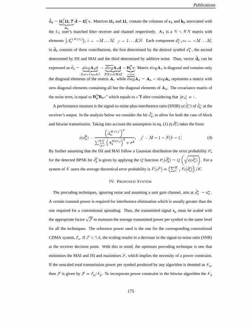
Publications

. Matrices

and

contain the columns of and associated with

the "! user’s matched filter receiver and channel respectively. # is a $&%'$ matrix with

elements ( )+*-,/.,1032 4 5, 6 87:98;;;<9>=@?ACBD;;; '$ . Each component

EGF =<HIJ7K9J;L;;<9,

in

consists of three contributions, the first determined by the desired symbolEMF

, the second

determined by ISI and MAI and the third determined by additive noise. Thus, vector

can be

expressed asNOPE 6RQGS1# TVUXW *ZY U[T\W^] FD_a`Rb

E 6cQdS1# eVf eGgVhT .ji e h ` * W[U . Matrix

E 6RQGS1# is diagonal and contains only

the diagonal elements of the matrix # while

E 6cQGS1# # 7kE 6cQGS1# represents a matrix with

zero diagonal elements containing all but the diagonal elements of # . The covariance matrix of

the noise term, is equal to lnm

which equals tolmpo

after considering that q q B.

A performance measure is the signal-to-noise-plus-interference ratio (SNIR) rns E F ut ofE F

at the

receiver’s output. In the analysis below we consider the bitEGv

, to allow for both the case of block

and bitwise transmission. Taking into account the assumption in eq. (1) rns E v t takes the form:

rws E v t x ) .,10p2 4zy m|AD~[ 3 yx ) .,1032 4 m l m =?1>9AB $sV 7AB t

(4)

By further assuming that the ISI and MAI follow a Gaussian distribution the error probability Ufor the detected BPSK bit

E v is given by applying the function U s E v t rns E v t[ . For a

system of ' users the average theoretical error probability is U s EGv t x | 3 0 U s EGv t ' .

IV. PROPOSED SYSTEM

The precoding techniques, ignoring noise and assuming a unit gain channel, aim atEGF EGF

.

A certain transmit power is required for interference elimination which is usually greater than the

one required for a conventional spreading. Thus, the transmitted signal must be scaled with

the appropriate factor to maintain the average transmitted power per symbol to the same level

for all the techniques. The reference power used is the one for the corresponding conventional

CDMA system, d . If BG;Z, the scaling results in a decrease in the signal-to-noise ratio (SNR)

at the receiver decision point. With this in mind, the optimum precoding technique is one that

minimises the MAI and ISI and maximises , which implies the necessity of a power constraint.

If the unscaled total transmission power per symbol produced by any algorithm is denoted as : ,then is given by . To incorporate power constraint in the bitwise algorithm the

175

Publications

must be expressed as a function of , which is a -length vector of pre-filter taps defined as

. It can be shown that:

(5)

where matrix "!#%$'& (*),+.-0/21 43 3 '3 4 65 is of dimension 879 ;:<'>= and

matrix is of dimension87?9 :?<'@=6 and is defined as:

BA0CEDF GIH,J +KB<L L L 7?9 :?< 3NM B<L L L

C DF G OPQ PR & +: M for SUT+: M T 7 :?<S otherwise

(6)

Equation (5) is used in what follows to develop the INVF algorithm using MMSE criterion with

power constraint1 in order to determine vector . The method is essentially different from the

ZF-DPF although they follow the same block diagram.

For simplicity we substitute the cascaded filters V .W and & 87 : W with an FIR filter of

length XY 7;9Z :;< and impulse response [ .W YV .W \]& 87 : W , as shown in Fig. 1.

After rearrangement (only to facilitate the mathematical analysis), the system can equivalently

be illustrated as in Fig. 2 for the ^`_a receiver. Signals bdce .W are defined as ’filtered reference

signals’ and are produced by passing the sequence of symbols )*f e & e gW through the filters with

impulse response ['c .W . This approach is essentially the one followed by [8] for stereophonic

sound reproduction systems. This block diagram arrangement is used to determine the optimal, in

MMSE terms, FIR filters, . The fact that noise is not included in the analysis doesn’t affect the

solution because the noise is not filtered by the inverse filters. The power constraint term imposed

in the solution gives good noise performance.

Vectors h ce .W i b ce gW j4 b ce .W :k 9 <'. correspond to the filtered reference signals.

Following the block diagram in Fig. 2 the blce gW are passed through the pre-filters to yield the

estimated desired data. The outputs mno gW can be written in matrix form as:mn o .W p .W 8 (7)qPower constraint has also been included in the technique developed in [7] but it is blockwise and is not examined further.

176

Publications

...

!

.... . .

... " (8)

We now seek the optimal filter vector # to minimise the time averaged squared error between the

actual and desired outputs. The desired outputs are sampled every symbol period $&%'% ()+*-, ,."/ 01222 , where,

is an imposed delay to the system which assists the equalisation of the

multipath channels. In the final cost function we must include, using Lagrange multipliers, the

constraint that 354 , eq. (5) should not exceed the reference transmitted power per symbol 674 . The

cost function to be minimised is:8 3:9 <; $ %=% > <; $ %'% >?1*A@B 3 4 # C; 6 4D (9)

where 3 denotes the expectation and&

is the vector of desired data defined as&E 9 F G H ? .

By using eq. (7) and after expansion eq. (9) takes the quadratic form:8 3I9 ?J; 0 3:9 $K%'% ? # * # 3I9 $L%=% $K%'% ? # *A@ B 3<4 # C; 6M4 D (10)

From vector gradient theory we find that NK3O4 # >P NK# 0MQ Q # . Therefore, the Wiener2 solution

for the taps of the pre-filters #R is given by

#CR TS 3I9 $K%'% $K%'% ?U*A@ Q Q:VW 3:9 $K%=% ? (11)

In order to complete the analysis, the expectation terms 3:9 $K%'% $L%=% ? and 3:9 $K%'% ?in eq. (11) must be calculated. As stated before XZY\[ I]M^[<_ [ <`ba Y <` _ Y )c;(

. Letd Y\[ e _ [ `fa Y <` _ Y g)h;i. The corresponding symbol in vector form is denoted asj Y\[ 9 d Y\[ klm H d Y\[ npo<;/? of length

nOob 0 )q*srt; 0 due to the convolution effect. Vector Y\[ , of length u , is given next as a function of the v 0Mw *x/vector

[ accounting for the ISI

effect. To assist the illustration of the Wiener solution it is assumed that,y*).z+no

,,y*).| u

(in fact they can be arbitrarily chosen). In eq. (12) EY~[ is a uxv matrix and Y\[ is written as:

Y~[ Y\[ [ (12)The assumption that users are transmitted with powers xx doesn’t affect the final Wiener solution. For different powers

Wiener solution is still 7 and the received powers will be proportionally different.

177

Publications

! #"%$'&()*+ ! #* , -./ .021 3'46587+) )9&:7,;

for <>= 4587+) )?&:7 =A@CB )D< otherwise

(13)

By combining eq. (8) and eq. (12) we obtain:

EF3HGJIKIL;MNOOOOOPQSR R TUTUT QSRV R V

.... . .

...QSR RV TUTUT QWRV RVXV

Y[ZZZZZ\ (14)

Taking into account the assumption in eq. (1) it is proved that:

]_^ E R 3HG IKI ;EF3'G IKI ;H`aNOOOOOPb V c d R e e

e . . . ee e b V c V R V

Y ZZZZZ\ (15)

]f^ E R 3'GgIKIL; QSh `a ^jik R TUTlT ik RVMV ` R (16)

whereik is a

"-length vector defined as

ik m n^o p om TUTUT q o `. om

is given by

eq. (13). By replacing now the expectation terms in eq. (11) with the right-hand side of eq. (15)

and eq. (16) the Wiener solution is fully determined in a closed form.

V. SIMULATION RESULTS

In this section the performance of the INVF is shown and compared to pre-RAKE, TP, JT and

DPF. The BER performance, we refer to, is the averaged BER over all the users. BPSK data

symbols rs t are spread by random binary spreading codes u t of length7vwUx

and transmitted

synchronously over the mobile channel. The mobile radio channels are different for each user and

the tap weights are normalised such that yz t y a. The delay profile adopted is consistent with

the UMTS European system and has a delay spread of |chips. In the current paper the

channels are assumed to be stationary with no Doppler effects. Perfect knowledge of the downlink

channel is presumed in the base station transmitter. For the DPF and INVF methods the delay4

in sampling the output at the receiver is set to half the pre-filter length.

The Wiener solution as stated in eq. (11) contains the power control term ~ R ~ . A question

arises as to what is the best choice for the parameter . Since is the power control term it is

178

Publications

expected that the best value for it is a function of . Figure 3 shows how affects the BER

for a variety of schemes. There is a range for which gives almost the optimum BER performance

with a variety of spreading codes and pre-filter lengths. This gives a degree of freedom about the

choice of . A critical issue, in CDMA systems is to provide all users with equivalent performance

under the assumption that signals of equal powers are addressed to them. That means that the

SNIR must be approximately the same for every user. By defining the SNIR spread as !" $#&%(')+*-,",",. we have a measure of the variety among the . individual

performances. Ideal values for / are close to unity. In Fig. 4 it is shown that large values of

result in significant differences in the users performance while small values result in similar

performance. A small value of minimises the contribution of the power control term in eq. (11)

and the Wiener solution cancels MAI and ISI for all users at the cost of increasing the transmitted

energy. This is reflected in a reduction of the receiver’s output SNR when the transmitted power is

normalised by 021 * . In the contrast, a large value of enhances the power control so as 023 *but the penalty is a degradation in the SNIR spread. In Fig. 4 it is shown that for 456 *"7 dB

ideal values for are close to 7897: .In Fig. 5 the BER versus the number of users is shown. The BER is averaged over ; 7 different

sets of random codes to smooth out the effect of codes with low or high crosscorrelation. It is

clear that INVF ( < is set to 32) outperforms TP, Pre-RAKE and DPF. The effect of the data-block

length on JT is also illustrated. The problem is alleviated by increasing at the cost of higher

complexity. When =?>@ , INVF achieves better performance than JT for a heavily loaded CDMA

system and equivalent for . 1BA5C@ . However, INVF displays significantly reduced complexity in

terms of multiplications required per transmitted symbol D . Ignoring the complexity of inverting

the appropriate matrices (it is identical for EF<GH>@ ), since it occurs only when the channel

changes, it can be shown that DIJLKMN?<AO :* @ and DQP)RSBUT . AVBW *"X @ 7 , for . : .The BER performance versus for . :#"*)Y is shown in Fig. 6. In the JT curves the

end-bits are being discarded to give the most optimistic performance. For . : JT and INVF

have similar performance. For . *)Y INVF is the best technique for reasonable Z with a

significant error floor in performance when <[O>@ . By increasing the number of taps to <F X7taps and selecting \ 78977 > , ideal for B@ 7 dB, INVF performance is further improved and

179

Publications

becomes constantly better than JT. However, the penalty is a degradation, in the low ratio

region. This is due to the fact that , selected for the case of , is not near optimum

for dB. The above leads to the idea that if the base station knows the noise power at

the receiver it can optimise the performance for high loaded systems by selecting the appropriate

value. Theory and simulations are in remarkable agreement in the graph.

VI. CONCLUSIONS

Inverse filters were proposed as a new efficient bitwise transmitter based pre-coding technique.

The technique takes the structure of DPF and develops the power constrained MMSE solution

for individually pre-filtering the spread data before transmission. The performance of the INVF

exceeds the one of Pre-RAKE, DPF and TP. It is competitive or better than JT but displays a lower

computational cost. INVF can be easily adjusted to any existing TDD/CDMA system with slowly

varying propagation channels.

REFERENCES

[1] R. Esmailzadeh and M. Nakagawa, “Pre-RAKE diversity combination for direct sequence spread spectrum communications

systems,” International Conference on Communications, vol. 1, pp. 463–467, Geneva 1993.

[2] S. Georgoulis and D.G.M. Cruickshank, “Pre-equalization, transmitter precoding and joint transmission techniques for time

division duplex CDMA,” IEE 3G 2001 Conference on Mobile Telecommunications Technologies, pp. 257–261, Mar. 2001.

[3] A. Papathanasiou, M. Meurer, T. Weber, and P.W. Baier, “A novel multiuser transmission scheme requiring no channel estim-

ation and no equalization at the mobile stations for the downlink of TD-CDMA operating in the TDD mode,” IEEE Vehicular

Technology Conference Fall 2000, pp. 203–210, 2000.

[4] B. R. Vojcic and W. M. Jang, “Transmitter precoding in synchronous multiuser communications,” IEEE Trans. on Communic-

ations, vol. 46, no. 10, pp. 1346–1355, Oct. 1998.

[5] M. Brandt-Pearce and A. Dharap, “Transmitter-based multiuser interference rejection for the down-link of a wireless CDMA

system in a multipath environment,” IEEE Journal on Selected Areas in Communications, vol. 18, no. 3, pp. 407–417, Mar.

2000.

[6] A. Klein, Multi-user detection of CDMA signals-algorithms and their application to cellular mobile radio, Fortschritt-Berichte

VDI, 1996.

[7] A.N. Barreto and G. Fettweis, “Capacity increase in the downlink of spread spectrum systems through joint signal precoding,”

in Proc. ICC, vol. 4, pp. 1142–1146, 2001.

[8] P.A. Nelson, H. Hamada, and S. Elliott, “Adaptive inverse filters for stereophonic sound reproduction,” IEEE Trans. on Signal

Processing, vol. 40, no. 7, pp. 1621–1632, Jul. 1992.

180

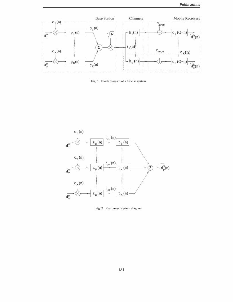
Publications

F

z K(n)Σ

d K

d 1

p (n)

m

m

1md (n)1

m

h (n)1

h (n)y (n)

K

1

d (n)

y (n)p (n)

v

awgn

awgn

1

s (n)p

v

c (Q−n)

c (Q−n)

K

K

c (n)

1

Base Station

K

KK

Channels Mobile Receiversc (n)

Fig. 1. Block diagram of a bitwise system

µ ν

µνΣ m

µ

µ1

1µ1md

m

dν

µΚ

ΚµKmd

p (n)r (n)

z (n) d (n)

r (n)p (n)z (n)

1c (n)

c (n)ν

p (n)r (n)

z (n)

Kc (n)

Fig. 2. Rearranged system diagram

181

Publications

0 0.05 0.1 0.15 0.2 0.25 0.3

10−4

10−3

10−2

10−1

100

λ

BE

R

16 taps32 taps

Fig. 3. BER performance for INVF vs for , , , dB. The solid lines represent

analytical results for 4 sets of 5 different random spreading codes when . The dashed lines represent analytical

results for 4 new sets of 5 randomly generated codes when .

0 0.05 0.1 0.15 0.2 0.25 0.31

1.5

2

2.5

3

3.5

4

λ

Φs

16 taps32 taps

Fig. 4. SNIR spread vs for !" , , # , dB. The solid lines represent analytical results

for 4 sets of 5 different random spreading codes when $ . The dashed lines represent analytical results for 4 new

sets of 5 randomly generated codes when %& .

182

Publications

2 4 6 8 10 12 14 16

10−4

10−3

10−2

10−1

100

Number of users

BE

R

pre−RAKETPDPFJT−block 1JT−block 3JT−block 20INVF

Fig. 5. Simulated BER performance vs number of users for dB, , . For TP the length of

the transmitted blocks has been set to . A length has been selected for INVF and DPF and for INVF.

0 5 10 15 2010

−5

10−4

10−3

10−2

10−1

100

Eb/N

o(dB)

BE

R

single user−simulation (sim)JT−sim−5 usersINVF−32 taps,λ=0.05−sim−5 usersJT−sim−14 usersINVF−32 taps,λ=0.05−sim−14 usersINVF−90 taps,λ=0.003−sim−14 usersanalytical results

Fig. 6. BER vs for ! "#%$ users. System parameters are & , '( . The markers correspond to the

simulation results and the dashed lines to the corresponding analytical ones.

183